An Inventory System with Retrial Demands and Working Vacation
30
International Journal of Scientific and Research Publications, Volume 4, Issue 12, December 2014 1 ISSN 2250-3153 An Inventory System with Retrial Demands and Working Vacation J. Kathiresan * , N. Anbazhagan * and K. Jeganathan ** * Department of Mathematics, Alagappa University, Karaikudi,India. ** Ramanujan Institute for Advanced Study in Mathematics, University of Madras, Chepauk, Chennai, India. Abstract- This article considers a continuous review retrial inventory system at a service facility, wherein an item demanded by a customer is issued after performing service on the item. The arrival time points of customers form a Poisson process. The inventory replenished according to an policy and the lead times are assumed to follow an exponential distribution. The demands that occur during the stock out period or the server busy (regular or working vacation) are permitted to enter into the orbit of infinite size. When the inventory level is zero or no demands in the system or both, server goes to a working vacation which is exponentially distributed. If the server is in working vacation or the inventory level is zero, the impatience occurs in orbiting customers, that follows an exponential distribution. The joint probability distribution of the number of demands in the orbit, the inventory level and the server status is obtained in the steady state case. Some system performance measures are derived, the long-run total expected cost rate is calculated and the results are illustrated numerically. Index Terms- Continuous review inventory system, Policy, Positive leadtime, Retrial demand, Working vacation. AMS Classification: 90B05, 60J27 I. INTRODUCTION he concept of server vacation in inventory with two servers was first introduced by Daniel and Ramanarayanan [1]. Also they have studied an inventory system in which the server takes rest when the level of the inventory is zero in [2]. They assumed that the demands that occurred during stock-out period are assumed to be lost. The inter-occurrence times between successive demands, the lead times, and the rest times are assumed to follow mutually independent general distributions. Using renewal and convolution techniques they obtained the state transition probabilities. T The various types of vacation models in queueing systems have been widely studied in the literature. We refer the reader to Doshi [4]. Working vacation is a kind of semi-vacation policy that was introduced by Servi and Finn[9]. In the classical vacation queuing models, during the vacation period the server doesn’t continue on the original work and such policy may cause the loss or dissatisfaction of the customers. For the working vacation policy, the server can still work during the vacation and may accomplish other assistant work simultaneously. So, the working vacation more reasonable that the classical vacation in some cases. Tien Van Do[8] studied, M/M/1 retrial queue with working vacations. Paul Manual et al. [10] analyzed a service facility inventory system with impatient customers. The authors have assumed the www.ijsrp.org
Transcript of An Inventory System with Retrial Demands and Working Vacation

International Journal of Scientific and Research Publications, Volume 4, Issue 12, December 20141
ISSN 2250-3153
An Inventory System with Retrial Demandsand Working Vacation
J. Kathiresan*, N. Anbazhagan* and K. Jeganathan**
*Department of Mathematics, Alagappa University, Karaikudi,India.** Ramanujan Institute for Advanced Study in Mathematics, University of Madras, Chepauk, Chennai,
India.
Abstract- This article considers a continuousreview retrial inventory system at aservice facility, wherein an item demandedby a customer is issued after performingservice on the item. The arrival timepoints of customers form a Poisson process.The inventory replenished according to an
policy and the lead times areassumed to follow an exponentialdistribution. The demands that occur duringthe stock out period or the server busy(regular or working vacation) are permittedto enter into the orbit of infinite size.When the inventory level is zero or nodemands in the system or both, server goesto a working vacation which isexponentially distributed. If the server isin working vacation or the inventory levelis zero, the impatience occurs in orbitingcustomers, that follows an exponentialdistribution. The joint probabilitydistribution of the number of demands inthe orbit, the inventory level and theserver status is obtained in the steadystate case. Some system performancemeasures are derived, the long-run totalexpected cost rate is calculated and theresults are illustrated numerically.Index Terms- Continuous review inventorysystem, Policy, Positive leadtime,Retrial demand, Working vacation.
AMS Classification: 90B05, 60J27
I. INTRODUCTIONhe concept of server vacation ininventory with two servers was first
introduced by Daniel and Ramanarayanan [1].Also they have studied an inventory systemin which the server takes rest when thelevel of the inventory is zero in [2]. Theyassumed that the demands that occurredduring stock-out period are assumed to belost. The inter-occurrence times betweensuccessive demands, the lead times, and therest times are assumed to follow mutuallyindependent general distributions. Usingrenewal and convolution techniques theyobtained the state transitionprobabilities.
T
The various types of vacation modelsin queueing systems have been widelystudied in the literature. We refer thereader to Doshi [4]. Working vacation is akind of semi-vacation policy that wasintroduced by Servi and Finn[9]. In theclassical vacation queuing models, duringthe vacation period the server doesn’tcontinue on the original work and suchpolicy may cause the loss ordissatisfaction of the customers. For theworking vacation policy, the server canstill work during the vacation and mayaccomplish other assistant worksimultaneously. So, the working vacationmore reasonable that the classical vacationin some cases. Tien Van Do[8] studied,M/M/1 retrial queue with working vacations.Paul Manual et al. [10] analyzed a servicefacility inventory system with impatientcustomers. The authors have assumed the
www.ijsrp.org
International Journal of Scientific and Research Publications, Volume 4, Issue 12, December 20142
ISSN 2250-3153 customers arrive in Poisson fashion. Theservice time, life time of items in stockand the lead time are all assumed to beindependently distributed as exponential. The concept of retrial demands ininventory was introduced by Artalejo et al.[3]. They have assumed Poisson demand,exponential lead time and exponentialretrial time. In that work, the authorsproceeded with an algorithmic analysis ofthe system. Jeganathan et al. [5] studied aretrial inventory system with non-preemptive priority service. Narayanan etal. [6] studied on an inventorypolicy with service time, vacation toserver and correlated lead time. In this present paper, we address acontinuous review inventory system withPoisson demand. The server served atdifferent service rates (working vacationand regular), which are exponentiallydistributed. When the server is busy or theinventory level is zero, any arrivingprimary demands enter into orbit. When theserver is in a working vacation or theinventory level is zero, the orbitingcustomer either may retry or may leave,which is exponentially distributed. Thejoint probability distribution of theinventory level, the number of customers inthe orbit and the server status is obtainedin the steady state case. Various systemperformance measures in the steady stateare derived and the long-run total expectedcost rate is calculated and some numericalexamples. The rest of the paper is organizedas follows. In Section 2, we describe themathematical model. In Section 3 and 4, wediscuss the steady-state analysis of themodel and some key system performancemeasures respectively. In Section 5,calculate the long-run total expected costrate and the final section 6, a costfunction is also studied numerically.
II. MODEL DESCRIPTION We consider a continuous reviewstochastic inventory system on thereplenishment policy of . The basicassumptions of this inventory model aredescribed as follows: we assume that theinter-arrival times of demands to a singleserver station according to a Poissonprocess with rate and demands onlysingle unit at a time. It is assumed thatthere is no waiting space in the system.The items are issued by a server to thecustomer after some service time due to theservice performed on the items. When theserver is busy (regular or workingvacation) or the inventory level is zero,any arriving primary demands enter into anorbit of infinite size. The service rates
are and ( , when the system isin regular and working vacation,respectively, which are exponentiallydistributed. The server takes a workingvacation at times when no customers in thesystem or the inventory level is zero orboth. Working vacation durations areexponentially distributed with parameter . At the completion time of the workingvacation, the server switches a regular
busy ((ie) service rate from to ) ifthere are customers (primary or retrial) inthe system. Otherwise, the server continuesthe working vacation. The orbitingcustomers may either retry or may leave theorbit. The leaving orbiting customers aredescribed as impatient(reneging) customers.If the server is in working vacation or theinventory level is zero, the impatienceoccurs in orbiting customers. An impatientcustomer leaves the orbit independenlyafter a random time which is distributedexponentially with parameter . We assume the constant retrialpolicy for these orbit demands, that isprobability of a repeated attempt of anorbiting demand is independent of thenumber of demands in the orbit. Retrial
www.ijsrp.org
International Journal of Scientific and Research Publications, Volume 4, Issue 12, December 20143
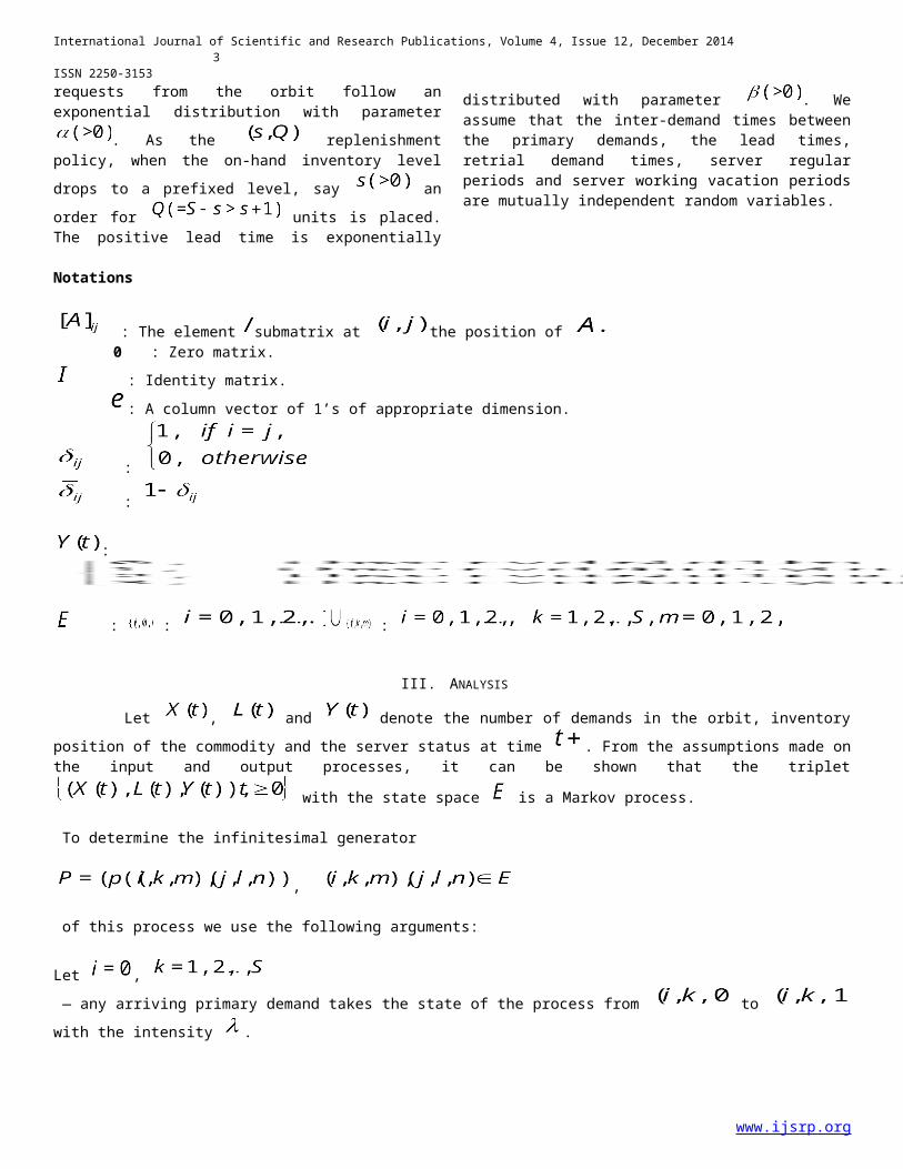
ISSN 2250-3153 requests from the orbit follow anexponential distribution with parameter
. As the replenishmentpolicy, when the on-hand inventory leveldrops to a prefixed level, say anorder for units is placed.The positive lead time is exponentially
distributed with parameter . Weassume that the inter-demand times betweenthe primary demands, the lead times,retrial demand times, server regularperiods and server working vacation periodsare mutually independent random variables.
Notations
: The element submatrix at the position of 0 : Zero matrix.
: Identity matrix. : A column vector of 1’s of appropriate dimension.
:
:
:
: : :
III. ANALYSIS
Let , and denote the number of demands in the orbit, inventoryposition of the commodity and the server status at time . From the assumptions made onthe input and output processes, it can be shown that the triplet
with the state space is a Markov process.
To determine the infinitesimal generator
,
of this process we use the following arguments:
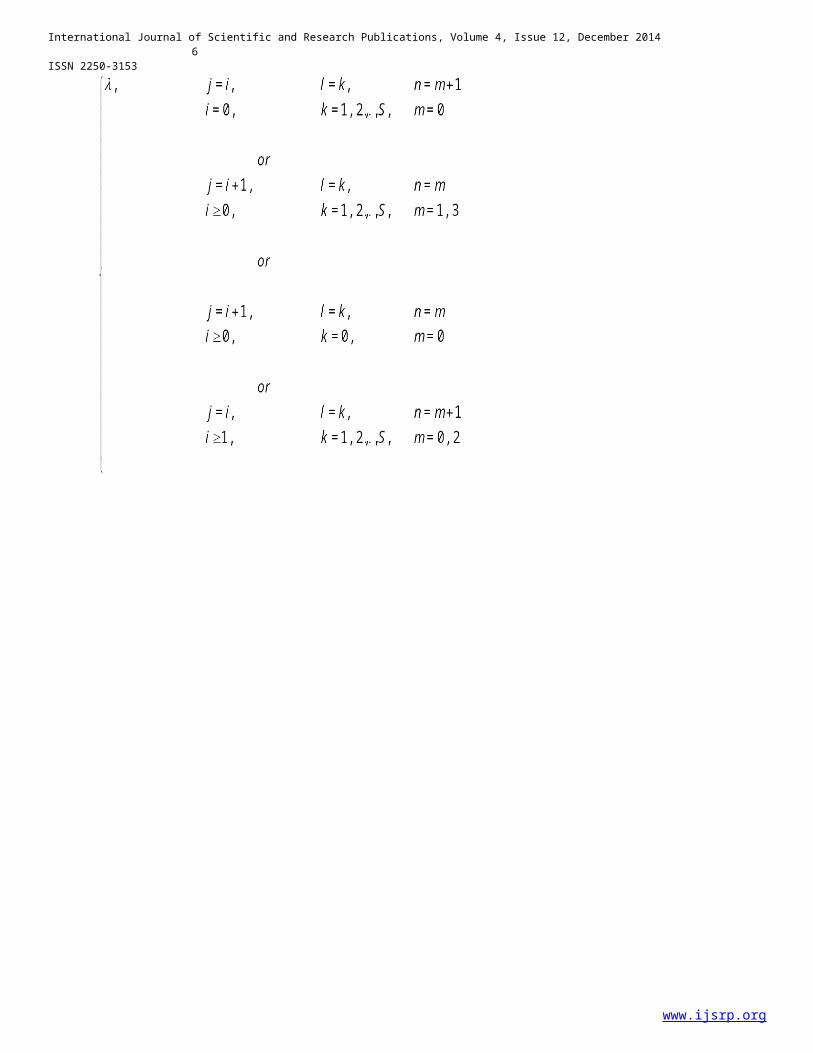
Let , — any arriving primary demand takes the state of the process from to with the intensity .
www.ijsrp.org
International Journal of Scientific and Research Publications, Volume 4, Issue 12, December 20144
ISSN 2250-3153
— any arriving primary demand takes the state of the process from to with the
intensity , .
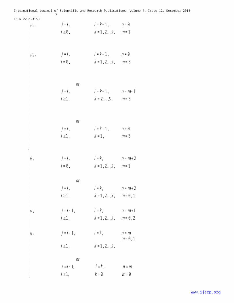
— The server changes from working vacation to regular takes the state of the process from to
with the intensity .
— The completion of service from primary demand makes a transition from to with the
intensity .
— The completion of service from primary demand makes a transition from to with the
intensity .
Let , — any arriving primary demand takes the state of the process from to
with the intensity .
Let , — any arriving primary demand takes the state of the process from to
with the intensity , m=0, 2.
— any arriving primary demand takes the state of the process from to with the
intensity , m=1, 3.
— The server changes from working vacation to regular takes the state of the process from to
with the intensity , m=0, 1.
— a retrial requests takes the state of the process from to with the intensity , m=0, 2.
www.ijsrp.org
International Journal of Scientific and Research Publications, Volume 4, Issue 12, December 20145
ISSN 2250-3153
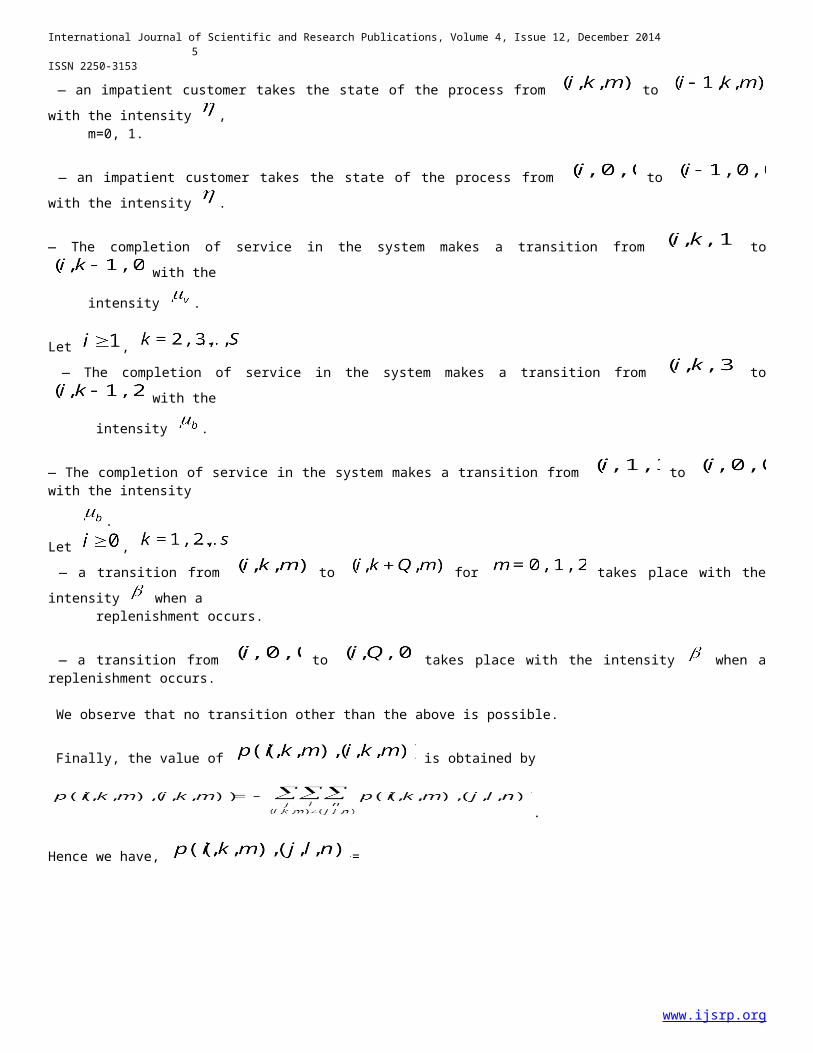
— an impatient customer takes the state of the process from to with the intensity , m=0, 1.
— an impatient customer takes the state of the process from to with the intensity .
— The completion of service in the system makes a transition from to with the
intensity .
Let , — The completion of service in the system makes a transition from to
with the
intensity .
— The completion of service in the system makes a transition from to with the intensity
.Let , — a transition from to for takes place with theintensity when a replenishment occurs.
— a transition from to takes place with the intensity when areplenishment occurs.
We observe that no transition other than the above is possible.
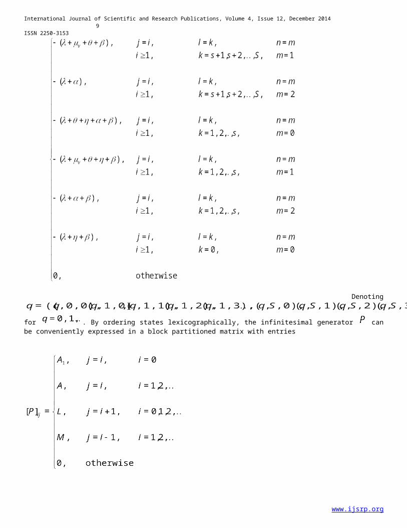
Finally, the value of is obtained by
.
Hence we have, =
www.ijsrp.org
International Journal of Scientific and Research Publications, Volume 4, Issue 12, December 20146
ISSN 2250-3153
www.ijsrp.org
International Journal of Scientific and Research Publications, Volume 4, Issue 12, December 20147
ISSN 2250-3153
www.ijsrp.org

International Journal of Scientific and Research Publications, Volume 4, Issue 12, December 20148
ISSN 2250-3153
www.ijsrp.org
International Journal of Scientific and Research Publications, Volume 4, Issue 12, December 20149
ISSN 2250-3153
Denoting
for . By ordering states lexicographically, the infinitesimal generator canbe conveniently expressed in a block partitioned matrix with entries
www.ijsrp.org
International Journal of Scientific and Research Publications, Volume 4, Issue 12, December 201410
ISSN 2250-3153
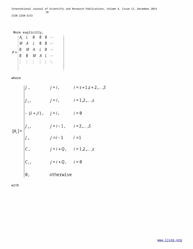
More explicitly,
where
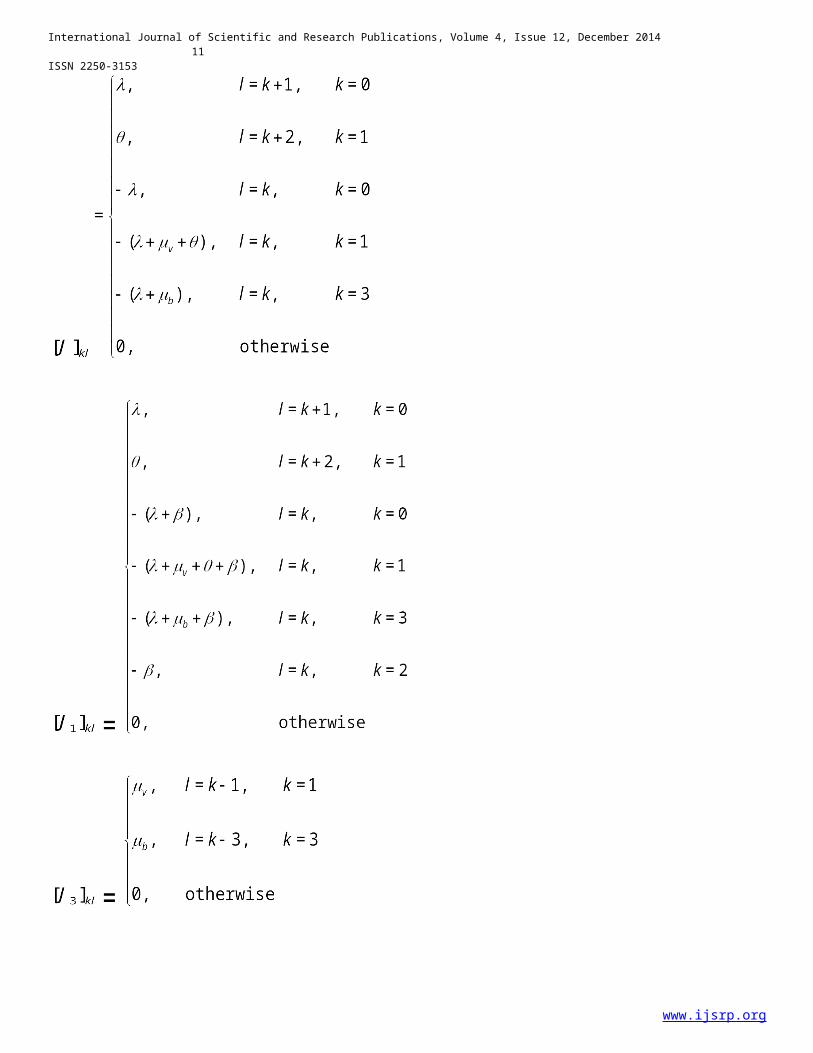
with
www.ijsrp.org
International Journal of Scientific and Research Publications, Volume 4, Issue 12, December 201411
ISSN 2250-3153
www.ijsrp.org
International Journal of Scientific and Research Publications, Volume 4, Issue 12, December 201412
ISSN 2250-3153
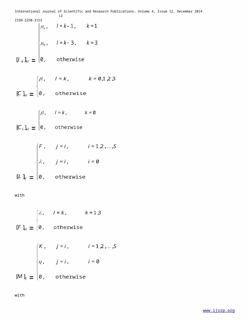
with
with
www.ijsrp.org
International Journal of Scientific and Research Publications, Volume 4, Issue 12, December 201413
ISSN 2250-3153
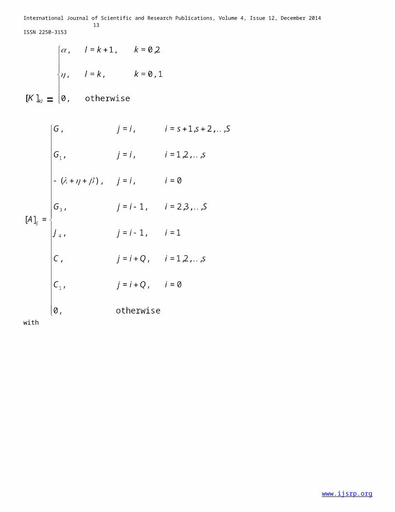
with
www.ijsrp.org

International Journal of Scientific and Research Publications, Volume 4, Issue 12, December 201414
ISSN 2250-3153
www.ijsrp.org
International Journal of Scientific and Research Publications, Volume 4, Issue 12, December 201415
ISSN 2250-3153
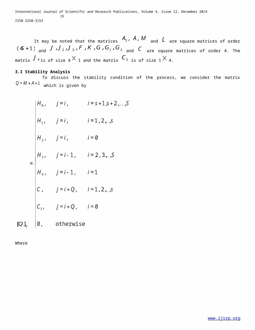
It may be noted that the matrices and are square matrices of order
and and are square matrices of order 4. The
matrix is of size 4 1 and the matrix is of size 1 4.
3.1 Stability Analysis To discuss the stability condition of the process, we consider the matrix
which is given by
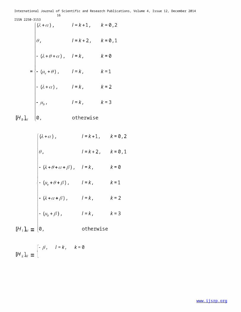
Where
www.ijsrp.org
International Journal of Scientific and Research Publications, Volume 4, Issue 12, December 201416
ISSN 2250-3153
www.ijsrp.org
International Journal of Scientific and Research Publications, Volume 4, Issue 12, December 201417
ISSN 2250-3153
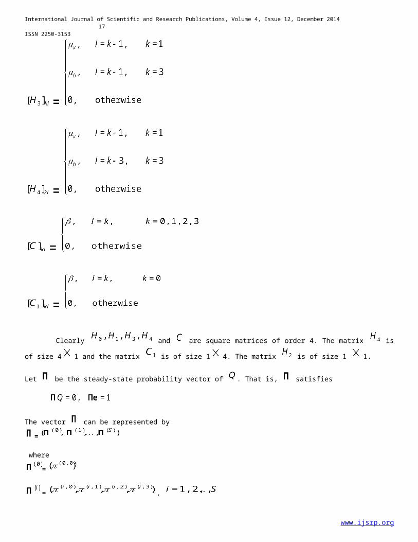
Clearly and are square matrices of order 4. The matrix is
of size 4 1 and the matrix is of size 1 4. The matrix is of size 1 1.
Let be the steady-state probability vector of . That is, satisfies
The vector can be represented by
=
where
=
= ,
www.ijsrp.org
International Journal of Scientific and Research Publications, Volume 4, Issue 12, December 201418
ISSN 2250-3153
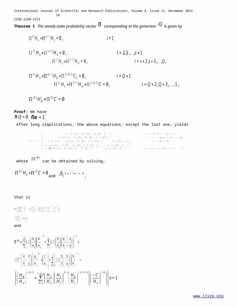
Theorem 1 The steady-state probability vector coresponding to the generator is given by
Proof: We have , .
After long simplications, the above equations, except the last one, yields
where can be obtained by solving,
and ,
that is
and
www.ijsrp.org
International Journal of Scientific and Research Publications, Volume 4, Issue 12, December 201419
ISSN 2250-3153
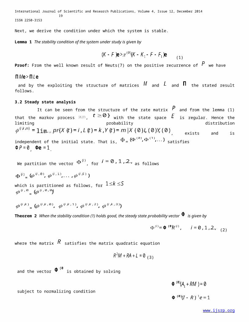
Next, we derive the condition under which the system is stable.
Lemma 1 The stability condition of the system under study is given by
(1)Proof: From the well known result of Neuts(7) on the positive recurrence of we have
and by the exploiting the structure of matrices and and the stated resultfollows.
3.2 Steady state analysis It can be seen from the structure of the rate matrix and from the lemma (1)that the markov process , with the state space is regular. Hence thelimiting probability distribution
, exists and is
independent of the initial state. That is, = satisfies , .
We partition the vector , for as follows
=which is partitioned as follows, for
=
=Theorem 2 When the stability condition (1) holds good, the steady state probability vector is given by
(2)
where the matrix satisfies the matrix quadratic equation
(3)
and the vector is obtained by solving
subject to normalizing condition
www.ijsrp.org
International Journal of Scientific and Research Publications, Volume 4, Issue 12, December 201420
ISSN 2250-3153
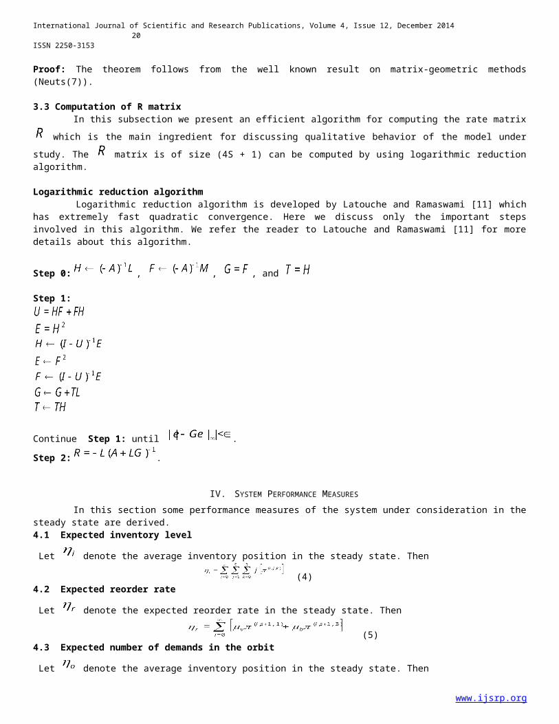
Proof: The theorem follows from the well known result on matrix-geometric methods(Neuts(7)).
3.3 Computation of R matrix In this subsection we present an efficient algorithm for computing the rate matrix
which is the main ingredient for discussing qualitative behavior of the model understudy. The matrix is of size (4S + 1) can be computed by using logarithmic reductionalgorithm.
Logarithmic reduction algorithm Logarithmic reduction algorithm is developed by Latouche and Ramaswami [11] whichhas extremely fast quadratic convergence. Here we discuss only the important stepsinvolved in this algorithm. We refer the reader to Latouche and Ramaswami [11] for moredetails about this algorithm.
Step 0: , , , and
Step 1:
Continue Step 1: until .
Step 2: .
IV. SYSTEM PERFORMANCE MEASURES In this section some performance measures of the system under consideration in thesteady state are derived. 4.1 Expected inventory level
Let denote the average inventory position in the steady state. Then
(4)4.2 Expected reorder rate
Let denote the expected reorder rate in the steady state. Then
(5)4.3 Expected number of demands in the orbit
Let denote the average inventory position in the steady state. Then
www.ijsrp.org
International Journal of Scientific and Research Publications, Volume 4, Issue 12, December 201421
ISSN 2250-3153
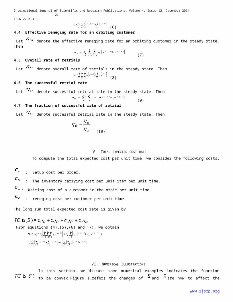
(6)4.4 Effective reneging rate for an orbiting customer
Let denote the effective reneging rate for an orbiting customer in the steady state.Then
(7)4.5 Overall rate of retrials
Let denote overall rate of retrials in the steady state. Then
(8)4.6 The successful retrial rate
Let denote successful retrial rate in the steady state. Then
(9)4.7 The fraction of successful rate of retrial
Let denote successful retrial rate in the steady state. Then
(10)
V. TOTAL EXPECTED COST RATE To compute the total expected cost per unit time, we consider the following costs.
: Setup cost per order.
: The inventory carrying cost per unit item per unit time.
: Waiting cost of a customer in the orbit per unit time.
: reneging cost per customer per unit time.
The long run total expected cost rate is given by
From equations (4),(5),(6) and (7), we obtain
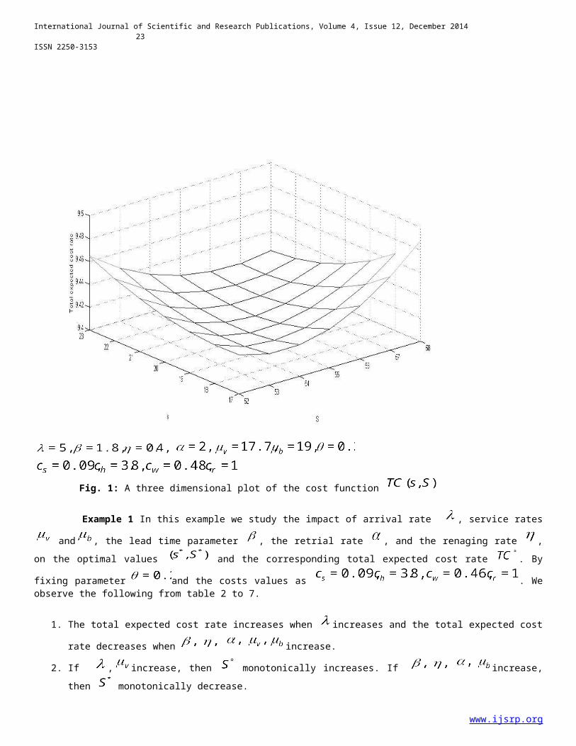
VI. NUMERICAL ILLUSTRATIONS In this section, we discuss some numerical examples indicates the function
to be convex.Figure 1.refers the changes of and are how to affect the
www.ijsrp.org
International Journal of Scientific and Research Publications, Volume 4, Issue 12, December 201422
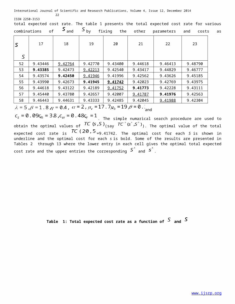
ISSN 2250-3153 total expected cost rate. The table 1 presents the total expected cost rate for variouscombinations of and by fixing the other parameters and costs as
and
. The simple numarical search procedure are used toobtain the optimal values of (say ). The optimal value of the totalexpected cost rate is =9.41742. The optimal cost for each S is shown inunderline and the optimal cost for each s is bold. Some of the results are presented inTables 2 through 13 where the lower entry in each cell gives the optimal total expectedcost rate and the upper entries the corresponding and .
Table 1: Total expected cost rate as a function of and
www.ijsrp.org
17 18 19 20 21 22 23
52 9.43446 9.42764 9.42770 9.43400 9.44618 9.46413 9.4879053 9.43385 9.42473 9.42213 9.42540 9.43417 9.44829 9.4677754 9.43574 9.42450 9.41946 9.41996 9.42562 9.43626 9.4518555 9.43990 9.42673 9.41945 9.41742 9.42023 9.42769 9.4397556 9.44618 9.43122 9.42189 9.41752 9.41773 9.42228 9.4311157 9.45440 9.43780 9.42657 9.42007 9.41787 9.41976 9.4256358 9.46443 9.44631 9.43333 9.42485 9.42045 9.41988 9.42304
International Journal of Scientific and Research Publications, Volume 4, Issue 12, December 201423
ISSN 2250-3153
Fig. 1: A three dimensional plot of the cost function
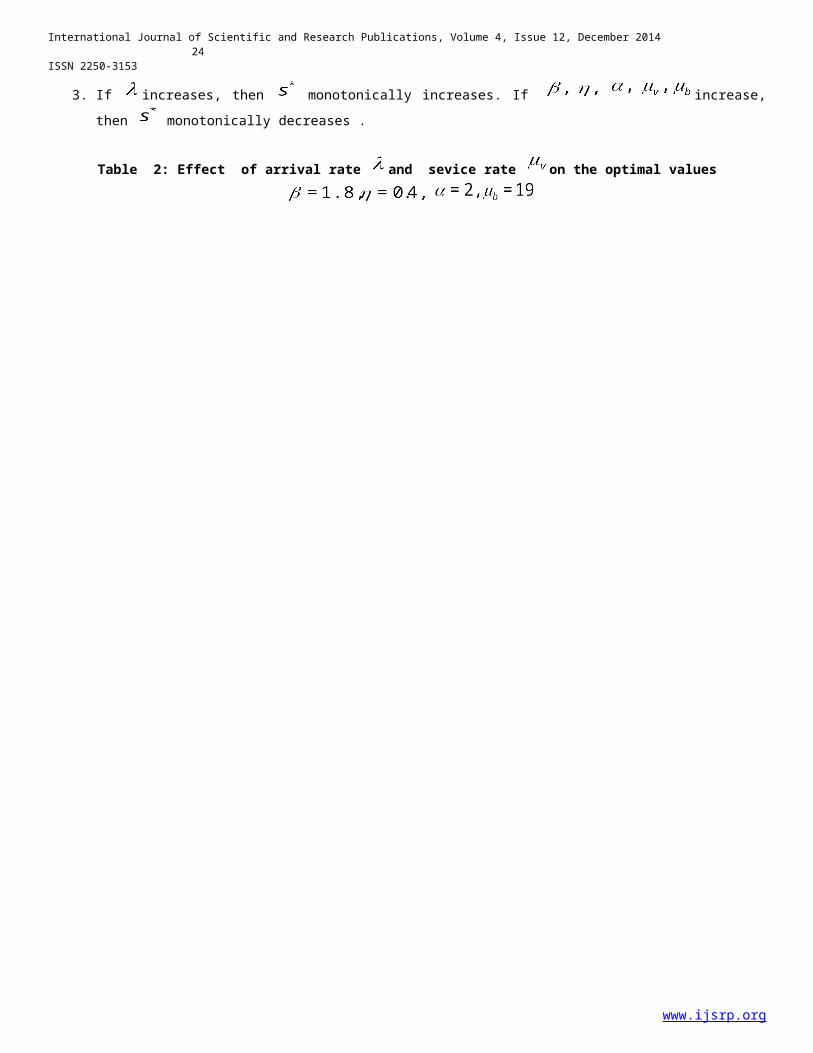
Example 1 In this example we study the impact of arrival rate , service rates
and , the lead time parameter , the retrial rate , and the renaging rate ,on the optimal values and the corresponding total expected cost rate . By
fixing parameter and the costs values as . Weobserve the following from table 2 to 7.
1. The total expected cost rate increases when increases and the total expected cost
rate decreases when increase.
2. If , increase, then monotonically increases. If increase,then monotonically decrease.
www.ijsrp.org
International Journal of Scientific and Research Publications, Volume 4, Issue 12, December 201424
ISSN 2250-3153
3. If increases, then monotonically increases. If increase,then monotonically decreases .
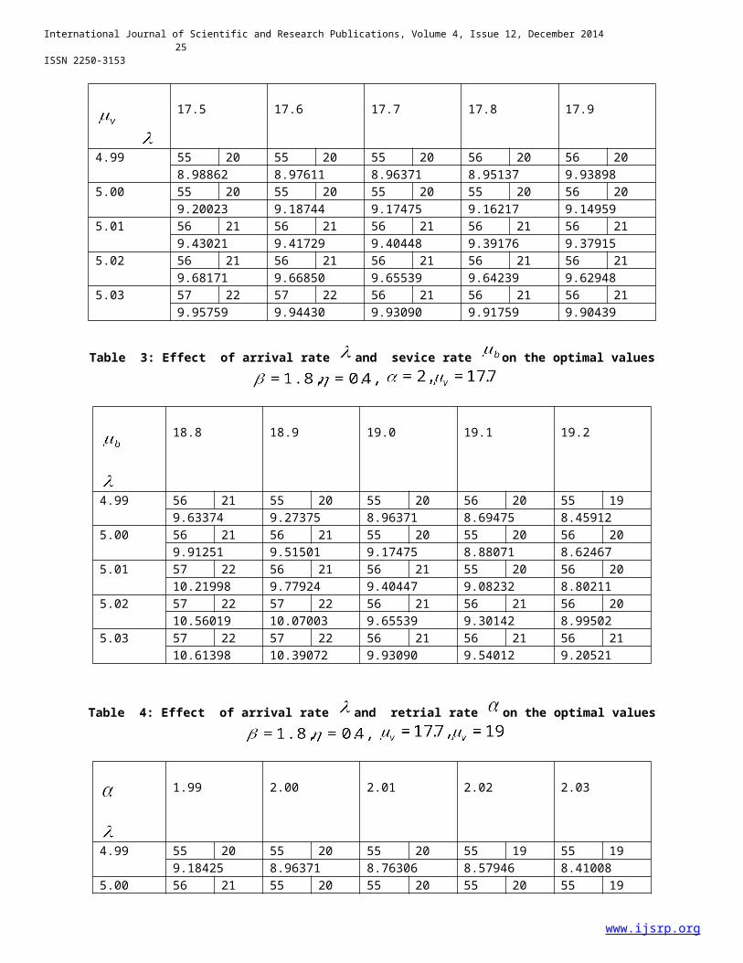
Table 2: Effect of arrival rate and sevice rate on the optimal values
www.ijsrp.org
International Journal of Scientific and Research Publications, Volume 4, Issue 12, December 201425
ISSN 2250-3153
17.5 17.6 17.7 17.8 17.9
4.99 55 20 55 20 55 20 56 20 56 208.98862 8.97611 8.96371 8.95137 9.93898
5.00 55 20 55 20 55 20 55 20 56 209.20023 9.18744 9.17475 9.16217 9.14959
5.01 56 21 56 21 56 21 56 21 56 219.43021 9.41729 9.40448 9.39176 9.37915
5.02 56 21 56 21 56 21 56 21 56 219.68171 9.66850 9.65539 9.64239 9.62948
5.03 57 22 57 22 56 21 56 21 56 219.95759 9.94430 9.93090 9.91759 9.90439
Table 3: Effect of arrival rate and sevice rate on the optimal values
18.8 18.9 19.0 19.1 19.2
4.99 56 21 55 20 55 20 56 20 55 199.63374 9.27375 8.96371 8.69475 8.45912
5.00 56 21 56 21 55 20 55 20 56 209.91251 9.51501 9.17475 8.88071 8.62467
5.01 57 22 56 21 56 21 55 20 56 2010.21998 9.77924 9.40447 9.08232 8.80211
5.02 57 22 57 22 56 21 56 21 56 2010.56019 10.07003 9.65539 9.30142 8.99502
5.03 57 22 57 22 56 21 56 21 56 2110.61398 10.39072 9.93090 9.54012 9.20521
Table 4: Effect of arrival rate and retrial rate on the optimal values
1.99 2.00 2.01 2.02 2.03
4.99 55 20 55 20 55 20 55 19 55 199.18425 8.96371 8.76306 8.57946 8.41008
5.00 56 21 55 20 55 20 55 20 55 19
www.ijsrp.org
International Journal of Scientific and Research Publications, Volume 4, Issue 12, December 201426
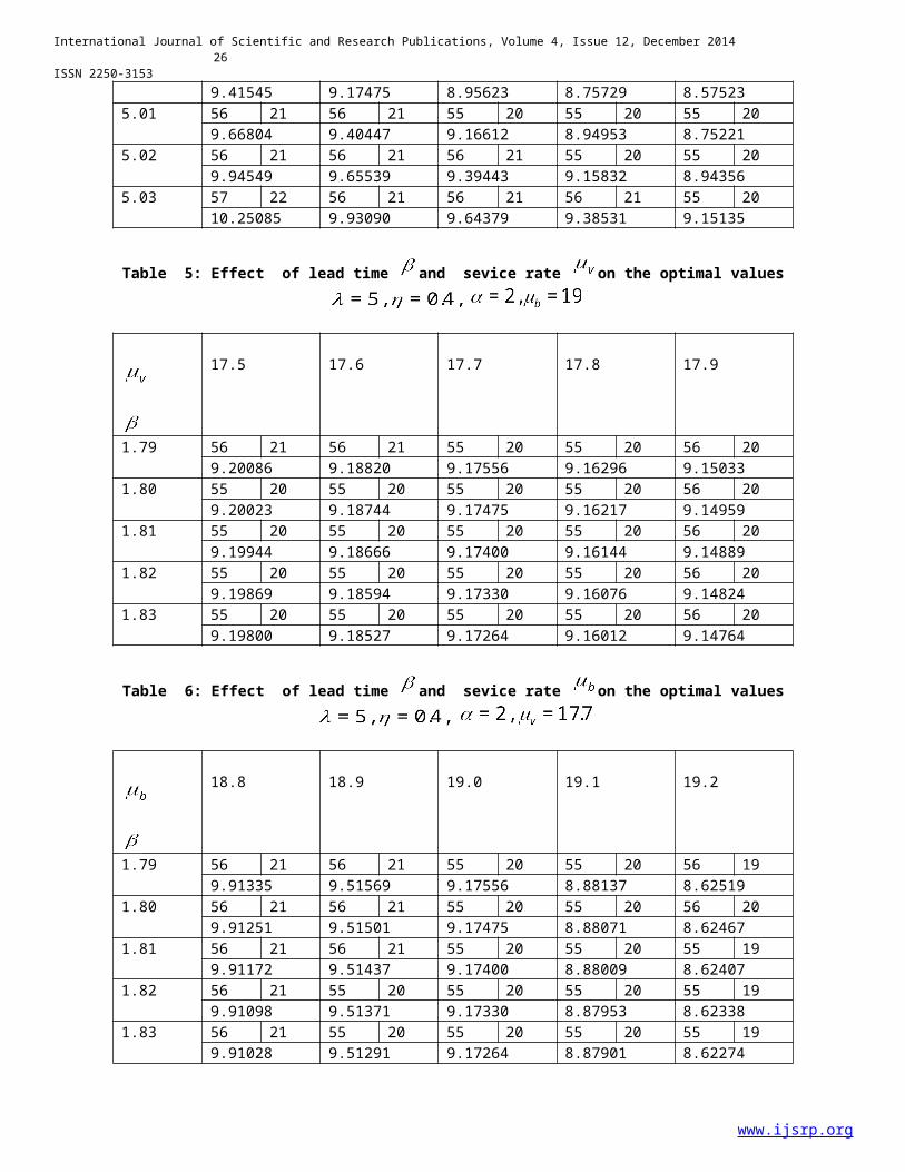
ISSN 2250-3153 9.41545 9.17475 8.95623 8.75729 8.57523
5.01 56 21 56 21 55 20 55 20 55 209.66804 9.40447 9.16612 8.94953 8.75221
5.02 56 21 56 21 56 21 55 20 55 209.94549 9.65539 9.39443 9.15832 8.94356
5.03 57 22 56 21 56 21 56 21 55 2010.25085 9.93090 9.64379 9.38531 9.15135
Table 5: Effect of lead time and sevice rate on the optimal values
17.5 17.6 17.7 17.8 17.9
1.79 56 21 56 21 55 20 55 20 56 209.20086 9.18820 9.17556 9.16296 9.15033
1.80 55 20 55 20 55 20 55 20 56 209.20023 9.18744 9.17475 9.16217 9.14959
1.81 55 20 55 20 55 20 55 20 56 209.19944 9.18666 9.17400 9.16144 9.14889
1.82 55 20 55 20 55 20 55 20 56 209.19869 9.18594 9.17330 9.16076 9.14824
1.83 55 20 55 20 55 20 55 20 56 209.19800 9.18527 9.17264 9.16012 9.14764
Table 6: Effect of lead time and sevice rate on the optimal values
18.8 18.9 19.0 19.1 19.2
1.79 56 21 56 21 55 20 55 20 56 199.91335 9.51569 9.17556 8.88137 8.62519
1.80 56 21 56 21 55 20 55 20 56 209.91251 9.51501 9.17475 8.88071 8.62467
1.81 56 21 56 21 55 20 55 20 55 199.91172 9.51437 9.17400 8.88009 8.62407
1.82 56 21 55 20 55 20 55 20 55 199.91098 9.51371 9.17330 8.87953 8.62338
1.83 56 21 55 20 55 20 55 20 55 199.91028 9.51291 9.17264 8.87901 8.62274
www.ijsrp.org
International Journal of Scientific and Research Publications, Volume 4, Issue 12, December 201427
ISSN 2250-3153
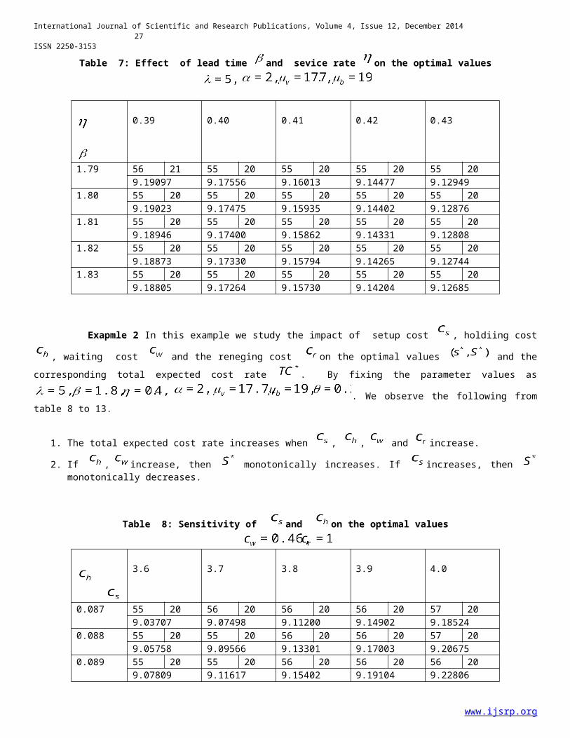
Table 7: Effect of lead time and sevice rate on the optimal values
0.39 0.40 0.41 0.42 0.43
1.79 56 21 55 20 55 20 55 20 55 209.19097 9.17556 9.16013 9.14477 9.12949
1.80 55 20 55 20 55 20 55 20 55 209.19023 9.17475 9.15935 9.14402 9.12876
1.81 55 20 55 20 55 20 55 20 55 209.18946 9.17400 9.15862 9.14331 9.12808
1.82 55 20 55 20 55 20 55 20 55 209.18873 9.17330 9.15794 9.14265 9.12744
1.83 55 20 55 20 55 20 55 20 55 209.18805 9.17264 9.15730 9.14204 9.12685
Exapmle 2 In this example we study the impact of setup cost , holdiing cost
, waiting cost and the reneging cost on the optimal values and thecorresponding total expected cost rate . By fixing the parameter values as
. We observe the following fromtable 8 to 13.
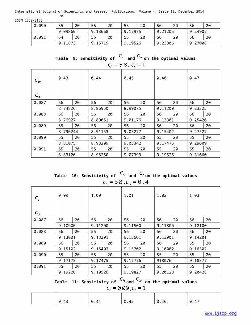
1. The total expected cost rate increases when , , and increase.
2. If , increase, then monotonically increases. If increases, then monotonically decreases.
Table 8: Sensitivity of and on the optimal values
3.6 3.7 3.8 3.9 4.0
0.087 55 20 56 20 56 20 56 20 57 209.03707 9.07498 9.11200 9.14902 9.18524
0.088 55 20 55 20 56 20 56 20 57 209.05758 9.09566 9.13301 9.17003 9.20675
0.089 55 20 55 20 56 20 56 20 56 209.07809 9.11617 9.15402 9.19104 9.22806
www.ijsrp.org
International Journal of Scientific and Research Publications, Volume 4, Issue 12, December 201428
ISSN 2250-3153 0.090 55 20 55 20 55 20 56 20 56 20
9.09860 9.13668 9.17975 9.21205 9.249070.091 54 20 55 20 55 20 56 20 56 20
9.11873 9.15719 9.19526 9.23306 9.27008
Table 9: Sensitivity of and on the optimal values
0.43 0.44 0.45 0.46 0.47
0.087 56 20 56 20 56 20 56 20 56 208.74826 8.86950 8.99075 9.11200 9.23325
0.088 56 20 56 20 56 20 56 20 56 208.76927 8.89051 9.01176 9.13301 9.25426
0.089 55 20 56 20 56 20 56 20 56 208.790244 8.91153 9.03277 9.15402 9.27527
0.090 55 20 55 20 55 20 55 20 55 208.81075 8.93209 9.05342 9.17475 9.29609
0.091 55 20 55 20 55 20 55 20 55 208.83126 8.95260 9.07393 9.19526 9.31660
Table 10: Sensitivity of and on the optimal values
0.99 1.00 1.01 1.02 1.03
0.087 56 20 56 20 56 20 56 20 56 209.10900 9.11200 9.11500 9.11800 9.12100
0.088 56 20 55 20 56 20 56 20 56 209.13001 9.13301 9.13601 9.13901 9.14201
0.089 56 20 56 20 56 20 56 20 55 209.15102 9.15402 9.15702 9.16002 9.16302
0.090 55 20 55 20 55 20 55 20 55 209.17175 9.17475 9.17776 918076 9.18377
0.091 55 20 55 20 55 20 55 20 55 209.19226 9.19526 9.19827 9.20128 9,20428
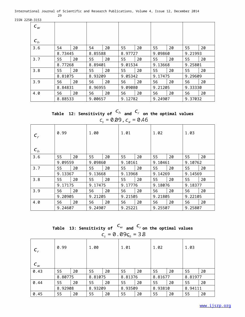
Table 11: Sensitivity of and on the optimal values
0.43 0.44 0.45 0.46 0.47
www.ijsrp.org
International Journal of Scientific and Research Publications, Volume 4, Issue 12, December 201429
ISSN 2250-3153
3.6 54 20 54 20 55 20 55 20 55 208.73445 8.85588 8.97727 9.09860 9.21993
3.7 55 20 55 20 55 20 55 20 55 208.77268 8.89401 9.01534 9.13668 9.25801
3.8 55 20 55 20 55 20 55 20 55 208.81075 8.93209 9.05342 9.17475 9.29609
3.9 56 20 56 20 56 20 56 20 56 208.84831 8.96955 9.09080 9.21205 9.33330
4.0 56 20 56 20 56 20 56 20 56 208.88533 9.00657 9.12782 9.24907 9.37032
Table 12: Sensitivity of and on the optimal values
0.99 1.00 1.01 1.02 1.03
3.6 55 20 55 20 55 20 55 20 55 209.09559 9.09860 9.10161 9.10461 9.10762
3.7 55 20 55 20 55 20 55 20 55 209.13367 9.13668 9.13968 9.14269 9.14569
3.8 55 20 55 20 55 20 55 20 55 209.17175 9.17475 9.17776 9.18076 9.18377
3.9 56 20 56 20 56 20 56 20 56 209.20905 9.21205 9.21505 9.21805 9.22105
4.0 56 20 56 20 56 20 56 20 56 209.24607 9.24907 9.25221 9.25507 9.25807
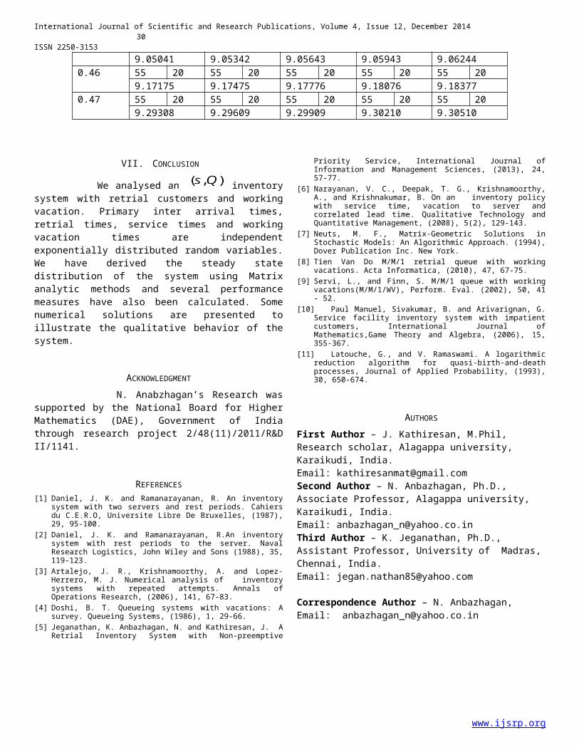
Table 13: Sensitivity of and on the optimal values
0.99 1.00 1.01 1.02 1.03
0.43 55 20 55 20 55 20 55 20 55 208.80775 8.81075 8.81376 8.81677 8.81977
0.44 55 20 55 20 55 20 55 20 55 208.92908 8.93209 8.93509 8.93810 8.94111
0.45 55 20 55 20 55 20 55 20 55 20
www.ijsrp.org
International Journal of Scientific and Research Publications, Volume 4, Issue 12, December 201430
ISSN 2250-3153 9.05041 9.05342 9.05643 9.05943 9.06244
0.46 55 20 55 20 55 20 55 20 55 209.17175 9.17475 9.17776 9.18076 9.18377
0.47 55 20 55 20 55 20 55 20 55 209.29308 9.29609 9.29909 9.30210 9.30510
VII. CONCLUSION
We analysed an inventorysystem with retrial customers and workingvacation. Primary inter arrival times,retrial times, service times and workingvacation times are independentexponentially distributed random variables.We have derived the steady statedistribution of the system using Matrixanalytic methods and several performancemeasures have also been calculated. Somenumerical solutions are presented toillustrate the qualitative behavior of thesystem.
ACKNOWLEDGMENT N. Anabzhagan’s Research wassupported by the National Board for HigherMathematics (DAE), Government of Indiathrough research project 2/48(11)/2011/R&DII/1141.
REFERENCES[1] Daniel, J. K. and Ramanarayanan, R. An inventory
system with two servers and rest periods. Cahiersdu C.E.R.O, Universite Libre De Bruxelles, (1987),29, 95-100.
[2] Daniel, J. K. and Ramanarayanan, R.An inventorysystem with rest periods to the server. NavalResearch Logistics, John Wiley and Sons (1988), 35,119-123.
[3] Artalejo, J. R., Krishnamoorthy, A. and Lopez-Herrero, M. J. Numerical analysis of inventorysystems with repeated attempts. Annals ofOperations Research, (2006), 141, 67-83.
[4] Doshi, B. T. Queueing systems with vacations: Asurvey. Queueing Systems, (1986), 1, 29-66.
[5] Jeganathan, K. Anbazhagan, N. and Kathiresan, J. ARetrial Inventory System with Non-preemptive
Priority Service, International Journal ofInformation and Management Sciences, (2013), 24,57-77.
[6] Narayanan, V. C., Deepak, T. G., Krishnamoorthy,A., and Krishnakumar, B. On an inventory policywith service time, vacation to server andcorrelated lead time. Qualitative Technology andQuantitative Management, (2008), 5(2), 129-143.
[7] Neuts, M. F., Matrix-Geometric Solutions inStochastic Models: An Algorithmic Approach. (1994),Dover Publication Inc. New York.
[8] Tien Van Do M/M/1 retrial queue with workingvacations. Acta Informatica, (2010), 47, 67-75.
[9] Servi, L., and Finn, S. M/M/1 queue with workingvacations(M/M/1/WV), Perform. Eval. (2002), 50, 41- 52.
[10] Paul Manuel, Sivakumar, B. and Arivarignan, G.Service facility inventory system with impatientcustomers, International Journal ofMathematics,Game Theory and Algebra, (2006), 15,355-367.
[11] Latouche, G., and V. Ramaswami. A logarithmicreduction algorithm for quasi-birth-and-deathprocesses, Journal of Applied Probability, (1993),30, 650-674.
AUTHORSFirst Author – J. Kathiresan, M.Phil, Research scholar, Alagappa university, Karaikudi, India.Email: [email protected] Author – N. Anbazhagan, Ph.D., Associate Professor, Alagappa university, Karaikudi, India.Email: [email protected] Third Author – K. Jeganathan, Ph.D., Assistant Professor, University of Madras,Chennai, India. Email: [email protected]
Correspondence Author – N. Anbazhagan, Email: [email protected]
www.ijsrp.org