Dyrobes Rotordynamics Software https://dyrobes.com0 8S®

AN INTRODUCTION TO VIBRATION ANALYSIS USING MATLAB by

E. J. Gunter, Ph.D., Fellow, ASME RODYN Vibration Analysis, Inc.

Charlottesville, VA

Introduction and Background

The development of the computer from the late 1950's has resulted in more powerful computers of smaller size and of such low cost that extensive computational power is available to engineers at an affordable cost. The recent extensive advances in the power of microprocessors has resulted in a generation of new desktop and portable computers that rival mainframe, and even super-computers, of only a decade ago. ·

With these high-powered personal computers have also come the development of powerful engineering software programs for use in computer-aided design and manufacturing ( CAD/CAM) and extensive finite element packages for the analysis of various statics, dynamics, and stress problems of interest to the engineer. Although there is an extensive array of pre-programmed software available to the engineer and scientist for various problems and tasks, this does not preclude his need or desire to perform his own specialized programming tasks. ·

Computer Languages

Computer languages can be described in terms of levels. The lowest level is machine language, which is closely tied to the computer hardware and is a binary language, since the instructions are written in binary sequences of zeros and ones. An assembly language is used to generate a binary code and also is machine specific. The instructions may resemble written statements instead of binary code, but the language does not have a rich array of commands or statements at its disposal. Thus, writing programs in assembly language can be very tedious and is generally not done by the engineer for normal problem solution. Programs written in assembly language are done in order to achieve the maximum speed of execution. Instrumentation that contains microprocessors are programmed in assembly language in order to run at maximum speed. These programs are called real time programs. For example, a controller for a magnetic bearing needs to run in real time to operate without failure.

Engineers usually write programs in terms of a higher level language such as FORTRAN (FORmula TRANslation). The initial version of FORTRAN was developed in the late 1950's for solving engineering and scientific problems. FORTRAN is a third-generation, high-level language, as compared to machine and assembly language programs. FORTRAN must first be compiled in order to execute on a computer. FORTRAN has been constantly updated, with new versions such as FORTRAN 77 and the current standard, FORTRAN 90. FORTRAN 90 has strong numerical computational capabilities and many of the features and structures found in C. Although FORTRAN has been the past choice of the scientific community, it lacks many features such as built-in graphical capabilities, GUI (graphical user interface), and advanced matrix and file manipulation capabilities. In order to enhance the capabilities of FORTRAN, various extensive library subroutines have been developed, such as the IMSL library. The main problem with FORTRAN is that it is a compiled language, rather than an interactive language, and hence the program must be compiled first, and errors in syntax corrected, before the program may be run. This process can be extremely time consuming and some bugs are difficult to trace and correct.

In order to teach computer programming with greater ease, BASIC (Beginner's All-Purpose Symbolic Instruction Code) was developed in the mid-1960's as an educational tool. Many PC computers have been supplied with a BASIC computer language, such as GW BASIC and MS BASIC. These BASIC programs are hardly adequate for scientific programming because of their lack of structure and inability to operate with large matrices in a rapid fashion. However, a major advantage of BASIC is that the language is interpretive in nature. That is, it is computed line by line, and hence one could identify the location of an error in logic and syntax with greater ease. This made debugging extremely easy. However, the normal BASIC languages lack speed and robustness for consideration as a serious engineering platform. Simultaneous with the development of BASIC, various Computer Science Departments were pushing the teaching of ALGOL and PASCAL as teaching languages. These languages had little appeal to the practicing engineer as they were simply lacking in any desirable mathematical or graphical features.

Matrix Theory in Vibration Analysis

Matrix theory had been well established by the 1950's as evidenced by texts such as Hildebrand, 1960. However, from an engineering standpoint, matrix theory had little practical application since it was impossible to compute even small order matrices without the aid of a computer. The idea of inversion of large matrices and eigenvalue extraction was not in the normal toolbox of practicing engineers without the aid of mainframe computers.

In the late 1970's the Hewlett Packard Corp. introduced a remarkable BASIC language which was to be later referred to as Rocky Mountain Basic or simply HP BASIC. This language could multiply and invert matrices. This lead to the possibility of using the numerical and transfer matrix methods ofMyklestad, Prohl, and Lund in the direct matrix formulation of rotor dynamics problems. The author presented a paper at the Vibration Institute in 1981 on Rotor Dynamics on The Minicomputer. The HP 9845 computer with the HP Basic language used at that time cost over $35,000. Although newer and more powerful and cheaper HP workstations were developed, the HP Basic was abandoned in favor of C ( HP BASIC, however, is available as HT BASIC.). The abandonment of HP BASIC with its extensive matrix and graphical commands was felt as a considerable loss to the vibration analysis community.

The MATLAB ( or Matrix Laboratory) language was developed originally for UNIX in C and was later ported to the PC computers. The current Windows NT computers with 128Meg of memory are equivalent to mainframe computers of the previous decade ( only better since they are more user friendly and in direct control of the engineer). This has given the engineer a new set of tools that may be applied to control theory, finite elements, graphics, as well as vibration analysis. Currently matrix theory is of great interest to the engineer and scientist as it now is easy to apply. The analogy is that one does not need to be a car mechanic to drive a car ( a little bit of training, however, does help to keep one from crashing! ). One does not need to be an expert in matrix theory to use it. There are currently a number of excellent texts on vibrations and dynamics that make use of matrix theory as listed in the references such as Bathe, Diamarogonous, Genta, and Kramer. Of particular interest is the text by Kwon & Bang on The Finite Element Method using MATLAB.

In this paper some 111A TLAB examples are presented to illustrate the application of MATLAB to vibration analysis. The examples represent about 1 % of the commands and functions available. The commands presented are sufficient to enable one to solve a large class of problems from forced response, transient analysis and eigenvalue analysis. One may also develop a multi-plane balancing program using the such matrix functions as singular value decomposition.

1.2

2. MATLAB Language and Syntax

The syntax of MATLAB is very easy to master if one has familiarity with any of the higher languages, such as FORTRAN, BASIC, or C. For engineers who are used to writing in FORTRAN, a MATLAB file can be constructed to resemble FORTRAN. However, its power resides in its extensive matrix capabilities. The language is constructed on the C platform and, hence, users who are familiar with C or C++ will recognize some of the more advanced constructs of the language. For simple problems, program commands may be generated at the MATLAB prompt. Since the program is interpretive, an answer is given immediately. However, the real power of MATLAB resides in the development of m files. The m file is simply an ASCII, or script, file representing a set of commands with an extension of .m, instead of .txt for the normal text file. All MATLAB script, or function files have the extension .m.

Common Functions

Table 2.1 represents some common functions used in MATLAB. The variable x may represent a real or an imaginary number. In addition to the standard functions familiar to those used in FORTRAN and BASIC, there are certain interesting functions in MATLAB that can operate on complex numbers. These are ABS, ANGLE, REAL, and IMAG. These functions return the absolute value of the complex number, the angle, and real and imaginary components. The ability to deal with complex numbers makes the language particularly suitable for vibration analysis and control theory. When entering a complex number with a real component of five and an imaginary component of ten, one could use the following:

A = 5.0 + 10.0 i or

A ~ 5.0 + 10.0*j

Note that either i or j could be used to indicate the imaginary value. Lower case must be used. Complex numbers may be multiplied or divided, similar to real numbers.

Table 2.2 represents more advanced functions and operations. The stated functions, as shown in Table 2.2, will provide the significant tools required for vibration analysis of a large class of problems. Since most of the listed functions are m files, the functions may be viewed in detail and even modified to suit a particular application.

Special Variables and Commands

ans - default name used for results pi- default value= 3.1416 eps - smallest number when whos - list of variables and sizes of arrays clear - clears variables from work space print - dwinc - send figure to color printer help 'topics' - gives help on listed topics diary (filename) - saves all terminal input and output to filename

2.1

Simple Matrix Commands

The ability to generate and manipulate matrices is the essence of MATLAB and is what makes the language so powerful and attractive to use for engineering analysis. A few simple matrix commands will be given to illustrate the ability to deal with matrices. The symbol>> represents the interactive MATLAB command window.

>> A = -3:3

A = -3 -2 -1 0 1 2 3

>> A = zeros (3)

A= 0 0 0

0 0 0

0 0 0

>> A = [ 1 -2 1

A = 1 -2 1

-2 3 -2

1 -2 4

>> det(a)

ans= -3

>> b = inv(a)

b = -2.6607

-2.0000

-2.0000

-0.3233

>> c = a*b

C = 1.0000

0

0

>> RT = [ 1

>> R=RT'

R= 1

4

1

>> X = A \R

X = -11

- 6

0

-1.0000

0

0

1.0000

0

4 1 ]

>> X = inv(A) * R

X = -11

- 6

0

-2 3 -2

-0.3333

0

0.3333

0

0

1.000

2.2

(specify array from -3 to 3)

(specify 3 xJ matrix of zeros)

1 -2 4 ] (specify a 3 xJ matrix)

(determinant of a)

(compute inverse matrix a)

(verify c = identity matrix)

(generate row vector)

(transpose of RT to generate a column vector)

(solution of R = A * A')

(solution of R = A * X by inversion of A matrix)

angle(z)

abs(x)

acos(x)

acosh(x)

angle(x)

asin(x)

asinh(x)

atan(x)

atan2(x,y)

atanh(x)

ceil(x)

conj(x)

cos(x)

cosh(x)

det(A)

exp(x)

fu:(x)

floor(x)

gcd(x,y)

imag(x)

lcm(x,y)

log(x)

loglO(x)

max(x)

real(x)

rem(x,y)

round(x) sign(x)

sin(x) sinh(x) sqrt(X) tan(x) tanh(x)

Table 2.1 - Common Functions

Angle of complex vector z, radians

Absolute value or magnitude of complex number

Inverse cosine

Inverse hyperbolic cosine

Four-quadrant angle of complex number

Inverse sine

Inverse hyperbolic sine

Inverse tangent

Four-quadrant inverse tangent

Inverse hyperbolic tangent

Round toward plus infinity

Complex conjugate

Cosine

Hyperbolic cosine

Determinant of square matrix A, scaler

Exponential: er Round toward zero

Round toward minus infinity

Greatest common divisor of integers x and y

Complex imaginary part

Least common multiple of integers x and y

Natural logarithm

Common logarithm

Maximum value of vector x

Complex real part

Remainder after division

Rem(x,y) gives the remainder ofx/y Round toward nearest integer Signum function: return sign of argument, e.g., sign(l.2)=1,sign(-23.4)= -1,sign(0)=0 Sine Hyperbolic sine Square root Tangent Hyperbolic tangent

2.3

Table 2.2 - Advanced Functions and Operations

Plot(x,y) - plots arrays x and yin a graph and scales both x and y coordinates. X and y must be the same dimension

y = det(A) - calculates the determinate of a matrix and returns scales value

b = Inv(A) - computes inverse of a matrix

xt = X ' - computes transpose of x

X=AIR - computes solution ofn simultaneous equations with {R} = [A] {X} where [A] may be real or imaginary

{V, DJ= eig (A,B) - solves the general eigenvalue problem of A * V = B * V * D where A and B are square matrices V = eigenvectors and D is a diagonal matrix of the eigenvalues or

{V, DJ= eig (A) - solves the eigenvalue problem of A*V=V*D

[U,S, VJ = svd(A) - singular value decomposition of nxm A matrix S = diagonal matrix of singular values May be used for least squared error solutions and more accurate eigenvalue compositions over QR

YI= Interpl (x,y,xl, 'cubic~ - Generates an interpolated set of points yl for given xl vector using cubic spline interpolation

a = polyfit (x,y,n) - Generates the coefficients for an nth order polynomial such that f(x) = ao xn + al xn-2 + ... ¾-1 X + ¾

Y= polyval (a,x) - computes values ofy for vector x corresponding to polynomial with coefficients a

Y = quad8( 'F ',A,B) - Numerical evaluation of integral F from A to B using 8-panel Newton­Cotes 8-panel method

Y = FFT(x,n) - Performs FFT analysis over vector x with n points

[T,YJ = ODE23('F~Time,Yo) -Integrates the equations Y' = F(t,y) with initial condition Yo

2.4

. 3 MATLAB Applications For Vibration Analysis

In this section some simple examples will be presented on the use of MATLAB for vibration analysis. The examples presented here are given in order to illustrate some of the power and ease of use of the MATLAB command structure. One of the problems facing anyone attempting to use a new programming language is the overwhelming number of commands available and the syntax of the language. However, to perform many of the basic computations involved in vibration analysis, one may be very effective with the use of only 1 % of the commands available to the programmer.

3.1 Fourier Approximation of a Square Wave

In Example 3.1 , a square wave is approximated by a Fourier series of 3 and 5 terms. It is a simple procedure to extend the analysis to 10 or 20 terms by means of a recursion loop. The equation for the square wave is given by:

4 cos(3ro *f) cos(Sro * f) x(t) = n x(cos(ro*f) - 4 + 5

cos(7 *ro *f) + ... ) 7

Three & Five Term Approxmations of a Square Wave 1.5.------,-----,--------r--- -,-----,--- --,-----,i-----.

1 - --+ --- - - - - 1- - - - - --4--- - -- - 1-- --1 I

0.5 - -I I I I I I

_ _ _ T _ __ --, --- -- -r-- ---r-- -- - 7 - - - --,-- - - --r-- ---

I 0 ___ ___ .L_ __ _ _ _ I_ _ _ _ _ _ I __ _

I

I

-0.5 - - - - - .,. - - - - - ..., - - - - - -J- - -I I

-1

1

I

I I ___ L ___ __ _ J. _ _ _ ___ I __ _

I

---~-- - ---t- - _ __ _, ___ ---~ --

1 I I

-1.5L__ _ _ ___..1_ ___ __J___ _ __ .,__ _ _ _,_ __ __._ ___ ...,__ _ _ ---:----=:--- ~ -2 -1 .5 -1 -0.5 0 0.5 1 1.5 2

t

Figure 3.1 Three and Five Term Approximation of a Square Wave

3.1

Table 3.l Fourier Series Script File

% sqrt3t.m % Plot Fourier approximation to a square wave t=-2: 0.005 2; % generate t vector with 801 elements omega=2*pi; % pi is 3.1416 built in function xl= cos (omega*t); % calculate xl vector with 801 elements x2=-cos(3*omega*t) /3; x3= cos (5*omega*t) /5; x =4*(xl +x2 +x3) /pi; plot(t,x, '-' ),grid % plot and scale the t vector vs x title('Three & Five Term Approximations of a Square Wave') xlabel ('t') hold on % hold figure for a second plot

x4=-cos(7*omega*t) /7; x5=cos(9*omega*t) /9; x7=4*(xl +x2+x3+x4+x5) /pi; plot( t,x7,'linewidth', 1)

Table 3 .1 represents the script file for the Fourier series representation of the square wave. This simple file illustrates the generation of a vector t from -2 to 2 with steps of 0.005, having 801 elements. Therefore, the computations for xl, x2, and x3 represent vectors with the same dimension as t . These elements also have 801 elements. The vectors of xl, x2, and x3 are automatically generated by the calculations involving the vector t. Thus, the programmer does not need to specify the dimension statement.

The graph is generated simply by the plot command of plot (t,x), grid to generate a plot with a grid. The scaling and labeling is automatically done. By using the command hold on, the graph is kept open and a second plot is generated. A title may be added with the use of the title command. Labels along the x and y axes are generated by xlable andylabel statements, respectively. If one wishes to change the scaling in the x and y directions, one would use the command axis ([xmin, xmax, ymin, ymax]). For example, if one wished to plot the x axis between -1 and+ I and they axis from -2 to +2, the corresponding statement would be axis ([-1, 1, -2, 21). The capabilities of MATLAB are such that one can use it for generating graphs, instead of using a standard plotting program. There are many advantages to using MATLAB for graphics and plottip.g of functions, as it is possible to plot in various colors, change line thickness, interpolate or curve fit experimental data, or numerically differentiate or integrate the area under the curves.

A value at any point on the curve may be obtained by the command

[x,y] = ginput(n) ; where:

n =no.of desired points [ x,y] = x, y vectors of coordinates of points

3.2

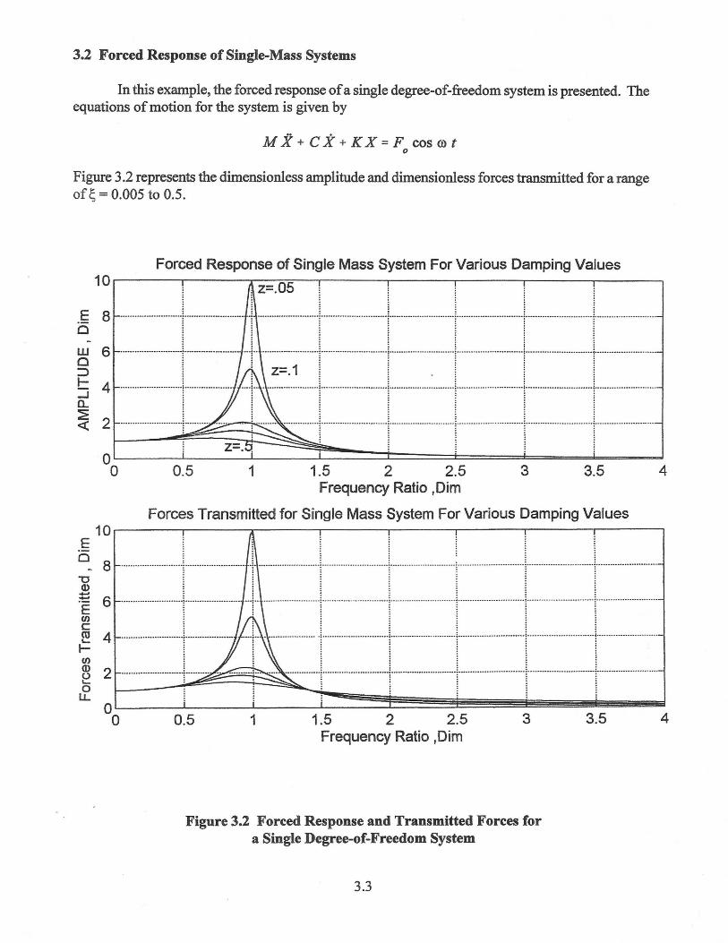
3.2 Forced Response of Single-Mass Systems

In this example, the forced response of a single degree-of-freedom system is presented. The equations of motion for the system is given by

M X + C X + K X = F cos co t 0

Figure 3 .2 represents the dimensionless amplitude and dimensionless forces transmitted for a range of~= 0.005 to 0.5.

10

E 8 Cl

w 6 Cl :::> r- 4 ...J a.. ~

2 <(

0 0

10 E Cl

8 "O Q) ..... ..... 6 .E Cl) C (lJ 4 I,...

..... (/) Q) 2 0 I,...

0 LL

0 0

Forced Response of Single Mass System For Various Damping Values

1 z=.05

I i I ! I I I ··························I ···················· ..•. : .. ·······················l····························l·················· ··········l·········· ····· ············.I.···························'··························

! 1 ! l ! I I 0.5 1 1.5 2 2.5 3 3.5

Frequency Ratio ,Dim

Forces Transmitted for Single Mass System For Various Damping Values

0.5 1 1.5 2 2.5 3 Frequency Ratio ,Dim

Figure 3.2 Forced Response and Transmitted Forces for a Single Degree-of-Freedom System

3.3

3.5

4

4

Table 3.2 Single Degree-of-Freedom Unbalance Response Script File

% Unbalance Response of single Degree of Freedom System % constant Forcing Function % E.J. Gunter Dept of Mech & Aerospace Engineering % A= amplitude vector for the various damping cases

% TRD = dynamic transmissibility = Ft/Fo

zeta=[0.05 0.1 0.2s 0.333 %freq=o:o.os:2; freq=linspace(0,4,200);

for k=1:s; z=zeta(k);

0.5];

for 1=1:200 % frequency sweep f=freq(l) ; f2=f•f; n1=(1. 0 -f2) A2; n2:(2*Z*f)-2; d =sqrt(n1 +n2); A(k,l)= 1.0/d ; % amplitude n=sqrt( 1 + n2); TRD(k,l)=n/d;

end; end; subpl.ot(2,1,1) plot(freq,A) grid xlabel(' Frequency Ratio ,Dim'); ylabel('AMPLITUDE, Dim'); title('Forced Response of Single Mass system For Various Dam.ping text(.B,.75, •z=.S'); text(1.1s,s,•z=.l'); text(l.OS,9.6,"z=.OS')

pause subplot(2,1,2) pl.ot(freq,TRD); hold on set(gca,'DefaultTextFont','Times','DefaultFontsize',14) grid xlabel(' Frequency Ratio ,Dim'); ylabel('Forces Transmitted, Dim'); title('Forces Transmitted for Single Mass system For various Dam.ping

In Table 3 .2, the calculation for the response was computed by using two nested do loops for k = 1 :5 for the five values of damping, and l = 1 :200 for the 200 values of the frequency. With 11M TLAB, one or more of the do or for loops may be condensed, but for those familiar with FORTRAN, one can write the program to be similar to FORTRAN. This procedure is recommended until one becomes more familiar with the compact 11M TLAB matrix statements.

In Figure 3.2, two plots are generated using the subplot command. Subplot(2,1,1) represents the first plot of two. The first plot is in the first column and first row. Subplot(2,1,2) represents the second plot in the second row. By using the subplot command, one may have as many plots on a page as desired. It should be noted that with the set command, one may change the font type and size.

3.4

Table 3.2 Single Degree-of-Freedom Unbalance Response Script File

% Unbalance Response of single Degree of Freedom system % constant Forcing Function % E.J. Gunter Dept of Mech & Aerospace Engineering % A= amplitude vector for the various damping cases

% TRD = dynamic transmissibility = Ft/Po

zeta=[o.os 0.1 0.25 0.333 %freq=O:O.OS:2; freq=linspace(0,4,200)i

for k=1:5; z=zeta C:lt) ;

0.5];

for 1=1:200 % frequency sweep f=freg(l) ;

end;

f2=f•f; n1=(1.o -f2)-2; D2:(2*Z*f) ~2; d =sqrt(n1 +n2); A(k,l)= 1.0/d ; % amplitude n=sqrt( 1 + n2); TRD(k,l)=n/d;

end; subplot(2,1,1) plot(freg,A) grid

pause

xlabel(' Frequency Ratio ,Dim'); ylabel('AHPLITUDE, Dim'); title('Forced Response of Single Mass system For various Damping text(.B,.75, •z=.S'); text(1.15,s,•z=.1'); text(1.05,9.6,'z=.0S')

subplot(2,1,2) plot(freq,TRD); hold on set(gca,'DefaultTextFont','Times','DefaultFontBize',14) grid xlabel{' Frequency Ratio ,Dim'); ylabel('Forces Transmitted, Dim'); title('Forces Transmitted for single Mass system For various Damping

In Table 3 .2, the calculation for the response was computed by using two nested do loops fork= 1 :5 for the five values of damping, and I= 1 :200 for the 200 values of the frequency. With MATLAB, one or more of the do or for loops may be condensed, but for those familiar with FORTRAN, one can write the program to be similar to FORTRAN. This procedure is recommended until one becomes more familiar with the compact MATLAB matrix statements.

In Figure 3.2, two plots are generated using the subplot command. Subplot(2,1,1) represents the first plot of two. The first plot is in the first column and first row. Subplot(2,1,2) reptesents the second plot in the second row. By using the subplot command, one may have as many plots on a page as desired. It should be noted that with the set command, one may change the font type and size.

3.4

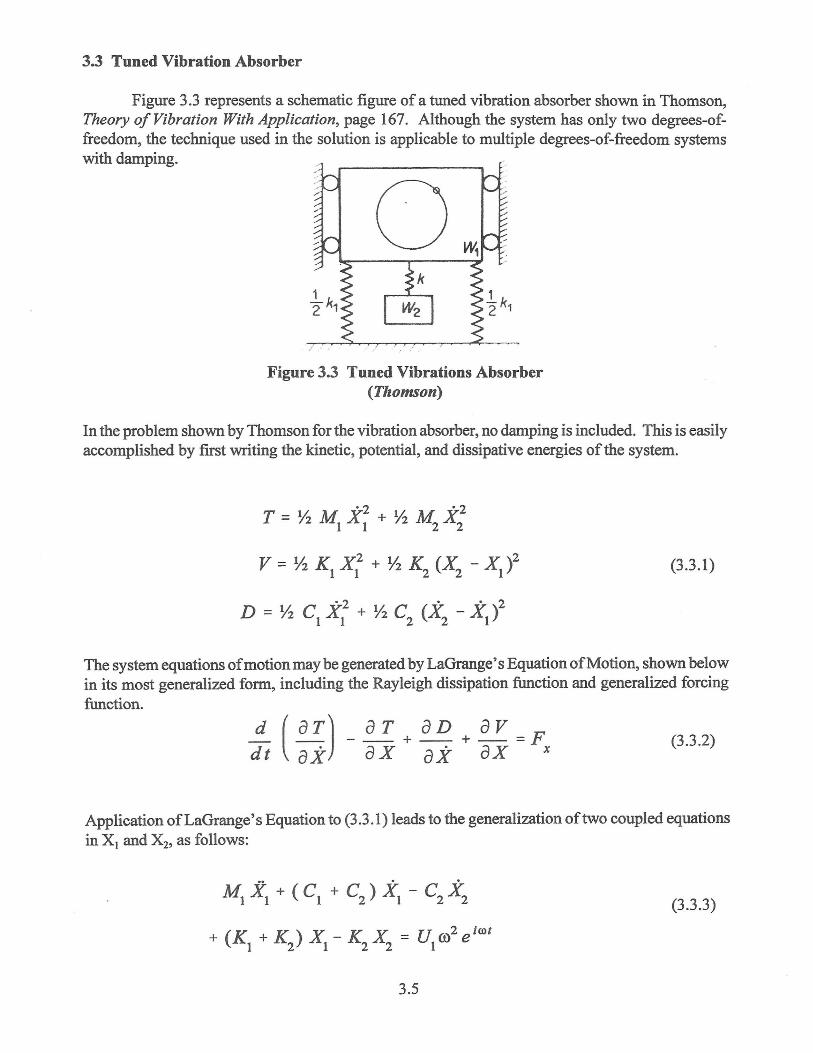
3.3 Tuned Vibration Absorber

Figure 3 .3 represents a schematic figure of a tuned vibration absorber shown in Thomson, Theory of Vibration With Application, page 167. Although the system has only two degrees-of­freedom, the technique used in the solution is applicable to multiple degrees-of-freedom systems with damping.

0 Figure 3.3 Tuned Vibrations Absorber

(Thomson)

In the problem shown by Thomson for the vibration absorber, no damping is included. This is easily accomplished by first writing the kinetic, potential, and dissipative energies of the system.

·2 ·2 T=½MX +½MX 1 1 2 2

(3.3.1)

• 2 • • 2 D=½CX +½C (X-X) I I 2 2 I

The system equations of motion may be generated by LaGrange' s Equation of Motion, shown below in its most generalized form, including the Rayleigh dissipation function and generalized forcing function.

d ( ar) dt ax

ar an av_F ---+ - -+ - --

ax ax ax x (3.3.2)

Application ofLaGrange's Equation to (3.3.1) leads to the generalization of two coupled equations in X1 and X2, as follows:

M1 .xI + ( c i + c2 ) xI - c2 x2 (3.3.3)

+ (K + K) X - K X = U al eirot 1 2 1 2 2 1

3.5

The general matrix form of the coupled linear equations of motion is

[M] {.X} + [C] {.X} + [K] {X} = 002 { U} eiwt (3.3.4)

Let X (t) =Xe icot for harmonic motion. The complex equations for forced response are

[ [ K] - ro2 [ M] + i ro [ C] ] {X} = ro2 { U} (3.3.5)

or

[A] {X} = {R} (3.3.6)

For the two degree-of-freedom problem shown with included damping, the complex a coefficients are given by

Table 3.3 represents the script file for the dynamic vibration absorber. The system is assumed to have a natural frequency at 1,850 RPM. The tuner is designed to be in resonance at 1,800 RPM, which is the operating speed of the rotor. The weight of the absorber is 50 lb and the weight of the rotor is 200 lb. The response is completed using two for loops for clarity to make the file similar to FORTRAN. The computation of the absolute value of the complex motion is achieved by using the·function abs.

3.6

Table 3.3 Vibration Absorber Script File

% V2dABS.M Vibration Absorber For Rotor Operating at 1800 rpm % Prob 5.37 pg 151 Thomson % Rotor Weight W1 =200 lb, W2=50 lb absorber weight % Absorber tuned for 1800 RPM % kl value tuned for critical speed at 1850 RPM % c2= absorber damper elf; clear W1:200; m2=W2/386; c2= [ 2 5

W2=50; m1=W1/386;

% Main weight & absorber weight

10 20 50 ]; % Values of damping-Lb-Sec/In Ntuned=1800 ; om2=(Ntuned/9.55)A2 k2= m2*om2 omcr=1850/9.55 kl=ml*omcr"'2 um::2.0/386

% %

%

absorber frequency tuned to running speed ;

Absorber spring rate tuned to 1800 RPM

% kl= major spring rate system

freq=linspace(1000,3000,200); for n=1:5;

for l=l:200; omega=freq(l)/9.55; omega2=(freq(l)/9.55 )"'2

% lb-in/g unbalance % Starting speed=1000 % Loop thru 5 damping % Loop thru 200 speed % Speed in Rad/sec

; %

tuned to 1850 RPM

,fina1=3000,200 cases values cases

fu=omega2*um ; % Rotating unbalance force, Lb a(1,1)= k1 + k2 -m1*omega2 a(2,1)=-k2 -i*omega*c2(n)

+ i*omega*c2(n) ; % Computer complex coef

a(l,2)= a(2,l) ; a(2,2)= k2-m2*omega2+ i*omega*c2(n) ; % influence coefficient matr: b=inv(a); % Invert complex matrix zl(n,l)=b(l,1)*fu ; zlmils(n,l)=abs(z1(n,1))*1000 ; z2(n,l)=b(2,l)*fu ; z2r(n,l)=zl(n,l)-z2(n,l) ; z2rmils(n,l)=abs(z2r(n,1))*1000; z2mils(n,l)=abs(z2(n,1))*1000; ftr=zl(n,l).*kl ; ftrans(n,l)=abs( £tr) ;

% Relative absorber motion % Amplitude in mils

% force traaansmmm.itted % trd(n,l)=k(n)/kd; % ftran(n,1)./fu ; % dynamic traansmissibility

end; end; subplot(2,1,1) plot(freq,zlmils, 1 linewidth 1 ,l), grid xlabel('Rotor Speed, RPM' ) ylabel( 'Amplitude, Mils') title( 1 RESPONSE With VARIOUS TUNED ABSORBER DAMPING VALUES') legend('C2=2','C2=5','C2=10','C2=20 1 , 1 C2=50 1 )

axis([l000 3000 0 800])

grid subplot(2,2,l) plot(freq,ftrans, 1 linewidth 1 ,l), xlabel('Rotor Speed, RPM' ) ylabel( 'Forces Transmitted title(• FORCES TRANSMITTED

, Lbs•)

axis( [ 1000 3000 0 3000 With Various ABSORBER DAMPER RATES') ] )

3.7

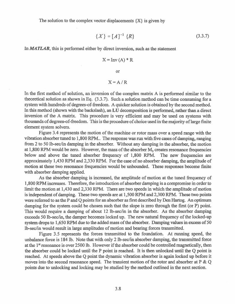
The solution to the complex vector displacements {X} is given by

(3.3.7)

In MATLAB, this is performed either by direct inversion, such as the statement

X=Inv(A) * R

or

X=A/R

In the first method of solution, an inversion of the complex matrix A is performed similar to the theoretical solution as shown in Eq. (3.3.7). Such a solution method can be time consuming for a system with hundreds of degrees-of-freedom. A quicker solution is obtained by the second method. In this method (shown with the backslash), an LU decomposition is performed, rather than a direct inversion of the A matrix. This procedure is very efficient and may be used on systems with thousands of degrees-of-freedom. This is the procedure of choice used in the majority oflarge finite element system solvers.

Figure 3.4 represents the motion of the machine or rotor mass over a speed range with the vibration absorber tuned to 1,800 RPM.. The response was run with five cases of damping, ranging from 2 to 50 lb-sec/in damping in the absorber. Without any damping in the absorber, the motion at 1,800 RPM would be zero. However, the mass of the absorber M2 creates resonance frequencies below and above the tuned absorber frequency of 1,800 RPM. The new frequencies are approximately 1,430 RPM and 2,330 RPM. For the case ofno absorber damping, the amplitude of motion at these two resonance frequencies would be unbounded. These responses become finite with absorber damping applied.

As the absorber damping is increased, the amplitude of motion at the tuned frequency of 1,800 RPM increases. Therefore, the introduction of absorber damping is a compromise in order to limit the motion at 1,430 and 2,330 RPM. There are two speeds in which the amplitude of motion is independent of damping. These two speeds are at 1,500 RPM and 2,300 RPM. These two points were referred to as the P and Q points for an absorber as first described by Den Hartog. An optimum damping for the system could be chosen such that the slope is zero through the first ( or P) point. This would require a damping of about 12 lb-sec/in in the absorber. As the absorber damping exceeds 50 lb-sec/in, the damper becomes locked up. The new natural frequency of the locked-up system drops to 1,650 RPM due to the added mass of the absorber. Damping values in excess of 50 lb-sec/in would result in large amplitudes of motion and bearing forces transmitted.

Figure 3.5 represents the forces transmitted to the foundation. At running speed, the unbalance force is 184 lb. Note that with only 2 lb-sec/in absorber damping, the transmitted force at the 1st resonance is over 2500 lb. However if the absorber could be controlled magnetically, then the absorber could be locked until the P point is reached. It is then unlocked until the Q point is reached. At speeds above the Q point the dynamic vibration absorber is again locked up before it moves into the second resonance speed. The transient motion of the rotor and absorber at P & Q points due to unlocking and locking may be studied by the method outlined in the next section.

3.8

RESPONSE Wrth VARIOUS TUNED ABSORBER DAMPING VALUES 140r---.--.----.--.---.---.-----,---.--~-~

-!----+----+-: +- c2k ! +-c2::i5

~C2~10 ~C2~0

I -t-~so '

.!!l i : __ ..;....__ -I'-- - r~=~---j ---1 ·--r---

Pooo 1200 1400

i

1600 1800 2000 2200 2400 2600 2800 3000 Rotor Speed, RPM

Figure 3.4 Amplitude of Rotor vs. Speed With Tuned Vibration Absorber for Various Values of Absorber Damping

FORCES TRANSMITTED Wrth Various ABSORBER DAMPER RATES

!

2500 . ---+--·i ~~~-----.-----\ Furb=t~ Lb t'eoo_R,__t_u_--+-_ i . .

I

~2000 l ...J

-0

4l! .E , ~ 1500 --·--·-·-···-· ..... ; - -l! . i I- .

I ------+-+--il------'--- i--

1

~ &1000

. ___ ____ ! - -···-· -

! ;

500 ----·---··· ...

1'boo 1200 1400 1soo 1aoo 2000 2200 2400 2600 2aoo 3000 Rotor Speed, RPM

Figure 3.5 Forces Transmitted vs. Speed For Various Values of Absorber Damping

3.9

3.4 Transient Response of Vibration Absorber

The initial transient motion of the absorber may be computed by writing the equations in state space formulation with four coupled first order equations in Y as follows

Y=f(Y,t) (3.4.1)

The derivatives of Y are given by

(3.4.2)

and the Y vector is given by

(3.4.3)

.MATLAB has a number of numerical integration procedures. In this example, the numerical integration function ODE23 will be used. This is a low order numerical integration routine based on a 2nd order Runge-Kutta integration method. For more information on this and other numerical methods, at the .MATLAB >> prompt type

>>help ODE23

In order to apply the function ODE23 or any of the other numerical integration procedures, a separate function file must be generated to have the derivatives of Y. The function file, called absorber.m is shown in Table 3.4. The first line of the function file must start with the word "function" and the file must be saved corresponding the function call. In this case, the file is saved as absorber.m. The function call differentiates the function file from the main body, which is a script file. The majority of the function calls of .MATLAB are ASCII files that may be modified.

Table 3.4 represents the functional file, which is stored as absorber.m. Note the important statements

[rows, cols] = size (y) yd= zeros (rows, cols)

These statements set dimension size and initialize the derivative matrix yd. The values of y(l) through y(4) are not single-valued functions, but are variable vectors with the dimension oft. As the absorber function is called, the variables are increased in dimension. The number of rows in the matrices yd and y are determined by the number of time steps. One has only to set the initial time (0) and the final time (I sec) and the increment and number of time steps are automatically computed. This is in considerable contrast to a FORTRAN program in which the size of the matrices must be initially set. This variable or dynamic dimensioning of the matrices is one of the powerful features of MATLAB. The author has encountered on many occasions the statement of DIMENSION

OUT OF BOUNDS in a FORTRAN transient analysis program.

3.10

Table 3.4 Function File for Absorber

function yd=absorber{t,y) % 2 mass system vibration absorber,Ml main mass, Kl main % M2 & K2 tuned to running speed at 1,800 RPM (omega=l94 % Her= system natural frequency at 1,850 RPM % y(2)=Xl motion, y(4)= X2 absorber absolute motion % y(l)=Xl velocity, y(3)= X2 absorber absolute velocity %global Ml M2 Kl K2 Cl C2 omega Fu Ml:200/386; M2=50/386; Cl:0.05; %Damping in rotor

stiffness rad/sec)

C2=2 ; %Relative damping in absorber Kl= 19444 omega=lS00/9.55; K2=M2*omega~2; Fu:200; [rows,cols]=size{y); yd=zeros(rows,cols);

% System spring lb/in-resonance at 1850 RPM % Operating speed, rad/sec % Absorber spring tuned to 1800 rpm % Applied Forcing function, Lb % * Set Matrix size, trows, 4 columns % * Set size matrix

% Specify the 1st order functional form yd(l)=-{(Cl+C2)*y(l)-C2*y{3) +(Kl+K2)*y(2)-K2*y{4))/Ml+Fu*sin(omega*t)/Ml; yd(2)= y{l); % Xl velocity yd{3)=-( C2*( y{3)-y{l) ) + K2*( y{4) -y{2) ) )/M2; % X2 acceleration yd(4)=y(3); % X2 velocity % end absorber function

Table 3.5 represents the main program or script file that calls the numerical integration procedure ODE23. Note that ODE23 calls the function absorber which contains the system first order derivatives. The response is plotted for one sec of motion, as shown in Figure 3.6. The first plot, using the sllbplo( command, is for the motion of the major mass. The array y (:;2) represents the second column, which is the motion ofX1 for all the time values. In Figure 3.6, the top figure represents the major mass.

It is seen that the maximum amplitude of motion after two cycles is approximately± 20 mils. After one sec of motion, the amplitude reduces to ± 4 mils. In this example, an absorber damper value of C2 = 2 lb-sec/in was assumed. Although the steady state response of the rotor mass is less than 4 mils, it is seen that the sudden application of the dynamic load may cause excessive amplitudes of motion. Therefore the final damping selected for the absorber may be a compromise based on range of operation and transient considerations.

The second figure represents the absolute motion of the absorber. Note that after two cycles of motion, the absorber peak amplitude is over ± 70 mils of motion. Thus, the absorber transient motion is almost four times as great as the main mass. After one sec of motion, the system is approaching steady-state conditions in which the absorber is moving with± 40 mils of motion. In Fig 3.6 (b) there appears to be a beating motion caused by the suddenly applied unbalance. This nature of the beating motion may be evaluated by performing an FFT analysis on the absorber.

3.11

Table 3.5 Script File Tranabs.m for Transient Analysis

% tranabs.m transient motion of two mass absorber with suddenly % applied unbalance % 11/19/96 E.J. Gunter % y(2)= xl main mass motion, y(4)= x2 absorber motion % global Ml M2 Kl K2 Cl C2 omega Fu elf clear Ml=200/386; % main mass M2=50/386 ; Cl=0.05 ; C2=2.0 ; N= 1800; omega=N/9.55 ; IC2=M2*omega"'2 ; Kl:19444 ; Fu=200

% speed rad/sec % tuned absorber to running speed % resonance at 1850 RPM original

t0=0.0 ; tf= 1.0 ; % initial & final time % set initial conditions as column vector yo = [ 0 • 0 ; 0 • 0 ; 0 • 0 ; O • 0] ; % v1 , xl , v2 , x2 [t,y]=ode23( 1 absorber 1 ,t0,tf,y0) ; % Call Numerical integrater

subplot(2,l,l) plot(t,y(:,2)*1000, 1 linewidth 1 ,l.S),grid xlabel('Time, Sec•) ylabel( 1 Amplitude, Mils') title('Motion With Suddenly Applied Unbalance With Tuned Absorber,C2=2')

subplot(2,l,2) plot(t,y(:,4)*1000,•linewidth•,l.S),grid xlabel('Time, Sec•) ylabel('Amplitude, Mils') title ( '~sorb~r Motion With !3ulf<ienlv Jlppl:i,P<i Unbalance , C2=2 •)

The classical method of solution of a transient response is by means of a convolution integral of the

form:

For the case of a damped single degree of freedom system, the convolution function of the integral

equation, h(t) is given by:

The convolution integral is difficult to evaluate for even the simplest of forcing functions. The theory also is applicable only to linear systems. For more complex systems, a damped eigenvalue analysis of the roots is first required. Therefore the classical method of transient analysis by convolution integral is obsolete. It should also be pointed out that a computer program is always required to plot out the results. MATLAB has a variety of equation solvers to handle nonlinear and

stiff equations.

3.12

Motion With Suddenly Applied Unbalance With Tuned Absorber,C2=2 20..---..----,----,----..----.---.-----.-----.---....--~

. . 10

. . -ilw---•-· ·.. -............. ~_ ; ..................... --.j ..... . . ............... i.--.................... c---------------.. ··-· · ...................... ;. .......................................... .. .

: i ' ! ! ! ! !

0 .. .... ---- .. ... .... ... .. ...... .. ... .. --1 .. .... ..

-20 I i I l 1

\ ; ! I I I I ! i i -30 .__ __ .,___ __ .,___ __ .,___ __ .,___ __ .,___ __ ,...._ __ ,...._ __ ,...._ __ .,___ _ ___,

0.2 0.3 0.4 0.5 0.6 Time, Sec

0.7 0.8 0.9 1 0 0.1

(a) Initial Transient Motion of Rotor For 1 Second

(b) Initial Transient Motion of Absorber For 1 Second

Figure 3.6 Transient Motion of Rotor and Absorber With Suddenly-Applied Unbalance

3.13

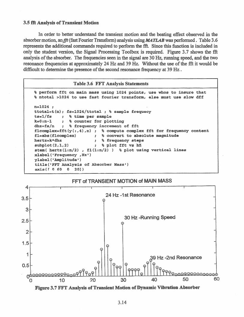
3.5 fft Analysis of Transient Motion

In order to better understand the transient motion and the beating effect observed in the absorber motion, an/ft (fast Fourier Transform) analysis using MATLAB was performed . Table 3.6 represents the additional commands required to perform the fft. Since this function is included in only the student version, the Signal Processing Toolbox is required. Figure 3.7 shows the fft analysis of the absorber. The frequencies seen in the signal are 30 Hz, running speed, and the two resonance frequencies at approximately 24 Hz and 39 Hz. Without the use of the fft it would be difficult to determine the presence of the second resonance frequency at 39 Hz.

Table 3.6 FFT Analysis Statements

% perform fft on main mass using 1024 points, use whos to insure that % ntotal >1024 to use fast fourier transform, else must use slow dff

n:1024; ttotal=t(n); fs=l024/ttotal; % sample frequecy ts=l/fs ; % time per sample k=0:n-1 % counter for plotting dhz=fs/n ; % frequency increment of £ft flcomplex=fft(y(:,4),n) ; % compute complex fft for frequency content fl=abs(flcomplex) ; % convert to absolute magnitude hertz=k*dhz ; % frequency steps subplot(2,1,2) ; % plot fft vs hZ stem( hertz(l:n/2) , fl(l:n/2) ) % plot using vertical lines xlabel('Frequency ,Hz') ylabel('Amplitude') title('FFT Analysis of Absorber Mass•) axis(r 0 60 o 20])

FFT of TRANSIENT MOTION of MAIN MASS 4.--------,r------~-------,---------.------.-------,

3.5

3

2.5

2

1.5

1

24 Hz -1st Resonance

30 Hz -Running Speed

Figure 3. 7 FFT Analysis of Transient Motion of Dynamic Vibration Absorber

3.14

ACKNOWLEDGMENT

The author wishes to acknowledge Robert L. (Rob) Howes, Senior Engineer- Acoustics and Vibrations of Cessna Aircraft, Wichita, Kansas for demonstrating to me the various applications of MATLAB in the aerospace industry and directing me towards the study and application ofthis language to vibration analysis and data processing.

REFERENCES

1. Bathe, K., and Wilson, E.L., Numerical Methods in Finite Element Analysis, Prentice-Hall, Englewood Cliffs,NJ, 1976

2. Biran, A. and Breiner, M .. , MATLAB For Engineers, Addison-Wesley Publishers, Ltd, Great Britain, 1995 ..

3. Den Hartog, J.P., Mechanical Vibrations, McGraw-Hill, Inc.,New York,NY, pp 112-132 4. Diamarogonas,A., Vibration For Engineers, Prentice Hall, Upper Saddle River, NJ, 1995 5. Ehrich, F. F., editor, Handbook of Rotordynamics, McGraw-Hill, Inc., New York, NY,

1992. 6. Genta, G., Vibration of Structures and Machines, Springer-Verlag ,New York,NY, 1995 7. Gunter, E.J., "Rotor Dynamics on The Minicomputer", Proceedings Vibration Institute,

April 1981 8. Gunter,E.J., and Sharp,W.L.,"Minicomputer Aids Rotor Research ",Industrial Research and

Development, May 1981,pp. 122-127 9. Hanselman, D. and Littlefield, B., Mastering MATLAB 5, Prentice-Hall, Inc., Englewood

Cliffs, NJ, 1998. 10. Hildebrand, F.B., Methods of Applied Mathematics, Prentice Hall Englewood Cliffs, NJ,

1960 11. Kramer,E., Dynamics of Rotors and Foundations Springer-Verlag ,New Y ork,NY, 1993 12. Kwon, Y. W. and Bang, H., The Finite Element Method Using MATLAB, CRC Press, Inc.,

Boca Raton, FL, 1997. 13. Leonard, N. E. and Levine, W. S., Using MATLAB to Analyze and Design Control

Systems, Addison-Wesley Publishers, Redwood City, CA, 1995. 14. Myklestad, N. 0., Fundamentals of Vibration Analysis, McGraw-Hill, New York, NY,

1956 15. Moler, C. and Costa, P. J., MATLAB Symbolic MathToolbox, The Math Works, Inc.,

Natick, MA, 1997 . . 16. Sigmon, Kermit, MATLAB Primer, Fifth Edition, CRC Press, Boca Raton, FL, 1998. 17. The Math Works, Inc., MATLAB User's Guide, The Math Works, Inc., Natick, MA, 1993. 18. Thomson, W. T., Theory of Vibration With Applications, Fourth Edition, Prentice-Hall,

Inc., Englewood Cliffs, NJ, 1993. 19. Wilson, H.B., and Turcotte, Louis H., Advanced Mathematics and Mechanics Applications

Using MATLAB, CRC Press, Inc., Boca Raton, FL, 1994.