AN INTELLIGENT WORKSTATION CONTROLLER FOR

COMPUTER INTEGRATED MANUFACTURING

A Dissertation

by

HYUNBO CHO

Submitted to the Office of Graduate Studies of

Texas A&M University in partial fulfillment of the requirements for the degree of

DOCTOR OF PHILOSOPHY

December 1993

Major Subject: Industrial Engineering

AN INTELLIGENT WORKSTATION CONTROLLER FOR

COMPUTER INTEGRATED MANUFACTURING

A Dissertation

by

HYUNBO CHO

Submitted to Texas A&M University in partial fulfillment of the requirements

for the degree of

DOCTOR OF PHILOSOPHY

Approved as to the style and content by:

Richard A. Wysk

(Chair of Committee)

Don T. Phillips (Member)

Jeffrey S. Smith (Member)

John E. Mayer, Jr. (Member)

Way Kuo

(Department Head)

December 1993

Major Subject: Industrial Engineering

iii

ABSTRACT

An Intelligent Workstation Controller for Computer Integrated Manufacturing.

(December 1993)

Hyunbo Cho

B.S., Seoul National University;

M.S., Seoul National University

Chair of Advisory Committee: Dr. Richard A. Wysk

A shop floor control system (SFCS), a central part of a computer integrated manufacturing

system, performs the production activities required to fill orders. In order to effectively control these

activities, it is necessary to define a control architecture and functional perspective of how a SFCS

operates. In this research, a hierarchical SFCS (shop, workstation, equipment) is adopted. In the

context of the hierarchical control architecture, each level fulfills its own responsibility using

planning, scheduling, and execution functions. The objective of the research is to develop an

intelligent workstation controller (IWC) at the middle level of a SFCS. The IWC is responsible for

selecting a specific process routing, allocating resources, scheduling and coordinating the activities

across the equipment, monitoring the progress of activities, detecting and recovering from errors,

and preparing reports. The requirements necessary for the development of the IWC are to create a

process plan representation model, to specify the evolution of a process plan from the shop down to

the equipment, and to define and implement all the functions to be integrated into an intelligent

controller. A deadlock detection and resolution model is also presented to maintain the system in a

deadlock-free state. Finally, the IWC software is created to demonstrate the architectural linkages

with other controllers. As a result, the development of the IWC will save cost and time in

developing control software for the automated manufacturing systems.

iv

DEDICATION

This dissertation is dedicated to

my wife, Aran,

my son, Charles,

my parents, and

my parents-in-law.

v

ACKNOWLEDGMENT

This dissertation could not have been successfully completed without the help and encouragement of my wife, Aran, who stood by me during a long and painful Ph.D. program. I would like to take this opportunity to express my appreciation for her endless love and sacrifice during her pregnancy. I would also like to acknowledge my parents and parents-in-law for their spiritual and financial support. Special thanks must also given to other members of my family. I would like to thank my committee chairman, Dr. Richard A. Wysk, for his constructive guidance, advice, and encouragement during this dissertation. He also provided academic counseling and taught me some of what it means to be a manufacturing engineer throughout my degree program. In particular, it was my pleasure to travel, ski, drink beer with him. Thanks are also extended to the other members of my dissertation committee: Drs. Don T. Phillips, John, E. Mayer, Richard J. Mayer, and Jeffrey S. Smith. Their guidance, suggestions, and comments helped me pursue a career as a healthy researcher. I would also like to express my appreciation to my colleagues, Annap, Trevor, Kumaran whose suggestions and co-work were extremely helpful and precious. I am also indebted to the individual members of a DARPA project group. My experience in manufacturing systems has been enriched through discussion with some of the best names in shop floor control (Drs. R. A. Wysk, A. Jones), process planning (Drs. R. A. Wysk, S. Joshi, S. R. Ray), simulation (Dr. D. Pegden), and ontology and system analysis (Dr. R. Mayer).

vi

TABLE OF CONTENTS

Page ABSTRACT....................................................................................................................... iii DEDICATION ................................................................................................................... iv ACKNOWLEDGMENT ......................................................................................................v TABLE OF CONTENTS .................................................................................................... vi LIST OF TABLES.............................................................................................................. ix LIST OF FIGURES..............................................................................................................x CHAPTER

I. INTRODUCTION ......................................................................................................1 I.1 Computer Integrated Manufacturing......................................................................1 I.2 Architecture of Shop Floor Control........................................................................3 I.3 Functionality of Shop Floor Control........................................................................4 I.4 Objectives ...........................................................................................................5 I.5 Motivation ...........................................................................................................6 I.6 Assumptions ........................................................................................................7 I.7 Organization of Dissertation..................................................................................7

II. LITERATURE REVIEW..........................................................................................8 II.1 Chapter Overview ..............................................................................................8 II.2 Control Architecture for Shop Floor Control .........................................................8

II.2.1 Centralized Control Architecture ...........................................................9 II.2.2 Hierarchical Control Architecture..........................................................9 II.2.3 Heterarchical Control Architecture...................................................... 13 II.2.4 Hybrid Control Architecture................................................................ 14

II.3 Temporal Decomposition within Each Level....................................................... 14 II.4 Chapter Summary............................................................................................. 18

III. OVERVIEW AND GENERAL CONCEPT...........................................................19 III.1 Chapter Overview........................................................................................... 19 III.2 Process Plan and Shop Floor Control................................................................ 19 III.3 Development of an Execution Function ............................................................. 20 III.4 Development of a Planning Function................................................................. 22 III.5 Development of a Scheduling Function.............................................................. 23 III.6 Development of a Deadlock Resolution Model.................................................. 25 III.7 Integration of Planning, Scheduling, and Execution............................................. 26 III.8 Chapter Summary ........................................................................................... 27

IV. PROCESS PLAN AND SHOP FLOOR CONTROL.............................................28 IV.1 Chapter Overview........................................................................................... 28 IV.2 Literature Survey............................................................................................ 28 IV.3 Process Plan Representation............................................................................ 29

IV.3.1 AND/OR Graph Representation........................................................ 30 IV.3.2 Example for Process Plan Representation .......................................... 32 IV.3.3 ISO Process Plan Model................................................................... 36

IV.4 Evolution of a Process Plan in a Shop Floor ...................................................... 37 IV.5 Example for Evolution of a Process Plan .......................................................... 40 IV.6 Chapter Summary........................................................................................... 42

vii

TABLE OF CONTENTS (continued)

Page V. PLANNING FUNCTION.........................................................................................44

V.1 Chapter Overview............................................................................................ 44 V.2 Framework and Problem Statement................................................................... 44 V.3 Related Work................................................................................................... 46 V.4 Shop Level Planning Function............................................................................ 47 V.5 Workstation Level Planning Function ................................................................. 48

V.5.1 Pruning of Workstation Form Feature Graph........................................ 50 V.5.2 Disaggregation of Workstation Form Feature Graph............................. 50 V.5.3 Generation of Workstation Plan Graph ................................................ 51 V.5.4 Generation of Operation Sequence Graph............................................ 52

V.6 Equipment Level Planning Function ................................................................... 60 V.7 Chapter Summary ............................................................................................ 61

VI. SCHEDULING FUNCTION..................................................................................62 VI.1 Chapter Overview........................................................................................... 62 VI.2 Framework and Problem Statement.................................................................. 62 VI.3 Related Work ................................................................................................. 70

VI.3.1 Mathematical Programming Technique .............................................. 71 VI.3.2 Scheduling Rules and Heuristics ........................................................ 71 VI.3.3 Real-time Scheduling Based on Simulation.......................................... 72 VI.3.4 Miscellaneous Approaches................................................................ 72 VI.3.5 Background of a Neural Network...................................................... 73

VI.4 Construction of a Neural Network as a Rule Selector ........................................ 75 VI.5 Multi-pass Simulator ........................................................................................ 78 VI.6 Event Generator.............................................................................................. 80 VI.7 Chapter Summary........................................................................................... 81

VII. DEADLOCK DETECTION AND RESOLUTION..............................................83 VII.1 Chapter Overview ......................................................................................... 83 VII.2 Taxonomy of System Deadlocks ..................................................................... 83

VII.2.1 Part Flow Deadlock......................................................................... 83 VII.2.2 Processing Resource Deadlock........................................................ 85 VII.2.3 Material Handler Deadlock.............................................................. 87

VII.3 Graph Preparation for Deadlock Detection ...................................................... 88 VII.4 Detection of Part Flow Deadlocks .................................................................. 91 VII.5 Detection of Impending Part Flow Deadlocks .................................................. 92 VII.6 Deadlock Resolution Scheme.......................................................................... 98 VII.7 Chapter Summary........................................................................................ 102

viii

TABLE OF CONTENTS (continued)

Page VIII. EXECUTION FUNCTION ...............................................................................103

VIII.1 Chapter Overview ...................................................................................... 103 VIII.2 Framework and Problem Statement ............................................................. 103 VIII.3 Related Work............................................................................................. 106 VIII.4 Definition of State Variables........................................................................ 108 VIII.5 Execution Function of the IWC.................................................................... 108

VIII.5.1 Interactions with a Shop Controller................................................ 111 VIII.5.2 Interactions with Equipment Controllers......................................... 113

VIII.6 Execution Function of the Equipment Controller............................................ 114 VIII.6.1 Execution Function for Machine Tools ........................................... 115 VIII.6.2 Execution Function for Robots ...................................................... 118

VIII.7 Chapter Summary....................................................................................... 120 IX. EXPERIMENTAL RESULTS AND CONCLUSION..........................................122

IX.1 Chapter Overview......................................................................................... 122 IX.2 Various Factors Affecting the Effectiveness of the IWC ................................. 122 IX.3 Experimental Design...................................................................................... 124

IX.3.1 Experimental Complexities and Assumptions..................................... 124 IX.3.2 Factorial Design.............................................................................. 125 IX.3.3 Performance Measure Used in the Experiment................................. 128 IX.3.4 Texas A&M CIM Lab.................................................................... 128 IX.3.5 Sample Part and Its Process Plan .................................................... 129 IX.3.6 Description of the Simulation Model................................................. 131

IX.4 Experimental Results ..................................................................................... 132 IX.4.1 Experimental Results for Average Flow Time ................................... 132 IX.4.2 Experimental Results for Throughput................................................ 133 IX.4.3 Experimental Results for Average Tardiness .................................... 134

IX.5 Sample Session of the IWC Software ............................................................. 135 IX.6 Conclusion of Dissertation.............................................................................. 136 IX.7 Further Research Topics................................................................................ 138 IX.8 Chapter Summary ......................................................................................... 139

REFERENCES ..............................................................................................................140 VITA ..............................................................................................................................153

ix

LIST OF TABLES

Page Table I.1 Functionality of a shop floor control system..............................................................5 Table III.1 Brief procedure of the planning function .............................................................. 23 Table III.2 Set of decision problems for shop floor control..................................................... 24 Table III.3 Taxonomy of system deadlocks for shop floor control........................................... 26 Table IV.1 Evolution of a process plan for shop floor control................................................. 38 Table V.1. Taxonomy of the planning function for shop floor control...................................... 45 Table VI.1 Inputs to and outputs from the scheduling function ............................................... 63 Table VI.2 Definition of workstation level entities for scheduling............................................ 63 Table VI.3 Characteristics of the input vector....................................................................... 77 Table VI.4 Set of messages and their parameters and description .......................................... 81 Table VII.1 Illustration of deadlock in operating systems ....................................................... 87 Table VIII.1 Taxonomy of the execution function for shop floor control ............................... 104 Table VIII.2 State variables used for the IWC and equipment controllers ............................. 108 Table VIII.3 Messages and their description for the IWC.................................................... 109 Table VIII.4 Messages and their specifications for the IWC................................................ 110 Table VIII.5 Messages and their description for a machine controller................................... 115 Table VIII.6 Messages and their specifications for a machine controller............................... 115 Table VIII.7 Messages and their description for a robot controller ....................................... 118 Table VIII.8 Messages and their specifications for a robot controller ................................... 118 Table IX.1 Design factors from the IWC's viewpoint .......................................................... 123 Table IX.2 Exogenous factors from the IWC's viewpoint .................................................... 124 Table IX.3 Assumptions for the demonstration of the IWC.................................................. 125 Table IX.4 Design matrix for data collection plan................................................................ 126 Table IX.5 Performance criteria used in the current experiment........................................... 128 Table IX.6 Experiment results for average flow time........................................................... 132 Table IX.7 Student's t-test for average flow time ................................................................ 132 Table IX.8 Experiment results for throughput...................................................................... 133 Table IX.9 Student's t-test for throughput ........................................................................... 133 Table IX.10 Experiment results for average tardiness.......................................................... 134 Table IX.11 Student's t-test for average tardiness ............................................................... 134

x

LIST OF FIGURES

Page Figure I.1 Integrated engineering wheel (Wysk [234]).............................................................1 Figure I.2 Texas A&M University CIM Lab ..........................................................................2 Figure I.3 Hierarchical shop floor control system (Joshi et al. [114]).........................................3 Figure I.4 Interactions between the control levels of the SFCS.................................................4 Figure II.1 Taxonomy of shop floor control architecture ..........................................................9 Figure II.2 AMRF control hierarchy..................................................................................... 10 Figure II.3 Trends of the manufacturing cell ......................................................................... 11 Figure II.4 CAM-i control hierarchy..................................................................................... 12 Figure II.5 Taxonomy of the functional decomposition method............................................... 14 Figure II.6 Three functions and their relationship (Joshi et al. [114])....................................... 15 Figure II.7 Three main functions and their activities (Jones and Saleh [111])........................... 16 Figure II.8 ESPRIT control structure (Boulet et al. [27]) ....................................................... 17 Figure II.9 Multi-blackboard structure for control (O'Grady and Lee [165]) ............................ 17 Figure II.10 Schematic overview of the five functions (Davis et al. [52])................................ 18 Figure III.1 Detailed message flow in the IWC..................................................................... 21 Figure III.2 IWC software testing environment..................................................................... 27 Figure IV.1 Illustrative example for three different kinds of alternatives ................................. 31 Figure IV.2 AND/OR graph representation of form features................................................. 31 Figure IV.3 Data structure for a form feature graph ............................................................. 32 Figure IV.4 Off-line process planning activity ....................................................................... 33 Figure IV.5 Illustrative rotational component......................................................................... 33 Figure IV.6 The set of design features making up the polyshape ............................................ 34 Figure IV.7 Design feature graph for the set of design features ............................................. 34 Figure IV.8 Consideration of tool access direction and depth of cuts ...................................... 35 Figure IV.9 Illustration of the union and decomposition of design features............................... 35 Figure IV.10 Form feature graph converted from a design feature graph................................ 35 Figure IV.11 STEP file of the ISO process plan model.......................................................... 36 Figure IV.12 Form feature graph decomposition in planning................................................... 37 Figure IV.13 Data structure for a shop level plan graph......................................................... 38 Figure IV.14 Data structure for a workstation level plan graph .............................................. 39 Figure IV.15 Example part for the evolution of a process plan ............................................... 40 Figure IV.16 Form feature graph for the example part .......................................................... 40 Figure IV.17 Form feature graph decomposition at shop level................................................ 41 Figure IV.18 Form feature graph decomposition at workstation level...................................... 42 Figure IV.19 Form feature graph decomposition at equipment level........................................ 42 Figure IV.20 Irregular and regular AND/OR graphs ............................................................. 43 Figure V.1 Comparison of problem reduction and form feature representation ........................ 49 Figure V.2 Scheme of the planning function.......................................................................... 49 Figure V.3 Illustration of a workstation form feature graph.................................................... 50 Figure V.4 Modified workstation form feature graph............................................................. 51 Figure V.5 The disaggregation of the workstation form feature graph..................................... 51 Figure V.6 Workstation plan graph obtained from a form feature graph.................................. 52 Figure V.7 Generation of operation sequence graphs............................................................. 52 Figure V.8 Structure of operation sequence graphs ............................................................... 53 Figure V.9 Three different cases for material handling activities ............................................ 54 Figure V.10 Two different subcases for case 1 in Figure V.9 ................................................ 54 Figure V.11 Illustrative example for heuristic V.1 ................................................................. 56

xi

LIST OF FIGURES (continued)

Page Figure V.12 Illustrative example for heuristic V.2 ................................................................. 59 Figure V.13 Illustrative example for heuristic V.3 ................................................................. 59 Figure VI.1 Illustrative example of scheduling problem I........................................................ 65 Figure VI.2 Illustrative example of scheduling problem II ...................................................... 66 Figure VI.3 Illustrative example of scheduling problem III ..................................................... 66 Figure VI.4 Illustrative example of scheduling problem IV..................................................... 67 Figure VI.5 Illustrative example of scheduling problem V...................................................... 68 Figure VI.6 Detailed scheme of the scheduling function ........................................................ 69 Figure VI.7 Processing neuron in a neural network............................................................... 74 Figure VI.8 Schematic overview of the role of the neural network......................................... 76 Figure VI.9 Input and output layers in the neural network...................................................... 77 Figure VI.10 Detailed flow chart of the multi-pass simulator .................................................. 79 Figure VI.11 Detailed flow chart of the event generator ........................................................ 81 Figure VII.1 Example of a part flow deadlock ...................................................................... 84 Figure VII.2 Example of an impending part flow deadlock..................................................... 85 Figure VII.3 Example of a potential impending part flow deadlock ......................................... 85 Figure VII.4 Example of a processing resource deadlock ...................................................... 86 Figure VII.5 Deadlock caused by different class of resources ............................................... 86 Figure VII.6 Material handler deadlock caused by AGVs...................................................... 87 Figure VII.7 Material handler deadlock caused by robots ...................................................... 88 Figure VII.8 Illustration of system status graphs ................................................................... 89 Figure VII.9 Illustration of three bounded circuits.................................................................. 90 Figure VII.10 Graphical illustration of a part flow deadlock.................................................... 92 Figure VII.11. Bounded circuit with one empty common node ............................................... 93 Figure VII.12 Bounded circuit with more than one empty common node................................. 94 Figure VII.13 Illustration of no impending part flow deadlock................................................. 95 Figure VII.14 Example of a non-empty common node which is not blocked............................ 97 Figure VII.15 Example of a non-empty common node which is blocked.................................. 98 Figure VII.16. Heuristic yields 'deadlock', but (a) is not in deadlock........................................ 98 Figure VII.17 Flow diagram to resolve (impending) part flow deadlocks ................................. 99 Figure VII.18 Example for deadlock resolution using recovery............................................. 101 Figure VII.19 Example of part flow deadlock interactions.................................................... 101 Figure VII.20 Two system status graphs for operation sequence alternatives........................ 102 Figure VIII.1 Control flow in the hierarchical control architecture ........................................ 104 Figure VIII.2 Conceptual framework for generating components ......................................... 107 Figure VIII.3 Schematic procedure for the execution function of the IWC............................ 109 Figure VIII.4 Messages for the execution function of the IWC............................................ 111 Figure VIII.5 Control and information flow for a new part................................................... 112 Figure VIII.6 Control and information flow for a finished part.............................................. 112 Figure VIII.7 Decomposition method of a rtransfer() message............................................. 113 Figure VIII.8 Decomposition method of a mtransfer() message ........................................... 114 Figure VIII.9 Decomposition method of a move() message ................................................. 114 Figure VIII.10 Messages and their flow diagram for the equipment controllers ..................... 115 Figure VIII.11 Execution graph for a load() message .......................................................... 116 Figure VIII.12 Execution graph for an unload() message ..................................................... 117

xii

LIST OF FIGURES (continued)

Page Figure VIII.13 Execution graph for sdone() and goahead() messages................................... 117 Figure VIII.14 Execution graph for a pick() message .......................................................... 119 Figure VIII.15 Execution graph for a put() message............................................................ 119 Figure VIII.16 Example of synchronization......................................................................... 120 Figure IX.1 Processing workstations in the Texas A&M University CIM Lab ...................... 129 Figure IX.2 Illustrative part for experiment ......................................................................... 130 Figure IX.3 Workstation level plan graph for the illustrative part........................................... 130 Figure IX.4 Detailed scheme of the simulation model.......................................................... 131 Figure IX.5 Illustrative file structure for a workstation level plan graph................................. 136

1

______________________________________ This dissertation follows the format requirements for the IIE Transactions.

CHAPTER I

INTRODUCTION I.1 Computer Integrated Manufacturing Computer integrated manufacturing (CIM) can be defined as an integrated system of manufacturing, business and other engineering functions through the use of a set of computers (Brown et al. [29], Chang et al. [37], Gatelmand [76], Gunasekaran [85]). CIM has provided the necessary flexibility to enable manufacturers to produce substantial benefits including lower manufacturing costs, rapid change to customer demands, improved and shortened lead times, increased quality of products (Miller and Walker [153], Sethi and Sethi [193], Slack [201]). All of the engineering functions in CIM, including design engineering, process planning engineering, and production engineering, play a crucial role in achieving the integration requirements between functions. Figure I.1 illustrates an integrated view of engineering (Wysk [234]).

FunctionCost, Weight User, etc.

Specification

Product Engineering

Raw Material

Processing

Assembly

Parts

A

B

C

Planning Design Control

Process Engineering

Production Engineering

Performance

Capabilities

Manufacturability

Product

Figure I.1 Integrated engineering wheel (Wysk [234])

2

Product engineering is responsible for the creation of the product model. The product model may be developed based on customer specifications and production costs. The product model may also be specified by means of component drawings, tolerance specifications, and a bill of material. Process engineering begins with the initial product model to develop a set of process plans used to produce the product. The process plan contains the sequence of the individual processing and assembly operations, resource requirements, and various machining parameters. Producability and manufacturability would be analyzed in this stage so that the set of features that is difficult to produce is returned to the product engineer. Production engineering is responsible for all of the manufacturing activities including plant design and analysis, material requirements planning, capacity resource planning, quality control, shop floor control, and so forth. Inconsistent process plans and design anomalies may be identified by the production engineer. (Chang et al. [37], Groover [84]). Among the production engineering functions, this research focuses on a shop floor control system (SFCS) which is a central part of a CIM system necessary to control the progress of production in a shop floor. For example, Figure I.2 depicts a shop floor located at Texas A&M University. The SFCS is concerned with various activities of several pieces of manufacturing equipment, such as machining, assembly, material handling and storage, inspection. The manufacturing equipment includes processing equipment (e.g., NC machining center), assembly equipment (e.g., carousel assembly machine), material handling equipment (e.g., robot), material transport equipment (e.g., conveyor), material storage equipment (e.g., AS/RS). The distinction between the material handling equipment and the material transport equipment is that the former can pick, move, and put parts, while the latter can only be used to move parts. In other words, the material handling equipment needs to serve the material transport equipment in order to load and unload parts.

Pratt&Whitney Machining

CenterLeadwell Turning Center

Sabre 500 Machining

Center

Kardex Mini

AS/RS

Adept

Shuttleworth Conveyor

Puma 760

GE-A4 Figure I.2 Texas A&M University CIM Lab.

3

I.2 Architecture of Shop Floor Control

The SFCS receives product orders provided by the business system. The related process plans are provided by the process planning engineer, and the product models are provided by the product engineer. The product orders may contain due-date, quantity, priority and so on. The SFCS is then responsible to coordinate the activities necessary to process the product orders across the equipment within the manufacturing facility. Specifically, the SFCS is responsible for selecting a specific process routing, allocating resources, scheduling the work pieces, downloading the processing instructions (e.g., RS-274 instructions for NC machines, VAL II programs for robot), monitoring the progress of activities, detecting and recovering from errors, and preparing reports on the status of the manufacturing system. It seems very difficult to integrate all of these activities within a control component. This results in three decomposition techniques which have been proposed to create a series of well-defined solvable problems: hierarchical, heterarchical, and hybrid. In this research, a three level hierarchical SFCS (shop, workstation, equipment) is adopted as shown in Figure I.3.

Shop

Workstation

Equipment

Workstation Workstation

Equipment Equipment Equipment Equipment Equipment

Figure I.3 Hierarchical shop floor control system (Joshi et al. [114]) The hierarchical SFCS is based on the lower three levels of the five-level control architecture developed in the National Institute of Standards and Technology (NIST) (Albus et al. [7], Jones and McLean [110], McLean [144, 145, 146], McLean and Brown [148], McLean et al. [147,149], Simpson et al. [200]). In order to establish a hierarchical control architecture, an equipment controller must be established which is connected to each physical device which requires a controller. Once each equipment controller is constructed, it is necessary to define the workstation control activities necessary to coordinate a group of equipment controllers. The grouping of equipment controllers necessary to create a workstation controller depends on the physical layout of the shop floor and the amount of interactions required to manufacture products (Jones and Saleh [111]). For example, the shop floor shown in Figure I.2 can be decomposed into four different workstations: two processing workstations (one consists of Pratt & Whitney machining center and Adept robot, and the other Leadwell turning center, Sabre machining center, and Puma 760 robot), one storage workstation (Kardex mini AS/RS and GE-A4 robot), one material transport workstation (Shuttleworth). In the same manner, a shop level controller coordinating a group of workstation controllers can be created, which is a unit in a factory which performs a specific set of related function (e.g., machining shop). The main character of the hierarchical control architecture is that the control decisions are made in a top-down manner, while status information is reported in a bottom-up fashion. It is to be noted that control flow and data flow are not always equated, meaning

4

that status information can be exchanged between any level controllers via peer-to-peer communications. The shop controller at the top level receives a list of job orders and information and retrieves process plans for each order from a database. It then implements the sequencing and scheduling of parts through workstations, and ensures cooperative control of the workstations. The workstation controller receives a series of orders and their related information from the shop level controller. The information content may include part types, part quantity, its due date, and process plans. The workstation controller then performs various activities, such as part routing specification, resource assignment, part scheduling, communication with other controllers, in order to ensure completion of the orders assigned by the shop controller. Finally, an equipment controller receives an order and its related information from the workstation controller, and coordinates the activities associated with a single piece of processing equipment. Specifically, this level is responsible for reading physical sensory data (e.g., manufacturing progress status, tool wearing) and downloading various device specific programs (e.g., NC instructions, robot programs). Figure I.4 depicts the interaction among the various control levels of the SFCS.

Factory Control System

Orders

MRPO

perational Inform

ation

Managerial

objectives

Intelligent Workstation Controller

Equipment Controller

Shop Controller

workstation

equipment

shop

factory

comm

ands

job orders query

equipment status error progress of order

workstation status error progress of order

shop status progress of order

shop schedules

workstation schedules

Figure I.4 Interactions between the control levels of the SFCS I.3 Functionality of Shop Floor Control Once the complex SFCS is decomposed into a series of smaller levels, each level consists of several functions determined by grouping events occurring at different frequencies. Each of the groups can be controlled by a function. The number of these functions, that is, different frequency groups, depends on the authors involved or the methodologies used. However, any intelligent controller must integrate a decision-making function (planning and scheduling) and an execution function (monitoring and error recovering) (Davis et al. [52], Albus [5]). Therefore, the controller at

5

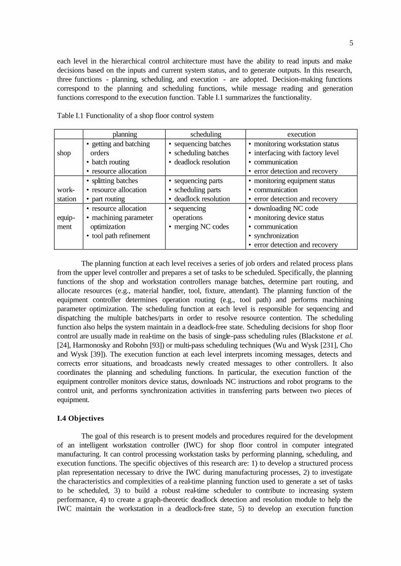
each level in the hierarchical control architecture must have the ability to read inputs and make decisions based on the inputs and current system status, and to generate outputs. In this research, three functions - planning, scheduling, and execution - are adopted. Decision-making functions correspond to the planning and scheduling functions, while message reading and generation functions correspond to the execution function. Table I.1 summarizes the functionality. Table I.1 Functionality of a shop floor control system planning scheduling execution shop

• getting and batching orders • batch routing • resource allocation

• sequencing batches • scheduling batches • deadlock resolution

• monitoring workstation status • interfacing with factory level • communication • error detection and recovery

work- station

• splitting batches • resource allocation • part routing

• sequencing parts • scheduling parts • deadlock resolution

• monitoring equipment status • communication • error detection and recovery

equip- ment

• resource allocation • machining parameter optimization • tool path refinement

• sequencing operations • merging NC codes

• downloading NC code • monitoring device status • communication • synchronization • error detection and recovery

The planning function at each level receives a series of job orders and related process plans from the upper level controller and prepares a set of tasks to be scheduled. Specifically, the planning functions of the shop and workstation controllers manage batches, determine part routing, and allocate resources (e.g., material handler, tool, fixture, attendant). The planning function of the equipment controller determines operation routing (e.g., tool path) and performs machining parameter optimization. The scheduling function at each level is responsible for sequencing and dispatching the multiple batches/parts in order to resolve resource contention. The scheduling function also helps the system maintain in a deadlock-free state. Scheduling decisions for shop floor control are usually made in real-time on the basis of single-pass scheduling rules (Blackstone et al. [24], Harmonosky and Robohn [93]) or multi-pass scheduling techniques (Wu and Wysk [231], Cho and Wysk [39]). The execution function at each level interprets incoming messages, detects and corrects error situations, and broadcasts newly created messages to other controllers. It also coordinates the planning and scheduling functions. In particular, the execution function of the equipment controller monitors device status, downloads NC instructions and robot programs to the control unit, and performs synchronization activities in transferring parts between two pieces of equipment. I.4 Objectives The goal of this research is to present models and procedures required for the development of an intelligent workstation controller (IWC) for shop floor control in computer integrated manufacturing. It can control processing workstation tasks by performing planning, scheduling, and execution functions. The specific objectives of this research are: 1) to develop a structured process plan representation necessary to drive the IWC during manufacturing processes, 2) to investigate the characteristics and complexities of a real-time planning function used to generate a set of tasks to be scheduled, 3) to build a robust real-time scheduler to contribute to increasing system performance, 4) to create a graph-theoretic deadlock detection and resolution module to help the IWC maintain the workstation in a deadlock-free state, 5) to develop an execution function

6

necessary to receive and interpret incoming messages and broadcast updated messages, and 6) to create the IWC software necessary to demonstrate the integration of the three functions and the architectural linkages with other controllers. The IWC has several characteristics. First, the IWC must be intelligent. In other words, the IWC must be able to act appropriately in an uncertain environment in order to increase the probability of success of the system's ultimate goal given the criteria of success (Albus [5]). To this end, the IWC is an integrated system of a decision-making function (planning and scheduling) and an execution function. For example, the system's ultimate goal is to produce an assigned product order, while the criteria of success is to meet its due-date. Second, the IWC must be a real-time controller, that is, the time frame over which various decisions are made corresponds to the dynamic character of the workstation being considered. Further, the time of response taken to make decisions needs to be short. The IWC belongs to soft real-time control systems in which an operation will go on even though response times are later than a given threshold (Burns and Wellings [32]). Note that hard real-time control systems are so sensitive to response times that a missed deadline can potentially cause a severe trauma (e.g., a flight control system). Third, the IWC must be robust. In other words, the IWC must perform well under a variety of workstation configurations (e.g., the number of machines, the number of buffers), workstation status (e.g., machine failure, tool breakage), and operating parameters (e.g., order arrival rate, processing time distribution) (Dooley and Mahmoodi [58], Velagapudi [223]). I.5 Motivation Most manufacturing controllers in existence today are application-specific, hand-woven systems, which lack an insight or a generic vision for manufacturing systems. A detailed investigation on the past research reveals a number of defects. The development of a IWC can overcome the disadvantages stated below. First, few controllers include the required integration of three basic functions necessary to create an intelligent controller: planning, scheduling, and execution. In fact, 80 percent of the workstation controllers in industry only perform monitoring functions, including monitoring the inputs of each machine (e.g., NC instructions), downloading orders, collecting output data, and generating alarms in case of conflict (Boulet et al. [27]). The workstation controller must be able to act in the way a foreman would manage the workstation. This implies that all the parts in the system must be planned and scheduled while moving through the system. Second, most manufacturing controllers ignore the importance of the role of process plans generated by process planning systems. In fact, process planning is viewed as an information generating function that provides essential instructions that are necessary for converting the raw material to the predetermined final product. Its results, including a set of form features, their attributes, and precedence relationships between form features, are stored in the process plan. The process plan becomes a primary input to a shop floor control system and drives the system to ensure the completion of assigned orders. This research takes a process plan representation model into account and addresses the evolution of the process plans from shop level down to the equipment.

7

Third, some manufacturing system controllers include the specified time delay for the state transitions (Chaar and Volz [35], Hadj-Alouane et al. [89], Naylor and Maletz [160], Naylor and Volz [161]). This time-driven method may result in undue complexity of system control as compared to an event-driven method. This research adopts an event-driven operating philosophy. The execution function in the IWC detects and classifies any events and distributes them to either the planning and scheduling functions, or the shop and equipment controllers. In other words, the planning and scheduling functions of the IWC are invoked by the execution functions for every necessary event. Fourth, some manufacturing controllers include the intermix of process plan and control (Crockett et al. [46], Kasturia et al. [117], Mettala [152]). This causes a change in a process plan to call for a change in the controller. Instead of the intermix, the IWC can retrieve part information from the process plan data base. This increases modularity between process plan and control. Process planning is viewed as an off-line rather than real-time activity. Fifth, few manufacturing system controllers employ the system deadlock detection and recovery models required to maintain a deadlock-free state. A system deadlock is a situation that arises due to resource sharing in manufacturing systems, when the flow of parts is permanently inhibited and/or operations on parts cannot be performed. The occurrence of system deadlocks, unlike blocking, stalls activities in portion of or the entire system and makes part flow impossible. This problem has been ignored by most scheduling and control studies which usually assume infinite queue capacity. For instance, in classical simulation models parts balk after the storage buffer becomes full. This research investigates various types of system deadlock and provides several procedures necessary to resolve these undesirable situations. I.6 Assumptions The following assumptions and conditions are made as part of this research. 1) A processing workstation consists of several processing machines and a robot and 2) A communication protocol has been defined (Ang [10]). I.7 Organization of Dissertation The remainder of the dissertation is organized as follows. Chapter II provides a detailed survey of the shop floor control system. In Chapter III, the overview of the IWC is presented. Chapter IV presents the structured representation of process plans and their evolution in the shop floor. Chapter V provides the characteristics and complexities of the planning function of the IWC. The multi-pass scheduling function driven by a neural network is presented in Chapter VI. Deadlock detection and resolution procedures using graph theory are presented and detailed in Chapter VII. Chapter VIII presents a detailed description on the execution functions of the IWC and equipment controllers. Chapter IX gives experimental design and results, the conclusion of the research, and further research topics.

8

CHAPTER II

LITERATURE REVIEW II.1 Chapter Overview In this chapter, a detailed survey of the shop floor control system is presented. In order to efficiently control any complex manufacturing system, many researchers have proposed various shop floor control structures. Two primary decomposition theories, spatial and temporal, provide the basis for constructing a specific architecture. In the spatial decomposition theory, an equipment controller is connected to each physical device that requires a controller. The equipment controller performs various device level activities, such as loading and unloading parts, downloading control programs (e.g., NC instructions, robot programs), reading sensory data. Next, interactions among equipment controllers must be taken into account. In general, three well-known approaches have been proposed: hierarchical, centralized (or flat), and heterarchical. In a hierarchical control system, a workstation level controller is constructed which coordinates the activities of the equipment controllers. In a centralized control system, a single tiered hierarchy is formed where the supervisor can address all devices in the system. In a heterarchical control system, each device controller cooperates through communication to pursue system goals without the master/slave relationship employed in the hierarchical or flat control architecture. The events that cause changes in the system state variables occur at many different frequencies. A temporal decomposition methodology decomposes the events into several groups, each of which can be controlled by a function. In other words, a well-defined SFCS performs several functions whose specifications depend on temporal decomposition. The frequency with which each function is performed in the top-level controller may be different from the frequency with which it is performed at the bottom level controller. This chapter is organized as follows: Section II.2 provides a detailed survey of the spatial decomposition of the SFCS architecture. Section II.3 introduces a survey of the temporal decomposition of the SFCS architecture. In Section II.4, a summary of the chapter is presented. II.2 Control Architecture for Shop Floor Control Since the complete problem of the SFCS is large and includes many complex interactions, a number of formal models have been developed (Adiga [2], Banerjee and Al-Maliki [15], Biemans and Blonk [22], Biemans and Vissers [23], Fowler [72], Jorysz and Vernadat [112, 113], Klittich [122], Maimon and Fisher [143], Russell [185], Suh [213], Tam [214], Williams and Upton [228]). Further, a decomposition of the control problems into several well-defined levels must provide clear “hooks” to integrate the various decomposed problems into an integrated system (Davis and Jones [51], Joshi et al. [114]). Such control structures demand a number of conditions, including, fault-tolerance, modifiability, extendibility, reconfigurability, reliability, and adaptability (Dilts et al. [56]). In other words, the control architecture must be suitable for physical reconfiguration and dynamic changes of any manufacturing systems, for example, dynamically adding or removing a robot. Various control structures have been presented as can be seen from Figure II.1. In general, four main decomposition approaches - centralized control, hierarchical control, heterarchical control,

9

and hybrid control structures - have been extensively studied (Dilts et al. [56]). In Figure II.1, the circles represent devices, the white boxes represent equipment controllers, the hatched boxes represent workstation controllers, and the black boxes represent shop controllers. The lines represent the control flow.

Centralized or flat control

Hierarchical control

Heterarchical control

Hybrid control

Centralized Decentralized

Figure II.1 Taxonomy of shop floor control architecture II.2.1 Centralized Control Architecture A centralized or flat control system has been proposed for the manufacturing systems by a few researchers (Achatz and Parrish [1], Hammer [90]). In a centralized control architecture, one controller controls the entire stock of equipment and maintains global information to record the activities of the whole system. In other words, a single shop floor controller is responsible for scheduling parts across the equipment, checking resource status in the system, downloading control programs, and monitoring the manufacturing progress. Some benefits of this control architecture can be characterized: 1) it is easy to access the complete global information database, 2) fewer computers may be required, and 3) global optimization may be possible since overall system status information can be easily extracted. However, there are several disadvantages: 1) the speed of response is relatively slow as the system becomes large, 2) the system reliability can be low since the failure of the central control computer implies that the entire manufacturing process cannot function, and 3) modifications to the control software can be difficult because of less modularity. II.2.2 Hierarchical Control Architecture Most manufacturing system controllers are based on a hierarchical control architecture since it provides significant advantages and has been more useful compared to other control structures (Albus et al. [7], Ammons et al. [9], Biemans and Vissers [23], Hitz [97], Jones and McLean [110], Joshi et al. [114], McLean [144, 145, 146], McLean and Brown [148], McLean et al. [147,149], McLean and Wenger [150], O'Grady et al. [163], O'Grady and Menon [167], Sandell et al. [187], Scogin and Titone [190], Simpson et al. [200], Wright [229]). The main character of the hierarchical control architecture is that the top level controller sends the control decisions downwards, while shop floor status information is sent upwards. The top level of the hierarchy makes the aggregate decisions and has the longest planning horizon. The planning horizon decreases as the level goes down. There are several variants in the hierarchical control architecture in terms

10

of the number of levels, the number of functions within each level, and data handling and communications (Jones et al. [109]). The National Institute of Standards and Technology (NIST) has embarked on a test-bed and demonstration facility, called the Automated Manufacturing Research Facility (AMRF), in support of the development of the manufacturing control software by workers from NIST, industry, academia, and other government agencies (Furlani et al. [74], Simpson et al. [200]). The main purpose of the AMRF is to support the needs for the automation of the small batch, discrete parts manufacturing industries, such as those supplying parts for aircraft, automobiles, and industrial machinery, which are known to produce 75 percent of all U.S. trade in manufacturing goods. In order to implement a system that provides sensory interaction along with the flexibility of software automation, the AMRF has adopted a hierarchical control architecture. The incorporation of CIM into existing factories required for real-time production control and implementation has been suggested and described (Simpson et al. [200], Jones and McLean [110]). To this end, the real-time control system is partitioned into a five level hierarchy - facility, shop, cell, workstation, and equipment. Figure II.2 illustrates the AMRF control hierarchy. The key characteristics of the AMRF control hierarchy include (McLean and Brown [148]): 1) the decomposition of the manufacturing control hierarchy into well-defined levels, 2) the uniform decomposition of work orders across the hierarchy, 3) the concept of a generic production control module for managing activities at each level, 4) the definition of work elements for all control systems, 5) a consistent process plan representation at each level, 6) separate and independent databases and communication services, and 7) a generic model of state transitions of major control systems.

Information Management Manufacturing Engineering Production Management

Task Management Resource Allocation

Batch Management Scheduling

Batch Splitting Equipment Tasking

Machining Handling Measurement

Facility

Shop

Cell

Workstation

Equipment

Figure II.2 AMRF control hierarchy At the top level of the hierarchy, facility level, three major functions are carried out: manufacturing engineering, information management, and production management. Manufacturing engineering functions are usually implemented with human involvement. Largely, these functions include computer-aided design and computer-aided process planning necessary to prepare the specification of all operations for orders. Information management functions provide necessary administrative or business management activities, such as, cost estimation, customer billing, inventory accounting, customer order handling. Production management functions place orders,

11

identify production resource requirements, generate long-range schedules, and summarize quality performance data. The shop level is responsible for coordinating the production activities, scheduling job orders, equipment maintenance, and shop support services. In order to manage workflow, it uses group technology classification codes based on processing requirements, geometric shape, tooling used, production costs, and material composition. The shop level is also responsible for allocating the production resources to the orders. An interesting aspect at the control hierarchy is at the cell control level. The evolutionary trends of the manufacturing cell controller are illustrated in Figure II.3 (McLean et al. [147]). In the figure, the virtual cell has no longer static control structures that were normally associated with a fixed physical grouping of workstations, but dynamically changes. Workstations will be allocated to cells by the shop level resource allocator by considering capabilities such as predicting needs, requisitioning resources, time sharing resources, and handshaking during hands-off of controlled subsystems. This philosophy was believed to provide much of the control software flexibility of automated manufacturing systems. The workstation level controller directs and coordinates the activities of small-integrated physical groupings of shop floor equipment. The controller sequences equipment level devices through job setup, part fixturing, cutting processes, chip removal, in-process inspection, job takedown, and cleanup operation. The workstation controller can be operated using state-tables or production rules.

GT cell Automated cell

Virtual cell

Intelligent cell

Part Family Robots

NC Tools

Robot Carts

Resource Sharing

Dynamic Control Structures

Planning

Optimization

Learning

Figure II.3 Trends of the manufacturing cell At the lowest level of the hierarchy are individual device controllers (e.g., machine tool controller, robot controller) that are responsible for reading sensory data (e.g., on-line ultrasonic surface finish sensing, chip form monitoring by acoustic emission, tool wear sensing) and downloading various device specific programs (e.g., NC instructions, robot programs). The other efforts along with the development of the control hierarchy include database systems and network communications. The main purpose of the database systems work is to: 1) define and develop the data structures necessary to contain all facility planning and control information, and 2) utilize database management systems to maintain the information required by the AMRF operation. Two distributed hierarchical databases are maintained: planning and control databases. The planning database contains: process plans, part mix, part dimension and geometry, desired grip points for robot handling, scheduling information, and tool and material requirements. The control database contains dynamic factory status information, including tool status, machine status, robot status, work orders in progress. The objective of the network communication project is to provide a communication link among any computers and control processes. Each computer can be accessed via a node reference to a logical name, interchange mailboxes, and the common data path.

12

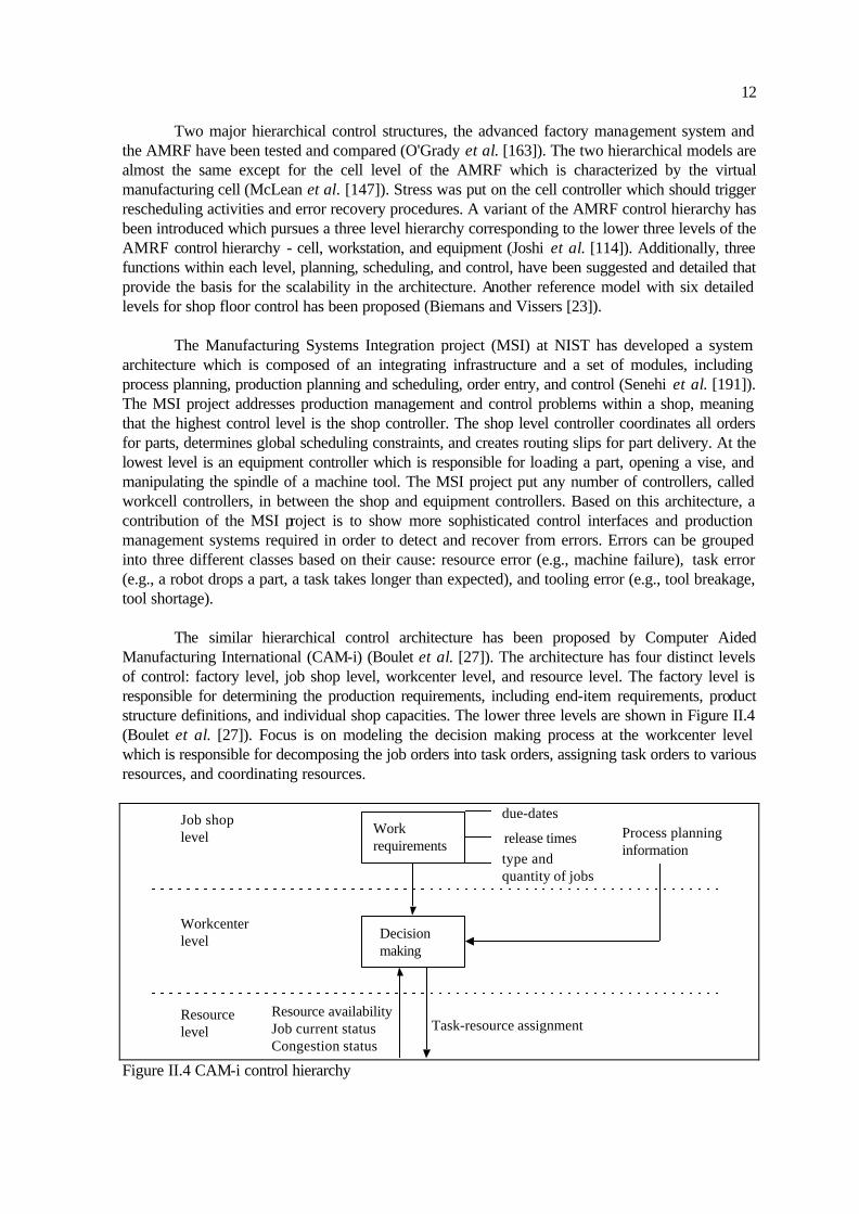
Two major hierarchical control structures, the advanced factory management system and the AMRF have been tested and compared (O'Grady et al. [163]). The two hierarchical models are almost the same except for the cell level of the AMRF which is characterized by the virtual manufacturing cell (McLean et al. [147]). Stress was put on the cell controller which should trigger rescheduling activities and error recovery procedures. A variant of the AMRF control hierarchy has been introduced which pursues a three level hierarchy corresponding to the lower three levels of the AMRF control hierarchy - cell, workstation, and equipment (Joshi et al. [114]). Additionally, three functions within each level, planning, scheduling, and control, have been suggested and detailed that provide the basis for the scalability in the architecture. Another reference model with six detailed levels for shop floor control has been proposed (Biemans and Vissers [23]). The Manufacturing Systems Integration project (MSI) at NIST has developed a system architecture which is composed of an integrating infrastructure and a set of modules, including process planning, production planning and scheduling, order entry, and control (Senehi et al. [191]). The MSI project addresses production management and control problems within a shop, meaning that the highest control level is the shop controller. The shop level controller coordinates all orders for parts, determines global scheduling constraints, and creates routing slips for part delivery. At the lowest level is an equipment controller which is responsible for loading a part, opening a vise, and manipulating the spindle of a machine tool. The MSI project put any number of controllers, called workcell controllers, in between the shop and equipment controllers. Based on this architecture, a contribution of the MSI project is to show more sophisticated control interfaces and production management systems required in order to detect and recover from errors. Errors can be grouped into three different classes based on their cause: resource error (e.g., machine failure), task error (e.g., a robot drops a part, a task takes longer than expected), and tooling error (e.g., tool breakage, tool shortage). The similar hierarchical control architecture has been proposed by Computer Aided Manufacturing International (CAM-i) (Boulet et al. [27]). The architecture has four distinct levels of control: factory level, job shop level, workcenter level, and resource level. The factory level is responsible for determining the production requirements, including end-item requirements, product structure definitions, and individual shop capacities. The lower three levels are shown in Figure II.4 (Boulet et al. [27]). Focus is on modeling the decision making process at the workcenter level which is responsible for decomposing the job orders into task orders, assigning task orders to various resources, and coordinating resources.

Work requirements

due-dates

release timestype and quantity of jobs

Job shop level

Workcenter level

Resource level

Process planning information

Task-resource assignmentResource availability Job current status Congestion status

Decision making

Figure II.4 CAM-i control hierarchy

13

Another agent working in this area is the European Strategic Program for Research and development in Information Technology (ESPRIT) that involves both European industry and academia (Boulet et al. [27]). ESPRIT has proposed a hierarchical control structure which was derived from the AMRF hierarchy. Each control level consists of decision-making units: planning control, interpretation control, and diagnostic control. The expert system at each level solves specific control tasks. In particular, the workcell controller generates a daily plan and updates daily plans according to the current state of the manufacturing system. There are significant benefits for the hierarchical control architecture: 1) development of control software can be flexible due to the modularity of the hierarchical structure and 2) the speed of response is fast since the size, functionality, and complexity of each level controller can be limited (Dilts et al. [56]). However, there are several disadvantages. First, a failure at some level paralyzes its lower level controllers (Jones and Saleh [111]). Second, the global decision making employed in the high level controller may be based on estimated shop information due to communication delays. Third, substantial knowledge of the relationship between control levels is required for development of fault-tolerance software. II.2.3 Heterarchical Control Architecture A number of researchers pointed out various disadvantages of the hierarchical control architecture, and suggested a heterarchical control structure (Duffie [60, 61, 62], Duffie and Piper [63], Hatvany [94], Rana and Taneja [180], Shaw [197], Upton [219], Upton et al. [220]). The main character of the heterarchical control structure is that each equipment controller cooperates through communication to pursue system goals without the master/slave relationship employed in the hierarchical controller architecture. Advances in the area of network communications and distributed computing systems are critical for the heterarchical control architecture (Hatvany [94]). In the heterarchical control system, all participant subsystems have: 1) equal rights of access to resources, 2) mutual access and accessibility to each other, 3) independent modes of operation, and 4) strict conformity to the protocol-rules of the overall system. Another important goal of the heterarchical control architecture is to eliminate or minimize global information in order to enhance system modularity, modifiability, extendibility, complexity reduction, and fault-tolerance. This implies that each equipment controller must contain a significant amount of detailed information. This results in the fact that the operating system used in this controller is more complex than that of the hierarchical control architecture . In order to organize activities between controllers, a negotiation based procedure is needed (Lin and Solberg [139], Lewis et al. [136], Shaw [197]). By using a negotiation procedure, each controller communicates and negotiates with other controllers in real-time through message passing and a bidding system in order to arrange scheduling and routing of parts. A distributed task assignment mechanism for shop level scheduling has been developed. Further, a knowledge based system for cell level scheduling using a heterarchical control mechanism has been implemented (Shaw [197]). The advantages associated with the heterarchical control architecture include: reduced software complexity, improved fault-tolerance, and ease of maintainability and modifiability, ease of human intervention, easy learning about part characteristics (Duffie [60, 61, 62], Upton [219]). There are many disadvantages: technical limits, no standard communications, local optimization, high network capacity, and lack of availability of software (Dilts et al. [56]).

14

II.2.4 Hybrid Control Architecture Both hierarchical and heterarchical control structures have been criticized and a control architecture with the best points of both systems has been proposed (Jones and Saleh [111]). Two decomposition methods, the multi-layer and multi-level control, have been applied to an automated manufacturing system. Each corresponds to a temporal decomposition and spatial decomposition, respectively. The exact number of spatial levels will vary from one implementation to another. Additionally, some issues related to the integration of these modules have been addressed: (1) how to connect process plans to the shop floor controller, (2) how to interface between the functions, (3) how to interface between supervisors and subordinates, and (4) how to integrate the shop floor controller with a global database management system (DBMS). Especially, the shop floor controller communicates with the global DBMS via the Open Systems Interconnection (OSI) reference model that provides the ways for separating the logical and physical data flow paths from the control flow paths (Barkmeyer [17]). Several advantages for this approach can be found (Davis et al. [52]) First, the number of layers varies as the system changes in size, complexity, and product mix. Second, mathematical programming can be applied to the spatial decomposition approach. Third, task decomposition removes one of the layer-dependent activities. II.3 Temporal Decomposition within Each Level Once the complex SFCS is decomposed into a series of smaller levels, each level consists of several functions determined by events occurring at different times. A temporal decomposition of each level generates these functions to be executed at different frequencies within the same level and across separate levels (Gershwin et al. [77], Jones and Saleh [111]). The number of these functions, that is, different frequency groups, depends on the authors involved or the methodologies used. However, any intelligent controller must integrate a decision-making function (planning and scheduling) and an execution function (monitoring and error recovering) (Davis et al. [52], Albus [5]). Figure II.5 illustrates function breakdowns within each level. These functions are directly related to the implementation of the manufacturing system. As the number of functions decreases, generalization increases, that is, a function contains more tasks to be carried out.

2 functions 3 functions 4 functions more than 4

SpecializationGeneralization

MRP

Planning

Control

Planning

Scheduling

Control

Planning

Scheduling

Monitoring

ExecutionPlanning

..Execution

Figure II.5 Taxonomy of the functional decomposition method Some researchers have proposed a decomposition of each level into two functions that include the planning/scheduling function and the execution function (O'Grady et al. [163], Wright [229]). A workstation controller has been developed whose functions performed scheduling

15

activities and the error recovery procedure (O'Grady et al. [163]). The scheduling module rearranges various activities within a workstation, while the error recovery procedure maintains the system involved in irregular operations. Many researchers have presented control systems consisting of three functions (Jones and Saleh [111], [Joshi et al. [114], Maimon [142], McLean et al. [147]). Three functions in the workstation level controller, task analysis and reporting, routing and scheduling, and dispatching and monitoring, have been proposed and analyzed (McLean et al. [147]). Three functions - planning, scheduling, and execution - necessary to provide the basis for the scalability in the architecture have been proposed (Joshi et al. [114]). Planning is the activity responsible for selecting part routings and generating completion time for parts. Scheduling is responsible for generating expected start and finish times for all the tasks necessary to execute assigned parts. Control initiates start-up and shutdown, downloads various command messages, monitors the execution of the scheduled tasks, and oversees error recovery. Execution of commands within each level occurs in a top-down manner, while error recovery and requests flow in a bottom-up manner. Figure II.6 illustrates the three functions and their relationship.

Interface with higher level controller

Interface with lower level controller

Command Execution

Error Recovery Requests

Planning

Scheduling

Control

Figure II.6 Three functions and their relationship (Joshi et al. [114]) Other variants of three major functions - adaptation, optimization, and regulation - have been proposed based on the frequencies at which they occur (Jones and Saleh [111]). Each level may be an independent control system with a temporal decomposition. Figure II.7 shows three functions and their activities. Adaptation performs generating and updating plans for tasks to be scheduled. Optimization evaluates planned tasks and generates their schedules. Regulation is concerned with interfacing with the lower level controller, receiving the status of manufacturing progress, and guiding the error recovery activity of the lower level controller. Another decomposition of a manufacturing system into the dynamic scheduler, the process sequence, and the communication function has been reported (Maimon [142]). It should be noted that these functions perform almost the same tasks in spite of different names. Each level in the ESPRIT control hierarchy has three distinct functions: action planning, interpretation, and diagnostic (Boulet et al. [27]). Figure II.8 shows the detailed scheme of the controller architecture. The action planning function is a decision process which optimizes a set of decision variables and selects the best plan. The constraints to be considered for this function include 1) constraints given by the upper level, 2) solution space issued by the same level, and 3) function specific model. The interpretation function is to initialize the static and dynamic models

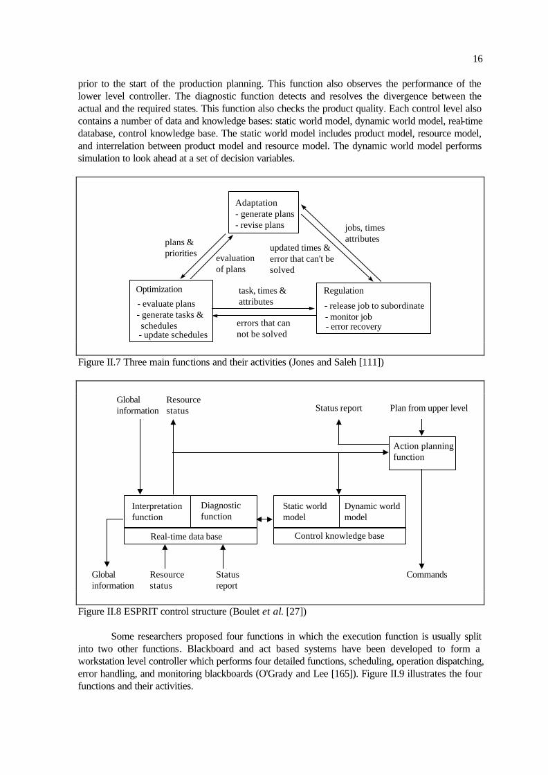
16

prior to the start of the production planning. This function also observes the performance of the lower level controller. The diagnostic function detects and resolves the divergence between the actual and the required states. This function also checks the product quality. Each control level also contains a number of data and knowledge bases: static world model, dynamic world model, real-time database, control knowledge base. The static world model includes product model, resource model, and interrelation between product model and resource model. The dynamic world model performs simulation to look ahead at a set of decision variables.

Adaptation - generate plans - revise plans

Optimization

- evaluate plans - generate tasks & schedules- update schedules

Regulation

- release job to subordinate - monitor job- error recovery

plans & priorities evaluation

of plans

jobs, times attributes

updated times & error that can't be solved

task, times & attributes

errors that can not be solved

Figure II.7 Three main functions and their activities (Jones and Saleh [111])

Action planning function

Interpretation function

Diagnostic function

Static world model

Dynamic world model

Real-time data base Control knowledge base

Plan from upper levelStatus reportResource status

Commands

Global information

Resource status

Status report

Global information

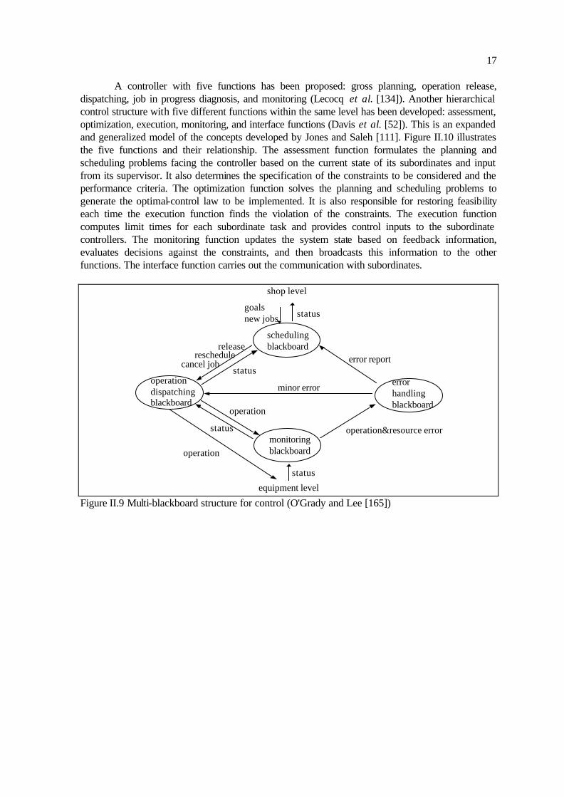
Figure II.8 ESPRIT control structure (Boulet et al. [27]) Some researchers proposed four functions in which the execution function is usually split into two other functions. Blackboard and act based systems have been developed to form a workstation level controller which performs four detailed functions, scheduling, operation dispatching, error handling, and monitoring blackboards (O'Grady and Lee [165]). Figure II.9 illustrates the four functions and their activities.

17

A controller with five functions has been proposed: gross planning, operation release, dispatching, job in progress diagnosis, and monitoring (Lecocq et al. [134]). Another hierarchical control structure with five different functions within the same level has been developed: assessment, optimization, execution, monitoring, and interface functions (Davis et al. [52]). This is an expanded and generalized model of the concepts developed by Jones and Saleh [111]. Figure II.10 illustrates the five functions and their relationship. The assessment function formulates the planning and scheduling problems facing the controller based on the current state of its subordinates and input from its supervisor. It also determines the specification of the constraints to be considered and the performance criteria. The optimization function solves the planning and scheduling problems to generate the optimal-control law to be implemented. It is also responsible for restoring feasibility each time the execution function finds the violation of the constraints. The execution function computes limit times for each subordinate task and provides control inputs to the subordinate controllers. The monitoring function updates the system state based on feedback information, evaluates decisions against the constraints, and then broadcasts this information to the other functions. The interface function carries out the communication with subordinates.

scheduling blackboard

operation dispatching blackboard

monitoring blackboard

error handling blackboard

statusgoals new jobs

releasereschedule

cancel jobstatus

minor error

error report

operation&resource error

status

operation

status

operation

shop level

equipment level Figure II.9 Multi-blackboard structure for control (O'Grady and Lee [165])

18

Assessment Function

Optimization Function

Monitoring Function

Execution Function

Interface Modules

Supervisor

Subordinate

problem formulations

selected control law

current control schedule

constraint evaluation

performance statistics

constraints

task&timesfeedback

feedbacktask&times

Figure II.10 Schematic overview of the five functions (Davis et al. [52]) A four level hierarchy with multiple number of functions - factory, shop, cell, and equipment - has been developed (O'Grady and Menon [167]). The factory level deals with process planning, CAD, master production scheduling, MRP, and the financial systems, while the shop level includes the master production scheduling II and on-line scheduling system. It is claimed that the functions are more important than the number of levels. II.4 Chapter Summary In this chapter, various control structures have been reviewed based on the spatial decomposition for efficient design of control architecture and the temporal decomposition for effective control of each level. In general, two spatial decomposition approaches have been utilized: hierarchical and heterarchical. The main difference between the two structures is how interactions between two control components can be resolved. In the hierarchical control architecture, the upper level controller organizes and coordinates the activities and contention of the subordinates. In the heterarchical control architecture, each controller cooperates through communication to pursue system goals without the master/slave relationship. Once a decomposition for the SFCS is obtained, it is necessary to consider the functionality of each level controller. The events that cause changes in the system state variables occur at many different frequencies. A temporal decomposition methodology decomposes the events into several groups, each of which can be controlled by a function. In other words, a well-defined SFCS performs several functions whose specifications depend on temporal decomposition. In general, two functions - a decision-making function and an execution function - are fundamental to the SFCS. Many other variants have been also reviewed.

19

CHAPTER III

OVERVIEW AND GENERAL CONCEPT III.1 Chapter Overview A SFCS, a central part of a computer integrated manufacturing system, plans, schedules, and executes the production activities required to fill orders received from the factory level control system. In order to effectively control these activities, it is necessary to define a control architecture and functional perspective of how a SFCS operates. In the context of the hierarchical control architecture, process plans for products play an important role in operating the shop floor. The structured evolution of the process plans from the shop down to the equipment is required. In particular, the IWC at the middle level of a SFCS is responsible for selecting a specific process routing, allocating resource, scheduling and coordinating the activities across the equipment, monitoring the progress of activities, detecting and recovering from errors, and preparing reports. The activities of the IWC are also addressed and detailed. One of the requirements for the IWC is that it must contain robust real-time planning and scheduling functions, and an execution function. It must also maintain the system in a deadlock-free state. As a result, the development of the IWC will save cost and time in developing control software for the automated manufacturing systems. The goal of this chapter is to describe and raise briefly the issues, models and procedures necessary to construct the IWC that can control processing workstation activities by performing planning, scheduling, and execution. The IWC is a robust real-time controller integrated with planning, scheduling, and execution functions. The specific objectives of this chapter are: 1) to address a structured plan representation and the evolution of process plans from the shop down to the equipment, 2) to describe a real-time planning function used to generate a set of tasks to be scheduled, 3) to introduce a robust scheduler to contribute to increasing system performance, 4) to raise several kinds of deadlock problems, 5) to briefly describe the execution function and its responsibility, and 6) to describe the integration of the three functions and the architectural linkages with other controller. The remainder of the chapter is organized as follows: In Section III.2, a process plan representation model for the integration of process planning and shop floor control is presented. The execution function of the IWC and the relationship of the three functions are described in Section III.3. A brief description on the planning function is presented in Section III.4. A real-time scheduling function of the IWC is discussed in Section III.5. Section III.6 addresses a system deadlock detection and resolution model. In Section III.7, an integration issue of the three functions is described. Finally, Section III.8 provides a conclusion of the chapter. III.2 Process Plan and Shop Floor Control A process plan plays an important role in conveying a large amount of processing information from process planning to shop floor control, such as part routings, operation sequences, material requirements, and resource requirements. In order to represent a process plan in an appropriate form that a shop floor controller can easily understand, operation charts and process routing summary have been used in the past. The major disadvantage of this approach is that it is difficult to address the power of alternatives in terms of operation sequences and resource requirements. Therefore, the development of a well-structured process plan representation model is needed which can accommodate various alternatives and information associated with manufacturing.

20

In this research, a process plan is represented as a form feature graph using an AND/OR graph concept. In other words, a form feature graph is an AND/OR graph used to represent a set of form features and their precedence relationship. An edge in the form feature graph represents the precedence relationship among form features. A node in the form feature graph is one of five different types: SPLIT-AND, SPLIT-OR, JOIN-AND, JOIN-OR, and FORM-FEATURE. A SPLIT-AND type node implies that all the paths following a SPLIT-AND type node must be manufactured in any sequence. A JOIN-AND type node is required to bring multiple paths back together after a SPLIT-AND type node. A SPLIT-OR type node implies that only one path following a SPLIT-OR type node must be selected to be machined. A JOIN-OR type node is required to bring multiple paths back together after a SPLIT-OR type node. A form feature, which is the base level activity that must be performed as a single depth of cut by utilizing a single fixture, tool, and machine resource, is represented in a FORM-FEATURE type node. The node contains manufacturing information associated with a form feature, such as machine, tool, fixture, machining parameters, NC instructions, etc. A form feature graph associated with a concerned product forms the principal input to the shop floor control system. A form feature graph in a shop floor evolves from the shop down to the equipment as the concerned part moves. Since a representation model based on form features is independent of the facility configuration and the shop floor control architecture, a form feature graph needs to be modified and refined using a resource based representation. The modified graph is called a plan graph, where a node refers to the collection of form features that are produced using the resource as specified by the node. The plan graph may also be represented using an AND/OR graph concept. A shop level plan graph is an aggregated form feature graph used to represent workstation activities and their precedence relationships. A node represents a workstation activity, which contains a set of form features, and their precedence relationships performed by equipment controllers within a workstation. When a new part arrives to a workstation, its associated form feature graph is also downloaded to the workstation controller. A workstation level plan graph is then created to represent operations and their precedence relationships. An operation contains a set of form features to be machined by a machine, or the refixturing activities supported by a material handler. A workstation level plan graph can be converted to an operation sequence graph by eliminating SPLIT-OR and JOIN-OR type nodes. This graph is the main input to the scheduling function of the workstation level controller. A form feature graph associated with an operation is downloaded to the equipment controller when a new part arrives to a machine. The detailed description on a process plan representation model and the evolution of a process plan in a shop floor is presented in Chapter IV. III.3 Development of an Execution Function As mentioned earlier, the IWC performs three main functions — planning, scheduling, and execution — in order to ensure completion of the orders assigned by the shop controller. In particular, the execution function plays a goal keeper role in coordinating the three functions and communicating with other controllers. In fact, the execution function accomplishes its own responsibility based on a set of messages coming in and going out of the IWC. It receives, interprets, and understands various messages incoming from the planning and scheduling functions, and other controllers. This processing can occur through a series of steps, that is, lexical analysis, syntactical analysis, and semantic processing. It then decomposes the messages into the detailed messages and broadcasts newly created messages. The detailed message flow through the execution function of the IWC is illustrated in Figure III.1.

21

The messages that can be processed may include status report to the shop controller, control commands about the movement of parts, refixturing activities, communication with planning and scheduling functions, etc. In terms of the movement of a part, the execution function can deal with the following three cases: Case 1) When a new part arrives to the workstation, Case 2) When a finished part leaves the workstation, and Case 3) When a part state changes within the workstation.

Planning

Scheduling

Execution

control message (arrive)

control message (plan)

control message (replan)

control

message

(move)

workstation plan graph

operation sequence graph

event m

essage

(done)

workstation status

equipment status

equipment process plan

workstation process plan

IWC

Shop controller

Machine controller

control message (load,unload)

control message (pick,put,transport)

equipment status

Robot controller Figure III.1 Detailed message flow in the IWC Case 1) When a new part arrives to the workstation When a new part arrives to a workstation, the shop controller sends a message about part arrival to the execution function of the IWC. The message carries the part identifier and its related workstation level process plan that is a workstation level form feature graph. The planning function invoked by the execution function then creates an operation sequence graph to determine part routing and to allocate resources (e.g., material handler, tool, fixture, attendant) to a specific operation. It is to be noted that the planning function is also invoked by the scheduling function each time replanning is required. The planning function then invokes the scheduling function in order to inform that a planning activity on the new part has just finished. Then, the scheduling function adds the new part to the part list that contains a set of parts to be dispatched. Case 2) When a finished part leaves the workstation When the scheduling function of the IWC determines to move a finished part to the port, the execution function informs the shop controller that the specified operations on the part have finished. After the shop controller arranges any material transport device to pick up the finished part, it downloads a message about part unloading to the IWC and a message about part loading to the

22

transport controller. The execution function of the IWC then commands a robot controller to pick up the concerned part from a machine tool and to put it down to the port. It is to be noted that the robot controller needs handshaking activities with the material transport controller, if synchronization is required. Case 3) When a part state changes within the workstation The execution function initiates the scheduling function by sending the event messages (e.g., a part has just been finished, a robot has just become free), which are received from the equipment controller. The scheduling function then sends various corresponding messages about the movement of parts, the assembly operation of parts, and the activities of the material handler. For instance, in order to move a part from one location to another, the scheduling function sends a macro message (e.g., move) or a sequence of detailed messages (e.g., rtransfer, transport, mtransfer). The rtransfer or mtransfer message is used to transfer a part to or from a robot. The detailed messages are useful when the scheduling function needs to specify the path of a material handler in order to avoid collision. When a move message is initiated by the scheduling function, the execution function prepares load and/or unload messages for a machine tool controller and pick and put messages for a robot controller. The execution function may also generate a number of transport messages for the material handler to arrive to the source location along with all the possible paths. If synchronization is required either when a part is transferred from a robot to a machine or when a part is transferred from a robot to a machine, the two equipment controllers need handshaking activities. To this end, an execution graph for a particular message in the equipment controller defines a sequence of actions to be taken and preconditions to be checked. A minute description and issues on the execution function are addressed in Chapter VIII. III.4 Development of a Planning Function The planning function of the IWC is invoked either by the execution function when a new batch/part arrives to the workstation, or by the scheduling function when replanning is required. When a new part arrives, the planning function receives its related workstation form feature graph. In general, planning can be defined informally as a function that generates a set of tasks to be scheduled in the future. Specifically, the planning function determines batch size, generates the plan graphs by aggregating the form feature graphs and an operation sequence graph by eliminating SPLIT-OR. An operation in the operation sequence graph is then committed to a set of resources, such as machines, fixtures, and attendants. The material handling activities between operations may also be specified. The objective of the planning function is to enable each order to be completed within the specified time limits. The criteria to be considered may include: 1) the amount of workload assigned to each machine is balanced, 2) resource utilization is maximized, 3) resource contention is minimized, 4) the possibility of system deadlocks is minimized, and 5) the number of operations is minimized. The planning function described above is similar to the problem reduction procedure using an AND/OR graph on which a graph search is performed to find a set of solvable primitive problems. The sequence of the paths following an AND type node is not important. This is known as a NP-complete problem (Horowitz and Sahni [99]). However, the planning procedure is more difficult, since interactions between operations must be considered when an operation sequence graph is selected. Therefore, this planning procedure is also NP-complete. Due to the nature of NP-completeness, the successful implementation of the planning functions is not easy. As a result, the planning function will be decomposed into several smaller problems in a hierarchical manner.

23

Given a part and its associated workstation form feature graph, a potential heuristic procedure for the planning function necessary to obtain an operation sequence graph is summarized in Table III.1. The detailed description on the planning function is addressed in Chapter V. Table III.1 Brief procedure of the planning function Step Activity Constraints Time span Input Output

1 Prune resource alternatives

Resources are not available off-line workstation form feature graph

pruned graph

2 Expand nodes with machine alternatives

A node contains only a form feature and a machine resource

off-line pruned graph

expanded graph

3 Group nodes A node contains multiple form features machined by a machine

off-line expanded graph

plan graph

4 Create a set of operation sequence graphs

Eliminate SPLIT-OR and JOIN-OR type nodes

off-line plan graph

operation sequence graphs

5 Select an operation sequence graph

1) Shortest operation time 2) Largest flexibility 3) Balancing machine load

on-line operation sequence graphs

an operation sequence graph

III.5 Development of a Scheduling Function The scheduling function is invoked when a planning activity on a new batch/part is finished, when an operation is finished at a machine tool, or when a device becomes idle. When the planning function invokes the scheduling function, an operation sequence graph associated with a new batch/part is transferred. An operation sequence graph specifies a set of operations and their precedence relationship. The outputs of the scheduling function to the execution function are a set of messages associated with what the next things can be done for every event. For example, the scheduling function determines the movement of a part and sends a corresponding message to the execution function. It is to be noted that the scheduling function may also deal with mobile resource movement activities, refixturing activities, and robot end-effector changing activities. The scheduling function described in this research is quite different from the traditional scheduling problems in several aspects. First, a broad review of the literature indicates that virtually all of the work contributed to date has been for domain-specific applications and scheduling is viewed differently by many researchers. Although the research community has developed titles for various scheduling problems, such as single machine problem, parallel machine problem, flow shop problem, and job shop problem, most researches are often unclear on what exactly the scheduling problem consists of. The scheduling function resolves various decision problems in real-time on the basis of current workstation status. To this end, all the decision problems are identified, each of which a specific rule is applied to. Second, most of traditional research in scheduling concentrates on two major classes of entities: 1) machines that process parts and 2) material handlers that move parts between machines. However, in CIM environments, the classes of entities that must be considered at the workstation level include: 1) batch, 2) part, 3) machines, 4) material handlers, 5) tools, 6) fixtures, 7), shared workspace and/or path, 8) buffers, and 9) attendants. The entity classes are differentiated according

24

to several attributes, such as mobility, flow pattern, flow direction, perishability, capacity, ownership, and passive or active. This classification scheme based on the attributes provides an insight for identifying scheduling problems. Third, the machining time associated with an operation on a machine tool is not known until the equipment controller sends an event message that the operation on the part is finished. This is because the equipment controller may modify those on the basis of the device status. For example, if the tool life of a specific tool is almost over, the equipment controller may reduce the machining speed, which results in the longer machining time than expected. This nature of the scheduling function may prevent the concerned problem from being formulated using a mathematical programming technique. From the characteristics described above, several observations can be collected and analyzed. First, the set of entities to be scheduled needs to be identified. Further, it needs to be addressed how the entities can be scheduled. Second, an event-driven scheduling concept is adopted. In other words, every time an decision problem is met, the rule to resolve the problem is applied. Third, all the decision problems to be resolved need to be discovered. By considering the workstation level entities to be scheduled, the client-server model can be used to define all the scheduling decision problems. A specific client requests either a server or multiple server(s). Any entity may become client or server, depending on how it can be used. The type of client usually is different from that of the server, but not always. Both client and server may belong to the same entity class. In this research, five different types of decision problems are identified and resolved. Table III.2 presents the detailed decision problems based on a client-server model. Table III.2 Set of decision problems for shop floor control Type Name Definition Client Server Example

I

Part releasing problem

When some clients of the same entity class request servers belonging to one entity class

part, batch

machine, material handler

When a pallet arrives, several groups of parts request each processor

II

Operation sequence problem

When a finished part has operation sequence alternatives specified by SPLIT-AND and JOIN-AND type nodes

part, batch

machine A finished part may go to any machine following a SPLIT-AND type node

III

Part buffering problem

When one client requests one of several different server classes

part, batch,

material handler, fixture, workspace, buffer

A finished part may go to: 1) buffer storage, 2) material handler, or 3) stay

IV

Part dispatching problem

When some clients of the same class request one server

part, batch

machine, fixture, material handler, tool, workspace, attendant

Many parts may request one empty processor at the same time

V

Robot location problem

When more than one choice exists for the next task to be performed for the material handler

material handler

machine, workspace

A robot may: 1) go to the home position, 2) go to the next server, or 3) stay

25

In order to resolve the decision problems in real-time, the scheduling function carries a rule for each problem and fires the rule every time the problem is encountered. To this end, a multi-pass scheduling technique is adopted which changes rules for every predetermined time period on the basis of current workstation status. The premise is that the evaluation and selection of rules over a series of short term horizons will lead to improved system performance, rather than using a single scheduling rule for an extended planning horizon. The scheduling function consists of four modules in order to perform nulti-pass scheduling: a rule selector, a multi-pass simulator, a system deadlock detection resolution module, and an event generator. When the existing rules need updating, the rule selector is invoked to suggest two rules for every problem. In this research, a neural network is used as a rule selector. The workstation status can be categorized with several elements — the number of machines, routing complexity, performance criteria, ratio of the material handling time to the processing time, system congestion, machine utilization, job late factor, and queue status factor. Simulation is primarily adopted in order to perform real-time evaluation and selection of the suggested scheduling rules. The outputs of the event generator are a set of messages associated with part movement, refixturing activities, etc. The simulator and event generator utilize the system deadlock resolution module to determine whether the movement of a part causes deadlock. The further definition and procedures of the scheduling function are detailed in Chapter VI. III.6 Development of a Deadlock Resolution Model Flexible manufacturing systems (FMS) usually have little or no queue capacity and limited sharing resources such as NC machines, robots, tools, fixtures. Furthermore, FMSs have the dynamic nature of manufacturing process due to the concurrent part flow of various parts. Even though those characteristics make possible more efficient use of resources, they bear practical, but undesirable problems, system deadlocks. The occurrence of system deadlocks, unlike blocking, causes all the activities in the entire system stalled and makes part flow impossible. As a result, system deadlocks may become a critical scheduling and control problem. Although this problem has been ignored by most scheduling and control studies in resource sharing unmanned manufacturing systems, it has received attention recently (Banaszak and Krogh [14], Minoura and Ding [154], Viswanadham et al. [225], Wysk et al. [235]). System deadlock may occur in several different patterns. As depicted in Table III.3, system deadlocks can be classified into three different types: part flow deadlock, processing resource (tool and fixture) deadlock, and material handler deadlock. This research focuses on developing a deadlock detection and resolution module that can be employed to (impending) part flow deadlocks. In the example of a part flow deadlock, part 1 at machine 1 has to go to machine 3 and part 3 at machine 3 has to go to machine 2 and part 2 at machine 2 is destined for machine 1. This circular waiting is called a part flow deadlock, if the machines and robots can only accommodate a part at a time with storage buffers full. One more serious phenomenon is an impending system deadlock in which transition(s) of a part is possible, but the system will terminate in part flow deadlock after some transitions. There are three methods to resolve (impending) part flow deadlocks: prevention, detection and recovery, and detection and avoidance. As a prevention method, parts are batched such that part flow is limited to a single direction. A deadlock detection and recovery method is to use an in-process storage buffer to switch parts in deadlock. A deadlock avoidance method consists of a detection module to identify (impending) system deadlocks and a control module to guide the part flow so that no deadlock occurs. The prevention method relies on an off-line procedure to prevent

26

deadlocks, while the detection and recovery method and the avoidance method can be applied to real time applications. Table III.3 Taxonomy of system deadlocks for shop floor control Deadlock Definition Resources Example

Part flow deadlock

a situation in which transition(s) of a part is impossible, since parts have been allocated in a cyclic request for machine resources.

Parts, Processors, Material handlers

Machine 1

21

31

2

3

Machine 3

Machine 2

Impending part flow deadlock

a situation in which transition(s) of a part is possible, but the system (or portion thereof) will terminate in part flow deadlock after some transitions

Parts, Processors, Material handlers

Machine 1 Machine 2

Machine 3

21

1 1

22

Processing resource deadlock

a cyclic request for resources in which a part with some resources cannot be processed since the flow of some more requested resources assigned to other parts is impossible.

Parts, Tools, Fixtures

1 2

tool 1

Machine 1 Machine 2

tool 1

Material handler deadlock

a situation in which transition(s) of a material handler is impossible, since material handlers have been allocated in a cyclic request for workspace and/or path.

Material handlers, Workspace and/or path

AGV

As mentioned in Section III.5, the deadlock detection and resolution model is invoked by the simulator or the event generator to check whether the movement of a part causes deadlock or not. If the transition of the concerned part does not cause any deadlock, the part can move to the next destination. If this movement causes a part flow deadlock and a recovery method is employed, this situation should be reported for the recovery process to be initiated. If this movement causes a part flow deadlock and an avoidance method is employed, the movement of the part is prohibited. A detailed description on the deadlock detection and resolution procedures appears in Chapter VII. III.7 Integration of Planning, Scheduling, and Execution In the previous sections, several issues have been raised and addressed, including process plan representation, planning, scheduling, execution, and system deadlock detection and resolution. The integration of those components as well as the architectural linkages between the IWC and other controllers must also be established. The execution function is mostly responsible for coordinating all the functions and communicating with other controllers. The detailed description and theory associated with the integration issue is addressed in Chapter VIII. In order to demonstrate

27

the completeness of the integration of the three functions and the architectural linkages, the IWC software was created and implemented in the Texas A&M CIM lab. The software-testing environment is depicted in Figure III.2.

IBM RISC/6000

Shop controller

IWC

Machine tool controller

Robot controller

Machine tool controller

Machine tool controller

486-PCs

arrive done

load unload pick, put

transport

donedone

Figure III.2 IWC software testing environment The shop controller continues to create parts and receives messages on the accomplishment of a specific order. The IWC software downloads various messages associated with the part movement to the equipment controllers. The machine tool controller spends the randomly generated time and replies the accomplishment of an assigned machining operation. The robot controller performs picking, putting, and transporting operations. The shop controller and IWC reside in IBM RISC/6000, while the equipment controllers run in the PCs. Further, the experimental design and results are provided to demonstrate that the IWC performs efficiently, which is detailed in Chapter IX. III.8 Chapter Summary The objective of this chapter is to raise and discuss briefly the issues related to the IWC which plans, schedules, and executes any processing workstation activities in real-time. In order to develop the IWC, it must contain a structured process plan representation from the shop-floor down to equipment, an efficient real-time planning function, a robust real-time scheduling function, a system deadlock detection and resolution module to maintain the system in a deadlock-free state, and an execution function. The process plan provides the principal input to the on-line shop floor control system. The execution function receives the series of control or information messages, and analyzes and understands them, and broadcasts newly created messages to other controllers. The planning functions of each level are responsible for decomposing of the process plan into a set of hierarchical process plans. The scheduling function generates a set of messages associated with what the next things are done for every event. The deadlock detection and resolution module supports the simulator and event generator in the scheduling function in order to maintain the workstation in a deadlock-free state.

28

CHAPTER IV

PROCESS PLAN AND SHOP FLOOR CONTROL IV.1 Chapter Overview The focus of this chapter is to illustrate a structured approach to developing an integrated manufacturing system of computer-aided process planning (CAPP) and shop floor control. The detailed objectives of this chapter are: 1) to define a process plan representation model, and 2) to show aggregation and disaggregation of process plans in the context of a three level hierarchical control architecture. A process plan in a shop floor may be converted into a hierarchical set of detailed plans, based on the planning criteria at each level in the control hierarchy, to reflect the processing requirements. The shop planning function decomposes the process plan into a set of workstation level plans. Each workstation level plan is aggregated into a set of equipment level plans by the workstation planning function. The equipment level plan is converted into a unique process sequence by the equipment controller. This sequence is then merged and executed according to specifications by the equipment level execution function. The remainder of the chapter is organized as follows: Section IV.2 presents a brief review of the existing work. In Section IV.3, process plan representation models are presented, including AND/OR graph representation and ISO process plan model. This section also illustrates an example of the process plan representation for rotational components. Section IV.4 shows the evolution of the process plans from shop down to the equipment in the control hierarchy. An example of the evolution of the process plan is presented in Section IV.5. Finally, Section IV.6 provides a summary of the chapter. IV.2 Literature Survey Several process plan representation models as a part of a modular process planning system have been presented (Catron and Ray [33], Paul [172]). ALPS, developed at the National Institute of Standards and Technology, is a process specification language based on a directed graph representation, which allows alternative plans and parallel activities (Carton and Ray [33]). The ISO process plan model, which dictates set-based process plan specifications, is still under development (Paul [172]). A related area of ongoing research is the representation of plans for mechanical assembly using robots. AND/OR graph representations have been used for feasible assembly sequences of assembly. The nodes in the directed graph represent stable set partitions of the set of feasible assembly sequences, and the arcs represent the assembly precedence between the sequences (De Mello and Sanderson [53]). Little has been done in describing the relationship between process planning and shop floor control based on the hierarchical control architecture (Mettala [152]). Some research has been done on single stage multi-functional machining systems (Agapiou [3]) and FMS planning problems (Stecke [204], Van Looveren et al. [221]). However, this research has not addressed process plan representation, integrated approaches to process planning and shop floor planning, and real-time planning issues.

29

A survey of computer aided process planning shows that efforts have been made in developing CAPP systems for various part types using three approach methods, variant, generative, and semi-generative (Alting and Zhang [8]). In particular, several process planning systems in the context of rotational components have been developed to implement the interface of CAD, CAPP, and CAM (Austin [12], Korde et al. [125], Wang and Wysk [226], Yeh and Fischer [238], Zhang and Alting [240]). In spite of these efforts, a lack of formalism in transforming from CAD to shop floor control through CAPP has disabled the structured interface between CAD, CAPP, and shop floor control. This research provides the basis for constructing an integrated hierarchical shop floor control system. A process planning system called AMOPPS has been developed which integrated the concepts from design to manufacturing for rotational components, but lacks in research on alternative operations and/or plans and optimization approaches to obtaining operation sequences (Yeh and Fischer [238]). An integrated system for feature-based design, expert process planning, and CAM for rotational components has been developed, but without employing a formal approach (Wang et al. [227]). Another CAPP system for rotational components has been presented which evaluates manufacturability and generates a feature graph for input features, and finally creates a process plan (Korde et al. [125]). As an important role in solving the CAD/CAPP interface problems for rotational components, several researchers have reported various approaches of part feature extraction such as syntactic pattern recognition approaches (Jakubowski [106], Li [137], Li and Hwang [138], Sahay et al. [186]), logic approaches (Madurai and Lin [141], Owusu-Ofori and Chen [169], Wang and Wysk [226]). Feature recognition methodologies, in fact, help a process planning system receive the part and material definitions as an input and generate a part feature precedence graph (Shah [194]). All possible features for rotational components to support the feature recognition systems has been described and classified (Kim et al. [152]). IV.3 Process Plan Representation Process plans convey a large amount of processing information, such as part routings, operation sequences, material requirements, and resource requirements related to different aspects controlling a shop floor. The process plan must be also capable of representing alternatives in terms of operation sequences, machine sequences, fixturing and tooling requirements in order to provide flexibility for the SFCS. A process plan may be represented at a detailed level in more than one way. A representation based on part features is independent of the facility configuration and the shop floor control architecture. A process plan may also be represented using a resource-based representation, where each node refers to the collection of part features that are produced using the resource as specified by the node. In traditional manufacturing systems, process plans have been represented by operation charts and process routing summaries (Chang and Wysk [36]). However, these representations do not meet the needs of flexible computer aided manufacturing. First, these representations are not computer sensible. Second, they do not possess the power to express concepts of parallelism and concurrency of form features. Process plan representation models including AND/OR graph, ALPS (Carton and Ray [33]), and ISO process plan model (Paul [172]), have emerged as typical alternative representations. In general, these models specify the possible precedence among a set of part features and leave the final decision to the SFCS.

30

IV.3.1 AND/OR Graph Representation A process plan can be represented as a form feature graph using an AND/OR graph concept. A form feature is defined as the base level activity that must be performed as a single depth of cut by utilizing a single fixture, tool, and machine resource. A form feature is non-decomposable in nature. A form feature graph can be employed to represent the precedence relationship between two form features. A form feature graph can be defined formally as follows: Definition IV.1 Form feature graph: A form feature graph is an AND/OR graph used to represent a set of form features, their attributes, and the precedence relationship among the form features. An edge in the form feature graph represents the precedence relationship between two nodes. A node in the form feature graph is one of five different types: SPLIT-AND, SPLIT-OR, JOIN-AND, JOIN-OR, and FORM-FEATURE. A SPLIT-AND type node provides the basis for facilitating form feature sequence alternatives in manufacturing a particular part. It implies that all the paths following a SPLIT-AND type node must be executed in any sequence. A JOIN-AND type node is required to bring multiple paths back together after a SPLIT-AND type node. A SPLIT-OR type node provides the basis for representing feature alternatives in manufacturing a particular part, which implies that only one of the form features following a SPLIT-OR type node must be selected to be machined. A JOIN-OR type node is required to bring multiple paths back together after a SPLIT-OR type node. A form feature is represented in a FORM-FEATURE type node, which must be machined in order to convert raw material form into finished form. Each form feature is associated with a set of attributes, such as a primary resource that will execute instructions to create the form feature (e.g., machine tool), auxiliary resources (e.g., tool, jig, and fixture), machining parameters (e.g., speed, feed, depth of cut), and machine level instructions (e.g., NC instruction). If a form feature can also be machined by another set of resources, this alternative needs to be represented inside a FORM-FEATURE type node. Provision of alternatives in process plans provides for flexible means of on-line planning and control. This representation provides three different kinds of alternatives: 1) form feature sequence alternatives, 2) form feature alternatives, and 3) resource alternative. First, the form feature sequence alternatives are specified using SPLIT-AND type nodes. All the paths following a SPLIT-AND type node must be manufactured in any sequence. The form feature sequence alternatives are useful when the material handling time taken in machining two form features is taken into account. For example, in Figure IV.1, four open slots (form features 3, 4, 5, and 6) and two holes (form features 7 and 8) can be done in any sequence after a blind slot (form feature 2) is machined. A corresponding form feature graph is depicted in Figure IV.2

31

1

3

4

5

6

2

78

910

Figure IV.1 Illustrative example for three different kinds of alternatives

2

3

4

5

6

7

8

9

10

3'

5' 8

7

[milling, {m1, tool1, f1, v=200, f=0.5, d=0.1, NC1}, {m2, tool2, f1, v=250, f=0.6, d=0.15, NC2}]

sa ja

2

1

sa ja sa ja

sojo

sa

ja

sa : SPLIT-AND so : SPLIT-OR ja : JOIN-AND jo : JOIN-OR

Figure IV.2 AND/OR graph representation of form features Second, the form feature alternatives are specified using SPLIT-OR type nodes. Only one of paths following a SPLIT-OR type node must be selected to be machined. It is to be noted that machining of any form feature among the alternatives yields the same part specification. The form feature alternatives are useful when a specific tool is not available, when the power of a particular machine is not sufficient, or when a particular machine fails. For example, in Figure IV.1, four open slots (form features 3, 4, 5, and 6) and a blind slot (form feature 2) can be done in two different ways: one is that the four open slots can be done after the blind slot is machined. The other is that form features 3' (which is a combined slot of form features 3 and 4) and 5' (which is a combined slot of form features 5 and 6) can be done before the blind slot (form feature 2) is machined.

32

Third, the resource alternatives are specified within a FORM-FEATURE type node. A form feature node can be machined by one of the resource alternatives specified in the FORM-FEATURE type node. The resource alternatives are useful for shop floor control when machines fail, when tools are broken, or when the machine workload is not balanced. For example, if form feature 2 in Figure IV.1 can be done on either machine m1 with tool tool1 or machine m2 with tool tool2, this can be represented within the FORM-FEATURE type node as shown in Figure VI.2. The two alternatives may also have different machining parameters. In order to store the form feature graph in a file, precedence and node information is stored as shown in Figure IV.3. Precedence information is provided by specifying the successors of a particular node, while form feature information for detailed form feature specifications is provided by a list structure.

node and precedence information :

node name

node type

# of successors

succ1, succ2..

# of resource alternatives

[ machine, tool, fixture, speed, feed, depth of cut, NC file name] ... [ ]

node number

Figure IV.3 Data structure for a form feature graph IV.3.2 Example for Process Plan Representation A set of design features completely describes any possible polyshape for the rotational class of components with exterior features. Design features associated with rotational parts can be defined as a well-defined shape surrounded by a grouping of geometric or topological entities. Relative machining precedence among these design features is the basis for generation of the design feature graph. Each design feature in the design feature graph does not necessarily correspond to a unique form feature. Associated with each form feature is the information required to process the part, including tooling and fixturing required, machining parameters required, and the NC instructions. Therefore, it is necessary to convert the design feature graph into the form feature graph by performing node substitution operations such as deletion and addition. An off-line process planning system containing all activities described above is depicted graphically in Figure IV.4.

33

AutoCAD DXF file

Determine geometric entities

Extract design features

Generate design feature graph

Convert into form feature graph

Off-line process planing

To Shop Floor Controller Figure IV.4 Off-line process planning activity As an illustration, a rotational component with exterior features can be represented in one view by three kinds of drawing entities, namely lines, polylines, and arcs. Figure IV.5 illustrates a rotational component. The part above the center line displays the shape of raw material, while a finished part can be pictured at the lower part from the center line. The hatched shape, which is called a polyshape, represents the material to be removed. The DXF file of the illustrative rotational component becomes the input to the process planning system.

Polyshape

Raw material status

Figure IV.5 Illustrative rotational component The constructed polyshape consists of the union of a number of design features. Removal of the polyshape from the original material status feature by feature results in a finished part status. Therefore, it is necessary to determine a decomposition of the polyshape into a set of design features, such that the union of the design features makes up the polyshape. Since the decomposition can be performed in an infinite number of ways, the objective of the design feature extraction stage is to obtain the minimum number of design features from several alternative sets of design features, in which any set can be employed to completely finish the rotational component. The polyshape can be decomposed into the set of design features as can be seen from Figure IV.6.

34

F1

F2

F3

F4F5

F6F7F8F9

F10F11F12F13F14

Figure IV.6 Set of design features making up the polyshape. While all design features from the DXF file are being extracted, a design feature graph is built and represented as an AND/OR graph. The design feature graph represents the processing precedence of those design features to be removed in terms of the tool approach direction and angle. A design feature graph is defined formally as follows: Definition IV.2 Design feature graph: A design feature graph is an AND/OR graph used to represent a set of design features, their attributes, and the precedence relationship among the design features. An edge in the design feature graph represents the precedence relationship between two nodes. A node in the design feature graph is one of five different types: SPLIT-AND, SPLIT-OR, JOIN-AND, JOIN-OR, and DESIGN-FEATURE. The specification of the nodes is the same as that of a form feature graph, except for DESIGN-FEATURE type nodes. A design feature is represented in a DESIGN-FEATURE type node which must be removed in order to convert a raw material form into a finished form. Each design feature is associated with a set of attributes, namely, design feature name, design feature shape, design feature dimension. A design feature graph shown in Figure IV.7 represents the precedence relationship among the extracted design features in Figure IV.6. For example, design feature F1, which is the first node in the graph, takes precedence over the remaining design features that are yet to be extracted. Two design features F2 and F3 can then be removed. Directed arcs from F1 to F2 and F3 are constructed. Both need to be extracted in any sequence since they are connected to F1 with a SPLIT-AND type node.

F1F4

F5

F6

F10

F11

F13

F12

F7

F9F8

F14

F2

F3

sa

sa

sa

sa

ja

ja

ja

ja

sa : SPLIT-AND ja : JOIN-AND

Figure IV.7 Design feature graph for the set of design features The extracted design features do not necessarily map into form features on a one-to-one basis since a design feature may not be manufacturable due to its thickness, tool approach angle,

35

surface finish, machining efficiency, etc. For example, an isolated rectangular design feature such as F3 in Figure IV.6 cannot be directly machined using a turning tool. As illustrated in Figure IV.8(a), this dictates a part-off operation T1 before the turning tool is introduced to machine other form features, T2, T3, and T4. The number of form features constituting a design feature is dictated by the number of passes required to completely machine a design feature, since some factors such as machine capacity, material type, tool characteristics, may prohibit the design feature from being machined as a single operation. Figure IV.8(b) illustrates the conversion of design feature F10 into a set of form features.

T1

T2

T3

T4

T5T6

T7

(a) Rectangle (b) Triangle Figure IV.8 Consideration of tool access direction and depth of cuts The unions of extracted design features are next considered. Consider the case where both triangular design feature F4 and rectangular design feature F2 share a line boundary, as indicated in Figure IV.6. The union of design features yields a certain form feature sequence which must be performed in order to machine both design features efficiently. Assuming that the depth of cut of the rectangular design feature is two, this generates the form features T8, T9, T10, and T11 as illustrated in Figure IV.9(a). If there exists a proper tool which deals with the shape of form feature T12, Figure IV.9(b) becomes an alternative decomposition. Figure IV.9(c) presents a way of decomposition of the union of design features F5 and F6. As a result, Figure IV.10 shows a partial form feature graph converted form a design form feature graph in Figure IV.7.

F4F2

F4F2

T8T9

T10T11

T12T13

F5F6

T14T15

T16T17

(a) (b) (c) Figure IV.9 Illustration of the union and decomposition of design features

T12 T13

so

T8T10

T9

T2T1 T3 T4

F1

T11sa ja

sa

jo

sa : SPLIT-AND ja : JOIN-AND so : SPLIT-OR jo : JOIN-OR

Figure IV.10 Form feature graph converted from a design feature graph

36

IV.3.3 ISO Process Plan Model The AND/OR graphs cannot represent timing constraints, and do not offer support for expressing synchronization and concurrency of tasks. They also do not offer support for expressing constraints on the content of the data associated with a node. Conceptual data modeling is a technology that may be used to address the issues involved in representing data for engineering applications. It combines characteristics of traditional database design with knowledge representation techniques; for example, semantic networks from the field of artificial intelligence. The result of the conceptual modeling activity is a conceptual schema. A conceptual schema is an abstraction of data about a system from the perspective of a systems designer, based on the synthesis of end user perspectives. The abstraction is independent of database implementation details, data access methods or application specific details (Morris et al. [156]). The flexibility enhanced by abstraction provides the basis for integration of different views of data. The ISO process plan model, as a conceptual schema for process plan representation, is described below. In the ISO process plan model, the form features are represented as sets of entities. Each entity, called process plan activity, has 10 different attributes to define a form feature. A STEP (The Standard for the Exchange of Product Model Data) file in Figure IV.11 has been created to represent the form feature graph in Figure IV.10, based on the document published in the National Institute of Standards and Technology (Van Maanen [222]). STEP; HEADER; ENDSEC; DATA; @1=PROCESS_PLAN_ACTIVITY('T8',#50,#100,#90,#150,#200,#300,#350,#400,); @2=PROCESS_PLAN_ACTIVITY('T9',#50,#100,#90,#151,#200,#302,#352,#402,); @3=PROCESS_PLAN_ACTIVITY('T10',#50,#100,#90,#152,#200,#304,#354,#404,); @4=PROCESS_PLAN_ACTIVITY('T11',#50,#100,#90,#153,#200,#306,#356,#406,); @5=PROCESS_PLAN_ACTIVITY('T12',#50,#100,#90,#154,#200,#308,#358,#408,); @6=PROCESS_PLAN_ACTIVITY('T13',#50,#100,#90,#155,#200,#310,#310,#410,); @7=PROCESS_PLAN_SET_ELEMENT(#5,,); @8=PROCESS_PLAN_SET_ELEMENT(#6,,); @9=SEQUENTIAL_SET(,2,(#7,#8)); @10=PROCESS_PLAN_ACTIVITY(`t56’,,,,,,,,,#9); @11=PROCESS_PLAN_SET_ELEMENT(#2,,); @12=PROCESS_PLAN_SET_ELEMENT(#3,,); @13=SERIAL_UNORDERED_SET(,2,(#11,#12)); @14=PROCESS_PLAN_ACTIVITY(`t23’,,,,,,,,,#13); @15=PROCESS_PLAN_SET_ELEMENT(#1,,); @16=PROCESS_PLAN_SET_ELEMENT(#14,,); @17=PROCESS_PLAN_SET_ELEMENT(#4,,); @18=SEQUENTIAL_SET(,3,(#15,#16,#17)); @19=PROCESS_PLAN_ACTIVITY(`t1234’,,,,,,,,,#18); @20=PROCESS_PLAN_SET_ELEMENT(#10,special_tool?,); @21=PROCESS_PLAN_SET_ELEMENT(#19,,); @22=BINARY_CHOICE_SET(,1,(#20,#21)); @23=PROCESS_PLAN_ACTIVITY(`t123456’,,,,,,,,,#2); .... ENDSEC; ENDSTEP; Figure IV.11 STEP file of the ISO process plan model

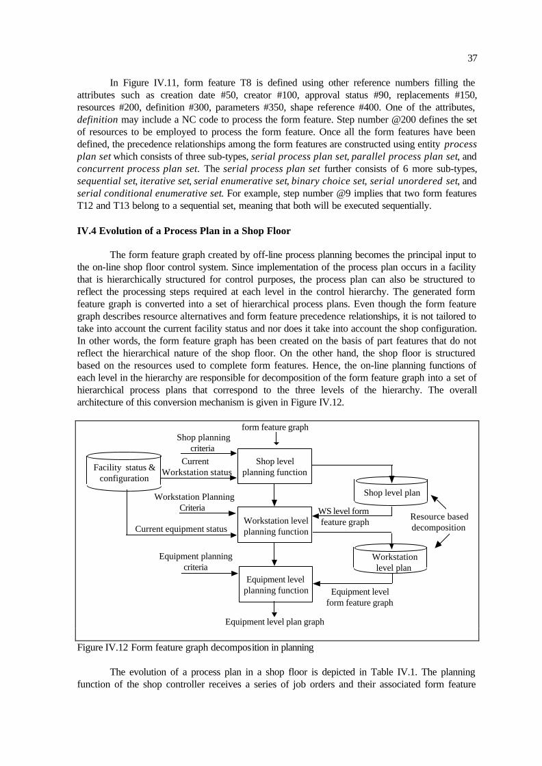
37

In Figure IV.11, form feature T8 is defined using other reference numbers filling the attributes such as creation date #50, creator #100, approval status #90, replacements #150, resources #200, definition #300, parameters #350, shape reference #400. One of the attributes, definition may include a NC code to process the form feature. Step number @200 defines the set of resources to be employed to process the form feature. Once all the form features have been defined, the precedence relationships among the form features are constructed using entity process plan set which consists of three sub-types, serial process plan set, parallel process plan set, and concurrent process plan set. The serial process plan set further consists of 6 more sub-types, sequential set, iterative set, serial enumerative set, binary choice set, serial unordered set, and serial conditional enumerative set. For example, step number @9 implies that two form features T12 and T13 belong to a sequential set, meaning that both will be executed sequentially. IV.4 Evolution of a Process Plan in a Shop Floor The form feature graph created by off-line process planning becomes the principal input to the on-line shop floor control system. Since implementation of the process plan occurs in a facility that is hierarchically structured for control purposes, the process plan can also be structured to reflect the processing steps required at each level in the control hierarchy. The generated form feature graph is converted into a set of hierarchical process plans. Even though the form feature graph describes resource alternatives and form feature precedence relationships, it is not tailored to take into account the current facility status and nor does it take into account the shop configuration. In other words, the form feature graph has been created on the basis of part features that do not reflect the hierarchical nature of the shop floor. On the other hand, the shop floor is structured based on the resources used to complete form features. Hence, the on-line planning functions of each level in the hierarchy are responsible for decomposition of the form feature graph into a set of hierarchical process plans that correspond to the three levels of the hierarchy. The overall architecture of this conversion mechanism is given in Figure IV.12.

form feature graph

Facility status & configuration

Shop level plan

Resource based decomposition

Equipment level plan graph

Current equipment status

WS level form feature graph

Equipment level form feature graph

Shop level planning function

Workstation level planning function

Workstation level plan

Equipment level planning function

Shop planning criteria

Workstation Planning Criteria

Equipment planning criteria

Current Workstation status

Figure IV.12 Form feature graph decomposition in planning The evolution of a process plan in a shop floor is depicted in Table IV.1. The planning function of the shop controller receives a series of job orders and their associated form feature

38

graphs from the factory level controller. It then creates batches and generates a shop level plan graph for each batch. A workstation sequence graph is obtained from the shop level plan graph by considering workstation availability, resource availability, travel times between workstations, workstation contentions with other batches. Definition IV.3 Shop level plan graph: A shop level plan graph is an aggregated form feature graph used to represent workstation activities and their precedence relationships. An edge in the shop level plan graph represents the precedence relationship between two nodes. A node in the shop level plan graph is one of five different types: WORKSTATION, SPLIT-AND, SPLIT-OR, JOIN-AND, and JOIN-OR. The specification of the nodes is the same as that of a form feature graph, except for WORKSTATION type nodes. A WORKSTATION type node contains a workstation form feature graph that specifies the set of form features performed the equipment controllers within a workstation, their attributes, and the precedence relationship among form features. In order to store the shop level plan graph in a file, precedence and node information is stored as shown in Figure IV.13. Precedence information is provided by specifying the successors of a particular node, while the information content in the WORKSTATION type nodes is provided as a file pointer. The node type attribute includes SPLIT-AND, SPLIT-OR, JOIN-AND, JOIN-OR, and WORKSTATION. The workstation index specifies a unique workstation identifier. Table IV.1 Evolution of a process plan for shop floor control Level Form Feature Graph Plan Graph Sequence Graph

Shop t3t4

t6t8t0

t1

t5

t2

t7

form feature graph w1 w2

so josa ja

W1 W2

W1 W2

workstation1

workstation2

Work-station

Workstation form feature graph w1

o1

o2

o3

t3t4

t6

t0

t1

t5

t2so jo

sa ja

o1o2

o3sa ja

o1o2

o3sa ja

Equip-ment

Equipment form feature graph o2

t3t4t1

t2so jo

Equipment plan graph

t3t4t1

t2so jo

t1 t2 t4

tool1

tool1

tool4

node and precedence information :

node name

node type

# of successors

succ1, succ2..

workstation index

workstation form feature graph file name

node number

Figure IV.13 Data structure for a shop level plan graph

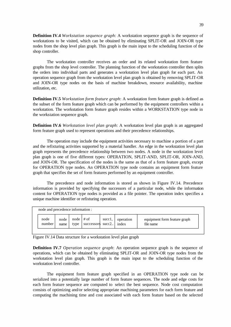
39

Definition IV.4 Workstation sequence graph: A workstation sequence graph is the sequence of workstations to be visited, which can be obtained by eliminating SPLIT-OR and JOIN-OR type nodes from the shop level plan graph. This graph is the main input to the scheduling function of the shop controller. The workstation controller receives an order and its related workstation form feature graphs from the shop level controller. The planning function of the workstation controller then splits the orders into individual parts and generates a workstation level plan graph for each part. An operation sequence graph from the workstation level plan graph is obtained by removing SPLIT-OR and JOIN-OR type nodes on the basis of machine breakdown, resource availability, machine utilization, etc. Definition IV.5 Workstation form feature graph: A workstation form feature graph is defined as the subset of the form feature graph which can be performed by the equipment controllers within a workstation. The workstation form feature graph resides within a WORKSTATION type node in the workstation sequence graph. Definition IV.6 Workstation level plan graph: A workstation level plan graph is an aggregated form feature graph used to represent operations and their precedence relationships. The operation may include the equipment activities necessary to machine a portion of a part and the refixturing activities supported by a material handler. An edge in the workstation level plan graph represents the precedence relationship between two nodes. A node in the workstation level plan graph is one of five different types: OPERATION, SPLIT-AND, SPLIT-OR, JOIN-AND, and JOIN-OR. The specification of the nodes is the same as that of a form feature graph, except for OPERATION type nodes. An OPERATION type node contains an equipment form feature graph that specifies the set of form features performed by an equipment controller. The precedence and node information is stored as shown in Figure IV.14. Precedence information is provided by specifying the successors of a particular node, while the information content for OPERATION type nodes is provided as a file pointer. The operation index specifies a unique machine identifier or refixturing operation.

node and precedence information :

node name

node type

# of successors

succ1, succ2..

operation index

equipment form feature graph file name

node number

Figure IV.14 Data structure for a workstation level plan graph Definition IV.7 Operation sequence graph: An operation sequence graph is the sequence of operations, which can be obtained by eliminating SPLIT-OR and JOIN-OR type nodes from the workstation level plan graph. This graph is the main input to the scheduling function of the workstation level controller. The equipment form feature graph specified in an OPERATION type node can be serialized into a potentially large number of form feature sequences. The node and edge costs for each form feature sequence are computed to select the best sequence. Node cost computation consists of optimizing and/or selecting appropriate machining parameters for each form feature and computing the machining time and cost associated with each form feature based on the selected

40

parameters. Edge costs represent non-cutting times, including tool change and rapid travel between form features. NC instructions are generated for non-machining activities on each edge in the sequence and merged with the NC instructions for machining activities into a single file. The file may now be downloaded to the equipment control box for execution or may be graphically emulated on the screen. Definition IV.8 Equipment form feature graph: An equipment form feature graph is defined as the subset of the workstation form feature graph, which is executed by an equipment controller. The equipment form feature graph resides within an OPERATION type node in the workstation level plan graph. Definition IV.9 Form feature sequence: A form feature sequence is the unique sequence of the set of form features. IV.5 Example for Evolution of a Process Plan An illustrative example for form feature graph decomposition is developed in this section. A graph-based representation is used in this example, since this is more intuitive. The example part and the polyshape that needs to be removed are shown in Figure IV.15. There are two possible decompositions of the polyshape.

Raw Material Finished Product

t : Turning f: Facing p: Parting c: Chamfering

Machining Operations

t1t2

t3

c1

t4

p0

f0

c1

t1t2

t5

t6

t7

t8

p0

f0

m : Milling

m1m2

polyshape

Figure IV.15 Example part for the evolution of a process plan A form feature graph can be seen from Figure IV.16. The form feature graph consists of nodes f0 and p0 which represent facing and parting-off, respectively. Nodes t1 through t8 represent straight or taper turning, and node c1 represents chamfering. Two nodes m1 and m2 represent the slot milling operation.

f0 t1 t2t3

t5

t4

t7

t8

p0

t6

c1so

sa ja

jom1

m2sa ja

Figure IV.16 Form feature graph for the example part The facility that is assumed for implementation of the process plans is the Texas A&M University CIM LAB shown in Chapter I. For control purposes, this facility may be hierarchically decomposed into two processing workstations. Workstation 1 consists of a Leadwell turning center,

41

a Sabre machining center, and an Puma 760 robot. Workstation 2 consists of a Pratt and Whitney machining center and an Adept robot.

Determination of the workstation sequence begins with modifying the form feature graph by identifying the workstation resources required for each node in the graph, on the basis of the current facility status and shop configuration. Adjacent nodes which use the same workstation resources, are aggregated into one node in order to create a workstation form feature graph. This results in the construction of a shop level plan graph. The work content of each aggregated node will be processed in a single workstation. Figure IV.17 illustrates a form feature graph, a shop level plan graph, and a workstation sequence graph. Among three workstation form feature graphs, w1 can be assigned to workstation 1, w2 can be assigned to either workstation 1 or workstation 2, and w3 can be assigned to workstation 1. Assume that the shop level controller chooses node w3 and sends it to workstation 1. The workstation controller receives a workstation form feature graph and utilizes current equipment status and workstation configuration information to determine the actual pieces of equipment on which the part will be produced. The workstation controller may be responsible for dividing the workload among the pieces of equipment in the workstation. First, the workstation form feature graph is modified into a workstation level plan graph by aggregating adjacent nodes that use common machine and fixture resources. This is done on the basis of availability of machine, tooling, and material handling resources in the workstation. Each node in the workstation level plan graph represents either an equipment level form feature graph or part re-orientation on a machine using a material handler. Figure IV.18 illustrates the activities of the workstation controller. Workstation 1 receives workstation form feature graph w3 and generates a workstation plan graph. All the form features associated with turning processes are assigned to the Leadwell turning center, while two form features associated with milling processes are assigned to the Sabre machining center.

f0 t1 t2t3

t5

t4

t7

t8

p0

t6

c1so

sa ja

jom1

m2sa ja

w1 w2w3

so jo

w1 w2

w3Shop level plan graph Workstation sequence graph

w3workstation 1

Figure IV.17 Form feature graph decomposition at shop level

42

f0 t1 t2t3

t5

t4

t7

t8

m1

m2p0

t6

c1so

sa ja

jo sa ja

o1 o2

o1 o2

Workstation level plan graph Operation sequence graph

Workstation form feature graph for workstation 1

o1 o2Leadwell Sabre

Figure IV.18 Form feature graph decomposition at workstation level The workstation controller downloads an equipment level form feature graph to the equipment controller. In Figure IV.19, the Leadwell turning center receives a form feature graph associated with operation o1, while the Sabre machining center receives a form feature graph associated with operation o2. A number of possible form feature sequences can be found by serializing the form feature graph. A node in this sequence represents a form feature and its attributes including a unique NC instruction, machining parameters. An arc represents activities performed between form features, including rapid tool motion and tool change. IV.6 Chapter Summary This chapter provides a structured approach to the integration of process planning and shop floor control for a hierarchical control architecture. A form feature graph is decomposed into a hierarchical set of process plans which reflect the resource requirements at each level in the control hierarchy. An illustration of this decomposition has been provided in order to fully explain the intermediate process plan representations. The final output is a sequence of NC instructions that may be directly downloaded to a NC machine or may be graphically validated on a computer.

f0 t1 t2t3

t5

t4

t7

t8

p0

t6

c1so

sa ja

jo m1

m2

sa ja

Equipment form feature graph for Leadwell Equipment form feature graph for Sabre

Form feature sequence for LeadwellForm feature sequence for Sabre

f0 t1 t2 t3 t4 p0c1 m1 m2

Figure IV.19 Form feature graph decomposition at equipment level While an example described in this chapter is specific to rotational parts with external features, the form feature graph decomposition and on-line planning functions are sufficiently generic in nature, and applicable to any metal machining. The approach provides a structured framework for developing a way of data interface between process planning and shop floor control. The approach also allows for a hierarchical aggregation of process plans, so that they can be used to provide scalability in shop floor control activities.

43

An AND/OR graph representation and its aggregation activities specified in this chapter cannot deal with any irregular AND/OR graph. The irregular AND/OR graph cannot be defined recursively as used in the ISO process plan representation. In other words, a set of form features surrounded by SPLIT-AND and JOIN-AND type nodes cannot be constructed. One way to represent the irregular AND/OR graph is to convert it into a regular AND/OR graph, in spite of losing some information. For example, an irregular AND/OR graph in Figure IV.20(a) can be converted into a regular graph in Figure IV.20(b). However, form feature 5 in Figure IV.20(a) can be machined after form feature 3, while form feature 5 in Figure IV.20(b) must be machined after two form features 2 and 3 in Figure IV.20(b).

1

2

3

4

5

6

1

2

3

ja sa

4

5

jasa 6

: SPLIT-AND

(a) Irregular AND/OR graph

(b) Regular AND/OR graph Figure IV.20 Irregular and regular AND/OR graphs

44

CHAPTER V

PLANNING FUNCTION

V.1 Chapter Overview In the previous chapter, the evolution of a process plan in a shop floor was presented, which is the responsibility of the planning function. In this chapter, the planning function of the IWC is detailed. The planning function receives information such as part type/quantity and its related workstation form feature graphs from the shop level controller. It then performs preparatory activities, such as batch splitting, generation of a workstation plan graph for each part, determination of the operation sequence of a part, resource assignment for each operation. As a result, a set of operations to be performed on each part can be represented as an operation sequence graph in which operation sequence alternatives are specified by SPLIT-AND and JOIN-AND type nodes. The operation sequence graph is sent to the scheduling function. The focus of this chapter is to describe and develop a real-time planning function to support the IWC that fits within the hierarchical SFCS architecture. The detailed objectives of this chapter are: 1) to present a taxonomy of planning functions for hierarchical shop floor control, 2) to describe the definition and procedures of the planning function of the IWC, and 3) to describe the planning function of the equipment controller. The remainder of the chapter is organized as follows: Section V.2 provides framework, problem statement, and a taxonomy of the planning functions for shop floor control. In Section V.3, related work is presented. In Section V.4, a brief description on the planning function of the shop controller is provided. A detailed description on the planning function of the IWC is discussed in Section V.5. Section V.6 addresses the planning function of the equipment controller. Finally, Section V.7 provides a summary of the chapter. V.2 Framework and Problem Statement Process planning is viewed as an information generating function that provides essential instructions that are necessary for converting the raw material to the final product. Further, it provides the basis of decision-making for shop floor control by providing detailed work instructions, such as machines to be used for specific machining operations, machining parameters, tool and fixture specifications. The planning function at each level is invoked by the execution function at the same level when a part/batch arrives at the loading port. The planning function is also invoked by the scheduling function when a replanning activity is needed. It is assumed that the form feature graphs associated with the part/batch under the purview of a controller are available in the database. The planning function at each level then performs various activities based on the form feature graphs, and shop configuration and status. Table V.1 shows a taxonomy of the planning functions for hierarchical shop floor control. Planning can be defined informally as a function that generates a set of tasks to be scheduled in the future. Specifically, planning determines batch size, generates the plan graphs by aggregating the form feature graphs, forms the sequence graphs by eliminating SPLIT-OR and JOIN-OR type nodes, and select a good operation sequence graph. The purpose of the planning function is to enable each order to be completed within the specified time limits.

45

Table V.1. Taxonomy of the planning function for shop floor control Level Problems Criteria Constraints Inputs Outputs

Shop

• order release • batching • form feature graph aggregation • resource selection (pallet, material transport, workstation) • plan graph serialization • due-date assignment

• resource utilization • balance workload • resource contentions • deadlock possibility • the number of workstation visits

• alternative workstation • form feature precedence • resource existence • technological constraints • capacity constraints • layout requirement

• order • process plan • shop status, configuration • expected machining time within workstation • transport time between workstations

• work- station sequence graph,

Work-station

• batch splitting • workstation form feature graph aggregation • resource selection (machine, fixture, set of tools, material handler) • plan graph serialization

• resource utilization • balance workload • resource contentions • deadlock possibility • the number of fixture changes and machine visits

• alternative machine, fixtures • form feature precedence • resource existence • technological constraints (surface finish) • capacity constraints

• order • workstation form feature graph • workstation status, configuration • expected machining, refixturing, handling time

• opera- tion sequence graph,

Equip-ment

• equipment form feature graph serialization • resource selection(tool) • parameter optimization

• machining time • non-machining time (tool change, rapid travel) • the number of form features

• alternative tools • form feature precedence • technological constraints (power, tool life)

• order • equipment form feature graph • tool status • task, tooling, travel time

• form feature sequence graph

The planning function of the shop controller receives a series of job orders and their related form feature graphs from the factory level controller. After creating batches from the orders, the planning function generates the best workstation sequence for each batch by aggregating the form feature graph. The material transport activities of each batch between workstations are also specified. In the same manner, the planning function of the IWC receives a batch and its related workstation form feature graph, and then splits the batch into parts. The workstation form feature graph associated with each part is converted to the workstation level plan graph which contains the set of operations and related resources necessary to be carried out on the part in the workstation. An operation sequence graph is then obtained by eliminating SPLIT-OR and JOIN-OR type nodes from the workstation level plan graph. In addition, an operation may require other resources, such as tools, fixtures, and attendants be available. The material handling activities of each part between operations are also specified.

46

Finally, the planning function of the equipment controller receives a part and its related equipment form feature graph. The planning function then finds the best form feature sequence on the basis of several factors, such as the number of tool changes required, tool changing time and rapid traverse time between two form features. The NC instructions of the serialized form features are merged into a file which includes all the machine level activities such as machining, tool changing. The execution function of the equipment controller will download the merged NC file to the control unit connected to the physical device. The successful implementation of the planning functions is not easy because: 1) a part may have alternative routings, 2) a machine may process various parts, 3) a part may be processed using alternative resources, 4) a part may have different processing times on various resources, 5) new parts may be introduced frequently, 6) new plans need to be generated each time errors occur, and 7) decisions must be made in real-time. As a result, the planning problems will be decomposed into a set of smaller problems in a hierarchical manner. V.3 Related Work In most cases, real-time scheduling for shop floor control does not become a concern until planning problems are defined and resolved. It is necessary, therefore, to define and resolve the planning problems in an automated manufacturing environment. Although planning is an on-line function which prepares a set of tasks to be scheduled in the future, the research community has developed various planning problems, such as a batching problem, machine grouping problem, production ratio problem, and resource allocation problem (Chung [42], Damodaran et al. [47], Dirne [57], Morton and Smunt [157], Stecke [204, 205], Stecke and Kim [206], Stecke and Solberg [208], Van Looveren et al. [221]). The batching problem consists of determining a subset of part types and part mix from the production requirements. This problem has been considered and solved by many authors using either mathematical programming techniques or heuristics (Avonts et al. [13], Bastos [18], Hwang [104], Rajagopalan [177], Stecke and Kim [207]). A batch may have the same part characteristics, such as part type, operation routings, resources to be used. For example, if each batch contains parts that need the same fixture, fixture changeovers may occur once a batch has been completed. The machine grouping problem consists of partitioning a set of machines into several groups such that the same set of operations can be performed within the same group (Lashkari and Guna [133], Stecke [205]). This problem is considered as a logical grouping of machines rather than physical hardware layout. Machines in a group are usually the same type and are equipped with identical or nearly identical tools in order to minimize the tooling operations and reduce the size of the problems to be solved (Stecke and Talbot [209]). The resource allocation problem consists of assigning a set of resources, such as fixture, pallet, to the batch selected for immediate simultaneous production (Kusiak [128], Solot [203]). This problem falls into a pure assignment problem with the constraints about fixture and pallet availability. The loading problem is to assign a set of operations and tools to a set of machines. This problem becomes complex since there are various part types, many operations on a part, and a variety of tools in a shop floor. A number of researchers have employed mathematical programming techniques to formulate this problem (Bretthauer et al. [28], Fernandes and Gomide [68], Kusiak [128], Shanker and Tzen [195], Stecke [205]). Most of the mathematical formulations are in the form of integer and mixed integer problems. Since solving large mathematical programming

47

problems require significant time and memory resources, there will be a need for robust heuristics which provide good solutions in real-time. A number of heuristics have been proposed to overcome the disadvantages of mathematical techniques (Fernandes and Gomide [68], Mukhopadhyay et al. [158], Shanker and Srinivasula [195], Stecke [205], Stecke and Solberg [208]). On the other hand, a few heuristics on dynamic machine selection problems have appeared (O'Keefe and Kasirajan [168], Ro and Kim [181], Shmilovici and Maimon [199], Yao and Pei [236]). Seven part selection rules and four machine center selection rules have been investigated and experimented using a physical simulator in order to show relative ranks for major decision rule sets according to ten performance measures (Choi and Malstrom [40]). The next operation of a part can be assigned dynamically to a machine based on the state of the system. Few people investigated how to select/update the process plans to be used in executing assigned jobs (Stecke [204], Choi and Malstrom [40], Kusiak and Finke [130], Bhaskaran [21], Ro and Kim [181]). The heuristic algorithms used to select a set of process plans have been developed with the objective of minimizing cost of removing the material, number of machine tools, and sum of the traveling distance in the context of metal cutting (Kusiak and Finke [130]). On the other hand, other objective functions have been proposed and tested: 1) to minimize the total processing time, 2) to minimize the total number of processing steps, and 3) to minimize the dissimilarity between the selected plans (Bhaskaran [21]). While a number of articles on planning have appeared, it is clear that the planning problem for automated manufacturing systems has been viewed differently by many researchers. This is primarily due to the uncoupling of decision-making problems (planning and scheduling) and control problems in a real-time situation. However, implementation of planning solutions always occurs within a control framework, and the functionality and relationship of the decision-making and control components must be well understood if a solution is to be successfully implemented. In fact, little effort has been made to define the planning problems from the viewpoint of the hierarchical SFCS. V.4 Shop Level Planning Function The planning function of the shop level controller receives a series of orders from the factory level controller, and retrieves their related form feature graphs. The planning function begins with loading parts associated with the orders so that the orders can be finished by the assigned due-date. The planning function then prepares various activities associated with those orders. It may be necessary to split the orders into batches. The batch size at this level depends on many factors, such as pallet size, material transport capacity, part mix, routing complexity. Once batches have been determined, the planning function generates the shop level plan graph for each batch. A shop level plan graph is an aggregated form feature graph necessary to represent workstation activities and their precedence relationships. A workstation sequence graph is generated from the shop level plan graph. The workstation sequence graph is the sequence of workstation activities to be performed, which is obtained by eliminating all the SPLIT-OR, and JOIN-OR type nodes from the shop level plan graph. The planning function may use other information, such as shop status, shop configuration, expected machining time within each workstation, expected material transportation time between workstations. Finally, the planning function assigns the due-dates to each WORKSTATION type node in the workstation sequence graphs. This graph is the main input to the scheduling function of the shop level controller.

48

The problems described above cannot be completely separated, but the resolution methods may depend on the problem complexity. The criteria to be considered are to 1) maximize resource utilization, 2) balance workload among workstations, 3) minimize resource contention, and 4) minimize the number of workstation visits. The constraints to be considered contain alternative workstations, form feature precedence, technological constraints (for example, existence of a specific machine within a workstation), capacity constraints (for example, workstation space), and workstation layout requirements. V.5 Workstation Level Planning Function The planning function of the IWC receives a related workstation form feature, each time a batch arrives to the workstation. It then organizes information and prepares various activities in order to assist the scheduling and execution functions. First, a batch that just arrived is split into a set of logical batches. Parts in a logical batch have the same part routings and resources assigned. Without loss of generality, it can be assumed that the size of a logical batch is one. The planning function then accepts a workstation form feature graph for each part as an input and generates an operation sequence graph as an output. The criteria to be considered are: 1) the amount of workload assigned to each machine is balanced, 2) resource utilization is maximized, 3) resource contention is minimized, 4) the possibility of system deadlocks is minimized, and 5) the number of operations is minimized. The result must adhere to several constraints, such as form feature precedence, resource existence, technological constraints (e.g., surface finish of each machine), and capacity constraints (e.g., machine size). A number of similar problems have been reported for problem reduction (Nilsson [162]) and assembly plan representations (De Mello and Sanderson [53]). In the AND/OR graph used to represent problem reduction, the start node corresponds to the original problem description, while the nodes corresponding to primitive problem descriptions are called terminal nodes. The terminal nodes represent solvable nodes. The main purpose of the search process carried out on the AND/OR graph is to show that there are paths from the start node to the terminal nodes, meaning that the start node is solved. If a non-terminal node has OR successors, then it is a solvable node if and only if at least one of its successors is solved. If a non-terminal node has AND successors, then it is a solvable node if and only if all of its successors are solved. The main difference between the problem reduction representations and form feature representations is that the sequence of AND successors is not important in the problem reduction representation, but not true in the form feature representation. This is due to the fact that the material handling or buffering activities are required in between two AND successors in the form feature representation. Figure V.1 illustrates the difference. Figure V.1(a) implies that problem A can be solved if two problems B and C can be solved. Hence, the sequence of B and C is not significant in this case. Figure V.1(b) implies that operation A can be done before two operations B and C are done. However, sequence A, B, and C requires two tool changes, while sequence A, C, and B requires only one tool change. Hence, the sequence of AND successors is significant. If there is a cost associated with each edge in the problem reduction representation graph, the total cost of a path from the start node to the terminal nodes can be computed. Consider a decision problem is to determine if the AND/OR graph has a path with a cost at most k , for k a given input. This problem is NP-complete (Horowitz and Sahni [99]). The solution of the form feature representation graph has more alternative sequences than that of the problem reduction representation graph. Hence, a decision problem to determine if there is a form feature sequence with a cost at most k, for k a given input, in the form feature graph is NP-complete. In this research,

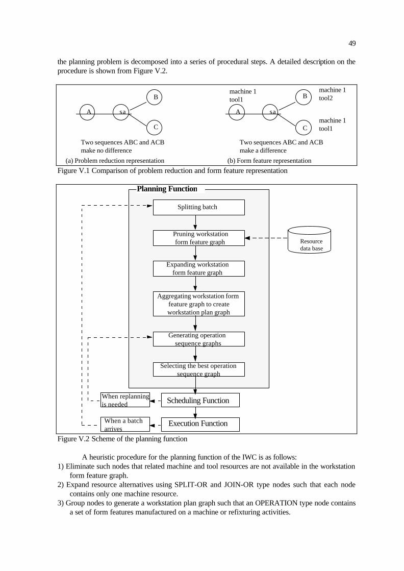
49

the planning problem is decomposed into a series of procedural steps. A detailed description on the procedure is shown from Figure V.2.

A sa

B

C

A sa

B

C

machine 1 tool1

machine 1 tool2

machine 1 tool1

Two sequences ABC and ACB make no difference

Two sequences ABC and ACB make a difference

(a) Problem reduction representation (b) Form feature representation Figure V.1 Comparison of problem reduction and form feature representation

Planning Function

Resource data base

Scheduling Function

Execution Function

Splitting batch

Pruning workstation form feature graph

Expanding workstation form feature graph

Aggregating workstation form feature graph to create workstation plan graph

Generating operation sequence graphs

Selecting the best operation sequence graph

When a batch arrives

When replanning is needed

Figure V.2 Scheme of the planning function A heuristic procedure for the planning function of the IWC is as follows: 1) Eliminate such nodes that related machine and tool resources are not available in the workstation

form feature graph. 2) Expand resource alternatives using SPLIT-OR and JOIN-OR type nodes such that each node

contains only one machine resource. 3) Group nodes to generate a workstation plan graph such that an OPERATION type node contains

a set of form features manufactured on a machine or refixturing activities.

50

4) Remove SPLIT-OR and JOIN-OR type nodes from the workstation plan graph to obtain the set of operation sequence graphs.

5) Select the best operation sequence graph. V.5.1 Pruning of Workstation Form Feature Graph Suppose a part has a form feature graph as illustrated in Figure V.3 and a workstation consists of two drilling machines, m1 and m2. Form feature t1 must be done before form feature t2, while form feature t3 must be done before form feature t4. Further, two form feature sets {t1, t2} and {t3, t4} are connected with SPLIT-AND and JOIN-AND type nodes. Each form feature has its own resources, machining parameters, and NC instructions defined in a FORM-FEATURE type node.

{drilling [m1, tool1, f1, v=100, f=50, NC1] [m2, tool2, f1, v=120, f=60, NC2]}

{drilling [m1, tool5, f1, v=80, f=50, NC5] [m2, tool6, f1, v=90, f=60, NC6] [m2, tool7, f1, v=105, f=65, NC7]}

{reaming [m1, tool3, f1, v=50, f=50, NC3] [m2, tool4, f1, v=70, f=60, NC4]}

{reaming [m1, tool8, f1, v=40, f=45, NC8] [m2, tool9, f1, v=60, f=30, NC9] [m2, tool10, f1, v=65, f=25, NC10]}

sa : SPLIT-AND ja : JOIN-AND

sa

t1 t2

ja

t3 t4

Figure V.3 Illustration of a workstation form feature graph The first step is to eliminate features or resource alternatives in the workstation form feature graph, whose related resources are not currently available. For example, Figure V.4 illustrates a pruned workstation form feature graph obtained from Figure V.3, where the second resource alternative for form feature t2 is pruned if tool4 is not available on machine m2. V.5.2 Disaggregation of Workstation Form Feature Graph The next step is to expand the workstation form feature graph by disaggregating FORM-FEATURE type nodes with machine resource alternatives. This implies that the FORM-FEATURE type nodes which contain multiple machine resource alternatives can be decomposed into a number of FORM-FEATURE type nodes which contain a single machine resource. Disaggregation of FORM-FEATURE type nodes provides a number of SPLIT-OR and JOIN-OR type nodes. Figure V.5 illustrates an expanded workstation form feature graph after FORM-FEATURE type nodes in Figure V.4 are disaggregated. Form feature node t1' has the same form feature as t1, but different machine resource specifications. Either t1' or t1 yields the same part shape. Hence, the two nodes, t1' and t1, are connected with SPLIT-OR and JOIN-OR type nodes.

51

sa

t1 t2

ja

t3 t4

{drilling [m1, tool1, f1, v=100, f=50, NC1] [m2, tool2, f1, v=120, f=60, NC2]}

{drilling [m2, tool6, f1, v=90, f=60, NC6] [m2, tool7, f1, v=105, f=65, NC7]}

{reaming [m1, tool3, f1, v=50, f=50, NC3]}

{reaming [m1, tool8, f1, v=40, f=45, NC8] [m2, tool9, f1, v=60, f=30, NC9] [m2, tool10, f1, v=65, f=25, NC10]}

Figure V.4 Modified workstation form feature graph

sa

t1

t2

ja

t3 jo

{drilling [m1, tool1, f1, v=100, f=50, NC1]

{drilling [m2, tool6, f1, v=90, f=60, NC6] [m2, tool7, f1, v=105, f=65, NC7]}

{reaming [m1, tool3, f1, v=50, f=50, NC3]}

{reaming [m1, tool8, f1, v=40, f=45, NC8]

t1'

so jo

t4

t4'

so

{reaming [m2, tool9, f1, v=60, f=30, NC8] [m2, tool10, f1, v=65, f=25, NC10]}

{drilling [m2, tool2, f1, v=120, f=60, NC2]}

Figure V.5 Disaggregation of the workstation form feature graph V.5.3 Generation of Workstation Plan Graph The third step is to generate a workstation plan graph by grouping a number of FORM-FEATURE nodes with the same machine resource. Aggregation of FORM-FEATURE type nodes yields an OPERATION type node which contains an equipment form feature graph to be used by a single equipment controller. It should be noted that when a number of FORM-FEATURE nodes are aggregated, if a refixturing operation is required, an OPERATION type node for a refixturing operation needs to be inserted between two successive machining operations. Figure V.6 illustrates a workstation plan graph obtained from Figure V.5. Figure V.6 also shows the equipment form feature graph corresponding to each operation.

52

o1

o2

o3 o4

o5 o6

o7 o8

sa ja

so jo

o1 t1 t2

t1'

t3sa jao3

t2

t4sa jao4

o5 t3

t1

t4sa jao6

t2

t1'

t3sa jao7

t4'

o8 t2

o2 t3 t4'= =

=

=

=

=

=

=

Figure V.6 Workstation plan graph obtained from a form feature graph V.5.4 Generation of Operation Sequence Graph The output from the planning function is an operation sequence graph which contains machine sequence alternatives, meaning that the operation sequence graph may contain SPLIT-AND and JOIN-AND type nodes. This operation sequence graph becomes the input to the scheduling function of the IWC. Hence, the objective function used in generating the operation sequence graph must be equivalent to performance criteria used in the scheduling function. To this end, a number of operation sequence graphs can be generated by eliminating SPLIT-OR and JOIN-OR type nodes. For example, Figure V.7 illustrates four different operation sequence graphs obtained from a workstation plan graph in Figure V.6.

o1

o2o3 o4

o5 o6

o7 o8

sa ja

so jo

o1

o2

sa ja

o3 o4

o5 o6

o7 o8

operation sequence graph 1 :

operation sequence graph 2 :

operation sequence graph 3 :

operation sequence graph 4 :

Figure V.7 Generation of operation sequence graphs The next step is to select the operation sequence graph for each part. A heuristic can be applied to determine an operation sequence graph from a workstation plan graph which provides the best results for the scheduling function. Several heuristics can be used: An operation sequence graph can be selected such that 1) its total processing and material handling time is shortest, 2) its routing flexibility indicator is largest, or 3) it contributes to balancing machine load. Following are a

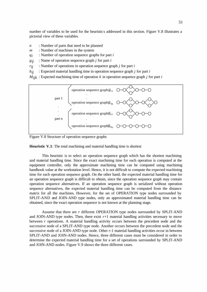
53

number of variables to be used for the heuristic s addressed in this section. Figure V.8 illustrates a pictorial view of these variables. n : Number of parts that need to be planned m : Number of machines in the system qi : Number of operation sequence graphs for part i gij : Name of operation sequence graph j for part i rij : Number of operations in operation sequence graph j for part i hij : Expected material handling time in operation sequence graph j for part i Mijk : Expected machining time of operation k in operation sequence graph j for part i

.

.

.

.

part 1

part n

.

.

.

g11operation sequence graph

operation sequence graph

operation sequence graph

operation sequence graph

g1q1

gn1

gnqn Figure V.8 Structure of operation sequence graphs Heuristic V.1: The total machining and material handling time is shortest This heuristic is to select an operation sequence graph which has the shortest machining and material handling time. Since the exact machining time for each operation is computed at the equipment controller, only the approximate machining time can be computed using machining handbook value at the workstation level. Hence, it is not difficult to compute the expected machining time for each operation sequence graph. On the other hand, the expected material handling time for an operation sequence graph is difficult to obtain, since the operation sequence graph may contain operation sequence alternatives. If an operation sequence graph is serialized without operation sequence alternatives, the expected material handling time can be computed from the distance matrix for all the machines. However, for the set of OPERATION type nodes surrounded by SPLIT-AND and JOIN-AND type nodes, only an approximated material handling time can be obtained, since the exact operation sequence is not known at the planning stage. Assume that there are r different OPERATION type nodes surrounded by SPLIT-AND and JOIN-AND type nodes. Then, there exist r+1 material handling activities necessary to move between r operations. A material handling activity occurs between the precedent node and the successive node of a SPLIT-AND type node. Another occurs between the precedent node and the successive node of a JOIN-AND type node. Other r-1 material handling activities occur in between SPLIT-AND and JOIN-AND nodes. Hence, three different cases must be considered in order to determine the expected material handling time for a set of operations surrounded by SPLIT-AND and JOIN-AND nodes. Figure V.9 shows the three different cases.

54

.......

.......

.......

.......

....... .......sa ja

Case 1 Case 2 Case 3

o1

o2

o3

o4

o6

o7

o8

o9 Figure V.9 Three different cases for material handling activities Case 1) Between the precedent and the successive nodes of a SPLIT-AND type node In this case, a material handling activity is required in order for one of operations o1, o2, o3, and o4 to be done in Figure V.9. The planning function cannot determine which operation is done first. Hence, only the approximate material handling time can be computed. Two subcases can be found: subcase 1) the precedent node of the SPLIT-AND type node is of OPERATION type node and subcase 2) the precedent node of the SPLIT-AND type node is of JOIN-AND type node. Figure V.10 illustrates two different subcases. For subcase 1), an average value of the material handling times between o1' and o1, o1' and o2, o1' and o3, and o1' and o4 can be computed. For subcases 2), all the possible operation sequences need to be considered. For example, subcase 2 in Figure V.10 illustrates twelve (= 3 ´ 4) possible material handling activities. Hence, an average value of the twelve material handling times can be also computed.

sa

o1

o2

o3

o4

sa

o1

o2

o3

o4

o1' ja

o1'

o2'

o3'

Subcase 1 Subcase 2 Figure V.10 Two different subcases for case 1 in Figure V.9 Case 2) In between SPLIT-AND and JOIN-AND type nodes It is to be noted that r-1 material handling activities can occur between SPLIT-AND and JOIN-AND type nodes if there are r operations. The total material handling time among all OPERATION type nodes can be computed as follows:

Teff >e

r

∑e=1

r

∑,

55

where Tef represents the material handling time between operation e and f. Since the total number of possible material handling activities is r(r-1)/2, the approximate time of a material handling activity between two nodes can be computed as follows:

Teff >e

r

∑e=1

r

∑ r r − 1( )2

Since the number of material handling activities is r-1 in between SPLIT-AND and JOIN-AND nodes, the approximate material handling time can be computed as follows:

Teff >e

r

∑e=1

r

∑ r r − 1( )2

× r − 1( ) = Teff >e

r

∑e=1

r

∑ r2

Case 3) Between the precedent and the successive nodes of a JOIN-AND type node This case can be resolved in the same manner as case 1). Using the three different cases described above, the expected material handling time (hij) for each operation sequence graph can be computed. Let Xij be 1 if operation sequence graph j is selected as the best operation sequence graph for part i, 0 otherwise. Then, an integer programming formulation can be constructed as follows:

min Mijkk =1

rij

∑ + hij

j =1

q i

∑ Xiji =1

n

∑

s.t. Xijj =1

qi

∑ = 1 ∀i

Xij = 0 or 1 For example, Figure V.11 illustrates how to obtain the expected machining and material handling time for an operation sequence graph. The machining time can be easily computed by adding the machining time of all the operations, which is 37 min. The material handling times between operations can be computed as follows: Between o1 and o2: 1.1 min Between o2 and either o3 or o5 (subcase 1): (1.3+1.8)/2 = 1.55 min Between SPLIT-AND and JOIN-AND: (1.2+1.4+2.0)/1.5 = 3.07 min Between either o4 or o5 and o6 (subcase 2): (1.5+2.0)/2 = 1.75 min Hence, the total material handling time is 7.47 min (= 1.1 + 1.55 + 3.07 + 1.75). Therefore, the expected machining and material handling time for an operation sequence graph is 44.47 min (= 37 + 7.47).

56

o1

o3 o4

o5

o6sa jao2

machine1 6 min

machine2 5min

machine3 4 min

machine4 7 min

machine5 9 min

machine6 6 min

1 2 3 4 5 6

1

2

3

4

5

6

1.1 1.3

1.3

1.71.5 2.0

1.6 1.8 2.1

1.2 1.4 1.7

2.0 1.5

2.0

Distance matrix between two machines (min)

Figure V.11 Illustrative example for heuristic V.1 Heuristic V.2: The routing flexibility indicator is largest Let Fij be the routing flexibility indicator of operation sequence graph j for part i. The routing flexibility indicator represents the quantification of the number of feasible sequences that can be generated from an operation sequence graph when it is serialized by the scheduling function (Dar-El [48]). In order to obtain the routing flexibility indicator for an operation sequence graph, a precedence matrix is generated from the graph. The number of rows and columns in the precedence matrix corresponds to the number of operations in the operation sequence graph. If an operation at row precedes another at column, the cell made by the row and column is filled with “1”. If there is no precedence between an operation at row and another at column, the cell is filled with “0”. Only the portion of above the main diagonal is needed in the precedence matrix. If zij is the number of zeros in the precedence matrix corresponding to operation sequence graph j for part i, the following equation represents the routing flexibility indicator.

Fij =zij

rij rij −1( ) 2

The routing flexibility indicator ranges from a value of “0” to “1”. If the routing flexibility indicator is “0”, all of the operations in the operation sequence graph are already serialized. If the routing flexibility indicator is “1”, all of the operations in the part routing graph have no precedence. For example, Figure V.12 illustrates how to obtain the routing flexibility indicator from a given operation sequence graph.

57

o1

o2

o3 o4

o5 o6

sa ja

sa

ja

o7 o8

1 2 3 4 5 6 7 8

1

2

3

4

5

6

7

8

0 0 0 0 0 0 0

0 0 0 0 0 0

1 0 0 0 0

0 0 00

1 1 1

1 1

1

Number of operations = 8 Number of cells = 28 Number of zeros = 21 Flexibility indicator = 0.75

Figure V.12 Illustrative example for heuristic V.2 Once a routing flexibility indicator for an operation sequence graph is obtained, an integer programming formulation can be constructed. Let Xij be 1 if part routing graph j is selected as the best part routing graph for part i, 0 otherwise.

min Fij Xijj =1

q i

∑i =1

n

∑

s.t. Xijj =1

qi

∑ = 1 ∀i

Xij = 0 or 1 Heuristic V.3: Machine load is balanced It is important to note that all the parts in a batch that need to be planned must be considered simultaneously in order to obtain the best operation sequence graph for each part. The reason is that the planning function cannot predict which part would be released first. All possible combinations of operation sequence graphs can be obtained. Let the number of possible

combinations be s = q1 × q2 × . .. × qn . Let wlu be the total machine load of machine u for an arbitrary combination l. Then, wlu can be computed as follows:

wlu = Miji k∀k done on machine u

∑i =1

n

∑

where ji is an operation sequence graph of part i selected for combination l. Then, a machine load vector can be computed, which can be represented as follows: wl1 ,wl 2 , ... , wlm for l = 1, . .. , s , where m is number of machine in the system.

Further, let wu be the machine load of machine u caused by the parts which are already released to the system. In other words, wu represents the current machine loading status. This can

58

be computed by summing up the machining time of all the parts which must be machined on machine u. Then, a machine load vector for all the machines in the system can be computed and represented as follows: w1 ,w2 , ... , wm

Then, the total machine load vector caused by all the parts by selecting an arbitrary combination of operation sequence graphs can be represented as follows: L l = wl1 + w1,wl 2 + w2 , ... wlm + wm for l = 1, ... ,s In order to normalize the machine load of each machine, it is divided by the sum of all the machine load.

L l =wl1 + w1

wlu + wu( )u =1

m

∑,

wl 2 + w2

wlu + wu( )u =1

m

∑, ... ,

wlm + wm

wlu + wu( )u=1

m

∑ for l = 1, ... ,s

Since the ratio of the ideal machine road is 1/m, the machine load of each machine is subtracted by 1/m

Ll =wl1 + w1

wlu + wu( )u=1

m

∑−

1m

,wl 2 + w2

wlu + wu( )u=1

m

∑−

1m

, ... , wlm + wm

wlu + wu( )u=1

m

∑−

1m

for l = 1, ... ,s

In order to obtain the indicator of the machine load balance, the size of the machine load vector can be computed as follows:

Ll =wl1 + w1

wlu + wu( )u=1

m

∑−

1m

2

+ . .. +wlm + wlm

wlu + wu( )u=1

m

∑−

1m

2

for l = 1, ... , s

The best operation sequence graph can be obtained by choosing combination l such that |Ll| is minimized. For example, each part has two operation sequence graphs in Figure V.13. Then, four possible combinations can be drawn as follows: g11 and g21, g11 and g22, g12 and g21, and g12 and g22. For each combination, a machine load vector can be computed as follows: < w11, w12, w13 > = < 29, 34, 8 > for g11 and g21, < w21, w22, w23 > = < 30, 26, 15 > for g11 and g22, < w31, w32, w33 > = < 20, 39, 10 > for g12 and g21, and < w41, w42, w43 > = < 21, 31, 17 > for g12 and g22,

59

o1

o3 o4

o5

o6sa jao2

machine1 6 min

machine2 5 min

machine3 4 min

machine2 7 min

machine1 9 min

machine1 6 min

o1 o3 o4o2machine1 12 min

machine2 8 min

machine3 6 min

machine2 9 min

o1

o2 o3

o4

o5sa ja

machine1 3 min

machine3 4 min

machine2 7 min

machine2 15 min

machine1 5 min

o1

o3

o4

o5sa jao2

machine1 3 min

machine2 6 min

machine1 6 min machine2

8 min

machine3 11 min

part 1

part 2

Current machine load = <30, 10, 18>

g11

g12

g21

g22

Figure V.13 Illustrative example for heuristic V.3 Since the current machine load vector caused by the parts which are already released is < 30, 10, 18 >, the total machine load vector caused by all of the parts including the parts that just arrived can be computed as follows: L1 = < w11 + w1, w12 +w2, w13 + w3 > = < 29+30, 34+10, 8+18 > = <59,44, 26> L2 = < w21 + w1, w22 +w2, w23 + w3 > = < 30+30, 26+10, 15+18 > = <60,36,33> L3 = < w31 + w1, w33 +w2, w33 + w3 > = < 20+30, 39+10, 10+18 > = <50,49,28> L4 = < w41 + w1, w42 +w2, w43 + w3 > = < 21+30, 31+10, 17+18 > = <51,41,35> Since the ideal machine load is 1/3, L1 = < 59/129-1/3, 44/129-1/3, 26/129-1/3 > = < 0.1525, -0.2196, -0.2661 > L2 = < 60/129-1/3, 36/129-1/3, 33/129-1/3 > = < 0.1318, -0.0543, -0.0775 > L3 = < 50/127-1/3, 49/127-1/3, 28/127-1/3 > = < 0.0604, 0.0525, -0.1129 > L4 = < 51/127-1/3, 41/127-1/3, 35/127-1/3 > = < 0.0682, -0.0105, -0.0577 > Finally, the size of the machine load vector for each combination can be computed. As shown below, the fourth combination, g12 and g22, contributes to balancing the machine workload.

60

L1 = 0.15252 + (−0.2196)2 + (−0.2661)2 = 0.3772

L2 = 0.13182 + (−0. 0543) 2 + (−0.0775)2 = 0 .1623

L3 = 0. 06042 + 0.05252 + (−0.1129)2 = 0.1384

L4 = 0.06822 + (−0.0105)2 + (−0. 0577)2 = 0. 0899 V.6 Equipment Level Planning Function The planning function of the equipment controller receives an order and its related equipment form feature graph. The planning function optimizes the operation of a single stage multi-functional machining system, under the assumption that there are no fixture changes in between form features. The productivity of a piece of equipment (for example, a NC machine) depends not only on cutting time, but also on non-cutting time such as tool change time and rapid travel time between form features. The planning function is also responsible for selecting the best form feature sequence. The constraints to be considered contain task precedence, tool status, and technological constraints such as machine power, surface finish requirement, cutting force, feed, spindle speed. A potential heuristic that can be used is as follows: 1) Eliminate some resource alternatives whose related tool resources are not available. 2) Expand resource alternatives using SPLIT-OR and JOIN-OR type nodes such that each node contains only one tool resource. 3) Optimize machining parameters and compute node costs for each form feature. 4) Serialize the equipment form feature graph and obtain the set of form feature sequences. 5) Compute an edge cost (that is, tool changing time, rapid travel time) for each form feature sequence. 6) Select the best form feature sequence based on node and edge costs. The first step in generating the best form feature sequence is to eliminate feature or resource alternatives in the equipment form feature graph, whose related resources (e.g., tools, NC instructions) are not currently available, or tool life expired. This step prunes the search space in transforming the equipment form feature graph to the form feature sequence graph. The next step is to expand the equipment form feature graph by disaggregating FORM-FEATURE type nodes with tool resource alternatives. This implies that the FORM-FEATURE type nodes with multiple tool resource alternatives can be decomposed into a number of FORM-FEATURE type nodes with a single tool resource. Disaggregation of FORM-FEATURE type nodes provides a number of SPLIT-OR and JOIN-OR type nodes. The cutting time for each form feature is calculated based on the cutting parameters for the particular form feature. The depth of cut is one of the factors that determine the number and nature of the form features that are required for milling or turning process. The depth of cut is fixed for each form feature when a feature graph is converted to a form feature graph. The other variables that affect the machining time are the cutting speed and feed. A form feature graph does not show an explicit form feature sequence from starting node to ending node. It implies that there can be a number of possible sequences from the form feature graph, since all descendants associated with JOIN-AND type nodes may have different sequences and one descendent associated with JOIN-OR type nodes must be selected. Therefore, it is

61

necessary to list all possible form feature sequences for each form feature graph. Each form feature sequence can be represented with node and edge alternately. To select the best operation sequence, each sequence should be evaluated in terms of its total machining time, tool change time, and quick travel time. Once the machining and non-machining times are computed, all the candidate sequences with node and edge costs can be evaluated to select the best sequence. V.7 Chapter Summary In this chapter, a detailed description on the planning function of the IWC was presented. The planning function of the IWC organizes information and prepares various activities in order to assist the scheduling and execution functions. Specifically, it determines batch size, generates the workstation level plan graphs by aggregating the workstation form feature graphs, forms the operation sequence graphs by eliminating SPLIT-OR and JOIN-AND type nodes and resource alternatives, and selects the best operation sequence graph which specifies machine sequence alternatives. The planning problem is decomposed into a series of procedural steps. A potential heuristic procedure for the planning function of the workstation controller is as follows: 1) Eliminate such nodes that related machine and tool resources are not available in the workstation form feature graph. 2) Expand resource alternatives using SPLIT-OR and JOIN-OR type nodes such that each node contains only one machine resource. 3) Group nodes to generate a workstation plan graph such that an OPERATION type node contains a set of form features manufactured on a machine or refixturing activities. 4) Remove SPLIT-OR and JOIN-OR type nodes from the workstation plan graph to obtain the set of operation sequence graphs. 5) Select the best operation sequence graph. The heuristics to be considered in selecting the best operation sequence graph are: 1) the total processing and material handling time is shortest, 2) the routing flexibility indicator is largest, or 3) the amount of workload assigned to each machine is balanced.

62

CHAPTER VI

SCHEDULING FUNCTION VI.1 Chapter Overview In this chapter, the scheduling function of the IWC is described and detailed. The scheduling function is invoked by the execution function for every necessary event. The operation sequence graph for every new part is received from the planning function. The scheduling function performs various activities required to resolve resource contention caused by the variety of parts. The output of the scheduling function contains a set of messages associated with each workstation level activity, such as part movement, material handler movement, robot end-effector changes, and so forth. The goal of this research is to develop a real-time scheduler to support the IWC which fits within the functional SFCS architecture. The detailed objectives of the chapter are: 1) to investigate and define what entities need to be scheduled and what decision problems need to be resolved, 2) to develop a neural network model that generates a goodness indicator for scheduling rules based on various workstation status, 3) to develop a multi-pass simulator that evaluates the generated rules in order to generate the best rule for every decision problem, and 4) to present an event generator which creates a set of control messages for the execution function. The remainder of the chapter is organized as follows: Section VI.2 provides the definition of the scheduling problems and an overview of the general architecture of the scheduling function. In Section VI.3, past work for real-time scheduling is presented. In Section VI.4, a detailed description on the neural network is provided. Section VI.5 addresses the procedure and characteristics of the multi-pass simulator. The event generator carried out based on the best rules is discussed in Section VI.6. Finally, Section VI.7 provides a summary of the chapter. VI.2 Framework and Problem Statement The literature on scheduling is composed of a variety of approaches ranging from simple dispatching rules to sophisticated mathematical programming applications. It is interesting to note that the research community has developed titles for various scheduling problems, such as single machine problem, parallel machine problem, flow shop problem, and job shop problem. A broad review of the literature indicates that virtually all of the work contributed to date has been for domain-specific applications and scheduling is viewed differently by many researchers. Most researches are often unclear on what exactly the scheduling problem consists of. Although a number of summary articles on scheduling have appeared (Burns [31], Gonzales and Sahni [81], Graves [83], Harmonosky and Robohn [93], Kovalev et al. [126], Parunak [171], Rodammer and White [182], Steffen [210], Tirpak et al. [217]), a general structure or taxonomy of the problem has yet to appear. The scheduling function receives an operation sequence graph for every part from the planning function. The output from the scheduling function to the execution function is a set of messages associated with what the next executable task is for every event. Table VI.1 shows some examples of these inputs and outputs. Given the inputs and outputs, several questions associated with scheduling arise:

63

1) What are the entities that exist in a manufacturing system? 2) Which entities should be scheduled? 3) Why should these entities be scheduled? 4) What constraints affect when the entities are scheduled? 5) What type of scheduling problems associated with the entities exist? 6) What information is available for resolving these scheduling problems? Table VI.1 Inputs to and outputs from the scheduling function

Inputs Outputs

o1 o2

sa jao2

o3o1

part 1 :

part 2 :

transport(robot, source, destination) move(part1, source, destination) refixture(part2, machine1) change_end-effector(robot, end-effector2) transfer(part1, machine1, robot)

Most of the traditional research done in scheduling concentrates on two major classes of entities: 1) machines that process parts and 2) material handlers that move parts between machines. However, in CIM environments, the classes of entities that must be considered at the workstation level include: 1) batch, 2) part, 3) machines, 4) material handlers, 5) tools, 6) fixtures, 7) shared workspace and/or paths between material handlers, 8) buffers, and 9) attendants. Table VI.2 introduces a taxonomy of workstation entities and their attributes that are related to scheduling. Seven attributes are identified as a basis for classification, and the entity classes are then differentiated according to these attributes. This classification scheme based on the attributes provides an insight for identifying the associated scheduling problems. The attributes across the top of this table are defined in more detail. Table VI.2 Definition of workstation level entities for scheduling

Entity Mobility Flow pattern

Flow direction

Perish- ability

Capacity Owner-ship

passive/ active

Batch mobile/ fixed

random/ static

uni/ multi

Y/N N/A shared N/A

Part mobile/ fixed

random/ static

uni/ multi

Y/N N/A shared N/A

Machine mobile/ fixed

random/ static

uni/ multi

Y/N limited/ unlimited

shared/ assigned

active

Material handler

mobile random/ static

uni/ multi

Y/N limited/ unlimited

shared/ assigned

passive/ active

Tool mobile/ fixed

random/ static

uni/ multi

Y/N limited/ unlimited

shared/ assigned

N/A

Fixture mobile/ fixed

random/ static

uni/ multi

Y/N limited/ unlimited

shared/ assigned

N/A

Workspace/ path

fixed N/A N/A N limited/ unlimited

shared passive

Buffer storage fixed N/A N/A N limited/ unlimited

shared/ assigned

passive

Attendant mobile/ fixed

random/ static

uni/ multi

Y/N limited/ unlimited

shared/ assigned

N/A

64

Mobility: This attribute indicates whether entities are movable or not. If a entity is mobile, the entity needs to be assigned to one of the fixed entities. For example, in a ship building problem, the part is fixed and machines are mobile. Hence, the flow characteristics of machines need to be addressed. Tools and fixtures can be also mobile or fixed. If tools are fixed to a machine, the machine has ownership of the tools, and the tools need not be scheduled. Flow Pattern: This attribute indicates whether the next transition of entities is random or static. The random flow of entities makes a great impact on scheduling problems. For example, if a part is mobile and its flow pattern is random, the operation sequence graph for the part contains SPLIT-AND and JOIN-AND type nodes. Flow Direction: This attribute indicates whether all of the entities have the same direction or not. This property shows the interactions between two entities of the same class if they are mobile. If the flow pattern and the flow direction of entities are static and uni-directional, respectively, the flow of entities is easy to control. Perishability: This attribute indicates whether entities are perishable or not. If the entities are perishable, entity wear must be considered as related criteria. For example, if a tool is perishable and shared and the remaining tool life is less than a specified value, machining parameters must be adjusted since tool wear depends on many of these parameters. Capacity: This attribute indicates whether entities are limited or not. Some entities (clients) need a set of related operations whose achievement requires other entities (servers). If the requested entities are limited, the clients will compete for time on them. Ownership: This attribute indicates whether entities (servers) are assigned to specific entities or shared by other entities (clients). The shared servers can be requested by several clients. Scheduling is not relevant unless the servers are shared. Passive/active : This attribute indicates whether entities are passive to the requests of other entities or not. Consider a number of types of material handlers. Direct-address material handlers, such as robots, AGVs, hoists, cranes, need to make a decision of the next destination after use. Indirect-address material handlers, such as conveyors, keep moving and are passively used by other entities. Considering the workstation level entities to be scheduled, the client-server model is used to define the scheduling problem. Any entity defined in Table VI.2 may become client or server, depending on how it can be used. A specific entity (client) requests other entities (server). Both client and server may belong to the same entity class. For example, a part may request a machine, tool, fixture, and attendant simultaneously in order to be machined. In the product assembly problem, a specific part may also request other parts in order to be assembled. Based on the client-server model, five different problems are defined and investigated. Problem I (Part releasing problem): When some clients of the same entity class request servers belonging to one entity class, the scheduling function needs to decide the sequence of the clients. This problem arises when a new pallet arrives to a system and parts on the pallet need to be released into the system. The scheduling function is then responsible for determining the sequence of the parts to be released into the system. Figure VI.1 illustrates a part releasing problem in which all four parts on a pallet are waiting for their first machines to visit. All the operation sequence graphs for each part are also shown in the figure. Parts 1 and 4 are waiting for machine m1, while

65

part 3 is waiting for machine m2. Part 2 can be processed first either on machine m1 or on machine m3. The possible rules that can be applied to this problem may include rules based on processing time (e.g., SPT), rules based on due-date (e.g., EDD), rules based on set-up times (e.g., SIMSET), rules based on number of operations (e.g., FOPNR), or rules based on costs (e.g., COVERT).

Part 1 : Part 2 : Part 3 : Part 4 :

m1 m2

Machine m1 Machine m2 Machine m3

Buffer

Loading station

Unloading station

Robot

sa jam2

m3

sa jam1

m3

m2 m1

m1

1 2

3 4

: Next possible operation : Operation already done

: Operation currently being done: Operation just finishedLegend

Figure VI.1 Illustrative example of scheduling problem I Problem II (Operation sequence problem): When a finished part has operation sequence alternatives specified by SPLIT-AND and JOIN-AND type nodes, a decision must be made regarding which operation should be processed first . For example, in Figure VI.2, a finished part 4 on machine m1 has sequence alternatives. In other words, part 4 may visit first either machine m2 or machine m3. The possible rules that can be applied to this problem may take some factors into account, such as machine busy status, material handling time, and/or system deadlock situations. Problem III: (Part buffering problem): This problem arises when one client requests one of several different server classes. The scheduling function is then responsible for granting one of the server classes to the client. A finished part on any machine may choose one of three options if the next machine is busy: 1) going to the buffer storage, 2) going to the material handler, or 3) stay at the same machine. For example, assume part 4 on machine m1 has just finished as shown in Figure VI.3. According to the operation sequence graph for part 4, the next possible operations must be done on either machine m2 or machine m3. However, those two machines are currently busy. Hence, the scheduling function needs to determine the next location of part 4. The possible rules that can be applied to this problem may consider factors, such as buffer status, material handling status and time.

66

Part 1 : Part 2 : Part 3 : Part 4 :

m1 m2

Machine m1 Machine m2 Machine m3

Buffer

Loading station

Unloading station

Robot

sa jam2

m3

sa jam1

m3

m2 m1

m1

1 2

3

4

: Next possible operation : Operation already done

: Operation currently being done: Operation just finishedLegend

Figure VI.2 Illustrative example of scheduling problem II

Part 1 : Part 2 : Part 3 : Part 4 :

m1 m2

Machine m1 Machine m2 Machine m3

Buffer

Loading station

Unloading station

Robot

sa jam2

m3

sa jam1

m3

m2 m1

m1

1

234

: Next possible operation : Operation already done

: Operation currently being done: Operation just finishedLegend

Figure VI.3 Illustrative example of scheduling problem III Problem IV (Part dispatching problem): When some clients of the same class request one server, the server need to be granted to one of the clients. For example, many parts may request one processor at the same time. The scheduling function is then responsible for selecting one of the parts to be dispatched to the processor. Many parts also may request one tool or one fixture at the same time. Figure VI.4 illustrates the case of this problem. When machine m1 becomes empty, it looks for the next part to be machined. In this example, two parts 1 and 2 request machine m1

67

simultaneously. The possible rules that can be applied to this problem may include rules based on processing time (e.g., SPT), rules based on due-date (e.g., EDD), rules based on set-up times (e.g., SIMSET), rules based on number of operations (e.g., FOPNR), or rules based on costs (e.g., COVERT).

: Machine just emptied

Part 1 : Part 2 : Part 3 : Part 4 :

m1 m2

Machine m1 Machine m2 Machine m3

Buffer

Loading station

Unloading station

Robot

sa jam2

m3

sa jam1

m3

m2 m1

m1

1

23

4

: Next possible operation : Operation already done

: Operation currently being done: Operation just finishedLegend

Figure VI.4 Illustrative example of scheduling problem IV Problem V (Robot location problem): It is commonly assumed that the flexibility of a FMS degrades when secondary resources including robots, tools, and fixtures are constrained (Hutchison and Khumawala [103]). Hence, secondary resources have been ignored when scheduling. One problem that has been ignored by most researchers is the scheduling of material handling devices. Very often in a FMS, more than one choice exists for the next task to be performed for the material handling resource. Figure VI.5 illustrates this case. The robot has just delivered part 1 from the loading station to machine m1. Then, the robot needs deciding what to do next: 1) move to the home position, 2) move to the next client, or 3) stay at the same position. The possible rules that can be applied to this problem may take some factors into account, such as material handling status and time, the next possible service location.

68

Part 1 : Part 2 : Part 3 : Part 4 :

m1 m2

Machine m1 Machine m2 Machine m3

Buffer

Loading station

Unloading station

Robot

sa jam2

m3

sa jam1

m3

m2 m1

m1

1 23

4

: Next possible operation : Operation already done

: Operation currently being done: Operation just finishedLegend

Figure VI.5 Illustrative example of scheduling problem V The scheduling function plays an important role in operating the IWC in order to either increase system performance or decrease job tardiness. The primary difference between real-time scheduling for automated manufacturing systems and traditional shop floor scheduling is that new parts arrive to the system continuously and the machining time of a specific operation is not known since the equipment controller refines machining parameters. Hence, the real-time scheduling problem may be attributed to the following factors: 1) shop status at the point of decision making needs to be considered, 2) the time frame over which scheduling decisions are made is short, and 3) the speed of response must be fast. In order to resolve the scheduling problems in real-time, a multi-pass scheduling technique is adopted. Figure VI.6 illustrates a schematic overview of the scheduling function. The scheduling function consists of four modules: a rule selector, a multi-pass simulator, a system deadlock detection resolution module, and an event generator. The scheduler is termed multi-pass, since decisions are made by consideration of multiple courses of action. The premise is that the evaluation and selection of rules over a series of short term horizons will lead to improved system performance, rather than using a single scheduling rule for an extended planning horizon. Simulation is primarily adopted for real-time scheduling in order to perform real-time evaluation and selection of scheduling rules. The scheduling function of the IWC is invoked by a set of messages received from the planning and execution functions. The planning function would send a message after the planning activities on the new parts are finishes. On receiving the message from the planning function, the scheduling function adds all the planned parts to the part list to be released in the future. On the other hand, the execution function sends various event messages when a part is finished on a particular machine, after a robot puts down a part, after a robot picks up a part, etc. The rules for each scheduling problem can be updated whenever a pre-specified number of events occurs. If the rules for each problem need to be updated, the rule selector and multi-pass

69

simulator are performed sequentially in order to provide the best rule for each problem. The rule selector suggests one or two rules for each problem based on current workstation status. Since many rules for the scheduling problem are available in the literature, a real-time rule selector is required. A neural network is used to recommend the rules for these problems.

Multi-pass simulator

Planning Function

Execution function

Event generator

Deadlock resolution

Scheduling Function

rule selector for problem I

rule selector for problem II

rule selector for problem III

rule selector for problem IV

rule selector for problem V

Rule selectors for each problem

Make a combination of rules r1=(R11, R21, R31, R41, R51) ..... r32=(R12, R22, R32, R42, R52)

(R11, R12) (R21, R22) (R31, R32) (R41, R42) (R51, R52)

A rule set

Rules need updating?

Yes

NoUpdate state variables

Event messages

Command messages

Information messages

Figure VI.6 Detailed scheme of the scheduling function The neural network retains all of the weights obtained from an off-line training programming. When the system status received from the preprocessor is put into the neural network, a set of promising scheduling rules (for example, SPT, FIFO, COVERT, etc.) to guide future courses of action across the equipment level are produced. In other words, the neural network plays a role of a decision maker that produces the rules suitable for current workstation status. The preprocessor used for the neural network generates an input vector for the neural network based on current workstation status. The input vector consists of several elements: the number of machines, routing complexity, performance criteria, ratio of the material handling time to the processing time, a means of system congestion, machine utilization, job lateness factor, and queue status factor. Other inputs can be added for system specific applications.

70

The multi-pass simulator is used to select the best rule for every problem from the rules recommended by the neural network. It evaluates two rules on the basis of performance criteria, and selects the best rule suitable for each scheduling problem. The multi-pass simulator utilizes the system deadlock resolution module to determine whether a particular movement of a part causes system deadlock or not. The outputs of the event generator are a set of messages associated with part movement and refixturing activities. The event generator also utilizes the system deadlock resolution module to determine whether the movement of a part causes deadlock. The possible format of the messages may be a descriptive language (e.g., move Object from Location1 to Location2), or a form of predicate calculus (e.g., move(Object, Location1, Location2)). These messages are used to change the state of the current workstation. These messages are sent to and executed by the execution function. The system deadlock detection and resolution module helps the system maintain in a deadlock-free state. In fact, the occurrence of system deadlocks, unlike a blocking situation, stalls activities in portion of or the entire system and makes part flow impossible. As a result, system deadlock has become a critical scheduling and control problem. If the movement of a part does not cause any deadlock, the concerned part can move to the next destination. If the movement causes a part flow deadlock, this situation should be reported for the recovery process to be initia ted or the movement of the part is prohibited for the avoidance process. A detailed description on the deadlock detection and resolution module is addressed in Chapter VII. VI.3 Related Work The term “real-time” is very hard to define, since the concept of real-time varies for different systems. The general idea of determining which resources are to be committed without precipitous delay may be termed as real-time scheduling (Harmonosky and Barrick [92]). The characteristics of real-time scheduling include the use of delayed commitment and the use of short time horizon for making scheduling decisions. In real-time scheduling, the time frame for making decisions is short. A robust sub-optimal solution is preferred to an optimal one, which may take a prohibitive time to compute. An event-driven scheduling policy is adopted since the machining time is unknown beforehand. The development of a reasonable schedule must emphasize the satisfaction of the set of constraints provided. Constraints can occur in the form of resource capacity and due dates. The traditional static approach to scheduling involves computing schedules for each resource in advance, typically at the beginning of a planning period. Such an approach ignores the dynamic character of the shop floor. By comparison, a dynamic real-time scheduler determines schedules by taking into account current status of the environment. Schedules generated in this fashion are far more flexible than static schedules, since real-time schedulers can react to unplanned events. Adaptive approaches attempt to combine the advantages of both the static and dynamic approaches. They utilize a predictive-reactive approach, where a static component determines all scheduling decisions for use during a pre-specified planning period, and a dynamic component reacts in response to disruptions in the static schedule. The effectiveness of a schedule can be compared each other using simulation methods based on performance criteria. In general, five performance criteria groups appear in the existing

71

literature: criteria based on completion time, criteria based on due date, criteria based on flow time, criteria based on in-process parts, and criteria based on processor data. A broad survey of literature on real-time scheduling for manufacturing reveals a number of different approaches that have been used for dealing with this problem. They may be categorized broadly into several methodologies. While some methodologies employed by researchers lend themselves to easy categorization under this classification, a number of approaches use combinations of these categories. VI.3.1 Mathematical Programming Technique Much effort has been put into the area of combinatorial optimization for real-time or near real-time scheduling. However, since most scheduling decision problems belong to the set of NP-complete problems (Garey and Johnson [75]), analytical methods such as integer programming and dynamic programming can solve only problems of limited size in real-time (Akella et al. [4], Bean et al. [19], Hutchison and Khumawala [103], Kimemia and Gershwin [120], Roundy et al. [183]). In some cases, limited size problems have been solved optimally, using special problem structure (Hadavi et al. [88], Stoyenko and Georgiadis [211]). Some of the common assumptions made in applying the mathematical programming formulations to the scheduling problems include: 1) no preemption is allowed, 2) sequences for tasks are well defined, 3) machines are always available, and 4) material handling times are negligible. The assumptions do not consider dynamic shop status. In other words, the mathematical programming approaches can only be applied to idealized environments, or in environments with a small number of machines (Blackstone et al. [24], Philipoom and Fry [174], Wu [230]). VI.3.2 Scheduling Rules and Heuristics The best way to efficiently solve real-time scheduling problems is to use dynamic scheduling rules or procedures. Many scheduling rules are classified based on dependence of the rules on the time and state of the shop, rule structure, and information content of the rules. Many people have investigated various scheduling rules using the simulation models of manufacturing systems (Anky [11], Blackstone et al. [24], Conway and Maxwell [45], Dar-El and Wysk [49], Denzler and Boe [54], Eilon et al. [64], Huang [102], Gupta et al. [86], Haupt [95], Hershauer and Ebert [96], Kiran and Smith [121], Lou and Van Ryzin [140], Panwalker and Iskander [170], Perkins and Kumar [173], Philipoom and Fry [174], Raman et al. [178], Ramasesh [179], Shanker and Tzen [196], Vepsalainen and Morton [224], Wu [230], Ye and Williams [237]). The major contribution of simulation studies is to show the fact that the performance of scheduling rules is sensitive to various shop conditions such as shop load, machine utilization, buffer status, performance criteria, queue length, and facility layout (Panwalker and Iskander [170], Blackstone et al. [24], Kiran and Smith [121], Philipoom and Fry [174]). Some parameters such as arrival distribution, number of machines, machine load balance, and part routing specifications do not appear to have any influence on the effectiveness of the selected rule (Blackstone et al. [24]) (Kiran and Smith [121]). In other words, it has been shown that no single rule consistently performs with superiority over all the other rules under all shop conditions. In fact, in a dynamic manufacturing system, the objectives change over time, depending on the part types being produced. Therefore, it would be more appropriate to consider system parameters which influence the effectiveness of the scheduling rule in order to choose a promising scheduling rule. This concept

72

provides the basis for research on simulation based real-time scheduling, which is used in this research. VI.3.3 Real-time Scheduling Based on Simulation The premise for multi-pass simulation is that the evaluation and selection over a series of short term horizons will lead to improved system performance, rather than using a single scheduling rule for an extended planning horizon (Davis and Jones [50], Harmonosky and Barrick [92], Kachitvichyanukul et al. [115]). This method is called multi-pass simulation based scheduling. The rule selector uses current shop status in order to choose a set of scheduling rules. There are a number of tools that could be used for this selection, including expert systems (Wu and Wysk [231, 232, 233]), neural networks (Cho and Wysk [39]), or algorithmic approaches (O'Grady and Harrison [164]). The multi-pass simulator is responsible for evaluating these rules by simulating the selected rules over a time period, performing statistical analysis on the simulation results, and selecting the best rule available. An important issue in using simulation for making scheduling decisions is how far into the future the simulation model should look ahead. Since a constant length scheduling interval cannot follow the system state changes, the performance of the multi-pass scheduler suffers. If the length of the look-ahead interval is too small, statistics on measures of performance may not be valid. Censored data introduces bias in the estimates of performance measures from the simulation (Blackstone et al. [24]). Censored data refers to the biased data obtained from simulation runs of short lengths, where a number of parts are left in the system at the end of the simulation run. Since a number of parts remain in the system when the simulation terminates, parts that are running slowly tend to be left behind in the system and to create a bias on the data collected. On the other hand, a long look-ahead interval has the following effects: 1) prediction mechanism may not be sensitive enough to shift between rules, 2) prediction mechanism will obtain average and aggregate measures of performance in each period, reducing the efficiency of multi-pass scheduling, and 3) the system is viewed from a static sense and less sensitive to dynamic variations. Moreover, a long look-ahead interval results in longer execution times of the simulation model, which reduces its ability to respond in real time (Harmonosky [91]). Various parameters have been used to determine the length of the look-ahead: 1) one, two, and three times the total processing time of jobs in the system (Wu [230], Cho and Wysk [39]), 2) number of events (Cho and Wysk [39]), 3) number of finished parts (Cho and Wysk [39]), and 4) number of parts in the system (Ishii and Talavage [105]). VI.3.4 Miscellaneous Approaches A Semi-Markov decision model has been presented for a truck scheduling problem where the objective is to maximize an expected reward function (Yih and Thesen [239]). By a means of a state transition diagram, the different states are defined that a system may be in during the course of manufacturing a part. The successive state occupancies are governed by the transition probabilities of a Markov process. The reward is measured by a gain or loss associated with the state transition. There are two main problems with this approach, the determination of state transition probabilities and the size of the state space to describe the problem. Reducing the state space consists of identifying expert schedulers and collecting a lengthy schedule from them. States that never show up in this schedule are eliminated from consideration. Transition probabilities are estimated by the frequencies of state transitions from this schedule. However, the real-time scheduling process cannot be fully automated due to the incompleteness of the reduced state space.

73

Another approach to real-time scheduling is the use of bidding as a mechanism for implementing delayed commitment scheduling (Lewis et al. [136], Lin and Solberg [139]). The system is modeled as a number of independent intelligent entities, each with its own interests, values, and modes of operation. Instead, they operate through the cooperative behavior of the entities that make up the system. This system is based on a single operation look ahead, waiting until the completion of the current operation before scheduling the next one. At each decision, an auction is held to determine which agent will perform the next operation on a part. The bids are then evaluated using an economic market model. While this method is very interesting from a systems engineering viewpoint, there are some disadvantages in using such an approach for scheduling and control. These include: 1) lack of global system level knowledge during bid evaluation, 2) a myopic approach due to the single operation look ahead mechanism, and 3) inability of the system to predict completion times of parts in a concrete fashion. A number of artificial intelligence and knowledge based scheduling systems have been reported in the literature (Erschler and Esquirol [65], Eversheim and Neitzel [67], Fox and Smith [73], Kim et al. [119], Kusiak and Villa [131], Sarin and Salgame [188], Sepulveda and Sullivan [192]). A few papers have proposed the rule -based expert systems to recommend the dispatching rules (Bel et al. [20], Shaw and Whinston [198], Subramanyam and Askin [212], Wu and Wysk [231]). A three level hierarchical structure has been developed for the part dispatching problem (Subramanyam and Askin [212]). First, the system decides three environment parameters, namely, system status, machine status, and job status. Then, the relatively most important performance criteria is determined, followed by the decision of the best dispatching rule. An integrated approach to the planning and scheduling problems using operations research and expert system techniques has been proposed (Bona et al. [26], Kusiak and Chen [129], Solot [203]). First, an expert system recognizes known scheduling situations and applies an operations research method dependent on the recognition of this analysis. Otherwise, it chooses a performance criterion and a dispatching rule that can be applied to the situation. VI.3.5 Background of a Neural Network Finding a promising rule for given system status reduces to the problem of classification that maps each system status into a set of scheduling rules. The problem of classification can be expressed as a partitioning problem where system status is divided into several regions, each of which corresponds to a specific scheduling rule which performs better than others. It is ideal to find a perfect classification model necessary to classify every set of system status into a set of corresponding rules. Therefore, it will be necessary to obtain a proper classification model to minimize the average cost of errors between a desired set and a set obtained by the model. One of the classical approaches to the problem of classification is found in Bayes decision theory. This is effective only when all of the probabilistic structure of the training samples are available (Duda and Peter [59]). If complete knowledge about the probability distribution is unknown, several ways such as maximum likelihood estimation and Bayesian estimation can be used to obtain the probabilistic structure of the problem. Another approach to the problem of classification involves non-parametric techniques that can be used even though the underlying density functions are unknown. If forms for the discriminant functions are known, the training samples can be used to estimate the values of parameters of the classification model. One of these techniques can be regression analysis.

74

Recently, the neural network approach has become an accepted non-parametric technique. The neural network, which is a learning system with many interconnected elements (that are commonly called neurons), is able to be adaptive to a changing environment by learning from many training samples (Caudill [34], Kohonen [124], Rumelhart et al. [184]). A back-propagation (BP) neural network is one of the well-known supervised learning techniques (Rumelhart et al. [184]). The BP neural network has an input layer and an output layer with several hidden layers. The neural network can be created by obtaining the best weights to minimize the values of errors between a desired output pattern and a generated output pattern. The number of neurons at an input layer and an output layer can be predetermined by the raw data. The number of hidden layers and the number of neurons at each hidden layer can, however, be determined empirically. Additionally, a learning rate is an important parameter which can also be obtained empirically. Figure VI.7 represents a typical neural network structure including an enlarged processing neuron to address how a hidden neuron is processed when it receives the output values of the succeeding neurons in order to produce its own output value.

1 nu...............layer u

layer v 1 nv.......... ..........j

Ou1p Ounu

p

Wu1jp

Wunujp

Wuijp

Ouip

Σi=1

nu•X vj

p=

Ovjp

= vjpf(X )

Figure VI.7 Processing neuron in a neural network

Each neuron at layer u has its own output values,Ou1p , Ou 2

p , ... , Ounu

p

,where p implies the pth sample among all of the training samples and nu the number of neurons at layer u. A neuron j

at layer v receives those values that are weighted with each weight Wu1 jp , Wu 2 j

p , ..., Wunu jp

,where Wuij

p

implies the value of the weight on the arc from a neuron i at layer u to a neuron j at the next

layer for the pth training sample. That is,

Xvjp = Wuij

p ⋅Ouip( )

i =1

nu

∑

The output value Ovjp

of neuron j at layer v will be

Ovjp

= f Xvjp( )

75

where f is a transfer function which is differentiable and non-decreasing. The transfer function

transforms Xvjp

into numbers between 0 and 1. The output vector of neuron j at layer v will then become an input vector for every neuron at the next layer. The most important factor in the neural network is how to change the weights in order to minimize the system error Ep ,

Ep = T ip - Omi

p( )i =1

nm

∑2

where nm is the number of neurons at the output layer and T ip

implies a desired output value for

the pth training sample. The generalized delta rule shows how to obtain the new weights when the next input

training sample p+1 is given. The new weight Wuijp

for the (p+1)th sample,

Wuijp +1 = Wuij

p + ηδvjpOui

p

,

where η is a learning rate. δ vjp

is known as a error signal of neuron j at layer v for the pth training sample. If v is an output layer, that is, v = m,

δ mjp = T i

p − Omjp( )⋅ ′ f Xvj

p( ). If v is a hidden layer,

δ vjp = ′ f Xvj

p( ) δv +1, kp ⋅ Wvjk

p( )k =1

nv +1

∑.

A few applications of neural networks to the job shop scheduling problem have been proposed. A neural network has been used to generate weights of the performance criteria at the workstation level based on performance measure for the shop level (Chryssolouris et al. [41]). Several modified neural networks has been used to solve NP-complete constraint satisfaction problems like job shop scheduling (Foo and Takefuji [69, 70, 71], Zhou et al. [241]). VI.4 Construction of a Neural Network as a Rule Selector The neural network is responsible for identifying promising scheduling rules based on current workstation status. The neural network structure consists of an input layer and an output layer including several internal layers. After the input layer receives current workstation status generated by the preprocessor, the output layer identifies the scheduling rules through the internal processing. To be embedded into the scheduling function, a proper neural network is constructed on the basis of a training set by an off-line training program. There are several reasons why the neural network model is appropriate for the scheduling function of the IWC. First, its main advantage is to be able to provide a potential answer for even noisy and incomplete input data. In other words, the neural network gives an approximate answer even for any machine utilization value that does not belong to a training set. Second, the response

76

time is so quick that the neural network can be easily embedded into a real-time controller. Third, the neural network can provide the sorted answer as the goodness indicator for each rule at the output layer so that the post-analysis is easy to perform. For example, the neural network generates the sorted rules based on performance criteria so that the multi-pass simulator can evaluate those rules from the best to the worst. Fourth, the neural network is proper for a large-size controller since it holds only the weights after it was trained with the sample data. Figure VI.8 illustrates the schematic overview of the role of the neural network.

Neural Network

off-line training

programming

Preprocessor

Multi-pass Simulator Data analyzer

input vector

rule sets

the best rule set

Figure VI.8 Schematic overview of the role of the neural network Workstation status, which is the input data of the neural network, is decomposed into the seven dependent factors. Figure VI.9 shows a detailed input and output layer except for the internal layers. The input layer includes the number of machines, routing complexity, performance criteria, ratio of the material traveling time to the processing time, system congestion, machine utilization, job late factor, and queue status factor. Table VI.3 illustrates the characteristics of the input vector. It is to be noted that the input layer can be extended if other important factors such as processing time distribution, operation sequence, are considered. The output layer consists of PLC, SPT, FIFO, EDD, MODD, SLACK/OPNR, WINQ, ATC, and COVERT. The PLC implies a programmable logic controller which will be used for the flow shop type. It is also to be noted that the output layer can be extended to as many rules as possible, if necessary.

77

Output Layer

Input Layers

PLC

1

SPT

2

FIFO

3

EDD

4

MODD

5

SLACK/OPNR

6

WINQ

7

ATC

8

COVERT

9

routing complexity

2

performance criteria

3

travel time processing

time

4

system congestion

5

job late

factor

7

machine utilization

6

queue status factor

8

.......... Internal Layers ..........

number of machines

1

Figure VI.9 Input and output layers in the neural network Several parameters must be determined to obtain a complete neural network. Those parameters include: number of hidden layers, number of hidden neurons at each layer, and a learning rate. Additionally, all of the weights on the arcs are empirically determined from the training samples. Table VI.3 Characteristics of the input vector Input vector Characteristics Number of machines 0: number of machine=1, 1: number of machine >1 Routing complexity 0: flow shop type, 1: dynamic job shop type Performance criteria 0: flow time, 1: throughput, 2: tardiness, 3: root

mean square of tardiness, 4: number of tardy parts Travel time/processing time (average transportation time)/(average processing time

of an operation) System congestion (machine utilization+job late factor+and queue status

factor) / 3 Machine utilization (average machine busy time)/(any time interval) Job lateness factor (number of late parts)/(total number of parts in system) Queue status factor (number of parts in queue)/(available queue size) A set of training samples can be collected from the existing literature. A set of training sample can be also obtained by performing single-pass simulation tests for the current system. A training sample consists of an input vector and a corresponding desired output vector. The output vector represents the goodness indicator to be selected for a given input vector. These training samples enable the scheduler to be adaptive. Once a set of training samples are collected, a neural network can be constructed by obtaining the best weights to minimize the system error E,

E = max tpj − opj( )2

j =1

9

∑,

78

where tpj implies the desired output vector for the jth component of the pth training sample and opj the actual output value generated by an intermediate neural network. The stopping time is the time when the system error is less than or equal to 0.01. VI.5 Multi-pass Simulator The multi-pass simulator receives a combination of scheduling rules from the rule selector. It is noted that there exist five different problems that require the rules. If the rule selector chooses two rules for each problem (e.g., R11 and R12 for problem I, R21 and R22 for Problem II, R31 and R32 for Problem III, R41 and R42 for Problem IV, R51 and R52 for Problem V), then there are 32 different rule sets (e.g., r1 = (R11, R21, R31, R41, R51), ..., r32 = (R12, R22, R32, R42, R52)). The simulator evaluates the rule sets one by one. Therefore, 32 separate simulations are needed to collect the resulting data for each rule set. The multi-pass simulator requires several inputs as follows: 1) rules generated by the rule selector, 2) performance criteria, 3) a description of the physical system, 4) part-mix, 5) current workstation status, 6) a simulation time window, and The resulting data for each rule set is evaluated on the basis of the given performance criteria and compared to other rule sets. The purpose of the multi-pass simulator is to select the best rule set by looking ahead. Figure VI.10 presents a detailed flow diagram of the multi-pass simulator. The multi-pass simulator maintains two lists, part list and machine list. The part list contains the parts that need to be dispatched or released. If a part is finished on a machine and a robot is not available, then the finished part is added to the part list. The machine list contains the machines that need to be loaded, that is, empty machines. The multi-pass simulator looks ahead the workstation by creating a series of events and by applying the rule to resolve any conflicts. The number of simulation runs amounts to the number of rule set. If a robot has just finished a service, it is checked if there are parts or machines that need the robot's service. If there is no request for the robot, the robot may stay at the same location or move to any other location according to the rule for problem type V. If a part has just finished on any machine, the part is added to the part list. Then, it is checked if a robot to handle the part is available. If no robot is available, the multi-pass simulator would create the next event. If a robot is available, a problem type is determined. According to the problem types defined, there are four different cases

79

More rule sets? Choose a rule set

Collect statistics

Select a problem type

Choose a machine

Stay or go to buffer

Choose a part

Choose a location

problem II

problem III

problem IV

problem V

Move

A robot is available?

Part and machine lists are empty?

Move Transport

If the origin is machine, add it to the machine list

a robot finishes a taska part is finished

Create an event

Yes

NoYesNo

Add the part to the part list to be dispatched

Get a rule set

Simulation time window is over?

No Yes

Yes No

Choose a part

Stay or moveMove

problem I

Figure VI.10 Detailed flow chart of the multi-pass simulator Case 1: If a part that needs to be dispatched or released is selected, but there are sequence alternatives for the next destination, the multi-pass simulator would find the next machine by applying the rule for problem type II. Then, the part is moved. If the origin of the part is any machine, the machine is added to the machine list to be loaded in the future. Case 2: If a part that needs to be dispatched or released to the storage buffer or to stay at the same location is selected, the multi-pass simulator would decide the choice by applying the rule for problem type III. Unless the part stays at the same location, the part is moved to the storage

80

buffer. If the origin of the part is any machine, the machine is added to the machine list to be loaded in the future. Case 3: If a part needs to be selected from the part list, the multi-pass simulator would find the next part to be dispatched or released by applying the rule for problem type I. If the selected part has sequence alternatives, this problem becomes Case 1. If the next destination of the selected part is not available, this problem becomes Case 2. If the next destination is available, the part is moved. If the origin of the part is any machine, the machine is added to the machine list to be loaded in the future. Case 4: If a machine to be loaded is selected, the multi-pass simulator would choose a part from the parts waiting for the machine by applying the rule for problem type IV. Then, the part is moved to the machine. If the origin of the part is any machine, the machine is added to the machine list to be loaded in the future. Each rule set will be applied for a given time window. If the length of the time window is a fixed constant, the simulator can be called regularly. However, the length of simulation window may have an effect on the system performance (Wu and Wysk [231]). Therefore, it would be better to adaptively select the length of simulation window based on performance criteria. If the simulation time is greater than a pre-specified simulation window, the performance criteria for the scheduling rule will be evaluated. All the rule sets are compared each other after they all were evaluated. Finally, the best rule set is selected on the basis of the performance criteria. VI.6 Event Generator The conceptual framework for the event generator is the same as that of the multi-pass simulator except that the event generator creates a set of control and information messages for the execution function. The events sent by the execution function include arrival of a batch, completion of an operation on a part, completion of robot's service, machine failure, an so forth. The event generator receives periodically the updated rule set from the multi-pass simulator. The rule set is applied for every problem the event generator deals with. Figure VI.11 presents a detailed flow diagram of the event generator. Table VI.4 illustrates a set of control messages and their attributes generated by the event generator. The messages are used to communicate with the execution function. Each message carries a set of parameters which define the characteristics of the message. The parameters are used as follows: 1) pid represents the part identifier, 2) mhid represents the material handler identifier, 3) mpid represents the machine identifier, 4) L represents the addressable location identifier, and 5) gid represents the end-effector identifier.

81

Receive an event message

Select a problem type

Choose a machine

Stay or go to buffer

Choose a part

Choose a location

problem II

problem III

problem IV

problem V

Send a move message

Add parts to the part list to be dispatched

A robot is available?

Part and machine lists are empty?

Send a move message

Send a move message

Send a transport message

If the origin is machine, add it to the machine list

a robot finishes a taska part/batch arrives or a part is finished

Yes

NoYesNo

If the origin is machine, add it to the machine list

If the origin is machine, add it to the machine list

problem I

Send a move message

Choose a part

If the origin is machine, add it to the machine list

Send a move message

Figure VI.11 Detailed flow chart of the event generator Table VI.4 Set of messages and their parameters and description Message Parameter Source Destination Description

transport mhid, L scheduling execution mhid must be transported to L mtransfer pid, mhid, L scheduling execution mhid must transfer pid to L rtransfer pid, mhid, L scheduling execution mhid must obtain pid from L refixture pid, mhid, L scheduling execution mhid must refixture pid at L c_grip mhid, gid scheduling execution mhid must change an end-effector gid move pid, mhid,

L1, L2 scheduling execution mhid must move pid from L1 to L2.

VI.7 Chapter Summary In this chapter, a taxonomy of workstation entities and their attributes that are related to scheduling have been presented. Seven attributes were identified as a basis for classification, and the entity classes were differentiated according to these attributes. Based on the attributes, five different problems are defined and investigated: Problem I (part releasing problem), Problem II (operation sequence problem), Problem III (part buffering problem), Problem IV (part dispatching problem), and Problem V (robot location problem).

82

A number of related issues in the use of simulation for real-time scheduling in a hierarchical shop floor control environment have been presented. The scheduling function of the IWC consists of a rule selector, a multi-pass simulator, an event generator, and a deadlock detection and resolution module. A neural network model as the rule selector generates the goodness indicator for the rules based on various workstation status. A multi-pass simulator is used to select the best rule for every problem among the rules recommended by the neural network. The outputs of an event generator are a set of messages associated with part movement, refixturing activities. The event generator and multi-pass simulator utilize the system deadlock resolution module to determine whether the movement of a part causes deadlock. An important result of this research is that some characteristics of the neural network, such as fast response time and potential answers for noisy input data, are appropriate for real-time control of manufacturing systems. Furthermore, the input layer and the output layer of the neural network can be extended if more shop status parameters and more scheduling rules are considered. The multi-pass simulator is suitable for the supporter of the neural network since the neural network generates the sorted rules based on the performance criteria so that it is easy for the simulator to evaluate two or three good rules one by one.

83

CHAPTER VII

DEADLOCK DETECTION AND RESOLUTION VII.1 Chapter Overview Flexible manufacturing systems are capable of producing a broad variety of products and changing their characteristics quickly and frequently. This flexibility provides for more efficient use of resources, but makes control of these systems more difficult. Problems previously unstudied now require practical resolution, like system deadlock. A system deadlock is a situation that arises due to resource sharing in manufacturing systems, when the flow of parts is permanently inhibited and/or operations on parts cannot be performed. The occurrence of system deadlocks, unlike blocking, stalls activities in part of or the entire system and makes part flow impossible. As a result, system deadlock has become a critical scheduling and control problem (Banaszak and Krogh [14], Minoura and Ding [154], Viswanadham et al. [225], Wysk et al. [235]). This problem has been ignored by most scheduling and control studies which usually assume infinite queue capacity. For instance, in classical simulation models parts balk after the storage buffer becomes full. For most practical FMS applications, this situation is not true. In this chapter, three different types of system deadlock are defined and illustrated: part flow deadlock, processing resource (for example, tool and fixture) deadlock, and material handler deadlock. Focusing on part flow deadlock, the chapter describes the methodology to obtain a system status graph for part routings. Furthermore, a deadlock detection procedure using graph theory is presented and detailed. A deadlock resolution scheme is also described, which is suitable for real-time control of manufacturing systems. The following assumptions and conditions are made as part of this analysis: 1) Part routings are linear, 2) No preemption is allowed, 3) Each machine can perform only one operation at any instant of time, and 4) Machines cannot be used as temporary buffers. The remainder of the chapter is organized as follows: In Section VII.2, a taxonomy of system deadlock is presented. Section VII.3 illustrates the method of constructing a system status graph used to provide the basis for part flow deadlock detection. A detailed description of the deadlock detection method is presented in Sections VII.4 and VII.5. Section VII.6 shows a deadlock resolution scheme. Finally, Section VII.7 provides a summary of the chapter. VII.2 Taxonomy of System Deadlocks VII.2.1 Part Flow Deadlock Definition VII.1 A part flow deadlock is a situation in which movement(s) of a part is impossible, e.g., some or all parts can no longer move in a manufacturing system, since parts have been allocated in a cyclic request for machines. A basic pattern of part flow deadlock is illustrated in Figure VII.1. Part 1 at machine 1 has to go to machine 3 and part 3 at machine 3 has to go to machine 2, and part 2 at machine 2 is destined for machine 1. Thus, each part is waiting for a machine that is held by another part. If the

84

machines and the robots accommodate one part at a time, this circular waiting causes a part flow deadlock. In this situation, the movement of each part cannot be continued without a storage buffer or human interference. Even if the system has some local buffers, part flow deadlocks can still occur after the buffers become full.

Machine 1 Machine 2

Machine 3

21

31 3

2 Figure VII.1 Example of a part flow deadlock This particular deadlock in Figure VII.1 can be resolved by placing a storage buffer so that part 1 at machine 1 can move to the storage buffer. Parts 2 and 3 at machines 2 and 3 can then move to their desired destinations. Finally, part 1 moves from the storage buffer to machine 3. This is called deadlock recovery. If a deadlock can be detected, another way to resolve this deadlock is to cancel the last movement of any part. This would correspond to checking for a deadlock before a part moves to the next destination and inhibiting the movement that causes deadlock. This is called deadlock avoidance. Part flow deadlocks can occur in FMSs that employ direct-address material handling devices, such as a robot and an AGV (Wysk et al. [235]). In the simplest form, part flow deadlocks can occur between two machines. However, they can also occur between several machines. Hence, it can be shown that the total number of deadlock possibilities for a given manufacturing system is

ni

i=2

n∑ , where n is the total number of machines. A circuit formed by the part routings is a

necessary condition for a part flow deadlock (Wysk et al. [235]). Further, a circuit becomes a sufficient condition if two conditions are held: 1) the number of edges in the circuit is equal to the number of parts and 2) the number of edges is equal to the number of machines. The petri-net techniques used to prevent and avoid deadlock have been proposed in several papers (Banaszak and Krogh [14], Minoura and Ding [154], Viswanadham et al. [225]). The deadlock prevention and avoidance methods presented by them are suitable for relatively small systems, since their methods make use of exhaustive search. However, a more serious phenomenon of deadlocks is a situation in which a circular request for machines is not sufficient for deadlock detection. Definition VI.2 An Impending Part Flow Deadlock is a situation in which movement(s) of a part is possible, but the system (or portion thereof) will terminate in a part flow deadlock after some finite movements. For example, the system status shown in Figure VII.2 is considered. Part 1 can move to machine 2 and part 2 can move to machine 3. Although the next movement of parts is possible, their movement will be inhibited eventually. In other words, the system will end up with a part flow deadlock after some movements. This situation is called an impending part flow deadlock . Impending part flow deadlocks are generally difficult to detect, since the complete routings of all the

85

parts flowing concurrently through the system have to be checked and analyzed. If an impending part flow deadlock can be detected, one way to resolve this deadlock is to employ deadlock avoidance. This would correspond to inhibiting the movement of any part to the next destination. Another way is to movement parts until a part flow deadlock occurs, and then recover from the deadlock using a storage buffer.

Machine 1

1 2

Machine 2 Machine 3 Machine 41 1 1

2 2 2 Figure VII.2 Example of an impending part flow deadlock Wysk, et al. has presented a method to detect this deadlock by investigating interaction between circuits (Wysk et al. [235]). Viswanadham, et al. has also presented a petri-net model to look ahead into the future evolution of the system (Viswanadham et al. [225]). Since their methods may not detect all impending part flow deadlocks, a recovery method would have to be employed in unison. It implies that a special storage buffer for recovery must be always reserved. This may decrease system efficiency. Another deadlock situation shown in Figure VII.3 is considered. If part 1 moves first, the situation represents a part flow deadlock, but if part 2 moves first, the situation does not represent a part flow deadlock. This situation is called a potential impending part flow deadlock. Formally, a potential impending part flow deadlock is a situation in which movement(s) of a part is possible, but the system may terminate in a part flow deadlock after some finite movements.

Machine 1

1 2

Machine 2 Machine 3 Machine 41 1

2 2 2 Figure VII.3 Example of a potential impending part flow deadlock VII.2.2 Processing Resource Deadlock A processing resource deadlock is a situation in which parts cannot be processed since parts with some resources request other resources in a cyclic fashion without releasing their own resources. In other words, parts cannot be processed since they cannot be allocated sufficient resources. Tools and fixtures may cause this deadlock in manufacturing. Recent developments of multiple-spindle machines executing many operations concurrently result in improved utilization of manufacturing resources and hence reducing the machining cost. For example, multiple -spindle drilling machines can drill a number of parallel holes. In such a manufacturing environment, the problem of processing resource deadlocks needs to be considered. Care must be taken to ensure that resource allocation policy does not cause processing resource deadlocks. It has been shown

86

that when the requests of each part are linearly ordered, processing resource deadlock detection can be computed in polynomial time (Coffman et al. [44]). For instance, consider the situation shown in Figure VII.4. Part 1 at machine 1 has been allocated tool 1 and tool 2, while part 2 at machine 2 has been allocated tool 3. Assume that completing the processing of part 1 requires an additional tool, tool 3, and completing the processing of part 2 requires an additional tool, tool 2. In this situation, machines 1 and 2 will release the requested tools only after completing the processing of parts 1 and 2. This chained request for resources is called a processing resource deadlock.

1

2

tool 1

tool 2

tool 3

Machine 1 Machine 2Part 1

Part 2

Figure VII.4 Example of a processing resource deadlock Figure VII.5 illustrates another example of a processing resource deadlock caused by two different classes of resources, tools and fixtures. Part 1 at machine 1 has been allocated tool 1 and requests an additional tool, tool 2 that has been assigned to part 2 at machine 2. Part 2 at machine 2 requests a fixture that is occupied by part 3 at machine 3. However, part 3 requests an additional resource, tool 1. There is a circulation request among three machines. This problem arises when each resource has been assigned to each part sequentially, and each part requests some resources held by the other without releasing its own resources.

1

2tool 1 tool 2

Machine 1 Machine 2

3 Machine 3

fixture

Figure VII.5 Deadlock caused by different class of resources A processing resource deadlock in FMSs is similar to deadlock that arises in multi-tasking computer operating systems and database management systems. In operating systems, system deadlock arises if a process is waiting for non-sharable, non-preemptable resources such as files, printers, tape drivers, and plotters which have been assigned to other processes (Blazewicz et al. [25], Cidon et al. [43], Coffman et al. [44], Gilgor and Shattuck [78], Gold [80], Gopal [82], Haberman [87], Holt [98], Howard [100], Karam and Buhr [116], Knapp [123], Kshemkalyani and Singhal [127], Leibfried [135], Murata et al. [159], Tsutsui and Fujimoto [218]). Table VII.1 provides an example of system deadlock arising in operating systems.

87

Table VII.1 Illustration of deadlock in operating systems

Process assigned request 1 plotter tape driver 2 tape driver printer 3 printer I/O channels 4 I/O channels plotter

VII.2.3 Material Handler Deadlock A material handler deadlock occurs when material handlers have been allocated in a manner that movement(s) of a material handler is impossible. In other words, the conditions are: 1) material handlers wait for other segments of workspace and/or path while holding some segments already allocated, 2) material handlers release the requested segments only after their requests for workspace and/or path are fulfilled, and 3) a cyclic request for workspace and/or segments exists. An analogy can be drawn from the part flow deadlock when workspace and/or path is the machine resource and the material handlers are parts. The difference is that workspace and/or path is continuous in nature while machines are discrete units. Workspace and/or path is divided into several segments so that a segment can be treated as a discrete unit. For example, Figure VII.6 illustrates a material handler deadlock where guided vehicles are unable to move because each vehicle is waiting for space occupied by another vehicle. If vehicle v shown in Figure 6 could be made to wait at location v', the deadlock can be avoided. This deadlock is similar to the gridlock that occurs in city traffic during peak congestion.

AGV

Figure VII.6 Material handler deadlock caused by AGVs Figure VII.7 illustrates a material handler deadlock caused by four robots. Robot 1 tries to move to buffer 1 to pick up a part, but should wait until a path occupied by robot 2 is cleared. Robot 2 and robot 3 have the same situation as that of robot 1. Finally, robot 4 should wait until a path occupied by robot 1 is cleared. This situation is a cyclic request of each robot's path.

88

buffer 2

buffer 3

buffer 4buffer 1

assembly place

robot 1

robot 2

robot 3

robot 4

Figure VII.7 Material handler deadlock caused by robots VII.3 Graph Preparation for Deadlock Detection This section describes the methodology to prepare a system status graph used to detect part flow deadlock and impending part flow deadlock. The system status graph can be represented as G=(V,E) where V represents machines and E represents the part routings of all the parts in the system. The system status graph is useful for presenting the deadlock detection procedure. Since the conditions are different in a part flow deadlock and an impending part flow deadlock, the preparation of the graphs are different for the two deadlocks. In order to detect a part flow deadlock, only the next immediate destination of each part in the system is needed. Therefore, the detection scheme is rather simple. On the other hand, in order to detect an impending part flow deadlock, the entire routings of parts in the system need to be converted into the system status graph. Definition VII.3 defines the system status graph which contains the entire part routings. The procedures described in this research are based on this system status graph. Definition VII.3 A system status graph G = (V, E) is defined as follows: 1) V is a finite set of machines. Each node is labeled as v(a,b) where a represents the machine identifier and b represents the machine status (b = i if machine a is occupied by part i, b = ¿ if machine a is empty). 2) E is a finite set movements of all the parts. Each edge is labeled as e(i,j) where i represents the part identifier and j represents the movement number of part i. For example, in the system status graph illustrated in Figure VII.8, v(A,1) implies that machine A is occupied by part 1 while v(B,¿) implies that machine B is empty. In terms of edges, e(1,1) represents the first movement of part 1 while e(1,2) implies the second movement of part 1. In particular, two unary operators, head and tail, can be defined as follows: head(e(i,j)) implies the node edge e(i,j) enters, and tail(e(i,j)) implies the node edge e(i,j) leaves. For example, in the system status graph illustrated in Figure VII.8, head(e(1,1)) = v(B,¿) and tail(e(1,1)) = v(A,1).

89

A

B

C

D

1

1

1

1

(A,1)

(C,?

(D,2)

(B,?

(1,1)

(1,2)

(1,3)

system status graph containing the entire part routings

(A,1)

(B,?

(1,1)

system status graph containing only the next destination

current system

2

2

2

(2,1)

(2,2)

(C,?

(D,2)

(2,1)

Figure VII.8 Illustration of system status graphs The system status graph is maintained by updating part routings and part locations each time the movement of a part occurs. Four different cases (five different events) arise that require updating the system status graph. Case 1: When a new part arrives to a machine or when an existing part moves from a buffer to a machine, the node corresponding to the machine is labeled with the part identifier and the edges corresponding to the part routings are added and labeled. Case 2: When a part moves from machine 1 to machine 2, the node corresponding to machine 1 becomes empty and the node corresponding to machine 2 is labeled with the part identifier. The edge from machine 1 to machine 2 is deleted and the movement numbers on the edges beyond machine 2 are decreased by one. Case 3: When a part exits from a machine out of the system, the node corresponding to the machine becomes empty. Case 4: When a part moves from a machine to a buffer, the node corresponding to the machine becomes empty and the edges corresponding to the part routings are deleted. The events described in cases 1 and 2 need to be checked for any deadlock before the events occur physically. To this end, a copy of the system status graph called a virtual system status graph is created. The virtual system status graph will be updated by any event described in cases 1 and 2, in order to check if the event causes any deadlock. The node corresponding to the machine just entered by a part is called a reference node. If the updated virtual system status graph does not represent any deadlock, the event is allowed to occur physically and the original system status graph is updated. If the updated virtual system status graph represents any deadlock and the avoidance method is employed, the event must be inhibited and the original system status graph should not be updated. If the updated virtual system status graph represents any deadlock and the recovery method is employed, the event is allowed to occur physically and the original system status graph is updated. The deadlock will then be recovered using a buffer. It should be noted that the

90

movement of a part to the storage buffer (case 4) is always allowed except for the storage buffer reserved for recovery. In the virtual system status graph, a path is an alternating sequence of vertices and edges. In other words, a path can be represented as v(a0,b0)e(r0,s0)v(a1,b1)e(r1,s1) ... v(ak,bk)e(rk,sk)v(ak+1,bk+1). For example, v(A,3)e(3,1)v(B,¿) is a path in Figure VII.9(a). A circuit is a path in which v(a0,b0) = v(ak+1,bk+1). In other words, a circuit is a path having the same starting node as the ending node. For example, v(A,3)e(3,1)v(B,¿)e(3,2) v(C,4)e(4,1)v(A,3) in Figure VII.9(a) and v(A,3)e(3,1)v(B,¿) e(1,2)v(A,3) in Figure VII.9(b) are circuits. In this research, however, bounded circuits (Definition VII.4) provide the basis for detecting deadlocks. In general, a bounded circuit can be obtained by traversing the routings of the part on the reference node until a non-empty node is found. Then, the routings of the part on the non-empty node just found can be traversed again until another non-empty node is found. If this searching process continues until the reference node is met, a bounded circuit is obtained. This concept is different from finding a elementary circuit of a directed circuit (Johnson [108], Tiernan [216]). For example, a bounded circuit in Figure VII.9(a) can be obtained by traversing the routings of part 3 until node v(C,4) is met, followed by traversing e(4,1) until the reference node is met. In the same manner, a bounded circuit in Figure VII.9(b) can be found: v(A,3)e(3,1)v(B,¿)e(3,2)v(C,5)e(5,1) v(B,¿)e(5,2)v(E,1)e(1,1)v(B,¿)e(1,2)v(A,3). Figure VII.9(c) contains two bounded circuits. One is the same as Figure VII.9(a). Another bounded circuit can be obtained by traversing the routings of part 3 until node v(D,5) is met, followed by traversing e(5,1) until node v(C,4) is met, and followed by traversing e(4,1) until the reference node is met. It should be noted that node v(C,4) is ignored after traversing e(3,2), since bounded circuit 1 was already found in Figure VII.9(a). A bounded circuit can be formally defined as follows:

(B,?

(A,3)

(C,4)(3,2)

(3,1) (4,1)

(E,1)

(B,?

(A,3)

(C,5)

(1,1)

(1,2)(3,1)

(3,2)(5,2)

(5,1)

(b) bounded circuit 2(a) bounded circuit 1

(B,?

(A,3)

(C,4) (D,5)

(3,1)

(3,2) (3,3)

(5,1)

(4,1)

(c) bounded circuit 3

reference node

reference node

reference node

Figure VII.9 Illustration of three bounded circuits Definition VII.4 A circuit starting at a reference node is a bounded circuit, if one of the following conditions is held for all sub-sequences e(r,s)v(a,b)e(r',s') in the circuit: 1) if r = r', then s'=s+1, 2) if r ≠ r', then r' = b (≠ 0) and s'=1. The first condition implies that if the part identifiers of an edge incoming to node v(a,b) and an edge outgoing from node v(a,b) are identical, the movement number of the outgoing edge must

91

be greater by one. It should be noted that it does not matter whether node v(a,b) is empty or not. If machine a is occupied by part b, meaning that b ­ ¿, node v(a,b) should have another outgoing edge whose part identifier is b. For example, node v(B,¿) is empty for e(3,1)v(B,¿)e(3,2) in Figure VII.9(a), while node v(E,4) is occupied for e(3,2)v(E,4)e(3,3) in Figure VII.9(c) since node v(E,4) has outgoing edge e(4,1). The second condition implies that if the part identifiers of an edge incoming to node v(a,b) and an edge outgoing from node v(a,b) are not identical, node v(a,b) should be occupied by the part corresponding to the outgoing edge. For example, for e(3,2)v(C,5)e(5,1) in Figure VII.9(b), node v(C,5) is occupied by part 5 and outgoing edge e(5,1) has the part identifier corresponding to the part in node v(C,5). A bounded circuit is simple if no node other the reference node appears twice. For example, bounded circuit 1 in Figure VII.9(a) represents a simple bounded circuit. A node other than the reference node is common in a bounded circuit if it appears more than once. The reference node is common if it appears more than twice. For example, bounded circuit 2 in Figure VII.9(b) represents a bounded circuit with one empty common node. Bounded circuit 3 in Figure VII.9(c) represents a bounded circuit with a non-empty common node. Algorithm VII.1 finds all the bounded circuits and classifies them. Algorithm VII.1 (To find all bounded circuits) step 1. Stack = ¿ and reference node = v(a,b) and let e(b,1) be an initial edge. step 2. Follow the initial edge until an occupied node v(a',b' ­ ¿) is met. If the flow of the part corresponding to the initial edge continues beyond v(a',b' ­ ¿), push an edge beyond v(a',b' ­ ¿) into stack . step 3. if a = a' and stack = ¿, all bounded circuit are detected and stop if a = a' and stack ­ ¿, a bounded circuit is detected and let an edge on the top of stack be an initial edge and go to step 2 if a ­ a', let e(b',1) an initial edge and go to step 2 VII.4 Detection of Part Flow Deadlocks A part flow deadlock is a situation in which it is impossible for any part to move in a manufacturing system as stated in Definition VII.1. The simple bounded circuits are investigated to detect part flow deadlock. Theorem VII.1 shows the methodology to determine whether a simple bounded circuit represents a part flow deadlock. If a simple bounded circuit satisfies the necessary and sufficient conditions, a part flow deadlock is detected. If the conditions are not satisfied, other simple bounded circuits need to be checked. If a simple bounded circuit represents a part flow deadlock then an appropriate resolving method can be employed as illustrated in Section VII.6. Figure VII.10 illustrates a simple bounded circuit representing a part flow deadlock. Theorem VII.1 (Sufficiency and necessary condition for part flow deadlock) A simple bounded circuit represents a part flow deadlock if and only if all the nodes in the simple bounded circuit are occupied. Proof. Suppose that there exists at least one simple bounded circuit c in which all nodes are occupied. Let a simple bounded circuit c be v(a0,b0)e(r0,s0)v(a1,b1)e(r1,s1) ... v(ak,bk)e(rk,sk)v(a0,b0). Then, ri = bi and si = 1 where 0 ² i ² k since all nodes are occupied. Thus c can be rewritten as c = v(a0,b0)e(b0,1)v(a1,b1)e(b1,1) ... v(ak,bk)e(bk,1)v(a0,b0). In other words, part b0 requests machine a1, part b1 requests machine a2, and so on. Finally, part bk

92

requests machine a0 in a cyclic fashion. According to the definition of a part flow deadlock, c represents a part flow deadlock. Conversely, we need to show that if c represents a part flow deadlock, then all nodes are occupied. Suppose that all nodes are not occupied for a simple bounded circuit c. Since at least one node is empty, there exist at least two successive edges e(r,s) and e(r',s') such that v(a,¿) = head(e(r,s)) = tail(e(r',s')). It implies that r = r' and s' = s + 1. Thus, part r moves to node a, and then other parts can move successively to their next destination. This contradicts the assumption that c represents a part flow deadlock. Therefore, all the nodes in c are occupied if c represents a part flow deadlock.

(C,3)

(B,2)

(A,1)

(D,4)

(E,5)

(3,1)

(1,1)

(2,1)

reference node

(4,1)

(5,1)

Figure VII.10 Graphical illustration of a part flow deadlock VII.5 Detection of Impending Part Flow Deadlocks Determination of an impending part flow deadlock plays a central role in developing the procedures for deadlock detection and resolution. As stated in Definition VII.2, an impending part flow deadlock implies that the next movement of some parts in a manufacturing system is possible, but all (or some) parts will be deadlocked in the future. As the number of machines in the system increase, impending part flow deadlocks become a reality. This section describes the methodology necessary to determine whether a non-simple bounded circuit represents an impending part flow deadlock. Once an impending part flow deadlock is detected, an appropriate resolving method is employed as illustrated in Section VII.6. Three different approaches based on the characteristics of the non-simple bounded circuits will be described: 1) for the non-simple bounded circuits with one empty common node (Theorem VII.2), 2) for the non-simple bounded circuits with more than one empty common node (Theorem VII.3), and 3) for the non-simple bounded circuits with non-empty common nodes (Heuristic VII.1). Theorem VII.2 A non-simple bounded circuit with one empty common node represents an impending part flow deadlock if all nodes other than the common node are occupied. Proof. For one empty common node v(A,¿) in a non-simple bounded circuit c, let {e(r1,s1), e(r2,s2), ..., e(r2k ,s2k)} be a set of edges such that head(e(r1,s1)) = v(A,¿), tail(e(r2,s2)) = v(A,¿), ... , tail(e(r2k ,s2k)) = v(A,¿) where k is an integer greater than 1, as illustrated in Figure VII.11. Since c is a bounded circuit and all nodes are occupied except the common node, r1 ­ r2k ,

93

r2 ­ r3, ..., and r2k-2 ­ r2k-1. Thus r1 is equivalent to one of edges outgoing from the common node except r2k . Again, r3 is equivalent to one of edges outgoing from the common node except r2, and so forth. Without loss of generality, it can be assumed that r1 = r2, r3 = r4, ..., and r2k-1 = r2k . Furthermore, all nodes are blocked except for the set of nodes corresponding to tail(e(r2i-1, s2i-1)) for 1 ² i ² k . Thus, only one of the parts in tail(e(r2i-1, s2i-1)) for 1 ² i ² k can move to the common node. Therefore, the movement of part r1 to the common node causes area Y to be deadlocked. Again, the movement of part r3 to the common node causes area Z to be deadlocked, and so forth. Any movement of a part to the common node causes a part flow deadlock. Hence, c contributes to an impending part flow deadlock if all nodes other than the common node are occupied. This completes the proof.

(A,?

•

••

•

•

•

.

.

..

....

....

(r1,s1

)

(r2,s2)

(r 4,s4)

(r 5,s5)

(r2k,s2k )

(r 3,s3)

X

Y

Z

reference node Figure VII.11. Bounded circuit with one empty common node It is not uncommon that a non-simple bounded circuit has more than one empty common node. However, Theorem VII.2 is related to only a bounded circuit with only one empty common node. Thus, it is needed to develop a method to check if a non-simple bounded circuit with more than one empty common node implies an impending deadlock. A neighbor circuit of a common node is defined to deal with this case. Definition VII.5 A neighbor circuit of a common node in a non-simple bounded circuit is a circuit containing the common node in which the number of nodes is the least. Figure VII.12 consists of four empty common nodes, v(A,¿), v(B,¿), v(C,¿), and v(D,¿). For example, three neighbor circuits of v(A,¿) consist of v(A,¿)e(r2k ,s2k) v(B,¿)e(r1,s1)v(A,¿), v(A,¿)e(r2,s2)v(C,¿)e(r3,s3)v(A,¿), and v(A,¿)e(r4,s4)v(D,¿)e(r5,s5)v(A,¿). Another empty common node v(B,¿) in Figure VII.12 contains two neighbor circuits: v(B,¿)e(r1,s1)v(A,¿)e(r2k ,s2k)v(A,¿) and a circuit formed by node v(B,¿) and nodes in area X. Theorem VII.3 states that if a non-simple bounded circuit with more than one empty common node represents an impending part flow deadlock. Theorem VII.3 A non-simple bounded circuit with more than one common node represents an impending part flow deadlock if 1) all nodes other than the common nodes are occupied and 2) all

94

nodes in the neighbor circuits of every empty common node can be occupied by moving parts except for the common node.

(A,?

•

••

•

•

•

....Z

.

.

..Y

....X

(r1,s1)(r2,s2)

(r 3,s3)

(r 4,s4) (r 5,s5)

(r2k,s2k)

(C,?

(D,?

(B,?

reference node

Figure VII.12 Bounded circuit with more than one empty common node Proof. Suppose that a non-simple bounded circuit c starting at a reference node has more than one common node. Figure VII.12 illustrates a situation where an empty common node v(A,¿) is surrounded by a set of empty common nodes. Then, we need to show that the movement of all the parts ends up with the situation described in Theorem VII.2. Since c is a bounded circuit and all nodes are occupied except the common nodes, r1 ­ r2k , r2 ­ r3,..., and r2k-2 ­ r2k-1 where k is an integer greater than 1. Thus r1 is equivalent to one of the edges outgoing from the common node v(A,¿) except r2k . Again, r3 is equivalent to one of the edges outgoing from the common node v(A,¿) except r2, and so forth. Without loss of generality, it can be assumed that r1 = r2, r3 = r4, ..., and r2k-1 = r2k . Furthermore, since c is a bounded circuit and all nodes are occupied except common nodes, part r1 resides in some node in area X. Again, part r3 resides in some node in area Y, and so forth. Therefore, only parts r2i-1 for 1 ² i ² k are not blocked. All the nodes in the neighbor circuits of v(A,¿), that is, all the nodes corresponding to tail(e(r2i-1, s2i-1)) for 1 ² i ² k , can be occupied by moving part r2i-1 for 1 ² i ² k by one step. This results in the situation described in Theorem VII.2. On the other hand, if part r1 moves to v(A,¿), all the nodes in the neighbor circuits of v(C,¿) are occupied except for v(C,¿). This also results in the situation described in Theorem VII.2. In the same way, all the nodes in the neighbor circuits of each node corresponding to tail(e(r2i-1, s2i-1)) for 1 ² i ² k are occupied except for tail(e(r2i-1, s2i-1)). It implies that for every empty common node. a bounded circuit with a empty common node can be formed by any movement of all the parts, which represents an impending part flow deadlock. This completes the proof.

95

For example, suppose that all the nodes in areas X, Y, and Z are occupied in Figure VII.12. A non-simple bounded circuit in Figure VII.12 contains four empty common nodes and other non-empty nodes. A common node v(A,¿) has three neighbor circuits in which node v(B,¿) can be occupied by moving a part in X, node v(C,¿) can be occupied by moving a part in Y, and node v(D,¿) can be occupied by moving a part in Z. Furthermore, the other three empty common nodes v(B,¿), v(C,¿), and v(D,¿) have two neighbor circuits. For the neighbor circuits of v(C,¿), all the nodes in area Y are occupied and node v(A,¿) can be also occupied by part r1. Every neighbor circuit of the other empty nodes can be occupied in the same manner. Therefore, a bounded circuit c in Figure VII.12 contributes to an impending part flow deadlock. However, a bounded circuit c in Figure VII.13 does not contribute to an impending part flow deadlock since a common node v(B,¿) has two neighbor circuits in which node v(C,¿) cannot be occupied.

(A,1) (B,? (C,?(1,1) (D,2)

(2,1)

(2,3)

(1,3)

(2,2)

(1,2)

bounded circuit : v(A,1)e(1,1)v(B,?e(1,2)v(C,?e(1,3)v(D,2)e(2,1)v(B,?e(2,2)v(C,?e(2,3)v(A,1)

reference node

Figure VII.13 Illustration of no impending part flow deadlock Based on Theorem VII.1, it can be determined if any simple bounded circuit represents a part flow deadlock or not. Furthermore, based on Theorems VII.2 and VII.3, it can be determined if any non-simple bounded circuit with empty common nodes represents an impending part flow deadlock or not. Theorems VII.2 and VII.3 state that an impending part flow deadlock can be detected based on the current status of a bounded circuit, meaning that it is not necessary to enumerate all possible part movements. However, for any non-simple bounded circuit with non-empty common nodes, both the current status of the bounded circuit and the complete routings of all the parts in the bounded circuit are needed One way to determine if a non-simple bounded circuit with non-empty common nodes represents an impending part flow deadlock is to completely enumerate all feasible part movements. This implies that the bounded circuit needs to be examined by looking ahead all feasible part movements until a part flow deadlock is detected or all parts associated with the bounded circuit exit the system. As for such an enumeration procedure, the computational requirements will be severe even for relatively small size of problems, so that there is no guarantee that the solution can be obtained in real-time. Therefore, a heuristic procedure that is useful for real-time control provides a good solution rather than an optimal solution. The main thrust of the proposed heuristic may be stated as follows: Once a non-simple bounded circuit with non-empty common nodes is found, a modified non-simple bounded circuit with empty common nodes is sought, so that Theorems VII.1, VII.2, and VII.3 can be applied to detect a part flow deadlock or an impending part flow deadlock. The non-simple bounded circuit with empty common nodes can be obtained by emptying the non-empty common nodes. So a complete

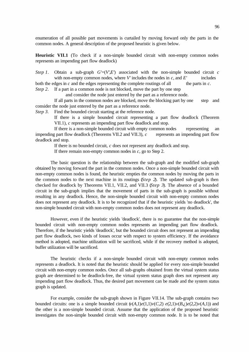
96

enumeration of all possible part movements is curtailed by moving forward only the parts in the common nodes. A general description of the proposed heuristic is given below. Heuristic VII.1 (To check if a non-simple bounded circuit with non-empty common nodes represents an impending part flow deadlock) Step 1. Obtain a sub-graph G'=(V',E') associated with the non-simple bounded circuit c with non-empty common nodes, where V' includes the nodes in c, and E' includes both the edges in c and the edges representing the complete routings of all the parts in c. Step 2. If a part in a common node is not blocked, move the part by one step and consider the node just entered by the part as a reference node. If all parts in the common nodes are blocked, move the blocking part by one step and consider the node just entered by the part as a reference node. Step 3. Find the bounded circuit starting at the reference node. If there is a simple bounded circuit representing a part flow deadlock (Theorem VII.1), c represents an impending part flow deadlock and stop. If there is a non-simple bounded circuit with empty common nodes representing an impending part flow deadlock (Theorems VII.2 and VII.3), c represents an impending part flow deadlock and stop. If there is no bounded circuit, c does not represent any deadlock and stop. If there remain non-empty common nodes in c, go to Step 2. The basic question is the relationship between the sub-graph and the modified sub-graph obtained by moving forward the part in the common nodes. Once a non-simple bounded circuit with non-empty common nodes is found, the heuristic empties the common nodes by moving the parts in the common nodes to the next machine in its routings (Step 2). The updated sub-graph is then checked for deadlock by Theorems VII.1, VII.2, and VII.3 (Step 3). The absence of a bounded circuit in the sub-graph implies that the movement of parts in the sub-graph is possible without resulting in any deadlock. Hence, the non-simple bounded circuit with non-empty common nodes does not represent any deadlock. It is to be recognized that if the heuristic yields 'no deadlock', the non-simple bounded circuit with non-empty common nodes does not represent any deadlock. However, even if the heuristic yields 'deadlock', there is no guarantee that the non-simple bounded circuit with non-empty common nodes represents an impending part flow deadlock. Therefore, if the heuristic yields 'deadlock', but the bounded circuit does not represent an impending part flow deadlock, two kinds of losses occur with respect to system efficiency. If the avoidance method is adopted, machine utilization will be sacrificed, while if the recovery method is adopted, buffer utilization will be sacrificed. The heuristic checks if a non-simple bounded circuit with non-empty common nodes represents a deadlock. It is noted that the heuristic should be applied for every non-simple bounded circuit with non-empty common nodes. Once all sub-graphs obtained from the virtual system status graph are determined to be deadlock-free, the virtual system status graph does not represent any impending part flow deadlock. Thus, the desired part movement can be made and the system status graph is updated. For example, consider the sub-graph shown in Figure VII.14. The sub-graph contains two bounded circuits: one is a simple bounded circuit (v(A,1)e(1,1)v(C,2) e(2,1)v(B,¿)e(2,2)v(A,1)) and the other is a non-simple bounded circuit. Assume that the application of the proposed heuristic investigates the non-simple bounded circuit with non-empty common node. It is to be noted that

97

e(3,2) does not belong to the bounded circuit, but appears in the sub-graph. Then, part 2 in node v(C,2) moves to node v(B,¿) to make v(C,2) empty (step 2). As illustrated in Figure VII.14(b), the resulting graph contains a non-simple bounded circuit with one empty common node, which represents an impending part flow deadlock according to Theorem 2 (step 3). Thus, it is concluded that the non-simple bounded circuit with a non-empty common node in Figure VII.14(a) represents an impending part flow deadlock.

(A,1) (B,? (C,2)(2,2) (D,3)(2,1)

(3,1)(3,2)

(1,1)(1,2)

bounded circuit : v(A,1)e(1,1)v(C,?e(1,2)v(D,3)e(3,1)v(C,2)e(2,1)v(B,?e(2,2)v(A,1)

reference node

(A,1) (B,2) (C,? (D,3)(2,1)

(3,1)(3,2)

(1,1)(1,2)

bounded circuit : v(B,2)e(2,1)v(A,1)e(1,1)v(C,?e(1,2)v(D,3)e(3,1)v(C,?e(3,2)v(B,2)

reference node

(a)

(b)

Figure VII.14 Example of a non-empty common node which is not blocked As another example, we consider the sub-graph in Figure VII.15. A reference node is a non-empty common node which is blocked by v(D,3). Since the non-empty common node cannot be emptied directly, part 3 at machine D moves to machine C (step 2). Node v(C,3) then becomes a reference node. Then a bounded circuit with one empty common node starting at node v(C,3) can be obtained as shown Figure VII.15(b). It should be noted that since part 2 does not contribute to the bounded circuit, node v(B,2) is considered as an empty node. The bounded circuit represents an impending part flow deadlock according to Theorem VII.2. Thus, the non-empty bounded circuit with a non-empty common node in Figure VII.15(a) represents an impending part flow deadlock.

98

(A,1) (B,2) (C,?

(2,1)

(D,3)

(3,1)(3,2)

(1,1)(1,2)

bounded circuit : v(B,2)e(2,1)v(D,3)e(3,1)v(C,?e(3,2)v(B,2)e(3,3)v(A,1)e(1,1)v(B,2)

reference node

(3,3)

(A,1) (B,2) (C,3)

(2,1)

(D,?

(3,1)(3,2)

(1,1)(1,2)

bounded circuit : v(C,3)e(3,1)v(B,?e(3,2)v(A,1)e(1,1)v(B,?e(1,2)v(C,3)

reference node

(a)

(b)

Figure VII.15 Example of a non-empty common node which is blocked However, even if the heuristic yields a 'deadlock', there is no guarantee that the non-simple bounded circuit with non-empty common nodes represents an impending part flow deadlock. Therefore, if the heuristic yields a 'deadlock', but the bounded circuit does not represent an impending part flow deadlock, two kinds of losses occur with respect to system efficiency. If the avoidance method is adopted, machine utilization will be sacrificed. If the recovery method is adopted, buffer utilization will be sacrificed. Figure VII.16 illustrates an example of this case. Figure VII.16(a) does not represent any deadlock, but the heuristic transforms Figure VII.16(a) into Figure VII.16(b) and yields a 'deadlock'.

(A,1) (B,2) (C,?

(2,1)

(D,?

(3,1)(3,2)

(1,1) (2,2)

bounded circuit : v(A,1)e(1,1)v(B,2)e(2,1)v(D,?e(2,2)v(E,3)e(3,1)v(D,?e(3,2)v(C,?e(3,3)v(B,2)e(3,4)v(A,1)

reference node

(3,3)

(a) (E,3)

(3,4)

(A,1) (B,? (C,? (D,2)

(3,1)(3,2)

(1,1) (2,1)

bounded circuit : v(D,2)e(2,1)v(E,3)e(3,1)v(D,2)

reference node

(3,3)

(b) (E,3)

(3,4)

Figure VII.16. Heuristic yields 'deadlock', but (a) is not in deadlock VII.6 Deadlock Resolution Scheme Deadlock resolution schemes can be classified into four types. First, deadlocks can be prevented by batching the parts such that part flow is limited to a single direction without backtracking. This will eliminate deadlocking completely since there is no cross flow of parts. However, flexibility of the system is sacrificed. Second, whenever a part flow deadlock occurs, the parts in question can be moved to the storage buffer, given that the system has the unlimited buffer

99

space. The resulting work-in-process inventory and transportation costs may be very expensive. A third way to resolve deadlocks would be to transfer one of the parts in the deadlock to a special storage buffer and then sequentially move the other parts. Finally, the part in the storage buffer can be moved to the next machine in its routings. This resolution scheme is called deadlock detection and recovery. A fourth way to resolve deadlocks would be to inhibit the movement of the part causing deadlocks in order to completely avoid deadlocks. This method can be applied to manufacturing systems that do not have any in-process storage buffers or systems whose buffers are full. This resolution scheme is called deadlock avoidance. The procedures defined in this research are designed to be utilized with either deadlock detection and recovery or deadlock avoidance. In order to illustrate the methodology to resolve deadlocks (See Figure VII.17), let it be assumed that a query move(p, L1, L2) for every movement of any part is sent from the scheduling function to a deadlock detection and resolution module. The query implies that “can part p move from location L1 to location L2?”.

Query : move( p, L1 , L2)?

Check if the transition of part p causes deadlock

without considering buffers

Check if part p was in an impending part flow deadlock

Y

Check if a buffer is available

N Allow part p to move physically Update the system status graph

N Do not allow part p to move physically

Y

Transition part p in the virtual system status graph

Create a virtual system status graph

Y

N

Allow part p to move physically Update the system status graph

Do not allow part p to move physically

Allow part p to move physically Update the system status graph Reserve a storage buffer

recovery avoidance

Figure VII.17 Flow diagram to resolve (impending) part flow deadlocks First, a virtual system status graph needs to be created. The movement of part p is then fulfilled on the virtual system status graph. Next, we determine if the movement of part p causes a part flow deadlock or an impending part flow deadlock without considering buffer status (Apply Theorems VII.1, VII.2, and VII.3, and Heuristic VII.1). If the movement of part p does not cause any deadlock, part p can move to the next destination, L2 and the original system status graph must be updated. If the movement of part p causes any deadlock, we check to see if part p was involved in an impending part flow deadlock. If so, the answer to the query is “yes” and the original system status graph must be updated, since a storage buffer was already reserved in order to recover the system when the impending part flow deadlock was detected. If this movement causes a part flow

100

deadlock, this situation should be reported to the controller, which should initiate the recovery process. If part p was not involved in an impending part flow deadlock, the availability of a storage buffer is checked. If a storage buffer is not available, the movement of part p must not be allowed to move physically to avoid deadlock. If a storage buffer is available, one of the two methods, recovery or avoidance method, needs to be selected. If the avoidance method is selected, the movement of part p is not allowed to move physically to avoid deadlock (i.e., the answer to the query is “no”). If the recovery method is selected, part p can move to the next destination, L2 and the original system status graph must be updated (i.e., the answer to the query is “yes”) after a storage buffer is reserved. If this movement causes a part flow deadlock, this situation should be reported to the controller, which should initiate the recovery process. It should be noted that care must be taken in the choice of the resolution methods. In general, the avoidance method may decrease machine utilization, since the part movement causing a deadlock is inhibited. The avoidance method is to operate compared to the recovery method, since the movement of the concerned part causing part flow deadlock or impending part flow deadlock can be simply inhibited. On the other hand, the recovery method may increase buffer utilization, especially if a storage buffer is reserved for every deadlock. It is difficult to select one method efficiently in real-time. This is affected by many factors, such as part processing time, material handling time, storage buffer size, etc. A sample recovery procedure for part flow deadlock is described below. With the aid of the deadlock detection and resolution module, a manufacturing system controller can recognize the parts involved in a part flow deadlock. In particular, the controller can recognize if a finished part is involved in a part flow deadlock or is being blocked when the finished part cannot move to the next destination. If the finished part is in a part flow deadlock, the controller should move the part to the reserved buffer and then sequentially move the other parts in their routings. Finally, the part in the storage buffer can be moved to the next machine in its routings. The system is in a deadlock-free state if a simple bounded circuit associated with the part flow deadlock disappears and the reserved buffer becomes empty. In other words, any machine in a part flow deadlock status must receive only the parts in the part flow deadlock until the deadlock is cleared. It should be noted that buffer utilization becomes an important factor when the recovery method is selected to resolve deadlocks. As mentioned above, reserving a buffer for every deadlock may increase buffer utilization and thus inhibit arrival of new parts. As illustrated in Figure VII.18, for example, assume that parts 1, 2, 3, and 4 arrive into the system one after another. When part 1 is in machine A, arrival of part 2 causes a part flow deadlock and a buffer needs to be reserved. Arrival of part 3 causes an impending part flow deadlock and another buffer also needs to be reserved. So does part 4. As a result, three special buffers are reserved to resolve this situation. If parts 4, 3, and 2 can move sequentially to the reserved storage buffers, the processing of part 1 can be completed at machines B, C, and D. Hence, all three reserved buffers are utilized. However, if the parts move intelligently, only one storage buffer is sufficient to resolve the deadlocks. Part 1 must move to the buffer, and then the other parts go through the machines in their routings.

101

(A,1) (B,2) (D,4)

(1,1)

(C,3)(4,2)

(1,2) (1,3)

(4,1)

(3,2)

(4,3)

(3,1)(2,1)

Figure VII.18 Example for deadlock resolution using recovery In fact, it is not difficult to prove that one buffer is a minimum requirement for the recovery method. If one buffer is always held for recovery, it is necessary to detect only part flow deadlocks. The system status graph then has only the next immediate movement of each part in the system. If two independent part flow deadlocks exist in the system, i.e., two simple bounded circuits associated with two different part flow deadlocks are found, then each independent part flow deadlock can be resolved sequentially using the same storage buffer. This is because a node in the system status graph can only contribute to one part flow deadlock. Theorem VII.4 proves this. It should be noted that a node may contribute to more than one impending part flow deadlock, however, which is not valid for the recovery method. Theorem VII.4 A node contributes to only one part flow deadlock. proof by contradiction: Suppose that a node contributes to more than one part flow deadlock. In other words, a node contributes to more than one simple bounded circuit with all nodes occupied. Without loss of generality, a simple bounded circuit consists of four nodes and four edges as shown in Figure VII.19. Then, there must exist at least two edges outgoing from the node which contributes to more than one part flow deadlock (for example, dotted line and plain line from node v(A,1)). However, since only the immediate movement of each part in the system is needed for a part flow deadlock, there is only one edge outgoing from the node at any instant of time. Therefore, any node in a part flow deadlock cannot have any other outgoing edges except that contributing to a part flow deadlock. This implies that any node in a part flow deadlock has only one incoming and outgoing edges (for example, the dotted line in Figure VII.18 is invalid). Thus, a node in a part flow deadlock cannot contribute to other part flow deadlocks. This contradicts the assumption. Hence, a node contributes to only one part flow deadlock. This completes the proof.

(A,1) (B,2)

(D,4)

(1,1)

(C,3)

(2,1)

(3,1)

(4,1)

Figure VII.19 Example of part flow deadlock interactions An interesting problem can be found if the first assumption described in Section VII.1 is dropped. In other words, a part may contain operation sequence alternatives, meaning that the operations surrounded by SPLIT-AND and JOIN-AND type nodes must be done in any sequence. Then, the deadlock detection and avoidance method cannot be applied in this case, since the complete operation sequence of a part cannot be predicted in the dynamic scheduling environment. On the other hand, all the next possible movements of each part need to be investigated for the recovery method. Figure VII.20 illustrates this case. If all the next possible movements of each part

102

cause part flow deadlock, the concerned parts are in a part flow deadlock. For example, part 3 has operation sequence alternatives, meaning that part 3 may visit first either machine A or machine D. Hence, the movement of part 2 to machine B causes a part flow deadlock. If one of the next possible movements of each part does not cause part flow deadlock, the system is not in a part flow deadlock. For example, if part 3 moves to machine D instead of Machine A, the movement of part 2 to machine B does not cause a part flow deadlock. Therefor, the movement of part 2 is allowed.

(A,1) (B,2)

(D,4)

(1,1)

(C,3)(3,1)

(4,1) (2,1)

(A,1) (B,2)(1,1)

(C,3)(3,1)

(2,1)

(D,?

(3,1) (3,1)

(a) Part flow deadlock (a) No part flow deadlock

reference node reference node

Figure VII.20 Two system status graphs for operation sequence alternatives VII.7 Chapter Summary A graph-theoretic deadlock detection and resolution procedure has been developed. The procedure finds and investigates four different kinds of bounded circuits from the system status graph— simple bounded circuit, non-simple bounded circuit with one empty common node, non-simple bounded circuit with more than one empty common node, and non-simple bounded circuit with non-empty common nodes. A simple bounded circuit represents a part flow deadlock if and only if all nodes are occupied. A non-simple bounded circuit with one empty common node represents an impending part flow deadlock if all nodes other than the common node are occupied. A non-simple bounded circuit with more than one empty common node represents an impending part flow deadlock if all nodes other than the empty common nodes are occupied and all neighbor circuits of every empty node can be occupied. As for a non-simple bounded circuit with non-empty common nodes, the complete part routings of all the parts in the non-simple bounded circuit are required to detect an impending part flow deadlock. A heuristic has been proposed to detect impending part flow deadlocks in such situations. If the proposed heuristic yields 'no deadlock', the non-simple bounded circuit with non-empty common nodes does not represent any deadlock. However, if the proposed heuristic yields 'deadlock', the non-simple bounded circuit may or may not represent any deadlock. Hence, the heuristic provides a conservative approach to deadlock detection.

103

CHAPTER VIII

EXECUTION FUNCTION VIII.1 Chapter Overview The controller at each level has the ability to read inputs, to make decisions based on the inputs and current system status, and to exchange and communicate information with supervisors and subordinates as a means of implementing those decisions. Decision-making functions correspond to the planning and scheduling functions, while message reading and generation functions correspond to the execution function. This chapter deals with the execution function. The execution function plays an important role in: 1) monitoring input messages and their semantic interpretation, 2) making execution-based decisions, and 3) generating output messages, broadcasting the messages, and downloading control programs. The goal of this chapter is to describe the execution function of the IWC and equipment controllers. The execution function of the IWC receives control messages necessary to process parts and manage resources, and sends the detailed messages down to the execution function of the equipment controller. Error handling activities are assumed to be out of the scope of this research. The execution function of the equipment controller holds a set of execution graphs, each of which specifies a sequence of actions to be taken for each incoming message. The remainder of the chapter is organized as follows: Section VIII.2 provides the framework and problem statement. In Section VIII.3, a critique of past work on the execution function for shop floor control is presented. Section VIII.4 describes the state variables to be used for control. A detailed description on the execution function of the IWC is presented in Section VIII.5. The two execution functions for NC machines and robots are discussed in Section VIII.6. Section VIII.7 provides a summary of the chapter. VIII.2 Framework and Problem Statement The execution function of the IWC and equipment controllers communicate with not only other controllers, but also with its own planning and scheduling functions. Communication is performed by exchanging messages. A message is classified into two different types: control and information. Control messages flow in a hierarchical manner through the execution function. However, information messages to be exchanged may flow through peer-to-peer communication. Figure VIII.1 illustrates a control flow scheme involved in the hierarchical control architecture. The arrows represent the direction of control flow. The execution function consists of the three subfunctions: 1) monitoring input messages and their semantic interpretation, 2) making execution-based decisions, and 3) generating and broadcasting output messages. The detailed description of the sub-functions is presented in Table VIII.1.

104

Planning function

Scheduling function

Execution function

Device control unit

Execution function

Planning function

Scheduling function

Planning function

Scheduling function

Execution function

Workstation Controller

Equipment Controller Equipment Controller

From Shop

Device control unit Figure VIII.1 Control flow in the hierarchical control architecture Table VIII.1 Taxonomy of the execution function for shop floor control Messages monitoring and

interpretation Execution-based decision-

making Messages broadcasting and machine codes downloading

Shop

• messages from the factory controller (e.g., produce) • messages from the scheduling function • feedback from the workstation (e.g., done) • parsing messages

• creating messages for normal workstation actions • error handling module • generating messages for error recovery • updating data base • generating reports

• downloading messages to the workstation controller • sending messages to the scheduling function • sending messages to the factory controller • commands for updating status of data base

Work- station

• messages from the shop controller (e.g., arrive) • messages from the scheduling function (e.g. move, refixture, assemble) • feedback from the equipment controller (e.g., done) • parsing messages

• creating messages for normal equipment actions (e.g., load,, pick) • creating messages for the planning/scheduling functions • error handling module • updating data base • generating reports

• downloading messages to the equipment controller (e.g. load, unload, pick, put) • sending messages to the scheduling function • sending messages to the shop controller (e.g., done) • commands for updating status of data base

Equip- ment

• messages from the workstation controller (e.g., load, transfer, pick) • sensory data from the control unit (e.g., done, data for checking tool breakage) • parsing messages

• interpreting sensory data (e.g., tool status) • primitive actions • error handling (e.g., part dropping error) • synchronization actions • updating data base • generating reports

• sending messages to the workstation controller (e.g., done) • commands for updating status of database • downloading NC instructions (RS274) and other robot programs

105

The monitoring subfunction plays an input gate-keeper's role of a controller by collecting messages from other controllers and communicating with its own planning and scheduling functions. It also performs semantic interpretation of each message and forwards it to the execution-based decision-making subfunction. Specifically, the monitoring subfunction at the equipment level receives various control messages associated with specific actions and reads sensory data from the control unit connected to the physical device. The actions for a machine controller include loading and unloading parts, downloading NC instructions, and machining parts, while the sensory data includes checking tool status, polling machine spindle status, etc. The actions for a robot controller include picking, putting, and transporting parts. The monitoring subfunction at the workstation and shop levels also receives various control messages associated with specific actions (e.g., batch/part arrival, the movement of parts and resources). The execution-based decision making subfunction may consist of a large number of detailed modules necessary to perform all of the real-time analysis. This subfunction includes various manufacturing tasks such as: part movement, end-effector change, refixturing activities, error handling activities, report generation, synchronization action, database updating, and so forth. The error-handling module is activated upon recognition of error conditions in the parsing of the input messages. The output subfunction broadcasts control and information messages created by the execution-based decision making subfunction to all of the other controllers and its own planning and scheduling functions. It also downloads NC instructions and robot programs at the equipment level. Several issues associated with the execution function described above remain to be investigated. Specifically, these issues include: 1) Control entities: Most of the traditional research done in control concentrates on the flow of one major class of entities: part. However, in flexible manufacturing environments, the classes of entities that must be considered include: parts, tools, fixtures, end-effectors, and so forth. If an entity is mobile, the entity is moved to one of the fixed entities. Therefore, the execution function must be able to address the flow of the mobile entities. 2) Relationship between planning/scheduling and execution: In general, two different approaches between scheduling and execution have been proposed. First, the scheduling function provides a dispatching rule that can be used to resolve any resource conflicts. The execution function then accesses the process plans of all the parts in the system in order to make a decision regarding which part must be selected at the time a machine becomes empty (Davis et al. [52], Huang and Chang [101], Kasturia et al. [117]). According to this conjecture, the execution function must be able to operate the manufacturing system if the serialized process plans of all the parts and the dispatching rule are provided. Second, the execution function is insulated from the process plans of all the parts and therefore just fulfills the detailed tasks generated by the scheduling function (Merabet [151], Smith [202]). This research adopts the second approach. 3) Relationship between execution at the equipment level and control unit: The control unit with a device provided by a vendor usually cannot be generic. In other words, the information that a control unit returns to the equipment controller may be different from that of other control units. In this research, it is assumed that the equipment controller can determine whether a NC program terminates normally.

106

4) Database management problem: The shop floor controller needs to explicitly specify the method of updating a wide variety of data necessary to carry out its functions. Even though the planning and scheduling functions at each level are responsible for updating their own data, the execution function must provide timely updates for device state, part state, and the state of other resources. It is to be noted that the state of the material handler plays an important role in updating the location of parts since a part cannot be moved without the materia l handler. 5) Information flow vs. control flow: In the past, control systems were limited by the available communications technologies of the time, which were point-to-point. Hence, most of the execution functions in a hierarchical control architecture equated information flow and control flow, meaning that the data needed for planning, scheduling, and execution are transmitted along with control flow (Jones and Saleh [111]). This concept provides two corresponding disadvantages (Barkmeyer [16]). First, complexity of the supervisory controller becomes maximized because it must communicate all of the data necessary for the functions of the subordinates as well as all of the data necessary for its own functions. Second, it enforces a fixed hierarchy in which control and data must come together. However, the information necessary to make decisions can be obtained by permitting peer-to-peer communication, e.g. IEEE 802 networks. In this research, a clear distinction is made between control and information flow. 6) Automated assembly tasks: The assembly operations form new parts by performing the fastening, joining, or bonding together of two or more separate parts. From the viewpoint of control, the execution function must support logical creation of new parts and logical deletion of old parts in the database. 7) Generic controller issues: Some of the execution functions can be automatically generated from the well-defined input data (Smith [202]), while others are described to be generic so that they can be applied to the different platform with changes of a few generic parameters (Naylor and Volz [161]). In this research, each equipment controller is responsible for reporting its own local activities to the IWC. The IWC is then insulated from the local activities in the equipment controller and can make a decision on the basis of the messages from the equipment controller. 8) Error handling issues: One of the most important responsibilities of the execution functions is to detect and react to unexpected error situations, such as machine failures, tool breakage, communication errors, material mishandling, etc. VIII.3 Related Work A study on existing workstation control software reveals that about 80% of the workstation controllers available currently in industry perform pure monitoring functions (Larin [132]). A few examples of such systems include Auto-Cell by Thesis Group, Cell-Pac by Arthur Anderson, and CELLworks by Fast Tech Integration, Inc. (Boulet et al. [27]). However, several papers focusing on the execution function in a manufacturing system have been reported. One of the techniques used widely for execution functions is petri-net (Huang and Chang [101], Kasturia et al. [117], Merabet [151]). Finite state machines have also been used for partial implementation of execution (Mettala [152], Smith [202]). Programmable logic controllers are not usually considered to be execution functions, since this tool becomes too complex and difficult to handle after a certain point and needs lots of program efforts (Larin [132]). An execution function, including machine synchronization, and tools and end-effector changing, has been proposed using petri-nets (Merabet [151]). The concept of colored petri-nets

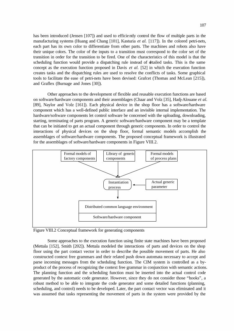
107

has been introduced (Jensen [107]) and used to efficiently control the flow of multiple parts in the manufacturing systems (Huang and Chang [101], Kasturia et al. [117]). In the colored petri-nets, each part has its own color to differentiate from other parts. The machines and robots also have their unique colors. The color of the inputs to a transition must correspond to the color set of the transition in order for the transition to be fired. One of the characteristics of this model is that the scheduling function would provide a dispatching rule instead of detailed tasks. This is the same concept as the execution function proposed in Davis et al. [52] in which the execution function creates tasks and the dispatching rules are used to resolve the conflicts of tasks. Some graphical tools to facilitate the ease of petri-nets have been devised: Grafcet (Thomas and McLean [215]), and Graflex (Burnage and Jones [30]). Other approaches to the development of flexible and reusable execution functions are based on software/hardware components and their assemblages (Chaar and Volz [35], Hadj-Alouane et al. [89], Naylor and Volz [161]). Each physical device in the shop floor has a software/hardware component which has a well-defined public interface and an invisible internal implementation. The hardware/software components let control software be concerned with the uploading, downloading, starting, terminating of parts program. A generic software/hardware component may be a template that can be initiated to get an actual component through generic components. In order to control the interactions of physical devices on the shop floor, formal semantic models accomplish the assemblages of software/hardware components. The proposed conceptual framework is illustrated for the assemblages of software/hardware components in Figure VIII.2.

Formal models of factory components

Library of generic components

Formal models of process plans

Actual generic parameter

Instantiation process

Distributed common language environment

Software/hardware component

Figure VIII.2 Conceptual framework for generating components Some approaches to the execution function using finite state machines have been proposed (Mettala [152], Smith [202]). Mettala modeled the interactions of parts and devices on the shop floor using the part contact vector in order to describe the possible movement of parts. He also constructed context free grammars and their related push down automata necessary to accept and parse incoming messages from the scheduling function. The CIM system is controlled as a by-product of the process of recognizing the context free grammar in conjunction with semantic actions. The planning function and the scheduling function must be inserted into the actual control code generated by the automatic code generator. However, since they do not consider those “hooks”, a robust method to be able to integrate the code generator and some detailed functions (planning, scheduling, and control) needs to be developed. Later, the part contact vector was eliminated and it was assumed that tasks representing the movement of parts in the system were provided by the

108

scheduling function (Smith [202]). However, these approaches are based on only the movement of parts among all the mobile shop floor entities. VIII.4 Definition of State Variables The shop floor controller makes a number of decisions based on the shop floor information. There are three different ways to manage that information: 1) the data necessary to carry out decision-making can flow as part of the control message, 2) each controller has its own database and database management system, and 3) each controller can request any information from a global database management system (Jones and Saleh [111]). In this research, a simple version of a memory-resident database for the execution functions of the workstation and equipment controllers is explicitly described. The dynamic database contains information on the status of the addressable physical locations which accommodate parts. Table VIII.2 describes several addressable locations and their related state variables. Even though the execution function at each level can access the state variables, the authority to modify particular state variables is given to a specific execution function which is responsible for manipulating the state variables. For example, a material handler controller must be able to know the location of all the parts, since the material handler must be involved in moving parts. Therefore, the scheduling function can update the state variables on the basis of the state of the material handler. Table VIII.2 State variables used for the IWC and equipment controllers

Loc-Id Type Owner Work-space

Syn PartNo Ready-Send

Ready-Get

Ready-Carry

L1 machine machine1 on on p1 on off - L2 machine machine1 on on φ off on - L3 machine machine1 on on φ off on - L4 machine machine2 on on p2 off off - L5 robot robot - - φ - - on L6 port transport off off φ - - - L7 buffer workstation off off p3 - - - L8 buffer workstation off off φ - - - L9 buffer workstation off off p4 - - -

VIII.5 Execution Function of the IWC The execution function of the IWC receives a set of control and information messages from its own planning and scheduling functions, and the execution functions of the shop and equipment controllers. The execution function then analyzes and understands the messages. This processing can occur through a sequence of steps, that is, lexical analysis, syntactical analysis, and semantic processing. Lexical analysis converts characters of the input messages into symbols. Syntactical analysis (in other words, parsing) then analyzes the syntactic structure of sentences, verifies that the sentence is syntactically well formed. Semantic processing gives the meaning of the sentence using any knowledge representation, that is, a conceptual graph, a conceptual dependency, a frame-based rule, or a logic-based rule. Finally, the execution function decomposes the input message and broadcasts the detailed messages to other functions and/or controllers. Figure VIII.3 illustrates this procedure.

109

Input messages

Broadcast the messages

shop controller equipment controller other workstation controllers

planning function

scheduling function

planning function

scheduling function

Lexical analysis

Syntactical analysis

Semantic processing

Decompose messages

Execution-based decision making subfunction

shop controller equipment controller other workstation controllers Figure VIII.3 Schematic procedure for the execution function of the IWC Each message carries the set of parameters which define the characteristics of the message. Table VIII.3 presents all the messages, parameters, and description. The parameters are used as follows: 1) pid represents the part identifier, 2) wfgid represents the workstation form feature graph identifier, 3) mhid represents the material handler identifier, 4) mpid represents the machine identifier, 5) L represents the addressable location identifier, 6) gid represents the end-effector identifier, and 7) N represents the number of parts to be loaded to a machine. Table VIII.3 Messages and their description for the IWC

Message Parameter Description arrive pid, wfgid, L pid with wfgid arrived at L s_load pid, L pid must be moved from L s_unload pid, L pid must be moved to L wdone pid pid has been finished at the workstation allow pid pid may be moved to the workstation transdone mhid, L mhid has been transported to L mdone pid, L pid is finished at L pickdone mhid, L mhid has picked a part from L putdone mhid, L mhid has put a part at L wplan pid pid must be planned transport mhid, L mhid must be transported to L goahead mpid mpid may continue to process mtransfer pid, mhid, L pid must be transferred from mhid to L rtransfer pid, mhid, L pid must be transferred from L to mhid refixture pid, mhid, L mhid must refixture pid at L c_grip mhid, gid mhid must change the end-effector into gid move pid, mhid, L1, L2, N mhid must move pid from L1 to L2. N implies the

number of parts that L2.Owner accommodates assemble pid1...pidN, mhid, L mhid must assemble pid1, pid2, ..., pid(N-1) into a

new part Pid(N) at location L

110

Table VIII.4 illustrates the specifications of the set of messages for the IWC. A message belongs to one of two types: control message (C) and information message (I). The control message flows in a hierarchical manner, while the status information message flows in either a flat or hierarchical manner. A message also belongs to one of two styles: primitive (P) and macro (M). If a message is of macro type, the message needs to be decomposed into detailed messages when it is broadcast to the other controllers or functions. Some messages become active only if some pre-specified preconditions are met. Table VIII.4 Messages and their specifications for the IWC Message Type Style source Preconditions messages created Message

arrive I P shop plan planning s_load C M shop pick mhid s_unload C M shop put mhid transdone C P mhid transdone scheduling mdone I P mpid mdone scheduling pickdone I P mhid pickdone scheduling putdone I P mhid putdone scheduling jdone I P mhid jdone scheduling goahead I P scheduling goahead mpid transport C P scheduling transport mhid mtransfer C M scheduling ReadyGet=on transport, put

load mhid L.Owner

rtransfer C M scheduling ReadySend=on ReadyCarry=on

transport, pick, unload mhid L.Owner

refixture C M scheduling ReadyCarry=on ReadySend=on

transport, pick, load, refixture, put, unload,

mhid L.Owner

c_grip C M scheduling ReadyCarry=on transport, c_grip mhid move C M scheduling ReadyCarry=on

ReadySend=on ReadyGet=on

transport, pick, put, load, wdone, allow, unload

mhid,shop L1.Owner L2.Owner

assemble C M scheduling ReadyCarry=on ReadySend=on

transport, pick, put, join, unload

mhid mpid

Figure VIII.4 illustrates a set of messages and their flow diagram going out from and coming in to the execution function of the IWC. The execution function communicates with two equipment controllers, robot and machine tool, using a different set of messages. In addition, this figure illustrates the explicit relationship among the planning, scheduling, and execution functions within the IWC. A solid line represents a control flow, while a dashed line represents an information flow.

111

Shop controller

Execution function

Planning function

Scheduling function

Robot controller

Transport controller

Workstation controller

mdone() pickdone() putdone() jdone()

communication if necessary

Machine controller

move(), rtransfer() mtransfer(), transport() refixture(), c_grip()

wdone() allow()

s_load() s_unload() arrive()

s_load() s_unload()

t_arrive()

transport() pick(), put() c_grip() refixture()

pickdone() putdone() jdone() transdone() mdone()

goahead() load() unload()

wplan()

wpdone()wreplan()

Figure VIII.4 Messages for the execution function of the IWC VIII.5.1 Interactions with a Shop Controller Every time the shop controller decides to have a workstation produce a part and recognizes the arrival of the part at the port, the shop controller sends an arrive() message to the execution function of the IWC. The arrive() message carries the part identifier and its rela ted workstation level form feature graph. The execution function then sends a wplan() message to the planning function. The planning function generates an operation sequence graph from the workstation level form feature graph, and then sends a wpdone() message to the scheduling function in order to inform that a planning activity on the part has just finished. The wpdone() message carries the part identifier and its related operation sequence graph. Then, the scheduling function adds the new part to the part list which contains a set of parts to be dispatched. If the scheduling function determines to dispatch the new part to either a machine or a buffer, it sends a move() message to the execution function. The execution function is then allowed to dispatch the new part and sends an allow() message to the shop controller. Recognizing an allow() message from the execution function of the IWC, the shop controller downloads a s_load() message to the IWC and a s_unload() message to the transport controller. Figure VIII.5 illustrates a control and information flow diagram carried out when a new part arrives to a workstation. The numbers in front of each message implies the sequence of the issued message.

112

Shop controller

Execution function

Planning function

Scheduling functionRobot

controller

Transport controller

Workstation controller

8) transport() pick()

7) s_unload()

2) a

rriv

e()

7) s

_loa

d()

6) a

llow

()

3) wplan()

4) wpdone()

5) move()

1) t_arrive()

communication if necessary

Figure VIII.5 Control and information flow for a new part Every time the scheduling function of the IWC decides to move a finished part to the port, the execution function sends a wdone() message to the shop controller in order to inform that the specified operations on the part have been finished. After the shop controller arranges any material transport device to pick up the finished part, it downloads a s_unload() message to the IWC and a s_load() message to the transport controller. The execution function of the IWC then downloads transport(), pick(), transport(), and put() messages to the robot controller. It is to be noted that the robot controller may need handshaking activities with the material transport controller. Figure VIII.6 illustrates a control and information flow diagram carried out when a finished part leaves a workstation. The numbers in front of each message implies the sequence of the issued message.

Shop controller

Execution function

Planning function

Scheduling function

Robot controller

Transport controller

Workstation controller

6) transport() pick() transport() put()

5) s_load

4) wdone 5) s_unload()

2) mdone

communication if necessary

Machine controller

1) mdone()

3) move()

Figure VIII.6 Control and information flow for a finished part

113

VIII.5.2 Interactions with Equipment Controllers The execution function of the IWC initiates the scheduling function by sending the event messages (e.g., transdone(), mdone(), pickdone(), putdone(), jdone()) which are received from the equipment controller. It is to be noted that when all the operations on a part are finished, the execution function needs to interact with the shop controller. The scheduling function updates the state of parts, machines, robots, and buffers on the basis of the event messages. Further, the scheduling function then creates the set of messages corresponding to the event messages and sends them to the execution function. The messages include the movement of parts (e.g., mtransfer(), rtransfer(), refixture(), move()), the assembly operation of parts (assemble()), and the activities of the material handler (e.g., transport(), c_grip()). In order to move a part from one location to another, the scheduling function uses the macro message (e.g., move()) or a sequence of detailed messages (e.g., rtransfer(), transport(), mtransfer()). The latter may be useful when the scheduling function needs to specify the path of a material handler in order to avoid collision. In order to control the transition of the material handler from one location to another, the workstation controller will use a transport() message . This message may be created by the scheduling function to perform the following activities: 1) the material handler can be moved to the location that requests service, 2) the material handler can be moved somewhere else to avoid collision. This message can also be created by the execution function when a macro message (e.g., move()) is decomposed. Two messages, rtransfer() and mtransfer(), which are issued by the scheduling function, are used to transfer a part to and from the robot. The rtransfer() message indicates that a specified material handler needs to pick up a part from a specified location. Figure VIII.7 illustrates a decomposition method for this message. Figure VIII.8 illustrates a decomposition method for the mtransfer() message.

rtransfer(pid, mhid, L)

to L.Owner to mhid

unload() pick()

(a) If (L.Owner ?workstation and L.Owner ?transport) and ( L.Workspace = "on" or L.Syn = "on")

rtransfer(pid, mhid, L)

to mhid

pick()

(b) If (a) is not true Figure VIII.7 Decomposition method of a rtransfer() message

114

mtransfer( pid, mhid, L)

to L.Owner to mhid

load() put()

mtransfer( pid, mhid, L)

to mhid

put()

(b) If (a) is not true

(a) If (L.Owner ?workstation and L.Owner ?transport) and ( L.Workspace = "on" or L.Syn = "on")

Figure VIII.8 Decomposition method of a mtransfer() message When a move(pid, mhid, L1, L2, N) message is initiated by the scheduling function, the execution function checks the three state variables: ReadyCarry for material handler mhid, ReadySend for source location L1, and ReadyGet for destination location L2. The execution function may generate a number of transport() messages for the material handler to get to location L1 along with all the possible paths. Then, the execution function will generate a rtransfer() message, a number of transport() messages, and a mtransfer() message. Figure VIII.9 illustrates a decomposition method of the move() message to be applied if the following conditions are true for both locations L1 and L2: 1) a workstation controller does not own both locations, 2) a material transport controller does not own both locations, 3) either L1.Workspace = “on” or L1.Syn = “on”, and 4) either L2.Workspace = “on” or L2.Syn = “on”.

move(( pid, mhid, L1, L2 , N)

to L1.Owner to mhid

unload() transport(), pick(), transport(), put()

to L2.Owner

load()

transport(), rtransfer(), transport(), mtransfer()

Figure VIII.9 Decomposition method of a move() message VIII.6 Execution Function of the Equipment Controller The execution function of the equipment controller receives messages from the IWC, maintains its own state, updates the addressable location table, and downloads NC instructions and robot programs. In addition, it must be able to read sensory data from the control unit connected to the physical device. This may be accomplished via a commercial I/O board. Figure VIII.10 illustrates a set of messages and their flow diagram going out from and coming in to the equipment controllers. The equipment controller must be able to communicate with the device control unit. A solid line represents a control flow, while a dashed line represents an information flow.

115

IWC

Execution function

Planning function

Scheduling function

Robot control unit

Transport controller

Machine tool controller

sdone() index() eunload()

communication if necessary

Machine control unit

NCdone()

transport() pick(), put() c_grip() refixture()

pickdone() putdone() jdone() transdone()

mdone()goahead() load() unload()

eplan()

epdone()ereplan()Robot controller

NCdone()

robot programs for transport, refixture, closing, opening, and changing end-effector

NC instructions for machining and starting, closing, opening, and indexing fixture

Figure VIII.10 Messages and their flow diagram for the equipment controllers VIII.6.1 Execution Function for Machine Tools A machine tool implies a function-specific material processor which requires a controller to make some decisions. This includes a machining center, a turning center, a coordinate measuring machine, and so forth. The machine tool transforms the information content associated with a part. Tables VIII.5 and VIII.6 present the set of messages and their characteristics involved in the execution function for machine tools. Table VIII.5 Messages and their description for a machine controller

Message Parameter Description unload pid, mhid, L mhid needs to unload pid from L load pid, mhid, L, N mhid needs to load pid to L index pid pid needs to be indexed eplan φ planning needs to be done sdone φ scheduling was finished eunload pid pid needs to be unload fixture_closed φ fixture was closed mdone pid, L pid was finished at L Table VIII.6 Messages and their specifications for a machine controller Message Type Style Source instructions Messages created Destination unload C P workstation open_fixture fixture_closed load C P workstation close_fixture fixture_closed,eplan planning goahead C P workstation mdone workstation sdone I P scheduling eunload workstation

116

The execution function for machine tools has an execution graph necessary to process each incoming message. The execution graph contains a sequence of actions to be taken and preconditions to be checked. A node represents actions to be taken. An edge represents the transition between two consecutive nodes. Once an execution graph for a message has been performed, the execution function waits for other messages. Two of the most important messages from the IWC to the execution function of machine tools are load() and unload(). Figure VIII.11 and VIII.12 illustrate the execution graphs for load() and unload() message.

load(pid, mhid, L, N)

update a L.ReadyGet state variable to "off"

check if a L.Syn state variable is "on"

download a NC instruction for closing fixture

send a fixture_closed() message to mhid

receive a workspace_clear() message from mhid

receive a ready_to_put() message from mhid

check preconditions (e.g., if door is closed)

check if N = 0

check if N > 0

send an eplan() message to the planning function of L.Owner

N = N - 1

check if a L.Syn state variable is "off"

download a NC instruction for closing fixture

receive a workspace_clear() message from mhid

Figure VIII.11 Execution graph for a load() message Figure VIII.13 illustrates an execution graph necessary to carry out an operation on a part. The execution graph also addresses the activities of a machine controller which can accommodate multiple parts at a time on an indexable fixture. After receiving a sdone() message, the execution function checks whether the fixture is indexable or not. If the fixture is indexable, the execution function must wait for either an index() or an eunload() message from the scheduling function. If the index() message is received to index a particular part on the fixture, the execution function downloads a NC instruction for indexing. The execution function then downloads another NC instruction for machining and sends a start() message to the control unit. After recognizing that the NC instruction is finished, the execution function sends a NCdone() message to the scheduling function. The scheduling function then sends either an index() or an eunload() message. If the index() message is received, the execution function returns to download a NC instruction for indexing. If the eunload() message is accepted, the execution function sends a mdone() message to the IWC.

117

receive an end-effector_closed() message mhid

unload( pid , mhid , L )

update a L.ReadySend state variable to

check if a L.Syn state variable is "on" check if a L.Syn state variable is "off"

download a NC instruction for opening fixture

send a fixture_open() message to mhid

receive a workspace_clear() message from mhid update a L.ReadyGet state variable to "on"

Figure VIII.12 Execution graph for an unload() message

sdone()

check if the fixture is indexable

receive a index() message from the scheduling function

download a NC instruction for machining

recognize that the NC instruction is finished

send a NCdone() message to the scheduling function

receive an eunload() message from the scheduling function

check preconditionsupdate a L.ReadySend state variable to "on"

send a mdone() message to the IWC

check if the fixture is not indexable

download a NC instruction for machining

recognize that the NC instruction is finished

receive an e_unload() message from the scheduling function

receive a index() message from the scheduling function

goahead()

send an eplan() message to the planning function

receive a sdone() message from the scheduling function

send a start() message to the control unit

send a start() message to the control unit

download a NC instruction for indexing

Figure VIII.13 Execution graph for sdone() and goahead() messages

118

VIII.6.2 Execution Function for Robots The robot controller receives several control messages from the IWC as shown in Tables VIII.7 and VIII.8. For some messages (e.g., pick(), put()), the robot controller needs handshaking activities with the controller of the specified location if the location requires synchronization or the workspace of the location needs to be controlled. Hence, the execution graphs for the pick() and put() messages must be able to deal with any location which requires synchronization or not. For other messages (e.g., transport(), join(), refixture(), c_grip()), the robot controller downloads their associated robot programs without interacting with other controllers. Table VIII.7 Messages and their description for a robot controller

Message Parameter Description pick pid, mhid, L mhid must pick pid up from L put pid, mhid, L mhid must put pid on L join pid1, mhid, pid2, L mhid must join pid1 to the base part and

create pid2 on L end-effector_closed φ end-effector was closed workspace_clear φ workspace was cleared ready_to_put φ part is ready to be transferred Table VIII.8 Messages and their specifications for a robot controller Message Type Style Message

source Robot

programs Messages created Message

destination pick C P work-

station approach, retract, close end-effector

end-effector_closed workspace_clear pickdone

machine controller

put C P work-station

approach, retract, open end-effector

ready_to_put workspace_clear putdone

machine controller

transport C P work-station

transport

refixture C P work-station

refixture

c_grip C P work-station

change_end-effector

join C P work-station

join jdone() workstation

Figure VIII.14 and VIII.15 illustrate execution graphs for pick() and put messages . The robot controller then downloads the robot program for approaching and grasping the part. Before the robot retracts or approaches its arm, the robot controller checks a L.Syn state variable to determine whether location L requires synchronization. If the location does not require synchronization (that is, Syn is set “off”), the robot controller would download a robot program for retracting out of the workspace. If synchronization is required for the location, the robot controller needs handshaking activities with the owner of L holding a part.

119

pick( pid, mhid, L)

update a ReadyCarry state variable to "off"

download a robot program for approaching L

check if a L.Syn state variable is "on"

download a robot program for closing end-effector

send an end-effector_closed() message to L.Owner

receive a fixture_open() message from L.Owner

download a robot program for retracting from L

send a pickdone() message to the workstation controller

send a workspace_clear() message to L.owner

check if a L.Syn state variable is "off"

check if a L.workspace state variable is "on" check if a L.workspace state variable is "off"

Figure VIII.14 Execution graph for a pick() message

put(pid, mhid, L)

download a robot program for approaching L

check if a L.Syn state variable is "on"

send a ready_to_put() message to L.Owner

receive a fixture_closed() message from L.Owner

download a robot program for opening end-effector

download a robot program for retracting from L

update a ReadyCarry state variable to "on"

send a putdone() message to the workstation controller

send a workspace_clear() message to L.owner

check if a L.Syn state variable is "off"

check if a L.workspace state variable is "on"

check if a L.workspace state variable is "off"

Figure VIII.15 Execution graph for a put() message

120

In order to illustrate how synchronization works, Figure VIII.16 shows the interactions between a pick() message for a robot controller and an unload() message for a machine tool controller. If synchronization is required while a part is transferred from a machine to a robot, a few communications are needed between the two controllers. The two controllers follow the solid lines in their own execution graphs until they reach a point which is supposed to receive a message from each opponent. The dashed line implies sending or receiving the external messages.

pick( pid, mhid, L)

ReadyCarry ← "off"

approach L

L.Syn ="on"

close end-effector

send L.Owner end-effector_closed()

receive fixture_open() from L.Owner

retract from L

send IWC pickdone()

send L.owner workspace_clear()

L.Syn ="off"

L.workspace = "on" L.workspace ="off"

receive end-effector_closed() from mhid

unload(pid, mhid, L)

L.ReadySend ← "off"

L.Syn = "on"L.Syn ="off"

open fixture

send mhid fixture_open()

receive workspace_clear() from mhid

L.ReadyGet ← "on"

L.workspace = "on" L.workspace ="off"

Figure VIII.16 Example of synchronization VIII.7 Chapter Summary The objective of the chapter is to describe the execution functions of the IWC and equipment controllers. Further, a critique of the past work on the execution function has been presented to justify the execution functions proposed in the research. A careful analysis of the past work shows that most of the execution functions do not address all of the issues brought forth.

121

The execution function of the IWC mainly receives a series of control messages about the movement of parts and resources, and send the detailed messages down to the equipment controller. The execution function of the equipment controller has execution graphs necessary to carry out the incoming messages, in which a node represents the set of actions, and an edge represents the transition between two nodes. Many unresolved problems associated with the execution functions need to be investigated: 1) error detection and handling issues, 2) development of a set of generic parameters in order to create a generic workstation controller, and 3) construction of an intelligent front-end generic configuration model to derive multiple equipment controllers for different vendors.

122

CHAPTER IX

EXPERIMENTAL RESULTS AND CONCLUSION IX.1 Chapter Overview In the preceding chapters, the requirements, problems, and models for the development of the IWC were introduced and illustrated. As such, a process plan model includes a set of selected resources and various instructions which are necessary for converting the raw material into the finished product. The process plan is represented as an AND/OR graph to accommodate resource alternatives and sequence alternatives. The IWC receives information such as part type and quantity, and process plans from the shop level controller and coordinates production activities. The IWC performs three main functions — planning, scheduling, and execution in real-time in order to ensure completion of jobs assigned by the shop controller. In this section, experimentation and validation of the IWC are addressed. A conclusion of the dissertation is also provided. The detailed objectives of this chapter are: 1) to select a pair of good planning and scheduling strategies which can be incorporated with an execution function to enhance the performance of the IWC, 2) to demonstrate that the IWC is robust over various exogenous factors, in other words, the performance of the IWC is not sensitive to the customer's environmental variables including number of machines, workstation layout, part attributes, etc., 3) to present an illustrative example for the operation of the IWC software, and 4) to provide a summary of the dissertation and recommendation of further research problems. The remainder of the chapter is organized as follows: Section IX.2 discusses the various factors which affect the effectiveness of the IWC. In Section IX.3, the experimental design and its related issues are presented. The experimental results are addressed in Section IX.4. An illustrative example for the operation of the IWC software is described in Section IX.5. In Section IX.6, a conclusion of the dissertation is presented. The recommendation and discussion of further research topics is provided in Section IX.7. Finally, Section IX.8 presents a summary of the chapter. IX.2 Various Factors Affecting the Effectiveness of the IWC Many manufacturing analysis studies have shown that system performance varies widely for various shop environments and other operating parameters. In other words, no fixed heuristic and/or procedure has turned out to be optimal for any general dynamic planning and scheduling problem. In fact, the relative effectiveness of the planning and scheduling procedures depends greatly on such system parameters as shop load, service distribution, machine utilization, performance criteria, queue length, and facility layout (Anky [11], Blackstone et al. [24], Conway and Maxwell [45], Dar-El and Wysk [49], Denzler and Boe [54], Eilon et al. [64], Huang [102], Gupta et al. [86], Haupt [95], Hershauer and Ebert [96], Kiran and Smith [121], Lou and Van Ryzin [140], Panwalker and Iskander [170], Perkins and Kumar [173], Philipoom and Fry [174], Raman et al. [178], Ramasesh [179], Shanker and Tzen [196], Vepsalainen and Morton [224], Wu [230],Ye and Williams [237]). The IWC is a robust workstation controller which plans, schedules, and executes the activities necessary to meet the system goal and performs well over various sources of variation. In order to demonstrate the characteristics of the IWC, it is necessary to find the sources of variation which may affect the effectiveness of the IWC.

123

There are several sources of variation which may affect the performance of the IWC, including planning strategies, scheduling strategies, part attributes, workstation attributes, and material handling systems' characteristics. These sources can be classified into two categories: design factors and exogenous factors. Design factors are those which are set by the controller developer and cannot be directly affected by the customer's decision. Some examples of design factors include planning strategies, scheduling strategies, multi-pass simulation time window, etc. Exogenous factors are those which vary with the customer's environment and usage and cannot be directly changed by the controller developer. Some examples of exogenous factors include number of machines, number of buffers, machine breakdown rates, processing time distribution, part mix, etc. Table IX.1 presents all the possible design factors from the IWC's viewpoint. Table IX.2 presents all the possible exogenous factors from the IWC's viewpoint. Table IX.1 Design factors from the IWC's viewpoint factors Detailed factors Experimental levels planning batching strategies flow shop, job shop strategies operation sequence

graph selection random, FOPNR, Shortest Total Processing Time(STPT), largest routing flexibility(LRF), balancing machine load(BML)

rule for part releasing random, EDD, SPT, fewest operations (FOPNR) rule for operation

sequence random, shortest machine load, SPT

rule for part buffering stay, go to buffer, go to material handler scheduling strategies

rule for part dispatching random, SPT, FIFO, EDD, COVERT, ATC

rule for robot location stay, home position, next event multi-pass simulation

time window number of events, number of parts in the system

existence of rule selector

random, neural network

deadlock resolution strategies

prevention, detection and recovery, detection and avoidance

124

Table IX.2 Exogenous factors from the IWC's viewpoint factors Detailed factors Experimental levels completion time make span, mean completion time performance in-process parts unfinished parts, throughput measure flow time mean flow time, mean waiting time due-date mean tardiness, number of tardy parts processors mean machine idle time, work load batch size 1,2,3 etc. number of different parts in

a batch 1,2,3 etc.

number of different parts in a workstation

1,2,3 etc.

part arrival rate constant, Poisson, etc. attributes arrival type periodic, instantaneous, pool, etc. service rate constant, exponential, etc. due-date assignment random, TWK, NOP part flow job shop, flow shop number of machines 1,2,3, etc. number of machine types 1,2,3, etc. workstation number of buffers 1,2,3, etc. attributes workload status low, medium, high workload balance uniform, bottleneck machine down rate constant, Poisson, etc. number of handlers 1,2,3, etc. material capacity 1,2,3, etc. handling handling time constant, uniform, exponential, etc. attributes handling time/ processing time 0.1, 0.2, 0.3, etc. next destination stay, home position, next event place IX.3 Experimental Design IX.3.1 Experimental Complexities and Assumptions The main objective of the experimental design is to find a selection of design factors with which the IWC performs well over exogenous factors. In order to demonstrate the efficiency of the IWC against other planning/scheduling heuristics, all the factors described above need to be considered. Once it turns out that the IWC performs well under a variety of exogenous factors, the IWC can be said to be robust. However, the possible combinations of the factors described above can create an infinite number of workstation configurations. Therefore, to fully validate the robustness of the IWC is extremely time consuming and far beyond the scope of this research. A full factorial design is composed of mp ́ nq experiment conditions, where there are m levels of p design factors and n levels of q exogenous factors. For example, if the IWC is tested with three different operation sequence graph selection rules, ten multi-pass simulation time windows, five different part arrival rates, three different arrival types, three different workstation load status, three different material handling time distributions, the possible combinations amount to 4050 (= 3 ´ 10 ´ 5 ´ 3 ´ 3 ´ 3) times. If each test is replicated 10 times, the number of simulation runs

125

is 40500 (= 4050 ´ 10). In order to avoid the combinatorial explosion of simulation runs, a careful experimental design is required. It is necessary to create a few different workstation configurations. To this end, four exogenous factors are selected: number of machines, number of buffers, workstation load, and the ratio of material handling time to processing time. The combination of those factors is then created and experimented. The other factors which affect the demonstration of the IWC are assumed and depicted in Table IX.3. Table IX.3 Assumptions for the demonstration of the IWC factors Detailed factors Assumptions scheduling multi-pass simulation time

window Number of machines+Number of buffers/2

strategies rule selector neural network deadlock resolution

strategies avoidance if no buffer exists, recovery if buffers exist.

batch size 1 number of different parts in

a batch 1

number of different parts in a workstation

5

part arrival rate Poisson attributes arrival type instantaneous service rate constant due-date assignment 4 times total work part flow job shop machine machine down rate No breakdown material number of handlers 1 handling capacity 1 attributes handling time constant IX.3.2 Factorial Design In order to demonstrate that the IWC is robust, the first step is to specify and collect design and exogenous factors. As mentioned in Section IX.2, there are many design and exogenous factors. Since the objective of the research is to demonstrate the robust performance of the IWC under a variety of shop configurations, planning and scheduling strategies become design factors. A planning strategy is a method that selects an operation sequence graph, that is, removes JOIN-OR and SPLIT-OR type nodes in the workstation level plan graph. The planning strategies consist of 3 different levels while the scheduling strategies 5. A full factorial design for the design factors is used, which results in 15 (= 3´5) different experimental base design. A. Planning strategies 1) Shortest total processing time (STPT), 2) Largest routing flexibility (LRF), and 3) Balancing machine load (BML). B. Scheduling strategies 1) Multi-Pass, 2) SPT,

126

3) EDD, 4) ATC, and 5) COVERT. Next, it is necessary to construct exogenous factors over which robustness is desired. Four different factors for exogenous factors are considered. Each factor consists of 3 different levels. A fractional factorial design for exogenous factors is used, which results in 27 (33) different experimental conditions. Then, including design factors, the number of total experiment treatments amounts to 405 (= 15´27). A. Number of machines 1) 2, 2) 3, and 3) 5. B. Number of buffers 1) 0, 2) 4, and 3) 10. C. Workstation load 1) low, 2) medium, and 3) high. D. Ratio of material handling time to processing time 1) 0.2, 2) 0.3, and 3) 0.5. Table IX.4 illustrates the design matrix for data collection plan. The rows in the lower left quadrant in the table represent a full factorial experimental design of design factors. The columns in the upper right quadrant in the table represent a fractional factorial experimental design of exogenous factors. Let yi,j be the mean performance measure over five replicates for each design factors set under each exogenous factors set. Table IX.4 Design matrix for data collection plan Exogenous factors set 1 2 ....... 27 2 2 ....... 5 0 0 ....... 10 60% 80% ....... 95%

Design factors set 0.2 0.3 ....... 0.5 Design 1: STPT Multi-pass y1,1 y1,2 ....... y1,27 Design 2: STPT SPT y2,1 y2,2 ....... y2,27 Design 3: STPT EDD y3,1 y3,2 ....... y3,27 Design 4: STPT ATC y4,1 y4,2 ....... y4,27 Design 5: LRF Multi-pass y5,1 y5,2 ....... y5,27 Design 6: LRF SPT y6,1 y6,2 ....... y6,27 ....... ....... ....... ....... ....... ....... ....... Design 15: BML ATC y15,1 y15,2 ....... y15,27

127

Assume that the number of the design factor sets is m and the number of exogenous factor sets is n. From Table IX.4, the average of the performance measure for each design factors set can be obtained as follows:

y i = yi, jj =1

n

∑ n, i = 1, ..., m

The variance of the performance measure for each design factors set can be obtained as follows:

vyi= yi , j − y i( )2

j =1

n

∑ n −1, i = 1, ..., m

Then, the robustness of the mean performance measure can be defined as follows:

ry i= log10

v yi , i = 1, ...,m On the other hand, the signal to noise ratio (SNR) can be computed to combine the average performance measure and robustness of performance, which implies the ratio of average performance to performance robustness. There are a few methods to compute SNR in terms of its interpretation: the smaller-the-better (e.g., SNR for average flow time), the larger-the-better (e.g., SNR for throughput), and the closer-the-better (e.g., SNR for average tardiness) (Dooley and Mahmoodi [58]). Let SNRs, SNRl, SNRt be the SNR of the smaller-the-better performance, the SNR of the larger-the-better performance, the SNR of the closer-the-better performance (Pignatiello [175]). Each SNR can be computed as follows:

SNRs = −10 logyi, j

2

j =1

n

∑ n

, i = 1,..., m

SNRl = −10logyi ,j

−2

j =1

n

∑ n

, i = 1,..., m

SNRt = − ry i

+ τ − y i( )2( ), i = 1,..., m

where, τ is a target value. On the basis of the SNR value, the best design factor set can be found. In order to determine if the experiment provides enough evidence to claim that the efficiency of the selected design factor set for the IWC dominates those of other planning and scheduling strategies, the Student's t test analysis was run. To this end, the exogenous factor sets are considered the randomized complete block (RCB) designs. The RCB designs remove an identified source of variability from the experimental error from a general design so that the test provides more precise results. The paired differences between the best design factor set and other design factor sets were compared using the following null hypothesis for each performance measure: H0: µbest = µk

where k implies other design factor sets. Let Dj be the difference in the individual pairs. Then, the sample furnishes an estimation of the standard deviation of the population of differences as follows:

128

sD =Dj − D ( )2

∑n − 1

=Dj

2 − Dj∑( )2n∑

n − 1 Hence, the important consequence of these results is that the quantity t

t =D sD

=D n

sD follows Student's t-distribution with (n-1) degree of freedom. The t-distribution can be used to test the null hypothesis. IX.3.3 Performance Measure Used in the Experiment The effectiveness of the IWC can be compared with other planning/scheduling strategies using simulation on the basis of performance criteria. In general, five performance criteria groups have appeared on the existing literature: criteria based on completion time, criteria based on due date, criteria based on flow time, criteria based on in-process parts, and criteria based on processor data. Table IX.5 presents the three performance criteria used in the current experiment. Let Ci, bi, di be completion time, ready time, due-date of part i, respectively. Table IX.5 Performance criteria used in the current experiment Performance Criteria

Description Mathematical Form

F Average flow time Ci − bi( ) N∑ N Throughput T Average tardiness max 0,Ci − di{ }( ) N∑

IX.3.4 Texas A&M CIM Lab The basic facility chosen for this experiment is the Texas A&M University CIM Lab (Figure IX.1). Several elementary manufacturing activities conducted by the hardware systems include processing, transportation, material handling, and storage and retrieval. The distinction between the material handling equipment and the material transport equipment is that the material handling equipment can pick, move, and put parts, while the material transport equipment can only be used to move parts. In other words, the material handling equipment needs to serve the material transport equipment in order to load and unload parts. Three NC machines, including Pratt & Whitney machining center, Leadwell turning center, Sabre 500 machining center, are the drivers of processing activities. Three robots, including Adept, GE-A4, and Puma 760 perform material handling activities. The Shuttleworth hardware system performs a material transportation activity. The AS/RS device performs a material storage and retrieval activity. Each device is connected to a piece of equipment controller which coordinates and organizes the equipment level tasks, including control program downloading, status report, synchronization, etc.

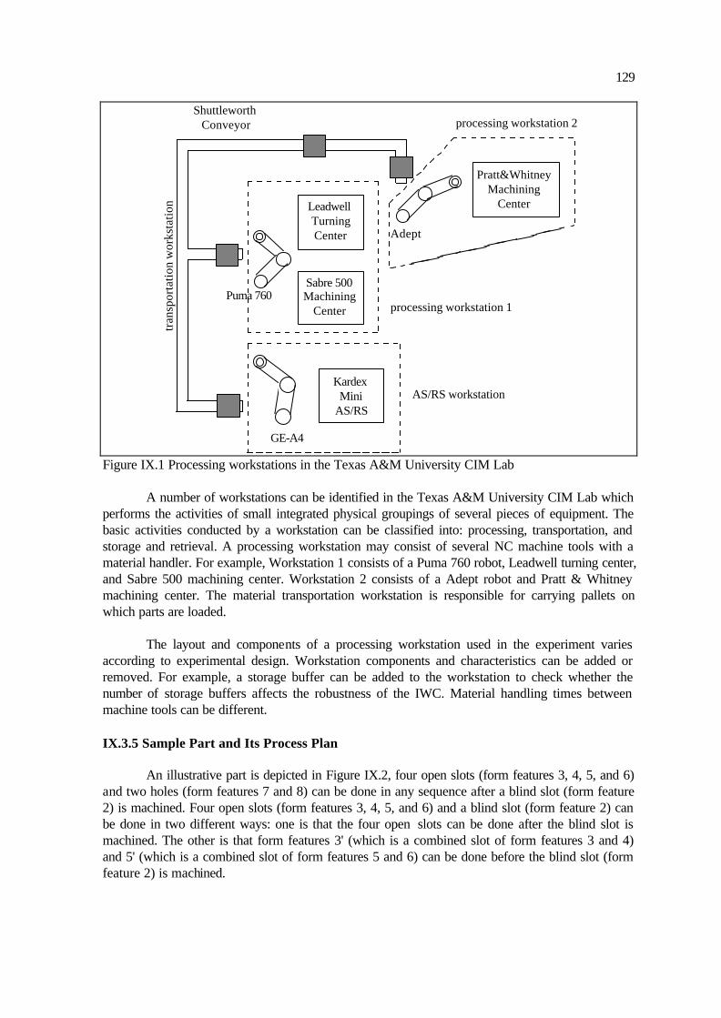
129

Pratt&Whitney Machining

CenterLeadwell Turning Center

Sabre 500 Machining

Center

Kardex Mini

AS/RS

Adept

Shuttleworth Conveyor

Puma 760

GE-A4

processing workstation 2

processing workstation 1

AS/RS workstation

tran

spor

tatio

n w

orks

tatio

n

Figure IX.1 Processing workstations in the Texas A&M University CIM Lab A number of workstations can be identified in the Texas A&M University CIM Lab which performs the activities of small integrated physical groupings of several pieces of equipment. The basic activities conducted by a workstation can be classified into: processing, transportation, and storage and retrieval. A processing workstation may consist of several NC machine tools with a material handler. For example, Workstation 1 consists of a Puma 760 robot, Leadwell turning center, and Sabre 500 machining center. Workstation 2 consists of a Adept robot and Pratt & Whitney machining center. The material transportation workstation is responsible for carrying pallets on which parts are loaded. The layout and components of a processing workstation used in the experiment varies according to experimental design. Workstation components and characteristics can be added or removed. For example, a storage buffer can be added to the workstation to check whether the number of storage buffers affects the robustness of the IWC. Material handling times between machine tools can be different. IX.3.5 Sample Part and Its Process Plan An illustrative part is depicted in Figure IX.2, four open slots (form features 3, 4, 5, and 6) and two holes (form features 7 and 8) can be done in any sequence after a blind slot (form feature 2) is machined. Four open slots (form features 3, 4, 5, and 6) and a blind slot (form feature 2) can be done in two different ways: one is that the four open slots can be done after the blind slot is machined. The other is that form features 3' (which is a combined slot of form features 3 and 4) and 5' (which is a combined slot of form features 5 and 6) can be done before the blind slot (form feature 2) is machined.

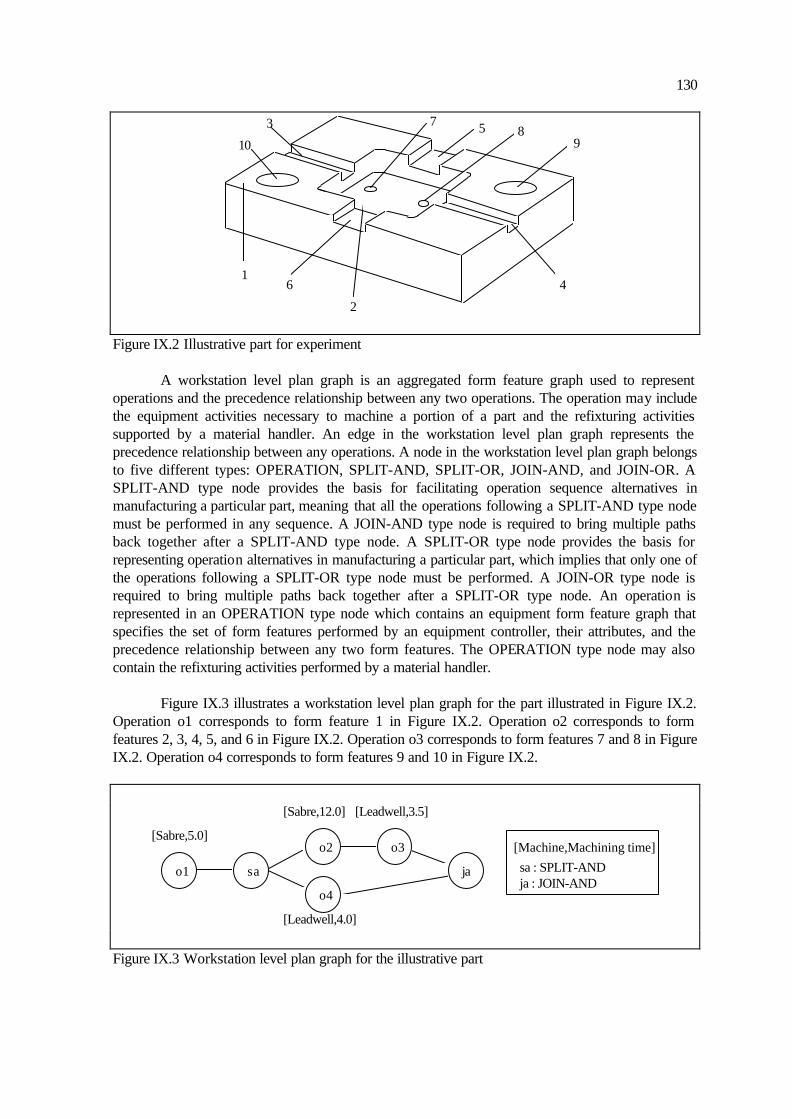
130

1

3

4

5

6

2

78

910

Figure IX.2 Illustrative part for experiment A workstation level plan graph is an aggregated form feature graph used to represent operations and the precedence relationship between any two operations. The operation may include the equipment activities necessary to machine a portion of a part and the refixturing activities supported by a material handler. An edge in the workstation level plan graph represents the precedence relationship between any operations. A node in the workstation level plan graph belongs to five different types: OPERATION, SPLIT-AND, SPLIT-OR, JOIN-AND, and JOIN-OR. A SPLIT-AND type node provides the basis for facilitating operation sequence alternatives in manufacturing a particular part, meaning that all the operations following a SPLIT-AND type node must be performed in any sequence. A JOIN-AND type node is required to bring multiple paths back together after a SPLIT-AND type node. A SPLIT-OR type node provides the basis for representing operation alternatives in manufacturing a particular part, which implies that only one of the operations following a SPLIT-OR type node must be performed. A JOIN-OR type node is required to bring multiple paths back together after a SPLIT-OR type node. An operation is represented in an OPERATION type node which contains an equipment form feature graph that specifies the set of form features performed by an equipment controller, their attributes, and the precedence relationship between any two form features. The OPERATION type node may also contain the refixturing activities performed by a material handler. Figure IX.3 illustrates a workstation level plan graph for the part illustrated in Figure IX.2. Operation o1 corresponds to form feature 1 in Figure IX.2. Operation o2 corresponds to form features 2, 3, 4, 5, and 6 in Figure IX.2. Operation o3 corresponds to form features 7 and 8 in Figure IX.2. Operation o4 corresponds to form features 9 and 10 in Figure IX.2.

sa : SPLIT-AND ja : JOIN-AND

o1 sa

o2 o3

o4

ja

[Sabre,5.0]

[Leadwell,4.0]

[Sabre,12.0] [Leadwell,3.5]

[Machine,Machining time]

Figure IX.3 Workstation level plan graph for the illustrative part

131

IX.3.6 Description of the Simulation Model In order to collect experimental data, a simulation mode is created which is a slight modification of the IWC. In particular, the execution function of the IWC is modified to accommodate part creation and system clock management activities. A detailed scheme of the simulation model is depicted in Figure IX.4. Parts are created according to Poisson distribution and the part type of the created part is randomly selected among five different part types. The inter-arrival time is increased to reduce workstation load. Each part type has its own attributes, such as part routings, machining time, due-date etc. The part routings are specified using an AND-OR graph. After a part is created, the execution function sends a plan message to the planning function to select an operation sequence graph. After planning is finished, a wpdone message is sent to the scheduling function, and then the new part becomes a dispatching candidate.

Part creation

System clock management

System clock > given time?

System clock > next arrival?

Start

Planning function

Scheduling function

pick,put transport load,unload

plan

wpdone

pickdone putdone transdone mdone

Collect data

End

Execution function

Y

N

YN

Figure IX.4 Detailed scheme of the simulation model The scheduling function sends to the execution function a set of command messages, such as pick , put, transport, load, and unload, which are associated with the movement of a part. After receiving those messages, the execution function advances the system clock on the basis of the machining time and the robot operation time. If the updated system clock is greater than the given simulation period, the execution function collects experimental data and analyzes statistics. In the mean time, if the next part arrival time is less than the updated system clock, a new part is created. Every time an even occurs, in other words, each operation specified by the scheduling function is finished, the execution function sends the event messages and invokes the scheduling function.

132

IX.4 Experimental Results IX.4.1 Experimental Results for Average Flow Time Table IX.6 shows the experimental results for the average flow time. Note that SNRs is used for the SNR. Average flow time is reduced dramatically by using the multi-pass scheduling technique and the BML planning strategy. With respect to the robust mean and SNR analysis, design 11 (BML for planning and Multi-pass for scheduling) provides the best results. Other scheduling strategies including SPT, EDD, ATC, and COVERT provide bad results compared to the multi-pass technique. In terms of planning, BML is better than the other two strategies with a combination of any scheduling rules. From the results, it can be concluded that the efficiency of the IWC with the BML strategy for planning and the multi-pass strategy for scheduling is much better than those of other planning/scheduling strategies. These results suggest that the utilization of the neural network and the multi-pass simulator is more robust in terms of the efficiency of manufacturing systems. Table IX.6 Experiment results for average flow time Design Planning

Strategies Scheduling Strategies

Average Variance Robust Mean

SNR mean

1 STPT Multi-pass 21.45 73.30 4.30 -62.74 2 STPT SPT 61.21 1010.47 6.92 -84.59 3 STPT EDD 64.69 1486.20 7.30 -86.33 4 STPT ATC 65.10 1535.02 7.34 -86.51 5 STPT COVERT 62.07 866.23 6.76 -84.52 6 LRF Multi-pass 21.40 72.98 4.29 -62.70 7 LRF SPT 59.69 979.06 6.89 -84.13 8 LRF EDD 57.88 927.18 6.83 -83.53 9 LRF ATC 58.40 945.55 6.85 -83.71

10 LRF COVERT 58.65 920.36 6.83 -83.72 11 BML Multi-pass 20.58 66.29 4.19 -61.89 12 BML SPT 61.30 639.08 6.46 -83.83 13 BML EDD 59.06 510.90 6.24 -82.89 14 BML ATC 59.44 527.42 6.27 -83.04 15 BML COVERT 61.65 739.42 6.61 -84.15

Table IX.7 shows the Student's t test to compare design 11 and other four designs 1, 2, 6, and 7 in terms of average flow time. It can be claimed that the null hypothesis is rejected at the significance level 0.001 for comparison with designs 2 and 7. The null hypothesis is also rejected at significance level 0.01 for comparison with designs 1 and 6. In other words, the IWC with design 11 dominates all other planning/scheduling strategies on the basis of the flow time-based performance criteria. Table IX.7 Student's t-test for average flow time Design 1 2 6 7 Planning Strategies STPT STPT LRF LRF Scheduling Strategies Multi-pass SPT Multi-pass SPT Difference mean ( D ) 0.87 40.63 0.85 37.85

Difference deviation(sD ) 0.32 5.62 0.32 6.01

t value 2.72 7.23 2.66 6.30 Significance probability 0.01 0.001 0.01 0.001

133

IX.4.2 Experimental Results for Throughput Table IX.8 shows the experimental results for throughput. Note that SNRl is used for the SNR. Throughput is increased dramatically by using the multi-pass scheduling technique and the BML planning strategy. With respect to the robust mean and SNR analysis, design 11 (BML for planning and Multi-pass for scheduling) provides the best results. Other scheduling strategies including SPT, EDD, ATC, and COVERT provides bad results compared to the multi-pass technique. In terms of planning, BML is better than the other two strategies with a combination of any scheduling rules. It can be concluded that the efficiency of the IWC with the BML strategy for planning and the multi-pass strategy for scheduling is much better than those of other planning/scheduling strategies in terms of throughput performance. Table IX.9 shows the Student's t test to compare design 11 and other four designs 1, 2, 6, and 7 in terms of throughput. It can be claimed that the null hypothesis is rejected at the significance level 0.001 for comparison with designs 2 and 7. The null hypothesis is also rejected at significance level 0.01 and 0.006 for comparison with designs 1 and 6. In other words, the IWC with design 11 dominates all other planning/scheduling strategies on the basis of the throughput-based performance criteria. Table IX.8 Experiment results for throughput Design Planning

Strategies Scheduling Strategies

Average Variance Robust Mean

SNR mean

1 STPT Multi-pass 1206.59 121447.86 11.71 139.98 2 STPT SPT 918.44 64317.64 11.07 134.15 3 STPT EDD 912.67 62967.23 11.05 134.07 4 STPT ATC 913.04 63176.05 11.05 134.06 5 STPT COVERT 912.93 63017.38 11.05 134.06 6 LRF Multi-pass 1212.12 123193.34 11.72 140.04 7 LRF SPT 935.30 68127.76 11.13 134.52 8 LRF EDD 927.11 64206.02 11.07 134.43 9 LRF ATC 927.85 65837.67 11.10 134.40

10 LRF COVERT 929.08 64917.23 11.08 134.44 11 BML Multi-pass 1234.59 123784.40 11.73 140.44 12 BML SPT 902.00 58181.77 10.97 133.87 13 BML EDD 897.59 58836.40 10.98 133.72 14 BML ATC 899.30 59544.67 10.99 133.73 15 BML COVERT 899.44 59238.19 10.99 133.75

Table IX.9 Student's t-test for throughput Design 1 2 6 7 Planning Strategies STPT STPT LRF LRF Scheduling Strategies Multi-pass SPT Multi-pass SPT Difference mean ( D ) 28.00 316.00 25.96 297.33

Difference deviation(sD ) 10.15 55.83 8.93 53.28

t value 2.76 5.66 2.91 5.58 Significance probability 0.01 0.001 0.006 0.001

134

IX.4.3 Experimental Results for Average Tardiness Table IX.10 shows the experimental results for average tardiness. Note that SNRt is used for the SNR. Average tardiness is reduced dramatically by using the multi-pass scheduling technique and the BML planning strategy. With respect to the robust mean and SNR analysis, design 11 provides the best results. In terms of planning, BML is better than the other two strategies with a combination of any scheduling rules. In conclusion, the efficiency of the IWC with the BML strategy for planning and the multi-pass strategy for scheduling is much better than those of other planning/scheduling strategies in terms of average tardiness performance. Table IX.10 Experiment results for average tardiness Design Planning

Strategies Scheduling Strategies

Average Variance Robust Mean

SNR mean

1 STPT Multi-pass 1.24 7.35 2.00 -3.54 2 STPT SPT 19.67 516.07 6.25 -393.16 3 STPT EDD 21.61 903.66 6.81 -473.80 4 STPT ATC 21.94 929.94 6.84 -488.20 5 STPT COVERT 19.49 363.92 5.90 -385.76 6 LRF Multi-pass 1.22 7.20 1.97 -3.46 7 LRF SPT 18.19 556.17 6.32 -337.20 8 LRF EDD 15.10 512.26 6.24 -234.25 9 LRF ATC 15.45 516.51 6.25 -244.95

10 LRF COVERT 16.46 484.82 6.18 -277.11 11 BML Multi-pass 0.93 4.49 1.50 -2.37 12 BML SPT 17.73 357.87 5.88 -320.23 13 BML EDD 15.12 250.28 5.52 -234.13 14 BML ATC 15.23 256.53 5.55 -237.50 15 BML COVERT 18.11 419.01 6.04 -334.01

Table IX.11 shows the Student's t test to compare design 11 and other four designs 1, 2, 6, and 8 in terms of average tardiness. It can be claimed that the null hypothesis is rejected at the significance level 0.001 and 0.002 for comparison with designs 2 and 7. However, the null hypothesis for comparison with designs 1 and 6 is not rejected. In other words, the effectiveness of the IWC with design 11 design factor set does not differ from designs 1 and 6. Table IX.11 Student's t-test for average tardiness Design 1 2 6 8 Planning Strategies STPT STPT LRF LRF Scheduling Strategies Multi-pass SPT Multi-pass EDD Difference mean ( D ) 0.30 18.73 0.31 14.15

Difference deviation(sD ) 0.18 4.41 0.18 4.37

t value 1.67 4.25 1.72 3.24 Significance probability 0.11 0.001 0.09 0.002

135

IX.5 Sample Session of the IWC Software In this section, the IWC software is addressed and demonstrated using a simple manufacturing workstation. The IWC software is a processing workstation controller on the basis of a three level hierarchical control structure (equipment, workstation, and shop). Therefore, the IWC software receives control commands from the shop controller and downloads updated control commands to the equipment controllers. The software can also receive status information commands from the equipment controllers and sends workstation status to the shop level controller. In convenience, the IWC software prints out the control commands and/or status commands instead of sending out those through a communication network. The IWC reads the control commands and/or status commands instead of receiving those through a communication network. First, a process plan must be represented in an appropriate way which drives part sequence and processing time. In order to store the workstation level plan graph as a file structure, precedence and node information is stored. Precedence information is provided by specifying the successors of a particular node, while the information content for OPERATION type nodes is provided as a file pointer. The node type can belong to -1,-2, or machine index, in which -1 implies SPLIT-AND type node and -2 implies JOIN-AND type node. Figure IX.5 illustrates a file structure for a sample workstation level plan graph. The flat file structure is represented as follows: Number of operation sequence graphs Number of nodes in the first operation sequence graph Node number, Node type, Operation time, Operation due-date, equipment form feature graph file name, Number of successor nodes, Successor1, Successor2,.... . Number of nodes in the last operation sequence graph Node number, Node type, Operation time, Operation due-date, equipment form feature graph file name, Number of successor nodes, Successor1, Successor2,.... In operating the software, a series of queries describing the workstation characteristics needed to be answered. The questions are displayed as follows: Number of machines? Number of Buffers? Pallet Size? Material handling time between machine tools? Performance criteria?(0-flow time,1-throughput,2-tardiness) After answering those questions, the IWC software waits for a message which is supposed to come through communication network from other controllers. However, in this demonstration, the user must type in any message directly. The following lists all different kinds of message types and their proper formats. arrive, part name, plan file name,...... mdone, machine index pickdone, location putdone, location transdone, location

136

sa : SPLIT-AND ja : JOIN-AND

o1 sa

o2 o3

o4

ja

[Sabre,5.0]

[Leadwell,4.0]

[Sabre,12.0] [Leadwell,3.5]

[Machine,Machining time]

1 6 0 0 5.0 20.0 "equip1" 1 1 1 -1 0.0 0.0 "" 2 2 3 2 0 12.0 68.0 "equip2" 1 4 3 1 4.0 75.0 "equip3" 1 5 4 1 3.5 90.0 "equip4" 1 5 5 -2 0.0 0.0 "" 0

Machine index 0 : Sabre 1 : Leadwell

Figure IX.5 Illustrative file structure for a workstation level plan graph The arrive message comes from the shop level controller. The mdone message comes from the machine tool controller. The pickdone, putdone, and transdone messages come from the robot controller. In this demonstration version, the user must type in. On the other hand, the IWC software responds to the message that the user types in. The following lists a set of messages that the IWC sends out to the other controllers. However, in this demonstration version, the IWC software displays on the screen. load, part index, machine index unload, part index, machine index pick, part index, location put, part index, location transport, location IX.6 Conclusion of Dissertation The goal of this research is to present the models and procedures required for the development of the IWC which can control processing workstation tasks by performing planning, scheduling, and execution. The specific objectives of this research are: 1) to develop a structured process plan representation necessary to drive the IWC during manufacturing processes, 2) to investigate the characteristics and complexities of a real-time planning function used to generate a set of tasks to be scheduled, 3) to build a robust real-time scheduler to contribute to increasing system performance, 4) to create a graph-theoretic deadlock detection and resolution module to help the IWC maintain the workstation in a deadlock-free state, 5) to develop an execution function necessary to receive and interpret incoming messages and broadcast updated messages, and 6) to create the IWC software to demonstrate the architectural linkages with other controllers. Most manufacturing controllers in existence today are application-specific and hand-woven systems which lack an insight or a generic vision of a manufacturing system. A detailed investigation on the past research reveals a number of defects. The development of the IWC can

137

overcome the disadvantages, provide several advantageous characteristics, and therefore save cost and time in developing control software for the automated manufacturing system. Furthermore, the future of shop floor control is enhanced if an integration module of a shop level controller and the IWC can be developed. 1) The IWC is intelligent, e.g., the IWC must be able to act appropriately in an uncertain environment in order to increase the probability of success of the system's ultimate goal given the criteria of success (Albus [5]). For example, the IWC detects and resolves system deadlock for every part movement. 2) The IWC is a real-time controller, that is, the time frame over which various decisions are made corresponds to the dynamic character of the workstation being considered. Further, the time of response taken to make decisions needs to be short. Specifically, the scheduling function is driven by a neural network and multi-pass simulation technique which provides the basis for real-time control. 3) The IWC is robust. In other words, the IWC performs well over a variety of workstation configurations (e.g., the number of machines, the number of buffers), workstation status (e.g., machine failure, tool breakage), and other exogenous operating parameters (e.g., order arrival rate, processing time distribution). A good planning strategy and a multi-pass scheduling policy enable the IWC to be robust. 4) The IWC includes the required integration of three basic functions: planning, scheduling, and execution. In fact, 80 percent of the workstation controllers in industry only perform monitoring functions, including monitoring the inputs of each machine (e.g., NC instructions), downloading orders, collecting output data, and generating alarms in case of conflict (Boulet et al. [27]). 5) The IWC observes the importance of the role of process plans generated by process planning systems and is able to read and control the AND/OR graph representation of a process plan. The AND/OR graph representation provides much flexibility of resource alternatives and sequence alternatives. 6) The IWC views process planning as an off-line rather than real-time activity unlike control. This concept enhances independence between process planning and control so that the development of a manufacturing system controller become easy. Some manufacturing controllers include the intermix of process plan and control (Crockett et al. [46], Kasturia et al. [117], Mettala [152]). This causes a change in a process plan to call for a change in the formal model. 7) The IWC adopts an event-driven operating philosophy. The execution function in the IWC detects and classifies any events and distributes them to either the planning and scheduling functions, or the shop and equipment controllers. In other words, the planning and scheduling functions of the workstation controller are invoked by the execution functions for every necessary event. Some manufacturing system controllers include the specified time delay for the state transitions (Chaar and Volz [35], Hadj-Alouane et al. [89], Naylor and Maletz [160], Naylor and Volz [161]). This time-driven method may result in undue complexity of system control as compared to an event-driven method. 8) The IWC employs the system deadlock detection and resolution models required to maintain a deadlock-free state. If no buffer is available in the system, the IWC adopts deadlock detection and avoidance. If any buffers are available, the IWC adopts deadlock detection and

138

recovery. This concept blocks the occurrence of system deadlocks and maintains the system in a deadlock-free state. IX.7 Further Research Topics This dissertation focused on the various activities of processing workstations and presented the definition and procedures of planning, scheduling, and execution functions which are the basic components of an intelligent workstation controller. Although this is only a small portion of a computer integrated manufacturing system, the techniques and methodologies presented in this dissertation can be applicable for developing other level controllers, including shop and equipment controllers. The increased affordability and application of the IWC will lead to identify further research topics. There are many potential issues associated with implementing a computer integrated manufacturing system: 1) In addition to a processing workstation controller, other workstation controllers, including an AS/RS workstation controller, a material transportation controller, an assembly workstation controller are needed. An AS/RS workstation controller is responsible for storing and retrieving several different types of materials by automated method. The principal control problem in AS/RS operation is to receive and interpret control commands from the shop level controller, and to store and retrieve requested materials in an efficient manner. A number of performance criteria can be employed, including maximum storage capacity, system throughput, and utilization (Groover [84]). A material transportation controller is responsible for carrying various materials and/or parts in between workstations. Receiving control commands from a shop level controller which may be a movement of a mobile entity from a location to another, the material transportation controller must be able to operate a variety of hardware systems (e.g., AGV, conveyor system) in such a way that the traveling time is minimized. An assembly workstation controller is responsible for operating several pieces of manual and automated devices to assemble a number of parts into a product. The assembly workstation controller must be flexible enough to kill or create parts. Further, the line balancing problem with precedence constraints specified in a assembly plan needs to be solved and implemented. 2) The development of a shop level controller is a challenging problem. A shop level controller is at the top of shop floor control and is responsible for communicating with a design system to support part geometry specifications and bill of materials for assemblies, parts, tools, and fixtures. It also communicates with a process planning system to import the specification for all operations for a given order. It then plans, schedules, and executes the various activities necessary to finish a number of orders within a specified due-date. Specifically, the shop level controller performs sequencing and scheduling batch jobs through workstations. Further, it analyzes resource requirements, prepares resource requisitions, and monitors the progress of the assigned tasks. 3) Equipment level controllers need to be developed, including a robot controller, a machine tool controller, an AGV controller, etc. Any equipment controller is a front-end system which is connected to the commercial equipment. Hence, it may not be generic in nature. A NC machine tool controller receives an order and its related information from the workstation controller and coordinates the activities associated with a single piece of processing equipment. On the other hand, a robot controller is responsible for moving parts a location to another, and refixturing activities. 4) A process planning system is another challenging problem which is able to generate a form feature graph associated with a specific part. A process plan contains important information necessary to manufacture a specific part type such as part routes, operation sequences, material

139

requirements, and resource requirements (Chang et al. [37]). The process plan must be capable of representing alternatives in terms of operation sequences, machine sequences, fixturing and tooling requirements, so that it provides flexibility for shop floor control. While these issues in a process plan have resulted in many process plan representation models, a process planning system has yet to come. IX.8 Chapter Summary This chapter presented experimental design and results necessary to demonstrate the effectiveness and robustness of the IWC. Further, this chapter provided the conclusion of the dissertation and further research topics. The best planning strategy and scheduling strategy are BML and multi-pass techniques for most performance criteria. This implies that the IWC with a BML for planning and a multi-pass technique for scheduling is superior to any other planning/scheduling strategies. This chapter also presented an illustrative example for the operation of the IWC software. The IWC software is supposed to be operating under well-defined communication environment. However, in this demonstration version, the user must type in all corresponding messages which are supposed to come from other controllers. Finally, the characteristics of the IWC were presented. The IWC is intelligent. The IWC is a real-time controller. The IWC is robust. The IWC includes the required integration of three basic functions: planning, scheduling, and execution. The IWC observes the importance of the role of process plans and is able to read and control the AND/OR graph representation of process plan. The IWC views process planning as an off-line rather than real-time activity unlike control. The IWC adopts an event-driven operating philosophy. The IWC employs the system deadlock detection and resolution models required to maintain a deadlock-free state.

140

REFERENCES [1] Achatz, R. and Parrish, D. J., “Host computer controls FMS at all levels,” The FMS

Magazine 5, 1, 21-25 (1987). [2] Adiga, S., “Software modeling of manufacturing systems: A case for an object-oriented

programming approach,” Annals of Operations Research 17, 3, 363-377 (1989). [3] Agapiou, J. S., “Sequence of operations optimization in single-stage multi-functional

systems,” Journal of Manufacturing Systems 10, 3, 194-208 (1991). [4] Akella, R., Choong, Y., and Gershwin, S. B., “Performance of hierarchical production

scheduling policy,” IEEE Transactions of CHMT CHMT-7, 3, 225-240 (1984). [5] Albus, J. S., “Outline for a theory of intelligence,” IEEE Transactions on Systems, Man,

and Cybernetics 21, 473-509, (1991). [6] Albus, J. S., McCain, H., and Lumia, R., “NASA/NBS standard reference model for

telerobot control system architecture,” NISTIR 89-1235, National Institute of Standards and Technology, Gaithersburg, Maryland (1989).

[7] Albus, J. S., Quintero, R., Lumina, R., Herman, M., Kilmer, R., and Goodwin, K., “Concept for a reference model architecture for real-time intelligent control,” NISTIR 90-1277, National Institute of Standards and Technology, Gaithersburg, Maryland (1990).

[8] Alting, L. and Zhang, H., “Computer aided process planning: the state-of-the-art survey,” International Journal of Production Research 27, 4, 553-585 (1989).

[9] Ammons, J. C., Govindaraj, T., and Mitchell, C. M., “A supervisory control paradigm for real-time control of flexible manufacturing systems,” Annals of Operations Research 15, 4, 313-335 (1988).

[10] Ang, C. L., “Technical planning of factory data communications systems,” Computers in Industry 9, 93-105 (1987).

[11] Anky, P. G., “A real-time, rule based FMS operation control strategy in CIM environment - Part I,” International Journal of Computer Integrated Manufacturing 1, 1, 55-72 (1988).

[12] Austin, B. L., “Computer aided process planning for machined cylindrical metal parts,” Proceedings of AUTOFACT'86, Detroit, Michigan (1986).

[13] Avonts, L. H. and Van Wassenhove, L. N., “The part mix and routing mix problem in FMS: A coupling between an LP model and a closed queuing network,” International Journal of Production Research 26, 12, 1891-1902 (1988).

[14] Banaszak, A. Z. and B. H. Krogh, “Deadlock avoidance in flexible manufacturing systems with concurrently competing process flows,” IEEE Transaction on Robotics and Automation 6, 724-734 (1990).

[15] Banerjee, S. K. and Al-Maliki, I., “A structured approach to FMS modeling,” International Journal of Computer Integrated Manufacturing 1, 2, 77-88 (1988).

[16] Barkmeyer, E. J., “Distributed data interfaces - The lessons of IMDAS,” Proceedings of the 1988 Conference on CIM Data Bases, Boston, Massachusetts, (1988).

[17] Barkmeyer, E. J., “Some interactions of information and control in integrated automation systems,” NATO ASI Series, Vol. F53, Advanced Information Technologies for Industrial Material Flow Systems, Springer-Verlag, New York, New York (1989).

[18] Bastos, J. M., “Batching and routing: Two functions in operational planning of flexible manufacturing systems,” European Journal of Operational Research 33, 230-244 (1988).

[19] Bean, J. C., Birge, J. R., Mittenthal, J., and Noon, C. E., “Match-up scheduling with multiple resources, release dates and disruptions,” Operations Research 39, 470-483 (1991).

141

[20] Bel, G., Bensana, E., Dubois, D., Erschler, J., and Esquirol, P., “A knowledge -based approach to industrial job shop scheduling,” Knowledge-based Systems in Manufacturing, edited by Kusiak, A., Taylor & Francis, Philadelphia, Pennsylvania (1989).

[21] Bhaskaran, K., “Process plan selection,” International Journal of Production Research 28, 1527-1539 (1990).

[22] Biemans, F., and Blonk, P., “On the formal specification and verification of CIM architectures using LOTOS,” Computers in Industry 7, 491-504 (1986).

[23] Biemans, F. P. and Vissers, C. A., “Reference model for manufacturing planning and control systems,” Journal of Manufacturing Systems 8, 35-46 (1989).

[24] Blackstone, J. H., Phillips, D. T., and Hogg, G. L., “A state-of-the-art of dispatching rules for manufacturing job shops operations,” International Journal of Production Research 20, 27-45 (1982).

[25] Blazewicz, J., Brzezinski, J., and Gambosi, G., “Time-stamp approach to store-and forward deadlock prevention,” IEEE Transactions on Communications COM-35, 5, 490-495 (1987).

[26] Bona, B., Brandimarte, P., Greco, C., and Menga, G., “Hybrid hierarchical scheduling and control systems in manufacturing,” IEEE Transactions on Robotics and Automation 6, 6, 673-686 (1990).

[27] Boulet, B., Chhabra, B., Harhalakis, G., Minis, I., and Proth, J. M., “Cell controllers: Analysis and comparison of three major projects”, Computers in Industry 16, 239-254 (1991).

[28] Bretthauer, K. M. and Venkataramanan, M. A., “Machine loading and alternate routing in a flexible manufacturing system,” Computers and Industrial Engineering 18, 3, 341-350 (1990).

[29] Brown, J., Dubois, D., Rathmill, K., Sethi, S., and Stecke, K. E., “Classifications of flexible manufacturing systems,” The FMS Magazine, 114-117 (April 1984).

[30] Burnage, D. and Jones, T., “A manufacturing controller implementation environment and its application at Rolls-Royce Sunderland,” Manufacturing Cells Control, Programming and Integration, Edited by Williams, D. J. and Rogers, P., Butterworth-Heinemann, Oxford, England, 86-117 (1991).

[31] Burns, A., “Scheduling hard real-time systems: A review,” Software Engineering Journal May, 116-127 (1991).

[32] Burns, A. and Wellings, A., Real-time systems and their programming languages, Addison-Wesley, Reading, Massachusetts (1990).

[33] Carton, B. A. and Ray, S., “ALPS: A language for process specification,” International Journal of Computer Integrated Manufacturing 4, 2, 105-113 (1991).

[34] Caudill, M., “Neural networks primer, Part II,” AI Expert February, 55-61 (1988). [35] Chaar, J. K. and Volz, R. A., “On the Ada implementation of a component-oriented rule-

based specification language for manufacturing systems control software,” Proceedings of the fifth annual conference on Artificial Intelligence and Ada, IEEE, Piscataway, New Jersey, 39-50 (1989).

[36] Chang, T. C. and Wysk, R. A., An introduction to automated process planning systems , Prentice-Hall, Englewood Cliffs, New Jersey (1987).

[37] Chang, T. C., Wysk , R. A. and Wang, H. P., Computer Integrated Manufacturing, Prentice-Hall, Englewood Cliffs, New Jersey (1991).

[38] Cho, H., Derebail, A., Hale, T., and Wysk, R. A., “A formal approach to integrating computer aided process planning and shop floor control,” ASME Transactions:Journal of Engineering for Industry , to appear (January 1994).

[39] Cho, H. and Wysk, R. A., “A robust adaptive scheduler for an intelligent workstation controller,” International Journal of Production Research 31, 4, 771-790 (1993).

142

[40] Choi, R. H. and Malstrom, E. M., “Evaluation of traditional work scheduling rules in a flexible manufacturing system with a physical simulator,” Journal of Manufacturing Systems 7, 33-45 (1988).

[41] Chryssolouris, G., Lee, M., and Domroese, M., “The use of neural networks in determining operational policies for manufacturing systems,” Journal of Manufacturing Systems 10, 166-175 (1991).

[42] Chung, C., “Planning tool requirements for flexible manufacturing systems,” Journal of Manufacturing Systems 10, 6, 476-483 (1991).

[43] Cidon, I., Jaffe, J. M., and Sidi, M., “Distributed store-and-forward deadlock detection and resolution algorithms,” IEEE Transactions on Communications COM-35, 11, 1139-1145 (1987).

[44] Coffman, E. G., Elphick, M. J. and Shoshani, A., “System deadlocks,” Computing Surveys 3, 67-78 (1971).

[45] Conway, R. W. and Maxwell, W. L., “Network dispatching by shortest operation discipline,” Operations Research 10, 51-73 (1962).

[46] Crockett, D., Desrochers, A., Dicesare, F., and Ward, T., “Implementation of a petri net controller for a machining workstation,” Proceedings of the IEEE Robotics and Automation Conference, Raleigh, North Carolina, 1861-1867 (1987).

[47] Damodaran, V., Lashkari, R. S., and Singh, N., “A production planning model for cellular manufacturing systems with refixturing considerations,” International Journal of Production Research 30, 7, 1603-1616 (1992).

[48] Dar-El, E. M., “Solving large single-model assembly line balancing problems - A comparative study,” AIIE Transactions 7, 3, 302-310 (1975).

[49] Dar-El, E. M. and Wysk, R. A., “Job shop scheduling - A systematic approach,” Journal of Manufacturing Systems 1, 77-88 (1982).

[50] Davis, W. J. and Jones, A. T., “A real-time production scheduler for a stochastic manufacturing environment,” International Journal of Computer Integrated Manufacturing 1, 101-112 (1988).

[51] Davis, W. J. and Jones, A. T., “A functional approach to designing architectures for CIM,” IEEE Transactions on Systems, Man, and Cybernetics 19, 164-174 (1989).

[52] Davis, W. J., Jones, A. T., and Saleh, A., “Generic architecture for intelligent control systems,” Computer Integrated Manufacturing Systems 5, 2, 105-113 (1992).

[53] De Mello, H. L. S. and Sanderson, A. C., “AND/OR graph representation of assembly plans,” Proceedings of AAAI-86 2, Philadelphia, Pennsylvania, 1113-1119 (1986).

[54] Denzler, D. R. and Boe, W. J., “Experimental investigation of the scheduling decision rules,” International Journal of Production Research 25, 979-994 (1987).

[55] Desrochers, A. A., Modeling and Control of Automated Manufacturing Systems , IEEE Computer Society Press, Los Alamitos, California (1990).

[56] Dilts, D. M., Boyd, N. P., and Whorms, H. H., “The evolution of control architectures for automated manufacturing systems,” Journal of Manufacturing Systems 10, 1, 79-93 (1991).

[57] Dirne, C. W. G. M., “Planning problems of flexible automated manufacturing cells in a job shop - a case study,” Proceedings of the Third ORSA/TIMS Conference on Flexible Manufacturing Systems: Operations Research Models and Applications, edited by Stecke, K. E. and Suri, R., Elsevier, Amsterdam, 61-66 (1989).

[58] Dooley, K. J. and Mahmoodi, F., “Identification of robust scheduling heuristics: Application of Taguchi methods in simulation studies,” Computers and Industrial Engineering 22, 359-368 (1992).

[59] Duda, R. O. and Peter, E. H., Pattern Classification and Scene Analysis, Wiley, New York, New York (1973).

143

[60] Duffie, N. A., “An approach to the design of distributed machinery control systems,” IEEE Transactions on Industry Applications 1A-18, 435-442, (1982).

[61] Duffie, N. A., Chitturi, R., and Mou, J., “Fault-tolerant heterarchical control of heterogeneous manufacturing system entities,” Journal of Manufacturing Systems 7, 315-327, (1988).

[62] Duffie, N. A., “Synthesis of heterarchical manufacturing systems,” Computers in Industry 14, 167-174, (1990).

[63] Duffie, N. A. and Piper, R. S., “Non-hierarchical control of a flexible manufacturing cell,” Robotics and Computer Integrated Manufacturing 3, 175-179, (1987).

[64] Eilon, S., Choudury, I. G., and Serghious, S. S., “Experiments with SIx rule in job shop scheduling,” Simulation 24, 45-48, (1975).

[65] Erschler, J. and Esquirol, P., “Decision-aid in job-shop scheduling: A knowledge-based approach,” Proceedings of the IEEE Robotics and Automation Conference, San Francisco, California, 1651-1656 (1986).

[66] ESPRIT Consortium AMICE, “Integrated manufacturing - A challenge for the 1990s,” Computing and Control Engineering Journal May, 101-108 (1991).

[67] Eversheim, W. and Neitzel, R. , “Expert systems for flexible manufacturing,” Intelligent manufacturing systems II, edited by Milacic, V. R., Elsevier, Amsterdam, 67-86 (1988).

[68] Fernandes, C. A. and Gomide, F. A. C., “A heuristic procedure for production planning of modern manufacturing systems,” Computers and Industrial Engineering 20, 4, 475-485 (1991).

[69] Foo, Y. S. and Takefuji, Y., “Integer linear programming neural networks for job-shop scheduling,” International Joint Conference on Neural Networks: Volume II, IEEE Neural Networks Council, New York, New York, 341-348 (1988).

[70] Foo, Y. S. and Takefuji, Y., “Stochastic neural networks for solving jobshop scheduling: Part 1. architecture and simulations,” International Joint Conference on Neural Networks: Volume II, IEEE Neural Networks Council, New York, New York, 283-290 (1988).

[71] Foo, Y. S. and Takefuji, Y., “Stochastic neural networks for solving jobshop scheduling: Part 2. problem representation,” International Joint Conference on Neural Networks: Volume II, IEEE Neural Networks Council, New York, New York, 275-282 (1988).

[72] Fowler, J. E., “A generic architecture for CIM software based on the product data exchange specification,” NISTIR 89-4168, National Institute of Standards and Technology, Gaithersburg, Maryland (1989).

[73] Fox, M. S. and Smith, S. F., “ISIS - a knowledge-based system for factory scheduling,” Expert Systems 1, 25-49 (1984).

[74] Furlani, C. M., Kent, E. W., Bloom, H. M., and McLean, C. R., “The AMRF at the National Bureau of Standards,” Proceedings of the Summer Simulation Conference, Vancouver, Canada, (July 1983).

[75] Garey, M. and Johnson, D., Computers and Intractability , Freeman, San Francisco, California (1979).

[76] Gatelmand C. D., “A survey of FMSs,” Journal of Manufacturing Systems 1, 1-15 (1982).

[77] Gershwin, S. B., Hildebrant, R. R., Suri, R., and Mitter, S. K., “A control perspective on recent trends in manufacturing systems,” Control Systems Magazine MCS-6, 2, 3-15 (1986).

[78] Gilgor, V. D. and Shattuck, S. H., “On deadlock detection in distributed systems,” IEEE Transactions on Software Engineering SE-6, 5, 435-440 (1980).

[79] Giorgio, L. and Franco, S., “Generalized AND/OR graphs,” Artificial Intelligence 7, 243-259 (1976).

144

[80] Gold, E. M., “Deadlock prediction: Easy and difficult cases,” SIAM Journal on Computing 7, 3, 320-336 (1978).

[81] Gonzales, T. and Sahni, S., “Flowshop and jobshop schedules: complexity and approximation,” Operations Research 26, 36-52 (1978).

[82] Gopal, I. S., “Prevention of store-and-forward deadlock in computer networks,” IEEE Transactions on Communications COM-33, 12, 1258-1264 (1985).

[83] Graves, S. C., “A review of production scheduling,” Operations Research 29, 646-675 (1981).

[84] Groover, M. P., Automation, Production Systems, and Computer Integrated Manufacturing, Prentice-Hall, Englewood Cliffs, New Jersey (1987).

[85] Gunasekaran, A., Martikainen, T., and Yli-Olli, P., “Flexible manufacturing systems: An investigation for research and applications,” European Journal of Operational Research 66, 1-26 (1993).

[86] Gupta, Y. P., Gupta, M. C., and Bector, C. R., “A review of scheduling rules in flexible manufacturing systems,” International Journal of Computer Integrated Manufacturing 2, 6, 356-377 (1989).

[87] Habermann, A. N., “Prevention of system deadlocks,” Communications of the ACM 12, 373-378 (1969).

[88] Hadavi, K., Hsu, W. L., Chen, T., and Lee, C. M., “An architecture for real-time distributed scheduling,” AI Magazine Fall, 46-56 (1992).

[89] Hadj-Alouane, N. B., Chaar, J. K., and Naylor, A. W., “The design and implementation of the control and integration software of a flexible manufacturing systems,” Proceedings of the IEEE International Conference on System Integration, IEEE, Piscataway, New Jersey, 494-502 (1990).

[90] Hammer, H., “Flexible manufacturing cells and systems with computer intelligence,” Robotics and Computer Integrated Manufacturing 3, 39-54 (1987).

[91] Harmonosky, C. M., “Implementation issues using simulation for real-time scheduling, control, and monitoring,” 1990 Winter Simulation Conference Proceedings, New Orleans, Louisiana, 595-598 (1990).

[92] Harmonosky, C. M. and Barrick, D. C., “Simulation in a CIM environment: structure for analysis and real-time control,” 1988 Winter Simulation Conference Proceedings, San Diego, California, 704-711 (1988).

[93] Harmonosky, C. M. and Robohn, S. F., “Real-time scheduling in computer integrated manufacturing: a review of recent research,” International Journal of Computer Integrated Manufacturing 4, 6, 331-340 (1991).

[94] Hatvany, J., “Intelligence and cooperation in heterarchical manufacturing systems,” Robotics and Computer Integrated Manufacturing 2, 101-104 (1985).

[95] Haupt, R., “A survey of priority rule-based scheduling,” OR Spectrum 11, 1, 3-16 (1989). [96] Hershauer, J. C. and Ebert, J., “Search and simulation selection of a job shop scheduling

rule,” Management Science 21, 7, 833-843 (1975). [97] Hitz, K., “Flexible integrated computer aided manufacturing systems increase productivity,”

Robotics and Computer Integrated Manufacturing 3, 123-128 (1987). [98] Holt, R. C., “Comments on prevention of system deadlocks,” Communications of the

ACM 14, 36-38 (1971). [99] Horowitz, E. and Sahni, S., Fundamentals of Computer Algorithms, Computer Science

Press, Potomac, Maryland (1978). [100] Howard, J. H., Jr., “Mixed solutions for the deadlock problem,” Communications of the

ACM 16, 427-430 (1973).

145

[101] Huang, H. P. and Chang, P. C., “Specification, modeling and control of a flexible manufacturing cell,” International Journal of Production Research 30, 11, 2512-2543 (1992).

[102] Huang, P. Y., “A comparative study of priority dispatching rules in a hybrid assembly/job shop,” International Journal of Production Research 22, 375-387 (1984).

[103] Hutchison, J. and Khumawala, B., “Scheduling random flexible manufacturing systems with dynamic environments,” Journal of Operations Management 9, 3, 335-350 (1990).

[104] Hwang, S., “Part selection problems in flexible manufacturing systems planning stage,” Proceedings of the Second ORSA/TIMS Conference on Flexible Manufacturing Systems: Operations Research Models and Applications, edited by Stecke, K. E. and Suri, R., Elsevier, Amsterdam, 61-66 (1986).

[105] Ishii, N., and Talavage, J. J., “A transient based real-time scheduling algorithm in FMS,” International Journal of Production Research 29, 12, 2501-2520 (1991).

[106] Jakubowski, R., “Syntactic characterization of machine parts shapes,” Cybernetics and Systems 3, 1-24 (1982).

[107] Jensen, K., “Colored petri nets and the invariant-method,” Theoretical Computer Science 14, 317-336 (1981).

[108] Johnson, D. B., “Finding all the elementary of a directed graph,” SIAM Journal on Computing 4, 77-84 (1991).

[109] Jones, A. T., Barkmeyer, E., and Davis, W. J., “Issues in the design and implementation of a system architecture for computer integrated manufacturing,” International Journal of Computer Integrated Manufacturing 2, 65-76 (1989).

[110] Jones, A. T. and McLean, C. R., “A proposed hierarchical control model for automated manufacturing systems,” Journal of Manufacturing Systems 5, 15-25 (1986).

[111] Jones, A. T. and Saleh, A., “A multi-level/multi-layer architecture for intelligent shop floor control,” International Journal of Computer Integrated Manufacturing 3, 60-70 (1990).

[112] Jorysz, H. R. and Vernadat, F. B., “CIM-OSA part 1: total enterprise modeling and function view,” International Journal of Computer Integrated Manufacturing 3, 3, 144-156 (1990).

[113] Jorysz, H. R. and Vernadat, F. B., “CIM-OSA part 2: information view,” International Journal of Computer Integrated Manufacturing 3, 3, 157-167 (1990).

[114] Joshi, S., Wysk, R. A., and Jones, A. T., “A scaleable architecture for CIM shop floor control,” Proceedings of CIMCON '90, National Institute of Standards and Technology, Gaithersburg, Maryland, 21-33 (May 1990).

[115] Kachitvichyanukul, V., Davis, W. J., Pegden, C. D., Musselman, K. J., Ingalls, R., and Trybula, W. J., “Simulation and scheduling (Panel discussion),” 1991 Winter Simulation Conference Proceedings, Phoenix, Arizona, 382-391 (1991).

[116] Karam, G. M. and Buhr, R. J. A., “Temporal logic -based deadlock analysis for Ada,” IEEE Transactions on Software Engineering 17, 10, 1109-1125 (1991).

[117] Kasturia, E., DiCesare, F., and Desrochers, A., “Real-time control of multilevel manufacturing systems using colored petri nets,” Proceedings of the IEEE International Conference on Robotics and Automation, Philadelphia, Pennsylvania, 1114-1119 (1988).

[118] Kim, J, Funk, K. H., and Fichter, E. F., “Towards an expert system for FMS scheduling: A knowledge acquisition environment,” Expert Systems and Intelligent Manufacturing, edited by Oliff, M. D., North-Holland, New York, New York, 215-234 (1988).

[119] Kim, J., O'Grady, P., and Young R. E., “Feature taxonomies for rotational parts: a review and proposed taxonomies,” International Journal of Computer Integrated Manufacturing 4, 6, 341-350 (1991).

[120] Kimemia, J. and Gershwin, S. B., “An algorithm for the computer control of a flexible manufacturing system,” IIE Transactions 15, 4, 353-362 (1983).

146

[121] Kiran, A. S. and Smith, M. L., “Simulation studies in job shop scheduling-II, Performance of priority rules,” Computers and Industrial Engineering 8, 2, 95-105 (1984).

[122] Klittich, M., “CIM-OSA part 1: CIM-OSA integrating infrastructure-the operational basis for integrated manufacturing systems,” International Journal of Computer Integrated Manufacturing 3, 3, 168-180 (1990).

[123] Knapp, E., “Deadlock detection in distributed databases,” ACM Computing Surveys 19, 4, 303-328 (1987).

[124] Kohonen, T., “An introduction to neural computing,” Neural Networks 1, 3-16 (1988). [125] Korde, U. P., Bora, B. C., Stelson, K. A., and Riley, D. R., “Computer-aided process

planning for turned parts using fundamental and heuristic principles,” ASME Transactions: Journal of Engineering for Industry 114, 31-40 (1992).

[126] Kovalev, M. Y., Shafranskij, Y. M., Strusevich, V. A., Tanaec, V. S., and Tuzikov, A. V., “Approximation scheduling algorithms: A survey,” Optimization 20, 6, 859-878 (1989)

[127] Kshemkalyani, A. D. and Singhal, M., “Invariant-based verification of a distributed deadlock detection algorithm,” IEEE Transactions on Software Engineering 17, 8, 789-799 (1991).

[128] Kusiak, A., “Loading models in flexible manufacturing systems,” Flexible Manufacturing, edited by Raouf, A. and Ahmad, S. I., Elsevier, Amsterdam, 119-132 (1985).

[129] Kusiak, A. and Chen, M., “Expert systems for planning and scheduling manufacturing systems,” European Journal of Operational Research 34, 113-130 (1988).

[130] Kusiak, A. and Finke, G., “Selection of process in automated manufacturing systems,” IEEE Journal of Robotics and Automation 4, 397-402 (1988).

[131] Kusiak, A. and Villa, A., “Architectures of expert systems for scheduling flexible manufacturing systems,” Proceedings of the 1987 IEEE International Conference on Robotics and Automation, Raleigh, North Carolina, 113-117 (1987).

[132] Larin, D. J., “Cell control: what we have, what we will need,” Manufacturing Engineering January, 41-48 (1989).

[133] Lashkari, R. S. and Guna, K. R., “Machine-part grouping in the presence of alternate process plans in flexible manufacturing systems,” Proceedings of Manufacturing International 1, American Society of Mechanical Engineers, New York, New York, 101-105 (1990).

[134] Lecocq, P., Guiot, T., and Fang, Q., “An expert systems application to increase the flexibility and the efficacy of real time flexible manufacturing system controllers,” Expert Systems and Intelligent Manufacturing, edited by Oliff, M. D., North-Holland, New York, New York (1988).

[135] Leibfried, T. F., Jr., “A deadlock detection and recovery algorithm using the formalism of a directed graph matrix,” Operating Systems Review 23, 2, 45-55 (1989).

[136] Lewis, W., Barash, M. M., and Solberg, J. J., “Computer integrated manufacturing system control: A data flow approach,” Journal of Manufacturing Systems 6, 3, 177-191 (1987).

[137] Li, R. K., “A part-feature recognition system for rotational parts,” International Journal of Production Research 26, 1451-1475 (1988).

[138] Li, R. K. and Hwang, T., “A part-feature recognition system for rotational parts: non-turning features,” International Journal of Computer Integrated Manufacturing 2, 5, 257-267 (1989).

[139] Lin, G., Y-J., and Solberg, J. J., “Integrated shop floor control using autonomous agents,” IIE Transactions 24, 3, 57-71 (1992).

[140] Lou, S. X. C. and Van Ryzin, G., “Optimal control rules for scheduling job shops,” Annals of Operations Research 17, 233-248 (1989).

[141] Madurai, S. S. and Lin, L., “Rule-based automatic part feature extraction and recognition from CAD data,” Computers and Industrial Engineering 22, 49-62 (1992).

147

[142] Maimon, O. Z., “Real-time operational control of flexible manufacturing systems,” Journal of Manufacturing Systems 6, 125-136 (1987).

[143] Maimon, O. Z. and Fisher, E. L., “An object-based representation method for a manufacturing cell controller,” Artificial Intelligence in Engineering, Elsevier, Amsterdam, (1988).

[144] McLean, C. R., “An architecture for intelligent manufacturing control,” Proceedings of Summer 1985 ASME Conference, Boston, Massachusetts, (1985).

[145] McLean, C. R., “Information architecture of the AMRF,” Proceedings of the Information Technologies Conference, Troy, New York, (June 1986).

[146] McLean, C. R., “The vertical machining workstation of the AMRF: Software integration,” Proceedings of the 1986 ASME Symposium on Intelligent and Integrated Manufacturing, Anaheim, California (1986).

[147] McLean, C. R., Bloom, H. M., and Hopp, T. H., “The virtual manufacturing cell”, Proceedings of Fourth IFAC/IFIP Conference on Information Control Problems in Manufacturing Technology, Maryland, (1982).

[148] McLean, C. R. and Brown, P. F., “The AMRF at the National Bureau of Standards,” Proceedings of the IFIP W. G. 5.7 Working Conference on New Technologies for Production Management Systems , Tokyo, Japan, (1986).

[149] McLean, C. R., Mitchell, M., and Barkmeyer, E., “A Computer Architecture for Small Batch Manufacturing,” IEEE Spectrum May, 59-64 (1983).

[150] McLean, C. R. and Wenger, C. E., “The AMRF material handling system architecture,” Proceedings of the Fifth Annual Control Engineering Conference, Rosemont, Illinois, 40-49 (May 1986).

[151] Merabet, A. A., “Synchronization of operations in a flexible manufacturing cell: The petri-net approach,” Journal of Manufacturing Systems 5, 161-169 (1986).

[152] Mettala, E. G., Automatic generation of control software in computer integrated manufacturing, Ph.D. Dissertation, Pennsylvania State University (1989).

[153] Miller R. K. and Walker T. C., FMS/CIM Systems Integration Handbook , The Fairmont Press, Lilburn, Georgia (1990).

[154] Minoura, T. and Ding C., “A deadlock prevention method for a sequence controller for manufacturing control,” International Journal of Robotics and Automation 6, 3, 149-155 (1991).

[155] Mize, J. H., Bhuskute, H. C., Pratt, D. B., and Kamath, M., “Modeling of integrated manufacturing systems using an objected-oriented approach,” IIE Transactions 24, 3, 14-26 (1992).

[156] Morris, K. C., Mitchell, M., Dabrowski, C, and Fong, E., “Database management systems in engineering,” NISTR 4987, National Institute of Standards and Technology, Gaithersburg, Maryland (1992)..

[157] Morton, T. E. and Smunt, T. L., “A planning and scheduling system for flexible manufacturing,” Modeling and design of Flexible Manufacturing Systems , edited by Kusiak, A., Elsevier, Amsterdam, 151-164 (1986).

[158] Mukhopadhyay, S. K., Midha, S., and Krishina V. M., “A heuristic procedure for loading problems in flexible manufacturing systems,” International Journal of Production Research 30, 9, 2213-2228 (1992).

[159] Murata, T., Shenker, B., and Shatz, S. M., “Detection of Ada deadlocks using petri net invariants,” IEEE Transactions on Software Engineering 15, 3, 314-326 (1989).

[160] Naylor, A. W. and Maletz, M. C., “The manufacturing game: A formal approach to manufacturing software,” IEEE Transactions on Systems, Man, and Cybernetics SMC-16, 321-334 (1986).

148

[161] Naylor, A. W. and Volz, R. A., “Design of integrated manufacturing system control software,” IEEE Transactions on Systems, Man, and Cybernetics SMC-17, 6, 881-897 (1987).

[162] Nilsson, N. J., Problem-solving methods in artificial intelligence, McGraw-Hill, New York, New York (1971).

[163] O'Grady, P. J., Bao, H., and Lee, K. H., “Issues in intelligent cell control for flexible manufacturing systems,” Computers in Industry 9, 25-36 (1987).

[164] O'Grady, P. and Harrison, C., “A general search sequencing rule for job-shop sequencing,” International Journal of Production Research 23, 6, 961-973 (1985).

[165] O'Grady, P. J. and Lee, K. H., “An intelligent cell control system for automated manufacturing,” Knowledge-based Systems in Manufacturing, edited by Kusiak, A., Taylor & Francis, Philadelphia, Pennsylvania (1989).

[166] O'Grady, P. J. and Menon, U., “A concise review of flexible manufacturing systems and FMS literature,” Computers in Industry 7, 155-167 (1986).

[167] O'Grady, P. J. and Menon, U., “A hierarchy of intelligent scheduling and control for automated manufacturing systems,” Proceedings of the symposium on real time optimization in automated manufacturing facilities, National Bureau of Standards, Gaithersburg, Maryland, (January 21-22 1986).

[168] O'Keefe, R. M. and Kasirajan, T., “Interaction between dispatching and next station selection rules in a dedicated flexible manufacturing system,” International Journal of Production Research 30, 8, 1753-1772 (1992).

[169] Owusu-Ofori, S. and Chen C. S., “A knowledge-based approach to form-feature recognition from engineering drawings,” Proceedings of Manufacturing International 1, American Society of Mechanical Engineers, New York, New York, 57-66 (1990).

[170] Panwalker, S. S. and Iskander, W., “A survey of scheduling rules,” Operations Research 25, 45-61 (1977).

[171] Parunak, H. “Characterizing the manufacturing scheduling problem,” Journal of Manufacturing Systems 10, 3, 241-259 (1991).

[172] Paul, G. A., “STEP working paper manufacturing-process plan; Version 3.1”, ISO TC184/SC4 Document N95 (1991).

[173] Perkins, J. R. and Kumar, P. R., “Stable, real-time scheduling of flexible manufacturing /assembly/disassembly systems,” IEEE Transactions on Automatic Control 34, 2, 139-148 (1989).

[174] Philipoom, P. R. and Fry, T. D., “The robustness of selected job shop dispatching rules with respect to load balance and work-flow structure,” Journal of the Operational Research 41, 897-906 (1990).

[175] Pignatiello, J. J., Jr., “An overview of the strategy and tactics of Taguchi,” IIE Transactions 20, 3, 247-254 (1988).

[176] Querenet, B., “The CIM-OSA integrating infrastructure,” Computing and Control Engineering Journal May, 118-125 (1991).

[177] Rajagopalan, S., “Formulation and heuristic solutions for parts grouping and tool loading in flexible manufacturing systems,” Proceedings of the Second ORSA/TIMS Conference on Flexible Manufacturing Systems: Operations Research Models and Applications, edited by Stecke, K. E. and Suri, R., Elsevier, Amsterdam, 311-320 (1986).

[178] Raman, N., Rachamadagu, R. V., and Talbot, B. F., “Real-time scheduling of an automated manufacturing center,” European Journal of Operational Research 40, 222-242 (1989).

[179] Ramasesh, R., “Dynamic job shop scheduling: A survey of simulation research,” Omega 18, 1, 43-57 (1990).

149

[180] Rana, S. P. and Taneja, S. K., “A distributed architecture for automated manufacturing systems,” International Journal of Advanced Manufacturing Technology 3, 81-98 (1988).

[181] Ro, I. and Kim, J., “Multi-criteria operational control rules in flexible manufacturing systems ,” International Journal of Production Research 28, 1, 47-63 (1990).

[182] Rodammer, F. A. and White, K. P. Jr., “A recent survey of production scheduling,” IEEE Transactions on Systems, Man, and Cybernetics 18, 6, 841-851 (1988).

[183] Roundy, R. O., Maxwell, W. L., Herer, Y. T., Tayur, S. R., and Getzler, A. W., “A price directed approach to real-time scheduling of production operations,” IIE Transactions 23, 2, 149-160 (1991).

[184] Rumelhart, D. E., Hinton, G. E., and Williams, R. J., “Learning internal representations by error propagation,” Parallel Distributed Processing , The MIT Press, Cambridge, Massachusetts (1988).

[185] Russell, P. J., “Modeling with CIM-OSA,” Computing and Control Engineering Journal May, 109-117 (1991).

[186] Sahay, A., Graves, G. R., Parks, C. M., and Mann, L. Jr., “A methodology for recognizing features in two-dimensional cylindrical part designs,” International Journal of Production Research 28, 8, 1401-1416 (1990).

[187] Sandell, N., Variya, R., Athans, M., and Safanov, M., “Survey of decentralized control methods for large scale systems,” IEEE Transactions on Automatic Control AC-23, 2, 108-128 (1978).

[188] Sarin, S. C. and Salgame, R., “A knowledge-based approach to dynamic scheduling,” Knowledge-based Systems in Manufacturing, edited by Kusiak, A., Taylor & Francis, Philadelphia, Pennsylvania (1989).

[189] Sata, T., Hiraoka, H., Miki, M., and Takata, S., “Functions Required for Advanced Flexible Manufacturing Systems,” Robotics and Computer Integrated Manufacturing 3, 4, 417-421 (1987).

[190] Scogin, D. N. and Titone, M. J., “AMRF based manufacturing system control software,” Proceedings of Manufacturing International 1, American Society of Mechanical Engineers, New York, New York, 39-48 (1990).

[191] Senehi, M. K., Wallace, S., and Luce, M. E., “An architecture for manufacturing systems integration,” Proceedings of Manufacturing International Conference, American Society of Mechanical Engineers, New York, New York, 293-304 (1992).

[192] Sepulveda, J. M. and Sullivan, W. G., “Knowledge based system for scheduling and control of an automated manufacturing cell,” Computers and Industrial Engineering 15, 59-66 (1988).

[193] Sethi, A. K. and Sethi, S. P., “Flexibility in manufacturing: A survey,” International Journal of Flexible Manufacturing Systems 2, 289-328 (1990).

[194] Shah, J. J., “Assessment of features technology,” Computer Aided Design 23, 5, 331-343 (1991).

[195] Shanker, K. and Srinivasulu, A., “Some solution methodologies for loading problems in a flexible manufacturing system,” International Journal of Production Research 27, 6, 1019-1034 (1989).

[196] Shanker, K. and Tzen, Y. J., “A loading and dispatching problem in a random flexible manufacturing system,” International Journal of Production Research 23, 3, 579-595 (1985).

[197] Shaw, M. J., “FMS scheduling as cooperative problem solving,” Annals of Operations Research 17, 323-345 (1989).

[198] Shaw, M. J. and Whinston, A. B., “An artificial intelligence approach to the scheduling of flexible manufacturing systems,” IIE Transactions 21, 2, 170-183 (1989).

150

[199] Shmilovici A. and Maimon, O. Z., “Heuristics for dynamic selection and routing of parts in an FMS,” Journal of Manufacturing Systems 11, 4, 285-296 (1992).

[200] Simpson, J. A., Hocken, R. J., and Albus, J. S., “The automated manufacturing research facility of the National Bureau of Standards,” Journal of Manufacturing Systems 1, 17-32 (1982).

[201] Slack, N, “Flexibility as a Manufacturing Objective,” International Journal of Production Management 3, 4-13 (1983).

[202] Smith, J. S., A formal design and development methodology for shop floor control in computer integrated manufacturing, Ph.D. dissertation, Pennsylvania State University (1992).

[203] Solot, P., “A concept of planning and scheduling in an FMS,” European Journal of Operational Research 45, 85-95 (1990).

[204] Stecke, K. E., “Design, planning, scheduling and control problems of flexible manufacturing systems,” Annals of Operations Research 3, 3-12 (1985).

[205] Stecke, K. E., “A hierarchical approach to solving machine grouping and loading problems in flexible manufacturing systems,” European Journal of Operational Research 24, 369-378 (1986).

[206] Stecke, K. E. and Kim, I., “A flexible approach to implementing the short-term FMS planning function,” Proceedings of the Second ORSA/TIMS Conference on Flexible Manufacturing Systems: Operations Research Models and Applications, edited by Stecke, K. E. and Suri, R., Elsevier, Amsterdam, 283-295(1986).

[207] Stecke, K. E. and Kim, I., “A flexible approach to part type selection in flexible flow systems using part mix ratios,” International Journal of Production Research 29, 53-75 (1991).

[208] Stecke, K. E. and Solberg, J. J., “Loading and control procedures for flexible manufacturing system,” International Journal of Production Research 19, 481-490 (1981).

[209] Stecke, K. E. and Talbot, F. B., “Heuristics for loading flexible manufacturing systems,” Proceedings of the Seventh International Conference on Production Research, Windsor, Ontario, Canada, (August 22-24 1983).

[210] Steffen, M. S., “A survey of AI-based scheduling systems,” Proceedings of the 1986 Fall IIE Conference, IIE, Norcross, Georgia, 395-405 (1986).

[211] Stoyenko, A. D. and Georgiadis, L., “On optimal lateness and tardiness scheduling in real-time systems,” Computing 47, 215-234 (1992).

[212] Subramanyam, S. and Askin, R. G., “An expert systems approach to scheduling in FMS,” Flexible Manufacturing Systems: Methods and Studies, Elsevier, Amsterdam (1986).

[213] Suh, N. P., “Development of the science base for the manufacturing field through the axiomatic approach,” Robotics & Computer Integrated Manufacturing 1, 397-415 (1984).

[214] Tam, K. Y., “Linguistic modeling of flexible manufacturing systems,” Journal of Manufacturing Systems 8, 2, 127-137 (1989).

[215] Thomas, B. H. and McLean C. R., “Using Grafcet to design generic controllers,” Proceedings of Rensselaer's First International Conference on Computer Integrated Manufacturing, IEEE Computer Society Press, Troy, New York, 100-119 (1988).

[216] Tiernan, J. C., “An efficient search algorithm to find the elementary circuits of graph,” Communications of the ACM 13, 722-726 (1970).

[217] Tirpak, T., Deligiannis, S., and Davis, W., “Real-time scheduling in Flexible Manufacturing,” Manufacturing Review 5, 3, 193-212 (1992).

[218] Tsutsui, S. and Fujimoto, Y., “Deadlock prevention in process computer systems,” The Computer Journal 30, 1, 20-26 (1987).

[219] Upton, D. M., “A flexible structure for CIM systems,” Manufacturing Review 5, 1, 58-74 (1992).

151

[220] Upton, D. M., Barash, M. M., and Matheson, A. M., “Architectures and auctions in manufacturing,” International Journal of Computer Integrated Manufacturing 4, 1, 23-33 (1991).

[221] Van Looveren, A. J., Gelders, L. F., and Van Wassenhove, L. N., “A review of FMS planning models,” Modeling and Design of Flexible Manufacturing Systems, edited by Andrew Kusiak, Elsevier, Amsterdam, (1986).

[222] Van Maanen, J., “STEP Part 21-Clear text encoding of the exchange structure,” ISO TC184/SC4 Document N78 (1991).

[223] Velagapudi, N. K., “Robust planning for FMS systems,” Computers and Industrial Engineering 21, 23-27 (1991).

[224] Vepsalainen, A. P. J. and Morton, T. E., “Priority rules for job shops with weighted tardiness costs,” Management Science 33, 1035-1047 (1987).

[225] Viswanadham N., Narahari Y., and Johnson T. L., “Deadlock prevention and deadlock avoidance in flexible manufacturing systems using petri net models,” IEEE Transactions on Robotics and Automation 6, 713-723 (1990).

[226] Wang, H. P. and Wysk, R. A., “A knowledge based approach for automated process planning,” International Journal of Production Research 26, 6, 999-1014 (1988).

[227] Wang, M. T., Waldron, M. B., and Miller, R. A., “Prototype integrated feature-based design and expert process planning system for turned parts,” International Journal of Systems Automation 1, 7-32, (1991).

[228] Williams, D. J. and Upton, D. M., “Syntactic models of manufacturing processing and control,” International Journal of Computer Integrated Manufacturing 2, 4, 229-237 (1989).

[229] Wright, J. S., “A Generic controller for manufacturing workcells,” Proceedings of the International Society for Optical Engineering, Orlando, Florida (1987).

[230] Wu, S. D., An expert system approach for the control and scheduling of flexible manufacturing cells, Ph.D. Dissertation, Pennsylvania State University (1987).

[231] Wu, S. D., and Wysk, R. A., “Multi-pass expert control system- a control/scheduling system for flexible manufacturing cells,” Journal of Manufacturing Systems 7, 107-120 (1988).

[232] Wu, D. S. and Wysk, R. A., “An application of discrete-event simulation to on-line control and scheduling in flexible manufacturing,” International Journal of Production Research 27, 1603-1624 (1989).

[233] Wu, D. S. and Wysk, R. A., “An inference structure for the control and scheduling of manufacturing systems,” Computers and Industrial Engineering 18, 247-262 (1990).

[234] Wysk, R. A., “Integration requirements for the engineering of a product,” Proceedings of AUTOFACT'92, Detroit, Michigan (1992).

[235] Wysk R. A., Yang, B. N., and Joshi, S., “A detection of deadlocks in flexible manufacturing cells,” IEEE Transactions on Robotics and Automation 7, 853-859 (1991).

[236] Yao, D. D. and Pei, F. F., “Flexible parts routing in manufacturing systems,” IIE Transactions 22, 1, 48-55 (1990).

[237] Ye, M. H. and Williams, G. B. “An expediting heuristic for the shortest processing time dispatching rule,” International Journal of Production Research 29, 209-213 (1991).

[238] Yeh C. H. and Fischer G. W., “A structured approach to the automatic planning of machining operations for rotational parts based on computer integration of standard design and process data,” International Journal of Advanced Manufacturing Technology 6, 285 - 298 (1991).

[239] Yih, Y., and Thesen, A., “Semi-Markov decision models for real-time scheduling,” International Journal of Production Research 29, 11, 2331-2346 (1991).

152

[240] Zhang, S. and Alting, L., “XPLAN-R: An expert process planning system for rotational parts,” Proceedings of IIE 1988 Integrated Systems Conference, St. Louis, Missouri (1988).

[241] Zhou, D. N., Cherkassky, V., Baldwin, T. R., and Hong, D. W., “Scaling neural network for job shop scheduling,” International Joint Conference on Neural Networks: Volume III, IEEE Neural Networks Council, New York, New York, 889-894 (1990).

153

VITA

HYUNBO CHO PERSONAL DATA Address: 557 ByungChun-Li OkJong-Myun KuyngNam, South Korea Date of Birth: 10/9/63 Birth Place: 557 ByungChun-Li OkJong-Myun KuyngNam, South Korea Marital Status: Married to Aran, December 25, 1990 Children: One son, Charles EDUCATION BACKGROUND Ph.D. : Industrial Engineering, Texas A&M University, College Station, TX Major Area - Manufacturing Systems Engineering Graduation Date - December 1993 M.S. : Industrial Engineering, Seoul National University, Seoul, South Korea Major Area - Operations Research Graduation Date - February 1988 B.S. : Industrial Engineering, Seoul National University, Seoul, South Korea Graduation Date - February 1986 PROFESSIONAL ACTIVITIES Member, Society of Manufacturing Engineers Member, Society of Industrial Engineers