An integrated approach to product design and process selection

UNIVERSITY OFILLINOIS LIBRARY

AT URbANA.-CHAMPAIGNBOOKSTACKS

CENTRAL CIRCULATION BOOKSTACKS

The person charging this materialis re-

for disciplinary action and moy result

the Unlwenlty. _„.„,_ /-ENTER. 333-8400

APR 6 1999

When renewing by phone, write new due date below

previous due date.

Digitized by the Internet Archive

in 2011 with funding from

University of Illinois Urbana-Champaign

http://www.archive.org/details/integratedapproa92178chha

Faculty Working Paper 92-0178

330

B385 bTX

An Integrated Approach to Product Design

and Process Selection

Ditip Chhajed Narayan RamanDepartment of Business Administration Department of Business Administration

University of Illinois University of Illinois

Bureau of Economic and Business Research

College of Commerce and Business Administration

University of Illinois at Urbana-Champaign

BEBRFACULTY WORKING PAPER MO. 92-0178

College of Commerce and Business Administration

University of Illinois at Clrbana-Champaign

November 1992



Dilip Chhajed

Narayan Raman

Department of Business Administration



Dilip Chhajed

Narayan Raman

Department of Business Administration

University of Illinois at Urbana-Champaign

Champaign, Illinois 61820

November 1992

ABSTRACT

The conventional approach to new product design involves a sequential flow of decisions. At

the first step, the marketing function determines the product profile by specifying the required

product attributes based upon consumer research. Manufacturing is then expected to determine the

appropriate processes capable of delivering these attributes efficiently. In practice, such a sequential

approach leads to substantial delays in product introduction and frequent product redesigns long

after it has been introduced. Increasing competitive pressure necessitates an alternative, integrated

approach in which the product design and the process selection decisions are made simultaneously.

This study models such an integrated approach for the objective of maximizing the producer's

incremental profit as an integer program. Process selection is merged with product design by

explicitly considering the alternative processes available, and the associated fixed and variable

costs, for providing an attribute at a given level. The overall decision involves simultaneously

determining the levels at which each attribute will be present in the new product as well as the

processes used for providing these attribute levels. In addition, we treat product price as an extrinsic

decision variable. In view of the problem complexity, we propose a heuristic solution method that

decomposes the overall problem into the product design and the process selection subproblems; the

solution algorithm essentially iterates between these two subproblems.

Computational studies indicate that the suggested algorithm performs effectively with respect to

the optimal solution. Furthermore, the relative effectiveness of the integrated approach is seen to

depend strongly on process related problem parameters. In particular, the integrated approach is

increasingly superior as the producer faces more intensive competition, greater product complexity,

and high fixed and variable process costs.

1 INTRODUCTION

Manufacturing and service firms need to introduce new products frequently in order to remain

competitive. Product design involves the consideration of the needs and preferences of individual

market segments, products offered by the competition, as well as the company's own existing

products in view of the possible cannibalization. The marginal profitability of the new product

clearly depends upon the fixed and variable production costs in addition to the incremental net

revenue generated. Thus, the process selection decision plays an important role in determining

the overall success of the new product. The traditional approach to product design and process

selection, also known as "over the wall approach" and " relay race", involves a sequential flow of

decisions. Marketing function determines the "product profile" by specifying the required product

attributes. Subsequently, the production function determines the processes capable of delivering

these attributes. While such a delineation of decisions appears to be logical conceptually, in practice

it leads to substantial delays in product introduction, bureaucracy, high cost, and frequent product

redesigns long after it has been introduced.

Increasing competitive pressure has necessitated a significant reduction in the lead time required for

introducing new products. This trend has generated increasing interest in an integrated approach in

which both product and process are designed concurrently. Such an integrated approach has been

operationalized in a variety of ways such as simultaneous engineering (Evans 1988), concurrent

engineering (Brazier and Leonard 1990), quality function deployment, house of quality (Hauser

and Clausing 1988). In particular, the house of quality provides a good framework for an objective

analysis as well as a tool for integrating the product design process. However, decisions on many

design alternatives are still made without considering the entire system. While there is substantive

empirical evidence suggesting the potential of the integrated approach, the literature on modeling

this problem is relatively sparse.

The bulk of the existing literature on product design focuses exclusively on consumer preferences.

Two approaches to this problem have been proposed - Multidimensional Scaling (MDS) and Con-

joint Analysis. In the MDS approach, each customer's ideal product is represented as a point in

a continuous multiattribute space whose dimensions are differentially weighted across customers.

The relative preference of any customer for a given product is inversely related to the "distance"

of the product from the customer's ideal point in this space. Product selection is either deter-

ministic, first-choice or probabilistic with the probability of a particular product being chosen is

related to its distance from the customer's ideal point. Product design optimization based on the

MDS approach was introduced by Shocker and Srinivasan (1974), has since been pursued by several

other researchers (see, for example, Zufreyden 1979, Hauser and Simmie 1981, Gavish, Horsky and

Srikanth 1983, Sudharshan, May and Shocker 1987, and Eliashberg and Manrai 1989). The objec-

tives commonly considered include maximizing incremental profit and maximizing market share.

Albers (1976) and Sudharshan, May and Gruca (1988) extend this line of research to a product

line.

In the typical Conjoint Analysis approach, which is the methodology used in this study, each at-

tribute is specified at one of several potential discrete levels. In most formulations, the overall

utility of the product for a given customer is given by the sum of the idiosyncratic part worth of the

level at which each attribute is active. The bulk of this research employs a deterministic first-choice

selection criterion. A customer chooses the product with highest utility; alternatively, if price is

considered as an extrinsic attribute, the product which provides the maximum surplus - utility

net of price, is selected. Optimal product design based on conjoint analysis was first developed

by Zufreyden (1977) for the objective of maximizing market share which has since been extended

by Green, Carroll and Goldberg (1981). Other objectives that have been studied in the context

of conjoint analysis include maximizing seller's return (Green and Kreiger 1985, Kohli and Krish-

namurthi 1987, Dobson and Kalish 1988, McBride and Zufreyden 1988) and maximizing buyer's

welfare (Green and Kreiger 1985). In their recent work, Kohli and Sukumar (1990) extend the ap-

proach proposed by Kohli and Krishnamurthi (1987) to include all three objectives for introducing

a product line.

Much of the existing research on product design does not explicitly consider the cost of providing

the product. As Johnson (1974) notes, these studies "..assume that these versions (of product) are

all feasible from a manufacturing and pricing standpoint, that we could produce any one of them,

and we wish to choose the "best" version." A notable exception is Dobson and Kalish (1988) who

consider both fixed and variable manufacturing costs of each product, and also consider price to

be an extrinsic variable. They construct a general model for selecting a line of products from a

prespecified set of candidate products, and construct a two stage heuristic to obtain the approximate

solution. However, Dobson and Kalish do not explicitly consider the process selection decision. In

imputing the manufacturing costs to a product, they assume, in effect, that this decision is made

independently and the optimal process is used for each product.

The model developed in this study addresses the introduction of a single new product for the

objective of maximizing the producer's incremental profit. The significant point of departure of this

work from previous research on product design lies in integrating the product design and process

selection decisions. Unlike the Dobson-Kalish model, we consider each attribute level explicitly,

and build the optimal (or near-optimal) product profile directly from these levels. Process selection

is integrated into the product design problem by explicitly considering the alternative processes

available, and the associated fixed and variable costs, for providing an attribute at a given level.

The overall decision involves simultaneously determining the levels at which each attribute will be

present in the new product(s) as well as the processes used for providing these attribute levels. In

addition, akin to the Dobson-Kalish model, we treat product price as an extrinsic decision variable.

The incorporation of manufacturing costs into the model enables us to consider the tradeoff between

using the processes currently available within the company and buying new equipment. Because

the new product is likely to share a number of common features with existing products (Srinivasan

and Shocker 1979), the current manufacturing facility may be capable of providing certain attribute

levels with negligible increase in fixed costs, while on the other hand, new equipment has the poten-

tial of reducing variable costs. Furthermore, the model provides a basis for evaluating the economic

worth of process flexibility. For example, consider the decision of selecting between a (relatively

inflexible) process that can provide only a limited number of attributes, and an alternative process

capable of providing a wider range of attributes, albeit less efficiently. The outcome of this decision

clearly depends upon the mix of attributes under consideration, as well as the demand volume

generated by the customers who switch to the new product. Similarly, whether or not an attribute

will be present at a given level depends upon the associated manufacturing cost, in addition to the

additional revenue that it will generate.

The paper is organized as follows. §2 discusses the major characteristics and assumptions of the

model. We formulate the problem as a nonlinear mixed integer program, and show that it is NP-

hard. In §3, we present an iterative heuristic solution procedure that decomposes the problem into

product design and process selection subproblems. The performance of this heuristic is evaluated in

§4. In addition, we demonstrate the merit of adopting the integrated approach over the sequential

approach to product design and process selection, and relate it to various model parameters. §5

summarizes the main results of this study. Proofs of mathematical results stated in the paper can

be found in Appendix 1.

2 Problem Description

The model is based on the conjoint analysis approach to estimating consumer preferences. The

product to be designed is comprised of K attributes. A given attribute k 6 /C is realized in the

product at exactly one of Jjt discrete levels. Some of these attributes can be options which occur

at two levels - 'present' and 'absent'. The set of levels for attribute k is denoted by J^. A product

profile is denoted by X = (Xi, . . .,Xk), where Xk = (in, . . . ,xjk k)

T.

X — (1,2,. . .,/) denotes the set of customers. A given customer i G J represents either an individual

or a segment. The weight p, is a measure of segment population and product purchase frequency

for customer i. Let Wijk denote the part worth of attribute k at level j for customer i. Consistent

with the most frequently used formulations of conjoint analysis, we assume that the utility U{ of

any product X for customer i, i = 1,.

.

.,/ is the sum of the part worths of individual attributes;

i. e., U{ = <7k<7]WijkXjk' We also assume that the customer employs a deterministic first-choice

selection criterion based on maximizing his/her surplus. Therefore, given the utility £/,-, price 7r

and surplus u,(= U{ — it) of the new product, customer i will switch if w, > u° where v,® refers to

the surplus of the product currently purchased by customer i. [Uf and icf are similarly defined.]

/, denotes the marginal contribution made by customer i to the firm; it is nonzero only if i is a

customer of one of the existing products made by the firm.

The model developed in this study does not address the competitive reaction to product design

decision made by the producer. Thus, the situations modeled here are that of no competition or

passive competition in the sense of Dobson and Kalish (1988).

The set of candidate processes is denoted by M, and \M\ = M . Each process m € M has a fixed

cost of fm , and a variable cost of Vjkm for producing attribute k at level j. In this paper, a process

denotes an entity that can deliver an attribute at a given level. Thus, a process can be a single

workcenter, a manufacturing cell or even an entire plant; it could also denote a subcontractor. We

assume that each process has unlimited capacity. While, as we discuss later in §3.2, it is possible to

include these constraints in the overall solution approach, doing so introduces discontinuities that

obscure the useful insights otherwise available from a basic model.

Aside from the assumptions made above, the model is quite general. No structure is imposed on

the part worths which can be defined arbitrarily in the multiattribute space for the individual

customers. The model allows for the cannibalization of existing customers by the new product.

Similarly, in regard to the process, no restriction is placed on the values that the fixed and variable

costs can take. The formulation also permits process flexibility, i. e., a given process can be used

for producing more than one attribute.

The integrated product design and process selection problem (PDPS) is formulated as the following

mathematical program:

PDPS

Z= max ^2(irpi-li)si- ^ fm qm - ^PiSi I 5Z ]C S vJkmZjkm I (1)

i€l meM i£l \meM k^fC j&Jk J

subject to

H ]C w'jkXjk - * - u° < Bst

Vz (2)

keiCjeJk

* ~ H S w*3kxjk + «? < 5 (1 - 5,-) Vi (3)

^x^l Vk (4)

^ ZjJfcm > Xj* Vj, k (5)

^fcm < ?m Vj, fc, m (6)

ir > 0;si,Zjkm,Xjk,qm € (0,1) Vi,j,k,m (7)

where 5, = 1 if customer i switches to the new product, otherwise; Xjk = 1 if attribute k is

provided at level j in the new product, otherwise; qm — 1 if process m is selected, otherwise;

and Zjkm = 1 if level j of attribute A: is assigned to process m, otherwise.

Expression (1) states the objective of maximizing the difference between net revenue - total revenue

less loss due to cannibalization, and incremental fixed and variable costs. Disjunctive constraints

(2) and (3) enforce the product selection criterion for each customer; the first term in (2) is the

total utility Uxprovided by the product to customer i. Constraint (4) requires each attribute to

be specified at exactly one level. Constraints (5) and (6) guarantee that the selected level of each

attribute is assigned to at least one process and the appropriate variable and fixed costs are taken

into account. Finally, constraints (7) specify the nature of the variables.

This formulation can be used to answer questions such as:

• Should a new product be introduced at all?

• Is it better to buy a flexible machine that is capable of providing a number of attributes or

should dedicated machines be purchased?

• Should a new option, favored by a large number of customers, be offered even if it requires

significant fixed expenditure?

• If a company is thinking about expanding its current line of products, which of the attribute

levels currently being offered should be duplicated in order to minimize incremental fixed

costs?

The following result indicates that it is unlikely that an efficient procedure for solving this problem

exactly can be constructed.

Remark 1. PDPS is NP-hard in the strong sense.

In view of the computational complexity of PDPS, we construct a heuristic solution approach for

solving it.

3 Heuristic Solution Procedure

The formulation of PDPS given by (l)-(7) indicates that it comprises two subproblems: (l)-(5)

and (7) define the problem of determining attribute levels, while (1), (5)-(7) specify the problem of

determining the processes. (5) provides the coupling constraints between these two subproblems;

also, variables s, appear in both subproblems. The proposed heuristic solution procedure exploits

this structure by decomposing PDPS into the subproblems which are solved iteratively.

3.1 The Basic Algorithm

A brief statement of the algorithm is given below.

Algorithm Basic-Design

Step 1: Initialization: Determine initial product profile X 1 by selecting appropriate values of

Xjk,k = 1,.. ., K, j = 1, . . ., Jk- Set n = 1, Z° = 0.

Step 2: Process Selection Problem: For the given product Xn at iteration n, determine the optimal

set of processes, the optimal set of switching customers and the optimal price. Let the set of

processes selected be M n. Determine the profit Zn corresponding to X n and M n

. Stop if (Zn —

Zn~ l )/Zn < e. Else, set n <— n + 1, and go to step 3.

Step 3: Attribute-Level Selection Problem: For the given set of processes M n~ l, find the best

product profile X n. Stop if Xn = Xn_1

. Else, go to step 2.

The initial product profile can be determined in one of several ways. For example, any one of the

existing products can serve as the starting profile. An approach to obtaining the initial solution

that we found to be particularly effective in our computational studies was to solve the product

design problem given in step 3 with all processes being available, i. e., M° = M. However, the

performance of the algorithm depends more critically on solving Steps 2 and 3 efficiently. The

solution approaches to these two problems are now discussed.

3.2 The Process Selection Problem

Consider the problem of determining the optimal set of processes for a given product X. Let

jk denote the level at which attribute k,k = 1,2,..., A' is active in this product. Its utility for

customer i is U{ = J2keic w*Jkk- The resulting problem is

PSP

Z(X) = max ^2(irpi-Ii)si- J2 /mtfm-^P' 5'! ]C Yl HC VJkmZjkm

subject to

Ui - 7T - M? < Bs%

Vl (8)

ir-Ui + v!j<B{l-Si) Vi (9)

£ Zjkkm> 1 Vfc (10)

Zjkkm < qm Vk,m (11)

* > 0;s,, zJkkm,qm e (0, 1) Vz',A;,m (12)

Now consider a restricted version of (PSP) with n = ir'. The set of customers J„./ who switch to

the new product is

JT, = {i\Ui - Ui > z'}. (13)

Let P„i = J2iei , Pi represent the total population of the switching customers. The restricted

problem can be written as

RPSP

Z(X,7r') = max

subject to

m€M \m€M k£)C

(10), (11), and zJkkm,qm € {0, 1} Vfc,m.

The first term in the objective is a constant with respect to the problem variables; it can, therefore,

be ignored for the purpose of finding the optimal solution. The remaining problem has the structure

of the uncapacitated facility location problem (UFL) if we treat attribute levels jk as the unit

demand points and the processes m as the candidate location sites. fm is the fixed cost of opening

a facility at location m, and PKiVjk km is the cost of satisfying the demand at jk from location

m. Although UFL is NP-hard, efficient solution procedures are available for obtaining strong

bounds and for solving reasonably large problems within acceptable computation time. In our

computational study, we use the dual ascent procedure DUALOC developed by Erlenkotter (1978).

Let Z'(X,7r') denote the optimal solution to UFL, then

Z(X,w') = n'Pir,- £ /

t-Z'(X,7r').

The solution to PSP is given by

Z{X) = max^ZiX,*) = Z(X,ir*).

Let <§, = U{ — u°. The following result indicates that the search for ir* involves considering at most

/ values of n.

Proposition!. K* E {61,62,- .., Si}.

Consequently, at each iteration, we need to solve at most / uncapacitated facility location problems

in order to determine the optimal set of processes. As shown in the proof of Proposition 1, this

step generates the best price and the set of switching customers as well.

If we impose capacity limitations on individual processes then (11) is replaced by constraints of the

form

P*>Z]k km < CAPm qm Vfc,m

where CAPm is the capacity of process m. In this case, the solution approach to PSP essentially

requires solving a number of capacitated facility location (CFL) problems, instead of the UFL prob-

lems considered here. While CFL is harder to solve optimally, several heuristic solution methods

exist for it so that from an algorithmic standpoint, capacity constraints can be included within the

solution approach.

3.3 The Attribute-Level Selection Problem

Now consider the problem for determining the optimal set of product attributes given a set of

processes M° = {m\qm = 1}. Let

f(M°)= £ fm ,and

m€M°

v']k = minmeMo{vj km} = v]krn ,.

Clearly, for a given (j,k), Zjkm equals 1 for m = m', and equals for all other m.

The attribute-level selection problem can now be stated as

ASP

-KM )Z(M°) = max £«6I ke>Cj€Jk

subject to

(2), (3) (4), and st,xjk e {0,1} V«,i,*.

ASP generalizes the model proposed by Kohli and Sukumar (1990) for the seller's return problem

to include product price as an extrinsic decision variable. We construct a heuristic solution method

that extends the Kohli-Sukumar algorithm to incorporate this generalization. This procedure uses

a dynamic programming like approach in which each attribute is treated as a stage, and individual

attribute levels are the states. Starting with attribute 1, this method successively performs a

local optimization with respect to adjacent attributes that is followed by attribute augmentation.

Specifically, at step k of the procedure, only attributes k and k + 1 are considered. Let Jt—

\Jt\-, t = l,...,K. For a level j 6 Jk+i, Jk partial product profiles are constructed by associating

each r E Jk with j. Of these Jk profiles, the profile (r*,j) that maximizes profit is selected, and r*

is merged into j. The next iterative step involving attributes k + 1 and k + 2 is then solved with

respect to these augmented attribute levels for attribute k + 1. Thus the heuristic forms partial

product profiles of increasing cardinality in attribute space, with the profile at the end of stage k

consisting of the first k + 1 attributes. A formal description of the procedure now follows.

Algorithm BuildProduct

Step 1: Initialization: For each customer i, determine the "partial price" of attribute k as

0* = *?U?k/U?.

where Ufk is the part worth of attribute k to customer i in the product that i buys currently. Set

fc = l.

Step 2: Recursion'.

a. Local Optimization: At step k, for each level of attribute k+l, determine the level r* of attribute

k that maximizes the overall contribution.

b. Attribute Augmentation : Set

v'hk+l = v'hk+l + vr . k

Step 3: Termination: If k < K — 1, set k = k + 1, and go to step 2. Else, determine the optimal

level fa for attribute K. Set x3 k

— 1 if J = j^-; Xjk = 0, otherwise. Do a backward pass; for

k = K — 1, . ..

, 1, set x T k = 1 if r = r* and x]tk+\ = 1; xrk — 0, otherwise.

The major step in this algorithm involves local optimization at each stage. For a given level j of

attribute k + 1, this problem can be formulated as:

Pl(j,*+1)

r*j = arg maxr€Jk^ (vi{* ~ v'jM1 - v'rk ) - /,) s { (14)

subject to

>ij,k+i + ™<rk -ir- (u?Mi + Ufk - (6lk - ditk+i) < Bs t (15)

10

Wi

7T - (wijj+i + wirk) + (U?M1 + Ul - (9lk - 9i,k+l ) < 5(1 - Si) (16)

5, € {0,1} Vi; 7T > 0.

Equation (14) enforces local optimization with respect to attributes k and k + 1, while equations

(15) and (16) insure that customer i will switch to the partial product if and only if it provides a

higher surplus than the surplus offered by the current partial product.

To solve Pl(j, k + 1), we first find the optimal price 7r*- corresponding to each r £ J7jt. The

maximum price that customer i is willing to pay to switch to the partial product defined by levels

r and j for attributes k and k + 1, respectively, is given by

e%

rj = Wij,k+l + Wirk ~ [U°k+l + U?k ~ 0*k ~ ^i,Jfe+l]-

The profit corresponding to a price of e' is given by

Eir = Y^M en ~ v'j,k+i ~ vrj) - lg]

ged

where Q = {g\g G J, e9r

. > el

rj }. Arguments similar to those used in the proof of Proposition 1 yield

Consequently, the maximal profit corresponding to level r of attribute k is given by

E*j = maxiex{EtT }.

Pl(j,k + 1) is then solved by

r*j = arg maxr€jk {E*j}.

At step 3 of BuildProduct, the optimal attribute level is given by

fa — arg maxjejK {Ej}, where Ej = E*.j.

Thus algorithm BasicDesign essentially iterates between the product and the process spaces,

thereby dealing separately with problems of reduced dimensionality. While it is difficult to analyze

its convergence properties theoretically, in all our computational experiments, it was found to

converge quite rapidly. However, there are instances in which it may converge to a solution that

is only locally optimal. In order to overcome this drawback, we imbed this algorithm within a

simulated annealing based approach. This enhancement is now described.

11

3.4 Algorithm Refinement Based on Simulated Annealing

Simulated annealing has been successfully employed for solving some difficult problems such as

graph partitioning (Johnson et al. 1989), pattern recognition (Geman and Geman 1984), VLSI

design (Kirkpatrick, Gelatt and Vecchi 1983), single machine minimum tardiness schedule (Matsuo,

Suh and Sullivan 1987a), job shop minimum makespan (Matsuo, Suh and Sullivan 1987b) and

operation partitioning (Ahmadi and Tang 1991 ). We give below a brief description of this approach.

For details, the interested reader is referred to Kirkpatrick et al. (1983), and Johnson et al. (1989).

Consider the following problem:

max h(y), subject to y 6 y.

where h(y) is a real-valued function on domain y. Each element y 6 y has an associated set of

neighborsM(y) such that any element y' 6 M(y) can be reached from y by a one-step perturbation.

A typical ascent algorithm based on neighborhood search moves from a given y to its neighbor y'

if h(y') > h(y). If there is no such neighbor, then the algorithm terminates having returned y as

the best solution. If h(y) is not concave, such an algorithm will frequently yield solutions that are

only locally optimal.

In contrast, simulated annealing permits occasional downhill moves, and thereby, provides a mech-

anism to escape from a local optima. Under simulated annealing, the probability that a move will

be made from y to y' is given by

a = exp{-{h(y) - h(y')}+ /TEMP(g))

where [t]+ denotes max(0,t), and TEMP(p) is a positive number. Thus, a profitable move will

always be accepted; however, there is a nonzero probability of accepting an unprofitable move as

well, a is a function of the difference in the objective function values at y and y', as well as the

temperature TEMP(<7) at a given state g. A simulated annealing algorithm goes through several

states of gradually decreasing temperatures. A commonly-used sequence of temperatures follows

a geometric series given by TEMP(y) = r * TEMP(<7 — 1) where r is the cooling rate such that

< r < 1. Clearly, the probability of accepting a downhill move decreases with a reduction in

temperature. The system is deemed to be frozen if there is virtually no change in the solution value

at successive temperatures. Under certain assumptions, it is possible to show ( Anily and Federgruen

1985; Geman and Geman 1984) the existence of certain values of r that guarantee that simulated

12

annealing will obtain the optimal solution in the limiting case. Although it is conjectured that

the rate of convergence may be slow, this approach has yielded good solutions for many practical

problems within reasonable computation time.

For PDPS, we define the neighborhood of a given solution individually for the process and the

product spaces. In the process space, the neighborhood Af\{Q r) of a given point Q r = (q[, . . .,q

TM )

consists of all points Q 5 = (q{ , . .. , q

s

M ) such that

9m = Qm for m = 1, . . .,Af; m ^ 71, and,

Qn = 1 " Qu-

it can be seen that the neighborhood of Q r consists of M points. Similarly, the neighborhood

A/2(X r) of a point X r = (X[, .

.

. , A£-) in the product space comprises all points X s such that

X a

k = XI ioik= 1,...,A' k^n,

XU = x)n (or j = l,...,Jk j ^ g, and,

x s = 1 — x T

It can be seen that the neighborhood of X r consists of Ylk=i(Jk ~ 1) points. For a given pair

(X r, Q s

) of points from the product and the process spaces, the optimum objective function value

Z(Y rs) can be obtained as follows. For each (j, k) such that x r

jk = 1, set Zjkm > — 1 where

m' = arg minm^jkmWm = 1} is the machine with the minimum variable cost for producing

attribute k at level j among all the open machines, and set all other Zjkm — 0- Next use the

approach given in §3.2 to determine the optimal values of s, and 7r. It follows, therefore, that a

solution Y to PDPS is completely determined by the selection of the product profile and the set

of open machines.

The parameters required for implementing this algorithm are the starting temperature INITTEMP;

the cooling rate r; the termination threshold c; and the maximum values N\ and Ar2 that the

counters which control the number of neighbors scanned can take. A formal statement of the

simulated annealing algorithm is given below. The various steps are described in detail subsequently.

In the following, Z(-) represents the optimal objective function corresponding to solution (•), Ymc

denotes the incumbent solution, and Zg is the best solution value obtained until temperature g.

13

Algorithm IntegratedDesign

Step 1: Initialization

Set the initial solution Y° = (X°,Q°) to the solution obtained from algorithm BasicDesign.

Set the incumbent solution Ymc = Y°. Also set TEMP(0)=INITTEMP; m = 0; g = 0; and

Z = Z(Y°). Go to Step 2.

Step 2: Annealing

If ni > Nu go to Step 5. Else, set g =g-l; TEMP(#) = r*TEMP(#+l); and n2 = 0. Go to Step

3.

Step 3: Neighborhood Scan

a) Set n 2 <- n 2 + 1. If n 2 < N2 , fix m = 1, and go to Step 3b). Otherwise, set Zg= Z(Ymc ). If

Zg < (1 + e)Zg-i, then set n\ *— n\ + 1. Else, set n\ = 0. Go to Step 2.

b) If ra > M, go to Step 3a). Else, determine the neighbor Q 1 of Q° by setting q^ = 1 — q^.

Determine X 1 and Y 1. Go to Step 4.

Step 4' Neighbor Selection

If Z(Y X) > Z(Y°), set Y° = Y*nc = Y1

, set m <- m+ 1, and go to step 3b). Otherwise, compute

a = expHZtY 1

)- Z(Y°)}/TEMP(^)].

Generate a random number a from the uniform distribution [0,1]. Set Y° = Y 1if a > a. Set

ra <— ra + 1. Go to step 3b).

Step 5: Reoptimization

Determine the optimal solution Y* corresponding to the incumbent product profile Xmc.

The algorithm is initialized with the solution obtained from BasicDesign in Step 1. Computational

experience (see, for example, Johnson et al. 1989, and Ahmadi and Tang 1981) indicates that good

starting solutions usually enhance the performance of simulated annealing. Step 2 implements the

specified cooling schedule; it also determines whether the frozen state is reached. This algorithm

maintains a counter n\ that is incremented by one each time the incumbent solution value obtained

at the end of the neighborhood search at any temperature does not exceed the incumbent solution

14

value at the previous temperature by the threshold c. The system is deemed to be frozen if the

counter value equals N\.

At each temperature, Step 3 controls the generation of neighbors. This is done by considering the

neighborhood of the partial solution Q° through N2 cycles. In any cycle, the algorithm generates

each of the M neighbors of Q° in turn. For any neighbor Q 1, the approach given in §3.3 is used to

determine the corresponding product profile X 1. Subsequently, Y 1

is determined from Q 1 and X 1.

Step 4 in the algorithm executes the logic pertaining to the acceptance of a neighboring solution,

and if necessary, updates the current and the incumbent solutions. The solution obtained at the end

of simulated annealing is reoptimized at Step 6. This is done by retaining the incumbent product

profile Xmc, and solving the process selection problem following the procedure given in §3.2 to

determine the optimal processes, the optimal price and the optimal set of switching customers.

Several parameter values were tested for implementing the simulated annealing phase of algorithm

IntegratedDesign. The values actually used in our computational study were r = 0.90; N\ = 5;

N2 = 10; and INITTEMP= 0.01 * Zq where Zq is the solution value obtained from BasicDesign.

4 Computational Experience

We conduct two sets of computational experiments. The first set addresses the performance of

algorithm IntegratedDesign with respect to the optimal solution, while the second set evaluates

the relative merit of adopting the integrated approach over the sequential approach as a function

of various problem parameters.

4.1 Experimental Details

In order to better focus on the impact of process characteristics, we keep certain customer-specific

parameters fixed across all experiments. For example, the part worths Wijk are generated initially

through random sampling from the uniform distribution [60, 340]; the realized values are retained in

all experiments. Similarly, in the second set of experiments, the total number of customers / is fixed

at 20 (/ is varied in the first set merely to generate a larger number of problem scenarios). Customer

populations are sampled from the uniform distribution [200, 600] and the resulting values remain

fixed subsequently. In all cases, the number of levels is the same for all attributes, i.e., \Jk\ = tj, Vfc.

Also, the marginal contributions /, = 0, Vz.

15

In each problem instance, we generate 1/5 competing products; the active attribute levels for these

products are assigned randomly. These products are assigned prices sampled from the uniform

distribution [aUave , bUaVe]-, where Uave is a measure of the average utility across all customers and

across all products currently available. UaVe — Kwave , where wave is the mean realized part worth

given by

_ E, Hk Ej WjkWave — T T ~

IKt)

and A' and 77 are, respectively, the number of attributes and the number of attribute levels consid-

ered in the problem instance. The best product and the resulting surplus u® for any customer i are

determined from the profiles of the competing products and their prices, as well as the part worths

Wijk- We vary a and b in our experiments to yield various values of the mean price of competing

products TTave = Uaveio* + b)/2.

The problem parameters of interest are i) the number of attributes K, ii) the number of levels

in each attribute 77, iii) the number of processes M, iv) the mean process fixed cost ///, v) the

coefficient of variation of process fixed cost Q, vi) the coefficient of variation of variable cost £„,

vii) the ratio p = pv/wave of the mean variable cost to the mean part worth, and viii) the ratio

i?ave/Uave which is a measure of the surplus enjoyed by the customers currently. The base values

of these parameters are given in Appendix 2.

The actual fixed costs fm used for the various processes are obtained by sampling from a uniform

distribution which has mean /z/, and for which the upper and lower limits are derived from pj and

C/. Similarly, the actual variable costs Vjkm are obtained from a uniform distribution determined

by nv and C«-

The first experiment considers 27 different scenarios comprising 3 values of the number of segments,

and 9 combinations of the number of attributes and the number of attribute levels as shown in

Table 1. The other problem parameters are retained at their base values indicated in Appendix

2. 10 instances of each scenario are generated. For a given instance, the optimal solution value

Zopt is obtained by first explicitly enumerating all r/A profiles. For each of these profiles, the

process selection problem is solved to determine the optimal set of processes and the optimal price

corresponding to that profile, and consequently the profit value as well. The optimal solution

for the overall problem is the best profit value across all these product profiles. For each problem

instance, we compute the performance ratio PRtn t= {Zopt - Ztnt )/(Zopt ), where Z,n< is the solution

16

value obtained from IntegratedDesign. Table 1 reports the average value of PRin tacross all 10

instances; also reported in parentheses is the number of times the optimal solution was obtained in

these 10 instances.

For comparison purposes, we also report the corresponding performance ratio PRseq for the se-

quential approach, where PRseq = {Zopt - Zseq )/(Zopt ) and Zseq is the sequential solution value.

In any problem instance, the sequential solution is obtained by first determining the product profile

using algorithm BuildProduct ignoring the attribute level variable costs Vjkm . These costs are

taken into account at the subsequent stage when we solve the process selection problem to yield

the optimal set of processes as well as the optimal price. It can be seen that, while the sequential

approach performs limited optimization with respect to the processes and the product price for the

selected product profile, it lacks the integrated approach's ability to revise this profile subsequently.

The exponential growth in the number of product profiles to be generated explicitly limits the

size of problems that can be considered in the first set of experiments. An alternative approach

of evaluating the performance of IntegratedDesign through the use of upper bounds, based on

Lagrangean relaxation, did not yield satisfactory results. We found that these bounds were quite

weak even for small problems. The major reason for the weakness of these bounds appears to be

the fact that the attribute-level selection problem has very little structure; it is essentially a general

integer program.

The second set of experiments examines the impact of eight parameters, which are varied one

at a time while the others are retained at their base values, on the relative performance of the

integrated approach vis-a-vis the sequential approach. Algorithm IntegratedDesign is used for

generating the integrated solution value while the sequential solution value is determined in the

manner described above. Each of M , K and r) are considered at the seven levels of 3, 5, 7, 9, 11, 13,

15. Similarly, C/ and Qv are tested at levels of 0.08, 0.16, 0.24, 0.32, 0.40, 0.48 and 0.56. [Note that

the largest value that the coefficient of variation of a uniformly distributed nonnegative random

variable can take is 0.58.] fif is considered at levels $60000, $120000, $180000, $240000, $300000,

$360000, and $420000. Mean fixed cost values higher than $420000 result in many solutions with

zero objective function values; consequently, they are not considered. We test p at the seven levels

of 0.1, 0.2, 0.3, 0.4, 0.5, 0.6, and 0.7. Finally, we generate problems for seven values of the ratio

^avel (Uave) ~ 0.60, 0.65, 0.70, 0.75, 0.80, 0.85 and 0.90.

17

The results of the second set of experiments are shown in Tables 2 through 9. As in the first set,

10 problem instances are generated randomly for each scenario. For reporting purposes, we take

the average of the solution values Zseq and Ztnt across these instances under the sequential and

integrated approaches, respectively. We use the measures PR = Zint/Zaeq and A = Ztnt - Zseq

to evaluate the relative performance of the integrated approach. In addition, we also record the

average optimum product prices 7T,n< and 7rse<7 obtained under the two approaches in each problem

scenario.

4.2 Experimental Results

Table 1 indicates that algorithm IntegratedDesign frequently finds the optimal solution. Across

the 27 scenarios and the 270 problem instances, it is 1% away from the optimal solution on average.

More importantly, its performance does not appear to be data-dependent; the worst performance

ratio for the integrated solution is 6.5% (averaged over 10 problems). It is also seen that, even for

these small problems, the integrated approach yields substantially superior results to the sequential

approach which is on average 16% away from the optimal solution.

INSERT TABLE 1 HERE

Tables 2 and 3 deal, respectively, with the impact of the mean variable cost and the mean fixed

cost on solution values. As seen in Table 2, while both Z{n t and Zseq decrease with an increase

in p (= p.v/wave ), Zint decreases more slowly. Consequently, except at very high values of p, AZ

increases leading to an exponential increase in PR. Furthermore, 7r,n * is more sensitive to variations

in />. A similar result is obtained for fj,j as indicated in Table 3 although in this case, the solution

values as well as PR are less sensitive to changes in ///.

INSERT TABLES 2 AND 3 HERE

Tables 4 and 5 deal with the impact of the coefficient of variation in the fixed and the variable costs

Q and £„, respectively. In each case, both Z,n< and Z3eq increase with an increase in the parameter

value. Recall that both approaches find the optimal set of processes and the optimal price, albeit for

(possibly) different product profiles. As (v (£/) increases, the probability of finding processes with

lower variable (fixed) costs to manufacture the profile selected by the sequential approach increases;

this, in turn, results in higher profit values. The integrated approach is similarly benefitted, so that

18

in Table 4, AZ does not change appreciably with £v . However, as Tables 5 shows, AZ tends to

decrease with an increase in £/. Also, any change in the value of (v has a greater impact on the Z

values relative to a similar change in £/.


Table 6 considers the number of candidate processes M . Both Zseq and Z{nt increase with an

increase in M which is attributable to the fact that as M increases, there is a increasing likelihood

of finding processes with lower cost structures. Note that, while both Zseq and Zjn < attenuate with

A/, the incremental benefits of increasing the number of candidate processes are greater for the

sequential approach which results in a decrease in both AZ and PR as M increases. Nonetheless,

the initial difference in the profits under these two approaches is large enough in that the sequential

approach requires much larger values of M to attain comparable profit levels.

INSERT TABLE 6 HERE

As seen in Table 7, the integrated approach is increasingly superior with an increase in the number

of attributes, and the incremental benefit generally appears to be additive. Clearly, this approach

is able to make a better use of the cost advantages resulting from higher process flexibility, i.e., the

ability of any process to deliver an increasing number of attributes. Similarly, Table 8 indicates

that the relative performance of the integrated approach, as measured by AZ, increases with an

increase in the number of attribute levels t] as well.


In Table 9 we use the ratio of the average price 7rave to the average utility Uave = (Kwave ) of

the products currently available as a surrogate to measure the intensity of the prevailing market

competition. Lower this ratio, higher is the surplus enjoyed currently by the average customer, and

therefore, less likely (s)he is to switch to the new product. As seen from the table, while increased

competition clearly erodes the profits obtained under both approaches, the integrated approach is

more robust especially at low values of xave/Uave signifying extensive competition.

INSERT TABLE 9 HERE

19

As seen from Tables 2 through 9, a common outcome across all the different scenarios tested in the

second set is that the optimum product price xtnt under the integrated approach is consistently

higher than the price Trseq under the sequential approach. This implies that the utility of the new

product for the average switching customer is higher under the integrated approach.

In summary, these experiments reveal that the integrated approach is increasingly preferable as the

problem instance becomes more tightly constrained. Such a tightness could be brought about by

the intensity of competition in the market - measured by Kave/Uave , that results in large consumer

surpluses. It also results from higher product complexity, expressed in terms of the number of

attributes and the number of attribute levels. In regard to the process, this tightness is caused by

high variable and fixed process costs, and from having a limited number of alternative candidate

processes.

5 Discussion and Summary

This paper models an integrated framework in which the decision on new product design is made

jointly with the selection of optimal processes required to manufacture the product. This problem

is formulated as nonlinear integer program. We construct a solution approach that has the concep-

tually appealing property of decomposing the problem into the product design and process selection

subproblems that represent the marketing and the manufacturing aspects of this decision, while

providing a mechanism to link these two subproblems together. Our emphasis in this paper is on

constructing a basic model for the integrated approach, and using this model to gain useful insights

into product-process interactions. To this extent, we makes certain simplifying assumptions. As

discussed elsewhere in this paper, algorithmic extensions within such an approach are certainly

possible; it is also possible, at a cost, to relax some of its assumptions. We have chosen not to do

so in order to avoid introducing discontinuities that detract from the insights that we obtain from

our computational experience.

The significance of product-process interactions at the system design level has been emphasized in

the literature on concurrent engineering, simultaneous engineering, and quality functional deploy-

ment. We believe that this study is one of the earliest attempts at modeling these interactions and

proposing an integrated solution approach. Furthermore, our computational experience also iden-

tifies conditions that heighten these interactions, and consequently, result in greater benefits from

20

adopting the integrated approach. These conditions relate to more intensive market competition,

greater product complexity, low contribution margins, and high fixed process costs.

With an increase in market competition, product-process design integration becomes increasingly

important in order to introduce products that sell well and that are profitable. In a niche market

where competition is non-existent, the need for integrated design may not be paramount. On the

other hand, intensive competition is forcing the major automobile manufacturers to integrate their

design and manufacturing activities. Chrysler, for example, has built a billion dollar center in order

to locate experts from different functional areas in the same facility (Woodruff and Lasly 1992).

Similarly, Nissan claims that simultaneous engineering and close interaction between the design

and manufacturing personnel played critically important roles in introducing Quest in the crowded

minivan market (Narita 1991).

In regard to product complexity, the computational study suggests that the integrated approach

is more desirable for products with more attributes and/or more attribute levels. As these two

parameter values increase, product and process decisions become more interrelated, and techniques

that consider the overall decision in totality become more useful. The results of this study also show

that the integrated approach is able to deliver a product with higher utility and is consequently

able to charge a higher price as well.

The results also suggest that when variable costs are high, there is a greater need to carefully select

the attribute levels. A number of new products with novel, well-conceived attributes have failed

during the growth stage of their life cycles primarily because the firms have underestimated the

costs associated with providing these attributes. A case in point is that of Ultrasofts Diapers (Swasy

1990). While the firm touted its design features such as the superabsorbent pulp material used

in these diapers to keep babies dry, they underestimated the associated processing costs and the

manufacturing problems that these features might entail. Consequently, in spite of strong customer

acceptance, this product flopped. The difference in the values of irint and irseq indicates that, by

explicitly accounting for the manufacturing costs, the integrated approach provides a more realistic

assessment of the optimal price.

Similarly, adopting the integrated approach becomes more important for larger investments result-

ing in high fixed costs. Again, there is empirical evidence to suggest that firms that have carefully

evaluated both product design and process selection alternatives before making major investments

21

have been successful. For example, before introducing its Sensor line of razors and blades, Gillette

spent considerable time and effort in insuring that the state-of-the-art technology in laser weld-

ing could indeed meet the required output rates without adversely affecting blade hardness and

sharpness (Ingrassia 1992). The success of Sensor (43% of the nondisposable razor market in less

than 3 years) and the higher price that it commands in the market testify to the wisdom of having

considered the product design and the manufacturing decisions simultaneously.

In highlighting the above conditions, we do not mean to suggest that the benefits of adopting

the integrated approach is limited to these conditions only. Rather, under these conditions, the

integrated approach is so significantly superior that its adoption is critical for achieving any measure

of competitiveness.

Acknowledgements

The authors thank Don Erlenkotter for providing the DUALOC code, and Marilyn Lucas for the

extensive computational support. This research was partly supported by a grant from the Research

Board at the University of Illinois.

22

References

1. Ahmadi, R. H. and C. S. Tang (1991), "An Operation Partitioning Problem for Automated

Assembly System Design," Operations Research, Vol. 39, 824-835.

2. Albers, S. (1976), "A Mixed Integer Nonlinear Programming Procedure for Simultaneously

Locating Multiple Products in Attribute Space," in Methods of Operations Research, edited

by R. Henn et al., Proceedings of the First Symposium on Operational Research, Univ. of

Heidelberg, Germany, 899-909.

3. Brazier, D. and M. Leonard (1990), "Concurrent Engineering: Participating in Better De-

signs," Mechanical Engineering, January, 52-53.

4. Corneujols, G., G. L. Nemhauser and L. A. Wolsey (1990), "The Uncapacitated Plant Lo-

cation Problem," in Discrete Location Theory, edited by R. L. Francis and P. Mirchandani,

John Wiley and Sons, New York, NY

5. Dobson, G. and S. Kalish (1988), "Positioning and Pricing a Product Line," Marketing Sci-

ence, Vol. 7, 107-125.

6. Eliashberg, J. and A. K. Manrai (1989), "Optimal Positioning of New Products: Some Analyt-

ical Implications and New Results," Working Paper No. 89-003, Wharton School, University

of Pennsylvania, Philadelphia, PA,

7. Erlenkotter, D. (1974), "A Dual-Based Procedure for Uncapacitated Facility Location "Operations

Research, Vol. 26, 992-1109.

8. Evans, B. (1988), "Simultaneous Engineering," Mechanical Engineering, February, 38-42.

9. Garey, M. R. and D. S. Johnson (1979), Computers and Intractability: A Guide to the Theory

of NP-Completeness, W. H. Freeman and Company, New York, NY.

10. Gavish, B., D. Horsky and K. N. Srikanth (1983), "An Approach to Optimal Positioning of

a New Product," Management Science, Vol. 29, 1277-1297.

11. Geman, S. and D. Geman (1984), "Stochastic Relaxation, Gibbs Distribution, and the Bayesian

Restoration of Images," IEEE Transactions on Pattern Analysis and Machine Intelligence,

Vol. 6, 721-741.

23

12. Green, P. E. and A. M. Kreiger (1985), "Models and Heuristics for Product Line Selection,"

Marketing Science, Vol. 4, 1-19.

13. Green, P. E., J. D. Carroll and S. M. Goldberg (1987), "A General Approach to Product

Design Optimization via Conjoint Analysis," Journal of Marketing, Vol. 45, 17-37.

14. Hauser, J. R. and P. Simmie (1981), "Profit Maximizing Perpetual Positions: An Integrated

Theory for the Selection of Product Features and Price," Management Science, Vol. 27,

33-56.

15. Hauser, J. R. and D. Clausing (1988), "The House of Quality," Harvard Business Review,

May-June, 63-73.

16. Ingrassia, L. (1992), "The Cutting Edge," Wall Street Journal, April 6.

17. Johnson, R. M. (1974), "Tradeoff Analysis of Consumer Values," Journal of Marketing Re-

search, Vol. 11, 121-127.

18. Johnson, D. S., C. R. Aragon, L. A. McGeoch and C. Schevon (1989), "Optimization by

Simulated Annealing: An Experimental Evaluation, Part I, Graph partitioning," Operations

Research, Vol. 37, 865-892.

19. Kirkpatrick, S., C. D. Gelatt, Jr. and M. P. Vecchi (1983), "Optimization by Simulated

Annealing," Science, Vol. 220, 671-680.

20. Kohli, R. and R. Krishnamurthi (1987), "A Heuristic Approach to Product Design," Man-

agement Science, Vol. 33, 1123-1133.

21. Kohli, R. and R. Sukumar (1990), "Heuristics for Product- Line Design," Management Sci-

ence, Vol. 36, 1464-1478.

22. Matsuo H., C. J. Suh and R. S. Sullivan (1987a), "A Controlled Search Simulated Annealing

Method for the Single Machine Weighted Tardiness Problem," Working Paper #87-12-2,

Graduate School of Business, Univ. of Texas, Austin, TX.

23. Matsuo H., C. J. Suh and R. S. Sullivan (1987b), "A Controlled Search Simulated Annealing

Method for General Job Shop Scheduling Problem," Working Paper, Graduate School of

Business, Univ. of Texas, Austin, TX.

24

24. McBride, R. D. and F. S. Zufreyden (1988), "An Integer Programming Approach to the

Optimal Product Line Selection Problem," Marketing Science, Vol. 7, 126-140.

25. Narita, R. (1991), "Designing Cars with "You" in Mind: The Hidden Source of Customer

Satisfaction," presented at the University of Michigan Automotive Management Briefing Sem-

inar, Traverse City, MI, August 8.

26. Shocker, A. D. and V. Srinivasan (1974), "A Consumer- Based Methodology for the Identifi-

cation of New Product Ideas," Management Science, Vol. 20, 921-937.

27. Sudharshan, D., J. H. May and A. D. Shocker (1987), "A Simulation Comparison of Methods

for New Product Location," Marketing Science, Vol. 6, 182-201.

28. Sudharshan, D., J. H. May and T. S. Gruca (1988), "DIFFSTRAT: An Analytical Procedure

for Generating New Product Concepts for a Differentiated-Type Strategy," European Journal

of Operational Research, Vol. 36, 50-65.

29. Swasy, A. (1990), "Unexpected Woes Can Kill New Products," Wall Street Journal, October

9.

30. Woodruff, D. and E. Lasly (1992), "Surge at Chrysler," Business Week, November 9, 88-96.

31. Zufreyden, F. S. (1977), "A Conjoint- Measurement- Based Approach for Optimal New Product

Design and Product Positioning," in Analytical Approaches to Product and Market Planning,

edited by A. D. Shocker, Marketing Science Institute, Cambridge, MA.

32. Zufreyden, F. S. (1979), "ZIPMAP-A Zero-One Integer Programming Model for Market Seg-

mentation and Product Positioning," Journal of the Operational Research Society, Vol. 30,

63-76.

25

Appendix 1

Proofs

Remark 1. PDPS is NP-hard in the strong sense.

Proof: The result is proved by restriction: we show that a special case of PDPS is NP-hard in the

strong sense. Consider the case in which / = 1, l\ — 0, p, = 1, ttj = 0, Jk = 1, and tom = 1, Vfc.

Clearly, in an optimal solution, ir = K, and s\ = 1. PDPS then reduces to

Z = max K - ^ fmqm - ]T] Vikm^lkm

subject to

^Um < 9m VA:,m

zikm,qm € (0, 1) Vfc,m

This problem has the structure of the uncapacitated facility location (UFL) problem [see, for

example, Erlenkotter 1974]. The result follows from the observation that the vertex cover problem

that is known to be NP-hard in the strong sense (see, for example, Garey and Johnson 1979) can

be transformed to UFL (Cornuejols, Nemhauser and Wolsey 1990). .

Proposition 1. x* £ {^i,#2> • • ->^/}-

Proof: Order <$, such that 6^ < 6[2 ]< • • < <$[/], and let 6[ ]

= 0. When tt =fy],

it follows from

(13) that Sj = 1 for j £ {[*]>[* + 1], • • - , [/]}, and s:= for all other j. s

3remains unchanged for

any value of tt in the interval (<S[,_i], <$[,]]• Consequently,

z(X,tt) < z(X,6i) for tt £ (6[i-i]j6\i]]-

Repeating this argument for each of / such intervals yields the desired result.

26

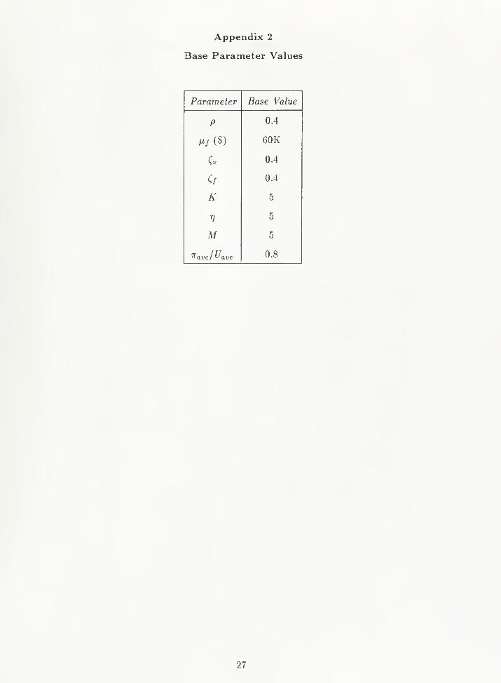
Appendix 2

Base Parameter Values

Parameter Base Value

P 0.4

Hf ($) 60K

Cv 0.4

0.4

K 5

V 5

M 5

"^avel U ave 0.8

27

TABLE 1 - Performance of Algorithm BuildProduct

Number of Number of Number of

Customers Attributes Levels (Zopt— Z3eq)/Zopt [Zopt ~ Ztnt)/Z pt

10 2 2 0.098 (9) 0.000 (10)

3 0.042 (4) 0.000(10)

4 0.096 (3) 0.007 (4)

3 2 0.027 (3) 0.000 (10)

3 0.107 (2) 0.000(10)

4 0.073 (2) 0.005 (8)

4 2 0.044 (3) 0.010 (9)

3 0.114 (3) 0.001 (8)

5 2 0.053 (2) 0.005 (8)

20 2 2 0.025 (5) 0.000 (10)

3 0.214 (6) 0.000 (10)

4 0.174 (5) 0.065 (9)

3 2 0.311 (8) 0.002 (9)

3 0.313 (3) 0.006 (9)

4 0.215 (5) 0.029 (9)

4 2 0.302 (4) 0.022 (8)

3 0.392 (4) 0.024 (9)

5 2 0.364 (3) 0.048 (9)

30 2 2 0.037 (8) 0.000(10)

3 0.107 (4) 0.000 (10)

4 0.172 (2) 0.000 (10)

3 2 0.221 (2) 0.000 (10)

3 0.209 (2) 0.001 (9)

4 0.234 (3) 0.003 (9)

4 2 0.153 (3) 0.018 (6)

3 0.149 (3) 0.002 (9)

5 2 0.188 (1) 0.017 (6)

28

TABLE 2 - Impact of p on the Relative Performance of the Integrated Approach

p

Seq. App. Int. App. Rel. Perf.

& seq l^seq %int Kint AZ PR

(million $) ($) (million $) ($) (million $)

0.1 2.275 403 2.351 427 0.076 1.033

0.2 1.749 403 1.867 450 0.118 1.067

0.3 1.267 403 1.565 487 0.298 1.236

0.4 0.832 438 1.226 492 0.394 1.475

0.5 0.470 478 0.941 538 0.471 2.001

0.6 0.182 544 0.726 601 0.544 3.998

0.7 0.043 613 0.545 652 0.502 12.724

TABLE 3 - Impact of pj on the Relative Performance of the Integrated Approach

Pi

($)


^seq

(million $)

" seq

($)

Zint

(million $)

^tnt

($)

AZ

(million $)

PR

60K

120K

180K

240K

300K

360K

420K

1.189

1.040

0.926

0.832

0.744

0.662

0.586

425

425

429

438

438

441

441

1.590

1.439

1.321

1.226

1.123

1.026

0.959

492

492

492

492

499

544

554

0.401

0.399

0.395

0.394

0.379

0.364

0.373

1.338

1.384

1.427

1.475

1.510

1.549

1.638

29

TABLE 4 - Impact of (v on the Relative Performance of the Integrated Approach

Cv

Seq. App. Int. App. Rel. Pe rf.

^ seq " seq Ztnt *int AZ PR


0.08 0.336 522 0.729 675 0.393 2.167

0.16 0.384 509 0.816 633 0.432 2.125

0.24 0.501 472 0.896 620 0.395 1.790

0.32 0.653 464 1.036 530 0.383 1.586

0.40 0.832 438 1.226 491 0.394 1.475

0.48 1.040 422 1.437 456 0.397 1.382

0.56 1.270 404 1.690 434 0.420 1.333

TABLE 5 - Impact of Qj on the Relative Performance of the Integrated Approach


7& seq

(million $)

^seq

($)

Ztn t

(million $) ($)

AZ

(million $)

PR

0.08

0.16

0.24

0.32

0.40

0.48

0.56

0.770

0.782

0.798

0.815

0.832

0.848

0.865

438

438

438

438

438

438

438

1.230

1.228

1.206

1.216

1.226

1.237

1.252

487

487

492

492

492

492

513

0.460

0.446

0.408

0.401

0.394

0.389

0.387

1.596

1.571

1.510

1.492

1.475

1.458

1.447

30

TABLE 6 - Impact of M on the Relative Performance of the Integrated Approach

MSeq. App. Int. App. Rel. Perf.

^seq ~seq Zint Xint AZ PR


3 0.649 447 1.196 491 0.547 1.843

5 0.832 438 1.226 491 0.394 1.475

7 1.053 408 1.409 489 0.356 1.339

9 1.040 414 1.402 518 0.362 1.349

11 1.100 408 1.450 479 0.350 1.318

13 1.238 408 1.558 480 0.320 1.258

15 1.368 417 1.527 468 0.159 1.116

TABLE 7 - Impact of A' on the Relative Performance of the Integrated Approach

K


^ seq " seq Zint Kint AZ PR


3 0.505 324 0.648 326 0.143 1.282

5 0.832 438 1.226 491 0.394 1.475

7 0.948 568 1.500 644 0.552 1.580

9 1.299 750 2.217 791 0.918 1.707

11 1.934 826 2.817 921 0.883 1.457

13 2.099 944 3.468 1112 1.369 1.654

15 2.968 1102 4.323 1250 1.355 1.457

31

TABLE 8 - Impact of n on the Relative Performance of the Integrated Approach

V


^ seq ""seq Zint Kint AZ PR


3 0.454 448 0.699 544 0.245 1.538

5 0.573 474 1.020 524 0.447 1.781

7 0.832 438 1.226 491 0.394 1.475

9 1.047 446 1.500 509 0.453 1.433

11 0.990 461 1.508 519 0.518 1.524

13 1.173 475 1.722 524 0.549 1.468

15 1.270 490 1.923 547 0.653 1.514

TABLE 9 - Impact of TTave/Uave on the Relative Performance of the Integrated Approach

"Ravel U ave

Seq. App. Int. App. Rel. Pe Tj.

^ seq " seq Ztn t Xint AZ PR


0.60 0.541 451 0.924 482 0.383 1.704

0.65 0.625 452 1.062 487 0.437 1.701

0.70 0.832 438 1.226 491 0.394 1.475

0.75 1.110 462 1.378 511 0.268 1.241

0.80 1.325 471 1.571 525 0.246 1.186

0.85 1.470 490 1.784 536 0.314 1.213

0.90 1.640 515 2.010 544 0.370 1.225

32

HECKMAN IXIBINDERY INC. |3|

JUN95Bound -Tb-Pta? N MANCHESTERbound i. r**e

,NDIANA 46962

An integrated approach to product design and process selection

Documents

Transcript of An integrated approach to product design and process selection