1

An Input-Output Approach to the Estimation of the

Maximum Attainable Economic Dependency Ratio in

four European Economies *

THEODORE MARIOLIS**

, GEORGE SOKLIS **

& HELENI GROZA **

**Department of Public Administration, Panteion University, Athens, Greece

ABSTRACT

The purpose of this paper is to explore, in terms of input-output models, the proximate

determinants of the maximum attainable Economic Dependency Ratio and to provide

estimates of that ratio in four European economies (Finnish, German, Greek,

Spanish). The evaluation of the results reveals certain central socio-technical features

of the actual economies under consideration.

KEY WORDS: Austrian rate of surplus labour, net labour saving from trade,

economic dependency ratio-consumptions-growth frontier

JEL CLASSIFICATION: C67, D57, E24, H55

1. Introduction

The so-called Economic Dependency Ratio or Labour Market Adjusted Dependency

Ratio, defined as the number of persons not employed (children under the age of 15,

students, home duties, unable to work, retired, unemployed, first time job seekers) per

person employed, reflects basic relationships between the productive and the

unproductive parts of the socio-economic system, and constitutes one of the most

Correspondence Address: Theodore Mariolis, Department of Public Administration, Panteion

University, 136, Syngrou Ave, Athens 17671, Greece; Email: mariolis@hotmail.gr

* A first draft of this paper was presented at a Workshop of the ‘Study Group on Sraffian Economics’ at

the Panteion University, in September 2007: We are indebted to Renetta Louca, Eleftheria Rodousaki

and Nikolaos Rodousakis for their helpful comments. We thank Menia Marioli for her inspiration and

encouragement. Furthermore, we are indebted to Bart Los for extremely helpful comments and

suggestions on an earlier version of the paper. The usual disclaimer applies.

2

important variables for the social security system.1 This paper, first, explores the

proximate determinants of the maximum attainable economic dependency ratio

(MEDR hereafter), defined as the economic dependency ratio compatible with the

ruling (i) technical conditions of production; and (ii) sizes and compositions of the

final consumption expenditures of the household sector, investments and net exports,

and, second, provides estimates of this ratio in actual economies. For this purpose we

use linear models, which have a modern ‘classical’ flavour (in the sense of Kurz and

Salvadori, 1998, Essays 1 and 2), but focus attention on the quantity side of the

system, and input-output data from the Finnish, German, Greek and Spanish

economies. This data selection is based on the guesstimate that between the said

European economies there will be remarkable differences and similarities in the

relative strength of the proximate determinants of the MEDR (e.g., Greek versus

German economy and Greek versus Spanish economy, respectively).

The remainder of the paper is structured as follows. Section 2 expounds the

models.2 Section 3 presents and critically evaluates the results of the empirical

analysis. Section 4 concludes and makes some remarks about the direction of future

research efforts.

1 For alternative (demographic and labour market adjusted) measures of ‘dependency’, see Foot (1989).

Many empirical studies find that over the next 50 years the old-age dependency ratio (the number of

persons aged 65 and over divided by the number of persons of working age, namely 15-64 years old)

will increase substantially in most countries of the world (see, e.g., United Nations, 2006, ch. 2).

According to Eurostat’s latest population projection scenario (EUROPOP2008 – convergence

scenario), for the EU-27 this ratio is expexted to increase substantially from its current levels of 25.4%

to 53.5% in 2060, whilst the young-age dependency ratio (the number of younger persons of an age

when they are generally economically inactive, namely 0-14, divided by the number of persons aged

15-64) is projected to rise moderately from its current levels of 23.3% to 25.1% in 2060.

2 This section is based on Mariolis (2006).

3

2. The Analytic Framework

We begin with a closed, linear system with only single-product industries, circulating

capital, homogeneous labour, which is not an input to the household sector, and

without ‘self-reproducing non-basic commodities’ (in the sense of Sraffa, 1960, §6

and Appendix B). The system (i) is viable, i.e., the Perron-Frobenius (P-F hereafter)

eigenvalue, A , of the n n matrix of input-output coefficients, A , is less than 1; and

(ii) follows a balanced, steady path of expansion at rate g . The net product is

distributed to gross profits and wages: gross profits split into income of the capitalists

(net profits) and income of the non-employed (transfer income), whilst wages are paid

at the end of the common production period and there are no savings out of this

income. There is a uniform consumption pattern, i.e., the composition of the vectors

of consumption out of wages, net profits and transfer income are identical and rigid,

and the givens in our analysis are (i) the technical conditions of production, i.e., the

pair ( , )A a , where Ta is the 1 n vector of direct labour inputs (‘ T ’ is the sign for

transpose); and (ii) the real wage rate, which is represented by the 1n vector b .

Finally, we suppose that all commodities enter, directly or indirectly, into the

production of wage goods, i.e., the matrix of the ‘augmented’ input-output

coefficients, TA ba , is irreducible.

On the basis of these assumptions, the quantity side of the system may be

described by the following relation:

Ix Ax c+i (1)

where

np neL L N c b b b (2)

np npcb b , ne necb b (3)

4

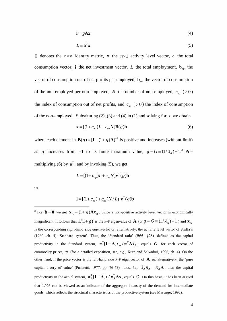
gi Ax (4)

TL a x (5)

I denotes the n n identity matrix, x the 1n activity level vector, c the total

consumption vector, i the net investment vector, L the total employment, npb the

vector of consumption out of net profits per employed, neb the vector of consumption

of the non-employed per non-employed, N the number of non-employed, npc ( 0 )

the index of consumption out of net profits, and nec ( 0 ) the index of consumption

of the non-employed. Substituting (2), (3) and (4) in (1) and solving for x we obtain

np ne[(1 ) ] ( )c L c N g x B b (6)

where each element in 1( ) [ (1 ) ]g g B I A is positive and increases (without limit)

as g increases from 1 to its finite maximum value, (1/ ) 1g G A .3 Pre-

multiplying (6) by Ta , and by invoking (5), we get:

T

np ne[(1 ) ] ( )L c L c N g v b

or

T

np ne1 [(1 ) ( / )] ( )c c N L g v b

3 For b 0 we get (1 )g A Ax Ax . Since a non-positive activity level vector is economically

insignificant, it follows that 1/(1 )g is the P-F eigenvalue of A (or (1/ ) 1g G A ) and Ax

is the corresponding right-hand side eigenvector or, alternatively, the activity level vector of Sraffa’s

(1960, ch. 4) ‘Standard system’. Thus, the ‘Standard ratio’ (ibid., §28), defined as the capital

productivity in the Standard system, T T[ ] / A Aπ I A x π Ax , equals G for each vector of

commodity prices, π (for a detailed exposition, see, e.g., Kurz and Salvadori, 1995, ch. 4). On the

other hand, if the price vector is the left-hand side P-F eigenvector of A or, alternatively, the ‘pure

capital theory of value’ (Pasinetti, 1977, pp. 76-78) holds, i.e., T T A A Aπ π A , then the capital

productivity in the actual system, T T[ ] /A Aπ I A x π Ax , equals G . On this basis, it has been argued

that 1/G can be viewed as an indicator of the aggregate intensity of the demand for intermediate

goods, which reflects the structural characteristics of the productive system (see Marengo, 1992).

5

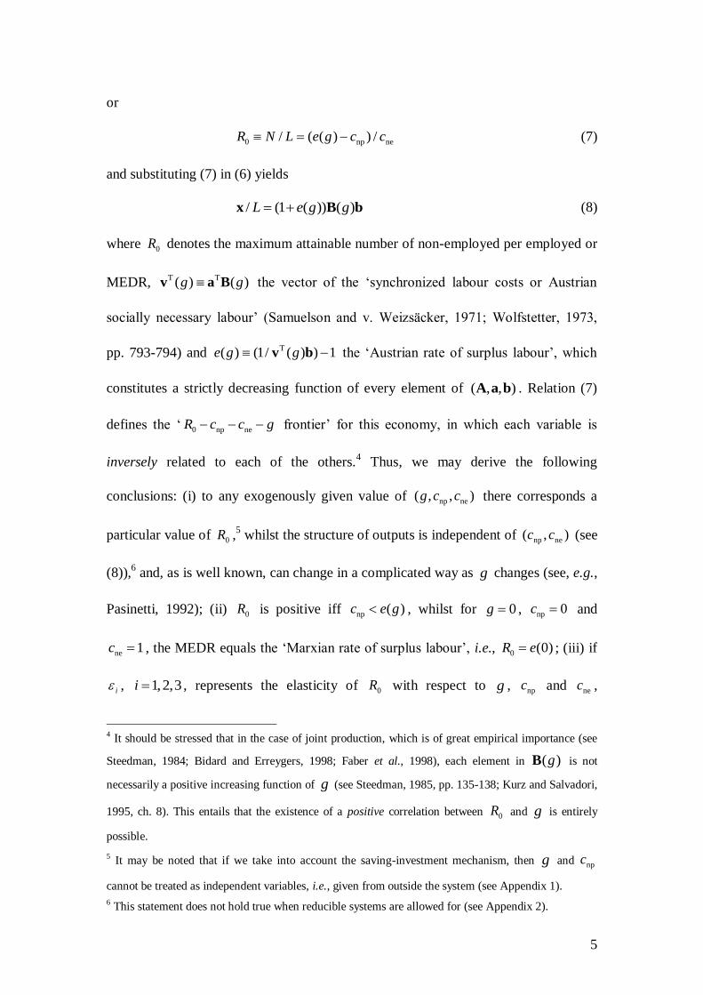
or

0 np ne/ ( ( ) ) /R N L e g c c (7)

and substituting (7) in (6) yields

/ (1 ( )) ( )L e g g x B b (8)

where 0R denotes the maximum attainable number of non-employed per employed or

MEDR, T T( ) ( )g gv a B the vector of the ‘synchronized labour costs or Austrian

socially necessary labour’ (Samuelson and v. Weizsäcker, 1971; Wolfstetter, 1973,

pp. 793-794) and T( ) (1/ ( ) ) 1e g g v b the ‘Austrian rate of surplus labour’, which

constitutes a strictly decreasing function of every element of ( , , )A a b . Relation (7)

defines the ‘ 0 np neR c c g frontier’ for this economy, in which each variable is

inversely related to each of the others.4 Thus, we may derive the following

conclusions: (i) to any exogenously given value of np ne( , , )g c c there corresponds a

particular value of 0R ,5 whilst the structure of outputs is independent of np ne( , )c c (see

(8)),6 and, as is well known, can change in a complicated way as g changes (see, e.g.,

Pasinetti, 1992); (ii) 0R is positive iff np ( )c e g , whilst for 0g , np 0c and

ne 1c , the MEDR equals the ‘Marxian rate of surplus labour’, i.e., 0 (0)R e ; (iii) if

i , 1,2,3i , represents the elasticity of 0R with respect to g , npc and nec ,

4 It should be stressed that in the case of joint production, which is of great empirical importance (see

Steedman, 1984; Bidard and Erreygers, 1998; Faber et al., 1998), each element in ( )gB is not

necessarily a positive increasing function of g (see Steedman, 1985, pp. 135-138; Kurz and Salvadori,

1995, ch. 8). This entails that the existence of a positive correlation between 0R and g is entirely

possible.

5 It may be noted that if we take into account the saving-investment mechanism, then g and npc

cannot be treated as independent variables, i.e., given from outside the system (see Appendix 1).

6 This statement does not hold true when reducible systems are allowed for (see Appendix 2).

6

respectively, it is then easy to see that, for 0 0R , 1 equals the ratio of net

investment to consumption of the non-employed in terms of Austrian socially

necessary labour,7 and 2 np ne 0 3) ( 1)c c R for np ( ) / 2c e g ; and (iv) technical

changes that fulfil the cost-minimizing criterion do not necessarily imply a rise in

( )e g (see Okishio, 1961) and, therefore, have ambiguous effects on 0R .8

It need hardly be said that government expenditure can be introduced into the

model by assuming, for example, that it is maintained as a constant fraction of the

capital stocks, i.e., dAx , or, alternatively, of the gross outputs, i.e., dx (clearly, these

relations are special cases of Dx , where D denotes an exogenously given n n

matrix). In the former case, (7) still holds, provided only that g is replaced by g d ,

whilst in the latter, (7) becomes

T

0 np ne[ ( , ) ( / ( , ) ) ]/R e g d d g d c c v b (7a)

where T T 1( , ) [ [(1 ) /(1 )] ]g d g d v a I A and

T( , ) (1/ ( , ) ) 1e g d g d v b . On the

other hand, by assuming that the non-employed are divided into k groups,

characterized by different consumption indices, (7) becomes

ne np

1

( ( ) ) / ( )k

i i

i

c N L e g c

, 1

k

i

i

N N

(7b)

or

7 Differentiation of (7) with respect to the rate of growth gives

T T 2

0 ne/ ( ) ( ) /[ ( ( ) ) ]R g g g c g v AB b v b

and recalling (8), T(1 ( )) ( ) 1e g g v b and the definition of 0R it follows that

T T

1 0 0 ne( / )( / ) ( ) /( ( ) )R g g R g c N g v i v b

8 For a theoretical analysis of different forms of technical change within the framework of static input-

output models, see Seyfried (1988). For a one-commodity model, which includes, however, fixed

capital and the degrees of its utilization, depreciation, supplementary or ‘overhead’ labour and

investment function(s), see Kurz (1990, pp. 226-235). For relevant empirical analyses, in terms of

dynamic input-output models, see Leontief and Duchin (1986) and Kalmbach and Kurz (1990).

7

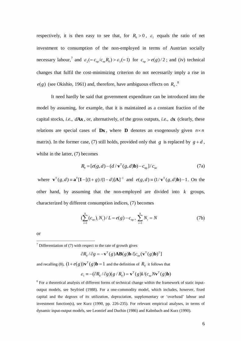
0 np ne 0 ne

1

( ) / [ ( ) ( ( ) ( ) )]/( )k

i i j j i

jj i

R N L e g c c R c

(7c)

where 0( )iR , ne( )ic , iN denote the MEDR, consumption index and population of the

i th group, respectively.

Now, consider the more realistic case of a non-proportionally growing and

open economy. Then (1) becomes

Ix Ax c i e (9)

where ( )gi Ax is now exogenously given and e denotes the exogenously given net

export vector. Substituting (2) and (3) in (9), and solving for x , leads to

np ne[(1 ) ] (0) (0)( )c L Nc x B b B i e (10)

Pre-multiplying (10) by Ta , and by invoking (5), we get:

T T

np ne[(1 ) ] (0) (0)( )L c L Nc v b v i e

or

T T

1 np ne/ { (0) [ (0)( ) / (0) ]}/R N L e c c v i e v b (11)

where i ( / L i ) denotes the vector of net investments per employed, e ( / L e ) the

vector of net exports per employed, and T (0) v e may be conceived as the ‘net

labour saving from trade’ (see Erdilek and Schive, 1976, pp. 318-319). As is well

known, international trade dictated by the cost-minimizing criterion do not necessarily

imply a positive net labour saving from trade (see ibid., p. 320; Steedman, 1979,

Essays 4, 9 and 12) and, therefore, has ambiguous effects on the MEDR (precisely

like technical changes).

An alternative, but rather different, determination of 1R is obtained by setting

ˆi AGx , where ˆ [ ]jgG denotes the diagonal matrix of the sectoral rates of growth,

8

and x e e Mx , where xe denotes the export vector and [ ]ijmM the matrix of

imports per unit activity level, giving

T T

1 np x ne[ ( , ) ( ( , ) / ( , ) )]/j ij j ij j ijR e g m c g m g m c v e v b (11a)

where T T 1ˆ( , ) [ [ ] ]j ijg m v a I A I G M , T( , ) (1/ ( , ) ) 1j ij j ije g m g m v b and

x x / L e e .

In what follows we shall estimate the MEDR in actual economies from (i) the

relation (7), with np 0c , ne 1c and *0 g g , where *g denotes the economically

significant value of the rate of growth that corresponds to *( ) 0e g , i.e., 0 ( ,0,1)R g ;

and (ii) the relation (11), with np 0c and ne 1c , i.e., 1(0,1)R .9

3. Results and their Evaluation

The results from the application of the previous analysis to the input-output tables of

the Finnish (for the years 1997 and 1998), German (for the year 2000), Greek (for the

years 1997 and 1998) and Spanish (for the year 2000) economies are displayed in

Tables 1 through 3.10

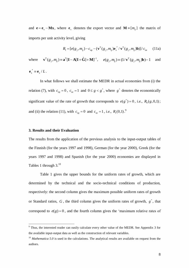
Table 1 gives the upper bounds for the uniform rates of growth, which are

determined by the technical and the socio-technical conditions of production,

respectively: the second column gives the maximum possible uniform rates of growth

or Standard ratios, G , the third column gives the uniform rates of growth, *g , that

correspond to ( ) 0e g , and the fourth column gives the ‘maximum relative rates of

9 Thus, the interested reader can easily calculate every other value of the MEDR. See Appendix 3 for

the available input-output data as well as the construction of relevant variables.

10 Mathematica 5.0 is used in the calculations. The analytical results are available on request from the

authors.

9

growth’, defined as the ratios of *g to G , i.e., * /g G (it goes without saying that

G , *g are strictly decreasing functions of every element of A and ( , , )A a b ,

respectively).

Table 1. Upper bounds for the uniform rates of growth

G *g

FIN 1997 1998 1997 1998 1997 1998

0.712 0.703 0.467 0.457 0.656 0.650

GE 2000 2000 2000

1.005 0.512 0.509

GR 1997 1998 1997 1998 1997 1998

0.608 0.492 0.528 0.440 0.868 0.894

SP 2000 2000 2000

0.664 0.392 0.590

Table 2 presents 0 ( ,0,1)R g or the Austrian rates of surplus labour (see relation (7)) as

functions of the uniform rate of growth.

Table 2. The Austrian rates of surplus labour as functions of the uniform rate of

growth

FIN GE GR SP

g 1997 1998 2000 1997 1998 2000

0 1.239 1.217 1.030 2.332 2.257 1.070

0.1 1.002 0.979 0.832 2.003 1.920 0.827

0.2 0.754 0.729 0.632 1.651 1.544 0.566

0.3 0.491 0.464 0.431 1.264 1.090 0.284

0.4 0.208 0.177 0.229 0.814 0.434 0

0.5 0 0 0.026 0.226 0 0

10

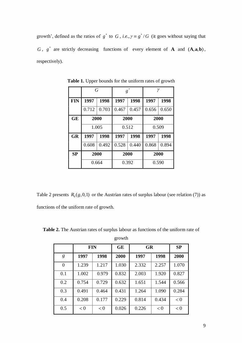
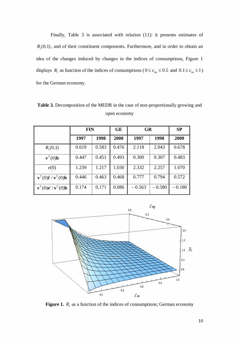
Finally, Table 3 is associated with relation (11): it presents estimates of

1(0,1)R , and of their constituent components. Furthermore, and in order to obtain an

idea of the changes induced by changes in the indices of consumptions, Figure 1

displays 1R as function of the indices of consumptions ( np0 0.5c and ne0.1 1c )

for the German economy.

Table 3. Decomposition of the MEDR in the case of non-proportionally growing and

open economy

Figure 1. 1R as a function of the indices of consumptions; German economy

FIN GE GR SP

1997 1998 2000 1997 1998 2000

1(0,1)R 0.619 0.583 0.476 2.118 2.043 0.678

T (0)v b 0.447 0.451 0.493 0.300 0.307 0.483

(0)e 1.239 1.217 1.030 2.332 2.257 1.070

T T(0) / (0)v i v b 0.446 0.463 0.468 0.777 0.794 0.572

T T(0) / (0)v e v b 0.174 0.171 0.086 0.563 0.580 0.180

11

From these tables, the associated numerical results and the hitherto analysis

we arrive at the following conclusions:

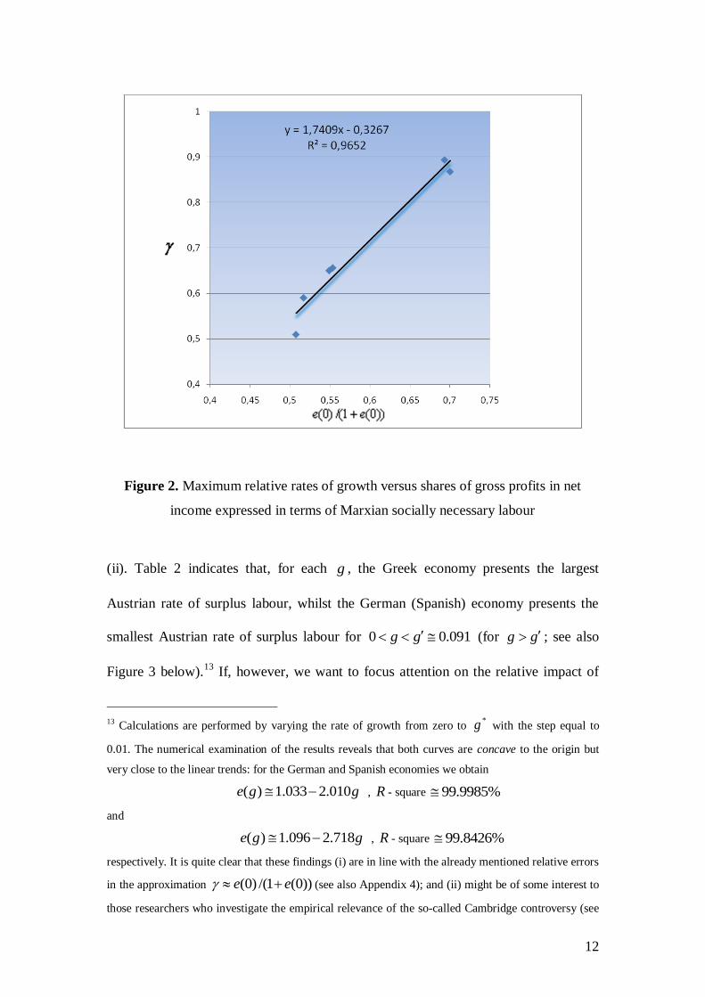
(i). Table 1 indicates that the German (Greek) economy presents the largest (smallest)

Standard ratio, G , and the smallest (largest) maximum relative rate of growth, .

Speaking somewhat loosely, one may say that the former implies that this economy is

characterized by the largest (smallest) capital productivity,11

whilst the latter is due to

the fact that this economy is characterized by the smallest (largest) Marxian rate of

surplus labour, (0)e (see the fourth row of Table 2). However, only if we set aside the

Greek economy (in which 1997 1998 and 1997 1998(0) (0)e e ), the ranking of the

economies according to coincides with their ranking according to (0)e . Moreover,

it is worth noting that, in the context of the economies under consideration, is

always greater than the share of gross profits in net income expressed in terms of

Marxian socially necessary labour, T1 (0) (0) /(1 (0))e e v b , and the relative errors

in the approximation (0) /(1 (0))e e are as follows: 0.4% (GE), 12.4% (SP),

15.5% (FIN, 1998), 15.7% (FIN, 1997), 19.4% (GR, 1997), and 22.5% (GR, 1998)

(see also Figure 2 that displays in a scatter diagram the relationship between

(0) /(1 (0))e e and : we observe a positive relationship and an R - square of

96.5%).12

11 See footnote 3. 12

For the theoretical relationships between and (0) /(1 (0))e e , see Appendix 4 (which builds

upon an idea presented in Mariolis, 2010).

12

Figure 2. Maximum relative rates of growth versus shares of gross profits in net

income expressed in terms of Marxian socially necessary labour

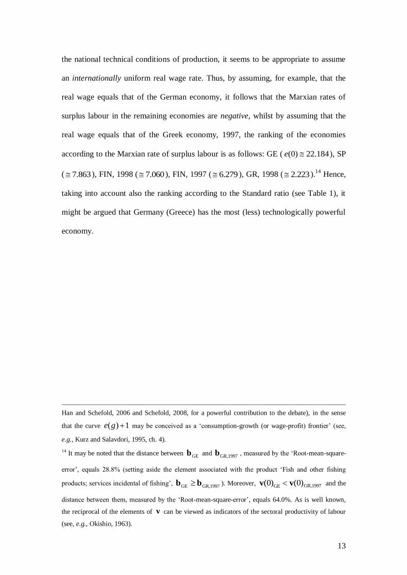
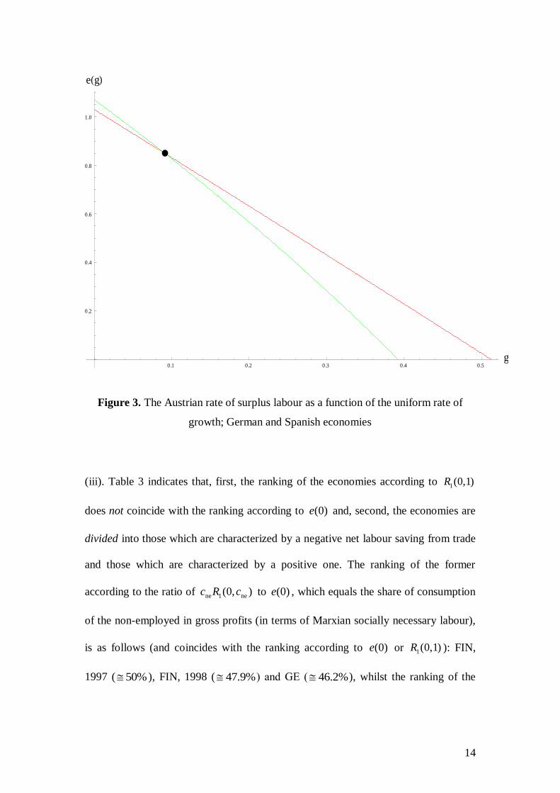
(ii). Table 2 indicates that, for each g , the Greek economy presents the largest

Austrian rate of surplus labour, whilst the German (Spanish) economy presents the

smallest Austrian rate of surplus labour for 0 0.091g g (for g g ; see also

Figure 3 below).13

If, however, we want to focus attention on the relative impact of

13 Calculations are performed by varying the rate of growth from zero to

*g with the step equal to

0.01. The numerical examination of the results reveals that both curves are concave to the origin but

very close to the linear trends: for the German and Spanish economies we obtain

( ) 1.033 2.010 e g g , R - square 99.9985%

and

( ) 1.096 2.718 e g g , R - square 99.8426%

respectively. It is quite clear that these findings (i) are in line with the already mentioned relative errors

in the approximation (0) /(1 (0))e e (see also Appendix 4); and (ii) might be of some interest to

those researchers who investigate the empirical relevance of the so-called Cambridge controversy (see

13

the national technical conditions of production, it seems to be appropriate to assume

an internationally uniform real wage rate. Thus, by assuming, for example, that the

real wage equals that of the German economy, it follows that the Marxian rates of

surplus labour in the remaining economies are negative, whilst by assuming that the

real wage equals that of the Greek economy, 1997, the ranking of the economies

according to the Marxian rate of surplus labour is as follows: GE ( (0) 22.184e ), SP

( 7.863 ), FIN, 1998 ( 7.060 ), FIN, 1997 ( 6.279 ), GR, 1998 ( 2.223 ).14

Hence,

taking into account also the ranking according to the Standard ratio (see Table 1), it

might be argued that Germany (Greece) has the most (less) technologically powerful

economy.

Han and Schefold, 2006 and Schefold, 2008, for a powerful contribution to the debate), in the sense

that the curve ( ) 1e g may be conceived as a ‘consumption-growth (or wage-profit) frontier’ (see,

e.g., Kurz and Salavdori, 1995, ch. 4).

14 It may be noted that the distance between GEb and

GR,1997b , measured by the ‘Root-mean-square-

error’, equals 28.8% (setting aside the element associated with the product ‘Fish and other fishing

products; services incidental of fishing’, GE GR,1997b b ). Moreover, GR,1997GE(0) (0)v v and the

distance between them, measured by the ‘Root-mean-square-error’, equals 64.0%. As is well known,

the reciprocal of the elements of v can be viewed as indicators of the sectoral productivity of labour

(see, e.g., Okishio, 1963).

14

0.1 0.2 0.3 0.4 0.5g

0.2

0.4

0.6

0.8

1.0

eg

Figure 3. The Austrian rate of surplus labour as a function of the uniform rate of

growth; German and Spanish economies

(iii). Table 3 indicates that, first, the ranking of the economies according to 1(0,1)R

does not coincide with the ranking according to (0)e and, second, the economies are

divided into those which are characterized by a negative net labour saving from trade

and those which are characterized by a positive one. The ranking of the former

according to the ratio of ne 1 ne(0, )c R c to (0)e , which equals the share of consumption

of the non-employed in gross profits (in terms of Marxian socially necessary labour),

is as follows (and coincides with the ranking according to (0)e or 1(0,1)R ): FIN,

1997 ( 50% ), FIN, 1998 ( 47.9% ) and GΕ ( 46.2% ), whilst the ranking of the

15

latter is as follows (and coincides with the ranking according to (0)e or 1(0,1)R ): GR,

1997 ( 90.8% ), GR, 1998 ( 90.5% ), and SP ( 63.4% ).15

Finally, it may be concluded that the main determinants of the relatively high level of

1(0,1)R in the Greek economy are the Marxian rate of surplus labour and the net

labour saving from trade, where the former (the most important) is not related to the

technological strength of the system but rather to the relatively low level of the real

wage rate, whilst the latter offsets, to a great extent (i.e., about

0.563(0.580)/0.777(0.794) 73%), the negative impact of investment. By contrast, the

net labour saving from trade of the Spanish economy offsets to a less extent (i.e.,

about 0.180/0.572 31.5%) the negative impact of investment.

(iv). Since there exist statistical estimates of the actual growth rates (of the real gross

domestic product), total populations (and their age distribution), employed persons,

unemployment rates and number of pensioners, we may compute the ‘actual’ Austrian

rates of surplus labour as well as the following three ‘actual’ economic dependency

ratios:

15 Stein (2009) argues that ‘the countries facing the greatest deterioration in their [old-age] dependency

ratio are generally also those with current account surpluses (i.e., excess savings). There are exceptions

to this rule: Spain is a deficit country, yet one with the prospect of a substantial demographic

deterioration over the next 45 years. So, to a lesser extent, are Italy and France. These countries are

likely to face substantial difficulties as their populations age – especially Italy, where the population

and the labor force are already shrinking and aging fast. As households increase their spending, some

other sector will have to save more. This must be either companies (i.e., they must become less

profitable), or governments (by moving into deficit, or further into deficit), or foreigners (i.e., countries

whose households are increasing their spending must move further into current account deficit). In

other, saving countries – for example, Germany, Korea, Japan, Singapore, to take those with the worst

demographic profile – the switch from household saving to spending can be more easily

accommodated, since it will simply require a smaller current account surplus – which, as it so happens,

is exactly what is needed for these countries from a global economic perspective.’. For an empirical

study of the relationships between demographic dependency ratios and current account balances, see

Chin and Prassad (2003).

16

- the ‘total economic dependency ratio’ (TEDR), defined as

TEDR (TP EP) / EP (12)

where TP denotes the total population and EP the employed persons;

- the ‘needs weighted (or expenditure) economic dependency ratio’ (WEDR; see, e.g.,

Foot, 1989, pp. 104-109; Osterkamp, 2003, pp. 69-70), defined as

1 1 2 2WEDR ( ) / EP ( TEDR)w N w N (13)

where 1N denotes the number of people aged 0-14, 2 1TP EPN N , 1 0.25w and

2 0.75w , i.e., 2 1/ 3w w (see also relation (7b));16

and, finally,

- the ‘unweighted effective economic dependency ratio’ (UEEDR), defined as

UΕEDR (UP P) / EP ( TEDR)

or, since UP [ /(1 )]EPu u ,

UΕEDR [ /(1 )] (P / EP)u u (14)

where UP denotes the unemployed persons, P the pensioners, and u the

unemployment rate. Given that, in the real world, there are non-employed who do not

receive any income transfer, it follows that the UΕEDR corresponds much more

closely to our notions of the MEDR.

Thus, we can compare the ‘actual’ 0 ( ,0,1)R g (or ‘actual’ Austrian rates of

surplus labour) and 1(0,1)R with the aforesaid ‘actual’ ratios: Table 4 presents data on

the actual growth rates, ag , population (1000 persons) and unemployment rates for

the considered economies. Table 5 presents a

0 ( ,0,1)R g , the three ‘actual’ ratios

16 It need hardly be said that the actual weights are not internationally uniform and the chosen weights

are therefore only representative, to give some indication of the WEDR (see also Clark et al., 1978,

pp.921-923; Gee, 2002, pp. 751-752).

17

(TEDR, WEDR and UEEDR), the percent differences between a

0 ( ,0,1)R g , 1(0,1)R

and the UEEDR, defined as

(RD) 100 ( ) UΕEDR /[( ( ) UΕEDR)/ 2]i i iR R , 0,1i

and, finally, the values of np ne( , )c c for which 1 np ne( , )R c c (see relation (11)) coincide

with the UEEDR.

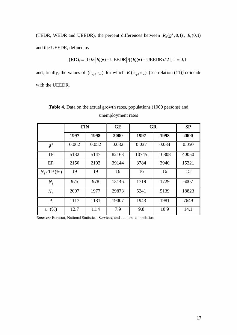
Table 4. Data on the actual growth rates, populations (1000 persons) and

unemployment rates

Sources: Eurostat, National Statistical Services, and authors’ compilation

FIN GE GR SP

1997 1998 2000 1997 1998 2000

ag 0.062 0.052 0.032 0.037 0.034 0.050

TP 5132 5147 82163 10745 10808 40050

EP 2150 2192 39144 3784 3940 15221

1 / TPN (%) 19 19 16 16 16 15

1N 975 978 13146 1719 1729 6007

2N 2007 1977 29873 5241 5139 18823

P 1117 1131 19007 1943 1981 7649

u (%) 12.7 11.4 7.9 9.8 10.9 14.1

18

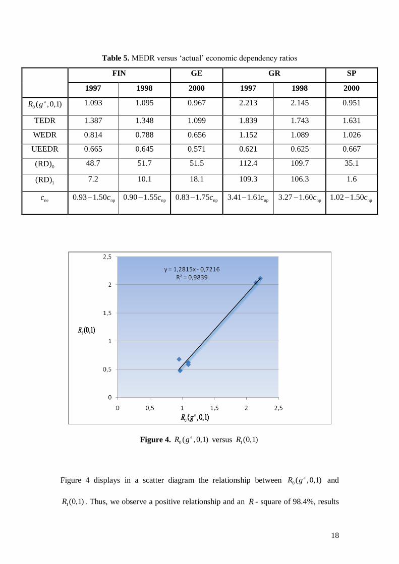
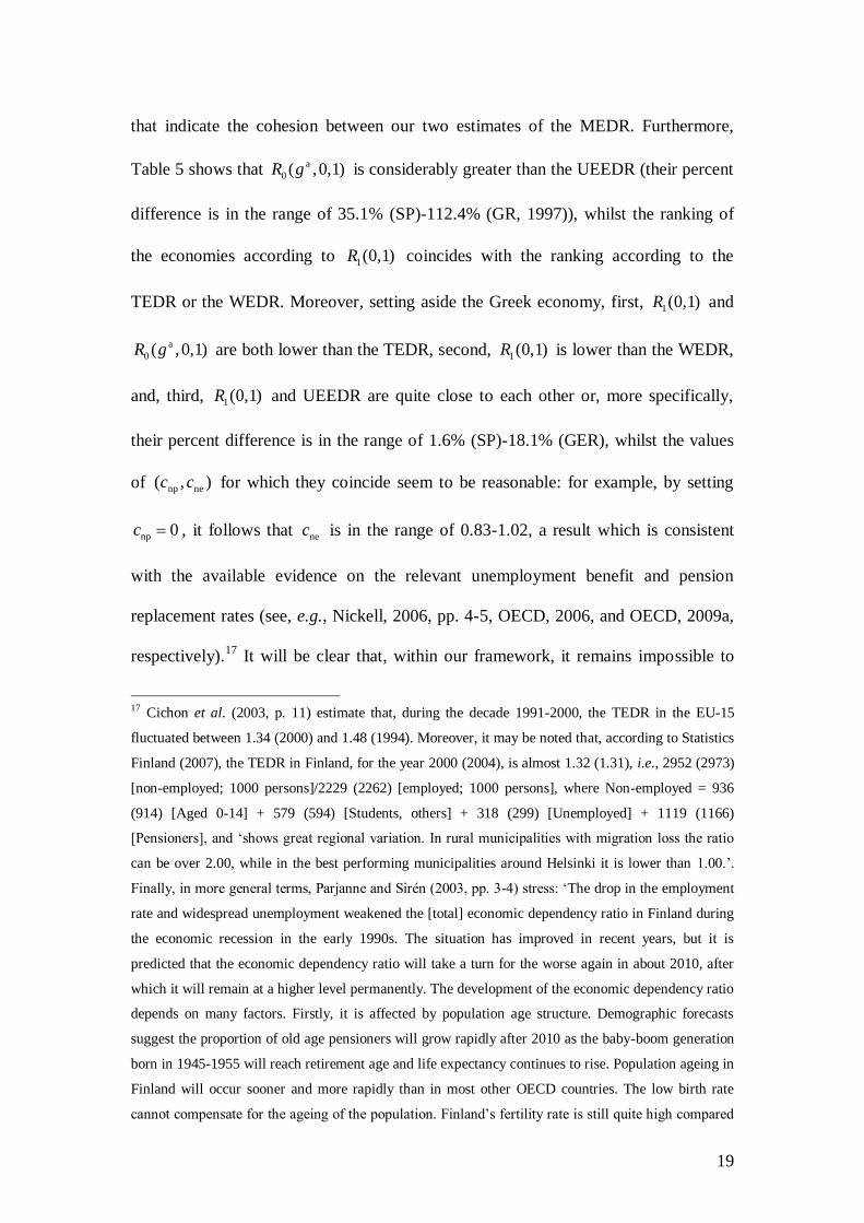
Table 5. MEDR versus ‘actual’ economic dependency ratios

Figure 4. a

0 ( ,0,1)R g versus 1(0,1)R

Figure 4 displays in a scatter diagram the relationship between a

0 ( ,0,1)R g and

1(0,1)R . Thus, we observe a positive relationship and an R - square of 98.4%, results

FIN GE GR SP

1997 1998 2000 1997 1998 2000

a

0 ( ,0,1)R g 1.093 1.095 0.967 2.213 2.145 0.951

TEDR 1.387 1.348 1.099 1.839 1.743 1.631

WEDR 0.814 0.788 0.656 1.152 1.089 1.026

UEEDR 0.665 0.645 0.571 0.621 0.625 0.667

0(RD) 48.7 51.7 51.5 112.4 109.7 35.1

1(RD) 7.2 10.1 18.1 109.3 106.3 1.6

nec np0.93 1.50c

np0.90 1.55c np0.83 1.75c np3.41 1.61c np3.27 1.60c np1.02 1.50c

19

that indicate the cohesion between our two estimates of the MEDR. Furthermore,

Table 5 shows that a

0 ( ,0,1)R g is considerably greater than the UEEDR (their percent

difference is in the range of 35.1% (SP)-112.4% (GR, 1997)), whilst the ranking of

the economies according to 1(0,1)R coincides with the ranking according to the

TEDR or the WEDR. Moreover, setting aside the Greek economy, first, 1(0,1)R and

a

0 ( ,0,1)R g are both lower than the TEDR, second, 1(0,1)R is lower than the WEDR,

and, third, 1(0,1)R and UEEDR are quite close to each other or, more specifically,

their percent difference is in the range of 1.6% (SP)-18.1% (GER), whilst the values

of np ne( , )c c for which they coincide seem to be reasonable: for example, by setting

np 0c , it follows that nec is in the range of 0.83-1.02, a result which is consistent

with the available evidence on the relevant unemployment benefit and pension

replacement rates (see, e.g., Nickell, 2006, pp. 4-5, OECD, 2006, and OECD, 2009a,

respectively).17

It will be clear that, within our framework, it remains impossible to

17 Cichon et al. (2003, p. 11) estimate that, during the decade 1991-2000, the TEDR in the EU-15

fluctuated between 1.34 (2000) and 1.48 (1994). Moreover, it may be noted that, according to Statistics

Finland (2007), the TEDR in Finland, for the year 2000 (2004), is almost 1.32 (1.31), i.e., 2952 (2973)

[non-employed; 1000 persons]/2229 (2262) [employed; 1000 persons], where Non-employed = 936

(914) [Aged 0-14] + 579 (594) [Students, others] + 318 (299) [Unemployed] + 1119 (1166)

[Pensioners], and ‘shows great regional variation. In rural municipalities with migration loss the ratio

can be over 2.00, while in the best performing municipalities around Helsinki it is lower than 1.00.’.

Finally, in more general terms, Parjanne and Sirén (2003, pp. 3-4) stress: ‘The drop in the employment

rate and widespread unemployment weakened the [total] economic dependency ratio in Finland during

the economic recession in the early 1990s. The situation has improved in recent years, but it is

predicted that the economic dependency ratio will take a turn for the worse again in about 2010, after

which it will remain at a higher level permanently. The development of the economic dependency ratio

depends on many factors. Firstly, it is affected by population age structure. Demographic forecasts

suggest the proportion of old age pensioners will grow rapidly after 2010 as the baby-boom generation

born in 1945-1955 will reach retirement age and life expectancy continues to rise. Population ageing in

Finland will occur sooner and more rapidly than in most other OECD countries. The low birth rate

cannot compensate for the ageing of the population. Finland’s fertility rate is still quite high compared

20

determine whether the detected peculiarities of the Greek economy are due to the so-

called ‘generosity’ (Bank of Greece, 1999, p. 182; see also OECD, 2009b, pp. 71-78)

of its social security system.18

Nevertheless, it may be argued that, in general, the

deviations between estimated and ‘actual’ values will be reduced by taking into

account relations (7a), (7b) and (11a), integrating the quantity and the price sides of

the considered systems and19

allowing for differentiated consumption patterns

(provided that the necessary data can be compiled). Therefore, in order to arrive at

valid conclusions, these two lines of research should be combined.

with many European countries; in 2000 it was 1.73, compared with the EU average of 1.53. There is a

risk, however, that it will fall closer to the EU average. Consequently, within the next few years, the

new workforce entering the labour market will already be smaller than the numbers leaving the labour

market. The fall in labour supply will jeopardize economic growth and tax base, while increases in

pensioners raises pension expenditures.’.

18 According to the Annual Report of the Bank of Greece for the year 1998, ‘[i]n view of international

experience, the pension system in Greece gives the impression of being comparatively generous. This

impression is based not only on the level of pensions in relation to earnings in active service, but also

on the ‘ease’ with which the right to receive a pension is established […]. The generosity of the system

is also reflected in the amount of accumulated claims of those insured by pension funds. According to

OECD data, insurance funds’ liabilities in Greece exceed 150 per cent of GDP and are among the

highest in the OECD area. Not only benefits, but also contributions to social security funds are very

high in Greece, particularly after the 1990-1992 reform. This fact, combined with the very low

competitiveness of the Greek economy and the heavy competition it will face after joining EMU, and

with the globalisation of economic activity, leaves no room for a further increase in social security

contributions (with the exception of certain isolated cases). Besides, it should be taken into account

that, after the entry of Greece into EMU, the Stability and Growth Pact provides essentially for an

effectively balanced budget, while efforts aimed at a further reduction in the debt-to-GDP ratio must

continue. In this context, the scope, if any, for financing insurance funds out of the ordinary budget

would be extremely limited. From the above it is obvious that in the medium and long term it is

difficult to maintain the present situation and immediate reforms are required. These reforms would

necessarily be oriented towards reducing benefits and introducing stricter eligibility criteria.’ (Bank of

Greece, 1999, pp. 182-183; emphasis added). 19 See Appendix 1 and 2, respectively.

21

4. Concluding Remarks

In this paper we have proposed, in terms of linear models, which have a modern

‘classical’ flavour, robust ways to estimate the maximum attainable economic

dependency ratio (MEDR) and we have applied the theoretical analysis to the input-

output tables of the Finnish, German, Greek and Spanish economies. It has been

found that although Greece has the less technologically powerful economy (in terms

of both labour and capital productivity), it presents the largest MEDR (it is almost

2.00). This is attributed, primarily, to the relatively low level of the real wage rate

and, secondarily, to the current account deficit, which offsets, to a great extent (i.e.,

about 73%), the negative impact of investment. By contrast, although Germany has

the most technologically powerful economy, it presents the smallest MEDR (it is in

the range of 0.476-0.967), and this is attributed primarily to the relatively high level

of the real wage rate and, secondarily, to the current account surplus. Setting aside

Spain’s current account deficit, which offsets, to relatively small extent (i.e., 31.5%),

the negative impact of investment on the MEDR, Finnish and Spanish economies tend

to share similar features with the German economy. Furthermore, it has been

indicated that our alternative estimates of the MEDR are consistent with each other as

well as with the available empirical evidence. Since there are, all over the world,

heated debates about the future of the social security systems, this line of enquiry

would seem to be of some interest.

Future work should, first, carry the analysis at a more concrete level by

including the presence of differentiated consumption patterns, fixed capital and the

degrees of its utilization, differential depreciation, imported inputs, ‘overhead’ labour

and pure joint products, second, estimate the effects of expected technical changes

(and/or changes in income distribution and consumptions) on the MEDR and, finally,

22

integrate income distribution, pricing, capital accumulation and government fiscal

activity considerations into a ‘two-country’ model.

References

Bank of Greece (1999) Annual Report 1998 (Athens: Bank of Greece).

Bidard, C. and Erreygers, G. (1998) Sraffa and Leontief on joint production, Review

of Political Economy, 10, pp. 427-446.

Chinn, M. and Prasad, E. (2003) Medium-term determinants of current accounts in

industrial and developing countries: an empirical exploration, Journal of

International Economics, 59, pp. 47-76.

Cichon, M., Knop, R. and Léger, F. (2003) White or Prosperous: How much

migration does the ageing European Union need to maintain its standard of

living in the twenty-first century?, paper presented at the 4th International

Research Conference on Social Security, ‘Social security in a long-life society’,

Antwerp, Belgium, 5-7 May 2003 (Geneva: International Labour Office).

Clark, R., Kreps, J. and Spengler, J. (1978) Economics of aging: a survey, Journal of

Economic Literature, 16, pp. 919-962.

Erdilek, A. and Schive, C. (1976) Can trade be harmful for a growing capitalist

economy?, Kyklos, 29, pp. 317-320.

Faber, M., Proops, J. L. R., Baumgärtner, S. (1998) All production is joint production.

A thermodynamic analysis, in: S. Faucheux, J. Gowdy, I. Nicolaï (Eds) (1998)

Sustainability and Firms: Technological Change and the Changing Regulatory

Environment, pp. 131-158 (Cheltenham: Edward Elgar).

Foot, D. K. (1989) Public expenditures, population aging and economic dependency

in Canada, 1921-2021, Population Research and Policy Review, 8, pp. 97-117.

23

Gee, E. M. (2002) Misconceptions and misapprehensions about population ageing,

International Journal of Epidemiology, 31, pp. 750-753.

Han, Z. and Schefold, B. (2006) An empirical investigation of paradoxes: reswitching

and reverse capital deepening in capital theory, Cambridge Journal of

Economics, 30, pp. 737-765.

Horn, R. A and Johnson, C. R. (1990) Matrix Analysis (Cambridge: Cambridge

University Press).

Kalmbach, P. and Kurz, H. D. (1990) Micro-electronics and employment: a dynamic

input-output study of the West German economy, Structural Change and

Economic Dynamics, 1, pp. 371-386.

Kurz, H. D. (1990) Technical change, growth and distribution: a steady-state

approach to ‘unsteady’ growth, in: H. D. Kurz (1990) Capital, Distribution and

Effective Demand. Studies in the ‘Classical’ Approach to Economic Theory, pp.

211-239 (Cambridge: Polity Press).

Kurz, H. D. and Salvadori, N. (1995) Theory of Production. A Long-Period Analysis

(Cambridge: Cambridge University Press).

Kurz H. D. and Salvadori N. (Eds) (1998) Understanding ‘Classical’ Economics:

Studies in Long-period Theory (London and New York: Routledge).

Leontief, W. and Duchin, F. (1986) The Future Impact of Automation on Workers

(New York and Oxford: Oxford University Press).

Marengo, L. (1992) The demand for intermediate goods in an input-output

framework: a methodological note, Economic Systems Research, 4, pp. 49-52.

Mariolis, T. (2006) Input-output Models for Estimating the Maximum Attainable

Economic Dependency Ratio (in Greek), Internal Report of the ‘Study Group on

24

Sraffian Economics’, June 2006, Department of Public Administration, Panteion

University.

Mariolis, T. (2010) Norm bounds for a transformed price vector in Sraffian systems,

Applied Mathematical Sciences, 4, pp. 551-574.

Miller, R. E. and Blair, P. D. (1985) Input-Output Analysis: Foundations and

Extensions (New Jersey: Prentice Hall).

Nickell, W. (2006) The CEP-OECD institutions data set (1960-2004), November

2006, Centre for Economic Performance, Discussion Paper No 759.

OECD (2006) Benefits and Wages: gross/net replacement rates, country specific files

and tax/benefit models, March 2006.

(http://www.oecd.org/document/0/0,3343,en_2649_34637_34053248_1_1_1_1,

00.html#statistics)

OECD (2009a) Pensions at a glance 2009: Retirement-income systems in OECD

countries. Online country Profiles, including personal income tax and social

security contributions.

(http://www.oecd.org/els/social/pensions/PAG).

OECD (2009b) OECD Economic Surveys: Greece (Paris: OECD).

Okishio, N. (1961) Technical change and the rate of profit, Kobe University Economic

Review, 7, pp. 85-99.

Okishio, N. (1963) A mathematical note on Marxian theorems, Weltwirtschaftliches

Archiv, 91, pp. 287-299.

Okishio, N. and Nakatani, T. (1985) A measurement of the rate of surplus value, in:

M. Krüger and P. Flaschel (Eds) (1993) Nobuo Okishio-Essays on Political

Economy, pp. 61-73 (Frankfurt am Main: Peter Lang).

Osterkamp, R. (2003) Demographic dependency ratios, Dice Report. Journal for

Institutional Comparisons, 1, pp. 69-71.

25

Parjanne, M. L. and Sirén, P. (2003) Social protection expenditure and its financing in

an ageing society: estimations on Finnish data, paper presented at the 4th

International Research Conference on Social Security, ‘Social security in a long-

life society’, Antwerp, Belgium, 5-7 May 2003.

(http://www.iesf.es/fot/Social-Protection-AgeingSociety-2003.pdf)

Pasinetti, L. (1973) The notion of vertical integration in economic analysis,

Metroeconomica, 25, pp. 1-29.

Pasinetti, L. (1977) Lectures on the Theory of Production (New York: Columbia

University Press).

Pasinetti, L. (1992) ‘Standard prices’ and a linear consumption/growth-rate relation,

in: L. Pasinetti (Ed.) (1992) Italian Economic Papers, vol. 1, pp. 265-277

(Oxford: Oxford University Press).

Samuelson, P. A. and v. Weizsäcker C. C. (1971) A new labor theory of value for

rational planning through use of the bourgeois profit rate, Proceedings of the

National Academy of Science, 68, pp. 1192-1194.

Schefold, B. (2008) Families of strongly curved and of nearly linear wage curves: a

contribution to the debate about the surrogate production function, Bulletin of

Political Economy, 2, pp. 1-24.

Seyfried, M. (1988) Productivity growth and technical change, in: M. Ciaschini (Ed.)

Input-Output Analysis, pp. 167-178 (London: Chapman and Hall).

Sraffa, P. (1960) Production of Commodities by Means of Commodities. Prelude to a

Critique of Economic Theory (Cambridge: Cambridge University Press).

Statistics Finland (2007) Finland 1917-2007: From slash-and-burn fields to post-

industrial society – 90 years of change in industrial structure, February 2007

(http://www.stat.fi/tup/suomi90/helmikuu_en.html).

26

Steedman, I. (Ed.) (1979) Fundamental Issues in Trade Theory (London: Macmillan).

Steedman, I. (1984) L’ importance empirique de la production jointe, in: C. Bidard

(1984) (Ed.) La Production Jointe, pp. 5-20 (Paris: Economica).

Steedman, I. (1985) Joint production and technical progress, Political Economy.

Studies in the Surplus Approach, 1, pp.127-138.

Stein, G. (2009) The impact of demographics on business and the world economy, in:

Q Finance: The ultimate resource, pp. 780-784 (London: A&C Black).

United Nations (2006) World Population Prospects: The 2004 Revision, vol. 3 (New

York: United Nations).

Wolfstetter, E. (1973) Surplus labour, synchronised labour costs and Marx’s labour

theory of value, Economic Journal, 83, pp. 787-809.

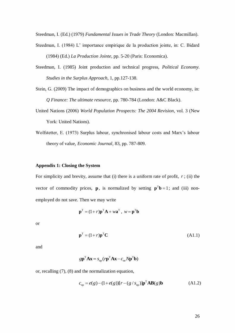
Appendix 1: Closing the System

For simplicity and brevity, assume that (i) there is a uniform rate of profit, r ; (ii) the

vector of commodity prices, p , is normalized by setting T 1p b ; and (iii) non-

employed do not save. Then we may write

T T T(1 )r w p p A a ,

Tw p b

or

T T(1 )r p p C (A1.1)

and

T T T

np ne( )g s r c N p Ax p Ax p b

or, recalling (7), (8) and the normalization equation,

T

np np( ) (1 ( ))[ ( / )] ( )c e g e g r g s g p AB b (A1.2)

27

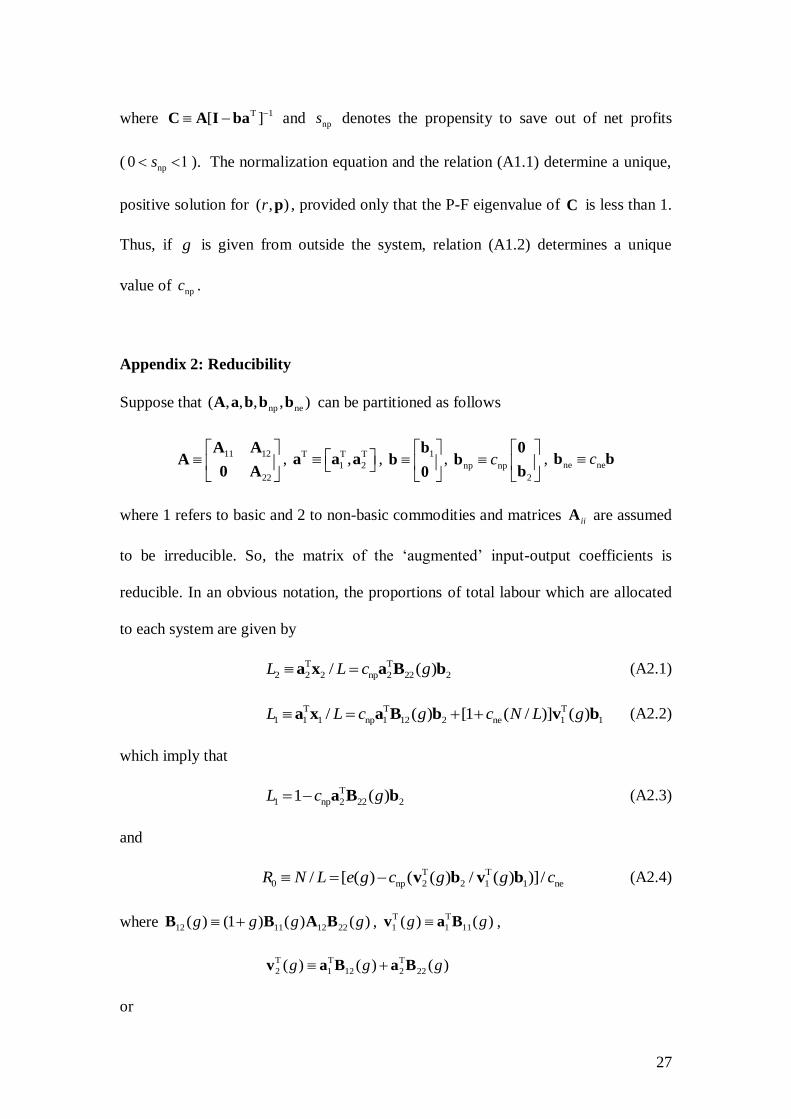
where T 1[ ] C A I ba and nps denotes the propensity to save out of net profits

( np0 s ). The normalization equation and the relation (A1.1) determine a unique,

positive solution for ( , )r p , provided only that the P-F eigenvalue of C is less than 1.

Thus, if g is given from outside the system, relation (A1.2) determines a unique

value of npc .

Appendix 2: Reducibility

Suppose that np ne( , , , , )A a b b b can be partitioned as follows

11 12

22

A AA

0 A, T T T

1 2, a a a , 1

bb

0,

np np

2

c

0b

b, ne necb b

where 1 refers to basic and 2 to non-basic commodities and matrices iiA are assumed

to be irreducible. So, the matrix of the ‘augmented’ input-output coefficients is

reducible. In an obvious notation, the proportions of total labour which are allocated

to each system are given by

T T

2 2 2 np 2 22 2/ ( )L L c g a x a B b (A2.1)

T T T

1 1 1 np 1 12 2 ne 1 1/ ( ) [1 ( / )] ( )L L c g c N L g a x a B b v b (A2.2)

which imply that

T

1 np 2 22 21 ( )L c g a B b (A2.3)

and

T T

0 np 2 2 1 1 ne/ [ ( ) ( ( ) / ( ) )]/R N L e g c g g c v b v b (A2.4)

where 12 11 12 22( ) (1 ) ( ) ( )g g g g B B A B , T T

1 1 11( ) ( )g gv a B ,

T T T

2 1 12 2 22( ) ( ) ( )g g g v a B a B

or

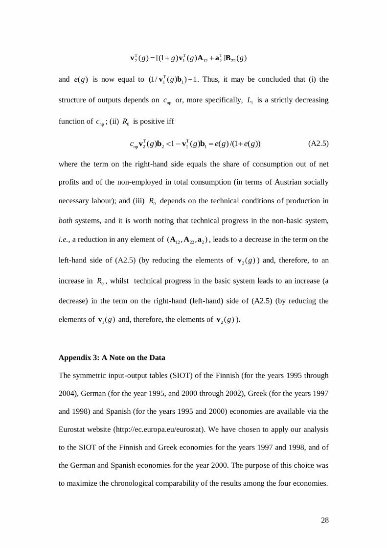
28

T T T

2 1 12 2 22( ) [(1 ) ( ) ] ( )g g g g v v A a B

and ( )e g is now equal to T

1 1(1/ ( ) ) 1g v b . Thus, it may be concluded that (i) the

structure of outputs depends on npc or, more specifically, 1L is a strictly decreasing

function of npc ; (ii) 0R is positive iff

T T

np 2 2 1 1( ) ( ) ( ) /(1 ( ))c g g e g e g v b v b (A2.5)

where the term on the right-hand side equals the share of consumption out of net

profits and of the non-employed in total consumption (in terms of Austrian socially

necessary labour); and (iii) 0R depends on the technical conditions of production in

both systems, and it is worth noting that technical progress in the non-basic system,

i.e., a reduction in any element of 12 22 2( , , )A A a , leads to a decrease in the term on the

left-hand side of (A2.5) (by reducing the elements of 2 ( )gv ) and, therefore, to an

increase in 0R , whilst technical progress in the basic system leads to an increase (a

decrease) in the term on the right-hand (left-hand) side of (A2.5) (by reducing the

elements of 1( )gv and, therefore, the elements of 2 ( )gv ).

Appendix 3: A Note on the Data

The symmetric input-output tables (SIOT) of the Finnish (for the years 1995 through

2004), German (for the year 1995, and 2000 through 2002), Greek (for the years 1997

and 1998) and Spanish (for the years 1995 and 2000) economies are available via the

Eurostat website (http://ec.europa.eu/eurostat). We have chosen to apply our analysis

to the SIOT of the Finnish and Greek economies for the years 1997 and 1998, and of

the German and Spanish economies for the year 2000. The purpose of this choice was

to maximize the chronological comparability of the results among the four economies.

29

The SIOT describe 59 products, which are classified according to CPA

(Classification of Product by Activity). However, in the case of the Spanish, German

and Greek economies, all the elements associated with the product with code 12

(Uranium and thorium ores) equal zero and, therefore, we remove them from our

analysis. So, the SIOT of Germany, Spain and Greece have dimensions 5858, whilst

those of Finland have dimensions 5959. The levels of sectoral employment of

Finland (1997 and 1998) and Germany (2000) are included in the input-output tables,

whilst those of Greece are included in the input-output table (1997) or provided by the

National Statistical Service of Greece (1998). Finally, the levels of sectoral

employment of Spain (2000) are provided via the website of the National Statistics

Institute of Spain (http://www.ine.es/).

The market prices of all products are taken to be equal to 1; that is to say, the

physical unit of measurement of each product is that unit which is worth of a

monetary unit (see, e.g., Miller and Blair, 1985, p. 356). Thus, the matrix of input-

output coefficients, A , is obtained by dividing element-by-element the inputs of each

sector by its gross output. Furthermore, wage differentials are used to homogenize the

sectoral employment (see, e.g., Sraffa, 1960, §10, and Kurz and Salvadori, 1995, pp.

322-325), i.e., the vector of inputs in direct homogeneous labour, j[a ]a , is

determined as follows: m m

j mina ( / )( / )j j jL x w w , where jL , jx , m

jw denote the total

employment, gross output and money wage rate, in terms of market prices, of the j th

sector, respectively, and m

minw the minimum sectoral money wage rate in terms of

market prices. By assuming that there are no savings out of wages and that

consumption out of wages has the same composition as the vector of the final

consumption expenditures of the household sector, ceh , directly obtained from the

30

input-output tables, the vector of the real wage rate, b , is determined as follows:

m T

min ce ce( / )wb s h h , where T [1,1,...,1]s denotes the row summation vector

identified with the vector of market prices (see also, e.g., Okishio and Nakatani, 1985,

pp. 66-67). Thus, the estimates of the MEDR are independent of the choice of the unit

of measurement of the quantity of labour. Finally, it must be noted that the available

input-output tables do not include inter-industry data on fixed capital stocks and on

imported inputs. As a result, our investigation is restricted to a circulating capital

model and, regarding the estimations associated with the case of non-proportionally

growing and open economy, (i) we replace i by the ‘gross capital formation’ vector,

which is obtained from the tables (and includes ‘gross fixed capital formation,

changes in inventories and acquisitions less disposal of valuables’); and (ii) we use

the net export vector, which is also obtained from the tables.

Appendix 4: Theoretical Relationships between the Maximum Relative Rate of

Growth and the Marxian Rate of Surplus Labour

From * *( )[ (1 ) ]g g B I A I , it follows that if * 1g G , then

* 1 * 1 1 1 1 2 2( ) [ ] [ ] [ ] [ ] [ ] [ ...]g g B I A I H I A I J I A I J J

or

* 1 1( ) [ ] [ [ ] ]g B I A I J I J (A4.1)

where 1[ ] H A I A denotes Pasinetti’s (1973) matrix of the vertically integrated

technical coefficients of production and the P-F eigenvalue of GJ H equals 1.Thus,

*( ) 0e g or T *( ) 1g a B b can be restated as

T T 1(0) (0) [ ] 1 v b v J I J b

or

31

T 1 T(0) [ ] 1 (0) (0) /(1 (0))e e v J I J b v b (A4.2)

In the trivial case in which T (0)v or b is the P-F eigenvector of J (or,

equivalently, of A ), (i) relation (A4.2) implies that

T[ /(1 )] (0) (0) /(1 (0))e e v b

or, since T(0) [(1 ) / ] 1e A a b and 1/(1 )G A ,

T(0) /(1 (0)) 1 [(1 ) / ]e e G G a b

i.e., the system constitutes a quasi-one-commodity economy and, therefore, equals

the share of gross profits in net income expressed in terms of Marxian socially

necessary labour (see also Sraffa, 1960, § 29); and (ii) ( )e g is a linear function of g ,

i.e.,

T( ) {[1 (1 )] / } 1e g g A a b

or

( ) (0) (1 (0))( / )e g e e g G (A4.3)

Now, consider the general case: let Jy be the positive left-hand side P-F

eigenvector of J (or, equivalently, of A ) and let ˆJy be the diagonal matrix formed

from the elements of Jy . Given that

T 1 T 1 T 1 Tˆ ˆ ˆ ˆ[ ] J J J J J Js y Jy y Jy y y s

it follows that J is similar to the column stochastic matrix 1ˆ ˆ J JK y Jy , the elements

of which are independent of the choice of physical measurement units (and the

normalization of y ). Substituting 1ˆ ˆ J JJ y Ky in (A4.2) yields

T 1(0) [ ] (0) /(1 (0))e e ω K I K β (A4.4)

32

where T T 1ˆ(0) (0) Jω v y , ˆ Jβ y b and T 1 T[ ] [1/(1 )] s I K s , which implies that

1[ ] 1/(1 ) I K , where denotes the ‘maximum column sum matrix norm’.

Thus, taking norms of (A4.4), and using the well-known Hölder’s inequality (see,

e.g., Horn and Johnson, 1990, p. 536), we obtain

[ /(1 )] (0) /(1 (0))f e e

or

F

where (0) /[ (1 (0)) (0)]F e f e e and T (0)f ω β . Since T T(0) (0)ω β v b and

T T(0) (0) f ω β ω β , where the equality holds iff T (0)v is the P-F eigenvector of

A , it follows that (1 (0)) 1f e . So, we conclude that F , a lower bound for , is no

greater than (0) /(1 (0))e e . Finally, ( )e g can be expressed as

T T 1( ) {1/[ (0) ( / ) (0) [ ( / ) ] ]} 1e g g G g G ω β ω K I K β

Thus, taking norms, we obtain

( ) [(1 ) / ] (1/ )( / )e g f f f g G

where the term on the right-hand side is no greater than the term on the right-hand

side of (A4.3), since (1 (0)) 1f e and / 1g G .