
An Innovative Seismic Risk Assessment Method and ...
188
An Innovative Seismic Risk Assessment Method and Implications of Strain-rate Dependency on Risk Estimates Dissertation submitted to, and approved by, the Department of Architecture, Civil Engineering and Environmental Sciences of the Technische Universität Carolo-Wilhelmina zu Braunschweig and the Faculty of Engineering Department of Civil Engineering of the University of Florence in candidacy for the degree of a Doktor-Ingenieur (Dr.-Ing.) / Dottore di Ricerca in Risk Management on the Built Enviroment *) by Sadık Cem Topcuoğlu from Antalya, Turkey Submitted on 31 March 2006 Oral examination on 19 May 2006 Professoral advisor Prof. Udo Peil Prof. Andrea Vignoli Prof. Luca Facchini 2006 *) Either the German or the Italian form of the title may be used.
-
Upload
khangminh22 -
Category
Documents
-
view
2 -
download
0
Transcript of An Innovative Seismic Risk Assessment Method and ...

An Innovative Seismic Risk Assessment Method and Implications of Strain-rate Dependency on Risk Estimates
Dissertation
submitted to, and approved by,
the Department of Architecture, Civil Engineering and Environmental Sciences
of the Technische Universität
Carolo-Wilhelmina
zu Braunschweig
and
the Faculty of Engineering
Department of Civil Engineering
of the University of Florence
in candidacy for the degree of a
Doktor-Ingenieur (Dr.-Ing.) / Dottore di Ricerca in Risk Management on the Built Enviroment *)
by
Sadık Cem Topcuoğlu
from Antalya, Turkey
Submitted on 31 March 2006
Oral examination on 19 May 2006
Professoral advisor Prof. Udo Peil
Prof. Andrea Vignoli
Prof. Luca Facchini
2006 *) Either the German or the Italian form of the title may be used.

The dissertation is published in an electronic form by the Braunschweig university library at the
address
http://www.biblio.tu-bs.de/ediss/data/

1
Contents
Abstract............................................................................................................................. 4
Abbreviations and Symbols.............................................................................................. 5
1. Latin...................................................................................................................... 5
2. Greek .................................................................................................................... 8
Introduction ...................................................................................................................... 9
Chapter 1. Founding principles of risk management in built environment .................... 10
1.1. Motive behind application of risk management in built environment................. 10
1.2. Risk management - definition ............................................................................. 10
1.3. Risk management in built environment due to natural hazards - definition........ 11
1.4. Lack of a uniform framework.............................................................................. 11
1.5. Principles of risk management in built environment due to natural hazards ...... 13
Chapter 2. Innovative method for seismic risk assessment of a single facility .............. 15
2.2. Phenomenological comprehension by means of a hazard tree ............................ 16
2.3. Risk measures decision........................................................................................ 18
2.4. Detection of loss paths by loss trees.................................................................... 19
2.5. Assigning governing variables to events ............................................................. 24
2.6. Stating the mathematical model .......................................................................... 26
2.7. Detection of potential hazard sources.................................................................. 28
2.8. Modeling hazard recurrence ................................................................................ 30
2.9. Modeling intermediate events ............................................................................. 34
2.9.1. Strong Motion Function ............................................................................... 36
2.9.1.1. Source spectrum .................................................................................... 37
2.9.1.2. Path model ............................................................................................. 39
2.9.1.3. Local soil and topographic effects model.............................................. 41
2.9.1.4. Source duration model........................................................................... 43
2.9.1.5 Path delay model .................................................................................... 43

2
2.9.1.6. Simulation.............................................................................................. 43
2.9.2. Strong motion - response intermediate function R Sf (x) .......................... 45
2.9.3. Response-damage intermediate function D Rf (x) .................................... 47
2.9.4. Damage-loss and response-collapse intermediate functions .................... 52
2.9.4.1. Collapse probability model................................................................ 52
2.9.4.2. Death and injury model ..................................................................... 53
2.9.4.3. Restoration cost model ...................................................................... 54
2.9.4.4. Serviceability interruption model ...................................................... 55
2.9.4.5. Monetary loss model -due to tangibles- ............................................ 55
2.10. Solution and dealing with uncertainty ............................................................... 55
Chapter 3. Example application of the method .............................................................. 58
3.1. Problem statement ............................................................................................... 58
3.2. Construction of mathematical model................................................................... 58
3. 3. Hazard assessment.............................................................................................. 64
3.3.1. Investigation of seismological setting .......................................................... 64
3.3.4. Structural response analysis ......................................................................... 71
3.3.5. Damageability and loss estimate .................................................................. 75
3.3.6. Presentation of results................................................................................... 77
Chapter 4. Investigations on sensitivity to strain-rate-dependency of seismic loss
estimates in steel frame structures .................................................................................. 87
4.1. On model sensitivity and motivation of the investigation................................... 87
4.2. Rate dependency as a commonly neglected phenomenon in seismic response
assessment .................................................................................................................. 87
4.2.1. Rate dependency at material level ................................................................ 90
4.2.2. Local level (component and cross-section) .................................................. 93
4.2.3. Global scale .................................................................................................. 94

3
4.3. Investigation on rate dependency sensitivity of seismic response of a steel frame
under severe strong motion ........................................................................................ 95
4.3.1. Example structure ......................................................................................... 95
4.3.2. Finite element model .................................................................................... 99
4.3.3. Material models and parameters................................................................... 99
4.3.3. Modal analysis............................................................................................ 100
4.3.4. Equivalent static analysis and code validation ........................................... 100
4.3.4. Used time histories ..................................................................................... 104
4.3.5. Computational aspects of dynamic analyses .............................................. 106
4.3.6. Data gathering and processing by Incremental Dynamic Analysis............ 106
4.4. Analysis of global results .................................................................................. 111
4.4.1. Range of maximum strain rates .................................................................. 111
4.4.2. Variability of maximum strain rates among varying records ..................... 111
4.4.3. Variability of recorded velocity and connected maximum strain rate
variability.............................................................................................................. 115
4.4.4. Variability of global response parameters .................................................. 122
Conclusions .................................................................................................................. 131
ANNEX.I. MATLAB Script .................................................................................... 132
ANNEX.II. ANSYS Script....................................................................................... 142
Bibliography ................................................................................................................. 183

4
Abstract
A probabilistic seismic risk assessment methodology for single facility is presented. It contains analyses of hazard, response, damage and loss. It is formed by synthesis of state-of-the-art approaches and own contributions. The consecutive steps of method are; (1) phenomenological comprehension, (2) source identification, (3) probabilistic hazard analysis, (4) stochastic strong motion simulation, (5) incremental dynamic time-history analysis, (5) probabilistic component-based damage and loss analysis. The method accounts for nonstructural and contents damage in addition to structural damage. The method is especially suitable for regions with poor instrumental seismic records, because of the use of stochastic strong motion simulation approach. The initial step of the method (phenomenological comprehension) can be implemented universally to other natural hazards’ risks in built environment.
The method is applied on an example steel frame structure. The fictive structure is located in a certain near-field site in a highly seismic region in Turkey. Regional seismicity data is gathered. 7 discrete hazard intensity levels between moment magnitudes of 5.0 and 8.0 are considered. 10 strong motion displacement time histories are simulated for each discrete magnitude level. Dynamic structural time history analyses are carried out on a finite element model of the structure. Monte Carlo simulation is utilized to treat response and damage variability. Results show that loss is dominated by nonstructural components, followed by contents and structural components. It is expected that the developed method and the example serve both research and practical purposes in future.
In the second part, implications of strain-rate dependency on seismic response of steel frame structures are investigated. This question constitutes an example to model sensitivity. Model sensitivity is an important question in risk assessment. An example structure is excited with 12 near-field severe strong motion records. This is carried out at 8 amplification levels, making a total of 96 time history analyses. Three varying material models are utilized. Inter-event, intra-event and inter-model response variabilities are investigated. The strong motion time histories used are representative for near-field seismic hazard (12 among 22 available records fitting the initial assumptions are included, the assumptions being soil type C, and, PGA>0.6g or PGV>1m/s). The results have shown that steel frames undergo strain rates up to 100 per second (on the brink of range for explosion and crash loading). The strain rates are shown to be depending on strong motion intensity and velocity characteristics. It is shown that global response is not affected by strain-rate-effects significantly (in the extreme cases in the order of 5%). This is shown by comparison of response data from time-independent and time-dependent multi-surface material models. So, modelling of time dependency is not significant for accurate risk estimates. This is not the case for modeling of progressive yielding. Multi-surface models deliver significantly different response results from that of the simpler multilinear model, especially at higher magnitude levels. This shows the considerable implications of material modeling on risk estimates.

5
Abbreviations and Symbols
1. Latin
a regional constant for hazard recurrence equation as source acceleration spectrum aw windowing function coefficient A fault rupture area ASI acceleration spectrum intensity Av-30 upper 30 m.-profile site amplification b slope of (the straight section of) hazard recurrence curve bw windowing function coefficient c indicator variable of collapse cs fault shape factor cw windowing function coefficient C restoration cost of a component CL mean loss ratio (loss / total facility value) in collapse state CSI mean cost of unit time serviceability interruption cost CT total facility value (structure,nonstructure and contents included) mean new construction cost of the whole facility (Note: the model assumes both equal) CCPDF cumulative complementary probability distribution function ds depth of local soil considered in local effects dam. damaging D component damage random variable DC damageability curve DS damage state el. elastic E (event of) fault rupture at an effective distance Ediss dissipated energy f frequency
cf corner frequency
J Kf ( j, k) conditional probability distribution function of random variable J
conditioned on random variable K maxf cutoff frequency
F free surface effect Fbase maximum base shear
YF (y) cumulative probability distribution function of Y evaluated at y FAS fourier acceleration spectrum FOSM first order second moment method g gravity acceleration g(r) geometrical spreading function G (event of) site ground failure (fault crack, liquefaction, landslide)
6
EG (x) hazard recurrence function
XG (x) complementary cumulative probability distribution function of function X HT hazard tree HV hazard governing variable HVAC heating-ventilation-air condition systems I (random variable) number of earthquake induced injuries in one year IDA incremental dynamic analysis interp. interpolation ISDmax maximum peak interstorey drift ratio L (random variable) earthquake induced loss of use in one year Lf characteristic fault dimension LT mean serviceability interruption time in collapse state LT loss tree
a sL (d , f ) local soil and topographic effects filter function sa sL (d , f ) wave impedance multiplier na sL (d , f ) soil-nonlinearity multiplier da sL (d , f ) site diminution multiplier ba sL (d , f ) sedimentary-basin related phenomena multiplier taL (f ) topographic multiplier
m moment magnitude
geom characteristic earthquake magnitude
intm intersection magnitude of characteristic frequency and b line ml lower magnitude bound for risk assessment
maxm maximum magnitude recmaxm regional maximum recorded magnitude
minm lower cutoff magnitude
om seismic moment mu upper magnitude bound for risk assessment mech. mechanism M (random variable) number of earthquake induced deaths in one year
R DM mean damageability vector of a component
R DD standard deviation damageability vector of a component MM1 material model 1; bilinear kinetic material model MM2 material model 2; multilinear kinetic material model MM3 material model 3; time independent two-surface material model MM4 material model 4; time dependent two-surface material model n number of simulations at each magnitude level n number of component types in the facility n(m) number of earthquakes exceeding a magnitude level m N (random variable) earthquake induced restoration cost in one year NAF North Anatolian Fault (System)

7
NDA nonlinear time-history dynamic analyses NSA nonlinear static analysis = pushover pY(y) probability (likelihood) of discrete random variable Y being equal to y pl. plastic P (random variable) earthquake induced monetary loss in one year
aP (r, f ) path filter function PFAmax maximum peak floor acceleration PFVmax maximum peak floor velocity PGA peak ground acceleration Q mean number of occupants Q(f ) attenuation operator r source-site distance rmax maximum distance criteria for effective faults rec. record (time history record) R maximum structural response random variable RI mean ratio of number of injured to number of occupants in collapse state RM mean ratio of number of deaths to number of occupants in collapse state RR ratio of loss (restoration cost) to value of a component RMB risk management in built environment due to natural hazards RN reverse-normal (fault) RV response governing variable RΘΦ radiation pattern s characteristic slip per earthquake
SMs (m) strong motion duration function
Ss source duration (rupture duration)
Ps path delay
Ls local site delay S site strong motion random variable Sa
max maximum pseudo-acceleration S(f) shape of source spectral SS strike-slip ST sensitivity type Sv
max maximum pseudo-velocity
t characteristic earthquake recurrence period tact recency criterion for active faults T period T1 first natural period
cT characteristic recurrence period TD maximum tip deflection v slip rate at the fault
sv shear-wave velocity at bedrock
sv shear wave velocity at source vicinity
sv representative shear wave velocity of path

8
sv (f ) average shear wave velocity, from the surface down to a depth of ¼ wavelength
visc. viscous V partition factor for shear waves and their energy in two components VSI velocity spectrum intensity VT mean restoration cost in collapse state w fault width w(f) windowing function for simulation
dX (random variable) capacity of a component to resist the damage state d
sZ seismic impedance at bedrock Z(f ) time-weighted average of seismic impedance from the surface down to a
depth of ¼ wavelength
2. Greek
∆m spacing between discrete magnitude levels of strong motion simulation ∆t time steps of earthquake records ∆σ stress drop ε strain ε windowing function coefficient ε strain rate (time variation of strain, d / dtε ) ε max maximum strain rate η windowing function coefficient µ shear modulus of the crust at fault µ mean value ρ density at source vicinity
(f )ρ average density, from the surface down to a depth of ¼ wavelength
sρ density at bedrock σ standard deviation σ stress σ stress rate (time variation of stress, d / dtσ )
aveσ average hysteresis stress
plσ mean average yield stress
uσ tensile strength
yσ mean yield limit, initial yield strength dynyσ mean yield limit under dynamic excitation statyσ mean yield limit under quasi-static excitation

9
Introduction
This thesis has two objectives; (1) stating a consistent and innovative seismic risk
assessment model, (2) investigating strain rate sensitivity of seismic loss estimates in
steel frame structures.
Chapter 1 provides the fundament for the succeeding chapters: It presents the essence of
risk management in built environment due to natural hazards. It points out the origins of
the subject in management science and its distinguishing characteristics from
conventional civil engineering task (design for safety).
Chapter 2 presents a consistent and original framework for seismic risk assessment. It is
based on synthesis of several state-of-the-art approaches. In several key points, it
includes original solutions. Provided method is advanced but also practically applicable.
Chapter 3 is an example application of the subject method. It proves the applicability
and practicality of the method.
Chapter 4 investigates a previously neglected phenomenon in earthquake engineering. It
addresses sensitivity of response of steel moment resisting frames to strain-rate
dependency. This phenomenon interacts with the particular velocity content phenomena
in near field. The analysis provide detailed insight by analysis of global response data.

10
Chapter 1. Founding principles of risk management in built environment
1.1. Motive behind application of risk management in built environment
Users and owners demand lifetime-integrity of civil engineering facilities against
potential perils. This should satisfy (1.) safety of life, (2.) security of inherent
investment and (3.) continuity of activities. Providing these is the moral responsibility
of the engineer. However, there are economical, temporal and epistemological limits to
this effort. Therefore, the engineer has to optimize investment and time to satisfy his/her
moral responsibility. Furthermore, he/she has to strive towards uniform safety levels
due to equality principles. These explain the motive behind application of risk
management methodology for civil engineering structures.
1.2. Risk management - definition
Risk management involves
(1.) identification and assessment of potential future perils (risks),
(2.) development and implementation of optimal strategies for risk prevention or
mitigation.
It is a specific application of management science. Management science is a form of
applied mathematics and refers to use of mathematical models, statistics and algorithms
for decision-making in complex real-world systems to improve or optimize
performance.
Risk management has a wide range of applications (for example in finance, business,
industrial safety, environmental protection, public health, traffic, urban systems and
civil engineering). Scale of applications range from single machinery, household,
business or facility to whole countries, regions, sectors.
Typical risk management decisions can be listed as in the following:
- justification of investment for mitigation of a particular risk
- distribution of resources for management of an ensemble of risks,
- risk acceptability criteria.

11
1.3. Risk management in built environment due to natural hazards - definition
Built environment (the totality of civil engineering structures) is exposed to a series of
natural hazards. They can be grouped according to their origins as in the following:
- geophysical (earthquake, landslide, volcanism),
- atmospheric (hurricane, tornado, extreme temperature, excessive precipitation),
- hydrological (flooding),
- combined (tsunami, avalanche).
These extreme events lead to varying degrees of partial damage or to collapse. The
potential consequences are varying degrees of (1) life loss; (2) injury and health
distraction; (3) wealth loss; (4) loss of social and business structures; (5) loss of
historical or ecological heritage; and, (6) interruption of social and business activities.
In that context, risk management in built environment due to natural hazards (RMB) can
be defined as follows:
“the task of scientific and proactive treatment of natural hazards’ consequences in
planning and maintenance of civil engineering structures, carried out by optimizing
investment, time and safety”.
The global humanitarian and economical significance of RMB is evident due to the (1)
increasing disaster loss, (2) population and wealth concentration in hazardous areas.
It is worth to mention that RMB is not synonymous with and is distinct from (1) design
for safety, (2) reliability engineering, (3) emergency management. (1) and (2) can
occasionally serve RMB purposes. (3) is a reactive task which marks its difference from
the essentially proactive RMB.
Some occasions for use of RMB decisions are safety-level decision in mitigation and
design, insurance premium justification and remaining lifetime estimates.
1.4. Lack of a uniform framework
There is a lack of a uniform framework for RMB in related publications. Similar
situation is reported for risk management in general in a comprehensive treatment of
risk analysis (Aven, 2003).
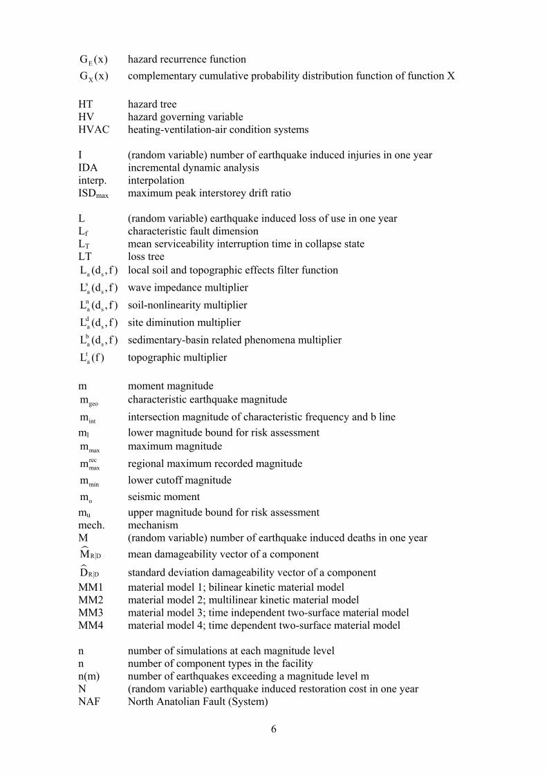
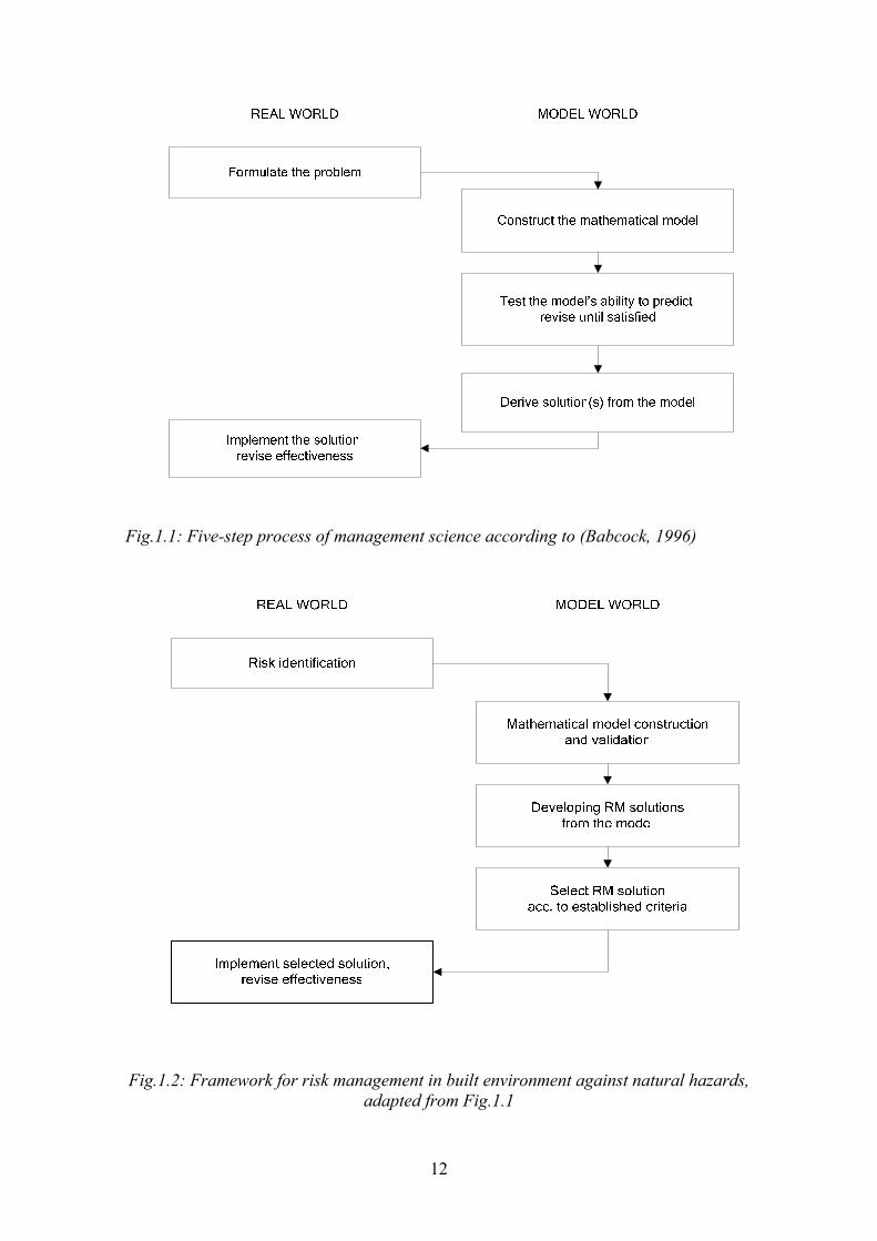
In order to respond this, the five step process of management science as depicted in
Fig.1.1 can be adapted to risk management as in Fig.1.2.
12
Fig.1.1: Five-step process of management science according to (Babcock, 1996)
Fig.1.2: Framework for risk management in built environment against natural hazards, adapted from Fig.1.1

13
1.5. Principles of risk management in built environment due to natural hazards
As seen in Fig.1.2, risk management utilizes models in both risk assessment and
solution development stages. Any model derives from synthesis of physical laws and
empirical relations deriving from actuarial, experimental and simulation data. So, model
uncertainty arises as an issue that should be treated by risk management alongside with
the randomness of future phenomena.
From this point, following essential principles for a framework of risk management in
built environment due to natural hazards could be drawn:
Principle I. Treatment of randomness and uncertainty
Since RM is based on model building, model uncertainty should be addressed alongside
with randomness of hazard and consequences. The tool for these is probabilistic
inference.
Principle II. Systems-view
RMB should adopt a systems-view of subject problem, (e.g. seismic risk management
should consider source, path, site, structure, safety and economy). Segmented
approaches can fail due to their inability to address (1) uncertainty propagation, (2)
correlation between phenomena (e.g. relation between near-field fling pulse phenomena
and rate dependency in seismic response of steel structures).
Principle III. Multi-disciplinary approach
As a consequence of Principle II, risk management operations should be
multidisciplinary (e.g. seismic risk management in community level should involve at
least seismology, geotechnical and structural engineering and public administration).
Principles II and III are in line with the distinguishing characteristics of management
science as given by (Babcock, 1996). The latter author mentions additionally “emphasis
on use of mathematical models, statistical and quantitative techniques” what we take for
granted since Fig.1.1.
RMB can be carried out either for a single facility or for a group of facilities (defined
geographically or over common characteristics like type, construction period, owner).
This distinction can be refered by the terms micro-RMB and macro-RMB. This
distinction is important for mathematical modeling, in terms of treatment of uncertainty
(Bazurro and Luco, 2005) and risk acceptability criteria (Porter 2002).

14
A further distinction is between uni- and multi-hazard RMB. Multi-hazard RMB
considers simultaneous or sequential occurrence of a group of natural hazards. Uni-
hazard RMB considers only a single type of natural hazard.
RMB methodology can be applied to new projects (safety-investment optimization, site
selection) or to existing facilities (decision among acceptance, mitigation, transfer,
abandonment or relocation). This distinction may be addressed by the terms RMB in
new project and RMB in existing facility.
This work focuses on seismic risk, one of the most significant natural hazards with
record and increasing life and monetary losses.
Based on the principles drawn above, a generic procedure for seismic risk assessment in
an existing facility is constructed and presented in the following.

15
Chapter 2. Innovative method for seismic risk assessment of a single facility
In this chapter, a framework method is presented for seismic risk assessment of an
existing civil engineering facility. It is based on the principles stated in Chapter 1. It
combines following approaches:
(1) probabilistic seismic hazard analysis,
(2) uniform hazard stochastic strong motion simulation,
(3) incremental dynamic time-history analysis,
(4) component based damage analysis.
The procedure answers the following questions for a single facility exposed to
earthquake hazard:
(1) what are the measures of risk?
(2) how to proceed with risk assessment?
(3) how to deal with randomness and model uncertainty?
The question of “how to decide among acceptance, mitigation, transfer, abandonment or
relocation alternatives given a risk level?” is not investigated. This can be done with
extending later with risk acceptability judgment and optimal strategy decision modules.
Most of the introduced concepts in the method can be implemented in context of other
natural hazards as well.
An example application of the method is given later in Chapter 3.
The method accounts only for facility-internal hazard consequences and neglects the
exterior consequences. The exterior consequences can be of social, economic, ecologic,
public-health nature. Those can be significant in several contexts like emergency-
planning, city planning and subvention decisions. However, they are only weakly
related to single facility risk assessment. Exceptions are (1) industrial and energy-
production facilities (e.g. nuclear-, chemical plants, waste disposal facilities, dams, oil
pipelines) with significant potential external effects to public-health and ecology, (2)
historical / monumental structures with heritage value, (3) strategic public facilities.
Reminder: the subject is a single facility exposed to a earthquake hazard and the
problem is “how to proceed with risk assessment?”.

16
2.2. Phenomenological comprehension by means of a hazard tree
The method starts with drawing an event tree as in Fig.2.3. This construction will be
referred as hazard tree (HT) in this work. Hazard is given without specification of
source, intensity or periodicity. HT simply answers the question “what are possible
consequences of a seismic event of significant intensity and sufficient vicinity?”.
HT reflects the qualitative phenomenological knowledge on the problem in an extensive
manner. So, it comprises also the events and paths which would be neglected in later
stages of assessment (neglect can be due to low probability, low intensity,
insignificance or non-conceivability). This approach helps to locate the assumptions
taken later. HT does not contain probabilities, intensities or hazard sources, since
gathering of such quantitative information is left to succeeding stages.
HT is an original proposal of this work and is based on conventional logical trees. For
treatment of the latter, refer to (Faber, 2005).

17
Fault rupture at an effective distance
Site ground failure
Site strong motion
Nonstructural damage
Structural damageDamage to
contents
Repair / replacement
need
Life loss / injury
Serviceability interruption
TANGIBLE LOSS
INTANGIBLE LOSS
Collapse
Monetary loss
Structural response
Fig.2.3: Hazard tree (HT) as tool for qualitative seismic risk identification. The initiator
event is a generic one. Probabilities and intensities are not specified. HT provides preliminary inspection of cause-consequence relations.

18
2.3. Risk measures decision
Next step is the decision on (1) what constitutes the risk, and, (2) how to quantify it.
The answers are respectively potential loss and loss estimates.
Potential loss comprises death, injury, monetary-loss and serviceability-interruption
components. Using annual estimates in line with convention, random variables are
defined as in following:
LOSS RANDOM VARIABLES M number of earthquake induced deaths in one year
I number of earthquake induced injuries in one year
N earthquake induced restoration cost in one year
L earthquake induced serviceability interruption in one year
P earthquake induced monetary loss in one year Table 2.1: Loss variables used in framework method
This reduces risk assessment problem to obtaining complementary cumulative
probability distribution functions M I N L pG (m),G (i),G (n),G (l),G (p) , namely the risk
measures. Specifically, expected values (so, x for GX(x)=0.5) are commonly taken as
risk measure.
The term ‘restoration’ as used above covers both repair and replacement operations.
Selection of a time unit of one year as decisional basis is conventional, yet arbitrary. Its
convenience stems from the typical projected life times of civil engineering facilities in
the order of 101 years.
The above mentioned loss variables are used by default in most problems. However,
some other loss variables can also be defined
- for limit state exceedance (e.g. collapse prevention, serviceability limit state, ultimate
limit state, operationality)
- occurrence of specified events (e.g. crack width > 5mm, breakdown of water supply).
For such cases, an indicator variable X with two possible values (1: occurrence, 0: non-
occurrence) is defined and risk measure is then pX (x=1) (annual probability of

19
exceedance or occurrence).
These risk measures can be utilized for compliance verification to standards or for
comparison with other facilities. They can be associated with the facility as a whole, its
structural/nonstructural components or contents. A commonly used one is exceedance
of collapse prevention limit state, with Cp (c 1)= as risk measure where C = indicator
variable of exceedance of collapse prevention limit state in one year.
Risk measures constitute criteria for risk acceptability and intervention decision.
It is worth to note that injury estimates could further be classified acc. to (1) degree of
severity (e.g. minor, moderate, severe, critical, fatal), (2) treatment category (e.g.
hospitalized, emergency dept. treat, self-treated), or (3) type (e.g. femur fracture). For
further discussion on this point, refer to the work by (Porter et al., 2005) which
demonstrates the vast numbers of injury cases even in moderate no-fatality events.
2.4. Detection of loss paths by loss trees
HT construction presented above facilitates qualitative comprehension by use of logical
trees understandable by both experts and layman. But it does not provide a basis for risk
measures quantification. For that end, another form of logical trees are necessary. Those
are loss trees (LT) drawn seperately for each risk measure.
A LT contains all scenarios leading to any change in the corresponding risk measure. It
is drawn mainly with conventional fault tree notation, with the following distinctive
features:
(1) a LT provide an illustrative basis for mathematical modeling rather than a failure
analysis,
(2) intermediate events in a LT can be continuous nonlinear functions as well as discrete
events.
Conventional fault trees are treated e.g. by (Faber, 2005).
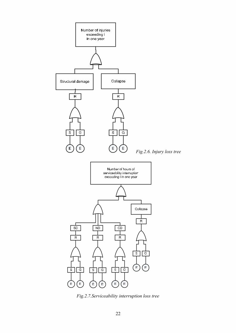
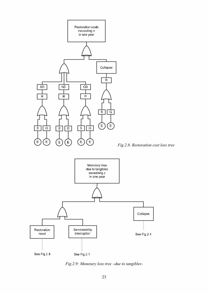
Loss trees derived from HT in Fig.2.3 are given in Fig.s 2.4 to 2.9. The abbreviations
and symbols used are explained in Table 2.2. There is no one-to-one correspondence
between the given HT and LT’s, due to these assumptions:
1. Contributions of nonstructural components’ and contents’ damage on death and
injury risks are assumed negligible in line with statistics.

20
2. Collapse probability is related directly to structural response in line with state-of-the-
art approach stated by (Krawinkler and Miranda, 2004).
The cause-consequence chain leading to loss is constructed as response→ damage→
loss. This is a useful construct for seismic risk assessment. Response refers to
structure’s mechanical behavior under excitation quantified by observable physical
parameters (drift, strain, force, settlement etc.). Damage refers to permanent physical
effects on structure, nonstructural components and contents. It is quantified by indicator
variables of damage state exceedance (in other words, of damage state membership).
Loss is the damage-associated monetary or social consequence, as formulated by
(McGuire, 2004).
ABBREVIATIONS AND SYMBOLS IN LOSS TREES E fault rupture at an effective distance
S site strong motion
G site ground failure (fault crack, liquefaction, landslide)
R structural response
SD structural damage
ND nonstructural damage
CD contents damage
Table 2.2: Notation used for construction of loss trees

21
Fig.2.4: Collapse limit state tree
Fig.2.5: Death loss tree
22
Fig.2.6. Injury loss tree
Fig.2.7.Serviceability interruption loss tree
23
Fig.2.8. Restoration cost loss tree
Fig.2.9: Monetary loss tree –due to tangibles-
24
2.5. Assigning governing variables to events
Most elements of loss trees are yet abstruse in mathematical sense. Since mathematical
modeling requires quantification, random variables representative of each event should
be assigned to those (e.g. flood height for flooding, peak ground acceleration for strong
motion). These will be referred as governing variable of each phenomenological event.
If a scalar can not represent an event sufficiently, use of a kx1 governing variable vector
or a nxm governing variable matrix is appropriate - at the expense of efficiency.
All above will be referred as governing variables in the remaining discussion.
Assigning a governing variable to an event is a challenging task, since a governing
variable should fulfill several criteria: A governing variable should be
(1) empirically observable,
(2) good measure of event over varying intensities,
(3) suitable as input in sequencing events.
(Vamsatsikos and Cornell, 2005) refer to these criteria as efficiency and sufficiency. In
practical applications, reference to professional state of the art is advised. The decision
on governing variables is a decisive step due to its effects on both model accuracy and
model economy.
All governing variables should be defined as annual maxima. This is in line with time
unit selection in Step2.
That implies that risk due to the annual maximum earthquake will be quantified
(maximum in sense of consequences). So, the contribution of less severe events to
annual loss is neglected. This neglect is discussed and validated by McGuire (2004).
Furthermore, structural degradation due to repeated earthquakes in one year is not
considered (as a reminder; (Wen and Loh, 2006) propose approaches to overcome this).
Table 2.3 gives the selected governing variables for the method. This is a state-of-the-
art and consistent selection. Concerning response, common governing variables are
maximum peak interstorey drift ratio (ISDmax), maximum peak floor velocity (PFVmax)
and maximum peak floor acceleration (PFAmax) (so, l=3).

25
The decision for governing variable of max. strong motion at site (2. line in Table 2.3.)
can be explained as follows: m= number of time steps of the longest simulated time
history, n= number of simulated time histories. For simulations with less than m time
steps, remaining elements are then zero. Then, S is composed of n vectors, each
containing time series information of the corresponding simulated time history.
EVENT (all in one year) GOVERNING VARIABLE ABB.
max. earthquake (separately for each seismogenic source)
moment magnitude E
max. strong motion at site [nxm] suite of simulated displacement time histories S
HAZARD
max. ground failure at site ground failure index G
RESPONSE max. structural response [kxl], k:hazard levels, l: number of response governing variables
R
DAMAGE max. component damage (defined separately for each component)
damage class D
max. death number of deaths M max. injuries number of injured I Collapse indicator variable (1=occ., 0=non.) C
max. serviceability interruption hours L
max. restoration cost (defined for all, a group or single element)
monetary unit N
LOSS
max. monetary loss due to tangibles monetary unit P
Table 2.3: Governing variables for phenomenological loss tree events.

26
2.6. Stating the mathematical model
This step corresponds to translation of loss trees into mathematical form. This is done
under consideration of governing variable selection.
Loss equations which form the risk assessment mathematical model are given in Table
2.4. They are derived from loss trees in Fig.2.4 to Fig.2.9 under consideration of
governing variables of Table 2.3.
Consequences of earthquake-induced ground failure (denoted with G in loss trees) are
not included in the model. This is done in order to maintain the limits of the discussion.
Indeed, they have relatively small effect on earthquake loss in building structures1.
Cornerstone of the model is the definitions of collapse prevention limit state and of
partial damage range.
Partial damage range refers to the whole range between the original no-damage state
and the collapse prevention limit state. In that range, loss is related to damage; damage
to response; response to hazard.
Collapse prevention limit state capacity is defined probabilistically. On the
consequences side, collapse loss is expressed deterministically. This can be justified
with two arguments related to the nature of earthquake risk building structures:
(1) Seismic collapse in building structures (especially high-rise) is a disastrous total
breakdown case. The variation of loss at collapse can thus be neglected.
(2) In case of modern structures, the probability of collapse is negligibly low. So,
the neglect of variation of collapse loss has a negligible effect.
In Eq.s 4 and 5, first and second lines are respectively partial and collapse damage state
contributions.
In stating the equations, several state-of-the-art approaches are consulted (e.g. PEER
Performance Based Framework, assembly based vulnerability). Definition of collapse as
the unique limit state is proposed by FEMA350 (2000).
1 (Bird and Bommer, 2004) proves the relatively small and rare contribution of ground failure to earthquake loss in building structures by loss statistics from 50 globally-distributed severe earthquakes from 1989 to 2003 (this assertion is not valid for transportation and utility lifelines). For detailed treatment of earthquake loss due to ground failure, refer to the latter source.

27
MATHEMATICAL MODEL OF SEISMIC RISK ASSESSMENT Collapse equation
C EC R R S S Er s x
p (c 1) f (c 1, r) f (r,s) f (s, x) dG (x)= = =∫ ∫ ∫ (1)
Loss Equation I. Deaths
M C MG (m) p (c 1)*Q *R= = (2)
Loss Equation II. Injuries
I C IG (i) p (c 1)*Q *R= = (3)
Loss Equation III. Serviceability interruption
k na a
L C EL D D R R S S Ea 1 d 1 r s x
C T
G (l) f (l,d) f (d, r) p (c 0 R r) f (r,s) f (s, x) dG (x)
p (C 1)*L= =
= = =
+ =
∑ ∑ ∫ ∫ ∫ (4)
Loss Equation IV. Restoration cost k n
a aV C EV D D R R S S E
a 1 d 1 r s x
C T
G (v) f (v,d) f (d, r) p (C 0 R r) f (r,s) f (s, x) dG (x)
p (C 1)*V= =
= = =
+ =
∑ ∑ ∫ ∫ ∫ (5)
Loss Equation V. Monetary loss -due to tangibles-
P P LG (p) G V (L*C )= + (6)
Abbreviations a : component type d: damage state Q: number of occupants RM : mean death ratio given collapse state RI : mean injury ratio given collapse state LT: mean serviceability interruption in collapse state VT: mean restoration cost in collapse state CT: total facility value (str.+nonstructure+contents) = tangible loss in collapse state CL: mean loss ratio (loss / total facility value) in collapse limit state For rest, see Table 2.1 to 2.3 Further explanations
Cp (c 1)= : probability of exceedance of collapse prevention limit state
Cp (c 0 R r)= = : probability of non-exceedance of collapse prevention limit state
R Sf (r,s) : response parameter R=r for a certain hazard intensity S=s
(other conditional functions similar like the latter) Table 2.4
28
As the mathematical model is stated as above, the problem is reduced to obtaining the
following:
- hazard recurrence function EG (x) ,
- remaining intermediate functions functions J Kf ( j, k) ,
- deterministic facility-specific parameters (Q, RM , RI , LT , VT , CL).
These will be obtained in next sections of the work.
There are two assumptions inherent in the model as stated in Table 2.4:
Causal Markovian dependence2 is assumed for the event chain: hazard → response →
damage → loss. This means that any n+1th element on the chain can be estimated solely
from nth element without considering preceding elements. So, for example, damage can
be estimated from response without considering hazard. For most cases in civil
engineering, Markov chain modeling of loss trees is suitable. The rare cases of limited
applicability is due to strong interaction between loading and deformation (like vortex
shedding in aerodynamics, frequency shift due to degradation in seismic response, soil-
structure interaction). Such cases can be detected through correlation and sensitivity
analysis, and then, models can be revised accordingly.
Damage functions (fD|R(d,r)) of varying component types are assumed to be mutually
independent between each other. Consequently, contributions from each component to
each loss variable are also assumed to be independent.
2.7. Detection of potential hazard sources
Only active faults capable of producing significant magnitudes at a certain maximum
distance can produce significant strong motion at the site. This step aims to find those
faults to be considered for risk assessment at site. The output is termed as site-specific
effective seismogenic sources.
Main sources are active fault maps, which are available for most seismic regions of the
world. They are produced by synthesis of topographical, petrological (rock science) and
instrumental data. They include exclusively faults which has undergone recent
2 A Markov process is a continuous process of possibly dependent random variables (x1,x2,x3,,…) with the property that any prediction of the value of xn, knowing (x1,x2,x3,,…, xn-1) may be based on xn-1 alone. Refer to (Benjamin and Cornell, 1970) for detailed explanation.

29
significant seismic movement. The recency criterion (tact) is defined in terms of
geological time scale and is controversial among varying institutions; ranging from last
tact = 104 (Holocene) to tact = 0.5x10⁶ years (Late Quaternary) (for details, refer to
(Krinitzsky et al., 1993)).
Lower magnitude bound (ml) refers to a magnitude level below which no damage and
loss is expected. It is subjectively decided and typical values range from m=6.0
(Krinitzsky et al., 1993) to m=4.0 or m=5.0 (Kramer, 1996). (Stewart at al. 2002)
mentions that smaller values are appropriate for brittle/stiff structures and soft soils.
Maximum distance criteria (rmax) is commonly taken as 100 km, but also may range
from 20 to 400-500 km. In distance criteria decision, following criteria should be
considered:
- fault size and potential
- seismological regime
- path and local soil characteristics
- facility vulnerability and criticality
Table 5.4 provides specific information for western United States. This can be taken as
basis for regions with similar seismological characteristics.
MAXIMUM SOURCE-SITE DISTANCE rmax (in km) OF EFFECTIVE SEISMOGENIC SOURCES
VULNERABILITY TYPE
Moment magnitude
Stable foundation
Liquefaction or permanent ground
displacement exposure
Soft soil site amplification
5.3 - 1 -
6.0 20 10 -
7.0 32 50 230
8.0 50 (intraplate: 150) 150 400
Table 2.5: Distance criteria (maximum source-site distance for consideration in risk assessment) given engineered construction in western USA (Krinitzsky et al., 1993)

30
Fig.2.10. Identification of effective sources (criteria: r=100km, m=5.0)
2.8. Modeling hazard recurrence
Seismic risk assessment uses time-variant and time-invariant models respectively for
short-term (instantaneous) and long-term prediction. The latter will be considered in this
work.
Within this context, recurrence relation for each source will be obtained. This is denoted
with EG (x) , and is equivalent to the complementary cumulative probability distribution
function, in other words, probability of exceedance of moment magnitude level x in 1
year.
There are two sources for relevant data: geology and seismicity.
Geological approach has two components: (1) estimation of characteristic earthquake
recurrence period, (2) estimation characteristic earthquake size.
Characteristic earthquake recurrence period t is obtained according to the following
equation after (Yeats and Gath, 2004)
t s / v= (7)
where s is slip per earthquake and v is slip rate at the fault. Both are obtained through
geological survey. The equation derives from elastic rebound theory.
s is estimated by measurement of surface ruptures or of offsets of features across a fault
(e.g. streams, archeological ruins), due to recent and historical earthquakes. s is variable
along the rupture, so an average value is used.
v is estimated from offset measurements on stratigraphic features, whose age are
estimated using paleoseismic techniques like radiocarbon dating and stimulated
31
luminescence as mentioned by (Yeats and Gath, 2004).
Characteristic earthquake seismic moment and moment magnitude can be obtained by
the following relations.
0m µ A s= (8)
02m log m 10.73
= − (9)
Eq. 8 yields seismic moment and Eq. 9 moment magnitude. The latter one is used as
magnitude measure3.
µ refer to shear modulus of the crust at fault ( 11 23.0 3.5x10 dyn / cm≈ − for crustal
rocks acc. to latter source; typically 11 23.0 5.0x10 dyn / cm− for shallow earthquakes
acc. to (Stein and Wysession, 2003)) ( 0m in dyn cmi ).
A is fault rupture area and is estimated by aftershock area, analysis of surface waves and
geodetic data from recent earthquakes at the particular fault (Scholz, 2002; Stein and
Wysession, 2003, dePolo and Slemmons, 1990).
Geological data generally relieves characteristic earthquake, which a particular fault
tend to produce repeatedly (but not necessarily periodically). This estimate is done
within a certain magnitude range near maximum. (Kramer, 1996) gives this range as 0.5
magnitude unit.
On the other hand, seismicity data is commonly limited to lower magnitudes. It is
gathered through regression on instrumental magnitude records (maximum 100 years
span) and historical intensity records (maximum several 1000 years). This investigation
is carried out for tectonic regions and not for single faults. Regional analysis is
necessary due to scarcity of statistically significant data for single faults (particularly for
intra-plate, developing or newly occupied regions). Basis of the method is Gutenberg-
Richter Recurrence Law. This law relates number of earthquakes exceeding a
magnitude level m (n(m)) to two regressive regional constants a and b:
a bmn(m) 10 10−= (10)
3 Moment magnitude should be used in hazard analysis as magnitude measure, since it is (1) the unique non-saturating and non-filtering magnitude measure, (2) related to slip, rupture dimensions (Eq.s 2,3), energy and stress drop (for latter two, see (Scholz, 2002).

32
where b is the slope of (the straight section of) the regional Gutenberg-Richter curve.
This law was originally inferred from observations on Californian faults, but it applies
globally (with b 1.0≅ ) and on regional basis. It is an example to self-similarity (syn.
scaling-invariance) in nature (Stein and Wyssession, 2003). For b regression algorithms,
refer to (McGuire, 2004).
When a lower cutoff magnitude minm and a maximum magnitude maxm (upper bound
for the subject seismogenic zone) is incorporated into this law, CCPDF for earthquake
magnitude can be written as in the following (after (McGuire, 2004)):
min(m m )min max
E
max
1-k k e m m mG (m)
0 m m
−β − + ≤ ≤= >
(11)
where β is a regional constant related to b, and, k is given below and:
max minß(m m ) 1k [1 e ]− − −= − (12)
The challenge is then to estimate β and maxm , and, to choose minm .
β is simply given by
b ln10β = (13)
( b as explained previously).
minm is chosen subjectively and typical values in literature are 4.0 (Ordaz, 2004), 4.0 to
5.0 (Kramer, 1996). (Bayrak et. al, 2005) propose to define it as border between the
straight and the convex parts of the regressed b-line (curvature is due to lack of small
earthquake data). minm values used by the latter in a recent application for varying
seismological regions of Turkey range from 3.2 to 4.5 depending on data availability.
minm is not necessarily equal to lm (which is explained previously).
mmax will be referred as maximum extrapolated magnitude in the rest discussion. It is
estimated by varying methods:
(1) using geologic evidence (fault length),
(2) geophysical data (crustal stress inference),
(3) analogy to similar tectonic regimes or by judgment (e.g. increasing maximum
historical earthquake by an amount) (1 to 3 after McGuire (2004)),

33
(4) by extrapolating from lower magnitudes (by e.g Gumbel III fit) (Bayrak et. al,
2005), or,
(5) by synthesis of methods.
(Krinitzsky et al. 1993) points out the subjective nature of this estimate. It is worth to
remind that mmax usually exceed maximum recorded magnitude ( recmaxm ) in subject
region.
The synthesis of geological and seismicity data often lead to magnitude-recurrence
relations similar to the one in Fig.2.11.
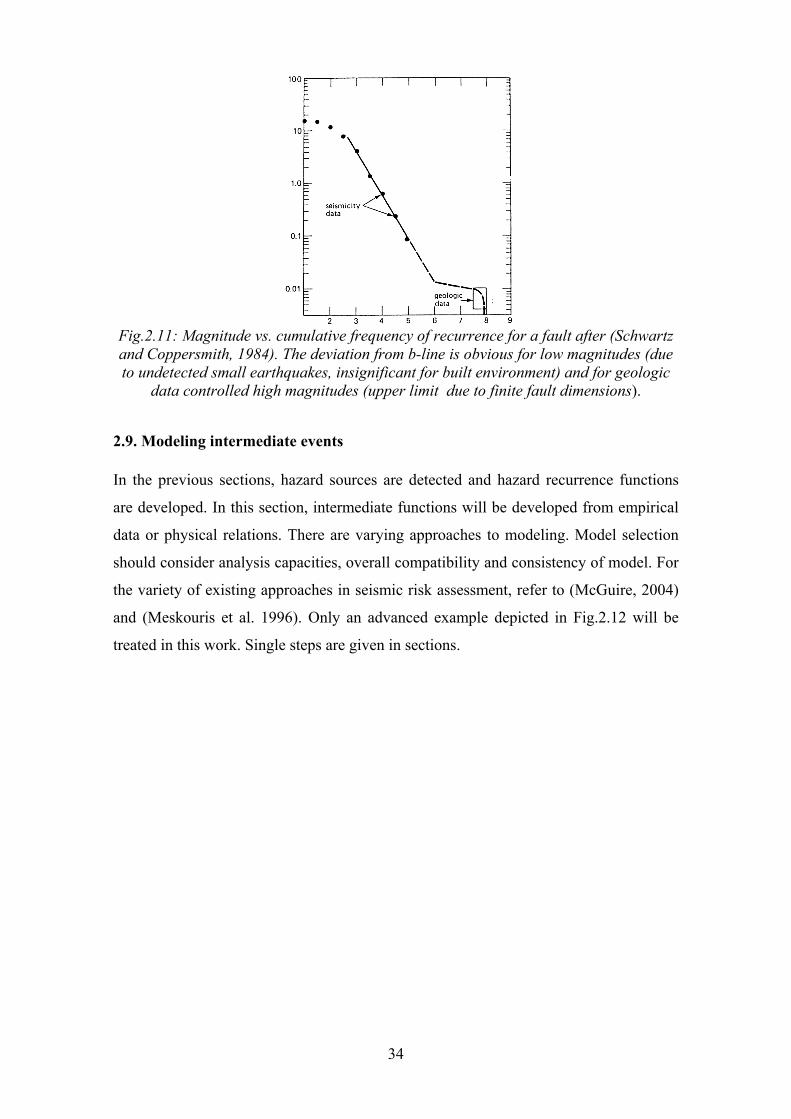
Typically, an inconsistency between geological and seismicity data is observed. This
corresponds to the condition, when c E geof G (m )> , where cf is the characteristic
frequency (equal to 1/Tc, Tc is the characteristic recurrence period) and E geoG (m ) is
calculated according to Eq.5 by relaxing the range of definition. This inconsistency can
be overcome by varying models discussed by e.g. (Ordaz, 2004), (McGuire, 2004),
(Speidel and Mattson, 1997). The latter author mentions that model choice should
depend on fault size, slip rate and length of historical seismicity observation.
An option is combining Eq.5 with uniform distribution for geologic-data-range, which
can be demonstrated as in the following:
min(m m )min int
int geoE geo
geo
m m m1-k k e
m m mG (m) f
m m0
−β − ≤ < + ≤ <=
≤
(14)
where, geom is the characteristic earthquake, intm is the intersection magnitude of
characteristic frequency and b line. intm can be easily extracted by equating cf to
E intG (m ) . Upper limit can be augmented subjectively to geom 0.5+ .
To remind, the output of this step is hazard function GE(x) for each source. The
presented procedure is known as probabilistic seismic hazard analysis.
34
Fig.2.11: Magnitude vs. cumulative frequency of recurrence for a fault after (Schwartz and Coppersmith, 1984). The deviation from b-line is obvious for low magnitudes (due to undetected small earthquakes, insignificant for built environment) and for geologic
data controlled high magnitudes (upper limit due to finite fault dimensions).
2.9. Modeling intermediate events
In the previous sections, hazard sources are detected and hazard recurrence functions
are developed. In this section, intermediate functions will be developed from empirical
data or physical relations. There are varying approaches to modeling. Model selection
should consider analysis capacities, overall compatibility and consistency of model. For
the variety of existing approaches in seismic risk assessment, refer to (McGuire, 2004)
and (Meskouris et al. 1996). Only an advanced example depicted in Fig.2.12 will be
treated in this work. Single steps are given in sections.

35
S Ef (y,z)
R Sf (y,z)
D Rf (y,z)
Y Df (y,z)
= for Y M,I,C, L,N,P
Fig.2.12: Risk assessment approach utilized in this work

36
2.9.1. Strong Motion Function
Aim in this section is to simulate a sufficient number of strong motion time histories to
represent hazard at site.
The motive behind the simulation is the lack of sufficient strong motion records for
most regions of the world. An example is Turkey as stated by (Akinci et al., 2001).
Exceptions are few seismic regions in economically developed countries (like western
North America, Japan and New Zealand). For alternative methods of utilizing processed
instrumental records and deaggregation, see (Wen, 2004).
Previously, it was stated that the magnitudes produced by a fault vary between a lower
and an upper value ( min maxm m m< < or min geom m m< < ). However, simulations will
be carried out for the range of ml<m<mu, with ml as described above and mu referring to
upper magnitude bound for risk assessment. mu can be equal to or slightly smaller than
mmax. Accordingly, simulations will be carried out for discrete magnitude levels at this
range. Decisions on the number of discrete levels and on the number of simulations for
each level will be discussed later.
Let start with analysis of site strong ground motion.
Strong motion time series can be decomposed into two functions: acceleration spectrum
and duration, each of which are dependent on characteristics of (1) source and rupture,
(2) path, (3) local soil and topographic conditions4.
Acceleration spectrum of strong motion at an arbitrary site can be written as (modified
from (Boore, 2003)):
SM S a aa (m, r, f ) a (m,f ) P (r, f ) L (d, f )= (15)
where m is magnitude level under consideration, r is the source-site distance, f is
frequency, as is the source acceleration spectrum, Pa and La are respectively path and
local filter functions, d is depth of local soil considered. Spectrum should be bounded
for a frequency range significant for engineering purposes.
Strong motion duration function can be written as
SM S P Ls s s s= + + (16)
4 Strictly speaking, local site and topographic conditions are a part of path effects, but due to the high sensitivity of site strong motion on their variation, they are treated separately.
37
where ss is the source duration function (syn. rupture duration), sp and sL are
respectively path and local site delay functions. sL can be neglected since sL<< sp,
SM S Ps s s= + (17)
The model deals only with absolute duration (not engineering duration) measures, so sp
is only source-site distance (r) dependent. Thus, problem reduces to obtaining
S a a S Pa (m,f ), P (r, f ), L (d, f ), s , s and simulating sufficient number of time histories
using these.
2.9.1.1. Source spectrum Source spectrum can be expressed after (Boore, 2003) as following;
S Sa (m,f ) C m S (m,f )= (18)
where C is a constant, m is magnitude level under consideration, SS (m,f ) is
displacement spectrum at source, named source spectral shape.
C is given by;
3sC R F V / (4 v )ΘΦ= π ρ (19)
where RΘΦ is the radiation pattern, F is the free surface effect, V is the partition factor
of shear wave energy in two components,ρ and sv are the density and shear wave
velocity in the source vicinity (in SI units).
RΘΦ is obtained by averaging over a range of azimuths and take-off angles (Boore,
2003), can be assumed approximately equal to 0.55 (Kramer 1996)). F is usually
assumed 2, which is actually exact only for SH waves (Boore, 2003). V is equal
to 2 / 2 .
Varying models differ in SS (m,f ) expression, exhaustive list is given by Boore (2003).
A recent model by (Atkinson and Silva, 2000) follows:
S 2 2 2c max
1S (m,f )(1 (f / f ) ) (1 (f / f ) )
− ε ε= ++ +
(20)
Where cf is corner frequency, maxf cutoff frequency and ε is a coefficient given by
log 0.605 0.255mε = − .
For southern Californian conditions, following values are given by (Atkinson and Silva,

38
2000): clog f 2.181 0.496m= − and maxlog f 2.41 0.408m= − (both in Hz)
maxf is otherwise obtained empirically for each geographical region (e.g. typically 15
and 40 Hz respectively for western and eastern North America (Kramer, 1996)).
fc can be derived theoretically (Boore, 2003):
13
6c s
o
f 4.9x10 vm
∆σ=
(21)
where sv (km / sec) as described above, om (dyn cm)⋅ as given in Eq.8, and (bar)∆σ
refering to stress drop. Eq.21 holds for all cases. ∆σ can be shown to be proportional to
mo and the characteristic fault dimension Lf(km) as in the following relation according
to e.g. (Stein and Wyssession, 2003) and (Scholz, 2002):
3s o fc m / L∆σ = (22)
where cs is fault shape factor. Eq.22 applied to strike-slip regime on a rectangular fault
(which is the case for example in Chapter 3) yields
o2
f
m2w L
∆σ =π
(23)
where w (km) is fault width. Simplifying Eq.11 by eliminating ∆σ and om , yields
13
6c s 2
f
2f 4.9x10 vw L
= π
(24)
Solutions for other shapes and regimes can be found in (Scholz, 2002).
Utilization of seismicity regression models (e.g. Eq.20) and maxf values developed for
certain regions should be avoided in other seismologic settings.
The cornerstone of source spectrum models is the typical shape of ground motion
spectrums marked with a corner frequency cf on low side of the spectra, an intermediate
plateau region and a cutoff frequency maxf on high side. This is seen in Fig.2.13. For
theoretical support of the models, refer to (Stewart et al., 2002).
39
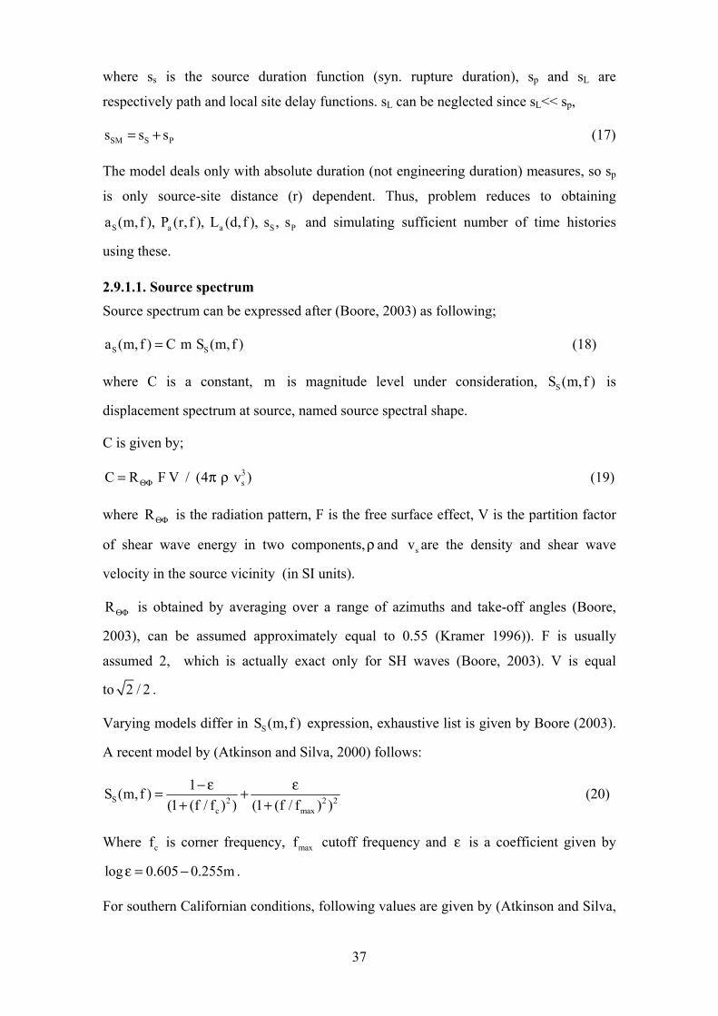
Fig.2.13. Acceleration spectra from two instrumental records of a m=7.1 event (Düzce,
Turkey, 11/12/1999) Source-instrument distances (closest to surface projection of rupture) are respectively 8.2 and 17.6 km. Similar corner and cutoff frequencies fc and fmax at ca. 0.04 and 40 Hz are visible. This property constitutes cornerstone of stochastic
source spectrum simulation method (source for records is (PEER, 2005), processed with software (SEISMOSIGNAL, 2005))
2.9.1.2. Path model The aim of this step is modeling path effects on spectrum. Those effects depend on
source-site distance and stratigraphy and rheology of the path.
Seismogenic sources (in other words active faults) are modeled as point, linear, areal or
volumetric sources. The selection of model shape depend on two factors:
(1) geometry of the source,
(2) ratio of source-site distance to fault size (higher ratios justify simpler models).
Usual assumptions are:
(1) all seismic energy is radiated from hypocenter,
(2) hypocenters of potential earthquakes are uniformly distributed along the fault.
Assumption (2) does not necessarily imply a uniform distribution of source-site

40
distance. So, source-site distance can be modeled by probability density functions
obtained through analytical or numerical methods, depending on the complexity of
source. For an example, refer to (Kramer, 1996).
Given the spatial distribution of hypocenter along the fault, path effect on the source
spectrum can be estimated by the following relation after (Boore, 2003) and (Kawase,
2003):
a sP (r, f ) g(r) exp[ f r / Q(f ) v ]= −π (25)
where g(r) and Q(f ) are described below and sv is the representative shear wave
velocity of the whole path. Eq.25 is derived from theory of wave propagation.
g(r) , geometrical spreading function, is the measure of energy distribution according
to (Lay and Wallace, 1995), and, is given by a piecewise continuous function after
(Boore, 2003):
( )
( )
1
n
o 1p
1 1 1 2
pn1 1
r / r r rQ r r / r r r r
g(r)
r rQ r r / r
<
< <= <
(26)
r is usually taken as the closest distance to the rupture surface (D) (or as equal to
2 2D h+ , where h is a period- and/or moment-dependent pseudo-depth). ip and ir
for 1 i n< < are to be estimated empirically (h is more important for <m=6.5 and for
near field, example values from an application by Atkinson and Boore (1995) for
eastern North America: o 1 2 1 2n 3, r 1, r 70, r 130, p 0.0, p 0.5= = = = = = ).
Q(f ) , attenuation operator, is the measure of energy loss. It can be idealized as a
piecewise continuous exponential function after (Boore, 2003):
t1
t1 t 2
t2
a f f fQ(f ) b f f f f
c f f f
α
β
ε
<= < < <
(27)
where a, b, c, 1 2t t, , , f , fα β ε are to be determined from regional analysis of weak-or
strong-motion data as stated by (Boore 2003).
41
2.9.1.3. Local soil and topographic effects model
This step involves estimation of local effects filter function a sL (d , f ) , ds indicates the
depth of soil profile considered and f frequency.
This function broadly includes;
(i) amplification through local younger strata over bedrock (wave impedance)
(ii) soil-nonlinearity induced de-amplification and predominant period prolongation
(iii) site diminution
(iv) sedimentary-basin related phenomena (basin-induced and -transduced surface
waves, edge effect, focusing)
(v) topographic amplification (ridge, hilltop) and deamplification (canyon, slope foot)
So, local effects on spectrum can be formulated as:
s n d b ta s a s a s a s a s aL (d , f ) L (d , f )L (d , f )L (d , f )L (d , f )L (f )= (28)
The study of these effects is commonly referred as geotechnical earthquake
engineering5. Due to vastness of the whole subject, a model will be given only for (i),
namely for sa sL (d , f ) of Eq.28.
(Note: (ii) can be integrated by equivalent linear or nonlinear soil models after (Pecker,
2005). (iii) is discussed by (Boore, 2003) providing a filter function for it. (iv) requires
2D or 3D modeling as stated by (Kawase, 2003). Simple formula for (v) can be found in
Kramer (1996) and EUROCODE 8, detailed discussion in (Faccioli and Vanini, 2003).
(Kawase, 2003) mentions the difficulties in modeling (v) due to highly varying
observations.)
According to (Pecker, 2005), (i) can be modeled in one-dimensional space with the
following assumptions:
(1) horizontally homogeneous and vertically varying medium (reasonable due to
mechanics of deposition and weathering),
(2) vertical wave propagation (justified by gradually upwards decreasing stiffness of
5 Its significance stems from the fact that site effects may cause amplifications in amplitudes up to two orders of magnitude, as stated by Kawase (2003).

42
strata over bedrock, which causes successive refraction)
In this context, exact theoretical amplification relation for a sinusoidal wave is given by
e.g. Kawase (2003). (Boore, 2003) provides an approximate relation for this:
sa s sL (d , f ) Z / Z(f )=
(29)
where sZ is seismic impedance at bedrock given by
s s sZ v= ρ (30)
where sρ is density and sv is shear-wave velocity at bedrock.
Z(f ) is the time-weighted average of seismic impedance from the surface down to a
depth of ¼ wavelength (this criteria determines sufficient ds for sa sL (d , f ) computation).
It is given by the following expression after (Boore, 2003):
sZ(f ) (f ) v (f )= ρ (31)
where (f )ρ is the average density, sv (f ) is the average shear wave velocity, given by
following expressions:
z(f )
0
1(f ) (z) dzz(f )
ρ = ρ∫ (32)
1z(f )
ss0
1v (f ) z(f ) dzv (z)
−
= ∫ (33)
where z(f ) is the depth of ¼ wavelength, (z)ρ is the density at depth z, sv (z) is the
shear wave velocity at depth z.
For the derivation of Eq.31 and following, refer to (Boore, 2003).
Implementation of the above formulae requires stratigraphic profile providing
sv (shear-wave velocity) and sρ (density) down to a depth of ¼ wavelength for the
lowest frequency considered. This is commonly 1 Hz for engineering purposes after
(Kramer and Stewart, 2004). This is usually an uneconomical task with existing
borehole techniques. For that reason, common practice is using amplification factors
derived from averaged sv in upper 30 m. This empirically supported approach is
referred as s 30v − scheme. In this scheme, variation of density ( sρ ) is not considered
43
due to the little variation at these depths. Selection of 30m as threshold is a convention
without any scientific reason.
s 30v − scheme is the basis for amplification factors given by seismic design provisions.
For detailed discussion, refer to (Kramer and Stewart, 2004).
2.9.1.4. Source duration model
Source duration is commonly modeled as inversely proportional to cf (corner
frequency):
1S cs (m) a.f −= (34)
whereas the constant a range between 0.5 to 1.0 among varying models (Boore, 2003).
An expression for cf is given by Eq.11
In the example in Chapter 3, this model is used with a=0.5 in line with (Atkinson and
Silva, 2000).
Logically, source duration should be proportional to source size (area or length) and
rupture velocity. After (Kramer, 1996), sS can be shown to be proportional to 3om .
Other theoretical and empirical approaches are not further discussed due to the
limitations of this work. Note that, engineering duration measures (bracketed,
significant etc.) are not of interest for the method.
2.9.1.5 Path delay model According to Boore (2003), path delay can be related to source-site distance r with a
piecewise function as in the following:
1
P 1 2
2
a r r rs (r) b / r r r r
c r r r
>= < < <
(35)
This relation is based on theoretical simulations and empirical data. However,
observations relieve significant dispersion from formula according to (Boore, 2003).
2.9.1.6. Simulation Initial decisions to take are
(1) discrete magnitude levels for simulations,
(2) number of simulations for each level.
44
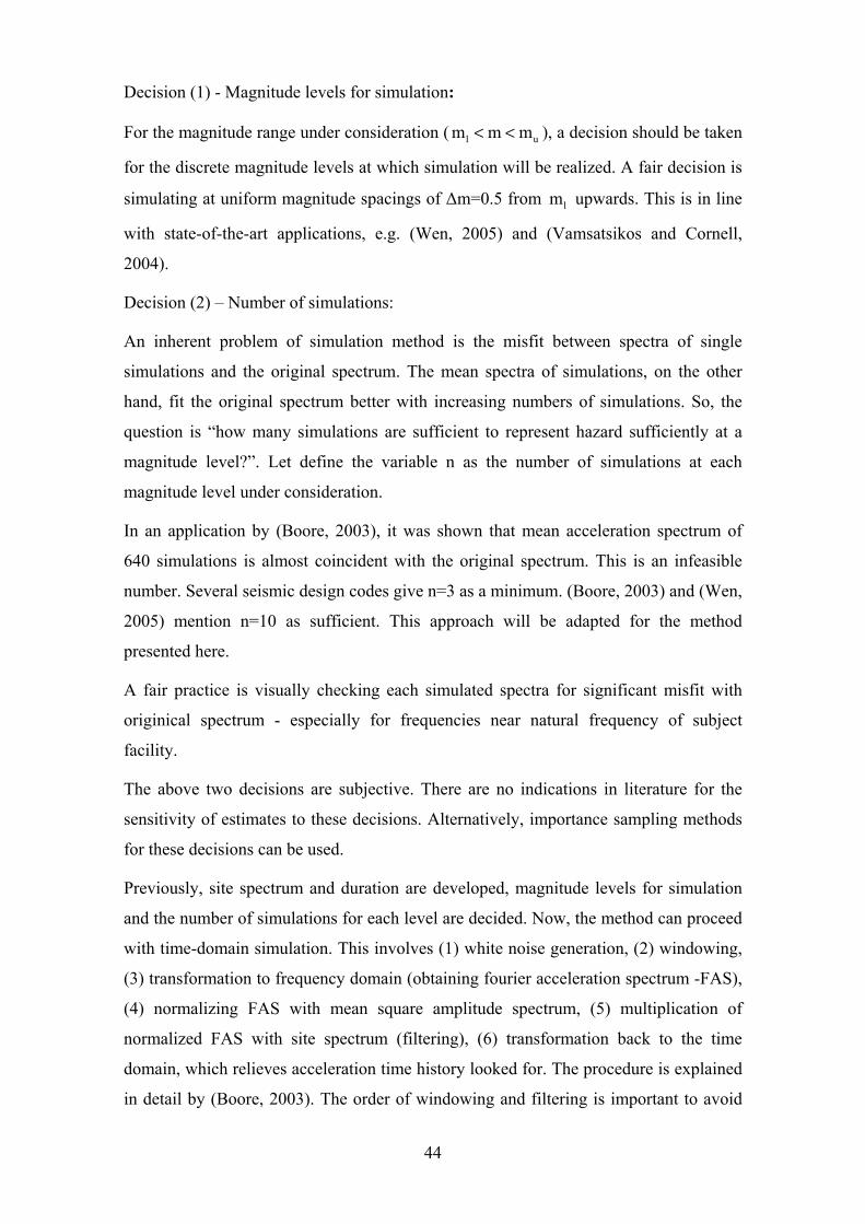
Decision (1) - Magnitude levels for simulation:
For the magnitude range under consideration ( l um m m< < ), a decision should be taken
for the discrete magnitude levels at which simulation will be realized. A fair decision is
simulating at uniform magnitude spacings of ∆m=0.5 from lm upwards. This is in line
with state-of-the-art applications, e.g. (Wen, 2005) and (Vamsatsikos and Cornell,
2004).
Decision (2) – Number of simulations:
An inherent problem of simulation method is the misfit between spectra of single
simulations and the original spectrum. The mean spectra of simulations, on the other
hand, fit the original spectrum better with increasing numbers of simulations. So, the
question is “how many simulations are sufficient to represent hazard sufficiently at a
magnitude level?”. Let define the variable n as the number of simulations at each
magnitude level under consideration.
In an application by (Boore, 2003), it was shown that mean acceleration spectrum of
640 simulations is almost coincident with the original spectrum. This is an infeasible
number. Several seismic design codes give n=3 as a minimum. (Boore, 2003) and (Wen,
2005) mention n=10 as sufficient. This approach will be adapted for the method
presented here.
A fair practice is visually checking each simulated spectra for significant misfit with
originical spectrum - especially for frequencies near natural frequency of subject
facility.
The above two decisions are subjective. There are no indications in literature for the
sensitivity of estimates to these decisions. Alternatively, importance sampling methods
for these decisions can be used.
Previously, site spectrum and duration are developed, magnitude levels for simulation
and the number of simulations for each level are decided. Now, the method can proceed
with time-domain simulation. This involves (1) white noise generation, (2) windowing,
(3) transformation to frequency domain (obtaining fourier acceleration spectrum -FAS),
(4) normalizing FAS with mean square amplitude spectrum, (5) multiplication of
normalized FAS with site spectrum (filtering), (6) transformation back to the time
domain, which relieves acceleration time history looked for. The procedure is explained
in detail by (Boore, 2003). The order of windowing and filtering is important to avoid
45
distortion of low-frequency motion. A suitable windowing equation is given by Boore
(2003):
bw(t, , , t ) a (t / t ) exp( c(t / t ))η η ηε η = − (36)
where a,b and c are determined so that w(t) equals the maximum 1 when t tη= ε and
w(t) = η when t tη= . a,b and c follow
wb ( ln ) /(1 (ln 1))= − ε η + ε ε − (37)
wc b /= ε (38)
wbwa (e / )= ε (39)
The latter author propose 0.2ε = and 0.05η = for applications.
Several authors provide programs for time domain simulation. An example is the open-
source Fortran program given and explained in (Boore, 2000). The reader is
recommended to utilize this program, since its background is well documented in
several publications like (Boore, 2003).
One must note that the variability in simulated time histories at a given magnitude level
is not representative for actual variability of ground motion.
As reminder, the output from this stage is a suite of time histories for each hazard level
(appr. 50 to 80 time histories) to represent site hazard.
2.9.2. Strong motion - response intermediate function R Sf (x)
The aim in this step is obtaining response governing variables for the considered hazard
range.
Initial decision is which response governing variables are sufficient and efficient
indicators of damage and loss. (Vamsatsikos and Cornell, 2004) provide in this context
the list in Table 2.6.
The approach presented there is in line with recent research: (Sarabandi et al., 2005)
proves more than 80% correlation between percent loss and interstorey drift ratio among
24 steel structures effected by Northridge 1994 Earthquake. (Boatwright et al., 2001)
shows similar high correlations between municipal safety tagging6 intensity and
6 Post-earthquake procedure of declaring buildings as uninhabitable by state officials.
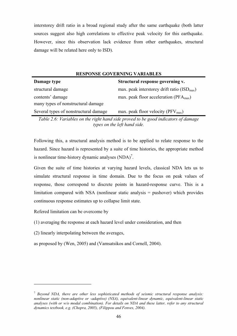
46
interstorey drift ratio in a broad regional study after the same earthquake (both latter
sources suggest also high correlations to effective peak velocity for this earthquake.
However, since this observation lack evidence from other earthquakes, structural
damage will be related here only to ISD).
RESPONSE GOVERNING VARIABLES Damage type Structural response governing v. structural damage max. peak interstorey drift ratio (ISDmax) contents’ damage many types of nonstructural damage
max. peak floor acceleration (PFAmax)
Several types of nonstructural damage max. peak floor velocity (PFVmax) Table 2.6: Variables on the right hand side proved to be good indicators of damage
types on the left hand side.
Following this, a structural analysis method is to be applied to relate response to the
hazard. Since hazard is represented by a suite of time histories, the appropriate method
is nonlinear time-history dynamic analyses (NDA)7.
Given the suite of time histories at varying hazard levels, classical NDA lets us to
simulate structural response in time domain. Due to the focus on peak values of
response, those correspond to discrete points in hazard-response curve. This is a
limitation compared with NSA (nonlinear static analysis = pushover) which provides
continuous response estimates up to collapse limit state.
Refered limitation can be overcome by
(1) averaging the response at each hazard level under consideration, and then
(2) linearly interpolating between the averages,
as proposed by (Wen, 2005) and (Vamsatsikos and Cornell, 2004).
7 Beyond NDA, there are other less sophisticated methods of seismic structural response analysis: nonlinear static (non-adaptive or -adaptive) (NSA), equivalent-linear dynamic, equivalent-linear static analyses (with or w/o modal combination). For details on NDA and these latter, refer to any structural dynamics textbook, e.g. (Chopra, 2005), (Filippou and Fenves, 2004).

47
2.9.3. Response-damage intermediate function D Rf (x)
Current task is estimating damage from structural response governing variables. It is
referred as damageability analysis8. A component-based approach will be adapted. This
means that damage will be estimated separately for each component type.
The term “component” refers to all structural and nonstructural components and
contents of the facility. Structural components are foundation components, columns,
beams, girders, decks etc. Nonstructural components comprise architectural (claddings,
ceilings, doors, windows, partitions etc.) and mechanical, electrical and plumbing
components (elevators, lights, piping, ducts, heating-ventilation-air condition systems
(HVAC), security systems, fire protection systems, communication systems etc.).
Contents comprise equipment, furniture and stored goods.
Damageability data relates structural response to component damage and is obtained
empirically (mainly experimentally) for each component type.
To enhance readability, the procedure is presented in steps:
Step I. Prepare a component inventory
Prepare an inventory of damageable component types making up the facility. A
component type is group of components with same damageability property (e.g. solid
brick wall of 3mx3m dimensions). If dimension is not relevant for damageability, a
component type may comprise units with varying dimensions as well.
The inventory includes
- list of component types,
- component class of each type (structural, nonstructural or content),
- performance group of each type (drift-, acceleration- or velocity-sensitive), and,
- number of components of the particular type in varying floor levels.
Performance groups are given in Table.2.7. Distinguishing between floor levels in
inventory enables to account for varying response at each floor level. The performance
group classification is due to empirical evidence. An exhaustive list of component types
can be found in (Taghavi and Miranda, 2003).
8 Used instead of “fragility” to avoid confusion, since latter is used interchangeably with vulnerability.

48
Damageability is not to more than two response governing variables here, for the sake
of simplicity and in line with the state-of-the-art (Moehle et al. 2005, Porter et al. 2001).
PERFORMANCE GROUPS
Performance group Comprises mainly SRGV Examples
Drift sensitive structural c.s ISDmax columns,beams,connections, walls,piping, glass,ornamentation
Acceleration sensitive Content some nonstructural c.s
PFAmax mechanical eq., electrical eq., suspended ceiling, elevators
Velocity sensitive some nonstructural c.s PFVmax Table 2.7: Performance group classification for building components. SREV (structural
response governing variable) selection is in line with evidence presented in section 2.9.2.2. after (Beck et al., 2002) (Moehle et al., 2005)
Step II. Define damage states
In this step, for each component type, a series of discrete damage states is defined.
Those should be experimentally observable and meaningful for repair actions.
Accordingly, after any earthquake, any component would be in one of several damage
states D=0,1,2,3,…n. D=0 denotes undamaged state.
(Porter et al. 2001) gives the assumptions in this approach as mutually-exclusiveness,
collectively-exhaustiveness and progressiveness of damage states. Progressiveness
means that the component under consideration should pass through damage state k to
reach damage state k+1.
Step III. Extract damageability curve
A damageability curve (DC) exposes exceedance probability of each damage state in
relation to a response governing variable. They are drawn separately for each
component type with the appropriate response governing variable. So, taking n =
number of component types in the facility, n damageability curves are needed. State-of-
the-art for producing damageability curves is lognormal fit on experimental data.
The vastness of damageability information brings in a data management problem. To
overcome this, the tabular presentation for each component type in Table.2.8 can be
used. This table combines approaches by (Taghavi and Miranda, 2003), (Krawinkler
and Miranda, 2004) and (Beck et al 2002).

49
Tabl
e 2.
8: D
amag
eabi
lity
and
rest
orat
ion
cost
dat
a fo
r a c
ompo
nent
. **
(col
umn
11) r
esto
ratio
n co
st /c
ompo
nent
val
ue
1 2
3 4
5 6
7 8
9 10
11
12
Capacity
**
Restoration
Duration hours/unit
Type no. Component type Dimension
Class
Performance Group
Damage State
Typ
e of
con
sequ
ence
In
form
atio
n S r
ev
µ σ
µ σ
µ σ
0 -
- -
-
- -
- -
Rep
air a
ctio
n M
inor
repa
ir o
f ext
erio
r fin
ishe
s D
amag
e co
nseq
uenc
e N
o B
uild
ing
func
tiona
lity
Ful
ly fu
nctio
nal
Life
safe
ty
Non
e 1
Com
pone
nt lo
ss o
f fun
ctio
n N
one
ISD
0.0039
0.15
0.0005
0.01
10
0.10
Rep
air a
ctio
n So
me
part
s may
nee
d de
mol
ition
and
re
cons
truc
tion.
Dam
aged
are
a ne
ed re
pair
ex
teri
or fi
nish
Dam
age
cons
eque
nce
EM
D o
n w
all p
oss.
stop
func
tion+
nee
d re
pair
Bui
ldin
g fu
nctio
nalit
y Lo
ss-o
f-us
e of
adj
acen
t roo
ms u
ntil
end
of
repa
ir
Life
safe
ty h
azar
d Sm
all
2
Com
pone
nt lo
ss o
f fun
ctio
n M
oder
ate
ISD
0.063
0.26
0.0045
0.10
36
0.20
Rep
air a
ctio
n C
ompl
ete
dem
oliti
on o
f dam
aged
are
a.
Rec
onst
ruct
ion.
D
amag
e co
nseq
uenc
e E
MS
may
bre
ak o
r not
wor
k
Bui
ldin
g fu
nctio
nalit
y Lo
ss-o
f-us
e of
adj
acen
t roo
ms u
ntil
end
of
reco
nstr
uctio
n.
Life
safe
ty
Hig
h
1
Solid brick wall
3m x 3m
Nonstructural
Acceleration- sensitive
3
Com
pone
nt lo
ss o
f fun
ctio
n H
igh
ISD
0.09
0.30
0.0125
0.03
120
0.40

50
Step IV. Mathematical formulation of damageability
The aim in this section has been to model D Rf (d, r) , conditional probability distribution
function of membership to damage state d, conditioned on structural response. In the
following, corresponding mathematical formulation will be presented. For a particular
component and a damage state d, d {0,1,2,.., n}∈ , one can write:
D Rf (d, r) p[D d R r]= = = (40)
where D denotes damage state and R denotes structural response.
Let denote the capacity of the component to resist the damage state d by a random
variable dX . Then we can write;
dd Xp[D d R r] p[r X ] F (r)≥ = = > = (41)
with dXF (r) denoting the cumulative probability distribution function of dX evaluated at
r.
As stated earlier, lognormal probabilistic model is commonly used for dXF (r) , which
can be given for any r by:
d
dX
d
ln(r / )F (r) ( )µ= Φσ
(42)
where dµ and dσ is the mean and standard deviation of dX and vary by component type
and damage state (can be found in column 10 and 11 in Table 2.8). Since being in a
damage state conditioned by response is lower-bounded by dX and upper-bounded by
d 1X + , we can write the following:
d d 1
d d 1d d 1 X X
d d 1
ln(r / ) ln(r / )p[D d R r] p[r X ] p[r X ] F (r) F (r) ( ) ( )+
++
+
µ µ= = = ≥ − ≥ = − = Φ − Φσ σ
(43)
Where ( )Φ denotes the cumulative standard normal distribution evaluated at the term in
parentheses. Equating Eq.40 and Eq.43 yields;
d d 1D R
d d 1
ln(r / ) ln(r / )f (d, r) ( ) ( )+
+
µ µ= Φ − Φσ σ
(44)
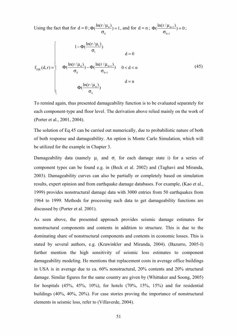
51
Using the fact that for d 0= ; d
d
ln(r / )( ) 1µΦ =σ
, and for d n= ; d 1
d 1
ln(r / )( ) 0+
+
µΦ =σ
;
1
1
d d 1D R
d d 1
n
n
ln(r / )1 ( )d 0
ln(r / ) ln(r / )( ) ( )f (d, r) 0 d n
d nln(r / )( )
+
+
µ − Φ σ = µ µ Φ − Φ= < < σ σ
=µ Φ σ
(45)
To remind again, thus presented damageability function is to be evaluated separately for
each component-type and floor level. The derivation above relied mainly on the work of
(Porter et al., 2001, 2004).
The solution of Eq.45 can be carried out numerically, due to probabilistic nature of both
of both response and damageability. An option is Monte Carlo Simulation, which will
be utilized for the example in Chapter 3.
Damageability data (namely iµ and iσ for each damage state i) for a series of
component types can be found e.g. in (Beck et al. 2002) and (Taghavi and Miranda,
2003). Damageability curves can also be partially or completely based on simulation
results, expert opinion and from earthquake damage databases. For example, (Kao et al.,
1999) provides nonstructural damage data with 3000 entries from 50 earthquakes from
1964 to 1999. Methods for processing such data to get damageability functions are
discussed by (Porter et al. 2001).
As seen above, the presented approach provides seismic damage estimates for
nonstructural components and contents in addition to structure. This is due to the
dominating share of nonstructural components and contents in economic losses. This is
stated by several authors, e.g. (Krawinkler and Miranda, 2004). (Bazurro, 2005-I)
further mention the high sensitivity of seismic loss estimates to component
damageability modeling. He mentions that replacement costs in average office buildings
in USA is in average due to ca. 60% nonstructural, 20% contents and 20% structural
damage. Similar figures for the same country are given by (Whittaker and Soong, 2005)
for hospitals (45%, 45%, 10%), for hotels (70%, 15%, 15%) and for residential
buildings (40%, 40%, 20%). For case stories proving the importance of nonstructural
elements in seismic loss, refer to (Villaverde, 2004).

52
Above presented damageability approach differs in many ways from conventional
fragility approaches, since it
(1) accounts for nonstructural components and contents damage,
(2) relates structural damage to response (instead of to hazard by means of conventional
fragility curves9 or damage indices10),
(3) utilizes probabilistic treatment of damage,
(4) uses component-based damage states (instead of macroscopic – global performance
levels).
2.9.4. Damage-loss and response-collapse intermediate functions The task in this section is obtaining the remaining intermediate functions and facility-
specific parameters.
2.9.4.1. Collapse probability model
Collapse probability is related to structural response as proposed by state-of-the-art.
The aim is to find collapse probability C Rf (c 1, r)= in Eq.1, where c denotes the
indicator variable of collapse (c=1 implying collapse, c=0 no collapse), and, r denotes
the (uncertain) response.
Leaning on the discussion on damage states in section 2.9.2.3., one can write
alternatively
C Rf (C 1, r) p[C 1 R r]= = = = (46)
Let treat the whole structure as a component in line with section 2.9.2.3.. Let denote the
capacity to resist collapse with CX . Research shows that lognormal distribution for the
random variable CX can be assumed. Probability of collapse can then be written as
CC Xp[C 1 R r] p[r X ] F (r)= = = ≥ = (47)
With CXF (r) denoting the cumulative probability distribution function of CX evaluated
9 For explanation of conventional fragility analysis, refer to ( Shinozuka et al. 2000) 10 For treatment of conventional damage indices, refer to (Williams and Sexsmith, 1995).
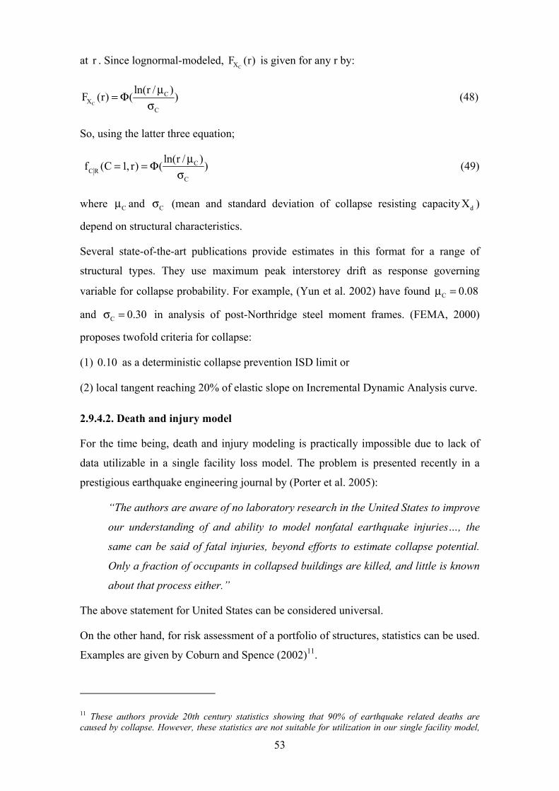
53
at r . Since lognormal-modeled, CXF (r) is given for any r by:
C
CX
C
ln(r / )F (r) ( )µ= Φσ
(48)
So, using the latter three equation;
CC R
C
ln(r / )f (C 1, r) ( )µ= = Φσ
(49)
where Cµ and Cσ (mean and standard deviation of collapse resisting capacity dX )
depend on structural characteristics.
Several state-of-the-art publications provide estimates in this format for a range of
structural types. They use maximum peak interstorey drift as response governing
variable for collapse probability. For example, (Yun et al. 2002) have found C 0.08µ =
and C 0.30σ = in analysis of post-Northridge steel moment frames. (FEMA, 2000)
proposes twofold criteria for collapse:
(1) 0.10 as a deterministic collapse prevention ISD limit or
(2) local tangent reaching 20% of elastic slope on Incremental Dynamic Analysis curve.
2.9.4.2. Death and injury model
For the time being, death and injury modeling is practically impossible due to lack of
data utilizable in a single facility loss model. The problem is presented recently in a
prestigious earthquake engineering journal by (Porter et al. 2005):
“The authors are aware of no laboratory research in the United States to improve
our understanding of and ability to model nonfatal earthquake injuries…, the
same can be said of fatal injuries, beyond efforts to estimate collapse potential.
Only a fraction of occupants in collapsed buildings are killed, and little is known
about that process either.”
The above statement for United States can be considered universal.
On the other hand, for risk assessment of a portfolio of structures, statistics can be used.
Examples are given by Coburn and Spence (2002)11.
11 These authors provide 20th century statistics showing that 90% of earthquake related deaths are caused by collapse. However, these statistics are not suitable for utilization in our single facility model,

54
For the current model, a collapse dependent death and injury model is assumed, with
75% dead and 25% injured among occupants in collapse limit state and no injury or
death due to any component or partial damage states.
Another component of this task is occupancy modeling. There are occupancy statistics
in literature e.g. given by (Coburn and Spence, 2002). Adaptation of these for single
facility case however can not be justified. So, considering lack of suitable information,
approximate assumptions can be made. For example, 18 hour occupancy for residential
use, 10 hour occupancy for other social use (public, business, recreational). The subject
of occupancy models for single facility deserves extended research.
2.9.4.3. Restoration cost model
The aim of this step is to model restoration cost for each component. This is denoted by
V Df (v,d) , refering to the probability distribution of normalized restoration cost
conditioned on (uncertain) damage state. Normalized restoration cost means component
restoration cost divided by mean new construction cost of the whole facility (CT).
Similar to damage models, lognormal models are utilized. So, for each component type
and each damage state, two parameters (mean and standard deviation) are needed for the
model. In the previously given sample damageability table in Table 2.8, corresponding
information is in Column 11.
Restoration cost data can be gathered from statistics and expert opinion. It is worth to
note that, only the direct costs (costs of labor, material, equipment) due to construction
and demolition are modeled in this task. For further discussion, refer to (Krawinkler and
Miranda, 2004) and (Porter et al., 2001).
since they are regressed from a population dispersed both in time and location The authors moreover provide death data classified among reinforced concrete (RC) and masonry structures and among near-field/high-frequency and distant/low-frequency dominant ground motion. These statistics show that in RC structures, at average, 50 to 70% of occupants remain trapped after a collapse. Among the factors effecting the ratio is building height. Among the trapped, average survival rates range from 10 to 30%. For a rough approximation for our model –translating reinforced concrete data to all types of structures- using the worst case values of the above, we can assert; ratio of deaths in occupant population = 70%*90%=63%~65%, injured among occupant population = 70%*10%= 7%~10% assuming that there are no injuries in case of no collapse. The assumptions are too tight and we use a regressive data from a very dispersed population both in time and location, which is rather suitable for using in macroseismic models.

55
2.9.4.4. Serviceability interruption model
Related statistical data is scarce as stated by (Porter et al., 2001). The approach
proposed here is to sum up all restoration durations for each single component. This is
based on following assumptions:
(1) Partial usability of the facility during restoration of a partial damage is neglected.
(2) Possibility of simultaneous restoration for any two components is neglected.
Scarcity of related statistical data (stated e.g. by (Porter et al., 2001), (Coburn and
Spence, 2002)) justifies the assumptions. Collapse state is excluded in the model.
Similar to the previous models, lognormal distribution is used. Necessary information is
given in Column 12 of the proposed sample damageability table in Table 2.8.
2.9.4.5. Monetary loss model -due to tangibles-
There are three components of monetary loss due to tangibles:
(1) restoration costs,
(2) serviceability interruption costs,
(3) loss due to collapse.
(1) and (2) are considered for partial damage range, (3) for collapse limit state. (1) and
(2) are modeled probabilistically, whereas (3) is based on deterministic estimate. (3)
contains by definition the serviceability interruption costs due to collapse
Two deterministic parameters should be estimated for this step:
CSI: mean cost of unit time serviceability interruption cost
CT: mean new construction cost of the whole facility (as refered in 2.9.4.3)
2.10. Solution and dealing with uncertainty
Each function contained in loss equations of Table 2.4 is explained above.
Solution of loss equations of Table 2.4 can not be carried out with analytical methods
due to the probabilistic and nonlinear relations. Numerical iterative techniques (like
Monte Carlo Simulation or First-Order Second Moment (FOSM)) should be utilized. In
the example given in Chapter 3, Monte Carlo Simulation is used. For an alternative
solution method (FOSM), refer to (Baker and Cornell, 2005).

56
The resulting risk estimates is called “risk profile”.
Accompanying the model solution, is the task of model validation. This is an important
and complicated task. It can be explained as seeking evidence to support or reject the
model.
This task include validation of following components of the model:
(1) phenomenological understanding,
(2) selection of governing variables,
(3) hazard model,
(4) probabilistic models and parameters of intermediate events.
Following strategies can be used for validation:
(1) comparison with observed data,
(2) comparison with other models,
(3) expert-opinion and review.
Risk assessment model validation should be object-oriented. That means it should be
validate that the model do not lead to wrong risk management decisions, rather than
seeking precision.
The previously presented model is constructed on the basis of state-of-the-art
publications. Due to this reason and due to the dimensions of this work, the task of
model validation will be skipped.
An important validation issue is treatment of uncertainty in loss estimate models12. A
practical question for the presented model is if uncertainty treatment is integrated
sufficiently.
The high uncertainty surrounding seismic loss estimate models is related to several
factors. (Bazurro, 2005) mentions in this context high sensitivity of loss estimates to:
(1) hazard analysis method,
12 Motives for addressing uncertainty in earthquake engineering is discussed by several authors: (Wen, 2004) mentions the undefined collapse and damage reliability of conventional procedures. (Bazurro, 2005) compares analysis examples with and without uncertainty treatment and show fallacy of latter. Uncertainty treatment is introduced gradually into seismic design codes (e.g. FEMA 350). For detailed treatment, refer to (Wen, 2004) and (Coburn and Spence, 2002).

57
(2) detailed soil description,
(3) directivity effects (especially in case of flexible structures),
(4) hazard description by a single ground motion parameter or a vector,
(5) (for macro risk management) accounting or neglecting for ground motion
correlation.
In the model presented, (1) and (4) are dealt with state-of-the-art methods; respectively,
with probabilistic seismic hazard analysis and stochastic strong motion simulation.
Concerning (2), only impedance effects are addressed. Factor (3) is not addressed in our
model. The model can be extended for the lacking components with future work.
On the other hand, (Porter, 2002) lists the top three contributors to uncertainty in
seismic loss estimates as:
(1) component capacity,
(2) shaking intensity, measured by damped elastic spectral acceleration,
(3) details of the ground motion given elastic spectra.
(Porter, 2002) includes case studies proving this assertion.
In line with the discussion above, presented method addresses (2) and (3) by stochastic
simulation of strong motion, and (1) by component-based approach.
(Wen, 2005) mention uncertainty in demand is much higher than that of capacity.
So, it can be asserted that the presented model treats major sources of uncertainty
recognized by the state-of-the-art. Detailed soil description and directivity effects are
lacking and can be integrated in the model by future work.
58
Chapter 3. Example application of the method
This chapter includes an example application of the risk assessment method discussed
in Chapter 2. The method reflects state-of-the-art of earthquake engineering and seismic
risk management. The method is actually applicable to more complex facilities with
arbitrary number of components and contents.
3.1. Problem statement
An owner demands annual seismic loss estimates for a facility, in order to use them for
risk management decisions. The facility is used for electrical supplies control and is
classified as a critical facility with full-time occupancy and operation. Relevant facility
data can be taken from Table 3.1, structural information from Fig.3.1 and Fig.s 5.5 and
5.6. Component inventory is depicted in Fig.s. 3.2 and 3.3. The task to be fulfilled is the
calculation of appropriate loss estimates.
3.2. Construction of mathematical model
The solution follows the algorithm constructed in Chapter 2.
It starts with hazard tree construction in Fig.3.4. This figure demonstrates the client
qualitatively the consequences of a potential earthquake on the facility.
Next step is risk measures decision. Appropriate risk measures are given in Table 3.2.
This follows construction of loss trees (refer to previous Fig.s 2.4, 2.5, 2.6, 2.8, not
repeated here). Next step is the decision on governing variables to represent each event
in loss trees, summarized in Table 3.3. All these steps serve for construction of
mathematical model presented in Table 3.4.

59
RELEVANT DATA FOR SEISMIC RISK ASSESSMENT Occupancy
3 persons full-time
Total structural reconstruction cost
300 000 euros
Cost of 1 hour loss of use
1000 euro
Geographical location
39.9160° N, 39.4064° E. In Province of Erzincan, Turkey.
Site soil conditions
average shear wave velocity at 30m profile, vs-30 200 m/s
susceptibility to topographic/basin amplification, ground failure (liquefaction, landslide, cracking)
none according to expert opinion
Structural components inventory
column profile HEA200 3m (12), beam profile HEA 200 5m (6), beam profile HEA 140 3m (6), cross brace L70x70 4.3m (12) (see Fig. 3.1 and 4.2)
Nonstructural components inventory
reinforced concrete deck 5mx3m (3), brick wall 3mx3m (6), brick wall 5mx3m (6), window 1mx1m (3), door 1mx2m (1), spiral stair 0.8mx6m (1) (see Fig. 3.3)
Contents inventory
generator (1), PC (2), technical precision equipment (2), electrical wiring, furniture (see Fig.3.3)
Table 3.1.
RISK MEASURES M number of hazard induced deaths in one year
I number of hazard induced injuries in one year
N hazard induced restoration (repair and replacement) cost in one year
P hazard induced monetary loss –due to tangibles- in one year Table 3.2

60
Fig. 3.1
Fig. 3.2
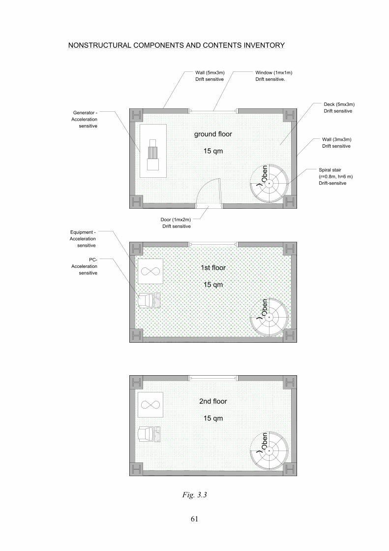
61
ground floor
15 qm
Obe
n1st floor
15 qm
Obe
n
2nd floor
15 qm
Obe
nPC-
Acceleration sensitive
Equipment -Acceleration
sensitive
Wall (5mx3m)Drift sensitive
Wall (3mx3m)Drift sensitive
Spiral stair (r=0.8m, h=6 m)Drift-sensitve
Door (1mx2m)Drift sensitive
Window (1mx1m)Drift sensitive.
Generator -Acceleration
sensitive
Deck (5mx3m)Drift sensitive
NONSTRUCTURAL COMPONENTS AND CONTENTS INVENTORY
Fig. 3.3
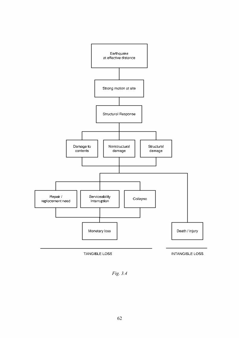
62
Fig. 3.4

63
GOVERNING VARIABLES DECISION
Event (annual maxima) Governing variable Abbr.earthquake (separately for each seismogenic source) moment magnitude E
Hazard strong motion at site
suite of simulated displacement time histories
S
Response structural response ISDmax , PFAmax, PFVmax R
Damage component damage damage class D
death number M
injuries number I
collapse indicator variable (1=occ., 0=non-occ.) C
Loss
restoration cost monetary unit N
Table 3.3
MATHEMATICAL MODEL OF SEISMIC RISK ASSESSMENT Collapse equation
C EC R R S S Er s x
p (C 1) f (C 1, r) f (r,s) f (s, x) dG (x)= = =∫ ∫ ∫
Loss Equation I. Death
M C MG (m) p (C 1)*Q *R= =
Loss Equation II. Injury
I C IG (i) p (C 1)*Q *R= =
Loss Equation III. Restoration cost k n
a aV C EV D D R R S S E
a 1 d 1 r s x
C T
G (v) f (v,d) f (d, r) p (C 0 R r) f (r,s) f (s, x) dG (x)
p (C 1)*V= =
= = =
+ =
∑ ∑ ∫ ∫ ∫
Loss Equation IV. Monetary loss -due to tangibles-
P P LG (p) G V (L*C )= +
Table 3.4
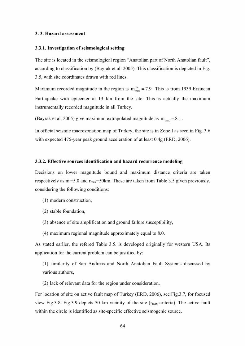
64
3. 3. Hazard assessment
3.3.1. Investigation of seismological setting
The site is located in the seismological region “Anatolian part of North Anatolian fault”,
according to classification by (Bayrak et al. 2005). This classification is depicted in Fig.
3.5, with site coordinates drawn with red lines.
Maximum recorded magnitude in the region is recmaxm 7.9= . This is from 1939 Erzincan
Earthquake with epicenter at 13 km from the site. This is actually the maximum
instrumentally recorded magnitude in all Turkey.
(Bayrak et al. 2005) give maximum extrapolated magnitude as maxm 8.1= .
In official seismic macrozonation map of Turkey, the site is in Zone I as seen in Fig. 3.6
with expected 475-year peak ground acceleration of at least 0.4g (ERD, 2006).
3.3.2. Effective sources identification and hazard recurrence modeling
Decisions on lower magnitude bound and maximum distance criteria are taken
respectively as ml=5.0 and rmax=50km. These are taken from Table 3.5 given previously,
considering the following conditions:
(1) modern construction,
(2) stable foundation,
(3) absence of site amplification and ground failure susceptibility,
(4) maximum regional magnitude approximately equal to 8.0.
As stated earlier, the refered Table 3.5. is developed originally for western USA. Its
application for the current problem can be justified by:
(1) similarity of San Andreas and North Anatolian Fault Systems discussed by
various authors,
(2) lack of relevant data for the region under consideration.
For location of site on active fault map of Turkey (ERD, 2006), see Fig.3.7, for focused
view Fig.3.8. Fig.3.9 depicts 50 km vicinity of the site (rmax criteria). The active fault
within the circle is identified as site-specific effective seismogenic source.
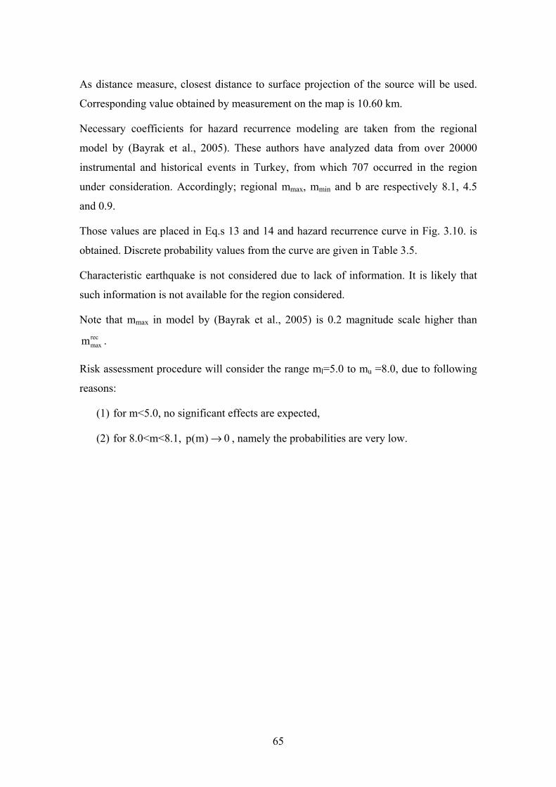
65
As distance measure, closest distance to surface projection of the source will be used.
Corresponding value obtained by measurement on the map is 10.60 km.
Necessary coefficients for hazard recurrence modeling are taken from the regional
model by (Bayrak et al., 2005). These authors have analyzed data from over 20000
instrumental and historical events in Turkey, from which 707 occurred in the region
under consideration. Accordingly; regional mmax, mmin and b are respectively 8.1, 4.5
and 0.9.
Those values are placed in Eq.s 13 and 14 and hazard recurrence curve in Fig. 3.10. is
obtained. Discrete probability values from the curve are given in Table 3.5.
Characteristic earthquake is not considered due to lack of information. It is likely that
such information is not available for the region considered.
Note that mmax in model by (Bayrak et al., 2005) is 0.2 magnitude scale higher than recmaxm .
Risk assessment procedure will consider the range ml=5.0 to mu =8.0, due to following
reasons:
(1) for m<5.0, no significant effects are expected,
(2) for 8.0<m<8.1, p(m) 0→ , namely the probabilities are very low.
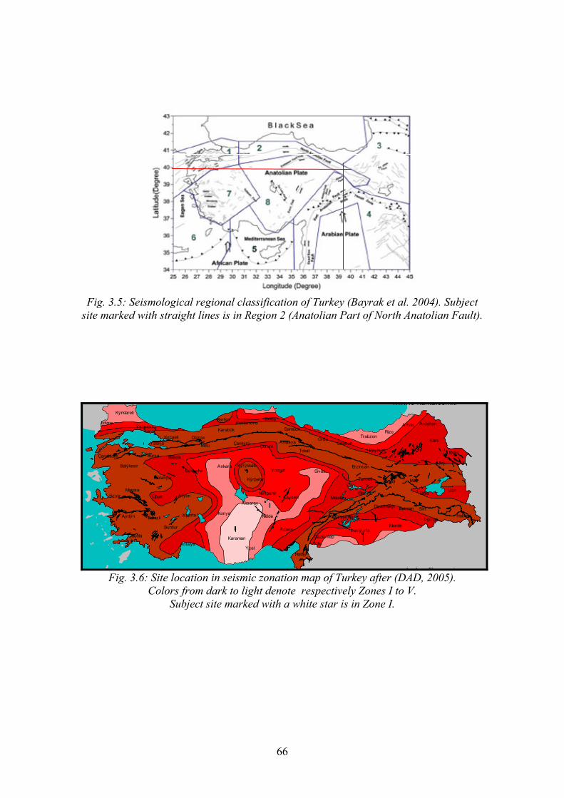
66
Fig. 3.5: Seismological regional classification of Turkey (Bayrak et al. 2004). Subject
site marked with straight lines is in Region 2 (Anatolian Part of North Anatolian Fault).
www.e harita.com.tr
i l fik t
Adana
Adýyaman
AfyonAksaray
Antalya
Aydýn
Balýkesir
Burdur
Bursa
Denizli
Edirne
Gaziantep
Isparta
Karaman
Kayseri
Kocaeli
Konya
Kütahya
Kýrklareli
Malatya
Manisa
Muðla
Niðde
Ordu
Sivas
Uþak
Yalova
Çanakkale
Ýstanbul
Ýzmir
Ýçel
Amasya
Ankara
ArdahanArtvin
Aðrý
Bartýn
Batman
BayburtBilecik
Bingöl
Bitlis
Bolu
Diyarbakýr
Düzce
Elazýð
Erzincan
Erzurum
Eskiþehir
Giresun
Hakkari
Hatay
Iðdýr
Karabük
Kars
Kastamonu
Kilis
Kýrýkkale
Kýrþehir
Mardin
Muþ
Nevþehir
RizeSamsun
Siirt
Sinop
Tokat
Trabzon
Tunceli
Van
Yozgat
Çankýrý Çorum
Þanlýurfa
Þýrnak
Fig. 3.6: Site location in seismic zonation map of Turkey after (DAD, 2005). Colors from dark to light denote respectively Zones I to V.
Subject site marked with a white star is in Zone I.

67
Adana
Adýyaman
AfyonAksaray
Antalya
Aydýn
Balýkesir
Burdur
Bursa
Denizli
Edirne
Gaziantep
Isparta
Karaman
Kayseri
Kocaeli
Konya
Kütahya
Kýrklareli
Malatya
Manisa
Muðla
Niðde
Ordu
Sivas
Uþak
Yalova
Çanakkale
Ýstanbul
Ýzmir
Ýçel
Amasya
Ankara
ArdahanArtvin
Aðrý
Bartýn
Batman
BayburtBilecik
Bingöl
Bitlis
Bolu
Diyarbakýr
Düzce
Elazýð
Erzincan
Erzurum
Eskiþehir
Giresun
Hakkari
Hatay
Iðdýr
Karabük
Kars
Kastamonu
Kilis
Kýrýkkale
Kýrþehir
Mardin
Muþ
Nevþehir
RizeSamsun
Siirt
Sinop
Tokat
Trabzon
Tunceli
Van
Yozgat
Çankýrý Çorum
Þanlýurfa
Þýrnak
Kayseri Malatya
Ordu
Sivas
Amasya
ArdahanArtvin
Aðrý
Bayburt
Bingöl
BitlisElazýð
Erzincan
Erzurum
Giresun
GümüþhaneIðdýr
Kars
þehir Muþ
Nevþehir
RizeSamsun
Tokat
Trabzon
Tunceli
Van
Yozgat
Çorum
i l fik t
Akıncılar Aşkale
Bayburt Demirözü
Divriği
Erzincan
Gölova Kelkit
Kemah
Otlukbeli
Ovacık
Pülümür
Refahiye
Suşehri
Tercan
Yedisu
Zara
Çamoluk
Çayırlı
Üzümlü
İliç
İmranlı
Şiran
Fig.3.7,8,9
68
Fig. 3.10: Site hazard curve
Table 3.5: Moment magnitude vs. annual probability of exceedance for discrete points considered in risk assessment procedure (ml - mu) and two extremes mmax and mmin .
M GE(m)
mmin 4.5 1.0000
ml 5.0 0.4551
5.5 0.2061
6.0 0.0923
6.5 0.0402
7.0 0.0164
7.5 0.0056
mu 8.0 0.0006
mmax 8.1 0.0001

69
3.3.3. Stochastic strong motion simulation
In line with section 2.9.2.1., 10 simulations for each ∆m=0.5 step between ml=5.0 and
mu=8.0 are carried out. This makes a total of 70 simulations.
An open-source Fortran program given by (Boore, 2000) (refered in 2.9.1.6 as well) is
used. The program uses time-domain stochastic strong motion simulation method after
(Boore 2003).
Table 3.6 gives simulation parameters, most of which are taken from the work by
(Akinci et al., 2001). These authors have determined source and attenuation
characteristics through analysis of regional microseismicity. The region they considered
was bounded by 39°15’N-40°00’N meridians and 39°20’E-40°15’ parallels, so
including the site considered in this problem.
For several other parameters, no regional data is available in literature. For those, state-
of-the art publications on Californian / western North-American conditions are
consulted. This approach can be justified by similarity of San Andreas and North
Anatolian Fault Systems discussed by various authors.
Record duration vary with magnitude level ranging from 5 seconds for m=5.0 to 100
seconds for m=8.0, with equal time steps of 0.005 seconds.
Acceleration time history of a sample simulation is depicted in Fig.3.11 and compared
to a real local record.
Time [sec]3836343230282624222018161412108642
Acc
eler
atio
n [g
]
0.200
0.000
-0.200
Time [sec]212019181716151413121110987654321
Acc
eler
atio
n [g
]
0.4
0.2
0
-0.2
Fig. 3.11: Above is a simulated acceleration time history for a m=7.0 event at the site (r=10.6 km). Below is the only available real record from the region (m=6.9, source-
site distance= 0.2 km, 13.03.1992). Simulated records have distinct time history patterns than real ones, especially in near field. However, they are useful considering
scarcity of real records in vast seismic regions of the world.
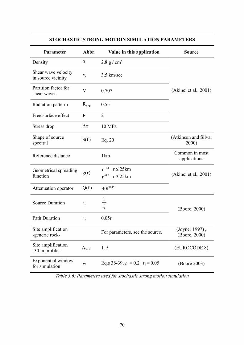
70
STOCHASTIC STRONG MOTION SIMULATION PARAMETERS
Parameter Abbr. Value in this application Source
Density ρ 2.8 g / cm³
Shear wave velocity in source vicinity sv 3.5 km/sec
Partition factor for shear waves V 0.707
Radiation patterm RΘΦ 0.55
Free surface effect F 2
Stress drop ∆σ 10 MPa
(Akinci et al., 2001)
Shape of source spectral
S(f ) Eq. 20 (Atkinson and Silva, 2000)
Reference distance 1km Common in most applications
Geometrical spreading function
g(r) 1.1
0.5
r 25kmrr 25kmr
−
−
≤≥
Attenuation operator Q(f ) 0.4540f
(Akinci et al., 2001)
Source Duration ss c
1f
Path Duration ps 0.05r
(Boore, 2000)
Site amplification -generic rock- For parameters, see the source. (Joyner 1997) ,
(Boore, 2000)
Site amplification -30 m profile- Av-30 1. 5 (EUROCODE 8)
Exponential window for simulation w Eq.s 36-39, 0.2ε = , 0.05η = (Boore 2003)
Table 3.6: Parameters used for stochastic strong motion simulation

71
3.3.4. Structural response analysis
A finite element model of the structure is constructed in ANSYS (a commercial
software). Refer to Annex.II for ANSYS-script used and to section 4.3.2 for details of
the model. Using this model, dynamic time history analyses are carried out for each of
the 70 simulated displacement time histories (strong motion simulation was explained in
section 3.3.3). Refer to section 4.3.5, for details of the time history computations. The
statements given there are valid for this part of the work as well.
As given previously in Table 3.3, response governing variables are ISDmax , PFAmax and
PFVmax. Corresponding data gathered from analyses is depicted in Fig.s 3.12 to 3.17.
Normal or lognormal fits are used as seen there (commercial software MATLAB is used
for this purpose). In succeeding steps, only lognormal model will be used, because
maxima are defined in absolute values.
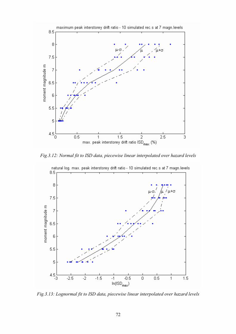
72
Fig.3.12: Normal fit to ISD data, piecewise linear interpolated over hazard levels
Fig.3.13: Lognormal fit to ISD data, piecewise linear interpolated over hazard levels
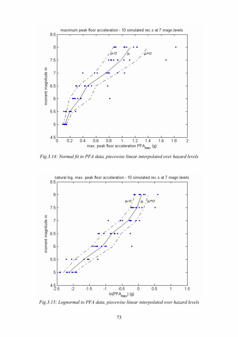
73
Fig.3.14: Normal fit to PFA data, piecewise linear interpolated over hazard levels
Fig.3.15: Lognormal to PFA data, piecewise linear interpolated over hazard levels

74
Fig.3.16: Normal fit to PFV data, piecewise linear interpolated over hazard levels
Fig.3.17: Lognormal fit to PFV data, piecewise linear interpolated over hazard levels

75
3.3.5. Damageability and loss estimate
Monte Carlo Simulation method is used for solution of loss equations given in Table
3.4. Input data is given in Tables 3.7 to 3.9. Cost breakdown information given there is
fictive, however, in line with common trends given by (Bazurro and Luco, 2005).
The procedure for simulations follows:
(1) Lognormal distribution is fit to response governing variable data at the 7 discrete
hazard levels between m=5.0 and m=8.0 as seen in Fig.s. 3.13, 15 and 17. This reveals
mean and standard deviation vectors for each response governing variable, namely for
ISD, PFA and PFV. So, a total of 6 1x7 vectors in form of R SM , R|SD are obtained,
whereas R=ISD, PFA and PFV.
(2) Overall structural and component damageability data is gathered. Refer to Tables 3.7
to 3.9 for this data. The sources for parameters are indicated there. Since a lognormal
distribution is fit for damage state membership, the natural logarithm of the mean values
are taken. So, for each component, two nx1 vectors are obtained: R DM , R DD . Those
are, respectively, mean and standard deviation damageability vectors, with R=ISD, PFA
or PFV depending on performance group of component (refer to Table 2.7 for the
concept).
(3) Random vectors are generated from vectors R SM and R|SD . Then, for each element
of generated vector, damage state membership probabilities are obtained in accordance
with Eq.45. In this application, 106 simulations are used. The algorithm implemented in
MATLAB is given in ANNEX.I.
Results are presented in following section 3.3.6.
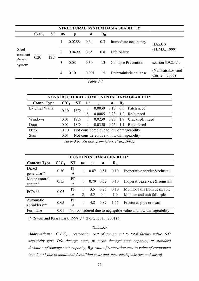
76
STRUCTURAL SYSTEM DAMAGEABILITY
C/ CT ST DS µ σ RR
1 0.0288 0.64 0.3 Immediate occupancy
2 0.0499 0.65 0.8 Life Safety
HAZUS (FEMA, 1999)
3 0.08 0.30 1.3 Collapse Prevention section 3.9.2.4.1.
Steel moment frame system
0.20 ISD
4 0.10 0.001 1.5 Deterministic collapse (Vamsatsikos and Cornell, 2005)
Table.3.7
NONSTRUCTURAL COMPONENTS’ DAMAGEABILITY Comp. Type C/CT ST DS µ σ RR
1 0.0039 0.17 0.5 Patch need External Walls 0.10 ISD 2 0.0085 0.23 1.2 Rplc. need
Windows 0.01 ISD 1 0.0230 0.28 1.8 Crack,rplc. need Door 0.01 ISD 1 0.0350 0.25 1.1 Rplc. Need Deck 0.10 Not considered due to low damageability Stair 0.01 Not considered due to low damageability
Table.3.8: All data from (Beck et al., 2002).
CONTENTS’ DAMAGEABILITY Content Type C/ CT ST DS µ σ RR Diesel generator * 0.30 PF
A 1 0.87 0.51 0.10 Inoperative,service&reinstall
Motor control center * 0.15 PF
A 1 0.79 0.52 0.10 Inoperative,service& reinstall
1 3.5 0.25 0.10 Monitor falls from desk, rplc PC’s ** 0.05 PFA 2 5.2 0.4 1.0 Monitor and unit fall, rplc
Automatic sprinklers** 0.05 PF
A 1 4.2 0.87 1.56 Fractured pipe or head
Furniture 0.01 Not considered due to negligible value and low damageability
(* (Swan and Kassawara, 1998),** (Porter et al., 2001) )
Table.3.9
Abbrevations: C / CT : restoration cost of component to total facility value, ST:
sensitivity type, DS: damage state, µ: mean damage state capacity, σ: standard
deviation of damage state capacity, RR: ratio of restoration cost to value of component
(can be >1 due to additional demolition costs and post-earthquake demand surge)

77
3.3.6. Presentation of results
Significant results for risk management are listed in Table 3.10.
SIGNIFICANT RESULTS FOR RISK MANAGEMENT DECISIONMAKING
Expected annual loss 0.83%
Expected annual loss due to structural components 0.03%
Expected annual loss due to nonstructural components 0.71%
Expected annual loss due to contents 0.09%
Annual structural collapse probability 0.384x10⁻⁶
Annual death expectancy for single occupant 0.288x10⁻⁶
Annual injury expectancy for single occupant 0.096x10⁻⁶
Table 3.10
The most significant result for risk management purposes is the expected annual loss,
obtained as 0.83% of total value. This result can be used for risk management decisions
Examples to such decisions are mitigation investment justification and insurance
premium determination.
Collapse probability (annual probability of exceeding collapse limit state) is obtained as
0.384x10⁻⁶ per year. This value is in the same order of magnitude with target breakdown
probability for civil engineering facilities, commonly taken as 10-6 as stated e.g. by
(Porter, 2002).
Injury and death expectancy for a single occupant are obtained respectively as 0.096x
10-6 and 0.288x10⁻⁶ per year. These values can be used for life safety verification
decisions and for life safety insurance premium decisions.
Death expectancy figure is almost equal to target death expectancy 0.28x10⁻⁶ obtained
by (Porter, 2002) for a fictive design after 1992 and 1994 NEHRP (National Earthquake
Hazards Reduction Program, USA) Recommendations. The case studied by (Porter,
2002) was based on weekly 45 hours occupancy –office conditions- in highest
seismicity region in USA.
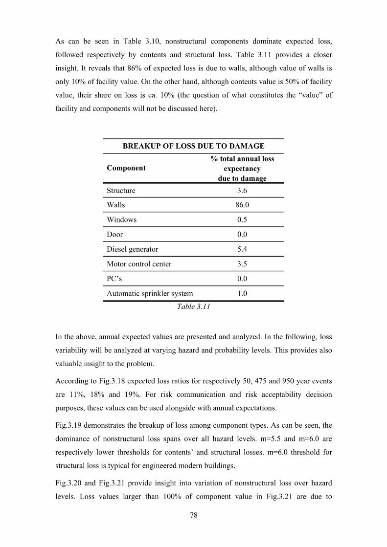
78
As can be seen in Table 3.10, nonstructural components dominate expected loss,
followed respectively by contents and structural loss. Table 3.11 provides a closer
insight. It reveals that 86% of expected loss is due to walls, although value of walls is
only 10% of facility value. On the other hand, although contents value is 50% of facility
value, their share on loss is ca. 10% (the question of what constitutes the “value” of
facility and components will not be discussed here).
BREAKUP OF LOSS DUE TO DAMAGE
Component % total annual loss
expectancy due to damage
Structure 3.6
Walls 86.0
Windows 0.5
Door 0.0
Diesel generator 5.4
Motor control center 3.5
PC’s 0.0
Automatic sprinkler system 1.0
Table 3.11
In the above, annual expected values are presented and analyzed. In the following, loss
variability will be analyzed at varying hazard and probability levels. This provides also
valuable insight to the problem.
According to Fig.3.18 expected loss ratios for respectively 50, 475 and 950 year events
are 11%, 18% and 19%. For risk communication and risk acceptability decision
purposes, these values can be used alongside with annual expectations.
Fig.3.19 demonstrates the breakup of loss among component types. As can be seen, the
dominance of nonstructural loss spans over all hazard levels. m=5.5 and m=6.0 are
respectively lower thresholds for contents’ and structural losses. m=6.0 threshold for
structural loss is typical for engineered modern buildings.
Fig.3.20 and Fig.3.21 provide insight into variation of nonstructural loss over hazard
levels. Loss values larger than 100% of component value in Fig.3.21 are due to
79
additional demolition costs. Same relations for contents are given in Fig.s 3.22 and 3.23,
and for structure in Fig.3.24.
Fig. 3.25 depicts variation of damage state probabilities over hazard levels. Considering
damage state III, namely the collapse prevention damage state, an abnormality is
obvious: Expected collapse probability for m=7.0 is exceeding that of m=7.5. This is
despite monotonic increase of mean response parameters with increasing hazard
intensity, depicted in Fig.s 3.12 to 3.17. This abnormality can be explained by the
higher dispersion of response at m=7.0 level with respect to m=7.5 level, demonstrated
in Fig.3.26 (see the twist at m=7.0). The higher dispersion m=7.0 is not coincidental and
is related to material modeling: Multilinear material model used is based on a sudden
and abrupt transition from elastic to inelastic regime. Where m=7.5 simulations lead
probably to yielding for all cases, m=7.0 simulations may or may not lead to yielding,
depending on pulse sequence or other arbitrary reasons. This leads to the increased
dispersion of response at m=7.0. Detailed analysis of dispersion of response estimates is
not the subject of this chapter, for further examples and explanation, refer to Chapter 4.
Fig.3.27 gives dispersion data for all response parameters at varying hazard levels.
Similar weaving behavior is observable at lower hazard levels for PFA and PFV. This,
on the other hand, can be either coincidental or related to hazard description (so,
acceleration and velocity maxima of ground motion simulations). For precise risk
assessment procedures, these phenomena should be investigated further. This is to some
extent done in Chapter 4.
Finally, Fig.3.28 depicts a performance-acceptance-check according to (FEMA 350,
2000) criteria. This publication reflects the state-of-the-art of performance and
reliability based provisions. Referred figure demonstrates the applicability of the
presented method for performance acceptance decision.
The depicted linear target curve is bounded by
(1) immediate occupancy drift criteria of 0.85% for 72 year event (50% in 50 years,
annual probability of 0.01376), obtained for the recommended 50% confidence
level for IO.
(2) collapse prevention drift criteria of 4.54% for 2475 year event (50% in 50 years,
annual probability of 0.01376), obtained for the recommended 90% confidence
level for CP.
Procedure for developing the criteria can be found in (FEMA 350, 2000).
80
As seen in the referred figure, performance curve is partially in the unacceptable region.
So, it can be stated that the overall performance is unacceptable according to (FEMA
350, 2000) criteria. Following statements explain the problem in detail with reference to
Fig.3.28:
(1) for hazard range m=6.5-7.5, it is likely -with 50% confidence- that the subject
structure will not satisfy the FEMA-SAC performance criterion. That implies
that excessive (more than acceptable) damage and loss can be expected. It can
be stated with confidence that the problem is only related to material loss and
not to life safety.
(2) for the range of hazard levels significant for life safety, the structure satisfies the
criterion with a significantly ample margin.
It is worth to note that the range over mu=8.0 (1649-year event, annual probability of
exceedance 0.6x10⁻³) is not covered by hazard assessment. This can be noticed as a
critical point to solution provided above. In applications, considering 2475 year event as
mu would be a good practice to conform to state-of-the-art conventions. However, in the
investigated case, no significant implications to results should be expected, as explained
in the following:
(1) Since probabilities at mu =8.0 - mmax = 8.1 hazard range are very low; significant
effects of neglect of hazard range 8.0 < m < 8.1 to expected loss should not be
expected.
(2) There is an ample margin between performance curve and criteria around mu.
This can comfortably be extrapolated to mmax level. So, performance can be
considered to be on the acceptable side at the considered range. As a result, life-
safety considerations are not effected by neglect of hazard range 8.0 < m < 8.1.

81
Fig.3.18
Fig.3.19

82
Fig.3.20
Fig.3.21

83
Fig.3.22
Fig.3.23

84
Fig.3.24
Fig.3.25
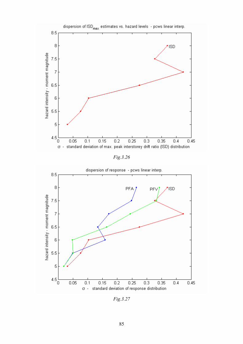
85
Fig.3.26
Fig.3.27

86
Fig.3.28
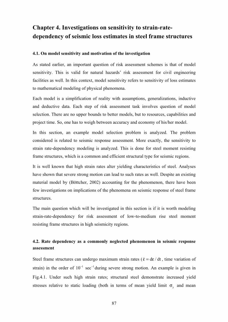
87
Chapter 4. Investigations on sensitivity to strain-rate-dependency of seismic loss estimates in steel frame structures
4.1. On model sensitivity and motivation of the investigation
As stated earlier, an important question of risk assessment schemes is that of model
sensitivity. This is valid for natural hazards’ risk assessment for civil engineering
facilities as well. In this context, model sensitivity refers to sensitivity of loss estimates
to mathematical modeling of physical phenomena.
Each model is a simplification of reality with assumptions, generalizations, inductive
and deductive data. Each step of risk assessment task involves question of model
selection. There are no upper bounds to better models, but to resources, capabilities and
project time. So, one has to weigh between accuracy and economy of his/her model.
In this section, an example model selection problem is analyzed. The problem
considered is related to seismic response assessment. More exactly, the sensitivity to
strain rate-dependency modeling is analyzed. This is done for steel moment resisting
frame structures, which is a common and efficient structural type for seismic regions.
It is well known that high strain rates alter yielding characteristics of steel. Analyses
have shown that severe strong motion can lead to such rates as well. Despite an existing
material model by (Böttcher, 2002) accounting for the phenomenon, there have been
few investigations on implications of the phenomena on seismic response of steel frame
structures.
The main question which will be investigated in this section is if it is worth modeling
strain-rate-dependency for risk assessment of low-to-medium rise steel moment
resisting frame structures in high seismicity regions.
4.2. Rate dependency as a commonly neglected phenomenon in seismic response assessment
Steel frame structures can undergo maximum strain rates ( d / dtε = ε , time variation of
strain) in the order of 1 110 sec− − during severe strong motion. An example is given in
Fig.4.1. Under such high strain rates; structural steel demonstrate increased yield
stresses relative to static loading (both in terms of mean yield limit yσ and mean

88
average yield stress plσ ). This increase is due to change in microphysical processes
which dominate plastic behavior.
Fig.4.1: Strain rate time history at a beam cross section of a 3-storey steel frame
structure subjected to 12.11.1999 Düzce (Turkey) record (PGA=0.822g).
The dependence of plastic metal behavior on loading velocity is termed as rate-
dependency. This term will be used in the following specifically for alteration of plastic
parameters of structural steel under high strain rates during earthquake loading.
Strain rates at a given cross section of a frame structure are related to ground shaking
velocity. Seismic loading is typically marked with sudden and rapidly changing
velocities. This translates almost linearly to local strain rates in critical cross sections as
shown in Fig.4.1. Moreover, strain rate show high variability along the height of the
structure (among components and at cross section with relative location from center of
inertia).
The practical problem related to rate dependency arises in two contexts:
(1) conventional material models do not account for the phenomena,
(2) material parameters utilized in structural design are gathered in static or quasi-static
experiments with no consideration of rate-dependency effects, as stated by (Böttcher
2002).
Increased strength due to rate dependency effects can be comprehended as beneficiary.
However, rate dependency has possible negative implications for global and local
structural response as well. Examples are increased drift, increased ductility demand in
connections due to beam overstrength and decreased connection ductility due to
inelasticity concentrations.

89
The physical phenomenon rate-dependency in structural steel is known since more than
one century according to (Böttcher 2002).
Microphysical explanation for the phenomenon is the gradual change of deformation
patterns at molecular level depending on loading velocities. For detailed treatment, refer
to (Böttcher 2002). The same author mentions that the effects are negligible at strain
rates less than 10-4. Acccordingly, we can list the possible types of dynamic loads under
which rate-dependency is of relevance to structural response as in Table 4.1 and Fig.
4.2.
Considering steel frame structures under seismic loading, implications of rate
dependency on structural behavior can be analyzed at three levels:
(1) material,
(2) local,
(3) global.
Material level refers to the governing stress-strain relation determined by microphysical
processes (molecular, atomic) which will not be addressed in this work. Local level
comprises both structural component behavior (columns, beams, connections, etc.) and
the cross-sectional-behavior of given components. Global level refers to overall
structural response formed by individual component action and interactions between
them.
In the following, rate dependency effects to seismic response of steel moment resisting
frame structures at these three scales are presented.
dyn staty y/σ σ
Parameter
Strain rates ε (1/s)
Duration (µs)
Loading Velocity (m/s) Comp. Tens.
Material behavior
Earthquake 10-3-100 107 - 1-1.3 1.8 Visc. el.-pl. Ocean waves 10-3-10-1 106 <5 1-1.3 1.7 Visc.-el. Collapse loads <101 106 <10 1-2.0 2.3 El.-pl. Plane crash 10-2-102 105 <90 1-1.3 2.5 El.-pl.-dam. Vehicle crash 10-2-102 104 <30 1-1.3 2.5 El.-pl.-dam. Blast 101-103 103 <4000 1-2.0 5 El.-pl.-dam. Conventional arms 102-103 - - 1.5-2.0 - Dam. Contact explosion <108 101 <9000 - - Hydro.-dam. Comet impact <108 101 >12000 - - Damped
Table 4.1: Engineering loading types with relevance to rate dependency. Given values are compiled by (Gebbeken and Ruppert, 1999) from various publications. Our dynamic
time history analyses proved the strain rate range for earthquake loading.
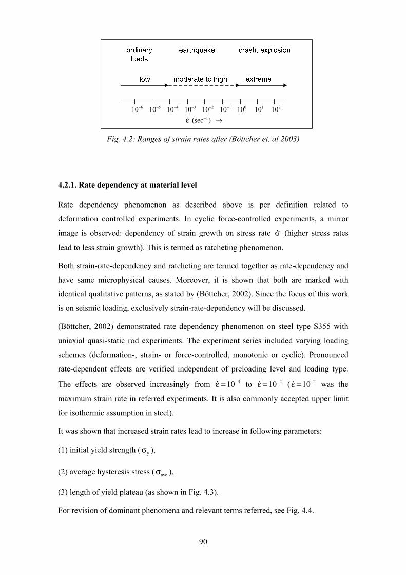
90
6 5 4 3 2 1 0 1 210 10 10 10 10 10 10 10 10− − − − − −
1(sec )−ε →
Fig. 4.2: Ranges of strain rates after (Böttcher et. al 2003)
4.2.1. Rate dependency at material level
Rate dependency phenomenon as described above is per definition related to
deformation controlled experiments. In cyclic force-controlled experiments, a mirror
image is observed: dependency of strain growth on stress rate σ (higher stress rates
lead to less strain growth). This is termed as ratcheting phenomenon.
Both strain-rate-dependency and ratcheting are termed together as rate-dependency and
have same microphysical causes. Moreover, it is shown that both are marked with
identical qualitative patterns, as stated by (Böttcher, 2002). Since the focus of this work
is on seismic loading, exclusively strain-rate-dependency will be discussed.
(Böttcher, 2002) demonstrated rate dependency phenomenon on steel type S355 with
uniaxial quasi-static rod experiments. The experiment series included varying loading
schemes (deformation-, strain- or force-controlled, monotonic or cyclic). Pronounced
rate-dependent effects are verified independent of preloading level and loading type.
The effects are observed increasingly from 410−ε = to 210−ε = ( 210−ε = was the
maximum strain rate in referred experiments. It is also commonly accepted upper limit
for isothermic assumption in steel).
It was shown that increased strain rates lead to increase in following parameters:
(1) initial yield strength ( yσ ),
(2) average hysteresis stress ( aveσ ),
(3) length of yield plateau (as shown in Fig. 4.3).
For revision of dominant phenomena and relevant terms referred, see Fig. 4.4.

91
Beyond the changes in above stated parameters, the shape of stress-strain curves
remained qualitatively stable with varying strain rates. No significant effects on initial
elastic module and in linear-elastic range are observed. Strain-rate memory effect
(memory of a previous strain-rate) is found to be negligible. Preloading mitigates rate-
dependency but negligibly. Rate dependency effects are negligible in quasi-static strain-
rate range; 410−ε < . It was also shown that multi-axial effects on rate dependency are
negligible.
For details on rate-depending material testing, refer to (Bruhns and Fossa, 1996).
Despite the observed effects, rate-dependency remain a secondary factor in forming
plastic behavior in comparison to the more dominant factors; loading intensity and
sequence and number of load cycles.
(Böttcher, 2002) developed a time-dependent material model to account for the
phenomena in finite element structural analyses. The model parameters were derived
from the referred experimental results. This model will be named MM4 in the
following.
MM4 combined two aspects:
- a time-dependent equilibrium definition,
- two-surface material model by (Scheibe, 1990) and (Reininghaus, 1994).
Scheibe-Reininghaus model will be named MM3 in the following. MM3 was based on a
quadratic expression to define tangent modulus in hardening sector. It allowed exact
computation of stress-strain curve of steel up to a strain level 8%.
For detailed treatment of Scheibe-Reininghaus model (MM3), refer to (Scheibe, 1990)
and (Reininghaus, 1994), for the time dependent material model (MM4) to (Böttcher
2002), in summary by (Böttcher et al. 2003).
MM4 accounts for rate dependency effects up to strain rates of 210−ε = . It presents a
unique opportunity to account for rate dependency effects in practical finite element
dynamic analyses.
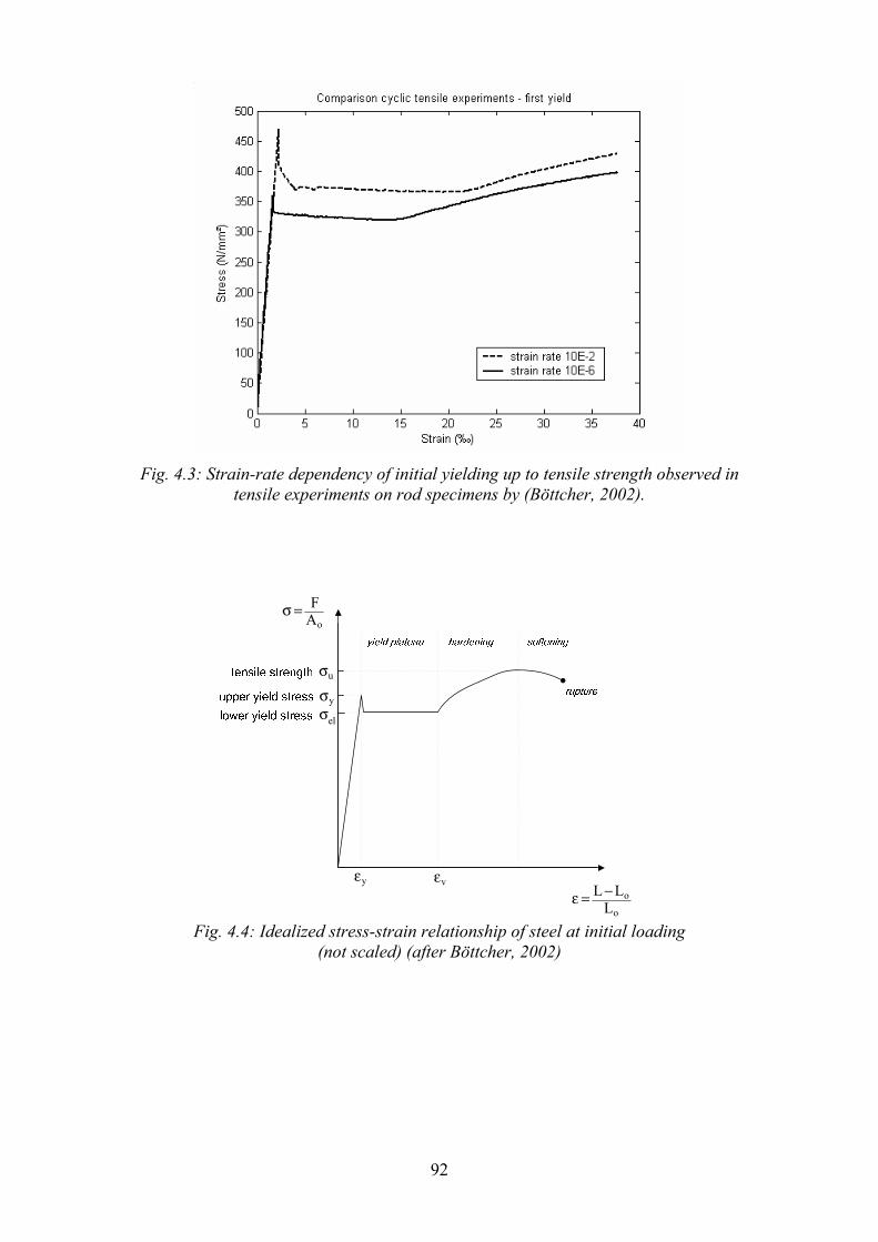
92
Fig. 4.3: Strain-rate dependency of initial yielding up to tensile strength observed in
tensile experiments on rod specimens by (Böttcher, 2002).
uσ
yεo
o
L LL−ε =
o
FAσ =
yσelσ
vε
Fig. 4.4: Idealized stress-strain relationship of steel at initial loading
(not scaled) (after Böttcher, 2002)
93
4.2.2. Local level (component and cross-section)
(Böttcher et al. 2003) mentions that the rate dependency effects were previously not
considered in experimental fragility analysis in earthquake engineering.
In cyclic experiments, intensity and loading sequence are usually varied, but loading
velocity and frequency was neglected. Recent examples are quasi-static tests by
(Sugimoto et al., 2001) and (Jones et al., 2002).
(Note: cyclic experiments are used for investigation of e.g. moment-rotation behavior
and rotation capacity of connections, low-cycle fatigue due to repeated plastic
excursions).
Unexpected damage in steel frame connections in Northridge (USA, 1994) and Kobe
(Japan, 1995) earthquakes gave impulse to consideration of rate dependency within
experiments on structural components.
(Mazzolani, 2001) reports European experiments on frame structures. Those proved
reduction of life-time due to rate-dependency effects in cyclic loaded moment resistant
connections. The cause for this can be explained sequentially as in the following:
(1) increased strain rates ( ε ) lead to increased yσ / uσ (yield limit to tensile strength
ratio)
(2) increased ( yσ / uσ ) lead to local concentration of inelastic deformations near
connections
(3) concentration results in higher local strains and strain rates at given global drift
levels, which in turn leads to less ductile connection behavior.
(Böttcher, 2002) observed in a series of experiments on holed plate sections that rapidly
changing loading velocities lead to sudden and significant changes in component
behavior.
Experimental results after both (Mazzolani, 2001) and (Böttcher, 2002) verify that
material-level rate dependency translates significantly to component behavior.
A previously not researched question is the implications on local sectional ductility at
plastic hinges. Previous plastic hinge models assumed uniform yield limits all along the
cross-section. This assumption can be questioned considering that flanges undergo
larger strain rates than the central regions.

94
4.2.3. Global scale
The author of this work has found no publications dealing explicitly with rate
dependency effects on seismic global behavior of steel frame structures. Exceptions are
preliminary efforts in (Wichers, 2001) and (Böttcher, 2002).
Seismic response analysis reports and steel material models do not consider the
phenomenon, e.g. (Fragiacomo et al. 2004), (Sivaselvan and Reinhorn, 2000). Seismic
design codes do not refer to the phenomena and there are no indications that rate
dependency is considered in their development. Several works dealing with explosion
loads address the phenomena, e.g. (Gebbeken and Ruppert, 1999).
In the previous section, local effects of rate dependency was discussed. Deriving from
these, one can suggest that rate dependency would lead in global scale to:
(1) Increased deformations,
(2) Decreased ductility.
In this work, only hypothesis (1) will be investigated by comparison of analyses results
carried out with and without rate dependency consideration.
The criteria for hypothesis (1) is global deformations. This can be measured by
maximum peak interstorey drift, peak floor acceleration and peak floor velocity. Those
are also indicators for structural and nonstructural seismic damage and thus loss as
stated previously. So, this enables to draw conclusions on implication of rate
dependency on loss estimates, as well.
Considering the not investigated hypothesis (2), the mechanisms which lead to
decreased ductility can be twofold;
(i) Migration of plastic hinges from their ideal location (beam ends with a secure
distance from connections) to relatively brittle connections due to beam overstrength
caused by rate dependency, or,
(ii) Decrease in individual component ductility (of connections, beams or columns).
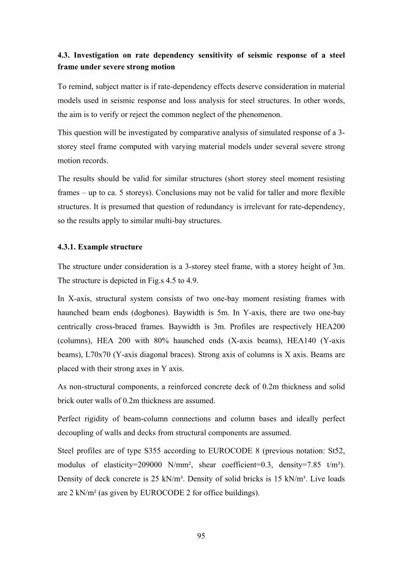
95
4.3. Investigation on rate dependency sensitivity of seismic response of a steel frame under severe strong motion
To remind, subject matter is if rate-dependency effects deserve consideration in material
models used in seismic response and loss analysis for steel structures. In other words,
the aim is to verify or reject the common neglect of the phenomenon.
This question will be investigated by comparative analysis of simulated response of a 3-
storey steel frame computed with varying material models under several severe strong
motion records.
The results should be valid for similar structures (short storey steel moment resisting
frames – up to ca. 5 storeys). Conclusions may not be valid for taller and more flexible
structures. It is presumed that question of redundancy is irrelevant for rate-dependency,
so the results apply to similar multi-bay structures.
4.3.1. Example structure
The structure under consideration is a 3-storey steel frame, with a storey height of 3m.
The structure is depicted in Fig.s 4.5 to 4.9.
In X-axis, structural system consists of two one-bay moment resisting frames with
haunched beam ends (dogbones). Baywidth is 5m. In Y-axis, there are two one-bay
centrically cross-braced frames. Baywidth is 3m. Profiles are respectively HEA200
(columns), HEA 200 with 80% haunched ends (X-axis beams), HEA140 (Y-axis
beams), L70x70 (Y-axis diagonal braces). Strong axis of columns is X axis. Beams are
placed with their strong axes in Y axis.
As non-structural components, a reinforced concrete deck of 0.2m thickness and solid
brick outer walls of 0.2m thickness are assumed.
Perfect rigidity of beam-column connections and column bases and ideally perfect
decoupling of walls and decks from structural components are assumed.
Steel profiles are of type S355 according to EUROCODE 8 (previous notation: St52,
modulus of elasticity=209000 N/mm², shear coefficient=0.3, density=7.85 t/m³).
Density of deck concrete is 25 kN/m³. Density of solid bricks is 15 kN/m³. Live loads
are 2 kN/m² (as given by EUROCODE 2 for office buildings).

96
Fi
g.s.
4.5,
4.6
: 3D
vie
ws o
f the
stru
ctur
e
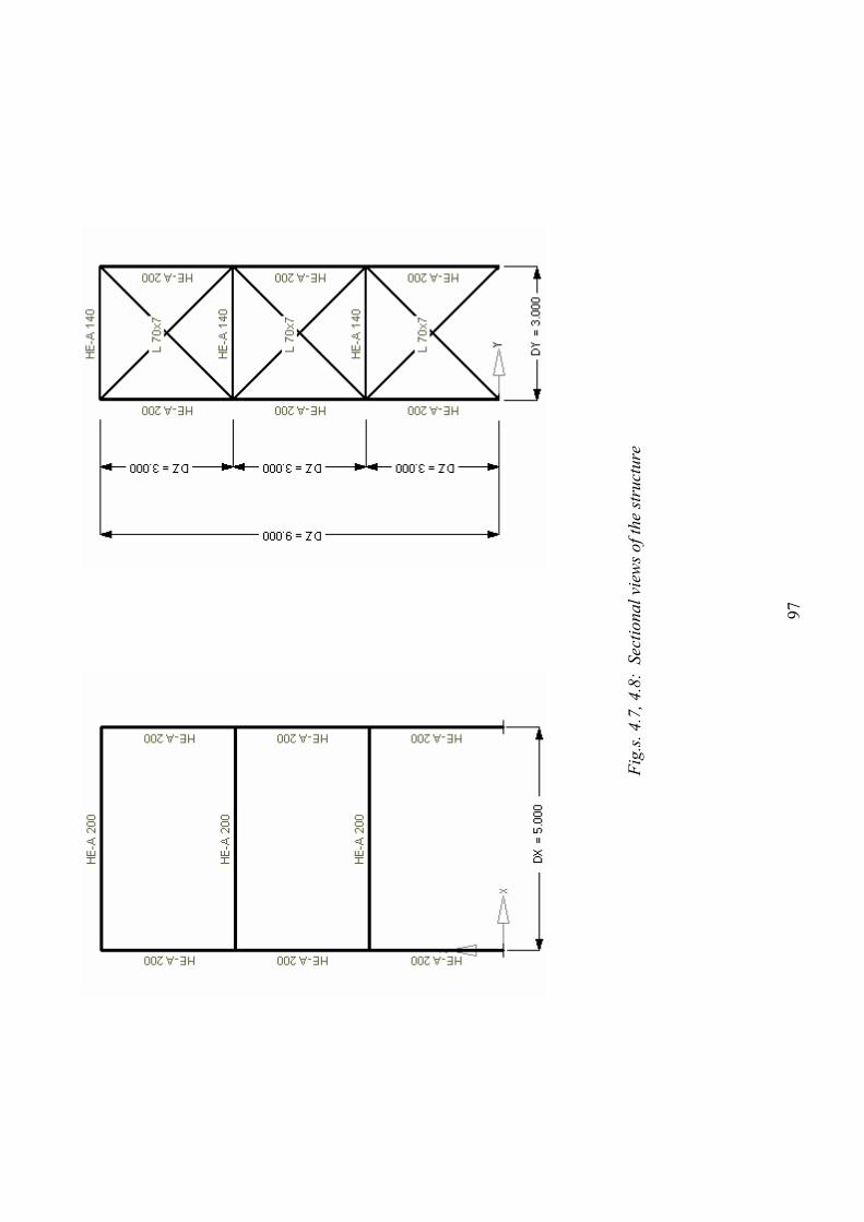
97
Fi
g.s.
4.7,
4.8
: Se
ctio
nal v
iew
s of t
he st
ruct
ure

98
Fig.
4.9
. Pl
an v
iew
of t
he st
ruct
ure
with
loca
tion
of h
aunc
hed
beam
end
s dep
icte
d.

99
4.3.2. Finite element model
A 3-D finite element model of the structure is prepared with commercial finite element
analysis program ANSYS. Corresponding ANSYS-script file is given in ANNEX.II.
The model consists of BEAM24 elements (simulating columns and beams) and
MASS21 elements (simulating masses due to walls, decks and live loads).
BEAM24 is a layered uniaxial finite element. It has tension-compression, flexure,
St.Venant torsion, shear deflection, plasticity, creep and swelling capabilities. It has 2
structural nodes with 3 deflectional and 3 rotational degree of freedoms for each.
Definition of a third non-colinear node is necessary for definition of element axis
system. Necessary profile data is extracted from a database provided by (Wichers,
2001). MASS21 is a point (one-node) element with 3 translational and 3 rotational
degree of freedoms.
Rigid column bases and beam-column connections are simulated. In-plane stiffness of
decks (diaphragm effect) and walls are neglected. These are in line with previous
statements in section 4.3.1. Damping ratio of 5% is given in line with the common
assumption for steel frame structures.
In the analyses, the structure will be excited simultaneously in two principal horizontal
axes and the vertical axis to simulate 3D conditions. However, only the deformation
results in the longer horizontal axis will be further analysed (namely for moment
resisting frames).
4.3.3. Material models and parameters
Four material models are considered in computations:
-bilinear kinetic material model (MM1),
-multilinear kinetic material model (MM2),
-time-independent two-surface material model (MM3),
-time-dependent two-surface material model (MM4).
MM1 and MM2 are ANSYS standard material models. Necessary material properties
input is provided in ANSYS-script file in ANNEX.II.
MM3 and MM4 work over an extensional Fortran interface by (Böttcher, 2002). Those
readers who are interested to obtain the referred interface are recommended to contact

100
Institute of Steel Structures, TU Braunschweig.
For detailed explanation of all four models, refer to (Wichers, 2001). .
The preliminary analyses with 5 time histories have shown that results from MM3 and
MM4 show negligible variation in the order of 1-2% for global response parameters.
The same is valid also for comparion of MM1 and MM2 results. Due to this negligible
variation, the results are demonstrated only for MM2 and MM4 in the following.
4.3.3. Modal analysis
The first four natural periods are 0.77sec, 0.36sec., 0.30 sec., 0.23 sec. and 0.15 sec.
according to the modal analysis of the finite element model. Modal shapes are depicted
in Fig. 4.10.
For low-rise structures like the subject frame, it can be presumed that the behaviour is
mainly dominated by the first eigenmode.
Note that, modal analysis model includes masses due to dead and live loads also,
respectively with coefficients 1.0 and 0.3 (first natural period of the bare structure
equals 0.27 sec which is unrealistic beyond construction phase).
Within the spectral regions concept13 depicted in 4.19, first natural period fits in the
velocity-sensitive region. This region is typically from ca. 0.5 to 3.0-4.0 sec.s
(depending on seismic regime). Response of structures with dominant modes in this
region appears better related to ground velocity than any other parameter, as stated by
(Chopra, 2004). Selection of a structure in this region is opportune for the purpose of
this study, because rate-dependency effects should be expected to be relatively higher in
this region due to the maximum pseudo-velocities
4.3.4. Equivalent static analysis and code validation
On a frame-stick model of the structure, lateral force method of analysis is carried out
according to EUROCODE 8. For this purpose, commercial finite element programme
RSTAB is used.
The site is assumed to be on type C ground and in seismic zone 4 acc. to EUROCODE 8
(maximum hazard zone). Earthquake loads are obtained based on EUROCODE 8 elastic
13 Spectral regions concept derives from the typical shapes of earthquake response spectra and is explained e.g. by (Chopra, 2004).

101
spectra. Accordingly, minimum design acceleration for 475 year earthquake is 0.4g
modified with corresponding soil and behaviour factors. Load combinations are
obtained accordingly.
Resulting tip deflection14 is 67% of code limit. This verifies conformity with
EUROCODE 8 criterion of the structure under consideration. So, it is shown that the
structure is a practical and realistic one. The details of the analysis are not given further.
14 Tip deflection is the horizontal displacement of the highest floor level of the structure. It is an indicator of earthquake effects on structure like interstorey drift.

102
Fi
g. 4
.10.
1
st, 2
nd,
3rd (a
bove
) 4th
and
5th
(nex
t pag
e) m
odal
shap
es
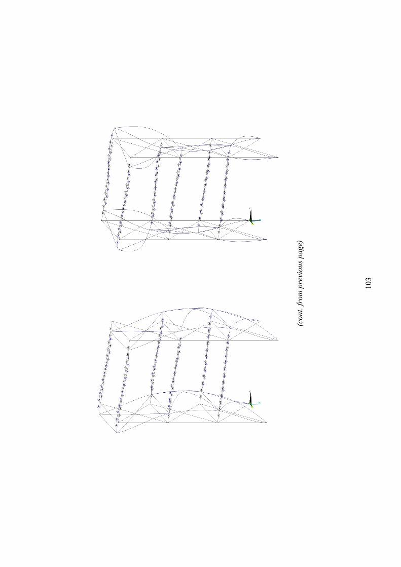
103
(con
t. fr
om p
revi
ous p
age)

104
4.3.4. Used time histories
Strong motion records used in analyses are listed in Table.4.2. They are taken from the
database (PEER, 2005). This open-source database is one of the most exhaustive and
well prepared strong motion databases. It is especially suitable for structural engineering
purposes.
Preliminary analyses have shown that the structure remains elastic when excited with
records with peak ground accelerations (PGA) less than 0.6g. The subject demands,
however, observation of inelastic behavior. So, the PGA=0.6g is selected as a lower
threshold for selection of records.
Moreover, a decision had to be taken concerning the soil type of the hypothetical site.
This is due to the significant variability of strong motion records among varying soil
types. For that reason, the analyses will be carried assuming Soil Type C (according to
both USGS (United States Geological Survey) and EUROCODE 8 classification). This
is a commonly found soft soil type.
In PEER database, there are a total of 18 records from 5 earthquakes conforming the
above conditions (PGA>0.6g, Soil Type C). Due to the time-intensive computations
related to two-surface models, 10 records are selected for analyses. This is done by
eliminating records with less peak ground velocities from the group. It can be stated that
the resulting group is broadly representative of PGA>0.6 g records on Soil C, since it
covers 10 of the 18 available records.
Moreover, further 5 records with peak ground velocities over 1 m/s are added to group.
The peak ground accelerations of those latter are between 0.4g and 0.6g. This extension
is done in order to include high velocity content records in analyses.
For each record, all 3 components (2 horizontal and 1 vertical) are acquired from the
database. In the analyses, seismic loads are applied as 3-dimensional column base
excitations. Loading at longer axis direction is always the horizontal component with
higher peak acceleration.
Excitation on shorter axis and in vertical direction is done for simulating 3-dimensional
loading conditions. Global deformation results will be gathered only at longer axis.
Record parameters given in Fig.4.6 are those related with these components.
105
Rec
ord
no.
PEE
R
reco
rd
no.
Ear
thqu
ake
Mec
h.M
om.
Mag
n.
Site
- So
urce
D
ista
nce
(km
) Sa
(T1)
(g
) Sv
(T1)
(m
/s)
PGA
(g
) PG
V
(m/s
) PG
V/
PGA
A
SI
VSI
V
SI/
ASI
1
P080
9 C
ape
Men
doci
no, U
SA, 2
5.04
.199
2R
N
7.1
9.50
1.
611
1.93
00.
662
0.89
71.
354
0.42
93.
191
7.43
32
P154
7 D
üzce
, Tur
key,
12.1
1.19
99
SS
7.1
17.6
0 1.
324
1.59
20.
822
0.62
10.
755
0.47
82.
554
5.34
43
P016
1 2.
50
0.89
9 1.
080
0.77
50.
459
0.59
30.
812
2.01
72.
483
4 P0
180
Impe
rial V
alle
y, U
SA, 1
5.10
.197
9 SS
6.
5 3.
80
0.50
0 0.
607
0.60
20.
543
0.90
20.
373
1.96
45.
262
5 P1
441
Chi
-Chi
, Tai
wan
,20.
09.1
999
RN
7.
6 0.
98
1.02
5 1.
236
0.81
41.
262
1.55
10.
385
3.55
99.
252
6 P0
934
6.40
1.
166
1.40
20.
843
1.29
41.
534
0.81
63.
890
4.76
67
P100
5 7.
10
2.03
3 2.
440
0.83
81.
661
1.98
20.
655
5.09
77.
787
8 P0
102
0.40
1.
429
1.71
80.
939
0.76
60.
816
0.81
72.
490
3.04
99
P102
1 14
.60
1.15
9 1.
395
0.87
70.
408
0.46
50.
511
1.96
03.
838
10
P102
3
Nor
thrid
ge, U
SA,
17.0
1.19
94
RN
6.
7
0.20
1.
620
1.94
60.
897
1.02
21.
139
0.50
74.
931
9.72
411
P0
178
Impe
rial V
alle
y,U
SA, 1
5.10
.197
9 SS
6.
5 1.
30
0.59
0 0.
710
0.43
91.
098
2.50
20.
312
1.78
75.
725
12
P096
3 N
orth
ridge
, USA
, 17.
01.1
994
RN
6.
7 6.
20
1.13
2 1.
360
0.42
41.
060
2.49
70.
291
2.84
09.
752
Ta
ble
4.2:
Ens
embl
e of
stro
ng m
otio
n re
cord
s use
d in
ana
lyse
s, so
urce
: (PE
ER, 2
005)
M
ech.
: mec
hani
sm, R
N: r
ever
se-n
orm
al, S
S: st
rike
-slip
, ASI
: acc
eler
atio
n sp
ectr
um in
tens
ity, V
SI: v
eloc
ity sp
ectr
um in
tens
ity
106
4.3.5. Computational aspects of dynamic analyses
Structural analyses are carried out with commercial finite element code ANSYS /
Mechanical U Version 6.0. Corresponding ANSYS-script is given in ANNEX.II. For
the computations with the two-surface material models (MM3 and MM4), an ANSYS-
interface by (Böttcher, 2002) is additionally used.
Full-transient dynamic time-history analyses are carried out. Material damping is
included. Newmark time integration method (with initial stiffness scheme without
adaptive descent) and Newton-Raphson nonlinear procedure are used. The parameters
used for Newmark method follow:
amplitude decay factor for 2nd order transient integration = 0.5,
oscillation limit criterion for automatic time stepping of 1st order transients = 50.
Time steps of earthquake records (∆t) are 0.005 sec. A criterion for checking resolution
issue of time steps is: 20∆t < minimum significant period considered. This indicates that
the analyses cover natural modes with T>0.1 sec.s. Those are the first 5 natural modes
of the structure. Knowing the dominancy of the first natural mode in low-rise frames,
this is more than satisfactory.
In preliminary tries, there had been iteration problems and unexpected high responses at
initial stages of records. This is found to be related to application of the dead loads and
additional masses. The abnormality is overcome by inserting 30 initial load steps with
only static loads. 15 of those are selected to be disproportionately long (105 times time-
step of record) and remaining 15 normal (equal to time step of record). This “trick” of
inserting a “relaxation period” between initial static gravity load application and start of
dynamic excitation solved the problem of initial abnormal response.
4.3.6. Data gathering and processing by Incremental Dynamic Analysis
In the frame of this work, several hypotheses will be tested through time history
analyses with 4 different material models and 12 strong motion records. Corresponding
hazard governing variables for each of the records are given in Table 4.2.
An innovative method called Incremental Dynamic Analysis (IDA) is used. This
method extends capacities of dynamic time-history analysis. It is developed at Stanford
University e.g. by (Vamsatsikos and Cornell, 2002). It is based on carrying out dynamic
analyses at varying amplification levels for a given record. For details of the method
107
refer to the latter source.
In the following, implementation of the method within this work is explained.
Let focus on a strong motion record (SM1) and a material model (MM4).
1. For the record under consideration, 5 hazard governing variables are obtained
(HV) (see Table 4.2).
2. Record under consideration will be amplified / de-amplified with a series of
factors (0.25, 0.5, 0.75, 1.0, 1.25, 1.5, 1.75, 2.0). Thus, one obtains a suite
containing 8 time histories. Each record will be called an IDA record: for
example “IDA 0.25 record of record 1” refer to record 1 deamplified with factor
0.25. Then “Record 1” itself corresponds to “IDA 1.00 record of record 1”. All
the IDA records of record 1 will be referred as “IDA record set of record 1”. For
each IDA record, HVs can be obtained by multiplication of HV of the original
record with amplification factor.
3. Dynamic time history analyses are done separately for each IDA record in the
set. So, 8 analyses are done for each record in Table 4.2. Each of these will be
referrd as IDA record analysis.
Global Analysis
4. Concerning global analysis, several maximum response governing variables
(RV) are extracted from each IDA record analysis. RV’s will assist in drawing
conclusions on structural response. RV’s are
- ISDmax (maximum peak interstorey drift),
- PFAmax (maximum peak floor acceleration),
- PFVmax (maximum peak floor velocity),
- TD (maximum tip deflection),
- Fbase (maximum base shear),
- Ediss (dissipated energy),
- ε max (maximum strain rate).
5. The information obtained above enables to correlate response to hazard at
varying amplification levels for a given record. For example, one can depict
ISDmax vs. Sa(T1) as in Fig.4.11.

108
6. Interpolation curves are fit to the data as in Fig.4.12. Method of fit may depend
on purpose of study. Within this section of this work, piecewise linear
interpolation is sufficient. For risk computations, smooth splines are more
suitable. Interpolation curves are termed as IDA curves. With these curves, the
evolution of response at varying amplification levels can be easily traced. For
example, in the case depicted in Fig.4.12, a severe hardening behaviour between
IDA records 1.25 and 1.50 can be observed (IDA record 1.50 leads to smaller
drift than IDA record 1.25). Such behaviour is caused by material nonlinearity.
Examples are explained in detail by (Vamsatsikos and Cornell, 2005). By
depicting 3D plots, one can obtain trends and relations to a third parameter as
well, as done later in the work.
7. When the procedure is repeated for another material model, one can
comparatively analyse the effects of material model selection at varying stages
of hazard. An example is given in Fig. 4.13. As can be seen, two material
models yield identical response in elastic range up to a 1S (T ) 0.75g≈ . Then,
hardening can be observed in both results. Hardening is relatively retarded but
more pronounced in time-dependent model.
8. When the procedure is repeated for other records, response variability at a
hazard level can be traced.
Thus is explained how the results are obtained during the analyses which will be
commented in following sections.
The procedure described above leans mainly on Incremental Dynamic Analysis (IDA)
as stated previously. IDA is gaining increased acceptance due to its ability to trace
structural behaviour at varying hazard levels as stated by (Wen, 2005).
Some capacities of IDA are the following:
(1) Several phenomena (like hardening, softening, structural resurrection, collapse) can
be traced in IDA-curves.
(2) Limit states can be associated with hazard levels.
(3) Variability of structural response under varying strong motion records of same
intensity or as in our case sensitivity to material modelling at varying response and
hazard ranges can be studied.

109
Fig.4.11
Fig.4.12

110
Fig.4.13

111
4.4. Analysis of global results
4.4.1. Range of maximum strain rates
In the beginning of the discussion, an approximate lower threshold of strain rate equal
to 10-4 sec-1 was set for significant rate dependency effects. This threshold is
experimentally shown by (Böttcher et al. 2003)) and mentioned by (Gebbeken and
Ruppert, 1999) as well.
(Gebbeken and Ruppert, 1999) suggest that earthquake loads lead to local strain rates up
to 100 sec-1. This latter hypothesis will be tested with the available results of this work:
Fig.4.14 and Fig.4.15 give maximum strain rates recorded for IDA sets of 12 records
(depicted vs. pseudo-acceleration at first natural period, respectively after time-
dependent two-surface model - MM4 and multilinear kinetic model - MM2).
Depicted strain rates range between orders of magnitude of 10-2 and 100 sec-1, justifying
the hypothesis stated above. Moreover, they are in the rate-dependency sensitive range
(>10-4 sec-1 ), even for the deamplified IDA records.
4.4.2. Variability of maximum strain rates among varying records
Several observations can be done concerning the subject:
OBSERVATION I.
Maximum strain rates show changing variability for different hazard levels and different
material models, as seen in Fig.s 4.14 and 4.15. This is more obvious in Fig.s 4.16 and
4.17, where the data is linearly interpolated for each IDA set.
OBSERVATION II.
Records 10 and 11 show distinct patterns than others. The common characteristic of
these records is their extremely short source-site distance (respectively 1.3 and 0.2 km).
This alone, however, can not explain the deviation since the similar distances of records
5 and 8. It can be hypothetically stated that the deviations should be related to velocity
content of subject records. This statement will be referred as HYPOTHESIS I and will
be checked later.

112
OBSERVATION III.
Another point of remark is the deviation of record 2 from mainstream at higher hazard
levels in MM4 results (Fig.4.16). This record distinguishes itself with the longest
source-site distance of 17.6 km. This is beyond 15 km given commonly as threshold for
near field effects. This may explain the deviation. In MM2 results, record 2 remains
within mainstream.
OBSERVATION IV.
MM4 and MM2 data (respectively Fig.s 4.16 and 17) show relatively distinct variability
patterns. Explanation can be the following hypotheses:
(1). At lower hazard levels (Sa(T1)~<0.75), the lower relative variability of MM4 data
can be related to yield retardation due to rate dependency effects with respect to MM2
data (HYPOTHESIS II).
(2). At medium levels (0.75<Sa(T1)<1.50), inelasticity can be presumed to settle in both
data (HYPOTHESIS III), leading to progressively increasing variability in MM4 data
and vice versa in MM2 data. This is due to the two distinct inelasticity modelling; time-
dependent two-surface model (MM4) is based on evolving yield criterion and patterns,
and so, inelastic behaviour (in that case strain rates) is more and more marked by
individual record characteristics with increasing hazard levels. On the other hand,
multilinear kinetic model (MM2) data, following the abrupt yield onsets, stabilizes more
and more with increasing hazard levels, and thus decreasing the dispersion within
0.75<Sa(T1)<1.50 range. This leads to the extreme hardening and weaving behaviour of
the records to the right (weaving behaviour is defined by (Vamsatsikos and Cornell,
2005)).
OBSERVATION V.
Despite the inter-record variability at constant hazard level, the average ranges of both
data remain stably comparable.
The hypotheses I,II and III, concerning observations II and IV will be checked in the
following sections.
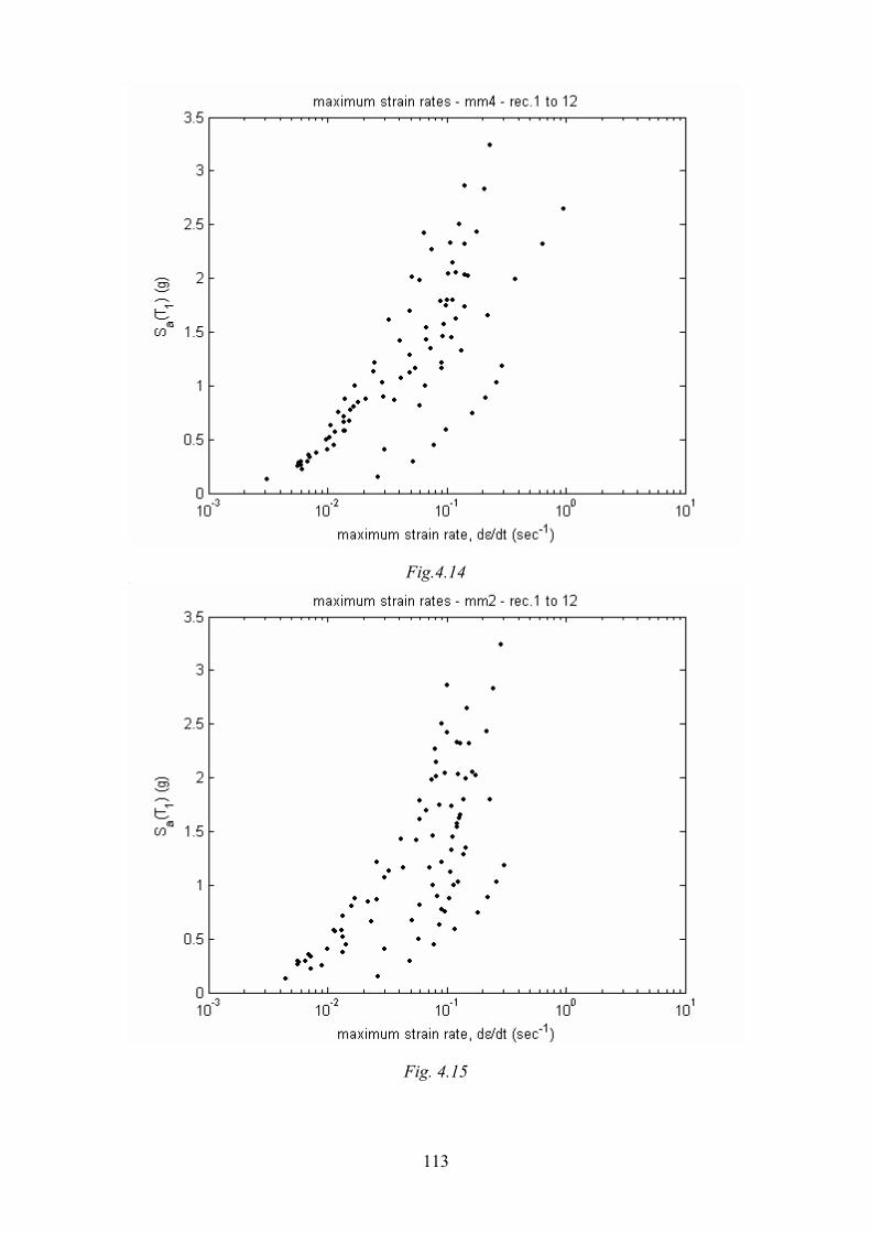
113
Fig.4.14
Fig. 4.15

114
Fig.4.16
Fig.4.17
115
4.4.3. Variability of recorded velocity and connected maximum strain rate variability
The task of this section is to search for strong motion parameters related to variability of
maximum strain rates at constant hazard levels. Within this task, particularly the reason
behind high strain rates in rec.11 and less pronouncedly in rec.10 will be sought for.
This problem is depicted in Fig.4.16 and 4.17. Preliminary hypothesis is that maximum
strain rates can be estimated with analysis of velocity content of records, as stated in
previous section.
Inspection of Table 4.2 and Table 4.3 reveals no significant correlation between the
maximum strain rates observed and any hazard parameter given there. However, the
common distinguishing property of rec.s 10 and 11 with less than 1.5 km source to site
distance can be observed.
Fig.4.18 gives the dispersion of pseudo-velocity spectra of each record and the
corresponding average. Despite the intra-record variability, average spectrum depicted
with blue is rather smooth. Average spectrum is depicted as well in Fig.4.19. This figure
contains the spectral regions concept. Accordingly, dispersion of spectral values in Fig.
4.18 is more dominant in displacement sensitive and to a lesser extent in velocity
sensitive regions. This is in line with trends given in literature, e.g. by (Chopra, 2004).
Comparison of rec.10 and 11 with rest records reveal that these are marked with
distinguishing characteristics of near field records15 -more pronouncedly for rec.11.-.
This is expectable due to the low source-to-site distances of these records.
Such records have high maximum pseudo-velocity to maximum pseudo-acceleration
ratios Svmax / Sa
max. This parameter varies markedly among near field to far field. So, it
could be an indicator for maximum strain rates at constant Sa(T1) levels. This
hypothesis, however, is not verified by Fig.s. 4.20 and 4.21:
Regarding Fig.4.20, despite two local maxima due to rec.s 11 and 2 (at Sa,levels ~ 1.25
and 2.75), contour curves are indifferent to Svmax / Sa
max ratio.
Same is generally valid for Fig.4.21, as well, except a slight correlation trend at the
15 Distinguishing characteristics of mean near field spectra with respect to far field are: (1) slight shift in maximum pseudo-velocity region to higher periods, (2) sharper max. pseudo velocity peak related with higher pseudo velocities, rather than the typical plateau.

116
extreme Sa range 2.50 and 3.00.
One can try to refine the failed indicator by replacing the denominator by the structure-
specific hazard parameter Sa(T1). Svmax / Sa(T1) related curves Fig. 4.22. and 4.23 show
clearer trends:
Fig.4.22 indicate strong correlation of maximum strain rates to Svmax / Sa(T1) for MM4
beyond Svmax / Sa(T1)=2. In the range Sv
max / Sa(T1)<2, the correlation is absent. This is
partly due to interference by exceptional records 2 and 10 (at respectively Svmax /
Sa(T1)=1.429 and 1.908). This can be proven with the existence of the same trend in
Fig.4.24, where dataset without records 2 and 10 is depicted.
MM2 data is depicted in Fig.4.23. There, the correlation beyond Svmax / Sa(T1)=2 is
slightly distorted in comparison to MM4 data in Fig.s 4.18 and 4.20. This is due to
extreme hardening / weaving behaviour of rec.s 3, 4 and 5 observed previously in
Fig.4.13 (these latter records are moderate Sa(T1) data with low site-source distances 1
to 4km, however this do not let us make a statement).
Since MM4 is a more realistic model than MM2, the conclusions will be drawn based
on MM4 data:
ELASTIC REGIME (range of Sa(T1)<~1.0g for our structure):
Mean maximum strain rates relate well to Sa(T1) - loglinearly and with low dispersion
(Fig. 4.16). The deviations seen in Fig. 4.16 are due to near-fault records (rec.10 and 11)
with d<1.5km. They presumably trigger yielding at lower Sa(T1) due to extreme
directivity-related fling pulses. Sv measures are shown to be not governing. Sd(T1)
measures are not checked.
INELASTIC REGIME (beyond ~1.0g level for our structure)
Dispersion of maximum strain rates with respect to Sa(T1) is due to yield onset. It is well
related to Svmax / Sa(T1), if Sv
max / Sa(T1) >2 (high-velocity ground motion) (Fig.s. 4.22
and 4.24). For Svmax/Sa(T1)<2, Sv
max / Sa(T1) and probably velocity content seem
irrelevant to maximum strain rate (Fig.s. 4.22 and 4.24). At these conditions, maximum
strain rate is probably related to acceleration content and to some other record-specific
characteristic like shape.
Over all ranges, Svmax/Sa(T1) appears to be a better indicator for maximum strain rates
than Svmax / Sa
max .

117
The phenomena observed above in MM4 data is slightly dimmed and interfered in
MM2 data at yield onset range due to MM2’s less elaborate yield model.
Rec. no. Svmax / Sa
max
(m/sec/g) Sv
max / Sa(T1)(m/sec/g)
1 4.258 1.245 2 5.228 1.429 3 2.897 2.007 4 3.986 2.448 5 7.720 2.969 6 2.928 1.749 7 5.664 1.411 8 2.654 1.297 9 3.158 1.403 10 7.393 1.908 11 9.314 4.261 12 8.478 2.113
Table 4.3. Tested velocity content indicators for maximum strain rates

118
Fig.
4.1
8
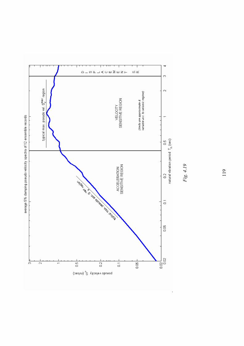
119
.
Fi
g. 4
.19

120
Fig. 4.20
Fig. 4.21

121
Fig. 4.22
Fig. 4.23

122
Fig. 4.24
4.4.4. Variability of global response parameters
In this section, the variability of global response parameters among varying records and
the relation of this variability to maximum strain rates are investigated.
As stated earlier, the common global response parameters are the maximum interstorey
drift ratio (for structural components), the maximum peak floor acceleration (for non-
structural components and some contents) and the maximum peak floor velocity
respectively (for remaining contents).
In Fig.s 25 and 26, ISDmax data from MM4 and MM2 computations are depicted.
Previously deviating records in maximum strain rate figures (rec.s 10 and 11) are in
both cases in line with mainstream.
Another observation is the deviation between MM2 and MM4 data for rec.2 at high
hazard levels. Identical situation is observed in terms of maximum strain rates
previously. To repeat, for the exceptional case of rec.2, different material models yield
significantly varying results; at maximum hazard level respectively ISDmax =9% and 7%
and ε max = 100 and 10-1. These can be due to an advancement of yield onset at higher
hazard levels leading to increase in number of inelastic cycles. This may alter yield
123
sequence, which imprints MM4 data in contrast to MM2 data (since yield sequence is
irrelevant for max MM2 data due to neglect of rattcheting and Bauschinger effects).
Another point of interest is the weaving forms observed especially in Fig.4.26, e.g.
rec.5. The reason for this is the same as explained in section 4.4.2.
Fig.s 4.27 and 4.28 illustrate the attempts to explain ISDmax variability by a further
parameter Svmax / Sa(T1). Investigation of these figures reveal no correlation of ISD to
Svmax / Sa(T1). This means that ISDmax is indifferent to changes in Sv
max / Sa(T1) (valley
at appr. Svmax / Sa(T1)=1.8 is due to lack of data from a record).
Hazard parameters incorporating spectral values at other periods like T2 or 1.5T1 are not
tested due to limitations of the work.
Let proceed further with response variability. Fig.s. 4.29 and 4.30 reveal increased
variability of PFVmax values at higher hazard levels with respect to ISDmax. However,
the variability over material models is much less. Fig.s 4.31 and 4.32 reveal strong
correlation of PFVmax to Svmax / Sa(T1) in a limited region, bounded by Sa(T1) >1 and
Svmax / Sa(T1) < 2. This region corresponds to inelastic regime with low velocity strong
motion. On the upper region bounded with Sa(T1) >1 and Svmax / Sa(T1) > 2, correlation
is much less.
Fig.s 4.33 to 4.36 depict same relations for PFA measure. In Fig.s 4.33 and 4.34, yield
onset at ca. Sa(T1) =1g is more obvious than in ISDmax and PFVmax. General trend is
saturation of PFAmax values after Sa(T1) =1g. This corresponds to moderate to
significant yielding.
In all 3-D graphs, it is obvious that Sa(T1) strongly correlates to all response parameters
at elastic range. In inelastic range, the correlation is partial.
Fig.s 4.37 and 4.38 depict maximum strain rate variability vs. PFVmax vs. Sa(T1). The
first two parameters can be presumed intuitionally to be correlated, since strain rates in
general relate to excitation velocity. However, no such trends are recognizable in the
referred figures.
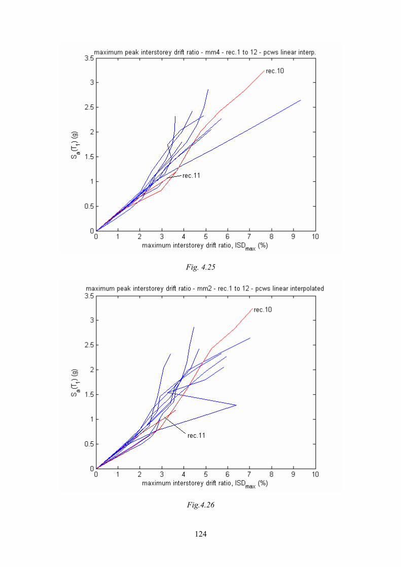
124
Fig. 4.25
Fig.4.26
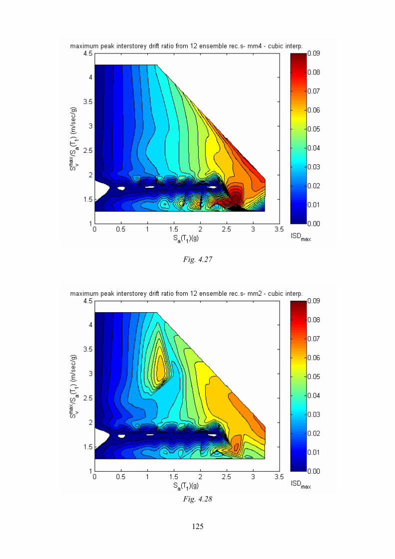
125
Fig. 4.27
Fig. 4.28
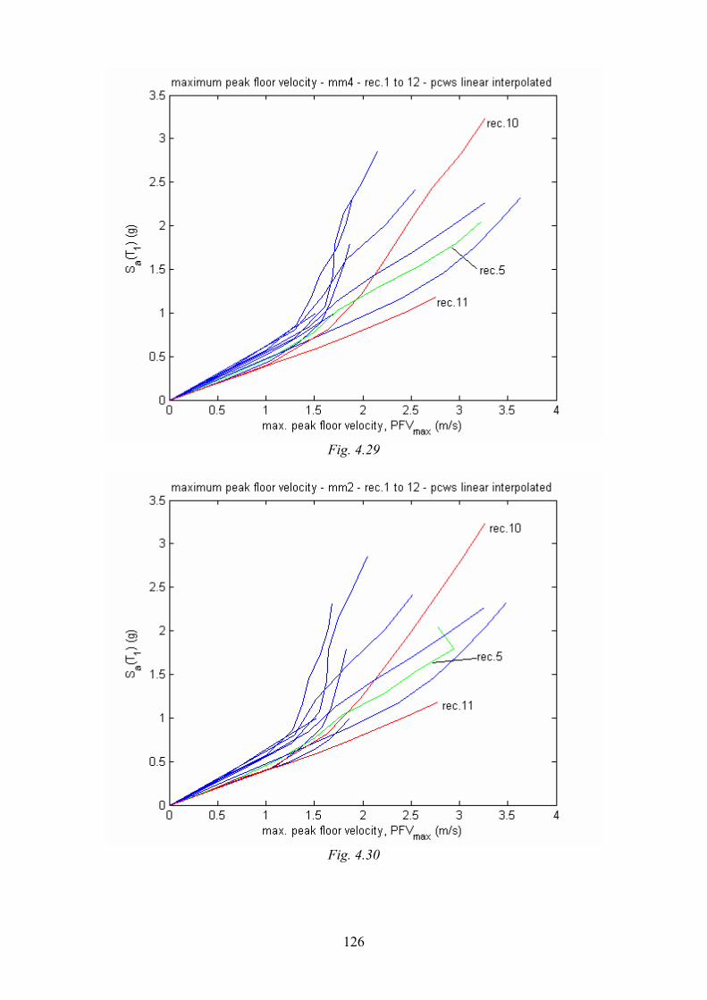
126
Fig. 4.29
Fig. 4.30
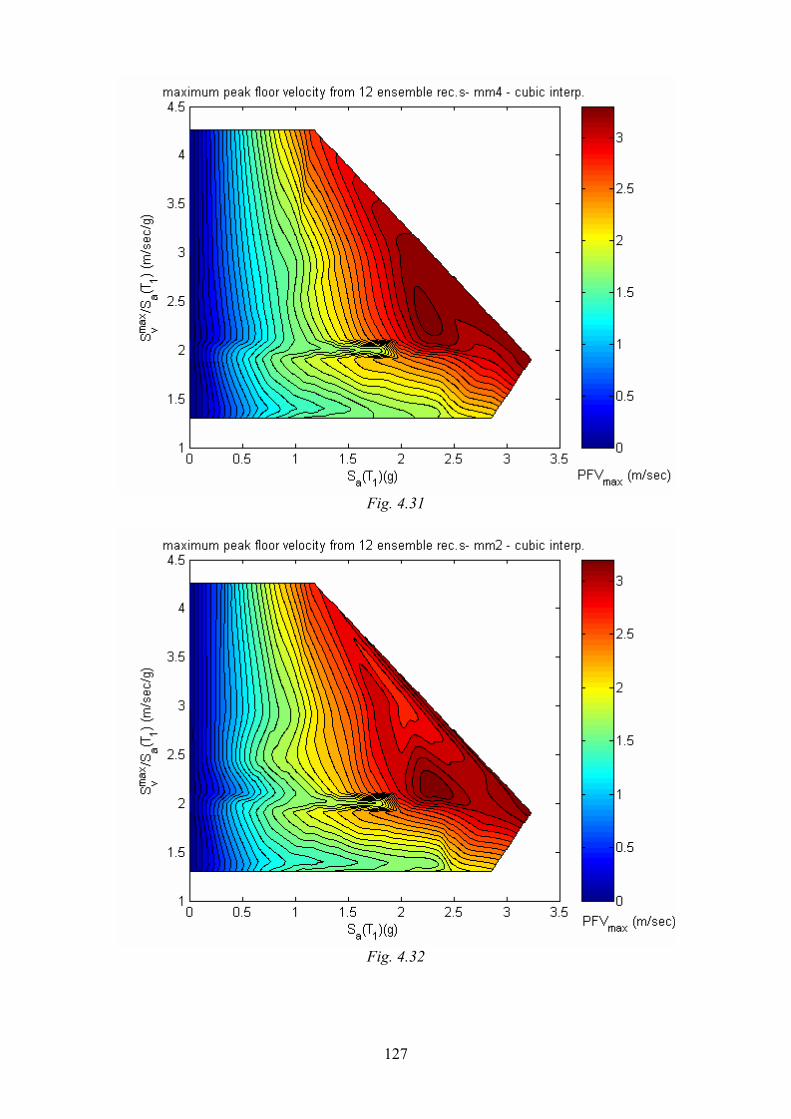
127
Fig. 4.31
Fig. 4.32
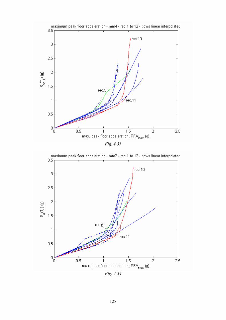
128
Fig. 4.33
Fig. 4.34
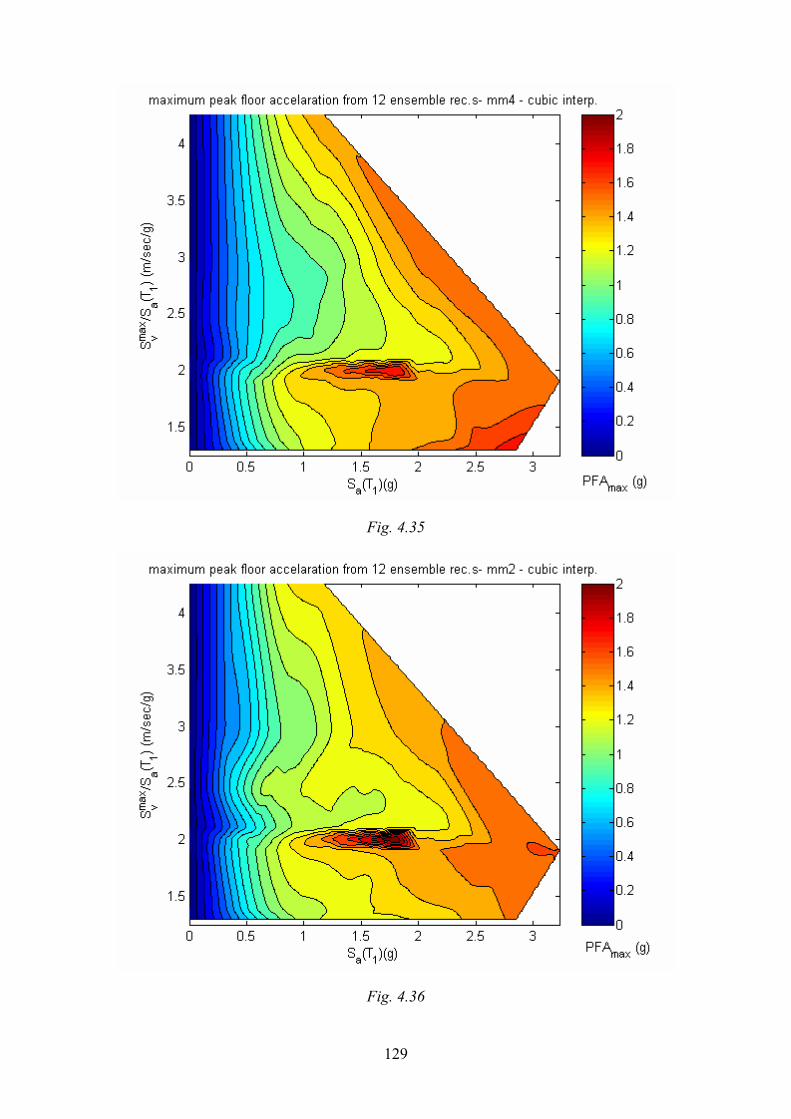
129
Fig. 4.35
Fig. 4.36

130
Fig. 4.37
Fig. 4.38

131
Conclusions
In Chapter 2, an advanced state-of-the-art method is developed for seismic risk
assessment. It is practically applicable as shown by the example in Chapter 3. The main
problem of the method is the availability of both hazard and damageability data. This
problem can be solved through more intensive efforts for creating open source
databases. Among best practices in this context are websites of USGS (United States
Geological Survey, USA) Hazard Program for hazard data and website of PEER
(Pacific Earthquake Engineering Research Institute, USA) Framework for
damageability data.
Continuing development of methods and tools in earthquake engineering leads to huge
volumes of disorganized information which is not directly adaptable by risk assessment
practice. An important contribution of this work has been to provide a complete method
synthesizing state-of-the-art approaches and enriching them with original contributions.
Investigations on sensitivity to rate dependency have revealed that the phenomena is not
significant for risk assessment purposes in terms of global response treatment. The
question of local response sensitivity remains a further research need. This is
particularly significant due to the very high strain rates on the brink of explosion load
ranges proven by the simulations. On the other hand, response estimates are shown to
be highly sensitive to progressive plasticity modeling demonstrated by comparison of
multilinear and two-surface model data. Moreover, interaction of global response with
near field seismological phenomena is observed. The outputs reveal that for better
estimates of response and consequently of damage and risk, such interactions should be
regarded.
As concluding remark, one can quote (Adams and Spence, 1999) “for all our present-
day scientific and technical skill, the world’s earthquake problem is still a long way
from being solved and so will require continuous attention” .

132
ANNEX.I. MATLAB Script
This annex is referred in section 3.3.5 of this work.
Following script is prepared as input for commercial software MATLAB. It is used for
the application in Chapter 3. The method used therein is explained in Chapter 2.
disp('*****PROGRAM FOR SEISMIC RISK ASSESSMENT METHOD *****')
disp('********prepared by: Sadik Cem Topcuoglu, 2006*****')
% PART I_ HAZARD ASSESSMENT ****************************************************
% INPUT HAZARD PARAMETERS
% [this part assumes that the user has obtained the site hazard curve previously]
b=input('enter b coefficient for hazard curve (Gutenberg-Richter relation) \n')
% [b: slope of (the straight section of) the regional Gutenberg-Richter curve]
% [refered in eq. 10. obtained by regional seismicity analysis, see section 2.8. for details]
% [input all magnitudes in moment magnitude]
mmax=input('enter lower cutoff magnitude of hazard curve\n')
% [refered in eq.s 11 & 12. max. magnitude considered in hazard assessment, see section 2.8]
mmin=input('enter maximum magnitude of hazard curve\n')
% [refered in eq.s 11 & 12. min. magnitude considered in hazard assessment, see section 2.8]
ml=input('enter lower magnitude bound for risk assessment \n')
% [lower bound to be considered in risk assessment, see section 2.8]
% [varies between m=4-6]
mu=input('enter upper magnitude bound for risk assessment\n')
% [upper bound to be considered in hazard assessment, see section 2.9.1]
% [equal or slightly smaller than mmax]
nhl=input('enter number of considered hazard levels\n')
% [no. of hazard levels ml=<m=<mu, at which simulation will be carried out]
% [this is a subjective resolution decision, see section 2.9.1]
% [usual recommendation is 0.5 magnitude resolution, so nhl=(mu-ml)/0.5]

133
% [calculation of hazard parameters:]
dm=(mu-ml) / (nhl-1)
% [∆m, magnitude step between each hazard simulation level, see section 2.9.1.6]
bet=b*log(10)
% [β, eq.13, section 2.8]
k=1/(1-exp(-bet*(mmax-mmin)))
% [k, eq.12, section 2.8]
% [implementation of eq. 11, giving cumulative prob.s:]
m=ml
for h=1:nhl
% [cumulative prob.s of occurrence, eq.11:]
gem(hc)=k*(exp(-bet*(m-mmin)))-k+1
m=m+dm
end
% [computation for interval probabilities:]
hp(1,nhl)=gem(nhl)
for h=1:(nhl-1)
hp(1,nhl-h)=gem(nhl-h)-gem(1,nhl-h+1)
end
for h=1:nhl
HM(h)= ml-ms+(h*ms)
end
% [input number of simulations per hazard level:]
nth=input('enter number of simulated time histories per hazard level\n')
% [n, decision (2) in section 2.9.1.6]
% EXTERNAL WORK: Strong Motion Simulation
% [at this point, use an appropriate stochastic simulation program
% to simulate nth time histories at each magnitude level ml, ml+dm, ml+2dm, …., mu]
% [procedure and necessary tools are explained in section 2.9.1, especially in 2.9.1.6]
% EXTERNAL WORK: Structural Analysis (Response Assessment)
% [for each simulated time histories refered above,
% carry out structural analysis of the structure with appropriate methods and tools
% explained in section 2.9.2.]

134
% [from each analysis, extract necessary response governing variables]
% [which are ISDmax, PFAmax, PFVmax, refered in Table 2.6]
% PART II_ RESPONSE INPUT *********************************************************
% [input of response governing variables to form necessary matrices for risk assessment,
% see section 2.9.2 for explanation]
% [response governing variables’ matrices are initially set to zero to prepare for input]
isd=zeros(nth,nhl)
pfa=zeros(nth,nhl)
pfv=zeros(nth,nhl)
% [input results from structural analysis one by one at each hazard level:]
for hl=1:nhl
disp('hazard level - magnitude')
mh=ml-ms+(hl*ms)
disp(mh)
% [input isd-max from structural analysis with each simulation at hazard level mh:]
isd(1:nth,hl)=input('enter isd-max from sim.s at the hazard level \n--bracketed & seperated with ;--\n')
% [input pfa-max from structural analysis with each simulation at hazard level mh:]
pfa(1:nth,hl)=input('enter pfa-max from sim.s at the hazard level \n--bracketed & seperated with ;--\n')
% [input pfv-max from structural analysis with each simulation at hazard level mh:]
pfv(1:nth,hl)=input('enter pfv-max from sim.s at the hazard level \n--bracketed & seperated with ;--\n')
end
% [natural logarithm of response governing variables,
% since lognormal distribution is assumed in line with literature:]
lisd=log(isd)
lpfa=log(pfa)
lpfv=log(pfv)
% [statistical inference of response governing variables at each hazard level:]
% [first three; mean values, rest; standard deviations]
lisdmu=mean(lisd)
lpfamu= mean(lpfa)
lpfvmu= mean(lpfv)
lisdsi=std(lisd)
lpfasi=std(lpfa)
lpfvsi=std(lpfv)

135
% PART III. DAMAGEABILITY INPUT**************************************************
% [input of damageability parameters of each component,
% see section 2.9.3 for explanation]
% [whole structure is treated as one component. nonstr.l components and contents add one by one]
% [guiding list is in table 2.7 in section 2.9.3]
ndsc=input('enter number of drift sensitive components\n')
nasc=input('enter number of acceleration sensitive components\n')
nvsc=input('enter number of velocity sensitive components\n')
% [calculation, nc: total no. of components]
nc=ndsc+ nasc+nvs
% [input, mcn: no of monte carlo simulations for each component]
% [input as 106 in application presented in chapter 3, explained in section 3.3.5]
mcn=input('enter number of simulations\n')
% [input, damage state capacity data,
% for an example: see Table 2.8,
% concept is explained in section 2.9.3]
% [WARNING: enter damageability data first for drift-sensitive, then for acc.-sensitive,
% finally for vel.-sensitive components]
% PART IV. DAMAGE AND LOSS ASSESSMENT *****************************************
% [loop for each component:]
for m=1:nc
disp('COMPONENT no.:')
disp(m)
% [input respectively mean capacity for 4 damage states for the component considered]
% [if less than 4 ds’s are defined for the component, give rest as very high numbers,
% e.g. 10E8 times the last defined damage state capacity]
dmu(1:4,m)=input('enter damage state mean capacities \n--bracketed & seperated with ;--\n')
% [example to mean capacity; Table 2.8., Column 10-left]
dsi(1:4,m)=input('enter damage state capacity standard dev.s\n--bracketed &…
seperated with ;--\n')
% [example to capacity standard dev.; Table 2.8., Column 10-right]
plr(1:4,m)=input('enter ratio of_damage state loss_to_comp. restoration cost_\n—bracketed &… seperated with ;--\n')

136
% [example to mean capacity; Table 2.8., Column 11]
rct(1,m)=input('enter ratio of _component restoration cost_ to _bld. restoration…
…cost_\n--bracketed--\n')
end
%**********************************************************
% [damage state prob. matrices are initially set to zero to prepare for input:]
% [damage state 1 matrix, rows: magnitude levels, columns: components]
pd1=zeros(nhl,nc)
% [damage state 2 matrix, rows: magnitude levels, columns: components]
pd2=zeros(nhl,nc)
% [damage state 3 matrix, rows: magnitude levels, columns: components]
pd3=zeros(nhl,nc)
% [damage state 4 matrix, rows: magnitude levels, columns: components]
pd4=zeros(nhl,nc)
% **********************************************************
% [damage state membership and loss calculation for each component:]
for m=1:nc
disp('calculation for component:')
nc
% [extraction of mean capacity vector for component considered:]
dammu=log(dmu(:,m))
% [extraction of capacity standard deviation vector for component considered:]
damsi=dsi(:,m)
% [extraction of appropriate response vector for the component:]
if m<=ndsc
respmu=lisdmu
respsi=lisdsi
elseif m<=(ndsc+nasc)
respmu=lpfamu
respsi=lpfasi
else
respmu=lpfamu
respsi=lpfasi
end

137
tp1=0
tp2=0
tp3=0
tp4=0
% [monte carlo simulation for the component considered,
% aim: obtain damage state membership conditional probabilities]
disp('simulation counter:')
for s=1:mcn
s
% [generate random vector from response distribution:]
y=lognrnd(respmu,respsi)
% [implementation of eq.s 41 & 42:] *********************
% [obtain probability of exceedance of damage state 1 capacity
% ,for the generated number:]
cp1=logncdf(y,dammu(1),damsi(1))
% [same for damage state 2, 3 and 4 respectively:]
cp2=logncdf(y,dammu(2),damsi(2))
cp3=logncdf(y,dammu(3),damsi(3))
cp4=logncdf(y,dammu(4),damsi(4))
% **************************************************
% [implementation of eq.s 43 & 44:] **********************
% [obtain probability of damage state 1 membership for generated vector:]
ap1=cp1-cp2
% [same for damage state 2, 3 and 4]
ap2=cp2-cp3
ap3=cp3-cp4
ap4=cp4
% **************************************************
% [cumulate probabilities of damage state membership:]
tp1=tp1+ap1
tp2=tp2+ap2
tp3=tp3+ap3
tp4=tp4+ap4
end

138
% [extract probability of damage state 1 membership for component considered…
% by dividing cumulated probability vector to number of simulations:]
pd1(:,m)=tp1/mcn
% [same for damage states 2,3 and 4:]
pd2(:,m)=tp2/mcn
pd3(:,m)=tp3/mcn
pd4(:,m)=tp4/mcn
%[ loop for each magnitude level :] ************************************************
for f=1:nhl
% loss|hazard as ratio of comp value
rplahl(f,m)=(pd1(f,m)*plr(1,m))+(pd2(f,m)*plr(2,m))+(pd3(f,m)*plr(3,m))+…
(pd4(f,m)*plr(4,m))
% loss|hazard as ratio of bld value
aplahl(f,m)=rplahl(f,m)*rct(m)
end
% ***************************************************************************
% [compute absolute probs of damage state membership: ] ******************************
% [multiply hazard probability vector with damage state 1 membership vector:]
apd1(m)=(hp*pd1(:,m))
% [same for damage states 2,3 and 4:]
apd2(m)=(hp*pd2(:,m))
apd3(m)=(hp*pd3(:,m))
apd4(m)=(hp*pd4(:,m))
% ***************************************************************************
% [unite damage state vectors to form dam. state probability matrix for component considered:]
apd(:,m)=[apd1(m);apd2(m);apd3(m);apd4(m)]
% ***************************************************************************
% [rel. damage loss per component, percent of comp. value:]****************************
rpl(m)=(plr(:,m))'*apd(:,m)
% ***************************************************************************
% [abs. damage loss vector per component - percent of total value:]***********************
apl(m)=rpl(m)*rct(m)
% ***************************************************************************

139
% [total loss due to the component - percent of total value:]******************************
aplt(m)=sum(apl(m))
end
% [loop for each component ended]********************************************************
% PART V. EXTRACTION OF RESULTS*************************************************
% [total loss - percent of total value:]
EXPLOSS=sum(apl)
EXPLOSS2=sum(aplt)
% [check: exploss should be equal to exploss2.]
% [further necessary data for risk assessment purposes can also be extracted at that point]*************
% [extraction of graphs:]
% [in the following are example commands for extraction of graphs.
% see the titles for explanation. fig.s 3.18 to 3.28 are produced with these commands.]
figure(1)
lossvshaz=sum(aplahl,2)
plot(lossvshaz*100,HM','b.-')
axis([0 20 4.5 8.5])
title('total percent loss estimate - pcws linear interp.'),...
xlabel('loss ratio (%)'),ylabel('moment magnitude')
figure(2)
lossstr=aplahl(:,1)
lossnstr=aplahl(:,2)+aplahl(:,3)+aplahl(:,4)
losscon=aplahl(:,5)+aplahl(:,6)+aplahl(:,7)+aplahl(:,8)
plot(lossvshaz,HM','b.-',lossnstr,HM','g.-',losscon,HM','r.-',lossstr,HM','k.-')
axis([0 0.20 4.5 8.5])
title('total loss ratio vs. hazard level - pcws linear interp.'),...
xlabel('loss / total building value (%)'),ylabel('hazard intensity - moment magnitude')
figure(3)
plot(lossvshaz,hp','b.-',lossnstr,hp','g.-',losscon,hp','r.-',lossstr,hp','k.-')
%axis([0 0.20 4.5 8.5])
title('total loss ratio vs. hazard level - pcws linear interp.'),...
xlabel('loss / total building value (%)'),ylabel('hazard intensity - moment magnitude')
140
figure(3)
set(gcf,'DefaultLineLineWidth',0.5)
plot(aplahl(:,2),HM','g.-',aplahl(:,3),HM','g.-',aplahl(:,4),HM','g.-',...
aplahl(:,5),HM','r.-',aplahl(:,6),HM','r.-',aplahl(:,7),HM','r.-',aplahl(:,8),HM','r.-')
axis([0 0.20 4.5 8.5])
title('component loss ratio vs. hazard level - pcws linear interp.'),...
xlabel('loss / total building value (%)'),ylabel('hazard intensity - moment magnitude')
figure(4)
set(gcf,'DefaultLineLineWidth',0.5)
plot(aplahl(:,2),HM','g.-',aplahl(:,3),HM','g.-',aplahl(:,4),HM','g.-')
axis([0 0.20 4.5 8.5])
title('nonstructural component loss ratio vs. hazard level - pcws linear interp.'),...
xlabel('loss / total building value (%)'),ylabel('hazard intensity - moment magnitude')
figure(5)
set(gcf,'DefaultLineLineWidth',0.5)
plot(aplahl(:,5),HM','r.-',aplahl(:,6),HM','r.-',aplahl(:,7),HM','r.-',aplahl(:,8),HM','r.-')
axis([0 0.20 4.5 8.5])
title('content loss ratio vs. hazard level - pcws linear interp.'),...
xlabel('loss / total building value (%)'),ylabel('hazard intensity - moment magnitude')
figure(7)
lossstr=rplahl(:,1)
lossnstr=rplahl(:,2)+rplahl(:,3)+rplahl(:,4)
losscon=rplahl(:,5)+rplahl(:,6)+rplahl(:,7)+rplahl(:,8)
plot(lossvshaz,HM','b.-',lossnstr,HM','g.-',...
losscon,HM','r.-',lossstr,HM','k.-')
axis([0 0.20 4.5 8.5])
title('component type loss ratio vs. hazard level - pcws linear interp.'),...
xlabel('loss / total value of component type value (%)'),ylabel('hazard intensity - moment magnitude')
figure(8)
set(gcf,'DefaultLineLineWidth',0.5)
plot(rplahl(:,1),HM','k.-')
axis([0 0.20 4.5 8.5])
title('structural loss ratio vs. hazard level - pcws linear interp.'),...
xlabel('loss / total value of structural components (%)'),ylabel('hazard intensity - moment magnitude')
141
figure(9)
set(gcf,'DefaultLineLineWidth',0.5)
plot(rplahl(:,2),HM','g.-',rplahl(:,3),HM','g.-',rplahl(:,4),HM','g.-')
axis([0 2 4.5 8.5])
title('nonstructural component loss ratio vs. hazard level - pcws linear interp.'),...
xlabel('loss / component value (%)'),ylabel('hazard intensity - moment magnitude')
figure(10)
set(gcf,'DefaultLineLineWidth',0.5)
plot(rplahl(:,5),HM','r.-',rplahl(:,6),HM','r.-',rplahl(:,7),HM','r.-',rplahl(:,8),HM','r.-')
axis([0 1 4.5 8.5])
title('content loss ratio vs. hazard level - pcws linear interp.'),...
xlabel('loss / content value (%)'),ylabel('hazard intensity - moment magnitude')
figure(11)
set(gcf,'DefaultLineLineWidth',0.5)
plot(pd1(:,1),HM','g.-',pd2(:,1),HM','b.-',pd3(:,1),HM','r.-')
%axis([0 1 4.5 8.5])
title('structure damage state probability vs. hazard level - pcws linear interp.'),...
xlabel('probability'),ylabel('hazard intensity - moment magnitude')
figure(11)
set(gcf,'DefaultLineLineWidth',0.5)
plot(pd1(:,1),hp,'g.-',pd2(:,1),hp,'b.-',pd3(:,1),hp,'r.-')
%axis([0 1 4.5 8.5])
title('structure damage state probability - pcws linear interp.'),...
figure(12)
set(gcf,'DefaultLineLineWidth',0.5)
plot(SDISD,HM,'r.-',SDPFA,HM,'b.-',SDPFV,HM,'g.-')
%axis([0 1 4.5 8.5])
title('dispersion of response - pcws linear interp.'),...
xlabel('/sigma standard deviation of response distribution '),ylabel('hazard intensity - moment magnitude')
% E N D ***********************************************************************
142
ANNEX.II. ANSYS Script
This annex is referred in sections 3.3.4, 4.3.2, 4.3.3 and 4.3.5 of this work.
Following script is prepared as input for commercial software MATLAB. It is used for
the applications in Chapter 3 and Chapter 4. Due to the dimensions of this work, only
one hazard amplification level for one time history and one material model is given as
example (amplification level 0.125 for time history p0809 – p0809 being number of
strong motion record in PEER Database (PEER, 2005)). Since it is necessary to clear
database in ANSYS after each computation, all structural and material data should be
input again after computation of each strong motion time-history.
The following script is based largely on a script in the work of (Wichers, 2001). Time
history ensemble used here is a different one than that of Wichers’. Several further
revisions are made in structural configuration and material properties. Profile database
referred in the script is also provided in the work by (Wichers, 2001). Details on the
script (e.g. generation of profiles, time history analysis aspects) are also given there.
The referred author has given permission to use a modified version of his script within
this work.
/BATCH /CLEAR /UNITS,SI /CONFIG,NRES,2000 /CWD,d:\cem\p0809x0.125_m2 /FILNAME,p0809x0.125_m2,1 /CONFIG,NRES,500000 iwert=1814 !Anzahl der Werte, die aus der Erdbebendatei gelesen werden ilang=1814 !Anzahl der Werte, die aus der Erdbebendatei gelesen werden deltat=0.02 skalt1=0.125 Moanaly=0 ! 0:transient or static analysis 1:modal analysis dynam=1 ! 0:static analysis(dl+ll) 1:transient analysis (dl+ll+eq) mscal=0.7 ! Skalierung der Masse weight=0.38692E+06 !weight of structure ! *** Werkstoffmodell *********************** modell=2 ! 0: linear-elastische Rechnung ! 1: bilineares Werkstoffmodell ! 2: multilineares Werkstoffmodell ! 3: TWO-Surface zeitunabhängig (Scheibe/Reinighaus) ! 4: TWO-Surface Zeitabhängig (Scheibe/Reinighaus/Böttcher) ! *** Profile ******************************* profils='hea200' profilr='hea200' profilv='L70x7' profilvr='hea140' !Die Profil-Datenbank liegt in mm vor profilba='d4hea200' profilbb='d3hea200' profilbc='d4hea200' ! *** Halterung Rahmeneckknoten in uy****** decuy=0 !0:keine halterung, 1:halterung

143
!*** Lastparameter/Dynamik *** masse=0.7 !Berücksichtigung der Massenträgheit 0: keine Berücksicht. 1: Berücksichtigung massw=2.105*mscal !Riegelmasse, corresponds to 21,05 kN/m when mscal=1 kg/m/1000 ! *** Geometry *** ibays=1 !0: 2D model, 1: rahmen in tiefe istock=3 !Anzahl der Stockwerke des Rahmens,1,2,3 [Anzahl] in Stück breit=5000 !Rahmenbreite [Breite] in mm breitq=3000 !Abstand der Rahmen in der Tiefe [Abstand] in mm hocheg=3000 !Höhe Erdgeschoß [Höhe EG] in mm hochoga=3000 !Höhe 1.Obergeschoß [Höhe 1.OG] in mm hochogb=3000 !Höhe 2.Obergeschoß [Höhe 2.OG] in mm einsp=1 !Fußpunkt Stütze 0: gelenkiger Fußpunkt 1: eingespannter Fußpunkt offset=0 !Abstand der Verbands-/Riegelknoten aus der Rahmenebene in mm unts=10 !Anzahl der Elemente in der Stütze [Anzahl] in Stück untr=10 !Anzahl der Elemente im Riegel [Anzahl] in Stück untv=10 !Anzahl der Elemente im Verbandsstab [Anzahl] in Stück bone=150 !Breite des 1/3-Bone-Elementes [Breite] in mm ! *** for calc of graphs weightcoef=100/weight hochcoef1=-100/hocheg hochcoef2=100/hocheg ! *** Sonstige Parameter *** loese=1 langsa=40000 !Zeitliche Verzögerung der Lastdauer-genutzt für erste lastspiele dskal=10*skalt1 askal=-9810 !Erdbeschleunigung [Beschleunigung] in mm/sec2 ! *** Konvergenzkriterien *** konv=0 konv2=0 cfak1=350 cfak2=0.05 iterat=1000 ! *** Steuerungsvariablen für Erdbeben*** KBCWERT=1 !sprungartig subzahl=1 ! *** Schubverformung setzen, Kappa nach Ahrens/Duddek *** DXI=0 DXJ=0 SHEARZ1=4.29 ! Stütze SHEARY1=1.34 ! Stütze SHEARZ2=4.29 ! Riegel SHEARY2=1.36 ! Riegel SHEARZ3=3.98 ! Dog-Bone innen SHEARY3=1.40 ! Dog-Bone innen SHEARZ4=3.66 ! Dog-Bone mitte SHEARY4=1.45 ! Dog-Bone mitte SHEARZ5=3.98 ! Dog-Bone außen SHEARY5=1.40 ! Dog-Bone außen SHEARZ6=4.58 ! Querriegel SHEARY6=1.32 ! Querriegel SHEARZ7=0 ! Verband SHEARY7=0 ! Verband ! *** Parameter für Werkstoffmodelle *** ! *** Allg. Parameter Werkstoff *** emod=209000 !E-Modul [E-Modul] in N/mm2 den=7.85e-9 !Dichte [Dichte] in kg/mm3/1000 ! = g/mm3 nue=0.3 !Querdehnzahl [nue] in --- ! *** Modellparameter Elast-Plast (BKIN) *** *if,modell,eq,1,then betas=360.0 !Streckgrenze [Spannung] in N/mm2 emodv=0.01*emod !Steigung der Verfestigung [Steigung] in N/mm2 *endif ! *** Modellparameter MKIN *** *if,modell,eq,2,then epsy=360/emod !Dehnung der Streckgrenze [Dehnung] in %o
144
epsy2=0.020 !Dehnung Punkt 2 [Dehnung] in %o epsy3=0.040 !Dehnung Punkt 3 [Dehnung] in %o epsy4=0.060 !Dehnung Punkt 4 [Dehnung] in %o epsy5=0.100 !Dehnung Punkt 5 [Dehnung] in %o betas=360 !Spannung im Punkt 1 (Streckgrenze) [Spannung] in N/mm2 betas2=360 !Spannung im Punkt 2 [Spannung] in N/mm2 betas3=430 !Spannung im Punkt 3 [Spannung] in N/mm2 betas4=470 !Spannung im Punkt 4 [Spannung] in N/mm2 betas5=520 !Spannung im Punkt 5 [Spannung] in N/mm2 *endif ! *** Modellparameter TWO-SURFACE SCHEIBE/REININGHAUS *** *if,modell,eq,3,then !Einlesen Steuerwerte /com ! *** Modellparameter TWO-SURFACE (Scheibe/Reininghaus/Böttcher) *** c1=1 !!! NDIM Dimension des Problems c2=2 !!! KFLIB c3=0 !!! KHARD/KBOUND/0:boundnurisotrop c4=1 !!! KALFA/1:reinermroz c5=1 !!! KBETA /com !Einlesen der Sp.-Dehn.-diagramme c6=36.0 !!! LOADING:k aktuell37.0 SEDKN(1,1) Grundwert Fließplateau c7=0.27 !!! LOADING:k monoton12.5 xmonfa y_1 c8=0.23 !!! LOADING:k saettigung10.0 xsaefa y_3 /com c9=36.0 !!! BOUNDING:k aktuell42.0 SEDKN(2,1) Grundwert Fließplateau /com !sonstige Parameter Scheibe c10=0.5 !!! CONMC1 c_a Param. strain-memory c11=0.5 !!! CONMC2 c_m Param. strain-memory c12=0.2 !!! CONMC3 c_s Param. strain-memory c13=5.0 !!! QSTERN c14=2.0 !!! CONLA b_1 Formparameter c15=-4.0 !!! CONLB b_2 Formparameter c16=0.60 !!! CONGH c17=3.0 !!! CONGC c18=-10.0 !!! CONGD c19=-1.8 !!! CONB e_1 Formparameter bounding c20=0.06 !!! DELBK z_1 Größenparam. zykl. Verfest. /com !Ergänzungen Reininghaus c21=1 !!! IELP c22=3.0 !!! h2 h_2 Formparam. kl. Dehn.-amplit. c23=2.5 !!! h3 h_3 Formparam. kl. Dehn.-amplit. c24=0.93 !!! a1=0.73286281 a_1 Größenparameter monot. Verfest. c25=0.019 !!! a2=0.0162018 a_2 Größenparameter monot. Verfest. c26=0 !!! IFT c27=0 !!! IFZ c28=10.5 !!! wzu c29=0.5 !!! wgr c30=0.35 !!! delfak0.35 /com !Steuerung WMTWOS c31=0.1 !!! EPVMAX c32=0.00001 !!! EPVMIN c33=0.00010 !!! GRFLI c34=0.00010 !!! grfle c35=1.0 !!! f1 c36=1.0 !!! f2 c37=1.0 !!! f3 /com !Steuerung ANSYS-Ausgabe !c38=10 !!! ausele !c39=1 !!! ausgau !c40=10 !!! plotele56 !c41=1 !!! plotgau1 /com !geändertes Qstern c42=5.0 !!! qtmod6 q_4_* %o c43=6.0 !!! qprop6 q_3_* %o c44=6.8 !!! qbou1(Verfest.)9.5 q_1_* unterstr. %o c45=6.2 !!! qbou26 q_2_* %o c46=5.0 !!! qquer6 /com !Ratcheting/ Mittelspannungsrelax. c47=0 !!! KDEL c48=2.4 !!! rexpo

145
c49=1.0 !!! rvorz c50=0 !!! krat c51=5 !!! wkina1=ddelta c52=1000 !!! wkina210 c53=0.01 !!! CHAB11 c54=0.01 !!! CHAB12 c55=0.0005 !!! rata c56=70 !!! forga c57=40 !!! forgb c58=3 !!! forgc c59=0.0059 !!! chab21 c60=0.0041 !!! chab22 c61=0.0001 !!! chab23_3.1 c62=0.0 !!! fkinbo0=reinisotrop c63=1.0 !!! xrat c64=50 !!! yrat c65=10 !!! betmax c66=42 !!! offbetino %o c67=1 !!! irel /com !Zeitabhängigkeit c68=0 !!! izeit(0=rate-indep.) c69=0.0 !!! ddelta/kN/cm2(ohnewurzel2/3)0.5 c70=7.5 !!! skvmax0.4 dk_0_dach kN/cm² max Add. auf Grundwert c71=0.8 !!! vmaxa s_2 c72=0.2 !!! vmaxb s_1 c73=0.001 !!! tmaxb p_1 c74=4.0 !!! dqmax dq_1_* %o max geschwind.-abhäng. Add. auf Grundwert c75=1 !!! imehr c76=4.0 !!! rloafa b_3 Formparameter c77=1.0 !!! ymonfa y_2 Faktor für ungesättigt c78=1.0 !!! ysaefa y_4 Faktor gesättigt c79=0.0 !!! sosfak u_1 Faktor für R_eH (FÜR OBERE STR.GR._Ausgeschaltet) c80=4.0 !!! strfak k_ostr_Dach kN/cm² ! Wert für R_eH (FÜR OBERE STR.GR._Ausgesch.) *endif ! *** 1.5 Modellparameter TWO-SURFACE SCHEIBE/REINGHAUS/BÖTTCHER *** *if,modell,eq,4,then c1=1 !!! NDIM Dimension des Problems c2=2 !!! KFLIB c3=0 !!! KHARD/KBOUND/0:boundnurisotrop c4=1 !!! KALFA/1:reinermroz c5=1 !!! KBETA /com !Einlesen der Sp.-Dehn.-diagramme c6=32.0 !!! LOADING:k aktuell37.0 SEDKN(1,1) Grundwert Fließplateau c7=0.27 !!! LOADING:k monoton12.5 xmonfa y_1 c8=0.23 !!! LOADING:k saettigung10.0 xsaefa y_3 /com c9=32.0 !!! BOUNDING:k aktuell42.0 SEDKN(2,1) Grundwert Fließplateau /com !sonstige Parameter Scheibe c10=0.5 !!! CONMC1 c_a Param. strain-memory c11=0.5 !!! CONMC2 c_m Param. strain-memory c12=0.2 !!! CONMC3 c_s Param. strain-memory c13=5.0 !!! QSTERN c14=2.0 !!! CONLA b_1 Formparameter c15=-4.0 !!! CONLB b_2 Formparameter c16=0.60 !!! CONGH c17=3.0 !!! CONGC c18=-10.0 !!! CONGD c19=-1.8 !!! CONB e_1 Formparameter bounding c20=0.06 !!! DELBK z_1 Größenparam. zykl. Verfest. /com !Ergänzungen Reininghaus c21=1 !!! IELP c22=3.0 !!! h2 h_2 Formparam. kl. Dehn.-amplit. c23=2.5 !!! h3 h_3 Formparam. kl. Dehn.-amplit. c24=0.93 !!! a1=0.73286281 a_1 Größenparameter monot. Verfest. c25=0.019 !!! a2=0.0162018 a_2 Größenparameter monot. Verfest. c26=0 !!! IFT c27=0 !!! IFZ c28=10.5 !!! wzu c29=0.5 !!! wgr c30=0.35 !!! delfak0.35 /com !Steuerung WMTWOS

146
c31=0.1 !!! EPVMAX c32=0.00001 !!! EPVMIN c33=0.00010 !!! GRFLI c34=0.00010 !!! grfle c35=1.0 !!! f1 c36=1.0 !!! f2 c37=1.0 !!! f3 /com !Steuerung ANSYS-Ausgabe !c38=10 !!! ausele !c39=1 !!! ausgau !c40=10 !!! plotele56 !c41=1 !!! plotgau1 /com !geändertes Qstern c42=5.0 !!! qtmod6 q_4_* %o c43=6.0 !!! qprop6 q_3_* %o c44=6.8 !!! qbou1(Verfest.)9.5 q_1_* unterstr. %o c45=6.2 !!! qbou26 q_2_* %o c46=5.0 !!! qquer6 /com !Ratcheting/ Mittelspannungsrelax. c47=0 !!! KDEL c48=2.4 !!! rexpo c49=1.0 !!! rvorz c50=0 !!! krat c51=5 !!! wkina1=ddelta c52=1000 !!! wkina210 c53=0.01 !!! CHAB11 c54=0.01 !!! CHAB12 c55=0.0005 !!! rata c56=70 !!! forga c57=40 !!! forgb c58=3 !!! forgc c59=0.0059 !!! chab21 c60=0.0041 !!! chab22 c61=0.0001 !!! chab23_3.1 c62=0.0 !!! fkinbo0=reinisotrop c63=1.0 !!! xrat c64=50 !!! yrat c65=10 !!! betmax c66=42 !!! offbetino %o c67=1 !!! irel /com !Zeitabhängigkeit c68=1 !!! izeit(0=rate-indep.) c69=0.0 !!! ddelta/kN/cm2(ohnewurzel2/3)0.5 c70=7.5 !!! skvmax0.4 dk_0_dach kN/cm² max Add. auf Grundwert c71=0.8 !!! vmaxa s_2 c72=0.2 !!! vmaxb s_1 c73=0.001 !!! tmaxb p_1 c74=4.0 !!! dqmax dq_1_* %o max geschwind.-abhäng. Add. auf Grundwert c75=1 !!! imehr c76=4.0 !!! rloafa b_3 Formparameter c77=1.0 !!! ymonfa y_2 Faktor für ungesättigt c78=1.0 !!! ysaefa y_4 Faktor gesättigt c79=0.0 !!! sosfak u_1 Faktor für R_eH !(FÜR OBERE STRECKGRENZE_Ausgeschaltet) c80=4.0 !!! strfak k_ostr_Dach kN/cm² Wert für R_eH !(FÜR OBERE STRECKGRENZE_Ausgeschaltet, s. c79) *endif ! STRUCTURAL SYSTEM ! *** Rahmen x/y/z-Ebene *** ! *** Lage der Keypoints für Erdgeschoß *** x1=0 y1=0 z1=0 x2=0 y2=0 z2=-hocheg x3=bone y3=0 z3=-hocheg

147
x4=2*bone y4=0 z4=-hocheg x5=3*bone y5=0 z5=-hocheg x6=breit-3*bone y6=0 z6=-hocheg x7=breit-2*bone y7=0 z7=-hocheg x8=breit-bone y8=0 z8=-hocheg x9=breit y9=0 z9=-hocheg x10=breit y10=0 z10=0 ! *** Lage der Keypoints für 1. Obergeschoß *** x11=0 y11=0 z11=z2-hochoga x12=bone y12=0 z12=z3-hochoga x13=2*bone y13=0 z13=z3-hochoga x14=3*bone y14=0 z14=z5-hochoga x15=breit-3*bone y15=0 z15=z6-hochoga x16=breit-2*bone y16=0 z16=z7-hochoga x17=breit-bone y17=0 z17=z8-hochoga x18=breit y18=0 z18=z9-hochoga ! *** Lage der Keypoints für 2. Obergeschoß *** x19=0 y19=0 z19=z11-hochogb x20=bone y20=0 z20=z12-hochogb x21=2*bone y21=0 z21=z13-hochogb x22=3*bone y22=0

148
z22=z14-hochogb x23=breit-3*bone y23=0 z23=z15-hochogb x24=breit-2*bone y24=0 z24=z16-hochogb x25=breit-bone y25=0 z25=z17-hochogb x26=breit y26=0 z26=z18-hochogb ! *** Aussteifungsebenen *** eben1=-2*offset eben2=-offset eben3=offset eben4=breit-offset eben5=breit+offset eben6=breit+2*offset ! *** Referenzknoten K zur Definition der z-Achse am BEAM24-Element *** ! *** Referenz in Längsrichtung *** xk1=breit/2 ! *** Referenz in QUerrichtung *** yk2=breitq/2 ! *** PREPROCESSING *** /PREP7 !Aufruf des Preprocessors ! *** Elementtyp *** ET,1,BEAM24 !Element-Typennr. 1 * Balkenelement BEAM24 * Stützenelementierung ET,2,BEAM24 !Element-Typennr. 2 * Balkenelement BEAM24 * Riegelelementierung ET,3,BEAM24 !Element-Typennr. 3 * Balkenelement BEAM24 ! * Dogbone-Elementierung innen ET,4,BEAM24 !Element-Typennr. 4 * Balkenelement BEAM24 ! * Dogbone-Elementierung mitte ET,5,BEAM24 !Element-Typennr. 5 * Balkenelement BEAM24 ! * Dogbone-Elementierung außen ET,6,BEAM24 !Element-Typennr. 6 * Balkenelement BEAM24 ! * Querriegelelementierung ET,7,BEAM24 !Element-Typennr. 7 * Balkenelement BEAM24 * Verbandselementierung *if,masse,gt,0,then !Prüfung ob Massenträgheit berücksichtigt werden muß ET,8,MASS21 !Element-Typennr. 8 * Massenelemen MASS21 *endif ! *** Elementoptionen *** KEYO,1,1,0 !!! Print additional cross-section check data !!! KEYO,1,2,0 !!! Consistent mass matrix !!! KEYO,1,3,1 !!! Centroid of Element at nodes !!! KEYO,1,6,0 !!! Print member forces + moments !!! KEYO,2,1,0 !!! Print additional cross-section check data !!! KEYO,2,2,0 !!! Consistent mass matrix !!! KEYO,2,3,1 !!! Centroid of Element at nodes !!! KEYO,2,6,0 !!! Print member forces + moments !!! KEYO,3,1,1 !!! Print additional cross-section check data !!! KEYO,3,2,0 !!! Consistent mass matrix !!! KEYO,3,3,1 !!! Centroid of Element at nodes !!! KEYO,3,6,0 !!! Print member forces + moments !!! KEYO,4,1,1 !!! Print additional cross-section check data !!! KEYO,4,2,0 !!! Consistent mass matrix !!!

149
KEYO,4,3,1 !!! Centroid of Element at nodes !!! KEYO,4,6,0 !!! Print member forces + moments !!! KEYO,5,1,1 !!! Print additional cross-section check data !!! KEYO,5,2,0 !!! Consistent mass matrix !!! KEYO,5,3,1 !!! Centroid of Element at nodes !!! KEYO,5,6,0 !!! Print member forces + moments !!! KEYO,6,1,0 !!! Print additional cross-section check data !!! KEYO,6,2,0 !!! Consistent mass matrix !!! KEYO,6,3,1 !!! Centroid of Element at nodes !!! KEYO,6,6,0 !!! Print member forces + moments !!! KEYO,7,1,0 !!! Print additional cross-section check data !!! KEYO,7,2,0 !!! Consistent mass matrix !!! KEYO,7,3,1 !!! Centroid of Element at nodes !!! KEYO,7,6,0 !!! Print member forces + moments !!! *if,masse,gt,0,then !Elementoptionen nur bei Massenberücksichtigung KEYO,8,3,2 !Keine Berücksichtigung der 3D-Massenträgheit infolge Rotation *endif ! *** Werkstoffparameter setzen *** !Festlegung der Werkstoffeigenschaften * Material-Nr.1 in Werkstofftabelle MP,EX,1,emod !Zuweisen des E-Moduls (Young's module) MP,NUXY,1,nue !Zuweisen der Querdehnzahl (Poisson's ratio, minor) MP,DENS,1,den !Zuweisen der Dichte *if,modell,eq,1,then !Prüfung ob Werkstoffmodell 1 vorliegt TB,BKIN,1,1 !Festlegung des bilinearen Werkstoffmodells TBDATA,1,betas,emodv !Eintrag der Paramenter *endif *if,modell,eq,2,then !Prüfung ob Werkstoffmodell 2 vorliegt TB,MKIN,1,1 !Festlegung des multilinearen Werkstoffmodells TBTEMP,,STRAIN !Definiert die nachfolgenden Einträge als Dehnung TBDATA,1,epsy,epsy2,epsy3,epsy4,epsy5 !Zuweisen der Dehnungen TBTEMP,0.0 !Ausgangstemperatur zu Null Grad setzen TBDATA,1,betas,betas2,betas3,betas4,betas5 !Eintrag der Spannungen zu Dehnungen *endif *if,modell,eq,3,then TB,USER,1,,80 TBDATA,1,c1 TBDATA,2,c2 TBDATA,3,c3 TBDATA,4,c4 TBDATA,5,c5 TBDATA,6,c6 TBDATA,7,c7 TBDATA,8,c8 TBDATA,9,c9 TBDATA,10,c10 TBDATA,11,c11 TBDATA,12,c12 TBDATA,13,c13 TBDATA,14,c14 TBDATA,15,c15 TBDATA,16,c16 TBDATA,17,c17 TBDATA,18,c18 TBDATA,19,c19 TBDATA,20,c20 TBDATA,21,c21 TBDATA,22,c22 TBDATA,23,c23 TBDATA,24,c24 TBDATA,25,c25 TBDATA,26,c26 TBDATA,27,c27 TBDATA,28,c28 TBDATA,29,c29 TBDATA,30,c30 TBDATA,31,c31 TBDATA,32,c32 TBDATA,33,c33 TBDATA,34,c34

150
TBDATA,35,c35 TBDATA,36,c36 TBDATA,37,c37 TBDATA,38,c38 TBDATA,39,c39 TBDATA,40,c40 TBDATA,41,c41 TBDATA,42,c42 TBDATA,43,c43 TBDATA,44,c44 TBDATA,45,c45 TBDATA,46,c46 TBDATA,47,c47 TBDATA,48,c48 TBDATA,49,c49 TBDATA,50,c50 TBDATA,51,c51 TBDATA,52,c52 TBDATA,53,c53 TBDATA,54,c54 TBDATA,55,c55 TBDATA,56,c56 TBDATA,57,c57 TBDATA,58,c58 TBDATA,59,c59 TBDATA,60,c60 TBDATA,61,c61 TBDATA,62,c62 TBDATA,63,c63 TBDATA,64,c64 TBDATA,65,c65 TBDATA,66,c66 TBDATA,67,c67 TBDATA,68,c68 TBDATA,69,c69 TBDATA,70,c70 TBDATA,71,c71 TBDATA,72,c72 TBDATA,73,c73 TBDATA,74,c74 TBDATA,75,c75 TBDATA,76,c76 TBDATA,77,c77 TBDATA,78,c78 TBDATA,79,c79 TBDATA,80,c80 *endif *if,modell,eq,4,then TB,USER,1,,80 TBDATA,1,c1 TBDATA,2,c2 TBDATA,3,c3 TBDATA,4,c4 TBDATA,5,c5 TBDATA,6,c6 TBDATA,7,c7 TBDATA,8,c8 TBDATA,9,c9 TBDATA,10,c10 TBDATA,11,c11 TBDATA,12,c12 TBDATA,13,c13 TBDATA,14,c14 TBDATA,15,c15 TBDATA,16,c16 TBDATA,17,c17 TBDATA,18,c18 TBDATA,19,c19 TBDATA,20,c20 TBDATA,21,c21 TBDATA,22,c22 TBDATA,23,c23 TBDATA,24,c24 TBDATA,25,c25 TBDATA,26,c26 TBDATA,27,c27 TBDATA,28,c28 TBDATA,29,c29

151
TBDATA,30,c30 TBDATA,31,c31 TBDATA,32,c32 TBDATA,33,c33 TBDATA,34,c34 TBDATA,35,c35 TBDATA,36,c36 TBDATA,37,c37 TBDATA,38,c38 TBDATA,39,c39 TBDATA,40,c40 TBDATA,41,c41 TBDATA,42,c42 TBDATA,43,c43 TBDATA,44,c44 TBDATA,45,c45 TBDATA,46,c46 TBDATA,47,c47 TBDATA,48,c48 TBDATA,49,c49 TBDATA,50,c50 TBDATA,51,c51 TBDATA,52,c52 TBDATA,53,c53 TBDATA,54,c54 TBDATA,55,c55 TBDATA,56,c56 TBDATA,57,c57 TBDATA,58,c58 TBDATA,59,c59 TBDATA,60,c60 TBDATA,61,c61 TBDATA,62,c62 TBDATA,63,c63 TBDATA,64,c64 TBDATA,65,c65 TBDATA,66,c66 TBDATA,67,c67 TBDATA,68,c68 TBDATA,69,c69 TBDATA,70,c70 TBDATA,71,c71 TBDATA,72,c72 TBDATA,73,c73 TBDATA,74,c74 TBDATA,75,c75 TBDATA,76,c76 TBDATA,77,c77 TBDATA,78,c78 TBDATA,79,c79 TBDATA,80,c80 *endif ! *** Übertragung der Geometrieparameter auf die Elemente *** ! *** Stützen-Element BEAM24 * Element-Typennr. 1 *** *DIM,ESTL,array,60,1 *VREAD,ESTL(1),profils,txt,d:\cem\profil\,1 (1F9.2) R,1,ESTL(1),ESTL(2),ESTL(3),ESTL(4),ESTL(5),ESTL(6) RMORE,ESTL(7),ESTL(8),ESTL(9),ESTL(10),ESTL(11),ESTL(12) RMORE,ESTL(13),ESTL(14),ESTL(15),ESTL(16),ESTL(17),ESTL(18) RMORE,ESTL(19),ESTL(20),ESTL(21),ESTL(22),ESTL(23),ESTL(24) RMORE,ESTL(25),ESTL(26),ESTL(27),ESTL(28),ESTL(29),ESTL(30) RMORE,ESTL(31),ESTL(32),ESTL(33),ESTL(34),ESTL(35),ESTL(36) RMORE,ESTL(37),ESTL(38),ESTL(39),ESTL(40),ESTL(41),ESTL(42) RMORE,ESTL(43),ESTL(44),ESTL(45),ESTL(46),ESTL(47),ESTL(48) RMORE,ESTL(49),ESTL(50),ESTL(51),ESTL(52),ESTL(53),ESTL(54) RMORE,ESTL(55),ESTL(56),ESTL(57),ESTL(58),ESTL(59),ESTL(60) RMORE,DXI,DXJ,SHEARZ1,SHEARY1 ! *** Riegel-Element BEAM24 * Element-Typennr. 2 *** *DIM,ERIL,array,60,1 *VREAD,ERIL(1),profilr,txt,d:\cem\profil\,1 (1F9.2) R,2,ERIL(1),ERIL(2),ERIL(3),ERIL(4),ERIL(5),ERIL(6) RMORE,ERIL(7),ERIL(8),ERIL(9),ERIL(10),ERIL(11),ERIL(12)
152
RMORE,ERIL(13),ERIL(14),ERIL(15),ERIL(16),ERIL(17),ERIL(18) RMORE,ERIL(19),ERIL(20),ERIL(21),ERIL(22),ERIL(23),ERIL(24) RMORE,ERIL(25),ERIL(26),ERIL(27),ERIL(28),ERIL(29),ERIL(30) RMORE,ERIL(31),ERIL(32),ERIL(33),ERIL(34),ERIL(35),ERIL(36) RMORE,ERIL(37),ERIL(38),ERIL(39),ERIL(40),ERIL(41),ERIL(42) RMORE,ERIL(43),ERIL(44),ERIL(45),ERIL(46),ERIL(47),ERIL(48) RMORE,ERIL(49),ERIL(50),ERIL(51),ERIL(52),ERIL(53),ERIL(54) RMORE,ERIL(55),ERIL(56),ERIL(57),ERIL(58),ERIL(59),ERIL(60) RMORE,DXI,DXJ,SHEARZ2,SHEARY2 ! *** Dogbone-Innen-Element BEAM24 * Element-Typennr. 3 *** *DIM,EBAL,array,60,1 *VREAD,EBAL(1),profilba,txt,d:\cem\profil\,1 (1F9.2) R,3,EBAL(1),EBAL(2),EBAL(3),EBAL(4),EBAL(5),EBAL(6) RMORE,EBAL(7),EBAL(8),EBAL(9),EBAL(10),EBAL(11),EBAL(12) RMORE,EBAL(13),EBAL(14),EBAL(15),EBAL(16),EBAL(17),EBAL(18) RMORE,EBAL(19),EBAL(20),EBAL(21),EBAL(22),EBAL(23),EBAL(24) RMORE,EBAL(25),EBAL(26),EBAL(27),EBAL(28),EBAL(29),EBAL(30) RMORE,EBAL(31),EBAL(32),EBAL(33),EBAL(34),EBAL(35),EBAL(36) RMORE,EBAL(37),EBAL(38),EBAL(39),EBAL(40),EBAL(41),EBAL(42) RMORE,EBAL(43),EBAL(44),EBAL(45),EBAL(46),EBAL(47),EBAL(48) RMORE,EBAL(49),EBAL(50),EBAL(51),EBAL(52),EBAL(53),EBAL(54) RMORE,EBAL(55),EBAL(56),EBAL(57),EBAL(58),EBAL(59),EBAL(60) RMORE,DXI,DXJ,SHEARZ3,SHEARY3 ! *** Dogbone-Mitte-Element BEAM24 * Element-Typennr. 4 *** *DIM,EBBL,array,60,1 *VREAD,EBBL(1),profilbb,txt,d:\cem\profil\,1 (1F9.2) R,4,EBBL(1),EBBL(2),EBBL(3),EBBL(4),EBBL(5),EBBL(6) RMORE,EBBL(7),EBBL(8),EBBL(9),EBBL(10),EBBL(11),EBBL(12) RMORE,EBBL(13),EBBL(14),EBBL(15),EBBL(16),EBBL(17),EBBL(18) RMORE,EBBL(19),EBBL(20),EBBL(21),EBBL(22),EBBL(23),EBBL(24) RMORE,EBBL(25),EBBL(26),EBBL(27),EBBL(28),EBBL(29),EBBL(30) RMORE,EBBL(31),EBBL(32),EBBL(33),EBBL(34),EBBL(35),EBBL(36) RMORE,EBBL(37),EBBL(38),EBBL(39),EBBL(40),EBBL(41),EBBL(42) RMORE,EBBL(43),EBBL(44),EBBL(45),EBBL(46),EBBL(47),EBBL(48) RMORE,EBBL(49),EBBL(50),EBBL(51),EBBL(52),EBBL(53),EBBL(54) RMORE,EBBL(55),EBBL(56),EBBL(57),EBBL(58),EBBL(59),EBBL(60) RMORE,DXI,DXJ,SHEARZ4,SHEARY4 ! *** Dogbone-Außen-Element BEAM24 * Element-Typennr. 5 *** *DIM,EBCL,array,60,1 *VREAD,EBCL(1),profilbc,txt,d:\cem\profil\,1 (1F9.2) R,5,EBCL(1),EBCL(2),EBCL(3),EBCL(4),EBCL(5),EBCL(6) RMORE,EBCL(7),EBCL(8),EBCL(9),EBCL(10),EBCL(11),EBCL(12) RMORE,EBCL(13),EBCL(14),EBCL(15),EBCL(16),EBCL(17),EBCL(18) RMORE,EBCL(19),EBCL(20),EBCL(21),EBCL(22),EBCL(23),EBCL(24) RMORE,EBCL(25),EBCL(26),EBCL(27),EBCL(28),EBCL(29),EBCL(30) RMORE,EBCL(31),EBCL(32),EBCL(33),EBCL(34),EBCL(35),EBCL(36) RMORE,EBCL(37),EBCL(38),EBCL(39),EBCL(40),EBCL(41),EBCL(42) RMORE,EBCL(43),EBCL(44),EBCL(45),EBCL(46),EBCL(47),EBCL(48) RMORE,EBCL(49),EBCL(50),EBCL(51),EBCL(52),EBCL(53),EBCL(54) RMORE,EBCL(55),EBCL(56),EBCL(57),EBCL(58),EBCL(59),EBCL(60) RMORE,DXI,DXJ,SHEARZ5,SHEARY5 ! *** Querriegel-Element BEAM24 * Element-Typennr. 6 *** *DIM,ERQL,array,60,1 *VREAD,ERQL(1),profilvr,txt,d:\cem\profil\,1 (1F9.2) R,6,ERQL(1),ERQL(2),ERQL(3),ERQL(4),ERQL(5),ERQL(6) RMORE,ERQL(7),ERQL(8),ERQL(9),ERQL(10),ERQL(11),ERQL(12) RMORE,ERQL(13),ERQL(14),ERQL(15),ERQL(16),ERQL(17),ERQL(18) RMORE,ERQL(19),ERQL(20),ERQL(21),ERQL(22),ERQL(23),ERQL(24) RMORE,ERQL(25),ERQL(26),ERQL(27),ERQL(28),ERQL(29),ERQL(30) RMORE,ERQL(31),ERQL(32),ERQL(33),ERQL(34),ERQL(35),ERQL(36) RMORE,ERQL(37),ERQL(38),ERQL(39),ERQL(40),ERQL(41),ERQL(42) RMORE,ERQL(43),ERQL(44),ERQL(45),ERQL(46),ERQL(47),ERQL(48) RMORE,ERQL(49),ERQL(50),ERQL(51),ERQL(52),ERQL(53),ERQL(54) RMORE,ERQL(55),ERQL(56),ERQL(57),ERQL(58),ERQL(59),ERQL(60) RMORE,DXI,DXJ,SHEARZ6,SHEARY6 ! *** Verbands-Element BEAM24 * Element-Typennr. 7 ***
153
*DIM,EVRL,array,60,1 *VREAD,EVRL(1),profilv,txt,d:\cem\profil\,1 (1F9.2) R,7,EVRL(1),EVRL(2),EVRL(3),EVRL(4),EVRL(5),EVRL(6) RMORE,EVRL(7),EVRL(8),EVRL(9),EVRL(10),EVRL(11),EVRL(12) RMORE,EVRL(13),EVRL(14),EVRL(15),EVRL(16),EVRL(17),EVRL(18) RMORE,EVRL(19),EVRL(20),EVRL(21),EVRL(22),EVRL(23),EVRL(24) RMORE,EVRL(25),EVRL(26),EVRL(27),EVRL(28),EVRL(29),EVRL(30) RMORE,EVRL(31),EVRL(32),EVRL(33),EVRL(34),EVRL(35),EVRL(36) RMORE,EVRL(37),EVRL(38),EVRL(39),EVRL(40),EVRL(41),EVRL(42) RMORE,EVRL(43),EVRL(44),EVRL(45),EVRL(46),EVRL(47),EVRL(48) RMORE,EVRL(49),EVRL(50),EVRL(51),EVRL(52),EVRL(53),EVRL(54) RMORE,EVRL(55),EVRL(56),EVRL(57),EVRL(58),EVRL(59),EVRL(60) RMORE,DXI,DXJ,SHEARZ7,SHEARY7 ! *** Massen-Element MASS21 * Element-Typennr. 8 *** *if,masse,gt,0,then !Prüfung ob Massenträgheit berücksichtigt werden muß massel=(massw*(breit-6*bone)/1000)/(untr+1) !Masse am Knoten zwischen BEAM24-Elementen R,8,massel !Element-Typennr. 8 Masse zuweisen *endif ! *** 5.4 Solid Model *** ! *** Erzeugung der Keypoints für den Rahmen *** ! *** Keypoints EG, vorderer Rahmen *** k,1,x1,y1,z1 !Verwendung der Geo.-Parameter zur Bildung von Keypoint-Nr. 1 k,2,x2,y2,z2 !Verwendung der Geo.-Parameter zur Bildung von Keypoint-Nr. 2 k,3,x3,y3,z3 !Verwendung der Geo.-Parameter zur Bildung von Keypoint-Nr. 3 k,4,x4,y4,z4 !Verwendung der Geo.-Parameter zur Bildung von Keypoint-Nr. 4 k,5,x5,y5,z5 !Verwendung der Geo.-Parameter zur Bildung von Keypoint-Nr. 5 k,6,x6,y6,z6 !Verwendung der Geo.-Parameter zur Bildung von Keypoint-Nr. 6 k,7,x7,y7,z7 !Verwendung der Geo.-Parameter zur Bildung von Keypoint-Nr. 7 k,8,x8,y8,z8 !Verwendung der Geo.-Parameter zur Bildung von Keypoint-Nr. 8 k,9,x9,y9,z9 !Verwendung der Geo.-Parameter zur Bildung von Keypoint-Nr. 9 k,10,x10,y10,z10 !Verwendung der Geo.-Parameter zur Bildung von Keypoint-Nr. 10 k,120,xk1,0,0 !Verwendung der Geo.-P. zur Bildung von Referenzpunkt-Nr. 120 *if,ibays,gt,0,then ! *** Keypoints EG, hinterer Rahmen *** k,31,x1,breitq,z1 !Verwendung der Geo.-Parameter zur Bildung von Keypoint-Nr. 31 k,32,x2,breitq,z2 !Verwendung der Geo.-Parameter zur Bildung von Keypoint-Nr. 32 k,33,x3,breitq,z3 !Verwendung der Geo.-Parameter zur Bildung von Keypoint-Nr. 33 k,34,x4,breitq,z4 !Verwendung der Geo.-Parameter zur Bildung von Keypoint-Nr. 34 k,35,x5,breitq,z5 !Verwendung der Geo.-Parameter zur Bildung von Keypoint-Nr. 35 k,36,x6,breitq,z6 !Verwendung der Geo.-Parameter zur Bildung von Keypoint-Nr. 36 k,37,x7,breitq,z7 !Verwendung der Geo.-Parameter zur Bildung von Keypoint-Nr. 37 k,38,x8,breitq,z8 !Verwendung der Geo.-Parameter zur Bildung von Keypoint-Nr. 38 k,39,x9,breitq,z9 !Verwendung der Geo.-Parameter zur Bildung von Keypoint-Nr. 39 k,40,x10,breitq,z10 !Verwendung der Geo.-Parameter zur Bildung von Keypoint-Nr. 40 k,121,xk1,breitq,0 !Verwendung der Geo.-P. zur Bildung von Referenzpunkt-Nr. 121 ! *** Keypoints EG, Querriegel *** k,60,eben2,0,z2 !Verwendung der Geo.-Parameter zur Bildung von Keypoint-Nr. 60 k,61,eben2,breitq,z2 !Verwendung der Geo.-Parameter zur Bildung von Keypoint-Nr. 61 k,123,eben2,yk2,0 !Verwendung der Geo.-P. zur Bildung von Referenzpunkt-Nr. 123 k,62,eben5,0,z9 !Verwendung der Geo.-P. zur Bildung von Keypoint-Nr. 62 k,63,eben5,breitq,z9 !Verwendung der Geo.-Parameter zur Bildung von Keypoint-Nr. 63 k,126,eben5,yk2,0 !Verwendung der Geo.-P. zur Bildung von Referenzpunkt-Nr. 126 ! *** Keypoints EG, Verband links *** k,80,eben1,0,0 !Verwendung der Geo.-Parameter zur Bildung von Keypoint-Nr. 80 k,81,eben1,breitq,z2 !Verwendung der Geo.-Parameter zur Bildung von Keypoint-Nr. 81 k,122,eben1,yk2,0 !Verwendung der Geo.-P. zur Bildung von Referenzpunkt-Nr. 122 k,100,eben3,breitq,0 !Verwendung der Geo.-Parameter zur Bildung von Keypoint-Nr. 100 k,101,eben3,0,z2 !Verwendung der Geo.-Parameter zur Bildung von Keypoint-Nr. 101 k,124,eben3,yk2,0 !Verwendung der Geo.-P. zur Bildung von Referenzpunkt-Nr. 124 ! *** Keypoints EG, Verband rechts *** k,82,eben6,0,0 !Verwendung der Geo.-Parameter zur Bildung von Keypoint-Nr. 82
154
k,83,eben6,breitq,z9 !Verwendung der Geo.-Parameter zur Bildung von Keypoint-Nr. 83 k,127,eben6,yk2,0 !Verwendung der Geo.-P. zur Bildung von Referenzpunkt-Nr. 127 k,102,eben4,breitq,0 !Verwendung der Geo.-Parameter zur Bildung von Keypoint-Nr. 102 k,103,eben4,0,z9 !Verwendung der Geo.-Parameter zur Bildung von Keypoint-Nr. 103 k,125,eben4,yk2,0 !Verwendung der Geo.-P. zur Bildung von Referenzpunkt-Nr. 125 *endif *if,istock,gt,1,then !Prüfung ob mehr Stockwerke als EG vorhanden sind ! *** Keypoints 1.OG, vorderer Rahmen *** k,11,x11,y11,z11 !Verwendung der Geo.-Parameter zur Bildung von Keypoint-Nr. 11 k,12,x12,y12,z12 !Verwendung der Geo.-Parameter zur Bildung von Keypoint-Nr. 12 k,13,x13,y13,z13 !Verwendung der Geo.-Parameter zur Bildung von Keypoint-Nr. 13 k,14,x14,y14,z14 !Verwendung der Geo.-Parameter zur Bildung von Keypoint-Nr. 14 k,15,x15,y15,z15 !Verwendung der Geo.-Parameter zur Bildung von Keypoint-Nr. 15 k,16,x16,y16,z16 !Verwendung der Geo.-Parameter zur Bildung von Keypoint-Nr. 16 k,17,x17,y17,z17 !Verwendung der Geo.-Parameter zur Bildung von Keypoint-Nr. 17 k,18,x18,y18,z18 !Verwendung der Geo.-Parameter zur Bildung von Keypoint-Nr. 18 ! *** Keypoints 1.OG, hinterer Rahmen *** k,41,x11,breitq,z11 !Verwendung der Geo.-Parameter zur Bildung von Keypoint-Nr. 41 k,42,x12,breitq,z12 !Verwendung der Geo.-Parameter zur Bildung von Keypoint-Nr. 42 k,43,x13,breitq,z13 !Verwendung der Geo.-Parameter zur Bildung von Keypoint-Nr. 43 k,44,x14,breitq,z14 !Verwendung der Geo.-Parameter zur Bildung von Keypoint-Nr. 44 k,45,x15,breitq,z15 !Verwendung der Geo.-Parameter zur Bildung von Keypoint-Nr. 45 k,46,x16,breitq,z16 !Verwendung der Geo.-Parameter zur Bildung von Keypoint-Nr. 46 k,47,x17,breitq,z17 !Verwendung der Geo.-Parameter zur Bildung von Keypoint-Nr. 47 k,48,x18,breitq,z18 !Verwendung der Geo.-Parameter zur Bildung von Keypoint-Nr. 48 ! *** Keypoints 1.OG, Querriegel *** k,64,eben2,0,z11 !Verwendung der Geo.-Parameter zur Bildung von Keypoint-Nr. 64 k,65,eben2,breitq,z11 !Verwendung der Geo.-Parameter zur Bildung von Keypoint-Nr. 65 k,66,eben5,0,z18 !Verwendung der Geo.-Parameter zur Bildung von Keypoint-Nr. 66 k,67,eben5,breitq,z18 !Verwendung der Geo.-Parameter zur Bildung von Keypoint-Nr. 67 ! *** Keypoints 1.OG, Verband links *** k,84,eben1,0,z2 !Verwendung der Geo.-Parameter zur Bildung von Keypoint-Nr. 84 k,85,eben1,breitq,z11 !Verwendung der Geo.-Parameter zur Bildung von Keypoint-Nr. 85 k,104,eben3,breitq,z2 !Verwendung der Geo.-Parameter zur Bildung von Keypoint-Nr. 104 k,105,eben3,0,z11 !Verwendung der Geo.-Parameter zur Bildung von Keypoint-Nr. 105 ! *** Keypoints 1.OG, Verband rechts *** k,86,eben6,0,z9 !Verwendung der Geo.-Parameter zur Bildung von Keypoint-Nr. 86 k,87,eben6,breitq,z18 !Verwendung der Geo.-Parameter zur Bildung von Keypoint-Nr. 87 k,106,eben4,breitq,z9 !Verwendung der Geo.-Parameter zur Bildung von Keypoint-Nr. 106 k,107,eben4,0,z18 !Verwendung der Geo.-Parameter zur Bildung von Keypoint-Nr. 107 *endif *if,istock,gt,2,then !Prüfung ob mehr Stockwerke als 1.OG vorhanden sind ! *** Keypoints 2.OG, vorderer Rahmen *** k,19,x19,y19,z19 !Verwendung der Geo.-Parameter zur Bildung von Keypoint-Nr. 19 k,20,x20,y20,z20 !Verwendung der Geo.-Parameter zur Bildung von Keypoint-Nr. 20 k,21,x21,y21,z21 !Verwendung der Geo.-Parameter zur Bildung von Keypoint-Nr. 21 k,22,x22,y22,z22 !Verwendung der Geo.-Parameter zur Bildung von Keypoint-Nr. 22 k,23,x23,y23,z23 !Verwendung der Geo.-Parameter zur Bildung von Keypoint-Nr. 23 k,24,x24,y24,z24 !Verwendung der Geo.-Parameter zur Bildung von Keypoint-Nr. 24 k,25,x25,y25,z25 !Verwendung der Geo.-Parameter zur Bildung von Keypoint-Nr. 25 k,26,x26,y26,z26 !Verwendung der Geo.-Parameter zur Bildung von Keypoint-Nr. 26 ! *** Keypoints 2.OG, hinterer Rahmen *** k,49,x19,breitq,z19 !Verwendung der Geo.-Parameter zur Bildung von Keypoint-Nr. 49 k,50,x20,breitq,z20 !Verwendung der Geo.-Parameter zur Bildung von Keypoint-Nr. 50 k,51,x21,breitq,z21 !Verwendung der Geo.-Parameter zur Bildung von Keypoint-Nr. 51 k,52,x22,breitq,z22 !Verwendung der Geo.-Parameter zur Bildung von Keypoint-Nr. 52 k,53,x23,breitq,z23 !Verwendung der Geo.-Parameter zur Bildung von Keypoint-Nr. 53 k,54,x24,breitq,z24 !Verwendung der Geo.-Parameter zur Bildung von Keypoint-Nr. 54 k,55,x25,breitq,z25 !Verwendung der Geo.-Parameter zur Bildung von Keypoint-Nr. 55 k,56,x26,breitq,z26 !Verwendung der Geo.-Parameter zur Bildung von Keypoint-Nr. 56
155
! *** Keypoints 2.OG, Querriegel *** k,68,eben2,0,z19 !Verwendung der Geo.-Parameter zur Bildung von Keypoint-Nr. 68 k,69,eben2,breitq,z19 !Verwendung der Geo.-Parameter zur Bildung von Keypoint-Nr. 69 k,70,eben5,0,z26 !Verwendung der Geo.-Parameter zur Bildung von Keypoint-Nr. 70 k,71,eben5,breitq,z26 !Verwendung der Geo.-Parameter zur Bildung von Keypoint-Nr. 71 ! *** Keypoints 2.OG, Verband links *** k,88,eben1,0,z11 !Verwendung der Geo.-Parameter zur Bildung von Keypoint-Nr. 88 k,89,eben1,breitq,z19 !Verwendung der Geo.-Parameter zur Bildung von Keypoint-Nr. 89 k,108,eben3,breitq,z11 !Verwendung der Geo.-Parameter zur Bildung von Keypoint-Nr. 108 k,109,eben3,0,z19 !Verwendung der Geo.-Parameter zur Bildung von Keypoint-Nr. 109 ! *** Keypoints 2.OG, Verband rechts *** k,90,eben6,0,z18 !Verwendung der Geo.-Parameter zur Bildung von Keypoint-Nr. 90 k,91,eben6,breitq,z26 !Verwendung der Geo.-Parameter zur Bildung von Keypoint-Nr. 91 k,110,eben4,breitq,z18 !Verwendung der Geo.-Parameter zur Bildung von Keypoint-Nr. 110 k,111,eben4,0,z26 !Verwendung der Geo.-Parameter zur Bildung von Keypoint-Nr. 111 *endif ! *** Erzeugung der Zwischen-Keypoints *** nstut=unts-1 !Anzahl der Zwischen-Keypoints Stütze nrieg=untr-1 !Anzahl der Zwischen-Keypoints Riegel nverb=untv-1 !Anzahl der Zwischen-Keypoints Verband ! *** Erdgeschoß *** ! *** vorderer Rahmen *** KFILL,1,2,nstut,500,1 !Einbau Zwischen-Keypoints Stütze links, ab Nr. 500 KFILL,5,6,nrieg,200,1 !Einbau Zwischen-Keypoints Riegel, ab Nr. 200 KFILL,10,9,nstut,600,1 !Einbau Zwischen-Keypoints Stütze rechts, ab Nr. 600 *if,ibays,gt,0,then ! *** hinterer Rahmen *** KFILL,31,32,nstut,550,1 !Einbau Zwischen-Keypoints Stütze links, ab Nr. 550 KFILL,35,36,nrieg,250,1 !Einbau Zwischen-Keypoints Riegel, ab Nr. 250 KFILL,40,39,nstut,650,1 !Einbau Zwischen-Keypoints Stütze rechts, ab Nr. 650 ! *** Querriegel *** KFILL,60,61,nrieg,1100,1 !Einbau Zwischen-Keypoints Querriegel links, ab Nr. 1100 KFILL,62,63,nrieg,1150,1 !Einbau Zwischen-Keypoints Querriegel rechts, ab Nr. 1150 ! *** Verbandsdiagonalen KFILL,80,81,nverb,1400,1 !Einbau Zwischen-Keypoints Verband links, ab Nr. 1400 KFILL,82,83,nverb,1450,1 !Einbau Zwischen-Keypoints Verband rechts, ab Nr. 1450 KFILL,100,101,nverb,1700,1 !Einbau Zwischen-Keypoints Verband links, ab Nr. 1700 KFILL,102,103,nverb,1750,1 !Einbau Zwischen-Keypoints Verband rechts, ab Nr. 1750 *endif ! *** 1. Obergeschoß *** *if,istock,gt,1,then !Prüfung ob 1.Obergeschoß zu berücksichtigen ist ! *** vorderer Rahmen *** KFILL,2,11,nstut,700,1 !Einbau Zwischen-Keypoints Stütze links, ab Nr. 700 KFILL,14,15,nrieg,300,1 !Einbau Zwischen-Keypoints Riegel, ab Nr. 300 KFILL,9,18,nstut,800,1 !Einbau Zwischen-Keypoints Stütze rechts, ab Nr. 800 ! *** hinterer Rahmen *** KFILL,32,41,nstut,750,1 !Einbau Zwischen-Keypoints Stütze links, ab Nr. 750 KFILL,44,45,nrieg,350,1 !Einbau Zwischen-Keypoints Riegel, ab Nr. 350 KFILL,39,48,nstut,850,1 !Einbau Zwischen-Keypoints Stütze rechts, ab Nr. 850 ! *** Querriegel *** KFILL,64,65,nrieg,1200,1 !Einbau Zwischen-Keypoints Querriegel links, ab Nr. 1200 KFILL,66,67,nrieg,1250,1 !Einbau Zwischen-Keypoints Querriegel rechts, ab Nr. 1250 ! *** Verbandsdiagonalen KFILL,84,85,nverb,1500,1 !Einbau Zwischen-Keypoints Verband links, ab Nr. 1500 KFILL,86,87,nverb,1550,1 !Einbau Zwischen-Keypoints Verband rechts, ab Nr. 1550 KFILL,104,105,nverb,1800,1 !Einbau Zwischen-Keypoints Verband links, ab Nr. 1800 KFILL,106,107,nverb,1850,1 !Einbau Zwischen-Keypoints Verband rechts, ab Nr. 1850
156
*endif ! *** 2. Obergeschoß *** *if,istock,gt,2,then !Prüfung ob 2.Obergeschoß zu berücksichtigen ist ! *** vorderer Rahmen *** KFILL,11,19,nstut,900,1 !Einbau Zwischen-Keypoints Stütze links, ab Nr. 900 KFILL,22,23,nrieg,400,1 !Einbau Zwischen-Keypoints Riegel, ab Nr. 400 KFILL,18,26,nstut,1000,1 !Einbau Zwischen-Keypoints Stütze rechts, ab Nr. 1000 ! *** hinterer Rahmen *** KFILL,41,49,nstut,950,1 !Einbau Zwischen-Keypoints Stütze links, ab Nr. 950 KFILL,52,53,nrieg,450,1 !Einbau Zwischen-Keypoints Riegel, ab Nr. 450 KFILL,48,56,nstut,1050,1 !Einbau Zwischen-Keypoints Stütze rechts, ab Nr. 1050 ! *** Querriegel *** KFILL,68,69,nrieg,1300,1 !Einbau Zwischen-Keypoints Querriegel links, ab Nr. 1300 KFILL,70,71,nrieg,1350,1 !Einbau Zwischen-Keypoints Querriegel rechts, ab Nr. 1350 ! *** Verbandsdiagonalen KFILL,88,89,nverb,1600,1 !Einbau Zwischen-Keypoints Verband links, ab Nr. 1600 KFILL,90,91,nverb,1650,1 !Einbau Zwischen-Keypoints Verband rechts, ab Nr. 1650 KFILL,108,109,nverb,1900,1 !Einbau Zwischen-Keypoints Verband links, ab Nr. 1900 KFILL,110,111,nverb,1950,1 !Einbau Zwischen-Keypoints Verband rechts, ab Nr. 1950 *endif ! *** Generierung der Knoten *** istut=unts-2 !Laufvariable zur Schleifenbildung irieg=untr-2 !Laufvariable zur Schleifenbildung iverb=untv-2 !Laufvariable zur Schleifenbildung ! *** Erdgeschoß *** ! *** vorderer Rahmen *** *DO,I,500,istut+500,1 !Schleife zur Knotenzuweisung, Stütze links NKPT,I,I !Knotenzuweisung ab Nr. 500 *ENDDO *DO,I,200,irieg+200,1 !Schleife zur Knotenzuweisung, Riegel NKPT,I,I !Knotenzuweisung ab Nr. 200 *ENDDO *DO,I,600,istut+600,1 !Schleife zur Knotenzuweisung, Stütze rechts NKPT,I,I !Knotenzuweisung ab Nr. 600 *ENDDO NKPT,120,120 !Referenzknoten über Keypoint erzeugen *if,ibays,gt,0,then ! *** hinterer Rahmen *** *DO,I,550,istut+550,1 !Schleife zur Knotenzuweisung, Stütze links NKPT,I,I !Knotenzuweisung ab Nr. 550 *ENDDO *DO,I,250,irieg+250,1 !Schleife zur Knotenzuweisung, Riegel NKPT,I,I !Knotenzuweisung ab Nr. 250 *ENDDO *DO,I,650,istut+650,1 !Schleife zur Knotenzuweisung, Stütze rechts NKPT,I,I !Knotenzuweisung ab Nr. 650 *ENDDO NKPT,121,121 !Referenzknoten über Keypoint erzeugen ! *** Querriegel *** *DO,I,1100,irieg+1100,1 !Schleife zur Knotenzuweisung, Querriegel links NKPT,I,I !Knotenzuweisung ab Nr. 1100 *ENDDO NKPT,123,123 !Referenzknoten über Keypoint erzeugen *DO,I,1150,irieg+1150,1 !Schleife zur Knotenzuweisung, Querriegel rechts NKPT,I,I !Knotenzuweisung ab Nr. 1150 *ENDDO NKPT,126,126 !Referenzknoten über Keypoint erzeugen ! *** Verband *** *DO,I,1400,iverb+1400,1 !Schleife zur Knotenzuweisung, Verband links NKPT,I,I !Knotenzuweisung ab Nr. 1400
157
*ENDDO NKPT,122,122 !Referenzknoten über Keypoint erzeugen *DO,I,1450,iverb+1450,1 !Schleife zur Knotenzuweisung, Verband rechts NKPT,I,I !Knotenzuweisung ab Nr. 1450 *ENDDO NKPT,127,127 !Referenzknoten über Keypoint erzeugen *DO,I,1700,iverb+1700,1 !Schleife zur Knotenzuweisung, Verband links NKPT,I,I !Knotenzuweisung ab Nr. 1700 *ENDDO NKPT,124,124 !Referenzknoten über Keypoint erzeugen *DO,I,1750,iverb+1750,1 !Schleife zur Knotenzuweisung, Verband rechts NKPT,I,I !Knotenzuweisung ab Nr. 1750 *ENDDO NKPT,125,125 !Referenzknoten über Keypoint erzeugen *endif ! *** 1. Obergeschoß *** *if,istock,gt,1,then !Prüfung ob 1.Obergeschoß zu berücksichtigen ist ! *** vorderer Rahmen *** *DO,I,700,istut+700,1 !Schleife zur Knotenzuweisung, Stütze links NKPT,I,I !Knotenzuweisung ab Nr. 700 *ENDDO *DO,I,300,irieg+300,1 !Schleife zur Knotenzuweisung, Riegel NKPT,I,I !Knotenzuweisung ab Nr. 300 *ENDDO *DO,I,800,istut+800,1 !Schleife zur Knotenzuweisung, Stütze rechts NKPT,I,I !Knotenzuweisung ab Nr. 800 *ENDDO ! *** hinterer Rahmen *** *DO,I,750,istut+750,1 !Schleife zur Knotenzuweisung, Stütze links NKPT,I,I !Knotenzuweisung ab Nr. 750 *ENDDO *DO,I,350,irieg+350,1 !Schleife zur Knotenzuweisung, Riegel NKPT,I,I !Knotenzuweisung ab Nr. 350 *ENDDO *DO,I,850,istut+850,1 !Schleife zur Knotenzuweisung, Stütze rechts NKPT,I,I !Knotenzuweisung ab Nr. 850 *ENDDO ! *** Querriegel *** *DO,I,1200,irieg+1200,1 !Schleife zur Knotenzuweisung, Querriegel links NKPT,I,I !Knotenzuweisung ab Nr. 1200 *ENDDO *DO,I,1250,irieg+1250,1 !Schleife zur Knotenzuweisung, Querriegel rechts NKPT,I,I !Knotenzuweisung ab Nr. 1250 *ENDDO ! *** Verband *** *DO,I,1500,iverb+1500,1 !Schleife zur Knotenzuweisung, Verband links NKPT,I,I !Knotenzuweisung ab Nr. 1500 *ENDDO *DO,I,1550,iverb+1550,1 !Schleife zur Knotenzuweisung, Verband rechts NKPT,I,I !Knotenzuweisung ab Nr. 1550 *ENDDO *DO,I,1800,iverb+1800,1 !Schleife zur Knotenzuweisung, Verband links NKPT,I,I !Knotenzuweisung ab Nr. 1800 *ENDDO *DO,I,1850,iverb+1850,1 !Schleife zur Knotenzuweisung, Verband rechts NKPT,I,I !Knotenzuweisung ab Nr. 1850 *ENDDO *endif ! *** 2. Obergeschoß *** *if,istock,gt,2,then !Prüfung ob 2.Obergeschoß zu berücksichtigen ist ! *** vorderer Rahmen *** *DO,I,900,istut+900,1 !Schleife zur Knotenzuweisung, Stütze links NKPT,I,I !Knotenzuweisung ab Nr. 900
158
*ENDDO *DO,I,400,irieg+400,1 !Schleife zur Knotenzuweisung, Riegel NKPT,I,I !Knotenzuweisung ab Nr. 400 *ENDDO *DO,I,1000,istut+1000,1 !Schleife zur Knotenzuweisung, Stütze rechts NKPT,I,I !Knotenzuweisung ab Nr. 1000 *ENDDO ! *** hinterer Rahmen *** *DO,I,950,istut+950,1 !Schleife zur Knotenzuweisung, Stütze links NKPT,I,I !Knotenzuweisung ab Nr. 950 *ENDDO *DO,I,450,irieg+450,1 !Schleife zur Knotenzuweisung, Riegel NKPT,I,I !Knotenzuweisung ab Nr. 450 *ENDDO *DO,I,1050,istut+1050,1 !Schleife zur Knotenzuweisung, Stütze rechts NKPT,I,I !Knotenzuweisung ab Nr. 1050 *ENDDO ! *** Querriegel *** *DO,I,1300,irieg+1300,1 !Schleife zur Knotenzuweisung, Querriegel links NKPT,I,I !Knotenzuweisung ab Nr. 1300 *ENDDO *DO,I,1350,irieg+1350,1 !Schleife zur Knotenzuweisung, Querriegel rechts NKPT,I,I !Knotenzuweisung ab Nr. 1350 *ENDDO ! *** Verband *** *DO,I,1600,iverb+1600,1 !Schleife zur Knotenzuweisung, Verband links NKPT,I,I !Knotenzuweisung ab Nr. 1600 *ENDDO *DO,I,1650,iverb+1650,1 !Schleife zur Knotenzuweisung, Verband rechts NKPT,I,I !Knotenzuweisung ab Nr. 1650 *ENDDO *DO,I,1900,iverb+1900,1 !Schleife zur Knotenzuweisung, Verband links NKPT,I,I !Knotenzuweisung ab Nr. 1900 *ENDDO *DO,I,1950,iverb+1950,1 !Schleife zur Knotenzuweisung, Verband rechts NKPT,I,I !Knotenzuweisung ab Nr. 1950 *ENDDO *endif ! *** Rahmeneckknoten *** NKPT,1,1 !Keypoint-Nr. 1 wird Knoten-Nr. 1 zugewiesen, vorderer Rahmen NKPT,2,2 !Keypoint-Nr. 2 wird Knoten-Nr. 2 zugewiesen, vorderer Rahmen NKPT,3,3 !Keypoint-Nr. 3 wird Knoten-Nr. 3 zugewiesen, vorderer Rahmen NKPT,4,4 !Keypoint-Nr. 4 wird Knoten-Nr. 4 zugewiesen, vorderer Rahmen NKPT,5,5 !Keypoint-Nr. 5 wird Knoten-Nr. 5 zugewiesen, vorderer Rahmen NKPT,6,6 !Keypoint-Nr. 6 wird Knoten-Nr. 6 zugewiesen, vorderer Rahmen NKPT,7,7 !Keypoint-Nr. 7 wird Knoten-Nr. 7 zugewiesen, vorderer Rahmen NKPT,8,8 !Keypoint-Nr. 8 wird Knoten-Nr. 8 zugewiesen, vorderer Rahmen NKPT,9,9 !Keypoint-Nr. 9 wird Knoten-Nr. 9 zugewiesen, vorderer Rahmen NKPT,10,10 !Keypoint-Nr. 10 wird Knoten-Nr. 10 zugewiesen, vorderer Rahmen *if,ibays,gt,0,then NKPT,31,31 !Keypoint-Nr. 31 wird Knoten-Nr. 31 zugewiesen, hinterer Rahmen NKPT,32,32 !Keypoint-Nr. 32 wird Knoten-Nr. 32 zugewiesen, hinterer Rahmen NKPT,33,33 !Keypoint-Nr. 33 wird Knoten-Nr. 33 zugewiesen, hinterer Rahmen NKPT,34,34 !Keypoint-Nr. 34 wird Knoten-Nr. 34 zugewiesen, hinterer Rahmen NKPT,35,35 !Keypoint-Nr. 35 wird Knoten-Nr. 35 zugewiesen, hinterer Rahmen NKPT,36,36 !Keypoint-Nr. 36 wird Knoten-Nr. 36 zugewiesen, hinterer Rahmen NKPT,37,37 !Keypoint-Nr. 37 wird Knoten-Nr. 37 zugewiesen, hinterer Rahmen NKPT,38,38 !Keypoint-Nr. 38 wird Knoten-Nr. 38 zugewiesen, hinterer Rahmen NKPT,39,39 !Keypoint-Nr. 39 wird Knoten-Nr. 39 zugewiesen, hinterer Rahmen NKPT,40,40 !Keypoint-Nr. 40 wird Knoten-Nr. 40 zugewiesen, hinterer Rahmen NKPT,60,60 !Keypoint-Nr. 60 wird Knoten-Nr. 60 zugewiesen, linker Querriegel NKPT,61,61 !Keypoint-Nr. 61 wird Knoten-Nr. 61 zugewiesen, linker Querriegel NKPT,62,62 !Keypoint-Nr. 62 wird Knoten-Nr. 62 zugewiesen, rechter Querriegel NKPT,63,63 !Keypoint-Nr. 63 wird Knoten-Nr. 63 zugewiesen, rechter Querriegel NKPT,80,80 !Keypoint-Nr. 80 wird Knoten-Nr. 80 zugewiesen, linker Verband NKPT,81,81 !Keypoint-Nr. 81 wird Knoten-Nr. 81 zugewiesen, linker Verband NKPT,82,82 !Keypoint-Nr. 82 wird Knoten-Nr. 82 zugewiesen, rechter Verband
159
NKPT,83,83 !Keypoint-Nr. 83 wird Knoten-Nr. 83 zugewiesen, rechter Verband NKPT,100,100 !Keypoint-Nr. 100 wird Knoten-Nr. 100 zugewiesen, linker Verband NKPT,101,101 !Keypoint-Nr. 101 wird Knoten-Nr. 101 zugewiesen, linker Verband NKPT,102,102 !Keypoint-Nr. 102 wird Knoten-Nr. 102 zugewiesen, rechter Verband NKPT,103,103 !Keypoint-Nr. 103 wird Knoten-Nr. 103 zugewiesen, rechter Verband *endif *if,istock,gt,1,then !Prüfung ob 1.Obergeschoß zu berücksichtigen ist NKPT,11,11 !Keypoint-Nr. 11 wird Knoten-Nr. 11 zugewiesen, vorderer Rahmen NKPT,12,12 !Keypoint-Nr. 12 wird Knoten-Nr. 12 zugewiesen, vorderer Rahmen NKPT,13,13 !Keypoint-Nr. 13 wird Knoten-Nr. 13 zugewiesen, vorderer Rahmen NKPT,14,14 !Keypoint-Nr. 14 wird Knoten-Nr. 14 zugewiesen, vorderer Rahmen NKPT,15,15 !Keypoint-Nr. 15 wird Knoten-Nr. 15 zugewiesen, vorderer Rahmen NKPT,16,16 !Keypoint-Nr. 16 wird Knoten-Nr. 16 zugewiesen, vorderer Rahmen NKPT,17,17 !Keypoint-Nr. 17 wird Knoten-Nr. 17 zugewiesen, vorderer Rahmen NKPT,18,18 !Keypoint-Nr. 18 wird Knoten-Nr. 18 zugewiesen, vorderer Rahmen NKPT,41,41 !Keypoint-Nr. 41 wird Knoten-Nr. 41 zugewiesen, hinterer Rahmen NKPT,42,42 !Keypoint-Nr. 42 wird Knoten-Nr. 42 zugewiesen, hinterer Rahmen NKPT,43,43 !Keypoint-Nr. 43 wird Knoten-Nr. 43 zugewiesen, hinterer Rahmen NKPT,44,44 !Keypoint-Nr. 44 wird Knoten-Nr. 44 zugewiesen, hinterer Rahmen NKPT,45,45 !Keypoint-Nr. 45 wird Knoten-Nr. 45 zugewiesen, hinterer Rahmen NKPT,46,46 !Keypoint-Nr. 46 wird Knoten-Nr. 46 zugewiesen, hinterer Rahmen NKPT,47,47 !Keypoint-Nr. 47 wird Knoten-Nr. 47 zugewiesen, hinterer Rahmen NKPT,48,48 !Keypoint-Nr. 48 wird Knoten-Nr. 48 zugewiesen, hinterer Rahmen NKPT,64,64 !Keypoint-Nr. 64 wird Knoten-Nr. 64 zugewiesen, linker Querriegel NKPT,65,65 !Keypoint-Nr. 65 wird Knoten-Nr. 65 zugewiesen, linker Querriegel NKPT,66,66 !Keypoint-Nr. 66 wird Knoten-Nr. 66 zugewiesen, rechter Querriegel NKPT,67,67 !Keypoint-Nr. 67 wird Knoten-Nr. 67 zugewiesen, rechter Querriegel NKPT,84,84 !Keypoint-Nr. 84 wird Knoten-Nr. 84 zugewiesen, linker Verband NKPT,85,85 !Keypoint-Nr. 85 wird Knoten-Nr. 85 zugewiesen, linker Verband NKPT,86,86 !Keypoint-Nr. 86 wird Knoten-Nr. 86 zugewiesen, rechter Verband NKPT,87,87 !Keypoint-Nr. 87 wird Knoten-Nr. 87 zugewiesen, rechter Verband NKPT,104,104 !Keypoint-Nr. 104 wird Knoten-Nr. 104 zugewiesen, linker Verband NKPT,105,105 !Keypoint-Nr. 105 wird Knoten-Nr. 105 zugewiesen, linker Verband NKPT,106,106 !Keypoint-Nr. 106 wird Knoten-Nr. 106 zugewiesen, rechter Verband NKPT,107,107 !Keypoint-Nr. 107 wird Knoten-Nr. 107 zugewiesen, rechter Verband *endif *if,istock,gt,2,then !Prüfung ob 2.Obergeschoß zu berücksichtigen ist NKPT,19,19 !Keypoint-Nr. 19 wird Knoten-Nr. 19 zugewiesen, vorderer Rahmen NKPT,20,20 !Keypoint-Nr. 20 wird Knoten-Nr. 20 zugewiesen, vorderer Rahmen NKPT,21,21 !Keypoint-Nr. 21 wird Knoten-Nr. 21 zugewiesen, vorderer Rahmen NKPT,22,22 !Keypoint-Nr. 22 wird Knoten-Nr. 22 zugewiesen, vorderer Rahmen NKPT,23,23 !Keypoint-Nr. 23 wird Knoten-Nr. 23 zugewiesen, vorderer Rahmen NKPT,24,24 !Keypoint-Nr. 24 wird Knoten-Nr. 24 zugewiesen, vorderer Rahmen NKPT,25,25 !Keypoint-Nr. 25 wird Knoten-Nr. 25 zugewiesen, vorderer Rahmen NKPT,26,26 !Keypoint-Nr. 26 wird Knoten-Nr. 26 zugewiesen, vorderer Rahmen NKPT,49,49 !Keypoint-Nr. 49 wird Knoten-Nr. 49 zugewiesen, vorderer Rahmen NKPT,50,50 !Keypoint-Nr. 50 wird Knoten-Nr. 50 zugewiesen, vorderer Rahmen NKPT,51,51 !Keypoint-Nr. 51 wird Knoten-Nr. 51 zugewiesen, vorderer Rahmen NKPT,52,52 !Keypoint-Nr. 52 wird Knoten-Nr. 52 zugewiesen, vorderer Rahmen NKPT,53,53 !Keypoint-Nr. 53 wird Knoten-Nr. 53 zugewiesen, vorderer Rahmen NKPT,54,54 !Keypoint-Nr. 54 wird Knoten-Nr. 54 zugewiesen, vorderer Rahmen NKPT,55,55 !Keypoint-Nr. 55 wird Knoten-Nr. 55 zugewiesen, vorderer Rahmen NKPT,56,56 !Keypoint-Nr. 56 wird Knoten-Nr. 56 zugewiesen, vorderer Rahmen NKPT,68,68 !Keypoint-Nr. 68 wird Knoten-Nr. 68 zugewiesen, linker Querriegel NKPT,69,69 !Keypoint-Nr. 69 wird Knoten-Nr. 69 zugewiesen, linker Querriegel NKPT,70,70 !Keypoint-Nr. 70 wird Knoten-Nr. 70 zugewiesen, rechter Querriegel NKPT,71,71 !Keypoint-Nr. 71 wird Knoten-Nr. 71 zugewiesen, rechter Querriegel NKPT,88,88 !Keypoint-Nr. 88 wird Knoten-Nr. 88 zugewiesen, linker Verband NKPT,89,89 !Keypoint-Nr. 89 wird Knoten-Nr. 89 zugewiesen, linker Verband NKPT,90,90 !Keypoint-Nr. 90 wird Knoten-Nr. 90 zugewiesen, rechter Verband NKPT,91,91 !Keypoint-Nr. 91 wird Knoten-Nr. 91 zugewiesen, rechter Verband NKPT,108,108 !Keypoint-Nr. 108 wird Knoten-Nr. 108 zugewiesen, linker Verband NKPT,109,109 !Keypoint-Nr. 109 wird Knoten-Nr. 109 zugewiesen, linker Verband NKPT,110,110 !Keypoint-Nr. 110 wird Knoten-Nr. 110 zugewiesen, rechter Verband NKPT,111,111 !Keypoint-Nr. 111 wird Knoten-Nr. 111 zugewiesen, rechter Verband *endif

160
! *** Einbau der Stützen- und Riegelelemente BEAM24 *** ! *** vorderer Erdgeschoß-Rahmen *** TYPE,1 !Anwendung des Stützenelementes REAL,1 ! *** Erdgeschoß Stütze links *** E,1,500,120 !Element Fußpunkt EG-Stütze links *DO,I,500,500+istut-1 !Schleife zur Elementzuweisung E,I,I+1,120 !Elemente EG-Stütze links *ENDDO E,500+istut,2,120 !Element EG-Stütze oben links ! *** Dogbone links *** TYPE,5 !Anwendung des Element Dogbone außen REAL,5 E,2,3,120 TYPE,4 !Anwendung des Element Dogbone mitte REAL,4 E,3,4,120 TYPE,3 !Anwendung des Element Dogbone innen REAL,3 E,4,5,120 TYPE,2 !Anwendung des Riegelelementes REAL,2 ! *** Erdgeschoß Riegel *** E,5,200,120 !Element Riegel EG links *DO,I,200,200+irieg-1 !Schleife zur Elementzuweisung E,I,I+1,120 !Elemente Riegel EG *ENDDO E,200+irieg,6,120 !Element Riegel EG rechts ! *** Dogbone rechts *** TYPE,3 !Anwendung des Element Dogbone innen REAL,3 E,6,7,120 TYPE,4 !Anwendung des Element Dogbone mitte REAL,4 E,7,8,120 TYPE,5 !Anwendung des Element Dogbone außen REAL,5 E,8,9,120 TYPE,1 !Anwendung des Stützenelementes REAL,1 ! *** Erdgeschoß Stütze rechts *** E,9,600+istut,120 !Element EG-Stütze oben rechts *DO,I,600+istut,601,-1 !Schleife zur Elementzuweisung E,I,I-1,120 !Elemente Stütze rechts *ENDDO E,600,10,120 !Element Fußpunkt EG-Stütze rechts *if,ibays,gt,0,then ! *** hinterer Erdgeschoß-Rahmen *** TYPE,1 !Anwendung des Stützenelementes REAL,1 ! *** Erdgeschoß Stütze links *** E,31,550,121 !Element Fußpunkt EG-Stütze links *DO,I,550,550+istut-1 !Schleife zur Elementzuweisung E,I,I+1,121 !Elemente EG-Stütze links *ENDDO E,550+istut,32,121 !Element EG-Stütze oben links ! *** Dogbone links *** TYPE,5 !Anwendung des Element Dogbone außen REAL,5 E,32,33,121 TYPE,4 !Anwendung des Element Dogbone mitte

161
REAL,4 E,33,34,121 TYPE,3 !Anwendung des Element Dogbone innen REAL,3 E,34,35,121 TYPE,2 !Anwendung des Riegelelementes REAL,2 ! *** Erdgeschoß Riegel *** E,35,250,121 !Element Riegel EG links *DO,I,250,250+irieg-1 !Schleife zur Elementzuweisung E,I,I+1,121 !Elemente Riegel EG *ENDDO E,250+irieg,36,121 !Element Riegel EG rechts ! *** Dogbone rechts *** TYPE,3 !Anwendung des Element Dogbone innen REAL,3 E,36,37,121 TYPE,4 !Anwendung des Element Dogbone mitte REAL,4 E,37,38,121 TYPE,5 !Anwendung des Element Dogbone außen REAL,5 E,38,39,121 TYPE,1 !Anwendung des Stützenelementes REAL,1 ! *** Erdgeschoß Stütze rechts *** E,39,650+istut,121 !Element EG-Stütze oben rechts *DO,I,650+istut,651,-1 !Schleife zur Elementzuweisung E,I,I-1,121 !Elemente Stütze rechts *ENDDO E,650,40,121 !Element Fußpunkt EG-Stütze rechts ! *** EG Querriegel links *** TYPE,6 !Anwendung des Querriegelelementes REAL,6 E,60,1100,123 !Element Querriegel links *DO,I,1100,1100+irieg-1 !Schleife zur Elementzuweisung E,I,I+1,123 !Elemente Querriegel links *ENDDO E,1100+irieg,61,123 !Element Querriegel links ! *** EG Verband links *** TYPE,7 !Anwendung des Verbandselementes REAL,7 E,80,1400,122 !Element Verband unten links *DO,I,1400,1400+iverb-1 !Schleife zur Elementzuweisung E,I,I+1,122 !Elemente Verband links *ENDDO E,1400+iverb,81,122 !Element Verband oben links E,100,1700,124 !Element Verband unten links *DO,I,1700,1700+iverb-1 !Schleife zur Elementzuweisung E,I,I+1,124 !Elemente Verband links *ENDDO E,1700+iverb,101,124 !Element Verband oben links ! *** EG Querriegel rechts *** TYPE,6 !Anwendung des Querriegelelementes REAL,6 E,62,1150,126 !Element Querriegel rechts *DO,I,1150,1150+irieg-1 !Schleife zur Elementzuweisung E,I,I+1,126 !Elemente Querriegel rechts *ENDDO E,1150+irieg,63,126 !Element Querriegel rechts ! *** EG Verband rechts *** TYPE,7 !Anwendung des Verbandselementes REAL,7

162
E,82,1450,127 !Element Verband unten rechts *DO,I,1450,1450+iverb-1 !Schleife zur Elementzuweisung E,I,I+1,127 !Elemente Verband rechts *ENDDO E,1450+iverb,83,127 !Element Verband oben rechts E,102,1750,125 !Element Verband unten rechts *DO,I,1750,1750+iverb-1 !Schleife zur Elementzuweisung E,I,I+1,125 !Elemente Verband rechts *ENDDO E,1750+iverb,103,125 !Element Verband oben rechts *endif ! *** 1.Obergeschoß *** *if,istock,gt,1,then !Prüfung ob 1.Obergeschoß zu berücksichtigen ist ! *** vorderer 1.OG-Rahmen *** TYPE,1 !Anwendung des Stützenelementes REAL,1 ! *** 1.OG Stütze links *** E,2,700,120 !Element Fußpunkt 1.OG-Stütze links *DO,I,700,700+istut-1 !Schleife zur Elementzuweisung E,I,I+1,120 !Elemente 1.OG-Stütze links *ENDDO E,700+istut,11,120 !Element 1.OG-Stütze oben links ! *** Dogbone links *** TYPE,5 !Anwendung des Element Dogbone außen REAL,5 E,11,12,120 TYPE,4 !Anwendung des Element Dogbone mitte REAL,4 E,12,13,120 TYPE,3 !Anwendung des Element Dogbone innen REAL,3 E,13,14,120 TYPE,2 !Anwendung des Riegelelementes REAL,2 ! *** 1.OG Riegel *** E,14,300,120 !Element Riegel 1.OG links *DO,I,300,300+irieg-1 !Schleife zur Elementzuweisung E,I,I+1,120 !Elemente Riegel 1.OG *ENDDO E,300+irieg,15,120 !Element Riegel 1.OG rechts ! *** Dogbone rechts *** TYPE,3 !Anwendung des Element Dogbone innen REAL,3 E,15,16,120 TYPE,4 !Anwendung des Element Dogbone mitte REAL,4 E,16,17,120 TYPE,5 !Anwendung des Element Dogbone außen REAL,5 E,17,18,120 TYPE,1 !Anwendung des Stützenelementes REAL,1 ! *** 1.OG Stütze rechts *** E,18,800+istut,120 !Element 1.OG-Stütze oben rechts *DO,I,800+istut,801,-1 !Schleife zur Elementzuweisung E,I,I-1,120 !Elemente Stütze rechts *ENDDO E,800,9,120 !Element Fußpunkt 1.OG-Stütze rechts ! *** hinterer 1.OG-Rahmen *** TYPE,1 !Anwendung des Stützenelementes

163
REAL,1 ! *** 1.OG Stütze links *** E,32,750,121 !Element Fußpunkt 1.OG-Stütze links *DO,I,750,750+istut-1 !Schleife zur Elementzuweisung E,I,I+1,121 !Elemente 1.OG-Stütze links *ENDDO E,750+istut,41,121 !Element 1.OG-Stütze oben links ! *** Dogbone links *** TYPE,5 !Anwendung des Element Dogbone außen REAL,5 E,41,42,121 TYPE,4 !Anwendung des Element Dogbone mitte REAL,4 E,42,43,121 TYPE,3 !Anwendung des Element Dogbone innen REAL,3 E,43,44,121 TYPE,2 !Anwendung des Riegelelementes REAL,2 ! *** 1.OG Riegel *** E,44,350,121 !Element Riegel 1.OG links *DO,I,350,350+irieg-1 !Schleife zur Elementzuweisung E,I,I+1,121 !Elemente Riegel 1.OG *ENDDO E,350+irieg,45,121 !Element Riegel 1.OG rechts ! *** Dogbone rechts *** TYPE,3 !Anwendung des Element Dogbone innen REAL,3 E,45,46,121 TYPE,4 !Anwendung des Element Dogbone mitte REAL,4 E,46,47,121 TYPE,5 !Anwendung des Element Dogbone außen REAL,5 E,47,48,121 TYPE,1 !Anwendung des Stützenelementes REAL,1 ! *** 1.OG Stütze rechts *** E,48,850+istut,121 !Element 1.OG-Stütze oben rechts *DO,I,850+istut,851,-1 !Schleife zur Elementzuweisung E,I,I-1,121 !Elemente Stütze rechts *ENDDO E,850,39,121 !Element Fußpunkt 1.OG-Stütze rechts ! *** 1.OG Querriegel links *** TYPE,6 !Anwendung des Querriegelelementes REAL,6 E,64,1200,123 !Element Querriegel links *DO,I,1200,1200+irieg-1 !Schleife zur Elementzuweisung E,I,I+1,123 !Elemente Querriegel links *ENDDO E,1200+irieg,65,123 !Element Querriegel links ! *** 1.OG Verband links *** TYPE,7 !Anwendung des Verbandselementes REAL,7 E,84,1500,122 !Element Verband unten links *DO,I,1500,1500+iverb-1 !Schleife zur Elementzuweisung E,I,I+1,122 !Elemente Verband links *ENDDO E,1500+iverb,85,122 !Element Verband oben links E,104,1800,124 !Element Verband unten links *DO,I,1800,1800+iverb-1 !Schleife zur Elementzuweisung E,I,I+1,124 !Elemente Verband links *ENDDO E,1800+iverb,105,124 !Element Verband oben links

164
! *** 1.OG Querriegel rechts *** TYPE,6 !Anwendung des Querriegelelementes REAL,6 E,66,1250,126 !Element Querriegel rechts *DO,I,1250,1250+irieg-1 !Schleife zur Elementzuweisung E,I,I+1,126 !Elemente Querriegel rechts *ENDDO E,1250+irieg,67,126 !Element Querriegel rechts ! *** 1.OG Verband rechts *** TYPE,7 !Anwendung des Verbandselementes REAL,7 E,86,1550,127 !Element Verband unten rechts *DO,I,1550,1550+iverb-1 !Schleife zur Elementzuweisung E,I,I+1,127 !Elemente Verband rechts *ENDDO E,1550+iverb,87,127 !Element Verband oben rechts E,106,1850,125 !Element Verband unten rechts *DO,I,1850,1850+iverb-1 !Schleife zur Elementzuweisung E,I,I+1,125 !Elemente Verband rechts *ENDDO E,1850+iverb,107,125 !Element Verband oben rechts *endif ! *** 2.Obergeschoß *** *if,istock,gt,2,then !Prüfung ob 2.Obergeschoß zu berücksichtigen ist ! *** vorderer 2.OG-Rahmen *** TYPE,1 !Anwendung des Stützenelementes REAL,1 ! *** 2.OG Stütze links *** E,11,900,120 !Element Fußpunkt 2.OG-Stütze links *DO,I,900,900+istut-1 !Schleife zur Elementzuweisung E,I,I+1,120 !Elemente 2.OG-Stütze links *ENDDO E,900+istut,19,120 !Element 2.OG-Stütze oben links ! *** Dogbone links *** TYPE,5 !Anwendung des Element Dogbone außen REAL,5 E,19,20,120 TYPE,4 !Anwendung des Element Dogbone mitte REAL,4 E,20,21,120 TYPE,3 !Anwendung des Element Dogbone innen REAL,3 E,21,22,120 TYPE,2 !Anwendung des Riegelelementes REAL,2 ! *** 2.OG Riegel *** E,22,400,120 !Element Riegel 2.OG links *DO,I,400,400+irieg-1 !Schleife zur Elementzuweisung E,I,I+1,120 !Elemente Riegel 2.OG *ENDDO E,400+irieg,23,120 !Element Riegel 2.OG rechts ! *** Dogbone rechts *** TYPE,3 !Anwendung des Element Dogbone innen REAL,3 E,23,24,120 TYPE,4 !Anwendung des Element Dogbone mitte REAL,4 E,24,25,120 TYPE,5 !Anwendung des Element Dogbone außen REAL,5

165
E,25,26,120 TYPE,1 !Anwendung des Stützenelementes REAL,1 ! *** 2.OG Stütze rechts *** E,26,1000+istut,120 !Element 2.OG-Stütze oben rechts *DO,I,1000+istut,1001,-1 !Schleife zur Elementzuweisung E,I,I-1,120 !Elemente Stütze rechts *ENDDO E,1000,18,120 !Element Fußpunkt 2.OG-Stütze rechts ! *** hinterer 2.OG-Rahmen *** TYPE,1 !Anwendung des Stützenelementes REAL,1 ! *** 2.OG Stütze links *** E,41,950,121 !Element Fußpunkt 2.OG-Stütze links *DO,I,950,950+istut-1 !Schleife zur Elementzuweisung E,I,I+1,121 !Elemente 2.OG-Stütze links *ENDDO E,950+istut,49,121 !Element 2.OG-Stütze oben links ! *** Dogbone links *** TYPE,5 !Anwendung des Element Dogbone außen REAL,5 E,49,50,121 TYPE,4 !Anwendung des Element Dogbone mitte REAL,4 E,50,51,121 TYPE,3 !Anwendung des Element Dogbone innen REAL,3 E,51,52,121 TYPE,2 !Anwendung des Riegelelementes REAL,2 ! *** 2.OG Riegel *** E,52,450,121 !Element Riegel 2.OG links *DO,I,450,450+irieg-1 !Schleife zur Elementzuweisung E,I,I+1,121 !Elemente Riegel 2.OG *ENDDO E,450+irieg,53,121 !Element Riegel 2.OG rechts ! *** Dogbone rechts *** TYPE,3 !Anwendung des Element Dogbone innen REAL,3 E,53,54,121 TYPE,4 !Anwendung des Element Dogbone mitte REAL,4 E,54,55,121 TYPE,5 !Anwendung des Element Dogbone außen REAL,5 E,55,56,121 TYPE,1 !Anwendung des Stützenelementes REAL,1 ! *** 2.OG Stütze rechts *** E,56,1050+istut,121 !Element 2.OG-Stütze oben rechts *DO,I,1050+istut,1051,-1 !Schleife zur Elementzuweisung E,I,I-1,121 !Elemente Stütze rechts *ENDDO E,1050,48,121 !Element Fußpunkt 2.OG-Stütze rechts ! *** 2.OG Querriegel links *** TYPE,6 !Anwendung des Querriegelelementes REAL,6 E,68,1300,123 !Element Querriegel links *DO,I,1300,1300+irieg-1 !Schleife zur Elementzuweisung E,I,I+1,123 !Elemente Querriegel links *ENDDO E,1300+irieg,69,123 !Element Querriegel links

166
! *** 2.OG Verband links *** TYPE,7 !Anwendung des Verbandselementes REAL,7 E,88,1600,122 !Element Verband unten links *DO,I,1600,1600+iverb-1 !Schleife zur Elementzuweisung E,I,I+1,122 !Elemente Verband links *ENDDO E,1600+iverb,89,122 !Element Verband oben links E,108,1900,124 !Element Verband unten links *DO,I,1900,1900+iverb-1 !Schleife zur Elementzuweisung E,I,I+1,124 !Elemente Verband links *ENDDO E,1900+iverb,109,124 !Element Verband oben links ! *** 2.OG Querriegel rechts *** TYPE,6 !Anwendung des Querriegelelementes REAL,6 E,70,1350,126 !Element Querriegel rechts *DO,I,1350,1350+irieg-1 !Schleife zur Elementzuweisung E,I,I+1,126 !Elemente Querriegel rechts *ENDDO E,1350+irieg,71,126 !Element Querriegel rechts ! *** 2.OG Verband rechts *** TYPE,7 !Anwendung des Verbandselementes REAL,7 E,90,1650,127 !Element Verband unten rechts *DO,I,1650,1650+iverb-1 !Schleife zur Elementzuweisung E,I,I+1,127 !Elemente Verband rechts *ENDDO E,1650+iverb,91,127 !Element Verband oben rechts E,110,1950,125 !Element Verband unten rechts *DO,I,1950,1950+iverb-1 !Schleife zur Elementzuweisung E,I,I+1,125 !Elemente Verband rechts *ENDDO E,1950+iverb,111,125 !Element Verband oben rechts *endif ! *** Koppelung der Knoten Rahmen/Verband *** NSEL,ALL !Alle Knoten selektieren NSEL,u,LOC,y,yk2 !Deselektierung von allen Knoten im Bereich breitq/2 zseg=z2+hocheg/2 !Mittelebene im EG zsog1=z11+hochoga/2 !Mittelebene im 1.OG zsog2=z19+hochogb/2 !Mittelebene im 2.OG NSEL,u,LOC,z,zseg !Deselektierung von allen Knoten im Bereich Mittelebene EG NSEL,u,LOC,z,zsog1 !Deselektierung von allen Knoten im Bereich Mittelebene 1.OG NSEL,u,LOC,z,zsog2 !Deselektierung von allen Knoten im Bereich Mittelebene 2. OG CPINTF,UX,offset+15 !Knoten sind im Toleranzbereich von 'offset' mit CPINTF,UY,offset+15 !ihren Freiheitsgraden in der jeweiligen Richtung CPINTF,UZ,offset+15 !gekoppelt CPINTF,ROTY,offset+15 ! allsel ! *** Einbau der Knotenmassen MASS21 in Riegelebene *** *if,masse,gt,0,then !Prüfung ob Massenträgheit berücksichtigt werden soll type,8 !Wahl des Masse-Elements MASS21 REAL,8 ! *** Erdgeschoß Riegel *** ! *** vorderer Rahmenriegel *** E,5 !Element Riegel EG links *DO,I,200,200+irieg,1 !Schleife zur Elementzuweisung E,I !Elemente Riegel EG *ENDDO

167
E,6 !Element Riegel EG rechts *if,ibays,gt,0,then ! *** hinterer Rahmenriegel *** E,35 !Element Riegel EG links *DO,I,250,250+irieg,1 !Schleife zur Elementzuweisung E,I !Elemente Riegel EG *ENDDO E,36 !Element Riegel EG rechts *endif *if,istock,gt,1,then !Prüfung ob 1.Obergeschoß zu berücksichtigen ist ! *** 1.Obergeschoß Riegel *** ! *** vorderer Rahmenriegel *** E,14 !Element Riegel 1.OG links *DO,I,300,300+irieg,1 !Schleife zur Elementzuweisung E,I !Elemente Riegel 1.OG *ENDDO E,15 !Element Riegel 1.OG rechts ! *** hinterer Rahmenriegel *** E,44 !Element Riegel 1.OG links *DO,I,350,350+irieg,1 !Schleife zur Elementzuweisung E,I !Elemente Riegel 1.OG *ENDDO E,45 !Element Riegel 1.OG rechts *endif *if,istock,gt,2,then !Prüfung ob 2.Obergeschoß zu berücksichtigen ist ! *** 2.Obergeschoß Riegel *** ! *** vorderer Rahmenriegel *** E,22 !Element Riegel 2.OG links *DO,I,400,400+irieg,1 !Schleife zur Elementzuweisung E,I !Elemente Riegel 2.OG *ENDDO E,23 !Element Riegel 2.OG rechts ! *** hinterer Rahmenriegel *** E,52 !Element Riegel 2.OG links *DO,I,450,450+irieg,1 !Schleife zur Elementzuweisung E,I !Elemente Riegel 2.OG *ENDDO E,53 !Element Riegel 2.OG rechts *endif *endif FINI !Beenden des Preprocessing-Moduls SAVE !Sichern der Daten ! *** AUFRUF DER SOLUTION *** *if,moanaly,eq,1,then *go,:Modalanl *endif /SOLU !Aufruf des Lösungsprozessors ANTYPE,trans,NEW !Festlegen der Analyseart, transient=zeitabhängig NLGEOM,OFF !Große Verformungen werden nicht berücksichtigt SSTIF,OFF !Steifigkeitseffekte infolge Spannung werden nicht berücksichtigt LUMPM,OFF !Benutzung einer vom Element abhängig Massenmatrix KBC,1 !Lastaufbringung stufenartig TRNOPT,FULL,,,1 !Lösungsmethode ohne Ersatzsystem (Full Method) TINTP,0.5,,,,50, SOLCONTROL,On NROPT,init,,OFF NEQIT,iterat !Maximale Anzahl der Gleichgewichtsiterationen im Unterschritt NCNV,2 ERESX,NO !Keine Ableitung der Ergebnisse an den Iterationspunkten zu allen Elementen OUTPR,all,none !Komplette Ausgabe der Ergebnisse - auch für die "Substeps"

168
OUTRES,all,all cutcontrol,PLSLIMIT,0.01 parsav,all !Sichern aller Parameter rescontrol,define,none,none autots,off !Keine automatische Zeitschrittfolge CNVTOL,U,,0.01*cfak2,konv2,1.0 !Festlegung der Konvergenzwerte für die Verschiebungen nsel,s,node,,1 !Selektion des Knoten Nr. 1 d,all,ux,0 !Lagerbedingungen: Halterung in x-Richtung d,all,uy,0 ! Halterung in y-Richtung d,all,uz,0 ! Halterung in z-Richtung !d,all,rotz,0 *if,einsp,eq,1,then !Prüfung ob Stütze eingespannt ist d,all,roty,0 !Halterung gegen Verdrehen um die y-Achse d,all,rotx,0 !Halterung gegen Verdrehen um die x-Achse *endif allsel nsel,s,node,,10 !Selektion des Knoten Nr. 10 d,all,ux,0 !Lagerbedingungen: Halterung in x-Richtung d,all,uy,0 ! Halterung in y-Richtung d,all,uz,0 ! Halterung in z-Richtung !d,all,rotz,0 *if,einsp,eq,1,then !Prüfung ob Stütze eingespannt ist d,all,roty,0 !Halterung gegen Verdrehen um die y-Achse d,all,rotx,0 !Halterung gegen Verdrehen um die x-Achse *endif *if,ibays,gt,0,then allsel nsel,s,node,,31 !Selektion des Knoten Nr. 31 d,all,ux,0 !Lagerbedingungen: Halterung in x-Richtung d,all,uy,0 ! Halterung in y-Richtung d,all,uz,0 ! Halterung in z-Richtung !d,all,rotz,0 *if,einsp,eq,1,then !Prüfung ob Stütze eingespannt ist d,all,roty,0 !Halterung gegen Verdrehen um die y-Achse d,all,rotx,0 !Halterung gegen Verdrehen um die x-Achse *endif allsel nsel,s,node,,40 !Selektion des Knoten Nr. 40 d,all,ux,0 !Lagerbedingungen: Halterung in x-Richtung d,all,uy,0 ! Halterung in y-Richtung d,all,uz,0 ! Halterung in z-Richtung !d,all,rotz,0 *if,einsp,eq,1,then !Prüfung ob Stütze eingespannt ist d,all,roty,0 !Halterung gegen Verdrehen um die y-Achse d,all,rotx,0 !Halterung gegen Verdrehen um die x-Achse *endif *endif allsel !Alles selektieren *if,loese,eq,1,then !Wenn Parameter "loese" = 1, dann *DIM,ZEIT,array,ilang+15,1 !Freihaltung von Speicher für Zeit, Felddaten, Werte bis ilang, eine Spalte *DIM,SCHIEBX,array,ilang+15,1 !Freihaltung von Speicher für Schrieb, Felddaten, Werte bis ilang, eine Spalte *DIM,SCHIEBY,array,ilang+15,1 !Freihaltung von Speicher für Schrieb, Felddaten, Werte bis ilang, eine Spalte *DIM,SCHIEBZ,array,ilang+15,1 !Freihaltung von Speicher für Schrieb, Felddaten, Werte bis ilang, eine Spalte *DIM,BESCHL,array,ilang+15,1 !Freihaltung von Speicher für Beschleunigung, Felddaten, Werte bis ilang, eine Spalte *DIM,Ampli,array,ilang+15,1 !Freihaltung von Speicher für Amplitudenrechnung, Felddaten, !Werte bis ilang, eine Spalte ! *** Einlesen der Bebendaten *** *VREAD,ZEIT(1),timeg1090,inp,d:\cem\eqs\,1 !Einlesen der Zeitdaten in das dimensionierte Array, Datendatei: timekobe.inp (1F14.5)

169
*VREAD,SCHIEBX(1),G01090_dth,inp,d:\cem\eqs\,1 !Einlesen der Schriebdaten in das dimensionierte Array, Datendatei: akobe.inp (5ES15.7E2) nsubst,1 !Anzahl der "Substeps" die für den Lastschritt verwendet werden ! *** Berechnung des Lastfalles Eigengewicht *** save *if,erdbes,gt,0,then !Prüfung ob Eigengewicht berücksichtigt werden soll ! *** Einbau von Halterungen in y-Richtung für statische Analyse *** D,2,uy,0 D,9,uy,0 *if,istock,gt,1,then !Prüfung ob 1.OG vorhanden D,11,uy,0 D,18,uy,0 *endif *if,istock,gt,2,then !Prüfung ob 2.OG vorhanden D,19,uy,0 D,26,uy,0 *endif allsel xende=breit-offset-1 xanfang=offset+1 nsel,s,loc,x,xanfang,xende d,all,rotx,0 allsel ESEL,S,type,,7 !Selektion der Verbandselemente EKILL,all !Töten der Verbandselemente allsel !Alles selektieren ACEL,0,0,-9810 !Beschreibung der linearen Beschleunigung der Struktur in z-Richtung time,0.001*langsa !Zeit am Ende der Lastaufbringung, keine Null, da sonst statische Analyse timint,off,all !Keine Berücksichtigung von Zeiteffekten, Anwendung auf alle geeigneten Einstellung solve !Starten der Lösungsberechnung *endif allsel ! *** Berechnung des Lastfalles Erdbeben *** *if,dynam,gt,0,then !Prüfung ob Erdbeben berücksichtigt werden soll ! *** Aufhebung der Bindung der Rahmeneckknoten *** *if,decuy,eq,0,then DDELE,2,uy DDELE,9,uy *if,istock,gt,1,then !Prüfung ob 1.OG vorhanden DDELE,11,uy DDELE,18,uy *endif *if,istock,gt,2,then !Prüfung ob 2.OG vorhanden DDELE,19,uy DDELE,26,uy *endif *endif ! *** ESEL,S,Type,,7 !Selektion der Verbandselemente EALIVE,ALL !Verbandselemente lebendig machen allsel TIMINT,ON,ALL !Berücksichtung von Zeiteffekten, Anwendung auf alle geeigeneten Einstellungen KBC,KBCWERT nsubst,subzahl !Anzahl der "Substeps" die für den Lastschritt verwendet werden ! *** Aufbringung der Verschiebungen infolge Erdbeben bzw. zyklischer Last *DO,i,1,iwert+15,1 !Einleitung der DO-Schleife *if,i,gt,15,then d,1,ux,dskal*SCHIEBX(i-15) !Verschiebung der Auflagerknoten in x-Richtung d,10,ux,dskal*SCHIEBX(i-15) !Verschiebung der Auflagerknoten in x-Richtung

170
d,1,uy,dskal*SCHIEBY(i-15) !Verschiebung der Auflagerknoten in y-Richtung d,10,uy,dskal*SCHIEBY(i-15) !Verschiebung der Auflagerknoten in y-Richtung d,1,uy,dskal*SCHIEBZ(i-15) !Verschiebung der Auflagerknoten in z-Richtung d,10,uy,dskal*SCHIEBZ(i-15) !Verschiebung der Auflagerknoten in z-Richtung *if,ibays,gt,0,then d,31,ux,dskal*SCHIEBX(i-15) !Verschiebung der Auflagerknoten in x-Richtung d,40,ux,dskal*SCHIEBX(i-15) !Verschiebung der Auflagerknoten in x-Richtung d,31,uy,dskal*SCHIEBY(i-15) !Verschiebung der Auflagerknoten in y-Richtung d,40,uy,dskal*SCHIEBY(i-15) !Verschiebung der Auflagerknoten in y-Richtung d,31,uz,dskal*SCHIEBZ(i-15) !Verschiebung der Auflagerknoten in z-Richtung d,40,uz,dskal*SCHIEBZ(i-15) !Verschiebung der Auflagerknoten in z-Richtung *endif *endif save *if,i,le,15,then *if,i,lt,4,then time,ZEIT(i)*langsa *endif *if,i,ge,4,then time,(ZEIT(3)*langsa)+(ZEIT(i-3)*langsa/10000) *endif *endif *if,i,gt,15,then time,(ZEIT(3)*langsa)+(ZEIT(12)*langsa/10000)+ZEIT(i-15) *endif solve !Starten der Lösungsberechnung *ENDDO !Sprung zum Schleifenanfang *endif *endif save FINI !Ende der kompletten Daten-/Berechnungssequenz *if,dynam,eq,0,then !Prüfung ob Erdbeben berücksichtigt werden soll *if,moanaly,eq,0,then !Prüfung ob Erdbeben berücksichtigt werden soll /POST1 !Aufruf der Ergebnisausgabe NSEL,S,,,1,10,9 NSEL,A,,,31,40,9 /Output,_WEIGHT_TOTAL_,VER, PRRSOL,FZ /OUTPUT allsel FINI *endif *endif *if,dynam,gt,0,then !Prüfung ob Erdbeben berücksichtigt werden soll /post26 !Aufruf des Postprocessors Time Lines,5000 !maximale Zeilenzahl pro Seite NUMVAR,200 !Maximale Anzahl der möglichen Variablen ! *** Definition von Variablen *** TIMERANGE !Alle Variablen im durchlaufenden Zeitbereich definieren *if,deltat,eq,0.02,then pltime,2401.36, *endif *if,deltat,eq,0.01,then pltime,1200.68, *endif *if,deltat,eq,0.005,then !Prüfung ob Beben 1090 berechnet werden soll pltime,600.34, *endif STORE,NEW ! *** GLOBAL RESPONSE PARAMETERS *** NSOL,2,1,U,X,UX_base !Ground Motion at base - ux - node1 NSOL,3,19,U,X,UX_tip !Tip deflection -absolute-ux- node19 ADD,4,2,3,,DRIFT_RATIO_X_percent_of_height,,,1/3*hochcoef1,1/3*hochcoef2 !story drift 1st stock-total drift for 1 storey bld NSOL,48,2,U,X,UX_storey1 !Ground Motion at base - ux - node1 NSOL,49,11,U,X,UX_storey2 !Tip deflection -absolute-ux- node9

171
ADD,50,2,48,,STOREY1_ISD_X_percent_of_height,,,hochcoef1,hochcoef2 !story drift 1st stock-total drift for 1 storey bld ADD,66,48,49,,STOREY2_ISD_X_percent_of_height,,,hochcoef1,hochcoef2 !story drift 1st stock-total drift for 1 storey bld ADD,67,49,3,,STOREY3_ISD_X_percent_of_height,,,hochcoef1,hochcoef2 !story drift 1st stock-total drift for 1 storey bld ESOL,5,1,1,F,X,FX_base_left !Base shear_left_el1_n1 ESOL,6,36,10,F,X,FX_base_right !Base shear_right_el36_n10 ADD,7,5,6,,BASE_SHEAR_Xdummy,,, save ESOL,8,37,31,F,X,FX_base_left !Base shear_left_el1_n1 ESOL,9,72,40,F,X,FX_base_right !Base shear_right_el36_n10 ADD,10,7,8,9,BASE_SHEAR_X_percent_of_weight,,,weightcoef,weightcoef,weightcoef ESOL,68,37,31,F,Z,FZ_base_col_comp !Base shear_left_el1_n1 ESOL,69,72,40,F,Z,FZ_base_col_comp !Base shear_right_el36_n10 DERIV,20,2,1,,_GROUND_VELOCITY_X,,, DERIV,30,20,1,,_GROUND_ACCELERATION_X,,, DERIV,46,3,1,,_TIP_VELOCITY_X,,, DERIV,47,46,1,,_TIP_ACCELERATION_X,,, DERIV,101,48,1,,_AFV_X_1,,, DERIV,102,101,1,,_AFA_X_1,,, DERIV,103,49,1,,_AFV_X_2,,, DERIV,104,103,1,,_AFA_X_2,,, DERIV,105,3,1,,_AFV_X_3,,, DERIV,106,105,1,,_AFA_X_3,,, /OUTPUT,PAFVX_PAFAX_max,VER,, EXTREM,101,102 EXTREM,103,104 EXTREM,105,106 /output /OUTPUT,PAFVX_PAFAX_th,VER,, PRVAR,101,102 PRVAR,103,104 PRVAR,105,106 /output /OUTPUT,GLOBAL_RESPONSE_X_th,VER,, ! OUTPUT IN EL_TEST.VER PRVAR,4,10 ! Table of drift & base shear /output /OUTPUT,GLOBAL_RESPONSE_X_max,VER,, ! OUTPUT IN EL_TEST.VER EXTREM,4,10,6 /output /OUTPUT,ISD_X_th,VER,, PRVAR,50,66,67 /output /OUTPUT,ISD_X_max,VER,, EXTREM,50 EXTREM,66,67 /output ! *** NSOL,107,1,U,Y,UY_base !Ground Motion at base - ux - node1 NSOL,108,19,U,Y,UY_tip !Tip deflection -absolute-ux- node19 ADD,109,107,108,,DRIFT_RATIO_Y_percent_of_height,,,1/3*hochcoef1,1/3*hochcoef2 !story drift 1st stock-total drift for 1 storey bld NSOL,110,2,U,Y,UY_storey1 !Ground Motion at base - ux - node1 NSOL,111,11,U,Y,UY_storey2 !Tip deflection -absolute-ux- node9 ADD,112,107,110,,STOREY1_ISD_Y_percent_of_height,,,hochcoef1,hochcoef2 !story drift 1st stock-total drift for 1 storey bld ADD,113,110,111,,STOREY2_ISD_Y_percent_of_height,,,hochcoef1,hochcoef2 !story drift 1st stock-total drift for 1 storey bld ADD,114,111,108,,STOREY3_ISD_Y_percent_of_height,,,hochcoef1,hochcoef2 !story drift 1st stock-total drift for 1 storey bld DERIV,115,107,1,,_GROUND_VELOCITY_Y,,, DERIV,116,115,1,,_GROUND_ACCELERATION_Y,,, DERIV,117,108,1,,_TIP_VELOCITY_Y,,, DERIV,118,117,1,,_TIP_ACCELERATION_Y,,,

172
DERIV,119,110,1,,_AFV_Y_1,,, DERIV,120,119,1,,_AFA_Y_1,,, DERIV,121,111,1,,_AFV_Y_2,,, DERIV,122,121,1,,_AFA_Y_2,,, /OUTPUT,PAFV_PAFA_Y_max,VER,, EXTREM,119,120 EXTREM,121,122 EXTREM,117,118 /output /OUTPUT,PAFV_PAFA_Y_th,VER,, EXTREM,119,120 EXTREM,121,122 EXTREM,117,118 /output /OUTPUT,GLOBAL_RESPONSE_Y_th,VER,, ! OUTPUT IN EL_TEST.VER PRVAR,109 ! Table of drift & base shear /output /OUTPUT,GLOBAL_RESPONSE_Y_max,VER,, ! OUTPUT IN EL_TEST.VER EXTREM,109 /output /OUTPUT,ISD_Y_th,VER,, PRVAR,112,113,114 /output /OUTPUT,ISD_Y_max,VER,, EXTREM,112 EXTREM,113,114 /output ! *** /OUTPUT,COL_COMP_max,VER,, EXTREM,68,69 /output /SHOW,TIFF,,, /GFILE,2400 /GTHK,AXIS,3 /GTHK,GRID,0 /GTHK,CURVE,2 /GROPT,AXNM,front /GROPT,CURL,1 /COLOR,AXES,BLAC /COLOR,AXLAB,BLAC /COLOR,CURVE,RED,1 /COLOR,GRID,LGRA /COLOR,AXNUM,BLAC /COLOR,WBAK,WHIT XVAR,1 /AXLAB,X,_TIME_(sec)_ /AXLAB,Y,_GROUND_DISPLACEMENT_in_mm PLVAR,2 XVAR,1 /AXLAB,X,_TIME_(sec)_ /AXLAB,Y,_GROUND_VELOCITY_in_mm/sec PLVAR,20 XVAR,1 /AXLAB,X,_TIME_(sec)_ /AXLAB,Y,_GROUND_ACCELERATION_in_mm/sec² PLVAR,30 XVAR,1 /AXLAB,X,_TIME_(sec)_ /AXLAB,Y,_TIP_DEFLECTION_in_mm PLVAR,3 XVAR,1 /AXLAB,X,_TIME_(sec)_ /AXLAB,Y,_TIP_VELOCITY_in_mm/sec PLVAR,46 XVAR,1 /AXLAB,X,_TIME_(sec)_ /AXLAB,Y,_TIP_ACCELERATION_in_mm/sec²
173
PLVAR,47 /AXLAB,X,_TIME_(sec)_ /AXLAB,Y,_DRIFT_RATIO_percent_of_height_ PLVAR,4 /AXLAB,X,_TIME_(sec)_ /AXLAB,Y,_BASE_SHEAR_percent_of_mass_ PLVAR,10 /AXLAB,X,_TIME_(sec)_ /AXLAB,Y,_COL_COMP_left PLVAR,68 /AXLAB,X,_TIME_(sec)_ /AXLAB,Y,_COL_COMP_right PLVAR,69 XVAR,2 /AXLAB,X,_GROUND_DISPLACEMENT_ /AXLAB,Y,_DRIFT_RATIO_percent_of_height_ PLVAR,4 XVAR,2 /AXLAB,X,_GROUND_DISPLACEMENT_ /AXLAB,Y,_BASE_SHEAR_percent_of_mass_ PLVAR,10 XVAR,4 /AXLAB,X,_DRIFT_RATIO_percent_of_height_ /AXLAB,Y,_BASE_SHEAR_percent_of_mass_ PLVAR,10 ! *********************************** ! *** LOCAL RESPONSE PARAMETERS *** ! *** Beam *** ! *** Definition der Variablen für Rotation *** Mitkno=untr/2 !Bestimmung der Riegelmittenknoten EGRIEG=200+Mitkno NSOL,11,EGRIEG,ROT,Y,RY_mid !Variable Nr.11 NSOL,12,2,ROT,Y,RY_n2 !Variable Nr.12 für node2, Rotation um y-Achse NSOL,13,3,ROT,Y,RY_n3 !Variable Nr.13 für node3, Rotation um y-Achse NSOL,14,4,ROT,Y,RY_n4 !Variable Nr.14 für node4, Rotation um y-Achse NSOL,15,5,ROT,Y,RY_n5 !Variable Nr.15 für node5, Rotation um y-Achse NSOL,16,6,ROT,Y,RY_n6 !Variable Nr.16 für n6, Rotation um y-Achse NSOL,17,7,ROT,Y,RY_n7 !Variable Nr.17 für n7, Rotation um y-Achse NSOL,18,8,ROT,Y,RY_n8 !Variable Nr.18 für n8, Rotation um y-Achse NSOL,19,9,ROT,Y,RY_n9 !Variable Nr.19 für n9, Rotation um y-Achse ! *** Definition der Variablen für Momente *** allsel !Alles selektieren NSEL,S,NODE,,EGRIEG NSEL,A,NODE,,EGRIEG+1 NSEL,A,NODE,,120 !Selektion Referenzknoten ESLN,S,1,ALL !Element zwischen den Knoten selektieren *GET,ELEMENT,ELEM,,NUM,MIN !Zuweisen der Elementnummer ESOL,21,ELEMENT,EGRIEG,M,y,My_mid !Variable für My am Knoten 2 allsel !Alles selektieren NSEL,S,NODE,,2 !Selektion des Knoten Nr. 2 NSEL,A,NODE,,3 !Selektion des Knoten Nr. 3 NSEL,A,NODE,,120 !Selektion Referenzknoten ESLN,S,1,ALL !Element zwischen den Knoten selektieren *GET,ELEMENT,ELEM,,NUM,MAX !Zuweisen der Elementnummer ESOL,22,ELEMENT,2,M,y,My_n2 !Variable für My am Knoten 2 allsel !Alles selektieren NSEL,S,NODE,,3 !Selektion des Knoten Nr. 3 NSEL,A,NODE,,4 !Selektion des Knoten Nr. 4 NSEL,A,NODE,,120 !Selektion Referenzknoten ESLN,S,1,ALL !Element zwischen den Knoten selektieren *GET,ELEMENT,ELEM,,NUM,MAX !Zuweisen der Elementnummer ESOL,23,ELEMENT,3,M,y,My_n3 !Variable für My am Knoten 3 allsel !Alles selektieren NSEL,S,NODE,,4 !Selektion des Knoten Nr. 4 NSEL,A,NODE,,5 !Selektion des Knoten Nr. 5 NSEL,A,NODE,,120 !Selektion Referenzknoten
174
ESLN,S,1,ALL !Element zwischen den Knoten selektieren *GET,ELEMENT,ELEM,,NUM,min !Zuweisen der Elementnummer ESOL,24,ELEMENT,4,M,y,My_n4 !Variable für My am Knoten 4 ESOL,25,ELEMENT,5,M,y,My_n5 !Variable für My am Knoten 4 allsel !Alles selektieren NSEL,S,NODE,,6 !Selektion des Knoten Nr. 2 NSEL,A,NODE,,7 !Selektion des Knoten Nr. 3 NSEL,A,NODE,,120 !Selektion Referenzknoten ESLN,S,1,ALL !Element zwischen den Knoten selektieren *GET,ELEMENT,ELEM,,NUM,min !Zuweisen der Elementnummer ESOL,26,ELEMENT,6,M,y,My_n6 !Variable für My am Knoten 2 allsel !Alles selektieren NSEL,S,NODE,,7 !Selektion des Knoten Nr. 3 NSEL,A,NODE,,8 !Selektion des Knoten Nr. 4 NSEL,A,NODE,,120 !Selektion Referenzknoten ESLN,S,1,ALL !Element zwischen den Knoten selektieren *GET,ELEMENT,ELEM,,NUM,MAX !Zuweisen der Elementnummer ESOL,27,ELEMENT,7,M,y,My_n7 !Variable für My am Knoten 3 allsel !Alles selektieren NSEL,S,NODE,,8 !Selektion des Knoten Nr. NSEL,A,NODE,,9 !Selektion des Knoten Nr. NSEL,A,NODE,,120 !Selektion Referenzknoten ESLN,S,1,ALL !Element zwischen den Knoten selektieren *GET,ELEMENT,ELEM,,NUM,max !Zuweisen der Elementnummer ESOL,28,ELEMENT,8,M,y,My_n8 !Variable für My am Knoten 4 ESOL,29,ELEMENT,9,M,y,My_n9 !Variable für My am Knoten 4 INT1,146,10,4,,GLOBAL_diss_energy_intBASEshTIPdefl,,,1.0/weightcoef,3.0/hochcoef2,0.0 INT1,166,21,11,,Diss_Energy_mid_beam_intMOMdROT,,,1.0,1.0,0.0 INT1,167,22,12,,Diss_Energy_n2_beam_edge_intMOMdROT,,,1.0,1.0,0.0 INT1,168,23,13,,Diss_Energy_n3_beam_intMOMdROT,,,1.0,1.0,0.0 INT1,169,24,14,,Diss_Energy_n4_beam_intMOMdROT,,,1.0,1.0,0.0 INT1,170,25,15,,Diss_Energy_n5_beam_intMOMdROT,,,1.0,1.0,0.0 /OUTPUT,DISS_ENERGY_max_,VER,, EXTREM,146 EXTREM,166,170,1 /output XVAR,1 /AXLAB,X,_TIME_(sec)_ /AXLAB,Y,_GLOBAL_DISS_ENERGY PLVAR,146 XVAR,1 /AXLAB,X,_TIME_(sec)_ /AXLAB,Y,_DISS_ENERGY_beam_mid_n2_3_4_5 PLVAR,166,167,168,169,170 /OUTPUT,BEAM_ROTY_th,VER,, PRVAR,11,12,13,14,15,16,17,18,19 /output /OUTPUT,BEAM_ROTY_max,VER,, EXTREM,11,19,1 /output /OUTPUT,BEAM_MOMY_th,VER,, PRVAR,21,22,23,24,25,26,27,28,29 /output /OUTPUT,BEAM_MOMY_max,VER,, EXTREM,21,29,1 /output ! curves can be named** XVAR,1 /AXLAB,X,_TIME_(sec)_ /AXLAB,Y,_BEAM_ROTY_th_ PLVAR,11,12,13,14,15 PLVAR,11,16,17,18,19 PLVAR,11,12,13,14,15,16,17,18,19 XVAR,1 /AXLAB,X,_TIME_(sec)_ /AXLAB,Y,_BEAM_MOMY_th_
175
PLVAR,21,22,23,24,25 PLVAR,21,26,27,28,29 PLVAR,21,22,23,24,25,26,27,28,29 XVAR,11 /AXLAB,X,_ROTY_mid_beam_ /AXLAB,Y,_MOMY_mid_beam_ PLVAR,21 XVAR,12 /AXLAB,X,_ROTY_n2_beam_edge_ /AXLAB,Y,_MOMY_n2_beam_edge_ PLVAR,22 XVAR,13 /AXLAB,X,_ROTY_n3_beam_ /AXLAB,Y,_MOMY_n3_beam_ PLVAR,23 XVAR,14 /AXLAB,X,_ROTY_n4_beam_ /AXLAB,Y,_MOMY_n4_beam_ PLVAR,24 XVAR,15 /AXLAB,X,_ROTY_n5_beam_ /AXLAB,Y,_MOMY_n5_beam_ PLVAR,25 XVAR,16 /AXLAB,X,_ROTY_n6_beam_ /AXLAB,Y,_MOMY_n6_beam_ PLVAR,26 XVAR,17 /AXLAB,X,_ROTY_n7_beam_ /AXLAB,Y,_MOMY_n7_beam_ PLVAR,27 XVAR,18 /AXLAB,X,_ROTY_n8_beam_ /AXLAB,Y,_MOMY_n8_beam_ PLVAR,28 XVAR,19 /AXLAB,X,_ROTY_n9_beam_ /AXLAB,Y,_MOMY_n9_beam_ PLVAR,29 allsel !Alles selektieren ! ***NODE2*** NSEL,S,NODE,,2 !Selektion des Knoten Nr. 2 NSEL,A,NODE,,3 !Selektion des Knoten Nr. 3 NSEL,A,NODE,,120 !Selektion Referenzknoten ESLN,S,1,ALL !Element zwischen den Knoten selektieren *GET,ELEMENT,ELEM,,NUM,MAX !Zuweisen der Elementnummer ESOL,31,ELEMENT,2,LEPPL,1,PL_STRAIN_n2_s1_ !Variable für plastische Dehnung im Element ESOL,32,ELEMENT,2,LEPEL,1,EL_STRAIN_n2_s1_ !Variable für elastische Dehnung im Element ADD,33,31,32,,TOT_STRAIN_n2_s1_,,, !Addition von plastischer und elastischer Dehnung im Bone 1 ESOL,34,ELEMENT,2,ls,1,AXL_STRESS_n2_s1_ !Längsspannung DERIV,35,33,1,,_STRAIN_RATE_n2_s1_,,, XVAR,1 /AXLAB,X,_TIME_(sec)_ /AXLAB,Y,_STRAIN_RATE_n2_s1_ PLVAR,35 XVAR,33 /AXLAB,X,_TOT_STRAIN_n2_s1_ /AXLAB,Y,_AXIAL_STRESS_n2_s1_ PLVAR,34 ESOL,36,ELEMENT,2,LEPPL,10,PL_STRAIN_n2_s10_ !Variable für plastische Dehnung im Element ESOL,37,ELEMENT,2,LEPEL,10,EL_STRAIN_n2_s10_ !Variable für elastische Dehnung im Element ADD,38,36,37,,TOT_STRAIN_n2_s10_,,, !Addition von plastischer und elastischer Dehnung im Bone 1
176
ESOL,39,ELEMENT,2,ls,10,AXL_STRESS_n2_s10_ !Längsspannung DERIV,40,38,1,,_STRAIN_RATE_n2_s10_,,, XVAR,1 /AXLAB,X,_TIME_(sec)_ /AXLAB,Y,_STRAIN_RATE_n2_s10_ PLVAR,40 XVAR,38 /AXLAB,X,_TOT_STRAIN_n2_s10_ /AXLAB,Y,_AXIAL_STRESS_n2_s10_ PLVAR,39 ESOL,41,ELEMENT,2,LEPPL,20,PL_STRAIN_n2_s20_ !Variable für plastische Dehnung im Element ESOL,42,ELEMENT,2,LEPEL,20,EL_STRAIN_n2_s20_ !Variable für elastische Dehnung im Element ADD,43,41,42,,TOT_STRAIN_n2_s20_,,, !Addition von plastischer und elastischer Dehnung im Bone 1 ESOL,44,ELEMENT,2,ls,20,AXL_STRESS_n2_s20_ !Längsspannung DERIV,45,43,1,,_STRAIN_RATE_n2_s20_,,, XVAR,1 /AXLAB,X,_TIME_(sec)_ /AXLAB,Y,_STRAIN_RATE_n2_s20_ PLVAR,45 XVAR,43 /AXLAB,X,_TOT_STRAIN_n2_s20_ /AXLAB,Y,_AXIAL_STRESS_n2_s20_ PLVAR,44 allsel ! *********** ! ***NODE3*** NSEL,S,NODE,,3 !Selektion des Knoten Nr. 3 NSEL,A,NODE,,4 !Selektion des Knoten Nr. 3 NSEL,A,NODE,,120 !Selektion Referenzknoten ESLN,S,1,ALL !Element zwischen den Knoten selektieren *GET,ELEMENT,ELEM,,NUM,MAX !Zuweisen der Elementnummer ESOL,51,ELEMENT,3,LEPPL,1,PL_STRAIN_n3_s1_ !Variable für plastische Dehnung im Element ESOL,52,ELEMENT,3,LEPEL,1,EL_STRAIN_n3_s1_ !Variable für elastische Dehnung im Element ADD,53,51,52,,TOT_STRAIN_n3_s1_,,, !Addition von plastischer und elastischer Dehnung im Bone 1 ESOL,54,ELEMENT,3,ls,1,AXL_STRESS_n3_s1_ !Längsspannung DERIV,55,53,1,,_STRAIN_RATE_n3_s1_,,, XVAR,1 /AXLAB,X,_TIME_(sec)_ /AXLAB,Y,_STRAIN_RATE_n3_s1_ PLVAR,55 XVAR,53 /AXLAB,X,_TOT_STRAIN_n3_s1_ /AXLAB,Y,_AXIAL_STRESS_n3_s1_ PLVAR,54 ESOL,56,ELEMENT,3,LEPPL,10,PL_STRAIN_n3_s10_ !Variable für plastische Dehnung im Element ESOL,57,ELEMENT,3,LEPEL,10,EL_STRAIN_n3_s10_ !Variable für elastische Dehnung im Element ADD,58,56,57,,TOT_STRAIN_n3_s10_,,, !Addition von plastischer und elastischer Dehnung im Bone 1 ESOL,59,ELEMENT,3,ls,10,AXL_STRESS_n3_s10_ !Längsspannung DERIV,60,58,1,,_STRAIN_RATE_n3_s10_,,, XVAR,1 /AXLAB,X,_TIME_(sec)_ /AXLAB,Y,_STRAIN_RATE_n3_s10_ PLVAR,60 XVAR,58 /AXLAB,X,_TOT_STRAIN_n3_s10_ /AXLAB,Y,_AXIAL_STRESS_n3_s10_ PLVAR,59 ESOL,61,ELEMENT,3,LEPPL,20,PL_STRAIN_n3_s20_ !Variable für plastische Dehnung im Element ESOL,62,ELEMENT,3,LEPEL,20,EL_STRAIN_n3_s20_ !Variable für elastische Dehnung im Element ADD,63,61,62,,TOT_STRAIN_n3_s20_,,, !Addition von plastischer und elastischer Dehnung im Bone 1 ESOL,64,ELEMENT,3,ls,20,AXL_STRESS_n3_s20_ !Längsspannung
177
DERIV,65,63,1,,_STRAIN_RATE_n3_s20_,,, XVAR,1 /AXLAB,X,_TIME_(sec)_ /AXLAB,Y,_STRAIN_RATE_n3_s20_ PLVAR,65 XVAR,63 /AXLAB,X,_TOT_STRAIN_n3_s20_ /AXLAB,Y,_AXIAL_STRESS_n3_s20_ PLVAR,64 allsel ! *********** ! ***NODE4*** NSEL,S,NODE,,4 !Selektion des Knoten Nr. 3 NSEL,A,NODE,,5 !Selektion des Knoten Nr. 3 NSEL,A,NODE,,120 !Selektion Referenzknoten ESLN,S,1,ALL !Element zwischen den Knoten selektieren *GET,ELEMENT,ELEM,,NUM,Min !Zuweisen der Elementnummer ESOL,71,ELEMENT,4,LEPPL,1,PL_STRAIN_n4_s1_ !Variable für plastische Dehnung im Element ESOL,72,ELEMENT,4,LEPEL,1,EL_STRAIN_n4_s1_ !Variable für elastische Dehnung im Element ADD,73,71,72,,TOT_STRAIN_n4_s1_,,, !Addition von plastischer und elastischer Dehnung im Bone 1 ESOL,74,ELEMENT,4,ls,1,AXL_STRESS_n4_s1_ !Längsspannung DERIV,75,73,1,,_STRAIN_RATE_n4_s1_,,, XVAR,1 /AXLAB,X,_TIME_(sec)_ /AXLAB,Y,_STRAIN_RATE_n4_s1_ PLVAR,75 XVAR,73 /AXLAB,X,_TOT_STRAIN_n4_s1_ /AXLAB,Y,_AXIAL_STRESS_n4_s1_ PLVAR,74 ESOL,76,ELEMENT,4,LEPPL,10,PL_STRAIN_n4_s10_ !Variable für plastische Dehnung im Element ESOL,77,ELEMENT,4,LEPEL,10,EL_STRAIN_n4_s10_ !Variable für elastische Dehnung im Element ADD,78,76,77,,TOT_STRAIN_n4_s10_,,, !Addition von plastischer und elastischer Dehnung im Bone 1 ESOL,79,ELEMENT,4,ls,10,AXL_STRESS_n4_s10_ !Längsspannung DERIV,80,78,1,,_STRAIN_RATE_n4_s10_,,, XVAR,1 /AXLAB,X,_TIME_(sec)_ /AXLAB,Y,_STRAIN_RATE_n4_s10_ PLVAR,80 XVAR,78 /AXLAB,X,_TOT_STRAIN_n4_s10_ /AXLAB,Y,_AXIAL_STRESS_n4_s10_ PLVAR,79 ESOL,81,ELEMENT,4,LEPPL,20,PL_STRAIN_n4_s20_ !Variable für plastische Dehnung im Element ESOL,82,ELEMENT,4,LEPEL,20,EL_STRAIN_n4_s20_ !Variable für elastische Dehnung im Element ADD,83,81,82,,TOT_STRAIN_n4_s20_,,, !Addition von plastischer und elastischer Dehnung im Bone 1 ESOL,84,ELEMENT,4,ls,20,AXL_STRESS_n4_s20_ !Längsspannung DERIV,85,83,1,,_STRAIN_RATE_n4_s20_,,, XVAR,1 /AXLAB,X,_TIME_(sec)_ /AXLAB,Y,_STRAIN_RATE_n4_s20_ PLVAR,85 XVAR,83 /AXLAB,X,_TOT_STRAIN_n4_s20_ /AXLAB,Y,_AXIAL_STRESS_n4_s20_ PLVAR,84 allsel ESOL,86,ELEMENT,5,LEPPL,21,PL_STRAIN_n5_s21_ !Variable für plastische Dehnung im Element ESOL,87,ELEMENT,5,LEPEL,21,EL_STRAIN_n5_s21_ !Variable für elastische Dehnung im Element ADD,88,86,87,,TOT_STRAIN_n5_s21_,,, !Addition von plastischer und elastischer Dehnung im Bone 1

178
ESOL,89,ELEMENT,5,ls,21,AXL_STRESS_n5_s21_ !Längsspannung DERIV,90,88,1,,_STRAIN_RATE_n5_s21_,,, XVAR,1 /AXLAB,X,_TIME_(sec)_ /AXLAB,Y,_STRAIN_RATE_n5_s21_ PLVAR,90 XVAR,88 /AXLAB,X,_TOT_STRAIN_n5_s21_ /AXLAB,Y,_AXIAL_STRESS_n5_s21_ PLVAR,89 ESOL,91,ELEMENT,5,LEPPL,30,PL_STRAIN_n5_s30_ !Variable für plastische Dehnung im Element ESOL,92,ELEMENT,5,LEPEL,30,EL_STRAIN_n5_s30_ !Variable für elastische Dehnung im Element ADD,93,91,92,,TOT_STRAIN_n5_s30_,,, !Addition von plastischer und elastischer Dehnung im Bone 1 ESOL,94,ELEMENT,5,ls,30,AXL_STRESS_n5_s30_ !Längsspannung DERIV,95,93,1,,_STRAIN_RATE_n5_s30_,,, XVAR,1 /AXLAB,X,_TIME_(sec)_ /AXLAB,Y,_STRAIN_RATE_n5_s30_ PLVAR,95 XVAR,93 /AXLAB,X,_TOT_STRAIN_n5_s30_ /AXLAB,Y,_AXIAL_STRESS_n5_s30_ PLVAR,94 ESOL,96,ELEMENT,5,LEPPL,40,PL_STRAIN_n5_s40_ !Variable für plastische Dehnung im Element ESOL,97,ELEMENT,5,LEPEL,40,EL_STRAIN_n5_s40_ !Variable für elastische Dehnung im Element ADD,98,96,97,,TOT_STRAIN_n5_s40_,,, !Addition von plastischer und elastischer Dehnung im Bone 1 ESOL,99,ELEMENT,5,ls,40,AXL_STRESS_n5_s40_ !Längsspannung DERIV,100,98,1,,_STRAIN_RATE_n5_s40_,,, XVAR,1 /AXLAB,X,_TIME_(sec)_ /AXLAB,Y,_STRAIN_RATE_n5_s40_ PLVAR,100 XVAR,98 /AXLAB,X,_TOT_STRAIN_n5_s40_ /AXLAB,Y,_AXIAL_STRESS_n5_s40_ PLVAR,99 /OUTPUT,STRAIN_RATES_th,VER,, PRVAR,35,40,45,55,60,65 PRVAR,75,80,85,90,95,100 /output /OUTPUT,STRAIN_RATES_max,VER,, EXTREM,35,100,5 /output allsel ! *********** ! ***NODE9*** NSEL,S,NODE,,9 !Selektion des Knoten Nr. 2 NSEL,A,NODE,,8 !Selektion des Knoten Nr. 3 NSEL,A,NODE,,120 !Selektion Referenzknoten ESLN,S,1,ALL !Element zwischen den Knoten selektieren *GET,ELEMENT,ELEM,,NUM,MAX !Zuweisen der Elementnummer ESOL,131,ELEMENT,9,LEPPL,21,PL_STRAIN_n9_s21_ !Variable für plastische Dehnung im Element ESOL,132,ELEMENT,9,LEPEL,21,EL_STRAIN_n9_s21_ !Variable für elastische Dehnung im Element ADD,133,131,132,,TOT_STRAIN_n2_s21_,,, !Addition von plastischer und elastischer Dehnung im Bone 1 ESOL,134,ELEMENT,9,ls,21,AXL_STRESS_n2_s21_ !Längsspannung DERIV,135,133,1,,_STRAIN_RATE_n9_s21_,,, XVAR,1 /AXLAB,X,_TIME_(sec)_ /AXLAB,Y,_STRAIN_RATE_n9_s21_ PLVAR,135
179
XVAR,133 /AXLAB,X,_TOT_STRAIN_n9_s21_ /AXLAB,Y,_AXIAL_STRESS_n9_s21_ PLVAR,134 ESOL,136,ELEMENT,9,LEPPL,30,PL_STRAIN_n9_s30_ !Variable für plastische Dehnung im Element ESOL,137,ELEMENT,9,LEPEL,30,EL_STRAIN_n9_s30_ !Variable für elastische Dehnung im Element ADD,138,136,137,,TOT_STRAIN_n9_s30_,,, !Addition von plastischer und elastischer Dehnung im Bone 1 ESOL,139,ELEMENT,9,ls,30,AXL_STRESS_n9_s30_ !Längsspannung DERIV,140,138,1,,_STRAIN_RATE_n9_s30_,,, XVAR,1 /AXLAB,X,_TIME_(sec)_ /AXLAB,Y,_STRAIN_RATE_n9_s30_ PLVAR,140 XVAR,138 /AXLAB,X,_TOT_STRAIN_n9_s30_ /AXLAB,Y,_AXIAL_STRESS_n9_s30_ PLVAR,139 ESOL,141,ELEMENT,9,LEPPL,40,PL_STRAIN_n9_s40_ !Variable für plastische Dehnung im Element ESOL,142,ELEMENT,9,LEPEL,40,EL_STRAIN_n9_s40_ !Variable für elastische Dehnung im Element ADD,143,141,142,,TOT_STRAIN_n9_s40_,,, !Addition von plastischer und elastischer Dehnung im Bone 1 ESOL,144,ELEMENT,9,ls,40,AXL_STRESS_n9_s40_ !Längsspannung DERIV,145,143,1,,_STRAIN_RATE_n9_s40_,,, XVAR,1 /AXLAB,X,_TIME_(sec)_ /AXLAB,Y,_STRAIN_RATE_n9_s40_ PLVAR,145 XVAR,143 /AXLAB,X,_TOT_STRAIN_n9_s40_ /AXLAB,Y,_AXIAL_STRESS_n9_s40_ PLVAR,144 allsel ! *********** ! ***NODE8*** NSEL,S,NODE,,8 !Selektion des Knoten Nr. 3 NSEL,A,NODE,,7 !Selektion des Knoten Nr. 3 NSEL,A,NODE,,120 !Selektion Referenzknoten ESLN,S,1,ALL !Element zwischen den Knoten selektieren *GET,ELEMENT,ELEM,,NUM,MAX !Zuweisen der Elementnummer ESOL,151,ELEMENT,8,LEPPL,21,PL_STRAIN_n8_s21_ !Variable für plastische Dehnung im Element ESOL,152,ELEMENT,8,LEPEL,21,EL_STRAIN_n8_s21_ !Variable für elastische Dehnung im Element ADD,153,151,152,,TOT_STRAIN_n8_s21_,,, !Addition von plastischer und elastischer Dehnung im Bone 1 ESOL,154,ELEMENT,8,ls,21,AXL_STRESS_n8_s21_ !Längsspannung DERIV,155,153,1,,_STRAIN_RATE_n8_s21_,,, XVAR,1 /AXLAB,X,_TIME_(sec)_ /AXLAB,Y,_STRAIN_RATE_n8_s21_ PLVAR,155 XVAR,153 /AXLAB,X,_TOT_STRAIN_n8_s21_ /AXLAB,Y,_AXIAL_STRESS_n8_s21_ PLVAR,154 ESOL,156,ELEMENT,8,LEPPL,30,PL_STRAIN_n8_s30_ !Variable für plastische Dehnung im Element ESOL,157,ELEMENT,8,LEPEL,30,EL_STRAIN_n8_s30_ !Variable für elastische Dehnung im Element ADD,158,156,157,,TOT_STRAIN_n8_s30_,,, !Addition von plastischer und elastischer Dehnung im Bone 1
180
ESOL,159,ELEMENT,8,ls,30,AXL_STRESS_n8_s30_ !Längsspannung DERIV,160,158,1,,_STRAIN_RATE_n8_s30_,,, XVAR,1 /AXLAB,X,_TIME_(sec)_ /AXLAB,Y,_STRAIN_RATE_n8_s30_ PLVAR,160 XVAR,158 /AXLAB,X,_TOT_STRAIN_n8_s30_ /AXLAB,Y,_AXIAL_STRESS_n8_s30_ PLVAR,159 ESOL,161,ELEMENT,8,LEPPL,40,PL_STRAIN_n8_s40_ !Variable für plastische Dehnung im Element ESOL,162,ELEMENT,8,LEPEL,40,EL_STRAIN_n8_s40_ !Variable für elastische Dehnung im Element ADD,163,161,162,,TOT_STRAIN_n8_s40_,,, !Addition von plastischer und elastischer Dehnung im Bone 1 ESOL,164,ELEMENT,8,ls,40,AXL_STRESS_n8_s40_ !Längsspannung DERIV,165,163,1,,_STRAIN_RATE_n8_s40_,,, XVAR,1 /AXLAB,X,_TIME_(sec)_ /AXLAB,Y,_STRAIN_RATE_n8_s40_ PLVAR,165 XVAR,163 /AXLAB,X,_TOT_STRAIN_n8_s40_ /AXLAB,Y,_AXIAL_STRESS_n8_s40_ PLVAR,164 allsel ! *********** ! ***NODE7-6*** NSEL,S,NODE,,7 !Selektion des Knoten Nr. 3 NSEL,A,NODE,,6 !Selektion des Knoten Nr. 3 NSEL,A,NODE,,120 !Selektion Referenzknoten ESLN,S,1,ALL !Element zwischen den Knoten selektieren *GET,ELEMENT,ELEM,,NUM,Min !Zuweisen der Elementnummer ESOL,171,ELEMENT,7,LEPPL,21,PL_STRAIN_n7_s21_ !Variable für plastische Dehnung im Element ESOL,172,ELEMENT,7,LEPEL,21,EL_STRAIN_n7_s21_ !Variable für elastische Dehnung im Element ADD,173,171,172,,TOT_STRAIN_n7_s21_,,, !Addition von plastischer und elastischer Dehnung im Bone 1 ESOL,174,ELEMENT,7,ls,21,AXL_STRESS_n7_s21_ !Längsspannung DERIV,175,173,1,,_STRAIN_RATE_n7_s21_,,, XVAR,1 /AXLAB,X,_TIME_(sec)_ /AXLAB,Y,_STRAIN_RATE_n7_s21_ PLVAR,175 XVAR,173 /AXLAB,X,_TOT_STRAIN_n7_s21_ /AXLAB,Y,_AXIAL_STRESS_n7_s21_ PLVAR,174 ESOL,176,ELEMENT,7,LEPPL,30,PL_STRAIN_n7_s30_ !Variable für plastische Dehnung im Element ESOL,177,ELEMENT,7,LEPEL,30,EL_STRAIN_n7_s30_ !Variable für elastische Dehnung im Element ADD,178,176,177,,TOT_STRAIN_n7_s30_,,, !Addition von plastischer und elastischer Dehnung im Bone 1 ESOL,179,ELEMENT,7,ls,30,AXL_STRESS_n7_s30_ !Längsspannung DERIV,180,178,1,,_STRAIN_RATE_n7_s30_,,, XVAR,1 /AXLAB,X,_TIME_(sec)_ /AXLAB,Y,_STRAIN_RATE_n7_s30_ PLVAR,180 XVAR,178 /AXLAB,X,_TOT_STRAIN_n7_s30_ /AXLAB,Y,_AXIAL_STRESS_n7_s30_ PLVAR,179

181
ESOL,181,ELEMENT,7,LEPPL,40,PL_STRAIN_n7_s40_ !Variable für plastische Dehnung im Element ESOL,182,ELEMENT,7,LEPEL,40,EL_STRAIN_n7_s40_ !Variable für elastische Dehnung im Element ADD,183,181,182,,TOT_STRAIN_n7_s40_,,, !Addition von plastischer und elastischer Dehnung im Bone 1 ESOL,184,ELEMENT,7,ls,40,AXL_STRESS_n7_s40_ !Längsspannung DERIV,185,183,1,,_STRAIN_RATE_n7_s40_,,, XVAR,1 /AXLAB,X,_TIME_(sec)_ /AXLAB,Y,_STRAIN_RATE_n7_s40_ PLVAR,185 XVAR,183 /AXLAB,X,_TOT_STRAIN_n7_s40_ /AXLAB,Y,_AXIAL_STRESS_n7_s40_ PLVAR,184 allsel ESOL,186,ELEMENT,6,LEPPL,1,PL_STRAIN_n6_s1_ !Variable für plastische Dehnung im Element ESOL,187,ELEMENT,6,LEPEL,1,EL_STRAIN_n6_s1_ !Variable für elastische Dehnung im Element ADD,188,186,187,,TOT_STRAIN_n6_s1_,,, !Addition von plastischer und elastischer Dehnung im Bone 1 ESOL,189,ELEMENT,6,ls,1,AXL_STRESS_n6_s1_ !Längsspannung DERIV,190,188,1,,_STRAIN_RATE_n6_s1_,,, XVAR,1 /AXLAB,X,_TIME_(sec)_ /AXLAB,Y,_STRAIN_RATE_n6_s1_ PLVAR,190 XVAR,188 /AXLAB,X,_TOT_STRAIN_n6_s1_ /AXLAB,Y,_AXIAL_STRESS_n6_s1_ PLVAR,189 ESOL,191,ELEMENT,6,LEPPL,10,PL_STRAIN_n6_s10_ !Variable für plastische Dehnung im Element ESOL,192,ELEMENT,6,LEPEL,10,EL_STRAIN_n6_s10_ !Variable für elastische Dehnung im Element ADD,193,191,192,,TOT_STRAIN_n6_s10_,,, !Addition von plastischer und elastischer Dehnung im Bone 1 ESOL,194,ELEMENT,6,ls,10,AXL_STRESS_n6_s10_ !Längsspannung DERIV,195,193,1,,_STRAIN_RATE_n6_s10_,,, XVAR,1 /AXLAB,X,_TIME_(sec)_ /AXLAB,Y,_STRAIN_RATE_n6_s10_ PLVAR,195 XVAR,193 /AXLAB,X,_TOT_STRAIN_n6_s10_ /AXLAB,Y,_AXIAL_STRESS_n6_s10_ PLVAR,194 ESOL,196,ELEMENT,6,LEPPL,20,PL_STRAIN_n6_s20_ !Variable für plastische Dehnung im Element ESOL,197,ELEMENT,6,LEPEL,20,EL_STRAIN_n6_s20_ !Variable für elastische Dehnung im Element ADD,198,196,197,,TOT_STRAIN_n6_s20_,,, !Addition von plastischer und elastischer Dehnung im Bone 1 ESOL,199,ELEMENT,6,ls,20,AXL_STRESS_n6_s20_ !Längsspannung DERIV,200,198,1,,_STRAIN_RATE_n6_s20_,,, XVAR,1 /AXLAB,X,_TIME_(sec)_ /AXLAB,Y,_STRAIN_RATE_n6_s20_ PLVAR,198 XVAR,198 /AXLAB,X,_TOT_STRAIN_n6_s20_ /AXLAB,Y,_AXIAL_STRESS_n6_s20_ PLVAR,199 /OUTPUT,STRAIN_RATES_th,VER,, PRVAR,135,140,145,155,160,165

182
PRVAR,175,180,185,190,195,200 /output /OUTPUT,STRAIN_RATES_max,VER,, EXTREM,135,200,5 /output XVAR,1 /AXLAB,X,_TIME_(sec)_ /AXLAB,Y,_STRAIN_RATES_s1 PLVAR,35,55,75,90,135,155,175,190 /AXLAB,Y,_STRAIN_RATES_s10 PLVAR,40,60,80,95,140,160,180,195 /AXLAB,Y,_STRAIN_RATES_s20 PLVAR,45,65,85,100,145,165,185,200 /AXLAB,X,_DUMMY /AXLAB,Y,_DUMMY PLVAR,197 allsel fini *endif SAVE /DELETE,d:\cem\p0809x0.25_m1\p0809x0.25_m1,rst, /CLEAR FINI /EXIT,SOLU FINI !***********************************************************************************

183
Bibliography
Adams R., Spence R., 1999. Earthquake. From: Natural Disaster Management- A presentation to commemorate IDNDR 1990-2000, Ed. J. Ingleton, Tudor Rose Akinci A., Malagnini L., Herrmann R.B., Pino N.A., Scognamiglio L., Eyidogan H., 2001. High-Frequency Ground Motion in the Erzincan Region, Turkey: Inferences from small earthquakes. Bulletin of the Seismological Society of America, 91, 6, pp. 1446-1455 Aven T., 2003. Foundations of risk analysis: a knowledge and decision-oriented perspective. Wiley, Chichester Babcock D.L., 1996. Managing Engineering and Technology. 2nd Ed. Prentice Hall, New Jersey Baker J.W., Cornell C.A., 2005. Uncertainty Specification and Propagation for Loss Estimation using FOSM Methods. available in www Bayrak Y., Yilmaztürk A., Öztürk S., 2005. Relationships Between Fundamental Seismic Hazard Parameters for the Different Source Regions in Turkey. Natural Hazards, 36: 445-462 Bazurro P., Luco N., 2005. Accounting for uncertainty and correlation in earthquake loss estimation. In: Proc. of IXth Int. Conf. on Structural Safety and Reliability, Ed.s Augusti G., Ciampoli M., Rome, Millpress, Rotterdam Beck J.L., Porter K.A., Shaikhutdinov R.V., Au S.K., Mizukoshi K., Miyamura M., Ishida H., Moroi T., Tsukada Y., Masuda M., 2002. Impact Of Seismic Risk On Lifetime Property Values. Report No. Eerl 2002-04, 2002, Pasadena Benjamin J.R., Cornell C.A., 1970. Probability, Statistics and Decision for Civil Engineers. McGraw-Hill, New York Bird J.F., Bommer J.J., 2004. Earthquake losses due to ground failure. Engineering Geology, 75, 147-179 Boatwright J., Thywissen K., Seekins L.C., 2001. Correlation of Ground Motion and Intensity for the 17,January,1994 Northridge,California, Earthquake. Bulletin of the Seismological Society of America, 91, 4, pp.739-752 Boore D.M., 2000. SMSIM – Fortran Programs for Simulating Ground Motions from Earthquakes: Version 2.0 – A Revision of OFR 96-80-A. USGS. available in www Boore D.M., 2003. Simulation of Ground Motion using the Stochastic Method. Pure appl. geophys., 160, 635-676, Birkhäuser Verlag, Basel Bozorgnia Y., Campbell K.W., 2004. Engineering Characterization of Ground Motion. From: Earthquake Engineering – From Engineering Seismology to Performance-Based Engineering, Ed.s. Bozorgnia Y., Bertero V.V., CRC Press, Boca Raton Bozorgnia Y., Bertero V.V., 2003. Damage Spectra: Characteristics and Applications to Seismic Risk Reduction. Journal of Structural Engineering, Vol.129, No.10 Böttcher C., 2002. Geschwindigkeitssensitivität des mechanischen Verhaltens unlegierter Baustähle bei wiederholter Beanspruchung bis in den inelastischen Bereich – experimentelle Untersuchung und Modellierung. Fortschritt-Berichte, Reihe 5, Grund- und Werkstoffe/Kunststoffe Nr.654, VDI Verlag, Düsseldorf Böttcher C., Reininghaus M., Peil U., 2003. Einfluß der Beanspruchungsgeschwindigkeit auf das mechanische Verhalten von unlegiertem Baustahl – Teil 1 u. 2. Stahlbau 72, Heft 11 u. 12
184
Bruhns O.T., Fossa Bj., 1996. Rate-depending material testing. From: Dynamics of Civil Engineering Structures. Ed.s: Krätzig W.B., Niemann H-.J., Balkema, Rotterdam Chéry, J., 2001. A Physical Basis for Time Clustering of Large Earthquakes. In: Bulletin of the Seismological Society of America, Bd. 91, 6, p.1685-1693 Chopra A. K., 2005. Earthquake dynamics of structures –a primer-. Earthquake Engineering Research Institute, 2nd Ed. Coburn A., Spence R., 2002. Earthquake Protection. 2nd Ed., John Wiley & Sons Ltd, Sussex, England ERD, 2006. Website of Earthquake Research Department, General Directorate of Disaster Affairs, Ankara, Turkey. www.deprem.gov.tr dePolo C., Slemmons D.B., 1990. Estimation of earthquake size for seismic hazards. In: Krinitzsky, E.L., Slemmons, D.B.. Neotectonics in earthquake evaluation. Boulder, Colorado, Geological Society of America Reviews in Engineering Geology, v.8. Faber M. H., 2005. Lecture Notes Risk and Safety in Civil Engineering. ETH Zurich, available in www FEMA, 1999. HAZUS – natural hazards loss estimation methodology software program, free distribution, info on http://nibs.org/hazusweb, Federal Emergency Management Agency, USA FEMA, 2000. Recommended Seismic Design Criteria for New Steel Moment-Frame Buildings, FEMA-350, Federal Agency for Emergency Management, USA Filippou F.C., Fenves G.L., 2004. Methods of Analysis for Earthquake Resistant Structures. From: Earthquake Engineering – From Engineering Seismology to Performance-Based Engineering, Ed.s. Bozorgnia Y., Bertero V.V., CRC Press, Boca Raton Fragiacomo M., Amadio C., Macorini L., 2004. Seismic response of steel frames under repeated earthquake ground motions. Engineering Structures 26, 2021-2035, available in www.sciencedirect.com Gebbeken N., Ruppert M., 1999. Ein Beitrag zur Simulation von Baustrukturen unter hochdynamischen Kurzzeitbeanspruchungen. Bauingenieur Bd. 74, Nr.11 Jones S.L., Fry G.T., Engelhardt M.D., 2002. Experimental Evaluation of Cyclically Loaded Reduced Bea Section Moment Connections. Journal of Structural Engineering, Vol.128, No.4, 441-451 Kao A., Soong T.T., Vender A., 1999. Nonstructural Damage Database. MCEER-99-0014, Microsoft Access Database, available in www Kawase H., 2003. Site Effects on Strong Ground Motions, from Int. Handbook of Earthquake and Engineering Seismology, Volume 81B, Int’l Assoc. Seismol. & Phys. Earth’s Interior Kramer S.L., Stewart J.P., 2004. Geotechnical Aspects of Seismic Hazards. From: Earthquake Engineering – From Engineering Seismology to Performance-Based Engineering, Ed.s. Bozorgnia Y., Bertero V.V., CRC Press, Boca Raton Krawinkler H., Miranda E., 2004. Performance-Based Earthquake Engineering. From: Earthquake Engineering – From Engineering Seismology to Performance-Based Engineering, Ed.s. Bozorgnia Y., Bertero V.V., CRC Press, Boca Raton Krinitzsky E.L., 1993. Earthquake probability in engineering – Part 2: Earthquake recurrence and limitations of Gutenberg-Richter b-values for the engineering of critical structures – The Third Richard H. Jahns Distinguished Lecture in Engineering Geology. Engineering Geology, 36, 1-52, Elsevier
185
Lay T., Wallace T.C., 1995. Modern Global Seismology. Academic Press Inc., London Luco N., Manuel L., Baldava S., Bazzurro P., 2005. Correlation of damage of steel moment-resisting frames to a vector valued set of ground motions. In: Proc. of IXth Int. Conf. on Structural Safety and Reliability, Ed.s Augusti G., Ciampoli M., Rome, Millpress, Rotterdam McGuire R.K., 2004. Seismic Hazard and Risk Analysis. Earthquake Engineering Research Institute, Monograph 10 Meskouris K., Dorka U.E., Durán M., 1996. Structural response to earthquake loads. From: Dynamics of Civil Engineering Structures. Ed.s: Krätzig W.B., Niemann H-.J., Balkema, Rotterdam Moehle J., Stojadinovic B., Der Kiureghian A., Yang T.Y., 2005. An application of PEER Performance-Based Earthquake Engineering Methodology. PEER Research Digest No. 2005-1, available in www MTA. Active Fault Map of Turkey, 2005. Maden Tetkik Arama Enstitüsü - Institute of Mineral Research and Exploration. available at www.sayisalgrafik.com.tr/deprem Pecker A., 2005. Maximum Ground Surface Motion in Probabilistic Seismic Hazard Analysis. Journal of Earthquake Engineering, Vol.9, Imperial College Press PEER, 2005. Strong Motion Database, University of California, available in www Porter K., Kiremidjian A.S., LeGrue J.S., 2001. Component-Based Vulnerability of Buildings and Its Use in Performance Evaluation. Earthquake Spectra, 17 (2), p.291-312 Porter K.. 2002. Life Safety Risk Criteria in Seismic Decisions. From: C.E. Taylor and E. VanMarcke, eds., Acceptable Risk Processes: Lifelines and Natural Hazards, Monograph No.21, ASCE Porter K., Shoaf K., Seligson H., 2005. Value of Injuries in the Northridge Earthquake - Technical Note. (accepted publication for Earthquake Spectra, 22 (2), May 2006). EERI, available in www Reininghaus M., 1994. Baustahl St 52 unter zweiachsiger plastischer Wechselbeanspruchung. Dissertation, TU Braunschweig Sarabandi P., Pachakis D., King S., Kiremidjian A., 2005. Development of Empirical Building Performance Functions Data from Past Earthquakes. Available in www. From John A. Blume Earthquake Engineering Center, Stanford Scheibe H.-J., 1990. Zum zyklischen Materialverhalten von Baustahl und dessen Berücksichtigung in Konstruktionsberechnungen. Dissertation, TU Braunschweig Schwartz D.P., 1984. Coppersmith K.J.. Fault behavior and characteristic earthquakes; Examples from Wasatch and San Andreas fault zones. Journal of Geophysical Research, v.89, p. 5681-5698 Scholz C.H., 2002. Earthquakes and Faulting. Cambridge University Press, Cambridge, UK, 2nd Ed. SEISMOSIGNAL, 2005. open-source software for strong motion time series analysis Sivaselvan M.V., Reinhorn A.M., 2000. Hysteretic models for deterioriating inelastic structures. Journal of Engineering Mechanics, Vol.126, No.6 Speidel, Mattson, 1997. Problems for Probabilistic Seismic Hazard Analyis. Natural Hazards 16: 165-179, Kluwer, Netherlands Stein S., Wyssession M., 2003. An Introduction to Seismology, Earthquakes and Earth Structure. Blackwell, Cornwall, UK

186
Stewart J.P., Chiou S.-J., Bray J.-D., Graves R.W., Somerville P.G., Abrahamson N.A., 2002. Ground motion evaluation procedures for performance-based design. Soil Dynamics and Earthquake Engineering 22, 765-772 Sugimoto H., Morita K., Takahashi Y., 2001. Prediction of Failure Mode of Haunched Beam to SHS Column Connections. Steel Structures 1, 185-199 Swan S.W., Kassawara R., 1998. The Use of Earthquake Experience Data for Estimates of the Seismic Fragility of Standard Industrial Equipment. ATC-29-1. Proc. Seminar on Seismic Design and Performance of Nonstructural Components, Applied Technology Council Taghavi, S., Miranda E., 2003. Response Assessment of Nonstructural Building Elements. PEER Report 2003/05., University of California, Berkeley, open-source-report, available in www Vamsatsikos D., Cornell C.A., 2002. Incremental Dynamic Analysis. Earthquake Engineering and Structural Dynamics; 31: 491-514 Vamsatsikos D., Cornell C.A., 2004. Applied Incremental Dynamic Analysis. Earthquake Spectra; Vol.20, p. 523-553 Vamsatsikos D., Cornell C.A., 2005. Developing efficient scalar and vector intensity measures for IDA capacity estimation by incorporating elastic spectral shape information. Earthquake Engineering and Structural Dynamics; 34: 1573-1600 Villaverde R., 2004. Seismic Analysis and Design of Nonstructural elements. From: Engineering Seismology to Performance-Based Engineering, Ed.s. Bozorgnia Y., Bertero V.V., CRC Press, Boca Raton Wen Y.K., 2004. Probabilistic Aspects of Earthquake Engineering. From: From Engineering Seismology to Performance-Based Engineering, Ed.s. Bozorgnia Y., Bertero V.V., CRC Press, Boca Raton Wen Y.K., 2005. Structural vulnerability and reliability-based design. In: Proc. of IXth Int. Conf. on Structural Safety and Reliability, Ed.s Augusti G., Ciampoli M., Rome, Millpress, Rotterdam Wen T.H., Loh C.H., 2006. Evaluation of the residual capacity of a structure in performance based seismic design (PBSD) through seismic hazard analysis. Structure and Infrastructure Engineering, Vol.2, No.1, p.1-11 Whittaker A.S., Soong T.T., 2005. An overview of nonstructural components research at three US Earthquake Engineering Research Centers. From: Proc. of Seminar on Seismic Design, Performance, and Retrofit of Nonstructural Components in Critical facilities, ATC-29-2, Applied Technology Council, available in www Wichers M., 2001. Untersuchung des Einflusses des zeitabhängigen Materialverhaltens bei der Berechnung erdbebenbeanspruchter Stahlkonstruktionen. Diplomarbeit, TU Braunschweig Williams M.S., Sexsmith R.G., 1995. Seismic Damage Indices for Concrete Structures: A State-of-the-art Review. Earthquake Spectra Vol.11, No.2 Yeats R.S., Gath E.M., 2004. The Role of Geology in Seismic Hazard Mitigation. From: Engineering Seismology to Performance-Based Engineering, Ed.s. Bozorgnia Y., Bertero V.V., CRC Press, Boca Raton