applied sciences

Article

An FCM–GABPN Ensemble Approach for MaterialFeeding Prediction of Printed Circuit Board Template

Shengping Lv , Rongheng Xian, Denghui Li, Binbin Zheng and Hong Jin *

College of Engineering, South China Agricultural University, Guangzhou 510642, China;lvshengping@scau.edu.cn (S.L.); xrh@stu.scau.edu.cn (R.X.); denghui.li@stu.scau.edu.cn (D.L.);zhengbinbin@stu.scau.edu.cn (B.Z.)* Correspondence: hjin@scau.edu.cn; Tel.: +86-138-2603-0067

Received: 30 August 2019; Accepted: 17 October 2019; Published: 21 October 2019�����������������

Featured Application: The application of the work is to optimize the material feeding of a printedcircuit board (PCB) template and therefore reduce the comprehensive cost caused by surplus andsupplemental feeding.

Abstract: Accurate prediction of material feeding before production for a printed circuit board (PCB)template can reduce the comprehensive cost caused by surplus and supplemental feeding. In this study,a novel hybrid approach combining fuzzy c-means (FCM), feature selection algorithm, and geneticalgorithm (GA) with back-propagation networks (BPN) was developed for the prediction of materialfeeding of a PCB template. In the proposed FCM–GABPN, input templates were firstly clustered byFCM, and seven feature selection mechanisms were utilized to select critical attributes related to scraprate for each category of templates before they are fed into the GABPN. Then, templates belonging todifferent categories were trained with different GABPNs, in which the separately selected attributeswere taken as their inputs and the initial parameter for BPNs were optimized by GA. After training,an ensemble predictor formed with all GABPNs can be taken to predict the scrap rate. Finally, anotherBPN was adopted to conduct nonlinear aggregation of the outputs from the component BPNs anddetermine the predicted feeding panel of the PCB template with a transformation. To validate theeffectiveness and superiority of the proposed approach, the experiment and comparison with otherapproaches were conducted based on the actual records collected from a PCB template productioncompany. The results indicated that the prediction accuracy of the proposed approach was betterthan those of the other methods. Besides, the proposed FCM–GABPN exhibited superiority to reducethe surplus and/or supplemental feeding in most of the case in simulation, as compared to othermethods. Both contributed to the superiority of the proposed approach.

Keywords: printed circuit board (PCB); material feeding; fuzzy c-means; back-propagation networks;genetic algorithm

1. Introduction

Printed circuit board (PCB) is found in practically all electrical and electronic equipment, beingthe base of the electronics industry [1]. Due to the rapid development of computer, communication,consumer electronics, 5G, and automotive electronics, as well as the update of their products, thedemand of PCB orders with specialized design features and manufacturing requirements, often referredto as a PCB template in the factory, has increased rapidly. The mode of production for a PCB factorywith lots of template orders has changed from mass production to customer-oriented small-batchproduction, and therefore causes companies to face serious challenges. Accurate prediction of materialfeeding for each order is one of the critical problems.

Appl. Sci. 2019, 9, 4455; doi:10.3390/app9204455 www.mdpi.com/journal/applsci

Appl. Sci. 2019, 9, 4455 2 of 18

After the feeding area and production panel (production unit) of each template order is accuratelypredicted, several goals (including the reduction of comprehensive cost caused overproduction orsupplemental feeding, alleviation of environment pollution, improvement of on-time delivery, etc.) canbe simultaneously achieved. However, it is difficult to determine the material feeding area of each PCBtemplate order in advance of the production by manual feeding. Many factories undergo the violentfluctuation in both surplus and supplemental feeding by empirical manual feeding. Individualizedsurplus templates can be placed only in inventory or directly disposed, while supplemental feedingbrings extra production costs and increases the probability of delivery tardiness compensation [2].Furthermore, surplus products bring extra chemical and heavy metal pollution for production anddisposal. This motivates us to explore the pattern of historical records that facilitate more reasonableand accurate prediction of material feeding for new template orders.

There are many applications of data mining (DM) or big data for quality improvement andoptimization of PCB production [3]. Lee et al. [4] developed a data mining (DM)-based approachto predict the yield of a PCB, using the event sequence. Tsai [5] proposed a hybrid DM approachfor soldering quality classification by using self-organizing map (SOM) and K-means, based on thestatistical process control databases. DB-based PCB manufacturing process optimization has alsoattracted many researches, such as the parameter optimization of hot solder dip [6], stencil printingprocess [7,8], reflow soldering [9,10], fluid dispensing for microchip encapsulation [11], and wavesoldering [12,13] for a component surface mount on a PCB. These models always combined artificialneural network (ANN), support vector machine (SVM), and multiple linear regression (MLR) forquality prediction with GA for parameters optimization simultaneously [7,10,11]. Meanwhile, manyDM approaches like adaptive genetic algorithm (GA)-artificial neural network (ANN) [14], decisiontree (DT) [15] have been employed for the defect diagnosis of PCB. The DM and/or big data werealso widely adopted for smart production in different industries, not only for PCB manufacturing,and many reviews of these applications were reported in recent two years [3,16,17]. However,few of the aforementioned studies are on the prediction and optimization of material feeding inPCB template orders. In addition, the reviewed studies seldom considered the situation of diverseexamples with different critical influence factors that require different prediction models to improvethe prediction accuracy.

Considering the abovementioned requirement of a PCB template, Lv et al. [2] developed a hybridmodel, multiple structural change (MSC)–ANN, to predict the feeding panel for each template, inwhich the template samples were pre-classified based on the required panel by the multiple structuralchange model. Then, the critical attributes for each category were selected based on neighborhoodcomponent approach; finally, the ANN prediction models were established for each category. Theexperimental results indicated that the attempt of the pre-classifying of inputs and establishing aprediction model for each category can indeed improve the prediction accuracy of material feedingfor PCB template production. However, the MSC–ANN considered only one attribute to classify thesample, and the attributes were selected for each category by only one feature selection approach.Meanwhile, a template might be partitioned into multiple categories with different degrees, while thepre-partition based on MSC is a hard clarification. Therefore, it seems to be insufficient to predict theproduction-feeding panel of each template by using a prediction approach suited to a single category.Besides, MSC–ANN cannot handle a template order belonging to the border of two adjacent categories,because neither of the prediction models for the two categories is suitable for the template. Furthermore,the initialization parameter optimization of ANN benefits accuracy improvement [11,18,19] but wasnot considered.

For tackling the aforementioned difficult problems, a fuzzy c-means (FCM) classifier was adoptedto handle the fuzzy classification and back-propagation network (BPN) ensemble with an aggregatorBPN was employed to tackle the prediction by considering the membership degree of each template. Thelinear correlation (LC) [20], maximum information coefficient (MIC) [21], recursive feature elimination(RFE) [22], LR [23], lasso regression [24], ridge regression [25], and random forest regression (RFR) [26]

Appl. Sci. 2019, 9, 4455 3 of 18

seven feature selection approaches were taken to select the critical attributes of each category dividedby FCM. The GA was used to optimize the initialization parameters of BPN for each category. Thereason for employing an FCM is that it accounts for the flexible classification (a template might beclustered into multiple categories with different membership degrees) and was widely used in manyfields [27–29]. The reason for applying GA is that GA is easy to encode the problem and achieve goodoptimization results. It was also widely employed to optimize the structure (the number of layers andnodes in each hidden layer) and/or initial weight and bias [18,19,30] for the purpose of improving theprediction effectiveness of BPN. An aggregator BPN was adopted to conduct nonlinear aggregationbecause, theoretically, a BPN can approximate any nonlinear relationship [31].

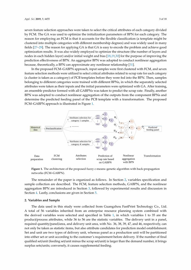
In the proposed FCM–GABPN approach, input samples were first clustered with FCM, and sevenfeature selection methods were utilized to select critical attributes related to scrap rate for each category(a cluster is taken as a category) of PCB templates before they were fed into the BPN. Then, samplesbelonging to different categories were trained with different BPNs, in which the separately selectedattributes were taken as their inputs and the initial parameters were optimized with GA. After training,an ensemble predictor formed with all GABPNs was taken to predict the scrap rate. Finally, anotherBPN was adopted to conduct nonlinear aggregation of the outputs from the component BPNs anddetermine the predicted feeding panel of the PCB template with a transformation. The proposedFCM–GABPN approach is illustrated in Figure 1.

Appl. Sci. 2019, x, x FOR PEER REVIEW 3 of 18

recursive feature elimination (RFE) [22], LR [23], lasso regression [24], ridge regression [25], and

random forest regression (RFR) [26] seven feature selection approaches were taken to select the

critical attributes of each category divided by FCM. The GA was used to optimize the initialization

parameters of BPN for each category. The reason for employing an FCM is that it accounts for the

flexible classification (a template might be clustered into multiple categories with different

membership degrees) and was widely used in many fields [27–29]. The reason for applying GA is

that GA is easy to encode the problem and achieve good optimization results. It was also widely

employed to optimize the structure (the number of layers and nodes in each hidden layer) and/or

initial weight and bias [18,19,30] for the purpose of improving the prediction effectiveness of BPN.

An aggregator BPN was adopted to conduct nonlinear aggregation because, theoretically, a BPN can

approximate any nonlinear relationship [31].

In the proposed FCM–GABPN approach, input samples were first clustered with FCM, and

seven feature selection methods were utilized to select critical attributes related to scrap rate for each

category (a cluster is taken as a category) of PCB templates before they were fed into the BPN. Then,

samples belonging to different categories were trained with different BPNs, in which the separately

selected attributes were taken as their inputs and the initial parameters were optimized with GA.

After training, an ensemble predictor formed with all GABPNs was taken to predict the scrap rate.

Finally, another BPN was adopted to conduct nonlinear aggregation of the outputs from the

component BPNs and determine the predicted feeding panel of the PCB template with a

transformation. The proposed FCM–GABPN approach is illustrated in Figure 1.

Figure 1. The architecture of the proposed fuzzy c-means–genetic algorithm with back-propagation

networks (FCM–GABPN).

The remainder of the paper is organized as follows. In Section 2, variables specification and

sample collection are described. The FCM, feature selection methods, GABPN, and the nonlinear

aggregation BPN are introduced in Section 3, followed by experimental results and discussion in

Section 4. Lastly, conclusions are given in Section 5.

2. Variables and Sample

The data used in this study were collected from Guangzhou FastPrint Technology Co., Ltd. A

total of 56 variables inherited from an enterprise resource planning system combined with the

derived variables were selected and specified in Table 1, in which variables 1 to 35 are the

product/process attributes, while 36 to 56 are the statistic variables. The delivery unit in a panel,

required quantity/panel/area, and delivery unit area, with No. 36, 38, 39, 47, and 46, respectively, can

not only be taken as statistic items, but also attribute candidates for prediction model establishment.

Set and unit are two types of delivery unit, whereas panel as a production unit will be partitioned

into either set or unit according to the customer’s requirement before delivery. If the number of final

………Historical data

1u

Ku

1

2

i1

...

1

2

iK

...

1

2

s

...

1

2

s

...

1

1

1

2...

2K

2K-1

1o

Ko

1

2

p

...

1o Predicted

feeding panel

Prediction of

scrap rate based

on GABPN

FCM

clustering

Attributes selection for

category 1 samples

Attributes selection for

category K samples

Attributes

selectionTransformationData

preparation

Nonlinear

aggregation

with BPN

Preclassification

Figure 1. The architecture of the proposed fuzzy c-means–genetic algorithm with back-propagationnetworks (FCM–GABPN).

The remainder of the paper is organized as follows. In Section 2, variables specification andsample collection are described. The FCM, feature selection methods, GABPN, and the nonlinearaggregation BPN are introduced in Section 3, followed by experimental results and discussion inSection 4. Lastly, conclusions are given in Section 5.

2. Variables and Sample

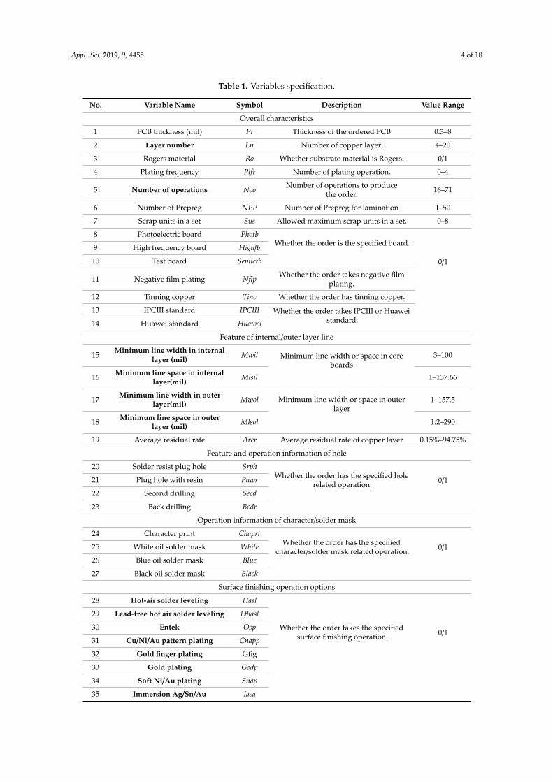
The data used in this study were collected from Guangzhou FastPrint Technology Co., Ltd.A total of 56 variables inherited from an enterprise resource planning system combined withthe derived variables were selected and specified in Table 1, in which variables 1 to 35 are theproduct/process attributes, while 36 to 56 are the statistic variables. The delivery unit in a panel,required quantity/panel/area, and delivery unit area, with No. 36, 38, 39, 47, and 46, respectively, cannot only be taken as statistic items, but also attribute candidates for prediction model establishment.Set and unit are two types of delivery unit, whereas panel as a production unit will be partitionedinto either set or unit according to the customer’s requirement before delivery. If the number of finalqualified set/unit (feeding set/unit minus the scrap set/unit) is larger than the demand number, it bringssurplus sets/units; conversely, it causes supplemental feeding.

Appl. Sci. 2019, 9, 4455 4 of 18

Table 1. Variables specification.

No. Variable Name Symbol Description Value Range

Overall characteristics

1 PCB thickness (mil) Pt Thickness of the ordered PCB 0.3–8

2 Layer number Ln Number of copper layer. 4–20

3 Rogers material Ro Whether substrate material is Rogers. 0/1

4 Plating frequency Plfr Number of plating operation. 0–4

5 Number of operations Noo Number of operations to producethe order. 16–71

6 Number of Prepreg NPP Number of Prepreg for lamination 1–50

7 Scrap units in a set Sus Allowed maximum scrap units in a set. 0–8

8 Photoelectric board PhotbWhether the order is the specified board.

0/1

9 High frequency board Highfb

10 Test board Semictb

11 Negative film plating Nflp Whether the order takes negative filmplating.

12 Tinning copper Tinc Whether the order has tinning copper.

13 IPCIII standard IPCIII Whether the order takes IPCIII or Huaweistandard.14 Huawei standard Huawei

Feature of internal/outer layer line

15 Minimum line width in internallayer (mil) Mwil Minimum line width or space in core

boards3–100

16 Minimum line space in internallayer(mil) Mlsil 1–137.66

17 Minimum line width in outerlayer(mil) Mwol Minimum line width or space in outer

layer1–157.5

18 Minimum line space in outerlayer (mil) Mlsol 1.2–290

19 Average residual rate Arcr Average residual rate of copper layer 0.15%–94.75%

Feature and operation information of hole

20 Solder resist plug hole SrphWhether the order has the specified hole

related operation. 0/121 Plug hole with resin Phwr

22 Second drilling Secd

23 Back drilling Bcdr

Operation information of character/solder mask

24 Character print ChaprtWhether the order has the specified

character/solder mask related operation. 0/125 White oil solder mask White

26 Blue oil solder mask Blue

27 Black oil solder mask Black

Surface finishing operation options

28 Hot-air solder leveling Hasl

Whether the order takes the specifiedsurface finishing operation. 0/1

29 Lead-free hot air solder leveling Lfhasl

30 Entek Osp

31 Cu/Ni/Au pattern plating Cnapp

32 Gold finger plating Gfig

33 Gold plating Godp

34 Soft Ni/Au plating Snap

35 Immersion Ag/Sn/Au Iasa

Appl. Sci. 2019, 9, 4455 5 of 18

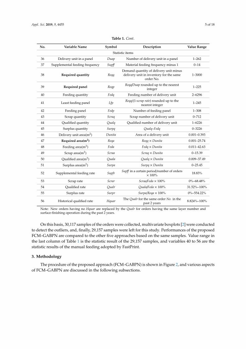
Table 1. Cont.

No. Variable Name Symbol Description Value Range

Statistic items

36 Delivery unit in a panel Duap Number of delivery unit in a panel 1–262

37 Supplemental feeding frequency Supff Material feeding frequency minus 1 0–14

38 Required quantity ReqqDemand quantity of delivery unit minusdelivery unit in inventory for the same

order No.1–3000

39 Required panel Reqp Reqq/Duap rounded up to the nearestinteger 1–225

40 Feeding quantity Fedq Feeding number of delivery unit 2–6296

41 Least feeding panel Lfp Reqq/(1-scrap rate) rounded up to thenearest integer 1–245

42 Feeding panel Fedp Number of feeding panel 1–308

43 Scrap quantity Scraq Scrap number of delivery unit 0–712

44 Qualified quantity Qualq Qualified number of delivery unit 1–6226

45 Surplus quantity Surpq Qualq–Fedq 0–3226

46 Delivery unit area(m2) Dunita Area of a delivery unit 0.001–0.393

47 Required area(m2) Reqa Reqq × Dunita 0.001–25.74

48 Feeding area(m2) Feda Fedq × Dunita 0.011–42.63

49 Scrap area(m2) Scraa Scraq × Dunita 0–15.39

50 Qualified area(m2) Quala Qualq × Dunita 0.009–37.49

51 Surplus area(m2) Surpa Surpq × Dunita 0–25.45

52 Supplemental feeding rate Supfr Supff in a certain period/number of orders× 100% 18.83%

53 Scrap rate Scrar Scraa/Feda × 100% 0%–68.48%

54 Qualified rate Qualr Quala/Feda × 100% 31.52%–100%

55 Surplus rate Surpr Surpa/Reqa × 100% 0%–554.22%

56 Historical qualified rate Hquar The Qualr for the same order No. in thepast 2 years 8.824%–100%

Note: New orders having no Hquar are replaced by the Qualr for orders having the same layer number andsurface-finishing operation during the past 2 years.

On this basis, 30,117 samples of the orders were collected, multivariate boxplots [2] were conductedto detect the outliers, and, finally, 29,157 samples were left for this study. Performances of the proposedFCM–GABPN are compared to the other five approaches based on the same samples. Value range inthe last column of Table 1 is the statistic result of the 29,157 samples, and variables 40 to 56 are thestatistic results of the manual feeding adopted by FastPrint.

3. Methodology

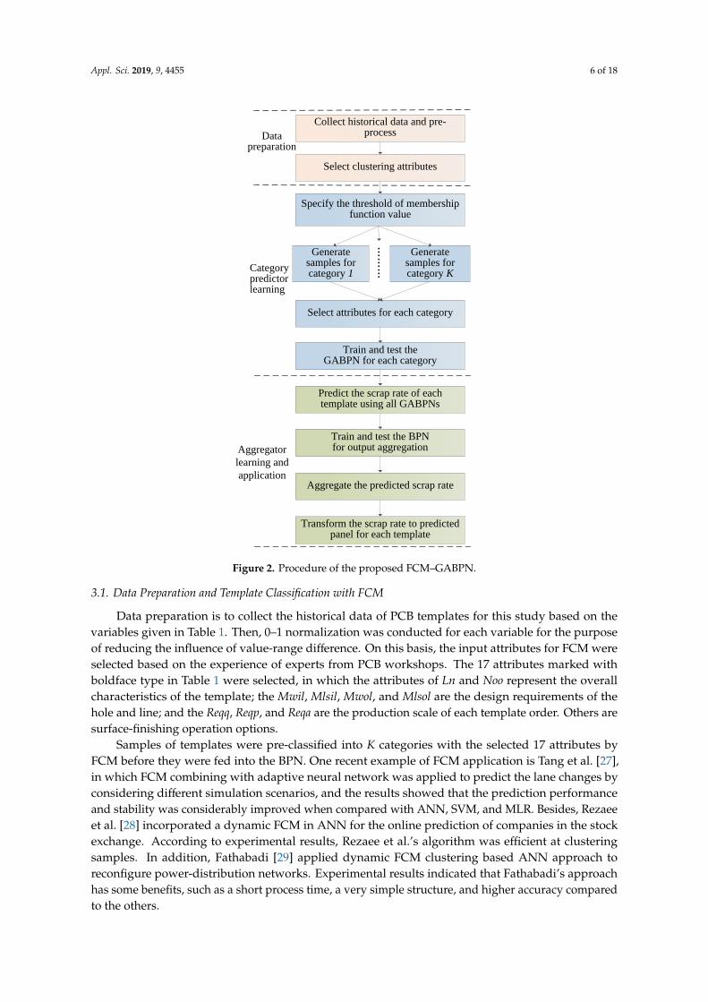
The procedure of the proposed approach (FCM–GABPN) is shown in Figure 2, and various aspectsof FCM–GABPN are discussed in the following subsections.

Appl. Sci. 2019, 9, 4455 6 of 18

Appl. Sci. 2019, x, x FOR PEER REVIEW 6 of 18

and stability was considerably improved when compared with ANN, SVM, and MLR. Besides,

Rezaee et al. [28] incorporated a dynamic FCM in ANN for the online prediction of companies in the

stock exchange. According to experimental results, Rezaee et al.’s algorithm was efficient at

clustering samples. In addition, Fathabadi [29] applied dynamic FCM clustering based ANN

approach to reconfigure power-distribution networks. Experimental results indicated that

Fathabadi’s approach has some benefits, such as a short process time, a very simple structure, and

higher accuracy compared to the others.

Figure 2. Procedure of the proposed FCM–GABPN.

FCM performs clustering by minimizing 2

( ) ( )

1 1

C nm

i c i c

c i

e

, where C is the required number of

clusters; n is the number of samples; ( )i c represents the membership of sample i belonging to

cluster c ; ( )i ce measures the distance from samples i to the centroid of c ; (1, )m is the

hyper-parameter that controls how fuzzy the cluster will be. The procedure of applying FCM to

cluster samples is as follows [31]:

(1) The cluster membership value, iju (the coefficient giving the degree of

ix being in the jth

cluster), are initialized randomly and establish an initial clustering result.

(2) (Iterations) obtain the centers of each cluster as ( ) ( ){ }c c jx x , ( ) ( ) ( )

1 1

/n n

m m

c j i c ij i c

i i

x u x u

,

1 17j , 2 2/( 1)

( ) ( ) ( )

1

1/ ( / )C

m

i c i c i c

i

u e e

, 2

( ) ( )

( )i c ij c j

all j

e x x , where ijx is the jth variable of the

selected 17 attributes of sample i, and ( )cx is the centroid of cluster c.

Select clustering attributes

Collect historical data and pre-processData

preparation

Specify the threshold of membership function value

……

… Generate samples for category K

Generate samples for category 1

Select attributes for each category

Train and test the GABPN for each category

Category predictor learning

Predict the scrap rate of each template using all GABPNs

Train and test the BPN for output aggregation

Aggregate the predicted scrap rate

Transform the scrap rate to predicted panel for each template

Aggregator

learning and

application

Figure 2. Procedure of the proposed FCM–GABPN.

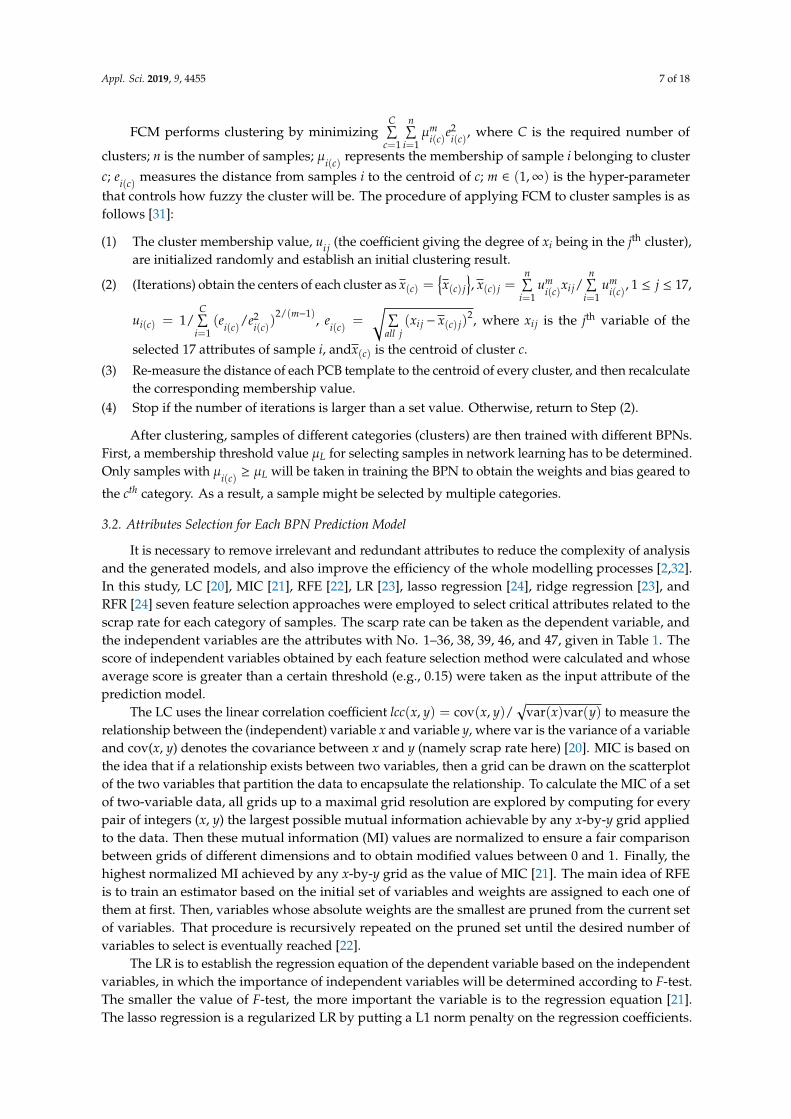
3.1. Data Preparation and Template Classification with FCM

Data preparation is to collect the historical data of PCB templates for this study based on thevariables given in Table 1. Then, 0–1 normalization was conducted for each variable for the purposeof reducing the influence of value-range difference. On this basis, the input attributes for FCM wereselected based on the experience of experts from PCB workshops. The 17 attributes marked withboldface type in Table 1 were selected, in which the attributes of Ln and Noo represent the overallcharacteristics of the template; the Mwil, Mlsil, Mwol, and Mlsol are the design requirements of thehole and line; and the Reqq, Reqp, and Reqa are the production scale of each template order. Others aresurface-finishing operation options.

Samples of templates were pre-classified into K categories with the selected 17 attributes byFCM before they were fed into the BPN. One recent example of FCM application is Tang et al. [27],in which FCM combining with adaptive neural network was applied to predict the lane changes byconsidering different simulation scenarios, and the results showed that the prediction performanceand stability was considerably improved when compared with ANN, SVM, and MLR. Besides, Rezaeeet al. [28] incorporated a dynamic FCM in ANN for the online prediction of companies in the stockexchange. According to experimental results, Rezaee et al.’s algorithm was efficient at clusteringsamples. In addition, Fathabadi [29] applied dynamic FCM clustering based ANN approach toreconfigure power-distribution networks. Experimental results indicated that Fathabadi’s approachhas some benefits, such as a short process time, a very simple structure, and higher accuracy comparedto the others.

Appl. Sci. 2019, 9, 4455 7 of 18

FCM performs clustering by minimizingC∑

c=1

n∑i=1

µmi(c)e

2i(c), where C is the required number of

clusters; n is the number of samples; µi(c) represents the membership of sample i belonging to cluster

c; ei(c) measures the distance from samples i to the centroid of c; m ∈ (1,∞) is the hyper-parameterthat controls how fuzzy the cluster will be. The procedure of applying FCM to cluster samples is asfollows [31]:

(1) The cluster membership value, ui j (the coefficient giving the degree of xi being in the jth cluster),are initialized randomly and establish an initial clustering result.

(2) (Iterations) obtain the centers of each cluster as x(c) ={x(c) j

}, x(c) j =

n∑i=1

umi(c)xi j/

n∑i=1

umi(c), 1 ≤ j ≤ 17,

ui(c) = 1/C∑

i=1(ei(c)/e2

i(c))2/(m−1), ei(c) =

√ ∑all j

(xi j − x(c) j)2, where xi j is the jth variable of the

selected 17 attributes of sample i, andx(c) is the centroid of cluster c.

(3) Re-measure the distance of each PCB template to the centroid of every cluster, and then recalculatethe corresponding membership value.

(4) Stop if the number of iterations is larger than a set value. Otherwise, return to Step (2).

After clustering, samples of different categories (clusters) are then trained with different BPNs.First, a membership threshold value µL for selecting samples in network learning has to be determined.Only samples with µi(c) ≥ µL will be taken in training the BPN to obtain the weights and bias geared to

the cth category. As a result, a sample might be selected by multiple categories.

3.2. Attributes Selection for Each BPN Prediction Model

It is necessary to remove irrelevant and redundant attributes to reduce the complexity of analysisand the generated models, and also improve the efficiency of the whole modelling processes [2,32].In this study, LC [20], MIC [21], RFE [22], LR [23], lasso regression [24], ridge regression [23], andRFR [24] seven feature selection approaches were employed to select critical attributes related to thescrap rate for each category of samples. The scarp rate can be taken as the dependent variable, andthe independent variables are the attributes with No. 1–36, 38, 39, 46, and 47, given in Table 1. Thescore of independent variables obtained by each feature selection method were calculated and whoseaverage score is greater than a certain threshold (e.g., 0.15) were taken as the input attribute of theprediction model.

The LC uses the linear correlation coefficient lcc(x, y) = cov(x, y)/√

var(x)var(y) to measure therelationship between the (independent) variable x and variable y, where var is the variance of a variableand cov(x, y) denotes the covariance between x and y (namely scrap rate here) [20]. MIC is based onthe idea that if a relationship exists between two variables, then a grid can be drawn on the scatterplotof the two variables that partition the data to encapsulate the relationship. To calculate the MIC of a setof two-variable data, all grids up to a maximal grid resolution are explored by computing for everypair of integers (x, y) the largest possible mutual information achievable by any x-by-y grid appliedto the data. Then these mutual information (MI) values are normalized to ensure a fair comparisonbetween grids of different dimensions and to obtain modified values between 0 and 1. Finally, thehighest normalized MI achieved by any x-by-y grid as the value of MIC [21]. The main idea of RFEis to train an estimator based on the initial set of variables and weights are assigned to each one ofthem at first. Then, variables whose absolute weights are the smallest are pruned from the current setof variables. That procedure is recursively repeated on the pruned set until the desired number ofvariables to select is eventually reached [22].

The LR is to establish the regression equation of the dependent variable based on the independentvariables, in which the importance of independent variables will be determined according to F-test.The smaller the value of F-test, the more important the variable is to the regression equation [21].The lasso regression is a regularized LR by putting a L1 norm penalty on the regression coefficients.

Appl. Sci. 2019, 9, 4455 8 of 18

Lasso regression will drive more coefficients of weak correlated independent variables to zero, andthen facilitate the selection of variables with strong correlation [24]. The ridge regression is similarto lasso regression by putting a L2 norm penalty on the regression to penalize the weak correlatedvariables for the regression model establishment [25]. RFR is an ensemble of unpruned classificationor regression trees, in which each branch of the trees will calculate the importance of each unusedattribute in previous steps and then facilitate important-attribute selection simultaneously [26]. Theabove seven approaches were realized by the encapsulated functions in the machine learning library“sklearn” in this study.

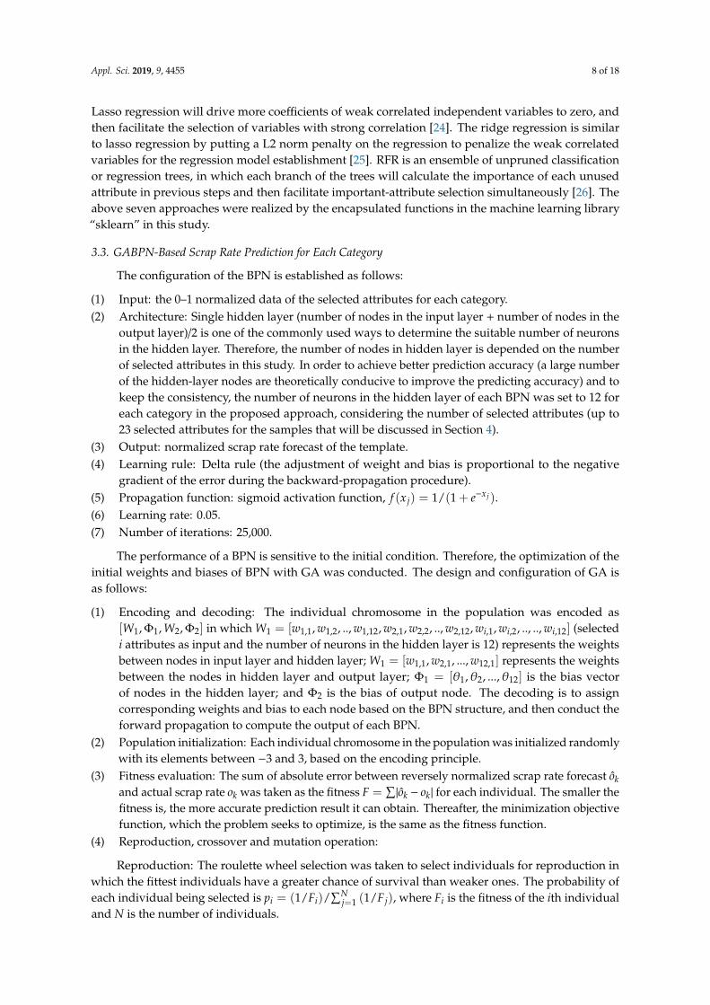
3.3. GABPN-Based Scrap Rate Prediction for Each Category

The configuration of the BPN is established as follows:

(1) Input: the 0–1 normalized data of the selected attributes for each category.(2) Architecture: Single hidden layer (number of nodes in the input layer + number of nodes in the

output layer)/2 is one of the commonly used ways to determine the suitable number of neuronsin the hidden layer. Therefore, the number of nodes in hidden layer is depended on the numberof selected attributes in this study. In order to achieve better prediction accuracy (a large numberof the hidden-layer nodes are theoretically conducive to improve the predicting accuracy) and tokeep the consistency, the number of neurons in the hidden layer of each BPN was set to 12 foreach category in the proposed approach, considering the number of selected attributes (up to23 selected attributes for the samples that will be discussed in Section 4).

(3) Output: normalized scrap rate forecast of the template.(4) Learning rule: Delta rule (the adjustment of weight and bias is proportional to the negative

gradient of the error during the backward-propagation procedure).(5) Propagation function: sigmoid activation function, f (x j) = 1/(1 + e−x j).(6) Learning rate: 0.05.(7) Number of iterations: 25,000.

The performance of a BPN is sensitive to the initial condition. Therefore, the optimization of theinitial weights and biases of BPN with GA was conducted. The design and configuration of GA isas follows:

(1) Encoding and decoding: The individual chromosome in the population was encoded as[W1, Φ1, W2, Φ2] in which W1 = [w1,1, w1,2, .., w1,12, w2,1, w2,2, .., w2,12, wi,1, wi,2, .., .., wi,12] (selectedi attributes as input and the number of neurons in the hidden layer is 12) represents the weightsbetween nodes in input layer and hidden layer; W1 = [w1,1, w2,1, ..., w12,1] represents the weightsbetween the nodes in hidden layer and output layer; Φ1 = [θ1,θ2, ...,θ12] is the bias vectorof nodes in the hidden layer; and Φ2 is the bias of output node. The decoding is to assigncorresponding weights and bias to each node based on the BPN structure, and then conduct theforward propagation to compute the output of each BPN.

(2) Population initialization: Each individual chromosome in the population was initialized randomlywith its elements between −3 and 3, based on the encoding principle.

(3) Fitness evaluation: The sum of absolute error between reversely normalized scrap rate forecast okand actual scrap rate ok was taken as the fitness F =

∑|ok − ok| for each individual. The smaller the

fitness is, the more accurate prediction result it can obtain. Thereafter, the minimization objectivefunction, which the problem seeks to optimize, is the same as the fitness function.

(4) Reproduction, crossover and mutation operation:

Reproduction: The roulette wheel selection was taken to select individuals for reproduction inwhich the fittest individuals have a greater chance of survival than weaker ones. The probability ofeach individual being selected is pi = (1/Fi)/

∑Nj=1 (1/F j), where Fi is the fitness of the ith individual

and N is the number of individuals.

Appl. Sci. 2019, 9, 4455 9 of 18

Crossover: Two empty offspring chromosomes, O1 and O2, were initialized first, and twochromosomes, P1 and P2, were randomly selected from the reproduced population. The crossoverlocation was randomly selected, and then the offspring O1 consisted of the genes of P1 before thecrossover location and genes of P2 after the crossover location; while offspring O2 consisted of thegenes of P2 before the crossover location and genes of P1 after the crossover location.

Mutation: One-point mutation was utilized as the mutation operator. The chromosome in thepopulation was randomly selected, and one gene was chosen randomly from the selected chromosome.Then, a random r with the value in (0, 1) was generated to mutate the value. If r > 0.5, thena j = a j + (a j − amax) × r, otherwise a j = a j + (amin − a j) × r, where a j is value of the jth position inthe chromosome selected for mutation, and amax and amin are the maximum and minimum of the jth

position of all chromosomes in current generation, respectively.

(5) Number of iterations: 100.

After the templates were clustered, a portion of the templates in each category were taken as “trainingsamples” into the GABPN to determine the weights and bias values for the category. Three phaseswere involved at the training stage. First, the initial weight and bias were optimized according the GA.Second, the forward propagation is conducted, in which the inputs (selected attributes with bias) weremultiplied with weights (weights of bias are 1), summated, and transferred to the hidden layer. Theresults of nodes in the hidden layer were further processed by sigmoid function and also transferredto the output layer with the same procedure. Finally, the output of GABPN was compared with theaccurate scrap rate, and the accuracy of the GABPN, represented with mean squared error (MSE),was evaluated.

Subsequently, the backward pass which propagates derivatives (error between prediction and theactual value) from the output layer to hidden layers was conducted. The backward pass for a 3-layerBPN starts by computing the partial derivative for the output node (only one node here), and the errorterms δ j of nodes j in the hidden layers can be calculated according to δ j = eW j f ′(x j), in which e iserror of the output node, W j is the weight connecting node j to the output node, and f ′(x j) is thederivative of the sigmoid activation function with the input x j. On this basis, adjustments were madeto the connection weights and bias to reduce the MSE. Network-learning stops when the iteration isgreater than a given number in this study.

The trained GABPN was tested by the remaining portion of the templates in each category withthe same performance indicator, MSE. Finally, the GABPN was used to predict the scrap rate of newtemplates that “completely” belonged to the clustered category. However, complete assignment oftemplate to only a category is usually impossible. When a new template order is coming, the selectedattributes associated with the new template are recorded, and the membership belonging to eachcategory is calculated. Then, an ensemble predictor formed with all GABPNs can be taken to predictthe scrap rate for the new template.

3.4. Nonlinear Aggregation with Another BPN and Transformation

For aggregating the predicted results from the component GABPNs into a single value representingthe predicted scrap rate of the template, another BPN was employed in this study to conduct nonlinearaggregation, and the configuration is set as follows:

(1) Input: 2K parameters consisted of the predicted results of each component GABPNs for thetemplate and the membership values of the template belonging to each category.

(2) Architecture: Single hidden layer and the number of nodes in the hidden layer were set to thesame as that in the input layer, 2K.

(3) Output: normalized scrap rate forecast of the template.(4) Learning rule: Delta rule.(5) Propagation function: sigmoid activation function.

Appl. Sci. 2019, 9, 4455 10 of 18

(6) Learning rate: 0.05.(7) Number of iterations: 10000.

The BPN also underwent training and testing. Then, the network output (i.e., the aggregationresult) determined the normalized scrap-rate prediction of the template. Finally, the transformation ofscrap rate to surplus rate and supplemental feeding rate were carried out. The reverse normalizationwas conducted for the output of the aggregation BPN and taking it as the predicted scrap rate(Scrar_Pd). Thereafter, the transformation for predicted feeding panel (Fedp_Pd) was conducted byFedq_Pd = 100×Reqq/(100− Scrar_Pd) and Fedp_Pd =

⌈Fedq_Pd/Duap

⌉, where Reqq is the required

quantity, Duap is the delivery unit in a panel, and Fedp_Pd is the predicted panel.

3.5. Performance Indicators

In order to evaluate the effectiveness of the model, the MSE, mean absolute error (MAE), and meanabsolute percentage error (MAPE) were adopted as the indicators to evaluate the performance of theapproaches, in which the predicted data oi are the predicted least feeding panel and the original data oi

are the least feeding panel. The MSE, MAE, and MAPE can be described as MSE =N∑

i=1(oi − oi)

2/N,

MAE =N∑

i=1|oi − oi|/N, and MAPE = 1

N

N∑i=1

∣∣∣∣ oi−oioi

∣∣∣∣× 100, respectively, where N is the number of samples.

The indicators surplus rate (Surpr) and supplemental feeding rate (Supfr) in the PCB templateworkshop were also considered. The predicted surplus rate (Surpr_Pd) and predicted supplementalfeeding rate Supfr_Pd can be computed with Equations (10) and (11) in [2], respectively. The finalperformance is evaluated by the MSE, MAE, MAPE, Supfr_Pd, and Surpr_Pd.

4. Experimental Results and Discussions

The proposed FCM–GABPN was implemented by Python 3.6. The number of clusters was set tothree while conducting FCM for the purpose of reducing the number of training, testing, and modelmaintenance in the workshop, but also to achieve good enough prediction accuracy based on someinitial test. The hyper-parameter m that controls how fuzzy the cluster was commonly set to 2 [31], andit was adopted here. The maximum number of iterations of FCM was set to 800.

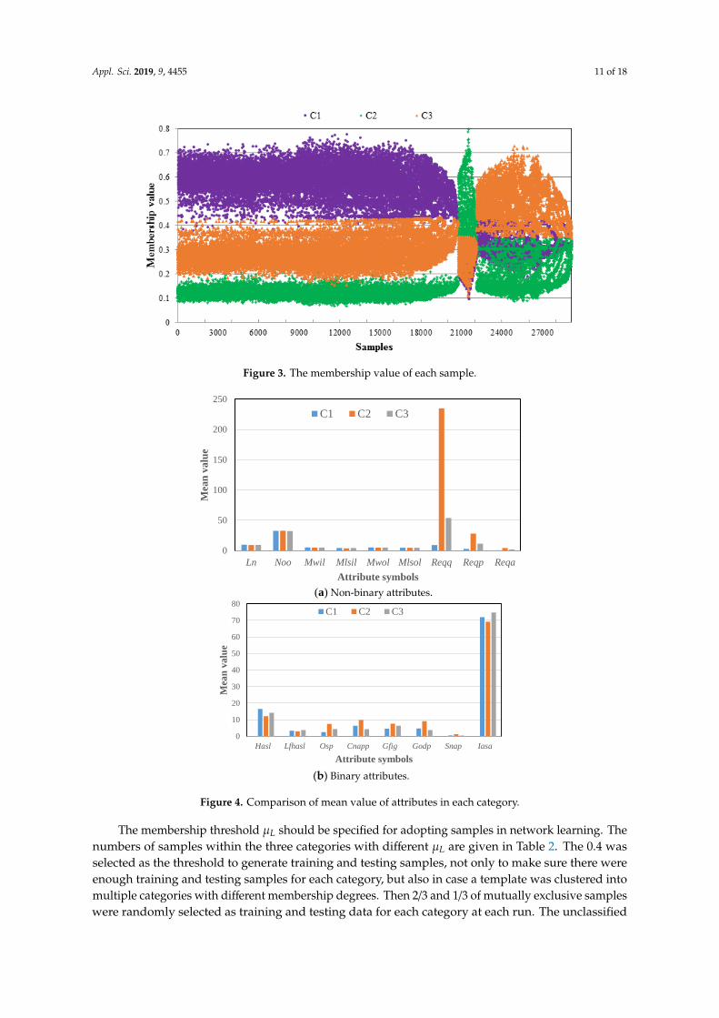
If FCM cluster samples fall into the category with the highest membership value, the templateswill be cluster into C1, C2, and C3, with 20,773, 1354, and 7030 samples, respectively. The membershipvalue giving the membership degree of each sample (samples were clustered into C1, C2, and C3 herefor visualization) being in the three categories is illustrated in Figure 3. The membership degree ofeach sample will be taken as part of the input of the aggregator BPN to perform nonlinear aggregation,as shown in Figure 1.

The mean values of input attributes in the three categories are given in Figure 4. The mean valuesof Reqq, Reqp, and Reqa are comparatively different in the three categories; and they are the mainattributes to distinguish and identify samples within each category, which is consistent with practice inwhich the workshop also regards order scale (Reqq, Reqp, and Reqa) as important variables to classifyorders. Meanwhile, the mean values of Mwil, Mlsil, and Mwol in C2 is lower than the correspondingvalues in C1 and C3, but the Ln is higher, which indicates that, the higher Ln is, the denser the linesthat coincide with the actual situation are.

Appl. Sci. 2019, 9, 4455 11 of 18Appl. Sci. 2019, x, x FOR PEER REVIEW 11 of 18

Figure 3. The membership value of each sample.

(a) Non-binary attributes.

(b) Binary attributes.

Figure 4. Comparison of mean value of attributes in each category.

Table 2. Numbers of samples within the three categories with different L .

L C1 C2 C3 Unclassified

0 29,157 29,157 29,157 0

0.1 29,156 27,608 29,157 0

0.2 28,922 3434 28,815 0

0.3 29,157 2193 15,529 0

0

50

100

150

200

250

Ln Noo Mwil Mlsil Mwol Mlsol Reqq Reqp Reqa

Mea

n v

alu

e

Attribute symbols

C1 C2 C3

0

10

20

30

40

50

60

70

80

Hasl Lfhasl Osp Cnapp Gfig Godp Snap Iasa

Mea

n v

alu

e

Attribute symbols

C1 C2 C3

Figure 3. The membership value of each sample.

Appl. Sci. 2019, x, x FOR PEER REVIEW 11 of 18

Figure 3. The membership value of each sample.

(a) Non-binary attributes.

(b) Binary attributes.

Figure 4. Comparison of mean value of attributes in each category.

Table 2. Numbers of samples within the three categories with different L .

L C1 C2 C3 Unclassified

0 29,157 29,157 29,157 0

0.1 29,156 27,608 29,157 0

0.2 28,922 3434 28,815 0

0.3 29,157 2193 15,529 0

0

50

100

150

200

250

Ln Noo Mwil Mlsil Mwol Mlsol Reqq Reqp Reqa

Mea

n v

alu

e

Attribute symbols

C1 C2 C3

0

10

20

30

40

50

60

70

80

Hasl Lfhasl Osp Cnapp Gfig Godp Snap Iasa

Mea

n v

alu

e

Attribute symbols

C1 C2 C3

Figure 4. Comparison of mean value of attributes in each category.

The membership threshold µL should be specified for adopting samples in network learning. Thenumbers of samples within the three categories with different µL are given in Table 2. The 0.4 wasselected as the threshold to generate training and testing samples, not only to make sure there wereenough training and testing samples for each category, but also in case a template was clustered intomultiple categories with different membership degrees. Then 2/3 and 1/3 of mutually exclusive sampleswere randomly selected as training and testing data for each category at each run. The unclassified

Appl. Sci. 2019, 9, 4455 12 of 18

samples were not taken as the input to train each GABPN; however, they will be taken as the samplesfor final test. The numbers of training and testing samples for each category are given in Table 3.

Table 2. Numbers of samples within the three categories with different µL .

µL C1 C2 C3 Unclassified

0 29,157 29,157 29,157 00.1 29,156 27,608 29,157 00.2 28,922 3434 28,815 00.3 29,157 2193 15,529 00.4 21,230 973 7037 13550.5 17,717 393 3097 79510.6 8455 184 446 20,0720.7 408 18 8 28,7230.8 0 0 0 29,1570.9 0 0 0 29,1571 0 0 0 29,157

Table 3. Number of samples selected for training and testing.

Training Samples Testing Samples

C1 14,153 8432C2 649 1679C3 4691 3701All 19,448 9709

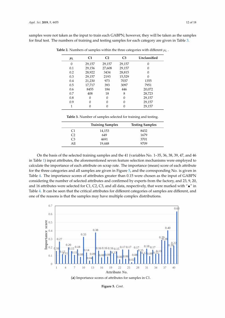
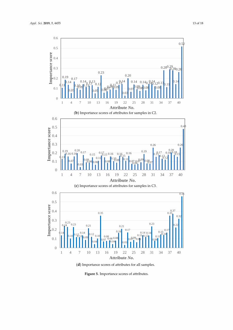
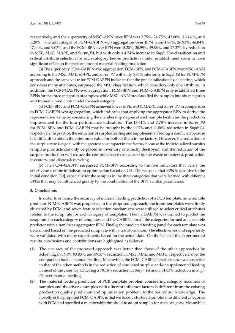
On the basis of the selected training samples and the 41 (variables No. 1–35, 36, 38, 39, 47, and 46in Table 1) input attributes, the aforementioned seven feature selection mechanisms were employed tocalculate the importance of each attribute on scrap rate. The importance (mean) score of each attributefor the three categories and all samples are given in Figure 5, and the corresponding No. is given inTable 4. The importance scores of attributes greater than 0.15 were chosen as the input of GABPNconsidering the number of selected attributes and confirmed by experts from the factory, and 23, 9, 20,and 16 attributes were selected for C1, C2, C3, and all data, respectively, that were marked with “N” inTable 4. It can be seen that the critical attributes for different categories of samples are different, andone of the reasons is that the samples may have multiple complex distributions.

Appl. Sci. 2019, x, x FOR PEER REVIEW 12 of 18

0.4 21,230 973 7037 1355

0.5 17,717 393 3097 7951

0.6 8455 184 446 20,072

0.7 408 18 8 28,723

0.8 0 0 0 29,157

0.9 0 0 0 29,157

1 0 0 0 29,157

Table 3. Number of samples selected for training and testing.

Training Samples Testing Samples

C1 14,153 8432

C2 649 1679

C3 4691 3701

All 19,448 9709

On the basis of the selected training samples and the 41 (variables No. 1–35, 36, 38, 39, 47, and 46

in Table 1) input attributes, the aforementioned seven feature selection mechanisms were employed

to calculate the importance of each attribute on scrap rate. The importance (mean) score of each

attribute for the three categories and all samples are given in Figure 5, and the corresponding No. is

given in Table 4. The importance scores of attributes greater than 0.15 were chosen as the input of

GABPN considering the number of selected attributes and confirmed by experts from the factory,

and 23, 9, 20, and 16 attributes were selected for C1, C2, C3, and all data, respectively, that were

marked with “▲” in Table 4. It can be seen that the critical attributes for different categories of

samples are different, and one of the reasons is that the samples may have multiple complex

distributions.

Each GABPN model was trained by the training samples and the selected attributes given in

Table 4. All samples belonging to a category compete in the same way in training the GABPN geared

to the category. Prediction models of GABPN were trained and tested for each category separately,

while the aggregator BPN was trained with all the training samples and tested by all the testing

samples.

The GA parameters of population size, crossover probability, mutational probability, and the

number of iterations of the three GABPNs were set to 100, 0.8, 0.05, and 100, according to some initial

test. The convergences of GA for the initial parameter optimization of the three BPNs are illustrated

in Figure 6. On the basis of the optimized parameters, the three BPNs were trained in parallel, and

the output of the three prediction models was set into the aggregator BPN, with the membership

degree of each sample obtained by FCM given in Figure 3. The predicted feeding panel of each

sample can be determined according to the transformation described in Section 3.4, based on the

reversely normalized output of the aggregator BPN.

(a) Importance scores of attributes for samples in C1.

0.16

0.27

0.12 0.11

0.20

0.15

0.11

0.18

0.08

0.33

0.14

0.04

0.09

0.38

0.16

0.08

0.16

0.09

0.16

0.13

0.15

0.06

0.17

0.06

0.17

0.02

0.08

0.17 0.15

0.12

0.18

0.09

0.17

0.12 0.13

0.29 0.28

0.40

0.20 0.22

0.63

0

0.1

0.2

0.3

0.4

0.5

0.6

0.7

1 4 7 10 13 16 19 22 25 28 31 34 37 40

Imp

ort

an

ce sc

ore

Attribute No.

Figure 5. Cont.

Appl. Sci. 2019, 9, 4455 13 of 18

Appl. Sci. 2019, x, x FOR PEER REVIEW 13 of 18

(b) Importance scores of attributes for samples in C2.

(c) Importance scores of attributes for samples in C3.

(d) Importance scores of attributes for all samples.

Figure 5. Importance scores of attributes.

Table 4. Selected attributes for each category/all samples.

No. Attributes C1 C2 C3 All No. Attributes C1 C2 C3 All

1 Pt ▲ 22 Secd

2 Ln ▲ ▲ ▲ ▲ 23 Bcdr ▲ ▲ ▲ ▲

3 Ro ▲ ▲ 24 Chaprt

4 Plfr 25 White ▲

0.11

0.19

0.14

0.05

0.17

0.10 0.09

0.14

0.11 0.13

0.13

0.05

0.12

0.23

0.06 0.07 0.09

0.11 0.09

0.13 0.14

0.03

0.20

0.07

0.14

0.09 0.08

0.14

0.08

0.14 0.14

0.12 0.08

0.13

0.28

0.11

0.29 0.28

0.14

0.26

0.52

0

0.1

0.2

0.3

0.4

0.5

0.6

1 4 7 10 13 16 19 22 25 28 31 34 37 40

Imp

ort

an

ce s

core

Attribute No.

0.13

0.19 0.16

0.07

0.16 0.20

0.03

0.17

0.09 0.08

0.15

0.06

0.11

0.17 0.15

0.08

0.16

0.10 0.08

0.16 0.15

0.11

0.16

0.07 0.06

0.07 0.09

0.19

0.08 0.07

0.26

0.15 0.17

0.13 0.12

0.18 0.20

0.18 0.15

0.26

0.48

0

0.1

0.2

0.3

0.4

0.5

0.6

1 4 7 10 13 16 19 22 25 28 31 34 37 40

Imp

ort

an

ce s

core

Attribute No.

0.14

0.24 0.23

0.10

0.23

0.12 0.12

0.14

0.09

0.21

0.12

0.04

0.10

0.35

0.07 0.08

0.08 0.04

0.08

0.16

0.21

0.03

0.17

0.07 0.09 0.06

0.11 0.14

0.12 0.14

0.23

0.08 0.11

0.15 0.14

0.17

0.35 0.37

0.22

0.32

0.56

0

0.1

0.2

0.3

0.4

0.5

0.6

1 4 7 10 13 16 19 22 25 28 31 34 37 40

Imp

ort

an

ce s

core

Attribute No.

Figure 5. Importance scores of attributes.

Appl. Sci. 2019, 9, 4455 14 of 18

Table 4. Selected attributes for each category/all samples.

No. Attributes C1 C2 C3 All No. Attributes C1 C2 C3 All

1 Pt N 22 Secd2 Ln N N N N 23 Bcdr N N N N3 Ro N N 24 Chaprt4 Plfr 25 White N5 Noo N N N N 26 Blue6 NPP N N 27 Black7 Sus 28 Hasl N N8 Photb N N 29 Lfhasl N9 Highfb 30 Osp10 Semictb N N 31 Cnapp N N N11 Nflp 32 Gfig N12 Tinc 33 Godp N N13 IPCIII 34 Snap14 Huawei N N N N 35 Iasa N15 Mwil N 36 Duap N N N16 Mlsil 37 Reqa N N N N17 Mwol N N 38 Reqq N N N N18 Mlsol 39 Reqp N N N19 Arcr N 40 Hquar N N N N20 Srph N N 41 Dunita N N N N21 Phwr N N N

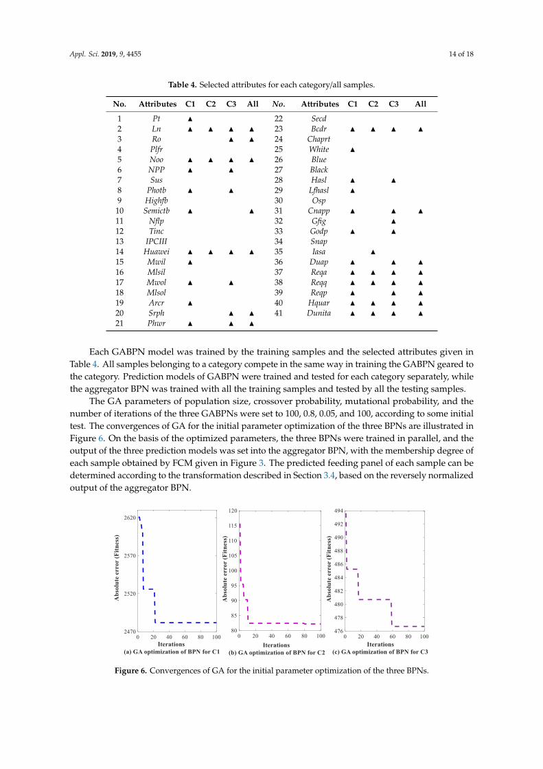
Each GABPN model was trained by the training samples and the selected attributes given inTable 4. All samples belonging to a category compete in the same way in training the GABPN geared tothe category. Prediction models of GABPN were trained and tested for each category separately, whilethe aggregator BPN was trained with all the training samples and tested by all the testing samples.

The GA parameters of population size, crossover probability, mutational probability, and thenumber of iterations of the three GABPNs were set to 100, 0.8, 0.05, and 100, according to some initialtest. The convergences of GA for the initial parameter optimization of the three BPNs are illustrated inFigure 6. On the basis of the optimized parameters, the three BPNs were trained in parallel, and theoutput of the three prediction models was set into the aggregator BPN, with the membership degree ofeach sample obtained by FCM given in Figure 3. The predicted feeding panel of each sample can bedetermined according to the transformation described in Section 3.4, based on the reversely normalizedoutput of the aggregator BPN.

Appl. Sci. 2019, x, x FOR PEER REVIEW 14 of 18

5 Noo ▲ ▲ ▲ ▲ 26 Blue

6 NPP ▲ ▲ 27 Black

7 Sus 28 Hasl ▲ ▲

8 Photb ▲ ▲ 29 Lfhasl ▲

9 Highfb 30 Osp

10 Semictb ▲ ▲ 31 Cnapp ▲ ▲ ▲

11 Nflp 32 Gfig ▲

12 Tinc 33 Godp ▲ ▲

13 IPCIII 34 Snap

14 Huawei ▲ ▲ ▲ ▲ 35 Iasa ▲

15 Mwil ▲ 36 Duap ▲ ▲ ▲

16 Mlsil 37 Reqa ▲ ▲ ▲ ▲

17 Mwol ▲ ▲ 38 Reqq ▲ ▲ ▲ ▲

18 Mlsol 39 Reqp ▲ ▲ ▲

19 Arcr ▲ 40 Hquar ▲ ▲ ▲ ▲

20 Srph ▲ ▲ 41 Dunita ▲ ▲ ▲ ▲

21 Phwr ▲ ▲ ▲

Figure 6. Convergences of GA for the initial parameter optimization of the three BPNs.

The regression of the predicted feeding panel versus the least feeding panel is given in Figure 7.

Results indicated that the predicted feeding panel coincides well with the least feeding panel, and,

therefore, the waste of surplus quantity and area can be reduced.

Figure 7. Regression of predicted feeding panel versus least feeding panel.

The FCM–BPBPN was compared to manual feeding, BPN, MSC–ANN, FCM–GABPN without

aggregation (indicated with FCM–GABPN w/o aggregation), and FCM–BPN five approaches to

quantify its performance. Manual feeding is to determine the feeding panel for each template based

on worker in PCB factory. BPN is to establish a single BPN prediction model without

Figure 6. Convergences of GA for the initial parameter optimization of the three BPNs.

Appl. Sci. 2019, 9, 4455 15 of 18

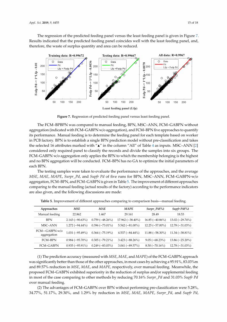
The regression of the predicted feeding panel versus the least feeding panel is given in Figure 7.Results indicated that the predicted feeding panel coincides well with the least feeding panel, and,therefore, the waste of surplus quantity and area can be reduced.

Appl. Sci. 2019, x, x FOR PEER REVIEW 14 of 18

5 Noo ▲ ▲ ▲ ▲ 26 Blue

6 NPP ▲ ▲ 27 Black

7 Sus 28 Hasl ▲ ▲

8 Photb ▲ ▲ 29 Lfhasl ▲

9 Highfb 30 Osp

10 Semictb ▲ ▲ 31 Cnapp ▲ ▲ ▲

11 Nflp 32 Gfig ▲

12 Tinc 33 Godp ▲ ▲

13 IPCIII 34 Snap

14 Huawei ▲ ▲ ▲ ▲ 35 Iasa ▲

15 Mwil ▲ 36 Duap ▲ ▲ ▲

16 Mlsil 37 Reqa ▲ ▲ ▲ ▲

17 Mwol ▲ ▲ 38 Reqq ▲ ▲ ▲ ▲

18 Mlsol 39 Reqp ▲ ▲ ▲

19 Arcr ▲ 40 Hquar ▲ ▲ ▲ ▲

20 Srph ▲ ▲ 41 Dunita ▲ ▲ ▲ ▲

21 Phwr ▲ ▲ ▲

Figure 6. Convergences of GA for the initial parameter optimization of the three BPNs.

The regression of the predicted feeding panel versus the least feeding panel is given in Figure 7.

Results indicated that the predicted feeding panel coincides well with the least feeding panel, and,

therefore, the waste of surplus quantity and area can be reduced.

Figure 7. Regression of predicted feeding panel versus least feeding panel.

The FCM–BPBPN was compared to manual feeding, BPN, MSC–ANN, FCM–GABPN without

aggregation (indicated with FCM–GABPN w/o aggregation), and FCM–BPN five approaches to

quantify its performance. Manual feeding is to determine the feeding panel for each template based

on worker in PCB factory. BPN is to establish a single BPN prediction model without

Figure 7. Regression of predicted feeding panel versus least feeding panel.

The FCM–BPBPN was compared to manual feeding, BPN, MSC–ANN, FCM–GABPN withoutaggregation (indicated with FCM–GABPN w/o aggregation), and FCM–BPN five approaches to quantifyits performance. Manual feeding is to determine the feeding panel for each template based on workerin PCB factory. BPN is to establish a single BPN prediction model without pre-classification and takesthe selected 16 attributes marked with “N” in the column “All” of Table 4 as inputs. MSC–ANN [2]considered only required panel to classify the records and divide the samples into six groups. TheFCM–GABPN w/o aggregation only applies the BPN to which the membership belonging is the highestand no BPN aggregation will be conducted. FCM–BPN has no GA to optimize the initial parameters ofeach BPN.

The testing samples were taken to evaluate the performance of the approaches, and the averageMSE, MAE, MAPE, Surpr_Pd, and Supfr Pd of five runs for BPN, MSC–ANN, FCM–GABPN-w/oaggregation, FCM–BPN, and FCM–GABPN is given in Table 5. The improvement of different approachescomparing to the manual feeding (actual results of the factory) according to the performance indicatorsare also given, and the following discussions are made:

Table 5. Improvement of different approaches comparing to comparison basis—manual feeding.

Approaches MSE MAE MAPE Surpr_Pd(%) Supfr Pd(%)

Manual feeding 22.862 1.467 29.161 28.49 18.53

BPN 2.143 (−90.63%) 0.759 (−48.26%) 17.962 (−38.40%) 16.85 (−40.86%) 13.02 (−29.74%)

MSC–ANN 1.272 (−94.44%) 0.396 (−73.01%) 5.542 (−81.00%) 12.25 (−57.00%) 12.78 (−31.03%)

FCM—GABPN-w/oaggregation 1.031 (−95.49%) 0.364 (−75.19%) 4.537 (−84.44%) 11.88 (−58.30%) 11.34 (−38.81%)

FCM–BPN 0.984 (−95.70%) 0.305 (−79.21%) 3.423 (−88.26%) 9.05 (−68.23%) 13.86 (−25.20%)

FCM–GABPN 0.935 (−95.91%) 0.249 (−83.03%) 3.041 (−89.57%) 8.50 (−70.16%) 12.78 (−31.03%)

(1) The prediction accuracy (measured with MSE, MAE, and MAPE) of the FCM–GABPN approachwas significantly better than those of the other approaches, in most cases by achieving a 95.91%, 83.03%mand 89.57% reduction in MSE, MAE, and MAPE, respectively, over manual feeding. Meanwhile, theproposed FCM–GABPN exhibited superiority in the reduction of surplus and/or supplemental feedingin most of the case comparing to other methods by reducing 70.16% Surpr_Pd and 31.03% Supfr Pdover manual feeding.

(2) The advantages of FCM–GABPN over BPN without performing pre-classification were 5.28%,34.77%, 51.17%, 29.30%, and 1.29% by reduction in MSE, MAE, MAPE, Surpr_Pd, and Supfr Pd,

Appl. Sci. 2019, 9, 4455 16 of 18

respectively, and the superiority of MSC–ANN over BPN was 3.79%, 24.75%, 42.60%, 16.14 %, and1.29%. The advantages of FCM–GABPN-w/o aggregation over BPN were 4.86%, 26.93%, 46.04%,17.44%, and 9.07%, and the FCM–BPN over BPN were 5.28%, 30.95%, 49.86%, and 27.37% by reductionin MSE, MAE, MAPE, and Surpr_Pd, but with only a 4.54% increase in Supfr. Pre-classification andcritical attribute selection for each category before prediction model establishment seem to havesignificant effect on the performance of material feeding prediction.

(3) The superiority FCM–GABPN-w/o aggregation, FCM–BPN, and FCM–GABPN over MSC–ANNaccording to the MSE, MAE, MAPE, and Surpr_Pd with only 5.83% inferiority in Supfr Pd for FCM–BPNapproach and the same value for FCM-GABPN indicates that the pre-classification by clustering, whichconsiders many attributes, surpassed the MSC classification, which considers only one attribute. Inaddition, the FCM–GABPN-w/o aggregation, FCM–BPN and FCM–GABPN only established threeBPNs for the three categories of samples, while MSC–ANN pre-classified the samples into six categoriesand trained a prediction model for each category.

(4) FCM–BPN and FCM–GABPN achieved lower MSE, MAE, MAPE, and Surpr_Pd in comparisonto FCM–GABPN-w/o aggregation, which indicates that applying the aggregator BPN to derive therepresentative value by considering the membership degree of each sample facilitates the predictionimprovement for the four performance indicators. The 13.61% and 7.78% increase in Surpr_Pdfor FCM–BPN and FCM–GABPN may be brought by the 9.07% and 11.86% reduction in Supfr Pd,respectively. In practice, the reduction of surplus feeding and supplemental feeding is conflicted becauseit is difficult to obtain the minimum value for both of them in the factory. However, the reduction ofthe surplus rate is a goal with the greatest cost impact in the factory because the individualized surplustemplate products can only be placed in inventory or directly destroyed, and the reduction of thesurplus production will reduce the comprehensive cost caused by the waste of material, production,inventory, and disposal/ recycling.

(5) The FCM–GABPN surpassed FCM–BPN according to the five indicators that verify theeffectiveness of the initialization optimization based on GA. The reason is that BPN is sensitive to theinitial condition [30], especially for the samples in the three categories that were learned with differentBPNs that may be influenced greatly by the combination of the BPN’s initial parameters.

5. Conclusions

In order to enhance the accuracy of material feeding prediction of a PCB template, an ensemblepredictor FCM–GABPN was proposed. In the proposed approach, the input templates were firstlyclustered by FCM, and seven feature selection mechanisms were utilized to select critical attributesrelated to the scrap rate for each category of templates. Then, a GABPN was trained to predict thescrap rate for each category of templates, and the GABPNs for all the categories formed an ensemblepredictor with a nonlinear aggregator BPN. Finally, the predicted feeding panel for each template wasdetermined based on the predicted scrap rate with a transformation. The effectiveness and superioritywere validated with many experiments based on the actual data. On the basis of the experimentalresults, conclusions and contributions are highlighted as follows:

(1) The accuracy of the proposed approach was better than those of the other approaches byachieving a 95.91%, 83.03%, and 89.57% reduction in MSE, MAE, and MAPE, respectively, over thecomparison basis—manual feeding. Meanwhile, the FCM–GABPN’s performance was superiorto that of the other methods in the reduction of simulated surplus and/or supplemental feedingin most of the cases, by achieving a 70.16% reduction in Surpr_Pd and a 31.03% reduction in SupfrPd over manual feeding.

(2) The material feeding prediction of PCB template problem considering category fuzziness ofsamples and the diverse samples with different influence factors is different from the existingproduction quality prediction and optimization problem, to the best of our knowledge. Thenovelty of the proposed FCM–GABPN is that we fuzzily clustered samples into different categorieswith FCM and specified a membership threshold to adopt samples for each category. Meanwhile,

Appl. Sci. 2019, 9, 4455 17 of 18

component GABPN prediction model for each category was established with separately selectedinput attributes and GA optimized initial parameter. Furthermore, an aggregator BPN wasemployed to aggregate the predicted results of each GABPN by considering the membershipvalues of each template.

Training an ensemble predictor with many sub-models that can extract shared attributes forsimilar templates automatically without explicit pre-classification needs to be studied, in which wedo not have to divide samples, select critical attributes for each category, and build the predictionmodel separately. Meanwhile, the rapid development and evolution of PCB template should also beconsidered. The transfer and lifelong learning may be the mechanisms worthy of attempting, in orderto handle the aforementioned problem.

Author Contributions: S.L. proposed the algorithm and wrote the paper; R.X. and D.L. implemented the algorithm;B.Z. conducted the experiments and analyzed the data; H.J. proposed the paper structure and wrote Section 4.

Funding: This research is funded by National Natural Science Foundation of China with grant number 51605169and Natural Science Foundation of Guangdong, China with grant number 2018A030310216.

Acknowledgments: This paper is supported by the National Natural Science Foundation of China (Grant No.51605169) and Natural Science Foundation of Guangdong, China (Grant No. 2018A030310216). The authorswould like to express their appreciation to the agency. The authors wish to thank Guangzhou FastPrint TechnologyCo., Ltd. for providing data for the study.

Conflicts of Interest: The authors declare no conflicts of interest.

References

1. Marque, A.C.; Cabrera, J.M.; Malfatti, C.F. Printed circuit boards: A review on the perspective of sustainability.J. Environ. Manag. 2013, 31, 298–306. [CrossRef] [PubMed]

2. Lv, S.P.; Zheng, B.B.; Kim, H.; Yue, Q.S. Data mining for material feeding optimization of printed circuitboard template production. J. Electr. Comput. Eng. 2018, 2018, 1852938. [CrossRef]

3. Lv, S.P.; Kim, H.; Zheng, B.B.; Jin, H. A review of data mining with big data towards its applications in theelectronics industry. Appl. Sci. 2018, 8, 582. [CrossRef]

4. Lee, H.; Kim, C.O.; Ko, H.H.; Kim, M.Y. Yield prediction through the event sequence analysis of the dieattach process. IEEE Trans. Semicond. Manuf. 2015, 28, 563–570. [CrossRef]

5. Tsai, T. Development of a soldering quality classifier system using a hybrid data mining approach. ExpertSyst. Appl. 2012, 39, 5727–5738. [CrossRef]

6. Stoyanov, S.; Bailey, C.; Tourloukis, G. Similarity approach for reducing qualification tests of electroniccomponents. Microelectron. Reliab. 2016, 67, 111–119. [CrossRef]

7. Khader, N.; Yoon, S.W.; Li, D.B. Stencil printing optimization using a hybrid of support vector regressionand mixed-integer linear programming. Procedia Manuf. 2017, 11, 1809–1817. [CrossRef]

8. Tsai, T.; Liukkonen, M. Robust parameter design for the micro-BGA stencil printing process using a fuzzylogic-based Taguchi method. Appl. Soft. Comput. 2016, 48, 124–136. [CrossRef]

9. Kwak, D.; Kim, K. A data mining approach considering missing values for the optimization ofsemiconductor-manufacturing processes. Expert Syst. Appl. 2012, 39, 2590–2596. [CrossRef]

10. Tsai, T. Thermal parameters optimization of a reflow soldering profile in printed circuit board assembly,A comparative study. Appl. Soft. Comput. 2012, 12, 2601–2613. [CrossRef]

11. Chan, K.Y.; Kwong, C.K.; Tsim, Y.C. Modelling and optimization of fluid dispensing for electronic packagingusing neural fuzzy networks and genetic algorithms. Eng. Appl. Artif. Intell. 2010, 23, 18–26. [CrossRef]

12. Liukkonen, M.; Havia, E.; Leinonenb, H.; Hiltunena, Y. Quality-oriented optimization of wave solderingprocess by using self-organizing maps. Appl. Soft. Comput. 2011, 11, 214–220. [CrossRef]

13. Liukkonen, M.; Hiltunen, T.; Havia, E.; Leinonen, H.; Hiltunen, Y. Modeling of soldering quality by usingartificial neural networks. IEEE Trans. Electron. Packag. Manuf. 2009, 32, 89–96. [CrossRef]

14. Srimani, P.K.; Prathiba, V. Adaptive data mining approach for PCB defect detection and classification. IndianJ. Sci. Technol. 2016, 9, 1–9. [CrossRef]

15. Sim, H.; Choi, D.; Kim, C.C. A data mining approach to the causal analysis of product faults in multi-stagePCB manufacturing. Int. J. Precis. Eng. Manuf. 2014, 15, 1563–1573. [CrossRef]

Appl. Sci. 2019, 9, 4455 18 of 18

16. Nagorny, K.; Lima-Monteiro, P.; Barata, J.; Colombo, A.W. Big data analysis in smart manufacturing:A Review. Int. J. Commun. Netw. Syst. Sci. 2017, 10, 31–58. [CrossRef]

17. Cheng, Y.; Chen, K.; Sun, H.M.; Zhang, Y.P.; Tao, F. Data and knowledge mining with big data towards smartproduction. J. Ind. Inform. Integr. 2018, 9, 1–13. [CrossRef]

18. Hashem, S.T.; Ebadati, E.O.M.; Kaur, H. A hybrid conceptual cost estimating model using ANN and GA forpower plant projects. Neural Comput. Appl. 2017, 2017, 1–12. [CrossRef]

19. Tang, L.; Yuan, S.; Tang, Y.; Qiu, Z.P. Optimization of impulse water turbine based on GA-BP neural networkarithmetic. J. Mech. Sci. Technol. 2019, 33, 241–253. [CrossRef]

20. Jiang, S.; Wang, L. Efficient feature selection based on correlation measure between continuous and discretefeatures. Inf. Proc. Lett. 2016, 116, 203–215. [CrossRef]

21. Reshef, D.N.; Reshef, Y.A.; Finucane, H.K.; Grossman, S.R.; McVean, V.; Turnbaugh, P.J.; Lander, E.S.;Mitzenmacher, M.; Sabeti, P.C. Detecting novel associations in large data sets. Science 2011, 334, 1518–1524.[CrossRef] [PubMed]

22. Gregorutti, B.; Michel, B.; Saint-Pierre, P. Correlation and variable importance in random forests. Stat.Comput. 2017, 27, 659–678. [CrossRef]

23. Hess, A.S.; Hess, J.R. Linear regression and correlation. Transfusion 2017, 57, 9–11. [CrossRef] [PubMed]24. Zhang, Z.; Tian, Y.; Bai, L.; Xiahou, J.B.; Hancock, E. High-order covariate interacted lasso for feature selection.

Pattern Recognit. Lett. 2017, 87, 139–146. [CrossRef]25. Ohishi, M.; Yanagihara, H.; Fujikoshi, Y. A fast algorithm for optimizing ridge parameters in a generalized

ridge regression by minimizing a model selection criterion. J. Stat. Plan. Inference 2019. [CrossRef]26. Ao, Y.; Li, H.Q.; Zhu, L.P.; Ali, S.; Yang, Z.G. The linear random forest algorithm and its advantages in

machine learning assisted logging regression modeling. J. Pet. Sci. Eng. 2019, 174, 776–789. [CrossRef]27. Tang, J.; Yu, S.W.; Liu, F.; Chen, X.Q. A hierarchical prediction model for lane-changes based on combination

of fuzzy C-means and adaptive neural network. Expert Syst. Appl. 2019, 130, 265–275. [CrossRef]28. Rezaee, M.J.; Jozmaleki, M.; Valipour, M. Integrating dynamic fuzzy C-means, data envelopment analysis

and artificial neural network to online prediction performance of companies in stock exchange. Phys. A Stat.Mech. Its Appl. 2018, 489, 78–93. [CrossRef]

29. Fathabadi, H. Power distribution network reconfiguration for power loss minimization using novel dynamicfuzzy c-means (dFCM) clustering based ANN approach. Int. J. Electr. Power 2016, 78, 96–107. [CrossRef]

30. Jia, W.; Zhao, D.; Zheng, Y.; Hou, S.J. A novel optimized GA–Elman neural network algorithm. NeuralComput. Appl. 2019, 31, 449–459. [CrossRef]

31. Chen, T. Incorporating fuzzy c-means and a back-propagation network ensemble to job completion timeprediction in a semiconductor fabrication factory. Fuzzy Sets Syst. 2007, 158, 2153–2168. [CrossRef]

32. Bolón-Canedo, V.; Sánchez-Maroño, N.; Alonso-Betanzos, A. A review of feature selection methods onsynthetic data. Knowl. Inf. Syst. 2013, 34, 483–519. [CrossRef]

© 2019 by the authors. Licensee MDPI, Basel, Switzerland. This article is an open accessarticle distributed under the terms and conditions of the Creative Commons Attribution(CC BY) license (http://creativecommons.org/licenses/by/4.0/).