An extended isogeometric thin shell analysis based on

Kirchhoff-Love theory

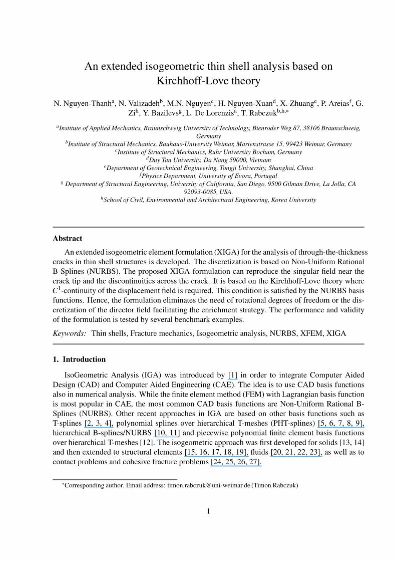
N. Nguyen-Thanha, N. Valizadehb, M.N. Nguyenc, H. Nguyen-Xuand, X. Zhuange, P. Areiasf, G.

Zih, Y. Bazilevsg, L. De Lorenzisa, T. Rabczukb,h,∗

aInstitute of Applied Mechanics, Braunschweig University of Technology, Bienroder Weg 87, 38106 Braunschweig,

GermanybInstitute of Structural Mechanics, Bauhaus-University Weimar, Marienstrasse 15, 99423 Weimar, Germany

cInstitute of Structural Mechanics, Ruhr University Bochum, GermanydDuy Tan University, Da Nang 59000, Vietnam

eDepartment of Geotechnical Engineering, Tongji University, Shanghai, ChinafPhysics Department, University of Evora, Portugal

g Department of Structural Engineering, University of California, San Diego, 9500 Gilman Drive, La Jolla, CA

92093-0085, USA.hSchool of Civil, Environmental and Architectural Engineering, Korea University

Abstract

An extended isogeometric element formulation (XIGA) for the analysis of through-the-thickness

cracks in thin shell structures is developed. The discretization is based on Non-Uniform Rational

B-Splines (NURBS). The proposed XIGA formulation can reproduce the singular field near the

crack tip and the discontinuities across the crack. It is based on the Kirchhoff-Love theory where

C1-continuity of the displacement field is required. This condition is satisfied by the NURBS basis

functions. Hence, the formulation eliminates the need of rotational degrees of freedom or the dis-

cretization of the director field facilitating the enrichment strategy. The performance and validity

of the formulation is tested by several benchmark examples.

Keywords: Thin shells, Fracture mechanics, Isogeometric analysis, NURBS, XFEM, XIGA

1. Introduction

IsoGeometric Analysis (IGA) was introduced by [1] in order to integrate Computer Aided

Design (CAD) and Computer Aided Engineering (CAE). The idea is to use CAD basis functions

also in numerical analysis. While the finite element method (FEM) with Lagrangian basis function

is most popular in CAE, the most common CAD basis functions are Non-Uniform Rational B-

Splines (NURBS). Other recent approaches in IGA are based on other basis functions such as

T-splines [2, 3, 4], polynomial splines over hierarchical T-meshes (PHT-splines) [5, 6, 7, 8, 9],

hierarchical B-splines/NURBS [10, 11] and piecewise polynomial finite element basis functions

over hierarchical T-meshes [12]. The isogeometric approach was first developed for solids [13, 14]

and then extended to structural elements [15, 16, 17, 18, 19], fluids [20, 21, 22, 23], as well as to

contact problems and cohesive fracture problems [24, 25, 26, 27].

∗Corresponding author. Email address: timon.rabczuk@uni-weimar.de (Timon Rabczuk)

1

The analysis of thin shell structures is of vital importance in many engineering applications

such as aircraft fuselages, storage tanks, ship hulls, pipes, etc. A variety of shell elements have

been developed to analyze shell structures which can be classified by the thickness of the shell

and the curvature of the mid-surface [28]. Depending on the thickness, shell elements can be

categorized into thin shell elements [29, 30, 31, 32, 33] and thick shell elements [34, 35, 36].

Thin shell elements are based on the Kirchhoff-Love (KL) theory [37] where transverse shear

deformations are negligible. The KL-theory requires C1 - continuity of the displacement field,

which is difficult to achieve for free-form geometries when a Lagrangian-type basis is used. Thin

shell theory requires the approximation of the deformation to have second-order square integrable

derivatives. Using higher continuous formulations in the context of thin shell analysis based on

KL-theory avoids the use of rotational degrees of freedom or discretization of the director field.

A formulation that only discretizes the mid-surface position and naturally fulfills the KL-theory

constraint by using a higher continuous formulation was first proposed in the context of meshfree

methods by [38, 39, 40]. These formulations include modeling of fracture through partition-of-

unity enrichment [41, 42, 43]. In the context of IGA,[44, 45] proposed thin shell formulations

based on KL-theory taking advantage of the higher-order continuity of the NURBS basis functions.

The formulation in [44] was extended by [8] to efficiently account for h-adaptive refinement.

An approach combining the extended finite element method (XFEM) and IGA for fracture in

continua was proposed by [46, 47, 48]. Instead of modeling the crack in IGA through partition-

of-unity enrichment, Verhoosel et. al. [49] applied the concept of knot insertion to create a dis-

continuous displacement field. An XFEM-shell formulation (for thick shells) based on Lagrange

polynomials was proposed by [50]. However, the formulation requires many degrees of freedom

(DOFs) per node. A simpler approach based on overlapping paired elements and discrete KL-

theory was suggested by [51] and applied to numerous interesting examples in [52]. In [53], a

phantom node method [54] for fracturing thin structures was proposed. The computation of the

interaction integral was derived for both Kirchhoff Love as well as Mindlin-Reissner theory. In

contrast to the approach in [51], this formulation allows the crack tip to be located inside an ele-

ment [55] allowing for much coarser discretizations.

In this manuscript, we present an extended isogeometric analysis (XIGA) method for cracked

thin shell structures. The method is capable of handling efficiently through-the-thickness cracks

in thin shells. NURBS basis functions ensure the C1-continuity of the generalized displacements.

Since no rotational degrees of freedom are used, the complexity of the enrichment strategy and the

computational cost is significantly reduced. The good performance of the method is confirmed by

numerical examples.

The content of the paper is outlined as follows. In Section 2, we describe the thin shell for-

mulation. The XIGA thin shell formulation is derived in Section 3. Section 4 presents several

benchmark examples before the paper closes with concluding remarks.

2. Thin shell formulation

In thin shell theory, the three-dimensional continuum description is reduced to the shell mid-

surface, and the transverse normal stress is neglected. Furthermore, the Kirchhoff-Love theory

assumes that the shell cross-section remains normal to its mid-surface in the deformed configura-

tion, which implies that the strain is assumed to be linear through the thickness and the transverse

2

shear strains are zero. In this paper, we have adopted the thin-shell formulation for intact continua

from [44, 8] and extended it to fracture problems.

2.1. Kinematics of the shell

The deformation of a thin shell can be fully described by the deformation of its mid-surface,

which is a two-dimensional manifold embedded in three-dimensional space. The mapping of the

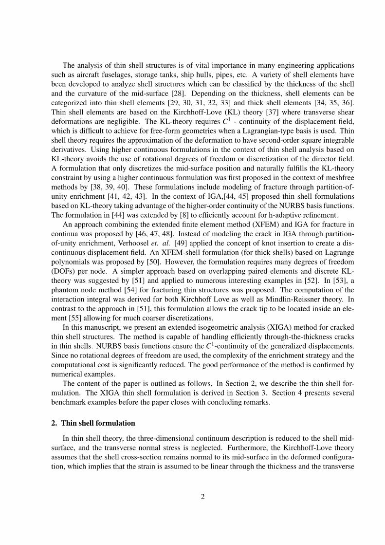
shell mid-surface is parameterized by curvilinear coordinates ξ 1,ξ 2 ∈ A ⊂ R2 (see Fig. 1).

Figure 1: Shell geometry in the reference and the deformed configurations.

The displacement of the points of the shell mid-surface is defined by

u(ξ 1,ξ 2

)= x

(ξ 1,ξ 2

)−X

(ξ 1,ξ 2

)(1)

where X is the position vector of a material point of the shell mid-surface in the reference configu-

ration, and x is the position vector of the same point in the deformed geometry. The position vector

of a material point in the reference geometry is given by

Φ(ξ 1,ξ 2,ξ 3

)= X

(ξ 1,ξ 2

)+ξ 3G3

(ξ 1,ξ 2

), (2)

and similar for the deformed geometry

ϕ(ξ 1,ξ 2,ξ 3

)= x

(ξ 1,ξ 2

)+ξ 3g3

(ξ 1,ξ 2

). (3)

where ξ 3 denotes the coordinate in thickness direction, −0.5t 6 ξ 3 6 0.5t, with t as the shell

thickness.

The deformation gradient is given by

F = ∇ϕ · (∇Φ)−1(4)

3

The covariant base vectors in the reference and current configurations are obtained from the deriva-

tives of the respective position vector fields with respect to the curvilinear coordinates, as follows

Gα = X,α ; gα = x,α (5)

where Greek indices take the values 1,2 and refer to the parametric directions on the shell mid-

surface, and (·),α := ∂ (·)/∂ξ α . The covariant metric coefficients of the surface are defined as

Gαβ = Gα ·Gβ ; gαβ = gα ·gβ , (6)

and the contravariant base vectors are computed by

Gα = Gαβ Gβ ; Gαβ =[Gαβ

]−1. (7)

The unit normal vectors of the middle surface are calculated by

G3 =G1 ×G2

|G1 ×G2|= t0 ; g3 =

g1 ×g2

|g1 ×g2|= t . (8)

The Green-Lagrange strain tensor is given by

E =1

2

(FT F− I

), (9)

where I is the identity tensor. The covariant strain components are given by

Eαβ = εαβ +ξ 3καβ (10)

The membrane strains εαβ are given by

εαβ =1

2

(gα ·gβ −Gα ·Gβ

)(11)

and the bending strains καβ , measuring the changes in curvature due to bending, are

καβ = gα ·g3,β −Gα ·G3,β (12)

Expanding Eq. (11) and Eq. (12) using Eq. (1) and omitting nonlinear terms, we obtain

εαβ =1

2

(Gα ·u,β −Gα ·u,α

)(13)

and

καβ =−u,αβ +1√

j

[u,1 ·

(Gα,β ×G2

)+u,2 ·

(G1 ×Gα,β

)]+

G3 ·Gα,β√

j[u,1 · (G2×G3)+u,2 · (G3 ×G1)]

(14)

where j = |G1 ×G2| .

4

2.2. Weak form

Applying the principle of virtual work, we seek u ∈ ϑ such that

δΠ = δΠint +δΠext = 0 ∀δu ∈ ϑ0 (15)

in which

ϑ =

u|u ∈ H2 (Ω0/Γc0) ,u = u on Γu

0, u discontinuous on Γc0

ϑ0 =

δu|δu ∈ H2 (Ω0/Γc0) , δu = 0 on Γu

0, δu discontinuous on Γc0

where Γc0 is the crack surface (or crack boundary) in the initial configuration; Γu

0 and Γt0 (introduced

later) are the partitions of the boundary where the Dirichlet and Neumann boundary conditions are

enforced, respectively.

The internal virtual work can be expressed as

δΠint =∫

Ω0

∫ t/2

−t/2σσσ :[δx,α ⊗gα +δ t⊗g3 +ξ 3δ t,α ⊗gα

]det(∇Φ)dξ 3dΩ0 (16)

where the prefix δ identifies the test function, and σσσ is the Cauchy stress tensor.

The external virtual work is given by

δΠext =

∫

Ω0/Γc0

ρ0b ·δudΩ0 +

∫

Γt0

t0 ·δudΓ0 (17)

where ρ0 is the initial density, b is the body force and t0 is the prescribed traction.

Integrating the Cauchy stress tensor σσσ over the thickness yields

nα =1

j

∫ t/2

−t/2σσσgα det(∇Φ)dξ 3 (18)

mα =1

j

∫ t/2

−t/2ξ 3σσσgα det(∇Φ)dξ 3 (19)

where nα denotes the resultant membrane stress vector and mα the result bending stress vector.

Substituting equations Eq. (18)-Eq. (19) into Eq. (16), we obtain

δΠint =∫

Ω0(nα ·δx,α +mα ·δ t,α)dΩ0

=∫

Ω0

nα ·δx,α︷ ︸︸ ︷

nαβ x,β ·δu,α +mαβ t,β ·δu,α +

mα ·δ t,α︷ ︸︸ ︷

mαβ x,β ·δ tα

dΩ0

=∫

Ω0

(

nαβ ·δεαβ + mαβ ·δκαβ

)

dΩ0

(20)

For a linear elastic material, the resultant effective membrane stress and bending stress can be

5

expressed by [56, 57]

nαβ = tDαβγδ εγδ ; mαβ =t3

12Dαβγδ κγδ (21)

Dαβγδ =E

1−ν

[

ν(X,αX,β )(X,γX,δ )+1

2(1−ν)(X,αX,γ)(X,δ X,β )+

1

2(1−ν)(X,αX,δ )(X,γX,β )

]

(22)

Using Voigt’s notation one can write

n =

n11

n22

n12

= tDεεε ; m =

m11

m22

m12

=t3

12Dκκκ ; εεε =

ε11

ε22

2ε12

; κκκ =

κ11

κ22

2κ12

(23)

where D is the constitutive tensor of the isotropic material, E is the Young’s modulus and ν is the

Poisson’s ratio.

D =E

1−ν2

(a11

0

)2νa11

0 a220 +(1−ν)

(a12

0

)2a11

0 a120

...(a22

0

)2a22

0 a120

symm · · · 12

[

(1−ν)a110 a22

0 − (1−ν)(a12

0

)2]

(24)

where aαβ0 = X,α ·X,β . Correspondingly, Eq. (20) can be rewritten in a compact form as

δΠint =

∫

Ω0

(n ·δεεε + m ·δκκκ)dΩ0 (25)

3. Discretization

3.1. A brief review on B-Spline/ NURBS basis functions

Let Ξ =[ξ1,ξ2, ...,ξn+p+1

]be a non-decreasing sequence of parameter values, ξi ≤ ξi+1, i =

1, ...,n+ p; ξi are the knots governing the approximation, and Ξ is called knot vector. If all knots

are equally spaced, then the knot vector is uniform; otherwise it is non-uniform. When the first and

the last knots are repeated p+1 times, the knot vector is called open. A B-Spline basis function

is C∞ continuous in the interior of each knot span and Cp−1 continuous at each unique knot. At a

knot of multiplicity k, the continuity is Cp−k.

The B-spline basis functions Ni,p(ξ ) are defined recursively on the corresponding knot vector.

The basis functions of order p = 0 are

Ni,0(ξ ) =

1 if ξi ≤ ξ < ξi+1

0 otherwise(26)

For p > 1, the basis functions are

Ni,p(ξ ) =ξ −ξi

ξi+p−ξiNi,p−1(ξ )+

ξi+p+1 −ξ

ξi+p+1 −ξi+1Ni+1,p−1(ξ ) . (27)

6

B-spline basis functions Ni,p possess important properties such as non-negativity, local support,

partition of unity and linear independence.

B-spline curves are defined by

C(ξ ) =n

∑i=1

Ni,p(ξ )Pi , (28)

where Pi are the n control points and Ni,p(ξ ) are the pth-order B-spline basis functions.

B-spline surfaces are defined by the tensor product of basis functions with parameters ξ ∈ Ξ1

and η ∈ Ξ2 expressed as

S(ξ ,η) =n

∑i=1

m

∑j=1

Ni,p(ξ )M j,q(η)Pi, j (29)

where Ni,p(ξ ) and M j,q(η) are B-spline basis functions defined on the knot vectors and Pi, j are a

n×m net of control points.

Non-uniform rational B-splines (NURBS) are preferred to B-splines due to their ability to

exactly represent conic sections such as circles and ellipses. A NURBS surface is defined as

S(ξ ,η) =n

∑i=1

m

∑j=1

Ri, j (ξ ,η)Pi, j ; Ri, j =Ni,p (ξ )M j,q (η)wi, j

∑ni=1 ∑m

j=1 Ni,p (ξ )M j,q (η)wi, j(30)

where wi, j are the weights. An example of the geometry representation of a free-form shape based

on cubic NURBS is illustrated in Fig. 2. The figure also includes the control points.

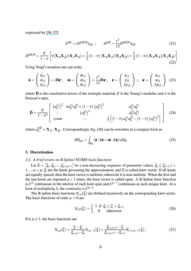
Figure 2: Physical mesh and control points for a cubic NURBS surface.

7

3.2. Partition-of-unity enrichment

3.2.1. In-plane enrichment

The displacement and membrane stress components at a crack tip can be expressed in polar

coordinates (r,θ) as follows [58]:

u1

u2

=KI

2µ

√r

2π

cos θ

2

(21−ν

1+ν +2sin2 θ2

)

sin θ2

(4

1+ν −2cos2 θ2

)

+KII

2µ

√r

2π

sin θ

2

(4

1+ν +2cos2 θ2

)

−cos θ2

(21−ν

1+ν −2sin2 θ2

)

(31)

σ11

σ12

σ22

=

KI√2πr

cosθ

2

1− sin θ2

sin 3θ2

sin θ2

cos 3θ2

1+ sin θ2

sin 3θ2

+

KII√2πr

cosθ

2

sin θ2

(2+ cos θ

2cos 3θ

2

)

cosθ2

(1− sin θ

2sin 3θ

2

)

sin θ2

cos θ2

cos 3θ2

(32)

where µ = E/2(1+ν) is the shear modulus, and KI and KII are membrane stress intensity factors

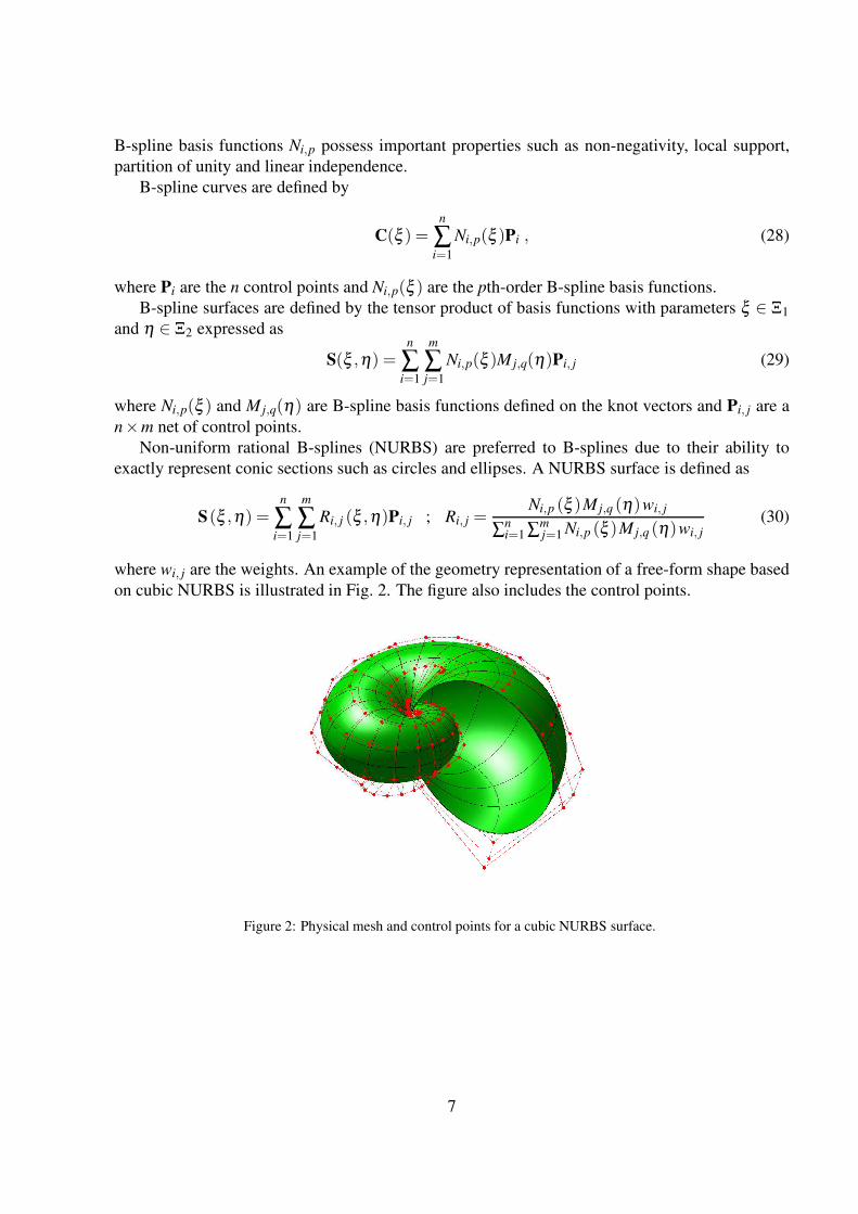
(SIFs) of mode I and mode II fracture, respectively. The different fracture modes are illustrated in

Fig. 3.

Figure 3: Fracture modes.

The membrane stress intensity factors are given by

KI = limr→0

√2πr (σθθ (r,0)) ; KII = lim

r→∞

√2πr (σrθ (r,0)) (33)

where σθθ and σrθ are stress components in polar coordinates.

It can be shown that the in-plane tip enrichment functions

ψψψ (r,θ) =

√r sin

(θ

2

)

,√

r cos

(θ

2

)

,√

r sin

(θ

2

)

sin(θ) ,√

r cos

(θ

2

)

sin(θ)

(34)

represent the asymptotic near crack tip solution [59].

8

3.2.2. Out-of-plane enrichments

The internal stresses due to bending can be computed by [60]

σrr

σrθ

σθθ

=

k1√2r

x3

2h

1

3+ν

(3+5ν)cos θ2− (7+ν)cos 3θ

2

−(1−ν)sin θ2+(7+ν)sin 3θ

2

(5+3ν)cos θ2+(7+ν)cos 3θ

2

+k2√2r

x3

2h

1

3+ν

−(3+5ν)sin θ2+(5+3ν)sin 3θ

2

(−1+ν)cos θ2+(5+3ν)cos 3θ

2

−(5+3ν)(sin θ

2+ sin 3θ

2

)

(35)

where x3 is the out of plane component of the current coordinate vector. The out-of-plane displace-

ment is given

u3 =(2r)

32(1−ν2

)

2Eh(3+ν)

k1

[1

3

(7+ν

1−ν

)

cos3θ

2− cos

θ

2

]

+ k2

[

−1

3

(5+3ν

1−ν

)

sin3θ

2+ sin

θ

2

]

(36)

where k1 and k2 are the bending and twisting stress intensity factors:

k1 = limr→0

√2rσθθ

(

r,0,h

2

)

; k2 = limr→0

3+ν

1+ν

√2rσrθ

(

r,0,h

2

)

(37)

The corresponding out of plane tip enrichment functions are given by [60]

F(r,θ) =

√r sin

(θ

2

)

,r32 sin

(θ

2

)

,r32 cos

(θ

2

)

,r32 sin

(3θ

2

)

,r32 cos

(3θ

2

)

(38)

3.2.3. Discretization of the displacement field

Similar to the enrichment strategy used in XFEM, the XIGA displacement field of the cracked

shell surface can be expressed as

u1

u2

=NI

∑I=1

RI

uI

1

uI2

+NJ

∑J=1

RJ (H (x)−H (xJ))

aJ

1

aJ2

+NK

∑K=1

RKLK

∑L=1

(ψL

K (x)−ψLK (xK)

)

bL1K

bL2K

(39)

u3 =NI

∑I=1

RIuI3 +

NJ

∑J=1

RJ (H (x)−H (xJ)) aJ3 +

NK

∑K=1

RKLK

∑L=1

(FL

K (x)−FLK (xK)

)bL

3K (40)

where R are NURBS basis functions, u1, u2, u3 are the standard DOFs, a1, a2, a3 and b1, b2, b3 are

additional DOFs, ψ and F are the tip-enrichment functions, and H is Heaviside function. There

are two different procedures for choosing the tip enriched area [61]: topological enrichment and

geometrical enrichment. Topological enrichment refers to the strategy in which the size of the tip

enriched area is proportional to the mesh size. By contrast, in geometrical enrichment a constant tip

enriched area independent of the mesh size is considered. In order to obtain optimal convergence

rates in crack applications, it is crucial to use the geometrical enrichment [62, 63]. The quartic

B-spline basis functions and the step-enriched shape functions affected by the crack are shown

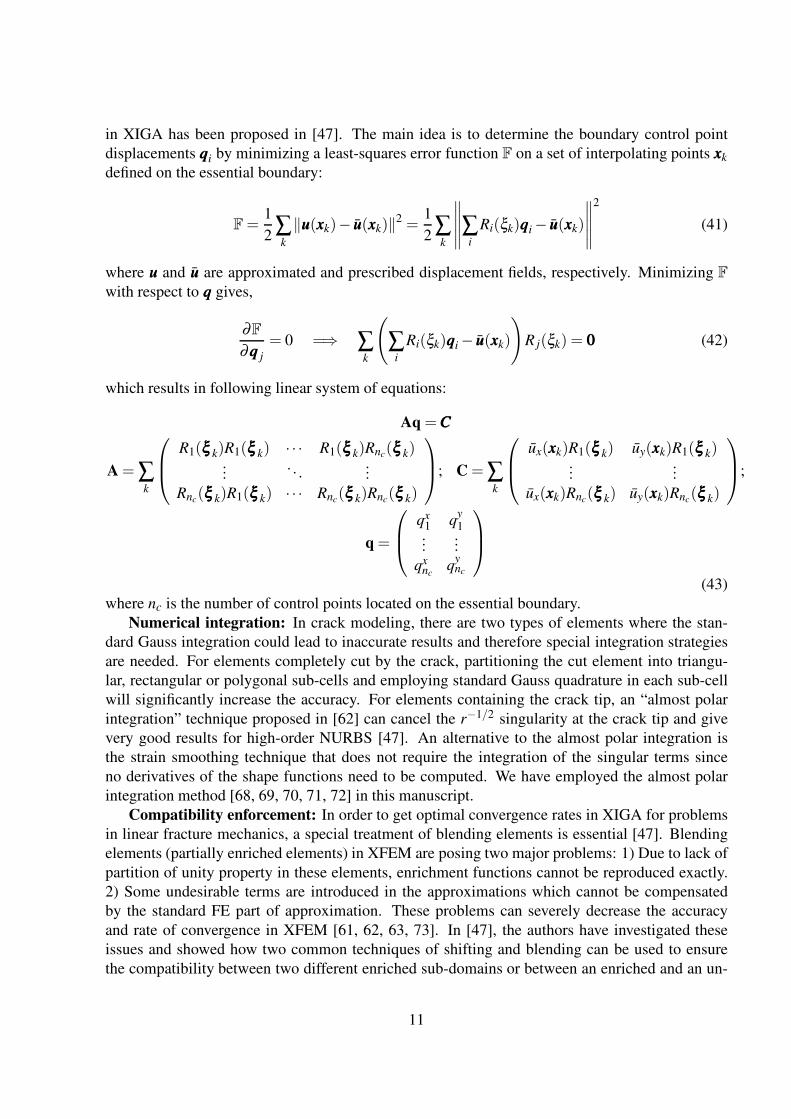
for a one-dimensional discretisation in Fig. 4. Fig. 5 presents the enriched control points and the

9

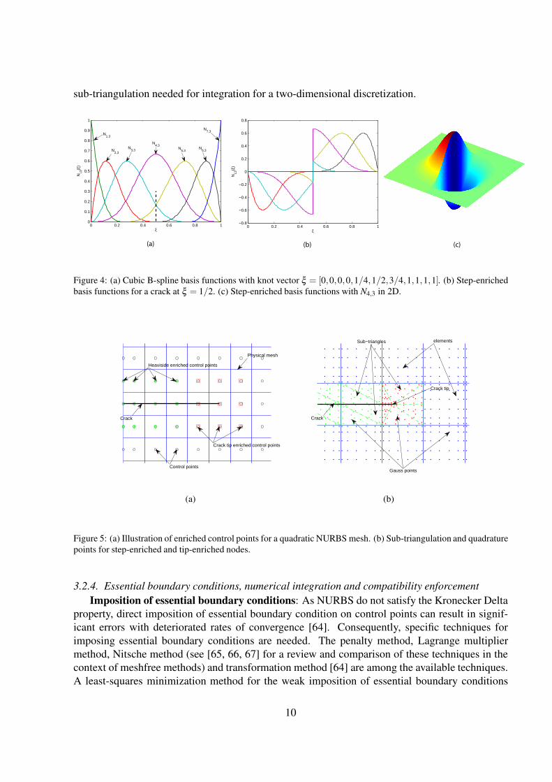
sub-triangulation needed for integration for a two-dimensional discretization.

0 0.2 0.4 0.6 0.8 1−0.8

−0.6

−0.4

−0.2

0

0.2

0.4

0.6

0.8

ξN

i,3(ξ

)

0 0.2 0.4 0.6 0.8 10

0.1

0.2

0.3

0.4

0.5

0.6

0.7

0.8

0.9

1

ξ

Ni,3

(ξ)

N2,3

N3,3 N

5,3N

6,3

N7,3

N1,3

N4,3

(a) (b) (c)

Figure 4: (a) Cubic B-spline basis functions with knot vector ξ = [0,0,0,0,1/4,1/2,3/4,1,1,1,1]. (b) Step-enriched

basis functions for a crack at ξ = 1/2. (c) Step-enriched basis functions with N4,3 in 2D.

Crack

Heaviside enriched control points

Crack tip enriched control points

Control points

Physical mesh

(a)

Crack

Crack tip

Gauss points

elementsSub−triangles

(b)

Figure 5: (a) Illustration of enriched control points for a quadratic NURBS mesh. (b) Sub-triangulation and quadrature

points for step-enriched and tip-enriched nodes.

3.2.4. Essential boundary conditions, numerical integration and compatibility enforcement

Imposition of essential boundary conditions: As NURBS do not satisfy the Kronecker Delta

property, direct imposition of essential boundary condition on control points can result in signif-

icant errors with deteriorated rates of convergence [64]. Consequently, specific techniques for

imposing essential boundary conditions are needed. The penalty method, Lagrange multiplier

method, Nitsche method (see [65, 66, 67] for a review and comparison of these techniques in the

context of meshfree methods) and transformation method [64] are among the available techniques.

A least-squares minimization method for the weak imposition of essential boundary conditions

10

in XIGA has been proposed in [47]. The main idea is to determine the boundary control point

displacements qqqi by minimizing a least-squares error function F on a set of interpolating points xxxk

defined on the essential boundary:

F=1

2∑k

‖uuu(xxxk)− uuu(xxxk)‖2 =1

2∑k

∥∥∥∥∥∑

i

Ri(ξk)qqqi − uuu(xxxk)

∥∥∥∥∥

2

(41)

where uuu and uuu are approximated and prescribed displacement fields, respectively. Minimizing F

with respect to qqq gives,

∂F

∂qqq j

= 0 =⇒ ∑k

(

∑i

Ri(ξk)qqqi − uuu(xxxk)

)

R j(ξk) = 000 (42)

which results in following linear system of equations:

Aq =CCC

A = ∑k

R1(ξξξ k)R1(ξξξ k) · · · R1(ξξξ k)Rnc(ξξξ k)

.... . .

...

Rnc(ξξξ k)R1(ξξξ k) · · · Rnc

(ξξξ k)Rnc(ξξξ k)

; C = ∑

k

ux(xxxk)R1(ξξξ k) uy(xxxk)R1(ξξξ k)...

...

ux(xxxk)Rnc(ξξξ k) uy(xxxk)Rnc

(ξξξ k)

;

q =

qx1 q

y1

......

qxnc

qync

(43)

where nc is the number of control points located on the essential boundary.

Numerical integration: In crack modeling, there are two types of elements where the stan-

dard Gauss integration could lead to inaccurate results and therefore special integration strategies

are needed. For elements completely cut by the crack, partitioning the cut element into triangu-

lar, rectangular or polygonal sub-cells and employing standard Gauss quadrature in each sub-cell

will significantly increase the accuracy. For elements containing the crack tip, an “almost polar

integration” technique proposed in [62] can cancel the r−1/2 singularity at the crack tip and give

very good results for high-order NURBS [47]. An alternative to the almost polar integration is

the strain smoothing technique that does not require the integration of the singular terms since

no derivatives of the shape functions need to be computed. We have employed the almost polar

integration method [68, 69, 70, 71, 72] in this manuscript.

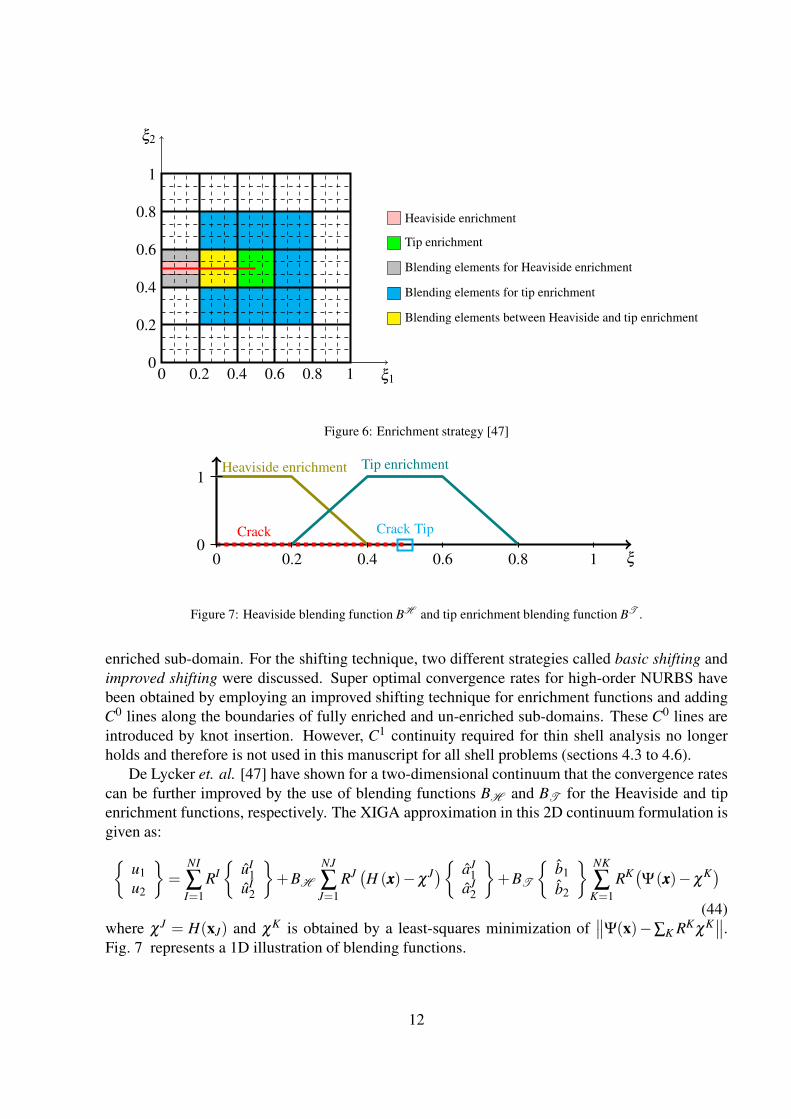
Compatibility enforcement: In order to get optimal convergence rates in XIGA for problems

in linear fracture mechanics, a special treatment of blending elements is essential [47]. Blending

elements (partially enriched elements) in XFEM are posing two major problems: 1) Due to lack of

partition of unity property in these elements, enrichment functions cannot be reproduced exactly.

2) Some undesirable terms are introduced in the approximations which cannot be compensated

by the standard FE part of approximation. These problems can severely decrease the accuracy

and rate of convergence in XFEM [61, 62, 63, 73]. In [47], the authors have investigated these

issues and showed how two common techniques of shifting and blending can be used to ensure

the compatibility between two different enriched sub-domains or between an enriched and an un-

11

Heaviside enrichment

Tip enrichment

Blending elements for Heaviside enrichment

Blending elements for tip enrichment

Blending elements between Heaviside and tip enrichment

0 0.2 0.4 0.6 0.8 10

0.2

0.4

0.6

0.8

1

ξ1

ξ2

Figure 6: Enrichment strategy [47]

ξ

Crack Tip

Tip enrichmentHeaviside enrichment

Crack

0 0.2 0.4 0.6 0.8 10

1

Figure 7: Heaviside blending function BH and tip enrichment blending function BT .

enriched sub-domain. For the shifting technique, two different strategies called basic shifting and

improved shifting were discussed. Super optimal convergence rates for high-order NURBS have

been obtained by employing an improved shifting technique for enrichment functions and adding

C0 lines along the boundaries of fully enriched and un-enriched sub-domains. These C0 lines are

introduced by knot insertion. However, C1 continuity required for thin shell analysis no longer

holds and therefore is not used in this manuscript for all shell problems (sections 4.3 to 4.6).

De Lycker et. al. [47] have shown for a two-dimensional continuum that the convergence rates

can be further improved by the use of blending functions BH and BT for the Heaviside and tip

enrichment functions, respectively. The XIGA approximation in this 2D continuum formulation is

given as:

u1

u2

=NI

∑I=1

RI

uI

1

uI2

+BH

NJ

∑J=1

RJ(H (xxx)−χJ

)

aJ1

aJ2

+BT

b1

b2

NK

∑K=1

RK(Ψ(xxx)−χK

)

(44)

where χJ = H(xJ) and χK is obtained by a least-squares minimization of∥∥Ψ(x)−∑K RKχK

∥∥.

Fig. 7 represents a 1D illustration of blending functions.

12

Remark. As in [74, 47], the tip enrichment function used here is the first term of the displacement

expansion near the crack tip for a pure mode I crack with unit stress-intensity factor. This is

originally based on the work [75] and known as vectorial enrichment in some references [76].

For the blending technique, a projected blending function which is compatible with high-order

NURBS functions can give the best results [47].

The displacement approximation used in the projected blending strategy is given as

u1

u2

=NI

∑I=1

RI

uI

1

uI2

+NJ

∑J=1

RJBJH H(xxx)

aJ

1

aJ2

+NK

∑K=1

RKBKT Ψ(xxx)

bK

1

bK2

(45)

where BJH

and BKT

being projected blending coefficients associated with the Heaviside and tip

enrichment, respectively. These coefficients are obtained by projecting a bilinear blending function

on the NURBS basis functions in a way that ∑J RJ(ξξξ )BJH

and ∑K RK(ξξξ )BKT

closely approximates

the blending functions BH and BT .

For all shell problems presented in sections 4.3 to 4.6, we have not used a compatibility enforce-

ment as the KL shell formulation requires C1 continuity. Only for the 2D benchmark problems in

section 4.1 and 4.2, we will show the performance of the compatibility enforcement.

3.3. Discretization

Substituting the discretization of the trial functions, Eqs. (39), (40), their derivatives, as well as

the test functions which have a similar structure to the trial functions into the weak form, Eq. (15),

the following linear system of equations is obtained:

Ku = f (46)

with the global stiffness matrix

Ki j =

∫

A

(

t (Bmi )

TDBm

j +t3

12

(

Bbi

)T

DBbj

)

jdξ 1dξ 2 (47)

in which Bm and Bb are the membrane and bending-strain matrices, respectively.

The standard membrane and bending strain matrices associated with node I are given by

BmI =

RI,1G1 · e1 RI

,1G1 · e2 RI,1G1 · e3

RI,2G1 · e1 RI

,2G1 · e2 RI,2G1 · e3(

RI,1G2 +RI

,2G1

)

· e1

(

RI,1G2 +RI

,2G1

)

· e2

(

RI,1G2 +RI

,2G1

)

· e3

(48)

and

BbI =

BbI1 · e1 BbI

1 · e2 BbI1 · e3

BbI2 · e1 BbI

2 · e2 BbI2 · e3

BbI3 · e1 BbI

3 · e2 BbI2 · e3

. (49)

13

The terms e1,e2,e3 are the global basis vectors of an orthonormal coordinate reference frame, and

BbI1 =−RI

,11G3 +1√

j

[RI,1G1,1 ×G2 +RI

,2G1 ×G1,1

]+

G3 ·G1,1√

j

[RI,1G2 ×G3 +RI

,2G3×G1

]

(50)

BbI2 =−RI

,22G3 +1√

j

[RI,1G2,2 ×G2 +RI

,2G1 ×G2,2

]+

G3 ·G2,2√

j

[RI,1G2 ×G3 +RI

,2G3×G1

]

(51)

BbI3 =−RI

,12G3 +1√

j

[RI,1G1,2 ×G2 +RI

,2G1 ×G1,2

]+

G3 ·G1,2√

j

[RI,1G2 ×G3 +RI

,2G3×G1

]

(52)

The force contribution of the ith node is

fi =∫

A

bRi jdξ 1dξ 2 +∫

∂A

pRi‖X,t‖dlξ (53)

where p are the forces per unit length on the boundary of the middle surface and dlξ is the line

element of the boundary of the middle surface.

3.3.1. Membrane B-matrix for XIGA

The BmH

associated to the Heaviside enrichment is given by

BmJH =

BmJH1

· e1 BmJH1

· e2 BmJH1

· e3

BmJH2

· e1 BmJH2

· e2 BmJH 2 · e3

BmJH3

· e1 BmJH2

· e2 BmJH3

· e3

(54)

whereBmJ

H1= RJ

,1 (H (xxx)−H (xxxJ))G1

BmJH2

= RJ,2 (H (xxx)−H (xxxJ))G2

BmJH3

=(RJ,1G2+RJ

,2G1

)(H (xxx)−H (xxxJ))

(55)

The BmT

associated to the tip enrichment is

BmKLT =

BmKLT1

· e1 BmKLT1

· e2 BmKLT1

· e3

BmKLT2

· e1 BmKLT2

· e2 BmKLT2

· e3

BmKLT3

· e1 BmKLT3

· e2 BmKLT3

· e3

(56)

where

BmKLT1

=[RK,1

(ψL

K (ξ )−ψLK (ξK)

)+RKψL

K,1 (ξ )]

G1

BmKLT2

=[RK,2

(ψL

K (ξ )−ψLK (ξK)

)+RKψL

K,2 (ξ )]

G2

BmKLT3

=(RK,1G2 +RK

,2G1

)(ψL

K (ξ )−ψLK (ξK)

)+RK

(ψL

K,1 (ξ )G2 +ψLK,2 (ξ )G1

)(57)

14

3.3.2. Bending B-matrix for XIGA

The BbJH

-matrix associated with the Heaviside-enriched DOFs is given by

BbJH

=(H (ξ )−H

(ξ J))

BbJH1

· e1 BbJH1

· e2 BbJH1

· e3

BbJH2

· e1 BbJH2

· e2 BbJH2

· e3

BbJH3

· e1 BbJH3

· e2 BbJH3

· e3

(58)

where BbJH1

,BbJH2

,BbJH3

are the same as in the standard part.

The contribution of the crack tip enrichment is calculated by

BbKLT =

BbKL1 · e1 BbKL

T1· e2 BbKL

T1· e3

BbKLT2

· e1 BbKLT2

· e2 BbKL2 · e3

BbKLT3

· e1 BbKLT3

· e2 BbKLT3

· e3

(59)

where BbKLT1

,BbKLT2

,BbKLT3

are similar to the standard bending terms, but replacing RI11,R

I22,R

I12,R

I1,R

I2

by the following terms

RI,11 → RK

,11

(ψL

K (ξ )−ψLK (ξK)

)+2RI

,1ψLK,1 (ξ )+RIψL

K,11 (ξ )

RI,22 → RK

,22

(ψL

K (ξ )−ψLK (ξK)

)+2RI

,2ψLK,2 (ξ )+RIψL

K,22 (ξ )

RI,12 → RK

,12

(ψL

K (ξ )−ψLK (ξK)

)+RI

,1ψLK,2 (ξ )+RI

,2ψLK,1 (ξ )+RIψL

K,12 (ξ )

RI,1 → RK

,1

(ψL

K (ξ )−ψLK (ξK)

)+RIψL

K,1 (ξ )

RI,2 → RK

,2

(ψL

K (ξ )−ψLK (ξK)

)+RIψL

K,2 (ξ ) .

(60)

3.4. Domain form for J-integral calculation

Consider a through-the-thickness crack with the crack front normal to the mid-surface of the

shell model. The J-integral is defined as [77]

f J =

∫

A

(

σi j∂ui

∂x1−Wδ1 j

)

n jqdA (61)

where W = 1/2σi jεi j is the strain energy density, σi j are the stress tensor components, εi j are the

strain tensor components, ui are the displacement components, n j are the components of the unit

normal vector to the surface A of a volume V surrounding the crack front, δ1 j is the Kronecker

delta and A is the cylindrical surface of V . The surface Ai (i = 1,2,ε) are illustrated in Fig. 8.

Commonly, a smooth function q is introduced which is equal to zero on A and non-zero on Aε and

f is the area under the q function curve along the crack front.

Applying the divergence theorem to Eq. (61), we obtain

f J =

∫

V

(

σi j∂ui

∂x1−W δ1 j

)∂ q

∂x jdV −

∫

A1+A2

(

σi j∂ui

∂x1−W δ1 j

)

n jqdA (62)

The cylinder around the crack front is limited by the upper and lower faces A1 and A2, respectively.

15

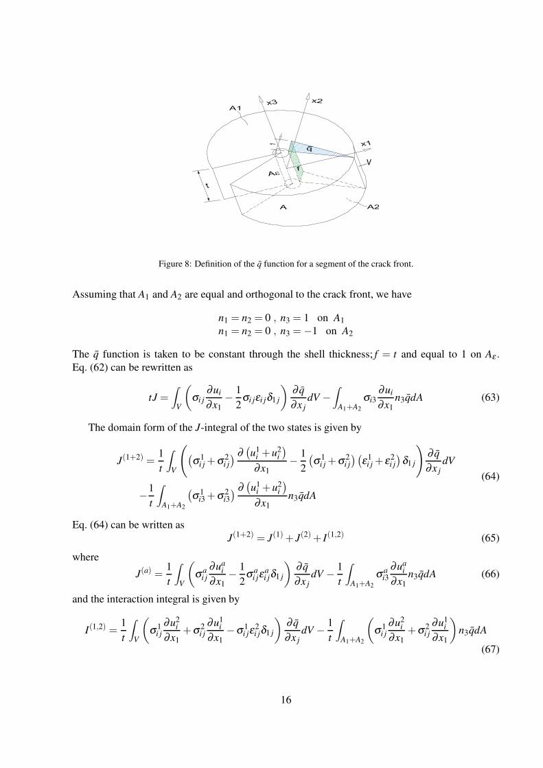
t

V

Figure 8: Definition of the q function for a segment of the crack front.

Assuming that A1 and A2 are equal and orthogonal to the crack front, we have

n1 = n2 = 0 , n3 = 1 on A1

n1 = n2 = 0 , n3 =−1 on A2

The q function is taken to be constant through the shell thickness; f = t and equal to 1 on Aε .

Eq. (62) can be rewritten as

tJ =

∫

V

(

σi j∂ui

∂x1− 1

2σi jεi jδ1 j

)∂ q

∂x jdV −

∫

A1+A2

σi3∂ui

∂x1n3qdA (63)

The domain form of the J-integral of the two states is given by

J(1+2) =1

t

∫

V

(

(σ 1

i j +σ 2i j

) ∂(u1

i +u2i

)

∂x1− 1

2

(σ 1

i j +σ 2i j

)(ε1

i j + ε2i j

)δ1 j

)

∂ q

∂x j

dV

−1

t

∫

A1+A2

(σ 1

i3 +σ 2i3

) ∂(u1

i +u2i

)

∂x1n3qdA

(64)

Eq. (64) can be written as

J(1+2) = J(1)+ J(2)+ I(1,2) (65)

where

J(a) =1

t

∫

V

(

σ ai j

∂uai

∂x1− 1

2σ a

i jεai jδ1 j

)∂ q

∂x jdV − 1

t

∫

A1+A2

σ ai3

∂uai

∂x1n3qdA (66)

and the interaction integral is given by

I(1,2) =1

t

∫

V

(

σ 1i j

∂u2i

∂x1+σ 2

i j

∂u1i

∂x1−σ 1

i jε2i jδ1 j

)∂ q

∂x jdV − 1

t

∫

A1+A2

(

σ 1i j

∂u2i

∂x1+σ 2

i j

∂u1i

∂x1

)

n3qdA

(67)

16

As the relationship between the interaction integral and the SIFs is given by

I(1,2) =2

E

(K1

I K2I +K1

IIK2II

)+

2π

3E

(1+ν

3+ν

)(k1

1k21 + k1

2k22

), (68)

we can finally write the J-integral as

J(1+2) = J(1)+ J(2)+2

E

(K1

I K2I +K1

IIK2II

)+

2π

3E

(1+ν

3+ν

)(k1

1k21 + k1

2k22

)(69)

4. Numerical benchmark examples

In this section, we present six numerical problems to test our XIGA-formulation. In section

4.1 and 4.2, we study two-dimensional examples and employ the compatibility enforcement as

discussed previously. The remaining four examples are benchmark problems for fracture in thin

shell analysis.

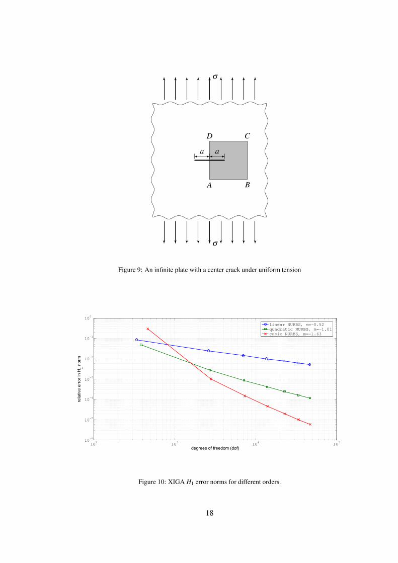
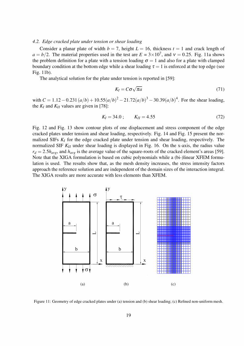
4.1. Infinite plate with a center crack under remote uniform tension

Let us consider an isotropic infinite plate with a center crack under remote uniform tension

(Fig. 9). A unit square domain ABCD with an edge crack of length 0.5 mm is modeled. The plain

strain state is assumed. The exact solution for this problem is given by

ux(r,θ) =2(1+ν)√

2π

KI

E

√r cos

θ

2

(

2−2ν − cos2 θ

2

)

uy(r,θ) =2(1+ν)√

2π

KI

E

√r sin

θ

2

(

2−2ν − cos2 θ

2

)

σxx(r,θ) =KI√2πr

cosθ

2

(

1− sinθ

2sin

3θ

2

)

σyy(r,θ) =KI√2πr

cosθ

2

(

1+ sinθ

2sin

3θ

2

)

σxy(r,θ) =KI√2πr

sinθ

2cos

θ

2cos

3θ

2

(70)

where KI = σ√

πa is the stress-intensity factor. Here the following material properties, geometric

parameters and loading conditions are considered: E = 107 N/mm2, ν = 0.3, a = 10 mm, and

σ = 102 N/mm2. The exact displacement field is imposed along the boundary of the square domain

using the least-squares minimization method. The approximation error in the H1 norm versus the

number of DOFs and the element size are shown in Fig. 10 for different orders of NURBS. Optimal

convergence rates are obtained in all cases. Note that for p=1, the XIGA formulation is identical

to “standard” XFEM (based on linear Lagrange polynomials, provided the weights corresponding

to the control points are all equal).

17

a a

A B

CD

σ

σ

Figure 9: An infinite plate with a center crack under uniform tension

102

103

104

105

10−6

10−5

10−4

10−3

10−2

10−1

100

degrees of freedom (dof)

rela

tive

erro

r in

H1 n

orm

linear NURBS, m=−0.52 quadratic NURBS, m=−1.01cubic NURBS, m=−1.63

Figure 10: XIGA H1 error norms for different orders.

18

4.2. Edge cracked plate under tension or shear loading

Consider a planar plate of width b = 7, height L = 16, thickness t = 1 and crack length of

a = b/2. The material properties used in the test are E = 3×107, and ν = 0.25. Fig. 11a shows

the problem definition for a plate with a tension loading σ = 1 and also for a plate with clamped

boundary condition at the bottom edge while a shear loading τ = 1 is enforced at the top edge (see

Fig. 11b).

The analytical solution for the plate under tension is reported in [59]:

KI =Cσ√

πa (71)

with C = 1.12−0.231(a/b)+10.55(a/b)2 −21.72(a/b)3 −30.39(a/b)4. For the shear loading,

the KI and KII values are given in [78]:

KI = 34.0 ; KII = 4.55 (72)

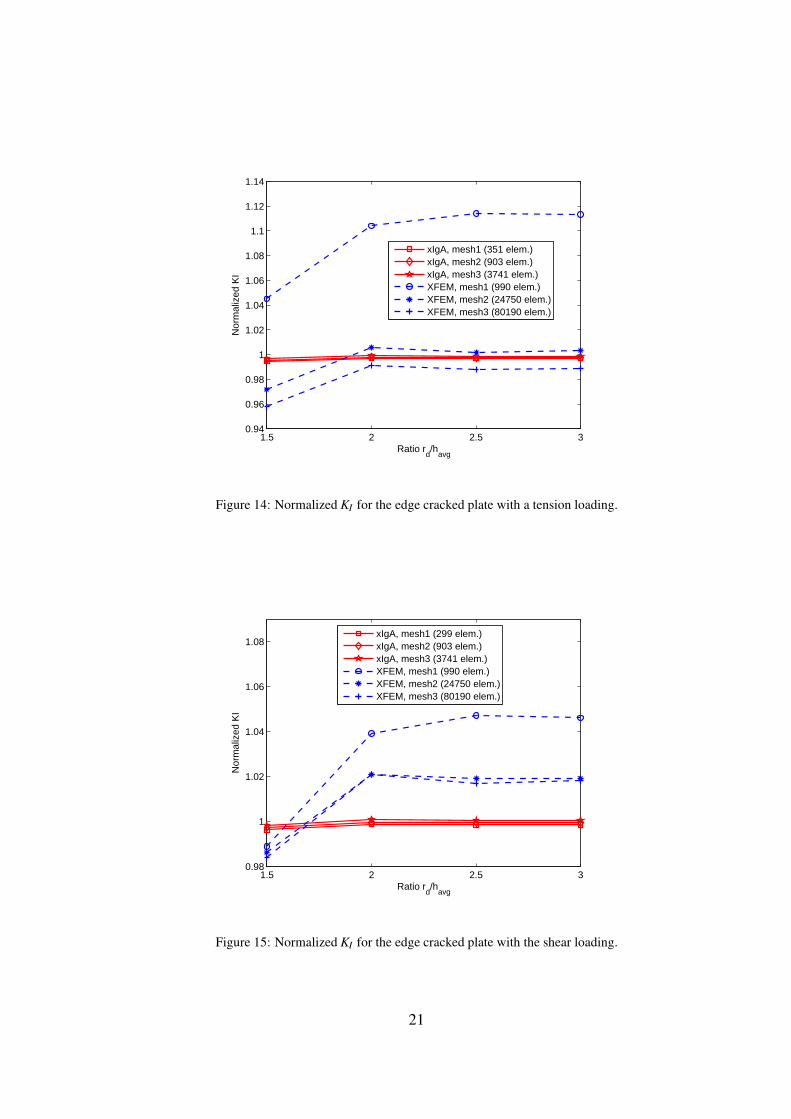
Fig. 12 and Fig. 13 show contour plots of one displacement and stress component of the edge

cracked plates under tension and shear loading, respectively. Fig. 14 and Fig. 15 present the nor-

malized SIFs KI for the edge cracked plate under tension and shear loading, respectively. The

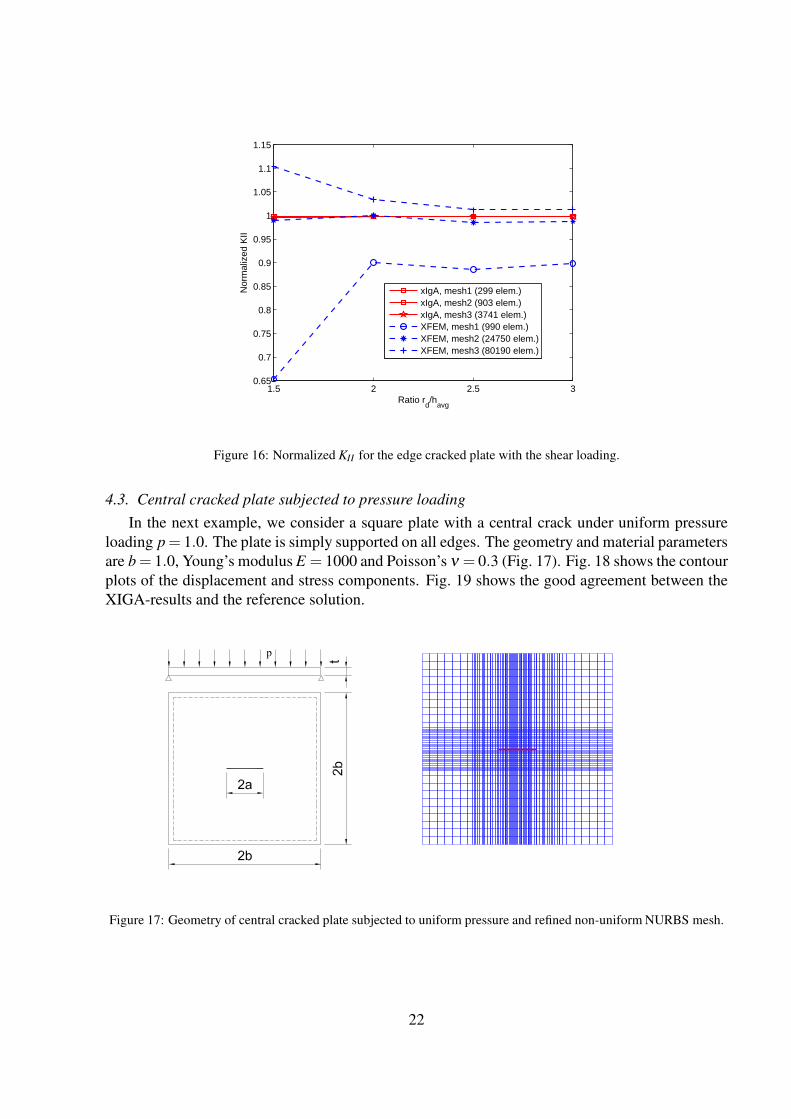
normalized SIF KII under shear loading is displayed in Fig. 16. On the x-axis, the radius value

rd = 2.5havg, and havg is the average value of the square-roots of the cracked element’s areas [59].

Note that the XIGA formulation is based on cubic polynomials while a (bi-)linear XFEM formu-

lation is used. The results show that, as the mesh density increases, the stress intensity factors

approach the reference solution and are independent of the domain sizes of the interaction integral.

The XIGA results are more accurate with less elements than XFEM.

(a) (b) (c)

Figure 11: Geometry of edge cracked plates under (a) tension and (b) shear loading; (c) Refined non-uniform mesh.

19

(a) (b)

Figure 12: Contour plots displacement of the plate under (a) tension and (b) shear loading.

(a) (b)

Figure 13: Contour plots stress of the plate under (a) tension and (b) shear loading.

20

1.5 2 2.5 30.94

0.96

0.98

1

1.02

1.04

1.06

1.08

1.1

1.12

1.14

Ratio rd/h

avg

Nor

mal

ized

KI

xIgA, mesh1 (351 elem.)xIgA, mesh2 (903 elem.)xIgA, mesh3 (3741 elem.)XFEM, mesh1 (990 elem.)XFEM, mesh2 (24750 elem.)XFEM, mesh3 (80190 elem.)

Figure 14: Normalized KI for the edge cracked plate with a tension loading.

1.5 2 2.5 30.98

1

1.02

1.04

1.06

1.08

Ratio rd/h

avg

Nor

mal

ized

KI

xIgA, mesh1 (299 elem.)xIgA, mesh2 (903 elem.)xIgA, mesh3 (3741 elem.)XFEM, mesh1 (990 elem.)XFEM, mesh2 (24750 elem.)XFEM, mesh3 (80190 elem.)

Figure 15: Normalized KI for the edge cracked plate with the shear loading.

21

1.5 2 2.5 30.65

0.7

0.75

0.8

0.85

0.9

0.95

1

1.05

1.1

1.15

Ratio rd/h

avg

Nor

mal

ized

KII

xIgA, mesh1 (299 elem.)xIgA, mesh2 (903 elem.)xIgA, mesh3 (3741 elem.)XFEM, mesh1 (990 elem.)XFEM, mesh2 (24750 elem.)XFEM, mesh3 (80190 elem.)

Figure 16: Normalized KII for the edge cracked plate with the shear loading.

4.3. Central cracked plate subjected to pressure loading

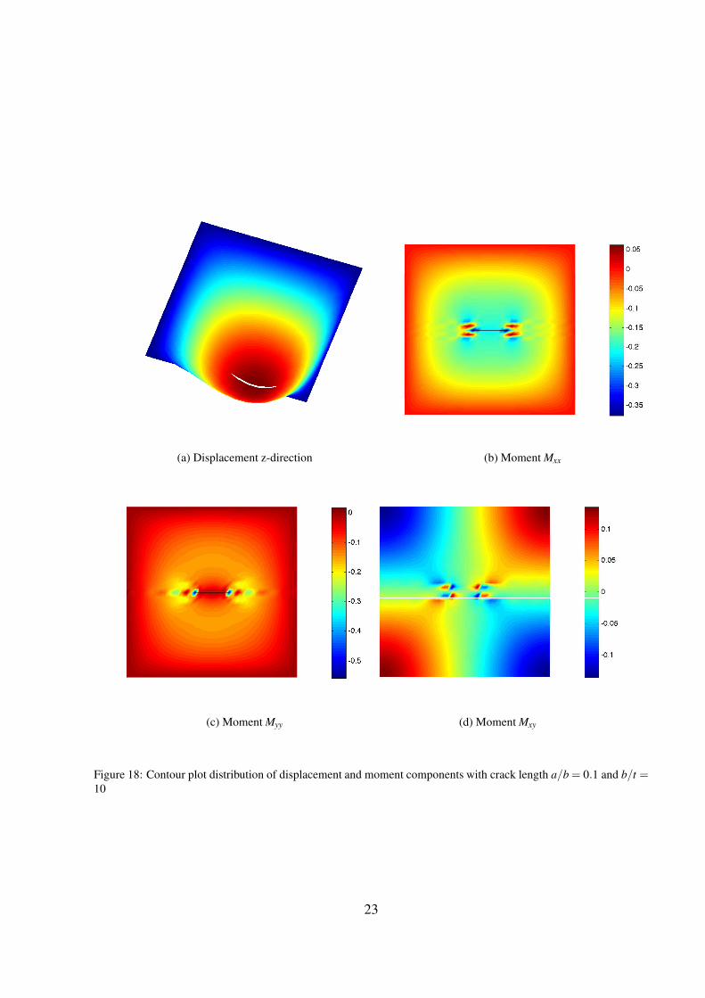
In the next example, we consider a square plate with a central crack under uniform pressure

loading p= 1.0. The plate is simply supported on all edges. The geometry and material parameters

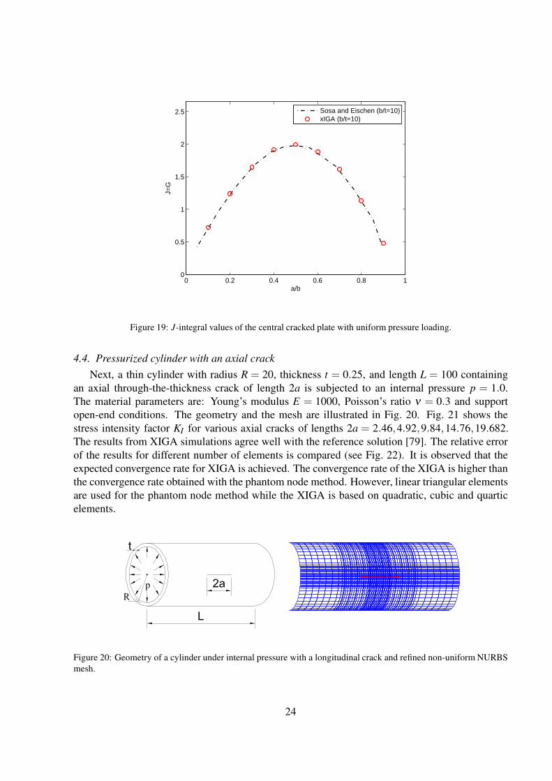
are b = 1.0, Young’s modulus E = 1000 and Poisson’s ν = 0.3 (Fig. 17). Fig. 18 shows the contour

plots of the displacement and stress components. Fig. 19 shows the good agreement between the

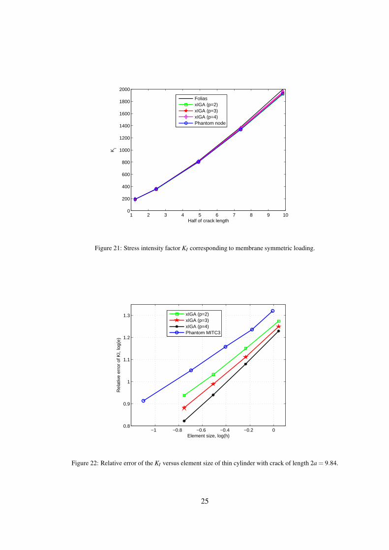
XIGA-results and the reference solution.

Figure 17: Geometry of central cracked plate subjected to uniform pressure and refined non-uniform NURBS mesh.

22

(a) Displacement z-direction (b) Moment Mxx

(c) Moment Myy (d) Moment Mxy

Figure 18: Contour plot distribution of displacement and moment components with crack length a/b = 0.1 and b/t =10

23

0 0.2 0.4 0.6 0.8 10

0.5

1

1.5

2

2.5

a/b

J=G

Sosa and Eischen (b/t=10)xIGA (b/t=10)

Figure 19: J-integral values of the central cracked plate with uniform pressure loading.

4.4. Pressurized cylinder with an axial crack

Next, a thin cylinder with radius R = 20, thickness t = 0.25, and length L = 100 containing

an axial through-the-thickness crack of length 2a is subjected to an internal pressure p = 1.0.

The material parameters are: Young’s modulus E = 1000, Poisson’s ratio ν = 0.3 and support

open-end conditions. The geometry and the mesh are illustrated in Fig. 20. Fig. 21 shows the

stress intensity factor KI for various axial cracks of lengths 2a = 2.46,4.92,9.84,14.76,19.682.

The results from XIGA simulations agree well with the reference solution [79]. The relative error

of the results for different number of elements is compared (see Fig. 22). It is observed that the

expected convergence rate for XIGA is achieved. The convergence rate of the XIGA is higher than

the convergence rate obtained with the phantom node method. However, linear triangular elements

are used for the phantom node method while the XIGA is based on quadratic, cubic and quartic

elements.

Figure 20: Geometry of a cylinder under internal pressure with a longitudinal crack and refined non-uniform NURBS

mesh.

24

1 2 3 4 5 6 7 8 9 100

200

400

600

800

1000

1200

1400

1600

1800

2000

Half of crack length

KI

FoliasxIGA (p=2)xIGA (p=3)xIGA (p=4)Phantom node

Figure 21: Stress intensity factor KI corresponding to membrane symmetric loading.

−1 −0.8 −0.6 −0.4 −0.2 00.8

0.9

1

1.1

1.2

1.3

Element size, log(h)

Rel

ativ

e er

ror

of K

I, lo

g(e)

xIGA (p=2)xIGA (p=3)xIGA (p=4)Phantom MITC3

Figure 22: Relative error of the KI versus element size of thin cylinder with crack of length 2a = 9.84.

25

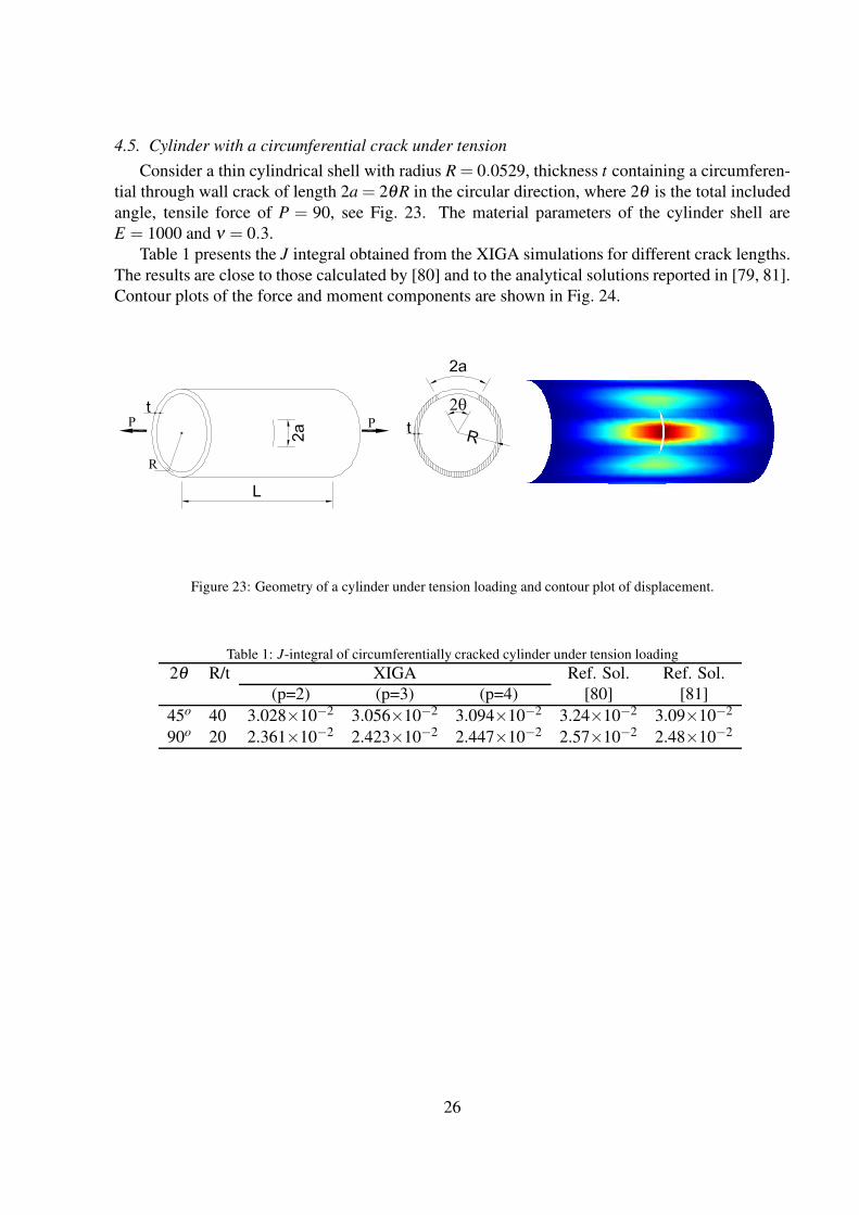
4.5. Cylinder with a circumferential crack under tension

Consider a thin cylindrical shell with radius R = 0.0529, thickness t containing a circumferen-

tial through wall crack of length 2a = 2θR in the circular direction, where 2θ is the total included

angle, tensile force of P = 90, see Fig. 23. The material parameters of the cylinder shell are

E = 1000 and ν = 0.3.

Table 1 presents the J integral obtained from the XIGA simulations for different crack lengths.

The results are close to those calculated by [80] and to the analytical solutions reported in [79, 81].

Contour plots of the force and moment components are shown in Fig. 24.

Figure 23: Geometry of a cylinder under tension loading and contour plot of displacement.

Table 1: J-integral of circumferentially cracked cylinder under tension loading

2θ R/t XIGA Ref. Sol. Ref. Sol.

(p=2) (p=3) (p=4) [80] [81]

45o 40 3.028×10−2 3.056×10−2 3.094×10−2 3.24×10−2 3.09×10−2

90o 20 2.361×10−2 2.423×10−2 2.447×10−2 2.57×10−2 2.48×10−2

26

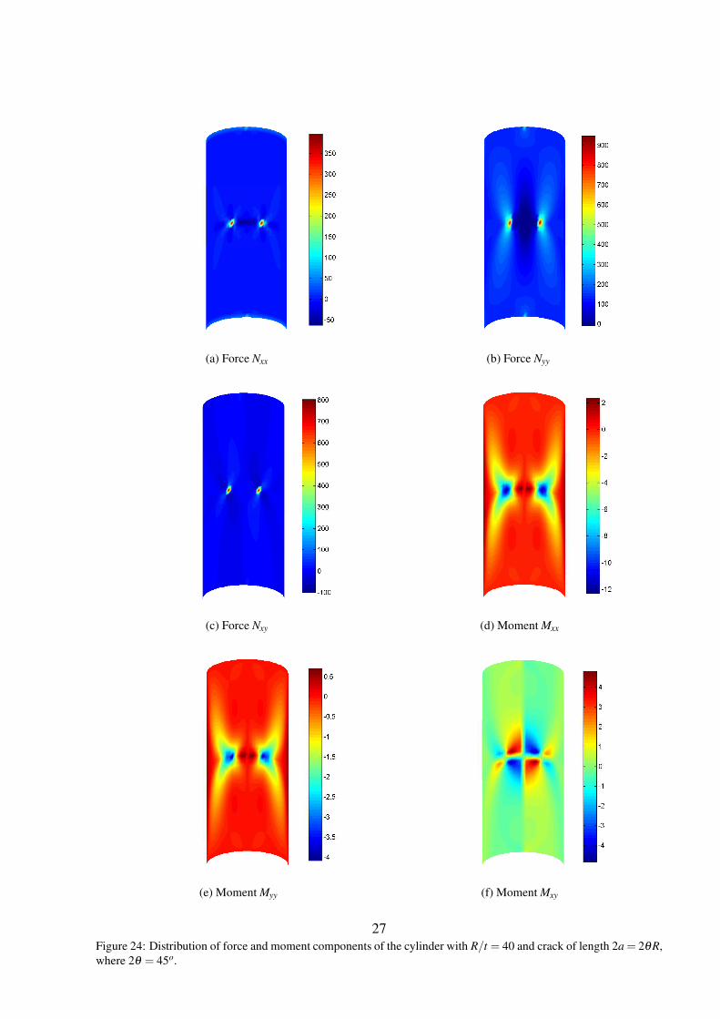
(a) Force Nxx (b) Force Nyy

(c) Force Nxy (d) Moment Mxx

(e) Moment Myy (f) Moment Mxy

Figure 24: Distribution of force and moment components of the cylinder with R/t = 40 and crack of length 2a = 2θR,

where 2θ = 45o.

27

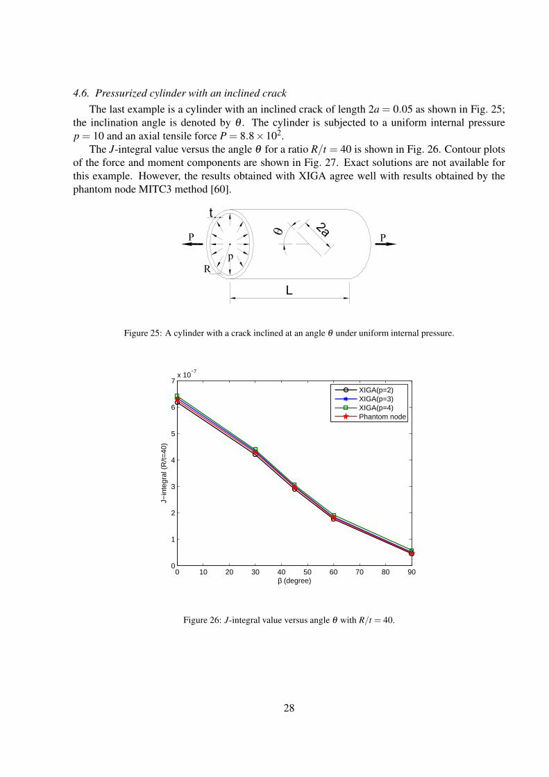
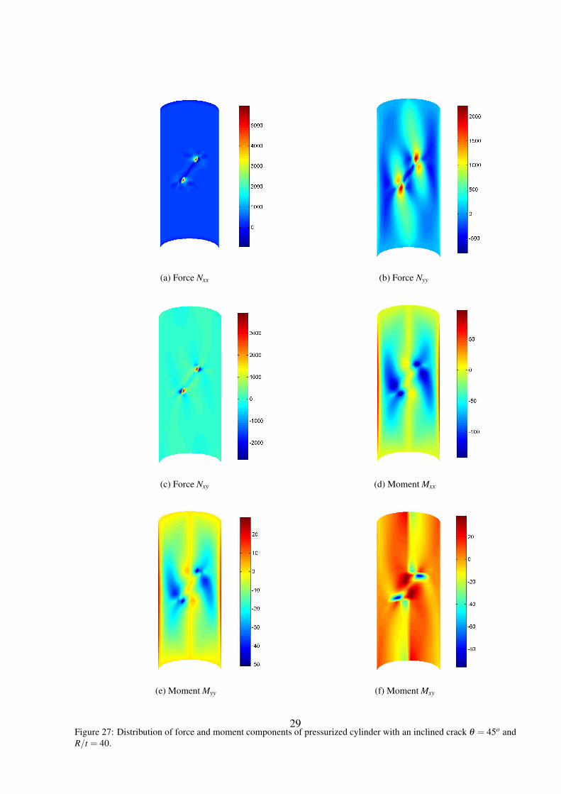
4.6. Pressurized cylinder with an inclined crack

The last example is a cylinder with an inclined crack of length 2a = 0.05 as shown in Fig. 25;

the inclination angle is denoted by θ . The cylinder is subjected to a uniform internal pressure

p = 10 and an axial tensile force P = 8.8×102.

The J-integral value versus the angle θ for a ratio R/t = 40 is shown in Fig. 26. Contour plots

of the force and moment components are shown in Fig. 27. Exact solutions are not available for

this example. However, the results obtained with XIGA agree well with results obtained by the

phantom node MITC3 method [60].

Figure 25: A cylinder with a crack inclined at an angle θ under uniform internal pressure.

0 10 20 30 40 50 60 70 80 900

1

2

3

4

5

6

7x 10

−7

β (degree)

J−in

tegr

al (

R/t=

40)

XIGA(p=2)XIGA(p=3)XIGA(p=4)Phantom node

Figure 26: J-integral value versus angle θ with R/t = 40.

28

(a) Force Nxx (b) Force Nyy

(c) Force Nxy (d) Moment Mxx

(e) Moment Myy (f) Moment Mxy

Figure 27: Distribution of force and moment components of pressurized cylinder with an inclined crack θ = 45o and

R/t = 40.

29

5. Conclusions

We presented an XIGA thin shell formulation based on the Kirchhoff-Love theory. The Heav-

iside and crack tip enrichment functions are introduced to the NURBS-based displacement field

to capture the strong discontinuity along the crack and the singularity at the crack tips. The en-

richment functions are defined on the parametric domain that is global to a patch. The thin shell

elements adopting the Kirchhoff-Love assumption are used to exploit the C1-continuity of NURBS

basis functions in the framework of IGA and no rotational degrees of freedom are needed facilitat-

ing the enrichment strategy. The XIGA results are in good agreement with analytical and reference

solutions. The authors believe that the present method is a very promising alternative to the ‘stan-

dard’ XFEM for analysis of cracked shell structures in practical applications.

Acknowledgments

Nhon Nguyen-Thanh and Laura De Lorenzis would like to acknowledge the financial support

from the European Research Council Starting Researcher Grant “INTERFACES”, Grant agree-

ment No. 279439. Xiaoying Zhuang gratefully acknowledges the support of NSFC (41130751),

National Basic Research Program of China (973 Program: 2011CB013800), and Shanghai Pujiang

Program (12PJ1409100).

References

[1] T. J.R. Hughes, J.A. Cottrell, and Y. Bazilevs. Isogeometric analysis: CAD, finite elements,

NURBS, exact geometry and mesh refinement. Computer Methods in Applied Mechanics

and Engineering, 194:4135–4195, 2005.

[2] T.W. Sederberg, D.L. Cardon, G.T. Finnigan, N.S. North, J. Zheng, and T. Lyche. T-splines

and local refinement. ACM Trans. Graphics, 23:276–283, 2004.

[3] Y. Bazilevs, V.M. Calo, J.A. Cottrell, J.A. Evans T.J.R Hughes, S. Lipton, and M.A. Scot-

tand T.W. Sederberg. Isogeometric analysis using T-splines. Computer Methods in Applied

Mechanics and Engineering, 199:229–263, 2010.

[4] M. Dorfel, B. Juttler, and B. Simeon. Adaptive isogeometric analysis by local h-refinement

with T-splines. Computer Methods in Applied Mechanics and Engineering, 199:264–275,

2010.

[5] J. Deng, F. Chen, X. Li, C. Hu, W. Tong, Z. Yang, and Y. Feng. Polynomial splines over

hierarchical T-meshes. Graphical Models, 70:76–86, 2008.

[6] J. Deng, F. Chen, and Y. Feng. Dimensions of spline spaces over T-meshes. Journal of

Computational and Applied Mathematics, 194:267–283, 2006.

[7] N. Nguyen-Thanh, H. Nguyen-Xuan, S. Bordas, and T. Rabczuk. Isogeometric analysis using

polynomial splines over hierarchical T-meshes for two-dimensional elastic solids. Computer

Methods in Applied Mechanics and Engineering, 200(21-22):1892–1908, 2011.

30

[8] N. Nguyen-Thanh, J. Kiendl, H. Nguyen-Xuan, R. Wuchner, K.U. Bletzinger, Y. Bazilevs,

and T. Rabczuk. Rotation free isogeometric thin shell analysis using PHT-splines. Computer

Methods in Applied Mechanics and Engineering, 200(47-48):3410–3424, 2011.

[9] N. Nguyen-Thanh, J. Muthu, X. Zhuang, and T. Rabczuk. An adaptive three-dimensional

RHT-splines formulation in linear elasto-statics and elasto-dynamics. Computational Me-

chanics, 53:369–385, 2013.

[10] D. Schillinger, L. Dede, M.A. Scott, J.A. Evans, M.J. Borden, E. Rank, and T.J.R. Hughes.

An isogeometric design-through-analysis methodology based on adaptive hierarchical refine-

ment of NURBS, immersed boundary methods, and T-spline CAD surfaces. Computer Meth-

ods in Applied Mechanics and Engineering, 249-252:116–150, 2012.

[11] A.-V. Vuong, C. Giannelli, B. Juttler, and B. Simeon. A hierarchical approach to adaptive

local refinement in isogeometric analysis. Computer Methods in Applied Mechanics and

Engineering, 200:3554–3567, 2012.

[12] S.K. Kleiss, B. Juttler, and W. Zulehner. Enhancing isogeometric analysis by a finite element

based local refinement strategy. Computer Methods in Applied Mechanics and Engineering,

213-216:168–182, 2012.

[13] T.W. Sederberg, J. Zheng, A. Bakenov, and A. Nasri A. T-splines and T-NURCCs. ACM

Trans. Graphics, 22:477–484, 2003.

[14] T.W. Sederberg, D.C. Anderson, and R.N. Goldman. Implicit representation of parametric

curves and surfaces. Computer Vision, Graphics and Image Processing, 28:72–84, 1984.

[15] T.J.R. Hughes, A. Reali, and G. Sangalli. Efficient quadrature for NURBS-based isogeo-

metric analysis. Computer Methods in Applied Mechanics and Engineering, 199:301–313,

2010.

[16] J.A. Cottrell, T.J.R Hughes, and A. Reali. Studies of refinement and continuity in geometry

and mesh refinement. Computer Methods in Applied Mechanics and Engineering, 196:4160–

4183, 2007.

[17] J.A. Cottrell, A. Reali, Y. Bazilevs, and T.J.R. Hughes. Isogeometric analysis of structural vi-

brations. Computer Methods in Applied Mechanics and Engineering, 195:5257–5297, 2006.

[18] S. Lipton, J.A Evans, Y. Bazilevs, T. Elguedj, and T.J.R. Hughes. Robustness of isogeo-

metric structural discretizations und severe mesh distortion. Computer Methods in Applied

Mechanics and Engineering, 199:357–373, 2010.

[19] H. Nguyen-Xuan, Loc V. Tran, Chien H. Thai, and C.V. Le. Plastic collapse analysis of

cracked structures using extended isogeometric elements and second-order cone program-

ming. Theoretical and Applied Fracture Mechanics, in press, 2014.

[20] Y. Bazilevs, V.M. Calo, T.J.R Hughes, and Y. Zhang. Isogeometric fluid-structure interaction:

theory, algorithms, and computations. Computational Mechanics, 43:3–37, 2008.

31

[21] Y. Bazilevs, M.-C.Hsu, I.Akkerman, S.Wright, K.Takizawa, B.Henicke, T.Spielman, and

T.E.Tezduyar. 3D simulation of wind turbine rotors at full scale. Part I: Geometry model-

ing and aerodynamics. International Journal for Numerical Methods in Engineering, 65(1-

3):207–235, 2011.

[22] Y. Bazilevs, M.-C. Hsu, J. Kiendl, R. Wuchner, and K.-U. Bletzinger. 3D simulation of wind

turbine rotors at full scale. Part II: Fluidstructure interaction modeling with composite blades.

International Journal for Numerical Methods in Engineering, 65(1-3):236–253, 2011.

[23] M.-C. Hsu and Y. Bazilevs. Blood vessel tissue prestress modeling for vascular fluid-structure

interaction simulations. Finite Elements in Analysis and Design, 47(6):593–599, 2011.

[24] L. De Lorenzis, I. Temizer, P. Wriggers, and G. Zavarise. A large deformation frictional

contact formulation using nurbs-based isogeometric analysis. International Journal for Nu-

merical Methods in Engineering, 87:1278–1300, 2011.

[25] L. De Lorenzis, P. Wriggers, and G. Zavarise. A mortar formulation for 3d large deformation

contact using NURBS-based isogeometric analysis and the augmented Lagrangian method.

Computational Mechanics, 49:1–20, 2012.

[26] R. Dimitri, L. De Lorenzis, M.A. Scott, P. Wriggers, R.L. Taylor, and G. Zavarise. Isogeo-

metric large deformation frictionless contact using T-splines. Computer Methods in Applied

Mechanics and Engineering, 269:394–414, 2014.

[27] R. Dimitri, L. De Lorenzis, P. Wriggers, and G. Zavarise. NURBS and T-spline-based isoge-

ometric cohesive zone modeling of interface debonding. Computational Mechanics, 54:369–

388, 2014.

[28] M. Bischoff, K.-U. Bletzinger, W.A. Wall, and E. Ramm. Models and Finite Elements for

Thin-Walled Structures. John Wiley and Sons, New York, 2004.

[29] P. Krysl and T. Belytschko. Analysis of thin shells by the element free Galerkin method.

International Journal of Solids and Structures, 33(20-22):3057–3080, 1996.

[30] F. Cirak, M. Ortiz, and P. Schroder. Subdivision surfaces: A new paradigm for thin shell

analysis. International Journal for Numerical Methods in Engineering, 47:2039–2072, 2000.

[31] D. Millan, A. Rosolen, and M. Arroyo. Thin shell analysis from scattered points with

maximum-entropy approximants. International Journal for Numerical Methods in Engineer-

ing, 85(6):723–751, 2011.

[32] L. Noels and R. Radovitzky. A new discontinuous Galerkin method for Kirchhoff-Love

shells. Computer Methods in Applied Mechanics and Engineering, 197:2901–2929, 2008.

[33] L. Chen, N. Nguyen-Thanh, H. Nguyen-Xuan, T. Rabczuk, S. Bordas, and G. Limbert. Ex-

plicit finite deformation analysis of isogeometric membranes. Computer Methods in Applied

Mechanics and Engineering, 277:104–130, 2014.

32

[34] C. Thai-Hoang, N. Nguyen-Thanh, H. Nguyen-Xuan, T. Rabczuk, and S. Bordas. A cell-

based smoothed finite element method for free vibration and buckling analysis of shells.

KSCE Journal of Civil Engineering, 15(2):347–361, 2011.

[35] N. Nguyen-Thanh, T. Rabczuk, H.Nguyen-Xuan, and S. Bordas. An alternative alpha finite

element method with stabilized discrete shear gap technique for analysis of Mindlin-Reissner

plates. Finite Elements in Analysis and Design, 47(5):519–535, 2011.

[36] N. Nguyen-Thanh, T. Rabczuk, H.Nguyen-Xuan, and S. Bordas. A smoothed finite ele-

ment method for shell analysis. Computer Methods in Applied Mechanics and Engineering,

198(2):165–177, 2008.

[37] S. Timoshenko and S. Woinowsky-Krieger. Theory of Plates and Shells (2nd edn). McGraw-

Hill, New York, 1959.

[38] T. Rabczuk and P.M.A. Areias. A meshfree thin shell for arbitrary evolving cracks based on an

external enrichment. Computer Methods in Applied Mechanics and Engineering, 16(2):115–

130, 2006.

[39] T. Rabczuk, P.M.A. Areias, and T. Belytschko. A meshfree thin shell method for non-linear

dynamic fracture. International Journal for Numerical Methods in Engineering, 72:524–548,

2007.

[40] T. Rabczuk, R. Gracie, J.H. Song, and T. Belytschko. Immersed particle method for fluid-

structure interaction. International Journal for Numerical Methods in Engineering, 81(1):48–

71, 2010.

[41] T. Rabczuk and G. Zi. A meshfree method based on the local partition of unity for cohesive

cracks. Computational Mechanics, 39:743–760, 2007.

[42] T. Rabczuk and T. Belytschko. Cracking particles: A simplified meshfree methods for

arbitrary evovling cracks. International Journal for Numerical Methods in Engineering,

61:2316–2343, 2004.

[43] T. Rabczuk and T. Belytschko. A three dimensional large deformation meshfree method

for arbitrary evolving cracks. Computer Methods in Applied Mechanics and Engineering,

196:2777–2799, 2007.

[44] J. Kiendl, K.-U. Bletzinger, J. Linhard, and R. Wuchner. Isogeometric shell analysis

with Kirchhoff-Love elements. Computer Methods in Applied Mechanics and Engineering,

198:3902–3914, 2009.

[45] J. Kiendl, Y. Bazilevs, M.-C. Hsu, R. Wuchner, and K.-U. Bletzinger. The bending strip

method for isogeometric analysis of Kirchhoff-Love shell structures comprised of multiple

patches. Computer Methods in Applied Mechanics and Engineering, 199:2403–2416, 2010.

[46] D.J. Benson, Y. Bazilevs, E. De Luycker, M.-C. Hsu, M. Scott, T.J.R. Hughes, and T. Be-

lytschko. A generalized finite element formulation for arbitrary basis functions: From iso-

geometric analysis to XFEM. International Journal for Numerical Methods in Engineering,

83:765–785, 2010.

33

[47] E. De Luycker, D.J. Benson, T. Belytschko, Y. Bazilevs, and M.C. Hsu. X-FEM in isogeo-

metric analysis for linear fracture mechanics. International Journal for Numerical Methods

in Engineering, 87:541–565, 2011.

[48] S.S. Ghorashi, N. Valizadeh, and S. Mohammadi. Extended isogeometric analysis for simu-

lation of stationary and propagating cracks. International Journal for Numerical Methods in

Engineering, 89:1069–1101, 2012.

[49] C.V. Verhoosel, M.A. Scott, R. de Borst, and T.J.R. Hughes. An isogeometric approach

to cohesive zone modeling. International Journal for Numerical Methods in Engineering,

87:336–360, 2011.

[50] P.M.A. Areias and T. Belytschko. Non-linear analysis of shells with arbitrary evolving cracks

using XFEM. International Journal for Numerical Methods in Engineering, 62:384–415,

2005.

[51] P.M.A. Areias, J.H. Song, and T. Belytschko. Analysis of fracture in thin shells by over-

lapping paired elements. International Journal for Numerical Methods in Engineering,

195:5343–5360, 2006.

[52] J-H Song and T. Belytschko. Dynamic fracture of shells subjected to impulsive loads. ASME

Journal of Applied Mechanics, 2009.

[53] T. Chau-Dinh, G. Zi, P.S. Lee, and J. Song T. Rabczuk. Phantom-node method for shell

models with arbitrary cracks. Computers & Structures, 92-93:242–256, 2012.

[54] J-H Song, P.M.A. Areias, and T. Belytschko. A method for dynamic crack and shear band

propagation with phantom nodes. International Journal for Numerical Methods in Engineer-

ing, 2006.

[55] T. Rabczuk, G. Zi, A. Gerstenberger, and W.A. Wall. A new crack tip element for the phantom

node method with arbitrary cohesive cracks. International Journal for Numerical Methods in

Engineering, 75:577–599, 2008.

[56] J.C. Simo and D.D. Fox. On a stress resultant geometrically exact shell-model 1. formulation

and optimal parametrization. Computer Methods in Applied Mechanics and Engineering,

72:267–304, 1989.

[57] J.C. Simo, D.D. Fox, and M.S. Rifai. On a stress resultant geometrically exact shell-model

2. the linear-theory - computational aspects. Computer Methods in Applied Mechanics and

Engineering, 73:53–92, 1989.

[58] A.T. Zehnder and M. J. Viz. Fracture mechanics of thin plates and shells under combined

membrane, bending, and twisting loads. Applied Mechanics Reviews ASME, 58:37–48, 2005.

[59] N. Moes, J. Dolbow, and T. Belytschko. A finite element method for crack growth without

remeshing. International Journal for Numerical Methods in Engineering, 46:133–150, 1999.

34

[60] T. Chau-Dinh, G. Zi, P.S. Lee, T. Rabczuk, and J.H. Song. Phantom-node method for shell

models with arbitrary cracks. Computers and Structures, 92-93:242–256, 2012.

[61] E. Bechet, H. Minnebo, N. Moes, and B. Burgardt. Improved implementation and robustness

study of the x-fem for stress analysis around cracks. International Journal for Numerical

Methods in Engineering, 64:1033–1056, 2005.

[62] P. Laborde, J Pommier, Y Renard, and M Salan. High-order extended finite element method

for cracked domains. International Journal for Numerical Methods in Engineering, 64:354–

381, 2005.

[63] T.P. Fries. A corrected xfem approximation without problems in blending elements. Interna-

tional Journal for Numerical Methods in Engineering, 75:503–532, 2008.

[64] D. Wang and J. Xuan. An improved nurbs-based isogeometric analysis with enhanced treat-

ment of essential boundary conditions. Computer Methods in Applied Mechanics and Engi-

neering, 199:2425–2436, 2010.

[65] S. Fernandez-Mendez and A. Huerta. Imposing essential boundary conditions in mesh-free

methods. Computer Methods in Applied Mechanics and Engineering, 193:1257–1275, 2004.

[66] T. Rabczuk, S.P. Xiao, and M. Sauer. Coupling of meshfree methods with finite elements:

Basic concepts and test results. Communications in Numerical Methods in Engineering,

22(10):1031–1065, 2006.

[67] V.P. Nguyen, T. Rabczuk, S. Bordas, and M. Duflot. Meshless methods: A review and com-

puter implementation aspects. Mathematics and Computers in Simulation, 79:763–813, 2008.

[68] N. Vu-Bac, H. Nguyen-Xuan, L. Chen, S. Bordas, P. Kerfriden, R.N. Simpson, G.R. Liu, and

T. Rabczuk. A node-based smoothed extended finite element method (nsxfem) for fracture

analysis. CMES-Computer Modeling in Engineering & Sciences, 73(4):331–355, 2011.

[69] N. Vu-Bac, H. Nguyen-Xuan, L. Chen, C.K. Lee, G. Zi, X. Zhuang, G.R. Liu, and

T. Rabczuk. A phantom-node method with edge-based strain smoothing for linear elastic

fracture mechanics. Journal of Applied Mathematics, vol. 2013:Article ID 978026, 2013.

[70] L. Chen, T. Rabczuk, G.R. Liu, K.Y. Zeng, P. Kerfriden, and S. Bordas. Extended finite

element method with edge-based strain smoothing (esm-xfem) for linear elastic crack growth.

Computer Methods in Applied Mechanics and Engineering, 212(4):250–265, 2012.

[71] S. Bordas, S. Natarajan, S. Dal Pont, T. Rabczuk, P. Kerfriden, D.R. Mahapatra, D. Noel, and

Z. Gao. On the performance of strain smoothing for enriched finite element approximations

(xfem/gfem/pufem). International Journal for Numerical Methods in Engineering, 86(4-

5):637666, 2011.

[72] S. Bordas, T. Rabczuk, H. Nguyen-Xuan, S. Natarajan, T. Bog, V.P. Nguyen, M.Q.Do, and

H. Nguyen Vinh. Strain smoothing in fem and xfem. Computers and Structures, 88(23-

24):1419–1443, 2010.

35

[73] J.E. TarancOn, A. Vercher, E. Giner, and F.J. Fuenmayor. Enhanced blending elements for

xfem applied to linear elastic fracture mechanics. International Journal for Numerical Meth-

ods in Engineering, 77:126–148, 2009.

[74] G. Ventura, R. Gracie, and T. Belytschko. Fast integration and weight function blending in

the extended finite element method. International Journal for Numerical Methods in Engi-

neering, 77:1–29, 2009.

[75] X. Liu, Q. Xiao, and B. Karihaloo. Xfem for direct evaluation of mixed mode sifs in ho-

mogeneous and bi-materials. International Journal for Numerical Methods in Engineering,

59:1103–1118, 2004.

[76] S. Nicaise, Y. Renard, and E. Chahine. Optimal convergence analysis for the extended finite

element method. International Journal for Numerical Methods in Engineering, 86:528548,

2011.

[77] G.P. Nikishkov and S.N. Atluri. Calculation of fracture mechanics parameters for an arbitrary

three-dimensional crack, by the “Equivalent Domain Integral” method. International Journal

for Numerical Methods in Engineering, 24:1801–1821, 1987.

[78] J.F. Yau, S.S. Wang, and H.T. Corten. A mixed-mode crack analysis of isotropic solids using

conservation laws of elasticity. Journal of Applied Mechanics ASME, 47:335–341, 1980.

[79] E.S. Folias. On the effect of initial curvature on cracked flat sheets. International Journal of

Fracture Mechanics, 5:327–346, 1968.

[80] P. Le Port, H.G. de Lorenzi, V. Kumar, and M.D. German. Virtual crack extension method

for energy release rate calculations in flawed thin shell structures. J. Press Vessel Technol

ASME, 109:101–107, 1987.

[81] Jr.J.L. Sander. Circumferential through-cracks in cylindrical shells under tension. Journal of

Applied Mechanics ASME, 49:103–107, 1982.

36