arX

iv:2

201.

1085

8v1

[m

ath.

CO

] 2

6 Ja

n 20

22

On Kirchhoff index and number of spanning trees of

linear pentagonal cylinder and Mobius chain graph

Md. Abdus Sahir* and Sk. Md. Abu Nayeem†

Department of Mathematics and Statistics, Aliah University, Kolkata – 700 160, India.

Abstract

In this paper, we derive closed-form formulas for Kirchhoff index and Wiener index of

linear pentagonal cylinder graph and linear pentagonal Mobius chain graph. We also obtain

explicit formulas for finding total number of spanning trees for both the graphs.

MSC (2020): Primary: 05C09; Secondary: 05C50.

Keywords. Pentagonal cylinder, Mobius chain, Kirchhoff index, Wiener index, spanning tree.

1 Introduction

Let G = (V,E) be a connected molecular graph having vertex set V and edge set E. A topological

index of G is a numerical quantity involving different graph parameters such as number of vertices,

number of edges, degree, eccentricity, distance between vertices, etc. Winner index, one of the

oldest topological indices, was introduced by Harold Wiener [22] and was defined as W (G) =

∑i< j

di j, where di j is the length of the shortest path between the vertices i and j. Motivated by the idea

of Wiener index, the idea of resistance distance and Kirchhoff index was introduced by Klein and

Randic [10]. Kirchhoff index, initially known as resistance index, was defined as K f (G) = ∑i< j

ri j,

where ri j is the effective resistance between vertex i and vertex j calculated using Ohm’s law

considering all the edges of G as unit resistors. Klein and Randic also proved that for any vertex

pair i, j in a graph G, ri j ≤ di j and K f (G)≤W (G) with equality holds if and only if G is a tree.

In the last few decades, researchers have focused on various topological indices such as Wiener

index, Randic index [19], Kirchhoff index, Gutman index [6], Estrada index [3], Zagreb index

[8] etc. Especially Kirchhoff index is seeking a lot of attention of researchers as it has wide

applications in physics, chemistry, graph theory and various related subjects. Readers are referred

to [4, 16, 20, 21, 23, 26, 27] for some recent works. Many researchers have concentrated on finding

*Email: abdussahir@gmail.com†Corresponding author. Email: nayeem.math@aliah.ac.in

1

the Kirchhoff index and the number of spanning trees for many interesting graphs such as linear

hexagonal chain [24], linear pentagonal chain [20], Mobius hexagonal chain [21], periodic linear

chain [1], crossed hexagonal chain [17], linear octagonal chain [28], Mobius/ cylinder octagonal

chain [12] and many others [5, 13, 14, 18]. Normalized Laplacian spectrum and the number of

spanning trees of linear pentagonal chains have been obtained by He et al. [9]. Although the

Kirchhoff index of linear pentagonal chain was found long back in 2010 [20], but to the best of

our knowledge, Kirchhoff indices for linear pentagonal cylinder and Mobius chains have not been

obtained so far. In the present paper, we aim to obtain those.

The Laplacian matrix L(G) = (li j) of a simple connected graph G is defined as,

li j =

di, if i = j

−1, if i ∼ j

0, otherwise,

where di is the degree of the vertex i.

Since L(G) is a symmetric matrix, all of its eigenvalues are real. Moreover all are non-negative,

i.e., if the eigenvalues λi,s (i = 1,2, . . . ,n) are indexed in the increasing order of their values,

0 = λ1 ≤ λ2 ≤ ·· · ≤ λn. Since G is connected, λ1 = 0 is a simple eigenvalue.

Gutman and Mohar [7] and Zhu et al. [29] obtained the following lemma.

Lemma 1 [7, 29] For a connected graph G with n-vertices, n ≥ 2,

K f (G) = nn

∑k=2

1

λk

·

Like Wiener index, Kirchhoff index also gives description of the underlying structure of a

molecular graph [23]. Obtaining closed-form formulae for Kirchhoff index of general graphs is

not straight forward, but we can derive closed-form formulae for some special classes of graphs

like cycles [11], complete graphs [15], circulant graph, etc.

In this paper, we derive closed-form formulas for Kirchhoff index and Wiener index of linear

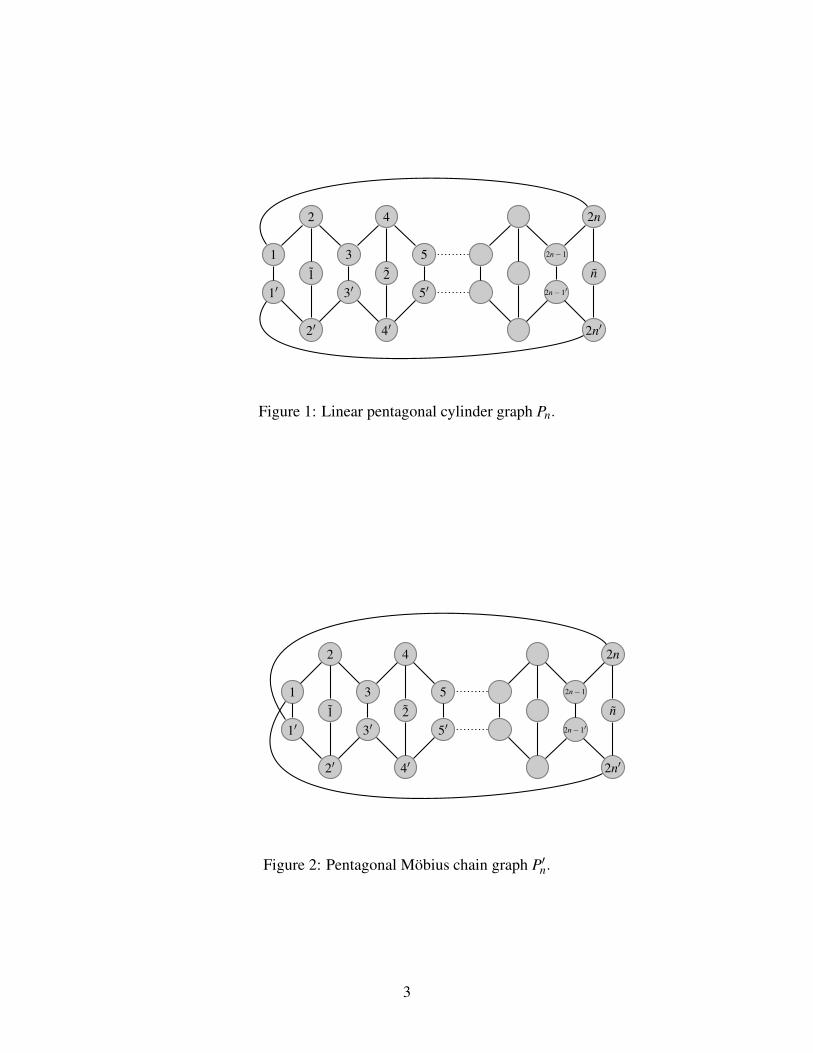
pentagonal cylinder graph Pn (Figure 1) and pentagonal Mobius chain graph P′n (Figure 2) on 5n

(n ≥ 2) vertices. Also we present the formulas for the total number of spanning trees for those

graphs.

2

1

1′

2

2′

1

3

3′

4

2

4′

5

5′

2n−1

2n−1′

2n

n

2n′

Figure 1: Linear pentagonal cylinder graph Pn.

1

1′

2

2′

1

3

3′

4

2

4′

5

5′

2n−1

2n−1′

2n

n

2n′

Figure 2: Pentagonal Mobius chain graph P′n.

3

2 Preliminaries

Let G be a graph with vertex set V (G). A permutation π of V (G) is called an automorphism if u and

v are adjacent in G if and only if π(u) and π(v) are also adjacent in G. Suppose V0 = {1, 2, . . . , p},

V1 = {1,2, . . . ,q} and V2 = {1′,2′, . . . ,q′} are the vertex partition for the automorphism π such that

π(i) = i for all i ∈V0,π(i) = i′ for all i ∈V1 and π(i′) = i for all i′ ∈V2. It is easy to follow that π

can be decomposed as product of disjoint 1-cycles and transpositions, i.e.,

π = (1)(2) · · ·(p)(1,1′)(2,2′) · · ·(q,q′),

where p+2q = |V (G)|. Then by suitable arrangement of vertices, the Laplacian matrix L(G) of G

can be expressed into the block matrix form –

L(G) =

LV0V0LV0V1

LV0V2

LV1V0LV1V1

LV1V2

LV2V0LV2V1

LV2V2

where the submatrix LVrVscorrespond to the vertices of Vr and Vs,r,s = 0,1,2 respectively.

Let

LA(G) =

[

LV0V0

√2LV0V1√

2LV1V0LV1V1

+LV1V2

]

and

LS(G) = LV1V1−LV1V2

.

Yang and Yu [25] and many others like Yang and Zhang [24] have used the Laplacian decomposi-

tion formula to find the Kirchhoff indices of certain classes of graphs where some automorphisms

are found. We describe it in the form of the following lemma.

Lemma 2 The characteristic polynomial of L(G) is equal to the product of that of LA(G) and

LS(G), i.e.,

det(L(G)−λ I) = det(LA(G)−λ I) ·det(LS(G)−λ I).

Let λi (i = 1,2, . . . ,3n) and µ j ( j = 1,2, . . . ,2n) are the eigenvalues of LA(G) and LS(G) ar-

ranged in ascending order of their values. Then by Lemma 2, the spectrum of L(G) is given by

{0 = λ1 ≤ λ2 ≤ ·· · ≤ λ3n}⋃

{µ1 ≤ µ2 ≤ ·· · ≤ µ2n}.

To avoid confusion, we denote LA(Pn) and LS(Pn) by LA and LS respectively and LA(P′n) and

LS(P′n) by L′

A and L′S respectively. Also we denote the block matrices constituting the Laplacian

4

matrix of linear pentagonal cylinder graph Pn by LVrVs,r,s = 0,1,2 and those of pentagonal Mobius

chain graph P′n by L′

VrVs,r,s = 0,1,2 respectively. Then,

LV0V0= L′

V0V0=

2 0 · · · 0

0 2 · · · 0...

.... . .

...

0 0 · · · 2

n×n

, LV0V1= L′

V0V1=

0 −1 0 0 · · · 0

0 0 0 −1 · · · 0...

......

.... . .

...

0 0 0 0 · · · −1

n×2n

LV1V1=

3 −1 0 · · · 0 −1

−1 3 −1 · · · 0 0

0 −1 3 · · · 0 0...

......

. . ....

...

0 0 0 · · · 3 −1

−1 0 0 · · · −1 3

2n×2n

, LV1V2=

−1 0 0 · · · 0 0

0 0 0 · · · 0 0

0 0 −1 · · · 0 0...

......

. . ....

...

0 0 0 · · · −1 0

0 0 0 · · · 0 0

2n×2n

, and

L′V1V1

=

3 −1 0 · · · 0 0

−1 3 −1 · · · 0 0

0 −1 3 · · · 0 0...

......

. . ....

...

0 0 0 · · · 3 −1

0 0 0 · · · −1 3

2n×2n

, L′V1V2

=

−1 0 0 · · · 0 −1

0 0 0 · · · 0 0

0 0 −1 · · · 0 0...

......

. . ....

...

0 0 0 · · · −1 0

−1 0 0 · · · 0 0

2n×2n

.

So,

LA = L′A =

2 0 · · · 0 0 −√

2 0 0 · · · 0

0 2 · · · 0 0 0 0 −√

2 · · · 0...

.... . .

......

......

.... . .

...

0 0 · · · 2 0 0 0 0 · · · −√

2

0 0 · · · 0 2 −1 0 0 · · · −1

−√

2 0 · · · 0 −1 3 −1 0 · · · 0

0 0 · · · 0 0 −1 2 −1 · · · 0

0 −√

2 · · · 0 0 0 −1 3 · · · 0...

.... . .

......

......

.... . .

...

0 0 · · · −√

2 −1 0 0 0 · · · 3

3n×3n

,

5

LS =

4 −1 0 0 · · · 0 0 −1

−1 3 −1 0 · · · 0 0 0

0 −1 4 −1 · · · 0 0 0

0 0 −1 3 · · · 0 0 0...

......

.... . .

......

...

0 0 0 0 · · · 3 −1 0

0 0 0 0 · · · −1 4 −1

−1 0 0 0 · · · 0 −1 3

2n×2n

,

and L′S =

4 −1 0 0 · · · 0 0 1

−1 3 −1 0 · · · 0 0 0

0 −1 4 −1 · · · 0 0 0

0 0 −1 3 · · · 0 0 0...

......

.... . .

......

...

0 0 0 0 · · · 3 −1 0

0 0 0 0 · · · −1 4 −1

1 0 0 0 · · · 0 −1 3

2n×2n

.

For our convenience, we denote the matrix

4 −1 0 0 · · · 0 0 0

−1 3 −1 0 · · · 0 0 0

0 −1 4 −1 · · · 0 0 0

0 0 −1 3 · · · 0 0 0...

......

.... . .

......

...

0 0 0 0 · · · 3 −1 0

0 0 0 0 · · · −1 4 −1

0 0 0 0 · · · 0 −1 3

2n×2n

by L0S, so that LS = L0

S−e1eT2n and L′

S = L0S+e1eT

2n where ei is the unit column vector of compatible

size with all its components 0 except the ith component which has the value 1.

In this paper, we shall use the following lemma, known as the matrix-determinant lemma to

compute the determinant of a matrix with rank one perturbation if the determinant of the original

matrix is known.

Lemma 3 Let M be an n× n matrix. Then det(M + uvT ) = det(M)+ vT adj(M)u, where u,v are

6

n×1 column vectors.

3 Kirchhoff index of pentagonal cylinder and Mobius chain

From Lemma 2, we have that the Kirchhoff index of linear pentagonal cylinder Pn is

K f (Pn) = 5n

(

3n

∑i=2

1

ρi+

2n

∑j=1

1

µ j

)

,n ≥ 2

where ρi, i = 1,2, . . . ,3n and µ j, j = 1,2, . . . ,2n are the eigenvalues of LA and LS respectively.

Let

det(xI3n −LA) = x3n +α1x3n−1 + · · ·+α3n−2x2 +α3n−1x,(since ρ1 = 0) (1)

and

det(xI2n −LS) = x2n +β1x2n−1 + · · ·+β2n−2x2 +β2n−1x+β2n. (2)

From Vieta’s formula, we have3n

∑i=2

1ρi=−α3n−2

α3n−1and

2n

∑j=1

1µi= β2n−1

β2n= β2n−1

det(LS)·

Hence

K f (Pn) = 5n

(

−α3n−2

α3n−1+

β2n−1

det(LS)

)

·

By similar argument,

K f (P′n) = 5n

(

3n

∑i=2

1

ρi+

2n

∑j=1

1

µ ′j

)

= 5n

(

−α3n−2

α3n−1+

β ′2n−1

det(L′S)

)

,

where µ ′j, j = 1,2, . . . ,2n are the eigenvalues of L′

S and β ′2n−1 is the coefficient of the first degree

term in the characteristic polyomial of L′S respectively.

Lemma 4 Let Rn =

−2 1 0 · · · 0 0

1 −2 1 · · · 0 0

0 1 −2 · · · 0 0...

......

. . ....

...

0 0 0 · · · −2 1

0 0 0 · · · 1 −2

n×n

, then det(Rn) = (−1)n(1+n).

7

Proof. Here det(R1) =−2, det(R2) = 3 and det(Rn) =−2det(Rn−1)−det(Rn−2), n ≥ 3. Solving

the recurrence relation, we get det(Rn) = (−1)n(1+n). �

Lemma 5 Let

Rn,m =

−2 1 0 · · · 0 0 0 · · · 0 0

1 −2 1 · · · 0 0 0 · · · 0 0

0 1 −2 · · · 0 0 0 · · · 0 0...

......

. . ....

......

. . ....

...

0 0 0 · · · −2 1 0 · · · 0 0

0 0 0 · · · 1 −3 1 · · · 0 0

0 0 0 · · · 0 1 −2 · · · 0 0...

......

. . ....

......

. . ....

...

0 0 0 · · · 0 0 0 · · · −2 1

0 0 0 · · · 0 0 0 · · · 1 −2

n×n

,

where −3 is at (m,m) position (m ≤ n). Then det(Rn,m) = (−1)n(1+n+m+mn−m2).

Proof. Observe that Rn,m = Rn − ememT . By Lemma 3, we have

det(Rn,m) = det(Rn)− eTm adj(Rn)e

m

= det(Rn)− cofactor of the entry at (m,m) position of Rn,m

= det(Rn)− (−1)m+m det(Rm−1) ·det(Rn−m)

= (−1)n(1+n)− (−1)m−1m · (−1)n−m(1+n−m) (by Lemma 4)

= (−1)n(1+n+m+mn−m2).

�

Lemma 6 For n ≥ 2,3n

∑i=2

1ρi=−α3n−2

α3n−1= 25n2+30n−13

60·

Proof. Let M be a square matrix. By M{i}, we denote the submatrix of M, obtained by deleting the

ith row and ith column of M. With this notation, we have from (1) that α3n−1 =3n

∑i=1

det(−LA{i}).

Now, for 1 ≤ i ≤ n, det(−LA{i}) =∣

∣

∣

∣

∣

−2In−1 S

ST Q

∣

∣

∣

∣

∣

, where S =−√

2LV0V1{i} and Q =−LV1V1

−

LV1V2. Using Schur complement, we have for 1≤ i≤ n, det(−LA{i})= det(−2In−1) ·det

(

Q+ 12ST S)

.

8

Now,

Q+1

2ST S =

−2 1 0 · · · 0 0 0 · · · 0 1

1 −2 1 · · · 0 0 0 · · · 0 0

0 1 −2 · · · 0 0 0 · · · 0 0...

......

. . ....

......

. . ....

...

0 0 0 · · · −2 1 0 · · · 0 0

0 0 0 · · · 1 −3 1 · · · 0 0

0 0 0 · · · 0 1 −2 · · · 0 0...

......

. . ....

......

. . ....

...

0 0 0 · · · 0 0 0 · · · −2 1

1 0 0 · · · 0 0 0 · · · 1 −2

2n×2n

,

with −3 at (2i,2i) position.

Thus, Q+ 12ST S = R2n,2i + e1eT

2n + e2neT1 .

Let R1 = R2n,2i + e1eT2n. Then,

det(

R1)

= det(R2n,2i)+ eT2n adj(R2n,2i)e1

= det(R2n,2i)+ cofactor of the entry at (1,2n) position of R2n,2i

= det(R2n,2i)+(−1)2n+1 ·1= 1+2n+2i+4ni−4i2−1 (by Lemma 5)

= 2n+2i+4ni−4i2.

9

Thus,

det

(

Q+1

2ST S

)

= det(

R1)

+ eT1 adj(R1)e2n

= det(

R1)

+ cofactor of the entry at (2n,1) position of R1

= det(R1)+(−1)2n+1 ·det

1 0 · · · 0 0 0 · · · 0 1

−2 1 · · · 0 0 0 · · · 0 0

1 −2 · · · 0 0 0 · · · 0 0...

.... . .

......

.... . .

......

0 0 · · · −2 1 0 · · · 0 0

0 0 · · · 1 −3 1 · · · 0 0

0 0 · · · 0 1 −2 · · · 0 0...

.... . .

......

.... . .

......

0 0 · · · 0 0 0 · · · −2 1

2n−1×2n−1

= det(R1)− [1+det(R2n−2,2i−1)]

= 2n+2i+4ni−4i2− [1+1+(2n−2)+(2i−1)+(4ni−2n−4i+2)

−(4i2 −4i+1)]

(by Lemma 5)

= 2n.

Hence det(−LA{i}) = (−2)n−1 ·2n = (−1)n−1n ·2n for i = 1,2, . . . ,n.

Again, for n+ 1 ≤ i ≤ 3n, det(−LA{i}) =∣

∣

∣

∣

∣

−2In U

UT Q{i−n}

∣

∣

∣

∣

∣

, where U = −√

2LV0V1and Q =

−LV1V1−LV1V2

. Using Schur complement, we have for n+1 ≤ i ≤ 3n,det(−LA{i}) = det(−2In) ·det(

Q{i−n}+ 12UTU

)

.

10

Now,

Q{i−n}+ 1

2UTU =

−2 1 0 · · · 0 0 0 · · · 0 1

1 −2 1 · · · 0 0 0 · · · 0 0

0 1 −2 · · · 0 0 0 · · · 0 0...

......

. . ....

......

. . ....

...

0 0 0 · · · −2 0 0 · · · 0 0

0 0 0 · · · 0 −2 1 · · · 0 0

0 0 0 · · · 0 1 −2 · · · 0 0...

......

. . ....

......

. . ....

...

0 0 0 · · · 0 0 0 · · · −2 1

1 0 0 · · · 0 0 0 · · · 1 −2

(2n−1)×(2n−1)

,

(

the diagonal blocks are of size (i−n−1)× (i−n−1)

and (3n− i)× (3n− i) respectively.)

= R2 + e1eT2n−1, where, R2 =

[

Ri−n−1 0

0 R3n−i

]

+ e2n−1eT1 .

Clearly, det(

R2)

= det(Rn−i−1) ·det(R3n−i) and hence,

det

(

Q{i−n}+ 1

2UTU

)

= det(Ri−n−1)det(R3n−i)+ cofactor of the entry at the

(1,2n−1) position of R2 (by Lemma 3)

= det(Ri−n−1)det(R3n−i)−det(Ri−n−2)det(R3n−i−1)

= −(n− i)(3n− i+1)+(i−n−1)(3n− i)

= −2n.

So, det(LA{i}) = (−1)n+1n ·2n+1 for n+1 ≤ i ≤ 3n.

11

Hence,

α3n−1 =3n

∑i=1

det(−LA{i})

=n

∑i=1

det(−LA{i})+3n

∑i=n+1

det(−LA{i})

= n · (−1)n+1n ·2n+2n · (−1)n+1n ·2n+1

= (−1)n+12n ·5n2. (3)

Again suppose M{i, j} denotes the principal submatrix of M obtained by deleting the ith row

and jth row and the corresponding columns. Then from (1), we have

α3n−2 = ∑1≤i< j≤3n

det(−LA{i, j})

= ∑1≤i< j≤n

det(−LA{i, j})+ ∑n+1≤i< j≤3n

det(−LA{i, j})+ ∑1≤i<n

n+1≤ j≤3n

det(−LA{i, j}).

For 1 ≤ i < j ≤ n,

det(−LA{i, j}) =∣

∣

∣

∣

∣

−2In−2 0(n−2)×2n

02n×(n−2) E2n×2n

∣

∣

∣

∣

∣

,

where

E =

−2 1 0 · · · 0 0 0 · · · 0 0 0 · · · 0 1

1 −2 1 · · · 0 0 0 · · · 0 0 0 · · · 0 0

0 1 −2 · · · 0 0 0 · · · 0 0 0 · · · 0 0...

......

. . ....

......

. . ....

......

. . ....

...

0 0 0 · · · −2 1 0 · · · 0 0 0 · · · 0 0

0 0 0 · · · 1 −3 1 · · · 0 · · · 0 · · · 0 0

0 0 0 · · · 0 1 −2 · · · 0 0 0 · · · 0 0...

......

. . ....

......

. . ....

......

. . ....

...

0 0 0 · · · 0 0 0 · · · −2 1 0 · · · 0 0

0 0 0 · · · 0 · · · 0 · · · 1 −3 1 · · · 0 0

0 0 0 · · · 0 0 0 · · · 0 1 −2 · · · 0 0...

......

. . ....

......

. . ....

......

. . ....

...

0 0 0 · · · 0 0 0 · · · 0 0 0 · · · −2 1

1 0 0 · · · 0 0 0 · · · 0 0 0 · · · 1 −2

2n×2n

,

12

with −3 at the (2i,2i) and at (2 j,2 j) positions.

By repeated application of Lemma 3, we get det(E) = 4n+ 8i j− 4n(i− j)− 4(i2 + j2) and

hence det(−LA{i, j}) = (−1)n−22n−2[4n+8i j−4n(i− j)−4(i2+ j2)] for 1 ≤ i < j ≤ n.

For n+1 ≤ i < j ≤ 3n, let p = i−n and q = j−n. So, 1 ≤ p < q ≤ 2n.

Then, det(−LA{p,q})=∣

∣

∣

∣

∣

−2In 0

0 F(2n−2)×(2n−2)

∣

∣

∣

∣

∣

,where F =

Rp−1 0 ep−1eT2n−q−1

0 Rq−p 0

e2n−q−1eTp−1 0 R2n−q−1

.

Proceeding as before, det(F) = 2n(q− p)+2pq− (p2+q2) and hence

det(−LA{p,q}) = (−1)n2n[2n(q− p)+2pq− (p2+q2)] for 1 ≤ p < q ≤ 2n.

Similarly, for 1 ≤ i < n, n+1 ≤ j ≤ 3n, let q = j−n, i.e., for 1 ≤ q ≤ 2n,

det(−LA{i,q}) =∣

∣

∣

∣

∣

−2In−1 0

0 H(2n−1)×(2n−1)

∣

∣

∣

∣

∣

,

where det(H) =

−q2 +4qi−4i2+2n+2n(q−2i), if 2i ≤ q

−q2 +4qi−4i2+2n−2n(q−2i), if 2i > q .

Hence,

α3n−2 = (−1)n−22n−2 x4 +6x3 −7x2

3+(−1)n2n 4x4 − x2

3+(−1)n2n−1 4n4 +12n3 −n2

3

= (−1)n2n−2 25n4+30n3 −13n2

3·

Hence3n

∑i=2

1ρi=−α3n−2

α3n−1= (−1)n+12n−2(25n4+30n3−13n2)

(−1)n+12n·15n2 = 25n2+30n−1360

· �

Lemma 7 Let, ri be the determinant of i× i submatrix of L0S formed by the first i rows and first

i columns of L0S. Then for 1 ≤ i ≤ 2n, ri = s1(

√2+

√3)i + s2(−

√2−

√3)i + s3(

√2−

√3)i +

s4(−√

2+√

3)i where s1 =(√

2+√

3)(2+√

3)

4√

6, s2 =

(√

2+√

3)(−2+√

3)

4√

6, s3 =

(√

2−√

3)(−2+√

3)

4√

6and s4 =

(√

2−√

3)(2+√

3)

4√

6·

Proof. By observation r1 = 4, r2 = 11, r3 = 40. If we choose r0 = 1, then for 2 ≤ i ≤ 2n

ri =

3ri−1 − ri−2, when i is even

4ri−1 − ri−2, when i is odd.

13

For 1 ≤ i ≤ n−1, let ci = r2i and di = r2i+1, then

ci = 3di−1 − ci−2, when i is even

di = 4ci −di−1, when i is odd.(4)

By substitution, we have

ri = 10ri−2− ri−4,4 ≤ i ≤ 2n.

The auxiliary equation for this recurrence relation is x4 −10x2 +1 = 0. Solving, we get

x =±(√

2+√

3), ± (√

2−√

3). (5)

Thus the general solution is ri = s1(√

2+√

3)i+s2(−√

2−√

3)i+s3(√

2−√

3)i+s4(−√

2+√3)i. Using the initial conditions r0 = 1, r1 = 4, r2 = 11 and r3 = 40 we get four linear equations

in s1,s2,s3 and s4. Solving those equations by Cramer’s rule, we get

s1 =(√

2+√

3)(2+√

3)

4√

6,

s2 =(√

2+√

3)(−2+√

3)

4√

6,

s3 =(√

2−√

3)(−2+√

3)

4√

6,

s4 =(√

2−√

3)(2+√

3)

4√

6·

�

Lemma 8 For n ≥ 2,3n

∑i=2

1µi= β2n−1

det(LS)=

7√

6192 [(4−2

√6)(5−2

√6)n−1−(4+2

√6)(5+2

√6)n−1]+ 7

√3

48 [(4n−2√

6n+1)(√

3−√

2)2n−1+(4n+2√

6n+1)(√

3+√

2)2n−1](√

2+√

3)2n+(√

2−√

3)2n−2and

3n

∑i=2

1µ ′

i=

β ′2n−1

det(L′S)=

7√

6192 [(4−2

√6)(5−2

√6)n−1−(4+2

√6)(5+2

√6)n−1]+ 7

√3

48 [(4n−2√

6n+1)(√

3−√

2)2n−1+(4n+2√

6n+1)(√

3+√

2)2n−1](√

2+√

3)2n+(√

2−√

3)2n+2.

Proof. Apply Lemma 3 on LS and L′S to get,

det(Ls) = r2n − r2n−2 −2

= (√

2+√

3)2n +(√

2−√

3)2n −2 (6)

14

and

det(L′s) = r2n − r2n−2 +2

= (√

2+√

3)2n +(√

2−√

3)2n +2 (7)

respectively.

It is not difficult to follow that β2n−1 = β ′2n−1 =

2n−1

∑i=0

rir′2n−1−i where r′i is the determinant of

i× i submatrix formed by last i rows and last i columns of L0S for 1 ≤ i < 2n. Note that r′1 = 4,

r′2 = 11 and r′3 = 30. For convenience, we also choose r′0 = 1.

Let f (x) =∞

∑i=0

rixi and g(x)=∞

∑i=0

r′ixi. Then β2n−1 = coefficients of x2n−1−coefficients of x2n−3

in f (x)g(x).

So,

f (x) =∞

∑i=0

rixi = 1+4x+11x2 +40x3 +∞

∑i=4

rixi

= 1+4x+11x2 +40x3 +∞

∑i=4

(10ri−2− ri−4)xi

= 1+4x+11x2 +40x3 +10x2∞

∑i=4

ri−2xi−2 − x4∞

∑i=4

ri−4xi−4

= 1+4x+11x2 +40x3 +10x2(

f (x)−1−4x)

− x4 f (x).

Hence, f (x) = x2+4x+1x4−10x2+1

·In a similar way, we can deduce that g(x) = x2+3x+1

x4−10x2+1·

Thus we have

f (x)g(x) =x4 +7x3 +14x2 +14x+1

(x4 −10x2 +1)2·

Expressing as partial fraction,

f (x)g(x) =12√

2−7√

6384

x+√

2+√

3+

−12√

2−7√

6384

x−√

2−√

3+

12√

2+7√

6384

x+√

2−√

3+

−12√

2+7√

6384

x+√

3−√

2

+12−7

√3

192

(x+√

2+√

3)2+

12+7√

3192

(x−√

2−√

3)2+

12+7√

3192

(x−√

3+√

2)2+

12−7√

3192

(x+√

3−√

2)2.

Observe that the coefficient of x2n−1 in

1

(x+√

2+√

3)2= 1

(√

2+√

3)2

(

1+ x√2+

√3

)−2

= (√

3−√

2)2

(

∞

∑i=0

( −1√2+

√3)ixi

)2

is

15

(√

3−√

2)2

(

2n−1

∑i=0

( −1√2+

√3)i( −1√

2+√

3)2n−1−i

)

=−2n(√

3−√

2)2n+1.

Considering the coefficients of x2n−1 and x2n−3 from each fraction obtained in similar manner,

we have β2n−1 = β ′2n−1 =

7√

6192

[

(4−2√

6)(5−2√

6)n−1 − (4+2√

6)(5+2√

6)n−1]

+7√

348

[

(4n−2√

6n+1)(√

3−√

2)2n−1 +(4n+2√

6n+1)(√

3+√

2)2n−1]

.

Hence3n

∑i=2

1µi

=7√

6192 [(4−2

√6)(5−2

√6)n−1−(4+2

√6)(5+2

√6)n−1]+ 7

√3

48 [(4n−2√

6n+1)(√

3−√

2)2n−1+(4n+2√

6n+1)(√

3+√

2)2n−1](√

2+√

3)2n+(√

2−√

3)2n−2and

3n

∑i=2

1µ ′

i

=7√

6192 [(4−2

√6)(5−2

√6)n−1−(4+2

√6)(5+2

√6)n−1]+ 7

√3

48 [(4n−2√

6n+1)(√

3−√

2)2n−1+(4n+2√

6n+1)(√

3+√

2)2n−1](√

2+√

3)2n+(√

2−√

3)2n+2.�

Combining Lemma 6 and Lemma 8, we have the following theorem.

Theorem 1 For n ≥ 2,

K f (Pn) = 5n

(

−α3n−2

α3n−1+

β2n−1

det(LS)

)

= 5n

25n2 +30n−13

60+

7√

6192 [(4−2

√6)(5−2

√6)n−1−(4+2

√6)(5+2

√6)n−1]

+ 7√

348 [(4n−2

√6n+1)(

√3−

√2)2n−1+(4n+2

√6n+1)(

√3+

√2)2n−1]

(√

2+√

3)2n +(√

2−√

3)2n −2

,

and

K f (P′n) = 5n

(

−α3n−2

α3n−1+

β ′2n−1

det(L′S)

)

= 5n

25n2 +30n−13

60+

7√

6192 [(4−2

√6)(5−2

√6)n−1−(4+2

√6)(5+2

√6)n−1]

+ 7√

348 [(4n−2

√6n+1)(

√3−

√2)2n−1+(4n+2

√6n+1)(

√3+

√2)2n−1]

(√

2+√

3)2n +(√

2−√

3)2n +2

·

In 1997, Chung [2] showed that the number of spanning trees τ(G) for a connected graph G is

equal to the product of non-zero Laplacian eigenvalues of G devided by the number of vertices of

G. From (3), (6) and (7) we have the following theorem.

16

Theorem 2 The total number of spanning trees of Pn is

τ(Pn) =

3n

∏i=2

λi

2n

∏j=1

µ j

5n

=(−1)3n−1α3n−1 det(Ls)

5n

= 2nn(

(√

2+√

3)2n +(√

2−√

3)2n −2)

and the total number of spanning trees of P′n is

τ(P′n) =

3n

∏i=2

λi

2n

∏j=1

µ ′j

5n

=(−1)3n−1α3n−1 det(L′

s)

5n

= 2nn(

(√

2+√

3)2n +(√

2−√

3)2n +2)

.

4 Relation between Kirchhoff index and Wiener index

First we calculate Wiener index for Pn and P′n.

Theorem 3 The Wiener index of Pn is

W (Pn) =

254

n3 +9n2, when n is even

254

n3 +9n2 − n4, when n is odd.

and the Wiener index of P′n is

W (P′n) =

254

n3 +9n2 −2n, when n is even

254

n3 +9n2 − 9n4, when n is odd.

Proof. There are three type of vertices of Pn,

1. a-type: vertex with degree 3 and non-adjacent to vertex of degree 2,

2. b-type: vertex with degree 3 and which is adjacent to a vertex of degree 2,

3. c-type: vertex of degree 2 (middle vertex) of Pn.

Now we observe the following.

17

1. Sum of the distances from an a-type vertex to

(a) all the upper vertices j : 2n−1

∑i=1

i+n = n2.

(b) all the lower vertices j′ : 2n

∑i=1

i+n = n2 +2n.

(c) all the middle vertices j:

i. when n is even: 4n/2

∑i=1

i = n2(n+2).

ii. when n is odd: 4(n+1)/2

∑i=1

i− (n+1) = 12(n+1)2.

2. Sum of the distances from a b-type vertex to

(a) all the upper vertices j : 2n−1

∑i=1

i+n = n2.

(b) all the lower vertices j′ : 2n

∑i=1

i+(n+1) = (n+1)2.

(c) all the middle vertices j:

i. when n is even: 2n/2

∑i=1

(2i−1)+n = n2

2+n.

ii. when n is odd: 2(n+1)/2

∑i=1

(2i−1)−1 = (n+1)2−22

+n.

3. Sum of the distances from a c-type vertex to

(a) all the upper vertices j : 2n

∑i=1

i+n = n2 +2n.

(b) all the lower vertices j′ : 2n

∑i=1

i+n = n2 +2n.

(c) all the middle vertices j:

i. when n is even: 4n/2

∑i=1

i+n−2 = n2+4n−42

.

ii. when n is odd: 4(n+1)/2

∑i=1

i−4 =(n+1)(n+3)

2−4.

18

Hence the Wiener index for Pn is

W (Pn) =

2n

∑j=1

(

2n2 +(n2 +2n)+(n+1)2+ n2(n+2)+ n2

2+n+n2 +2n

)

+2n

∑j=1

(

n2+4n−42

)

2

=2n(

2n2 +(n2 +2n)+(n+1)2+ n2(n+2)+ n2

2+n+n2 +2n

)

+n(

n2+4n−42

)

2

=25

4n3 +9n2,

when n is even and

W (Pn) =

2n

∑j=1

(

2n2 +(n2 +2n)+ 12(n+1)2+(n+1)2 + (n+1)2−2

2+n2 +2n

)

+n

∑j=1

(

(n+1)(n+3)2

−4)

2

=2n(

2n2 +(n2 +2n)+ 12(n+1)2+(n+1)2 +

(n+1)2−22

+n2 +2n)

+n(

(n+1)(n+3)2

−4)

2

=25

4n3 +9n2 − n

4,

when n is odd.

By similar approach we get the Wiener index for P′n as

W (P′n) =

{

254

n3 +9n2 −2n, when n is even,254

n3 +9n2 − 9n4, when n is odd.

�

From Theorem 1 and Theorem 3 we have the following theorem.

Theorem 4

limn→∞

W (Pn)

K f (Pn)= 3

and

limn→∞

W (P′n)

K f (P′n)

= 3.

In Table 1, for different values of n, we list the values of Kirchhoff indices and Wiener indices

and the ratios of Wiener indices to Kirchhoff indices for both Pn and P′n. It is evident from the table

that both the ratios are gradually approaching to 3.

19

n K f (Pn) W (Pn)W (Pn)K f (Pn)

K f (P′n) W (P′

n)W (P′

n)K f (P′

n)

2 39.083333 86 2.200426458 38.5 82 2.12987012987

3 107.715909 249 2.3116362505 107.583333 243 2.25871418206

4 226.166667 544 2.40530581812 226.142857 536 2.37018319796

5 406.806193 1005 2.47046386533 406.802434 995 2.44590473616

6 662.098485 1674 2.52832477029 662.097938 1662 2.51020265222

7 1004.536492 2583 2.57133515862 1004.536417 2569 2.55739857363

8 1446.619048 3776 2.61022416732 1446.619038 3760 2.5991639134

9 2000.845977 5283 2.64038314829 2000.845975 5265 2.63138695621

10 2679.717254 7150 2.66819194799 2679.717254 7130 2.660728474

20 19073.869017 53600 2.81012729783 19073.869017 53560 2.80803018791

99 2080862.36308 6152553 2.95673231885 2080862.36308 6152355 2.95663768188

Table 1: Kirchhoff index and Wiener index of pentagonal cylinder chain Pn and pentagonal Mobius

chain P′n for different values of n ≥ 2.

5 Concluding remarks

In this paper, we have derived explicit formulas for Kirchhoff index and Wiener index of linear

pentagonal cylinder chain graph Pn of 5n vertices and linear pentagonal Mobius chain graph P′n of

5n vertices. We have also established that for large values of n, Wiener index is almost three times

the Kirchhoff index for both the graphs.

Acknowledgement

University Grants Commission, India has provided a partial support through Senior Research Fel-

lowship to the first author for this work.

References

[1] A. Carmona, A.M. Encinas, M. Mitjana, Kirchhoff index of periodic linear chains, J. Math.

Chem. 53 (2015) 1195–1206.

[2] F.R.K. Chung, Spectral Graph Theory, Am. Math. Soc., Providence, 1997.

[3] E. Estrada, Characterization of 3D molecular structure, Chem. Phys. Lett., 319 (2000) 713–

718.

20

[4] E. Estrada, N. Hatano, Topological atomic displacements, Kirchhoff and Wiener indices of

molecules, Chem. Phys. Lett., 486 (2010) 166–170.

[5] X. Geng, P. Wang, L. Lei, S. Wang, On the Kirchhoff indices and the number of spanning

trees of Mobius phenylenes chain and cylinder phenylenes chain, Polycycl. Aromat. Comp.

41 (2021) 1681 – 1693.

[6] I. Gutman, Selected properties of the Schultz molecular topological index, J. Chem. Inf.

Comput. Sci. 34 (1994) 1087-1089.

[7] I. Gutman, B. Mohar, The quasi-Wiener and the Kirchhoff indices coincide, J. Chem. Inf.

Comput. Sci., 36 (1996) 982–985.

[8] I. Gutman, N. Trinajstic, Graph theory and molecular orbitals. Total φ -electron energy of

alternant hydrocarbons, Chem. Phys. Lett., 17 (1972) 535–538.

[9] C. He, S. Li, W. Luo, Calculating the normalized Laplacian spectrum and the number of

spanning trees of linear pentagonal chains, J. Comput. Appl. Math. 344 (2018) 381-393.

[10] D.J. Klein, M. Randic, Resistance distance, J. Math. Chem., 12 (1993) 81–95.

[11] D. J. Klein, I. Lukovits, I. Gutman, On the definition of the hyper-Wiener index for cycle-

containing structures, J. Chem. Inf. Comput. Sci., 35 (1995) 50–52.

[12] J. B. Liu, T. Zhang, Y. Wang, W. Lin, The Kirchhoff index and spanning trees of Mobius/

cylinder octagonal Chain, Disc. Appl. Math. 307 (2022) 22-31.

[13] ] J.B. Liu, J. Zhao, Z. Zhu, On the number of spanning trees and normalized Laplacian of

linear octagonal-quadrilateral networks, Int. J. Quantum Chem. 119 (2019) e25971.

[14] C. Lui, Y. Pan, J. Li, On the Laplacian spectrum and Kirchhoff index of generalized

phenylenes, Polycycl. Aromat. Comp. 41 (2021) 1892-1901.

[15] I. Lukovits, S. Nikolic, N. Trinajstic, Resistance distance in regular graphs, J. Theor. Comput.

Chem., 71 (3) (1999) 217-225.

[16] A.D. Maden, A.S. Cevik, I.N. Cangul, K.C. Das, On the Kirchhoff matrix, a new Kirchhoff

index and the Kirchhoff energy, J. Inequal. Appl., 337 (2013) 83–94.

[17] Y. Pan, J. Li, Kirchhoff index, multiplicative degree-Kirchhoff index and spanning trees of

the linear crossed hexagonal chains, Int. J. Quantum Chem. 118 (2018) e25787.

21

[18] Y. Peng, S. Li, On the Kirchhoff index and the number of spanning trees of linear phenylenes,

MATCH Commun. Math. Comput. Chem. 77 (2017) 765-780.

[19] M. Randic, Characterization of molecular branching, J. Am. Chem. Soc., 97(23) (1975)

6609–6615.

[20] Y. Wang, W. Zhang, Kirchhoff index of linear pentagonal chains, Int. J. Quantum Chem., 110

(2010) 1594–1604.

[21] G. Wang, B. Xu, Kirchhoff index of hexagonal Mobius graphs, In Proc. Int. Conf. Multimedia

Tech. (2011), IEEE Explore, doi: 10.1109/ICMT.2011.6002507.

[22] H. Wiener, Structural determination of paraffin boiling points, J. Amer. Chem. Soc., 69 (1947)

17–20.

[23] W. Xiao, I. Gutman, Resistance distance and Laplacian spectrum, Theor. Chem. Acc., 110

(2003) 284–289.

[24] Y.J. Yang, H.P. Zhang, Kirchhoff index of linear hexagonal chains, Int. J. Quantum Chem.

108 (2008) 503–512.

[25] Y.L. Yang, T.Y. Yu, Graph theory of viscoelasticities for polymers with starshaped, multiple-

ring and cyclic multiple-ring molecules, Macromolecular Chem. Phys., 186 (1985) 609–631.

[26] Z. You, L. You, W. Hong, Comment on Kirchhoff index in line, subdivision and total graphs

of a regular graph, Discrete Appl. Math., 161 (18) (2013) 3100–3103.

[27] B. Zhou, N. Trinajstic, A note on Kirchhoff index, Chem. Phys. Lett., 455 (2008) 120–123.

[28] Q. Zhu, Kirchhoff index, degree-Kirchhoff index and spanning trees of linear octagonal

chains, Australas. J. Combin. 153 (2020) 69–87.

[29] H.Y. Zhu, D.J. Klein, I. Lukovits, Extensions of the Wiener number, J. Chem. Inf. Comput.

Sci. 36 (1996) 420–428.

22