An Exchange Window for the Injection of Antarctic Intermediate Water into the South Pacific

An Exchange Window for the Injection of Antarctic Intermediate Water into theSouth Pacific

DANIELE IUDICONE

Laboratoire d’Oceanographie et du Climat: Experimentations et Approches Numeriques, Unite Mixte de Recherche 7159CNRS/IRD/UPMC/MNHN, Institut Pierre Simon Laplace, Paris, France, and Stazione Zoologica “Anton Dohrn,” Naples, Italy

KEITH B. RODGERS

Laboratoire d’Oceanographie et du Climat: Experimentations et Approches Numeriques, Unite Mixte de Recherche 7159CNRS/IRD/UPMC/MNHN, Institut Pierre Simon Laplace, Paris, France

RICHARD SCHOPP

Laboratoire de Physique des Océans, CNRS-IFREMER-UBO, Plouzané, France

GURVAN MADEC

Laboratoire d’Oceanographie et du Climat: Experimentations et Approches Numeriques, Unite Mixte de Recherche 7159CNRS/IRD/UPMC/MNHN, Institut Pierre Simon Laplace, Paris, France

(Manuscript received 18 March 2005, in final form 22 February 2006)

ABSTRACT

Antarctic Intermediate Water (AAIW) occupies the intermediate horizon of most of the world oceans.Formed in the Southern Ocean, it is characterized by a relative salinity minimum. With a new, denser in situNational Oceanographic Data Center dataset, the authors have reanalyzed the export characteristics ofAAIW from the Southern Ocean into the South Pacific Ocean. These new data show that part of the AAIWis exported from the subpolar frontal region by the large-scale circulation through an exchange window of10° width situated east of 90°W in the southeast corner of the Pacific basin. This suggests the origin of thiswater to be in the Antarctic Circumpolar Current. A set of numerical modeling experiments has been usedto reproduce these observed features and to demonstrate that the dynamics of the exchange window iscontrolled by the basin-scale meridional pressure gradient. The exchange of AAIW between the Southernand Pacific Oceans must therefore be understood in the context of the large basin-scale dynamical balancerather than simply local effects.

1. Introduction

The Southern Ocean is known to play a key role inthe global ocean circulation, as it is the region of ex-change between the deep thermohaline circulation andthe wind-driven circulation. In particular, the SouthernOcean is a region characterized by large formationrates of both Subantarctic Mode Water (SAMW) andAntarctic Intermediate Water (AAIW) (Hanawa andTalley 2001; Sloyan and Rintoul 2001a). However,

there are many unanswered questions regarding theformation, ventilation, and circulation characteristics ofthese water masses, in large part owing to data sparcityin the region. Our main goal in this study is to arrive atan improved understanding of the origin, pathways, anddynamical controls of the export of AAIW into thePacific Ocean.

Two scenarios have been previously presented in theliterature for the formation of AAIW. The first is acircumpolar scenario (e.g., Sverdrup et al. 1942; Søren-sen et al. 2001), and the second is a local formationscenario (e.g., McCartney 1977; Talley 1996; England etal. 1993). The first scenario involves a relatively zonallyhomogeneous production and export (via diffusive pro-

Corresponding author address: Dr. Daniele Iudicone, StazioneZoologica “A. Dohrn,” Villa Comunale 1, 80121 Naples, Italy.E-mail: [email protected]

JANUARY 2007 I U D I C O N E E T A L . 31

DOI: 10.1175/JPO2985.1

© 2007 American Meteorological Society

JPO2985

cesses) of AAIW from the subpolar front. The secondscenario implies local formation via air–sea fluxes pre-dominantly in the southeast Pacific, with subsequentventilation of the Pacific and Atlantic Ocean basins, thelatter via Drake Passage (see also Piola and Georgi1982; McCartney 1982).

There is as yet no consensus regarding the pathwaysof export of AAIW into the Pacific. Tomczak and God-frey (1994) and Talley (1996) suggest that AAIW leavesthe Southern Ocean in the southeastern corner of thePacific, as this pathway is consistent with the low salin-ity of the isopycnal surface corresponding to AAIW.On the other hand, Reid (1986, 1997) argued for a flowat 800-m depth turning northward from the AntarcticCircumpolar Current (ACC) at 110°W. Russell andDickson (2003) used World Ocean Circulation Experi-ment (WOCE) tracer distributions to argue for an ex-change scenario consistent with that of Reid (1986,1987).

The uncertainties regarding the export and ventila-tion of AAIW have served as an obstacle to a moredirect consideration of the physical processes that con-trol the export itself. Gnanadesikan (1999) and Mar-shall and Radko (2003) argue that a dynamical balanceexists in the ACC between the northward Ekman trans-port and the southward transport due to the eddy re-sidual circulation, thus invoking mesoscale dynamics asplaying a role in the export of AAIW. Interestingly, thestudy of the transient response to an abrupt closing ofthe Indonesian Throughflow by Hirst and Godfrey(1994) showed that pycnocline depth perturbations inthe western equatorial Pacific propagate eastward via asecond baroclinic Kelvin wave mode and bifurcate atthe eastern coast, with coastal Kelvin waves subse-quently propagating to the tip of South America whileradiating Rossby waves westward into the eastern sub-tropical gyre. Farther west, the structure of the poten-tial vorticity (PV) field, shaped by the wind-forcedSverdrup circulation, exhibits eastward advectedRossby waves preventing pycnocline depth perturba-tions from penetrating further into the subtropical gyre.The eastern part of the South Pacific subtropical inte-rior gyre acts therefore as a north–south orientedRossby waveguide able to connect the southeast cornerof the Pacific with the western equatorial region. Thisparticular dynamical framework is used here as a start-ing point for the investigation of the dynamics of theAAIW export.

To address the central question of this study (loca-tion, pathways, and dynamical controls of AAIW ex-port), we use both analyses of ocean measurements andan ocean model. For data, we rely on the relativelynewly available National Oceanographic Data Center

(NODC01) dataset (Conkright et al. 2002). The use ofa model, in conjunction with Lagrangian diagnostics,allows us to characterize the circulation of the upperocean in the region of interest, and to understand itsrelation to the basin-scale circulation. In addition, sen-sitivity studies with the ocean model provide a means togain insight into the dynamical controls of the export.

This paper is organized as follows. Section 2 de-scribes, on the basis of in situ data, the circulation pat-tern and tracer distributions associated with AAIW inthe southeast Pacific. In section 3 an ocean model simu-lation is analyzed in order to help to interpret the dataand to further our goal of articulating a ventilation sce-nario for AAIW export. In section 4 the sensitivity ofthe flow to a variety of model parameter settings andforcing configurations for the same model is examined.Sections 5 and 6 consist of a discussion and conclusions,respectively.

2. The southeast Pacific circulation from in situdata

The hydrographic station data (high- and low-vertical-resolution CTD data and bottle data) used in this studyare the totality of the publicly available data for theperiod from 1941 to 2001 in the region 20°–80°S, 170°–68°W (Fig. 1). They were obtained from the NationalOceanographic Data Center (Conkright et al. 2002).1

Stations where measurements did not extend to a depthof at least 1000 m were excluded. NODC quality flags

1 Nevertheless, these data are biased toward austral summerand early autumn (Conkright et al. 2002).

FIG. 1. Spatial distribution of the NODC01 data used in theanalysis in section 2.

32 J O U R N A L O F P H Y S I C A L O C E A N O G R A P H Y VOLUME 37

were used to filter the data. The interpolation of datawas done on neutral density surfaces (McDougall 1987)using the Ocean Data View (ODV) software utility(Schlitzer 2004). All subsequent tracer fields are pro-jected on these surfaces.

In the present work three different neutral densitysurfaces (27.0, 27.25, 27.8) in this region are consideredin order to characterize the vertical current structure inthe upper 1500 m. The 27.25 neutral density surfacecorresponding to AAIW was chosen after visual inspec-tion of salinity profiles to trace the intermediate salinityminimum in the southeast Pacific.

a. Subsurface circulation

The depth of the 27.0 neutral surface is shown in Fig.2a. The subtropical gyre is centered around 20°S whilea sharp front extends along 40°S. The dynamic height at10 m (Fig. 2b, referenced to 2500-m depth) shows thatthe surface geostrophic circulation is essentially zonal,with two main fronts—one associated with the ACC atapproximately 55°S, the other at the southern boundaryof the subtropical gyre at about 38°S. The latter featurecorresponds to the 2.22 dyn m isopleth. Between thetwo fronts a secondary circulation appears to separatefrom the ACC at the East Pacific Rise, at approxi-mately 140°W, flowing northeastward to 120°W whereit becomes a weak zonal flow. This circulation joins aneastward-flowing water mass (West Drift) at 40°–50°S,120°W; upon reaching the coast of Chile this drift bi-furcates into a northward and southward flow (the Pe-ru–Chile Current and the Cape Horn Current, respec-tively, although the latter is not well defined in Fig. 2b)(see also Reid 1997; Rojas et al. 1995; Stramma et al.1995; Strub et al. 1998; Shaffer et al. 2004; Tomczak andGodfrey 1994; Chaigneau and Pizarro 2005). TheNODC01 dataset, which includes all available data,thus allows for a characterization of structures thatwere not well defined with pre-WOCE data (e.g.,Stramma et al. 1995, their Fig. 1).

b. The AAIW circulation

The depth of the AAIW 27.25 neutral surface isshown in Fig. 2c. The ACC front is clearly evident as anelongated structure along 55°S. The signature of thesubtropical gyre can be seen in the deepening of thissurface toward the southwestern part of this region.This feature appears to have two cores with each ex-hibiting a local depth maximum—one at 35°S corre-sponding to the wind-driven Sverdrup flow and a sec-ond, deeper core at 47°S, which most likely correspondsto a wind-driven recirculation gyre. The eastward ex-tension of the northern core is larger than the eastwardextension of the southern core, a feature again consis-

tent with a recirculation gyre imbedded in a Sverdrupflow (Pedlosky 1998). In particular, the northern corereaches at least 85°W, while the southern core onlyreaches 100°W. A plateau or flattening of this neutralsurface is observed between 42° and 50°S, 100°W andthe coast.

A map of the 700 m/2500 m dynamic topography isshown in Fig. 2d. The ACC elongation and the southerncore of the subtropical gyre (48°S) are clearly recogniz-able at this depth. The dynamic height between 100°Wand the Chilean coast reveals the presence of north-ward flow leaving the subpolar front, with a diversion tothe northwest north of 40°S. A comparison with Fig. 2creveals that a northward flow occupies the region char-acterized by the plateau and then crosses orthogonallythe upper front at 40°S. The presence of a plateau indensity inhibits the existence of vertical shearing mo-tions owing to thermal wind balance but does not ex-clude the possibility of a vertically coherent horizontalvelocity field. It is only to the north of 40°S that thecirculation follows the topography of the neutral sur-face. The circulation is found to be vertically coherentbetween 600 and 1000 m (not shown) from the subpolarfront to 35°S. South of 35°S, we observe a southwest-ward displacement of the subtropical gyre with depth,with isopleths backing from northwestward to west-ward (Fig. 2). Additionally, it is worth noting that thenorthward deviation from the zonal path at 54°S, 97°Wof both the geostrophic circulation and the 650–700-mneutral surface isobaths is not linked to any large-scaletopographic feature.

It is constructive to consider how the circulationfields that we have inferred from the NODC data arecomparable with the circulation scenarios on interme-diate densities presented in previous studies (Reid1986, 1997; Davis 1998, 2005). A map of geostrophicpressure at 900 m from the Autonomous LagrangianCirculation Explorer (ALACE) floats (Davis 1998;their Fig. 6) exhibits large-scale features similar tothose found in this study (Fig. 2d). Some of these fea-tures are (i) the existence of an ACC meander; (ii) anorthward flow from the ACC to the subtropics at120°W, both coincident with the East Pacific Rise; and(iii) the presence of a closed recirculation around140°W. Nevertheless, in the NODC01 data we haveidentified clear evidence of a large-scale northwardflow at 40°–50°S between 100°W and the coast of Chile.This is in stark contrast to the circulation in this regiondescribed in the analysis of Davis (1998) where most ofthe isobars in the region between 50° and 30°S intersectthe coast of Chile, a consequence of the sparcity of theirdataset in this region. However, the float dataset usedby Davis (2005) shows flow pathways consistent with


FIG. 2. Depths of three different neutral surfaces along with dynamics heights calculated on levels correspondingto the mean of the depth of the surface in the region shown. (The ODV gridding parameter is chosen to be 50 inall of the figures created with ODV software.) The first column shows the surface depth, and the second columnshows the dynamic height (referred to 2500 m; note the uneven isoline interval): (a) depth of the 27.0 surface; (b)dynamic height at 10 m; (c) depth of the 27.25 surface; (d) dynamic height at 700 m; (e) depth of the 27.8 surface;(f) dynamic height at 1500 m.


what is revealed by the NODC01 data. The analysis ofpre-WOCE data, of Reid (1997), implies instead thatthe direction of the circulation east of 110°W is south-ward, with the direction of flow being the opposite ofthat identified here.

c. Circulation at 1500 m

For the 27.8 neutral surface (Fig. 2e), the deep coreof the subtropical gyre is centered at 48°S with a pla-teau located east of 100°W. The associated circulation(Fig. 2f) reveals the deep gyre core, while vanishingcurrents are found to the east, compatible with ashadow-type eastern boundary regime (Pedlosky 1998;Huang and Qiu 1998). The circulation identified on theintermediate density horizon between 100°W and theChilean coast is not found on this deeper layer. Thus,the northward transport in this region is localized in thevertical to intermediate layers.

In agreement with Huang and Qiu (1998), the circu-lation on the three density horizons discussed aboveshows the core of the subtropical gyre to shift to thesouthwest with increasing density. This feature is anexpression of the beta spiral, based on potential vortic-ity conservation and thermal wind balance, through thesouthwestward strengthening of the wind-forced zonalshear capable of building up western recirculation re-gimes with deep constant potential vorticity pools(Rhines and Young 1982a,b). Furthermore, the meridi-onal spatial data sampling reveals that the deep core ofthe subtropical gyre, as seen in Fig. 2e and Fig. 2f, is stillwell defined at 1500 m. At this depth the core is nowlocated close to (within a few degrees of) the subpolarfront. The presence of such a deep subtropical recircu-lation core can be accounted for by its connection to anAntarctic circumpolar flow (Haynes 1985).

d. Tracer distribution on the AAIW isopycnal andobserved circulation

To test whether the northward circulation featureidentified on the AAIW horizon is coherent with tracermeasurements from the same NODC dataset in thisregion, we consider tracer distributions projected onthe 27.25 neutral surface. We begin with the salinitydistribution (Fig. 3a) and consider its relation to thecirculation implicit in Fig. 2d. The ACC is identified bythe sharp front near 55°S, which corresponds roughly tothe winter outcrop near 57°S (see section 2f). To thesouth of this front/outcrop, surface values of salinity areshown. Across 50°S, the zonal structure reveals salinitydecreasing between 180°W and the Chilean coast, withminimum values confined between 100°W and thecoast, corresponding to the injection of the freshest

AAIW (salinity of about 34.25 psu) from the ACC intothe subtropical gyre. Furthermore, the meridional gra-dient of salinity between the subpolar front and 50°S inthis region is weaker than it is for the region farther tothe west. Between 55° and 20°S, the northward trans-port of the low salinity signal can be seen, with an in-dication of a westward transport near 30°S. Maximumsalinity values can be seen near 20°S, 70°W where theChile–Peru Undercurrent flows along the Americancoast.

Next we consider oxygen on the same neutral surface(Fig. 3b). AAIW is known to have high oxygen concen-tration (Russell and Dickson 2003). As with salinity, asharp front can be seen along 55°S, corresponding tothe northern flank of the ACC. Likewise, the zonalstructure across 50°S reveals increasing oxygen concen-tration between 100°W and the Chilean coast, whichcorresponds to the weakening of the salinity gradientseen on the same surface. As with salinity, the oxygenmaximum propagates northward, with the signalstrongly present north of 40°S. The oxygen is minimumat approximately 20°S within 1000 km of the SouthAmerican coast, with this feature corresponding to thePeru–Chile Undercurrent signature (Fig. 3b).

The Southern Ocean is a region of substantial up-welling of deep waters that are rich in nutrients. Ironlimitation of the phytoplankton blooms at the surfaceresults in different rates of removal of Si and NO3 insurface waters of the Southern Ocean (Brzezinski et al.2003). The distribution of the Si on the AAIW horizon(Fig. 3c) shows, in fact, large minima along the mainACC path and high values in the Antarctic divergencesouth of it. The low Si signal is observed to propagatenorthward into the South Pacific in a manner consistentwith the salinity and oxygen signals in the southeasterncorner of the basin. The nitrate and phosphate distri-butions (not shown) are somewhat patchy, but are con-sistent with the Si pattern.

Taken together, the tracer distributions shown in Fig.3 reveal patterns that are consistent with the circulationfeature identified in Fig. 2 (see schematics in Fig. 4).Given that the three tracers shown are independentinsofar as their sources and sinks are distinct, this indi-cates that the common structure in the region between100°W and the Chilean coast between 40° and 55°S is arobust feature and is not a peculiarity of any particulartracer. For the 27.25 neutral surface depth (Fig. 2c) andthe tracers, the polar front represents a sharply definedstructure between 180° and 100°W. Between 90°W (i.e.,to the east of the deep extension of the subtropicalgyre) and the coast of Chile the meridional gradientassociated with the front is significantly weaker withtracer properties more like those of the subpolar front.


e. Potential vorticity

The PV distribution on the 27.25 neutral surface (Fig.3d) reveals a large-scale pattern, consistent with whatwas found for the tracer distributions (Figs. 3a–c). Themain difference between the PV and the tracer distri-butions can be seen in a distinct PV minimum observedat about 48°S, 85°W, while another minimum is ob-served to the southeast, close to the coast of SouthAmerica (e.g., Talley 1996). These extrema are, in fact,embedded in a low PV anomaly (values lower than60 � 10�12 m�1 s�1), whose southern boundary is asharp zonal front along the ACC. This low PV signalpropagates northward along the main flow (see alsoFig. 2d) with a very good correspondence with the flowat 700 m as well as with the pattern of the tracers dis-cussed above. High PV values are observed along 50°Sin the region corresponding to the deep core of thesubtropical gyre and in the Peru–Chile Undercurrent,with elevated values being due to the strong stratifica-tion present at those depths. It is also worth noting that

the vertical current shear in the southeast Pacific (seeFigs. 2b,d,f), with weak eastward subsurface flow andnorthward intermediate flow, is compatible with large-scale PV conservation and thermal wind dynamics. Anorthward flowing intermediate layer, which maintainsconstant PV while moving over a deep ocean at rest,sees its upper interface deepening toward the equator,inducing an eastward flow in the upper layer compat-ible with thermal wind balance.

f. AAIW origins

Talley (1996) proposed a local origin of AAIW byventilation,2 followed by a northward spreading, to ex-plain the minimum in PV in the region to the north ofthe subpolar front in the southeast corner of the Pacificbasin (see also Tsuchiya and Talley 1998). To addressventilation by the mixed layer of the PV minimum iden-

2 Ventilation here is meant to be the ensemble of processesacting on a layer in contact with the mixed layer.

FIG. 3. Tracers from the NODC dataset projected onto the 27.25 neutral surface: (a) salinity, (b) oxygen (mLL�1), (c) silicate (�mol L�1), and (d) potential vorticity from NODC01 data projected onto the 27.25 neutralsurface in color (10�12 m�1 s�1). The thin black contours show the dynamic height (dyn m) superimposed with acontour interval of 0.02 dyn m; contours less than 1.0 dyn m are not shown. The thick black contours have beendrawn to emphasize the correspondence between the potential vorticity and the dynamic height over this region.


Fig 3 live 4/C

tified in Fig. 3d, it is necessary to evaluate the wintermixed layer depth in the region of interest, togetherwith the meridional position of the winter outcrop ofthe 27.25 neutral surface.

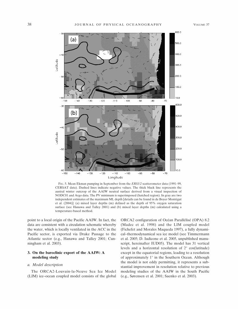
Figure 5 shows two independent estimates of themaximum mixed layer (ML) depth for the region ofinterest (de Boyer Montégut et al. 2004, their Fig. 14).The first estimate (Fig. 5a) is calculated using the depthof the 95% oxygen saturation surface (see also Hanawaand Talley 2001), and the second (Fig. 5b) is calculatedusing a temperature-based method. [The details on thedata spatial and time distribution and on the analysismethods can be found in de Boyer Montégut et al.(2004).] Both reveal a maximum ML depth near 55°S,90°W with a value of approximately 350 m in the firstcase and 450 m in the second case. In the first case theminimum is relatively isolated, but in the second it iscontiguous with a zonally oriented band of relativelylarge ML values.

There is no net separation between the regions of PVminima (Fig. 3d) and maximum ML (Fig. 5). Neverthe-less, the difference in location between the northern-most absolute PV minimum (48°S, see Fig. 3d) and theabsolute maximum ML depth (55°S, see Fig. 5) wouldfavor a nonlocal AAIW formation origin. On the con-trary, the southern PV minimum, located around 55°S,indicates a more local formation, but this water massenters Drake Passage rather than the Pacific. Addition-ally, the location of the ML maximum depth regionappears as a large-scale open-ocean feature rather thanthe coastal process proposed by England et al. (1993).

These statements have to be kept only as indicativeowing to the sparse winter–spring data in this region,and further studies are needed to address the issue.

Of equal importance for the question of whether ven-tilation is local, the outcrop line of the 27.25 surfaceduring austral winter (computed from the inspection ofsingle CTD profiles and depicted on Fig. 5) is found tobe to the south of the ML depth maximum, at about57°S. This serves to underscore that the density horizoncorresponding to the PV minimum is not directly incontact with the base of the region of maximum MLdepth. Preliminary analysis of the ARGO floats re-leased in the region indicates a latitude of outcrop forthe 27.25 surface, consistent with that identified withthe NODC01 data. Last, when considering the circula-tion at the surface and 700 m, the outcrop appears tooccur in a region of the ACC within the main ACCstream, flowing toward Drake Passage.

Climatology of the Ekman pumping has been com-puted using monthly values of the wind stress curl de-rived from the European Remote Sensing Satellite(ERS)-1/2 scatterometer data [1991–99, Centre de Re-cherche et d’Exploitation Satellitaire (CERSAT) data]in order to identify whether there is evidence of wind-driven subduction of AAIW. The annual-mean Ekmanpumping distribution (not shown) reveals a line of zeropumping oriented zonally along 50°S, with upwelling tothe south and downwelling to the north. Thus, thesouthernmost part of the PV minimum region coincidesroughly with a region where the annual mean vertical/wind-driven component of subduction is not important.The seasonal variability in Ekman pumping, however,reveals that the zero line moves to approximately 56°Sin winter (September, see Fig. 5). Nevertheless the out-crop line of the 27.25 surface is to the south of thesouthernmost seasonal excursion of the zero Ekmanpumping line.

Analyzing tracer data, Russell and Dickson (2003)proposed that along 90°W AAIW is not the newestAAIW in the South Pacific; that is, it is at least mixedwith older waters. Comparing the salinity and oxygenmaps (Fig. 3) and considering the AAIW pathway inFig. 2b and Fig. 4, the fresher AAIW is actually enter-ing the South Pacific east of 85°W. In fact, the resultspresented here and in Russell and Dickson (2003) canalso be interpreted as showing that AAIW is at mostpartially ventilated in the southeastern Pacific. Thispartial ventilation could occur via vertical diffusive pro-cesses at the base of the mixed layer (M. S. McCartney2003, personal communication).

In conclusion, the analysis of the NODC01 datasetsuggests that the Pacific AAIW enters the basin mostlyin the southeast corner. The analysis of data does not

FIG. 4. Sketch of the surface (red arrows) and 700-m (bluearrows) mean circulations resulting from the data analysis (Fig. 2).The light blue lines summarize the salinity distribution on theAAIW neutral surface (Fig. 3a). The coastal circulation (dashedarrows) was deduced from the literature discussed in section 2 andvia the model Lagrangian analysis (section 3).


Fig 4 live 4/C

point to a local origin of the Pacific AAIW. In fact, thedata are consistent with a circulation schematic wherebythe water, which is locally ventilated in the ACC in thePacific sector, is exported via Drake Passage to theAtlantic sector (e.g., Hanawa and Talley 2001; Cun-ningham et al. 2003).

3. On the baroclinic export of the AAIW: Amodeling study

a. Model description

The ORCA2-Louvain-la-Neuve Sea Ice Model(LIM) ice–ocean coupled model consists of the global

ORCA2 configuration of Océan Parallélisé (OPA) 8.2(Madec et al. 1998) and the LIM coupled model(Fichefet and Morales Maqueda 1997), a fully dynami-cal–thermodynamical sea ice model (see Timmermannet al. 2005; D. Iudicone et al. 2005, unpublished manu-script, hereinafter IUD05). The model has 31 verticallevels and a horizontal resolution of 2° cos(latitude)except in the equatorial regions, leading to a resolutionof approximately 1° in the Southern Ocean. Althoughthe model is not eddy permitting, it represents a sub-stantial improvement in resolution relative to previousmodeling studies of the AAIW in the South Pacific(e.g., Sørensen et al. 2001; Saenko et al. 2003).

FIG. 5. Mean Ekman pumping in September from the ERS1/2 scatterometer data (1991–99,CERSAT data). Dashed lines indicate negative values. The thick black line represents theaustral winter outcrop of the AAIW neutral surface derived from a visual inspection ofNODC01 and Argo data. The PV minimum is superimposed (hatched region). In gray are twoindependent estimates of the maximum ML depth [details can be found in de Boyer Montégutet al. (2004)]: (a) mixed layer depths (m) defined as the depth of 95% oxygen saturationsurface (see Hanawa and Talley 2001) and (b) mixed layer depths (m) calculated using atemperature-based method.


After 1500 years of spinup (without acceleration),the model has reached an equilibrium state. In a par-allel study (IUD05) the model circulation has been vali-dated using transient tracers. There the simulated chlo-rofluorocarbon (CFC) inventories along WOCE P18section in the South Pacific show very good agreementwith the CFC inventories measured during the WOCEcampaign (Fine et al. 2001), and the simulated ventila-tion of the upper ocean reveals a marked improvementover the inventories simulated by the models partici-pating in the Ocean Carbon-Cycle Model Intercom-parison Project (Dutay et al. 2002).

b. The circulation associated with the AAIWinjection into the South Pacific

The model’s salinity distribution as well as the me-ridional component of circulation for a section at 43°Sacross the entire Pacific basin in shown in Fig. 6. Thesalinity field is characterized by two subsurface minima:the first localized to the eastern side of the basin atapproximately 150-m depth, a signature of the subsur-face salinity minimum water (SSMW) consistent withobservations (e.g., Schneider et al. 2003; Karstensen2004), and the second, a less intense minimum at inter-mediate depth (approximately 1000 m), elongated zon-ally along the whole section. This second minimum isthe signature of the AAIW circulation. This salinityminimum associated with AAIW is deeper (in both

depth and density space) than the observed salinityminimum, and the salinity values characteristic of thesalinity minimum are larger by approximately 0.2 psuthan observation values (Sloyan and Rintoul 2001a).

On the western side of the basin, the southward flowof the western boundary current is associated with thehighest salinity values along the section (Fig. 6). Atdepth, the southward flow is the return flow of thePacific Deep Water, which leaves the basin on its wayto rejoining the ACC. Between 170° and 100°W, thewind-driven gyre is characterized by several northwardcurrents that are surface intensified with velocities van-ishing at a depth of approximately 1200 m. On the east-ern side of the basin, a subsurface current is found toflow southward in the upper 400 m. Below it, between400 and 1500 m, a northward flow occupies the regionbetween 100°W and the Chilean coast, with velocitiesup to 0.0035 m s�1 and a transport of 2.5 Sv (Sv � 106

m3 s�1), consistent with the estimate for the supply ofnew AAIW given by Sloyan and Rintoul (2001a). TheAAIW salinity minimum is partly linked to the deepestpart of the wind-driven gyre in the center of the basin,but in the easternmost region is clearly related to theobserved intermediate flow. This current is boundedabove by a counterflow at the surface, suggesting theexistence of a baroclinic current system, with a south-ward flow in the upper layer and a northward one atintermediate depths. The latter current appears in theannual mean as a relatively broad (large scale) and

FIG. 6. In color, zonal section of salinity at 43°S in the ORCA2-LIM model (model year 1501, annual mean).Isopleths are the corresponding meridional velocity (m s�1).


Fig 6 live 4/C

weak flow. In fact, at 43°S it has a pronounced seasonalvariability, with amplitude of as much as 50% of thetotal transport (not shown), with instantaneous veloci-ties up to 0.01 m s�1. During the months from Januaryto June, there is a southward coastal flow over the up-per 1500 m. This southward flow separates from thecoast during the second half of the year, while progres-sively weakening through the end of the year. The sea-sonal cycle of this current is outside of the scope of thisstudy and is left as a subject for further investigation.

The relation of the flow observed on the section at43°S and the three-dimensional circulation field in theSouth Pacific has been characterized by means of quan-titative offline Lagrangian diagnostics (Blanke andRaynaud 1997), which provide a means of characteriz-ing water mass pathways. The origins and fate of thetwo cores of the baroclinic current at 43°S have beenquantified by integrating Lagrangian trajectories bothbackward and forward in time. By releasing particles inthe AAIW current core (in a zonal band at 43°S be-tween 90°W and the coast, see Fig. 6) and integratingforward in time, it is found that approximately 80% ofthe AAIW flow reaches 10°S, following the northernflank of the subtropical gyre and reaching the NewGuinea Coastal Undercurrent.

Integrating trajectories backward in time until par-ticles reach either a Tasmania–Antarctica section or43°S, 56% of the AAIW is found to originate in theACC, north of the subantarctic front (SAF) (denseSAMW), and 34% to originate at 43°S in the westernboundary current east of New Zealand. Most of AAIWthus originates as SAMW flowing north of the subpolarfront, which has become denser along the pathway.Moreover, there is no evidence for intersection of thetrajectories with the mixed layer in the southeast Pacificfor calculations performed with the time-reversed cir-culation fields.

The subsurface southward flow, shown schematicallyby the dashed arrows in Fig. 4, has been traced back intime with Lagrangian trajectories from 43°S to twosources: a zonal section across 32°S and the ACC (ameridional section between Antarctica and Tasmania).The surface flow has been found to have a transport ofabout 1.1 Sv and a density �0 � 26.2. This flow corre-sponds to the southern flank of the West Drift and hasits origins as a shallow branch of the ACC (Fig. 4).Moreover, along the Australia–Antarctica section it isfound to be at the surface (depth �100 m) south of theSAF at 55°S and of the same density as the UpperCircumpolar Deep Water (Sloyan and Rintoul 2001b).This indicates that the Ekman transport has exportedthis water from the ACC core to its northernmost front.

c. Model tracer fields on model AAIW horizon

To investigate how the model fields compare with theobservations presented in section 2, model tracer fieldshave been projected onto the 27.4 neutral surface (Fig.7: McDougall 1987; Jackett and McDougall 1997), themodel surface corresponding to the salinity minimum.This allows for a validation of the structure of the pen-etration of the salinity minimum from the SouthernOcean into the South Pacific and, specifically, how thepathway identified using the Lagrangian tracers ismanifested for various properties associated with thissurface.

On the basin scale, the salinity distribution on the27.4 neutral surface in Fig. 7a exhibits isopleths directedfrom southwest to northeast between 50° and 30°S. Thistilt results from the wind-driven advective–diffusive cir-culation that advects the tracer around the gyre. There-fore, the isopleths are situated farther south in the westthan in the east, indicating a preferential northwardinjection of salinity-minimum waters to the east. Far-ther to the north, this east to north inclination de-creases, as this corresponds to the shadow zone regionwhere velocities are lower on this surface.

The depth of the 27.4 neutral surface is shown in Fig.7b. The maximum depth associated with the deep coreof the subtropical gyre circulation is found to reachapproximately 50°S, in agreement with the observa-tions in section 2. Furthermore, as in the NODC data,the eastern extension of the subtropical gyre structureis consistent with data in that it extends to the Ameri-can coast at 35°S, while at 50°S it only reaches 110°W.To the east of 110°W along 50°S, the zonal gradient ofthe depth of the 27.4 surface is very small, again con-sistent with observations.

The PV distribution associated with the same neutralsurface is shown in Fig. 7d. A striking feature is thelocal minimum that extends meridionally from 55° to35°S. Along 50°S, the PV minimum is found between100° and 80°W. This minimum coincides with the re-gion of relatively uniform depth of the 27.4 surfaceidentified in Fig. 7b, and is found in the same locationas in the data. Dynamically, the associated weak me-ridional PV gradient helps to break dynamical con-straints on meridional transport, and allows northwardtransport of waters and offers a window for meridionalinjection of subpolar frontal waters into the South Pa-cific. This window is imbedded in the large-scale gyrecirculation between an eastern region and a westernrecirculation-type gyre and is not connected to eithereastern or western boundaries. In contrast, a PV maxi-mum is found farther west in the Pacific, correspondingto the deepest recirculation region of the subtropical


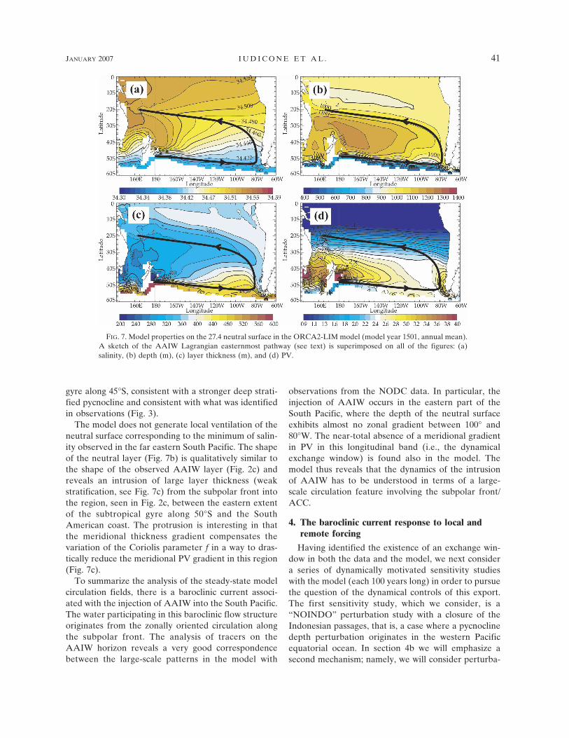
gyre along 45°S, consistent with a stronger deep strati-fied pycnocline and consistent with what was identifiedin observations (Fig. 3).

The model does not generate local ventilation of theneutral surface corresponding to the minimum of salin-ity observed in the far eastern South Pacific. The shapeof the neutral layer (Fig. 7b) is qualitatively similar tothe shape of the observed AAIW layer (Fig. 2c) andreveals an intrusion of large layer thickness (weakstratification, see Fig. 7c) from the subpolar front intothe region, seen in Fig. 2c, between the eastern extentof the subtropical gyre along 50°S and the SouthAmerican coast. The protrusion is interesting in thatthe meridional thickness gradient compensates thevariation of the Coriolis parameter f in a way to dras-tically reduce the meridional PV gradient in this region(Fig. 7c).

To summarize the analysis of the steady-state modelcirculation fields, there is a baroclinic current associ-ated with the injection of AAIW into the South Pacific.The water participating in this baroclinic flow structureoriginates from the zonally oriented circulation alongthe subpolar front. The analysis of tracers on theAAIW horizon reveals a very good correspondencebetween the large-scale patterns in the model with

observations from the NODC data. In particular, theinjection of AAIW occurs in the eastern part of theSouth Pacific, where the depth of the neutral surfaceexhibits almost no zonal gradient between 100° and80°W. The near-total absence of a meridional gradientin PV in this longitudinal band (i.e., the dynamicalexchange window) is found also in the model. Themodel thus reveals that the dynamics of the intrusionof AAIW has to be understood in terms of a large-scale circulation feature involving the subpolar front/ACC.

4. The baroclinic current response to local andremote forcing

Having identified the existence of an exchange win-dow in both the data and the model, we next considera series of dynamically motivated sensitivity studieswith the model (each 100 years long) in order to pursuethe question of the dynamical controls of this export.The first sensitivity study, which we consider, is a“NOINDO” perturbation study with a closure of theIndonesian passages, that is, a case where a pycnoclinedepth perturbation originates in the western Pacificequatorial ocean. In section 4b we will emphasize asecond mechanism; namely, we will consider perturba-

FIG. 7. Model properties on the 27.4 neutral surface in the ORCA2-LIM model (model year 1501, annual mean).A sketch of the AAIW Lagrangian easternmost pathway (see text) is superimposed on all of the figures: (a)salinity, (b) depth (m), (c) layer thickness (m), and (d) PV.


Fig 7 live 4/C

tions of the pycnocline in the Southern Ocean directlyaffecting the AAIW injection into the South Pacific.

a. The role of equatorial dynamics in setting AAIWexport

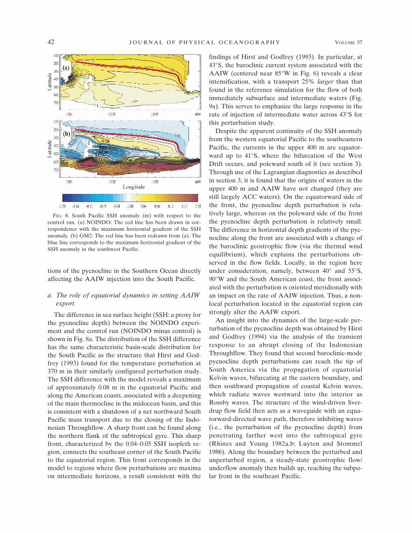
The difference in sea surface height (SSH: a proxy forthe pycnocline depth) between the NOINDO experi-ment and the control run (NOINDO minus control) isshown in Fig. 8a. The distribution of the SSH differencehas the same characteristic basin-scale distribution forthe South Pacific as the structure that Hirst and God-frey (1993) found for the temperature perturbation at370 m in their similarly configured perturbation study.The SSH difference with the model reveals a maximumof approximately 0.08 m in the equatorial Pacific andalong the American coasts, associated with a deepeningof the main thermocline in the midocean basin, and thisis consistent with a shutdown of a net northward SouthPacific mass transport due to the closing of the Indo-nesian Throughflow. A sharp front can be found alongthe northern flank of the subtropical gyre. This sharpfront, characterized by the 0.04–0.05 SSH isopleth re-gion, connects the southeast corner of the South Pacificto the equatorial region. This front corresponds in themodel to regions where flow perturbations are maximaon intermediate horizons, a result consistent with the

findings of Hirst and Godfrey (1993). In particular, at43°S, the baroclinic current system associated with theAAIW (centered near 85°W in Fig. 6) reveals a clearintensification, with a transport 25% larger than thatfound in the reference simulation for the flow of bothimmediately subsurface and intermediate waters (Fig.9a). This serves to emphasize the large response in therate of injection of intermediate water across 43°S forthis perturbation study.

Despite the apparent continuity of the SSH anomalyfrom the western equatorial Pacific to the southeasternPacific, the currents in the upper 400 m are equator-ward up to 41°S, where the bifurcation of the WestDrift occurs, and poleward south of it (see section 3).Through use of the Lagrangian diagnostics as describedin section 3, it is found that the origins of waters in theupper 400 m and AAIW have not changed (they arestill largely ACC waters). On the equatorward side ofthe front, the pycnocline depth perturbation is rela-tively large, whereas on the poleward side of the frontthe pycnocline depth perturbation is relatively small.The difference in horizontal depth gradients of the pyc-nocline along the front are associated with a change ofthe baroclinic geostrophic flow (via the thermal windequilibrium), which explains the perturbations ob-served in the flow fields. Locally, in the region hereunder consideration, namely, between 40° and 55°S,90°W and the South American coast, the front associ-ated with the perturbation is oriented meridionally withan impact on the rate of AAIW injection. Thus, a non-local perturbation located in the equatorial region canstrongly alter the AAIW export.

An insight into the dynamics of the large-scale per-turbation of the pycnocline depth was obtained by Hirstand Godfrey (1994) via the analysis of the transientresponse to an abrupt closing of the IndonesianThroughflow. They found that second baroclinic-modepycnocline depth perturbations can reach the tip ofSouth America via the propagation of equatorialKelvin waves, bifurcating at the eastern boundary, andthen southward propagation of coastal Kelvin waves,which radiate waves westward into the interior asRossby waves. The structure of the wind-driven Sver-drup flow field then acts as a waveguide with an equa-torward-directed wave path, therefore inhibiting waves(i.e., the perturbation of the pycnocline depth) frompenetrating farther west into the subtropical gyre(Rhines and Young 1982a,b; Luyten and Stommel1986). Along the boundary between the perturbed andunperturbed region, a steady-state geostrophic flow/underflow anomaly then builds up, reaching the subpo-lar front in the southeast Pacific.

FIG. 8. South Pacific SSH anomaly (m) with respect to thecontrol run. (a) NOINDO: The red line has been drawn in cor-respondence with the maximum horizontal gradient of the SSHanomaly. (b) GM2: The red line has been redrawn from (a). Theblue line corresponds to the maximum horizontal gradient of theSSH anomaly in the southwest Pacific.


Fig 8 live 4/C

b. The role of Southern Ocean dynamics in settingAAIW export

We are now interested in considering whether extra-tropical pycnocline perturbations, specifically ACCperturbations, are also able to affect the AAIW export.This is considered within the context of a range of pre-vious studies (e.g., Toggweiler and Samuels 1998;Gnanadesikan 1999; Borowski et al. 2002; Karsten et al.2002; Marshall and Radko 2003), which have arguedthat there are two main perturbation mechanisms thatcan modify the pycnocline depth in the ACC: one beinga modification of the eddy forcing and the other amodification of the Ekman transport.

1) THE ROLE OF EDDIES IN THE EXPORT OF

PACIFIC AAIW

A numerical experiment (named GM2) has been per-formed for which the bolus transport coefficient in theGent and McWilliams (1990) eddy parameterization istwice as large for the Southern Hemisphere as it is forthe reference experiment, with values in the NorthernHemisphere kept the same as in the reference experi-ments. Note that, since the model eddy transfers de-pend on the local baroclinicity (Treguier et al. 1997) aswell, it does not necessarily imply that the resultingeddy transports are 2 times as large.

Not surprisingly, the steepness of the ACC front isdecreased for GM2 relative to the control run. In theAtlantic and Indian sectors, there is a large perturba-tion in SSH that corresponds to a flattening of the ACCisopycnals (not shown). A perturbation of opposite signis also found all along the SAF. This feature can beunderstood in terms of a meridional shift of the fronts.On the other hand, in the Pacific the ACC SSH per-turbation penetrates northward (Fig. 8b) far into thebasin between 100°W and the Chilean coast, crossingthe main fronts and reaching the subtropics east of NewZealand. In fact, for the GM2 case, the stratificationchange in the ACC owing to the increased eddy trans-fers propagates northward within a region bounded tothe east by the same dynamic boundary as the onepresent in the NOINDO case (red curve in Figs. 8a and8b). It is bounded to the west by the deep recirculatinggyre (blue curve in Fig. 8b) where the velocity anomalypresents a coherent vertical structure over the first 1000m, and thus it is controlled by the first baroclinicRossby-type mode. The subtropical intrusion of theACC pycnocline anomaly alters the pycnocline slopealong the red line in Fig. 8b and thus weakens thenorthward flowing AAIW current in the eastern Pa-cific, even if the largest signal is in the west. In fact, asshown in Fig. 9b, this effect produces a significant re-

FIG. 9. Anomalies with respect to the control run in the meridional velocity field along a zonal sectionat 43°S (as in Fig. 6) in the ORCA2-LIM model (model year 100, annual mean; units: m s�1, intervals:5 � 10�4 m s�1). (a) NOINDO � reference. (b) GM2 � reference. (c) SWIND2 � reference.


duction of the mean advective AAIW export throughthe weakening of the baroclinic current system east of100°W. The anomaly is deeper than in the case wherethe perturbation has an equatorial origin (NOINDO),coherent with the southern origins of the pycnoclineperturbation.

2) THE ROLE OF THE SOUTHERN OCEAN WINDS

Two additional sensitivity experiments for which thewind stress in the Southern Ocean has been increasedby 50% have been performed. The northward limit ofthe 50% perturbation is located at 50°S in the first ex-periment (SWIND1) and at 35°S in the second one(SWIND2) with a smooth transition to climatologicalvalues north of these latitudes. The goal of SWIND1 isto investigate the effects of a local forcing (the windcurl between 50° and 40°S is changed) altering the ACCnorthward deviation (e.g., Nuñez and Rojas 1998). Theaim of SWIND2 is to force both the circulation of thesouthern part of the subtropical gyre by changing thewind curl at midlatitudes and, above all, the depth andstrength of the ACC (e.g., Borowski et al. 2002).

In SWIND1 the resulting anomaly at 43°S (notshown) presents an enhancement (weakening) of theintermediate current at 90°W (80°W). The opposite isobserved at the surface. This result is somewhat differ-ent with respect to the experiments NOINDO andGM2 discussed previously. It corresponds to a west-ward shift of the entire baroclinic system, as observed inthe seasonal cycle of the control run (see also Nuñezand Rojas 1998), without any change in the transport.This is due to the fact that the subtropical gyre deepenswithout increasing in strength (Haynes 1985), as well asto the shift westward of the different regimes (the redand green curves in Fig. 8b), owing to an increase of theRossby wave speed. SWIND1 therefore shows how thelocal circulation is sensitive to changes in the local windstress curl, which alters the current patterns but has noinfluence on the net baroclinic AAIW export.

The SWIND2 case presents a large SSH negativeperturbation along the whole ACC that corresponds toan uplifting of isopycnals. The circulation perturbationat 43°S east of 90°W (Fig. 9c) is similar to the GM2experiment (with only reversed signs, see Fig. 9b) withan enhancement of the baroclinic system at 80°W. As inGM2, the perturbation is deeper than in the NOINDOcase and is related to a northward intrusion of the ACCperturbation. A major difference with the GM2 experi-ment is the blocking of the northward extension of theSSH signal at about 35°S by the large zonal perturba-tion within the gyre produced by the wind stress curlmodification.

5. Discussion

a. A scenario for the dynamics of the AAIW export

We wish to point out first that the different regionsand fronts observed to characterize the propagation oftracers on the AAIW horizon are compatible with theexistence of an eastern shadow zone (Luyten and al.1983), western and eastern regimes (regimes defined interms of Rossby wave propagation speeds), as is thecase for PV (black curves in Fig. 3d). Interestingly, thedynamical significance of these regions also emerged inthe sensitivity model study. Furthermore, Huang andQiu (1998) provided an estimate of the wind-drivencirculation in the South Pacific. On the AAIW horizon,the absence of local ventilation in their dataset gener-ates a closed anticyclonic recirculation gyre in the west-ern subbasin (the Rhines–Young PV pool) while in theeast a region of zero flow is predicted, due to the pres-ence of a shadow zone. In fact the northward flow,exporting the AAIW, is imbedded in and almost coin-cides with the shadow zone of Huang and Qiu (1998).

Second, nonfrictional large-scale meridional trans-ports allow for the existence of a cross-gyre window(Schopp and Arhan 1986; Schopp 1988; Chen andDewar 1993; Pedlosky 1998) only if certain specific dy-namical conditions along the zero wind curl line aresatisfied, notably an arrested Rossby wave condition.Once these conditions are satisfied, the circulation isable to connect the ACC to the subtropical gyre. Thesewindows, based on blocked divergent Rossby waves byzonal mean currents, are imbedded between easternregimes (shadow type) with westward-propagating per-turbations and western regimes with eastward-advectedRossby waves. Meridional northward propagation is al-lowed in this window north of the zero wind curl line.Remarkably, the mean zero curl line lies along 50°S,that is, just north of the ACC. Therefore, the northwarddiversion of the ACC at the surface east of the EastPacific Rise (EPR) (Fig. 4), finally joining the zonallyelongated West Drift, could be the invasion of thesouthern gyre (here the ACC) across the zero windstress curl line in the surface field, as depicted inSchopp and Arhan (1986). Additionally, the presenceof a dynamical window locally altering the stratificationcould also explain the PV minimum and the very weakPV meridional gradient (Chen and Dewar 1993). Bot-tom topography, instead, controls the diversion occur-ring at the EPR. The northward diversion of the ACCis then due to a combination of the two mechanisms.

Last, the exchange-window scenario implies the ex-istence of an eastward surface flow, allowing it to stopor to reverse the second-baroclinic-mode Rossby


wave propagation (Schopp and Arhan 1986). In fact, aneastward surface flow of ACC origin is observed at thesurface between 55° and 40°S (Fig. 4). Furthermore,Killworth and Blundell (2003a) recently presentedglobal estimates for the baroclinic Rossby wave propa-gation, including the effect of topographic slope andmean velocity field. Their results support the scenarioproposed here. First, both first and second baroclinicmodes have an absolute zonal minimum in the zonalwave speed between 53° and 43°S, 120°W and the coastwith a discontinuity at 100°W in both fields [see figuresin Killworth and Blundell (2003a) to appraise howstriking this anomaly is with respect to mean values atthe same latitude]. More significantly, the minimum as-sociated with the second baroclinic mode is actuallyrelated to the interaction with a mean zonal eastwardflow, while a marked topographic effect concerns thefirst-mode minimum (not shown; P. Killworth and J.Blundell 2004, personal communication).

b. The AAIW export mechanism as part of anoceanic teleconnection?

The AAIW injection into the southeast Pacific isruled by local baroclinic dynamics. The model sensitiv-

ity studies discussed above showed that the local baro-clinic perturbations are actually only the local expres-sion of large-scale perturbations. For instance, theanomaly of the local zonal isopycnal slope observed inthe NOINDO experiment was due to a change of depthof the pycnocline to the east of the current core, with aperturbation signal originating at the Indonesian straitsclosure, having propagated clockwise around the basinand radiated westward from the eastern boundary. Thehorizontal pressure gradient associated with the pycno-cline slope has been shown to be sensitive as well to achange of the pycnocline depth south or west of thearea of interest, that is, by a change in the vertical struc-ture of the ACC. This corresponds to vertically displac-ing the isopycnals to the west of the meridional frontand producing a perturbation of the horizontal gradientas large as the one produced by the equatorialNOINDO case (see sketch in Fig. 10). In this case theperturbation cannot come from the southern tip of theAmerican continent because coastal Kelvin waves areconstrained to propagate poleward along easternboundaries. West of this region there is the meridionalPV window discussed in the previous section (Figs. 3dand 7d). Considering that the intermediate flow is di-

FIG. 10. Sketch on the vertical plane of examples of the mechanisms that can affect theAAIW transport at �43°S. The 27.0 neutral surface is considered here as the interface be-tween the AAIW and the upper layers. The slope of the interface (indicated by the grayarrow) is associated with the baroclinic current system and thus the AAIW export. Dashedline represents the interface in case of a deepening of the Southern Ocean pycnocline, whichpropagated northward through the exchange window. Dotted–dashed line represents theinterface in presence of an equatorial-originated rise of the pycnocline along the coast. Bothmechanisms can produce a change in the slope of the interface and then in the AAIW export.The change in the slope (and the consequent transport anomaly) is observed along the wholewestern boundary of the eastern regime (green line in Figs. 8a,b; see also Hirst and Godfrey1993).


rected northward, one could speculate that the ACCsets the meridionally constant PV value. The PV is, infact, locally related to the vertical separation of isopyc-nals; therefore, a change of the isopycnal depth in theACC (e.g., in GM2 and SWIND2) would alter theAAIW potential vorticity along the subpolar front. ThePV (or stratification) perturbation is propagated north-ward through the dynamical window, altering the pyc-nocline depth north of 55°S and changing, eventually,the zonal slope of the flow/underflow isopycnal inter-face. This would accelerate or decelerate the AAIWmain flow, exactly as it occurs in the case in whichthe perturbation is applied in the equatorial region(NOINDO).

In summary, the equatorward penetration of AAIWappears to be located exactly at the junction of theRossby western and eastern regimes (see sketch in Fig.11). The strength of the wind-forced mean current ad-vects waves either eastward west of this window orwestward east of it. The strength of this front at thejunction can therefore be affected either by perturba-tions originating in the equatorial region via the easternregime or by Southern Ocean perturbations via thewestern regime (e.g., Hughes 1996). A third regimecould also be a locally forced ventilation-type pertur-

bation along the zero wind curl line inside the window:a regime able to radiate signals to the north into thesubtropical gyre and to the south into the ACC. Thislatter regime has been excluded because ventilationdoes not seem to occur along the zero wind stress curlline. The AAIW export is ruled by the large-scale me-ridional pressure gradient between the ACC and theequator, projected into a local zonal baroclinic shearvia planetary wave propagation. It can be expected thatremote baroclinic forcing can change the current char-acteristics via wave propagations, that is, the AAIWexport into the Pacific. The wave mechanism is, in fact,very rapid and is able to affect remote regions on shorttime scales (even ENSO-like: e.g., Hormazabal et al.2001, 2002; Vega et al. 2003;). Recently, the existence ofremote oceanic teleconnections in the thermohaline cir-culation due to planetary wave (first baroclinic mode)propagation has been proposed (e.g., Cessi et al. 2004;Huang et al. 2000). Here we do not address these vari-ability issues, but on the basis of previous consider-ations we can speculate that the mechanism for thecontrol of the interbasin exchange at intermediatedepths (via the second baroclinic mode) proposed hereis an extension of the type of teleconnected mechanismproposed in these studies. For instance, the ACC den-

FIG. 11. Sketch on the horizontal plane of the mechanisms that can affect the AAIW export superimposed onthe model mean SSH (m) and the model 1000-m isobath. Meandering arrows indicate the possible wave propa-gations, which are responsible for the mapping of remote pycnocline anomalies onto the southeast Pacific. Theeastern boundary of the western regime is indicated by the dotted line. Notably, it bounds the deep core of thesubtropical gyre (thick black line). The dashed–dotted line represents the boundary of the eastern regime, whichcoincides with the region of sensitivity of the slope of the interface (i.e., the AAIW transport) to remote changesin the pycnocline depth (see text and Fig. 10). The region between the two lines can be affected by the northwardpropagation of anomalies from the Southern Ocean through the exchange window (indicate by a straight arrow).The coastal region can be affected by anomalies originated at the equator.


sity structure can be altered by changes occurring in theNorth Atlantic Deep Water formation region, as dis-cussed by, for example, Goodman (2001); comparetheir distribution of the anomaly of the pycnoclinedepth in the South Pacific with our Fig. 8b.

6. Conclusions

In this study, NODC data have been used in conjunc-tion with output from an ocean circulation model toaddress the ventilation pathways and dynamical con-trols on the injection of AAIW into the South Pacific.The analysis allowed for a better identification of apathway for the renewal of Pacific AAIW, with thatpathway consisting of a northward flow in the south-western South Pacific. This has been shown to be con-sistent with tracer distributions on a neutral surface cor-responding to AAIW. Concerning the ventilationsource of this AAIW, this study did not reveal any clearevidence of a local origin for AAIW, although owing todata sparcity a local ventilation source cannot be ex-cluded. A more complete study on the formationmechanisms is, in any case, necessary to address theissue.

In terms of its dynamics, the weak meridional gradi-ent in potential vorticity associated with AAIW exporthas been interpreted here as being due to the existenceof a dynamical exchange window where Rossby wavescarry perturbation signals northward around the SouthPacific subtropical gyre, connecting the ACC with thesubtropics. This scenario is supported by the existenceof a local minimum in the Rossby wave zonal speedobserved in previous in situ data analyses (Killworthand Blundell 2003a,b). Furthermore, we speculatedthat, because of the vanishing meridional Sverduptransport, most of the AAIW export should occur aspart of a strictly baroclinic current structure.

The main features of the AAIW export, togetherwith observed PV fields, have been well reproduced bya global ocean model. Another important result is thatthe modeling experiments clearly indicate that thelarge-scale baroclinic current structure west of the Chil-ean coast is driven by the basin-scale meridional pres-sure gradient field. In other words, this study clearlyshows the existence of a remote connection mechanismbetween the Tropics and the Southern Ocean—a purelyoceanic mechanism. Similar remote connectionsmechanisms have been recently proposed to explain thevariability of the upper thermohaline circulation, but,importantly, here we have shown its importance for theintermediate circulation. The SAMW is supposed to beexported by subduction along the subantarctic front(Hanawa and Talley 2001). Another consequence of

this study is thus that SAMW and AAIW appear to beruled by a different export mechanism. Although thisstudy was performed with climatological forcing, it willbe left for further investigation to evaluate how thesepotentially decoupled circulation features vary in theirrespective transports. Additionally, care should betaken when analyzing data or model results in trying toidentify a global warming signal in the ocean.

The AAIW exports freshwater and nutrients towardthe Tropics and the equator. If at least part of its exportis driven by the equatorial variability, as proposed here,it can represent a possible feedback on the equatorial/tropical physical and biological dynamics (e.g., Dugdaleet al. 2002; Sarmiento et al. 2004). By being alsocontrolled by the Southern Ocean, on the other hand, itcan represent a remote forcing to the equatorial dy-namics. Last, even if their lower latitudes do not allowfor a direct connection between the Southern Oceanand the Tropics, the mechanism proposed here for theinterbasin exchange could also be at work in other east-ern regions such as Africa or Australia. This could bethe case, for instance, for AAIW injection into theNorth Atlantic basin where it forms the return branchof the basin thermohaline circulation, which recentlyhas been associated with the intermediate flow ob-served just to the east of South Africa (e.g., Schmid etal. 2001).

Acknowledgments. We acknowledge the NationalOceanographic Data Center as well as the CERSATdata center for making their rich databases publiclyavailable. Peter Killworth and Jeff Blundell kindly al-lowed us to access their estimates of Rossby wavespeeds. Clement de Boyer Montégut provided us withthe climatology of the mixed layer depths, and SophieCravatte gave us access to postprocessed ARGO data.The producers of the ODV software are also acknowl-edged, as well as D.R. Jackett and T. McDougall fortheir software for the neutral density computation.

The authors gratefully acknowledge discussions withMichel Arhan, who suggested that we consider the ex-istence of an exchange window, and Lynne Talley, forinteresting discussions and whose seminal papers onAAIW were the inspirations for this research. Discus-sions with Peter Killworth, Michael S. McCartney, Et-tore Salusti, Sabrina Speich, Anne Marie Treguier, andMaurizio Ribera D’Alcalà are also kindly acknowl-edged. The several scientific discussions with B. Linnéwere also very fruitful.

This research was part of the French BILBO projectsupported by the Programme National d’Etude du Cli-mat (PNEDC). Computational time was provided bythe Institut du Developpement et des Ressources en


Informatique Numerique (IDRIS). A contributionfrom the Italian PNRA (Project CANOPO) is also ac-knowledged.

REFERENCES

Blanke, B., and S. Raynaud, 1997: Kinematics of the Pacific Equa-torial Undercurrent: An Eulerian and Lagrangian approachfrom GCM results. J. Phys. Oceanogr., 27, 1038–1053.

Borowski, D., R. Gerdes, and D. Olbers, 2002: Thermohaline andwind forcing of a circumpolar channel with blocked geo-strophic contours. J. Phys. Oceanogr., 32, 2520–2540.

Brzezinski, M. A., M.-L. Dickson, D. M. Nelson, and R. Sam-brotto, 2003: Ratios of Si, C and N uptake by microplanktonin the Southern Ocean. Deep-Sea Res. II, 50, 619–633.

Cessi, P., K. Bryan, and R. Zhang, 2004: Global seiching of ther-mocline waters between the Atlantic and the Indian–PacificOcean Basins. Geophys. Res. Lett., 31, L04302, doi:10.1029/2003GL019091.

Chaigneau, A., and O. Pizarro, 2005: Mean surface circulation andmesoscale turbulent flow characteristics in the eastern SouthPacific, from satellite tracked drifters. J. Geophys. Res., 110,C05014, doi:10.1029/2004JC002628.

Chen, L. G., and W. K. Dewar, 1993: Intergyre communication ina three-layer model. J. Phys. Oceanogr., 23, 855–878.

Conkright, M. E., and Coauthors, 2002: Introduction. Vol. 1,World Ocean Database 2001, NOAA Atlas NESDIS 42,160 pp.

Cunningham, S. A., S. G. Alderson, B. A. King, and M. A. Bran-don, 2003: Transport and variability of the Antarctic Circum-polar Current in Drake Passage. J. Geophys. Res., 108, 8084,doi:10.1029/2001JC001147.

Davis, R. E., 1998: Preliminary results from directly measuringmid-depth circulation in the tropical and south Pacific. J.Geophys. Res., 103, 24 619–24 639.

——, 2005: Intermediate-depth circulation of the Indian andSouth Pacific Oceans measured by autonomous floats. J.Phys. Oceanogr., 35, 683–707.

de Boyer Montégut, C., G. Madec, A. S. Fischer, A. Lazar, and D.Iudicone, 2004: Mixed layer depth over the global ocean: Anexamination of profile data and a profile-based climatology.J. Geophys. Res., 109, C12003, doi:10.1029/2004JC002378.

Dugdale, R. C., A. G. Wischmeyer, F. P. Wilkerson, R. T. Barber,F. Chai, M. Jiang, and T.-H. Peng, 2002: Meridional asym-metry of source nutrients to the equatorial Pacific upwellingecosystem and its potential impact on ocean–atmosphereCO2 flux; A data and modeling approach. Deep-Sea Res. II,49, 2513–2533.

Dutay, J.-C., and Coauthors, 2002: Evaluation of ocean modelventilation with CFC-11: Comparison of 13 global oceanmodels. Ocean Modell., 4, 89–120.

England, M. H., J. S. Godfrey, A. C. Hirst, and M. Tomczak, 1993:The mechanism for Antarctic Intermediate Water renewal ina world ocean model. J. Phys. Oceanogr., 23, 1553–1560.

Fichefet, T., and M. A. Morales Maqueda, 1997: Sensitivity of aglobal sea ice model to the treatment of ice thermodynamicsand dynamics. J. Geophys. Res., 102, 609–646.

Fine, R. A., K. A. Maillet, K. S. Sullivan, and D. Willey, 2001:Circulation and ventilation flux of the Pacific Ocean. J. Geo-phys. Res., 106, 22 159–22 178.

Gent, P. R., and J. C. McWilliams, 1990: Isopycnal mixing inocean circulation models. J. Phys. Oceanogr., 20, 150–155.

Gnanadesikan, A., 1999: A simple predictive model for the struc-ture of the oceanic pycnocline. Science, 283, 2077–2079.

Goodman, P. J., 2001: Thermohaline adjustment and advection inan OGCM. J. Phys. Oceanogr., 31, 1477–1497.

Hanawa, K., and L. D. Talley, 2001: Mode waters. Ocean Circu-lation and Climate, G. Siedler and J. Church, Eds., Interna-tional Geophysics Series, Vol. 77, Academic Press, 373–386.

Haynes, P. H., 1985: Wind gyres in circumpolar oceans. J. Phys.Oceanogr., 15, 670–683.

Hirst, A. C., and J. S. Godfrey, 1993: The role of Indonesianthroughflow in a global ocean GCM. J. Phys. Oceanogr., 23,1057–1086.

——, and ——, 1994: The response to a sudden change in Indo-nesian throughflow in a global ocean GCM. J. Phys. Ocean-ogr., 24, 1895–1910.

Hormazabal, S., G. Shaffer, J. Letelier, and O. Ulloa, 2001: Localand remote forcing of sea surface temperature in the coastalupwelling system off Chile. J. Geophys. Res., 106, 16 657–16 672.

——, ——, and O. Pizarro, 2002: Tropical Pacific control of in-traseasonal oscillations off Chile by way of oceanic and at-mospheric pathways. Geophys. Res. Lett., 29, 1081,doi:10.1029/2001GL013481.

Huang, R. X., and B. Qiu, 1998: The structure of the wind-drivencirculation in the subtropical South Pacific Ocean. J. Phys.Oceanogr., 28, 1173–1186.

——, M. Cane, N. Naik, and P. J. Goodman, 2000: Global adjust-ment of the thermocline in response to deep water formation.Geophys. Res. Lett., 27, 759–762.

Hughes, C. W., 1996: The Antarctic circumpolar current as awaveguide for Rossby waves. J. Phys. Oceanogr., 26, 1375–1387.

Jackett, D. R., and T. J. McDougall, 1997: A neutral density vari-able for the world’s oceans. J. Phys. Oceanogr., 27, 237–263.

Karsten, R., H. Jones, and J. Marshall, 2002: The role of eddytransfer in setting the stratification and transport of a Cir-cumpolar Current. J. Phys. Oceanogr., 32, 39–54.

Karstensen, J., 2004: Formation of the South Pacific shallow sa-linity minimum: A Southern Ocean pathway to the tropicalPacific. J. Phys. Oceanogr., 34, 2398–2412.

Killworth, P. D., and J. R. Blundell, 2003a: Long extratropicalplanetary wave propagation in the presence of slowly varyingmean flow and bottom topography. Part I: The local problem.J. Phys. Oceanogr., 33, 784–801.

——, and ——, 2003b: Long extratropical planetary wave propa-gation in the presence of slowly varying mean flow and bot-tom topography. Part II: Ray propagation and comparisonwith observations. J. Phys. Oceanogr., 33, 802–821.

Luyten, J., and H. Stommel, 1986: Gyres driven by combined windand buoyancy flux. J. Phys. Oceanogr., 16, 1551–1560.

——, J. Pedlosky, and H. Stommel, 1983: The ventilated ther-mocline. J. Phys. Oceanogr., 13, 292–309.

Madec, G., P. Delecluse, M. Imbard, and C. Lévy, 1998: OPA 8.1Ocean General Circulation Model reference manual. InstitutPierre-Simon Laplace Note du Pôle de Modélisation No. 11,91 pp.

Marshall, J., and T. Radko, 2003: Residual mean solutions for theAntarctic Circumpolar Current and its associated overturn-ing circulation. J. Phys. Oceanogr., 33, 2341–2354.

McCartney, M. S., 1977: Subantarctic Mode Water. A Voyage ofDiscovery: George Deacon 70th Anniversary Volume, M. V.Angel, Ed., Pergamon, 103–119.


——, 1982: The subtropical recirculation of mode waters. J. Mar.Res., 40 (Suppl.), 427–464.

McDougall, T. J., 1987: Neutral surfaces. J. Phys. Oceanogr., 17,1950–1964.

Nuñez, R., and R. Rojas, 1998: Circulation offshore SouthernChile, PR14 Repeated Hydrography Section. InternationalWOCE Newsletter, Vol. 32, WOCE International Project Of-fice, Southampton, United Kingdom, 40–42.

Pedlosky, J., 1998: Ocean Circulation Theory. Springer-Verlag,453 pp.

Piola, A. R., and A. L. Georgi, 1982: Circumpolar properties ofAntarctic Intermediate Water and Subantarctic Mode Water.Deep-Sea Res., 29, 687–711.

Reid, J. L., 1986: On the total geostrophic circulation of the SouthPacific Ocean: Flow patterns, tracers and transports. Progressin Oceanography, Vol. 16, Pergamon, 1–61.

——, 1997: On the total geostrophic circulation of the PacificOcean: Flow patterns, tracers, and transports. Progress inOceanography, Vol. 39, Pergamon, 263–352.

Rhines, P. B., and W. R. Young, 1982a: Homogenization of po-tential vorticity in planetary gyres. J. Fluid Mech., 122, 347–367.

——, and ——, 1982b: A theory of the wind-driven circulation. I.Midocean gyres. J. Mar. Res., 40 (Suppl.), 559–596.

Rojas, R., N. Silva, W. Garcia, and Y. Guerriero, 1995: WHPrepeated hydrography section PR14, offshore southern Chile.International WOCE Newsletter, WOCE International Proj-ect Office, Southampton, United Kingdom, Vol. 20, 31–33.

Russell, J. L., and A. G. Dickson, 2003: Variability in oxygen andnutrients in South Pacific Antarctic Intermediate Water.Global Biogeochem. Cycles, 17, 1033, doi:10.1029/2000GB001317.

Saenko, O., A. J. Weaver, and M. H. England, 2003: A region ofenhanced northward Antarctic Intermediate Water transportin a coupled climate model. J. Phys. Oceanogr., 33, 1528–1535.

Sarmiento, J. L., N. Gruber, M. Brzezinksi, and J. Dunne, 2004:High latitude controls of thermocline nutrients and low lati-tude biological productivity. Nature, 426, 56–60.

Schlitzer, R., cited 2004: Ocean data view. Alfred Wegener Insti-tut. [Available online at http://www.awi-bremerhaven.de/GEO/ODV.]

Schmid, C., R. L. Molinari, and S. L. Garzoli, 2001: New observa-tion of the intermediate depth circulation in the tropical At-lantic. J. Mar. Res., 59, 281–312.

Schneider, W., R. Fuenzalida, E. Rodríguez-Rubio, J. Garcés-Vargas, and L. Bravo, 2003: Characteristics and formation ofEastern South Pacific Intermediate Water. Geophys. Res.Lett., 30, 1581, doi:10.1029/2003GL017086.

Schopp, R., 1988: Spin up toward communication between oce-anic subpolar and subtropical gyres. J. Phys. Oceanogr., 18,1241–1259.

——, and M. Arhan, 1986: A ventilated middepth circulationmodel for the eastern North Atlantic. J. Phys. Oceanogr., 16,344–357.

Shaffer, G., S. Hormazabal, O. Pizarro, and M. Ramos, 2004:Circulation and variability in the Chile Basin. Deep-Sea Res.I, 51, 1367–1386.

Sloyan, B. M., and S. R. Rintoul, 2001a: Circulation, renewal andmodification of Antarctic mode and intermediate water. J.Phys. Oceanogr., 31, 1005–1030.

——, and ——, 2001b: The Southern Ocean limb of the globaldeep overturning circulation. J. Phys. Oceanogr., 31, 143–173.

Sørensen, J. V. T., J. Ribbe, and G. Shaffer, 2001: On AntarcticIntermediate Water mass formation in ocean general circu-lation models. J. Phys. Oceanogr., 31, 3295–3311.

Stramma, L., R. G. Peterson, and M. Tomczak, 1995: The SouthPacific Current. J. Phys. Oceanogr., 25, 77–91.

Strub, P. T., J. M. Mesias, V. Montecino, J. Rutllant, and S. Sali-nas, 1998: Coastal ocean circulation off western SouthAmerica. The Sea, A. R. Robinson and K. H. Brink, Eds.,Regional Studies and Syntheses, Vol. 11, Wiley, 273–313.

Sverdrup, H. U., M. W. Johnson, and R. H. Fleming, 1942: TheOceans: Their Physics, Chemistry and General Biology. Pren-tice Hall, 1087 pp.

Talley, L. D., 1996: Antarctic Intermediate Water in the SouthAtlantic. The South Atlantic: Present and Past Circulation, G.Wefer et al., Eds., Springer-Verlag, 219–238.

Timmermann, R., H. Goosse, G. Madec, T. Fichefet, C. Ethe, andV. Dulière, 2005: On the representation of high latitude pro-cesses in the ORCALIM global coupled sea ice–oceanmodel. Ocean Modell., 8, 175–201.

Toggweiler, J. R., and B. Samuels, 1998: On the ocean’s large-scale circulation near the limit of no vertical mixing. J. Phys.Oceanogr., 28, 1832–1852.

Tomczak, M., and J. S. Godfrey, 1994: Regional Oceanography:An Introduction. Pergamon, 422 pp.

Treguier, A. M., I. M. Held, and V. D. Larichev, 1997: On theparameterization of quasi-geostrophic eddies in primitiveequation ocean models. J. Phys. Oceanogr., 27, 567–580.

Tsuchiya, M., and L. D. Talley, 1998: A Pacific hydrographic sec-tion at 88°W: Water property distribution. J. Geophys. Res.,103, 12 899–12 918.

Vega, A., Y. du-Penhoat, B. Dewitte, and O. Pizarro, 2003: Equa-torial forcing of interannual Rossby waves in the easternSouth Pacific. Geophys. Res. Lett., 30, 1197, doi:10.1029/2002GL015886.


An Exchange Window for the Injection of Antarctic Intermediate Water into the South Pacific

Documents

Transcript of An Exchange Window for the Injection of Antarctic Intermediate Water into the South Pacific