An Ex-ante Rural/Urban Analysis of Common Agricultural Policy

Options

D. PSALTOPOULOS

1*, E. PHIMISTER

2, T. RATINGER

3, D. ROBERTS

2,

D. SKURAS1, F. SANTINI

4, S. GOMEZ Y PALOMA

4, E. BALAMOU

1,

M. ESPINOSA4, S. MARY

1

*Contact Author, Department of Economics, University of Patras, Rio 26500, Greece.

Email: dempsa@upatras.gr 1Department of Economics, University of Patras, Greece

2 University of Aberdeen Business School, Scotland

3UZEI, Czech Republic

4IPTS, JRC, Seville

Paper prepared for presentation at the EAAE 2011 Congress Change and Uncertainty Challenges for Agriculture,

Food and Natural Resources

August 30 to September 2, 2011 ETH Zurich, Zurich, Switzerland

Copyright 2011 by Phimister, Psaltopoulos, Ratinger, Roberts, Skuras, Santini,

Gomez y Paloma, Balamou, Espinosa, Maryi. All rights reserved. Readers may make

verbatim copies of this document for non-commercial purposes by any means,

provided that this copyright notice appears on all such copies.

1

1. Introduction

Since the early 1990s, the Common Agricultural Policy (CAP) has been substantially

reformed in its objectives and instruments used to achieve them (European

Commission, 2009a). In recent years, the structural transformation of EU rural areas

has attracted increased attention from policy makers, in their effort to respond to

issues such as the diminishing importance of agriculture, demand for recreation and

environmental concerns. This policy focus has been “embodied” into significantly

greater EU expenditure on rural development policy (RDP) measures and an effort to

implement these interventions in a more “integrated” framework.

Two EU Regulations have played a major role in facilitating this new RDP approach.

Regulation 1257/99 (European Commission, 1999) specified a menu of rural policy

measures to be implemented „at the most appropriate geographical level‟. Regulation

1698/2005 (European Commission, 2005) further reinforced EU RDP, through the

introduction of a single funding and programming instrument (EAFRD), and

emphasizing complementarities between Pillars 1 and 2 (European Commission,

2006); in parallel, it specified three major intervention objectives, namely, improving

competitiveness of agriculture and forestry (Axis 1), improving the environment and

the countryside (Axis 2) and improving the quality of life in rural areas and

encouraging diversification of economic activity (Axis 3). The above reforms were

further reinforced by the 2008 CAP Health Check agreement (European Commission,

2009b; 2009c; 2009d), while new challenges led the Commission to issue a

communication on the “CAP towards 2020” (European Commission, 2010),

suggesting further changes to the CAP.

Currently, the CAP is a “multi-dimensional” form of public intervention structured

around two complementary Pillars. It aims to provide a safety net to a market-oriented

European agriculture and in parallel, promotes the restructuring of farming, the

sustainable management of natural resources and (ultimately) the balanced territorial

development of European rural areas.

Empirical evidence on the effectiveness of RDP measures in relation to their broad,

economy-wide, policy goals are limited (Midmore et al., 2010). There is however

evidence of an unequal distribution of EU policy impacts amongst rural regions

(Psaltopoulos et al., 2004; Shucksmith et al., 2005) and the considerable leakages of

rural policy benefits to urban areas (Baldock et al., 2001; Psaltopoulos et al., 2006;

Roberts et al., 2009). As far as EU rural policy is concerned, few attempts have been

made to assess the regional economic impacts of measures currently classified as Axis

1 and 3, due to data difficulties and the rather blurred distinction between several

policy instruments. Also, the fact that the economic effects of such measures are

likely to be small (even in the case of small rural economies), due to the small

financial weight of RDP relative to both Pillar 1 and other national and EU policies

affecting rural areas (Hill and Blandford, 2008), might have influenced the interest of

researchers.

The aim of this paper is to apply a Computable General Equilibrium (CGE) modelling

approach to the ex-ante assessment of the effects of rural policy measures so as to

increase understanding of the way such policies work and are mediated by region-

specific characteristics. The main focus of the simulations is to consider how

changing the structure of Pillar 2 spending or a decrease in Pillar 1 funds, affect rural

2

development. Analysis is focussed at the NUTS 3 level to complement previous more

aggregate-level analysis and based on six specially-selected EU case study areas.

The paper is structured as follows: the next Section briefly deals with the selection of

the six study regions and also presents some indicative characteristics of these areas.

Section 3 presents the CGE modelling framework applied in this analysis, while this

is followed by a Section on the model construction process. Section 5 deals with the

application of the policy shocks, while model results are presented in Section 6.

Section 7 concludes.

2. The Six Study Regions

Six case study areas were selected with different structural characteristics. The

selection process utilized two existing rural typologies at the NUTS 3 level, namely

the Diversification typology of the TERA-SIAP project (Weingarten et al., 2009)

which classifies EU regions according to economic diversification status and

potential; and the OECD-based typology (European Commission, 2009e) which

classifies regions according to the extent of rurality and peripherality. These two

typologies identified a preliminary pool of 30 study regions with different degrees of

economic diversification, remoteness and rurality.

Table 1: Case Study Regions (2005)

Arkadia

(GR252)

Potenza

(ITF51)

Jihomoravsky

Kraj (CZ064)

Aberdeen &

Aberdeenshire

(UKM50)

Guipúzcoa

(ES212)

Rheintal-

Bodenseegebiet

(AT342)*

OECD type Rural

Peripheral

Rural

Accessible

Intermediate

Closed Space

Intermediate

Closed Space

Urban Open

Space

Urban Closed

Space

TERA-SIAP

type

Agri dependent/

low farm

pluriactivity

Agri average/

low farm

pluriactivity

Agri average/

high farm

pluriactivity

Agri low/

low farm

pluriactivity

Agri low/

low farm

pluriactivity

Agri low/

High farm

pluriactivity

Population

(thousands)

89.30

391.10

1130.30

504.40

682.10

273.20

Per capita GDP (thousand euros)1

Total 14 12 9 30 26 27

Rural 11 12 8 22 25 26

Urban 21 16 9 37 27 27

Contribution of agriculture to rural areas (%)

Employment 37.5 11.5 2.9 0.8 1.0 0.1

Value added 12.5 6.6 2.6 2.8 0.8 0.2

Nature of CAP support

% of RDP in

CAP spend 47% 32% 34% 28% 30% 80%

% share Axis 3

in CAP spend 8% 6% 9% 6% 2% 6% 1 Derived from base year SAM (2005) for each case study region

* Combined contribution of agriculture, forestry and fishing to employment and value added.

For these 30 areas, a further set of criteria on economic size, agricultural structures,

employment, sectoral structures and agricultural/rural policy, was applied, aiming at

obtaining a characterisation of the study regions reflecting differences in their

economic functioning. Following a cluster analysis, the final six selected areas were

Arkadia (GR252), Potenza (ITF51), Jihomoravsky kraj (CZ064), Aberdeen City and

Aberdeenshire (UKM50), Guipúzcoa (ES212) and Rheintal-Bodenseegebiet (AT342).

The six study areas represent a variety of rural contexts in Europe. Table 1 indicates

3

their classification according to the two typologies used, as well as their diversity in

terms of population, income per capita, importance of agriculture and CAP support.

3. A Dynamic - Recursive CGE Model for CAP Impact Assessment

Economic modelling efforts aiming to assess CAP impacts are methodologically

diverse. Partial equilibrium models have mainly focussed on the assessment of the

impacts of Pillar 1 support on agriculture (e.g. Britz et al., 2008), while in terms of

multisectoral analysis, several studies on the economy-wide effects of a change in

farm support have been based on linear Leontief methods (e.g. Midmore, 1993).

CGE models provide a more sophisticated theoretical and analytical general

equilibrium framework. In addition to their ability to capture policy-specific direct,

indirect and induced effects, they can also account for potential displacement effects

in factor and product markets. In recent years, the construction and use of CGE

models in agricultural policy analysis has been widely applied to the investigation of

trade policy issues (Tongeren et al., 2001). Several CGE studies have investigated the

impacts of changes in farm support at the EU or national levels (e.g. Bascou et al.,

2006; Gohin and Latruffe, 2006), but very few regional or sub-regional applications

exist.

A simple, static CGE model can be utilized to assess development policy impacts in

an economy. Such an approach considers the economy as being in long-run

equilibrium at a given point in time, and therefore, simulations can investigate how

exogenous shocks change its long-run (fully adjusted) position. However, a weakness

of the static approach is that it cannot take into account that development policies are

often implemented in a phased manner over time, and usually take several years to

full effect. More fundamentally, they are often aimed at increasing the capacity of an

economy through investment. However, the static model can be extended by allowing

period-to-period updating of key parameters, either endogenously or exogenously,

and then solved recursively in each period. In this way it is possible to generate a

dynamic time path for model simulations. Such dynamic models lose some of their

consistency with microeconomic theory, in the sense that actors are treated as myopic,

solving one-period problems rather than an overall dynamic optimisation problem.

However, they allow adjustment processes to be incorporated in a straightforward

way and thus time paths to new equilibrium can be assessed.

Within this context, models constructed here are dynamic – recursive CGE models,

adapted from the standard models developed by IFPRI, with the within-period model

developed from the static CGE model (Lofgren et al., 2002), and the recursive

dynamic part adapted from Thurlow (2008). This framework has been applied widely

both at the national and regional level (Partridge and Rickman, 2008).

A number of model modifications were carried out to capture rural-urban linkages and

the small regional nature of the study areas. In more detail, production activities are

spatially disaggregated, while commodities are not. It is argued that the market

integration of the rural and urban areas in the study regions is very high so that

assuming, a priori, the existence of separate rural and urban commodity markets

would suggest a higher than actual isolation of urban and rural space. Households are

disaggregated according to their rural/urban location while government and the Rest

of the World are each portrayed in an aggregate manner.

4

To control model dynamics, a number of exogenous “between period” adjustments on

variables such as productivity growth or/and government spending are imposed.

Population and labour supply are also exogenous between periods, while capital

adjustment for each sector between periods is typically endogenous, with investment

by commodity in the solution of the model in period t-1 used to update capital stocks

before the model solution in period t. As in the Thurlow model, to map this to capital

stock in activities it is assumed that the commodity composition of capital stock is

identical across activities. Effectively, the allocation of new capital across activities

then uses a partial adjustment mechanism, with those activities where returns are

higher than average obtaining a higher than average share of the available capital.

This then determines, after accounting for (exogenous) depreciation, for the

adjustment in capital stock in each activity. Alternatively, the growth rate of capital

stock in a specific sector may be set exogenously. In this case, the amount of

investment required for this sector is calculated and then the amount of investment

available for endogenous allocation reduced accordingly.

4. Model Construction

The SAM tables for the six study regions were constructed through a four-stage

process. Stage 1 involved the regionalization of existing national (or in the case of

Guipuzcoa, NUTS 2) Input-Output Tables for year 2005, through the use of location

quotient and RAS procedures. This was followed by the rural-urban disaggregation of

sectors and households, performed here through the utilization of secondary data (for

example, employment data to split sectors, population data to split households). A key

issue required at this point is the definition of rural and urban boundaries in the

region. In some cases (e.g. Arkadia), this was straightforward as the urban area

consists solely of the city of Tripoli. In others (e.g. Guipuzcoa), the definition of rural

and urban was based on population density at the municipality level.

Stage 2 mainly involved the disaggregation of agricultural activity and commodity

entries (through the use of FADN information on farm-types) and then, the

conversion of the regional Input-Output Table into a SAM structure by filling in the

inter-institutional transactions of the SAM table. The latter was carried out via the

utilization of regional household income and expenditure data, as well as information

from key informants (regional agencies and local policy makers). In Stage 3, initial

SAM entries were “superiorised”, in other words replaced with values considered

more accurate, collected from elite interviews with local policy-makers and

stakeholders. Finally, Stage 4 involved the application of the cross entropy

optimization procedure (Robinson et al., 2001) in order to estimate balanced SAMs.

The structure of the six SAMs is identical across all study regions, but there are some

differences in terms of the degree of disaggregation of accounts, as a result of both

data availability and different regional characteristics. For example, more food

processing activities are included in the Arkadia SAM because a greater

disaggregation of such activities in present in the Greek national Input-Output table

than the Scottish or Czech tables. The choices of factor and household accounts are

very similar across study areas, with one extra labour skills category in the Arkadia

SAM compared to the other regions, while due to data availability constraints, the

Jihomoravsky kraj SAM is the only one to distinguish rural households by commuting

status. In five of the six SAMs (the exception Rheintal-Bodenseegebiet), separate

farm household accounts are distinguished.

5

SAM construction was followed by model calibration, which required the

specification of elasticities, exogenous region-specific trends and closure rules. The

choices of model elasticities and trend parameters varied between the study areas,

reflecting differences in economic structure. In contrast, the choice of model closure

rules was almost identical in all six models; in the government account balance it was

assumed that savings adjust endogenously and tax rates are fixed; in the external

balance, real exchange rate were set as endogenous and the current account deficit as

fixed; finally in the Savings-Investment balance, investment was taken as fixed and

savings were assumed to adjust. Regarding factor markets, only the labour market

closure rules varied, with two models assuming an upward-sloping labour supply

function for both skilled and unskilled workers while the other four models assumed

neoclassical adjustment in the unskilled labour market. Full details of the six SAMs

and choice of elasticities/trend values are available from the authors on request.

5. Policy Shocks

5.1 Scenario Specification

The recursive dynamic CGE model allowed the assessment of policy scenario impacts

over the current and future EU programming periods. The 2006-2020 time-span

accommodates the assessment of the impacts of EU budget and CAP reform

decisions, and also contains an adequate time period for RDP intervention to operate

and produce secondary/long-run economic impacts. As the aim is to compare the

economic impacts of alternative “paths” of Pillar 1 and 2 measures with those of the

current policy context, the baseline of this analysis is specific to the implementation

of the CAP Health Check and the 2007-13 RDPs, with adjustments made to reflect

national choices on the CAP Health-Check (i.e. SFP model, definition of eligibility,

partial decoupling, Article 68, etc.). Modulation rates follow the Fischler reform and

CAP Health Check decision and study-area-specific equivalent amounts are

transferred to Pillar 2 and increased by national co-financing. In the Czech case study,

direct payments (including a national top-up) are gradually increased and reach their

100% level in 2013.

The next three policy scenarios aim to assess the impacts of relatively extreme EU

agricultural and rural policy changes on the economies of the six study areas:

Scenario 1 – “Agricultural” RDP: RDP spending is characterized by a sectoral (i.e.

agriculture) targeting and concentrates on Axes 1 and 2. Pillar 1 flows observe the

baseline conditions. Axis 3 expenditure is distributed to Axes 1 and 2 measures,

proportionately to already-defined budget shares of measures within Axes 1 and 2.

Scenario 2 – Diversification RDP: RDP spending targets the non-agricultural, rural

economy and also pursues an improvement in the quality of life in rural areas and

concentrates only on Axis 3. Pillar 1 is as in the baseline. The distribution of funds to

Axis 3 measures follows the procedure adopted for Scenario 1.

Scenario 3 – Reduction of Pillar 1 support: This Scenario takes into account the

current CAP orientations and assumes a 30% decrease in Pillar 1 support. Pillar 2 is as

in the baseline, but as Pillar 1 is reduced, modulation funds are also reduced.

Each scenario represents a different combination of positive and/or negative shocks to

agriculture and non-agricultural rural industries. The associated direct effects of these

6

depend on the implementation of Pillar 1 and 2 measures, which varies widely across

study areas.

5.2 Modelling Scenario Simulations

The mechanism used to implement the scenarios in the models is focussed on the

assumed induced changes in investment and capital stock within key industries. This

choice was largely determined by the fact that (in contrast to conventional static

demand shocks) the dynamic CGE model can accommodate that RDP investment

projects (and their economic effects) are implemented over a given period.

To operationalize this approach, Axes 1 and 3 spending in each region was mapped

into investments in specific SAM sectors of the models. Data availability, and the way

the RDP has been implemented, varies considerably across study regions and thus,

region-specific supplementary assumptions were required. For example, in Scotland,

regions set rural priorities and total funding is allocated via “Options” which do not

map simply into the RDP measures, while differences also exist in the sectoral

targeting of RDP measures among study areas.

Once the assumed allocation of RDP spending to specific sectors has been made, the

simulations are carried out in a series of steps. First, the model is run with all sectors

treated as endogenous. This defines the growth rate without RDP spending in the

sectors which are assumed to benefit from it. The growth rate of capital stock in these

sectors is calculated after the RDP spending was added and then the model is re-run

with these capital growth rates set exogenously. Further, the foreign savings inflow is

increased by the amount of the RDP spending assumed to be funded by EU and/or

national government and/or private funds. Next, some of the models are adjusted to

changes in ownership of factor incomes, due to RDP. Finally, investment-driven

savings (with overall investment increased to allow for extra RDP investment) plus

exogenous foreign savings are used as closure rules in the base run. This ensures that

extra economic activity due to the extra RDP investment and subsidy inflows is not

conflated with changes in investment due to changes in savings behaviour. The

reduction in Pillar 1 spending in Scenario 3 was modelled as a reduction in decoupled

farm household income and, in some study areas, a reduction in coupled support.

Axis 2 measures were modelled as coupled support with income received directly by

the relevant farm type. This is recognised as a simplification in the current analysis as

discussed further in the conclusions.

6. Impact Analysis

Impacts are presented as average annual difference between scenario and baseline

values over the period 2006-2020. Estimated effects are small, due to the relatively

low importance of the agricultural sector and farm households in most areas and/or

the small size of CAP expenditure relative to the size of the regional economy.

Figure 1 shows the aggregate (economy-wide) GDP impacts of the three scenarios.

Estimated effects of all scenarios are very small, with Jihomoravsky Kraj showing the

largest GDP impact. Indeed, only in this region and Aberdeen can the total effects of

the policies be viewed as non-negligible. In Scenario 1 (Agricultural RDP), the

redistribution of Axis 3 funds towards Axes 1 and 2, impacts negatively non-

agricultural rural GDP due to capital stock reduced in affected secondary and tertiary

sectors. This scenario decreases (compared to the baseline) output levels in all these

7

sectors. In Scenario 2 (Diversification RDP) non-agricultural rural sectors are favored

over agriculture and the shift in Pillar 2 towards Axis 3 gives rise to positive effects in

five of the six areas, and especially in those with a diversified economy

(Jihomoravsky, Aberdeen, Rheintal-Bodensegeebiet). Arkadia, characterised by its

significant dependence on agriculture is the exception, reacting negatively.

In Scenario 3, the decrease in Single Farm Payment affects farm incomes, while in

areas where coupled support still applies, a negative effect on farm output should also

be expected. The small decrease in modulation funds will slightly decrease rural

investment, but effects cannot be expected to be more than marginal. Economy-wide

impacts are zero or positive and only in the Czech area the estimate is non-negligible.

This finding can be attributed to both the low importance of agriculture in some of the

areas and gains in allocative efficiency.

Figure 1: Average annual percentage change in total GDP, 2006-2020

Source: Authors' calculations.

Figures 2 and 3 present scenario-specific rural-urban spillover effects. Scenario 1

(Agricultural RDP) generates very small but positive rural effects in agriculturally-

dependent regions of Arkadia (0.08%) and Potenza (0.02%), and with the exception

of Guipúzcoa (zero effects), negative rural effects appear in the four intermediate and

urban regions. In contrast, the Diversification RDP Scenario 2 generates negative

rural effects in agriculturally-dependent regions and positive ones in intermediate and

urban areas. Also, with the exception of Jihomoravsky kraj, urban effects mirror rural

ones; indicatively, in agriculturally-dependent areas, rural gains are "accompanied" by

urban losses in Scenario 1, while in Scenario 2, rural losses are accompanied by urban

gains. In Scenario 3 (reduction of Pillar 1 support), rural impacts are very low.

8

Figure 2: Average annual percentage change in rural GDP, 2006-2020

Source: Authors' calculations.

Figure 3: Average annual percentage change in urban GDP, 2006-2020

Source: Authors' calculations.

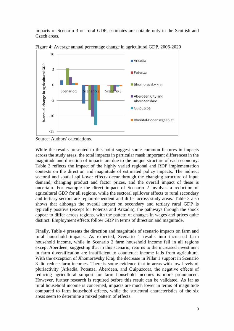
The scenario impacts on agricultural GDP are presented in Figure 4. Estimated

impacts are substantially higher compared to those presented above. In the

Agricultural RDP Scenario, higher investment on agriculture and food processing

result in notable gains in Jihomoravsky kraj (5.4%), Aberdeen (2.5%) and to a lesser

extent, Arkadia (1.5%). In contrast, a diversification strategy (Scenario 2) leads to a

significant decline of agricultural GDP in all areas but Potenza. Further, in both RDP

Scenarios, there seems to be a trade-off between rural and agricultural GDP impacts

in the four diversified economies where Scenario 1 generates rural losses and

agricultural gains, while the opposite is observed in Scenario 2. In contrast, in the two

agriculturally-dependent areas, rural and agricultural impacts of these two Scenarios

are in the same direction. Finally, a decrease in Pillar 1 support generates small

negative impacts on agriculture in all study areas. However, as in the case of the

-1

0

1

2

3

4

5

Scenario 1 Scenario 2 Scenario 3

% a

nn

ual

ch

ange

in r

ura

l GD

PArkadia

Potenza

Jihomoravsky kraj

Aberdeen City and Aberdeenshire

Guipuzcoa

Rheintal-Bodensegeebiet

9

impacts of Scenario 3 on rural GDP, estimates are notable only in the Scottish and

Czech areas.

Figure 4: Average annual percentage change in agricultural GDP, 2006-2020

Source: Authors' calculations.

While the results presented to this point suggest some common features in impacts

across the study areas, the total impacts in particular mask important differences in the

magnitude and direction of impacts are due to the unique structure of each economy.

Table 3 reflects the impact of the highly varied regional and RDP implementation

contexts on the direction and magnitude of estimated policy impacts. The indirect

sectoral and spatial spill-over effects occur through the changing structure of input

demand, changing product and factor prices, and the overall impact of these is

uncertain. For example the direct impact of Scenario 2 involves a reduction of

agricultural GDP for all regions, while the sectoral spillover effects to rural secondary

and tertiary sectors are region-dependent and differ across study areas. Table 3 also

shows that although the overall impact on secondary and tertiary rural GDP is

typically positive (except for Potenza and Arkadia), the pathways through the shock

appear to differ across regions, with the pattern of changes in wages and prices quite

distinct. Employment effects follow GDP in terms of direction and magnitude.

Finally, Table 4 presents the direction and magnitude of scenario impacts on farm and

rural household impacts. As expected, Scenario 1 results into increased farm

household income, while in Scenario 2 farm household income fell in all regions

except Aberdeen, suggesting that in this scenario, returns to the increased investment

in farm diversification are insufficient to counteract income falls from agriculture.

With the exception of Jihomoravsky Kraj, the decrease in Pillar 1 support in Scenario

3 did reduce farm incomes. There is some evidence that in areas with low levels of

pluriactivity (Arkadia, Potenza, Aberdeen, and Guipúzcoa), the negative effects of

reducing agricultural support for farm household incomes is more pronounced.

However, further research is required before this result can be validated. As far as

rural household income is concerned, impacts are much lower in terms of magnitude

compared to farm household effects, while the structural characteristics of the six

areas seem to determine a mixed pattern of effects.

10

Table 3: Direction of sectoral GDP, Employment, Wage and Price effects, Scenario 2

(Diversification RDP)

Arkadia Potenza Jihomora-

vsky Kraj

Aberdeen

&

Aberdeen

-shire

Guipúzcoa

Rhiental-

Bodensee-

gebiet

GDP Agriculture - - - - - -

Rural secondary + - + + + +

Rural tertiary - + + + + +

Employment

Rural secondary + - + + + +

Rural tertiary - + + + + + Wages (Semi) Skilled

Labour - + -

- + +

Unskilled Labour + - - - - -

Prices

Total manufacturing + + - + 0 +

Total services - - - - - - Source: Authors' calculations.

Table 4: Direction and Magnitude of Farm and Rural Household Income Effects

Arkadia Potenza Jihomoravs

ky Kraj

Aberdeen &

Aberdeen

-shire

Guipúzcoa

Rhiental-

Bodensee-

gebiet

Farm Household Income Effects1

Scenario 1 + + + - + n/a

Scenario 2 - - - + - n/a

Scenario 3 - - + - - n/a

Min/Max % Change -8.5/0.3 -25.6/0.1 -0.01/0.02 -10.8/ 3.5 -10.4/0.3 .

Rural Household Income Effects

Scenario 1 -

+ - + - 0

Scenario 2 - - + - + -

Scenario 3 0 - + - 0 0

Min/Max % Change -0.2/ 0 -0.1/0.04 -0.03/0.05 -0.06/0.03 -0.02/0.3 -0.2/0 1 Impact for Small and Large farm Household respectively.

Source: Authors' calculations.

To test the robustness of findings, basic sensitivity tests were carried out. These

included changes in macro-economic closure rules (assumptions of endogenous

foreign savings or savings-driven behavior) and elasticities (doubling of Armington

and production elasticities). Sensitivity results showed little effect on GDP changes,

while although some regional impact signs differ, relative results remain the same.

7. Conclusions

This paper has applied a CGE modeling approach to the ex-ante assessment of the

rural/urban effects of rural policy measures in six selected EU NUTS 3 regions. It can

11

be possibly argued that its contribution is mainly methodological, due to the scale of

regions studied and way RDP policy shocks are implemented to allow for the

capacity-enhancing nature of several RDP measures.

In general, economy-wide effects of both changes in the distribution of Pillar 2 funds

and a decrease in Pillar 1 support are projected to be small. However, these small total

effects mask more significant adjustments at the sectoral or sub-regional level. At the

sectoral level, agricultural GDP is projected to decline if a diversification RDP (Axis

3) strategy is chosen and if Pillar 1 funds decrease. On the contrary, an agricultural

RDP (Axes 1 and 2) strategy benefits agricultural economic activity.

At the sub-regional level, it seems that regional economic structures mediate the

direction and magnitude of policy effects. Indicatively, at least in these case study

regions, a RDP emphasis on economic diversification measures seems to benefit rural

economic activity in regions where the local economy has already diversified. On the

contrary, in local economies which still significantly depend on agriculture or/and are

characterised by weak rural economic linkages, RDP measures oriented towards

agriculture and food processing have the highest welfare effects. This finding might

imply that even in cases where current economic structures do not seem to (currently)

favour a diversification-RDP policy option, rural economic welfare might in the

“longer-term” pursued through development initiatives which increase rural

interdependence and promote rural economic structural change. Last, but not least,

this analysis has shown that an emphasis on coupled Pillar 1 support does not seem to

promote rural economic welfare.

This analysis and its findings could also point out to several policy implications.

Where farm household income is an explicit objective of the CAP, support associated

with agricultural production remains an important determinant of farm household

income. In such cases, it appears difficult to compensate for a reduction in

agriculture-related support through measures aimed at diversification. In terms of

territorial differences, the diversity of results across study areas reinforces the menu-

driven nature of the RDP. Horizontal policies or measures that are implemented using

readily available indicators to represent regional differences, will inevitably fail to

take into account territorial factors that mediate policy impacts.

Finally, this effort has showed that further research is needed on topics such as the

impact of the size and integration of local labour markets, and the spatial distribution

of upstream and downstream firms within a region. Also, further research is needed

on the way that Axis 2 measures are modelled, as in certain contexts (e.g. Southern

Europe), the assumption that measures such as LFA payments “represent” coupled

farm support (instead of income transfers to farm households or enterprises) might be

debatable.

References Baldock, D., Dwyer, J., Lowe, P., Petersen, J-E. and Ward, N. (2001). The Nature of Rural

Development: towards a Sustainable Integrated Rural Policy in Europe. London: Institute for

European Environmental Policy.

Bascou, P., Londero, P., & Munch, W. (2006). Policy Reform and Adjustment in the European Union:

Changes in the CAP and Enlargement. In Blandford, D., & Hill, B. (eds), Policy Reform and

Adjustment in the Agricultural Sectors of Developed Countries. Wallingford: CABI.

Britz, W., Heckelei, T., and Kempen, M. (2008). Description of the CAPRI Modelling System.

Available at: http://www.capri-model.org/docs/capri_documentation.pdf.

12

European Commission (1999). Council Regulation (EC) No 1257/99. Brussels: Official Journal of the

European Union L 160.

European Commission (2005). Council Regulation (EC) No 1698/2005. Brussels: Official Journal of

the European Union L 277.

European Commission (2006). Council Decision on Community Strategic Guidelines for Rural

Development (Programming Period 2007 to 2013). Brussels: Official Journal of the European

Union L 55.

European Commission (2009a). The CAP in Perspective: From Market Intervention to Policy

Innovation. Brussels: Agricultural Policy Perspectives, Brief no 1.

European Commission (2009b). Council Regulation (EC) No 72/2009. Brussels: Official Journal of the

European Union L 30.

European Commission (2009c). Council Regulation (EC) No 73/2009. Brussels: Official Journal of the

European Union L 30.

European Commission (2009d). Council Regulation (EC) No 74/2009. Brussels: Official Journal of the

European Union L 30.

European Commission (2009e). Definition of Rural Areas – OECD Methodology. DG AGRI L2. RD

Network TWG1 Expert Preparatory Meeting, Brussels.

European Commission (2010). The CAP towards 2020: Meeting the Food, Natural Resources and

Territorial Challenges of the Future. Brussels: COM (2010) 672 final.

Gohin, A. and Latruffe, L. (2006). The Luxembourg Common Agricultural Policy Reform and the

European Food Industries: What‟s at Stake? Canadian Journal of Agricultural Economics 54:

175-94.

Hill, B. and Blandford, D. (2008). Where the US and EU Rural Development Money Goes.

Eurochoices 7: 28-29.

Lofgren, H., Harris, R. L. and Robinson, S. (2002). A Standard Computable General Equilibrium

Model (CGE) in GAMS. Microcomputers in Policy Research 5. Washington: IFPRI.

Midmore, P. (1993). Input-Output Forecasting of Regional Agricultural Policy Impacts. Journal of

Agricultural Economics, 44: 284-300.

Midmore, P., Partridge, M.D., Olfert, R., and Ali, K. (2010). The Evaluation of Rural Development

Policy: Macro and Micro Perspectives,. EuroChoices 9: 24-29.

Partridge, M. D. and Rickman, D. S. (2008). Computable General Equilibrium (CGE) Modelling for

Regional Economic Development Analysis. Regional Studies 44: 1311-1328.

Psaltopoulos, D., Thomson, K.J., Efstratoglou, S., Kola, J. and Daouli, A. (2004). Regional SAMs for

Structural Policy Analysis in Lagging EU Rural Regions, European Review of Agricultural

Economics 31: 149-178.

Psaltopoulos, D., Balamou, E. and Thomson, K.J. (2006). Rural-Urban Impacts of CAP Measures in

Greece: An Inter-regional SAM Approach, Journal of Agricultural Economics, 57: 441-458.

Roberts, D. (2005). The Role of Households in Sustaining Rural Economies. European Review of

Agricultural Economics 32: 393-420.

Roberts, D., Pouliakas, K., Psaltopoulos, D. and Balamou, E. (2009). The Rural-Urban Effects of a

Reduction in Farm Support: A Bi-regional CGE Analysis. Paper Presented at the 83rd Annual

Conference of the Agricultural Economics Society, Dublin, 30 March - 1April.

Robinson, S., Cattaneo, A. and El-Said, M. (2001). Updating and Estimating a Social Accounting

Matrix Using Cross Entropy Methods. Economic Systems Research 13: 47-64.

Shucksmith, M., Thomson, K.J. and Roberts, D. (2005) (eds.). CAP and the Regions: Territorial

Impact of Common Agricultural Policy. Wallingford: CAB International.

Thurlow J (2008). A Recursive Dynamic CGE Model and Microsimulation Poverty Module for South

Africa. Washington: IFPRI.

Tongeren, van F., Meijl, van H. and Surry, Y. (2001). Global Models Applied to Agricultural and

Trade Policies: A Review and Assessment. Agricultural Economics 26: 149-172.

Weingarten, P., Neumeier, S., Copus, A., Psaltopoulos, D., Skuras, D. and Balamou, E. (2009).

Building a Typology of European Rural Areas for the Spatial Impact Assessment of Policies :

Final Report, Seville: JRS-IPTS.

i Research on which this paper is based was supported by the EU-funded research project RURAL

ECMOD (Contract 151408-2009 A08-GR). The authors wish to thank Zuzana Bednarikova and

Frantisek Nohel (members of the UZEI research team), as well as Ken Thomson, Kostas Mattas,

Hannu Torma, Lourdes Viladomiu and Thomas Dax for their valuable comments and suggestions.