Georgia State University Georgia State University

ScholarWorks @ Georgia State University ScholarWorks @ Georgia State University

AYSPS Dissertations Andrew Young School of Policy Studies

Fall 10-15-2020

An Examination into Teacher Hiring: Preferences, Efficiency, An Examination into Teacher Hiring: Preferences, Efficiency,

Stability, and Student Outcomes Stability, and Student Outcomes

Katherine Stewart Georgia State University

Follow this and additional works at: https://scholarworks.gsu.edu/aysps_dissertations

Recommended Citation Recommended Citation Stewart, Katherine Georgia State University, "An Examination into Teacher Hiring: Preferences, Efficiency, Stability, and Student Outcomes." Dissertation, Georgia State University, 2020. doi: https://doi.org/10.57709/20346038

This Dissertation is brought to you for free and open access by the Andrew Young School of Policy Studies at ScholarWorks @ Georgia State University. It has been accepted for inclusion in AYSPS Dissertations by an authorized administrator of ScholarWorks @ Georgia State University. For more information, please contact scholarworks@gsu.edu.

ABSTRACT

AN EXAMINATION INTO TEACHER HIRING: PREFERNCES, EFFICIENCY, STABILITY,

AND STUDENT OUTCOMES

BY

KATHERINE ANN STEWART

October 2020

Committee Chair: Dr. Tim Sass

Major Department: Economics

This dissertation studies teacher hiring practices, an avenue to potentially raise teacher

quality which has not been studied extensively. I analyze three aspects of the teacher hiring

process, which, if improved, could promote education quality: the principal hiring decision, the

teacher application decision, and the effects of information on teacher behavior and market

outcomes in the teacher labor market. The first two are empirical studies utilizing administrative

data from an urban school district, and the last is a laboratory experiment.

Education is a labor focused enterprise where outcomes are largely determined by teacher

quality, so hiring the most productive teachers is paramount. Hiring is even more important

given that teaching is a high-turnover profession, thus hiring occurs frequently. I first compare

the elements of a teacher’s application that predict principal hiring decisions to those predicting

teacher performance and retention outcomes. Similar to other recent work, I find disparities

between the two sets of predictors. I utilize additional methods to study the relation of the size

and quality of the applicant pool, as well as how those factors relate to the quality of the selected

candidate. The results indicate that the applicant pools do not systematically vary by school

characteristics in an obvious manner. Also, while the quality of the candidate pool may influence

principal hiring decisions, it is not the dominate factor.

Given that teaching sorting across schools occurs in the new-teacher labor market (Sass,

et al. 2012) and in post-hire differential patterns of teacher mobility,1 which in turn create

disparities in access to effective teachers, it is important to understand the mechanisms that lead

to teacher sorting across schools. In chapter 2, I study how teacher application behavior reveals

teacher preferences over schools. The preferences can lead to differences in application pools,

thereby affecting principals’ ability to hire quality candidates. I find that the application

decisions of new-to-the-district candidates may be affected by accountability pressures or the

resource level in high-needs schools, but current teachers’ revealed preferences agree with those

previously found in the research literature.

It has also been found that a teacher’s compatibility with a school can affect their ability

to improve student outcomes and their own satisfaction (which decreases mobility, thereby

increasing experience and decreasing turnover costs). In my third chapter, I use a laboratory

experiment to examine teacher and school behavior and their effects on outcomes in a controlled

setting while varying the preference structure of the market and the information agents have on

competitors’ actions. I find that information on competitor behavior affects signaling behavior

and the market efficiency and payoffs, but that these effects are dependent on the preference

structure. I also find that the preference structure affects the stability of the matches.

1 Darling-Hammond, 2001; Viadero, 2002; Gordon & Maxey, 2000; Goldhaber et al., 2007; Feng & Sass, 2017

AN EXAMINATION INTO TEACHER HIRING: PREFERNCES, EFFICIENCY, STABILITY,

AND STUDENT OUTCOMES

BY

KATHERINE ANN STEWART

A Dissertation Submitted in Partial Fulfillment

of the Requirements for the Degree

of

Doctor of Philosophy

in the

Economics Department – Andrew Young School of Policy Studies

of

Georgia State University

GEORGIA STATE UNIVERSTIY

2020

Copyright by

Katherine Ann Stewart

2020

ACCEPTANCE

This dissertation was prepared under the direction of the candidate’s Dissertation

Committee. It has been approved and accepted by all members of that committee, and it has been

accepted in partial fulfillment of the requirements for the degree of Doctor of Philosophy in

Economics in the Andrew Young School of Policy Studies of Georgia State University.

Dissertation Chair: Dr. Tim Sass

Committee: Dr. Jonathan Smith

Dr. Vjollca Sadiraj

Dr. Ross Rubenstein

Electronic Version Approved,

Mary Beth Walker, Dean

Andrew Young School of Policy Studies

Georgia State University

October, 2020

iv

Dedication

I dedicate my dissertation to my family and friends. My parents, John and Gay Stewart,

and sister, Bernadette Stewart, supported me emotionally and physically to complete the program

with a wealth of humor and care. Many friends supported me to completing this dissertation and

program, but a special thanks must be given to Alicia Plemmons who was ready to edit a paper if

needed and always gave me an ear for my emotional wellbeing and research planning.

v

Acknowledgements

I never could have completed this dissertation without my family, friends, and mentors.

Dr. Tim Sass not only invested a level of time and care I would expect of a family member, but

he is also the individual that reminded me that education research is my true passion and helped

me to find the direction I wanted to take professionally. My committee members Jon, Vjollca,

and Ross all gave crucial support and direction on my research to promote its quality and create a

thesis of which I am truly proud. I also need to thank the other students of the program who gave

me help and inspiration whenever it was needed. I also need to acknowledge Skye Duckett who

was an excellent partner to my research and showed me how fulfilling it can be to directly work

with experts in the field to improve policy. Lastly, I need to recognize the generous Dan E.

Sweat dissertation fellowship and the CEAR Small-Scale Project Support for supporting my

ability to complete this dissertation.

vi

Table of Contents

Dedication ....................................................................................................................... iviii Acknowledgements ............................................................................................................. v

Table of Contents ............................................................................................................... vi List of Figures .................................................................................................................. viii List of Tables ..................................................................................................................... ix Introduction ........................................................................................................................ xi 1 Missed Opportunities or Making the Best of Bad Situations? Principal Selection of Teacher

Applicants ........................................................................................................................... 1 1.1 Introduction ............................................................................................................... 1

1.2 Literature Review...................................................................................................... 7

1.3 The Studied School District .................................................................................... 12

1.3.1 The School District’s Hiring Process ............................................................... 12

1.3.2 Measures of Teacher Quality ........................................................................... 14

1.3.3 The Data ........................................................................................................... 15

1.3.4 The Analysis Sample ....................................................................................... 16

1.4 Methods ............................................................................................................... 18

1.4.1 Poor Decision Making?.................................................................................... 18

1.4.2 Or Making the Best of Bad Situations? ........................................................... 21

1.5 Findings ............................................................................................................... 24

1.5.1 Evidence of Poor Decision Making ................................................................. 24

1.5.2 Evidence of Making the Best of Bad Situations .............................................. 26

1.6 Policy Discussion and Next Steps........................................................................... 31

1.7 Tables ............................................................................................................... 34

1.8 Appendix 1 .............................................................................................................. 47

2 Where They Stop Nobody Knows: What Drives Teacher Placement Decisions? ......... 53 2. 1. Introduction ........................................................................................................... 53

2.2. Literature Review................................................................................................... 57

2.3. The School District’s Hiring Process ..................................................................... 60

2.4. Data ............................................................................................................... 61

2.4.1 Partner District Administrative Data ............................................................... 61

2.5. Model ............................................................................................................... 61

2.5.1 Research Question: Which Schools are more likely to Receive Applications?63

2.6. Results ............................................................................................................... 65

2.7. Conclusion ............................................................................................................. 72

2.8. Tables ............................................................................................................... 75

vii

3. Who Knew? An Experimental Examination of Information Effects on a Teacher Labor Market

........................................................................................................................................... 89 3.1 Introduction ............................................................................................................. 89

3.2 Literature Review: .................................................................................................. 93

3.3 Theoretical Model ................................................................................................... 98

3.3.1 Assumptions ..................................................................................................... 98

3.3.2 Information Environment................................................................................. 98

3.3.3 Wage Structure................................................................................................. 99

3.3.4 Investment ...................................................................................................... 100

3.3.5 Matching Mechanism..................................................................................... 102

3.3.6 Market Efficiency and Payoffs ...................................................................... 103

3.3.7 Market Stability ............................................................................................. 104

3.3.8 Risk ................................................................................................................ 104

3.4 Experimental Design ............................................................................................. 105

3.4.1 Treatments...................................................................................................... 105

3.4.2 Implementation .............................................................................................. 106

3.5 Results ............................................................................................................. 109

3.5.1 Signaling Decision ......................................................................................... 110

3.5.2 Market Efficiency and Payoffs ...................................................................... 113

3.5.3 Market Stability ............................................................................................. 114

3.6 Conclusion ............................................................................................................ 115

3.7 Tables ................................................................................................................ 116

3.8 Figures............................................................................................................... 131

3.9 Appendix A. Strategic Behavior ....................................................................... 138

Bibliography ................................................................................................................ 141

viii

List of Figures

Figure A1.1. Relation of GPA of First Selected Candidates to Number of Applicants and Portion

of the Pool with a High GPA…………………………………………………….………………50

Figure A1.2. Relation of GPA of All Selected Candidates to Number of Applicants and Portion

of the Pool with a High GPA………………………………………………….………………....51

Figure 3.1. Simultaneous Investment Screen………………………………….………………..131

Figure 3.2. Sequential Investment Screen……………………………………..………………..131

Figure 3.3. Firm Investment Screen………………………………………………….…………132

Figure 3.4. Worker Decision Screen - Offer……………………………………………………132

Figure 3.5. Worker Decision Screen - No Offer………………………..………………………133

Figure 3.6. Match Outcome All Market Members…………...…………………………………133

Figure 3.7. Match Outcome Payoff Screen…………………………..…………………………134

Figure 3.8. Risk Task Example………………………………………………………................134

Figure 3.9. Investment Scatter Plot-All Workers……………………………………………….135

Figure 3.10. Investment Scatter Plot –Information Treatment and Same Preferences…………135

Figure 3.11. Investment Scatter Plot –Information Treatment and Different Preferences…..….136

Figure 3.12. Investment Scatter Plot –Not Information Treatment and Same Preferences.....…136

Figure 3.13. Investment Scatter Plot –Not Information Treatment and Different Preferences...137

ix

List of Tables

Table 1.1 Candidate and Hires Characteristics…………………………………………..….…...34

Table 1.2 School and Principal Characteristics of the Schools who Hired Applicants….….…...35

Table 1.3 Summary Statistics of Outcome Variables………………………...…………….……36

Table 1.4 Estimates of the Determinants of Hiring Requests, Teacher Productivity, Teacher

Persistence and Teacher Attendance (All Applicants) …………..…………….….…..….…..….37

Table 1.5 Estimates of the Determinants of Hiring Requests, Teacher Productivity, Teacher

Persistence and Teacher Attendance (New Applicants) …………………….…….…..….…..…38

Table 1.6 Number and Quality of Applicants by School Characteristics and by Subject Area...39

Table 1.7 Estimates of the Determinants of the Candidate Pool Size and Quality…..…..….…..40

Table 1.8 Estimates of the Determinants of the Grade Point Average of the Applicants who were

Selected by Principals for their first request……………………………….…..….…..….….…42

Table 1.9 Estimates of the Determinants of the Likelihood of Being Selected for a Hiring

Request – All Applicants and Positions Combined Versus Separate Pools for Each Position…..44

Table 1.10 Estimates of the Determinants of the Likelihood of Being Selected for a Hiring

Request – All Applicants and Positions Combined Versus Separate Pools for Each Position (New

Applicants) ………………………………………..…………………….….…..….…..….….....45

Table 1.11 Alternative Specific Conditional Logistic Regression of Principal Hiring Choice

(Marginal Effects) ……………………………………….………………………….…..….…....46

Table A1.1 Principal Decision Using Hired instead of Hiring Request……………...….….…...47

Table A1.2 Estimates of the Determinants of the Grade Point Average of the Applicants who

were Selected by Principals for all their Requests……………………….…………….………...48

Table A1.3 Alternative Specific Conditional Logistic Regression Selection Probabilities….…..52

x

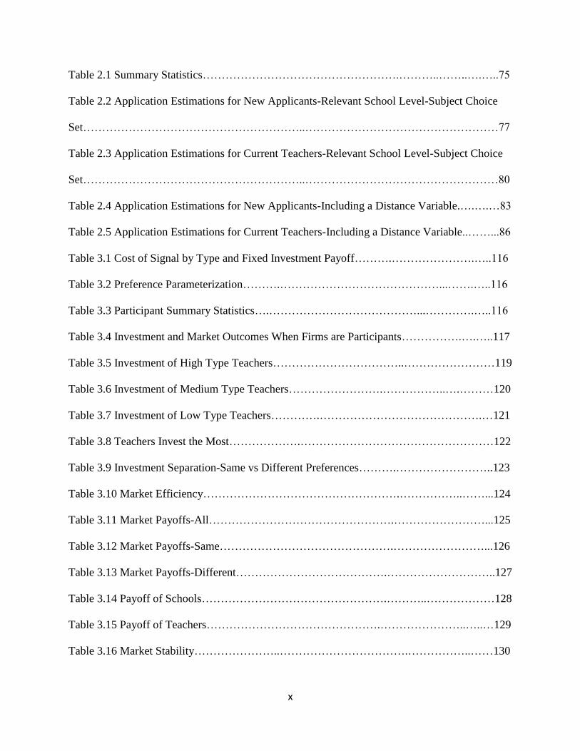
Table 2.1 Summary Statistics…………………………………………….………..……..….…..75

Table 2.2 Application Estimations for New Applicants-Relevant School Level-Subject Choice

Set…………………………………………………..……………………………………………77

Table 2.3 Application Estimations for Current Teachers-Relevant School Level-Subject Choice

Set…………………………………………………..……………………………………………80

Table 2.4 Application Estimations for New Applicants-Including a Distance Variable.….….…83

Table 2.5 Application Estimations for Current Teachers-Including a Distance Variable..……...86

Table 3.1 Cost of Signal by Type and Fixed Investment Payoff……….………………….…..116

Table 3.2 Preference Parameterization……….……………………………………...…….…..116

Table 3.3 Participant Summary Statistics….…………………………………...………….…..116

Table 3.4 Investment and Market Outcomes When Firms are Participants…………….….…..117

Table 3.5 Investment of High Type Teachers……………………………..……………………119

Table 3.6 Investment of Medium Type Teachers…………………….……………..….………120

Table 3.7 Investment of Low Type Teachers………….…………………………………….…121

Table 3.8 Teachers Invest the Most……………….……………………………………………122

Table 3.9 Investment Separation-Same vs Different Preferences……….……………………..123

Table 3.10 Market Efficiency…………………………………………….……………..……...124

Table 3.11 Market Payoffs-All………………………………………….……………………...125

Table 3.12 Market Payoffs-Same……………………………………….……………………...126

Table 3.13 Market Payoffs-Different………………………………….………………………..127

Table 3.14 Payoff of Schools………………………………………….………..………………128

Table 3.15 Payoff of Teachers……………………………………….…………………..…..…129

Table 3.16 Market Stability…………………..…………………………….……………..……130

xi

Introduction

There are many possible avenues for improving teacher quality, including pre-service

training, professional development, performance-based compensation, and selective retention.

While these mechanisms have been studied extensively, until recently there has been little

attention paid to another potentially efficient means of raising teacher quality: improving the

system for selecting and hiring teachers. In this dissertation, I research three aspects of teacher

hiring that could be adjusted to promote education quality, if they were better understood. The

first chapter examines how principals make hiring decisions. The second chapter uses teacher job

applications as a tool to understand teacher preferences over place of employment. These

chapters are both empirical works applicant and employment data for an Atlanta metropolitan

area school district. The third chapter utilizes a lab experiment designed to provide preliminary

evidence regarding the effects of information on competitor behavior in a school district’s hiring

process on signaling investment and the match outcomes between schools and teachers.

In the first chapter, I investigate principals’ decisions during the hiring process. Hiring

the most productive workers is paramount in service sectors where human resources are the

primary input. This is particularly true in education, where teachers are the most important factor

in promoting student achievement and turnover is considerable, which in turn leads to substantial

hiring on a persistent basis. I study the hiring decisions of principals using data on applicants for

teaching positions in a mid-sized urban school district. I compare characteristics of teaching

candidates that are associated with a higher likelihood of receiving a job offer with those that

enhance productivity as a teacher. Similar to other recent work, I find multiple instances where

the factors driving hiring decisions do not align with the factors associated with teacher

productivity. Other studies infer this misalignment is due to a lack of information or incorrect

xii

choices on the part of principals and suggest an appropriate policy response would be to provide

better information to principals or to reduce principal discretion and centralize hiring decisions.

In contrast, I account for the fact that work environments differ across schools and thus different

principals face de-facto different pools of teaching candidates. I find that the quality of the pool

may affect principal decisions, but that the pool does not systematically vary by school

characteristics within the system in an obvious manner.

In the second chapter, I study how differences in teacher preferences can affect the

variation in makeup of the applicant pool across schools. Given the importance of teachers in

determining student outcomes, policymakers are concerned that teacher sorting across schools

may limit access to high-quality teachers for minority, impoverished, or low-performing

students. Teacher sorting may occur in the new teacher labor market (Sass, et al. 2012) as well as

through post-hire differential patterns of teacher mobility.2 It is possible that disparities in access

to high-quality teachers can be mitigated by targeted hiring and retention policies.3 I restructure

the data used in Chapter 1 to represent the choice set of the teachers. I implement a conditional

logistic model to estimate the impacts of school characteristics on prospective and current

teachers’ application likelihoods. I find evidence that the applicants who are new to the district

may be attracted to high-needs schools which may have greater resources. However, the

application probabilities of current teachers coincide with the findings of prior research.

Outside of a teachers’ baseline ability, their school compatibility (Jackson 2013) and

experience4 also affects their ability to improve student outcomes. Teacher satisfaction within a

2 Darling-Hammond 2001; Viadero 2002; Gordon and Maxey 2000; Goldhaber, Gross, and Player 2007; Feng and Sass 2017 3 Adnot, Dee, Katz, and Wycoff 2017 4 Chingos and Peterson 2011; Staiger and Rockoff 2010; Rivkin, Hanushek, and Kane 2005; Clotfelter, Ladd, and Vigdor 2006;

Dobbie 2011; Wiswall 2013; Papay and Kraft 2015; Rockoff 2004

xiii

school leads to prolonged tenure, which naturally increases experience. Extending the length of

time a teacher remains in a school also decreases the pecuniary and non-pecuniary turnover costs

to schools.5 Therefore, in attempting to provide quality education, it is imperative to understand

how the hiring process affects teacher-school matches. My third chapter utilizes a laboratory

experiment to examine teacher and school behavior. This is a simplified teacher labor market

modeled through a two-sided matching markets framework. I introduce information asymmetry

by making teacher quality unknown to employers. Teachers then signal their quality through a

costly signal, either simultaneously or sequentially, where later applicants observe prior

signaling investment amounts. In addition, I examine two preferences rankings to ensure the

effects found are not driven by the enforced preferences. The matching procedure School Hiring

(SH), designed by mimicking a current hiring policy of a metropolitan Atlanta school district

hiring process, is very similar to the Priority (Boston) matching procedure. I find that the effects

of participants having additional information on competitor investment amounts and participant

payoffs are dependent on the structure of the preferences, In addition, the information treatment

decreases the portion of the time that investments are type revealing. The market stability is

unaffected by the information treatment, but is higher when the preferences of participating

agents are homogenous.

5 Milanowski and Odden 2007; Guin 2004

1

1 Missed Opportunities or Making the Best of Bad Situations? Principal

Selection of Teacher Applicants

1.1 Introduction

Creating the best match between employees and employers has long been shown to

improve productivity, satisfaction, and employee tenure (Liu & Johnson, 2006; Koch &

McGrath, 1996). To create successful matches, both job seekers and firms must gather

information regarding their counterparts in order to choose an optimal employment match.

However, existing research regarding employers’ search for employees is somewhat limited,

particularly regarding the reasons and beliefs informing hiring decisions in the public sector.

This paper examines employer search in the context of the public school teacher labor

market in a mid-size urban school district. As the teaching profession is one wherein the quality

of workers substantially affects the benefits accrued by their students, both short-run academic

achievement and labor market outcomes as adults, the characteristics of the labor market are of

considerable policy importance (Rivkin, Hanushek, & Kain, 2005; Aaronson, Barrow, & Sander,

2007; Kane, Rockoff, & Staiger, 2008; Chetty et al., 2011; Chetty, Friedman, & Rockoff, 2014).

Given that researchers have demonstrated the ability of careful hiring to improve the average

worker’s productivity in several professions, and that teaching is a profession with substantial

amounts of employee turnover (Darling-Hammond, 2001; Viadero, 2002) and, therefore,

persistent hiring, improving the teacher-hiring process could significantly impact the quality of

employees in this field. Compared to other school-based methods used to improve teacher

performance (performance pay, selective retention, and professional development) employing

hiring as a policy lever to promote performance has potential advantages, such as fewer

implementation barriers or being more cost effective.

2

Furthermore, preventing sub-par teacher hires is crucial as there are significant barriers to

removing low-performing teachers (Griffith & McDougald, 2016; Painter, 2000; Levin et al.,

Schunck, 2005), and those students taught by the low-performing teachers are permanently

affected by their teachers’ relative lack of performance quality. Studying the teacher labor

market is also particularly advantageous for research on employer search, as schools collect

productivity measures of those hired so that the quality of the employer's choice can be

evaluated.

There are constraints on a principal’s ability to hire the best teacher; these barriers, if

acknowledged, could potentially be circumvented in order to ultimately improve hiring

outcomes. For example, the hiring process may not provide enough information for principals to

identify superior teachers (Liu & Johnson, 2006; Donaldson, 2013; Neild et al., 2003;

DeArmond et al., 2010; Bruno & Strunk, 2019; Jacob et al., 2018), or the principals may not use

the information they have (Jacob et al., 2018; Bruno & Strunk, 2019). A principal could be too

inexperienced with the hiring process to successfully find and hire the best candidate (Loeb et

al., 2012; Dipboy & Jackson, 1999). In addition, teacher salary schedules are often fixed, so

superior teachers may seek higher paying employment in other fields or districts (Imazeki, 2005;

Feng, 2014; Feng, 2009). Procedural barriers also exist that may inhibit a principal’s ability to

hire superior teacher candidates: late leave notices, insufficient human resources staff, and delays

associated with collective bargaining and belated budgets (e.g. Levin & Quinn, 2003; Liu et al.,

2008; Strunk et al., 2018; Levin et al., 2005; Odden & Kelley, 2008; Campbell et al., 2004; Bassi

& McMurrer, 2007; Flandez, 2009; Grensing-Pophal, 2017; Ryan et al., 2000; Converse et al.,

2004). In addition to these constraints, principals also work in a non-profit sector so they may

3

make choices to maximize their own utility rather that to maximize educational output, such as

selecting teachers with amenable personalities regardless of quality.

Jacob et al. (2018) and Bruno and Strunk (2019) study principal hiring choices in

Washington, DC and Los Angeles, CA, respectively. The two papers employ a similar strategy;

they use pooled district-wide data to estimate both the relationship between candidate

characteristics and the likelihood of being hired and the relationship between candidate

characteristics and subsequent teacher performance. They then compare the factors that are

correlated with hiring and the factors that are associated with teacher performance. These two

papers find that some candidate information and hiring procedures correlate with teacher

performance; however, discrepancies between the predictors of principal hiring decisions and the

predictors of teacher performance suggest that principals may not be making the best hiring

decisions and thus there may be room for improvement in the teacher hiring process.

The use of pooled district-wide data in previous studies to compare the factors driving

hiring decisions with those determining teacher performance appear to be a function of data

availability. In the case of the District of Columbia Public Schools (DCPS), prospective teachers

could apply for a recommendation through a centralized process called TeachDC, or they could

apply directly to a school. During the period studied by Jacob, et al. (2011-2013), about half of

new hires came from candidates in the TeachDC system. Jacob and co-authors only had access

to applications submitted through TeachDC and could not observe candidates who applied

directly to individual schools. They examined the relationship between scores on the

components of the recommendation, as well as getting recommended, on the probability of being

hired and eventual performance as a teacher. In the Los Angeles Unified School District

(LAUSD), all applications for teaching were submitted through a centralized application system.

4

Neither Jacob et al. or Bruno and Strunk indicate that applicants to the centralized system could

indicate preferences for a particular school or schools. Yet both papers make clear that no matter

how applications were initially received, hiring decisions were decentralized. In both DCPS and

LAUSD, principals or other site administrators decided which candidates would be offered a

teaching position.

Pooling data across schools makes the implicit assumption that every principal within a

given district has access to the same teacher applicant pool and that candidates have no outside

options. Even though all teachers who meet the district standards might be in a single “available”

pool (as in LAUSD), the de-facto applicant pool could be still vary widely between schools,

based on teacher preferences and opportunity costs. In this paper I consider not only the district-

wide pool of prospective teachers, but also the pool of candidates who apply for a position at a

particular school.

This research delves into factors that may lead an apparent discrepancy between the

candidate who is expected to be the most effective teacher and the candidate actually selected by

the principal, previously interpreted as principals making poor hiring decisions. Each possible

factor has a significantly different policy implication, which will be included in the policy

discussion section. Principals must compete against each other in order to hire quality

candidates, which causes principals to be uncertain of being able to successfully hire a candidate.

Aspects of this competition between principals, such as attractiveness of one’s position and the

loss of potential alternate candidates while waiting for the outcome of an extant offer, means

principals may make strategic selections regarding which candidate to attempt to hire.

As this research seeks to go beyond prior district-wide analyses, I first establish that there

are differences between the hiring and performance predictions for the studied school district as a

5

whole, in similar manner as the prior work by Jacob et al. and Bruno and Strunk. In contrast to

prior work, which measures actual hires, I consider the earlier decision of initiating a request to

offer a position to a candidate. This change in approach allows the choices of the teacher and the

district to be disentangled from the decisions of the principal. Jacob et al. also examined offer

choices briefly, but found it had few differences from hires and thus did not examine the decision

closely. In addition to disentangling the applicant choice like the offer does, the hiring request

decision also precludes the district rejecting the principal’s choice.

I also analyze the systemic variation in the applicant pool and how this variation may

affect the relationship between characteristics of the candidate pool and the selected candidate,

while controlling for position, school, and principal characteristics. Given that college GPA

predicts multiple measures of teacher performance in my teacher quality estimations, I use it as

my measure of candidate quality.6 Then I directly estimate the relationship between pool

characteristics and selected teacher candidate quality. Since the applicant pool may affect the

principals’ decisions, I then use conditional logistic specifications to estimate the principals’

hiring decisions in the context of the pools of applicants available to them.

When I follow the approach of prior researchers and pool all candidates districtwide, I

find that principals over-select transfer candidates as well as those candidates with education

majors or teaching certification, while also under-selecting candidates with high college GPAs

and those who on average apply quickly after the position is posted. As GPA is a non-malleable

characteristic of job candidates that seems to be indicative of superior teacher performance on

several measures, it is a good candidate for use in a screening policy based on these initial

6 This is a strong assumption but characterizing teacher quality has always been difficult. In my analysis of the relationship

between candidate characteristics and teacher performance, college GPA is the most consistent statistically significant predictor.

6

results. However, when examining how the characteristics contextualizing the hiring decision

(the school, the principal, the subject, the applicant pool) relate to the college GPA of the

selected, I find that schools with better and larger applicant pools select candidates with higher

college GPAs. This result suggests that variation in principals’ offer decisions could be driven in

part by differences between applicant pools.

Furthermore, when controlling for different applicant pools using conditional logistic

regression, I find that teaching certification, education majors (for only the new sample), and

finding a job through another district employee, no longer affect hiring-request decisions, and

thus no longer present a contradiction between their estimated impacts on hiring requests and

performance indicators. This finding suggests that a portion of the apparent mismatch is due to

assuming that all principals within a district face the same applicant pool. However, these results

may be the result of statistical noise.

This research contributes to the employer search literature through additional empirical

analysis of employer decision-making when applicant pools are endogenous and hiring managers

compete for quality applicants. In addition, this research focuses on identifying why a principal

might select candidates who do not appear to the best qualified, while previous research on

principal hiring decisions implicitly assumes the selection and performance misalignment results

entirely from the principal’s lack of information or poor choices. Finally, rather than measure

employment outcomes, which are a function of both employment offers and candidate

acceptances, this research analyzes principals’ hiring requests, data on which have not previously

been available. The advantage of this approach is that it isolates employer decision making,

whereas employment outcomes are a function of employer (principal), organization (district),

and candidate decisions.

7

1.2 Literature Review

As this paper studies factors which can influence hiring decisions, the literature review

discusses the existing relevant research regarding the decisions hiring managers make and

various aspects of the hiring process. This includes a brief review of the employer search

literature. Then the research on how hiring manager choices are affected by the uncertainty over

a candidate’s commitment to the firm (either prospective tenure or willingness to accept an offer)

and competition over quality candidates. In addition, the research on how applicant pools can

differ will be reviewed. This section will finish with a discussion of the existing research on the

information that influences hiring managers’ decisions and the prior findings on how principals

use information, as well as my contributions to these research areas.

Most of the empirical employer search literature has focused on vacancy duration (e.g.,

Andrews et al., 2008; van Ours & Ridder. 1991; Barron et al., 1987; Gorter et al. 1996) or

recruitment and screening methods (e.g. Murphy, 1986; Barron et al. 1985; Holzer, 1987; Russo

et al., 2000; DeVaro, 2005; Hoffman, et al., 2018; Burks, et al. 2015; Barling et al. 2009). Much

of the research on employer candidate selection has been theoretical or experimental, especially

in situations where employers compete for high-quality candidates, and each firm has an

endogenous sets of applicants (Spence 1973; Immorlica et al., 2006; Vanderbei 2012;

Abdulkadiroğlu & Sönmez, 2003; Abdulkadiroğlu et al., 2005; Ergin & Sönmez, 2006; Chen &

Sönmez, 2006; Galperin et al., 2019). Outside of studying employee referrals, there has been

relatively little empirical analysis of the reasoning firms use to select a given candidate (Coles et

al., 2010; Fahr & Sunde, 2001).

To understand how a hiring manager’s perceptions of a candidate’s commitment to a firm

affect hiring decisions, Galperin et al. (2019) conducted an online experiment. They find that

8

hiring managers trade some amount of candidate capability for perceived organizational

commitment. Commitment takes the form of valuing the firm more or staying with the firm

longer. They did not find evidence that the choice of candidate was affected by the manager’s

beliefs regarding offer acceptance.

Although a candidate’s probability of accepting an offer had no effect on the hiring

managers’ decisions in Galperin et al. (2019), its affects have been shown in other hiring

situations. In theoretical labor markets covered under the umbrella of “Secretary Games,”

employers compete against each other for high-quality candidates. The research in this area finds

that competition results in earlier offers, and can also lead to the use of “exploding offers” (offers

that candidates are given a short time frame to consider) in order to pressure better candidates to

accept (Immorlica et al., 2006; Vanderbei 2012; Fahr & Sunde 2001).

The literature on how to match two pools of people, such as matching employers to

employees, called the Matching Markets literature, shows several circumstances where a

participant may not choose their top candidate as part of a strategic choice. In particular, hiring

managers have a rank-ordered list of candidates regarding quality; however, each candidate also

has an acceptance probability. Hiring managers may issue offers to candidates lower on the

quality ranking who have higher acceptance probabilities to minimize the risk of losing certain

employee candidates.

A set of studies that analyze how Boston public schools matched students to schools

demonstrates strategic selection in a matching market. Students were assigned a school at which

they had priority acceptance and were then asked to rank all the schools according to where they

would most like to attend. Students who strategically ranked their schools (listed the best schools

they could enter first) got into better schools compared to those who ranked schools strictly

9

according to where they would prefer to attend (Abdulkadiroğlu & Sönmez, 2003;

Abdulkadiroğlu et al., 2005; Ergin & Sönmez, 2006; Chen & Sönmez, 2006).

In the economics academic job market, a similar phenomenon happens. Employee

candidates apply to a large number of positions, but universities have a limited number of

interview slots. The universities could easily fill all their interview slots with top candidates, but

these top candidates have low chances of accepting if they are eventually given an offer. So the

universities act strategically and assign some of their interview spots to less appealing candidates

who have a higher likelihood of later accepting an offer (Coles et al., 2010).

Employer search is partially a function of the pool of candidates who applied to the job.

A firm cannot select the best candidate if the candidate never applies. However, applicant pools

can endogenously vary between jobs and locations. For example, Manning (2000) found that

pecuniary and non-pecuniary aspects of the job affect the number of applicants to a vacancy for

low-wage jobs. For teachers trying to match to jobs, Boyd et al. (2013) finds teachers strongly

prefer certain non-pecuniary aspects of schools, including location and student demographics.

These teacher preferences can cause considerable variations among schools in the pools of

applicants they select from. A great deal of additional research demonstrates that the preferences

of already-employed teachers are consistent with the applicants’ preferences found in Boyd et al.

(2013) (e.g. Sass et al., 2012; Levin & Quinn, 2003; Liu et al., 2008; Hanushek & Rivkin, 2007;

Boyd et al., 2011; Lankford et al., 2002; Imazeki, 2005; Scafidi et al., 2007).

In addition to the external factors in hiring, hiring managers must also be able to discern

candidate quality using the information they gather. Hiring managers have access to candidate-

supplied information from applications and resumes. The hiring managers may also gather

information through their professional networks and by conducting candidate interviews. This

10

private information is the most interesting and also the most troublesome. The sheer amount of

research on the importance of the interview to information gathering and decision-making is

staggering. This voluminous research points yields two broad conclusions. First, the interview is

heavily relied on by hiring managers (e.g. Rutledge et al., 2008; Schmidt & Hunter, 1998).

Second, hiring managers who ignore firm-based screens of candidates in favor of their interview

results often hire lower performing candidates (Dipboye & Jackson, 1999; Hoffman et al., 2018).

This reliance on interviews is often explained as the hiring manager being biased or mistaken in

their information usage. Another source of private information is a hiring manger’s professional

network. This informal information gathering is hard to capture, so the research has mainly

focused on employee referrals. Several studies find that hiring managers use referrals to decrease

the uncertainty regarding the candidate’s acceptance of a job offer and tenure with the firm

(Dustmann et al., 2016; Burks et al., 2015).

Two papers have examined how principal information usage in the hiring decisions

compares to the information related to teacher quality, Jacob et al. (2018) and Bruno and Strunk

(2019). Jacob et al. (2018), studies the effects of Washington DC Public School’s 2011

implementation of a recommendation process. Teacher candidates participated voluntarily, and

those who took part completed several screens (e.g., interviews, sample lessons, and written

assessments). Then a recommended list containing candidates who passed every screen was

distributed to principals, as was all the information gathered during the process. The authors find

that while principals use the recommendation in their hiring decisions, they do not use the

component scores that determine recommendation status. They also find that the candidate

characteristics that are correlated with teacher performance are not the same characteristics as

those that are associated with principal hiring decisions. In some cases characteristics that are

11

positively associated with better teacher performance (e.g. SAT scores and college GPAs) are

actually negatively correlated with the probability of being hired. These results suggest that

principals undervalue some attributes that are indicative of superior teacher performance. If true,

this suggests that modifying the selection process could improve the average quality of hired

teachers.

Bruno and Strunk (2019) analyzes the teacher hiring process in the Los Angeles Unified

School District. The researchers find that the overall score on a multi-component screening

system predicts principal hiring decisions, teacher attendance, teacher impact on student test

scores, and teacher evaluation scores, but not teacher retention within the district. However, the

way individual components of the screening system correlate with the teacher quality measures

varies considerably, highlighting the potential multi-dimensionality of teacher quality. Bruno and

Strunk find that the adoption of the screening system as a whole improves teacher quality in the

district relative to the average quality of teachers in similar districts. They also find that while the

scores on screens are predictive of some teacher outcomes, they are not strongly correlated with

hiring decisions, echoing the findings in Jacob et al. (2018).

This paper expands on the extant hiring research in several ways. Few researchers have

had access to all job applications, hiring requests, and performance outcomes of hired workers,

particularly for public-sector occupations. This paper, using unique data, adds to the empirical

research on employer search and decision making under competition with endogenous applicant

pools. The previous principal hiring-decision research established that there is misalignment

between statistical predictors of principal hiring choices and teacher performance at the district

level (Jacob et al., 2018; Bruno & Strunk, 2019). The current paper seeks to understand why

these misalignments may occur and determine if they are they are the result of poor decisions by

12

principals. First, I will determine if the districtwide misalignments uncovered in Los Angeles and

Washington, DC also occur in the district I study. Second, I will investigate whether there is

significant variation in the pools of candidates that schools attract and whether the misalignment

between candidate characteristics that are associated with teacher quality and the traits that

predict whether a principal makes a request to hire a candidate continue to appear when

comparisons are made at the school level rather than at the district level.

1.3 The Studied School District

1.3.1 The School District’s Hiring Process

For the past several years, the studied school district, located in the Atlanta metropolitan-

area, implemented a series of changes intended to improve the teacher hiring process. Before

these changes, teacher candidates would apply online to the district for open positions, and then

the district simply conducted a background and credential check before posting a candidate’s

information to a hiring portal that is accessible to principals. In December 2015, the district

initiated the use of the GALLUP TeacherInsight exam, which was meant to check the

candidate’s compatibility with the school district. The Human Resources (HR) department set 70

out of 100 to be a passing score on the GALLUP assessment and encouraged principals to hire

candidates with a passing score. Initially, however, candidates were not required to complete the

test to be considered for a position, and principals did not have to limit their selection to

candidates with a passing score. In January 2019, passing the test became a requirement to enter

the teacher candidate pool.

In January 2017, following a pilot period, the district introduced a video interview tool,

HireVue. Candidates were not required to submit a video, and completing a HireVue interview

continues to be voluntary. Beginning the next year, in 2018, a group of 24 trained teacher-leaders

13

started scoring the video interviews on a five-point scale, though the scoring was only for

candidates applying before the end of May. The HR Department then posts both the video and

the accompanying score to the hiring portal. Principals were encouraged to select candidates with

a score of three or above. The present analysis does not include the HireVue scores due to the

limited number currently available.

The principals may interview any qualified candidate once the applicant's information is

posted to the hiring portal. They are able to view the candidate information for any applicant to

the school system though they can also filter their views to only those candidates who applied to

their school. However, before starting the process to hire a candidate, the principal must have the

candidate submit a school-specific application if they had not already done so (candidates can

initially apply to generic openings, like “middle school math teacher”). The vast majority of

candidates did apply prior to their selection for a hiring request. Once the principal has selected a

candidate, they then send an official request to HR to hire the candidate. If HR approves the

request, they issue a formal offer to the applicant. The applicant is then free to accept or reject

the offer. There is no official limit on the number of days a candidate can take to respond;

however, principals can withdraw the offer.

In addition to the implementation of new screeners, the district also adjusted the

requirements, the content, or both the content and requirements of several questions in the

teacher candidate application in January 2019. These changes were done based on

recommendations from the Metropolitan Atlanta Policy Lab for Education research team. All

changes were designed to improve the information available to principals and improve the

quality of data for future research.

14

1.3.2 Measures of Teacher Quality

Evaluating the efficacy of the principal’s ability to identify and select quality teachers

during the teacher hiring process requires a measure of teacher quality. Since there is no

consensus on an ideal teacher quality metric, I utilize several measures, including official teacher

evaluations scores, student growth percentiles (SGPs), a teacher’s continued employment in their

initial school or the district, and the percent of the year the teacher is present or in staff

development. Because SGPs are only calculated for teachers in tested grades and subjects, the

sample size for analyzing the relation between candidate characteristics and Mean Student

Growth Percentile is relatively small; results should be considered in the context of this

limitation. For simplicity, the phrase “teacher quality” refers to these measures as a whole.

The official teacher evaluation system in Georgia is the Teacher Keys Evaluation System

(TKES). The TKES score is comprised of several components. The first component is the

teacher’s median SGP score, when available, and the mean SGP score for the school when a

teacher’s subject is not tested. SGPs measure the year-to-year growth in student achievement

relative to that of students with similar prior test scores. The other two components are an

evaluation of how the teacher followed their prescribed teacher growth plan and the teacher’s

score on a set of classroom observations from a credentialed evaluator, generally the principal.

The remaining measures have a less direct connection to student outcomes, and all

represent a type of persistence in the school. A teacher staying in the school or district is

beneficial as it prevents the costs of teacher departure (Milanowski & Odden, 2007) and

mechanically increases teacher experience, which has been shown to improve student outcomes

(Chingos & Peterson, 2011; Staiger & Rockoff, 2010; Rivkin, et al., 2005; Clotfelter, Ladd, &

Vigdor, 2006; Dobbie, 2001; Wiswall, 2013; Papay & Kraft, 2015; Rockoff, 2004). All else

15

equal among candidates, teachers with high rates of absenteeism are less desirable. This is

because teacher absences are disruptive to student learning and require that the absent teacher is

temporarily replaced with an often-less-effective substitute teacher, which can be a time

consuming and costly process. The negative effect of teacher absenteeism on students has been

documented in Miller et al. (2008), Coltfelter et al. (2009), and Gershenson (2016), and been

shown to particularly affect schools serving primarily disadvantaged students. For this research,

teacher attendance is defined as the portion of contractual employment days a teacher is present

or in staff development.

1.3.3 The Data

The Metropolitan Atlanta Policy Lab for Education (MAPLE) provided the data for this

research. MAPLE has a data-sharing agreement in place with five partner school districts in the

Atlanta Metro Area. For this project, the researcher was allowed access to student performance,

demographics, attendance, and discipline records, teacher attendance, employment, and

evaluation records, and principal employment and evaluation records for school years 2015/16,

2016/17, and 2017/18. In addition, the studied district provided rich application and hiring

decision data for the period between December 2015 and May 2018, which includes the bulk of

hiring for school years 2016/17 through 2018/19. All applications were shared with the

researcher, not just those selected for a hiring request or subsequent hires. The candidate

information recorded in the applications includes their education, work history, student teaching

experience, certification status, address, and scores on the district screening tools. Also, I further

confirmed previous work experience within the district using the basic personnel files of the

studied district for school years 1999-2000 through 2017-2018.

16

1.3.4 The Analysis Sample

The underlying supply and demand for teachers can vary across subject areas. For

example, special education, secondary math and science, and foreign languages are typically

considered “hard-to-staff” areas (Feng & Sass, 2017). Also, teachers may be hired for their

ability to coach a sports team, rather than for their instructional skills in academic subjects. To

minimize issues related to specialized positions while maintaining statistical power, the research

removes any candidates who only applied to physical education, career, technical, and

agricultural education, gifted education, foreign languages, special education, art, or remediation

positions from the sample.

In each year, the district employs close to 4000 teachers and must fill approximately 600

open teaching positions, including roughly 150 that are filled by internal hires. These openings

together attract approximately 7000 unique candidates. This number includes many candidates

who do not complete their applications and many who submit multiple applications. For the

analysis of hiring decision misalignment with teacher performance, following Bruno and Strunk

(2019) and Jacob et al. (2018), each applicant has one observation per year they applied. Each

observation consists of the candidate’s characteristics, the subjects,7 and school levels the

candidate applied to, their number of applications, and whether they were requested for hire.

Then for all those hired, the observation also includes the candidate’s performance data, the

characteristics of the principal who oversaw the candidate during their school year of

employment, and some attributes of the school at which the candidate taught. These elements are

also included when examining other factors that lead to the observed differences between the

hiring and performance predictions. The sample consists of observations at the

7 General Elementary, Math, Science, ELA, and Social Studies

17

applicant/school/subject level/year level (e.g. a person who applies to middle-school math

positions in schools A and B and to middle-school science positions at schools B and C in March

2016 would have generate four observations.) For this purposes of this paper, general

elementary teachers are being categorized as a subject. This is meant to mimic application-level

observations, but in a manner that permits merging the application and hiring request data. Often

the job titles specified in the application and the hiring request do not perfectly match. This is

especially true at the elementary level where a teacher may apply to teach fourth grade, but only

a hire for third grade occurs. The information in every observation includes the applicant,

position, and school characteristics, as well as the following outcomes: (i) whether the school

submitted a request to hire that applicant in the specified subject, (ii) if the request succeeded,

and (iii) the performance of the teacher candidate during their first year if they were hired.

When comparing the hired candidates’ characteristics with those of the entire candidate

pool, a greater portion of those hired are certified, did their student-teaching in the district, or

were previously district employees. Those hired were also more likely to have found the job

through a district employee, possess an advanced degree, possess an education major, or applied

to a non-core academic position. Those hired also had higher college grade point averages,

higher GALLUP scores, and applied to more jobs. The characteristics of the applicants and hired

candidates are reported in Table 1.1. In the performance regressions the attributes of the school

and the principal at which the teacher taught are also taken into account, these characteristics are

summarized in Table 1.2.

Not all of the 1443 hiring requests led to a candidate being hired, many are rejected by

the by the requested candidate or the district. Of the 1,128 hired candidates, 743 were officially

18

evaluated according to the Georgia Teacher Keys of Effectiveness System.8 The official

evaluation is scored on a scale of zero to thirty and hired candidates averaged a score of 19.9

points. Mean Student Growth Percentile is only available for a much smaller sample number of

teachers (245), since not all subjects and grades are tested. The candidates received an average

SGP score of 47.7. A total of 803 hired candidates are observed entering a district school,9 63.5

percent of whom remain in their school for a second year of employment. The district as a whole

retained 69.0 percent of the 922 candidates who entered employment somewhere in the district.10

For the 884 hired teacher candidates with attendance data, were present for work for 96.1 percent

of their contractual employment days on average. More details regarding the hiring and

performance outcomes of the candidates are reported in Table 1.3. For all other teachers in the

district, their average official evaluation score was slightly higher at 21.1 points, as were there

SGP scores at 49.7, a school retention rate of 68.9 percent, a district retention rate of 75.6

percent. The other teachers in the district did have slightly lower attendance of 95.3 percent of

their contractual employment days.

1.4 Methods

1.4.1 Poor Decision Making?

For the first portion of the analysis, I follow the approach employed in previous research

and focus on the principals’ use of available information on the prospective teachers in the hiring

decision. I determine which candidate characteristics are correlated with the teacher performance

measures discussed previously. Similarly, I estimate the correlation between the same candidate

8 Not all teachers appear in the evaluation data. 9 Hired in this paper are those marked as hired in the HR data, but there is melt between that confirmation and starting at the

school. This is why there is a difference between the number of teachers entering a school and number hired. 10 Teachers in this data set are structured as hired to a specific school but some teachers are hired but enter a different school in

the district that the one they are reported as hired to.

19

characteristics and the likelihood of being selected for a hiring request by a principal. I then

compare the extent to which the factors influencing hiring requests align with the characteristics

correlated with teacher quality. If there are observable candidate characteristics that predict later

performance but do not influence hiring requests, it suggests that principals may not be fully

utilizing available information and thus making “poor decisions.” Principals could also be

making poor choices if they base their hiring decisions on candidate characteristics which are

unrelated to future teacher performance.

1.4.1.1 Identifying Quality Teachers

To give context to a principal’s decision, the predictors of teacher quality must be

identified first. To do this, I estimate a multivariate regression model of teacher quality. In the

model, teacher quality is a function of the teacher’s observable characteristics and other possible

factors. The estimation takes the following form:

𝑃𝑟(𝑦𝑖𝑗𝑡|𝐻𝑖𝑟𝑒𝑑𝑖𝑡) = 𝛽0 + 𝛽1𝑋𝑖𝑡 + 𝛽2𝑆𝑗𝑡 + 𝛽3𝜑𝑡𝑗 + 𝜀𝑖𝑡𝑗 (1)

where subscript i denotes the teacher, subscript j denotes the school, and subscript t denotes the

year. 𝑦𝑖𝑗𝑡 is the teacher quality measure and, depending on the measure in question, can either be

continuous, binary, or a fraction. The form of the outcome variable dictates the exact regression

functional form used, either linear, probit, or fractional probit. 𝐻𝑖𝑟𝑒𝑑𝑖𝑡 is an indicator of whether

the candidate was hired or not. Since the teacher quality measures can only be observed for the

hired candidates, the estimations only include the sample of candidates who are hired. 𝑋𝑖𝑡 is the

set of candidate characteristics that the principal can see during the hiring process such as highest

degree attained, district screening scores, college grade point average, certifications held, student

teaching assignments, and previous work experience. The model also controls for the number of

application submissions, average speed of application, and whether a candidate applied to any

20

positions in non-core subjects. 𝑆𝑗𝑡 is the set of school attributes, such as the percentage of

students directly certified (a measure of the proportion of students who are economically

disadvantaged in the school), the percentage of students of a given race or gender, the school’s

college and career readiness index, or the Georgia Department of Education assigned school

report card grade indicators. 𝜑𝑡𝑗 is the set of characteristics of the principal overseeing the

teacher during the evaluation period. The principal characteristics include the principal’s official

state evaluation score, experience, and race and gender interacted with the teacher’s race and

gender. The characteristics of the principal are included in the model due to the extensive

research on the effects of the presiding principal on the various measures of quality being used in

the analysis. Specifically, a teacher’s decision to remain in a school (teacher retention), their

satisfaction with their school, and their performance. As there is evidence of principal’s effects

on teachers, not including their characteristics would allow additional possibilities of omitted

variable bias (assuming that teachers sort into schools in part based on perceptions of the quality

of school principals). The parameters of interest are the vector of coefficients 𝛽1, which provide

the partial correlations between the candidate characteristics and teacher quality. This estimation

does not control for selection into being hired for two reasons. First, there was no sufficiently

exogenous instrumental variable to use in a Heckman selection model. Second, prior work

(Jacob et al., 2018 and Goldhaber et al., 2017) found little difference in estimates in the models

with and without corrections for selection.

1.4.1.2 Identifying Principal Hiring Decisions

The principal’s hiring request decision is estimated using a probit regression due to the

binary nature of the decision. The decision to place a hiring request is modeled as the function of

the candidate’s observable characteristics, and takes the following form:

21

𝑃𝑟(ℎ𝑖𝑟𝑒 𝑟𝑒𝑞𝑢𝑒𝑠𝑡𝑖𝑡) = 𝜑(𝛽0 + 𝛽1𝑋𝑖𝑡) (2)

where ℎ𝑖𝑟𝑒 𝑟𝑒𝑞𝑢𝑒𝑠𝑡𝑖𝑡 is an indicator of whether the candidate was the subject of any principal’s

hiring request. 𝑋𝑖𝑡 includes the same set of observable candidate characteristics used in the

teacher quality estimations. 𝛽1 are the parameters of interest, as they provide the partial

correlations between teacher candidate characteristics and the principals’ hiring decisions. The

estimation is also completed with the outcome of hired for the full sample.

1.4.2 Or Making the Best of Bad Situations?

While a district-level misalignment between the candidate characteristics affecting hiring

decisions and those associated with later teacher performance could be indicative of poor

decision making by principals, I argue that mis-alignment at the district level could also reflect

differences in the pool of candidates that principals can choose from and the likelihood a

candidate will accept an offer of employment from a particular school. This section addresses the

estimation methods employed to account for variation in the applicant pools. Due to

identification difficulties,11 there are no models specifically identifying the effects of applicant

acceptance probabilities on the hiring decisions.

1.4.2.1 Demonstrating the Differences in Candidate Pools across Schools

In this paper, I demonstrate that principals face considerable variation in the applicant

pool for an open teaching position. I first examine the mean and variation of the number of

candidates and the portion of candidates in the top quintile of GPA for all applicants within and

between key aspects of the school and job. These aspects are the school's state-issued grade,

number of students, grade level (elementary/middle/high), incidence of students from low-

11 I could determine no reliable way to estimate acceptance probabilities, and thus account for their effects of principal decision

making. At most, I could make a strong assumption that more talented teachers are less likely to accept at qualitatively more

difficult schools. But this was determined to strong and too noisy.

22

income households, and the academic subject of the position. The continuous variables are

binned to create categories. Then, I determine if both the size and quality of the candidate pool

are systematically related to school quality. To do this, I estimate linear regressions where the

dependent variable is either the size of the applicant pool for a position (measured by the number

of applicants) or the quality of the pool (measured by the proportion of applicants with college

GPAs in the top quintile of the districtwide distribution of candidates).12 Explanatory variables

include a subset of school, subject, and principal characteristics used in equation (1). This takes

the following form:

Outcomei=βi School Level +αi School Characteristics +γi Subject +ψi School*Subject+

λi Principal Characteristics + єi (3)

1.4.2.2 Relation of the Applicant Pool to Selected Candidate Quality

After estimating whether that candidate pools vary systematically across school-subjects,

I study if the differences in available prospective teachers influence principal hiring request

decisions. To do this, I regress the college GPA of selected applicants (a measure of candidate

quality) on aspects of the applicant pool. Then I add further controls for a collection of job,

school, and principal characteristics which may also affect the ways principals perceive

acceptance probabilities and thereby influence the minimum acceptable candidate quality. In the

estimations, I analyze both the sample of first-selected candidates and the full set of selected

candidates with an additional control for request order.

12 GPA was selected because it is a readily observable characteristic of prospective teachers that has been shown to be predictive

of teacher performance (Jacob et al., 2018).

23

1.4.2.3 Contextual Effects of the Applicant Pool on Selection

The analyses described in the two previous sub-sections are intended to determine if there

are differences in the candidate pools and if these differences affect who is selected for a hiring

request. The analysis in this section is intended to determine estimating the decision within the

principals’ specific for the hiring pool affects estimates of the weight that principals place on

various candidate characteristics.

I compare the estimates of the hiring-request decision from the initial probit specification,

which assumes all principals face the same pool, to estimates from a conditional logit model,

which accounts for each principal facing different candidate pools. Conditional logit is a

particular form of general discrete choice models where an individual is faced with J options to

choose from, with each option yielding a particular level of utility. Individuals are assumed to

choose the option that maximizes their utility. In the typical multinomial logit model approach,

the expected utilities of the options are modeled as a function of the characteristics of the

individuals making the choice. In the conditional logit approach, first introduced by

McFadden (1973), the expected utilities are modeled as a function of the characteristics of the

alternatives rather than attributes of the individuals. This model, like most logistic choice

models, assumes that the error term follows an extreme value distribution and is independent

across alternatives. In the present context, a principal is choosing among J candidates for a

position, with candidates varying in the levels of a set of characteristics they possess. I use

observations at the application level to construct each principal’s choice sets, allowing the set of

options to vary between each school and subject. As this specification only allows for one

positive outcome. The choice set is all individuals applying to the position before the first

request. Conditional logit takes the following form:

24

Pr(𝑌𝑗|𝑌𝑗𝜖{𝐴𝑝𝑝𝑙𝑖𝑐𝑎𝑛𝑡 𝑆𝑒𝑡}) =exp (𝑥𝑖𝑗

′ 𝛽)

exp(𝑥𝑖𝑗′ 𝛽) + ∑ exp (𝑥𝑖′𝑗

′ 𝛽) 𝑖′𝜖𝐼^𝑗

(4)

Where i is the set of applicants, and j is the set of open positions.

In addition, I estimate an alternative-specific conditional logistic regression to account for

variation in the applicant pools for different positions while also controlling for interactions with

characteristics of the principals making the hiring request decision. Traditional conditional logit

assumes the property of Independence of Irrelevant Alternatives, that is, the odds of choosing

alternative j over alternative k should be independent of the choice set for all pairs j,k. The

classic example of a situation where this assumption does not hold is commuters choosing

between three transportation alternatives, a train, a red bus and a blue bus. If consumers do not

care about bus color, the choice between a train and a red bus will vary with the availability of

blue buses, violating the assumption, which is resolved by using the alternative-specific

conditional estimation model, which takes the following form:

Pr(𝑌𝑗|𝑌𝑗𝜖{𝐴𝑝𝑝𝑙𝑖𝑐𝑎𝑛𝑡 𝑆𝑒𝑡}, 𝜆𝑖) =exp (𝑥𝑖𝑗

′ 𝛽 + 𝜆𝑖)

exp(𝑥𝑖𝑗′ 𝛽 + 𝜆𝑖) + ∑ exp (𝑥𝑖′𝑗

′ 𝛽 + 𝜆𝑖) 𝑖′𝜖𝐼^𝑗

(5)

Where all main difference is now that principal-subject specific variables (𝜆𝑖) are allowed to

affect the choices over alternatives.

1.5 Findings

1.5.1 Evidence of Poor Decision Making

The main results evaluating the principals’ choices in the context of later teacher

performance use the sample of all applicants who applied to at least one core academic position:

Elementary general education, Math, Science, English, or Social Science. Table 1.4 reports the

marginal effects of the of candidate characteristics on the probability of being selected for a

hiring request and (for those that are hired) on various teacher performance measures. Table 1.5

25

presents the estimates for the sub-sample of candidates who could not be identified as having

previously worked in the district and are denoted as “New.” This second sample is meaningful as

the application requirements differed between new and internal hires (internal hires can only be

hired during April and are not required to complete the screening tools), and principals may

evaluate internal hires differently. In addition, in Table A1.1 it can be seen for the full sample

that the following results would not change much if the hired outcomes was used instead of the

hiring request outcome.

The estimates show that in both the full and new-applicant samples, teaching

certification, student teaching in the district, employee referral, advanced degrees and education

majors are associated with a greater likelihood of being selected for a hiring offer. Advanced

degrees are positively related with state evaluation and negatively related with attendance for the

full sample only, as well as negatively related with both retention measures for both samples.

Student teaching in the district is positively related with attendance for both samples. The

marginal effect of teaching experience is negative for state evaluation scores and retention in the

school for the full sample. Certifications were rarely related to positive performance outcomes in

the two analysis samples. College GPA is positively related with the state teacher observation

measure and one retention measure in both analysis samples. Referrals are negatively correlated

with attendance in the new-teacher sample and are not significantly related to any other teacher

performance measure. Possessing an Education degree is not significantly correlated with any

performance measure.

Despite using different application information than what is employed in prior studies,

the results are consistent with the findings on college GPA in Jacob et al. (2018) and Bruno and

Strunk, 2019. However, possibly due to a noisy measure of teacher experience and different

26

measures of being a local applicant, my results differ from those of Jacob et al. on those

characteristics of candidates.

If one were to rely on district wide comparisons, the policy implications (if teacher

quality is the only factor in the hiring decision) are those where the direction of the predictors of

the principal hiring decision and teacher quality do not match. The most important mismatches

are those where candidate characteristics associated with improved classroom performance or

persistence are uncorrelated or negatively correlated with principal hiring decisions. My

estimates yield two such mismatches, college GPA and submitting an application close to the

posting date. College GPA is positively correlated with official evaluation scores and the

persistence of a teacher in their initial placement school, with no discernable effect on the

principal hiring decision. Submitting an application soon after a job is posted has a small,

positive effect on hiring decisions, but is negatively correlated with official evaluation scores and

persistence in the initial school and district.

However, as the sample sizes of hired candidates are relatively small, the estimated

models exhibit only modest explanatory power. As such, the mismatches between indicators of

teacher quality and hiring decisions are based on the comparison of two relatively imprecise

relationships. However, the relationships being noisy is in line with prior research, which has

long found that identifying superior teachers from observable characteristics is difficult.

1.5.2 Evidence of Making the Best of Bad Situations

Beyond statistical issues, there are more fundamental reasons to caution against drawing

firm conclusions from the previous principal decision analysis. Like other recent quantitative

studies of the principal hiring decisions, the analysis implicitly assumes that, in an optimal

situation, principals should select the best teacher candidate among all applicants to the district.

27

Thus, the observable characteristics associated with selection for a hiring request differing from

those associated with superior teacher performance implies that principals are making poor

choices. Therefore, a policy altering principal decisions would improve hiring outcomes.

However, this inference that the disparities stem entirely from the principals’ decisions

might be incorrect for several reasons. One reason is that principals could obtain valuable

information about candidates from sources other than the application, either through professional

networks or during the interview process, and then use this private information to make their

decisions. In this case, it may appear that principals are ignoring information which predicts

teacher performance, when they are instead relying on other candidate-specific information that

may better predict later teaching performance. However, since there is no recorded information

about what information is obtained in interviews, I cannot examine principal usage of private

information.

Second, the pool of candidates for a given position may differ from the total set of

applicants for the district. For example, many studies have shown that given the fixed salary

schedules for teachers, schools with low-performing, disruptive, or disadvantaged students have

greater difficulty in attracting and retaining teachers (e.g. Sass et al., 2012; Levin & Quinn, 2003;

Liu et al., 2008; Hanushek & Rivkin, 2007; Boyd et al., 2011; Lankford et al., 2002; Imazeki,

2005; Scafidi et al. 2007). Therefore, what appears to be a sub-optimal selection in the aggregate

estimation, may be the best choice among the candidates willing to work at the school.

To provide context, Tables 1.6 provides descriptive evidence on variation in the size and

quality of the applicant pool across schools and subjects. The statistics reported in Table 1.6

show that smaller schools receive more applications per position and greater portions of those

applicants have relatively high GPAs. English and Social sciences have the greatest number of

28

applicants of the 6-12 subjects, but math has the highest portion of high-GPA candidates.

Elementary has a much higher number of applicants, but this is most likely an artifact of how

every elementary hire at a school has to be aggregated into one “position” based on how the data

set was constructed at the subject-school-year level and there are no consistent subject

designations for elementary positions. Interestingly, however, even with these larger-pool

elementary positions had a higher mean portion of candidates with high GPAs and a lower

standard deviation. There is little relation between the portion of students who are economically

disadvantaged at a school and the number of applicants, but a greater share of the applicants to

low poverty schools had higher GPAs. Without adjusting for the school level or subject area,

schools that received a grade of A have more applicants than F schools, but there is no clear

overall relation between school grade and number of applicants.

Table 1.7 presents estimates of the coefficients from multivariate regressions predicting

candidate pool size and quality. In this way, both the school level and subject area, as well as

characteristics of interest can be controlled for simultaneously. In this estimation, there are no

systematic differences in pool size or pool quality (as measured by the portion of candidates with

a high GPA) across school grades or student body characteristics. The sample size for this

regression may seem small in comparison to the number of hires, but this is due to the sample

being at most four positions per year per middle and high school, and one per elementary school,

as well as all hires for a non-core positions being removed from the sample. For the applicant

pool size, there is no significant relationship outside of the other subjects and school levels

having fewer applicants than elementary school positions, but this is probably due to the way the

data set was constructed as discussed earlier.

29

Table 1.8 presents the estimated relationship between the GPA of the selected candidates

and the pool of candidates for the position while controlling for other aspects of the position.

With controls, the average GPA of the first selected candidate is unrelated to pool size, but does

increase with the proportion of the pool with high GPAs, though this relation may be purely

mechanical. With a greater proportion of high-GPA candidates in the pool, it is more likely that a

high-GPA candidate is selected, even if principals are choosing randomly. However, these

results are consistent with the notion that the apparent principal selection misalignment could

partially stem from differences in the applicant pool. The results are very similar when all

principal selections (not just the first choice) are included in the estimation; these results are in

appendix Table A1.1. The relationship between the GPA of the selected candidate and pool

characteristics is illustrated in the scatter plots in presented in Figures A1.1 and A1.2 in the

appendix. These plots show that among similar applicants pools there is dramatic variation in

selected the candidates’ GPA, which does not support the hypothesis that the mismatches in

Tables 1.4 and 1.5 are driven by applicant pool differences.

Using the conditional logistic regression model as a method to statistically control for the

applicant pool when estimating principal choices, the discrepancies between the significant

determinants of hiring offers and teacher productivity largely vanish, though this could likely be

an artifact of decreased sample size and increased standard errors. In most instances the point

estimates are roughly comparable across models, but the standard errors are generally

considerably higher for the estimates from the conditional logit model, which reduces statistical

significance. With the reduction in statistical significance there are no longer statistically

significant mismatches between influence on hiring offers and teacher productivity for how the

candidate learned about the job, having an advanced degree, being teaching certified, and the

30

application timing. However, allowing for the differences in candidate pools using the

conditional logistic model does not alter the basic finding that candidate GPA is unrelated to the

probability of a request to hire. The comparisons of conditional logistic results and probit results

are reported in Tables 1.9 (for all applicants) and 1.10 (for new hires only).

The estimates from the alternative specific conditional logit, which are presented in Table

1.11, are rather noisy, and as there is no consistent relation between principal characteristics and

choices; the results do not support the hypothesis that the principal’s experience or evaluation

scores are related to the quality of candidate they selected. The few significant relationships may

suggest that principals with higher evaluation scores are less likely to choose worse candidates

when controlling for their applicant pool. Specifically, principals with experience are less likely

to pick candidates with top attributes who are inexperienced, are also more likely to pick a

teacher with all other top candidate characteristics that applied later, and less likely to choose a

candidate without any top candidate characteristics. Higher rated pricnipals are more willing to

select a top GPA candidate with no other top characteristics, and less likely to select a candidate

with only experience.

A third possible reason for the apparent misalignment between candidate selection and

candidate quality is that principals may recognize that they compete with other schools for

candidates, and strategically choose potentially lower-quality candidates who have a higher

probability of acceptance. (Murphy, 1986; Abdulkadiroğlu & Sönmez, 2003; Abdulkadiroğlu et

al., 2005; Ergin & Sönmez, 2006; Chen & Sönmez, 2006). Partial evidence of this can be seen in

Table A1.2 where the candidates requested later by the school have slightly lower college GPAs.

During the time between an offer being made and its rejection by a candidate, the quantity and

most likely the quality of remaining candidates may decline as they accept other offers (Ryan et

31

al., 2000, Bruno & Strunk, 2019). In the district I study, the time frame for a request to be settled,

whether accepted or rejected, varied between four days and two months in the peak hiring

season. Unfortunately, at this time I cannot offer evidence to test the possibility that strategic

decision making is occurring.

1.6 Policy Discussion and Next Steps

The extant literature provides evidence which suggests that by manipulating principal

decisions, either through training principals or directly screening candidates at the district level,

the quality of newly hired teachers can be improved (Jacob et al., 2018; Bruno & Strunk, 2019).

To implement a screening policy based on a characteristic, the characteristic must be something

that cannot be easily manipulated by the candidates. When relying on the district-wide estimates,

college GPA is the most reliable prospect for a screener as it appears to be under-utilized and is

not malleable by candidates. These properties suggest that the district could improve the

classroom performance of recently hired teachers by establishing minimum GPA requirements or

incentivizing principals to more strongly consider candidates with higher GPAs.

However, for this type of policy to improve hiring outcomes, principals must currently be

making sub-optimal choices in their selection of candidates to receive job offers. Due to the

success of the screening system studied in Bruno and Strunk (2019), principal decision

misalignment with teacher performance is likely to be part of the reason for potentially sub-

optimal candidate selections. The current paper, however, provides preliminary evidence that

principal decisions may be more complicated than choosing the best unemployed teacher in the

area. What appear to be poor decisions by principals may in fact be optimal, given they may

face different applicant pools while competing with other principals to hire quality candidates.

32

These additional influences on the principals’ choices have contrasting policy

implications. If competition is a contributing factor, districts may want to use programs to

promote their schools’ appeal to candidates, such as bonus programs or other non-pecuniary

benefits. However, if differences in applicant pools lead to misalignment between hiring and

teacher quality predictors, then implementing screeners can actually exacerbate the hiring

difficulties that high-needs schools face as the number of teachers in their pool is already limited

and they may not be able to hire a candidate meeting the screening criteria. To correct for

variation in principal selections due to differences in the pools of applicants, a district would

need to take steps to alter the distribution of candidates. There are a variety of ways in which this

might be accomplished, including providing information about school quality to candidates,

restricting the number of candidates that can apply to more desirable positions, requiring

candidates apply to multiple schools (with perhaps a preference ordering) and offering monetary

inducements to work in “high-need” schools. Districts could also engage in active recruitment to

bolster the pool quality and size for positions with inadequate applicant pools.

However, from the current analysis, altering the candidate pools is unlikely to close the

teacher quality gaps in hiring as there are no readily observable systematic differences in the size

and quality of the applicant pools. In addition, no readily observable principal characteristics are

associated with “better” hires, so any targeted professional learning or interventions regarding

talent recruitment and hiring need to be assigned based on hiring outcomes and not observable

principal characteristics. Due to this finding, it is likely that the disconnect between the relation

of GPA to hiring requests and GPA to teacher quality is not fully attributable to applicant pool

differences, and is in some part principal error which may be possible to correct with more

information or incentives to select candidates with more desirable observable characteristics.

33

Due to the finding that a pool with a greater portion of high GPA candidates is related with a

selection of candidates with a higher GPA, it may be tempting to return to the notion of

screening on GPA. If the goal is to hire candidates with higher GPAs this is a good strategy, but

the use of GPA as a single measure of candidate quality can be problematic if other unobserved

factors are significant determinants of teacher quality.

34

1.7 Tables

Table 1.1 Candidate and Hires Characteristics New to the District All Candidates All Hires

Mean St. Dev. Mean St. Dev. Mean St. Dev.

Certified in Georgia* 0.680 0.466 0.733 0.442 0.855 0.352

Certified Outside of Georgia* 0.216 0.411 0.160 0.366 0.082 0.274

Did Not Report Certification

Status

0.414 0.493 0.368 0.482 0.132 0.339

National Board Certified* 0.075 0.263 0.072 0.259 0.059 0.239

Did Not Report National Board

Status

0.294 0.455 0.393 0.488 0.970 0.171

Student Taught in District* 0.146 0.353 0.183 0.387 0.317 0.466

Did Not Report Student

Teaching

0.704 0.456 0.730 0.444 0.704 0.457

Some Teaching Experience* 0.345 0.475 0.356 0.479 0.364 0.481

More than Five Years Teaching

Experience

0.174 0.379 0.244 0.430 0.404 0.491

Previously Worked in District* N/A N/A 0.259 0.438 0.490 0.500

Did Not Report Work History 0.026 0.160 0.024 0.154 0.022 0.147

Currently Under Contract* 0.185 0.388 0.195 0.396 0.308 0.468

Did Not Answer Previous

Employment Questions

0.174 0.379 0.294 0.456 0.965 0.183

Found the Job through District

Employee*

0.095 0.293 0.107 0.309 0.175 0.380

Did Not Report How Found Job 0.020 0.140 0.072 0.258 0.120 0.325

Advanced Degree* 0.524 0.499 0.565 0.496 0.683 0.465

Education Major* 0.535 0.499 0.572 0.495 0.706 0.456

Did Not Report Education 0.029 0.168 0.028 0.166 0.004 0.059

College GPA* 3.150 0.428 3.141 0.429 3.175 0.425

Did Not Report Any College

GPA

0.314 0.464 0.310 0.463 0.197 0.398

Applied Before April 0.390 0.488 0.406 0.491 0.388 0.488

Average Application Date

Percentile

46.517 27.667 45.628 27.578 49.153 24.713

Average Application Date

Percentile Missing

0.091 0.287 0.093 0.291 0.066 0.249

Number of Positions Applied to 6.630 9.707 7.059 10.574 11.029 14.408

Applied to a Non-Standard

Positions

0.318 0.466 0.345 0.475 0.370 0.483

GALLUP Score* 74.587 10.114 74.566 10.270 75.816 9.559

No GALLUP Score 0.672 0.469 0.699 0.459 0.543 0.498

Female* 0.789 0.408 0.786 0.410 0.779 0.415

Did Not Report Gender 0.062 0.241 0.114 0.317 0.148 0.355

Race Black* 0.759 0.428 0.785 0.411 0.772 0.419

Race Non-White Other* 0.026 0.160 0.025 0.157 0.024 0.152

Did Not Report Race 0.089 0.285 0.139 0.346 0.170 0.376

Number of Applicants or

Hires±

11,048 14,884 1,128

Notes: *All summary statistics for these fields is reported with the missing values suppressed. The values seen are

the summary statistics for the applicants who answered those fields. In some cases the number of candidates who

answered a question can be quite small. ±One observation per person per year.

35

Table 1.2 School and Principal Characteristics of the Schools who Hired Applicants

All Hires

VARIABLES Mean St. Dev

Middle School 0.172 0.378

High School 0.212 0.409

Other School Level 0.017 0.129

School Accountability (CCRPI) Score 47.430 31.965

School Accountability Score Missing 0.281 0.450

School Climate (STAR) Score 2.059 1.528

School Climate Score Missing 0.288 0.453

Received a School Grade of C or Higher 0.477 0.500

No GADOE School Grade 0.252 0.434

Number of Students in the School (100s) 6.003 4.803

Portion of Students Directly Certified 45.635 34.004

Portion of the Students Female 0.364 0.218

Portion of Students Hispanic 0.054 0.080

Portion of Students Black 0.615 0.421

Student Characteristics Missing 0.246 0.431

Principal’s Experience in the District 2.987 3.264

Principal’s Evaluation Score 12.270 7.402

No Principal’s Evaluation Score 0.259 0.438

Principal and Hire are Black 0.410 0.492

Principal and Hire are Female 0.267 0.443

No Principal Characteristics 0.253 0.435

Number of Applicants Hired to the District± 1,128 Notes: ±One observation per person per year.

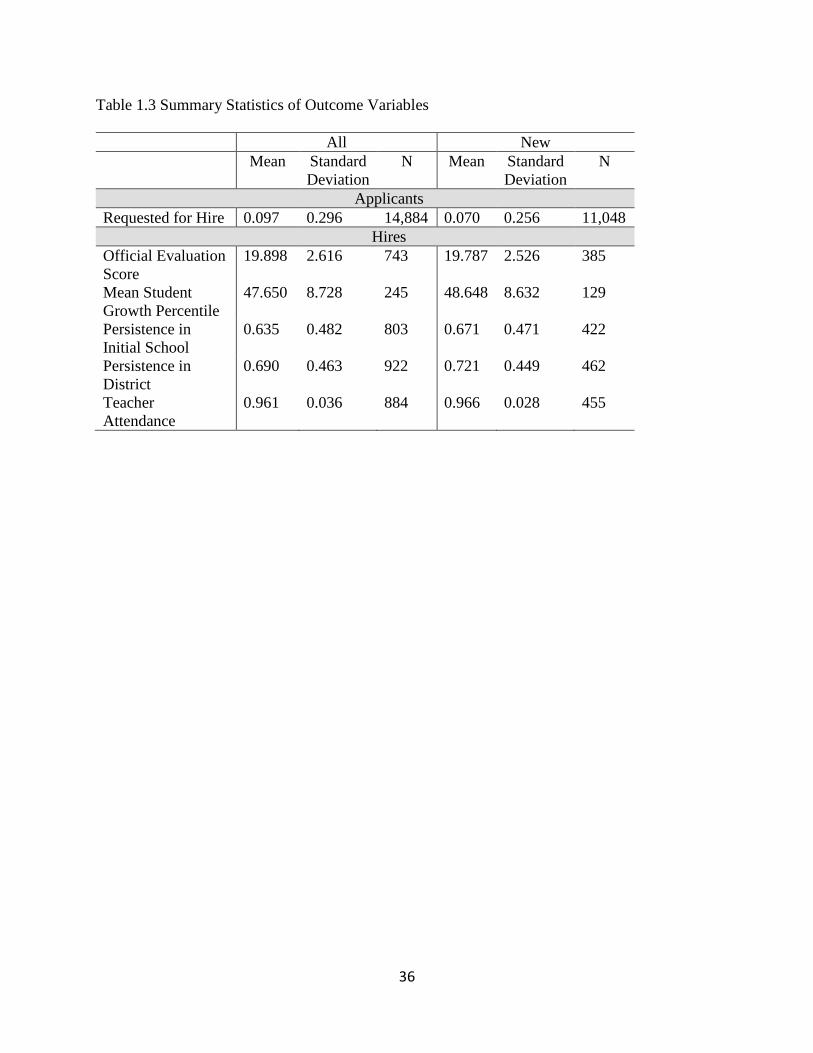
36

Table 1.3 Summary Statistics of Outcome Variables

All New

Mean Standard

Deviation

N Mean Standard

Deviation

N

Applicants

Requested for Hire 0.097 0.296 14,884 0.070 0.256 11,048

Hires

Official Evaluation

Score

19.898 2.616 743 19.787 2.526 385

Mean Student

Growth Percentile

47.650 8.728 245 48.648 8.632 129

Persistence in

Initial School

0.635 0.482 803 0.671 0.471 422

Persistence in

District

0.690 0.463 922 0.721 0.449 462

Teacher

Attendance

0.961 0.036 884 0.966 0.028 455

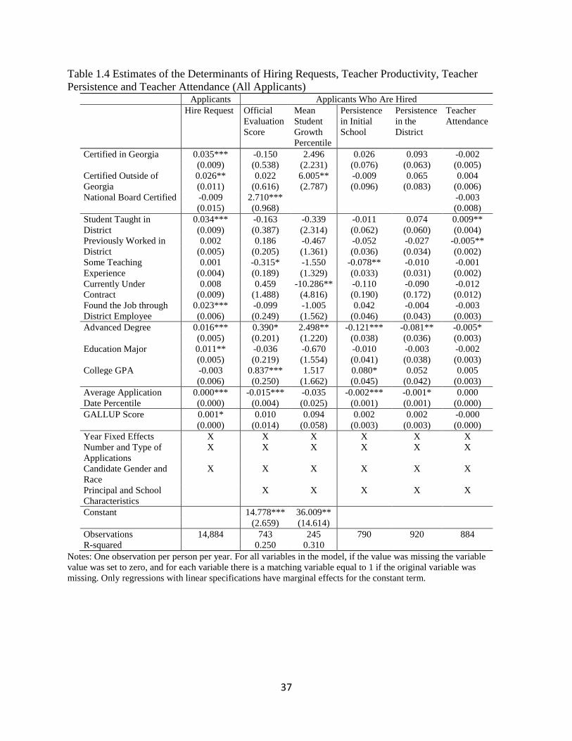
37

Table 1.4 Estimates of the Determinants of Hiring Requests, Teacher Productivity, Teacher

Persistence and Teacher Attendance (All Applicants) Applicants Applicants Who Are Hired

Hire Request Official

Evaluation

Score

Mean

Student

Growth

Percentile

Persistence

in Initial

School

Persistence

in the

District

Teacher

Attendance

Certified in Georgia 0.035*** -0.150 2.496 0.026 0.093 -0.002

(0.009) (0.538) (2.231) (0.076) (0.063) (0.005)

Certified Outside of

Georgia

0.026** 0.022 6.005** -0.009 0.065 0.004

(0.011) (0.616) (2.787) (0.096) (0.083) (0.006)

National Board Certified -0.009 2.710*** -0.003

(0.015) (0.968) (0.008)

Student Taught in

District

0.034*** -0.163 -0.339 -0.011 0.074 0.009**

(0.009) (0.387) (2.314) (0.062) (0.060) (0.004)

Previously Worked in

District

0.002 0.186 -0.467 -0.052 -0.027 -0.005**

(0.005) (0.205) (1.361) (0.036) (0.034) (0.002)

Some Teaching

Experience

0.001 -0.315* -1.550 -0.078** -0.010 -0.001

(0.004) (0.189) (1.329) (0.033) (0.031) (0.002)

Currently Under

Contract

0.008 0.459 -10.286** -0.110 -0.090 -0.012

(0.009) (1.488) (4.816) (0.190) (0.172) (0.012)

Found the Job through

District Employee

0.023*** -0.099 -1.005 0.042 -0.004 -0.003

(0.006) (0.249) (1.562) (0.046) (0.043) (0.003)

Advanced Degree 0.016*** 0.390* 2.498** -0.121*** -0.081** -0.005*

(0.005) (0.201) (1.220) (0.038) (0.036) (0.003)

Education Major 0.011** -0.036 -0.670 -0.010 -0.003 -0.002

(0.005) (0.219) (1.554) (0.041) (0.038) (0.003)

College GPA -0.003 0.837*** 1.517 0.080* 0.052 0.005

(0.006) (0.250) (1.662) (0.045) (0.042) (0.003)

Average Application

Date Percentile

0.000*** -0.015*** -0.035 -0.002*** -0.001* 0.000

(0.000) (0.004) (0.025) (0.001) (0.001) (0.000)

GALLUP Score 0.001* 0.010 0.094 0.002 0.002 -0.000

(0.000) (0.014) (0.058) (0.003) (0.003) (0.000)

Year Fixed Effects X X X X X X

Number and Type of

Applications

X X X X X X

Candidate Gender and

Race

X X X X X X

Principal and School

Characteristics

X X X X X

Constant 14.778*** 36.009**

(2.659) (14.614)

Observations 14,884 743 245 790 920 884

R-squared 0.250 0.310

Notes: One observation per person per year. For all variables in the model, if the value was missing the variable

value was set to zero, and for each variable there is a matching variable equal to 1 if the original variable was

missing. Only regressions with linear specifications have marginal effects for the constant term.

38

Table 1.5 Estimates of the Determinants of Hiring Requests, Teacher Productivity, Teacher

Persistence and Teacher Attendance (New Applicants)

Applicants Applicants Who Are Hired

Hire

Request

Official

Evaluation

Score

Mean

Student

Growth

Percentile

Persistence

in Initial

School

Persistence

in the

District

Teacher

Attendance

Certified in Georgia 0.030*** 0.035 -1.887 0.209* 0.115 -0.006

(0.010) (0.860) (2.746) (0.121) (0.097) (0.006)

Certified Outside of

Georgia

0.030*** 0.453 2.564 0.120 0.061 -0.005

(0.011) (0.908) (3.372) (0.133) (0.112) (0.007)

National Board

Certified

-0.012 0.047 -0.009

(0.014) (0.997) (0.021)

Student Taught in

District

0.024*** -0.374 1.269 -0.047 0.052 0.013**

(0.009) (0.518) (3.247) (0.079) (0.076) (0.005)

Some Teaching

Experience

-0.004 -0.072 -2.680 -0.073 -0.023 0.001

(0.004) (0.271) (1.884) (0.047) (0.044) (0.003)

Currently Under

Contract

0.012* 1.664 0.081 -0.053 -0.019

(0.007) (1.229) (0.411) (0.364) (0.022)

Found Job through

District Employee

0.023*** -0.140 -1.018 0.072 -0.027 -0.006*

(0.005) (0.321) (2.005) (0.058) (0.051) (0.003)

Advanced Degree 0.014*** 0.391 1.768 -0.170*** -0.095** -0.004

(0.004) (0.257) (1.625) (0.050) (0.045) (0.003)

Education Major 0.008* -0.083 2.539 0.070 0.048 -0.003

(0.004) (0.339) (2.228) (0.053) (0.050) (0.003)

College GPA -0.003 0.790*** 2.074 0.095 0.115** 0.002

(0.005) (0.293) (2.493) (0.061) (0.054) (0.003)

Average Application

Date Percentile

0.000*** -0.014*** -0.094** -0.001 -0.001 0.000**

(0.000) (0.005) (0.040) (0.001) (0.001) (0.000)

GALLUP Score 0.000 0.019 0.193*** 0.001 0.001 0.000

(0.000) (0.019) (0.066) (0.003) (0.003) (0.000)

Number and Type of

Applications

X X X X X X

Year Fixed Effects X X X X X X

Candidate Gender

and Race

X X X X X X

Principal

Characteristics

X X X X X

School

Characteristics

X X X X

Constant 14.295*** -0.602

(3.525) (21.585)

Observations 11,048 385 129 413 460 455

R-squared 0.336 0.461

Notes: One observation per person per year. For all variables in the model, if the value was missing the variable

value was set to zero, and for each variable there is a matching variable equal to 1 if the original variable was

missing. Only regressions with linear specifications have marginal effects for the constant term.

39

Table 1.6 Number and Quality of Applicants by School Characteristics and by Subject Area

Number of Applicants

% of Candidates

in the top Quintile

of Applicant GPA

Mean

Standard

Deviation Mean

Standard

Deviation

To All Schools 198.745 233.352 20.000 0.000

By Core Subjects

Elementary 369.915 290.250 17.500 5.869

English 120.107 118.740 16.481 17.081

Social Science 134.277 138.101 12.135 5.253

Math 81.968 82.780 14.022 6.613

Science 76.516 72.955 12.050 5.204

By Number of Students in the School

Less Than 500 207.456 299.004 15.403 10.821

Between 500 and 750 247.594 212.542 16.712 10.633

Between 750 and 1000 159.227 177.190 14.056 7.069

Greater than 1000 97.364 88.138 14.151 6.313

Missing 404.68 339.418 13.326 4.782

By School Level

Elementary 371.287 290.958 17.551 5.862

Middle School 89.354 84.907 13.529 13.475

High School 112.281 122.761 13.921 5.914

Other School Level 81.091 31.536 12.457 3.419

By Percent of Students Directly Certified

Less than 25 188.259 167.642 17.154 6.540

25 to 50 288.091 249.547 15.569 7.022

50 to 75 143.447 213.728 14.174 8.894

Greater than 75 228.630 227.833 15.638 10.501

Missing 404.68 339.418 13.326 4.782

By School Grade

A 248.826 191.091 17.482 6.204

B 136.042 164.886 15.135 6.424

C 169.870 184.655 15.954 6.414

D 169.460 176.359 15.619 10.809

F 187.681 249.583 14.153 9.240

40

Table 1.7 Estimates of the Determinants of the Candidate Pool Size and Quality

VARIABLES Total Size of

the Pool

Total Size of

the Pool Before

the first hire

request

% of

Applicants in

the top GPA

quintile

% of

Applicants in

the top GPA

quintile before

first hire

request

Middle School -220.579*** -205.755*** -0.043 -0.036

(77.127) (61.715) (0.037) (0.045)

High School -247.748* -228.932* -0.024 -0.055

(134.627) (130.100) (0.064) (0.093)

Other School Level 2.094 7.402 -0.066 -0.059

(103.241) (99.716) (0.049) (0.071)

Portion of Students

Directly Certified

-1.075 -2.065 -0.000 -0.000

(1.677) (1.610) (0.001) (0.001)

GADOE School Climate

STAR Score

3.925 6.754 -0.003 -0.006

(12.868) (12.413) (0.006) (0.009)

Number of Students

(100s)

0.517 0.650 -0.002 -0.001

(3.717) (3.578) (0.002) (0.003)

Portion of Students

Hispanic

-294.847 -167.649 -0.045 -0.053

(211.934) (203.296) (0.101) (0.145)

Portion of Students

Black

-53.222 43.561 -0.081 -0.071

(172.874) (165.517) (0.082) (0.118)

GADOE School Grade

A

-86.965 -69.931 -0.019 -0.023

(62.450) (59.119) (0.030) (0.042)

GADOE School Grade

B

-65.623 -47.214 -0.015 -0.060*

(48.039) (46.024) (0.023) (0.033)

GADOE School Grade

D

-13.973 6.747 0.010 0.004

(37.669) (36.397) (0.018) (0.026)

GADOE School Grade F 27.974 65.736* 0.000 -0.007

(39.052) (37.685) (0.019) (0.027)

Science -256.321*** -246.111*** 0.026 -0.025

(95.278) (91.940) (0.046) (0.066)

Math -225.686** -219.509** 0.011 0.014

(102.652) (99.212) (0.049) (0.071)

Social Science -279.119* -263.123* -0.002 -0.043

(144.253) (139.351) (0.069) (0.100)

English -283.504** -262.394** 0.014 -0.012

(117.420) (113.462) (0.056) (0.081)

Middle School Science 200.917* 194.489* -0.025 -0.039

(118.764) (107.382) (0.057) (0.077)

High School Science 178.540 176.938 -0.045 0.001

(160.893) (155.411) (0.077) (0.111)

Middle School Math 152.635 158.525 -0.028 -0.027

(125.104) (114.235) (0.060) (0.082)

High School Math 167.196 164.793 0.007 0.007

(164.416) (158.917) (0.078) (0.113)

Middle School English 240.104* 226.613* 0.044 0.009

(141.762) (129.858) (0.068) (0.093)

High School English 253.939 235.969 -0.008 0.006

41

(176.652) (170.713) (0.084) (0.122)

Middle School Social

Science

234.702 221.917 -0.008 -0.028

(160.221) (149.781) (0.076) (0.107)

High School Social

Science

287.744 274.808 -0.019 0.020

(192.442) (185.949) (0.092) (0.133)

Number of Applicants

for Pool

-0.003 -0.007*

(0.003) (0.004)

Constant 478.299*** 384.704*** 0.287*** 0.320***

(122.235) (117.173) (0.059) (0.085)

Observations 357 361 357 361

R-squared 0.446 0.408 0.122 0.110

Notes: Subjects omitted Elementary which was denoted as its own subject. School levels also omitted elementary.

Standard errors in parentheses *** p<0.01, ** p<0.05, * p<0.1.

42

Table 1.8 Estimates of the Determinants of the Grade Point Average of the Applicants who were

selected by Principals for their first request VARIABLES Pool

Characteristics

Pool and

School

Characteristics

Pool, School,

and Principal

Characteristics

Pool, School,

Principal, and

Subject

Characteristics

Pool Characteristics

Number of Applicants to

School-Subject Before

the First Request (100s)

0.040*** 0.013 0.020 0.016

(0.010) (0.013) (0.014) (0.015)

Percent of Candidates

before the First Request

with a GPA in the top

Quintile

0.866*** 0.659*** 0.668*** 0.641***

(0.137) (0.144) (0.153) (0.157)

School Characteristics

Middle School -0.117 -0.054 -0.097

(0.091) (0.093) (0.267)

High School -0.111 -0.037 0.449***

(0.095) (0.099) (0.125)

Other School Level -0.276** -0.255** 0.127

(0.111) (0.117) (0.284)

Portion of Students

Directly Certified

-0.003 -0.002 -0.002

(0.003) (0.004) (0.004)

GADOE School Climate

STAR Score

0.001 -0.008 -0.003

(0.034) (0.036) (0.037)

GADOE School CCRPI

Score

-0.002 -0.002 -0.001

(0.003) (0.003) (0.003)

Number of Students

(100s)

-0.013 -0.015* -0.010

(0.008) (0.009) (0.009)

Portion of Students

Hispanic

-0.371 -0.314 -0.287

(0.409) (0.412) (0.413)

Portion of Students

Black

-0.122 -0.138 -0.130

(0.334) (0.361) (0.363)

Principal

Characteristics

Principal Years of

Experience

-0.003 -0.003

(0.003) (0.003)

Principals LKES Score 0.021 0.019

(0.015) (0.015)

Subject Controls

Science -0.550

(0.338)

Math -0.380

(0.256)

Social Science -0.169

(0.331)

English -0.541

(0.334)

Middle School Science 0.489

(0.421)

High School Science 0.019

(0.346)

Middle School Math 0.418

43

(0.352)

High School Math -0.103

(0.254)

Middle School English 0.591

(0.425)

High School English 0.094

(0.368)

Middle School Social

Science

0.255

(0.396)

High School Social

Science

-0.328

(0.336)

Constant 2.939*** 3.678*** 3.292*** 3.237***

(0.040) (0.289) (0.364) (0.373)

Observations 293 293 293 293

R-squared 0.108 0.171 0.191 0.207

Notes: Standard errors in parentheses. *** p<0.01, ** p<0.05, * p<0.1. Subjects omitted Elementary which was

denoted as its own subject. School levels also omitted elementary. Outcome is the Candidate’s GPA. The sample is

all candidates who were selected first in a school-subject pool.

44

Table 1.9 Estimates of the Determinants of the Likelihood of Being Selected for a Hiring

Request – All Applicants and Positions Combined Versus Separate Pools for Each Position

Hiring Requests-All Applicants Probit Probit Conditional Logit

Full Candidate

Pool*

Candidates in the

Clogit Pool±

Different

Applicant Pools°

Certified in Georgia 0.035*** 0.039** 0.065 (0.009) (0.017) (0.131)

Certified Outside of

Georgia

0.026** 0.026 0.039

(0.011) (0.017) (0.440)

National Board

Certified

-0.009 0.006 -0.115

(0.015) (0.016) (0.258)

Student Taught in

District

0.034*** 0.043*** 0.106**

(0.009) (0.013) (0.016)

Previously Worked

in District

0.002 -0.002 -0.008

(0.005) (0.008) (0.722)

Some Teaching

Experience

0.001 0.057 0.018

(0.004) (0.006) (0.351)

Currently Under

Contract

0.008 0.083 0.099***

(0.009) (0.012) (0.002)

Found the Job

through District

Employee

0.023*** 0.013 0.045

(0.006) (0.010) (0.105)

Advanced Degree 0.016*** 0.014* 0.001 (0.005) (0.007) (0.963)

Education Major 0.011** 0.005 0.537** (0.005) (0.008) (0.030)

College GPA -0.003 -0.028 0.215 (0.006) (0.296) (0.396)

Average

Application Date

Percentile

0.000*** 0.001*** 0.000

(0.000) (0.000) (0.687)

GALLUP Score 0.001* 0.001 0.000 (0.000) (0.000) (0.976)

N 14,884 7,528 19,215 Notes: Standard errors in parentheses. *** p<0.01, ** p<0.05, * p<0.1. The first two columns have one observation

per person per year. The third column is one observation per applicant per school-subject-year.

*This column also appears in Table 1.4. ±This pool removes all candidates who applied after the first request that

was placed.

45

Table 1.10 Estimates of the Determinants of the Likelihood of Being Selected for a Hiring

Request – All Applicants and Positions Combined Versus Separate Pools for Each Position (New

Applicants)

Hiring Requests-New Applicants Probit Probit Conditional Logit

Full Candidate Pool* Candidates in

the Clogit Pool±

Different

Applicant Pools

Certified in

Georgia

0.030*** 0.035** 0.047

(0.010) (0.015) (0.065)

Certified Outside

of Georgia

0.030*** 0.030** 0.084

(0.011) (0.015) (0.079)

National Board

Certified

-0.012 -0.004 -0.127

(0.014) (0.014) (0.116)

Student Taught in

District

0.024*** 0.018 0.114**

(0.009) (0.012) (0.061)

Some Teaching

Experience

-0.004 -0.002 -0.007

(0.004) (0.006) (0.024)

Currently Under

Contract

0.012* 0.106 0.109**

(0.007) (0.010) (0.043)

Found the Job

through District

Employee

0.023*** 0.013* 0.050

(0.005) (0.007) (0.034)

Advanced Degree 0.014*** 0.014** -0.004 (0.004) (0.006) (0.840)

Education Major 0.008* 0.008 0.518 (0.004) (0.006) (0.037)

College GPA -0.003 -0.006 -0.007 (0.005) (0.007) (0.034)

Average

Application Date

Percentile

0.000*** 0.000*** 0.000

(0.000) (0.000) (0.001)

GALLUP Score 0.000 0.000 0.000 (0.000) (0.000) (0.001)

N 11,048 5,396 8,373 Notes: Standard errors in parentheses. *** p<0.01, ** p<0.05, * p<0.1. The first two columns have one observation

per person per year. The third column is one observation per applicant per school-subject-year.

*This column also appears in Table 5. ±This pool removes all candidates who applied after the first request that was

placed.

46

Table 1.11 Alternative Specific Conditional Logistic Regression of Principal Hiring Choice

(Marginal Effects) Probability

the Choice

Category

was

Selected

Characteristics of Choice Category Marginal Effect on

Principal’s Hiring Request

Choice

In Top 30%

of all

Applicant

GPAs

More than

Five Years

of

Experience

First 20%

of

Applicants

Certified Principal

Experience

Principal

Evaluation

Score

0.038

-0.002

(0.004)

0.002

(0.004)

0.016

-0.004*

(0.002)

-0.000

(0.001)

0.024

0.004*

(0.002)

0.003

(0.003)

0.074

-0.002

(0.005)

0.013*

(0.007)

0.105

0.003

(0.006)

-0.003

(.004)

0.098

-0.000

(0.006)

0.008

(0.006)

0.256

0.004

(0.008)

-0.019**

(0.009)

0.168

-0.013**

(0.007)

0.005

(0.010)

0.000

0.000

(0.000)

0.000

(0.000)

0.000

0.000

(0.000)

0.000

(0.000)

0.074

0.013

(0.010)

-0.004

(0.006)

0.031

-0.003

(0.004)

-0.000

(0.004)

0.016

0.002*

(0.001)

0.000

(0.001)

0.000

0.000

(0.000)

0.000

(0.000)

0.062

-0.005

(0.007)

-0.001

(0.003)

0.036

0.004

(0.003)

-0.003

(0.003)

Notes: Category had this Characteristic.

47

1.8 Appendix 1

Table A1.1 Principal Decision Using Hired instead of Hiring Request

All New

VARIABLES Hired Hired

Certified in Georgia 0.032*** 0.033***

(0.008) (0.007)

Certified Outside of Georgia 0.016 0.022**

(0.010) (0.009)

National Board Certified -0.050 -0.035

(0.033) (0.038)

Student Taught in District 0.034*** 0.027***

(0.009) (0.008)

Previously Worked in District -0.002 N/A

(0.005)

Some Teaching Experience -0.002 -0.008**

(0.004) (0.004)

Currently Under Contract -0.012 0.000

(0.012) (0.012)

Found the Job through District

Employee

0.024*** 0.020***

(0.006) (0.005)

Advanced Degree 0.013*** 0.007**

(0.005) (0.004)

Education Major 0.010** 0.010**

(0.004) (0.004)

College GPA -0.003 0.000

(0.005) (0.005)

Average Application Date

Percentile

0.000*** 0.000***

(0.000) (0.000)

GALLUP Score 0.000 -0.000

(0.000) (0.000)

Observations 14,884 11,048 Notes: Standard errors in parentheses. *** p<0.01, ** p<0.05, * p<0.1.

48

Table A1.2 Estimates of the Determinants of the Grade Point Average of the Applicants who

were selected by Principals for all their Requests VARIABLES Pool

Characteristics

Pool and School

Characteristics

Pool, School, and

Principal

Characteristics

Pool, School,

Principal, and

Subject

Characteristics

Pool Characteristics

Number of Applicants to

School-Subject (100s)

0.017*** 0.013** 0.017*** 0.016***

(0.005) (0.005) (0.006) (0.006)

Percent of All

Candidates with a GPA

in the top Quintile

1.381*** 0.697*** 0.662*** 0.689***

(0.297) (0.218) (0.223) (0.222)

School Characteristics

Middle School -0.107** -0.088* 0.051

(0.049) (0.048) (0.146)

High School -0.092** -0.055 0.621***

(0.046) (0.051) (0.082)

Other School Level 0.170 0.177 0.189

(0.123) (0.132) (0.228)

Portion of Students

Directly Certified

0.001 0.002 0.002

(0.002) (0.002) (0.002)

GADOE School Climate

STAR Score

0.002 -0.003 -0.002

(0.018) (0.018) (0.019)

GADOE School CCRPI

Score

0.002 0.002 0.002

(0.002) (0.002) (0.002)

Number of Students

(100s)

-0.000 -0.001 -0.000

(0.005) (0.005) (0.005)

Portion of Students

Hispanic

-0.400* -0.369* -0.371*

(0.204) (0.207) (0.207)

Portion of Students

Black

-0.364* -0.401* -0.388*

(0.190) (0.205) (0.207)

Principal

Characteristics

Principal Years of

Experience

-0.003** -0.003*

(0.002) (0.002)

Principals LKES Score 0.018** 0.017**

(0.007) (0.007)

Subject Controls

Science 0.006

(0.197)

Math 0.011

(0.282)

Social Science -0.259

(0.249)

English 0.039

(0.296)

Middle School Science -0.099

(0.242)

High School Science -0.699***

(0.203)

Middle School Math -0.101

(0.319)

High School Math -0.738***

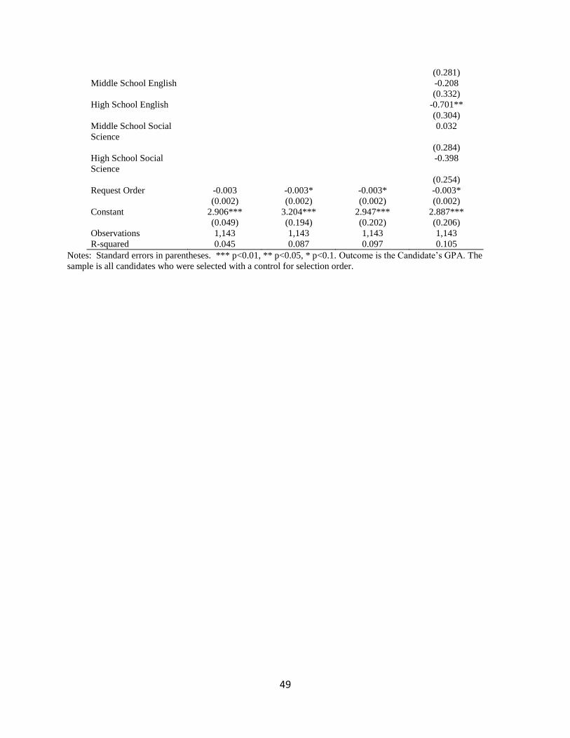
49

(0.281)

Middle School English -0.208

(0.332)

High School English -0.701**

(0.304)

Middle School Social

Science

0.032

(0.284)

High School Social

Science

-0.398

(0.254)

Request Order -0.003 -0.003* -0.003* -0.003*

(0.002) (0.002) (0.002) (0.002)

Constant 2.906*** 3.204*** 2.947*** 2.887***

(0.049) (0.194) (0.202) (0.206)

Observations 1,143 1,143 1,143 1,143

R-squared 0.045 0.087 0.097 0.105

Notes: Standard errors in parentheses. *** p<0.01, ** p<0.05, * p<0.1. Outcome is the Candidate’s GPA. The

sample is all candidates who were selected with a control for selection order.

50

Figure A1.1 Relation of GPA of First Selected Candidates to Number of Applicants and Portion of the Pool with a High GPA

Coll

ege

GP

A

Fraction of Candidates in the Top Quintile of GPA before the First Request Number of Applicants to School-Subject before the first request (100s)

51

Figure A1.2 Relation of GPA of All Selected Candidates to Number of Applicants and Portion of the Pool with a High GPA

Coll

ege

GP

A

Fraction of All Candidates in the Top Quintile of GPA Number of Applicants to School-Subject

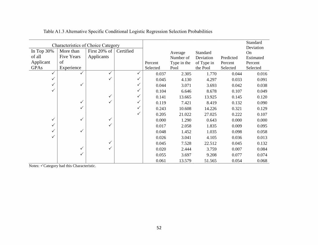
52

Table A1.3 Alternative Specific Conditional Logistic Regression Selection Probabilities

Characteristics of Choice Category

Percent

Selected

Average

Number of

Type in the

Pool

Standard

Deviation

of Type in

the Pool

Predicted

Percent

Selected

Standard

Deviation

On

Estimated

Percent

Selected

In Top 30%

of all

Applicant

GPAs

More than

Five Years

of

Experience

First 20% of

Applicants

Certified

0.037 2.305 1.770 0.044 0.016

0.045 4.130 4.297 0.033 0.091

0.044 3.071 3.693 0.042 0.038

0.104 6.646 8.678 0.107 0.049

0.141 13.665 13.925 0.145 0.120

0.119 7.421 8.419 0.132 0.090

0.243 10.608 14.226 0.321 0.129

0.205 21.022 27.025 0.222 0.107

0.000 1.290 0.643 0.000 0.000

0.017 2.058 1.835 0.009 0.095

0.048 1.452 1.035 0.098 0.058

0.026 3.041 4.105 0.036 0.013

0.045 7.528 22.512 0.045 0.132

0.020 2.444 3.759 0.007 0.084

0.055 3.697 9.208 0.077 0.074

0.061 13.579 51.565 0.054 0.068 Notes: Category had this Characteristic.

53

2 Where They Stop Nobody Knows: What Drives Teacher Placement

Decisions?

2. 1. Introduction

To understand the labor market, how workers and firms come together to produce

goods and services, it is vital to understand how workers enter a given firm. To

understand this, there are two sides, the firms’ hiring decisions and the workers’

employment decisions. The preferences workers have over firms drive their decisions by

affecting their search efforts and their probability of accepting an offer from a firm.

Hence, understanding worker preferences is crucial to labor market research.

Much of the research on worker preferences has focused on the wage differences

needed to compensate for disparities in non-pecuniary workplace benefits and conditions.

However, school districts typically utilize fixed salary schedules across schools. These

schedules do not allow for salary to offset the undesirable aspects of a school. Prior work

has documented that the combination of teacher preferences and rigid pay schedules can

lead to disparities in student access to quality teachers. Policymakers are concerned that

teacher sorting across schools may limit access to high-quality teachers, particularly for

minority, impoverished, or low-performing students. Teacher sorting may occur in the

job market for hiring new teachers (Sass et al., 2012; Reininger, 2012) as well as through

post-hire differential patterns of teacher mobility.13 The disparity in access to quality

teachers has lasting impacts as teacher quality affects not only their student’s academic

outcomes, but also their students’ lifetime earnings.14

13 Darling-Hammond 2001; Viadero 2002; Gordon & Maxey 2000; Goldhaber et al., 2007; Feng & Sass 2017

14 Rivkin et al., 2005; Aaronson et al., 2007; Kane et al., 2008; Chetty et al., 2011, Chetty et al., 2014

54

District policies can possibly mitigate disparities in access to high-quality

teachers. Some policies that have been tested are bonuses for high-performing teachers to

remain in or to transfer to low-performing schools, state bonus schemes for teachers in

high-poverty and low-performing schools, or differential retention programs. Analysis of

the Talent Transfer Initiative showed that monetary incentives might have to be very

large to induce highly effective teachers to transfer to low-performing schools. The

teachers who transferred could improve student scores on math and reading exams in

elementary schools, but had no impact on math or reading scores for middle school

students (Glazerman et al., 2013). A North Carolina bonus scheme for math, science, and

special education teachers working in high-poverty or low-performing schools

significantly reduced teacher turnover (Clotfelter et al., 2008). Similarly, a selective

retention bonus scheme for highly effective teachers in low-performing schools in

Tennessee led to improved teachers retention in tested grades and subjects (Springer et

al., 2016) and improved student test-score gains (Springer et al., 2019). Further, targeted

recruitment strategies may reduce disparities in the supply of new teachers resulting from

teachers’ geographic preferences (Reininger, 2012; Boyd et al., 2005a).

The fact that teachers have preferences over the characteristics of their workplace

means that to address disparities in access to effective teachers, policymakers must know

how teacher preferences vary and the compensating differentials required to offset those

preferences. In chapter 1, I found evidence that apparent errors in principal hiring

decisions that affect the initial distribution of teachers may partially stem from

differences in the pool of applicants, as well as from sub-optimal use of information by

principals. Hence, in this chapter, I examine how teachers’ preferences affect their

55

application behavior and thereby affect principals’ hiring choice sets. The results can

inform schools’ and districts’ decisions regarding teacher recruitment policies or

adjustments to the application process. For example, the findings can shed light on the

existing differences in application behavior which can be targeted to improve the

principals’ hiring choice sets.

The teacher preference research is extensive and ever-growing, to add to that

literature in a meaningful way I focus on how candidate preferences affect the choice of

where to apply. While the majority of the literature uses labor market decisions such as

transfers and initial placements to determine teacher preferences, few prior studies

examine the teacher’s decision of where to apply. Those that do consider only particular

segments of the applicant pool, such as inter-school transfers of existing teachers (Boyd

et al., 2011), application choices at job fairs (Engel et al., 2014), or recent college

graduates (Cannata, 2010), or focus on specific aspects such as the role of geography

(Goff & Bruecker, 2017). Leveraging a partnership with an Atlanta metropolitan area

school district, the present research will employ rich data that covers both initial and

transfer applications, which does allow me to compare part of my results to the findings

of Boyd et al. 2011. I estimate the teacher’s choices to apply to a school by using

conditional logistic choice models.

I find that in relation to schools with a Governor’s Office of Student Achievement

(GOSA) School Report Card letter grade of C, teachers are more likely to apply to a

school with a grade of F and less likely to apply to schools with a grade of A, B, or D.

This is an odd result that warrants further investigation in the future but could be due to a

variety of factors including differences in accountability pressures, variation in resources,

56

and differences in recruitment. I also find that, in accordance with the current preference

literature, school climate scores are positively correlated with current employee

application likelihoods, however, the opposite is true for teacher applicants who are new

to the district. The difference could be due to differences in information availability,

recruitment efforts, or randomness in applications of new teachers, and warrants further

investigation. Increases in the proportion of students “directly certified” (a measure of

poverty) negatively impacts only the application likelihood of current teachers, but there

is a positive relationship between the number of students and the application likelihoods

for all teachers. The portion of minority students, Black or Hispanic, in a school is

negatively correlated with the likelihood of a candidate applying to work in the school,

Black teaching applicants do have increased application likelihoods to schools with

greater portions of black students. Of the principal characteristics examined, only the

principal’s years of experience is positively related to application likelihood for all

teacher subsamples. The principal’s evaluation score and principal tenure in the school

either have negative or no relation with the likelihood of an application submission.

When the interaction of applicant teaching experience with key school characteristics15

are added to the analysis, they only show a significant relationship for current teachers.

However, when the applicant’s college GPA is interacted with the same key school

characteristics as applicant teaching experience as well as the principal characteristics,16

it only has statistically significant impacts for new teachers. The inclusion of these

interactions minimally impacts the magnitude of the relations discussed previously.

15 These characteristics are the GOSA Report Card Grade Dummy Variables, the GADOE School Climate Score, the

number of students, and the percent of students who are Black, Hispanic, or Directly Certified. 16 These characteristics are the principal’s experience, years in the current school, and their official evaluation score.

57

The next section reviews the employee preference literature for teachers and is

followed by section 3, which details the hiring processes of the participating district.

Section 4 discusses the data, and section 5 details the methodology. Section 6 provides

the results while section 7 summarizes and concludes this essay.

2.2. Literature Review

Researchers have long examined the relationships between workplace

characteristics and employee placement and mobility decisions. As the current work is

focused on teacher employment preferences, this section will review the research specific

to teacher workplace preferences. The teacher preference research includes analyses of

teacher job applications, initial placements, job satisfaction, and teacher mobility

decisions. In these studies, researchers have considered several factors affecting teacher

labor market decisions, including school characteristics, salary, student population

demographics, teacher peer groups, school facilities, administrative support, mentoring,

and geography.

Perceived job difficulty varies with the attributes of schools and the students who

attend them. Given fixed salary schedules, schools often cannot offer higher wages to

compensate for undesirable workplace characteristics. The most common payment

schedule is where a teacher’s salary depends solely on their years of teaching experience

and educational attainment. Salaries may vary across districts, however, and there is

evidence that teachers will transfer to nearby districts that have higher salaries or remain

in schools with higher salaries when wage variation exists.17 However, some research

17 Imazeki, 2005, Feng 2014, Feng 2009

58

finds that when teachers exit the profession, it is not in search of higher pay.18 Taken

together, these findings suggest that salary is an important factor in placement decisions

throughout a teacher’s work history, but that due to rigid wages, non-pecuniary factors

are more important in subsequent transfer or exit decisions. This conclusion is further

supported by its own body of research.19 However, as a contrast, the Talent Transfer

Initiative offered substantial bonuses of twenty thousand dollars to high performing

teachers if they transferred to high-needs schools. Few teachers even participated in the

information session, let alone accepted the bonuses to transfer to low-performing schools

(Glazerman et al., 2013).

An additional body of research shows that teachers tend to move away from urban

schools and schools with high portions of minority or low-income students.20 Urban

schools also have lower application rates during the hiring process.21 Further research

demonstrates that the movement away from schools with high portions of minority

students is driven largely by the choices of white teachers. Black and Hispanic teachers

seem to prefer schools with student and teacher22 or principal demographics (Grissom &

Keiser, 2011) similar to their own. Additionally, teachers were found to move away from

schools with substantial disciplinary problems (Feng, 2009, 2010). Teachers were also

found to prefer supportive administrators and peers as well as mentorship opportunities.23

18 Podgursky et al., 2004; Scafidi et al., 2006; Stinebrickner, 2002

19 Clotfelter et al., 2011, Hanushek & Rivkin 2007, Feng 2009 20 Boyd et al. 2011; Lankford et al., 2002; Hanushek et al., 2004; Boyd et al., 2005a,b; Imazeki, 2005, Scafidi et al.,

2007; Feng, 2009; Goldhaber et al., 2011; Clotfelter et al., 2011; Feng & Sass, 2017; Goldhaber et al., 2015; West &

Chingos, 2009; Neild et al., 2003; Hanushek & Rivkin 2007

21 Levin & Quinn, 2003; Levin et al., 2005; Liu et al., 2008; Donaldson, 2013

22 Strunk & Robinson 2006; Hanushek & Rivkin, 2007

23 Smith & Ingersoll, 2004; Ingersoll, 2001; Horng, 2009; Loeb et al., 2005

59

Location has also been shown to strongly affect teacher employment decisions.

Teachers more frequently accept an initial placement in the area where they grew up

(Reininger, 2012, Boyd et al., 2005a), where they attended college (Boyd et al., 2005a),

close to their current home address (Boyd et al., 2005b, Boyd et al. 2013, Engel &

Cannata, 2015), with a shorter commute (Engel et al., 2014; Horng 2009), or in a specific

type of geography (Goff & Bruecker, 2017). In addition, teachers are found to prefer

schools that have characteristics like those of their hometown (Boyd et al., 2005a). The

geography of the district can affect subsequent mobility decisions as well. For example,

transient teachers are less likely to move to geographically isolated districts (Neild et al.,

2003).

Engel, Jacob, and Curran (2014) found that school characteristics strongly

predicted application choices when studying behavior at the Chicago Public Schools job

fair. However, Cannata (2010) found that if school-specific information is limited,

teachers may make application decisions based on characteristics of the district as a

whole. Both of these papers also find that applicants prefer schools with lower portions of

minority students

The hiring process can also affect labor supply decisions by imposing additional

constraints on teacher choices. For example, increases in the amount of screening and

certification requirements are negatively correlated with the number of candidates

(Delfgaaw & Dur, 2007; DeVaro, 2005). However, the direction of causation is not

entirely clear, as the supply of candidates can affect the way schools structure their hiring

process (Rynes & Barber, 1990, Ryan & Tippins, 2004). Winter et al. (2004) find the

attractiveness of a job offering to teachers is positively correlated with hiring-process

60

factors such as ease, length, and timeliness. Similarly, Rynes and Barber (1990) find that

decreasing the application process length and the number of steps enhanced the

attractiveness of a job to candidates. In addition to the hiring process, laws dictating

evaluation standards can affect teacher choices. For example, the accountability standards

imposed by the No Child Left Behind Act unintentionally exacerbated supply problems

faced by high-needs schools by making schools with low-performing students less

attractive to teachers (Rutledge et al., 2010).

2.3. The School District’s Hiring Process

Each year the studied school district, located in the Atlanta metropolitan area, fills

roughly 600 teaching positions. Applications for these positions occur year-round but are

concentrated in the period from January to August, as shown in Figure 1. Historically, a

teacher candidate’s information would be available to principals in a hiring portal upon

the submission of an online application and a simple background and credential check.

For the past several years, however, the district has implemented changes to the teacher

hiring process. The main change has been to provide principals additional information

about teacher candidates through scores from a compatibility screener, GALLUP

TeacherInsight, and a video interview tool, HireVue. In January 2019, obtaining a

minimum score on the TeacherInsight test became a requirement for a candidate to enter

the teacher candidate pool available to principals. However, this paper only studies

applications through May 2018. The GALLUP TeacherInsight and HireVue tools are

only applied to teachers new to the current district. The current teachers instead are

limited by a transfer window which begins in March and ends in April.

61

Any candidate accepted into the candidate pool can apply for specific school-

subject positions or to generic pools such as middle-school math. Principals can then

review the applications and offer interviews to candidates. After the interviews,

principals make hiring requests to the district’s Human Resources Department, who then

extends a formal offer (provided the candidate does not already have an outstanding offer

from another school in the district). A teacher must reject their current offer to receive

further offers from within the district.

2.4. Data

2.4.1 Partner District Administrative Data

For the bulk of the analysis, I use employment and hiring data from the Human

Resources Department of the studied school district. This means I have, when available,

all information collected about every applicant during the hiring process, not just those

that are hired. The data also include this information for the transfer process. The

applicant’s address at the time of application was used to generate distance-to-school

measures and the specific addresses will not be available to the researcher.

2.5. Model

This work builds upon the methodology used by Boyd et al. 2011, in their study

of teacher retention and school choices regarding teacher transfer hires in New York City.

However, in contrast to Boyd et al., I use all applications (both new and transfers), not

just applications from currently-employed teachers seeking to transfer. In addition, I

focus more on the impact of school characteristics, as opposed to the characteristics of

the teacher.

62

While a variety of models have been employed by other researchers, the approach

of Boyd, et al., seems most relevant for the current analysis. For example, I do not use the

methods of Biasi (2019) as they emphasize preferences over payment methods, and no

significant policy changes occurred in the districts and period I study. In addition, I use

the method from Boyd et al., to capitalize on the application data, which were not

available for Boyd et al. (2013). There are also several related papers in the

compensating-wage literature, such as Lavetti (2020), which utilize changes in wages and

benefits over time to identify worker preference. That approach is not feasible in the

present context, where there were no significant changes in compensation or benefits.

Other papers directly use employer- to-employer transfers analyzed within the revealed

preference framework as Sorkin (2018). However, the revealed-preference literature

either focuses on the direction of flows of workers or uses choice experiments to pin

down the value of specific firm characteristics (Maestas et al., 2018; Wiswall & Zafar,

2017), their methods, however, are infeasible for this work.

For this work, the characteristics of schools studied have previously been studied

and found to have effects on teacher preference in the prior literature. School quality

measures of the GOSA school report card grade (performance and demographics) and the

GADOE school climate measures (quality of school environment) are included to capture

applicant preferences over readily available quality measures. Then due to the extensive

literature about teacher flight from high-needs schools, I incorporated variables to

represent the school's minority (percent of black or Hispanic) and poverty (percent of

students directly certified for aid) status. Black and Hispanic were separated due to the

studied district being primarily black in students and staff, so percent minority as an

63

aggregate variable may not have accurately demonstrated preferences. As the studied

district is highly urban with no internal variation, this factor of traditionally high-needs

schools was excluded. As defined by the number of students, the school's size was

included to further capture preferences over readily observable school aspects. The

principal characteristics were included as they are the primary interaction of the candidate

with the school and, to a large extent, represent the school’s administrative environment.

The applicant characteristics chosen for interactions were also carefully selected.

Firstly applicant race with student race due to the extensive literature showing that by

including the interaction, the results can be substantially different in magnitude and

potentially even reverse the effects. In the previous chapter, applicant GPA represented

applicant quality, so in this chapter, applicant GPA is interacted with all of the preference

aspects to study if quality had noticeable effects on preferences, which could contribute

to disparate distributions of quality teachers. There is similar reasoning behind including

interactions with and applicant's teaching experience as this candidate aspect has been

strongly related with teacher performance in the literature.

2.5.1 Research Question: Which Schools are more likely to Receive Applications?

Conditional on applying to the district, teachers can choose to apply to any school

with an opening. The likelihood of a teacher applying to a school is modeled as a

conditional logistic function.24 This particular estimation method was chosen to represent

the application choice of teachers who must choose what schools to apply to amongst a

set of alternatives. This approach allows unobserved characteristics of teacher to be

24 In addition to the conditional logit specification, a traditional logit estimation was run on the same analysis sample

which yielded very similar results and is therefore not being added to this paper.

64

accounted for and provides more precise estimation of the teachers’ preferences. The

model includes the interactions between each school's characteristics and a key set of

each teacher's characteristics. The model can be represented as:

Pr(𝑌𝑗|𝑌𝑗𝜖{𝑅𝑒𝑣𝑒𝑙𝑎𝑛𝑡 𝑂𝑝𝑒𝑛𝑖𝑛𝑔𝑠}) =exp (𝑥𝑖𝑗

′ 𝛽)

exp(𝑥𝑖𝑗′ 𝛽) + ∑ exp (𝑥𝑖′𝑗

′ 𝛽) 𝑖′𝜖𝐼^𝑗

(1)

where i represents the school-subject in question and j all other alternatives. The

choice set is constructed to be all schools with at least one hiring request in the school-

level/subjects the teacher applied to in the year of application. Therefore, equation (1)

represents the odds of choosing alternative i of their choice set. The probability is a

function of the characteristics of the school they apply to and the interactions with key

teacher characteristics. When using conditional logit, due to the estimation being within a

teacher’s choice set, any initial location effects and any teacher characteristic effects that

are not interacted with the school drop out of the model since there is no variation. The

analysis is split into applicants who have never worked in the district denoted as “New”

pool, the transfer or “Current” applicant pool, and the combined or “All” applicant pool.

In the analysis, I estimate seven specifications. The first only includes a single

measure of school quality, the letter grade assigned to the school in the Governor’s Office

of Student Achievement (GOSA) Georgia School Grades Report, with a grade of C being

the omitted category. These grades are assigned based on the school performance on state

assessments, the schools demographics, the graduation rate, and other accountability

measures. In the second specification, I control for a set of characteristics I will group as

“other school characteristics” including the Georgia Department of Education (GADOE)

65

school climate score, the percent of students directly certified,25 school size (measured by

the number of students enrolled), the percent of students who are Black, and the percent

of students who are Hispanic. In the third specification, I control for both sets of school

characteristics (school grade and specific school characteristics). Then in the fourth, I

also control for the characteristics of the principal of the school, namely their experience,

evaluation score, and their years in the school. These three sets of controls are then used

in the remaining three specifications, where in the fifth I also control for the interaction of

student and applicant race. Then instead of applicant race, I interact the school grade and

specific school characteristics with applicant teaching experience. In the last specification

the characteristics as well as the principal characteristics are interacted with applicant

GPA (a proxy for teacher quality) instead of experience. These key characteristics were

selected based on prior research that demonstrates these school and applicant aspects are

important to the labor market decisions of teachers.

2.6. Results

The estimation results for the sample of new applicants to the district are

presented in Table 2.2. The first set of variables introduced are dummy variables for the

school receiving a give GOSA School Report Card letter grade. The first specification

includes only these variables and yields estimates that schools with a letter grade of F

receive more applications than schools with a C grade, but that schools of other grades

receive fewer applications. This result is true for all six specifications including these

variables. This result may seem odd, as it suggests that teachers are most willing to apply

25 The students determined to be eligible for free or reduced-price meal based on certification directly from government

agencies without the need for households to verify the need of the child.

66

to the schools rated the worst level. However, there are a few reasons this result can be

plausible, and the underlying truth is likely to be a combination of factors. First,

accountability pressure in high-ranked schools can cause intrinsic pressure to not apply to

higher-ranked schools. The preference for less accountability pressure has been shown in

Feng, Figlio, & Sass (2018). Further, these low-ranked schools may offer the lure of

additional resources and rewards, as argued in Dizon-Ross, 2020. These additional

benefits could be an extrinsic motivation towards applying to lower-ranked schools.

There is also the possibility that higher-graded schools may be better able to utilize

personal networks and thus reach out and determine their hire quickly, not leaving the

window open long enough for most applicants to submit (Engel & Finch, 2015). In

addition to the applicant motivations that could cause the estimates, the model is unable

to account for the prevalence of alternatives due to following the Independence from

Irrelevant Alternatives property meaning if a certain school aspect is overly prevalent in

the possible options the model is unable to decrease its weight in the estimates.

Therefore, due to the prevalence of F ranked schools in the district, the estimated result

may appear if applicants apply randomly. However, I do not think this is the reason, as in

that case, D ranked schools should also have a positive point estimate, which they do not.

In addition to the GOSA letter grades, the number of students in the school, a

descriptor of student poverty, the GADOE school climate score, and the portion of Black

or Hispanic students were also incorporated into the analysis. The three non-race

variables have interesting estimated impacts on application probabilities for the sample of

new applicants; they differ from prior research findings regarding teacher preferences.

67

For all specifications, the number of students is positively related with application

submission probabilities. There is the possibility that this sample of teachers finds appeal

in larger schools, which may offer a larger professional learning community. It is more

likely a result of the short-comings in the data set construction. As the choice set is made

at the teacher-subject-school level, and any applications within that category are counted.

Larger schools probably have more positions, increasing the likelihood that at least one of

those positions appeals to the applicant. In addition, if the applicant applied to any

positions in lower levels but were primarily targeting positions for a higher level this

result could also occur. For example, if an applicant submitted an application for any

middle school math position, all middle school math positions were placed in their choice

set, but if that applicant was primarily applying to high schools which are by nature larger

schools the estimate could be positive.

Traditionally, in the teacher preference literature, the proportion of students

experiencing poverty is associated with lower application probabilities and increased

likelihood of teacher exit from a school. For the sample of new teachers though, there is

either no relationship or a positive relation among student poverty and application

probabilities. This could coincide with the reasoning that struggling schools receive

more resources, which balances with the teachers’ preference to teach more economically

advantaged students. There is also the possibility that applicants to this district are aware

that the district has a large portion or disadvantaged students, and therefore, that

information does not factor into their choices. I posit that this same reasoning can be

applied to the finding that the school climate score has a negative correlation with

application probabilities.

68

Across specifications and samples there is a large negative relationship between

the percent of students who are Black and the probability of the average candidate

applying to a school. However, while together with the large effect on its own of the

portion of Black students, the total effect is still negative, the likelihood a black candidate

applies to a school increases with the proportion of students in the school who are black.

There is also a negative correlation between the percentage of students who are Hispanic

and the probability that the average candidate will apply to a school. This negative

correlation is even greater for Black candidates. These results support the previous

research findings on teacher mobility that indicate white teachers are more likely to exit

schools with high proportions of non-white students.

New applicants are more likely to apply to schools with more experienced

principals. Taken in isolation, this result could support the previous finding that teachers

prefer more supportive principals26 or indicate that teachers prefer schools with greater

staff stability. But when the negative estimated relationship with the principal’s duration

in the school is also considered, the former explanation seems unlikely. The two variables

association with application probabilities could indicate that teachers may be willing to

follow a principal or be attracted by a change in a school led by an experienced principal.

In the sixth specification, the GOSA School Grade variables, the school climate,

size, as well as student poverty and race, are interacted with applicant experience. In the

new-applicant sample, none of the coefficients on the interactions between applicant

experience and school characteristics are statistically significant, indicating that the

impact of school characteristics on candidate choices do not differ between new

26 Ingersoll, 2001; Horng, 2009; Loeb et al., 2005

69

applicants who have never taught and those with prior experience in other school

districts. This result is not surprising as most new applicants have no prior experience,

and those that do typically have few years of experience.

The final set of interactions is between the applicant’s college GPA (a proxy for

candidate quality) and the principal characteristics and the characteristics previously

interacted with experience. Within the sample of new applicants, the likelihood of an

prospective teacher to apply to schools with higher climate scores, greater portions of

Hispanic students, and to Grade A, D, and F schools (relative to Grade C Schools)

increases with higher applicant GPAs. Further, applicants having a higher GPA makes

them less likely to apply to schools where the principal has a higher evaluation score or

more experience. The direction of the interaction with principal evaluation scores,

principal experience, and Grade-F interactions further compound on the existing effect of

those variables when un-interacted on application submission likelihoods. The other

significant interaction effects have directions opposing the un-interacted variable

estimates, which with large enough magnitude could reverse the total effect at large

enough GPA values. However, as GPA is on a scale of zero to four, there is no GPA an

applicant can have to make the total effect positive. For example, the school having a

Grade of A, the effect of the applicant having a GPA of four would still be -0.125 (-0.233

+ (.027×4)). Having a higher GPA makes the estimates of the total effect closer to the

current teacher sample, so possibly candidates with higher college GPAs are better able

to gather information about their possible options.

In discussing the results from the current-teacher sample I will compare my

findings those of Boyd et al. (2011). Though they employ different sample construction

70

and techniques, the two paper’s estimations yield similar results. Both studies find

negative effects of the percent of students who are Black or Hispanic. Though the student

population with the largest effect is different, (Hispanics in my sample and Blacks in

Boyd et al, 2011); I believe this is due to the differences in the racial composition of the

teachers (my sample is predominantly black while theirs has a large Hispanic

population). Both studies find that greater student poverty and worse school climates are

associated with lower probabilities of application to a school.

The main area where we both have significant estimates, but opposing results, is

school size. This result could be due to their inclusion of the school level (elementary,

middle, high), and my sample construction, which as discussed for the new applicant

estimation, is likely to have this unexpected positive result since larger schools having

more openings for a single “position,” and the fact that different levels of schools are

different sizes so if enough teachers prefer a high school when those are in their choice

set this could lead to this positive effect of school size.

There are a few areas where the results from the current-teachers and new-

applicant samples differ substantially; estimates for the effects of the school climate

score, student poverty, and the interactions with GPA and experience all have

qualitatively different estimated impacts on application probabilities. Current teachers

follow the expected preferences regarding school climate scores and student poverty,

while new applicants do not. A possible explanation for this difference is that current

teachers have greater knowledge of the school system and are better able to direct their

applications to the more desirable schools. Another possible reason is that current

teachers may value “easier” teaching environments relatively more than do new teachers

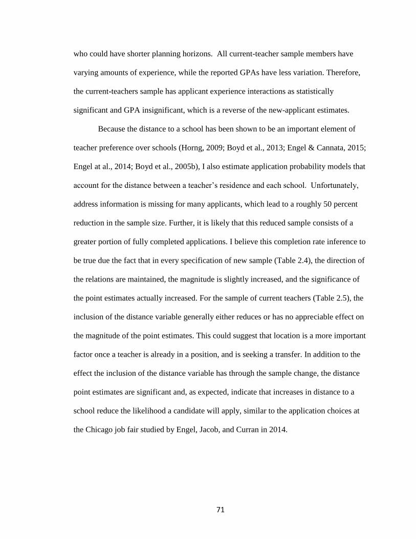
71

who could have shorter planning horizons. All current-teacher sample members have

varying amounts of experience, while the reported GPAs have less variation. Therefore,

the current-teachers sample has applicant experience interactions as statistically

significant and GPA insignificant, which is a reverse of the new-applicant estimates.

Because the distance to a school has been shown to be an important element of

teacher preference over schools (Horng, 2009; Boyd et al., 2013; Engel & Cannata, 2015;

Engel at al., 2014; Boyd et al., 2005b), I also estimate application probability models that

account for the distance between a teacher’s residence and each school. Unfortunately,

address information is missing for many applicants, which lead to a roughly 50 percent

reduction in the sample size. Further, it is likely that this reduced sample consists of a

greater portion of fully completed applications. I believe this completion rate inference to

be true due the fact that in every specification of new sample (Table 2.4), the direction of

the relations are maintained, the magnitude is slightly increased, and the significance of

the point estimates actually increased. For the sample of current teachers (Table 2.5), the

inclusion of the distance variable generally either reduces or has no appreciable effect on

the magnitude of the point estimates. This could suggest that location is a more important

factor once a teacher is already in a position, and is seeking a transfer. In addition to the

effect the inclusion of the distance variable has through the sample change, the distance

point estimates are significant and, as expected, indicate that increases in distance to a

school reduce the likelihood a candidate will apply, similar to the application choices at

the Chicago job fair studied by Engel, Jacob, and Curran in 2014.

72

2.7. Conclusion

This research provides an analysis of teacher application preferences in an Atlanta

Metropolitan area school district. My main contribution to the extensive teacher

preference literature is using the applications of prospective teachers to examine the

preferences of teachers entering a school district. The majority of my findings for new

teachers is consistent with the prior teacher preference research. Still, there are several

notable exceptions: the school climate, student poverty, school size, and the GOSA

School Report Card Grade. The new applicants were less likely to apply to schools with a

higher climate score and more likely to apply to a school with a higher portion of

economically disadvantaged students. This finding could result if positions in struggling

or difficult schools are more likely to be supported with increased resources, or the

vacancy is open longer due to the search being more difficult to complete and, therefore,

more likely to be up during any given window an applicant is applying. The odd result

for applicants being more likely to apply to schools with more students could also be due

to the search duration of the school leading the position to be open for a longer time or

could be a result of the sample construction whereby larger schools should have more

vacancies posted, but I am unable to observe and therefore account for total vacancies.

I also found that applicants were more likely to apply to schools with a GOSA

School Report Card letter grade of F, and less likely to apply to the other grades as

compared to grade C schools. There are several possible reasons. There is a higher

prevalence of grade F schools in the school district and if applicants apply somewhat

randomly is could seem they prefer grade F schools. In that case, though, there should

also be an increase in applications to grade D schools, and there is not. It could also be

73

the preferences against accountability pressures previously found in Feng, Figlio, and

Sass (2018) presenting in the application behavior, or preferences for increased resources

and rewards that may be allocated to low-ranked schools, as shown in Dizon-Ross

(2020). Furthermore, the result may due to the window of time the vacancy is posted in

the higher graded schools is too short for the applicants to complete their submission.

Engel and Finch (2015) found that higher-graded schools may have principals able to

utilize their personal networks to quickly complete their hiring process.

In general, my findings for current teachers are also consistent with those from

previous studies in the teacher preference literature. The primary exceptions are the

GOSA School Report Card and the number of students in a school, though they could be

explained by the factors discussed above for new applicants results discussed above.

Also, my results indicate a negative relationship between application probabilities and the

evaluation scores of a school’s principal. This evaluation score effect could mean that the

evaluation is capturing portions of the principal’s performance, which are unappealing to

teachers, and current teachers can capitalize on this information due to informal

information networks and apply elsewhere. If this is the reason behind the evaluation

result, then the evaluating entity may want to consider changing the measure to better

reflect the ability of the principal to attract teachers.

Together the findings for the new applicants and current teachers could support

the notion that teachers, as they progress in the profession, increasingly value “easier-to-

teach” positions and leverage their knowledge of the school system to obtain them.

Regardless, the differences mean that efforts to change a school’s appeal to candidates

should account for potentially varying impacts prospective teachers. For example, if a

74

school is attempting to attract current teachers, they should demonstrate that the school

climate is improving even if they cannot affect the student population. For both current

and new teachers, the distance of the school from their residence had a negative relation

with application probabilities. Therefore if the system was able to offer housing subsidies

to live close to the schools, they may be able to entice more applicants to those schools.

75

2.8. Tables

Table 2.1 Summary Statistics

All New Current All

Mean

Std.

Dev. Mean

Std.

Dev. Mean

Std.

Dev. Min Max

Applied to the

position 0.116 0.321 0.108 0.310 0.160 0.366 0 1

GADOE School

Climate Score

(STAR) 3.118 1.057 3.120 1.053 3.110 1.077 0 5

GADOE School

Climate Score

(STAR) missing 0.050 0.217 0.049 0.216 0.053 0.224 0 1

Percent of Students

Directly Certified 60.270 26.438 60.230 26.454 60.474 26.356 0 91.9

Percent of Students

Directly Certified

Missing 0.025 0.155 0.024 0.151 0.030 0.170 0 1

Number of

Students (100s) 6.665 2.669 6.648 2.643 6.754 2.802 0 20.09

Percent of Students

Black 0.775 0.314 0.775 0.313 0.773 0.317 0 1

Percent of Students

Hispanic 0.075 0.101 0.076 0.101 0.074 0.100 0 0.540

GOSA Report Card

Grade A 0.110 0.313 0.110 0.313 0.109 0.312 0 1

GOSA Report Card

Grade B 0.073 0.260 0.073 0.260 0.073 0.261 0 1

GOSA Report Card

Grade C 0.107 0.308 0.109 0.311 0.096 0.294

GOSA Report Card

Grade D 0.302 0.459 0.305 0.461 0.286 0.452 0 1

GOSA Report Card

Grade F 0.365 0.481 0.360 0.480 0.386 0.487 0 1

Principal

Experience 10.670 9.778 10.676 8.982 10.638 9.078 0 42.5

Principal

Experience

Missing 0.105 0.307 0.105 0.306 0.106 0.308

Principal

Evaluation Score 16.814 2.055 16.836 2.048 16.700 2.086 12 23

Principal

Evaluation Score

Missing 0.062 0.241 0.060 0.237 0.073 0.260 0 1

Principal Years in

the School 3.791 2.812 3.805 2.804 3.720 2.847 0 17

Principal Years in

the School Missing 0.060 0.237 0.061 0.240 0.051 0.221 0 1

Black Applicant 0.806 0.395 0.807 0.395 0.803 0.398 0 1

White Applicant 0.171 0.377 0.171 0.376 0.1773 0.378 0 1

Non-White Other

Applicant 0.023 0.149 0.023 0.149 0.024 0.153 0 1

76

Applicant Race

Missing 0.148 0.355 0.126 0.332 0.262 0.440 0 1

Applicant College

GPA 2.174 1.497 2.103 1.516 2.521 1.346

Applicant College

GPA Missing 0.334 0.472 0.359 0.480 0.209 0.407 0 1

Applicant Teaching

Experience 2.881 5.297 2.079 4.344 6.922 7.403 0 56

Applicant Teaching

Experience

Missing 0.019 0.138 0.022 0.146 0.008 0.086 0 1

Applicant Distance

to the School 171.768 581.807 189.967 620.486 64.872 224.677 0.059 14045

Applicant Distance

to the School

Missing 0.452 0.498 0.438 0.496 0.522 0.500 0 1

N 533,806 446,423 87,383 Notes: N is for the total sample. These summary statistics are unsuppressed in the regressions the mean will

be lower because all missing values are replaced with zero and an indicator for missing is included.

77

Table 2.2 Application Estimations for New Applicants-Relevant School Level-Subject Choice Set

1 2 3 4 5 6 7

GO

SA

Rep

ort

Car

d

Gra

de

Grade A -0.043*** -0.150*** -0.171*** -0.174*** -0.169*** -0.233***

(0.006) (0.005) (0.010) (0.010) (0.010) (0.015)

Grade B -0.118*** -0.097*** -0.122*** -0.123*** -0.121*** -0.126***

(0.007) (0.005) (0.008) (0.008) (0.008) (0.010)

Grade D -0.046*** -0.007*** -0.015*** -0.015*** -0.014*** -0.058***

(0.004) (0.003) (0.002) (0.002) (0.003) (0.006)

Grade F 0.048*** 0.043*** 0.024*** 0.024*** 0.025*** 0.010**

(0.004) (0.003) (0.002) (0.003) (0.003) (0.004)

Oth

er S

cho

ol

Ch

aract

eris

tics

GADOE School

Climate Score

(STAR)

-0.012*** -0.003*** -0.005*** -0.005*** -0.006*** -0.007***

(0.002) (0.001) (0.001) (0.001) (0.001) (0.001)

Percent of

Student Directly

Certified

0.002*** -0.000 0.000 0.000 0.000 0.000

(0.000) (0.000) (0.000) (0.000) (0.000) (0.000)

Number of

Students (100s)

0.004*** -0.000 0.002*** 0.002*** 0.001*** 0.001**

(0.001) (0.000) (0.000) (0.000) (0.000) (0.000)

Percent of

Students Black

-0.183*** -0.204*** -0.246*** -0.304*** -0.245*** -0.263***

(0.018) (0.011) (0.016) (0.012) (0.016) (0.024)

Percent of

Students

Hispanic

-0.344*** -0.409*** -0.397*** -0.356*** -0.399*** -0.544***

(0.019) (0.014) (0.023) (0.023) (0.023) (0.037)

Pri

nci

pal

Ch

arac

teri

stic

s

Experience 0.004*** 0.004*** 0.004*** 0.006***

(0.000) (0.000) (0.000) (0.000)

Evaluation Score -0.000 -0.000 -0.000 0.001

(0.000) (0.000) (0.000) (0.001)

Years in the

School

-0.001*** -0.001*** -0.001*** -0.001**

(0.000) (0.000) (0.000) (0.000)

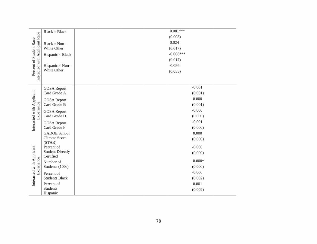
78

Per

cen

t o

f S

tud

ent

Rac

e

Inte

ract

ed w

ith

App

lica

nt

Rac

e Black × Black 0.081***

(0.008)

Black × Non-

White Other

0.024

(0.017)

Hispanic × Black -0.068***

(0.017)

Hispanic × Non-

White Other

-0.086

(0.055)

Inte

ract

ed w

ith

App

lica

nt

Ex

per

ien

ce

GOSA Report

Card Grade A

-0.001

(0.001)

GOSA Report

Card Grade B

0.000

(0.001)

GOSA Report

Card Grade D

-0.000

(0.000)

GOSA Report

Card Grade F

-0.001

(0.000)

GADOE School

Climate Score

(STAR)

0.000

Inte

ract

ed w

ith

App

lica

nt

Ex

per

ien

ce

(0.000)

Percent of

Student Directly

Certified

-0.000

(0.000)

Number of

Students (100s)

0.000*

(0.000)

Percent of

Students Black

-0.000

(0.002)

Percent of

Students

Hispanic

0.001

(0.002)

79

Inte

ract

ed w

ith

App

lica

nt

Co

lleg

e G

PA

GOSA Report

Card Grade A

0.027***

(0.003)

GOSA Report

Card Grade B

0.003

(0.002)

GOSA Report

Card Grade D

0.018***

(0.002)

GOSA Report

Card Grade F

0.005***

(0.002)

GADOE School

Climate Score

(STAR)

0.001*

(0.000)

Number of

Students (100s)

-0.000

(0.000)

Percent of

Student Directly

Certified

-0.000

(0.000)

Percent of

Students Black

0.010

(0.004)

Percent of

Students

Hispanic

0.066***

(0.009)

Principal Years

in the School

-0.000

(0.000)

Principal

Evaluation Score

-0.000***

(0.000)

Principal

Experience

-0.001***

(0.000)

N 444,403 444,403 444,403 444,403 444,403 444,403 444,403

Notes: For each of the non-interacted variables there is a non-reported indicator equal to one if the variable was missing and zero if not.

80

Table 2.3 Application Estimations for Current Teachers-Relevant School Level-Subject Choice Set

1 2 3 4 5 6 7

GO

SA

Rep

ort

Car

d

Gra

de

Grade A 0.004 -0.176*** -0.145*** -0.147*** -0.149** -0.167***

(0.011) (0.010) (0.013) (0.013) (0.015) (0.022)

Grade B -0.068*** -0.117*** -0.110*** -0.108*** -0.086*** -0.118***

(0.012) (0.011) (0.014) (0.013) (0.013) (0.020)

Grade D -0.053*** 0.008 -0.004 -0.004 0.012* -0.016

(0.008) (0.007) (0.005) (0.005) (0.007) (0.013)

Grade F -0.037*** 0.046*** 0.023*** 0.022*** 0.041*** 0.017

(0.008) (0.008) (0.007) (0.007) (0.009) (0.013)

Oth

er S

chool

Char

acte

rist

ics

GADOE School

Climate Score

(STAR)

0.008*** 0.010*** 0.007*** 0.007*** 0.005** 0.009**

(0.003) (0.003) (0.002) (0.002) (0.003) (0.004)

Percent of

Student Directly

Certified

-0.001*** -0.002*** -0.002*** -0.002*** -0.001*** -0.002***

(0.000) (0.000) (0.000) (0.000) (0.000) (0.001)

Number of

Students (100s)

0.010*** 0.004*** 0.003*** 0.004*** 0.004*** 0.003**

(0.001) (0.001) (0.001) (0.001) (0.001) (0.001)

Percent of

Students Black

0.037 -0.097*** -0.080*** -0.163*** -0.123*** -0.078

(0.039) (0.365) (0.029) (0.030) (0.034) (0.054)

Percent of

Students

Hispanic

-0.031 -0.279*** -0.210*** -0.212*** -0.252*** -0.188***

(0.036) (0.032) (0.028) (0.036) (0.036) (0.059)

Pri

nci

pal

Ch

arac

teri

stic

s

Experience 0.002*** 0.002*** 0.002*** 0.002***

(0.000) (0.000) (0.000) (0.001)

Evaluation Score -0.005*** -0.005*** -0.005*** -0.005***

(0.001) (0.001) (0.001) (0.001)

Years in the

School

-0.001 -0.001 -0.001 -0.001

(0.001) (0.001) (0.001) (0.001)

81

Per

cent

of

Stu

den

t R

ace

Inte

ract

ed w

ith A

ppli

can

t

Rac

e

Black × Black 0.135***

(0.020)

Black × Non-

White Other

-0.003

(0.049)

Hispanic × Black 0.005

(0.034)

Hispanic × Non-

White Other

-0.076

(0.123)

Inte

ract

ed w

ith A

ppli

cant

Exper

ience

GOSA Report

Card Grade A

0.001

(0.001)

GOSA Report

Card Grade B

-0.004***

(0.001)

GOSA Report

Card Grade D

-0.003***

(0.001)

GOSA Report

Card Grade F

-0.003***

(0.001)

GADOE School

Climate Score

(STAR)

0.000

Inte

ract

ed w

ith

Ap

pli

can

t

Ex

per

ien

ce

(0.000)

Percent of

Student Directly

Certified

-0.000**

(0.000)

Number of

Students (100s)

-0.000

(0.000)

Percent of

Students Black

0.007**

(0.003)

Percent of

Students

Hispanic

0.007**

(0.003)

82

Inte

ract

ed w

ith A

ppli

cant

Coll

ege

GP

A

GOSA Report

Card Grade A

0.009

(0.007)

GOSA Report

Card Grade B

0.004

(0.005)

GOSA Report

Card Grade D

0.005

(0.004)

GOSA Report

Card Grade F

0.002

(0.004)

GADOE School

Climate Score

(STAR)

-0.001

(0.001)

Number of

Students (100s)

0.000

(0.000)

Percent of

Student Directly

Certified

-0.000

(0.000)

Percent of

Students Black

-0.001

(0.019)

Percent of

Students

Hispanic

-0.009

(0.012)

Principal Years

in the School

0.000

(0.000)

Principal

Evaluation Score

0.000

(0.000)

Principal

Experience

-0.000*

(0.000)

N 86,747 86,747 86,747 86,747 86,747 86,747 86,747

Notes: For each of the non-interacted variables there is a non-reported indicator equal to one if the variable was missing and zero if not.

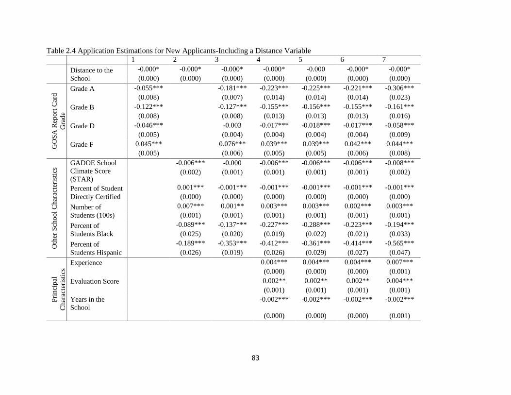
83

Table 2.4 Application Estimations for New Applicants-Including a Distance Variable 1 2 3 4 5 6 7

Distance to the

School

-0.000* -0.000* -0.000* -0.000* -0.000 -0.000* -0.000*

(0.000) (0.000) (0.000) (0.000) (0.000) (0.000) (0.000)

GO

SA

Rep

ort

Car

d

Gra

de

Grade A -0.055*** -0.181*** -0.223*** -0.225*** -0.221*** -0.306***

(0.008) (0.007) (0.014) (0.014) (0.014) (0.023)

Grade B -0.122*** -0.127*** -0.155*** -0.156*** -0.155*** -0.161***

(0.008) (0.008) (0.013) (0.013) (0.013) (0.016)

Grade D -0.046*** -0.003 -0.017*** -0.018*** -0.017*** -0.058***

(0.005) (0.004) (0.004) (0.004) (0.004) (0.009)

Grade F 0.045*** 0.076*** 0.039*** 0.039*** 0.042*** 0.044***

(0.005) (0.006) (0.005) (0.005) (0.006) (0.008)

Oth

er S

chool

Char

acte

rist

ics

GADOE School

Climate Score

(STAR)

-0.006*** -0.000 -0.006*** -0.006*** -0.006*** -0.008***

(0.002) (0.001) (0.001) (0.001) (0.001) (0.002)

Percent of Student

Directly Certified

0.001*** -0.001*** -0.001*** -0.001*** -0.001*** -0.001***

(0.000) (0.000) (0.000) (0.000) (0.000) (0.000)

Number of

Students (100s)

0.007*** 0.001** 0.003*** 0.003*** 0.002*** 0.003***

(0.001) (0.001) (0.001) (0.001) (0.001) (0.001)

Percent of

Students Black

-0.089*** -0.137*** -0.227*** -0.288*** -0.223*** -0.194***

(0.025) (0.020) (0.019) (0.022) (0.021) (0.033)

Percent of

Students Hispanic

-0.189*** -0.353*** -0.412*** -0.361*** -0.414*** -0.565***

(0.026) (0.019) (0.026) (0.029) (0.027) (0.047)

Pri

nci

pal

Ch

arac

teri

stic

s

Experience 0.004*** 0.004*** 0.004*** 0.007***

(0.000) (0.000) (0.000) (0.001)

Evaluation Score 0.002** 0.002** 0.002** 0.004***

(0.001) (0.001) (0.001) (0.001)

Years in the

School

-0.002*** -0.002*** -0.002*** -0.002***

(0.000) (0.000) (0.000) (0.001)

84

Per

cent

of

Stu

den

t R

ace

Inte

ract

ed w

ith A

ppli

can

t

Rac

e

Black × Black 0.092***

(0.011)

Black × Non-

White Other

0.013

(0.028)

Hispanic × Black -0.079***

(0.025)

Hispanic × Non-

White Other

-0.178**

(0.090)

Inte

ract

ed w

ith A

ppli

cant

Exper

ience

GOSA Report

Card Grade A

-0.001

(0.001)

GOSA Report

Card Grade B

0.000

(0.001)

GOSA Report

Card Grade D

-0.000

(0.001)

GOSA Report

Card Grade F

-0.002**

(0.001)

GADOE School

Climate Score

(STAR)

0.000

Inte

ract

ed w

ith

Ap

pli

can

t

Ex

per

ien

ce

(0.000)

Percent of Student

Directly Certified

0.000

(0.000)

Number of

Students (100s)

0.000

(0.000)

Percent of

Students Black

-0.002

(0.004)

Percent of

Students Hispanic

0.001

(0.003)

85

Inte

ract

ed w

ith A

ppli

cant

Coll

ege

GP

A

GOSA Report

Card Grade A

0.036***

(0.005)

GOSA Report

Card Grade B

0.004

(0.004)

GOSA Report

Card Grade D

0.016***

(0.003)

GOSA Report

Card Grade F

-0.004

(0.003)

GADOE School

Climate Score

(STAR)

0.001

(0.001)

Number of

Students (100s)

-0.000

(0.000)

Percent of Student

Directly Certified

0.000*

(0.000)

Percent of

Students Black

-0.010

(0.012)

Percent of

Students Hispanic

0.068***

(0.014)

Principal Years in

the School

0.000

(0.000)

Principal

Evaluation Score

-0.001***

(0.000)

Principal

Experience

-0.002***

(0.000)

N 254,964 254,964 254,964 254,964 254,964 254,964 254,964

Notes: For each of the non-interacted variables there is a non-reported indicator equal to one if the variable was missing and zero if not.

86

Table 2.5 Application Estimations for Current Teachers-Including a Distance Variable

1 2 3 4 5 6 7

Distance to the

School

-0.000** -0.000** -0.000** -0.000** -0.000* -0.000** -0.000**

(0.000) (0.000) (0.000) (0.000) (0.000) (0.000) (0.000)

GO

SA

Rep

ort

Car

d

Gra

de

Grade A -0.029* -0.167*** -0.114*** -0.116*** -0.116*** -0.134***

(0.016) (0.013) (0.016) (0.015) (0.017) (0.027)

Grade B -0.096*** -0.121*** -0.095*** -0.095*** -0.078*** -0.106***

(0.016) (0.017) (0.020) (0.019) (0.018) (0.027)

Grade D -0.025** 0.021** 0.003 0.002 0.011 -0.018

(0.011) (0.009) (0.006) (0.006) (0.008) (0.014)

Grade F -0.036*** 0.045*** 0.010 0.009 0.019** -0.001

(0.011) (0.010) (0.007) (0.007) (0.009) (0.015)

Oth

er S

chool

Char

acte

rist

ics

GADOE School

Climate Score

(STAR)

0.001 0.004 0.001 0.002 0.002 0.001

(0.004) (0.003) (0.002) (0.002) (0.003) (0.004)

Percent of Student

Directly Certified

-0.002*** -0.003*** -0.002*** -0.002*** -0.001** -0.001**

(0.001) (0.001) (0.000) (0.000) (0.000) (0.001)

Number of

Students (100s)

0.008*** 0.002 0.001 0.001 0.002 0.002

(0.002) (0.002) (0.001) (0.001) (0.001) (0.002)

Percent of

Students Black

0.105** -0.047 -0.026 -0.106*** -0.072* -0.029

(0.053) (0.054) (0.035) (0.031) (0.038) (0.060)

Percent of

Students Hispanic

0.085* -0.162*** -0.091*** -0.066 -0.132*** -0.036

(0.050) (0.052) (0.033) (0.045) (0.037) (0.069)

Pri

nci

pal

Ch

arac

teri

stic

s Experience 0.001*** 0.001*** 0.001*** 0.002***

(0.000) (0.000) (0.000) (0.001)

Evaluation Score -0.006*** -0.006*** -0.006*** -0.007***

(0.001) (0.001) (0.001) (0.001)

Years in the

School

-0.001 -0.001 -0.001 -0.002

(0.001) (0.001) (0.001) (0.002)

87

Per

cent

of

Stu

den

t R

ace

Inte

ract

ed w

ith A

ppli

can

t

Rac

e

Black × Black 0.122***

(0.026)

Black × Non-

White Other

0.013

(0.053)

Hispanic × Black -0.038

(0.039)

Hispanic × Non-

White Other

-0.184

(0.155)

Inte

ract

ed w

ith A

ppli

cant

Exper

ience

GOSA Report

Card Grade A

0.000

(0.001)

GOSA Report

Card Grade B

-0.004**

(0.002)

GOSA Report

Card Grade D

-0.002*

(0.001)

GOSA Report

Card Grade F

-0.002*

(0.001)

GADOE School

Climate Score

(STAR)

-0.000

Inte

ract

ed w

ith

Ap

pli

can

t

Ex

per

ien

ce

(0.000)

Percent of Student

Directly Certified

-0.000**

(0.000)

Number of

Students (100s)

-0.000

(0.000)

Percent of

Students Black

0.009**

(0.004)

Percent of

Students Hispanic

0.008**

(0.004)

88

Inte

ract

ed w

ith A

ppli

cant

Coll

ege

GP

A

GOSA Report

Card Grade A

0.008

(0.008)

GOSA Report

Card Grade B

0.004

(0.006)

GOSA Report

Card Grade D

0.008*

(0.005)

GOSA Report

Card Grade F

0.004

(0.005)

GADOE School

Climate Score

(STAR)

0.000

(0.001)

Number of

Students (100s)

-0.000

(0.001)

Percent of Student

Directly Certified

-0.000

(0.000)

Percent of

Students Black

0.001

(0.020)

Percent of

Students Hispanic

-0.021

(0.022)

Principal Years in

the School

0.000

(0.001)

Principal

Evaluation Score

0.000

(0.000)

Principal

Experience

-0.000*

(0.000)

N 42,267 42,267 42,267 42,267 42,267 42,267 42,267

Notes: For each of the non-interacted variables there is a non-reported indicator equal to one if the variable was missing and zero if not.

89

3. Who Knew? An Experimental Examination of Information Effects on a Teacher

Labor Market

3.1 Introduction

Several studies find that teachers are the most important school provided input

into a child’s education,27 in addition to being an anecdotal truth believed by most people.

However, there has been shown to be a disparity in access to quality teachers between

key student sub-groups. The disparity can occur due to differential job mobility patterns28

or in the hiring process,29 making the teacher labor market of particular interest.

Further research has shown that the quality of the match between the teacher and

the school, how well the teacher fits in with their peers and students can also affect the

teacher’s ability to contribute to their students’ growth.30 An additional benefit of a good

teacher-school match is that it increases the likelihood of prolonged tenure at the school,

which is of particular interest as experience is a teacher aspect positively related to

student achievement consistently.31 Improving the way teachers match to schools during

the hiring process seems an attractive intervention to improve equity in accessibility and

quality of education. Lastly, improving teacher tenure through improving their matches to

schools decreases the teacher turnover rate and, in turn, decreases the pecuniary and non-

pecuniary costs of turnover,32 allowing those resources to be directed into further helping

student achievement.

27 Rivkin et al., 2005; Aaronson et al., 2007; Kane et al., 2008 28 Darling-Hammond, 2001; Viadero 2002; Gordon & Maxey, 2000; Goldhaber et al. 2007; Feng & Sass, 2017

29 Sass, et al., 2012; Reininger, 2012 30 Jackson, 2013 31 Chingos & Peterson, 2011; Staiger & Rockoff, 2010; Rivkin et al., 2005; Clotfelter et al., 2006; Dobbie, 2011;

Wiswall, 2013; Papay & Kraft, 2015; Rockoff, 2004 32 Milanowski & Odden 2007; Guin, 2004

90

The possible benefits of improving matching in the teacher labor market stress the

importance of identifying behaviorally stable and efficient matching procedures between

teachers and schools. In this chapter, I use a laboratory experiment to examine the effect

of information about the teachers’ competitors on (i) teachers’ choices of signaling their

quality, (ii) the efficiency of the matching market, and (iii) the market stability. The

experimental design allows the identification of the effect of the information as I control

for the environment, namely the productivity of teacher-school pairing, a challenging task

for observational data. A novel feature of the experimental design is the integration of the

matching mechanism and (Spence) signaling model. These two models, widely used in

economic literature, will be described in detail later in this paper.

Matching markets theory offers a framework to model the teacher labor market I

am examining. The matching markets framework was initially designed to represent the

marriage market and the housing market (Gale & Shapley 1962) but has since been used

in many contexts such as medical residency placements (Roth & Xing, 1994, 1997; Kagel

& Roth, 2000; Roth, 1984, 1991) organ transplants (Roth et al., 2005), and school

assignments (Abdulkadiroğlu et al. 2005; Chen & Sönmez, 2006). The procedure I use

will be called the school hiring (SH) mechanism for the rest of this paper. The model is

based on the partner school district studied in the two other chapters of this dissertation.

However, in the markets modeled, there are varying levels of information. I examine the

effect of information about competitors on applicants’ choices and how school

assignments are affected by teachers’ strategic actions. It is hard to identify quality

teachers in the hiring process. A lot of the initial judgment stems from credentials, which

should be easier to achieve for high-type teachers when aligned adequately to teacher

91

quality. Examples of possible ability signals are licensure test scores, college selectivity,

college grade point average, and the degrees obtained.

Embedding a signaling model of applicant productivity in a two-sided matching

market is the main contribution of this experiment to the existing experimental economics

literature. Hopkins first developed the combination of the Spence model with the

matching markets framework in 2012. The concept of combining a two-sided matching

market with signaling was further expanded by Coles et al. (2013). However, Hopkins

focused on the effects of matching markets on the signaling equilibrium, and Coles et al.

focused on signals of interest. I use a two by two design of homogenous or heterogeneous

preferences over partners and additional versus no additional information in my

experiment. The purpose of the experiment is to generate data than can inform on the

effect of information on signaling investments and the market efficiency and stability of

the observed matches.

I examine information value in a lab setting for several reasons. The first being

that any policy interventions should be evidence based before being imposed on the

actual labor market. Creating that data as a survey has a problem regarding the difficulty

of ensuring the salience of answers and being unable to represent the market's two-sided

nature. Then, even if I could find districts following the treatments, the administrative

data would be so complicated that empirical identification would still be difficult. The

data issues are especially true for estimating market efficiency and payoffs, given that

many of the benefits teachers and schools receive from a given match cannot clearly be

measured due to being subjective. Besides, in the actual labor market, schools and

teachers can seek additional information outside of the signals, through methods such as

92

interviews, phone calls, and personal connections. Many of these interactions are never

recorded, thus muddling that aspect of an empirical analysis.

Further there are a plethora of hiring process variations which can affect the

match outcomes, such as teachers using the placement as a way to transfer somewhere

more preferred (indicating the markets are unstable),33 collective bargains,34 and other

policies that can disrupt placement planning.35 More importantly, when empirically

studying the existing labor market, both the schools’ and teachers’ true preferences are

unknown, meaning the market must be stable to allow for the calculation of self-sorting

(Boyd et al., 2013). The market I am interested in studying empirically is not stable based

on the large amounts of mobility.36 A further complication preventing studying this

question using observational data is that the geographic area I am studying has many

competing sub-markets causing the system to be very complex and challenging to

empirically model. Creating a controlled market and observing participants’ decisions in

this market, I can develop an initial understanding of how information can affect

applicants’ behavior in a two-sided matching market with the SH mechanism.

In light of these difficulties arising from asymmetric information, when and what

agents know becomes crucial. In the experiment, all signaling investments are

simultaneous in one treatment (the baseline), whereas in another treatment, investments

are sequential. That is, investments occur in random order and workers observe all earlier

investments. Also, to examine how the degree of competitiveness in the labor market

33 Reininger 2012; Boyd et al. 2005a,b; Boyd et al. 2013 34 Strunk et al. 2018; Levin et al., 2005 35 DeArmond et al., 2010; Cohen-Vogel et al., 2019; Heneman & Milanowski 2004, 2007 36 Ingersoll, 2001; Hanushek et al., 2004; Scafidi et al., 2007; Clotfelter et al., 2011; Feng, 2009; Jackson, 2013;

Goldhaber et al., 2011

93

affects the outcomes, I induce two preference sets in the experiment. I used these two

preference sets to study agents' choices when preferences are identical (competitive) or

heterogeneous (reduced competition).

The theoretical model (discussed in section 3.3) guided the parameterization of

the experiment. The participants in the experiment were Georgia State University

students recruited using the ExCEN online recruiter. After participants completed the

matching markets portion of the experiment, I also collected their demographic

information and behavior on a risk elicitation task, to control for individual idiosyncratic

characteristics.

Data from the experiment suggests that heterogeneous preferences decrease

agents investment amounts when not participating in the information treatment. Further,

the information treatment negatively impacts investment amounts when preferences are

homogenous. The information treatment also leads to the signaling investments revealing

worker type less often. The treatment has no effect however on market efficiency, but the

preferences being homogenous does result in higher efficiency. The information

treatment negatively affects firms’ payoffs when preferences are heterogeneous, but

positively affects firms’ payoffs when preferences are homogenous. However, no single

firm type bore the brunt of the effects of information. Regarding market stability, the

stability was higher for when the preferences were homogenous.

3.2 Literature Review:

In 1962, the matching markets framework was formalized by Gale and Shapley to

model college admissions and marriage market stability. This initial paper proposed the

Deferred Acceptance procedure, where agents from one side (the man or applicant) issue

94

an offer to one agent from the other side (the woman or college). The side receiving

offers can receive multiple offers and decides which to keep. Rejected agents then issue

offers to their next preferred, and so forth until no more rejections occur. The mechanism

is strategy-proof for the applicants (no applicant has an incentive to misrepresent their

preferences) and stable (no pair of applicant and college would both prefer each other

over their assigned partner). However, markets using Deferred Acceptance are not always

efficient, so in some cases, agents' total payoffs could increase in a non-equilibrium

solution (Roth, 1982).

The Deferred Acceptance mechanism is widely used and studied; however, for

this experiment, the matching procedure studied bears greater similarity to the Priority

(Boston) matching algorithm. The Priority algorithm is most easily described in the

context of student placements to Boston Public Schools in the early 2000s, such as in the

works of Abdulkadiroğlu et al. (2005) and Chen & Sönmez (2006). The schools each

have a priority ranking of all students based on several factors such as siblings, distance,

etc. While knowing the schools at which they had priority, students created a preference

ranking of schools to be submitted to the system for the assignment procedure. In the first

round, schools accepted any students within capacity constraints. If they had a surplus of

applicants, they retained students in the order of priority. Students who were not assigned

enter the second round of placements. The same procedure takes place at their second-

ranked school, but if the seat has already been filled, being a priority student will not

allow the student to receive a spot in the school. The matching procedure continues for as

many rounds as are needed to assign each student a school. This assignment procedure

gives students (the agents placing active offers or rankings) a strong incentive to

95

strategically order their preferences, such that schools for which they have priority are

ranked higher on their submitted preferences than in their true preferences. The strategic

ranking allows the students to receive a better final assignment than if they submitted

their true preferences. The primary difference between the Priority mechanism and the

School Hiring mechanism used in this paper is that those being proposed to can reject an

offer even if their quota is not full. This should not change the theoretical properties that

we would expect in a priority matching environment.

In addition to school assignment procedures, the Priority procedure has also

appeared in US and European medical student residency markets. The procedure was the

most commonly used unstable algorithm. The residency markets often were unstable

(leading to next period rematching) or matched unreasonably early. When introducing

various procedures into these markets as field experiments, the early matching only

decreased modestly under the priority algorithm, and instability increased (Roth, 1984,

1991).

For this experiment, agents also cannot defer acceptance, and thus workers must

reject their current offer to receive future offers. These workers may then accept a less

preferred partner early in the market to avoid the outcome of no or worse matches. The

main difference from the traditionally studied Priority algorithm is that for one side of the

market type (true productivity) is private information. Those agents must then use a

costly signal to demonstrate their type. Agents still have incentives to misrepresent their

preferences or type (act strategically) to make a better match like in the original Priority

procedure. This paper aims to determine if additional information regarding competitor

actions or the competition created by similar preferences impacts strategic behavior.

96

The model incorporated into two-sided matching markets to characterize the

incomplete information regarding agent type is the Spence signaling model (Spence

1973). In the model, workers know their productivity, but this information is not known

to firms. Agents signal their productivity by making costly investments where cost is

inversely related to productivity. Firms then observe signaling investments. The workers

can chose investment amounts (a separating equilibrium) that allow firms to determine

worker types or the workers can choose to invest the same amount (a pooling

equilibrium) or other amounts which result in firms being unable to determine worker

type. In the original (Spence) signaling game, their investments did not increase

productivity, and thus any amount of investment was socially inefficient. In this

experiment, the investment will be productivity increasing, with the increases occurring

at units 1, 4, and 7 to mimic preparation program completion effects, allowing the

investment to represent a properly-aligned signal of teacher quality.

Both the Spence Signaling Game and Matching Markets have been extensively

tested experimentally, and developed theoretically, in isolation. Researchers have tested

variation in the Spence Signaling game regarding the equilibrium type,37 behavior,38 and

the signal’s purpose.39 The research within the Matching Markets literature has covered a

variety of matching mechanisms40 comparative statics (Hopkins, 2012), levels of

asymmetric information,41 utility transferability (Becker, 1973, 1974), market types,42

37 Brandts & Holt, 1992; Banks et al., 1994; Cho & Kreps, 1987 38 Cooper & Kagel, 2003; Potters & van Winden, 1996 39 Coles et al., 2013; Miller & Plott, 1985; Kübler et al., 2008 40 Gale & Shapley, 1962; Shapley & Scarf, 1974; Roth, 1982, 1984, 1991; Roth & Xing, 1994, 1997; Hylland &

Zuckhauser, 1972; Abdulkadiroğlu & Sönmez, 1999; Sönmez & Ünver, 2011; Chen & Sönmez, 2003 41 Hopkins, 2012; Bikhchandani, 2017; Ehlers & Masso, 2015; Chen & Sönmez, 2003; Coles et al., 2013; Hoppe et al.,

2009 42 Gale & Shapley, 1962; Roth & Xing, 1997; Roth, 1991; Roth et al., 2004; Chen & Sönmez, 2006

97

and preference types (Becker, 1973, 1974). The listed research listed are examples in a

large body of experimental and theoretical work. This work shows that properties of

matching market outcomes can vary dramatically with the information environment.

Other experimentalists and theorists have developed research regarding the effects

of introducing varied preferences of the agents to study the impact on behavior and

prevent preference-specific results. Additional researchers have introduced information

asymmetry into two-side matching markets. Coles et al., 2013 developed a matching

market experiment that introduced signals as an element of the market. In their market,

the signals were to demonstrate interest or enthusiasm for the match in a congested hiring

market as preferences were private information. Also, in their experiment the worker

quality is known to firms and thus public information. The researchers show that signals

benefit searchers, do not harm employers, and work best under balanced markets. For the

signal to work, the number of signals must be limited. The study also examined the

effects of block correlated preferences, which are useful when firms have multiple

attributes by allowing for idiosyncrasies within worker preferences. In their experiment,

they have only one block, and the match's quality does not change due to the preferences,

so just being able to create any match is the target outcome.

In my model and experimental design, I draw upon various previous studies on

signaling games and matching procedures but did focus on insights from works focused

on the role of information on the market performance. This paper is not the first to

theoretically combine the two models (that honor goes to Hopkins, 2012). Still, it is the

first to examine it experimentally, and the focus of the theory is substantially different to

reflect the questions of interest in the experiment.

98

3.3 Theoretical Model

3.3.1 Assumptions

1) There is a one-to-one matching between teachers and schools.

2) There is a set of schools seeking to fill one teaching position.43

3) The sets of possible investment levels, teacher types, and school types are finite.

3.3.2 Information Environment

All agents' preferences over agents on the other side of the market are unknown to

the other agents and are private information. The school types are public information,

known to all. Each teacher knows their true value over matching with any possible

school. Teacher type is private information, known only to the teacher. All agents know

the set of possible teacher and school characterizations or types. The differences between

types are modeled by varying the matches' productivity, and their investment cost

represents the teacher's general productivity. There are three types of workers and three

types of firms in the experiment. In each market, there is one of each type of firm and

worker. Members of the market are unable to directly associate a type with a given

teacher. Teachers attempt to signal their types to the schools by making costly

investments. The investments are visible to all schools, all teachers when offers are being

made, and any teacher investing afterward in the Information treatment. Assigning the

match benefits induces the agents' preferences towards their possible partners. The

schools can infer a teacher's true type from their investment choice. There are high,

medium, and low general productivity teacher types represented in their investment cost,

43 This assumption appears to be strong, given that schools have many teachers and are often hiring more than one in a

year. However, this assumption operates using the concept that the positions available at a school are often vastly

different, resulting in disparate search efforts, and thus the final match is similar to a one-to-one match.

99

which are 10, 20, and 30, respectively. The firm types are 1, 2, and 3 defined by their

preference structure (which is identical in the competitive treatment) and the differential

productivity of their matches.

3.3.3 Wage Structure

Given that I am modeling the teacher labor market, I use a somewhat novel wage

structure. Generally, in the teacher labor market, the wage structure is rigid, with salary

being determined by where the teacher's experience and educational attainment place

them in a fixed salary schedule. The schedule means all new teachers with a bachelor's

degree earn essentially the same starting wage within a school system. Due to this

rigidity, non-pecuniary benefits of the match drive teacher preferences over schools

(Scafidi et al., 2007; Hanushek & Rivkin, 2007). These benefits consist of location (Boyd

et al., 2005a, b; Reininger, 2012), the characteristics of the student population at the

school, the perceived quality of the faculty and leadership, and a range of other factors.44

Instilling non-pecuniary preferences in the participants would not be salient, so to

parameterize these benefits, there is a school-specific wage the teachers received upon a

match. The benefits vary by the match and change only once during the experiment. I

could have parameterized investment with no productivity returns, as Spence did in his

1973 work. However, as the teacher wage has an adjustment to salary schedule based on

degree attainment, I decided to have the hybrid fixed payments as in Table 3.1. These

payments jump at specific investment values but remain the same in the interim.

44 Lankford et al., 2002; Hanushek et al., 2004; Imazeki, 2005; Feng, 2009; Feng & Sass, 2017; Goldhaber et al., 2015;

West & Chingos 2009

100

In the experiment, teachers and schools always receive a payment of 300 for

matching with their top choice, 200 from the second, and 100 from the bottom choice.

Table 3.2 presents the two preferences sets. The first set of preferences were chosen to be

the most competitive, given that all participant preferences are identical. The second set

of preferences decreases competition and increase the discordance between agents'

preferences over the other side. The choice of these two sets of preferences was to

prevent the results from being preference structure dependent.

3.3.4 Investment

Given the parameterization, the investment which will afford a teacher the

greatest payoff at each firm is 7 for a high type teacher, 4 for medium, and 1 for low. If

the teacher adopts a maximin strategy or believes that they have an equal probability of

matching with any given school, these would be the teachers' optimal investment. There

would be a separation of investment, revealing the teacher types.45

The maximum payoff for the market requires that high types invest 7, medium

types invest 4, and low types invest 1 resulting in investment payoffs of 100, 40, and 10.

If investments for each type deviate, this causes their investment payoff to decrease,

decreasing the maximum possible total payoff for the market. If a worker cannot make a

match, the cost of over-investment is greater as they also do not receive the payment for

investment.46 If they can make a match, overinvestment is offset for most types by the

additional pay from investment, especially for high type workers.47 Under the

45 Separation occurring is likely to be impacted by workers making strategic investments to obtain more preferred

matches. This is not studied directly in this paper, but the theory is discussed in Appendix A. 46 For high types, if they make no match and have invested nine instead of their maximin seven, or lower values like

six, they receive a payoff of negative ninety versus negative seventy or sixty. 47 For high types, if they invest eight instead of seven their payoff is ninety plus the match payoff instead of when they

underinvest at six only receiving sixty plus the match payoff.

101

competitive (homogenous) preferences, it is expected that the overinvestment will be

greater, as agents have the most direct benefit of presenting themselves as the high type.

If the worker achieves a better match of one rank by investing more, the worker's

payoff always increases. This means that under the competitive preferences, where the

highest investor should match with the best firm, an agent will invest more than their

competitors' investment when they can. Due to the incentive to misrepresent their type,

agents are more likely to do so when they have more information about their competitors'

actions and are thus able to pick their apparent type decreasing the likelihood investment

is in a type revealing ranking.48

Hypothesis 1: Agents will invest more when the preference rankings are

homogenous.

Hypothesis 2: Agents will invest more if they observe higher competitor

investment under competitive preferences.

Hypothesis 3: Agents are less likely to engage in separating investment in the

information treatment.

48 In preference set 1, (7, 4, 1) is not an equilibrium because the medium worker has an incentive to deviate and invest

8. (7, 4,1 ) is also not an equilibrium in preference set 2 as the low type worker has incentive to deviate and invest 8, or

the high and medium type workers have incentive to deviate and invest 1. However, there is a partial pooling

equilibrium in the simultaneous investment game of 9, 9, 1. High has no incentive to deviate as the expected payoff

from investing 9 due to ties being broken randomly is 330, which is greater than the most profitable deviation of

investing 7 and earning 300. The medium worker has no incentive to deviate as the expected payoff from investing 9 is

240, which is equal to the payoff from the most profitable deviation of investing 4 and being assigned to firm 2 (as

high’s investment is 9). Low has no incentive to deviate as low’s payoff from investing 1 is 110 which is larger than the

most profitable deviation of investing 9, which results in and being equally likely assigned to either firm and an

expected payoff of 100. For preference set 2, non-type revealing separating equilibrium is (7, 0, 8). High type has no

reason to deviate because as they receive 300 and the expected payoff of their next best investment 0 is 250. The

medium type has no reason to deviate because while they could obtain more at 4 this would make 0 the best option for

the high type decreasing medium types payoff at four. Low type has no incentive to deviate as their next best payoff is

210 when investing 1 as opposed to their current payoff of 230.

102

3.3.5 Matching Mechanism

In the experiment, I use a decentralized design where offers are transmitted

directly from schools to teachers to elicit behavior as similar to the real labor market as

possible, given that the actual market is decentralized. The other matching market

possibility is centralized, where all agents list their preferences and submit them to a

central matching organization. It is important to reemphasize that the primary difference

between this mechanism, and the priority matching mechanism is that those being

proposed to can reject an offer even if their quota is not full. This should not change the

theoretical properties that we would expect in a priority matching environment.

3.3.5.1 The School Hiring Mechanism

1) Teachers know school types, own type, and the distribution of competitor types. They

also know all of their possible payoffs from each combination of investment and

match.

2) After observing the available information, teachers choose an amount of investment.

3) Once a teacher’s investment is chosen, they apply to all schools. This is the point

when schools can observe the teachers' investments.

4) Schools cannot observe true types, but they do observe all investments and make

decisions on offers to workers.

5) Round 1.

a. Schools issue their first an offer to a teacher.

b. Teachers only receive up to one offer at a time.

i. If multiple schools issue an offer to one teacher, the offer from the school

ranked highest by that teacher is presented to the teacher.

c. The teachers then accept or reject the offer.

i. If the teacher accepts, the match is implemented, removing both the teacher

and the school from the market. Offers can continue to be received, but they

will be automatically rejected.

ii. The teacher must reject the offer to receive future offers.

103

6) Round k.

a. Any school rejected in round k-1 issues an offer to the next teacher in their list

that has not previously rejected the school.

b. Teachers only receive up to one offer at a time.

i. If multiple schools issue an offer to one teacher, the offer from the school

ranked highest by that teacher is presented to the teacher.

c. The teachers then accept or reject the offer.

i. The teacher must reject the offer to receive future offers.

7) End: The rounds continue until no more rejections occur.49

3.3.6 Market Efficiency and Payoffs

In this experiment's parameterization, under preference set 1, the maximum total

payoff is 1350 points and can be achieved in any matches. As long as the workers invest

their maximin amount, the surplus will just be redistributed. However, under preference

set 2, the maximum total payoff is 1450 in a single match outcome (S1T2, S2T3, and

S3T1), but this match outcome is not stable. As market efficiency is in terms of total

possible payoff, if agents invest the maximin amount and enter a stable match outcome,

efficiency would be lower in preference set 2. If the efficiency is not lower, then this is

due to the deviation in investment in preference set 1 being substantially higher.

Hypothesis 4: There will be a decrease in efficiency under preference set two

because the max payoff is greater than in preference set one, but achieving the maximum

outcome is unlikely.

Hypothesis 5: Due to agents deviating from the maximin investment by more with

additional participant information and under the homogenous preferences, payoffs will be

lower in those treatments.

49 This matching mechanism reporting format is based from the work Chen and Sönmez (2006).

104

3.3.7 Market Stability

In the case of a separating investment equilibria and workers following a sincere

acceptance strategy, the SH mechanism produces a stable matching. As teachers gain

more information about their competitors' actions, they will be better able to represent

themselves favorably. The deceptive representation can lead to increased instability as it

is more likely for a teacher-school pair who prefer each other cannot match due to the

firm not being able to discern type accurately.

Hypothesis 6: When teachers have more information about competitors' actions,

the outcomes will be less stable.

3.3.8 Risk

There are several ways the risk attitudes of agents may affect the outcomes.

There is strategic risk in the teachers' choices in the simultaneous investment game as

they learn the schools' preferences during the rounds or other teachers' investments. The

optimality of their investment is dependent on the choices of competitors. Teachers may

over invest to ensure they have a greater investment than their competitors under the

competitive preference rankings. The probability of matching with a given school is

affected by how their investment ranks affect school offers. Since the SH mechanism

requires teachers to accept or reject an offer, there is the risk a teacher may remain

unmatched in the case of rejecting an offer. Thus risk-averse teachers would be more

likely to accept an early offer from a less preferred school. Risk-averse schools are more

likely to issue offers to a less-preferred teacher if the perceived probability of acceptance

from the most-preferred worker is low enough.

105

3.4 Experimental Design

3.4.1 Treatments

There are four treatments in this experiment. Participants took part in a market

where the teachers were making simultaneous or sequential investments and were then

matched to a school using the SH matching procedure. These two investment structures

which affect participants' information were implemented as a between-subject design.

The information treatment is crossed with competitive preferences (preference set 1) and

less competitive preferences (preference set 2). Participants experienced both sets of

preferences, and thus this was a within-subject implementation.

When teachers invested simultaneously, each teacher chose their investments

without any knowledge of the other teachers' investment decisions. However, they do

view their competitors' investments during the market decision. This design is the most

similar to the true market as applicants cannot control the composition of their competing

cohort of applicants. However, they may be able to gather information during the

interview process about where they stand and how likely they are to receive an offer.

However, this lack of information adds an additional component of strategic risk to their

decision. The second treatment of sequential investments was implemented to examine

the effects of added information on investment decisions. In this treatment, teachers

chose their investments one at a time in random order and could view the preceding

workers' investments. To better separate the differences between the two treatments'

investment behavior and allow the participants to understand the game better, all

participants in the first few rounds (part one stage one) of the experiment made signaling

investment decisions and were automatically matched to schools.

106

Seven sessions were run in total. In five of the sessions, the participants

completed the automated firm portion, the active firms and workers portion, and the risk

task. In the other two sessions, the participants could not complete the active firm portion

due to technical difficulties. Three of the completed sessions had sequential investing,

with a total of 66 participants. The other two completed sessions had simultaneous

investing with a total of 42 participants. The decisions from the incomplete sessions were

in the simultaneous investment environment. This resulted in 208 rounds of Simultaneous

investment with the same preferences and automated firms and 142 in the same

environment with heterogeneous preferences. In the rounds, where firms were also

agents, there were 41 rounds in the homogenous, simultaneous treatment, 61 rounds in

the homogenous, sequential treatment, 45 rounds in the heterogeneous, simultaneous

treatment, and 89 rounds in the heterogeneous, sequential treatment.

3.4.2 Implementation

In the second and third stages of part one of the experiment, the teachers and

schools were both active participants. The participants were Georgia State University

students recruited using the ExCEN online recruiter. The participants were recruited for

seven separate sessions, and in each session, there was only one information treatment,

making this a between-subjects design. The experimental set up allowed for comparison

within participants of the effects of the different parameterizations.

In part one stage one (the first few (seven to ten) rounds), all participants were

teachers (called workers in the experiment), and the assignment to schools (called firms

in the experiment) was automatic based on the rank order of their investments. This

means that in the portion where the firms were automated participants only experienced

107

preference set 1. In the remaining (13 to 20) rounds, participants were split equally into

the roles of teachers or schools. Half of the rounds, termed part 1 stage 2, teachers and

schools were randomly assigned a unit investment cost and their preference from either 1

or 2. Then in part 1 stage 3, the participants remained as either a teacher or a school,

randomly assigned a unit investment cost, and followed the other preferences. The

ordering of preferences 1 and 2 was varied between sessions.

In each round, participants matched with a new group to better represent the

teacher labor market. Matching in this manner has been shown not to simulate one-shot

game behavior resulting in systematic differences from perfect stranger matching in

public goods games (Botelho et al., 2009). However, it does simulate a market where the

teachers have rapid turnover and compete with similar sets of competitors through their

careers. Besides, it is not feasible to complete this experiment with perfect stranger

matching due to the requisite number of participants to complete the matchings.

3.4.2.1 Decision Tasks

1. In each round a “teacher” chooses an investment between 0 and 9. The treatment

determines investment order, which is randomized in the sequential treatments. (Figures

3.1 and 3.2)

2. “Schools” know their own preferences over types but can’t observe teachers’ types.

They issue offers to teachers after observing teachers’ investments. (Figure 3.3)

3. Teachers know their preferences over schools. They make decisions on whether to

accept or reject an outstanding offer knowing that acceptance ends the game. (Figures 3.4

and 3.5)

108

4. Steps 2 and 3 are repeated until there are no rejections or all possible firm offers have

been extended. This results in a maximum of three offers and six decisions per round.

5. Once matches are finalized, the participants’ payoffs for the round are revealed, both

the round and the stage average. The round payoff is shown to all members of the group.

(Figures 3.6 and 3.7)

3.4.2.2 Risk Task

After completing the first two phases of the experiment, the participants completed

a risk elicitation section consisting of up to 50 tasks. Each task consists of a choice between

two lotteries, Left and Right. The participants knew one task would be randomly selected

using a dice roll, and that they would be paid based on the resolution of the lottery they had

selected for the random task. Between the 50 tasks, the possible prizes of the lotteries and

the probabilities of each prize were varied. The task design emulated Harrison and Ng

(2016). Each lottery had up to three prize states, with each probability being a multiple of

twenty-five percent. The order the tasks administered were randomized between

participants. The first three sessions had different tasks and the number of tasks due to

calibration, timing, and technical issues. (Figure 3.8)

3.4.2.3 Demographic Survey and Participant Summary Statistics

The sessions ended with a demographic survey of participants' gender, parent

income, parental education, major, college grade point average, and race. 132 participants

completed the demographic survey in six sessions. In the seventh session, technical

difficulties prevented the administration of the demographic survey. The summary

statistics of their answers are reported in Table 3.3. The majority of the participants were

109

black. There was a fairly wide range of parental income and education. The participants

had an average GPA of 3.7.

3.4.2.4 Payment

The participants were paid the sum of the average payoff from all rounds in part 1

separated by stage, and the outcome after the resolution of the lottery in the randomly-

selected risk task.

Each round, the payoff was determined and recorded electronically following the

investment decisions and the realized payoffs. Then to determine the outcome of the risk

task, the proctor went to each participant and rolled a pair of dice to determine which risk

task was chosen for implementation and then used dice or a spinner app to resolve the

lottery. The total payment amount was written on a slip of paper for the participant to

take to another proctor for payment. Only the experimenters, not the other participants,

saw the payment outcomes; this ensured the experiment utilized a single-blind payment

procedure.

Participants were informed of this payment method before the experiment began.

The payment mechanism's salience was assured due to maintaining an appropriate

average payoff of $24.6, with a minimum payoff of $9 and a maximum payoff of $55.

The experiment duration was two hours or less, including the time needed to explain the

instructions and pay the participants, so the average payoff was higher than the minimum

wage.

3.5 Results

In this experiment, I examine the effects of the information treatment and

preference set variation on participant investment decisions, market efficiency and

110

payoffs, and market stability. For each outcome, I estimate the effects separately for each

preference set. Each agent in the market had different incentives, so I estimate the effects

by participant type for investment amounts and market payoffs. I split this investment

analysis into changes to investment amount and the prevalence of participants selecting a

type-revealing separating equilibrium. Except for individual market payoffs and the

estimation of each worker types' likelihood to invest the most, each estimation has two

specifications. The first includes controls to the information treatment, the firms being

active participants, and period and session fixed effects. The second includes the

participants' demographic and risk preference information. The additional variables

account for the effects that participants' idiosyncratic characteristics could have on the

decisions. For market efficiency and payoffs, I also estimate a specification including a

binary variables for homogenous preferences and information treatment interacted with

homogenous preferences.

3.5.1 Signaling Decision

Result 1: Heterogeneous preferences decrease investment amounts when

participants are not in the information treatment.

Support: In the rounds with simultaneous investment, all types invest more when

the preferences are homogenous. In the information treatment, the amount is higher for

high and low types under the heterogeneous preference set (Table 3.4). Then, when

estimating the investment amount, the constant term (the baseline investment amount) is

not statistically different for heterogeneous preferences than for homogenous preferences

except for high type workers where there is an increase (Tables 3.5, 3.6, and 3.7).

111

Result 2: The information treatment negatively impacts the investment amount

when preferences are homogenous.

Support: Under homogenous preferences, the information treatment negatively

impacts the amount of worker signaling investment. The decrease in investment due to

information, while holding other factors constant, brings the medium and low type

workers’ investment closer to the most efficient (for the market) investment amount.

During the rounds with the heterogeneous preference set, high types also invest closer to

the efficient amount (Tables 3.5, 3.6, and 3.7). Under the same preferences, all workers

invest less in the investment treatment, and the medium type worker also invests less in

the information treatment under heterogeneous preferences. Though the largest treatment

effect that can be seen is that low type workers invest substantially more on average

under different preferences (Table 3.4).

To further investigate this phenomenon, I studied which worker types invest the

most. When examining the averages, the high type is less likely to be the greatest investor

in the information treatment when there are heterogeneous preferences (Table 3.4). When

empirically estimating the probabilities of being the highest investor, the information

treatment has a statistically significant negative effect on high types in both preference

sets (Table 3.8). This is to be expected because in the simultaneous signaling game with

homogeneous preferences, a high type invests 7, 8, or 9. A risk-averse type would invest

9 to increase the likelihood of a preferred match with an additional cost of only 20 points.

However, in the sequential signaling game, the risk-averse type would also invest 9 when

they move first and probably second, but their investment is the max of seven and the

112

largest Observed Maximum Investment when moving last. Therefore high types are

expected to invest less in the sequential game.

Result 3: The signaling investments are less informative when there is additional

information on competitors’ actions and heterogeneous preferences because the portion

of the time investments are type revealing decreases.

Support: For investments to reveal type (be separating), the investment amounts

need to be negatively related to their investment costs. The high type workers invest the

most, the middle second, and the low type the least. There is a smaller separation between

types when there is sequential investment except for high types in preference set 2 when

the averages are compared. When looking at the portion of the time the investments are

completely separating, this is lower in the treatment in preference set 2 (Table 3.4). The

remaining pooling outcome possibility that is not reported is when there are no ties, and

the order is not type revealing.

When agents have homogenous preferences, and the firms are also participants,

the likelihood of investment separation increases. The information treatment decreases

separation likelihoods under both preference sets, but the effect is greater when

preferences are heterogeneous. In homogenous preferences, the information treatment

also increases the likelihood of two participants selecting the same investment amount

(Table 3.9). A scatter plot of the average investment in a period shows consistent

investment separation (Figure 3.9). The investment is also mainly separated within

treatments on average. When comparing the plots for the information treatment (Figures

113

3.10 and 3.12) to the non-information treatment plots (Figures 3.12 and 3.13), there is

less separation in the information treatment.50

3.5.2 Market Efficiency and Payoffs

Result 4: The information treatment has no impact on market efficiency, and the

market efficiency is higher when the preferences are homogenous.

Support: Market efficiency estimations, as defined by the realized payoff divided

by the maximum payoff (1350 for preference set 1 and 1450 for preference set 2), are

reported in Table 3.10. When examining the information treatment point estimates, there

is no statistical impact. However, when the constant terms are studied, it is revealed that

when preferences are homogenous, the market is closer to the efficient outcome. The

impact of the preferences may be because only investments can impact the total market

payoff when there are homogenous preferences (the difference between matches is the

distribution of the wealth). In contrast, under heterogeneous preferences, the match can

affect the maximum total payoff as well.

Result 5: The information treatment has a negative impact on the firms’ payoffs

when preferences are heterogeneous, and these decreases for firms in total are not

consistently at the detriment of a single firm type.

Support: On average, firms receive a higher payoff when there are homogenous

preferences in the information treatment and the most negative outcome when

preferences are heterogeneous in the information treatment (Table 3.4). The information

treatment negatively impacts total firm payoff when estimating across all rounds with

50 There were no consistently estimated period effects, so there appears to be little participant learning over the course

of a session.

114

controls for preferences set and information treatment interacted with the preference set.

However, the negative impact of the information treatment is mostly negated by the

positive impact of the information treatment interacted with the homogenous preference

set (Table 3.11). Further, while there are no estimated impacts of the information

treatment in the estimates separated by preference type, each group's baseline payoff

amount is higher when the preferences are homogenous (Tables 3.12 and 3.13). When

examining the payoffs by individual type, none of the firm types are negatively impacted

by the information treatment under either preference set (Table 3.14). Within worker

types, the high-type worker is negatively impacted by information under homogenous

preferences, which matches the fact they underinvest when preferences are homogenous.

Medium type workers are positively impacted by information under heterogeneous

preferences but negatively impacted when preferences are homogenous on average. This

outcome may reverse when taking into account participant risk preferences. Low type

workers are unaffected by the information treatment. (Table 3.4 and 3.15).

3.5.3 Market Stability

Result 6: The information treatment does not impact market stability, which is

greater when preferences are homogenous.

Support: When examining the portion of matches from the set of stable matches

in Table 3.16, there are no statically significant estimates regarding the impact of the

information treatment. In contrast, when examining the same preference terms, it can be

seen that a greater portion of the matches are from the stable outcome when the

preferences are the same; this may because the workers do not prefer the stable match in

preference set 2 and therefore, may attempt more vigorously to alter the outcome.

115

3.6 Conclusion

In this experiment, I was able to identify that subjects do change their investment

behavior when they possess additional information regarding their competitors' actions

and between preference structures. Further, market efficiency can decrease when workers

have additional information, but this decrease depends on the market's preference

structure. The data suggest that the differences caused by the treatments are larger for

schools on average. The most negative effect on payoffs occurs when examining the

impact of the information treatment within the heterogeneous preferences. The greatest

positive difference being homogenous preferences over heterogeneous preferences within

the information treatment. The workers' average payoffs decrease the most when moving

from preference set 2 to preference set 1 within the information treatment. Still, their

payoffs are always higher in preference set 2 than preference set 1 and in the information

treatment on average.

Overall the interaction of the Spence signaling game and two-sided matching

markets leads to interesting participant behavior. In this labor market, it appears best to

not let the teachers observe their competitors' investments if the goal is to promote the

schools' welfare, mainly when the preferences of schools and teachers are varied.

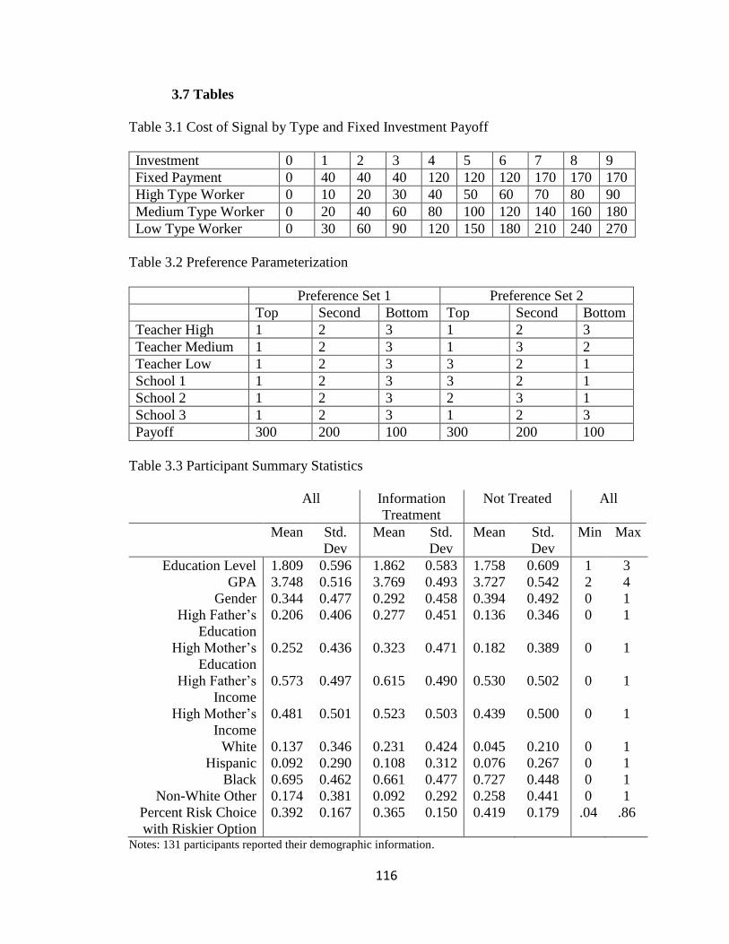
116

3.7 Tables

Table 3.1 Cost of Signal by Type and Fixed Investment Payoff

Investment 0 1 2 3 4 5 6 7 8 9

Fixed Payment 0 40 40 40 120 120 120 170 170 170

High Type Worker 0 10 20 30 40 50 60 70 80 90

Medium Type Worker 0 20 40 60 80 100 120 140 160 180

Low Type Worker 0 30 60 90 120 150 180 210 240 270

Table 3.2 Preference Parameterization

Preference Set 1 Preference Set 2

Top Second Bottom Top Second Bottom

Teacher High 1 2 3 1 2 3

Teacher Medium 1 2 3 1 3 2

Teacher Low 1 2 3 3 2 1

School 1 1 2 3 3 2 1

School 2 1 2 3 2 3 1

School 3 1 2 3 1 2 3

Payoff 300 200 100 300 200 100

Table 3.3 Participant Summary Statistics

All Information

Treatment

Not Treated All

Mean Std.

Dev

Mean Std.

Dev

Mean Std.

Dev

Min Max

Education Level 1.809 0.596 1.862 0.583 1.758 0.609 1 3

GPA 3.748 0.516 3.769 0.493 3.727 0.542 2 4

Gender 0.344 0.477 0.292 0.458 0.394 0.492 0 1

High Father’s

Education

0.206 0.406 0.277 0.451 0.136 0.346 0 1

High Mother’s

Education

0.252 0.436 0.323 0.471 0.182 0.389 0 1

High Father’s

Income

0.573 0.497 0.615 0.490 0.530 0.502 0 1

High Mother’s

Income

0.481 0.501 0.523 0.503 0.439 0.500 0 1

White 0.137 0.346 0.231 0.424 0.045 0.210 0 1

Hispanic 0.092 0.290 0.108 0.312 0.076 0.267 0 1

Black 0.695 0.462 0.661 0.477 0.727 0.448 0 1

Non-White Other 0.174 0.381 0.092 0.292 0.258 0.441 0 1

Percent Risk Choice

with Riskier Option

0.392 0.167 0.365 0.150 0.419 0.179 .04 .86

Notes: 131 participants reported their demographic information.

117

Table 3.4 Investment and Market Outcomes When Firms are Participants

Preferences over other

side of the market

Same Different

Signaling Game Simultaneous

N=41

Sequential

N=61

Simultaneous

N=45

Sequential

N=89

Investments

High Type Workers 6.927

(1.603)

[2, 9]

6.311

(1.639)

[1,9]

6.422

(1.196)

[4,8]

6.427

(1.269)

[4,9]

Medium Type Workers 5.682

(2.360)

[1,9]

5.344

(1.806)

[1,8]

4.489

(2.232)

[0,9]

4.247

(2.352)

[1,9]

Low Type Workers 3.512

(2.481)

[1,9]

3.311

(2.446)

[0,9]

3.000

(2.384)

[0,9]

4.315

(2.410)

[1,9]

Market Outcomes

Efficiency and Distribution

Workers Payoff 689.756

(150.988)

[350,940]

650.656

(111.383)

[380,750]

702.000

(149.721)

[230,950]

697.303

(199.845)

[270,950]

Firms Payoff 504.878

(107.124)

[200,600]

550.820

(95.957)

[300,600]

517.778

(119.257)

[200,700]

446.067

(139.036)

[200,900]

Total Payoff 1194.634

(199.187)

[650,1340]

1201.475

(199.030)

[750,1350]

1219.778

(201.297)

[690,1440]

1143.371

(244.310)

[610,1400]

Distribution Across Types

High Type Workers 305.122

(115.285)

[-90,400]

287.377

(136.356)

[-80,400]

314.444

(121.123)

[-80,400]

296.405

(142.041)

[-90,400]

Medium Type Workers 218.781

(118.178)

[-160,340]

199.672

(114.192)

[-140,340]

214.000

(120.405)

[-140,340]

226.966

(125.394)

[-180,340]

Low Type Workers 165.854

(135.185)

[-240,310]

163.607

(111.101)

[-210,310]

173.556

(103.202)

[-120,310]

173.933

(110.130)

[-240,310]

Type 1 Firms 182.927

(91.931)

[0,300]

222.951

(84.446)

[100,300]

208.889

(87.444)

[100,300]

142.697

(78.172)

[0,300]

Type 2 Firms 165.854

(85.469)

[0,300]

181.967

(78.546)

[0,300]

175.556

(82.999)

[0,300]

135.955

(90.763)

[0,300]

Type 3 Firms 156.098

(83.812)

[0,300]

145.902

(107.353)

[0,300]

133.333

(82.572)

[0,300]

167.416

(80.869)

[0,300]

118

Separation and Pooling Decisions

High Type Workers

Invest Most

0.537

(0.505)

[0,1]

0.541

(0.502)

[0,1]

0.555

(0.503)

[0,1]

0.472

(0.502)

[0,1]

Medium Type Workers

Invest Most

0.268

(0.449)

[0,1]

0.197

(0.401)

[0,1]

0.089

(0.288)

[0,1]

0.135

(0.343)

[0,1]

Low Type Workers Invest

Most

0.073

(0.264)

[0,1]

0.098

(0.300)

[0,1]

0.044

(0.208)

[0,1]

0.157

(0.366)

[0,1]

Completely Separating

Investment

.293

(.461)

[0,1]

0.361

(0.484)

[0,1]

0.311

(0.468)

[0,1]

0.112

(0.318)

[0,1]

Partially Pooling

Investment

.293

(.461)

[0,1]

0.426

(0.499)

[0,1]

0.467

(0.505)

[0,1]

0.506

(0.503)

[0,1]

Completely Pooling

Investment

0

(0)

[0,0]

0.016

(0.128)

[0,1]

0.022

(0.149)

[0,1]

0.022

(0.149)

[0,1] Notes: Means, Standard deviation in parentheses, and then the minimum and maximum in square brackets.

119

Table 3.5 Investment of High Type Teachers

Same Different

VARIABLES No Descriptors Descriptors No Descriptors Descriptors

Information

Treatment

-2.136*** -2.193*** -0.328 -2.873***

(0.539) (0.518) (0.556) (0.676)

Active Firms -0.672 -0.607

(0.541) (0.764)

Percent of Risky

Choices Selected

0.859 3.146***

(0.713) (0.970)

Observed Maximum

Investment

0.006 0.010

(0.046) (0.038)

Education Level 2 0.632** 0.856**

(0.293) (0.352)

Education Level 3 0.725 -0.124

(0.507) (0.246)

GPA Reported 0.149 -0.983**

(0.245) (0.435)

Gender 0.399 -0.410

(0.290) (0.640)

Father had Higher

Education

-0.602* 2.332***

(0.354) (0.640)

Mother had Higher

Education

0.311 1.256***

(0.312) (0.323)

Black -0.518* -0.766**

(0.287) (0.276)

Constant 5.689*** 4.866*** 6.520*** 9.961***

(0.401) (0.997) (0.866) (1.505)

Period Fixed Effects X X X X

Session Fixed

Effects

X X X X

Observations 452 394 134 134

R-squared 0.264 0.328 0.065 0.316 Notes: The dependent variable is the investment amount of the worker in a single round. Active firms is a

binary indicator for if the rounds were after stage 1 of part 1. Percent of Risky Choices Selected is the

number of choices in the risk task the participant selected the one with greater variance in outcomes divided

by total number of completed choices. Observed Maximum Investment of others is zero for the

simultaneous game and first investors, and the maximum of the earlier investors for the second and third

investors in the sequential game. Education level 2 is some college and Education level 3 is college degree

or greater. Gender is a binary variable equal to 1 if the participant was female. Mother and Father had a

Higher Education means the parent in question had a master’s degree, a doctorate, or a professional degree.

120

Table 3.6 Investment of Medium Type Teachers

Same Different

VARIABLES No Descriptors Descriptors No Descriptors Descriptors

Information

Treatment

-0.777 -1.085* -2.100 -1.655

(0.523) (0.621) (1.532) (1.828)

Active Firms -0.046 -0.458

(0.691) (0.954)

Percent of Risky

Choices Selected

1.327 0.525

(0.927) (1.796)

Observed Maximum

Investment

0.022 0.087

(0.048) (0.088)

Education Level 2 0.358 0.467

(0.329) (0.528)

Education Level 3 0.661 0.347

(0.526) (1.632)

GPA Reported -0.243 -1.180*

(0.279) (0.620)

Gender -0.164 -0.060

(0.397) (1.110)

Father had Higher

Education

-0.736* -0.832

(0.374) (0.847)

Mother had Higher

Education

0.395 -0.107

(0.336) (1.054)

Black -0.442 -0.719

(0.354) (0.836)

Constant 5.048*** 5.601*** 4.438** 8.255**

(0.454) (1.236) (1.820) (3.845)

Period Fixed Effects X X X X

Session Fixed

Effects

X X X X

Observations 452 396 134 134

R-squared 0.128 0.166 0.356 0.486 Notes: Dependent variable is the investment amount of the worker in a single round. All explanatory

variables are as defined in the note of Table 7.

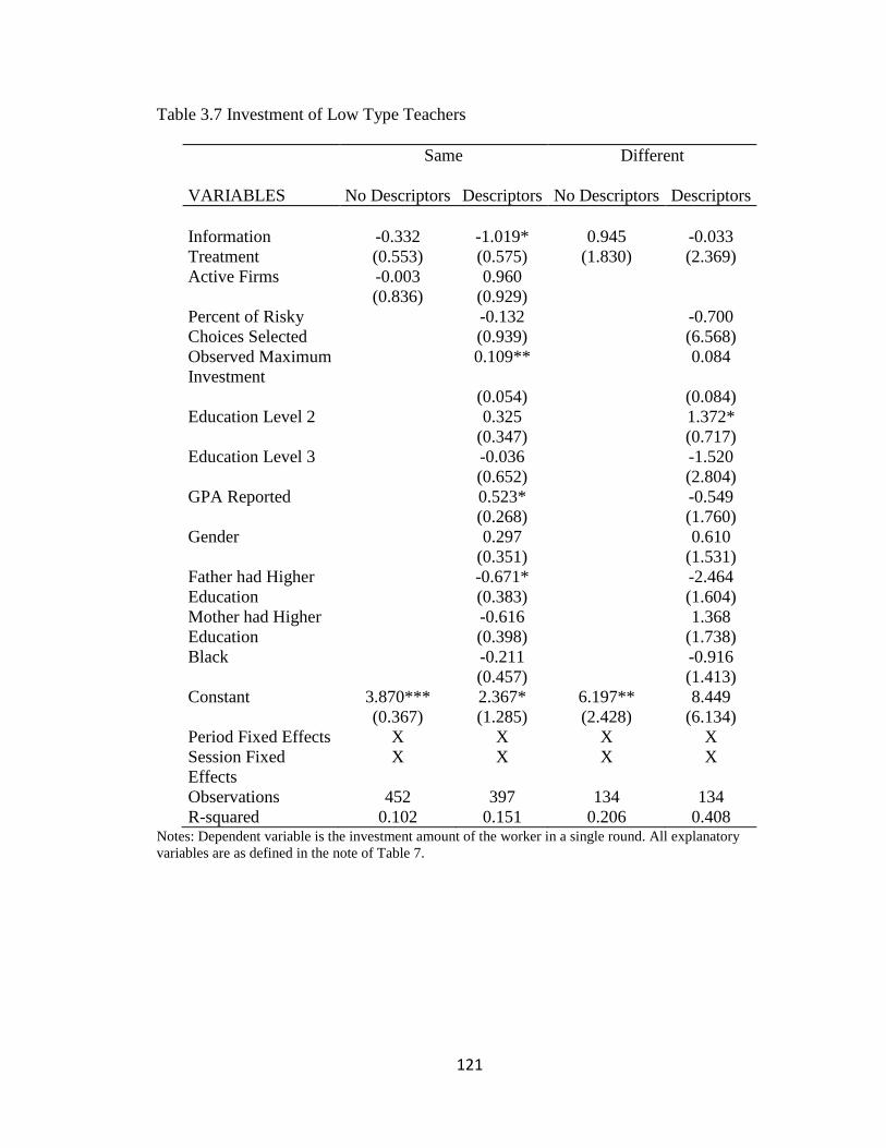
121

Table 3.7 Investment of Low Type Teachers

Same Different

VARIABLES No Descriptors Descriptors No Descriptors Descriptors

Information

Treatment

-0.332 -1.019* 0.945 -0.033

(0.553) (0.575) (1.830) (2.369)

Active Firms -0.003 0.960

(0.836) (0.929)

Percent of Risky

Choices Selected

-0.132 -0.700

(0.939) (6.568)

Observed Maximum

Investment

0.109** 0.084

(0.054) (0.084)

Education Level 2 0.325 1.372*

(0.347) (0.717)

Education Level 3 -0.036 -1.520

(0.652) (2.804)

GPA Reported 0.523* -0.549

(0.268) (1.760)

Gender 0.297 0.610

(0.351) (1.531)

Father had Higher

Education

-0.671* -2.464

(0.383) (1.604)

Mother had Higher

Education

-0.616 1.368

(0.398) (1.738)

Black -0.211 -0.916

(0.457) (1.413)

Constant 3.870*** 2.367* 6.197** 8.449

(0.367) (1.285) (2.428) (6.134)

Period Fixed Effects X X X X

Session Fixed

Effects

X X X X

Observations 452 397 134 134

R-squared 0.102 0.151 0.206 0.408 Notes: Dependent variable is the investment amount of the worker in a single round. All explanatory

variables are as defined in the note of Table 7.

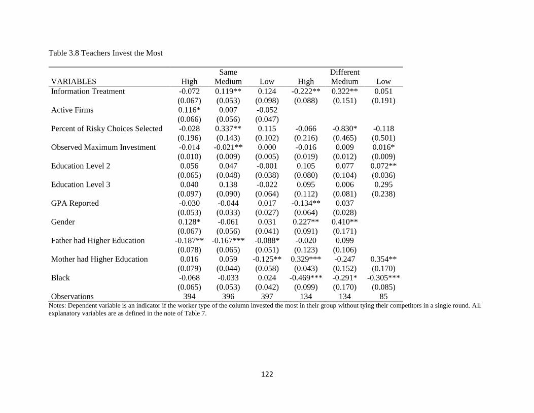
122

Table 3.8 Teachers Invest the Most

Same Different

VARIABLES High Medium Low High Medium Low

Information Treatment -0.072 0.119** 0.124 -0.222** 0.322** 0.051

(0.067) (0.053) (0.098) (0.088) (0.151) (0.191)

Active Firms 0.116* 0.007 -0.052

(0.066) (0.056) (0.047)

Percent of Risky Choices Selected -0.028 0.337** 0.115 -0.066 -0.830* -0.118

(0.196) (0.143) (0.102) (0.216) (0.465) (0.501)

Observed Maximum Investment -0.014 -0.021** 0.000 -0.016 0.009 0.016*

(0.010) (0.009) (0.005) (0.019) (0.012) (0.009)

Education Level 2 0.056 0.047 -0.001 0.105 0.077 0.072**

(0.065) (0.048) (0.038) (0.080) (0.104) (0.036)

Education Level 3 0.040 0.138 -0.022 0.095 0.006 0.295

(0.097) (0.090) (0.064) (0.112) (0.081) (0.238)

GPA Reported -0.030 -0.044 0.017 -0.134** 0.037

(0.053) (0.033) (0.027) (0.064) (0.028)

Gender 0.128* -0.061 0.031 0.227** 0.410**

(0.067) (0.056) (0.041) (0.091) (0.171)

Father had Higher Education -0.187** -0.167*** -0.088* -0.020 0.099

(0.078) (0.065) (0.051) (0.123) (0.106)

Mother had Higher Education 0.016 0.059 -0.125** 0.329*** -0.247 0.354**

(0.079) (0.044) (0.058) (0.043) (0.152) (0.170)

Black -0.068 -0.033 0.024 -0.469*** -0.291* -0.305***

(0.065) (0.053) (0.042) (0.099) (0.170) (0.085)

Observations 394 396 397 134 134 85 Notes: Dependent variable is an indicator if the worker type of the column invested the most in their group without tying their competitors in a single round. All

explanatory variables are as defined in the note of Table 7.

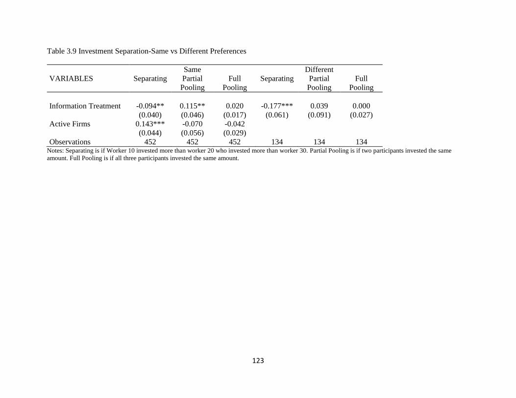
123

Table 3.9 Investment Separation-Same vs Different Preferences

Same Different

VARIABLES Separating Partial

Pooling

Full

Pooling

Separating Partial

Pooling

Full

Pooling

Information Treatment -0.094** 0.115** 0.020 -0.177*** 0.039 0.000

(0.040) (0.046) (0.017) (0.061) (0.091) (0.027)

Active Firms 0.143*** -0.070 -0.042

(0.044) (0.056) (0.029)

Observations 452 452 452 134 134 134 Notes: Separating is if Worker 10 invested more than worker 20 who invested more than worker 30. Partial Pooling is if two participants invested the same

amount. Full Pooling is if all three participants invested the same amount.

124

Table 3.10 Market Efficiency

All Preferences All

Preferences

Same

Preferences

Same

Preferences

Different

Preferences

Different

Preferences

No Descriptors Descriptors No Descriptors Descriptors No Descriptors Descriptors

Information Treatment -0.072* -0.053 0.016 -0.009 -0.068 -0.024

(0.038) (0.058) (0.099) (0.116) (0.047) (0.073)

Same Preferences 0.082* 0.075*

(0.042) (0.044)

Information x Same

Preferences

0.010 0.019

(0.053) (0.055)

Average Percent Risky

Choices Selected

-0.103 -0.007 -0.075

(0.186) (0.303) (0.248)

Average GPA 0.108 -0.011 0.219**

(0.071) (0.123) (0.088)

Percent Female 0.053 0.046 0.022

(0.081) (0.117) (0.116)

Percent Black 0.057 0.015 0.085

(0.078) (0.119) (0.105)

Percent with High

Mother’s Income

0.070 -0.066 0.309***

(0.068) (0.096) (0.102)

Percent with High

Mother’s Education

-0.045 -0.017 -0.128

(0.086) (0.134) (0.115)

Session Fixed Effect X X X X X X

Period Fixed Effect X X X X X X

Constant 0.797*** 0.350 0.908*** 0.952* 0.815*** -0.115

(0.088) (0.321) (0.055) (0.522) (0.109) (0.406)

Observations 236 225 102 97 134 128

R-squared 0.158 0.182 0.147 0.142 0.165 0.290 Notes: Dependent variable is the sum of the payoffs to a group divided by the maximum possible payoff (1350 under homogenous preferences and 1450 under

heterogeneous preferences) in a single round. All explanatory variables are as defined in the note of Table 7.

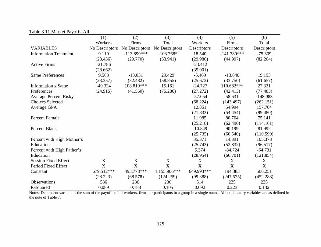
125

Table 3.11 Market Payoffs-All

(1) (2) (3) (4) (5) (6)

Workers Firms Total Workers Firms Total

VARIABLES No Descriptors No Descriptors No Descriptors Descriptors Descriptors Descriptors

Information Treatment 9.110 -113.899*** -103.768* 18.540 -141.789*** -75.309

(23.436) (29.770) (53.941) (29.980) (44.997) (82.204)

Active Firms -21.786 -23.412

(28.662) (35.901)

Same Preferences 9.563 -13.031 29.429 -5.469 -13.640 19.193

(23.357) (32.482) (58.855) (25.672) (33.750) (61.657)

Information x Same

Preferences

-40.324 108.819*** 15.161 -24.727 110.682*** 27.331

(24.915) (41.550) (75.286) (27.272) (42.413) (77.483)

Average Percent Risky

Choices Selected

-57.054 58.631 -148.083

(68.224) (143.497) (262.151)

Average GPA 12.851 54.994 157.704

(21.832) (54.454) (99.480)

Percent Female 11.985 80.764 75.141

(25.218) (62.490) (114.161)

Percent Black -10.849 90.199 81.992

(25.735) (60.540) (110.599)

Percent with High Mother’s

Education

35.371 14.391 105.378

(25.743) (52.832) (96.517)

Percent with High Father’s

Education

5.374 -84.724 -64.731

(28.954) (66.701) (121.854)

Session Fixed Effect X X X X X X

Period Fixed Effect X X X X X X

Constant 679.512*** 493.778*** 1,155.906*** 649.993*** 194.383 506.251

(28.223) (68.578) (124.259) (99.388) (247.575) (452.288)

Observations 586 236 236 514 225 225

R-squared 0.089 0.188 0.105 0.092 0.223 0.132 Notes: Dependent variable is the sum of the payoffs of all workers, firms, or participants in a group in a single round. All explanatory variables are as defined in

the note of Table 7.

126

Table 3.12 Market Payoffs-Same

(1) (2) (3) (4) (5) (6)

Workers Firms Total Workers Firms Total

VARIABLES No

Descriptors

No

Descriptors

No

Descriptors

Descriptors Descriptors Descriptors

Information Treatment -3.324 9.524 22.143 -1.075 -25.635 -11.834

(13.712) (61.507) (134.008) (18.965) (65.418) (155.975)

Active Firms -9.546 -21.042

(21.797) (28.904)

Average Percent Risky

Choices Selected

0.887 -39.175 -9.974

(48.980) (171.544) (409.011)

Average GPA -5.864 -35.377 -14.969

(15.351) (69.709) (166.208)

Percent Female 12.197 87.724 61.665

(17.498) (66.492) (158.537)

Percent Black -11.448 40.029 20.637

(18.069) (67.250) (160.343)

Percent with High Mother’s

Education

6.086 -70.188 -89.760

(18.165) (54.317) (129.508)

Percent with High Father’s

Education

4.641 -21.685 -22.400

(20.393) (75.793) (180.713)

Session Fixed Effect X X X X X X

Period Fixed Effect X X X X X X

Constant 668.365*** 553.810*** 1,226.324*** 691.275*** 683.412** 1,285.462*

(13.279) (34.320) (74.775) (67.673) (295.726) (705.099)

Observations 452 102 102 386 97 97

R-squared 0.115 0.330 0.147 0.107 0.388 0.142 Notes: Dependent variable is the sum of the payoffs of all workers, firms, or participants in a group in a single round. All explanatory variables are as defined in

the note of Table 7.

127

Table 3.13 Market Payoffs-Different

(1) (2) (3) (4) (5) (6)

Workers Firms Total Workers Firms Total

VARIABLES No

Descriptors

No

Descriptors

No

Descriptors

Descriptors Descriptors Descriptors

Information Treatment -32.657 -65.718 -98.375 67.183 -102.359 -35.177

(52.679) (39.782) (67.917) (85.979) (64.654) (106.261)

Average Percent Risky

Choices Selected

-239.415 130.979 -108.436

(291.493) (219.196) (360.255)

Average GPA 187.820* 129.603* 317.423**

(103.496) (77.827) (127.911)

Percent Female -16.028 47.264 31.236

(136.578) (102.703) (168.796)

Percent Black -4.023 127.585 123.563

(122.773) (92.323) (151.734)

Percent with High Mother’s

Education

286.069** 162.090* 448.159***

(119.615) (89.948) (147.832)

Percent with High Father’s

Education

-19.692 -166.161 -185.853

(135.435) (101.844) (167.383)

Session Fixed Effect X X X X X X

Period Fixed Effect X X X X X X

Constant 779.354*** 402.076*** 1,181.430*** 65.640 -231.957 -166.316

(122.932) (92.836) (158.491) (475.805) (357.795) (588.046)

Observations 134 134 134 128 128 128

R-squared 0.196 0.168 0.165 0.268 0.245 0.290 Notes: Dependent variable is the sum of the payoffs of all workers, firms, or participants in a group in a single round. All explanatory variables are as defined in

the note of Table 7.

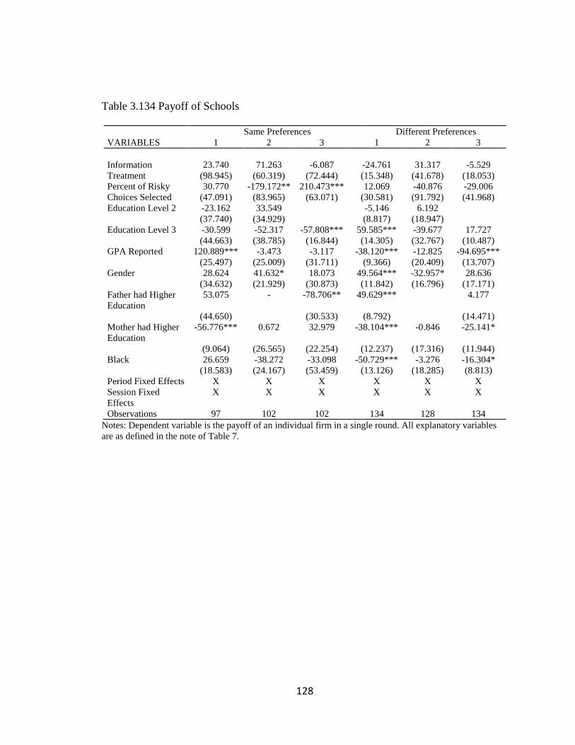
128

Table 3.134 Payoff of Schools

Same Preferences Different Preferences

VARIABLES 1 2 3 1 2 3

Information

Treatment

23.740 71.263 -6.087 -24.761 31.317 -5.529

(98.945) (60.319) (72.444) (15.348) (41.678) (18.053)

Percent of Risky

Choices Selected

30.770 -179.172** 210.473*** 12.069 -40.876 -29.006

(47.091) (83.965) (63.071) (30.581) (91.792) (41.968)

Education Level 2 -23.162 33.549 -5.146 6.192

(37.740) (34.929) (8.817) (18.947)

Education Level 3 -30.599 -52.317 -57.808*** 59.585*** -39.677 17.727

(44.663) (38.785) (16.844) (14.305) (32.767) (10.487)

GPA Reported 120.889*** -3.473 -3.117 -38.120*** -12.825 -94.695***

(25.497) (25.009) (31.711) (9.366) (20.409) (13.707)

Gender 28.624 41.632* 18.073 49.564*** -32.957* 28.636

(34.632) (21.929) (30.873) (11.842) (16.796) (17.171)

Father had Higher

Education

53.075 - -78.706** 49.629*** 4.177

(44.650) (30.533) (8.792) (14.471)

Mother had Higher

Education

-56.776*** 0.672 32.979 -38.104*** -0.846 -25.141*

(9.064) (26.565) (22.254) (12.237) (17.316) (11.944)

Black 26.659 -38.272 -33.098 -50.729*** -3.276 -16.304*

(18.583) (24.167) (53.459) (13.126) (18.285) (8.813)

Period Fixed Effects X X X X X X

Session Fixed

Effects

X X X X X X

Observations 97 102 102 134 128 134

Notes: Dependent variable is the payoff of an individual firm in a single round. All explanatory variables

are as defined in the note of Table 7.

129

Table 3.145 Payoff of Teachers

Same Preferences Different Preferences

VARIABLES High Same Middle Low High Middle Low

Information

Treatment

-81.506*** 43.578** 28.229 0.049 -66.183* 45.173

(22.532) (21.954) (17.847) (70.584) (33.522) (36.276)

Active Firms -29.747 -2.193 -2.515

(28.151) (38.740) (38.800)

Percent of Risky

Choices Selected

59.690* 6.271 1.466 -66.300 -100.711** -196.799*

(33.834) (29.638) (28.642) (110.202) (38.572) (108.693)

Observed

Maximum

Investment

-2.548 -1.853 -0.241 -11.277 6.467 -5.204**

(2.694) (2.234) (1.965) (6.878) (4.800) (2.377)

Education Level 2 32.733** 33.639*** 0.821 -34.916 -19.060** 7.022

(12.650) (11.568) (9.349) (40.002) (8.925) (20.057)

Education Level 3 25.585 38.043** 10.714 -44.259** -117.788*** -11.127

(17.016) (16.287) (19.009) (18.795) (37.268) (53.524)

GPA Reported 13.038 -9.291 -0.922 -0.213 17.401 -21.897

(11.559) (9.665) (8.407) (37.321) (13.021) (24.290)

Gender 3.268 3.932 -6.150 13.207 -2.672 -8.068

(11.783) (12.047) (9.413) (44.059) (23.796) (30.659)

Father had Higher

Education

-36.921*** -5.997 -4.936 104.674 6.218 16.658

(11.951) (13.795) (9.982) (65.089) (12.831) (18.450)

Mother had

Higher Education

-10.571 17.322 -9.810 43.808 -20.501 -

71.955**

*

(11.559) (11.984) (11.680) (27.790) (14.521) (17.046)

Black -16.042 -17.205 10.528 112.372**

*

3.730 13.610

(11.863) (12.470) (9.757) (37.524) (17.664) (33.276)

Period Fixed

Effects

X X X X X X

Session Fixed

Effects

X X X X X X

Observations 394 396 397 134 134 134 Notes: Dependent variable is the payoff of an individual worker in a single round. All explanatory variables

are as defined in the note of Table 7.

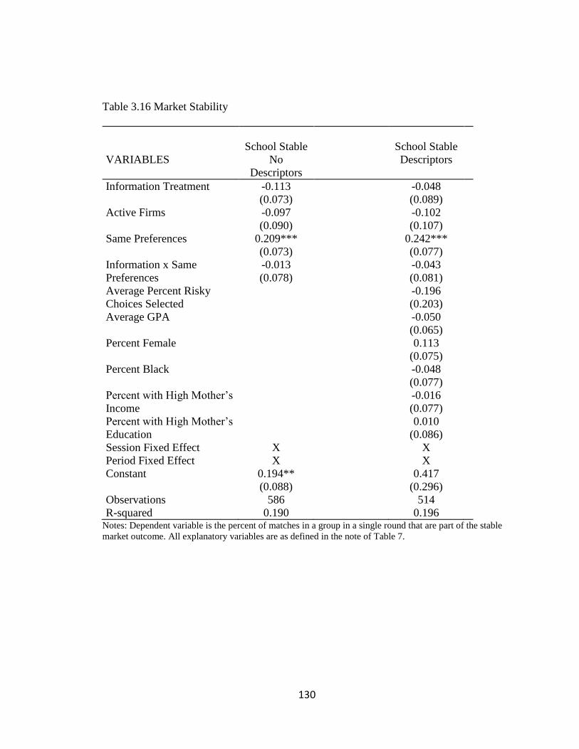
130

Table 3.16 Market Stability

School Stable School Stable

VARIABLES No

Descriptors

Descriptors

Information Treatment -0.113 -0.048

(0.073) (0.089)

Active Firms -0.097 -0.102

(0.090) (0.107)

Same Preferences 0.209*** 0.242***

(0.073) (0.077)

Information x Same

Preferences

-0.013 -0.043

(0.078) (0.081)

Average Percent Risky

Choices Selected

-0.196

(0.203)

Average GPA -0.050

(0.065)

Percent Female 0.113

(0.075)

Percent Black -0.048

(0.077)

Percent with High Mother’s

Income

-0.016

(0.077)

Percent with High Mother’s

Education

0.010

(0.086)

Session Fixed Effect X X

Period Fixed Effect X X

Constant 0.194** 0.417

(0.088) (0.296)

Observations 586 514

R-squared 0.190 0.196 Notes: Dependent variable is the percent of matches in a group in a single round that are part of the stable

market outcome. All explanatory variables are as defined in the note of Table 7.

131

3.8 Figures

Figure 3.1 Simultaneous Investment Screen

Figure 3.2 Sequential Investment Screen

132

Figure 3.3 Firm Investment Screen

Figure 3.4 Worker Decision Screen - Offer

133

Figure 3.5 Worker Decision Screen - No Offer

Figure 3.6 Market Match Outcomes

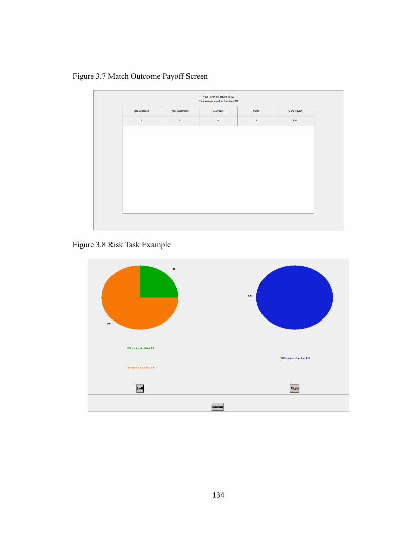
134

Figure 3.7 Match Outcome Payoff Screen

Figure 3.8 Risk Task Example

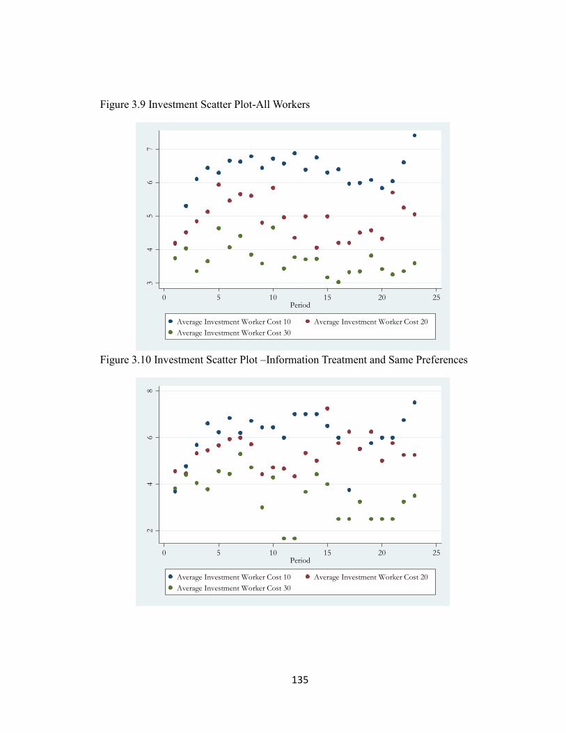
135

Figure 3.9 Investment Scatter Plot-All Workers

Figure 3.10 Investment Scatter Plot –Information Treatment and Same Preferences

34

56

7

0 5 10 15 20 25Period

Average Investment Worker Cost 10 Average Investment Worker Cost 20

Average Investment Worker Cost 30

24

68

0 5 10 15 20 25Period

Average Investment Worker Cost 10 Average Investment Worker Cost 20

Average Investment Worker Cost 30

136

Figure 3.11 Investment Scatter Plot –Information Treatment and Different Preferences

Figure 3.14 Investment Scatter Plot –Not Information Treatment and Same Preferences

02

46

8

5 10 15 20Period

Average Investment Worker Cost 10 Average Investment Worker Cost 20

Average Investment Worker Cost 30

34

56

78

0 5 10 15Period

Average Investment Worker Cost 10 Average Investment Worker Cost 20

Average Investment Worker Cost 30

137

Figure 3.13 Investment Scatter Plot –Not Information Treatment and Different

Preferences

23

45

67

12 14 16 18 20 22Period

Average Investment Worker Cost 10 Average Investment Worker Cost 20

Average Investment Worker Cost 30

138

3.9 Appendix A. Strategic Behavior

Strategic behavior is likely to occur in the worker investment decisions as the

benefits of matching with their preferred school (100 for every rank higher) outweigh the

investment benefits of selecting the maximin investment amount51. If the worker achieves

a better match of one rank by investing more the worker’s payoff always increases. The

considerable boost from better matches gives the teachers incentives to invest

strategically to attract a more preferred firm and attempt to receive a higher overall

payoff. This strategic action requires workers to know what type their firm prefers, which

is likely to occur with the rapid turnover and thus repeated participation of teachers in the

teacher labor market. An example of the strategic investment in the true teacher labor

market could be the amount of education they complete or the credentials they achieve to

improve their chances of a better placement. In the market, teachers can also strategically

accept or reject offers.

By a similar token as workers rejecting a firm if they believe they can receive a

better offer, schools can strategically order their offers. If multiple firms make offers to

the same worker simultaneously, the system presents only the worker's most preferred

option. The mechanism is not strategy-proof for schools in any information environment

as schools can obtain a better match by issuing an offer to a teacher who is not their most

preferred teacher but who would be more likely to accept an early offer, particularly in

preference set 1. Making an offer to their most preferred teacher might result in losing

51 The max additional payoff from the investment is 100 for high types (170 (investment payoff)-70 (investment cost)),

then 40 for medium (120 (investment payoff)-80 (investment cost)), and 10 for low types (40 (investment payoff)-30

(investment cost)).

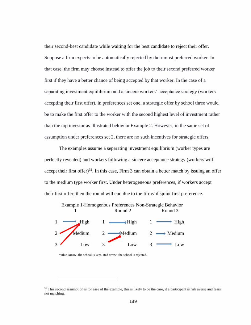
139

their second-best candidate while waiting for the best candidate to reject their offer.

Suppose a firm expects to be automatically rejected by their most preferred worker. In

that case, the firm may choose instead to offer the job to their second preferred worker

first if they have a better chance of being accepted by that worker. In the case of a

separating investment equilibrium and a sincere workers’ acceptance strategy (workers

accepting their first offer), in preferences set one, a strategic offer by school three would

be to make the first offer to the worker with the second highest level of investment rather

than the top investor as illustrated below in Example 2. However, in the same set of

assumption under preferences set 2, there are no such incentives for strategic offers.

The examples assume a separating investment equilibrium (worker types are

perfectly revealed) and workers following a sincere acceptance strategy (workers will

accept their first offer)52. In this case, Firm 3 can obtain a better match by issuing an offer

to the medium type worker first. Under heterogeneous preferences, if workers accept

their first offer, then the round will end due to the firms' disjoint first preference.

Example 1-Homogenous Preferences Non-Strategic Behavior

1 Round 2 Round 3

1 High 1 High 1 High

2 Medium 2 Medium 2 Medium

3 Low 3 Low 3 Low

*Blue Arrow -the school is kept. Red arrow -the school is rejected.

52 This second assumption is for ease of the example, this is likely to be the case, if a participant is risk averse and fears

not matching.

140

Example 2-Homogenous Preferences Strategic Behavior

1 Round 2 Round 3

1 High 1 High 1 High

2 Medium 2 Medium 2 Medium

3 Low 3 Low 3 Low

*Blue Arrow -the school is kept. Red arrow -the school is rejected.

Example 3-Heterogeneous Preferences

1

1 High

2 Medium

3 Low

*Blue Arrow -the school is kept. Red arrow -the school is rejected, Black is no match

141

Bibliography

Aaronson, D., Barrow, L., & Sander, W. (2007). Teachers and Student Achievement in the

Chicago Public High Schools. Journal of Labor Economics, 25 (1), 95-135.

Abdulkadiroğlu, A., Pathak, P. A., Roth, A. E., & Sönmez, T. (2005). The Boston Public School

Match. American Economic Review, 95 (2), 368-371.

Abdulkadiroğlu, A. & Sönmez, T. (1999). House Allocation with Existing Tenants. Journal of

Economic Theory, 88 (2), 233-260.

Banks, J., Camerer, C., & Porter, D. (1994). An Experimental Analysis of Nash Refinements in

Signaling Games. Games and Economic Behavior, 6 (1), 1–31.

Barron, J. M., Berger, M. C., & Black, D.A. (1997). Employer Search, Training, and Vacancy

Duration. Economic Inquiry, 35, 167-192.

Barron, J. M., Bishop, J., & Dunkelberg, W.C. (1985). Employer Search: The Interviewing and

Hiring of New Employees. Review of Economics and Statistics, 67, 43-52.

Bartling, E., Fehr, E., & Schmidt, K. M. (2012). Screening, Competition, and Job Design:

Economic Origins of Good Jobs. American Economic Review, 102 (2), 834-864.

Bassi, L., & McMurrer, D. (2007). Maximizing Your Return on People. Harvard Business

Review.

Becker, G. S. (1973). A Theory of Marriage: Part I. Journal of Political Economy 81 (4), 813.

Becker, G. S. (1974). A Theory of Marriage: Part II. Journal of Political Economy, 82 (2), 11.

Biasi, B. (2019). Higher Salaries or Higher Pensions? Inferring Preferences from Teachers’

Retirement Behavior. New Haven, CT: Yale School of Management (September 30).

Bikhchandani, S. (2017). Stability with One-Sided Incomplete Information. Journal of Economic

Theory, 168, 372-399.

142

Boyd, D., Lankford, H., Loeb, S., Ronfeldt, M., & Wyckoff, J. (2011). The Role of Teacher

Quality in Retention and Hiring: Using Applications to Transfer to Uncover Preferences

of Teachers and Schools. Journal of Policy Analysis and Management, 30 (1), 88-110.

Boyd, D., Lankford, H., Loeb, S., & Wyckoff, J. (2005a). The Draw of Home: How Teachers’

Preferences for Proximity Disadvantage Urban Schools. Journal of Policy Analysis and

Management, 24(1), 1134–1132.

Boyd, D., Lankford, H., Loeb, S., & Wyckoff, J. (2005b). Explaining the Short Careers of High-

Achieving Teachers in Schools with Low-Performing Students. The American Economic

Review, 95 (2), 166-171.

Boyd, D., Lankford, H., Loeb, S., & Wyckoff, J. (2013). Analyzing the Determinants of the

Matching Public Schools Teachers to Jobs: Disentangling the Preferences of Teachers

and Employers. Journal of Labor Economics, 31 (1), 83-117.

Bruno, P., & Strunk, K.O. (2019). Making the Cut: The Effectiveness of Teacher Screening and

Hiring in the Los Angeles Unified School District. Educational Evaluation and Policy

Analysis, https://journals.sagepub.com/doi/full/10.3102/0162373719865561.

Burks, S. V., Cowgill, D., Hoffman, M., & Housman, M. (2015). The Value of Hiring Through

Employee Referrals. The Quarterly Journal of Economics, 130 (2), 805-839.

Brandts, J. & Holt, C. (1992). An Experimental Test of Equilibrium Dominance in Signaling

Games. The American Economic Review, 82 (5), 1350–1365.

Cannata, M. 2010. Understanding the Teacher Job Search Process: Espoused Preferences and

Preferences in Use. Teachers College Record, 112 (12), 2889-2934.

Campbell, C., DeArmond, M., & Schumwinger, A. (2004). From Bystander to Ally.

Transforming the District Human Resources Department. A Report to the Center on

Reinventing Public Education.

143

Chen, Y. & Sönmez, T. (2003). Improving Efficiency of On-Campus Housing: An Experimental

Study. American Economic Review, 92 (5), 1669-1686.

Chen, Y. & Sönmez, T. (2006). School choice: An Experimental Study. Journal of Economic

Theory, 127, 202-231.

Chetty, R., Friedman, J., Hilger, N., Saez, E., Schazenbach, E. W., & Yagan, D. (2011). How

Does Your Kindergarten Classroom Affect Your Earnings? Evidence from Project Star.

Educational Administration Quarterly, 53 (2), 180-222.

Chetty, R., Friedman, J., & Rockoff, J. (2014). Measuring the Impacts of Teachers II: Teacher

Value-Added and Student Outcomes in Adulthood. American Economic Review, 104 (9),

2633-2679.

Chingos, M., & Peterson, P. (2011). It’s Easier to Pick a Good Teacher Thank to Train One:

Familiar and New Results on the correlates of Teacher Effectiveness. Economics of

Education Review, 30, 449-465.

Cho, I. & Kreps, D. (1987). Signaling Games and Stable Equilibria. The Quarterly Journal of

Economics, 102 (2), 179-222.

Clotfelter, C., Glennie, E., Ladd, H., & Vigdor, J. (2008). Would Higher Salaries Keep Teachers

in High-Poverty Schools? Evidence from a Policy Intervention in North Carolina."

Journal of Public Economics, 92 (5-6), 1352-1370.

Clotfelter, C., Ladd, H., & Vigdor, J. (2006). Teacher-Student Matching and the Assessment of

Teacher Effectiveness. Journal of Human Resources, 41 (4), 778-820.

Clotfelter, C., Ladd, H., & Vigdor, J. (2011). Teacher Mobility, School Segregation, and Pay-

Based Policies to Level the Playing Field. Education Finance and Policy, 6 (3), 399-438.

144

Cohen-Vogel, L., Little, M., & Fierro, C. (2019). Evidence-Based Staffing in High Schools:

Using Student Achievement Data in Teacher Hiring, Evaluation, and

Assignment. Leadership and Policy in Schools, 18 (1), 1-34.

Coles, P., Cawley, J., Levine, P. B., Niederle, M., Roth, A. E., & Siegfried, J. J. (2010). The Job

Market for new Economists: A Market Design Perspective. Journal of Economic

Perspectives, 24 (4), 187-206.

Coles, P., Kushnir, A., & Niederle, M. (2013). Preference Signaling in Matching

Markets. American Economic Journal: Microeconomics, 5 (2), 99-134.

Converse, P., Oswald, F., Gillespie, M., Field, K., & Bizot, E. (2004). Matching Individuals to

Occupations Using Abilities and the O*NET: Issues and an Application in Career

Guidance. Personnel Psychology, 57, 451-487.

Cooper, D. & Kagel, J. (2003). The Impact of Meaningful Context on Strategic Play in Signaling

Games. Journal of Economic Behavior & Organization, 50 (3), 311–337.

Darling-Hammond, L. (2001). The Challenge of Staffing our Schools. Educational Leadership,

58 (8), 12-17.

DeArmond, M., Gross, B., & Goldhaber, D. (2010). Is it Better to Be Good or Lucky?

Decentralized Teacher Selection in 10 Elementary Schools. Educational Administration

Quarterly, 46 (3), 322-362.

Delfgaauw, J. & Dur, R. (2007). Signaling and Screening of Workers’ Motivation. Journal of

Economic Behavior and Organization, 62, 605-624.

DeVaro, J. (2005). Employer Recruitment Strategies and Labor Market Outcomes of new Hires.

Economic Inquiry, 43 (2), 263-382.

Dipboye, R., & Jackson, S. (1999). Interviewer Experience and Expertise Effects. The

Employment Interview Handbook, 229-292.

145

Dizon-Ross, R. (2020). How Does School Accountability Affect Teachers? Evidence from New

York City. The Journal of Human Resources. 55 (1): 76-118.

Dobbie, W. (2011). Teacher Characteristics and student Achievement: Evidence from Teach for

America. http://blogs.edweek.org/edweek/teacherbeat/teachercharacteristicsjuly2011.pdf

Donaldson, M. (2013). Principal’s Approaches to Cultivating Teacher Effectiveness: Constraints

and Opportunities in Hiring, Assigning, Evaluating, and Developing Teachers.

Educational Administration Quarterly, 49 (5), 838-882.

Dustmann, C., Glitz, A., Schönberg, U., & Brücker, H. (2016). Referral-Based Job Search

Networks. Review of Economic Studies, 83, 514-546.

Engel, M. & Marisa Cannata. 2015. Localism and Teacher Labor Markets: How Geography and

Decision Making May Contribute to Inequality. Peabody Journal of Education. 90, 84-92

Engel, M. & Finch, M. A. (2015). Staffing the Classroom: How Urban Principals Find Teachers

and Make Hiring Decisions. Leadership and Policy in Schools, 14 (1), 12-41.

Engel, M., Jacob, B., & Curran, F. C. (2014). New Evidence on Teacher Labor Supply. American

Educational Research Journal, 51 (1), 36-72.

Ergin, H., & Sӧnmez, T. (2006). Games of School Choice under the Boston Mechanism. Journal

of Public Economics, 90 (1-2), 215-237.

Ehlers, L. & Masso, J. (2015). Matching Markets under (in)complete Information. Journal of

Economic Theory, 157, 295-314.

Fahr, R , & Sunde, U. (2001). Strategic Hiring Behavior in Empirical Matching Functions. IZA

Discussion Papers, Number 320.

Feng, L. (2009). Opportunity Wages, Classroom Characteristics, and Teacher Mobility. Southern

Economic Journal, 75 (4), 1165-1190.

146

Feng, L. (2014). Teacher Placement, Mobility, and Occupational Choices after Teaching.

Education Economics, 22 (1), 24-47.

Feng, L., Figlio, D., & Sass, T. R. (2018). School Accountability and Teacher Mobility. Journal

of Urban Economics, 103 (C), 1-17.

Feng, L. & Sass, T. R. (2017). Teacher quality and teacher mobility. Education Finance &

Policy, 12 (3), 396-418.

Gale, D. & Shapley, L. S. (1962). College Admissions and the Stability of Marriage. The

American Mathematical Monthly, 69 (1), 9-15.

Galperin, R. V., Hahl, O., Sterling, A. D., & Gou, J. (2019). Too Good to Hire? Capability and

Inferences about Commitment in Labor Markets. Administrative Science Quarterly, 1-39.

Gershenson, S. (2016). Linking teacher quality, student attendance, and student

achievement. Education Finance and Policy, 11 (2), 125-149.

Glazerman, S., Protik, A., Teh, B. R., Bruch, J., & Max, J. (2013). Transfer Incentives for High-

Performing Teachers: Final Results from a Multisite Randomized Experiment. NCEE

2014-4004. National Center for Education Evaluation and Regional Assistance.

Goff, P. & Bruecker, E. (2017). The Role of Place: Labor Market Dynamics in Rural and Non-

rural School Districts. Wisconsin Center for Education Research Working Paper No.

2014-4.

Goldhaber, D., Gross, B., & Player, D. (2007). Are Public Schools Really Losing Their Best?

Assessing the Career Transitions of Teachers and Their Implications for the Quality of

the Teacher Workforce. National Center for Analysis of Longitudinal Data in Education

Research Working Paper 12.

147

Goldhaber, D., Gross, B., & Player, D. (2011). Teacher career paths, teacher quality, and

persistence in the classroom: Are public schools keeping their best? Journal of Policy

Analysis & Management, 30 (1), 57-87.

Goldhaber, D., Lavery, L., & Theobald, R. (2015). Uneven Playing Field? Assessing the Teacher

Quality Gap between Advantaged and Disadvantaged Students. Educational Researcher,

44 (5), 293-307.

Gordon, S. & Maxey S. (2000). How to Help Beginning Teachers Succeed (2nd Edition).

Association for Supervision and Curriculum Development. Alexandria, VA.

Gorter, C., Nijkamp, P., & Rietveld, P. (1996). Employers Recruitment Behaviour and Vacancy

Duration: An Empirical Analysis of the Dutch Labour Market. Applied Economics, 28,

1463-1474.

Grensing-Pophal, L. (2017). Recruiting: Why Traditional Methods Still Matter. Retrieved from

www.shrm.org.

Griffith, D., & McDougald. (2016). Undue Process: Why Bad Teachers in Twenty-Five Diverse

Districts Rarely Get Fired. Thomas B. Fordham Institute.

Grissom, J. A. & Keiser, L. R. (2011). A Supervisor like Me: Race, Representation, and the

Satisfaction and Turnover Decisions of Public Sector Employees. Journal of Policy

Analysis and Management, 30 (3), 557-580.

Guin, K. (2004). Chronic Teacher Turnover in Urban Elementary Schools. Education Policy

Analysis Archives, 12 (42), 1-30.

Hanushek, E., Kain, J., & Rivkin, S. (2004). Why Public Schools Lose Teachers. Journal of

Human Resources. 39 (2): 326-354.

Hanushek, E., & Rivkin, S. (2007). Pay, Working Conditions, and Teacher Quality. The Future of

Children, 17 (1), 69-86.

148

Heneman III, H. G. & Milanowski, A. T. (2004). Alignment of Human Resource Practices and

Teacher Performance Competency. Peabody Journal of Education, 79 (4), 108-125.

Heneman III, H. G. & Milanowski, A. T. (2007). Assessing Human Resource Alignment: The

Foundation for Building Total Teacher Quality Improvement. Madison, WI: University

of Wisconsin-Madison.

Hoffman, M., Kahn, L., & Li, D. (2018). Discretion in Hiring. The Quarterly Journal of

Economics, 133 (2), 765-800.

Holzer, H. J. (1987). Hiring Procedures in the Firm: Their Economic Determinants and

Outcomes. Human Resources and Firm Performance, ed. By Richard Block, et al.

Industrial Research Association.

Hopkins, E. (2012). Job Market Signaling of Relative Position, or Becker Married to Spence.

Journal of the European Economic Association, 10 (2), 290-322.

Hoppe, H., Moldovanu, B., & Sela, A. (2009). The Theory of Assortative Matching Based on

Costly Signals. The Review of Economic Studies, 76 (1), 253-281.

Horng, E. L. (2009). Teacher Tradeoffs: Disentangling Teachers’ Preferences for Working

Conditions and Student Demographics. American Educational Research Journal, 46 (3),

690-717.

Hylland, A. & Zeckhauser, R. (1979). The Efficient Allocation of Individuals to Positions.

Journal of Political Economy, 87 (2), 293-314.

Imazeki, J. (2005). Teacher Salaries and Teacher Attrition. Economics of Education Review, 24,

431-449.

Immorlica, N., Klienberg, R., & Mahdian, M. (2006, December). Secretary Problems with

Competing Employers. In International Workshop on International Workshop on Internet

and Network Economics (pp. 389-400). Springer, Berlin, Heidelberg.

149

Ingersoll, R. (2001). Teacher Turnover and Teacher Shortages: An Organizational Analysis.

American Educational Research Journal, 38: 499-534.

Jackson, C. K. (2013). Match Quality, Worker Productivity, and worker mobility: Direct

Evidence from Teachers. Review of Economics & Statistics, 95, (4), 1096.

Jacob, B., Rockoff, J., Taylor, E., Lindy, B., & Rosen, R. (2018). Teacher Applicant Hiring and

Teacher Performance: Evidence form DC Public Schools. Journal of Public Economics,

166, 81-97.

Kagel, J. H. & Roth, A. E. (2000) The Dynamics of Reorganization in Matching Markets: A

Laboratory Experiment Motivated by a Natural Experiment, The Quarterly Journal of

Economics, 115 (1), 201–235.

Kane, T. J., Rockoff, J., & Staiger, D. (2008). What Does Certification Tell Us about Teacher

Effectiveness? Evidence from New York City. Economics of Education Review, 277,

615-631.

Koch, M., & McGrath, R. (1996). Improving Labor Productivity: Human Resource Management

Policies Do Matter. Strategic Management Journal, 17, 335-354.

Lankford, H., Loeb, S., & Wyckoff, J. (2002). Teacher Sorting and the Plight of Urban Schools:

A Descriptive Analysis. Educational Evaluation and Policy Analysis, 24 (1), 37-62.

Lavetti, K. (2020). The estimation of compensating wage differentials: Lessons from the

Deadliest Catch. Journal of Business & Economic Statistics, 38 (1), 165-182.

Levin, J., & Quinn, M. (2003). Missed Opportunity: How I Keep High-Quality Teachers Out of

Urban Classroom. The New Teacher Project.

Levin, J., Mulhern, J., & Schunck, J. (2005) Unintended Consequences: The Case for Reforming

the Staffing Rules in Urban Teacher Union Contracts. The New Teacher Project.

150

Liu, E., & Johnson, S. M. (2006). New Teachers’ Experiences of Hiring: Late, Rushed, and

Information Poor. Educational Administration Quarterly, 42 (3), 324-360.

Liu, E., Rosenstein, J., Swan, A., & Khalil, D. (2008). When Districts Encounter Teacher

Shortages: The Challenges of Recruiting and Retaining Mathematics Teachers in urban

Districts. Leadership and Policy in Schools, 7 (3), 296-323.

Loeb, S, Darling-Hammond, L., & Luczak, J. (2005). How teaching conditions predict teacher

turnover in California schools. Peabody Journal of Education, 80 (3), 44-70.

Loeb, S., Kalogrides, D., & Beteille, T. (2012). Effective Schools: Teacher Hiring, Assignment,

Development, and Retention. Education Finance and Policy, 7 (3), 269-304.

Maestas, N., Mullen, K. J., Powell, D., Von Wachter, T., & Wenger, J. B. (2018). The value of

working conditions in the united states and implications for the structure of wages (No.

w25204). National Bureau of Economic Research.

Manning, A. (2000). Pretty Vacant: Recruitment in Low-Wage Labor Markets. Oxford Bulletin of

Economics and Statistics, 62, 747-770.

McFadden, D. (1973). Conditional Logit Analysis of Qualitative Choice Behavior.

Milanowski, A., & Odden, A. (2007). A New Approach to the Cost of Teacher Turnover. School

finance Redesign Project, Working Paper 13.

Miller, R. & Charles, P. (1985). Product Quality Signaling in Experimental Markets.

Econometrica: Journal of the Econometric Society, 53 (4), 837–872.

Murphy, K. R. (1986). When Your Top Choice Turns You Down: Effect of Rejected Offers on

the Utility of Selection Tests. Psychological Bulletin, 99 (1), 133-138.

Neild, R. C., Useem, E., Travers, E., & Lesnick, J. (2003). Once and For All. Placing a Highly

Qualified Teacher in Every Philadelphia Classroom. What I Know and Need to Do. A

Report from Learning from Philadelphia’s School Reform.

151

Odden, A., & Kelley, J. (2008) Strategic Management of Human Capital in Public Education.

Strategic Management of Human Capital. A Project of the Consortium for Policy

Research in Education.

Painter, S. (2000). Principals’ Perceptions of Barriers to Teacher Dismissal. Journal of Personnel

Evaluation in Education, 14 (3): 253-264.

Papay, J., & Kraft, M. (2015). Productivity Returns to Experience in the Teacher Labor Market:

Methodological Challenges and new Evidence on long-Term Career Improvement.

Journal of Public Economics, 130, 105-119.

Podgursky, M, Monroe, R., & Watson, D. (2004). The Academic Quality of Public School

Teachers: An Analysis of Entry and Exit Behavior. Economics of Education Review, 23

(5), 507-518.

Potters, J. & Van Winden, F. (1996). Comparative Statics of a Signaling Game: An Experimental

Study. International Journal of Game Theory, 25 (3), 329–353.

Reininger, M. (2012). Hometown disadvantage? It depends on where you’re from: Teachers’

location preferences and the implications for staffing schools. Educational Evaluation

and Policy Analysis, 34 (2), 127–145.

Rivkin, S., Hanushek, E., & Kain, J. (2005). Teachers, Schools, and Academic Achievement.

Econometrica, 73 (2), 417-458.

Rockoff, J. (2004). The Impact of Individual Teachers on Student Achievement: Evidence from

Panel Data. The American Economic Review, 94 (2), 247-252.

Roth, A. E. (1982). The Economics of Matching: Stability and Incentives. Mathematics of

Operations Research, 7 (4), 617-628.

Roth, A. E. (1984). The Evolution of the Labor Market for Medical Interns and Residents: A Case

Study in Game Theory. Journal of Political Economy, 92 (6), 991-1016.

152

Roth, A. E. (1991). A Natural Experiment in the Organization of Entry-Level Labor Markets:

Regional Markets for New Physicians and Surgeons in the United Kingdom. The

American Economic Review, 81 (3), 415-440.

Roth, A., Sönmez, T., & Ünver, M. U. (2004). Kidney Exchange. Quarterly Journal of

Economics, 119 (2), 457-488.

Roth, A., Sönmez, T., & Ünver, M. U. (2005). Pairwise Kidney Exchange. Journal of Economic

Theory, 125 (2), 151-188.

Roth, A. E., & Xing, X. (1994). Jumping the Gun: Imperfections and Institutions Related to the

Timing of Market Transactions. The American Economic Review, 84 (4), 992-1044

Roth, A. E., & Xing, X. (1997). Turnaround Time and Bottlenecks in Market Clearing:

Decentralized Matching in the Market for Clinical Psychologists. Journal of Political

Economy, 105 (22), 284-329.

Russo, G., Rietvel, P., Nijkamp, P., & Gorter, C. (2000). Recruitment Channel Use and Applicant

Arrival: An Empirical Analysis. Empirical Economics, 25, 673-697.

Rutledge, S., Harris, D., & Ingle, W. (2010). How Principals “Bridge and Buffer” the New

Demands of Teacher quality and Accountability: A Mixed-Methods Analysis of Teacher

Hiring. American Journal of Education, 116, 211-242.

Rutledge, S., Harris, D., Thompson, C., & Ingle, W. K. (2008). Certify, Blink, Hire: An

Examination of the Process and Tools of Teacher Screening and Selection. Leadership and

Policy in Schools, 7, 237-263.

Ryan, A. M., Sacco, J., McFarland, L., & Kriska, D. (2000). Applicant Self-Selection: Correlates

of Withdrawal from a Multiple Hurdle Process. Journal of Applied Psychology, 85, (2),

163-179.

153

Rynes, S. & Barber, A. (1990). Applicant Attraction Strategies: An Organizational Perspective.

Academy of Management Review, 15 (2), 286-310.

Sass, T., Hannaway, J., Xu, Z., Figlio, D. N., & Feng, L. (2012). Value added of Teachers in

High-Poverty Schools and Lower Poverty Schools. Journal of Urban Economics, 72,

104-122.

Scafidi, B., Sjoquist, D. L., & Stinebrickner, T. R. (2006). Do Teachers Really Leave for Higher

Paying Jobs in Alternative Occupations? Advances in Economic Analysis & Policy, 6 (1),

1-42.

Scafidi, B., Sjoquist, D. L., & Stinebrickner, T. R. (2007). Race, Poverty, and Teacher Mobility,

Economic of Education Review, 26 (2), 145-159.

Schmidt, F. L., & Hunter, J. E. (1998). The Validity and Utility of Selection methods in

Personnel Psychology: Practical and Theoretical Implications of 85 Years of Research

Findings. Psychological Bulletin, 124 (2), 262-274.

Shapley, L. & Scarf, H. 1974. On Cores and Indivisibility. Journal of Mathematical Economics, 1

(1), 23-37.

Smith, T. & Ingersoll, R. (2004). What are the Effects of Induction and Mentoring on Beginning

Teacher Turnover? American Educational Research Journal, 41 (3), 681-714.

Sönmez, T., & Ünver, M. U. (2011). Matching, Allocation, and Exchange of Discrete Resources.

In Handbook of Social Economics, 1, 781-852.

Sorkin, I. (2018). Ranking Firms using Revealed Preference. The Quarterly Journal of

Economics, 133 (3), 1331-1393.

Spence, M. (1973). Job Market Signaling. Thee Quarterly Journal of Economics, 87 (3), 355-374.

Spence, M. (1974). Competitive and Optimal Responses to Signals: An Analysis of Efficiency

and Distribution. Journal of Economic Theory, 7, 296–332.

154

Springer, M G., Swain, W. A., & Rodriguez, L. A. (2016). Effective Teacher Retention Bonuses:

Evidence from Tennessee. Educational Evaluation and Policy Analysts, 38 (2), 199-221.

Staiger, D., & Rockoff, J. (2010). Searching for Effective Teachers with Imperfect Information.

Journal of Economic Perspectives, 24 (3), 97-117.

Stinebrickner, T. (2002). An Analysis of Occupational Change and Departure from the Labor

Force: Evidence of the Reasons that Teachers Leave. Journal of Human Resources, 37

(1), 192-216.

Strunk, K. O., Cowen, J. M., Goldhaber, D., Marianno, B. D., Kilbride, T. & Theobald, R.

(2018). It is in the Contract: How the Policies Set in Teachers’ Unions’ Collective

Bargaining Agreements Vary across States and Districts. Educational Policy, 32 (2), 280-

312.

Strunk, K. O., & Robinson, J. P. (2006). Oh, Won't You Stay: A Multilevel Analysis of

the Difficulties in Retaining Qualified Teachers. Peabody Journal of Education,

81 (4), 65-94.

Swain, W. A., Rodriguez, L. A., & Springer, M. G. (2019). Selective retention bonuses

for highly effective teachers in high poverty schools: Evidence from Tennessee.

Economics of Education Review, 68, 148-160.

Van Ours, J., & Ridder, G. (1993). Vacancy Duration: Search or Selection? Oxford

Bulletin of Economics and Statistics, 55, 187-198.

Vanderbei, R. J. (2012). The Postdoc Variant of the Secretary Problem. Technical report,

Princeton University.

Viadero, Z. D. (2002). Researcher Skewers Explanations behind Teacher Shortage.

Education Week, 21 (30), 7.

155

West, M. R. & Chingos, M. M. (2009). Teacher Effectiveness, Mobility, and Attrition in

Florida. In Performance Incentives: Their Growing Impact on American K–12

Education, edited by Matthew G. Springer, pp. 251–72. Washington, DC:

Brookings Institution Press.

Winter, P., Ronau, R., & Munoz, M. (2004). Evaluating Urban Teacher Recruitment

programs: An Application of Private Sector Recruitment Theories. Journal of

School Leadership, 14 (1), 85-104.

Wiswall, M. (2013). The Dynamics of Teacher Quality. Journal of Public Economics,

100, 61-78.

Wiswall, M., & Zafar, B. (2018). Preference for the Workplace, Investment in Human

Capital, and Gender. The Quarterly Journal of Economics, 133 (1), 457-507.