An evolutionary-based datamining technique for assessment

of civil engineering systemsMohammad Rezania and Akbar A. Javadi

Computational Geomechanics Group, School of Engineering,Computing and Mathematics, University of Exeter, Exeter, UK, and

Orazio GiustolisiDepartment of Civil and Environmental Engineering,

Technical University of Bari, Bari, Italy andEngineering Faculty of Taranto, Taranto, Italy

Abstract

Purpose – Analysis of many civil engineering phenomena is a complex problem due to theparticipation of a large number of factors involved. Traditional methods usually suffer from a lack ofphysical understanding. Furthermore, the simplifying assumptions that are usually made in thedevelopment of the traditional methods may, in some cases, lead to very large errors. The purpose ofthis paper is to present a new method, based on evolutionary polynomial regression (EPR) forcapturing nonlinear interaction between various parameters of civil engineering systems.

Design/methodology/approach – EPR is a data-driven method based on evolutionary computing,aimed to search for polynomial structures representing a system. In this technique, a combination ofthe genetic algorithm and the least-squares method is used to find feasible structures and theappropriate constants for those structures.

Findings – Capabilities of the EPR methodology are illustrated by application to two complexpractical civil engineering problems including evaluation of uplift capacity of suction caissonsand shear strength of reinforced concrete deep beams. The results show that the proposed EPRmodel provides a significant improvement over the existing models. The EPR models generate atransparent and structured representation of the system. For design purposes, the EPR models,presented in this study, are simple to use and provide results that are more accurate than theexisting methods.

Originality/value – In this paper, a new evolutionary data mining approach is presented for theanalysis of complex civil engineering problems. The new approach overcomes the shortcomings of thetraditional and artificial neural network-based methods presented in the literature for the analysis ofcivil engineering systems. EPR provides a viable tool to find a structured representation of the system,which allows the user to gain additional information on how the system performs.

Keywords Modelling, Civil engineering, Data mining, Polynomials

Paper type Research paper

IntroductionMany civil engineering problems lack a precise analytical theory or model for theirsolutions. This is usually because of an inadequate understanding of the phenomenainvolved and the factors affecting them, as well as a limited quantity and poor quality ofinformation available. In order to cope with the complexity of civil engineeringproblems, traditional forms of engineering design solutions have been widely developed.

The current issue and full text archive of this journal is available at

www.emeraldinsight.com/0264-4401.htm

EC25,6

500

Received 10 April 2007Revised 14 February 2008Accepted 14 February 2008

Engineering Computations:International Journal forComputer-Aided Engineering andSoftwareVol. 25 No. 6, 2008pp. 500-517q Emerald Group Publishing Limited0264-4401DOI 10.1108/02644400810891526

The information has been usually collected, synthesized and presented in the form ofdesign charts, tables or empirical formulae.

In recent years, by pervasive developments in computational software andhardware, several alternative computer-aided data classification approaches have beendeveloped. The main idea is that a pattern recognition system (e.g. neural network orfuzzy logic) learns adaptively from experience and extracts various discriminants, eachappropriate for its purpose. Although there are other general purpose data-driventechniques, artificial neural networks (ANNs) are the most widely used patternrecognition procedures that have been introduced to model complex civil engineeringproblems and capture nonlinear interactions between various parameters in a system.So far, ANNs have been used for a wide range of civil engineering disciplines such as ingeotechnical engineering (e.g. Abu-Kiefa, 1998; Juang et al., 2001; Javadi, 2006),structural engineering (e.g. Ankireddi and Yang, 1999; Feng and Bahng, 1999; Huangand Loh, 2001), construction engineering (e.g. Adeli and Karim, 1997; Adeli and Wu,1998; Arditi et al., 1998), environmental and water resources engineering (e.g.Thirumalaiah and Deo, 1998; Coulibaly et al., 2000; Liu and James, 2000) andtransportation engineering (e.g. Gagarin et al., 1994; Celikoglu and Cigizoglu, 2007).

The basic architecture of neural networks has been covered widely (e.g. Lippmann,1987; Flood and Kartam, 1994). A neural network consists of a number of interconnectedprocessing elements, commonly referred to as neurons. The neurons are arranged intotwo or more layers and interact with each other via weighted connections. The data arepresented to the neural network using an input layer; and an output layer holds theresponse of the network to the input. The input-output relationship is captured byrepeatedly presenting examples of the input-output datasets to the ANN and adjustingthe model coefficients (i.e. connection weights) in an attempt to minimize an errorfunction between the historical outputs and the outputs predicted by the model.

Although it has been shown by researchers that ANNs offer great advantages in theanalysis of many civil engineering applications, they have their own drawbacks.One of the disadvantages of the ANN is that the optimum structure of the network(such as number of inputs, hidden layers, transfer functions, etc.) must be identified apriori, which is usually done through a time-consuming trial and error procedure.Furthermore, the main disadvantage of the neural network-based models is the largecomplexity of the network structure, as it represents the knowledge in terms of aweight matrix that is not accessible to the user.

In this paper, a new approach is introduced to model civil engineering systems. Thisnew technique is evolutionary polynomial regression (EPR) which uses evolutionarysearch to find polynomial expressions for a system. Previous applications of EPR haveproved its effectiveness in the fields of environmental modelling (Giustolisi et al., 2007)and water system management (Savic et al., 2006). The capabilities of the EPRtechnique will be demonstrated here by application to two practical examples of civilengineering.

EPROverviewEPR is a data-driven method based on evolutionary computing, aimed to search forpolynomial structures representing a system. A physical system having an output y,dependent on a set of inputs X and parameters u, can be mathematically formulated as:

Assessment ofcivil engineering

systems

501

y ¼ FðX; uÞ ð1Þ

where F is a function in an m-dimensional space where m is the number of inputs.Data-driven techniques, such as genetic programming (GP) and ANN, tend toreconstruct F from input-output data. GP generates a population of expressions for F,coded in tree structures of variable size, and performs a global search of the best-fitexpression for F. The ANN goal, on the other hand, is to map F rather than to find afeasible structure for it.

GP and ANN are both very powerful nonlinear modelling techniques, but they havetheir own drawbacks. GP tends to search for mathematical expressions for F using anevolutionary approach, but the parameter values (vector u) are generated asnon-adjustable constants, referred to as ephemeral random constants. Therefore, theconstants do not necessarily represent optimal values as in numerical regressionmethods and good structures of F can be missed in the process. Furthermore, thenumber of terms in GP-based expressions can expand greatly and the evolutionarysearch within GP can be quite slow. Some of the disadvantages of ANN approach havebeen highlighted in the previous section.

EPR model constructionTo avoid the problem of mathematical expressions growing rapidly in length with timeassociated with GP, in EPR, the evolutionary procedure is conducted in the way that itsearches for the exponents of a polynomial function with a fixed maximum number ofterms, rather than performing a general evolutionary search as used in normal GP.Furthermore, during one execution, it returns a number of expressions with increasingnumbers of terms up to a limit set by the user, to allow the optimum number of terms tobe selected. The general form of expression used in EPR can be presented as (Giustolisiand Savic, 2006):

y ¼Xmj¼1

FðX; f ðXÞ; ajÞ þ a0 ð2Þ

where y is the estimated vector of output of the process; aj is a constant; F is a functionconstructed by the process;X is the matrix of input variables; f is a function defined by theuser; andm is the number of terms of the target expression. The first step in identificationof the model structure is to transfer equation (2) into the following vector form:

YN£1ðu;ZÞ ¼ IN£1 ZjN£m

h i£ a0 a1 . . . amh iT

¼ ZN£d £ uTd£1 ð3Þ

where YN£1(u, Z) is the least-squares (LS) estimate vector of the N target values; ud£1

is the vector of d ¼ m þ 1 parameters aj and a0 (uT is the transposed vector); and ZN£d

is a matrix formed by I (unitary vector) for bias a0, and m vectors of variables Z j. Fora fixed j, the variables Z j are a product of the independent predictor vectors of inputs,X ¼ ,X1 X2 . . . Xk. .

In general, EPR is a two-stage technique for constructing symbolic models:

(1) initially, using standard genetic algorithm (GA), it searches for the best form ofthe function structure, i.e. a combination of vectors of independent inputs,Xs¼1:k; and

EC25,6

502

(2) it performs a LS regression to find the adjustable parameters, u, for eachcombination of inputs. In this way, a global search algorithm is implemented forboth the best set of input combinations and related exponents simultaneously,according to the user-defined cost function. The matrix of inputs, X, isconsidered as:

X ¼

x11 x12 x13 · · · x1k

x21 x22 x23 · · · x2k

x31 x32 x33 · · · x3k

· · · · · · · · · · · · · · ·

xN1 xN2 xN3 · · · xNk

2666666664

3777777775¼ X1 X2 X3 · · · XK

h ið4Þ

where kth column of X represents the candidate variable for the jth term of equation (3).Therefore, the jth term of equation (3) can be written as:

ZjN£1 ¼ ½ðX1Þ

ESð j;1Þ · ðX2ÞESð j;2Þ · ðX3Þ

ESð j;3Þ · · · ðXkÞESð j;kÞ� ;j ¼ 1· · ·m ð5Þ

where Z j is the jth column vector whose elements are products of candidateindependent inputs and ES is a matrix of exponents. The aim is to find the matrixESk£m of exponents whose elements can assume values within user-defined bounds.For example, if a vector of candidate exponents for input parameters, X, is chosen to beEX ¼ [22, 21, 0, 1, 2], the number of terms (m) is assumed to be 4 and the number ofindependent inputs (k) is 3, the polynomial regression problem is to search for a matrixof exponent ES4£ 3. An example of such a matrix can be like the following:

ES4£3 ¼

21 0 1

0 2 21

1 0 0

22 1 0

2666664

3777775 ð6Þ

Each exponent in ES corresponds to a value from the user-defined vector EX.Also, each row of ES determines the exponents of the candidate variables of jth term inequations (2) and (3). By implementing the above values in equation (5), the followingset of expressions is obtained:

Z1 ¼ ðX1Þ21 · ðX2Þ

0 · ðX3Þ1 ¼ X21

1 ·X3

Z2 ¼ ðX1Þ0 · ðX2Þ

2 · ðX3Þ21 ¼ X2

2 ·X213

Z3 ¼ ðX1Þ1 · ðX2Þ

0 · ðX3Þ0 ¼ X1

Z4 ¼ ðX1Þ22 · ðX2Þ

1 · ðX3Þ0 ¼ X22

1 ·X2

ð7Þ

Therefore, based on the matrix given in equation (6), the expression of equation (3) isgiven as:

Assessment ofcivil engineering

systems

503

Y ¼ a0 þ a1Z1 þ a2Z2 þ a3Z3 þ a4Z4 ¼ a0 þ a1X3

X1þ a2

X22

X3þ a3X1 þ a4

X2

X21

ð8Þ

The adjustable parameters, aj, can now be evaluated, by means of the linear LS methodbased on the minimization of the sum of squared errors (SSE) as the cost function. TheLS estimation is regularized in order to avoid the problem of ill-conditioning asreported in Giustolisi and Savic (2006). The SSE function that is used to guide thesearch process toward the best-fit model is as follows:

SSE ¼

XNi¼1

ð ya 2 ypÞ2

Nð9Þ

where ya are the target values in the training dataset and yp are the model predictions.Note that each row of ES determines the exponents of the candidate variables of jthterm in equations (2) and (3). Each of the exponents in ES corresponds to a value fromthe user-defined vector EX. This allows the transformation of the symbolic regressionproblem into one of finding the best ES, i.e. the best structure of the EPR equation, e.g.in equation (8).

The global search for the best form of equation (8) is performed by means of astandard GA over the values in the user-defined vector of exponents (i.e. EX). The GAoperates based on Darwinian evolution that begins with random creation of an initialpopulation of solutions. Each parameter set in the population represents theindividual’s chromosomes. Each individual is assigned a fitness based on how well itperforms in its environment. Through crossover and mutation operations, with theprobabilities Pc and Pm, respectively, the next generation is created. Fit individuals areselected for mating, whereas weak individuals die off. The mated parents create a child(offspring) with a chromosome set that is a mix of parents’ chromosomes. For example,if parent 1 has chromosome ABCDE and parent 2 has chromosome FGHIJ, one possiblechromosome for the child is ABHIJ, where the position between B and H is thecrossover point. It is also possible that one parent chromosome undergoes mutationoperation to form the offspring (e.g. ABCDO from parent 1). The standard GA usesbinary strings of 0’s and 1’s to form the chromosomes. Instead, in EPR, integer GAcoding is used to determine the location of the candidate exponents of EX in the matrixES. For example, the positions in EX ¼ [22, 21, 0, 1, 2] correspond to the followingstring for the matrix of equation (6) and the expression of equation (8):

½2 3 4; 3 5 2; 4 3 3; 1 4 3� ð10Þ

Additionally, it is clear that the presence of one zero in EX assures the ability toexclude some of inputs and/or input combinations from the regression equation. TheEPR process stops when the termination criterion, which can be either the maximumnumber of generations, the maximum number of terms in the target mathematicalexpression or a particular allowable error, is satisfied. A typical flow diagram for theEPR procedure is illustrated in Figure 1.

In regression-based modelling, the “fitness” usually refers to a measure of howclosely the regression expression fits the data points. However, it is widely accepted thatthe best modelling approach is also the simplest that fits the purpose of the application.

EC25,6

504

There is also a need to include a measure of trade-off between the model complexity(i.e. addition of new parameters) and the quality of fit in the fitness.

For a given set of observations or data, a regression-based technique needs to searchamong a large, if not an infinite, number of possible models to explain those data.By varying the exponents for the columns of matrix X and by searching for the best-fit

Figure 1.Typical flow diagram for

the EPR procedure

Start

Initialize the input matrix

Create initial population of exponentvectors, randomly

Assign exponent vectors to the corresponding columns of the input

matrix (to create a population ofmathematical structures)

Evaluate coefficients usingleast square method (to create a

population of equations)

Evaluate fitness of equations inthe population

Is the termination criterion satisfied? Output results

EndSelect individuals from matingpool of exponent vectors

Select two exponent vectors(to perform crossover)

Select one exponent vector(to perform mutation)

Create offspring generation ofexponent vectors

Yes

No

GA tool

Assessment ofcivil engineering

systems

505

set of parameters u, the EPR methodology searches among all those models. It does,however, require an objective function that will ensure the best fit, without theintroduction of unnecessary complexity. Therefore, the key objective here is to find asystematic means to avoid the problem of overfitting. There are three possibleapproaches to this problem:

(1) to penalize the complexity of the expression by minimising the number ofterms;

(2) to control the variance of aj constants (the variance of estimates) with respect tothe their values; and

(3) to control the variance of aj ·Zj terms with respect to the variance of residuals.

Extension of EPREPR uses pseudo-polynomial expressions as in equations (2) and (3), allowingstructures such as:

Y¼a0þXmj¼1

aj ·ðX1ÞESð j;1Þ . . .ðXkÞ

ESð j;kÞ ·f ððX1ÞESð j;kþ1ÞÞ . . .f ððXkÞ

ESð j;2kÞÞ case1

Y¼a0þXmj¼1

aj ·f ððX1ÞESð j;1Þ . . .ðXkÞ

ESð j;kÞÞ case2

Y¼a0þXmj¼1

aj ·ðX1ÞESð j;1Þ . . .ðXkÞ

ESð j;kÞ ·f ððX1ÞESð j;kþ1Þ . . .ðXkÞ

ESð j;2kÞÞ case3

Y¼g a0þXmj¼1

aj ·ðX1ÞESð j;1Þ . . .ðXkÞ

ESð j;kÞ

!case4

ð11Þ

Thus, EPR’s model space may be extended by the structures in equations (11), whichremain based on polynomial regression as in equation (3). User-specified functions freported in equations (11) may be natural logarithmic, exponential, tangent hyperbolic,etc. Note that the last model structure shown in equations (11) (i.e. case 3) requires theassumption of an invertible g function because of the subsequent parameter estimation.

ExamplesTwo examples are presented to illustrate the capabilities of the EPR approach incapturing nonlinear relationships between input and output variables in civilengineering systems. The accuracy of every proposed model for each particularapplication is evaluated based on the coefficient of determination (COD) and root meansquare error (RMSE), which are defined as:

COD ¼ 1 2N

PðYa 2 YpÞ

2

N

PðYaÞ2

1N

N

PYa

!2ð12Þ

EC25,6

506

RMSE ¼N

PðYa 2 YpÞ

2

N

0B@

1CA

0:5

ð13Þ

where Ya is the actual measured value; Yp is the predicted value; and N is the number ofsamples.

Example A: uplift capacity of suction caissonsSuction caissons are used as anchor foundations of large offshore structures. A suctioncaisson is designed to initially penetrate the seabed by its own weight. If it is requiredto penetrate to its full design depth, suction is usually applied by pumps in order tocreate an under pressure inside the caisson, relative to the water pressure outside. Theschematic sketch of a typical suction caisson is presented in Figure 2.

The inclined uplift capacity of suction caissons is a critical issue that needs to beevaluated reliably. During recent years, ANN has been used to predict the uplift capacityof suction caissons using experimental data (Rahman et al., 2001; Vijayalakshmi Pai,2005). The ANN-based (black box) models have been able to successfully capture theinput-output relationship for the given set of data but they do not provide a transparentrelationship that can be used in engineering practice.

In this research, an EPR model has been developed using a database of suctioncaisson experiments gathered from 12 independent studies and presented by Rahmanet al. (2001). Five variables have been selected as the model inputs, which include:

(1) L/d, where L is the embedded length of the caisson and d is its diameter in plan;

(2) Su is the initial undrained shear strength of soil at the tip of the caisson;

(3) Tk ¼ k/v, where k is the permeability of the soil and v is the load rate at whichthe caisson is pulled from the ground;

(4) u is the angle that the applied load makes with the horizontal; and

(5) D/L is the relative depth of the lug to which the incoming force is applied, whereD is the depth of application of the lateral force from the ground surface.

The model has one output representing the total uplift capacity, q. The range of valuesfor each parameter, used in the development of the EPR models, is listed in Table I.

Figure 2.Schematic sketch of

a typical suction caisson

d

DP

q L

Assessment ofcivil engineering

systems

507

From the total of 62 case histories of recorded uplift capacity of suction caissons in thedatabase, 50 cases (80.6 per cent) were used for training of the EPR models while theremaining 12 cases (19.4 per cent) were used for the validation of the trained EPR models.It is important to emphasize that the test set was never used in the model constructionphase, thereby allowing the evaluation of the generalization capabilities of the models. Inthis way, an unbiased performance indicator was obtained on real capability of themodels. It should be noted that in evolutionary-based modelling, the way in which thedata are divided into training and validation sets has a significant effect on the results( Javadi et al., 2006). In this study, the dataset was divided into several randomcombinations of training and validation sets until a robust representation of the wholepopulation was achieved for both training and validation sets. To select the most robustrepresentation, a statistical analysis was performed on the input and output parametersof the randomly selected training and validation sets. The aim of the analysis was toensure that the statistical properties of the data in each of the subsets were as close toeach other as possible and therefore they represented the same statistical population.After the analysis, the most statistically consistent combination was used for theconstruction and validation of the EPR models. The parameters used in statisticalanalysis include the maximum, minimum, mean and standard deviation.

After feeding the data and before starting the evolutionary procedure, a number ofconstraints can be put to control the evolutionary constructed models in terms of thetype of EPR structure, type of functions used, number of terms in the equations, rangeof exponents, number of generations, etc. For this example, a population size of 1,000individuals was used in the evolutionary process. The general form of expression usedin the development of the EPR model was the same as case 2 of equations (11) withoutfunction f. For simplicity of the evolved expressions, the power of variables wasrestricted to integer values from 22 to 2 in addition to 20.5 and 0.5. Also, themaximum number of terms was set to 10.

For a particular setting like the one described above, during the evolutionary process,different participating parameters are gradually picked up in order to form the equationsrepresenting the input-output relationship. The level of accuracy for the output EPRmodels at each generation is evaluated based on the fitness function as described in theprevious section. During the evolutionary search, the EPR model selection is led by amultiobjective strategy. The three objectives considered for this process are:

(1) the number of constants;

(2) the total number of inputs involved in each formula; and

(3) the model fitness in terms of COD estimated on the training set of data.

Parameter Minimum value Maximum value

L/d 0.23 4Su (kPa) 1.8 38Tk 1.00 £ 1025 4.00 £ 1022

u (degree) 0 90D/L 0 0.69q (kPa) 10.1 387.2

Table I.The range of values forthe parameters used inthe development of theEPR models for theprediction of upliftcapacity of suctioncaissons

EC25,6

508

This approach ranks the returned formulae in terms of the fitness to data, the numberof constant values and the total number of inputs involved in each formula. If themodel fitness is not acceptable or the other termination criteria (in terms of maximumnumber of generations and maximum number of terms) are not satisfied, the currentmodel should go through another evolution in order to obtain a new model. The EPRprocedure was found to be very efficient in modelling the uplift capacity of suctioncaissons. Figure 3 shows the variation of the COD with the number of generations. It isshown that the COD value increases rapidly with increasing the number of generationseven at early generations. The EPR analysis with the setting outlined above took2 min and 28 s on a Pentium 4 personal computer with 3.00 GHz of processor speedand 512 Mb of memory. A summary of the results from the EPR analysis ispresented in Table II. From Table II, it is clear that the obtained relationships up to thefifth generation are not useful as they do not include all the affecting parameters.

Figure 3.Increase in COD value at

early generations up to20 s after starting the EPR

procedure on suctioncaissons data

0.5

0.6

0.7

0.8

0.9

1

0 10 20 30 40Generation Number

Coe

ffic

ient

of D

eter

min

atio

n

Evolutionarystep

Parameters involved inthe EPR model

COD value for training(per cent)

COD value for validation(per cent)

1 None <0.0 <0.02 L/d, Su, Tk 74.2 63.33 Su, u, D/L 88.5 86.54 Su, u, D/L 96.1 95.85 Su, Tk, u, D/L 96.7 96.36 L/d, Su, Tk, u, D/L 97.2 96.67 L/d, Su, Tk, u, D/L 97.4 97.28 L/d, Su, Tk, u, D/L 97.9 97.39 L/d, Su, Tk, u, D/L 98.4 95.6

10 L/d, Su, Tk, u, D/L 98.5 95.9

Table II.A summary of the EPR

analysis for suctioncaisson

Assessment ofcivil engineering

systems

509

Among the remaining relationships, the one in the eighth generation was selectedaccording to its performance on both training and testing sets. The selected model is:

q ¼ 2270T0:5k u 0:5 þ 4:03Tku

2 2 521351:3T2k þ 24:02Su½D=L�

2

þ 0:94Suu0:5 þ 0:13S2

u 2 1:93Su½L=d�0:5 þ 24:75

ð14Þ

The values of COD and RMSE for the training set of the selected model were 0.98 and11.11 kPa, respectively. For the validation set, these values were 0.97 and 15.87 kPa,respectively. It is observed that the EPR is able to learn the complex relationship betweenthe inclined uplift capacity of suction caisson and the main contributing factors with avery high accuracy. For example, Figure 4 shows the comparison of the results for thetraining and validation sets, obtained from the EPR model. It can be seen that the trainedmodel predicts the uplift capacity and generalizes the learning to unseen cases with a verygood precision. The results of the EPR model for the uplift capacity prediction are alsocompared with the results obtained from an ANN-based model as well as a finite-element(FE) method. For the ANN-based model, a backpropagation neural network was trainedand validated using the same training and validation datasets as those used in thedevelopment of the EPR models. The neural network model consisted of one hidden layerwith ten neurons. The structure and the parameters of the neural network were kept thesame as those proposed by Rahman et al. (2001). The FE analysis of the behaviour ofsuction caissons was carried out by Deng and Carter (1999a, b). The Modified Cam-claymodel was used to represent the stress-strain behaviour of the soil. The soil wasconsidered to be saturated, and it was assumed that the flow of pore water through the soilwas governed by Darcy’s law. Caissons subjected to inclined and vertical uplift loadingwere analyzed. The FE study covered a range of loading rates, from slow ratescorresponding to fully drained conditions to undrained loading cases and intermediateloading rates at which partial drainage will occur. Various sets of model parameters wereadopted covering both normally consolidated and over-consolidated seabed deposits.Figure 5 illustrates the scatter plot of the results of these three methods. The COD value forthe EPR results is slightly better than that for the ANN results. The results are alsocomparable with those obtained from the FE method.

Figure 4.Predicted versusmeasured suction caissonuplift capacities for bothtraining and testing cases,using the EPR model

0

100

200

300

400

0 100 200 300 400

Measured Uplift Capacity (kPa)

Pred

icte

d U

plif

t Cap

acity

(kP

a)

Training set

Testing set

EC25,6

510

Vijayalakshmi Pai (2005) argues that the ANN model for the uplift capacity prediction(Rahman et al., 2001) requires the determination of optimal training parametersthrough a trial and error procedure before the training can start. Rahman et al. (2001)list eight parameters that need to be tuned to find the optimal network structure; aprocedure that could be quite tedious.

The proposed EPR model does not require any parameter tuning, and the structureand the parameters of the model are automatically identified during the trainingprocess.

Example B: shear strength of reinforced concrete deep beamsReinforced concrete (RC) deep beams are widely used elements in different types ofstructures from tall buildings to offshore gravity structures. The prediction of theultimate shear strength of these elements has been the subject of many experimentaland theoretical studies (Sanad and Saka, 2001), as an accurate evaluation of thisstrength is of prime importance for reliable design. Yet no dominant accurate theoryexists for predicting the ultimate shear strength of RC deep beams (Sanad and Saka,2001). A description of the conventional and theoretical methods for this purpose isbeyond the scope of this paper. Due to the complexity of the problem, in past few years,some researchers applied ANNs for the determination of shear strength of this type ofbeams using experimental data (Goh, 1994; Sanad and Saka, 2001); however, thesemethods cannot provide a well-formulated scheme that can be used by practicingengineers and academics. In this paper, the capability of EPR approach to predict theultimate shear strength of RC deep beams is studied. EPR models have been developedusing a database of 63 experimental cases, collected from the literature (Mau and Hsu,1987; Siao, 1993; Goh, 1994). These experimental data cover the shear strength of thespecimens that are simply supported and subjected to two point loads actingsymmetrically with respect to the centreline of the span. The schematic sketch of atypical experimented RC beam is presented in Figure 6.

Figure 5.Predicted versus

measured suction caissonuplift capacities for testing

cases, using the EPRmodel and conventional

methods

0

100

200

300

400

0 100 200 300 400

Measured Uplift Capacity (kPa)

Pred

icte

d U

plif

t Cap

acity

(kP

a)

EPR Method

ANN Method

FE Method

CODEPR=98.6%CODANN=97.4%CODFEM=99.0%

Assessment ofcivil engineering

systems

511

Six input variables have been considered including the reinforcement ratio ofhorizontal tensile steel, rh; the reinforcement ratio of vertical steel, rv; the cylindercompressive strength of concrete, f 0c; the effective depth of beam, d; the width of beam,b; and a/h ratio, where a is the effective span of the beam and h is the height of thebeam. Ultimate shear strength, Vu, has been the single output variable. The range ofvalues for each parameter, used in the development of EPR models, is listed in Table III.

The database was divided into two subsets; first, a training set of 43 case histories(68.3 per cent) was used for the model construction and, second, a test set of 20cases (31.7 per cent) was used for testing of the developed model. Data division wasperformed based on the statistical analysis of the participating parameters, asexplained in the previous example. The EPR analysis has been conducted with thesame specifications as those used in the prediction of uplift capacity of suction caissonsin order to obtain a number of potential relationships describing the shear strength ofRC beams as a function of the selected input parameters. The analysis took 1 min and56 s on a Pentium 4 personal computer with 3.00 GHz of processor speed and 512 Mbof memory. A summary of the results from EPR analysis is presented in Table IV.From Table IV, it is clear that the obtained relationships up to the sixth generation arenot useful as they do not include all the participating parameters. Among theremaining relationships, the one in the eighth generation was selected according to itsperformance on both training and testing sets. The selected model is:

V u ¼10:1

½a=h�r2v

270:8

rv2 32; 607

r0:5h

f 02c2 83:5r0:5

v ½a=h�0:5

þ 1; 285rh

f 0cþ 50:74b 0:5 þ 8:5d 0:5 2 325:4

ð15Þ

Figure 6.The schematic sketch of atypical RC beam

d

baV V

V V

CL

h

Parameter Minimum value Maximum value

rh (per cent) 0.0 0.91rv (per cent) 0.18 2.45f 0c (MPa) 16.07 24.55d (mm) 203.2 723.9b (mm) 76.2 101.6a/h 0.33 1.29Vu (kN) 77.8 249.1

Table III.The range of values forthe parameters used inthe development ofthe EPR model for theprediction of the ultimateshear strength of RC deepbeams

EC25,6

512

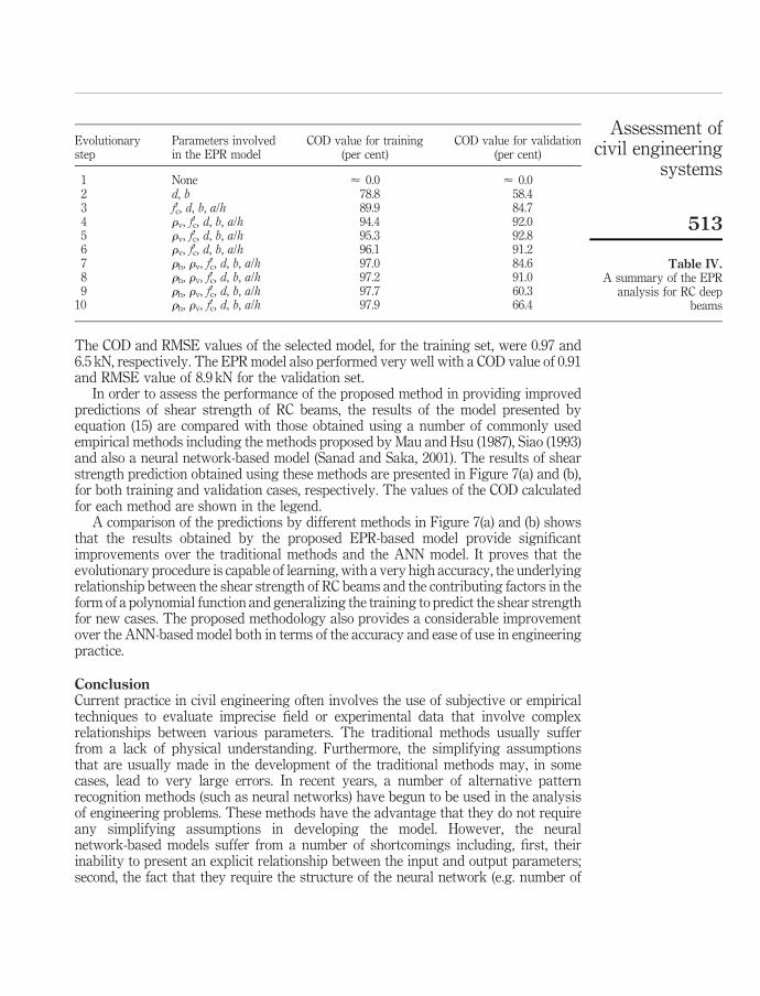
The COD and RMSE values of the selected model, for the training set, were 0.97 and6.5 kN, respectively. The EPR model also performed very well with a COD value of 0.91and RMSE value of 8.9 kN for the validation set.

In order to assess the performance of the proposed method in providing improvedpredictions of shear strength of RC beams, the results of the model presented byequation (15) are compared with those obtained using a number of commonly usedempirical methods including the methods proposed by Mau and Hsu (1987), Siao (1993)and also a neural network-based model (Sanad and Saka, 2001). The results of shearstrength prediction obtained using these methods are presented in Figure 7(a) and (b),for both training and validation cases, respectively. The values of the COD calculatedfor each method are shown in the legend.

A comparison of the predictions by different methods in Figure 7(a) and (b) showsthat the results obtained by the proposed EPR-based model provide significantimprovements over the traditional methods and the ANN model. It proves that theevolutionary procedure is capable of learning, with a very high accuracy, the underlyingrelationship between the shear strength of RC beams and the contributing factors in theform of a polynomial function and generalizing the training to predict the shear strengthfor new cases. The proposed methodology also provides a considerable improvementover the ANN-based model both in terms of the accuracy and ease of use in engineeringpractice.

ConclusionCurrent practice in civil engineering often involves the use of subjective or empiricaltechniques to evaluate imprecise field or experimental data that involve complexrelationships between various parameters. The traditional methods usually sufferfrom a lack of physical understanding. Furthermore, the simplifying assumptionsthat are usually made in the development of the traditional methods may, in somecases, lead to very large errors. In recent years, a number of alternative patternrecognition methods (such as neural networks) have begun to be used in the analysisof engineering problems. These methods have the advantage that they do not requireany simplifying assumptions in developing the model. However, the neuralnetwork-based models suffer from a number of shortcomings including, first, theirinability to present an explicit relationship between the input and output parameters;second, the fact that they require the structure of the neural network (e.g. number of

Evolutionarystep

Parameters involvedin the EPR model

COD value for training(per cent)

COD value for validation(per cent)

1 None < 0.0 < 0.02 d, b 78.8 58.43 f0c, d, b, a/h 89.9 84.74 rv, f0c, d, b, a/h 94.4 92.05 rv, f0c, d, b, a/h 95.3 92.86 rv, f0c, d, b, a/h 96.1 91.27 rh, rv, f0c, d, b, a/h 97.0 84.68 rh, rv, f0c, d, b, a/h 97.2 91.09 rh, rv, f0c, d, b, a/h 97.7 60.3

10 rh, rv, f0c, d, b, a/h 97.9 66.4

Table IV.A summary of the EPR

analysis for RC deepbeams

Assessment ofcivil engineering

systems

513

inputs, kernel type, transfer functions, number of hidden layers, etc.) to be identifieda priori; and, third, that the optimum structure and the parameters of the networkare obtained by trial and error.

In this paper, a new approach has been introduced for the analysis of complex civilengineering problems using EPR. The capabilities of EPR methodology have beenillustrated by application to two practical problems including prediction of upliftcapacity of suction caissons and shear strength of RC deep beams. The results showthat the EPR models provide a significant improvement over the existing models.Furthermore, the proposed EPR models generate a transparent and structuredrepresentation of the system allowing a physical interpretation of the problem that

Figure 7.Predicted versusmeasured shear strengthof RC deep beams usingthe EPR model andconventional methods

50

100

150

200

250

50 100 150 200 250

Measured Shear Strength (kN)

Pred

icte

d Sh

ear

Stre

ngth

(kN

)

EPR ModelMau and Hsu (1987)Siao (1993)ANN Model

(a) Training

CODEPR=97.2% CODMau & Hsu=70.8% CODSiao=76.5%CODANN=96.1%

100

150

200

250

100 150 200 250

Measured Shear Strength (kN)

Pred

icte

d Sh

ear

Stre

ngth

(kN

)

EPR ModelMau and Hsu (1987)Siao (1993)ANN Model

(b) Validation

CODEPR=91.2%CODMau & Hsu=88.2%CODSiao=63.9%CODANN=88.1%

EC25,6

514

gives the user an insight into the relationship between input and output data. Fordesign purposes, the EPR models, presented in this study, are simple to use andprovide results that are more accurate than the existing methods. In the EPR approach,no preprocessing of the data is required and there is no need for normalization orscaling of the data.

An interesting feature of EPR is in the possibility of getting more than one model fora complex phenomenon. Each different model can be trained according to a specificcost function. A further feature of EPR is the high level of interactivity between theuser and the methodology. The user physical insight can be used to make hypotheseson the elements in the function F(X, u) and on its structure (equation (1)). Selecting anappropriate objective function, assuming pre-selected elements in equation (1) (basedon engineering judgement) and working with dimensional information enable therefinement of final models (Giustolisi and Savic, 2006). The best models are chosen onthe basis of their performances on a test set of unseen data. For this purpose, the initialdataset is split into two subsets:

(1) training set which is used for model construction; and

(2) testing set which is used for model validation.

The test set is never used in the phase of model construction, which allows examiningthe generalization capabilities of each constructed model. Thus, an unbiasedperformance indicator is obtained on the real capability of the models.

Another major advantage of the EPR approach is that as more data becomeavailable, the quality of the prediction can be easily improved by retraining the EPRmodel using the new data. However, it should be noted that the EPR models should notbe used for extrapolation, i.e. for new cases where one or more parameters fall outsidethe range of the parameters used in training (see Tables I–III), the predicted resultsshould be taken with caution and allowance should be made for the uncertainty.

References

Abu-Kiefa, M.A. (1998), “General regression neural networks for driven piles in cohesionlesssoils”, ASCE Journal of Geotechnical and Geoenvironmental Engineering, Vol. 124 No. 12,pp. 1177-85.

Adeli, H. and Karim, A. (1997), “Scheduling/cost optimization and neural dynamics model forconstruction”, ASCE Journal of Construction Engineering andManagement, Vol. 123 No. 4,pp. 450-8.

Adeli, H. and Wu, M. (1998), “Regularization neural network for construction cost estimation”,ASCE Journal of Construction Engineering and Management, Vol. 124 No. 1, pp. 18-24.

Ankireddi, S. and Yang, H.T.Y. (1999), “Neural networks for sensor fault correction in structuralcontrol”, ASCE Journal of Structural Engineering, Vol. 125 No. 9, pp. 1056-64.

Arditi, D., Oksay, F.E. and Tokdemir, O.B. (1998), “Predicting the outcome of constructionlitigation using neural networks”, Computer-Aided Civil and Infrastructure Engineering,Vol. 13 No. 2, pp. 75-81.

Celikoglu, H.B. and Cigizoglu, H.K. (2007), “Public transportation trip flow modeling withgeneralized regression neural networks”, Journal of Advances in Engineering Software,Vol. 38 No. 2, pp. 71-9.

Assessment ofcivil engineering

systems

515

Coulibaly, P., Anctil, F. and Bobee, B. (2000), “Neural network based long term hydropowerforecasting system”, Computer-Aided Civil and Infrastructure Engineering, Vol. 15 No. 5,pp. 355-64.

Deng, W. and Carter, J.P. (1999a), “Vertical pullout behaviour of suction caissons”, researchreport, Centre for Geotechnical Research, The University of Sydney, Sydney.

Deng, W. and Carter, J.P. (1999b), “Analysis of suction caissons subjected to inclined upliftloading”, research report, Centre for Geotechnical Research, The University of Sydney,Sydney.

Feng, M.Q. and Bahng, E.Y. (1999), “Damage assessment of jacketed RC columns using vibrationtests”, ASCE Journal of Structural Engineering, Vol. 125 No. 3, pp. 256-71.

Flood, I. and Kartam, N. (1994), “Neural networks in civil engineering II principles andunderstanding”, Journal of Computing in Civil Engineering, Vol. 8 No. 2, pp. 149-62.

Gagarin, N., Flood, I. and Albrecht, P. (1994), “Computing truck attributes with artificial neuralnetworks”, ASCE Journal of Computing in Civil Engineering, Vol. 8 No. 2, pp. 179-200.

Giustolisi, O. and Savic, D.A. (2006), “A symbolic data-driven technique based on evolutionarypolynomial regression”, Journal of Hydroinformatics, Vol. 8 No. 3, pp. 207-22.

Giustolisi, O., Doglioni, A., Savic, D.A. and Webb, B. (2007), “A multi-model approach to analysisof environmental phenomena”, Environmental Modelling & Software, Vol. 22 No. 5,pp. 674-82.

Goh, A.T.C. (1994), “Some civil engineering applications of neural networks”, Proceedings of ICE,Structures and Buildings, Vol. 104, pp. 463-9.

Huang, C.C. and Loh, C.H. (2001), “Nonlinear identification of dynamic systems using neuralnetworks”, Computer-Aided Civil and Infrastructure Engineering, Vol. 16 No. 1, pp. 28-41.

Javadi, A.A. (2006), “Estimation of air losses in compressed air tunneling using neural network”,Journal of Tunnelling and Underground Space Technology, Vol. 21 No. 1, pp. 9-20.

Javadi, A.A., Rezania, M. and Mousavi Nezhad, M. (2006), “Evaluation of liquefaction inducedlateral displacements using genetic programming”, Computers and Geotechnics, Vol. 33Nos 4/5, pp. 222-33.

Juang, C.H., Jiang, T. and Christopher, R.A. (2001), “Three-dimensional site characterisation:neural network approach”, Geotechnique, Vol. 51 No. 9, pp. 799-809.

Lippmann, R.P. (1987), “An introduction to computing with neural nets”, IEEE Acoustics, Speechand Signal Processing Magazine, Vol. 14 No. 2, pp. 4-22.

Liu, W. and James, C.S. (2000), “Estimation of discharge capacity in meandering compoundchannels using artificial neural networks”, Canadian Journal of Civil Engineering, Vol. 27,pp. 297-308.

Mau, S.T. and Hsu, T.T.C. (1987), “Shear strength prediction for deep beams with webreinforcement”, ACI Structural Journal, Vol. 84 No. 6, pp. 513-23.

Rahman, M.S., Wang, J., Deng, W. and Carter, J.P. (2001), “A neural network model for the upliftcapacity of suction caissons”, Computers and Geotechnics, Vol. 28 No. 4, pp. 269-87.

Sanad, A. and Saka, M.P. (2001), “Prediction of ultimate shear strength of reinforced concretedeep beams using neural networks”, ASCE Journal of Structural Engineering, Vol. 127No. 7, pp. 818-28.

Savic, D.A., Giustolisi, O., Berardi, L., Shephard, W., Djordjevic, S. and Saul, A. (2006), “Modelingsewers failure using evolutionary computing”, Proceeding of ICE, Water management,Vol. 159 No. 2, pp. 111-8.

EC25,6

516

Siao, W.B. (1993), “Strut-and-tie model for shear behavior in deep beams and pile caps failing indiagonal splitting”, ACI Structural Journal, Vol. 90 No. 4, pp. 356-63.

Thirumalaiah, K. and Deo, M.C. (1998), “Real-time flood forecasting using neural networks”,Computer-Aided Civil and Infrastructure Engineering, Vol. 13 No. 2, pp. 101-11.

Vijayalakshmi Pai, G.A. (2005), “Prediction of uplift capacity of suction caissons using aneuro-genetic network”, Engineering with Computers, Vol. 21 No. 2, pp. 129-39.

Corresponding authorAkbar A. Javadi can be contacted at: a.a.javadi@ex.ac.uk

Assessment ofcivil engineering

systems

517

To purchase reprints of this article please e-mail: reprints@emeraldinsight.comOr visit our web site for further details: www.emeraldinsight.com/reprints