AN ENHANCED ALGORITHM FOR SURFACE RECONSTRUCTION FROM A CLOUD OF POINTS

AN ENHANCED ALGORITHM FOR SURFACE RECONSTRUCTION

FROM A CLOUD OF POINTS

M. S. Abdel-Wahab, A. S. Hussein, I. Taha, M. S. Gaber Faculty of computer and information science, Ain shams university, Cairo, Egypt.

[email protected], [email protected], [email protected], [email protected] Abstract In this paper, a comparative study is performed between the most eminent computational geometry based surface reconstruction algorithms. These algorithms are the Crust, the Power Crust, the Tight Cocone and the Ball Pivoting algorithm. The key issues for the comparison are the quality of the reconstructed surface, the reconstruction time, and the total memory usage. To guarantee a proper comparison, the algorithms were implemented using the same programming tools and tested on the same platform. Several benchmark test cases were used to validate the implemented algorithms. The Crust and Power Crust algorithms showed a balanced trade-off between execution time and memory usage. The Ball Pivoting algorithm exhibited minimum execution time and memory usage, followed by the Tight Cocone. The experiments showed that applying any of the four algorithms on a non-uniformly distributed cloud may create poor quality surface. To deal with such clouds, an enhanced algorithm based on Ball Pivoting algorithm and Radial Basis Functions is proposed. The enhanced algorithm has the capability of filling any detected hole within the surface reconstruction process. The proposed algorithm exhibited high robustness in reconstructing objects with non-uniform sampling and misregistrations. Keywords: Surface Reconstruction, Surface Modeling, Shape Recognition, Voronoi Diagram, Delaunay Triangulation. 1. Introduction There is a wide range of applications in science and engineering for which surface reconstruction from scattered point data is important, including reverse engineering, cartography, medical imaging and industrial design. In many scientific systems, the surface data of 3D shapes—reaching from bodies to landscapes—is required for further processing. Scanning of these 3D shapes provide the source of data for the surface reconstruction process. Surfaces also open the application of the wide-spread surface-oriented visualization and rendering techniques. For example, surfaces may be used for visualizing other information e.g. coded in textures

(data textures or real textures) mapped on the surface (adapted from [19]).

Mathematically, the problem can be expressed as follows, given a set of points S={sn 1,s2,…,sn}, which are sampled from some unknown smooth surface U , find a mesh M that approximates the surface U , i.e. the mesh and the surface are near everywhere [16]. The output is initially some mesh (mostly a triangulation) that has the same general shape of the original surface. If the generated mesh connects the original input points, then it interpolates the surface. Alternatively, the mesh may connect generated points other than those of the input set. In the latter case, the mesh is said to approximate the surface. A common classification criterion of surface reconstruction techniques is to categorize the technique as either a surface interpolation algorithm or a surface approximation one [20].

One of the first surface interpolation algorithms is the one presented by Edelsbrunner and Mucke in [13], which uses the heuristic α -shapes. Amenta and Bern [1] used the properties of the medial axis and Voronoi diagram to introduce the Crust algorithm, which was the first guaranteed surface reconstruction algorithm. They extracted an approximated triangulated surface from the Delaunay triangulation of the input set. Amenta et al. [3] described the co-cone term and used it in their Cocone algorithm. The Cocone computes the Delaunay triangulation of the input set, and selects candidate triangles to construct the surface. Dey and Goswami [12] modified the Cocone into a new algorithm—the Tight Cocone—to solve problem instances of specific domains that require hole-free surfaces. They also introduced the Boundary algorithm [10] and suggested using it [12] in the Tight Cocone as preprocessing. The Boundary algorithm is an algorithm which detects undersampled regions in the input point set. Kolluri et al. [18] introduced a noise-resistant algorithm for watertight surfaces. The latter algorithm uses a variant of spectral graph partitioning to select triangles from the Delaunay triangulation to construct the surface. All the aforementioned algorithms can be described as Voronoi based algorithms and they generally suffer from slow performance and difficulty in handling large data. To overcome this problem, Dey et al. [11] partitioned the entire sample space into smaller clusters using octree

GVIP 05 Conference, 19-21 December 2005, CICC, Cairo, Egypt

subdivision. Then, they applied the Cocone algorithm on each of these clusters separately, and they called this algorithm the Super Cocone. An interesting interpolation non-Voronoi based algorithm is the Ball Pivoting algorithm (BPA), presented by Bernardini et al. [5]. This algorithm uses a rolling ball to construct triangles one by one and add them to the surface.

Typical examples of surface approximation algorithms are the algorithms presented by Hoppe et al. [16] and by Curless and Levoy [8]. They used the normal orientations to estimate the tangent planes and approximate the local surface. Another surface approximation algorithm was introduced by Boissonat and Cazals [6] that is based on natural neighbor interpolation and represents the surface implicitly as a zero-set of some pseudo-distance function. Gopi et al. [15] suggested an algorithm that uses a plane projection technique where the neighbors of a sample point is computed by projecting its close points onto its tangent plane. Amenta et al. [4] suggested using the power diagram (dual of weighted Delaunay triangulation) in their Power Crust algorithm. Although the Power Crust algorithm is a Voronoi based algorithm, but—unlike the algorithms belonging to this family—it is classified as a surface approximation algorithm.

Algorithms of another family use the implicit surface approach, which is suitable for reconstructing point clouds with local problems, but these algorithms are not suitable for processing large clouds [7, 9, 17].

In this paper, a new hybrid system is proposed. The proposed algorithm is based on the BPA—as an efficient surface reconstruction algorithm—integrated with the Radial Basis Functions (RBFs) to gain the edge of RBF as a powerful surface interpolation tool to generate vertices within holes and misregistration domains. The performance of the BPA is validated by a comparative study between four eminent computational geometry based surface reconstruction algorithms using benchmark data as test cases. The efficiency of the algorithms is measured by the execution time and the memory usage for processing the data samples, while the quality is measured by the mesh size and points distribution. Finally, the hybrid system exhibited high robustness in reconstructing data which suffer from severe holes and misregistrations. 2. Theoretical Background In this section, general geometric concepts are depicted. Then, quick notes about each of the most eminent algorithms are introduced in a separate subsection. 2.1 General Concepts The Crust and Power Crust algorithms require the input sample to be a "Good" sample. This sampling criterion was first defined by Amenta et al. [2]. In general, a "Good" sample is a sample that is dense at detailed areas, while featureless areas can be sparse or dense. Then, the same authors defined in [2] as the sample where the distance from any sample point to the nearest point in the sample is at most r times the distance from this sample point to the medial axis. Amenta et al. [2] found that

r sample−

0.5r = is sufficient.

Some models—such as CAD designs—require hole-free surfaces. For these models, the Power Crust and the Tight Cocone algorithms are suitable because they produce watertight surfaces. A water tight surface is formally defined by Dey el al. [12] as a 2-complex embedded in whose underlying space is same as the boundary of the closure of a 3-manifold in .

3R3R

2.2 The Crust Algorithm The first algorithm in the present study is the Crust algorithm by Amenta et al. [2]. The only prerequisite of the Crust is that the input data set should satisfy the previously mentioned sampling criterion. It was named Crust because the word "crust" is the formal name of the geometric structure which this algorithm constructs as an approximation to the required surface. The worst case complexity of three-dimensional Voronoi diagram construction or Delaunay triangulation is . Since the Voronoi diagram and Delaunay triangulation computations are the main steps of the algorithm, the algorithm complexity is too. Notice that the Voronoi diagram is constructed for points, while the Delaunay triangulation is computed for at most points [2]. It is noteworthy that the worst-case complexity for the three-dimensional Delaunay triangulation almost never arises in practice as Amenta stated in [2].

2( )O n

2( )O nn

3n

Beside its simplicity, the Crust algorithm has the advantage of being theoretically prominent. On the other hand, the Crust does not work properly in the case of non-uniform sampling or in the presence of sharp edges. If the given cloud is non-uniformly sampled, the Crust faces difficulty and may create holes.

2.3 The Power Crust Algorithm This algorithm was named after the structure that it builds—the "power crust" structure. The "power crust" structure was proved by Amenta et al. [4] to be a geometrically and topologically correct piecewise-linear approximation to the surface. The power crust is a subset of another construction, called the power diagram, which can be thought of as a weighted Voronoi diagram. Unlike Voronoi diagrams, the power diagram is computed for weighted points (balls; points with radii) rather than ordinary points, as defined by Amenta et al. in [4].

The power diagram computation is the dominant factor in determining the time complexity of the Power Crust. Since the power diagram is a variant of the Voronoi diagram, it has the same quadratic time complexity , and so does the Power Crust. Therefore, the Power Crust and the Crust algorithms have the same worst case quadratic time complexity

. Note that the power diagram is computed for at most points, hence, the Power crust is faster than the Crust in practice.

2( )O n

2( )O n2n

The Power Crust algorithm is theoretically guaranteed and works under the same sampling criterion of the Crust. No 'clean up' operations—as holes filling or manifold extraction—are needed to modify the reconstructed surface. Also, the generated mesh is a watertight surface, which makes this algorithm suitable for CAD applications. On the other hand, the output


surface mesh is very dense and usually needs to be simplified. In addition, the output surface consists of a set of two-dimensional faces, not triangles. 2.4 The Tight Cocone Algorithm The Tight Cocone algorithm—introduced by Dey and Goswami in [12] —employs another algorithm, the Cocone, as a preprocessor. The output of the Cocone algorithm is the initial surface to the Tight Cocone algorithm. The main purpose of the Tight Cocone is to build watertight surfaces for models that require hole-free outputs. Two processes, marking and peeling, are performed on the initial surface to turn it into a watertight surface.

Again, as a Voronoi based algorithm, the time complexity of the Tight Cocone is dominated by the three dimensional Voronoi diagram computation complexity. Thus, for an input sample of points, the algorithm runs in time in the worst case. It should be noted that the Delaunay Triangulation is computed only once and only for the original input points, hence, the Tight Cocone is faster than both the Crust and Power Crust in practice.

n2( )O n

n

2.5 The Ball Pivoting Algorithm According to Bernardini et al. [5], the Ball Pivoting Algorithm (BPA) can process very large data sets in a little execution time, using small amount of memory, and yield output with good quality. The BPA is closely related to the α -shapes of Edelsbrunner and Mucke [13]. The surface reconstructed by the BPA retains some of the qualities of the α -shapes: It has provable reconstruction guarantees under certain sampling assumptions, and an intuitively simple geometric meaning, as claimed by Bernardini et al. [5]. Although the BPA is very efficient, it produces holes if the sample is not sufficiently sampled.

Unlike the other three algorithms, the BPA is described as an advancing front algorithm. The output mesh is formed incrementally one triangle at a time in ( )O n time complexity. As for space complexity, the

main structure is the known front structure used by all advancing front algorithms, which is linear in the input size. The BPA does not compute the Voronoi diagram of the point set or any related structure; hence it is relieved from the burden both in time and memory complexity. This linear complexity makes the BPA superior to the other three algorithms, which is emphasized by the comparison results in section 4.

2( )O n

The BPA needs only one parameter, ρ . The sampling condition of the BPA is that a ball with radius ρ cannot pass through the surface without touching any sample points. So, the sampling density of the sample points determines the ρ value.

In spite of the fast execution time and low memory usage of this algorithm, it may produce holes if the object is not sufficiently sampled, or if the surface normals orientations are not correct. 3. Enhanced Ball Pivoting Algorithm

Any surface reconstruction algorithm has its advantages and disadvantages. In this section, we propose an enhanced algorithm based on the BPA, yet, lacks its problems.

Usually, in real samples, the scanned points may not cover all the surface areas equally. The distribution of the points can be sparse at some regions, which violates the sampling criteria. As a result, applying any of the considered algorithms on such a sample might create a poor quality surface. As for the BPA, for instance, if a ball with a large ρ value was used, the quality of the surface will be deteriorated. It may seem better and more realistic to use a small ρ value ball, but in such a case, the algorithm will need to check the validity of each generated triangle. Besides, using a small ρ will lead to constructing a surface with holes at the sparse regions. The new hybrid approach is suggested to handle real-life samples without creating holes in the output surface.

The new system is basically a hybrid framework that integrates both the BPA as a surface reconstruction algorithm with the RBFs as an interpolation tool. The BPA was selected to perform the initial reconstruction phase because of its linear efficiency, in contrast with the quadratic behavior of the Voronoi based algorithms [14]. The purpose of the second phase—the interpolation phase—is to post process the initial reconstructed surface by filling the holes. RBFs are popular for interpolating scattered data as the associated system of linear equations is guaranteed to be invertible under very mild conditions on the locations of the data points. In the system, the bi-harmonic basic function was chosen to guarantee a smooth surface in the fitting process. Using tri-harmonic RBFs is also possible. The idea is to apply the BPA on the sample points to create an initial mesh. Then, RBFS are used to generate new points that fill any existing holes in the mesh. Finally The BPA is used again to triangulate the generated points.

Figure 1 shows a flowchart that demonstrates how the hybrid system works. The main processes of the system are the following:

-BPA: Applying the regular BPA on the sample points with appropriate ρ value. -Hole detection: In this process, any hole in the output mesh of the regular BPA is detected. A hole is identified by its boundaries. This process starts by tracing all edges, and marking the edges that has one triangle on its side. A hole boundary consists of a sequence of such edges. The end points of each edge are used to determine the next and previous edges in the sequence. Tracing boundary edges continues, until they are finished and all holes are detected. During this process too, the neighborhood of each hole is determined. The neighborhood of a hole is the set of points that surround it, or equivalently, lie within a specific radius from the hole center. -RBF estimation: In this process, the interpolation function—which is the RBF—is estimated using the bi-harmonic basic function. The interpolation function is in the form of weighted sum of translations of a radially symmetric basic function augmented by a polynomial term. More precisely, the function takes the form


1( ) ( ) ( )

N

i ii

s x p x x xλϕ=

= + −∑ .

Where is a polynomial of degree at most,p k iλ is a real valued weight. |x-xi| is simply the distance between point x and point xi. The neighborhood points are provided as the data points which the RBF should satisfy. -Points generation: Now, a set of x, y coordinates are generated. These coordinates, when associated with an interpolated z coordinate, represent the new points that fill the hole. The values of x, y pairs are set to form a grid that fills the hole plane, within the boundaries of the hole. The hole plane is considered to be the two dimensional surface which best fits the hole, and it is computed using PCA (principal component analysis). The two eigen vectors, associated with the larger eigen vectors, form a basis for the hole plane surface. -Interpolation: The interpolation function is used to compute the distance (the z coordinate) of the 2D points (x, y pairs) from the hole plane. -BPA: The BPA is used again to triangulate the newly generated points. -Surface accumulation and assembling: Finally, the initial mesh and the small meshes (of the holes) are all accumulated to form the object surface. The new small meshes are “pasted” to the initial mesh.

Ball Pivoting Hole Detection

RBF Estimation2D Points Generating

scanned points reconstructed surface

with holes

RBF

holes

boundaries

reconstructed surface

with holes

small meshes

hole-free reconstructed

surface

neighborhood points

2D points

Triangulation and

Surface AccumulationInterpolationBall Pivoting

generated

points

Figure 1. Framework of the enhanced BPA.

4. Implementation and Results All the four considered algorithms—the Crust, Power Crust, Tight Cocone and BPA—were implemented using Microsoft visual C++ version 6 on the same operating system (Windows XP) and the same hardware configurations (3GHz Pentium 4 PC with 512 MB cache memory and 1 GB RAM). The Tight Cocone executable program was downloaded from [21]. Three of these algorithms—the Crust, Power Crust and Tight Cocone—compute the Voronoi diagram or other dual structures—Delaunay triangulation and power diagram. The CGAL library [22] was used to compute these structures. The comparison is performed against three key issues: execution time, memory usage and reconstructed surface quality. 4.1 Test Cases Three models—each with different resolutions—were used in the comparison, namely the Stanford Bunny (4 resolutions: 1889, 1889, 8171 and 35947 points), Stanford Dragon (3 resolutions: 5205, 22998 and 100250

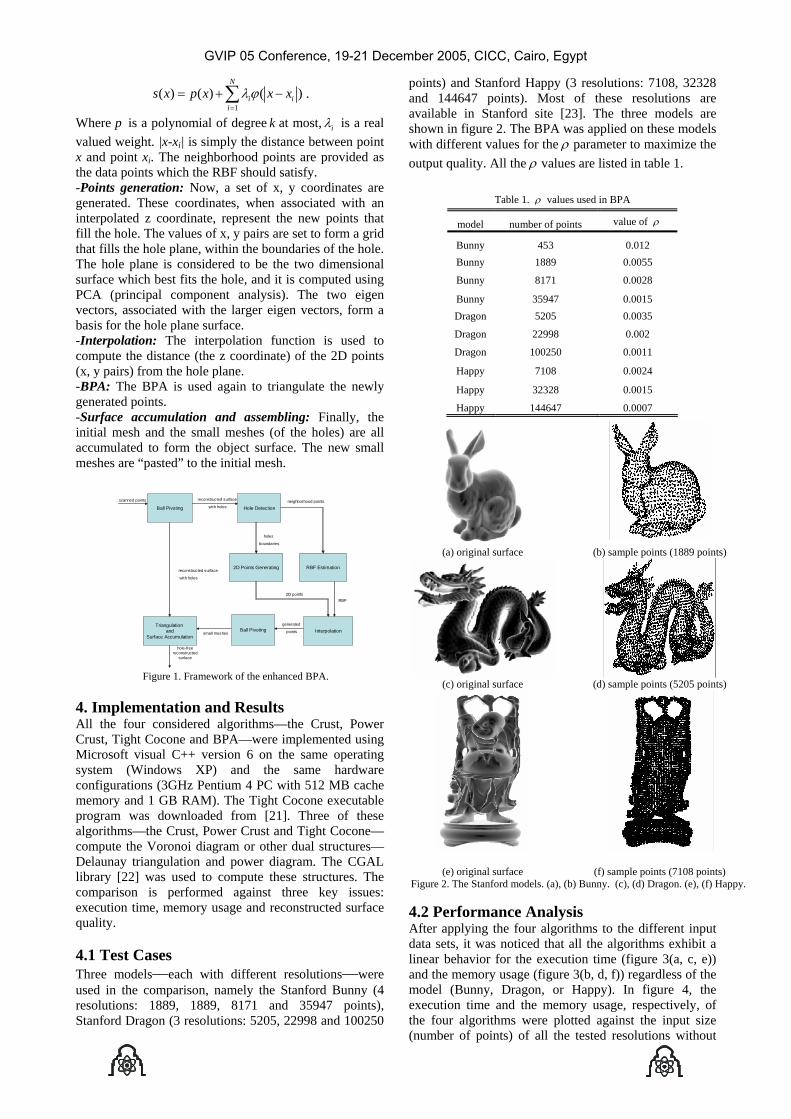
points) and Stanford Happy (3 resolutions: 7108, 32328 and 144647 points). Most of these resolutions are available in Stanford site [23]. The three models are shown in figure 2. The BPA was applied on these models with different values for the ρ parameter to maximize the output quality. All the ρ values are listed in table 1.

Table 1. ρ values used in BPA

model number of points value of ρ

Bunny 453 0.012 Bunny 1889 0.0055

Bunny 8171 0.0028

Bunny 35947 0.0015 Dragon 5205 0.0035

Dragon 22998 0.002

Dragon 100250 0.0011

Happy 7108 0.0024

Happy 32328 0.0015

Happy 144647 0.0007

4.2 Performance Analysis After applying the four algorithms to the different input data sets, it was noticed that all the algorithms exhibit a linear behavior for the execution time (figure 3(a, c, e)) and the memory usage (figure 3(b, d, f)) regardless of the model (Bunny, Dragon, or Happy). In figure 4, the execution time and the memory usage, respectively, of the four algorithms were plotted against the input size (number of points) of all the tested resolutions without

(a) original surface (b) sample points (1889 points)

(c) original surface (d) sample points (5205 points)

(e) original surface (f) sample points (7108 points) Figure 2. The Stanford models. (a), (b) Bunny. (c), (d) Dragon. (e), (f) Happy.


considering the model, and the linear behavior is still valid. It can be concluded that the considered algorithms are linear in execution time and memory usage, and the model shape has no effect on their attitude. In general, the figures show that the BPA bested others in execution time, memory usage and mesh size.

For different cloud sizes, the BPA has the best time perf

cted, for the reas

ormance, as shown in figure 4(a), followed by the Tight Cocone, then the Power Crust and finally the Crust. A statistical regression test was performed on the four curves, and table 2 shows the test results. The slopes of the regression lines can be used to numerically compare the algorithms performance. The BPA is about 3 times faster than its closest competent, the Tight Cocone. The Tight Cocone is about 2 times faster than the Power Crust, and 2.4 times faster than the Crust.

This order of efficiency was expeons mentioned in section 2. For the Voronoi based

algorithms, it was expected that the Tight Cocone to be 2 times faster than the Power Crust and 3 times faster than the Crust. The computed efficiency ratios were near to the expected. It can only be noted that the Crust algorithm is faster than the expected (2.4 times slower than the Tight Cocone rather than 3 times). This can be interpreted as follows. The Power Crust takes considerable time to extract the huge final mesh from the power diagram, and the Tight Cocone takes considerable time to construct the surface from the Delaunay triangulation, while the time taken by the additional computations of the Crust is negligible.

020406080

100120140160

0 10 20 30 40x 1000input size

time

in s

ecs

crustpowertightpivot

020406080

100120140160180

0 10 20 30 40x 1000input size

mem

ory

in M

B


(a) execution time (b) memory usage

0

100

200

300

400

500

600

0 20 40 60 80 100 120x 1000input size

time

in s

ecs


0

100

200

300

400

500

600

0 20 40 60 80 100 120x 1000input size

mem

ory

in M

B


(c) execution time (d) memory usage

0100200300400500600700800900

0 20 40 60 80 100 120 140 160x 1000input size

time

in s

ecs


0100200300400500600700800

0 20 40 60 80 100 120 140 160x 1000input size

mem

ory

in M

B


(e) execution time (f) memory usage

Figure 3 ments for the fo we. Efficiency measure ur algorithms (Crust, Po r Crust, Tight Cocone and BPA) for the Stanford models. (a), (b) Bunny.

(c), (d) Dragon. (e), (f) Happy.

0100200300400500600700800900

0 50 100 150x 1000input size

time

in s

ecs


0100200300400500600700800

0 50 100 150x 1000input size

mem

ory

in M

B


(a) execution time (b) memory usage Figure 4. Efficiency measurements for the four algorithms (Crust,

Power Crust, Tight Cocone and BPA) for all sample sizes, regardless of the model.

Again, the BPA has the best storage performance

followed by the Tight Cocone, while the Crust shows better performance than the Power Crust, as shown in figure 4(b). The regression tests in table 3 show that The BPA is about 2.6 times better than the Tight Cocone in storage efficiency. The tests show also that the Tight Cocone is about 1.45 times better than the Crust, and about 2.7 times better than the Power Crust.

The “front” structure used in the BPA, as well as all the necessary arrays, is linear in the input size [5], which explains its behavior. Like in time efficiency, the fact that the Tight Cocone computes a single Delaunay triangulation on size input makes it the best Voronoi based algorithm in storage efficiency. The maximum amount of memory consumed by the Power Crust is not used during power diagram computation, but during the surface extraction phase. The large size of the output surface is the reason behind the large amount of memory consumed by the Power Crust.

n

Table 2. Regression test results of time curves

algorithm slope intercept

Crust 0.0055445 -21.203998 Power Crust 0.0043864 -25.64276

Tight Cocone 0.0022699 -10.568449 BPA 0.0007672 -3.221019

Table 3. Regression test results of memory curves


Crust 0.002643 0.388838 Power Crust 0.0049222 -0.6786798

Tight Cocone 0.0018191 0.1775423 BPA 0.0006766 0.3165781

The output size of the meshes that the four

algorithms construct, regardless of the model shape, has the same linear behavior of the time and memory. In figure 5, where output size is plotted against input size, this fact is proved. As the Power Crust output mesh is not triangular and its vertices are not the original input points, it is not appropriate to plot its size with the meshes sizes of the other three algorithms. Otherwise, the number of vertices and the output size of the Power Crust output meshes are written separately in table 5.

Table 4 shows that the slope values of the BPA and the Tight Cocone are very close, which indicates that


neither one of them competes the other. Actually, the closeness of the two algorithms curves in figure 5(d) assures this. The mesh sizes of the Crust algorithms is the larger than both, with about %145 percentage.

020

406080

100

120140

0 10 20 30 40

x 1000

x 1000input size

mes

h si

ze

crust

tight

pivot

0

50100

150200

250300

350

0 20 40 60 80 100 120

x 1000

x 1000input size

mes

h si

ze

crust

tight

pivot

(a) (b)

050

100150200250300350400450

0 20 40 60 80 100 120 140 160

x 1000

x 1000input size

mes

h si

ze

crust

tight

pivot

050

100150200250300350400450

0 20 40 60 80 100 120 140 160

x 1000

x 1000input size

mes

h si

ze

crust

tight

pivot

(c) (d)

Figure 5. Mesh size after applying the (Crust, Tight Cocone and BPA) on the (a) Bunny. (b) Dragon. (c) Happy. (d) all models.

Table 4. Regression test results of mesh size curves


Crust 2.846683661 2295.995241 Tight Cocone 1.965305546 473.1170324 Ball Pivoting 1.932187649 685.2362592

Table 5. Power Crust mesh size values

input size number of vertices number of polygons

1889 17272 12085

5205 50872 35738 5827 58243 41044 7108 65100 44927 8171 79840 56195 22998 235724 166179 32328 1009530 224077 35947 354655 247621 70006 750568 536243 95958 320553 717425

100250 1081151 772715

144647 1526626 1084386

Figure 6 shows the reconstructed meshes of the 1889

Bunny model after applying the different algorithms on it. The Crust output (figure 6(a)) is good but it is not a manifold. The BPA output (figure 6(d)) shows a problem at the right ear end and another one at the left ear. Besides being watertight, the Power Crust output (figure 6(b)) may be the best of the four, except that the mesh is very dense and not triangular. The Tight Cocone output (figure 6(c)) is also watertight, but shows a problem at the left ear end (a triangle is not connected to the rest of the ear).

(a) Crust (b) Power Crust

(c) Tight Cocone (d) BPA

Figure 6. The output meshes of the four algorithms when applied on 1889 Stanford Bunny.

4.3 The Noise Effect All the previous results were obtained by applying the four algorithms on noise-free models. To test the effect of noise on the output quality, a Gaussian noise with variance 610− was added to the 1889 Bunny model. The difference in the execution time and memory usage are negligible, which emphasizes our conclusion that the size of the input—not the shape of the original object—is the only dominant factor for the time and space efficiency.

Figure 7 shows the reconstructed meshes after applying the four algorithms on the noisy Bunny. Generally, each algorithm output retains the same expected features (the Crust output is not a manifold, the Power Crust output is dense, etc), but the noise effect appeared in the number of holes in each mesh. The BPA (figure 7(d)) and the Crust (figure 7(a)) outputs have the largest number of holes, but the BPA holes are slightly wider. The Tight Cocone output (figure 7(c)) has the less number of holes, followed by the Power Crust output (figure 7(b)), but the Tight Cocone mesh is not correctly built at the ears.

(a) Crust (b) Power Crust

(c) Tight Cocone (d) BPA

Figure 7. The output meshes of the four algorithms when applied on the noisy 1889 Stanford Bunny.


4.4 The Proposed System Results The new hybrid system was tested on a 28060 points sample of an incomplete Bunny model. The model is shown in figure 8. The code used for the RBF part is available in [24]. The cloud of points contains many undersampled regions and represents a good example of a misregistered data set. The BPA was applied using 0.5ρ = . Figure 9(a, b) shows that the reconstructed surface after applying the BPA (phase one) contains many holes in different places (the back, the tail, the head …etc) with different sizes. Figure 9(c, d) also shows how the holes disappeared after applying the additional phases of the system. The output surface is 29967 points in size.

(a) Side view (b) Top view

Figure 8. Incomplete Bunny sample points (28060 points).

(a) Side view (b) Top view

(c) Side view (d) Top view Figure 9. Different views of the 28060 points Bunny. (a) after applying the raw BPA. (b) after applying the hybrid system.

4.5 Accuracy Assessment The new approach was tested by calculating the error of the RBF interpolation process. A hole—with radius 0.025—was artificially created at the back of the 8171 vertices Bunny by extracting a group of points from that area, and saving the coordinates of these extracted points. Figure 10 shows the Bunny model with the artificial hole. The x and y components of the extracted points were used to interpolate new values for the third component—z. The difference between the original z component and

the computed z component is the error value. Different radii of neighborhood were used in the interpolation process. Table 6 shows several statistics about the error with different neighborhood radii. Figure 11 shows the relation between the mean of the error and the neighborhood radius. The error mean decreases exponentially with increasing neighborhood radius.

Table 6. error statistics with different neighborhood radii

statistic r= 0.03 r= 0.04 r= 0.05

mean 0.041464 0.032969 0.03132 median 0.044996 0.03542 0.0329

min 0.003843 0.001771 0.001435

max 0.066538 0.05251 0.051554

..

.

....

.

.

.

.

..

.

.

.

.

..

. ..

..

..

.

..

.

.

.

..

. ..

.

.

.

.

..

. ...

.

..

.

..

.

....

.

.

.

.

.

.

..

.

.

.

.

.

.

.

.

.

.

.

.

.

.

.

. .

.

.

.

.

.

...

. .

.

.

.

.

..

.

..

..

..

. .

. .

.

. .

.

.

.

.

.

.

.

..

..

..

.

.. ...

.

.

.

.

.

.

.

.

.

.

..

.

. . .

.

.

.

.

..

.

.

. .

... . .

.

.

.

. . .

..

.

. ..

.

.

.

. .

.

.

.

...

..

.

.

.

.

.

.

.

. . ...

.. . .

. . .

.

.

.

.

.

.

.

.. ..

..

...

. .

..

. .

.

.. . . .

...

.... .

.

... . .. .

.

.

.

. .

..

..

.

.

.

. .

.

.

.

. ..

...

.

.

. .

...

.. . . . . .. . .... . . .

..

.. .

..

.

..

.

.. .

.

..

.

..

.

.

.

..

.

. . . . . ....

.. ..

.

.

. . . . . .

. .. .

.

.

.

.

..

. .

.

.

..

.

.

.

...

.

.

.

. . .

.

.

. . . . . . . . . . . ... .

.

.

.

. .

. .

.

..

. . .

..

..

.. ..

.. .

.

...

. . . . . . . .

...

. . . . . . . .

.

.

.

.

.

.. ..

. .

..

.

..

..

.

.

. . .

.

.

.

.

. . . ...... . . . . . . .

.

.

.

.

.

.

.

.

..

.

.

.

..

. . . .

..

.

.

.

.

.

.

.

. .

..

..... . . . . ...... . . . .

..

.

..

...

..

..

.

.

.

.

.

.

.

.

.

. .

.

. .

. .. . .... . . . . .

.

.

. ..

.

.

.

.

. .

.

.

.. ...

. .

.

.

.

..

. ...

.... . . . .

.

.

.

.....

...

.

.

.

.

.

...

.

.

.

.

.

.

...

.

...

.

.

.

.

..

.

.

.

. . .

. . .. . . . . . ...

..

.

. .

.

.. ..

. . ...

.

.

.

.

.

. .. .

..

.. . ... . .

.

.

. .

.

...

.

.

.

.

.

.

.

.

.

.

.

.

.

.

..

.

.

.

.

.

.

.

..

.

..

.

.

. . . . . . . . .

..

..

.

.

. . . .

..

.

.

..

. .

.

...

.

.

. . . . . ..

.

.. ...

.. .. .. ..

.

. .. .

..

.

.

.

.

.

.

.

.

.

..

.

.

.

. ..

.. . . .. . . . .

. ....

.

. ...

.

.

.. . ..

. . . . .

.

..

.

.

.. .

..

.

.

. ... .. .

.

..

..

.

.

.

.

.

.

.

..

.

.

.

.

.

..

.

.....

.

..

. ...

.

. . . . .

. .

.

.

.

. . ..

.

.

..

..

.

.

.. . . .

.

.

.

.

.

.. .

.

..

. .

. .

...

... ... .. . . . .. .

.. ..

. .....

.

. . .

.

.

.

..

.

.

.

.

. .

. .

. .

. . .

..

.

..

. .

..

.

.

.

.

.

..

. . . ..

.

..

.

..

..

.

.

. .

.

. .

.

...

. . . .

..

.

. . ... . . ... . .

.

.

.

.

.

..

.

.

.

.

.

.

..

.

.

.

.

.

.

.

.

. .. . ..

.

.

.

....

.

. . .. .

.

.

..

.

..

..

.. ... .

..

.

.

.

.

.

.

. ..

.

.

.

.

.

.

.

.

. ... . . . . . ...

.. .

.

.. .

.

.

.

.

.

.

..

.

.

.

.

.

..

.

.

.

..

.

. .

. .

.

.

. .

. . . . . ....

.

.

. .

..

.

.. .

..

.

.

.

.

.

.

...

.

..

.

.

.

..

.

.

. . . .

. .

. . . . . . . . . .

..

.

.

.

.

..

.

.

..

.

.

..

..

.

. ... . . . . . . . . ....

.

.

.

. .

.. ..

.

.

.

.

..

.

.

.

..

.

...

.

.

.

.

. . . . . . . . . . .

....

.

.

. .

.

.

..

.

.

.

. .

.

.

. . . . . . . . . . ...

.

.

.

.

. ..

. ..

.

.

.

.

.

..

.

.

.

.

...

.

.

. . . . . . . . ... .

.

.

.

..

.

.

.

..

..

. . .... .. . . . . . . .

.

.

.

. .. ..

.

.

.

. .

.

..

.

.

..

...

.

.

.

. .

....

. . . . . . . . . .

.

.

.

..

.

.

.

..

..

.

. .. ... . . ... . . . . ..

.

. ...

.

.

..

.

..

.

.

.

.

.. .

.

.

. .

.

. . . . . . . . . ..

. . .

.

.

.

..

...

.

... . . . . . ... . . . ..

. .

.

.

.

. . ..

..

..

.

.

...

.

.

.

. ... . . . . . . . . .

.

.

.

.

.

.

..

.

.

. .

..

... . . . . ... . . . . .. . . . ..

.

. .

.

..

..

.

. . .

.

.

.

.

.

..

. .

.

. . . . . . . .... . .... .. . . ... ... . . ...

.

. .

.

..

..

.

.

.

. . . . . . .

.

.

..

..

.. . ... ........ . . ... . . .

..

. . . . . . . .. . . .

.

. . .

.

.

.

.

..

..

..

.

. . . .. .

.

.. .. . . .

..

.

.

.

.

. . . . . . . . . . . . . ... ....

.

.

.

.

.

.

. . . . ... .

..

..

.

.

.

.

. .

. . .

. .

..

.

.

.

.

.

.

..

.

.

..

.

. . . . . . . . . . . . . . . . ... ... . .

.

.

.

. . .. . ... .

.

.

.

.

.

..

..

. . . . .. .

.

. .. .. . .

.

.

.

. .

.

. . . .. .. . . . .

.

. . .

.

. . .. .. . .

.

.

.

.

.

..

.

. . . . . .. . .. . . ... . . . . . . .

.

.

.

..

. . . . . . . . .

.

.

.

.

. .

.

..

.

.. . . . . . . . . . . .. ... . . . . . . . . . . . . . . . . . .. . .

.

.

...

.

.

.

.

.. . . . . . .

..

.

.

.

.

.

..

...

.

.. . . . . . . .... . . . . . .... . .. . . . . . . . . . . . ... .

.

.

.

.

.

. .

.

..

..

. . .

.

.

. .

..

.

.

. . . . . .. .

....

.

.

..

..

..

. . .

.

.

.

.

.

.

.

.

. .

..

.. ..

.

.. .

.

.

.

..

. . .

.

. ...

.

. ..

.

.

.

.

. .....

.

.

.

.

...

.

.

.

.

.

.

.. .

.

. . ....

.

. .... ... .

.

.

..

.

.

.

.

.

.

.

.

.

.

...

. .

. .

.

..

.

..

. .......

. .

..

.

.

.

.. .

.

..

..

. .

.

. . ...

.

.. .

.

..

.

. .

.

.

.

.

..

.

..

.

.

.

.

.

.

..

.

...

.

.

.

.

.

.

..

.

.

..

... ........

..

.

.

.

.

..

.

. .

..

..

..

.

...

....

.

.

.

.

.

.

.

.

.

.

.

.

. . ..

..

.

.

.

..

.

.

.

.

.

.

.

.

.

.

..

.... . . ......

..

.

......

.

.

.

.

.

.

.. .

.

.

.

..

.

.

.

.

..

. .

.

..

.

. .

..

.

. . .

.

.

.

.

.

.

...

.

.... .

.

..

.

.

.

.

.... ..........

.

.

...

.

.......

.

.

..

.

.

.

.

.

..

.

. .

..

.

.

.

.

.

.

. . .

.

.

.

.

.

.

.

.

.

..

.

..

.

. .

.

. .

.

.

.

... ....... ...

.

.

.

.

. ....

..

.

.

.

.

.

.

.

.

..

.

. .

.

. .

.

.

.

..

.

.

.

.

.

. . ........ ....

.

.

..

......

..

. .

.

...

.

.

.. .

.

. .

.

..

.

.

..

.

.

..

.

. . ...... ......

...

.....

.

.

.

.

..

.

.

.

. . .

.

.

.

.

.

.

..

.

.

.

...... ... ....

.

. ...

.

.

.

.

.

.

.

.

.

.

.

... . .

.

.

..

.

.

..

.

.

..

..

. .

.

....

..

..

.

..

........ . . . ....

.

.

..

..

.

.

.

.

.. .

.

.

.

.

..

.

.

.

..

...

.

.

.......... ... ....

.

.

..

.

.

.

.

.

.

..

.

.

.

.

..

.

.

.

.

.

..

.

.

..

..

..

... . . . .... ......

..

.

.

.

.

.

.

.

. . . .

.

.

.

.

.

.

.

.

.

.. .

..

.

.

... ........ ........

.. .

.. .

.

. ...

.

.

...

. .

. . ...... .........

...

.

.

..

.

.

.

. .....

.

.

.

.

.

.

.

. . ........... .

. .

.

. ..

.

.

. . ........

...

.

.

..

.

.

.

.

.

.

.

.

.

.

.... ........... .....

..

.

.

..

.

.

..

.

..

..

.

.

.

.

..

.

.

.

. .. ..............

.

.

.

.

.

.

.

.

.

.

..

.

... .............

...

.

.

.

.

. .

.

.

.

.

.

.

..

.

.

.

.

..

.

.

. . .

..

...

.

.

...

.

.

.

.

.

.

.

.

....... ...

.

..

.

.

.......

.

.

.

..

.

.

.

.. .

......

.

.........

.

.

.

.

.

..

.

..

.

.

.

.

.........

.

.

....

.

.

..

..

.

.

.

.

.

.......

.

.

.

........

.

.

..

.

. ..

.

.

.

...

..

.

..

.

.

.

.

.

.

. .

.

.

.

.

..........

.

......

.

..

.

.

.

..

. .

.

.

...

...........

.

..

.

.

.

. .

..

.

.

.

.

..

............

.

..

......

.

..

. .

.

.

.

.

..

...

. .

.

.

.

.

..

...

.

.

.........

..

........

.

.

.

.

.

.

.

.

.

.

.....

..

.

...

..

..

.

.

.

...........

.

......

. ..

.

...

.

..

.

.

.

.

.

..

.....

.

.

.

.

.

..

...

.

..

........

.

.......

.

.

.

.

.

.

..

.

..

..

.

.

.

.

.....

.

..

...

.

.

.

.

.

.

.

........

..

.

..........

.

.

.

.

.

..

.

..

.

... .

.

.

.

.

.

.

.

.

.

.......

..

.

........

..

.

.

.

.

..

.

..

..

..

..

.

.

.

.

.

.

.

.

.

.

.

.

.

.. .......

.

.

.

..

............

.

.

...

.

.

.

.

.

.

.

.

.

.

.

...

.

.

.

....

.

.

.

.

..........

.

.

.

.

.

.

.

.

.

.

.

..

.

.

.

.

.

..

.

.............

.

.

.

. .

. .

.

.

.

.

..

.

.

.

..

.

.

.

.

.............

.

.

..

.

.

.

.

...

.

.

. .

.

.

.

.

.

.

.

.

.

.

.

................

.

.

.

.

.

.

.

..

.

.

.

.

.

.

.

.

.

.

.

.

.

..................

.

..

..

..

.

.

.

.

.

.

.

. .

.

.

.

.

.

............

.

.

.

.

..

. ..

.

..

..

.

.

..

..

..

.

.....

. .

.

.

..

.

.

...

. . ..

.....

.

.

.

..

.

.

... .

.

.

..

..

.

.

.

.

..

..

.

. ..

......

.

. .. ...

. .... ..

.

..

.

.

..

.. .

.

... .

.

.

.

.

.

.

.

.

.

.

.....

.

.

..

.. .

..

.

.

. .

..

.

.

..

....

.

.

.

.

.

..

.

. .

.

. ...

.....

.

.

.

..

.

...

... .

.

.

.

...

.

.

.

.

...

.

.

..

.

.....

..

..

.

.

.

.

.

.

.

..

..

. .. .

.

..

.

.

.

..

..

.

.

.

....

.

....

..

. ...

..

.

.

.

.

..

..

.

.

...

.

..

.

..

.

.....

.....

..

.

.

.

.

.

.

.

.

...

..

..

.

..

. .

.

....

..

.....

.

. .

.

..

.

.

.

....

....

.

.

.

.

.

...

.

..

.

.

.

.

.

...

...

....

..

.

.

.

.

.

......

...

.

....

.

.

..

. .

.

.

.

..

.

....

.

.

.

.

...

.

...

.

.

. ..

..

....... .

.

.

.

.

.. .

.

.

.

.

.......... .

.

.

... .

...

.

.. ...........

. .

. .

. ..

.. .

.

..

.

.

.

........

.. .

..

.....

..

...

.

.

... ........

.

.

.

. .

.

. .

.

.

.

. .

.

.. . .

.

.

.

.

.

.

.

. .

..... .

.

..

.

.

.

. ..

....... ..

.

.

.

....

..

.

.

. .

.

..

.

.

.

...

.

..

.

. .

.

.

.

.

.

...

.

...

..

.

.

..

.

... .

.

..... ...

.

.

.

.

..

...

.

.

..

.

. .

.

.

.

.

.

.

.

.

.

.

. . .

.

.

.

.

..

.

.

.

.

. .

.

.

.

..

.

.

.

.

..

.

..

... . .

.

.

.

..

.

..

.

.

..

..

.

.

.

.

.

.

. .

...

.

. .

.

.

.

.

....

.

..

..

.

. .

.

..

..

.

.

.

..

..

.

.

...

.

.

.

. .

.

.

.

..

..

.

.

.

.

.

.

.

.

.

.

....

.

...

.

.

.

..

..

...... .....

..

..

..

.

.

..

.

.

.

..

.

.

.

.

.

.

.

.

.........

.

......

.

...

.

.

. ..

.

..

.

. .. ......

..

.

..

.. . .

.

.

.

.

.

.. .

.

.

.

.

.

.

.

.

.

.

.

.

.......

.

.

.

.

.

.

.

.

..

. .

.

..

.

.

. .

.

.

.

.

.

.

........

.

.

.

.

.

.

. .

.

.

.. .

.

.

. ..

..

...

.......

.

.

..

.

.

.

......

..

.

.

.

..

.

.

.

.

..

..

......

..

..

... .. .

.

......

.

. ...

.

.

.

.

.

.

.

.

........

..

.

......

..

.

..

..

..

.

.

.

.

..

...

.

.

.

.

.............. .......

..

...

.

.

....

..

.......

.

......

...

.....

.

..

.....

...

.

...

.

....... ........

.

.

..

.

.....

..

.

....

..

....

.

.

.

.

.

.

........

..

.....

.

.

....

.

...

.....

.

..

.

.

.

..

..

.

.....

.

..

........ .

.

.

.

.

.

.

.

.

.

.

.

...

.

.......

..

......... .

.

.

.

.

.

.

..

.

.

.

.

..............

.

.

. .

.

. .

. .

..

...

..

.. .

. .

.........

.

.

. .

. ..

.

..

.

.

.

.

..

.

.

....

.

.

.

.

..

..

.

..........

..

....

.

.

..

.

.

.

.

.

..

..

..

.

.

.

. .

........

. .

........

..

.

.

.

.

.

.....

..

.

..

.

.

.

.......

.

.

.

..

.......

.

.

..

....

.

... .

..

.

.

..

.

.....

..

.

.

.

............

.

.

..

.

.

. .

..

......

.

.

.

......

.

.

............

.

.

..

...

. .

..

.

..... ..

.

.

.

.

....

. ..

...

.

...............

..

..

.

....

.

.

..

.

..

.

...

.

.

................

...

......

. . .

.

..

.

.

.

................

..

.............

.

.

..

.

.............

.

.........

.

.

..

.

.

.

.

.

..

.

.

..

. .

.

..

.

.

.

..

.

.

.

...

.

.

.

.

.

...

.

..

..

.

.

.

.

.

.

...

.

.

.

.

.

...

.

.

..

.

.

.

.

.

.

.

.

.

.

.

. .

.

...

.

.

..

.

.

.

.

.

.

..

.

.

. ..

...

.

.

.

..

.. .

. .

.

... .

.

.

.

.

.

.

.

.

.

.

..

..

.

.

...

. ..

.

.

. . .

.

.

.

..

. .

..

....

.

..

.

.

.

..

. ..

.

.

. .. .

. ..

..

.

.

..

. .

...

.

.

.

.

.

.

.

.

..

.

..

.

.

.

..

.

.

.

.

.

.

..

.

.

.

..

.

.

.

.

.

.

.

..

.

.

.

..

.

.

.

.

.

.

.

.

.. .

.

.

.

.

. .

. .

..

.

.....

.

. .

. .

. .

.. .

.

..

. .

..

.

. ..

. .

.

.

.

. .

.

.

.. .

.

. . .

.

. . .

.

. .

.

.

.

. .

. .

.

.

.

. ....

.

.

. .

.

. . . .. . . . . . . .

.

..

.

.

.. . ..

.

..

. . .

.

..

. . . . . . . . .

..

.

. . .

.

.

.

. . . .. . . . . . . ...

.... ......

.

..

.

..

.

..

..

.

..

....

.

..

.

. .

.

.. .

..

.................

..

.

.

. .....

..

.

... ..

.

................

.

.

.

.......

.

.

.

.

...

...................

.

....

.

.

...........

.

.

.

....

.

.

...

.

....................

.

.

...

.........

.

...

.

.

.

.

.......................

.

.

...........

.

.

.......

.

.

....................

.

.

..

......

.

.

.

....

.

.

......

.

.................... .....

.

.

.

.

...

.

........

.

.

.

.................

.

...

.

.

.

.

..........

.

.

.

.

.

.................

.

..

.

.

.

.

.

....

...

.

.

.

..........

.

..

....

.

....................

.

......

.

.

.

.

...

........

.

.

..

......................

.

.

...........

..

.

...

.

...........

.

.....................

.

.

....... .. .....................

..

.

....................

.

.....

.

.

......................

.

............................

.

.

....

.

............

..

................... ................................

.

.

.....

.

.

.

...................

.

.

.

..........

..... ..........

.

.

.

.

...

.

. .. . . ... . . . ... . ... . . . . . . .... .. . . ..

.

. . .. . . . . . . . . . .. . .. .. . . . . . . ... . . . . . . . . . .... ... . . . . . . . . . . . . .... . . . . . . . .... .. . ... . . . . . . . . . . . . .. . .

.

. . . . . . . . . . ... . . .. . . ... ...

.

.

. . . . . . . . .... . . . . . .

.

. . . . . . . . . .. ... ....

.

.

.. . . . . . .... . . ....... . . . . . . . . . ... ....... .... . . . . . ... .

..

.. . ... . . .. . .. .. . .. ..

. .

. . .. . . . . .. .. . .. .. . .... . ... .... . . ...

.

..... .. ... . . .. . . . .

. .

. ... .. . .. . . . . . . . . ... . . . ... . .. .. . .. .. . . . . .

..

. .. .. ... . .. . . . . ... . . . ..

.

.

. . . . . .. . . .. .. . . . . ..

.

. . .. . . . . . . . . ... .

.

.

. . . . . .. . . . ... .. ....

. .

.

.

. . ... . . . . . .. ..

.

.

.

...

.. . . . . . . . ... . ...

.. ..

. . ... . . . . . . .. .

.

..

.

. ...

. . . . . . .. ...

.. .

. . .

. ... . . . . . . . . .

.

.... ..

. . . . . . .. . . . . .

... .

. .. . . . . . . . . .

..

. .. . . .

. . . . . .. . . .. .

.... ..

. . ... . . . .

..

.. . .. .

. .. . .. . . .

.

.. . . . .

. . . . ... . . . .. .

... . . .

. . . . . . . . .

.. . . .

.. . .. . . . .

... .

.

. . . . . .

..

.. . .

.. .

.

..

......

..

..

.

.

... . ..

. ...

.. ..

...

..

... .

.

..

...

.. ..

. ..

.. ..

.

.

.

. ....

.

..

....

..

..

. ...

..

..

.

Figure 10. Bunny with hole at the back. The circle surrounds the hole.

0

0.01

0.02

0.03

0.04

0.05

0.06

0.07

0.08

0.09

0.02 0.025 0.03 0.035 0.04 0.045 0.05 0.055radius of neighborhood

erro

r

Figure 11. Relation between mean value of the error and the

neighborhood radius

5. Conclusion In this study, the computational cost and surface quality of the most eminent surface reconstruction algorithms were compared, using different data sets (all from Stanford site). One important conclusion of this study is that all the four algorithms are linear in time, memory, and output size. It was also proved that the input size is the only factor that affects the considered criteria, not its geometric shape.

The experiments showed that the BPA has the best time and memory performance among the four algorithms, and the Tight Cocone comes next. Also, the two algorithms output meshes have the smallest sizes too. Ignoring any post-processing operations—like manifold extraction in Crust and holes filling in BPA—the Power Crust reconstructed surface has the best


distribution. The two drawbacks of the Power Crust reconstructed mesh are that it is very dense and not triangular.

Although the BPA is not theoretically guaranteed, it can be concluded from the above discussion that it achieves better results in all the considered aspects. The only problem of the BPA is that it requires the normals on the surface at each input point. It is recommended to use the BPA when the normals are available or easy to compute.

Another problem with the BPA is that it may produce holes in the reconstructed surface if the sample is not uniformly distributed, which is the case in real samples. So, a new hybrid system was introduced that combines the BPA with a hole filling technique based on RBF interpolation. The new system showed good results on real samples.

6. Acknowledgments

We would like to thank Tamal Dey for the Tight Cocone code, Jonathan Shewchuk for the code of computing the poles coordinates, and Ravi Kolluri for sending us the latter code. We also thank Stanford Data Repository for the models we used in the research, Amtec Engineering for giving us a month license to use their Tecplot, which we used to view the results. Finally, we thank Ravi Kolluri, Nina Amenta, Marshall Bern, Tamal Dey, Fausto Bernardini for their useful answers to our questions.

7. References [1] N. Amenta, M. Bern. Surface reconstruction by

Voronoi filtering. In proceedings of the 14th annual symposium on Computational geometry, pp. 39-48, 1998.

[2] N. Amenta, M. Bern, M. Kamvysselis. A new Voronoi-based surface reconstruction algorithm. In proceedings of the 25th annual conference on Computer graphics and interactive techniques, pp. 415-421, 1998.

[3] N. Amenta, S. Choi, T. K. Dey, N. Leekha. A simple algorithm for homeomorphic surface reconstruction. In proceedings of the 16th annual symposium on Computational geometry, pp. 213-222, 2000.

[4] N. Amenta, S. Choi, R. K. Kolluri. The Power Crust, Union of Balls, and the Medial Axis Transform. International Journal of Computational Geometry and its Applications, 19(2-3):127-153, 2001.

[5] F. Bernardini, J. Mittleman, H. Rushmeier, C. Silva and G. Taubin. The ball-pivoting algorithm for surface reconstruction. IEEE Transactions Visualization Computational Graphics, 5(4):349-359, 1999.

[6] J. D. Boissonnat, F. Cazals. Smooth surface reconstruction via natural neighbor interpolation of distance functions. In proceedings of the 16th annual symposium on Computational geometry, pp. 223-232, 2000.

[7] J. C. Carr, R. K. Beatson, J. B. Cherrie, T. J. Mitchell, W. R. Fright, B. C. McCallum, T. R. Evans. Reconstruction and representation of 3D objects with radial basis functions. In proceedings of

the 28th annual conference on Computer graphics and interactive techniques, pp. 67-76, 2001.

[8] B. Curless, M. Levoy. A volumetric method for building complex models from range images. In proceedings of the 23rd annual conference on Computer graphics and interactive techniques, pp. 303-312, 1996.

[9] P. Dalmasso, R. Nerino. Hierarchical 3D surface reconstruction based on radial basis functions. In proceedings of the 3D Data Processing, Visualization, and Transmission, 2nd International Symposium on (3DPVT'04), pp. 574-579, 2004.

[10] T. K. Dey, J. Giesen. Detecting undersampling in surface reconstruction. In proceedings of the 17th annual symposium on Computational geometry, pp. 257-263, 2001.

[11] T. K. Dey, J. Giesen, James Hudson. Delaunay based shape reconstruction from large data. In proceedings of the IEEE 2001 symposium on parallel and large-data visualization and graphics, pp. 19-27, 2001.

[12] T. K. Dey, S. Goswami. Tight Cocone: A water-tight surface reconstructor. In proceedings of the 8th ACM symposium on Solid modeling and applications, pp. 127-134, 2003.

[13] H. Edelsbrunner, E. P. Mücke. Three-dimensional alpha shapes. ACM Transactions on Graphics (TOG), 13(1): 43 - 72, 1994.

[14] S. Funke, E. A. Ramos. Smooth surface reconstruction in near linear time. In proceedings of the 13th annual ACM-SIAM symposium on Discrete algorithms, pp. 781-790, 2002.

[15] M. Gopi, S. Krishnan, C. Silva. Surface reconstruction using lower dimensional localized Delaunay triangulations. In proceedings of Eurographics, 19(3):467–478, 2000.

[16] H. Hoppe, T. DeRose, T. Duchamp, J. McDonald, W. Stuetzle. Surface reconstruction from unorganized points. In proceedings of the 19th annual conference on Computer graphics and interactive techniques, pp. 71-78, 1992.

[17] N. Kojekine, V. Savchenko, I. Hagiwara. Surface reconstruction based on compactly supported radial basis functions. Kluwer Academic Publishers, 2004.

[18] R. Kolluri, J. R. Shewchuk, J. F. O'Brien. Spectral surface reconstruction from noisy point clouds. In proceedings of the 2004 Eurographics/ACM SIGGRAPH symposium on Geometry processing, pp. 11-21, 2004.

[19] R. Mencl, H. Muller. Reconstruction of surfaces from unorganized three-dimensional point clouds. PhD thesis, Dortmund University, 2001.

[20] Y. Yu. Surface reconstruction from unorganized points using self-organizing neural networks. In proceedings of IEEE Visualization, pp. 61-64, 1999.

[21] http://www.cse.ohio-state.edu/~tamaldey/cocone.html

[22] http://www.cgal.org/ [23] http://www-graphics.stanford.edu/data/3Dscanrep/ [24] http://www.farfieldtechnology.com/products/toolbox

/theory/directmethods.html


AN ENHANCED ALGORITHM FOR SURFACE RECONSTRUCTION FROM A CLOUD OF POINTS

Documents

Transcript of AN ENHANCED ALGORITHM FOR SURFACE RECONSTRUCTION FROM A CLOUD OF POINTS