INTERNATIONAL JOURNAL FOR NUMERICAL METHODS IN ENGINEERING, VOL. 39,2265-2282 (1 996)

AN ENERGY-CONSERVING CO-ROTATIONAL PROCEDURE FOR THE DYNAMICS OF

PLANAR BEAM STRUCTURES

U. GALVANEITO AND M. A. CRISFIELD*

Department of Aeronautics, Imperial College, Prince Consort Road, London, SW72BY, U.K.

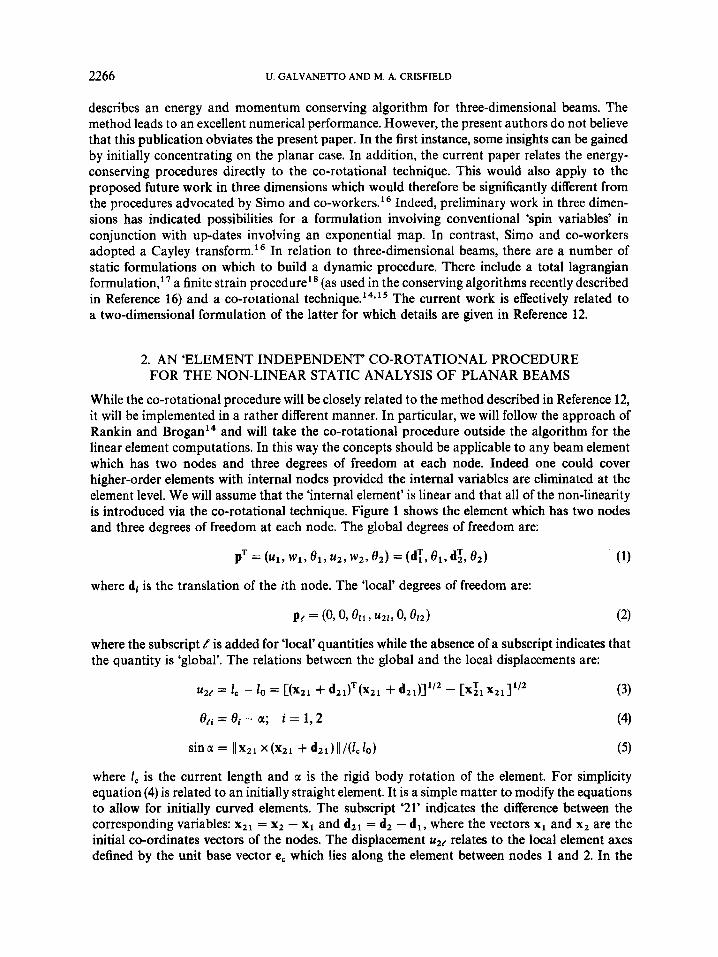
SUMMARY The paper describes an energyconserving procedure for the implicit non-linear dynamic analysis of planar beam structures. The method is based on a form of co-rotational technique which is ‘external to the element’. A range of numerical results are presented which clearly demonstrate the improved numerical performance in comparison with more conventional techniques.

KEY WORDS: energy-conservation; dynamics; beams; co-rotation

1. INTRODUCTION

Various forms of Newmark time-integration procedure’ are often used for the non-linear dynamic analysis of beams. However, both the second author and c o - ~ o r k e r s ~ . ~ and Simo and Tarnow4 have recently highlighted the potential pitfalls which can involve a sudden increase in strain energy, followed by a form of ‘dynamic locking’ in which there is a sharp increase in the higher-frequency strain energy components and a ‘freezing’ of the rotational kinetic energy. An attractive solution involves the introduction of some form of ‘energy conserving time-integration procedure’. Early work in this area is due to Huag et aL6 and Hughes et al.,’ who used Lagrangian multipliers to enforce the energy constraints. More recently, Simo and Tarnow4.’ have adopted a form of ‘mid-point equilibrium’ which follows on from the work of Hilber et a1.* and Zienkiewicz et aL9 Downer et aI.” have described an energy-conserving procedure for beams which involves a form of explicit-implicit staggered time-integration procedure due to Park et a[.” The second author has described an implicit energyconserving technique’.’ that has strong links with the work of Simo and Tarnow4.’ and is closely related to the co-rotational technique12 but was originally restricted to ‘truss elements’. The first steps of an extension to planar beams have been described in Reference 3 and the more recent developments outlined in Reference 13. Full details are given in the present paper which concentrates on the development of an ‘element independent’ co-rotational technique which, in a static context, was proposed by Rankin and Brogan.I4 The work is, at present, limited to planar beams but it is believed that the concepts can be extended to threedimensional beams using, for example, a modification of the static co-rotational formulation described by the second author in Reference 15. Since the original submission of this work, a paper has been published by Simo and co-workers16 which

* FEA Professor

CCC 0029-5981/96/132265-18 0 1996 by John Wiley & Sons, Ltd.

Received 29 July 1994 Revised 21 July 1995

2266 U. GALVANETTO A N D M. A. CRISFIELD

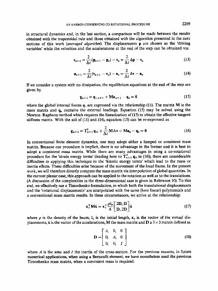
describes an energy and momentum conserving algorithm for three-dimensional beams. The method leads to an excellent numerical performance. However, the present authors do not believe that this publication obviates the present paper. In the first instance, some insights can be gained by initially concentrating on the planar case. In addition, the current paper relates the energy- conserving procedures directly to the co-rotational technique. This would also apply to the proposed future work in three dimensions which would therefore be significantly different from the procedures advocated by Simo and co-workers.’6 Indeed, preliminary work in three dimen- sions has indicated possibilities for a formulation involving conventional ‘spin variables’ in conjunction with up-dates involving an exponential map. In contrast, Simo and co-workers adopted a Cayley transform.16 In relation to three-dimensional beams, there are a number of static formulations on which to build a dynamic procedure. There include a total lagrangian formulation,’ a finite strain procedure” (as used in the conserving algorithms recently described in Reference 16) and a co-rotational technique.14*15 The current work is effectively related to a two-dimensional formulation of the latter for which details are given in Reference 12.

2. AN ‘ELEMENT INDEPENDENT’ CO-ROTATIONAL PROCEDURE FOR THE NON-LINEAR STATIC ANALYSIS OF PLANAR BEAMS

While the co-rotational procedure will be closely related to the method described in Reference 12, it will be implemented in a rather different manner. In particular, we will follow the approach of Rankin and Brogan14 and will take the co-rotational procedure outside the algorithm for the linear element computations. In this way the concepts should be applicable to any beam element which has two nodes and three degrees of freedom at each node. Indeed one could cover higher-order elements with internal nodes provided the internal variables are eliminated at the element level. We will assume that the ‘internal element’ is linear and that all of the non-linearity is introduced via the co-rotational technique. Figure 1 shows the element which has two nodes and three degrees of freedom at each node. The global degrees of freedom are:

where di is the translation of the ith node. The ‘local’ degrees of freedom are:

where the subscript L‘ is added for ‘local’ quantities while the absence of a subscript indicates that the quantity is ‘global’. The relations between the global and the local displacements are:

0 c i = 8 i - u ; i = l , 2 (4)

where I, is the current length and a is the rigid body rotation of the element. For simplicity equation (4) is related to an initially straight element. It is a simple matter to modify the equations to allow for initially curved elements. The subscript ‘21’ indicates the difference between the corresponding variables: x21 = x2 - x1 and dzl = d2 - dl , where the vectors x1 and x2 are the initial co-ordinates vectors of the nodes. The displacement uZr relates to the local element axes defined by the unit base vector e, which lies along the element between nodes 1 and 2. In the

AN ENERGY-CONSERVING CO-ROTATIONAL PROCEDURE

Z

( w,

2267

current configuration

I t i a i configuration

C

P O

1

Figure 1. (a) Two-noded beam element, (b) the local displacement uz I , (c) the local displacement O,,

current configuration e, can be computed from

with the unit vector f,, normal to ec, being defined as

fc = [ - cos sin P c "1 (7)

The variables Oi may be slopes (in the Bernoulli element) or rotations of the normal (in a Timoshenko element).

2268 U. GALVANEIT0 AND M. A. CRISFIELD

Applications of the element-independent procedure consists of the following points:

(1) the local nodal displacements pc are computed from the global nodal displacements p using the relations (3)-(5) while their changes are obtained via:

6pC = T 6 p (8)

where T is the matrix which relates the increments of the local displacements to those of the global displacements and is given by

T =

OT

OT

f: f;f -, 1, - -, 0 1, 1,

- ef, 0, e:, 0 (9)

The matrix T can be derived by differentiation of the relations (3) and (4).

with the standard relationship: (2) The local nodal generalized forces qci are computed from the local nodal displacements

qti = K/ PC (10)

where KC is the standard linear stiffness matrix. For a beam the vector qCi contains the local nodal forces work conjugate to the local displacements pC so that the first two terms consists of the forces in the xC and y, directions (Figure l(a)) at node 1 and the third term is the equivalent local moment.

(3) The global nodal generalized forces can be expressed by means of the corresponding local quantities as follows:

qi = TTq,, = TTK,pc (1 1)

This expression can be derived by equating the virtual work in the local and global systems so that qn6pCv = q’dp,. T

(4) The tangent stiffness equations can be finally written as

6qi = TT6q,i + 6TTqCi = TTKCT6p + Kt,6p (12)

where TT Kc T is usually called the ‘linear’ tangent stiffness matrix and K,, is the ‘geometric’ or ‘initial stress’ matrix.

3. THE STANDARD NEWMARK ALGORITHM

As an introduction to the new method a description is given of the conventional trapezoidal rule (or Newmark algorithm with y = 0-5 and a = 0.25 Reference 1). This algorithm is widely utilized

AN ENERGY-CONSERVING CO-ROTATIONAL PROCEDURE 2269

in structural dynamics and, in the last section, a comparison will be made between the results obtained with the trapezoidal rule and those obtained with the algorithm presented in the next sections of this work (averaged algorithm). The displacements p are chosen as the ‘driving variables’ while the velocities and the accelerations at the end of the step can be obtained via:

2 2 A t A t = - ( v , + ~ -vn) -an=-Av-an

If we consider a system with no dissipation, the equilibrium equations at the end of the step are given by

g n + i = qi,n+l + Man+l - qe = 0 (15)

where the global internal forces qi are expressed via the relationship (11). The matrix M is the mass matrix and qe contains the external loadings. Equation (15) may be solved using the Newton-Raphson method which requires the linearization of (1 5) to obtain the effective tangent stiffness matrix. With the aid of (11) and (14), equation (15) can be re-expressed as

(16) 2

At gn+l = TX+tqci +-MAv -Man - qe = 0

In conventional finite element dynamics, one may adopt either a lumped or consistent mass matrix. Because our procedure is implicit, there is no advantage in the former and it is best to adopt a consistent mass matrix. While there are many advantages in using a co-rotational procedure for the ‘strain energy terms’ (leading here to TT, qci in (16)), there are considerable difficulties in applying this technique to the ‘kinetic energy terms’ which lead to the mass or inertia effects. These difficulties arise because of the movement of the local frame. In the present work, we will therefore directly compute the mass matrix via interpolation of global quantities. In the current planar case, this approach can be applied to the rotation as well as to the translations. (A discussion of the complexities in the three-dimensional case is given in Reference 10). To this end, we effectively use a Timoshenko formulation, in which both the translational displacements and the ‘rotational displacements’ are interpolated with the same (here linear) polynomials and a conventional mass matrix results. In these circumstances, we arrive at the relationship:

xTMX = X, -

where p is the density of the beam, lo is the initial length, x, is the vector of the virtual dis- placements, x is the vector of the accelerations, M the mass matrix and D a 3 x 3 matrix defined as

D = 0, A, 0 in” 1: 11 where A is the area and I the inertia of the cross-section. For the previous reasons, in future numerical applications, when using a Bernoulli element, we have nonetheless used the previous Timoshenko mass matrix, when a consistent mass is required.

2270 U. GALVANETTO AND M. A. CRISFIELD

4. THE AXIAL CONTRIBUTION

For a truss element with only axial deformation, the matrix Tn+ in (16) is a 4 x 4 matrix given by

r oT 1

and the local nodal force vector qri is

f : l so that equation (16) can be re-written as

In a previous paper' an algorithm was introduced for the non-linear dynamics of simple truss elements. Although the method was based on a form of co-rotational procedure, in contrast to the work of Section 2 (which we will follow later), the co-rotational aspects were not divorced from the conventional element formulation. In the time-integration scheme, equation (14) was replaced by

Av A t

a =-

with the end point equilibrium of (21) being replaced by a mid-point equilibrium. That algorithm exactly conserves the energy but requires the introduction of a mid-point configuration charac- terized by the unit vector em (Figure 2) and the corrected normal force N, with:

where P is

The equilibrium equation is given by

where qiSm is the mid-point internal force vector. Following Simo and Tarnow? an attempt was then made3 to introduce an 'averaged' formulation for the truss element which gave rise to

AN ENERGY-CONSERVING CO-ROTATIONAL PROCEDURE 227 1

2

Figure 2. The truss element

a second form of mid-point equilibrium equation in which the internal nodal forces were defined as follows:

It is possible to show that such a formulation coincides with the earlier formulation of (23-26) (see also Reference 3) if the time step tends to zero and works well for moderately small time steps. However, it does not exactly conserve the energy.

The key to energy conservation is to be able to write the total energy change over the increment, A@, in the form:

where A+ is the strain energy change, AK the kinetic energy change and A P the potential energy change. Once the equilibrium iterations have converged so that g, = 0 the change of energy from (28) is bound to be zero. Full details on the energy conservation will be given later but for the present purposes, we note that in order to achieve (28), for a truss element, we must be able to express the strain energy change as

= [ It will be shown that the averaged internal forces q:,, (from (27)) have to be corrected by the introduction of the term 2/( 1 + cos Aa) so that energy can be exactly conserved. In this case the expression for the internal nodal forces becomes

q t m =

2212 U. GALVANETTO AND M. A. CRISFIELD

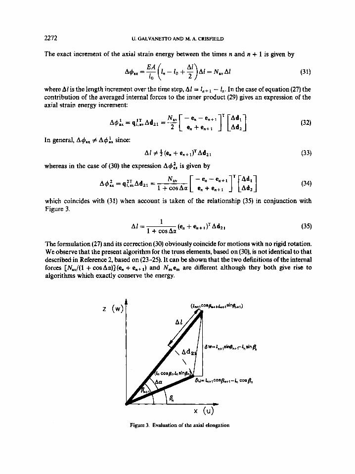
The exact increment of the axial strain energy between the times n .and n + 1 is given by

where A1 is the length increment over the time step, A1 = l,,+ - I,,. In the case of equation (27) the contribution of the averaged internal forces to the inner product (29) gives an expression of the axial strain energy increment:

In general, A4ax # since:

whereas in the case of (30) the expression A4Zx is given by

which coincides with (31) when account is taken of the relationship (35) in conjunction with Figure 3.

The formulation (27) and its correction (30) obviously coincide for motions with no rigid rotation. We observe that the present algorithm for the truss elements, based on (30), is not identical to that described in Reference 2, based on (23-25). It can be shown that the two definitions of the internal forces [N,,/(1 + cos Aa)] (en + en+ and N, em are different although they both give rise to algorithms which exactly conserve the energy.

x (4 Figure 3. Evaluation of the axial elongation

AN ENERGY-CONSERVING CO-ROTATIONAL PROCEDURE 2273

5. THE BENDING CONTRIBUTION

Following the idea developed in the previous section we want to define the bending part of the internal nodal forces so that energy can be conserved. The starting point is still given by an averaged formulation of the following type:

fn f n + 1 fn f n + 1

4 L + l l n I n + , -+-,-+-

[::::;I

where Mi,av = (Mi,, + Mi,,+ 1)/2, i = 1,2 are the averaged nodal moments. Equation (36) can be derived with the aid of (9) and (1 1). The expression of the increment of strain energy due to the bending forces during a time step is given by

A h = M1.av A ~ I + M2.avA62 - (M1,av + M2,av)A~ (37)

If we express the increment of energy as the product between the internal forces and the increment of the displacements we obtain

1 A+: =- 2

The first two terms in equation (37), related to the nodal rotations, have the exact correspondent in equation (38) whereas a correcting coefficient y has to be introduced for the four components of the bending forces in the directions of the translational degrees of freedom. Imposing the equivalence between the last term of equation (37) and the relevant contributions from relation (38), it is possible to provide the following equation:

which is true for rigid rotations without axial extension if we choose:

Aa y=- sin Aa

This definition of y also guarantees the almost exact conservation of the energy as long as the expression [(f,,/In + fn+ Ad2J2] is a good approximation of sin Aa, which is true for small axial deformations. The examples of Section 8 will show that the error associated to this

2274 U. GALVANETTO AND M. A. CRISFIELD

approximation is negligible in the case of motions with small axial deformations. Following the previous developments, the final expression for the mid-point residual forces is given by

Au +- 2 sin Aa

fn f n + l fn f n + l -+-,-+- I n 1n+1 1. 1n+1

0,o

1 A t

+ -MAv - k::] = 0

[:::::I

It is important to stress that the coefficient which multiplies the axial forces allows an exact conservation of the energy whereas the coefficient which multiplies the translational contribu- tions of the bending forces is only exact if A1 0. This limitation is not restrictive in many applications. In equation (41) the e's and f's are two-dimensional vectors, M is a 6 x 6 matrix, A v is a vector with 6 components and qel and qez are three-dimensional vectors.

6. EXTERNALIZING THE CO-ROTATIONAL FORMULATION AND ENERGY CONSERVATION

In this section we will aim to rewrite the equation of equilibrium (41) following the form of Section 2 so that the co-rotational procedure is taken outside the algorithm for the linear element computations and our method can be applied to any beam model with 2 nodes and 3 d.0.f per node. In this way we will point out the changes that have to be introduced in standard co-rotational codes in order to make them energy-conserving.

The averaged nodal internal forces corresponding to the translational degrees of freedom can be expressed as

where T: and T:+ are the transformation matrices introduced in Section 2, at time n and n + 1, respectively, in which the diagonal terms corresponding to the nodal rotations are set to zero. The vectors qLn and qtn+ are the local internal nodal forces at time n and n + 1, respectively. The index 0 in q: indicates that the third and the sixth component in the vector (nodal moments) are zeros. All the quantities in the previous equation (42) are considered standard in that they are

AN ENERGY-CONSERVING CO-ROTATIONAL PROCEDURE 2275

computed at time n or n + 1 in a conventional manner. The corrected definition of the internal nodal forces for the translational degrees of freedom is given via the definition of a corrected averaged transformation matrix:

Tav = D T ~ (43) where D is a diagonal matrix:

Au 2 Aa sinAa’ 1 + COSAU’ *, -) sinAa

In (44) the *’s are not defined because these terms multiply only zeros, The corrected nodal internal forces are

(45)

(46)

which takes into account the rotations at the ends of the beam and the corresponding nodal moments. With the aid of (42H46), the equilibrium equation (41) can be rewritten in the form:

Qm = ( T T v + T I q t a v

diage) = (0, 0, 1, 0, 0, 1)

where 1 is the diagonal matrix:

where [qel, qcz] are the external loads applied to nodes which are constant in order to show that the averaged algorithm conserves energy. The total energy increment over the time step consists of three terms: the strain energy increment, the kinetic energy increment and the potential energy increment. In a conservative system the sum of these three terms has to be zero. For a single element the strain energy increment is given by the relations (34) for the axial energy, and (38) (with the correction of y which multiplies the translational terms) for the bending energy while the kinetic energy increment is

(48) AK = vTV MAv = - AvT MAP

where vav = (v, + v,+ J2. In the case of fixed conservative external forces the potential energy increment is

1 A t

The total energy increment is given by

A@ = A4ax + A& + AK + A P = gzr Ap

When the numerical integration reaches convergence, so that g z system is conserved (if the axial strain is small).

0, the total energy of the

7. THE CONSISTENT TANGENT STIFFNESS MATRIX

The solution of the numerical problem requires the definition of the variation of the corrected nodal internal forces given in (45):

(51) S q m = ( T T v + T)sqc,av + S(T;f, + ‘i)qt,av

2276 U. GALVANETTO AND M. A. CRISFIELD

The second term on the r.h.s. of equation (51) can be developed in the following way:

6(TTV +I) = sT;f, = GT::D + T::~D (52)

The three terms to be computed which appear in the equations (51) and (52) are: (r;fv + I)6qC,av, 6Tt:D and Tt:,TD. Following equation (12) the contribution of the first term, which can be considered the initial tangent stiffness matrix, is immediately obtained as

K 1 = f ( T r v +T)KtTn+l (53)

Obviously Kl is not symmetric and consequently the global stiffness matrix will be non-symmet- ric. It should be emphasized that this non-symmetry is not a consequence of the co-rotational formulation but rather of the adopted energy-conserving form of 'mid-point equilibrium'. Such non-symmetric terms have also been observed by Simo and co-workers.16 When the current planar co-rotational procedure is applied to an end-point equilibrium in conjunction with the Newmark trapezoidal rule, a fully symmetric tangent stiffness matrix is obtained.

To derive the contribution to the stiffness matrix of the second term we require:

The term 6Tn+ is required in a conventional static co-rotational formulation" and follows from the variation of the T matrix of (9). For completness we re-detail the steps here. The following quantities are required:

din+ 1 = e;T+ 1 SdZl (57)

- 1 6f,+l en+lfT+l + F f n + l e : + l ) N z l 1 (58)

n + 1

(for simplicity's sake in the present section our notation changes in the following way: Aa -a, 6(Aa)=.6a, 6(AdZ1)=Z6dz1, . .) It is now possible to write the second contribution to the consistent stiffness matrix (from 6T:: Dq,.,,)

K z = [ A, - "1 -A , A

where A is a 3 x 3 matrix given by

(59)

AN ENERGY-CONSERVING CO-ROTATIONAL PROCEDURE 2277

The third term of the stiffness matrix, which involves 6D (see (44)), requires the following algebraic manipulations:

sin a - a cos a sina-acosa 1 6a = - fX+16d21 6 (2) = sin2 a sin’u I , , ,

sin a sina 1 6 ( )= 6u = - f;f+ i 8dzi 1 + cosa (1 + cosa)? (1 + cosa)’ l n + l

We are now able to express the terms of the stiffness matrix which come from the linearization of the diagonal matrix D multiplied by T:,? and by the averaged internal forces, as

sina - acosa Ma,,l + sin2 a K31 =

sina & r , - C ] (1 + cosa)2 - C, C K32 =

where B and C are three by three matrices given by [ - ~ + 3 f X + 1 , 0 ]

OT, 0 B =

Finally, the consistent stiffness matrix is given by

8. EXAMPLES

In this section we present some examples which illustrates the main features of the new integration algorithm for the non-iinear dynamics of planar beams. In some cases, a comparison will be drawn with the Newmark integration to highlight the improvements of the new method.

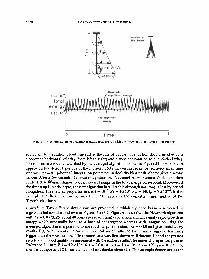
Example 1: The first example, defined in Figure 4, shows the free oscillations of a cantilever beam. The physical properties of the beam are: EA = 2-1 x lo9 (axial stiffness), EZ = 1.75 x lo6 (bending stiffness), A p = 75 (linear density). The mesh is composed to four Bernoulli elements with lumped mass matrix. The initial conditions are given in the figure. The time step of 0.001 is a good approximation of the maximum time step for which the Newmark integration converges as can be seen by the wide variations of the energy numerically computed. In contrast the averaged algorithm gives a constant energy, as it should for a system with no damping and with only gravitational loads. Moreover, the averaged integration procedure converges with much bigger time steps, which can be up to 003.

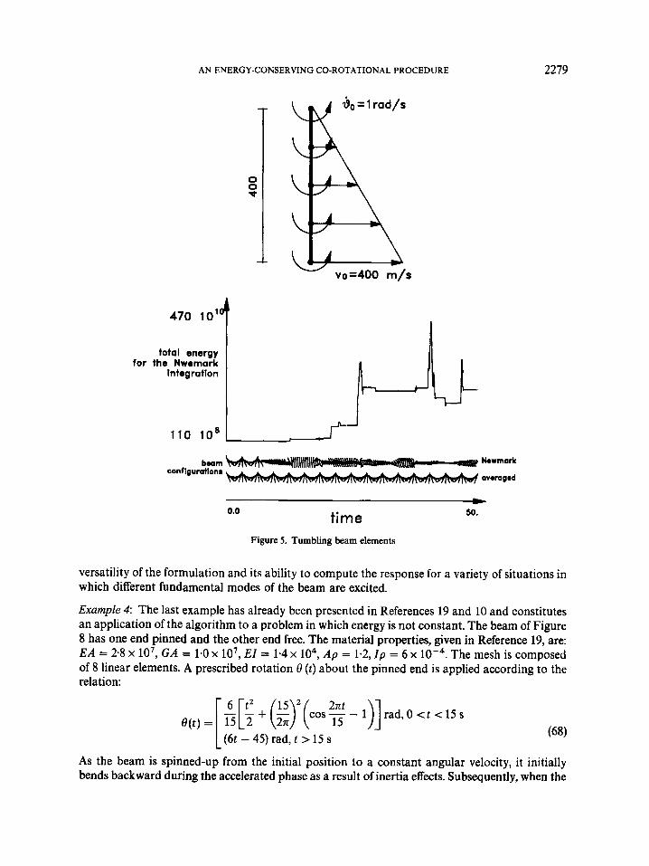
Example 2: The second example is similar to the four chain system example of Reference 2 with the difference that in the present case the four elements are Bernoulli beams instead of trusses. The beam (see Figure 5 ) is free to fly into absence of gravity and initially has no velocity in the y direction, a linear distribution of horizontal velocities and a uniform rotational velocity which is

2278 U. GALVANETTO AND M. A. CRISFIELD

motion of tho beam

new olgorlthm energy

I

5 0 time

Figure 4. Free oscillations of a cantilever beam, total energy with the Newmark and averaged integrations

equivalent to a rotation about one end at the rate of 1 rad/s. The motion should involve both a constant horizontal velocity (from left to right) and a constant rotation rate (anti-clockwise). The motion is correctly described by the averaged algorithm, in fact in Figure 5 it is possible to approximately detect 8 periods of the motion in 50 s. In contrast even for relatively small time step with A t = 0.1 (about 63 integration points per period) the Newmark scheme gives a wrong answer. After a few seconds of correct integration the 'Newmark beam' becomes folded and then contorted in different shapes to which several jumps in the total energy correspond. Moreover, if the time step is made larger, the new algorithm is still stable although accuracy is lost by period elongation. The material properties are: EA = lo'', EI = 1-5 lo6, A p = 1.0, I p = 7-5 lop6. In this example and in the following ones the mass matrix is the consistent mass matrix of the Timoshenko beam.

Example 3: Two different simulations are presented in which a pinned beam is subjected to a given initial impulse as shown in Figures 6 and 7. Figure 6 shows that the Newmark algorithm with A t = 0.0378125 (about 40 points per revolution) experiences an increasingly rapid growth in energy which eventually leads to a lack of convergence whereas with integration using the averaged algorithm it is possible to use much larger time steps (At = 0.15) and gives satisfactory results. Figure 7 presents the same mechanical system affected by an initial impulse ten times bigger than the previous one. This second case was first shown in Reference 10 and the present results are in good qualitative agreement with the earlier results. The material properties, given in Reference 10, are: EA = 4.0 x lo7, G A = 2-0 x lo7, E l = 1.3 x lo', A p = 0.98, I p = 0.033. The mesh is composed of 8 linear elements (Timoshenko elements). This example demonstrates the

AN ENERGY-CONSERVING CO-ROTATIONAL PROCEDURE

total energy for the Nwernark

fntegration

110 l o 8

2279

I

I

P t-

r

470 10’ 4

beam ~ l l l l l l l l l l Nowmark

avemgod conftgumtlons

0.0 time -

50.

Figure 5. Tumbling beam elements

versatility of the formulation and its ability to compute the response for a variety of situations in which different fundamental modes of the beam are excited.

Example 4: The last example has already been presented in References 19 and 10 and constitutes an application of the algorithm to a problem in which energy is not constant. The beam of Figure 8 has one end pinned and the other end free. The material properties, given in Reference 19, are: EA = 2.8 x lo7, G A = 1.0 x lo’, EZ = 1.4 x lo4, Ap = 1.2, Zp = 6 x The mesh is composed of 8 linear elements. A prescribed rotation 0 (t) about the pinned end is applied according to the relation:

O ( t ) = [“[I’ 15 2 + ( ~ ~ ( c o s ~ - l)] rad,0 < t 4 5 s

1 (6t - 45) rad, t > 15 s

As the beam is spinned-up from the initial position to a constant angular velocity, it initially bends backward during the accelerated phase as a result of inertia effects. Subsequently, when the

2280 U. GALVANETTO AND M. A. CRISFIELD

Figure 6. Rotating beam with a ‘small’ initial impulse

600 unlh/aoc

.~ 200.

x i 0’ 1 4

12

10

8

‘1 drain enemy 2

0 0 9,s

Figure 7. Rotating beam with a ‘large’ initial impulse

AN ENERGY-CONSERVING CO-ROTATIONAL PROCEDURE 2281

e6.0 W.6

b7.0

5.0 c

CXs.8

2.6

1.4

- -

points of A S f m o h vu-ouoc

-

0.0 time 30.0

0.0 time 30.0

Figure 8. Driven rotation of a beam

angular velocity reaches a constant value of 6 rad/s, the centrifugal force tends to straighten the beam. During this steady-state phase, the beam undergoes a small vibration about its nominal position. Several deformed configurations of the beam and time histories of the tip displacements relative to the rotating frame are given in Figure 8. There is an excellent agreement with the results of the previous researchers even if the adopted time step is 0-05, which is ten times larger than that used in Reference 19.

9. CONCLUSIONS

The paper has described the development of an energy-conserving time-integration procedure for planar beams which is based around a co-rotational technique that is external to the conventional linear finite element computations. Using this approach, it has been possible to introduce the procedure using relatively few alterations and additions to existing computer coding. The numerical examples have highlighted the major benefits that result. In contrast to more conven- tional Newmark-based procedures, it is now possible to use large time-steps without introducing the ‘dynamic locking’ that can plague these techniques. The work has paved the way for future procedures aimed at co-rotational formulations for three-dimensional beams and shells. While the three-dimensional case is certainly far more complex, preliminary results indicate that such

2282 U. GALVANETTO AND M. A. CRISFIELD

a formulation can nonetheless be based on the extension of the ideas described in this paper for the planar case.

REFERENCES

1. N. M. Newmark, ‘A method of computation for structural dynamics’, J. Eng. Mech. Div. ASCE, EM3, 85, 67-94 (1959).

2. M. A. Crisfield and J. Shi, ‘A co-rotational element/time-integration strategy for non-linear dynamics’, Int. j. nmer . methods eng., 37, 1897-1913 (1994).

3. M. A. Crisfield and J. Shi, ‘An energy conserving co-rotational procedure for non-linear dynamics with finite elements’, in M. S . Perera et al. (eds.), Proc. N A T O Advanced Study Inst. on Computer Aided Analysis of Rigid and Flexible Mechanical Systems, Vol. 11, IDMEC, Troia, Portugal, July 1993, pp. 197-214 (and Nonlinear D y n m k s , 9,

4. J. C. Simo and N. Tarnow, ‘The discrete energy-momentum method. Conserving algorithms for nonlinear elas- todynamics’, Z. angnew Math. Phys., 43,757-792 (1992).

5. J. C. Simo and N. Tarnow, ‘A new energy and momentum conserving algorithm for the non-linear dynamics of shells’, Int. j. numer. methods eng., 37,2527-2549 (1994).

6. E. Haug, 0. S. Nguyen and A. L. De Rouvray, ‘An improved energy conserving implicit time integration algorithm for nonlinear dynamics structural analysis’, Proc. 4th Int. Con$ on Struct. Mech. in Reactor Tech., San Francisco, Aug. 1977.

7. T. J. R. Hughes, W. K. Liu and P. Caughy, ‘Transient finite element formulations that preserve energy’, J. Appl. Mech.,

8 . H. M. Hilber, T. J. R. Hughes and R. L. Taylor, ‘Improved numerical dissipation for time integration algorithms’, Int.

9. 0. C. Zienkiewicz, W. L. Wood and R. L. Taylor, ‘An alternative single-step algorithm for dynamic problems’,

10. J. D. Downer, K. C. Park and J. C. Chiou, ‘Dynamics of flexible beams for multibody systems: a computational

11. K. C. Park, J. C. Chiou and J. D. Downer, ‘Explicit-implicit staggered procedure for multibody dynamics’, J.

12. M. A. Crisfield, Non-linear Finite Element Analysis of Solids and Structures, Vol. 1, Wiley, New York, 1991. 13. M. A. Crisfield, G. F. Moita and U. Galvanetto, ‘Some unconventional applications of the co-rotational techniques to

continua and dynamics’, Con$ honoring Professor R. L. Taylor, Palo Alto, California, Sept. 19-21, 1994. 14. C. C. Rankin and F. A. Brogan, ‘An element independent corotational procedure for the treatment of large rotation’,

ASME J. Pressure Vessel Technol. 108, 165-174 (1986). 15. M. A. Crisfield, ‘A consistent co-rotational formulation for non-linear, three-dimensional, beam-elements’, Comput.

Methods Appl. Mech. Eng., 81, 131-150 (1990). 16. J. C. Simo, N. Tarnow and M. Doblare, ‘Non-linear dynamics, of three-dimensional rods: exact energy and

momentum conserving algorithms’, Int. j. numer. methods eng., 38, 1431-1473 (1995). 17. L. Crivelli and C. A. Felippa, ‘A three-dimensional non-linear Timoshenko beam element based on the core-

congruential formulation’, Int. j . numer. methods eng., 36, 3647-3673 (1993). 18. J. C. Simo and L. Vu-Quoc, ‘A three-dimensional finite strain model. Part 11: Computational aspects’, Comput

Methods Appl. Mech. Eng., 58, 79-116 (1986). 19. J. C. Simo and L. Vu-Quoc, ‘On the dynamics in space of rods undergoing large motions-a geometrically exact

approach’, Comput Methods Appl. Mech. Eng., 66, 125-161 (1988).

37-52 (1996)).

45, 366-370 (1978).

j . earthquake eng. struct. dyn., 5,283-292 (1977).

J . earthquake eng. struct. dyn., 8, 3 1 4 0 (1980).

procedure’, Comput. Methods Appl. Mech. Eng., 96, 373408 (1992).

Guidance, 13, 562-570 (1990).