1

An empirical study of the Chinese short-term interest rate:

A comparison of the predictive power of rival one-factor models

Hai Yan Xu Bert D. Ward

Gilbert Nartea

[Presented by H.Y. Xu at the New Zealand Econometrics Study Group conference, University of

Otago, Dunedin, August 2006]

Abstract:

This paper uses the one-factor models proposed by Chan, Karolyi, Longstaff and Sanders (CKLS,

1992) to study the short-term interest rate in China. Eight stochastic models of the short-term

interest rate were estimated with Generalised Method of Moments (GMM). All models examined

allow the conditional mean and conditional variance to be functions of the current short-term

interest rate. For the Chinese one-month inter bank loan rate, the research finds strong evidence

for a mean-reverting feature in the short-term interest yield curve, but no evidence was found to

indicate that the volatility is highly positively correlated with the level of interest rates. What is

more, evidence was found that the CKLS model, the CIR SR model, and the Brennan-Schwartz

model are correctly specified to model the Chinese short rate, so that these three models are able

to sufficiently capture the dynamics of the Chinese short rates. Finally, Theil’s U2 statistics and

the Diebold and Mariano test (DM test) were applied to explicitly evaluate the predictive power of

the single factor models. For China’s short-term interest rate the research found that all the one-

factor models have similar forecasting ability in terms of predicting China’s short rate.

JEL Classification: C52; E43

Key words: single -factor models, mean reversion, GMM estimation, prediction tests

All authors are affiliated with the Economics and Finance Group, Lincoln University. The

author for correspondence is BD Ward, Snr Lecturer in Economics, wardb@lincoln.ac.nz.

2

1. Introduction

The short-term interest rate plays a vital role in many financial areas and it has strong implications for

the pricing of fixed income securities and interest rate derivatives, such as bond pricing models,

derivative security pricing models etc. What is more, it also has been used in general asset pricing

(John, 2001) and as an input in macroeconomic models, e.g. in the analysis of the business cycle. It is

also an important target instrument for monetary authorities in implementing monetary policy and a

key indicator monitored by financial institutions in pricing floating rate loans. In addition, valuation of

more exotic interest rate derivatives such as American style swap options, callable bonds and

structured notes rely on term structure models, some of which can be constructed by specifying the

behaviour of short-term interest rates. Therefore, modelling of interest rate dynamics has become a

very hot topic for many researchers to work on in this field. As a result, many term structure models

have developed to estimate the short-term interest rate dynamics in recent years. The spot rate term

structure modelling approach assumes that spot interest rates are sufficient statistics for the stochastic

movement of current term structure, so that the price of bonds and interest rate derivatives securities

can be derived in terms of the spot rate. In general, the term structure models can be broadly

categorized into three groups (Litterman and Scheinkman, 1991).

The first group contains the single factor models proposed by Chan, Karolyi, Longstaff and Sanders

(CKLS 1992). The model provides a simple description of the stochastic nature of interest rates that is

consistent with the empirical observation that interest rates tend to be mean-reverting. The one factor

models have been widely used in practice due to their tractability and their ability to fit the dynamics

of the short term interest rates reasonably well. Group 2 is made up of the two-factor models which

aim to better capture the rich yield curve structure by invoking another source of randomness.

Longstaff and Schwartz (1992) and Chen and Scott (1992) developed continuous-time two-factor

models along the line of CIR (Cox, Ingersoll and Ross, 1985) that can incorporate random volatility in

the evolution for the short rate and offer an analytical solution for bonds and other interest rate

derivatives. What is more, Brenner et al (1996) showed that interest rate models that include both a

level effect (where the interest rate volatility is a function of its level) and a Generalized

Autoregressive Conditional Heteroscedasticity (GARCH) specification outperform those models that

exclude these features. Models in group 3 consist of the three-factor models developed recently by

researchers to study the behaviour of short-term interest rates. For instance, Litterman and

Scheinkman (1991) argued that at least three factors are needed to fully capture the variability of

interest rates. In another important study, Chen (1996) developed a three-factor model and showed that

the three-factor model can be merged into the Heath, Jarrow and Morton (HJM, 1992) framework.

However, although the three-factor models can be made to better fit the term-structure of interest rates,

they are generally more difficult to apply. This is principally due to the fact that the underlying state

3

variables of the HJM models are un-observable quantities, and the dynamics are usually non-

Markovian and non-linear in their (latent) state variables (HJM, 1992).

Obviously, the more advanced models such as multifactor models and HJM models have the advantage of

modelling the reality more precisely, but they may suffer from complications, even impossibility, in

implementation. In contrast, single-factor models constitute a relatively simple class of models where the

whole term structure is driven by a single state variable, the short-term interest rate. Thus, in current

literature it contains many papers using one factor models to study short term interest rates. For example ,

Chan et al. (1992) studied U.S short rates, Treepongkaruna and Gray (2002) applied one factor models to

estimate short rates for eight major countries, Tse (1995) and Dahlquist (1996) extended the analysis of

CKLS to international short-term interest rates, Murphy (1995) studied UK short term interest rates, and the

New Zealand short-term interest rate was studied by Treerongkaruna (2003). However, a literature search

revealed that there are few papers studying China short term interest rates. For example, Xie and Wu (2002)

empirically tested the Vasicek model and the CIR model by the one-month inter-bank interest rate, while

Fan and Fang (2002) empirically analyzed the pricing of convertible bonds in China. In another study,

Zheng and Lin (2003) estimated the term structure, liquidity premium and credit risk premium in China’s

bond market, but the models were all static approximations and did not test the dynamic behaviour of the

interest rate in China.

Since accurate interest rate forecasts are crucial for savings and investment decisions as well as for

macroeconomic and monetary policy decisions, another aim of this paper is to explicitly show the

predictive power among the one factor models. In current literature it shows that many researchers use

the Nelson-Siegel (1987) exponential components framework to distill the entire yield curve, period

by period. A number of authors have explored the model’s performance in out-of-sample yield curve

forecasting by re-interpreting the Nelson–Siegel yield curve as a modern three-factor dynamic model

of level, slope and curvature. Other researchers have proposed extensions to Nelson-Siegel to enhance

flexibility, including Bliss (1997b), Soderlind and Svensson (1997), Bjork and Christensen (1999),

Filipovic (1999, 2000), Bjork (2000), and Bjork and Landen (2000). In particular, they showed that

forecasts appear much more accurate at long horizons than various standard benchmark forecasts.

However, China was using a centrally planned economic policy and China’s interest rate was thus

controlled by the government. Thus, in the past literature it is hard to find a paper that compares the

predictive power of single factor models for Chinese short rates.

This paper is designed to empirically study China’s short-term yield curve and test if the one factor

models have the ability to capture the dynamic nature of the short term interest rate for China.

Moreover, this study focuses on the comparison of the predictive power of the rival one-factor term

structure models for the Chinese short-term interest rates. If the single factor models analysed in

4

CKLS (1992) are able to characterize the behaviour of China’s short-term interest rate, we would

compare the predictive power of the single factor models. We carried out an empirical study based on

one-month Chinese inter bank loan rates over the past two years. In order to achieve this objective,

this paper has applied the generalized method of moments (GMM) for estimation of the one factor

models and for the forecasting test, Theil’s U2 statistics and the Diebold and Mariano forecasting test

(DM) are also used.

The remainder of this paper is structured as follows. Section 2 presents an overview of China’s

economy. Following that, Section 3 discusses methodological approach and describes the data set used

for the empirical analysis. The fourth section presents the results of the study, and Section 5 concludes

with a discussion of these results.

2. Overview of the Chinese economy

In late 1978 the Chinese leadership began moving the economy from a sluggish, inefficient, Soviet-

style centrally planned economy to a more market-oriented system. Since shifting to an open-door and

reform policy in the late 1970s, China has entered a period of high economic growth. Because of the

rapid economic growth, China has emerged as a potential economic powerhouse in the Asia -Pacific

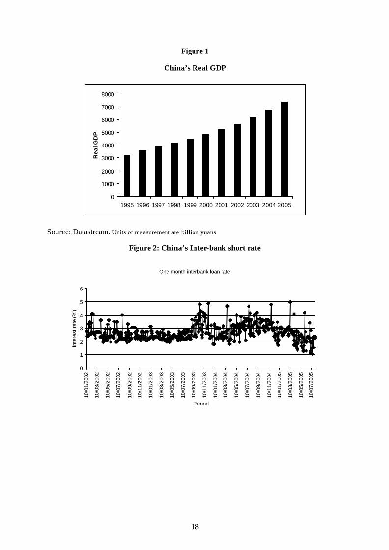
region. Figure 1 shows the Chinese real gross domestic product (GDP) in the last 10 years.

[Figure 1 about here]

From Figure 1 it can be seen that real GDP grew continuously at a fast pace. The real GDP in 2005 is

more than twice its size in 1995. However, we can hardly lose sight of the fact that the growth in net

exports is the main force driving the Chinese economy’s growth. Undoubtedly, China’s comparative

advantage lies in its abundant cheap labour supply. Therefore, China’s industrialization increases the

supply of labour-intensive goods to international markets while raising the demand for capital and

technology-intensive goods, leading to a decline in the prices. In some ways the pegged exchange rate

can lead to growth in net exports, but a pegged exchange rate policy is not appropriate for a major

economy in the global system such as China (Laurenceson and Qin 2005). Therefore, recently China

started switching from the pegged exchange rate to a more flexible exchange rate regime. However,

under interest rate parity conditions (CIP and UIP), it can be seen that the exchange rate is closely

related to the interest rate (Copeland, 2005). For example if the interest rate in China is high, making

the earning in interest rate differential much larger in absolute value than the loss in foreign exchange,

arbitrage will appear. Then large amount of funds would flow from foreign countries into China,

putting pressure on China to lower its interest rate. Therefore, the dynamic behaviour of China’s short

term interest rate is very critical in terms of real GDP growth and the exchange rate. Even though

exchange rate policy for China is still an open question, this study will leave this problem and focus on

studying the short term interest rate in China.

5

By the nature of the Chinese market, we have to employ China’s inter-bank loan rate as an

approximation of a risk free rate. In recent years the overall trend for the Chinese one month inter-

bank loan rate is not very volatile , ranging from a minimum of about 1% to a maximum of

approximately 5% as shown in Figure 2.

[Figure 2 about here]

Figure 2 shows that during 2002 the interest rate was relatively low, being just above 2%. Since then,

however, the interest rate has started climbing and eventually in 2005 the interest rate reached its

highest point, which is approximately 5%. Thereafter, the interest rate started falling in later 2005.

Moreover, the material in Figure 2 suggests that increases in the Chinese one month interbank loan

rate tend to be followed by decreases in the rate. Conversely, when they drop, they tend to be followed

by rate increases. In other words, from the figure it can be seen that there is neither a down sloping

trend nor an up sloping trend. Instead, the interest rate seems to wander around a value of about 2.5%.

Therefore, the long run tendency of the one month interbank loan rate is to revert to a ‘normal rate’.

From the above discussion we have strong reasons to believe that mean reversion is an important

feature for the Chinese short-term interest rate. In the later stage of our analysis the statistical

description of the data will not only be discussed in detail, but the mean reverting feature of the data

will also be explicitly shown by using the econometric approach.

3. Data and Methodology:

In China, the interest rate is regulated and decided by the central bank (People’s Bank of China)

without any daily change. Since there have been absolute changes in the policies before and after

1980, we neglect the short-term interest rate before 1980 and utilize the data after 2001 to estimate the

short-term interest rate (since it is the best data set we can obtain). In the research, the 1-month China

inter-bank loan rate is used as a proxy for the short-term rate for the Chinese market. Since the best

choice for modelling short rate is to use risk free rate, many researchers use T-bill rate as a proxy for

the short-term interest. However, owing to the nature of China’s financial market, the one-month

interbank loan rate is the best data we can obtain for the Chinese market. The data are obtained from

the DataStream and are retrieved daily from 10 January 2002 to 29 July 2005. In total there are 927

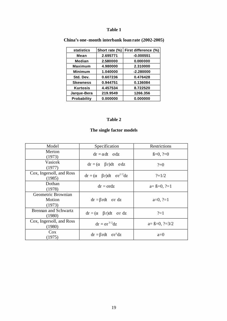
observations, the main features of which are shown in Table 1.

[Table 1 about here]

Table 1 presents descriptive statistics for the actual level of the interest rate and its first difference.

From the table it can be seen that China’s short term interest rate has not been very volatile in last two

years, and the both statistics suggest that there is strong mean reverting feature for Chinese short term

interest rates. Moreover, the Jarque-Bera test suggests non-normality due to excess kurtosis in the

distributions.

6

In this paper we focus on modelling China’s short term interest rates by applying one factor models.

The single factor models for modelling short term interest rates assume that the only factor driving the

term structure of interest rate is the short rate itself. In the models the short rate is assumed to follow a

diffusion (a continuous time stochastic) process. CKLS (1992) proposed the following generalized

diffusion model for short-term interest rates that allows for mean-reversion:

dr ( r)dt r dzγ= α + β + σ (1)

In this model r is the short-term interest rate and z is a geometric Brownian motion process. What is

more, the parameters ,α σ and γ are assumed to be non-negative. Therefore, both drift, rα + β , and

the conditional variance of the interest rate process, 2 2r γσ , depend upon the level of the interest rate.

The parameter of β captures the speed of the adjustment while α is the product of the speed of

adjustment and the long-run mean.

In order to estimate the parameters of the continuous-time model in equation (1), it is convenient to

use a discrete-time econometric specification, which is shown below.

t 1 t t t 1r r r+ +− = α + β + ε (2a)

t 1E[ ] 0,+ε = 2 2 2t 1 tE[ ] r γ+ε = σ (2b)

This discrete-time model has the advantage of allowing the variance of interest rate changes to depend

directly on the level of the interest rate in a way consistent with the continuous-time model. From

equation (2a) we can also see the mean-reverting feature such as the β has been negative. In other

words, the more negative the value of β , the faster r responds to the deviations.

As we know the stochastic differential equation given in (1) defines a broad class of interest rate

processes, which includes many well-known interest rate models. These models can be obtained from

equation (1) by simply placing the appropriate restrictions on the four parameters , , andα β σ γ . In this

section we concentrate on the eight different specifications of the dynamics of the short-term riskless

rate that have appeared in the literature, which are given below:

[Table 2 about here]

In Table 2, these eight specifications and the corresponding parameter restrictions are summarized.

From the table it can be seen that Model 2 is used in Merton (1973), which is just simple Brownian

motion with drift for short-term interest rate. The model of Vasicek (1977) is the Ornstein-Uhlenbeck

process which reflects an elastic random walk. This Gaussian process has been used widely by

7

researchers and practitioners in valuing bond options, futures, future options and other types of

contingent claims, such as Jamshidain (1989) and Gibson and Schwartz (1990). Both of these models

are assuming that the conditional volatility of changes in the riskless rate is constant. The model of

Cox, Ingersoll and Ross (1985) is frequently referred to as the square-root process, which restricts γ to

0.5 thereby imposing a linear relationship between the instantaneous variance and the level of the

interest rate.

The fourth specification of the single -factor model is used by Dothan (1978) in valuing discount bonds

and has also been used by Brennan and Schwartz (1980) in developing numerical models of savings,

retractable and callable bonds. The Geometric Brownian Motion (GBM) was used by Black and

Scholes (1973) to derive the prices of options, which was referred to as the implied volatility of the

option. All three of these models imply that the conditional volatility of changes in the riskless rate is

proportional to 2γ .

The CIR VR model was introduced by CIR (1980) in their study of variable -rate (VR) securities. The

CIR VR model allows a non-linear relationship between the instantaneous variance and the level of

the interest rate but has no mean reversion features. The last model shown in Table 2 is the constant

elasticity of variance (CEV) process introduced by Cox (1975), which does not impose restrictions on

the variance but restricts the mean reversion term.

This research uses the Generalised Methods of Moments (GMM) estimator, a Likelihood ratio type

test and misspecification tests to empirically analyse the one-factor models. The GMM procedure of

Hansen (1982) is used to estimate the parameters of all the models under consideration. As the

technical details of the GMM method can be found in Hansen (1988) and any advanced econometrics

textbook, we merely provide an intuitive summary of its main features here.

GMM is closely related to the classical method of moments and instrumental variables estimation. The

classical method of moments uses moment restrictions to estimate model parameters, where these

restrictions can be written as population moments whose expectation is zero when evaluated at the true

parameter values. One of the key concepts behind GMM is that there is a set of moment conditions

involving the parameter vector in such a way that the expected value of conditions involving the

parameter vector is zero. In instrumental variable estimation, the key idea is to find a set of

instruments that is correlated with the regressors but uncorrelated with the error terms. In other words,

the instrument vector must be orthogonal to the errors. Instrumental variable estimation can be cast in

a GMM framework where the momentum conditions are given by the requirement that the instrument

vector be orthogonal to the errors. This technique has a number of important advantages that make it

8

an ideal choice for the estimation of the continuous-time interest rate process. For example, the GMM

approach does not require that the distribution of interest rate changes be normal and the asymptotic

justification for the GMM procedure requires only that the distribution of interest rate changes both be

stationary and ergodic and that the relevant expectations exist. Because of this, the GMM approach

has been used by a number of researchers for studying interest rate models, for example Chan et al.

(1992), Vetzal (1997) and so on.

To consider the unrestricted case of the interest rate process (1), we need to estimate the parameter

vector ( , , , )θ = α β σ γ .

Firstly we set t 1 t 1 tr (1 )r+ +ε = − α − + β . Thus, let the vector tf ( )θ be

t 1

t 1 tt 2 2 2

t 1 t

2 2 2t 1 t t

rf ( )

r

( r )r

+

+

γ+

γ+

ε ε θ = ε − σ

ε − σ

(3)

If the restrictions implied by (2a) and (2b) are true, then E(f( )) 0.θ = The GMM procedure consists

of replacing E(f( ))θ with its sample counterpart

t T

T tt 1

1g ( ) f ( )

T

=

=

θ = θ∑

and then choosing parameter estimates to minimize the quadratic form

J( ) g'( )W( )g( )θ = θ θ θ

where 1W( ) S ( )−θ = θ and 't tS( ) E(f ( )f ( ))θ = θ θ

W( )θ is a positive semi-definite weighting matrix. For the unrestricted model, the parameters are just

identified and J( )θ attains zero for all choice of W( )θ .

In testing restrictions for single factor models the Likelihood ratio like tests to evaluate the restrictions

imposed by various models on the unrestricted models. The hypothesis-testing methods were

developed by Newey and West (1987), and the test sta tistic is ˆR n[q( ) q( )]= θ − θ ,

where q( )θ is the restricted model’s objective function value and ˆq( )θ is the unrestricted model’s

objective function value. The value of the LR-type test is the difference in the J statistics between the

restricted model and unrestricted model. The J test is discussed in a later section.

9

. Under the null-hypothesis test the test statistic of R is asymptotically distributed 2kχ where the

degrees of freedom parameter (k) is equal to the number of restrictions under the hypothesis test.

For testing misspecification the paper applies the J-test developed in Hansen (1982). The over-

identifying test statistic is shown below:

' 1T T 0 T

ˆ ˆJ ( ) Tg ( ) S g ( )−θ = θ θ

If the model is correctly specified this statistic is asymptotically 2χ distributed with degrees of

freedom equal to m-k, where m is number of moments and k is number of unknown parameters.

4. Empirical Results

4.1 GMM estimation results

In order to estimate the one factor interest rate models the paper applies the GMM. The estimation

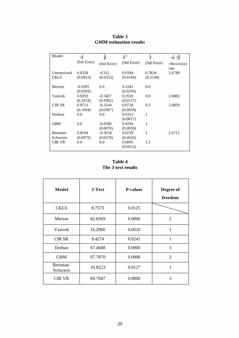
results displayed in Table 3.were obtained using RATS econometric software.

[Table 3 about here]

From the table it can be seen that with exception of the Merton model, GMM estimates of α in the

CKLS model, the Vasicek model, the CIR SR model, and the Brennan-Schwartz model not only

satisfy the positive requirement, but they are also statistically significantly greater than zero at 5%.

Table 3 also reports that in all the models GMM estimates of β not only satisfy the negativity

constraint, but also they are statistically significantly different from zero at 5% significance level.

Furthermore (with the exception of the GBM model) the CKLS model, the Vasicek model, the CIR SR

model and the Brennan-Schwartz model all show that the estimated coefficient of β is around 0.3.

Since β is the speed of adjustment to the long run mean of /−α β , it indicates that China’s one month

inter bank loan rate has been quickly pulled back towards its long-run mean in the past two years.

Finally, the negative sign of β suggests that there is a strong evidence of the mean reverting feature in

China’s one month inter bank loan rate. According to the estimation result, we find that the CKLS

model indicates the implied long mean of the short rate is 2.6788%, the Vasicek model shows a long

run mean of 2.6882%, the CIR SR model shows a long run mean of 2.6859%, and the Brennan-

Schwartz model shows a long run mean of 2.6711%. Therefore, in the last two years the implied long

run mean of China’s inter bank loan rate is approximately 2.68%. The implied long run means, ˆˆ /−α β ,

correspond closely to the unconditional mean reported in Table 1. Results for the CEV model are not

included because they were numerically meaningless - for example, the estimated variance of the

CEV model is equal to -47.2822, which does not make any sense.

10

Table 3 also reports the GMM estimates of the diffusion function, which are statistically significantly

different from zero at 5% significance level in all models. The diffusion function is constant for the

Merton model and the Vasicek model, linear for the CIR SR model and non-linear for the rest of the

models. According to Table 3 it can be seen that the estimate of volatility 2ˆ( )σ from the Merton

model is larger than for the rest of the models. In contrast, the CIR VR model shows the smallest

estimation result in volatility. Chan et. al (1992) used the CKLS model to estimate the 30 days U.S T-

bills, and they found that models that allowed the volatility of short interest rates to highly depend

upon the level of interest rate captured the dynamic behaviour of short-term interest rate more

successfully. For the case of China’s one month inter bank loan rate, we find that the value of

γ = 0.7834 in the unrestricted CKLS model, which is not very high. Nevertheless, this value is

statistically significantly different from zero at 5% significance level in the model. In other words, we

do not reject non-linearity in the diffusion for the CKLS model, providing strong evidence to support

non-linearity in the diffusion process. The positive sign of γ indicates that interest rate volatility is

positively correlated with the level of interest rates However, the small size of γ suggests that this

relationship is not nearly as strong as for the USA or the UK, where the coefficient had values around

1.5.

4.2 Testing the rival models:

The previous section discusses mean reverting features and diffusion terms in the rival one factor

models. This section will not only perform the J-test to detect the goodness-of-fit of the models, but

also apply Likelihood ratio type tests to the nested models.

The hypotheses for the misspecification test are as the follows:

0H :Moments are correctly specified vs aH : Moments are misspecified.

[Table 4 about here]

According to the Table 4, it can be seen that five models (Merton, Vasicek, Dothan, GBM, and CIR

VR) show evidence of misspecification at 1% significance level. However, the CKLS model, the

Brennan-Schwartz model and the CIR SR model cannot be rejected at the 1% significance level. In

other words, these three models are correctly specified to capture the dynamic features of China’s

short rate. Therefore, the J-tests find evidence favouring the CKLS model, the Brennan-Schwartz

model and the CIR SR model.

In order to evaluate the restrictions imposed by various models on the unrestricted model, we follow

the hypothesis-testing methods developed by Newey and West (1987). The likelihood like type tests

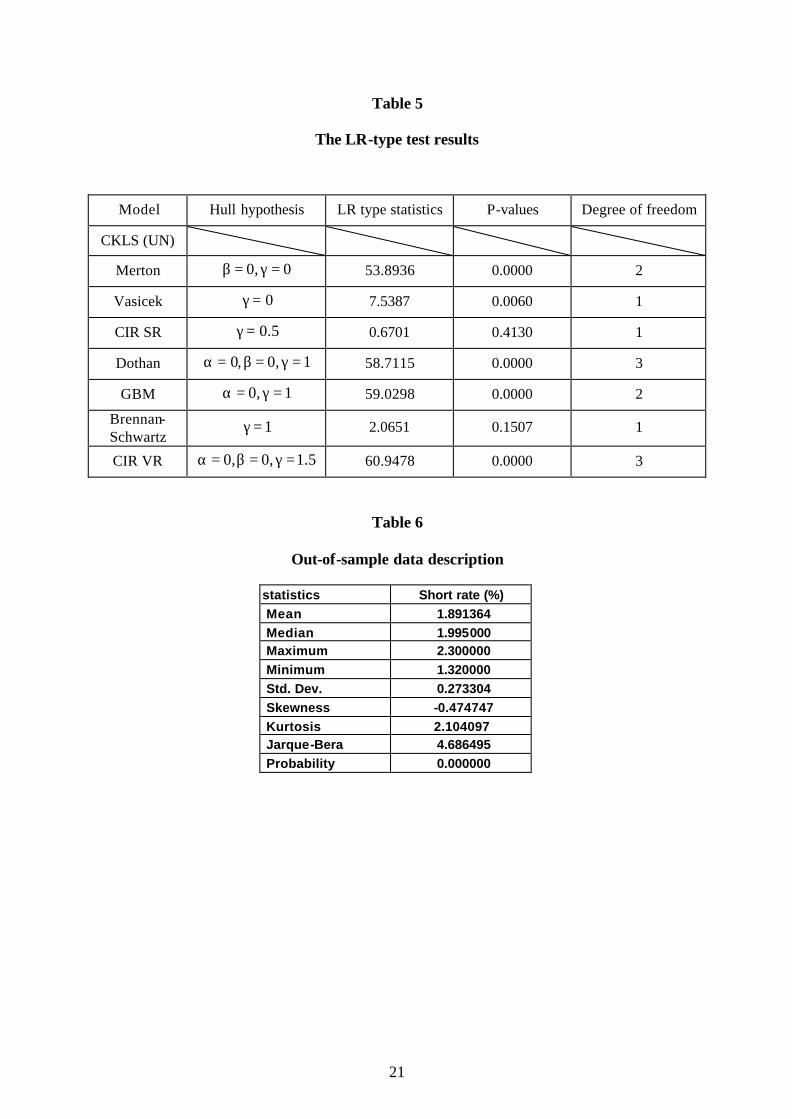
results shown in Table 5.

11

[Table 5 about here]

The results show evidence that under the LR-type tests the five restricted models (Merton, Vasicek,

Dothan, GBM, and CIR VR) cannot survive, since they all have such small p-values. However, we do

not reject the null hypothesis of the CIR SR model and the Brennan-Schwartz model at either the 1%

or the 5% significance levels. In other words, these later two models exhibit more ability to capture the

distinguishing feature of the Chinese short rate.

4.3 Out of sample forecast

4.3.1 Forecast test strategy and the out-of-sample yield data:

In order to show the forecasting ability among the one factor models, Theil’s U2 statistics and Diebold

and Mariano’s (DM) forecasting test are carried out. Theil’s U2 statistics are used as relative measures

to compare forecasts for the same time series across different models. In this paper for Theil’s U2

statistics will be calculated and the forecasting power compared in the same out sample period

1/08/2005-13/10/2005 for nine models. According to the criterion models having smalle r U2 statistics

(i.e. closer to zero) are preferred. The reason for this is because the smaller the mean square error, the

better the forecasting ability of that model. The equation for obtaining Theil’s U2 statistics can be

expressed as the following, where h depicts the number of periods for which variable y is forecasted

(see Pindyck and Rubinfeld (1991, Chapter 12) :

Theil’s Inequality Coefficient:

T h2

t tt T 1

T h T h2 2t t

t T 1 t T 1

ˆ(y y ) / hU2

y / h y / h

+

= +

+ +

= + = +

−=

+

∑

∑ ∑

Moreover, the U2 coefficient can be decomposed into three parts: bias proportion, variance proportion

and covariance proportion, as follows:

Bias proportion: 2

t2

t t

ˆ(( y /h) y)B

ˆ(y y ) / h−

=−

∑∑

Variance proportion: 2

y y2

t t

(s s )V

ˆ(y y ) / h

−=

−∑

Covariance proportion y y2

t t

2(1 r)s sC

ˆ(y y ) / h−

=−∑

where = is the coefficient of linear correlation between the values of y and y , and y ys ands are their

respective standard deviations.

12

Models having large values of C are preferred. However, since the U2 statistic is not a formal test to

detect the model’s predictive power, the DM test will also be applied to test forecasting ability. In this

test the quality of the forecasts is judged according to some loss function. The loss function is defined

as a direct function of the forecast error t 1t 1tˆg(y , y ) g(e )= . Moreover, they define the loss differential

as t 1t 2td g(e ) g(e )= − . Thus, the DM test of equal predictive accuracy can be conducted as a simple t-

test that:

0 tH :E(d ) 0= (Equal predictive accuracy) v.s a tH :E(d ) 0≠

The t-test statistic is as follows:

dDM

V(d)=

where d is the mean of the loss differential, and V(d) is an estimate of its asymptotic variance.

The observed out-of-sample period yield data is provided by the Datastream and summary statistics

are in Table 6. For the Chinese interbank loan the yield maturities are monthly. The data are daily and

cover the period from 1 August 2005 to 31 October 2005, providing 66 observations. Table 6 presents

descriptive statistics for out of sample in the one-month inter-bank loan rate, r. The mean value of r

over the sample period is 1.891364 per cent, and it ranges from a low of 1.32 per cent to a high of 2.3

percent. The interest rate has a standard deviation of 0.273304 per cent during the out of sample

period. This suggests that the short- term interest rate is not volatile in these three months.

[Table 6 about here]

4.3.2 Forecast evaluation results:

As noted in the previous section Theil’s U2 statistic is a relative measure to compare the forecasts with

actual series. If the U2 statistic is equal to zero, it will suggest that the forecast perfectly fits the actual

series. In other words, models with the smallest U2 statistics have the highest predictive power

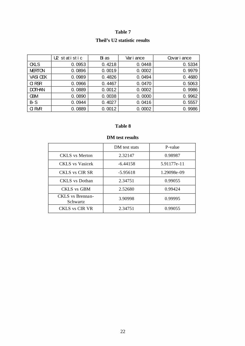
according to the criterion. Table 7 shows the U2 statistics and its decomposition results.

Overall, the whole class of one-factor models is very close in terms of the U2 statistics. All models

have very small U2 values, the range being 0.0889 to 0.0989. The variance proportion is also not

much different among the models, where the variance proportion range is from about 0.0494 for the

Vasicek model to the lowest value of virtually zero in the GBM model. However, there is a large

variation for the bias proportion and the range is from the highest 0.4826 to smallest 0.0012. The large

variation in bias proportion suggests that mean of the forecasts produced by some models is far from

the mean of actual series.

13

From the theoretical point of view, we may say that the Vasicek model does a relatively poor job of

tracking the trend of the actual series among the models, since it has the highest U2 statistic. In

contrast, according to the ir U2 statistics, the Dothan the CIR VR models have higher predictive

powers than the rest of models in terms of forecasting China’s short term interest rate. However, we

can hardly deny the fact that all models have very small U2 values. Thus, from a practical point of

view, we would conclude that all the one factor models do a good job of tracking the actual series. In

other words, all one factor models have good ability to predict the Chinese short rate.

As discussed previously, the DM test is a formal test to detect the model’s forecasting accuracy.

Therefore, we will use the CKLS model as the benchmark model against which to test the other

models. Table 8 contains the DM test statistics and their corresponding P-values, as produced by the

RATS software programme

[Table 8 about here]

From the DM test results it can be seen that we reject the Vasicek model and the CIR SR model, because

they both have very low p-values. In other words, the DM tests results favour the CKLS model over the

Vasicek model and CIR SR model in terms of forecasting ability for China’ short term interest rate.

However, since the remaining hypothesis tests have very high p-values, we can not reject the associated

models. Thus, the results suggest that the DM tests can not distinguish the CKLS model from the Merton

Model, the Dothan model, the GBM model, the Brennan Schwartz models, and the CIR VR model in

terms of predictive power for China’s short rates.

5. Conclusion:

This paper applies one-factor term structure models to capture the dynamic feature of China’s short

rate. In general, these models assume that the expected short rate is some function of the conditional

mean and variance of the short rate itself. In other words, for a given time-series short rate model, we

should be able to forecast tomorrow’s short rate from the knowledge of today’s short rate and a set of

parameter estimates. Therefore, our research is designed to test whether the single factor models are

able to characterize the dynamic behaviour of China’s short-term interest rate. What is more, from

practical point of view the research tests the one factor model’s forecasting power for China short term

interest rates.

In order to estimate one factor models for China’s short rates, GMM has been applied. The GMM

estimation results provide a number of interesting insights into the dynamics of the Chinese short term

rates. First, there appears to be strong evidence of a mean reversion feature in the short rate, the

estimated parameter β being statistically significant in all the one factor models. Second, in the

diffusion term we find that the estimated value of ˆ 0.7834γ = , although being statistically significant in

14

the unrestricted model, has such a low value that we infer that the volatility of China’s one month inter

bank loan rate is not strongly positively correlated with the level of interest rates. We also find that the

CEV model produces meaningless results for China’s short rate, which suggests that the CEV model is

not adequate to capture dynamic features of China’s short rate.

Since the CKLS family provides eight models to model the short interest rate, the J test is carried out to

detect whether the models are misspecified in terms of modelling China’s short rate. From the J tests we

conclude that only the CKLS model, the CIR SR model, and the Brennan-Schwarz model are correctly

specified, the rest of the models being misspecified. In the LR type test results it indicates that the

restrictions imposed by the CIR SR model and the Brennan-Schwartz model are not rejected at 1%

significance level. Therefore, the results of both the J tests and LR type tests broadly confirm that the

CKLS model, the Brennan-Schwartz model and the CIR SR model are sufficient to capture the dynamics

of China’s short rate.

In order to further illustrate the performance of the one factor models, we tested their forecasting ability.

According to Theil’s U2 statistics, we find that the all values of U2 statistics are very small, the range is

from the lowest 0.0889 to the highest 0.0989. Therefore, we conclude that all one factor models do a

good job of tracking the actual series trend. In other words, the CKLS, Merton, Vasicek, GBM, CIR SR,

Dothan, Brennan-Schwartz, and the CIR VR model perform well in term of forecasting China’s short

rates. Finally, the DM test is carried out to illustrate the forecasting ability in CKLS model competing

with the rest of the restricted models. Under the DM tests we have found that the results favour the

CKLS model over the Vasicek and the CIR SR model in terms of predicting for China’s short rate.

However, the DM tests can not distinguish the CKLS model from the Merton Model, the Dothan model,

the GBM model, the Brennan Schwartz model, and the CIR VR model in terms of predicting ability for

the Chinese short rates.

According to the finding of this research, it can be seen that the CKLS model, the CIR SR model and

the Brennan-Schwartz model are sufficient to capture the dynamics of Chinese short rates. In other

words, the CKLS model, the CIR SR model and the Brennan-Schwartz model are strongly

recommended for modelling China’s short rate. Moreover, the study shows one factor models do a

good job in terms of forecasting ability. Therefore, from a practical standpoint, the one factor models

can be recommended in terms of the modelling dynamic movements in, and the forecasting of,

Chinese short rates. That is, there does not seem to be much advantage in trying to develop and use

the more complicated multi-factor models.

15

References:

Bjork, T. and Christensen, B., (1999), “Interest rate dynamics and consistent forward rate

curves”, Mathematical Finance, 9: 323-348.

Bjork, T. and Landen, C., (2002), “On the construction of finite dimensional realizations for

nonlinear forward rate models”, Finance and Statistics, 6: 273-302.

Bjork, T., (2000), “A geometric view of interest rate theory”, in Jouini, E., Cvitanic, J. and

Musiela, M. (eds), Handbook of Mathematical Finance, Cambridge University Press,

Cambridge, pp. 241-277.

Black, F., and Scholes, M., (1973), “The pricing of options and corporate liabilities”,

Journal of Political Economy, 81: 637-654.

Bliss, R., (1997), “Testing Term Structure Estimation Methods”, Advances in Futures and

Options Research, 9: 97–231.

Brennan, M. L., and Schwartz, E.L., (1980), “Analyzing convertible bonds”, Journal of

Financial and Quantitative Analysis, 15: 907-929.

Brenner, R.H., Harjers, R. and Kroner, K., (1996), “Another look at models of short-term

interest rates”, Journal of Financial and Quantitative Analysis, 31: 85-107.

Chan, K.C., Karolyi, G.A., Longstaff, F.A. and A.B.Sanders, A.B., (1992), “An empirical

comparison of alternative models of the short-term interest rates”, The Journal of Finance,

1209-1227.

Chen.R., and Scott, L., (1992), “Pricing interest rate options in a two-factor Cox-Ingersoll-

Ross model of the term structure”, Review of Financial Studies, 5: 613-636.

Chen, L. (1996), Interest rate dynamics, derivatives pricing and risk management. Lecture

Notes in Economics and Mathematical Systems. Springer-Verlag, Berlin.

Copeland, L.,(2005), Exchange Rates and International Finance. 4rd edition, Prentice Hall,

New Jersey.

Cox, J. C., (1975), Note on option pricing I: Constant elasticity of variance diffusion,

Working paper, Stanford University.

Cox, J.C., Ingersoll, J.E. and Ross, S.A., (1980), “An analysis of variable rate loan

contracts”, Journal of Finance, 35: 389-403.

Cox, J.C., Ingersoll, J.E., and Ross, S.A., (1985a), “An intertemporal general equilibrium

model of asset prices”, Econometrica, 53: 363-384.

Cox, J.C., Ingersoll, J.E., and Ross, S.A., (1985b), “A theory of the term structure of interest

rates”, Econometrica, 53: 385-408.

16

Dahlquist, M., (1996), “On Alternative Interest Rate Processes”, Journal of Banking and

Finance, 20: 1093–1119.

Diebold, F., and Mariano,R., (1995), “Comparing predictive accuracy”, Journal of Business

and Economic Statistics, 13: 53-263.

Dothan. U.L., (1978), “On the term structure of interest rates”, Journal of Financial

Economics, 6: 59-69.

Fan, X., and Zhaoben, F., (2001), Empirical Test on Convertible Bond Pricing Model under

Stochastic Interest Rate, University of Iowa working paper.

Filipovic, D., (1999), “A note on the Nelson-Siegel family”, Mathematical Finance, 9: 349-

359.

Filipovic, D., (2000), “Exponential-Polynomial families and the term structure of interest

rates”, Bernoulli, 6: 1081- 1107.

Gibson R., and Schwartz, E.S., (1990), “Stochastic convenience yield and the pricing of oil

contingent claims”, Journal of Finance, 45: 959-976.

Hansen, L. P., (1982), “Large sample properties of Generalized Method of Moments

estimators”, Econometrica , 22: 305-333.

Heath, D., Jarrow, R. and Morton, A., (1992), “Bond pricing and the term structure of

interest rates: A new methodology for contingent claims valuation”. Econometrica, 60: 77-

105.

Laurenceson, J. and Qin, F., (2005), China’s exchange rate policy: The case against

abandoning the dollar peg, Center for Economic Research, Tilburg University Discussion

Paper No. 2005-70, Tilburg, Netherlands.

Jamshidian F., (1989), “An exact bond option formula”, Journal of Finance, 44: 205-209.

Cochrane, J., (2001), Asset Pricing 1st edition, Princeton University Press, New Jersey.

Litterman, R., and J.Scheinkman, J., (1991), “Common factors affecting bond returns”,

Journal of Fixed Income, 3: 54-61.

Longstaff, F.A., and E.Schwartz, E., (1992), “Interest rate volatility and term structure: A

two-factor general equilibrium model”, Journal of Finance, 47: 1259-1228.

Merton, R. C., (1973), “Theory of rational option pricing”, Bell Journal of Economics and

Management Science, 4: 141-183.

Nelson, C.R. and Siegel, A.F., (1987), “Parsimonious modelling of yield curves”, Journal

of Business, 60: 473-489.

17

Newey, W., and West, K., (1987), “Hypothesis testing with efficient method of moments

estimation”, International Economic Review , 28: 777-787.

Soderlind, P. and Svensson, L.E.O., (1997), “New techniques to extract market

expectations from financial instruments”, Journal of Monetary Economics, 40: 383-430.

Treepongkaruna, S. (2003), “Quasi-maximum likelihood estimates of Kiwi short term

interest rate”, Applied Economics Letters, 10: 937-942.

Treepongkaruna, S. and Gray, S.F., (2002), “On the robustness of short-term interest rate

models”, Accounting and Finance, 43: 87-121.

Tse, Y. K., (1995), “Some international evidence on stochastic behaviour of interest rates”,

Journal of International Money and Finance, 14: 721–738.

Vasicek, O., (1977), “An equilibrium characterization of the term structure.

Journal of Financial Economics 5, 177-188.

Vetzak, K. R., (1997), “Stochastic volatility, movements in short term interest rates, and

bond option values”, Journal of Banking and Finance, 169-196.

Xie, Chi and Wu, X., (2002), “An empirical test of interest rate behaviour in

China’s monetary market using the Vasicek model and the CIR model”, Chinese Journal of

Management Science, 10: 12-15.

Zheng, Z, and Lin, H., (2003a), “Static approximation of term structure in China”, Wuhan

Finance Monthly , 3: 33-37.

Zheng, Z. and Lin, H., (2003b), Research on liquidity premium of interest rate in China,

Working Paper of Xianmen University. http://efinance.nease.net/1966.htm.

Zheng, Z. and Lin, H., (2003c), “Research on default risk premium in China”, Securities

Market Herald, 6: 41-45.

18

Figure 1

China’s Real GDP

0

1000

2000

3000

4000

5000

6000

7000

8000

1995 1996 1997 1998 1999 2000 2001 2002 2003 2004 2005

Rea

l GD

P

Source: Datastream. Units of measurement are billion yuans

Figure 2: China’s Inter-bank short rate

One-month interbank loan rate

0

1

2

3

4

5

6

10/0

1/20

02

10/0

3/20

02

10/0

5/20

02

10/0

7/20

02

10/0

9/20

02

10/1

1/20

02

10/0

1/20

03

10/0

3/20

03

10/0

5/20

03

10/0

7/20

03

10/0

9/20

03

10/1

1/20

03

10/0

1/20

04

10/0

3/20

04

10/0

5/20

04

10/0

7/20

04

10/0

9/20

04

10/1

1/20

04

10/0

1/20

05

10/0

3/20

05

10/0

5/20

05

10/0

7/20

05

Period

Inte

rest

rat

e (%

)

19

Table 1

China’s one-month interbank loan rate (2002-2005)

statistics Short rate (%) First difference (%) Mean 2.695771 -0.000551

Median 2.580000 0.000000 Maximum 4.980000 2.310000 Minimum 1.040000 -2.280000 Std. Dev. 0.607236 0.476428 Skewness 0.944751 0.136084 Kurtosis 4.457534 8.722520

Jarque-Bera 219.9549 1266.356 Probability 0.000000 0.000000

Table 2

The single factor models

Model Specification Restrictions Merton (1973) dr dt dz= α + σ ß=0, ?=0

Vasicek (1977)

dr ( r)dt dz= α + β + σ ?=0

Cox, Ingersoll, and Ross (1985)

1/2dr ( r)dt r dz= α + β + σ ?=1/2

Dothan (1978)

dr rdz= σ a= ß=0, ?=1

Geometric Brownian Motion (1973)

dr rdt r dz= β + σ a=0, ?=1

Brennan and Schwartz (1980) dr ( r)dt r dz= α + β + σ ?=1

Cox, Ingersoll, and Ross (1980)

3 /2dr r dz= σ a= ß=0, ?=3/2

Cox (1975) dr rdt r dzγ= β + σ a=0

20

Table 3

GMM estimation results

Model α (Std Error)

β

(Std Error)

2σ (Std Error)

γ (Std Error)

ˆˆ /−α β

=Reversion rate

Unrestricted CKLS

0.8358 (0.0923)

-0.312 (0.0353)

0.0394 (0.0184)

0.7834 (0.2148)

2.6788

Merton -0.0295 (0.0209)

0.0 0.2241 (0.0204)

0.0

Vasicek 0.9293 (0.1019)

-0.3457 (0.0392)

0.1920 (0.0157)

0.0

2.6882

CIR SR 0.8713 (0.1004)

-0.3244 (0.0387)

0.0728 (0.0059)

0.5

2.6859

Dothan 0.0 0.0 0.0313 (0.0037)

1

GBM 0.0 -0.0186 (0.0078)

0.0294 (0.0030)

1

Brennan-Schwartz

0.8104 (0.0979)

-0.3034 (0.0378)

0.0239 (0.0020)

1 2.6711

CIR VR 0.0 0.0 0.0095 (0.0012)

1.5

Table 4 The J-test results

Model

J-Test

P-values

Degree of

freedom

CKLS 8.7573 0.0125

Merton 62.6509 0.0000 2

Vasicek 16.2960 0.0010 1

CIR SR 9.4274 0.0241 l

Dothan 67.4688 0.0000 3

GBM 67.7870 0.0000 2

Brennan-Schwartz

10.8223 0.0127 1

CIR VR 69.7047 0.0000 3

21

Table 5

The LR-type test results

Model Hull hypothesis LR type statistics P-values Degree of freedom

CKLS (UN)

Merton 0, 0β = γ = 53.8936 0.0000 2

Vasicek 0γ = 7.5387 0.0060 1

CIR SR 0.5γ = 0.6701 0.4130 1

Dothan 0, 0, 1α = β = γ = 58.7115 0.0000 3

GBM 0, 1α = γ = 59.0298 0.0000 2

Brennan- Schwartz

1γ = 2.0651 0.1507 1

CIR VR 0, 0, 1.5α = β = γ = 60.9478 0.0000 3

Table 6

Out-of-sample data description

statistics Short rate (%) Mean 1.891364 Median 1.995000 Maximum 2.300000 Minimum 1.320000 Std. Dev. 0.273304 Skewness -0.474747 Kurtosis 2.104097 Jarque-Bera 4.686495 Probability 0.000000

22

Table 7

Theil’s U2 statistic results

U2 statistic Bias Variance Covariance CKLS 0.0953 0.4218 0.0448 0.5334 MERTON 0.0896 0.0019 0.0002 0.9979 VASICEK 0.0989 0.4826 0.0494 0.4680 CIRSR 0.0966 0.4467 0.0470 0.5063 DOTHAN 0.0889 0.0012 0.0002 0.9986 GBM 0.0890 0.0038 0.0000 0.9962 B-S 0.0944 0.4027 0.0416 0.5557 CIRVR 0.0889 0.0012 0.0002 0.9986

Table 8

DM test results

DM test stats P-value

CKLS vs Merton 2.32147 0.98987

CKLS vs Vasicek -6.44158 5.91177e-11

CKLS vs CIR SR -5.95618 1.29098e-09

CKLS vs Dothan 2.34751 0.99055

CKLS vs GBM 2.52680 0.99424

CKLS vs Brennan-Schwartz

3.90998 0.99995

CKLS vs CIR VR 2.34751 0.99055