An Automated Antenna Measurement SystemUtilizing Wi-Fi Hardware

Vittorio PiccoIEEE Student Member

Department of Electrical and Computer EngineeringUniversity of Illinois at Chicago, USA

Email: vpicco2@uic.edu

Keith MartinIEEE Student Member

Department of Electrical and Computer EngineeringUniversity of Illinois at Chicago, USA

Email: kmarti28@uic.edu

Abstract—We propose a system that measures 3D gain patternsof an unknown antenna using the Received Signal StrengthIndicator (RSSI) provided by Wi-Fi hardware. Our system useswidely available Wi-Fi routers to generate the RF signal andmeasure incident power. A simple two-axis positioner allowsthe full 3D pattern of the antenna to be measured, and aLabVIEW interface lets users control measurements and viewresults. We make use of inexpensive, readily available materialsand rudimentary construction techniques.

I. INTRODUCTION

Measuring the radiation pattern and gain of an antenna is anessential step in assessing compliance with simulation resultsand design specifications. It is also important for the user thatneeds to verify the performance of an unknown antenna.

These measurements are typically performed with a networkanalyzer and an antenna positioner, usually located in ananechoic chamber. A computer synchronizes the movementof the antenna and the network analyzer measurements. Asa result, a complete antenna measurement system can costwell over $100 000, making it an inaccessible commodity formany individuals and institutions. By operating in a limitedfrequency range and in a non-anechoic environment, it ispossible to use widely available components to dramaticallydecrease the cost of the system. This is accomplished whileintroducing only minor inaccuracies compared to a typicalantenna measurement system.

In this paper we propose an antenna measuring system thatmakes use of widely available Wi-Fi routers to generate andmeasure an RF signal at 2.4 GHz. A simple two-axis positionerallows the full 3D pattern of the antenna to be measured, and aLabVIEW interface lets users control measurements and viewresults. We use inexpensive, readily available materials andrudimentary construction techniques.

II. THEORY OF ANTENNA MEASUREMENTS

The principles of radiation pattern and gain measurementare well standardized, and rely on the use of at least twoantennas. One is referred to as the Measurement Antenna(MA) and the other as the Antenna Under Test (AUT). Oneworks as the transmitter, generating a known field, and theother as the receiver, converting a portion of the incidentfield into a measurable signal. The reciprocity principle allowseither antenna to work as the transmitter or the receiver.

Fig. 1. Two-axis roll-over-yaw positioner realizing great-circle (a) or conicalsection (b) scans

A. Pattern measurements

Assuming that the MA is used as the transmitter and theAUT as the receiver, a pattern measurement is obtained byrotating the AUT in front of the MA and recording theincident power received as function of the relative angularposition between the two antennas. Full 3D or 2D scans canbe achieved depending on the positioner used to rotate theAUT.

We describe the realization of a two axis positioner thatallows full 3D pattern measurements. The system allows twoaxes to be controlled: a lower axis with a vertical axis ofrotation – henceforth referred to as the yaw axis – and anupper axis with a horizontal axis of rotation – henceforthreferred to as the roll axis. A schematic representation ofthe positioner is available in Fig. 1. The imaginary spheresurrounding the antenna can be sampled in different waysusing the same positioner structure, depending on how the twoaxes are controlled. Varying the yaw axis over a constant rollaxis position produces great-circle scans; each scan representsa cross-section of the outer sphere, i.e., a circle of maximumdiameter. Alternatively, by varying the roll axis for a fixedyaw value, conical section scans are obtained. These representcircles of varying diameter. These circles are the bases ofcones of a fixed angle θ, the position of the yaw axis.When this method is used, each axis maps directly to theaxes of the standard spherical coordinate system. The yaw

axis is equivalent to movement in the θ direction, and theroll axis is equivalent to movement in the φ direction. Toavoid cumbersome coordinate conversions, the conical sectionmethod is adopted here.

From this procedure a relative pattern measurement isobtained. In order to obtain an absolute measurement of anantenna’s gain, an additional measurement must be performed.

B. Gain measurements

Gain measurements are obtained by first aligning the AUTand the MA along the maximum found in the pattern mea-surement. Then, different techniques can be used to find theabsolute gain of the AUT. Two common methods are the gaintransfer (or gain comparison) method, and the three-antennamethod. An extensive description of these and other techniquescan be found in [1].

The gain transfer method is based on the use of an antennaof known (standard) gain Gsg , whose received power, (Psg), iscompared to the received power measured by the AUT, (Paut).The gain of the antenna under test, (Gaut) is then found as:

Gaut = Gsg + Paut − Psg, (1)

all quantities expressed in dB.The three-antenna method is used when no standard gain

antenna is available. In this case three antennas, all of unknowngain, are used; three measurements are taken, one for each ofthree combinations of transmitting and receiving antennas. Foreach measurement the Friis transmission equation is used andthe gain of all three antennas can be found by solving a systemof three equations in three unknowns, each one of the form:

(Ga)dB + (Gb)dB = 20 log10

(4πRλ

)+ 10 log10

(PrbPta

).

(2)

C. Polarization effects

The MA can be linearly or circularly polarized. If the MAand AUT are both linearly polarized, the polarization of theAUT can be found and the co- and cross-polarization patternscan be measured. By properly mounting the MA and AUT theuser can ensure that only the co- or cross-polarized pattern ismeasured in a 2D scan. This is not possible when performinga 3D scan; therefore, two scans must be performed, rotatingthe MA by 90 degrees between each scan.

If one antenna is circularly polarized and the other linearlypolarized, polarization mismatch can no longer occur. How-ever, no polarization information can be obtained, and thegain measurement obtained will be 3 dB lower than the actualvalue.

All these factors can lead to substantially different designsand operating procedures. In the following section the detailsof our approach are presented and our rationale explained.

III. DESCRIPTION OF SYSTEM

A. RF architecture

1) Approach: The design of the RF section is inspiredby a main competition requirement: a system operating at

a frequency of 2.4 GHz. Many consumer devices radiate inthis frequency, including Wi-Fi (IEEE 802.11 b/g) and Blue-tooth (IEEE 802.15) devices, cordless phones, and microwaveovens. This results in significant interference in the 2.4 GHzband. However, this also makes a multitude of inexpensiveRF devices accessible to the designer. In addition, the Wi-Fi standard provides mechanisms implemented at both thephysical and data link layers to avoid collisions, reject noise,and even estimate the power of a received signal. For thesereasons, our design is based on the use of two inexpensiveand widely available Wi-Fi routers. One router acts as atransmitter, generating an RF signal. The other measures thereceived power of this signal, allowing antenna gain andpattern measurements to be made.

The IEEE 802.11 family of protocols envisions “an optionalparameter that has a value of 0 through RSSI Max. This pa-rameter is a measure by the PHY of the energy observed at theantenna [. . . ]. RSSI is intended to be used in a relative manner.Absolute accuracy of the RSSI reading is not specified” [2].This generic definition is implemented by manufacturers indifferent ways, with the goal of providing the user a visualestimation of the strength of a Wi-Fi network. The RSSI iscomputed by estimating the power in the preamble of a Wi-Fibeacon. An Access Point (AP) transmits this beacon repeatedlyat fixed intervals, broadcasting basic information about theWi-Fi network that the AP is creating. Devices that receivethis beacon generate an estimate of the incident signal power.This mechanism allows us to obtain not only a received powerestimate, but also to discriminate between different networks,and obtain a measure with improved noise immunity.

The router chosen to function as both the signal generatorand received power meter is the Linksys WRT54G. This choiceis motivated by two main factors. The first is that accordingto the manufacturer’s specifications, Linksys routers providetheir RSSI reading as an integer between 0 to 100. Thisappears to be the finest quantization of the RSSI measureoffered by commercial routers, resulting in better sensitivityto small RSSI changes. The second reason is that the LinksysWRT54G supports customized firmware maintained by a largeopen source community. This open source firmware allows theuser to manipulate otherwise inaccessible parameters, such asthe transmit power and the beacon transmission interval. AnSSH shell interface is also available in some versions, allowingcommand line control of the device. We chose the dd-wrt v24Micro-plus firmware, which specifically allows SSH access.

2) Calibration: RSSI is a precise measure of the incidentpower, but not an accurate one. While repeated tests under thesame conditions lead to repeatable results, the result cannot beused to directly measure incident power. Calibration is neededto relate RSSI to gain. To calibrate the system, the followingprocedure is adopted. Any antennas can be used as the MAand the AUT; neither needs to be characterized precisely. Asplitter allows the signal received by the AUT to be sent tothe receiving router and to a spectrum analyzer. The routerRSSI and spectrum analyzer measurements are recorded fora range of transmitter power levels. The transmitted power is

Fig. 2. Incident power on the AUT measured using RSSI and a spectrumanalyzer

Fig. 3. Difference between the RSSI value returned by the router and thespectrum analyzer measurement as function of the RSSI itself

varied in increments of 3 dB to cover its full dynamic range.The router RSSI readings and the spectrum analyzer powermeasurements are shown in Fig. 2.

The nonlinearities that appear in the spectrum analyzermeasurement are caused by differences between the desiredtransmitted power and the actual transmitted power. The RSSIis linear within an approximately 30 dB range of incidentpower.

The difference between the two measurements is shownin Fig. 3. It can be seen that the difference between thetwo readings is small for high levels of received power andincreases when the signal strength decreases. The measureddifferences are interpolated using a third order polynomialestimator, which allows a correction coefficient to be computedfrom the following function:

C = −0.00057 ∗RSSI3 − 0.0836 ∗RSSI2+− 4.1314 ∗RSSI − 61.863. (3)

This correction coefficient is applied to the RSSI valuesobtained from the router, allowing the RSSI values to match

the power measurements obtained from the spectrum analyzer.This calibration operation is advisable, but it is not strictly

necessary. Since the routers proved to behave sufficientlylinearly, the RSSI reading could be used directly as a powerestimate, adding only a few decibels of uncertainty in themeasured result. Because the routers are mass produced, itmay also be possible to assume that all routers of this modeland version number will behave similarly. This would allowthe same calibration to be reused.

3) Pattern measurement: Our LabVIEW interface allowsfully automated measurement of radiation patterns in eitherprincipal plane. The user can specify which principal plane toscan, the angle to scan, and the angular separation betweendata points. The user can also opt to average several mea-surements for each data point. The computer uses the router’sSSH interface to retrieve RSSI measurements and controls thedriver used to rotate the positioner. Once the desired angularspan is covered, the normalized pattern is displayed on a polarplot.

This procedure is valid regardless of the MA used, giventhat care is taken in mounting the antennas so that theyare co-polarized. Nonetheless, to avoid reflections from theenvironment it is advisable to choose a directive antenna witha narrow main lobe. The MA should be in the far field of theAUT, with its main lobe pointed directly at the AUT.

For a 3D scan two sets of measurements are needed to avoidspurious cross-polarization effects. The MA is first mountedto produce a vertically polarized field, and both axes arescanned. Then the MA is rotated 90 degrees and the scansare repeated. The first measurement returns the theta-polarizedpart of the radiation pattern, while the second returns phi-polarized component. The two components can be combinedtogether to obtain the total radiation pattern. Because thereceived electric field is measured only in terms of power(i.e. magnitude squared), the two sets of measurements aresummed in this way:

Gaut =√G2θ +G2

φ. (4)

4) Gain measurement: To obtain an absolute gain mea-surement we use the gain comparison technique. This methodrequires a standard gain antenna, but offers some advantagesover the three antenna method. The three-antenna methodrequires knowledge of many parameters: the distance betweenthe antennas, the transmitted power, and an accurate measureof the received power. In addition, all three antennas mustbe identically aligned and impedance matched, and reflectionsneed to be minimized. Most of these variables cannot berigorously controlled in our system. The estimated gain provedto be unreliable, with large variations between trials.

In the gain comparison method, the only parameters re-quired are the gain of a known antenna and received powermeasurements obtained with the known antenna and the AUT.This implies that as long as the transmitted power and thedistance between the MA and AUT are not changed, the powerincident on the receiving antenna will be constant. In order to

Fig. 4. 3 GHz dipole antenna

further improve the measurement, multiple RSSI readings aretaken for a range of transmitter power levels and averaged. It isimportant to remark that the MA and the standard gain antennaserve different purposes. The MA works as a transmitter anddoes not need to be known, while the standard gain works asa receiver and needs to have a known absolute gain.

In industry, expensive standard gain horns are normallyused for gain comparison measurements. To minimize thenumber of antennas users need to purchase, we determinedthe gain of our MA. Users can then use this MA as a standardgain antenna when performing a gain measurement. Any usersupplied antenna can be used as the MA during the gainmeasurement. To determine the gain of our MA, we performeda gain comparison measurement using a half-wave dipole. Thegain of the dipole can be determined analytically to be 2.1 dBi.This antenna was available in our lab at no cost, and is onlyneeded once to determine the gain of the MA.

5) Antenna selection: A planar Yagi antenna is selectedto serve as the MA during pattern measurements, and as thestandard gain during gain measurements. A linearly polarizedantenna was chosen because linearly polarized antennas arewidely available for use in Wi-Fi. The Yagi is a directiveantenna, which helps minimize the effect of reflections. Thegain of the Yagi is determined by performing a gain compar-ison measurement with a half-wave dipole, allowing it to alsofunction as a standard gain. While the dipole offers a knowngain and can be constructed easily, its low directivity wouldresult in more reflections from the environment. Therefore, adipole was not chosen as the MA.

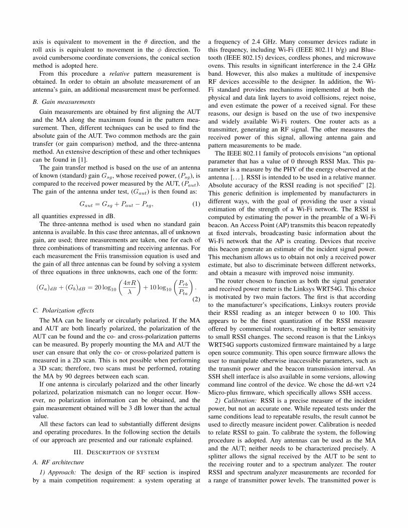
To validate the system, we chose to test a 2x2 planar arrayof microstrip patch antennas. This antenna is also linearlypolarized. Its array factor can be computed analytically, andits far field pattern can be determined through simulation.Comparing our measurements to the analytical and simulationresults will allow the performance of our system to be judged.

The dipole, patch array, and Yagi antennas are shown inFig. 4, 5, and 6 respectively. The coordinate system used tomeasure each antenna is also indicated.

Fig. 5. 2x2 array of microstrip patch antennas

Fig. 6. 5-element Yagi antenna

B. Two-axis positioner design and assembly

The positioner is designed with three objectives in mind.First, it must be able to rotate the AUT with the necessaryprecision, and provide a stable and repeatable platform formeasurements. Second, it must cause minimal scattering ofthe incident field, so that the behavior of the AUT is notinfluenced by the structure. Finally, constructing the positionerneeds to be within the capabilities of students who may nothave extensive experience with fabrication.

We elected to use stepper motors to move the positioner.Stepper motors allow rotation in predetermined increments,so they allow the positioner to be rotated through the desiredangle by simply specifying the number of steps to move. Thesize of each step is extremely consistent, allowing open loopcontrol of the motors. We configured the drive to operatein microsteps, which provides the lowest level of vibrationand highest control of the positioner. In this mode, eachstep rotates the shaft of the motor 0.225◦. The motors aredriven by a Xylotex 3-Axis Stepper Motor Driver Board. Thisboard accepts signals from a PC parallel port, and providesthe necessary outputs for driving stepper motors. The driver,motors, and power supply are available as a kit from Xylotex,

Fig. 7. Xylotex stepper motor driver board

Fig. 8. Yaw axis motor, belt and pulley. The roll motor is mounted on thelarge yaw pulley

simplifying the design.A stepper motor drives each axis through a belt and pulley

system. While a direct drive between a wheel on the shaft ofthe motor and the base of the column was initially considered,this was abandoned when it was found that this would requirethe base to be perfectly concentric. The belt drive allowsconsistent, repeatable movements even if the base is notcompletely circular. In the yaw axis the motors operate at agear ratio of approximately 17:1. This equates to a single stepprecision of 0.013◦. To maximize accuracy, the exact gear ratiois determined empirically after the system is constructed.

The roll axis is driven by a stepper motor attached to thebase of the column. This reduces the effects of scattering fromthe conductive body of the motor. Here the belt drive alsoallows increased separation between the motor and the axis.The gear ratio is approximately 6:1, resulting in a single steprotation of 0.038◦.

The column is constructed of 1.25 in (3.18 cm) oak dowels,with the ends attached to wooden disks using mortise andtenon joints. The disks are fabricated to make this joint strongand easy to assemble. Each disk is made by laminating several

Fig. 9. Column supporting the upper disc and the roll wheel

0.125 in (0.32 cm) thick disks together. A set of three disksis laminated together, and 1.25 in (3.18 cm) holes are drilledinto the disks to accept the dowels. The holes are located120◦ apart using a geometric construction. Two more disksare then laminated onto the drilled disk, so that the finisheddisk has three holes that are guaranteed to be of equal depth.This process is repeated for a second disk. The dowels arethen glued into each hole in the disks, resulting in a strongand square column.

The largest available 0.125 in (0.32 cm) thick disks were 10in (25.4 cm) in diameter, which did not provide enough roomto mount the roll axis motor. Therefore, the entire column wasthen attached to the next largest available disk, an 18 in (45.7cm) diameter, and 1 in (2.54 cm) thick circle. This disk camewith a rounded edge. To make the edge more suitable for abelt drive, the radius was removed using a band saw at theUIC machine shop. The work was performed at no cost. Thedisk was mounted on a 12 in (30.5 cm) diameter turntablebearing, which was then fixed to a 24 in x 24 in (61 cm x 61cm), 0.75 in (1.90 cm) thick plywood base.

The centers of the 18 in (45.7 cm) disk and the diskat the bottom of the column were found using geometricconstruction. A hole was drilled in the disk at the bottomof the column, so that the center of the 18 in (45.7 cm) diskwould be visible when the column was centered on the largerdisk. The column was then secured to the base using woodscrews.

Fig. 10. Roll axis complete with roll pulley, shaft, bearings and belt flange.The shaft is cut longitudinally to allow for easy AUT connection with, forexample, double-sided tape, like shown in this figure

To allow rotation in the roll direction, an additional bearingwas needed. The bearing is supported by a section of 2 inx 4 in (5.08 cm x 10.16 cm) lumber attached to the top ofthe column. A 1.25 in (3.18 cm) diameter hole is drilled inthis bearing block to accept a bearing and a shaft to mountthe antenna. The hole is located high enough to allow theantenna to roll through 360◦, and is offset from the center ofthe column so that the antenna can be mounted on the yawaxis of rotation. To prevent scattering from a metallic bearing,a plastic sleeve bearing is selected. This bearing fits into thebearing block and is held in place by a flange. The bearingaccepts a 1 in (2.54 cm) oak dowel, allowing the shaft to turnfreely while being held orthogonal to the yaw axis. A pulleyis fabricated from 6 in (15.24 cm) diameter, 0.125 in (0.32cm) thick disks, and secured to the dowel using a plastic shaftcollar. A plastic shaft collar with mounting holes on its facewas not available, so holes are drilled through the collar andthe pulley so that nylon machine screws can be used to attachthe pulley to the shaft.

Obtaining pre-made belts in the correct sizes also proveddifficult, so we chose to fabricate our own belts. The belts areconstructed out of several layers of adhesive tape. To constructthe belts, the required circumference is measured. Then thepulleys are clamped to a table to provide a stable surface. Thedistance between the pulleys determines the circumference ofthe belt. To provide durability and a high friction interfacebetween the belt and pulleys, the inner surface of the belt ismade of duct tape. Several layers of Scotch brand transparenttape are then applied over the duct tape, followed by a finalouter layer of duct tape. This method produces an inexpensiveand resilient belt in any length desired.

The roll axis motor must rotate with the column when itis moved around the yaw axis, so it is mounted to the baseof the column. We fabricated our own mount from a 0.125 in(0.32 cm) thick 1 in x 1 in (2.54 cm x 2.54 cm) angle ironprofile. First, we cut two 3.5 in (8.89 cm) long segments fromthe profile. Using a #5 (0.522 cm) drill bit, we then drilledholes in each segment to match the mounting holes on the

face of the motor. On the other side of the profile, we drilledand countersunk holes for wood screws. The two profiles areattached to the motors using long #10 (0.483 cm) machinescrews and nuts, which are then cut to length. Nylon spacersare placed underneath the mount so that the height of the motorcan be adjusted if necessary. This allows the tension in the beltto be altered. Wood screws secure the motor to the base of thecolumn. To enhance friction between the motor and the belt,a 1 in (2.54 cm) soft rubber wheel is used as the drive pulleyfor the motor.

The yaw axis motor is suspended upside down to allow itsshaft to be in the same plane as the base of the column. Abrace is constructed of 2 in x 4 in (5.08 cm x 10.16 cm)lumber, held together by wood screws. Slots are cut in the topof the brace so that the position of the motor can be adjustedif necessary, as when installing or removing the belt. Long#10 (0.483 cm) machine screws between the mounting holesof the motor and the slots in the brace secure the motor. A 1in (2.54 cm) soft rubber drive wheel is used as a pulley hereas well. The brace is secured to the plywood base plate usingright angle joist brackets.

In addition to the positioner, we also needed to hold theMA in a fixed position. The base of the MA mount is an18 in x 18 in (45.72 cm x 45.72 cm) square cut from a 3/4in (1.90 cm) thick sheet of plywood. Self-adhesive felt feetare placed under the base to improve its stability. A 36 in(91.44 cm) long segment of 2 in x 4 in (5.08 cm x 10.16cm) lumber is oriented vertically above the center of the base.Right angle joist brackets are used to ensure that the verticalsegment is normal to the base, and wood screws are usedto secure it to the base. The mount is tall enough so thatthe height of the MA can be adjusted so that it is alignedwith the AUT. The mount is suitable for attaching severalantenna geometries. The mounting procedure is similar to thatused with the AUT. Styrofoam blocks are placed between themount and the antenna to prevent anomalies caused by locatingmicrostrip lines next to dielectric materials other than air. Theantenna is secured using double-sided tape. Other antennas,such as the dipole, can be secured using nylon cable ties.

C. Software

A LabVIEW application is developed to control the move-ment of the positioner and to retrieve the RSSI measurementsfrom the router. LabVIEW makes it easy to develop a so-phisticated GUI and a hardware interface suitable for motorcontrol.

The positioner’s motions are controlled using the computer’sparallel port. The mapping of the data register of the parallelport is shown in Table I.

The LabVIEW program determines the direction andamount of rotation, and computes the number of micro-stepsnecessary. It then applies the appropriate values to the parallelport. The direction of rotation is controlled by the directionbit, and the motor rotates one microstep each time a risingedge occurs on the step bit. The same procedure is valid forboth axes.

TABLE IPARALLEL PORT DATA REGISTER BITS

Bit # Function0 Direction axis 11 Stepping axis 12 Direction axis 13 Stepping axis 2

The program Plink is used to communicate with the router.Plink is a freeware tool that provides a Windows-compatibleSSH client. Combined with the dd-wrt firmware, it allows anSSH connection to be established automatically. LabVIEW ex-ecutes Plink, opens an SSH connection and authenticates itselfas root user, executes the command wl -rssi, and readsthe standard output of Plink to retrieve the RSSI measure.The procedure is completely automated and requires no userintervention.

The program allows the user to rotate the axes and takemeasurements manually, or to run automated scans of theprincipal planes. To perform an automated scan, LabVIEWexecutes a series of movements, each followed by an RSSImeasure. The span, angular step size and axis to controlare defined by the user, as is the number of RSSI samplesto collect and average for each position. The program usesthe interpolator polynomial described in the RF architecturesection to automatically determine the correction to be applied.When the scan is completed the data collected are saved asan ASCII text file and presented to the user in the form of apolar plot. During the scan operation no user intervention isrequired at all.

The speed of a scan is determined by the amount of move-ment requested, by the step size, and by the number of samplesto average. A 360-degree scan with steps of 5 degrees and 8RSSI samples per position takes approximately 20 minutes.By combining multiple scans for different AUT positions inan environment such as MATLAB, full 3D patterns can beobtained from the raw ASCII text files saved by LabVIEW.For the purpose of demonstrating the operation and capabilitiesof the system, only 2D cuts are presented in the Test Resultssection.

IV. BILL OF MATERIALS

Description Source Cost ($)RF MeasurementLinksys WRT54G, 2x Amazon 113.08Ethernet cable, 10 ft Amazon 3.95PCB Patch Antenna Amazon 34.95PCB Yagi Antenna Amazon 32.95RP-TNC / N-m, 2x Amazon 9.96Adpt N-f / SMA, 2x Amazon 8.26Adpt SMA-f / SMA-f, 2x Digikey 8.90SMA cables, 4 ft, 2x L-com.com 36.00SoftwareLabVIEW student license NI.com 59.95

Positioner controlMotor kit xylotex.com 310.00DB25 10 ft extension Amazon 3.99Braided wire Home Depot 5.00Positioner hardwarePlywood base Home Depot 7.0018 in Wood Circle Lowes 13.1712 pk 10 in Wood Circle craftparts.com 11.886 in Wood Circle, 12x craftparts.com 7.441 1/4 in x 36 in Dowel, 3x craftparts.com 18.7512 in Turntable McMaster 10.678 ft 2 in x 4 in Lumber Home Depot 1.981in x 36in Oak Dowel Home Depot 4.37Acetal Flanged Bearing McMaster 9.60Slimline Drive Roller, 2x McMaster 59.36Transparent Tape, 1/2 in Staples 7.49Duct Tape, black Staples 7.991 in x 1 in Angle Iron Home Depot 7.10Clamp on Shaft Collar McMaster 14.39Nylon Screws 2in McMaster 7.23Nylon Hex Nuts, 3/8in McMaster 6.24Plastic Mesh Flange Joann fabric 0.60Tension Pins, Spacers Home Depot 15.16Machine Screws and Nuts McMaster 27.05Screws, Joist Angles, Glue Menard’s 16.01Carpet Tape Ace Hardware 4.9212 3/4in Felt Pads Home Depot 3.61Shipping costs, total 35.46TOTAL 924.46

V. TEST RESULTS

The performance of the system was evaluated by measuringthe far field patterns of the patch array, dipole, and Yagi anten-nas. The test was performed outdoors to minimize the effectof reflections, in the area behind a team member’s home. Thetest setup is shown in Fig. 11. The test area was approximately5 m x 5 m square, with the main lobe of the MA pointed at awooden fence. The positioner and MA were placed on tablesto elevate them above the ground. The ground consisted of agrass lawn and a concrete surface. The positioner was placedover the grass region, as we felt this would minimize the effectof scattering on the measurement. The relative permittivity ofsoil, εr, is approximately 3, compared to 4.5 for concrete. Aswill be shown below, the ground was the largest source ofreflections. A 360◦ scan in 5◦ increments was made in bothprincipal planes of each antenna. Eight samples were averagedin each position.

To validate the test results, the far fields of the patch array,Yagi and dipole antenna were simulated using FEKO. Thecurved microstrip feed structure of the patch array proveddifficult to replicate in FEKO. Therefore, we simulated eachpatch with its own feed, with all the patches feed in phase andwith the same amplitude. The patch is also simulated with aninfinite substrate. This provides a reasonable approximation ofthe far field pattern of the patch array. The measured values

Fig. 11. Outdoor measurement setup

Fig. 12. Dipole antenna, θ principal plane

are normalized, and superimposed with the simulation resultsto facilitate comparison.

A. Half-wave dipole

The pattern of the dipole is well known and can bedetermined analytically with relative ease. Because of this,measuring a dipole will provide an excellent example of theperformance of our system. In the θ plane, the half-wave dipoleis expected to have a toroidal pattern. Our measured resultsclearly show this toroidal pattern, with nulls at 90◦ and 270◦.Both the simulated pattern and the measured pattern are shownin Fig. 12. While some irregularities are present, the distinctpattern of the dipole is readily apparent.

In the φ plane, the half-wave dipole is expected to have aperfectly circular pattern. The measured result and simulationresults are shown in Fig. 13. Some irregularities betweenmeasured and simulated data are expected, and the measuredresults do not show an extreme deviation from the expectedcircular pattern. By comparing our test results to the well

Fig. 13. Dipole antenna, φ principal plane

defined pattern of the half-wave dipole, we can conclude thatour system provides reliable pattern measurements.

B. 2x2 patch array

Based on the simulation results, the patch array is expectedto produce a single, large lobe. This is confirmed by ananalytical computation of the array factor of a 2 by 2 planararray. Because the simulation is performed with an infinitesubstrate, the actual results will show some variation dueto diffraction effects from the finite substrate. The measuredresults in the θ plane are shown in Fig. 14 along with thesimulation results. The measured results clearly show a singlelarge lobe, with a small back lobe. Small side lobes are alsopresent; these may be the results of the finite substrate of thearray. Due to the symmetry and recurrence of these features inmultiple measurements, we do not believe they are spurious.They are also visible in the φ plane, as seen in Fig. 15.The large main lobe in the φ plane coincides well with thesimulation results, and the small side lobes are present hereas well, further proof that they are legitimate.

While conducting the measurements of the patch array, wewere able to observe the effect of reflections off the ground.These were first recognized as distinctive asymmetrical lobesin the θ plane pattern of the array. These lobes occurred whenthe broadside lobe and the backlobe were pointed towards theground. Comparing Fig. 16 (left) with Fig. 14, the large lobesat 300◦ and 145◦ are very noticeable.

To confirm that this effect was due to reflections off theground, the scan was repeated while rotating the positionerin the opposite direction. Because the 0◦ position is alwaysassigned to the start of the scan, with the angle increasing asthe scan progresses, the pattern should be reflected by 180◦.This is indeed the case, as is shown by Fig. 16 (right). In thiscase the main lobe is pointed at the ground at 60◦, and theback lobe is pointed at the ground at 225◦. Fig. 16 (right) isa near perfect reflection of Fig. 16 (left).

Fig. 14. Patch array antenna, θ principal plane

Fig. 15. Patch array antenna, φ principal plane

Fig. 16. Patch array antenna, θ principal plane scanned clockwise (left) andcounter-clockwise (right) showing reflection of side lobe positions

The surface of the ground was wet from recent rain, whichlikely increased the relative permittivity of the surface andincreased its reflection coefficient. To eliminate this effect, weperformed the scan again, this time scanning with the yaw axisof the positioner. To maintain the co-polarization with the MA,

Fig. 17. Yagi antenna, θ principal plane

both the AUT and the MA were rotated. In this configuration,the AUT is never pointed at the ground. Fig. 14 shows that theground reflections are no longer present when this method isused. Unless otherwise indicated, all results shown here weregathered using yaw scans. This effect may be diminished whenthe surface is dry, however, this test condition was difficult toobtain at our locale.

C. 5-element Yagi

Unlike the dipole and the patch array, an analytical compu-tation cannot be made to confirm the simulation results of theYagi antenna. However, our previous measurements have beenvery representative of the results obtained analytically andthrough simulation. We show that the measured pattern of theYagi antenna also represents the expected pattern accurately.The entire Yagi antenna is simulated, including the feedstructure, on a finite dielectric substrate. In the θ principalplane, a large main lobe is expected, along with a smallerback lobe. The measured results in Fig. 17 show a large mainlobe that coincides very well with the simulation results. Asmall additional back lobe is present. This may be the resultof scattering caused by the coaxial feed cable mounted on theback of the antenna.

D. Gain

The gain measurement procedure is tested on the 5-elementYagi, which is advertised as having an 8.5 dBi gain, and onthe patch array, which is advertised as having an 11.5 dBigain. A half-wave dipole available in the lab is used as thestandard gain antenna. A half-wave dipole is expected have again of 2.15 dBi. However, the dipole at hand was designed tooperate at 3 GHz, making it slightly smaller than a half-wavelength at 2.4 GHz. Therefore, we estimate the gain at 2.4 GHzto be 2 dBi. Once the gain of the Yagi antenna is known, thehalf-wave dipole is not needed. The Yagi itself can be used asthe standard gain antenna for future gain measurements. Whenperforming a gain measurement any antenna can be used as

TABLE IIGAIN MEASUREMENT TEST, YAGI ANTENNA

Pt [mW] Gsg [dBi] Psg [dBm] Paut [dBm] Gaut [dBi]128 2 -41.0 -35.0 8.064 2 -44.9 -38.9 8.032 2 -49.0 -39.9 11.116 2 -50.5 -41.4 11.18 2 -53.6 -44.9 10.7

Average 9.8

TABLE IIIGAIN MEASUREMENT TEST, PATCH ARRAY

Pt [mW] Gsg [dBi] Psg [dBm] Paut [dBm] Gaut [dBi]128 2 -43.6 -37.6 7.964 2 -49.1 -39.1 12.032 2 -51.5 -41.9 11.616 2 -53.9 -44.3 11.68 2 -56.3 -48.3 10.0

Average 10.6

the MA. When measuring the gain of the Yagi in our teststhe patch array was used as the MA. The Yagi was used asthe MA when measuring the gain of the patch array. The gainmeasurements of the Yagi are available in Table II.

The gain measurements of the patch array are presented inTable III. The Yagi antenna shows a larger discrepancy fromits nominal value (1.3 dBi difference) than the patch array(0.9 dBi difference). It is not known how the manufacturerdetermines the gain of these antennas, or what tolerance isexpected in the nominal gain. Additional errors may be intro-duced by mechanical misalignment of the antennas, imperfectimpedance matching, and by operating in a non-anechoic envi-ronment. In particular, the Yagi antenna’s reflection coefficientS11 proved to be very susceptible to perturbations in its nearfield. Even placing styrofoam in contact with the antenna’smicrostrip had a significant effect on the return loss. Thesenear field effects may have contributed to the discrepancy inthe gain measurement. However, as the manufacturer providesonly the nominal gain, more information would be needed toadequately judge our gain measurements.

For these reasons, we believe that the goal of ±0.5 dBerror in the gain measure can be achieved in an anechoicenvironment, provided that particular care is taken to attachthe antennas to the positioner without influencing the reactivenear field of the antenna.

VI. CONCLUSION

We have shown that it is possible to realize a completeantenna measurement system operating at 2.4 GHz using onlyinexpensive and readily available equipment. The designedsystem is able to measure accurate radiation patterns evenin non-anechoic environments. Precaution should be taken inchoosing the axes of rotation so as to avoid obvious reflectionsfrom surfaces such as the floor or walls, depending on theoperating environment. Radiation patterns in each principalplane can be measured automatically. In principle both 2Dand 3D radiation patterns can be measured, although the timerequired for a complete 4π srad scan may be large.

The gain measure proved to be more difficult because of thelarge number of variables involved that need to be controlled.By minimizing user errors such as polarization mismatch, areasonable argument is presented that the system could achieve± 0.5 dB gain accuracy in an anechoic environment.

ACKNOWLEDGMENT

The authors would like to thank Prof. Konrad Kaczmarski ofUIC for his numerous design suggestions, Tadahiro Negishi ofUIC for the invaluable help in simulating antennas with FEKO,and Prof. Danilo Erricolo of UIC for his guidance throughoutthe project.

REFERENCES

[1] IEEE Standard Test Procedures for Antennas, IEEE Std 149-1979,Published by IEEE, Inc., 1979

[2] IEEE Standard for Information technology. Local and metropolitan areanetworks - Specific requirements. Part 11: Wireless LAN Medium Accesscontrol and Physical Layer Specifications, section 14.2.3.2, IEEE Std802.11-2007, 2007

[3] C. A. Balanis, Antenna Theory Analysis and Design, 3rd ed., Wiley-Interscience, 2005

[4] R. H. Bishop, LabVIEW 8 Student Edition, 1st ed., Pearson Education,2007

[5] K. J. Kaczmarski, An “exact” inverse source reconstruction, Ph.D.dissertation, University of Illinois at Chicago, Chicago, IL, 2008

Vittorio Picco (S ’09) was born in Mondovı̀ (Cu-neo), Italy, in 1985. He received the B.Sc. in elec-tronic engineering and the M.Sc. (summa cum laude)in telecommunications engineering from the Politec-nico di Torino, Italy, in 2007 and 2010, respectively.He received the M.Sc. in electrical and computer en-gineering from the University of Illinois at Chicago(UIC) in 2010.

Since January 2010 he is pursuing his Ph.D.degree in electrical and computer engineering atUIC, in the Andrew Electromagnetics Laboratory.

His research interests include electromagnetic propagation and scattering withapplications to narrowband non-destructive underground imaging, and antennadesign.

Mr. Picco is a member of Eta Kappa Nu.

Keith Martin (S ’11) was born in St. Charles, Illi-nois, in 1985. He received the B.S. in electrical en-gineering from Northwestern University, Evanston,Illinois, in 2007.

He has worked as an Electronic Engineer at PECProducts and a Systems Integration and TechnologyAnalyst at Accenture. Since August 2011 he ispursuing his M.S degree in electrical and computerengineering at UIC, in the Andrew ElectromagneticsLaboratory. His research interests include guided andfree space electromagnetic propagation and the use

of computational methods.Mr. Martin is a member of Eta Kappa Nu.