Decision Support System Framework and its Implementation ...
Upload
khangminh22Category
view
3download
0
AN APPROACH TO DECISION SUPPORT FOR STRATEGIC
REDESIGN
A Dissertation Presented to
The Academic Faculty
by
Matthew Kipp Chamberlain
In Partial Fulfillment of the Requirements for the Degree
Doctor of Philosophy in the School of Mechanical Engineering
Georgia Institute of Technology December, 2007
Copyright 2007 by Matthew Kipp Chamberlain

AN APPROACH TO DECISIONS SUPPORT FOR STRATEGIC
REDESIGN
Approved by: Dr. Janet K. Allen, Co-Advisor The George W. Woodruff School of Mechanical Engineering Georgia Institute of Technology
Dr. David Rosen The George W. Woodruff School of Mechanical Engineering Georgia Institute of Technology
Dr. Farrokh Mistree, Co-Advisor The George W. Woodruff School of Mechanical Engineering Georgia Institute of Technology
Dr. Dimitri Mavris School of Aerospace Engineering Georgia Institute of Technology
Dr. Chris Paredis The George W. Woodruff School of Mechanical Engineering Georgia Institute of Technology
Dr. Kwok Tsui School of Industrial Systems and Engineering Georgia Institute of Technology
Date Approved: November 13, 2007

To my wife Kristi, about whom I will someday have to write another thesis on support, dedication, patience, and love.

iv
ACKNOWLEDGEMENTS
One point that has been hammered home by the last seven years in the Systems
Realization Laboratory at Georgia Tech have is that without the support, cooperation, and
help of a vast and diverse group of people, few things great or small would ever get done.
Such is the case with this dissertation, which gets only one author but in truth owes a
great deal to a large number of people. First and foremost, the author would like to thank
Dr. Farrokh Mistree and Dr. Janet Allen for their support and advice over the years.
Sometimes all they needed to do was listen as a problem was described, as the process of
talking it out brought to light conclusions that should have been obvious. Those occasions
are outweighed, however by the guidance they have given in steering the overall direction
of this work. All of the members of the reading committee have been so helpful at
various times that the author has wished more than once that he could do progress report
presentations once a month just to get the feedback he needed.
The group that directly supported this work goes way beyond the reading
committee, however. Dr. Tim Simpson at Penn State, Dr. Wei Chen at Northwestern
University, and Dr. Jaroslaw Sobieski, formerly of NASA Langley have each contributed
either with data, suggestions of literature to review, contacts in academia, or just a kind
ear. Dr. Eduardo Bascaran of Xerox served as a great sounding board and shared
anecdotes that inspired much of this research. Similarly, Dr. Michelle Kirby and Simon
Briceño of the Aerospace Systems Design Lab at Georgia Tech helped bounce ideas
around, sharing insight from their experience in the aerospace industry.
The vast majority of the advice, counsel, and support that made this research
possible, however, came from the past and present students of the Systems Realization

v
Laboratory. The author owes a great deal to the hard work of Dr. Gabriel Hernandez,
Chris Williams, and Rakesh Kulkarni, upon whose work his is based. The initial direction
of the research presented here came about due to sage advice from Dr. Carolyn Conner
Seepersad, Dr. Marco Fernández, Dr. Haejin Choi, and Dr. Jitesh Panchal, all of whom
participated in numerous lab “research meetings” where ideas bounced back and forth in
a wonderful collegial atmosphere. In later years, Jitesh, Matthias Messer, Nathan Young,
and Kenway Chen have all lent their ears to the struggles of doing research, providing
valuable sanity checks when the author got too deep into his own research. As things
have wrapped up, Dr. Benay Sager has checked in from time to time, also lending his
time to consult on research questions, dissertation writing, and larger issues.
The author is grateful to all of the faculty and staff of Georgia Tech, particularly
Craig Womack in the Registrar’s office and everyone in Savannah who went out of their
way to be welcoming, helpful both in research and job hunting. Pat Potter, Dr. David
Scott, and Dr. David Frost were particularly helpful at various times and in various ways.
The people at Dynamic Concepts Inc. have also been very accommodating to the ever-
changing schedule for the completion of this dissertation over the last few months.
The author would also like to gratefully acknowledge the financial support given
him by Georgia Tech Savannah and by the National Science Foundation in granting him
a Graduate Research Fellowship. This research has also been supported by an Air Force
Office of Scientific Research (AFOSR) Multidisciplinary University Research Initiative
(MURI) grant (#1606U81). Without this support, much of the work that went into this
dissertation over the last few years would not be possible.

vi
On a more personal level, the author wishes to thank his friends in the lab, Scott
Duncan for years of fun times and robot bands, Andrew Schnell for not throwing things
on top of the ventilation shaft, Nathan Rolander for justifying his purchase of a fog
machine, Tarun Rathnam for getting his back, and Steve Rekuc for making every get
together a little more extreme. Thanks are also due to all the other students in the SRL for
giving life in the lab in Atlanta the kind of atmosphere that made it a joy to come to work.
Elza Bystrom and the whole “Turkish mafia” did their best to make Savannah just as fun.
Similarly, he must also thank his friends Jason Crump and Scott Duncan for the
accommodations that they shared on all the trips back to Atlanta to work on research in
the last two years. Even on a few moments notice they were not hesitant to make their
couch available for the night. Chris Williams deserves special mention, not just for his
help with Constructal Theory and the Product Platform Constructal Theory Method but
also for his friendship throughout the last few tough years, sharing in the often
excruciating process of trying to graduate. Way too many hours have been spent on
GoogleTalk discussing the finer points of space elements, moaning about failed
experiments, or moaning even louder about things that could be done in place of writing a
dissertation. Like Scott and Jason, Chris’ wife Justine also deserves acknowledgement for
sharing her house on so many visits to Atlanta to work in the lab.
It is with a heavy heart that the author must thank the Phillies for choking in the
playoffs so that he didn’t have to choose between baseball and graduating. He would also
like to thank coffee purveyors throughout Huntsville, composers of movie soundtracks
everywhere, and in particular the band Explosions in the Sky for providing the

vii
environment he needed to work over the last two months. Funding for this research was
provided by the good people at Mastercard.
The author’s family has been as supportive as can be over the last few years. His
aunts and uncle have listened patiently over the years, offering advice when possible and
support whenever it was needed. His mother is always available to listen and offer sage
advice that seems to come from some bottomless well of reason. His little brother has
even become a source of wisdom when it comes to jobs, work, and negotiations even
though sometimes it is hard to remember that he is not still eighteen years old. His father
–who is never far from his mind- will surely be contributing a broad SEG from above
come the second Friday in December.
Finally -as the dedication implies- the author owes so very much to his wife
Kristi. She has been the model of patience, resilience, and support over the last four years
as graduate school has taken them from Atlanta to lonely Savannah and away from most
everyone they know. She has shown great understanding through five degree petitions,
innumerable research setbacks, two moves, and five rounds of proposals, presentations,
and defenses. She puts up with days where “not much got done”, with purposely vague
descriptions of design activities, a house that has gone two months without getting
unpacked, and seemingly endless tales of research woe. She listens, offers constructive
advice, and even helps where she can. She provided the light at the end of many long
days in the lab. Truly, it is as hard to sum up all of her contributions in a few sentences as
it is to imagine how life could be good without her in it.
viii
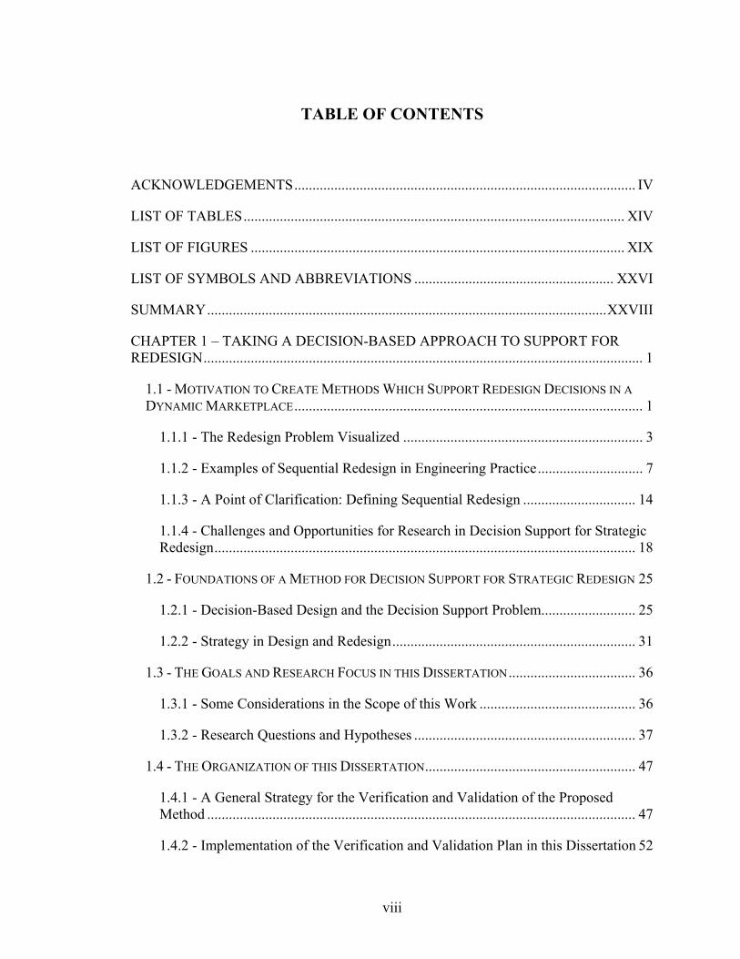
TABLE OF CONTENTS
ACKNOWLEDGEMENTS.............................................................................................. IV
LIST OF TABLES......................................................................................................... XIV
LIST OF FIGURES ....................................................................................................... XIX
LIST OF SYMBOLS AND ABBREVIATIONS ....................................................... XXVI
SUMMARY..............................................................................................................XXVIII
CHAPTER 1 – TAKING A DECISION-BASED APPROACH TO SUPPORT FOR REDESIGN......................................................................................................................... 1
1.1 - MOTIVATION TO CREATE METHODS WHICH SUPPORT REDESIGN DECISIONS IN A DYNAMIC MARKETPLACE................................................................................................ 1
1.1.1 - The Redesign Problem Visualized .................................................................. 3
1.1.2 - Examples of Sequential Redesign in Engineering Practice............................. 7
1.1.3 - A Point of Clarification: Defining Sequential Redesign ............................... 14
1.1.4 - Challenges and Opportunities for Research in Decision Support for Strategic Redesign.................................................................................................................... 18
1.2 - FOUNDATIONS OF A METHOD FOR DECISION SUPPORT FOR STRATEGIC REDESIGN 25
1.2.1 - Decision-Based Design and the Decision Support Problem.......................... 25
1.2.2 - Strategy in Design and Redesign................................................................... 31
1.3 - THE GOALS AND RESEARCH FOCUS IN THIS DISSERTATION................................... 36
1.3.1 - Some Considerations in the Scope of this Work ........................................... 36
1.3.2 - Research Questions and Hypotheses ............................................................. 37
1.4 - THE ORGANIZATION OF THIS DISSERTATION.......................................................... 47
1.4.1 - A General Strategy for the Verification and Validation of the Proposed Method ...................................................................................................................... 47
1.4.2 - Implementation of the Verification and Validation Plan in this Dissertation 52

ix
1.5 - STATUS AND PROMISE ........................................................................................... 59
CHAPTER 2 – OFFERING VARIETY IN A CHANGING MARKETPLACE – A LITERATURE REVIEW ................................................................................................. 61
2.1 - A PREVIEW OF THIS CHAPTER’S CONTENTS........................................................... 61
2.2 - NARROWING THE SCOPE OF THE ISSUES OF INTEREST IN STRATEGIC REDESIGN .... 61
2.3 - A REVIEW OF LITERATURE ON TOPICS OF RELEVANCE IN THE STUDY OF SYSTEMATIC REDESIGN ................................................................................................. 64
2.3.1 - Alternatives to Redesign................................................................................ 64
2.3.2 - Systematic Prescriptive and Descriptive Approaches to Redesign from Design Theory........................................................................................................... 70
2.3.3 - Means of and Alternatives to Offering Product Variety OR Means of Offering Product Variety .......................................................................................... 89
2.3.4 - A Summary of Relevant Literature on Commonality and Reuse in Product Family Design and Commentary on its Usefulness in Serial Redesign.................. 107
2.3.5 - Support for Long-Term Decision-Making .................................................. 133
2.4 - REVISITING THE RESEARCH QUESTIONS AND HYPOTHESES IN LIGHT OF THE LITERATURE REVIEW................................................................................................... 146
2.5 - CONTRIBUTIONS IN THIS CHAPTER TO THE DOMAIN-INDEPENDENT STRUCTURAL VALIDITY OF THE PROPOSED METHOD ........................................................................ 151
2.6 - STATUS AND PROMISE ......................................................................................... 153
CHAPTER 3 – ADDRESSING STRATEGIC REDESIGN AS A LIMITED PROBLEM OF OPTIMIUM ACCESS IN A GEOMETRIC SPACE ............................................... 154
3.1 - A PREVIEW OF THIS CHAPTER’S CONTENTS......................................................... 154
3.2 - DEVELOPMENT OF INDICES APPROPRIATE TO CHARACTERIZING THE GOODNESS OF REDESIGN .................................................................................................................... 155
3.2.1 - Motivation to Develop an Indices for Goodness in a Redesign Project ...... 155
3.2.2 - A Redesign Metric Thought Exercise.......................................................... 156
3.2.3 - A Pair of Proposed Indices for Difficulty the Early Stages of Redesign .... 167
3.2.4 - A Proposed Index for Redesign Effort and Commonality / Non-Commonality the Early Stages of Redesign .................................................................................. 174

x
3.2.5 - Modification of the Proposed Indices for Use in Synthesis ........................ 179
3.2.6 - A Critical Evaluation of the Proposed Redesign Metrics............................ 185
3.3 - ADAPTATION OF THE PRODUCT PLATFORM CONSTRUCTAL THEORY METHOD TO SEQUENTIAL STRATEGIC REDESIGN............................................................................. 189
3.3.1 - Accommodation of Multiple Discrete Redesign Targets and Strategic Redesign Goals Using a Compromise Decision Support Problem in the Product Platform Constructal Theory Method ..................................................................... 191
3.3.2 - Abstraction of Concepts in the Product Platform Constructal Theory Method to the Redesign of Engineering Systems ................................................................ 195
3.4 - A CONSTRUCTAL-INSPIRED REDESIGN DECISION SUPPORT METHOD.................. 201
3.4.1 - Step 1 – Definition of the Redesign Problem .............................................. 202
3.4.2 - Step 2 – Formulate Objective Functions ..................................................... 205
3.4.3 - Step 3 – Identify and Describe Redesign Options ....................................... 208
3.4.4 - Step 4 – Identify Number of Stages, Narrow Redesign Options, Create Groups and Hierarchically Rank Them .................................................................. 209
3.4.5 - Step 5 – Define Boundaries of Market Space.............................................. 210
3.4.6 - Step 6 – Formulate the Multistage Problem ................................................ 211
3.4.7 - Step 7 – Solve the Multistage Problem ....................................................... 215
3.4.8 - Step 8 – Examine Redesign Portfolios an Consider Iteration...................... 220
3.5 - CONTRIBUTIONS IN THIS CHAPTER TO THE DOMAIN-INDEPENDENT STRUCTURAL VALIDITY OF THE PROPOSED METHOD ........................................................................ 222
3.6 - STATUS AND PROMISE ......................................................................................... 224
CHAPTER 4 – EXAMPLE PROBLEM: REDESIGN OF FAMILIES OF UNIVERSAL MOTORS........................................................................................................................ 225
4.1 - A PREVIEW OF THIS CHAPTER’S CONTENTS......................................................... 225
4.2 - INTRODUCTION TO THE FULL UNIVERSAL MOTOR EXAMPLE............................... 227
4.3 - VERIFICATION AND VALIDATION OF PROPOSED REDESIGN INDICES .................... 237
4.3.1 - Plan for Verification and Validation of the Proposed Indices..................... 238

xi
4.3.2 - A Simple Universal Motor Redesign Scenario for Verification and Validation of the Proposed Indices ........................................................................................... 240
4.3.3 - Implementation of the Simple Redesign Scenario ...................................... 243
4.3.4 - Redesign Solutions for Varying Index Parameters and Weights................. 246
4.3.5 - The Role of these Redesign Scenarios in the Empirical Structural and Performance Validity of Hypothesis #1.................................................................. 274
4.4 - VERIFICATION AND VALIDATION OF THE PROPOSED APPROACH TO SEQUENTIAL AND STRATEGIC REDESIGN.......................................................................................... 277
4.4.1 - “Simple Redesign” Example Scenario ........................................................ 281
4.4.2 - “Redesign Based on Variety” Example Scenario........................................ 299
4.4.3 - “Redesign for Variety” Example Scenarios ................................................ 307
4.4.4 - General, More Complicated Redesign Scenarios ........................................ 317
4.4.5 - Revisiting the Metric Validation Examples................................................. 323
4.5 - CONTRIBUTIONS IN THIS CHAPTER TO THE DOMAIN-SPECIFIC STRUCTURAL AND PERFORMANCE VALIDITY OF THE PROPOSED METHOD................................................ 330
4.6 - STATUS AND PROMISE ......................................................................................... 336
CHAPTER 5 - CLOSURE.............................................................................................. 337
5.1 - A PREVIEW OF THE CHAPTER’S CONTENTS ......................................................... 337
5.2 - A SUMMARY OF THE WORK COMPLETED............................................................. 337
5.2.1 - Revisiting Research Questions and Hypotheses.......................................... 337
5.2.2 - A Summary of the Confidence Building Process and the Validity of the Proposed Method .................................................................................................... 341
5.3 - A CRITICAL REVIEW OF THE WORK AND THE ASSUMPTIONS MADE .................... 352
5.3.1 - General Comments ...................................................................................... 352
5.3.2 - Thoughts on Redesign Metrics .................................................................... 354
5.3.3 - Thoughts on the Implementation of this Approach ..................................... 356
5.3.4 - Thoughts on the Redesign Examples........................................................... 357

xii
5.4 - A REVIEW OF INTELLECTUAL CONTRIBUTIONS.................................................... 360
5.5 - AVENUES OF FUTURE WORK ............................................................................... 365
5.5.1 - Extension of Example Problems.................................................................. 365
5.5.2 - A Preemptive Approach Involving Redesign of Existing Systems............. 367
5.5.3 - Exploring New Opportunities for Variety in the Redesign Solution........... 367
5.5.4 - Use of Different Solution Strategies............................................................ 368
5.5.5 - Other Naturally-Inspired Approaches to Exploring Commonality ............. 369
5.6 - A PERSONAL STATEMENT.................................................................................... 370
APPENDIX A - EXPANDED DATA FROM VALIDATION OF METRICS/INDICES......................................................................................................................................... 379
APPENDIX B – MATLAB FUNCTIONS AND SCRIPTS .......................................... 398
B.1.1 – “solvequasicon.m” Program....................................................................... 399
B.1.2 – “redesigninputs.m” Program ...................................................................... 404
B.1.3 – “createcomoppmatrix.m” Program............................................................. 408
B.1.4 – “checkndiv.m” Program ............................................................................. 410
B.1.5 – “createspaceelements.m” Program............................................................. 411
B.1.6 – “checkexistinelem.m” Program.................................................................. 413
B.1.7 – “createtargassignments.m” Program .......................................................... 415
B.1.8 – “narrowtargassignments.m” Program ........................................................ 416
C.1.9 – “createeqconst.m” Program........................................................................ 418
B.1.10 – “checkelements.m” Program.................................................................... 421
B.1.11 – “findgoodstart.m” Program ...................................................................... 422
B.1.12 – “findmidstart.m” Program........................................................................ 423
B.1.13 – “findlowstart.m” Program ........................................................................ 425
B.1.14 – “findhighstart.m” Program ....................................................................... 428
B.1.15 – “portfolioeval.m” Program....................................................................... 430

xiii
B.1.16 – “evalcontinuousri.m” Program................................................................. 432
B.1.17 – “evalcontinuouscdf.m” Program .............................................................. 433
B.1.18 – “evalvalue.m” Program ............................................................................ 434
B.1.19 – “createnonlconst.m” Program .................................................................. 434
B.2.1 – Experimental Input and Executable ........................................................... 437
B.2.2 – “solveAAO.m” Program ............................................................................ 438
B.2.3 – “createeqconstAAO.m” Program ............................................................... 441
B.2.4 – “findclosestartAAO.m” Program ............................................................... 443
B.2.5 – “findlowstartAAO.m” Program ................................................................. 446
B.2.6 – “findmidstartAAO.m” Program ................................................................. 448
C.2.7 – “findhighstartAAO.m” Program ................................................................ 451
B.2.8 – “portfolioevalAAO.m” Program ................................................................ 454
B.2.9 – “createnonlocnstAAO.m” Program............................................................ 456
REFERENCES ............................................................................................................... 461
VITA............................................................................................................................... 474

xiv
LIST OF TABLES
Table 1-1 – Major Revisions of B-52 Models, Based on Data from (Anonymous 2006) 11
Table 1-2 – Verbal Summary of Sequential Strategic Redesign Problem........................ 23
Table 1-3 – Research Challenges and Resulting Requirements of a Redesign Method... 39
Table 1-4 – A Summary of Research Questions and Hypotheses .................................... 46
Table 1-5 – Steps in the Validation of an Engineering Design Method (Pederson, Emblemsvag et al. 2000)................................................................................................... 51
Table 1-6 – Basic Sequential Redesign Problem Sub-Types............................................ 57
Table 2-1 – Assumed Features of a Strategic Sequential Redesign problem ................... 63
Table 2-2 – Condensed Requirements List for a Sequential Redesign Decision Support Method .............................................................................................................................. 63
Table 2-3– Summary of Information Included in Commonality/Non-Commonality Indices ............................................................................................................................. 109
Table 2-4 – Rating System for both CI-S (supplied changes due to coupling) and CI-R (changes received due to coupling) (Martin and Ishii 2002) .......................................... 120
Table 2-5 – Rating System for GVI (Martin and Ishii 2002) ......................................... 121
Table 2-6 – Relevance of Selected Existing Product Family Measures to Requirements for Sequential Redesign .................................................................................................. 132
Table 2-7 – A Summary of the Relevance of Literature Reviewed in this Chapter ....... 147
Table 3-1 – Original Design and Redesign Options for Robot Family .......................... 158
Table 3-2 – Proposed Redesigned Robot Family ........................................................... 159
Table 3-3 – The Robot Family with Redesign Choices Made........................................ 159
Table 3-4 – Four Different Types of Commonality Discounting Factors ...................... 173
Table 3-5 – Interpretations of CDF and RI Values......................................................... 177
Table 3-6 – Summary of Simple One-Variable Redesign Problem for Graphical Analysis......................................................................................................................................... 182

xv
Table 3-7 – Summary of Simple Redesign Problem for Graphical Analysis with New Existing Systems and Differences in Commonality Discounts ...................................... 184
Table 3-8 – Basic Redesign Decision at Any Stage i ..................................................... 194
Table 3-9 – Basic Redesign Decision at Any Stage in the Multistage Process .............. 214
Table 4-1 – Universal Motor Redesign Variables .......................................................... 229
Table 4-2 – Universal Motor Responses of Interest ....................................................... 231
Table 4-3 – cDSP Formulation of Redesign Problem for Validation of Indices ............ 241
Table 4-4 – Baseline Family Design for Simple Redesign Scenario.............................. 249
Table 4-5 – Baseline Family Responses for Simple Redesign Scenario ....................... 249
Table 4-6 – Summary of cDSP Reformulated to Test RI ............................................... 250
Table 4-7 – Unique Values of a Difficult Na for Increasing RI Archimedean Weight .. 251
Table 4-8 – Family with Na Difficult to Change and RI Given a Weight of 0.625 ....... 252
Table 4-9 – Unique Values of an Easy Na for Increasing RI Archimedean Weight ...... 253
Table 4-10 – Family with Na Easy to Change and RI Given a Weight of 0.625 ........... 254
Table 4-11 – Summary of cDSP Reformulated to Test CDF ......................................... 256
Table 4-12 – Unique Values of a Valuable Na for Increasing CDF Archimedean Weight......................................................................................................................................... 257
Table 4-13 – Family with Na Commonality Valuable and CDF Given a Weight of 0.625......................................................................................................................................... 258
Table 4-14 – Unique Values of a Worthless Na for Increasing CDF Archimedean Weight......................................................................................................................................... 259
Table 4-15 – Family with Na Commonality Worthless and CDF Given a Weight of 0.625......................................................................................................................................... 260
Table 4-16 – Instances of Valuable Staggered Retirement Commonality for Increasing CDF Archimedean Weight ............................................................................................. 261
Table 4-17 – Family in Which Staggered Retirement Commonality is Particularly Valuable with CDF Given a Weight of 0.625................................................................. 263
Table 4-18 – Instances of Valuable Staggered Production Commonality for Increasing CDF Archimedean Weight ............................................................................................. 264

xvi
Table 4-19 – Instances of Worthless Staggered Retirement Commonality for Increasing CDF Archimedean Weight ............................................................................................. 266
Table 4-20 –Family in Which Staggered Retirement Commonality is Worthless with CDF Given a Weight of 0.625 ........................................................................................ 267
Table 4-21 –Effect of Increasing CDF Weight on Instances of Design Reuse in a Scenario with Equally Valuable Commonality.............................................................................. 268
Table 4-22 – Summary of cDSP Reformulated to Test RI and CDF Together .............. 270
Table 4-23 –Sample Redesigned Family Using Both RI and CDF with Weights of 1/3 Each................................................................................................................................. 270
Table 4-24 – Summary of cDSP Reformulated to Make Use of the PFPF..................... 272
Table 4-25 – Unique Variable Values for Increasing PFPF Archimedean Weight........ 273
Table 4-26 – Summary of “Simple Redesign” Problem................................................. 282
Table 4-27 – Redesign Difficulties Assigned to Variables in “Simple Redesign” Scenario......................................................................................................................................... 284
Table 4-28 – Commonality Discounts Associated with the Variables and Types of Production Overlap Present in the “Simple Redesign” Scenario.................................... 285
Table 4-29 – The First Stage Decision in the “Simple Redesign” Scenario................... 289
Table 4-30 – The Second Stage Decision in the “Simple Redesign” Scenario .............. 290
Table 4-31 – The Third Stage Decision in the “Simple Redesign” Scenario ................. 291
Table 4-32 – Most Promising Solution “Simple Redesign” Problem Based Solely on Objective Function Value ............................................................................................... 294
Table 4-33 – Original and Newly Tested Construct Arrangements ............................... 296
Table 4-34 – Most Promising Solution “Simple Redesign” Problem Using New Mode Arrangement #3 and Constructal Commonality ............................................................. 298
Table 4-36 – Summary of “Redesign Based on Variety” Problem ................................ 301
Table 4-36 – Most Promising “Redesign Based on Variety” Solution Based Solely on Objective Function Value ............................................................................................... 304
Table 4-37 – Most Promising “Redesign Based on Variety” Solution Utilizing Constructal Commonality and Indices............................................................................ 305

xvii
Table 4-38 – Most Promising “Redesign Based on Variety” Solution Utilizing Constructal Commonality Alone .................................................................................... 306
Table 4-40 – Summary of “Redesign for Variety” Problem........................................... 309
Table 4-29 – The First Stage Decision in the “Redesign for Variety” Scenario ............ 312
Table 4-41 – The Second Stage Decision in the “Redesign for Variety” Scenario........ 313
Table 4-42 – The Third Stage Decision in the “Redesign for Variety” Scenario........... 314
Table 4-43 – Most Promising “Redesign for Variety” Solution Utilizing Constructal Commonality and Indices ............................................................................................... 316
Table 4-44 – Summary of “General Redesign” Problem................................................ 319
Table 4-45 – Most Promising “General Redesign” Solution.......................................... 320
Table 4-47 – Most Promising “General Redesign” Solution Utilizing Constructal Commonality Only.......................................................................................................... 322
Table 4-47 – Most Promising Redesign Plan for Validation Scenario #1 According to Objective Function Value Only ...................................................................................... 324
Table 4-48 – Most Promising Redesign Plan for Validation Scenario #1 Utilizing Constructal-Inspired Commonality................................................................................. 325
Table 4-49 – Most Promising Redesign Plan for Validation Scenario #2 Without Use of Either Index..................................................................................................................... 327
Table 4-50 – Most Promising Redesign Plan for Validation Scenario #2 With Use of Both Indices ............................................................................................................................. 329
Table A-1 – Unique Values of a Difficult L for Increasing RI Archimedean Weight ....380
Table A-2 – Redesigned Family with L Difficult to Change and RI Given a Weight of 0.625.................................................................................................................................381 Table A-3 – Unique Values of an Easy L for Increasing RI Archimedean Weight ........382 Table A-4 – Family with L Easy to Change and RI Given a Weight of 0.625................383 Table A-5 – Unique Values of a Valuable Nf for Increasing CDF Archimedean Weight ..........................................................................................................................................384 Table A-6 – Family with Nf Commonality Valuable and CDF Given a Weight of 0.625 ..........................................................................................................................................385

xviii
Table A-7 – Unique Values of a Valuable L for Increasing CDF Archimedean Weight ..........................................................................................................................................385 Table A-8 – Family with L Commonality Valuable and CDF Given a Weight of 0.625 ..........................................................................................................................................387 Table A-9 – Unique Values of a Worthless Nf for Increasing CDF Archimedean Weight ..........................................................................................................................................388 Table A-10 – Family with Nf Commonality Worthless and CDF Given a Weight of 0.625 ..........................................................................................................................................389 Table A-11 – Unique Values of a Worthless L for Increasing CDF Archimedean Weight ..........................................................................................................................................389 Table A-12 – Family with L Commonality Worthless and CDF Given a Weight of 0.625 ..........................................................................................................................................390 Table A-13 – cDSP Formulation of Special Redesign Problem for Validation of Indices ..........................................................................................................................................391 Table A-14 – Instances of Valuable SP Commonality for Increasing CDF Archimedean Weight in the Special Scenario ........................................................................................392 Table A-15 – Special Scenario Family in Which SP Commonality is Particularly Valuable with CDF Given a Weight of 0.625..................................................................393 Table A-16 – Instances of Valuable PG Commonality for Increasing CDF Archimedean Weight in the Special Scenario ........................................................................................394 Table A-17 – Special Scenario Family in Which PG Commonality is Particularly Valuable with CDF Given a Weight of 0.625..................................................................395 Table A-18 – Instances of Worthless Perfect Commonality for Increasing CDF Archimedean Weight .......................................................................................................396 Table A-19 –Family in Which Perfect Commonality is Worthless with CDF Given a Weight of 0.625 ...............................................................................................................397
xix
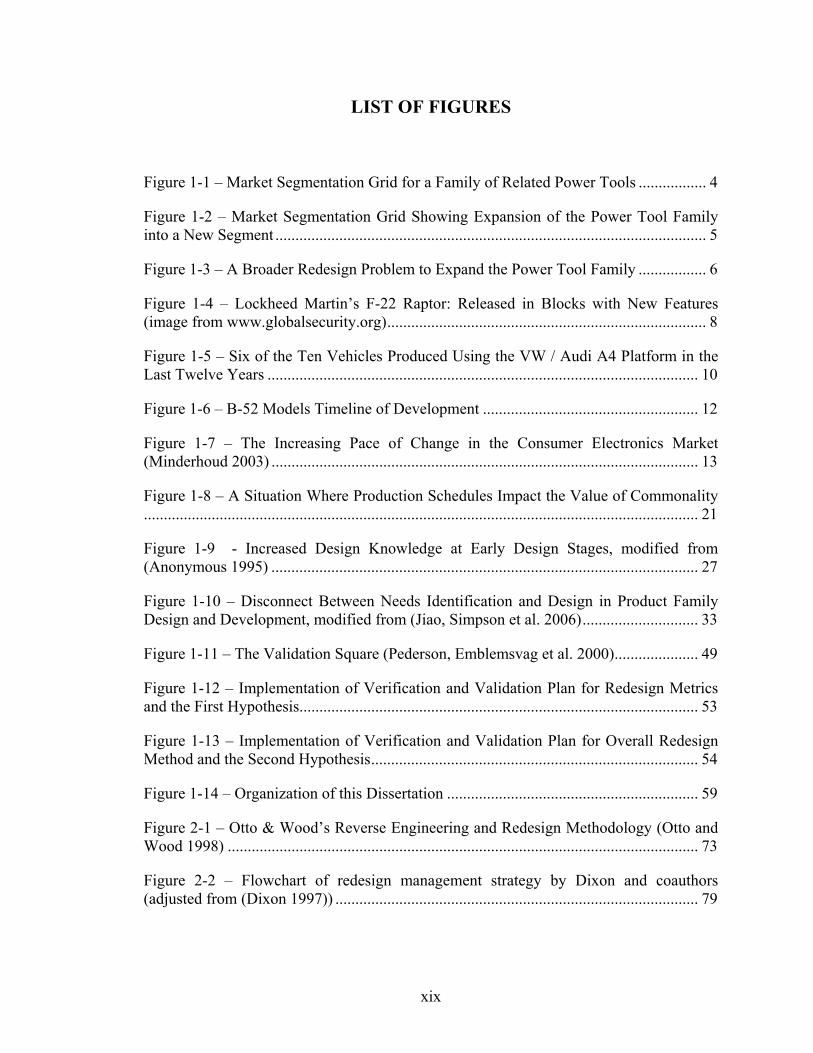
LIST OF FIGURES
Figure 1-1 – Market Segmentation Grid for a Family of Related Power Tools ................. 4
Figure 1-2 – Market Segmentation Grid Showing Expansion of the Power Tool Family into a New Segment ............................................................................................................ 5
Figure 1-3 – A Broader Redesign Problem to Expand the Power Tool Family ................. 6
Figure 1-4 – Lockheed Martin’s F-22 Raptor: Released in Blocks with New Features (image from www.globalsecurity.org)................................................................................ 8
Figure 1-5 – Six of the Ten Vehicles Produced Using the VW / Audi A4 Platform in the Last Twelve Years ............................................................................................................ 10
Figure 1-6 – B-52 Models Timeline of Development ...................................................... 12
Figure 1-7 – The Increasing Pace of Change in the Consumer Electronics Market (Minderhoud 2003) ........................................................................................................... 13
Figure 1-8 – A Situation Where Production Schedules Impact the Value of Commonality........................................................................................................................................... 21
Figure 1-9 - Increased Design Knowledge at Early Design Stages, modified from (Anonymous 1995) ........................................................................................................... 27
Figure 1-10 – Disconnect Between Needs Identification and Design in Product Family Design and Development, modified from (Jiao, Simpson et al. 2006)............................. 33
Figure 1-11 – The Validation Square (Pederson, Emblemsvag et al. 2000)..................... 49
Figure 1-12 – Implementation of Verification and Validation Plan for Redesign Metrics and the First Hypothesis.................................................................................................... 53
Figure 1-13 – Implementation of Verification and Validation Plan for Overall Redesign Method and the Second Hypothesis.................................................................................. 54
Figure 1-14 – Organization of this Dissertation ............................................................... 59
Figure 2-1 – Otto & Wood’s Reverse Engineering and Redesign Methodology (Otto and Wood 1998) ...................................................................................................................... 73
Figure 2-2 – Flowchart of redesign management strategy by Dixon and coauthors (adjusted from (Dixon 1997)) ........................................................................................... 79
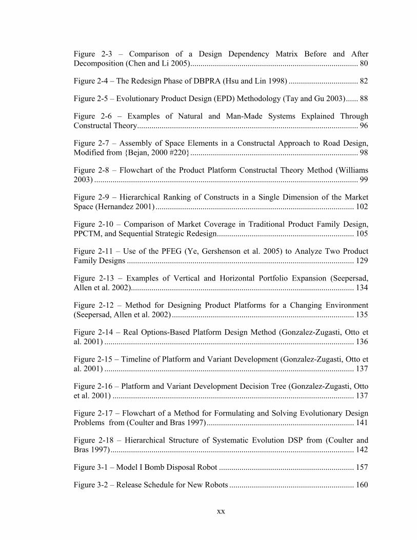
xx
Figure 2-3 – Comparison of a Design Dependency Matrix Before and After Decomposition (Chen and Li 2005).................................................................................. 80
Figure 2-4 – The Redesign Phase of DBPRA (Hsu and Lin 1998) .................................. 82
Figure 2-5 – Evolutionary Product Design (EPD) Methodology (Tay and Gu 2003)...... 88
Figure 2-6 – Examples of Natural and Man-Made Systems Explained Through Constructal Theory............................................................................................................ 96
Figure 2-7 – Assembly of Space Elements in a Constructal Approach to Road Design, Modified from {Bejan, 2000 #220}.................................................................................. 98
Figure 2-8 – Flowchart of the Product Platform Constructal Theory Method (Williams 2003) ................................................................................................................................. 99
Figure 2-9 – Hierarchical Ranking of Constructs in a Single Dimension of the Market Space (Hernandez 2001) ................................................................................................. 102
Figure 2-10 – Comparison of Market Coverage in Traditional Product Family Design, PPCTM, and Sequential Strategic Redesign................................................................... 105
Figure 2-11 – Use of the PFEG (Ye, Gershenson et al. 2005) to Analyze Two Product Family Designs ............................................................................................................... 129
Figure 2-13 – Examples of Vertical and Horizontal Portfolio Expansion (Seepersad, Allen et al. 2002)............................................................................................................. 134
Figure 2-12 – Method for Designing Product Platforms for a Changing Environment (Seepersad, Allen et al. 2002) ......................................................................................... 135
Figure 2-14 – Real Options-Based Platform Design Method (Gonzalez-Zugasti, Otto et al. 2001) .......................................................................................................................... 136
Figure 2-15 – Timeline of Platform and Variant Development (Gonzalez-Zugasti, Otto et al. 2001) .......................................................................................................................... 137
Figure 2-16 – Platform and Variant Development Decision Tree (Gonzalez-Zugasti, Otto et al. 2001) ...................................................................................................................... 137
Figure 2-17 – Flowchart of a Method for Formulating and Solving Evolutionary Design Problems from (Coulter and Bras 1997)........................................................................ 141
Figure 2-18 – Hierarchical Structure of Systematic Evolution DSP from (Coulter and Bras 1997)....................................................................................................................... 142
Figure 3-1 – Model I Bomb Disposal Robot .................................................................. 157
Figure 3-2 – Release Schedule for New Robots ............................................................. 160

xxi
Figure 3-3 – Two Products with Completely Coincident Production Schedules ........... 161
Figure 3-4 – Two Generic Products with Staggered Introduction Schedules................. 162
Figure 3-5 – Two Generic Products with Staggered Retirements .................................. 162
Figure 3-6 – Two Generic Products with Completely Staggered Production ................ 163
Figure 3-7 – Two Generic Products with Completely Staggered but Overlapping Production....................................................................................................................... 164
Figure 3-8 – Two Generic Products with a Production Gap........................................... 164
Figure 3-9 – Example of the Role of Difficulty in Redesign.......................................... 166
Figure 3-10 – Example of Module-Swapping to Redesign ............................................ 167
Figure 3-11 – Redesign Schedule ................................................................................... 169
Figure 3-12 –Commonality Opportunity Matrix ............................................................ 170
Figure 3-13 – Plot of CDF Versus RI ............................................................................. 177
Figure 3-14 – CDF Plots for Simple One-Variable Example ......................................... 182
Figure 3-15 – RI Plots for Simple One-Variable Example............................................. 183
Figure 3-16 – CDF Plots for Simple One-Variable Example with New Existing Systems and Weights .................................................................................................................... 184
Figure 3-17 – RI Plots for Simple One-Variable Example with New Existing Systems 185
Figure 3-18 – Parallels Between PPCTM and Proposed Method................................... 191
Figure 3-19 – Buffer Zone for Market Space Explained ................................................ 199
Figure 3-20 – Flowchart of Proposed Constructal-Inspired Redesign Method .............. 202
Figure 3-21 – Creation of the Commonality Opportunity Matrix .................................. 204
Figure 3-22 – Explanation of Role of Existing Systems in Constraining Modes in Space Elements.......................................................................................................................... 212
Figure 3-23 – Rationale for Deciding Element Will or Will Not Contain Solution ....... 215
Figure 3-24 – Flowchart of Solution Process ................................................................. 217
Figure 3-25 – The "Common Sense Rule" of Space Element Assignments Explained . 219

xxii
Figure 3-26 - Assignment of Targets to Space Elements Explained .............................. 220
Figure 3-27 – Summary of Developments that Went Into the Proposed Method .......... 222
Figure 4-1 – The Role of Example Problems in Verification and Validation in this Chapter............................................................................................................................ 227
Figure 4-2 – Universal Motor Schematic (AMETEK, Inc., 2006) ................................. 229
Figure 4-3 – Universal Motor Components, Modified from (Hernandez, Allen et al. 2002)......................................................................................................................................... 230
Figure 4-4 – Production Schedule for Simple Universal Motor Redesign Scenario ...... 240
Figure 4-5 – Flowchart of Matlab Implementation of Simplified Problem Solving Approach......................................................................................................................... 244
Figure 4-6 – Random Assignment of Existing System Values to Start Points.............. 245
Figure 4-7 – Objective Function Values for Increasing Numbers of Start Points .......... 246
Figure 4-8 – Effect of Increasing RI Weight on Instances of Redesign in a Difficult Na......................................................................................................................................... 251
Figure 4-9 – Effect of Increasing RI Weight on Instances of Redesign in an Easy Na.. 253
Figure 4-10 – Effect of Increasing RI Weight on Instances of Redesign When All Options are Equally-Difficult ....................................................................................................... 255
Figure 4-11 – Effect of Increasing CDF Weight on Instances of Redesign in an Valuable Na.................................................................................................................................... 257
Figure 4-12 – Effect of Increasing CDF Weight on Instances of Redesign with a Worthless Na................................................................................................................... 259
Figure 4-13 – Effect of Increasing CDF Weight on Instances of Staggered Retirement Commonality................................................................................................................... 262
Figure 4-14 – Effect of Increasing CDF Weight on Instances of Staggered Production Commonality................................................................................................................... 264
Figure 4-15 – Special Redesign Scenario Run to Further Test CDF.............................. 265
Figure 4-16 – Effect of Increasing CDF Weight on Instances of Worthless Staggered Retirement Commonality................................................................................................ 267
Figure 4-17 – Effect of Increasing CDF Weight on Instances of Design Reuse When All Commonality is Equally Valuable .................................................................................. 268

xxiii
Figure 4-18 – Effect of Weight Given to PFPF on Total Number of Unique Variable Values in Family ............................................................................................................. 274
Figure 4-19 – Flowchart of Matlab Implementation of Full Constructal-Inspired Approach......................................................................................................................... 280
Figure 4-20 – Flowchart Representation of the Issues in Simple Redesign ................... 281
Figure 4-21 – Redesign Schedule Matrix for the “Simple Redesign” Scenario ............. 282
Figure 4-22 – Commonality Opportunity Matrix for the “Simple Redesign” Scenario . 282
Figure 4-23 – Redesign Market Space for “Simple Redesign” Example ....................... 288
Figure 4-24 – Space Element Arrangement of Most Promising Solution Using Old Constructs ....................................................................................................................... 295
Figure 4-25 – Space Element Arrangement for Most Promising Solution Utilizing Constructal Commonality and Third New Mode Arrangement ..................................... 298
Figure 4-26 – Flowchart Representation of the Issues in Redesign Based on Variety... 300
Figure 4-27 – Redesign Schedule Matrix for the “Redesign Based on Variety” Scenario......................................................................................................................................... 301
Figure 4-28 – Commonality Opportunity Matrix for “Redesign Based on Variety Scenario”......................................................................................................................... 301
Figure 4-29 – Redesign Market Space for “Redesign Based on Variety” Example....... 303
Figure 4-30 – Space Element Arrangement for Most Promising Plan for “Redesign Based on Variety”...................................................................................................................... 305
Figure 4-31 – Space Element Arrangement for “Redesign Based on Variety” Scenario Utilizing Only Constructal-Forced Commonality .......................................................... 307
Figure 4-32 – Flowchart Representation of the Issues in Redesign for Variety............. 308
Figure 4-33 – Redesign Schedule Matrix for the “Redesign for Variety” Scenario....... 309
Figure 4-34 – Commonality Opportunity Matrix for the “Redesign for Variety” Scenario......................................................................................................................................... 309
Figure 4-35 – Redesign Market Space for “Redesign for Variety” Example................. 311
Figure 4-36 – Most Promising Arrangement of Space Elements for “Redesign for Variety” Scenario............................................................................................................ 316
Figure 4-37 – Flowchart Representation of the Issues in General Redesign.................. 317

xxiv
Figure 4-38 – Redesign Schedule Matrix for the “General Redesign” Scenario............ 318
Figure 4-39 – Commonality Opportunity Matrix for the “General Redesign” Scenario 318
Figure 4-40 – Redesign Market Space for “General Redesign” Example...................... 320
Figure 4-41 – Most Promising Arrangement of Space Elements for “General Redesign” Scenario........................................................................................................................... 321
Figure 4-42 – Most Promising Space Element Arrangement for the “General Redesign” Scenario Utilizing Constructal Commonality Only........................................................ 322
Figure 4-43 – Space Element Arrangement for Most Promising Constructal-Inspired Solution to First Metric Validation Example.................................................................. 326
Figure 4-44 – Space Element Arrangement for Most Promising Constructal-Inspired Solution to Second Metric Validation Example Without Use of Indices ....................... 328
Figure 4-45 – Space Element Arrangement for Most Promising Constructal-Inspired Solution to Second Metric Validation Example With Use of Both Indices ................... 329
Figure 5-1 – Exploded View of the Validation Square in Which Step 6 is the Focus Here......................................................................................................................................... 342
Figure 5-2 – Exploring Opportunities for New Variety from Shared Space Elements .. 368
Figure 5-3 – Structured Genetic Algorithm Approach to Describing a Redesign Solution......................................................................................................................................... 369
Figure 5-4 – An Example of a Situation Where Amount of Overlap Might Matter....... 376
Figure A-1 – Effect of Increasing RI Weight on Instances of Redesign in a Difficult L Variable ...........................................................................................................................381
Figure A-2 – Effect of Increasing RI Weight on Instances of Redesign in an Easy L ....382
Figure A-3 – Effect of Increasing CDF Weight on Instances of Redesign in a Valuable Nf ..........................................................................................................................................384
Figure A-4 – Effect of Increasing CDF Weight on Instances of Redesign in a Valuable L ..........................................................................................................................................386
Figure A-5 – Effect of Increasing CDF Weight on Instances of Redesign with a Worthless Nf ....................................................................................................................388
Figure A-6 – Effect of Increasing CDF Weight on Instances of Redesign in a Worthless L ..........................................................................................................................................390

xxv
Figure A-7 – Effect of Increasing CDF Weight on Instances of SP Commonality in the Special Scenario...............................................................................................................393
Figure A-8 – Effect of Increasing CDF Weight on Instances of PG Commonality in the Special Scenario...............................................................................................................394
Figure A-9 – Effect of Increasing CDF Weight on Instances of Worthless Perfect Commonality....................................................................................................................396

xxvi
LIST OF SYMBOLS AND ABBREVIATIONS
General Nomenclature CDF Commonality Discount Factor cDSP Compromise Decision Support Problem CI1 Commonality Index (Martin and Ishii 1996) CI2 Commonality Index (Martin and Ishii 1997) CoupI Coupling Index (Martin and Ishii 2002) CPCI Component and Process Commonality Indices (Jiao and
Tseng 2000) DCI Design Capability Indices (Chen, Simpson et al. 1996) DF Design Freedom (Simpson, Rosen et al. 1998) DomI Degree of Commonality Index (Collier 1981) DSP Decision Support Problem DSPT Decision Support Problem Technique GVI Generational Variety Index (Martin and Ishii 2002) NCI Non-Commonality Index (Simpson, Seepersad et al. 2001) PCI Percent Commonality Index (Siddique and Rosen 1998) PDI Performance Deviation Index (Simpson, Seepersad et al.
2001) PFEG Product Family Evaluation Graphs (Ye, Gershenson et al.
2005) PFPF Product Family Penalty Function (Messac, Martinez et al.
2002; Messac, Martinez et al. 2002) PLCI Product Line Commonality Index (Kota, Sethuraman et al.
2000) PPCTM Product Platform Concept Exploration Method RDI Redesign Difficulty Index (for individual variables) RI Redesign Index based on RDI sDSP Selection Decision Support Problem TCCI Total Constant Commonality Index (Wacker and Treleven
1986) TCPI Total Cost of Providing Variety (Martin and Ishii 1996) u-cDSP Utility-based Compromise Decision Support Problem
Key Nomenclature Related to Universal Motor Example η Efficiency φ Magnetic flux in motor ℑ Megnetomotive Force ℜ Reluctance µ Permability ρ Density
ω Radial velocity Awa Cross-sectional area of wire in the wrappings of the
armature/rotor Awf Cross-sectional area of the wire in the field/stator

xxvii
H Magnetizing intensity I Current K Motor constant L Stack length lc Mean magnetic path length of stator lgap Air gap lr Diameter of armature m Mass Na Number of wire turns in armature/rotor Nc Number of wire turns in rotor/armature Nf` Number of wire turns in field/stator Ns Number of wire turns in stator/field P Power R Resistance r Radius of the motor Sat Magnetizing intensity T Torque t Thickness of field/stator Vi Voltage

xxviii
SUMMARY
Researchers have paid relatively little attention to the fact that most design
activities are actually more like redesign. These activities are characterized by an attempt
to leverage experience, knowledge, and the capital that a company has already invested
into existing engineering systems. In this dissertation, it is proposed that an approach be
developed to aid designers in making decisions in redesign problems when there exist
systems to be leveraged and multiple new systems to be created. In addition, strategy is
introduced to the problem through the consideration that new systems may not be offered
all at once, as is often assumed in product family design research. In this dissertation, the
aim of the designer is assumed to be a creation, through redesign, of a series of new
systems with desirable and distinct performance levels. In addition, a plan is required to
involve as little redesign effort throughout the life of the family of systems as possible
The proposed approach is based upon the concepts of Constructal Theory and
previous work to create methods for the design of mass customized families of products.
The existing methods are abstracted and heavily modified through the infusion of the
compromise Decision Support Problems at all stages of the decision-making process. In
addition, two indices are developed to represent considerations unique to redesign as
opposed to original design. These indices for redesign effort and commonality value are
utilized in the overall objective formulation for the approach. Through a thorough
validation process and a large number of redesign scenarios, it is shown that the overall
approach proposed can lead the designer towards promising redesign plans involving
leveraging of existing systems, but that the constructal-inspired approach in and of itself
has certain limitations when applied to redesign.

1
CHAPTER 1
TAKING A DECISION-BASED APPROACH TO SUPPORT FOR REDESIGN
1.1 - MOTIVATION TO CREATE METHODS WHICH SUPPORT REDESIGN
DECISIONS IN A DYNAMIC MARKETPLACE
Very little that we see around us in the world today is new. Products may newly
constructed, newly discovered, or new to us, but when it comes to man-made artifacts,
there is little around us that is truly original. Even the best known ground-breaking,
genre-bending, and market segment-defying products are built upon the foundation of
products, components, materials, technologies, and ideas developed long before them.
One need not look any further than the popular iPod for an example of how incremental
improvements to what would otherwise be off-the-shelf technology can lead to a break-
through product. The truth of the matter is that nearly everything we as a society produce
comes about as a result of redesign. Sometimes that redesign takes place at a conceptual
level. For instance, when developing a new pen, at least the basic concept of a long
cylindrical tool with a writing tip is usually retained from earlier models. Oftentimes,
however, the redesign takes place at a more practical level where generations of products
or systems come about through a sequence of gradual change; a phenomenon described
here as serial or sequential redesign.

2
The evolutionary process that is sequential redesign can take on many shapes and
forms. The demand for new product revisions that create this shape can be driven by all
manner of factors including but not limited to:
• Expansion or contraction of market segments as customers around the world
become reachable by a company’s products or trends fizzle;
• Emergence of new technologies that expand product capabilities or improve those
that existed previously;
• Complementary products or technology that create or enhance market niches; and
• Myriad unforeseen events including weather, war, terrorism, or the combined
effects of multiple factors.
Regardless of the driving factors, the result is that families of products emerge
over time, either in a planned manner or haphazardly. Too often, the emergence of new
products or systems is governed in an ad-hoc manner as needs arise. This leads to a
situation in which redesign decisions are made using incomplete information about their
effects on the system as a whole and entirely without consideration of the larger
implications of the changes to be made. Even if the changes made result in workable new
designs, unwise redesign decisions can set the family of systems that will be developed in
the future up for failure. Poor decisions can design the family into a corner, making it
harder or more costly to achieve later goals.
The goal in carrying out the work described in this dissertation is to present, test,
and evaluate a method of decision support for engineers who are attempting to redesign.
It is hoped that by using this method, engineers might avoid ad-hoc decisions that may

3
lead to sub-par system performance and assure that future redesigns are both less costly
and more likely to succeed.
1.1.1 - The Redesign Problem Visualized
The market segmentation grid (Meyer 1997) provides a convenient way of
visualizing the problems facing engineers who want to redesign a system to meet shifting
needs. In the market segmentation grid, a market is plotted in two dimensions and broken
down vertically according the price segments of different products a company offers and
horizontally according to the various functions of the company’s products. The market
segmentation grid has commonly been used to identify opportunities and strategies for
two types of leveraging. Horizontal leveraging occurs when products with different basic
functions but similar price scales share components. Vertical leveraging occurs when
products of different prices and performance levels but with common functions share
components. In Figure 1-1, however, the market segmentation grid is used to display a
hypothetical family of power tools produced by one company –some of which share
common power supplies, motors, and other components in an attempt to realize cost
savings.
The products plotted in the market segmentation grid in Figure 1-1 may serve
their individual market niches well, but what happens when the power tool manufacturer
decides to expand upon its offerings by offering a belt sander? This situation is portrayed
in Figure 1-2. Given the company executives’ interest in cost savings and improved
reliability, it is natural for engineers and designers to look for ways to reuse pieces of
existing products and realize new goals through redesign. How should designers go about

4
creating a preliminary redesign plan in a systematic manner? How do the designers take
into account the various components and capabilities of all the pre-existing products?
Figure 1-1 – Market Segmentation Grid for a Family of Related Power Tools

5
Figure 1-2 – Market Segmentation Grid Showing Expansion of the Power Tool Family into a New Segment
The problem becomes even more complicated if a broader long-term perspective
is taken and the designers are allowed to know the next goals of the company: to further
expand the new belt-sander product line in the years to follow while simultaneously
expanding their offerings of circular saws and reciprocating saws. This situation is shown
in Figure 1-3. In essence, the company will be asking its engineers to sequentially
redesign elements of the existing product family to meet new needs.

6
Figure 1-3 – A Broader Redesign Problem to Expand the Power Tool Family
The natural tendency of the engineer faced with a redesign problem is to look for
the easiest ways to change a system to meet new needs or accommodate new technology.
Based on previous experience with a given system, it may seem obvious to a designer
how the system can best be redesigned to meet new goals. Even if the course of action is
not obvious –the subsection in which the changes should occur or the discipline expert
who should oversee them may seem to be clear. Ideally, such an expert or group of
experts can find the needed changes in their subsystem, resulting in a smooth transition to
a new system model. What happens however, when the course of action is not clear;
when it is not obvious which subsystems should be modified or who can make all of the
needed changes? Furthermore, how can one be sure that a given group subsystem can
realize all the needed changes and that those changes will not spill over into a cascade of
rework in other subsystems? How does the designer know that the seemingly obvious
solution is really going to be the least costly over the long term? Unfortunately, while

7
there are any number of established methods for systematically designing engineering
artifacts from scratch (Pugh 1991; Pahl and Beitz 1996; Cagan; Ulrich and Eppinger
2004), only a few similarly rigorous methods for redesign have been demonstrated. Many
of those redesign methods are limited to handling small, simple products (Otto and Wood
1998), redesigning only a single existing system to realize one new system(Dixon and
Colton 2000), identifying complications in redesign processes (Hsu and Lin 1998),
reducing the order of math models needed for redesign (Chen, Ding et al. 2005; Chen and
Li 2005; Chen and Li 2005; Chen, Li et al. 2005; Chen and Macwan 2005), or handling
the data involved in redesign(Tseng and Jiao 1998; Tay and Gu 2003).
While the situation put forward in this section involves a hypothetical power tool
maker, the issues facing that imaginary company are the same as those facing real
manufacturers and their designers today. In the next section, this fact is born out in a
series of examples that show the potential upsides and downsides of adopting redesign
strategies with long-term goals in mind.
1.1.2 - Examples of Sequential Redesign in Engineering Practice
Examples of products based on sequential redesign can be found in industries of
all sorts producing systems of all sizes and complexities. That redesign can take place
over time scales both long and short. The types of changes made and the impacts they
have can be either minimal –making a product seem to evolve over time- or more
pronounced –producing distinctive products that sometimes make it hard to realize that
they are the result of a redesign process.

8
In the aircraft industry, where development periods for some products can span
decades, a given aircraft model may be offered in several blocks throughout its lifespan.
Blocks are numerical designations of groups of aircraft with the same configuration.
(Sherman 2005). The F-22 Raptor, a cutting-edge fighter aircraft manufactured by
Lockheed Martin, first became operational in December of 2005. By mid-2007, there are
already plans for at least five blocks of aircraft emerging over the next few years, each
incorporating more of the electronic systems, new radar capabilities, improved weaponry,
and even the equipment needed for electronic warfare (Anonymous 2006). This timed
release of new product features is a planned part of the aircraft’s program, but it also has
large implications since any changes made in early blocks must either be carried forward
and accommodated in later blocks or revised again at extra cost. The ongoing
development of the F-22 and other modern aircraft will, if successful, show that planned
evolution from a starting point is possible when well managed.
Figure 1-4 – Lockheed Martin’s F-22 Raptor: Released in Blocks with New Features (image from www.globalsecurity.org)

9
One familiar example of sequential redesign at work is seen in the families of
vehicles produced by automotive manufacturers throughout the world. Many cars, trucks,
SUVs, and vans are based upon common platforms upon which different bodies and
features are built. Oftentimes, these platforms go years without major changes but each
year sees a “new” model of each vehicle emerge. A good example of the type of iteration
seen in an automobile platform is the Volkswagen / Audi A4 platform, which was
introduced in 1996 for use in the Audi A3. Part of a major effort to consolidate the
number of platforms used by Volkswagen (VW), the A4 is still in use today for
production of the New Beetle. In the last twelve years, it has also been used for
production of the Jetta, Golf, Audi TT, and several cars sold only in foreign countries. A
total of ten different models of cars (some of which are shown in Figure 1-5) were in
production at once using the same platform, and each of those models was revised in each
year it was offered (Whitney 2000; Anonymous 2003). The results of this consolidation
were that by the end of the 1990’s, VW vehicles shared 70% of their parts with other
vehicles and that the overall number of platforms needed was consolidated from 16 down
to just 4 (Winter and Zoia 2001). The downside of this strategy was only seen over the
course of several years as sales of some high-end models that used the platform slipped
and VW’s profit margin failed to improve. This situation was largely blamed on
customers who realized that they could buy a car with the same basic architecture,
engine, and underbody as a high-end model but pay less by choosing a lower-end VW
brand name. In the United States, customers opted for VW vehicles over Audis. In
Germany, they opted for Skodas made in the Czech Republic over VW’s(Miller 1999;

10
Miller 2002). To make matters worse, the platform strategy adopted by VW never
achieved the cost savings envisioned for it.
Figure 1-5 – Six of the Ten Vehicles Produced Using the VW / Audi A4 Platform in the Last Twelve Years
The Volkswagen A4 platform is an example of redesign and design leveraging
being taken too far, of valuing commonality and cost savings over good service to the
niches in one’s customer based, and of a company underestimating their customers’
powers of perception. Clearly, in redesigning an existing system or building a system
based on an existing platform, the recognition and preservation of distinct market niches
is an important goal to consider alongside achieving cost savings through commonality.
A more famous example of redesign in practice in the aerospace industry is the
evolution of the Boeing B-52 “Stratofortress” bomber. Eight distinct generations of this
aircraft (summarized in Table 1-1) have served the United States Air Force since it first
entered service in 1954 and the latest generation –first delivered in 1961- is expected to
serve well into the 21st century. Over the years, military and political leaders of the
United States have seen fit to continue to upgrade, maintain, and repair a fleet of B-52’s
instead of opting for a totally new design. This robust airframe is the result of successive
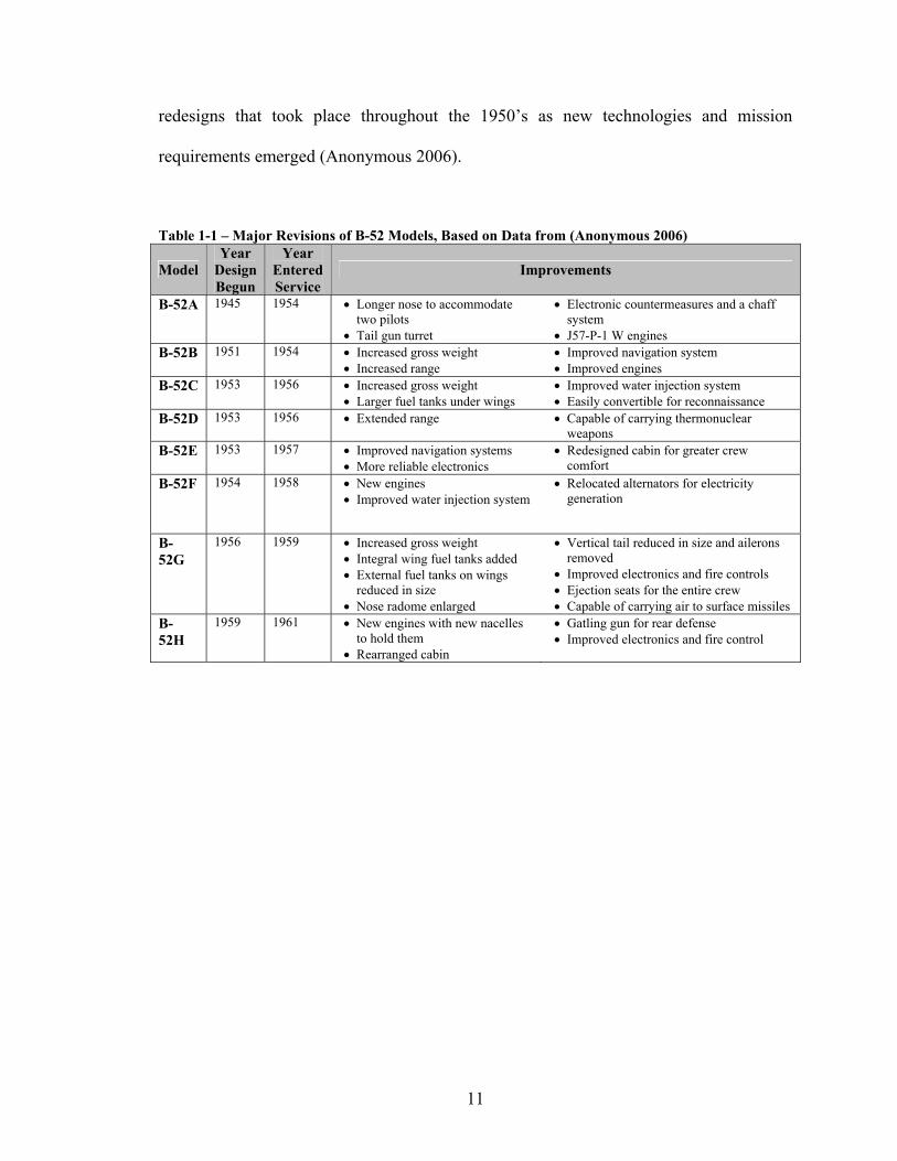
11
redesigns that took place throughout the 1950’s as new technologies and mission
requirements emerged (Anonymous 2006).
Table 1-1 – Major Revisions of B-52 Models, Based on Data from (Anonymous 2006)
Model Year
Design Begun
Year Entered Service
Improvements
B-52A 1945 1954 • Longer nose to accommodate two pilots
• Tail gun turret
• Electronic countermeasures and a chaff system
• J57-P-1 W engines B-52B 1951 1954 • Increased gross weight
• Increased range • Improved navigation system • Improved engines
B-52C 1953 1956 • Increased gross weight • Larger fuel tanks under wings
• Improved water injection system • Easily convertible for reconnaissance
B-52D 1953 1956 • Extended range • Capable of carrying thermonuclear weapons
B-52E 1953 1957 • Improved navigation systems • More reliable electronics
• Redesigned cabin for greater crew comfort
B-52F 1954 1958 • New engines • Improved water injection system
• Relocated alternators for electricity generation
B-52G
1956 1959 • Increased gross weight • Integral wing fuel tanks added • External fuel tanks on wings
reduced in size • Nose radome enlarged
• Vertical tail reduced in size and ailerons removed
• Improved electronics and fire controls • Ejection seats for the entire crew • Capable of carrying air to surface missiles
B-52H
1959 1961 • New engines with new nacelles to hold them
• Rearranged cabin
• Gatling gun for rear defense • Improved electronics and fire control

12
B-52 A
B-52 B
B-52 D
B-52 C
B-52 G
B-52 H
B-52 E
B-52 F
1945 1950 1955 1960 1965
In Service
In Service
In Service
In Service
In Service
In Service
In Service
Design & Development
Design & Development
Design & Development
Design & Development
Design & Development
Design & Development
Design & Development
In ServiceDesign & Development
Figure 1-6 – B-52 Models Timeline of Development
Sequential redesign is not limited to large, seemingly complex systems like
aircraft and automobiles. Research conducted by Philips elucidates a trend in recordable
media players that they say is representative of wider trends throughout the consumer
electronics industry. When the numbers for units sold and price per unit over the last few
decades are plotted for VHS tape recorders, CD recorders, and DVD recorders (see
Figure 1-7), it is readily apparent that something about the market is changing at a
quickening pace. As competition has increased in the electronics industry, products have
become commodities faster. This means that for the company that is first to market with a
new technology, and which usually has to price their product at a high level to recoup
their research and development costs, they have a very small window of opportunity to

13
capitalize on the high prices that early adopters are willing to pay. With increased
competition, other companies have become better at quickly copying technologies or
working product concepts, producing them more cheaply, and driving down prices.
Another byproduct of this situation is the need to continuously produce new variants of
products to introduce slight technological advances, manufacturing changes that lower
costs, or even redesigned parts. Companies like Philips find themselves producing these
product revisions at a much faster clip than they had to do in the past (Minderhoud 2003).
Figure 1-7 – The Increasing Pace of Change in the Consumer Electronics Market (Minderhoud 2003)
The examples given from Lockheed Martin, Volkswagen, Boeing, and Philips
demonstrate that in a situation where a family of products is needed, it is oftentimes
possible to know ahead of time what will differentiate these products, and that it is
possible to design with these differences in mind. What happens if demand for related
products continues to grow and change, however? In this case, it is necessary to redesign
existing families of products to suit. Philips sees the need for new revisions as a constant

14
struggle in the electronics industry; Lockheed Martin must look ahead to anticipate this
need in the future; Boeing and Volkswagen have each seen the respective positive and
negative ramifications of a redesign strategy built around a product platform. Facing
these new needs requires balancing a number of complex issues including:
• The number of new systems to be developed;
• The speed with which the new systems need to be ready and the staggered
schedule by which they will be produced;
• Distinct performance objectives for each new system being designed;
• The conflict between individual system’s performance goals and overall
companywide goals such as:
o Reduction of costs;
o Improvement of commonality
o Reduction of part quantities
• Consideration of what will come next beyond the current redesign task; will there
be more future revisions, and if so, how can their success be ensured?
Addressing these issues is the research goal described in this dissertation. In the
section that follows, some clarification between design and redesign is made in order to
clear up misconceptions that commonly occur when talking about “redesign.”
1.1.3 - A Point of Clarification: Defining Sequential Redesign

15
There are any number of systematic design methods which are widely taught and
accepted in engineering practice. Rarely do these methods touch upon how a designer
should go about realizing a system that is not to be designed from scratch. In the
systematic design methodology of Pahl and Beitz (Pahl and Beitz 1996), for instance,
three types of design are described:
• Original design, wherein a novel new artifact is created from scratch;
• Adaptive design, wherein a proven solution is adjusted to suit a new set of
requirements or a new application, possibly requiring some original design; and
• Variant design, wherein a proven solution is simply tweaked to meet a distinct set
of requirements;
Unfortunately, most of Pahl and Beitz’s attention is directed towards original
design, rarely even dropping a hint as to when pieces of their methodology should be
utilized or skipped to create an adaptive for variant design most effectively.
For the purposes of this work, redesign is taken to entail not just the creation of
the plans for how the existing system in question will be changed to meet new goals, but
also planning for what must be done to effect those changes. Applied to a physical
example, the redesign plan for a new model year of a car would include not only the
description of the changes to the exterior of the vehicle but also these three important
aspects: the description of the resulting changes to the manufacturing procedures, the
engineering time and costs associated with making the design changes, and any other
overhead associated with making the needed changes. In short, the concern in this
dissertation is not only with how a system might be changed to realize new technical
goals, but also how difficult it will be to begin producing the newly redesigned system.
16
“Redesign” is a term that is interpreted in a number of widely different ways
throughout the engineering design research community. Therefore, it is useful to discuss
the ways in which its use in this dissertation is unique. Any internet search for the word
“redesign” or “redesign method” will turn up myriad hits for articles and research papers.
A vast majority of these articles, however, deal only with redesign in the sense that the
paper concerns a design effort whose results can be compared to an existing product. As
such, these articles are more concerned with original design than with the question of
how one enterprise might best transition from one version of a product to another. A
typical example of this type of redesign is provided by Lim and Erdman (Lim and
Erdman 2002), who redesign a surgical instrument using type synthesis. The authors’
goals are not to change the function or performance of the instrument in any way.
Instead, their goals are to decrease the number of parts in the product, create a simpler
design internally, and make it easier to assemble.
Along similar lines, support for product family design research is often based
upon comparison between a family of products that are designed independently of one
another and a family of products that are designed simultaneously using systematic
product family design techniques. A good overview of such product family design
techniques is given by Simpson (Simpson 2003) and examples of this type of comparison
between new and existing products can be seen in numerous papers. A few examples of
product family redesign include the following: the redesign of an automotive underbody
to identify a platform by partitioning combinatorial design spaces Corbett and Rosen
(Corbett and Rosen 2004); the redesign of a family of xerographic machines using
function and variety heuristics by Zamirowski and Otto (Zamirowski and Otto 1999); the

17
identification of a product platform to redesign a family of motors by Simpson and
coauthors (Simpson, Maier et al. 1999); the use of formal concept analysis to increase
commonality by Nanda and coauthors(Nanda, Thevenot et al. 2005); the development of
life cycle modularity metrics to aid in redesigning the components of a product
(Newcomb, Bras et al. 1998; Newcomb, Rosen et al. 2003); and lastly the redesign of a
family of products to increase their modularity, reduce the part-count, and improve life-
cycle considerations by Bryant and coauthors (Bryant, Sivaramakrishnan et al. 2004).
For the purposes of the research described in this dissertation, redesign is defined
as follows:
Any design activity in which the goal of leveraging existing systems in order to
produce one or more systems with distinct new performance characteristics must be
balanced against the desire to minimize the resources involved through reuse of as much
as possible of existing systems, their design, and their manufacturing infrastructure.
Furthermore, it is posited here that important characteristics of redesign includes:
• The cost of switching over to new manufacturing facilities or processes;
• The cost of researching, developing, designing, and testing new components or
subsystems;
• Schedules of product release that do not exhibit perfect overlap; that is, not all
systems are offering simultaneously, bringing into question some of the
economies-of-scale argument for commonality; and

18
• An understanding of where the evolution of a product family is going next may
exist, allowing designers to consider the needs of future products when making
revisions today.
Based on these assumptions and the definition of “redesign” offered above,
sequential redesign and serial redesign are taken to mean:
Any design activity in which the system or systems being redesigned and the new
system or systems whose design are being synthesized are not offered simultaneously and
for which both the effort involved in changing over to the production of new designs and
effects of economies of scale are expected to have significant impact on the economic
viability of the family of systems.
These characteristics are assumed to be present in at least some redesign problems
for the purposes of this dissertation and are believed by the author to be justified by both
the examples in Section 1.1.2 and innumerable other evolving product families in the
world today. As such, they serve as the rationale for much of the research presented here.
1.1.4 - Challenges and Opportunities for Research in Decision Support for Strategic
Redesign
In the preceding sections, situations in which designers are faced with sequential
redesign decisions have been presented and the pitfalls associated with those decisions
laid out. It would be beneficial if a method for supporting sequential strategic redesign

19
decisions existed. Before such a method can be shown to be valuable, however, a number
of challenges clearly need to be addressed.
First, in supporting sequential redesign decisions, it is important to consider all of
the existing systems. As they are already in production, they likely represent a significant
level of investment on the part of the company producing them. The idea of redesigning
these systems offers an opportunity to continue leveraging that investment, but may also
serve to create new systems that are flawed from birth because of their connection to old
systems. Given the complex nature of many systems, even an expert designer often
cannot predict the feasible interactions and behavior of systems and may not be able to
predict what will be the outcome of a given redesign scenario. It may be possible to
leverage parts of multiple existing systems in such a way that the number of new or
redesigned subsystems is minimized. On the other hand, the original design of the
existing systems may have made them largely incompatible with new demands, meaning
redesign will not be a fruitful task. A decision support method for sequential redesign
should aid designers in exploring all the options to leverage existing systems or to leave
them behind and start anew.
The second challenge faced in this work is the heterogeneous nature of redesign
problems in general. That is, not all redesign projects involve the creation of one new
design based on one old design; a common assumption in thinking about redesign.
Similarly, not all product families are completely redesigned and replaced, as is often
assumed in product family research involving design. It may often be the case that
multiple existing systems are redesigned to create a string of new systems over time, with
one or more new systems emerging at a time. This scattered release schedule and the

20
leveraging of multiple existing systems must be handled in a method to support
sequential and strategic redesign.
A third challenge in addressing sequential redesign is to model and take into
account the investment involved in modifying an existing system or subsystem. As
mentioned above, each existing piece of a system represents an investment. Every new
piece will require some investment for research, development, prototyping, testing, and
the setup of new manufacturing facilities. Accounting for the relative amounts of effort
involved in different redesign options would be of great aid to a designer.
Along similar lines, the savings involved in making pieces of a new system
common with older existing systems must be considered carefully in sequential redesign.
The fourth challenge that must be addressed in order to support sequential redesign
decisions is the variable value of leveraging and commonality. Not all commonality is
equal; there are likely some pieces of a system that it would be more beneficial to avoid
redesigning and, in a family of systems that are produced over time, production schedules
that make commonality between two systems more valuable. Just such a situation is
displayed in Figure 1-8. When considering how Models 100 through 400 might be used
to create two new models, a designer might value commonality with parts of Model 400
over commonality with Model 100 since production of the components and subsystem of
the latter model ended years ago. On the other hand, there may be pieces of a system for
which the cost of switching over to a new design is so minimal as to not have strategic
significance. A part that is already custom-made for each product is one example of such
a situation.

21
A fifth research challenge is to offer variety in new system offerings in multiple
dimensions. Many existing product family design methods only support the creation of
families with variety measured using only one performance measure. Simpson (Simpson
2003) provides a good summary of such methods and their capabilities. Real products, on
the other hand, are usually differentiated from one another in multiple ways that may be
related, but not directly so. MP3 players, for instance, are principally differentiated from
one another based on their storage capacity, but also may have screens of different sizes
with or without color capacity, may support different file types, and may be available in
various colors with various accessories. The ability to adjust existing systems to create
multiple valuable new product features would be beneficial to any company serving a
marketplace full of a diverse array of customers.
Figure 1-8 – A Situation Where Production Schedules Impact the Value of Commonality
Just as it would benefit the customer to have access to products with multiple
different features, it would be beneficial for a company to be able to offer those features

22
in different ways. Supporting the creation of variety using various means is a final
challenge facing those who want to support sequential redesign. Too often, when a
system is somewhat complex, the tendency is to look for the subsystem most directly
related to desired system changes and focus all efforts on making needed design changes
only in those areas. Such an approach does not take into account subsystem interactions
initially and fails to consider that minor tweaks of more than one subsystem might lead to
better importance. At the same time, many theoretical product family design methods are
aimed at using just one means such as scaling or the addition and subtraction of modules
to offer variety. In supporting sequential redesign, it would be best to help the designer
consider as many potential ways of changing existing systems as possible.
In Table 1-2, a summary of the sequential strategic redesign problem is shown in
the form of a compromise Decision Support Problem. The language in this description is
intentionally as general as possible. Key features of this problem that differentiate it from
others are the inclusion of scheduling information and two assumptions:
1. There are significant economies of scale advantages to having systems with
common components manufactured on as similar a schedule to one another if
possible; and
2. Significant amounts of effort are required to affect some but not all design
changes to the systems.
One important term that is used at the top of Table 1-2 is market space. The
definition of this term is modified from that used by Hernandez (Hernandez 2001): “A
market space is the set of all feasible combinations of values of product specifications
that a manufacturing enterprise is willing to satisfy.” In this dissertation, a market space

23
is defined as the range of system performance values over which a family of related
systems is expected to vary through redesign over time.
Table 1-2 – Verbal Summary of Sequential Strategic Redesign Problem Given • An Msysgoal-dimensional market space MMsysgoal = {(a1,a2,…aMsysgoal)}
where ai is a system attribute that is expected to change over time through redesign
• One or more existing systems that are to be left unchanged but improved through redesign to create new systems
• The parameters that describe the existing systems and mathematical models of them
• A schedule that delineates the start and end dates of production for each existing and new system in the family being redesigned
• Significant economies of scale advantages to having systems with common components manufactured on as similar a schedule to one another if possible
• Significant amounts of effort required to effect some but not all design changes to the systems
• Assumptions used to model the domain of interest • All other relevant information:
Nex number of existing systems to be leveraged Nnew Number of new systems to be produced n number of system redesign variables p number of equality constraints q number of inequality constraints p + q Tot al number of system constraints Msysgoal number of goals for attributes that will change as a result
of redesign (number of targets for each new system) Moverall number of higher goals for the redesign project itself
(maximization of value, minimization of effort, etc) Mtot = Moverall +
Nnew(Msysgoal) total number of system goals
gi(X) system constraint function Ai(X) System redesign goals Gi(X) System redesign targets { }( )min _effA X Overall minimization of effort goal
{ }( )max _comA X Overall maximization of commonality value goal
Find The values of the independent system redesign variables (describe the
physical attributes of an artifact) that describes the state of the most promising new set of systems

24
{ } { }1, ,newNnew
X X X= …
where ,1 ,2 ,, , ,j j j j nX X X X= … 1, newj N= … The values of the deviation variables (indicate the extent to which the goals are achieved) for each of the new systems
+−ii dd , mi ,,1…=
Satisfy The system constraints that must be satisfied for the solutions to be
feasible including the restriction that the new design must be different from the existing system. (There is no restriction placed on linearity or convexivity.)
gi(X) = 0, pi ,,1…= gi(X) ≥ 0, qpi += ,,1…
The system goals that must achieve a specified target value as far as possible for each new system (There is no restriction place on linearity or convexivity.)
( )( )
,, ,
,
1j k jj k j k
j k j
A Xd d
G X− ++ − = , 1, newj N= … and 1, sysgoalk M= …
{ }( )min_eff min_eff min_eff 1A X d d− ++ − =
{ }( )max_com max_com max_com 1A X d d− ++ − =
The lower and upper bounds on each system maxminjjj XXX ≤≤ , nj ,,1…=
0, ≥+−ii dd and 0=⋅ +−
ii dd , mi ,,1…= Minimize The deviation function, which is a measure of the deviation of the system
performance from that implied by the set of goals and a measure of the resource expenditure due to the amount of design change that has to take place over the life of the system.:
( )
( ) ( )
( )
1
min _eff min _eff min _eff max_com max_com max_com
, , ,1 1
min _eff max_com ,1 1
where 1
sysgoalnew
sysgoalnew
Mtot
i i ii
MN
j k j k j kj k
MN
j kj k
Z w d d
Z w d d w d d
w d d
Z w w w
− +
=
− + − +
− +
= =
= =
= +
= + + +
+ +
= + + =
∑
∑ ∑
∑ ∑
Note: Formulation of goal depends on whether target is being approached from above or below. Formulation shown is for approach from below. See (Mistree, Hughes et al. 1993) for a full description of all formulations

25
Having identified the basic problem to be addressed in this dissertation here, the
framework in which the work discussed here is introduced in Section 1.2.
1.2 - FOUNDATIONS OF A METHOD FOR DECISION SUPPORT FOR STRATEGIC
REDESIGN
The work described in this dissertation is carried out in the context of a broad
body of work in design theory and design decision support. It is founded upon the base of
a decision-based view of design and guided by an interest in making more strategic
design decisions. In this section, the decision-based view is introduced and its
implications are described. The impact of strategic thinking on the dissertation is also
discussed.
1.2.1 - Decision-Based Design and the Decision Support Problem
Design methodologies are often are assigned to one of two broad categories based
on the way in which they describe design. Prescriptive models of design are generally
based on one rigorous systematic theory or method whereas Descriptive models tend to
be used to explain the way design is carried out in practice. Both categories of design
methods are embraced by their supporters for the various ways in which they can
improve the effectiveness and efficiency of design processes (Mistree, Smith et al. 1990).
Indeed, the two categories can be used to describe many widely recognized design
methodologies such as the prescriptive model proposed by Pahl and Beitz (Pahl and Beitz
1996). Still other methods of categorization exist.
Decision-Based Design (DBD) (Mistree, Smith et al. 1990; Mistree, Smith et al.
1993) is an entirely distinct paradigm for design based on concurrent engineering. As

26
opposed to traditional prescriptive or descriptive design methods that focus on the
creation of the artifact, the focus in concurrent engineering is on the coincident creation
of both the design process and the artifact, trusting that the creation of the artifact will be
a natural byproduct of a well-designed process. The aim in carrying out concurrent
engineering is twofold:
• Facilitate increased knowledge early in the design process (See Figure 1-9) and an
increase in the qualitative ratio of hard to soft information (Mistree, Smith et al.
1993); and
• Minimize total life cycle costs of the product without sacrificing quality or
performance (Mistree, Smith et al. 1990).

27
Con
cept
Prel
imin
ary
Det
ail
Prot
otyp
e
Rew
ork
Cum
ulat
ive
0
100%
DesignTimeLine
Design Freedom
(conventional process)
Know
ledg
e Ab
out D
esig
n
(con
vent
iona
l pro
cess
)
Des
ign
Phas
eIncreased Design
Knowledge
Figure 1-9 - Increased Design Knowledge at Early Design Stages, modified from (Anonymous 1995)
Decision-Based Design serves as the foundation upon which the research
described in this dissertation is conducted. Formulating, evaluating, and making decisions
become the key activities when design is considered from a decision-based perspective.
In practice, the DBD paradigm also brings along with it a set of key assumptions
concerning decision-making in design (Mistree, Smith et al. 1990; Mistree, Smith et al.
1993):
• The principal role of a designer is to make decisions;
• Design problems may involve both sequential and concurrent decisions;
• Design problems may involve hierarchical decision-making;

28
• Some of the information needed to make a decision may not be available at any
given time;
• Some of the information needed in decision-making may be hard (quantitative)
and some may be soft (qualitative);
• The interaction between decisions must be taken into account in modeling a
problem;
• The definition of the problem to be solved may be loose and open to change; and
• Any decision support method must ideally be process-based, and discipline
independent.
As is stated in the first point, a designer is assumed to be, at the most basic level,
a decision-maker. While a designer is necessarily a decision-maker, the same cannot be
said in reverse. Throughout this dissertation, a person engaged in the process of solving a
design problem is referred to as a designer. In describing situations or methods that go
beyond the scope of engineering design, reference will, at times, be made to a decision-
maker. When this occurs, it simply is meant to point to the fact that the discussion at
hand is not limited to the realm of engineering design. Regardless, these principles of
DBD are assumed to be as equally applicable to Decision-Based Re-Design as they are to
original design. Aside from the assumptions about decision-making mentioned above,
taking a DBD perspective leads to the important conclusion that the designer cannot be
removed from the design process. Given the presence of fuzzy, loose, open, soft
information and the absence of other information, the final decision must remain with

29
what is assumed to be an expert designer who can fill in the gaps in the models that are
often created to facilitate systematic design.
Practically, this focus on the designer dictates that any computer programs,
algorithms, or methods described in this dissertation exist simply to help the designer
make better decisions. The ultimate is not to automate the activities of the designer –
although automation of ancillary activities may be beneficial- but rather to support
him/her with the best information possible at the time the final decision must be made.
Therefore, the focus of the work in this dissertation is not on the generation of the best,
most optimal design for a narrow set of circumstances. Instead, the goal is to help in
identifying a “satisficing” solution (Simon 1957) that is good enough to let him/her steer
a conceptual redesign project in the most promising direction. As this is considered
conceptual redesign, it is acceptable if one clear winning redesign plan is not found so
long as the choices are greatly narrowed.
A second practical way in which the adoption of a decision-based perspective
impacts this research is that it dictates the use of the Decision Support Problem
Technique to formulate basic design problems. The Decision Support Problem (DSP)
Technique gives designers a mathematical means of modeling the various types of
decisions that may arise in engineering design problems. Capable of modeling problems
based on quantitative “hard” information and qualitative “soft” information, the DSP
Technique is built around an assumption. At the core of the DSPT is the assumption that
in the real world, in the early stages of design, it is impossible to have all of the

30
information necessary to completely and accurately model a solution. Thus, even if an
optimal solution is found to the problem as stated, the incompleteness of the available
information will keep that solution from ever being optimal in a real-world situation. For
this reason, Decision Support Problems (DSPs) are intended only to guide the decision-
maker in the process of discovering a superior solution (Mistree, Hughes et al. 1993;
Mistree, Lewis et al.). While the capability to handle soft or fuzzy information is
interesting, it is not useful for the type of strategic redesign problem described here,
wherein all information is known. It is recognized, however, that this is a gross
oversimplification of matters. Using DSP’s in this work may lay the groundwork for later
research into problems with less concrete information.
Depending on the formulation of the problem at hand, DSPs have been
used to solve problems of various types including (Marston, Allen et al. 2000):
• Selection Decision Support Problems (sDSP) – wherein a choice is made between
a suite of possibilities. Multiple measures of merit may be used as criteria in the
decision;
• Compromise Decision Support Problems (cDSP) – wherein a best but not
necessarily optimal “satisficing” solution is found under multiple, sometimes
conflicting goals; and
• Derived / Couple Decision Support Problems – wherein more complex decisions
are modeled by combining the primary forms of selection and compromise to
form compromise/compromise, selection/selection, and compromise/selection
decisions.

31
It can be shown that selection problems can be reformulated as cDSPs, but not the
opposite. In addition, numerous methods have been developed based upon one or more of
these Decision Support Problems. Most recently, research has gone into the development
of both a utility-based compromise DSP (Seepersad 2001) and a utility-based selection
DSP (Fernández, Seepersad et al. 2001).
DSPs provide a flexible framework upon which models of a variety of types of
decisions can be placed. They can be used alone for simple decision-making activities or
as the backbone of more complex design methods like the Robust Concept Exploration
Method (RCEM) (Chen, Allen et al. 1996; Chen, Mavris et al. 1996) or the Product
Platform Concept Exploration Method (PPCEM) (Simpson 1999; Simpson, Chen et al.
1999). They have been utilized in a diverse variety of applications from the design of
ships to aircraft and everywhere in between. It is proposed here that given the decision-
based perspective of this work, the basic decision-making processes in any method for
supporting strategic sequential redesign be formulated using Decision Support Problems.
The impact of this decision is discussed further in throughout Chapters 2 and 3.
1.2.2 - Strategy in Design and Redesign
In design theory, a boundary line is oftentimes drawn between the domains of
management and engineering, separating the definition of customer needs from the
identification of design parameters to meet those needs. A good example of this

32
separation is shown in Figure 1-10 in the context of simultaneously designing families of
products. The work of designers typically does not stray into the left side of this figure.
Rarely do designers get the chance to determine customer demands or translate them into
requirements for new products. Engineers are cut off from the context in which they are
working by erecting a wall between those that identify needs and those that find solutions
to address them. In a sequential redesign problem, this arrangement has profound effects.
Unaware that those who work in marketing have already identified other market needs
and/or future market needs, the engineer will be tempted to redesign the existing system
with only the narrowly defined goals of the most current market need in mind. Cut off as
he/she is, the designer cannot know how decision he/she makes will affect the company’s
product offerings for the future.
The example of Philips recordable media devices (see Figure 1-7) shows two
reasons for adopting a different arrangement when considering the sequential redesign of
engineering systems. First, a general trend can be seen in the evolution of the market, so
designers should have a good idea in which direction their next redesign projects will go.
Second, the pace of change in the marketplace is quickening, meaning that redesigned
systems will need to emerge in shorter periods of time in the future, suggesting that any
steps that can be taken to hasten the redesign process would be beneficial.

33
Note the planned separation between needs definition and design
Figure 1-10 – Disconnect Between Needs Identification and Design in Product Family Design and Development, modified from (Jiao, Simpson et al. 2006)
It is suggested here that in cases of sequential redesign where future revisions are
known or expected, the redesign process should take a more strategic slant. The word
strategy comes from the Greek for generalship, which in turn is derived from the word for
a military general. One dictionary defines it, in part, as “the science of planning and
directing… forces into the most advantageous position prior to actual engagement
(Anonymous 1983).” Another source (Anonymous 2002) defines strategy as “the art of
devising or employing plans… towards a goal.” It is suggested that in sequential
redesign, to ensure the ongoing success of a family of systems, strategy should be
employed in making decisions. It is further suggested that sequential strategic redesign be
considered a subset of strategic design, so defined by Seepersad and coauthors
(Seepersad, Cowan et al. 2002):

34
“Strategic design is a comprehensive approach for forecasting shifts or
changes in markets, associated customer requirements, and technical
capabilities and for devising artifacts that accommodate these shifts
efficiently and effectively. It is a marriage of strategic product planning
and market analysis, methods for leveraging and adapting existing
products, procedures for assessing and infusing technological
innovations, and systematic evaluation techniques for comparing and
selecting among a portfolio of options.”
In redesigning strategically, it is suggested that designers ignore the usual barrier
between management, marketing, and engineering to the greatest extent possible,
absorbing all available information about future goals and conditions. Practically
speaking, strategy introduces a broader perspective that has impacts on all parts of a
design problem including:
• Objectives may include redesign projects beyond the immediate goal of producing
new systems, meaning that the goal is really to redesign multiple systems at once
instead of one system at a time;
• Existing systems must be described in terms of the objectives that are important
both now and in the future, even if offering variety in those areas is not important
at this point;
• Objectives that may tend to be at a higher level than were only a single system be
under design. Furthermore, as the redesign problem reaches further into the
future, modeling of uncertainty may be necessitated and surrogate “means

35
objectives” may be substituted in place of fundamental objectives like cost for
which models become too unpredictable; and
• Variables must be considered to include not just possibilities available today but
also those that will become available within the scope of the redesign problem.
The downside of expanding the redesign problem to think strategically is that
even an expert designer cannot be expected to project or model the economic conditions
that will be present for future generations of a family. Still, the economic characteristics
of a redesign solution generally serve as one of the most important factors in deciding
whether to adopt or abandon the solution. For this reason, it is important to find ways to
reflect economic considerations without wasting time on complex models that probably
will not accurately reflect the future. In this dissertation, an attempt has been made to
identify metrics and objectives that have three appealing characteristics for those carrying
out strategic sequential redesign:
• They provide indirect indications of a solution’s potential for economic viability
over the life of the family of systems;
• They are relative, rather than absolute measures so that the designer can evaluate
their success by simply considering whether two solutions with different values
are preferred to one another, not by how much they are preferred over one
another; and
• They are relatively easy for a designer to calculate based on knowledge that
he/she can reasonably be expected to have given the fact that one or more systems
in the family already exist.

36
In summary, by thinking strategically when redesigning, the redesign problem is
expanded to not just include the current revision but also any planned future generations.
In choosing to look far ahead, the designer treads into a realm where his/her
understanding of economic models may be insufficient, meaning that while performance
objectives can be quantified easily enough, the economic viability may be hard to project
in monetary terms. For this reason, indirect indications of economic performance are
needed.
1.3 - THE GOALS AND RESEARCH FOCUS IN THIS DISSERTATION
The work described in this thesis is carried out with the goal of creating a method
to support redesign decision-making under certain circumstances. In this section, those
circumstances are spelled out clearly so that the formal research goals and their
associated hypotheses can be introduced.
1.3.1 - Some Considerations in the Scope of this Work
The reader is referred back to Figure 1-3 for a concise picture of the problem
facing designers wishing to strategically redesign a family of products that is expected to
be released sequentially over time. Several important assumptions are made in this
dissertation in order to limit its scope and make it more manageable. The ramifications of
these assumptions is studied throughout the rest of this document and summarized in
Section 5.3 but they are introduced briefly here.
First, it is assumed that given the task of the designer is to identify the best way(s)
in which to adjust existing systems to address new needs, that mathematical models of

37
these systems are available to the designer. Furthermore, it is assumed that these models
are flexible within the realm of the current redesign problem. That is, the understanding
of the system is broad enough so that the mathematical model does not fail within the
range of the redesign variables.
Second, it is assumed that all system performance characteristics are known and
modeled with certainty. This is a simplifying assumption which is not reflective of
reality. It is also assumed that all redesign goals are known with certainty. This may be
the case in certain applications such as consumer electronics or the automobile industry,
but would not always be the case for as long periods of time as are used in this
dissertation.
Lastly, it is assumed throughout this dissertation that the designer is an expert
both with regard to the systems being redesigned and with regard to the redesign method
presented here. The former assumption means that he/she has a good enough
understanding of the system to be able to identify which variables are most likely to have
large impacts on its various performance characteristics and to know the role that
redesign variables would play on the manufacturing of the system. The latter assumption
means that the designer can be trusted to create subjective metrics for the redesign
process, understanding the impact that the weights in such metrics would have upon the
outcome of the redesign process.
1.3.2 - Research Questions and Hypotheses
If the method presented in this dissertation is to be successful, it must address the
research challenged presented in Section 1.1.3 through the decision-based and strategic

38
perspectives introduced in Section 1.2.1 and Section 1.2.2. It is useful to revisit these
challenges as requirements for the method, as these requirements will serve to define the
usefulness that must be demonstrated later on. These refined challenges are shown as
requirements in Table 1-3. Most of the requirements in Table 1-3 flow directly from the
discussion in Section 1.1.3. The final two requirements are exceptions to this rule. They
are drawn from the foundations of this method in Decision-Based Design and strategic
thinking respectively.
In this section, only the primary research questions and hypothesis are introduced.
At the end of the second chapter, having reviewed relevant literature, these are described
in greater detail and the research question is broken into secondary questions. It is my
opinion that this arrangement makes more sense from a scholarly point of view than to
introduce all the hypotheses before the literature that justifies them is presented.
It is noted here that for the purposes of this dissertation, commonality is taken to
mean the sharing of two identical components or variable values between two distinct
systems. In application, this definition is hard to implement as many applications can
handle floating point variables with a large amount of precision. In this dissertation, for
every variable, the designer is expected to choose a level of detail beyond which he/she
does not care about differences between two variable values. Hence, the definition of
commonality for practical purposes is taken to be the sharing between two distinct
systems of two variable values that are sufficiently similar to one another to assume that
they could be produced in the same manner.

39
Table 1-3 – Research Challenges and Resulting Requirements of a Redesign Method Research Challenge Requirements
Existing systems, their design parameters, and performance characteristics should be modeled and considered as a starting point for the redesign problem.
Support consideration of the possibility of reusing existing systems Reuse of elements of existing systems should be
considered as a piece of the redesign plan
Account for the effort involved in switching over to new designs
The effort involved in designing new subsystems, researching their technology, prototyping them, testing them, and setting up their manufacturing facilities should be taken into consideration when comparing two redesign options.
In two systems with common subsystems, the impact of the schedule whereby they are produced on the value of commonality should be taken into consideration if it is significant. Account for the variable
value of commonality and leveraging
The relative value of commonality between different variables or subsystems should be taken into consideration if it is significant
Commonality should not be limited to be available to only certain variables
Commonality should not be limited to only applying to certain groups of variables in “platforms”
Allow exploration of commonality throughout the emerging family of systems Platforms of common variables should not be limited to
certain sizes or to being all common versus all unique. Support creation of new systems with variety in multiple dimensions
The method should foster the creation through redesign of a family of systems that vary in multiple performance characteristics
Support use of multiple means of redesigning systems to offer variety
The method should foster the creation through redesign of a family of systems that are differentiated through fundamentally different manners of adjustment
Support the high-level conceptual redesign of systems
The method should support conceptual redesign decisions at a systems level and thus be useful to those designers who may only be able to think in terms of top-level design variables
Redesign decisions should be made as strategically appropriate as possible
The method should support redesign decisions that take into account all known future redesign projects and their associated goals.

40
In this dissertation, a method to support decision-making for sequential strategic
redesign of engineering systems is developed. The requirements of such a method are
spelled out in Section 1.3.2 and are motivated by industrial examples explained in
Section 1.1.2. Taking a decision-based strategic view of these problems leads to the
following Overall Problem Statement:
Redesign is a fact of life in engineering but it is usually carried out in an ad hoc manner
as new needs arise while design research focuses on clean-sheet projects or simple
hands-on adjustments. Little consideration is given to the effect of small subsystem
changes on the larger system and even less is given to how such changes could affect the
future viability of the system when demands change even further. The danger is that
engineers involved in redesign might make decisions that seem appropriate to the current
state of demand and inadvertently close off parts of the design space that will become
desirable as demands change further –necessitating larger design changes in the future
or at an extreme the abandonment of the product family entirely. Existing design methods
do little to support high level redesign, let alone the tweaking of multiple existing systems
to create multiple new systems over time. There is a need for methods to support
decision-making in such situations, fostering commonality and variety in multiple
dimensions using as many means of offering variety as possible.
This problem statement leads to the following Primary Research Question, a
refinement of what has already been stated:
How can an existing system be most effectively redesigned as the basis for a product
family while taking into account the demands of the present and future? How can the

41
staggered release schedules of future product variants be accommodated, costly future
redesigns be minimized, and commonality between product family members used most
effectively, all in the course of making decisions as to how an existing system will be
redesigned? How can multiple redesign goals be achieved using multiple basic means of
offering product variety?
It is proposed here that a systematic method be developed based around a
constructal-inspired (Bejan 1996; Bejan 1997; Bejan and Ledezma 1998; Bejan 2000)
solution strategy which affords the use of multiple means of offering system variety in
multiple dimensions. Thus, the Primary Research Hypothesis associated with the
primary research question presented above is as follows:
The overall goal of achieving a desired amount and type of variety while minimizing
design changes and maximizing the value of non-commonality can be achieved through
the use of a modified constructal-inspired approach based on the Product Platform
Constructal Theory Method (Hernandez 2001; Hernandez, Allen et al. 2002; Hernandez,
Allen et al. 2003) which is in turn based on Constructal Theory(Bejan 1996; Bejan 1997;
Bejan and Ledezma 1998; Bejan 2000). By incorporating simple and intuitive indices for
redesign difficulty the need for redesign can be minimized in the pieces of a system where
it is expected to be most expensive. By using an index for commonality value, sharing of
components between systems can be targeted to where it is most useful from a strategic
perspective.

42
The primary research question and hypothesis can be broken down into several
parts that are more practical to take on as research tasks. In this project, the tasks are
broken down into two key parts: the creation of an overall solution strategy inspired by
Constructal Theory and the development of two overall redesign metrics to serve as
indirect economic indicators. As a result, Secondary Research Question #1 is as
follows:
How can design changes be minimized and commonality used most effectively in a
conceptual strategic redesign problem?
Hypothesis #1: Through the use of two indices as objectives in a redesign problem, better
redesign strategies utilizing fewer design changes and more valuable targeted
commonality can be identified.
This overall secondary hypothesis will be proven if the tertiary supporting
hypotheses are shown to be correct and if the use of both indices together yields better
results than can be found using either alone. The tertiary supporting research questions
and hypotheses deal with each of these indices individually, starting with a measure for
the effort involved in the creation of newly redesigned systems relative to the option of
leaving all the system variables the same. Research Question #1.1, which deals with this
issue, is the following:
How can design changes requiring less effort be encouraged in a simple manner in the
course of making redesign decisions?

43
Hypothesis #1.1: By utilizing the minimization of the Redesign Index (RI) as an objective
in a redesign problem, a decision-maker’s attention can be directed to redesign solutions
involving lower numbers of design changes in targeted parts of a system.
While Research Question #1.1 deals with one factor of redesign that makes them
distinct from original design problems, Research Question #1.2 is meant to address
another issue: the effect that varying production schedules and manufacturing processes
have on the value of commonality between individual systems and the value of
commonality in certain variables. The research question addressing this issue is:
How can commonality between future product variants with staggered release schedules
be encouraged in a simple manner, taking into account the effort involved in producing
specific components?
Hypothesis #1.2: By utilizing the minimization of the Commonality Discount Factor
(CDF) as an objective in a redesign problem, the designer’s attention can be directed to
combinations commonality in the most valuable parts of a system that is being
redesigned.
The two indices that are the subject of Research Question #1 provide a measure of
the economic performance of a plan for redesigning existing systems to create new
systems. These indices are a crucial tool in an overall method for identifying such
redesign plans. It is this method, which is inspired by Constructal Theory and based upon
existing product family design methods, which is the subject of Research Question #2:
How can the redesign of one or more existing systems for the creation of one or more

44
new systems be supported in such a way that multiple conflicting redesign goals can be
achieved simultaneously, multiple means of changing the system may be employed,
strategic considerations are taken into account, elements of designs are reused in the
most effective way possible?
Hypothesis #2: The redesign problem can be characterized as a problem of optimal
access in a geometric space made up of the redesign objectives and solved using a
modified, constructal-inspired approach based on the Product Platform Constructal
Theory Method (PPCTM) using the Redesign Index (RI) and Commonality Discount
Factor (CDF) as overall objectives in conflict with the individual systems’ goals.
Research Question #2 is broken down into two parts in order to sort out the
individual contributions of the two main components of the work in this dissertation the
development of indices for redesign and the development of a constructal-inspired
approach to structuring and solving a redesign problem. Research Question #2.1 deals
with the use of the constructal-inspired approach to structure the problem:
How can the problem of strategically redesigning existing systems to create specific new
systems with distinct performance goals be structured in such a way that commonality
between related systems is encouraged?
Hypothesis #2.1: The strategic sequential redesign problem can be structured as a
problem of optimal access in a geometric space and solved using an approach based on
the Product Platform Constructal Theory Method (PPCTM), abstracting its inner
workings towards redesign applications and infusing the use of the multi-objective
compromise Decision Support Problem at every stage of the decision-making process.

45
Meanwhile, the contribution of the redesign indices RI and CDF are addressed in
Research Question #2.2:
How can a finer level of commonality as well as commonality between geometrically
distant systems both be encouraged in the context of an approach to constructal-inspired
redesign decision support?
Hypothesis #2.2: By utilizing the Redesign Index (RI) and Commonality Discount
Function (CDF) as overall objectives in the constructal-inspired redesign commonality
exploration method, design reuse can be considered between systems that are not close to
one another in the market space and between individual elements of subsystems or modes
of collections of subsystems.
The overall problem statement, primary and secondary research questions, and
hypotheses are all summarized in Table 1-4. As is clear from Hypothesis #2, the two
indices developed in answer to Research Question #1 are intimately involved in the
second portion of this research. Therefore, the validation of the indices and the overall
method must be handled carefully so as not to confuse and intertwine the meaning of
results. The way in which both the indices and the overall method are verified and
validated is explained in the Section 1.4.

46
Table 1-4 – A Summary of Research Questions and Hypotheses
Overall Problem
Statement
Redesign is a fact of life in engineering but it is usually carried out in an ad hoc manner as new needs arise while design research focuses on clean-sheet projects or simple hands-on adjustments. Little consideration is given to the effect of small subsystem changes on the larger system and even less is given to how such changes could affect the future viability of the system when demands change even further. The danger is that engineers involved in redesign might make decisions that seem appropriate to the current state of demand and inadvertently close off parts of the design space that will become desirable as demands change further –necessitating larger design changes in the future or at an extreme the abandonment of the product family entirely.
Primary Research Question
How can an existing system be most effectively redesigned as the basis for a product family while taking into account the demands of the present and future? How can the staggered release schedules of future product variants be accommodated, costly future redesigns be minimized, and commonality between product family members used most effectively, all in the course of making decisions as to how an existing system will be redesigned? How can multiple redesign goals be achieved using multiple basic means of offering product variety?
Overall Hypothesis
The overall goal of achieving a desired amount and type of variety while minimizing design changes and maximizing the value of non-commonality can be achieved through the use of a modified constructal-inspired approach based on the Product Platform Constructal Theory Method (PPCTM). By incorporating simple and intuitive indices for redesign difficulty the need for redesign can be minimized in the pieces of a system where it is expected to be most expensive. By using an index for commonality value, sharing of components between systems can be targeted to where it is most useful from a strategic perspective.
Research Question 1 Hypotheses 1
RQ
# 1
How can design changes be minimized and commonality used most effectively in a conceptual strategic redesign problem?
Through the use of two indices as objectives in a redesign problem, better redesign strategies utilizing fewer design changes and more valuable targeted commonality can be identified.
Research Question 1.1 Hypotheses 1.1
RQ
#
1.1
How can design changes requiring less effort be encouraged in a simple manner in the course of making redesign decisions?
By utilizing the minimization of the Redesign Index (RI) as an objective in a redesign problem, the goal of minimizing design changes in targeted areas can be achieved.
Research Question 1.2 Hypotheses 1.2
RQ
# 1
.2 How can commonality between future product
variants with staggered release schedules be encouraged in a simple manner, taking into account the effort involved in producing specific components?
By utilizing the minimization of the Commonality Discount Factor (CDF) as an objective in a redesign problem, commonality in the most valuable parts of a redesign problem can be encouraged.
Research Question 2 Hypotheses 2
RQ
#2
How can the redesign of one or more existing systems for the creation of one or more new systems be supported in such a way that multiple conflicting redesign goals can be achieved simultaneously, multiple means of changing the system may be employed, strategic considerations are taken into account, and elements of designs are reused effectively?
The redesign problem can be characterized as a problem of optimal access in a geometric space made up of the redesign objectives and solved using a modified, constructal-inspired approach based on the Product Platform Constructal Theory Method (PPCTM) using the Redesign Index (RI) and Commonality Discount Factor (CDF) as overall objectives in conflict with the individual systems’ goals.
Research Question 2.1 Hypothesis 2.1
RQ
# 2
.1 How can the problem of strategically
redesigning existing systems to create specific new systems with distinct performance goals be structured in such a way that commonality between related systems is encouraged?
The strategic sequential redesign problem can be structured and solved using an approach based on the PPCTM, abstracting its inner workings towards redesign applications and infusing the use of the cDSP at every stage of the decision-making process.
Research Question 2.2 Hypothesis 2.2
RQ
# 2
.2
How can a finer level of commonality and commonality between geometrically distant systems both be encouraged?
By utilizing the RI and CDF as overall objectives in the constructal-inspired redesign commonality exploration method, such design reuse can be encouraged.

47
1.4 - THE ORGANIZATION OF THIS DISSERTATION
The rationale behind the organization of this dissertation is the idea that the
purpose of this document is to provide the evidence that the reader will need to gain
confidence in the hypotheses presented in Section 1.3 and the general approach they
suggest. The reader is guided through a systematic process of verification and validation
based on the structure of the Validation Square (Pederson, Emblemsvag et al. 2000). The
hope is that, by following this structure, the reader will gain enough confidence so that
he/she will see the proposed method’s broad usefulness beyond the engineering examples
presented in this dissertation. With this plan in mind, the philosophy and structure of the
validation square are introduced in Section 1.4.1, while the implementation of that
structure in this dissertation and a roadmap it creates are introduced in Section 1.4.2.
1.4.1 - A General Strategy for the Verification and Validation of the Proposed
Method
In proposing and testing new engineering design methods, it is often useful to
follow a systematic process in order to both verify the methods’ consistency and validate
any claims that are to be made about their usefulness. The way in which the methods
proposed in this dissertation will be validated and verified is best described by the
“validation square” (see Figure 1-11) described by Pederson and coauthors (Pederson
1999; Pederson, Emblemsvag et al. 2000; Seepersad, Pederson et al. 2006). As Pedersen
and coauthors point out, “Validation refers to internal consistency (i.e. a logical problem),
whereas verification deals with justification of knowledge claims.” Traditionally,

48
validation of engineering methods has been rooted in logic, induction, and/or deduction,
an approach that has worked because much of engineering deals with mathematical
models. A special approach to validation is needed when studying engineering design,
however, as it often depends at least partly on more qualitative statements and measures
of merit. The structure of the validation square is drawn from the assertion that rigorous
mathematical validation of an engineering design method’s internal consistency does not
necessarily dictate that the method also has external, real-world relevance. Rather, to
gain confidence in a method’s external validity, a set of appropriate but limited real-
world example problems must be chosen and solved so that all aspects of the method are
tested thoroughly. Given a thorough set of example problems and consideration of the
implications of use of the methods beyond the chosen examples, the generality of the
method can justly be claimed.
The validation strategy proposed by Pedersen and coauthors has six main steps
that are distributed throughout the square’s four quadrants, each of which represents a
major milestone in the validation process. It is suggested that each of the first three
quadrants must be fully addressed before it be considered whether it is appropriate to
make a “leap of faith” to the fourth quadrant’s acceptance of the methods’ external
validity. In this way, the validation process can be viewed as a confidence-building
exercise wherein the reader of this dissertation will, by reviewing the steps taken, grow
more and more assured that the methods proposed do in fact fulfill the purpose for which
they are proposed.

49
Figure 1-11 – The Validation Square (Pederson, Emblemsvag et al. 2000)
The steps towards validation and the measures recommended for each step are
summarized in Table 1-5. In Step 1, the pieces of the proposed methods or constructs
upon which they are built are examined for validity, oftentimes through a literature
review meant to check that they solve problems of the type being solved here. The reader
may wish to look for inconsistencies in variable types, in measures of uncertainty used, or
even in the types of results generated. Small problems might be solved to check the
results suggested in the literature. In Step 2, the methods or constructs are examined

50
together as a whole with an eye towards checking their consistency. Ideally, any
mathematical consistencies between constructs are identified in the first step while, in the
second step, the method is checked to make sure that the types of information and data
needed at each step of the method are in fact available and that assumptions are
consistent throughout. Thus, in the first quadrant of the validation square, the theoretical
structure of the proposed method has been checked in every way possible.
In the second quadrant and third step of the process, the proposed example
problems are examined in previous steps. The features of the problem including
variables, constraints, assumptions, and data generated are all checked to make sure that
they are similar to those for which the constructs of the proposed have been demonstrated
previously. The data that is expected to be generated is also checked to make sure that it
will be good enough to generate conclusions at later stages of the validation process.
Thus confidence that the structure of the example problems is appropriate to the research
at hand is built up.
In the third quadrant, the fourth step involves examination of the results of
application of the proposed methods to the example problems that have been chosen. The
data generated must be compared to known results or that which is generated using
alternative solution techniques to make sure that the proposed methods are producing
believable results. In the fifth step, any valid data is again examined in order to identify
any benefits that may have been achieved with the methods proposed here. If benefits are
identified, it must be shown that these are produced as a result of using the proposed
method and cannot be explained in any other way. Thus in the third quadrant of the

51
validation square, confidence in the validity of the empirical results of using the proposed
methods is built.
Table 1-5 – Steps in the Validation of an Engineering Design Method (Pederson, Emblemsvag et al. 2000)
Step 1 -Acceptance of the construct’s validity
This step is generally based on a literature search to make sure that the construct is generally accepted.
Quadrant I
Theoretical Structural
Validity Step 2 – Acceptance of the method’s consistency
Flow charts are extremely useful to check for incorrect assumptions and that for each step there is both a valid input of information and a valid output.
Quadrant II
Empirical Structural Validity
Step 3 – Acceptance of the example problems
Acceptance comes from documentation that the example problems are similar to those for which the constructs are generally used, that they are similar to the actual problems that the method is intended for, and that the available data supports conclusions
Step 4 – Acceptance of the usefulness of the method for example problems
The “usefulness” of the design method is usually tied to whether the design solutions are believed correct.
Quadrant III
Empirical Performance
Validity
Step 5 – Acceptance that usefulness is linked to the application of the new method
To tie the new construct to the usefulness found in the previous step, the design solution or results with and without the construct should be compared to one another and the new construct should be compared with existing approaches.
Quadrant IV
Theoretical
Performance Validity
Step 6 – Acceptance of the usefulness of the method beyond the given example problems
This step involves a “leap of faith” based on the confidence built up in the previous steps. If adequate confidence in the construct has been produced, the leap to generality can be made.
Transitioning to the final quadrant of the square involves consideration of the
degree of confidence in the proposed method that has been generated in the course of the
research conducted. All previous quadrants are reviewed with this in mind. It is also
important to look back at the original purpose put forward for the research, to question
whether the proposed method has really been shown to be useful with respect to that
purpose, and whether all of the features of the proposed methods have been adequately

52
exercised in the example problems presented. If the answer to all of these questions is
affirmative, then it is possible to make a “leap of faith” to claim wider applicability for
the methods. The methods that are proposed as answers to the research questions posed
in Section 1.3.3 can be generally described as an approach to decision support for
strategic redesign of a system or systems. The main research contributions associated
with this approach are associated with two new metrics that are proposed as ways of
measuring the merit of redesign plans and an overall constructal-based solution strategy.
The methods that make up these contributions must be validated to a certain extent in this
dissertation.
The way in which this plan is put into practice in the validation of the methods
proposed in this work is described in further detail in the following section in the course
of laying out the organization of this dissertation.
1.4.2 - Implementation of the Verification and Validation Plan in this Dissertation
The steps of the validation square provide the rationale for the structure of the rest
of this dissertation, as shown in Figure 1-14. The purpose of each chapter and each sub-
section is to provide further support for the hypotheses put forward in Section 1.3.2 and
to add to the level of comfort that the reader has with the usefulness of the proposed
methods with respect to their established purpose: the support of decision-making in
cases of high-level, sequential and strategic redesign. With that in mind, here at the end
of the first chapter, the reader should be familiar with this purpose, the types of problems
that inspire this work, and the level of usefulness expected of the proposed method: that
redesign solutions exhibiting valuable commonality and lessened need for redesign can

53
be identified. The steps whereby this usefulness is demonstrated throughout this
dissertation are shown in the form of more detailed validation squares for each of the
secondary research questions in Figure 1-12 and Figure 1-13.
Theoretical Perform
ance V
alidityE
mpirical Perform
ance V
alidity
The
oret
ical
Str
uctu
ral
Val
idity
Em
piri
cal S
truc
tura
l V
alid
ity
Step 1 Constructs for redesign metrics shown to be valid
Section 3.2.2 to Section 3.2.6
Step 2 Redesign metrics shown to be consistent
Section 3.2.4 to Section 3.2.6
Step 3 Universal motor example problem (simple and complete versions) accepted as appropriate
Section 4.2,Section 4.3.1 to Section 4.3.2,Section 4.3.5
Step 6 “Leap of faith” made to accept that the usefulness demonstrated and assumptions made warrant assuming wider usefulness
Section 5.2.2
Step 5 Usefulness linked to use of redesign metrics themselves
Section 4.3.4Section 4.4
Step 4 Usefulness of metrics accepted based on results
Section 4.3.4Section 4.4
Acceptance of wider usefulness and identification of further uses
Purpose established in Chapter 1
Gap in existing work identified in Chapter 2
Figure 1-12 – Implementation of Verification and Validation Plan for Redesign Metrics and the First Hypothesis
In Chapter 2, existing literature is critically evaluated to determine its usefulness
in the strategic sequential redesign problem. The author puts forward the idea that the
type of problem being framed here is unlike those addressed by previous research but that
some elements of this problem have been solved separately. The elements that have been
addressed serve as a foundation for the development of a new method and indices that fill
in the gaps that have not been addressed. It is the establishment of the areas in which

54
previous research is useful and the gaps in the capabilities of existing methods that is the
purpose of Chapter 2.
Em
pirical Performance
Validity
Step 5 Usefulness linked to use of overall method itself
Section 4.4
Step 4 Usefulness of method accepted based on results
Section 4.4
Theoretical Perform
ance V
alidity
The
oret
ical
Str
uctu
ral
Val
idity
Em
piri
cal S
truc
tura
l V
alid
ity
Acceptance of wider usefulness and identification of further uses
Purpose established in Chapter 1
Gap in existing work identified in Chapter 2
Step 1 Constructs for redesign method shown to be valid
Section 3.3
Step 2 Overall method shown to be consistent
Section 3.3 Section 3.4
Step 3 Universal motor example problem accepted as appropriate for testing overall redesign method, generating conclusions
Section 4.2Section 4.4
Step 6 “Leap of faith” made to accept that the usefulness demonstrated and assumptions made warrant assuming wider usefulness
Section 5.2.2
Figure 1-13 – Implementation of Verification and Validation Plan for Overall Redesign Method and the Second Hypothesis
Details of the development of the methods proposed in the research hypotheses
are provided in Chapter 3. The focus of Section 3.2 is on the development and initial
validation of the Redesign Index (RI) and Commonality Discount Factor (CDF) based on
existing indices for product family design. In Section 3.3, the overall method is
developed and explained in detail. Through literature review, analysis, and simple
problems, the theoretical structural validity of the proposed method and indices is
demonstrated in Chapter 3.

55
The empirical performance validity of the indices for redesign is demonstrated in
solving two scenarios for the modification of an evolving family of simple universal
motors in Section 4.3.4. The empirical structural validity of this universal motor example
is discussed in these sections as well. In Section 4.4, the universal motor example is made
more complex through the addition of a larger number of redesign options and the
introduction of multiple redesign objectives. The whole redesign method is employed in
solving these larger problems, lending credence to its empirical performance validity.
Furthermore, by the end of Chapter 4, it is expected that the following characteristics will
have been demonstrated by the indices and method that are the focus of the research
hypotheses:
• For the Redesign Index (RI):
o Show that RI reduces the instances of redesign without significant
sacrifice of other objectives
o Show that by using redesign difficult indices, the location of commonality
can be controlled –reducing design variation in parts of the product that
are hard to redesign.
o Show that increasing the weight given to RI in the overall decision-
making process increases the amount of commonality seen. (really part of
the overall method’s validation)
• For the Commonality Discount Factor (CDF):
o Show that CDF reduces the instances of redesign without significant
sacrifice of other objectives

56
o Show that by using penalties to reflect the relative merit of commonality
for different variables, commonality in specific variables can be increased
at the expense of commonality in other variables
o Show that by using penalties to reflect the relative merit of commonality
for different types of overlap in production schedules, more valuable
commonality can be promoted
o Show that increasing the weight given to CDF in the overall decision-
making process increases the amount of commonality seen.
• For the overall constructal-inspired redesign method:
o Show that it can produce viable platforms of arbitrary size and shape
o Show that it can produce families of products with features roughly
equivalent to those produced using simple optimization
o Show that it can sometimes produce better families of products
o Show that the overall approach works for:
One-to-one redesign
One-to-two redesign
Two-to-one redesign
General cases of redesign
The last four bullets require some explanation and are broken down in Table 1-6.
In this work, it is assumed that there exist four distinct types of sub-problems within what
has been defined as sequential strategic redesign.

57
Table 1-6 – Basic Sequential Redesign Problem Sub-Types Market space Schedule Features
4321 4321
Basic Redesign a.k.a. “One to One Redesign”
• One existing system • One new system being designed
4321 4321
Redesign for Variety a.k.a. “One to Two Redesign”
• One existing system • Two current and future planned new
systems
4321 4321
Redesigned Based on Variety a.k.a. “Two to One Redesign”
• Two existing or past systems • One new system being designed
4321 4321
General Redesign • One or more existing or past systems • One or more new systems being
redesigned
The basic “one-to-one redesign” paradigm is the type that could be supported by
Otto and Wood’s (Otto and Wood 1998) approach based on disassembly. It is the most
basic, simple type of redesign and thus the first to be tackled. One existing system is
redesigned to create one new system with an overlapping production schedule.
The second type, dubbed “one-to-two redesign” or “redesign for variety” involves
the leveraging of one existing system for the creation of two new systems, each of which
have production schedules that overlap with the original system. It involves two distinct
sets of goals for the two new systems but also a common concern for identifying
opportunities for reuse and commonality with the original system

58
The third type, called “two-to-one redesign” or “redesign based on variety”
involves two or more existing systems and a new system to be designed based on them
and be produced on an overlapping schedule. In this type of problem, the special concern
is that there are multiple options for design reuse and commonality in the multiple
existing systems.
The fourth and final type, called “general redesign” is envisioned as having at
least two existing systems being leveraged to create at least two new systems, meaning
that all the issues tackled in the three other subtypes are combined. It is assumed here
that, ignoring issues of scalability and computer power, the ability to solve the general
problem type indicates the ability to solve any more complex redesign problems.
Finally, in Chapter 5, the accomplishments and research contributions described
in the dissertation are revisited, the progress towards the validation of the proposed
method and indices in the first four chapters is summarized, and the work completed is
critically evaluated. The assumptions made in this work are recounted, as are the
limitations of the method. Based on this information, the potential for making the
philosophical “leap of faith” to claiming theoretical performance validity and broader
usefulness for the indices and overall redesign method is discussed. In order to do this,
the problems solved are examined for factors that would have to change or be flexible for
them to be truly representative of broader, more general redesign scenarios. Finally, some
ideas for future work based on this dissertation are shared, as are some personal
reflections on the research that went into this dissertation.

59
Figure 1-14 – Organization of this Dissertation
1.5 - STATUS AND PROMISE
In this chapter, the reader has been introduced to the problem of strategic and
sequential redesign from a high-level, decision-based perspective. It has been proposed
that a constructal-inspired method be developed to support decision-makers facing such

60
redesign problems. In Chapter 2, it is shown that there is no single existing decision-
support method that tackles the type of redesign problem envisioned here but that there
are some tools and techniques that, when modified and used together, can form the
foundation for a useful method. The development of this method is explained in Chapter
3 and it is shown in action in Chapter 4. Finally, in Chapter 5, the requirements that are
outlined in this chapter are revisited to ensure that the constructal-inspired method meets
all the needs set forth for it. It is only then that the method can be examined for broader
capabilities.

61
CHAPTER 2
OFFERING VARIETY IN A CHANGING MARKETPLACE – A LITERATURE REVIEW
2.1 - A PREVIEW OF THIS CHAPTER’S CONTENTS
In Chapter 1, a case is made for methods that support designers in situations
where they must redesign existing systems repeatedly to meet multiple conflicting goals.
In this chapter, the literature on redesign and design methodologies is examined to see in
what ways sequential redesign is supported. The case is made that although no existing
work deals with this problem head-on, there are areas of previous work that can
contribute to some of the requirements of a sequential design decision support method.
Based on the positive and negative aspects of this previous work, gaps are identified and
solidified, providing further justification for the research questions and hypotheses
presented in Chapter 1. These hypotheses serve as the basis for the redesign decision
support method described in Chapter 3 and exercised in the design of universal motors in
Chapter 4.
2.2 - NARROWING THE SCOPE OF THE ISSUES OF INTEREST IN STRATEGIC
REDESIGN
As stated in Section 1.1 – sequential redesign as described here is a topic that is
new to the engineering design community. As such, a comprehensive literature review is
difficult, as the issues and problems being addressed by the most relevant previous
research are still tangential at best to the concerns of this dissertation. Lacking clear

62
foundations or competitors, the literature review contained in this chapter is organized
around assumed characteristics of the strategic sequential redesign problem (see Table
2-1), the requirements laid out for a redesign decision support method (see Table 2-2) and
a series of questions that emerge when one considers the overall themes present:
• What are the alternatives to carrying out redesign? This question is answered
in Section 2.3.1 because it is often posed when this research is presented.
• How do existing methods support systematic redesign? This question is
addressed in Section 2.3.2.
• How do existing methods support the creation of variety amongst a group of
related systems? Although the subject matter overlaps slightly with that of
other sections, this question provides the main focus for Section 2.3.3.
• How is commonality between related systems encouraged in existing decision-
support methods? This question is answered in Section 2.3.4.
• How is strategic decision-making supported in existing design methods? This
question is addressed in Section 2.3.5.
This critical literature review is not meant to be exhaustive in all the areas that it
covers, as some areas involve a large amount of ongoing research. Instead, the focus of
the review –particularly in those sections that involve product family design and strategic
thinking in design- is on work that could directly contribute to this dissertation or which
fulfills more than one requirement of a decision-support method for strategic sequential
redesign. For instance, a modular design method aimed at handling uncertain future
objectives such as that developed by Allada and Lan (Allada and Lan 2002) has more
interest than work on design for modularity by itself.

63
Table 2-1 – Assumed Features of a Strategic Sequential Redesign problem Features of a Strategic Sequential Redesign Problem Family of systems includes at least one existing system Goal of activity is to realize new system designs, leveraging existing designs where possible New redesign targets are known Mathematical models of the systems exist and can be stretched to be used in new redesign variable space Schedules whereby new systems will be released are known The effort involved in employing an option to change the existing systems (redesigning a component or subsystem) is significant to the long-term economic viability of the family of systems The savings in effort associated with the economies of scale achieved by having systems share components is significant to the long-term economic viability of the family of systems The savings associated with economies of scale is dependent upon both the redesign option being considered (a redesign variable) and the way in which the schedules of systems releases overlap The designer is an expert capable of assessing both the effort involved in redesign options, the savings associated with commonality under different circumstances, the relative impacts of different redesign options on performance goals, and the best way to best represent his/her redesign preferences using Archimedean weights in an objective functionAll quantities in the problem are known with certainty
Table 2-2 – Condensed Requirements List for a Sequential Redesign Decision Support Method Desirable Features of Method (Drawn from Requirements in Section 1.3.2)
Overall: Supports redesign decision-making Considers features and performance of existing systems Considers possibility of design reuse, a.k.a. commonality Considers redesign effort Considers relative value of commonality based on schedule Considers relative value of commonality in variables Commonality not limited to certain variables No defined platforms No defined platform shape Multiple dimensions of variety Multiple manners of adjustment Systems level decision-making Support strategic thinking in redesign

64
2.3 - A REVIEW OF LITERATURE ON TOPICS OF RELEVANCE IN THE STUDY OF
SYSTEMATIC REDESIGN
It is hoped that the main point that will be drawn out of this literature review is
that there are systematic methods for designing single systems from scratch, designing
multiple systems from scratch, designing systems from scratch that are capable of
evolutional changes but there is little support for redesigning existing systems to meet
evolving goals and little attention is paid to what a good redesign is. In each section and
sub-section, the existing work will be compared to the requirements list from Section
1.1.3 -to show how some but not all requirements are ever met. The tough part about this
literature review is that there really isn’t previous work in this area. That is, nobody has
really done a high-level systematic redesign method for multiple new and existing
systems, so it is hard to compare things on an even plane. Instead, pieces of the overall
research question are posed in each subsection and then answered through the literature
review. At the end of each subsection, the deficiencies in the existing work when it
comes to answering the research questions should be clear. These deficiencies are the
source of the question asked in the next subsection and make up the meat of the summary
in the next-to-last section of the chapter.
2.3.1 - Alternatives to Redesign
In Section 1.1.3, a distinction is made between the problem being addressed in
this dissertation –conceptual, strategic, and sequential redesign of one or more existing
systems- and other common problems in which the word “redesign” crops up. This
distinction is made for the purpose of avoiding confusion regarding terminology. In the

65
author’s experience, when discussing sequential redesign, it is also common for a number
of alternative approaches to be suggested in the course of questioning just why research
in to redesign decision support is needed. The most common suggestions involve
improved original design the adoption of alternative philosophies of design like
“openness” (Simpson, Lautenschlager et al. 1998), “flexibility” (Ferguson and Lewis
2004; Olewnik, Brauen et al. 2004), information re-use (See Section 2.3.2), and product
family design as ways of avoiding the need for redesign in the first place. What these
approaches have in common is that they start from a very different place in the life of a
family of products or systems –usually the point at which the first family members are
conceptualized and designed. Each of these approaches and suggestions are touched upon
briefly here.
The most basic suggestion is that original design be done better in the first place.
Ignoring the fact that this does not consider the reuse of existing systems, there are two
ways of taking this suggestion:
• One is that designers should suck it up and try to accomplish redesign by carrying
out original design again and hoping for the best, but as is pointed out in Section
1.1, this ad-hoc approach leaves any similarity between new and old systems up
to chance; while
• The other is that original design can simply be used iteratively to accomplish new
goals, adjusting the design each time if it proves insufficient.
The crux of the second argument is that whereas going about redesign
haphazardly or using original design techniques may have drawbacks, it has proved
successful in myriad products in the world, so why not do it again? There are two key

66
counterpoints to this argument. First, it can be pointed out that while redesigned systems
existing in the world today may be successful, they might have been even better had they
been designed systematically but the customer will never know. Second, the consumer
may never get the opportunity to perceive what makes the product of a redesign process
unsuccessful. The fault may be internal, may have been corrected through redesign
iteration, or the costliness of the poorly redesigned system may have been covered up by
a company more willing to accept a dent in profits than raise prices.
Another common suggestion is that in place of redesign, that more “open”
solutions should be identified. Simpson and coauthors (Simpson, Lautenschlager et al.
1998) define Open Engineering Systems (OES) as products, services, or processes that
retain their competitive edge in the market through adaptation, improvement, and growth
based on existing technology. In creating OES, designers aim to leverage the adaptability
of their product to respond to customers’ demands more quickly, improve customization,
enhance capabilities, increase quality, all of which should lead to decreased time-to-
market and increased return on investment. At the heart of Open Engineering Systems is
the creation of a common baseline model that is flexible enough to allow slightly
modified versions to address as much of the market as possible for as long as possible. In
essence, the goal in designing a new OES is the same as the goal in the strategic
sequential redesign process, the key difference being that the individual engaged in
redesign must consider how existing systems may have already created the baseline
model from which they should direct their future developments.
“Flexible” systems are the subject of some research into how a system can be
designed to function in a number of very distinct operating conditions (Ferguson and

67
Lewis 2004; Olewnik, Brauen et al. 2004). The solution put forward by researchers is to
design systems with the capability of being reconfigured while in service to suit the
operating conditions at hand. Such a system is useful in varying conditions, but only in so
far as the original designer is able to anticipate:
1. That operating conditions will change
2. The features of the changing operating conditions
It is assumed in this sequential strategic redesign problem that the designer is
tasked with modifying an existing system, not original design, so the starting assumptions
are entirely different from those of a designer seeking a “flexible” system. A more
relevant question that is beyond this scope of this dissertation is whether the designer
should redesign the existing system to create a series of new systems or invest in creating
a single “flexible” design that can meet all of the known future needs. Even in that case,
the flexible system would face the drawback of having to meet all future needs at once,
potentially requiring greater up-front research and development costs and greater per-unit
production costs.
A number of methods focus on the reuse of design information in a redesign
process or the organization of information for future reuse. Some of these methods are
discussed in Section 2, but many are not, as they are considered to be supportive to the
overall task of identifying promising redesign plans. For the purposes of this dissertation,
it is assumed that the designer has the information at his/her fingertips that is needed to
identify or synthesize legitimate redesign plans. It is realized that this may be an
oversimplification, but it is necessary to limit the scope of this work.

68
Product family design methods are also frequently suggested as alternative
approaches to sequential strategic redesign. Indeed, a sequential strategic redesign
problem, shown pictorially in a market space does indeed resemble a product family
design problem. There are two major differences between product family design
methods and a method fitting the needs of sequential strategic redesign. First, the
redesign problem starts with the assumption that one or more systems already exist and
represent sunk costs to be leveraged if possible while product family design methods
generally focus on original design. Second, it is oftentimes assumed in product family
design that all products will be offered simultaneously. As a result, many but not all
product family methods also seek any and all commonality that can be achieved,
believing that all commonality is good and that it is equally good. It is a guiding premise
of this dissertation that all commonality is not equal and that both production schedules
and redesign difficulties may make two instances of commonality have different values in
a designer’s mind. The similarities between product family design problems and the
redesign problem being addressed here are too great, however, to diminish the usefulness
of much existing work in the field. For that reason, various product family design
methods and metrics associated with product families are discussed at points throughout
this chapter.
On a related note, one way of achieving a family of related products is to create a
modular product architecture wherein there is as close as possible to a one-to-one
correspondence between components and functions in a system. In essence, this task is
almost a specialized application of the product family redesign methods mentioned in

69
Section 1.1.3. Zhang and coauthors (Zhang, Gershenson et al. 2001) point out a number
of benefits of modularity in a family of products:
1. Economies of scale for components that are shared across the family;
2. Easier updates to products by replacing modules;
3. More product variety from a smaller number of components;
4. Shorter order lead-time needed as a result of a smaller number of components
5. Easier design and testing due to functional decoupling between modules;
6. Easier service; and
7. Easier retirement, disassembly, and remanufacturing.
However, in their work Zhang and coauthors also show through study of one
design example that the relationship between modularity and retirement cost may not be
as strong as previously thought.
Examples of methods to support redesign for modularity include but are not
limited to (Sanderson and Uzumeri 1995; Newcomb, Bras et al. 1996; Feitzinger and Lee
1997; Allen and Carlson-Skalak 1998; Zamirowski and Otto 1999; Dahmus, Gonzalez-
Zugasti et al. 2001; Bryant, Sivaramakrishnan et al. 2004). Allada and Lan also present a
method for planning how new modules should be released over time to meet new
demands. Redesign to create a modular architecture is considered to go one step beyond
the scope of this dissertation in that it is hoped that the approach presented here will
enable designers to identify redesign plans that do not require total revisions of their
existing systems.
To be sure, many of these methods tackle problems with many of the same
features as the sequential redesign problem envisioned here and for that reason many

70
appear in later sections of this chapter. However, as they start from different points in the
problem, suggesting them as an overall solution to the problem of sequential redesign is
akin to answering the question “how do you get to the stadium from the library” by
suggesting that the individual not go to the library in the first place. The methods put
forward to create Open Engineering Systems, Flexible Systems, and product families are
all predicated on starting in a fundamentally different place from the designer tasked with
sequential strategic redesign.
2.3.2 - Systematic Prescriptive and Descriptive Approaches to Redesign from Design
Theory
While attracting nowhere near the attention that original design has garnered,
redesign has been the subject of study in a variety of research tackling the issue of what
designer should do when he/she is not starting from scratch. The melancholy upside of
this situation is that it is much easier to get a grasp on the whole body of research into
systematic redesign methods than if one were to attempt the same for clean-sheet design.
The review of systematic redesign methods contained in this section is subdivided into a
number of topics. The first to be discussed is a small group of comprehensive redesign
methods that could be viewed as the most direct spiritual peers to the work in this
dissertation. The work described in the second group all involves what might be
considered a sub-topic of redesign: the cascading effect of change propagation in
redesign. Lastly, a body of work on the reuse of information in redesign is discussed.
This section is closed with an analysis of the benefits and shortcomings of the works
discussed in it.

71
Systematic Redesign Methods
One of the few structured approaches to redesigning and existing product is
presented by Otto and Wood (Otto and Wood 1998). They propose that there are two
major justifications for redesign. The first one comes early in a product’s life when it is
still in the initial horizontal phase of a technology S-curve (Rogers 1995) and generally
involves small changes to the product, its components, and its manufacturing process.
The second justification for redesign emerges at the top of the S-curve, as a technology is
reaching the end of its useful lifespan and more drastic design changes such as the
introduction of new technologies or entirely new manufacturing process may be needed.
They offer a comprehensive but straightforward approach meant to guide a designer step-
by-step through the process of gathering customer requirements, tearing down an existing
product, generating functional models, analysis, and redesign if it is needed. Extensive
use in educational and industry settings has shown that designers favor this structured
approach to redesign over ad-hoc approaches.
The method proposed by Otto and Wood (see Figure 2-1) is composed of up to
ten steps grouped into three stages:
• Stage I: Reverse Engineering
o Step 1: Investigation, Prediction, and Hypothesis – First, the product is
characterized as a black box and its overall function characterized by the
designer. This is done to get an impression of the system’s goals without
being biased by an understanding of the existing way in which the system
embodies or achieves those goals. The customer’s needs are then

72
characterized using any one of the various methods for doing so, and the
product’s weaknesses with respect to those needs are identified. Using the
customer needs, a hypothetical function structure is then generated.
o Step 2: Product Teardown and Experimentation – In order to better
understand the current product architecture, it is disassembled
systematically, taking note of each component and the way in which it is
removed. As this goes on, the function of each part is noted, it is added to
the Bill-of-Materials, and a disassembly plan is generated as a means of
later developing a re-assembly plan. The product and its components can
also be tested at this time to gather data for later tasks.
o Step 3: Functional Analysis – The actual function structure of the existing
product is generated, as are maps of force flow and energy flow through
the system. The sub-functions associated with the customer’s key needs
are then identified as potential areas of improvement in adaptive design
later on
o Step 4: Constraint Propagation – In order to identify components that
share the key functions of the product and those that are incompatible, the
authors suggest creation of a morphological matrix (Pahl and Beitz 1996)
with solution principles for all the key functions. This matrix can then be
scanned for instances of components fulfilling multiple functions and/or
components that are not compatible with each other.
o Step 5: Forming Engineering Specifications – The first piece of this step is
the generation of quantitative redesign metrics for each function in the

73
product and targets for each metric in a manner that characterizes the
customer’s needs and desires for the new product.
Figure 2-1 – Otto & Wood’s Reverse Engineering and Redesign Methodology (Otto and Wood 1998)
• Stage II: Modeling & Analysis
o Step 6: Model Development – For each component related to a key
customer need and a functional metric, a physical model must be

74
developed. These can then be combined into a higher-level model.
Alternatively, physical prototypes may be built if time constraints or the
types of customer needs being addressed –comfort, for example- preclude
the creation of mathematical models.
o Step 7: Analysis Strategies – If a mathematical model is being used, it
must be calibrated to ensure its accuracy with respect the physical product
and then a plan for carefully testing the model must be generated. Creating
this plan involves the identification of objective functions, constraints, and
noise factors. A similar plan for experiments must be generated for a
physical prototype as well.
• Stage III: Redesign (one of the following three steps must be chosen based on
circumstances)
o Step 8: Parametric Redesign – In this type of redesign, new product
parameters are identified using optimization, simulation, or any other
solution technique. This type of redesign may be a second step after
adaptive redesign is used to change subsystems, add, or subtract functions
from a system. A mathematical model is needed to carry out parametric
redesign.
o Step 9: Adaptive Redesign – The goal in this type of redesign is to utilize
different solution principles from the original product, to add features to it,
or to subtract features from it. Once the solution principles involved in the
new product have been identified, new models must be developed and

75
tested, constraints must be checked again, and then parametric redesign
may be necessary as well.
o Step 10: Original Redesign – This is the most drastic alternative, involving
development of a wholly new function structure based on the customer’s
needs and perhaps the first unbiased structure developed in Step 1. From
that point on, the rest of the redesign process is carried out anew.
The drawback to Otto and Wood’s work from the perspective of the problem at
hand is that it is a long and detailed process based on physical experience –chiefly
teardowns of the existing product. The authors also do not consider the creation of
multiple systems based on redesign, positioning for future market needs, or leveraging of
multiple existing products.
Dixon and co-authors (Dixon 1997; Dixon and Colton 2000) present a description
of and strategy for re-design as way of managing what would otherwise be an ad-hoc
process. The goal of the research carried out was to better understand and manage the
manner in which successful designer approach the task of re-designing mechanical and
electromechanical systems. The resulting description and strategy are based upon a
several concepts from psychology including natural human reasoning and judgment
heuristics including the following assertions:
• Redesign solutions are based on pre-existing solutions
• Carrying out redesign preempts the use of most prescriptive design methods
because of the fact that it is started from a different point with different
information available
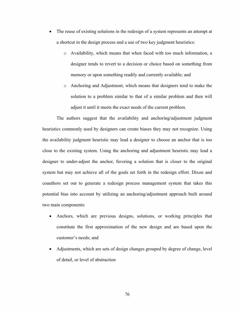
76
• The reuse of existing solutions in the redesign of a system represents an attempt at
a shortcut in the design process and a use of two key judgment heuristics:
o Availability, which means that when faced with too much information, a
designer tends to revert to a decision or choice based on something from
memory or upon something readily and currently available; and
o Anchoring and Adjustment, which means that designers tend to make the
solution to a problem similar to that of a similar problem and then will
adjust it until it meets the exact needs of the current problem.
The authors suggest that the availability and anchoring/adjustment judgment
heuristics commonly used by designers can create biases they may not recognize. Using
the availability judgment heuristic may lead a designer to choose an anchor that is too
close to the existing system. Using the anchoring and adjustment heuristic may lead a
designer to under-adjust the anchor, favoring a solution that is closer to the original
system but may not achieve all of the goals set forth in the redesign effort. Dixon and
coauthors set out to generate a redesign process management system that takes this
potential bias into account by utilizing an anchoring/adjustment approach built around
two main components:
• Anchors, which are previous designs, solutions, or working principles that
constitute the first approximation of the new design and are based upon the
customer’s needs; and
• Adjustments, which are sets of design changes grouped by degree of change, level
of detail, or level of abstraction

77
The redesign management process is monitored using two metrics developed by
the authors:
• deltaSpecs, which are measures of how well adjustments of the anchor drive the
redesigned system towards the goals set for and is formally defined as follows:
deltaSpec(i,j) =
[ TargetSpecification(i) ] – [ Current Specification (i.j) ]
where
i = the current specification under consideration
j = the current redesign iteration under consideration
[2.1]
• Jump Metric, which determines when in a design process it becomes necessary to
move from one level of change to another as a result of the lower level of change
being unable to provide the needed change in deltaSpecs.
In the first step of the method (shown in flowchart form in Figure 2-2), the
designer queries the customers to identify their needs and uses these needs to generate an
appropriate problem statement. In the second step, a rough initial approximation of the
redesigned system is created to serve as the anchor for the redesign process. In the third
step, the customers’ needs are used to define the deltaSpecs that will be used to judge the
level of achievement in each redesign iteration. The adjusted design is then checked
against the deltaSpecs to determine whether the goals associated with them (minimizing
or eliminating the deltaSpecs) have been achieved. The process shown in Steps 5-8 in

78
Figure 2-2 is repeated until either the jump metric is exceeded or the deltaSpecs are
eliminated. The jump metric is a measure of whether or not the strategy of adjusting the
anchor at a certain level of detail has been achieved. If too cycles of the process have
occurred without elimination of the deltaSpecs, the jump metric is exceeded, signaling
that change at a higher level must occur.
Dixon and co-authors (Dixon 1997; Dixon and Colton 2000) develop their model
of redesign as an anchoring-and-adjustment process based on industrial experience and
then use case studies to show that their model is accurate in describing engineering
practice when the deltaSpecs and jump metric are chosen appropriately. What is not
shown is the result of using their entire formal process on industrial redesign problems
from their inception.
The anchoring-and-adjustment approach is interesting for the fact that it provides
structure to the process of redesigning an existing system in multiple ways to achieve
multiple redesign goals. However, the adjustment plans detailing which aspects of the
system are to be changed at a given time are generated by hand and must be revisited if
redesign fails. The success or failure of this approach is highly dependent upon the ability
of the designer to create these plans, rank the identified goals of the redesign effort, and
determine which goals are most strongly associated with each subsystem. In addition, the
anchoring-and-adjustment approach provides little guidance to a designer with multiple
“anchors” or multiple new systems to design.
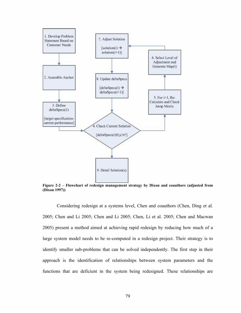
79
Figure 2-2 – Flowchart of redesign management strategy by Dixon and coauthors (adjusted from (Dixon 1997))
Considering redesign at a systems level, Chen and coauthors (Chen, Ding et al.
2005; Chen and Li 2005; Chen and Li 2005; Chen, Li et al. 2005; Chen and Macwan
2005) present a method aimed at achieving rapid redesign by reducing how much of a
large system model needs to be re-computed in a redesign project. Their strategy is to
identify smaller sub-problems that can be solved independently. The first step in their
approach is the identification of relationships between system parameters and the
functions that are deficient in the system being redesigned. These relationships are

80
portrayed graphically in a Design Dependency Matrix (DDM), which the authors then
rearrange into patterns of blocks that are used to decompose the problem as shown in
Figure 2-3. Two metrics are used to evaluate the patterns whereby the DDM can be
rearranged. The intensity metric is based on the number of components being
recalculated and weights that are meant to reflect the difficulty of those calculations. The
interdependency metric is meant to reflect the degree of coupling between the
decomposed parts of the system in a proposed pattern. Based on the pattern, a redesign
roadmap is then generated and used to find a redesign solution that is just good enough to
meet the new system goals while still minimizing expected the computational costs that
make up the redesign effort.
Figure 2-3 – Comparison of a Design Dependency Matrix Before and After Decomposition (Chen and Li 2005)
Hsu and Lin (Hsu and Lin 1998) present a method for redesigning existing
products that is based on Design for Assembly (Boothroyd and Dewhurst 1991) and on
analysis of the functions of the product. Their DFA-based redesign approach (DBPRA)
has three key components:
81
• A knowledge representation scheme called Assembly Functional Representation
(AFP) in which the allocation of functions to components of the product is
studied, as are the surfaces of components that come into contact during
assembly. The aim in this step is to identify those components that are associated
with problems in the assembly process.
• A problem recommendation-driven mechanism (PRDM) which separates
components associated with assembly problems into those that are shared across
multiple functional areas and those that are unique to a particular functional area
and then, depending on the circumstances, recommends either eliminating or
modifying that part.
• A redesign procedure –as shown in Figure 2-4- that includes a number of steps
starting with standard DFA analysis of the existing product, identification of
constraints associated with each functional area, identification of contacts
between components that mate with one another, and a number of redesign
strategies for grouping together or singling out the design problems. No precise
direction is given on how the needed design changes should be made.
The authors claim that the benefit of their approach is that by taking it, designers
can identify both promising “local” changes (parametric component modifications) and
promising “global” changes (modifications to the whole area that serves a particular
function) to the existing design. However, by basing their method around DFA and
focusing their language on components, surfaces, and contacts, it is hard to see how this
method could be applied at a systems level.

82
Figure 2-4 – The Redesign Phase of DBPRA (Hsu and Lin 1998)
Studies of Change Propagation
Change propagation is the focus of a great deal of study, particularly in computer
science where modeling problem solving, design, and the way in which iteration occurs
are all topics of interest to those developing systems for autonomous decision-making.
There are a number of examples of change propagation role in engineering design
applications being studied, some of which are interested solely in being able to quickly
revise a design to meet changing demands, and some of which are solely interested in
identifying the ramifications of making a change in a complex system.
The efforts of Goel and coauthors (Goel and Chandrasekaran 1989; Goel and
Prabhakar 1994; Goel, Garza et al. 1997) to develop the KRITIK computer program fall
into the first category. KRITIK makes use of case-based reasoning, model-based
reasoning, and stored, well known Structure-Behavior-Function (SBF) relationships to
automatically identify and modify previous designs to make them suited to new
applications. Existing designs are modified by comparing the functions that they perform

83
to the desired function. From a group of candidate modifications, the computer program
determines which will best achieve the desired change in function. From the decision-
based design perspective, this process is too automated, as there is little focus on
verifying and modeling the views of the designer.
RedesignIT (Ollinger and Stahovich 2001) is a computer program that uses
model-based reasoning to develop possible redesign plans. The program takes as its
input a model of the system in question –the model consisting of relevant physical
parameters and a mapping of the relationships between those parameters. Based on a
user’s input of a desired magnitude of change in one of those parameters, the program
generates a list of changes to other parameters that could be used to produce the desired
change and to mitigate any negative interactions. The program makes use of a “semi-
quantitative” representation in which relationships between parameters and changes to
those parameters are expressed simply in orders of magnitude. This semi-quantitative
approach is a significant drawback unless the only goal of the redesign process is to
identify those parts of the system that will have to be modified to get close to a desired
change. As such, it provides one piece of a hypothetical redesign process –much like the
first half of the work by Chen and coauthors (Chen, Ding et al. 2005; Chen and Li 2005;
Chen and Li 2005; Chen, Li et al. 2005; Chen and Macwan 2005)– but the resolution of
what values the new system’s variables should have is left up to later work.
Clarkson and coauthors (Clarkson, Simons et al. 2001) consulted with engineers
and others at GKN Westland to study the way in which a particular helicopter design is
redesigned to meet the needs of various customers. The result of their work is an
analytical prediction model for change propagation, a Change Prediction Method (CPM)

84
that makes use of this model, and a piece of software meant to support the prediction of
changes. The CPM is verified by comparing predicted results to three historic examples
at GKN Westland, but not demonstrated elsewhere, so it is unclear whether the success of
the models is tied to the helicopter design field in which it has been developed. The result
of using the method is a measure of the risk of a change in one subsystem leading to a
cascaded change each other subsystem but it is unclear how this measure could be used
proactively to resolve issues in a system’s design before they occur.
Change propagation studies offer one piece of the information that a designer
faced with a redesign project needs. As such, they provide some guidance to the designer
but don’t help him/her develop an entire redesign plan, but they choose to focus on the
small iterative changes that are needed as a result of larger changes –they do not
necessarily guide a designer toward the big changes he/she will need to meet widely
different demands. DesignIT and KRITIK also run somewhat in conflict with the DBD
perspective in that the designer is almost completely taken out of the process (although
DesignIT does allow a user to inspect each candidate redesign plan generated by the
program and make the decision whether or not to accept the plan or continue looking for
better solutions.) Another drawback to all these approaches is that while they can assist a
designer faced with the task of creating one new system, they do not help to identify
opportunities for reuse that are valuable for a series of new systems.
Reuse of Design Information for Redesign
Tay and Gu (Tay and Gu 2003) propose their “Evolutionary Product Design”
(EPD) methodology as a means of increasing the productivity of a designer engaged in

85
the redesign of a system that evolves over time. The primary intent of the authors in
creating this method is to support those who work in computer-aided design (CAD) since
-as they assert- the amount of design information captured by current CAD systems is not
nearly sufficient to support reuse. The system they suggest (see the flowchart in Figure
2-5) makes use of stored information regarding the pattern of functions in existing
designs. When new functional requirements are entered, the system identifies similar
patterns in existing systems and then tries to swap out dissimilar functions. While useful
for a CAD engineer, such a support method does not meet many of the criteria put forth
here for a systematic serial redesign method. The level of detail at which it operates is
too low to be used for a large complex system without broadening the concepts used
beyond the realm of CAD by modeling and simulating other aspects of the system
besides its physical structure. On the positive side, the system is capable of leveraging
multiple existing designs in the realization of a new system and of doing so in a way that
reuses pieces of existing systems.
Tseng and Jiao (Tseng and Jiao 1998) describe a database system they have
developed to support customers and designers in the early conceptual stages of
evolutionary design. The authors seek to alleviate the “tedious” period of product
definition wherein customer requirements are translated into functional requirements that
can be addressed with engineering solutions. They point out that the product definition
process is often “time-consuming and error prone” as a result of miscommunication or
uncertainty on the part of the customers, fuzzy or poorly-worded requirements, a lack of
understanding of the engineering consequences of requirements, and life-cycle concerns.
To leverage existing products, the authors demonstrate a process whereby the functional
86
requirements of existing systems may be catalogued in a database and then identified
according to similarities or patterns in those requirements when customers appear with
demands similar to those met by existing products. The basic idea behind this work is that
if there is a similarity between the customer’s needs and the functional requirements of an
existing system, it is better to start from the completed product definition of that existing
system than begin original design with a clean slate and risk creating an ill-formed
definition.
Kawakami and coauthors (Kawakami, Katai et al. 1996) leverage concepts from
Axiomatic Design (Suh 1990) in creating a method to find deeper knowledge in the
function structures of existing physical systems in order to better understand why they
succeed. Their Explanation Based Learning (EBL) system uses the ideas put forward by
Suh to generate an Explanation Based Generalization (EBG) from the function structure.
The EBG has a standardized form that is meant to help the designers resolve how
multiple subsystem or lower-level goals can be balanced in achieving the system’s
ultimate goal. The authors’ purpose in putting forward this method is to gather insight
into what constitutes a “good design” by studying successful existing systems and thus to
leverage the best parts in future designs.
At an even higher level, Sferro and coauthors (Sferro, Bolling et al. 1993) have
developed Omni-Engineer, a database of design and manufacturing information captured
as constraints that could be used to reduce the lead-time of new designs. If the idea put
forth by the authors were more than a proposal, it might be of interest in this research, but
at last report it had not progressed beyond a very conceptual stage.

87
All of these information reuse methods support designers in the identification of
promising modes of change and reuse. Tay and Gu (Tay and Gu 2003) and Sferro and
coauthors (Sferro, Bolling et al. 1993) represent a totally different way of looking at the
design/redesign process. Instead of looking for promising modes of change first, they
look for promising modes of repeat. That is, they look for functional similarities between
what is being demanded and what is available in the database from previous designs.
Then they look for dissimilarities and search again for functional modules to match those
changes. In this way, they can reuse parts of multiple systems as long as models of those
systems are stored in the database. One potential drawback to this approach is that
reusing the old data does not ensure that the reuse will carry over to the physical world
unless the company in question is actively producing the system whose parts are being
reused.
Each of the major areas of work discussed in this section has a major drawback
when applied to a sequential strategic redesign problem. All the systematic redesign
processes address a fundamentally different problem: Otto and Wood (Otto and Wood
1998) offer a careful plan but only for one-to-one redesign of a system one can
disassemble; Dixon (Dixon 1997; Dixon and Colton 2000) also focuses on one-to-one
redesign and requires an intensive program of redesign plan development; Chen and
coauthors (Chen, Ding et al. 2005; Chen and Li 2005; Chen and Li 2005; Chen, Li et al.
2005; Chen and Macwan 2005) choose to focus on the computer issues involved in
redesign; and Hsu and Lin (Hsu and Lin 1998) require hands-on assembly information to
use their method. The methods for studying change propagation discussed here all tend to
focus on the changes needed to compensate for the large systems-level modifications that

88
are of interest in this dissertation. The methods for design information reuse seem to
operate at a different meta-level above that of this dissertation; they could be useful but
do not address the central problem. In short, there is no existing redesign method that can
be leveraged wholesale to support sequential strategic redesign, however many of the
methods discussed here could be useful to those carrying out the redesign process after
the conceptual exploration activities discussed in this dissertation have taken place.
Figure 2-5 – Evolutionary Product Design (EPD) Methodology (Tay and Gu 2003)

89
2.3.3 - Means of and Alternatives to Offering Product Variety OR Means of
Offering Product Variety
One of the central questions posed by a number of the requirements of a
sequential strategic redesign method in Section 1.3.2 is, how can a variety of systems be
redesigned so that they share as much in relation to one another as possible? In this
section, various ways of creating related engineering systems are explored and compared
to the requirements of sequential strategic redesign in the hope that some piece or pieces
of the existing methods can be leveraged to support redesign.
Repeatedly Carry Out Original Design
The most obvious way to create a number of existing systems is to design each
individually while keeping the others in mind. There are any number of systematic
approaches to original design such as the work of Pahl and Beitz (Pahl and Beitz 1996),
Ulrich and Eppinger (Ulrich and Eppinger 2004), and Pugh (Pugh 1991) just to name a
few. Any of these approaches can be repeated over and over anew in an effort to redesign
an existing system and would undoubtedly yield better results than an entirely ad-hoc
design process from scratch. Still, doing so could result in exactly the situation that is
meant to be avoided in this work. If considerations such as commonality or redesign
difficulty are to be considered, it is not clear how is to be done, nor is it clear how the
designer can assess the parts of the existing system that need to be changed. Even an
expert designer might not fail to consider promising redesign options. In order to achieve
the cost savings that are the goal of leveraging an existing system, other approaches are
needed.

90
Rely Upon Alternatives to Redesign
Several of the approaches discussed in Section 2.3.2 can be used to create a
variety of product offerings. The assumption inherent is of course that these approaches
have already been adopted to create open, flexible, or modular systems that can be
adjusted at a low cost to meet new needs. If any of these approaches has been taking and
the change in demands that is forecast stays within the expansion possibilities of the base
system, the redesign problem is solved. It is assumed here, however, that this is not the
case –that the original system or systems were designed without future expansion in mind
but that the company wishes to make up for this lack of foresight with wise redesign
decisions at this time.
Product Platform Design Methods
Meyer and Lehnerd (Meyer and Lehnerd 1997) define a product platform as “a
set of common components, modules, or parts from which a stream of derivative products
can be efficiently developed and launched”. A substantial amount effort has been
expended on product platform research in the last ten or so years as academics and
corporations attempt to understand what makes platforms successful and how platforms
can be systematically identified. As a result numerous disparate approaches to designing
platforms for families of products have been suggested in the literature. A very
exhaustive review of product family design methods, applications, and ongoing areas of
research can be found in (Simpson 2003; Simpson 2004; Jiao, Simpson et al. 2006).
Simpson offers a useful distinction between two major groups of product platform design

91
methods. He describes the vast majority of methods as “bottom-up”, meaning that the
family is the result of redesign of existing systems with an eye towards increasing their
commonality and thus making the overall set of system offerings more competitive. One
example of these methods in action is the effort to modify the universal motors inside
Black & Decker tools to increase standardization, which resulted in decreased costs sales
that eventually increased to more than compensate for the original cost of the redesign
(Lehnerd 1987). Other examples of successful applications of bottom-up product
platform strategies come from Lutron (Pessina and Renner 1998), John Deere (Shirley
1990), and as discussed in Section 1.1.1, Volkswagen (Whitney 2000; Anonymous 2003).
Academic research has resulted in other bottom-up approaches examples of which
include the work of Anderson (Anderson 1997), Ericsson and Erixon (Ericsson and
Erixon 1999), Siddique and Rosen (Siddique and Rosen 1999), and Pederson (Pederson
1999).
Aside from increased standardization across a family of systems, “bottom-up”
approaches have the advantage of making use of existing designs, meaning that they can
be more easily and quickly modified by a more novice designer, the costs associated with
new parts can be estimated more accurately, and manufacturing facilities can be modified
to suit the redesigned systems more easily. One commonly presumed disadvantage of
“bottom-up” approaches as opposed to other options is that they are only useful for the
redesign of an existing system, meaning that time and money has been expended in the
design and setup for manufacturing facilities for what has turned out to be an inefficient
family of systems. These are costs that can never be retrieved, regardless of the quality of
the method. For the purposes of this dissertation, however, this disadvantage becomes an

92
advantage, as redesign is assumed from the start. The envisioned goal for strategic
sequential redesign is not, however, to modify the existing systems rather to
accommodate them in a plan for developing new systems.
The systematic bottom-up product family design methods developed in academia
tend to have several major drawbacks in a sequential strategic redesign scenario.
Generally, the focus of the methods is on the creation of the redesigned product family,
with little or no attention paid to the amount of effort involved in transitioning a
manufacturing enterprise from one point to another. Also, as it is generally assumed that
the product family members are offered simultaneously, it is often likewise assumed that
all commonality is equally beneficial. The static set of product family members means
that there is no need to juggle commonality, system performance, and the desire to cut
down on the amount of redesign present.
The other major division within product family design methods defined by
Simpson (Simpson 1998) includes those approaches described as “top-down” in that they
involve an up-front effort to design a platform that will be common across the family of
systems. Sanderson and Uzumeri offer the original design of the early Sony Walkman as
one example of successful application of a suite of top-down methods in the development
of a new product line (Sanderson and Uzumeri 1995). Another successful example of this
approach in action can be seen in the design of the family of Kodak disposable
cameras(Wheelwright and Clark 1995). Examples of systematic top-down approaches
developed in academia are too numerous to list, but characteristic examples include the
scale-based Product Platform Concept Exploration Method (PPCEM) (Simpson 1998;
Simpson 1999), the two-stage Variation-Based Platform Design Methodology (Nayak,

93
Chen et al. 2002), the Product Variety Tradeoff and Exploration Method (PVTEM) that
seeks to balance variance in a family’s variables against deviation from target (Simpson,
Seepersad et al. 2001), and the work of Seepersad and coauthors to identify product
platforms of various extents (Seepersad, Hernandez et al. 2000; Seepersad, Allen et al.
2002).
The major advantage of these types of methods -as pointed out by Wheelwright
and Clark (Wheelwright and Clark 1992)- is that by tackling standardization in the initial
process of designing the family of systems, a “bottom-up” redesign process is not
necessarily needed later on and the process of adding more products to the family later on
may be made smoother. In the context of sequential redesign, however, this is not truly an
advantage. From the perspective of a designer faced with a sequential redesign scenario,
there are several major disadvantages associated with the majority of top-down product
family design methods, although there are exceptions to each: Disadvantages:
• Typically, the methods involve the separation of the set of design variables into
just two sets: platform variables that are common across the whole family and
non-platform variables that are unique to each family member. Exceptions to this
rule include (Seepersad, Hernandez et al. 2000; Seepersad, Allen et al. 2002;
Simpson and D'Souza 2004)). Separating the variables in this way can require a
negative tradeoff between commonality and the performance of individual
systems. Hernandez (Hernandez, Allen et al. 2002) suggests this also limits the
size of the family that can be considered. Applied to the design of a family of
aircraft, for instance, such a division might require that adjustments in payload
capacity be achieved using different fuselage lengths and engines for each family

94
member while requiring that the wings, cockpit, and tail remain exactly the same
throughout the family.
• Many methods only allow for variety to be offered in one dimension, feature, or
performance characteristic. For instance, a family of aircraft designed in this way
might only differ significantly in their length, providing a greater or lesser number
of seats for passengers, but airlines would not be able to choose the width, range,
or speed of the aircraft they purchase.
• Oftentimes, top-down methods only make use of only one mode of modifying the
family members to produce variety. That is, the family is produced by scaling one
variable upward or downward, by swapping modules, or by adding on prescribed
amounts of a variable. A greater variety of systems and greater flexibility can be
achieved by considering mixes of these modes and others including adjustable or
flexible components at the same time. Applied to the example of designing a
family of aircraft again, if designers were only allowed to vary the length of the
fuselage of the aircraft, the possible new product family members might be
severely limited.
One drawback that is common to the majority of both “bottom-up” and “top-
down” methods is their reliance upon a very limited number of means of offering variety.
That is, oftentimes, only one variable is scaled to create a family or one module is
replaced to offer different functions, greatly decreasing the variety that can be created. At
the same time, the majority of approaches in both groups generally can only handle
variety in one dimension. This drawback means that in the example of a family of cars
engines of greater horsepower could be accommodated, but not different body styles.

95
Both types of product family design methods also suffer from the assumption that all of
the variants in a family will be stated ahead of time, anticipating all future needs. Taking
such a perspective may encourage designers to optimize their product family design to
the specific demands of the family, ignoring the possibility of building flexibility into the
family to meet changing future needs and allow for ease in redesigning the system.
Assuming that all of the product family’s variants are known ahead of time also can lead
designers to conclude that all commonality in a product family is good and equal in
value. This may not be the case, however, if the variants are released over time and the
cost of repeatedly starting and stopping production of common components is significant.
To address some of the drawbacks of both product family design paradigms, a
new “top-down” approach called the Product Platform Constructal Theory Method
(PPCTM) has been developed by Hernandez and coauthors (Hernandez 2001; Hernandez,
Allen et al. 2002; Hernandez, Allen et al. 2003). As the name of the approach implies, it
is based on Constructal Theory. This theory rests on the premise that a single principle –
the constrained optimization of global performance – is the generating mechanism of
organization, complexity, and hierarchic structure in nature, engineering, and even
management. It is posed by Bejan as a means of explaining the similarities that can be
seen in both natural and man-made systems like those shown in Figure 2-6. The crux of
constructal theory is the concept that hierarchic organizations observed in nature are the
result of a sequential optimization process with the objective of the maximization of
access or, alternatively, the minimization of resistance, or losses. Following the basic
tenants of constructal theory, this optimization process should proceed in a specific time
direction: from the optimization of the basic elements to the higher-order assemblies of

96
the structure. As this process is repeated, a familiar hierarchical structure like tree roots or
lightening emerges. Bejan and coauthors (Bejan 1996; Bejan 1997; Bejan and Ledezma
1998; Bejan 2000) have successfully applied Constructal Theory to design tasks ranging
from heat exchangers to fluid channels to road layouts.
Figure 2-6 – Examples of Natural and Man-Made Systems Explained Through Constructal Theory
PPCTM is based upon two key constructs: Constructal Theory and Hierarchical
Systems Theory (Simon 1996). From the latter, two key ideas are drawn and posits
developed. First, Simon suggests that complex natural systems are self-organized into a
hierarchy. Second, he suggests that a hierarchical organization in a system allows the
system to be more efficient in its response to changes around it. PPCTM, as developed by
Hernandez, utilizes these theories to organize a strategy for building families of products
that can be easily mass customized to meet a wide range of needs quickly. In order to
apply this method, a market space is defined to show the range of dimensions through
which the family will be customized. This space is subdivided into a hierarchical series of
“space elements” that represent a piece of the market that will all be served with a
common set of variables. Each hierarchical level of space element is larger than the
previous one and involves making a distinctly more important set of variables common
across a larger piece of the market. The groups of variables made common across the
space elements are termed “constructs” and are organized hierarchically so that each

97
grouping addresses specific dimensions of customization and it can have a more
significant impact on those dimensions. In a product family design problem in which
PPCTM is utilized, there are then two main sets of variables:
• Those that describe the size and shape of the space elements;
• Those that describe the variable values made common in each space
elements.
In practice, the focus of research into the use of PPCTM has been on finding the
variables that describe the size and shape of the space elements. In order to reduce the
complexity of the design problem, the engineering examples used are frequently simple
enough that constraints can be used to pick variable values based on the most demanding
performance characteristics inside a space element. In some examples in (Williams
2003), however, the examples are difficult enough that the variable values must be found
by formulating a utility-based compromise Decision Support Problem (Seepersad 2001).
A good analogy to help explain the way in which constructs and space elements
are used in PPCTM comes from the road construction problem discussed in (Bejan 1996)
and shown in Figure 2-7. The problem at hand is how best to design a network of roads
such that people spread out in a given space can get out of that space in the fastest
average time possible. In this problem, the constructs being applied are roads of different
sizes and speeds. The demand they must address is a uniform distribution of people who
live throughout the given space at locations P(x,y) and can walk with speed V0 to a road.
The first step is to determine, given an element of a certain area S1, the dimensions H1
and L1 of that area such that a road with speed V1 that gets the people in that space
element to the exit the fastest. At the second stage, the question that faces a designer is

98
how best to assemble a number of the smallest elements so that a road with speed V2 gets
all the people in the space to the exit the fastest possible. Subsequent steps continue
building up using combinations of the previous steps’ space elements until the largest
road is used.
S1
x
y
V1
L1
H1
P(x,y)
First Space Element
xV2
L2
H2
S2
Second Space Element(not to scale with first element)
S1
S1 S1
L1
H1
Time, Complexity, Evolution
S3S4
S5S6
S2
S1
Figure 2-7 – Assembly of Space Elements in a Constructal Approach to Road Design, Modified from (Bejan 2000)
Ideally, when applying Constructal Theory to a problem, the decisions as to how
design variable values will be set for each level are made by optimizing the system
design at each level. In the road design problem, this process is simple, as the objective at
all levels is the same: to get the people in each space to the exit as quickly as possible on
average. Hernandez (Hernandez 2001) realizes that this situation is not always the case in
more complex engineering systems where it is not so easy to tie the value of low-level

99
variables directly to the way in which the product meets or fails to meets the demands in
that space element, let alone how it impacts the economic viability larger system that is
the family of products. Applying optimization over and over to succeeding hierarchical
levels seems to have the effect of a greedy algorithm and can definitely lead to
suboptimal system performance. For this reason, researchers have utilized various
solutions schemes to solve the constructal problem, from dynamic programming
(Hernandez 2001) to exhaustive search (Williams 2003; Williams, Allen et al. 2004;
Williams, Rosen et al. 2004), to simulated annealing and genetic algorithms (Kulkarni,
Allen et al. 2005). The creation of a design by building up constructs is a key tenet of
Constructal Theory in the opinion of this author, so henceforth, PPCTM and the
approach proposed in this dissertation will be referred to as “constructal-inspired” to
avoid confusion.
Figure 2-8 – Flowchart of the Product Platform Constructal Theory Method (Williams 2003)
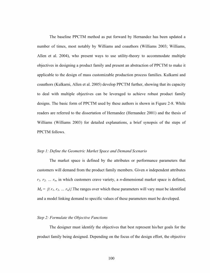
100
The baseline PPCTM method as put forward by Hernandez has been updated a
number of times, most notably by Williams and coauthors (Williams 2003; Williams,
Allen et al. 2004), who present ways to use utility-theory to accommodate multiple
objectives in designing a product family and present an abstraction of PPCTM to make it
applicable to the design of mass customizable production process families. Kulkarni and
coauthors (Kulkarni, Allen et al. 2005) develop PPCTM further, showing that its capacity
to deal with multiple objectives can be leveraged to achieve robust product family
designs. The basic form of PPCTM used by these authors is shown in Figure 2-8. While
readers are referred to the dissertation of Hernandez (Hernandez 2001) and the thesis of
Williams (Williams 2003) for detailed explanations, a brief synopsis of the steps of
PPCTM follows.
Step 1: Define the Geometric Market Space and Demand Scenario
The market space is defined by the attributes or performance parameters that
customers will demand from the product family members. Given n independent attributes
r1, r2, … rn, in which customers crave variety, a n-dimensional market space is defined,
Mn = {( r1, r2, … rn)}.The ranges over which these parameters will vary must be identified
and a model linking demand to specific values of these parameters must be developed.
Step 2: Formulate the Objective Functions
The designer must identify the objectives that best represent his/her goals for the
product family being designed. Depending on the focus of the design effort, the objective

101
function might involve the minimization of cost, maximization of profit, maximization of
quality, minimization of lead-time, or some combination thereof. The objective function
is evaluated by previous researchers in one of two different ways, either using a
summation of a discretized analysis:
1,max 2,max ,max
1,min 2,min ,min
1, 2, ,overall obj ( , , )n
n
r r r
i j n ki r j r k r
Obj r r r= = =
= ∑ ∑ ∑… … [2.2]
(where Obj is the objective function), or using the integral of a continuous analysis:
1,max 2,max ,max
1,min 2,min ,min
1, 2, , 1 2overall obj ( , , )n
n
r r r
i j n k ni r j r k r
Obj r r r dr dr dr= = =
= ∫ ∫ ∫… … … [2.3]
In both formulas, rmin and rmax refer to the upper and lower bounds of each
dimension of the market space.
Step 3: Identify Modes for Managing Product Variety
The designer must identify the ways in which he/she proposes to offer the variety
present in the targeted market space. The modes chosen will depend entirely upon the
problem and the preferences of the designer. Basic forms suggested by Williams
(Williams 2003) include component commonality, dimensional commonality,
modularity, and standardization. Depending on one’s perspective, these modes can be
viewed as either ways of making components or features common across pieces of the
market or ways of adjusting products to realize the variety desired.
Step 4: Identify the Number of Hierarchical Levels and Allocate the Modes for Managing
Variety to the Levels

102
In utilizing PPCTM, the market space will be divided up into smaller space
elements in a number of stages. At each successive stage, the divisions must be at least as
large as the ones found in previously. The number of stages to be used must be identified
in this step and the modes assigned to stages. More than one mode can be assigned to a
stage. In general, it is advised that the modes be arranged such that those at the higher
levels have the greatest impact on the attributes being varied and/or have the largest cost
to provide variety. There is no clear-cut way to set the number of stages or determine
which modes should be assigned to which particular stages but the assignment is critical,
as the results depend heavily upon how this is done. The decision variables in each space
element at each stage make up the construct that is pieced together at the next stage, as
shown in Figure 2-9.
Figure 2-9 – Hierarchical Ranking of Constructs in a Single Dimension of the Market Space (Hernandez 2001)

103
One final important piece of this step if the market space is more than one-
dimensional is the allocation of response space dimensions to each stage. It is assumed
that the first stage space elements address a space element with as many dimensions as
the overall markets space. Constructs at higher levels may be used to provide variety in
any combination of dimensions or just one, but the assignment is critical to the success of
the overall method.
Step 5: Formulate a Multistage Utility-Based Compromise Decision Support Problem
Given the assignment of modes to stages in the previous step, the design problem
must now be formulated as a series of utility-based Compromise Decision Support
Problems (u-cDSP). Starting at the first stage with the smallest space elements, the
decision variables that must be identified using the u-cDSP are the dimensions
[ ]1 2, , nr r r∆ ∆ ∆… of the n-dimensional space element across which the first stage’s modes
of managing product variety will be made common. The goal in each u-cDSP is the
minimization of the deviation variables associated with the expected utility of the
solution. Based on the sizes of each stage’s space elements, the values for the modes of
managing product variety are either deduced using constraints or synthesized based upon
the most stringent attributes in each space element. Williams (Williams 2003) calls this
decision within each space element “Decision 0”.
Step 6: Solve the Multi-stage Utility-Based Compromise Support Problem
Solving the series of u-cDSP’s generated in the previous step in series in a
constructal manner could easily lead to vastly inferior solutions, as the decisions made as

104
to the smaller less-important mode values would be made in the early stages before
larger, more important variable values were set. To address this problem, various authors
have implemented a number of solution schemes for identifying space element sizes
including dynamic programming (Hernandez 2001), exhaustive search (Hernandez, Allen
et al. 2002; Hernandez 2003; Williams 2003), and genetic algorithms (Kulkarni, Allen et
al. 2005). Because solution schemes have tended to avoid building upward from the
smallest space elements and because in some previous work, space elements that do not
nest together have been created, it has been suggested (Williams 2003) that the use of the
term “Constructal” in the name for PPCTM is entirely inappropriate and confusing. A
more appropriate choice of words for describing PPCTM and the work based on it might
be “constructal inspired.”
The Product Platform Constructal Theory method is interesting because it
addresses a combination of challenges in sequential strategic redesign that are unmet by
any product family design methods. Most notably, it allows a designer to:
• Design families of products based on multiple platforms of arbitrary size
and shape;
• Utilize multiple means of offering variety including scaling,
customization, and the addition or subtraction of modules; and
• Create a product family in such a way that any customer demand within a
multi-dimensional market space can be addressed, meaning that problems
in which a product family with variety in multiple dimensions is desirable
can be solved (see Figure 2-10).

105
“Traditional” Product Family Design Methods
Response #1
Res
pons
e #2
Model 100
Model 110
Model 200 Model 210 Model 220 Model 230
Platform 200
Platform 100
Traditional product family design methods tend to address families in which products are distinguished from one another in only one way and in which one means of offering variety (scaling of a certain variable or replacement of certain modules) is utilized.
Constructal-Inspired Product Family Design Methods
Response #1
Res
pons
e #2
Group of Potential ProductsIn Every Market Niche
By utilizing multiple means of offering variety in concert, constructal-inspired product family methods based on PPCTM are able to support the design of families with variety in a number of dimensions.
Sequential Strategic Redesign Problems
Response #1
Res
pons
e #2
Model 201
Model 102 Model 303 Model 401
Model 202
Model 101
Model 204
Model 302
Model 301
Model 203
Product families that emerge over time as a result of redesign may include individuals that are differentiated through various performance characteristics and features. It will be desirable to be able to achieve this, perhaps through use of various means.
Figure 2-10 – Comparison of Market Coverage in Traditional Product Family Design, PPCTM, and Sequential Strategic Redesign

106
There are several ways in which PPCTM fails to address the needs of one
engaged in sequential strategic redesign, however. Obviously, in previous applications of
PPCTM, no attention is paid to redesign effort or scheduling differences, as it is assumed
that the mass customized product families being designed are brand new. Looking
beyond the focus of the method on original design as opposed to redesign, the practical
ways in which PPCTM falls short include:
• The lack of consideration of existing systems in creating product family
designs.
• Its focus on the creation of family designs that address a whole market space.
Even within space element subdivisions of this space, individual systems are
based on over-design to meet the most stringent demands represented there.
There is no way to account for specific customer demands in a market space.
• The assumption that there is a level of performance change that a customer
cannot discern. One key assumption in PPCTM involves the size of the
smallest space element, a small piece of the market in which it is assumed that
any customer whose demand falls there will be satisfied, so long as the
system’s performance also falls there.
• The assumption that geometric proximity between two systems in a market
space implies that commonality between those two particular systems is
preferable. By exploring how contiguous pieces of the market space can be
combined into spaces that can share variable values in common, reuse of
components is achieved, but opportunities to share components between
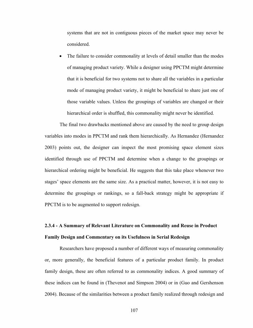
107
systems that are not in contiguous pieces of the market space may never be
considered.
• The failure to consider commonality at levels of detail smaller than the modes
of managing product variety. While a designer using PPCTM might determine
that it is beneficial for two systems not to share all the variables in a particular
mode of managing product variety, it might be beneficial to share just one of
those variable values. Unless the groupings of variables are changed or their
hierarchical order is shuffled, this commonality might never be identified.
The final two drawbacks mentioned above are caused by the need to group design
variables into modes in PPCTM and rank them hierarchically. As Hernandez (Hernandez
2003) points out, the designer can inspect the most promising space element sizes
identified through use of PPCTM and determine when a change to the groupings or
hierarchical ordering might be beneficial. He suggests that this take place whenever two
stages’ space elements are the same size. As a practical matter, however, it is not easy to
determine the groupings or rankings, so a fall-back strategy might be appropriate if
PPCTM is to be augmented to support redesign.
2.3.4 - A Summary of Relevant Literature on Commonality and Reuse in Product
Family Design and Commentary on its Usefulness in Serial Redesign
Researchers have proposed a number of different ways of measuring commonality
or, more generally, the beneficial features of a particular product family. In product
family design, these are often referred to as commonality indices. A good summary of
these indices can be found in (Thevenot and Simpson 2004) or in (Guo and Gershenson
2004). Because of the similarities between a product family realized through redesign and

108
one that is both designed and released all-at-once, it seems logical to look at some of
these indices for inspiration in the creation of an index for redesign. This will also help
elucidate the ways in which existing measures for commonality and effort fall short when
applied to redesign. The metrics discussed in this section are also summarized in Table
2-3 based on their features and whether they are calculated based on analysis of each part
in a family or based on a measure of the family as a whole.
Degree of Commonality Index (DComI) by (Collier 1981)
DComI is a measure of the average number of common parent items per
component in a family of products. Component parts are considered to be any part in the
family of products besides the final assemblies offered at market. Parent items are
considered to be any part in the family of products that is made up of component parts.
The DComI is easy to compute but its major limitation is that because of the way it is
computed, it has no fixed boundaries. The lack of boundaries makes it difficult to use the
DComI to compare families of products to one another.
1
i d
jj iDCI
d
+
= +
Φ=∑
[2.4]
where:
jΦ = the number of immediate parent components that part j has amongst all
products offered
d = the total number of unique parts in all of the finished end products offered
i = the total number of finished end products offered
and the range of DCI is:

109
1 DCI β≤ ≤ , 1
i d
jj i
β+
= +
= Φ∑
The other drawback to using DCI in the design or redesign of future systems, is
that intimate information about the structure and makeup of the systems is required in
order to sort out which components go with which system and the organization of parent
components. This is the kind of information that may be difficult to generate for a
hypothetical future system for which redesign plans are being generated. This is a
drawback that spreads to many of the other commonality measures discussed in this
chapter, as many have used Collier’s work as a starting point for their own.
Table 2-3– Summary of Information Included in Commonality/Non-Commonality Indices Type of
Commonality Measure
Type of Information Included in Index
Name and Source of Index Part
-Bas
ed
Fam
ily-B
ased
Num
ber
of C
omm
on o
r U
niqu
e C
ompo
nent
s
Part
/Var
iabl
e R
ange
, R
esul
ting
Var
iabi
lity,
or
Pe
rfor
man
ce R
ange
s
Ove
rall
Cos
t of R
edes
ign
Typ
es o
f Man
ufac
turi
ng
Proc
esse
s
Mat
eria
ls
Typ
es o
f Ass
embl
y Pr
oces
ses
Sequ
ence
of
Man
ufac
turi
ng
Ope
ratio
ns
Con
nect
ions
and
Fa
sten
ing
Vol
ume
of d
eman
d in
M
arke
t
Degree of Commonality Index (DComI) (Collier 1981)
Total Constant Commonality Index (TCCI) (Wacker and Treleven 1986)
Product Line Commonality Index (PLCI) (Kota, Sethuraman et al. 2000)
Percent Commonality Index (PCI) (Siddique and Rosen 1998)
Commonality Index (CI1) (Martin and Ishii 1996)
Commonality Index (CI2) (Martin and Ishii 1997)
Total Cost of Providing Commonality (TCPI) (Martin and Ishii 1996)
Coupling Index (CoupI) (Martin and Ishii 2002)

110
Generational Variety Index (GVI) (Martin and Ishii 2002)
Component and Process Commonality Indices (CPCI) (Jiao and Tseng 2000)
Product Family Penalty Function (PFPF) (Messac, Martinez et al. 2002)
?
Design Capability Indices (DCI) (Chen, Simpson et al. 1996)
Non-Commonality Index (NCI) (Simpson, Seepersad et al. 2001)
Performance Deviation Index (PDI) (Simpson, Seepersad et al. 2001)
Design Freedom (DF) (Simpson, Rosen et al. 1998)
Total Constant Commonality Index (TCCI) by (Wacker and Treleven 1986)
The TCCI is a modified version of the DCI presented by Collier (Collier 1981).
The major difference between the TCCI and the original DCI is that the former is
computed such that it is always between 0 and 1, making it possible to use the TCCI as a
relative measure of the value of product families.
1
111
d
jj
dTCCI
=
−= −
Φ −∑
[2.5]
where:
jΦ = the number of immediate parent components that part j has amongst all
products offered
d = the total number of unique parts in all of the finished end products offered
i = the total number of finished end products offered
and the range of TCCI is:
0 1.0TCCI≤ ≤

111
Commonality Index (CI1) by (Martin and Ishii 1996)
This version of the CI1 is based on Collier’s work (Collier 1981) but is much
simpler. It is simply the ratio of the total number of unique parts in a family to the total
number of parts in all of the members of the family. A lower number indicates that more
parts have been made common across the family.
1
1nv
jj
uCIp
=
=
∑
[2.6]
where:
u = the number of unique parts
pj = the number of parts in model j
vn = the final number of varieties of models offered
and the range of CI1 is:
0 1 1.0CI≤ ≤
Design Capability Indices (DCI) by (Chen, Simpson et al. 1996)
Developed based on Process Control Indices used in manufacturing quality
control, the DCI is computed using a nominal design and an assumed amount
(percentage) of variability in its variable values. This variability is used to calculate the
distribution of system responses of interest. The DCI is the percentage of the resulting
range of system responses that overlaps the stated desirable range. Generally, the
variation in the variables is assumed, meaning that the design task is to determine the
nominal variable settings that maximize the DCI’s for the responses of interest. As a

112
design tool, the DCI is useful for identifying the rough “top-level design specifications”
of a family, but it is not useful for the designer whose task it is to find the design variable
values of the individual family members, nor is it a measure or indicator of the amount of
commonality that will be present in a resulting product family design. If the preliminary
design process is repeated using different amounts of assumed variance, the designer
might be able to identify top-level specifications that offer greater promise of final
designs with more commonality.
Total Cost of Providing Variety (TCPI) by (Martin and Ishii 1996)
Martin and Ishii propose to regress a function for the total cost of providing
variety in a family as a function of not just the CI1 but also as a function of the
Differentiation Point Index (DPI) and Setup Index (SI). The DPI is a measure of how late
in the manufacturing process variety is created, the presumption being that adding variety
later is advantageous. The SI is a measure of the contribution made by setup costs to the
total cost of all the products in the system.
0 1 2 3
1
1
11
1
1
1
1n
n
v
jj
n
i i ii
n
n ii
n
i iiv
jj
TCPI CI DI SIuCIp
d v aDPI
nd v a
v cSI
C
β β β β
=
=
=
=
=
= + + +
=
=
=
∑
∑
∑
∑
∑
[2.7]
where:

113
0 1 2 3, , ,β β β β are regression coefficients
u = the number of unique parts
pj = the number of parts in model j
vn = the final number of varieties of models offered
di = average throughput time from process i to sale
d1 = average throughput time from beginning of production to sale
ai = value added in process i
ci = cost of setup at process i
Cj = total cost (material, labor, and overhead) of product j
And:
0 1 1.00 1.00 1.0
CIDPISI
≤ ≤≤ ≤≤ ≤
In proposing the TCPI, Martin and Ishii choose to include the perspectives of
those who manage the flow of a manufacturing process. It is also interesting to note the
use of the abstract term “value” in the term ai in the computation of the DPI. It can be
argued that all of the commonality measures discussed here suffer from the common
liability of not linking their values to an absolute measure of the success of a product
platform and that particular values of the measures have no real meaning. In using ai, the
DPI takes one more subjective step away from being tied to practical quantities.
Commonality Index (CI2) by (Martin and Ishii 1997)
This index by the same authors as the previously-discussed Commonality Index
and labeled with the same name is again based on the basic ideas put forth by Collier

114
(Collier 1981) but is constrained to the range between 0 and 1. The CI2 measures is based
on ratio between the total number of parts in a family that provide variety and total
number of parts in all of the members of the family.
1
max2
maxn
jv
j jj
u pCI
p p=
−=
−∑
[2.8]
Where:
u = the number of unique parts
pj = the number of parts in model j
vn = the final number of varieties of models offered
and the range of CI2 is:
0 2 1.0CI≤ ≤
Percent Commonality Index (PCI) by (Siddique and Rosen 1998)
The overall percent commonality measure suggested by the Siddique and Rosen
can be calculated in a number of ways, but the suggested form is the weighted sum of a
number of sub-indices, each of which reflects a product platform’s commonality from a
different perspective. The sub-indices each measure commonality in the architecture and
assembly of the products in the family. The two architecture indices measure the
percentage of components and connections that are common in the family while the
assembly indices measure the percentage of the assembly processes and assembly
workstations that are common across the family.
4
1i i c c n n l l a a
iPCI I C I C I C I C I C
=
= = + + +∑ [2.9]

115
where:
Ii = the importance (weighting) of each viewpoint’s sub-index
Ci = the percent commonality for each viewpoint, more specifically:
ccommon componentsC 100
common components + unique components= × ,
acommon connectionsC 100
common connections + unique connections= × ,
ccommon assembly component loadingC 100
common assembly component loading + unique assembly component loading= × ,
and
ccommon assembly workstationsC 100
common assembly workstations + unique assembly workstations= ×
If 4
11i
iI
=
=∑ then 0 100PCI≤ ≤
The PCI is the commonality measure which Guo and Gershenson (Guo and
Gershenson 2004) identify as being both the most consistent with other measures and the
most sensitive to small changes in proposed product family designs. It also incorporates a
higher-level view of the value of commonality with respect to manufacturing than the
other works discussed thus far.
Product Line Commonality Index (PLCI) by (Kota, Sethuraman et al. 2000)
The PLCI can be used to compare a product family to the ideal situation in which
all of the parts that do not serve to differentiate the various family members are shared
across the entire family, have the same size and shape, are made of the same materials,
and are made the same way. The PLCI is measured on a scale between 0 and 100, with
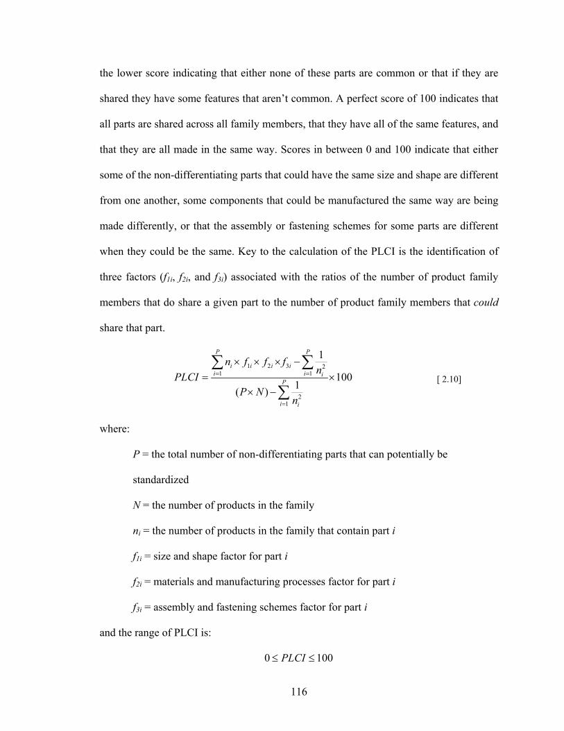
116
the lower score indicating that either none of these parts are common or that if they are
shared they have some features that aren’t common. A perfect score of 100 indicates that
all parts are shared across all family members, that they have all of the same features, and
that they are all made in the same way. Scores in between 0 and 100 indicate that either
some of the non-differentiating parts that could have the same size and shape are different
from one another, some components that could be manufactured the same way are being
made differently, or that the assembly or fastening schemes for some parts are different
when they could be the same. Key to the calculation of the PLCI is the identification of
three factors (f1i, f2i, and f3i) associated with the ratios of the number of product family
members that do share a given part to the number of product family members that could
share that part.
1 2 3 21 1
21
1
1001( )
P P
i i i ii i i
P
i i
n f f fnPLCI
P Nn
= =
=
× × × −= ×
× −
∑ ∑
∑ [ 2.10]
where:
P = the total number of non-differentiating parts that can potentially be
standardized
N = the number of products in the family
ni = the number of products in the family that contain part i
f1i = size and shape factor for part i
f2i = materials and manufacturing processes factor for part i
f3i = assembly and fastening schemes factor for part i
and the range of PLCI is:
0 100PLCI≤ ≤
117
Thevenot and coauthors (Thevenot, Nanda et al. 2005) utilize the PLCI as a
measure of the number of components that do not serve to externally differentiate the
product family members. The authors’ research is aimed at creating a method for
identifying both the best redesign strategy and the components of a product that
contribute most to commonality in general. In addition to the commonality goal, several
constraints are added to ensure that unique components that serve to differentiate specific
products are preserved, that components that are already shared across the whole family
are not altered, and that a certain maximum number of design changes is not exceeded.
By adding these constraints, the authors are in effect placing reasonable limits on the cost
of the redesign effort without explicitly calculating it. There are several significant
drawbacks to this work, which do not have to do with the PLCI itself. First, the proposed
redesign plans are never checked for feasibility, meaning that some commonality may be
achieved at the cost of impossible designs. Second, since certain design changes are
ignored due to the constraints, the possible benefits of a change in a small number of
common parts is ignored in favor of more changes in less common parts.
Component and Process Commonality Indices (CPCI) by (Jiao and Tseng 2000)
One half of the CPCI is based on Collier’s DCI (Collier 1981) but expands that
measure by incorporating product volume, cost per part, and quantity per operation into
the Component Part Commonality CI(c). The other half of the CPCI is made up of a
Process Commonality Index (CI(P)) which is modified from a process flexibility measure
put forward by Tsubone et al (Tsubone, Matsuura et al. 1994) and reflects lot sizes,
schedule sequencing, and overall process flexibility. As Thevenot and Simpson

118
(Thevenot and Simpson 2004) point out, one advantage of the CI(C) as compared to other
measures of part commonality is that greater weight is given to making an expensive part
common across a family as opposed to a cheaper part. The flip side of this advantage is
that the dependency on cost estimates, which decrease the value of this index if they are
not accurate.
1 1 1( )
1 1
( )
( )
d m m
j ij i ijj i ic
d m
j i ijj i
P V QCI
P V Q
= = =
= =
Φ
=
∑ ∑ ∑
∑ ∑ [2.11]
where:
d = total number of components in a product family
j = index of each component
Pj = price or cost of each part
m = total number of products in the family
i = index of each product in the family
Vi = volume of each product in the family
ijΦ = number of immediate parents for part dj “over all the product levels of
product i of the family
Qij = quantity of part dj required by product i
And:
( )
1 11
d mC
ijj i
CI= =
≤ ≤ Φ∑∑

119
By separating the overall CPCI into two sub-indices, the authors are better able to
differentiate between changes that have value from the perspective of part commonality
and from the perspective of process commonality. Like CI before it, the CPCI requires in-
depth part-level understanding of a product and careful accounting for the structure of
each product family member, information that may be difficult to obtain when
conceptually redesigning a system.
Coupling Index (CoupI) by (Martin and Ishii 2002)
The Coupling Index proposed by Martin and Ishii can be used at either a
component level or at a product/system level. It is first calculated for individual
components in a product before being added to create a measure of the system as a
whole. At the component level, it is a subjective measure of both the strength of the
impact of changes in a component on other components (CI-S) and the strength of the
impact received in the component in question because of changes in other components
(CI-R). Each of these impacts is rated on a scale of 1 to 9. The authors suggest the
minimization of CI-R and the Generational Variety Index as a way of promoting
standardization across generations and suggest the minimization of CI-S as a way of
promoting modularity. As such, CoupI is not truly a commonality measure, but rather a
measure of the degree to which elements of a system design are tied to one another and
an aid in identifying more promising decoupled designs.

120
Table 2-4 – Rating System for both CI-S (supplied changes due to coupling) and CI-R (changes received due to coupling) (Martin and Ishii 2002) Rating Description 9 High Sensitivity – Meaning that even a small change in specification
impacts the receiving component 6 Medium-high sensitivity 3 Medium-low sensitivity 1 Low Sensitivity – Meaning that it takes a large change in specification to
impact the receiving component 0 No specifications are affecting the component in question. Note: The total CI-S value for a component may be higher than 9 as a result of adding up multiple supplied or received impacts from expected specification changes
Generational Variety Index (GVI) by (Martin and Ishii 2002)
The Generation Variety Index is computed based on the results of Quality
Function Deployment (QFD), in which expected changes in customer requirements are
described and the impacts of those changes on engineering metric targets estimated.
These estimates are then used by an engineering team to forecast, based on their
judgment, what percentage of the original cost to design each component will have to be
reinvested to redesign that component to meet the most stringent new engineering metric
targets. These costs are expressed on a scale of 1 to 9 (see Table 2-5) and total costs are
indicated by adding up the component redesign costs associated with each change in
customer requirements.
One downside of this approach is the use of percentages in the rating system
means that the values generated are only meaningful in comparison to the original
system. Furthermore, by only considering how much of the original design cost will have
to be reinvested in the new component, an inherent assumption is made that all
components are equally important or cost the same amount. That is, under the current
GVI rating system, a $1000 component with a GVI rating of 6 is just as important as a $5
component with the same rating. The cost structure is in reality problem dependant, it

121
might make more sense to either create rating systems on a case-by-case basis. The
assignment of the GVI rating scheme to percentages of original design cost is also made
arbitrarily depending on the preferences of the designer and the problem at hand.
The GVI is interesting because of the way in which the authors (Martin and Ishii
2002) propose to use it to judge the impact of proposed redesign plans. The GVI is used
in concert with CoupI to strategically estimate the amount of redesign effort that will be
needed to realize future revisions of a system, thus meeting one of the requirements of the
method being developed in this dissertation. However, due to its discrete nature, it works
better as a yardstick for measuring the merit of a completed redesign plan than as a tool
for guiding a redesign process towards more promising plans.
Table 2-5 – Rating System for GVI (Martin and Ishii 2002)
Rating Description Percent of Original Design Costs that Must be Invested in Redesign
9 Requires major redesign of the component
>50%
6 Requires partial redesign of component
<50%
3 Requires numerous simple changes
<30%
1 Requires few minor changes <15% 0 Requires no changes None Note: The total GVI value for a component may be higher than 9 as a result of the impact of multiple expected engineering changes
Product Family Penalty Function (PFPF) by Messac, Martinez, and Simpson (Messac,
Martinez et al. 2002; Messac, Martinez et al. 2002)
In an attempt to identify the best scaling variables for a scalable product platform,
the coauthors suggest using the variability of each design variable as a measure of how
difficult it would be to make that variable common across the family of products.
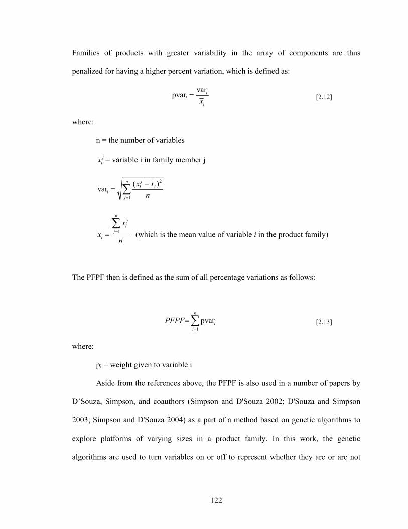
122
Families of products with greater variability in the array of components are thus
penalized for having a higher percent variation, which is defined as:
varpvar ii
ix= [2.12]
where:
n = the number of variables
jix = variable i in family member j
2
1
( )varjn
i ii
j
x xn=
−= ∑
1
nj
ij
i
xx
n==∑
(which is the mean value of variable i in the product family)
The PFPF then is defined as the sum of all percentage variations as follows:
1pvar
n
ii
PFPF=
=∑ [2.13]
where:
pi = weight given to variable i
Aside from the references above, the PFPF is also used in a number of papers by
D’Souza, Simpson, and coauthors (Simpson and D'Souza 2002; D'Souza and Simpson
2003; Simpson and D'Souza 2004) as a part of a method based on genetic algorithms to
explore platforms of varying sizes in a product family. In this work, the genetic
algorithms are used to turn variables on or off to represent whether they are or are not

123
part of the family’s platform. Commonality in this family is driven by minimization of a
fitness function based on the PFPF.
The PFPF is basically a measure of weighted variance in a variable. It is shown by
Messac, D’Souza, Simpson, and coauthors to be useful in both in identifying variables to
be used for scaling a product family and in identifying platforms of various sizes. It could
be used to measure the variability in a family of products based on redesign, however the
pi weights it uses would have to be tied somehow to the relative difficulty of redesigning
the elements of the system or the relative value of commonality in various components.
Non-Commonality Index (NCI) and Performance Deviation Index (PDI) by (Simpson,
Seepersad et al. 2001)
In proposing a Product Variety Tradeoff Method for exploring varying amounts
of commonality in a product platform, the authors suggest the use of two indices to
evaluate the candidate platform designs. The NCI is a weighted sum of the normalized
average deviations in each parameter across the family. The weighting used indicates the
difficulty in varying that parameter. The PDI is actually a weighted sum of weighted
sums. For each product, its deviations from target values are normalized and added up,
with weights corresponding to the importance of each performance value. These
deviation sums for each product are then added up with weights corresponding to the
relative importance of each product within the family. The authors suggest seeking
product platform designs that minimize both the NCI and PDI. The NCI and PDI are
calculated as follows:

124
1
m
j jj
NCI w DI=
= ∑ [2.14]
1
n
i ii
PDI w Z=
=∑ [2.15]
where:
m = the number of variables
n = the number of products in the family
q = the number of performance parameters
wi = the weight or importance of product i in the family
wj = the weight or difficulty of varying variable j
wk = the weight or importance of performance parameter k
1
n
iji
j
NdiffDI
n==∑
, the average normalized difference for each variable
max minj ij
ijj j
xNdiff
x xµ −
=−
, the normalized difference for each variable
jµ = the mean value of a design variable throughout the family
1
q
i k ikk
Z w dnorm=
= ∑ , the sum of the weighted, normalized performance deviations
target perf - actual perftarget perfikdnorm = , the normalized deviation of product i for
performance parameter k
The creators of the NCI and PDI recognize that the approach of minimizing both
measures as a goal for product family design has two major drawbacks: the assumption
that greater commonality is always desirable and the assumption that the platform

125
architecture is actually good for the whole family. Still, in formulating the NCI, they
tackle one of the challenges put forward in this dissertation by attempting to account for
the difficulty in adjusting designs. They also chose to balance this with a performance
measure in the form of PDI, although they do not consider whether all the commonality is
valued equally.
Design Freedom (DF) by (Simpson, Rosen et al. 1998)
The authors suggest the design of open engineering systems –systems that can be
easily adapted to changing demands through ongoing improvement to a “technological
base.” Towards this end, they propose a metric for design freedom, which they define to
be extent to which parameters in a system can be changed while still meeting design
specifications. If both the expected performance of a system and the targets for that
performance measure can be expressed as a range, then DF is calculated by taking the
weighted sum of the ratio of the overlaps of the ranges over the initial performance range
when the design process starts. The weights are determined based on the relative
importance of each performance measure. A design freedom value of 1.0 indicates that
the design’s performance can be tweaked to achieve any of the desired target values.
Design Freedom is calculated as follows:
1 1 ,
Overlap1 1Initial Performance Range
n ni i i
i ii i initial
TR PRDFn n PR= =
∩= =∑ ∑ [2.16]
where:
iTR = target range for performance measure i
,i initialPR = initial feasible performance range for performance measure i

126
iPR = feasible performance range for performance measure i during design
process
While DF allows a designer to get a feel for the flexibility inherent in the
architecture of a system design, it includes the assumption that all the proposed tweaks
are possible and equally difficult. As such, it is a good tool for gauging the initial design
of a system that is to be adjusted later, but perhaps not suited to measuring plans for
redesigning a system to meet future needs over time.
Some authors have made an attempt to study and test various measures of
commonality in a bid to identify one that is most promising. Several of the metrics and
indices discussed in this section and summarized and tested by Thevenot and Simpson
(Thevenot and Simpson 2004) with the goal of identifying the circumstances under which
each measure of commonality is most useful. They found that the usefulness of the
indices depended upon the amount of information available and the perspective that the
designer chooses to take; for instance, some might choose to focus on maximizing the
number of common components in a family while others might want to focus on
minimizing the number of unique parts. In the end, they propose that certain indices such
as the Total Constant Commonality Index (Wacker and Treleven 1986) and Commonality
Index (Martin and Ishii 1997) be utilized early in a design process while others are
chosen for use later on. It is also pointed out that none of the measures can be evaluated
in terms of accuracy as there is no one universal measure of the goodness of a certain
amount of commonality.

127
In the pursuit of a standardized approach to design for modularity, Gershenson
and coauthors (Zhang, Gershenson et al. 2001; Gershenson, Prasad et al. 2004; Guo and
Gershenson 2004; Ye, Gershenson et al. 2005) have also devoted a significant amount of
effort to the study of measures of commonality, modularity, and variety. After an
exhaustive survey, they find that the methods that make use of these measures in the
pursuit of perfect or improved modularity often have several weaknesses. The first
weakness is that they require that huge amounts of information be input into them, some
of which may not be readily or rapidly available to a single designer. Second, the
calculations the modularity measures employ are large enough in number and complexity
that computerized implementation is usually necessary. Third, it is pointed out that the
modularity measures usually only consider gross modular changes to systems, ignoring
the other small changes that might be necessary to accommodate the switching of
modules. Lastly, none of the methods or their measures of commonality has been used to
create a design that can be independently verified as having improved modularity
(Gershenson, Prasad et al. 2004).
Elsewhere, it is suggested that most measures of modularity include some amount
of subjectivity and that they have not been rigorously verified and validated (Guo and
Gershenson 2004). In response to this situation, Guo and Gershenson (Guo and
Gershenson 2004) compare a number of modularity measures. Noting that many of the
measures are very similar in structure, the authors use clustering analysis to look for
measures that are the most consistently close to one another in their evaluation of the
modularity of a number of consumer products. The authors also examined which of the
measures is most sensitive to small changes in product architectures. In the end, the

128
authors conclude that the Percent Commonality Index (PCI) by Siddique and Rosen
(Siddique and Rosen 1998) performs best according to these measures but point out that
even their tests include subjectivity and are prone to the need to input large amounts of
information.
Ye and coauthors (Ye, Gershenson et al. 2005) go a step further, suggesting that
once a good commonality measure is rigorously validated, it should be used to trade off
options against a hypothetical variety index. They propose to use Product Family
Evaluation Graphs (PFEG) to demonstrate these tradeoffs and analyze modular product
family designs. As shown in Figure 2-11, two potential product family designs are plotted
as vectors according to their commonality and variety ratings. A third, dotted line called
the life-cycle strategy unit vector ( )pα is also plotted to represent the strategy of the
company. It is suggested by the authors that the angle α of the strategy vector be picked
based on a number of factors that might influence the amount of variety or commonality
that is desirable in a product family. For instance, a strategy involving more
customization, longer life of products in the marketplace, a larger number of product
family members, and some attempts to make products more environmentally friendly can
result in larger values of α. At the same time, the authors suggest that a desire to avoid
the use of new technologies, decrease the complexity of the product designs, decrease
development time, and improve maintenance costs could lead to a smaller α value.
Prospective family designs are evaluated by projecting their positioning vector against
the chosen strategy vector, with longer values indicating greater adherence to the desired
strategy. While conceptually useful for both the evaluation and graphical presentation of
product family alternatives, as a practical tool for designers, the PFEG lacks two of the

129
legs it needs to stand. While there are a number of existing measures of commonality to
choose from earlier in this chapter, there is no established and comprehensive measure of
variety in a product family. In addition, the idea of setting the product family strategy
angle α is put forward without a good understanding of all of the factors that should be
included, let alone what relative impact they should have on the angle.
α - Life-cycle product family strategy angle Pα - Life-cycle strategy unit vector F1,F2 – Product family design options 1 and 2
1 2,F F - Position vector for respective product family design options 1 and 2
,1 ,1,P Pα α - Life-cycle strategy achievement vector of design options 1 and 2 Figure 2-11 – Use of the PFEG (Ye, Gershenson et al. 2005) to Analyze Two Product Family Designs
All of the metrics and indices discussed here have been developed with a common
goal in mind: establishing some measure of the merit of a proposed design of a family of
products. Most are based upon the goal of increasing the commonality present in a
product family design or decreasing the amount of a family that is unique to individual
products. The indices differ greatly in the amount of information that is needed to
compute them and in the perspectives they choose include or exclude. As shown in Table

130
2-3, different indices choose to focus on part design, production volumes, manufacturing
processes, or even fastening methods. This review of relevant metrics and indices has
intentionally been organized chronologically so that the reader can see the growth in
thought that is put into them –there is even visible change in thought on the part of
individual authors represented here. Over time, researchers have chosen to remove
certain assumptions used by previous authors, but have often had to neglect other
assumptions or impose new restrictions of their own to suit the problem at hand. For
instance, the work of Collier (Collier 1981) that has been leveraged greatly includes a
number of inherent assumptions, most notably that:
• Components all have the same cost;
• Product family members are all produced in equal numbers; and
• The total number of end components in the family will be the same for all
possible family designs.
The last assumption that is removed by Wacker and Treleven (Wacker and
Treleven 1986) in putting forward their index, but other assumptions remain. These
assumptions create a number of gaps when it comes to addressing the requirements of
sequential strategic redesign problems, as shown in Table 2-6. All of the indices and
metrics discussed here have been developed for the purpose of aiding designers creating
new families of products, so it is not entirely fair to criticize them for not considering
issues related only to redesign. However, this fundamental difference in mission brings
with it the key assumptions that:
• The product family is to be designed from scratch;
• All product family members will be offered simultaneously; and

131
• There are not yet any sunk costs associated with the family that need to be
leveraged in redesigned entities.
These are the gaps that are addressed in developing two new metrics specifically
for redesign in Section 3.2.

132
Table 2-6 – Relevance of Selected Existing Product Family Measures to Requirements for Sequential Redesign
Name and Source of Index Enc
oura
ge C
omm
onal
ity?
Con
side
r R
edes
ign
Eff
ort?
Sche
dulin
g of
Pro
duct
Rel
ease
?
Rel
ativ
e V
alue
of C
omm
onal
ity
Bet
wee
n Sy
stem
s?
Mul
tiple
Var
iabl
es U
tiliz
ed?
Mod
el a
nd E
ncou
rage
C
omm
onal
ity in
All
Var
iabl
es?
Plat
form
s Can
Con
tain
Any
V
aria
ble?
Plat
form
s of D
iffer
ent S
ize?
Mul
tiple
Dim
ensi
ons o
f Cha
nge
in
Perf
orm
ance
?
Con
side
r Sy
stem
Per
form
ance
?
Syst
ems-
Lev
el T
hink
ing?
Mul
tiple
Str
ateg
ic R
edes
ign
Goa
ls?
Degree of Commonality Index (DComI) (Collier 1981)
Total Constant Commonality Index (TCCI) (Wacker and Treleven 1986)
Product Line Commonality Index (PLCI) (Kota, Sethuraman et al. 2000)
Percent Commonality Index (PCI) (Siddique and Rosen 1998)
Commonality Index (CI1) (Martin and Ishii 1996)
Commonality Index (CI2) (Martin and Ishii 1997)
Total Cost of Providing Commonality (TCPI) (Martin and Ishii 1996)
Coupling Index (CoupI) (Martin and Ishii 2002)
Generational Variety Index (GVI) (Martin and Ishii 2002)
Component and Process Commonality Indices (CPCI) (Jiao and Tseng 2000)
Product Family Penalty Function (PFPF) (Messac, Martinez et al. 2002)
Design Capability Indices (DCI) (Chen, Simpson et al. 1996)
?
Non-Commonality Index (NCI) (Simpson, Seepersad et al. 2001)
Performance Deviation Index (PDI) (Simpson, Seepersad et al. 2001)
Design Freedom (DF) (Simpson, Rosen et al. 1998)

133
2.3.5 - Support for Long-Term Decision-Making
Taking inspiration from the definition of Strategic Design (Seepersad, Cowan et
al. 2002), the question being pursued in this section is, how do designers create
engineering systems in anticipation of future needs? It is understood that a broader
definition of strategy could be used, taking into account technology forecasts or
uncertainty, but for the purposes of this dissertation, it is assumed that designers are
dealing with well-understood and fully-defined future design targets in the context of the
other requirements explained in Section 1.3.2. As in other sections of this chapter, there
are various areas in which other researchers make contributions to strategic thinking in
design. These include product family design, iterative design change management, and
flexible product platform design.
Strategic Thinking in Up-Front Product Family Design
Seepersad and coauthors (Seepersad, Allen et al. 2002) use physical programming
to design a scale-based product family with a product platform that is robust to a set of
scenarios for how the distribution of demand in a market space might change during the
expected lifespan of the product platform. Based on an initial snapshot of the market and
the scenarios for future demand, a compromise Decision Support Problem is formulated
and solved, the goal being to identify the most promising platform strategy (See Figure
2-12) regardless of which scenario turns out to be accurate. The scenarios are given equal
weight in the governing objective function of the method, meaning that it is assumed that
the designer has a good idea of what the future demand scenario could look like, just not
which of his/her ideas will come true.

134
Figure 2-12 – Examples of Vertical and Horizontal Portfolio Expansion (Seepersad, Allen et al. 2002)
A flowchart of the approach used by Seepersad and coauthors is shown in Figure
2-13. Kulkarni and coauthors (Kulkarni, Allen et al. 2005) use a similar approach to
modeling potential market shifts as a part of a method to support the design of a
hierarchical product family of customizable systems that is robust to both variations in
the distribution of demand throughout the market space and changes in the size of the
market space. Both sets of authors’ approaches offer a way of realizing a large amount of
variety for changing demand but both include the assumption that the platform should be
designed up-front with all future demands in mind.

135
Figure 2-13 – Method for Designing Product Platforms for a Changing Environment (Seepersad, Allen et al. 2002)
Elsewhere, Gonzalez-Zugasti and coauthors (Gonzalez-Zugasti, Otto et al. 2001)
use real options to design a product platform based on uncertainties in design problem
like technology, funding, market conditions, and competition. The value of a design

136
option is based on the sum of the benefits realized minus the cost of investment to
achieve them. Their method has two steps, as shown in Figure 2-14. In the first, a group
of “equally good” candidate product platforms along a Pareto frontier are identified using
deterministic information about future demands. The variants in the product families
based on these platforms a plotted along a timeline like that shown in Figure 2-15 and are
then designed.
Figure 2-14 – Real Options-Based Platform Design Method (Gonzalez-Zugasti, Otto et al. 2001)
In the second step, real options are used to pick the best –meaning most flexible-
of these platforms given the uncertainties in the requirements of each variant in the
family and in the payoffs from each of the variants. As a part of this process, a decision
tree with uncertain outcomes is generated as shown in Figure 2-16. Ideally, the result of

137
the application of this method is a flexible system that is meant to be easily adjustable
based on slight changes in how the design scenario plays out but no plan is presented for
how such adjustments might take place.
Figure 2-15 – Timeline of Platform and Variant Development (Gonzalez-Zugasti, Otto et al. 2001)
Figure 2-16 – Platform and Variant Development Decision Tree (Gonzalez-Zugasti, Otto et al. 2001)
Allada and Lan (Allada and Lan 2002) present a method for designing an
evolving system by planning the launch of new modules. Their method is based upon
perfect knowledge of the emergence, availability, and performance of new modules as
well as perfect knowledge of the profit that will be obtained from a given system

138
realization. The design problem is reduced to planning out when and if the new modules
should be launched. The result is a plan for a system that will evolve over time to meet
different demands but the plan for how those changes will occur is essentially assumed at
the beginning of the problem.
Iterative Redesign to Make Large Changes
The work of Coulter and Bras (Coulter and Bras 1997; Coulter 1998) is inspired
by the desire to make products more environmentally friendly over time. The authors
realize that there are often a number of limiting factors restraining designers from making
the big changes needed to make products like automobiles more environmentally
friendly. In products like cars and consumer electronics in which small revisions are
made quite frequently, justifying huge one-time revisions can be hard whereas smaller
incremental changes over multiple iterations of the product may fit more easily into
budgets. The example used is the improvement of the amount of an automobile that is
recyclable. The authors suggest that by adopting a systematic strategy for product
evolution (see flowchart in Figure 2-17), large changes can be achieved over time. The
crux of the authors’ approach to this iterative problem involves modeling the various
uncertainties in the problem, identifying targets for each revision of the system, and
prioritization of the limiting factors so that they are addressed one-by-one during each
iteration. Their method for doing this is broken down into five steps:
Task 1 – Characterize the Existing Product Design – The goal in this step is to
produce a Decision-Support Problem-based mathematical model of the existing product.

139
This model could be based on measurements or on historical records. It should include
the designer’s perceptions of what the variables are that fully describe the product as well
as the constraints and goals that are most relevant to its function.
Task 2 – Identify Problem – In this task, the designer must identify a general or
rough set of targets for the redesign process. These targets can be based on the current
product information, the company’s business strategy, and external factors such as
regulatory changes.
Task 3 – Select Metrics – The goal in carrying out this task is to build goal
formulations for the objectives of the redesign process. To do this, metrics are needed.
These metrics could be carryovers from the original design of the product and may have
been identified in the course of carrying out Task 2.
Task 4 – Define Design Space – In this task, the designer must identify both the
variables that can be changed and the range of values that each variable can take on. The
choice of variables may be influenced by the original product design, the goals for the
redesign process, and the level of abstraction at which the redesign is being considered.
Another important piece of this task is the decision as to how many revisions will be a
part of the redesign strategy. For instance, in an automotive example, the designer would
need to decide over how many model years the desired changes would take place.
Task 5 – Identify / Prioritize Factors – The final task is the most complicated as in
it, the solution to the evolutionary redesign problem is found. The first part of this task is
the generation of targets for the intermediate steps of the redesign process. One way of
doing this when aspects of the redesign problem are uncertain is to use Monte Carlo
Simulations to test sets of targets to see whether they achieve the desired end goals.

140
Repeated use of these simulations can eventually lead to a workable set of targets. The
second part of this task is the identification of key limiting factors. These factors can also
be thought of as the design variables that offer the best tradeoff between cost and impact
on the metrics of interest and can be identified using a selection Decision Support
Problem using soft information including metrics related to the problem, the number of
design iterations prescribed, and any limits there might be on the amount of resources
that can be expended in each iteration. The third step is to “prioritize” the limiting
factors, which is another way of saying that the factors need to be assigned to their
respective intermediate steps. In a problem with purely qualitative information, the step
can be achieved by ranking the possible design changes according to a loose cost/benefit
ratio and picking the best options. In more quantitative applications, the redesign takes on
the form of a General Assignment Problem (GAP) like the Traveling Salesman example
and can be solved by any number of means including exhaustive search, genetic
algorithms, or simulated annealing. At the high end of complexity, the most difficult
problems can be addressed by formulated a hierarchical arrangement of Decision Support
Problems as seen in Figure 2-18. At the upper level an iteration management Decision
Support Problem (IM-DSP) controls the iteration strategy in the redesign solution,
including the targets associated with each revision. At the lower level, product
instantiation Decision Support Problems (PI-DSP) control the changes to be made at each
iteration in order to meet targets controlled by the IM-DSP. This step is discussed in great
detail in (Coulter, McIntosh et al. 1998).

141
Task 1 – Characterize Design
Current Product
Design History
Task 2 – Identify Problem
Product ModelFuture Needs
Problems w/ Current Goals
Product Model
Current Metrics
Problems to be Addressed
Task 3 – Select Metrics
Product Model
Redesign Info (Resources,
etc.)
Goal Formulations for Problems to be
Addressed
Future Technology
Changes
Task 4 – Define Design Space
Task 5 – Identify and Prioritize Factors
Decide if Solution is Acceptable
Product Model
Prioritized List of Design Changes
by Iteration
Design Space Definition
Goal Formulations for Problems to be
Addressed
Systematic Evolution Strategy
Figure 2-17 – Flowchart of a Method for Formulating and Solving Evolutionary Design Problems from (Coulter and Bras 1997)

142
Systematic Evolution Strategy
Iteration Management DSP (IM-DSP)
Design of Initial Product
Design of 2nd
Iteration of Product
Product Instantiation DSP
(PI-DSP)
Iteration Management
Product Instantiation
Design of 3rd
Iteration of Product
Product Instantiation DSP
(PI-DSP)
Design of nth
Iteration of Product
Product Instantiation DSP
(PI-DSP)
Design targets for each iteration Achievement of targets
Figure 2-18 – Hierarchical Structure of Systematic Evolution DSP from (Coulter and Bras 1997)
The work of Coulter and coauthors is generic enough to be used more broadly
than just on the redesign of systems to achieve environmental goals, however this is not
demonstrated. It is also not clear whether the approach used would work for multiple
redesign goals or in the presence of multiple existing systems, as the authors focus
instead on managing design change in one system. They also choose not to model the
effort involved in realizing the design changes prescribed, focusing solely on breaking up
that effort over the course of a prescribed length of time.
Flexible Product Platforms / Design for Flexibility
The idea of this work (Suh, Kim et al. 2004; Suh 2005) is to embed flexibility into
an existing or planned product platform using a multi-step process. First, alternatives for
embedding flexibility are generated. Each of these designs is then optimized for both
maximum performance and minimum cost. Next, the economic performance of the
optimized flexible designs under uncertainties in factors such as market demand is

143
evaluated using a Monte Carlo simulation. Suh and coauthors take their definition of
flexibility from (Anonymous 2001) to mean “the ease of changing the system’s
requirements with a relatively small increase in complexity (and rework).”They suggest
that product platform strategies have three downsides: increased commonality in a family
can lead to performance losses that effect competitiveness; sharing of components
between low-end and high-end products can cannibalize the sales of the latter; and the
costs associated with implementing new technologies across a whole platform can deter a
company from choosing to adopt them. In response, the authors suggest embedding
flexibility in the platform itself by identifying one critical component that should be made
flexible.
• Step I – Identify Critical Uncertainties – In this step, any facets of the design
problem that are uncertain in the future are identified and quantified. These facets
might include changes in geometric constraints, emergence of new product
variants, or changes in quantity or type of demand in the marketplace.
• Step II – Generate Flexible Component Designs – In this step, the designer must
generate a number of alternative ways in which flexibility can be built into the
product platform to deal with the expected uncertainties.
• Step III – Structural and Economic Simulation – The first part of this step of the
method is the structural optimization of each alternative way of building
flexibility into the platform. The authors suggest that each alternative’s physical
characteristics be optimized to not only achieve structural requirements but also to
minimize the complexity of the resulting design and to minimize the cost of
setting it up. In the second piece of this step, the optimized platform designs are

144
put through economic simulations to determine how well each performs as each
uncertain value in the problem is allowed to vary. The authors suggest using the
average expected Net Present Value to calculate the economic performance of
each platform alternative.
There are a number of drawbacks to the approach suggested by Suh and coauthors
when considering utilizing it for strategic sequential redesign as envisioned in this
dissertation. First, the whole method is based upon uncertain future demand as opposed
to specific future redesign targets and discrete new system releases. Second, the authors
choose to focus on embedding flexibility utilizing one component, a choice that may limit
the flexibility they can produce. Lastly, the whole method is based upon the use of Net
Present Value, necessitating complex economic models that may not be easily accessible
to designers.
All of the strategic design methods discussed in this section suffer from serious
drawbacks when considered against the demands of a sequential strategic redesign
method. The most obvious and overriding gap in their capabilities is that none consider
redesign in the sense of modeling existing systems and considering what it will take to
get from those existing systems to new ones.
The robust product platform approach taken by Seepersad and coauthors
(Seepersad, Allen et al. 2002) and Kulkarni and coauthors (Kulkarni, Allen et al. 2005) is
a way of offering variety in a way that takes some market changes into account. The
problem is that these approaches only take the anticipated changes into account and, as
more anticipated changes are taken into account, the goal becomes to create a product
platform that is robust to everything. At that point, either the design problem becomes

145
impossible or the meaning of the “robustness” of the platform must be reduced. Another
positive aspect of this work is that commonality across the product family is encouraged.
In the case of the work conducted by Kulkarni and coauthors (Kulkarni, Allen et al.
2005), this is even handled inherently in the way that the customizable family is designed
hierarchically.
Gonzalez-Zugasti and coauthors (Gonzalez-Zugasti, Otto et al. 2001) explicitly
take into account the schedule whereby products might be released, but funding decisions
and other aspects of their problem are uncertain. Coulter and Bras (Coulter and Bras
1997; Coulter 1998) meanwhile end up with a schedule for the release of product
revisions over time, but the creation of this schedule is actually one of their design tasks.
Neither of these methods fit the needs of redesign.
The overriding advantage of the approaches taken by Gonzalez-Zugasti and
coauthors (Gonzalez-Zugasti, Otto et al. 2001) and Allada and Lan (Allada and Lan
2002) is that in their own ways, they anticipate future market conditions and support
decisions with those conditions in mind. In the case of the latter piece of work, the
authors assume that they know all future requirements while in the former the authors
assume that various factors in the future are uncertain. Suh and coauthors (Suh, Kim et al.
2004; Suh 2005), meanwhile, do not forecast certain future demands, choosing instead to
run uncertain models over and over again. They also pursue a strategy of infusing
flexibility that can be limited in the magnitude and dimensions of the responses it
reproduces.

146
The impression drawn from this review of existing methods for designing
strategically is that none of them should be used as-is for redesign but rather that lessons
learned from their drawbacks can be utilized in creating a new approach.
2.4 - REVISITING THE RESEARCH QUESTIONS AND HYPOTHESES IN LIGHT OF
THE LITERATURE REVIEW
In this chapter, a broad review of literature relevant to sequential strategic
redesign has been presented. The methods dissected here have been examined against a
set of requirements developed in Section 1.3.2 and summarized in the top row of Table
2-7. As can be seen in this table, the body of existing research related to redesign is found
to be lacking in a number of respects when compared to these requirements. The gaps in
the capabilities of existing methods should help to elucidate the reasoning behind the
hypotheses posed in Section 1.3.2. In the rest of this section, the gaps are touched upon
again –as are the research questions and hypotheses- in the hope of justifying the
direction that this research takes in Chapter 3 and beyond.
As discussed in Section 2.3.1, ad-hoc approaches to design are not even
guaranteed to yield the desired performance changes in the system, can lead to designs
that are harder to change later on to meet future needs, and can lead to a cascade of
design changes to other pieces of the system that weren’t intended. These methods are
shown in aggregate in one row of Table 2-7.
At the same time, existing systematic approaches to redesign are few and far
between. All are either meant for small-scale product reverse engineering, are only
capable of realizing one new system at a time, or are only capable of predicting the
cascade of design changes that will be needed to realize a desired change in performance
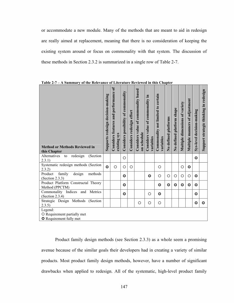
147
or accommodate a new module. Many of the methods that are meant to aid in redesign
are really aimed at replacement, meaning that there is no consideration of keeping the
existing system around or focus on commonality with that system. The discussion of
these methods in Section 2.3.2 is summarized in a single row of Table 2-7.
Table 2-7 – A Summary of the Relevance of Literature Reviewed in this Chapter
Method or Methods Reviewed in this Chapter Su
ppor
ts r
edes
ign
deci
sion
-mak
ing
Con
side
rs fe
atur
es a
nd p
erfo
rman
ce o
f ex
istin
g sy
s
Con
side
rs p
ossi
bilit
y of
com
mon
ality
Con
side
rs r
edes
ign
effo
rt
Con
side
rs v
alue
of c
omm
onal
ity b
ased
on
sche
dule
C
onsi
ders
val
ue o
f com
mon
ality
in
vari
able
s C
omm
onal
ity n
ot li
mite
d to
cer
tain
va
riab
les
No
defin
ed p
latf
orm
s
No
defin
ed p
latf
orm
shap
e
Mul
tiple
dim
ensi
ons o
f var
iety
Mul
tiple
man
ners
of a
djus
tmen
t
Sys-
leve
l dec
isio
n-m
akin
g
Supp
ort s
trat
egic
thin
king
in r
edes
ign
Alternatives to redesign (Section 2.3.1) Systematic redesign methods (Section 2.3.2) Product family design methods (Section 2.3.3) Product Platform Constructal Theory Method (PPCTM) Commonality Indices and Metrics (Section 2.3.4) Strategic Design Methods (Section 2.3.5) Legend:
Requirement partially met Requirement fully met
Product family design methods (see Section 2.3.3) as a whole seem a promising
avenue because of the similar goals their developers had in creating a variety of similar
products. Most product family design methods, however, have a number of significant
drawbacks when applied to redesign. All of the systematic, high-level product family

148
design methods with the exception of that of Suh and coauthors (Suh, Kim et al. 2004;
Suh 2005) and the Product Platform Constructal Theory Method (Hernandez, Allen et al.
2002; Hernandez 2003; Williams, Allen et al. 2004; Williams, Allen et al. 2005) utilize
only one means of offering product variety such as scaling or modularity, but not
multiple means even when it is a possibility. Many product family design methods
require that the design variables be separated into two groups, one of which is allowed to
vary in every family member and another of which is kept constant across the entire
family. The PPCTM is again an exception to this rule. Finally, all product family design
methods presume that the design process is being started from scratch and most assume
that all products will be offered at once. As a result, the difficulty of redesigning existing
systems to realize the new ones is not considered by any existing method, nor is the
difference in commonality between products that are offered simultaneously and those
that are not.
It is because of the capabilities that make it unique that the PPCTM has been
chosen as the starting point to structure the redesign problem and solve it. PPCTM is
alone amongst product family design methods in its ability to:
• Utilize multiple modes of commonality, permitting a designer to use scaling
variables or modules in the same product family;
• Handle product families with variety in any number of dimensions;
• Create product platforms of arbitrary size and shape without needing to
specify them ahead of time; and
• Address the need for customized products at any point in a geometric space.
Given these characteristics, it should be clear why the second hypothesis is:
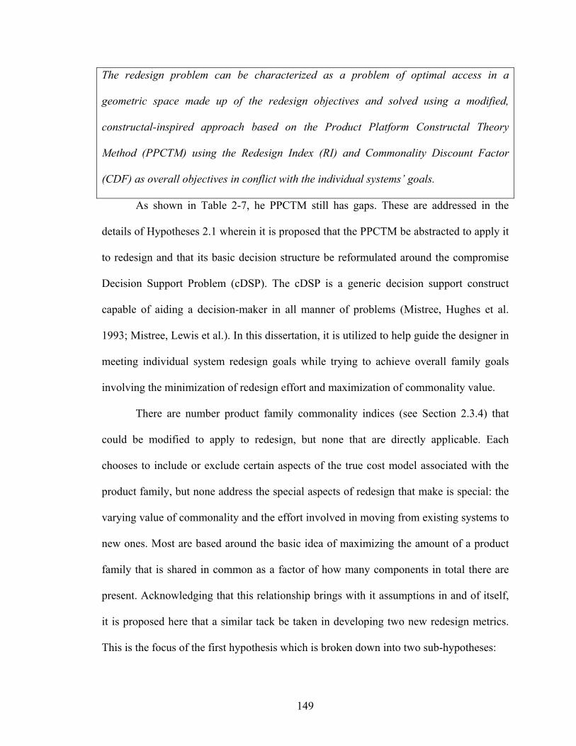
149
The redesign problem can be characterized as a problem of optimal access in a
geometric space made up of the redesign objectives and solved using a modified,
constructal-inspired approach based on the Product Platform Constructal Theory
Method (PPCTM) using the Redesign Index (RI) and Commonality Discount Factor
(CDF) as overall objectives in conflict with the individual systems’ goals.
As shown in Table 2-7, he PPCTM still has gaps. These are addressed in the
details of Hypotheses 2.1 wherein it is proposed that the PPCTM be abstracted to apply it
to redesign and that its basic decision structure be reformulated around the compromise
Decision Support Problem (cDSP). The cDSP is a generic decision support construct
capable of aiding a decision-maker in all manner of problems (Mistree, Hughes et al.
1993; Mistree, Lewis et al.). In this dissertation, it is utilized to help guide the designer in
meeting individual system redesign goals while trying to achieve overall family goals
involving the minimization of redesign effort and maximization of commonality value.
There are number product family commonality indices (see Section 2.3.4) that
could be modified to apply to redesign, but none that are directly applicable. Each
chooses to include or exclude certain aspects of the true cost model associated with the
product family, but none address the special aspects of redesign that make is special: the
varying value of commonality and the effort involved in moving from existing systems to
new ones. Most are based around the basic idea of maximizing the amount of a product
family that is shared in common as a factor of how many components in total there are
present. Acknowledging that this relationship brings with it assumptions in and of itself,
it is proposed here that a similar tack be taken in developing two new redesign metrics.
This is the focus of the first hypothesis which is broken down into two sub-hypotheses:

150
Hypothesis #1: Through the use of two indices as objectives in a redesign problem, better
redesign strategies utilizing fewer design changes and more valuable targeted
commonality can be identified.
Hypothesis #1.1: By utilizing the minimization of the Redesign Index (RI) as an objective
in a redesign problem, a decision-maker’s attention can be directed to redesign solutions
involving lower numbers of design changes in targeted parts of a system..
Hypothesis #1.2: By utilizing the minimization of the Commonality Discount Factor
(CDF) as an objective in a redesign problem, the designer’s attention can be directed to
combinations commonality in the most valuable parts of a system that is being
redesigned.
Finally, thinking strategically in Section 2.3.5, no existing method considers the
future design possibilities inherent in a family. An argument could be made that Design
Capability Indices (Chen, Simpson et al. 1996; Chen, Simpson et al. 1999) do this but
they only provide a range, which is of little use if the variety of interest lies inside that
range.
Having gone through the literature review in the earlier sections of this chapter,
the research questions and hypotheses are filled out in greater detail, the argument is
made here that given a decision-based-design perspective, the starting building blocks of
an approach to strategic sequential redesign should be the Product Platform Constructal
Theory Method, the compromise Decision Support Problem, and two indices that still
need to be developed later in this dissertation. In the next section, the role of this chapter
in the larger process of proving the research hypotheses and validating the proposed
methods is discussed.

151
2.5 - CONTRIBUTIONS IN THIS CHAPTER TO THE DOMAIN-INDEPENDENT
STRUCTURAL VALIDITY OF THE PROPOSED METHOD
In this chapter, it has been demonstrated that there are significant gaps in the
ability of existing methods to support a designer faced with conceptual sequential
redesign of an engineering system. There are positive and negative ways of viewing this
gap. On the negative side, while many of the requirements for supporting such a redesign
process are met by particular methods that have been developed for different types of
problems, no one method addresses all of the features that are important in this
dissertation. However, having clearly elucidated this gap, the research presented in this
dissertation is shown to be even more important than previously understood. On the
positive side, the fact that there is only a gap –meaning there is strong footing on either
side- means that there are methods upon which this research can be built.
The process of identifying this gap has contributed to the Theoretical Structural
Validity of the work in this dissertation. By further clarifying the gap, the purpose of this
research is also made clearer. By identifying the shortcomings of existing work when
applied to a sequential redesign problem, the usefulness that must be demonstrated by the
proposed method here is spelled out in greater detail.
The first construct discussed in this chapter is the Product Platform Constructal
Theory Method (PPCTM) (Hernandez 2001; Hernandez, Allen et al. 2002; Carone,
Williams et al. 2003; Hernandez, Allen et al. 2003; Williams 2003; Williams, Allen et al.
2004; Williams, Rosen et al. 2004; Kulkarni, Allen et al. 2005) based upon the ideas of
constructal theory (Bejan 1996; Bejan 1997; Bejan and Ledezma 1998; Bejan 2000). The

152
PPCTM has several features that make it particularly interesting in this dissertation,
chiefly the ability to utilize multiple modes of changing a product to create variety in
multiple dimensions without a need to specify sizes or numbers of product platforms
ahead of time.
The second construct is the compromise Decision Support Problem (Mistree,
Hughes et al. 1993; Mistree, Lewis et al.). that will be infused into the decision-making
process of PPCTM to support the redesign of individual systems to meet new individual
goals. The cDSP has been used widely in all sorts of engineering applications and has
been utilized as the basic building block for the development of techniques for robust
design (Chen, Allen et al. 1996; Chen, Mavris et al. 1996), product family design
(Simpson 1999; Simpson, Chen et al. 1999), hierarchical systems design (Kuppuraju,
Ganesan et al. 1985; Bascaran 1987; Shupe 1987; Bascaran, Bannerot et al. 1989;
Karandikar 1989; Vadde, Allen et al. 1994), and many other problems.
The final constructs will be developed in this dissertation. These are two indices
for assessing the merit of redesign plans based on the amount of redesign effort entailed
and the value of the commonality present. While developed from scratch, they adopt
many of the advantages and disadvantages seen in product family commonality indices
(see Section 2.3.4) in that they are quick to compute but may vastly oversimplify the
problem that is being solved.
These constructs are discussed in greater detail in Chapter 3, finishing the
assessment of their Theoretical Structural Validity, but the refinement of their purpose
and the identification of the ways in which they succeed in addressing sequential
redesign’s demands are both important first steps in the process of validation.

153
2.6 - STATUS AND PROMISE
Through the critical evaluation of literature contained in this chapter, it has been
shown that the problem of high-level sequential strategic redesign is not fully addressed
by any existing decision support methods. By clarifying the deficiencies of these
methods, the purpose of the approach proposed here is refined. By identifying the ways in
which these methods hold promise in meeting some of the demands of sequential
strategic redesign, some of the constructs of the proposed approach are chosen. Both the
refinement of purpose and the identification of constructs help to address the Theoretical
Structural Validity of the proposed approach and of the hypotheses put forward in
Section 1.3.2. In the coming sections of Chapter 3, the rest of the proposed approach is
developed using the constructs of the Design Capability Index, the Product Platform
Constructal Theory Method, and the compromise Decision Support Problem. In the
course of the rest of this development, the Theoretical Structural Validity of the approach
will be completely demonstrated. In Chapter 4, this approach is used in the redesign of
various families of universal motors, lending credence to the Empirical Structural
Validity and Empirical Performance Validity of the research hypotheses.

154
CHAPTER 3
ADDRESSING STRATEGIC REDESIGN AS A LIMITED PROBLEM OF OPTIMUM ACCESS IN A GEOMETRIC SPACE
3.1 - A PREVIEW OF THIS CHAPTER’S CONTENTS
In the Sections 2.3 and 2.4, it is shown that no known approach exists to address
the problem of sequential strategic redesign. In addition, a number of gaps are shown to
exist in even the most promising methods when they are applied to the problem of
strategically redesigning one or more systems to realize a string of new systems over
time. A constructal approach has been identified as a promising way of exploring the
possibility of reusing elements of existing systems and encouraging new systems to share
components where possible. Previous uses of constructal-inspired product family design
methods have demonstrated the ability to explore commonality but do not support design
towards specific demands and fail to account for existing systems, the effort involved in a
redesign project, or the varying value of commonality between systems. It is proposed in
Section 1.3.2 that these gaps be addressed through the adaptation of a constructal-inspired
product platform design method to redesign by creating two new indices to measure the
merit of a redesign plan and by incorporating a compromise Decision Support Problem
(DSP) into the decision-making process.
In this chapter, the way in which these changes are implemented is explained. The
indices for redesign are developed in Section 3.2 and the logic behind them is explained.
In Section 3.3, the infusion of the cDSP into the constructal-inspired approach is
explained, as are the rippling effects that this change has on other activities. In addition,
the abstractions that need to be made to convert the constructal-inspired product platform

155
design method into a redesign decision support method are discussed. Finally, in Section
3.4, the adjusted approach is explained step-by-step and one potential solution process is
laid out.
3.2 - DEVELOPMENT OF INDICES APPROPRIATE TO CHARACTERIZING THE
GOODNESS OF REDESIGN
As discussed in Section 2.4, there are two key characteristics of redesign
problems that are not reflected in the indices that are commonly used in original design
and product family design to encourage commonality between related systems. In this
section of the chapter, two indices are developed to model the amount of redesign effort
in a proposed redesign plan and the value of commonality present between members of
family based on redesign. First, in Section 3.2.1, the motivation to develop these indices
is discussed. In Section 3.2.2, the reader is taken through a thought exercise to
demonstrate the thinking behind the Commonality Discount Factor (CDF) and Redesign
Index (RI), which are developed in Sections 3.2.3 and 3.2.4 respectively. These indices
are further developed to make them better suited to the synthesis of redesign plans in
work presented in Section 3.2.5. Finally, the indices are critically evaluated in Section
3.2.6.
3.2.1 - Motivation to Develop an Indices for Goodness in a Redesign Project
The motivation to develop metrics for the goodness of a redesign project is
twofold. The first piece of motivation is due to the fact that there is no existing metric for
redesign. In Section 2.3.4 and Section 2.4, it is also pointed out that commonality metrics

156
fail to take into account several factors that make redesign problems distinct from
original design of a single product, product family design, or even design under
uncertainty. The existing indices fall short in that they:
• Do not consider that there may be existing systems to be leveraged in the
redesign project;
• Do not model the effort involved in moving from production of any existing
systems to production of new systems, a change which may involve
investments in research, design, development, testing, and manufacturing
infrastructure; and
• Assume that all product family members are offered simultaneously so that
economies of scale can always be exploited.
The second piece of motivation comes from the decision to pursue a constructal-
inspired approach to commonality exploration in the redesign problem. As discussed in
Sections 2.4 and 2.5, one of the drawbacks to using this approach based on the Product
Platform Constructal Theory Method is that opportunities for commonality are not
pursued if they occur between geometrically dispersed systems or at a finer level of detail
than the prescribed stages. Creating a metric or metrics for redesign commonality and
incorporating it into the decision-making process can help alleviate this problem.
3.2.2 - A Redesign Metric Thought Exercise
In most product family design applications, the implicit assumption is that all
products will be offered at the same time, meaning that any commonality that the
products can have with one another is valuable. This is the concept of pure commonality

157
and is the basis for most indices or metrics for product families. What happens, however,
when the products are not all offered at once? Furthermore, what happens when one
product is leveraged through redesign to create the rest of the family? To help explore
these questions, a simple example is introduced here.
Consider the example of a small company that designs and manufactures a small
mobile robot used by police and the military in bomb disposal actions as shown in Figure
3-1. Moving on a pair of treads over mildly rough terrain, the robot is radio controlled
and has a short battery life. Sitting on top of its main body is a swiveling “tool package”
with a set of manipulators, lights, and simple cameras that broadcast images back to the
controller. The company is interested in expanding its product offerings in coming years
by exploring new design options for locomotion, for the main body, and for the tool
package that rides on top. More specifically, they are interested in making their vehicle
faster, enabling it to travel over rougher terrain, giving it a longer battery life, equipping
it with better sensors for intelligence-gathering applications, and improving its
control/communications technologies.
Figure 3-1 – Model I Bomb Disposal Robot
After a considerable amount of work, the company develops a set of new redesign
options as shown in Table 3-1. Each of these options helps the company achieve one or
more of its objectives for the new product family based on Model I. Using these options,

158
the company has identified five candidate designs, as shown in Table 3-2. Each of these
redesigned robots is meant to meet a new market niche in which the company is
interested. The redesigned product family shown in Table 3-2 is an attractive solution
because it only uses design changes in three main areas and it only involves one design
change in two of those areas as shown in Table 3-1. The product family members share
many components in common and reuse a number of the features of the existing system,
meaning that some of the costs that would be associated with designing, manufacturing,
and servicing a group of individually-optimized robots can probably be saved. This fact is
born out in the high values of TCCI and CI2 shown in Table 3-2.
Table 3-1 – Original Design and Redesign Options for Robot Family
Type A(existing design)
Type B
Type A(existing design)
Type B
Type A(existing design)
Type B
Type C
Tool
Pac
kage
Mai
n B
ody
Loco
mot
ion
Bomb disposal toolkit with manipulator, lights, simple camera, and simple radio communications
Reconnaissance package with improved satellite communications, multiple cameras, microphones, and other sensors
Low-profile body with limited storage for batteries
High-profile body with large storage space for batteries, increasing running time
Tracked system which is slow but very good at traversing uneven terrain
Wheeled system which is fast but can only handle smooth terrain
Hovercraft technology which is very fast and allows for travel over somewhat uneven terrains but is very expensive

159
Table 3-2 – Proposed Redesigned Robot Family
Model I
Model II
Model III
Model IV
Model V
Model VI
Degree of Commonality Index (Collier 1981) DComI = 2.5714 Total Constant Commonality Index (Wacker and Treleven 1986) TCCI = 0.6471
Selected Product Family Metrics:
Commonality Index (Martin and Ishii 1996) CI2 = 0.7333
Table 3-3 – The Robot Family with Redesign Choices Made Tool Package Main Body Locomotion Model I A A A Model II B A A Model III B B B Model IV B A B Model V B A C Model VI A A C
Measuring the value of this design reuse and commonality is difficult if the
schedule by which the newly redesigned systems will be released (shown in Figure 3-2)
is taken into account. With only one exception, none of the robots are released and retired
at the same time. Five of the six family members are to be redesigned based on one
existing system. This schedule reveals several problems with the assumption inherent in
all existing product family commonality indices that all commonality is desirable. Each
of these problems is discussed in greater detail below. For the purposes of this discussion,

160
two products with common features are being considered. What varies from case to case
is the schedule by which they are released, manufactured, and retired from the market.
Model I
Model II
Model III
Model IV
Model V
Model VI
Year 0 Year 5 Year 10 Year 15 Year 20 Year 25 Year 30 Figure 3-2 – Release Schedule for New Robots
Scenario #1: Commonality Between Products with Completely Coincident Production
This is the ideal case that is generally assumed in product family design examples
wherein the two product family members are designed, manufactured, and retired at the
same time as shown in Figure 3-3. This type of commonality can be seen between Model
III and Model IV in Figure 3-2 as well.

161
Year 1 Year 2 Year 3 Year 4
Product #1
Product #2
Time
Figure 3-3 – Two Products with Completely Coincident Production Schedules
Scenario #2: Commonality Between Products with Staggered Introduction Schedules
In the case shown in Figure 3-4, two products share features in common but one is
released after the other. An example of this situation is the commonality between the
main body and type of locomotion employed in Model I and Model II in Figure 3-2. A
comparison between Scenario #1 above and this case begs the question of whether or not
the type of commonality shown here is just as valuable as that in Scenario #1. In existing
product family metrics/indices this type of commonality would be equally-valued since
the production timetable is not taken into consideration. The delay between the releases
of the products could mean that further design work and testing on Product #2 needs to
occur, that some of the efficiency of the shared manufacturing systems is lost, or that
some of the benefit of having a shared inventory of parts is lost. The point to be taken
away here is that in some but not all cases, the type of commonality shown in Scenario #1
is preferred over that type shown here. There are exceptions to this rule –for instance
when the design changes in Product #2 involve no costs because they are modular- but
generally there is some cost in time and money to redesigning a new product family
member.

162
Product #1
Product #2
Year 1 Year 2 Year 3 Year 4
Time
Figure 3-4 – Two Generic Products with Staggered Introduction Schedules
Scenario #3: Commonality Between Products with Staggered Retirement
In the case shown in Figure 3-5, two products that share common features are
being offered at the same time, but one is retired before the other. An example of this
situation can be seen in Figure 3-2 between Model V and Model VI, which share
hovercraft technology. Model V is retired before Model VI. It would be preferable to
have common parts with a system that shares an entire production schedule for many of
the same reasons listed for Scenario #2. Namely, by retiring one product family member
earlier, some of the benefits of economies-of-scale are lost. Again, there may be
exception to this rule, but generally, one would prefer Scenario #1 to the situation shown
here if the choice was possible.
Year 1 Year 2 Year 3 Year 4
Product #2
Product #1
Time
Figure 3-5 – Two Generic Products with Staggered Retirements
Scenario #4: Commonality Between Products with Totally Staggered Production

163
In the case shown in Figure 3-8 and Figure 3-7, the production schedules of two
products with common features overlap but are introduced and retired at different points
in time. Figure 3-6 shows one variant of this scenario in which the production schedules
are completely staggered while Figure 3-7 shows a different variant in which one
product’s lifespan starts earlier and ends later than another member of its product family.
An example of the former scenario can be seen in Figure 3-2 where the Model IV and
Model V have staggered production schedules. Either of the variants of this scenario is
generally preferred less than Scenario #1, but the degree to which that is true depends on
the example at hand. They are less preferred for all of the reasons cited for Scenarios #2
and #3, namely the need for more testing and the lost potential savings as a result of
economies of scale. In addition, both variants involve two disturbances in the
manufacturing process, whereas Scenarios #2 and #3 involve only one. In this work, it is
suggested that neither of the two variants should be preferred over the other.
Year 1 Year 2 Year 3 Year 4
Product #1
Product #2
Time
Figure 3-6 – Two Generic Products with Completely Staggered Production

164
Year 1 Year 2 Year 3 Year 4
Product #1
Product #2
Time
Figure 3-7 – Two Generic Products with Completely Staggered but Overlapping Production
Scenario #5: Commonality Between Products with a Production Gap
In the case shown in Figure 3-8, two products share common components but
there is a gap between their production schedules. This is essentially a more extreme
combination of both Scenario #2 and Scenario #3. The gap in production means that the
value of commonality between the products might be further eroded by the loss of
knowledge of the system, by the need to set up or revitalize dormant manufacturing
facilities, and by the need to replenish supplies and materials that may no longer be on-
hand. Again, the main point to be taken away here is that commonality between products
in this situation is not as preferable as between products in Scenario #1.
Product #2
Year 1 Year 2 Year 3 Year 4
Product #1
Time
Figure 3-8 – Two Generic Products with a Production Gap
The four different types or degrees of beneficial commonality discussed above are
not differentiated in any existing product family metrics/indices. To be useful in

165
evaluating product families that evolve over time through redesign as discussed in the
robot example, the ability to differentiate and place values on these types of commonality
would be beneficial.
There is one other special aspect of a redesign scenario like the robot example that
is not captured using existing product family metrics. The basis for the simplest of these
metrics like Degree of Commonality Index (DComI) (Collier 1981) and Total Constant
Commonality Index (TCCI) (Wacker and Treleven 1986) is the counting of the number
of unique components out of the total number of components. Counting these
components might be useful in a redesign example since each new unique component
represents a redesign activity that must occur. In product family design, the numbers of
unique components can be weighted by their cost, the frequency with which they are
used, or various aspects relating to the difficulty of their manufacturing process as in the
Product Line Commonality Index (PLCI) (Kota, Sethuraman et al. 2000) and the Percent
Commonality Index (PCI) (Siddique and Rosen 1998). From a redesign perspective,
these are all important factors, but there are other factors not included in existing metrics
that are worth consideration. Aside from the cost of the production of the members of a
product family that evolves over time, there are overhead and startup costs associated
with every design change made. These costs –both in terms of man-hours and dollars-
come about due to the need to design variant or new components, to test those new
components and the whole new system, and to set up new manufacturing facilities. These
costs might be small in the case of a variant of a component that is designed using CAD
and manufactured using a CNC machine but they can be large if the new component, the
procedure by which it is tested, or the process by which it is manufactured are large,

166
complicated, or expensive. An example of this situation is shown in Figure 3-9 where the
decision is being made to change the system of locomotion in the robot. The decision-
maker must decide between a proven component that might require less investment to
develop and test and a component that relies on new, high-performance technology that
might cost much more to develop.
Figure 3-9 – Example of the Role of Difficulty in Redesign
Accounting for the cost or effort involved in redesign is made more complicated
by two more factors. First, even if the cost of redesigning individual components is small
compared to the rest of the costs to produce the family of products, the effect of redesign
cost can be cumulative in a family with a number of generations that emerge over time
through redesign to meet a variety of changing performance targets. Second, even in a
situation in which only existing components are being reused in a new design, there is
some cost to creating this redesign. An example of this is shown in Figure 3-10 where
two existing systems are being leveraged to create one new system. Even though all the

167
components used in the creation of the newly redesigned system already exist, they have
not been used together, tested, or manufactured together, meaning that some effort must
be expended to realize the new system.
Figure 3-10 – Example of Module-Swapping to Redesign
Typically, the cumulative cost of the effort involved in redesigning a system to
create new product family members is not counted in the metrics/indices used to evaluate
product family designs. The costs associated with module-swapping are also not
accounted for since all products are assumed to be designed and produced
simultaneously. All of these factors could have a significant impact on the person making
decisions as to what parts of a system should be redesigned and in what way to assure the
ongoing financial success of an evolving family of systems.
The ideas explored in this section are exploited in the next one to help guide the
development of two indices: one aimed at gauging the effort involved in redesigning
existing systems over time to meet new needs and another aimed at encouraging
commonality where it is most valuable to the designer.
3.2.3 - A Pair of Proposed Indices for Difficulty the Early Stages of Redesign

168
In previous sections, it has been shown that existing metrics/indices for product
family design fail to account for two important factors in redesign: the varying value of
commonality depending on the product release schedule and the effort involved in
making design changes. In this section, it is therefore proposed that some of the ideas
used in existing metrics/indices be adapted to create two metrics that do account for these
factors. These metrics are meant to work together to give the designer an indication of the
relative merit of various redesign plans.
A Weighted Commonality Discount Factor
A Commonality Discount Factor (CDF) is proposed which would take into
account the schedule by which newly redesigned members of the product family will be
released, manufactured, and retired. The basic idea behind the proposed factor is that,
ideally, commonality would occur between systems that are designed, tested,
manufactured, and retired at the same time. This situation would offer all of the savings
often attributed to product families (Robertson and Ulrich 1998). In its simplest form, the
factor could be calculated as follows:
instances of less than ideal commonalityall instances of commonality
CDF = ∑∑
[3.1]
In order to organize oneself and help recognize instances of commonality, it is
proposed that the designer construct a schedule like that shown in Figure 3-2 or Figure
3-11 and then use this schedule to construct a Commonality Opportunity Matrix (COM)
an example of which is shown in Figure 3-12. In the COM, instances of overlap in
production are shaded and coded for the type of commonality that exists between the two
systems, for instance SP to indicate “staggered production” like that shown in Figure 3-4

169
or SR for “staggered retirement” like that shown in Figure 3-5. The four types of
commonality proposed here are described in detail in Table 3-4 but it should always be
remembered that these are only one way of defining commonality value differences. Other
models with greater or lesser amounts of detail can be constructed to suit the problem at
hand. The inclusion of the amount of overlap between systems might be useful, for
instance. The remaining spaces are left white to indicate a gap in production between two
family members.
Model 1000
Model 900
Model 800
Model 700
Model 600
Model 500
Model 400
Model 300
Model 200
Model 100
Year of Production10987654321
Model 1000
Model 900
Model 800
Model 700
Model 600
Model 500
Model 400
Model 300
Model 200
Model 100
Year of Production10987654321
Figure 3-11 – Redesign Schedule

170
Figure 3-12 –Commonality Opportunity Matrix
Next the designer must consider each redesign variable and how much each type
of sub-ideal commonality would hurt the value of commonality for that variable. The
designer must select a value on a scale from 0 to 1.0 where:
• A value of 0 indicates that regardless of the staggered nature of production or
the gap in production, the value of commonality between two products with
the same variable value is the same as if production were started and ended at
the same time. This might indicate that there are no costs associated with
starting up manufacturing after a gap in production or that there were no cost
savings due to simultaneous manufacturing to be lost through staggered
production.

171
• A value of 1.0 indicates that a gap in production or staggered production
schedules for two products sharing a common value of the variable in question
completely negates the value of commonality. Essentially, choosing a
discount factor of 1.0 means that the production schedule is such that the
company might as well design a new component from scratch. Some reasons
why this might occur could be a lack of economies-of-scale savings due to
commonality or excessive costs associated with setting manufacturing
facilities back up after a gap in production.
Using the discount factors described in Table 3-4, a detailed definition of CDF is
given as follows:
( ) ( ) ( ) ( )
( )1
1
i i i i
n
i SII i SRI i SPI i PGIi
n
new jj
SII SRI SPI PGICDF
N n
ψ ψ ψ ψ=
=
⋅ + ⋅ + ⋅ + ⋅ =
⋅ − Φ
∑
∑ [3.2]
where:
Φj = the number of instances of design changes that result in new values of
variable i
SIIi = the number of instances of commonality between products with staggered
introduction schedules
SRIi = the number of instances of commonality between products with staggered
retirement schedules
SPIi = the number of instances of commonality between products with completely
staggered production schedules

172
PGIi = the number of instances of commonality between products with gaps
between their production schedules
ΨSIIi = the discount associated with instances of commonality between products
with staggered introduction schedules for variable i
ΨSRIi = the discount associated with instances of commonality between products
with staggered retirement schedules for variable i
ΨSPIi = the discount associated with instances of commonality between products
with completely staggered production schedules for variable i
ΨPGIi = the discount associated with instances of commonality between products
with gaps between their production schedules for variable i
n = the number of redesign variables used to characterize family members
Nnew = the number of new systems planned to be added to the family through
redesign
CDF = commonality discount factor
and:
0 ≤ ΨSIIi ≤ 1.0
0 ≤ ΨSRIi ≤ 1.0
0 ≤ ΨSPIi ≤ 1.0
0 ≤ ΨPGIi ≤ 1.0
Using this formulation, CDF ranges from a value of 1.0, which would indicate
that all of the commonality seen is so invaluable as to essentially be as advisable as
designing all the changed components from scratch to a value of 0, which would indicate

173
that either all of the instances of commonality have the ideal form seen in Figure 3-3 or
that the discount factors for all the other types of commonality are all 0.
Table 3-4 – Four Different Types of Commonality Discounting Factors Situation Discount Factor Pertinent Question
1. Staggered Introduction Product #1
Product #2
Year 1 Year 2 Year 3 Year 4
Time
Staggered Introduction Index (SII) Symbol: ,SII iψ
For the variable in question, how much does a staggered production schedule hurt the value of sharing values between two products?
2. Staggered Retirement
Year 1 Year 2 Year 3 Year 4
Product #2
Product #1
Time
Staggered Retirement Index (SRI) Symbol: ,SRI iψ
For the variable in question, how much does having two products retire at different times hurt the value of sharing values between them?
3. Totally Staggered Production
Year 1 Year 2 Year 3 Year 4
Product #1
Product #2
Time
Year 1 Year 2 Year 3 Year 4
Product #1
Product #2
Time
Staggered Production Index (SPI) Symbol: ,SPI iψ
For the variable in question, how much does having two products introduced at different times and retired at different times hurt the value of sharing values between them?
4. Production Gap
Product #2
Year 1 Year 2 Year 3 Year 4
Product #1
Time
Production Gap Index (PGI) Symbol: ,PGI iψ
For the variable in question, how much does a gap in the production schedule hurt the value of sharing values between two products?
Note: it is assumed in this table that perfect commonality has no discount, however it could be added as a fifth commonality type. The definition of the types of commonality is up to the discretion of the designer and will depend on the characteristics of the redesign problem at hand.
This formulation of CDF would give a decision-maker an indication of the value
of the commonality in a product family that evolves over time through redesign, taking

174
into account various aspects of the production schedule and even addressing the problem
of module swapping discussed in Section 3.2.3. On the other hand the proposed
formulation of CDF does not take into account the length of times associated with
delays/overlaps, meaning that a small gap is valued identically to a large gap. This is a
problem which could be addressed by adding a multiplier to each term in the definition of
CDF. The multiplier could weigh the discount of each instance of sub-ideal commonality
by the amount of time over which it occurs –either in weeks, months, or years depending
on the application at hand.
3.2.4 - A Proposed Index for Redesign Effort and Commonality / Non-Commonality
the Early Stages of Redesign
For preliminary redesign concept exploration at a high level, it seems most
appropriate to use as basic an indicator of commonality as possible. Most product family
commonality indices make use of some variant of Collier’s Degree of Commonality
Index (Collier 1981), which is based around the concept of maximizing the ratio of
products in a family to unique components used in the family. Put another way, the goal
is the minimization of the number of unique parts. The parallel to this concept in redesign
would be the minimization of the number of design changes or the ratio of number of
design changes to the total number of design variables needed to characterize the systems
making up the family. One formulation of this index (RI) on a scale of 0 to 1.0 would be:

175
(# design changes)+1Redesign Index = (# new family members)(# variables in system)
(# unique variable values)RI(# new family members)(# variables in system)
or
=
[3.3]
A redesign difficulty index (RDI) can be added to the formulation to represent the
relative difficulty of making changes in different variables/components/subsystems. The
RDI would also be on a scale between 0 and 1.0. A RDI value of 0 would indicate that
changing the variable in question comes with no cost in dollar terms, setup time, etc. One
example of such a change might be a CNC-machined part based on a parametric CAD
model that simply would need to be updated. A RDI value of 1.0 would be pegged to the
design change that, out of all the options available, is expected to be the most difficult,
costly, and/or time consuming. The rest of the design changes could be pegged according
to this scale. Using this scale for RDI means that a very simple design change with an
RDI of 0 would be equivalent to keeping the value common. The more formal
formulation of RI would now be the following:
( )1
n
i ii
new
RDIRI
N n=
⋅Φ=
⋅
∑ [3.4]
where:
Φi = the number of instances of design changes that result in new values of
variable i
n = the number of redesign variables used to characterize family members
Nnew = the number of new systems planned to be added to the family through
redesign
RDi = redesign difficulty index for the change Φi

176
and:
0 ≤ RDIi ≤ 1.0
The redesign index, as it is now formulated, would still have a range between 0
and 1.0. A value of 0 could indicate that either no redesign occurs, meaning all variable
values are common throughout the family, or that the RDI values for all of the variables
that are changed in the family are all 0. A value of 1.0 indicates that every
component/subsystem in the family is redesigned using the most difficult option for each
new family member, that all of the new products are released share common variable
values but that the value of commonality is nil as a result of the difficulty of bringing
back old subsystems, or that some combination of these two scenarios occurs.
The two redesign indices proposed, CDF and RI, can be used in concert to help
the decision-maker judge the relative merit of alternative redesign plans. In general, the
designer will want to maximize both CDF and RI as part of the overall objectives of the
redesign plan, as shown in Figure 3-13. To help with the interpretation of various values
of CDF and RI, a summary of possible interpretations of high and low values of the
respective indices are given in Table 3-5

177
Figure 3-13 – Plot of CDF Versus RI
Table 3-5 – Interpretations of CDF and RI Values Potential Interpretations
Low RI • Small number of design changes • Proposed changes are generally inexpensive/easy
High RI • Large number of design changes • Proposed changes are generally expensive/difficult/intense
Low CDF
• All of the products are offered at once • Despite a staggered production schedule, significant savings can
be realized from the types of commonality proposed in the redesign plan
High CDF • The nature of the production schedule makes the commonality worthless
It is assumed here that accurate estimations of the actual costs associated with
redesign decisions are not available for use as an objective in this problem. As Keeney

178
and Raiffa (Keeney and Raiffa 1976; Keeney 2002) note, the only way to make good
value trade-offs is to use the actual objective in any problem. Lacking the ability to model
that objective, summary statistics can be used as “means objectives” so long as care is
taken to make sure that these statistics are consistent with the designer’s real preferences
and that they should be:
• Comprehensive, meaning that for a given level of that statistic, the designer
has a good idea of how well his/her objectives have been achieved; and
• Measurable, meaning that for each alternative, it is possible to obtain either a
probability distribution for a given range of the statistic or a point value and
that the decision-maker’s preferences can be assessed at all possible values of
the attribute.
The degree to which the indices proposed here measure up to the standards put
forth by Keeney and Raiffa depends on the care taken in setting them up and testing
them. Consistency with the decision-maker’s preferences and comprehensiveness can
only be checked through testing using examples from whatever problem is at hand. At
best, obtaining an index that is perfectly comprehensive will be difficult, likely
impossible. Depending on how high a level from which the design problem is to be
viewed, the primary objective changes. If a very high level view is taken, the objective is
the maximization of profit. Thus the objectives of maximizing commonality and
minimizing redesign effort would be means objectives for the overall objective. The
metrics proposed would only be indicators for those means objectives. To test how
accurate they are, the decision maker would have to be able to assess profit, which is two
levels of abstraction higher than the indices. Still, considering that there is no absolute

179
scale for “commonality” and that the assumption in this research that there is no accurate
way to estimate the dollar cost of redesign, these indices are the best that can be done.
3.2.5 - Modification of the Proposed Indices for Use in Synthesis
While the indices proposed in Section 3.2.5 are useful for analysis of redesign
plans in much the same way as the product family indices discussed in Section 3.2.2, it is
much harder to make use of them for synthesis. The fact that the indices are based on a
count of common parts makes them discontinuous, meaning that new redesign plans must
either be generated by hand or through use of an algorithm capable of handling
discontinuous objectives. Optimization methods for discontinuous objectives include but
are not limited to genetic and evolutionary algorithms, simulated annealing, particle
swarm methods, and simple exhaustive search or grid search. The latter option –a grid or
exhaustive search- is by far the simplest to implement but requires that the redesign
variables be evaluated at discrete values, a process that becomes cumbersome as the
number of variables is increased and the grid is reduced to a level suitable to model
variables that are in reality allowed to vary continuously. A much wider array of
optimization and synthesis algorithms are available for continuous objectives and
variables, so it is beneficial to seek new definitions of the indices that fulfill the same
roles as those tested in Section 3.2.6 but do so in a manner that results in an objective
function that is at least piecewise continuous.
The proposed new form is as follows for CDF:
( )( )( )
comm type1 1
min 1new
jk
N n
ijkj i
new
CDFN n
= =
−Ψ ⋅∆=
⋅
∑∑ [3.5]

180
where:
( )( )comm typemin 1jk jk−Ψ ⋅∆ = minimum weighted distance between variable i in
system j and any other system k given the type of commonality
relationship (perfect, SII, SRI, SPI, or PGI) between systems j and k.
�jik = the normalized distance between the values of variable j for systems k and l
ΨSIIjk = the discount associated with instances of commonality between products
with staggered introduction schedules for variable i
ΨSRIjk = the discount associated with instances of commonality between products
with staggered retirement schedules for variable i
ΨSPIjk = the discount associated with instances of commonality between products
with completely staggered production schedules for variable i
ΨPGIjk = the discount associated with instances of commonality between products
with gaps between their production schedules for variable i
n = the number of redesign variables used to characterize family members
Nnew = the number of new systems planned to be added to the family through
redesign
CDF = commonality discount factor
and:
0 ≤ ΨSIIik ≤ 1.0
0 ≤ ΨSRIik ≤ 1.0
0 ≤ ΨSPIik ≤ 1.0
0 ≤ ΨPGIik ≤ 1.0

181
It should be noted that a value of 0 should never be used for the commonality
discount in this formulation of CDF, as it will effectively eliminate the variable
interaction in question from consideration, as explained later in this section.
The proposed piece-wise continuous form for RI is as follows:
( )1 1
minnewNn
i ijki j
new
RDIRI
N n= =
⋅∆=
⋅
∑∑ [3.6]
where:
( )min j jklRDI ⋅∆ = the minimum weighted distance between the value of variable
i for system j and that of any other system k that preceded it
�ijk = the normalized distance between the values of variable i for systems j and k
n = the number of redesign variables used to characterize family members
Nnew = the number of new systems planned to be added to the family through
redesign
RDIi = redesign difficulty index for change in variable i
and:
0 ≤ RDIi ≤ 1.0
As a simple graphical check of the formulations of RI and CDF proposed here,
consider a redesign problem in which there is only one variable to be adjusted, three
existing systems with distinct values of that variable, and two new systems to be realized
based on redesign. This problem is summarized in Table 3-6.

182
Table 3-6 – Summary of Simple One-Variable Redesign Problem for Graphical Analysis
Given: Two existing systems with variable values of 1, 3, and 8 respectively
Equal commonality discounts between all systems
Find: X1 and X2, the variable values for two new systems that are to be created
based on redesigns of the three existing systems
Minimize The values of RI and CDF for the entire family.
Intuitively, if RI is working correctly, it should provide minimum values
whenever both of the new designs use the same values as the existing systems. Similarly
given that all the commonality discounts are set evenly, CDF should be at a minimum
whenever the two variables each take on a value used in the existing systems. This is in
fact the result generated if every value of X1 and X2 is plotted for values of each ranging
between 0 and 10, as shown in Figure 3-14 and Figure 3-18.
a.) Isometric View
b.) Overhead View (dark areas are low points)
Figure 3-14 – CDF Plots for Simple One-Variable Example

183
a.) Isometric View
b.) Overhead View (dark areas are low points)v
Figure 3-15 – RI Plots for Simple One-Variable Example
The simple redesign problem with one variable, three existing systems, and two
new systems is changed slightly as shown in Table 3-7 to have one existing system with a
value of 7 and to have commonality discounts that favor the following:
• Commonality between new system #1 and the existing system with a variable
value of 1; and
• Commonality between new system #2 and the existing system with a variable
value of 8.
Under these circumstances, it can be expected that some of the minimum values
for RI and CDF should move from the previous existing system value of 3 to the new
value of 7 and that as a result of the varying values of the commonality discounts:
• the slope of CDF in the X1 direction near the variable value for existing
system #1 will be steeper than elsewhere; and
• The slope of CDF in the X2 direction approaching the variable value for
existing system #2 will be steeper than elsewhere.

184
These desirable outcomes are just what can be observed in Figure 3-16 and Figure
3-17. Again, these plots are based upon assessing the indices for values of X1 and X2
between 0 and 10 at a refinement of 0.25.
Finally, in the simple one-variable experiment shown above, it should be noted
that, as suggested in the development of RI and CDF, they are not continuous functions.
Rather, each is a piecewise continuous linear function for a portion of the space between
minima. This fact will come into play later in Chapter 4 when the task of solving for a
redesign solution based on these indices is tackled. Discontinuities require special
approaches when algorithms are to be used to search along such objective functions.
Table 3-7 – Summary of Simple Redesign Problem for Graphical Analysis with New Existing Systems and Differences in Commonality Discounts Given: Two existing systems with X values of 1, 7, and 8 respectively
Increased value of commonality between new system #1 and the existing system with a value of 1. Increased value of commonality between new system #2 and the existing system with a value of 8.
Find: X1 and X2, the values of X for two new systems that are to be created based on redesigns of the three existing systems
Minimize The values of RI and CDF for the entire family.
a.) Isometric View
b.) Overhead View (dark areas are low points)
Figure 3-16 – CDF Plots for Simple One-Variable Example with New Existing Systems and Weights

185
a.) Isometric View
b.) Overhead View (dark areas are low points)
Figure 3-17 – RI Plots for Simple One-Variable Example with New Existing Systems
3.2.6 - A Critical Evaluation of the Proposed Redesign Metrics
It is pointed out in discussing product family metrics in Section 2.3.4 and Section
2.4 that none of those reviewed are perfect; their developers all picked and chose the
types of information to be included, thus building assumptions into the metrics either
consciously or subconsciously. The same can definitely be said for the two indices
proposed in this chapter.
First, it is assumed that the designer is enough of an expert on the system being
redesigned and the future of the family of systems to be able to fill in all of the weights
and commonality discounts in the two indices. It is also assumed that he/she has an
understanding of the influences of those weights upon the resulting redesign portfolios so
that he/she can set them in a way that accurately reflects his/her preferences. Lastly, the
indices are assumed to be accurate indicators of redesign effort and commonality value
respectively. Using these together as the overall goals neglects myriad other factors that
might concern the designer including manufacturing costs, production volumes, volumes
of demand in the market for each product, and any uncertainties in the problem.

186
So are these indices good things to use as objectives in a redesign problem?
Keeney (Keeney 2002) suggests that the only way to make good value trade-offs is to
deal directly with the fundamental objectives in the problem. Clear measures of the
degree of achievement of fundamental objectives are needed in order for this to work. At
the very least –he suggests- it is necessary to find means objectives that are consistent
with your preferences. He uses the trade-off between reducing the costs associated with
reducing air pollution and minimizing the health effects of air pollution. In studies, it is
common to see objectives like reduction of concentrations of pollution in the air, but
these don’t really measure what we care about: the effect of those concentrations on
people. Anything else besides the fundamental objectives is a means objective or is at
best an indicator of a fundamental objective.
An alternative they suggest are proxy attributes which indirectly indicate the
degree to which a fundamental objective has been satisfied. Such an attribute is useful
when the fundamental objectives are not numerical or cannot be measured. As the
Keeney and Raiffa (Keeney and Raiffa 1976) point out, the downside of using proxy
attributes is that it forces the decision-maker to process more information internally than
if he/she could use fundamental attributes.
“Essentially, the introduction of proxy attributes requires that some of the
modeling of the system be done in the decision maker’s head. This is what
we would often like to avoid, because there is too much information in
complex problems to handle effectively this way. However, when it is
unavoidable, careful thinking may permit the decision maker to express a
useful set of relationships between proxy attributes and the original

187
objectives. It is probably safe to say that, in general, when a smaller part
of the model must be implicitly considered by the decision maker, the
quantified preferences more accurately reflect his true preferences for the
basic objectives.” -Keeney and Raiffa
As mentioned earlier, Keeney and Raiffa (Keeney and Raiffa 1976) suggest that
in order to be useful to a decision-maker in a complex problem, an attribute must be both
comprehensive and measurable. Comprehensiveness refers to the degree to which the
attribute yields the information needed while measurability refers to whether it is possible
to calculate the data needed to use the attribute.
In the end, the goal of including these indices is to achieve results that are closer
to those that the designer really would prefer, so the only thing that matters is that his/her
preferences are modeled as well as possible. A conscious decision has been made here to
make the indices developed as simple as possible. Just as the example used in Section
3.2.2 is simple, the idea behind these indices is that they should be relatively simple and
easy to compute. One of the common criticisms of the existing metrics and indices for
product family design is that many of them require huge amounts of input information
and are too complicated even for an expert designer to evaluate and understand. To be
sure, a more complex model of value could be used and the designer’s preferences
assessed with respect to that model. Rather than build a complex model of value, it has
been proposed here that a simple model be built around these two indices and their
included biases. At their core, both indices are meant to increase commonality but also to
push commonality in certain places for various reasons.

188
This push towards commonality begs the question of whether or not commonality
is truly the outcome towards which the designer should be pushing. Indeed, some of the
product family metrics are criticized in Section 2.3.4 and Section 2.4 for valuing all
commonality equally. Here commonality is sought for a variety of reasons. It has
strategic benefits in addition to cost-savings in that it can: (McDermott and Stock 1994)
• Help to reduce the time needed for design –a particularly important factor in the
technologically sensitive automobile, telecommunications, and aircraft industries;
and
• Result in time and cost savings in manufacturing as fewer parts are kept in
inventory, setup times are reduced, and the production line needs to be shut down
less often to switch parts;
• Enhance product quality, as new products depend more upon proven platforms
and less upon newly designed components that have to be tested and for which
new manufacturing processes might be needed; and
• Reduce time-to-market as design cycle times become shorter.
Robertson and Ulrich point out that a company can release new, more highly-customized
products in a more efficient manner using product platforms (Robertson and Ulrich
1998). Wheelwright and Clark point out that the firm that is better able to bring their
products to market quickly is the firm that is more likely to survive (Wheelwright and
Clark 1992). In the redesign context, commonality in product platforms takes on a special
context because every instance of reuse of existing systems represents sunken resources
that continue to pay dividends. Still, in the end, both of the indices proposed here are
built upon the assumption that commonality in certain areas is an indicator of future

189
economic viability, and a proxy objective that serves as an indicator that pleases the
designer.
To be sure, the indices presented here do not meet the needs of Keeney. They are
proxy attributes at best, but as they are just intended for conceptual redesign and for
finding satisficing solutions, it is felt that they provide sufficient for the needs of a
designer interested in scoping out potential solutions, not identifying the final best design.
3.3 - ADAPTATION OF THE PRODUCT PLATFORM CONSTRUCTAL THEORY
METHOD TO SEQUENTIAL STRATEGIC REDESIGN
In order to make the Product Platform Constructal Theory method useful in
sequential strategic redesign, a number of arguments need to be made and some
abstractions drawn so that the gaps in PPCTM identified in Section 2.3.3 can be filled.
Specifically, the five gaps being addressed in this section are:
1. The lack of consideration of existing systems in creating product family designs;
2. The focus on designing a continuous range of products for a market space instead
of meeting the specific needs of customers with discrete demands for a certain
number of products over time;
3. The assumption that there is a level of performance change that a customer cannot
discern;
4. The assumption that geometric proximity between two systems in a market space
implies that commonality between those two particular systems is preferable; and
5. The failure to consider commonality at levels of detail smaller than the modes of
managing product variety.

190
The way in which each of these five gaps is addressed is the subject of this section
of the chapter. There is not a direct one-to-one correspondence between the changes
made to PPCTM and the gaps that are being filled because some changes affect more
than one gap while some changes necessitate further important changes. Two important
additions to PPCTM are the dual goals of minimizing RI and CDF, which are described
in detail in Section 3.2. The addition of these goals and their inclusion in a new
compromise DSP formulation of PPCTM go a long way towards addressing gaps 3, 4 and
5 above. The way in which this change is carried out is explained in Section 3.3.1.
Meanwhile, the rest of the first three gaps are handled by making the conscious decision
to abstract the mass customization problem for which PPCTM is intended to the redesign
problem at hand, modeling new features and interpreting existing features in new ways.
This is the subject of the discussion in Section 3.3.2. The resulting redesign decision
support method is explained in full in Section 3.4, but as a preview, PPCTM is shown
alongside the proposed redesign decision support method in Figure 3-18 to give an
impression of how pieces of the original method are reused and what new material is to
be presented here.
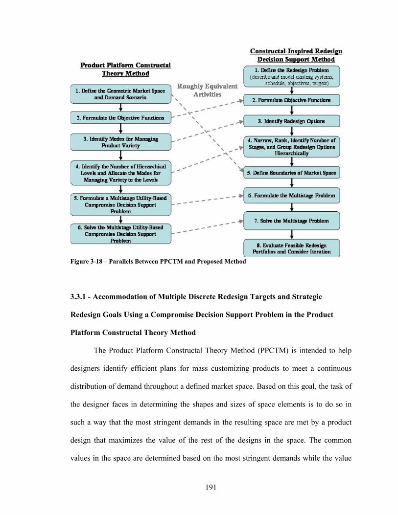
191
Figure 3-18 – Parallels Between PPCTM and Proposed Method
3.3.1 - Accommodation of Multiple Discrete Redesign Targets and Strategic
Redesign Goals Using a Compromise Decision Support Problem in the Product
Platform Constructal Theory Method
The Product Platform Constructal Theory Method (PPCTM) is intended to help
designers identify efficient plans for mass customizing products to meet a continuous
distribution of demand throughout a defined market space. Based on this goal, the task of
the designer faces in determining the shapes and sizes of space elements is to do so in
such a way that the most stringent demands in the resulting space are met by a product
design that maximizes the value of the rest of the designs in the space. The common
values in the space are determined based on the most stringent demands while the value
192
is determined based upon a continuous model of demand and cost/benefit for the whole
market. In framing the sequential strategic redesign problem, it has been envisioned that
a designer will be given certain redesign targets and a known schedule whereby the new
systems should be released. With discrete redesign targets and no knowledge of volumes
of demand, it makes little sense to use PPCTM in its current state for redesign For this
reason, a new type of baseline decision for this constructal-inspired method must be
identified.
Based on the problem description in Section 1.1, the decisions the designer must
make in fully describing each space element of a constructal-inspired redesign approach
can be identified. These goals, which would be the same for every space element at every
stage of a constructal-inspired approach, would be:
• Satisfy the redesign goals (targets values for responses of interest) of the
individual new systems;
• Minimize the amount of redesign effort that will be needed to create the
new systems based on the features of earlier systems; and
• Maximize the value of the sharing of components between systems based
on the proposed production schedule.
As is discussed in Section 2.4, the multi-objective compromise Decision Support
Problem (cDSP) has been chosen as the construct to guide this baseline decision because
of its flexibility, generality, and proven track record in design problems of all sorts. Later
versions of PPCTM, most notably that developed by Williams and coauthors (Williams
2003; Williams, Allen et al. 2004; Williams, Rosen et al. 2004), have made use of a
utility-based CDSP (u-cDSP) as the base for decisions in each space element. This is the

193
version of PPCTM most closely related to that which is proposed here, but it is still
fundamentally different. The new cDSP-based version for redesign is presented in Table
3-8. Key differences that should be noted appear in the variables to be found, the goals,
and the deviation function that results from those goals.
Unlike in PPCTM, it is necessary to identify the redesigned systems’ variables as
a part of the decision-making process. Previously, the decision-maker needed only
identify the space element size at each stage and then derive the system variables from
there. Thus in the redesign process, at each stage, the space element size must be
determined and at the same time, a set of the stage’s redesign variables must be found for
each new system in that element.
The goals at each stage are the same and are made up of goals for each individual
redesigned system as well as overall goals for the redesign process. The individual
system redesign goals represent the changes in performance that are desired. These
changes are modeled as targets using the compromise Decision Support Problem, so the
goal for each changing performance measure is to minimize the deviation from those
targets. The goals for the overall redesign process are represented using the Redesign
Index (RI) and Commonality Discount Function (CDF) which are meant to subjectively
measure the redesign effort and commonality value respectively. At any stage, the
designer’s goal is to minimize both RI and CDF towards their ideal (but impossible)
value of zero.

194
Table 3-8 – Basic Redesign Decision at Any Stage i For each stage i
Given: • The = Msysgoal-dimensional market space M Msysgoal = {(a1,a2,…aMsysgoal)} where ai is a system attribute that is expected to change over time through redesign
• The decision variables of the previous stages (1), (2), , ( 1)a a a i∆ ∆ ∆ −… and { } { } { }1 2 1
, , ,i
X X X−
…
• The existing systems { } { }1 2, , ,
Nexex ex ex exX X X X= … ,where
,1 ,2 ,, , ,
j j j j nex ex ex exX X X X= … and 1, exj N= …
• The modes of managing product change to be utilized at Stage i,{ }iX
where { } { }i newX X⊆
Find: The value of decision variables
• [ ]1 2( ) ( ), ( ), , ( )Nx i r i r i r i= ∆ ∆ ∆… to determine sizes of space elements; and
• { } { }, ,1 , ,2 , ,,
, , ,ii k i k i k ni k
X X X X= … for each space element k where ni is the
number of redesign variables used in construct i at stage i. The deviation variables and b bd d− + , for all Mtot goals
Satisfy: Bounds: • Variable bounds, i.e. min max1 , ,1 1i kX X X≤ ≤
• Space element sizes 0 ( )l la i a≤ ∆ ≤ ,where l is the number of dimensions of variety provided by construct i
• , 0b bd d− + ≥ for b = 1,…Mtot • 0b bd d− +× = for b = 1,…Mtot
Constraints: • ( ) ( 1)l la i a i∆ ≥ ∆ − Goals: • ( ) 1b
b bb
A x d dG− ++ − = for achievement of each of the
Msysgoal targets for each of the Nnew new systems • ( ) 0RI RI RIA x d d− ++ − = for RI • ( ) 0CDF CDF CDFA x d d− ++ − = for CDF
Minimize: ( )
( )
( )1
1where 1.0
new sysgoal
new sysgoal
N M
RI RI CDF CDF b b bb
N M
RI CDF bb
Z w d w d w d d
w w w
×+ + − +
=
×
=
= ⋅ + ⋅ +
+ + =
∑
∑
Note: Formulation of target-matching goal depends on whether target is being approached from above or below. Formulation shown is for approach from below. See (Mistree, Hughes et al. 1993) for a full description of all formulations

195
The objective function that results from these goals is shown at the bottom of
Table 3-8. An Archimedean or weighted sum form is used forth this objective function,
but there is no reason why another function with a preemptive form or a different rule
regarding the sum total of the weights cannot be used. In using the Archimedean form,
the designer must decide which weights best express his/her preferences towards the
goals present. However, these weights have no absolute meaning, so the designer must be
sure to closely inspect the results obtained. Iterating by reusing this decision support
method with slightly different weights may result in a redesign solution with significantly
different characteristics. For this reason, the designer must assign the weights carefully,
but with full recognition of the fact that the results produced may not be what he/she
originally intended.
3.3.2 - Abstraction of Concepts in the Product Platform Constructal Theory Method
to the Redesign of Engineering Systems
There are two key elements of PPCTM that do not translate directly from it and
the mass customization examples for which it is intended to the constructal-inspired
redesign method proposed here. In applying PPCTM, it is critically important that the
designer understand the role of these elements and that he/she describe them accurately.
The way in which each of these is abstracted to a sequential strategic redesign application
is described in this section.
The first concept that must be abstracted from PPCTM is the mode of managing
product or process variety. In previous applications, a mode of managing variety can be
viewed from one of two perspectives either as a way of achieving change in a

196
product/process or as a way of handling commonality across a selected piece of the
market. In the approach proposed here, the definition of these modes of offering system
change are not treated any differently but the criteria for selecting the modes may
change. More specifically, the list of modes of offering system change may differ from
the modes of managing product variety that the same designer would identify for original
design in that those modes for redesign will be:
• Smaller in number, as a result of a desire to leverage certain aspects of
existing systems or because of increased insight into the relationship between
the performance characteristics of the system and the original design
variables; or
• Made up of some groups of original design variables which together control a
function or particular performance characteristic of the system.
For these reasons, even a designer familiar with the design processes that created
the present existing systems must take care in identifying the modes of offering system
change. Although it is suggested above that the list of modes for redesign will likely be
shorter than the list of modes available in original design, there may be some new modes
not previously recognized that are now open for change as a result of better
understanding of a system’s characteristics.
The implementation of these modes across space elements must also be abstracted
to translate the capabilities of the PPCTM for designing a continuous range of products to
the capability to create a certain number of new systems with discrete performance
characteristics through redesign. In PPCTM, it is assumed that there is a level of each
performance measure below which the customer cannot or chooses not to differentiate

197
between systems. The practical impact is that customers whose exact demands fall in the
smallest space element possible are assumed to be satisfied with any performance levels
that also reside in that element. In designing mass customized systems using PPCTM, it
is generally assumed that it is safe to over-engineer in choosing the redesign variables at
each stage so that the resulting product in each space element is acceptable to those with
less stringent demands. In redesigning to create systems with certain performance
characteristics instead of a continuous range of products, it makes less sense to assume
that the customer will be satisfied with any performance “close” to what they asked for.
Given that they expressed certain demands, it makes sense to only design towards those
demands. The way in which this situation is accommodated in the method proposed in
this dissertation is to remove the assumptions in the smallest space elements, place all
variables into the modes that are applied at each stage and structure decisions at every
stage as a compromise Decision Support Problem in which achievement of redesign goals
is part of the objective.
The market space is the second element of PPCTM that deserves some translation
to the present redesign application. Recall the definition of market space given in Section
1.1.4: A market space is the range of system performance values over which a family of
related systems is expected to vary through redesign over time.
This definition differs significantly from that which is used in PPCTM. In that
method, the market space or space of customization is a pre-defined aspect of the mass
customization design problem as a piece of the market over which a demand distribution
is known. In the type of sequential strategic redesign problem envisioned here, there is no
known demand distribution, nor is there demand for systems outside of the discrete
198
redesign targets given, so the market space is not defined up front. Instead, it is proposed
here that the market space for redesign be derived based on other known aspects of the
problem, namely the existing system’s performance characteristics and the nominal
redesign targets that have been set. These values can be plotted in a Msysgoal-dimensional
space, where Msysgoal is the number of dimensions of change desired to be seen in the
newly redesigned systems. This process is shown in Figure 3-19. Having done this, it is
suggested that the designer identify an appropriate buffer space around the most extreme
values of the existing system and nominal new systems’ performance points. These
buffer zones are proposed for two reasons. First, by adding a buffer, design targets will
not lie right at the border of the market space. During the solution process, such a
situation could confuse algorithms that seek to keep solutions away from constraints but
close as possible to nominal target values. Second, the buffer zone provides the designer
with the opportunity to consider redesign compromise solutions that lie on either side of
the nominal target values, not simply the side that lies closest to the rest of the systems in
the family. The amount of buffer added to the market space is determined at the
discretion of the expert designer who is assumed to be carrying out the redesign process.

199
a.) A redesign problem with two existing systems and three new systems
b.) A potential buffer zone for the redesign problem at hand
Figure 3-19 – Buffer Zone for Market Space Explained
It is difficult to explain point-by-point all the changes that need to be made to the
PPCTM to create a method suitable to redesign, as many of the changes are interrelated,
depending upon one another to create the desired impact. Once these changes are made,
however, a whole new approach to sequential strategic redesign emerges. As is discussed

200
at the outset of this section, the goal in making these changes and abstractions is to
address the five key gaps in PPCTM when compared the requirements of a sequential
strategic redesign problem. The key modifications and abstractions discussed here in
Section 3.3 and earlier in Section 3.2 are as follows:
• Use of the Redesign Index (RI) and Commonality Discount Factor (CDF)
which roughly model the effort required to create all of the new redesigned
systems and the value of the common items shared between them while at the
same time providing objective functions to drive commonality at a level
PPCTM is not capable of;
• Incorporation of a multi-objective compromise Decision Support Problem
formulation for the redesign decision at each stage of the constructal-inspired
approach, which allows the designer to balance out overall goals such as the
minimization of RI and CDF while at the same time considering the specific
design goals of each new system;
• Abstraction of the concept of modes of managing product/process variety
PPCTM to make them reflect the needs of a designer engaged in a redesign
project who wants to apply modes of change in a system; and
• Abstraction of the purpose and process whereby the market space is defined
so that specific redesign targets can be addressed as a part of a compromise
solution that may involve underachievement or overachievement of target
values.

201
3.4 - A CONSTRUCTAL-INSPIRED REDESIGN DECISION SUPPORT METHOD
The gaps in the Product Platform Constructal Theory Method from the
perspective of one who needs to solve a sequential strategic design problem are addressed
in the preceding three sections of this chapter. Having developed new indices for redesign
that can serve as overall objectives, modified the basic decision-making structure at each
stage of the process, and abstracted the basic elements of the PPTCM, what is left is an
almost entirely new approach to redesign. This approach allows a designer to synthesize
redesign options while exploring commonality in what is best termed a constructal-
inspired manner. Where the constructal-inspired approach fails to find good solutions or
fosters only a limited amount of commonality, the redesign indices pick up the slack,
permitting a designer to identify opportunities for reuse even when the existing systems
are very different from one another. Having taken apart PPCTM, revised key elements of
it, and abstracted the remaining pieces to apply them to redesign, a new eight-step
process is developed as shown in Figure 3-20. The steps of this process and the way in
which a designer would carry them out are explained in this section of the chapter.

202
Figure 3-20 – Flowchart of Proposed Constructal-Inspired Redesign Method 3.4.1 - Step 1 – Definition of the Redesign Problem
The first step in the constructal-inspired redesign decision support method is the
definition of the background elements of the problem. The designer must identify the
existing systems that are candidates for leveraging in the new designs. The existing
systems must be described in detail and mathematical models that relate physical
parameters of those systems to their performance must either be obtained or created. It is

203
assumed that any system models obtained are valid beyond the performance range of the
existing systems, so that they can be used to model newly redesigned systems as well.
Next, the number of new systems must be chosen. Redesign targets must be
identified based on an assessment of how the market is expected to expand in the
foreseeable future. It is assumed that the designer only includes those redesign targets and
new systems for which he/she has a solid understanding of its performance demands and
desired release schedule. For each new system, the designer must pick measures of the
changed performance desired and set ideal target values G(x). The number Msysgoal of
performance attributes in which change is desired will be utilized later in Step 5 to
determine the number of dimensions in the market space while the target values will be
used in Step 2 to create the objective functions.
Having identified the redesign targets and the number of new systems to be
produced, the designer must lay out the schedule by which systems will be released and
retired. This schedule can then be used to create a Commonality Opportunity Matrix (See
Section 3.2.3) in which the designer identifies the types of commonality present between
the systems in the family. This process is explained graphically in Figure 3-21.

204
Figure 3-21 – Creation of the Commonality Opportunity Matrix
Finally, the designer must consider whether any further objectives are needed in
the redesign problem. It is assumed here that the designer will always want to minimize
the amount of effort involved in the redesign scenario being developed and maximize the
value of commonality present between systems. For this reason, minimization of both the
Redesign Index (RI) and Commonality Discount Function (CDF) are assumed to be
overall objectives. Other objectives that might be considered at a high level like the

205
minimization of RI and CDF could include family-wide goals such as similarity of shape
or size, minimization of variance in power requirements.
3.4.2 - Step 2 – Formulate Objective Functions
Having gathered all the information discussed in the first step, the next one
involves the formulation of objective functions based on the targets and overall
objectives. As discussed in Section 3.3.1, the redesign decision at each stage of the
constructal-inspired approach has been reformulated as a compromise Decision Support
Problem (cDSP). In the cDSP formulation, the designer’s preferences are expressed
through target values Gi(x) for each objective i and weights wi that are meant to model the
relative importance of each objective. The overall objective function in the Archimedean
form of the cDSP is a weighted sum of the deviation variables di+ and di
-, which represent
the amount by which each target value is over or under achieved, respectively. The
resulting objective function is as follows:
( )1
totM
i i ii
Z w d d− +
=
= +∑ [3.7]
where Mtot is the total number of redesign targets and overall objectives in the redesign
problem and the deviation variables di+ and di
- are found by calculating the achievement
of each design plan with respect to each goal. The way in which this achievement is
calculated depends upon the type of goal –be it minimization, maximization, or target
matching- as well as the target value for that goal. According to Mistree, Hughes, and
Bras, (Mistree, Hughes et al. 1993) there are three basic ways of calculating the deviation
variables based on the achievement value Ai(x) and the target Gi(x):

206
• If the goal is to be maximized towards some ideal value Gi(x), then the form
is:
( )i i i iA x d d G− ++ − = [3.8]
Or, when normalized, it can be formulated as:
( ) 1ii i
i
A x d dG− ++ − = [3.9]
In either case, in this form, it is id − that should be minimized and included in
the overall objective function.
• If the goal is to be minimized towards some ideal value Gi(x), then the form is:
( )i i i iG d d A x− ++ − = [3.10]
Or, when normalized, it can be formulated as:
1( )i
i ii
G d dA x− ++ − = [3.11]
In either case, in this form, it is id − that should be minimized and included in
the overall objective function unless the target value is zero, in which case the
achievement should be normalized by the maximum possible value of that
performance measure as follows
max
( ) 0( )i
i ii
A x d dA x− + + − =
[3.12]
And the goal should be to minimize id + .
• If the goal is to get as close as possible to some target value Gi(x) and it is to
be approached from below, the objective can be formulated like the
maximization goal discussed above.

207
• If the goal is to get as close as possible to some target value Gi(x) and it is to
be approached from above, the objective can be formulated like the
minimization goal discussed above.
• If the goal is to get as close as possible to some target value of zero, then the
objective can be formulated like the minimization objective above, but the
sum of the deviation variables ( )i id d− ++ that should be minimized.
Redesign targets for each response of the newly redesigned systems can be
modeled as target-matching objectives while the overall goals of minimizing CDF and RI
can be formulated as objectives that should be minimized towards zero. Other overall
goals may be formulated differently. If the only overall goals are to minimize CDF and
RI, then the objective function has the following form:
( )( )
( )1
1where 1.0
new sysgoal
new sysgoal
N M
RI RI CDF CDF b b bb
N M
RI CDF bb
Z w d w d w d d
w w w
×+ + − +
=
×
=
= ⋅ + ⋅ +
+ + =
∑
∑ [3.13]
The Archimedean weighted sum form of the objective function which is discussed
here is just one of several different ways in which a design problem has been formulated
using a cDSP. Alternatives include the preemptive or lexicographic formulation (Mistree,
Smith et al. 1993) as well as forms that describe problems using fuzzy information
(Allen, Krishnamachari et al. 1992; Vadde, Krishnamachari et al. 1993) or utility theory
(Seepersad 2001). The preemptive form allows a designer to group objectives and rank
those groups hierarchically so that lower-level goals are only pursued so long as they do
not require a drop-off in the achievement of higher-level goals. The preemptive form is
not used here because the designer would have to choose certain levels of achievement

208
for the top-level goals beyond which he/she did not require further improvement. Such
target levels would be hard to set for CDF or RI as their values have no absolute
meaning. Similarly, it might be hard to anticipate what levels of achievement of the many
redesign targets are even possible. The Archimedean form provides a much simpler way
of formulating the problem. The fuzzy and utility-based formulations are not used here
because their usefulness is rooted in problems fraught with quantifiable uncertainty. To
be sure, the redesign problems described here do involve uncertainty, however to
simplify the problem, it is assumed that all information is certain.
3.4.3 - Step 3 – Identify and Describe Redesign Options
The designer’s goal in step 3 is to identify and describe the modes of offering
system change that will be applied using the constructal-inspired approach. These modes
are ways in which the existing systems may be changed in order to realize the redesign
targets set for the new systems. In order to identify the modes, the designer may want to
consult any available information about the original design of the existing systems in
order to sort out the most promising changes. In considering these changes for inclusion
in the redesign decision-making process, it may be useful to consider the ramifications of
each change, both impacts from the change itself like the need to test a newly redesigned
component and from the ripple effects of a change. The ramifications in the latter
category might include other small design changes that will have to be made to
accommodate a mode or incompatibilities between modes being considered. The designer
may also want to consider the mathematical models of system performance that he/she
has to make sure that proposed changes can actually be modeled accurately.

209
The modes can be thought of as ways of changing the existing systems to realize
new performance characteristics, but they also may be thought of as ways of extending
the usefulness of the capital that has been sunk into the existing systems. That is, if a
mode is kept the same as in the existing system or systems, could the new systems be
designed around that mode? Using this way of thinking, modes would take on a
definition closer to that which is used in PPCTM. The question the designer would want
to ask him or herself in this case is “how much of the market could this mode cover with
a set value?”
Having identified the modes, the designer must assign redesign difficulties and
commonality discounts to each value. The redesign difficulties are assumed to be
constant for all members of the family of systems, but the commonality discounts may
vary depending upon the type of overlap present between the systems in the family. The
designer may want to consult the Production Schedule (Figure 3-11) and the
Commonality Opportunity Matrix (Figure 3-12) for help in assigning these values.
3.4.4 - Step 4 – Identify Number of Stages, Narrow Redesign Options, Create
Groups and Hierarchically Rank Them
The fourth step may at first seem unimportant, but it plays a crucial role in
determining the usefulness of the constructal-inspired approach. In this step, the designer
must decide when and in what order each of the modes will be used to reach each of the
new systems in the market space. There may be as many stages to the constructal-
inspired approach as there are modes identified in Step 3. If there are fewer stages than
modes, the modes must be grouped together at times to form a construct.

210
In general, the guidelines for grouping and ranking the modes into constructs
hierarchically are as purposefully vague as they are for PPCTM for the simple reason that
it may not be immediately clear to the designer how this should happen. No systematic
method for making the groups or ranking them exists at this point, but in general it is
suggested that the modes that offer the smallest change and most change per unit cost be
ranked at the bottom in the early stages. Meanwhile, the modes that offer large change or
that incur high costs when they are varied are grouped and ranked at the top for use in the
later stages of a constructal-inspired method (Hernandez 2001; Williams 2003).
Hernandez and coauthors (Hernandez 2003) also suggest that the designer create these
groupings and rank them to the best of his/her ability, solve the problem, and then inspect
the most promising arrangements of space elements. The authors also opine that if two
stages’ space elements are the same size, it is likely that the higher stage is restricting the
lower stage and that the problem should be re-solved with the stages flipped. This advice
is likely just as useful for constructal-inspired redesign.
3.4.5 - Step 5 – Define Boundaries of Market Space
In this step, the market space that is to be addressed in a constructal-inspired
manner is given its boundaries. Whereas in PPCTM, the market space is pre-defined as a
given value, in this approach it is derived based upon the inputs from the first four steps.
As discussed in Section 3.3.2 -, the size and shape of the market is defined by a designer
based upon the locations of existing systems, the nominal locations of the redesign
targets, and his/her preferences towards achievement of those targets. The market space

211
should contain all the existing systems as well as the nominal performance targets, but it
should also include a buffer zone of the designer’s choosing.
3.4.6 - Step 6 – Formulate the Multistage Problem
With the market defined, the objectives determined, and the modes described,
ranked, and grouped if needed, the multistage problem can be formulated. One of the
primary differences between the constructal-inspired redesign decision support method
proposed here and previous work on constructal-inspired design methods for mass-
customized families lies in this step. In it, the designer must describe the decisions that
must be made at each stage of the constructal-inspired process. The basic form that these
decisions take is shown earlier in Table 3-8. At each stage, the basic decisions that the
designer must make are:
1. How large that stage’s space elements should be in each direction, or put another
way, how many space elements should the market be divided up into at each
stage; and
2. What the values of the modes of offering system change should be in each space
element at that stage.
These issues remain the focus of each stage’s decision-making process however
the basic form discussed previously does not take into account two special situations in
dealing with the presence of existing systems and potentially large numbers of space
elements in a solution. Each of these situations is discussed in turn below and is shown in
mathematical form in Table 3-9.

212
First, because of the reformulation of the baseline decision at any stage and in any
space element, there can only be one solution –one value for the mode of offering product
change- in each element. As one of the goals of this redesign process is to explore
commonality, it is assumed that the existing system is unchanged, meaning that wherever
it sits in the market space, it restricts the variable values of solutions that share space
elements, as shown in Figure 3-22. Therefore, the constraints in the basic cDSP decision
formulation for each stage must be modified as shown in Table 3-9 to force any space
element that contains an existing system to take on that system’s variable values for the
modes applied at that stage.
a.) A Possible Arrangement of Space Elements for Problem with One Existing System
b.) Resulting Sharing of Features of Existing System Throughout Space Elements
Figure 3-22 – Explanation of Role of Existing Systems in Constraining Modes in Space Elements
Second, to simplify the solution to the redesign problem, it is assumed in this
dissertation that –as in early applications of constructal theory- all space elements equally
divide the space in which they reside. It is also assumed that no space element at any
stage i is smaller than those at stage (i – 1). Because existing systems and redesign targets

213
may be spaced out unevenly throughout the redesign market space as shown in Figure
3-23, it may be necessary to have space elements made up of more divisions of the
market space in each direction than there are redesign targets. In such a situation, not all
space elements created are needed, nor should they necessarily be used. Instead, it must
be decided which elements will contain a solution and which redesign target that solution
is serving. The other alternative is that each space element could be left as in Table 3-8,
in which case every decision in every element would be attempting to maximize its
contribution to the objective function. A problem would arise, however, if one of the
redesign targets was harder to achieve than others. In that case, there might be a number
of solutions produced for each easy target but none for the most difficult. The other
practical problem with this approach is that it could make the redesign problem
enormously large. In the example portrayed in Figure 3-23, for instance, the total number
of redesign variables present would increase sevenfold as all fourteen open elements are
considered.

214
Table 3-9 – Basic Redesign Decision at Any Stage in the Multistage Process
For each stage i Given: • The Msysgoal-dimensional market space M Msysgoal = {(a1,a2,…aMsysgoal)}
where ai is a system attribute that is expected to change over time through redesign
• The decision variables of the previous stages (1), (2), , ( 1)a a a i∆ ∆ ∆ −… and { } { } { }1 2 1
, , ,i
X X X−
…
• The existing systems { } { }1 2, , ,
Nexex ex ex exX X X X= … ,where
,1 ,2 ,, , ,
j j j j nex ex ex exX X X X= … and 1, exj N= …
• The modes of managing product change to be utilized at Stage i,{ }iX
where { } { }i newX X⊆
Find: The value of decision variables • [ ]1 2( ) ( ), ( ), , ( )Nx i r i r i r i= ∆ ∆ ∆… to determine sizes of space elements; and
• { } { }, ,1 , ,2 , ,,, , ,
ii k i k i k ni kX X X X= … for each space element k where ni is the
number of redesign variables used in construct i at stage i. The deviation variables and b bd d− + , for all Mtot goals
Satisfy: Bounds: • Variable bounds, i.e. min max1 , ,1 1i kX X X≤ ≤
• Space element sizes 0 ( )l la i a≤ ∆ ≤ ,where l is the number of dimensions of variety provided by construct i
• , 0b bd d− + ≥ for b = 1,…Mtot • 0b bd d− +× = for b = 1,…Mtot
Constraints: • { } { }, exi k iX X
ε= where { }ex i
Xε
are the variables from the
ith construct from any existing system ε that happens to be contained in space element k
• ( ) ( 1)l la i a i∆ ≥ ∆ − Goals: • ( ) 1b
b bb
A x d dG− ++ − = for achievement of each of the
Msysgoal targets for each of the Nnew new systems • ( ) 0RI RI RIA x d d− ++ − = for RI • ( ) 0CDF CDF CDFA x d d− ++ − = for CDF
Minimize: ( )
( )
( )1
1where 1.0
new sysgoal
new sysgoal
N M
RI RI CDF CDF b b bb
N M
RI CDF bb
Z w d w d w d d
w w w
×+ + − +
=
×
=
= ⋅ + ⋅ +
+ + =
∑
∑
Note: Formulation of target-matching goal depends on whether target is being approached from above or below. Formulation shown is for approach from below. See (Mistree, Hughes et al. 1993) for a full description of all formulations

215
Figure 3-23 – Rationale for Deciding Element Will or Will Not Contain Solution
3.4.7 - Step 7 – Solve the Multistage Problem
The next to last step of the approach requires the designer to solve the multi-stage
problem. A strict interpretation of Constructal Theory would guide a designer to proceed
through the stages of the problem, starting by solving the cDSP’s for the first stage and
working upward to larger space elements and more important modes. In early work with
PPCTM, however, it has been shown that this approach can lead to highly unfavorable
solutions, as the designer is forced to nail down less important facets of the family before
getting to the more important and widely used ones (Hernandez 2001). To address this
problem, previous researchers have relied on dynamic programming (Hernandez 2001),
or on collapsing the problem into one big cDSP that can be solved using exhaustive

216
search (Williams, Allen et al. 2004; Williams, Allen et al. 2005) or even genetic
algorithms and simulated annealing (Kulkarni, Allen et al. 2005) to determine space
element sizes.
The sequential strategic redesign problem is made more complicated by three
factors. First, the presence of specific redesign targets makes it impossible to assume that
the size of a space element implies a certain type of system performance. To compensate
for this, the modes must be handled explicitly as variables in addition to the space
element size variables. Second, the assumptions that all space elements divide the space
evenly and nest inside one another –while making the problem easier to understand-
creates a set of space elements that are discrete. Third, because not all space elements
will contain a solution, the decision as to which elements will be used must be tackled,
creating a type of assignment problem, but not a simple one.
With a constructal-inspired approach, numerous objectives, both continuous and
discrete variables, and targets that need to be assigned, the approaches to solving the
mass customization problem in PPCTM would either fail outright, would take incredible
amounts of time to complete, or become quite labor intensive. Instead what is proposed is
a mixed approach as shown in Figure 3-24.

217
Figure 3-24 – Flowchart of Solution Process
At the start and given all the information gathered in the previous six steps, the
designer must decide upon the maximum number of divisions of the redesign market
space. There must be at least as many divisions in a given dimension as there are existing
systems and redesign targets with distinct values of the performance parameter that
measures that dimension. Adding a few more divisions to that number will give the
constructal-inspired approach more flexibility.
Next, given that maximum number of divisions of the market space, a list of all
feasible arrangements of space elements can be generated by taking into account the
assumptions that all elements must nest inside later-stage elements and that all elements
evenly divide the market space.
In the next step, for a given arrangement of space elements, all the possible
assignments of targets to the elements are generated. For a large number of open

218
elements (those that do not contain an existing system and thus are free to be changed
using the modes), the number of potential assignments can become prohibitively large.
For this reason, a common sense rule is used to eliminate a large number of assignments.
Following this rule, which is explained in Figure 3-25, all assignment schemes that would
require the resulting systems to have performance characteristics that contradict the
relationships between their nominal target values are eliminated from consideration. The
one way in which the “common sense rule” can fail is if two targets or existing systems
fall close together in a market space, but if this is the case, the designer may want to
consider whether or not he/she really wants or needs the small differentiation between
systems. An example of the impact of the common sense rule in an example with two
existing systems, two new redesign targets, and a two-stage space element arrangement is
shown in Figure 3-26.
For any valid assignment of targets to the space elements, the next step is to
synthesize the most promising redesign solution using all of the objectives, constraints,
and bounds found in the basic decision shown in cDSP form in Table 3-9. The next step
in the solution process is to try another set of target assignments, try another arrangement
of space elements, or complete the process by inspecting the results.
It is notated that the manner for solving the redesign problem discussed here is
just one of a myriad of potential avenues that the designer could choose to take. Given
slightly different assumptions, even more possibilities would appear. Some of these
possibilities are discussed in Section 5.3 and Section 5.5.

219
a.) A General Redesign Problem
b.) Space Element Assignment Violating Common Sense Rule Between Targets
c.) Space Element Assignment Violating Common Sense Rule Between Target and Existing System
Figure 3-25 – The "Common Sense Rule" of Space Element Assignments Explained

220
Figure 3-26 - Assignment of Targets to Space Elements Explained 3.4.8 - Step 8 – Examine Redesign Portfolios an Consider Iteration
The final step of the redesign process involves the inspection of the potential
redesign portfolios that have been developed thus far. Experience has shown that there is
oftentimes very little discernible difference between the top few portfolios for different
space element arrangements, particularly when they are ranked based solely on the size of
their objective function. Small differences in this function may not necessarily translate
to significant changes in the amount of design reuse or valuable commonality present in a
solution. For this reason, the designer should inspect some of the best solutions visually,
checking the results to make sure that they exhibit the characteristics that are desired. If
the solutions are unsatisfactory, the designer might consider altering the formulation of

221
the objective functions, increasing the modes of redesign allowed, rearranging the
groupings of modes, or even increasing the maximum number of market space divisions
allowed in the solution process in Step 7.

222
3.5 - CONTRIBUTIONS IN THIS CHAPTER TO THE DOMAIN-INDEPENDENT
STRUCTURAL VALIDITY OF THE PROPOSED METHOD
The methods and indices developed in this chapter combine to create an approach
to decision support for strategic and sequential redesign. The resulting approach and all
the major developments that go into it are shown in Figure 3-27. The details of that
approach flesh out the proposals made in the hypotheses in Section 1.3.2, showing how
gaps are filled and needs met.
Figure 3-27 – Summary of Developments that Went Into the Proposed Method
In this section, the approach and its constructs are again compared to one another
and to the requirements list in Table 1-3. In order to accept the Theoretical Structural

223
Validity (a.k.a. Domain-Independent Structural Validity) of the proposed approach and
its constructs, it must be shown that:
1. Each construct is appropriate to the sequential strategic redesign problem; and
2. The resulting approach is internally consistent.
The first major construct of the approach developed here is the Product Platform
Constructal Theory Method (PPCTM), which has been abstracted and heavily modified
to address redesign problems. PPCTM provides the designer with the capability of using
multiple means to realize a family of products with variety in multiple dimensions
without requiring that he/she specify product platforms ahead of time. This is a key
requirement for strategic and sequential redesign.
The second major construct is the compromise Decision Support Problem (cDSP)
which provides structure for the decisions that are made at each stage of the constructal-
inspired redesign problem. The cDSP is employed because it is a flexible way of
characterizing a multi-objective problem that can include both minimization goals like
the Redesign Index (RI) and Commonality Discount Function (CDF) and target goals like
the performance values that will change within a product family.
The final major constructs are the RI and CDF indices, which are developed from
scratch to represent distinct redesign perspectives. Although they have their drawbacks,
as discussed in Section 3.2.6, they serve the purpose put forward for them in that they
give a rough indication of a designer’s preferences towards minimizing redesign effort or
maximizing commonality in certain pieces of an engineering system.
The consistency of the proposed approach is seen in that all the information
needed for each step is appropriate to the way the problem is framed in Section 1.1. All

224
information is assumed to be deterministic and all models to be flexible enough to
operate at all values of the redesign variables.
Having shown that the proposed approach is theoretically structurally valid, the
next step is to discuss an engineering example that is appropriate to test it. A universal
motor redesign example is introduced to fill this need in Section 4.3.2. Once this step is
complete (the third step and the second quadrant of the validation square), the next task
will be to demonstrate the usefulness of the approach with that example in Section 4.4.
3.6 - STATUS AND PROMISE
The approach developed in this chapter fulfills the requirements set forth in
Section 1.3.2 for an approach to decision support for strategic and sequential redesign.
The gaps in the capabilities of existing methods that are demonstrated in Section 2.4 are
filled in this chapter by adapting and abstracting an existing constructal-inspired product
family design method to the task. A new decision-making construct is introduced in the
cDSP and new overall goals are introduced in the two redesign indices developed here.
The finished approach is exercised in two forms in Chapter 4. A simplified version is
used to demonstrate the effectiveness of the indices both separately and together. Then a
full version of the problem is used in increasingly complex scenarios to demonstrate the
effectiveness of the constructal-inspired approach both with and without the use of the
indices. Through these examples, the Empirical Performance Validity of the proposed
approach is established.

225
CHAPTER 4
EXAMPLE PROBLEM: REDESIGN OF FAMILIES OF UNIVERSAL MOTORS
4.1 - A PREVIEW OF THIS CHAPTER’S CONTENTS
The goal in presenting the materials in this chapter is to demonstrate -through
increasingly complex redesign scenarios involving the design of a family of universal
motors- how the redesign decision support method proposed here is used to identify
promising solutions to redesign problems of various types. In accordance with the
existence of two very distinct research questions, there are two major sections of this
chapter. As explained in Figure 4-1, both sections make use of the universal motor
example, a well-known product family design problem that is introduced in Section 4.2.
In this section, it is also demonstrated that the universal motor redesign problem can be
described in such a way that it embodies all the characteristics of strategic sequential
redesign as described in Section 1.1.1. By demonstrating this, support is added to the
theoretical performance validity of the proposed method.
Initially, a universal motor redesign problem of reduced complexity is used to
build confidence in the redesign indices’ ability to support basic redesign decision
making that encourages targeted commonality. Presented in Section 4.3, this simple
version of the example is used to build support in the reader’s mind for the empirical
performance validity of the indices by themselves. It is shown that not only do they help
the designer in identifying opportunities for valuable and effort-saving commonality, but
that also that the benefits shown are tied to the indices themselves. The goal in presenting

226
this section of the chapter is the support of the Hypothesis #1, which is introduced in
Section 1.3.2:
Hypothesis #1: Through the use of two indices as objectives in a redesign problem, better
redesign strategies utilizing fewer design changes and more valuable targeted
commonality can be identified.
Next, in Section 4.4, a broader universal motor example utilizing more redesign
variables is used to show the utility of the constructal-inspired approach, both with and
without the use of the redesign indices, lending credence to the second hypothesis and the
empirical performance validity of the overall method proposed in this dissertation.
Several basic types of redesign are shown first, followed by several more complex
scenarios involving larger families of motors in different combinations. As a reminder,
Hypothesis #2, which is the supported by the work in Section 4.4, is introduced in
Section 1.3.2 and is defined as follows:
Hypothesis #2: The redesign problem can be characterized as a problem of optimal
access in a geometric space made up of the redesign objectives and solved using a
modified, constructal-inspired approach based on the Product Platform Constructal
Theory Method (PPCTM) using the Redesign Index (RI) and Commonality Discount
Factor (CDF) as overall objectives in conflict with the individual systems’ goals.
Finally, the chapter closes in Sections 4.5 and 4.6 with a discussion of the results
gathered thus far and their role in the overall task of validating the methods proposed in
this dissertation.

227
a.) Simple universal motor model using only four variables
Section 4.3 Variables per motor: 4 Redesign scenarios: 2 Purpose: Support empirical performance validity of indices proposed in Hypothesis #1 (defined in Section 1.3.2)
b.) More complex model using eight variables per motor
Section 4.4 Variables per motor: 8 Redesign scenarios: 4 Purpose: Support empirical performance validity of overall constructal-inspired approach proposed in Hypothesis #2 (defined in Section 1.3.2)
Figure 4-1 – The Role of Example Problems in Verification and Validation in this Chapter
4.2 - INTRODUCTION TO THE FULL UNIVERSAL MOTOR EXAMPLE
In order to provide support for the performance validity of the hypotheses
proposed in this dissertation, engineering redesign examples are presented in this chapter.
Instead of utilizing a number of different examples to show the utility of different aspects
of the proposed approach, a single system is used with varying degrees of detail involved
in the redesign scenarios. These scenarios are modeled with increasing complexity
throughout the course of the chapter as additional pieces of the approach are
demonstrated. It is hoped that through the escalated use of this single example, the reader

228
will gain familiarity both with the problem and with the usefulness of the proposed
approach.
The system chosen is a universal electric motor (see Figure 4-2), which is so
named because of its capability to function using either direct or alternating current. They
can produce more torque for a given amount of current than any other type of single-
phase motor (Chapman 1999) and are commonly found in household appliances such as
drills, saws, blenders, vacuums, and sewing machines (Veinott and Martin 1986).
Universal motors consist of two main components: an armature (also known as a rotor)
and a field (also known as a stator). The armature is made up of a metal shaft and slats
around which a wire is wrapped longitudinally as many as a few thousand times. The
field is made up of a hollow metal cylinder with its own slats that are wrapped
longitudinally hundreds of times with wire. The armature rotates within the field and both
are wired in series, meaning that both run on the same amount of current. The design of
the motor also enables it to operate in the same direction regardless of the direction of DC
current as a result of the magnetic field created by the passage of electrical current
through the wires.
The model of the universal motor that is used in this work is directly derived from
that which is presented by Simpson and coauthors (Simpson, Maier et al. 2001). This
model has been shared by researchers interested in product family design, appearing in a
number of other publications (Messac, Martinez et al. 2002; Messac, Martinez et al.
2002; Hernandez 2003; Akundi, Simpson et al. 2005) and receiving focus in a special
session of the 2007 ASME Design Engineering Technical Conferences. As a result of all
the work that has been done with the universal motor example, it can be demonstrated

229
that families of products can successfully be built around platforms with anywhere from
two to six of the most important design variables in the problem. It is this flexibility in
product platform design problems that makes the problem interesting for redesign, as it is
likely that regardless of the configuration of existing systems, extendable platforms can
be developed based on them. The eight major variables are presented in Table 4-1 and in
a simplified drawing in Figure 4-3.
Figure 4-2 – Universal Motor Schematic (AMETEK, Inc., 2006)
Table 4-1 – Universal Motor Redesign Variables Variable Name (Name in Matlab Code) Symbol Min Value Max Value Units Num of turns in armature/rotor (NARM) Nc or Na 100 1500 Cross-sect area of wire in armature/rotor (AWA)
Awa 0.01 1.0 [mm2]
Num of turns in field/stator (NFIELD) Ns or Nf 1.0 500 Cross-sect area of wire in field/stator (AWF) Awf 0.01 1.0 [mm2] Outer radius of field/stator (RADIUS) ro 1.0 10.0 [cm] Thickness of the field/stator (THICK) t 0.5 10.0 [cm] Stack length (LENGTH) L 1.0 10.0 [cm] Current (CURRNT) I 0.1 6.0 [Amp]

230
Figure 4-3 – Universal Motor Components, Modified from (Hernandez, Allen et al. 2002)
The mathematical model developed by Simpson and coauthors is presented here
in summary form, but for further details on the derivation of certain formulas, the reader
should consult (Simpson, Maier et al. 2001), (Simpson 1998), or the electrical machinery
handbooks (Cogdell 1996; Chapman 1999) upon which the original model is based. The
mathematics presented here are just what is enough to understand the Matlab code for the
universal motor, which is presented in Appendix A. The goal in explaining these
calculations is to show how seven key response values are generated. These responses,
which are summarized in Table 4-2, include one value that needs explanation. Feasibility
(F) is a measure of whether the design of the motor is physically impossible as a result of
the armature radius exceeding the size of the inner radius of the field.

231
Table 4-2 – Universal Motor Responses of Interest Attribute Name Symbol Min Value Max Value Units Torque T 1.9041 x10⁻⁹ 0.011357 [Nm] Mass Mtot 0.022007 1.9998 [kg] Efficiency η 15.086 98.258 [%] Magnetizing Intensity (SAT) H 0.50219 4846.6 [Amp*turns/m] Power P 1.7349 676.93 [W] Feasibility (check of radii) F 1 155 Speed ω 10326 5.8676 x10⁹ [rad/s]
Torque Calculations:
The torque output of the motor is governed by the following basic equation:
T K Iφ= ⋅ ⋅ [4.1]
where K is a motor constant and φ is the magnetic flux in the motor. The motor constant
is found using the following if one assumes that the armature has simplex winding and
that the number of poles in the motor is two:
cNK π= [4.2]
while the computation of the magnetic flux involves a more laborious process. At a basic
level, the flux is found by dividing the magnetomotive force (ℑ ) by the total reluctance
in the motor (ℜ ):
φ ℑ= ℜ [4.3]
The magnetomotive force is simply the product of the current and the number of wire
turns in the stator:
sN Iℑ = ⋅ [4.4]
The basic formula for reluctance is:

232
( )( )cross-sectional
Magnetic Path LengthRelative Permeability Area
ℜ = [4.5]
where the relative permeability (µ) is the permeability of the material as compared to the
permeability of free space (µo). For the whole motor, the total reluctance of the stator,
rotor, and air gaps must be considered:
2tot stator rotor airℜ =ℜ +ℜ + ℜ [4.6]
where,
( )
( )
22
2 2
o
cs
steel o s steel o
r tl
A t L
π
µ µ µ µ
+ ℜ = =
⋅ ⋅ ⋅ ⋅ ⋅ ⋅ ⋅ [4.7]
rrr
steel o r
llAµ µ
ℜ = =⋅ ⋅ steel o rlµ µ⋅ ⋅( )
1
steel o LL µ µ=
⋅ ⋅⋅ [4.8]
gapaa
air o a
llAµ µ
ℜ = =⋅ ⋅
air o gaplµ µ⋅ ⋅( )1
air o LL µ µ=
⋅ ⋅⋅ [4.9]
and the permeability of steel (µsteel), a characteristic of the material, is a curve
approximated in three sections by the following expressions:
( )
20.2279 52.41 3115.811633.5 1486.33 ln
1000
steel
steel
steel
H HH
µµ
µ
= − ⋅ + ⋅ +
= − ⋅
=
220
220 10001000
HH
H
≤< ≤
> [4.10]
The magnetizing intensity (H) is given by:
2c
c r gap
N IHl l l
⋅=
+ + ⋅ [4.11]
where lc is the mean magnetic path length of the stator/field, which is taken to be half of
the stator’s inner circumference, lr is the diameter of the armature, and lgap is the length of
the air gap.

233
Equation 4.11 is notable because it is known to be mistakenly doubled in the computer
code in at least two publications (Simpson 1998; Simpson, Maier et al. 2001). The correct
value is given in the work of Simpson (Simpson 1998) and Chapman (Chapman 1999).
Given the similarity of results in other publications, this mistake seems likely to have
been carried forward by others who use the same example. The effect of the error is to
make a much wider range of torques available through the manipulation of the motor
design variables. Since part of the interest in using the universal motor example comes
from the ability to compare results with previous work, the error has been preserved but
is noted here and in the Matlab code in Appendix A.
Mass Calculations:
The mass model used in this problem involves a greatly simplified motor whose two
major parts are an armature that is a solid steel cylinder and a stator that is a hollow steel
cylinder. The mass of the copper windings is included as well, so that the overall formula
for the mass of the motor is:
armature stator wireMass=M +M +M [4.12]
where
( )0armature steel gapM L r t lπ ρ= ⋅ ⋅ − − [4.13]
( )( )22stator steel o oM L r r tπ ρ= ⋅ ⋅ − − [4.14]
( )( ) ( )( )g2 4 2 2 4wire copper c wa o ap s wf oM N A L r t l N A L r tρ = ⋅ + − − + ⋅ ⋅ + − [4.15]

234
Power Calculations
The overall equation for computing the power output of the motor is given by subtracting
the power losses in the motor from the power input.
in lossesP P P= − [4.16]
where the input power is given by the product of the voltage of the motor and the current
entering it:
in tP V I= ⋅ [4.17]
The losses in the model occur for a variety of reasons including the heating of the wires,
the friction in the motor’s bearings, the interface between the motor’s brushes and the
armature, as well as hysteresis and eddy currents in the motor core. If it is assumed that if
the motor is designed well enough and used properly, many of these losses can be
ignored, leading to a simplified expression for power losses based solely on the brush
interfaces and the wire heating:
losses copper brushP P P= + [4.18]
where
( )2copper a sP I R R= + [4.19]
where aR and sR are the resistances in the wire windings of the armature and stator
respectively and
brushP Iα= ⋅ [4.20]
where α is typically set to 2 volts.
The general equation for resistance in a wire is given by:

235
( )( )Resistivity LengthResistance=
Cross-Sectional Area [4.21]
The resistivity (ρ) of the wire is a property of the wire, but the effective length must be
calculated. If it is assumed that the wires have roughly rectangular cross sections, then it
can be shown that the respective resistances of the armature and stator are:
( )( )cross-section,armature wire
2 4a o gapa
N L r t lR
A
ρ ⋅ ⋅ + − −= [4.22]
and
( )( )cross-section,field wire
2 2 4s os
N L r tR
Aρ ⋅ ⋅ + −
= [4.23]
Efficiency Calculation
The efficiency of the motor can be derived directly from the power calculations in
Equations 4.16 and 4.17:
( )in losses
in in
P PPP P
η−
= = [4.24]
The redesign variables used to control the motor responses are listed in Table 4-1.
Throughout Sections 4.3 and 4.4, the weighting factors that represent redesign difficulties
in the Redesign Index (see Equation 3.6) and commonality discounts in the Commonality
Discount Function (see Equation 3.5) are adjusted based on the redesign scenario being
addressed. While the setting of these weights ultimately depends on the preferences of the
designer, there is some higher thinking behind the settings of those weighting variables.

236
The salient features of each redesign variables are discussed here to give a general idea
from where weightings presented later in the chapter are drawn.
It is assumed that the numbers of turns of wire in the armature (Na) and field (Nf)
are both whole numbers. It is also assumed that it is relatively easy to adjust the number
of wire turns in a motor, as whatever mechanism it is that winds the wire around these
parts can simply be programmed to add or subtract windings. At the same time, assuming
that this change can be made with a simple programming change, commonality for these
variables has very little value in that there is no sunk cost associated with a certain value
of them.
The areas of the wire for the armature (Awa) and field (Awf) would be more
difficult to change than the numbers of turns of wire. Instead of just adding or subtracting
turns of wire, the machinery needed to turn wire would need to handle wire of different
sizes and stocks of existing wire could not be reused. The value of commonality between
areas of wire would be greater than turns of wire as it would mean that the same stocks of
wire could be utilized, making better use of volume purchasing discounts. The value of
sharing common values for wire diameters between two systems that not being produced
at the same time would be lower. In order for this type of commonality be valuable, the
machinery to handle the wire or stocks of the wire would have to be saved.
The radius (r) and thickness (t) are both dimensions of the stator, (a.k.a. field) of
the motor. As such, they control the design of the steel element that determines much of
the shape of the motor. It is assumed here that each of these variables has a significant
redesign difficulty associated with it because of the effort that will be needed to produce
a new shape of field. Changing them would result in the need to create new molds and/or
237
tools for machinery to create the new fields. As a result, commonality in these variables
is considered extremely valuable. Although it is not shown in this dissertation, in future
work it would be useful to consider them even more valuable when both of their values
are kept common across two motors. These variables have high commonality values for
perfect or near-perfect overlap between production schedules of motors as a result of the
infrastructure needed to produce them.
The stack length (L) is a variable with a large impact on the rest of the motor and
thus has a large redesign difficulty. It affects the sizes of the windings and general layout
of the motor. It is assumed that changing this variable will result in a cascade of smaller
design changes that need to be accounted for in other pieces of the motor not modeled
here. Like the radius and thickness of the field, the stack length has a high commonality
value because it controls the shape of the two main steel pieces of the motor. It also
carries a high value of commonality for the same reasons as the radius and thickness of
the field.
Finally, the current in the motor (I) is assumed to be the easiest redesign option to
implement, as its implementation is largely external to the motor. Still, changing the
current is not without redesign cost, as the new motor design will have to be modeled and
tested before it can be produced. Since it is so simple to change, the current carries little
commonality value and there is little differentiation in the value between perfect overlap
schemes and ones in which there is a gap in production.
4.3 - VERIFICATION AND VALIDATION OF PROPOSED REDESIGN INDICES
In this section, a multitude of redesign scenarios are run repeatedly with slightly
different to demonstrate the effectiveness of the indices RI and CDF in pushing

238
commonality in certain places when the designer wants it. The universal motor example
used in this section has been simplified from the form described in Section 4.2 to use just
four variables. It is shown that not only are both indices effective in their intended ways,
but also that they exceed the capabilities of other measures in pushing for commonality in
the most valuable pieces of an evolving family of products.
As a reminder to the reader, a number of abbreviations that are used constantly
throughout this section are summarized here:
• Types of commonality overlap (see Section 3.2.2) :
PG – Production Gap
SP – Staggered Production
SI – Staggered Introduction
SR – Staggered Retirement
• Universal motor variables of interest:
Na – Number of wire turns in the armature
Nf – Number of wire turns in the field
L – Stack length
4.3.1 - Plan for Verification and Validation of the Proposed Indices
In Sections 4.3.2, 4.3.4, and 4.3.5, an example of a typical sequential strategic
redesign scenario is presented, implemented, and solved in many different ways. The
goal in presenting and solving this problem in a number of different ways is to
demonstrate to the reader both the empirical structural validity and the empirical

239
performance validity of the indices that are proposed in the two subsections of
Hypothesis #1.
The empirical structural validity is discussed in Section 4.3.2, wherein the
example scenario itself is described. Key points to consider when evaluating the
empirical structural validity are the features of the problem and whether they match up
with the type of sequential strategic redesign problem described in Chapter 1, whether the
example scenario can generate meaningful results, and whether the results generated can
be used to validate the first hypothesis.
The empirical performance validity of the first hypothesis and the proposed
indices is shown through the results in Section 4.3.4 and the discussion in Section 4.3.5.
In validating the proposed indices, it is important to demonstrate that their use creates
commonality of the desired types in the desired areas in the family. It is shown in Section
4.3.4 that by adjusting the redesign difficulties in the Redesign Index (RI) and the weight
given to RI, commonality can be encouraged in certain variables deemed more difficult to
change. Similarly, it is shown that by adjusting commonality discounts in the
Commonality Discount Factor (CDF) and the weight given to CDF, that commonality in
certain less valuable variables or less valuable relationships can be discouraged.
Furthermore, in demonstrating empirical performance validity it is important to show that
the impact of the indices can be tied to the use of the particular indices proposed here and
not just as a result of adding any commonality or non-commonality index. This is shown
through comparison with results generated with other similar indices from product family
design.

240
4.3.2 - A Simple Universal Motor Redesign Scenario for Verification and Validation
of the Proposed Indices
Consider a company that produces universal motors for two different applications
with torques of 0.35 Nm and 0.25 Nm. A new customer has asked them to produce a
special low-torque model for the first of a new family of hand tools that will have varying
torque demands. The customer already has a planed release schedule for their tools,
which would translate into a motor production schedule like the one seen in Figure 4-4.
Five new motors with distinct torque requirements would need to be produced over the
next eight years.
Figure 4-4 – Production Schedule for Simple Universal Motor Redesign Scenario
There are only two other requirements that have been stated by the tool
manufacturer. The first desire is that all the tools have the same sort of feel in the palm of
a customer’s hand, so the mass should be relatively constant at around 0.50 Kg. The
second request is that the performance of the motors be relatively consistent, with
efficiencies of around 70%.

241
Based on some preliminary research and a review of the paper by Simpson,
Maier, and Mistree (Simpson, Maier et al. 2001), the motor producer knows that it is
possible to scale a family of universal motors around a platform of fixed values of the
armature and field wires (Awa and Awf respectively) as well as the thickness and radius
of the motor (t and r respectively). Accordingly, it is decided that those four variables
will be frozen for the new motors and that as much of the existing motors as possible
should be reused in the production of the new ones.
In order to help identify redesign solutions that make use of as much of pre-
existing motors as possible, the company decides to formulate a compromise Decision
Support Problem with the minimization of RI and CDF as goals of the designer. In
addition, they add physical constraints to make sure of the motor’s feasibility, power
requirements, and magnetizing intensity. The resulting formulation is shown in Table 4-3
with goals for the minimization of CDF and RI, the achievement of mass and efficiency
targets, and the achievement of torque targets for each of the new motors.
There are a number of values in the cDSP formulation shown in Table 4-3 that are
left in variable form on purpose. These include the weightings given to the various
deviation variables in the overall objective function as well as the redesign difficulties in
RI and the commonality discounts in CDF. In Section 4.3.4, this redesign scenario is
solved in a number of ways using different weightings, difficulties, and discounts to
represent different desires on the part of the designer. The goal in doing this is to show
that by adjusting these values in the ways that common sense would dictate, the redesign
plans that are most promising are adjusted accordingly.
Table 4-3 – cDSP Formulation of Redesign Problem for Validation of Indices

242
Given • An 1-dimensional market space of torque values that are to be changed
over time through redesign • Two existing systems with torques of 0.25 Nm and 0.35 Nm • Five new systems to be released over the next 7 years with torques of
0.05 Nm, 0.10 Nm, 0.15 Nm, 0.20 Nm, and 0.30 Nm • The schedule of production shown in Figure 4-4 • A set of values for certain platform variables (Awa, Awf, r, and t) that
is to be constant through all of the new motor designs: Awa = 0.241 mm
Awf = 0.376 mm r = 2.69 cm t = 6.66 cm
Find The values of the independent system redesign variables:
{ } { }1 5, ,new
X X X= …
where { }, , ,j jj a f j jX N N L I= 1, 5j = …
The values of the deviation variables (indicate the extent to which the goals are achieved) for each of the new systems
+−ii dd ,
where i = 1,…Mtot and Mtot is the total number of individual and system-wide goals.
Satisfy The system constraints:
Mass: 2.0kg
Efficiency: 15%
Power: 300
Saturation: 5000
Physical feasibility: 1.0
j
j
j
j
j
m
P W
H
Feas
η
≤
≥
=
≤
≥
System average mass goal of 0.50Kg:
10.50 avg avg
avgm m
m d dKg− ++ − =
System average efficiency goal of 0.70:
10.15 avg avg
avg d dη ηη − ++ − =
System minimization of CDF goal: { }( ) CDF CDF 1CDF X d d− ++ − =
System minimization of RI goal: { }( ) RI RI 1RI X d d− ++ − =
Individual motor torque goals:

243
( )( ) 1
j j
jT T
j j
T Xd d
G X− ++ − = , 1, 5j = …
The lower and upper bounds on each system 100 1500
1 500
1 10
0.1 6
j
j
a
f
j
j
N
N
cm L cm
A I A
≤ ≤
≤ ≤
≤ ≤
≤ ≤
1,...,5j =
0, ≥+−ii dd and 0=⋅ +−
ii dd , 1,..., toti M= Minimize The deviation function:
( ) ( )( ) ( ) ( )
f
5
1
5
1
where 1
avg avg avg avg avg avg
j j j
avg avg j
m m m
CDF CDF RI RI T T Tj
m CDF RI Tj
Z w d d w d d
w d w d w d d
Z w w w w w
η η η
η
− + − +
+ + − +
=
=
= + + +
+ + + +
= + + + + =
∑
∑
4.3.3 - Implementation of the Simple Redesign Scenario
The overall constructal-inspired approach to redesign that is described in Section
3.4 is implemented in Matlab and discussed later both in Section 4.4 Appendix B. In
order to solve the simpler cDSP formulation of this redesign scenario, a simplified
version of the Matlab implementation is used. Code for this simpler version is shown in
Appendix B while the overall organization of the implementation is shown in Figure 4-5.
In this implementation, variables are normalized on a scale of 0 to 1 and the deviation
function is minimized using the built-in Matlab fmincon script. This script makes use of
sequential quadratic programming (SQP), which is suitable for local minimization of
objective functions that can be accurately approximated using a second order curve.

244
Figure 4-5 – Flowchart of Matlab Implementation of Simplified Problem Solving Approach
The fmincon script requires that it be fed a starting point or initial guess. Repeated
use of fmincon using different starting points will frequently yield different results and
experience shows that better values of CDF and RI can be found if those starting points
incorporate the values of the existing systems. For these reasons, the Matlab
implementation makes use of seven different starting points, choosing only the result that
yields the smallest deviation function values. This number has been chosen following
thorough analysis of the impact of using increasing numbers of starting points randomly
created using pieces of existing systems. This analysis involved the repeated running of

245
the simple validation example presented in Section 4.3.2 over and over again with
different start points generated using elements of the existing system as shown in Figure
4-6.
Figure 4-6 – Random Assignment of Existing System Values to Start Points
After running the experiment a certain number of times Ntests, the best final
objective function value is recorded. For each value of Ntests, five separate treatments are
carried out with the best final objective function value recorded for each of the five
random groups. The value of Ntests is spread out between 5 and 1000 in Figure 4-7,
showing that there is relatively little value in generating extra random start points for this
scenario. Based on these results, the number of starting points is set at seven including

246
five randomly assigned starting points and two that are based directly upon one of the
two existing systems.
y = -9E-07x + 0.0276R2 = 0.1937
0
0.005
0.01
0.015
0.02
0.025
0.03
0.035
0 200 400 600 800 1000 1200
Number of Start Points Attempted
Ove
rall
Obj
ectiv
e Fu
nctio
n V
alue
Figure 4-7 – Objective Function Values for Increasing Numbers of Start Points
4.3.4 - Redesign Solutions for Varying Index Parameters and Weights
As described in Section 1.4.2, there are a number of features of the two proposed
indices that are desirable when redesigning existing systems to realize a stream of new
ones. Series of runs of the redesign scenario described in Section 4.3.2 are used in this
section to show that the Redesign Index (RI) and Commonality Discount Factor (CDF)
exhibit the following important features:

247
• The ability to reduce design changes in a certain difficult variable using RI;
• The ability to reduce design changes in general at the expense of a certain
variable using RI;
• The increasing presence of design reuse in the family as RI is given more
weight;
• The ability to increase the instances of commonality in a certain variable for
which design reuse is valuable using CDF;
• The ability to increase commonality in general in a family at the expense of a
certain variable with less valuable commonality using CDF;
• The ability to increase the instances of commonality in a certain type of
valuable commonality using CDF;
• The ability to increase commonality in general in a family at the expense of a
certain type of commonality with less value using CDF;
• The increasing presence of design reuse in the family as CDF is given more
weight; and finally
• The increasing presence of design reuse in the family as CDF and RI are used
together.
These nine features express what is expected out of the indices if they are to be
considered useful for strategic sequential redesign. As such, they are also the
requirements for demonstrating the empirical performance validity of the indices. Each
point is covered one at a time throughout the rest of this section.
In considering the rest of this section, the reader should set aside for a moment the
discussion of the redesign difficulties and commonality discounts associated with certain

248
redesign options or types of commonality. In this section, the difficulties and discounts
associated with the redesign options in the simple universal motor redesign scenario are
adjusted somewhat arbitrarily to show how RI and CDF perform under certain
circumstances. The values used to demonstrate these behaviors are not meant to be
representative of realistic values in any way.
For comparison’s sake, the compromise Decision Support Problem presented in
Table 4-3 is solved with zero Archimedean weight given to both RI and CDF. The
resulting solution yields what are essentially individually redesigned motors for the five
new torque goals as each motor is only designed with the torque, mass, and efficiency
goals in mind. No attempt is made to make any of the motors similar to another. This
baseline solution is presented in Table 4-4 and Table 4-5 as a point with which solutions
throughout the rest of this section can be compared.

249
Table 4-4 – Baseline Family Design for Simple Redesign Scenario Motor Na Awa
(mm2) Nf Awf
(mm2) r
(cm) t
(cm) L
(cm) I (A)
Existing Motor #1 1056 0.237 73 0.260 2.51 6.46 2.81 4.36Existing Motor #2 1007 0.224 73 0.246 2.35 6.17 2.61 4.02New Motor #1 655 0.241 109 0.376 2.69 6.66 0.80 3.10New Motor #2 913 0.241 100 0.376 2.69 6.66 1.05 3.40New Motor #3 1242 0.241 82 0.376 2.69 6.66 1.26 4.14New Motor #4 1108 0.241 91 0.376 2.69 6.66 1.18 3.74New Motor #5 1404 0.241 57 0.376 2.69 6.66 1.16 5.99Note: Italicized values are constants Table 4-5 – Baseline Family Responses for Simple Redesign Scenario Motor Torque
(Nm) Mass (Kg)
Efficiency Power Saturation Feasibility Speed (rad/s)
Existing Motor #1 0.351 0.750 0.570 5041 286 3.89 814Existing Motor #2 0.249 0.619 0.624 4966 289 3.81 1161New Motor #1 0.050 0.341 0.840 5000 300 4.04 6000New Motor #2 0.100 0.443 0.768 5000 300 4.04 3000New Motor #3 0.200 0.552 0.630 5000 300 4.04 1500New Motor #4 0.150 0.508 0.698 5000 300 4.04 2000New Motor #5 0.300 0.545 0.435 5000 300 4.04 1000Note: Italicized values are constants
Demonstrating the Reduction of Redesign in a Variable Using the Redesign Index (RI)
In order to show that RI is useful in targeting certain redesign options as being far
more difficult than others and thus requiring more effort, the compromise Decision
Support Problem formulation of the universal motor redesign scenario shown in Table
4-3 is modified. The goal of minimizing the Commonality Discount Function (CDF) is
not used in this new formulation, which is summarized in Table 4-6. In the first series of
tests, the only variable considered difficult to redesign is the number of wire turns in the
armature (Na), which is given a redesign difficulty index (RDI) of 1.0 as opposed to
values of 0.1 given to the other variables. Ideally, this arrangement will lead to a large
amount of commonality throughout the resulting redesigned family but little design reuse
in Na.

250
Table 4-6 – Summary of cDSP Reformulated to Test RI Given • The redesign scenario formally described in Table 4-3 Find • Redesign variables
• Deviation variables • Redesign difficulties as follows:
RDI(Na) = 1.0 RDI(Nf) = 0.1
RDI(L) = 0.1 RDI(I) = 0.1
Satisfy • System constraints
• System average mass goal of 0.50Kg • System average efficiency goal of 0.70 • System minimization of CDF goal:
{ }( ) RI RI 1RI X d d− ++ − =
• Individual motor torque goals • The lower and upper bounds on each system • Deviation variable constraints
Minimize The deviation function:
( ) ( )( ) ( )
f
5
1
5
1
where 1
avg avg avg avg avg avg
j j j
avg avg j
m m m
RI RI T T Tj
m RI Tj
Z w d d w d d
w d w d d
Z w w w w
η η η
η
− + − +
+ − +
=
=
= + + +
+ + +
= + + + =
∑
∑
The cDSP shown in Table 4-6 is solved for increasingly heavy Archimedean
weights for the minimization of RI. As the weight is increased from 0.1667 to 0.625, the
instances of commonality in Na tend to increase, as the amount of redesign in that
variable is decreased. This relationship is shown in the data displayed in Table 4-7 and
plotted in Figure 4-8.

251
Table 4-7 – Unique Values of a Difficult Na for Increasing RI Archimedean Weight Weight
Given to RI
Final RI Value Achieved
Total Number of Unique Values of Na
(total max possible is 7)
Total Number of Unique Variable Values
(total max possible is 27) 0 0.0451 7 27
0.167 0.0205 7 27 0.250 0.0171 6 26 0.375 0.0147 5 25 0.500 0.0121 5 25 0.625 0.0087 3 22
Unique Variable Values for Different Weights of RI in Test Aimed at Increasing Commonality in Number of Wire Turns in Armature (Na) Only
0
5
10
15
20
25
30
0 0.1 0.2 0.3 0.4 0.5 0.6 0.7
Archimedean Weight Given to RI
Tota
l Num
ber o
f Uni
que
Var
iabl
e V
alue
s In
Fam
ily
Total # of Unique Variable Values in FamilyTotal # of Unique Values of Wire Turns in Armature (Na) in Family
Figure 4-8 – Effect of Increasing RI Weight on Instances of Redesign in a Difficult Na
As an example of the types of solutions achieved using the cDSP formulated in
this way, the solution for an RI weight of 0.625 is shown in Table 4-4. All of the new
motors listed achieve their torque targets almost exactly while meeting all physical
constraints. The average mass of the resulting family is 0.559 Kg while the average
efficiency is 66.8%. The reader should note that whereas previously the number of

252
windings in the armature (Na) changed for each motor, there are now only three values
used throughout the entire family with one value reused for two later motors. Also, while
not expressly the goal of this test, one value for the motor’s current is reused.
Table 4-8 – Family with Na Difficult to Change and RI Given a Weight of 0.625 Motor Na Nf L (cm) I (A) Existing Motor #1 1056 73 2.81 4.36 Existing Motor #2 1007 73 2.61 4.02 New Motor #1 1007 94 0.52 3.35 New Motor #2 1007 97 0.93 3.48 New Motor #3 1124 86 1.47 3.93 New Motor #4 1124 90 1.15 3.76 New Motor #5 1124 78 1.99 4.36
The type of effect shown here when the number of windings in the armature (Na)
is considered difficult to redesign is also shown to be true for the stack length (L) of the
motor. The data to support this claim is presented in Appendix A for the sake of brevity.
Demonstrating the General Reduction of Redesign at the Expense of a Certain Variable
Using the Redesign Index (RI)
In order to show that the Redesign Index (RI) can be used to encourage
commonality in a family while ignoring a particularly easy redesign option, the
compromise Decision Support Problem summarized in Table 4-6 is modified so that the
redesign difficulties are flipped with only the number of wire turns in the armature (Na)
given a difficulty of 0.1 while the number of wire turns in the field (Nf), the stack length
(L), and the amount of current I are given difficulties of 1.0. The cDSP is solved for RI
weights of between 0.1667 and 0.625 again, with the final redesign solutions, total
numbers of unique variable values, and RI values all recorded. As is seen in Table 4-11

253
and Figure 4-9, increasing the weight of RI when the cDSP is formulated in this way
does reduce design change in most of the family while barely touching Na, just as
intended.
Table 4-9 – Unique Values of an Easy Na for Increasing RI Archimedean Weight Weight
Given to RI
Final RI Value Achieved
Total Number of Unique Values of Na
(total max possible is 7)
Total Number of Unique Variable Values
(total max possible is 27) 0 0.0451 7 27
0.167 0.0755 7 26 0.250 0.0705 7 25 0.375 0.0697 7 26 0.500 0.0576 6 22 0.625 0.0502 7 22
0
5
10
15
20
25
30
0 0.1 0.2 0.3 0.4 0.5 0.6 0.7
Archimedean Weight Given to RI
Tota
l Num
ber o
f Uni
que
Var
iabl
e V
alue
s In
Fam
ily
Total # of Unique Variable Values in FamilyTotal # of Unique Values of Wire Turns in Armature (Na) in Family
Figure 4-9 – Effect of Increasing RI Weight on Instances of Redesign in an Easy Na

254
As an example of the types of solutions achieved using the cDSP formulated in
this way, the solution for an RI weight of 0.625 is shown in Table 4-22. Again, all motors
have good torque, mass, and efficiency values and meet the required constraints. The
total number of unique values of Na has stayed the same as in the baseline solution while
the number of other variable values has dropped from 20 to 15. In Appendix A, a similar
relationship is shown to exist when the RI weight is adjusted and only the stack length is
given a low redesign difficulty.
Table 4-10 – Family with Na Easy to Change and RI Given a Weight of 0.625 Motor Na Nf L (cm) I (A) Existing Motor #1 1056 73 2.81 4.36 Existing Motor #2 1007 73 2.61 4.02 New Motor #1 746 74 0.99 3.17 New Motor #2 791 86 1.46 3.32 New Motor #3 1127 86 1.46 3.93 New Motor #4 1245 86 0.99 3.93 New Motor #5 1259 71 1.63 4.76
Demonstrating the Increased Presence of Design Reuse in a Family Using the Redesign
Index (RI)
It can be seen quite clearly in Figure 4-8 and Figure 4-9 that increasing the
Archimedean weight given to RI results in a general increase in design reuse or
commonality across the redesigned product family. To further demonstrate this trend, the
cDSP formulation of the redesign scenario is changed so that all redesign options are
evenly difficult, with index values of 0.5. When the weight given to RI is adjusted
between 0.1667 and 0.625, commonality again increases, as seen in Figure 4-10.

255
0
5
10
15
20
25
30
0 0.1 0.2 0.3 0.4 0.5 0.6 0.7
Archimedean Weight Given to RI
Tota
l Num
ber o
f Uni
que
Var
iabl
e V
alue
s In
Fam
ily
Total # of Unique Variable Values in Family Figure 4-10 – Effect of Increasing RI Weight on Instances of Redesign When All Options are Equally-Difficult
Demonstrating the Increase in Commonality in a Variable in Which it is Valuable Using
the Commonality Discount Factor (CDF)
In order to demonstrate that the Commonality Discount Factor (CDF) is capable
of directing the designer’s attention towards solutions in which commonality in a certain
variable in which design reuse is particularly valuable, the cDSP formulation of the
redesign scenario in Table 4-3 is adjusted as is summarized in Table 4-11. The major
change made is that the goal of minimizing RI is dropped from the objective function.
The variable representing change in the number of wire turns in the armature (Na) is
given the only low commonality discount (CD), representing the idea that commonality
in it is much more valuable than reuse of other variable values. The other values for

256
which commonality is not as valuable are the number of wire turns in the field (Nf), the
stack length (L), and the current (I).
Table 4-11 – Summary of cDSP Reformulated to Test CDF Given • The redesign scenario formally described in Table 4-3 Find • Redesign variables
• Deviation variables • Commonality Discounts as follows:
CD(Na) = 0.1 CD(Nf) = 1.0
CD(L) = 1.0 CD(I) = 1.0
Satisfy • System constraints
• System average mass goal of 0.50Kg • System average efficiency goal of 0.70 • System minimization of CDF goal:
{ }( ) CDF CDF 1CDF X d d− ++ − =
• Individual motor torque goals • The lower and upper bounds on each system • Deviation variable constraints
Minimize The deviation function:
( ) ( )( ) ( )
f
5
1
5
1
where 1
avg avg avg avg avg avg
j j j
avg avg j
m m m
CDF CDF T T Tj
m CDF Tj
Z w d d w d d
w d w d d
Z w w w w
η η η
η
− + − +
+ − +
=
=
= + + +
+ + +
= + + + =
∑
∑
The cDSP summarized in Table 4-11 is solved for varying amounts of
Archimedean weight given to the goal of minimizing CDF. The weights are varied
between 0.1667 and 0.625. As can be seen in Table 4-22 and Figure 4-11, as the weights
increase, commonality in Na does increase as is desirable. At the same time, there is
some increase in commonality amongst other redesign options, but not nearly as much.

257
Table 4-12 – Unique Values of a Valuable Na for Increasing CDF Archimedean Weight Weight
Given to CDF
Final CDF Value Achieved
Total Number of Unique Values of Na
(total max possible is 7)
Total Number of Unique Variable Values
(total max possible is 27) 0 0.0406 7 27
0.167 0.0044 6 26 0.250 0.0035 4 24 0.375 0.0033 4 24 0.500 0.0034 4 24 0.625 0.0033 5 24
0
5
10
15
20
25
30
0 0.1 0.2 0.3 0.4 0.5 0.6 0.7
Archimedean Weight Given to CDF
Tota
l Num
ber o
f Uni
que
Var
iabl
e V
alue
s In
Fam
ily
Total # of Unique Variable Values in Family Total # of Unique Values of Wire Turns in Armature (Na) in Family
Figure 4-11 – Effect of Increasing CDF Weight on Instances of Redesign in an Valuable Na
The family redesign plan shown in Table 4-13 is an example of the type of
solution that is generated when CDF is given a high Archimedean weight of 0.625 in the
cDSP formulation. By using such a weight, the number of unique values of Na is reduced
from seven to four as is the goal. The same sort of results can be achieved with the

258
number of wire turns in the field (Nf) and the stack length (L) of the motor. The data
associated with the tests of these variables is found in Appendix A.
Table 4-13 – Family with Na Commonality Valuable and CDF Given a Weight of 0.625 Motor Na Nf L (cm) I (A) Existing Motor #1 1056 73 2.81 4.36 Existing Motor #2 1007 73 2.61 4.02 New Motor #1 811 98 0.67 3.20 New Motor #2 811 102 1.21 3.31 New Motor #3 1275 80 1.21 4.21 New Motor #4 1057 92 1.25 3.67 New Motor #5 1275 70 1.58 4.82
Demonstrating the Increase in Commonality in General in a Family at the Expense of
Greater Redesign in a Certain Variable Using the Commonality Discount Factor (CDF)
To show that the Commonality Discount Function (CDF) can be used to
encourage commonality in general while not favoring reuse of values of a certain
variable, the weightings are flipped from the formulation discussed above. The cDSP
summarized in Table 4-11 is changed by giving the number of wire turns in the armature
(Na) the highest commonality penalty of 1.0 to represent the fact that commonality in that
variable is not particularly valuable. At the same time, the other redesign options are all
given commonality discounts of 0.1. The cDSP is solved repeatedly using these discounts
with CDF weights of between 0.1667 and 0.625. The aim in this series of tests is to show
overall commonality can be encouraged while commonality in Na is not necessarily
discouraged but rather encouraged to a much smaller degree than the other variables.
The results of this series of tests are summarized in Table 4-14 and plotted in
Figure 4-12. As the CDF weight is increased, the total number of unique variable values

259
is decreased reduced 18.5% while the number of unique values of Na stays relatively
constant. These results are exactly in line with what is expected and desired.
Table 4-14 – Unique Values of a Worthless Na for Increasing CDF Archimedean Weight Weight
Given to CDF
Final CDF Value Achieved
Total Number of Unique Values of Na
(total max possible is 7)
Total Number of Unique Variable Values
(total max possible is 27) 0 0.0406 7 27
0.167 0.0216 7 25 0.250 0.0189 7 25 0.375 0.0152 7 22 0.500 0.0134 6 22 0.625 0.0118 7 22
0
5
10
15
20
25
30
0 0.1 0.2 0.3 0.4 0.5 0.6 0.7
Archimedean Weight Given to CDF
Tota
l Num
ber o
f Uni
que
Var
iabl
e V
alue
s In
Fam
ily
Total # of Unique Variable Values in FamilyTotal # of Unique Values of Wire Turns in Armature (Na) in Family
Figure 4-12 – Effect of Increasing CDF Weight on Instances of Redesign with a Worthless Na
A sample solution from this series of tests is shown in Table 4-15. This solution,
from a problem formulation in which CDF is given a weight of 0.625, shows the overall

260
18.5% reduction in design change mentioned above with only one instance of reuse in
values of Na. All of the motors in this redesigned family meet their torque goals nearly
dead-on while achieving good mass and efficiency values.
Table 4-15 – Family with Na Commonality Worthless and CDF Given a Weight of 0.625 Motor Na Nf L (cm) I (A) Existing Motor #1 1056 73 2.81 4.36 Existing Motor #2 1007 73 2.61 4.02 New Motor #1 696 104 0.77 3.13 New Motor #2 728 104 1.37 3.26 New Motor #3 1179 84 1.37 4.02 New Motor #4 1441 78 0.77 4.36 New Motor #5 1328 67 1.44 5.08
Demonstrating the Increase in Design Reuse in a Certain Type of Valuable Commonality
Using the Commonality Discount Factor (CDF)
Fort the last few series of tests, the commonality discounts associated with
individual variables have been changed to reflect a general level of value associated with
reuse in those particular variables. For all of the tests thus far, the discounts have been
kept constant regardless of the type of commonality present. It is desirable to show that
the commonality types can also be differentiated in this way. For this reason, the cDSP
summarized in Table 4-11 is modified to give the Staggered Retirement (SR) type of
commonality a lower commonality discount of 0.1 than all other types present, which
receive a discount of 1.0. The aim in this test is to show that as the Archimedean weight
of CDF in the overall objective function is increased, more and more instances of SR
commonality are seen. It is hoped that other commonality occurs as well, but that an extra
kick is given to SR-type commonality. As a side note, the redesign scenario used
throughout this section (see Figure 4-4) exhibits four of the five types of commonality

261
delineated in Section 3.3.2, the lone exception being the Staggered Introduction type of
commonality.
Table 4-16 and Figure 4-13 summarize the results of this series of tests. As the
weight of CDF in the objective function is increased from 0.1667 to 0.625, there is some
increase in commonality throughout the whole family but absolutely no SR commonality
until the CDF weight reaches 0.625.
Table 4-16 – Instances of Valuable Staggered Retirement Commonality for Increasing CDF Archimedean Weight
Weight Given to
CDF
Final CDF Value Achieved
Total Number of Instances of SR Commonality
(total max possible is 8)
Total Number of Unique Variable Values
(total max possible is 27)
0 0.0406 0 27 0.167 0.0045 0 27 0.250 0.0039 0 26 0.375 0.0043 0 27 0.500 0.0038 0 26 0.625 0.0029 1 25

262
0
5
10
15
20
25
30
0 0.1 0.2 0.3 0.4 0.5 0.6 0.7
Archimedean Weight Given to CDF
Tota
l Num
ber o
f Uni
que
Var
iabl
e V
alue
s or I
nsta
nces
of
Com
mon
ality
In F
amily
Total # of Unique Variable Values in Family Total # of Instances of Staggered Retirement Comm in Family Figure 4-13 – Effect of Increasing CDF Weight on Instances of Staggered Retirement Commonality
It is not known exactly why this result is seen in the series of tests, or in the series
of tests favoring just Perfect Commonality which can be seen in Appendix A. It is noted
in Table 4-17, however, that even when CDF is given a weight of 0.625, there are just
three other instances of commonality: two instances of Staggered Production
commonality between new motors and the two pre-existing motors and one instance of
Perfect Commonality between two new motors (see Table 4-17). In other words, no one
type of commonality received a big push from this test. It is interesting to note, however
that there are two sets of values of Na and I that are very close to one another. It is
possible that, re-run with slightly different settings or with these variables constrained to
be equal to one another, another good solution could be found with more commonality
present.

263
Table 4-17 – Family in Which Staggered Retirement Commonality is Particularly Valuable with CDF Given a Weight of 0.625 Motor Na Nf L (cm) I (A) Existing Motor #1 1056 73 2.81 4.36 Existing Motor #2 1007 73 2.61 4.02 New Motor #1 740 107 0.69 3.16 New Motor #2 955 99 0.99 3.43 New Motor #3 1332 78 1.12 4.35 New Motor #4 955 95 1.43 3.56 New Motor #5 1333 66 1.43 5.11
To try to further elucidate the impact of CDF when it is used to promote
commonality of only one type, a third series of tests is run with the commonality
discounts set such that only Staggered Production commonality has a low discount. The
results of these tests are show in Table 4-16 and Figure 4-14. The commonality discounts
given clearly encourage Staggered Production commonality as most all of the design
reuse seen in the family at each weight is made up of sharing between systems with that
type of overlap. These results may, however, be misleading as because of the definitions
of the types of overlap used here, the vast majority of opportunities for design reuse are
between systems that can have only the Staggered Production type of commonality. In
fact, were it possible, all of the new systems could have the Staggered Production type of
commonality with the two pre-existing systems. This number of opportunities is far
larger than that associated with any other commonality type.

264
Table 4-18 – Instances of Valuable Staggered Production Commonality for Increasing CDF Archimedean Weight
Weight Given to
CDF
Final CDF Value Achieved
Total Number of Instances of SP Commonality
(total max possible is 20)
Total Number of Unique Variable Values
(total max possible is 27)
0 0.0406 0 27 0.167 0.0065 1 26 0.250 0.0064 2 25 0.375 0.0046 4 24 0.500 0.0042 3 24 0.625 0.0039 4 23
0
5
10
15
20
25
30
0 0.1 0.2 0.3 0.4 0.5 0.6 0.7
Archimedean Weight Given to CDF
Tota
l Num
ber o
f Uni
que
Var
iabl
e V
alue
s or I
nsta
nces
of
Com
mon
ality
In F
amily
Total # of Unique Variable Values in Family Total # of Instances of Staggered Production Comm in Family Figure 4-14 – Effect of Increasing CDF Weight on Instances of Staggered Production Commonality
To back up the observations made here, a totally new redesign scenario shown in
Figure 4-15 is solved in Appendix A. This scenario is especially capable of testing CDF
as a result of the fact that it involves only two types of commonality: Staggered
Production and Production Gap. There is also a potential for equal amounts of either type
of overlap although Staggered Production commonality is still at an advantage on account

265
of the fact that the motors close to each other in the production schedule have similar
torque targets. The results of this example are largely similar to those shown here,
suggesting that CDF can have a positive impact on a certain type of commonality given
that the schedule of product releases gives ample opportunities for the type of
commonality in question.
Figure 4-15 – Special Redesign Scenario Run to Further Test CDF
Demonstrating the Increase in Design Reuse in General in a Family at the Expense of a
Certain Type of Valuable Commonality Using the Commonality Discount Factor (CDF)
While it has not been shown that CDF is useful in encouraging commonality of
certain types, the opposite is the aim of the series of experiments discussed here. Just as it
is desirable to be able to encourage commonality, it is desirable to be able to show that
commonality of one type can be discouraged in favor of other types. For this reason, the
cDSP summarized in Table 4-11 is adjusted to give Staggered Retirement commonality a
high discount of 1.0 as compared to Perfect, Staggered Production, and Production Gap
Commonalities, which all receive discounts of 0.1. The Archimedean weight of CDF in

266
the objective function is again adjusted between 0.1667 and 0.625 to see if commonality
can be improved without increasing Staggered Retirement commonality as much. Given
the results of the previous series of tests, it should not be a surprise to see in Table 4-19
and Figure 4-16 that the desired result is achieved.
Table 4-19 – Instances of Worthless Staggered Retirement Commonality for Increasing CDF Archimedean Weight
Weight Given to
RI
Final CDF Value Achieved
Total Number of Instances of SR Commonality
(total max possible is 8)
Total Number of Unique Variable Values
(total max possible is 27)
0 0.0406 0 27 0.167 0.0178 0 26 0.250 0.0177 0 25 0.375 0.0160 0 24 0.500 0.0102 0 23 0.625 0.0115 0 22
The sample results shown in
Table 4-20 are similar to those in Table 4-17 in that only a small amount of commonality
is present except in the variable Na. All the motors designed in this experiment with a
CDF weight of 0.625 meet their torque goals with an average family mass of 0.551 Kg
and an average efficiency of 66.5%.

267
0
5
10
15
20
25
30
0 0.1 0.2 0.3 0.4 0.5 0.6 0.7
Archimedean Weight Given to CDF
Tota
l Num
ber o
f Uni
que
Var
iabl
e V
alue
s or I
nsta
nces
of
Com
mon
ality
In F
amily
Total # of Unique Variable Values in Family Total # of Instances of Staggered Retirement Comm in Family Figure 4-16 – Effect of Increasing CDF Weight on Instances of Worthless Staggered Retirement Commonality
Table 4-20 –Family in Which Staggered Retirement Commonality is Worthless with CDF Given a Weight of 0.625 Motor Na Nf L (cm) I (A) Existing Motor #1 1056 73 2.81 4.36 Existing Motor #2 1007 73 2.61 4.02 New Motor #1 780 106 0.65 3.18 New Motor #2 928 99 1.03 3.41 New Motor #3 1056 87 1.62 3.84 New Motor #4 1219 87 1.03 3.89 New Motor #5 1219 73 1.73 4.62
Demonstrating the Increase in Design Reuse in General in a Family as the Commonality
Discount Factor (CDF is Given More Weight)
A pattern emerges in viewing the results of the previous series of tests. That
pattern demonstrates quite clearly that increasing the weight of CDF in the objective
function does lead to a general increase in design reuse throughout the family. To back up

268
this observation, an extra series of experiments is run with all commonality discounts set
to equal values of 0.5. As the Archimedean weight is increased throughout the series of
tests, the observed pattern in solutions to the cDSP repeats (as seen in Table 4-21 and
Figure 4-17) with design reuse increasing as desired.
Table 4-21 –Effect of Increasing CDF Weight on Instances of Design Reuse in a Scenario with Equally Valuable Commonality
Weight Given to CDF Final CDF Value Achieved
Total Number of Unique Variable Values
(total max possible is 27) 0 0.0406 27
0.167 0.0158 26 0.250 0.0157 25 0.375 0.0148 24 0.500 0.0094 23 0.625 0.0119 21
0
5
10
15
20
25
30
0 0.1 0.2 0.3 0.4 0.5 0.6 0.7
Archimedean Weight Given to CDF
Tota
l Num
ber o
f Uni
que
Var
iabl
e V
alue
s in
Fam
ily
Totaly # of Unique Variable Values in Familky Figure 4-17 – Effect of Increasing CDF Weight on Instances of Design Reuse When All Commonality is Equally Valuable

269
Demonstrating the Increased Presence of Design Reuse in a Family as CDF and RI are
used Together
From the series of experiments presented thus far, it should be clear that both
CDF and RI used separately can encourage or discourage commonality in certain
variables when used properly. To make sure that both indices work together well, the
cDSP for the redesign scenario is again reformulated as summarized in Table 4-22 to
include both the Redesign Index and the Commonality Discount Factor with even
weights.
A sample of the type of solution that is generated when RI and CDF are used in
concert is shown in
Table 4-23. The cDSP that is formulated to generate this family features even weights of
¼ for RI and CDF in the Archimedean objective function, with target achievement given
1/3 of the weight and the achievement of family mass and efficiency goals each given 1/6
of the weight. In the makeup of RI, the number of wire turns in the armature (Na) is the
only variable that is considered an easy redesign option. In the makeup of the CDF, Na is
considered the only redesign option for which commonality is valuable. As a result, as
seen in
Table 4-23, the number of unique values of Na is reduced from seven to three, with only
one value that is not based on the pre-existing systems. There is also one value of Nf that
is very close to two others, suggesting that upon iteration, a good solution could be found
with those three values constrained to be equal.

270
Table 4-22 – Summary of cDSP Reformulated to Test RI and CDF Together Given • The redesign scenario formally described in Table 4-3 Find • Redesign variables
• Deviation variables • Redesign difficulties as follows:
RDI(Na) = 1.0 RDI(Nf) = 0.1
RDI(L) = 0.1 RDI(I) = 0.1
• Commonality Discounts as follows: CD(Na) = 0.1
CD(Nf) = 1.0 CD(L) = 1.0 CD(I) = 1.0
Satisfy • System average mass goal of 0.50Kg
• System average efficiency goal of 0.70 • System minimization of RI goal:
{ }( ) RI RI 1RI X d d− ++ − = • System minimization of CDF goal:
{ }( ) CDF CDF 1CDF X d d− ++ − =
• Individual motor torque goals • The lower and upper bounds on each system • Deviation variable constraints
Minimize The deviation function:
( ) ( )( ) ( ) ( )
5
1
5
1
where 1
avg avg avg avg avg avg
j j j
avg avg j
m m m
RI RI CDF CDF T T Tj
m RI CDF Tj
Z w d d w d d
w d w d w d d
Z w w w w w
η η η
η
− + − +
+ + − +
=
=
= + + +
+ + + +
= + + + + =
∑
∑
Table 4-23 –Sample Redesigned Family Using Both RI and CDF with Weights of 1/3 Each Motor Na Nf L (cm) I (A) Existing Motor #1 1056 73 2.81 4.36 Existing Motor #2 1007 73 2.61 4.02 New Motor #1 1007 101 0.48 3.35 New Motor #2 1056 96 0.87 3.53 New Motor #3 1205 83 1.32 4.07 New Motor #4 1205 87 1.04 3.87

271
New Motor #5 1205 74 1.77 4.57 Comparison to An Alternative Commonality/Non-Commonality Measure
Although it is shown through the results earlier in this section that both the
Redesign Index and the Commonality Discount Factor are effective in encouraging
commonality in the ways they are intended, this is only the first step of demonstrating the
empirical performance validity of the first hypothesis. The second step of this quadrant of
the Validation Square (Pederson, Emblemsvag et al. 2000; Seepersad, Pederson et al.
2005) is the demonstration that the positive results shown thus far can be tied to the use
of these particular indices. It is difficult to identify a comparative index or metric against
which to judge RI and CDF as they are meant for purposes quite distinct from earlier
product family indices. In addition, they utilize a continuous range of redesign variables
whereas many of the metrics discussed in Section 2.3.4 are predicated upon an ability to
distinguish solely that certain elements of two family members are or are not exactly the
same. The Product Family Penalty Function (PFPF) introduced by Messac and coauthors
(Messac, Martinez et al. 2002; Messac, Martinez et al. 2002) is one exception. As
discussed earlier, the PFPF is a sum of percentages of variation in each variable in a
product family. As such, it makes use of a continuous range of design variables, albeit
without a specific focus on issues related to redesign.
In order to compare the results of use of the PFPF in the redesign scenario with
the results demonstrated earlier in this section, the compromise Decision Support
Problem in Table 4-3 is reformulated as is summarized in Table 4-24. The only major
difference in this formulation is the replacement of both RI and CDF with PFPF, for
which the goal is minimization.

272
Table 4-24 – Summary of cDSP Reformulated to Make Use of the PFPF Given • The redesign scenario formally described in Table 4-3 Find • Redesign variables
• Deviation variables Satisfy • System constraints
• System average mass goal of 0.50Kg • System average efficiency goal of 0.70 • System minimization of PFPF goal:
{ }( ) CDF CDF 1PFPF X d d− ++ − =
where PFPF is given by Equations 2.13 and 2.14 • Individual motor torque goals • The lower and upper bounds on each system • Deviation variable constraints
Minimize The deviation function:
( ) ( )( ) ( )
f
5
1
5
1
where 1
avg avg avg avg avg avg
j j j
avg avg j
m m m
PFPF PFPF T T Tj
m PFPF Tj
Z w d d w d d
w d w d d
Z w w w w
η η η
η
− + − +
+ − +
=
=
= + + +
+ + +
= + + + =
∑
∑
This formulation is implemented in Matlab and solved as in the other cases earlier
in this section with increasing Archimedean weight given to PFPF between 0.1667 and
0.667. The torque targets collectively receive 1/3 of the remaining Archimedean weights,
as do the average mass and efficiency goals. Given seven starting points, the solutions
with lowest objective function values are chosen and inspected. Those most promising
solutions are summarized in Table 4-25, where it can be seen that the PFPF does indeed
have a positive effect on the family. Use of the PFPF encourages commonality between

273
product family members and does so in increasing quantities as it is given more weight in
the overall objective function. This result is plotted in Figure 4-18. What the PFPF cannot
do, however, is help a designer identify solutions that contain increased commonality in
certain variables or between systems that have a certain type of commonality as can RI
and CDF respectively.
Table 4-25 – Unique Variable Values for Increasing PFPF Archimedean Weight
Archimedean Weight Given to Product Family Penalty Function
Total Number of Unique Variable Values
(out of a total possible number of 27) 0 27
0.167 25 0.250 26 0.375 24 0.500 26 0.625 21
In closing, it should be noted that the data presented in this section is a mere
fraction of that which is generated from the series of tests that are described here and in
Appendix A. Presenting all of this data would be both impossible and of little use to the
reader. One of the reasons why the universal motor example is used throughout this
dissertation is that although there are tradeoffs to be made between commonality, torque,
mass, and efficiency goals, there are a number of feasible designs for any given set of
targets. Even where it is not mentioned explicitly, all of the solutions presented here
exhibit excellent performance characteristics in all ways including low masses close to
the goal of 0.50 Kg, high efficiencies in the range of the goal of 70%, power
requirements at or very near 300 Watts, and a physical layout that can be feasibly created.

274
0
5
10
15
20
25
30
0 0.1 0.2 0.3 0.4 0.5 0.6 0.7
Archimedean Weight Given to Product Family Penalty Function (PFPF)
Num
ber o
f Uni
que
Var
iabl
e V
alue
s in
Fam
ily
Figure 4-18 – Effect of Weight Given to PFPF on Total Number of Unique Variable Values in Family
4.3.5 - The Role of these Redesign Scenarios in the Empirical Structural and
Performance Validity of Hypothesis #1
In Section 4.3.4, a typical strategic sequential redesign problem is solved dozens
of times in planned series of tests that demonstrate the effectiveness of the Redesign
Index (RI) and Commonality Discount Factor (CDF) relative to their respective intended
purposes. This fact, which will be discussed in greater detail here, lends credulity to the
claim that the first hypothesis has both theoretical performance validity and empirical
performance validity.
One redesign scenario is used for much of this section of the chapter. In that
example, two universal motors are redesigned in a limited way to realize a stream of five
new motors over the next seven years. The redesign targets are known as is the schedule
275
of the release of the new systems to meet those targets. The designer has four different
redesign options to employ as many times and in as many combinations as he/she wants.
One of the goals of the designer in the problem is the minimization of the amount of
redesign effort that will be needed to create the new motors. In a slightly different
problem, one existing motor is leveraged to create a stream of six new motors over eight
years. All of the characteristics of both problems match up perfectly with the type of
sequential and strategic redesign problem envisioned for the indices in Section 1.3.2. For
this reason, it is claimed here that with respect to the first hypothesis, theoretical
performance validity is demonstrated and that the redesign problems solved here are
appropriate to use.
In several series of tests using the first redesign scenario, it is shown that the
Redesign Index (RI) is effective in increasing the amount of commonality in a redesign
plan both in general and in specific variables. Increasing the difficulty associated with
certain variables is shown to lead to an increase in design reuse in the final solutions,
reflecting a desire to avoid complicated design changes. Decreasing one variable’s
difficulty is shown to lead to more variety in that variable across the family. Not only is
the RI effective in all of these ways, it stands apart from the Product Family Penalty
Function (PFPF) (Messac, Martinez et al. 2002) to which it is compared in that the
reduced design changes can be targeted to certain variables.
In a much larger number of series of tests, the utility of the Commonality
Discount Function (CDF) is shown in a very similar way. The usefulness of the CDF in
increasing design reuse in general is shown by using it with all commonality discounts set
to even levels. By setting discounts for certain variables to be low while all others are

276
high, it is shown that commonality can be encouraged in the variables in which it is the
most valuable. It is also shown that decreasing the penalty associated with just one type
of production overlap can lead to increases in commonality between systems with that
overlap. However, this is the weakest effect shown in the chapter and may be heavily tied
to the amount of the type of overlap that is present in the redesign scenario and in the
types of systems that have that overlap. Finally, the opposites of all of these effects are
shown to be true: increasing the discount associated with a certain variable will
discourage commonality in it and increasing the discount associated with one type of
commonality will largely keep those opportunities from being used. In fact, the CDF is
shown to be almost more effective in discouraging commonality in certain places than in
encouraging it. It is also observed that when attempting to encourage commonality in
certain parts of a solution while discouraging it elsewhere, the most effective strategy is
to use extreme values of the commonality discounts for each. Again, as compared to the
PFPF, the commonality discount factor has the advantage of being able to target certain
variables or types of commonality overlap for special consideration.
Through these series of tests, it is shown that both of the indices are useful with
respect to their intended purposes and that the contributions made can be tied directly to
their use. The effect of using both in concert is also shown. Accordingly, the case for the
empirical performance validity of the indices, the first hypothesis, and the overall
research hypothesis is given a great boost. In Section 4.4, the indices are used
successfully in concert with the constructal-inspired approach to redesign, lending them
further credence.
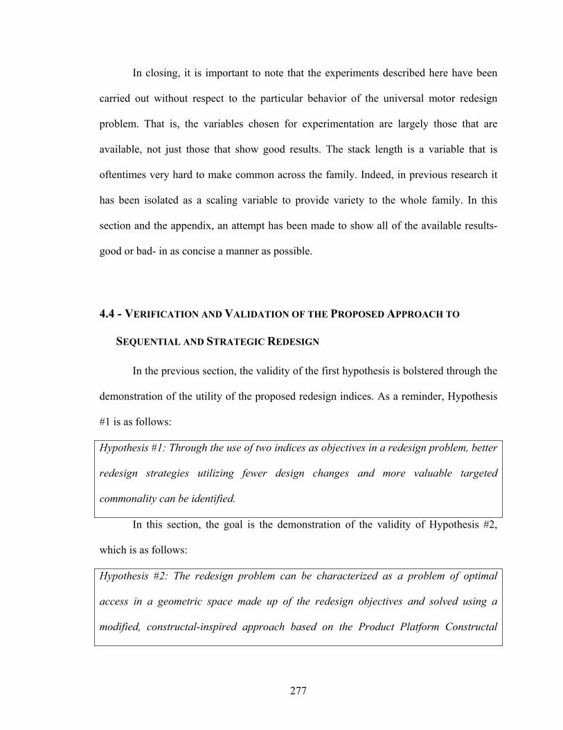
277
In closing, it is important to note that the experiments described here have been
carried out without respect to the particular behavior of the universal motor redesign
problem. That is, the variables chosen for experimentation are largely those that are
available, not just those that show good results. The stack length is a variable that is
oftentimes very hard to make common across the family. Indeed, in previous research it
has been isolated as a scaling variable to provide variety to the whole family. In this
section and the appendix, an attempt has been made to show all of the available results-
good or bad- in as concise a manner as possible.
4.4 - VERIFICATION AND VALIDATION OF THE PROPOSED APPROACH TO
SEQUENTIAL AND STRATEGIC REDESIGN
In the previous section, the validity of the first hypothesis is bolstered through the
demonstration of the utility of the proposed redesign indices. As a reminder, Hypothesis
#1 is as follows:
Hypothesis #1: Through the use of two indices as objectives in a redesign problem, better
redesign strategies utilizing fewer design changes and more valuable targeted
commonality can be identified.
In this section, the goal is the demonstration of the validity of Hypothesis #2,
which is as follows:
Hypothesis #2: The redesign problem can be characterized as a problem of optimal
access in a geometric space made up of the redesign objectives and solved using a
modified, constructal-inspired approach based on the Product Platform Constructal

278
Theory Method (PPCTM) using the Redesign Index (RI) and Commonality Discount
Factor (CDF) as overall objectives in conflict with the individual systems’ goals.
In order to demonstrate the validity of this hypothesis, a series of increasingly
difficult redesign problems are addressed using the constructal inspired approach that has
been proposed in Section 1.3.2 and described in detail in Chapter 3. The constructal-
inspired approach not only provides structure to the overall problem-solving process but
also organizes the exploration of commonality between geometrically similar systems. It
is hoped that by carrying out this series of tests, the reader can come to comprehend the
utility of the constructal-inspired approach in both these regards and to see how the
indices bolster that utility, backing it up in certain ways.
The example used throughout this section is an expanded version of the universal
motor problem used earlier. As shown in Figure 4-1b, the number of variables in the
problem has been increased from four to eight although the goals in each of the scenarios
that follow are similar: motors with new torque values are to be created based on redesign
while minimizing the effort expended, maximizing the use of valuable commonality, and
bringing both the mass and efficiency of the whole family close to targets. As a reminder
to the reader, the redesign options available to the designer are as follows:
• Na – Number of turns of wire in the armature/rotor
• Awa – Cross-sectional area of the wire in the armature/rotor
• Nf – Number of wire turns in the field/stator
• Awf – Cross-sectional area of the wire in the field/stator
• r – Radius of the motor

279
• t – Thickness of the field/stator
• L – Stack length of the motor
• I – Current
In order to solve the redesign problems presented here in a constructal-inspired
manner, the solution scheme has been implemented in Matlab as shown in Figure 4-19.
While this implementation appears wildly different from that which is used in the
previous section to exercise the indices, it is actually made up of more complicated
versions of many of the same functions in Figure 4-5 with several unique functions added
to handle the space elements that fill the market space. These functions can all be seen in
Section C.1.

280
Figure 4-19 – Flowchart of Matlab Implementation of Full Constructal-Inspired Approach

281
4.4.1 - “Simple Redesign” Example Scenario
The most basic type of redesign is the leveraging of one existing system to create
one new system, as shown in Figure 4-20. This is the basic redesign scenario addressed in
here. One existing universal motor is to be redesigned to realize one new motor with
different torque requirements. While not a strategic and sequential redesign problem like
the ones envisioned in Chapter 1, this is considered a building block towards the solution
of those problems. The major issue facing a designer in this situation is how –if at all- he
or she will leverage elements of the existing motor. The goal in this section is to illustrate
how a constructal-based approach can be used to help identify the most promising
leveraging opportunities. The approach is explained step-by-step throughout the rest of
this section.
Figure 4-20 – Flowchart Representation of the Issues in Simple Redesign
Step 1 – Definition of the Redesign Problem
In this scenario, a designer would like to leverage an existing universal motor
with an output of 0.050 Nm to create a new motor with a torque output of 0.250 Nm that
will be rolled out and eventually supplant the existing motor as shown in the schedule in
Figure 4-21. The commonality opportunity matrix that results from this schedule is
shown in Figure 4-22. It is desirable for the two motors to have an average efficiency of

282
70% and an average mass of around 0.500 Kg. At the same time, the designer would like
to minimize the amount of effort associated with the realization of the new motor, using
the most valuable commonality available, so minimization of both the Redesign Index
(RI) and Commonality Discount Function (CDF) will be goals.
New Motor #1Existing Motor #1
Year4321
New Motor #1Existing Motor #1
Year4321
New Motor
Existing Motor
XSP
SPX
New Motor
Existing Motor
New Motor
Existing Motor
XSP
SPX
New Motor
Existing Motor
Figure 4-21 – Redesign Schedule Matrix for the “Simple Redesign” Scenario
Figure 4-22 – Commonality Opportunity Matrix for the “Simple Redesign” Scenario
This basic redesign problem is summarized in Table 4-26 with unknown values
and targets highlighted in boldfaced text. In the next step, the objective functions that will
be used in this problem are formulated.
Table 4-26 – Summary of “Simple Redesign” Problem Existing Motor #1 New Motor #1 Responses of Interest Torque 0.05 Nm 0.25 Nm
Mass 0.499 Kg Family Goal: Average mass of 0.50 Kg
Efficiency 71.7 % Family Goal: Average efficiency of 70%
Variables Number of Wire Turns in the Armature (Na) 730 ?
Area of Wire in Armature (Awa) 0.205 mm2 ? Number of Wire Turns in Field (Nf) 45 ? Area of Wire in Field (Awf) 0.203 mm2 ? Radius of motor (r) 3.62 cm ? Thickness of motor (t) 9.69 cm ? Stack Length (L) 0.998 cm ? Current (I) 3.65 A ?

283
Step 2 – Formulate Objective Functions
Based on the problem description put together in the first step, the designer’s
goals can be formulated as objective functions. The goals described thus far include:
• Bringing the new motor’s torque output close to the target value of 0.250 Nm;
• Bringing the pair of motors’ average mass and average efficiency close to
their targets of 0.500 Kg and 70% respectively; and
• Minimization of RI and CDF in an effort to minimize the effort and maximize
the value associated with the redesign effort.
Each of these goals is described and modeled here in detail. First, the torque goal
is described using Equation 3.9 as follows:
( ) 10.250 T TT x d d− ++ − = [4.25]
Next, the mass and efficiency goals are similarly described using Equation 3.9
and Equation 3.11:
( ) 10.50family
m mm x d d− ++ − =
[4.26]
10.70family d dη η
η − ++ − = [4.27]
Equation 3.12 is used to model the goals related to the minimization of the RI and
CDF as follows:
max
( ) 0( ) RI RIRI x d dRI x
− + + − =
[4.28]
max
( ) 0( ) CDF CDFCDF x d dCDF x
− + + − =
[4.29]

284
Since the maximum values for both RI and CDF are 1.0 if constraints are not
violated, the goals become:
( ) 0RI RIRI x d d− ++ − = [4.30]
( ) 0CDF CDFCDF x d d− ++ − = [4.31]
In order to assess the values for RI, the designer must determine the redesign
difficulties associated with each option, which in this case are the adjustment of the eight
variables in Table 4-1. The difficulties chosen are shown in Table 4-27 and are based
partially upon the reasoning explained in Section 4.2 and partially upon the observations
made in Section 4.3.4 where it is noted that extreme values of both the redesign
difficulties and commonality discounts yield better differentiation between results. The
values noted in Table 4-27 will be used in the scenarios presented throughout the rest of
Section 4.4.
Table 4-27 – Redesign Difficulties Assigned to Variables in “Simple Redesign” Scenario Number
of Turns
of Wire in Arm.
Area of Wire in Arm.
Number of
Turns of Wire in Field
Area of Wire in
Field
Radius of
Motor
Thickness of Field
Stack Length Current
(Na) (Awa) (Nf) (Awf) (r) (t) (L) (I) 0.1 0.5 0.1 0.5 0.5 0.5 1.0 0.1
Similarly, in order to assess values of CDF, the designer must decide on discounts
that represent the value of commonality in each variable for each type of production
overlap. The values chosen for this problem are shown in Table 4-28. Although there is
only Staggered Production commonality present in the “Simple Redesign” scenario being

285
addressed here, all of the discounts have been described for use in scenarios later Section
4.4.
Table 4-28 – Commonality Discounts Associated with the Variables and Types of Production Overlap Present in the “Simple Redesign” Scenario
Number of Turns of Wire in Arm.
Area of Wire in Arm.
Number of
Turns of Wire in Field
Area of Wire in
Field
Radius of
Motor
Thickness of Field
Stack Length Current
Type of Commonality (Na) (Awa) (Nf) (Awf) (r) (t) (L) (I) Perfect 0 0 0 0 0 0 0 0 Staggered Production 0.2 0.6 0.2 0.6 0.6 0.6 0.6 0.2
Staggered Introduction 0.1 0.5 0.1 0.5 0.5 0.5 0.5 0.1
Staggered Retirement 0.1 0.4 0.1 0.4 0.4 0.4 0.4 0.1
Production Gap 0.3 0.7 0.3 0.7 0.3 0.3 0.3 0.3
Finally, the designer must formulate the overall objective function for the
redesign problem. The designer here chooses to utilize an Archimedean weighted sum
approach, generating the following goal:
( ) ( )( ) ( ) ( )
where: 0.222
0.3330.111
avg avg avg avg avg avg
avg avg
m m m
RI RI CDF CDF T T T
T
RI CDF
m
Z w d d w d d
w d w d w d d
ww ww w
η η η
η
− + − +
+ + − +
= + + +
+ + + +
== == =
[4.32]
While a cDSP goal-programming formulation is used to model the designer’s
goals and preferences here, there is no reason why other models such as value theory,
utility theory, or physical programming could not be used for this step. As mentioned in

286
Section 3.4.2, there are also different goal formulations for goals in the cDSP such as
maximization that have not been utilized here.
Step 3 – Identify and Describe Redesign Options
As is hinted earlier, the redesign options available to the designer include all eight
of the basic universal motor variables listed in Table 4-1. These variables are organized
into stages or constructs in the next step.
Step 4 – Identify Number of Stages, Narrow Redesign Options, Create Groups and
Hierarchically Rank Them
Having identified the redesign options to be explored in this problem, they are
now grouped and ranked hierarchically according to their expected impact on the
responses of interest. In the case of this redesign scenario, the primary response of
interest is the changing torque output since it is the major differentiating factor between
the existing universal motor and the new one.
Based on the results presented in Section 4.3.4, it can be seen that it is definitely
possible to make some design variables constant across a large number of universal
motors. Meanwhile, there are other variables like the stack length and current which are
more difficult to reuse from motor to motor. As a starting point, the variables are
organized according to the groupings used by Hernandez and coauthors (Hernandez,
Allen et al. 2002) who designed a mass customized family of motors for a similar range
of torques. These groupings are:
• Stage 1 (smallest space elements, most commonly changed variables):

287
Radius of the motor (r)
Thickness of the field (t)
• Stage 2 (middle-range space elements, variables less likely to be changed):
Cross-sectional area of wire in the armature (Awa)
Cross-sectional area of wire in the field (Awf)
• Stage 3 (largest space elements, variables that can be made common across
the whole space or which are costly to change):
Number of wire turns in armature (Na)
Number of wire turns in field (Nf)
Stack length (L)
Current (I)
While this arrangement of modes is used successfully by Hernandez and
coauthors in their work and seems to make sense logically at first, it is shown later on in
this section that it does not serve the redesign problem well.
Step 5 – Define Boundaries of Market Space
The existing system and redesign target provide initial definitions for the redesign
space. However to make sure that there is enough room around these two nominal torque
values to consider designs that compromise torque output in one direction or another, a
buffer of 5% of the preliminary range is added. This results, as shown in Figure 4-23, in a
redesign space that starts at a torque value of 0.0477 Nm and extends to 0.2625 Nm. This
is the space that will be addressed in a constructal-inspired manner.

288
Figure 4-23 – Redesign Market Space for “Simple Redesign” Example
Step 6 – Formulate the Multistage Problem
Having defined the redesign space and established the modes that will be used at
each stage of the constructal-inspired approach, the multi-stage problem can now be
formulated. As Discussed in Section 3.4.6, the major change in this step from its parallel
in the Product Platform Constructal Theory Method (Hernandez, Allen et al. 2003) is that
in addition to deciding the shape of each stage’s space elements, the values of the modes
to be used in each stage must be found.
From Table 3-9Table 3-9, the redesign decision at the first stage can be
formulated. At this stage, the designer’s task is to decide on the shape and size of the
smallest space elements and to decide the radius and thickness that will be used in each
space element that is active. In Table 4-29, this first-stage decision is summarized in the
form of a compromise Decisions Support Problem.

289
Table 4-29 – The First Stage Decision in the “Simple Redesign” Scenario For Stage 1
Given: • The one -dimensional market space of torque values • The design of the existing system, with a torque output of 0.05 Nm • The modes of managing product change to be utilized at Stage 1:
• Radius of the motor (r) • Thickness of the field (t)
Find: The value of decision variables • [ ](1) (1)x T= ∆ to determine sizes of space elements; and
• { } { }1,,k kk
X r t= for each space element k
The deviation variables and b bd d− + , for all four goals Satisfy: Bounds: • Variable bounds:
1.0 10.00.5 10.0
cm r cmcm t cm
≤ ≤≤ ≤
• Space element sizes 0.0477 (1) 0.2625Nm T Nm≤ ∆ ≤ • , 0b bd d− + ≥ for b = 1,…4 • 0b bd d− +× = for b = 1,…4
Constraints: • { } { }, exi k iX X
ε= where { }ex i
Xε
are the variables from the
ith construct from any existing system ε that happens to be contained in space element k
• Power = 300 W • Feasibility ≥ 1.0
Goals: • Torque goal: ( ) 10.250 T TT x d d− ++ − =
• Mass goal: ( ) 10.50family
m mm x d d− ++ − =
• Efficiency goal: 10.70family d dη η
η − ++ − =
• RI goal: ( ) 0RI RIRI x d d− ++ − = • CDF goal: ( ) 0CDF CDFCDF x d d− ++ − =
Minimize: ( ) ( )( ) ( ) ( )
where: 0.222, 0.333, and 0.111
avg avg avg avg avg avg
avg avg
m m m
RI RI CDF CDF T T T
T RI CDF m
Z w d d w d d
w d w d w d d
w w w w w
η η η
η
− + − +
+ + − +
= + + +
+ + + +
= = = = =

290
At the second of the three stages, the designer’s goal is first to determine how
many first-stage space elements will be combined to form each of the second-stage
elements. It is assumed here that the second-stage space elements can be no smaller than
those of the previous stage. The designer’s second goal is to determine the values of the
second-stage modes of redesign that will be made common across each second-stage
space element. Thus, the second-stage decision is a slightly more complicated than was
that of the first stage, as shown in Table 4-30.
Table 4-30 – The Second Stage Decision in the “Simple Redesign” Scenario For Stage 2
Given: • The one -dimensional market space of torque values • The design of the existing system, with a torque output of 0.05 Nm • The decision variables of the previous stage [ ](1) (1)x T= ∆ and
{ } { }1,, , ,
k ka f k kkX N N L I=
• The modes of managing product change to be utilized at Stage2: • Cross-sectional area of wire in the armature (Awa)
• Cross-sectional area of wire in the field (Awf) Find: The value of decision variables
• [ ](2) (2)x T= ∆ to determine sizes of space elements; and
• { } { }2,,
k kwa wfkX A A= for each space element k
The deviation variables and b bd d− + , for all four goals Satisfy: Bounds: • Variable bounds:
2 2
2 2
0.01 1.0
0.01 1.0wa
wf
mm A mm
mm A mm
≤ ≤
≤ ≤
• Space element sizes 0.0477 (2) 0.2625Nm T Nm≤ ∆ ≤ • , 0b bd d− + ≥ for b = 1,…Mtot • 0b bd d− +× = for b = 1,…Mtot
Constraints: • { } { }, exi k iX X
ε= where { }ex i
Xε
are the variables from the
ith construct from any existing system ε that happens to be contained in space element k
• (2) (1)T T∆ ≥ ∆
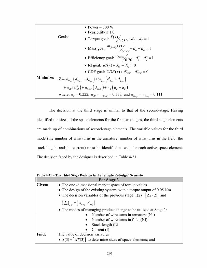
291
• Power = 300 W • Feasibility ≥ 1.0
Goals: • Torque goal: ( ) 10.250 T TT x d d− ++ − =
• Mass goal: ( ) 10.50family
m mm x d d− ++ − =
• Efficiency goal: 10.70family d dη η
η − ++ − =
• RI goal: ( ) 0RI RIRI x d d− ++ − = • CDF goal: ( ) 0CDF CDFCDF x d d− ++ − =
Minimize: ( ) ( )( ) ( ) ( )
where: 0.222, 0.333, and 0.111
avg avg avg avg avg avg
avg avg
m m m
RI RI CDF CDF T T T
T RI CDF m
Z w d d w d d
w d w d w d d
w w w w w
η η η
η
− + − +
+ + − +
= + + +
+ + + +
= = = = =
The decision at the third stage is similar to that of the second-stage. Having
identified the sizes of the space elements for the first two stages, the third stage elements
are made up of combinations of second-stage elements. The variable values for the third
mode (the number of wire turns in the armature, number of wire turns in the field, the
stack length, and the current) must be identified as well for each active space element.
The decision faced by the designer is described in Table 4-31.
Table 4-31 – The Third Stage Decision in the “Simple Redesign” Scenario For Stage 3
Given: • The one -dimensional market space of torque values • The design of the existing system, with a torque output of 0.05 Nm • The decision variables of the previous stage [ ](2) (2)x T= ∆ and
{ } { }2,,
k kwa wfkX A A=
• The modes of managing product change to be utilized at Stage2: • Number of wire turns in armature (Na)
• Number of wire turns in field (Nf) • Stack length (L) • Current (I)
Find: The value of decision variables • [ ](3) (3)x T= ∆ to determine sizes of space elements; and

292
• { } { }3,, , ,
k ka f k kkX N N L I= for each space element k
The deviation variables and b bd d− + , for all four goals Satisfy: Bounds: • Variable bounds:
100 15001 500
1.0 100.1 6.0
a
f
NN
cm L cmA I A
≤ ≤
≤ ≤
≤ ≤≤ ≤
• Space element sizes 0.0477 (3) 0.2625Nm T Nm≤ ∆ ≤ • , 0b bd d− + ≥ for b = 1,…Mtot • 0b bd d− +× = for b = 1,…Mtot
Constraints: • { } { }, exi k iX X
ε= where { }ex i
Xε
are the variables from the
ith construct from any existing system ε that happens to be contained in space element k
• (3) (2)T T∆ ≥ ∆ • Power = 300 W • Feasibility ≥ 1.0
Goals: • Torque goal: ( ) 10.250 T TT x d d− ++ − =
• Mass goal: ( ) 10.50family
m mm x d d− ++ − =
• Efficiency goal: 10.70family d dη η
η − ++ − =
• RI goal: ( ) 0RI RIRI x d d− ++ − = • CDF goal: ( ) 0CDF CDFCDF x d d− ++ − =
Minimize: ( ) ( )( ) ( ) ( )
where: 0.222, 0.333, and 0.111
avg avg avg avg avg avg
avg avg
m m m
RI RI CDF CDF T T T
T RI CDF m
Z w d d w d d
w d w d w d d
w w w w w
η η η
η
− + − +
+ + − +
= + + +
+ + + +
= = = = =
Step 7 – Solve the Multistage Problem
As is discussed in Section 3.4.7, the redesign problem is solved partially
exhaustively and partially by solving compromise Decision Support Problems. If it is
assumed that all space elements evenly divide up the redesign market space, then the
realm of all possible arrangements of space elements can be searched exhaustively. It is

293
assumed here that the designer arbitrarily chose that there can be no more than four space
elements dividing up the space at any stage. This number is excessive since there are only
two motors at either end of the space, but it gives the search flexibility. Thus, the number
of space elements at each stage is searched exhaustively. For each space element
arrangement that is feasible –meaning that the second space elements are larger than the
first stage ones and so on- all possible assignments of the space elements to the redesign
target are considered. Those that fail the “common sense test” explained in Section 3.4.7
are eliminated. For those that remain, the compromise Decision Support Problems are
solved using the Matlab code in Appendix B and the built-in fmincon function. The
fmincon function utilizes sequential linear programming to identify variable values
meeting the physical constraints, the constraints of the space elements, and any equality
constraints from space elements that are shared with the existing system. Seven start
points are used for each target assignment in an attempt to see if they have any effect on
the end solution. The redesign plans that are generated are discussed in the next section.
Step 8 – Examine Redesign Portfolios an Consider Iteration
In this step, it is the designer’s task to examine the solutions identified as most
promising according to their objective function values and consider whether they are
truly representative of the goals that he/she had when beginning the redesign task.
Solving the redesign problem for the scenario described here yields the solution shown in
Table 4-32 with instances of redesign use in highlighted boxes. A motor with good
physical qualities that shares some commonality with the original is found. While it has a
good low mass, its efficiency is a little bit low.

294
What is more interesting, however, is that this solution is found using a space
element arrangement shown in Figure 4-24 wherein the existing motor and the new one
share absolutely no space elements. In short, all of the commonality seen in the solution
comes as a result of use of the Redesign Index and Commonality Discount Factor. In fact,
the most promising solution in which the space element setup mandates sharing of certain
values fails, with the variable values violating their respective constraints by a wide
margin. All the other redesign options in which commonality is forced by space elements
suffer from similar problems, if not worse. It should be noted that these solutions are not
bad in that they meet the redesign goals, but clearly the constructal-inspired commonality
exploration is not working.
Table 4-32 – Most Promising Solution “Simple Redesign” Problem Based Solely on Objective Function Value Existing Motor #1 New Motor #1 Responses of Interest Torque 0.05 Nm 0.25 Nm Mass 0.499 Kg 0.537 Kg Family Average: 0.518 Kg Efficiency 71.7 % 56.6% Family Average: 64.2% Variables Number of Wire Turns in the Armature (Na) 730 730 Area of Wire in Armature (Awa) 0.205 mm2 0.217 mm2 Number of Wire Turns in Field (Nf) 45 69 Area of Wire in Field (Awf) 0.203 mm2 0.203 mm2 Radius of motor (r) 3.62 cm 3.29 cm Thickness of motor (t) 9.69 cm 9.69 cm Stack Length (L) 0.998 cm 1.32 cm Current (I) 3.65 A 6.00 A Note: instances of design reuse shown in boldly outlined cells

295
Figure 4-24 – Space Element Arrangement of Most Promising Solution Using Old Constructs
To get some insight into the failure of all solutions that utilize the commonality
created by the space elements, the problem is re-solved without the use of the redesign
metrics RI and CDF. After the problem is solved, all the solutions are re-evaluated using
RI and CDF to see how much commonality is present in each. The point of this test is to
see whether feasible designs with some commonality can be found utilizing the
constructal-based approach. Without the redesign metrics in the objective function, the
most promising feasible solutions should be those in which motors’ variables share space
elements. Instead, all those cases feature infeasible designs or the solution process failed
outright. Again, the best redesign options feature good designs, but utilize arrangements
of variables that violate the space element arrangements set forth for them. Clearly,
forcing commonality to be present in the arrangement of modes chosen by Hernandez
and coauthors (Hernandez, Allen et al. 2002) is not working.
Based on the body of results from this problem, it seems clear that the
arrangement of modes into constructs used by Hernandez and coauthors (Hernandez,

296
Allen et al. 2002) is not appropriate for this redesign problem as not only is it not helping
identify promising solutions but also seems to be hindering the hunt for good redesign
plans. Further experimentation with the old constructs suggested by Hernandez and
coauthors in the more complicated scenarios that are solved in the following three
sections has shown such negative results repeatedly. Those space element arrangements
in which some elements are shared invariably result in solutions that are inferior, if not
completely infeasible. In response, three other arrangements of modes shown in Table
4-33 are proposed and tested thoroughly utilizing both this redesign scenario and the ones
in the three subsequent sections. For the sake of brevity, the results of these tests are not
shown here.
Table 4-33 – Original and Newly Tested Construct Arrangements
Variable
Original Constructs (Hernandez, Allen et al.
2002)
New Construct Arrangement
#1
New Construct Arrangement
#2
New Construct Arrangement
#3
Na 3rd stage 3rd stage 3rd stage 2nd stage Awa 2nd stage 1st stage 3rd stage 3rd stage Nf 3rd stage 3rd stage 2nd stage 1st stage Awf 2nd stage 1st stage 3rd stage 4th stage r 1st stage 2nd stage 1st stage 1st stage t 1st stage 1st stage 2nd stage 4th stage L 3rd stage 2nd stage 1st stage 3rd stage I 3rd stage 3rd stage 1st stage 2nd stage Note: 1st stage elements are the smallest. Sizes for subsequent elements must be at least as large.
While each arrangement in Table 4-33 improves slightly upon the last, the final
one (#3) delivers the most consistently superior results in all the experiments discussed in
this chapter. The criteria for making this statement is based in the second hypothesis in
which it is suggested that the constructal-inspired approach should provide a way for

297
organizing the exploration of commonality between existing and new systems that are
geometrically close to one another. If Hypothesis 2.1 is to be demonstrated to be true,
then it must be shown that at some times in some situations, the use of variables arranged
into stages leads to good solutions, even if still better solutions are found by adding the
use of the two redesign metrics.
On the flip side of the argument, if Hypothesis 2.2 is to be shown to be true, then
it must be shown that even in cases where the use of constructal-inspired space elements
leads to commonality, the use of redesign indices can improve the amount or location of
commonality as judged by the designer’s preferences. What this means is that it is not
enough to show that constructal-inspired solutions are best but also that they can work in
conjunction with the indices.
With these statements in mind, the reader is asked to consider the solutions
presented previously in Table 4-32 and below in Table 4-34. In Table 4-32, a solution is
presented that is generated using the original arrangement of variables/modes into
stages/constructs. It has the best objective function value of any space element
arrangement although the space elements force no commonality. In Table 4-34, a solution
is presented that makes use of the shared space elements as shown in Figure 4-25 to have
just as many instances of design reuse as the other solution. The design is actually only
slightly different from that obtained using the previous arrangement of modes (see Table
4-32) but it does so without violating any constraints. Similar results have been generated
for each of the next three scenarios, so for the rest of this chapter, only this new four-
stage arrangement of modes is used.

298
Table 4-34 – Most Promising Solution “Simple Redesign” Problem Using New Mode Arrangement #3 and Constructal Commonality Existing Motor #1 New Motor #1 Responses of Interest Torque 0.05 Nm 0.25 Nm Mass 0.499 Kg 0.537 Kg Family Average: 0.518 Kg Efficiency 71.7 % 56.6 % Family Average: 64.2 % Variables Number of Wire Turns in the Armature (Na) 730 730
Area of Wire in Armature (Awa) 0.205 mm2 0.217 mm2 Number of Wire Turns in Field (Nf) 45 69
Area of Wire in Field (Awf) 0.203 mm2 0.203 mm2 Radius of motor (r) 3.62 cm 3.28 cm Thickness of motor (t) 9.69 cm 9.69 cm Stack Length (L) 0.998 cm 1.33 cm Current (I) 3.65 A 6.00 A Note: instances of design reuse shown in boldly outlined cells
Figure 4-25 – Space Element Arrangement for Most Promising Solution Utilizing Constructal Commonality and Third New Mode Arrangement

299
At this point, the designer would want to consider whether the results generated
are similar to what he/she was hoping to get out of the redesign exercise. As shown here,
if the results are not acceptable, the designer might consider expanding the redesign
market space buffer or rearranging the modes into different stages. If commonality is
present but not in the places where it would be most valuable or would lead to a reduction
in redesign effort, the designer may wish to adjust the redesign difficulties or
commonality discounts and re-solve the problem.
4.4.2 - “Redesign Based on Variety” Example Scenario
Having demonstrated “simple redesign” in the previous section, a slightly more
complicated scenario (see Figure 4-26) is addressed here. In this scenario, a designer
would like to leverage the elements of two universal motors that provide the most value
and change only those elements that require little effort in the process of creating the
design for one new motor. The major issue that now faces the designer is how best to
utilize leveraging in the presence of even more options. Which elements, if any, should
be taken from each motor? Which elements should be redesigned and from which
existing motor should the redesign process start for each element. This is the problem
solved in a constructal-inspired manner here.
Many of the steps of the constructal-inspired approach to this scenario are similar
to that which is addressed in Section 4.4.1, so here the discussion of the steps is limited to
those changes that are dictated by the new scenario.

300
Figure 4-26 – Flowchart Representation of the Issues in Redesign Based on Variety
Step 1 – Definition of the Redesign Problem
In this redesign scenario, the designer wishes to leverage two existing motors with
torques of 0.05 Nm and 0.25 Nm respectively to create one new motor with a torque of
0.15 Nm that will be rolled out next year and replace the two existing motors as shown in
the schedule in Figure 4-27. The opportunities for commonality are shown in Figure
4-28, but are slightly misleading, as the perfect commonality between the two existing
systems is not really an “opportunity.” The only meaningful overlap is of the “Staggered
Production” type and is between the two existing motors and the one new motor.

301
Again, the designer has the goal of minimizing the effort associated with this
redesign process and of maximizing the value of those elements that are carried over to
the new motor. The designer also desires an average family mass of 0.50 Kg with an
average family efficiency of 70%. This redesign scenario is summarized in Table 4-35.
New Motor #1Existing Motor #2Existing Motor #1
Year4321
New Motor #1Existing Motor #2Existing Motor #1
Year4321
SPXExisting Motor #2
SP
Existing Motor #2
XSPNew Motor
SP
New Moto
Existing Motor #1 X
Existing Motor #1
SPXExisting Motor #2
SP
Existing Motor #2
XSPNew Motor
SP
New Moto
Existing Motor #1 X
Existing Motor #1
Figure 4-27 – Redesign Schedule Matrix for the “Redesign Based on Variety” Scenario
Figure 4-28 – Commonality Opportunity Matrix for “Redesign Based on Variety Scenario”
Table 4-35 – Summary of “Redesign Based on Variety” Problem Existing Motor #1 Existing Motor #2 New Motor #1 Responses of Interest Torque 0.05 Nm 0.25 Nm 0.15 Nm
Mass 0.499 Kg 0.619 Kg Family Goal: Average mass of 0.50 Kg
Efficiency 71.7 % 62.5 % Family Goal: Average efficiency of 70%
Variables Number of Wire Turns in the Armature (Na) 730 1007 ?
Area of Wire in Armature (Awa) 0.205 mm2 0.224 mm2 ? Number of Wire Turns in Field (Nf) 45 73 ? Area of Wire in Field (Awf) 0.203 mm2 0.246 mm2 ? Radius of motor (r) 3.62 cm 2.35 cm ? Thickness of motor (t) 9.69 cm 6.17 cm ? Stack Length (L) 0.998 cm 2.61 cm ? Current (I) 3.65 A 4.02 A ?

302
Step 2 – Formulate Objective Functions
The objective functions for this scenario are exactly the same as for the “simple
redesign scenario” presented in Section 4.4.1. The commonality discounts and redesign
difficulties are also the same.
Step 3 – Identify and Describe Redesign Options
The redesign options employed in this scenario are exactly the same as for the
“simple redesign scenario” presented in Section 4.4.1.
Step 4 – Identify Number of Stages, Narrow Redesign Options, Create Groups and
Hierarchically Rank Them
As discussed in Section 4.4.1, experimentation with this scenario and the others
has led to the decision to utilize the third new arrangement of the modes (see Table 4-33),
which creates a four-stage approach.
Step 5 – Define Boundaries of Market Space
Although there is a third motor in this redesign scenario, the extreme values of
torque remain the same. Given the same 5% buffer as is used in the previous example in
Section 4.4.1, the market space is of the same size, as shown in Figure 4-29.

303
Figure 4-29 – Redesign Market Space for “Redesign Based on Variety” Example
Step 6 – Formulate the Multistage Problem
The only change to the decision process at each stage is that the designer must
consider the presence of two existing motors as opposed to one. This situation comes into
play in assessing the feasibility of an arrangement of space elements since two existing
systems with different variable values at a particular stage cannot share a space element
at that stage. Otherwise, the problem is the same as in the “simple redesign” scenario.
Step 7 – Solve the Multistage Problem
As a result of the presence of three motors in the redesign space, the decision is
made to utilize as many as eight space elements in dividing up the redesign space. Again,
this decision is somewhat arbitrary, but is made in such a way that it provides flexibility
to place space elements all throughout the redesign space if needed.
Otherwise, the solution process for this scenario is exactly the same as for the
“simple redesign” scenario.” With the addition of more possible space element
arrangements, the solution process takes a significantly longer period of time.

304
Step 8 – Examine Redesign Portfolios an Consider Iteration
The two existing motors are quite different from each in design, meaning that
there is twice the opportunity for the newly redesigned motor to share variable values
with pre-existing systems. Indeed, when the redesign plans are examined, the new motor
exhibits much more design reuse than in the “simple redesign” scenario in Section 4.4.1.
The solution summarized in Table 4-36 is the one with the best overall objective function
value, but as shown in Figure 4-30 it again makes no use of space elements to promote
commonality.
Table 4-36 – Most Promising “Redesign Based on Variety” Solution Based Solely on Objective Function Value Existing Motor #1 Existing Motor #2 New Motor #1 Responses of Interest Torque 0.05 Nm 0.25 Nm 0.150 Nm
0.499 Kg 0.619 Kg 0.500 Kg Mass Family Average: 0.540 Kg 71.7 % 62.5 % 70.5 % Efficiency Family Average: 68.0 %
Variables Number of Wire Turns in Armature (Na) 730 1007 730 Area of Wire in Armature (Awa) 0.205 mm2 0.224 mm2 0.205 mm2 Number of Wire Turns in Field (Nf) 45 73 64 Area of Wire in Field (Awf) 0.203 mm2 0.246 mm2 0.246 mm2 Radius of motor (r) 3.62 cm 2.35 cm 2.26 cm Thickness of motor (t) 9.69 cm 6.17 cm 6.17 cm Stack Length (L) 0.998 cm 2.61 cm 2.61 cm Current (I) 3.65 A 4.02 A 4.02 A Note: instances of design reuse shown in boldly outlined cells

305
Figure 4-30 – Space Element Arrangement for Most Promising Plan for “Redesign Based on Variety”
Interestingly, if the most promising solution that does make use of constructal-
inspired forced commonality is inspected in Table 4-37, it can be seen that there is as
much design reuse present. However, the slightly higher objective function value
achieved by this redesign plan is a result of the commonality discounts and redesign
difficulties. In the slightly better solution shown in Table 4-36, there is one instance of
commonality in Awa, a variable in which commonality is more highly valued.
Table 4-37 – Most Promising “Redesign Based on Variety” Solution Utilizing Constructal Commonality and Indices Existing Motor #1 Existing Motor #2 New Motor #1 Responses of Interest Torque 0.05 Nm 0.25 Nm 0.15 Nm
0.499 Kg 0.619 Kg 0.500 Kg Mass Family Average: 0.540 Kg 71.7 % 62.5 % 70.0 % Efficiency Family Average: 68.0 %
Variables Number of Wire Turns in Armature (Na) 730 1007 1005 Area of Wire in Armature (Awa) 0.205 mm2 0.224 mm2 0.212 mm2

306
Number of Wire Turns in Field (Nf) 45 73 73 Area of Wire in Field (Awf) 0.203 mm2 0.246 mm2 0.203 mm2 Radius of motor (r) 3.62 cm 2.35 cm 2.15 cm Thickness of motor (t) 9.69 cm 6.17 cm 9.69 cm Stack Length (L) 0.998 cm 2.61 cm 2.61 cm Current (I) 3.65 A 4.02 A 3.65 A Note: instances of design reuse shown in boldly outlined cells
To show the value of the constructal-inspired approach, the problem is resolved
without the use of the redesign metrics RI and CDF, utilizing only that commonality
found as a result of the constructal-inspired approach and the start points for the fmincon
function in Matlab. Afterwards, the results are measured using RI and CDF to judge the
amount of redesign and commonality present. The most promising solution found this
way is shown in Table 4-38 and Figure 4-31. It features good mass and efficiency values,
a torque that is right on target, and design reuse in two out of its eight variables. Clearly,
comparing these results to those found using the indices in the solution process, the
indices have advantages even when the same space element scheme is implemented.
Table 4-38 – Most Promising “Redesign Based on Variety” Solution Utilizing Constructal Commonality Alone Existing Motor #1 Existing Motor #2 New Motor #1 Responses of Interest Torque 0.05 Nm 0.25 Nm 0.150 Nm
0.499 Kg 0.619 Kg 0.496 Kg Mass Family Average: 0.538 Kg 71.7 % 62.5 % 70.1 % Efficiency Family Average: 68.0%
Variables Number of Wire Turns in Armature (Na) 730 1007 996 Area of Wire in Armature (Awa) 0.205 mm2 0.224 mm2 0.203 mm2 Number of Wire Turns in Field (Nf) 45 73 87 Area of Wire in Field (Awf) 0.203 mm2 0.246 mm2 0.203 mm2 Radius of motor (r) 3.62 cm 2.35 cm 2.40 cm Thickness of motor (t) 9.69 cm 6.17 cm 9.69 cm Stack Length (L) 0.998 cm 2.61 cm 2.10 cm Current (I) 3.65 A 4.02 A 3.41 A Note: instances of design reuse shown in boldly outlined cells

307
Figure 4-31 – Space Element Arrangement for “Redesign Based on Variety” Scenario Utilizing Only Constructal-Forced Commonality
4.4.3 - “Redesign for Variety” Example Scenarios
In this next scenario, the designer is faced with the problem of leveraging just one
existing system in order to create two new ones as shown in Figure 4-32. Whereas the
primary challenge in the previous scenario is the decision as to which elements of the
existing systems will be chosen for leveraging, here the challenge is to decide between
leveraging the existing system and creating two new systems with a great deal in
common. The former has the advantage leveraging effort that has already been put into
the existing system while the latter may have the advantage of economies of scale as the
two systems are produced simultaneously.
Again, many of the steps of the constructal-inspired approach to this scenario are
similar to that which is addressed in Section 4.4.1, so here the discussion of the steps is
limited to those changes that are dictated by the new scenario.

308
Figure 4-32 – Flowchart Representation of the Issues in Redesign for Variety
Step 1 – Definition of the Redesign Problem
The designer faces the problem of redesigning one existing motor with a torque
output of 0.05 Nm to create two new motors with torques of 0.15 Nm and 0.25 Nm that
will be rolled out next year to replace the existing one as shown in Figure 4-33. The
commonality opportunity matrix in Figure 4-34 is of more interest in this scenario as it
helps to keep track of the fact that there are opportunities for both “Staggered
Production” commonality and “Perfect” commonality in creating the designs for the new
motors.

309
New Motor #2New Motor #1Existing Motor #1
Year4321
New Motor #2New Motor #1Existing Motor #1
Year4321
XSPNew Motor #1
SP
New Motor #1
New Motor #2
Existing Motor
XSP
SPX
New Motor #2
Existing Motor
XSPNew Motor #1
SP
New Motor #1
New Motor #2
Existing Motor
XSP
SPX
New Motor #2
Existing Motor
Figure 4-33 – Redesign Schedule Matrix for the “Redesign for Variety” Scenario
Figure 4-34 – Commonality Opportunity Matrix for the “Redesign for Variety” Scenario
As before, the designer has mass and efficiency goals for the family as a whole
and would like to both minimize the effort associated with the redesign project and
maximize the value of the commonality in the redesigned family. The redesign problem
is summarized in Table 4-39.
Table 4-39 – Summary of “Redesign for Variety” Problem Existing Motor #1 New Motor #1 New Motor #2 Responses of Interest Torque 0.05 Nm 0.15 Nm 0.25 Nm
Mass 0.499 Kg Family Goal: Average mass of 0.50 Kg
Efficiency 71.7 % Family Goal: Average efficiency of 70%
Variables Number of Wire Turns in Armature (Na) 730 ? ? Area of Wire in Armature (Awa) 0.205 mm2 ? ? Number of Wire Turns in Field (Nf) 45 ? ? Area of Wire in Field (Awf) 0.203 mm2 ? ? Radius of motor (r) 3.62 cm ? ? Thickness of motor (t) 9.69 cm ? ? Stack Length (L) 0.998 cm ? ? Current (I) 3.65 A ? ?

310
Step 2 – Formulate Objective Functions
The objective functions are the same as those used in the earlier scenarios, except
that with two new motors to be created, there are two torque target goals present.
Step 3 – Identify and Describe Redesign Options
The redesign options are the same as those used in the scenarios in Sections 4.4.1
and 4.4.2.
Step 4 – Identify Number of Stages, Narrow Redesign Options, Create Groups and
Hierarchically Rank Them
The new ranking of the redesign modes that is employed in the example in
Section 4.4.2 is used again here.
Step 5 – Define Boundaries of Market Space
As the redesign targets and existing systems lay in the same nominal locations in
the torque market space as in the previous two scenarios, the boundaries of the redesign
space are the same as well. The redesign space is shown in Figure 4-35.

311
Figure 4-35 – Redesign Market Space for “Redesign for Variety” Example
Step 6 – Formulate the Multistage Problem
The problem facing the designer in this scenario has some slight changes that
must be addressed. At the first stage, as seen in Figure 4-29, the designer must consider
redesign variables (modes) for both new systems and two target goals, each of which has
its own weight. For this scenario, it has been decided that each of the two new systems’
torque goals should carry the same weight, dividing in two the value they have in
previous scenarios.
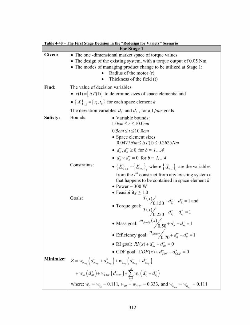
312
Table 4-40 – The First Stage Decision in the “Redesign for Variety” Scenario For Stage 1
Given: • The one -dimensional market space of torque values • The design of the existing system, with a torque output of 0.05 Nm • The modes of managing product change to be utilized at Stage 1:
• Radius of the motor (r) • Thickness of the field (t)
Find: The value of decision variables • [ ](1) (1)x T= ∆ to determine sizes of space elements; and
• { } { }1,,k kk
X r t= for each space element k
The deviation variables and b bd d− + , for all four goals Satisfy: Bounds: • Variable bounds:
1.0 10.00.5 10.0
cm r cmcm t cm
≤ ≤≤ ≤
• Space element sizes 0.0477 (1) 0.2625Nm T Nm≤ ∆ ≤
• , 0b bd d− + ≥ for b = 1,…4 • 0b bd d− +× = for b = 1,…4
Constraints: • { } { }, exi k iX X
ε= where { }ex i
Xε
are the variables
from the ith construct from any existing system ε that happens to be contained in space element k
• Power = 300 W • Feasibility ≥ 1.0
Goals: • Torque goal: 1 1
2 2
( ) 1 and 0.150( ) 10.250
T T
T T
T x d d
T x d d
− +
− +
+ − =
+ − =
• Mass goal: ( ) 10.50family
m mm x d d− ++ − =
• Efficiency goal: 10.70family d dη η
η − ++ − =
• RI goal: ( ) 0RI RIRI x d d− ++ − = • CDF goal: ( ) 0CDF CDFCDF x d d− ++ − =
Minimize: ( ) ( )( ) ( ) ( )
1 2
2
1
where: 0.111, 0.333, and 0.111
avg avg avg avg avg avg
i i i
avg avg
m m m
RI RI CDF CDF T T Ti
T T RI CDF m
Z w d d w d d
w d w d w d d
w w w w w w
η η η
η
− + − +
+ + − +
=
= + + +
+ + + +
= = = = = =
∑

313
Similar changes can also be seen in the decision facing the designer at the second
stage in Table 4-41 and the third stage in Table 4-42.
Table 4-41 – The Second Stage Decision in the “Redesign for Variety” Scenario For Stage 2
Given: • The one -dimensional market space of torque values • The design of the existing system, with a torque output of 0.05 Nm • The decision variables of the previous stage [ ](1) (1)x T= ∆ and
{ } { }1,, , ,
k ka f k kkX N N L I=
• The modes of managing product change to be utilized at Stage2: • Cross-sectional area of wire in the armature
(Awa) • Cross-sectional area of wire in the field (Awf)
Find: The value of decision variables • [ ](2) (2)x T= ∆ to determine sizes of space elements; and
• { } { }2,,
k kwa wfkX A A= for each space element k
The deviation variables and b bd d− + , for all four goals Satisfy: Bounds: • Variable bounds:
2 2
2 2
0.01 1.0
0.01 1.0wa
wf
mm A mm
mm A mm
≤ ≤
≤ ≤
• Space element sizes 0.0477 (2) 0.2625Nm T Nm≤ ∆ ≤
• , 0b bd d− + ≥ for b = 1,…4 • 0b bd d− +× = for b = 1,…4
Constraints: • { } { }, exi k iX X
ε= where { }ex i
Xε
are the variables
from the ith construct from any existing system ε that happens to be contained in space element k
• (2) (1)T T∆ ≥ ∆ • Power = 300 W • Feasibility ≥ 1.0
Goals: • Torque goal: 1 1
2 2
( ) 1 and 0.150( ) 10.250
T T
T T
T x d d
T x d d
− +
− +
+ − =
+ − =
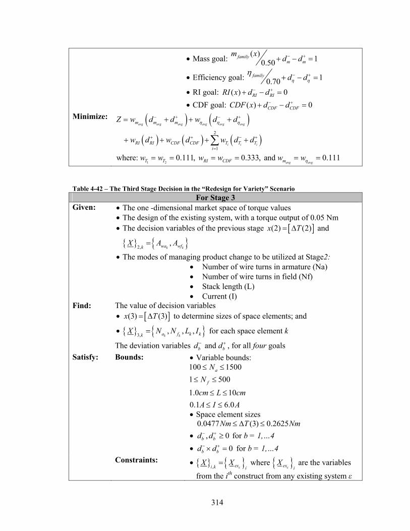
314
• Mass goal: ( ) 10.50family
m mm x d d− ++ − =
• Efficiency goal: 10.70family d dη η
η − ++ − =
• RI goal: ( ) 0RI RIRI x d d− ++ − = • CDF goal: ( ) 0CDF CDFCDF x d d− ++ − =
Minimize: ( ) ( )( ) ( ) ( )
1 2
2
1
where: 0.111, 0.333, and 0.111
avg avg avg avg avg avg
i i i
avg avg
m m m
RI RI CDF CDF T T Ti
T T RI CDF m
Z w d d w d d
w d w d w d d
w w w w w w
η η η
η
− + − +
+ + − +
=
= + + +
+ + + +
= = = = = =
∑
Table 4-42 – The Third Stage Decision in the “Redesign for Variety” Scenario For Stage 3
Given: • The one -dimensional market space of torque values • The design of the existing system, with a torque output of 0.05 Nm • The decision variables of the previous stage [ ](2) (2)x T= ∆ and
{ } { }2,,
k kwa wfkX A A=
• The modes of managing product change to be utilized at Stage2: • Number of wire turns in armature (Na)
• Number of wire turns in field (Nf) • Stack length (L) • Current (I)
Find: The value of decision variables • [ ](3) (3)x T= ∆ to determine sizes of space elements; and
• { } { }3,, , ,
k ka f k kkX N N L I= for each space element k
The deviation variables and b bd d− + , for all four goals Satisfy: Bounds: • Variable bounds:
100 15001 500
1.0 100.1 6.0
a
f
NN
cm L cmA I A
≤ ≤
≤ ≤
≤ ≤≤ ≤
• Space element sizes 0.0477 (3) 0.2625Nm T Nm≤ ∆ ≤
• , 0b bd d− + ≥ for b = 1,…4 • 0b bd d− +× = for b = 1,…4
Constraints: • { } { }, exi k iX X
ε= where { }ex i
Xε
are the variables
from the ith construct from any existing system ε

315
that happens to be contained in space element k • (3) (2)T T∆ ≥ ∆ • Power = 300 W • Feasibility ≥ 1.0
Goals: • Torque goals: 1 1
2 2
( ) 1 and 0.150( ) 10.250
T T
T T
T x d d
T x d d
− +
− +
+ − =
+ − =
• Mass goal: ( ) 10.50family
m mm x d d− ++ − =
• Efficiency goal: 10.70family d dη η
η − ++ − =
• RI goal: ( ) 0RI RIRI x d d− ++ − = • CDF goal: ( ) 0CDF CDFCDF x d d− ++ − =
Minimize: ( ) ( )( ) ( ) ( )
1 2
2
1
where: 0.111, 0.333, and 0.111
avg avg avg avg avg avg
i i i
avg avg
m m m
RI RI CDF CDF T T Ti
T T RI CDF m
Z w d d w d d
w d w d w d d
w w w w w w
η η η
η
− + − +
+ + − +
=
= + + +
+ + + +
= = = = = =
∑
Step 7 – Solve the Multistage Problem
The solution process used here is the same as that which is used in the example
problem in Section 4.4.2.
Step 8 – Examine Redesign Portfolios an Consider Iteration
As in the previous example, it pays for the designer to carefully inspect the most
promising redesign plans generated. Two identical designs share equal objective
functions, one making use of constructal-inspired commonality while the other does not.
The best solution that does utilize this commonality is shown in Table 4-37 and Table
4-43. This solution results in a family of motors with a high average efficiency and seven
instances of design reuse across the family. This is also the first result shown here that
uses one single space element across the whole redesign market space. It is also noted
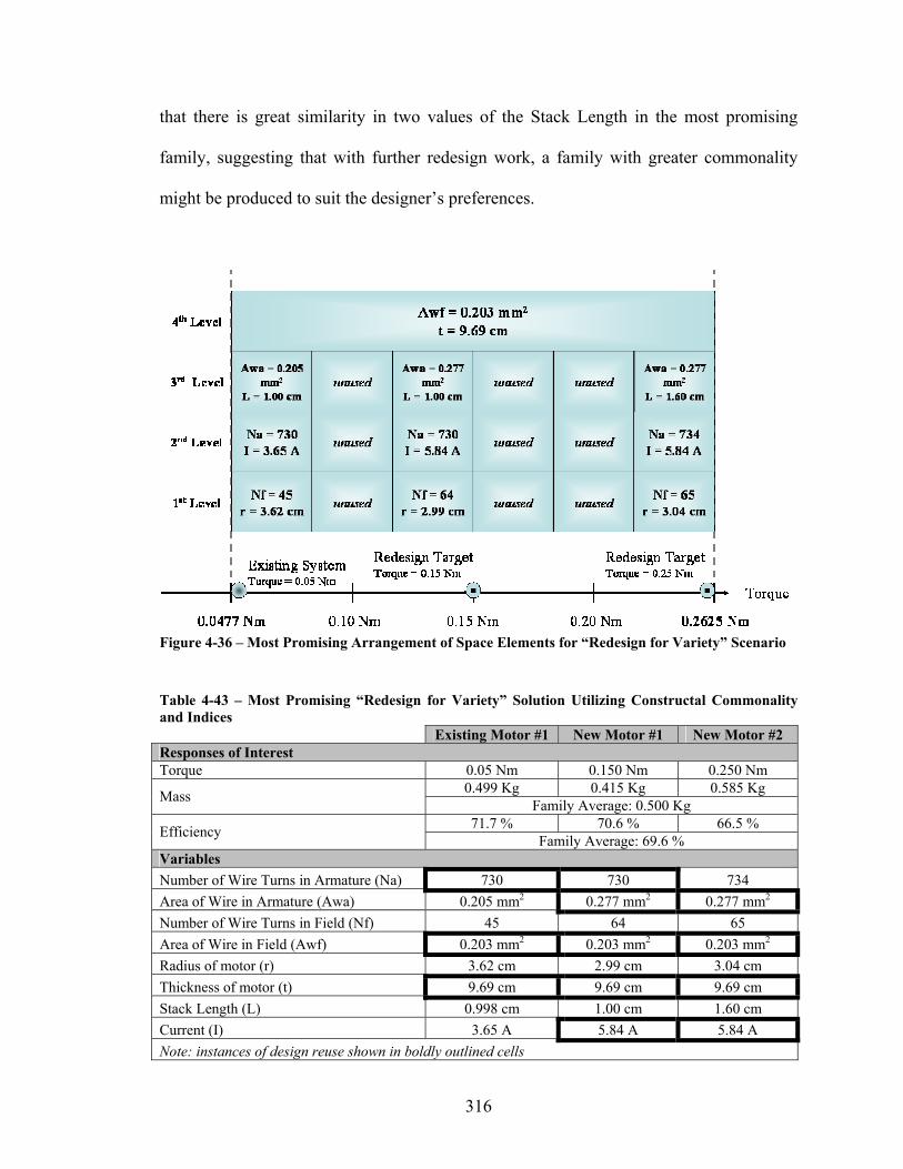
316
that there is great similarity in two values of the Stack Length in the most promising
family, suggesting that with further redesign work, a family with greater commonality
might be produced to suit the designer’s preferences.
Figure 4-36 – Most Promising Arrangement of Space Elements for “Redesign for Variety” Scenario
Table 4-43 – Most Promising “Redesign for Variety” Solution Utilizing Constructal Commonality and Indices Existing Motor #1 New Motor #1 New Motor #2 Responses of Interest Torque 0.05 Nm 0.150 Nm 0.250 Nm
0.499 Kg 0.415 Kg 0.585 Kg Mass Family Average: 0.500 Kg 71.7 % 70.6 % 66.5 % Efficiency Family Average: 69.6 %
Variables Number of Wire Turns in Armature (Na) 730 730 734 Area of Wire in Armature (Awa) 0.205 mm2 0.277 mm2 0.277 mm2 Number of Wire Turns in Field (Nf) 45 64 65 Area of Wire in Field (Awf) 0.203 mm2 0.203 mm2 0.203 mm2 Radius of motor (r) 3.62 cm 2.99 cm 3.04 cm Thickness of motor (t) 9.69 cm 9.69 cm 9.69 cm Stack Length (L) 0.998 cm 1.00 cm 1.60 cm Current (I) 3.65 A 5.84 A 5.84 A Note: instances of design reuse shown in boldly outlined cells

317
4.4.4 - General, More Complicated Redesign Scenarios
The final scenario addressed in this chapter is a generalization of the three
scenarios presented in the preceding sections. The designer is faced with a problem like
the one pictured in Figure 4-37 wherein two existing systems must be redesigned to
realize two new systems. The challenge here is to figure out the best balance of design
reuse and commonality between the two new systems.
Again, many of the steps of the constructal-inspired approach to this scenario are
similar to that which is addressed in Section 4.4.1, so here the discussion of the steps is
limited to those changes that are dictated by the new scenario.
Figure 4-37 – Flowchart Representation of the Issues in General Redesign

318
Step 1 – Definition of the Redesign Problem
This is the only step that is significantly different from the steps needed to address
the scenario presented in Section 4.4.3. As shown in Figure 4-38, the designer would like
to redesign two existing motors with torque outputs of 0.05 Nm and 0.25 Nm to create
two new motors with torques of 0.15 Nm and 0.10 Nm. These new motors will roll out
simultaneously and eventually take the place of the existing motors. As shown in the
commonality opportunity matrix in Figure 4-39, this scenario presents the designer with
opportunities for both “Perfect” commonality and “Staggered Production” commonality
New Motor #2New Motor #1Existing Motor #2Existing Motor #1
Year4321
New Motor #2New Motor #1Existing Motor #2Existing Motor #1
Year4321
SPSPXExisting Motor #2
SP
SP
Existing Motor #2
XSPNew Motor #1
SP
New Motor #1
New Motor #2
Existing Motor #1
XSP
SPX
New Motor #2
Existing Motor #1
SPSPXExisting Motor #2
SP
SP
Existing Motor #2
XSPNew Motor #1
SP
New Motor #1
New Motor #2
Existing Motor #1
XSP
SPX
New Motor #2
Existing Motor #1
Figure 4-38 – Redesign Schedule Matrix for the “General Redesign” Scenario
Figure 4-39 – Commonality Opportunity Matrix for the “General Redesign” Scenario
The redesign scenario is summarized in Table 4-44. As before, two existing
motors have been designed separately based on results from Simpson and coauthors
(Simpson, Maier et al. 2001) so that they on one hand offer more opportunities for design
reuse while on the other hand not making it excessively easy to fit space elements into the
resulting redesign space.
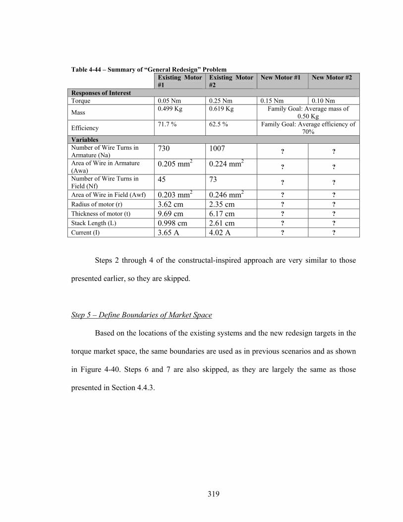
319
Table 4-44 – Summary of “General Redesign” Problem Existing Motor
#1 Existing Motor #2
New Motor #1 New Motor #2
Responses of Interest Torque 0.05 Nm 0.25 Nm 0.15 Nm 0.10 Nm
Mass 0.499 Kg 0.619 Kg Family Goal: Average mass of 0.50 Kg
Efficiency 71.7 % 62.5 % Family Goal: Average efficiency of 70%
Variables Number of Wire Turns in Armature (Na)
730 1007 ? ? Area of Wire in Armature (Awa)
0.205 mm2 0.224 mm2 ? ? Number of Wire Turns in Field (Nf)
45 73 ? ? Area of Wire in Field (Awf) 0.203 mm2 0.246 mm2 ? ? Radius of motor (r) 3.62 cm 2.35 cm ? ? Thickness of motor (t) 9.69 cm 6.17 cm ? ? Stack Length (L) 0.998 cm 2.61 cm ? ? Current (I) 3.65 A 4.02 A ? ?
Steps 2 through 4 of the constructal-inspired approach are very similar to those
presented earlier, so they are skipped.
Step 5 – Define Boundaries of Market Space
Based on the locations of the existing systems and the new redesign targets in the
torque market space, the same boundaries are used as in previous scenarios and as shown
in Figure 4-40. Steps 6 and 7 are also skipped, as they are largely the same as those
presented in Section 4.4.3.

320
Figure 4-40 – Redesign Market Space for “General Redesign” Example
Step 8 – Examine Redesign Portfolios an Consider Iteration
The most promising redesign solution found for this scenario is shown Table
4-45. As seen in Figure 4-41, this solution is derived from the use of an arrangement of
space elements that forces commonality, but a great deal of extra commonality is pushed
by the indices. Also, as before, there are several values of Nf and L that are very similar
but not equal to each other, suggesting that further work could product commonality.
Table 4-45 – Most Promising “General Redesign” Solution Existing
Motor #1 Existing Motor #2
New Motor #1
New Motor #2
Responses of Interest Torque 0.05 Nm 0.25 Nm 0.10 Nm 0.15 Nm
0.499 Kg 0.619 Kg 0.345 Kg 0.539 Kg Mass Family Average: 0.501 Kg
71.7 % 62.5 % 72.8 % 72.7 % Efficiency Family Average: 69.7 % Variables Number of Wire Turns in Armature (Na) 730 1007 1007 730 Area of Wire in Armature (Awa) 0.205 mm2 0.224 mm2 0.224 mm2 0.205 mm2 Number of Wire Turns in Field (Nf) 45 73 80 74 Area of Wire in Field (Awf) 0.203 mm2 0.246 mm2 0.203 mm2 0.246 mm2 Radius of motor (r) 3.62 cm 2.35 cm 2.57 cm 2.35 cm Thickness of motor (t) 9.69 cm 6.17 cm 9.69 cm 6.17 cm Stack Length (L) 0.998 cm 2.61 cm 1.00 cm 2.61 cm Current (I) 3.65 A 4.02 A 4.02 A 3.65 A Note: instances of design reuse shown in boldly outlined cells
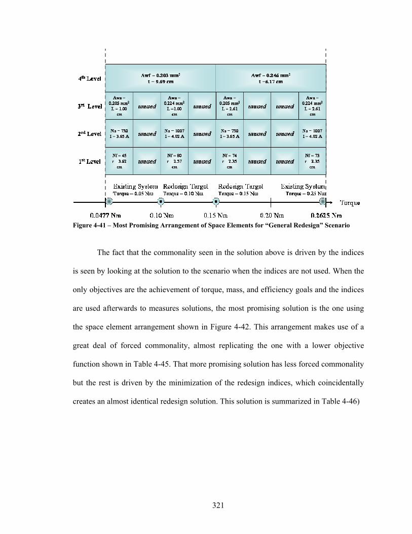
321
Figure 4-41 – Most Promising Arrangement of Space Elements for “General Redesign” Scenario
The fact that the commonality seen in the solution above is driven by the indices
is seen by looking at the solution to the scenario when the indices are not used. When the
only objectives are the achievement of torque, mass, and efficiency goals and the indices
are used afterwards to measures solutions, the most promising solution is the one using
the space element arrangement shown in Figure 4-42. This arrangement makes use of a
great deal of forced commonality, almost replicating the one with a lower objective
function shown in Table 4-45. That more promising solution has less forced commonality
but the rest is driven by the minimization of the redesign indices, which coincidentally
creates an almost identical redesign solution. This solution is summarized in Table 4-46)

322
Table 4-46 – Most Promising “General Redesign” Solution Utilizing Constructal Commonality Only Existing
Motor #1 Existing Motor #2
New Motor #1
New Motor #2
Responses of Interest Torque 0.05 Nm 0.25 Nm 0.10 Nm 0.15 Nm
0.499 Kg 0.619 Kg 0.430 Kg 0.449 Kg Mass Family Average: 0.499 Kg 71.7 % 62.5 % 72.0 % 68.7 % Efficiency Family Average: 68.7 %
Variables Number of Wire Turns in Armature (Na) 730 1007 730 1007 Area of Wire in Armature (Awa) 0.205 mm2 0.224 mm2 0.205 mm2 0.224 mm2 Number of Wire Turns in Field (Nf) 45 73 101 59 Area of Wire in Field (Awf) 0.203 mm2 0.246 mm2 0.203 mm2 0.246 mm2 Radius of motor (r) 3.62 cm 2.35 cm 3.21 cm 1.89 cm Thickness of motor (t) 9.69 cm 6.17 cm 9.69 cm 6.17 cm Stack Length (L) 0.998 cm 2.61 cm 1.00 cm 2.61 cm Current (I) 3.65 A 4.02 A 3.65 A 4.02 A Note: instances of design reuse shown in boldly outlined cells
Figure 4-42 – Most Promising Space Element Arrangement for the “General Redesign” Scenario Utilizing Constructal Commonality Only

323
4.4.5 - Revisiting the Metric Validation Examples
In this section, the two redesign scenarios used for validating the redesign metrics
are revisited, this time with the full complement of universal motor redesign variables in
play. The goal in showing the redesign solutions for these two examples is to demonstrate
that the approach exercised in the four basic types of redesign earlier is still useful even
as the redesign scenario gets larger (more variables and more systems) and more complex
(more redesign, more types of commonality.)
For both of these examples, the preferences expressed by the designer with
respect to redesign difficulties and commonality discounts for the earlier examples
remains the same. The grouping of redesign options/modes into stages and the
hierarchical ranking of those stages also remains the same as that shown in the far right-
hand column of Table 4-33.
The schedule for the first scenario is that which is shown in Figure 4-4. In this
scenario, two existing systems are redesigned to create a series of five new systems
whose production is spread out over the next seven years. The two most promising
solutions to this redesign problem have nearly identical objective function values of
0.00136 and 0.00139. One, which is summarized in Table 4-47 makes use of no forced
constructal-inspired commonality at all. The other, summarized in Table 4-48, does make
use of this commonality as shown in the space element arrangement in Figure 4-43.

324
Table 4-47 – Most Promising Redesign Plan for Validation Scenario #1 According to Objective Function Value Only Existing Motors New Motors #1 #2 #1 #2 #3 #4 #5 Responses of Interest Torque [Nm] 0.35 0.25 0.05 0.10 0.15 0.20 0.30
0.750 0.619 0.340 0.494 0.465 0.523 0.678 Mass [Kg] Family Average: 0.550 Kg 57.0 % 62.5 % 82.0 % 75.4 % 69.0 % 64.6 % 59.5 % Efficiency Family Average: 67.0 %
Variables Number of Wire Turns in Armature
1056 1007 900 1007 900 1007 1056
Area of Wire in Armature [mm] 0.237 0.224 0.224 0.215 0.215 0.215 0.237
Number of Wire Turns in Field 73 73 57 73 58 66 67
Area of Wire in Field [mm] 0.260 0.246 0.246 0.246 0.246 0.246 0.260
Radius of motor [cm] 2.51 2.35 1.60 2.03 2.03 2.13 2.35
Thickness of motor [cm] 6.46 6.17 6.17 6.17 6.17 6.46 6.46
Stack Length [cm] 2.81 2.61 2.61 2.61 2.61 2.61 2.81
Current [A] 4.36 4.02 2.77 2.77 4.03 4.02 4.36 Instances of design reuse are shaded
It is interesting to note that the solution based on the forced commonality features
fewer total variable values throughout the family meaning that less redesign has to
happen, yet it has a higher objective function value. The difference in objective function
value is owed to the fact that the few variable values that are not reused in the solution in
Table 4-47 are very close to other values nonetheless. This drives down the values of
both the Redesign Index and Commonality Discount Factor. Still, this case illustrates the
necessity of Step 8 of the proposed approach wherein the designer considers whether the
top solution according to the objective function really is the most promising one present.
Lastly, both the solution presented in Table 4-47 and the one in Table 4-48 are
much more preferable to the solution (see

325
Table 4-23) found using just the redesign metrics for the simplified problem. Both
of these solutions have more design reuse and show this reuse in an example when twice
as many variables are allowed to be changed.
Table 4-48 – Most Promising Redesign Plan for Validation Scenario #1 Utilizing Constructal-Inspired Commonality Existing Motors New Motors #1 #2 #1 #2 #3 #4 #5 Responses of Interest Torque [Nm] 0.35 0.25 0.05 0.10 0.15 0.20 0.30
0.750 0.619 0.346 0.518 0.437 0.521 0.678 Mass [Kg] Family Average: 0.550 Kg 57.0 % 62.5 % 81.9 % 77.3 % 67.8 % 64.5 % 59.5 % Efficiency Family Average: 67.0 %
Variables Number of Wire Turns in Armature
1056 1007 1007 1007 1080 1080 1056
Area of Wire in Armature [mm] 0.237 0.224 0.237 0.237 0.224 0.224 0.237
Number of Wire Turns in Field 73 73 56 73 56 64 67
Area of Wire in Field [mm] 0.260 0.246 0.246 0.246 0.246 0.246 0.260
Radius of motor [cm] 2.51 2.35 1.53 2.05 1.81 2.05 2.35
Thickness of motor [cm] 6.46 6.17 6.46 6.46 6.17 6.17 6.46
Stack Length [cm] 2.81 2.61 2.61 2.61 2.61 2.61 2.81
Current [A] 4.36 4.02 2.78 2.78 4.02 4.02 4.36 Instances of design reuse are shaded
It is interesting to note the degree of commonality between systems in the family
shown in Figure 4-43that are widely different in torque outputs. The motors with torques
of 0.05 Nm and 0.35 Nm –the two extremes in the family- show a particularly large
amount of commonality. While some of this may be identified randomly in the design
space exploration, a certain amount of it may also be present as a result of the fact that
those two motors share valuable “staggered production” commonality. In order to explore

326
this relationship further, it would be necessary to either adjust the value of “staggered
production” commonality or carry out further experiments with different types of overlap
between the two motors in question would be needed.
Figure 4-43 – Space Element Arrangement for Most Promising Constructal-Inspired Solution to First Metric Validation Example
The schedule for the second scenario used in Section 4.3.4 for validation of the
redesign metrics is shown Figure 4-15. In this scenario, a single existing system is
leveraged to create a stream of six new motors that are to be released one at a time over
the next nine years with each year’s model increasing the torque output over previous
years’ offerings. As with the previous example, the constructal-inspired approach proves
very useful in identifying redesign solutions that utilize design reuse throughout the
family. Table 4-49 and Figure 4-44 display in tabular and graphical form the most
promising redesign plan that the constructal-inspired exploration can identify without the
use of the redesign indices.

327
Table 4-49 – Most Promising Redesign Plan for Validation Scenario #2 Without Use of Either Index New Motors
Existing Motor #1 #2 #3 #4 #5 #6
Responses of Interest Torque [Nm] 0.05 0.10 0.15 0.20 0.25 0.30 0.35
0.499 0.403 0.385 0.463 0.525 0.582 0.643 Mass [Kg] Family Average: 0.500 Kg
71.7 % 73.0 % 72.5 % 68.4 % 64.3 % 60.0 % 57.1 % Efficiency Family Average: 66.7 %
Variables Number of Wire Turns in Armature
730 730 860 860 978 1080 1080
Area of Wire in Armature [mm] 0.205 0.205 0.279 0.279 0.279 0.279 0.279
Number of Wire Turns in Field 45 106 48 54 52 52 56
Area of Wire in Field [mm] 0.203 0.203 0.203 0.203 0.203 0.203 0.203
Radius of motor [cm] 3.62 3.08 2.33 2.61 2.53 2.53 2.69
Thickness of motor [cm] 9.69 9.69 9.69 9.69 9.69 9.69 9.69
Stack Length [cm] 0.998 1.00 1.51 1.51 1.79 1.95 1.95
Current [A] 3.65 3.65 6.00 6.00 6.00 6.00 6.00 Note: instances of design reuse are shaded
All the motors in the redesign plan shown in Table 4-49 and Figure 4-44 have
desirable torque values and the family as a whole has the amount of part variety reduced
by 54 % from 56 to 26 unique variable values. As in some other experiments, there are
values of Nf and L that are very similar, suggesting that further experimentation might
reveal a redesign solution with even greater commonality.

328
Figure 4-44 – Space Element Arrangement for Most Promising Constructal-Inspired Solution to Second Metric Validation Example Without Use of Indices
When the redesign indices are used in concert with the constructal-inspired
commonality exploration, similar results are obtained, as seen in Table 4-50 and the
space element arrangement in Figure 4-45. What is most interesting about these results is
that the total amount of variety in the redesign plan is actually higher than when the
indices are not used. This result comes about because of the relative values of
commonality in different variables and the relative difficulty in changing different
variable values. The choices made by the designer in setting up the problem cause a
tradeoff that produces a greater amount of variety with lower variety in certain parts of
the family.

329
Table 4-50 – Most Promising Redesign Plan for Validation Scenario #2 With Use of Both Indices New Motors
Existing Motor #1 #2 #3 #4 #5 #6
Responses of Interest Torque [Nm] 0.05 0.1000 0.1500 0.2000 0.2500 0.3000 0.3500
0.499 0.4032 0.3872 0.4729 0.5136 0.579 0.6442 Mass [Kg] Family Average: 0.500 Kg
71.7 % 0.73 0.7269 0.6835 0.6293 0.5968 0.565 Efficiency Family Average: 66.4 %
Variables Number of Wire Turns in Armature
730 730 805 805 1062 1062 1062
Area of Wire in Armature [mm] 0.205 0.205 0.273 0.273 0.273 0.274 0.274
Number of Wire Turns in Field 45 106 52 59 52 56 60
Area of Wire in Field [mm] 0.203 0.203 0.234 0.234 0.235 0.235 0.235
Radius of motor [cm] 3.62 3.08 2.50 2.82 2.50 2.69 2.88
Thickness of motor [cm] 9.69 9.69 9.70 9.70 9.69 9.69 9.69
Stack Length [cm] 0.998 1.00 1.35 1.35 1.70 1.70 1.70
Current [A] 3.65 3.65 6.00 6.00 6.00 6.00 6.00 Note: instances of design reuse shown in boldly outlined cells are shaded
Figure 4-45 – Space Element Arrangement for Most Promising Constructal-Inspired Solution to Second Metric Validation Example With Use of Both Indices

330
Having examined the usefulness of the constructal-inspired commonality
exploration approach and the redesign indices in several more complex redesign
scenarios here, the impacts and relevance of the results are discussed in the next section.
4.5 - CONTRIBUTIONS IN THIS CHAPTER TO THE DOMAIN-SPECIFIC
STRUCTURAL AND PERFORMANCE VALIDITY OF THE PROPOSED METHOD
In this chapter, a universal motor example problem has been used in six different
redesign scenarios to show the usefulness of the redesign metrics and the overall
constructal-inspired approach to redesign with respect to their intended purposes. In
doing so, contributions are made to the domain-specific structural validity and domain-
specific performance validity of both Hypothesis 1 and Hypothesis 2.
As a reminder, Hypothesis #1, as posited on Section 1.3.2 is:
Hypothesis 1: Through the use of two indices as objectives in a redesign problem, better
redesign strategies utilizing fewer design changes and more valuable targeted
commonality can be identified.
The redesign scenarios used in Section 4.3.4 of this chapter have been picked
specifically for the testing of the redesign metrics. The first one, which is used throughout
that section of the chapter, employs almost all of the different types of production overlap
described in this dissertation and, with five new systems to be redesigned, offers ample
opportunity for design reuse. The scenario involves specific, known, deterministic
redesign targets over a known schedule. It also involves a reduced set of variables so that
the impacts of the metrics are easier to distinguish. The second scenario that is used to
test the ability of CDF to push certain types of commonality is also designed specifically
with that task in mind, making two types of commonality opportunities readily available.

331
As such, the redesign scenarios used in this chapter are appropriate to the redesign
metrics and can generate the type of data needed to make conclusions. Thus, for the first
hypothesis they help address the second quadrant of the validation square, which is
known alternatively as the “empirical structural validity” and “domain-specific structural
validity”.
The results generated in Section 4.3.4 clearly demonstrate the utility of the
Redesign Index (RI) and the Commonality Discount Factor (CDF) in encouraging
commonality in certain redesign variables for their respective reasons. The RI is shown
over and over to help the designer identify redesign plans that involve fewer changes in
redesign variables that require more effort to change. The CDF is shown to increase
commonality in redesign variables for which reuse is most valuable. It is also shown that
both metrics can discourage commonality in certain variables. Finally, the CDF is shown
to be capable of both encouraging and discouraging certain types of commonality
depending on the type of overlap there is in the production schedules of certain products.
This capability is the most difficult to demonstrate and requires the use of a second
example scenario with more opportunities for commonality of both types present. It is
suggested in Section 4.3.4 that the difficulty associated with certain types of commonality
may be linked to the number of opportunities there are present in a given product release
schedule and in how similar the performance characteristics of the systems are to one
another.
The impact of both metrics is also compared to an alternative metric, the Product
Family Penalty Function (Messac, Martinez et al. 2002) and shown to produce a similar
level of commonality. Both metrics, however, have the advantage of being able to target

332
this design reuse in certain variables and types of production overlap. By showing that
the metrics are not only useful with respect to their intended purpose and that this
usefulness is tied distinctly to the use of just these metrics, the empirical performance
validity”, also known as the “domain-specific performance validity” of Hypothesis #2 is
established.
The second research hypothesis is as follows:
Hypothesis 2: The redesign problem can be characterized as a problem of optimal access
in a geometric space made up of the redesign objectives and solved using a modified,
constructal-inspired approach based on the Product Platform Constructal Theory
Method (PPCTM) using the Redesign Index (RI) and Commonality Discount Factor
(CDF) as overall objectives in conflict with the individual systems’ goals.
A more complicated series of universal motor examples is used in Section 4.4 in
the validation of the first hypothesis. These example scenarios have all of the features of
those used to validate the redesign metrics but make use of all eight of the motor’s
redesign variables, creating a much larger problem when it comes to the juggling of
opportunities for design reuse. The universal motor and the scenarios in which it is used
fit all the features of the sequential strategic redesign problem described in Chapter 1,
thus satisfying the second quadrant of the Validation Square.
In order to validate the second hypothesis, it is desirable to show that the
constructal-inspired approach based on PPCTM does provide value in giving structure
and identifying commonality opportunities in the solutions to redesign problems.
Through the examples in Section 4.4, it is shown that the constructal-inspired approach
can handle the challenges associate with increasingly difficult problems, allowing a

333
designer to identify promising solutions with commonality present in valuable locations.
As a result of the use of the redesign metrics as objectives in this approach, the results are
not always as one might expect. In some cases, the solutions that have the best objective
function values do not make use of the commonality forced by sharing of space elements
between motors. Oftentimes, the solutions that appear best according to the objective
function value are not very different from those that make use of forced commonality.
These solutions drop in rankings simply because of the redesign difficulties and the
commonality discounts chosen by the designer. If those values were set differently or if
the redesign schedule was slightly different, the constructal-inspired solutions might
seem more promising at first blush. When the redesign metrics are not used, the
constructal-inspired approach produces feasible solutions that sometimes include a great
deal of design reuse. These inconsistencies again point to the importance of Step 8 of the
proposed approach wherein the designer considers whether the solutions with the best
objective functions really are what he/she desires.
It is noted in Section 4.4 that the usefulness of the constructal-inspired approach is
tied strongly to the arrangement of the redesign modes into hierarchical stages. It is
shown that stages used for the constructal-inspired design of mass-customized product
families in previous work do not work here. Several alternative arrangements are
proposed and tested before a new four-stage setup is settled upon.
Through the four redesign scenarios in Section 4.4, it is shown that the
constructal-inspired approach, when used without the redesign metrics, and generate
promising redesign solutions exhibiting targeted design reuse. However, the utility of this
approach is tied strongly to the use of proper groupings and rankings of the redesign

334
modes. In addition, when the redesign metrics are used in the objective function,
solutions that do not make use of forced constructal-inspired commonality are often seen
with the lowest objective function values. This makes sense because when all of the
redesign variables are unrestricted, more opportunities for the types of commonality
favored by the settings in RI and CDF may be available.
The reader may also have noted that in all of the redesign scenarios addressed in
this section, the redesign targets and existing systems are spaced out quite well and
relatively evenly in the redesign market space. Experimentation shows that there are
certain types of redesign problems for which the constructal approach is ill-suited. The
approach is ill-suited to problems in which existing systems and redesign goals are
clustered close to one another in a redesign market space. In this case, it may be hard to
realize the new system if many of the redesign variables are constrained in space
elements that it shares with the existing system. When this occurs, the designer may want
to consider whether the redesign targets associated with the new system truly differentiate
it from the existing system enough to justify a new product offering. A small change in
some targets might make the problem much easier to handle. The constructal-inspired
approach is also ill-suited to problems in which all the existing systems are grouped close
to one another while all the redesign targets are grouped together but distance from the
existing systems. In this case, unless the existing systems are very similar to one another
already, their proximity forces a space element arrangement with many small elements
that is inefficient in exploring commonality. This is a problem that may be addressed by
breaking up the redesign problem into several smaller ones or by choosing on some
existing systems for leveraging.

335
It is also interesting to note that in a number of experiments, the values of some
redesign variables are very close to one another yet not quite close enough that they are
counted as “common” here. It is observed earlier in this chapter that these instances
might be signs of opportunities for commonality that have not yet been exploited. It is
possible that upon iteration, these values might be found equal in slightly different
configurations of the redesign plan or that, if the values were constrained to be equal,
valid redesign plans might be identified anyway. These options have not been pursued
however. In a related issue, the values presented in this chapter are, by and large, rounded
to three significant figures. The scheme for rounding the values presented here is
borrowed from previous work on the universal motor example, most notably (Messac,
Martinez et al. 2002) and (Simpson, Maier et al. 2001). This scheme for rounding –which
is sometimes inconsistent with respect to significant figures- has been used so that results
may be compared with the previous literature. It is entirely possible that if a different
rounding scheme were used, the results shown here would be significantly different, as
the rounding effects what is considered a reused variable value and what is considered
unique.
Thus, in Section 4.4, it is shown that the constructal approach can lend structure
that leads to good redesign plans. The value of the constructal-inspired sharing of space
elements is shown to be less strong, as it heavily depends on the setup of the stages and
on the settings of the commonality metrics. For this reason, it is claimed that the second
hypothesis is conditionally shown to have empirical performance validity, satisfying the
third quadrant of the Validation Square.

336
4.6 - STATUS AND PROMISE
The experimentation described in this chapter provides results that help to address
the second and third quadrants of the Validation Square for both Hypothesis #1 and #2,
demonstrating that the proposed metrics and overall approach fill the gaps in existing
literature when used in the universal motor redesign scenarios presented in this chapter.
Having satisfied the requirements to claim validity in three out of the four quadrants of
the Validation Square, it is time to consider the fourth quadrant. This is the task that faces
the reader in Chapter 5. In that chapter, the contributions to the validity of the hypotheses
are revisited and the broader usefulness of the proposed approach is considered in light of
the features that are likely to be present in other problems. The work described in this
dissertation is also critically reviewed, intellectual contributions are claimed, and ideas
for future work shared.

337
CHAPTER 5
CLOSURE
5.1 - A PREVIEW OF THE CHAPTER’S CONTENTS
In this chapter, the arguments, hypotheses, data, and observations presented in the
first four chapters are tied up with a review and some closing thoughts. The work
completed and discussed in this dissertation is summarized in Section 5.2. Particular
attention is paid in that discussion to the confidence in the proposed constructal-inspired
redesign method that has been built up through the research presented here. In Section
5.3, the research is critically reviewed with an eye towards identifying those places where
the work falls short and where assumptions may be skewing the outcomes. With those
criticisms in mind, the intellectual contributions made in this dissertation are discussed in
Section 5.4 and ideas for future work are shared in Section 5.5. In closing, some personal
comments on the work make up Section 5.6.
5.2 - A SUMMARY OF THE WORK COMPLETED
In this section, the work presented in the first four chapters is summarized at a
high level, looking at the research questions and hypotheses that guide the research from
the start and the validation process that is followed in order to back up those hypotheses
with supporting data.
5.2.1 - Revisiting Research Questions and Hypotheses

338
In Chapter 1, a new type of design problem is identified and described as a
strategic and sequential redesign problem. In such a problem, a designer is faced with the
task of redesigning one or more existing systems to meet both immediate and well-known
future goals to expand the family in multiple directions. It behooves the designer to create
as good a new design as possible, meeting as many performance targets as he/she can, but
there are other considerations as well. It would be beneficial to minimize the amount of
design change in the family to keep the effort that goes into producing the new family
members as low as possible. Along similar lines, not all commonality is equally valuable
to eh designer. Thus is framed the problem addressed in this dissertation. The primary
hypothesis put forward to address this problem is as follows:
The overall goal of achieving a desired amount and type of variety while minimizing
design changes and maximizing the value of non-commonality can be achieved through
the use of a modified constructal-inspired approach based on the Product Platform
Constructal Theory Method (Hernandez 2001; Hernandez, Allen et al. 2002; Hernandez,
Allen et al. 2003) which is in turn based on Constructal Theory (Bejan 1996; Bejan 1997;
Bejan and Ledezma 1998; Bejan 2000). By incorporating simple and intuitive indices for
redesign difficulty the need for redesign can be minimized in the pieces of a system where
it is expected to be most expensive. By using an index for commonality value, sharing of
components between systems can be targeted to where it is most useful from a strategic
perspective.
The primary research question and hypothesis is broken down into two main parts
that are more practical to take on as research tasks. In the first part, the problem of
measuring the merit of a redesign plan is tackled. As mentioned above, the designer is

339
interested in minimizing the effort involved in a project while maximizing the value of
any commonality created between systems in the family. There exist no metrics for the
“goodness” of a product family created through redesign, so the following secondary
hypothesis is posed:
Hypothesis #1: Through the use of two indices as objectives in a redesign problem, better
redesign strategies utilizing fewer design changes and more valuable targeted
commonality can be identified.
This secondary hypothesis is broken down even further, dividing the dual
concerns of minimizing redesign effort and maximizing commonality value into two
separate hypotheses:
Hypothesis #1.1: By utilizing the minimization of the Redesign Index (RI) as an objective
in a redesign problem, a decision-maker’s attention can be directed to redesign solutions
involving lower numbers of design changes in targeted parts of a system..
Hypothesis #1.2: By utilizing the minimization of the Commonality Discount Factor
(CDF) as an objective in a redesign problem, the designer’s attention can be directed to
combinations commonality in the most valuable parts of a system that is being
redesigned.
The two indices that are the subject of Research Question #1 provide an indirect
measure of the economic performance of a plan for redesigning existing systems to create
new systems. These indices are a crucial tool in an overall method for identifying such
redesign plans. It is this method, which is inspired by Constructal Theory and based upon
existing product family design methods, which is the subject of the second major part of
the research and the second secondary hypothesis:

340
Hypothesis #2: The redesign problem can be characterized as a problem of optimal
access in a geometric space made up of the redesign objectives and solved using a
modified, constructal-inspired approach based on the Product Platform Constructal
Theory Method (PPCTM) using the Redesign Index (RI) and Commonality Discount
Factor (CDF) as overall objectives in conflict with the individual systems’ goals.
Research Question #2 is broken down into two parts in order to sort out the
individual contributions of the two main components of the work in this dissertation the
development of indices for redesign and the development of a constructal-inspired
approach to structuring and solving a redesign problem. The resulting sub-hypotheses are
as follows:
Hypothesis #2.1: The strategic sequential redesign problem can be structured as a
problem of optimal access in a geometric space and solved using an approach based on
the Product Platform Constructal Theory Method (PPCTM), abstracting its inner
workings towards redesign applications and infusing the use of the multi-objective
compromise Decision Support Problem at every stage of the decision-making process.
Hypothesis #2.2: By utilizing the Redesign Index (RI) and Commonality Discount
Function (CDF) as overall objectives in the constructal-inspired redesign commonality
exploration method, design reuse can be considered between systems that are not close to
one another in the market space and between individual elements of subsystems or modes
of collections of subsystems.
These are the hypotheses that are to be validated by following the Validation
Square (Pederson, Emblemsvag et al. 2000; Seepersad, Pederson et al. 2005) in

341
conducting the research in this dissertation. The way in which this has been done is
explained in the next section.
5.2.2 - A Summary of the Confidence Building Process and the Validity of the
Proposed Method
The philosophy behind the Validation Square is explained in detail in Section
1.4.1. In following validation process symbolized by the square, the author hopes that the
reader sees that a systematic and reasoned approach has been taken to the process of
proving the validity of the hypotheses. If this systematic process is perceived as
successful and the value demonstrated thus far is accepted, then the discussion of the
wider usefulness of the proposed approach can be carried forward in this section. It is
hoped that, having reviewed the material in this section, the reader can make some sort of
leap forward into the fourth quadrant of the validation square (see Figure 5-1).
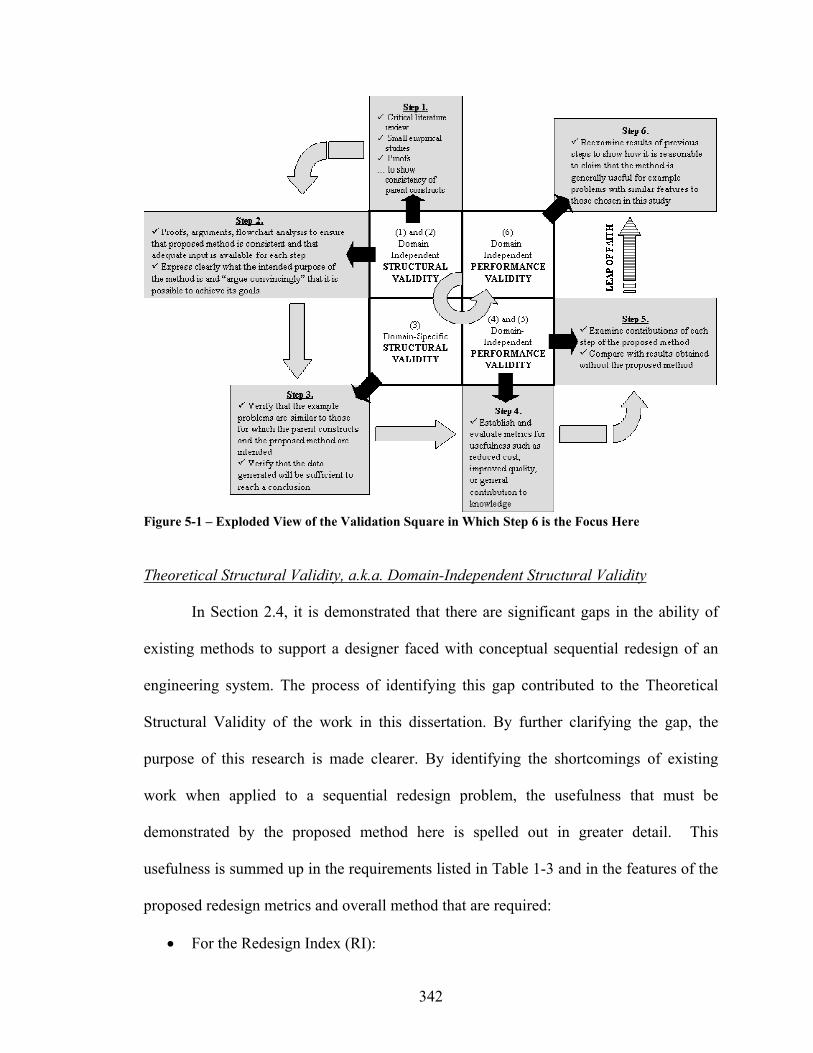
342
Figure 5-1 – Exploded View of the Validation Square in Which Step 6 is the Focus Here
Theoretical Structural Validity, a.k.a. Domain-Independent Structural Validity
In Section 2.4, it is demonstrated that there are significant gaps in the ability of
existing methods to support a designer faced with conceptual sequential redesign of an
engineering system. The process of identifying this gap contributed to the Theoretical
Structural Validity of the work in this dissertation. By further clarifying the gap, the
purpose of this research is made clearer. By identifying the shortcomings of existing
work when applied to a sequential redesign problem, the usefulness that must be
demonstrated by the proposed method here is spelled out in greater detail. This
usefulness is summed up in the requirements listed in Table 1-3 and in the features of the
proposed redesign metrics and overall method that are required:
• For the Redesign Index (RI):

343
o Show that RI reduces the instances of redesign without significant
sacrifice of other objectives
o Show that by using redesign difficult indices, the location of commonality
can be controlled –reducing design variation in parts of the product that
are hard to redesign.
o Show that increasing the weight given to RI in the overall decision-
making process increases the amount of commonality seen. (really part of
the overall method’s validation)
• For the Commonality Discount Factor (CDF):
o Show that CDF reduces the instances of redesign without significant
sacrifice of other objectives
o Show that by using penalties to reflect the relative merit of commonality
for different variables, commonality in specific variables can be increased
at the expense of commonality in other variables
o Show that by using penalties to reflect the relative merit of commonality
for different types of overlap in production schedules, more valuable
commonality can be promoted
o Show that increasing the weight given to CDF in the overall decision-
making process increases the amount of commonality seen.
• For the overall constructal-inspired redesign method:
o Show that it can produce viable platforms of arbitrary size and shape
o Show that it can produce families of products with features roughly
equivalent to those produced using simple optimization

344
o Show that it can sometimes produce better families of products
o Show that the overall approach works for:
One-to-one redesign
One-to-two redesign
Two-to-one redesign
General cases of redesign
The constructs of the proposed metrics and the overall approach are discussed in
Chapter 2. The first one described is the Product Platform Constructal Theory Method
(PPCTM) (Hernandez 2001; Hernandez, Allen et al. 2002; Carone, Williams et al. 2003;
Hernandez, Allen et al. 2003; Williams 2003; Williams, Allen et al. 2004; Williams,
Rosen et al. 2004; Kulkarni, Allen et al. 2005) based upon the ideas of constructal theory
(Bejan 1996; Bejan 1997; Bejan and Ledezma 1998; Bejan 2000). The PPCTM has
several features that make it particularly interesting in this dissertation, chiefly the ability
to utilize multiple modes of changing a product to create variety in multiple dimensions
without a need to specify sizes or numbers of product platforms ahead of time. However,
it is meant to design continuous ranges of products from scratch, so it has never been
used for redesign or for the creation of certain specific products. Abstracted and heavily
modified to address redesign problems, the PPCTM provides the designer with the
capability of using multiple means to realize a family of products with variety in multiple
dimensions without requiring that he/she specify product platforms ahead of time. This is
a key requirement for strategic and sequential redesign. The PPCTM has been shown to
be internally consistent in previous research and use. Thus it is accepted that PPCTM is

345
appropriate as a construct for this research and the theoretical structural validity (the first
quadrant of the Validation Square) of the second hypothesis is taken to be proven.
The second construct discussed is the compromise Decision Support Problem
(Mistree, Hughes et al. 1993; Mistree, Lewis et al.) The cDSP is infused into the
decision-making process of PPCTM to support the redesign of individual systems to meet
new individual goals. The cDSP has been used widely in all sorts of engineering
applications and has been utilized as the basic building block for the development of
techniques for robust design (Chen, Allen et al. 1996; Chen, Mavris et al. 1996), product
family design (Simpson 1999; Simpson, Chen et al. 1999), hierarchical systems design
(Kuppuraju, Ganesan et al. 1985; Bascaran 1987; Shupe 1987; Bascaran, Bannerot et al.
1989; Karandikar 1989; Vadde, Allen et al. 1994), and many other problems. The cDSP
is employed because it is a proven flexible way of characterizing a multi-objective
problem that can include both minimization goals like the Redesign Index (RI) and
Commonality Discount Function (CDF) and target goals like the performance values that
will change within a product family. It is entirely capable of describing and facilitating
the solution of strategic and sequential redesign problems. Thus the theoretical structural
validity of the first hypothesis is also accepted.
The final constructs are developed later in Chapter 3 of this dissertation. These
two indices are meant to assess the merit of redesign plans based on the amount of
redesign effort entailed and the value of the commonality present. While developed from
scratch, they adopt many of the advantages and disadvantages seen in product family
commonality indices (see Section 2.3.4) in that they are quick to compute but may vastly
oversimplify the problem that is being solved. Although they have their drawbacks, as

346
discussed in Section 3.2.6, they serve the purpose put forward for them in that they give a
rough indication of a designer’s preferences towards minimizing redesign effort or
maximizing commonality in certain pieces of an engineering system.
The consistency of the proposed approach is seen in that all the information
needed for each step is appropriate to the way the problem is framed in Chapter 1. All
information is assumed to be deterministic and all models to be flexible enough to
operate at all values of the redesign variables. Having shown the consistency and
appropriateness of both the constructs and the overall approach, it is claimed that the first
quadrant of the validation square (theoretical structural validity) is complete.
Empirical Structural Validity, a.k.a. Domain-Specific Structural Validity
Having shown that the proposed approach is theoretically structurally valid, the
next step is to discuss an engineering example that is appropriate to test it. The redesign
scenarios used in Section 4.3.4 of this chapter are picked specifically for the testing of the
redesign metrics. The first one, which is used throughout that section of the chapter,
employs almost all of the different types of production overlap described in this
dissertation and, with five new systems to be redesigned, offers ample opportunity for
design reuse. The scenario involves specific, known, deterministic redesign targets over a
known schedule. It also involves a reduced set of variables so that the impacts of the
metrics are easier to distinguish. The second scenario that is used to test the ability of
CDF to push certain types of commonality is also designed specifically with that task in
mind, making two types of commonality opportunities readily available. As such, the
347
redesign scenarios used in this chapter are appropriate to the redesign metrics and can
generate the type of data needed to make conclusions. Thus, for the first hypothesis they
help address the second quadrant of the validation square, which is known alternatively
as the “empirical structural validity” and “domain-specific structural validity”.
A more complicated series of universal motor examples is used in Section 4.4 in
the validation of the first hypothesis. These example scenarios have all of the features of
those used to validate the redesign metrics but make use of all eight of the motor’s
redesign variables, creating a much larger problem when it comes to the juggling of
opportunities for design reuse. The universal motor and the scenarios in which it is used
fit all the features of the sequential strategic redesign problem described in Chapter 1,
thus satisfying the second quadrant of the Validation Square in Figure 5-1.
Empirical Performance Validity, a.k.a. Domain-Specific Performance Validity
In several series of tests in Section 4.3.4 that make use of the first redesign
scenario, it is shown that the Redesign Index (RI) is effective in increasing the amount of
commonality in a redesign plan both in general and in specific variables. Increasing the
difficulty associated with certain variables is shown to lead to an increase in design reuse
in the final solutions, reflecting a desire to avoid complicated design changes. Decreasing
one variable’s difficulty is shown to lead to more variety in that variable across the
family. Not only is the RI effective in all of these ways, it stands apart from the Product
Family Penalty Function (PFPF) (Messac, Martinez et al. 2002) to which it is compared
in that the reduced design changes can be targeted to certain variables.

348
In a much larger number of series of tests, the utility of the Commonality
Discount Function (CDF) is shown in a very similar way. The usefulness of the CDF in
increasing design reuse in general is shown by using it with all commonality discounts set
to even levels. By setting discounts for certain variables to be low while all others are
high, it is shown that commonality can be encouraged in the variables in which it is the
most valuable. It is also shown that decreasing the penalty associated with just one type
of production overlap can lead to increases in commonality between systems with that
overlap. However, this is the weakest effect shown in the chapter and may be heavily tied
to the amount of the type of overlap that is present in the redesign scenario and in the
types of systems that have that overlap. Finally, the opposites of all of these effects are
shown to be true: increasing the discount associated with a certain variable will
discourage commonality in it and increasing the discount associated with one type of
commonality will largely keep those opportunities from being used. In fact, the CDF is
shown to be almost more effective in discouraging commonality in certain places than in
encouraging it. It is also observed that when attempting to encourage commonality in
certain parts of a solution while discouraging it elsewhere, the most effective strategy is
to use extreme values of the commonality discounts for each. Again, as compared to the
PFPF, the commonality discount factor has the advantage of being able to target certain
variables or types of commonality overlap for special consideration.
Through these series of tests, it is shown that both of the indices are useful with
respect to their intended purposes and that the contributions made can be tied directly to
their use. The effect of using both in concert is also shown. Accordingly, the case for the
empirical performance validity of the indices, the first hypothesis, and the overall
349
research hypothesis is given a great boost. In Section 4.4, the indices are used
successfully in concert with the constructal-inspired approach to redesign, lending them
further credence.
In order to validate the second hypothesis, it is desirable to show that the
constructal-inspired approach based on PPCTM does provide value in giving structure
and identifying commonality opportunities in the solutions to redesign problems.
Through the examples in Section 4.4, it is shown that the constructal-inspired approach
can handle the challenges associated with increasingly difficult problems, allowing a
designer to identify promising solutions with commonality present in valuable locations.
As a result of the use of the redesign metrics as objectives in this approach, the results are
not always as one might expect. In every case, the solutions that have the best objective
function values do not make use of the commonality forced by sharing of space elements
between motors. Oftentimes, the solutions that appear best according to the objective
function value are not very different from those that make use of forced commonality.
These solutions drop in rankings simply because of the redesign difficulties and the
commonality discounts chosen by the designer. If those values were set differently or if
the redesign schedule was slightly different, the constructal-inspired solutions might
seem more promising at first blush. When the redesign metrics are not used, the
constructal-inspired approach produces feasible solutions that sometimes include a great
deal of design reuse.
It is noted in Section 4.4 that the usefulness of the constructal-inspired approach is
tied strongly to the arrangement of the redesign modes into hierarchical stages. It is
shown that stages used for the constructal-inspired design of mass-customized product

350
families in previous work do not work here. Several alternative arrangements are
proposed and tested before a new four-stage setup is settled upon.
Through the four redesign scenarios in Section 4.4, it is shown that the
constructal-inspired approach, when used without the redesign metrics, and generate
promising redesign solutions exhibiting targeted design reuse. However, the utility of this
approach is tied strongly to the use of proper groupings and rankings of the redesign
modes. In addition, when the redesign metrics are used in the objective function,
solutions that do not make use of forced constructal-inspired commonality are often seen
with the lowest objective function values. This makes sense because when all of the
redesign variables are unrestricted, more opportunities for the types of commonality
favored by the settings in RI and CDF may be available.
Thus, in Section 4.4, it is shown that the constructal approach can lend structure
that leads to good redesign plans. The value of the constructal-inspired sharing of space
elements is shown to be less strong, as it heavily depends on the setup of the stages and
on the settings of the commonality metrics. For this reason, it is claimed that the second
hypothesis is conditionally shown to have empirical performance validity, satisfying the
third quadrant of the Validation Square in Figure 5-1.
Empirical Performance Validity, a.k.a. Domain-Specific Performance Validity
At this point it is important to look back at what has been done and question the
strength of the claims made thus far.
Theoretical structural validity for both hypotheses is proven by inspecting the
constructs that make up the proposed approach and comparing them to the requirements

351
of a sequential strategic redesign method. In every respect, both the constructs and the
overall method meet the requirements.
Empirical structural validity is shown by picking universal motor redesign
problems with features that exactly match the types of problems envisioned in Chapter 1.
As the problems are hand-picked, they test out all of the desired features of the proposed
approach.
The empirical performance validity of the proposed approach is shown through
numerous experiments using simplified universal motor redesign scenarios and a number
of more complicated scenarios with more variables present. The proposed approach is
shown to be useful with respect to every intended purpose, although in several ways there
is room for further experimental evidence. The Commonality Discount Function can only
weakly encourage commonality of certain types whereas it has a great impact when used
to encourage commonality in certain variables. The overall constructal approach is shown
capable of generating good redesign solutions but its utility depends heavily on the way
in which redesign modes are arranged and its effects can be swamped by the effects of
the redesign metrics. By showing the results of using the approach without the indices
however, the approach’s utility is demonstrated. The approach is also ill-suited to
problems in which existing systems and redesign goals are clustered close to one another
in a redesign market space.
So now, what of the leap of faith to claim broader usefulness beyond the universal
motor examples presented here? It is clear that any redesign problem that is to be solved
must meet very specific conditions in order for the constructal-inspired approach
proposed here to work. The problem must involve definite information about multiple

352
new redesign targets that are relatively well spaced out from existing systems in the
redesign market space. The system being redesigned must be modeled mathematically
and the designer must be familiar enough with it to evaluate redesign difficulties and
commonality discounts. The designer must also be able to arrange the redesign modes in
such a way that commonality can explored in a constructal-inspired manner. If all these
conditions are met, there is no reason why the approach proposed here would not work.
Scaling up the implementation shown in Appendix B might be a painful process, but this
is not truly relevant to the domain-independent performance validity of the approach.
There are definite limits to the approach described in this dissertation, but that is the
subject of the next section.
5.3 - A CRITICAL REVIEW OF THE WORK AND THE ASSUMPTIONS MADE
In the previous section, it is claimed that the proposed constructal-inspired
approach to redesign could be applied to a much broader array of problems besides the
universal motor examples used in this dissertation. There are limitations to that claim
however. Identifying and discussing these limitations is the task in this section.
5.3.1 - General Comments
The one limiting assumption that generally draws the most attention from
audiences is the presumption that the designer has perfect information about future
redesign goals, system capabilities and redesign variables. With much effort in the design
community being expended on modeling and handling uncertainty, this assumption
seems a throwback to yesteryear. Still, as shown in Section 1.1.2, there are cases in which
designers could know where they will be going next if the information was shared with

353
them. Whether they know as far in advance as is described in some of the universal motor
examples in Chapter 4 depends on the application and situation. In addition to knowing
the future, the designer must have confidence that the information that he/she provides as
input to this approach such as the redesign difficulties and commonality discounts will
continue to be as valid tomorrow as they are today. In some applications like automobiles
and consumer electronics, it seems almost imperative that the designer be thinking ahead
a few steps and having knowledge of options emerging in the future. Choosing to utilize
uncertain information or a stochastic model of system performance would not necessarily
ruin the approach proposed here It would require that the first few steps be modified to
build a model of the problem based on combinations of uncertain inputs, and assess the
designer’s preferences given uncertainty.
In this dissertation, only scalable redesign options have been demonstrated. It is
suggested that, like the Product Platform Constructal Theory Method that is also inspired
by Constructal Theory, this approach could make use of modular or discrete redesign
options but this ability has not been shown. Just as with PPCTM, implementing such
variables would simply require some programming effort and a slightly modified solution
process as an algorithm like fmincon could not be used to minimize the deviation function
using discrete variables. One interesting question involves whether new technologies
could be modeled as redesign options using this approach. In order to solve a redesign
problem in which changing technologies used in the system is an option, one would have
to consider two issues: how that change in technology is represented in the variable
domain and how the change is modeled to relate to meaningful responses of interest. If
the technology can be implemented such that the decision to use or not use it is

354
represented by a scalar variable then there is no issue in using it in the implementation
presented in this dissertation. Otherwise a new process for solving the multi-stage
problem must be found. Implementation would also be easy if changing the technology
used does not impact the models used to find the systems performance. Otherwise, some
effort would have to be expended to change the implementation to switch models, a
process that could make identifying a solution more difficult.
5.3.2 - Thoughts on Redesign Metrics
Furthermore, there are limitations associated with the redesign metrics
themselves. The overarching assumption that the designer is an “expert” is made in this
research, but this puts a great burden on the designer to know all things about all aspects
of a redesign and manufacturing process that may stretch well into the future so that
he/she can assess the Redesign Index (RI) and the Commonality Discount Factor (CDF).
The utility of the Redesign Index, for instance, is predicated upon the significance of the
cost of redesigning a system. What are not considered in RI are the potential losses that
can come about when customers realize the similarity between products. The
Volkswagen case discussed in Section 1.1.2 (Anderson 1997) is a good example of this
scenario in action. As an aside, it is assumed that the designer, as an “expert,” can assess
redesign difficulties and commonality discounts, but the rationality of the designer is
definitely bounded in other respects. Most notably, one of the founding premises of this
research is that the designer is incapable of assembling a redesign plan all at once without
confusion.

355
The RI and CDF are chosen as indirect measures of economic success, but other
potentially more important measures of success are ignored intentionally to focus on
these two factors as they are perceived to be unique to strategic and sequential redesign.
It is possible that in certain redesign problems the cost of redesign or the savings
associated with commonality may be small relative to the overall cost of manufacturing
the product family. Nowhere in the work presented here is it ever directly considered that
one of the “easy” redesign options or “valuable” instances of commonality may be
extremely costly to manufacture. Also, the production volumes associated with individual
family members is not considered, implicitly creating the assumption that all family
members are created in equal numbers. Development and testing can also play a role in
the value of commonality if the cost associated with those activities is high relative to the
savings associated with economies of scale. In that case, the cost of testing and
assimilating old components in a new product might be prohibitive; meaning the value of
commonality is low. It is assumed that:
At a more detailed level, the particular formulation chosen for the piecewise-
linear versions of RI and CDF come with some advantages and some drawbacks. The
advantage of using this formulation is that, assuming the rest of the problem is
approximately linear, a much wider array of algorithms are available to help minimize the
deviation function in the cDSP that is solved at each stage. The disadvantage is
demonstrated in the numerical analysis of the indices shown at the end of Section 3.2.5.
In the plots displayed in that section, it can be seen that no matter the redesign difficulty
settings or commonality discounts, the RI and CDF functions and multi-modal, having as
many local minima as there are distinct variable values in a family. Increasing the
356
weights or discounts simply adjusts the local slope around certain variable values. The
point of choosing RI and CDF formulations in which only the closest pairs of variable
values are counted is to encourage commonality by driving values that are already close
together even closer. The problem is that since the metrics both have numerous local
minima, it is entirely possible for the solution process to get stuck. The only solutions to
this problem are to use a surrogate model to simplify the functions or to utilize a global
optimization approach such as a genetic algorithm, particle swarm optimization or
simulated annealing.
5.3.3 - Thoughts on the Implementation of this Approach
The redesign problems presented in this dissertation involve a small system (the
universal motor) in relatively small redesign scenarios of up to seven motors. Product
family design papers utilizing the same universal motor example oftentimes involve up to
ten motors but make a great number of simplifying assumptions to reduce the number of
variables to a level lower than in the problems in this dissertation. The scenarios used
here are not made larger because of the complexity that would result from handling eight
variables for every member of the product family plus the variables associated with space
element size. This problem can be solved; however it takes a significant amount of time.
In this respect, the problems could be scaled up but the conscious choice has been made
not to do so. At some point, the number of variables would get too large for the fmincon
algorithm to operate so other solution schemes would have to be considered.
Another concern with tackling a problem larger than the universal motor is the
management of the redesign modes and the stages into which they must be grouped. In

357
this dissertation, the problems associated with organizing the modes for the small
universal motor are discussed. It is inconceivable that a designer could handle the
organization of a much larger group of modes unless the system being designed behaved
in such a way that the groupings were obvious and easy.
The way in which the space elements have been used and constrained in the work
presented in this dissertation is very limiting in that it will only work well for families in
which the targets for the systems are well-spaced out and will only work very well if
those targets closest to each other also have the most valuable commonality. It is also
assumed for the sake of simplification that all space elements must evenly divide the
redesign market space. Space elements of the nth stage are also assumed to be at least as
large as those of the (n-1)th stage in each direction. This is an assumption copied from the
earliest constructal-inspired product family design work (Hernandez, Allen et al. 2002;
Hernandez 2003; Hernandez, Allen et al. 2003). The impact of this assumption is that no
two new or existing systems can share a 1st-level space element as doing so will imply
that they share all other space elements and thus must have the same design. Williams
and coauthors (Williams, Allen et al. 2004; Williams, Allen et al. 2005) have shown that
good results can be achieved in the design of mass-customized product families when this
restriction is removed.
5.3.4 - Thoughts on the Redesign Examples
Upon close inspection of the results in Chapter 4, there are a number of pairs of
variable values that, while very close to one another, are not counted as common here
because the solution process did not push those values closer. It is entirely possible that

358
the designer could iterate by adjusting a solution given by the constructal-inspired
approach to force these close values to be equal. This adjustment has not been attempted
in here since doing so would require fixing the variable values throughout a great deal of
Matlab code, but it is likely to work. It should be remembered that in adopting a decision-
based approach to this research it is assumed that the designer plays a key role in making
the final decisions as to how the existing systems will be redesigned. The computer code
in Appendix B has been run and produced the values that are seen in Chapter 4 but it is
still up to the designer to decide how this information will or will not be used. The
approach proposed here is assumed to be an attention-directing tool only, not a redesign
automation system. Because of this assumption, it is reasonable to assume that the
designer will carefully examine any results, make adjustments, and re-run experiments in
an effort to fully explore the redesign space. In using an attention-directing tool, the
design is simply seeking a promising direction in which to take a redesign project, not the
final embodiment of each new system.
The universal motor example has been chosen for experimentation in this
dissertation because its prior uses have shown that it is a very flexible product family
example capable of offering variety and commonality in multiple ways. Another redesign
problem might not be so flexible. It is assumed that the designer will be capable of
determining whether a project is suitable for this approach. The project should involve
known redesign targets and deterministic models of system performance. In addition, the
designer may want to consider how sensitive the system is to the values of the redesign
variables chosen. If there are not multiple feasible ways to design the system using those

359
variables, it is probably not a good idea to utilize the constructal inspired approach
described here.
The reader may also have noted that in all of the redesign scenarios addressed in
this section, the redesign targets and existing systems are spaced out quite well and
relatively evenly in the redesign market space. Experimentation shows that there are
certain types of redesign problems for which the constructal approach is ill-suited. The
approach is ill-suited to problems in which existing systems and redesign goals are
clustered close to one another in a redesign market space. In this case, it may be hard to
realize the new system if many of the redesign variables are constrained in space
elements that it shares with the existing system. When this occurs, the designer may want
to consider whether the redesign targets associated with the new system truly differentiate
it from the existing system enough to justify a new product offering. A small change in
some targets might make the problem much easier to handle. The constructal-inspired
approach is also ill-suited to problems in which all the existing systems are grouped close
to one another while all the redesign targets are grouped together but distance from the
existing systems. In this case, unless the existing systems are very similar to one another
already, their proximity forces a space element arrangement with many small elements
that is inefficient in exploring commonality. This is a problem that may be addressed by
breaking up the redesign problem into several smaller ones or by choosing on some
existing systems for leveraging.
Finally, the redesign solutions obtained using the approach suggested here are
highly dependent upon the schedule of product release created. The schedule and the
commonality opportunity matrix drawn from it are in turn heavily dependent upon the

360
definitions of five types of production overlap laid out in Section 3.2.2. These five types
of overlap are used because they illustrate the key reasons why commonality might not be
of equal value throughout a family. There is no reason, however, why a designer should
stick with this number of overlap types nor adhere to the definitions chosen here. In
addition, if the schedule is changed just slightly, the solutions generated might be very
different. Whether or not the designer has control of the schedule depends on the
problem. For instance, an automotive designer might not be able to change the frequency
with which new cars are released but might be able to convince superiors to swap a
redesign target between release dates. The work of Coulter and coauthor (Coulter and
Bras 1997; Coulter 1998; Coulter, McIntosh et al. 1998) is interesting if this is the avenue
the designer chooses.
5.4 - A REVIEW OF INTELLECTUAL CONTRIBUTIONS
The intellectual contributions presented in this dissertation are introduced briefly
in Chapter 1 but realized without proper mention throughout this dissertation. In
summation, these contributions are:
• The description of a problem type that is new to design theory: the sequential and
strategic redesign problem (See Sections 1.1-1.3);
• A metric for the amount of effort associated with a plan to strategically redesign a
product family over time (see Section 3.2)
• A metric for the value of commonality present in a plan to strategically redesign a
product family over time (see Section 3.2)

361
• A constructal-inspired approach to strategic redesign capable of leveraging
multiple existing systems using multiple modes of redesign to create a stream of
related new systems (see Sections 3.3 and 3.4.)
But what is the value of these contributions? How have they added to the
fundamental knowledge of the field of design theory? The first contribution helps the
engineering design community by exposing a problem that has not previously been
addressed and which existing methods cannot solve. The sequential strategic redesign
problem involves more systems than traditional structured redesign methods can handle.
It considers product family members to be entities that have independent schedules rather
than modeling them as a solid block that will be designed from scratch and produced
simultaneously. As a result, the designer can consider whether commonality between all
the members of the product family is really equivalent in value. Unlike product family
design methods, the existence of current products is considered, as is the effort associated
with moving from the existing product family design to the new one.
Product family commonality/non-commonality indices have existed for decades
but their focus is narrowed by two key assumptions they generally include:
• The family is taken to be designed from scratch, hence no consideration of the
effort involved in redesigning existing systems; and
• All the members of the family are taken to be produced simultaneously; hence
commonality between any two systems is equally valuable.

362
These assumptions ignore important factors unique to redesign that might
influence the importance of commonality in certain areas. The idea that commonality
between variables of different types might have different levels of importance is not new.
What is new is that in the proposed redesign metrics it is taken into consideration that:
• The difference in value associated with commonality might flow from the effort
that would otherwise be expended to make systems each have unique values (the
idea behind the Redesign Index); and
• The difference in value associated with commonality might flow from the
production schedules of the two systems that share common variable values (the
idea behind part of the Commonality Discount Factor).
Therefore, the redesign indices presented here plug a gap in the capabilities of the
indices that have been developed up to this point. None of those indices consider the
ramifications of changing a design that already exists or the ramifications of a production
schedule that has the family being produced asynchronously.
In addition, the Commonality Discount Factor takes into account a feature of
redesign problems not previously modeled in product family metrics. The CDF also
allows the designer to distinguish variables according to the value of commonality that is
inherent to them. Manufacturing concerns can lead to a decrease in the value of
commonality associated with a certain redesign option/mode if producing variety in the
related component is easy and cheap. An example of the latter situation would be a part
that has to be custom made for each system by CNC machining, meaning that the value
of commonality is only that more designs do not have to be stored and managed.

363
The overall constructal-inspired approach represents a wholly new use of
Constructal Theory in design and solves a type of redesign problem not previously
addressed. Built upon previous work on mass-customized product families, the approach
is nevertheless heavily abstracted and modified through the inclusion of compromise
decision-making at all levels. It is capable of taking into account multiple distinct existing
systems in creating a plan to redesign them to create multiple new systems that will
emerge over time. The redesign plan can involve multiple redesign options and
potentially multiple types of variables including modular switching, scaling, and the
addition or subtraction of parts. The new systems can be differentiated from one another
in multiple dimensions meaning that a product family could be scaled in more than one
performance parameter simultaneously. By including compromise decision-making and
abstracting the previous constructal-inspired approaches it is possible to redesign with
specific targets in mind instead of designing the best system to serve a whole segment of
a market. By directly considering how well a redesign plan achieves its redesign targets
using compromise decision-making, the approach proposed here implicitly solves a
problem mentioned by Ye and coauthors (Ye, Gershenson et al. 2005). They point out the
lack of a metric for variety in product family design. Unlike most product family design
methods in which the amount of variety is assumed and target performance values are
constraints, the approach presented here allows for compromise decisions to include
performance values that deviate from their nominal targets. By including this target
deviation, a lack of variety can be punished in the overall objective function.
Taken together, the overall constructal-inspired approach with its redesign metrics
solves a previously unsolved –if narrowly focused- redesign problem in a new way.

364
Because the problem addressed here is entirely different from those tackled previously, it
can be hard to even compare the work described here with previously existing methods.
Instead, it is necessary to examine the gaps in existing methods (summarized in Section
2.4) when it comes to fulfilling the needs of strategic sequential redesign.
Unlike existing systematic redesign methods, the approach described here does
not depend on disassembly of the existing systems and is not limited to leveraging just
one system to realize one new system. Unlike “redesign” examples seen frequently in
design theory research publications (Newcomb, Bras et al. 1998; Simpson, Maier et al.
1999; Zamirowski and Otto 1999; Newcomb, Rosen et al. 2003; Bryant,
Sivaramakrishnan et al. 2004; Corbett and Rosen 2004; Nanda, Thevenot et al. 2005), the
effort involved in transitioning between the existing systems and the new ones is
considered in making redesign decisions. Other methods –particular product family
design methods- tend to refer to the replacement of a system or family as redesign
without considering the transitional effort.
Additionally, whereas most product family design methods limit the decision-
maker to a single design option and offer variety in only a single dimension, the
constructal inspired approach shown here can handle any number of redesign options in
an effort to provide variety in a market space with any number of dimensions. Whereas
product family methods often require the definition of product platforms up front and the
explicit delineation of each system’s performance characteristics, the redesign plans
found using this approach are generated without defining strict platforms and with the
flexibility to allow “satisficing solutions” wherein there may be performance tradeoffs.

365
Finally, while most product family design methods and redesign methods assume
that all production will occur simultaneously, the approach described here allows a
designer to delineate a schedule whereby new products will emerge over time, looking
ahead of the current redesign project to future needs. By doing so, the impact of the
schedule on the value of commonality between systems can be considered and design
choices with negative future consequences avoided.
Thus, the approach described here plugs many of the gaps identified in Section
1.1.4 and Section 2.4. The philosophy with which the designer can approach the redesign
problem is in essence changed from the status quo, enabling strategic thinking, flexible
redesign options, variety in a number of dimensions, and consideration of the effort it will
take to get there. This combination is unique in design theory.
5.5 - AVENUES OF FUTURE WORK
The work presented in this dissertation could be just the beginning of a much
larger effort to explore decision support for redesign and naturally-inspired design
decision support. In this section, a few ideas for how this effort could be carried forward
are shared.
5.5.1 - Extension of Example Problems
The example problems presented in this dissertation are intentionally simple; both
to aid in demonstration of the capabilities of the redesign approach and ensure that the
Matlab implementation of that approach is capable of finding a solution. It would be
interesting to see the method applied to other, larger problems. To make such problems
tenable, it is likely that the problem would need to be one in which the grouping of

366
redesign modes is obvious, the existing systems already have a degree of commonality,
or –like the universal motor- there are many different ways in which each system can be
designed. In addition, to handle larger, more complex systems such as aircraft or
automobiles, a very high-level approach to the problem would have to be taken. The
redesign variables would have to be chosen carefully for impact on the system and to
make sure that the total number of redesign options is low. A large problem like the
redesign of an aircraft –in which there may be thousands or millions of variables- would
never be tackled outright using the constructal-inspired approach described here.
One interesting aspect of redesign that has not been addressed in this dissertation
is the infusion of new technologies. Future work could involve the use of new
technologies in the system and study how their use affects capabilities down the road.
The use of a historic example could give a researcher a better basis for evaluating
redesign difficulties and commonality discounts as well.
A still more interesting possibility is the use of the constructal-inspired approach
in a historic example of a system that evolved over time through redesign. A historic
example would provide the definite information about release schedules, redesign targets,
and system capabilities that is needed to use this approach. It would also give an
investigator the opportunity to play “what-if” games with the redesign scenario to see:
• How redesign decisions that were made negatively affected the performance
of systems later on and/or limited the redesign options available later;
• Whether better redesign plans could have been identified; and
• How knowing more or less about the future redesign plans for the system
might have affected the redesign decisions made.

367
5.5.2 - A Preemptive Approach Involving Redesign of Existing Systems
One avenue of redesign that is not explored in the work here is the redesign and
replacement of the existing systems themselves. Changing just a few variable values in
the existing systems in the example problems in Chapter 4 might lead to much greater
opportunities for commonality between the pre-existing systems and the new ones.
Because of the effort that has already been expended on designing, testing, and setting up
manufacturing for the pre-existing systems, this option would likely be considered second
after the other redesign options are exhausted. The use of a preemptive decision-making
formulation might help the designer consider adjustment of the new systems first and
adjustment of the pre-existing systems at a second, lower priority level. In order to make
the problem realistic and interesting, it would be necessary to consider the effect of
redesigning the existing systems on the overall effort involved in the redesign project as
opposed to the option of leaving the existing systems alone. There must be tradeoffs
between changing the pre-existing systems and their manufacturing facilities and keeping
them the same while accepting the penalty of producing more variety of certain
components or subsystems.
5.5.3 - Exploring New Opportunities for Variety in the Redesign Solution
In the arrangements of space elements from the solutions to the redesign scenarios
in Section 4.4, one thing that sticks out is the presence of many unused space elements.
These unused space elements (see Figure 5-2) come about because the maximum number
of space elements is set to be larger than the number of systems and because the space

368
elements are constrained to evenly divide the space. The result is that some elements are
assigned to targets while others sit unused. One avenue of future research is to see how
the elements of the redesign solution might be used to create more new systems. This
would be a sort of design-using-available-assets problem. The goal would simply be to
see, based on the release schedule for the new products and the variables that make them
up, whether systems could be designed to fill the unused space elements. The purpose of
this exercise would be to see how much opportunity for expansion there is in the family
at any point in time so that, if a need suddenly arises for new systems, it might be met
quickly.
Torque
0.0477 Nm 0.2625 Nm0.20 Nm0.15 Nm0.10 Nm
Existing SystemTorque = 0.05 Nm
Redesign TargetTorque = 0.25 Nm
1st Level
2nd Level
3rd Level
4th Level
unused
unused
unusedunused unused
unused
unused unused
unusedunused
The unused space elements in this The unused space elements in this solution share some space solution share some space
elements with the existing new elements with the existing new systems. Might this represent an systems. Might this represent an
opportunity to offer more variety?opportunity to offer more variety?
Figure 5-2 – Exploring Opportunities for New Variety from Shared Space Elements 5.5.4 - Use of Different Solution Strategies
The solution strategy utilized in this dissertation is a sort of two staged mixed
exhaustive search and compromise Decision Support Problem formulation. It is a

369
compromise solution to the problem of having to assign space elements to targets but its
weaknesses are twofold. First, the exhaustive search of space element arrangements is
excessively slow if the number of systems is high or the number of divisions is high. The
speed of the solution strategy has never been intended as one of its selling points,
however. Second, the solution process for the compromise DSP portion makes use of a
gradient-based optimization algorithm that is only really fitting for local optimization. As
is discussed in Section 5.3.2, both RI and CDF have many local minima that might trap
such an optimization algorithm. It is for this reason that a global optimization algorithm
like particle swarm optimization, simulated annealing, or genetic algorithms might be of
interest for future research. Any one of these would be less likely to get stuck around
certain opportunities for commonality. Genetic algorithms in particular are interesting
because of the possibility of structuring the genes to express problem setup issues like the
size of space elements in one section while expressing the design of the actual systems in
an entirely different section as shown in Figure 5-3.
| 2 4 8 | 0 1 4 0 2 0 3 5 | x11 x21 x31 x41 | x21 x22 x23 x24 | …| xn1 xn2 xn3 xn4 |
Sizes of space
elements
Assignments of redesign targets to elements
Variables for individual product family members
Figure 5-3 – Structured Genetic Algorithm Approach to Describing a Redesign Solution
5.5.5 - Other Naturally-Inspired Approaches to Exploring Commonality
In Section 5.5.4, it is mentioned that one of the drawbacks to the solution strategy
used in this dissertation is that it is slow. More importantly, not only is it slow, but with

370
the constraints imposed by the author and the adherence [as close as possible to]
Constructal Theory the exploration of commonality is restricted in ways not foreseen at
the beginning of this research. What is done in effect is to try to impose a constructal
regime on a problem involving pre-existing systems that were not designed with the
constructal regime in mind. It should be obvious that this strategy will fail quite
frequently. Since the goal is to move through the redesign space from the existing
systems to the new ones via the path of least resistance, it might be more appropriate to
look elsewhere in nature for ideas about exploring commonality. One intriguing
possibility is the growth of crystals, which form around an initial nucleus and grow in
rates governed by the shape of the initial nucleus, the presence of foreign bodies that prop
up the structure, and any dislocations in the latticework of the crystal.
Having discussed a number of ideas for how the work described in this
dissertation might be expanded upon in the future, the dissertation is closed in Section 5.6
with some personal thoughts on this work and where it takes both the design community
and the author himself.
5.6 - A PERSONAL STATEMENT
One of the greatest struggles that I have had throughout the course of this research
has been the temptation to travel down the side roads that are constantly presenting
themselves. Most of the avenues of research discussed in Section 5.5 came about as these
avenues emerged over time. Some of these were exceptionally hard to let go, particularly
those in Sections 5.5.3 through 5.5.5 but in a research project in which the initial
objectives are hard to achieve, pursuing side projects seemed not to be the best idea. Still,
I would like to make a personal plea for the ideas for future work contained in those

371
sections. There is something elegant and enticing about Constructal Theory and its
connection to nature. Having studied it, one can suddenly see the cascading path of a
river in the design of a heat exchanger and the tendrils of a root system in the
organization of a product family. Solutions generated using these constructal-inspired
methods seem to have the stamp of nature on them. When I look at the results provided
using the method proposed and tested in this dissertation, I see solutions that nature
would reject. The excessive searching through arrangement of space elements and the
unused space elements that remain in many solutions cry out with waste that nature
would certainly make use of in some way. This is why I was and am still so interested in
finding better solution strategies and in making use of all of the market space where
possible. The idea of using a biologically inspired global optimization method like a
genetic algorithm or particle swarm optimization fits neatly into this theme, as does the
idea of moving from constructal space elements to crystal space elements. The reasoned
rationales for these ideas are given in Section 5.5 but I felt that the urge behind them had
better be explained here.
Without further ado, I would like to share some thoughts on other important
topics throughout the rest of this section.
Why even bother to solve this problem in a constructal-inspired manner at all?
It seems clear at this time that the constructal-inspired commonality exploration
seems to be best-suited to problems in which the systems being designed or redesigned
are spread out as evenly as possible in the market space or in which the designer is
willing to sit patiently while solutions with huge numbers of empty space elements are

372
explored. In this work, the organization of the space elements in the constructal-inspired
method has been limited so that each level’s elements fit neatly inside the next higher
level’s elements. This system of organization, size, and shape comes directly from
constructal theory, but in applications of constructal theory, it is often assumed that the
driving force from which the constructal shape is derived is constant throughout space. In
previous work on constructal-inspired product family design (Williams, Allen et al. 2004;
Williams, Rosen et al. 2004), it has been shown that good results can be obtained even
when the market demand that drives the space element shapes is non-uniform. The
variance in market demand is handled in part by allowing space elements to have any
size, the only restriction being that lower level elements must be no larger than higher
level elements.
This arrangement can lead to much less organized space elements but also lends
more freedom to the solution. Eliminating the restriction that dictates the maximum size
of small elements would lend even greater freedom as well. As these restrictions are
eliminated, however, a philosophical question rears its head: at what point does this work
cease to be related to constructal theory?
It could be argued that all previous work related to product design and product
family design differs enough from the basic tenets of constructal theory to warrant not
using the word “constructal” anywhere. This conclusion is based on the fact that, in
product design there is rarely a single deterministic objective that can be quantified and
optimized at every level of detail of the system. There is also a problem of
interdependence: in applications of constructal theory, the approach works because the
solutions in adjacent space elements do not depend upon each other. For example, the

373
length of the driveway of your neighbor a block away does not affect the amount of time
it takes you to walk to your car in the morning. In a more complex engineering system,
however, such interactions cannot be ignored.
So, back to the question at hand, why use a constructal-inspired approach? The
answer is best phrased by Chris Williams in the closure to his Master’s thesis (Williams
2003) but I will attempt to paraphrase. In using this constructal approach, multiple
existing systems can be redesigned in any number of ways to meet changed goals in
multiple dimensions. That is a capability that constructal-inspired methods alone have.
No other product family design methods allow the designer to explore the creation of a
product family changing in multiple dimensions at once. With the addition of the research
in this dissertation, constructal inspired methods can now be used to solve problems in
which the product family emerges over time something that is also unmatched by other
product family design methods. These capabilities more than justify our interest in
Constructal Theory.
It is incorrect to assume that even an expert designer could anticipate the proper
formulation of the constructs into which the variables should be placed. Even for the
simple universal motor problem, constructs that seem obvious based on previous work or
suggested by studying analysis of variance on the problem do not prove to be the best. If
the assumption that you know the proper makeup of the constructs was removed, a
method for defining the makeup would be needed. No such method exists at this time.
What kind of study would be needed?
Why shouldn’t we consider uncertainty in the redesign problem?

374
It has been suggested to me repeatedly that, given the focus of this work on future
needs and capabilities, it only makes sense to assess the impact of uncertainty on the
decisions being made. Certainly, a designer considering the impact of current redesign
decisions will not know perfectly how new technologies will perform when implemented
in future generations, nor will he/she know perfectly what market demands will look like
in the future. On the other hand, as hard as it might be for the designer to be sure about
the capabilities of future systems, it could be even harder to quantify how uncertain
he/she is about those capabilities. As the automotive, consumer electronics, and
aerospace examples discussed in Section 1.1.2 illustrate, there are numerous instances in
which systems are redesigned with the full knowledge that future revisions will be
necessary to produce new models at a later date. Considering that the method presented
in this dissertation is intended to be a decision support method for designers considering
the conceptual redesign of existing system in the context of ongoing sequential design, it
seems reasonable to let the designer express his/her expert opinion about future demands
and capabilities. If he/she is uncomfortable with certain values, sensitivity analysis can be
done at a later time to see if incorporating uncertainty is worthwhile.
What makes my approach not ad-hoc?
This question occurred to me as I wrote Chapter 1 and spoke harshly about the
potential downsides of “ad-hoc” approaches to redesign. “If ad-hoc is so bad, what is
better about this redesign method that I have assembled in an ad-hoc manner,” I thought
to myself. For a few moments, this thought bounced around in my head and probably

375
made my eyes widen a bit as I envisioned the whole meta-rationale for my work slowly
circling the drain.
What makes the approach presented here systematic as opposed to ad-hoc is the
fact that it builds upon past work. By building upon past research and generally accepted
engineering methods, I hoped to ensure safe footing as I stepped just beyond what others
have done before. The research presented here involves a carefully framed type of
problem that exhibits just enough new and challenging characteristics to make it
interesting. At the same time, the redesign problem is close enough in structure to
problems solved in the past to allow pre-existing work to serve as the basis for the few
small strides that I have made. I hope that these similarities are obvious. I have chosen to
make the strides forward by adding, subtracting from, and modifying existing methods in
ways I hope to have justified. There are certainly instances of choices that I made for one
reason that could just as logically have been made in a different direction by a different
researcher. For instance, I chose to pursue a very simple but solution scheme, eschewing
pursuing a potentially more interesting approach using genetic algorithms. It is my
opinion that this does not diminish the significance of my research contribution –the
solution scheme is not claimed as a significant contribution in any case- nor does it
diminish the promise of the road not taken. To summarize, I hope that by following the
steps of the validation square to ensure that the steps forward I took fit with both the
existing work I was leveraging and the characteristics of the redesign problem, it can be
seen that the resulting method is as systematic as the approach taken to create it.
Is the model of time flow I use too simplistic?

376
In the work I present in this dissertation, I chose to model the emergence and
retirement of products using event-based time in terms of discrete years. There is no
reason I couldn’t have changed this to be weeks, months, or decades. Instead of using
five classifications of types of overlap in schedules as I did here, a more complicated
formula could be used –perhaps counting the number of years of overlap or gap between
products and using this as a factor in determining the value of commonality between
those two products. Making this change could help differentiate between the situation
shown in Figure 5-4 where –all things being equal- it might make more sense to choose
to make the new Model 300 have as much in common with the Model 200 as possible as
opposed to encouraging commonality with Model 100. This decision is derived from the
fact that production between Models 200 and 300 overlap for four years as opposed to
just one year of overlap between Model 100 and Model 300. This change was not made
because it would make assigning weights to CDF much more complicated and less
intuitive.
Model 300
Model 200
Model 100
Year of Production10987654321
Model 300
Model 200
Model 100
Year of Production10987654321
Figure 5-4 – An Example of a Situation Where Amount of Overlap Might Matter
A related issue involves the assumption in my work that the designer is only
concerned with the total effort in a redesign project, not the effort expended per unit of

377
time. One realistic goal of a designer thinking strategically about a series of upcoming
regularly-occurring revisions to an existing product or product would be to want to
control the rate of design changes over generations. The goal in the example problems
solved in this dissertation is to reduce the overall number of changes needed, however
ignoring when, where, and in what quantity these changes take over time may not make
sense to a manager trying to allocate design and development funds over periods of years.
This is the type of problem that might face automobile designers trying to allocate their
funds to the changes that go into their vehicles each year. This is also the type of problem
that motivates the work of Stewart Coulter (Coulter and Bras 1997; Coulter 1998). The
problem with extending the work in this dissertation to attempt to control the rate of
redesign over time would be doing so in a way that flows logically from realistic
management objectives. One way to do this would be break down the overall objectives
of minimizing RI and CDF into yearly goals to reduce the values of those metrics for the
family that exists at that point. The level of achievement for each year could be weighted
according heavily in inverse to the amount of money available for research, development,
and design work to produce that year’s revision.
I have enjoyed writing about this research when I have the time to do so at a
relaxed pace and with careful consideration of each sentence. For two reasons, it has at
times seemed like torture to do the actual work that went into the research described here.
On the one hand, most of the experiments described here have been run at least a dozen
times as the constructal-inspired approach has been refined, bugs have been worked out,
and various preferences adjusted. On the other hand, it has at times been very tempting to
look beyond the small steps I have taken here to think about the ideas for future work

378
discussed both here and in Section 5.5. I find many of these ideas exciting, so it has been
hard to be satisfied with the metaphorical bird in the hand. Perhaps this discomfort
exhibits a bit of the explorer mentality in me: never satisfied with just staying where I am
or taking small steps; always interested in what is beyond the next hill. If I remember
correctly, this was the focus of my college application essays twelve years ago. I hope to
maintain that spirit of exploration but am content at this time with the first few small
steps up the hill of systematic strategic sequential redesign decision support that have
been taken in this dissertation.
379
APPENDIX A - EXPANDED DATA FROM VALIDATION OF
METRICS/INDICES
The data presented in this appendix is meant to support the activities in Section
4.3 to demonstrate the effectiveness of the Redesign Index (RI) and Commonality
Discount Factor (CDF). The data presented in that section is purposefully brief, as the
reader would be overwhelmed by the bulk of what can possibly be shown. The data
presented here is broken down by many of the same headings used in Section 4.3.4 when
discussing the nine characteristics of RI and CDF that are desirable.
As a reminder, a number of abbreviations that are used constantly throughout this
appendix are summarized here:
• Types of commonality overlap (see Section 3.2.2) :
PG – Production Gap
SP – Staggered Production
SI – Staggered Introduction
SR – Staggered Retirement
• Universal motor variables of interest:
Na – Number of wire turns in the armature
Nf – Number of wire turns in the field
L – Stack length
A.1 – FURTHER DEMONSTRATING THE REDUCTION OF REDESIGN IN A
VARIABLE USING THE REDESIGN INDEX (RI)
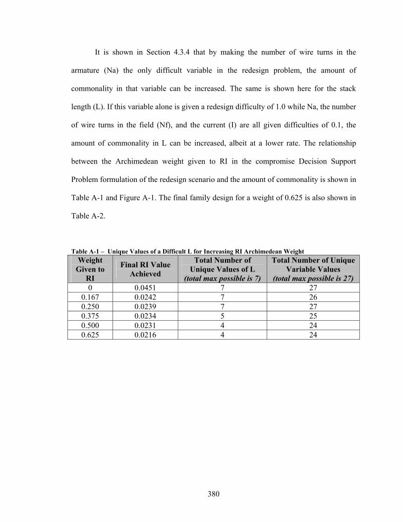
380
It is shown in Section 4.3.4 that by making the number of wire turns in the
armature (Na) the only difficult variable in the redesign problem, the amount of
commonality in that variable can be increased. The same is shown here for the stack
length (L). If this variable alone is given a redesign difficulty of 1.0 while Na, the number
of wire turns in the field (Nf), and the current (I) are all given difficulties of 0.1, the
amount of commonality in L can be increased, albeit at a lower rate. The relationship
between the Archimedean weight given to RI in the compromise Decision Support
Problem formulation of the redesign scenario and the amount of commonality is shown in
Table A-1 and Figure A-1. The final family design for a weight of 0.625 is also shown in
Table A-2.
Table A-1 – Unique Values of a Difficult L for Increasing RI Archimedean Weight Weight
Given to RI
Final RI Value Achieved
Total Number of Unique Values of L
(total max possible is 7)
Total Number of Unique Variable Values
(total max possible is 27) 0 0.0451 7 27
0.167 0.0242 7 26 0.250 0.0239 7 27 0.375 0.0234 5 25 0.500 0.0231 4 24 0.625 0.0216 4 24

381
0
0.005
0.01
0.015
0.02
0.025
0.03
0.035
0.04
0.045
0.05
0 0.1 0.2 0.3 0.4 0.5 0.6 0.7
Archimedean Weight Given to RI
Red
esig
n In
dex
(RI)
Figure A-1 – Effect of Increasing RI Weight on Instances of Redesign in a Difficult L Variable
Table A-2 – Redesigned Family with L Difficult to Change and RI Given a Weight of 0.625 Motor Na Nf L (cm) I (A) Existing Motor #1 1056 73 2.81 4.36Existing Motor #2 1007 73 2.61 4.02New Motor #1 493 112 1.09 3.02New Motor #2 757 103 1.31 3.27New Motor #3 1213 83 1.31 4.08New Motor #4 1022 93 1.31 3.63New Motor #5 1371 62 1.31 5.42
A.2 – FURTHER DEMONSTRATING THE GENERAL REDUCTION OF REDESIGN AT
THE EXPENSE OF A CERTAIN VARIABLE USING THE REDESIGN INDEX (RI)
In Section 4.3.4, it is shown that if the number of wires in the armature (Na) is the
only variable that is easy to change then even for increasing Archimedean weights given
to RI, solutions to the cDSP formulation of the redesign scenario can be found in which
the level of commonality in Na stays relatively constant while other design reuse is

382
encouraged. The same relationship is shown here for a situation in which the stack length
(L) is the only easy variable. For this scenario, only L is given a difficulty of 0.1 while
Na, the number of wire turns in the field (Nf), and the current (I) are all given hard
difficulties of 1.0. As the weight given to RI is increased, the trends shown in Table A-3
and Figure A-2 become clear. The level of commonality in L remains constant while
change in other variables is reduced.
Table A-3 – Unique Values of an Easy L for Increasing RI Archimedean Weight
Weight Given to
RI
Final RI Value Achieved
Total Number of Unique Values of Na
(total max possible is 7)
Total Number of Unique Variable Values
(total max possible is 27) 0 0.0451 7 27
0.167 0.0589 7 26 0.250 0.0430 7 25 0.375 0.0275 7 23 0.500 0.0225 7 19 0.625 0.0149 7 22
0
0.01
0.02
0.03
0.04
0.05
0.06
0.07
0 0.1 0.2 0.3 0.4 0.5 0.6 0.7
Archimedean Weight Given to RI
Red
esig
n In
dex
(RI)
Figure A-2 – Effect of Increasing RI Weight on Instances of Redesign in an Easy L

383
Table A-4 is presented as an example of the kind of solutions that can be found
using RI in this way. This solution is found using an Archimedean weight of 0.625 for RI
with redesign difficulties set such that the stack length is the only design variable
considered easy to change.
Table A-4 – Family with L Easy to Change and RI Given a Weight of 0.625 Motor Na Nf L (cm) I (A) Existing Motor #1 1007 73 2.81 4.36Existing Motor #2 1179 73 2.61 4.02New Motor #1 1179 84 0.58 3.36New Motor #2 1056 92 0.75 3.67New Motor #3 1179 84 1.37 4.02New Motor #4 1007 92 1.26 3.67New Motor #5 1179 75 1.84 4.50
A.3 – FURTHER DEMONSTRATING THE INCREASE IN COMMONALITY IN A
VARIABLE IN WHICH IT IS VALUABLE USING THE COMMONALITY DISCOUNT
FACTOR (CDF)
In Section 4.3.4, it is shown that the number of unique values of the variable Na
(number of wire turns in the armature) in the universal motor example can be reduced
through judicious use of the CDF. The same can also be shown for both the number of
wire turns in the field (Nf) and the stack length (L). Table A-5 and Figure A-3, results for
a cDSP formulation in which Nf is the only variable with valuable commonality are
shown. As the Archimedean weight is increased, a drop in both the number of unique
values of Nf and the number of unique variable values overall can be seen.

384
Table A-5 – Unique Values of a Valuable Nf for Increasing CDF Archimedean Weight Weight
Given to CDF
Final CDF Value Achieved
Total Number of Unique Values of Nf
(total max possible is 7)
Total Number of Unique Variable Values
(total max possible is 27) 0 0.0406 6 27
0.167 0.0066 6 27 0.250 0.0054 6 25 0.375 0.0044 5 24 0.500 0.0040 5 24 0.625 0.0038 5 24
0
5
10
15
20
25
30
0 0.1 0.2 0.3 0.4 0.5 0.6 0.7
Archimedean Weight Given to CDF
Tota
l Num
ber o
f Uni
que
Var
iabl
e V
alue
s In
Fam
ily
Total # of Unique Variable Values in Family Total # of Unique Values of Wire Turns in Field (Nf) in Family Figure A-3 – Effect of Increasing CDF Weight on Instances of Redesign in a Valuable Nf
Table A-6 contains a description of a redesign option identified by solving a
cDSP in which Nf is the only variable with a low commonality discount and CDF is
given a weight of 0.625 in the overall objective function. From these results, it is clear
that the impact on the amount of design reuse in Nf is not great, but that there is a general
development of reuse opportunities throughout the family.

385
Table A-6 – Family with Nf Commonality Valuable and CDF Given a Weight of 0.625 Motor Na Nf L (cm) I (A) Existing Motor #1 1056 73 2.81 4.36Existing Motor #2 1007 73 2.61 4.02New Motor #1 796 101 0.67 3.19New Motor #2 871 101 1.11 3.36New Motor #3 1363 76 1.07 4.44New Motor #4 1007 94 1.34 3.62New Motor #5 1364 63 1.34 5.35
The series of tests meant to show that CDF can be used to target design reuse in
the stack length (L) variable have more promising results, as seen in Table A-7 and
Figure A-4.
Table A-7 – Unique Values of a Valuable L for Increasing CDF Archimedean Weight
Weight Given to
CDF
Final CDF Value Achieved
Total Number of Unique Values of L
(total max possible is 7)
Total Number of Unique Variable Values
(total max possible is 27) 0 0.0406 7 27
0.167 0.0091 7.00 27 0.250 0.0067 5.00 25 0.375 0.0069 5.00 25 0.500 0.0063 5.00 23 0.625 0.0059 4.00 22

386
0
5
10
15
20
25
30
0 0.1 0.2 0.3 0.4 0.5 0.6 0.7
Archimedean Weight Given to CDF
Tota
l Num
ber o
f Uni
que
Var
iabl
e V
alue
s In
Fam
ily
Total # of Unique Variable Values in Family Total # of Unique Values of Stack Length (L) in Family Figure A-4 – Effect of Increasing CDF Weight on Instances of Redesign in a Valuable L
The redesigned family that is found when the cDSP is solved with CDF given an
Archimedean weight of 0.625 and L is the only variable with a low commonality
discount is seen in Table A-8. Overall, there is a good amount of overlap in the values of
stack length used by the product family members.

387
Table A-8 – Family with L Commonality Valuable and CDF Given a Weight of 0.625 Motor Na Nf L (cm) I (A) Existing Motor #1 1056 73 2.81 4.36Existing Motor #2 1007 73 2.61 4.02New Motor #1 614 102 0.93 3.08New Motor #2 835 102 1.17 3.33New Motor #3 1302 79 1.17 4.27New Motor #4 1302 84 0.93 4.04New Motor #5 1403 57 1.17 5.95
A.4 – FURTHER DEMONSTRATING THE INCREASE IN COMMONALITY IN
GENERAL IN A FAMILY AT THE EXPENSE OF GREATER REDESIGN IN A CERTAIN
VARIABLE USING THE COMMONALITY DISCOUNT FACTOR (CDF)
The next series of tests is aimed at demonstrating the opposite effect of CDF. In
Section 4.3.4, it is shown that by manipulating the commonality discounts associated
with certain variables, commonality can be encouraged in general while encouraged to a
lesser degree in the number of wire turns in the armature (Na). A series of experiments
explained here are aimed at showing the same trend for the number of wire turns in the
field (Nf). A cDSP is formulated in which only Nf has a low commonality discount of 0.1
while Na, the stack length (L), and the current (I) all have high discounts of 1.0. The
results in Nf, even as the weight given to CDF is increased, are not huge, as seen in Table
A-9 and FigureA-5. This is the desired result.

388
Table A-9 – Unique Values of a Worthless Nf for Increasing CDF Archimedean Weight Weight
Given to CDF
Final CDF Value Achieved
Total Number of Unique Values of Nf
(total max possible is 6)
Total Number of Unique Variable Values
(total max possible is 27) 0 0.0406 6 27
0.167 0.0066 6 26 0.250 0.0054 6 23 0.375 0.0044 6 23 0.500 0.0131 6 22 0.625 0.0135 6 22
0
5
10
15
20
25
30
0 0.1 0.2 0.3 0.4 0.5 0.6 0.7
Archimedean Weight Given to CDF
Tota
l Num
ber o
f Uni
que
Var
iabl
e V
alue
s In
Fam
ily
Total # of Unique Variable Values in Family Total # of Unique Values of Wire Turns in Field (Nf) in Family Figure A-5 – Effect of Increasing CDF Weight on Instances of Redesign with a Worthless Nf
As seen in Table A-10, while the number unique values for Nf stays relatively
constant even when CDF receives a weight of 0.625, the total amount of design reuse in
the family is quite high. Commonality can be seen in each of the other three variables.

389
Table A-10 – Family with Nf Commonality Worthless and CDF Given a Weight of 0.625 Motor Na Nf L (cm) I (A) Existing Motor #1 1056 73 2.81 4.36Existing Motor #2 1007 73 2.61 4.02New Motor #1 1007 84 0.57 3.36New Motor #2 1007 97 0.93 3.48New Motor #3 1056 88 1.60 3.83New Motor #4 1268 85 0.97 3.97New Motor #5 1268 71 1.60 4.79 A similar series of experiments is run for the stack length (L) in an attempt to
show that CDF can encourage commonality in general while focusing away from L. As
seen Table A-11 and Figure A-6, the results of this series are even better than for Nf. The
redesigned family shown in Table A-12 has even more design re-use although there is
one repeat of a value of L.
Table A-11 – Unique Values of a Worthless L for Increasing CDF Archimedean Weight Weight
Given to CDF
Final CDF Value Achieved
Total Number of Unique Values of L
(total max possible is 7)
Total Number of Unique Variable Values
(total max possible is 27) 0 0.0406 7 27
0.167 0.0218 7.00 24 0.250 0.0138 7.00 24 0.375 0.0109 7.00 24 0.500 0.0050 7.00 20 0.625 0.0071 7.00 22

390
0
5
10
15
20
25
30
0 0.1 0.2 0.3 0.4 0.5 0.6 0.7
Archimedean Weight Given to CDF
Tota
l Num
ber o
f Uni
que
Var
iabl
e V
alue
s In
Fam
ily
Total # of Unique Variable Values in Family Total # of Unique Values of Stack Length (L) in Family Figure A-6 – Effect of Increasing CDF Weight on Instances of Redesign in a Worthless L
Table A-12 – Family with L Commonality Worthless and CDF Given a Weight of 0.625 Motor Na Nf L (cm) I (A) Existing Motor #1 1056 73 2.81 4.36Existing Motor #2 1007 73 2.61 4.02New Motor #1 952 97 0.54 3.31New Motor #2 1007 97 0.93 3.48New Motor #3 1179 84 1.37 4.02New Motor #4 952 95 1.44 3.56New Motor #5 1179 75 1.84 4.50
A.5 – FURTHER DEMONSTRATING THE INCREASE IN DESIGN REUSE IN A
CERTAIN TYPE OF VALUABLE COMMONALITY USING THE COMMONALITY
DISCOUNT FACTOR (CDF)
The results presented in Section 4.3.4 do not strongly demonstrate the benefit of
using CDF when a certain type of commonality is more valuable than others. The

391
argument is also made that a redesign scenario in which there are more opportunities of
each type might show this benefit more clearly. In an effort to back up this supposition, a
totally new redesign scenario is presented in Figure 4-15 and summarized in cDSP form
in Table A-13.
Table A-13 – cDSP Formulation of Special Redesign Problem for Validation of Indices Given • An 1-dimensional market space of torque values that are to be changed
over time through redesign • One existing system with at torque output of 0.05 Nm • Six new systems to be released over the next 8 years, each with a
torque output 0.05 Nm greater than the previous year’s new model • The schedule of production shown in Figure 4-15 • A set of values for certain platform variables (Awa, Awf, r, and t) that
is to be constant through all of the new motor designs: Awa = 0.241 mm
Awf = 0.376 mm r = 2.69 cm t = 6.66 cm
Find • Redesign variables
• Deviation variables Satisfy The system constraints:
• System average mass goal of 0.50Kg • System average efficiency goal of 0.70 • System minimization of CDF goal:
{ }( ) CDF CDF 1CDF X d d− ++ − =
• Individual motor torque goals • The lower and upper bounds on each system • Deviation variable constraints
Minimize The deviation function:
( ) ( )( ) ( )
f
5
1
5
1
where 1
avg avg avg avg avg avg
j j j
avg avg j
m m m
CDF CDF T T Tj
m CDF Tj
Z w d d w d d
w d w d d
Z w w w w
η η η
η
− + − +
+ − +
=
=
= + + +
+ + +
= + + + =
∑
∑

392
The cDSP summarized in Table A-13 is solved in three series of tests to see
whether Staggered Production (SP) commonality and Production Gap (PG) commonality
can be encouraged at the exclusion of other types in this scenario. It should be noted that
given the redesign schedule shown in Figure 4-15, these are the only two types of
commonality possible. It should also be noted that while the total number of commonality
types possible has dropped, the SP commonality may still have a head start on account of
the systems with overlapping production schedules having similar required torque
outputs.
The results from solving the cDSP when only Staggered Production is given a low
commonality discount are promising. As seen in Table A-14 and Figure A-7, a good
amount of commonality is encouraged as the weight given to CDF is increased, with
most of it going to SP commonality.
Table A-14 – Instances of Valuable SP Commonality for Increasing CDF Archimedean Weight in the Special Scenario
Weight Given to
CDF
Final CDF Value Achieved
Total Number of Instances of Perfect
Commonality (total max possible is 20)
Total Number of Unique Variable Values
(total max possible is 28)
0 0.010348 0 28 0.167 0.006924 0 28 0.250 0.006917 3 25 0.375 0.004936 3 25 0.500 0.004446 6 22 0.625 0.010348 4 22

393
Unique Variable Values for Different Weights of CDF in Test Favoring Only Staggered Production Type Commonality
0
5
10
15
20
25
30
0 0.1 0.2 0.3 0.4 0.5 0.6 0.7
Archimedean Weight Given to CDF
Tota
l Num
ber o
f Uni
que
Var
iabl
e V
alue
s or
Inst
ance
s of C
omm
onal
ity In
Fam
ily
Total # of Unique Variable Values in Family Total # of Instances of Staggered Production Comm in Family Figure A-7 – Effect of Increasing CDF Weight on Instances of SP Commonality in the Special Scenario
The solution found when CDF is given a weight of 0.625 is shown in Table A-15.
The redesigned family has an average mass of 0.544 Kg and average efficiency of 57.7
%, which is not great. Still, all of the torque targets are met almost exactly.
Table A-15 – Special Scenario Family in Which SP Commonality is Particularly Valuable with CDF Given a Weight of 0.625 Motor Na Nf L (cm) I (A) Existing Motor #1 730 45 1.00 3.65New Motor #1 730 104 1.37 3.26New Motor #2 1496 35 1.00 5.61New Motor #3 1496 60 0.91 5.19New Motor #4 1133 82 1.73 4.15New Motor #5 1387 60 1.25 5.61New Motor #6 1312 60 1.53 5.67

394
Table A-16 – Instances of Valuable PG Commonality for Increasing CDF Archimedean Weight in the Special Scenario
Weight Given to
CDF
Final CDF Value Achieved
Total Number of Instances of Perfect
Commonality (total max possible is 20)
Total Number of Unique Variable Values
(total max possible is 28)
0 0 28 0 0.167 0 28 0 0.250 0 28 0 0.375 0 28 0 0.500 0 28 0 0.625 3 22 3
Unique Variable Values for Different Weights of CDF in Test Favoring Only Production Gap Type Commonality
0
5
10
15
20
25
30
0 0.1 0.2 0.3 0.4 0.5 0.6 0.7
Archimedean Weight Given to CDF
Tota
l Num
ber o
f Uni
que
Var
iabl
e V
alue
s or
Inst
ance
s of C
omm
onal
ity In
Fam
ily
Total # of Unique Variable Values in Family Total # of Instances of Production Gap Comm in Family Figure A-8 – Effect of Increasing CDF Weight on Instances of PG Commonality in the Special Scenario
The solution found when CDF is given a weight of 0.625 is shown in Table A-17.
The redesigned family has an average mass of 0.526 Kg and average efficiency of 57.3

395
%, which is not great. Still, all of the torque targets are met almost exactly. The PG
commonality in this family is seen in the sharing of values of Nf and L.
Table A-17 – Special Scenario Family in Which PG Commonality is Particularly Valuable with CDF Given a Weight of 0.625 Motor Na Nf L (cm) I (A) Existing Motor #1 730 45 1.00 3.65New Motor #1 706 104 1.42 3.24New Motor #2 1479 56 0.89 4.70New Motor #3 1479 69 0.89 4.91New Motor #4 1391 69 1.18 4.93New Motor #5 1404 56 1.16 6.00New Motor #6 1330 56 1.42 6.00
A.6 – FURTHER DEMONSTRATING THE INCREASE IN DESIGN REUSE IN
GENERAL IN A FAMILY AT THE EXPENSE OF A CERTAIN TYPE OF VALUABLE
COMMONALITY USING THE COMMONALITY DISCOUNT FACTOR (CDF)
Returning to the original redesign scenario used throughout Section 4.3.4, it is
shown here that the CDF can be used to emphasize commonality in general while not
encouraging much design reuse between systems that have “perfect” overlap in their
production schedules. This type of Perfect Commonality is only seen in this example
between the fourth and fifth new motors. To show the effectiveness of CDF in this
regard, the cDSP formulation is again adjusted to give any Perfect Commonality a high
discount while all other types receive low ones. As is seen in Table A-18 and Figure A-9,
this adjustment successfully yields lower and lower amounts of change in the new
systems as the weight given to CDF in the objective function is increased.

396
Table A-18 – Instances of Worthless Perfect Commonality for Increasing CDF Archimedean Weight
Weight Given to
RI
Final CDF Value Achieved
Total Number of Instances of Perfect
Commonality (total max possible is 8)
Total Number of Unique Variable Values
(total max possible is 27)
0 0.0406 0 27 0.167 0.0106 0 25 0.250 0.0089 0 23 0.375 0.0083 0 23 0.500 0.0062 0 22 0.625 0.0059 0 21
Unique Variable Values for Different Weights of CDF in Test Favoring All Commonality Aside from Perfect Commonality
0
5
10
15
20
25
30
0 0.1 0.2 0.3 0.4 0.5 0.6 0.7
Archimedean Weight Given to CDF
Tota
l Num
ber o
f Uni
que
Var
iabl
e V
alue
s or
Inst
ance
s of C
omm
onal
ity In
Fam
ily
Total # of Unique Variable Values in Family Total # of Instances of Perfect Comm in Family Figure A-9 – Effect of Increasing CDF Weight on Instances of Worthless Perfect Commonality
A sample solution from this formulation of the cDSP is shown in Table A-19.
This redesign solution exhibits design reuse throughout and achieves all torque goals with
an average mass of 0.543 Kg and average efficiency of 64.7%.

397
Table A-19 –Family in Which Perfect Commonality is Worthless with CDF Given a Weight of 0.625 Motor Na Nf L (cm) I (A) Existing Motor #1 1056 73 2.81 4.36Existing Motor #2 1007 73 2.61 4.02New Motor #1 868 78 0.77 3.25New Motor #2 868 101 1.11 3.36New Motor #3 1337 78 1.11 4.36New Motor #4 1294 84 0.94 4.02New Motor #5 1337 66 1.42 5.14
As noted in Section 4.3.4, it is impossible to show all of the data for each of the
experiments in each of the series discussed here. However, it is hoped that by showing
examples and summaries of trends, the reader will get an idea of the effectiveness of the
proposed indices and their real impact on the redesign solutions that are identified.

398
APPENDIX B – MATLAB FUNCTIONS AND SCRIPTS
B.1 – MATLAB CODE FOR VERIFICATION AND VALIDATION OF OVERALL
CONSTRUCTAL INSPIRED METHOD
In order to be able to quickly run experiments with new redesign scenarios, much
of the constructal-inspired redesign decision support method presented in this dissertation
has been automated in Matlab programs and scripts. The information flows between these
programs and scripts are shown in Figure 4-19. Almost all of this code has been written
in such a way that it can be reused with minimal effort for problems that differ in the
number of:
• Dimensions of customization (a.k.a. system responses) in the problem;
• Redesign variables;
• Stages to the constructal-inspired approach;
• Existing systems;
• New systems to be created through redesign;
• Overall objectives like the CDF, RI, mass, and efficiency goals used in the
examples in Chapter 4; and
• Space elements allowed to be used to break up the space.
In addition, the user can quickly adjust weights, redesign difficulty indices (RDI),
commonality discounts, and redesign targets to better represent his/her preferences. The
groupings of variables (modes of managing product variety) into constructs can also be
easily adjusted. All of this was done so that future researchers could easily use this code
on other example problems besides the universal motor problem exercised here.

399
Much of the Matlab code utilized in the verification and validation of the overall
constructal-inspired method is the same as that which is used to validate the indices by
themselves. As a result, the only scripts and programs displayed in Section C.2 are those
that differ significantly from their counterparts here or which are unique to the overall
method.
B.1.1 – “solvequasicon.m” Program
This is the main function for the implementation of the constructal-inspired
approach to solving the redesign problem. It calls all of the rest of the functions and
scripts that are displayed in Section C.1, setting up the redesign problem, generating start
points for fmincon, analyzing the results, sorting the results, and saving everything of
value for analysis later on. The only values that should need to be changed for use of this
function in different example problems is the file name used to save the Matlab diary and
the data file.
%%%%%%%%%%%%%%%%%%%%%%%%%%%%%%%%%%%%%%%%%%%%%%%%%%%%%%%%%%%%%%%%%%%%%%%%%% % solvequasicon3.m % % Updated by: Matt Chamberlain % % Description: This script is meant to be the main program used to solve % the universal motor redesign problem in a constructal-inspired manner. % %%%%%%%%%%%%%%%%%%%%%%%%%%%%%%%%%%%%%%%%%%%%%%%%%%%%%%%%%%%%%%%%%%%%%%%%%% [schedule,existingsys,existingsysres,targets,overallobjs,weights,... physcons,physconflags,physconseq,physconseqflags,minndiv,maxndiv,... responsebounds,numvars,constructs,lbounds,ubounds,x0,commindices,rdi]... = redesigninputs2; numexsys = size(existingsys,1); numtargets = size(targets,1); % Make a non-dimensional set of existing systems existingsysnondim = zeros(numexsys,numvars); for countexsys = 1:size(existingsys,1) existingsysnondim(countexsys,:) = ... (existingsys(countexsys,:) - lbounds') ./ (ubounds' - lbounds'); end % Create the redesign difficulty and scheduling matrices [commmatrix,startprod,endprod] = createcomoppmatrix2(schedule,numvars,commindices);

400
maxvalue = 0; validndiv = 0; numconstructs = size(unique(constructs),2); % This loop runs an exhaustive search of the number of space element % divisions possible ndiv = maxndiv * ones(numconstructs,1) tracendiv(:,1) = ndiv; savepoint = 2; while (sum(ndiv) > numconstructs) % Don't go forward without an ndiv formulation that might % possibly work if (checkndiv(ndiv,existingsys,targets) == 0) clear spaceelements validflag existingsysflag Aeq Beq; clear currsetup alltargassignments startvars2; % Based on the ndiv, create the bounds for the space elements spaceelements = createspaceelements(responsebounds,ndiv); % checkexistingelem2 checks to see if the arrangement of % existing elements inside [validflag,existingsysflag,openspaceflag] = ... checkexistinelem(spaceelements,existingsys,existingsysres,constructs,ndiv); % The "if" statement on the next line makes sure there is no % conflict regarding the space elements in which the existing % system sit if (validflag == 1) tic validndiv = validndiv + 1 %#ok<NOPTS> savedndiv(validndiv,:) = ndiv; %#ok<AGROW> if (ndiv(1,1) < (numtargets+numexsys)) commflag(validndiv,1) = 1; %#ok<AGROW> else commflag(validndiv,1) = 0; %#ok<AGROW> end numdimensions = size(responsebounds,1); numelements = ndiv(:,1); for countelements = 2:numdimensions numelements = numelements .* ndiv(:,countelements); end totnumvars = numvars * numelements(numconstructs); % Figure out number of elements that may contain new % systems numnewsols = numelements(numconstructs,1) - numexsys; % Figure out all the possible assignments of new % systems to redesign targets alltargassignments = createtargassignments(numnewsols,numtargets); numassignments = size(alltargassignments,1) %#ok<NOPTS> [narrowedassignments] = narrowtargassignments(alltargassignments,... spaceelements,openspaceflag,responsebounds,numelements,... numconstructs,targets,existingsysres); numnarrowedassignments = size(narrowedassignments,1) %#ok<NOPTS> % Search through the narrowed number of assignments for searchassignments = 1:numnarrowedassignments clear startvars2; searchassignments %#ok<NOPTS> currsetup = narrowedassignments(searchassignments,:); % Generate an array to show which targets each % system in the variable array is assigned to % ("VARTARGASSIGN") vartargassign = nonzeros(currsetup)'; % Generate an array to show which space element % each system in the variable array is assigned to % ("VARSPACEELEMASSIGN") varspaceelemassign = zeros(1,numtargets); assignments = 0; for i = 1:size(currsetup,2)
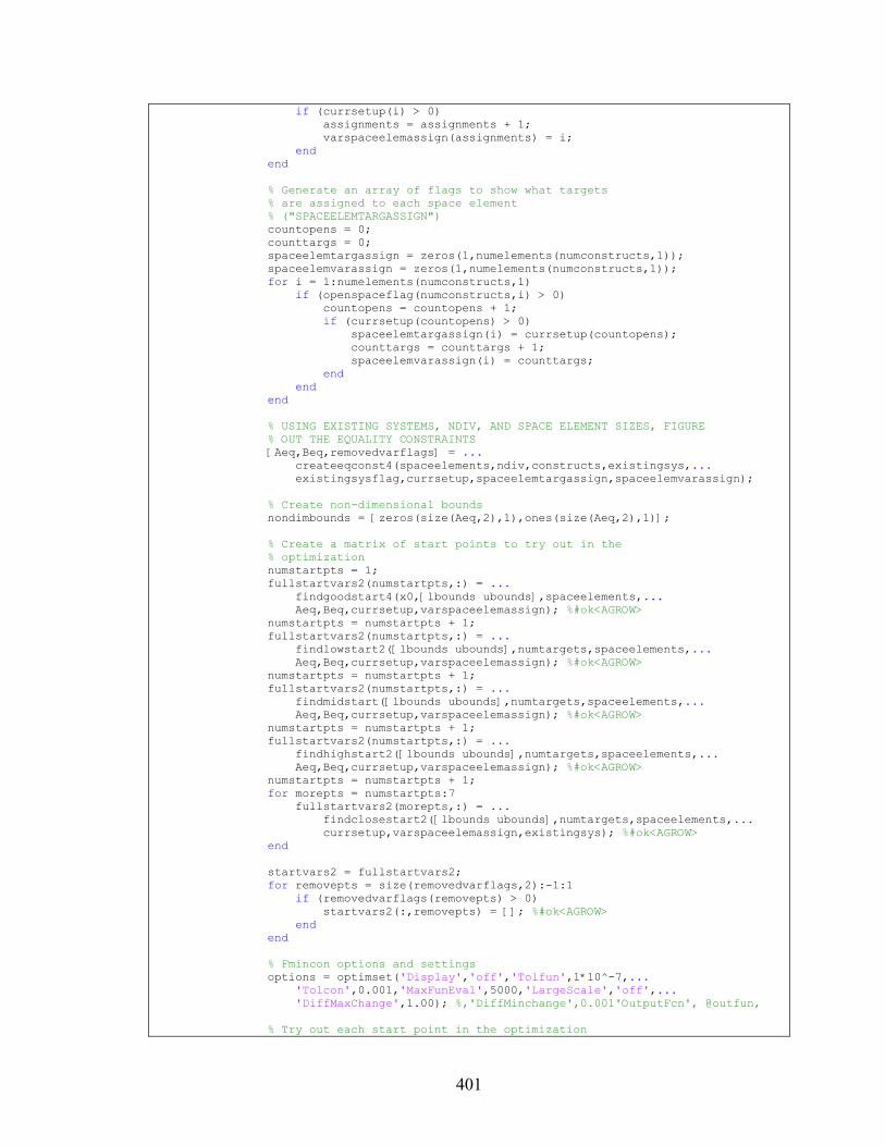
401
if (currsetup(i) > 0) assignments = assignments + 1; varspaceelemassign(assignments) = i; end end % Generate an array of flags to show what targets % are assigned to each space element % ("SPACEELEMTARGASSIGN") countopens = 0; counttargs = 0; spaceelemtargassign = zeros(1,numelements(numconstructs,1)); spaceelemvarassign = zeros(1,numelements(numconstructs,1)); for i = 1:numelements(numconstructs,1) if (openspaceflag(numconstructs,i) > 0) countopens = countopens + 1; if (currsetup(countopens) > 0) spaceelemtargassign(i) = currsetup(countopens); counttargs = counttargs + 1; spaceelemvarassign(i) = counttargs; end end end % USING EXISTING SYSTEMS, NDIV, AND SPACE ELEMENT SIZES, FIGURE % OUT THE EQUALITY CONSTRAINTS [Aeq,Beq,removedvarflags] = ... createeqconst4(spaceelements,ndiv,constructs,existingsys,... existingsysflag,currsetup,spaceelemtargassign,spaceelemvarassign); % Create non-dimensional bounds nondimbounds = [zeros(size(Aeq,2),1),ones(size(Aeq,2),1)]; % Create a matrix of start points to try out in the % optimization numstartpts = 1; fullstartvars2(numstartpts,:) = ... findgoodstart4(x0,[lbounds ubounds],spaceelements,... Aeq,Beq,currsetup,varspaceelemassign); %#ok<AGROW> numstartpts = numstartpts + 1; fullstartvars2(numstartpts,:) = ... findlowstart2([lbounds ubounds],numtargets,spaceelements,... Aeq,Beq,currsetup,varspaceelemassign); %#ok<AGROW> numstartpts = numstartpts + 1; fullstartvars2(numstartpts,:) = ... findmidstart([lbounds ubounds],numtargets,spaceelements,... Aeq,Beq,currsetup,varspaceelemassign); %#ok<AGROW> numstartpts = numstartpts + 1; fullstartvars2(numstartpts,:) = ... findhighstart2([lbounds ubounds],numtargets,spaceelements,... Aeq,Beq,currsetup,varspaceelemassign); %#ok<AGROW> numstartpts = numstartpts + 1; for morepts = numstartpts:7 fullstartvars2(morepts,:) = ... findclosestart2([lbounds ubounds],numtargets,spaceelements,... currsetup,varspaceelemassign,existingsys); %#ok<AGROW> end startvars2 = fullstartvars2; for removepts = size(removedvarflags,2):-1:1 if (removedvarflags(removepts) > 0) startvars2(:,removepts) = []; %#ok<AGROW> end end % Fmincon options and settings options = optimset('Display','off','Tolfun',1*10^-7,... 'Tolcon',0.001,'MaxFunEval',5000,'LargeScale','off',... 'DiffMaxChange',1.00); %,'DiffMinchange',0.001'OutputFcn', @outfun, % Try out each start point in the optimization

402
minobj = 1*10^6; for searchstartpts = 1:7 [reducedtempvars2,tempobjvalue2,tempexitflag2,output,lambda] = ... fmincon(@(solutionset)portfolioeval4(solutionset,existingsys,... targets,responsebounds,weights,schedule,startprod,commmatrix,... rdi,currsetup,vartargassign,[lbounds, ubounds],removedvarflags),... startvars2(searchstartpts,:),[],[],Aeq,Beq,nondimbounds(:,1),... nondimbounds(:,2),... @(solutionset)createnonlconst3(solutionset,spaceelements,... existingsys,physcons,physconflags,currsetup,spaceelemvarassign,... [lbounds, ubounds],removedvarflags),options); searchstartpts tempobjvalue2 tempexitflag2 if (tempobjvalue2 <= minobj) minobj = tempobjvalue2; % Next few lines put removed vars back in! reducedplace = 1; tempvars2 = zeros(1,size(removedvarflags,2)); for i = 1:size(removedvarflags,2) if (removedvarflags(i) == 0) tempvars2(i) = reducedtempvars2(reducedplace); reducedplace = reducedplace + 1; end end vars2(validndiv,searchassignments,:) = tempvars2; %#ok<AGROW> finalobjvalue2(validndiv,searchassignments) = tempobjvalue2; %#ok<AGROW> exitflag2(validndiv,searchassignments) = tempexitflag2; %#ok<AGROW> setup2(validndiv,searchassignments,1:size(currsetup,2)) = currsetup; %#ok<AGROW> startpointused2(validndiv,searchassignments) = searchstartpts; %#ok<AGROW> end end % Change the best non-dimensional array of % variables back into a dimensional form and an % easy-to-read form countrows = 1; dimvarsinrows = zeros(numtargets,numvars); nondimvarsinrows = zeros(numtargets,numvars); for i = 1:numvars:(numvars*numtargets) nondimvarchunk(1:numvars) = ... vars2(validndiv,searchassignments,i:(i + numvars - 1)); dimvarchunk = (nondimvarchunk .* (ubounds' - lbounds')) + lbounds'; dimvarsinrows(countrows,:) = dimvarchunk; nondimvarsinrows(countrows,:) = nondimvarchunk; countrows = countrows + 1; end % Reevaluate RI and CDF finalri2(validndiv,searchassignments) = ... evalcontinuousri(existingsysnondim, nondimvarsinrows, ... rdi, vartargassign, schedule, startprod); %#ok<AGROW> finalcdf2(validndiv,searchassignments) = ... evalcontinuouscdf2(existingsysnondim, nondimvarsinrows, ... commmatrix, vartargassign); %#ok<AGROW> finalvars2(validndiv,searchassignments,1:numtargets,1:numvars) = ... dimvarsinrows; %#ok<AGROW> % Reevaluate the torques of the new motors for countfinalsys = 1:numtargets output = ... TSunivmotor(finalvars2(validndiv,searchassignments,countfinalsys,:)); finalsystorques2(validndiv,searchassignments,countfinalsys) = ... output(1); %#ok<AGROW>

403
finalsysresponsesall2(validndiv,searchassignments,countfinalsys,:) = ... output; %#ok<AGROW> end % Check for negative variable values in the % solution (a sign of a failed optimization % process) if (min(vars2(validndiv,searchassignments,:)) < 0) negativevarflag2(validndiv,searchassignments,1) = -1; %#ok<AGROW> end end % loop to search through setups timelog(validndiv) = toc; %#ok<AGROW> end end tempndiv = ndiv; % tempndiv(numconstructs,1) = tempndiv(numconstructs,1) - 1; tempndiv(1,1) = tempndiv(1,1) - 1; % if (tempndiv(numconstructs,1) < 1) if (tempndiv(1,1) < 1) % tempndiv(numconstructs,1) = maxndiv; tempndiv(1,1) = maxndiv; % searchplace = numconstructs - 1; searchplace = 2; done = 0; % while (searchplace > 0) && (done == 0) while (searchplace <= numconstructs) && (done == 0) if (tempndiv(searchplace,1) > 1) tempndiv(searchplace,1) = tempndiv(searchplace,1) - 1; done = 1; else tempndiv(searchplace,1) = maxndiv; % searchplace = searchplace - 1; searchplace = searchplace + 1; end end end ndiv = tempndiv savepoint = savepoint + 1; end minobjval = 10000; % Special section to compute the objective function values using target % achievement using RI and CDF for experiment #39 in which RI and CDF were % not used in the optimiziation process if ( (weights(numtargets+1,1) == 0) && (weights(numtargets+2,1) == 0) ) finalobjvalue2original = finalobjvalue2; for i = 1:size(finalobjvalue2,1) for j = 1:size(finalobjvalue2,2) finalobjvalue2(i,j) = (finalobjvalue2(i,j) + finalri2(i,j) + ... finalcdf2(i,j)) / 3; %#ok<AGROW> end % WHAT ABOUT THE MASS AND EFFICIENCE GOALS!??? end end % Find the smallest objective function value for i = 1:size(finalobjvalue2,1) for j = 1:size(finalobjvalue2,2) if (finalobjvalue2(i,j) <= minobjval) && (finalobjvalue2(i,j) > 0) minobjval = finalobjvalue2(i,j); minloc = [i,j]; end end end % Sort the results by objective function value sortedobjvalues = 0; sortedlocs = [0,0]; sortedcommflags = [0,0]; numsorted = 0;

404
for i = 1:size(finalobjvalue2,1) for j = 1:size(finalobjvalue2,2) if (finalobjvalue2(i,j) > 0) numsorted = numsorted + 1; sortloc = 1; while (sortloc < numsorted) && (sortedobjvalues(sortloc) < finalobjvalue2(i,j)) sortloc = sortloc + 1; end sortedobjvalues(sortloc+1:numsorted) = sortedobjvalues(sortloc:numsorted-1); sortedobjvalues(sortloc) = finalobjvalue2(i,j); %#ok<AGROW> sortedlocs(sortloc+1:numsorted,:) = sortedlocs(sortloc:numsorted-1,:); sortedlocs(sortloc,:) = [i,j]; sortedcommflags(sortloc+1:numsorted,:) = sortedcommflags(sortloc:numsorted-1,:); %#ok<AGROW> sortedcommflags(sortloc,1) = commflag(i,1); %#ok<AGROW> end end end % save test13onethirdweightswith8ndivGabrielsConstructsNoCDForRIOct03Platonewndivsetup % WARNING THAT PROGRAM HAS ENDED for countbeeps = 1:5 beep; end diary off
B.1.2 – “redesigninputs.m” Program
This script is the main source of information that should be input by the designer
to describe the redesign problem, his/her preferences towards the goals, the redesign
difficulties, and the commonality discounts. There are also several values relevant to the
solution procedure that must be set, including the buffer for the redesign market space,
the maximum number of market space divisions, and the arrangement of the redesign
variables/modes into stages.
function [schedule,existingsys,existingsysres,targets,overallobjs,weights,... physcons,physconflags,physconseq,physconseqflags,minndiv,maxndiv,... responsebounds,numvars,constructs,lbounds,ubounds,x0,commindices,rdi]... = redesigninputs() % Initializes many of the parameters necessary to describe the redesign % problem %%%%%%%%%%%%%%%%%%%%%%%%%%%%%%%%%%%%%%%%%%%%%%%%%%%%%%%%%%%%%%%%%%%%%%%%%% % redesigninputs2.m % % Written by: Matt Chamberlain % December 11th, 2006 % % Description: This script is a consolidation of all of the initiation % functions previously used to address the constructal redesign problem. % This script is made up of pieces of the following old functions: % -initconstraints.m % -initexistingsys.m % -initobjectives.m % -initresponsespace.m % -initschedule.m

405
% -initvars.m % -initcommandredesignfactors.m % %%%%%%%%%%%%%%%%%%%%%%%%%%%%%%%%%%%%%%%%%%%%%%%%%%%%%%%%%%%%%%%%%%%%%%%%%% %%%%%%%%%%%%%%%%%%%%%%%%%%%%%%%%%%%% %%%%% PRODUCT RELEASE SCHEDULE %%%%% %%%%%%%%%%%%%%%%%%%%%%%%%%%%%%%%%%%% % The number of total product family members anticipated: numprods = 4; % The number of years/months/quarters that is known or anticipated at this % time: numyears = 4; % Initialize the matrix with zeros which indicate that a product is not % being made during that time period schedule = zeros(numprods,numyears); % THESE TEN SYSTEMS ARE FOR MY BASIC EVOLVING 10-SYSTEM FAMILY schedule(1,1:3) = 1; % Schedule of production for product #1 schedule(2,1:3) = 1; % Schedule of production for product #2 schedule(3,2:4) = 1; % Schedule of production for product #3 schedule(4,2:4) = 1; % Schedule of production for product #4 % schedule(5,3:6) = 1; % Schedule of production for product #5 % schedule(6,6:7) = 1; % Schedule of production for product #7 % schedule(7,6:7) = 1; % Schedule of production for product #8 %%%%%%%%%%%%%%%%%%%%%%%%%%%% %%%%% EXISTING SYSTEMS %%%%% %%%%%%%%%%%%%%%%%%%%%%%%%%%% % These are the individualy-optimized systems from Simpson, Maier, and % Mistree (2001) % Torques of the motors: % (1) 0.05 (2) 0.10 (3) 0.125 (4) 0.15 (5) 0.20 (6) 0.25 (7) 0.30 (8) 0.35 (9) 0.40 (10) 0.50 existingsystemp = zeros(10, 8); existingsystemp(:,1) = [730, 750, 760, 785, 988, 1007, 1030, 1056, 1082, 1087]; existingsystemp(:,2) = [0.205, 0.203, 0.203, 0.205, 0.217, 0.224, 0.230, 0.237, 0.243, 0.247]; existingsystemp(:,3) = [45, 76, 89, 95, 74, 73, 73, 73, 72, 72]; existingsystemp(:,4) = [0.203, 0.186, 0.190, 0.205, 0.241, 0.246, 0.253, 0.260, 0.267, 0.284]; existingsystemp(:,5) = [3.62, 3.31, 3.12, 2.82, 2.26, 2.35, 2.44, 2.51, 2.58, 2.71]; existingsystemp(:,6) = [9.69, 11.77, 11.20, 8.88, 5.75, 6.17, 6.35, 6.46, 6.67, 7.15]; existingsystemp(:,7) = [0.998, 1.28, 1.41, 1.63, 2.38, 2.61, 2.74, 2.81, 2.87, 3.16]; existingsystemp(:,8) = [3.65, 3.73, 3.73, 3.70, 3.84, 4.02, 4.19, 4.36, 4.53, 4.71]; % These are systems chosen using GA in Simpson book chapter (2005) % existingsystemp = zeros(10, 8); % existingsystemp(:,1) = [1056, 1056, 1056, 1056, 1056, 1056, 1055, 1056, 1056]; % existingsystemp(:,2) = [0.234, 0.234, 0.234, 0.234, 0.234, 0.234, 0.234, 0.234, 0.234, 0.234]; % existingsystemp(:,3) = [55, 55, 55, 55, 56, 57, 55, 57, 55, 55]; % existingsystemp(:,4) = [0.348, 0.356, 0.356, 0.356, 0.357, 0.359, 0.355, 0.354, 0.351, 0.356]; % existingsystemp(:,5) = [2.54, 2.54, 2.54, 2.54, 2.52, 2.54, 2.54, 2.54, 2.54, 2.54]; % existingsystemp(:,6) = [6.91, 6.96, 6.99, 6.99, 6.99, 6.99, 6.99, 6.99, 6.99, 6.99]; % existingsystemp(:,7) = [0.880, 1.547, 1.808, 2.039, 2.408, 2.632, 2.855, 2.926, 3.027, 2.995]; % existingsystemp(:,8) = [3.38, 3.61, 3.73, 3.84, 4.08, 4.29, 4.59, 4.83, 5.15, 5.79]; % MOVE AROUND SOME EXISTING SYSTEMS FOR DIFFERENT SITUATIONS % existingsystemp(1,:) = existingsystemp(8,:); existingsystemp(2,:) = existingsystemp(6,:); % for T = 0.25 % existingsystemp(2,:) = existingsystemp(4,:); % for T = 0.15 numexsys = 0; for countexsys = 1:size(schedule,1) if (schedule(countexsys,1) > 0) numexsys = numexsys + 1;

406
end end j = numexsys + 1; while (j <= size(existingsystemp,1)) existingsystemp(j,:) = []; end existingsys = existingsystemp; for i = 1:numexsys existingsysres(i,:) = TSunivmotor(existingsys(i,:)); end %%%%%%%%%%%%%%%%%%%%%% %%%%% OBJECTIVES %%%%% %%%%%%%%%%%%%%%%%%%%%% %%% DESIGNER'S PREF'S FOR EACH TARGET %%% % Note: The target matrix below is of size m row x n columns where m is the % number of new systems being redesigned and n is the number of dimensions % in which there are new redesign targets % Note: Targets MUST be put in here in chronological order as in the % schedule matrix targets(1,1) = 0.050; targets(2,1) = 0.250; targets(3,1) = 0.100; targets(4,1) = 0.150; % targets(5,1) = 0.200; % targets(6,1) = 0.150; % targets(7,1) = 0.300; targets(1:numexsys,:) = []; numtargets = size(targets,1); %%% DESIGNER'S PREFS FOR OVERALL OBJECTIVES %%% % This is not used anymore. It was supposed to help model different overall % objectives but since RI and CDF have been adopted, it is unused overallobjs(1,:) = [0,1]; % points on the value curve for CDF overallobjs(2,:) = [0,1]; % points on the value curve for RI % overallobjs(1,:) = [0,.6,1]; % points on the value curve for CDF % overallobjs(2,:) = [0,.6,1]; % points on the value curve for RI %%% GATHER WEIGHTS FOR OBJECTIVE FUNCTION %%% % Assume there is one row for each target, with one column for each % dimension of a redesign target % After the weights for the targets are the weights for CDF, RI, mass, and % efficiency overall family goals, each in its own rows cdfportion = 1/3; riportion = 1/3; targportion = 2 * (1 - cdfportion - riportion) / 3; % Divide up target/mass/efficiency goals three ways weights = [(targportion/(numtargets)); ... (targportion/(numtargets));... (targportion/(numtargets));... (targportion/(numtargets));... (targportion/(numtargets));... (targportion/(numtargets));... (targportion/(numtargets));... (targportion/(numtargets));... (targportion/(numtargets));... (targportion/(numtargets));... (targportion/(numtargets));... cdfportion;... %CDF riportion;... % RI targportion/4;... % Avg Mass targportion/4]; % Avg Efficiency weights((numtargets+1):(size(weights,1)-4),:) = []; %#ok<NASGU> %%%%%%%%%%%%%%%%%%%%%%% %%%%% CONSTRAINTS %%%%%

407
%%%%%%%%%%%%%%%%%%%%%%% % INEQUALITIES: % This arrray will have the values that the respones are compared to. The % standard form for these constraints is assumed to be c(x) <= 0 % We'll assume that the inequalities measured here are of the form: % response(i) <= physcons(i) % physcons = [5000 1.0 2 0.15]; % Old constraints physcons = [0 0 2 0.15 1.0 5000 0 1.0 0]; % New constraints to maintain realism % This array simply keeps track of which of the response values describing % the system are related to physcons(i) % A positive flag indicates a "less-than" physical constraint for that % response value, for instance Mass(x) < 2kg % A negative flag indicates a "greater-than" physical constraint for that % response value, for instance Effic(x) > 15% % physconflags = [4 -6 2 -3]; % Old flags physconflags = [-1 -2 2 -3 3 4 -5 -6 -7]; % EQUALITIES: % Similar approach to above except that its assumed that they have the % following form: response(i) = physconseq(i) physconseq = 300; % For the flags, there is no need for positive or negative signs physconseqflags = 5; %%%%%%%%%%%%%%%%%%%%%%%%%%%%%%%%% %%%%% CREATE RESPONSE SPACE %%%%% %%%%%%%%%%%%%%%%%%%%%%%%%%%%%%%%% maxndiv = 4; minndiv = 1; numdimensions = size(maxndiv,1); minloc = 1; %place in target array where min value will be found maxloc = size(targets,3); %place in target array where max value is found % Search through the extreme values of the targets and the extreme values % of the existing systems to find the overall extreme values minres(1:numdimensions) = existingsysres(1,1:numdimensions); maxres(1:numdimensions) = existingsysres(1,1:numdimensions); for countexissys = 1:size(existingsysres,1) for countres = 1:numdimensions if (existingsysres(countexissys,countres) > maxres(countres)) maxres(countres) = existingsysres(countexissys,countres); elseif (existingsysres(countexissys,countres) < minres(countres)) minres(countres) = existingsysres(countexissys,countres); end end end % Process targets to get most extreme values in each dimension/response for counttargets = 1:size(targets,1) for countres = 1:numdimensions if (targets(counttargets,countres,maxloc) > maxres(countres)) maxres(countres) = targets(counttargets,countres,maxloc); elseif (targets(counttargets,countres,minloc) < minres(countres)) minres(countres) = targets(counttargets,countres,minloc); end end end % Export the extreme values as the response bounds responsebounds = [minres',maxres']; % Export the extreme values as the response bounds responsebounds = [(0.95 * minres'),(1.05 * maxres')]; %%%%%%%%%%%%%%%%%%%%% %%%%% VARIABLES %%%%% %%%%%%%%%%%%%%%%%%%%% %%% NUMBER OF VARIABLES % We'll just assume that we know the number of variables. All this program % does is store the arrangement of constructs that has been chosen numvars = 8;

408
%%% CONSTRUCTS % NOTE: FOR THE PURPOSES OF THIS PROGRAM, THE NUMBERS IN THE 'CONSTRUCTS' % ARRAY ARE REVERSED FROM WHAT THEY ARE COMMONLY LABELED, SO 1 MEANS THE % BIGGEST ELEMENT, AND SO ON % vars: Na/Nc, Awa, Nf/Ns, Awf, r, t, L, I % Gabriel's version constructs = [3,2,3,2,1,1,3,3]; % Version I have used mainly, a.k.a. "my original" % constructs = [3,1,3,1,2,1,2,3]; % My newer version based on observations a.k.a. "First New" % constructs = [3,3,2,3,1,2,1,1]; % My second newer version based on observations, a.k.a. "Second New" % constructs = [2,3,1,4,1,4,3,2]; %%% VARIABLE BOUNDS % order in which the variables appear in the bounds matrix: % NARM - NUMBER OF OF TURNS IN THE ARMATURE (a.k.a. Nc sometimes) % AWA - CROSS-SECT AREA OF THE ARMATURE % NFIELD - NUMBER OF TURNS IN THE FIELD PER POLE (a.k.a. Ns sometimes) % AWF - CROSS-SECT AREA OF WIRE IN FIELD % RADIUS - RADIUS OF THE STATOR % THICK - THICKNESS OF THE STATOR % LENGTH - STACK LENGTH % CURRNT - CURRENT bounds = [100,1500;... 0.01,1.0;... 1.0,500;... 0.01,1.0;... 1.0,10.0;... 0.5,10.0;... 0.0566,5.18;... 0.1,6.0]; lbounds = bounds(:,1); ubounds = bounds(:,2); %%%%%%%%%%%%%%%%%%%%%%%%%%%%%%%%%%%%%%%%%%%%%%%%%%%% %%%%% COMMONALITY AND REDESIGN RELATED FACTORS %%%%% %%%%%%%%%%%%%%%%%%%%%%%%%%%%%%%%%%%%%%%%%%%%%%%%%%%% % COMMONALITY INDICES INDICATE THE VALUE (ON A SCALE OF 0 TO 1) OF % COMMONALITY IN THAT PARTICULAR VARIABLE UNDER THE CONDITOIN IN QUESTION % A 1.0 INDICATES THAT COMMONALITY IS WORTHLESS, 0 THAT IT IS EQUIVALENT % TO PERFECT COMMONALITY commindices = [0 0 0 0 0 0 0 0; 0.2 0.6 0.2 0.6 0.6 0.6 0.6 0.2; 0.1 0.5 0.1 0.5 0.5 0.5 0.5 0.1; 0.1 0.4 0.1 0.4 0.4 0.4 0.4 0.1; 0.3 0.7 0.3 0.7 0.3 0.3 0.3 0.3]; % RDI SIGNIFIES THE DIFFICULTY ASSOCIATED WITH REDESIGNING EACH VARIABLE % INDIVIDUALIZED VALUES: rdi = [0.1,0.5,0.1,0.5,0.5,0.5,1.0,0.1]; %#ok<NASGU>
B.1.3 – “createcomoppmatrix.m” Program
This function takes the commonality discounts entered by the designer in
“redesigninputs.m” along with the stated redesign schedule and creates the commonality
opportunity matrix (see Figure 3-12 ) that will be used later on to evaluate CDF values

409
for proposed redesign plans. This function will only need to be adjusted for use in other
problems if the designer wishes to change the definitions of the types of overlap used.
function [commmatrix,startprod,endprod] = createcomoppmatrix(SCHEDULE, numvars, commindices) % Creates a matrix to keep track of all commonality discounts in the prob %%%%%%%%%%%%%%%%%%%%%%%%%%%%%%%%%%%%%%%%%%%%%%%%%%%%%%%%%%%%%%%%%%%%%%%%%% % createcomoppmatrix.m % % Written by: Matt Chamberlain % % Description: This program instantiates the various matrices used later on % to evaluate the merit of a proposed portfolio of redesign solutions based % on their production schedules. The input to this script is the schedule % of system release while the outputs are matrics dealing with staggered % production, staggered retirement, and production gaps. Another matrix % stores all instances of complete commonality in production schedules % %%%%%%%%%%%%%%%%%%%%%%%%%%%%%%%%%%%%%%%%%%%%%%%%%%%%%%%%%%%%%%%%%%%%%%%%%% % The inputted schedule matrix is composed of ones and zeros, the ones % indicating a time period in which the system in that row is produced. numyears = size(SCHEDULE,2); numprods = size(SCHEDULE,1); % Array that tracks when each product started production startprod = zeros(numprods,1); % Array that tracks when each product ended production endprod = zeros(numprods,1); commmatrix = zeros(numvars,numprods,numprods); % Matrix that tracks totally staggered production releases stagproduction = zeros(numprods,numprods); % Matrix that tracks staggered introduction stagintroduction = zeros(numprods,numprods); % Matrix that tracks staggered retirement stagretirement = zeros(numprods,numprods); % Matrix that tracks gaps in production productiongap = zeros(numprods,numprods); % Matrix that tracks when two product's production schedules perfectly % match up perfectcomm = zeros(numprods,numprods); % This loop creates two arrays to help keep track of when each system is % expected to start and end production for countprods = 1:numprods for countyears = 1:numyears if (SCHEDULE(countprods,countyears) == 1) && (startprod(countprods) == 0) % Note the first appearance of a 1 in each row, record this in % a "start of production" array startprod(countprods) = countyears; end if (startprod(countprods) > 0) && (endprod(countprods) == 0) && ... (SCHEDULE(countprods,countyears) == 0) % If the sys is not produced in the given year and production is % listed as having started, but end of production has not been % listed, then the previous year was the last year of % production endprod(countprods) = countyears - 1; elseif (countyears == numyears) && (endprod(countprods) == 0) % if the sys is still being produced at the end of the % schedule, assume its production ends there endprod(countprods) = countyears; end end end

410
% Compare production schedules to create the Staggered Production, % Staggered Retirement, Production Gap, and Perfect Commonality Matrices for countprods1 = 1:numprods for countprods2 = 1:numprods if (endprod(countprods1) == endprod(countprods2)) & ... (startprod(countprods1) == startprod(countprods2)) % Perfect Commonality perfectcomm(countprods2,countprods1) = 1; elseif (startprod(countprods1) > endprod(countprods2)) | ... (startprod(countprods2) > endprod(countprods1)) % Production gap productiongap(countprods2,countprods1) = 1; elseif ((startprod(countprods1) > startprod(countprods2)) | ... (startprod(countprods2) > startprod(countprods1))) &... (endprod(countprods1) == endprod(countprods2)) % Staggered Introduction ONLY stagintroduction(countprods2,countprods1) = 1; elseif ((endprod(countprods1) > endprod(countprods2)) | ... (endprod(countprods2) > endprod(countprods1))) &... (startprod(countprods1) == startprod(countprods2)) % Staggered Retirement ONLY stagretirement(countprods2,countprods1) = 1; elseif ((startprod(countprods1) > startprod(countprods2)) & ... (endprod(countprods2) > endprod(countprods1))) |... ((startprod(countprods1) > startprod(countprods2)) & ... (endprod(countprods2) < endprod(countprods1)) & ... (startprod(countprods1) <= endprod(countprods2))) |... ((startprod(countprods1) < startprod(countprods2)) & ... (endprod(countprods2) > endprod(countprods1)) &... (startprod(countprods2) <= endprod(countprods1))) |... ((startprod(countprods1) < startprod(countprods2)) & ... (endprod(countprods1) > endprod(countprods2))) % Staggered Production stagproduction(countprods2,countprods1) = 1; end end end commmatrices(1,:,:) = perfectcomm; commmatrices(2,:,:) = stagproduction; commmatrices(3,:,:) = stagintroduction; commmatrices(4,:,:) = stagretirement; commmatrices(5,:,:) = productiongap; for countvars = 1:numvars for countmatrices = 1:size(commmatrices,1) commmatrix(countvars,:,:) = commmatrix(countvars,:,:) + ... (commmatrices(countmatrices,:,:) * commindices((countmatrices),countvars)); end end
B.1.4 – “checkndiv.m” Program
This function checks to make sure that a proposed arrangement of space elements
(which is referred to as “ndiv” in the code) provides enough distinct space elements to
accommodate all of the existing systems and redesign targets present in the redesign
scenario.

411
function [invalidflag] = checkndiv(ndiv,existingsys,targets) % Checks to make sure there are enough space elems and they nest correctly %%%%%%%%%%%%%%%%%%%%%%%%%%%%%%%%%%%%%%%%%%%%%%%%%%%%%%%%%%%%%%%%%%%%%%%%%% % checkndiv.m % % Written by: Matt Chamberlain % Last Edited: July 11, 2006 % % Description: This program is simply meant to check to make sure that a % potential set of space element divisions is valid in two respects: 1.) % that the smaller space elements actually fit into the larger ones evenly % and 2.) that there are enough distinct space elements for each existing % system and new system to sit in its own space. %%%%%%%%%%%%%%%%%%%%%%%%%%%%%%%%%%%%%%%%%%%%%%%%%%%%%%%%%%%%%%%%%%%%%%%%%% invalidflag = 0; % 1. Check to make sure that the larger elements are divided evenly by the % smaller ones for countdimensions = 1:size(ndiv,2) for countconstructs = 1:(size(ndiv,1) - 1) % If the larger cannot be divided into the smaller evenly, make % exitflag equal to 1.0 if (rem(ndiv(countconstructs+1,countdimensions),... ndiv(countconstructs,countdimensions)) > 0)... || (ndiv(countconstructs+1,countdimensions) < ... ndiv(countconstructs,countdimensions)) invalidflag = 1; end end end % 2.) Check to make sure that there are enough space elements to at least % conceivably house all the distinct existing systems and new targets numdimensions = size(ndiv,2); numexsys = size(existingsys,1); numtarg = size(targets,1); totalnumsys = numexsys + numtarg; numelements = ndiv(:,1); for countelements = 2:numdimensions numelements = numelements .* ndiv(:,countelements); end if ( numelements < totalnumsys ) invalidflag = 1; end
B.1.5 – “createspaceelements.m” Program
This function defines the boundaries of the space elements based upon the
boundaries of the whole redesign market space, the number of divisions in the solution
being assessed, and the construct arrangement selected by the designer.
function [spaceelements] = createspaceelements(dimensionbounds,ndiv) % Defines space elements based on the bounds and number of divisions %%%%%%%%%%%%%%%%%%%%%%%%%%%%%%%%%%%%%%%%%%%%%%%%%%%%%%%%%%%%%%%%%%%%%%%%%% % createspaceelements.m % % Written by: Matt Chamberlain % Last Edited: July 26, 2006 % % Description: This program is meant to take in the bounds of the response % space in which redesign is taking place and the number of divisions for % each dimension of that space. The program ouputs the bounds of each space % element in each dimension. %

412
%%%%%%%%%%%%%%%%%%%%%%%%%%%%%%%%%%%%%%%%%%%%%%%%%%%%%%%%%%%%%%%%%%%%%%%%%% % INPUTS: % dimensionbounds = an m by 2 matrix, where m is the number of dimensions % in the market space being addressed in this problem % ndiv = a matix of size n x m where n is the number of constructs to be % used in this problem. The value at (n,m) indicates the number of % divisions of the mth dimension in the nth construct's space elements % OUTPUTS: % spaceelements(i,j,k,l) % where % i = level/construct number, with the lowest numbers denoting the smallest % elements % j = element # from amongst all the elements at that level % k = response / market dimension % l = lower (1) and upper (2) bounds of the space element dimensionranges = dimensionbounds(:,2) - dimensionbounds(:,1); numconstructs = size(ndiv,1); numdimensions = size(dimensionbounds,1); numelements = ndiv(:,1); for countelements = 2:numdimensions numelements = numelements .* ndiv(:,countelements); end % Pre-allocate the memory for the basic setup of the space elements basicsetup = zeros(numconstructs,max(numelements),numdimensions); for i = 1:numconstructs tempndiv = ndiv(i,:); singledivcount = 0; for j = 1:numdimensions if (ndiv(i,j) == 1) singledivcount = singledivcount + 1; % keep track of which column the ones should be in oneflag(singledivcount) = j; end end if (singledivcount > 0) % now go back again and take out those columns numremoved = 0; for j = 1:numdimensions if (ndiv(i,j) == 1) tempndiv(j-numremoved) = []; numremoved = numremoved + 1; end end if (size(tempndiv,2) > 0)%(tempndiv ~= []) % Create the setup without columns of 1's tempsetup = fullfact(tempndiv) - 1; % Put the columns of 1's back in the correct place for j = 1:singledivcount place = oneflag(j); if (place == 1) % put the column at the beginning (only two pieces) tempsetup = cat(2,zeros(size(tempsetup,1),1),... tempsetup(:,1:size(tempsetup,2))); elseif (place == numdimensions) % put the column at the end (only two pieces) tempsetup = cat(2,tempsetup(:,1:place-1),... zeros(size(tempsetup,1),1)); else % put together the three pieces of the matrix tempsetup = cat(2,tempsetup(:,1:place-1),... zeros(size(tempsetup,1),1),tempsetup(:,place:size(tempsetup,2))); end end else % The case when all of the divisions are zero, tempndiv = [] tempsetup = zeros(1,numdimensions); end else % The case when there are no single-division elements tempsetup = fullfact(tempndiv) - 1; end

413
basicsetup(i,1:numelements(i,1),:) = tempsetup; end spaceelements = zeros(numconstructs,numelements(numconstructs,1),numdimensions,2); for countconstructs = 1:numconstructs for countelements = 1:numelements(numconstructs,1) for countdims = 1:numdimensions % Calculate what the real bounds of each element are in each dimension % Calculate lower bound in a dimension: spaceelements(countconstructs,countelements,countdims,1) = ... dimensionbounds(countdims,1) + ... ( basicsetup(countconstructs,countelements,countdims) * ... dimensionranges(countdims) / ndiv(countconstructs,countdims) ); % Calculate upper bound in a dimension: spaceelements(countconstructs,countelements,countdims,2) = ... dimensionbounds(countdims,1) + ... ( (basicsetup(countconstructs,countelements,countdims) + 1) * ... dimensionranges(countdims) / ndiv(countconstructs,countdims) ); end end end
B.1.6 – “checkexistinelem.m” Program
As the name of this function implies, its purpose is to check a given arrangement
of space elements to see whether it is valid. The space elements must be checked to make
sure that the commonality that they force does not conflict with the locations of existing
systems. It is assumed that only one existing system may lie in each of the smallest space
elements because otherwise, a space element at a later stage may contain two existing
systems with different variable values –a violation of the basic ideas behind the
constructal-inspired approach.
function [validflag,existingsysflag,openspaceflag] = ... checkexistinelem(spaceelem,existingsys,existingsysres,constructs,ndiv) % Checks to see where existing sys lay and that they match space elems %%%%%%%%%%%%%%%%%%%%%%%%%%%%%%%%%%%%%%%%%%%%%%%%%%%%%%%%%%%%%%%%%%%%%%%%%% % checkexistinelem.m % % Written by: Matt Chamberlain % Last Edited: August 24, 2006 % % Description: This program checks to see if a proposed arrangement of % space elements fits with the existing systems (or vice versa depending on % your point of view.) The existing systems are compared to the makeup of % the space elements to make sure that they have the correct degree of % commonality. % %%%%%%%%%%%%%%%%%%%%%%%%%%%%%%%%%%%%%%%%%%%%%%%%%%%%%%%%%%%%%%%%%%%%%%%%%% % OUTPUT: % The validflag is set to zero to signify that the setup of the space % elements does not work with the existing systems. This will occur if two % existing systems with different variable values share the same element. % The insideflag matrix is of size (m x n ) where: % m = # of constructs

414
% n = # of space elements at each level % The value of insideflag(i,j) is determined by the presence (or lack % thereof) of an existing system in that element. % insideflag is initially set to zeros to signify that no existing systems % reside in those elements. % If an existing system is found in an element, the value of the flag for % that element is changed to numconstructs = size(spaceelem,1); numdimensions = size(spaceelem,3); numexsys = size(existingsysres,1); numelements = ndiv(:,1); for countelements = 2:numdimensions numelements = numelements .* ndiv(:,countelements); end %existingsysflag = zeros(size(spaceelem,1),size(spacelem,2),size(spaceleme,3)); % one flag is available for each existing element so that if all are in one % element, they can all be listed... otherwise, the flags are zeros existingsysflag = zeros(size(spaceelem,1),size(spaceelem,2),size(existingsys,1)); openspaceflag = ones(size(spaceelem,1),size(spaceelem,2),size(existingsys,1)); validflag = 1; for countlevel = 1:numconstructs for countelems = 1:numelements(countlevel,1) exsysinsidecount = 0; % counter for how many ex sys are in each element for countexsys = 1:numexsys outsideelemflag = 0; countres = 1; while (countres <= numdimensions) & (outsideelemflag == 0) % Search through the response bounds that characterize the % space element in question to see if the existing system % is inside if (existingsysres(countexsys,countres) > ... spaceelem(countlevel,countelems,countres,2)) ... || (existingsysres(countexsys,countres) < ... spaceelem(countlevel,countelems,countres,1)) outsideelemflag = 1; else countres = countres + 1; end end if (outsideelemflag == 0) exsysinsidecount = exsysinsidecount + 1; existingsysflag(countlevel,countelems,exsysinsidecount) = countexsys; openspaceflag(countlevel,countelems,exsysinsidecount) = 0; end if (outsideelemflag == 0) && (exsysinsidecount > 1) % case when there's already an existing system noted for % this element --> indicates that we should check to see if % the variables are equal for the construct that is used at % this level space element firstexsysinelement = existingsysflag(countlevel,countelems,1); for countvars = 1:size(constructs,2) % compare the current ex sys (exsysinsidecount) with % the one in slot 1... if (constructs(countvars) <= countlevel) && ... ( existingsys(countexsys,countvars) ~= ... existingsys(firstexsysinelement,countvars) ) % NOTE: FOR THE PURPOSES OF THIS PROGRAM, THE % NUMBERS IN THE 'CONSTRUCTS' ARRAY ARE REVERSED % FROM WHAT THEY ARE COMMONLY LABELED, SO 1 MEANS % THE BIGGEST ELEMENT, AND SO ON validflag = 0; end end end end end end

415
B.1.7 – “createtargassignments.m” Program
This function generates a list of all possible assignments of empty space elements
(those that do not have an existing system inside of them) to the redesign targets.
function [finalsetup] = createtargassignments(numnewsols,numtargets) % Creates all the possible assignments of targets to space elements %%%%%%%%%%%%%%%%%%%%%%%%%%%%%%%%%%%%%%%%%%%%%%%%%%%%%%%%%%%%%%%%%%%%%%%%%% % evalvalue.m % % Written by: Matt Chamberlain % October 25, 2006 % % Description: This program figures out all of the possible assignments of % the new systems in the proposed ndiv setup to the targets. % %%%%%%%%%%%%%%%%%%%%%%%%%%%%%%%%%%%%%%%%%%%%%%%%%%%%%%%%%%%%%%%%%%%%%%%%%% % Note: the next line is the major bottleneck in the whole program basicsetup = ff2n(numnewsols); basicsetup(1,:) = []; count = 1; while (count <= size(basicsetup,1)) if ( sum(basicsetup(count,:)) > numtargets ) basicsetup(count,:) = []; elseif ( sum(basicsetup(count,:)) < numtargets ) basicsetup(count,:) = []; else count = count + 1; end end % 2.) Create a matrix of all the possible assignments of solutions to % targets if (numtargets > 1) for i = 1:numtargets % i counts each column in the target assignment setup colplace = 1; % Repeat pattern N^(i-1) times for j = 1:numtargets^(i-1) % Repeat each number up to numtargets N^(N-i) times for k = 1:numtargets for l = 1:numtargets^(numtargets - i) targassnmts(colplace,i) = k; colplace = colplace + 1; end end end end count = 1; while (count <= size(targassnmts,1)) if (size( unique(targassnmts(count,:)),2) < numtargets ) % Look at each row of the target setup. If the row contains % multiple instances of the same target assignment (which would % mean two solutions contributing to the same target), then that % row is eliminated because the setup is invalid targassnmts(count,:) = []; else count = count + 1; end end else targassnmts = 1; end % 3.) Create the overall setup using multiplications of the two matrices % line-by-line

416
finalsetupplace = 1; for counttest = 1:size(basicsetup,1) for counttarg = 1:size(targassnmts,1) targetplace = 1; for countelements = 1:size(basicsetup,2) if (basicsetup(counttest,countelements) == 1) finalsetup(finalsetupplace,countelements) = ... basicsetup(counttest,countelements) * ... targassnmts(counttarg,targetplace); targetplace = targetplace + 1; end end finalsetupplace = finalsetupplace + 1; end end
B.1.8 – “narrowtargassignments.m” Program
This function takes in the long list of all possible target assignments created by
“createtargassignments.m” and applies the “common sense rule” explained in Section
3.4.7 in order to pare down the number of assignments that must be considered. All those
assignments that fail this test are eliminated. Oftentimes, this can cut down the list of
assignments by two orders of magnitude, making it far more manageable.
function [narrowedassignments] = narrowtargassignments(assignments,... spaceelements,openspaceflag,responsebounds,numelements,... numconstructs,targets,existingsysres) % Narrows the list of possible target assignments using "common sense rule" %%%%%%%%%%%%%%%%%%%%%%%%%%%%%%%%%%%%%%%%%%%%%%%%%%%%%%%%%%%%%%%%%%%%%%%%%% % narrowtargassignments.m % % Written by: Matt Chamberlain % % Description: This program is meant to eliminate all target assignments % that do not pass a "common sense" test to make sure that distinct targets % described as being greater than or less than one another are not % addressed using solutions that have the opposite relationship. The space % elements are inspected to check for this situation, as well as any wrong % relationships with existing systems. % %%%%%%%%%%%%%%%%%%%%%%%%%%%%%%%%%%%%%%%%%%%%%%%%%%%%%%%%%%%%%%%%%%%%%%%%%% numassignments = size(assignments,1); % maxdist = responsebounds(:,2) - responsebounds(:,1); numdims = size(responsebounds,1); numtargets = size(targets,1); % halfnumtargets = ceil(numtargets/2); numexsys = size(existingsysres,1); % Build target-to-target relationship matrix % (only build the matrix for one more than half the number of targets since % the matrix shows relationships with one another. Otherwise, would be % rechecking the same relationships) targtargrelation = zeros(numtargets,numtargets,numdims,1); for counttarg1 = 1:numtargets for counttarg2 = 1:numtargets for countdims = 1:numdims if (targets(counttarg1,countdims) < targets(counttarg2,countdims))
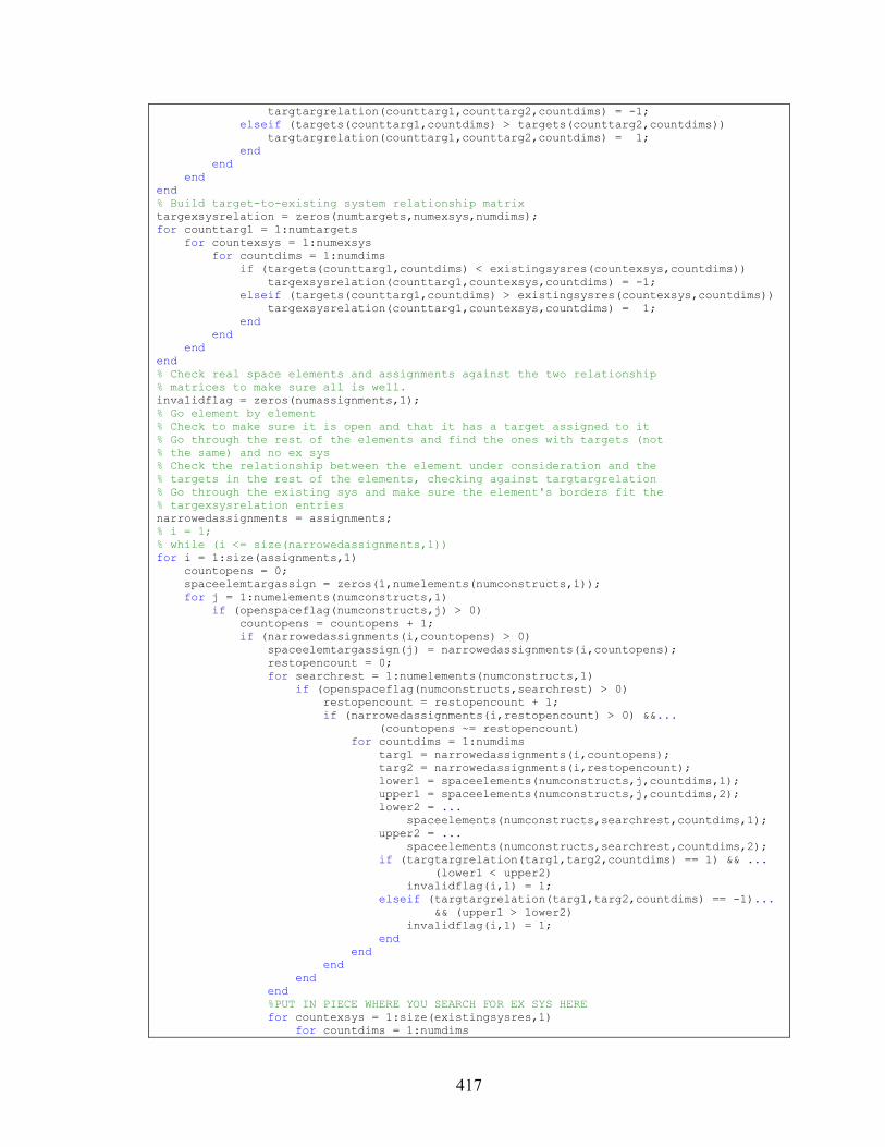
417
targtargrelation(counttarg1,counttarg2,countdims) = -1; elseif (targets(counttarg1,countdims) > targets(counttarg2,countdims)) targtargrelation(counttarg1,counttarg2,countdims) = 1; end end end end % Build target-to-existing system relationship matrix targexsysrelation = zeros(numtargets,numexsys,numdims); for counttarg1 = 1:numtargets for countexsys = 1:numexsys for countdims = 1:numdims if (targets(counttarg1,countdims) < existingsysres(countexsys,countdims)) targexsysrelation(counttarg1,countexsys,countdims) = -1; elseif (targets(counttarg1,countdims) > existingsysres(countexsys,countdims)) targexsysrelation(counttarg1,countexsys,countdims) = 1; end end end end % Check real space elements and assignments against the two relationship % matrices to make sure all is well. invalidflag = zeros(numassignments,1); % Go element by element % Check to make sure it is open and that it has a target assigned to it % Go through the rest of the elements and find the ones with targets (not % the same) and no ex sys % Check the relationship between the element under consideration and the % targets in the rest of the elements, checking against targtargrelation % Go through the existing sys and make sure the element's borders fit the % targexsysrelation entries narrowedassignments = assignments; % i = 1; % while (i <= size(narrowedassignments,1)) for i = 1:size(assignments,1) countopens = 0; spaceelemtargassign = zeros(1,numelements(numconstructs,1)); for j = 1:numelements(numconstructs,1) if (openspaceflag(numconstructs,j) > 0) countopens = countopens + 1; if (narrowedassignments(i,countopens) > 0) spaceelemtargassign(j) = narrowedassignments(i,countopens); restopencount = 0; for searchrest = 1:numelements(numconstructs,1) if (openspaceflag(numconstructs,searchrest) > 0) restopencount = restopencount + 1; if (narrowedassignments(i,restopencount) > 0) &&... (countopens ~= restopencount) for countdims = 1:numdims targ1 = narrowedassignments(i,countopens); targ2 = narrowedassignments(i,restopencount); lower1 = spaceelements(numconstructs,j,countdims,1); upper1 = spaceelements(numconstructs,j,countdims,2); lower2 = ... spaceelements(numconstructs,searchrest,countdims,1); upper2 = ... spaceelements(numconstructs,searchrest,countdims,2); if (targtargrelation(targ1,targ2,countdims) == 1) && ... (lower1 < upper2) invalidflag(i,1) = 1; elseif (targtargrelation(targ1,targ2,countdims) == -1)... && (upper1 > lower2) invalidflag(i,1) = 1; end end end end end %PUT IN PIECE WHERE YOU SEARCH FOR EX SYS HERE for countexsys = 1:size(existingsysres,1) for countdims = 1:numdims

418
lower1 = spaceelements(numconstructs,j,countdims,1); upper1 = spaceelements(numconstructs,j,countdims,2); currtarg = spaceelemtargassign(j); if (targexsysrelation(currtarg,countexsys,countdims) == -1)... && (lower1 > existingsysres(countexsys,countdims)) invalidflag(i,1) = 1; elseif (targexsysrelation(currtarg,countexsys,countdims) == 1)... && (upper1 < existingsysres(countexsys,countdims)) invalidflag(i,1) = 1; end end end end end end end elimcount = 1; while (elimcount <= size(narrowedassignments,1)) if (invalidflag(elimcount,1) == 1) narrowedassignments(elimcount,:) = []; invalidflag(elimcount,:) = []; else elimcount = elimcount + 1; end end
C.1.9 – “createeqconst.m” Program
This function creates the “Aeq” and “beq” matrices needed by fmincon to run.
These matrices represent any equality constraints on the redesign variables that might be
present as a result of commonality forced by space elements or by physical constraints on
the system itself.
function [Aeq,Beq,removedvarflags] = ... createeqconst4(spaceelements,ndiv,constructs,existingsys,... existingsysflag,currsetup,spaceelemtargassign,spaceelemvarassign) % Creates equality constrints and removes redundant variables %%%%%%%%%%%%%%%%%%%%%%%%%%%%%%%%%%%%%%%%%%%%%%%%%%%%%%%%%%%%%%%%%%%%%%%%%% % createeqconst4.m % % Written by: Matt Chamberlain % % Description: This program creates the two matrices that are used to % describe the equality constraints in the constructal solution to the % redesign problem. % New version that takes out variables that aren't needed due to equality % constraints. The two new outputs are arrays that mark where in % %%%%%%%%%%%%%%%%%%%%%%%%%%%%%%%%%%%%%%%%%%%%%%%%%%%%%%%%%%%%%%%%%%%%%%%%%% % Assume that x array is a row with n*numvars spaces (one for each variable % in each of the smallest space elements) numconstructs = size(ndiv,1); numdimensions = size(ndiv,2); numnewsys = size(find(currsetup),2); numvars = size(existingsys,2); numelements = ndiv(:,1); for countelements = 2:numdimensions numelements = numelements .* ndiv(:,countelements); end

419
% CHECK TO SEE WHICH SMALL SPACE ELEMENTS ARE IN THE LARGER SPACE % ELEMENTS, SETTING THE APPROPRIATE VARIABLE VALUES. THEN LOOK FOR OTHER % SMALL SPACE ELEMENTS THAT ARE ALSO WITHIN THE LARGER ELEMENT AND CREATE % EQUALITY CONSTRAINTS BY ADDING A LINE TO AEQ AND BEQ counteqconst = 0; % Counter to keep track of which line of the eq cons we are on countvareqconst = 0; % Sub-Counter to keep track of variable equalities countexsyseqconst = 0; % Sub-Counter for ex sys equalities for countlevels = 1:(numconstructs-1) % only check for equalities if there are actually multiple smaller % elements inside of the element you are currently checking (otherwise % you are doing the same check twice at the next lower level %if (isequal(ndiv(countlevels,:),ndiv(countlevels+1,:)) == 0) % Go through each element in the current level for countinlevelelements = 1:numelements(countlevels,1) % Go through each of the lowest-level elements to see which are % inside the element at the current level in question numinside = 0; exsysinside = 0; for countsmallest = 1:numelements(numconstructs,1) % Check each element using checkelements.m insideflag = checkelements... (spaceelements(countlevels,countinlevelelements,:,:),... spaceelements(numconstructs,countsmallest,:,:)); if ( ((insideflag == 1) && ... (existingsysflag(numconstructs,countsmallest,1) > 0)) ||... ((insideflag == 1) && ... (spaceelemtargassign(countsmallest) > 0)) ) % If it is inside and it contains one of the systems % being used, set numinside = numinside + 1; numinside = numinside + 1; if ((numinside == 1) && ... (existingsysflag(numconstructs,countsmallest,1) > 0 )) % Save the "first element's" place so we can set it % equal to all others inside the larger element % This is the case when it's an existing system exsysinside = countsmallest; exsysinsideflag = ... existingsysflag(numconstructs,countsmallest,1); elseif ((numinside == 1) && (spaceelemtargassign(countsmallest) > 0)) % Save the "first element's" place so we can set it % equal to all others inside the larger element % This is the case when it's one of the new systems firstsysinsideflag = spaceelemvarassign(countsmallest); elseif ((numinside > 1) && (exsysinside > 0)) % Case when there is an exsys inside the element in % question ... means elements should be set equal % to that exsys ... also assumes target is found % second for countvars = 1:numvars % Look for flags saying which variables are % common at this level of construct if (constructs(countvars) == countlevels) counteqconst = counteqconst + 1; countexsyseqconst = countexsyseqconst + 1; Beq(counteqconst) = ... existingsys(exsysinsideflag,countvars); %#ok<AGROW> Aeq(counteqconst,1:(numnewsys*numvars)) = ... zeros( 1,(numnewsys * numvars) ); %#ok<AGROW> newsysplace = ... countvars + ... ( (spaceelemvarassign(countsmallest) - 1) * numvars); Aeq(counteqconst,newsysplace) = 1; %#ok<AGROW> end end elseif ((numinside > 1) && (exsysinside == 0) && ... (existingsysflag(numconstructs,countsmallest,1) > 0 )) % Case when an existing sys is found second after a % target is found in a given element exsysinside = countsmallest; exsysinsideflag = ... existingsysflag(numconstructs,countsmallest,1);

420
for countvars = 1:numvars % Look for flags saying which variables are % common at this level of construct if (constructs(countvars) == countlevels) counteqconst = counteqconst + 1; countexsyseqconst = countexsyseqconst + 1; Beq(counteqconst) = ... existingsys(exsysinsideflag,countvars); %#ok<AGROW> Aeq(counteqconst,1:(numnewsys*numvars)) = ... zeros( 1,(numnewsys * numvars) ); %#ok<AGROW> newsysplace = ... countvars + ( (firstsysinsideflag - 1) * numvars); Aeq(counteqconst,newsysplace) = 1; %#ok<AGROW> end end elseif ((numinside > 1) && (exsysinside == 0) && ... (existingsysflag(numconstructs,countsmallest,1) == 0 )) % Case when there are no exsys in the element in % question ... means that two new sys should be set % equal at that construct for countvars = 1:numvars % Look for ffindlags saying which variables are % common at this level of construct if (constructs(countvars) == countlevels) counteqconst = counteqconst + 1; countvareqconst = countvareqconst + 1; Beq(counteqconst) = 0; %#ok<AGROW> blank = zeros( 1,(numnewsys * numvars) ); Aeq(counteqconst,1:(numnewsys*numvars)) = blank; %#ok<AGROW> secondsysinsideflag = spaceelemvarassign(countsmallest); firstnewsysplace = ... countvars + ( (firstsysinsideflag - 1) * numvars); secondnewsysplace = ... countvars + ( (secondsysinsideflag - 1) * numvars); Aeq(counteqconst,firstnewsysplace) = -1; %#ok<AGROW> Aeq(counteqconst,secondnewsysplace) = 1; %#ok<AGROW> end % if statement end % countvars loop end % if/else statement (numinside) end % if statement (insideflag) end % countsmallest loop end % countinlevelelements loop end % countlevels (constructs) loop % In case there are no equality constraints at all if (counteqconst == 0) Aeq = zeros( 1,(numnewsys * numvars) ); Beq = 0; removedvarflags = zeros(1,(numvars * numnewsys)); else % SCAN THROUGH AEQ AND BEQ TO FIND CASES WE ARE LOOKING FOR: % Look for Beq lines that are nonzero % Or look for instances of "-1"'s in Aeq and then take out the one with a % "1" as it signifies the second variable removedvarflags = zeros(1,(numvars * numnewsys)); % Creates an array called "removedvarflags" that has a zero if a var % stays in the list of variables and a non-zero index if that var is to % be removed because of redundancy. The index indicates what var in the % original array the removed variable is equal to (for reassembly % later) % Also creates an array "removerow" that will tell later on which rows % need to be eliminated. numremoved = 0; removeequalitylist = zeros(1,(numvars * numnewsys)); removevarlist = zeros(1,(numvars * numnewsys)); i = 1; while (i <= size(Aeq,1)) [minval,minloc] = min(Aeq(i,:)); [maxval,maxloc] = max(Aeq(i,:)); countones = 0; countnegones = 0;

421
for searchforones = 1:size(Aeq,2) if (Aeq(i,searchforones) == 1) countones = countones + 1; elseif (Aeq(i,searchforones) == -1) countnegones = countnegones + 1; end end if (minval == -1) && (maxval == 1) && (countones == 1) && ... (countnegones == 1) numremoved = numremoved + 1; % list of rows in Aeq to be removed removeequalitylist(i) = 1; %#ok<AGROW> % list of the variables that are taking the place of removed % ones removedvarflags(maxloc) = minloc; % list of columns (variables) that are being removed removevarlist(maxloc) = 1; %#ok<AGROW> end i = i + 1; end j = size(Aeq,2); while (j >= 1) if (removevarlist(j) == 1) Aeq(:,j) = []; %#ok<AGROW> end j = j-1; end k = size(Aeq,1); while (k >= 1) if (removeequalitylist(k) == 1) Aeq(k,:) = []; %#ok<AGROW> Beq(k) = []; %#ok<AGROW> end k = k - 1; end end
B.1.10 – “checkelements.m” Program
This Matlab function simply checks to see whether one space element fits cleanly
inside another one, returning a flag value to signal success or failure. This function is
called by other functions as part of their routines.
function [insideflag] = checkelements(elementbig,elementsmall) % Checks to see if one space element contains another one %%%%%%%%%%%%%%%%%%%%%%%%%%%%%%%%%%%%%%%%%%%%%%%%%%%%%%%%%%%%%%%%%%%%%%%%%% % checkelements.m % % Written by: Matt Chamberlain % Last Edited: Sept 22, 2006 % % Description: This program checks to see if the first space element % contains the second space element. It returns a value of 1 to signify % that the smaller element does lay within the larger and a 0 if this is % not the case. This function is called by the createeqconst.m function. % % NOTE: It is assumed that the inputs are descriptions of the bounds of the % two elements in question. The inputs should be of size (m x 2) where m is % the number of dimensions in the redesign market space %%%%%%%%%%%%%%%%%%%%%%%%%%%%%%%%%%%%%%%%%%%%%%%%%%%%%%%%%%%%%%%%%%%%%%%%%% insideflag = 1; for i = 1:size(elementbig,3) % Check to see if lower bound of smaller element is below that of the

422
% larger element or if the upper bound of the smaller element is above % that of the larger one. if (elementsmall(1,1,i,1) < elementbig(1,1,i,1)) |... (elementsmall(1,1,i,2) > elementbig(1,1,i,2)) % If so, put up the flag that the smaller element doesn't fit insideflag = 0; end end
B.1.11 – “findgoodstart.m” Program
This function generates a start point for fmincon to use. Experimentation has
shown that the fmincon function is much more likely to be able to converge to a viable
solution if the start point it is given is viable to begin with. For this reason,
“findgoodstart.m”, “findmidstart.m”, “findlowstart.m”, and “findhighstart.m” have been
written to generate a series of starting points spread throughout the variable space of the
problem. This particular function generates starting points by trying to make the resulting
systems fit into their respective space elements. This function and its subfunctions have
been written specifically for the universal motor example problem and thus would have
to be changed for future use in other applications.
function [newstartpoints] = findgoodstart4(x0,varranges,spaceelements,Aeq,Beq,currsetup,varspaceelemassign); % Finds a good starting point for fmincon using ex sys variable values %%%%%%%%%%%%%%%%%%%%%%%%%%%%%%%%%%%%%%%%%%%%%%%%%%%%%%%%%%%%%%%%%%%%%%%%%%% % findgoodstart4.m % % Written by: Matt Chamberlain % % This program finds better starting points for the system in each space % element (in the hope that doing so causes fewer ndiv setups to fail to % converge. % %%%%%%%%%%%%%%%%%%%%%%%%%%%%%%%%%%%%%%%%%%%%%%%%%%%%%%%%%%%%%%%%%%%%%%%%%%% % REARRANGE THE x0 VARIABLES INTO ONE ROW PER SYSTEM numvars = size(varranges,1); numdimensions = size(spaceelements,3); numconstructs = size(spaceelements,1); numsys = size(find(currsetup),2); % FIND A MODIFIED VERSION OF EACH STARTING POINT THAT IS CLOSE TO THE % TARGET IN THE CENTER OF THE SPACE ELEMENT % NOTE: THIS IS ONE OF THE STEPS THAT WOULD HAVE TO BE DIFFERENT IF THERE % WERE MULTIPLE DIMENSIONS TO EACH SPACE ELEMENT for k = 1:numsys cell = varspaceelemassign(k); firstvar = ((cell-1) * numvars) + 1; lastvar = numvars * cell; bunkstartpoint = x0( firstvar:lastvar ); target =( ( spaceelements(numconstructs,cell,1,2) - ...

423
spaceelements(numconstructs,cell,1,1) ) / 2 ) + ... spaceelements(numconstructs,cell,1,1); [base,T,d] = patternsearchMKC(bunkstartpoint,varranges,target); lastbasept = size(base,1); firstvarnewarray = (k - 1) * numvars + 1; lastvarnewarray = firstvarnewarray + numvars - 1; newstartpoints(firstvarnewarray:lastvarnewarray) = (base(lastbasept,:) - ... varranges(:,1)') ./ (varranges(:,2) - varranges(:,1))'; end
B.1.12 – “findmidstart.m” Program
This function generates a start point for fmincon to use. Experimentation has
shown that the fmincon function is much more likely to be able to converge to a viable
solution if the start point it is given is viable to begin with. For this reason,
“findgoodstart.m”, “findmidstart.m”, “findlowstart.m”, and “findhighstart.m” have been
written to generate a series of starting points spread throughout the variable space of the
problem. This particular function generates starting points by initially trying to use
variable values at the middle of their ranges. This function and its subfunctions have been
written specifically for the universal motor example problem and thus would have to be
changed for future use in other applications.
function [midstartpoints] = findmidstart2(varranges,targets,responsebounds,vartargassign); % Finds a good starting point for fmincon at middle of variables' ranges %%%%%%%%%%%%%%%%%%%%%%%%%%%%%%%%%%%%%%%%%%%%%%%%%%%%%%%%%%%%%%%%%%%%%%%%%%% % findmidstart2.m % % Written by: Matt Chamberlain % % This program finds better starting points for the system close to each % target (whereas the previous version just looked for starting points in % each element) % %%%%%%%%%%%%%%%%%%%%%%%%%%%%%%%%%%%%%%%%%%%%%%%%%%%%%%%%%%%%%%%%%%%%%%%%%%% numvars = size(varranges,1); numtargets = size(targets,1); numsys = numtargets; countvars = 1; for i = 1:numtargets for j = 1:size(varranges,1) newstartpoints(countvars) = 0.5 * (varranges(j,2) - ... varranges(j,1)) + varranges(j,1); countvars = countvars + 1; end end % FIND A MODIFIED VERSION OF EACH STARTING POINT THAT IS CLOSE TO THE % TARGET IN THE CENTER OF THE SPACE ELEMENT % NOTE: THIS IS ONE OF THE STEPS THAT WOULD HAVE TO BE DIFFERENT IF THERE % WERE MULTIPLE DIMENSIONS TO EACH SPACE ELEMENT

424
for k = 1:numsys firstvar = ((k-1) * numvars) + 1; lastvar = numvars * k; bunkstartpoint = newstartpoints( firstvar:lastvar ); newvars = ... optindivmotorlow(bunkstartpoint,targets(vartargassign(k),1,:),responsebounds); firstvarnewarray = (k - 1) * numvars + 1; lastvarnewarray = firstvarnewarray + numvars - 1; midstartpoints(firstvarnewarray:lastvarnewarray) = ... (newvars - varranges(:,1)') ./ (varranges(:,2) - varranges(:,1))'; end end %%%%%%%%%%%%%%%%%%%%%%%%%%%%%%%%%%%%%%%%%%%%%%%%%%%%%%%%%%%%%%%%%%%%%%%%%%% function newvars = optindivmotorlow(vars,target,responsebounds) % This subfunction does the optimization of one motor x0 = vars; bounds = [100,1500;... 0.01,1.0;... 1.0,500;... 0.01,1.0;... 1.0,10.0;... 0.5,10.0;... 0.0566,5.18;... 0.1,6.0]; lb = bounds(:,1); ub = bounds(:,2); options = optimset('Display','on','Tolfun',0.001,'Tolcon',0.01,'LargeScale','off'); exitflag = 0; % additions = 0; while (exitflag < 1) [newvars,value,exitflag] = ... fmincon(@(vars)inelement(vars,target,responsebounds),x0,[],[],[],[],... lb,ub,@(vars)confun(vars),options) % additions = additions + 0.1; x0 = x0 + (0.1 * (ub' - lb')); end end %%%%%%%%%%%%%%%%%%%%%%%%%%%%%%%%%%%%%%%%%%%%%%%%%%%%%%%%%%%%%%%%%%%%%%%%%%% function [dev] = inelement(vars, target, responsebounds) % This subfunction calculates deviation variable values % incoming variables: Nc = vars(1); Awa = vars(2); Ns = vars(3); Awf = vars(4); r = vars(5); t = vars(6); L = vars(7); I = vars(8); % calculate response values Input = [Nc,Awa,Ns,Awf,r,t,L,I]; responses = TSunivmotor(Input); res = responses(1); % Calculate deviation from desired space element boundaries % if (T > spaceelem(1,1,1,2)) % dev = (T - spaceelem(1,1,1,2)) / spaceelem(1,1,1,2); % elseif (T > spaceelem(1,1,1,1)) & (T < spaceelem(1,1,1,2)) % dev = 0; % else % dev = (spaceelem(1,1,1,1) - T) / spaceelem(1,1,1,1); % end % % end if (res <= target(1,1,2)) %&& (res >= responsebounds(2)) % target matching when the point is below midpoint

425
value = (res - responsebounds(1)) / (target(1,1,2) - responsebounds(1)); elseif (res > target(1,1,2)) %&& (res <= responsebounds(2)) % target matching when the point is above the midpoint value = 1 - (res - target(1,1,2)) / (responsebounds(2) - target(1,1,2)); else value = 0; end dev = 1-value; end %%%%%%%%%%%%%%%%%%%%%%%%%%%%%%%%%%%%%%%%%%%%%%%%%%%%%%%%%%%%%%%%%%%%%%%%%%% function [c,ceq] = confun(vars) % This subfunction calculates constraint values % incoming variables: Nc = vars(1); Awa = vars(2); Ns = vars(3); Awf = vars(4); r = vars(5); t = vars(6); L = vars(7); I = vars(8); % calculate response values Input = [Nc,Awa,Ns,Awf,r,t,L,I]; responses = TSunivmotor(Input); % This arrray will have the values that the respones are compared to. The % standard form for these constraints is assumed to be c(x) <= 0 % We'll assume that the inequalities measured here are of the form: % response(i) <= physcons(i) physcons = [0 0 2 0.15 1.0 5000 0 1.0 0]; % This array simply keeps track of which of the response values describing % the system are related to physcons(i) physconflags = [-1 -2 2 -3 3 4 -5 -6 -7]; nonlconcount = 0; for countpcons = 1:size(physcons,2) nonlconcount = nonlconcount + 1; if (physconflags(countpcons) > 0) % case when the flag is positive c(nonlconcount) = ... responses(physconflags(countpcons)) - physcons(countpcons); elseif (physconflags(countpcons) < 0) % case when the flag is negative c(nonlconcount) = ... (-1 * responses((-1 * physconflags(countpcons)) )) - physcons(countpcons); end end ceq = ones(9,1); % not sure if I need to do this ceq = []; end
B.1.13 – “findlowstart.m” Program
This function generates a start point for fmincon to use. Experimentation has
shown that the fmincon function is much more likely to be able to converge to a viable
solution if the start point it is given is viable to begin with. For this reason,
“findgoodstart.m”, “findmidstart.m”, “findlowstart.m”, and “findhighstart.m” have been

426
written to generate a series of starting points spread throughout the variable space of the
problem. This particular function generates starting points by initially trying to use
variable values at the bottom of their ranges. This function and its subfunctions have been
written specifically for the universal motor example problem and thus would have to be
changed for future use in other applications.
function [lowstartpoints] = findlowstart2(varranges,numtargets,spaceelements,... Aeq,Beq,currsetup,varspaceelemassign); % Finds a good starting point for fmincon at bottom of variables' ranges %%%%%%%%%%%%%%%%%%%%%%%%%%%%%%%%%%%%%%%%%%%%%%%%%%%%%%%%%%%%%%%%%%%%%%%%%%% % findlowstart2.m % % Written by: Matt Chamberlain % % This program finds low better starting points for the system in each space % element (in the hope that doing so causes fewer ndiv setups to fail to % converge. % %%%%%%%%%%%%%%%%%%%%%%%%%%%%%%%%%%%%%%%%%%%%%%%%%%%%%%%%%%%%%%%%%%%%%%%%%%% numvars = size(varranges,1); numdimensions = size(spaceelements,3); numconstructs = size(spaceelements,1); numsys = size(find(currsetup),2); countvars = 1; for i = 1:numtargets for j = 1:size(varranges,1) newstartpoints(countvars) = varranges(j,1); countvars = countvars + 1; end end % FIND A MODIFIED VERSION OF EACH STARTING POINT THAT IS CLOSE TO THE % TARGET IN THE CENTER OF THE SPACE ELEMENT % NOTE: THIS IS ONE OF THE STEPS THAT WOULD HAVE TO BE DIFFERENT IF THERE % WERE MULTIPLE DIMENSIONS TO EACH SPACE ELEMENT for k = 1:numsys cell = varspaceelemassign(k); firstvar = ((k-1) * numvars) + 1; lastvar = numvars * k; bunkstartpoint = newstartpoints( firstvar:lastvar ); newvars = optindivmotorlow(bunkstartpoint,spaceelements(1,cell,:,:)); firstvarnewarray = (k - 1) * numvars + 1; lastvarnewarray = firstvarnewarray + numvars - 1; lowstartpoints(firstvarnewarray:lastvarnewarray) = ... (newvars - varranges(:,1)') ./ (varranges(:,2) - varranges(:,1))'; end end %%%%%%%%%%%%%%%%%%%%%%%%%%%%%%%%%%%%%%%%%%%%%%%%%%%%%%%%%%%%%%%%%%%%%%%%%%% function newvars = optindivmotorlow(vars,spaceelem) % This subfunction does the optimization of one motor x0 = vars; bounds = [100,1500;... 0.01,1.0;... 1.0,500;... 0.01,1.0;... 1.0,10.0;... 0.5,10.0;... 0.0566,5.18;... 0.1,6.0]; lb = bounds(:,1);
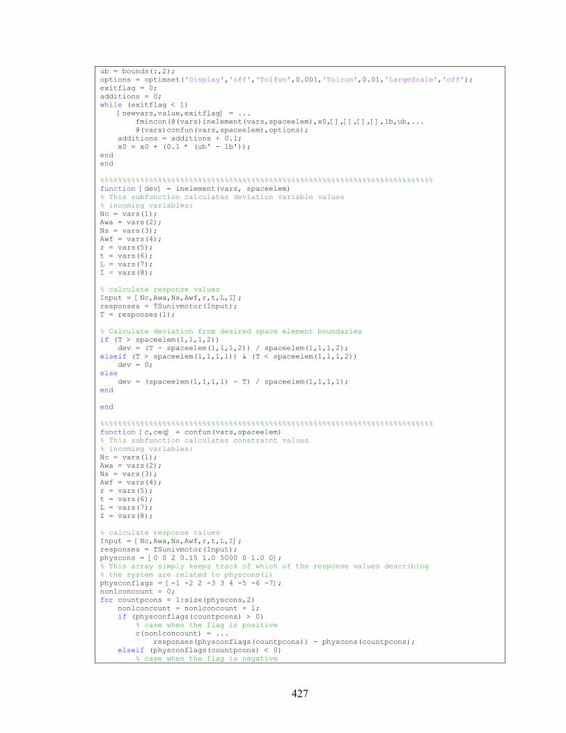
427
ub = bounds(:,2); options = optimset('Display','off','Tolfun',0.001,'Tolcon',0.01,'LargeScale','off'); exitflag = 0; additions = 0; while (exitflag < 1) [newvars,value,exitflag] = ... fmincon(@(vars)inelement(vars,spaceelem),x0,[],[],[],[],lb,ub,... @(vars)confun(vars,spaceelem),options); additions = additions + 0.1; x0 = x0 + (0.1 * (ub' - lb')); end end %%%%%%%%%%%%%%%%%%%%%%%%%%%%%%%%%%%%%%%%%%%%%%%%%%%%%%%%%%%%%%%%%%%%%%%%%%% function [dev] = inelement(vars, spaceelem) % This subfunction calculates deviation variable values % incoming variables: Nc = vars(1); Awa = vars(2); Ns = vars(3); Awf = vars(4); r = vars(5); t = vars(6); L = vars(7); I = vars(8); % calculate response values Input = [Nc,Awa,Ns,Awf,r,t,L,I]; responses = TSunivmotor(Input); T = responses(1); % Calculate deviation from desired space element boundaries if (T > spaceelem(1,1,1,2)) dev = (T - spaceelem(1,1,1,2)) / spaceelem(1,1,1,2); elseif (T > spaceelem(1,1,1,1)) & (T < spaceelem(1,1,1,2)) dev = 0; else dev = (spaceelem(1,1,1,1) - T) / spaceelem(1,1,1,1); end end %%%%%%%%%%%%%%%%%%%%%%%%%%%%%%%%%%%%%%%%%%%%%%%%%%%%%%%%%%%%%%%%%%%%%%%%%%% function [c,ceq] = confun(vars,spaceelem) % This subfunction calculates constraint values % incoming variables: Nc = vars(1); Awa = vars(2); Ns = vars(3); Awf = vars(4); r = vars(5); t = vars(6); L = vars(7); I = vars(8); % calculate response values Input = [Nc,Awa,Ns,Awf,r,t,L,I]; responses = TSunivmotor(Input); physcons = [0 0 2 0.15 1.0 5000 0 1.0 0]; % This array simply keeps track of which of the response values describing % the system are related to physcons(i) physconflags = [-1 -2 2 -3 3 4 -5 -6 -7]; nonlconcount = 0; for countpcons = 1:size(physcons,2) nonlconcount = nonlconcount + 1; if (physconflags(countpcons) > 0) % case when the flag is positive c(nonlconcount) = ... responses(physconflags(countpcons)) - physcons(countpcons); elseif (physconflags(countpcons) < 0) % case when the flag is negative

428
c(nonlconcount) = ... (-1 * responses((-1 * physconflags(countpcons)) )) - physcons(countpcons); end end % create a pair of constraints to get the motor inside its element nonlconcount = nonlconcount + 1; spaceelemlb = spaceelem(1,1,1,1); c(10) = spaceelemlb - responses(1); nonlconcount = nonlconcount + 1; spaceelemub = spaceelem(1,1,1,2); c(11) = responses(1) - spaceelemub; ceq = ones(11,1); % not sure if I need to do this ceq = []; end
B.1.14 – “findhighstart.m” Program
This function generates a start point for fmincon to use. Experimentation has
shown that the fmincon function is much more likely to be able to converge to a viable
solution if the start point it is given is viable to begin with. For this reason,
“findgoodstart.m”, “findmidstart.m”, “findlowstart.m”, and “findhighstart.m” have been
written to generate a series of starting points spread throughout the variable space of the
problem. This particular function generates starting points by initially trying to use
variable values at the top of their ranges. This function and its subfunctions have been
written specifically for the universal motor example problem and thus would have to be
changed for future use in other applications.
function [highstartpoints] = findhighstart2(varranges,numtargets,spaceelements,... Aeq,Beq,currsetup,varspaceelemassign); % Finds a good starting point for fmincon at top of variables' ranges %%%%%%%%%%%%%%%%%%%%%%%%%%%%%%%%%%%%%%%%%%%%%%%%%%%%%%%%%%%%%%%%%%%%%%%%%%% % findhighstart2.m % % Written by: Matt Chamberlain % % This program finds better high starting points for the system in each space % element (in the hope that doing so causes fewer ndiv setups to fail to % converge. % %%%%%%%%%%%%%%%%%%%%%%%%%%%%%%%%%%%%%%%%%%%%%%%%%%%%%%%%%%%%%%%%%%%%%%%%%%% numvars = size(varranges,1); numdimensions = size(spaceelements,3); numconstructs = size(spaceelements,1); numsys = size(find(currsetup),2); countvars = 1; for i = 1:numtargets for j = 1:size(varranges,1) newstartpoints(countvars) = varranges(j,2);

429
countvars = countvars + 1; end end % FIND A MODIFIED VERSION OF EACH STARTING POINT THAT IS CLOSE TO THE % TARGET IN THE CENTER OF THE SPACE ELEMENT % NOTE: THIS IS ONE OF THE STEPS THAT WOULD HAVE TO BE DIFFERENT IF THERE % WERE MULTIPLE DIMENSIONS TO EACH SPACE ELEMENT % newsyslocs = find(currsetup); for k = 1:numsys cell = varspaceelemassign(k); firstvar = ((k-1) * numvars) + 1; lastvar = numvars * k; bunkstartpoint = newstartpoints( firstvar:lastvar ); newvars = optindivmotor(bunkstartpoint,spaceelements(1,cell,:,:)); firstvarnewarray = (k - 1) * numvars + 1; lastvarnewarray = firstvarnewarray + numvars - 1; highstartpoints(firstvarnewarray:lastvarnewarray) = ... (newvars - varranges(:,1)') ./ ((varranges(:,2) - varranges(:,1))'); end end %%%%%%%%%%%%%%%%%%%%%%%%%%%%%%%%%%%%%%%%%%%%%%%%%%%%%%%%%%%%%%%%%%%%%%%%%%% function newvars = optindivmotor(vars,spaceelem) % This subfunction does the optimization of one motor x0 = vars; bounds = [100,1500;... 0.01,1.0;... 1.0,500;... 0.01,1.0;... 1.0,10.0;... 0.5,10.0;... 0.0566,5.18;... 0.1,6.0]; lb = bounds(:,1); ub = bounds(:,2); options = optimset('Display','off','Tolfun',0.001,'Tolcon',0.01,'LargeScale','off'); [newvars,value,exitflag] = ... fmincon(@(vars)inelement(vars,spaceelem),x0,[],[],[],[],lb,ub,... @(vars)confun(vars,spaceelem),options); end %%%%%%%%%%%%%%%%%%%%%%%%%%%%%%%%%%%%%%%%%%%%%%%%%%%%%%%%%%%%%%%%%%%%%%%%%%% function [dev] = inelement(vars, spaceelem) % This subfunction calculates deviation variable values % incoming variables: Nc = vars(1); Awa = vars(2); Ns = vars(3); Awf = vars(4); r = vars(5); t = vars(6); L = vars(7); I = vars(8); % calculate response values Input = [Nc,Awa,Ns,Awf,r,t,L,I]; responses = TSunivmotor(Input); T = responses(1); % Calculate deviation from desired space element boundaries if (T > spaceelem(1,1,1,2)) dev = (T - spaceelem(1,1,1,2)) / spaceelem(1,1,1,2); elseif (T > spaceelem(1,1,1,1)) & (T < spaceelem(1,1,1,2)) dev = 0; else dev = (spaceelem(1,1,1,1) - T) / spaceelem(1,1,1,1); end end
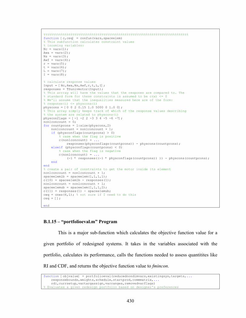
430
%%%%%%%%%%%%%%%%%%%%%%%%%%%%%%%%%%%%%%%%%%%%%%%%%%%%%%%%%%%%%%%%%%%%%%%%%%% function [c,ceq] = confun(vars,spaceelem) % This subfunction calculates constraint values % incoming variables: Nc = vars(1); Awa = vars(2); Ns = vars(3); Awf = vars(4); r = vars(5); t = vars(6); L = vars(7); I = vars(8); % calculate response values Input = [Nc,Awa,Ns,Awf,r,t,L,I]; responses = TSunivmotor(Input); % This arrray will have the values that the respones are compared to. The % standard form for these constraints is assumed to be c(x) <= 0 % We'll assume that the inequalities measured here are of the form: % response(i) <= physcons(i) physcons = [0 0 2 0.15 1.0 5000 0 1.0 0]; % This array simply keeps track of which of the response values describing % the system are related to physcons(i) physconflags = [-1 -2 2 -3 3 4 -5 -6 -7]; nonlconcount = 0; for countpcons = 1:size(physcons,2) nonlconcount = nonlconcount + 1; if (physconflags(countpcons) > 0) % case when the flag is positive c(nonlconcount) = ... responses(physconflags(countpcons)) - physcons(countpcons); elseif (physconflags(countpcons) < 0) % case when the flag is negative c(nonlconcount) = ... (-1 * responses((-1 * physconflags(countpcons)) )) - physcons(countpcons); end end % create a pair of constraints to get the motor inside its element nonlconcount = nonlconcount + 1; spaceelemlb = spaceelem(1,1,1,1); c(10) = spaceelemlb - responses(1); nonlconcount = nonlconcount + 1; spaceelemub = spaceelem(1,1,1,2); c(11) = responses(1) - spaceelemub; ceq = ones(6,1); % not sure if I need to do this ceq = []; end
B.1.15 – “portfolioeval.m” Program
This is a major sub-function which calculates the objective function value for a
given portfolio of redesigned systems. It takes in the variables associated with the
portfolio, calculates its performance, calls the functions needed to assess quantitites like
RI and CDF, and returns the objective function value to fmincon.
function [objvalue] = portfolioeval(reducednondimvars,existingsys,targets,... responsebounds,weights,schedule,startprod,commmatrix,... rdi,currsetup,vartargassign,varranges,removedvarflags) % Evaluates a given redesign portfolio based on designer's preferences

431
%%%%%%%%%%%%%%%%%%%%%%%%%%%%%%%%%%%%%%%%%%%%%%%%%%%%%%%%%%%%%%%%%%%%%%%%%% % portfolioeval.m % % Updated by: Matt Chamberlain % % Description: This program will take in a set of possible redesigned % systems (a "portfolio" of redesign options) and evaluate it against the % designer's preferences. % %%%%%%%%%%%%%%%%%%%%%%%%%%%%%%%%%%%%%%%%%%%%%%%%%%%%%%%%%%%%%%%%%%%%%%%%%% numvars = size(existingsys,2); numdimensions = size(targets,2); numtargets = size(targets,1); reducedplace = 1; nondimvars = zeros(1,size(removedvarflags,2)); % PUT THE REMOVED VARIABLES BACK INTO THE LIST for i = 1:size(removedvarflags,2) if (removedvarflags(i) == 0) nondimvars(i) = reducednondimvars(reducedplace); reducedplace = reducedplace + 1; end end for j = 1:size(removedvarflags,2) if (removedvarflags(j) > 0) nondimvars(j) = nondimvars(removedvarflags(j)); end end % RE-ARRANGE THE LIST OF VARIABLES INTO ROWS (ONE FOR EACH SYSTEM) AND TURN % INTO DIMENSIONALIZED FORM solutionsetnondim = zeros(numtargets,numvars); solutionset = zeros(numtargets,numvars); for i = 1:numtargets firstvar = ((i-1) * numvars) + 1; lastvar = numvars * i; solutionsetnondim(i,:) = nondimvars( firstvar:lastvar ); solutionset(i,:) = (nondimvars( firstvar:lastvar ) .* ... (varranges(:,2)' - varranges(:,1)')) + varranges(:,1)'; end numnewsols = size(solutionset,1); % MAKE A NON-DIMENSIONAL SET OF EXISTING SYSTEMS existingsysnondim = zeros(size(existingsys,1),numvars); for i = 1:size(existingsys,1) existingsysnondim(i,:) = (existingsys(i,:) - varranges(:,1)') ./ ... (varranges(:,2)' - varranges(:,1)'); end % MODEL THE NEW SYSTEMS newdesignsres = zeros(numnewsols,7); for n = 1:numnewsols newdesignsres(n,:) = TSunivmotor(solutionset(n,:)); end overallvalue = 0; countposflag = 0; for countelem = 1:size(currsetup,2) % Look for the systems that are flagged for use in the portfolio in % this setup if (currsetup(countelem) > 0) countposflag = countposflag + 1; currenttarget = currsetup(countelem); % Go through and evaluate the current system against its target % in each dimension for countdims = 1:numdimensions targvalue = ... evalvalue(newdesignsres(countposflag,countdims),... targets(currenttarget,countdims,:),responsebounds(countdims,:)); devtarget = targvalue; weighted = devtarget * weights(currenttarget,countdims); overallvalue = overallvalue + weighted;

432
end end end % CALCULATE THE HIGH-LEVEL OBJECTIVE VALUES AND CONVERT TO DEVIATION % For right now, the value of these is not evaluated; we're just trying % to get cdf and ri as close to 1.0 as possible cdf = ... evalcontinuouscdf2(existingsysnondim, solutionsetnondim, commmatrix,... vartargassign); cdfdev = cdf; weightedcdfdev = cdfdev * weights( (numtargets+1), 1); ri = ... evalcontinuousri(existingsysnondim, solutionsetnondim, rdi, ... vartargassign, schedule, startprod); ridev = ri; weightedridev = ridev * weights( (numtargets+2), 1); avgmass = sum(newdesignsres(:,2)) / numtargets; dweightedavgmass = (avgmass/0.5 - 1) * weights( (numtargets+3),1); if (dweightedavgmass < 0) dweightedavgmass = 0; end avgeffic = sum(newdesignsres(:,3)) / numtargets; dweightedavgeffic = (1 - (avgeffic/0.7)) * weights( (numtargets+4),1); if (dweightedavgeffic < 0) dweightedavgeffic = 0; end objvalue = overallvalue + weightedcdfdev + weightedridev + ... dweightedavgmass + dweightedavgeffic;
B.1.16 – “evalcontinuousri.m” Program
This function caluculates the Redesign Index value for a given portfolio of
existing systems and newly redesigned systems given the redesign difficulties associated
with changing each variable.
function [RI] = evalcontinuousri(existingsys, newdesigns, RDI, ... vartargassign, schedule, startsys) % Calculates the RI value for a redesign portfolio %%%%%%%%%%%%%%%%%%%%%%%%%%%%%%%%%%%%%%%%%%%%%%%%%%%%%%%%%%%%%%%%%%%%%%%%%% % evalcontinuousri.m % % Updated by: Matt Chamberlain % % Description: This program calculates the Redesign Index (RI) for a given % portfolio of redesigned systems % %%%%%%%%%%%%%%%%%%%%%%%%%%%%%%%%%%%%%%%%%%%%%%%%%%%%%%%%%%%%%%%%%%%%%%%%%% numsys = size(schedule,1); % RE-SORT THE NEW SYSTGEMS INTO CHRONOLOGICAL ORDER USING 'VARTARGASSIGN' numvars = size(existingsys,2); portfolio = zeros(numsys,numvars); numexsys = size(existingsys,1); numnewsys = size(newdesigns,1); portfolio(1:numexsys,:) = existingsys; for countnewsys = 1:numnewsys

433
% Put the new sys in the order of the target to which they are % assigned portfolio(numexsys + vartargassign(countnewsys),:) = newdesigns(countnewsys,:); end pvar = zeros(1,numvars); % FOR EVERY VARIABLE IN EVERY NEW SYSTEM for countvars = 1:numvars for countsys = (numexsys + 1):numsys smallestdiff = 1*10^6; % CHECK USING SCHEDULE / STARTDATE TO SEE IF ANY OTHER NEW SYS THAT IS % MADE BEFOREHAND OR EXISTING SYS HAS THE CLOSEST VARIABLE VALUE for comparevars = 1:numsys diff = abs( (portfolio(countsys,countvars) - ... portfolio(comparevars,countvars)) ); percentdiff = diff * RDI(countvars); if ( comparevars ~= countsys ) &&... (startsys(comparevars) < startsys(countsys)) &&... (percentdiff <= smallestdiff) smallestdiff = percentdiff; end end % CALCULATE PVAR FOR THE SELECTED SYS WITH THE CLOSEST VAR VALUE % ADD TO THE PVAR FOR THAT VAR (DIVIDED BY THE NUMBER OF NEW SYS) pvar(countvars) = pvar(countvars) + (smallestdiff / (numnewsys*numvars)); end % countsys for loop end % countvars for loop % CALCULATE THE TOTAL RI/RDF FOR SOLUTION BY ADDING UP WEIGHTED SUM OF ALL % PVARS RI = sum(pvar);
B.1.17 – “evalcontinuouscdf.m” Program
This function calculates the Commonalit Discount Factor for a given portfolio of
existing systems and newly redesigned systems given the commonality discounts
associated with each redesign variable and each type of overlap in production.
function [CDF] = evalcontinuouscdf(existingsys, newdesigns, commmatrix, vartargassign) % Calculates the CDF value for a given portfolio and comm discounts %%%%%%%%%%%%%%%%%%%%%%%%%%%%%%%%%%%%%%%%%%%%%%%%%%%%%%%%%%%%%%%%%%%%%%%%%% % evalcontinuouscdf.m % % Updated by: Matt Chamberlain % % Description: This program calculates the Commonality Discount Factor % (CDF) for a given portfolio of redesigned systems % %%%%%%%%%%%%%%%%%%%%%%%%%%%%%%%%%%%%%%%%%%%%%%%%%%%%%%%%%%%%%%%%%%%%%%%%%% numsys = size(commmatrix,2); % RE-SORT THE NEW SYSTGEMS INTO CHRONOLOGICAL ORDER USING 'VARTARGASSIGN' numvars = size(existingsys,2); portfolio = zeros(numsys,numvars); numexsys = size(existingsys,1); numnewsys = size(newdesigns,1); portfolio(1:numexsys,:) = existingsys; for countnewsys = 1:numnewsys % Put the new sys in the order of the target to which they are % assigned portfolio(numexsys + vartargassign(countnewsys),:) = newdesigns(countnewsys,:); end

434
% CALCULATE CDF pvar = zeros(1,numvars); for countvars = 1:numvars for countsys = 1:numsys smallestdiff = 1*10^6; % CHECK TO SEE WHICH IS SMALLEST PERCENT DIFFERENCE * COMMONALITY % DISCOUNT TOTAL for comparevars = 1:numsys % COMPAREVARS IS ALSO A SYS SEARCH VARIABLE diff = abs( (portfolio(countsys,countvars) - ... portfolio( comparevars,countvars) ) ); weighteddiff = diff * ( commmatrix(countvars,countsys,comparevars)); if ( comparevars ~= countsys ) &&... (weighteddiff <= smallestdiff) smallestdiff = weighteddiff; end end % CALCULATE PVAR FOR THE SELECTED SYS WITH THE CLOSEST AND MOST % VALUABLE COMMONALITY (AND DIVIDE BY N*P FOR EACH TERM) pvar(countvars) = pvar(countvars) + (smallestdiff / (numsys*numvars)); end % countsys for loop end % countvars for loop % CALCULATE THE TOTAL CDF CDF = sum(pvar);
B.1.18 – “evalvalue.m” Program
This function was at one point much more complicated, but currently is just used
to calculate deviation variable values for target-matching goals in a compromise Decision
Support Problem. The two inputs are the system performance and the target value for that
performance. It is assumed here that the target is not zero.
function [dev] = evalvalue(res,target) % Evaluate the deviation variable values for achievement of a given target %%%%%%%%%%%%%%%%%%%%%%%%%%%%%%%%%%%%%%%%%%%%%%%%%%%%%%%%%%%%%%%%%%%%%%%%%% % evalvalue.m % % Updated by: Matt Chamberlain % % Description: This is a basic form from the original formulatoin of a % cDSP. We now assume that there is just one target value. % %%%%%%%%%%%%%%%%%%%%%%%%%%%%%%%%%%%%%%%%%%%%%%%%%%%%%%%%%%%%%%%%%%%%%%%%%% dplus = (res/target) - 1.0; dminus = 1.0 - (res/target); if (dplus >= 0) dev = dplus; elseif (dminus > 0) dev = dminus; end
B.1.19 – “createnonlconst.m” Program

435
This function calculates the nonlinear constraints associated with a proposed
portfolio of existing systems and newly redesigned systems. The nonlinear constraints are
made up of space element boundaries that should not be breached as well as any
nonlinear physical constraints associated with the redesign problem at hand. The function
returns values for the constraints in a form that fmincon will accept.
function [c,ceq] = createnonlconst(reducednondimvars,spaceelements,... existingsys,physcons,physconflags,currsetup,spaceelemvarassign,varranges,... removedvarflags) % Calculates nonlinear constraint values from approach and physical cons %%%%%%%%%%%%%%%%%%%%%%%%%%%%%%%%%%%%%%%%%%%%%%%%%%%%%%%%%%%%%%%%%%%%%%%%%% % createnonlconst.m % % Written by: Matt Chamberlain % % Description: This program calculates and ouptputs the nonlinear % constraint values for the constructal-inspired appraoch. The nonlinear % constraints come both from the approach itself and the physical % constraints of the systems being redesigned. This version of the program % also puts any redundant variables back into the design matrix. % % fmincon expects the constraints to be written in the following form: % c(x) <= 0 % %%%%%%%%%%%%%%%%%%%%%%%%%%%%%%%%%%%%%%%%%%%%%%%%%%%%%%%%%%%%%%%%%%%%%%%%%% nonlconcount = 0; numvars = size(existingsys,2); numdimensions = size(spaceelements,3); numsolutions = (size(nonzeros(currsetup),1)); numconstructs = size(spaceelements,1); reducedplace = 1; nondimvars = zeros(1,size(removedvarflags,2)); % PUT THE REMOVED VARIABLES BACK INTO THE LIST for i = 1:size(removedvarflags,2) if (removedvarflags(i) == 0) nondimvars(i) = reducednondimvars(reducedplace); reducedplace = reducedplace + 1; end end for j = 1:size(removedvarflags,2) if (removedvarflags(j) > 0) nondimvars(j) = nondimvars(removedvarflags(j)); end end % RE-ARRANGE THE LIST OF VARIABLES INTO ROWS (ONE FOR EACH SYSTEM) portfolio = zeros(numsolutions,numvars); for i = 1:numsolutions firstvar = ((i-1) * numvars) + 1; lastvar = numvars * i; portfolio(i,:) = (nondimvars( firstvar:lastvar ) .* ... (varranges(:,2)' - varranges(:,1)')) + varranges(:,1)'; end numexsys = size(existingsys,1); numtotalelements = numexsys + size(currsetup,2); % MODEL THE NEW SYSTEMS AND SAVE THE RESPONSES % NOTE: In this program, it is assumed that the the responses that make up % the redesign market space are the first responses delivered by the % simulation program and are delivered in the same order alldesignsres = zeros(numsolutions,7);

436
for n = 1:numsolutions alldesignsres(n,:) = TSunivmotor(portfolio(n,:)); end % Go through each of the bounds for each element and make sure that % c(x) <= 0 ..... which equates to ..... % response <= ub ... response - ub <= 0 ... c(x) = response - ub % lb - response = c(x) % countnewsys = 0; % for countelements = 1:numtotalelements numphyscons = size(physcons,2); totnumcons = (numphyscons * numsolutions) + (numsolutions * numdimensions * 2); c = zeros( totnumcons ); for countelements = 1:numtotalelements % See if the element has a system and target assigned to it if (spaceelemvarassign(countelements) > 0) % If it does, create the element border constraints for countdimensions = 1:numdimensions nonlconcount = nonlconcount + 1; % next line calculates: lb - response = c(x) c(nonlconcount) = ... spaceelements(numconstructs,countelements,countdimensions,1) ... - alldesignsres(spaceelemvarassign(countelements),countdimensions); nonlconcount = nonlconcount + 1; % next line calculates: c(x) = response - ub c(nonlconcount) = ... alldesignsres(spaceelemvarassign(countelements),countdimensions) ... - spaceelements(numconstructs,countelements,countdimensions,2); end % Create the physical constraints for each new system for countpcons = 1:numphyscons nonlconcount = nonlconcount + 1; if (physconflags(countpcons) > 0) % case when the flag is positive indicating a "less-than" % physical constraint of the form Mass(x) < 2 kg c(nonlconcount) = ... alldesignsres(spaceelemvarassign(countelements),physconflags(countpcons))... - physcons(countpcons); elseif (physconflags(countpcons) < 0) % case when the flag is negative indicating a "greater-than" % physical constraint of the form Effic(x) > 15% c(nonlconcount) = ... (-1 * alldesignsres(spaceelemvarassign(countelements),... (-1 * physconflags(countpcons)) ) ) + physcons(countpcons); end end end end % Nonlinear EQUALITY Constraints ceq = [];
B.2 – MATLAB CODE FOR VERIFICATION AND VALIDATION OF REDESIGN
INDICES
To quickly run the huge number of fast experiments necessary to verify and
validate the redesign metrics proposed in this dissertation, the Matlab code written for the
constructal-inspired approach to the redesign problem has been modified to make a

437
simpler “all-at-once” version that collapses a simple problem down into the form of one
compromise Decision Support Problem. While this approach is seemingly far simpler
than the constructal-inspired one, the code used to implement it is actually made up of
functions and scripts from the constructal-inspired version that have been mildly revised
and shortened. The code presented in this section is only that which differs significantly
from the original Matlab code presented in Section C.1. The manner in which these
programs and scripts interact is shown in flowchart form in Figure 4-5.
B.2.1 – Experimental Input and Executable
This Matlab script is used to set up an experiment and execute the main Matlab
code “solveAAO”, which is short for “Solve All At Once”, which alludes to the fact that
in these experiments, the whole redesign problem is condensed into a single compromise
Decision Support Problem. Oftentimes, dozens of experiments are run at a time by
repeating the code here over and over again, adjusting the values for the designer’s
preferences, redesign difficulties, and commonality discounts to try to show trends. One
experiment’s inputs are shown here for the sake of brevity.
% Boilerplate setup for all experiments in this series schedule(1,1:3) = 1; % Schedule of production for product #1 schedule(2,2:4) = 1; % Schedule of production for product #2 schedule(3,3:5) = 1; % Schedule of production for product #3 schedule(4,4:6) = 1; % Schedule of production for product #4 schedule(5,5:7) = 1; % Schedule of production for product #5 schedule(6,6:8) = 1; % Schedule of production for product #6 schedule(7,7:9) = 1; % Schedule of production for product #6 existingsystemp = zeros(10, 8); existingsystemp(:,1) = [730, 750, 760, 785, 988, 1007, 1030, 1056, 1082, 1087]; existingsystemp(:,2) = [0.205, 0.203, 0.203, 0.205, 0.217, 0.224, 0.230, 0.237, 0.243, 0.247]; existingsystemp(:,3) = [45, 76, 89, 95, 74, 73, 73, 73, 72, 72]; existingsystemp(:,4) = [0.203, 0.186, 0.190, 0.205, 0.241, 0.246, 0.253, 0.260, 0.267, 0.284]; existingsystemp(:,5) = [3.62, 3.31, 3.12, 2.82, 2.26, 2.35, 2.44, 2.51, 2.58, 2.71]; existingsystemp(:,6) = [9.69, 11.77, 11.20, 8.88, 5.75, 6.17, 6.35, 6.46, 6.67, 7.15]; existingsystemp(:,7) = [0.998, 1.28, 1.41, 1.63, 2.38, 2.61, 2.74, 2.81, 2.87, 3.16]; existingsystemp(:,8) = [3.65, 3.73, 3.73, 3.70, 3.84, 4.02, 4.19, 4.36, 4.53, 4.71]; numexsys = 1; %%% MUST BE ADJUSTED!
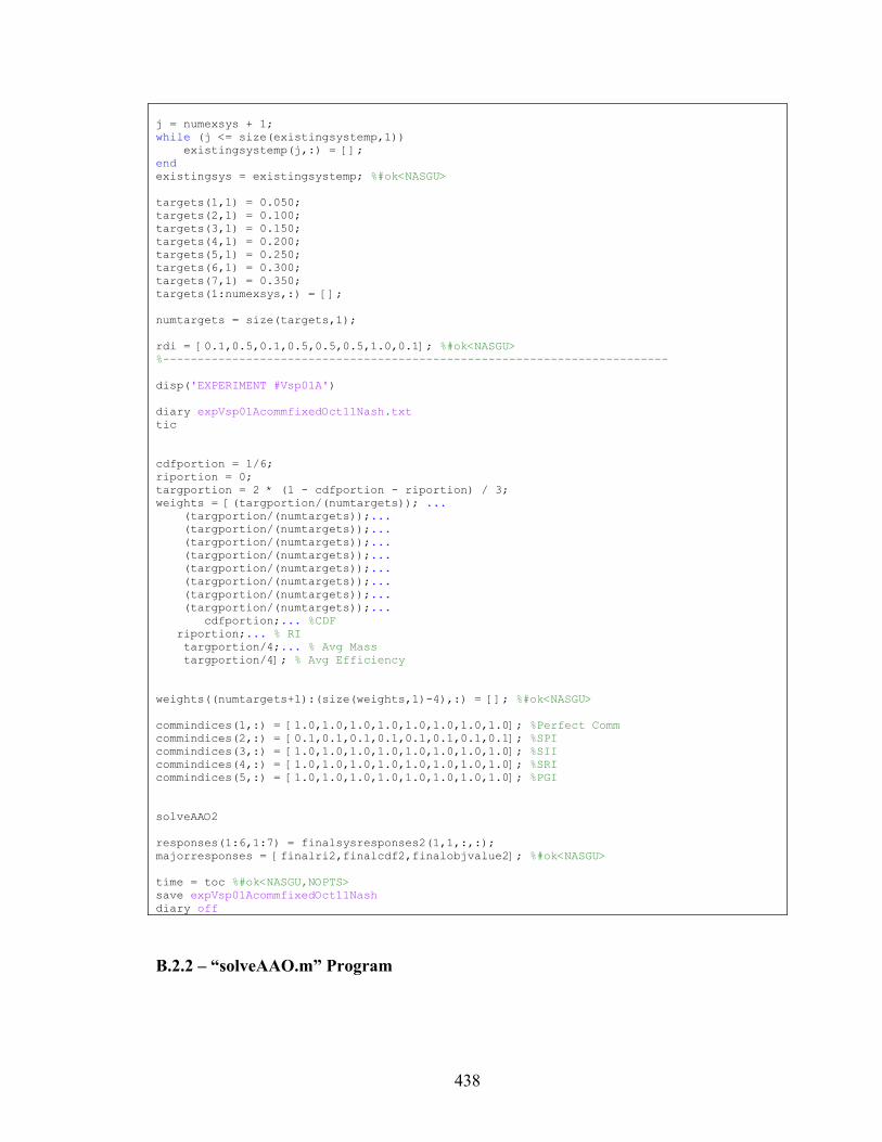
438
j = numexsys + 1; while (j <= size(existingsystemp,1)) existingsystemp(j,:) = []; end existingsys = existingsystemp; %#ok<NASGU> targets(1,1) = 0.050; targets(2,1) = 0.100; targets(3,1) = 0.150; targets(4,1) = 0.200; targets(5,1) = 0.250; targets(6,1) = 0.300; targets(7,1) = 0.350; targets(1:numexsys,:) = []; numtargets = size(targets,1); rdi = [0.1,0.5,0.1,0.5,0.5,0.5,1.0,0.1]; %#ok<NASGU> %------------------------------------------------------------------------- disp('EXPERIMENT #Vsp01A') diary expVsp01AcommfixedOct11Nash.txt tic cdfportion = 1/6; riportion = 0; targportion = 2 * (1 - cdfportion - riportion) / 3; weights = [(targportion/(numtargets)); ... (targportion/(numtargets));... (targportion/(numtargets));... (targportion/(numtargets));... (targportion/(numtargets));... (targportion/(numtargets));... (targportion/(numtargets));... (targportion/(numtargets));... (targportion/(numtargets));... cdfportion;... %CDF riportion;... % RI targportion/4;... % Avg Mass targportion/4]; % Avg Efficiency weights((numtargets+1):(size(weights,1)-4),:) = []; %#ok<NASGU> commindices(1,:) = [1.0,1.0,1.0,1.0,1.0,1.0,1.0,1.0]; %Perfect Comm commindices(2,:) = [0.1,0.1,0.1,0.1,0.1,0.1,0.1,0.1]; %SPI commindices(3,:) = [1.0,1.0,1.0,1.0,1.0,1.0,1.0,1.0]; %SII commindices(4,:) = [1.0,1.0,1.0,1.0,1.0,1.0,1.0,1.0]; %SRI commindices(5,:) = [1.0,1.0,1.0,1.0,1.0,1.0,1.0,1.0]; %PGI solveAAO2 responses(1:6,1:7) = finalsysresponses2(1,1,:,:); majorresponses = [finalri2,finalcdf2,finalobjvalue2]; %#ok<NASGU> time = toc %#ok<NASGU,NOPTS> save expVsp01AcommfixedOct11Nash diary off
B.2.2 – “solveAAO.m” Program

439
This is the main function for solving a simplified redesign problem all at once. It
is a greatly simplified version of the “solvequasicon.m” function shown in Section C.1.1.
%%%%%%%%%%%%%%%%%%%%%%%%%%%%%%%%%%%%%%%%%%%%%%%%%%%%%%%%%%%%%%%%%%%%%%%%%% % solveAAO2.m % % Written by: Matt Chamberlain % % Description: This script is meant to be the main program used to solve % the universal motor redesign problem all at once % % This version is meant to help run a whole bunch of tests at once using % some custom inputs instead of getting all inputs from redesigninputs.m as % was done previously % %%%%%%%%%%%%%%%%%%%%%%%%%%%%%%%%%%%%%%%%%%%%%%%%%%%%%%%%%%%%%%%%%%%%%%%%%% % INITIALIZE ALL OF THE GIVENS FOR THE PROBLEM AT HAND [existingsysres,overallobjs,... physcons,physconflags,physconseq,physconseqflags,minndiv,maxndiv,... responsebounds,numvars,constructs,lbounds,ubounds,x0]... = redesigninputs3(schedule,existingsys,targets,weights,commindices,rdi); numexsys = size(existingsys,1); numtargets = size(targets,1); % Make a non-dimensional set of existing systems existingsysnondim = zeros(numexsys,numvars); for countexsys = 1:size(existingsys,1) existingsysnondim(countexsys,:) = ... (existingsys(countexsys,:) - lbounds') ./ (ubounds' - lbounds'); end % CREATE THE REDESIGN DIFFICULTY AND SCHEDULING MATRICES [commmatrix,startprod,endprod] = createcomoppmatrix3(schedule,numvars,commindices); % Calculate the maximum number of elements based on maxndiv (THIS WILL ONLY % WORK FOR 1-DIMENSIONAL PROBLEMS) maxnumelem = 1; for countndiv = 1:size(maxndiv,1) maxnumelem = maxnumelem * maxndiv(countndiv,1); end maxvalue = 0; validndiv = 0; savedvars = zeros(1, (numvars * maxnumelem) ); % saves room for variables maxnumassignments = 2520; numvalidndiv = 22; numdimensions = size(responsebounds,1); totnumvars = numvars * numtargets; % Figure out number of elements that may contain new % systems numnewsols = numtargets; assignnumber = 1; validndiv = 1; currsetup = 1:numtargets; % Generate an array of flags to show what targets nondimbounds = [zeros(numvars*numtargets,1),ones(numvars*numtargets,1)]; % Set options for fmincon options = optimset('Display','on','Tolfun',1*10^-7,'Tolcon',0.001,... 'MaxFunEval',10000,'LargeScale','off','DiffMaxChange',1.00); ...

440
%,'DiffMinchange',0.001'OutputFcn', @outfun, % Generate various start points for fmincon findstartpoints = 1; [tempx0(findstartpoints,:),tempstartvarflag(findstartpoints)] = ... findlowstartAAO([lbounds ubounds],targets,responsebounds) findstartpoints = findstartpoints + 1; [tempx0(findstartpoints,:),tempstartvarflag(findstartpoints)] = ... findmidstartAAO([lbounds ubounds],targets,responsebounds) findstartpoints = findstartpoints + 1; [tempx0(findstartpoints,:),tempstartvarflag(findstartpoints)] = ... findhighstartAAO([lbounds ubounds],targets,responsebounds) findstartpoints = findstartpoints + 1; while (findstartpoints <= 7) [tempx0(findstartpoints,:),tempstartvarflag(findstartpoints)] = ... findclosestartAAO2([lbounds ubounds],targets,responsebounds,existingsys) findstartpoints = findstartpoints + 1; end % Sets the "platform" variable values for the "simplified" problem for countstartpts = 1:7 for counttargs = 0:1:(numtargets - 1) tempx0(countstartpts,(counttargs*numvars)+2) = ... (0.241-lbounds(2,1))/(ubounds(2,1) - lbounds(2,1)); tempx0(countstartpts,(counttargs*numvars)+4) = ... (0.376-lbounds(4,1))/(ubounds(4,1) - lbounds(4,1)); tempx0(countstartpts,(counttargs*numvars)+5) = ... (2.69-lbounds(5,1))/(ubounds(5,1) - lbounds(5,1)); tempx0(countstartpts,(counttargs*numvars)+6) = ... (6.66-lbounds(6,1))/(ubounds(6,1) - lbounds(6,1)); end end goodfound = 0; mintemp = 500; for trypoints = 1:size(tempx0,1) trypoints [tempvars2(trypoints,:),tempfinalobjvalue2(trypoints),... tempexitflag2(trypoints),output,lambda] = ... fmincon(@(solutionset)portfolioevalAAO4(solutionset,existingsys,targets,... weights,schedule,startprod,commmatrix,rdi,currsetup,[lbounds, ubounds]),... tempx0(trypoints,:),[],[],[],[],nondimbounds(:,1),nondimbounds(:,2),... @(solutionset)createnonlconstAAO(solutionset,physcons,physconflags,... physconseq,physconseqflags,currsetup,[lbounds, ubounds]),options) if (min(tempvars2(trypoints,:)) < 0) tempnegativevarflag(trypoints) = -1; else tempnegativevarflag(trypoints) = 10000; end % New few loops determine if a solution is good enough to be saved and % recorded as the best found thus far. if ( (goodfound == 0) && ... ((tempnegativevarflag(trypoints) == -1) || ... (tempexitflag2(trypoints) < 0))) bestpoint = trypoints; mintemp = tempfinalobjvalue2(trypoints); elseif ( (goodfound == 0) && ... (tempnegativevarflag(trypoints) > -1) && ... (tempexitflag2(trypoints) >= 0) ) bestpoint = trypoints; mintemp = tempfinalobjvalue2(trypoints); goodfound = 1; elseif ( (goodfound == 1) && ... (tempnegativevarflag(trypoints) > -1) && ... (tempexitflag2(trypoints) >= 0) && ... (tempfinalobjvalue2(trypoints) < mintemp) ) bestpoint = trypoints;

441
mintemp = tempfinalobjvalue2(trypoints); end end % Save the best values found vars2(validndiv,assignnumber,:) = tempvars2(bestpoint,:); finalobjvalue2(validndiv,assignnumber) = tempfinalobjvalue2(bestpoint); exitflag2(validndiv,assignnumber) = tempexitflag2(bestpoint); % Put the "platform" values back in countrows = 1; dimvarsinrows = zeros(numtargets,numvars); nondimvarsinrows = zeros(numtargets,numvars); for i = 1:numvars:(numvars*numtargets) nondimvarchunk(1:numvars) = vars2(validndiv,assignnumber,i:(i + numvars - 1)); dimvarchunk = (nondimvarchunk .* (ubounds' - lbounds')) + lbounds'; dimvarsinrows(countrows,:) = dimvarchunk; dimvarsinrows(countrows,2) = 0.241; dimvarsinrows(countrows,4) = 0.376; dimvarsinrows(countrows,5) = 2.69; dimvarsinrows(countrows,6) = 6.66; nondimvarsinrows(countrows,:) = nondimvarchunk; nondimvarsinrows(countrows,2) = (0.241-lbounds(2,1))/(ubounds(2,1) - lbounds(2,1)); nondimvarsinrows(countrows,4) = (0.376-lbounds(4,1))/(ubounds(4,1) - lbounds(4,1)); nondimvarsinrows(countrows,5) = (2.69-lbounds(5,1))/(ubounds(5,1) - lbounds(5,1)); nondimvarsinrows(countrows,6) = (6.66-lbounds(6,1))/(ubounds(6,1) - lbounds(6,1)); countrows = countrows + 1; end finalri2(validndiv,assignnumber) = ... evalcontinuousriAAO(existingsysnondim, nondimvarsinrows, rdi, schedule, startprod); finalcdf2(validndiv,assignnumber) = ... evalcontinuouscdfAAO3(existingsysnondim, nondimvarsinrows, commmatrix); finalvars2 = dimvarsinrows; for countfinalsys = 1:numtargets output = TSunivmotor(finalvars2(countfinalsys,:)); finalsystorques2(validndiv,assignnumber,countfinalsys) = output(1); finalsysresponses2(validndiv,assignnumber,countfinalsys,:) = output; end if (min(vars2(validndiv,assignnumber,:)) < 0) negativevarflag2(validndiv,assignnumber,1) = -1; else negativevarflag2(validndiv,assignnumber,1) = 1; end % WARNING THAT PROGRAM HAS ENDED for countbeeps = 1:5 beep; end
B.2.3 – “createeqconstAAO.m” Program
This function creates the equality constraints needed by fmincon for the
simplified approach to solving the redesign problem.
function [Aeq,Beq] = ... createeqconstAAO(spaceelements,ndiv,numvars,constructs,existingsys,... existingsysflag,currsetup,spaceelemtargassign,spaceelemvarassign) % Creates equality constraints appropriate to the all-at-once solution %%%%%%%%%%%%%%%%%%%%%%%%%%%%%%%%%%%%%%%%%%%%%%%%%%%%%%%%%%%%%%%%%%%%%%%%%% % createeqconstAAO.m % % Written by: Matt Chamberlain % % Description: This program creates the two matrices that are used to

442
% describe the equality constraints in the all-at-once solution % %%%%%%%%%%%%%%%%%%%%%%%%%%%%%%%%%%%%%%%%%%%%%%%%%%%%%%%%%%%%%%%%%%%%%%%%%% % Assume that x array is a row with n*numvars spaces (one for each variable % in each of the smallest space elements) numconstructs = size(ndiv,1); numdimensions = size(ndiv,2); numnewsys = size(find(currsetup),2); numelements = ndiv(:,1); for countelements = 2:numdimensions numelements = numelements .* ndiv(:,countelements); end for countlevels = 1:(numconstructs-1) % only check for equalities if there are actually multiple smaller % elements inside of the element you are currently checking (otherwise % you are doing the same check twice at the next lower level %if (isequal(ndiv(countlevels,:),ndiv(countlevels+1,:)) == 0) % Go through each element in the current level for countinlevelelements = 1:numelements(countlevels,1) % Go through each of the lowest-level elements to see which are % inside the element at the current level in question numinside = 0; exsysinside = 0; for countsmallest = 1:numelements(numconstructs,1) % Check each element using checkelements.m insideflag = checkelements... (spaceelements(countlevels,countinlevelelements,:,:),... spaceelements(numconstructs,countsmallest,:,:)); if ( ((insideflag == 1) & (existingsysflag(numconstructs,countsmallest,1) > 0)) |... ((insideflag == 1) & (spaceelemtargassign(countsmallest) > 0)) ) % If it is inside and it contains one of the systems % being used, set numinside = numinside + 1; numinside = numinside + 1; if ((numinside == 1) & (existingsysflag(numconstructs,countsmallest,1) > 0 )) % Save the "first element's" place so we can set it % equal to all others inside the larger element % This is the case when it's an existing system % firstelementflag = countsmallest; exsysinside = countsmallest; exsysinsideflag = existingsysflag(numconstructs,countsmallest,1); elseif ((numinside == 1) & (spaceelemtargassign(countsmallest) > 0)) % Save the "first element's" place so we can set it % equal to all others inside the larger element % This is the case when it's one of the new systems firstsysinsideflag = spaceelemvarassign(countsmallest); elseif ((numinside > 1) & (exsysinside > 0)) % Case when there is an exsys inside the element in % question ... means elements should be set equal % to that exsys for countvars = 1:numvars % Look for flags saying which variables are % common at this level of construct if (constructs(countvars) == countlevels) counteqconst = counteqconst + 1; Beq(counteqconst) = existingsys(exsysinsideflag,countvars); Aeq(counteqconst,1:(numnewsys*numvars)) = ... zeros( 1,(numnewsys * numvars) ); newsysplace = ... countvars + ( (spaceelemvarassign(countsmallest) - 1) * numvars); Aeq(counteqconst,newsysplace) = 1;
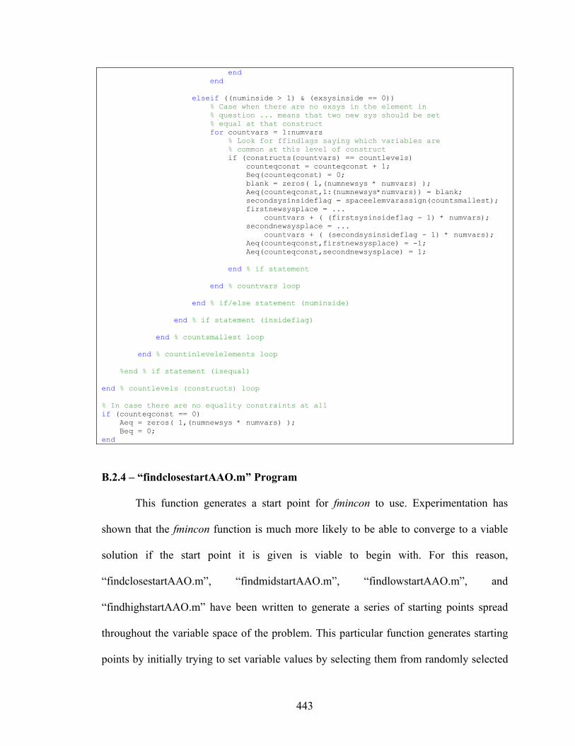
443
end end elseif ((numinside > 1) & (exsysinside == 0)) % Case when there are no exsys in the element in % question ... means that two new sys should be set % equal at that construct for countvars = 1:numvars % Look for ffindlags saying which variables are % common at this level of construct if (constructs(countvars) == countlevels) counteqconst = counteqconst + 1; Beq(counteqconst) = 0; blank = zeros( 1,(numnewsys * numvars) ); Aeq(counteqconst,1:(numnewsys*numvars)) = blank; secondsysinsideflag = spaceelemvarassign(countsmallest); firstnewsysplace = ... countvars + ( (firstsysinsideflag - 1) * numvars); secondnewsysplace = ... countvars + ( (secondsysinsideflag - 1) * numvars); Aeq(counteqconst,firstnewsysplace) = -1; Aeq(counteqconst,secondnewsysplace) = 1; end % if statement end % countvars loop end % if/else statement (numinside) end % if statement (insideflag) end % countsmallest loop end % countinlevelelements loop %end % if statement (isequal) end % countlevels (constructs) loop % In case there are no equality constraints at all if (counteqconst == 0) Aeq = zeros( 1,(numnewsys * numvars) ); Beq = 0; end
B.2.4 – “findclosestartAAO.m” Program
This function generates a start point for fmincon to use. Experimentation has
shown that the fmincon function is much more likely to be able to converge to a viable
solution if the start point it is given is viable to begin with. For this reason,
“findclosestartAAO.m”, “findmidstartAAO.m”, “findlowstartAAO.m”, and
“findhighstartAAO.m” have been written to generate a series of starting points spread
throughout the variable space of the problem. This particular function generates starting
points by initially trying to set variable values by selecting them from randomly selected

444
existing systems, the idea being that commonality can be encouraged in this way. This is
one of the few functions and scripts that would have to be adjusted for use in an example
problem different from the universal motor, as constraints and variables relevant to that
problem have been hard-wired into this code.
function [closestartpoints,startvarflag] = ... findclosestartAAO(varranges,targets,responsebounds,existingsys) % Finds a good start point for fmincon close to existing systems %%%%%%%%%%%%%%%%%%%%%%%%%%%%%%%%%%%%%%%%%%%%%%%%%%%%%%%%%%%%%%%%%%%%%%%%%%% % findclosestartAAO.m % % Written by: Matt Chamberlain % % This program finds better starting points for the system based on a % random assortment of values from existing systems' variables % %%%%%%%%%%%%%%%%%%%%%%%%%%%%%%%%%%%%%%%%%%%%%%%%%%%%%%%%%%%%%%%%%%%%%%%%%%% numvars = size(varranges,1); numtargets = size(targets,1); numsys = numtargets; numexsys = size(existingsys,1); % FIND A START POINT THAT IS CLOSE TO THE VALUES OF THE EXISTING SYSTEMS % newsyslocs = find(currsetup); for k = 1:numsys goodpoint = 0; while (goodpoint == 0) randvars = rand(1,numvars);% make an array of random variables randvars = randvars ./ (1/numexsys);% divide each by (1/numexsys) randvars = floor(randvars) + 1;% chop off the remainder % remaining number is the existing system from which each variable % comes (for loop) for findexsysvars = 1:numvars bunkstartpoint(findexsysvars) = ... existingsys(randvars(findexsysvars),findexsysvars); end [newvars,startvarflag] = ... optindivmotorlow(bunkstartpoint,targets(k,1,:),responsebounds); if (startvarflag >= 0) goodpoint = 1; end firstvarnewarray = (k - 1) * numvars + 1; lastvarnewarray = firstvarnewarray + numvars - 1; closestartpoints(firstvarnewarray:lastvarnewarray) = ... (newvars - varranges(:,1)') ./ ... ((varranges(:,2) - varranges(:,1))'); end end end %%%%%%%%%%%%%%%%%%%%%%%%%%%%%%%%%%%%%%%%%%%%%%%%%%%%%%%%%%%%%%%%%%%%%%%%%%% function [newvars,startvarflag] = optindivmotorlow(vars,target,responsebounds) % This subfunction does the optimization of one motor % Inside, it calls fmincon % Also computes Aeq and Beq ... or are these not needed? % Need separate function to compute the deviation itself % Need separate function co compute physical constraints x0 = vars; bounds = [100,1500;... 0.01,1.0;...
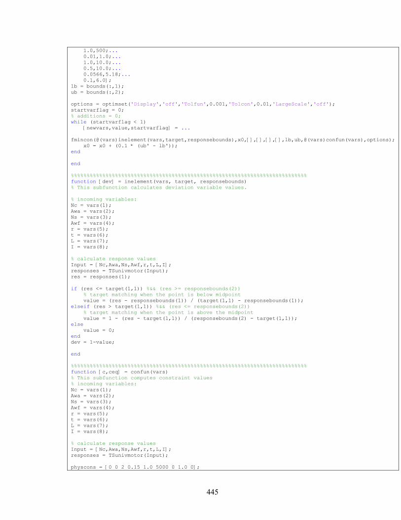
445
1.0,500;... 0.01,1.0;... 1.0,10.0;... 0.5,10.0;... 0.0566,5.18;... 0.1,6.0]; lb = bounds(:,1); ub = bounds(:,2); options = optimset('Display','off','Tolfun',0.001,'Tolcon',0.01,'LargeScale','off'); startvarflag = 0; % additions = 0; while (startvarflag < 1) [newvars,value,startvarflag] = ... fmincon(@(vars)inelement(vars,target,responsebounds),x0,[],[],[],[],lb,ub,@(vars)confun(vars),options); x0 = x0 + (0.1 * (ub' - lb')); end end %%%%%%%%%%%%%%%%%%%%%%%%%%%%%%%%%%%%%%%%%%%%%%%%%%%%%%%%%%%%%%%%%%%%%%%%%%% function [dev] = inelement(vars, target, responsebounds) % This subfunction calculates deviation variable values. % incoming variables: Nc = vars(1); Awa = vars(2); Ns = vars(3); Awf = vars(4); r = vars(5); t = vars(6); L = vars(7); I = vars(8); % calculate response values Input = [Nc,Awa,Ns,Awf,r,t,L,I]; responses = TSunivmotor(Input); res = responses(1); if (res <= target(1,1)) %&& (res >= responsebounds(2)) % target matching when the point is below midpoint value = (res - responsebounds(1)) / (target(1,1) - responsebounds(1)); elseif (res > target(1,1)) %&& (res <= responsebounds(2)) % target matching when the point is above the midpoint value = 1 - (res - target(1,1)) / (responsebounds(2) - target(1,1)); else value = 0; end dev = 1-value; end %%%%%%%%%%%%%%%%%%%%%%%%%%%%%%%%%%%%%%%%%%%%%%%%%%%%%%%%%%%%%%%%%%%%%%%%%%% function [c,ceq] = confun(vars) % This subfunction computes constraint values % incoming variables: Nc = vars(1); Awa = vars(2); Ns = vars(3); Awf = vars(4); r = vars(5); t = vars(6); L = vars(7); I = vars(8); % calculate response values Input = [Nc,Awa,Ns,Awf,r,t,L,I]; responses = TSunivmotor(Input); physcons = [0 0 2 0.15 1.0 5000 0 1.0 0];
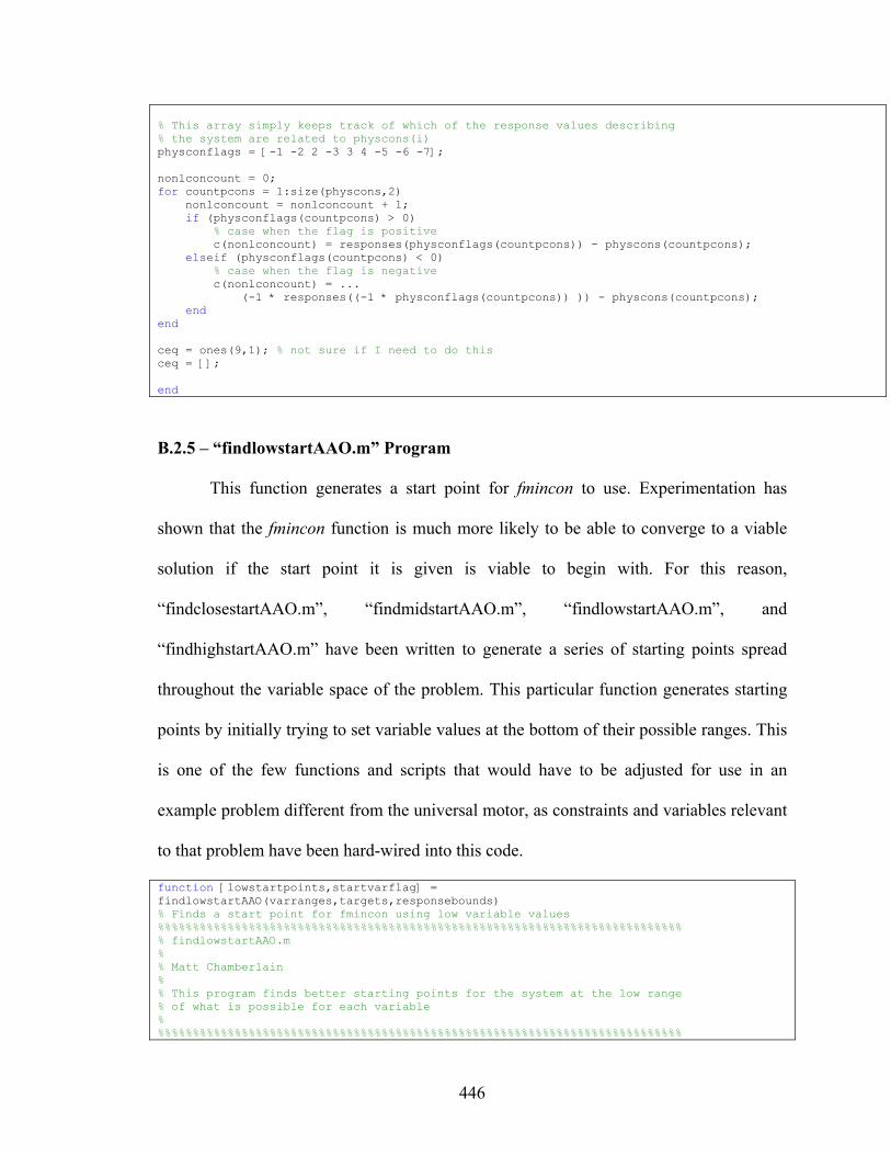
446
% This array simply keeps track of which of the response values describing % the system are related to physcons(i) physconflags = [-1 -2 2 -3 3 4 -5 -6 -7]; nonlconcount = 0; for countpcons = 1:size(physcons,2) nonlconcount = nonlconcount + 1; if (physconflags(countpcons) > 0) % case when the flag is positive c(nonlconcount) = responses(physconflags(countpcons)) - physcons(countpcons); elseif (physconflags(countpcons) < 0) % case when the flag is negative c(nonlconcount) = ... (-1 * responses((-1 * physconflags(countpcons)) )) - physcons(countpcons); end end ceq = ones(9,1); % not sure if I need to do this ceq = []; end
B.2.5 – “findlowstartAAO.m” Program
This function generates a start point for fmincon to use. Experimentation has
shown that the fmincon function is much more likely to be able to converge to a viable
solution if the start point it is given is viable to begin with. For this reason,
“findclosestartAAO.m”, “findmidstartAAO.m”, “findlowstartAAO.m”, and
“findhighstartAAO.m” have been written to generate a series of starting points spread
throughout the variable space of the problem. This particular function generates starting
points by initially trying to set variable values at the bottom of their possible ranges. This
is one of the few functions and scripts that would have to be adjusted for use in an
example problem different from the universal motor, as constraints and variables relevant
to that problem have been hard-wired into this code.
function [lowstartpoints,startvarflag] = findlowstartAAO(varranges,targets,responsebounds) % Finds a start point for fmincon using low variable values %%%%%%%%%%%%%%%%%%%%%%%%%%%%%%%%%%%%%%%%%%%%%%%%%%%%%%%%%%%%%%%%%%%%%%%%%%% % findlowstartAAO.m % % Matt Chamberlain % % This program finds better starting points for the system at the low range % of what is possible for each variable % %%%%%%%%%%%%%%%%%%%%%%%%%%%%%%%%%%%%%%%%%%%%%%%%%%%%%%%%%%%%%%%%%%%%%%%%%%%

447
numvars = size(varranges,1); % numdimensions = size(spaceelements,3); % numconstructs = size(spaceelements,1); numtargets = size(targets,1); numsys = numtargets; countvars = 1; for i = 1:numtargets for j = 1:size(varranges,1) newstartpoints(countvars) = varranges(j,1); countvars = countvars + 1; end end % FIND A MODIFIED VERSION OF EACH STARTING POINT THAT IS CLOSE TO THE % TARGET IN THE CENTER OF THE SPACE ELEMENT % NOTE: THIS IS ONE OF THE STEPS THAT WOULD HAVE TO BE DIFFERENT IF THERE % WERE MULTIPLE DIMENSIONS TO EACH SPACE ELEMENT for k = 1:numsys firstvar = ((k-1) * numvars) + 1; lastvar = numvars * k; bunkstartpoint = newstartpoints( firstvar:lastvar ); [newvars,startvarflag] = optindivmotorlow(bunkstartpoint,targets(k,1),responsebounds); firstvarnewarray = (k - 1) * numvars + 1; lastvarnewarray = firstvarnewarray + numvars - 1; lowstartpoints(firstvarnewarray:lastvarnewarray) = ... (newvars - varranges(:,1)') ./ (varranges(:,2) - varranges(:,1))'; end end %%%%%%%%%%%%%%%%%%%%%%%%%%%%%%%%%%%%%%%%%%%%%%%%%%%%%%%%%%%%%%%%%%%%%%%%%%% function [newvars,startvarflag] = optindivmotorlow(vars,target,responsebounds) % This subfunction does the optimization of one motor % This does the optimization of one motor % Inside, it calls fmincon % Also computes Aeq and Beq ... or are these not needed? x0 = vars; bounds = [100,1500;... 0.01,1.0;... 1.0,500;... 0.01,1.0;... 1.0,10.0;... 0.5,10.0;... 0.0566,5.18;... 0.1,6.0]; lb = bounds(:,1); ub = bounds(:,2); options = optimset('Display','off','Tolfun',0.00001,'Tolcon',0.01,'LargeScale','off'); startvarflag = 0; while (startvarflag <= 1) && (x0(1) <= bounds(1,2)) [newvars,value,startvarflag] = ... fmincon(@(vars)inelement(vars,target,responsebounds),x0,... [],[],[],[],lb,ub,@(vars)confun(vars),options); x0 = x0 + (0.1 * (ub' - lb')); end end %%%%%%%%%%%%%%%%%%%%%%%%%%%%%%%%%%%%%%%%%%%%%%%%%%%%%%%%%%%%%%%%%%%%%%%%%%% function [dev] = inelement(vars, target, responsebounds) % This subfunction calculates the deviation variable values % incoming variables:

448
Nc = vars(1); Awa = vars(2); Ns = vars(3); Awf = vars(4); r = vars(5); t = vars(6); L = vars(7); I = vars(8); % calculate response values Input = [Nc,Awa,Ns,Awf,r,t,L,I]; responses = TSunivmotor(Input); res = responses(1); if (res <= target(1,1)) %&& (res >= responsebounds(2)) % target matching when the point is below midpoint value = (res - responsebounds(1)) / (target(1,1) - responsebounds(1)); elseif (res > target(1,1)) %&& (res <= responsebounds(2)) % target matching when the point is above the midpoint value = 1 - (res - target(1,1)) / (responsebounds(2) - target(1,1)); else value = 0; end dev = 1-value; end %%%%%%%%%%%%%%%%%%%%%%%%%%%%%%%%%%%%%%%%%%%%%%%%%%%%%%%%%%%%%%%%%%%%%%%%%%% function [c,ceq] = confun(vars) % This subfunction computes the constraint values % incoming variables: Nc = vars(1); Awa = vars(2); Ns = vars(3); Awf = vars(4); r = vars(5); t = vars(6); L = vars(7); I = vars(8); % calculate response values Input = [Nc,Awa,Ns,Awf,r,t,L,I]; responses = TSunivmotor(Input); physconflags = [-1 -2 2 -3 3 4 -5 -6 -7]; nonlconcount = 0; for countpcons = 1:size(physcons,2) nonlconcount = nonlconcount + 1; if (physconflags(countpcons) > 0) % case when the flag is positive c(nonlconcount) = responses(physconflags(countpcons)) - physcons(countpcons); elseif (physconflags(countpcons) < 0) % case when the flag is negative c(nonlconcount) = ... (-1 * responses((-1 * physconflags(countpcons)) )) - physcons(countpcons); end end ceq = ones(9,1); % not sure if I need to do this ceq = []; end
B.2.6 – “findmidstartAAO.m” Program

449
This function generates a start point for fmincon to use. Experimentation has
shown that the fmincon function is much more likely to be able to converge to a viable
solution if the start point it is given is viable to begin with. For this reason,
“findclosestartAAO.m”, “findmidstartAAO.m”, “findlowstartAAO.m”, and
“findhighstartAAO.m” have been written to generate a series of starting points spread
throughout the variable space of the problem. This particular function generates starting
points by initially trying to set variable values at the middle of their possible ranges. This
is one of the few functions and scripts that would have to be adjusted for use in an
example problem different from the universal motor, as constraints and variables relevant
to that problem have been hard-wired into this code.
function [midstartpoints,startvarflag] = findmidstartAAO(varranges,targets,responsebounds) % Finds a start point for fmincon using mid-range variable values %%%%%%%%%%%%%%%%%%%%%%%%%%%%%%%%%%%%%%%%%%%%%%%%%%%%%%%%%%%%%%%%%%%%%%%%%%% % findmidstartAAO.m % % Matt Chamberlain % % This program finds better starting points for the system using variable % values as close to the middle of the range of each variable % %%%%%%%%%%%%%%%%%%%%%%%%%%%%%%%%%%%%%%%%%%%%%%%%%%%%%%%%%%%%%%%%%%%%%%%%%%% numvars = size(varranges,1); numtargets = size(targets,1); numsys = numtargets; countvars = 1; for i = 1:numtargets for j = 1:size(varranges,1) newstartpoints(countvars) = ... 0.5 * (varranges(j,2) - varranges(j,1)) + varranges(j,1); countvars = countvars + 1; end end % FIND A MODIFIED VERSION OF EACH STARTING POINT THAT IS CLOSE TO THE % TARGET IN THE CENTER OF THE SPACE ELEMENT % NOTE: THIS IS ONE OF THE STEPS THAT WOULD HAVE TO BE DIFFERENT IF THERE % WERE MULTIPLE DIMENSIONS TO EACH SPACE ELEMENT for k = 1:numsys firstvar = ((k-1) * numvars) + 1; lastvar = numvars * k; bunkstartpoint = newstartpoints( firstvar:lastvar ); [newvars,startvarflag] = optindivmotorlow(bunkstartpoint,targets(k,1),responsebounds); firstvarnewarray = (k - 1) * numvars + 1; lastvarnewarray = firstvarnewarray + numvars - 1; midstartpoints(firstvarnewarray:lastvarnewarray) = ... (newvars - varranges(:,1)') ./ (varranges(:,2) - varranges(:,1))';

450
end end %%%%%%%%%%%%%%%%%%%%%%%%%%%%%%%%%%%%%%%%%%%%%%%%%%%%%%%%%%%%%%%%%%%%%%%%%%% function [newvars,startvarflag] = optindivmotorlow(vars,target,responsebounds) % This subfunction does the optimization of one motor % Inside, it calls fmincon % Also computes Aeq and Beq ... or are these not needed? x0 = vars; bounds = [100,1500;... 0.01,1.0;... 1.0,500;... 0.01,1.0;... 1.0,10.0;... 0.5,10.0;... 0.0566,5.18;... 0.1,6.0]; lb = bounds(:,1); ub = bounds(:,2); options = optimset('Display','off','Tolfun',0.001,'Tolcon',0.01,'LargeScale','off'); startvarflag = 0; % additions = 0; while (startvarflag < 1) && (x0(1) <= bounds(1,2)) [newvars,value,startvarflag] = ... fmincon(@(vars)inelement(vars,target,responsebounds),x0,... [],[],[],[],lb,ub,@(vars)confun(vars),options); x0 = x0 + (0.1 * (ub' - lb')) end end %%%%%%%%%%%%%%%%%%%%%%%%%%%%%%%%%%%%%%%%%%%%%%%%%%%%%%%%%%%%%%%%%%%%%%%%%%% function [dev] = inelement(vars, target, responsebounds) % This subfunction calculates the deviation variable values % incoming variables: Nc = vars(1); Awa = vars(2); Ns = vars(3); Awf = vars(4); r = vars(5); t = vars(6); L = vars(7); I = vars(8); % calculate response values Input = [Nc,Awa,Ns,Awf,r,t,L,I]; responses = TSunivmotor(Input); res = responses(1); if (res <= target(1,1)) %&& (res >= responsebounds(2)) % target matching when the point is below midpoint value = (res - responsebounds(1)) / (target(1,1) - responsebounds(1)); elseif (res > target(1,1)) %&& (res <= responsebounds(2)) % target matching when the point is above the midpoint value = 1 - (res - target(1,1)) / (responsebounds(2) - target(1,1)); else value = 0; end dev = 1-value; end %%%%%%%%%%%%%%%%%%%%%%%%%%%%%%%%%%%%%%%%%%%%%%%%%%%%%%%%%%%%%%%%%%%%%%%%%%% function [c,ceq] = confun(vars) % This subfunction computes the constraint values

451
% incoming variables: Nc = vars(1); Awa = vars(2); Ns = vars(3); Awf = vars(4); r = vars(5); t = vars(6); L = vars(7); I = vars(8); % calculate response values Input = [Nc,Awa,Ns,Awf,r,t,L,I]; responses = TSunivmotor(Input); physcons = [0 0 2 0.15 1.0 5000 0 1.0 0]; % This array simply keeps track of which of the response values describing % the system are related to physcons(i) physconflags = [-1 -2 2 -3 3 4 -5 -6 -7]; nonlconcount = 0; for countpcons = 1:size(physcons,2) nonlconcount = nonlconcount + 1; if (physconflags(countpcons) > 0) % case when the flag is positive c(nonlconcount) = responses(physconflags(countpcons)) - physcons(countpcons); elseif (physconflags(countpcons) < 0) % case when the flag is negative c(nonlconcount) = ... (-1 * responses((-1 * physconflags(countpcons)) )) - physcons(countpcons); end end ceq = ones(9,1); % not sure if I need to do this ceq = []; end
C.2.7 – “findhighstartAAO.m” Program
This function generates a start point for fmincon to use. Experimentation has
shown that the fmincon function is much more likely to be able to converge to a viable
solution if the start point it is given is viable to begin with. For this reason,
“findclosestartAAO.m”, “findmidstartAAO.m”, “findlowstartAAO.m”, and
“findhighstartAAO.m” have been written to generate a series of starting points spread
throughout the variable space of the problem. This particular function generates starting
points by initially trying to set variable values at the top of their possible ranges. This is
one of the few functions and scripts that would have to be adjusted for use in an example

452
problem different from the universal motor, as constraints and variables relevant to that
problem have been hard-wired into this code.
function [highstartpoints,startvarflag] = findhighstartAAO(varranges,targets,responsebounds) % Finds a start point for fmincon using high variable values %%%%%%%%%%%%%%%%%%%%%%%%%%%%%%%%%%%%%%%%%%%%%%%%%%%%%%%%%%%%%%%%%%%%%%%%%%% % findhighstartAAO.m % % Matt Chamberlain % % This program finds better starting points for the system using variable % values at the high range of what is possible % %%%%%%%%%%%%%%%%%%%%%%%%%%%%%%%%%%%%%%%%%%%%%%%%%%%%%%%%%%%%%%%%%%%%%%%%%%% numvars = size(varranges,1); % numdimensions = size(spaceelements,3); % numconstructs = size(spaceelements,1); numtargets = size(targets,1); numsys = numtargets; countvars = 1; for i = 1:numtargets for j = 1:size(varranges,1) newstartpoints(countvars) = varranges(j,2); countvars = countvars + 1; end end % FIND A MODIFIED VERSION OF EACH STARTING POINT THAT IS CLOSE TO THE % TARGET IN THE CENTER OF THE SPACE ELEMENT % NOTE: THIS IS ONE OF THE STEPS THAT WOULD HAVE TO BE DIFFERENT IF THERE % WERE MULTIPLE DIMENSIONS TO EACH SPACE ELEMENT for k = 1:numsys firstvar = ((k-1) * numvars) + 1; lastvar = numvars * k; bunkstartpoint = newstartpoints( firstvar:lastvar ); [newvars,startvarflag] = optindivmotorlow(bunkstartpoint,targets(k,1),responsebounds); firstvarnewarray = (k - 1) * numvars + 1; lastvarnewarray = firstvarnewarray + numvars - 1; highstartpoints(firstvarnewarray:lastvarnewarray) = ... (newvars - varranges(:,1)') ./ (varranges(:,2) - varranges(:,1))'; end end %%%%%%%%%%%%%%%%%%%%%%%%%%%%%%%%%%%%%%%%%%%%%%%%%%%%%%%%%%%%%%%%%%%%%%%%%%% function [newvars,startvarflag] = optindivmotorlow(vars,target,responsebounds) % This subfunction does the optimization of one motor % This does the optimization of one motor % Inside, it calls fmincon % Also computes Aeq and Beq ... or are these not needed? x0 = vars; bounds = [100,1500;... 0.01,1.0;... 1.0,500;... 0.01,1.0;... 1.0,10.0;... 0.5,10.0;... 0.0566,5.18;... 0.1,6.0]; lb = bounds(:,1);

453
ub = bounds(:,2); options = optimset('Display','off','Tolfun',0.001,'Tolcon',0.01,'LargeScale','off'); startvarflag = 0; % additions = 0; while (startvarflag < 1) && (x0(1) >= bounds(1,1)) [newvars,value,startvarflag] = ... fmincon(@(vars)inelement(vars,target,responsebounds),x0,... [],[],[],[],lb,ub,@(vars)confun(vars),options); x0 = x0 - (0.1 * (ub' - lb')); end end %%%%%%%%%%%%%%%%%%%%%%%%%%%%%%%%%%%%%%%%%%%%%%%%%%%%%%%%%%%%%%%%%%%%%%%%%%% function [dev] = inelement(vars, target, responsebounds) % This subfunction calculates the deviation variable values % incoming variables: Nc = vars(1); Awa = vars(2); Ns = vars(3); Awf = vars(4); r = vars(5); t = vars(6); L = vars(7); I = vars(8); % calculate response values Input = [Nc,Awa,Ns,Awf,r,t,L,I]; responses = TSunivmotor(Input); res = responses(1); if (res <= target(1,1)) %&& (res >= responsebounds(2)) % target matching when the point is below midpoint value = (res - responsebounds(1)) / (target(1,1) - responsebounds(1)); elseif (res > target(1,1)) %&& (res <= responsebounds(2)) % target matching when the point is above the midpoint value = 1 - (res - target(1,1)) / (responsebounds(2) - target(1,1)); else value = 0; end dev = 1-value; end %%%%%%%%%%%%%%%%%%%%%%%%%%%%%%%%%%%%%%%%%%%%%%%%%%%%%%%%%%%%%%%%%%%%%%%%%%% function [c,ceq] = confun(vars) % This subfunction computes the constraint values % incoming variables: Nc = vars(1); Awa = vars(2); Ns = vars(3); Awf = vars(4); r = vars(5); t = vars(6); L = vars(7); I = vars(8); % calculate response values Input = [Nc,Awa,Ns,Awf,r,t,L,I]; responses = TSunivmotor(Input); physcons = [0 0 2 0.15 1.0 5000 0 1.0 0]; % This array simply keeps track of which of the response values describing % the system are related to physcons(i) physconflags = [-1 -2 2 -3 3 4 -5 -6 -7];

454
nonlconcount = 0; for countpcons = 1:size(physcons,2) nonlconcount = nonlconcount + 1; if (physconflags(countpcons) > 0) % case when the flag is positive c(nonlconcount) = responses(physconflags(countpcons)) - physcons(countpcons); elseif (physconflags(countpcons) < 0) % case when the flag is negative c(nonlconcount) = ... (-1 * responses((-1 * physconflags(countpcons)) )) - physcons(countpcons); end end ceq = ones(9,1); % not sure if I need to do this ceq = []; end
B.2.8 – “portfolioevalAAO.m” Program
This is the main subfunction used for calculating the objective function value
associated with a given redesign portfolio. One of the major differences between this
function and the one used in the constructal-inspired approach is that this one is hard-
wired to set the fixed variable values in the simplified universal motor example.
function [objvalue] = portfolioevalAAO(nondimvars,existingsys,targets,... weights,schedule,startprod,commmatrix,... rdi,currsetup,varranges) % Evaluates a redesign solution against the designer's preferences %%%%%%%%%%%%%%%%%%%%%%%%%%%%%%%%%%%%%%%%%%%%%%%%%%%%%%%%%%%%%%%%%%%%%%%%%% % portfolioevalAAO.m % % Updated by: Matt Chamberlain % % Description: This program will take in a set of possible redesigned % systems (a "portfolio") and evaluate its value as compared to the % designer's set of preferences, the redesign schedule, etc. This is a % special "all-at-once" version. % %%%%%%%%%%%%%%%%%%%%%%%%%%%%%%%%%%%%%%%%%%%%%%%%%%%%%%%%%%%%%%%%%%%%%%%%%% numvars = size(existingsys,2); numdimensions = size(targets,2); numtargets = size(targets,1); % RE-ARRANGE THE LIST OF VARIABLES INTO ROWS (ONE FOR EACH SYSTEM) AND TURN % INTO DIMENSIONALIZED FORM solutionsetnondim = zeros(numtargets,numvars);

455
solutionset = zeros(numtargets,numvars); for i = 1:numtargets firstvar = ((i-1) * numvars) + 1; lastvar = numvars * i; solutionsetnondim(i,:) = nondimvars( firstvar:lastvar ); solutionset(i,:) = (nondimvars( firstvar:lastvar ) .*... (varranges(:,2)' - varranges(:,1)')) + varranges(:,1)'; % NEXT FEW LINES ARE FOR SIMPLIFYING THE PROBLEM BY SETTING "PLATFORM" % VARIABLES FOR A SUBSET OF VARIABLES AT ALL TIMES. solutionset(i,2) = 0.241; solutionset(i,4) = 0.376; solutionset(i,5) = 2.69; solutionset(i,6) = 6.66; solutionsetnondim(i,2) = (0.241-varranges(2,1))/(varranges(2,2) - varranges(2,1)); solutionsetnondim(i,4) = (0.376-varranges(4,1))/(varranges(4,2) - varranges(4,1)); solutionsetnondim(i,5) = (2.69-varranges(5,1))/(varranges(5,2) - varranges(5,1)); solutionsetnondim(i,6) = (6.66-varranges(6,1))/(varranges(6,2) - varranges(6,1)); end numnewsols = size(solutionset,1); % MAKE A NON-DIMENSIONAL SET OF EXISTING SYSTEMS existingsysnondim = zeros(size(existingsys,1),numvars); for i = 1:size(existingsys,1) existingsysnondim(i,:) = (existingsys(i,:) - varranges(:,1)') ./ ... (varranges(:,2)' - varranges(:,1)'); end % MODEL THE NEW SYSTEMS newdesignsres = zeros(numnewsols,7); for n = 1:numnewsols newdesignsres(n,:) = TSunivmotor(solutionset(n,:)); end overallvalue = 0; for countsys = 1:numnewsols % Look for the systems that are flagged for use in the portfolio in % this setup currenttarget = countsys; % Go through and evaluate the current system against its target % in each dimension for countdims = 1:numdimensions devtarget = evalvalueAAO(newdesignsres(countsys,countdims),... targets(currenttarget,countdims)); weighted = devtarget * weights(currenttarget,countdims); overallvalue = overallvalue + weighted; end end % CALCULATE THE HIGH-LEVEL OBJECTIVE VALUES AND CONVERT TO DEVIATION % For right now, the value of these is not evaluated; we're just trying

456
% to get cdf and ri as close to 1.0 as possible cdf = evalcontinuouscdfAAO3(existingsysnondim, solutionsetnondim, commmatrix); cdfdev = cdf; weightedcdfdev = cdfdev * weights( (numtargets+1), 1); ri = evalcontinuousriAAO(existingsysnondim, solutionsetnondim, rdi, schedule, startprod); ridev = ri; weightedridev = ridev * weights( (numtargets+2), 1); avgmass = sum(newdesignsres(:,2)) / numtargets; dweightedavgmass = (avgmass/0.5 - 1) * weights( (numtargets+3),1); if (dweightedavgmass < 0) dweightedavgmass = 0; end avgeffic = sum(newdesignsres(:,3)) / numtargets; dweightedavgeffic = (1 - (avgeffic/0.7)) * weights( (numtargets+4),1); if (dweightedavgeffic < 0) dweightedavgeffic = 0; end overallvalue = overallvalue + weightedcdfdev + weightedridev + ... dweightedavgmass + dweightedavgeffic; objvalue = overallvalue;
B.2.9 – “createnonlocnstAAO.m” Program
This function calculates and returns to fmincon the nonlinear constraint values
associated with a proposed redesign portfolio. In this simplified version which has been
customized for the universal motor example, the only nonlinear constraints modeled are
the physical constraints on each motor.
function [c,ceq] = createnonlconstAAO(nondimvars,... physcons,physconflags,physconseq,physconseqflags,currsetup,varranges) % Models nonlinear constraints of the all-at-once solution for fmincon %%%%%%%%%%%%%%%%%%%%%%%%%%%%%%%%%%%%%%%%%%%%%%%%%%%%%%%%%%%%%%%%%%%%%%%%%% % createnonlconstAAO.m % % Written by: Matt Chamberlain % % Description: This program models the nonlinear physical constraints in % the all-at-once solution approach % %%%%%%%%%%%%%%%%%%%%%%%%%%%%%%%%%%%%%%%%%%%%%%%%%%%%%%%%%%%%%%%%%%%%%%%%%% % fmincon expects the constraints to be written in the following form: % c(x) <= 0 % eventually, we need to calculate c(x) in this program and set ceq = []; nonlconcount = 0;

457
nonleqconcount = 0; numvars = size(varranges,1); numsolutions = (size(nondimvars,2)/numvars); % RE-ARRANGE THE LIST OF VARIABLES INTO ROWS (ONE FOR EACH SYSTEM) portfolio = zeros(numsolutions,numvars); for i = 1:numsolutions firstvar = ((i-1) * numvars) + 1; lastvar = numvars * i; portfolio(i,:) = (nondimvars( firstvar:lastvar ) .* (varranges(:,2)' ... - varranges(:,1)')) + varranges(:,1)'; % NEXT FEW LINES ARE FOR SIMPLIFYING THE PROBLEM BY SETTING "PLATFORM" % VARIABLES FOR A SUBSET OF VARIABLES AT ALL TIMES. portfolio(i,2) = 0.241; portfolio(i,4) = 0.376; portfolio(i,5) = 2.69; portfolio(i,6) = 6.66; end % MODEL THE NEW SYSTEMS AND SAVE THE RESPONSES % NOTE: In this program, it is assumed that the the responses that make up % the redesign market space are the first responses delivered by the % simulation program and are delivered in the same order alldesignsres = zeros(numsolutions,7); for n = 1:numsolutions alldesignsres(n,:) = TSunivmotor(portfolio(n,:)); end % Go through each of the bounds for each element and make sure that % c(x) <= 0 ..... which equates to ..... % response <= ub ... response - ub <= 0 ... c(x) = response - ub % lb - response = c(x) % countnewsys = 0; numphyscons = size(physcons,2); numphysconeqs = size(physconseq,2); totnumcons = (numphyscons * numsolutions); totnumeqcons = (numphysconeqs * numsolutions); c = zeros( totnumcons,1 ); ceq = zeros( totnumeqcons,1 ); for countsys = 1:numsolutions % Create the physical constraints for each new system for countpcons = 1:numphyscons nonlconcount = nonlconcount + 1; if (physconflags(countpcons) > 0) % case when the flag is positive indicating a "less-than" % physical constraint of the form Mass(x) < 2 kg c(nonlconcount) = ... alldesignsres(countsys,physconflags(countpcons)) - ... physcons(countpcons); elseif (physconflags(countpcons) < 0) % case when the flag is negative indicating a "greater-than" % physical constraint of the form Effic(x) > 15% c(nonlconcount) = (-1 * alldesignsres(countsys,(-1 * ... physconflags(countpcons)) ) ) + physcons(countpcons); end end for countpconeqs = 1:numphysconeqs nonleqconcount = nonleqconcount + 1; ceq(nonleqconcount) = ... alldesignsres(countsys,physconseqflags(countpconeqs)) - ... physconseq(countpconeqs); end end
B.3 – MATLAB VERSION OF UNIVERSAL MOTOR MODEL

458
This Matlab program is a direct conversion of Fortran code developed by Tim
Simpson for use in his Ph.D. dissertation and subsequent later publications. None of the
math in the code has been changed in any way. It should be noted, however, that there is
an error in this code in the calculation of magnetizing intensity (Sat). This error has been
missed by Dr. Simpson and other researchers who have used the same code to exercise
their product family design methods and was deliberately left in this code in an attempt to
make the results comparable in some way to the body of existing publications.
function [OUTPUT] = TSunivmotor(INPUT) % Models a universal motor based on Tim Simpson's calculations %%%%%%%%%%%%%%%%%%%%%%%%%%%%%%%%%%%%%%%%%%%%%%%%%%%%%%%%%%%%%%%%%%%%%%%%%% % TSunivmotor.m % % Updated by: Matt Chamberlain % January 23, 2006 % Updated by: Matt Chamberlain % June 7, 2006 % % Description: This is an updated version of Tim Simpson's code for the % Universal Motor Problem. It uses all the same calculations as Simpson's % code, including one mistake in the calcuation of the air gap area. % including the area of the air gap. % Some variable names have also been changed to make them more self- % explanatory. (LATER) % Vestiges of the original FORTRAN program have also been erased. %%%%%%%%%%%%%%%%%%%%%%%%%%%%%%%%%%%%%%%%%%%%%%%%%%%%%%%%%%%%%%%%%%%%%%%%%% %%%%%%%%%%%%%%%% % ...INPUTS... %%%%%%%%%%%%%%%% % NARM - NUMBER OF OF TURNS IN THE ARMATURE (a.k.a. Nc sometimes) NARM = INPUT(1); % AWA - CROSS-SECT AREA OF THE ARMATURE AWA = INPUT(2); % NFIELD - NUMBER OF TURNS IN THE FIELD PER POLE (a.k.a. Ns sometimes) NFIELD = INPUT(3); % AWF - CROSS-SECT AREA OF WIRE IN FIELD AWF = INPUT(4); % RADIUS - RADIUS OF THE STATOR RADIUS = INPUT(5); % THICK - THICKNESS OF THE STATOR THICK = INPUT(6); % LENGTH - STACK LENGTH LENGTH = INPUT(7); % CURRNT - CURRENT CURRNT = INPUT(8); %%%%%%%%%%%%%%%%%%%%% % ...PARAMETERS... %%%%%%%%%%%%%%%%%%%%% % PI = 3.14159 % Note, this is built into Matlab LGAP = 0.0007; % WHAT ARE THESE VALUES? % 'm' MAY BE THE 'PLEX' OF THE ARMATURE WINDING (FROM THESIS)

459
% c Poles = 2 This value is now included *implicitly* in all eqns % c m =1 This value is now included *implicitly* in all eqns VOLTAG = 115; % terminal voltage POLES = 2; % number of poles RESIST = 1.69E-8; % resistivity of copper [Ohms/m] DCOPPR = 8960; % density of copper [kg/m^3] DSTEEL = 7850; % density of steel [kg/m^3] SATLEV = 220; % first region of magnetizing intensity SATLV2 = 1000; % first region of magnetizing intensity MUO = 4*3.14159E-7; % permeability of free space [Henrys / m]??? % %%%%%%%%%%%%%%%%% % % ...CONVERSIONS... % % %%%%%%%%%%%%%%%%% % % THICKNESS OF THE STATOR THICK = THICK / 1000; % convert units from mm to m % OUTER RADIUS OF THE STATOR??? RADIUS = RADIUS / 100; % convert units from cm to m % STACK LENGTH LENGTH = LENGTH / 100; % convert units from cm to m % CROSS-SECTIONAL AREA OF THE WIRES ON THE FIELD AWF = AWF / 1000000; % convert units from mm^2 to m^2 % CROSS-SECTIONAL AREA OF THE WIRES ON THE ARMATURE AWA = AWA / 1000000; % convert units from mm^2 to m^2 % DIAMETER OF THE ARMATURE (lr) RDIAM = 2*(RADIUS - THICK - LGAP); % FEAS > 1 FOR FEASIBILITY % (outer radius of motor must be greater than the thickness of the stator) FEAS = RADIUS / THICK; % %%%%%%%%%%%%%%%%%%%%%%%%%%%%%%%%%%%%%%%%%%%%%%%%%%%%%%%%% % .................POWER CALCULATIONS...................... % %%%%%%%%%%%%%%%%%%%%%%%%%%%%%%%%%%%%%%%%%%%%%%%%%%%%%%%%% % % RESISTANCE OF ARMATURE WINDINGS RA = RESIST * NARM * ( (2 * LENGTH) + (2 * RDIAM) ) / AWA; % RESISTANCE OF FIELD WINDINGS RS = RESIST * 2 * NFIELD * ( (2* LENGTH) + (4 * (RADIUS-THICK)) ) / AWF; LOSS = ((CURRNT^2) * (RA + RS)) + (2 * CURRNT); POWER = (VOLTAG * CURRNT) - LOSS; EFFIC = POWER / (VOLTAG * CURRNT); % %%%%%%%%%%%%%%%%%%%%%%%%%%%%%%%%%%%%%%%%%%%%%%%%%%%% % C...............TORQUE CALCULATIONS................. % %%%%%%%%%%%%%%%%%%%%%%%%%%%%%%%%%%%%%%%%%%%%%%%%%%%% % KT = NARM / pi; % ASSUMES THAT THERE ARE TWO POLES % MEAN MAGNETIC PATH LENGTH IN THE STATOR (LC) LC = pi * ((2 * RADIUS) + THICK) / 2; % SAT IS THE MAGNETIZING INTENSITY OF THE STEEL IN THE STATOR AND THE % ARMATURE (WHY IS THERE A '2' IN THE FORMULA? ... THIS IS NOT WHAT IS SHOWN % ON PAGE 141 IN SIMPSON'S DISSERTATION) % OR IS THE '2' FOR THE TWO POLES? % SAT = 2.*NFIELD*CURRNT/(LC+RDIAM+2.*LGAP) SAT = 2 * NFIELD * CURRNT / (LC + RDIAM + (2 * LGAP));

460
if (SAT <= SATLEV) MUR = (-0.22791 * (SAT ^ 2)) + (52.411 * SAT) + 3115.8; elseif (SAT >= SATLV2) MUR = 1000; else MUR = 11633.5 - (1486.33 * log(SAT)); end % CROSS SECTIONAL AREA OF THE STATOR AS = THICK * LENGTH; % APPROXIMATE CROSS-SECTIONAL AREA OF THE ARMATURE AR = RDIAM * LENGTH; % WHY IS THIS FORMULA THE SAME AS THE ONE ABOVE? % SHOULD THIS BE THE CROSS-SECTIONAL AREA OF THE AIR GAP? % THAT WOULD BE AA = LGAP * LENGTH = % OLD VERSION: AA = RDIAM * LENGTH; %AA = LGAP * LENGTH; % NEW VERSION!!! % RELUCTANCE OF THE STATOR RRS = LC / (2 * MUR * MUO * AS); % RELCUTANCE OF THE ROTOR RRR = RDIAM / (MUR * MUO * AR); % WRITE(6,*) "RRR=",RRR % RELUCTANCE OF THE AIR GAPS RRA = LGAP / (MUO * AA); % MAGNETOMOTIVE FORCE FFF = NFIELD * CURRNT; % % TOTAL RELUCTANCE RR = RRS + RRR + (2 * RRA); % FLUX THROUGH MAGNETIC CIRCUIT PHI = FFF / RR; % TORQUE TORQUE = KT * PHI * CURRNT; SPEED = POWER/TORQUE; % % %%%%%%%%%%%%%%%%%%%%%%%%%%%%%%%%%%%%%%%%%%%%%%%%%%%% % .................MASS CALCULATIONS.................. % %%%%%%%%%%%%%%%%%%%%%%%%%%%%%%%%%%%%%%%%%%%%%%%%%%%% % MASS OF STATOR MSTATOR = pi * LENGTH * DSTEEL * (RADIUS^2 - (RADIUS - THICK)^2); % MASS OF ROTOR MROTOR = pi * LENGTH * DSTEEL * ((RDIAM / 2)^2); % MASS OF WINDINGS MWIND = DCOPPR * ( (AWA * NARM * ( (2 * LENGTH) + (2 * RDIAM) ) ) + ... ( ( (2 * LENGTH) + (4 * (RADIUS - THICK) ) ) * AWF * 2 * NFIELD) ); % TOTAL MASS (DOES NOT INCLUDE ARMATURE FOR SOME REASON) MASS = MSTATOR + MROTOR + MWIND; A = 1; OUTPUT = [TORQUE, MASS, EFFIC, SAT, POWER, FEAS, SPEED];

461
REFERENCES
Akundi, S. V. K., T. W. Simpson and P. M. Reed, 2005, "Multi-Objective Design
Optimization for Product Platform and Product Family Design Using Genetic Algorithms," Computers and Information in Engineering Conference, Long Beach, CA ASME, DETC2005-84905.
Allada, V. and J. Lan, 2002, "New Modules Launch Planning for Evolving Modular
Product Families," ASME Design Engineering Technical Conferences and Computer and Information in Engineering Conference, Montreal, Canada, September 29 - October 2, ASME, DETC2002/DFM-34190.
Allen, J. K., R. S. Krishnamachari, J. Masetta, D. Pearce, D. Rigby and F. Mistree, 1992,
"Fuzzy Compromise: An Effective Way to Solve Hierarchical Design Problems," Structural Optimization, Vol. 4: pp. 21-43.
Allen, K. R. and S. Carlson-Skalak, 1998, "Defining Product Architecture During
Conceptual Design," ASME Design Engineering Technical Conferences, Atlanta, GA ASME, DETC98/DTM-5650.
Anderson, D. M., 1997, Agile Product Development for Mass Customization, Chicago,
Irwin Professional Publishing. Anonymous, 1983, Webster's New Universal Unabridged Dictionary, New York, Dorset
& Baber. Anonymous, 1995, "Research Opportunities in Engineering Design," NSF Strategic
Planning Workshop, J. Shah Ed., Gold Canyon, AZ. Anonymous, 2001, "Engineering Systems Division Terms and Definitions," ESD
Symposium Committee, Massachusetts Institute of Technology Engineering Systems Division.
Anonymous, 2002, "Merriam-Webster's Collegiate Dictionary," from http://www.m-
w.com/cgi-bin/dictionary, Accessed: September, 2002. Anonymous, 2003 "German Company: Volkswagen's Sharing Has Downsides," EIU
ViewsWire. Anonymous, 2006, (Last Updated: January, 2005), "B-52 Stratofortress," from
http://www.globalsecurity.org/wmd/systems/b-52.htm, Accessed: July, 2007. Anonymous, 2006, (Last Updated: November, 2006), "F-22 Raptor," from
http://www.globalsecurity.org/military/systems/aircraft/f-22.htm, Accessed: July, 2007.

462
Bascaran, E., Bannerot, R., Mistree, F., 1987, "The Conceptual Development of a
Methodology for Solving Multi-Objectiove Hierarchical Thermal Design Problems," National Heat Transfer Conference, Pittsburgh, PA, August, 1987, ASME 87-HT-62.
Bascaran, F., R. B. Bannerot and F. Mistree, 1989, "Hierarchical Selection Decision
Support Problems in Conceptual Design," Engineering Optimization, Vol. 14: pp. 207-238.
Bejan, A., 1996, "Street Network Theory of Organization in Nature," Journal of
Advanced Transportation, Vol. 255, No. 7: pp. 85-107. Bejan, A., 1997, Advanced Engineering Thermodynamics (2nd ed.), New York, John
Wiley & Sons. Bejan, A., 2000, Shape and Structure: From Engineering to Nature, New York,
Cambridge University Press. Bejan, A. and G. A. Ledezma, 1998, "Streets Tree Networks and Urban Growth: Optimal
Geometry for Quickest Access Between a Finite-Sized Volume and One Point," Physica A, Vol. 255: pp. 211-217.
Boothroyd, G. and P. Dewhurst, 1991, Product Design for Assembly, Wakefield, MA,
Boothroyd and Dewhurst, Inc. Bryant, C. R., K. L. Sivaramakrishnan, M. Van Wie, R. B. Stone and D. A. McAdams,
2004, "A Modular Design Approach to Support Sustainable Design," Computers and Information in Engineering Conference, Salt Lake City, UT ASME, DETC2004-57775.
Cagan, J., 2002, Creating Breakthrough Products: Innovation from Product Planning to
Program Approval, Upper Saddle River, NJ, Financial Times Prentice Hall. Carone, M. J., C. B. Williams, J. K. Allen and F. Mistree, 2003, "An Application of
Constructal Theory in the Multi-Objective Design of Product Platforms," 15th International Conference on Design Theory and Methodology, Chicago, IL ASME, DETC2003/DTM-48668.
Chapman, S. J., 1999, Elecrtric Machinery Fundamentals, Boston, WCB McGraw-Hill. Chen, L., Z. Ding and S. Li, 2005, "A Formal Two-Phase Method for Decomposition of
Complex Design Problems," Journal of Mechanical Design, Vol. 127: pp. 184-195.

463
Chen, L. and S. Li, 2005, "Analysis of Decomposability and Complexity for Design Problems in the Context of Decomposition," Journal of Mechanical Design, Vol. 127: pp. 545-557.
Chen, L. and S. Li, 2005, "Towards Rapid Redesign - Pattern-Based Redesign Planning
for Large-Scale and Complex Redesign Problems," ASME Computers and Information in Engineering Conference, Long Beach, September 24-28, ASME, DETC2005-84890.
Chen, L., S. Li and A. Macwan, 2005, "Towards Rapid Redesign - Decomposition
Patterns for Large-Scale and Complex Redesign Problems," ASME Computers and Information in Engineering Conference, Long Beach, September 24-28, ASME, DETC2005-84887.
Chen, L. and A. Macwan, 2005, "Towards Rapid Redesign - Pattern-Based Design
Diagnostics for Large-Scale and Complex Redesign Problems," ASME Computers and Information in Engineering Conference, Long Beach, September 24-28, ASME, DETC2005-84888.
Chen, W., J. K. Allen, K.-L. Tsui and F. Mistree, 1996, "A Procedure for Robust Design:
Minimizing Variations Caused by Noise Factors and Control Factors," ASME Jounal of Mechanical Design, Vol. 118, No. 4: pp. 478-485.
Chen, W., D. N. Mavris and F. Mistree, 1996, "A Concept Exploration Method for
Determining Robust Top-Level Specifications," Engineering Optimization, Vol. 26, No. 2: pp. 137-158.
Chen, W., T. W. Simpson, J. K. Allen and F. Mistree, 1996, "Using Design Capability
Indices to Satisfy Ranged Sets of Design Requirements," ASME Design Engineering Technical Conferences and Computers in Engineering Conference, Irvine, CA ASME, 96-DETC/DAC-1090.
Chen, W., T. W. Simpson, J. K. Allen and F. Mistree, 1999, "Satisfying Ranged Sets of
Design Requirements Using Design Capability Indices as Metrics," Engineering Optimization, Vol. 31: pp. 615-639.
Clarkson, P. J., C. Simons and C. Eckert, 2001, "Predicting Change Propagation in
Complex Design," ASME Computers and Information in Engineering Conference, Pittsburgh ASME, DETC2001/DTM-21698.
Cogdell, J. R., 1996, Foundations of Electrical Engineering, Upper Saddle River, NJ,
Prentice Hall. Collier, D. A., 1981, "The Measurement and Operating Benefits of Component Part
Commonality," Decision Sciences, Vol. 12, No. 1: pp. 85-96.

464
Corbett, B. and D. W. Rosen, 2004, "A Configuration Design Based Method for Platform Commonalization for Product Families," Artificial Intelligence for Engineering Design Analysis, and Manufacturing, Vol. 18: pp. 21-39.
Coulter, S. and B. Bras, 1997, "Reducing Environmental Impact Through Planned
Product Revisions," International Journal of Environmentally Conscious Design and Manufacturing, Vol. 6, No. 2: 1-10.
Coulter, S. L., 1998, Reducing Environmental Impact through Systematic Product
Evolution, Ph.D. Dissertation: George W. Woodruff School of Mechanical Engineering, Georgia Institute of Technology, Atlanta, Georgia.
Coulter, S. L., M. W. McIntosh, B. Bras and D. W. Rosen, 1998, "Identification of
Limiting Factors for Improving Design Modularity," Design Theory and Methodology Conference, Atlanta, GA ASME, DETC98/DTM-5659.
D'Souza, B. S. and T. W. Simpson, 2003, "A Genetic Algorithm Based Method for
Product Family Deisgn Optimization," Engineering Optimization, Vol. 35, No. 1: pp. 1-18.
Dahmus, J. B., J. P. Gonzalez-Zugasti and K. N. Otto, 2001, "Modular Product
Architecture," Design Studies, Vol. 22: pp. 409-424. Dixon, L. A., 1997, An Anchoring and Adjustment Strategy for Re-Design, G.W.
Woodruff School of Mechanical Engineering, Georgia Institute of Technology, Atlanta.
Dixon, L. A. and J. S. Colton, 2000, "A Process Management Strategy for Re-Design: An
Anchoring Adjustment Approach," Journal of Engineering Design, Vol. 11, No. 2: pp. 159-173.
Ericsson, A. and G. Erixon, 1999, Controlling Design Variants: Modular Product
Platforms, New York, ASME. Feitzinger, E. and H. L. Lee, 1997, "Mass Customization at Hewlett-Packard: The Power
of Postponement," Harvard Business Review, Vol. 75, No. 1: pp. 116-121. Ferguson, S. M. and K. Lewis, 2004, "Effective Development of Flexible Systems in
Multidisciplinary Optimization," 10th AIAA/USAF/NASA/ISSMO Symposium on Multidisciplinary Analysis and Optimization, Albany, NY AIAA, AIAA-2004-4309.
Fernández, M. G., C. C. Seepersad, D. W. Rosen, J. K. Allen and F. Mistree, 2001,
"Utility-Based Decision, Support for Selection in Engineering Design," 13th International Conference on Design Theory and Methodology, Pittsburgh, PA.

465
Gershenson, J. K., G. J. Prasad and Y. Zhang, 2004, "Product Modularity: Measures and Design Methods," Journal of Engineering Design, Vol. 15, No. 1: pp. 33-51.
Goel, A. K. and B. Chandrasekaran, 1989, "Functional Representation of Designs and
Redesign Problem Solving," Eleventh International Joint Conference on Artificial Intelligence, Detroit Morgan Kaufmann Publishers.
Goel, A. K., A. G. S. Garza, N. Grue, J. W. Murdock and M. M. Recker, 1997,
"Functional Explanations in Design," Fifteenth International Joint Conference on Artificial Intelligence, Workshop on Modeling and Reasoning About Function, Nagoya, Japan, August 25.
Goel, A. K. and S. Prabhakar, 1994, "A Control Architecture for Redesign and Design
Verification," Second Australian and New Zealand Conference on Intelligent Information Systems, Brisbane, Qld, Australia, November 29 - December 2, IEEE.
Gonzalez-Zugasti, J. P., K. N. Otto and J. D. Baker, 2001, "Assessing Value in
Platformed Product Family Design," Research in Engineering Design, Vol. 13, No. 1: 30-41.
Guo, F. and J. K. Gershenson, 2004, "A Comparison of Modular Product Design
Methods Based on Improvement and Iteration," ASME Computers and Information in Engineering Conference, Salt Lake City, September 28 - October 2, ASME.
Hernandez, G., 2001, Platform Design for Customizable Products as a Problem of Access
in Geometric Space, PhD dissertation: G.W. Woodruff School of Mechanical Engineering, Georgia Institute of Technology, Atlanta, GA.
Hernandez, G., 2003, "A Theory and Method for Combining Multiple Approaches for
Product Customization," Second Interdisciplinary Congress on Mass Customization and Personalization, Munich, Germany Technische Universitat Munchen.
Hernandez, G., J. K. Allen and F. Mistree, 2002, "Design of Hierarchic Platforms for
Customizable Products," ASME Advances in Design Automation, Montreal ASME, DETC2002/DAC-34095.
Hernandez, G., J. K. Allen and F. Mistree, 2003, "Design of Platforms for Customizable
Products as a Problem of Access in a Geometric Space," Engineering Optimization, Vol. 35, No. 3: pp. 229-254.
Hsu, H. Y. and G. C. Lin, 1998, "A Design-for-Assembly-Based Product Redesign
Approach," Journal of Engineering Design, Vol. 9, No. 2: pp. 171195.

466
Jiao, J., T. W. Simpson and Z. Siddique, 2006, "Product Family Design and Platform-Based Product Development: A State-of-the-Art Review," Journal of Intelligent Manufacturing: Special Issue on Product Family Design and Platform-Based Product Development.
Jiao, J. and M. M. Tseng, 2000, "Understanding Product Family for Mass Customization
by Developing Commonality Indices," Journal of Engineering Design, Vol. 11, No. 3: pp. 225-243.
Karandikar, H. M., 1989, Hierarchical Decision Making for the Integration of
Information from Design anf Manufacturing Processes in Concurrent Engineering, Ph. D. Dissertation: Mechanical Engineering, University of Houston, Houston, TX.
Kawakami, H., O. Katai, T. Sawaragi, T. Konishi and S. Iwai, 1996, "Knowledge
Acquisition Method for Conceptual Design Based on Value Engineering and Axiomatic Design Theory," Artificial Intelligence in Engineering, Vol. 1: pp. 187-202.
Keeney, R. L., 2002, "Common Mistakes in Making Value Trade-Offs," Operations
Research, Vol. 50, No. 6: pp. 935-945. Keeney, R. L. and H. Raiffa, 1976, Decisions with Multiple Objectives: Preferences and
Value Tradeoffs, New York, John Wiley & Sons. Kota, S., K. Sethuraman and B. Miller, 2000, "A Metric for Evaluating Design
Commonality in Product Families," ASME Journal of Mechanical Design, Vol. 122, No. 4: pp. 403-410.
Kulkarni, R. S., J. K. Allen and F. Mistree, 2005, "Designing Product Families for a
Changing Marketplace," International Design Engineering Technical Conferences & Computers and Information in Engineering Conference Long Beach, CA ASME, DETC2005-85164.
Kuppuraju, N., S. Ganesan, F. Mistree and J. S. Sobieski, 1985, "Hierarchical Decision
Making in System Design," Engineering Optimization, Vol. 8: pp. 223-252. Lehnerd, A. P., 1987, Revitalizing the Manufacture and Design of Mature Global
Products, Washington, D.C., National Academy Press. Lim, J. J. B. and A. G. Erdman, 2002, "Application of Type Synthesis Theory to the
Redesign of a Complex Surgical Instrument," Journal of Biomechancal Engineering Vol. 124: pp. 265-271.
Marston, M., J. K. Allen and F. Mistree, 2000, "The Decision Support Problem
Technique: Integrating Descriptive and Normative Approaches," Engineering

467
Valuation & Cost Analysis, Special Issue on Decision-Based Design: Status and Promise, Vol. 3: pp. 107-129.
Martin, M. and K. Ishii, 1996, "Design for Variety: A Methodology for Understanding
the Costs of Product Proliferation," ASME Design Theory and Methodology Conference, K. Wood Ed., Irvine, CA ASME, DETC96/DTM-1610.
Martin, M. V. and K. Ishii, 1997, "Design for Variety: Development of Complexity
Indices and Design Charts," ASME Design for Manufacturing Conference, Sacramento, CA ASME, DETC97/DFM-4359.
Martin, M. V. and K. Ishii, 2002, "Design for Variety: Developing Standardized and
Modularized Product Platform Architectures," Research in Engineering Design, Vol. 13: pp. 213-235.
McDermott, C. M. and G. N. Stock, 1994, "The Use of Common Parts and Designs in
High-Tech Industries: A Strategic Approach," Production and Inventory Management Journal, Vol. 35, No. 3: 65-68.
Messac, A., M. P. Martinez and T. W. Simpson, 2002, "Effective Product Family Design
Using Physical Programming," Engineering Optimization, Vol. 124, No. 3: pp. 245-261.
Messac, A., M. P. Martinez and T. W. Simpson, 2002, "Introduction of a Product Family
Penalty Function Using Physical Programming," ASME Journal of Mechanical Design, Vol. 124, No. 2: 164-172.
Meyer, M. H., 1997, "Revitalize Your Product Lines Through Continuous Platform
Renewal," Research Technology Management, Vol. 40, No. 2: pp. 17-28. Meyer, M. H. and A. P. Lehnerd, 1997, The Power of Product Platforms: Building Value
and Cost Leadership, New York, Free Press. Miller, S., 1999, "VW Sows Confusion With Common Pattern for Models --- Investors
Worry Profits May Suffer As Lines Compete," Wall Street Journal, New York, NY: 25.
Miller, S., 2002, "Volkswagen to Overhaul Audi Brand --- Effort Is First Step By
European Car Maker To Shed Conservative Image," Wall Street Journal, New York, NY: 8.
Minderhoud, S., 2003, "Philips Centre for Industrial Technology (Philips CFT) " 9th
Cambridge Technology Management Symposium WS3, Cambridge, England. Mistree, F., O. F. Hughes and B. A. Bras, 1993, "The Compromise Decision Support
Problem and the Adaptive Linear Programming Algorithm," Structural
468
Optimization: Status and Promise, M. P. Kamat, Washington, D.C., AIAA: pp. 247-286.
Mistree, F., K. Lewis and L. Stonis, 1994, "Selection in the Conceptual Design of
Aircraft," AIAA/NASA/USAF/ISSMO Symposium on Multidisciplinary Analysis and Optimization, Panama City, FL, September 7-9, AIAA, AIAA-94-4382-CP.
Mistree, F., W. F. Smith and B. A. Bras, 1993, "A Decision-Based Approach to
Concurrent Engineering," Handbook of Concurrent Engineering, H. R. Parsaei and W. Sullivan, New York, Chapman & Hall: pp. 127-158.
Mistree, F., W. F. Smith, B. A. Bras, J. K. Allen and D. Muster, 1990, "Decision-Based
Design: A Contemproary Paradigm for Ship Design," Transactions, Society of Naval Architects and Marine Engineers, Vol. 98: pp. 565-597.
Nanda, J., H. J. Thevenot and T. W. Simpson, 2005, "Product Family Representation and
Redesign: Increasing Commonality Using Formal Concept Analysis," Computers and Information in Engineering Conference, Long Beach, CA ASME, DETC2005-84818.
Nayak, R. U., W. Chen and T. W. Simpson, 2002, "A Variation-Based Method for
Product Family Design," Engineering Optimization, Vol. 34, No. 1: 65-81. Newcomb, P. J., B. Bras and D. W. Rosen, 1998, "Implications of Modularity on Product
Design for the Life Cycle," Journal of Mechanical Design, Vol. 120, No. 3: pp. 483-491.
Newcomb, P. J., B. A. Bras and D. W. Rosen, 1996, "Implications of Modularity on
Product Design for the Life Cycle," 1996 ASME Design Theory and Methodology Conference, ASME Design Engineering Technical Conferences and Computers in Engineering Conference, Irvine, California, August 22-24, ASME, 96-DETC/DTM-1516.
Newcomb, P. J., D. W. Rosen and B. Bras, 2003, "Life Cycle Modularity Metrics for
Product Design," EcoDesign2003: Third International Symposium on Environmentally Conscious Design and Inverse Manufacturing Tokyo, Japan IEEE, EcoDesign2003/1D-8.
Olewnik, A., T. Brauen, S. M. Ferguson and K. Lewis, 2004, "A Framework For Flexible
Systems And Its Implementation In Multiattribute Decision Making," Journal of Mechanical Design, Vol. 126: pp. 412-419.
Ollinger, G. A. and T. F. Stahovich, 2001, "RedesignIT - A Constraint-Based Tool for
Managing Design Changes," ASME Computers and Information in Engineering Conference, Pittsburgh ASME, DETC2001/DTM-21702.

469
Otto, K. N. and K. L. Wood, 1998, "Product Evolution: A Reverse Engineering and Redesign Methodology," Research in Engineering Design, Vol. 10: pp. 226-243.
Pahl, G. and W. Beitz, 1996, Engineering Design: A Systematic Approach, London,
Springer. Pederson, K., 1999, Designing Platform Families: An Evolutionary Approach to
Developing Engineering Systems, PhD dissertation: G.W. Woodruff School of Mechanical Engineering, Georgia Institute of Technology, Atlanta, GA.
Pederson, K., J. Emblemsvag, R. Bailey, J. K. Allen and F. Mistree, 2000, "Validating
Design Methods & Research: The Validation Square," ASME Design Theory and Methodology Conference, Pittsburgh, PA, DETC2000/DTM-14579.
Pessina, M. W. and J. R. Renner, 1998, "Mass Customization at Lutron Electronics - A
Total Company Process," Agility & Global Competition, Vol. 2, No. 2: pp. 50-57. Pugh, S., 1991, Total Design, New York, NY, Addison-Wesley. Robertson, D. and K. T. Ulrich, 1998, "Planning for Product Platforms," Sloan
Management Review, Vol. 39, No. 4: pp. 113-114. Rogers, E., 1995, The Diffusion of Innovations, New York, Free Press. Sanderson, S. and M. Uzumeri, 1995, "Managing Product Families: The Case of the
Sony Walkman," Research Policy, Vol. 24: pp. 761-782. Seepersad, C. C., 2001, The Utility-Based Compromise Decision Support Problem with
Applications in Product Platform Design, MS Thesis: The G.W. Woodruff School of Mechanical Engineering, Georgia Institute of Technology, Atlanta, GA.
Seepersad, C. C., J. K. Allen and F. Mistree, 2002, "A Quantitative Approach for
Designing Multiple Product Platforms for an Evolving Portfolio of Products," ASME Advances in Design Automation, Montreal, Canada ASME, DETC2002/DAC-34096.
Seepersad, C. C., F. S. Cowan, M. K. Chamberlain and F. Mistree, 2002, "Strategic
Design: Leveraging and Innovation for a Changing Marketplace," Computer-Based Design: Engineering Design Conference 2002, T. M. M. Shahin Ed., King's College London, UK, July 9-11.
Seepersad, C. C., G. Hernandez and J. K. Allen, 2000, "A Quantitative Approach to
Determining Product Platform Extent," Advances in Design Automation, Baltimore, MD ASME, DECT2000/DAC-14288.

470
Seepersad, C. C., K. Pederson, J. Emblemsvag, R. Bailey, J. K. Allen and F. Mistree, 2005, "The Validation Square: How Does One Verify and Validate a Design Method?," Decision-Based Design: Making Effective Decisions in Product and Systems Design, W. Chen, K. Lewis and L. Schmidt, New York, ASME Press.
Seepersad, C. C., K. Pederson, J. Emblemsvag, R. R. Bailey, J. K. Allen and F. Mistree,
2006, "The Validation Square: How Does One Verify and Validate a Design Method?," Decision-Based Design: Making Effective Decisions in Product and Systems Design, W. Chen, K. Lewis and L. Schmidt, New York, ASME Press.
Sferro, P. R., G. F. Bolling and R. H. Crawford, 1993, "It's Time for the Omni-Engineer,"
Manufacturing Engineering, Vol. 110, No. 6: pp. 60-63. Sherman, R., 2005, (Last Updated: December 1, 2005), "F-16 Fighting Falcon," from
http://www.fas.org/man/dod-101/sys/ac/f-16.htm, Accessed: June 15. Shirley, G. V., 1990, "Models for Managing the Redesign and Manufacture of Product
Sets," Journal of Manufacturing and Operations Management, Vol. 3, No. 2: pp. 85-104.
Shupe, J., Mistree, F., Sobieski, J., 1987, "Compromise: An Effective Approach for the
Hierarchical Design of Structural Systems," Computers and Structures, Vol. 26, No. 6: pp. 1027-1037.
Siddique, Z. and D. W. Rosen, 1998, "On the Applicability of Product Variety Design
Concepts to Automotive Platform Commonality," ASME Design Theory and Methodology Conference, K. Otto Ed., Atlanta, GA ASME, DETC98/DTM-5661.
Siddique, Z. and D. W. Rosen, 1999, "Product Platform Design: A Graph Grammar
Approach," ASME Design Engineering Technical Conferences, Las Vegas, September 12-16, ASME, DETC99/DTM-8762.
Simon, H. A., 1957, "A Behavioral Model of Rational Choice," Models of Man, Social
and Rational: Mathematical Essays on Rational Human Behavior in a Social Setting, New York, NY, Wiley.
Simon, H. A., 1996, Sciences of the Artificial, Cambridge, MA, The MIT Press. Simpson, T. W., 1998, A Concept Exploration Method for Product Family Design, Ph.D.
Dissertation: G.W. Woodruff School of Mechanical Engineering, Georgia Institute of Technology, Atlanta, GA.
Simpson, T. W., 2003, "Product Platform Design and Optimization: Status and Promise,"
ASME Computers and Information in Engineering Conference, Chicago, September 2-6, ASME, DETC2003-DAC-48717.
471
Simpson, T. W., 2004, "Product Platform Design and Optimization: Status and Promise," Artificial Intelligence for Engineering Design, Analysis and Manufacturing, Vol. 18, No. 1: pp. 3-20.
Simpson, T. W., W. Chen, J. K. Allen and F. Mistree, 1999, "Use of the Robust Concept
Exploration Method to Facilitate the Design of a Family of Products," Simultaneous Engineering: Methodologies and Applications, U. Roy and J. M. Usher, New York, Chapman-Hall: pp. 247-278.
Simpson, T. W. and B. S. D'Souza, 2002, "Assessing Variable Levels of Platform
Commonality Within a Product Family Using a Mutliobjective Genetic Algorithm," 9th AIAA/ISSMO Symposium on Multidisciplinary Analysis and Optimization, Atlanta AIAA, AIAA 2002-5427.
Simpson, T. W. and B. S. D'Souza, 2004, "Assessing Variable Levels of Platform
Commonality Within a Product Family Using a Multiobjective Genetic Algorithm," Concurrent Engineering, Vol. 12, No. 2: pp. 119-129.
Simpson, T. W., J.R.A. Maier, and F. Mistree, 1999, "A Product Platform Concept
Exploration Method for Product Family Design," ASME Design Theory and Methodology Conference, Las Vegas, NV ASME, DETC99/DTM-8761.
Simpson, T. W., U. Lautenschlager and F. Mistree, 1998, "Mass Customization in the
Age of Information: The Case for Open Engineering Systems," The Information Revolution: Current and Future Consequences, W. Read and A. Porter, Greeenwich, Connecticut, Ablex Publications: pp. 49-71.
Simpson, T. W., J. R. A. Maier and F. Mistree, 1999, "A Product Platform Concept
Exploration Method for Product Family Design," ASME Design Theory and Methodology, D. Thurston Ed. ASME, ASMEDETC99/DTM 876.
Simpson, T. W., J. R. A. Maier and F. Mistree, 2001, "Product Platform Design: Method
and Application," Research in Engineering Design, Vol. 13: pp. 2-22. Simpson, T. W., D. Rosen, J. K. Allen and F. Mistree, 1998, "Metrics for Assessing
Design Freedom and Information Certainty in the Early Stages of Design," ASME Journal of Mechanical Design, Vol. 120, No. 4: pp. 628-635.
Simpson, T. W., C. C. Seepersad and F. Mistree, 2001, "Balancing Commonality and
Performance Within the Concurrent Design of Multiple Products in a Product Family," Concurrent Engineering Research and Applications, Vol. 9, No. 3: pp. 177-190.
Suh, E. S., 2005, Flexible Product Platforms, Engineering Systems Division,
Massachusetts Institute of Technology, Cambridge, MA.

472
Suh, E. S., I. Y. Kim, O. L. De Weck and D. Chang, 2004, "Design for Flexibility: Performance and Economic Optimization of Product Platform Components," 10th AIAA/ISSMO Multidisciplinary Analysis and Optimization Conference, Albany AIAA, AIAA 2004-4310.
Suh, N. P., 1990, Principles of Design, Oxford, U.K., Oxford University Press. Tay, F. E. H. and J. Gu, 2003, "A Methodology for Evolutionary Product Design,"
Engineering with Computers Vol. 19: pp. 160-173. Thevenot, H. J., J. Nanda and T. W. Simpson, 2005, "A Methodology to Support Product
Family Redesign Using a Genetic Algorithm and Commonality Indices," Computers and Information in Engineering Conference, Long Beach, CA ASME, DETC2005-84927.
Thevenot, H. J. and T. W. Simpson, 2004, "A Comparison of Commonality Indices for
Product Family Design," ASME Computers and Information in Engineering Conference, Salt Lake City ASME, DETC2004/DAC-57141.
Tseng, M. M. and J. Jiao, 1998, "Computer-Aided Requirement Management for Product
Definition: A Methodology and Implementation," Concurrent Engineering: Research and Applications, Vol. 6, No. 3: pp. 145-160.
Tsubone, H., H. Matsuura and S. Satoh, 1994, "Component Part Commonality and
Process Flexibility Effects on Manufacturing Performance," International Journal of Production Research, Vol. 43, No. 10: pp. 2479-2493.
Ulrich, K. T. and S. D. Eppinger, 2004, Product Design and Development, New York,
NY, McGraw-Hill. Vadde, S., J. K. Allen and F. Mistree, 1994, "Compromise Decision Support Problems
for Hierarchical Design Involving Uncertainty," Computers and Structures, Vol. 52, No. 4: 645-658.
Vadde, S., R. S. Krishnamachari, J. K. Allen and F. Mistree, 1993, "The Bayesian
Compromise Decision Support Problem for Multilevel Design Involving Uncertainty," ASME Journal of Mechanical Design, Vol. 116: pp. 388-395.
Veinott, C. G. and J. E. Martin, 1986, Fractional and Subfractional Horsepower Electric
Motors, New York, McGraw-Hill. Wacker, J. G. and M. Treleven, 1986, "Component Part Standardization: An Analysis of
Commonality Sources and Indices," Journal of Operations Management, Vol. 6, No. 2: pp. 219-244.

473
Wheelwright, S. C. and K. B. Clark, 1992, "Creating Project Plans to Focus Product Development," Harvard Business Review, Vol. 70, No. 2: 70-82.
Wheelwright, S. C. and K. B. Clark, 1995, Leading Product Development, New York,
NY, Free Press. Whitney, T., 2000, "Customers, Automakers Benefit from Platform Sharing Techniques,"
Modern Purchasing: p. 42. Williams, C. B., 2003, Platform Design for Customizable Products and Processes with
Non-Uniform Demand, MS Thesis: G.W. Woodruff School of Mechanical Engineering, Georgia Institute of Technology, Atlanta, GA.
Williams, C. B., J. K. Allen, D. W. Rosen and F. Mistree, 2004, "Designing Platforms for
Customizable Products in Markets with Non-Uniform Demand," 16th International Conference on Design Theory and Methodology, Salt Lake City, UT ASME, DETC2004/DTM-57469.
Williams, C. B., J. K. Allen, D. W. Rosen and F. Mistree, 2005, "Process Parameter
Platform Design to Manage Workstation Capacity," Product Platform and Product Family Design: Methods and Applications, T. W. Simpson, Z. Siddique and J. Jiao, New York, Springer: pp. 421-456.
Winter, D. and D. E. Zoia, 2001, "Rethinking Platform Engineering," Wards Auto World. Ye, X., J. K. Gershenson, K. Khadke, X. Lai and F. Guo, 2005, "An Introduction to
Product Family Evaluation Graphs," Computers and Information in Engineering Conference, Long Beach, CA ASME, DETC2005-85229.
Zamirowski, E. J. and K. N. Otto, 1999, "Identifying Product Portfolio Architecture
Modularity Using Function and Variety Heuristics," International Conference on Design Theory and Methodology, Las Vegas, September 12-15, ASME, DETC99/DTM-8760.
Zhang, Y., J. K. Gershenson and S. Allamneni, 2001, "Determining Relationships
Between Modularity and Cost in Product Retirement," ASME Computers and Information in Engineering Conference, Pittsburgh, September 9-12, ASME, DETC2001/DTM-21686.

474
VITA
Matthew Kipp Chamberlain was born on May 10th, 1978 in Philadelphia, Pennsylvania.
He grew up in and around Philadelphia, graduating from Cheltenham High School in
1996 before going on to study Mechanical Engineering at Carnegie Mellon University.
He graduated with a Bachelor’s degree with Carnegie Institute of Technology and
Carnegie Mellon Honors for undergraduate research in robotics while working summers
at IBM, the Bechtel Bettis Atomic Power Laboratories, and several local appliance repair
shops. He received a Master’s degree in Mechanical Engineering from Georgia Institute
of Technology in 2002. His graduate work was supported by a National Science
Foundation Graduate Research Fellowship, a Georgia Tech President’s Fellowship,
Office of Naval Research grant #N000140110267, Rohm & Haas Inc., Office of
Scientific Research (AFOSR) Multidisciplinary University Research Initiative (MURI)
grant (#1606U81) and Georgia Tech Savannah. He is currently employed by Dynamic
Concepts, Inc. in Huntsville, Alabama.
Copyright © 2022 FDOKUMEN