Electronic Notes in Theoretical Computer Science 46 (2001)URL: http://www.elsevier.nl/locate/entcs/volume46.html 11 pages

An Approach for the Estimation of thePrecision of a Real Object from its Digitization

Fabien Feschet 1

UMR 5823 - LASSUniversite Claude Bernard Lyon 1

69622 Villeurbanne, France

Laure Tougne 2

Laboratoire ERICUniversite Lumiere Lyon 2

69676 Bron, France

Abstract

In this article, we study the problem of the estimation of the rigid transformations,composed by translations and rotations, of a real object such that the discretizationsbefore and after the transformation are the same. Our method is based on thepolyhedral simplex representation associated to the set of lines compatible with eachborder of a real polygon. We give some algorithms that allow to decide whethera transformation is “valid” for a polygon and to compute the “maximal possibletransformations”.

Keywords: discrete curve, polygonalisation, discretization, error estimation.

1 Introduction

In the following, we tackle the problem: having obtained a discretization of anobject of R

2, we try to recover the set of real objects generated by rigid trans-formations of the original one such that the discretization viewed as a set of Z

n

remains fixed. This problem comes from medical imaging. In the context ofcancer therapy, the problem is to irradiate a tumor. Dosimetry techniques aimat computing the beam energy level which is necessary to damage the tumorat most. The beams must be concentrated on the tumor itself through the useof multi-leaves collimators which deform the beam into a shape similar to the

1 Email: feschet@univ-lyon1.fr2 Email: ltougne@univ-lyon2.fr

c©2001 Published by Elsevier Science B. V.

203

Feschet and Tougne

one of the tumor in the projection plane of irradiation. However, dosimetryand beam correction suppose that the tumor is at the center of the irradiationbeam. To ensure this, there are mainly two techniques. The first one usesmoulds of the patient so to forbid all moves. This is routinely used but is nota simple protocol. In the second technique, it is proposed to use automaticor semi-automatic registration algorithms [6,3] to detect mispositioning. Thecurrent position of the patient is compared to its theoretical one. However,one important point in those algorithms is to have an idea of the precisionof the registration in order to check if the result is compatible or not withthe limits imposed by medical constraints. The precision is computed on thedigital image of the tumor. So the purpose of this study is to check, given adiscrete set, if the set of real objects, whose digitization is the given set, has alow scattering or not. Indeed, we conjecture that from a given discretizationof an object, the set of possible real objects is not large. One result in thatdirection is the one of Newman [7]. Given a positive ε, there is a positiveδ such that any closed convex plane curve whose curvature is bounded by δmust come within ε of a lattice point. Thus, for any closed convex curve thereexist some anchors points which limit the permissible movements. We can alsomake a close relation to the studies done in discrete geometry. Consideringobjects as a set of n-cells, these works are related to the discovery of geomet-rical structure. In theses approaches there are mainly two different ways. Oneconsists in defining discrete geometrical primitives and to search for subsetsof n-cells verifying them. We can cite the recognition of lines [5] or circles [2].An other approach consists in finding continuous primitives inside a discreteset so to recover a continuous structure compatible with it. We refer to thework of Vittone and Chassery [10] for the recovery of plane and to the workof Vialard and Braquelaire [9,4] with the introduction of Euclidean Paths.

In the following, we first introduce the discretization scheme we use andpropose an analysis in the case of a real segment. This analysis is then ex-tended to the case of a polygonal curve. This approach is based on the useof the polyhedral domain associated to the set of lines compatible with thediscretization scheme. This domain can be defined for every edges of thepolygonal curve. We first study the problem that consists in deciding whethera transformation is valid or not. Valid in this case means that the discretiza-tions before and after the transformations remain the same. We then solvethe problem of computing the “largest transformations” allowed. Such a workleads us to consider a more general one that consists in looking for the “farthestreal polygons” such that their digitizations are the same given one. Finally,we propose some future works.

2 Study of one segment case

Let us consider one border B of a polygon P. Let us denote respectivelyby ml and mr the extremities of the border B. Without lost of generality,

204

Feschet and Tougne

we can suppose B to be in the first octant, we can proceed symmetricallyin the others cases. Consequently, ml and mr respectively correspond to theleft and right extremities of the border B. Let us denote by D a process ofdigitization of the segment B. We call B the corresponding digitization, thatis to say: B = D(B). Let us denote by Ml and Mr the respective left and rightextremities of the discrete segment B. The goal of this part is to characterizethe family of straight lines F that have the same discretization between thepoints Ml and Mr.

2.1 Discretization scheme

We suppose B to be a segment without restriction concerning either its slopeor its extremities. Consequently, we can define it as the set of points of R

2

such that y = ax + b with a the slope and b the second axis coordinate, withx between ml and mr (points of R

2).

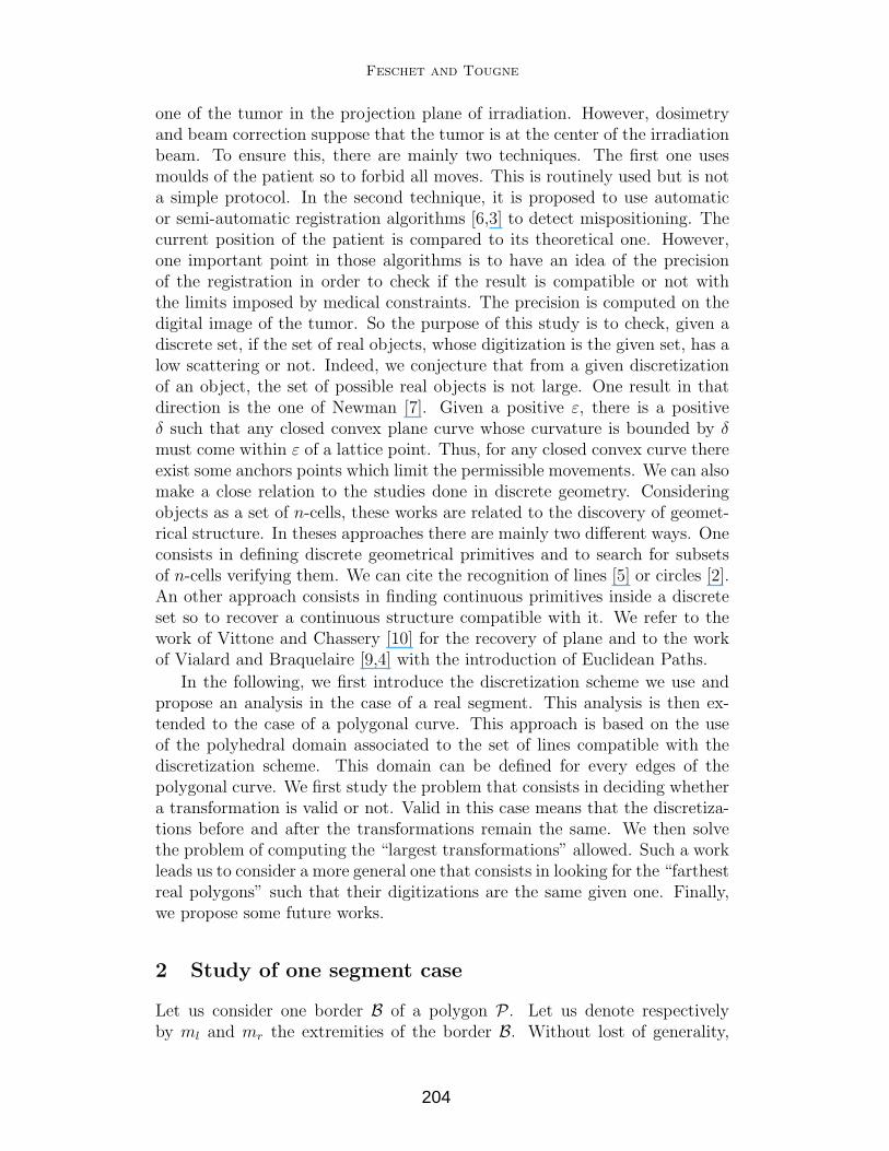
Many discretization schemes are possible. For the sake of clarity of theexplanations and figures, we can fix the process of digitization D. For example,we can consider D(B) to be the set of integer points (x, y) such that xMl

≤x ≤ xMr with xMl

= �xml� and xMr = �xmr, and y = [ax + b] where [x]

denote the nearest integer from x. But, the algorithms we will describe in thefollowing will be available for every “good” discretization process. The figure1 shows an example of real segment and its discretization obtained by such adigitization process.

2

4

6

8

5 10 15 20 25

Fig. 1. An example of real segment and its discretization

2.2 Intervals

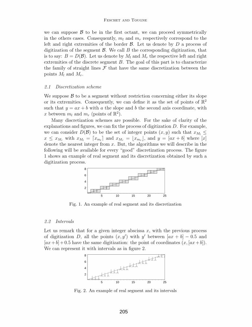
Let us remark that for a given integer abscissa x, with the previous processof digitization D, all the points (x, y′) with y′ between [ax + b] − 0.5 and[ax+ b]+0.5 have the same digitization: the point of coordinates (x, [ax+ b]).We can represent it with intervals as in figure 2.

2

4

6

8

5 10 15 20 25

Fig. 2. An example of real segment and its intervals

205

Feschet and Tougne

This remark leads us to formulate the problem of one straight line case asfollows.

Problem 2.1 What are the parameters A and B of the real lines of equationy = Ax + B that satisfy:

for all x in [Ml,Mr], [ax + b]− 0.5 < Ax + B ≤ [ax + b] + 0.5

In the following part, we explain a way to solve such a problem.

2.3 Resolution of one segment problem

The set of previous equations can be viewed as the constraint equations of atwo variables (A and B) linear programming problem and our goal is to findthe “feasible region” R in the A-B parameters space.

Such a problem has already been studied in a more general context byO’Rourke [8]. In his paper, O’Rourke presents an on-line linear algorithm forfitting straight lines between data ranges. As a matter of fact, each equationof the previous system represents two half-planes with parallel edges in theA-B space and the “feasible region” R can be constructed as the intersectionof such half-planes.

Consequently, if we suppose a segment to be given by these extremities(ml and mr), we can summarize the process as follows.

Feasible-Region-Segment (ml,mr)Compute the slope aCompute the second axis coordinate bCompute the coordinates of Ml and Mr

S = ∅For all x in [xMl

, xMr ]S = S ∪ {[ax + b]− 0.5 < Ax + B, Ax + B ≤ [ax + b] + 0.5}

R = SolveORourke(S)

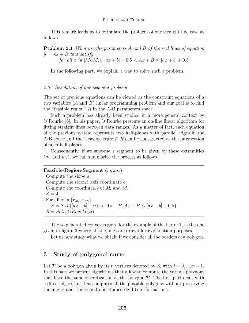
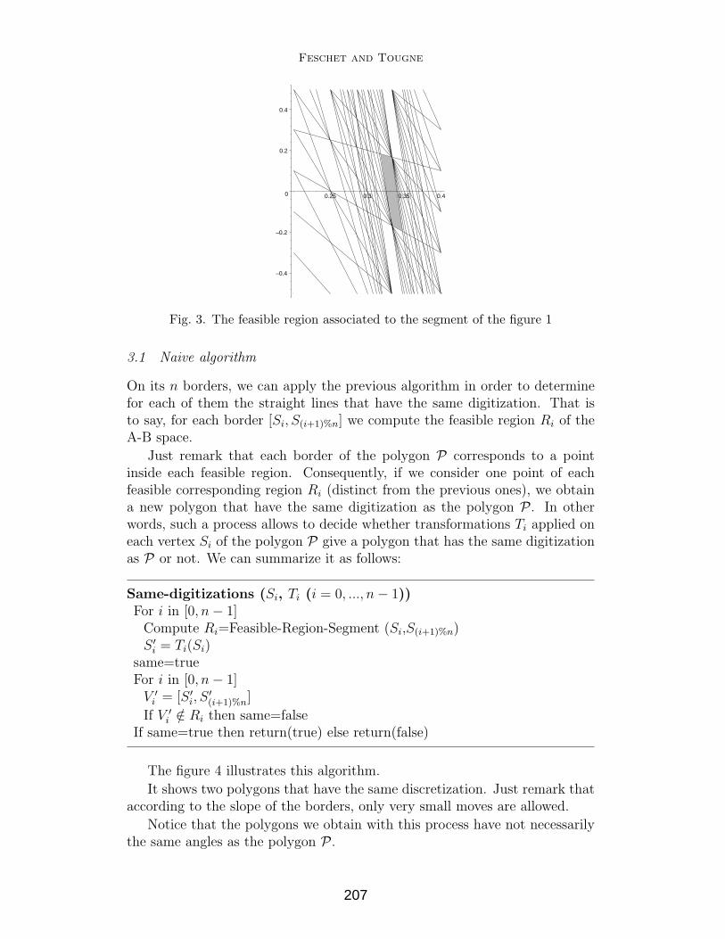
The so generated convex region, for the example of the figure 1, is the onegiven in figure 3 where all the lines are drawn for explanation purposes.

Let us now study what we obtain if we consider all the borders of a polygon.

3 Study of polygonal curve

Let P be a polygon given by its n vertices denoted by Si with i = 0, ..., n− 1.In this part we present algorithms that allow to compute the various polygonsthat have the same discretization as the polygon P . The first part deals witha direct algorithm that computes all the possible polygons without preservingthe angles and the second one studies rigid transformations.

206

Feschet and Tougne

–0.4

–0.2

0

0.2

0.4

0.25 0.3 0.35 0.4

Fig. 3. The feasible region associated to the segment of the figure 1

3.1 Naive algorithm

On its n borders, we can apply the previous algorithm in order to determinefor each of them the straight lines that have the same digitization. That isto say, for each border [Si, S(i+1)%n] we compute the feasible region Ri of theA-B space.

Just remark that each border of the polygon P corresponds to a pointinside each feasible region. Consequently, if we consider one point of eachfeasible corresponding region Ri (distinct from the previous ones), we obtaina new polygon that have the same digitization as the polygon P. In otherwords, such a process allows to decide whether transformations Ti applied oneach vertex Si of the polygon P give a polygon that has the same digitizationas P or not. We can summarize it as follows:

Same-digitizations (Si, Ti (i = 0, ..., n − 1))For i in [0, n − 1]Compute Ri=Feasible-Region-Segment (Si,S(i+1)%n)S ′

i = Ti(Si)same=trueFor i in [0, n − 1]

V ′i = [S ′

i, S′(i+1)%n]

If V ′i /∈ Ri then same=false

If same=true then return(true) else return(false)

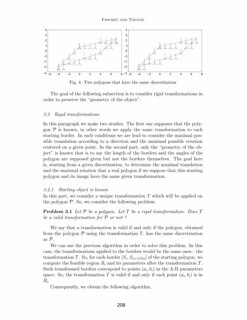
The figure 4 illustrates this algorithm.

It shows two polygons that have the same discretization. Just remark thataccording to the slope of the borders, only very small moves are allowed.

Notice that the polygons we obtain with this process have not necessarilythe same angles as the polygon P .

207

Feschet and Tougne

–4

–3

–2

–1

0

1

2

3

4

–6 –4 –2 0 2 4 6 8 –4

–3

–2

–1

0

1

2

3

4

–6 –4 –2 0 2 4 6 8

Fig. 4. Two polygons that have the same discretization

The goal of the following subsection is to consider rigid transformations inorder to preserve the “geometry of the object”.

3.2 Rigid transformations

In this paragraph we make two studies. The first one supposes that the poly-gon P is known, in other words we apply the same transformation to eachstarting border. In such conditions we are lead to consider the maximal pos-sible translation according to a direction and the maximal possible rotationcentered on a given point. In the second part, only the “geometry of the ob-ject” is known that is to say the length of the borders and the angles of thepolygon are supposed given but not the borders themselves. The goal hereis, starting from a given discretization, to determine the maximal translationand the maximal rotation that a real polygon if we suppose that this startingpolygon and its image have the same given transformation.

3.2.1 Starting object is known

In this part, we consider a unique transformation T which will be applied onthe polygon P . So, we consider the following problem.

Problem 3.1 Let P be a polygon. Let T be a rigid transformation. Does Tbe a valid transformation for P or not ?

We say that a transformation is valid if and only if the polygon, obtainedfrom the polygon P using the transformation T , has the same discretizationas P.

We can use the previous algorithm in order to solve this problem. In thiscase, the transformations applied to the borders would be the same ones : thetransformation T . So, for each border [Si, S(i+1)%n] of the starting polygon, wecompute the feasible region Ri and its parameters after the transformation T .Such transformed borders correspond to points (ai, bi) in the A-B parametersspace. So, the transformation T is valid if and only if each point (ai, bi) is inRi.

Consequently, we obtain the following algorithm.

208

Feschet and Tougne

Valid-Transformation (Si, T )For i in [0, n − 1]Compute Ri=Feasible-Region-Segment (Si,S(i+1)%n)S ′

i = T (Si)valid=trueFor i in [0, n − 1]

V ′i = [S ′

i, S′(i+1)%n]

If V ′i /∈ Ri then valid=false

If valid=true then return(true) else return(false)

The figure 5 illustrates this method. It shows the feasible region of each

0

0.2

0.4

0.6

0.8

1

1.2

1.4

1.6

1.8

2

0.2 0.4 0.6 0.8 1 1.2 1.4 1.6 1.8 2 0

0.2

0.4

0.6

0.8

1

1.2

1.4

1.6

1.8

2

0.2 0.4 0.6 0.8 1

–5

–4

–3

–2

–1

00.2 0.4 0.6 0.8 1 1.2 1.4 1.6 1.8 2

–3

–2.5

–2

–1.5

–1

–0.5

00.2 0.4 0.6 0.8 1

Fig. 5. Feasible region of each border of the polygons of the figure 4 and thecorresponding points of the started (points) and obtained (crosses) borders

border of the polygons of the figure 4 and the corresponding points of thestarted (points) and obtained (crosses) borders.

209

Feschet and Tougne

Such an approach leads us to study the “maximal possible transforma-tions”. In fact, we first interest ourselves to the maximal possible translationaccording to a direction and generalize the result to general transformations.

Let us consider the case of translation. Then the goal is to compute thelargest α such that the translation of vector α(vx, vy) is valid for the startingpolygon P . As a translation corresponds to a vertical move of the correspond-ing point in the feasible region, it is enough to compute for each border thecorresponding parameter B′

i obtained after translation (function of α). Thenthe maximal possible translation is given by taking the largest α such thatall the obtained points are inside the corresponding feasible regions. Thealgorithm is the following one.

Maximal-Translation (Si, (vx, vy))For i in [0, n − 1]Compute Ri=Feasible-Region-Segment (Si,S(i+1)%n)B′

i = Bi + α(vy − Aivx)Compute αmax

i such that B′i ∈ Ri

α = min{αmaxi | i = 0 . . . n − 1}

return(α)

Just remark that the case of rotation is quite similar. As a matter of fact,we can decompose a rotation centered on any point into a rotation centered onan extremity of the border and a translation. As previously, the translationcorresponds to a vertical move of the corresponding point in the feasible regionand the rotation centered on an extremity of the border corresponds to anhorizontal move (only the slope of the border changes). Consequently, we justhave to compute for each border the corresponding parameters obtained in thefeasible region. Such parameter are functions of α the angle of the rotationand the maximal rotation is given by the maximal angle such that all thecorresponding points are inside the feasible regions.

More generally, every transformation that can be decomposed into a rota-tion and a translation can be proceeded as previously.

Until here we have supposed the starting polygon P to be known. In fact,it corresponds to a preliminary work to a more general one which consistsin finding the “farthest real polygons” which correspond to the same givendigitization. In the following part, we explain such a problem and give someideas according to the previous paragraphs to solve it.

3.2.2 Unknown borders

In the following, we do not suppose to know the borders of the real polygonbut only its angles (αi). Thus, the data is composed of those angles and thedigitization of the real polygon. From this digitization, we can compute allthe feasible regions of the different borders using the previous algorithms. We

210

Feschet and Tougne

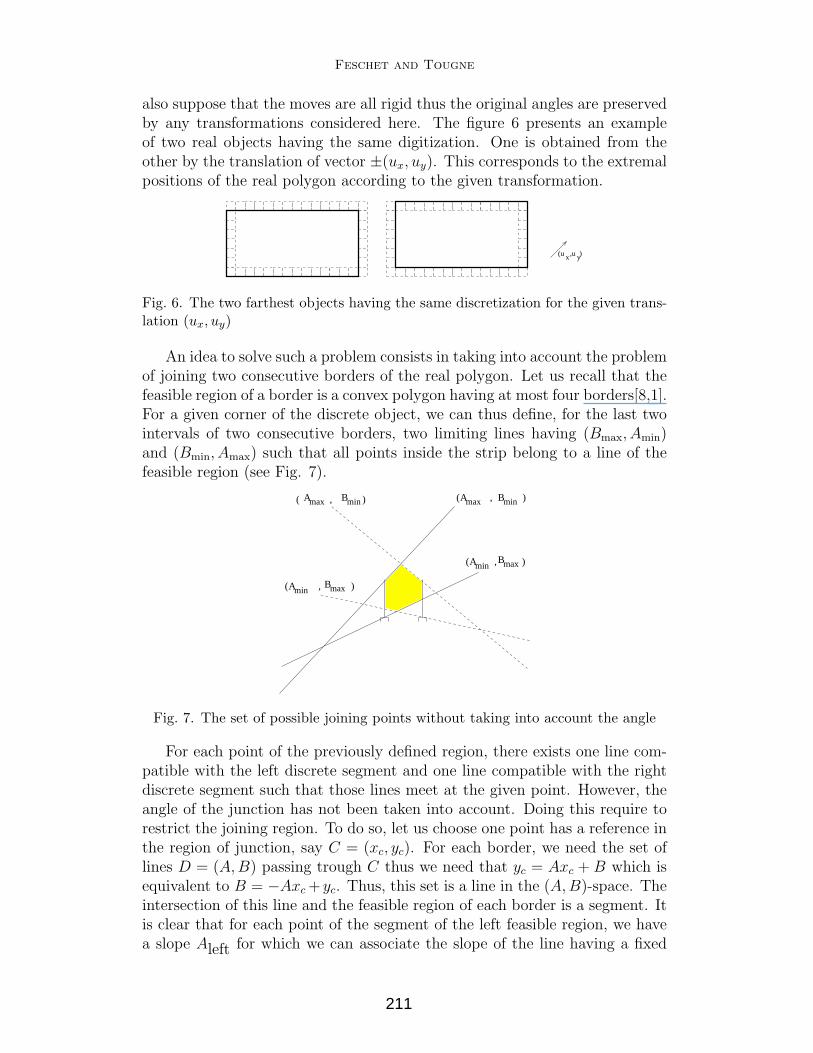
also suppose that the moves are all rigid thus the original angles are preservedby any transformations considered here. The figure 6 presents an exampleof two real objects having the same digitization. One is obtained from theother by the translation of vector ±(ux, uy). This corresponds to the extremalpositions of the real polygon according to the given transformation.

x(u ,u )y

Fig. 6. The two farthest objects having the same discretization for the given trans-lation (ux, uy)

An idea to solve such a problem consists in taking into account the problemof joining two consecutive borders of the real polygon. Let us recall that thefeasible region of a border is a convex polygon having at most four borders[8,1].For a given corner of the discrete object, we can thus define, for the last twointervals of two consecutive borders, two limiting lines having (Bmax, Amin)and (Bmin, Amax) such that all points inside the strip belong to a line of thefeasible region (see Fig. 7).

AminBmax

BminAmax

AminBmax

BminAmax( , )( , )

( , )

( , )

Fig. 7. The set of possible joining points without taking into account the angle

For each point of the previously defined region, there exists one line com-patible with the left discrete segment and one line compatible with the rightdiscrete segment such that those lines meet at the given point. However, theangle of the junction has not been taken into account. Doing this require torestrict the joining region. To do so, let us choose one point has a reference inthe region of junction, say C = (xc, yc). For each border, we need the set oflines D = (A,B) passing trough C thus we need that yc = Axc + B which isequivalent to B = −Axc+ yc. Thus, this set is a line in the (A, B)-space. Theintersection of this line and the feasible region of each border is a segment. Itis clear that for each point of the segment of the left feasible region, we havea slope Aleft for which we can associate the slope of the line having a fixed

211

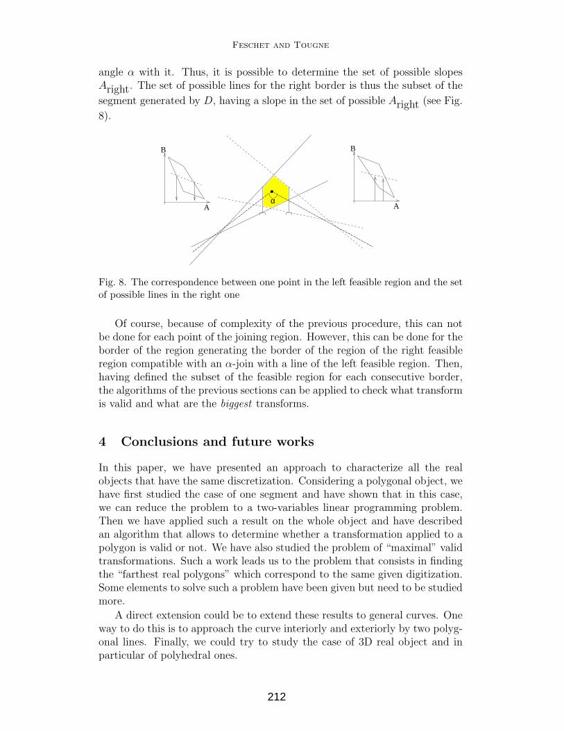
Feschet and Tougne

angle α with it. Thus, it is possible to determine the set of possible slopesAright. The set of possible lines for the right border is thus the subset of the

segment generated by D, having a slope in the set of possible Aright (see Fig.

8).

B B

AAα

Fig. 8. The correspondence between one point in the left feasible region and the setof possible lines in the right one

Of course, because of complexity of the previous procedure, this can notbe done for each point of the joining region. However, this can be done for theborder of the region generating the border of the region of the right feasibleregion compatible with an α-join with a line of the left feasible region. Then,having defined the subset of the feasible region for each consecutive border,the algorithms of the previous sections can be applied to check what transformis valid and what are the biggest transforms.

4 Conclusions and future works

In this paper, we have presented an approach to characterize all the realobjects that have the same discretization. Considering a polygonal object, wehave first studied the case of one segment and have shown that in this case,we can reduce the problem to a two-variables linear programming problem.Then we have applied such a result on the whole object and have describedan algorithm that allows to determine whether a transformation applied to apolygon is valid or not. We have also studied the problem of “maximal” validtransformations. Such a work leads us to the problem that consists in findingthe “farthest real polygons” which correspond to the same given digitization.Some elements to solve such a problem have been given but need to be studiedmore.

A direct extension could be to extend these results to general curves. Oneway to do this is to approach the curve interiorly and exteriorly by two polyg-onal lines. Finally, we could try to study the case of 3D real object and inparticular of polyhedral ones.

212

Feschet and Tougne

Acknowledgments

We thank Professor Serge Miguet of University of Lyon 2 for his constantsupport.

References

[1] Anderson, T. A. and C. E. Kim, Representation of digital line segments andtheir preimages, in: Seventh International Conference on Pattern Recognition(Montreal, Canada, July 30-August 2, 1984), IEEE Publ. 84CH2046-1 (1984),pp. 501–504.

[2] Andres, E., Discrete Circles, Rings and Spheres, Computer and Graphics 18(1994), pp. 695–706.

[3] Bansal, R., L. Staib, Z. Chn, A. Rangarajan, J. Knisely, R. Nath and J. Duncan,A novel approach for the registration of 2d portal and 3d ct images for treatmentsetup verification in radiotherapy, in: W. Wells, A. Colchester and S. Delp,editors, MICCAI 98, LNCS 1496 (1998).

[4] Braquelaire, J. P. and A. Vialard, Euclidean Paths: A new Representation ofBoundary of Discrete Regions, Graphical Models and Image Processing 61(1999), pp. 16–43.

[5] Debled-Rennesson, I. and J. P. Reveilles, A linear algorithm for segmentation ofdigital curves, Parallel Image Analysis: Theory and Applications (1993), pp. 73–100.

[6] Feschet, F., “Technique d’imagerie pour l’aide au positionnement en dosimetrieconformationnelle,” Ph.D. thesis, Insa de Lyon (1999).

[7] Newman, D. J., A gradually turning curve must come near a lattice point,Journal of Number Theory 6 (1974), pp. 7–10.

[8] O’Rourke, J., An on-line algorithm for fitting straight lines between data ranges,Communications of the ACM 24 (1981), pp. 574–578.

[9] Vialard, A., Geometrical parameters extraction from discrete paths, in:S. Miguet, A. Montanvert and S. Ubeda, editors, 6th International Conferenceon Discrete Geometry for Computer Imagery (DGCI’96), LNCS 1176 (1996),pp. 24–35.

[10] Vittone, J. and J. M. Chassery, (n-m)-cubes and farey nets for naiveplanes understanding, in: G. Bertrand, M. Couprie and L. Perroton, editors,8th International Conference on Discrete Geometry for Computer Imagery(DGCI’99), LNCS 1568 (1999), pp. 76–87.

213