An Analytical Model of Reactive Diffusion for Transient Electronics

www.afm-journal.de

FULL

PAPER

310

www.MaterialsViews.com

Rui Li , Huanyu Cheng , Yewang Su , Suk-Won Hwang , Lan Yin , Hu Tao , Mark A. Brenckle , Dae-Hyeong Kim , Fiorenzo G. Omenetto , John A. Rogers , * and Yonggang Huang *

An Analytical Model of Reactive Diffusion for Transient Electronics

6

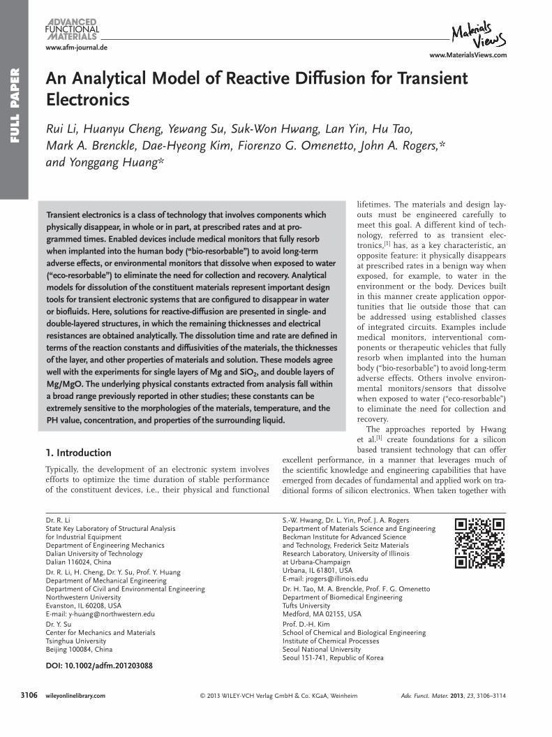
Transient electronics is a class of technology that involves components which physically disappear, in whole or in part, at prescribed rates and at pro-grammed times. Enabled devices include medical monitors that fully resorb when implanted into the human body (“bio-resorbable”) to avoid long-term adverse effects, or environmental monitors that dissolve when exposed to water (“eco-resorbable”) to eliminate the need for collection and recovery. Analytical models for dissolution of the constituent materials represent important design tools for transient electronic systems that are confi gured to disappear in water or biofl uids. Here, solutions for reactive-diffusion are presented in single- and double-layered structures, in which the remaining thicknesses and electrical resistances are obtained analytically. The dissolution time and rate are defi ned in terms of the reaction constants and diffusivities of the materials, the thicknesses of the layer, and other properties of materials and solution. These models agree well with the experiments for single layers of Mg and SiO 2 , and double layers of Mg/MgO. The underlying physical constants extracted from analysis fall within a broad range previously reported in other studies; these constants can be extremely sensitive to the morphologies of the materials, temperature, and the PH value, concentration, and properties of the surrounding liquid.

1. Introduction

Typically, the development of an electronic system involves efforts to optimize the time duration of stable performance of the constituent devices, i.e., their physical and functional

© 2013 WILEY-VCH Verlag GmbH & Co. KGaA, Weinheimwileyonlinelibrary.com

DOI: 10.1002/adfm.201203088

Dr. R. LiState Key Laboratory of Structural Analysis for Industrial Equipment Department of Engineering Mechanics Dalian University of Technology Dalian 116024, China Dr. R. Li, H. Cheng, Dr. Y. Su, Prof. Y. HuangDepartment of Mechanical Engineering Department of Civil and Environmental Engineering Northwestern University Evanston, IL 60208, USA E-mail: [email protected] Dr. Y. SuCenter for Mechanics and Materials Tsinghua University Beijing 100084, China

S.-W. Hwang, Dr. L. Yin,Department of MaterialBeckman Institute for Aand Technology, FrederiResearch Laboratory, Unat Urbana-Champaign Urbana, IL 61801, USA E-mail: jrogers@illinois Dr. H. Tao, M. A. BrenckDepartment of BiomediTufts University Medford, MA 02155, US Prof. D.-H. KimSchool of Chemical andInstitute of Chemical PrSeoul National UniversiSeoul 151-741, Republic

lifetimes. The materials and design lay-outs must be engineered carefully to meet this goal. A different kind of tech-nology, referred to as transient elec-tronics, [ 1 ] has, as a key characteristic, an opposite feature: it physically disappears at prescribed rates in a benign way when exposed, for example, to water in the environment or the body. Devices built in this manner create application oppor-tunities that lie outside those that can be addressed using established classes of integrated circuits. Examples include medical monitors, interventional com-ponents or therapeutic vehicles that fully resorb when implanted into the human body (“bio-resorbable”) to avoid long-term adverse effects. Others involve environ-mental monitors/sensors that dissolve when exposed to water (“eco-resorbable”) to eliminate the need for collection and recovery.

The approaches reported by Hwang et al. [ 1 ] create foundations for a silicon based transient technology that can offer

excellent performance, in a manner that leverages much of the scientifi c knowledge and engineering capabilities that have emerged from decades of fundamental and applied work on tra-ditional forms of silicon electronics. When taken together with

Prof. J. A. Rogerss Science and Engineering dvanced Science ck Seitz Materials iversity of Illinois

.edu le, Prof. F. G. Omenettocal Engineering

A

Biological Engineering ocesses ty of Korea

Adv. Funct. Mater. 2013, 23, 3106–3114

http://doi.wiley.com/10.1002/adfm.201203088

FULL P

APER

www.afm-journal.dewww.MaterialsViews.com

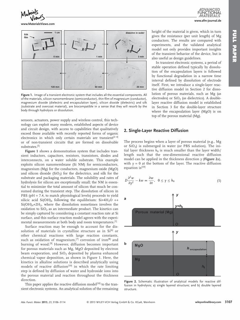
Figure 1 . Image of a transient electronic system that includes all the essential components. All of the materials, silicon nanomembrane (semiconductor), thin fi lm of magnesium (conductor), magnesium dioxide (dielectric and encapsulation layer), silicon dioxide (dielectric) and silk (substrate and overcoat material), are biocompatible in a sense that they will resorb by the body through hydrolysis or dissolution.

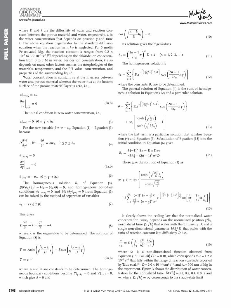
Figure 2 . Schematic illustration of analytical models for reactive dif-fusion in hydrolysis; a) single layered structure; and b) double layered structure.

sensors, actuators, power supply and wireless control, this tech-nology can exploit many modern, established aspects of device and circuit design, with access to capabilities that qualitatively exceed those available with recently reported forms of organic electronics in which only certain materials are transient [ 2 − 4 ] or of non-transient circuits that are formed on dissolvable substrates. [ 5 ]

Figure 1 shows a demonstration system that includes tran-sient inductors, capacitors, resistors, transistors, diodes and interconnects, on a water soluble substrate. This example exploits silicon nanomembrane (Si NM) for semiconductors, magnesium (Mg) for the conductors, magnesium oxide (MgO) and silicon dioxide (SiO 2 ) for the dielectrics, and silk for the substrate and packaging materials. The solubility and rates of hydrolysis for silicon are exceptionally small; the NM is essen-tial to minimize the total amount of silicon that much be con-sumed during the transient step. The dissolution of silicon in PBS (pH = 7.4, to match physiological levels) proceeds to yield silicic acid Si(OH) 4 following the equilibrium: Si + 4H 2 O ↔ Si(OH) 4 + 2H 2 , where the dissolution sometimes involves the oxidation to SiO 2 as an intermediate product. The kinetics can be simply captured by considering a constant reaction rate at Si surface, and this surface reaction model agrees with the experi-mental measurements at both body and room temperatures. [ 1 ]

Surface reaction may be enough to account for the dis-solution of materials in crystalline structure as in Si [ 6 ] or other chemical reactions with large reaction constants, such as oxidation of magnesium, [ 7 ] corrosion of iron [ 8 ] and burning of wood. [ 9 ] However, diffusion becomes important for porous materials such as Mg, MgO deposited by electron beam evaporation, and SiO 2 deposited by plasma enhanced chemical vapor deposition, as shown in Figure 1 . Here, the kinetics in alkaline solutions is described analytically using models of reactive diffusion [ 10 ] in which the rate limiting step is defi ned by diffusion of water and hydroxide ions into the porous material and reaction throughout the thickness direction.

This paper applies the reactive diffusion model [ 10 ] to the tran-sient electronic systems. An analytical solution of the remaining

© 2013 WILEY-VCH Verlag GmbH & Co. KGaA, WeinAdv. Funct. Mater. 2013, 23, 3106–3114

height of the material is given, which in turn gives the resistance (per unit length) of Mg conductors. The results are compared with experiments, and the validated analytical model not only provides important insights of the transient behavior of the device, but is also useful as design guidelines.

In transient electronic systems, a period of stable operation defi ned typically by dissolu-tion of the encapsulation layers is followed by functional degradation in a narrow time interval defi ned by dissolution of electrode itself. First, we introduce a single-layer reac-tive diffusion model in Section 2 for disso-lution of porous materials, such as Mg (as electrodes) or SiO 2 (as dielectrics). A double-layer reactive diffusion model is established in Section 3 for the double-layer structure where the encapsulation layer (MgO) is on top of the porous material (Mg).

2. Single-Layer Reactive Diffusion

The process begins when a layer of porous material (e.g., Mg or SiO 2 ) is submerged in water (or PBS solution). The ini-tial layer thickness h 0 is much smaller than the layer width/length such that the one-dimensional reactive diffusion model can be applied in the thickness direction y ( Figure 2 a), with y = 0 at the bottom of the layer. The reactive diffusion equation is [ 10 ]

D

∂2w

∂y2− kw = ∂w

∂t, 0 ≤ y ≤ h0

(1)

3107wileyonlinelibrary.comheim

FULL

PAPER

3108


where D and k are the diffusivity of water and reaction con-stant between the porous material and water, respectively, w is the water concentration that depends on position y and time t . The above equation degenerates to the standard diffusion equation when the reaction term kw is neglected. For 5 mol% Fe-activated Mg, the reaction constant k ranges from 0.2 × 10 − 3 to 3 × 10 − 3 s − 1 , [ 11 ] depending on the chloride ion concentra-tion from 0 to 5 M in water. Besides ion concentration, k also depends on many other factors such as the morphologies of the materials, temperature, and the PH value, concentration, and properties of the surrounding liquid.

Water concentration is constant w 0 at the interface between water and porous material whereas the water fl ux at the bottom surface of the porous material layer is zero, i.e.,

w|y=h0= w0

∂w

∂y

∣∣∣∣y=0

= 0

(2a,b)

The initial condition is zero water concentration, i.e.,

w|t=0 = 0 (0 ≤ y < h0) (3)

For the new variable θ = w − w 0 , Equation (1) – Equation (3) become

D

∂2θ

∂y2− kθ − ∂θ

∂t= kw0, 0 ≤ y ≤ h0

(4)

θ |y=h0= 0

∂θ

∂y

∣∣∣∣y=0

= 0

(5a,b)

θ |t=0 = −w0 (0 ≤ y < h0) (6)

The homogeneous solution θ h of Equation (4) , D∂2θh

/∂y2 − kθh − ∂θh/∂t = 0 , and homogeneous boundary

conditions θh|y=h0= 0 and ∂θh/∂y|y=0 = 0 from Equation (5)

can be solved by the method of separation of variables

θh = Y (y) T (t) (7)

This gives

D

Y ′ ′

Y− k = T ′

T= −λ

(8)

where λ is the eigenvalue to be determined. The solution of Equation (8) is

Y = A sin

(√λ − k

Dy

)+ B cos

(√λ − k

Dy

)

T = e−λt

(9a,b)

where A and B are constants to be determined. The homoge-neous boundary conditions become Y|y=h0

= 0 and Y ′ | y = 0 = 0, which give A = 0 and

wileyonlinelibrary.com © 2013 WILEY-VCH Verlag G

cos

(√λ − k

Dh0

)= 0

(10)

Its solution gives the eigenvalues

λn =

(2n − 1

2h0π

)2

D + k (n = 1, 2, 3, · · ·)

(11)

The homogeneous solution is

θh =

∞∑n=1

{Bne

−[(

2n−12h0

π)2

D+k

]tcos

(2n − 1

2h0πy

)}

(12)

where the constants B n are to be determined. The general solution of Equation (4) is the sum of homoge-

neous solution in Equation (12) and a particular solution,

θ =∞∑

n= 1

{Bne

−[(

2n−12h0

π)2

D+ k

]tcos

(2n − 1

2h0πy

)}

+ w0

⎡⎢⎣ cosh

(√kD y)

cosh(√

kD h0

) − 1

⎤⎥⎦

(13)

where the last term is a particular solution that satisfi es Equa-tion (4) and Equation (5) . Substitution of Equation (13) into the initial condition in Equation (6) gives

Bn = 4 (−1)n (2n − 1) π Dw0

4kh20 + (2n − 1)2 π 2 D

(14)

These give the solution of Equation (1) as

w (y, t) = w0

⎧⎪⎪⎨⎪⎪⎩

cosh(√

kh20

Dy

h0

)

cosh√

kh20

D

+ 2∞∑

n= 1

(−1)n n − 12

)π

kh20

D + n − 12

)2π 2

e−[

kh20

D + (n− 12 )2

π2

]Dth2

0 cos[(

n − 1

2

)π

y

h0

]⎫⎬⎭

(15)

It clearly shows the scaling law that the normalized water concentration, w / w 0 , depends on the normalized position y / h 0 , normalized time Dt

/h2

0 that scales with the diffusivity D , and a single non-dimensional parameter kh2

0

/D that scales with the

ratio of reaction constant k to diffusivity D , i.e.,

w

w0= w̄

(y

h0,

Dt

h20

,kh2

0

D

)

(16)

where w̄ is a non-dimensional function obtained from Equation (15) . For kh2

0

/D = 0.18, which corresponds to k = 1.2 ×

10 − 3 s − 1 that falls within the range of reaction constants reported by Taub et al., [ 11 ] D = 6.0 × 10 − 12 cm 2 s − 1 , and h 0 = 300 nm of Mg in the experiment, Figure 3 shows the distribution of water concen-tration for the normalized time Dt

/h2

0 = 0.1, 0.2, 0.4, 0.8, 2 and ∞ , where Dt

/h2

0 = ∞ corresponds to the steady-state limit

mbH & Co. KGaA, Weinheim Adv. Funct. Mater. 2013, 23, 3106–3114

FULL P

APER


Figure 3 . Distribution of water concentration in the Mg layer.

0w

w

0y h

20 0.1Dt h

0.2

0.4

2

∞

0.8

0.00 0.25 0.50 0.75 1.000.00

0.25

0.50

0.75

1.00

20 0.18kh D =

=

w (y, t → ∞) = w0

cosh(√

kh20

Dy

h0

)

cosh√

kh20

D

(17)

which is effectively attained at fi nite time Dt/

h20 = 2. Figure 4

shows the water concentration versus time at the middle ( y = h 0 /2) and bottom ( y = 0) of the layer. It confi rms that the steady-state limit is reached at Dt

/h2

0 = 2. Let q denote the number of water molecules that react with

each atom of the porous material. Since kw gives the mass

© 2013 WILEY-VCH Verlag G

Figure 4 . Water concentration versus time at the middle ( y/h0 = 1/2 ) and bottom ( y/h0 = 0 ) of the Mg layer.

0.0 0.5 1.0 1.5 2.00.00

0.25

0.50

0.75

1.00

0w

w

20Dt h

20 0.18kh D

0 0=

=

y h

1 2

Adv. Funct. Mater. 2013, 23, 3106–3114

of water that reacts at a given location (per unit volume), the mass of dissolved porous material (per unit volume) is kwM

/(q MH2O

) , where M and MH2O are the molar masses of

porous material and water, respectively. The net mass of porous material dissolved is obtained by integrating Equation (15) over both the thickness direction y and time t , where in turn gives a scaling law of the thickness h of the porous material layer nor-malized by its initial thickness h 0 before complete physical dis-appearance as

h

h0= 1 − w0 M

qρMH2O

kh20

D⎧⎪⎪⎨⎪⎪⎩

Dt

h20

· tanh√

kh20

D√kh2

0D

− 2∞∑

n=1

1 − e−[

kh20

D +(n− 12 )2

π2

]Dth2

0[kh2

0D + (

n − 12

)2π 2]2

⎫⎪⎪⎬⎪⎪⎭

(18)

where ρ is the mass density of porous material. It is clear that the normalized thickness, h / h 0 , depends on the normalized time Dt

/h2

0 , non-dimensional parameter kh20

/D , and is linear

with a single combination of water concentration w 0 and mass density ρ of porous material, w0 M

/(qρMH2O

) .

For the parameters k and D in the present study, the summa-tion on the right hand side of Equation (18) is negligible such that the thickness has a simple and approximate expression

h ≈ h0 − w0 M

qρMH2O

√kD tanh

√kh2

0

D· t

(19)

which decreases linearly with time t . This means that the steady-state solution in Equation (17) dominates the contribu-tion to the water concentration in Equation (15) . The normal-ized form of Equation (19) is

h

h0≈ 1 − t

tc (20)

where

tc = h0√kD

qρMH2O

w0 M

1

tanh√

kh20

D (21)

is the critical time for the thickness to reach zero. For Mg (molar mass M = 24 g mol − 1 , mass density ρ = 1.738 g cm − 3 ) with the initial thickness h 0 = 300 nm to react with water (molar mass MH2O = 18 g mol−1 , water concentration w 0 = 1 g cm − 3 , and q = 2 water molecules reacting with 1 Mg atom), this crit-ical time t c is 38 min, which agrees reasonably well with experi-ments, to be discussed in Figure 5 . Equation (20) shows that the thickness deceases linearly with time. Therefore, the rate of dissolution is

vdissolution = −dh

dt≈ h0

tc=

√kD

w0 M

qρMH2Otanh

√kh2

0

D (22)

As shown in Table 1 , the rate of dissolution is 0.044, 0.13, and 0.20 nm s − 1 (or equivalently 160, 470, and 710 nm h − 1 ) for 100, 300, and 500-nm-thick Mg layers, respectively. They are on the same order as the rate of dissolution reported in

3109wileyonlinelibrary.commbH & Co. KGaA, Weinheim

FULL

PAPER

3110


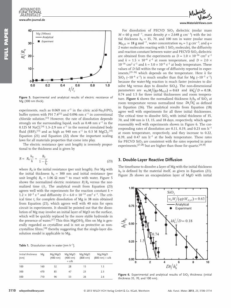
Figure 5 . Experimental and analytical results of electric resistance of Mg (300 nm thick).

0.0 0.2 0.4 0.6 0.8 1.00

10

20

30

40

Analytical

Experiment

ct t

0R

R

Mg (300nm)

0h

h

20 0.63H Ow M q M

20 0.18kh D

0.74

0.50

0.75

1.00

Analytical Experiment

2SiO

ρ( ( =

=

experiments, such as 0.069 nm s − 1 in the citric acid-Na 2 HPO 4 buffer system with PH 7.4 [ 12 ] and 0.096 nm s − 1 in conventional chloride solution. [ 13 ] However, the rate of dissolution depends strongly on the surrounding liquid, such as 0.48 nm s − 1 in the 0.125 M NaCl, [ 14 ] 1.3–2.9 nm s − 1 in the normal simulated body fl uid (SBF), [ 15 ] and as high as 940 nm s − 1 in 0.3 M MgCl 2 . [ 16 ] Equation (21) and Equation (22) show the important scaling laws for all materials properties that come into play.

The electric resistance (per unit length) is inversely propor-tional to the thickness and is given by

R = R0h0

h≈

R0

1 − ttc

(23)

where R 0 is the initial resistance (per unit length). For Mg with the initial thickness h 0 = 300 nm and initial resistance (per unit length) R 0 = 1.06 Ω mm − 1 to react with water, Figure 5 shows the normalized electric resistance R / R 0 versus the nor-malized time t / t c . The analytical result from Equation (23) agrees well with the experiments for the reaction constant k = 1.2 × 10 − 3 s − 1 and diffusivity D = 6.0 × 10 − 12 cm 2 s − 1 . The crit-ical time t c for complete dissolution of Mg is 38 min obtained from Equation (21) , which agrees well with 40 min for open circuit in experiments. It should be pointed out that the disso-lution of Mg may involve an initial layer of MgO on the surface, which will be quickly replaced by the more stable hydroxide in the presence of water. [ 17 ] This thin Mg(OH) 2 fi lm on Mg is gen-erally regarded as crystalline and is not as protective as non-crystalline fi lms, [ 18 ] thereby suggesting that the single-layer dis-solution model is applicable to Mg.


Table 1. Dissolution rate in water [nm h − 1 ].

Initial thickness [nm]

Mg Mg/MgO (400 nm)

Mg/MgO (400 nm)

+ silk

Mg/MgO (800 nm)

Mg/MgO (800 nm) + silk

100 160 52 28 15 1.5

300 470 85 47 23 2.3

500 710 96 53 26 2.6

For dissolution of PECVD SiO 2 dielectric (molar mass M = 60 g mol − 1 , mass density ρ = 2.648 g cm − 3 ) with the ini-tial thickness h 0 = 35, 70, and 100 nm in water (molar mass MH2O = 18 g mol−1 , water concentration w 0 = 1 g cm − 3 , and q = 2 water molecules reacting with 1 SiO 2 molecule), the diffusivity and reaction constant between water and PECVD SiO 2 dielectric are obtained from the experiments as D = 1.0 × 10 − 16 cm 2 s − 1 and k = 1.5 × 10 − 6 s − 1 at room temperature, and D = 2.0 × 10 − 16 cm 2 s − 1 and k = 3.0 × 10 − 6 s − 1 at body temperature. These values of D fall within the range of diffusivity reported in exper-iments, [ 19 − 26 ] which depends on the temperature. Here k for SiO 2 ( ∼ 10 − 6 s − 1 ) is much smaller than that for Mg ( ∼ 10 − 3 s − 1 ) because the water-Mg reaction is much faster (minutes to dis-solve Mg versus days to dissolve SiO 2 ). The non-dimensional parameters are w0 M

/(qρMH2O

) = 0.63 and kh20

/D = 0.18 ,

0.74 and 1.5 for three initial thicknesses and room tempera-ture. Figure 6 shows the normalized thickness h / h 0 of SiO 2 at room temperature versus normalized time Dt

/h2

0 as defi ned in Equation (16) . The analytical results from Equation (18) agree well with experiments for all three initial thicknesses. The critical time to dissolve SiO 2 with initial thickness of 35, 70, and 100 nm is 13, 15, and 18 days, respectively, which agree reasonably well with experiments shown in Figure 6 . The cor-responding rates of dissolution are 0.11, 0.19, and 0.23 nm h − 1 at room temperature, respectively, and they increase to 0.22, 0.39, and 0.47 nm h − 1 at the body temperature. These rates for PECVD SiO 2 are consistent with the rates reported in prior experiments, [ 27 , 28 ] but are higher than those for quartz. [ 29 , 30 ]

3. Double-Layer Reactive Diffusion

The timeframe to dissolve a layer of Mg with the initial thickness h 0 is defi ned by the material itself, as given in Equation (21) . Figure 2 b shows an encapsulation layer of MgO with initial

mbH & Co. KGaA, Weinheim

Figure 6 . Experimental and analytical results of SiO 2 thickness (initial thickness 35, 70, and 100 nm).

20Dt h

1.5

0 2 4 6 8 100.00

0.25

Adv. Funct. Mater. 2013, 23, 3106–3114

FULL P

APER


thickness h encapsulation to provide another stage that the device functions stably. For the Mg layer, the reactive diffusion equa-tion (1) , zero water fl ux condition at the bottom surface y = 0 in Equation (2b) , and zero initial condition at t = 0 in Equation (3) still hold. For the MgO encapsulation, the governing equation, boundary condition and initial condition are

Dencapsulation∂2w

∂y2− kencapsulationw

= ∂w

∂t

(h0 ≤ y ≤ h0 + hencapsulation

)w|y=h0+hencapsulation

= w0

w|t=0 = 0(h0 ≤ y ≤ h0 + hencapsulation

)

(24a-c)

where D encapsulation and k encapsulation are the diffusivity of water and reaction constant between the encapsulation layer (e.g., MgO) and water, respectively. The constant water concentration condition in Equation (2a) is replaced by the continuity of concentration and fl ux of water molecules across the MgO/Mg interface, i.e.,

w|y=h0−0 = w|y=h0+0

D∂w

∂y

∣∣∣∣y=h0−0

= Dencapsulation∂w

∂y

∣∣∣∣y=h0+0

.

(25a,b)

The water concentration w can be represented by a sum of the homogenous solution w h and a particular solution w p , i.e., w = w h + w p . Here the homogeneous solution w h satisfi es the following homogeneous boundary equations and boundary conditions

⎧⎪⎪⎨⎪⎪⎩

D′ ∂2wh∂y2 − k′wh = ∂wh

∂t

wh|y=h0+hencapsulation= 0

∂wh∂y

∣∣∣y=0

= 0

(26a-c)

where D ′ = D and k ′ = k for 0 ≤ y ≤ h 0 , and D ′ = D encapsulation and k ′ = k encapsulation for h 0 ≤ y ≤ h 0 + h encapsulation . The above equa-tion can be solved by the method of separation variables, which gives the solution

wh =

⎧⎪⎪⎪⎪⎪⎨⎪⎪⎪⎪⎪⎩

Ee−λt cos(√

λ−kD y

), 0 ≤ y ≤ h0

F e−λt sin[√λ−kencapsulation

Dencapsulation

(h0 + hencapsulation − y

)],

h0 ≤ y ≤ h0 + hencapsulation (27a,b)

where E and F are constants to be determined. The continuity conditions in Equation (25) is applied to the homogeneous solution, which gives

⎡⎣ cos

(√λ−k

D h0

)−√(λ − k) D sin

(√λ−k

D h0

)− sin

(√λ−kencapsulation

Dencapsulationhencapsulation

)√

λ − kencapsulation

)Dencapsulation cos

(√λ−kencapsulation


)⎤⎥⎥⎦

(EF

)= 0

(28)

© 2013 WILEY-VCH Verlag GAdv. Funct. Mater. 2013, 23, 3106–3114

The vanishing of its determinant, in order to have a non-trivial solution, leads to the following eigen equation

tan

√λ − k

Dh2

0 tan

√λ − kencapsulation

Dencapsulationh2

encapsulation

=

√λ − kencapsulation

)Dencapsulation

(λ − k) D

(29)

from which a series of roots λ n ( n = 1, 2, 3, ···) can be deter-mined. The homogeneous solution can then be obtained as

wh = w0

∞∑n=1

Cne−λnt fn (y)

(30)

where the coeffi cients C n , which replace E and F via Equa-tion (28) , are to be determined, and

fn (y) ≡

⎧⎪⎪⎪⎪⎪⎪⎪⎪⎪⎪⎨⎪⎪⎪⎪⎪⎪⎪⎪⎪⎪⎩

sin(√

λn−kencapsulation


)cos

(√λn−k

D y)

, 0 ≤ y ≤ h0

cos(√

λn−kD h0

)sin[√

λn−kencapsulation

Dencapsulation

(h0 + hencapsulation − y

)],


The particular solution w p , satisfying the Equations (1) and Equation (24a) , non-homogeneous boundary conditions (2b) and (24b), and continuity conditions (25), is obtained as

wp = w0g (y) (32)

where

g (y) ≡

⎧⎪⎪⎪⎪⎪⎨⎪⎪⎪⎪⎪⎩

G cosh(√

kD y)

, 0 ≤ y ≤ h0

cosh(ξ

h0+hencapsulation−y

hencapsulation

)−H sinh

(ξ

h0+hencapsulation−y

hencapsulation

),


G = 1√Dk

Dencapsulationkencapsulationsinh

√kh2

0D sinh ξ + cosh

√kh2

0D cosh ξ

H =√

DkDencapsulationkencapsulation

tanh√

kh20

D + tanh ξ√Dk

Dencapsulationkencapsulationtanh

√kh2

0D tanh ξ + 1

(34a,b)

and ξ =√

kencapsulationh2encapsulation

/Dencapsulation . The water

concentration w is the sum of w h in Equation (30) and w p in Equation (32) ,

w = w0

[ ∞∑n=1

Cne−λnt fn (y) + g (y)

]

(35)


FULL

PAPER

3112


The initial conditions (3) and (20c) require

∞∑n=1

Cn fn (y) + g (y) = 0

(36)

The orthogonality of eigenfunctions h0+ hencapsulation∫

0 f m ( y ) f n ( y ) dy = 0 (if m ≠ n ) gives analytically the coeffi cient C n as

Cn = −

h0+ hencapsulation∫0

fn(y)g (y)dy

h0+ hencapsulation∫0

f 2n (y)dy

=

⎡⎢⎢⎢⎣− 2

λn

√λn − kencapsulation

)Dencapsulation

cos(√

λn−kD h0

)⎤⎥⎥⎥⎦

⎧⎪⎪⎪⎪⎪⎪⎪⎪⎪⎪⎪⎪⎪⎪⎪⎪⎪⎪⎪⎨⎪⎪⎪⎪⎪⎪⎪⎪⎪⎪⎪⎪⎪⎪⎪⎪⎪⎪⎪⎩

h0 sin2

(√λn−kencapsulation


)[

1 +sin(

2√

λn−kD h0

)2√

λn−kD h0

]+ hencapsulation cos2

(√λn−k

D h0

)⎡⎣1 −

sin(

2

√λn−kencapsulation


)

2

√λn−kencapsulation


⎤⎦

⎫⎪⎪⎪⎪⎪⎪⎪⎪⎪⎪⎪⎪⎪⎪⎪⎪⎪⎪⎪⎬⎪⎪⎪⎪⎪⎪⎪⎪⎪⎪⎪⎪⎪⎪⎪⎪⎪⎪⎪⎭

(37)

Its substitution into Equation (35) gives the solution of the double-layer reactive diffusion equation. Besides depending on the normalized position y / h 0 , time Dt

/h2

0 , and the non-dimensional parameters kh2

0

/D as in the single-

layer solution in Section 2, the normalized water concentra-tion w / w 0 also depends on the normalized reaction constant kencapsulationh2

encapsulation

/Dencapsulation of the encapsulation, and

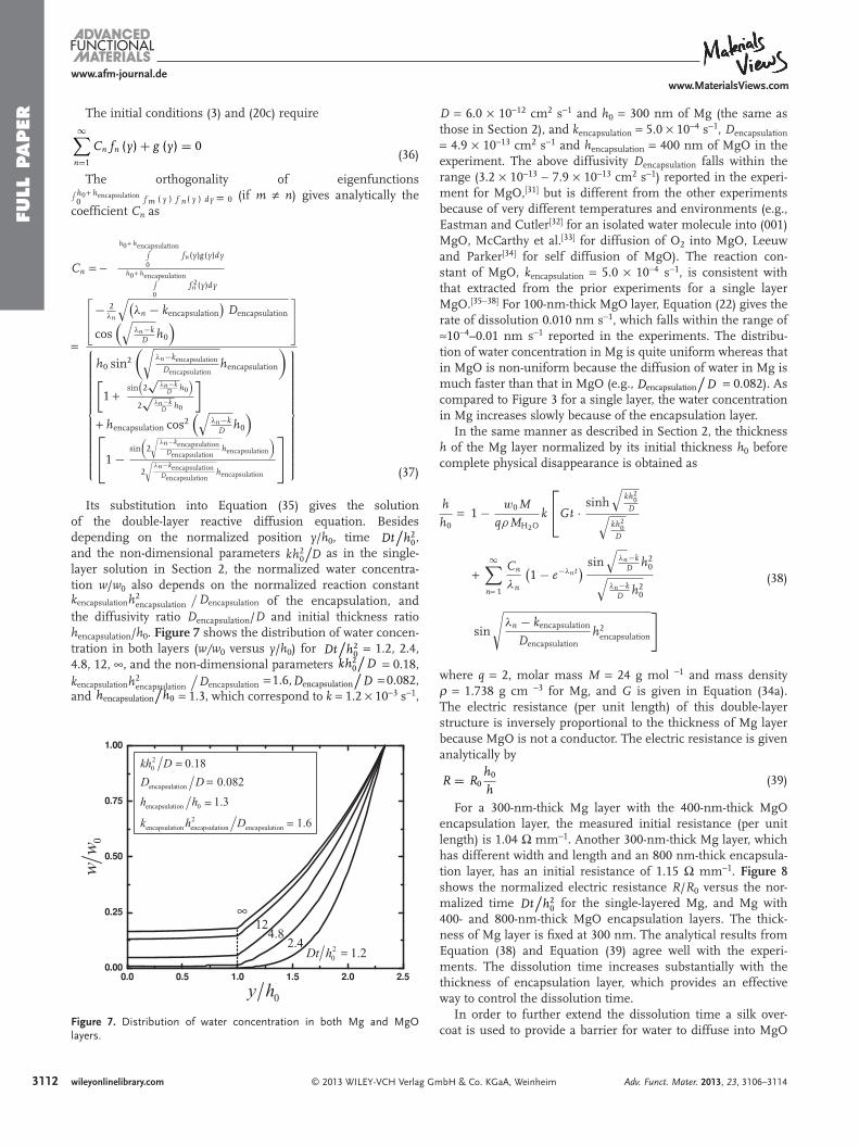
the diffusivity ratio D encapsulation / D and initial thickness ratio h encapsulation / h 0 . Figure 7 shows the distribution of water concen-tration in both layers ( w/w 0 versus y / h 0 ) for Dt

/h2

0 = 1.2, 2.4, 4.8, 12, ∞ , and the non-dimensional parameters kh2

0

/D = 0.18,

kencapsulationh2encapsulation

/Dencapsulation = 1.6, Dencapsulation

/D = 0.082,

and hencapsulation

/h0 = 1.3, which correspond to k = 1.2 × 10 − 3 s − 1 ,


Figure 7 . Distribution of water concentration in both Mg and MgO layers.

0w

w

0y h

20

encapsulation

encapsulation 0

2encapsulation encapsulation encapsulation

0.18

0.082

1.3

1.6

kh D

D D

h h

k h D

=

=

=

=

=

∞

20 1.2Dt h

2.4

124.8

0.0 0.5 1.0 1.5 2.0 2.50.00

0.25

0.50

0.75

1.00

D = 6.0 × 10 − 12 cm 2 s − 1 and h 0 = 300 nm of Mg (the same as those in Section 2), and k encapsulation = 5.0 × 10 − 4 s − 1 , D encapsulation = 4.9 × 10 − 13 cm 2 s − 1 and h encapsulation = 400 nm of MgO in the experiment. The above diffusivity D encapsulation falls within the range (3.2 × 10 − 13 ∼ 7.9 × 10 − 13 cm 2 s − 1 ) reported in the experi-ment for MgO, [ 31 ] but is different from the other experiments because of very different temperatures and environments (e.g., Eastman and Cutler [ 32 ] for an isolated water molecule into (001) MgO, McCarthy et al. [ 33 ] for diffusion of O 2 into MgO, Leeuw and Parker [ 34 ] for self diffusion of MgO). The reaction con-stant of MgO, k encapsulation = 5.0 × 10 − 4 s − 1 , is consistent with that extracted from the prior experiments for a single layer MgO. [ 35 − 38 ] For 100-nm-thick MgO layer, Equation (22) gives the rate of dissolution 0.010 nm s − 1 , which falls within the range of ≈ 10 − 4 –0.01 nm s − 1 reported in the experiments. The distribu-tion of water concentration in Mg is quite uniform whereas that in MgO is non-uniform because the diffusion of water in Mg is much faster than that in MgO (e.g., Dencapsulation

/D = 0.082). As

compared to Figure 3 for a single layer, the water concentration in Mg increases slowly because of the encapsulation layer.

In the same manner as described in Section 2, the thickness h of the Mg layer normalized by its initial thickness h 0 before complete physical disappearance is obtained as

h

h0= 1 − w0 M

qρMH2Ok

⎡⎣Gt · sinh

√kh2

0D√

kh20

D

+∞∑

n= 1

Cn

λn1 − e−λnt

) sin√

λn−kD h2

0√λn−k

D h20

sin

√λn − kencapsulation

Dencapsulationh2

encapsulation

]

(38)

where q = 2, molar mass M = 24 g mol − 1 and mass density ρ = 1.738 g cm − 3 for Mg, and G is given in Equation (34a) . The electric resistance (per unit length) of this double-layer structure is inversely proportional to the thickness of Mg layer because MgO is not a conductor. The electric resistance is given analytically by

R = R0

h0

h (39)

For a 300-nm-thick Mg layer with the 400-nm-thick MgO

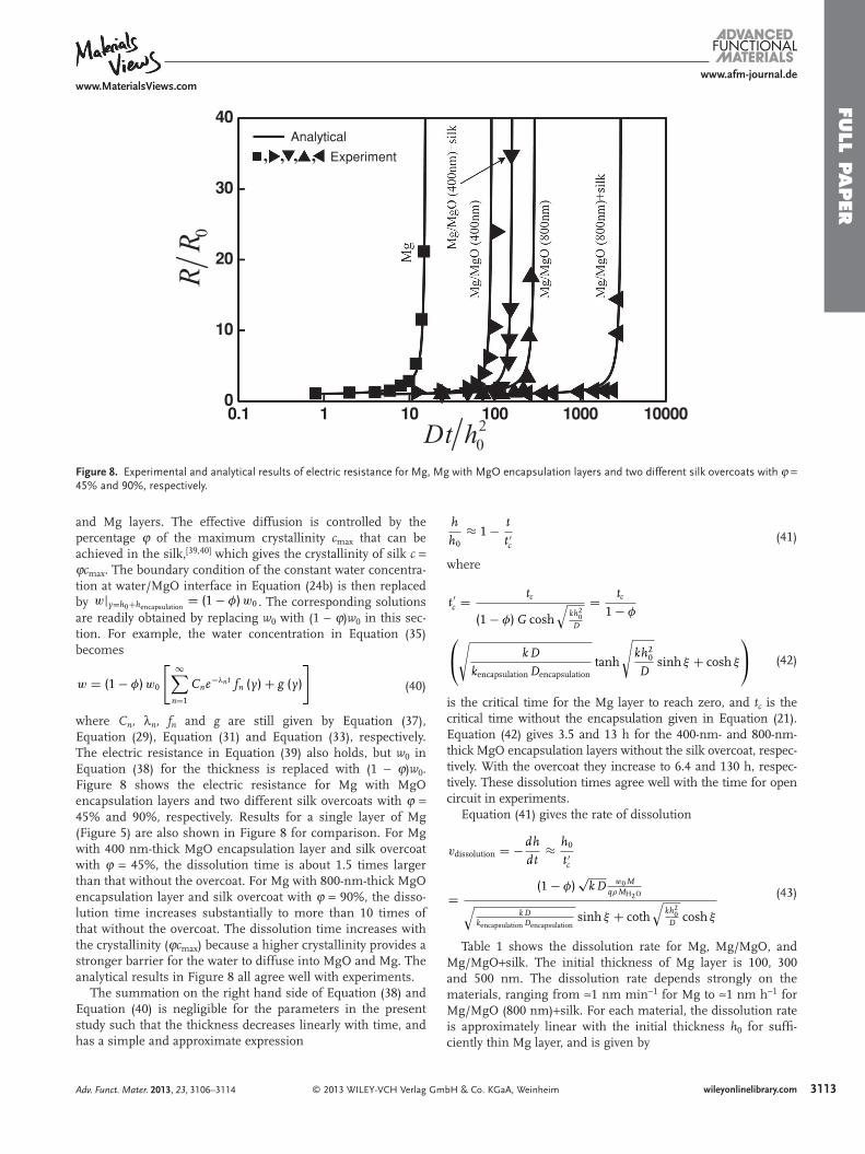
encapsulation layer, the measured initial resistance (per unit length) is 1.04 Ω mm − 1 . Another 300-nm-thick Mg layer, which has different width and length and an 800 nm-thick encapsula-tion layer, has an initial resistance of 1.15 Ω mm − 1 . Figure 8 shows the normalized electric resistance R / R 0 versus the nor-malized time Dt

/h2

0 for the single-layered Mg, and Mg with 400- and 800-nm-thick MgO encapsulation layers. The thick-ness of Mg layer is fi xed at 300 nm. The analytical results from Equation (38) and Equation (39) agree well with the experi-ments. The dissolution time increases substantially with the thickness of encapsulation layer, which provides an effective way to control the dissolution time.

In order to further extend the dissolution time a silk over-coat is used to provide a barrier for water to diffuse into MgO

mbH & Co. KGaA, Weinheim Adv. Funct. Mater. 2013, 23, 3106–3114

FULL P

APER


Figure 8 . Experimental and analytical results of electric resistance for Mg, Mg with MgO encapsulation layers and two different silk overcoats with ϕ = 45% and 90%, respectively.

0.1 1 10 100 1000 100000

10

20

30

40

Experiment

Analytical

20Dt h

0R

R, ,,,

and Mg layers. The effective diffusion is controlled by the percentage ϕ of the maximum crystallinity c max that can be achieved in the silk, [ 39 , 40 ] which gives the crystallinity of silk c = ϕ c max . The boundary condition of the constant water concentra-tion at water/MgO interface in Equation (24b) is then replaced by w|y=h0+hencapsulation

= (1 − φ) w0 . The corresponding solutions are readily obtained by replacing w 0 with (1 − ϕ ) w 0 in this sec-tion. For example, the water concentration in Equation (35) becomes

w = (1 − φ) w0

[ ∞∑n=1

Cne−λnt fn (y) + g (y)

]

(40)

where C n , λ n , f n and g are still given by Equation (37) , Equation (29) , Equation (31) and Equation (33) , respectively. The electric resistance in Equation (39) also holds, but w 0 in Equation (38) for the thickness is replaced with (1 − ϕ ) w 0 . Figure 8 shows the electric resistance for Mg with MgO encapsulation layers and two different silk overcoats with ϕ = 45% and 90%, respectively. Results for a single layer of Mg (Figure 5 ) are also shown in Figure 8 for comparison. For Mg with 400 nm-thick MgO encapsulation layer and silk overcoat with ϕ = 45%, the dissolution time is about 1.5 times larger than that without the overcoat. For Mg with 800-nm-thick MgO encapsulation layer and silk overcoat with ϕ = 90%, the disso-lution time increases substantially to more than 10 times of that without the overcoat. The dissolution time increases with the crystallinity ( ϕ c max ) because a higher crystallinity provides a stronger barrier for the water to diffuse into MgO and Mg. The analytical results in Figure 8 all agree well with experiments.

The summation on the right hand side of Equation (38) and Equation (40) is negligible for the parameters in the present study such that the thickness decreases linearly with time, and has a simple and approximate expression

© 2013 WILEY-VCH Verlag GAdv. Funct. Mater. 2013, 23, 3106–3114

h

h0≈ 1 − t

t ′c

(41)

where

t ′c = tc

(1 − φ) G cosh√

kh20

D

= tc

1 − φ

⎛⎝√

kD

kencapsulation Dencapsulationtanh

√kh2

0

Dsinh ξ + cosh ξ

⎞⎠

(42)

is the critical time for the Mg layer to reach zero, and t c is the critical time without the encapsulation given in Equation (21) . Equation (42) gives 3.5 and 13 h for the 400-nm- and 800-nm-thick MgO encapsulation layers without the silk overcoat, respec-tively. With the overcoat they increase to 6.4 and 130 h, respec-tively. These dissolution times agree well with the time for open circuit in experiments.

Equation (41) gives the rate of dissolution

vdissolution = −dh

dt≈ h0

t ′c

=(1 − φ)

√kD w0 M

qρMH2O√kD

kencapsulation Dencapsulationsinh ξ + coth

√kh2

0D cosh ξ

(43)

Table 1 shows the dissolution rate for Mg, Mg/MgO, and Mg/MgO + silk. The initial thickness of Mg layer is 100, 300 and 500 nm. The dissolution rate depends strongly on the materials, ranging from ≈ 1 nm min − 1 for Mg to ≈ 1 nm h − 1 for Mg/MgO (800 nm) + silk. For each material, the dissolution rate is approximately linear with the initial thickness h 0 for suffi -ciently thin Mg layer, and is given by


FULL

PAPER

3114

www.afm-journal.de

vdissolution = (1 − φ )

ω0 M

qρ MH2O

kh0

coshξfor kh2

0

/D 1.

(44)

The dissolution rate increases with the initial thickness h 0 . For relatively large h 0 , it saturates at

vdissolution

= (1 −φ )

√kD ω0 M

qρMH2O√kD

kencapsulation Dencapsulationsinhξ + coshξ

for kh20

/D 1

(45)

4. Concluding Remarks and Discussion

Analytical models for the transient electronic systems have been established. For single- and double-layered structures (with or without the silk overcoat) in solution, the remaining height and electric resistance of the system are obtained ana-lytically. In particular, the dissolution time and rate of dissolu-tion are given analytically in terms of the reaction constant and diffusivity of each material in the solution, molar masses and mass density of materials and solution, solution con-centration, number of solution molecules reacting with each atom, crystallinity of silk overcoat, and thickness of each layer. The analytical models agree well with the experiments for Mg single layer, Mg/MgO double layer (with and without overcoat), and are useful for design of transient electronic components.

The model of reactive diffusion can also be applied at the system level. To demonstrate this capability, in vivo transi-ence of an implantable RF metamaterial antenna is tested. The quality factor or Q factor [ 41 ] measured in experiments, which describes how under-damped a resonator is, or equivalently, characterizes a resonator’s bandwidth relative to its center frequency, also agrees well with the analytical models. [ 1 ]

It should be pointed out that the range of reaction constant reported in the literature is very large because it depends on many factors that can vary vastly in experiments, such as mor-phologies of the materials, temperature, and the PH value, concentration, and properties (e.g., ion concentration) of the surrounding liquid. The reaction constants and diffusivities reported in this paper for Mg, MgO, and SiO 2 are close to, or on the same order as, those reported in the literature under similar conditions. However, any of these constants can be extremely sensitive to the conditions so that those provided in this paper do not have to be universal.

Acknowledgements R.L., H.C., and Y.S. contributed equally to this work. The authors acknowledge support from NSF-INSPIRE (1242240).

Received: October 22, 2012 Revised: December 16, 2012

Published online: January 21, 2013

wileyonlinelibrary.com © 2013 WILEY-VCH Verlag

www.MaterialsViews.com

[ 1 ] S.-W. Hwang , H. Tao, D.-H. Kim, H. Cheng, J.-K. Song, E. Rill, M. A. Brenckle, B. Panilaitis, S. M. Won, Y.-S. Kim, Y. M. Song, K. J. Yu, A. Ameen, R. Li, Y. Su, M. Yang, D. L. Kaplan, M. R. Zakin, M. J. Slepian, Y. Huang, F. G. Omenetto, J. A. Rogers , Science 2012 , 337 , 1640.

[ 2 ] C. J. Bettinger , Z. Bao , Adv. Mater. 2010 , 22 , 651. [ 3 ] M. Irimia-Vladu , P. A. Troshin, M. Reisinger, L. Shmygleva,

Y. Kanbur, G. Schwabegger, M. Bodea, R. Schwodiauer, A. Mumyatov, J. W. Fergus, V. F. Razumov, H. Sitter, N. S. Sariciftci, S. Bauer , Adv. Funct. Mater. 2010 , 20 , 4069.

[ 4 ] C. Legnani , C. Vilani, V. L. Calil, H. S. Barud, W. G. Quirino, C. A. Achete, S. J. L Ribeiro, M. Cremona , Thin Solid Films 2008 , 517 , 1016.

[ 5 ] D. H. Kim , J. Viventi, J. J. Amsden, J. L. Xiao, L. Vigeland, Y. S. Kim, J. A. Blanco, B. Panilaitis, E. S. Frechette, D. Contreras, D. L. Kaplan, F. G. Omenetto, Y. G. Huang, K. C. Hwang, M. R. Zakin, B. Litt, J. A. Rogers , Nat. Mater. 2010 , 9 , 511.

[ 6 ] H. Seidel , L. Csepregi, A. Heuberger, H. Baumgärtel , J. Electrochem. Soc. 1990 , 137 , 3612.

[ 7 ] D. H. Davies , G. T. Burstein , Corrosion 1980 , 36 , 416. [ 8 ] V. Fournier , P. Marcus, I. Olefjord , Surf. Interface Anal. 2002 , 34 , 494. [ 9 ] M. J. Spearpoint , J. G. Quintiere , Combust. Flame 2000 , 123 , 308. [ 10 ] P. V. Danckwerts , Trans. Faraday Soc. 1950 , 46 , 300. [ 11 ] I. A. Taub , W. Roberts, S. LaGambina, K. Kustin , J. Phys. Chem. A

2002 , 106 , 8070. [ 12 ] W. F. Ng , K. Y. Chiu, F. T. Cheng , Mater. Sci. Eng. C 2010 , 30 , 898. [ 13 ] H. Inoue , K. Sugahara, A. Yamamoto, H. Tsubakino , Corros. Sci.

2002 , 44 , 603. [ 14 ] A. Yamamoto , S. Hiromoto , Mater. Sci. Eng. C 2009 , 29 , 1559. [ 15 ] G. Song , S. Song , Adv. Eng. Mater. 2007 , 9 , 298. [ 16 ] E. J. Casey , R. E. Bergeron, G. D. Nagy , Can. J. Chem. 1962 , 40 , 463. [ 17 ] M. Pourbaix , Atlas of electrochemical equilibria in aqueous solutions ,

National Association of Corrosion Engineers , Houston 1974 . [ 18 ] T. P. Hoar , J. Electrochem. Soc. 1970 , 117 , 17C. [ 19 ] R.K. Iler , J. Colloid Interface Sci. 1973 , 43 , 399. [ 20 ] M. Nogami , M. Tomozawa , J. Am. Ceram. Soc. 1984 , 67 , 151. [ 21 ] H. Wakabayashi , M. Tomozawa , J. Am. Ceram. Soc. 1989 , 72 , 1850. [ 22 ] K. Fukuda , T. Nakano, M. Fujishima, N. Mura, K. Tokunaga,

S. Ichinose , Jap. J. Appl. Phys. 1994 , 33 , L1445. [ 23 ] S. Ulutan , D. Balköse , J. Membr. Sci. 1996 , 115 , 217. [ 24 ] R. H. Doremus , Earth Planet. Sci. Lett. 1998 , 163 , 43. [ 25 ] M. Tomozawa , K. M. Davis , Mat. Sci. Eng. 1999 , A272 , 114. [ 26 ] J. Thurn , J. Non-Cryst. Solids 2008 , 354 , 5459. [ 27 ] D. C. Hurd , F. Theyer , Adv. Chem. Ser. 1975 , 147 , 211. [ 28 ] G. S. Wirth , J. M. Gieskes , J. Colloid Interface Sci. 1979 , 68 , 492. [ 29 ] K. G. Knauss , T. J. Wolery , Geochim. Cosmochim. Acta 1988 , 52 , 43. [ 30 ] W. G. Worley , Dissolution kinetics and mechanisms in quartz- and

grainite-water systems, Ph. D. thesis, Massachusetts Institute of Technology , 1994.

[ 31 ] B. Joachim , E. Gardés, R. Abart, W. Heinrich , Contrib. Mineral. Petrol. 2011 , 161 , 389.

[ 32 ] P. F. Eastman , I. B. Cutler , J. Am. Chem. Soc. 1966 , 49 , 526. [ 33 ] M. I. McCarthy , G. K. Schenter, C. A. Scamehorn, J. B. Nicholas , J.

Phys. Chem. 1996 , 100 , 16989. [ 34 ] N. H. de Leeuw , S. C. Parker , Phys. Rev. B 1998 , 58 , 13901. [ 35 ] D. D. Macdonald , D. Owen , Can. J. Chem. 1971 , 49 , 3375. [ 36 ] K. Sangwal , J. Mater.Sci. 1982 , 17 , 3598. [ 37 ] O. Fruhwirth , G. W. Herzog, I. Hollerer, A. Rachetti , Surf. Technol.

1985 , 24 , 301. [ 38 ] J. A. Mejias , A. J. Berry, K. Refson, D. G. Fraser , Chem. Phys. Lett.

1999 , 314 , 558. [ 39 ] L. Segal , J. J. Creely, A. E. Martin Jr., C. M. Conrad , Text. Res. J. 1959 ,

29 , 786. [ 40 ] W. Ruland , Acta Crystallogr. 1961 , 14 , 1180. [ 41 ] M. Rodahl , F. Hook, A. Krozer, P. Brzezinski, B. Kasemo , Rev. Sci.

Instrum. 1995 , 66 , 3924.

GmbH & Co. KGaA, Weinheim Adv. Funct. Mater. 2013, 23, 3106–3114

An Analytical Model of Reactive Diffusion for Transient Electronics

Documents

Transcript of An Analytical Model of Reactive Diffusion for Transient Electronics