An Analytical and Numerical Study of the Electric Double ...

Department of Physics

Department of Mathematics

Bachelor Thesis

Eleonora van den Dungen

Double Bachelor Physics & Mathematics

An Analytical and Numerical Study of the ElectricDouble Layer in a Cylindrical Nanochannel with a

Concentration Gradient

Supervisors:

Prof. dr. R. van RojiInstitute for Theoretical Physics

Prof. dr. ir. J. E. FrankMathematic Institute

MSc. W. BoonInstitute for Theoretical Physics

January 15, 2020

Abstract

This work aims to extend the study of the formation of the heterogeneous electric double layer. Thiselectric double layer occurs at the interface of a solution in a channel with a salt concentration differenceat either side of the channel and the surface charge of the channel walls. This behaviour is described bythe Nernst-Planck, Navier-Stokes and Poisson equations. First a modified Debye length depending on theconcentration is derived analytically to take this concentration gradient into account and is used to deriveanalytical expressions for the electric potential and the fluid velocity. The modelling program COMSOLMultiphysics is used to build a simulation of this system consisting of a concentration gradient over ananochannel. It is found that at small concentration differences, the in this work derived analyticalsolutions describe the system very well. However, for large concentration gradients these analyticalexpressions do no longer hold. Further research needs to be done to understand the behaviour occurringdue to a large concentration gradient.

i

CONTENTS ii

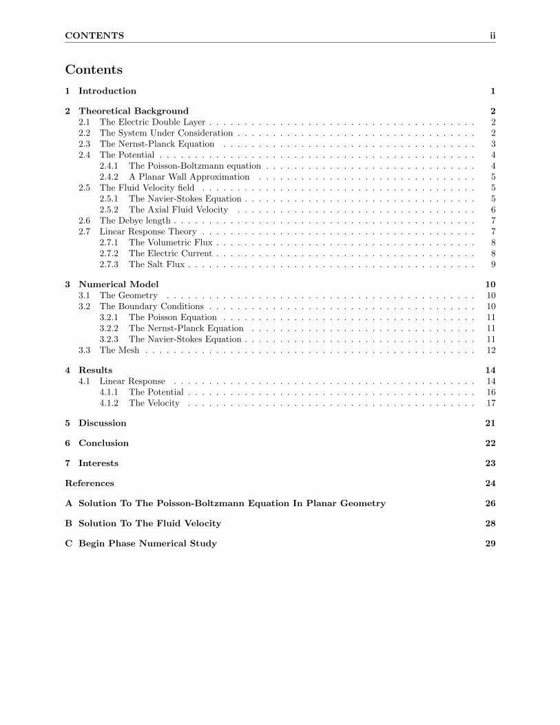
Contents

1 Introduction 1

2 Theoretical Background 22.1 The Electric Double Layer . . . . . . . . . . . . . . . . . . . . . . . . . . . . . . . . . . . . . . 22.2 The System Under Consideration . . . . . . . . . . . . . . . . . . . . . . . . . . . . . . . . . . 22.3 The Nernst-Planck Equation . . . . . . . . . . . . . . . . . . . . . . . . . . . . . . . . . . . . 32.4 The Potential . . . . . . . . . . . . . . . . . . . . . . . . . . . . . . . . . . . . . . . . . . . . . 4

2.4.1 The Poisson-Boltzmann equation . . . . . . . . . . . . . . . . . . . . . . . . . . . . . . 42.4.2 A Planar Wall Approximation . . . . . . . . . . . . . . . . . . . . . . . . . . . . . . . 5

2.5 The Fluid Velocity field . . . . . . . . . . . . . . . . . . . . . . . . . . . . . . . . . . . . . . . 52.5.1 The Navier-Stokes Equation . . . . . . . . . . . . . . . . . . . . . . . . . . . . . . . . . 52.5.2 The Axial Fluid Velocity . . . . . . . . . . . . . . . . . . . . . . . . . . . . . . . . . . 6

2.6 The Debye length . . . . . . . . . . . . . . . . . . . . . . . . . . . . . . . . . . . . . . . . . . . 72.7 Linear Response Theory . . . . . . . . . . . . . . . . . . . . . . . . . . . . . . . . . . . . . . . 7

2.7.1 The Volumetric Flux . . . . . . . . . . . . . . . . . . . . . . . . . . . . . . . . . . . . . 82.7.2 The Electric Current . . . . . . . . . . . . . . . . . . . . . . . . . . . . . . . . . . . . . 82.7.3 The Salt Flux . . . . . . . . . . . . . . . . . . . . . . . . . . . . . . . . . . . . . . . . . 9

3 Numerical Model 103.1 The Geometry . . . . . . . . . . . . . . . . . . . . . . . . . . . . . . . . . . . . . . . . . . . . 103.2 The Boundary Conditions . . . . . . . . . . . . . . . . . . . . . . . . . . . . . . . . . . . . . . 10

3.2.1 The Poisson Equation . . . . . . . . . . . . . . . . . . . . . . . . . . . . . . . . . . . . 113.2.2 The Nernst-Planck Equation . . . . . . . . . . . . . . . . . . . . . . . . . . . . . . . . 113.2.3 The Navier-Stokes Equation . . . . . . . . . . . . . . . . . . . . . . . . . . . . . . . . . 11

3.3 The Mesh . . . . . . . . . . . . . . . . . . . . . . . . . . . . . . . . . . . . . . . . . . . . . . . 12

4 Results 144.1 Linear Response . . . . . . . . . . . . . . . . . . . . . . . . . . . . . . . . . . . . . . . . . . . 14

4.1.1 The Potential . . . . . . . . . . . . . . . . . . . . . . . . . . . . . . . . . . . . . . . . . 164.1.2 The Velocity . . . . . . . . . . . . . . . . . . . . . . . . . . . . . . . . . . . . . . . . . 17

5 Discussion 21

6 Conclusion 22

7 Interests 23

References 24

A Solution To The Poisson-Boltzmann Equation In Planar Geometry 26

B Solution To The Fluid Velocity 28

C Begin Phase Numerical Study 29

1 INTRODUCTION 1

1 Introduction

As global demand for energy continues to rise, a lot of research is done into a sustainable energy source. Oneof these sources is a saline gradient in a fluid. This source of energy exists at the interface between bodies ofdifferent salinities, primarily at the place where fresh water flows into the ocean [1].Due to recent rapid developments in technology enables engineering on a nano scale, this energy is potentiallyavailable [2]. Reverse electro dialysis is a membrane-based technology which exists to convert this energyinto a useful power source. One of the ways this technology can be applied is on the transport of ions in ananochannel. However, the mechanism behind this electrokinetic transport is not completely understood [3].Rice and Whitehead were one of the first give a complete analysis of electro-osmotic flow in round capillaries[4]. After this, a lot of works on electrokinetics were published building on their analysis. Due to thefact that non-steady state solutions of the coupled partial differential equation which govern electrokinetictransport are quite complex to solve, most of the studies done until recent focus on the steady state situations[5, 6, 7, 8, 9]. However, developments in the usage of finite element analysis and an rise in computing ability,enables the process of solving a complex non-steady state situation with an numerical approach [10, 11]. Thisallows for the study of the complete physical behaviour of a system instead of only looking at a theoreticframe. For example in chemistry, finite element modelling is used on a nano pore detector or nanochannels ina cell membrane [12, 13, 14]. This finite element method can be used to gain an insight into the mechanismbehind the ionic transport in a nanochannel. To describe the principles governing the fluid flow in a porousmembrane with a salinity gradient, a theoretical system is considered.The theoretical system considered consists of a charged nanochannel with a radius of the orders of nanometresand a length of the orders of micrometers. The channel is connected to two reservoirs. Due to concentrationconstraints in the interior of the two reservoirs, a concentration gradient is imposed across the system. Thesystem is filled with a solution of symmetrical monovalent electrolyte, of which the ions are modelled as pointcharges. The concentration constraint and the surface charge result in a inhomogeneous charge distributionin the channel. The electric potential of ions in the electric double layers at the interface between the nanochannel wall and the electrolyte will strongly influence the rates of axial ion transport, the streaming potentialwhich is the electric field created by the motion of the ionized fluid along the stationary charged surface andthe flow of the bulk.As the intrinsic heterogeneities of the electric double layer in the channel by an applied salinity gradient makethe system very challenging and not well understood, more research needs to be done on these heterogeneitiesto gain an insight into the behaviour of the diffusio-osmotic currents which result from a concentrationgradient [15]. First of all it is required to know how the fluxes react to different linear concentration gradient.This raises the question if it is possible to describe the electric potential for the heterogeneous electric doublelayer with an analytical expression. Maybe it is possible to find an analytical expression for the fluid velocityfield as well, as this combined with the electric potential describes a large part of the fluxes in the system. Tofind an answer to these questions, a research will be constructed in the following manner. For the research, theconcentration difference between the two reservoirs will be the main variable considered. In the theoreticalbackground, the electric double layer will be discussed. Furthermore an expression for the electric potentialand velocity field will be derived. The linear relation between the chemical driving force and the fluxes will bediscussed as well. Afterwards, a model will be constructed which employs the coupled Poisson, Nernst-Planckand Navier-Stokes equation to describe the diffusio-osmotic flow in a finite charged cylindrical channel. Acomparison will be made between the quantities obtained through this numerical model and the derivedanalytical expressions for the electric potential and velocity field. This method of research is used to see ifthe numerical model verifies the analytical expressions found in the theory section for a certain regime ofconcentration gradients and it enables the finding of an answer to the questions raised, which will give abetter insight into this system and its intrinsic values.

2 THEORETICAL BACKGROUND 2

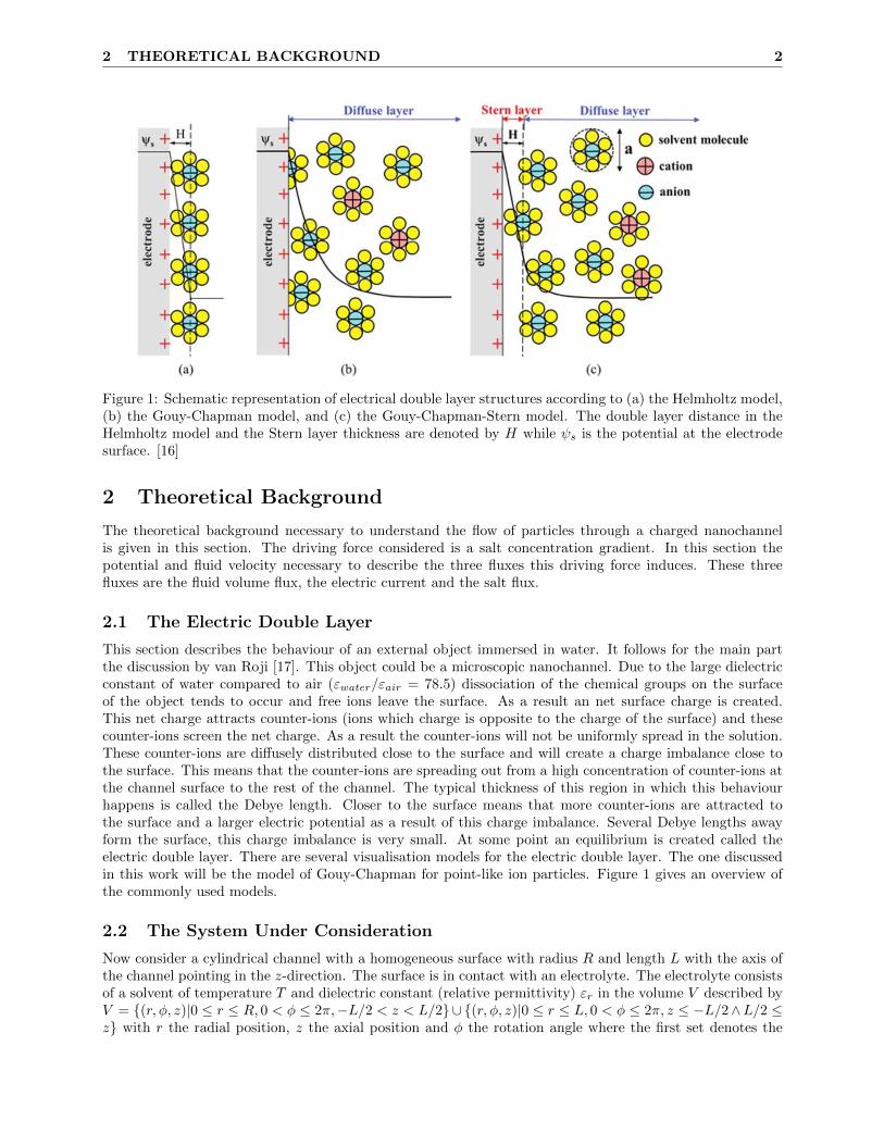
Figure 1: Schematic representation of electrical double layer structures according to (a) the Helmholtz model,(b) the Gouy-Chapman model, and (c) the Gouy-Chapman-Stern model. The double layer distance in theHelmholtz model and the Stern layer thickness are denoted by H while ψs is the potential at the electrodesurface. [16]

2 Theoretical Background

The theoretical background necessary to understand the flow of particles through a charged nanochannelis given in this section. The driving force considered is a salt concentration gradient. In this section thepotential and fluid velocity necessary to describe the three fluxes this driving force induces. These threefluxes are the fluid volume flux, the electric current and the salt flux.

2.1 The Electric Double Layer

This section describes the behaviour of an external object immersed in water. It follows for the main partthe discussion by van Roji [17]. This object could be a microscopic nanochannel. Due to the large dielectricconstant of water compared to air (εwater/εair = 78.5) dissociation of the chemical groups on the surfaceof the object tends to occur and free ions leave the surface. As a result an net surface charge is created.This net charge attracts counter-ions (ions which charge is opposite to the charge of the surface) and thesecounter-ions screen the net charge. As a result the counter-ions will not be uniformly spread in the solution.These counter-ions are diffusely distributed close to the surface and will create a charge imbalance close tothe surface. This means that the counter-ions are spreading out from a high concentration of counter-ions atthe channel surface to the rest of the channel. The typical thickness of this region in which this behaviourhappens is called the Debye length. Closer to the surface means that more counter-ions are attracted tothe surface and a larger electric potential as a result of this charge imbalance. Several Debye lengths awayform the surface, this charge imbalance is very small. At some point an equilibrium is created called theelectric double layer. There are several visualisation models for the electric double layer. The one discussedin this work will be the model of Gouy-Chapman for point-like ion particles. Figure 1 gives an overview ofthe commonly used models.

2.2 The System Under Consideration

Now consider a cylindrical channel with a homogeneous surface with radius R and length L with the axis ofthe channel pointing in the z-direction. The surface is in contact with an electrolyte. The electrolyte consistsof a solvent of temperature T and dielectric constant (relative permittivity) εr in the volume V described byV = {(r, φ, z)|0 ≤ r ≤ R, 0 < φ ≤ 2π,−L/2 < z < L/2}∪ {(r, φ, z)|0 ≤ r ≤ L, 0 < φ ≤ 2π, z ≤ −L/2∧L/2 ≤z} with r the radial position, z the axial position and φ the rotation angle where the first set denotes the


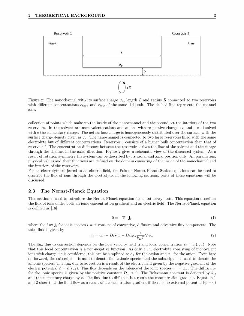
Figure 2: The nanochannel with its surface charge σe, length L and radius R connected to two reservoirswith different concentrations chigh and clow of the same [1:1] salt. The dashed line represents the channelaxis.

collection of points which make up the inside of the nanochannel and the second set the interiors of the tworeservoirs. In the solvent are monovalent cations and anions with respective charge +e and −e dissolvedwith e the elementary charge. The net surface charge is homogeneously distributed over the surface, with thesurface charge density given as σe. The nanochannel is connected to two large reservoirs filled with the sameelectrolyte but of different concentrations. Reservoir 1 consists of a higher bulk concentration than that ofreservoir 2. The concentration difference between the reservoirs drives the flow of the solvent and the chargethrough the channel in the axial direction. Figure 2 gives a schematic view of the discussed system. As aresult of rotation symmetry the system can be described by its radial and axial position only. All parameters,physical values and their functions are defined on the domain consisting of the inside of the nanochannel andthe interiors of the reservoirs.For an electrolyte subjected to an electric field, the Poisson-Nernst-Planck-Stokes equations can be used todescribe the flux of ions through the electrolyte, in the following sections, parts of these equations will bediscussed.

2.3 The Nernst-Planck Equation

This section is used to introduce the Nernst-Planck equation for a stationary state. This equation describesthe flux of ions under both an ionic concentration gradient and an electric field. The Nernst-Planck equationis defined as [18]

0 = −∇ · ji, (1)

where the flux ji for ionic species i = ± consists of convective, diffusive and advective flux components. Thetotal flux is given by

ji = uci −Di∇ci −Dizicie

kBT∇ψ.. (2)

The flux due to convection depends on the flow velocity field u and local concentration ci = ci(r, z). Notethat this local concentration is a non-negative function. As only a 1:1 electrolyte consisting of monovalentions with charge ±e is considered, this can be simplified to c+ for the cation and c− for the anion. From hereon forward, the subscript + is used to denote the cationic species and the subscript − is used to denote theanionic species. The flux due to advection is a result of the electric field given by the negative gradient of theelectric potential ψ = ψ(r, z). This flux depends on the valence of the ionic species z± = ±1. The diffusivityfor the ionic species is given by the positive constant D± > 0. The Boltzmann constant is denoted by kBand the elementary charge by e. The flux due to diffusion is a result the concentration gradient. Equation 1and 2 show that the fluid flow as a result of a concentration gradient if there is no external potential (ψ = 0)


will be constant. An in depth discussion of the electric potential will happen in the next section. The flowvelocity field as a result of this electric potential will be discussed later.

2.4 The Potential

To describe the behaviour of the electric double layer, it is necessary to understand the physics and equationsgoverning the local electric potential inside the nanochannel. This will be done in this section. First thePoisson equation will be discussed. Combined with the Boltzmann distribution, this equation will give rise tothe Poisson-Boltzmann equation. To find the electric potential a dimensionless potential will be introduced,after which the cylindrical system will be approximated to a planar system to find the solution to thedimensionless potential.

2.4.1 The Poisson-Boltzmann equation

The Poisson equation can be used to describe the characteristics for the electric double layer. The Poissonequation describes the change in electric potential of the electrolyte due to the excess charge over space. Forthe cylindrical channel this becomes

−∇2ψ =ρeε0εr

, (3)

where εr is the dielectric constant of the solvent and ε0 is the permittivity of free space. The local electriccharge density ρe is given by

ρe = eNA(c+ − c−), (4)

with NA being Avogadro’s number and c± is denoted in mole per cubic meter. A special notation will beintroduced to denote the ion concentration on the channel axis, c0±(z) = c±(0, z) as due to the differentbulk concentrations in the two reservoirs, the concentration of the ions is not uniform along the nanochannelaxis. This imposed concentration gradient prevents the system from creating an equilibrium. The Boltzmanndistribution model is often used to describe concentrations in an equilibrium state. However the assumptionsthat the Debye length is much smaller than the distance under which c0±(z) changes and that there is noradial component to the flow velocity, enables the use of the Boltzmann distribution. The local equilibriumhypothesis can be used to derive this Boltzmann distribution. The local equilibrium hypothesis assumes thata system can be viewed as formed of subsystems where the rules of equilibrium thermodynamics apply. Thisimplies that there is no flux in the radial direction (j± · r = 0, with r the unit vector in the radial direction).From Equation 2 then follows that

∂rc± = ∓c±e

kBT∂rψ. (5)

The integration of this gives the same result as the Boltzmann distribution for only electric work. TheBoltzmann distribution is given as

c±(r, z) = c0±(z) · e−W±kBT , (6)

in which W± is the work required to move an ion with charge ± closer to the charged surface from thechannel axis. In the case of the work consisting only of electric work it can be rewritten as W±(r, z) =±(eψ(r, z) − eψ0(z)) in which ψ0(z) denotes the potential on the channel axis. The concentration can begiven as

c± = c0±e∓ ekBT

(ψ(r,z)−ψ0(z)), (7)

and therefore the local charge density can be written as

ρeeNA(c0+e−φ − c0−eφ), (8)

where the dimensionless potential φ = ekBT

(ψ − ψ0) is introduced. The dimensionless potential describesthe difference between an electric potential in the cylinder (r,z) and the potential on the central axis (0,z).After substituting this back in the Poisson equation, the Poison-Boltzmann equation for the dimensionlesspotential becomes

∇2φ = − e

kBT

e

ε0εrNA(c0+e

−φ − c0−eφ). (9)


Another way to get to the Poisson-Boltzmann equation is by using Gibbs’ variational principle for thermalequilibrium consisting of minimizing the system free energy, which will not be touched upon here. Howeverit is interesting to look into [19]. In the next section a solution to the the Poison-Boltzmann equation for thedimensionless potential will be derived.

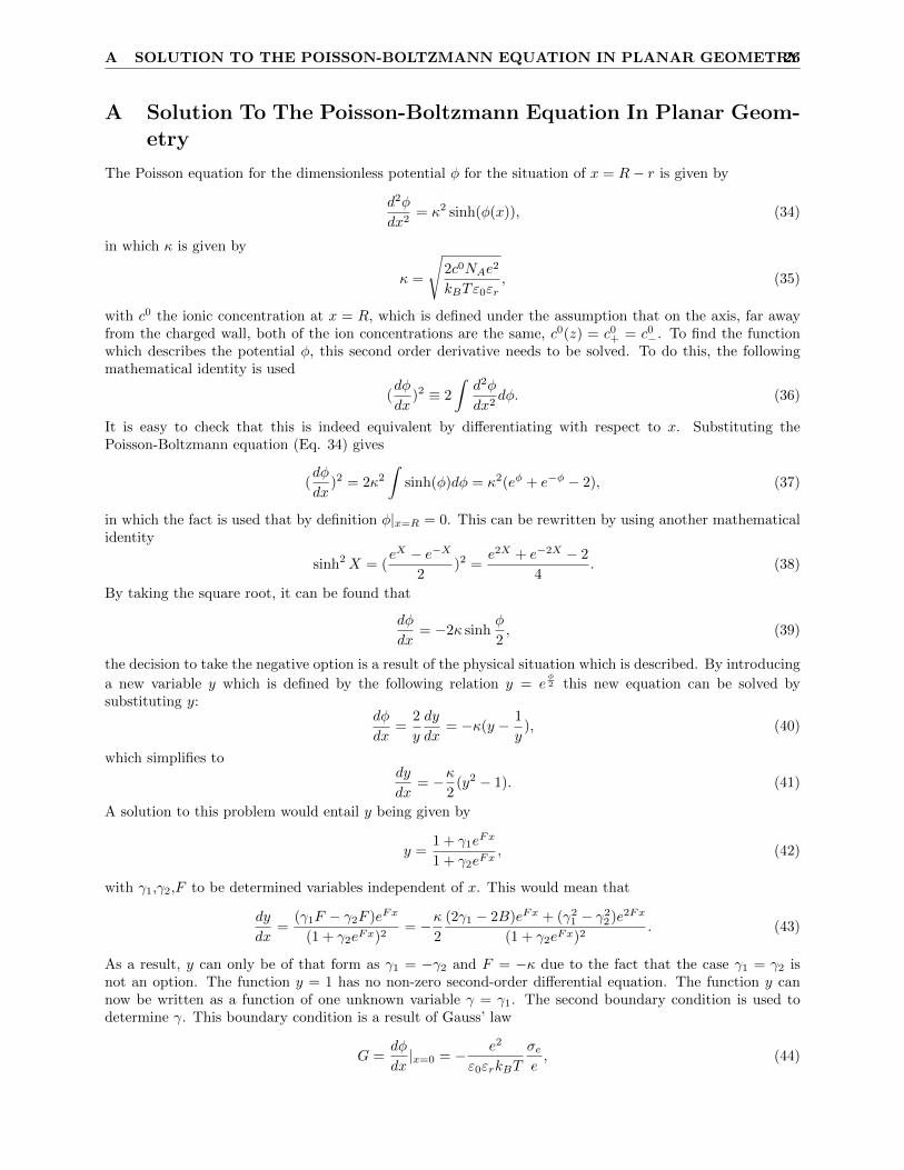
2.4.2 A Planar Wall Approximation

The dimensionless Poisson equation for the cylidrical system has been previously discussed. However, untilnow an analytical solution to this differential equation has not been found for the cylindrical case, which

entails the Laplacian being ∇2 = 1rddr (r ddr ) + d2

dz2 . Under the assumption that the induced electric fieldEr = −∇φr in the radial direction as a result of the electric double layer is much larger than the induced

electric field along the axis due to particle flow, d2

dz2φ �1rddr (r ddr )φ, the derivative to the z component can

be omitted. The notation φr refers to the potential for a arbitrary value of z. If this is combined with theassumption that the radius R of the channel is much larger than the Debye length, the Laplacian can be

assumed to be d2

dx2 , with x = R − r as 1rddr (r ddr ) = d2

dx2 + 1R−x

ddx . The final term can be ignored as a higher

order term on the account of R� x for the x close to the channel wall, where the electric double layer is.Under this assumption, the surface of the channel wall can be considered a planar wall instead of a cylindricalwall, with x being the distance to the wall. The Poisson-Boltzmann as a result of these specifications canbe solved under the assumption that on the channel-axis both ion species have the same concentrationc0(x = R, z) = c0+ = c0− as the dimensionless Poisson-Boltzmann is now given as

d2

dx2φ = − e

kBT

e

ε0εrNA(c0+e

−φ − c0−eφ) = NAc0 e

kBT

e

ε0εr(eφ − e−φ) = κ2 sinhφ, (10)

with κ(z) =√

2NAc0e

kBTe

ε0εr. This second-order partial differential equation can be solved under the

following two boundary conditions. The first boundary condition is a symmetry condition dφdx |x=R = 0 and

the second boundary condition is given by dφdx |x=0 = − e2

ε0εrkBTσee , which is a result of Gauss’ law. These

boundary conditions, combined with the use of a couple of mathematical identities and rewriting, give theunique solution to the second order derivative. The analytical non-linear solution for the dimensionlesspotential is given by

φ(x, z) = 2 ln1 + γe−κ(z)x

1− γe−κ(z)x, (11)

with γ = 2κG −

√( 2κG )2 + 1, κ(z) =

√2c0NAe2

kBTε0εrand G = − e2

ε0εrkBTσee . The explicit derivation of this solution

can be found in appendix A. It is important to note that G is independent of axial position z and the onlyz dependent part of γ is κ. Using the fact that x = R− r this can be substituted again to give the potentialdepending on r. This heterogeneous solution can be reduced to the homogeneous solution for the potentialwhich is already known, under the condition that the Debye length is independent of the axial position andthere is no concentration gradient [20, 21, 22, 23, 24].

2.5 The Fluid Velocity field

In the case of no external potential, which is (ψ = 0), the fluid flow as a result of a concentration gradient willbe constant. This is shown by Equation 1 and 2. So the only way a concentration gradient can influence a fluidflow is due to an external potential. In this section the flow velocity field is derived using the Navier-StokesEquation by treating the electric double layer as external potential.

2.5.1 The Navier-Stokes Equation

The stationary Navier-Stokes Equation for an incompressible fluid is given by

−∇p+ η∇2u + F = 0, ∇ · u = 0, (12)

with η the viscosity and p the pressure, under the assumption that the flow of the system is slow (this meansa low Reynold’s number). The flow velocity field u = u(r, z) is divergence-free. The volume force is denoted


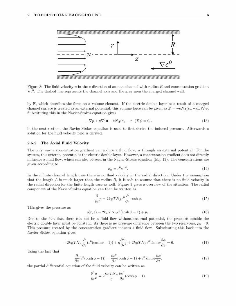
Figure 3: The fluid velocity u in the z direction of an nanochannel with radius R and concentration gradient∇c0. The dashed line represents the channel axis and the grey area the charged channel wall.

by F, which describes the force on a volume element. If the electric double layer as a result of a chargedchannel surface is treated as an external potential, this volume force can be given as F = −eNA(c+− c−)∇ψ.Substituting this in the Navier-Stokes equation gives

−∇p+ η∇2u− eNA(c+ − c−)∇ψ = 0, . (13)

in the next section, the Navier-Stokes equation is used to first derive the induced pressure. Afterwards asolution for the fluid velocity field is derived.

2.5.2 The Axial Fluid Velocity

The only way a concentration gradient can induce a fluid flow, is through an external potential. For thesystem, this external potential is the electric double layer. However, a concentration gradient does not directlyinfluence a fluid flow, which can also be seen in the Navier-Stokes equation (Eq. 13). The concentrations aregiven according to

c± = c0e∓φ. (14)

In the infinite channel length case there is no fluid velocity in the radial direction. Under the assumptionthat the length L is much larger than the radius R, it is safe to assume that there is no fluid velocity inthe radial direction for the finite length case as well. Figure 3 gives a overview of the situation. The radialcomponent of the Navier-Stokes equation can then be written as

∂

∂rp = 2kBTNAc

0 ∂

∂rcoshφ. (15)

This gives the pressure asp(r, z) = 2kBTNAc

0(coshφ− 1) + p0. (16)

Due to the fact that there can not be a fluid flow without external potential, the pressure outside theelectric double layer must be constant. As there is no pressure difference between the two reservoirs, p0 = 0.This pressure created by the concentration gradient induces a fluid flow. Substituting this back into theNavier-Stokes equation gives

− 2kBTNA∂

∂z(c0(coshφ− 1)) + η

∂2u

∂r2+ 2kBTNAc

0 sinhφ∂φ

∂z= 0. (17)

Using the fact that∂

∂z(c0(coshφ− 1)) =

∂c0

∂z(coshφ− 1) + c0 sinhφ

∂φ

∂z, (18)

the partial differential equation of the fluid velocity can be written as

∂2u

∂r2= 2

kBTNAη

∂c0

∂z(coshφ− 1). (19)


This second order derivative can be solved by using the substitution x = R − r and the following twoboundary conditions. The first boundary condition is that the fluid velocity constant is, ∂u

∂r |r=0 = 0 Thesecond boundary condition is the no-slip boundary condition at the channel wall. u|r=R = 0. These boundaryconditions, combined with the use of a couple of mathematical identities and rewriting, give an unique solutionto the second order derivative. The analytical solution for the z component of the fluid velocity as a resultof the concentration gradient is given by

u =−4kBTNAκ

−2

η

∂c0

∂zln

1− γ2e−2κx

1− γ2, (20)

with γ = 2κG −

√( 2κG )2 + 1 and κ =

√2c0NAe2

kBTε0εrand G = − e2

ε0εrkBTσee . The explicit derivation of this solution

can be found in appendix B. Using the fact that x = R − r this can be substituted again to give the fluidvelocity in the z direction depending on r,

u =−4kBTNAκ

−2

η

∂c0

∂zln

1− γ2e−2κ(R−r)

1− γ2. (21)

2.6 The Debye length

The Debye screening length, which describes the thickness of the electric double layer is given by

κ−1 =

√kBTε0εr2c0NAe2

, (22)

with c0 in mM. Due to the fact that c0 is not homogeneous on the channel axis, the Debye length is expectedto change in the channel as well. As Reservoir 1 has a higher bulk concentration, the concentration of ions onthe channel axis close to Reservoir 1 is higher than the concentration on the channel axis close to Reservoir 2.As according to the equation, the Debye length is inversely proportional to the concentration on the axis, itmeans that close to Reservoir 1 the Debye length will be smaller and the electric double layer will be thinneras compared to close to Reservoir 2.At room temperature (T = 298.15K) and in water (εr = 78.5) [25], the Debye length is related to theconcentration as

κ−1 =3.04√c0

A (23)

with c0 now expressed in the unit M. As a result, for c0 at 0.2, 0.5 and 1 M, the Debye length will be 6.8,4.3 and 3.0 A respectively. The Debye length κ−1 represents the distance it takes for the local potential todecrease to the e-th part of the potential at the surface, ψ(κ−1) = e−1ψ(R) [26]. Therefore at three Debyelengths away from the electrode, the potential will have dropped to be a mere 0.6% of the original potential.For the three earlier named concentrations, three Debye lengths mean two or less nanometres.

2.7 Linear Response Theory

For small changes in the driving forces, the induced fluxes can be described by linear response theory. Inthis section the linear response theory will be discussed. It follows for the main part the discussion byWerkhoven [?]. In linear response theory, the relation between different driving forces (pressure, potentialand concentration differences) and induced fluxes (volumetric flow rate Q, electric current I and salt flux J)as a result of these driving forces are quantified by a matrix M,QI

J

=πR2

LM

∆p∆ψ∆µ

(24)

with M a symmetric 3 × 3 matrix and Mij the transport coefficient. This matrix was first described byOnsager and is therefore called the Onsager matrix. These linear relation hold only for small changes in thedriving forces (small ∆p, ∆ψ and ∆µ). As the nanochannel of interest is a electric short-circuit channel,


this means that there is no potential dependent driving force (∆ψ = 0 over the channel), and is assumedto have a mechanical closed-circuit channel condition, no pressure dependent driving force (∆p = 0 overthe channel), where the solvent can freely flow. It is however possible that the system has local pressuredifferences and potential differences. As a result, only the concentration gradient is non-zero. As a resultvolumetric flow rate Q, electric current I and salt flux J can be given as only a function of ∆µ, which is thechemical potential.The chemical potential describes how species flow between different parts of a system. In an equilibriumstate, the chemical potential of a species is uniform throughout the system and the net flow of particles iszero. If, however, there are heterogeneities of the chemical potential in the system, then particles will flowto decrease these overall differences in chemical potential. The chemical potential can be derived from theGibbs free energy, which is given by

dG = −SdT + V dp+ µ+dc+ + µ−dc−, (25)

under the assumption that the temperature and the pressure are fixed in the two reservoirs, which is globallythe case. This means that

µ± = (dG

dc±)T,p. (26)

The chemical potential is given by

µ±(0, z →∞)− µ±(0, z → −∞) = ∆µ = kBT lnchighclow

, (27)

with chigh and clow the concentration in the reservoirs.The matrix elements which are globally relevant, can be understood by looking at the chemical potentialand the induced fluxes. The matrix element M31, M32 and M33 can be explicitly calculated for this systemwith a no slip boundary (u(R, z) = 0) on all the wall and equal mobility for both the cations and anions(D± = D). The decision has been made to take the explicit formulas for these matrix elements out of thearticle made by Werkhoven instead of deriving them here [27].

2.7.1 The Volumetric Flux

The matrix element M31 describes the ratio between the concentration difference and the induced volumetricflux Q. In the case of an infinitely long channel, the volumetric flux can be given by

Q =

∫dAu(r), (28)

where u(r) is the z-component of the velocity field. which entails the surface integral∫dA = 2π

∫ R0drr

described by a plane with a fixed z cross sectioned with the channel. If the channel length is infinitelylarge, the velocity field is independent of translation on the z axis and there is no radial velocity. Under theassumption that the radius of the channel is far smaller than the length of the channel R � L the formulafor the volumetric flux can still be applied to the finite channel situation, as long as the cross section is faraway enough from the channel entrances, so the influence of entrance effects will be rather small.The explicit matrix element for the volumetric flux is given by

M13 =2e2

ηε0εrkBT(2 ln cosh

1

4φs −

κ2

2R

∫ ∞0

ds(coshφ(s)− 1)), (29)

with φs = 2 ln 1+γ1−γ the potential at the channel surface and γ as defined in the solution of the dimensionless

potential (Eq. 11) [27].

2.7.2 The Electric Current

The matrix element M32 describes the relation between the concentration difference and the induced electriccurrent I. In the case of an infinitely long channel, the volumetric flux can be given by

I = e

∫dA(j+(r)− j−(r)), (30)


where j± denotes the z-component of the ionic flux j± and the surface integral∫dA = 2π

∫ R0drr as in the

volumetric flux The explicit matrix element for the electric current is given by

M23 = − 2D

kBT

σezsR

− 2ε0εrkBT

eκ−1ηR

zsε0εrkBT

e2(4

σezseσ∗

− 2|φ(R)|), (31)

with σ∗ = 4κ−1c0NA and zs = σe|σe| [27].

2.7.3 The Salt Flux

The matrix element M32 describes the relation between the concentration difference and the induced saltflux J .

J =

∫dA(j+(r) + j−(r)), (32)

with its components as defined in the section of the electric current. The explicit matrix element for the saltflux is given by

M33 =2Dc0NAkBT

(1− 2κ−1

R(2

√1 + (

σeσ∗e

)2 − 2)) +4ε0εrkBTκ

−1c0NAe2ηR

(4

√1 + (

σeeσ∗

)2 − 4− 16 ln coshφ(R)

4).

(33)[27]The theoretical values resulting from these matrix elements will be compared to the numerical calculationsof the full Poisson-Nernst-Planck-Stokes equation. In the next section discusses the numerical model used inthe calculations.

3 NUMERICAL MODEL 10

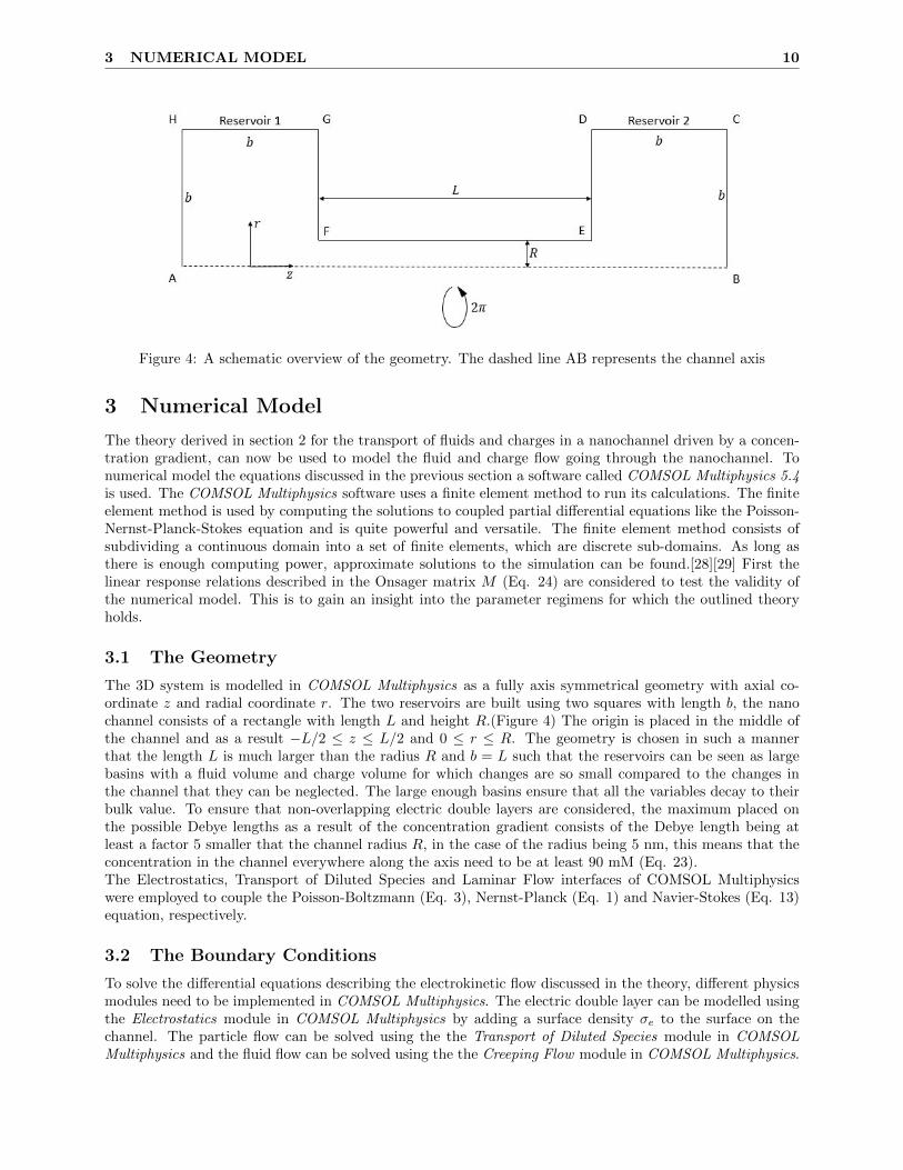
Figure 4: A schematic overview of the geometry. The dashed line AB represents the channel axis

3 Numerical Model

The theory derived in section 2 for the transport of fluids and charges in a nanochannel driven by a concen-tration gradient, can now be used to model the fluid and charge flow going through the nanochannel. Tonumerical model the equations discussed in the previous section a software called COMSOL Multiphysics 5.4is used. The COMSOL Multiphysics software uses a finite element method to run its calculations. The finiteelement method is used by computing the solutions to coupled partial differential equations like the Poisson-Nernst-Planck-Stokes equation and is quite powerful and versatile. The finite element method consists ofsubdividing a continuous domain into a set of finite elements, which are discrete sub-domains. As long asthere is enough computing power, approximate solutions to the simulation can be found.[28][29] First thelinear response relations described in the Onsager matrix M (Eq. 24) are considered to test the validity ofthe numerical model. This is to gain an insight into the parameter regimens for which the outlined theoryholds.

3.1 The Geometry

The 3D system is modelled in COMSOL Multiphysics as a fully axis symmetrical geometry with axial co-ordinate z and radial coordinate r. The two reservoirs are built using two squares with length b, the nanochannel consists of a rectangle with length L and height R.(Figure 4) The origin is placed in the middle ofthe channel and as a result −L/2 ≤ z ≤ L/2 and 0 ≤ r ≤ R. The geometry is chosen in such a mannerthat the length L is much larger than the radius R and b = L such that the reservoirs can be seen as largebasins with a fluid volume and charge volume for which changes are so small compared to the changes inthe channel that they can be neglected. The large enough basins ensure that all the variables decay to theirbulk value. To ensure that non-overlapping electric double layers are considered, the maximum placed onthe possible Debye lengths as a result of the concentration gradient consists of the Debye length being atleast a factor 5 smaller that the channel radius R, in the case of the radius being 5 nm, this means that theconcentration in the channel everywhere along the axis need to be at least 90 mM (Eq. 23).The Electrostatics, Transport of Diluted Species and Laminar Flow interfaces of COMSOL Multiphysicswere employed to couple the Poisson-Boltzmann (Eq. 3), Nernst-Planck (Eq. 1) and Navier-Stokes (Eq. 13)equation, respectively.

3.2 The Boundary Conditions

To solve the differential equations describing the electrokinetic flow discussed in the theory, different physicsmodules need to be implemented in COMSOL Multiphysics. The electric double layer can be modelled usingthe Electrostatics module in COMSOL Multiphysics by adding a surface density σe to the surface on thechannel. The particle flow can be solved using the the Transport of Diluted Species module in COMSOLMultiphysics and the fluid flow can be solved using the the Creeping Flow module in COMSOL Multiphysics.


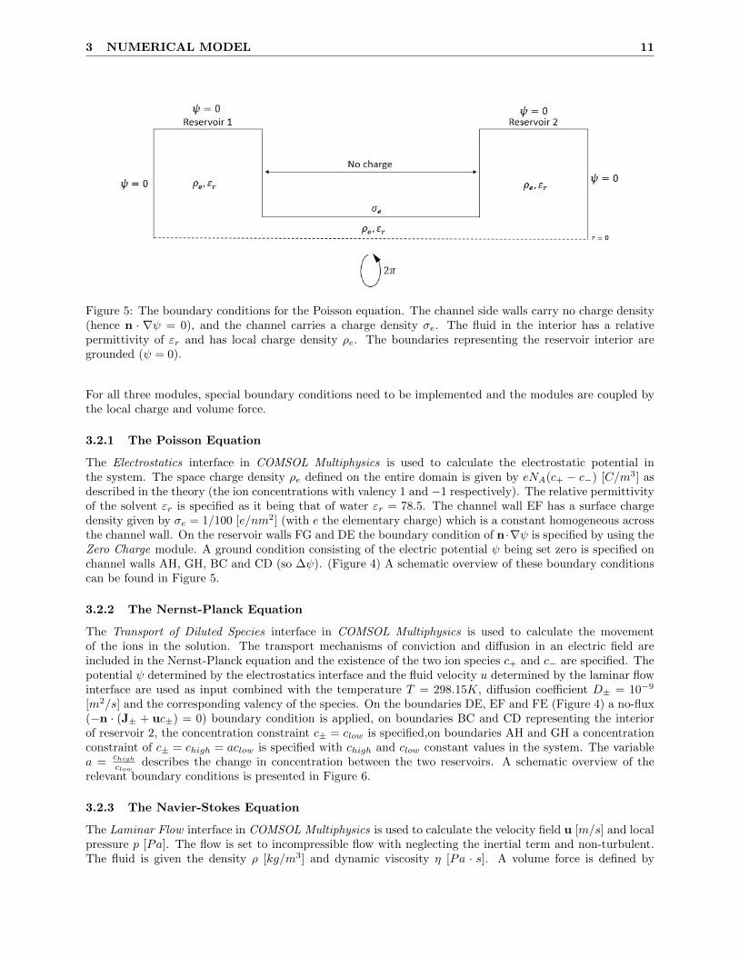
Figure 5: The boundary conditions for the Poisson equation. The channel side walls carry no charge density(hence n · ∇ψ = 0), and the channel carries a charge density σe. The fluid in the interior has a relativepermittivity of εr and has local charge density ρe. The boundaries representing the reservoir interior aregrounded (ψ = 0).

For all three modules, special boundary conditions need to be implemented and the modules are coupled bythe local charge and volume force.

3.2.1 The Poisson Equation

The Electrostatics interface in COMSOL Multiphysics is used to calculate the electrostatic potential inthe system. The space charge density ρe defined on the entire domain is given by eNA(c+ − c−) [C/m3] asdescribed in the theory (the ion concentrations with valency 1 and −1 respectively). The relative permittivityof the solvent εr is specified as it being that of water εr = 78.5. The channel wall EF has a surface chargedensity given by σe = 1/100 [e/nm2] (with e the elementary charge) which is a constant homogeneous acrossthe channel wall. On the reservoir walls FG and DE the boundary condition of n ·∇ψ is specified by using theZero Charge module. A ground condition consisting of the electric potential ψ being set zero is specified onchannel walls AH, GH, BC and CD (so ∆ψ). (Figure 4) A schematic overview of these boundary conditionscan be found in Figure 5.

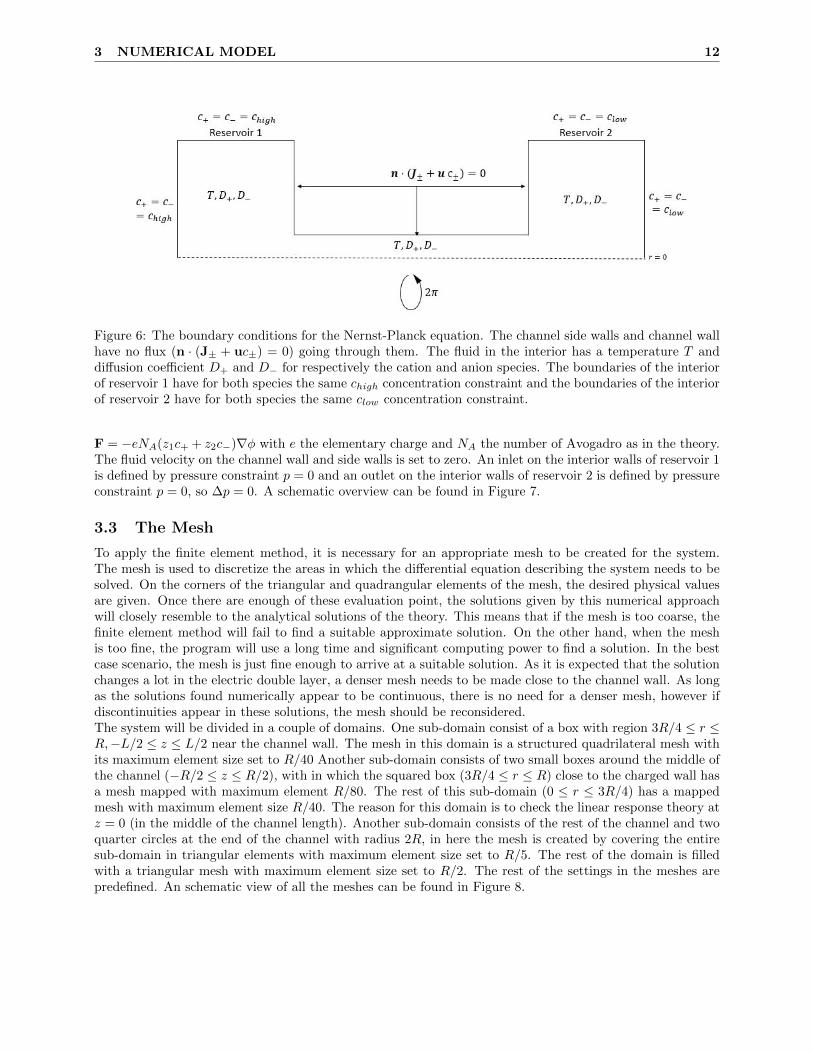
3.2.2 The Nernst-Planck Equation

The Transport of Diluted Species interface in COMSOL Multiphysics is used to calculate the movementof the ions in the solution. The transport mechanisms of conviction and diffusion in an electric field areincluded in the Nernst-Planck equation and the existence of the two ion species c+ and c− are specified. Thepotential ψ determined by the electrostatics interface and the fluid velocity u determined by the laminar flowinterface are used as input combined with the temperature T = 298.15K, diffusion coefficient D± = 10−9

[m2/s] and the corresponding valency of the species. On the boundaries DE, EF and FE (Figure 4) a no-flux(−n · (J± + uc±) = 0) boundary condition is applied, on boundaries BC and CD representing the interiorof reservoir 2, the concentration constraint c± = clow is specified,on boundaries AH and GH a concentrationconstraint of c± = chigh = aclow is specified with chigh and clow constant values in the system. The variablea =

chighclow

describes the change in concentration between the two reservoirs. A schematic overview of therelevant boundary conditions is presented in Figure 6.

3.2.3 The Navier-Stokes Equation

The Laminar Flow interface in COMSOL Multiphysics is used to calculate the velocity field u [m/s] and localpressure p [Pa]. The flow is set to incompressible flow with neglecting the inertial term and non-turbulent.The fluid is given the density ρ [kg/m3] and dynamic viscosity η [Pa · s]. A volume force is defined by


Figure 6: The boundary conditions for the Nernst-Planck equation. The channel side walls and channel wallhave no flux (n · (J± + uc±) = 0) going through them. The fluid in the interior has a temperature T anddiffusion coefficient D+ and D− for respectively the cation and anion species. The boundaries of the interiorof reservoir 1 have for both species the same chigh concentration constraint and the boundaries of the interiorof reservoir 2 have for both species the same clow concentration constraint.

F = −eNA(z1c+ + z2c−)∇φ with e the elementary charge and NA the number of Avogadro as in the theory.The fluid velocity on the channel wall and side walls is set to zero. An inlet on the interior walls of reservoir 1is defined by pressure constraint p = 0 and an outlet on the interior walls of reservoir 2 is defined by pressureconstraint p = 0, so ∆p = 0. A schematic overview can be found in Figure 7.

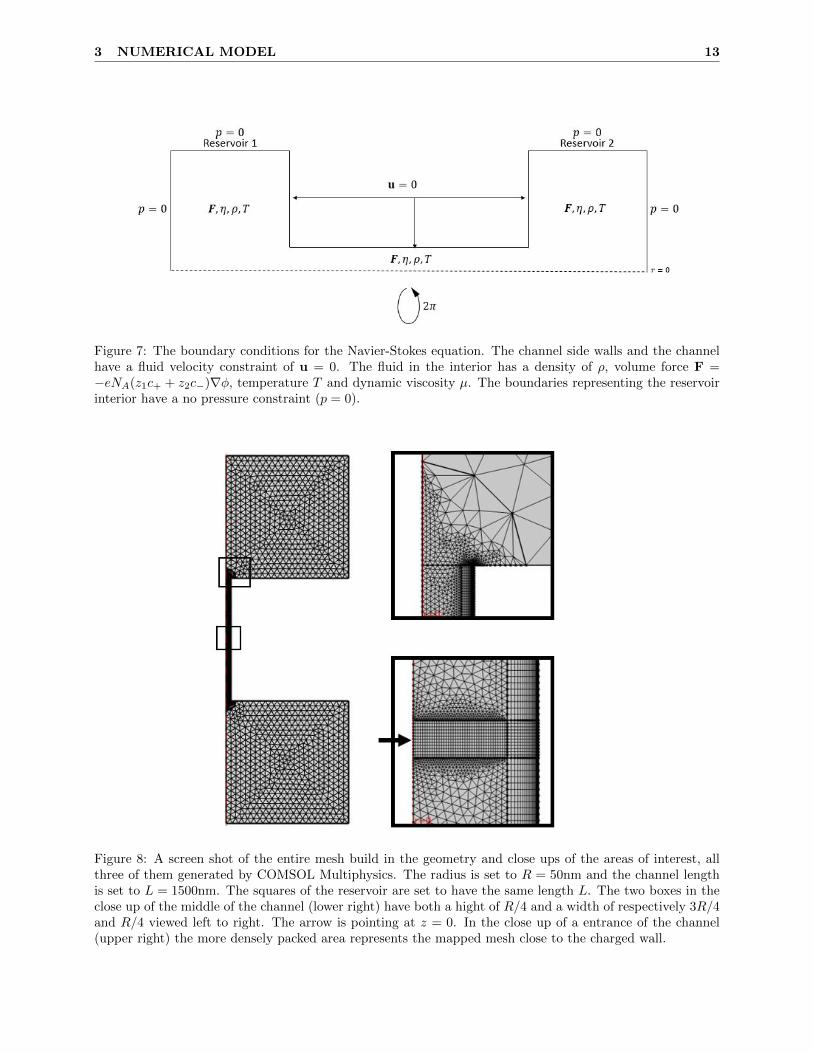
3.3 The Mesh

To apply the finite element method, it is necessary for an appropriate mesh to be created for the system.The mesh is used to discretize the areas in which the differential equation describing the system needs to besolved. On the corners of the triangular and quadrangular elements of the mesh, the desired physical valuesare given. Once there are enough of these evaluation point, the solutions given by this numerical approachwill closely resemble to the analytical solutions of the theory. This means that if the mesh is too coarse, thefinite element method will fail to find a suitable approximate solution. On the other hand, when the meshis too fine, the program will use a long time and significant computing power to find a solution. In the bestcase scenario, the mesh is just fine enough to arrive at a suitable solution. As it is expected that the solutionchanges a lot in the electric double layer, a denser mesh needs to be made close to the channel wall. As longas the solutions found numerically appear to be continuous, there is no need for a denser mesh, however ifdiscontinuities appear in these solutions, the mesh should be reconsidered.The system will be divided in a couple of domains. One sub-domain consist of a box with region 3R/4 ≤ r ≤R,−L/2 ≤ z ≤ L/2 near the channel wall. The mesh in this domain is a structured quadrilateral mesh withits maximum element size set to R/40 Another sub-domain consists of two small boxes around the middle ofthe channel (−R/2 ≤ z ≤ R/2), with in which the squared box (3R/4 ≤ r ≤ R) close to the charged wall hasa mesh mapped with maximum element R/80. The rest of this sub-domain (0 ≤ r ≤ 3R/4) has a mappedmesh with maximum element size R/40. The reason for this domain is to check the linear response theory atz = 0 (in the middle of the channel length). Another sub-domain consists of the rest of the channel and twoquarter circles at the end of the channel with radius 2R, in here the mesh is created by covering the entiresub-domain in triangular elements with maximum element size set to R/5. The rest of the domain is filledwith a triangular mesh with maximum element size set to R/2. The rest of the settings in the meshes arepredefined. An schematic view of all the meshes can be found in Figure 8.


Figure 7: The boundary conditions for the Navier-Stokes equation. The channel side walls and the channelhave a fluid velocity constraint of u = 0. The fluid in the interior has a density of ρ, volume force F =−eNA(z1c+ + z2c−)∇φ, temperature T and dynamic viscosity µ. The boundaries representing the reservoirinterior have a no pressure constraint (p = 0).

Figure 8: A screen shot of the entire mesh build in the geometry and close ups of the areas of interest, allthree of them generated by COMSOL Multiphysics. The radius is set to R = 50nm and the channel lengthis set to L = 1500nm. The squares of the reservoir are set to have the same length L. The two boxes in theclose up of the middle of the channel (lower right) have both a hight of R/4 and a width of respectively 3R/4and R/4 viewed left to right. The arrow is pointing at z = 0. In the close up of a entrance of the channel(upper right) the more densely packed area represents the mapped mesh close to the charged wall.

4 RESULTS 14

Quantity Symbol Value Unit

Surface charge density σe 1 · 10−2 e/nm

Diffusion coefficient D = D+ = D− 1 · 10−9 m2/s

Charge valency z+ = −z− 1 1

Dynamic viscosity η 8.925 · 10−4 pa·sMass density solvent ρ Value Unit

Temperature T 298.15 K

Relative permittivity εr 78.5 1

Channel radius R 50 nm

Channel length L 1500 nm

Ionic concentration lower boundary clow 1 mM

Ionic concentration higher boundary chigh = a · clow 1 mM

Fraction of concentration change a = chigh/clow 1 1

Table 1: For the simulation of the nanochannel, relevant parameter values of water are used in COMSOLMultiphysics. Parameters used in COMSOL to simulate the linear response behaviour for small concentrationdifferences.

4 Results

In this section will first consider the linear response relation between the chemical driving force as a result ofa concentration gradient and the induced fluxes by this concentration gradient, consisting of the fluid volumeflux Q, the electric current I and the salt flux J . After this, the analytical expressions found for the potentialand the fluid velocity field will be compared to the numerical results given by COMSOL Multiphysics.

4.1 Linear Response

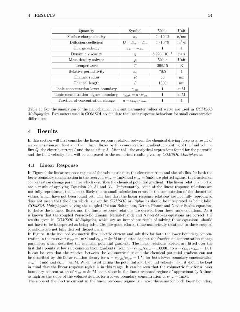
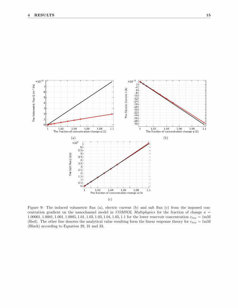
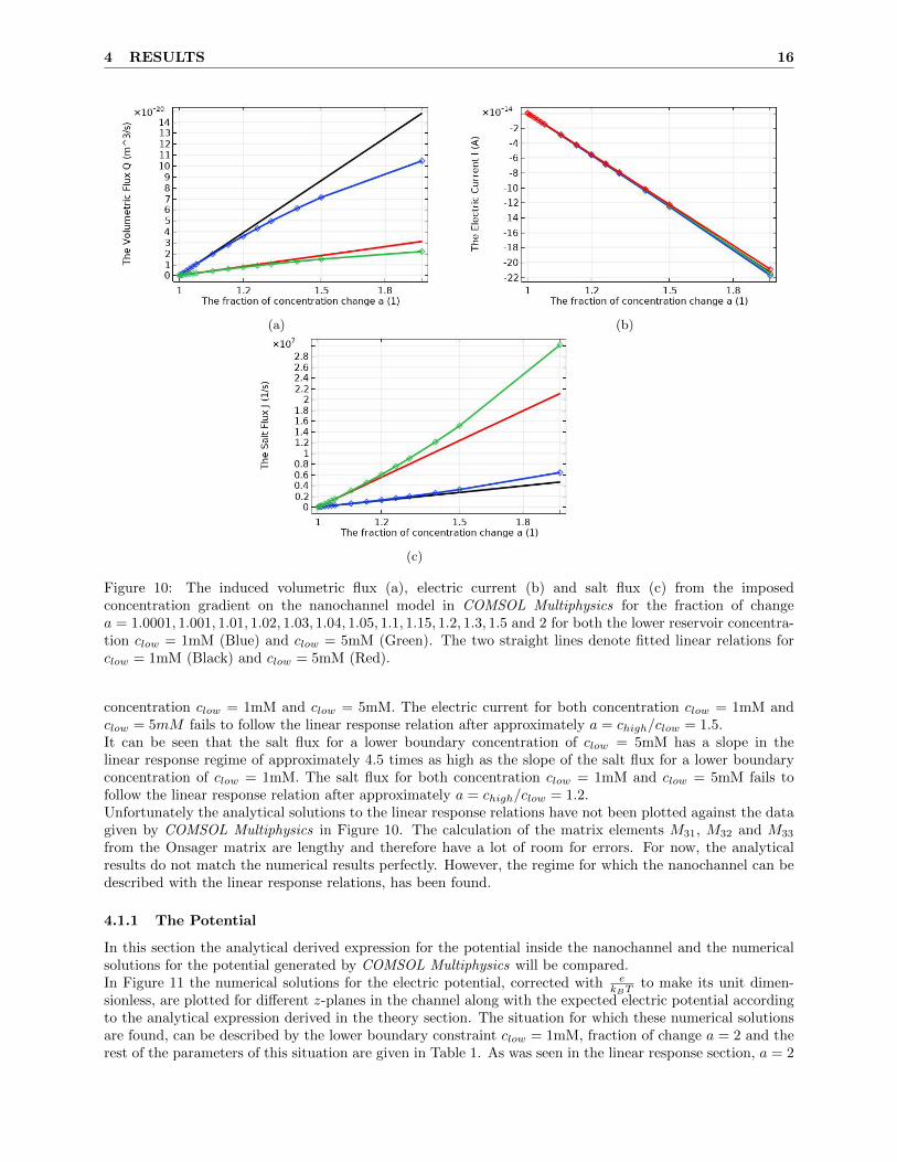
In Figure 9 the linear response regime of the volumetric flux, the electric current and the salt flux for both thelower boundary concentration in the reservoir clow = 1mM and clow = 5mM are plotted against the fraction onconcentration change parameter which describes the chemical potential gradient. The linear relations plottedare a result of applying Equation 29, 31 and 33. Unfortunately, some of the linear response relations arenot fully reproduced, this is most likely due to small calculation errors in the computation of the theoreticalvalues, which have not been found yet. The fact that the linear response relations are not fully reproduceddoes not mean that the data which is given by COMSOL Multiphysics should be interpreted as being false.COMSOL Multiphysics solving the coupled Poisson-Boltzmann, Nernst-Planck and Navier-Stokes equationsto derive the induced fluxes and the linear response relations are derived from these same equations. As itis known that the coupled Poisson-Boltzmann, Nernst-Planck and Navier-Stokes equations are correct, theresults given in COMSOL Multiphysics, which are an immediate result of solving these equations, shouldnot have to be interpreted as being false. Despite good efforts, these numerically solutions to these coupledequations are not fully derived theoretically.In Figure 10 the induced volumetric flux, electric current and salt flux for both the lower boundary concen-tration in the reservoir clow = 1mM and clow = 5mM are plotted against the fraction on concentration changeparameter which describes the chemical potential gradient. The linear relations plotted are fitted over thefirst data points at low salt concentration gradients, from a = chigh/clow = 1.00001 to a = chigh/clow = 1.01.It can be seen that the relation between the volumetric flux and the chemical potential gradient can notbe described by the linear relation theory for a = chigh/clow = 1.5. for both lower boundary concentrationclow = 1mM and clow = 5mM. When investigating the potential and the fluid velocity field, it should be keptin mind that the linear response region is in this range. It can be seen that the volumetric flux for a lowerboundary concentration of clow = 5mM has a slope in the linear response regime of approximately 5 timesas high as the slope of the volumetric flux for a lower boundary concentration of clow = 1mM.The slope of the electric current in the linear response regime is almost the same for both lower boundary

4 RESULTS 15

(a) (b)

(c)

Figure 9: The induced volumetric flux (a), electric current (b) and salt flux (c) from the imposed con-centration gradient on the nanochannel model in COMSOL Multiphysics for the fraction of change a =1.00001, 1.0001, 1.001, 1.0005, 1.01, 1.02, 1.03, 1.04, 1.05, 1.1 for the lower reservoir concentration clow = 1mM(Red). The other line denotes the analytical value resulting form the linear response theory for clow = 1mM(Black) according to Equation 29, 31 and 33.

4 RESULTS 16

(a) (b)

(c)

Figure 10: The induced volumetric flux (a), electric current (b) and salt flux (c) from the imposedconcentration gradient on the nanochannel model in COMSOL Multiphysics for the fraction of changea = 1.0001, 1.001, 1.01, 1.02, 1.03, 1.04, 1.05, 1.1, 1.15, 1.2, 1.3, 1.5 and 2 for both the lower reservoir concentra-tion clow = 1mM (Blue) and clow = 5mM (Green). The two straight lines denote fitted linear relations forclow = 1mM (Black) and clow = 5mM (Red).

concentration clow = 1mM and clow = 5mM. The electric current for both concentration clow = 1mM andclow = 5mM fails to follow the linear response relation after approximately a = chigh/clow = 1.5.It can be seen that the salt flux for a lower boundary concentration of clow = 5mM has a slope in thelinear response regime of approximately 4.5 times as high as the slope of the salt flux for a lower boundaryconcentration of clow = 1mM. The salt flux for both concentration clow = 1mM and clow = 5mM fails tofollow the linear response relation after approximately a = chigh/clow = 1.2.Unfortunately the analytical solutions to the linear response relations have not been plotted against the datagiven by COMSOL Multiphysics in Figure 10. The calculation of the matrix elements M31, M32 and M33

from the Onsager matrix are lengthy and therefore have a lot of room for errors. For now, the analyticalresults do not match the numerical results perfectly. However, the regime for which the nanochannel can bedescribed with the linear response relations, has been found.

4.1.1 The Potential

In this section the analytical derived expression for the potential inside the nanochannel and the numericalsolutions for the potential generated by COMSOL Multiphysics will be compared.In Figure 11 the numerical solutions for the electric potential, corrected with e

kBTto make its unit dimen-

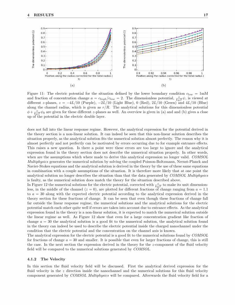
sionless, are plotted for different z-planes in the channel along with the expected electric potential accordingto the analytical expression derived in the theory section. The situation for which these numerical solutionsare found, can be described by the lower boundary constraint clow = 1mM, fraction of change a = 2 and therest of the parameters of this situation are given in Table 1. As was seen in the linear response section, a = 2

4 RESULTS 17

(a) (b)

Figure 11: The electric potential for the situation defined by the lower boundary condition clow = 1mMand fraction of concentration change a = chigh/clow = 2. The dimensionless potential, e

kBTψ, is viewed at

different z-planes, z = −4L/10 (Purple), −2L/10 (Light Blue), 0 (Red), 2L/10 (Green) and 4L/10 (Blue)along the channel radius, which is given as r/R. The analytical solutions for this dimensionless potentialφ+ e

kBTψ0 are given for these different z-planes as well. An overview is given in (a) and and (b) gives a close

up of the potential in the electric double layer.

does not fall into the linear response regime. However, the analytical expression for the potential derived inthe theory section is a non-linear solution. It can indeed be seen that this non-linear solution describes thesituation properly, as the analytical solution fits the numerical solution almost perfectly. The reason why it isalmost perfectly and not perfectly can be motivated by errors occurring due to for example entrance effects.This raises a new question. Is there a point were these errors are too large to ignore and the analyticalexpression found in the theory section does not describe the numerical situation properly. In other words,when are the assumptions which where made to derive this analytical expression no longer valid. COMSOLMultiphysics generates the numerical solution by solving the coupled Poisson-Boltzmann, Nernst-Planck andNavier-Stokes equations and the analytical solution is derived in the theory by the use of these same equationsin combination with a couple assumptions of the situation. It is therefore more likely that at one point theanalytical solution no longer describes the situation than that the data generated by COMSOL Multiphysicsis faulty, as the numerical solution does match the theory for the situation described above.In Figure 12 the numerical solutions for the electric potential, corrected with e

kBTto make its unit dimension-

less, in the middle of the channel (z = 0), are plotted for different fractions of change ranging from a = 1.1to a = 30 along with the expected electric potential according to the analytical expression derived in thetheory section for these fractions of change. It can be seen that even though these fractions of change fallfar outside the linear response regime, the numerical solutions and the analytical solutions for the electricpotential match each other quite well if errors are taken into account due to entrance effects. As the analyticalexpression found in the theory is a non-linear solution, it is expected to match the numerical solution outsidethe linear regime as well. As Figure 12 show that even for a large concentration gradient like fraction ofchange a = 30 the analytical solution is a good fit to the numerical solution, the analytical solution foundin the theory can indeed be used to describe the electric potential inside the charged nanochannel under thecondition that the electric potential and the concentration on the channel axis is known.The analytical expression for the electric potential is a good fit to the numerical solutions found by COMSOLfor fractions of change a = 30 and smaller. It is possible that even for larger fractions of change, this is stillthe case. In the next section the expression derived in the theory for the z-component of the fluid velocityfield will be compared to the numerical solutions generated by COMSOL.

4.1.2 The Velocity

In this section the fluid velocity field will be discussed. First the analytical derived expression for thefluid velocity in the z direction inside the nanochannel and the numerical solutions for this fluid velocitycomponent generated by COMSOL Multiphysics will be compared. Afterwards the fluid velocity field for a

4 RESULTS 18

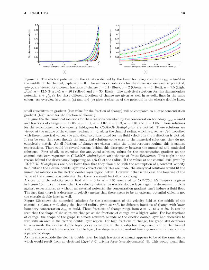
(a) (b)

Figure 12: The electric potential for the situation defined by the lower boundary condition clow = 5mM inthe middle of the channel, z-plane z = 0. The numerical solutions for the dimensionless electric potential,e

kBTψ, are viewed for different fractions of change a = 1.1 (Blue), a = 2 (Green), a = 4 (Red), a = 7.5 (Light

Blue), a = 12.5 (Purple), a = 20 (Yellow) and a = 30 (Black). The analytical solutions for this dimensionlesspotential φ + e

kBTψ0 for these different fractions of change are given as well in as solid lines in the same

colour. An overview is given in (a) and and (b) gives a close up of the potential in the electric double layer.

small concentration gradient (low value for the fraction of change) will be compared to a large concentrationgradient (high value for the fraction of change.)In Figure 13a the numerical solutions for the situations described by low concentration boundary clow = 5mMand fractions of change a = 1.005, a = 1.01, a = 1.02, a = 1.03, a = 1.04 and a = 1.05. These solutionsfor the z-component of the velocity field,given by COMSOL Multiphysics, are plotted. These solutions areviewed at the middle of the channel, z-plane z = 0, along the channel radius, which is given as r/R. Togetherwith these numerical values, the analytical solutions found for the fluid velocity in the z-direction is plotted.It can be seen that even though the analytical solutions come close to the numerical solutions, they do notcompletely match. As all fractions of change are chosen inside the linear response regime, this is againstexpectations. There could be several reasons behind this discrepancy between the numerical and analyticalsolutions. First of all, to calculate the analytical solution, values for the concentration gradient on thechannel axis were requested in COMSOL Multiphysics with the use of Point Evaluation. This might be thereason behind the discrepancy happening on 4/5-th of the radius. If the values at the channel axis given byCOMSOL Multiphysics are a bit lower than that they should be with the assumption of a constant velocityfield outside the electric double layer and corrections for this are made, the analytical solutions would fit thenumerical solutions in the electric double layer region better. However if that is the case, the lowering of thevalue at the channel axis indicates that there is a small back-flow occurring.A close up of the velocity vector field at z = 0 for a = 1.05 generated by COMSOL Multiphysics is givenin Figure 13c. It can be seen that the velocity outside the electric double layer region is decreasing. This isagainst expectations, as without an external potential the concentration gradient can’t induce a fluid flow.The fact that there is a decrease in velocity means that there needs to be an external potential which is notthe electric double layer as well.Figure 13b shows the numerical solutions for the z-component of the velocity field at the middle of thechannel, z-plane z = 0, along the channel radius, given as r/R, for different fractions of change with lowerboundary concentration clow = 5mM. These fractions of change range from a = 1.1 to a = 30. It can beseen that the shape of the solutions changes as the fractions of change are a higher value. For low fractionsof change, the shape of the graph is almost constant outside of the electric double layer and decreases tozero with an arch in the electric double layer region. For high fractions of change, the graph still decreasesto zero inside the electric double layer (as expected due to the no-slip boundary condition on the channelwall), however outside the electric double layer, the shape is not a constant line any more but appears to bea parabolic shape.As the shape outside the electric double layer for high fractions of change appears to be of the same shapewhich would result from an electrical (∆psi 6= 0) driving force (electric-osmosis) [9]. This would mean that

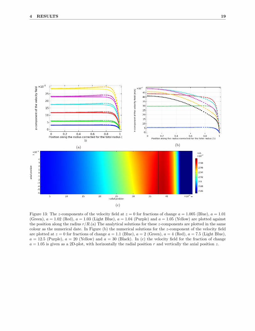
4 RESULTS 19

(a)(b)

(c)

Figure 13: The z-components of the velocity field at z = 0 for fractions of change a = 1.005 (Blue), a = 1.01(Green), a = 1.02 (Red), a = 1.03 (Light Blue), a = 1.04 (Purple) and a = 1.05 (Yellow) are plotted againstthe position along the radius r/R.(a) The analytical solutions for these z-components are plotted in the samecolour as the numerical date. In Figure (b) the numerical solutions for the z-component of the velocity fieldare plotted at z = 0 for fractions of change a = 1.1 (Blue), a = 2 (Green), a = 4 (Red), a = 7.5 (Light Blue),a = 12.5 (Purple), a = 20 (Yellow) and a = 30 (Black). In (c) the velocity field for the fraction of changea = 1.05 is given as a 2D-plot, with horizontally the radial position r and vertically the axial position z.

4 RESULTS 20

(a) (b)

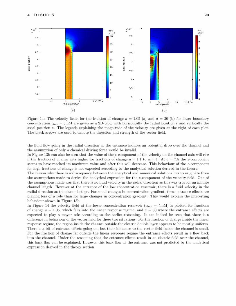
Figure 14: The velocity fields for the fraction of change a = 1.05 (a) and a = 30 (b) for lower boundaryconcentration clow = 5mM are given as a 2D-plot, with horizontally the radial position r and vertically theaxial position z. The legends explaining the magnitude of the velocity are given at the right of each plot.The black arrows are used to denote the direction and strength of the vector field.

the fluid flow going in the radial direction at the entrance induces an potential drop over the channel andthe assumption of only a chemical driving force would be invalid.In Figure 13b can also be seen that the value of the z-component of the velocity on the channel axis will riseif the fraction of change gets higher for fractions of change a = 1.1 to a = 4. At a = 7.5 the z-componentseems to have reached its maximum value and after this will decrease. This behaviour of the z-componentfor high fractions of change is not expected according to the analytical solution derived in the theory.The reason why there is a discrepancy between the analytical and numerical solutions has to originate fromthe assumptions made to derive the analytical expression for the z-component of the velocity field. One ofthe assumptions made was that there is no fluid velocity in the radial direction as this was true for an infinitechannel length. However at the entrance of the low concentration reservoir, there is a fluid velocity in theradial direction as the channel stops. For small changes in concentration gradient, these entrance effects areplaying less of a role than for large changes in concentration gradient. This would explain the interestingbehaviour shown in Figure 13b.In Figure 14 the velocity field at the lower concentration reservoir (clow = 5mM) is plotted for fractionsof change a = 1.05, which falls into the linear response regime, and a = 30 where the entrance effects areexpected to play a mayor role according to the earlier reasoning. It can indeed be seen that there is adifference in behaviour of the vector field for these two situations. For the fraction of change inside the linearresponse regime, the region inside the channel outside the electric double layer appears to be mostly uniform.There is a bit of entrance effects going on, but their influence to the vector field inside the channel is small.For the fraction of change far outside the linear response regime the entrance effects result in a flow backinto the channel. Under the reasoning that the entrance effects result in an electric field over the channel,this back flow can be explained. However this back flow at the entrance was not predicted by the analyticalexpression derived in the theory section.

5 DISCUSSION 21

5 Discussion

This discussion will primarily focus on changes in the potential and fluid velocity field depending on theconcentration gradient since the linear response relations are expected outcomes and will therefore not leadto new insights regarding the research questions outlined in the introduction. Even though the linear responsetheory has not exactly verified the simulations of the model build with COMSOL Multiphysics, it is onlya matter of thoroughly going over the calculations until its validity is assured. This is not the case atthe moment and since the Onsager matrix from the linear response theory should verify the considerednanochannel systems up to errors coming from the entrance effects. The results of the linear response theoryfor the different induced fluxes are to be used as indication of the valid regimes for which in principle analyticalsolutions for the potential and fluid velocity field can be found.The results given in the previous section show that the analytical expression derived to describe the electricpotential of the electric double layer inside the channel match the numerical results generated by COMSOLMultiphysics. However it has to be noted that to get the Debye length, the concentration of the ionic speciesis gained with Point Evaluation from COMSOL Multiphysics as was done for the electric potential on thechannel axis to get the full analytical expression. This implies that the analytical expression describes thesystem quite well, provided that the values taken in from the channel axis are valid. This may also explainthe fact that the analytical expression matches the numerical solutions generated by COMSOL Multiphysicsfar outside the linear response regime, as data points were taken from these numerical solutions. It thereforeraises the question of what the regime in which applicability of this analytical expression would be valid ifthe potential along the axis was described in an analytical manner.The most interesting results of those who will be discussed, are the results of the fluid velocity field fordifferent concentration gradients. The results show that inside the linear response regime, the analyticalexpression for the z-component matches the numerical solutions generated by COMSOL Multiphysics fairlywell. There is however a small decrease in velocity outside the electric double layer region. This behaviourcan be motivated by entrance effects. It is however important to note that Point Evaluation was used againto get the necessary values of the parameters on the channel axis for the analytical expression.Far outside the linear response regime, with fraction of change a = chigh/clow ≥ 4, the entrance effect havea large influence on the fluid vector field of the system and the analytical and numerical solution do notmatch. The most likely cause for this discrepancy in the z-component of the velocity field to happen, wouldbe the fact that at the channel entrance, the assumption that there is no fluid flow in the radial direction isno longer valid. This fluid flow may give rise to a difference in potential over the channel, which will be adriving force as well. If there is a bigger difference in concentration between the two reservoirs, the fluid flowin the radial direction will be larger as well. This means that the driving force as a result of this fluid flowhas a greater influence on the fluid flow in the channel. This may be a reason behind the parabolic shapefound in the results for the z-component of the velocity.As the analytical expression does not take this back flow as a result of entrance effects into account, it doesnot properly describe the situation in the nanochannel. However, for small concentration differences it canstill be used to get an estimation of the behaviour inside the channel.

6 CONCLUSION 22

6 Conclusion

A nanochannel subjected to a concentration gradient in a system described by the concentration boundarieschigh > clow and the rest of the parameters as described in Table 1 will generate a volumetric flux, electriccurrent and salt flux. These induced fluxes are linear with respect to the chemical driving force at least untilchigh/clow = 1.1. For smaller concentration differences then this, the induced fluxes can be described byOnsager’s linear response theory.The dimensionless potential derived in the theory section which takes the axial dependent Debye length intoaccount, can be used to describe the electric potential of the discussed system and the heterogeneities of theelectric double layer in the nanochannel. This answers the research question raised in the introduction. It isindeed possible to describe the heterogeneous electric double layer for this system in an analytical manner.The same can’t be said for the fluid velocity field. It appears that the complete behaviour of the fluid velocityfield in the system can not be completely described in an analytical manner as of now. However, for specialsituations the behaviour can be predicted.Leaving as a conclusion is that the velocity field can be described by the analytical expression for the z-component, derived in theory section, for small concentration gradients inside the linear response regime.The analytical expression can not be used outside this regime due to the fact that entrance effects give riseto a back flow into the channel at the lower concentration reservoir entrance and outside the linear regimethis back flow is large enough to reverse the fluid flow.The first priority in going further with research in this area is verifying the different linear response relationsused. As it has been shown that that these relations have to hold for a cylindrical system in the consideredregime [27], the verification is not impossible. Another aspect to look into is how the values on the channelaxis can be described in an analytical manner. Furthermore an theory describing the entrance effects in thevelocity field needs to be drawn up as these are the main contributor to the back flow which is created at thelow concentration reservoir entrance. It is also interesting to look into the effects of a difference in mobility(D+ 6= D=) for the two ionic species considered, as equal mobility was assumed to simplify the complexsystem of a concentration gradient over a charged nanochannel.

7 INTERESTS 23

7 Interests

There are no conflicts to declare.

REFERENCES 24

References

[1] Wick, G.L. (1977) Power from salinity gradients. Energy, 1978.

[2] Bocquet,L.,& Tabeling, P. (2014). Physics and technological aspects of nanofluidics. Lab on a Chip, 2014.

[3] Alizadeh, A.,& Wang, M. (2018) Reverse electrodialysis through nanochannels with inhomogeneouslycharged surfaces and overlapped electric double layer.

[4] Rice, C.L.,& Whitehead, R. (1965) Electrokinetic Flow in a Narrow Cylindrical Capillary. The Journalof Physical Chemistry, 1965.

[5] Burgreen, D.,& Nakache, F.R. (1963) Electrokinetic Flow in Ultrafine Capillary Slits1. The Journal ofPhysical Chemistry, 1964.

[6] Ohshima, H.,& Kondo, T. (1989) Electrokinetic flow between two parallel plates with surface chargelayers: Electro-osmosis and streaming potential. Journal of Colloid and Interface Science, 1990

[7] Pennathur, S.,& Santiago, J.G. (2005) Electrokinetic Transport in Nanochannels. 1. Theory. AnalyticalChemistry, 2005.

[8] Yang, C.,& Li, D. (1997) Analysis of electrokinetic effects on the liquid flow in rectangular microchannels.Colloids and Surfaces A: Physicochemical and Engineering Aspects, 1998.

[9] Masliyah, J.H.,& Bhattacharjee, S. 2006 Electrokinetic and Colloid Transport Phenomena. Hoboken, NJ:John Wiley & Sons, Incorporated.

[10] Qian, S.,& Ai, Y. (2012) Electrokinetic Particle Transport in Micro-/Nanofluidics: Direct NumericalSimulation Analysis. Boca Raton, Fl: CRC Press

[11] Delgado, A.V. (2001) Interfacial Electrokinetics and Electrophoresis. Boca Raton, Fl: CRC Press

[12] Liu, X., Zeng, Q., Liu, C., Yanga, J.,& Wang, L. (2019) Experimental and finite element method studiesfor femtomolar cobalt ion detection using a DHI modified nanochannel. Analyst, 2019.

[13] Yan, F., Yao, L., Chen, K., Yanga, Q.,& Su, B. (2018) An ultrathin and highly porous silica nanochannelmembrane: toward highly efficient salinity energy conversion. Journals of Materials Chemistry A, 2019

[14] Li-Chang Hung, L.,& Minh, M.N. (2015) Stationary Solutions to the Poisson-Nernst-Planck Equationswith Steric Effects.

[15] Tagliazucchi, M.,& Szleifer, I. (2017) Theoretical Basis for Structure and Transport in Nanopores andNanochannels. Chemically Modified Nanopores and Nanochannels (2017)

[16] Pilon, L., Wang, H.,& d’Entremont, A. (2014) Recent Advances in Continuum Modeling of Interfacialand Transport Phenomena in Electric Double Layer Capacitors. Journal of The Electrochemical Society,2015.

[17] Van Roji, R. (2019) Soft Condensed Matter Theory.

[18] Constantin, P.,& Ignatova, M. (2018) On the Nernst-Planck-Navier-Stokes system. Archive for RationalMechanics and Analysis, 2019.

[19] Gray, C.G.,& Stiles, P.J. (2018). Nonlinear Electrostatics. The Poisson-Boltzmann Equation. EuropeanJournal of Physics, 2018.

[20] Yuan, Z., Garcia, A.L., Lopez, G.P.,& Petsev, D.N. (2006) Electrokinetic transport and separations influidic nanochannels. Electrophoresis, 2007.

[21] Bagotsky, V.S.,& Mueller, K. (2005) Fundamentals of Electrochemistry, 2nd Edition. Hoboken, NJ: JohnWiley & Sons, Incorporated.

REFERENCES 25

[22] D’yachkov, L.G. (2004) Analytical Solution of the Poisson–Boltzmann Equation in Cases of Sphericaland Axial Symmetry. Technical Physics Letters,2005.

[23] Outhwaite, C.W., Bhuiyan, L.B.,& Levine, S. (1979) Theory of the electric double layer using a modifiedpoisson–boltzman equation. Journal of the Chemical Society Faraday Transactions, 1980.

[24] Prieve, D.C, Anderson, J.L.,& Ebel, J.P.,& Lowell, M.E. (1982) Motion of a particle generated by chem-ical gradients. Part 2. Electrolytes. Journal of Fluid Mechanics, 1984.

[25] Malmberg, C.G.,& Maryott, A.A. (1955) Dielectric Constant of Water from 0o to 100o C. Journal ofResearch of the National Bureau of Standards, 1956.

[26] Debye, P.,& Huckel, E. (1923) The theory of electrolytes. I. Freezing point depression and related phe-nomena. Translated and Typeset by Braus, M.J. (2019)

[27] Werkhoven, B.L.,& Van Roji, R. (2019) Coupled water, charge and salt transport in heterogeneous nano-fluidic systems.

[28] Dow, J.O. (1999) Introduction to Problem Definition and Development. A Unified Approach to the FiniteElement Method and Error Analysis Procedures, 1999.

[29] Chakrabarty, A., Mannan, S.,& Cagin, T. (2016) Finite Element Analysis in Process Safety Applications.Multiscale Modeling for Process Safety Applications, 2016.

A SOLUTION TO THE POISSON-BOLTZMANN EQUATION IN PLANAR GEOMETRY26

A Solution To The Poisson-Boltzmann Equation In Planar Geom-etry

The Poisson equation for the dimensionless potential φ for the situation of x = R− r is given by

d2φ

dx2= κ2 sinh(φ(x)), (34)

in which κ is given by

κ =

√2c0NAe2

kBTε0εr, (35)

with c0 the ionic concentration at x = R, which is defined under the assumption that on the axis, far awayfrom the charged wall, both of the ion concentrations are the same, c0(z) = c0+ = c0−. To find the functionwhich describes the potential φ, this second order derivative needs to be solved. To do this, the followingmathematical identity is used

(dφ

dx)2 ≡ 2

∫d2φ

dx2dφ. (36)

It is easy to check that this is indeed equivalent by differentiating with respect to x. Substituting thePoisson-Boltzmann equation (Eq. 34) gives

(dφ

dx)2 = 2κ2

∫sinh(φ)dφ = κ2(eφ + e−φ − 2), (37)

in which the fact is used that by definition φ|x=R = 0. This can be rewritten by using another mathematicalidentity

sinh2X = (eX − e−X

2)2 =

e2X + e−2X − 2

4. (38)

By taking the square root, it can be found that

dφ

dx= −2κ sinh

φ

2, (39)

the decision to take the negative option is a result of the physical situation which is described. By introducing

a new variable y which is defined by the following relation y = eφ2 this new equation can be solved by

substituting y:dφ

dx=

2

y

dy

dx= −κ(y − 1

y), (40)

which simplifies tody

dx= −κ

2(y2 − 1). (41)

A solution to this problem would entail y being given by

y =1 + γ1e

Fx

1 + γ2eFx, (42)

with γ1,γ2,F to be determined variables independent of x. This would mean that

dy

dx=

(γ1F − γ2F )eFx

(1 + γ2eFx)2= −κ

2

(2γ1 − 2B)eFx + (γ21 − γ22)e2Fx

(1 + γ2eFx)2. (43)

As a result, y can only be of that form as γ1 = −γ2 and F = −κ due to the fact that the case γ1 = γ2 isnot an option. The function y = 1 has no non-zero second-order differential equation. The function y cannow be written as a function of one unknown variable γ = γ1. The second boundary condition is used todetermine γ. This boundary condition is a result of Gauss’ law

G =dφ

dx|x=0 = − e2

ε0εrkBT

σee, (44)

A SOLUTION TO THE POISSON-BOLTZMANN EQUATION IN PLANAR GEOMETRY27

and describes the relation between the potential at the wall and the surface charge of the wall. As all of theexponents in y will be zero at x = 0, this boundary condition can be given by

G = −κ(1 + γ

1− γ− 1− γ

1 + γ) = −κ 4γ

1− γ2. (45)

This gives γ = 2κG ±

√( 2κG )2 + 1, and as |γ| < 1 the unique solution of the potential can be given as

φ = 2 ln1 + γe−κx

1− γe−κx, (46)

with γ = 2κG −

√( 2κG )2 + 1 and κ =

√2c0NAe2

kBTε0εr. Using the fact that x = R − r this can be substituted again

to give the potential depending on r,

φ(r) = 2 ln1 + γe−κ(R−r)

1− γe−κ(R−r). (47)

B SOLUTION TO THE FLUID VELOCITY 28

B Solution To The Fluid Velocity

The second partial differential equation of the fluid velocity is given by

∂2u

∂r2= 2

kBTNAη

∂c0

∂z(coshφ− 1). (48)

As was done in the derivation of the solution to the dimensionless potential, the substitution x = R − r isintroduced. This gives a new partial differential equation for the fluid velocity in the z-direction,

∂2u

∂x2= 2

kBTNAη

∂c0

∂z(coshφ− 1). (49)

This combined with the solution found for the dimensionless potential (Eq. 47) gives

∂2u

∂x2=kBTNA

η

∂c0

∂z(

4γe−κx

(1− γe−κx)2+−4γe−κx

(1 + γe−κx)2), (50)

where is used that

2(coshφ− 1) =(1 + γe−κx)2

(1− γe−κx)2+

(1− γe−κx)2

(1 + γe−κx)2− 2 =

4γe−κx

(1− γe−κx)2+−4γe−κx

(1 + γe−κx)2. (51)

Keeping in mind that

f(y) =1

1 +Be−κy→ f ′(y) =

Bκe−κy

(1 +Be−κy)2, (52)

simple integration of both sides gives

∂u

∂x=−4kBTNAκ

η

∂c0

∂z(

1

1− γe−κx+

1

1 + γe−κx+ 2 + C1), (53)

with C1 an integration constant independent of x (it may depend on z).Using the fact that

1

1− γe−κx+

1

1 + γe−κx=

2

1− γ2e−2κx=

2e2κx

e2κx − γ2, (54)

combined with

f(y) = ln (e2κx − γ2)→ f ′(y) =2κe2κx

e2κx − γ2, (55)

andln (e2κx − γ2) = ln (1− γ2e−2κx) + 4κx, (56)

The fluid velocity can be given as

u =−4kBTNAκ

−1

η

∂c0

∂z(κ−1 ln (1− γ2e−2κx) + (2 + 4 + C1)x+ C2), (57)

with C2 another integration constant independent of x. The boundary condition for C1 is taken such thatthe linear x term disappears, as the fluid velocity outside the electric double layer is constant, as there is nopotential for the concentration gradient to induce a fluid flow. The second boundary condition which needsto be taken into account is the no-slip boundary u = 0 at x = 0 (on the channel wall) is used to determineC2. This enables the rewriting of the fluid velocity to

u(x) =−4kBTNAκ

−2

η

∂c0

∂zln

1− γ2e−2κx

1− γ2. (58)

The fluid velocity in the z-direction depending on r is found can be found with the use of the substitutionx = R− r,

u(r) =−4kBTNAκ

−2

η

∂c0

∂zln

1− γ2e−2κ(R−r)

1− γ2. (59)

C BEGIN PHASE NUMERICAL STUDY 29

C Begin Phase Numerical Study

In the begin phase of the numerical aspect of this study, a lot of time was spent on reproducing a cylindricalnanochannel with a pressure gradient instead of a concentration gradient. It falls a bit outside the scope ofthis paper, however it is important to understand the reasoning behind this earlier recreation. Comparedto the concentration gradient system, the pressure system is far better understood. This is due to the factthat the pressure gradient is constant over the channel and the Debye length describing the electric doublelayer doesn’t depend on the radial position r and axial position z. As a result this pressure system is lesscomplex and therefore uses less computing power and time when computed numerically. As there was noearlier experience with the modelling program COMSOL Multiphysics, it seemed logical to start with thisas both a means to gain experience with COMSOL Multiphysics and to remove errors easier (to estimate,a pressure system calculation took around 5 minutes, while a diffusio-osmotic system calculation often tookover an hour). A lot of the evaluation of the mesh sizes with respect to efficiency (a decision between a betterapproximate solution and less computing time and power) was done in this earlier stage. This pressuresystem was checked for both linear response theory for pressure gradients and the Poisseuille flow (whichdescribes the axial velocity for pressure gradients). After this, the pressure system was rebuild to the chemicalgradient system, which is discussed in here discusses. For anyone using COMSOL Multiphysics to numericallycalculate the diffusio-osmotic system, We encouraged to look into the pressure driven system first.

An Analytical and Numerical Study of the Electric Double ...

Documents

Transcript of An Analytical and Numerical Study of the Electric Double ...