- 4 -

)(ln)(ln)1(),(ln qbuqauquF (1)

Because the distance function possesses the same properties as the cost function, except of

substituting quantities for prices, )(ln qa and )(ln qb are basically defined analogous to those

in the development of the AIDS model.

j

k j

kkjk

k

k qqrqqa lnln2

1lnln *

0 (2)

kk

qqaqb 0lnln (3)

Thus, the IAIDS distance function is written

k

kk

jk

k j

kjk

k

k puqqrpquF 0

*

0 lnln2

1ln,ln (4)

The compensated inverse demand function can be derived directly from equation (4). The

quantity derivatives of the distance function are the normalized prices demanded, i.e., by

Shepherd’s Lemmax

p

q

quF i

i

),( where x denotes total expenditure. Multiplying both sides by

),( quF

qi yields

iii

i

wx

qp

q

quF

ln

),(ln (5)

where iw is the budget share of good i . Hence, logarithmic differentiation of (4) gives the

budget shares as a function of quantities and utility:

k

kij

j

ijii quqrw 0ln

(6)

where )(2

1 **

jiijij rrr .

Inverting the distance function at the optimal quantity yields the direct utility function which may

be substituted into equation (6).

)](ln)(/[lnln)( qaqbqaqU (7)

- 5 -

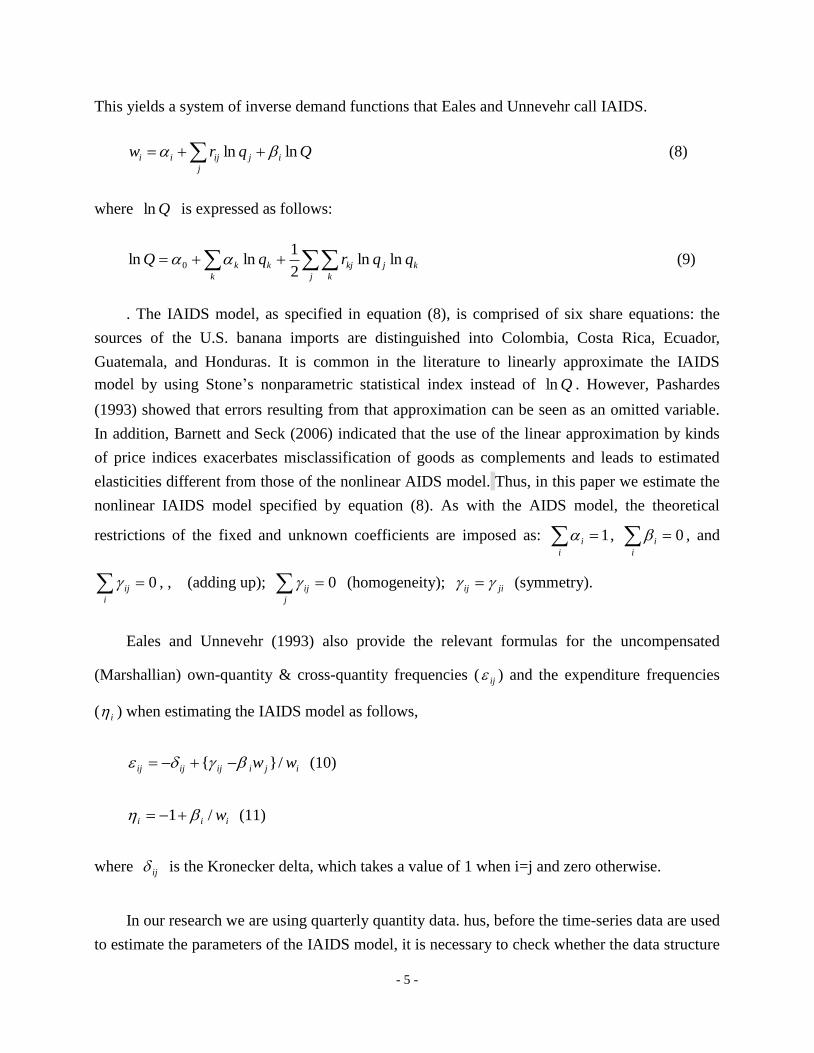
This yields a system of inverse demand functions that Eales and Unnevehr call IAIDS.

Qqrw ij

j

ijii lnln (8)

where Qln is expressed as follows:

kj

j k

kjk

k

k qqrqQ lnln2

1lnln 0 (9)

. The IAIDS model, as specified in equation (8), is comprised of six share equations: the

sources of the U.S. banana imports are distinguished into Colombia, Costa Rica, Ecuador,

Guatemala, and Honduras. It is common in the literature to linearly approximate the IAIDS

model by using Stone’s nonparametric statistical index instead of Qln . However, Pashardes

(1993) showed that errors resulting from that approximation can be seen as an omitted variable.

In addition, Barnett and Seck (2006) indicated that the use of the linear approximation by kinds

of price indices exacerbates misclassification of goods as complements and leads to estimated

elasticities different from those of the nonlinear AIDS model. Thus, in this paper we estimate the

nonlinear IAIDS model specified by equation (8). As with the AIDS model, the theoretical

restrictions of the fixed and unknown coefficients are imposed as: 1i

i , 0i

i , and

0i

ij , , (adding up); 0j

ij (homogeneity); jiij (symmetry).

Eales and Unnevehr (1993) also provide the relevant formulas for the uncompensated

(Marshallian) own-quantity & cross-quantity frequencies ( ij ) and the expenditure frequencies

( i ) when estimating the IAIDS model as follows,

ijiijijij ww /}{ (10)

iii w/1 (11)

where ij is the Kronecker delta, which takes a value of 1 when i=j and zero otherwise.

In our research we are using quarterly quantity data. hus, before the time-series data are used

to estimate the parameters of the IAIDS model, it is necessary to check whether the data structure

- 6 -

of each of the variables in the model is not-stationary using an autoregressive model. In statistics,

the augmented Dickey–Fuller test (Dickey and Fuller, 1981) that is valid in large samples is

commonly used. In general, economic time series data is often violated in the stationary

assumption, i.e., the data is the existence of a long-term trend. For this situation, it is important

for the data to be differenced to render stationary. According to Engle and Granger’s (1987)

explanation, if a non-stationary time-series data is differenced d times to reach stationary,

expressed as I(d) (integrated of order d), there are d unit roots in the series. All variables to be

employed in the IAIDS model are integrated of the order 1, I(1), i.e. stationary in the first

difference form.

2.2 New Empirical Industrial Organization

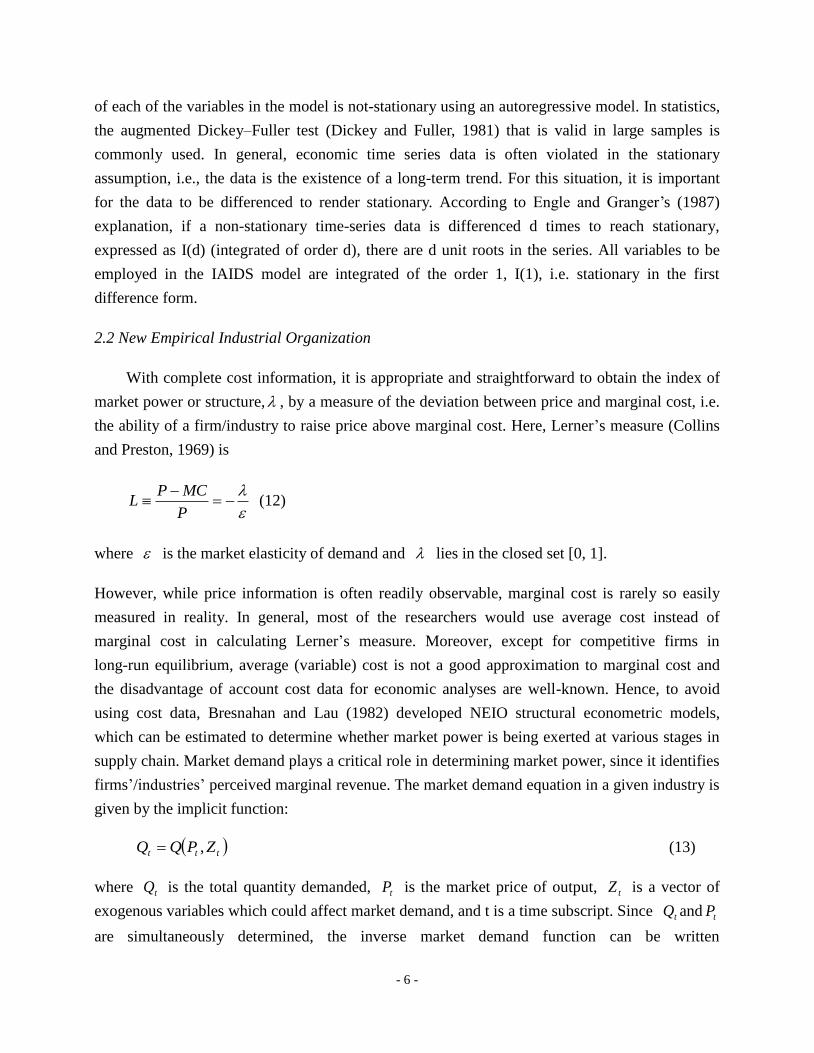
With complete cost information, it is appropriate and straightforward to obtain the index of

market power or structure, , by a measure of the deviation between price and marginal cost, i.e.

the ability of a firm/industry to raise price above marginal cost. Here, Lerner’s measure (Collins

and Preston, 1969) is

P

MCPL (12)

where is the market elasticity of demand and lies in the closed set [0, 1].

However, while price information is often readily observable, marginal cost is rarely so easily

measured in reality. In general, most of the researchers would use average cost instead of

marginal cost in calculating Lerner’s measure. Moreover, except for competitive firms in

long-run equilibrium, average (variable) cost is not a good approximation to marginal cost and

the disadvantage of account cost data for economic analyses are well-known. Hence, to avoid

using cost data, Bresnahan and Lau (1982) developed NEIO structural econometric models,

which can be estimated to determine whether market power is being exerted at various stages in

supply chain. Market demand plays a critical role in determining market power, since it identifies

firms’/industries’ perceived marginal revenue. The market demand equation in a given industry is

given by the implicit function:

ttt ZPQQ , (13)

where tQ is the total quantity demanded, tP is the market price of output, tZ is a vector of

exogenous variables which could affect market demand, and t is a time subscript. Since tQ and tP

are simultaneously determined, the inverse market demand function can be written

- 7 -

as ttt ZQPP , . Industry revenue is defined as ttt QPR * and, thus, perceived marginal

revenues )}({ tMR can be expressed as

t

tttt dQ

dPQPMR )( (14)

The value of represents the rotations of the perceived marginal revenue curve away from

consumer demand (Bresnahan, 1982). If =0, the given industry is perfectly competitive and the

producers perceive that they face a horizontal demand cure. As >0, producers face a

downward-sloping market demand so there is a departure of perceived marginal revenues from

market demand and some seller market power exists. If =1, full monopoly market power is

being exerted and firms are behaving as if a single firm is acting as a monopoly. In equilibrium,

tt MCMR and this relationship can be expressed as

MCdQ

dPQP

t

ttt

(15)

Given the above-mentioned concepts, the following equations can be adopted to estimate the

degree of imperfect competition in the U.S. fresh banana import market. For fresh banana imports,

the market demand function is specified in linear form:

trttt ePPCBIMPQ 1210 (16)

where tIMPQ is the total quantity of bananas imported into United States (thousand

pounds/year); tPCB is per-capita consumption of banana (pound/year); rtP is the retail price of

bananas (US$/thousand pounds) and te1 is the error term, where ),(~ 2

1 Ne t . In addition,

suppose that a marginal cost takes the following functional form:

wtt PMC 10 (17)

where wtP is the wholesale price of bananas as an approximation of the cost of bananas to

retailers. Substituting the marginal cost function (17) into the profit-maximizing condition (15)

and rearranging terms, we get the optimality equation

twttttrt ePIMPIEarningsIMPQP 2

2

43210 )()ln( (18)

where )ln( is the natural logarithm; tEarnings is average hourly earnings in trade, transportation

- 8 -

and utilities industries (US$); tIMPI is the import price index of fruit and fruit preparations;

wtP is the wholesale price of bananas (US$/thousand pounds), and te2 is the error term.

Conspicuously an absent explanatory variable in equation (17) and (18) which is used by

Deodhar and Sheldon (1995) is time trend variable due to statistical insignificance in the model.

From (18)

t

rt

dIMPQdP

1 and ),(~ 2

2 Ne t . By differentiating (16) with respect to

tIMPQ , we derive that 2

1

t

rt

dIMPQdP

. Thus, Use the estimates of equation (16) and

(18), we can obtain an estimate of the market-power parameter 21 * .

3. Data

The dependent variables in our six equation IAIDS are the quarterly shares of the U.S.

expenditures on bananas from Colombia, Costa Rica, Ecuador, Guatemala, Honduras and the

rest of the world.. The expenditure shares were constructed using U.S. expenditures on imported

bananas from each of the six countries divided by the total expenditure on bananas from these

countries. The quarterly expenditure and quarterly quantity data were obtained from the U.S.

International Trade Commission (USITC) website.

To derive the market-power parameter, using the NEIO model, equations (16) and (18)

were estimated with 2SLS and 3SLS using annual data over the period 1985~2008. These annual

data were obtained from different sources. The per-capita consumption and retail prices of

bananas were collected from the United States Department of Agriculture (USDA) website, data

on average hourly earnings in trade, transportation and utility industries along with the import

price index of fruit and fruit preparations were taken from the United States Department of Labor

website, and the information about the wholesale price of bananas is obtained from the Banana

Statistics (2001, 2003, 2005, 2009) and the World Banana Economy 1985~2002 of Food and

Agriculture Organization (FAO). All nominal variables involving prices and earnings were

deflated by the consumer price index.

4. Results

Table 1 presents the econometric results from the MLE method of the nonlinear IAIDS

model. With respect to the Costa Rican share equation; seven out of eight estimated parameters

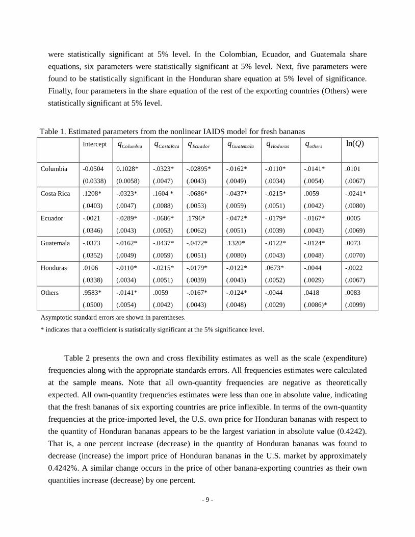
- 9 -

were statistically significant at 5% level. In the Colombian, Ecuador, and Guatemala share

equations, six parameters were statistically significant at 5% level. Next, five parameters were

found to be statistically significant in the Honduran share equation at 5% level of significance.

Finally, four parameters in the share equation of the rest of the exporting countries (Others) were

statistically significant at 5% level.

Table 1. Estimated parameters from the nonlinear IAIDS model for fresh bananas

Intercept Columbiaq CostaRicaq

Ecuadorq Guatemalaq Hodurasq othersq )ln(Q

Columbia -0.0504

(0.0338)

0.1028*

(0.0058)

-.0323*

(.0047)

-.02895*

(.0043)

-.0162*

(.0049)

-.0110*

(.0034)

-.0141*

(.0054)

.0101

(.0067)

Costa Rica .1208*

(.0403)

-.0323*

(.0047)

.1604 *

(.0088)

-.0686*

(.0053)

-.0437*

(.0059)

-.0215*

(.0051)

.0059

(.0042)

-.0241*

(.0080)

Ecuador -.0021

(.0346)

-.0289*

(.0043)

-.0686*

(.0053)

.1796*

(.0062)

-.0472*

(.0051)

-.0179*

(.0039)

-.0167*

(.0043)

.0005

(.0069)

Guatemala -.0373

(.0352)

-.0162*

(.0049)

-.0437*

(.0059)

-.0472*

(.0051)

.1320*

(.0080)

-.0122*

(.0043)

-.0124*

(.0048)

.0073

(.0070)

Honduras .0106

(.0338)

-.0110*

(.0034)

-.0215*

(.0051)

-.0179*

(.0039)

-.0122*

(.0043)

.0673*

(.0052)

-.0044

(.0029)

-.0022

(.0067)

Others .9583*

(.0500)

-.0141*

(.0054)

.0059

(.0042)

-.0167*

(.0043)

-.0124*

(.0048)

-.0044

(.0029)

.0418

(.0086)*

.0083

(.0099)

Asymptotic standard errors are shown in parentheses.

* indicates that a coefficient is statistically significant at the 5% significance level.

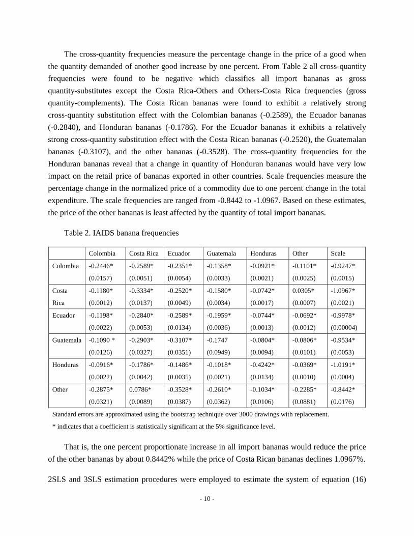
Table 2 presents the own and cross flexibility estimates as well as the scale (expenditure)

frequencies along with the appropriate standards errors. All frequencies estimates were calculated

at the sample means. Note that all own-quantity frequencies are negative as theoretically

expected. All own-quantity frequencies estimates were less than one in absolute value, indicating

that the fresh bananas of six exporting countries are price inflexible. In terms of the own-quantity

frequencies at the price-imported level, the U.S. own price for Honduran bananas with respect to

the quantity of Honduran bananas appears to be the largest variation in absolute value (0.4242).

That is, a one percent increase (decrease) in the quantity of Honduran bananas was found to

decrease (increase) the import price of Honduran bananas in the U.S. market by approximately

0.4242%. A similar change occurs in the price of other banana-exporting countries as their own

quantities increase (decrease) by one percent.

- 10 -

The cross-quantity frequencies measure the percentage change in the price of a good when

the quantity demanded of another good increase by one percent. From Table 2 all cross-quantity

frequencies were found to be negative which classifies all import bananas as gross

quantity-substitutes except the Costa Rica-Others and Others-Costa Rica frequencies (gross

quantity-complements). The Costa Rican bananas were found to exhibit a relatively strong

cross-quantity substitution effect with the Colombian bananas (-0.2589), the Ecuador bananas

(-0.2840), and Honduran bananas (-0.1786). For the Ecuador bananas it exhibits a relatively

strong cross-quantity substitution effect with the Costa Rican bananas (-0.2520), the Guatemalan

bananas (-0.3107), and the other bananas (-0.3528). The cross-quantity frequencies for the

Honduran bananas reveal that a change in quantity of Honduran bananas would have very low

impact on the retail price of bananas exported in other countries. Scale frequencies measure the

percentage change in the normalized price of a commodity due to one percent change in the total

expenditure. The scale frequencies are ranged from -0.8442 to -1.0967. Based on these estimates,

the price of the other bananas is least affected by the quantity of total import bananas.

Table 2. IAIDS banana frequencies

Colombia Costa Rica Ecuador Guatemala Honduras Other Scale

Colombia -0.2446*

(0.0157)

-0.2589*

(0.0051)

-0.2351*

(0.0054)

-0.1358*

(0.0033)

-0.0921*

(0.0021)

-0.1101*

(0.0025)

-0.9247*

(0.0015)

Costa

Rica

-0.1180*

(0.0012)

-0.3334*

(0.0137)

-0.2520*

(0.0049)

-0.1580*

(0.0034)

-0.0742*

(0.0017)

0.0305*

(0.0007)

-1.0967*

(0.0021)

Ecuador -0.1198*

(0.0022)

-0.2840*

(0.0053)

-0.2589*

(0.0134)

-0.1959*

(0.0036)

-0.0744*

(0.0013)

-0.0692*

(0.0012)

-0.9978*

(0.00004)

Guatemala -0.1090 *

(0.0126)

-0.2903*

(0.0327)

-0.3107*

(0.0351)

-0.1747

(0.0949)

-0.0804*

(0.0094)

-0.0806*

(0.0101)

-0.9534*

(0.0053)

Honduras -0.0916*

(0.0022)

-0.1786*

(0.0042)

-0.1486*

(0.0035)

-0.1018*

(0.0021)

-0.4242*

(0.0134)

-0.0369*

(0.0010)

-1.0191*

(0.0004)

Other -0.2875*

(0.0321)

0.0786*

(0.0089)

-0.3528*

(0.0387)

-0.2610*

(0.0362)

-0.1034*

(0.0106)

-0.2285*

(0.0881)

-0.8442*

(0.0176)

Standard errors are approximated using the bootstrap technique over 3000 drawings with replacement.

* indicates that a coefficient is statistically significant at the 5% significance level.

That is, the one percent proportionate increase in all import bananas would reduce the price

of the other bananas by about 0.8442% while the price of Costa Rican bananas declines 1.0967%.

2SLS and 3SLS estimation procedures were employed to estimate the system of equation (16)

- 11 -

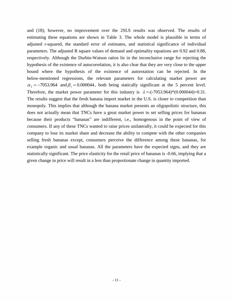
and (18); however, no improvement over the 2SLS results was observed. The results of

estimating these equations are shown in Table 3. The whole model is plausible in terms of

adjusted r-squared, the standard error of estimates, and statistical significance of individual

parameters. The adjusted R square values of demand and optimality equations are 0.92 and 0.88,

respectively. Although the Durbin-Watson ratios lie in the inconclusive range for rejecting the

hypothesis of the existence of autocorrelation, it is also clear that they are very close to the upper

bound where the hypothesis of the existence of autorotation can be rejected. In the

below-mentioned regressions, the relevant parameters for calculating market power are

964.70532 and 000044.01 , both being statically significant at the 5 percent level.

Therefore, the market power parameter for this industry is =-(-7053.964)*(0.000044)=0.31.

The results suggest that the fresh banana import market in the U.S. is closer to competition than

monopoly. This implies that although the banana market presents an oligopolistic structure, this

does not actually mean that TNCs have a great market power to set selling prices for bananas

because their products “bananas” are indifferent, i.e., homogenous in the point of view of

consumers. If any of these TNCs wanted to raise prices unilaterally, it could be expected for this

company to lose its market share and decrease the ability to compete with the other companies

selling fresh bananas except, consumers perceive the difference among these bananas, for

example organic and usual bananas. All the parameters have the expected signs, and they are

statistically significant. The price elasticity for the retail price of bananas is -0.66, implying that a

given change in price will result in a less than proportionate change in quantity imported.

- 12 -

Table 3. 2SLS estimation of the model

Coefficient P-value Elasticity

Intercept 4,542,441

**

(980,911.3)

0.000

tPCB 273,126.6

**

(29084.96)

0.000

rtP -7,053.96

**

(661.32)

0.000 -0.66

Adjusted R square 0.92

Durbin-watson 0.959<DW=1.218<1.298

Intercept -537.4846

*

(245.2847)

0.041

tIMPQ 0.000044

*

(0.0000186)

0.029

)ln( tEarnings 252.3885

**

(51.6981)

0.000

tIMPI

1.855343**

(0.5055642)

0.002

2)( wtP 0.0004011

*

(0.0001865)

0.045

Adjusted R square 0.88

Durbin-watson 0.805<DW=1.433<1.527

* and ** indicate that a coefficient is statistically significant at the

5% and 1% significance level, respectively.

5. Summary and Conclusion

Banana consumption in the U.S. is highly dependent on imports and these imports come

from a concentrated market that is controlled by a few TNCs. First, using a structural

econometric model, based on a method originally developed by Bresnahan (1982), the results

show that the U.S. fresh banana import market is imperfectly competitive and implies that the

TNCs are exercising some market power. Furthermore, the findings of this study show two

variables, retail price of bananas and per-capital consumption of bananas, to have a significant

impact on import quantity. Next, we employed the nonlinear IAIDS model developed by Eales

and Unnevehr (1993) to serve the following purpose. We believe that estimating the relationship

- 13 -

between the U.S. fresh banana imports using prices as the dependent is a better specification

given that bananas are highly perishable and it is the price (not quantities) that clears the market.

From the perspective of the U.S. market this is an important step toward understanding demand

conditions and the difference of competitiveness. Own-quantity effects are relatively inflexible

(flexible) in the Guatemalan (Honduran) equation so that a one percent increase in the quantity of

bananas induces a less than (more than) one percent fall in the own-price. In addition, in term of

the cross quantity effects, the results suggest that Costa Rican and Ecuador bananas have stronger

quantity-substitution effect on the other rival bananas while Honduran bananas: weaker

quantity-substitution effect on the other rival bananas.

References

Barnett, W.A., and O. Seck. 2008. “Rotterdam Model versus Almost Ideal Demand System: Will

the Best Specification Please Stand Up?” Journal of Applied Econometrics 23:795-824.

Burrell, A., and A. Henningsen. 2001. An Empirical Investigation of the Demand for Bananas in

Germany. Agrarwirtschaft 50(4), pp. 242-249.

Chern, W.S., Ishibashi, K., Taniguchi, K., Yokoyama, Y., 2003. Analysis of Food Consumption

Behavior by Japanese Households. FAO Economic and Social Development Paper, 152.

Deaton, A., and J. Muellbauer. 1990. An Almost Ideal Demand System. American Economic

Review 70:312-326.

Deodhar, S.Y., and I.M. Sheldon. 1995. Is Foreign Trade (IM) Perfectly Competitive?: An

Analysis of the German Market for Banana Imports. Journal of Agricultural Economics

46(3):336-348

Eales, J.S., and L.J. Unnevehr. 1994. The Inverse Almost Ideal Demand System. European

Economic Review 38:101-115

Grant, J.H., D.M. Lambert and K.A. Foster. 2010. ASeasonal Inverse Almost Ideal Demand

System for North American Fresh Tomatoes. Canadian Journal of Agricultural Economics

58:215-234.

Haden, K. 1990. The Demand for Cigarettes in Japan. American Journal of Agricultural

Economics 72:446-50.

- 14 -

Hatirli, S.A., Jones, E., and A.R. Aktas. 2003. Measuring the Market Power of the Banana Import

Market in Turkey. Turkish Journal of Agriculture and Forestry 27: 367-373.

Huang, K.S. 1988. An Inverse Demand System for U.S. Composite Foods. American Journal of

Agricultural Economics 70:902-909.

Moschini, G., and A. Vissa. 1992. A Linear Inverse Demand System. Journal of Agricultural and

Resource Economics 17:292-302.