
U.S. import and export prices in 2004
162
Monthly Labor Review July 2005 3 Import and Export Prices, 2004 U.S. import and export prices in 2004 Import and export prices increased at an accelerated rate in 2004, as each continued the upward trend that began in 2002; the increases for both indexes were driven by industrial supplies and materials, which trended upward because of higher fuel and raw material prices Kristen Locatelli Kristen Locatelli is an economist in the Division of International Prices at the Bureau of Labor Statistics. E-mail: locatelli.kristen@ bls.gov T he Bureau of Labor Statistics import and export price indexes both increased for a third consecutive year in 2004. Import prices were up 6.7 percent for the year, almost triple the 2.4-percent increase seen in 2003. Ex- port prices saw the highest increase in 15 years with a 4.0-percent advance in 2004; the increase in the previous year was only 2.2 percent. Prices within the industrial supplies and mate- rials index had the most impact on the import side, increasing 22.0 percent for the year. The indus- trial supplies and materials price index comprises the fuel price index, which increased 31.5 percent, and the nonfuel industrial supplies and materials price index, which increased 13.4 percent. Im- port prices were up in all major categories, with the exception of the capital goods index. Down- ward movements for computer, peripheral, and semiconductor prices caused the contrasting trend in the capital goods index. On the export side, annual price increases were posted for each of the major indexes, except for the foods, feeds, and beverages price index, which decreased 4.5 per- cent. Similar to the import price index, the largest movement in the export price index was seen in the nonagricultural industrial supplies and mate- rials price index, which posted a 16.6-percent in- crease in 2004. (See table 1.) The key factor behind the substantial import and export price movements in 2004 was the growth in international demand, especially from China, for raw materials such as petroleum and steel. According to statistics from China’s Cus- toms Bureau, the total value of imports into China increased 36 percent. Import increases were most significant in iron ore and fine mine products (161.8 percent), crude oil (71.4 percent), un- wrought copper (37.9 percent), and plastics (31.5 percent). 1 China’s demand for these raw materials led to tight global supplies and higher interna- tional prices, which put additional upward pres- sure on prices for manufactured goods. Changes in the exchange rate were also a factor behind the increases in import prices, as the U.S. dollar weakened against the currencies of several major trading partners. In 2004, the exchange rate decreased between the U.S. dollar and the United Kingdom (UK) pound (10.2 percent), the euro (9.1 percent), the Canadian dollar (7.8 percent), and the Japanese yen (3.8 percent). The U.S. dollar, which has been weakening for 2 years, put upward pres- sure on prices of goods imported from these coun- tries, which in 2004 accounted for 45.5 percent of the total dollar value for goods imported into the United States. 2 Other price measures The Consumer Price Index (CPI) and the Producer Price Index (PPI) increased at an accelerated rate in 2004 because of higher energy costs. The CPI mea- sures monthly changes in the prices paid by urban
-
Upload
khangminh22 -
Category
Documents
-
view
1 -
download
0
Transcript of U.S. import and export prices in 2004

Monthly Labor Review July 2005 3
Import and Export Prices, 2004
U.S. import andexport prices in 2004Import and export prices increased at an accelerated rate in 2004,as each continued the upward trend that began in 2002;the increases for both indexes were drivenby industrial supplies and materials, which trended upwardbecause of higher fuel and raw material prices
Kristen Locatelli
Kristen Locatelli isan economist inthe Division ofInternational Pricesat the Bureau ofLabor Statistics.E-mail:[email protected]
The Bureau of Labor Statistics import andexport price indexes both increased for athird consecutive year in 2004. Import
prices were up 6.7 percent for the year, almosttriple the 2.4-percent increase seen in 2003. Ex-port prices saw the highest increase in 15 yearswith a 4.0-percent advance in 2004; the increasein the previous year was only 2.2 percent.
Prices within the industrial supplies and mate-rials index had the most impact on the import side,increasing 22.0 percent for the year. The indus-trial supplies and materials price index comprisesthe fuel price index, which increased 31.5 percent,and the nonfuel industrial supplies and materialsprice index, which increased 13.4 percent. Im-port prices were up in all major categories, withthe exception of the capital goods index. Down-ward movements for computer, peripheral, andsemiconductor prices caused the contrasting trendin the capital goods index. On the export side,annual price increases were posted for each of themajor indexes, except for the foods, feeds, andbeverages price index, which decreased 4.5 per-cent. Similar to the import price index, the largestmovement in the export price index was seen inthe nonagricultural industrial supplies and mate-rials price index, which posted a 16.6-percent in-crease in 2004. (See table 1.)
The key factor behind the substantial importand export price movements in 2004 was thegrowth in international demand, especially from
China, for raw materials such as petroleum andsteel. According to statistics from China’s Cus-toms Bureau, the total value of imports into Chinaincreased 36 percent. Import increases were mostsignificant in iron ore and fine mine products(161.8 percent), crude oil (71.4 percent), un-wrought copper (37.9 percent), and plastics (31.5percent).1 China’s demand for these raw materialsled to tight global supplies and higher interna-tional prices, which put additional upward pres-sure on prices for manufactured goods.
Changes in the exchange rate were also a factorbehind the increases in import prices, as the U.S.dollar weakened against the currencies of severalmajor trading partners. In 2004, the exchange ratedecreased between the U.S. dollar and the UnitedKingdom (UK) pound (10.2 percent), the euro (9.1percent), the Canadian dollar (7.8 percent), and theJapanese yen (3.8 percent). The U.S. dollar, whichhas been weakening for 2 years, put upward pres-sure on prices of goods imported from these coun-tries, which in 2004 accounted for 45.5 percent ofthe total dollar value for goods imported into theUnited States.2
Other price measures
The Consumer Price Index (CPI) and the ProducerPrice Index (PPI) increased at an accelerated rate in2004 because of higher energy costs. The CPI mea-sures monthly changes in the prices paid by urban

4 Monthly Labor Review July 2005
Import and Export Prices, 2004
was boosted by a 13.4-percent increase in energy prices anda 3.1-percent increase in food prices. Excluding food andenergy prices, overall producer prices increased a more mod-est 2.3 percent. (See chart 1.)
Import price trends
Energy. Increases in energy prices were the most signifi-cant factor in import prices in 2004. The price index forpetroleum and petroleum products increased 30.3 percent forthe year, following a 12.8-percent increase in 2003 and a56.9-percent increase in 2002. Crude oil prices started outstrong in January at just more than 34 dollars per barrel,
Table 1. U.S. import and export price indexes annual percent changes for selected categories of goods, 1995–2004
Relative Description importance Percent change for 12 months ended in December—
November20041
1995 1996 1997 1998 1999 2000 2001 2002 2003 2004
Imports
All commodities .................................................. 100.000 2.6 1.5 –5.2 –6.4 7.0 3.2 –9.1 4.2 2.4 6.7All imports, excluding petroleum ........................ 84.578 2.4 –1.8 –2.8 –3.3 .0 1.3 –4.5 .3 1.2 3.7All imports, excluding fuels ................................. 82.340 – – – – – – – .0 1.0 3.0
0 Foods, feeds, and beverages .......................... 4.554 –2.7 –1.3 1.3 –3.1 –.3 –4.0 –4.7 5.9 3.0 8.0
1 Industrial supplies and materials ..................... 32.127 6.1 9.1 –10.4 –17.1 33.7 13.8 –24.6 21.9 9.5 22.0Excluding petroleum .................................. 16.705 6.4 –2.4 –1.7 –6.7 5.1 11.2 –14.6 5.8 7.2 16.4Excluding fuels. ......................................... 14.467 – – – – – – – 3.6 6.3 13.4
10 Fuels and lubricants ..................................... 17.661 5.7 34.4 –23.8 –36.5 114.7 27.1 –41.9 53.7 13.2 31.5100 Petroleum and petroleum products ........... 15.423 6.0 33.7 –25.5 –40.8 137.2 17.6 –39.5 56.9 12.8 30.3
2 Capital goods ................................................... 22.031 1.1 –3.8 –7.4 –5.0 –3.3 –2.1 –2.7 –2.4 –1.1 –.8Excluding computers, peripherials,
and semiconductors .................................. 14.947 2.1 –2.6 –4.7 –2.1 –1.8 –1.1 –1.0 –1.3 1.2 2.0
3 Automotive vehicles, parts and engines .......... 16.703 2.3 .0 .5 .0 .7 .7 –.2 .5 .9 1.8
4 Consumer goods, excluding automotives ....... 24.585 1.8 –.7 –.9 –1.3 –.4 –1.2 –.8 –.7 .1 .9
Exports
All commodities .................................................. 100.000 3.3 –1.1 –1.2 –3.4 .5 1.1 –2.5 1.0 2.2 4.0Agricultural commodities .................................... 8.753 17.3 –6.9 –2.9 –9.3 –6.8 3.1 –1.8 8.0 13.4 –5.9Nonagricultural commodities .............................. 91.247 1.7 –.4 –1.0 –2.7 1.2 .9 –2.5 .4 1.3 5.0
0 Foods, feeds, and beverages .......................... 8.034 19.9 –6.5 –3.3 –8.3 –5.7 1.7 –.5 7.9 12.6 –4.5
1 Industrial supplies and materials ..................... 27.940 1.5 –2.3 –1.4 –7.1 5.3 3.6 –8.6 5.0 6.8 15.1Nonagricultural industrial supplies
and materials ................................................ 26.456 1.6 –2.2 –1.3 –6.9 6.3 3.3 –8.4 4.8 6.3 16.6
2 Capital goods ................................................... 40.721 1.8 .1 –1.6 –1.8 –1.1 .3 –.8 –1.3 –.6 .7Excluding computers, peripherals
and semiconductors .................................. 30.254 2.8 1.4 –.3 –.7 –.4 .8 .0 .5 .9 2.1
3 Automotive vehicles, parts, and engines ......... 11.379 1.6 .4 .8 .5 1.0 .5 .4 .8 .5 1.1
4 Consumer goods, excluding automotives ....... 11.877 1.6 1.4 .8 –.8 .6 –.4 .2 –.6 .6 1.3
1 Relative importance figures are based on 2002 trade values. NOTE: Dash indicates data not available.
Enduse
consumers for a representative basket of goods and services.After posting an increase of 1.9 percent in 2003, the CPI forAll Urban Consumers (CPI–U) rose 3.3 percent in 2004, thelargest increase since 2000. The increase was driven by a16.6-percent gain in energy prices and a 2.7-percent gain infood prices. Excluding food and energy prices, the indexincreased at a lesser rate of 2.2 percent.
The PPI measures monthly changes in the selling pricesreceived by domestic producers for their output. The PPI forfinished goods increased 4.2 percent in 2004, slightly abovethe 4.0-percent advance in 2003. The 4.2-percent advancein the PPI was the largest movement published since 1990,when the index gained 5.7 percent.3 The increase in 2004

Monthly Labor Review July 2005 5
D e c e m b e r J u n e D e c e m b e r J u n e D e c e m b e r J u n e D e c e m b e r J u n e D e c e m b e r J u n e D e c e m b e r-6
-4
-2
0
2
4
6
-6
-4
-2
0
2
4
6
Chart 1. Changes in the CPI, PPI, and import and export price indexes, 1999–200412-month
percent change12-month
percent change
–
–
–
–
–
–
CPI less food and energy
PPI for finished goods less food and energy
U.S. export price index excluding agricultural products
U.S. import price index excluding petroleum
1999 2000 01 02 03 04
Dec. June Dec. June Dec. June Dec. June Dec. June Dec.
peaked in October at 53.32 dollars per barrel, and eased backat the end of the year to 43.12 dollars per barrel.4 Whileconcerns about potential supply interruptions continued toplay a role in these price movements, demand factors werealso prominent in 2004.
Total world oil demand increased by 2.5 million barrelsper day (mb/d), or slightly more than 3.0 percent, represent-ing the largest increase in demand in 28 years. Increased de-mand brought excess capacity (the volume over that which isneeded to meet expected demand) to the lowest level sincethe conclusion of the Gulf War in 1991. The largest changein demand was witnessed in China, where demand increased15.5 percent over 2003 because of an expanding economyand rapid industrial development. In 2004, China surpassedJapan to become the second largest consumer of oil behindthe United States. Oil demand was also up in the UnitedStates and Western Europe, increasing 2.0 percent and 1.5percent, respectively.5
With demand at such high levels, perceived threats to sup-ply affected oil prices. Toward the end of 2003, a strike inVenezuela halted oil production, refining, and export at theState oil company, Petroleos de Venezuela, S.A. The situa-tion improved by the beginning of 2004, but supplies on theworld market were still recovering from the loss of some 200
million barrels of oil and gasoline. Additional threats to oilsupplies developed during 2004, such as Hurricane Ivan andlabor conflicts in Nigeria and Norway. Hurricane Ivan causedmajor delays in oil shipments, resulting in many U.S refiner-ies shutting down or cutting back production. The hurricaneinitially cut production of approximately 1.0 mb/d at the re-finery level because of damages in the oil infrastructure inthe Gulf. By the end of 2004, production had yet to fullyrecover in the Gulf.6 Responding to the surge in demand andthe supply concerns, the Organization of the Petroleum Ex-porting Countries (OPEC) increased its production of oil 15percent by the end of 2004. These changes to the OPEC sup-ply ceiling led to a positive world oil demand/supply balance,reversing the negative balances witnessed in 2002 and 2003.Concurrently, the import petroleum and petroleum productsprice index decreased in November and December, down 6.0percent and 11.4 percent, respectively.7 (See chart 2.)
Nonfuel industrial supplies and materials. The nonfuel in-dustrial supplies and materials import price index increased13.4 percent in 2004, more than double the 6.3-percent in-crease in 2003 and more than triple the 3.6-percent increasein 2002. The index was affected chiefly by higher metal,chemical, and lumber prices. As previously mentioned, world

6 Monthly Labor Review July 2005
Import and Export Prices, 2004
demand and Chinese industrial expansion were major fac-tors for these price increases.
The unfinished metals index increased 39.6 percent in2004, the highest annual increase since 1982 when the in-dex was first published. Within this index, steelmaking andferroalloying materials prices increased 56.2 percent; ironand steel mill product prices increased 69.1 percent; andnonferrous metals prices increased 23.5 percent. StrongChinese and international demand raised concerns aboutcommodity shortages for steel products, such as pig ironand scrap. According to the International Iron and SteelInstitute, China accounted for 56.4 percent of the increasein global steel consumption between 2001 and 2004 be-cause of expansion in its construction and manufacturingindustries.8
Chemical prices rose 5.3 percent because of higher fuelfeedstock costs, strong demand, and tight global supplies forproducts such as fertilizers, insecticides, and plastics. Theindustry has faced higher energy feedstock prices since thespring of 2003 when oil prices began a steady upward climb.Strong demand from end-users also placed upward pressureon chemical prices. According to the Purchasing Manager’sIndex published by the Institute for Supply Management,both the manufacturing economy and overall economy ex-
panded throughout 2004.9 Strength in the manufacturingeconomy tends to drive up demand for chemicals, which areprimary inputs into the consumer goods industry and the au-tomobile industry.
The lumber import price index gained 11.4 percent alsobecause of strong Chinese and international demand. A short-age of available space onboard shipping vessels placed up-ward pressure on lumber prices for U.S. importers. China’sdemand for raw materials strained the availability of ship-ping vessels as additional capacity was needed to bring thelarge quantities of lumber, iron ore, and other materials toChinese ports.10
Capital goods. The capital goods import price index re-corded a downward movement of 0.8 percent in 2004, theindex’s ninth consecutive annual decrease. The decline wasled by computer prices, which continued to trend downwardin 2004 as weak demand and oversupply led companies tocontinue competitive pricing mechanisms. In recent years,computer companies have been lowering prices through in-novation and by shifting manufacturing locations, in an ef-fort to offset a decline in sales.11 A significant amount ofproduction in this industry was shifted to China, which hasbecome a major exporter of computers, peripherals, and
Chart 2. Import price trends, 200412-month
percent change12-month
percent change
J a n u a ry M a rc h M a y J u ly S e p te m b e r N o v e m b e r-1 0
0
1 0
2 0
3 0
4 0
5 0
6 0
7 0
-1 0
0
1 0
2 0
3 0
4 0
5 0
6 0
7 0
– –
Petroleum andpetroleum products
Nonpetroleum industrialsupplies and materials
All imports
January March May July September November

Monthly Labor Review July 2005 7
semiconductors into the United States. The value of importsof these goods from China accounted for 8.2 percent of thevalue of total imports in 2000 and 30.5 percent in 2004.12
In contrast, the capital goods price index excluding com-puters, peripherals, and semiconductors posted an increaseof 2.0 percent in 2004 following a 1.2-percent increase in2003. Price increases were published in 2004 for the electricgenerating equipment price index, the nonelectrical machin-ery price index, and the transportation equipment excludingmotor vehicles price index. Higher steel prices had a largeeffect on the manufacturing costs of machinery, especiallyindustrial and service machinery, which posted a 4.1-percentannual increase. Prices were also affected by exchange rateincreases as the dollar weakened against the currencies ofJapan, Canada, Mexico, and Germany, which were the topexporters to the United States of the capital goods includedin this category.13
Automotive vehicles, parts, and engines. Import prices forautomotive vehicles, parts, and engines increased 1.8 per-cent in 2004, as compared with the 0.9-percent increase pub-lished in 2003. Canada and Japan were the top two export-ers of automotive vehicles, parts, and engines to the UnitedStates, representing 30 percent and 21 percent of the totalvalue of export trade, respectively. As the dollar weakenedagainst the Canadian dollar and the Japanese yen, exportsfrom those countries became relatively more expensive.14
Consumer goods. After posting a 0.1-percent increase in2003, the consumer goods import price index increased 0.9percent in 2004. The 2-year upward trend in the index is areversal of the downward trend that occurred between theyears 1996 and 2002. Higher jewelry and medical suppliesprices were contributing factors to the index movement in2004. The jewelry price index increased 6.2 percent, greaterthan the 3.5-percent increase published in 2003. Higher pre-cious metals prices, such as silver and gold, increased themanufacturing costs for jewelry. As the dollar weakenedthroughout most of 2004, demand for precious metalsstrengthened as precious metals became a better option forinvestors and fund managers seeking higher rates of return.15
An increase of 4.2 percent for the medical supplies priceindex was also a significant factor in the consumer goodsprice index. The movement was the third consecutive increasein the index and the largest published increase since 1993.The research and development of new medicines requires anenormous amount of time and money, and unsuccessful re-search attempts dip further into the company’s profits. Devel-opment of major drugs takes 7 to 10 years with costs rangingbetween $200 million and $1 billion. New pharmaceuticalsbrought to the market, both over-the-counter and prescription,have been met with strong demand from consumers.16
Foods, feeds, and beverages. The foods, feeds, and bever-ages import price index increased 8.0 percent in 2004, morethan double the 3.0-percent increase in 2003. The vegetableprice index recorded the largest movement with an annualincrease of 21.6 percent. Hurricanes and tropical stormsbrought winds and heavy rains to tomato producers in Florida,destroying crops and postponing early fall plantings. ByNovember, there was a severe shortage of U.S. grown toma-toes as total shipments of Florida tomatoes declined 42 per-cent in 2004. The decrease in domestic tomato productionled to an increase in the demand for imported tomatoes, put-ting upward pressure on prices. Pest infestation in the Bajaregion of Mexico and wet California weather also added tothe higher tomato prices.17 The meat and poultry price indexincreased 10.8 percent in 2004 because of strong demand forpork products. Mad cow disease (Bovine Spongiform En-cephalopathy, or BSE) and the avian flu curtailed demand forbeef and chicken, respectively, creating a strong demand forpork.18
The price index for green coffee, cocoa beans, and sugargained 19.3 percent in 2004 because of global shortages andstrong demand. In 2002, green coffee prices were one-thirdthe 1998 price levels because of excess supply overloadingthe market. However, the situation changed by 2003, and in2004 coffee demand exceeded supply for the second con-secutive year because of production cutbacks in a number ofexporting countries as a result of the previous lower prices.Poor weather conditions in Brazil also added supply pres-sure.19 The price index for fish and shellfish increased 7.0percent. An ongoing trade dispute regarding imported shrimpled to higher prices as importers stocked up on shrimp in thebeginning of 2004 prior to the implementation of tariffs laterin 2004.20
Locality of Origin price index. In order to better delineateand analyze price trends in U.S. trade, BLS publishes importprice indexes by Locality of Origin. These price indexesinclude imports from Industrialized Countries, Other Coun-tries, Canada, the European Union (EU), France, Germany,the UK, Latin America, Mexico, the Pacific Rim, China, Ja-pan, the Asian Newly Industrialized Countries, the Associa-tion of Southeast Asian Nations (ASEAN), and Asia Near East.21
All of the above indexes, except those for China and the Asiannewly industrialized countries, increased at an acceleratedrate in 2004 when compared with 2003 price movements.The Canadian price index had the largest price change withan 11.7-percent increase, followed by the EU price index witha 7.0-percent increase, the Mexican price index with a 4.0-percent increase, and the Japanese price index with a 1.3-percent increase. Overall, import prices from the Industrial-ized Countries increased 7.5 percent, while import pricesfrom the Other Countries increased 6.0 percent. The two

8 Monthly Labor Review July 2005
Import and Export Prices, 2004
main factors behind these upward price movements werehigher petroleum prices and exchange rate movements be-tween the U.S. dollar and several major trading partners.Meanwhile, import prices from China decreased 1.0 percentin 2004.
Export price trends
Foods, feeds, and beverages. The agricultural goods priceindex decreased 4.5 percent in 2004, reversing the 12.6-per-cent increase observed in the previous year. The upwardmovement in the agricultural goods price index in 2003 wasled by increases in the soybean price index and the corn priceindex. After gaining 33.0 percent in 2003, soybean pricesremained strong in the beginning of 2004 because of exportdemand and harvest shortages. As a result of favorableweather conditions and higher market prices, farmers in-creased soybean plantings ahead of schedule. In June, soy-bean prices began to trend downward, because of a reboundin both United States and global supplies, and ended the yearwith a 28.4-percent annual price decline. According to U.S.Department of Agriculture figures, world soybean produc-tion rose 16 percent in 2004, with North American soybeanproduction rising a record high 28 percent over the previousyear’s production. High prices and favorable weather condi-
tions similarly affected corn plantings, as U.S. corn produc-tion increased 16.8 percent. The price index for corn de-creased 16.3 percent overall, reversing the 3.8-percent in-crease published in 2003.22 (See chart 3.)
Industrial supplies and materials. The export price indexfor industrial supplies and materials increased 15.1 percentin 2004, more than double the 6.8-percent increase in 2003.Price movements on the export side displayed trends similarto those previously noted on the import side. The fuels andlubricants index increased 26.7 percent because of low crudeoil, gasoline, and coking coal stocks. High crude oil pricesand low crude oil inventories led to lower petroleum productstocks and put upward pressure on prices, especially gaso-line prices. Damage caused by Hurricane Ivan in Septemberled to further inventory declines for gasoline and distillatefuels. As a result, the U.S. national average price for regulargasoline set a record in October, reaching 1.55 dollars pergallon (excluding taxes). Coking coal prices were also highin 2004 because of strong demand from the steel industry.23
Higher prices for petroleum products also impacted the U.S.chemical industry. Increases in energy feedstock prices werethe largest factor behind the 18.5-percent advance for thechemicals price index.
Significant price increases occurred in the iron and steel
Chart 3. Export price trends, 200412-month
percent change12-month
percent change
Foods, feeds,and beverages
Industrial suppliesand materials
All exports
J a n u a ry M a rc h M a y J u ly S e p te m b e r N o v e m b e r-1 0
0
1 0
2 0
3 0
4 0
5 0
6 0
7 0
-1 0
0
1 0
2 0
3 0
4 0
5 0
6 0
7 0
– –January March May July September November

Monthly Labor Review July 2005 9
products price index and the nonferrous and other metalsprice index, which increased 53.1 percent and 24.8 percent,respectively. Strong demand from the construction andmanufacturing industries, coupled with higher transportationand raw material costs, put upward pressure on prices. Chi-nese demand for U.S. metals increased significantly. For in-stance, the value of U.S. exports to China increased 78 per-cent for nonferrous metals, 57 percent for aluminum, and 38percent for steelmaking materials.24
Capital goods. The capital goods price index, which in-cludes machinery and transportation equipment not includedin the automotive index, increased 0.7 percent, reboundingfrom a 3-year decline. Excluding computers, peripherals,and semiconductors from the index, the increase was up by amore significant 2.1 percent. Similar to price trends on theimport side, higher prices were attributed to the increases inraw material costs for steel, copper, and energy. The trans-portation equipment price index increased 3.6 percent.
The computers, peripherals, and semiconductors index de-clined 3.0 percent, continuing a downward trend that beganin 1989. High inventories and soft market demand condi-tions led to competitive pricing, as companies tried to keepcosts and prices down. Prices for telecommunication equip-ment also put some downward pressure on the capital goodsindex. This index decreased 2.2 percent because of low de-mand and high competition, factors similar to those influ-encing the computer industry.
Automotive vehicles, parts, and engines. The automotivevehicles, parts, and engines price index increased 1.1 per-cent in 2004, higher than the 0.5-percent increase publishedin 2003. The primary factor behind the increase was thehigher costs of raw materials, especially steel, aluminum,plastic, and rubber. Producer prices for these goods, as mea-sured by the PPI, increased in 2004 because of strong demandand restrictive supplies, putting upward pressure on automo-bile prices. Producer prices increased 40.7 percent for ironand steel, 14.6 percent for aluminum, 6.1 percent for plastic,and 3.0 percent for rubber.
Consumer goods. The export consumer goods price indexincreased 1.3 percent in 2004 because of price increases formedical supplies and household goods. As in the importmarket, export medical supply prices were up because of con-tinued high manufacturing costs and increases in demand forpharmaceuticals. The household goods index, which includesfurniture, cookware, and textile floorcoverings, increased 1.8percent because of higher raw material costs. The 1.3-per-cent increase in 2004 for the consumer goods price index is
more than double the 0.6-percent increase published in 2003.These increases more than offset lower textile apparel and
footwear prices, which decreased 0.5 percent. An increasein import volumes, especially from China, and a decline ininternational demand led to competitive pricing within theUnited States and the international textile industry.25 Thevalue of textile and apparel imports into the United Statesfrom China increased 23 percent in 2004 and has increased86 percent since 2001, the year China formally entered theWorld Trade Organization (WTO). The influx of imports fromChina put downward pressure on U.S. domestic and exportapparel prices.
Services price trends
BLS publishes a limited number of international services priceindexes, and the majority of those showed increases in 2004.Each of the major BLS services indexes increased in 2004.Import air passenger fares increased 4.4 percent in 2004, re-versing the 0.2-percent decline published in 2003. Fares forflights destined to the Latin American and Caribbean regionincreased 6.0 percent, followed by the European region witha 5.6-percent increase in fares. On the export side, pricesrose for the fourth consecutive year with a 13.2-percent in-crease, slightly lower than the 14.7-percent increase in 2003.The European index and the Asian index drove the upwardmovement, gaining 13.6 percent and 13.5 percent, respec-tively. 26 The import air freight price index rose 10.4 percent,and the export air freight price index rose 11.2 percent. Thoseprice movements followed increases in 2003 of 7.5 percenton the import side and 0.2 percent on the export side.27 Theupward movements in the air passenger fares indexes andthe air freight indexes were both affected by fuel cost in-creases. Fuel consumption by U.S. airlines increased 4.2percent, while the cost of fuel increased 39.7 percent.28
After increasing 26.3 percent in 2003, the inbound oceanliner freight price index increased at a lesser rate of 4.2 per-cent. After 2 years of lackluster demand, the industry re-bounded in 2003 and continued to strengthen throughout2004. The inbound crude oil tanker freight price index in-creased 107.2 percent, the largest price increase publishedsince 2000, when the index increased 130.5 percent. Inboundocean liner freight prices and crude oil tanker freight pricescontinued their upward trends because of robust demand fromChina, Southeast Asia, and the United States for the ship-ment of goods. In 2004, both industries were characterizedby vessel shortages and limited capacity. The increased costswitnessed in these indexes factored into the upward pricemovements previously mentioned in the import and exportproduct price indexes.
10 Monthly Labor Review July 2005
Import and Export Prices, 2004
Notes
ACKNOWLEDGMENTS: The author thanks Brian Costello and David Meadfor their assistance in the preparation of this article.
1 Chinese data obtained from the Ministry of Commerce of the People’sRepublic of China, on the Internet at http://english. mofcom.gov.cn (vis-ited June 3, 2005).
2 Trade data obtained from the Foreign Trade Statistics Division of theU.S. Census Bureau.
3 The 5.7-percent gain in 1990 was largely attributable to a 30.7-per-cent gain in energy, which coincided with the Iraqi invasion of Kuwait inAugust 1990.
4 Prices are based on West Texas Intermediate (WTI) crude oil, which isthe U.S. benchmark grade. WTI crude oil is a light sweet crude; therefore,it is generally more expensive than the OPEC basket, which is an average oflight sweet crude oils and heavier sour crude oils.
5 See OPEC Monthly Oil Market Report (Organization of the PetroleumExporting Countries, January 2005), pp. 1, 20–22) on the Internet at http://www.opec.org/home/Monthly%20Oil%20Market%20Reports/2005/MR062005.htm (visited Mar. 16, 2005).
6 OPEC Monthly Oil Market Report, pp. 2–4.7 On July 1, the ceiling was increased from 23.5 mb/d to 25.5 mb/d; on
August 1, it was increased to 26 mb/d; and on November 1, to 27 mb/d.See EIA Country Analysis Briefs: OPEC (U.S. Department of Energy, En-ergy Information Administration, Last updated Mar. 8, 2005), on theInternet at http://www.eia.doe.gov/emeu/cabs/opec.html (visited Mar.16, 2005).
8 World Steel in Figures: 2005 (International Iron and Steel Institute,2005), p. 20, on the Internet at http://www.worldsteel.org/media/wsif/wsif2005.pdf (visited June 15, 2005).
9 ISM Manufacturing Report on Business (Institute for Supply Man-agement), on the Internet at http://www.ism.ws/ISMReport/PMIndex.cfm (visited June 15, 2005).
10 “Ocean freight issues a growing factor in overseas trading,” RandomLengths International (Random Lengths Publications, Inc., Apr. 14, 2004),pp. 1–2.
11 Andrew Park, “Computers Get Their Groove Back,” Business Week,Jan. 20, 2004, pp. 96–97.
12 Trade data obtained from the Foreign Trade Statistics Division of theU.S. Census Bureau.
13 In 2004, Japan accounted for 15.7 percent of the imports of capitalgoods, excluding computers, peripherals, and semiconductors into theUnited States; Canada for 12.5 percent; Mexico for 12.3 percent; and Ger-many for 10.0 percent.
14 Product trade data were obtained from the Foreign Trade StatisticsDivision of the U.S. Census Bureau.
See Peter Coy, “The Auto Deficit: Stuck in Neutral,” Business Week,Dec. 6, 2004, pp. 39–40.
15 See Amey Stone, “Gold is Flashing Warnings,” Business Week Online,Oct. 21, 2004, on the Internet at http://www.businessweek.com/bwdaily/dnflash/oct2004/nf20041021_1307_db035.htm (visited Jan. 20, 2005).
16 See Samuel Greengard, “No Quick Fixes for the Spiraling Costs of
Prescription Drugs,” Workforce Management, August 2004; and ArnoldS. Relman, “A Prescription for Controlling Drug Costs,” Newsweek, De-cember 2004, p. 74.
17 Vegetables and Melons Outlook (U.S. Department of Agriculture,Economic Research Service, Dec. 16, 2004), on the Internet at http://www.ers.usda.gov/Publications/vgs/ (visited Jan. 20, 2005).
18 Livestock and Poultry: World Markets and Trade (U.S. Departmentof Agriculture, Foreign Agricultural Service, November 2004), pp. 1, 5,on the Internet at http://www.fas.usda.gov/dlp/circular/2004/04-10LP/toc.htm (visited Jan. 20, 2005).
19 Coffee Market Reports (International Coffee Organization, January,June, and December 2004).
20 In July, the Commerce Department imposed anti-dumping duties ofup to 93.1 percent on shrimp from Vietnam, and up to 112.8 percent onshrimp from China. See “Shrimp Wars,” The Economist, July 10, 2004, p.26. Note: BLS import price indexes do not include duties to ensure compa-rability with similar statistics published by other countries.
21 The following import price indexes by Locality of Origin were firstpublished in 2004: France, Germany, the UK, Mexico, the Pacific Rim,China, ASEAN, and Asia Near East.
The Other Countries Locality of Origin (LOO) price index includescountries that are not included in the Industrialized Countries LOO priceindex. The following countries are excluded: Andorra, Australia, Austria,Belgium, Canada, Denmark, Faroe Islands, Finland, France, Germany,Gibraltar, Greece, Greenland, Iceland, Ireland, Italy, Japan, Liechtenstein,Luxembourg, Malta, Monaco, Netherlands, New Zealand, Norway, Portu-gal, San Marino, South Africa, Spain, St. Pierre and Miquelon, Svalbardand Jan Mayen Island, Sweden, Switzerland, and the United Kingdom.
22 NASS Crop Production 2004 Summary (National Agricultural Statis-tics Service, Jan. 2005), pp. 5–6, on the Internet at http://usda.mannlib.cornell.edu/reports/nassr/field/pcp-bban/cropan05.pdf (visited Jan.20, 2005) and Global Crop Production Review, 2004 (U.S. Department ofAgriculture’s Joint Agricultural Weather Facility), pp. 5–6.
23 Data were obtained from the Energy Information Association’s (EIA)Petroleum Product Prices for the United States, on the Internet at http://www.eia.doe.gov/emeu/states/oilprices/oilprices_us. html (visited Mar.23, 2005).
24 Product trade data were obtained from the Foreign Trade StatisticsDivision of the U.S. Census Bureau.
25 “Losing Their Shirts,” The Economist, Oct. 16, 2004, pp. 59–60.26 The import air passenger fares index measures fares paid by U.S.
residents flying out of the United States on foreign carriers. The exportair passenger fares index measures fares paid by foreign residents flyinginternationally on U.S. carriers.
27 The import air freight price index measures changes in rates paid forthe transportation of freight from foreign countries into the United Stateson foreign air carriers. The export air freight price index measures changesin rates paid for the transportation of freight from the United States toforeign countries on U.S. carriers.
28 ATA Monthly Jet Fuel Report: U.S. Major, National, and Large Re-gional Passenger and Cargo Airlines (Air Transport Association), on theInternet at http://www.airlines.org/econ/d.aspx?nid=5806 (visited Mar.24, 2005).

Monthly Labor Review July 2005 11
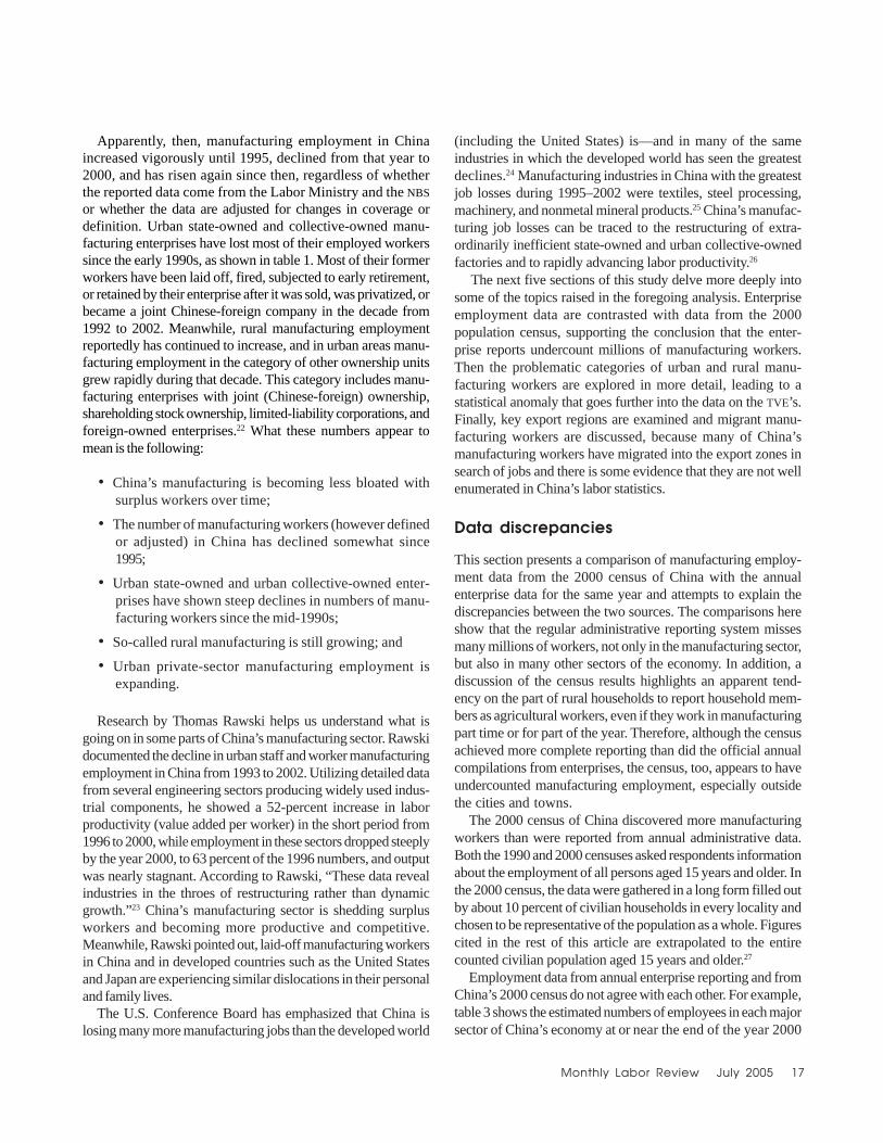
In recent decades, China has become amanufacturing powerhouse. The country’sofficial data showed 83 million manufacturing
employees in 2002, but that figure is likely to beunderstated; the actual number was probably closerto 109 million. By contrast, in 2002, the Group ofSeven (G7) major industrialized countries had a totalof 53 million manufacturing workers. In the late1990s through the year 2000, China saw decliningnumbers of manufacturing workers, caused byrestructuring and the privatization of state-ownedand urban collective-owned factories in the cities.Both massive layoffs of urban manufacturingworkers and sharp increases in manufacturing laborproductivity ensued. Since then, private-sectormanufacturing has thrived in both urban and ruralareas of China. The reorganized factories are moreproductive than state-owned and collective-ownedfactories and are competitive in the domestic andglobal economies. China’s manufacturing em-ployment began to rise again after 2000, regainingthe upward trend of the period from 1980 to 1995.
This article begins with an overview of China’sstatistical system, including a description of thesources of data used in the analysis presented.Three main sources of statistics on China’s manu-facturing employment are compared and con-trasted, and a hybrid data series is derived thathelps evaluate Chinese manufacturing employmentlevels and trends from 1990 through 2002. Theprobable biases in China’s statistics on the coun-try’s numbers of manufacturing workers are as-
The scale of manufacturing employment in Chinadwarfs the numbers of manufacturing workersin other countries; China’s manufacturing sectorhas shed surplus workers from inefficientstate-owned factories, while increasing employmentin the private sector
Manufacturing employmentin China
Judith Banister
Judith Banister is aconsultant workingwith JavelinInvestments in Beijing,China. She is formerhead of theInternationalPrograms Center atthe U.S. CensusBureau. E-mail:[email protected]
sessed, both at the national level and in the keyexport-manufacturing zones.
The analysis emphasizes issues of data qualityand the remaining legacies of the commandeconomy reflected in China’s labor statistics.Among the factors included is the excessive focusof China’s published statistics on city manu-facturing employees, to the near exclusion ofdetailed data on the more numerous manufacturingemployees working outside the administrativeboundaries of cities. Even within the cities, datacollection and reporting remain concentrated onthe rapidly declining state-owned and urbancollective-owned manufacturing enterprises,giving short shrift to the not yet adequatelycollected or published statistics on the thriving,growing, dynamic private manufacturing sector. Amajor reason for China’s statistical neglect of theprivate sector is that the dominance of private andcorporate businesses in today’s economy does notfit easily into Marxist theory or Mao Zedong’sideology.
Because of the many data limitations, a greatdeal of uncertainty remains in the work presentedhere. A more exacting analysis awaits new andbetter data collection and more detailed metadatafrom China’s statistical system.
This article is the first of a two-part series onChina’s manufacturing labor statistics. The sec-ond article, to be published in the next issue ofthe Review, will analyze manufacturing wagesand labor compensation. A more detailed exposition
Manufacturing Employment in China

12 Monthly Labor Review July 2005
Manufacturing Employment in China
of the analysis in the two articles is found on the Bureau ofLabor Statistics (BLS) Web site.1 The analysis in the currentarticle refers to the People’s Republic of China (mainland China;hereinafter, “China”) and excludes statistics for Hong Kong,Macao, and Taiwan. Occasionally, Chinese terminology will beused, because the standard English translations of the terms aremisleading or ambiguous and in some cases because there is nosuccinct, accurate English translation of the term.
Background
China’s statistical system has been greatly strengthened duringthe most recent quarter century of economic reform.2 Statisticiansin China are steadily learning from international practice aspromoted by the World Bank, the Asian Development Bank, theInternational Monetary Fund, and the United Nations system.China’s statistical organizations endeavor to apply best practicesfrom other countries—especially developed countries—to theChinese economy. Their efforts have been particularly suc-cessful in China’s population censuses and in some economicand demographic surveys—for example, the annual urban andrural household income and consumption surveys. Never-theless, China’s statistical system is still affected by categoriesand procedures that were established during the commandeconomy period before 1978 and never revised. Those outdatedcategories hamper the analysis of levels and trends of economicgrowth, inflation or deflation, employment, wages, and economicchange in the urban and rural economies. In addition, despiteexpanding its use of censuses and representative samplesurveys, China continues to employ the method of regular(usually annual) statistical reporting by all production oradministrative units as its primary data collection instrument.
Most statistics in China are recorded and collected under thecentral guidance of the National Bureau of Statistics (NBS).According to one source, “The NBS carries the responsibility fororganizing, directing and coordinating the statistical workthroughout the country.”3 However, as will be shown later, otherministries have certain statistical turf that is their particularresponsibility for historical or bureaucratic reasons, and thereseems to be little coordination among the relevant ministries. Forinstance, with regard to manufacturing employment statistics,the Ministry of Labor and Social Security (hereinafter, LaborMinistry) gathers data on most components of the city econ-omies, leaving a small, but rapidly growing, segment to the StateAdministration for Industry and Commerce. However, the col-lection of data and the reporting of statistics on manufacturingin rural areas and in towns are left to a part of the Ministry ofAgriculture.4
The analysis that follows is based as much as possible oninformation in Chinese sources published by official statisticalorganizations. The most useful sources turn out to be statistical
yearbooks from various government ministries. Later sectionsof this article compile and compare data on China’s manu-facturing employment from the 1995 industrial census and the2000 population census, as well as administrative data collectedfrom manufacturing enterprises and reported annually. Thearticle explains discrepancies among the data sets, to the extentpossible, and discusses the effects of definitional changes onthe available official series of manufacturing employment statis-tics. Strengths and weaknesses in the published statistics arehighlighted.
Recent employment statistics
Employment figures for China are usually confusing andnonstandard. They reflect, in part, conventions from the Maoistcommand economy period from 1949 to 1978, as well as newconventions for the semimarket economy of the economicreform period since 1978. The available data also reflect China’sattempts to make its economic statistics more internationallycomparable. Recent employment statistics are pieced togetherprimarily from annual enterprise data. Each enterprise, economicunit, small business, or self-employed individual or group issupposed to report employment data each year according to its“labor situation” in the previous year and at the previous year’send. The data are then compiled upward in a statistical reportingchain to the national government.
Enterprise data refer to who is working in what kind of work atthe end of the relevant year (end of December). The urbanenterprise statistical reporting form that is required to besubmitted to authorities early in a calendar year and that refersto the previous calendar year asks enterprises for the “laborsituation” (in particular, for the “actual situation that year”)—and specifically for the numbers of each category of workers atthe end of the previous year.5 Accountants or those who reportemployment and wage figures on behalf of their enterprises orother work units (at least those enterprises or other work unitsin urban areas) are given detailed instructions on how to reportmonthly, quarterly, yearend, and annual average figures onemployment and wages. The instructions are based onregulations released by China’s NBS, especially in 1990 and withfurther clarifications in 1998 and 2002, regarding how to reportemployment and wages.6
The annually reported figures on total manufacturingemployment in China include all manufacturing employees:production workers, salaried workers, and supervisory work-ers. China does not show separate data for these groups ofworkers. Table 1 presents figures from China’s annual enter-prise reporting system on the numbers of employed manu-facturing workers in the country from 1978 through 2002, brokendown into the various categories reported (described in thenext section).

Monthly Labor Review July 2005 13
Structure of manufacturing employment
Chart 1 (based partly on table 1) displays the structure ofChina’s manufacturing employment at the end of 2002, thelatest date for which enough statistics are currently available.The country’s NBS and Labor Ministry published a figure of83 million manufacturing employees in China, of whom 45million were called rural and 38 million were classified asurban. But these data do not take full account of the 71 milliontown and village enterprise (TVE) manufacturing workersreported by the Ministry of Agriculture. The TVE categoryincludes large factories in industrial parks outside cities, as
Furthermore, there is evidence that the official figure of 83 millionmanufacturing workers excludes millions of migrant manu-facturing workers. (See also later.)
Of the 38 million urban manufacturing employees at yearend2002 indicated in Chart 1, 30 million were employed in so-calledurban manufacturing units (danwei), and of these, 29 millionwere on-post (not laid-off or unemployed) staff and workers.Most of these urban manufacturing staff and workers (16 million)were employed by corporations, joint ventures, and other com-panies in China’s growing private sector. By the end of 2002,manufacturing employment in urban state-owned enterpriseshad dropped steeply, to 10 million, and in urban collective unitshad declined to only 3 million. (See table 1.)
There is considerable overlap between the two categoriesmaking up the urban manufacturing classification: manu-facturing employment in urban units and urban manufacturingstaff and workers (zhigong). Urban manufacturing staff andworkers (all of whom have been on-post workers since 1998) are
Official reported manufacturing employment in China, yearend 1978–2002
1978 ...................... 53.32 17.34 35.98 — — — 35.95 24.49 11.46 — 17.34 —
1980 ...................... 58.99 19.42 39.57 — — — 39.47 26.01 13.46 — 19.42 —
1985 ...................... 74.12 27.41 46.71 — — — 46.20 29.75 16.08 .37 41.37 —1986. ..................... 80.19 31.39 48.80 — — — 48.20 30.96 16.80 .46 47.62 —1987. ..................... 83.59 32.97 50.62 — — — 49.88 32.09 17.24 .58 52.67 —1988 ...................... 86.52 34.13 52.39 — — — 51.49 33.27 17.45 .77 57.03 —1989................... 85.47 32.56 52.91 — — — 52.06 33.44 17.54 1.08 56.24 —1990 ...................... 86.24 32.29 53.95 — — — 53.04 33.95 17.73 1.35 55.72 51.501991 ...................... 88.39 32.68 55.71 — — — 54.43 34.82 17.82 1.80 58.14 53.731992 ...................... 91.06 34.68 56.38 — — — 55.08 35.26 17.47 2.36 63.36 58.561993 ...................... 92.95 36.59 56.36 — — — 54.69 34.44 15.95 4.30 72.60 67.10
1994................... 96.13 38.49 57.64 54.92 30.31 24.61 54.34 33.21 15.15 5.98 69.62 64.341995 ...................... 98.03 39.71 58.32 54.93 30.11 24.82 54.39 33.26 14.17 6.96 75.65 69.921996 ...................... 97.63 40.19 57.44 53.44 29.52 23.92 52.93 32.18 13.46 7.28 78.60 72.651997 ...................... 96.12 40.32 55.80 51.30 28.44 22.86 50.83 30.11 12.44 8.27 361.49 356.841998. ..................... 383.19 339.29 343.90 338.26 — — 337.69 318.83 37.42 311.44 73.34 67.791999 ...................... 81.09 39.53 41.56 35.54 20.12 15.42 34.96 16.48 6.22 12.25 73.95 68.352000 ...................... 80.43 41.09 39.34 33.01 18.75 14.25 32.40 14.15 5.19 13.06 74.67 69.012001 ...................... 80.83 42.96 37.87 30.70 17.52 13.18 30.10 11.94 4.25 13.91 76.15 70.382002 ...................... 83.07 45.06 38.02 29.81 16.98 12.83 29.07 9.79 3.46 15.82 76.68 70.87
1 Derived urban manufacturing employment is calculated as nationalmanufacturing employment minus rural manufacturing employment.
2 TVE manufacturing employment was reported officially only for 2002,when it constituted 92.4 percent of TVE industry employment; figures forother years are estimated, using the same percentage.
3 Break in series.
NOTES: Dash indicates data not available. All figures refer to the
mainland provinces of China, not including Hong Kong, Macao, or Taiwan.The data are from China’s annual yearend reporting system, not from censusdata and not adjusted to agree with census data.
SOURCES: China National Bureau of Statistics and China Ministry ofLabor, compilers, China Labor Statistical Yearbook 2003 (Beijing, ChinaStatistics Press, 2003), pp. 8, 10, 13, 16, 21, 23–26, 171, 473. China,Ministry of Agriculture, China TVE Yearbook Editorial Committee, editors,China Village and Town Enterprise Yearbook 2003 [in Chinese] (Beijing, ChinaAgriculture Publishing House, 2003), p. 130.
Manufac- turing2IndustryDerived
urban1Total Rural Total Men Women Total
Otherownership
units
Urbancollective-
ownedunits
State-owned
units
Table 1.
[In millions]
Manufacturing employment
well as suburban, town, and rural factories.7 On the basis ofthe reasonable assumption that the 38 million urban and 71million TVE manufacturing employment categories are mutuallyexclusive, the total manufacturing employment at yearend 2002was about 109 million, as shown in Chart 1. (This contradictionand its implications are addressed more fully later in the article.)
Urban manufacturing staffand workers
Town and villageenterprises (TVE’s)
Manufacturing employment in urban units
Year

14 Monthly Labor Review July 2005
Manufacturing Employment in China
included by definition in the category of manufacturing em-ployment in urban units.8 In every year for which both series areavailable, namely, 1994–2002, the category of manufacturingemployment in urban units is slightly (0.5–0.7 million) larger thanthat of urban manufacturing staff and workers. (See table 1.) Theresidual half a million to three-quarters of a million workers inurban manufacturing units include urban reemployed formerretirees and foreign employees of manufacturing units, as wellas employees from Hong Kong, Macao, and Taiwan.9
For example, at yearend 2002, China recorded 29.807 millionemployed in urban manufacturing units and 29.069 million urbanmanufacturing staff and workers, the difference between thetwo categories being approximately 738,000. (See table 1 andchart 1.10) This residual is accounted for by the category of otherurban manufacturing employment, with 738,885 reported foryearend 2002, of whom 150,470 were reemployed and continuingworkers of retirement age.11 Who, then, were the remaining588,000 employees in urban manufacturing units? The LaborMinistry clearly has collected data on how many of them areforeign personnel, but China Labor Statistical Yearbook 2003does not report this information. (The volume does report that,in all sectors of the economy, only 50,045 out of all those in thecategory of other urban employment, totaling 4.28 million, were“Hong Kong, Macao, Taiwan & Foreign Personnel” at yearend2002. This small number implies that the great majority of thehundreds of thousands of foreign experts, technical and admini-strative workers, teachers, managers, and entrepreneurs actuallyworking in China have been classified—or misclassified—asworking in rural areas or are not recorded as working at all.)Therefore, only a small proportion of the unexplained 0.59 millionworkers under the classification of “other” urban manufacturingemployees at yearend 2002 could be recorded in the statistics asforeign personnel. The rest of the “other” urban manufacturingemployees work for urban manufacturing enterprises, but are instatistical categories such as employees lent from anothercompany, workers holding a second job, and those workingwithout a contract because they have not completed employ-ment formalities.12
The larger urban category of manufacturing employment inurban units included 29.8 million of the 38.0 million total foryearend-2002 urban manufacturing employment. (See table 1and chart 1.) The other 8.2 million were in relatively small privatelyowned and privately operated enterprises (siying qiye) or wereself-employed individual or family enterprises (geti jiuye) inurban manufacturing.13 China’s urban (chengzhen) manu-facturing workforce in 2002 included 2.6 million workers in getihu(individual and household enterprises) and 5.6 million workingin privately owned siying qiye. In the latter category, 0.8 millionworkers were categorized as “investors” in their own companies,and 4.8 million were called hired laborers or hired hands.14
On the basis of China’s urban manufacturing employmentdata (see table 1 and chart 1), 13 million urban manufacturingworkers remain in public-sector (state-owned and urban
collective-owned) work units. Thus, the private sector nowemploys 25 million of China’s reported 38 million urbanmanufacturing workers.15 Private-sector manufacturing workersare counted, and their numbers are reported, but otherwise, farless information is published about the private sector than thepublic sector.
Because of the city bias of employment statistics in China,there are almost no further readily available details about the 45million rural or 71 million TVE manufacturing employees. Thisinformation gap is the biggest weakness of China’s statistics onmanufacturing employment. (The article returns to the problem-atic classifications of urban and rural statistics in a later section.)
Reported trends in manufacturingemployment
As shown in table 1, the officially reported number of em-ployed manufacturing workers in China rose dramaticallyduring the post-Mao economic reform period, from 53 millionin 1978 to an all-time high of 98 million in 1995, declined sharplyto 80 million in 2000, and then rose again to 83 million by yearend2002. Rural manufacturing employment has risen with fewsetbacks throughout this 24-year period, peaking at a reported45 million as of the end of 2002. The difference between China’sreported national and rural manufacturing employment shouldbe urban manufacturing employment; but this number was notpublished for a number of years, and the column in table 1 isderived as a residual calculation. The figures so derived indicatethat urban manufacturing employment in China rose from 36million in 1978 to a high of 58 million in 1994–95 and then droppedto 38 million by yearend 2002. A figure of 38.018 million for urbanmanufacturing employment is directly reported in a publishedtable.16 Therefore, the procedure used to derive urban manu-facturing employment in table 1 appears to be defensible.Employment in urban manufacturing units reportedly droppedfrom 55 million in 1994–95 to 30 million by yearend 2002, andtotal urban manufacturing staff and workers increased from 36million in 1978 to 55 million in 1992–93, thereafter declining to 29million by the end of 2002, on the basis of the reported statisticsin table 1. These employment trends based on the official data,however, are misleading. The next two sections discuss changesin definition and coverage that affect the available manufacturingemployment statistics and the trends in manufacturing employ-ment during 1990–2002 after adjusting for the changes to theextent possible.
Change in the definition of urbanemployed
What do the preceding numbers mean? In the first place,successive figures are sometimes not comparable due tochanges in coverage or redefinition. In particular, the number

Monthly Labor Review July 2005 15
for implied urban manufacturing employment droppedsharply, from 55.8 million at the end of 1997 to 43.9 million atyearend 1998, an apparent decline of 12 million in 1 year. Asimilar drop is shown for manufacturing employment inurban units, from 51.3 million at the end of 1997 to 38.3 millionat the end of 1998, and thus down 13 million during 1998.Employment numbers for urban manufacturing staff andworkers also declined, from 50.8 million to 37.7 million thatyear, a drop of 13 million as well. Figures for manufacturingstaff and workers in state-owned units decreased by 11million that year and went down by 5 million in urbancollective-owned units, while increasing by 3 million in“other” ownership units.
What happened to these manufacturing employmentstatistics during 1998? One reported change was that therewas an important shift in the employment statistics coverage inurban areas. Starting in 1998, workers who had been laid offfrom active employment, but were still connected with theirformer employment unit, were no longer deemed employedand were thus excluded from the employment figures.17
Therefore, these laid-off (“off-post” or “not-on-post” in theEnglish translation of China’s statistical yearbooks) urbanmanufacturing workers are not included in the 1998–2002numbers for urban manufacturing employment, manufacturing
employment in urban units, or urban on-post manufacturing staffand workers.18 By yearend 2002, the net result of the layoff andrehiring processes was that the number of laid-off urban manufac-turing staff and workers totaled 9.13 million.
Adjusted trends in manufacturingemployment
In order to gauge trends in manufacturing employment in China,the analyst must adjust for definitional changes and changes incoverage in the urban data. It is important to recognize that before,and even after, the definitional change in 1998, reported urbanmanufacturing employment figures for China included, andcontinue to include, millions of surplus workers.19 By the end of2002, of those surplus manufacturing workers, 9.13 million were inthe laid-off category, but through 1997 they were still nominallyemployed in their manufacturing work units.
One method for attempting to gauge true trends in manu-facturing employment in China is to subtract the reported laid-offmanufacturing workers from the pre-1998 total manufacturingemployment figures (which still included laid-off employees), inorder to get comparable figures for before 1998 and afterwards.There were reported to be 2 million laid-off manufacturing em-ployees still nominally connected to their work units in 1995 and
of which on-post staff and workers: 29.07 of which State owned: 9.79 urban collective: 3.46 other ownership: 15.82 other: 0.74
NOTE: Official total yearend-2002 manufacturing employment in China was 83.07 million, of which 38.02 million was urban and 45.06 million was rural. But if nonurban manufacturing employment was best represented by TVE employment of 70.87 million, then the total yearend-2002 manufacturing employment in China was 108.88 million.
SOURCES: Table 1 and text.
Town and village enterprise.1
of which private enterprises: 5.64 of which investors: 0.79 hired workers: 4.85 individual and household: 2.57
of which employment in urban units: 29.81
of which individual and private business: 8.21
of which rural reported: 45.06 or TVE: 70.87
of which urban: 38.02
Total reported: 83.07 or (urban and TVE ) 108.881
Chart 1. Structure of manufacturing employment in China, yearend 2002 (numbers in millions)

16 Monthly Labor Review July 2005
Manufacturing Employment in China
3 million in 1996. Table 2 shows that, after adjustment of the1995–96 totals for the reported definitional shift, there still was asteep drop in official total and official urban manufacturingemployment between 1996 and 1998 that cannot be explained bythe one definitional change that has been reported. This tablewould appear to indicate that on-post (not laid-off) manu-facturing employment in China declined from 96 million in 1995,to 94 million in 1996, to 83 million in 1998, to 81 million in 1999. Ifon-post manufacturing employment were indeed dropping by 2million manufacturing workers a year, then the total would havebeen 92 million in 1997, 90 million in 1998, and 88 million in 1999.So the official figures for total manufacturing employment from1997 to 1998 had a loss of 7 million workers that is not accountedfor by the one reported definitional change.
There is no discontinuity between 1997 and 1998 in the officialrural manufacturing data series. The definitional shifts appear tobe only in urban data, and these shifts come entirely fromchanged coverage of urban manufacturing staff and workers.The category of on-post urban manufacturing staff and workerswas dropping by about 2½ million from 1995 to 1996 and againfrom 1998 to 1999. If we were to assume that the trend wascontinuous from 1995 to 1999, then we would see the followingapproximate numbers in the category of staff and workers: 52.3million in 1995, 49.7 million in 1996, 47 million in 1997, 44.5 millionin 1998, and 42 million in 1999. Instead, the reported 1998 figurewas 37.7 million. Therefore, about 7 million workers were droppedfrom the category between 1997 and 1998, in addition to thoseworkers dropped due to the known definitional shift fromincluding laid-off workers in employment figures to excludingthem.
Now consider again the trends in China’s manufacturingemployment based on official data, keeping in mind the un-explained loss of 7 million manufacturing workers from the
numbers up through 1997 to the figures for 1998 and there-after. In 1995, on the basis of official data, China had 96 millionon-post manufacturing workers, and the numbers were drop-ping through 1997. The reported 1998 official national totalwas 83 million. If the inexplicably missing 7 million are addedback in, then perhaps the total was really 90 million, althoughthat figure still signifies a significant drop in manufacturingemployment from 1995 to 1998. By yearend 2000, the reportedtotal was 80.4 million (but the true number could have beenmore than 87 million if the missing workers were included).No matter how the official data are adjusted, China’s totalmanufacturing employment dropped by around 8.5 million ormore from 1995 to 2000. The official total then rose by 2.6million from yearend 2000 to 2002. So the net loss of manufac-turing jobs in China during 1995–2002 was about 6 million.Nevertheless, it is important to note that the trend of decliningmanufacturing employment in China was apparently reversedafter the year 2000.
Below the national level, official figures for rural manu-facturing employment rose until 1995–96 and stabilized from1995 through 1999, thereafter rising every year since 1999.Therefore, on the basis of the official series, all the declines inChina’s manufacturing employment in the late 1990s happenedin urban areas. Many who lost their jobs were laid off while stillreceiving basic living subsidies from their enterprises, and manyothers were subjected to mandatory early retirement. Somemanufacturing workers in urban China also have become fullyrecognized as unemployed.20 Of the yearend-2002 registeredunemployed urban workers who were previously employed (2.17million), 41 percent had lost manufacturing jobs.21 This reductionin the workforce implies that 0.89 million former urbanmanufacturing workers were classified as unemployed as of theend of 2002.
Manufacturing employment excluding surplus laid-off manufacturing workers in China, yearend 1995–2002
Total Surplus laid-off Rural Derived urban Manufacturing Manufacturingmanufacturing manufacturing manufacturing manufacturing employment in urban staff andemployment1 workers employment employment1 urban units1 workers1
1995 ..................... 95.90 2.13 39.71 56.19 52.80 52.261996 ..................... 94.40 3.23 40.19 54.21 50.21 49.701997 ..................... — — — — — —1998 ..................... 83.19 (3) 39.29 43.90 38.26 37.691999 ..................... 81.09 (3) 39.53 41.56 35.54 34.962000 ..................... 80.43 (3) 41.09 39.34 33.01 32.402001 ..................... 80.83 (3) 42.96 37.87 30.70 30.102002 ..................... 83.07 (3) 45.06 38.02 29.81 29.07
1 Excludes surplus laid-off manufacturing workers. Data for 1995–96 arecalculated from the reported figures, shown in table 1, minus surplus laid-offmanufacturing workers. Data for 1998–2002 are the reported figures.
2 Break in series.
3 Data not shown because surplus laid-off manufacturing workers arenot included in total manufacturing employment after 1997. Only 1995 and
1996 data are used to calculate estimates presented in this table.
NOTE: Dash indicates data not available.
SOURCES: Table 1; China National Bureau of Statistics and ChinaMinistry of Labor, compilers, China Labor Statistical Yearbook 1996 (Beijing,China Statistics Press, 1996), p. 409, and China Labor Statistical Yearbook1997 (Beijing, China Statistics Press, 1997), p. 405.
2
[In millions]
Table 2.
Year
Monthly Labor Review July 2005 17
Apparently, then, manufacturing employment in Chinaincreased vigorously until 1995, declined from that year to2000, and has risen again since then, regardless of whetherthe reported data come from the Labor Ministry and the NBSor whether the data are adjusted for changes in coverage ordefinition. Urban state-owned and collective-owned manu-facturing enterprises have lost most of their employed workerssince the early 1990s, as shown in table 1. Most of their formerworkers have been laid off, fired, subjected to early retirement,or retained by their enterprise after it was sold, was privatized, orbecame a joint Chinese-foreign company in the decade from1992 to 2002. Meanwhile, rural manufacturing employmentreportedly has continued to increase, and in urban areas manu-facturing employment in the category of other ownership unitsgrew rapidly during that decade. This category includes manu-facturing enterprises with joint (Chinese-foreign) ownership,shareholding stock ownership, limited-liability corporations, andforeign-owned enterprises.22 What these numbers appear tomean is the following:
• China’s manufacturing is becoming less bloated withsurplus workers over time;
• The number of manufacturing workers (however definedor adjusted) in China has declined somewhat since1995;
• Urban state-owned and urban collective-owned enter-prises have shown steep declines in numbers of manu-facturing workers since the mid-1990s;
• So-called rural manufacturing is still growing; and
• Urban private-sector manufacturing employment isexpanding.
Research by Thomas Rawski helps us understand what isgoing on in some parts of China’s manufacturing sector. Rawskidocumented the decline in urban staff and worker manufacturingemployment in China from 1993 to 2002. Utilizing detailed datafrom several engineering sectors producing widely used indus-trial components, he showed a 52-percent increase in laborproductivity (value added per worker) in the short period from1996 to 2000, while employment in these sectors dropped steeplyby the year 2000, to 63 percent of the 1996 numbers, and outputwas nearly stagnant. According to Rawski, “These data revealindustries in the throes of restructuring rather than dynamicgrowth.”23 China’s manufacturing sector is shedding surplusworkers and becoming more productive and competitive.Meanwhile, Rawski pointed out, laid-off manufacturing workersin China and in developed countries such as the United Statesand Japan are experiencing similar dislocations in their personaland family lives.
The U.S. Conference Board has emphasized that China islosing many more manufacturing jobs than the developed world
(including the United States) is—and in many of the sameindustries in which the developed world has seen the greatestdeclines.24 Manufacturing industries in China with the greatestjob losses during 1995–2002 were textiles, steel processing,machinery, and nonmetal mineral products.25 China’s manufac-turing job losses can be traced to the restructuring of extra-ordinarily inefficient state-owned and urban collective-ownedfactories and to rapidly advancing labor productivity.26
The next five sections of this study delve more deeply intosome of the topics raised in the foregoing analysis. Enterpriseemployment data are contrasted with data from the 2000population census, supporting the conclusion that the enter-prise reports undercount millions of manufacturing workers.Then the problematic categories of urban and rural manu-facturing workers are explored in more detail, leading to astatistical anomaly that goes further into the data on the TVE’s.Finally, key export regions are examined and migrant manu-facturing workers are discussed, because many of China’smanufacturing workers have migrated into the export zones insearch of jobs and there is some evidence that they are not wellenumerated in China’s labor statistics.
Data discrepancies
This section presents a comparison of manufacturing employ-ment data from the 2000 census of China with the annualenterprise data for the same year and attempts to explain thediscrepancies between the two sources. The comparisons hereshow that the regular administrative reporting system missesmany millions of workers, not only in the manufacturing sector,but also in many other sectors of the economy. In addition, adiscussion of the census results highlights an apparent tend-ency on the part of rural households to report household mem-bers as agricultural workers, even if they work in manufacturingpart time or for part of the year. Therefore, although the censusachieved more complete reporting than did the official annualcompilations from enterprises, the census, too, appears to haveundercounted manufacturing employment, especially outsidethe cities and towns.
The 2000 census of China discovered more manufacturingworkers than were reported from annual administrative data.Both the 1990 and 2000 censuses asked respondents informationabout the employment of all persons aged 15 years and older. Inthe 2000 census, the data were gathered in a long form filled outby about 10 percent of civilian households in every locality andchosen to be representative of the population as a whole. Figurescited in the rest of this article are extrapolated to the entirecounted civilian population aged 15 years and older.27
Employment data from annual enterprise reporting and fromChina’s 2000 census do not agree with each other. For example,table 3 shows the estimated numbers of employees in each majorsector of China’s economy at or near the end of the year 2000

18 Monthly Labor Review July 2005
Manufacturing Employment in China
from the two major data sources. On November 1, 2000, thecensus recorded a total employed population of approx-imately 709.7 million workers. Two months later, administrativecompilations of data from enterprises, economic units, andself-employed individuals recorded a total of 629.8 millionworkers, 80 million fewer than the census. (See table 3.)
What are the sources of the discrepancies between these twosets of data? We can see from table 3 that the census recorded123 million more workers in agriculture than did annualadministrative data. One reason for this large difference is thatthe census asked about employment only in the last week ofOctober 2000, the week just prior to the date the census wastaken. The census surely detected individuals who work inagriculture during peak planting and harvest seasons, but notthe rest of the time, and these workers were counted as employedin agriculture during the peak autumn harvest season.
The way employment questions are asked in China’s cen-suses and the instructions for filling out the census formsapparently bias rural household respondents in favor of re-porting all household members as agricultural workers, even ifsome adults in the family actually work in nonagricultural sectorsof the economy most of the time.28 Therefore, the decennialcensuses may overreport employment in agriculture and under-report employment in many industrial and service sectors of theeconomy. In particular, the censuses of 1990 and 2000 probablyunderreported the total number of manufacturing employees inChina.
In most other employment categories outside of agriculture,the census also estimated a larger employed population for thelatter months of the year 2000 than did enterprise data compiledby the Labor Ministry and the NBS. This may mean that thecensus detected millions of workers that the administrativereporting system is regularly missing. (See table 3.) For example,in services, the annual reporting system seems to be leaving outmillions of workers, perhaps because many service workers arein the informal economy. By contrast, the regular administrativereporting system recorded more workers than the census did inconstruction, in transport, in the small categories of geologicalprospecting and water conservancy, and in research andtechnical services. The annual system also reported 56 millionpeople at yearend 2000 in the category of other unclassifiedworkers, while the census was able to classify most workers intoone of its standard employment categories. (See table 3.) Someof these “other” workers may in fact work in two parts of theeconomy, such as agriculture during peak seasons andmanufacturing during another, or even the same, part of theyear.
The discrepancy between census and enterprise data on thenumber of manufacturing workers in China was not large in theyear 2000, at least if census data are compared with the totalemployment figures by sector compiled by China’s LaborMinistry and the NBS and reported in table 3. The two datasets are as close together as they are because the censusalso likely undercounted rural manufacturing workers. (See
Employment in China: comparison of census and enterprise data, 2000
Sector Census data Enterprise data Difference1
Total employment ............................................................................... 709.71 629.78 79.93Farming, forestry, animal husbandry, and fisheries ..................... 456.89 333.55 123.34Mining and quarrying ..................................................................... 7.41 5.97 1.44Manufacturing ................................................................................ 88.43 80.43 8.00Production and supply of electricity, gas, and water ................... 4.44 2.84 1.60Construction .................................................................................. 19.05 35.52 –16.47Geological prospecting and water conservancy .......................... .90 1.10 –.20Transport, storage, post, and telecommunications ...................... 18.30 20.29 –1.99Wholesale and retail trade and catering services ........................ 47.48 46.86 .62
Finance and insurance .................................................................. 4.19 3.27 .92Real estate trade .......................................................................... 1.64 1.00 .64Social services. ............................................................................ 15.27 9.21 6.06Health care, sports, and social welfare. ...................................... 7.53 4.88 2.65Education, culture and arts, radio, film, and television ............... 18.16 15.65 2.51Scientific research and polytechnical services ........................... 1.59 1.74 –.15Government and party agencies and social organizations .......... 16.69 11.04 5.65Others ........................................................................................... 1.74 56.43 –54.69
1 Difference is census figure minus enterprise figure.
NOTES: Enterprise data are for yearend 2000; census data are fromNovember 1, 2000, which was 2 months earlier. Therefore, the numbers fromthe two sources are not expected to be exactly the same. Census figuresare derived by the author from the census long-form sample and refer topopulation aged 15 and older.
SOURCES: Census data are from China National Bureau of Statistics,Tabulation on the 2000 Population Census of the People’s Republic ofChina, vol. 2 [in Chinese] (Beijing, China Statistics Press, 2002), pp. 1569–70. Enterprise data are from China National Bureau of Statistics and ChinaMinistry of Labor, compilers, China Labor Statistical Yearbook 2003 (Beijing,China Statistics Press, 2003), pp. 8–9.
[In millions]
Table 3.
Monthly Labor Review July 2005 19
later.) The census estimated 88.43 million persons employed inmanufacturing the last week of October 2000. On the basis of thenational employment totals published by the NBS and the LaborMinistry, economic units reported that employment in manufac-turing totaled 80.43 million at yearend 2000.29
What can account for this discrepancy of 8 million manu-facturing workers between census data and the officiallycompiled enterprise data? First, the census counted each part-time worker as an employed worker. Anyone who worked morethan 1 hour for pay in the week before the census was countedas one employed worker. Of manufacturing workers counted inthe census, 3 percent worked fewer than 4 days in the previousweek, and 97 percent worked full time or overtime. Morespecifically, 39 percent of manufacturing employees worked forincome 4 or 5 days in the previous week, and 58 percent worked6 or 7 days during the 7 days before the census.30 It is possiblethat annually reported employment figures tend to neglect thosewho work less than full time. Therefore, part-time manufacturingworkers might explain some of the discrepancy—no more than 2to 3 million—between the census-based estimate of manufac-turing workers in late 2000 and the official NBS-Labor Ministrycompilation of yearend-2000 enterprise data on manufacturingemployees.
Temporary workers in manufacturing who happened to be atwork during the last week of October 2000 would have, or at leastshould have, been reported by the census as employed in manu-facturing. Annual enterprise data also capture some temporaryworkers. For example, it was reported that, within the category ofon-post urban manufacturing staff and workers in state-ownedenterprises in 2002, 9.31 million (95 percent) of 9.79 million werein long-term manufacturing employment, while 0.47 million (5percent) were in temporary manufacturing employment.31
However, long-term or temporary status is reported only for this10 million of China’s reported total of 83 million on-postmanufacturing workers in 2002. The annual enterprise reportingsystem classifies all urban on-post employees as either “longterm,” defined as having been working for 1 or more years, or“temporary, provisional,” defined as having worked for less than1 year.32 Many of the latter employees may simply be workerswho have not yet been on the job long enough to qualify aslong-term workers, even though that is the intent of bothemployer and employee. It is possible that the census includedmore of China’s actual temporary manufacturing workers thanare included in the annual enterprise reports, although there doesnot appear to be any proof that such a bias or shortfall exists inenterprise data.
A minor cause of differences in manufacturing employmentbetween census data and annual data is that the censuses of1990 and 2000 recorded employment of the population aged 15years and older, whereas compiled annual data are supposed torefer to the population aged 16 years and older.33 According to2000 census data, China had a total of 334,000 manufacturing
workers who were exactly age 15 in the last week of October2000.34 Therefore, 0.33 million of the 8.00 million differentialbetween census and annual enterprise numbers of manu-facturing workers in China in 2000 could have been caused bythe inclusion of workers aged 15 years in census data andtheir apparent exclusion from annual employment data.
At the older end of the working ages, the census was sup-posed to include as employed everyone aged 15 years and olderin the long-form sample population who had worked for incomeeither part time or full time in the week before the census, nomatter what their age. China’s regular employment statisticsdefine working ages as 16–59 years for men, 16–54 years forwomen working in white-collar jobs, and 16–49 years for womenin blue-collar jobs. In theory, with regard to urban workers, onlythose in these age groups are included in the category of staffand workers. Employed people who are still working beyond thestatutory working ages or who have been rehired after retiringfrom a job are supposed to be included in the category of “other”urban employment, in a subcategory of retirement-age workerswho have been rehired or who have continued working. Theaforementioned working ages do not apply to agriculturalemployment, and it is not clear whether they have any relevanceto rural or town manufacturing employment. In theory, annualemployment statistics, as well as census employment statistics,should include all those people in their fifties, sixties, and olderwho are working to earn income. Therefore, at the older workingages, there should be no age cutoff in employment statisticsand no definitional difference between census figures andannual enterprise data on manufacturing or other employment.
Urban and rural manufacturing workers
In China’s annual statistics on employment in manufacturing,the categories “rural” (xiangcun) and “urban” (chengzhen) areprofoundly problematic.35 If these employment statistics followedChina’s official statistical definition of urban and rural places andpopulations, then urban would include manufacturingemployment in cities (chengshi or cheng) and in towns incor-porated as urban places (zhen). The urban manufacturing figuresshould include actual workers in manufacturing in cities andtowns, regardless of whether the workers have or do not havetheir permanent residence or registration there. If rural villagersare employed full time in manufacturing in an urban town (zhen)or in a city, then, on the basis of the NBS statistical definition ofurban, these manufacturing employees should be classified inthe data as urban manufacturing workers.
Indeed, China’s census of November 1, 2000, reported that thenation had 41.96 million manufacturing workers in cities and 18.41million in urban towns (zhen), for a total of 60.36 million urbanmanufacturing workers, constituting 68 percent of all themanufacturing workers in China. The census also counted 28.07million rural (xiangcun) manufacturing workers, 32 percent of
20 Monthly Labor Review July 2005
Manufacturing Employment in China
the enumerated manufacturing workers.36 As it is, the 2000 censusmay have underestimated the urban proportion of manufacturingemployment because rural workers who had moved to towns orcities within the previous 6 months and who were working inmanufacturing there would be counted for the census back intheir villages and therefore might be called rural manufacturingworkers or even rural agricultural workers.
Table 1 shows, however, that the annual statistics for yearend2000 recorded urban manufacturing employment at only 39million (fewer than the 2000 census counted in the cities alone),just 49 percent of the reported national total, while rural manufac-turing employment, at 41 million, constituted more than half ofChina’s manufacturing employment. The category of manufac-turing employment in urban units was reported at only 33 millionthat year, and that of urban manufacturing staff and workers wasreported at 32 million. China’s 2000 census used a comparativelycareful definition of urban population and employment that hasbeen refined by the NBS during the last two decades. The NBSofficial statistical definition of urban and rural populations andemployment is arguably the best standard for other Chinesestatistics. Interestingly, the breakdown of China’s annualmanufacturing employment statistics into the rural classificationand the various urban categories is inconsistent with China’sown statistical definitions of urban and rural.
The inconsistencies between census data and annuallyreported data on urban and rural manufacturing employmentarise in part because annual data are “administrative.” The regularstatistics are based on administrative geographical boundaries,rather than on statistical distinctions between rural and urbanemployment. In the administrative data, urban encompasses onlycities and perhaps also the political county seat (called the“county town”) of each county in China, while rural denoteseverywhere else, including all other towns that are officiallyestablished as urban.37 In the annual manufacturing employmentstatistics, however, the word urban appears to be a misnomer.The data ostensibly refer to manufacturing employment only inChina’s cities and perhaps some of their immediate suburbs andthe county towns. Apparently, almost all of China’s manu-facturing employment in urban towns (zhen) and rural areas islumped together as rural manufacturing employment.
In truth, the discrepancy between the annual administrativedata and the census data is even greater than the precedingparagraph asserts. According to the NBS, some “urban” data onmanufacturing employment include data from units that are notin fact located in any urban area.38 Specifically, if a state-ownedfactory is located in a remote rural area, its data might still beincluded in urban data on employment and wages in manu-facturing. This categorization is a legacy of the planned-econ-omy practice of reporting data by administrative subordinationrather than geographic locality. In addition, according to theNBS, there is at least one case of a rural county in Guangdongprovince that was reclassified and established as a city, after
which all the factories in the new “city” continued to be classifiedand reported as TVE’s; indeed, it may still be that no manufac-turing employment or wage data from this new “city” are reportedas urban.
Fortunately, of late China has been making a gradual transitionto compiling statistical data on the basis of geographic localityrather than administrative subordination.39 Still, there appears tobe no concrete information that can help quantify what propor-tion of the reported data on “urban” manufacturing employmentand wages is actually from rural locations or what proportion of“rural” or “TVE” manufacturing employment or wages actuallyrefers to manufacturing units located in cities.
A major statistical anomaly
China’s statistics on manufacturing employment suffer from animportant inconsistency. The Labor Ministry concerns itselfprimarily with city employment, while the Ministry of Agricultureis responsible for data on rural and town (zhen) employment.This division of responsibility is a legacy of the Maoist command-economy era, and it has not yet been corrected. Therefore, theLabor Ministry publication China Labor Statistical Yearbookconcerns itself almost entirely with city employment and wagestatistics; even within cities, the Labor Ministry focuses its datacollection and reporting on the rapidly declining urban state-owned and collective enterprises. The Labor Ministry calls thesedata “urban” statistics. Meanwhile, the Agriculture Ministrycollects employment and wage data from the TVE’s, includingthose engaged in manufacturing, and publishes the data in itsown publications. It appears that there is no coordination betweenthe two ministries. For example, in calculating total manufacturingemployment in China, NBS and the Labor Ministry seem to ignorethe Agriculture Ministry data from the TVE’s.
This problem is illustrated in table 1 and chart 1. The rightmosttwo columns of the table report Ministry of Agriculture data onemployment in industry (gongye) TVE’s since 1978. Thiscategory is almost all employment in manufacturing. (The rest of“industry” employment comprises the two relatively smallcategories of mining and the production and supply of electricity,gas, and water.) In 2003, a Ministry of Agriculture publicationreported for the first time the number of TVE manufacturingemployees (for yearend 2002), and that number constituted 92.4percent of TVE industry employment. Arbitrarily using that samepercentage for the years starting in 1990, the far right column ofthe table presents estimated TVE manufacturing employmentduring 1990–2001.
It is important to note that TVE industry employment data hadan abrupt definitional shift in 1997 in which the total reporteddropped sharply, only to rise again the following year. Part of thejump in the number of TVE manufacturing employees in 1998may be associated with the unexplained statistical loss of 7million urban manufacturing staff and workers that year, as

Monthly Labor Review July 2005 21
discussed earlier. In 1998, the NBS reclassified the group ofdirectly reporting enterprises to those with annual sales revenueabove a certain amount and exempted smaller enterprises.40 Asreporting requirements were reduced for small and medium-sizedenterprises in urban areas, 7 million manufacturing workersinexplicably dropped out of the urban numbers entirely and werenot picked up anywhere in the official rural or in the official totalmanufacturing employment series. However, they may have beenadded to the TVE employment category, boosting its manu-facturing employment numbers in 1998.
It is unclear just what the TVE industry employment numbersactually mean and do not mean or how part-time or part-yearemployees are treated in the data. Therefore, it is unclear whetherTVE industry employee numbers are overstated, understated,or about right. Nevertheless, the TVE data must be consideredin evaluating China’s manufacturing employment levels andtrends, and evidence discussed in the remainder of this articleargues for using those data, rather than the official series onrural manufacturing employment, to estimate noncity manufac-turing employment in China. In addition, the TVE data providethe only figures on rural earnings, and those earnings must beused in constructing earnings and compensation estimates forall of China.41
The column giving data on total manufacturing employmentin table 1 does not include all the reported TVE manufacturingemployees. How do we know this? The reason is that all oralmost all of the reported “urban” manufacturing employees inChina are not in TVE’s. The category of urban “staff andworkers” explicitly excludes all TVE employees.42 The rules abouthow to report the “other” urban enterprise employees who, to-gether with staff and workers, constitute “employment in urbanunits” have nothing to do with TVE’s.43
It may be that some of the residual 8.21 million “urban”manufacturing employees who were self-employed or whoworked in private enterprises in 2002 also were called TVEemployees, but this overlapping of categories appears unlikely,given the way urban and rural employment data for China arereported.44 These workers are in cities, whereas TVE manu-facturing employees generally work outside the cities, in ruralareas and in towns. In fact, instructions for filling out China’slabor force survey specifically state, “TVE employees areonly those who work in enterprises located in rural townshipsand villages.”45 Among manufacturing workers in 2002, therewere 21.35 million employees in private enterprises (siyingqiye) or in individual or family enterprises (geti duzi qiye). Ofthese, 8.21 million were in the cities, while 13.14 million wereclassified as “rural,” meaning noncity; it is likely that thelatter group was included in 2002 TVE manufacturing employ-ment and wage statistics.46
If the 29.81 million manufacturing employees working inurban units at yearend 2002 are subtracted from the totalmanufacturing employment figure for the same year (table 1),the result is 53 million manufacturing employees who could be
working in TVE’s. Yet the Agriculture Ministry reported 70.87million TVE employees in manufacturing that year. (See table 1.)
Chart 2 graphs two different estimates of total manufacturingemployment in China. The “reported” series is that constructedby the NBS and the Labor Ministry and titled “Total manu-facturing employment” in table 1. The series titled “Urban andTVE” in the chart assumes that the columns for derived urbanmanufacturing employment (referring to cities) and TVE manu-facturing employment (referring primarily to towns andvillages—the rightmost column in the table) are mutuallyexclusive and do not overlap; the chart series is the sum of thosetwo sets of data. (Data from the two series in Chart 2 are given intable 4.) Both series indicate that (1) total manufacturing employ-ment in China peaked in the mid-1990s; (2) there was a slowdecline in Chinese manufacturing employment in the late 1990s;and (3) beginning in 2001 or 2002, there was a slight increase innational manufacturing employment. (Note that there weredefinitional shifts in TVE industry employment data, and then inurban manufacturing employment data, from 1996 to 1998.)
The “urban and TVE” series in chart 2 and table 4 suggeststhat China had 109 million manufacturing employees by yearend2002, whereas the officially compiled series reported 83 million, adifference of 26 million. Which series is correct or, at least, morenearly correct?
On the one hand, if the yearend-2000 totals from the twoseries in the chart and the table are compared with 2000 census-based estimates of manufacturing employment, it becomesevident that the census found about 8 million more manu-facturing workers in China than did the NBS-Labor Ministrycompilation that year (see table 3), but 20 million fewer than theTVE and urban manufacturing employment total for that date.The census number is closer to the official series, which wouldargue in favor of that series.
On the other hand, the urban and TVE series agrees with theresults of the 1995 industrial census, which counted 147 millionworkers in industry (gongye) nationwide. China’s officialadministrative data series for the whole country (not only forTVE’s) reported that, in 1995, 89 percent of all of China’s “indus-try” employees were in manufacturing. Applying this per-centage to the industry employment data from the 1995 industrialcensus would translate into 131 million manufacturing workersnationwide that year.47 The total of urban and TVE manufacturingemployment for yearend 1995 was 128 million. Therefore,evidence from the 1995 industrial census of China argues forusing the urban and TVE series to estimate total manufacturingemployment in China.48
More information is needed to determine which series is morenearly correct for total manufacturing employment in Chinaduring 1990–2002. Tentatively, it would appear that the urbanand TVE series on manufacturing employment would be moreuseful than the official series. One reason is that the NBS andthe Labor Ministry have little usable information associatedwith their figure of 45 million “rural” manufacturing workers.

22 Monthly Labor Review July 2005
Manufacturing Employment in China
Nothing is published except that one number, and no infor-mation is available on how this number was derived or estimated.By contrast, a branch of the Agriculture Ministry has gatheredand published some information on the TVE manufacturingemployees and on the earnings paid to them. The only regularreporting system that collects detailed data for rural enterprises,including manufacturing enterprises, is the data collectionsystem run by the Township Enterprise Bureau of the Ministryof Agriculture:
The Township Enterprise Bureau of the AgricultureMinistry collects detailed data on township-run andvillage-run collective enterprises, and basic statistics onco-operative enterprises, private enterprises and individ-ual-owned enterprises. The NBS assists the TownshipEnterprise Bureau in the design of the statistical reportingforms. The Township Enterprise Bureau collects the dataand makes some of them regularly available to the NBS.The NBS relies on the Township Enterprise Bureau’s dataand has no independent regular reporting system forrural enterprises.49
If the urban and TVE series is the more nearly correct one,then the 2000 census long form may have underestimated the
true number of manufacturing workers in China on November 1,2000, by about 20 million (108,000,000 – 88,000,000). (See tables3 and 4.) One study has pointed out that the census ques-tionnaire and the instructions for enumerators may tend to biasthe responses of rural households in favor of reporting allmembers as engaged in agricultural employment, even if a familymember is working in manufacturing.50 Another problem is thatwhen the 2000 census enumerators located migrants, theyprobably handed them a short census form to fill out, whereashouseholds were sampled to decide which would receive thelong form. The result of these procedures might be that em-ployment in industry or service sectors favored by migrants isunderestimated by the census long form.51 Also, in some partsof China, the last week of October is still a heavy harvest season,and the census might have counted as agricultural workersmillions of manufacturing employees who were only temporarilydiverted into agriculture.
If the urban and TVE manufacturing series is the preferredone, then China reported about 105 million manufacturingemployees at yearend 1990, a figure that rose to 128 million atyearend 1995 and 130 million at yearend 1996. (See table 4.) In1997 and 1998, statistical changes and corrections, as well asredefinitions, in both TVE data and urban employment dataresulted in a drop in China’s total manufacturing (urban and
Chart 2. Manufacturing employment in China, yearend 1990–2002
Millions Millions
Reported
SOURCE: Calculated from Table 1.
Town and village enterprises; manufacturing employment in this sector is derived from reported TVE industry employment.1
Urban and TVE 1
1990 1991 1992 1993 1994 1995 1996 1997 1998 1999 2000 2001 200260
70
80
90
100
110
120
130
140
60
70
80
90
100
110
120
130
140

Monthly Labor Review July 2005 23
TVE) employment figure, to approximately 112 million byyearend 1998, of which 44 million were called “urban” andabout 68 million “TVE.” (See table 1.) Since then, TVE manu-facturing employment apparently rose slowly each year, to71 million at yearend 2002, while on-post (not laid-off) urbanmanufacturing employment dropped from 44 million to 38million. Total urban and TVE manufacturing employment inChina declined by 4 million, from 112 million in 1998 to 108million in 2000–01, and then rose slightly to 109 million byyearend 2002, as shown in table 4 and chart 2.
Manufacturing in key export regions
Many establishments in China engage in manufacturing that ispart of global trade. These manufacturing enterprises importlarge quantities of components, inputs, raw materials, andmachinery, primarily from other Asian countries, and they employlarge numbers of nonnative managers and professionals. Theyexport some of their final product to the global market, chieflythe United States, Europe, and developed countries in Asia.52
The two leading manufacturing regions producing for the globalmarket today are the Pearl River (Zhujiang) Delta (near HongKong and Macao) of Guangdong Province, which includes 9cities, and the Yangtze River (Changjiang) Delta, which includes15 cities in Shanghai Municipality, Zhejiang Province, and thesouthern half of Jiangsu Province.53 Both areas include manynoncity manufacturing centers.
At yearend 2002, on the basis of the NBS and Labor Ministrycompilation, these four provinces reported a total manufacturingemployment of 2.69 million in Shanghai Municipality, 7.81 millionin Zhejiang Province, 7.45 million in Jiangsu Province, and 7.81million in Guangdong Province.54 Except in Shanghai Muni-cipality, the majority of the manufacturing employees wereclassified as rural in these export-oriented provinces. Ruralmanufacturing employees totaled 1.09 million in Shanghai
Municipality, 5.82 million in Zhejiang Province, 4.61 million inJiangsu Province, and 4.25 million in Guangdong Province.55
If the Agriculture Ministry were to report the numbers of TVEmanufacturing workers by province, the numbers for thosefour provinces would undoubtedly be much higher than thereported numbers of rural manufacturing employees there. Iftheir TVE manufacturing workers constitute about 92.4 percentof their TVE industry workers, then the four provinces haveapproximately the following numbers of manufacturing workersoutside their cities: Shanghai, 1.50 million; Zhejiang, 8.00 million;Jiangsu, 6.96 million; and Guangdong, 7.61 million, for a total ofabout 24 million.56 These numbers are far greater than thenumbers of rural manufacturing workers reported by the NBSand the Labor Ministry for those provinces.
Of China’s reported 70.9 million TVE manufacturing em-ployees in 2002, only 13.4 million were reported to be producingfor export, while 57.5 million were apparently producing only forthe domestic market. Most of the TVE employees producing forthe export market probably were located in the Pearl River andYangtze River Deltas.
Migrant manufacturing workers
Where are the migrant manufacturing workers in China’sstatistics? Most published data on manufacturing employmentdo not single out migrants. Therefore, it is difficult to discoverhow many migrant manufacturing workers there are andwhere they are.
Many of China’s urban manufacturing workers, especially inthe export-manufacturing zones, have migrated into cities andtheir suburbs from rural areas. These rural-to-urban in-migrantsare supposed to be included in 2000 census figures on urbanmanufacturing employees if they have been in the city for 6months or longer. Also, annual enterprise data for urban manu-facturing units are, in theory, required to include workers fromrural areas in the category of urban manufacturing “staff andworkers.” Specifically, the urban employment classification “on-post staff and workers” includes the category “workers whosepopulation registration is in rural areas”; all these figures are tobe reported monthly, quarterly, and annually.57 According to theNBS, the official series on manufacturing employment in urbanunits (see table 1) included a total of 4.59 million migrantmanufacturing workers (whose household registration was stillin rural areas) at yearend 2002. The 4.59 million figure constituted15 percent of the 29.81 million manufacturing employment inurban units; the number of in-migrant manufacturing workerswith rural population registration increased to 5.46 million atyearend 2003, or 18 percent of manufacturing employment inurban units at the end of that year.58
Many millions of young rural workers have migrated toChina’s export-manufacturing zones in the most recent decadeand a half to work in factories. Sometimes these factories are
Manufacturing employment in China: two
Urban and TVE1 Official reportedmanufacturing manufacturingemployment employment
1990 ..................... 105.45 86.241991 ..................... 109.44 88.391992 ..................... 114.94 91.061993 ..................... 123.46 92.951994 ..................... 121.98 96.131995 ..................... 128.24 98.031996 ..................... 130.09 97.631997 ..................... 112.64 96.121998 ..................... 111.69 83.191999 ..................... 109.91 81.092000 ..................... 108.35 80.432001 ..................... 108.25 80.832002 ..................... 108.88 83.07
1 Town and village enterprises. SOURCE: Calculated from table 1.
[In millions]
alternative series, yearend 1990–2002Table 4.
Year

24 Monthly Labor Review July 2005
Manufacturing Employment in China
within city administrative boundaries, but often they arelocated in industrial parks, suburban areas, built-up periurbanindustrial zones, towns, or rural regions where agriculturalland is being taken over for manufacturing zones. Bothforeign and domestic employers who are eager to keep downtheir labor costs and statistical reporting requirements mayprefer that their export-processing factories be classified asrural or TVE.59 Under such a classification, they need meetfew, if any, requirements to pay social insurance and otherwelfare obligations for their hundreds or thousands of pro-duction and hand-assembly workers, and, at the same time,data-reporting requirements for their enterprises are minimal.Many of the migrant manufacturing workers in these factoriesmay be counted in China “rural” manufacturing employmentfigures or in the TVE manufacturing industry employmentnumbers. (See table 1.)
There is, however circumstantial evidence that not all migrantworkers are included in China’s official annual employment data.China’s November 1, 2000, census estimated that there werealready 14.60 million migrant rural-to-urban manufacturingworkers, constituting 25 percent of all manufacturing workers incities and urban towns.60 Worker migration has been increasingsince then, especially for manufacturing, so the number likelywas larger by the end of 2002.
Other indirect evidence from one province points to thesame conclusion. Shanghai Municipality carried out adetailed survey of its “floating population” (liudong renkou)as of August 1, 2003.61 The survey estimated that in-migrantsfrom other provinces who had been in Shanghai Municipalityfor a day or more totaled 4.99 million. Of these individuals,3.75 million were employed, yet the Shanghai Statistical
Yearbooks exclude even long-term in-migrants from theirfigures on the total population of the municipality and,therefore, probably from the total employment figures (7.43million at yearend 2002; 8.13 million at yearend 2003) and themanufacturing employment figures as well.62 Data on manu-facturing employment in Shanghai Municipality in the ChinaLabor Statistics Yearbooks are based on the data in theShanghai Statistical Yearbooks. Shanghai Municipalityreportedly had 2.69 million manufacturing workers at yearend2002 and about 2.61 million at yearend 2003.63 As of August 1,2003, there were 1.27 million floating in-migrant manu-facturing workers in Shanghai Municipality. It appears thatthese migrant manufacturing workers were largely excludedfrom the official data series on Shanghai. Unless they werecounted in China’s official data series as manufacturingworkers back in their home provinces, they also were miss-ing from the official national manufacturing employmentseries that is compiled from provincial data.
A global perspective
Table 5 gives BLS compilations of levels and trends of manu-facturing employment in the Group of Seven (G7) developedcountries; in 2002, these countries had a total of 53 millionmanufacturing workers. China’s official data showed 83 millionmanufacturing employees that year, but, as mentioned earlier,that figure was likely an understatement, and the true numberwas probably closer to 109 million. (See table 4.) Most of thecountries listed in table 5 have had declining numbers ofmanufacturing workers, as did China in the late 1990s, because
Manufacturing employment in G7 countries, 1995–2002
Year G71 total United States Canada Japan France Germany Italy
1995 ......................... 59,825 20,493 1,907 14,520 4,115 9,017 4,831 4,9421996 ......................... 59,437 20,518 1,926 14,420 4,073 8,643 4,781 5,0761997 ......................... 259,567 220,835 2,016 14,390 4,035 8,521 4,746 5,0241998 ......................... 259,204 220,733 2,102 13,790 4,047 8,688 4,820 5,0241999 ......................... 258,024 220,070 2,202 13,410 4,031 28,591 4,820 4,9002000 ......................... 257,353 219,644 2,254 13,180 4,081 8,646 4,796 4,7522001 ......................... 55,606 18,434 2,230 12,800 4,127 8,626 4,774 4,6152002 ......................... 53,321 17,233 2,291 11,990 4,059 8,491 4,814 4,443
[In thousands]
Table 5.
1 The G7 countries are the United States, Canada, Japan, France, Germany,Italy, and the United Kingdom.
2 Break in series. For the United States, all breaks are due to updated populationcontrols. Furthermore, data for 2000 forward for the United States are based onthe 2002 North American Industry Classification System; data for earlier yearsare based on the 1987 Standard Industrial Classification. The 1999 break forGermany reflects the incorporation of an improved method of data calculation anda change in coverage to persons living in private households only.
NOTE: The data in this table are obtained mainly from householdsurveys, such as the Current Population Survey for the United States.Household surveys are more comparable across countries than areestablishment surveys.
SOURCE: Comparative Civilian Labor Force Statistics, Ten Countries,1960–2004 (Bureau of Labor Statistics, May 13, 2005); on the Internetat http://www.bls.gov/fls/flslforc.pdf.
UnitedKingdom

Monthly Labor Review July 2005 25
of both rising productivity and increasing global competition inmanufacturing.64
In addition, the share of manufacturing in total employmenthas been declining in most of the G7 countries.65 In 1990,manufacturing employment ranged from 15 percent to 32 percentof total employment in these developed countries, but by 2002,the share was down to 12 percent to 24 percent of total em-ployment. In China, meanwhile, official data showed thatmanufacturing constituted only 14 percent of total employmentin 1990, after which it declined to 12 percent in 2002. Thedifference between China and the developed countries, ofcourse, is that agriculture still employs a large proportion of theworking population in China. Chart 3 shows that, even thoughmanufacturing employs a similar proportion of workers in theUnited States and China, most other workers in the UnitedStates are in services, whereas in China the service sector iscomparatively underdeveloped and agriculture continues toemploy more workers than services.
Why does China have so many more manufacturing workersthan other countries? First, much of China’s manufacturingproduction is still labor intensive rather than capital intensive,so more workers are required in China to produce the sameoutput. Second, China is extremely competitive in the globalmarket for manufactured products and is able to sell its
manufactures around the world, not only because it pays lowwages, but for many other good reasons as well. Third, themanufacturing sector in China serves the country’s own hugedomestic market as well as the international market.66
Summary and conclusions
This article has collected and assessed the available statisticson manufacturing employment in China. Official data from theChina National Bureau of Statistics and the Labor Ministry showa steep drop in urban manufacturing employment in China from1995 to 2001 and in total manufacturing employment from 1995to 2000, after which the numbers stabilized or began to rise. Thedeclines in Chinese manufacturing employment in the late 1990swere caused by (1) massive layoffs and early retirements ofredundant workers in China’s urban state-owned and urbancollective-owned manufacturing enterprises, (2) a change incoverage starting in 1998 that has included only on-post (notlaid-off) manufacturing workers in the urban employmentnumbers from 1998 to the present, and (3) another definitionalshift from 1997 to 1998 that has not been explained. The analysispresented here has shown that, even after adjustment for thedefinitional shifts, China has lost millions of manufacturingworkers since the mid-1990s.
12.6
7.7
78.0
1.7
United States
12.3
6.6
32.9
48.2
China
Chart 3. Employment by sector in the United States and China, 2002, in percent
SOURCES: U.S. data are from Comparative Civilian Labor Force Statistics, Ten Countries, 1960–2004 (Bureau of Labor Statistics, May 13, 2005); on the Internet at http://www.bls.gov/fls/flslforc.pdf. Chinese data are from official yearend enterprise reports as published in China Statistical Yearbook 2003 (Beijing, China Statistics Press, 2003), pp. 128–29.
Agriculture
Agriculture
ManufacturingManufacturing
Mining and construction
Mining and construction
Services
Services

26 Monthly Labor Review July 2005
Manufacturing Employment in China
Published labor statistics for China continue to emphasizedata for the declining urban state-owned and collective-owned enterprises, while neglecting the healthiest and mostdynamic parts of the economy. This approach means that theemployment numbers put out by the Labor Ministry and bythe National Bureau of Statistics are becoming ever moreirrelevant. In manufacturing, the action has moved to theprivate sector. In urban statistics, the booming private domes-tic, foreign-owned, and multinational manufacturing enter-prises and corporations are lumped under the umbrella term“other ownership units.” Privately owned and family-ownedurban siying qiye manufacturing businesses are ignored inthe employment data from the Labor Ministry and the NBS,and the same is true of self-employed manufacturing workersin the cities. Yet it is the urban private sector that has seenever-increasing manufacturing employment. “Other” urbanmanufacturing ownership units had only 1.35 million em-ployees in 1990, but the number has grown every year sincethen and reached 15.82 million by yearend 2002. Meanwhile,the residual category of urban manufacturing workers em-ployed in the privately owned siying qiye and getihu rosefrom less than 1 million in 1990 to 8.21 million by yearend2002. It appears that government statistical and labor agen-cies do not pay adequate attention to the private-sectormanufacturing corporations and the small manufacturingbusinesses in China’s cities.
China’s employment statistics focus on the cities, whilethe expanding “rural,” town, suburban, and industrial parkmanufacturing enterprises all over the country are almostentirely left out of the statistics. Apparently, virtually all ofChina’s manufacturing enterprises and factories located outsidestrict city limits are lumped together under the category “townand village enterprises” (TVE’s). This term is a misnomer for allthe employers, both private and collective, both domestic andforeign, of the 71 million noncity manufacturing employees inChina who are referred to as TVE manufacturing employees.Most TVE’s were privatized by the late 1990s; therefore, theprivate sector has become important in employing TVE workersas well as urban workers.67
In a holdover from the Maoist decades, the Ministry ofAgriculture is responsible for supervising and collectingstatistics on all the industrial enterprises located outside citylimits in China. In 2003, for the first time, one of the agency’spublications, the China Village and Town Enterprise Yearbook,published the number of TVE manufacturing employees inChina.68
Adding together official manufacturing employment numbersfor the cities and estimates for the TVE’s suggests that Chinahad about 105 million manufacturing employees in 1990, and thetotal increased in the early 1990s to a peak of 130 million in 1996.This large number may have included some overreporting ofTVE manufacturing employees, along with the surplus urban
manufacturing employees not yet deleted from the total urbanmanufacturing employment figures. After statistical correctionsin both urban and TVE data, China was estimated to haveapproximately 112 million manufacturing employees at yearend1998. The number declined to about 108 million in 2000–01 androse slightly to 109 million by yearend 2002. All of these estimatesare based on the supposition that there is no overlap betweenTVE and official urban manufacturing employee figures.
This article has demonstrated that manufacturing employ-ment in China increased during the 1980s and early 1990s, peakedin about 1995–96, declined during the late 1990s until 2000–01,and increased again in 2002.
Future research priorities
The following areas should have high priority for future datacollection in China and future research on Chinese manu-facturing:
1. Migrant manufacturing workers. Publicly availabledata on China’s manufacturing employees do not pro-vide enough information about how many migrantmanufacturing workers there are in China and where theyare working. Yet migrants from the rural areas are fuelingthe country’s manufacturing boom, and there are tens orhundreds of millions more surplus workers in agriculture,some of whom could migrate to join factories in thefuture. Migrant workers help keep China globallycompetitive in manufacturing. Further collection anddissemination of information on China’s migrant manu-facturing workers are needed.
2. Rural manufacturing employment. Much better datacollection and reporting, and much more research, areneeded to try to fill in some of the missing informationon rural and town manufacturing employment. Reportingis routinely more thorough for city manufacturing unitsin China.
3. Conflicting data. More work is needed by China’sstatistical leaders and by analysts of labor force data toreconcile and make sense of the conflicting sets ofmanufacturing employment data so far released. Commu-nication, coordination, and better statistical oversightare needed among the NBS, the Labor Ministry, theMinistry of Agriculture, and the State Administrationfor Industry and Commerce and with scholars who utilizeChina’s official labor force statistics.
4. Labor force surveys. China needs to design, carry out,and publish results of labor force surveys using inter-national standards and definitions. The surveys shouldcover the rural as well as the urban labor force. Chinahas been conducting experimental labor force surveys,

Monthly Labor Review July 2005 27
but most of the results have not yet been released.Reportedly, China will conduct a regular labor forcesurvey in 2006 and begin publishing data from thatsurvey.
5. National economic census. During 2005, withreference year 2004, China is conducting its firstnational census of the economy. This census is expect-
ed to refine, correct, and update data on who workswhere in manufacturing. The census “is sure to findthat private-sector employment is much higher thanis currently reported.”69 When results of the eco-nomic census become available at the end of 2005,the new information should be used to updateresearch on China’s manufacturing sector.
Notes
ACKNOWLEDGMENT: This article was written under contract to theU.S. Department of Labor, Bureau of Labor Statistics (BLS) in order tofurther the knowledge of China’s manufacturing labor statistics. Theviews expressed are those of the author and do not necessarily reflectthe views of the Bureau. This research project has benefited from thevaluable feedback of Chinese and foreign colleagues on China’seconomy and on Chinese business practices. In particular, economistsLoraine A. West and Nicholas R. Lardy served as expert discussants ata November 2004 BLS seminar on an early draft of the full report.Official statistical organizations in China have helped to correct someerrors and point to missing pieces of information. BLS economists—inparticular, Constance Sorrentino, Aaron Cobet, Susan Fleck, MarieClaire Guillard, Erin Lett, Gary Martin, and Ann Neff—have suppliedtheir expertise and graphics for international comparisons of manufac-turing employment. I would especially like to thank Xing Yan (LeLe),Xing Shuo, Song Jintao, Xing Shuqin, Wang Jianping, Li Fang, Xue Jianwen,and Robert Boyer for their dedicated research assistance. The opinions,analysis, and conclusions expressed in this report are solely mine; any
became classified as TVE’s. Now the TVE category, in addition to encom-passing small local enterprises, can include very large factories inindustrial parks outside cities, as well as suburban, town, and ruralfactories. Indeed, companies have incentives to have their factoriesclassified as TVE’s because mandatory social insurance payments arevery low, statistical reporting requirements are minimal, and manylegal and taxation benefits accrue to TVE’s.
8 See Banister, “Manufacturing Employment and Compensation inChina.” Some of the terms are defined in the “Glossary and Defini-tions” section of this paper.
9 China National Bureau of Statistics and China Ministry of Labor,compilers, China Labor Statistical Yearbook 2003 (Beijing, ChinaStatistics Press, 2003), p. 638.
10 See also China Labor Statistical Yearbook 2003, pp. 13, 230.11 Ibid., p. 249.12 Enterprise statistical reporting forms, 2004; wage-reporting
instructions, 2004.13 China Labor Statistical Yearbook 2003, p. 169.14 China State Administration for Industry and Commerce, Zhong-
guo gongshang xingzheng guanli nianjian 2003 (Yearbook of theIndustry and Commerce Administration of China 2003) (Beijing, ChinaIndustry and Commerce Press, 2003), pp. 583, 587.
15 See also Ming Lu, Jianyoung Fan, Shejian Liu, and Yan Yan,“Employment restructuring during China’s economic transition,”Monthly Labor Review, August 2002, pp. 25–31; on the Internet athttp://www.bls.gov/opub/mlr/2002/08/art3full.pdf.
16 China Labor Statistical Yearbook 2003, p. 10.17 Ibid., p. 20.18 Ibid., p. 243. See also Banister, “Manufacturing Employment and
Compensation in China.” The terms laid-off staff and workers, not-on-post staff and workers, off-post staff and workers, and on-post staffand workers are defined in the “Glossary and Definitions” section ofthat paper.
19 Ray Brooks and Ran Tao, “China ’s Labor Market Performanceand Challenges,” IMF Working Paper WP/03/210 (Beijing, InternationalMonetary Fund, November 2003); on the Internet at http://www.imf.org/external/pubs/ft/wp/2003/wp03210.pdf; see alsoRobert H. McGuckin and Matthew Spiegelman, China’s Experiencewith Productivity and Jobs (New York, The Conference Board, 2004),p. 12.
20 See Banister, “Manufacturing Employment and Compensation inChina.” The term unemployment rate is defined in the “Glossary andDefinitions” section of that paper.
21 China Labor Statistical Yearbook 2003, pp. 96, 126.22 Ibid., p. 637.
6 Copies of the enterprise statistical reporting form (laodongqingkuang biao, or “labor situation form“) for 2004 were submitted
mistakes or errors remain my responsibility.
1 Judith Banister, “Manufacturing Employment and Compensationin China,” on the Internet at http://www.bls.gov/fls/#publications.
2 See Jeffrey R. Taylor and Judith Banister, Statistical Reliability inChina (U.S. Census Bureau, 1989).
3 Carsten A. Holz, The Institutional Arrangements for the Productionof Statistics, Statistics Directorate, OECD-China Governance Project,OECD Statistics Working Paper STD/DOC (2005), 1 (Paris, Organizationfor Economic Cooperation and Development, 2005), p. 5.
4 Banister, “Manufacturing Employment and Compensation inChina.” (See “Ministries” in the “Glossary and Definitions” section ofthat paper for a list of the ministries involved in the collection andreporting of manufacturing employment in China.)
5 For relevant Chinese language terms, see Banister, “ManufacturingEmployment and Compensation in China.” “Actual situation,” “laborsituation,” and “yearend number of workers” are defined in the“Glossary and Definitions“ section of that paper.
to urban authorities by the end of February 2004 and reported 2003data for urban companies and work units; wage-reporting instructions(laodong gongzi—tongji taizhang, or “labor wages—statisticalaccounts”) for 2004 were from the Beijing Municipality StatisticalBureau. (See especially p. 2-1 of the latter.)
7 The TVE’s were originally established as collective economic unitsrun by local governments in rural areas and towns. The purpose of TVE’swas, and still is, to employ small farmers and rural laborers in industrialor service occupations in locations not far from their family homes.This practice allows the modernization of China’s vast countrysidewithout necessitating massive migration from villages to cities. In the1980s, and especially from the 1990s to today, TVE’s shifted frompublic toward private ownership, and many foreign-funded enterprises

28 Monthly Labor Review July 2005
Manufacturing Employment in China
23 Thomas G. Rawski, Recent Developments in China’s LaborEconomy (Geneva, International Labor Office, November 2003)(revised from a report prepared in January 2002).
24 McGuckin and Spiegelman, China’s Experience, p. 5.25 See Changming Li, China Industrial Development Report 1997
(Beijing, Economic Management Press, 1997), especially Chapter 11,“China’s textile industry: From size to strength”; also in ChristopherHowe, Y. Y. Kueh, and Robert Ash (eds.), China’s Economic Reform:A Study with Documents (London, RoutledgeCurzon, 2003), pp. 165–75.
26 McGuckin and Spiegelman, China’s Experience, pp. 4–5, 11–13,17.
27 The calculation procedure for estimating the nationwide employedpopulation from the long-form sample sidesteps the problem thatthere was a severe undercount of children below age 10 or so in the2000 census. The count of the population aged 15 years and older inthe 2000 census was quite complete, in that it matched the expectedadult population as projected from the 1990 census and taking intoaccount all available demographic information for the interim period,even though there is controversy about whether some young and middle-aged adults were counted in the wrong places. (See Weimin Zhang andHongyan Cui, “Dui Zhongguo 2000 nian renkou pucha zhunque xingde guji“ (“Estimates of the accuracy of China’s 2000 populationcensus”), Renkou yanjiu (Population Research), vol. 27, no. 4, 2003,pp. 25–35; Kam Wing Chan, “Chinese census 2000: New opportunitiesand challenges,” The China Review, Fall 2003, pp. 1–12; DanielGoodkind and Gregory Robinson, “Intercensal evaluations of year2000 censuses: Issues and surprises in the United States and China,”paper presented at the International Seminar on China’s 2000 Popu-lation and Housing Census, Beijing, April 2004.
28 Alwyn Young, Gold into base metals: Productivity growth in thePeople’s Republic of China during the reform period, NBER WorkingPaper Series no. 7856 (Cambridge, MA, National Bureau of EconomicResearch, 2000), pp. 22–23.
29 China Labor Statistical Yearbook 2003, pp. 8–9.30 China National Bureau of Statistics, Tabulation on the 2000
Population Census of the People’s Republic of China, vol. 2 [inChinese] (Beijing, China Statistics Press, 2002), pp. 1578–79.
31 China Labor Statistical Yearbook 2003, pp. 23, 362.32 Wage-reporting instructions, 2004, p. 1-2.33 Compare “Di wu ci quanguo renkou pucha biao chang biao”
(“The fifth national population census form, long form”) (Beijing,China National Bureau of Statistics, 2000), columns R17–R22, withChina National Bureau of Statistics, China Statistical Yearbook 2003(Beijing, China Statistics Press, 2003), p. 181.
34 China National Bureau of Statistics, Tabulation on the 2000Population Census of the People’s Republic of China, vol. 1, p. 570;vol. 2, pp. 800, 1269.
35 See Banister, “Manufacturing Employment and Compensation inChina.” The terms urban and rural are defined in the “Glossary andDefinitions“ sections of that paper.
36 Tabulation on the 2000 Population Census of the People’sRepublic of China, vol. 2, pp. 888, 942, 996, 1050.
37 Louise Fox and Yaohui Zhao, “China’s labor market reform:Performance and prospects,” background paper for the China 2002Country Economic Memorandum (Washington, DC, World Bank,2002), p. 27.
38 Most of the information that follows is from an interview withNBS statistics officials in Beijing Jan. 10, 2005.
39 Holz, The Institutional Arrangements, p. 12.
40 Ibid., p. 17.41 See Judith Banister, “Manufacturing earnings and compensation
in China,” Monthly Labor Review, forthcoming, August 2005.42 China Statistical Yearbook 2003, p. 181.43 Enterprise statistical reporting forms, 2004; wage-reporting
instructions, 2004, pp. 1-1 to 1-2.44 China Statistical Yearbook 2003, p. 123; Loraine A. West,
discussant, BLS seminar, Washington, DC, Nov. 8, 2004.45 “2004 nian chengzhen laodongli diaocha zhidu” [“The 2004
Urban Labor Force Survey System”] (China National Bureau ofStatistics, Nov. 17, 2004), p. 20.
46 China Statistical Yearbook 2003, pp. 146–47.47 China Labor Statistical Yearbook 2003, p. 8.48 Young also showed that the official NBS and Labor Ministry compi-
lation of national manufacturing employment in 1995 was highlyinconsistent with the 1995 industrial census results. (See Young, Goldinto base metals, 2000, p. 22 and table XI.)
49 Holz, The Institutional Arrangements, pp. 15–16.50 Young, Gold into base metals, 2000, pp. 22–23.51 Daniel Goodkind, personal communication, Nov. 8, 2004.52 Nicholas R. Lardy, “United States-China ties: reassessing the
economic relationship,” testimony presented before the HouseCommittee on International Relations, U.S. House of Representatives,Oct. 21, 2003; on the Internet at http://www.iie.com/publications/papers/lardy1003.htm.
53 Zhong Wu, “Guangdong keeps foreign trade lead,” The Standard,Greater China’s Business Newspaper, May 18, 2004.
54 China labor Statistical yearbook 2003, p. 8.55 Ibid., p. 26.56 Ministry of Agriculture, China TVE Yearbook Editorial Committee,
eds., China Village and Town Enterprise Yearbook 2003 [in Chinese](Beijing, China Agriculture Publishing House, 2003), pp. 156, 174.
57 Wage-reporting instructions, 2004; enterprise statistical reportingforms, 2004.
58 Personal communication with NBS officials, Jan. 10, 2005; table1, this article; China National Bureau of Statistics and China Ministryof Labor, compilers, China Labor Statistical Yearbook 2004 (Beijing,China Statistics Press, 2004), p. 9.
59 Fox and Zhao, “China’s labor market reform,” pp. 13–14.60 “Chengzhen jiuye yu shiye wenti yanjiu—2000 nian di wu ci
quanguo renkou pucha shuju fenxi” [“Research on UrbanEmployment and Unemployment Problems—Analysis of Year 20005th National Census Data”] (Beijing, Chinese Academy of SocialSciences, CASS Population and Labor Economics Research Institute,2003), p. 47.
61 “Shanghai Shi 2003 nian wailai liudong renkou diaocha—shujushouce” [“Survey of the Floating Population of Shanghai in 2003—Data Handbook”] (Shanghai, Shanghai Municipal Statistics Bureau,2004).
62 Shanghai tongji nianjian 2003 [Shanghai Statistical Yearbook2003] (Beijing, Shanghai Municipal Statistics Bureau, China StatisticsPress, 2003), pp. 62, 98; Shanghai Statistical Yearbook 2004 data-base.
63 China Labor Statistical Yearbook 2003, p. 8; Shanghai StatisticalYearbook 2003, pp. 78–81; Shanghai Statistical Yearbook 2004 data-base.
64 For manufacturing productivity trends in the advanced industrialcountries, see International Comparisons of Manufacturing Produc-

Monthly Labor Review July 2005 29
tivity and Unit Labor Cost Trends, Revised Data for 2003 (Bureau of LaborStatistics, Feb. 25, 2005), on the Internet at http://www.bls.gov/news.release/pdf/prod4.pdf; and International Comparisons ofManufacturing Productivity and Unit Labor Cost Trends, SupplementaryTables (Bureau of Labor Statistics, Feb. 25, 2005), on the Internet athttp://www.bls.gov/fls/prodsupptabletoc.htm.
65 Comparative Civilian Labor Force Statistics, Ten Countries, 1960–2004 (Bureau of Labor Statistics, May 13, 2005), Table 6; on theInternet at http://www.bls.gov/fls/flslforc.pdf.
66 See Banister, “Manufacturing Employment and Compensation in China,” for a discussion of China’s domestic market, of factors
enhancing and factors inhibiting China’s competitiveness, and of thequestion whether China has an “inexhaustible” supply of labor.
67 Fang Cai, Albert Park, and Yaohui Zhao, “The Chinese labormarket,” paper presented at the Conference on China’s EconomicTransition: Origins, Mechanisms, and Consequences, Pittsburgh,Pennsylvania, November 2004, p. 17.
68 China Village and Town Enterprise Yearbook 2003; data were for2002.
69 “China, no right to work,” The Economist, Sept. 11, 2004, pp.27–28.

30 Monthly Labor Review July 2005
Productivity Measures for Retail TradeProductivity Measures for Retail Trade
Productivity measures for retailtrade: data and issues
Alternative concepts for the output of retail trade industrieshave been proposed and implemented,but the conclusion of strong labor productivity growthin this sector is robust to the choice of measure
Marilyn E. Manser
Marilyn E. Manser isthe associatecommissionerof the Office ofProductivityand Technology,Bureau of LaborStatistics. A preliminaryversion of this articlewas presented at theWorkshop on Services,held at theOrganisation forEconomicCo-operation andDevelopment,Paris, France,November 15–16, 2004.
The retail trade industry is a majorcomponent of the U.S. economy, withemployment exceeding that in manu-
facturing. Yet only recently has the strongproductivity performance of the retail sector beenwidely noted. Analysis of productivity growth inretail trade is especially challenging because itinvolves defining what output is for the industry,and different concepts can be used.
This article discusses conceptual and otherissues in measuring productivity for retail tradeindustries, and presents current information onproductivity in these industries in the United States.First it discusses the classification of retail tradeactivities. Second, it focuses on issues in definingthe output concept for retail trade and in obtainingoperational measures. Third, it presents data andcomparisons for various measures and fourth, itaddresses issues in comparing changes in retailtrade productivity across countries.
Classification of retail trade
Recently, U.S. data have been converted to thenew North American Industry ClassificationSystem (NAICS). NAICS retail trade (industries 44–45) includes stores and nonstore retailers andexcludes food services and drinking places(NAICS 722). Both NAICS and the earlier StandardIndustrial Classification (SIC) system classifyretail stores according to the types of goods thatare being moved to the consumer. Eating anddrinking places were classified as part of the retailtrade division under the SIC (industries 52–59).
Two other major differences between NAICS andSIC also affect the classification of retail trade.Under NAICS, unlike SIC, auxiliary units involved inmanagement or support activities such as trans-portation, warehousing, accounting and relatedservices, and repair and maintenance are classifiedinto specialized industries rather than includingthem in the industries they support, including retailtrade. In addition, NAICS considers the method ofselling when classifying establishments intowholesale versus retail trade, whereas the SICsystem focused on the class of customer. This latterchange caused a noticeable increase in the size ofthe retail trade sector, with a corresponding de-crease in wholesale trade.
All of the changes previously described wereintroduced with the initial 1997 version of NAICSand continue under the 2002 NAICS revision. Therewere no changes at the three-digit level for retailtrade between 1997 and 2002, but additional detailis provided for two retail trade industries underNAICS 2002. This article uses the NAICS 2002definition of retail trade, unless otherwise noted.
Output concepts and issues
Industry output and productivity concepts. Thebroadest measure of productivity is multifactorproductivity, which relates output to an index ofall the inputs used in its production. Multifactorproductivity (MFP) change measures the jointinfluences on economic growth of technologicalchange, efficiency improvements, returns toscale, and other factors. The most commonly

Monthly Labor Review July 2005 31
used measure of productivity is labor productivity, which isdefined simply as output per hour. Labor productivitymeasures are produced and used more widely than multifactormeasures because data needed for inputs other than laborare not available on a quarterly basis, are not as timely, andare not available or not measured precisely for manyindustries. Besides measuring the joint influences of thefactors noted, labor productivity change also reflects thesubstitution of other inputs for labor in the productionprocess.
To measure either labor or multifactor productivity forindustries, we must define output. The Bureau of LaborStatistics (BLS) prefers the sectoral output concept formeasuring industry output and productivity growth in theUnited States. Sectoral output is defined as gross output ofthe industry less intraindustry transfers.1 This choice arises fromthe recommendation of the U.S. National Academy of Sciencesthat manufacturing industry multifactor productivity measuresinclude intermediate inputs along with capital and labor inputs,as well as from subsequent research. An alternative outputmeasure is value-added output, which is equal to sectoral outputminus all intermediate inputs.
For retail trade, there are additional considerations. Anotheroutput measure, uniquely used for the distributive trades, isgross margins, which equals sectoral output less the cost ofgoods sold. It equals the sum of operating costs including otherintermediate goods, other inputs, and residual profits.
In general, a retail trade industry produces sectoral outputusing labor hours, capital services, goods purchased for resale,and (other) intermediate inputs. The most general repre-sentation of the production process is:
f(O, M, I, K, L) = 0.Often, we write:
O = g(M, I, K, L),where:
O is the quantity of sectoral output;M is the amount of goods purchased for resale;I is the amount of intermediates;K is the input of capital servicesL is the input of labor hourspi is the price of i, i = O, M, I, K, L.
Thus, gross-margin based output (GMO) is O – M, and value-added output (VA) is O – M – I.2
It is often noted in studies of production and productivitythat use of a value-added measure assumes a type ofseparability between intermediate and other inputs, and doesnot allow for substitution possibilities between I, K, and L. Ineffect, beginning a study with gross-margin-based outputdoes the same, allowing for no substitution among the typesof goods purchased and other inputs. Ideally, one would like to
have data on all the components of the model to test which isthe appropriate approach. Unfortunately, sufficient informationfor these purposes is not available at present. In the absence ofcomplete information on all the inputs identified, which is neededto produce a multifactor productivity measure, it is worthwhileconsidering merits and availability of alternative outputmeasures for use in productivity studies.
There are a variety of conceptual issues affecting retail tradeoutput, and various researchers have favored one or the otherof the alternative concepts for output of this sector. Walter Oiargues that “The principal function of a retailer is to transferpossession of its merchandise lines to the ultimate consumer.3 Itassembles a product line, displays it at a convenient place andtime, and provides ancillary services....” Generally, a retailer takesownership of the products until they are sold to consumers.Thus, sales (sectoral output) is a commonly used measure ofoutput for this industry sector. On balance, Oi prefers the sectoraloutput approach, rather than the gross margins approach, formeasuring retail sector output for two primary reasons.4 First, asalready noted, “[t]he principal ‘product’ is a flow of transactionsthat transfers possession to material goods.” Second, grossmargins are the sum of value added (payments to labor andcapital) plus monopoly rents. Changes in gross margins, likechanges in sales, appropriately will reflect changes in efficienciesin store operations. But as Oi notes, gross margins also canincrease as a result of businesses securing market power.5
Increased monopolization, however, does not reflect increasedoutput provided to consumers.6 In contrast, sales as a measureof output does not have this problem, because monopolizationreduces sales. Other researchers have favored gross margins.7
If a retailer switches from purchasing products from a supplierwhose products require more effort at the store to assemble ordisplay (or both) to one whose products can be much morereadily transferred to consumers, yet which are the same fromthe viewpoint of the consumer, that switch will show up as nochange in sectoral output for retail trade. In this case, grossmargins will fall (assuming the supplier provides more servicesand charges more for the latter product).8 But the output toconsumers will be unaffected.9
It can be argued that the gross margins concept is preferable,at least for some types of retail establishments, because themerchant just buys a product and does not transform it in anyway before the consumer takes it home and, further, thepurchased good does not substitute for any other factor input.But even for a basic product, such as a can of beans sold by agrocery store, there must be a minimal amount of transformationjust from changing the location of the good to make it moreaccessible to the consumer. The way the cans of beans arepackaged together may directly affect the amount of laborrequired to display them. Further, different packagingcharacteristics may affect the amount of spoilage, breakage,or pilfering. Most products require more transformation than

32 Monthly Labor Review July 2005
Productivity Measures for Retail Trade
does a can of beans. Thus, the purchased goods are notseparable from the services being delivered to the customer,which argues that gross output is the preferable measure ofoutput.
Our preference would be to construct MFP measures forretail trade, defining output as sectoral output and treatinggoods purchased for resale as an input along with otherinputs (capital and labor services and other intermediategoods and services). In the absence of data to do this, weexamine labor productivity based on existing measures of boththe quantity of sectoral output (O) and gross-margin basedoutput (GMO).
Measurement issues. As noted earlier, BLS uses the sectoraloutput concept for purposes of measuring U.S. productivitygrowth. U.S. data on the value of sales of retail trade industriesare available from the Census Bureau in its Annual BenchmarkReport for Retail Trade and Food Services.10 The annual reportbenchmarks monthly collected data to the Annual Retail TradeSurvey. The retail sales data are further benchmarked in theannual report to data available from the quinquennial censuses.To measure output for a given industry at the most detailed level,BLS starts with the value of goods sold by item type j, deflates itby a retail selling price pj , usually a Consumer Price Index (CPI),then combines all j products in the industry using Törnqvistaggregation.11 The only exception among retail industries occursfor new car dealers (NAICS 441110). Output for this industry isconstructed based on counts of vehicles sold by these dealersand current dollar sales of their service departments.12
In producing the National Accounts, the Bureau ofEconomic Analysis (BEA) produces output series for tradeindustries that, in concept, are gross margins, in accord withthe approach taken by the international System of NationalAccounts.13 The Census Bureau data include information onthe nominal value of gross margins. BEA’s measure of nominalgross margins is based on those data, but is larger than thecensus estimate because BEA makes several adjustments toit.14 BEA assumes that, at the detailed industry level, the realgross margin rates do not change from the benchmark values.Nominal gross margin rates are allowed to change, however,depending on the availability of annual census data. Incalculating real gross margins, BEA must use the sameavailable price indexes that BLS uses to calculate sectoraloutput, generally CPIs. Thus, in practice, the BEA and BLSmeasures are constructed in a much more similar fashion thanthe concepts would imply.
In concept, it would be appropriate to measure gross marginoutput starting with the value of gross margins for item k,then deflating by the price of gross margins, pMk , which wouldbe collected directly. In practice, this was not possible in thepast. Recently, the BLS Producer Price Index (PPI) programhas begun developing price indexes designed to measure
gross margins. BEA is not yet using the new retail PPIs thathave been developed to date, but will begin evaluating them forfuture use. In the following section, which describes the data, weprovide information on the retail trade PPIs that are availablenow and we compare them with the industry implicit pricedeflators (largely based on CPIs) from the BLS industryproductivity database. As PPIs become available for additionalindustries, and the time series lengthen, it will be important, forresearch purposes, to continue to compare them. Future BEA andBLS data comparisons could assess the implication of use ofalternative price measures as well as other differences for thevarious output series for retail trade.
Another approach to developing price measures for grossmargins is to calculate them from other information using “doubledeflation.” As already noted, BEA does not calculate margin priceindexes using double deflation. This approach has not beenadopted by statistical agencies, probably primarily because all ofthe error resulting from the numerous assumptions that need tobe made would be reflected in the estimated margin pricemeasures and the resulting real gross margin output measures.Marcel P. Timmer, Robert Inklaar, and Bart van Ark haveconstructed this type of measure for the United States, which isof interest for research purposes.15
The ability to produce high-quality measures of intermediateinputs, whether for use together with sectoral output inmeasuring multifactor productivity or for use in constructingvalue added, depends on available data. In general, directinformation on the current-dollar value of intermediate purchasesis somewhat limited for the United States. Construction of thereal value of intermediates is made more problematic in somecases by the absence of fully suitable deflators. Some goods andservices are imported, so both PPIs and import price deflators areneeded. In sum, intermediates are a weak area in the U.S. data.
In constructing value-added measures, current-dollar valueadded can be constructed from the income side of the nationalincome accounts, rather than by subtracting intermediate inputsfrom gross output. BEA recently completed a partial integrationof the national income accounts. The input-output accounts andthe value added by industry measures have been integrated.Now the current-dollar value-added levels are based on infor-mation from both sources. Issues about deflation remain.
Data and comparisons
Trends in labor productivity growth in retail trade. B u s i -ness sector productivity growth was strong over the 1990–2003 period. Productivity growth in retail trade also wasstrong, at 3.4 percent per year, on average. (See table 1.)16
Retail trade productivity growth was slightly below that inmanufacturing for this entire period and for each subperiodconsidered. The acceleration in labor productivity growthbetween the first half and latter half of the long business cycle of

Monthly Labor Review July 2005 33
1990–2000, however, was greater in retail trade than inmanufacturing: an increase of 1.3 percent per year for the former,compared with 0.7 percent per year for the latter. Productivitygrowth is typically strong in the first 3 years after a businesscycle peak. For example, after the peak in 2000, the businesssector as a whole and both the manufacturing and retail tradesectors experienced strong productivity growth in 2000–03. Forthe business sector as a whole, productivity growth from thefirst quarter of 2001 to the first quarter of 2004 was the highest forany 12-quarter period following a peak in the last 50 years.
Almost certainly, the factor related to the U.S. productivityspeedup of the 1990s which has received the most attention isthe rapid growth in the high-tech (information processingequipment and software) sector. Our data show that thecombination of two effects, the use of high-tech capital servicesthroughout the economy and the multifactor productivityimprovements in the industries that produce high-tech capital,accounted for more than two-thirds of the speedup in laborproductivity growth in 1995–2000, compared with the growthduring 1990–95. This result is consistent, however, with a strongrole for productivity growth in certain other sectors such asretail. First, industries producing high-tech capital equipmenthad by far the strongest productivity growth rates amongmanufacturing industries, but growth in many othermanufacturing industries was weak. Some industries both withinand outside of manufacturing experienced negative multifactorproductivity growth. Second, some of the labor productivitygrowth in retail trade can be attributed to the effects of usinghigh-tech capital.
Also included in table 1 are figures for productivity change infood services and drinking places. Notice that although thisindustry did experience an acceleration of productivity growthin the latter half of the 1990s, the growth rate was low in each ofthe subperiods considered. In earlier studies of U.S. productivitygrowth in retail trade, SIC-based data for retail trade, which includeeating and drinking places, would have been used. Productivityin retail trade on an SIC basis grew at an annual average rate of2.4 percent over the 1990–2000 period, compared with 3.2 percenton a NAICS basis.17
Comparison of alternative output series. As noted earlier,BEA and BLS utilize different concepts of “gross” output; BLSuses sectoral output, whereas BEA uses gross margins. Table2 reports output change in retail trade for both of thesemeasures, as well as for BEA’s value-added output measure,over the 1990–2003 period.18 Although changes in the threemeasures differ somewhat over this period, all show a strongincrease in retail trade output growth in the latter half of the1990s compared with growth over the 1990–95 period. Inaddition, all show at least some decrease in the rate of growthof output for 2000–2003 compared with 1995–2000, but thedifference between the size of the output increase for value-added output compared with the other two measures isparticularly striking.
The differences between the three alternative measures aresomewhat larger than those shown by the earlier comparisons ofoutput change in retail trade using SIC-based data reported byJack E. Triplett and Barry P. Bosworth.19 They noted that the datashowed a close correspondence in the growth of output over theperiod they considered, 1987–2001. Since that time, BEA revisedtheir SIC-based data and both agencies converted their outputdata to NAICS.
BEA and BLS are in the process of comparing and assessingtheir various output measures, with the long-term goal ofremoving arbitrary differences and explaining any differencesthat remain for program-related reasons. Preliminary comparisonsof output change for some detailed retail industries show somesignificant differences over the periods compared, 1990–95 and1995–2000, but additional work is needed on those comparisons.
Productivity results for retail trade industries. Table 3presents average annual rates of change in labor productivityfor the three-digit NAICS industries that comprise retail trade.20
All 12 of these industries experienced productivity growthover the 1990–2003 period. The productivity speedup of thelate 1990s was widespread among these industries; all butgasoline stations (NAICS 447) and miscellaneous store retailers(NAICS 953) experienced productivity accelerations in 1995–2000, as compared with 1990–95. Notable trends that occurred
Labor productivity in the United States, 1990–2003, average annual rates of change
1990–2003 1990–1995 1995–2000 2000–2003
Business sector1 ....................... 111,747 2.5 1.5 2.7 3.7Manufacturing ............................ 14,807 4.0 3.4 4.1 4.9Retail trade ................................ 15,866 3.4 2.6 3.9 4.1Food services and drinkingplaces ...................................... 8,791 .4 –.5 .6 1.4
Sector2003 employment (in thousands)
1 The business sector measure, produced using a value-added outputconcept, is not directly comparable to the industry measures, for which the
output concept is sectoral output.
Table 1.[In percent]

34 Monthly Labor Review July 2005
Productivity Measures for Retail Trade
in U.S. retailing during the 1990s were increased concentrationand growth in investment in information technologies.21
Electronics and appliance stores (NAICS 443) and nonstoreretailers (NAICS 454) experienced the strongest growth ratesamong these industries over the 1990–2003 period. Nonstoreretailers consist of electronic shopping and mail-order houses(40.3 percent of nonstore retail employment in 2003), vendingmachine operators (10.4 percent of nonstore retail employment),and direct selling establishments (49.3 percent of nonstore retailemployment). Productivity growth was especially high inelectronic shopping and mail-order houses; 14.0 percent per yearon average over the 1990–2003 period, with a particularly strongacceleration in the 1995–2000 period.
High-tech goods represent a significant share of the goodssold by retailers in both electronics and appliance stores(NAICS 443) and nonstore retailers (NAICS 454).22 It has beenargued that these are industries in which the sectoral outputconcept is undesirable because the output gains and decliningoutput prices arise from the manufacture of the goods sold, notfrom the activities of the retailers, which simply sell the computers(or other goods) incorporating the high-tech components. Underthis view, that productivity gains in these retail industries reflectthe pass-through of productivity gains from manufacturing,measured productivity in these retail industries is biasedupward because of the use of this concept.23 One way to get arough estimate of the maximum amount of possible overstatementin retail trade productivity due to the sale of these high-techgoods is to look at productivity in retail trade excludingelectronics and appliance stores and nonstore retailers.24 Theconclusion about the strong productivity growth and theproductivity speedup in retail trade remains if these industriesare excluded. Labor productivity in retail trade excludingelectronics and appliance stores and nonstore retailers grew atan annual average rate of 2.1 percent in 1990–95, sped up to 3.1percent per year in 1995–2000, and continued to grow strongly at3.3 percent from 2000 to 2003. Some of the productivity gains inelectronics and appliance stores and nonstore retailers are likelyto arise from sources other than simply a pass-through ofproductivity gains in the production of goods sold, and some ofthe gains arise from the sale of goods other than high-tech goods.
Therefore, the difference between productivity growth for all ofretail trade and for retail trade excluding these two industries, 0.7percent per year on average for 1990–2003, is likely to be anoverstatement of any effect from the pass-through of gains frommanufacture of high-tech goods.
Productivity growth among retail trade industries was lowestin food and beverage stores (NAICS 445), at 0.5 percent, and formotor vehicle and parts dealers (NAICS 441), at 1.7 percent, overthe 1990–2003 period. The food and beverage store industryexperienced the lowest growth in output, 0.4 percent, of the 12retail industries.25 It has experienced notable changes of varioustypes over this period. One change was a movement towardsuperstores (some of which are classified as part of NAICS 452,general merchandise stores) and toward convenience stores(some of which are operated in combination with gasolinestations and are classified in NAICS 447). There has been growthof specialized retailers that carry extensive lines of organicproducts or various high-end products (or both), but do notstock many standard food and beverage products, along withgrowth of specialized services in these and other stores. Certainmeasurement issues that Oi discusses arise for these industries,but it is unknown to what extent they trade off against eachother.26 For instance, on the one hand, if there is more in-storelabor used to produce high-quality specialty products such asfresh prepared foods, measured productivity might decline. Onthe other hand, new, lower cost retailers may provide lower qualityservices (such as not packing up the purchases or having longerwaits for check-out) in ways that are not captured in the outputmeasures.
Motor vehicle and parts dealers experienced the third lowestoutput growth of the retail industries over the study period, 3.1percent per year on average. Over this period, automobilesbecame more highly computerized, and reliability generallyimproved. In addition, service departments increasingly usedcomputer diagnostic equipment to detect needed repairs.
Comparison of alternative price deflators for retail trade.Beginning in 2000, BLS began introducing monthly PPIs forvarious retail trade industries. For products for which the PPIprogram determines that margin prices exist and are meaningful,
Output in retail trade, 1990–2003 average annual rates of change
1990–1995 1995–2000 2000–2003
Sectoral output (BLS)1 ....................... 4.2 3.4 5.4 3.5Gross output (gross margins)
(BEA)2 ............................................... 4.8 4.1 6.0 4.0Value-added output (BEA)2 ................. 5.4 4.1 6.5 6.0
1 Bureau of Labor Statistics data classified according to NAICS 2002.
Output measure 1990–2003
Table 2.
2 Bureau of Economic Analysis data classified according to NAICS 1997.
[In percent]

Monthly Labor Review July 2005 35
the retail trade output concept is margins.27 The approach takenis to capture the margin price of an individual product. The marginprice is found by taking the selling price and subtracting thepurchase price of the last shipment received (less all rebates andallowances) for the specific good.28
As an example of procedures, consider food stores, a verylarge industry and one of the first retail industries for which PPIswere published. Development of PPIs requires specific decisionson the underlying output concept. The PPI views food stores asproviding all of the marketing functions necessary to allowcustomers to make unit purchases of items rather than beingrequired to buy in bulk. Typically, consumers cannot gain accessto these products directly from manufacturers or wholesalers.Basic functions of retailers involve standardizing or grading,storing and transporting, buying, risk bearing, financing, selling,and product planning. Storage functions include displayinginventory in the store for customers to purchase. Storagefunctions also include maintaining supplies housed elsewhereor obtaining a constant flow from suppliers (or both). The PPIprogram identified a minority of items within this industry ascases in which retail priced items, not margin prices, are measuredbecause further processing is performed by the seller. A bakedgood that is made on the premises is an example of an item thatdoes not have a margin price. The PPI program, based on itsinvestigation of the industry, recognized that the CPI ismeasuring something quite different than the margin price anddid not expect that PPIs and CPIs would move together.
CPIs are not developed for specific retail trade industries, butrather for products. Implicit price deflators for various retail tradeindustries based primarily on CPIs are available from the BLSindustry productivity program, however. These deflators arederived by dividing current dollar sales in the industry by theindustry output index, and they represent selling prices in the
industry. Table 4 presents these implicit price deflators alongwith annual average PPIs for retail industries where PPIs arepublished. Of the 39 observations on annual price changes whereboth price measures are available, the PPI increases faster (orfalls less) than the implicit price deflator in 30 cases (77 percent).Both series demonstrate volatility, although volatility of the PPIsseems somewhat greater. The different behavior of the two priceseries implies that application of selling prices to deflate grossmargins is not appropriate. It is not possible to assess how acompletely margin-based output measure would compare withthe sectoral output measure without taking the next step, whichis to develop an actual data series on gross margins and deflateit, using the new PPIs. BEA had asked for margin-based PPIsand, as noted earlier, they will be exploring their use for thenational accounts.
International comparisons
International comparisons of industry labor productivity involveissues such as classifying industries, measuring output, andmeasuring labor input. The exclusion of eating and drinking placesfrom retail trade makes the NAICS definition more similar to retailtrade as defined by the International Standard IndustrialClassification (ISIC) system, in which retail trade (division 52),excludes restaurants. Under ISIC, however, retail trade includesrepair of personal and household goods, which is excluded fromthe NAICS and SIC definitions of retail trade. The otherclassification changes from NAICS to SIC may work in thedirection of making the U.S. system and ISIC more dissimilar.
Although alternative conceptual definitions of output werediscussed earlier, there are other issues that affect the com-parability of real output measures for various countries, evenwhen the concept is the same. They include valuation, that is the
Output per hour in retail trade industries, average annual rates of change, 1990–2003
1990–2003 1990–1995 1995–2000 2000–2003
44, 45 Retail trade .......................................... 15,866 3.4 2.6 3.9 4.1441 Motor vehicle and parts dealers ...... 1,975 1.7 1.6 2.0 1.4442 Furniture and home furnishings
stores ............................................ 597 3.9 3.1 4.2 4.8443 Electronics and appliance stores .... 544 15.6 14.2 14.9 19.1444 Building material and garden equipment
and supplies dealers ..................... 1,242 3.6 2.7 4.2 4.1445 Food and beverage stores ............... 2,953 .5 –.9 .4 2.8446 Health and personal care stores ...... 981 2.6 –.1 3.8 5.1447 Gasoline stations ............................. 905 2.6 3.3 1.4 3.6448 Clothing and clothing accessories
stores ............................................ 1,391 5.3 5.6 5.7 4.4451 Sporting goods, hobby, book, and
music stores .................................. 727 3.7 2.9 5.4 2.0452 General merchandise stores ............ 2,827 4.7 4.2 5.4 4.2453 Miscellaneous store retailers ........... 1,112 4.1 4.8 4.3 2.5454 Nonstore retailers ............................. 613 10.4 7.5 13.2 10.3
Industry 2003 employment (in thousands)
Table 3.
NAICS
[In percent]

36 Monthly Labor Review July 2005
Productivity Measures for Retail Trade
use of basic prices versus market prices.29 They also include theuse of base-year versus chained price index formulas. Anotherimportant issue is the extent of quality adjustment, particularlythe use of hedonic techniques. To the extent that hedonic orother quality adjustment procedures used by one countrycapture more of the quality improvement in an industry’s outputthan do the procedures used for another country to which it isbeing compared, some of the difference in measured productivitymay be due to measurement procedures. Robert Gordon madethis point in assessing the higher measured productivity growthfor the United States than for European countries since 1995.30 Insum, though, he concluded that the main source of the relativelystrong U.S. performance has been the information andcommunication technology-using industries of wholesale andretail trade, and he discussed various characteristics of the U.S.economy that contributed to that strong performance.
In assessing industry productivity change for the UnitedStates, we prefer the sectoral output concept, as noted earlier forthe case of retail trade. For a number of years, BLS has regularlypublished comparisons of manufacturing labor productivitychange across countries, and for that series we use value-addedoutput (from BEA). A practical reason is that these data are more
readily available. In addition, there are considerations, such asdifferences among countries in the extent of vertical integrationof industries, that may make value added a better concept forinternational comparisons of labor productivity, at least for someindustries such as manufacturing. For international comparisonsof productivity, comparable measures of hours changes also areneeded.31
BLS currently is investigating the possibility of developinginternational comparative series on productivity change forselected service sector industries. Retail trade is a likelycandidate.
All of the differences in concepts and methods that affectcomparisons of productivity change across countries wouldaffect comparisons of productivity levels. In fact, the differencesdiscussed in this study are likely to be much more significant forcomparisons of levels. In addition, as each country measuresindustry output in its own currency units, a common unit ofmeasure is needed in order to make comparisons amongcountries. Market exchange rates are not suitable. What is neededare purchasing power parities, which are the number of foreigncurrency units required to buy goods and services for the foreigncountry equivalent to what can be bought with one unit of
Annual percent changes in retail trade Producer Price Indexes and Implicit Price Deflators, 2000–03
44111 New car dealers ................................. 3.4 5.4 2.6 –0.1 1.5 4.044121 Recreational vehicles dealers ............ – – –2.2 .8 –1.5 –2.2
441222 Boat dealers ....................................... – – 5.5 – – –4413 Automotive parts, accessories and
tire stores ....................................... – – 3.3 3.0 1.8 1.2443130 Camera and photographic supply
stores .............................................. – –6.1 21.3 – – –445 Food and beverage stores ................. 5.6 3.5 3.7 2.9 1.6 1.7
445110 Grocery stores ................................... 5.5 3.4 3.8 2.9 1.6 1.74453 Beer, wine, and liquor stores ............. – .6 3.3 2.6 2.1 1.3
44611 Pharmacies and drug stores .............. – 9.8 3.7 3.8 3.3 1.8446130 Optical goods stores .......................... – 4.9 4.2 3.2 .6 .2446191 Food supplement stores ..................... 20.7 5.7 6.5 1.4 .4 1.3
447 Gasoline stations ............................... – – –19.0 –1.5 –4.1 11.6448310 Jewelry stores .................................... – 3.7 .6 .0 –2.8 1–3.2448320 Luggage and leather goods stores .... – –9.7 1.2 – – –451110 Sporting goods stores ........................ – 3.5 –2.6 –1.6 –2.0 –1.2451120 Hobby, toy, and game shops ............. – –7.9 9.1 –4.1 –5.3 –6.1451130 Sewing, needlework, and piece goods – –4.2 .3 –.2 –.4 –2.4451211 Book stores ........................................ – –1.0 6.4 – – –453110 Florists ............................................... – 2.2 .8 2.9 .0 –.9453210 Stationery stores ............................... – 7.0 8.3 –3.1 –3.8 –4.6453220 Gift, novelty, and souvenir shops ..... – –.7 –1.0 .5 –1.0 –2.4454113 Catalog and mail-order houses .......... – 2.9 –.7 – – –454210 Automatic merchandising machine
operators ......................................... – 1.0 3.9 3.3 1.9 2.245431 Fuel dealers ........................................ – –5.6 7.8 1.1 –8.9 18.4
Industry
Table 4.
NAICS2000–2001
2001–2002
2002–2003
2000–2001
2001–2002
2002–2003
Producer Price Index Implicit Price Deflator
1 The implicit deflator is for NAICS 4483, jewelry, luggage and leathergoods stores; jewelry stores account for about 94 percent of industry sales.
NOTE: All industries in the retail trade sector for which Producer Price
Indexes are published for the time period are included. Dash indicates datanot available.

Monthly Labor Review July 2005 37
currency of the base country. Although purchasing powerparities are available for gross domestic product from theOrganisation for Economic Co-operation and Development(OECD), these parities are developed for comparing expendituresmade by consumers, business, and government for goods andservices, not for comparing value added by industry. Paritieshave not been developed for the purpose of comparing valueadded by industry. We have not explored options for construc-ting a common unit of measure specifically for any industry,including retail trade.
There are other reasons as well to be very cautious in makinglevels comparisons of labor productivity. One concernsinterpretation of the results. As an extreme example, consider thevalidity of comparing output per hour in an automobile assemblyplant with output per hour in a corner bakery. Of course, theformer would have far higher output per hour due to far highercapital services inputs, but what does that mean? It would largelyreflect differing use of capital services and intermediate inputs.Comparisons of output per hour across countries have the sameproblem, because countries differ greatly in their industrycomposition. Although comparisons of multifactor productivity
levels would not have this particular problem, there are likely tobe measurement issues affecting comparability of capital servicesmeasures, where they exist. And measures of hours levels alsosuffer from comparability issues. Because there is considerableinterest in international hours comparisons, BLS is studying thecomparability of hours measures for various countries.
ALTHOUGH RETAIL TRADE is an industry that generally isviewed as more amenable to measurement than are many servicesector industries, there are major conceptual challenges.Issues concerning what is meant by output in this industryare noted throughout the article. From the discussion onalternative output concepts, this article concludes that sectoraloutput is, in theory, the desirable concept for measuringproductivity change for retail trade. Because of various datalimitations, it seems useful to analyze the various U.S. measuresthat are available, however. U.S. productivity trends for theretail trade sector and its component industries are presentedand discussed. For purposes of comparing productivitytrends across countries, the use of value-added output mea-sures may be preferable.
Notes1 For trade and most other service sector industries, gross output is
measured as total shipments. For manufacturing and a few otherindustries, gross output is measured as total shipments to otherindustries less inventory change. For a few industries, output is aphysical quantity measure.
2 The value of sectoral output is pOO, and so forth. In practice,output quantities generally are constructed from values and prices.
3 Walter Oi, “Retail Trade in a Dynamic Economy,” unpublished paperpresented at the Brookings Institution Workshop on productivitymeasurement in the services sector, September 2000, p. 15.
4 Oi, “Retail Trade in a Dynamic Economy,” p. 4.5 According to Oi, “Retail Trade in a Dynamic Economy,” the gap
between estimates of gross margin and value added for retail tradewidened slightly over the 1983–97 period.
6 Oi, “Retail Trade in a Dynamic Economy,” also argues that datashould be disaggregated by store format, at least chain versusindependent, and by breadth of output line.
7 Jack E. Triplett and Barry P. Bosworth, Productivity in the U.S.Services Sector: New Sources of Economic Growth (Washington, DC,The Brookings Institution, 2004), ch. 8, discuss the pros and cons ofuse of sales versus gross margins, and provide additional references.
8 In this case, labor productivity would be expected to rise using thesectoral output concept and might either rise or fall using the grossmargins concept.
9 For additional discussion, see Oi, “Retail Trade in a DynamicEconomy.”
10 Annual Benchmark Report for Retail Trade and Food Services:January 1992 Through February 2004 Current Business Reports, BR/03-A (U.S. Census Bureau, March 2004), on the Internet atwww.census.gov/prod/2004pubs/br03-a.pdf (visited July 13, 2005).
11 In general, the historical consumer price data used are researchseries CPIs.
12 Counts of new vehicles sold are based on Ward’s Automotive data.Counts of used cars sold in new car dealer industries (NAICS 441110) arefrom National Automobile Dealers Association (NADA) data. Theservice and parts segment of the industry measure is based on detailedservice department current dollar sales from NADA, deflated using CPIs.Indexes for the three industry segments are aggregated into an outputindex for new car dealer industries using base year employment weightsbased on NADA data.
Beginning with release of data for 2004, BLS will revise its proceduresto construct output data for new car dealers based on the same datasources and methodology used for the other retail trade industries.
13 BEA calls this series “gross output;” a term which we do not use inthis article in order to avoid confusion.
14 First, sales of services and parts installed (for example, servicesprovided on new cars by car dealers) are included in output. Second, BEAadds its own estimates of retail sales taxes and excise taxes, rather thanuse the Census Bureau estimates of taxes. Third, own account softwareand own account construction are added. Fourth, BEA makes adjustmentsfor misreporting, misfiling, and nonemployers.
Figures reported in this article are based on data available as of June2, 2005.
15 Marcel P. Timmer, Robert Inklaar, and Bart van Ark, “Alternativeoutput measurement for the U.S. retail trade sector,” Monthly LaborReview, July 2005, pp. 39–45.
16 Figures reported in this article are based on data available as ofJune 2, 2005.
17 For an analysis of the NAICS reclassification and of industryproductivity trends under NAICS, see Lisa Usher, Matthew Russell, and

38 Monthly Labor Review July 2005
Productivity Measures for Retail Trade
Paul Takac, “Industry productivity trends under the North AmericanIndustry Classification system,” Monthly Labor Review, November2004, pp. 31–42.
18 As noted earlier in the article, the BLS sectoral output data are ona NAICS 2002 basis. The BEA NAICS data are on a NAICS 1997 basis.
19 See for instance, Triplett and Bosworth, Productivity in the U.S.Services Sector.
20 BLS also produces productivity and related measures for all four-digitindustries in retail trade and, where possible, for five- and six-digitindustries. Those data are available upon request by contacting theDivision of Industry Productivity Studies by e-mail: [email protected] orby calling 202-691-5618.
21 For additional discussion of trends in retailing, see Mark Seiling,Brian Friedman, and Mark Dumas, “Labor productivity in retail trade,”Monthly Labor Review, December 2001, pp. 3–14. This article presentsproductivity trends from 1987–99 using SIC-based data.
22 Computer hardware, software, and supplies accounted for 42.0percent of sales in the electronics and appliance stores industry (NAICS443) and for 19.0 percent of industry sales in the nonstore retailersindustry (NAICS 454) in 1997. Together, sales in these two industriesaccounted for 92.2 percent of all retail sales of this merchandise line.
23 See, for instance, Triplett and Bosworth, Productivity in the U.S.Services Sector. Or see Timmer and others, “Alternative OutputMeasurement.”
24 BLS does not have productivity data for all the components ofelectronics and appliance stores (NAICS 443) that would be needed toundertake this exercise at a lower level of detail.
25 Output data are available on the Internet at ftp://ftp.bls.gov/
pub/special.requests/opt/dipts/outin.txt (visited June 2, 2005).26 Oi, “Retail Trade in a Dynamic Economy.”27 This discussion of PPI procedures is based largely on an unpublished
“Industry Synopsis” prepared prior to beginning pricing of the industry.A shorter discussion, “Retail Trade Industries in the PPI,” was publishedin the PPI Detailed Report (Bureau of Labor Statistics, July 2000). If ameaningful margin price does not exist, such as for some deli items orbaked goods made on the premises, the net sales price is captured.
PPI uses the term “margin prices;” these prices are appropriate fordeflating what we have termed, “the value of gross margin output,”that is, sales minus the cost of goods purchased for resale.
28 Although it was recognized that the national accounts define themargin price as the selling price of a good in the retail market less thecost of replacing the good in the store’s stock, it was determined to beinfeasible to operationalize that definition.
Also, discounts are taken into account and quality adjustmentprocedures are used.
29 Basic price is what the producer actually receives. Therefore, itexcludes indirect business taxes and transportation costs, which areincluded in the market price.
30 Robert Gordon, “Why Was Europe Left at the Station WhenAmerica’s Productivity Locomotive Departed?” NBER Working Paper10661 (Cambridge, MA, National Bureau of Economic Research, August2004).
31 For a discussion of issues in measuring hours, see Lucy P. Eldridge,“Hours Measures for Productivity Measurement and NationalAccounting,” paper prepared for the Paris group, September 2004,available on the Internet at www.insee.fr/en/nom_def_met/colloques/citygroup/2004_meeting_papers.htm, item d. “Substan-tive papers for session 3,” United States (visited July 13, 2005).
Monthly Labor Review July 2005 39
Alternative output measurementfor the U.S. retail trade sector
Marcel P. Timmer,Robert Inklaar,andBart van Ark
An experimental alternative estimate of real output in retail trade,based on double deflated margins might be a viable methodologyfor measuring retail trade output, but important data issuesneed to be resolved and further research is necessary
Marcel P. Timmer isassistant professor,Robert Inklaar isresearcher, andBart van Ark isprofessorat the GroningenGrowth andDevelopment Centre,University ofGroningen,The Netherlands,and all are associatedwith The ConferenceBoard. E-mail:[email protected].
One of the main features of the resur- about half of which are computers, declined onaverage at an annual rate of 12 percent due todramatic technical improvements. As a result, salesvolume grew by a phenomenal 17 percent annually.But, as pointed out by Jack E. Triplett and Barry P.Bosworth: “Electronic stores are in the business ofselling boxes that they obtain from the manu-facturer…An index that combines the improve-ments within the box with changes in the number ofboxes bears little relationship to the actual activitiesof the retail store.”4 In the remainder of this article,we call this the “inside-the-box” effect.
An alternative way of measuring retail output,which may circumvent the inside-the-box effect, atleast conceptually, is to make a clear distinctionbetween the products sold by a retailer and theretail services delivered. Retailers are seen assupplying services through storing and displayinga selection of goods in convenient locations andmaking them conveniently available for customersto buy. The goods purchased are not treated aspart of the intermediate consumption needed tosupply these services, when they are resold withonly minimal processing such as grading, cleaning,packaging, and so forth. The difference betweenthe value of the goods sold and the value of thegoods that would need to be purchased to replacethem is called the margin value. This margin conceptof trade output is used in the System of NationalAccounts which underlies the construction of thenational accounts around the world.5
To measure productivity growth, the measuresof current margins will need to be converted into
Alternative Output Measurement
gence in U.S. labor productivitygrowth after 1995 is the strongcontribution by both wholesale and
retail trade. In fact, the productivity performanceof these sectors is the foremost reason why theAmerican economy grew so much faster than theEuropean economy over the past decade.1
Naturally, this has attracted attention to the wayin which output and productivity in the tradesector is measured in the United States andEurope.2
There is no consensus on how to measure outputin retail trade for the purpose of productivitymeasurement. Many productivity studies, includingBLS studies in the Review, use real sales per hourworked as an indicator of labor productivitygrowth.3 Using sales volume as an indicator for realtrade output assumes that there is a one-to-onerelationship between the number of products soldand the trade services delivered. For example, if anautomobile dealership sells twice as many cars, it isassumed to deliver twice as many trade services.This assumption may of course be criticized from astatistical viewpoint. For example, with the moreintensive use of quality-adjusted price indexes forthe deflation of sales values, the resulting salesvolume is not such a correct proxy for trade servicesanymore. Nowadays, this problem is most visiblewhen one measures computer sales. For example,nominal sales of the electronic and appliance stores(NAICS 4431) grew on average at 5 percent per yearduring 1995–2002. The prices of these products,

40 Monthly Labor Review July 2005
tAlternative Output Measuement
volume measures of margin. The first way to do this is bydeflating current margins by a margin price index which isdirectly observed. Recently, BLS has introduced a newinitiative to measure margin prices in its Producer Price Indexprogram by surveying the difference between the sales priceof a specific item and its acquisition cost. However, so far,these measures cover only a limited number of tradeindustries and years.6 The second way is to apply a doubledeflation technique, that is, to use sales prices and purchaseprices to construct an estimated margin price. Indeed if pricesof goods purchased and goods sold are measured separatelywith indexes that use the same techniques for qualityadjustment, double deflated measures of the real margin willnot suffer from the inside-the-box problem.
However, although most national statistical offices within theOrganisation for Economic Co-operation and Development(OECD) use margin-based output in current prices, as yet, fewstatistical offices actually deflate margin values to derive marginvolumes. Instead they use, as indicated earlier, sales volumes asa proxy for margin volumes. Why do statistical offices not usedouble-deflated measures of retail trade output in practice? Animportant practical reason is that price data of purchases ofgoods for resale is scarce and generally not available at asufficiently detailed level. Moreover, when purchased goodsaccount for a large share of total sales, and when the reliability ofthe price indexes for purchased goods is not very high, theestimate of the volume of the margin, which is a residual, canbecome highly erratic.
In this article, we attempt double deflation of retail output on anexperimental basis. Admittedly, data availability is far from perfectand various assumptions need to be made in order to be able toderive double-deflated measures of trade margins. But our resultsshow that the approach should not be ruled out beforehand. Thenew estimates allow us to assess the difference between the growthin real sales and real margins. We stress that the real margins approachis not the only possible concept of trade output when measuringproductivity. As mentioned by Marilyn E. Manser, productivitymeasurement requires the most general framework of data possibleso that various approaches can be tried and compared.7 But giventhe increasing questions about the current methodology of usingreal sales for productivity measurement, it is worthwhile to alsopursue research into the alternative of double deflation and indicateareas for further data improvements. Although the double deflationapproach may be relevant for the entire trade sector, we focus on theretail trade sector as this sector has attracted the most attention instudies of U.S. economic growth and because data for this sector aremore abundant than those for the wholesale sector.
Double deflation
For double deflation of retail margins, two sets of prices areneeded: retail sales prices and retail purchase prices. The
main problem is the derivation of purchase prices. In exhibit 1,we provide a stylized view of the flow of goods through variouspurchase channels. Retailers still purchase “goods for resale”mainly through wholesalers (for example, 68 percent of totalpurchases in the United States in 1997). But increasingly, thewholesale sector is bypassed and goods are acquired directlyfrom domestic and foreign manufacturers.
For each merchandise line, the change in retail purchaseprices ( R
Cp ) can be calculated as a weighted average ofchanges in wholesaling sales prices ( W
Sp ), producer prices( Dp ), and import prices ( Ip ) as follows:
DDR
IIR
WS
WR
RC pvpvpvp &&&& ++= (1)
with ip& denoting a price change and Rv the share in totalretail purchases of wholesaling, imports, and domesticproduction respectively. Domestic producer prices can bederived from BLS, Producer Price Indexes. Import prices canbe derived from BEA, End Use Import Price Indexes. Un-fortunately, no data are available on wholesale sales prices.But an estimate of wholesale sales prices can be made usingthe domestic producer and import prices and information onthe shares of imports in wholesale purchases. To this end,we need to assume that changes in wholesale sales prices( W
Sp& ) are proportional to changes in wholesale purchaseprices ( W
Cp& ). The sensitivity of our results for thisassumption is discussed as:
DDW
IIW
WC
WS pvpvpp &&&& +== (2)
with IWv and D
Wv the share of imports and domesticproduction in total wholesale purchases. Substituting (2) in(1), we can express the change in the purchase prices ofgoods for resale faced by the retailers in terms of producerand import prices only as follows:
The weights are given by the retail purchase share of thesum of the direct and indirect (though wholesale) purchasesof domestic produce and imports. There are no data availableon the share of imports in wholesale purchases ( I
Wv ) or onthe share of imports bought directly by retailers in all retailpurchases (vI
R). Therefore, we assume that the share ofimports in wholesale purchases and the share of imports inretailers’ purchases not made through wholesalers are equal
( ) ( ) DDW
WR
DR
IIW
WR
IR
RC pvvvpvvvp &&& +++= (3)
WR
IRI
WI
vv
vv−
==1
to the total import share in total purchases Iv :
(4)
In parallel, a similar assumption is made for domesticproduction. Substituting (4) in (3) and using the identity that

Monthly Labor Review July 2005 41
)1( ID vv −= we can derive the change in the retail pur-
DIIIRC pvpvp &&& )1( −+= (5)
The share of imports in total purchases of each type ofgood is obtained from BEA 1997 import matrix, under theassumption that the share of each merchandise line in totalpurchases equals the share of each merchandise line in totalconsumption. Retail purchase prices are derived for eachmerchandise line by matching a producer price index and animport price index to each final consumption good category,such as food and clothing. This was done for about 150products.
Margin prices and volume
Retail purchase prices for merchandise lines given by (5) areaggregated to a retail industry and combined with totalmargins (M) and sales (S) to construct retail margin prices
Index Research Series for the 1987–2002 period. We combinethese with data on sales and margins at current prices fromthe annual Census of Wholesale Trade and the Census ofRetail Trade, covering the 1993–2002 period. The combineddata set contains 20 retail industries. In this article, resultsare given for 12 aggregated three-digit industries usingTörnqvist aggregation procedures.
Table 1 compares retail sales prices, purchase pricesderived using equation (5), and the implicit margin pricesderived using equation (7). Looking first at the purchaseprices, one can see that average annual growth in the 1993–2002 period is 0.4 percent at the aggregate retail level.However, purchase prices declined in four retail industries.In sporting goods, hobby, book and music stores (NAICS 451)purchase prices declined by 0.5 percent per year. The majorpart of purchases by this industry consists of imports, andprices for those goods fell by 0.7 percent. Miscellaneousstore retailers (NAICS 453) also benefited from decliningpurchase prices through imports. Purchase prices of nonstoreretailers (NAICS 454) and especially of electronics andappliance stores (NAICS 443) declined at a much faster pace,mainly because of price declines in domestic goods. The pricedecline in the latter industry was mainly due to decliningprices of computers and peripherals, which made up 19percent and 42 percent of purchases respectively, and forwhich domestic producer prices declined by 34 percent.
By comparing the sales price in column 1 with the purchaseprice in column 2, one can also trace whether the finalcustomers benefited from slow growth or declines in purchaseprices. At the aggregate level, retail sales prices grew 0.5percent annually, which was slightly faster than purchaseprices. But at the industry level, price changes variedstrongly. Sales prices were growing slower than purchaseprices for 7 out of 12 industries. In clothing stores (NAICS448), furniture stores (442), general merchandising (452), andmiscellaneous retail stores (453) sales prices grew slower than
( RMp& ). For a particular retail industry, sales prices are given
by:
RCR
RRMR
RRS p
SMp
SMp &&& ⎥
⎦
⎤⎢⎣
⎡−+= 1 (6)
so that margin prices can be implicitly derived by:
⎟⎟⎠
⎞⎜⎜⎝
⎛⎥⎦
⎤⎢⎣
⎡−−= R
CR
RRSR
RRM p
SMp
MSp &&& 1 (7)
The productivity program derives retail industry sales pricesfrom the detailed price index series of the Consumer Price
Exhibit 1. Simplified flow of goods between trade and production sectors
Imports
Wholesale
Domesticproduction
Retail tradeFinal
consumption
,chase price as:

42 Monthly Labor Review July 2005
tAlternative Output Measuement
purchase prices by at least 0.5 percent per year. For example,purchase prices for clothing stores grew by 0.3 percent,whereas sales prices declined by 1.8 percent per year.However, declines in purchase prices of electronic stores werenot completely passed on to the customer. In food stores,sales prices increased much faster (2.2 percent) than purchaseprices (1.0 percent).
Using equation (7), we can derive margin prices. Theseprices reflect the implicit price of the trading service, ratherthan the sales price of the good sold. The last column in table1 shows that margin prices grew slowly at the aggregate leveland in line with sales and purchase prices. But the change inmargin prices varies across the various retail industries.Margin prices increased by 4 percent or more in food stores(445) and health and personal care stores (446). But in mostretail industries, margin prices declined between 1993 and2002. In five industries, margin prices declined by a rangebetween 1.1 and 2.1 percent, compared with two industriesthat experienced price declines of more than 4 percent(clothing stores, NAICS 448 and electronics retailing, NAICS443).
An appropriate application of the double-deflation methodrequires that prices for both sales and purchases are correctedfor quality changes to the same extent.8 For most goods, boththe CPI, and the PPI and IPP use standard quality adjustmentprocedures, so one can probably assume that this conditionholds. The difference is likely to be greatest where hedonictechniques are used for the index of sales prices, but not forpurchase prices. This is currently the case for many clothingtypes and certain consumer electronics and household appliance
products (other than computers and peripherals). For thoseconsumer products, the CPI, not the PPI and IPP, is based onhedonic adjustment methods. One may expect that this shouldlead to an upward bias in the margin price index, but this is notnecessarily the case. For example, for apparel consumer priceindexes, a BLS study found no significant bias in the nonhedonic-based sales price series compared with the hedonic ones. Bothupward and downward discrepancies were found for variousapparel categories, which almost cancelled out at the aggregate.9Electronics and appliance stores (NAICS 443) is a special case.For computers and peripherals, the CPI and the PPI and IPP arebased on hedonic adjustment techniques. But given the fact thatwe could only match sales and purchase prices of onemerchandise line (computers and peripherals as a whole), theestimate of the margin price in electronics and appliance storesas a whole should still be treated with caution. Further informationon the differences in quality-adjustment methods between CPIon the one hand, and PPI and IPP on the other is needed beforeconclusive remarks on this issue can be made.
Using the margin prices for the deflation of the currentmargin value, a comparison can now be made between realsales and real margin growth. Although the former measuresthe volume of sales, the latter measures the changes in thevolume of trade services delivered. At the aggregate retaillevel, we find no substantial difference between the twomeasures of retail output. During the 1993–2002 period, realmargins and real sales in retailing grew at almost 5 percent peryear. (See table 2.) But again, differences are substantial forindividual retail industries. According to the double-deflatedmargin concept, output growth in the electronics stores is
44–45 Retail trade ............................................................... 0.5 0.4 0.7 –0.3 26 0.6441 Motor vehicle and parts dealers .......................... .8 .8 .7 .2 24 .4442 Furniture and home furnishings stores ................ .1 1.0 1.1 –.2 25 –1.1443 Electronics and appliance stores ........................ –10.6 –12.7 –8.4 –4.3 51 –4.3444 Building material and garden equipment and
supplies dealers ............................................... .0 .3 .4 –.1 59 –.6445 Food and beverage stores ................................. 2.2 1.0 1.0 .0 7 5.5446 Health and personal care stores ......................... 2.3 1.5 1.5 .0 32 4.3447 Gasoline stations ................................................. 2.4 2.9 2.6 .3 6 .6448 Clothing and clothing accessories stores ........... –1.8 .3 .1 .1 60 –4.7451 Sporting goods, hobby, book, and music stores ... –.9 –.5 .2 –.7 63 –1.5452 General merchandise stores ................................ –.2 .4 .5 –.1 38 –1.7453 Miscellaneous store retailers ............................... –1.1 –.6 –.1 –.5 50 –1.8454 Nonstore retailers ................................................ –3.3 –4.4 –2.7 –1.6 36 –2.1
NAICS97 Industry
Table 1.
Share ofimports in
totalpurchases(percent)
Purchase price contribution Implicit
marginpricesDomestic
products Imports
Salesprices
Purchase prices
SOURCES: Sales prices are from the BLS, Office of Productivity andTechnology; import prices are from the Bureau of Economic Analysis (BEA)Import Price Indexes; domestic prices are from the BLS Producer PriceIndexes; import share is from the BEA 1997 import matrix; otherwise authors’
own calculations. Sales shares by merchandise line from Census Bureau.Double-deflated margin prices are calculated (using equation 7 in the text)using margin-to-sales ratio from Annual Retail Trade Census, and authors’own calculations.
Sales, purchase, and margin prices growth, U.S. retail industries 1993–2002

Monthly Labor Review July 2005 43
still high, but much lower than that suggested by salesvolumes (10.7 percent instead of 17.4 percent per year). Thisis because the rapid decline of computer sales prices is partlyoffset by a similarly rapid decline in prices of the samecomputers purchased by the electronics stores. Also, in foodstores (NAICS 445) and health care stores (NAICS 446), margin-based output grew slower than real sales. But in the othernine retail industries, real margin growth was faster than realsales growth. The difference is biggest in clothing stores(NAICS 448), furniture stores (NAICS 442), building materialstores (NAICS 444), and sporting goods, hobby, book, andmusic stores (NAICS 451). Margin-based output growth inclothing stores is now growing at the highest rate of all retailindustries, except for nonstore retailers and electronicsretailing, whereas, on basis of sales volume, clothing onlyranked eighth out of 12 retail industries.
Caveats
It needs to be stressed that the output estimates based ondouble-deflated margins presented in this article are of anexperimental nature, and require a careful assessment ofpotential (systematic) errors. One of the reasons for nationalstatistical offices to avoid double deflation in obtaining thevolume of the margin for distributive trade industries is thatall possible measurement errors in both sales and purchasesprices will end up in the margin prices. As a result, double-deflated margin prices are more sensitive to price measurementerrors than sales prices. Retail industries can be moresusceptible to this problem than other industries as margin-to-sales ratios can be rather low. In table 3, we provide anindication of the severity of this problem by showing thecoefficient of variation of the annual growth rates of real salesand real margins over the 1993–2002 period. As was to be
expected, the volatility of real margins is higher than thevolatility of real sales in all industries, in particular, in foodstores and gasoline stations, but only marginally so infurniture stores, clothing stores, and miscellaneous stores.Interestingly, in some industries, the volatility of real marginsis actually lower than the volatility of real sales in otherindustries.
An important potential measurement error in our pro-cedures is that we allocate all the change in margin prices toretailing, thereby ignoring the role of changes in wholesale,transport, and tax margins. The latter two will only have smalleffects, but ignoring the change in wholesale margins mightpotentially have a bigger impact.10 Table 4 indicates the shareof retail and wholesale margins in the total trade margins onsales by retail industries. The share of wholesale margins intotal margins vary from about one-seventh in the case ofclothing stores (NAICS 448), miscellaneous stores (NAICS 453),and nonstore retailers (NAICS 454) to about one-quarter inmost other industries. On average, wholesale margins makeup less than a quarter (22 percent) of the total margin onconsumer goods. As explained earlier, we needed to assumethat the change in purchase and sales prices in the wholesalesector were the same. So if, for example, wholesalers havemanaged to bring down their margin prices more than theirpurchase price, our estimates of retail margin price changesare upwardly biased. This bias will depend on the share of thewholesale margin in total margin as given in table 4, times thedifference in wholesale purchase and margin prices. Withoutdata on wholesale sales prices, this issue cannot be resolved.
Another weakness is the way by which we had to allocateproducer and import price indexes to products sold by retailindustries. Although indexes are allocated at a relativelydetailed level, matching is based on comparatively conciseproduct descriptions, so mismatches cannot be ruled out. We
Growth of real sales and real margins of U.S. retail industries, 1993–2002
Sales Margins Difference
44–45 Retail trade ................................................................................ 4.8 4.8 0.0441 Motor vehicle and parts dealers ........................................... 5.6 5.9 .3442 Furniture and home furnishings stores ................................. 5.3 6.9 1.6443 Electronics and appliance stores .......................................... 17.4 10.7 –6.7444 Building material and garden equipment and supplies
dealers ................................................................................ 6.2 7.3 1.2445 Food and beverage stores .................................................... .6 –1.0 –1.6446 Health and personal care stores ........................................... 5.0 2.7 –2.3447 Gasoline stations ................................................................... 2.1 3.1 .9448 Clothing and clothing accessories stores ............................ 5.3 8.8 3.4451 Sporting goods, hobby, book, and music stores ................. 5.6 6.7 1.1452 General merchandise stores ................................................. 6.1 6.2 .2453 Miscellaneous store retailers ................................................ 6.8 6.9 .1454 Nonstore retailers .................................................................. 11.1 9.5 –1.6
NAICS
Table 2.
Industry
NOTE: Real margins are calculated using double-deflated margin pricesfrom table 1.
SOURCE: Table 1, Annual Retail Trade Census, and authors’ owncalculations.
Real growth

44 Monthly Labor Review July 2005
tAlternative Output Measuement
have not been able to come up with a measure of the potentialseverity of this problem. More detailed producer price andimport price indexes might alleviate this problem.
Other potential measurement errors in our procedures stemfrom assumptions concerning the shares of goods categoriesin purchases. Due to data limitations, we assume that theshare of imports in purchases of each category in a particularretail industry is equal to the share of imports in total consumerdemand for this category. Mismeasurement due to theseassumptions about shares will probably only have a modestimpact on our results. For example, if the import share forproducts sold by food stores (NAICS 445) were twice our
Coefficient of variation of annual growth of real sales in U.S. retail industries, 1993–2002
44–45 Retail trade .................................................................................................................. 0.4 1.0441 Motor vehicle and parts dealers ............................................................................ .6 2.3442 Furniture and home furnishings stores .................................................................. .5 .5443 Electronics and appliance stores .......................................................................... .3 1.7444 Building material and garden equipment and supplies dealers ............................ .4 .9445 Food and beverage stores ..................................................................................... 2.0 4.3446 Health and personal care stores ........................................................................... .3 1.5447 Gasoline stations ................................................................................................... 1.2 6.8448 Clothing and clothing accessories stores ............................................................. .5 .5451 Sporting goods, hobby, book, and music stores ................................................. .5 .7452 General merchandise stores .................................................................................. .2 .6453 Miscellaneous store retailers ................................................................................. .7 .8454 Nonstore retailers ................................................................................................... .4 .8
SOURCE: Data from table 2, growth of real sales and real margins, and authors' own calculations.
NAICS97
Table 3.
Industry Sales Margins
estimated share (14 percent instead of 7 percent—see table1), the purchase price would rise by 0.9 percent instead of 1.0percent. In general, as long as price changes are modest, errorsin the measurement of shares will only result in small errors inpurchase prices.11
Concluding remarks
In this article, we have argued that at times of rapid changesin retail formats, improvements in the quality of distributiveservices and in the quality of goods sold, conventionalmeasures of trade output using the growth of real sales are
Average share of retail and wholesale margins in total retail sales, 1993–2002
44–45 Retail trade ............................................................................................... 32.8 78 22441 Motor vehicle and parts dealers ......................................................... 23.7 74 26442 Furniture and home furnishings stores ............................................... 52.9 81 19443 Electronics and appliance stores ....................................................... 36.0 74 26444 Building material and garden equipment and supplies dealers ......... 37.0 76 24445 Food and beverage stores .................................................................. 31.8 82 18446 Health and personal care stores ........................................................ 40.8 75 25447 Gasoline stations ................................................................................ 28.5 74 26448 Clothing and clothing accessories stores .......................................... 48.4 86 14451 Sporting goods, hobby, book, and music stores .............................. 49.7 76 24452 General merchandise stores ............................................................... 37.0 72 28453 Miscellaneous store retailers .............................................................. 49.6 86 14454 Nonstore retailers ................................................................................ 50.2 87 13
NAICS97
Table 4
Industry Share of retailmargin
(in percent)
Total trademargin sharein retail sales
Share ofwholesale
margin(in percent)
Total trade
SOURCES: Wholesale margins are attributed to retail industries based onthe product composition of wholesale sales by industry from the 1997 Census,merchant wholesalers margin to sales ratios from the Annual Census of
Wholesale Trade, and the share of wholesale sales to retailers from the1997 census.
Monthly Labor Review July 2005 45
becoming increasingly questionable. Sales-based outputmeasures confounds the two types of quality improvementsmentioned earlier. Using an experimental approach, weconstructed alternative estimates of trade output based ondouble-deflated margins. This alternative measure suffers lessfrom the inside-the-box effect as long as both sales andpurchases prices are corrected for quality changes to the sameextent. At the aggregate level of the retail sector and in manyspecific retail industries, output growth measures based on realmargins are not radically different from those based on real sales.But for example, output growth in clothing stores appears to bemuch higher when measured on the basis of double-deflatedmargins, whereas output growth in food and beverage stores ismuch less. Importantly, output growth in electronics andappliance stores based on double-deflated margins was found
to be still high, but much lower than growth of real sales.It should be stressed that the estimates in this article are of
an experimental nature. There are important data issues to beresolved before our estimates can be treated as a genuinealternative to the present real sales-based estimates. Forexample, the increasing complexity of discount practices puta high demand on the data, and may be a reason in favor of adirect measurement of margin prices rather than through ourdouble-deflation approach. Separation of retail and wholesalemargins is complicated due to the lack of wholesale sale prices.In addition, none of the current methods discussed here isable to deal directly with the actual improvements in servicequality in retail industries.12 However, this article has shownthat double deflation is a viable methodology for measuringretail trade output and deserves further research.
1 See, for example, Bart van Ark, Robert Inklaar, and R. H. McGuckin,“ICT and productivity in Europe and the United States, Where do thedifferences come from?” CESifo Economic Studies, vol. 49, March2003, pp. 295–318.
2 See, for example, The EU Economy 2004 Review, EuropeanEconomy no. 6 (Luxembourg, European Commission, Office forOfficial Publications, 2004).
3 See Christopher Kask, David Kiernan, and Brian Friedman, “Laborproductivity growth in wholesale trade, 1990–2000,” Monthly LaborReview, December 2002, pp. 3–14 and Mark Sieling, Brian Friedman,and Mark Dumas, “Labor productivity in the retail trade industry,1987–99,” Monthly Labor Review, December 2001, pp. 3–14.
4 See Jack E. Triplett and Barry P. Bosworth, Productivity in theU.S. Services Sector. New Sources of Economic Growth, ch. 8(Washington, DC, The Brookings Institution, 2004), p. 240.
5 The Bureau of Economic Analysis (BEA) produces the NationalIncome and Product Accounts (NIPA) for the United States. The BEAuses the margin concept as the concept for retail industry output.
6 See Triplett and Bosworth Productivity in the U.S. Services Sector,2004 and Marilyn E. Manser, “Productivity measures for retail trade:data and issues,” Monthly Labor Review, July 2005, pp. 30–38. Someservices, such as service shops of automobile dealers, provide directlypriced services which can be surveyed as well.
7 Manser, “Productivity measures for retail trade: data.” See alsoWalter Oi, “Productivity in the Distributive Trades: The Shopper and
Notes
the Economies of Massed Reserves,” in Zvi Griliches, ed., OutputMeasurement in the Service Sector (Chicago, University of ChicagoPress, 1992); B. T. Ratchford, “Has the productivity of retail foodstores really declined?” Journal of Retailing, vol. 79, issue 3, 2003,pp. 171–82; and Triplett and Bosworth, Productivity in the U.S.Services Sector, for a discussion about various output and productivitymeasures in trade industries.
8 See Jack E. Triplett, “High Tech Industry Productivity and HedonicPrice Indices,” in OECD, Industry Productivity. InternationalComparison and Measurement Issues, OECD Proceedings, Paris, 1996,pp. 119–42.
4 See Paul Liegey, “Apparel price indexes: effects of hedonicadjustments,” Monthly Labor Review, May 1994, pp. 38–45.
10 Ignoring transport margins is not a major problem as transportmargins only represent a small share of personal consumptionexpenditure. Not taking taxes into account is potentially more serious:sales and excise taxes have been rising at about 5 percent per yearbetween 1993 and 2002. Still, the potential impact on our results islimited: taxes that represent 7 percent of the total sales value, andincrease at about 5 percent per year, add 0.35 percent to sales priceson annual basis.
11 We also have to assume that shares of product categories intotal sales are representative of their shares in total purchases. Inthe case where margins differ by product within a particular retailindustry, the share of a product in purchases will not be equal to itsshare in total sales. For example, if margins on computers aresmaller than on other products sold by electronic and appliancesstores, we underestimate the share of computers in the purchasesprice index. Given the fact that computer prices decline faster thanprices of other products sold by this retailing industry, we probablyunderestimate the price decline of purchases. It is possible toperform some ad hoc sensitivity analysis but, as mentioned before,we have no formal way to evaluate these potential measurementerrors.
12 See, for example, Ratchford, “Has the productivity of retail foodstores really declined?”
ACKNOWLEDGMENTS: The authors are grateful to John Duke forproviding unpublished data sources underlying the published industryproductivity data and Marilyn Manser, Lucy Eldridge, and BrianFriedman, all from BLS, for helpful advice and suggestions forimprovement. The authors also received helpful comments fromparticipants at an EU workshop on service statistics on September 21,2004, at the final conference of the Employment Prospects in theKnowledge Economy (EPKE) project in London, October 28–29, 2004,and the OECD Workshop on Services, November 15–16, 2004;especially from Barry P. Bosworth, Robert McGuckin, and WernerRoeger. The usual disclaimer applies.
Evaluating BLS Projections
46 Monthly Labor Review July 2005
Evaluating BLS Projections
H.O. Stekleris a research professorin—and Rupin Thomas,a graduate of—theDepartmentof Economics,George WashingtonUniversity.E-mail:[email protected]
In 1989, BLS first projected estimates for the year 2000of the labor force, employment, and occupations;in most cases, the accuracy of BLS projections werecomparable to estimates from naïve extrapolated models
Evaluating BLS labor force, employment,and occupation projections for 2000
H.O. SteklerandRupin Thomas The purpose of any evaluation of economic
forecasts is to find the sources of the errorsand to improve future forecasts. The er-
rors may result from internal procedures, assump-tions, or methods, and from external inputs.1 More-over, because the forecasts are intended to be usedfor some function or purpose, the evaluation shouldpose questions that determine how well the predic-tions fulfilled this intended purpose.
Thus, for a forecast evaluation to be valuable, itmust pose the right questions that need to be ad-dressed. This is true whether the forecasts are short-term macroeconomic predictions or the long-termBLS projections of labor force, employment, andoccupation trends. However, an evaluation of theseBLS long-term projections poses three methodologi-cal issues that usually are not encountered in analy-ses of short-term macroeconomic forecasts. First,no other organization made projections of thesevariables. Consequently, there is no benchmark forjudging the BLS forecasts. Second, these projec-tions are long-term rather than the short-term mac-roeconomic forecasts that have been evaluated inthe past. Thus, the questions that must be addressedin this evaluation can differ from those addressedin the macro forecasts. Finally, this is a one-timeforecast—that is, the evaluation is concerned withthe BLS projections for a single year, 2000—whilemost forecast evaluations have examined multipleforecasts.
This article evaluates the labor force, employ-ment by industry, and occupation projections thatBLS made in 1989 for the year 2000.2 While theseforecasts have already been evaluated individu-
ally,3 it is possible to both ask additional ques-tions that were not addressed in those studies andto use evaluation methodologies different fromthose employed previously. In addition, this ar-ticle, whenever possible, uses the same method-ologies to evaluate the projections of all three ofthese variables.
Methodological issues
Because there are no other forecasts that are com-parable to the BLS projections, it is necessary toconstruct a benchmark for the projections of eachvariable. In each case, BLS projections are com-pared with similar data obtained from the fore-casts of a benchmark. The benchmarks that wereselected all use data that were available at the timewhen BLS projections were prepared. In actual-ity, the benchmarks are naïve models such as: (1)projecting the latest available information; or (2)predicting that the change over the forecast pe-riod is equal to that observed over the previoustime interval, which is of the same length as theforecast period.4
Because the projections that are being ana-lyzed in this article were prepared in 1988, theforecast period is 12 years in length. Conse-quently, the change from 1976 to 1988 was usedas the basis for this benchmark.
At a minimum, the BLS projections should bemore accurate than the forecasts of these naïvemodels.
Long-term projections vs. short-term forecasts.The questions that are appropriate for evaluating

47 Monthly Labor Review July 2005
the short-term forecasts have been examined in detail,5 butthe questions that should be asked in analyzing longer runprojections have not been given the same degree of attention.Because BLS projections primarily focus on long-run trends,the questions asked and the statistics used in evaluating theseforecasts should be related to the primary emphasis of theforecast. Thus, the two basic questions to be asked in evalu-ating these projections are: (1) Have the trends, especiallystructural changes, been predicted correctly? (2) Were theseforecasts better than those that could have been produced bya benchmark method? Additional questions such as what thesources of the errors were and if the forecasts improved overtime can also be posed.
The statistics that can answer these questions include thefollowing: (1) the percentage of components where the di-rection of change was predicted correctly; (2) dissimilarityindexes that measure the structure of the labor force, and soforth; (3) contingency tables that determine whether the ac-tual and predicted directions of change are related; and (4)Spearman Rank Correlation Coefficients that measure the re-lationship between the predicted and actual changes of thecomponents of an aggregate forecast. Whenever possible,the same statistical procedures are used to measure the accu-racy of the forecasts of all three variables for which BLS madeprojections.
One-time projections. In most forecast evaluations, the ana-lyst examines a set (time series) of forecasts. It is then pos-sible to discuss the characteristics of the average forecast.We cannot do this here, because BLS projections do not con-stitute a time series of forecasts. Rather, the projections (ofthe labor force, employment by industry, and of occupationalemployment) that BLS made in 1989 for the year 2000 areexamples of predictions made for a single end point. Conse-quently, there are two reasons why the procedures that havebeen employed to evaluate sets of forecasts cannot be utilizedin this case.6
First, the magnitude of the forecast error involving predic-tions made for a single end point may be a function of eventsthat were unique to that particular year. This would be espe-cially true if the target year is a recessionary year and not onein which full employment prevails. Thus, one should not basethe forecast evaluation of this one prediction on how closethe projection was to the outcome.7 Instead, it is necessary todevelop measures and to use benchmarks or standards of com-parison that are independent of the magnitude of uniqueevents.
Second, evaluations of a set of forecasts consider the charac-teristics of the average forecast. By focusing on the averageforecast, the random shocks that affect particular years are can-celed out. In such evaluations, it has been customary to use
quantitative measures such as mean absolute error (MAE), meanabsolute percentage error (MAPE), or mean square error (MSE)to describe the characteristics of the forecasts.8
Because we are evaluating a single forecast, we use mea-sures that are appropriate and that answer the two basic ques-tions listed above. However, the questions asked and the de-scriptive statistics used in past forecast evaluations were alsoexamined. The analysis is done separately for the forecastsof the three different variables.
Labor force projectionsThe BLS projection of the labor force for 2000 was based ontwo estimates obtained from different sources. The CensusBureau provided the population estimates for 2000 for 14classifications of age and gender. BLS then multiplied thesepopulation numbers by its own participation rate estimatesfor each of these 14 classifications. It then summed the 14estimates to obtain the overall estimate of the labor force sizein 2000. This projection has been evaluated by Howard NFullerton, Jr.9
Exhibit 1 presents some of the questions that were askedin both the original forecast and subsequent evaluation. Theseinclude: What is the projected size of the labor force, by ageand gender? What is the growth rate of the labor force? Whatare the participation rates of the various groups? What is thedistribution of the total labor force by age and gender? Theerror measures that were used in evaluating these projectionsare also presented in exhibit 1. They include the direction oferror, the absolute and percentage error, the dissimilarity in-dex, and so forth. The limitations of these questions and sta-tistics are also noted.
Both the questions and measures used to evaluate the pro-jections are relevant and appropriate. The major shortcomingis that there are no benchmark standards with which the fore-casts can be compared. In addition, there are several otherquestions that can be posed in these evaluations.
Was the labor force projection accurate relative to the bench-mark? Table 1 indicates that 1989’s projection of the 2000labor force overestimated the actual data by 0.2 million per-sons. Fullerton, however, also indicates that this small errorwas the result of offsetting errors made by both the CensusBureau (in underestimating the population) and by BLS (inoverestimating the participation rates). In order to evaluatethis projection, we calculated three alternative estimates ofthe 2000 labor force. The first uses the actual 2000 popula-tion in combination with the predictions of the participationrates made in 1989. This estimate can be used to measure themagnitude of the error that is entirely attributable to the mis-estimates of the participation rates. This projection is 3.8million too high. (See table 1).
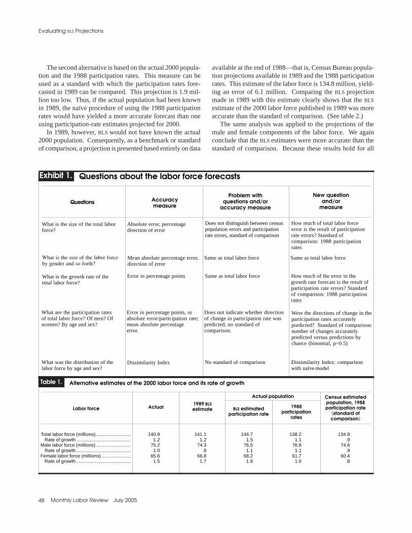
Evaluating BLS Projections
48 Monthly Labor Review July 2005
The second alternative is based on the actual 2000 popula-tion and the 1988 participation rates. This measure can beused as a standard with which the participation rates fore-casted in 1989 can be compared. This projection is 1.9 mil-lion too low. Thus, if the actual population had been knownin 1989, the naïve procedure of using the 1988 participationrates would have yielded a more accurate forecast than oneusing participation-rate estimates projected for 2000.
In 1989, however, BLS would not have known the actual2000 population. Consequently, as a benchmark or standardof comparison, a projection is presented based entirely on data
available at the end of 1988—that is, Census Bureau popula-tion projections available in 1989 and the 1988 participationrates. This estimate of the labor force is 134.8 million, yield-ing an error of 6.1 million. Comparing the BLS projectionmade in 1989 with this estimate clearly shows that the BLSestimate of the 2000 labor force published in 1989 was moreaccurate than the standard of comparison. (See table 2.)
The same analysis was applied to the projections of themale and female components of the labor force. We againconclude that the BLS estimates were more accurate than thestandard of comparison. Because these results hold for all
Actual1989 BLSestimate BLS estimated
participation rate1988
participationrates
Labor force
Census estimatedpopulation, 1988participation rate
(standard ofcomparison)
Table 1.
Actual population
Total labor force (millions) .......................... 140.9 141.1 144.7 138.2 134.8Rate of growth ......................................... 1.2 1.2 1.5 1.1 .9
Male labor force (millions) .......................... 75.2 74.3 76.5 76.8 74.6Rate of growth ......................................... 1.0 .9 1.1 1.1 .9
Female labor force (millions) ...................... 65.6 66.8 68.2 61.7 60.4Rate of growth ......................................... 1.5 1.7 1.8 1.0 .8
Alternative estimates of the 2000 labor force and its rate of growth
Questions about the labor force forecasts
Accuracymeasure
Problem withquestions and/or
accuracy measure
New questionand/or
measureQuestions
Exhibit 1.
What is the size of the total laborforce?
What is the growth rate of thetotal labor force?
Absolute error, percentagedirection of error
Does not distinguish between censuspopulation errors and participationrate errors, standard of comparison
How much of total labor forceerror is the result of participationrate errors? Standard ofcomparison: 1988 participationrates
What is the size of the labor forceby gender and so forth?
What are the participation ratesof total labor force? Of men? Ofwomen? By age and sex?
Mean absolute percentage error,direction of error
Error in percentage points, orabsolute error/participation rate;mean absolute percentageerror.
Dissimilarity Index No standard of comparison
Does not indicate whether directionof change in participation rate waspredicted, no standard ofcomparison.
Same as total labor force
Same as total labor force
Dissimilarity Index: comparisonwith naïve model
Were the directions of change in theparticipation rates accuratelypredicted? Standard of comparison:number of changes accuratelypredicted versus predictions bychance (binomial, p=0.5)
How much of the error in thegrowth rate forecast is the result ofparticipation rate errors? Standardof comparison: 1988 participationrates
What was the distribution of thelabor force by age and sex?
Error in percentage points
Same as total labor force

49 Monthly Labor Review July 2005
Table 3. Participation rates, actual 1988, BLS forecast for 2000, actual 2000 and forecast errors
Total, 16 and older ..................................... 65.9 69.0 67.2 –1.8 1.3
Men
16 years and older ..................................... 76.2 75.9 74.7 –1.2 –1.516 to 19 ................................................... 56.9 59.0 53.0 –6.0 –3.920 to 24 ................................................... 85.0 86.5 82.6 –3.9 –2.425 to 34 ................................................... 94.3 94.1 93.4 –.7 –.935 to 44 ................................................... 94.5 94.3 92.6 –1.7 –1.945 to 54 ................................................... 90.9 90.5 88.6 –1.9 –2.355 to 64 ................................................... 67.0 68.1 67.3 –.8 .365 and older ............................................ 16.5 14.7 17.5 2.8 1.0
Women
16 and older ............................................... 56.6 62.6 60.2 –2.4 3.616 to 19 ................................................... 53.6 59.6 51.3 –8.3 –2.320 to 24 ................................................... 72.7 77.9 73.3 –4.6 .625 to 34 ................................................... 72.7 82.4 76.3 –6.1 3.635 to 44 ................................................... 75.2 84.9 77.3 –7.6 2.145 to 54 ................................................... 69.0 76.5 76.8 .3 7.855 to 64 ................................................... 43.5 49.0 51.8 2.8 8.365 and older ............................................ 7.9 7.6 9.4 1.8 1.5
Actual1988
BLS 2000forecast Actual 2000 BLS
GroupNaïve (1988)
Table 2.
Participation rates Forecast error
labor force size estimates, a fortiori, the same conclusionsapply to the estimates of the various growth rates.10
The accuracy of participation rates. Although the BLS pro-jections of the 2000 labor force were more accurate thanthose of the standard of comparison, they benefitted fromoffsetting errors. The Census Bureau population estimateswere too low, while the participation rates were overesti-mated. In evaluating these estimates of the participationrates, the following two questions are posed: (1) Did theestimates correctly predict the direction of change between1988 and 2000? (2) Were these projections of the level ofthe participation rates more accurate than those generated bya standard of comparison?
There are 14 classifications of the labor force based on ageand gender. (See table 2). The direction of change between1988 and 2000 was projected correctly for 9 of these 14 clas-sifications.11 Using the binomial distribution with p = 0.5, itis possible to test the null hypothesis that this favorable resultcould have occurred purely by chance. We are unable to re-ject this hypothesis. As an additional test, we compared thelevels of the participation rates observed in 2000 with the fol-lowing: (1) the ones that BLS projected for 2000; and (2) the1988 participation rates, which are used as the benchmark.The latter had smaller absolute errors in a majority of thecases. These results indicate that there was room for improv-ing the projections of participation rates.
Measuring structural change: dissimilarity indexes. In order todetermine whether the structural changes and major trends thatoccurred between 1988 and 2000 were predicted accurately, astatistic is used that directly addresses this question. The forecastof the total labor force is an aggregated estimate, and it isimportant to also examine the disaggregated componentpredictions. Such an analysis enables one to determine whetherthe structure of the aggregate has been predicted accurately.
If the aggregate, X, is predicted according to some scenario(for example, full employment), one would want to determinewhether the structure is accurate even if the total is wrong. R.A.Kolb and H.O. Stekler developed a procedure for decomposingthe total error into two components—where the first measuresthe scenario discrepancy and the second, the structural error.12
They calculated the proportion of the aggregate predicted andactual totals that were associated with each of the i components.While their analysis was based on an information content statis-tic, using dissimilarity indexes would yield the same result.
A dissimilarity index is a statistic that can be used to deter-mine whether one distribution approximates another one.Specifically, it measures the amount by which the forecasteddistribution would have to change to be identical to the actualdistribution. The formula for the dissimilarity index is:
D = 0.5 3 | (Pfi / Pf )- (Pai / Pa) |
where Pfi is the forecast of the labor force that will be in the

Evaluating BLS Projections
50 Monthly Labor Review July 2005
ith group, and Pf is the forecast for the total labor force. Simi-larly, Pai and Pa are the corresponding actual data. D isbounded in the interval 0 to 100 percent. The smaller the valueof D, the smaller the difference is between the predicted andactual distributions—that is, the more accurate the forecast.
The dissimilarity index for the BLS projections was basedon the 14 age/gender categories that had been used in 1989 toprepare the estimates for 2000. Similar dissimilarity indexeswere constructed for the other distributions that serve as stan-dards of comparison. The values of the various dissimilarityindexes are presented in table 3.
The results are mixed. In some cases, the dissimilarity in-dexes obtained from the BLS projections are smaller (and thusmore accurate) than those of the standards of comparison. Inother cases, the opposite results were obtained. However, thedissimilarity index for the actual BLS forecast never exceeds 2percent for all age/gender categories or for men and womenseparately. The values of the dissimilarity indexes of the stan-dards of comparison were also around 2 percent, indicatingthat the BLS projection was comparable to but not superior tothese (naïve) benchmark forecasts.
While there is no statistical distribution for the dissimilar-ity index, the BLS projection substantially predicted the struc-tural changes that occurred in the labor force between 1988
and 2000. On the other hand, similar results were obtainedfrom the naïve models that served as the benchmarks.
Did the forecasts improve? The primary focus of this analy-sis is on the projections that were published in 1989 for 2000.While there had been a second set of projections for industryemployment by industry and occupation, BLS actually madefive forecasts of the 2000 labor force. These were publishedin 1987, 1989, 1991, 1993, and 1995.13 It is thus possible todetermine whether the accuracy of the forecasts improved asthe forecast horizon declined.
The results are mixed. (See table 4.) The forecasts of thelabor force that were made in 1988 (and published in 1989)were more accurate than those made in any other year. Thus,they did not improve with the passage of time—that is, as theforecast horizon became smaller. On the other hand, as theforecast horizon declined, so did the errors in the forecastsof the participation rates.
Employment by industry
The questions asked about the employment-by-industry pro-jections are presented in exhibit 2. These questions were dis-cussed in both the original forecast and in the subsequent
Table 3. Dissimilarity indexes of labor force projections
Gender, age ............................ 1.83 2.02 2.24 2.32Men, age ................................. 1.63 .91 .62 1.37Women, age ............................ 1.91 2.86 2.4 1.32
BLS participation rate 1988 participation rate
BLSprojections
Census populationestimate and—
Table 3.
Standards of comparison
Actual population and—
1988 participation rate
Age
Table 3. Errors in labor force and participation rate projections for 2000, various horizons
Labor force ................................................. –1.5 .2 1.5 .7 –.6
Participation rate: All ............................................................. .6 1.8 1.5 1.0 –.2
Men ........................................................... .0 1.2 1.3 .6 –.7 Women ...................................................... 1.3 2.4 1.8 1.4 .4
1986 1988 1990 1992Projection 1994
Table 4.
Errors made in—
51 Monthly Labor Review July 2005
evaluation of that forecast. These include: What is employ-ment by major industry group? What is employment by in-dustry? Which industries are expected to grow the fastest?In which industries will employment decline? These are allquestions that involve structural change and should be evalu-ated correspondingly. The measures that previously have beenused in the evaluations and some of the limitations of thesemeasures are also listed in exhibit 2.
Mean absolute percent error. How accurate were the em-ployment-by-industry projections? The accuracy of the em-ployment-by-industry projections has conventionally beenevaluated by calculating the mean absolute percent error(MAPE). Again, an evaluation of a single prediction shouldnot be based on the magnitude of the error regardless ofwhether it is measured in absolute or percentage terms. Nev-ertheless, we use this statistic in order to note that it can becalculated in two ways: (1) the simple average of the abso-lute percentage error of the forecast for each industry; or (2) aweighted average of the industries’ errors, with the weightsequal to the industry’s share of employment.14 The secondmeasure reduces the weight of small industries, which mighthave large percentage errors.
The standard of comparison was a naïve forecast. It wasassumed that the employment growth rate in each industrybetween 1988 and 2000 would be the same as the one that
had occurred between 1976 and 1988. The mean absolutepercent errors (MAPEs) of the BLS projections and of the naïvemodel are presented in the following tabulation:
BLS Naïve
Unweighted Weighted Unweighted Weighted
Majorindustrysectors ........ 11.9 7.4 11.8 7.2
174disaggregatedindustries ... 18.8 13.6 24.6 14.4
They are divided into several categories: unweighted andweighted MAPEs for the 12 major industry sectors and the 174disaggregated industries. For the 12 major sectors, there isvery little difference between the errors of the BLS projectionsand those of the naïve model used as the standard of compari-son. The MAPEs of the BLS projections for the 174 disaggre-gated industries are less than those of the naïve standard ofcomparison. This is especially true for the unweighted MAPEs.
The BLS projections correctly predicted the direction ofemployment change in 135 of 174 industries. The naïvemodel made a larger number of mistakes, 49. Because mostindustries grew during this period, a better measure is to de-
Questions about the employment forecasts
Accuracymeasure
Problem withquestions and/or
accuracy measure
New questionand/or
measureQuestions
Exhibit 2.
How many people will be employedin each industry?
What is the distribution ofemployment by industry?
Percentage error, meanabsolute percent error
No standard of comparison; givesequal weight to large and smallindustries
Standard of comparison: ratesof growth equal to previous ratesof growth; mean weighted percenterror
Which industries would havehighest (lowest) employment growthrates?
Compare the number ofindustries projected to grow thefastest (slowest) with those thatdid grow fastest (slowest).
Model simulations None
No standard of comparison
No standard of comparison; noanalysis of all industries’ projectedand actual growth rates.
—
Standard of comparison: same shareas in 1988 and shares based onprevious growth rates
What were the sources of theindustry employment forecastserrors?
Dissimilarity Index
Standard of comparison:forecasts of fastest (slowest)growing industries from naïvemodel; Spearman rankcorrelation coefficient for allindustries

Evaluating BLS Projections
52 Monthly Labor Review July 2005
termine whether industries in which employment was ex-pected to grow rapidly (or slowly), actually experienced thistype of growth. (This is done later where rank correlationcoefficients and contingency tables are used.)
Measuring structural change: dissimilarity indexes. As withthe labor force projections, we use dissimilarity indexes todetermine whether the structural employment changes thatoccurred were forecast accurately. These dissimilarity indexeswere for the 12 major industry sectors as well as for the 174different smaller industries—and for the benchmarks used asthe standards of comparison. Two naïve models serve asbenchmarks. The first assumes that each industry’s share oftotal employment would be the same in 2000 as it had been in1988. The second assumes that each industry’s share (si) oftotal employment would increase from 1988 to 2000 by thesame amount as occurred between 1976 and 1988—that is,si2000 = si1988 + (si1988 -si1976).
The results are mixed. The following tabulation shows thedissimilarity indexes for BLS projections and naïve modelestimates:
12 majorindustries ..... 3.75 6.03 3.60
174industries ..... 6.89 10.38 8.09
The dissimilarity indexes associated with the BLS projectionsare smaller than those derived from the naïve standard thatassumed the shares of industrial employment would remainconstant between 1988 and 2000. In comparison with thenaïve growth model, the BLS projections were better for thedisaggregated industries, but slightly worse for the 12 majorgroupings. These results suggest that the BLS projections wereable to capture the structural changes that occurred in industryemployment as least as well as would have been obtained froma simple extrapolation.
Structural change: Spearman rank correlations. Anotherway to determine whether the projections captured the struc-tural changes that occurred is to compare the forecastedgrowth rates of industrial employment with the actual growthrates. The original projections had listed the 20 industriesexpected to have the largest employment growth rates and the20 industries that were expected to show the largest employ-ment declines.15 Only 12 of the industries that were expected
to experience the fastest growth actually did so. It is difficultto interpret these results without a standard of comparison.The naive extrapolation model is again used as the bench-mark. That model actually identified 13 of the 20 industriesthat had the highest employment growth rates. (See table 5).Similar results were obtained for the 20 slowest growing in-dustries. BLS and the naïve model identified 8 and 7 of those20 industries, respectively. Consequently, we conclude thatthe BLS projections of the fastest and slowest growing indus-tries were not substantially different from the forecasts gener-ated by a naïve model.
Rather than merely focus on the 20 industries in thetwo tails of the distributions, the Spearman rank correla-tion coefficient between the predicted and actual growthrates for all 174 industries were also calculated. This co-efficient was 0.64 for both the BLS projections and thenaïve extrapolation model. This result indicates that bothsets of forecasts were able to forecast many of the struc-tural changes that occurred, but there was no differencebetween the BLS projections and the extrapolations ob-tained from a naïve model.
Structural change: contingency table. The Spearman rankcorrelation coefficient provides an overall assessment of therankings of the predicted and actual employment growthrates. Another method for demonstrating the same result isto construct a contingency table. After the employmentgrowth rates of the 174 industries had been ranked, they weredivided into quintiles, with the 35 industries having the high-est growth rates placed in the first quintile, and so forth. Thisprocedure was applied to both the projected and actualgrowth rates, and a 5X5 contingency table was constructed.We then tested the null hypothesis that there was no relation-ship between the predicted and actual growth rates of thesequintiles. A similar procedure was used to evaluate the fore-casts of the naïve extrapolation model. The contingencytables are presented in table 6. While the null of indepen-dence is clearly rejected, less than half of the observations ofboth the BLS and naïve model projections lie on the maindiagonal (indicating that the forecasted and actual growthrates were in the same quintile). However, a majority of theremaining observations lie in the adjacent cells. These re-sults are consistent with those obtained from the Spearmanrank correlation coefficients.
The main result is that the BLS projections do not differsignificantly from those obtained from the naïve extrapola-tive model.16
What were the sources of error in the employment projec-tions? Arthur Andresassen used computer simulations andfactor analysis to determine why the employment errors oc-
BLSprojections
No changefrom 1988
Same change 1988–2000 as 1976–88
Dissimilarity indexesfor naïve models

53 Monthly Labor Review July 2005
curred.17 He showed that there were two basic errors thatoffset each other. The low projection of gross domestic prod-uct was offset by inaccurate employment-output relationships.Our analysis did not attempt to replicate this analysis.
Rank of the 20 industries exhibiting the highest employment growth rates, 1988–2000 by rank of BLS and naïvemodel projections
Computer and data processing services .................................. 1 9 2Personnel supply services ........................................................ 2 10 1Health services ......................................................................... 3 3 5Amusement and recreation services ........................................ 4 39 44Miscellaneous transport services ............................................. 5 16 28
Residential care ........................................................................ 6 11 3Individual and miscellaneous social services ........................... 7 14 13Research and testing ................................................................ 8 38 12Water and sanitation ................................................................. 9 6 22Security and commodity brokers and exchanges ..................... 10 19 6
Commercial sports .................................................................... 11 94 69Credit agencies and investment offices .................................... 12 1 15Motion pictures and video tape rentals ..................................... 13 92 42Miscellaneous business services ............................................. 14 22 17Job training and related services .............................................. 15 43 10
Child daycare services .............................................................. 16 131 29Oil and gas field services .......................................................... 17 4 95Personal services ...................................................................... 18 5 9Miscellaneous equipment rental and leasing ........................... 19 2 4Air transportation ...................................................................... 20 104 8
Actual BLS ProjectionIndustry
Table 5.
Rank
Naïve model projection
Occupational employment
The questions discussed in the occupation projections andin the subsequent evaluation are analogous to those of the
Relationship between ranks of predicted and actual growth rates of employment by industry quintiles, BLSprojections and Naïve model
Ta BLS projection1
1–35 ........................................................... 18 13 2 1 136–70 ......................................................... 9 12 10 2 271–105 ....................................................... 5 5 11 7 7106–140 ..................................................... 1 4 10 12 8141–174 ..................................................... 2 1 2 13 16
Naïve model2
1–35 ........................................................... 21 11 3 0 036–70 ......................................................... 6 12 6 4 771–105 ....................................................... 6 7 11 7 4106–140 ..................................................... 1 4 11 10 9141–174 ..................................................... 1 1 4 14 14
1 x2= 93.61 P = 02 x2= 92.22 P = 0
36–701–35 71–105 106–140Projected growth
141–174
Table 6.
Actual growth

Evaluating BLS Projections
54 Monthly Labor Review July 2005
employment by industry estimates. (See exhibit 3.) Inpresenting the projections, the analysis included theoccupation’s share of employment; the occupations thatare likely to grow the fastest or decline; and the occupa-tions that are likely to have the largest number of new jobs.The evaluation by Andrew Alpert and Jill Auyer consid-ered the absolute percent change of actual and projectedoccupational employment; the numerical change in thesecategories; and the share of employment of each occupa-tional group. Again, these are appropriate measures, butit is possible to use additional measures and compare themwith a standard of comparison. The benchmark is the naïvemodel in which it is assumed that the growth in each occu-pation between 1988 and 2000 was equal to the growthrate that occurred between 1976 and 1988.18
The following tabulation shows MAPEs for BLS projectionsand naïve model estimates:
BLS Naïve
Unweighted Weighted Unweighted Weighted
Majoroccupations .... 5.86 5.29 13.8 11.8
338disaggregatedoccupations .... 45.2 15.0 – –
The mean absolute percent errors of the projections of themajor occupational groups are substantially smaller than thoseof the naïve model. Moreover, the BLS projections correctlypredicted the direction of change for eight of the major occu-pational groupings, with agriculture being the exception.19 Onthe other hand, the unweighted MAPE for the 338 smaller oc-cupational groups is substantial (45.2 percent), indicating thatthere were substantial errors in many of these occupationalgroups. Because the weighted MAPE is smaller (15.0 percent),the larger percentage errors occurred in the smaller occupa-tional groups.
Structural change: dissimilarity indexes. As with the projec-tions of the other two variables, dissimilarity indexes are used todetermine whether the structural employment changes that oc-curred were forecast accurately. These dissimilarity indexeswere for the 9 major occupational groups, as well as for the 338different occupational classifications and for the benchmarksused as the standards of comparison. For the major occupa-tional groups, two naive models are used as benchmarks. Thefirst assumes that each occupation’s share of total employmentwould be the same in 2000 as it had been in 1988. The secondassumes that each occupation’s share (si) of total employmentwould increase from 1988 to 2000 by the same amount as oc-curred between 1976 and 1988—that is, si2000 = si1988 + (si1988 -si1976). There is only one naive benchmark for the 338 occupa-
Questions about occupational forecasts
Accuracymeasure
Problem withquestions and/or
accuracy measure
New questionand/or
measureQuestions
Exhibit 3.
How many people will be employedin each occupation?
Which occupations will have thelargest job growth?
Absolute error, absolutepercent error
No standard of comparison; givesequal weight to large and smalloccupations
Which occupations will growfastest?
What is the distribution ofemployment by occupation?
Compare the number ofoccupations projected to growthe fastest with those that didgrow fastest; distribution ofgrowth rates by growthadjectives
Compare the number ofoccupations that were projectedto have largest job growth withthose that did
Absolute percent error
Model simulations None
No standard of comparison
No standard of comparison
No standard of comparison;analysis of all occupations’projected and actual growth rates
Dissimilarity Index: comparisonwith naïve model
Standard of comparison not possibledue to definitional changes
Spearman rank correlationcoefficient; standard of comparisonnot possible due to definitionalchanges
What were the sources oferrors?
—
Standard of Comparison: Naïvemodel: same growth; meanweighted percent error

55 Monthly Labor Review July 2005
tions because the definition of some of the occupations changed,and, thus, it was not possible to construct the comparable growthrates. Consequently, for these 338 occupations, we only usedthe first of these naïve models—that is, the distribution of occu-pational shares would be the same in 2000 as it had been in1988.
The results in the following tabulation indicate that the BLSprojections captured the structural changes that occurred inoccupational employment better than the naïve models did.The dissimilarity indexes associated with those projectionswere substantially smaller than those of the naïve models.Shown below are the dissimilarity indexes for BLS projectionsand the naïve models.
Majoroccupations .... 2.12 3.12 4.53
338disaggregatedoccupations .... 7.64 8.43 –
Structural change: Spearman rank correlation. Similar to theemployment-by-industry projections, the BLS estimates listed the20 occupations that were expected to grow the fastest. Of these20 occupations, only 6 actually had the fastest growth. Insteadof focusing on the occupations that were in the tail of the distri-bution, we calculated the Spearman rank correlation coefficientbetween the predicted and actual growth rates for all 338 occu-pations. That coefficient is 0.43; it is statistically significant,but because there is no comparable benchmark, there is no basisof comparison. We can only note that this Spearman coefficientis substantially less than the comparable coefficient for the em-ployment by industry data.
Structural change: contingency table. In presenting the dis-tributions of the actual and projected growth rates of the 338
BLSprojections
No change(2000=1988)
Same change 1988–2000 as 1976–88
Dissimilarity indexesfor naïve models
Relationship between ranks of predicted and actual growth rates of occupational employment, quintiles, BLSprojections and actual growth
1–67 ....................................................... 32 14 8 7 668–135 ..................................................... 12 17 16 15 8
136–203 ..................................................... 12 17 15 13 11204–271 ..................................................... 8 13 19 16 12242–338 ..................................................... 3 7 10 17 30
68–1351–67 136–203 204–271Projected growth
272–338
Table 7.
Actual growth
occupations, Alpert and Auyer divided them into six growthcategories, ranked from declining to growing much fasterthan average. While they did not test the null hypothesis thatthere is no relation between the projected and actual growthrates, this hypothesis can be rejected. We also constructed acontingency table (see table 7), but it is based on the quintilesof each distribution rather than on growth categories. Thehypothesis that there is no relationship between the projectedand actual growth rates is also rejected, but it should be notedthat there are many observations that are not on the maindiagonal or in the adjacent cells. This result indicates thatthe projections for many occupations were clearly inaccu-rate and explains why the Spearman rank correlation coeffi-cient is only 0.43.
What were the sources of error in the occupation projections?Alpert and Auyer identified some of the sources of error inthe occupation projections. Some of the errors were attribut-able to assumptions made about technological changes thatwere expected to occur between 1988 and 2000. These in-cluded increases in automation that did not occur in manyoccupations, thus accounting for larger increases in employ-ees than was anticipated. In addition, these authors ran simu-lations to show that in some cases inaccurate staffing patternswere the source of the errors, while in other cases the misesti-mates could be attributed to the mistakes made in the industryprojections. We did not replicate this analysis.
Overall conclusions
This study established a set of procedures for evaluatingBLS projections of the labor force, industry employment,and occupational employment. These procedures werethen used to evaluate the projections for 2000 that werepublished in 1989. The projections were compared withbenchmarks derived from naïve models. Our resultsshowed that in most cases, the accuracy of the BLS projec-tions were comparable to estimates obtained from naïveextrapolative models.

Evaluating BLS Projections
56 Monthly Labor Review July 2005
Notes
NOTE: This article was written under contract with the Bureau of LaborStatistics to explore current projection evaluation techniques and to sug-gest new approaches for effective evaluation of the Bureau’s long-termprojections of employment. BLS published its own evaluation of the 2000projections relative to actual outcomes in the October 2003 Review. Thecurrent paper suggests additional evaluation approaches, including a com-parison with what a simple extrapolation would have produced and theuse of contingency tables. BLS intends to employ the new techniques sug-gested here in addition to all of its more traditional evaluation techniquesin its examination of future employment projections.
1 A governing principle of such an evaluation is that the forecastershould not be penalized for external errors nor benefit if the external errorsoffset the internal mistakes.
2 See Howard N Fullerton, Jr., “New labor force projections, spanning1988 to 2000,” Monthly Labor Review, November 1989, pp. 3–11; ValeriePersonick, “Industry output and employment: a slower trend for thenineties,” Monthly Labor Review, November 1989, pp. 25–41; and GeorgeSilvestri and John Lukasiewicz, “Projections of occupational employment,”Monthly Labor Review, November 1989, pp. 42–65.
3 See Howard N Fullerton, Jr., “Another look at the labor force,”Monthly Labor Review, November 1993, pp. 31–40; Andrew Alpert andJill Auyer, “Evaluating the BLS 1988–2000 employment projections,”Monthly Labor Review, October 2003, pp. 3–12; and Arthur Andreassen,“An evaluation of the 2000 employment by industry projections,” Bureauof Labor Statistics mimeo.
4 Because the projections that are being analyzed in this article wereprepared in 1988, the forecast period is 12 years in length. Consequently,the change from 1976 to 1988 was used as the basis for this benchmark.
5 H.O. Stekler, “Macroeconomic Forecast Evaluation Techniques,” In-ternational Journal of Forecasting, Vol. 7, 1991, pp. 375–84.
6 The problem is not due to the length of the forecast horizon becauselong-run population forecasts have been evaluated using these error mea-sures. Rather, this problem occurs when there are a small number of obser-vations. See Stanley K. Smith and Terry Sinich, “Evaluating the ForecastAccuracy and Bias of Alternative Population Projections for States,” Inter-national Journal of Forecasting, Vol. 8, 1992, pp. 495–508.
7 However, if a set of such single forecasts is available, the quantitativemeasures could then be used to evaluate the set of these predictions. It isthus imperative to also calculate the quantitative statistics so that eventuallyan entire set of forecasts can be evaluated.
8 H.O. Stekler (1991) and R. Fildes and Stekler (2002) noted that theseerror measures are descriptive statistics and do not inform whether the fore-casts are “good” or “bad”. To make such a judgment, a benchmark is re-quired. It is then possible to determine whether the forecasts being evalu-ated are more accurate than those generated by the benchmark procedure.In addition, it is desirable to be able to use a statistical test to determinewhether the two sets of forecasts are significantly different. See H.O. Stekler,“Macroeconomic Forecast Evaluation…”; and R. Fildes and H.O. Stekler,“The State of Macroeconomic Forecasting,” Journal of MacroeconomicForecasting, Vol. 24, 2002, pp. 435–468.
9 Howard N Fullerton, Jr., “Evaluating the BLS labor force projections to2000,” Monthly Labor Review, October 2003, pp. 3–12.
10 The BLS forecast is also more accurate than a naïve model that wouldhave predicted the growth rate from 1988–2000 would be identical to thatobserved from 1976–1988. That naïve model would have predicted thelabor force to grow at an annual rate of 2 percent. See Howard N Fullerton,Jr., “New Labor Force Projections, Spanning…”
11 The errors occurred in the youngest and oldest age groups of both menand women.
12 R.A. Kolb and H.O. Stekler, “Information Content of Long-Term Em-ployment Forecasts,” Applied Economics, 1992, pp. 593–96.
13 See Howard N Fullerton, Jr., “Labor force projections: 1986 to 2000,”Monthly Labor Review, September 1987, pp. 19–29; “New labor force pro-jections, Spanning…”; “Labor force projections: the baby boom moves on,”Monthly Labor Review, November 1991, pp. 31–44; “Another look at thelabor force…”; and “The 2005 labor force: growing, but slowly,” MonthlyLabor Review, November 1995, pp. 29–44.
14 Even though the MAPE is not useful in evaluating a single forecast,this statistic can be used when single forecasts are combined into a set offorecasts.
15 Valerie Personick, “Industry output and employment…”16 This result suggests that extrapolative methods may have been the ba-
sis of the BLS projections.17 Arthur Andreassen, “An Evaluation of the 2000 Employment…”18 This benchmark could only be used for the major occupational group-
ings because the definitions of the disaggregated groupings have changed.19 The naïve model generated identical results.

Monthly Labor Review July 2005 57
High-Tech Employment
Among high-technology industries—those with a highproportion of scientists, engineers, and technicians—some are projected to grow rapidly; overall, however,this group of industries is expected to continue to grow slowly
High-technology employment:a NAICS-based update
Daniel E. Hecker
Daniel E. Hecker is aneconomist in theOffice ofOccupationalStatistics andEmploymentProjections, Bureau ofLabor Statistics.E-mail: [email protected]
High technology receives a great deal ofattention due to its association with newproducts and new production processes
and its implications for productivity, internationalcompetitiveness, overall economic growth, and thecreation of well-paying jobs. Numerous studieshave resulted in the publication of high-tech rank-ings of States and metropolitan areas, while Stateand local governments have established task forcesto assess the potential of high technology to stim-ulate their economies and have developed strat-egies to lure high-technology firms.1
It is important to define the term high tech-(nology), both to assess the claims about its effecton the economy and to develop policies and pro-grams. Four articles previously published in theReview presented definitions of high-technologyindustries and occupations and analyzed high-techemployment trends and projections.2 Because thereare a number of methods of identifying high-techindustries, the lists of such industries produced inthe literature differ from one another. Using BLS data,this article presents one particular method, lists theresulting industries, discusses employment in thoseindustries, and examines several other approaches.Along with describing employment in high-techindustries in 2002, the article considers employ-ment in 1992, projected employment for 2012, andgrowth over the 1992–2002 and 2002–12 periods,as well as earnings in high-tech industries andoccupations in 2004. The updated list of high-techindustries is based on the 2002 North AmericanIndustry Classification System (NAICS), whichreplaces the Standard Industrial Classification
System (SIC) used in earlier articles. The articledescribes the criterion used to select the in-dustries and, in the final section, examines otherselection criteria that were suggested in a March2004 interagency conference on defining hightechnology.
Definitions and data
The term high tech has been used broadly todescribe not only industries, but also occupationsand products. A Congressional Office of Tech-nology Assessment document describes high-technology firms as those “engaged in the design,development, and introduction of new productsand/or innovative manufacturing processesthrough the systematic application of scientific andtechnical knowledge.”3 The document also pointsout that high-technology firms typically use state-of-the-art techniques and, in terms of quantifiableresources, devote a “high” proportion of expendi-tures to research and development (R&D) andemploy a “high” proportion of scientific, technical,and engineering personnel. A National ScienceFoundation report on science and technologyresources also refers to the employment of scien-tists, engineers, and technicians and to measuresof R&D activities as “two of the most importantparameters of innovation” and uses those twoparameters “as surrogates for measuring thebroader concept of innovation.”4 Articles in theReview, as well as other sources, have used one orboth of these input-based criteria to identify high-tech industries. Studies specify thresholds for

58 Monthly Labor Review July 2005
High-Tech Employment
these measures, such as a percentage of total employment inscience, engineering, and technician occupations or spendingon R&D as a percentage of sales or value added. Industries thatexceed these thresholds are identified as high tech.5 Other studiesrely on judgment, generally about output, to identify high-techindustries. For example, the American Electronic Associationdefines an industry as high tech if it was a “maker/creator oftechnology.”6 Using the judgment of industry analysts, theCensus Bureau identifies high-tech products as those em-bodying new or leading-edge technologies.7
A March 2002 Review article by Christopher Kask and EdwardSieber points out that both input-based and output-based meth-ods have advantages and drawbacks.8 Input-based approachesrest on easily obtainable nonsubjective data, but in the absenceof an obvious threshold above which an industry is deemedhigh tech, the resulting lists must be considered arbitrary.Furthermore, such methods suffer from a failure to take accountof the products of an industry and may include industries withproducts not commonly thought of as high tech (although, ofcourse, an industry using high-tech production methods mightbe considered high tech even if its output is not). In contrast toinput-based definitions, output-based definitions tend toprovide lists that match popular conceptions of high tech, butrely on judgments that smack of subjectivity.
In March 2004, the Bureau conducted an interagency seminarto evaluate its most recent methodology for defining high-techindustries, as described in a June 1999 review article.9 Theattendees concluded that many factors contribute to an indus-try’s high-tech nature and that the Bureau should explore all ofthose factors, including the following:
• high proportion of scientists, engineers, and tech-nicians (science, engineering, and technician occu-pation intensity), as defined in the Bureau’s 1999study;
• high proportion of R&D employment (R&D employ-ment intensity), as defined in the Bureau’s 1999 study;
• production of high-tech products, as specified on aCensus Bureau list of advanced-technology products;
• use of high-tech production methods, includingintense use of high-tech capital goods and services inthe production process.
In addition, it was recommended that the relationship betweenhigh-tech industries and productivity growth, discussed inKask and Sieber’s article,10 be explored for the NAICS-basedlist of industries.
Due to data and conceptual problems, only science, engi-neering, and technician occupation intensity was used todevelop a list of industries in the analysis that follows. R&Demployment intensity was not used, because the Occupational
Employment Statistics (OES) survey no longer collects data onR&D employment and because National Science Foundation(NSF) R&D employment data, discussed later in this article,have only limited comparability to Bureau data. Had compa-rable R&D data been available, industries might have beenconsidered high tech only if they met an R&D criterion as well.This was the approach used in the 1999 BLS study.11 If betterinformation had been available, other combinations of criteria,as well as alternative lists of high-tech industries, also wouldhave been possible. However, all information available on thehigh-tech nature of industries, as well as on productivitygrowth, is tabulated and discussed in this article.
Defining high-technology employment
High-technology occupations are scientific, engineering, andtechnician occupations, the same group of occupations used todefine high-tech industries in this and earlier studies. Theyinclude the following occupational groups and detailedoccupations: computer and mathematical scientists, StandardOccupational Classification (SOC) 15-0000; engineers, SOC 17–2000; drafters, engineering, and mapping technicians, SOC 17–3000; life scientists, SOC 19–1000; physical scientists, SOC 19–2000; life, physical, and social science technicians, SOC 19–4000;computer and information systems managers, SOC 11–3020;engineering managers, SOC 11–9040; and natural sciencesmanagers, SOC 11–9120. Workers in these occupations need anin-depth knowledge of the theories and principles of science,engineering, and mathematics underlying technology, a knowl-edge generally acquired through specialized post-high schooleducation in some field of technology leading up to an awardranging from a vocational certificate or an associate’s degree toa doctorate. Individuals employed in these occupations arecollectively referred to as technology-oriented workers. Sometechnology-oriented workers are engaged in R&D, increasingscientific knowledge and using it to develop products and pro-duction processes; others apply technology in other activities,including the design of equipment, processes, and structures; com-puter applications; sales, purchasing, and marketing; quality man-agement; and the management of these activities.12
Data for calculating industries’ technology-oriented workerintensity are from the BLS National Employment Matrix, whichshows occupational employment by four-digit NAICS industryfor 2002.13 The 2002 staffing patterns in the matrix are based onemployment data from the 2000, 2001, and 2002 OES surveys,while earnings are from the May 2004 survey.14 An industry isconsidered high tech if employment in technology-orientedoccupations accounted for a proportion of that industry’s totalemployment that was at least twice the 4.9-percent average forall industries. With this relatively low threshold, 46 four-digitNAICS industries are classified as high tech.15 Within thatgroup, three levels of high technology were specified. Level I

Monthly Labor Review July 2005 59
includes the 14 industries in which these occupations accountedfor a proportion that was at least 5 times the average or greaterand constituted 24.7 percent or more of industry employment.Level II includes the 12 industries in which the high-techoccupations were 3.0 to 4.9 times the average (constituting 14.8percent to 24.7 percent of total employment), and Level IIIincludes the 20 industries with a proportion that was 2.0 to 2.9times the average (making up 9.8 percent to 14.7 percent of totalemployment).16
These high-tech industries are a heterogeneous group in termsof production processes and output, covering a broad range ofindustries. Level I includes the computer and electronic products,aerospace, and pharmaceutical and medicine manufacturingindustries; the computer software, Internet, and data processingindustries in the information sector; and three professional,scientific, and technical services industries, as shown in table 1.Levels I, II, and III combined cover all four-digit industries withincomputer and electronic products manufacturing (NAICS 334), aswell as merchant wholesalers of professional and commercialequipment and supplies (a category that encompasses whole-salers of computers, software, and some electronic instruments).Levels I, II, and III combined also include all but one of thetelecommunications industries within the information sector, fourmachinery-manufacturing industries, and all but one industry inchemical manufacturing.17 Finally (but not exhausting the list),included as well are (1) four industries within professional,scientific, and technical services; (2) the Federal Government,except the Postal Service; (3) all three pipeline industries in NAICS486; and (4) management of companies and enterprises, a cate-gory with no equivalent in the SIC.18 Biotechnology andnanotechnology are not on the list of high-tech industries,because they are not identified as industries in the NAICS. Mostbiotech companies are located in scientific R&D services or phar-maceutical and medicine manufacturing industries, according toa recent Commerce Department survey.19 No similar informationhas been found regarding nanotechnology.
Strictly defined, the preceding industries should be calledindustries that are technology-oriented-occupation intensive.However, data discussed later suggest that almost all Level-Iindustries are also R&D intensive and that some in Levels IIand III may be as well. In addition, all Level-I goods-producingindustries have some products defined as high tech by theCensus Bureau, as do some Level-II industries. Because ofthis supporting evidence—and for brevity—the 46 industrieson the list are referred to as high tech. Lists of industriesbased on criteria other than their proportion of technology-oriented occupations would differ from this one.20
Employment in 2002
High-tech industries accounted for 14.4 million wage andsalary jobs in 2002, about 11 percent of total nonfarm wageand salary jobs in the economy.21 (See table 1.) Level-I indus-
tries accounted for 5.9 million jobs, 4.5 percent of the total. Level-II industries accounted for 4.5 million jobs, 3.4 percent of thetotal, and Level-III industries accounted for 4 million jobs, 3.1percent of the total. About 3.8 million (26 percent) of the 14.4million jobs in high-tech industries in 2002 were in manufacturing.High-tech manufacturing industries made up nearly a quarter ofall manufacturing employment that year. Level-I manufacturingindustries accounted for 2.2 million jobs.
Employment trends, 1992, 2002, and 2012. Employment inhigh-tech industries increased 7.5 percent over the 1992–2002period, compared with 19.7 percent for the economy as awhole, and accounted for 5 percent of total employmentgrowth. (See table 1.) During the same period, high-techemployment declined from 12.2 percent to 11 percent of totalemployment. Projections for the 2002–12 period show high-tech employment continuing to grow more slowly than theeconomy overall, at 11.4 percent compared with 16.5 percent.By 2012, high-tech employment is projected to add 1.6 millionjobs, about 8 percent of all projected growth, and account for10.5 percent of total employment. Growth for Level-I indus-tries, at 23.0 percent from 1992 to 2002 and projected at 15.6percent from 2002 to 2012, is closer to the total for the economy.Employment change among the 46 high-tech industries varieswidely. As the following tabulation shows, most projectedgrowth is in eight service-providing industries, including fivecomputer and related industries:
Projected change in employment, 2002–12
Number Industry (thousands) Percent
Computer systems design and relatedservices ................................................ 635 54.6
Management, scientific, and technical consulting services .............................. 406 55.4Management of companies andenterprises ........................................... 195 11.4
Software publishers .............................. 174 67.9Merchant wholesalers of professionaland commercial equipment andsupplies (including computers) .......... 130 19.8
Data processing, hosting, and relatedservices ................................................ 125 40.8
Wireless telecommunications carriers (except satellite) .................................. 99 50.5Internet service providers and web searchportals ................................................. 91 64.2
All of these industries except management of companies andenterprises also are projected to grow faster than the averagefor all industries. Twenty of the 46 industries are projected tocontract. The largest declines are expected for four Level-Imanufacturing industries, as well as one Level-III commu-nications industry:

60 Monthly Labor Review July 2005
High-Tech Employment
High-technology employment, 1992, 2002, and projected 2012
… Total nonfarm wage and salary, allindustries2 ...................................................... 109,526 131,063 152,690 21,537 21,627 19.7 16.5 $28,770
… Total, three levels of high-technologyindustries ....................................................... 13,415 14,422 16,067 1,006 1,646 7.5 11.4 (3)
… Level-I industries .............................................. 4,783 5,883 6,804 1,100 921 23.0 15.63254 Pharmaceutical and medicine manufacturing 225 293 361 68 68 30.2 23.2 43,9303341 Computer and peripheral equipment
manufacturing ............................................. 329 250 182 –79 –68 –24.0 –27.1 61,8303342 Communications equipment manufacturing ... 210 191 201 –19 10 –9.0 5.4 45,5203344 Semiconductor and other electronic
component manufacturing .......................... 519 531 452 12 –79 2.3 –14.9 39,2103345 Navigational, measuring, electromedical, and
control instruments manufacturing ............ 549 451 396 –98 –55 –17.8 –12.2 47,9603364 Aerospace product and parts manufacturing 711 468 386 –242 –83 –34.1 –17.6 51,9905112 Software publishers ........................................ 114 256 430 142 174 125.0 67.9 69,8805161 Internet publishing and broadcasting ............ 16 35 49 19 14 116.1 41.1 53,4705179 Other telecommunications ............................. 16 10 8 –6 –2 –39.2 –21.9 45,4705181 Internet service providers and Web search
portals ......................................................... 39 142 233 103 91 265.3 64.2 52,7805182 Data processing, hosting, and related
services ...................................................... 220 305 430 86 125 39.0 40.8 45,5705413 Architectural, engineering, and related
services ...................................................... 902 1,251 1,306 349 54 38.7 4.3 48,5705415 Computer systems design and related
services ...................................................... 445 1,163 1,798 718 635 161.3 54.6 63,3505417 Scientific research-and-development services 490 537 573 47 36 9.7 6.7 57,890
… Level-II industries ............................................. 4,760 4,528 4,998 –231 470 –4.9 10.7 (3)1131, 32 Forestry .......................................................... 10 10 10 0 0 .0 4.0 –
2111 Oil and gas extraction .................................... 182 123 88 –60 –34 –32.8 –27.8 49,2902211 Electric power generation, transmission, and
distribution .................................................. 537 436 405 –101 –31 –18.8 –7.1 53,3303251 Basic chemical manufacturing ....................... 246 171 140 –76 –31 –30.8 –18.0 45,9703252 Resin, synthetic rubber, and artificial synthetic
fibers and filaments manufacturing ........... 151 114 89 –37 –26 –24.5 –22.6 42,7303332 Industrial machinery manufacturing ............... 142 132 125 –10 –6 –7.1 –4.7 39,4803333 Commercial and service industry machinery
manufacturing ............................................. 138 132 141 –6 9 -4.6 6.6 35,9403343 Audio and video equipment manufacturing .... 58 42 38 –16 –3 –27.7 –7.7 32,4603346 Manufacturing and reproducing, magnetic and
optical media .............................................. 44 57 63 13 6 30.5 11.1 35,7204234 Professional and commercial equipment and
supplies, merchant wholesalers ................ 584 659 790 76 130 13.0 19.8 41,7705416 Management, scientific, and technical
consulting services .................................... 358 732 1,137 374 406 104.4 55.4 45,610… Federal Government, excluding Postal Service 2,311 1,922 1,972 –389 50 –16.8 2.6 (4)
… Level-III industries ............................................ 3,8723 4,010 4,265 137 255 3.5 6.3 (3)3241 Petroleum and coal products manufacturing . 152 119 102 –33 –18 –21.8 –14.8 48,3403253 Pesticide, fertilizer, and other agricultural
chemical manufacturing ............................. 54 45 35 –10 –10 –17.7 –21.3 39,6803255 Paint, coating, and adhesive manufacturing .... 81 72 62 –8 –11 –10.3 –14.7 35,1103259 Other chemical product and preparation
manufacturing ............................................. 144 112 79 –32 –33 –21.9 –29.4 35,3903336 Engine, turbine, and power transmission
equipment manufacturing ........................... 111 100 100 –11 0 –9.6 .2 37,3103339 Other general-purpose machinery
manufacturing ............................................. 317 288 339 –29 51 –9.0 17.7 35,3203353 Electrical equipment manufacturing ............... 219 176 180 –43 4 –19.4 2.2 32,5203369 Other transportation equipment
manufacturing ............................................. 36 40 40 4 0 10.3 .5 34,2304861 Pipeline transportation of crude oil ................ 10 7 7 –3 0 –27.0 –2.7 52,0204862 Pipeline transportation of natural gas ........... 42 29 30 –13 1 –31.0 2.1 49,6504869 Other pipeline transportation ......................... 7 5 5 -2 0 –25.7 –7.7 50,5705171 Wired telecommunications carriers ................ 637 662 600 25 –62 4.0 –9.4 50,9405172 Wireless telecommunications carriers
(except satellite) ........................................ 48 196 295 148 99 309.8 50.5 38,4805173 Telecommunications resellers ........................ 173 1856 188 13 2 7.6 1.3 49,4005174 Satellite telecommunications ......................... 19 19 17 0 –2 1.6 –10.4 50,7805211 Monetary authorities, central bank ................ 24 23 23 –1 0 –2.5 .9 40,840
IndustryNAICScode 1992 2002 2012
Percentchange, 2002–12
Change in level,
1992–2002
Percentchange,
1992–2002
Medianannualwage,
May 20041
Changein level,2002–12
Table 1.[Levels in thousands]
Employment Employment change

Monthly Labor Review July 2005 61
Projected change, 2002–12, in— Employment Output, Number average annual Industry (thousands) Percent rate of changeAerospace products andparts ................................... –83 –17.6 0.1
Semiconductor and otherelectronic components ...... –79 –14.9 1.1
Computer and peripheralequipment .......................... –68 –27.1 24.2
Wired telecommunicationscarriers ............................... –62 –9.4 4.9
Navigational, measuring,electromedical, and controlinstruments ........................ –55 –12.2 3.2
Despite the projected employment declines, only 3 of the46 high-tech industries are anticipated to have output de-clines; in addition, 7 Level-I computer and communications-related industries have the fastest-growing output among allindustries for the 2002–12 period.22 The following tabulationshows the average annual rate of growth for the 7:23
Industry Rate of growthComputer and peripheral equipmentmanufacturing ...................................................... 24.2
Communications equipment manufacturing ......... 10.4Internet publishing and broadcasting .................... 10.3Internet service providers and web searchportals ................................................................. 10.3
Data processing, hosting, and related services ..... 10.3Computer systems design and related services .... 9.0Software publishers .............................................. 8.4
High-tech manufacturing industries. Employment in the 20high-tech manufacturing industries, in total, is projected to
decline 7 percent from 2002 to 2012, compared with a 1-percentdecline in overall manufacturing. Over the 1992–2002 period,these 20 industries declined 15 percent, as opposed to a 9-percent decline for total manufacturing. Employment in the 6Level-I high-tech manufacturing industries is projected todecline 9 percent during 2002–12; over the 1992–2002 period,employment in these industries declined 14 percent. The onlyhigh-tech manufacturing industry with faster-than-averageprojected employment growth from 2002 to 2012 is Level-Ipharmaceuticals and medicine, which is expected to add 68,000jobs.
The 5 computer information and computer systems designindustries (all Level I), including 4 of the 8 with the mostgrowth (see tabulation on page 59), attracted much attentionduring the late 1990s. As a group, their employment more thandoubled from 1992 to 2002 and is projected to grow 54.6 percentduring 2002–12. (See table 2.) Despite its prominence, thisgroup is relatively small, with employment of 1.9 million in2002, less than 1.5 percent of the total. Nevertheless, withoutthese industries, Level-I employment is projected to decline3.0 percent, compared with 15.6-percent growth with them.Also, without these industries, total high-tech employment isprojected to grow only 4.8 percent, as opposed to 11.4 percentwith them. Finally, without the 5 industries, neither Level-Inor total high-tech employment changed much over the 1992–2002 period.24
High-tech earnings
A number of studies have stated that high-tech jobs are high-paid jobs.25 Clearly, that was the case for the industries andoccupations in this article. The Occupational EmploymentStatistics survey collected data on 44 of the 46 high-tech
Continued—High-technology employment, 1992, 2002, and projected 2012
Employment
5232 Securities and commodity exchanges ........... 10 10 10 0 1 –4.0 7.3 $61,6205511 Management of companies and enterprises .. 1,623 1,711 1,906 88 195 5.4 11.4 43,4005612 Facilities support services ............................. 68 104 146 36 42 52.9 40.4 28,9108112 Electronic and precision equipment repair
and maintenance ........................................ 99 105 101 6 –4 6.1 –3.8 32,750
IndustryNAICScode 1992 2002 2012
Percentchange, 2002–12
Change in level,
1992–2002
Percentchange,
1992–2002
Medianannualwage,
May 20041
Changein level,2002–12
Table 1.
1 Annual earnings rates are hourly rates times 2,080 hours. Data do notcover the Federal Government or forestry.
2 See Jay M. Berman, “Industry output and employment projections to2012,” Monthly Labor Review, February 2004, pp. 58–79, table 3.
3 Not calculated. 4 The average salary for full-time nonpostal Federal employees as of
March 31, 2004, was $60,517. (See Pay Structure of the Federal CivilService (U.S. Office of Personnel Management, May 2005 ), p. 2. )
NOTE: Employment data for 1992 in NAICS 4861, 4862, 4869, 5174, 5232,1131, and 1132 are estimated. Dash indicates industry not surveyed.
SOURCES: Employment data are from Berman, “Industry output,” table 3;National Employment Matrix, 2002–12; and unpublished sources. Earningsdata are from the Occupational Employment Statistics Survey.
[Levels in thousands]
Employment change

62 Monthly Labor Review July 2005
High-Tech Employment
industries; all had median earnings greater than the median for allindustries in May 2004. (See table 1.) In 5 of the industries, wageswere at least twice the median for all industries, and in 21 moreindustries, wages exceeded the median for all industries by 50percent to 99 percent. Only in facilities support services werethey close to the median for all.
Median earnings in all of the 71 technology-oriented occupa-tions exceeded the median for all workers in May 2004, except forforest and conservation technicians, as shown in table 3. In 6occupations, earnings exceeded 3 times the median; in 34 more,earnings were twice the median; and in another 17, earningsexceeded the median by 50 percent to 99 percent. Thirteen otheroccupations, almost all technicians and drafters, had earningsthat exceeded the median by less than 50 percent.
In sum, high tech is projected to grow more slowly than theaverage for all industries, but some high-tech industries, includ-ing computer-related services, management and technical con-sulting, and wireless telecommunications, are projected to growvery rapidly. High-tech manufacturing is expected to declinefaster than overall manufacturing; however, output in many high-tech industries is projected to grow rapidly, and most high-techindustries and occupations have high earnings.
Other selection criteria
As noted earlier, there is no single widely accepted criterionfor defining high-technology industries; accordingly, theinteragency group recommended three criteria for selectinglists of such industries, besides the criterion of technology-oriented occupation intensity. The information that followsmay be useful to those desiring to amend the list presented in
this article or to those wishing to develop their own list. BothR&D employment intensity and having products on a CensusBureau list of high-tech products were judged to be usefulcriteria, but due to data problems, neither was used to rankindustries in terms of being high tech. For a number of reasons,the R&D data were not comparable to BLS data. As for high-tech products, there are no data showing the proportion theseproducts are of each industry’s output, and the list of productsprovides little information about service industries. Still, bothsources can provide information which
• supports the inclusion of specific industries on theBLS high-tech list.
• raises doubts about the inclusion of specific industrieson the list.
• suggests that some industries not on the list mightnonetheless be considered high tech.
All available information on high-tech industries for all criteriais presented in table 4, which ranks industries by their percent-age of employment in technology-oriented occupations in2002.
The R&D data show (on a company basis—see the moredetailed discussion of the data that follows) that almost allLevel-I industries have a high R&D intensity. The data alsosuggest that R&D takes place in some Level-II and Level-IIIindustries, but at a lower intensity than in Level-I industries.(See table 4.) Further, the data suggest that several Level-IIand Level-III industries have a low intensity of R&D. Amonggoods-producing industries, all those at Level I have productson the Census Bureau high-tech list, as do some Level-II, but
High-technology employment, 1992, 2002, and projected 2012, in five computer information and computersystems design industries
… Total, three levels of high-technologyindustries ................................................. 13,415 14,422 16,067 1,006 1,646 7.5 11.4
… LeveI-I industries .............................................. 4,783 5,883 6,804 1,100 921 23.0 15.6… Five computer industries ............................... 834 1,901 2,940 1,067 1,039 127.9 54.6
5112 Software publishers .................................... 114 256 430 142 174 125.0 67.95161 Internet publishing and broadcasting ......... 16 35 49 19 14 116.1 41.15181 Internet service providers and Web search
portals ...................................................... 39 142 233 103 91 265.3 64.25182 Data processing, hosting, and related
services ................................................... 220 305 430 86 125 39.0 40.85415 Computer systems design and related
services ................................................... 445 1,163 1,798 718 635 161.3 54.6… Total, three levels of high-technology industries,
except for five computer industries ............... 12,581 12,521 13,127 –61 606 –.5 4.8… High-technology level I, except for five
computer industries ........................................ 3,949 3,982 3,864 33 –118 .8 –3.0
IndustryNAICScode 1992 2002 2012
Percentchange, 2002–12
Change in level,
1992–2002
Percentchange,
1992–2002
Changein level,2002–12
Table 2.
SOURCE: Jay M. Berman, “Industry output and employment projections to 2012,” Monthly Labor Review, February 2004, table 3; and National EmploymentMatrix.
[Levels in thousands]
Employment changeEmployment

Monthly Labor Review July 2005 63
… All occupations .................................................. $28,770
11–3021 Computer and information systems managers ... 92,57011–9041 Engineering managers ........................................... 97,63011–9121 Natural sciences managers ................................... 88,660
15–1011 Computer and information scientists, research .... 85,19015–1021 Computer programmers ........................................ 62,89015–1031 Computer software engineers, applications ........ 74,98015–1032 Computer software engineers, systems
software ............................................................. 79,74015–1041 Computer support specialists .............................. 40,43015–1051 Computer systems analysts ............................... 66,46015–1061 Database administrators ....................................... 60,65015–1071 Network and computer systems administrators ... 58,19015–1081 Network systems and data communications
analysts ............................................................. 60,60015–2011 Actuaries ............................................................... 76,34015–2021 Mathematicians .................................................... 81,24015–2031 Operations research analysts ............................... 60,19015–2041 Statisticians ........................................................... 58,62015–2091 Mathematical technicians ..................................... 38,460
17–2011 Aerospace engineers ............................................ 79,10017–2021 Agricultural engineers ............................................ 56,52017–2031 Biomedical engineers ............................................ 67,69017–2041 Chemical engineers .............................................. 76,77017–2051 Civil engineers ...................................................... 64,23017–2061 Computer hardware engineers .............................. 81,15017–2071 Electrical engineers ................................................ 71,61017–2072 Electronics engineers, except computer ............... 75,77017–2081 Environmental engineers ...................................... 66,48017–2111 Health and safety engineers, except mining safety
engineers and inspectors .................................. 63,73017–2112 Industrial engineers .............................................. 65,02017–2121 Marine engineers and naval architects ................ 72,04017–2131 Materials engineers .............................................. 67,11017–2141 Mechanical engineers ........................................... 66,32017–2151 Mining and geological engineers, including mining
safety engineers ............................................... 64,69017–2161 Nuclear engineers ................................................. 84,880
OccupationSOCcode
Medianwages
Table 3.
19–2041 Environmental scientists and specialists,including health ................................................. 51,080
19–2042 Geoscientists, except hydrologists andgeographers ....................................................... 68,730
19–2043 Hydrologists .......................................................... 61,51019–4011 Agricultural and food science technicians ............. 29,73019–4021 Biological technicians ............................................ 33,21019–4031 Chemical technicians ............................................ 38,17019–4041 Geological and petroleum technicians .................. 40,26019–4051 Nuclear technicians ................................................ 59,20019–4091 Environmental science and protection
technicians, including health ............................. 35,34019–4092 Forensic science technicians ................................. 44,01019–4093 Forest and conservation technicians ..................... 27,330
17–2171 Petroleum engineers ............................................. $88,50017–3011 Architectural and civil drafters ............................. 39,19017–3012 Electrical and electronics drafters ..................... 43,18017–3013 Mechanical drafters ............................................ 43,00017–3021 Aerospace engineering and operations technicians 52,50017–3022 Civil engineering technicians ............................... 38,48017–3023 Electrical and electronic engineering technicians .... 46,31017–3024 Electromechanical technicians ............................. 41,44017–3025 Environmental engineering technicians ............... 38,55017–3026 Industrial engineering technicians ....................... 43,59017–3027 Mechanical engineering technicians .................... 43,40017–3031 Surveying and mapping technicians ................... 30,380
19–1011 Animal scientists ................................................ 49,92019–1012 Food scientists and technologists ..................... 50,84019–1013 Soil and plant scientists ..................................... 51,20019–1021 Biochemists and biophysicists ........................... 68,95019–1022 Microbiologists .................................................... 54,84019–1023 Zoologists and wildlife biologists ....................... 50,33019–1031 Conservation scientists ...................................... 52,48019–1032 Foresters ............................................................. 48,23019–1041 Epidemiologists .................................................. 54,80019–1042 Medical scientists, except epidemiologists ....... 61,32019–2011 Astronomers ........................................................ 97,32019–2012 Physicists ........................................................... 87,45019–2021 Atmospheric and space scientists ..................... 70,10019–2031 Chemists ............................................................ 56,06019–2032 Materials scientists ............................................. 72,390
SOCcode
NOTE: Data are for all industries except agriculture (minus agriculturalservices, which are covered) and the Federal Government. Data are notshown for eight “all other” occupation categories.
MedianwagesOccupation
Median annual wages of wage and salary workers in technology-oriented occupations, May 2004
Annual rates are hourly rates times 2,080 hours.
SOURCE: Occupational Employment Statistics Survey.
no Level-III, industries. There also are four industries that arenot on the high-tech list, but that produce high-tech products.However, without information on how large a part they are ofindustry output, it is not possible to make a case for theirinclusion within the high-tech sector.
The data on the use of high-tech capital goods and services inthe production process is only partially consistent with thetechnology-oriented occupation-based list. A list based on such
data ranks as high some industries designated high tech, othersas very low. Also, some industries that neither are on the high-tech list, nor meet an R&D or high-tech product criterion, nor arementioned on other lists in the high-tech literature rank high bythis standard.26 Therefore, those data were not considered usefulin identifying high-tech industries. The discussion that followscovers each criterion in more detail, as well as the connectionbetween high-tech industries and growth in output per hour.

64 Monthly Labor Review July 2005
High-Tech Employment
Ranking of industries by percent of employment in science, engineering, and technician (technology-oriented) occupations in 2002, along with data for other criteria, by industry
Total, wage and salary workers, all industries5 ... 132,279 4.9 1,066.1 65 … … … …
Level I
5415 Computer systems design and related services . 1,163 60.2 90.8 7259 4 73.6 2 –5112 Software publishers ........................................... 256 56.4 80.8 245 4 70.6 3 17.25413 Architectural, engineering, and related services . 1,251 51.5 32.2 104 – 66.3 5 –5417 Scientific research and development services ... 537 46.4 50.0 302 1 58.9 7 –5181 Internet service providers and web search
portals ............................................................ 142 43.8 623.3 698 – 655.6 12 –3341 Computer and peripheral equipment
manufacturing ................................................ 250 42.9 15.1 170 3, 4 57.4 8 24.95161 Internet publishing and broadcasting ............... 35 38.7 623.3 698 – 655.6 12 –3345 Navigational, measuring, electromedical, and
control instruments manufacturing ................ 451 34.7 75.9 7126 2, 4 43.0 28 3.95182 Data processing, hosting, and related services .. 305 34.3 623.3 98 – 70.0 4 –3364 Aerospace product and parts manufacturing ... 468 31.3 32.5 743 8 44.2 27 2.23342 Communications equipment manufacturing ....... 191 29.2 740.9 7264 4 649.4 19 10.53344 Semiconductor and other electronic
component manufacturing ............................. 531 28.7 73.3 180 3,5,7 22.6 77 20.73254 Pharmaceutical and medicine manufacturing ... 293 28.4 51.8 137 1, 2 39.4 30 .95179 Other telecommunications ................................ 10 27.7 6,78.5 (6,8) – 656.7 10 –
Level II
2111 Oil and gas extraction ....................................... 123 21.3 (6,8) (6,8) No 7.5 116 2.61131, 32 Forestry ............................................................. 10 20.3 …. No 65.1 118 –3333 Commercial and service industry machinery
manufacturing ................................................ 132 20.0 656.5 672 No 37.2 33 .83346 Manufacturing and reproducing magnetic and
optical media .................................................. 57 19.6 64.4 6171 4, 7 47.0 24 .63251 Basic chemical manufacturing .......................... 171 18.9 8.5 54 10 32.3 44 1.44234 Professional and commercial equipment and
supply merchant wholesalers ........................ 659 18.5 6134.5 684 – – – 13.43332 Industrial machinery manufacturing .................. 132 17.9 656.5 672 6 25.2 64 2.4
… Federal Government, excluding PostalService ........................................................... 1,922 17.3 – – – – – –
5416 Management, scientific, and technical consulting services ........................................ 732 17.2 68.9 628 – 55.9 11 –
3343 Audio and video equipment manufacturing ....... 42 15.9 64.4 6171 No 649.4 19 5.42211 Electric power generation, transmission,
and distribution .............................................. 436 15.7 6– 62 – 22.8 76 3.13252 Resin, synthetic rubber, and artificial synthetic
fibers and filaments manufacturing ............... 114 15.3 12.8 97 – 40.7 29 2.2
Level III
5171 Wired telecommunications carriers ................... 662 14.5 6,78.5 (6,8) – 656.7 10 5.85511 Management of companies and enterprises ..... 1,711 14.3 1.5 66 – 50.7 18 –4862 Pipeline transportation of natural gas ............... 29 13.5 (6,8) (6,8) – 632.4 43 –5211 Monetary authorities—central bank .................. 23 13.3 618.9 624 – – –5172 Wireless telecommunications carriers
(except satellite) ............................................ 196 13.3 6,78.5 (6,8) – 656.7 10 6.25173 Telecommunications resellers ........................... 186 13.2 6,78.5 (6,8) – 656.7 10 –5174 Satellite telecommunications ............................ 19 13.1 6,78.5 (6,8) – 656.7 10 –3353 Electrical equipment manufacturing .................. 176 12.9 614.0 640 No 32.7 42 2.83259 Other chemical product and preparation
manufacturing ................................................ 112 12.9 613.9 6,768 No 39.0 31 2.83339 Other general-purpose machinery
manufacturing ................................................ 288 12.6 656.6 672 No 29.6 49 2.03336 Engine, turbine, and power transmission
equipment manufacturing .............................. 100 12.3 656.6 672 No 28.7 53 3.53255 Paint, coating, and adhesive manufacturing .... 72 12.2 613.9 6,768 No 35.6 35 1.23241 Petroleum and coal products manufacturing .... 119 12.0 6,74.3 6,720 No 28.0 56 3.28112 Electronic and precision equipment repair and
maintenance ................................................... 105 11.5 – – – – –
IndustryNAICScode
Totalemployment,
alloccupations(thousands)
Output oncensustrade
productlist3
Percent Rank
Averageannual
percentchange inoutput per
hour,1987–2001,1987–2002,
or1987–20034
Table 4.
Perthousand
employeesin
R&D-performingcompanies1
Employment,January
2003(thousands)
Percent intechnology-
orientedoccupations
R&D scientists andengineers1,2
Investment fromLevel-I industries
in 19971

Monthly Labor Review July 2005 65
Proportion of R&D employment. As noted earlier, the R&Ddata used to define high-tech industries in the 1999 BLS studyare no longer collected in the OES survey—the survey thatprovides data on employment by occupation and industry.The National Science Foundation’s annual Survey of Indus-trial Research and Development collects data on the employ-ment of R&D scientists and engineers, but that survey’sdefinitions and coverage severely limit comparisons with OES-based data.
Nevertheless, data from the 2002 Industrial Research andDevelopment survey are analyzed and presented in table 4.The key differences between the two surveys are as follows:
• The reporting unit for the OES survey (and other BLSindustry employment surveys) is the establishment, which
Continued—Ranking of industries by percent of employment in science, engineering, and technician(technology-oriented) occupations in 2002, along with data for other criteria, by industry
5612 Facilities support services ................................. 104 11.3 – – – – – –3253 Pesticide, fertilizer, and other agricultural
chemical manufacturing .................................. 45 11.2 613.9 6,768 No 38.2 32 1.15232 Securities and commodity exchanges ............... 10 – 618.9 624 – – – –4861 Pipeline transportation of crude oil .................... 7 10.3 (6,8) (6,8) – 632.4 43 –3369 Other transportation equipment manufacturing ..... 40 10.0 6,77.3 6,750 No 630.9 45 5.14869 Other pipeline transportation .............................. 5 10.0 (6,8) (6,8) – 632.4 43 –
Other industries meeting at least one criterion
3329 Other fabricated metal product manufacturing .. 296 9.3 613.1 626 9 629.7 48 .53359 Other electrical equipment and component
manufacturing .................................................. 152 9.0 614.0 640 7 25.2 65 2.73363 Motor vehicle parts manufacturing ..................... 731 8.8 683.2 676 No 626.7 60 2.83361 Motor vehicle manufacturing .............................. 267 8.3 683.2 676 No 626.7 60 2.63335 Metalworking machinery manufacturing ............. 217 8.0 656.5 672 6 34.0 40 1.33324 Boiler, tank, and shipping container
manufacturing .................................................. 95 4.9 613.1 626 10 24.0 70 1.43362 Motor vehicle body and trailer manufacturing .... 154 4.7 683.2 676 No 626.7 60 1.1
IndustryNAICScode
Totalemployment,
alloccupations(thousands)
Output oncensustrade
productlist3 Percent Rank
Averageannual
percentchange inoutput per
hour,1987–2001,1987–2002,
or1987–20034
Table 4.
Perthousand
employeesin
R&D-performingcompanies1
Employment,January
2003(thousands)
Percent intechnology-
orientedoccupations
1 Data are for 1997 NAICS industries. 2 Data are for full-time equivalent employment of scientists and engineers.
The reporting unit for the survey in which the R&D data were collected is thecompany. The reporting unit for the Occupational Employment Survey dataused to develop the ranking in this table is the establishment. Ratios arebased on industry employment during the week containing March 12 and onscientist and engineer employment the following January. 3 Products were assigned to NAICS industries by the Bureau of LaborStatistics. (See exhibit 1.) Numbers refer to 1 of 10 major technology areas. 4 Data are available through 2001 for manufacturing industries, through2002 for service-producing industries and for mining and utilities industries,and through 2003 for wholesale trade, retail trade, and food services anddrinking places industries, at http://www.bls.gov/lpc/. Data are not availablefor all four-digit NAICS industries.
5 Includes 1.216 million primary (but not secondary) jobs in agriculture,forestry, logging, fishing, and hunting that are not included in table 1.
6 Data are for an industry grouping that is broader than this four-digitNAICS industry.
7 Imputation of more than 50 percent. 8 Data have been withheld to avoid disclosing operations of individual
companies.
NOTE: Dash indicates data not available or not surveyed.
SOURCES: Data on total employment and on percent in tech-orientedoccupations are from the 2002–12 National Employment Matrix; researchand development data are from 2002 Survey of Industrial R&D, NationalScience Foundation, Division of Science Resources. Studies are availableat http://www.nsf.gov/sbe/srs/indus/start.htm. High-tech investment dataare calculated from Douglas S. Meade, Stanislaw J. Rzeznik, and Darlene C.Robinson-Smith, “Business Investment by Industry in the U.S. Economy for1997,” Current Business, November 2003, pp. 18–70. Productivity data arefrom the BLS Office of Productivity and Technology. The Census Bureau listof industries is published in National Science Board, Science and Engi-neering Indicators—2002, NSB-02-1 (Arlington, VA, National ScienceFoundation, 2002), p. 6–11, and is developed in the BLS Foreign TradeDivision.
R&D scientistsand engineers1,2
Investment fromLevel-I industries
in 19971
generally is a single physical location where business isconducted or where services or industrial operations areperformed. Examples of establishments are a factory, astore, a sales office, and a hotel. By contrast, the reportingunit for the NSF survey is the company, firm, or enterprise,a designation that includes all establishments undercommon ownership or control. All information about eachcompany is classified under a single NAICS code. There-fore, an establishment that falls under one industry in theOES survey may appear in a different industry in the NSF
survey, creating doubts about the comparability ofindustry data from the two surveys. Corresponding datafrom each survey are thus useful in supporting orquestioning whether industries listed in this article are

66 Monthly Labor Review July 2005
High-Tech Employment
high tech only to the extent that there is some reasonablyclose comparability between the data.
• While most Level-I industries have correspondingfour-digit-industry NSF survey data, most Level-II andLevel-III industries do not. The most comparable dataare for the NAICS industry sectors designated with twodigits, industry subsectors (three digits), or othergroupings of four-digit industries to which theybelong. Since R&D employment could be unevenlydistributed among a group’s component four-digitindustries, the data are only suggestive of R&D forthose industries. Nevertheless, if little or no R&D isevident in a broader group, it can reasonably be con-cluded that there is not much R&D in any four-digithigh-tech industries in that group—assuming reason-able comparability between establishment and com-pany data.
• NSF data are for full-time-equivalent employment, ratherthan being a job count, as are Bureau data, and includescientists and engineers, but not technicians or otherR&D workers.
• Data are classified according to the 1997 NAICS, insteadof the 2002 NAICS used for the OES employment data.However, there are no significant problems in matchingdata, except for some industries within NAICS 51, infor-mation.
• NSF’s calculated ratios of R&D scientists and engineersper 1,000 employees apply to R&D-performingcompanies only, rather than to all companies in anindustry, so that unless all companies perform R&D,the ratio of R&D scientists and engineers to all employ-ees would be lower. The preceding ratios, along withnumbers of full-time-equivalent R&D scientists andengineers, are presented in table 4.27
Almost all of the high-tech Level-I industries show ratiosof R&D scientists and engineers that are well above theaverage for all industries, suggesting that those industriesare among the most R&D intensive. In many Level-II and Level-III industries, data for their broader industry group showsignificant R&D employment, as well as ratios ranging fromwell above the average to well below it. However, somebroader groups show very low R&D employment: NAICS 22,utilities (which includes NAICS 2211, electric power gener-ation, transmission, and distribution); NAICS 48 and 49,transportation and warehousing (which includes NAICS 4861,4862, and 4863, pipeline transportation);28 and NAICS 55,management of companies and enterprises (consisting onlyof NAICS 5511). This situation suggests that their componentfour-digit industries have low R&D employment and might be
excluded, as were industries with low R&D ratios in the 1999BLS study. In addition, data for the five telecommunicationsindustries combined exhibit relatively low R&D employment.The data show no four-digit industries with high R&D that arenot on the high-tech list, except for three motor vehicle manu-facturing industries combined: NAICS 3361, 3362, and 3363.However, it is not clear how much of the reported R&D is inestablishments classified within those three industries in theBLS data.29
Production of high-tech products. The Census Bureaudeveloped a classification system for exports and imports thatembody new or leading-edge technologies, allowing trade tobe examined in 10 major technology areas. The system focuseson specific advanced-technology products, rather than thetotal output of high-tech industries. The Bureau of LaborStatistics assigned products in the 10 categories to four-digitNAICS industries that produce them, as shown in exhibit 1 andtable 4. Because there are no data on the proportion theseproducts make up of each industry’s output, and becauseservice industry output has limited coverage, no industryranking can be developed. However, it is possible to identifythe goods-producing industries among the 46 that producehigh-tech products.
Every Level-I goods-producing or software industry madeat least some products on the Census Bureau list. (Someservice industries on the list provided services related to theproducts.) Among level-II goods-producing industries, oiland gas extraction, NAICS 2111; forestry, NAICS 1131 and 1132;commercial and service industry machine manufacturing,NAICS 3333; and audio and video equipment manufacturing,NAICS 3343, had no products on the list, and neither did anylevel-III industry. Four industries that are not classified ashigh tech—other fabricated metal products manufacturing,NAICS 3329; other electrical equipment and componentmanufacturing, NAICS 3359; metalworking machinery, NAICS3335; and boiler, tank, and shipping container manufacturing,NAICS 3324—produce some high-tech products. However,without data on high-tech products’ share of output, it is notpossible to make a case for classifying those industries ashigh-tech industries.
Use of “high-tech” production methods. There do not appearto be any earlier studies that define industries as high tech solelyon the basis of their innovative or state-of-the art manufacturingprocesses. Industries using high-tech production methods couldbe identified by judgment, by the intensity of their use of high-tech capital goods, or by the intensity of their technology-oriented-occupation employment in production and production-related R&D. Although there do not appear to have been anysystematic efforts to list industries judged to be users of high-tech production methods, individual industries, such as mining

Monthly Labor Review July 2005 67
Industries producing products in 10 new or leading-edge technology areas
1. Biotechnology—the medical and industrialapplication of advanced genetic research to thecreation of drugs, hormones, and other therapeuticproducts for both agriculture and human uses.
NAICS code
NAICS titleMajor technology area
32545417
Pharmaceutical and medicine manufacturingScientific R&D services
2. Life science technologies—the applicationof nonbiological scientific advances to medicine.For example, advances such as nuclear magneticresonance imaging, echocardiography, and novelchemistry, coupled with the manufacture of newdrugs, have led to new products that helpcontrol or eradicate disease.
3345
3254
Navigational, measuring, electromedical, and controlinstrument manufacturingPharmaceutical and medicine manufacturing
33413344
Computer and peripheral equipment manufacturingSemiconductor and other electronic componentmanufacturing
3. Optoelectronics—the development of electronicsand electronic components that emit or detect light.Among such devices are optical scanners, opticaldisk players, solar cells, photosensitive semicon-ductors,and laser printers.
334133423345
51125415
4. Information and communications—thedevelopment of products that process increasingamounts of information in shorter periods of time.Among such products are fax machines, telephoneswitching apparatuses, radar apparatuses, com-munications satellites, central-processing units,and peripheral units such as disk drives, controlunits, modems, and computer software.
Computer and peripheral equipment manufacturingCommunications equipment manufacturingNavigational, measuring, electromedical, and controlinstrument manufacturingSoftware publishersComputer systems design and related services
5. Electronics—the development of electroniccomponents (other than optoelectronic components),including integrated circuits, multilayer printed circuitboards, and surface-mounted components, such ascapacitors and resistors, that result in improved per-formance and capacity and, in many cases, reducedsize.
3344 Semiconductor and other electronic componentmanufacturing
6. Flexible manufacturing—the development ofproducts for industrial automation that permitgreater flexibility in the manufacturing process andreduce human intervention. Among such productsare robots, numerically controlled machine tools,and automated guided vehicles.
Industrial machinery manufacturingMetalworking machinery manufacturing
33323335
Exhibit 1.
68 Monthly Labor Review July 2005
High-Tech Employment
and textile mills, have been referred to as high tech because theyuse highly automated production techniques.30 Note that,although there are no data on the employment of technology-oriented workers in production activities by industry, theseworkers are included in the employment totals used to definehigh-tech industries in this article. Therefore, this measure ofhigh-tech production intensity is reflected in the industryrankings.
The intensity of high-tech capital-goods use in the productionprocess cannot be measured directly, but can be inferred fromdata developed by the Commerce Department’s Bureau ofEconomic Analysis. The data show the flow of new capital goodsand services between industries in 1997 and permit a calculationof the proportion of each industry’s investment in equipment,software, and structures that consisted of high-tech industryoutput. Absent an independent definition of high tech, industries
were ranked by the proportion of their investment in equipment,software, and structures that was from Level-I industries. Datagenerated on the basis of this criterion are mixed. Many of the 46industries on the high-tech list invest heavily in the output ofLevel-I industries, as shown in table 4. However, some on thehigh-tech list, such as Level-I semiconductor and other electroniccomponent manufacturing and Level-II oil and gas extractionand industrial machinery manufacturing, rank low. In general,goods-producing industries rank lower than service-producingindustries, due to their fairly high proportion of purchases fromnon-high-tech construction and machinery industries. However,if industries are ranked by the proportion of their investmentthat was from both Level-I and Level-II industries, somemanufacturing industries rank higher, due primarily topurchases from Level-II industrial machinery manufacturing.By this standard, semiconductor and other electronic com-
Continued—Industries producing products in 10 new or leading-edge technology areas
NAICS code
NAICS titleMajor technology area
7. Advanced materials—the development ofmaterials, including semiconductor materials, opticalfiber cable, and videodisks, that enhance the appli-cation of other advanced technologies.
3344
3346
Semiconductor and other electronic componentmanufacturingManufacturing and reproducing magnetic andoptical mediaOther electrical equipment and component
8. Aerospace—the development of aircrafttechnologies, such as the newest military andcivilian airplanes, helicopters, spacecraft (withthe exception of communications satellites), turbojetaircraft engines, flight simulators, and automaticpilots.
3364 Aerospace product and parts manufacturing
9. Weapons—the development of technologies withmilitary applications, including guided missiles,bombs, torpedoes, mines, missile and rocketlaunchers, and some firearms.
3329 Other fabricated metal products manufacturing
10. Nuclear technology—the development ofnuclear production apparatuses, includingnuclear reactors and parts, isotopic separationequipment, and fuel cartridges. (Nuclear medicalapparatuses are included in life sciences ratherthan this category.)
3324 Boiler, tank, and shipping container manufacturingBasic chemical manufacturing
Exhibit 1.

Monthly Labor Review July 2005 69
ponent manufacturing ranks 7th out of 123 (compared with 77thon the basis of purchases from Level I alone), largely becauseindustrial machinery manufacturing includes semiconductor-making machinery manufacturing. Industrial machinery manu-facturing also includes textile machinery, printing machinery, andcigarette-making machinery, so that textile mills, tobacco manu-facturing, and printing and related support activities rank muchhigher by this standard as well. Interestingly, the standard doesnot rank mining industries higher, because agricultural, construc-tion, and mining machinery manufacturing is not on the high-tech list.
Twelve of the 30 industries with the most intense investmentin equipment, software, and buildings are not on the high-techlist. (See table 5.) Air transportation ranks highest because itinvests primarily in aerospace products and navigational andother instruments, with little invested in products from non-high-tech industries. Other highly ranked service industries, includingtravel arrangement and reservation services and accounting andbookkeeping services, invest primarily in computers and soft-
ware. Both cable networks and program distribution, on the onehand, and radio and TV broadcasting, on the other, ranked highbecause they are heavy purchasers of communications equip-ment.
These industries do not have significant R&D, have fewtechnology-oriented workers, and are not on other lists of high-tech industries.31 For example, only 2.2 percent of the airtransportation industry workforce and 2.6 percent of the travelarrangement and reservation services industry’s workforceconsisted of technology oriented workers in 2002, well below the4.9-percent average for all industries. It is difficult to make a casefor classifying these industries as high tech solely on the basisof their intense investment in the output of high-tech industries.
Growth in output per hour. In their 2002 Review article,Kask and Sieber, of the BLS Office of Productivity and Tech-nology (OPT), examined the 10 most high-tech manufacturing(SIC) industries from the 1999 list and found that only the 3information technology industries—computer and office
Ranking of industries by proportion of total purchases of new equipment, software, and structuresthat were from high-tech Level-I industries, 1997
1481 Air transportation ....................................................................... 77.4 not5415 Computer systems design and related services ....................... 73.6 I5112 Software publishers ................................................................... 70.6 I
25142 Data processing services .......................................................... 70.0 I5413 Architectural and engineering services ..................................... 66.3 I5412 Accounting and bookkeeping services ..................................... 59.0 not5417 Scientific research and development services ......................... 58.9 I3341 Computer and peripheral equipment manufacturing .................. 57.4 I5615 Travel arrangement and reservation services ........................... 57.1 not
35133 Telecommunications ................................................................... 56.7 I and III5416 Management and technical consulting services ....................... 55.9 II5141 Information services .................................................................. 55.6 I5132 Cable networks and program distribution .................................. 54.1 not
45131 Radio and television broadcasting ............................................ 54.0 not5331 Lessors of nonfinancial intangible assets ................................ 52.7 not1523 Securities, commodity contracts, and investments .................. 52.4 part is III5613 Employment services ................................................................ 51.9 not
55 Management of companies and enterprises ............................. 50.7 III
3342, 43 Audio, video, and communications equipment manufacturing .. 49.4 I and II521, 522 Monetary authorities, credit intermediation, and related
activities ................................................................................. 48.6 part is III1524 Insurance carriers and related activities .................................. 47.7 not5411 Legal services ........................................................................... 47.5 not1483 Water transportation .................................................................. 47.1 not3346 Magnetic media manufacturing and reproducing ....................... 47.0 II5418 Advertising and related services .............................................. 45.1 not3122 Tobacco manufacturing .............................................................. 44.9 not3364 Aerospace product and parts manufacturing ............................ 44.2 I3345 Electronic instrument manufacturing ......................................... 43.0 I3252 Resin, rubber, and artificial fibers manufacturing ..................... 40.7 II
IndustryNAICScode Percent High-technology
status or level
Table 5.
3254 Pharmaceutical and medicine manufacturing ............................ 39.4 I
1 Data are for the three-digit industry only. 2 NAICS 5182 in 2002. 3 NAICS 5171, 5172, 5173, 5174, and 5179 in 2002. 4 NAICS 5151 in 2002.
SOURCE: BLS calculation from Douglas S. Meade, Stanislaw J. Rzez-nik, and Darlene C. Robinson-Smith, “Business Investment by Industry inthe U.S. Economy for 1997,” Survey of Current Business, November 2003,pp. 18–70, using data available at www.bea.gov/bea/pub/1103cont.htm.

70 Monthly Labor Review July 2005
High-Tech Employment
equipment, communications equipment, and electronic com-ponents manufacturing—exhibited particularly strong growthin output per hour over the 1987–99 period.32 The currentarticle analyzes OPT data, covering all sectors, on averageannual percent change in output per hour for 1987–2001, 1987–2002, or 1987–2003, depending on the sector.33 Growth isgreater than 10 percent for 7 NAICS industries, correspondingto the 3 noted by Kask and Sieber—the computer and periph-eral equipment, semiconductor and other electronic compo-nents, and communications equipment industries—as well asfor high-tech software publishers and for merchant whole-salers of professional and commercial equipment and supplies.(See table 6.) Also included in the 7 are 2 non-high-techelectronics-related retail trade industries. Both wired andwireless telecommunications carriers ranked high as well.
(Data on some computer-related service industries, such ascomputer systems design, on the one hand, and Internet serv-ice providers and web search portals, on the other, are notavailable.) However, as Kask and Sieber found, growth inoutput per hour was at or below average for many high-techNAICS industries, including the aerospace, pharmaceutical andmedicine, and several machinery and chemicals manufacturingindustries.34 (See table 4.) Nineteen of the 30 industries withthe fastest growth in output per hour, including electronicshopping and mail-order houses, other general merchandisestores (including warehouse clubs and supercenters), andcut and sew apparel manufacturing, are not on the high-techlist, and few, if any, have significant technology-oriented orR&D employment, produce high-tech products, or are on otherhigh-tech industry lists.35
Ranking of industries by average annual percent change in output per hour, 1987–2001, 1987–2002,or 1987–20031
… Nonfarm business sector ............................................. 1.9 2.1 2.2 … …… Manufacturing sector ................................................... 3.2 3.4 3.5 … …
3341 Computer and peripheral equipment manufacturing ... 24.9 – – I yes3344 Semiconductors and other electronic components
manufacturing ........................................................... 20.7 – – I yes5112 Software publishers ...................................................... – 17.2 – I yes4431 Electronics and appliance stores ................................ – – 14.0 not yes4234 Professional and commercial equipment and supplies,
merchant wholesalers ............................................... – – 13.4 II yes4541 Electronic shopping and mail-order houses ................ – – 12.5 not yes3342 Communications equipment manufacturing ................. 10.5 – – I yes4236 Electrical and electronic goods, merchant wholesalers .. – – 9.3 not yes4529 Other general merchandise stores .............................. – – 7.9 not no5172 Wireless telecommunications carriers (except satellite) . – 6.2 – III yes
3365 Railroad rolling stock manufacturing ........................... 6.0 – – not no5171 Wired telecommunications carriers .............................. – 5.8 – III yes4532 Office supplies, stationery, and gift stores ................. – – 5.7 not no3343 Audio and video equipment manufacturing .................. 5.4 – – II yes3369 Other transportation equipment manufacturing ........... 5.1 – – III no2122 Metal ore mining ........................................................... – 4.8 – not no4481 Clothing stores ............................................................. – – 4.7 not no3152 Cut and sew apparel manufacturing ............................ 4.6 – – not no3162 Footwear manufacturing ............................................... 4.6 – – not no4511 Sporting goods, hobby, and musical instrument stores .. – – 4.3 not no4251 Wholesale electronic markets and agents and brokers .. – – 4.5 not yes
2121 Coal mining ................................................................... – 4.4 – not no4483 Jewelry, luggage, and leather goods stores ................ – – 4.2 not no4482 Shoestores ................................................................... – – 4.1 not no3352 Household appliances manufacturing .......................... 4.0 – – not no3345 Navigational, measuring, electromedical, and control
instruments manufacturing ....................................... 3.9 – – I yes3131 Fiber, yarn, and thread mills ........................................ 3.7 not no3311 Iron and steel mills and ferroalloy production ............. 3.7 – – not no2212 Natural gas distribution ................................................ – 3.7 – not no3336 Engine, turbine, and power transmission equipment
manufacturing ........................................................... 3.5 – – III no
IndustryNAICScode 1987–2001 1987–2002 1987–2003
High-technologystatus or
level
Communicationsor
electronicsstatus
Table 6.
1 Data are through 2001 for manufacturing industries, through 2002 forservice-producing industries and for mining and utilities industries, andthrough 2003 for wholesale trade, retail trade, and food services and drinking
places industries, at http://www.bls.gov/lpc/. Data are not available for allfour-digit NAICS industries.SOURCE: BLS Office of Productivity and Technology.

Monthly Labor Review July 2005 71
These results are not surprising. Rapid growth in industryoutput per hour could result from factors unrelated to whetheran industry is high tech, while an industry that uses tech-nology-oriented workers intensively, relies heavily on R&D,and generates products judged to be high tech could havelow growth in output per hour.
In sum, the high-tech-investment criterion is not anunequivocal measure of whether an industry should beclassified as high tech. Nor do the R&D and Census Bureauproduct lists provide any strong evidence for adding indus-tries to the list of 46, although the R&D data suggest that at
least some parts of motor vehicle manufacturing might becategorized as high tech. The R&D data also suggest thatneither electric power generation, transmission, and distri-bution pipelines nor management of companies and enter-prises should be so categorized. Finally, the Census Bureauproduct list suggests that oil and gas extraction, forestry,audio and video equipment manufacturing, and all 8 Level-IIIgoods-producing industries be excluded, while the R&D data,although not completely applicable, suggest that some R&Dactivity goes on in all of these industries except forestry, whichis not covered.
Notes1 The Dynamics of Technology-Based Economic Development, State
Science and Technology Indicators, 4th ed. (Office of TechnologyPolicy, Technology Administration, U.S. Department of Commerce),p. 1-1.
2 Richard W. Riche, Daniel E. Hecker, and John U. Burgan, “Hightechnology today and tomorrow: a small slice of the employment pie,”Monthly Labor Review, November, 1983, pp. 50–58; Paul Hadlock,Daniel Hecker, and Joseph Gannon, “High technology employment:another view,” Monthly Labor Review, July 1991, pp. 26–30; WilliamLuker, Jr., and Donald Lyons, “Employment shifts in high-technologyindustries, 1988–96,” Monthly Labor Review, June 1997, pp. 12–25;and Daniel E. Hecker, “High-technology employment: a broader view,”Monthly Labor Review, June 1999, pp. 18–28.
3 Technology, Innovation, and Regional Economic Development(U.S. Congress, Office of Technology Assessment), Sept. 9, 1982.
4 Science and Technology Resources in U.S. Industry, special reportNSF 88–321 (Arlington, VA, National Science Foundation, December1988), p. vii.
5 Some studies exclude service industries or industries with littleemployment.
6 Cyberstates 2005: A State-by-State Overview of the High-Technology Industry (Washington, DC, American ElectronicAssociation, 2005), p. 161.
7 See National Science Board, Science and Engineering Indicators—2002, NSB-02-1 (Arlington,VA, National Science Foundation, 2002), pp.6-11; see also the last section and exhibit 1 of the current article.
8 Christopher Kask and Edward Sieber, “Productivity growth in ‘high-tech’ manufacturing industries,” Monthly Labor Review, March 2002,pp. 16–31.
9 See Hecker, “High-technology employment.” Attendees were fromthe BLS Office of Employment and Unemployment Statistics and fromother Federal organizations with an interest in defining high-techindustries, including the Department of Commerce, the Employmentand Training Administration of the Department of Labor, and theNational Science Foundation (NSF).
10 Kask and Sieber, “Productivity growth.”11 Hecker, “High-technology employment”; R&D alone was used as
the criterion in the 1991 BLS study; see Hadlock, Hecker, and Gannon,“High technology employment.”
12 BLS surveys do not collect data separately for these categories, butthe National Science Foundation does. (See Scientists and EngineersStatistical Data System by SRS; on the Internet at http://srsstats.sbe.nsf.gov/docs/source.html#instruments .)
13 Data are available at http://www.bls.gov/emp.14 Data are available at http://www.bls.gov/oes. Federal employ-
ment data are from the U.S. Office of Personnel Management, andforestry employment data are from the Bureau’s Current PopulationSurvey (CPS).
15 What one ordinarily might think of as one industry—forestry—is viewed as two industries in NAICS: 1131, timber tract operations; and1132, forest nurseries and gathering of forest products. Data in the CPS(see previous footnote) are for the two industries combined, which aretreated as a single industry in the analysis that follows.
16 There was a significant break between the lowest-ranked Level Iand the highest-ranked Level II industry. This methodology is similarto the one used in Karen Chapple, Ann Markusen, Greg Schrock,Daisaku Yamamoto, and Pingkang Yu, “Gauging Metropolitan ‘High-Tech’ and ‘I-Tech’ Activity,” Economic Development Quarterly,February 2004, pp. 10–29. Using 1998 OES (SIC-based) data, the authorsdefined high-tech industries as those employing scientists andengineers, but not technicians, at a proportion that was at least 3times the national average. The 1999 BLS study by Hecker consideredindustries high tech if employment in both R&D and technology-oriented occupations accounted for a proportion of total employmentthat was at least twice the average for all industries. The 1999 studyalso defined a subset of high-tech industries that were even “more”high tech, namely, those industries with both ratios at least 5 times theaverage.
17 Cable and other program distribution, NAICS 5175; and soap,cleaning compounds, and toilet preparations (NAICS 3256, within thecategory of chemical manufacturing) are excluded. Level-I pharma-ceutical and medicine manufacturing is part of that industry.
18 This four-digit industry, NAICS 5511, is the only industry in thecategory NAICS 55.
19 “A Survey of the Use of Biotechnology in U.S. Industry” (U.S.Department of Commerce, Technology Administration, October2003). Data are on a company, rather than establishment, basis.
20 Data discussed later in this article suggest industries that might bedeleted from or added to the list just set forth. For information onother lists of high-tech industries, see table 5 in Hecker, “High-

72 Monthly Labor Review July 2005
High-Tech Employment
technology employment.” Post-June 1999 lists include those inCyberstates 2005; Chapple, Markusen, Schrock, Yamamoto, and Yu,“Gauging Metropolitan High Tech”; Joseph Cortright and HeikeMayer, “High Tech Specialization: A Comparison of High TechnologyCenters,” survey series (Washington, DC, The Brookings Institution,Center on Urban and Metropolitan Policy, January 2001); and RossDeVol, America’s High-tech Economy: Growth, Development, andRisks for Metropolitan Areas, (Santa Monica, CA, Milken Institute,July 13, 1999). Although most of these lists are formulated on an SICbasis, many industries have coverage that is close to that of high-techNAICS industries. The Organization for Economic Cooperation andDevelopment (OECD) also has developed a list that the NSF has used inNational Science Board, Science and Engineering Indicators—2002,pp. 6-6, 6-7.
21 The 31 three-digit SIC industries covered in Hecker’s 1999 Reviewarticle had 9.3 million employment in 1996, which was 7.8 percent oftotal nonfarm wage and salary employment. Employment in those in-dustries was projected to reach 11.4 million in 2006, 8.4 percent oftotal employment. The addition of “Federal Government, excludingPostal Services,” with 1.9 million employment, to the 2002 list is amajor factor in the difference, as is the addition of the industry titled“management of companies and enterprises,” which has no equivalentin the SIC.
22 See Jay M. Berman, “Industry output and employment projectionsto 2012,” Monthly Labor Review, February 2004, pp. 58–79, especiallytable 5, p. 74. The three industries in question are oil and gas extraction;basic chemical manufacturing; and resin, synthetic rubber, and artificialsynthetic fibers and filaments manufacturing. (See table 3, pp. 62–70.) Some output projections are for more aggregated industries—forexample, pipeline transportation (NAICS 486) and wholesale trade(NAICS 42).
23 Data for Internet publishing and broadcasting; Internet serviceproviders and web search portals; and data processing, hosting, andrelated services are for the three industries combined, plus otherinformation services industries.
24 A description of the methods and assumptions used to develop allof the foregoing projections is presented in the February 2004 MonthlyLabor Review in a series of articles collectively titled “Employmentoutlook: 2002–12.” Outsourcing is not specifically projected. However,the aforementioned projections are based on an analysis of data thatincorporate trends in overseas outsourcing of high-tech jobs through2002. (For further discussion, see Michael W. Horrigan, “Conceptsand content,” Monthly Labor Review, February 2004, pp. 13–14.
25 See Science and Engineering Indicators 2002, pp. 6-5, 6-16;Cyberstates 2005; and Hecker, “High-technology employment.”
26 See notes 2, 6, 16, and 20 for other studies.27 Ratios are based on industry employment during the week contain-
ing March 12 and on R&D scientist and engineer employment the fol-lowing January. Data are available at http://www.nsf.gov/sbe/srs/indus/start.htm .
28 Low R&D employment for NAICS 48 and 49 is shown in the 2001Survey of Industrial Research and Development.
29 Motor vehicle manufacturing, SIC 371, was included among otherhigh-technology industries in Hecker, “High-technology employ-ment.”
30 Coal mining, NAICS 2121; metal ore mining, NAICS 2122; and fiber,yarn, and thread mills, NAICS 3131, have exhibited rapid increases inoutput per hour, as shown in table 5.
31 See notes 2, 6, 16, and 20 for other studies.32 Kask and Sieber, “Productivity growth.”33 Data are available through 2001 for manufacturing industries,
through 2002 for service-producing industries and for mining andutilities industries, and through 2003 for wholesale trade, retail trade,and food services and drinking places industries, at http://www.bls.gov/lpc/. Data are not available for all four-digit NAICS industries.
34 Kask and Sieber, “Productivity growth.”35 See notes 2, 6, 16, and 20 for other studies.
Monthly Labor Review July 2005 73
PrecisPrécis
Wage inequality andtechnological change
By nearly all measures, inequality inboth hourly and weekly earnings amongU.S. workers has increased over the lastseveral decades. Not surprisingly, thedifference is particularly evident amongworkers with varying levels of edu-cation and technical skills. But the so-called wage gap can also be observed inworkers with similar levels of edu-cational attainment. In a recent studyentitled “Evidence on Wage Inequality,Worker Education, and Technology,”published in the Federal Reserve Bankof St. Louis Review, economistChristopher H. Wheeler examines thesetrends and reaches some interestingresults.
The reasons most often cited for thegrowing wage disparity include in-creased international trade, decliningunionization, rising immigration, and—perhaps most importantly—tech-nological change. Wheeler points outthat while economists and otheranalysts disagree about the relativeimportance of each of these factors, anear consensus has neverthelessemerged around one theory—what hasbeen called “skill-biased technologicalchange” (SBTC). The basic SBTChypothesis is as follows: the supplyof highly educated workers has grownsubstantially in recent decades.Between 1950 and 1990, for example,the proportion of U.S. workers with atleast some college grew from 17percent to 57 percent. At the sametime, the U.S. economy has exper-ienced tremendous technologicalgrowth, especially in the area ofinformation technology. Togetherthese trends have led to increasedwages among more highly skilledworkers and decreased wages amongthose with less education and skill.
Using data from the CurrentPopulation Survey (CPS), Wheeler looks
at various measures of wage inequalityin light of union membership, edu-cational attainment, and the use ofcomputers in the workplace. He findsevidence suggesting that, while some ofthe growing disparity in wages is due todeclining union membership andrepresentation, “the vast majority of therise in U.S. wage inequality over the pasttwo decades is the product of increasinggaps between workers within the sameindustry rather than between workersacross industries.” Interestingly, thiswithin-industry wage disparity holdseven among workers with similar levelsof education. Moreover, such disparityis positively associated with both the“college employment fraction” (theproportion of workers with collegedegrees) and the frequency of computerusage. Together these findings supportthe notion that skill-biased technologicalchange has contributed substantially tothe growth in wage inequality amongU.S. workers in recent decades.
New numbers
Two new statistical indicators ofconditions in the labor market came toour attention this month. The Societyof Human Resource Management(SHRM) sent us an invitation to receivean e-mail notice of the Leading Indicatorof National Employment (LINE) thatthey have developed in collaborationwith the Rutgers University School ofManagement and Labor Relations. Firstannounced in November of last year, theSHRM/Rutgers LINE data are collectedthrough a survey of human resourceexecutives at more than 500 manu-facturing firms. The index is a weightedaverage of diffusion indexes for fivecomponents: total employment (0.6),total vacancies (0.1), recruiting difficulty(0.1), new hire compensation (0.1), andemployment expectations (0.1). A LINEreading above 50.0 suggests that
manufacturing employment is generallyexpanding, while an index below 50.0suggests manufacturing employment iscontracting. A diffusion index iscalculated as the percentage of re-spondents reporting an increase plusone-half of the percentage reporting nochange. For example, if 45 percent ofrespondents reported increased re-cruiting difficulty, 31 percent reportedless difficulty, and 24 percent reportedno change, the diffusion index for thatcomponent would be 45 plus 12, or 57.The SHRM/Rutgers LINE was 63.7 inJune, indicating moderate job growth,according to SHRM.
The Conference Board, a businessresearch organization based in NewYork, issued its first release on help-wanted online on July 19. The Con-ference Board Help-Wanted OnLineData Seriestm is based on counts of new,unduplicated, first-time job postings onany of approximately 1,200 computer jobboards. These job boards include onlysites that require an employer to take apositive action to post a job on anexternal site and exclude in-houseboards that list only positions internalto the company. Jobs posted on anynew sites that meet these criteria will beadded to the data.
The online help-wanted data arepresented both as counts rounded to thenearest thousand and as rates per 100persons in the labor force (employedplus unemployed) as reported by theBureau of Labor Statistics (BLS). Thedata are national in coverage and are notstratified by industry or region. Therewas a total of just over 2 million newonline jobs posted in June, representing1.39 jobs per 100 persons in the laborforce. The Conference Board suggeststhat these data be used cautiously until alonger series is available to understandany seasonal patterns and correlationswith other labor market statistics such asthe Board’s help-wanted index andemployment and vacancy data from BLS.

74 Monthly Labor Review July 2005
Book ReviewsBook Review
Alternative dispute resolution
A History of Alternative Dispute Reso-lution: The Story of a Political, So-cial, and Cultural Movement. ByJerome T. Barrett and Joseph P.Barrett. San Francisco, Jossey-Bass,2004, 336 pp., $40/hardcover.
In this wide-ranging and lively book,author Jerome T. Barrett, assisted by hisjournalist son, Joseph P. Barrett, lays outthe ancient roots and modern history ofalternative dispute resolution (ADR), anapproach to solving conflict that, Barrettargues, existed in various forms longbefore it was known by that name.Barrett’s notion of ADR is very broad,encompassing negotiation, arbitration,mediation, factfinding, and consensusbuilding in a wide range of disputes andconflicts. He defines its history as oneof “unsung heroes who have struggledto find a level playing field that allowsthe weak and strong to address their dif-ferences based on rights and interests.”His book seeks to provide understand-ing of how ADR came about and shedlight on the obstacles it and its precur-sors faced. Barrett’s hope is that thelessons of history will inform further de-velopment of this method of reducingstrife and achieving fair results.
In the “ADR Timeline” at the front ofthe book, the first event listed was in1800 B.C. when mediation and arbitra-tion were used to settle disputes betweenkingdoms in the ancient Middle East.Chapter 1, “The Roots of ADR,” providesmore fascinating examples of ADR pre-
cursors among the Bushmen of theKalihari Desert, the Hawaiian Islanders,the Yoruba of Nigeria and others; it de-scribes roots in a wide range of religiousfaiths, beginning in the Biblical Wisdomof Solomon in 960 B.C. After surveyingancient to early-modern uses of ADR pre-cursors around the world in businessand land disputes and in internationalrelations, Barrett brings the story to theshores of the United States in chapter 2,where the focus largely remains. Fol-lowing an interesting discussion of dis-pute resolution from the Colonial to theCivil War eras, he homes in on the meatand potatoes of the history: resolutionof labor-management disputes from theIndustrial Revolution to modern times.The story broadens again, beginning inthe 1960s, as ADR methods were appliedto the black Civil Rights revolution, andlater were extended to environmentalproblems, Native American issues, pris-oners’ rights, and, once again, foreignrelations matters. The last third of thebook concerns the modern institution-alization of ADR and concludes with achapter on its status and prospects inthe 21st century.
Barrett succeeds admirably in depict-ing the surprisingly deep and wide rootsof ADR in world history. The writing islively and clear—and a great deal of re-search has gone into the book, as docu-mented in embedded references and anextensive bibliography. The author hasalso drawn on a lifetime of experienceand research in the labor-managementand ADR areas. The flaws are minor. Attimes the chronological narrative be-
comes disjointed: for example, after achapter on diplomacy ending in 1919, thediscussion shifts back to 17th centuryNorth America. The concept of ADR isoccasionally stretched to accommodatehistorical events that seem questionable,such as Lee’s surrender at Appomattoxand the Treaty of Versailles endingWorld War I. Negotiating conclusionsto conflicts in which millions died seemsmore like a failure than a triumph of dis-pute resolution. Barrett might more ap-propriately have cited the moment inWagner’s operatic cycle Ring of theNibelung when Wotan, king of the gods,commands to some unruly deities,“Nichts durch Gewalt” (“[resolve] noth-ing through force”). Nevertheless, theauthor performs a valuable service bydiscussing in one place a wide range ofresolutions and conclusions of disputes,whether they literally fit the ADR mold ornot.
This popularly written book is a valu-able contribution to the extensive litera-ture on ADR which, until this point, didnot include a history. Perhaps it willspark labor historians to delve in moredetail into the roots of ADR. The book isrecommended for practitioners and stu-dents of ADR and for all who are inter-ested in learning about the centuries-long effort to lay aside weapons andother unfair advantages and resolve dif-ferences in a truly civilized manner.
—Judson MacLaury
U.S. Department of Labor

Current Labor Statistics Monthly Labor Review July 2005
NOTE: Many of the statistics in the following pages were subsequently revised. These pages have not been updated to reflect the revisions. To obtain BLS data that reflect all revisions, see http://www.bls.gov/data/home.htm For the latest set of "Current Labor Statistics," see http://www.bls.gov/opub/mlr/curlabst.htm

Monthly Labor Review July 2005 75
Notes on labor statisticsComparative indicators1. Labor market indicators .................................................... 892. Annual and quarterly percent changes in
compensation, prices, and productivity ....................... 903. Alternative measures of wages and
compensation changes ................................................... 90
Labor force data4. Employment status of the population,
seasonally adjusted ....................................................... 915. Selected employment indicators,
seasonally adjusted ....................................................... 926. Selected unemployment indicators,
seasonally adjusted ....................................................... 937. Duration of unemployment,
seasonally adjusted ....................................................... 938. Unemployed persons by reason for unemployment,
seasonally adjusted ....................................................... 949. Unemployment rates by sex and age,
seasonally adjusted ....................................................... 9510. Unemployment rates by State,
seasonally adjusted ....................................................... 9611. Employment of workers by State,
seasonally adjusted ....................................................... 9712. Employment of workers by industry,
seasonally adjusted ....................................................... 9813. Average weekly hours by industry,
seasonally adjusted ....................................................... 10114. Average hourly earnings by industry, seasonally adjusted ........................................................ 10215. Average hourly earnings by industry ................................ 10316. Average weekly earnings by industry ............................... 10417. Diffusion indexes of employment change,
seasonally adjusted ....................................................... 10518. Job openings levels and rates, by industry and regions, seasonally adjusted......................................................... 10619. Hires levels and rates by industry and region, seasonally adjusted..........................................................10620. Separations levels and rates by industry and region, seasonally adjusted..........................................................10721. Quits levels and rates by industry and region, seasonally adjusted..........................................................10722. Quarterly Census of Employment and Wages,
10 largest counties ......................................................... 10823. Quarterly Census of Employment and Wages, by State... 11024. Annual data: Quarterly Census of Employment
and Wages, by ownership ............................................. 11125. Annual data: Quarterly Census of Employment and Wages,
establishment size and employment, by supersector ... 11226. Annual data: Quarterly Census of Employment and
Wages, by metropolitan area ......................................... 11327. Annual data: Employment status of the population ........ 11828. Annual data: Employment levels by industry .................. 11829. Annual data: Average hours and earnings level,
by industry..................................................................... 119
Labor compensation and collectivebargaining data30. Employment Cost Index, compensation........................... 12031. Employment Cost Index, wages and salaries.................... 12232. Employment Cost Index, benefits, private industry ........ 12433. Employment Cost Index, private nonfarm workers,
by bargaining status, region, and area size .................... 12534. Participants in benefit plans, medium and large firms ...... 12635. Participants in benefits plans, small firms and government ............................................................. 12736. Work stoppages involving 1,000 workers or more ........... 128
Price data37. Consumer Price Index: U.S. city average, by expenditure
category and commodity and service groups ................ 12938. Consumer Price Index: U.S. city average and
local data, all items ........................................................ 13239. Annual data: Consumer Price Index, all items
and major groups ........................................................... 13340. Producer Price Indexes by stage of processing ................. 13441. Producer Price Indexes for the net output of major
industry groups ............................................................. 13542. Annual data: Producer Price Indexes
by stage of processing ................................................... 13643. U.S. export price indexes by Standard International Trade Classification ....................................................... 13744. U.S. import price indexes by Standard International Trade Classification....................................................... 13845. U.S. export price indexes by end-use category ................. 13946. U.S. import price indexes by end-use category................. 13947. U.S. international price indexes for selected
categories of services ..................................................... 139
Productivity data48. Indexes of productivity, hourly compensation,
and unit costs, data seasonally adjusted ....................... 14049. Annual indexes of multifactor productivity ...................... 14150. Annual indexes of productivity, hourly compensation,
unit costs, and prices .................................................... 14251. Annual indexes of output per hour for select
industries ....................................................................... 143
International comparisons data52. Unemployment rates in nine countries,
data seasonally adjusted ................................................ 14653. Annual data: Employment status of the civilian
working-age population, 10 countries ........................... 14754. Annual indexes of productivity and related measures, 15 economies ................................................................. 148
Injury and illness data55. Annual data: Occupational injury and illness ................... 15056. Fatal occupational injuries by event or exposure .............. 152
.............................. 76
Current Labor Statistics

76 Monthly Labor Review July 2005
Current Labor Statistics
tional comparisons data, see InternationalComparisons of Unemployment, Bulletin1979.
Detailed data on the occupational injuryand illness series are published in Occupa-tional Injuries and Illnesses in the UnitedStates, by Industry, a BLS annual bulletin.
Finally, the Monthly Labor Review car-ries analytical articles on annual and longerterm developments in labor force, employ-ment, and unemployment; employee com-pensation and collective bargaining; prices;productivity; international comparisons;and injury and illness data.
Symbols
n.e.c. = not elsewhere classified.n.e.s. = not elsewhere specified.
p = preliminary. To increase the time-liness of some series, preliminaryfigures are issued based on repre-sentative but incomplete returns.
r = revised. Generally, this revisionreflects the availability of laterdata, but also may reflect otheradjustments.
Comparative Indicators(Tables 1–3)
Comparative indicators tables provide anoverview and comparison of major BLS sta-tistical series. Consequently, although manyof the included series are available monthly,all measures in these comparative tables arepresented quarterly and annually.
Labor market indicators include em-ployment measures from two major surveysand information on rates of change in com-pensation provided by the EmploymentCost Index (ECI) program. The labor forceparticipation rate, the employment-popula-tion ratio, and unemployment rates for ma-jor demographic groups based on the Cur-rent Population (“household”) Survey arepresented, while measures of employmentand average weekly hours by major indus-try sector are given using nonfarm payrolldata. The Employment Cost Index (compen-sation), by major sector and by bargainingstatus, is chosen from a variety of BLScompensation and wage measures becauseit provides a comprehensive measure ofemployer costs for hiring labor, not justoutlays for wages, and it is not affectedby employment shifts among occupationsand industries.
Data on changes in compensation,prices, and productivity are presented in
index number of 150, where 1982 = 100,the hourly rate expressed in 1982 dollars is$2 ($3/150 x 100 = $2). The $2 (or any otherresulting values) are described as “real,”“constant,” or “1982” dollars.
Sources of information
Data that supplement the tables in this sec-tion are published by the Bureau in a vari-ety of sources. Definitions of each series andnotes on the data are contained in later sec-tions of these Notes describing each set ofdata. For detailed descriptions of each dataseries, see BLS Handbook of Methods, Bul-letin 2490. Users also may wish to consultMajor Programs of the Bureau of Labor Sta-tistics, Report 919. News releases providethe latest statistical information publishedby the Bureau; the major recurring releasesare published according to the schedule ap-pearing on the back cover of this issue.
More information about labor force, em-ployment, and unemployment data and thehousehold and establishment surveys under-lying the data are available in the Bureau’smonthly publication, Employment andEarnings. Historical unadjusted and season-ally adjusted data from the household sur-vey are available on the Internet:
http://www.bls.gov/cps/Historically comparable unadjusted and sea-sonally adjusted data from the establishmentsurvey also are available on the Internet:
http://www.bls.gov/ces/Additional information on labor force datafor areas below the national level are pro-vided in the BLS annual report, GeographicProfile of Employment and Unemployment.
For a comprehensive discussion of theEmployment Cost Index, see EmploymentCost Indexes and Levels, 1975–95, BLS Bul-letin 2466. The most recent data from theEmployee Benefits Survey appear in the fol-lowing Bureau of Labor Statistics bulletins:Employee Benefits in Medium and LargeFirms; Employee Benefits in Small PrivateEstablishments; and Employee Benefits inState and Local Governments.
More detailed data on consumer and pro-ducer prices are published in the monthlyperiodicals, The CPI Detailed Report andProducer Price Indexes. For an overview ofthe 1998 revision of the CPI, see the Decem-ber 1996 issue of the Monthly Labor Re-view. Additional data on international pricesappear in monthly news releases.
Listings of industries for which produc-tivity indexes are available may be foundon the Internet:
http://www.bls.gov/lpc/For additional information on interna-
This section of the Review presents the prin-cipal statistical series collected and calcu-lated by the Bureau of Labor Statistics:series on labor force; employment; unem-ployment; labor compensation; consumer,producer, and international prices; produc-tivity; international comparisons; and injuryand illness statistics. In the notes that fol-low, the data in each group of tables arebriefly described; key definitions are given;notes on the data are set forth; and sourcesof additional information are cited.
General notes
The following notes apply to several tablesin this section:
Seasonal adjustment. Certain monthlyand quarterly data are adjusted to eliminatethe effect on the data of such factors as cli-matic conditions, industry productionschedules, opening and closing of schools,holiday buying periods, and vacation prac-tices, which might prevent short-term evalu-ation of the statistical series. Tables contain-ing data that have been adjusted are identi-fied as “seasonally adjusted.” (All otherdata are not seasonally adjusted.) Seasonaleffects are estimated on the basis of currentand past experiences. When new seasonalfactors are computed each year, revisionsmay affect seasonally adjusted data for sev-eral preceding years.
Seasonally adjusted data appear in tables1–14, 17–21, 48, and 52. Seasonally ad-justed labor force data in tables 1 and 4–9were revised in the February 2005 issue ofthe Review. Seasonally adjusted establish-ment survey data shown in tables 1, 12–14,and 17 were revised in the March 2005 Re-view. A brief explanation of the seasonaladjustment methodology appears in “Noteson the data.”
Revisions in the productivity data intable 54 are usually introduced in the Sep-tember issue. Seasonally adjusted indexesand percent changes from month-to-monthand quarter-to-quarter are published for nu-merous Consumer and Producer Price In-dex series. However, seasonally adjusted in-dexes are not published for the U.S. aver-age All-Items CPI. Only seasonally adjustedpercent changes are available for this series.
Adjustments for price changes. Somedata—such as the “real” earnings shown intable 14—are adjusted to eliminate the ef-fect of changes in price. These adjustmentsare made by dividing current-dollar valuesby the Consumer Price Index or the appro-priate component of the index, then multi-plying by 100. For example, given a currenthourly wage rate of $3 and a current price
Notes on Current Labor Statistics

Monthly Labor Review July 2005 77
table 2. Measures of rates of change of com-pensation and wages from the EmploymentCost Index program are provided for all ci-vilian nonfarm workers (excluding Federaland household workers) and for all privatenonfarm workers. Measures of changes inconsumer prices for all urban consumers;producer prices by stage of processing; over-all prices by stage of processing; and over-all export and import price indexes aregiven. Measures of productivity (output perhour of all persons) are provided for majorsectors.
Alternative measures of wage andcompensation rates of change, which re-flect the overall trend in labor costs, are sum-marized in table 3. Differences in conceptsand scope, related to the specific purposesof the series, contribute to the variation inchanges among the individual measures.
Notes on the data
Definitions of each series and notes on thedata are contained in later sections of thesenotes describing each set of data.
Employment andUnemployment Data(Tables 1; 4–29)
Household survey data
Description of the seriesEmployment data in this section are ob-tained from the Current Population Survey,a program of personal interviews conductedmonthly by the Bureau of the Census for theBureau of Labor Statistics. The sample con-sists of about 60,000 households selected torepresent the U.S. population 16 years ofage and older. Households are interviewedon a rotating basis, so that three-fourths ofthe sample is the same for any 2 consecu-tive months.
Definitions
Employed persons include (1) all thosewho worked for pay any time during theweek which includes the 12th day of themonth or who worked unpaid for 15 hoursor more in a family-operated enterprise and(2) those who were temporarily absent fromtheir regular jobs because of illness, vaca-tion, industrial dispute, or similar reasons.A person working at more than one job iscounted only in the job at which he or sheworked the greatest number of hours.
Unemployed persons are those who did
X-12 ARIMA for seasonal adjustment of thelabor force data and the effects that it hadon the data.
At the beginning of each calendar year,historical seasonally adjusted data usuallyare revised, and projected seasonal adjust-ment factors are calculated for use duringthe January–June period. The historical sea-sonally adjusted data usually are revised foronly the most recent 5 years. In July, newseasonal adjustment factors, which incorpo-rate the experience through June, are pro-duced for the July–December period, but norevisions are made in the historical data.
FOR ADDITIONAL INFORMATION on na-tional household survey data, contact theDivision of Labor Force Statistics: (202)691–6378.
Establishment survey data
Description of the series
Employment, hours, and earnings data inthis section are compiled from payrollrecords reported monthly on a voluntary ba-sis to the Bureau of Labor Statistics and itscooperating State agencies by about160,000 businesses and government agen-cies, which represent approximately400,000 individual worksites and representall industries except agriculture. The activeCES sample covers approximately one-thirdof all nonfarm payroll workers. Industriesare classified in accordance with the 2002North American Industry Classification Sys-tem. In most industries, the sampling prob-abilities are based on the size of the estab-lishment; most large establishments aretherefore in the sample. (An establishmentis not necessarily a firm; it may be a branchplant, for example, or warehouse.) Self-em-ployed persons and others not on a regularcivilian payroll are outside the scope of thesurvey because they are excluded from estab-lishment records. This largely accounts forthe difference in employment figures betweenthe household and establishment surveys.
Definitions
An establishment is an economic unitwhich produces goods or services (such asa factory or store) at a single location and isengaged in one type of economic activity.
Employed persons are all persons whoreceived pay (including holiday and sickpay) for any part of the payroll period in-cluding the 12th day of the month. Personsholding more than one job (about 5 percentof all persons in the labor force) are counted
not work during the survey week, but wereavailable for work except for temporary ill-ness and had looked for jobs within the pre-ceding 4 weeks. Persons who did not lookfor work because they were on layoff are alsocounted among the unemployed. The unem-ployment rate represents the number unem-ployed as a percent of the civilian labor force.
The civilian labor force consists of allemployed or unemployed persons in the ci-vilian noninstitutional population. Personsnot in the labor force are those not classi-fied as employed or unemployed. This groupincludes discouraged workers, defined aspersons who want and are available for ajob and who have looked for work some-time in the past 12 months (or since the endof their last job if they held one within thepast 12 months), but are not currently look-ing, because they believe there are no jobsavailable or there are none for which theywould qualify. The civilian noninstitu-tional population comprises all persons 16years of age and older who are not inmatesof penal or mental institutions, sanitariums,or homes for the aged, infirm, or needy. Thecivilian labor force participation rate isthe proportion of the civilian nonin-stitutional population that is in the laborforce. The employment-population ratio isemployment as a percent of the civiliannoninstitutional population.
Notes on the data
From time to time, and especially after a de-cennial census, adjustments are made in theCurrent Population Survey figures to cor-rect for estimating errors during theintercensal years. These adjustments affectthe comparability of historical data. A de-scription of these adjustments and their ef-fect on the various data series appears in theExplanatory Notes of Employment andEarnings. For a discussion of changes in-troduced in January 2003, see “Revisionsto the Current Population Survey Effectivein January 2003” in the February 2003 is-sue of Employment and Earnings (availableon the BLS Web site at: http://www.bls.gov/cps/rvcps03.pdf).
Effective in January 2003, BLS began us-ing the X-12 ARIMA seasonal adjustment pro-gram to seasonally adjust national labor forcedata. This program replaced the X-11 ARIMAprogram which had been used since January1980. See “Revision of Seasonally AdjustedLabor Force Series in 2003,” in the Feb-ruary 2003 issue of Employment andEarnings (available on the BLS Web siteat http:www.bls.gov/cps/cpsrs.pdf) for adiscussion of the introduction of the use of

78 Monthly Labor Review July 2005
Current Labor Statistics
third month of their appearance. Thus, De-cember data are published as preliminary inJanuary and February and as final in March.For the same reasons, quarterly establish-ment data (table 1) are preliminary for thefirst 2 months of publication and final in thethird month. Fourth-quarter data are pub-lished as preliminary in January and Febru-ary and as final in March.
FOR ADDITIONAL INFORMATION on estab-lishment survey data, contact the Divisionof Current Employment Statistics: (202)691–6555.
Unemployment data byStateDescription of the series
Data presented in this section are obtainedfrom the Local Area Unemployment Statis-tics (LAUS) program, which is conducted incooperation with State employment securityagencies.
Monthly estimates of the labor force,employment, and unemployment for Statesand sub-State areas are a key indicator oflocal economic conditions, and form the ba-sis for determining the eligibility of an areafor benefits under Federal economic assis-tance programs such as the Job TrainingPartnership Act. Seasonally adjusted unem-ployment rates are presented in table 10.Insofar as possible, the concepts and defi-nitions underlying these data are thoseused in the national estimates obtainedfrom the CPS.
Notes on the dataData refer to State of residence. Monthlydata for all States and the District of Co-lumbia are derived using standardized pro-cedures established by BLS. Once a year,estimates are revised to new population con-trols, usually with publication of Januaryestimates, and benchmarked to annual aver-age CPS levels.
FOR ADDITIONAL INFORMATION on data inthis series, call (202) 691–6392 (table 10)or (202) 691–6559 (table 11).
Quarterly Census ofEmployment and Wages
Description of the series
Employment, wage, and establishment datain this section are derived from the quar-terly tax reports submitted to State em-ployment security agencies by private andState and local government employers sub-
sue of the Review. With the release in June2003, CES completed a conversion from theStandard Industrial Classification (SIC) sys-tem to the North American Industry Classi-fication System (NAICS) and completed thetransition from its original quota sample de-sign to a probability-based sample design.The industry-coding update included recon-struction of historical estimates in order topreserve time series for data users. Nor-mally 5 years of seasonally adjusted data arerevised with each benchmark revision.However, with this release, the entire newtime series history for all CES data serieswere re-seasonally adjusted due to the NAICSconversion, which resulted in the revisionof all CES time series.
Also in June 2003, the CES program in-troduced concurrent seasonal adjustment forthe national establishment data. Under thismethodology, the first preliminary estimatesfor the current reference month and the re-vised estimates for the 2 prior months willbe updated with concurrent factors witheach new release of data. Concurrent sea-sonal adjustment incorporates all availabledata, including first preliminary estimatesfor the most current month, in the adjustmentprocess. For additional information on all ofthe changes introduced in June 2003, see theJune 2003 issue of Employment and Earningsand “Recent changes in the national CurrentEmployment Statistics survey,” Monthly La-bor Review, June 2003, pp. 3–13.
Revisions in State data (table 11) oc-curred with the publication of January 2003data. For information on the revisions forthe State data, see the March and May 2003issues of Employment and Earnings, and“Recent changes in the State and Metropoli-tan Area CES survey,” Monthly Labor Re-view, June 2003, pp. 14–19.
Beginning in June 1996, the BLS uses theX-12-ARIMA methodology to seasonally ad-just establishment survey data. This proce-dure, developed by the Bureau of the Cen-sus, controls for the effect of varying sur-vey intervals (also known as the 4- versus5-week effect), thereby providing improvedmeasurement of over-the-month changesand underlying economic trends. Revisionsof data, usually for the most recent 5-yearperiod, are made once a year coincident withthe benchmark revisions.
In the establishment survey, estimates forthe most recent 2 months are based on in-complete returns and are published as pre-liminary in the tables (12–17 in the Review).When all returns have been received, the es-timates are revised and published as “final”(prior to any benchmark revisions) in the
in each establishment which reports them.Production workers in the goods-pro-
ducing industries cover employees, upthrough the level of working supervisors,who engage directly in the manufacture orconstruction of the establishment’s product.In private service-providing industries, dataare collected for nonsupervisory workers,which include most employees except thosein executive, managerial, and supervisorypositions. Those workers mentioned intables 11–16 include production workers inmanufacturing and natural resources andmining; construction workers in construc-tion; and nonsupervisory workers in all pri-vate service-providing industries. Produc-tion and nonsupervisory workers accountfor about four-fifths of the total employmenton private nonagricultural payrolls.
Earnings are the payments productionor nonsupervisory workers receive duringthe survey period, including premium payfor overtime or late-shift work but exclud-ing irregular bonuses and other specialpayments. Real earnings are earnings ad-justed to reflect the effects of changes inconsumer prices. The deflator for this se-ries is derived from the Consumer Price In-dex for Urban Wage Earners and ClericalWorkers (CPI-W).
Hours represent the average weeklyhours of production or nonsupervisoryworkers for which pay was received, and aredifferent from standard or scheduled hours.Overtime hours represent the portion of av-erage weekly hours which was in excess ofregular hours and for which overtime pre-miums were paid.
The Diffusion Index represents the per-cent of industries in which employment wasrising over the indicated period, plus one-half of the industries with unchanged em-ployment; 50 percent indicates an equal bal-ance between industries with increasing anddecreasing employment. In line with Bureaupractice, data for the 1-, 3-, and 6-monthspans are seasonally adjusted, while thosefor the 12-month span are unadjusted. Table17 provides an index on private nonfarmemployment based on 278 industries, and amanufacturing index based on 84 industries.These indexes are useful for measuring thedispersion of economic gains or losses andare also economic indicators.
Notes on the dataEstablishment survey data are annually ad-justed to comprehensive counts of employ-ment (called “benchmarks”). The March2003 benchmark was introduced in Febru-ary 2004 with the release of data for Janu-ary 2004, published in the March 2004 is-

Monthly Labor Review July 2005 79
ject to State unemployment insurance (UI)laws and from Federal, agencies subjectto the Unemployment Compensation forFederal Employees (UCFE) program. Eachquarter, State agencies edit and process thedata and send the information to the Bu-reau of Labor Statistics.
The Quarterly Census of Employmentand Wages (QCEW) data, also referred as ES-202 data, are the most complete enumerationof employment and wage information by in-dustry at the national, State, metropolitanarea, and county levels. They have broad eco-nomic significance in evaluating labor mar-ket trends and major industry developments.
Definitions
In general, the Quarterly Census of Employ-ment and Wages monthly employment datarepresent the number of covered workerswho worked during, or received pay for, thepay period that included the 12th day of themonth. Covered private industry employ-ment includes most corporate officials, ex-ecutives, supervisory personnel, profession-als, clerical workers, wage earners, pieceworkers, and part-time workers. It excludesproprietors, the unincorporated self-em-ployed, unpaid family members, and certainfarm and domestic workers. Certain typesof nonprofit employers, such as religious or-ganizations, are given a choice of coverageor exclusion in a number of States. Workersin these organizations are, therefore, re-ported to a limited degree.
Persons on paid sick leave, paid holiday,paid vacation, and the like, are included. Per-sons on the payroll of more than one firmduring the period are counted by each UI-subject employer if they meet the employ-ment definition noted earlier. The employ-ment count excludes workers who earned nowages during the entire applicable pay pe-riod because of work stoppages, temporarylayoffs, illness, or unpaid vacations.
Federal employment data are based onreports of monthly employment and quar-terly wages submitted each quarter to Stateagencies for all Federal installations withemployees covered by the UnemploymentCompensation for Federal Employees (UCFE)program, except for certain national secu-rity agencies, which are omitted for securityreasons. Employment for all Federal agen-cies for any given month is based on thenumber of persons who worked during orreceived pay for the pay period that includedthe 12th of the month.
An establishment is an economic unit,such as a farm, mine, factory, or store, thatproduces goods or provides services. It is
typically at a single physical location andengaged in one, or predominantly one, typeof economic activity for which a single in-dustrial classification may be applied. Oc-casionally, a single physical location encom-passes two or more distinct and significantactivities. Each activity should be reportedas a separate establishment if separaterecords are kept and the various activi-ties are classified under different NAICSindustries.
Most employers have only one establish-ment; thus, the establishment is the predomi-nant reporting unit or statistical entity forreporting employment and wages data. Mostemployers, including State and local govern-ments who operate more than one establish-ment in a State, file a Multiple Worksite Re-port each quarter, in addition to their quar-terly UI report. The Multiple Worksite Re-port is used to collect separate employmentand wage data for each of the employer’sestablishments, which are not detailed on theUI report. Some very small multi-establish-ment employers do not file a MultipleWorksite Report. When the total employ-ment in an employer’s secondary establish-ments (all establishments other than the larg-est) is 10 or fewer, the employer generallywill file a consolidated report for all estab-lishments. Also, some employers either can-not or will not report at the establishmentlevel and thus aggregate establishments intoone consolidated unit, or possibly severalunits, though not at the establishment level.
For the Federal Government, the report-ing unit is the installation: a single loca-tion at which a department, agency, or othergovernment body has civilian employees.Federal agencies follow slightly different cri-teria than do private employers when break-ing down their reports by installation. Theyare permitted to combine as a single state-wide unit: 1) all installations with 10 or fewerworkers, and 2) all installations that have acombined total in the State of fewer than 50workers. Also, when there are fewer than 25workers in all secondary installations in aState, the secondary installations may becombined and reported with the major in-stallation. Last, if a Federal agency has fewerthan five employees in a State, the agencyheadquarters office (regional office, districtoffice) serving each State may consolidatethe employment and wages data for that Statewith the data reported to the State in whichthe headquarters is located. As a result ofthese reporting rules, the number of report-ing units is always larger than the numberof employers (or government agencies) butsmaller than the number of actual establish-ments (or installations).
Data reported for the first quarter aretabulated into size categories ranging fromworksites of very small size to those with1,000 employees or more. The size categoryis determined by the establishment’s Marchemployment level. It is important to note thateach establishment of a multi-establishmentfirm is tabulated separately into the appro-priate size category. The total employmentlevel of the reporting multi-establishmentfirm is not used in the size tabulation.
Covered employers in most States reporttotal wages paid during the calendar quar-ter, regardless of when the services were per-formed. A few State laws, however, specifythat wages be reported for, or based on theperiod during which services are performedrather than the period during which com-pensation is paid. Under most State laws orregulations, wages include bonuses, stockoptions, the cash value of meals and lodg-ing, tips and other gratuities, and, in someStates, employer contributions to certain de-ferred compensation plans such as 401(k)plans.
Covered employer contributions for old-age, survivors, and disability insurance(OASDI), health insurance, unemployment in-surance, workers’ compensation, and privatepension and welfare funds are not reportedas wages. Employee contributions for thesame purposes, however, as well as moneywithheld for income taxes, union dues, andso forth, are reported even though they arededucted from the worker’s gross pay.
Wages of covered Federal workers rep-resent the gross amount of all payrolls forall pay periods ending within the quarter.This includes cash allowances, the cashequivalent of any type of remuneration, sev-erance pay, withholding taxes, and retire-ment deductions. Federal employee remu-neration generally covers the same types ofservices as for workers in private industry.
Average annual wage per employee forany given industry are computed by divid-ing total annual wages by annual average em-ployment. A further division by 52 yieldsaverage weekly wages per employee. Annualpay data only approximate annual earningsbecause an individual may not be employedby the same employer all year or may workfor more than one employer at a time.
Average weekly or annual wage is af-fected by the ratio of full-time to part-timeworkers as well as the number of individu-als in high-paying and low-paying occupa-tions. When average pay levels betweenStates and industries are compared, thesefactors should be taken into consideration.For example, industries characterized byhigh proportions of part-time workers will

80 Monthly Labor Review July 2005
Current Labor Statistics
show average wage levels appreciably lessthan the weekly pay levels of regular full-time employees in these industries. The op-posite effect characterizes industries withlow proportions of part-time workers, or in-dustries that typically schedule heavy week-end and overtime work. Average wage dataalso may be influenced by work stoppages,labor turnover rates, retroactive payments,seasonal factors, bonus payments, and so on.
Notes on the data
Beginning with the release of data for 2001,publications presenting data from the Cov-ered Employment and Wages program haveswitched to the 2002 version of the NorthAmerican Industry Classification System(NAICS) as the basis for the assignment andtabulation of economic data by industry.NAICS is the product of a cooperative efforton the part of the statistical agencies of theUnited States, Canada, and Mexico. Due todifference in NAICS and Standard IndustrialClassification (SIC) structures, industry datafor 2001 is not comparable to the SIC-baseddata for earlier years.
Effective January 2001, the program be-gan assigning Indian Tribal Councils and re-lated establishments to local governmentownership. This BLS action was in responseto a change in Federal law dealing with theway Indian Tribes are treated under the Fed-eral Unemployment Tax Act. This law re-quires federally recognized Indian Tribes tobe treated similarly to State and local gov-ernments. In the past, the Covered Employ-ment and Wage (CEW) program coded IndianTribal Councils and related establishmentsin the private sector. As a result of the newlaw, CEW data reflects significant shifts inemployment and wages between the privatesector and local government from 2000 to2001. Data also reflect industry changes.Those accounts previously assigned to civicand social organizations were assigned totribal governments. There were no requiredindustry changes for related establishmentsowned by these Tribal Councils. These tribalbusiness establishments continued to becoded according to the economic activity ofthat entity.
To insure the highest possible qualityof data, State employment security agen-cies verify with employers and update, ifnecessary, the industry, location, and own-ership classification of all establishmentson a 3-year cycle. Changes in establish-ment classification codes resulting from theverification process are introduced with thedata reported for the first quarter of the year.
Changes resulting from improved employerreporting also are introduced in the firstquarter. For these reasons, some data, es-pecially at more detailed geographic lev-els, may not be strictly comparable withearlier years.
County definitions are assigned accord-ing to Federal Information Processing Stan-dards Publications as issued by the NationalInstitute of Standards and Technology. Ar-eas shown as counties include those desig-nated as independent cities in some juris-dictions and, in Alaska, those areas desig-nated by the Census Bureau where countieshave not been created. County data also arepresented for the New England States forcomparative purposes, even though town-ships are the more common designation usedin New England (and New Jersey).
The Office of Management and Budget(OMB) defines metropolitan areas for use inFederal statistical activities and updatesthese definitions as needed. Data in this tableuse metropolitan area criteria established byOMB in definitions issued June 30, 1999(OMB Bulletin No. 99-04). These definitionsreflect information obtained from the 1990Decennial Census and the 1998 U.S. Cen-sus Bureau population estimate. A completelist of metropolitan area definitions is avail-able from the National Technical Informa-tion Service (NTIS), Document Sales, 5205Port Royal Road, Springfield, Va. 22161,telephone 1-800-553-6847.
OMB defines metropolitan areas in termsof entire counties, except in the six NewEngland States where they are defined interms of cities and towns. New England datain this table, however, are based on a countyconcept defined by OMB as New EnglandCounty Metropolitan Areas (NECMA) be-cause county-level data are the most detailedavailable from the Quarterly Census of Em-ployment and Wages. The NECMA is a county-based alternative to the city- and town-basedmetropolitan areas in New England. TheNECMA for a Metropolitan Statistical Area(MSA) include: (1) the county containing thefirst-named city in that MSA title (this countymay include the first-named cities of otherMSA, and (2) each additional county havingat least half its population in the MSA inwhich first-named cities are in the countyidentified in step 1. The NECMA is officiallydefined areas that are meant to be used bystatistical programs that cannot use the regu-lar metropolitan area definitions in NewEngland.
FOR ADDITIONAL INFORMATION on thecovered employment and wage data, contactthe Division of Administrative Statistics andLabor Turnover at (202) 691–6567.
Job Openings and LaborTurnover Survey
Description of the series
Data for the Job Openings and Labor Turn-over Survey (JOLTS) are collected and com-piled from a sample of 16,000 business es-tablishments. Each month, data are collectedfor total employment, job openings, hires,quits, layoffs and discharges, and other sepa-rations. The JOLTS program covers all privatenonfarm establishments such as factories,offices, and stores, as well as Federal, State,and local government entities in the 50 Statesand the District of Columbia. The JOLTSsample design is a random sample drawn froma universe of more than eight million estab-lishments compiled as part of the operationsof the Quarterly Census of Employment andWages, or QCEW, program. This program in-cludes all employers subject to State unem-ployment insurance (UI) laws and Federalagencies subject to Unemployment Compen-sation for Federal Employees (UCFE).
The sampling frame is stratified by owner-ship, region, industry sector, and size class.Large firms fall into the sample with virtualcertainty. JOLTS total employment estimates arecontrolled to the employment estimates of theCurrent Employment Statistics (CES) survey.A ratio of CES to JOLTS employment is used toadjust the levels for all other JOLTS data ele-ments. Rates then are computed from the ad-justed levels.
The monthly JOLTS data series begin withDecember 2000. Not seasonally adjusted dataon job openings, hires, total separations, quits,layoffs and discharges, and other separationslevels and rates are available for the total non-farm sector, 16 private industry divisions and2 government divisions based on the NorthAmerican Industry Classification System(NAICS), and four geographic regions. Season-ally adjusted data on job openings, hires, totalseparations, and quits levels and rates are avail-able for the total nonfarm sector, selected in-dustry sectors, and four geographic regions.
Definitions
Establishments submit job openings infor-mation for the last business day of the refer-ence month. A job opening requires that (1)a specific position exists and there is workavailable for that position; and (2) workcould start within 30 days regardless ofwhether a suitable candidate is found; and(3) the employer is actively recruiting fromoutside the establishment to fill the position.Included are full-time, part-time, permanent,

Monthly Labor Review July 2005 81
short-term, and seasonal openings. Activerecruiting means that the establishment istaking steps to fill a position by advertisingin newspapers or on the Internet, postinghelp-wanted signs, accepting applications,or using other similar methods.
Jobs to be filled only by internal transfers,promotions, demotions, or recall from lay-offs are excluded. Also excluded are jobs withstart dates more than 30 days in the future,jobs for which employees have been hiredbut have not yet reported for work, and jobsto be filled by employees of temporary helpagencies, employee leasing companies, out-side contractors, or consultants. The jobopenings rate is computed by dividing thenumber of job openings by the sum of em-ployment and job openings, and multiplyingthat quotient by 100.
Hires are the total number of additions tothe payroll occurring at any time during thereference month, including both new and re-hired employees and full-time and part-time,permanent, short-term and seasonal em-ployees, employees recalled to the locationafter a layoff lasting more than 7 days, on-call or intermittent employees who returnedto work after having been formally separated,and transfers from other locations. The hirescount does not include transfers or promo-tions within the reporting site, employeesreturning from strike, employees of tempo-rary help agencies or employee leasing com-panies, outside contractors, or consultants.The hires rate is computed by dividing thenumber of hires by employment, and multi-plying that quotient by 100.
Separations are the total number of termi-nations of employment occurring at any timeduring the reference month, and are reportedby type of separation—quits, layoffs and dis-charges, and other separations. Quits are vol-untary separations by employees (except forretirements, which are reported as other separa-tions). Layoffs and discharges are involuntaryseparations initiated by the employer and in-clude layoffs with no intent to rehire, formallayoffs lasting or expected to last more than 7days, discharges resulting from mergers,downsizing, or closings, firings or other dis-charges for cause, terminations of permanentor short-term employees, and terminations ofseasonal employees. Other separations includeretirements, transfers to other locations, deaths,and separations due to disability. Separationsdo not include transfers within the same loca-tion or employees on strike.
The separations rate is computed by di-viding the number of separations by employ-ment, and multiplying that quotient by 100.The quits, layoffs and discharges, and otherseparations rates are computed similarly,
dividing the number by employment andmultiplying by 100.
Notes on the data
The JOLTS data series on job openings, hires,and separations are relatively new. The fullsample is divided into panels, with one panelenrolled each month. A full complement ofpanels for the original data series based onthe 1987 Standard Industrial Classification(SIC) system was not completely enrolled inthe survey until January 2002. The supple-mental panels of establishments needed tocreate NAICS estimates were not completelyenrolled until May 2003. The data collectedup until those points are from less than afull sample. Therefore, estimates from ear-lier months should be used with caution, asfewer sampled units were reporting data atthat time.
In March 2002, BLS procedures for col-lecting hires and separations data were revisedto address possible underreporting. As a re-sult, JOLTS hires and separations estimates formonths prior to March 2002 may not be com-parable with estimates for March 2002 andlater.
The Federal Government reorganizationthat involved transferring approximately180,000 employees to the new Departmentof Homeland Security is not reflected in theJOLTS hires and separations estimates for theFederal Government. The Office of Person-nel Management’s record shows these trans-fers were completed in March 2003. Theinclusion of transfers in the JOLTS definitionsof hires and separations is intended to coverongoing movements of workers between es-tablishments. The Department of HomelandSecurity reorganization was a massive one-time event, and the inclusion of these inter-governmental transfers would distort theFederal Government time series.
Data users should note that seasonal ad-justment of the JOLTS series is conducted withfewer data observations than is customary.The historical data, therefore, may be sub-ject to larger than normal revisions. Becausethe seasonal patterns in economic data seriestypically emerge over time, the standard useof moving averages as seasonal filters to cap-ture these effects requires longer series thanare currently available. As a result, the stableseasonal filter option is used in the seasonaladjustment of the JOLTS data. When calculat-ing seasonal factors, this filter takes an aver-age for each calendar month after detrendingthe series. The stable seasonal filter assumesthat the seasonal factors are fixed; a neces-sary assumption until sufficient data are avail-
able. When the stable seasonal filter is nolonger needed, other program features alsomay be introduced, such as outlier adjustmentand extended diagnostic testing. Additionally,it is expected that more series, such as lay-offs and discharges and additional industries,may be seasonally adjusted when more dataare available.
JOLTS hires and separations estimates can-not be used to exactly explain net changes inpayroll employment. Some reasons why it isproblematic to compare changes in payrollemployment with JOLTS hires and separations,especially on a monthly basis, are: (1) thereference period for payroll employment isthe pay period including the 12th of themonth, while the reference period for hiresand separations is the calendar month; and(2) payroll employment can vary from monthto month simply because part-time and on-call workers may not always work during thepay period that includes the 12th of themonth. Additionally, research has found thatsome reporters systematically underreportseparations relative to hires due to a num-ber of factors, including the nature of theirpayroll systems and practices. The shortfallappears to be about 2 percent or less over a12-month period.
FOR ADDITIONAL INFORMATION on the JobOpenings and Labor Turnover Survey, con-tact the Division of Administrative Statisticsand Labor Turnover at (202) 961-5870.
Compensation andWage Data(Tables 1–3; 30–36)
Compensation and waged data are gatheredby the Bureau from business establishments,State and local governments, labor unions,collective bargaining agreements on filewith the Bureau, and secondary sources.
Employment Cost Index
Description of the series
The Employment Cost Index (ECI) is aquarterly measure of the rate of change incompensation per hour worked and includeswages, salaries, and employer costs of em-ployee benefits. It uses a fixed marketbasket of labor—similar in concept to theConsumer Price Index’s fixed market bas-ket of goods and services—to measurechange over time in employer costs of em-ploying labor.
Statistical series on total compensation
82 Monthly Labor Review July 2005
Current Labor Statistics
costs, on wages and salaries, and on ben-efit costs are available for private nonfarmworkers excluding proprietors, the self-em-ployed, and household workers. The totalcompensation costs and wages and salariesseries are also available for State and localgovernment workers and for the civiliannonfarm economy, which consists of pri-vate industry and State and local govern-ment workers combined. Federal workersare excluded.
The Employment Cost Index probabilitysample consists of about 4,400 private non-farm establishments providing about 23,000occupational observations and 1,000 Stateand local government establishments pro-viding 6,000 occupational observations se-lected to represent total employment in eachsector. On average, each reporting unit pro-vides wage and compensation informationon five well-specified occupations. Data arecollected each quarter for the pay period in-cluding the 12th day of March, June, Sep-tember, and December.
Beginning with June 1986 data, fixedemployment weights from the 1980 Censusof Population are used each quarter tocalculate the civilian and private indexesand the index for State and local govern-ments. (Prior to June 1986, the employmentweights are from the 1970 Census of Popu-lation.) These fixed weights, also used toderive all of the industry and occupationseries indexes, ensure that changes in theseindexes reflect only changes in compensa-tion, not employment shifts among indus-tries or occupations with different levels ofwages and compensation. For the bargain-ing status, region, and metropolitan/non-metropolitan area series, however, employ-ment data by industry and occupation arenot available from the census. Instead, the1980 employment weights are reallocatedwithin these series each quarter based on thecurrent sample. Therefore, these indexes arenot strictly comparable to those for the ag-gregate, industry, and occupation series.
Definitions
Total compensation costs include wages,salaries, and the employer’s costs for em-ployee benefits.
Wages and salaries consist of earningsbefore payroll deductions, including pro-duction bonuses, incentive earnings, com-missions, and cost-of-living adjustments.
Benefits include the cost to employersfor paid leave, supplemental pay (includ-ing nonproduction bonuses), insurance, retire-ment and savings plans, and legally required
benefits (such as Social Security, workers’compensation, and unemployment insurance).
Excluded from wages and salaries andemployee benefits are such items as pay-ment-in-kind, free room and board, and tips.
Notes on the data
The Employment Cost Index for changes inwages and salaries in the private nonfarmeconomy was published beginning in 1975.Changes in total compensation cost—wagesand salaries and benefits combined—werepublished beginning in 1980. The series ofchanges in wages and salaries and for totalcompensation in the State and local govern-ment sector and in the civilian nonfarmeconomy (excluding Federal employees)were published beginning in 1981. Histori-cal indexes (June 1981=100) are availableon the Internet:
http://www.bls.gov/ect/FOR ADDITIONAL INFORMATION on the
Employment Cost Index, contact the Officeof Compensation Levels and Trends: (202)691–6199.
Employee Benefits SurveyDescription of the series
Employee benefits data are obtained fromthe Employee Benefits Survey, an annualsurvey of the incidence and provisions ofselected benefits provided by employers.The survey collects data from a sample ofapproximately 9,000 private sector and Stateand local government establishments. Thedata are presented as a percentage of em-ployees who participate in a certain benefit,or as an average benefit provision (for ex-ample, the average number of paid holidaysprovided to employees per year). Selecteddata from the survey are presented in table34 for medium and large private establish-ments and in table 35 for small private estab-lishments and State and local government.
The survey covers paid leave benefitssuch as holidays and vacations, and personal,funeral, jury duty, military, family, and sickleave; short-term disability, long-term dis-ability, and life insurance; medical, dental,and vision care plans; defined benefit anddefined contribution plans; flexible benefitsplans; reimbursement accounts; and unpaidfamily leave.
Also, data are tabulated on the inci-dence of several other benefits, such asseverance pay, child-care assistance, well-ness programs, and employee assistanceprograms.
Definitions
Employer-provided benefits are benefitsthat are financed either wholly or partly bythe employer. They may be sponsored by aunion or other third party, as long as there issome employer financing. However, somebenefits that are fully paid for by the em-ployee also are included. For example, long-term care insurance and postretirement lifeinsurance paid entirely by the employee areincluded because the guarantee of insurabil-ity and availability at group premium ratesare considered a benefit.
Participants are workers who are cov-ered by a benefit, whether or not they usethat benefit. If the benefit plan is financedwholly by employers and requires employ-ees to complete a minimum length of ser-vice for eligibility, the workers are consid-ered participants whether or not they havemet the requirement. If workers are re-quired to contribute towards the cost of aplan, they are considered participants onlyif they elect the plan and agree to make therequired contributions.
Defined benefit pension plans use pre-determined formulas to calculate a retire-ment benefit (if any), and obligate the em-ployer to provide those benefits. Benefitsare generally based on salary, years of ser-vice, or both.
Defined contribution plans generallyspecify the level of employer and employeecontributions to a plan, but not the formulafor determining eventual benefits. Instead,individual accounts are set up for partici-pants, and benefits are based on amountscredited to these accounts.
Tax-deferred savings plans are a typeof defined contribution plan that allow par-ticipants to contribute a portion of their sal-ary to an employer-sponsored plan and de-fer income taxes until withdrawal.
Flexible benefit plans allow employeesto choose among several benefits, such aslife insurance, medical care, and vacationdays, and among several levels of coveragewithin a given benefit.
Notes on the data
Surveys of employees in medium and largeestablishments conducted over the 1979–86 period included establishments that em-ployed at least 50, 100, or 250 workers,depending on the industry (most serviceindustries were excluded). The survey con-ducted in 1987 covered only State and lo-cal governments with 50 or more employ-

Monthly Labor Review July 2005 83
ees. The surveys conducted in 1988 and1989 included medium and large establish-ments with 100 workers or more in privateindustries. All surveys conducted over the1979–89 period excluded establishmentsin Alaska and Hawaii, as well as part-timeemployees.
Beginning in 1990, surveys of State andlocal governments and small private estab-lishments were conducted in even-num-bered years, and surveys of medium andlarge establishments were conducted in odd-numbered years. The small establishmentsurvey includes all private nonfarm estab-lishments with fewer than 100 workers,while the State and local government sur-vey includes all governments, regardless ofthe number of workers. All three surveys in-clude full- and part-time workers, andworkers in all 50 States and the District ofColumbia.
FOR ADDITIONAL INFORMATION on theEmployee Benefits Survey, contact the Of-fice of Compensation Levels and Trends onthe Internet:
http://www.bls.gov/ebs/
Work stoppagesDescription of the seriesData on work stoppages measure the num-ber and duration of major strikes or lock-outs (involving 1,000 workers or more) oc-curring during the month (or year), the num-ber of workers involved, and the amount ofwork time lost because of stoppage. Thesedata are presented in table 36.
Data are largely from a variety of pub-lished sources and cover only establish-ments directly involved in a stoppage. Theydo not measure the indirect or secondaryeffect of stoppages on other establishmentswhose employees are idle owing to materialshortages or lack of service.
Definitions
Number of stoppages: The number ofstrikes and lockouts involving 1,000 work-ers or more and lasting a full shift or longer.
Workers involved: The number ofworkers directly involved in the stoppage.
Number of days idle: The aggregatenumber of workdays lost by workers in-volved in the stoppages.
Days of idleness as a percent of estimatedworking time: Aggregate workdays lost as apercent of the aggregate number of standardworkdays in the period multiplied by total em-ployment in the period.
Notes on the data
This series is not comparable with the oneterminated in 1981 that covered strikes in-volving six workers or more.
FOR ADDITIONAL INFORMATION on workstoppages data, contact the Office of Com-pensation and Working Conditions: (202)691–6282, or the Internet:
http:/www.bls.gov/cba/
Price Data(Tables 2; 37–47)
Price data are gathered by the Bureauof Labor Statistics from retail and pri-mary markets in the United States. Price in-dexes are given in relation to a base period—December 2003 = 100 for many ProducerPrice Indexes (unless otherwise noted), 1982–84 = 100 for many Consumer Price Indexes(unless otherwise noted), and 1990 = 100 forInternational Price Indexes.
Consumer Price Indexes
Description of the series
The Consumer Price Index (CPI) is a mea-sure of the average change in the prices paidby urban consumers for a fixed market bas-ket of goods and services. The CPI is calcu-lated monthly for two population groups,one consisting only of urban householdswhose primary source of income is derivedfrom the employment of wage earners andclerical workers, and the other consisting ofall urban households. The wage earner in-dex (CPI-W) is a continuation of the historicindex that was introduced well over a half-century ago for use in wage negotiations.As new uses were developed for the CPI inrecent years, the need for a broader and morerepresentative index became apparent. Theall-urban consumer index (CPI-U), introducedin 1978, is representative of the 1993–95buying habits of about 87 percent of the non-institutional population of the United Statesat that time, compared with 32 percent rep-resented in the CPI-W. In addition to wageearners and clerical workers, the CPI-U cov-ers professional, managerial, and technicalworkers, the self-employed, short-termworkers, the unemployed, retirees, and oth-ers not in the labor force.
The CPI is based on prices of food, cloth-ing, shelter, fuel, drugs, transportation fares,doctors’ and dentists’ fees, and other goodsand services that people buy for day-to-dayliving. The quantity and quality of theseitems are kept essentially unchanged be-
tween major revisions so that only pricechanges will be measured. All taxes directlyassociated with the purchase and use ofitems are included in the index.
Data collected from more than 23,000 re-tail establishments and 5,800 housing unitsin 87 urban areas across the country are usedto develop the “U.S. city average.” Separateestimates for 14 major urban centers are pre-sented in table 38. The areas listed are as in-dicated in footnote 1 to the table. The areaindexes measure only the average change inprices for each area since the base period,and do not indicate differences in the levelof prices among cities.
Notes on the dataIn January 1983, the Bureau changed theway in which homeownership costs aremeaured for the CPI-U. A rental equivalencemethod replaced the asset-price approach tohomeownership costs for that series. InJanuary 1985, the same change was made inthe CPI-W. The central purpose of the changewas to separate shelter costs from the invest-ment component of homeownership so thatthe index would reflect only the cost of shel-ter services provided by owner-occupiedhomes. An updated CPI-U and CPI-W wereintroduced with release of the January 1987and January 1998 data.
FOR ADDITIONAL INFORMATION, contactthe Division of Prices and Price Indexes:(202) 691–7000.
Producer Price Indexes
Description of the series
Producer Price Indexes (PPI) measure av-erage changes in prices received by domes-tic producers of commodities in all stagesof processing. The sample used for calcu-lating these indexes currently contains about3,200 commodities and about 80,000 quo-tations per month, selected to represent themovement of prices of all commodities pro-duced in the manufacturing; agriculture, for-estry, and fishing; mining; and gas and elec-tricity and public utilities sectors. The stage-of-processing structure of PPI organizesproducts by class of buyer and degree of fab-rication (that is, finished goods, intermedi-ate goods, and crude materials). The tradi-tional commodity structure of PPI orga-nizes products by similarity of end use ormaterial composition. The industry andproduct structure of PPI organizes data inaccordance with the 2002 North American In-dustry Classification System and productcodes developed by the U.S. Census Bureau.

84 Monthly Labor Review July 2005
Current Labor Statistics
To the extent possible, prices used in cal-culating Producer Price Indexes apply to thefirst significant commercial transaction inthe United States from the production orcentral marketing point. Price data are gen-erally collected monthly, primarily by mailquestionnaire. Most prices are obtained di-rectly from producing companies on a vol-untary and confidential basis. Prices gener-ally are reported for the Tuesday of the weekcontaining the 13th day of the month.
Since January 1992, price changes forthe various commodities have been averagedtogether with implicit quantity weights rep-resenting their importance in the total netselling value of all commodities as of 1987.The detailed data are aggregated to obtainindexes for stage-of-processing groupings,commodity groupings, durability-of-prod-uct groupings, and a number of special com-posite groups. All Producer Price Index dataare subject to revision 4 months after origi-nal publication.
FOR ADDITIONAL INFORMATION, contactthe Division of Industrial Prices and PriceIndexes: (202) 691–7705.
International Price Indexes
Description of the seriesThe International Price Program producesmonthly and quarterly export and importprice indexes for nonmilitary goods and ser-vices traded between the United States andthe rest of the world. The export price in-dex provides a measure of price changefor all products sold by U.S. residents toforeign buyers. (“Residents” is defined asin the national income accounts; it in-cludes corporations, businesses, and indi-viduals, but does not require the organi-zations to be U.S. owned nor the individu-als to have U.S. citizenship.) The importprice index provides a measure of pricechange for goods purchased from othercountries by U.S. residents.
The product universe for both the importand export indexes includes raw materials,agricultural products, semifinished manu-factures, and finished manufactures, includ-ing both capital and consumer goods. Pricedata for these items are collected primarilyby mail questionnaire. In nearly all cases,the data are collected directly from the ex-porter or importer, although in a few cases,prices are obtained from other sources.
To the extent possible, the data gatheredrefer to prices at the U.S. border for exportsand at either the foreign border or the U.S.border for imports. For nearly all prod-ucts, the prices refer to transactions com-
pleted during the first week of the month.Survey respondents are asked to indicateall discounts, allowances, and rebates ap-plicable to the reported prices, so that theprice used in the calculation of the indexesis the actual price for which the productwas bought or sold.
In addition to general indexes of prices forU.S. exports and imports, indexes are alsopublished for detailed product categories ofexports and imports. These categories are de-fined according to the five-digit level of detailfor the Bureau of Economic Analysis End-useClassification, the three-digit level for the Stan-dard International Trade Classification (SITC),and the four-digit level of detail for the Har-monized System. Aggregate import indexes bycountry or region of origin are also available.
BLS publishes indexes for selected cat-egories of internationally traded services,calculated on an international basis and ona balance-of-payments basis.
Notes on the data
The export and import price indexes areweighted indexes of the Laspeyres type. Thetrade weights currently used to computeboth indexes relate to 2000.
Because a price index depends on thesame items being priced from period to pe-riod, it is necessary to recognize when aproduct’s specifications or terms of transac-tion have been modified. For this reason, theBureau’s questionnaire requests detailed de-scriptions of the physical and functionalcharacteristics of the products being priced,as well as information on the number of unitsbought or sold, discounts, credit terms, pack-aging, class of buyer or seller, and so forth.When there are changes in either the specifi-cations or terms of transaction of a product,the dollar value of each change is deleted fromthe total price change to obtain the “pure”change. Once this value is determined, a link-ing procedure is employed which allows forthe continued repricing of the item.
FOR ADDITIONAL INFORMATION, contactthe Division of International Prices: (202)691–7155.
Productivity Data(Tables 2; 48–51)
Business and major sectors
Description of the series
The productivity measures relate real out-
put to real input. As such, they encompass afamily of measures which include single-factor input measures, such as output perhour, output per unit of labor input, or out-put per unit of capital input, as well as mea-sures of multifactor productivity (output perunit of combined labor and capital inputs).The Bureau indexes show the change in out-put relative to changes in the various inputs.The measures cover the business, nonfarmbusiness, manufacturing, and nonfinancialcorporate sectors.
Corresponding indexes of hourly com-pensation, unit labor costs, unit nonlaborpayments, and prices are also provided.
Definitions
Output per hour of all persons (labor pro-ductivity) is the quantity of goods and ser-vices produced per hour of labor input. Out-put per unit of capital services (capital pro-ductivity) is the quantity of goods and ser-vices produced per unit of capital servicesinput. Multifactor productivity is the quan-tity of goods and services produced per com-bined inputs. For private business and pri-vate nonfarm business, inputs include laborand capital units. For manufacturing, inputsinclude labor, capital, energy, nonenergy ma-terials, and purchased business services.
Compensation per hour is total compen-sation divided by hours at work. Total com-pensation equals the wages and salaries ofemployees plus employers’ contributions forsocial insurance and private benefit plans,plus an estimate of these payments for theself-employed (except for nonfinancial cor-porations in which there are no self-em-ployed). Real compensation per hour iscompensation per hour deflated by thechange in the Consumer Price Index for AllUrban Consumers.
Unit labor costs are the labor compen-sation costs expended in the productionof a unit of output and are derived by divid-ing compensation by output. Unit nonlaborpayments include profits, depreciation,interest, and indirect taxes per unit of out-put. They are computed by subtractingcompensation of all persons from current-dollar value of output and dividing by out-put.
Unit nonlabor costs contain all thecomponents of unit nonlabor payments ex-cept unit profits.
Unit profits include corporate profitswith inventory valuation and capital con-sumption adjustments per unit of output.
Hours of all persons are the total hoursat work of payroll workers, self-employedpersons, and unpaid family workers.

Monthly Labor Review July 2005 85
Labor inputs are hours of all persons ad-justed for the effects of changes in the edu-cation and experience of the labor force.
Capital services are the flow of servicesfrom the capital stock used in production. Itis developed from measures of the net stockof physical assets—equipment, structures,land, and inventories—weighted by rentalprices for each type of asset.
Combined units of labor and capitalinputs are derived by combining changes inlabor and capital input with weights whichrepresent each component’s share of totalcost. Combined units of labor, capital, energy,materials, and purchased business services aresimilarly derived by combining changes ineach input with weights that represent eachinput’s share of total costs. The indexes foreach input and for combined units are basedon changing weights which are averages of theshares in the current and preceding year (theTornquist index-number formula).
Notes on the data
Business sector output is an annually-weighted index constructed by excludingfrom real gross domestic product (GDP) thefollowing outputs: general government, non-profit institutions, paid employees of privatehouseholds, and the rental value of owner-occupied dwellings. Nonfarm business alsoexcludes farming. Private business and pri-vate nonfarm business further exclude gov-ernment enterprises. The measures are sup-plied by the U.S. Department of Commerce’sBureau of Economic Analysis. Annual esti-mates of manufacturing sectoral output areproduced by the Bureau of Labor Statistics.Quarterly manufacturing output indexesfrom the Federal Reserve Board are adjustedto these annual output measures by the BLS.Compensation data are developed from dataof the Bureau of Economic Analysis and theBureau of Labor Statistics. Hours data aredeveloped from data of the Bureau of LaborStatistics.
The productivity and associated costmeasures in tables 48–51 describe the rela-tionship between output in real terms andthe labor and capital inputs involved in itsproduction. They show the changes from pe-riod to period in the amount of goods andservices produced per unit of input.
Although these measures relate output tohours and capital services, they do not mea-sure the contributions of labor, capital, orany other specific factor of production.Rather, they reflect the joint effect of manyinfluences, including changes in technol-ogy; shifts in the composition of the labor
force; capital investment; level of output;changes in the utilization of capacity, en-ergy, material, and research and develop-ment; the organization of production; mana-gerial skill; and characteristics and effortsof the work force.
FOR ADDITIONAL INFORMATION on thisproductivity series, contact the Division ofProductivity Research: (202) 691–5606.
Industry productivitymeasures
Description of the series
The BLS industry productivity indexes mea-sure the relationship between output andinputs for selected industries and industrygroups, and thus reflect trends in industryefficiency over time. Industry measures in-clude labor productivity, multifactor pro-ductivity, compensation, and unit laborcosts.
The industry measures differ in meth-odology and data sources from the produc-tivity measures for the major sectors be-cause the industry measures are developedindependently of the National Income andProduct Accounts framework used for themajor sector measures.
Definitions
Output per hour is derived by dividing anindex of industry output by an index of la-bor input. For most industries, output in-dexes are derived from data on the value ofindustry output adjusted for price change.For the remaining industries, output indexesare derived from data on the physical quan-tity of production.
The labor input series is based on thehours of all workers or, in the case of sometransportation industries, on the number ofemployees. For most industries, the seriesconsists of the hours of all employees. Forsome trade and services industries, the se-ries also includes the hours of partners, pro-prietors, and unpaid family workers.
Unit labor costs represent the laborcompensation costs per unit of output pro-duced, and are derived by dividing an indexof labor compensation by an index of out-put. Labor compensation includes payrollas well as supplemental payments, includ-ing both legally required expenditures andpayments for voluntary programs.
Multifactor productivity is derived bydividing an index of industry output by anindex of combined inputs consumed in pro-
ducing that output. Combined inputs in-clude capital, labor, and intermediate pur-chases. The measure of capital input rep-resents the flow of services from the capitalstock used in production. It is developedfrom measures of the net stock of physicalassets—equipment, structures, land, and in-ventories. The measure of intermediatepurchases is a combination of purchasedmaterials, services, fuels, and electricity.
Notes on the data
The industry measures are compiled fromdata produced by the Bureau of Labor Sta-tistics and the Census Bureau, with addi-tional data supplied by other governmentagencies, trade associations, and othersources.
FOR ADDITIONAL INFORMATION on this se-ries, contact the Division of Industry Pro-ductivity Studies: (202) 691–5618.
International Comparisons(Tables 52–54)
Labor force andunemployment
Description of the series
Tables 52 and 53 present comparative meas-ures of the labor force, employment, andunemployment approximating U.S. con-cepts for the United States, Canada, Austra-lia, Japan, and six European countries. Thelabor force statistics published by other indus-trial countries are not, in most cases, compa-rable to U.S. concepts. Therefore, the Bureauadjusts the figures for selected countries, forall known major definitional differences, to theextent that data to prepare adjustments areavailable. Although precise comparability maynot be achieved, these adjusted figures pro-vide a better basis for international compari-sons than the figures regularly published byeach country. For further information on ad-justments and comparability issues, seeConstance Sorrentino, “International unem-ployment rates: how comparable are they?”Monthly Labor Review, June 2000, pp. 3–20(available on the BLS Web site at http://w w w. b l s . g o v / o p u b / m l r / 2 0 0 0 / 0 6 /art1full.pdf).
DefinitionsFor the principal U.S. definitions of the la-bor force, employment, and unemployment,see the Notes section on Employment and

86 Monthly Labor Review July 2005
Current Labor Statistics
Unemployment Data: Household surveydata.
Notes on the data
The foreign country data are adjusted asclosely as possible to U.S. concepts, with theexception of lower age limits and the treatmentof layoffs. These adjustments include, but arenot limited to: including older persons in thelabor force by imposing no upper age limit,adding unemployed students to theunemployed, excluding the military and familyworkers working fewer than 15 hours from theemployed, and excluding persons engaged inpassive job search from the unemployed.
Data for the United States relate to thepopulation 16 years of age and older. The U.S.concept of the working age population hasno upper age limit. The adjusted to U.S.concepts statistics have been adapted, insofaras possible, to the age at which compulsoryschooling ends in each country, and theSwedish statistics have been adjusted toinclude persons older than the Swedish upperage limit of 64 years. The adjusted statisticspresented here relate to the population 16years of age and older in France, Sweden,and the United Kingdom; 15 years of age andolder in Australia, Japan, Germany, Italy, andthe Netherlands. An exception to this rule isthat the Canadian statistics are adjusted tocover the population 16 years of age andolder, whereas the age at which compulsoryschooling ends remains at 15 years. In the laborforce participation rates and employment-population ratios, the denominator is thecivilian noninstitutionalized working agepopulation, except that the institutionalizedworking age population is included in Japanand Germany.
In the United States, the unemployedinclude persons who are not employed andwho were actively seeking work during thereference period, as well as persons on layoff.Persons waiting to start a new job who wereactively seeking work during the referenceperiod are counted as unemployed under U.S.concepts; if they were not actively seekingwork, they are not counted in the labor force.In some countries, persons on layoff areclassified as employed due to their strong jobattachment. No adjustment is made for thecountries that classify those on layoff asemployed. In the United States, as in Australiaand Japan, passive job seekers are not in thelabor force; job search must be active, suchas placing or answering advertisements,contacting employers directly,or registeringwith an employment agency (simply readingads is not enough to qualify as active search).Canada and the European countries classify
passive jobseekers as unemployed. Anadjustment is made to exclude them in Canada,but not in the European countries where thephenomenon is less prevalent. Persons waitingto start a new job are counted among theunemployed for all other countries, whetheror not they were actively seeking work.
The figures for one or more recent yearsfor France, Germany, and the Netherlands arecalculated using adjustment factors based onlabor force surveys for earlier years and areconsidered preliminary. The recent yearmeasures for these countries are thereforesubject to revision whenever more currentlabor force surveys become available.
There are breaks in series for the UnitedStates (1994, 1997, 1998, 1999, 2000, 2003),Australia (2001), and Germany (1999).
For the United States, beginning in 1994,data are not strictly comparable for prior yearsbecause of the introduction of a majorredesign of the labor force survey question-naire and collection methodology. Theredesign effect has been estimated to increasethe overall unemployment rate by 0.1percentage point. Other breaks noted relateto changes in population controls that hadvirtually no effect on unemployment rates.
For a description of all the changes in theU.S. labor force survey over time and theirimpact, see Historical Comparability in the“Household Data” section of the BLS publi-cation Employment and Earnings (availableon the BLS Web site at http://www.bls.gov/cps/eetech_methods.pdf).
For Australia, the 2001 break reflects theintroduction in April 2001 of a redesignedlabor force survey that allowed for a closerapplication of International Labor Officeguidelines for the definitions of labor forcestatistics. The Australian Bureau of Statisticsrevised their data so there is no break in theemployment series. However, the reclassi-fication of persons who had not activelylooked for work because they were waiting tobegin a new job from “not in the labor force”to “unemployed” could only be incorporatedfor April 2001 forward. This reclassificationdiverges from the U.S. definition wherepersons waiting to start a new job but notactively seeking work are not counted in thelabor force. The impact of the reclassificationwas an increase in the unemployment rate by0.1 percentage point in 2001.
For Germany, the 1999 break reflects theincorporation of an improved method of datacalculation and a change in coverage topersons living in private households only.
For further qualifications and historicaldata, see Comparative Civilian Labor ForceStatistics, Ten Countries, on the BLS Web siteat http://www.bls.gov/fls/flslforc.pdf
FOR ADDITIONAL INFORMATION on thisseries, contact the Division of ForeignLabor Statistics: (202) 691-5654 [email protected]
Manufacturing productivityand labor costs
Description of the series
Table 54 presents comparative indexes ofmanufacturing labor productivity (output perhour), output, total hours, compensation perhour, and unit labor costs for the United States,Australia, Canada, Japan, Korea, Taiwan, andnine European countries. These measures aretrend comparisons—that is, series that mea-sure changes over time—rather than level com-parisons. There are greater technical problemsin comparing the levels of manufacturing out-put among economies.
BLS constructs the comparative indexesfrom three basic aggregate measures—out-put, total labor hours, and total compensa-tion. The hours and compensation measuresrefer to all employed persons (wage and sal-ary earners plus self-employed persons andunpaid family workers) with the exceptionof Belguim and Taiwan, where only employ-ees (wage and salary earners) are counted.
Definitions
Output, in general, refers to value added inmanufacturing from the national accountsof each country. However, the output se-ries for Japan prior to 1970 is an index ofindustrial production, and the national ac-counts measures for the United Kingdomare essentially identical to their indexes ofindustrial production.
The output data for the United States arethe gross product originating (value added)measures prepared by the Bureau of EconomicAnalysis of the U.S. Department of Com-merce. Comparable manufacturing output datacurrently are not available prior to 1977.
U.S. data from 1998 forward are basedon the 1997 North American Industry Clas-sification System (NAICS). Output is in realvalue-added terms using a chain-type an-nual-weighted method for price deflation.(For more information on the U.S. measure,see “Improved Estimates of Gross Productby Industry for 1947–98,” Survey of Cur-rent Business, June 2000, and “ImprovedAnnual Industry Accounts for 1998–2003,”Survey of Current Business, June 2004).Most of the other economies now also useannual moving price weights, but earlieryears were estimated using fixed price

Monthly Labor Review July 2005 87
To preserve the comparability of the U.S.measures with those for other economies,BLS uses gross product originating in manu-facturing for the United States for these com-parative measures. The gross product origi-nating series differs from the manufactur-ing output series that BLS publishes in itsnews releases on quarterly measures of U.S.productivity and costs (and that underlies themeasures that appear in tables 48 and 50 inthis section). The quarterly measures are ona “sectoral output” basis, rather than a value-added basis. Sectoral output is gross outputless intrasector transactions.
Total labor hours refers to hours workedin all economies. The measures are developedfrom statistics of manufacturing employmentand average hours. The series used for Austra-lia, Canada, Demark, France (from 1970 for-ward), Norway, and Sweden are official seriespublished with the national accounts. For Ger-many, BLS uses estimates of average hoursworked developed by a research institute con-nected to the Ministry of Labor for use withthe national accounts employment figures. Forthe United Kingdom from 1992, an officialannual index of total manufacturing hours isused. Where official total hours series are notavailable, the measures are developed by BLSusing employment figures published with thenational accounts, or other comprehensive em-ployment series, and estimates of annual hoursworked.
Total compensation (labor cost) in-cludes all payments in cash or in-kind madedirectly to employees plus employer expen-ditures for legally-required insurance pro-grams and contractual and private benefitplans. The measures are from the nationalaccounts of each economy, except those forBelgium, which are developed by BLS usingstatistics on employment, average hours, andhourly compensation. For Australia,Canada, France, and Sweden, compensa-tion is increased to account for other sig-nificant taxes on payroll or employment. Forthe United Kingdom, compensation is re-duced between 1967 and 1991 to accountfor employment-related subsidies. Self-em-ployed workers are included in the all-em-ployed-persons measures by assuming thattheir compensation is equal to the averagefor wage and salary employees.
Notes on the data
In general, the measures relate to total manu-facturing as defined by the InternationalStandard Industrial Classification. However,the measures for France include parts of
The measures for recent years may bebased on current indicators of manufactur-ing output (such as industrial production in-dexes), employment, average hours, andhourly compensation until national accountsand other statistics used for the long-termmeasures become available.
Official published data for Australia arein fiscal years that begin on July 1. The Aus-tralian Bureau of Statistics has finished cal-endar-year data for recent years for outputand hours. For earlier years and for com-pensation, data are BLS estimates using 2-year moving averages of fiscal year data.
FOR ADDITIONAL INFORMATION on this se-ries, contact the Division of Foreign LaborStatistics: (202) 691–5654.
Occupational Injuryand Illness Data(Tables 55–56)
Survey of OccupationalInjuries and Illnesses
Description of the series
The Survey of Occupational Injuries and Ill-nesses collects data from employers abouttheir workers’ job-related nonfatal injuries andillnesses. The information that employers pro-vide is based on records that they maintain un-der the Occupational Safety and Health Act of1970. Self-employed individuals, farms withfewer than 11 employees, employers regulatedby other Federal safety and health laws, andFederal, State, and local government agenciesare excluded from the survey.
The survey is a Federal-State coopera-tive program with an independent sampleselected for each participating State. A strati-fied random sample with a Neyman alloca-tion is selected to represent all private in-dustries in the State. The survey is stratifiedby Standard Industrial Classification andsize of employment.
Definitions
Under the Occupational Safety and HealthAct, employers maintain records of nonfa-tal work-related injuries and illnesses thatinvolve one or more of the following: lossof consciousness, restriction of work or mo-tion, transfer to another job, or medical
treatment other than first aid.Occupational injury is any injury such
as a cut, fracture, sprain, or amputation thatresults from a work-related event or a single,instantaneous exposure in the work environ-ment.
Occupational illness is an abnormal con-dition or disorder, other than one resultingfrom an occupational injury, caused by ex-posure to factors associated with employ-ment. It includes acute and chronic illnessesor disease which may be caused by inhala-tion, absorption, ingestion, or direct contact.
Lost workday injuries and illnesses arecases that involve days away from work, ordays of restricted work activity, or both.
Lost workdays include the number ofworkdays (consecutive or not) on which theemployee was either away from work or atwork in some restricted capacity, or both, be-cause of an occupational injury or illness. BLSmeasures of the number and incidence rateof lost workdays were discontinued begin-ning with the 1993 survey. The number ofdays away from work or days of restrictedwork activity does not include the day of in-jury or onset of illness or any days on whichthe employee would not have worked, suchas a Federal holiday, even though able towork.
Incidence rates are computed as thenumber of injuries and/or illnesses or lostwork days per 100 full-time workers.
Notes on the data
The definitions of occupational injuries andillnesses are from Recordkeeping Guide-lines for Occupational Injuries and Ill-nesses (U.S. Department of Labor, Bureauof Labor Statistics, September 1986).
Estimates are made for industries and em-ployment size classes for total recordablecases, lost workday cases, days away fromwork cases, and nonfatal cases without lostworkdays. These data also are shown sepa-rately for injuries. Illness data are available forseven categories: occupational skin diseasesor disorders, dust diseases of the lungs, respi-ratory conditions due to toxic agents, poison-ing (systemic effects of toxic agents), disor-ders due to physical agents (other than toxicmaterials), disorders associated with repeatedtrauma, and all other occupational illnesses.
The survey continues to measure the num-ber of new work-related illness cases whichare recognized, diagnosed, and reported dur-ing the year. Some conditions, for example,long-term latent illnesses caused by exposureto carcinogens, often are difficult to relate tothe workplace and are not adequately recog-
weights, with the weights typically updatedevery 5 or 10 years.
mining as well.

88 Monthly Labor Review July 2005
Current Labor Statistics
nized and reported. These long-term latent ill-nesses are believed to be understated in thesurvey’s illness measure. In contrast, the over-whelming majority of the reported new ill-nesses are those which are easier to directlyrelate to workplace activity (for example, con-tact dermatitis and carpal tunnel syndrome).
Most of the estimates are in the form ofincidence rates, defined as the number of in-juries and illnesses per 100 equivalent full-time workers. For this purpose, 200,000 em-ployee hours represent 100 employee years(2,000 hours per employee). Full detail onthe available measures is presented in the an-nual bulletin, Occupational Injuries and Ill-nesses: Counts, Rates, and Characteristics.
Comparable data for more than 40 Statesand territories are available from the BLS Of-fice of Safety, Health and Working Condi-tions. Many of these States publish data onState and local government employees in ad-dition to private industry data.
Mining and railroad data are furnished toBLS by the Mine Safety and Health Adminis-tration and the Federal Railroad Administra-tion. Data from these organizations are in-cluded in both the national and State data pub-lished annually.
With the 1992 survey, BLS began publish-ing details on serious, nonfatal incidents re-sulting in days away from work. Included aresome major characteristics of the injured andill workers, such as occupation, age, gender,race, and length of service, as well as the cir-cumstances of their injuries and illnesses (na-ture of the disabling condition, part of bodyaffected, event and exposure, and the sourcedirectly producing the condition). In general,
these data are available nationwide for detailedindustries and for individual States at moreaggregated industry levels.
FOR ADDITIONAL INFORMATION on occupa-tional injuries and illnesses, contact the Of-fice of Occupational Safety, Health andWorking Conditions at (202) 691–6180, oraccess the Internet at: http://www.bls.gov/iif/
Census of FatalOccupational Injuries
The Census of Fatal Occupational Injuriescompiles a complete roster of fatal job-re-lated injuries, including detailed data aboutthe fatally injured workers and the fatalevents. The program collects and crosschecks fatality information from multiplesources, including death certificates, Stateand Federal workers’ compensation reports,Occupational Safety and Health Administra-tion and Mine Safety and Health Adminis-tration records, medical examiner and au-topsy reports, media accounts, State motorvehicle fatality records, and follow-up ques-tionnaires to employers.
In addition to private wage and salaryworkers, the self-employed, family mem-bers, and Federal, State, and local gov-ernment workers are covered by the pro-gram. To be included in the fatality cen-sus, the decedent must have been em-ployed (that is working for pay, compen-sation, or profit) at the time of the event,engaged in a legal work activity, orpresent at the site of the incident as a re-quirement of his or her job.
Definition
A fatal work injury is any intentional or un-intentional wound or damage to the body re-sulting in death from acute exposure to en-ergy, such as heat or electricity, or kineticenergy from a crash, or from the absence ofsuch essentials as heat or oxygen caused bya specific event or incident or series of eventswithin a single workday or shift. Fatalitiesthat occur during a person’s commute toor from work are excluded from the cen-sus, as well as work-related illnesses,whichcan be difficult to identify due to long la-tency periods.
Notes on the data
Twenty-eight data elements are collected,coded, and tabulated in the fatality program,including information about the fatally in-jured worker, the fatal incident, and the ma-chinery or equipment involved. Summaryworker demographic data and event charac-teristics are included in a national news re-lease that is available about 8 months afterthe end of the reference year. The Census ofFatal Occupational Injuries was initiated in1992 as a joint Federal-State effort. MostStates issue summary information at thetime of the national news release. FOR ADDITIONAL INFORMATION on theCensus of Fatal Occupational Injuries con-tact the BLS Office of Safety, Health, andWorking Conditions at (202) 691–6175, orthe Internet at: http://www.bls.gov/iif/

Monthly Labor Review July 2005 89
1. Labor market indicators 2003 2004 2005
I II III IV I II III IV I
Employment data
Employment status of the civilian noninstitutional
population (household survey):1
Labor force participation rate........................................................ 66.2 66.0 66.3 66.4 66.2 66.1 66.0 66.0 66.0 66.0 65.8 Employment-population ratio........................................................ 62.3 62.3 62.4 62.3 62.1 62.2 62.2 62.3 62.4 62.4 62.3 Unemployment rate………………………………………………….… 6.0 5.5 5.8 6.1 6.1 5.9 5.6 5.6 5.5 5.4 5.3 Men………………………………………………..…….….………… 6.3 5.6 6.1 6.5 6.4 6.1 5.7 5.7 5.6 5.6 5.4 16 to 24 years........................................................................... 13.4 12.6 12.8 13.9 13.7 13.0 12.6 12.9 12.5 12.6 13.2 25 years and older.................................................................... 5.0 4.4 5.0 5.2 5.1 4.9 4.5 4.5 4.4 4.3 4.1 Women……………………………………………….….…………… 5.7 5.4 5.5 5.7 5.8 5.6 5.6 5.4 5.3 5.2 5.1 16 to 24 years........................................................................... 11.4 11.0 11.2 11.8 11.5 10.9 11.1 10.9 10.9 10.9 10.4 25 years and older.................................................................... 4.6 4.4 4.5 4.6 4.7 4.6 4.5 4.4 4.3 4.2 4.1
Employment, nonfarm (payroll data), in thousands:1
Total nonfarm…………………….................................................... 129,931 131,480 130,093 129,845 129,890 130,168 130,541 131,125 131,731 132,302 132,772 Total private....................................................................... 108,356 109,862 108,467 108,253 108,320 108,614 108,986 109,737 110,095 110,600 111,038
Goods-producing……………………………………………….………….. 21,817 21,884 22,036 21,828 21,700 21,684 21,725 21,868 21,932 22,000 220,471 Manufacturing………….………………..………………………… 14,525 14,329 14,787 14,555 14,377 14,313 14,285 14,338 14,353 14,338 14,314
Service-providing……………………………………………….………….. 108,114 109,596 108,057 108,017 108,190 108,483 108,816 109,457 109,799 110,302 110,725
Average hours:
Total private........................................…………......................... 33.7 33.7 33.8 33.6 33.6 33.7 33.8 33.7 33.7 33.7 33.7 Manufacturing………...…………………………………………… 40.4 40.8 40.3 40.2 40.3 40.7 41.0 40.8 40.8 40.6 40.6 Overtime……..………….………………...……………………… 4.2 4.6 4.2 4.0 4.1 4.4 4.5 4.5 4.6 4.5 4.5
Employment Cost Index2
Percent change in the ECI, compensation: All workers (excluding farm, household and Federal workers)...... 3.8 3.7 1.4 .8 1.1 .5 1.4 .9 1.0 .5 1.1 Private industry workers.............………...................................... 4.0 3.8 1.7 .8 1.0 .4 1.5 .9 .8 .5 1.1
Goods-producing3……………………………………………….………… 4.0 4.7 1.8 .9 .7 .5 2.3 .9 .9 .6 1.5
Service-providing3……………………………………………….………… 4.0 3.3 1.5 .8 1.1 .5 1.1 1.0 .8 .3 1.0
State and local government workers………………………………… 3.3 3.5 .7 .4 1.7 .5 .7 .4 1.7 .6 .9
Workers by bargaining status (private industry): Union…………………………………………………………………… 4.6 5.6 1.6 1.2 1.0 .7 2.8 1.5 .8 .5 .7 Nonunion………………………………………………………………… 3.9 3.4 1.6 .8 1.0 .4 1.3 .8 .9 .4 1.3
Selected indicators 2003 2004
1 Quarterly data seasonally adjusted.2 Annual changes are December-to-December changes. Quarterly changes are calculatedusing the last month of each quarter.3 Goods-producing industries include mining, construction, and manufacturing. Service-providing industries include all other private sector industries.
NOTE: Beginning in January 2003, household survey data reflect revised population controls. Nonfarm data r eflect the conversion to the 2002 version of the North American Industry Classification System (NAICS), replacing the Standard Industrial Classification (SIC) system. NAICS-based data by industry are not comparable with SIC-based data.

Current Labor Statistics: Comparative Indicators
90 Monthly Labor Review July 2005
2. Annual and quarterly percent changes in compensation, prices, and productivity 2003 2004 2005
I II III IV I II III IV I
Compensation data1,2
Employment Cost Index—compensation (wages,
salaries, benefits): Civilian nonfarm.................................................................. 3.8 3.7 1.4 0.8 1.1 0.5 1.4 0.9 1.0 0.5 1.1 Private nonfarm.............................................................. 4.0 3.8 1.7 .8 1.0 .4 1.5 .9 .8 .5 1.1
Employment Cost Index—wages and salaries: Civilian nonfarm………………………………………………. 2.9 2.4 1.0 .6 .9 .3 .6 .6 .9 .3 .7 Private nonfarm.............................................................. 3.0 2.4 1.1 .7 .8 .4 .7 .7 .9 .2 .7
Price data1
Consumer Price Index (All Urban Consumers): All Items...... 2.3 3.3 1.8 –.3 –.2 –.2 1.2 1.2 .2 .2 1.0
Producer Price Index:
Finished goods.................................................................... 3.2 4.1 3.7 –.8 .3 .0 1.2 1.2 .0 1.1 2.0 Finished consumer goods................................................. 4.2 4.6 2.4 1.8 .3 .0 1.5 1.4 –1.7 .9 –2.6 Capital equipment…………………………………………… .4 2.4 .6 –.6 –.1 .0 .6 .5 .4 1.6 2.1 Intermediate materials, supplies, and components………… 4.6 9.1 6.5 –2.1 –.1 .0 2.5 3.0 1.9 .9 3.5 Crude materials.................................................................... 25.2 18.0 28.0 –10.6 3.4 14.4 6.0 7.6 –5.1 8.3 9.7
Productivity data3
Output per hour of all persons:
Business sector.................................................................... 4.4 3.9 3.3 8.4 7.9 1.9 3.9 3.4 1.5 3.8 2.6 Nonfarm business sector...................................................... 4.3 4.0 3.4 7.2 8.6 2.7 3.8 4.1 .9 2.3 2.9
Nonfinancial corporations4……………….…………...……………… 4.1 4.2 2.1 7.8 7.9 3.9 .9 3.3 4.9 9.0 2.7
Selected measures 2003 2004
1 Annual changes are December-to-December changes. Quarterly changes are
calculated using the last month of each quarter. Compensation and price data are not
seasonally adjusted, and the price data are not compounded.
2 Excludes Federal and private household workers.
3 Annual rates of change are computed by comparing annual averages.
Quarterly percent changes reflect annual rates of change in quarterly indexes.
The data are seasonally adjusted.
4 Output per hour of all employees.
3. Alternative measures of wage and compensation changes
Quarterly change Four quarters ending—
Components 2004 2005 2004 2005
I II III IV I I II III IV I
Average hourly compensation:1
All persons, business sector......................................................... 2.8 5.5 5.8 11.1 6.0 4.5 4.2 4.4 6.3 7.1 All persons, nonfarm business sector........................................... 2.1 6.0 5.5 10.2 6.3 4.4 4.4 4.4 5.9 7.0
Employment Cost Index—compensation:
Civilian nonfarm2……….………………………………………….…………..… 1.4 .9 1.0 .5 .5 3.8 3.9 3.8 3.7 3.5
Private nonfarm…....................................................................... 1.5 .9 .8 .5 .5 3.9 4.0 3.7 3.8 3.4 Union………….......................................................................... 2.8 1.5 .8 .5 .5 5.7 6.0 5.8 5.6 3.6 Nonunion………….................................................................... 1.3 .8 .9 .4 .4 3.6 3.5 3.4 3.4 3.4 State and local governments…................................................... .7 .4 1.7 .6 .6 3.3 3.4 3.4 3.5 3.6
Employment Cost Index—wages and salaries:
Civilian nonfarm2……….………………………………………….…………..… .6 .6 .9 .3 .3 2.5 2.5 2.4 2.4 2.4
Private nonfarm…....................................................................... .7 .7 .9 .2 .2 2.6 2.6 2.6 2.4 2.4 Union………….......................................................................... .6 1.0 .8 .4 .4 2.5 2.9 3.0 2.8 2.3 Nonunion………….................................................................... .7 .6 .8 .2 .2 2.6 2.5 2.5 2.4 2.4 State and local governments…................................................... .4 .2 1.0 .5 .5 2.1 1.9 2.0 2.1 2.3
1 Seasonally adjusted. "Quarterly average" is percent change from a quarter ago, at an annual rate.
2 Excludes Federal and household workers.

Monthly Labor Review July 2005 91
4. Employment status of the population, by sex, age, race, and Hispanic origin, monthly data seasonally adjusted [Numbers in thousands]
Annual average 2004 2005
2003 2004 May June July Aug. Sept. Oct. Nov. Dec. Jan. Feb. Mar. Apr. May
TOTALCivilian noninstitutional population1
……………………. 221,168 223,357 222,967 223,196 223,422 223,677 223,941 224,192 224,422 224,640 224,837 225,041 225,236 225,441 225,670 Civilian labor force.............. 146,510 147,401 147,018 147,386 147,823 147,676 147,531 147,893 148,313 148,203 147,979 148,132 148,157 148,762 149,122 Participation rate......... 66.2 66.0 65.9 66.0 66.2 66.0 65.9 66.0 66.1 66.0 65.8 65.8 65.8 66.0 66.1 Employed....................... 137,736 139,252 138,846 139,158 139,639 139,658 139,527 139,827 140,293 140,156 140,241 140,144 140,501 141,099 141,475 Employment-pop-
ulation ratio2…………… 62.3 62.3 62.2 62.3 62.5 62.4 62.3 62.4 62.5 62.4 62.4 62.3 62.4 62.6 62.7
Unemployed................... 8,774 8,149 8,172 8,228 8,184 8,018 8,005 8,066 8,020 8,047 7,737 7,988 7,656 7,663 7,647 Unemployment rate.... 6.0 5.5 5.6 5.6 5.5 5.4 5.5 5.4 5.5 5.4 5.2 5.4 5.2 5.2 5.1 Not in the labor force........ 74,658 75,956 75,950 75,809 75,599 76,001 76,410 76,299 76,109 76,437 76,858 76,909 77,079 76,679 76,547
Men, 20 years and overCivilian noninstitutional population1
……………………. 98,272 99,476 99,279 99,396 99,512 99,642 99,776 99,904 100,017 99,476 100,219 100,321 100,419 100,520 100,634
Civilian labor force.............. 74,623 75,364 75,095 75,631 75,567 75,615 75,462 75,632 75,866 75,754 75,594 75,816 75,921 76,173 76,439 Participation rate......... 75.9 75.8 75.6 75.8 75.9 75.9 75.6 75.7 75.9 75.7 75.4 75.6 75.6 75.8 76.0 Employed....................... 70,415 71,572 71,226 71,575 71,830 71,847 71,701 71,895 71,134 72,020 72,029 72,131 72,429 72,817 73,100 Employment-pop-
ulation ratio2…………… 71.7 71.9 71.7 72.0 72.2 72.1 71.9 72.0 72.1 71.9 71.9 71.9 72.1 72.4 72.6
Unemployed................... 4,209 3,791 3,869 3,786 3,737 3,768 3,761 3,736 3,733 3,733 3,565 3,685 3,492 3,356 3,339 Unemployment rate.... 5.6 5.0 5.2 5.0 4.9 5.0 5.0 4.9 4.9 4.9 4.7 4.9 4.6 4.4 4.4 Not in the labor force……… 23,649 24,113 24,184 24,035 23,945 24,026 24,314 24,272 24,151 24,372 24,625 24,505 24,498 24,347 24,195
Women, 20 years and overCivilian noninstitutional population1
……………………. 106,800 107,658 107,483 107,586 107,687 107,801 107,920 108,032 108,129 107,658 108,316 108,403 108,486 108,573 108,672
Civilian labor force.............. 64,716 64,923 64,803 64,989 65,085 64,909 65,008 65,126 65,244 65,260 65,318 65,270 65,051 65,420 65,479 Participation rate......... 60.6 60.3 60.3 60.4 60.4 60.2 60.2 60.3 60.3 60.3 60.3 60.2 60.0 60.3 60.3 Employed....................... 61,402 61,773 61,723 61,731 61,902 61,877 61,939 62,024 62,145 62,208 62,295 62,202 62,099 62,384 62,464 Employment-pop-
ulation ratio2…………… 57.5 57.4 57.4 57.4 57.5 57.4 57.4 57.4 57.5 57.5 57.5 57.4 57.2 57.5 57.5
Unemployed................... 3,314 3,150 3,080 3,259 3,183 3,032 3,069 3,102 3,099 3,051 3,023 3,068 2,952 3,036 3,015 Unemployment rate.... 5.1 4.9 4.8 5.0 4.9 4.7 4.7 4.8 4.7 4.7 4.6 4.7 4.5 4.6 4.6 Not in the labor force……… 42,083 42,735 42,680 42,597 42,603 42,892 42,912 42,906 42,885 42,961 42,998 43,133 43,435 43,153 43,192
Both sexes, 16 to 19 yearsCivilian noninstitutional population1
……………………. 16,096 16,222 16,205 16,214 16,222 16,234 16,246 16,257 16,293 16,222 16,302 16,317 16,332 16,347 16,364
Civilian labor force.............. 7,170 7,114 7,120 7,036 7,172 7,152 7,062 7,165 7,202 7,189 7,066 7,046 7,185 7,168 7,204 Participation rate......... 44.5 43.9 43.9 43.4 44.2 44.1 43.5 43.9 44.2 44.1 43.3 43.2 44.0 43.9 44.0 Employed....................... 5,919 5,907 5,896 5,853 5,907 5,934 5,887 5,908 6,014 5,927 5,917 5,811 5,973 5,897 5,911 Employment-pop-
ulation ratio2…………… 36.8 36.4 36.4 36.1 36.4 36.6 36.2 36.3 36.9 36.4 36.3 35.6 36.6 36.1 36.1
Unemployed................... 1,251 1,208 1,223 1,184 1,265 1,217 1,175 1,227 1,188 1,262 1,150 1,235 1,212 1,271 1,293 Unemployment rate.... 17.5 17.0 17.2 16.8 17.6 17.0 16.6 17.2 16.5 17.6 16.3 17.5 16.9 17.7 17.9 Not in the labor force……… 8,926 9,108 9,086 9,178 9,051 9,082 9,184 9,122 9,074 9,104 9,235 9,271 9,147 9,179 9,160
White3
Civilian noninstitutional population1
……………………. 181,292 182,643 182,384 182,531 182,676 182,846 183,022 183,188 183,340 183,483 183,640 183,767 183,888 184,015 184,167
Civilian labor force.............. 120,546 121,686 120,997 121,212 121,383 121,278 120,995 121,273 121,606 121,509 121,553 121,621 121,484 121,961 122,177 Participation rate......... 66.5 66.3 66.3 66.4 66.4 66.3 66.1 66.2 66.3 66.2 66.2 66.2 66.1 66.3 66.3 Employed....................... 114,235 115,239 115,006 115,199 115,610 115,526 115,318 115,618 115,966 115,910 116,158 116,022 116,135 116,574 116,791 Employment-pop-
ulation ratio2…………… 63.0 63.1 63.1 63.1 63.3 63.2 63.0 63.1 63.3 63.2 63.3 63.1 63.2 63.4 63.4
Unemployed................... 6,311 5,847 5,991 6,013 5,773 5,752 5,677 5,655 5,640 5,600 5,395 5,598 5,349 5,387 5,386 Unemployment rate.... 5.2 4.8 5.0 5.0 4.8 4.7 4.7 4.7 4.6 4.6 4.4 4.6 4.4 4.4 4.4 Not in the labor force……… 60,746 61,558 61,387 61,319 61,293 61,568 62,027 61,915 61,735 61,973 62,088 62,146 62,403 62,054 61,989
Black or African American3
Civilian noninstitutional population1
……………………. 25,686 26,065 26,002 26,040 26,078 26,120 26,163 26,204 26,239 26,273 26,306 26,342 26,377 26,413 26,450
Civilian labor force.............. 16,526 16,638 16,480 16,521 16,775 16,721 16,711 16,820 16,728 16,713 16,721 16,708 16,741 16,940 17,050 Participation rate......... 64.3 63.8 63.4 63.4 64.3 64.0 63.9 62.4 63.8 63.6 63.6 63.4 63.5 64.1 64.5 Employed....................... 14,739 14,909 14,837 14,825 14,937 14,972 14,981 15,012 14,913 14,907 14,946 14,890 15,025 15,184 15,329 Employment-pop-
ulation ratio2…………… 57.4 57.2 57.1 56.9 57.3 57.3 57.3 57.3 56.8 56.7 56.8 56.5 57.0 57.5 58.0
Unemployed................... 1,787 1,729 1,642 1,696 1,838 1,749 1,730 1,808 1,814 1,806 1,775 1,818 1,716 1,756 1,721 Unemployment rate.... 10.8 10.4 10.0 10.3 11.0 10.5 10.4 10.7 10.8 10.8 10.6 10.9 10.3 10.4 10.1 Not in the labor force……… 9,161 9,428 9,523 9,520 9,303 9,399 9,452 9,384 9,512 9,559 9,585 9,634 9,636 9,473 9,400
See footnotes at end of table.
Employment status

Current Labor Statistics: Labor Force Data
92 Monthly Labor Review July 2005
4. Continued–Employment status of the population, by sex, age, race, and Hispanic origin, monthly data seasonally adjusted [Numbers in thousands]
2004
2003 2004 May June July Aug. Sept. Oct. Nov. Dec. Jan. Feb. Mar. Apr. May
Hispanic or Latinoethnicity
Civilian noninstitutional population1
…………………….. 27,551 28,109 27,968 28,059 28,150 28,243 28,338 28,431 28,520 28,608 28,642 28,729 28,815 28,902 28,989 Civilian labor force.............. 18,813 19,272 19,297 19,302 19,432 19,463 19,444 19,524 19,552 19,544 19,379 19,458 19,541 19,665 19,761 Participation rate.......... 68.3 68.6 69.0 68.8 69.0 68.9 68.6 68.7 68.6 68.3 67.7 67.7 67.8 68.0 68.2 Employed........................ 17,372 17,930 17,959 18,013 18,102 18,128 18,079 18,213 18,238 18,252 18,198 18,211 18,425 18,412 18,578 Employment-pop- ulation ratio2
…………… 63.1 63.8 64.2 64.2 64.3 64.2 63.8 64.1 63.9 63.8 63.5 63.4 63.9 63.7 64.1 Unemployed................... 1,441 1,342 1,338 1,289 1,330 1,335 1,366 1,311 1,313 1,292 1,181 1,248 1,117 1,252 1,183 Unemployment rate.... 7.7 7.0 6.9 6.7 6.8 6.9 7.0 6.7 6.7 6.6 6.1 6.4 5.7 6.4 6.0 Not in the labor force………… 8,738 8,837 8,671 8,756 8,717 8,780 8,894 8,907 8,968 9,064 9,263 9,270 9,273 9,237 9,228
Annual average 2005
1 The population figures are not seasonally adjusted. 2 Civilian employment as a percent of the civilian noninstitutional population.3 Beginning in 2003, persons who selected this race group only; persons who selected
more than one race group are not included. Prior to 2003, persons who reported morethan one race were included in the group they identified as the main race.
NOTE: Estimates for the above race groups (white and black or African American) do not sumto totals because data are not presented for all races. In addition, persons whose ethnicity isidentified as Hispanic or Latino may be of any race and, therefore, are classified by ethnicity aswell as by race. Beginning in January 2003, data reflect revised population controls used in thehousehold survey.
Employment status
5. Selected employment indicators, monthly data seasonally adjusted
[In thousands]
Annual average
2003 2004 May June July Aug. Sept. Oct. Nov. Dec. Jan. Feb. Mar. Apr. May
CharacteristicEmployed, 16 years and older.. 137,736 139,252 138,846 139,158 139,639 139,658 139,527 139,827 140,293 140,156 140,241 140,144 140,501 141,099 141,475 Men...................................... 73,332 74,524 74,118 74,501 74,811 74,824 74,629 74,852 75,188 74,938 74,934 74,964 75,375 75,735 75,985 Women............................…… 64,404 64,728 64,728 64,658 64,828 64,834 64,898 64,975 65,104 65,218 65,307 65,180 65,127 65,364 65,490
Married men, spouse present............................... 44,653 45,084 44,763 44,958 44,948 45,099 45,093 45,127 45,462 45,315 45,171 45,351 45,382 45,482 45,725
Married women, spouse present............................... 34,695 34,600 34,536 34,487 34,607 34,494 34,704 34,808 34,961 34,878 34,739 34,601 34,307 34,539 34,747
Persons at work part time1
All industries: Part time for economic reasons…………………….… 4,701 4,567 4,634 4,504 4,488 4,509 4,476 4,762 4,533 4,474 4,395 4,269 4,344 4,293 4,361 Slack work or business
conditions…………......... 3,118 2,841 2,845 2,801 2,642 2,816 2,805 3,052 2,761 2,735 2,768 2,629 2,643 2,613 2,741 Could only find part-time work……………………… 1,279 1,409 1,449 1,400 1,472 1,403 1,312 1,385 1,420 1,440 1,329 1,296 1,419 1,363 1,346 Part time for noneconomic noneconomic reasons…… 19,014 19,380 19,570 19,564 19,737 19,657 19,410 19,704 19,499 19,502 19,089 19,555 19,458 19,584 19,435 Nonagricultural industries: Part time for economic reasons…………………….… 4,596 4,469 4,567 4,423 4,390 4,408 4,400 4,656 4,404 4,382 4,303 4,153 4,268 4,186 4,280 Slack work or business
conditions....................... 3,052 2,773 2,801 2,753 2,580 2,722 2,750 2,971 2,685 2,682 2,702 2,572 2,592 2,540 2,705 Could only find part-time work……………………… 1,264 1,399 1,458 1,382 1,484 1,388 1,320 1,363 1,396 1,397 1,309 1,268 1,411 1,351 1,331 Part time for noneconomic
reasons.................………… 18,658 19,026 19,145 19,123 19,327 19,204 19,061 19,288 19,141 19,176 18,765 19,254 19,182 19,226 19,160
1 Excludes persons "with a job but not at work" during the survey period for such reasons as vacation, illness, or industrial disputes.
NOTE: Beginning in January 2003, data reflect revised population controls used in the household survey.
2004 2005Selected categories

Monthly Labor Review July 2005 93
6. Selected unemployment indicators, monthly data seasonally adjusted
[Unemployment rates]
2004 2005
2003 2004 May June July Aug. Sept. Oct. Nov. Dec. Jan. Feb. Mar. Apr. May
CharacteristicTotal, 16 years and older........................... 6.0 5.5 5.6 5.6 5.5 5.4 5.4 5.5 5.4 5.4 5.2 5.4 5.2 5.2 5.1 Both sexes, 16 to 19 years..................... 17.5 17.0 17.2 16.8 17.6 17.0 16.6 17.2 16.5 17.6 16.3 17.5 16.9 17.7 17.9 Men, 20 years and older........................ 5.6 5.0 5.2 5.0 4.9 5.0 5.0 4.9 4.9 4.9 4.7 4.9 4.6 4.4 4.4 Women, 20 years and older................... 5.1 4.9 4.8 5.0 4.9 4.7 4.7 4.8 4.7 4.7 4.6 4.7 4.5 4.6 4.6
White, total1……………………………… 5.2 4.8 5.0 5.0 4.8 4.7 4.7 4.7 4.6 4.6 4.4 4.6 4.4 4.4 4.4 Both sexes, 16 to 19 years................ 15.2 15.0 15.6 14.8 14.9 15.4 14.7 15.1 14.4 15.7 14.0 15.5 14.5 15.3 15.4 Men, 16 to 19 years....................... 17.1 16.3 18.5 16.2 15.5 15.8 15.9 17.4 15.5 17.9 16.3 18.1 17.7 17.8 17.8 Women, 16 to 19 years.................. 13.3 13.6 12.7 13.3 14.2 15.0 13.5 12.6 13.2 13.4 11.8 12.9 11.0 12.8 13.0 Men, 20 years and older................... 5.0 4.4 4.7 4.5 4.3 4.4 4.3 4.2 4.2 4.2 4.0 4.1 4.0 3.8 3.8 Women, 20 years and older.............. 4.4 4.2 4.1 4.4 4.2 4.0 4.0 4.0 4.1 3.9 3.9 3.9 3.8 4.0 3.9
Black or African American, total1……… 10.8 10.4 10.0 10.3 11.0 10.5 10.4 10.7 10.8 10.8 10.6 10.9 10.3 10.4 10.1 Both sexes, 16 to 19 years................ 33.0 31.7 32.3 32.7 37.2 29.4 28.6 34.7 32.7 30.8 30.2 31.5 32.6 35.5 35.8 Men, 16 to 19 years....................... 36.0 35.6 30.4 34.4 37.9 34.9 35.9 37.1 38.1 37.7 30.0 34.1 35.8 37.8 36.3 Women, 16 to 19 years.................. 30.3 28.2 33.9 31.2 36.6 24.2 21.1 32.4 27.0 24.0 30.5 28.6 29.2 32.8 35.3 Men, 20 years and older................... 10.3 9.9 9.4 9.5 10.3 10.4 10.2 10.2 10.5 10.7 10.4 10.9 9.2 9.3 9.2 Women, 20 years and older.............. 9.2 8.9 8.4 9.0 9.1 8.7 8.9 8.9 9.0 9.1 8.9 9.1 8.9 8.8 8.4
Hispanic or Latino ethnicity……………… 7.7 7.0 6.9 6.7 6.8 6.9 7.0 6.7 6.7 6.6 6.1 6.4 5.7 6.4 6.0 Married men, spouse present............... 3.8 3.1 3.1 3.2 3.2 3.1 3.0 3.0 3.1 3.1 3.1 3.0 3.0 2.7 2.7 Married women, spouse present........... 3.7 3.5 3.3 3.7 3.5 3.5 3.1 3.1 3.4 3.4 3.2 3.2 3.0 3.3 3.1 Full-time workers................................... 6.1 5.6 5.7 5.6 5.6 5.5 5.5 5.4 5.4 5.4 5.2 5.4 5.1 5.1 5.0 Part-time workers.................................. 5.5 5.3 5.2 5.5 5.2 5.2 5.0 5.5 5.4 5.4 5.3 5.4 5.4 5.3 5.6
Educational attainment2
Less than a high school diploma................ 8.8 8.5 8.7 8.7 8.3 8.2 8.9 8.2 8.0 8.3 7.5 7.8 7.8 8.4 7.8
High school graduates, no college3………. 5.5 5.0 5.0 5.1 5.0 4.9 4.8 4.9 4.9 4.9 4.7 4.9 4.7 4.4 4.5 Some college or associate degree……….. 4.8 4.2 4.0 4.2 4.2 4.1 4.0 4.2 4.3 4.3 4.1 4.2 4.0 3.9 3.9
Bachelor's degree and higher4……………. 3.1 2.7 2.9 2.7 2.7 2.7 2.6 2.5 2.5 2.5 2.4 2.4 2.4 2.5 2.4
Annual averageSelected categories
1 Beginning in 2003, persons who selected this race group only; persons whoselected more than one race group are not included. Prior to 2003, persons whoreported more than one race were included in the group they identified as themain race.2 Data refer to persons 25 years and older.
3 Includes high school diploma or equivalent.4 Includes persons with bachelor's, master's, professional, and doctoral degrees.
NOTE: Beginning in January 2003, data reflect revised population controls used in the
household survey.
7. Duration of unemployment, monthly data seasonally adjusted
[Numbers in thousands]
Weeks of 2004 2005
unemployment 2003 2004 May June July Aug. Sept. Oct. Nov. Dec. Jan. Feb. Mar. Apr. May
Less than 5 weeks........................... 2,785 2,696 2,731 2,715 2,803 2,605 2,796 2,753 2,611 2,865 2,599 2,755 2,531 2,666 2,699 5 to 14 weeks.................................. 2,612 2,382 2,376 2,397 2,458 2,521 2,251 2,290 2,361 2,264 2,343 2,317 2,319 2,268 2,262 15 weeks and over.......................... 3,378 3,072 3,059 3,051 2,885 2,924 2,971 3,032 3,012 2,961 2,824 2,888 2,817 2,698 2,667 15 to 26 weeks............................. 1,442 1,293 1,277 1,294 1,198 1,243 1,227 1,261 1,294 1,325 1,201 1,255 1,165 1,093 1,133 27 weeks and over....................... 1,936 1,779 1,783 1,757 1,686 1,681 1,744 1,771 1,718 1,636 1,623 1,633 1,652 1,615 1,534
Mean duration, in weeks................. 19.2 19.6 19.8 19.8 18.5 19.2 19.6 19.7 19.8 19.3 19.3 19.1 19.5 19.6 18.8 Median duration, in weeks............... 10.1 9.8 9.9 10.8 8.9 9.5 9.5 9.5 9.8 9.5 9.4 9.3 9.3 8.9 9.1
NOTE: Beginning in January 2003, data reflect revised population controls used in the household survey.
Annual average

Current Labor Statistics: Labor Force Data
94 Monthly Labor Review July 2005
8. Unemployed persons by reason for unemployment, monthly data seasonally adjusted
[Numbers in thousands]
Reason for 2004 2005
unemployment 2003 2004 May June July Aug. Sept. Oct. Nov. Dec. Jan. Feb. Mar. Apr. May
Job losers1…………………….……… 4,838 4,197 4,190 4,117 4,228 3,978 4,014 4,074 4,066 4,108 4,048 3,980 3,784 3,675 3,646
On temporary layoff...................... 1,121 998 920 1,009 1,068 971 919 947 941 965 966 965 961 838 864 Not on temporary layoff................ 3,717 3,199 3,270 3,108 3,160 3,007 3,094 3,127 3,124 3,144 3,082 3,015 2,823 2,837 2,782 Job leavers...................................... 818 858 855 909 896 885 830 829 880 898 819 965 855 897 942 Reentrants....................................... 2,477 2,408 2,437 2,426 2,333 2,440 2,417 2,411 2,388 2,361 2,324 2,405 2,364 2,356 2,353 New entrants............................…… 641 686 723 642 686 699 697 747 723 709 624 745 711 747 728
Percent of unemployed
Job losers1…………………….……… 55.1 51.5 51.1 50.9 51.9 49.7 50.4 50.5 5.1 50.9 51.8 49.2 49.1 47.9 47.5
On temporary layoff...................... 12.8 12.2 11.2 12.5 13.1 12.1 11.6 11.8 11.7 11.9 12.4 11.9 12.5 10.9 11.3 Not on temporary layoff................ 42.4 39.3 39.3 38.4 38.8 37.6 38.9 38.8 38.8 38.9 39.4 37.2 36.6 37.0 36.3 Job leavers...................................... 9.3 10.5 10.4 11.2 11.0 11.1 10.4 10.3 10.9 11.1 10.5 11.9 11.1 11.7 12.3 Reentrants....................................... 28.2 29.5 29.7 30.0 28.6 30.5 30.4 29.9 29.6 29.2 29.7 29.7 30.6 30.7 30.7 New entrants............................…… 7.3 8.4 8.8 7.9 8.4 8.7 8.8 9.3 9.0 8.8 8.0 9.2 9.2 9.7 9.5
Percent of civilian
labor force
Job losers1…………………….……… 3.3 2.8 2.8 2.8 2.9 2.7 2.7 2.8 2.7 2.8 2.7 2.7 2.6 2.5 2.4
Job leavers...................................... .6 .6 .6 .6 .6 .6 .6 .6 .6 .6 .6 .7 .6 .6 .6 Reentrants....................................... 1.7 1.6 1.7 1.6 1.6 1.7 1.6 1.6 1.6 1.6 1.6 1.6 1.6 1.6 1.6 New entrants............................…… .4 .5 .5 .4 .5 .5 .5 .5 .5 .5 .4 .5 .5 .5 .5
1 Includes persons who completed temporary jobs.
NOTE: Beginning in January 2003, data reflect revised population controls used in the household survey.
Annual average

Monthly Labor Review July 2005 95
9. Unemployment rates by sex and age, monthly data seasonally adjusted
[Civilian workers]
2004 2005
2003 2004 May June July Aug. Sept. Oct. Nov. Dec. Jan. Feb. Mar. Apr. May
Total, 16 years and older.................. 6.0 5.5 5.6 5.6 5.5 5.4 5.4 5.5 5.4 5.4 5.2 5.4 5.2 5.2 5.1 16 to 24 years............................... 12.4 11.8 12.1 12.0 11.9 11.6 11.8 12.2 11.5 11.7 11.7 12.4 11.6 11.8 11.8 16 to 19 years............................ 17.5 17.0 17.2 16.8 17.6 17.0 16.6 17.2 16.5 17.6 16.3 17.5 16.9 17.7 17.9 16 to 17 years......................... 19.1 20.2 21.5 20.5 20.3 20.7 19.6 20.6 21.2 20.6 19.3 20.6 19.4 19.9 20.0 18 to 19 years......................... 16.4 15.0 14.7 14.4 16.1 14.9 14.9 15.2 13.5 15.4 14.4 15.5 15.0 16.9 16.3 20 to 24 years............................ 10.0 9.4 9.7 9.7 9.2 9.0 9.5 9.8 9.2 8.9 9.5 10.0 9.0 8.9 8.8 25 years and older........................ 4.8 4.4 4.4 4.5 4.4 4.3 4.3 4.3 4.3 4.3 4.1 4.2 4.0 4.0 4.0 25 to 54 years......................... 5.0 4.6 4.5 4.5 4.6 4.4 4.4 4.4 4.4 4.5 4.2 4.3 4.2 4.1 4.2 55 years and older.................. 4.1 3.7 3.9 3.9 3.7 3.7 3.7 3.8 3.7 3.5 3.5 3.6 3.5 3.5 3.2
Men, 16 years and older................. 6.3 5.6 5.8 5.6 5.5 5.6 5.6 5.6 5.5 5.6 5.3 5.6 5.3 5.1 5.1 16 to 24 years............................. 13.4 12.6 13.0 12.7 12.2 12.5 12.9 13.0 12.4 12.5 12.7 14.1 12.9 13.0 12.5 16 to 19 years.......................... 19.3 18.4 19.0 18.0 17.8 18.1 18.2 19.2 18.2 20.3 18.2 20.4 19.9 20.4 20.0 16 to 17 years....................... 20.7 22.0 23.2 22.3 21.2 21.9 20.6 22.1 23.0 24.3 22.0 25.0 22.9 22.2 22.5 18 to 19 years....................... 18.4 16.3 16.6 15.9 15.9 16.1 16.8 17.7 14.8 17.8 16.1 17.7 17.5 19.9 18.4 20 to 24 years.......................... 10.6 10.1 10.3 10.4 9.7 10.0 10.5 10.2 9.8 9.0 10.2 11.3 9.7 9.5 9.2 25 years and older...................... 5.0 4.4 4.6 4.4 4.4 4.4 4.3 4.3 4.3 4.4 4.0 4.1 4.0 3.8 3.8 25 to 54 years....................... 5.2 4.6 4.7 4.4 4.5 4.5 4.4 4.4 4.4 4.6 4.1 4.2 4.1 3.9 4.0 55 years and older................ 4.4 3.9 4.1 4.3 3.8 4.0 3.9 4.1 3.7 3.5 3.9 3.7 3.6 3.5 3.0
Women, 16 years and older........... 5.7 5.4 5.3 5.6 5.5 5.2 5.2 5.3 5.2 5.2 5.1 5.2 5.0 5.2 5.2 16 to 24 years............................. 11.4 11.0 11.1 11.2 11.6 10.6 10.6 11.3 10.5 10.8 10.5 10.6 10.1 10.4 10.9 16 to 19 years.......................... 15.6 15.5 15.4 15.6 17.5 15.9 15.0 15.1 14.6 14.8 14.3 14.6 13.7 14.9 15.8 16 to 17 years………………… 17.5 18.5 20.1 18.9 19.5 19.7 18.6 19.0 19.3 17.2 16.8 16.5 15.8 17.5 17.7 18 t0 19 years………………… 14.2 13.5 12.7 12.7 16.4 13.5 12.8 12.5 12.1 12.9 12.7 13.2 12.2 13.9 14.2 20 to 24 years.......................... 9.3 8.7 9.0 9.0 8.7 7.9 8.4 9.4 8.5 8.9 8.7 8.6 8.3 8.2 8.4 25 years and older...................... 4.6 4.4 4.2 4.5 4.4 4.3 4.3 4.2 4.3 4.2 4.1 4.2 4.0 4.2 4.1 25 to 54 years....................... 4.8 4.6 4.4 4.7 4.7 4.4 4.4 4.4 4.4 4.4 4.4 4.4 4.2 4.4 4.3 55 years and older1………… 3.7 3.6 3.3 3.8 3.8 3.9 3.5 3.3 3.6 3.2 3.3 3.5 3.2 3.2 3.2 1 Data are not seasonally adjusted.
NOTE: Beginning in January 2003, data reflect revised population controls used in the household survey.
Annual averageSex and age

Current Labor Statistics: Labor Force Data
96 Monthly Labor Review July 2005
10. Unemployment rates by S tate, seasonally adjusted
StateApr.
2004Mar.
2005p
Apr.
2005p StateApr.
2004Mar.
2005p
Apr.
2005p
Alabama............................………………… 5.6 4.7 4.4 Missouri……………………………………… 5.4 5.7 5.6 Alaska....................................................... 7.4 6.6 6.7 Montana.................................................... 4.4 4.6 4.4 Arizona............................…………………… 5.2 4.7 5.0 Nebraska............................………………… 3.7 4.0 3.9 Arkansas................................................... 5.7 5.2 4.9 Nevada...................................................... 4.5 3.9 4.0 California............................………………… 6.4 5.4 5.4 New Hampshire............................………… 4.0 3.7 3.4
Colorado.................................................... 5.5 5.1 5.3 New Jersey............................................... 5.1 4.3 4.2 Connecticut............................……………… 5.0 4.9 4.9 New Mexico............................……………… 5.8 5.9 6.0 Delaware................................................... 4.1 3.9 3.9 New York................................................... 6.0 4.6 4.9 District of Columbia............................…… 7.9 7.8 7.7 North Carolina............................…………… 5.7 5.2 5.3 Florida....................................................... 4.8 4.4 4.2 North Dakota............................................. 3.2 3.3 3.2
Georgia............................………………… 4.4 5.0 5.0 Ohio............................……………………… 6.1 6.3 6.1 Hawaii....................................................... 3.4 2.8 2.9 Oklahoma.................................................. 5.0 4.4 4.5 Idaho............................……………………… 4.9 4.2 4.0 Oregon............................…………………… 7.4 6.1 6.5 Illinois........................................................ 6.2 5.6 5.9 Pennsylvania............................................. 5.4 5.4 4.9 Indiana............................…………………… 5.1 5.6 5.4 Rhode Island............................…………… 5.3 4.5 4.7
Iowa............................……………………… 4.7 5.1 4.5 South Carolina............................………… 6.7 6.7 6.5 Kansas...................................................... 5.5 5.4 5.2 South Dakota............................................ 3.4 3.7 3.7 Kentucky............................………………… 5.5 5.3 5.6 Tennessee............................……………… 5.4 5.8 5.8 Louisiana................................................... 5.7 5.3 5.1 Texas........................................................ 6.2 5.6 5.5 Maine............................…………………… 4.4 4.7 4.7 Utah............................……………………… 5.2 4.8 4.9
Maryland............................………………… 4.2 4.3 4.3 Vermont............................………………… 3.8 3.4 3.3 Massachusetts.......................................... 5.3 4.9 4.7 Virginia...................................................... 3.7 3.3 3.6 Michigan............................………………… 6.7 6.9 7.0 Washington............................……………… 6.3 5.2 5.5 Minnesota.................................................. 4.5 4.4 4.0 West Virginia............................................. 5.4 5.2 5.1 Mississippi............................……………… 5.6 7.0 6.8 Wisconsin............................……………… 5.0 4.6 4.5
Wyoming................................................... 3.6 3.1 3.5
p = preliminary
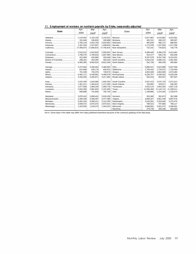
Monthly Labor Review July 2005 97
11. E mployment of workers on nonfarm payrolls by S tate, seasonally adjusted
StateApr.
2004Mar.
2005p
Apr.
2005p StateApr.
2004Mar.
2005p
Apr.
2005p
Alabama............................………… 2,144,932 2,153,150 2,143,531 Missouri……………………………… 3,027,981 3,016,881 3,023,591 Alaska............................................ 331,646 336,833 339,688 Montana......................................... 482,151 490,247 490,597 Arizona............................………… 2,765,126 2,810,730 2,834,853 Nebraska............................………… 982,835 990,127 988,902 Arkansas........................................ 1,301,333 1,327,837 1,338,943 Nevada........................................... 1,173,229 1,207,926 1,217,259 California............................………… 17,495,673 17,656,815 17,746,916 New Hampshire............................… 722,231 729,623 733,778
Colorado........................................ 2,510,512 2,543,820 2,559,003 New Jersey.................................... 4,389,445 4,396,279 4,413,481 Connecticut............................……… 1,798,276 1,789,618 1,807,993 New Mexico............................…… 910,377 935,178 942,006 Delaware........................................ 422,484 426,866 429,449 New York....................................... 9,337,079 9,331,794 9,410,201 District of Columbia........................ 298,181 303,350 303,233 North Carolina............................… 4,254,216 4,286,131 4,301,942 Florida............................................ 8,365,395 8,560,910 8,622,259 North Dakota.................................. 352,728 356,230 355,964
Georgia............................………… 4,372,563 4,456,654 4,469,954 Ohio............................……………… 5,880,021 5,923,898 5,947,936 Hawaii............................................ 614,838 626,179 630,913 Oklahoma....................................... 1,709,442 1,720,072 1,725,450 Idaho............................…………… 701,439 725,376 728,573 Oregon............................…………… 1,854,928 1,863,090 1,873,284 Illinois............................................. 6,381,171 6,448,951 6,495,078 Pennsylvania.................................. 6,256,757 6,336,022 6,329,209 Indiana............................…………… 3,166,330 3,206,971 3,217,082 Rhode Island............................…… 563,310 564,027 567,637
Iowa............................……………… 1,622,439 1,643,096 1,645,255 South Carolina............................… 2,037,413 2,070,732 2,072,512 Kansas........................................... 1,461,311 1,465,613 1,471,560 South Dakota................................. 426,992 429,917 430,352 Kentucky............................………… 1,977,938 1,983,259 1,993,718 Tennessee............................……… 2,916,124 2,902,034 2,907,118 Louisiana........................................ 2,054,296 2,081,643 2,101,000 Texas............................................. 11,005,460 11,144,714 11,208,511 Maine............................…………… 696,898 701,658 705,740 Utah............................……………… 1,199,880 1,224,262 1,233,673
Maryland............................………… 2,879,103 2,899,401 2,915,228 Vermont............................………… 353,365 352,673 352,288 Massachusetts............................... 3,395,348 3,369,587 3,377,480 Virginia........................................... 3,806,027 3,861,448 3,897,576 Michigan............................………… 5,062,165 5,099,411 5,142,355 Washington............................……… 3,228,281 3,253,606 3,270,470 Minnesota...................................... 2,948,472 2,970,372 2,970,541 West Virginia.................................. 789,513 797,866 798,117 Mississippi............................……… 1,323,535 1,343,373 1,343,322 Wisconsin............................……… 3,068,691 3,051,571 3,058,501
Wyoming........................................ 279,740 283,436 283,805
NOTE: Some data in this table may differ from data published elsewhere because of the continual updating of the data base.

Current Labor Statistics: Labor Force Data
98 Monthly Labor Review July 2005
12. Employment of workers on nonfarm payrolls by industry, monthly data seasonally adjusted [In thousands]
2004 2005
2003 2004 May June July Aug. Sept. Oct. Nov. Dec. Jan. Feb Mar. Apr.p Mayp
TOTAL NONFARM................ 129,999 131,480 131,373 131,479 131,562 131,750 131,880 132,162 132,294 132,449 132,573 132,873 132,995 133,269 133,347 TOTAL PRIVATE...................... 108,416 109,862 109,787 109,908 109,976 110,105 110,203 110,462 110,588 110,749 110,863 111,140 111,264 111,525 111,598GOODS-PRODUCING……………… 21,816 21,884 21,888 21,890 21,902 21,946 21,947 21,982 21,996 22,022 22,004 22,066 22,093 22,135 22,149
Natural resources and mining…………..……….......…… 572 591 592 591 596 595 597 595 599 602 607 602 619 622 623 Logging.................................. 69.4 67.8 68.9 67.6 67.4 67.5 68.0 67.0 66.9 67.9 68.0 67.3 68.7 64.8 64.7 Mining........................................ 502.7 523.2 523.3 523.8 528.9 527.8 528.5 527.7 532.5 534.4 538.7 545.0 549.8 557.5 558.5 Oil and gas extraction………… 120.2 123.1 123.7 123.2 123.2 123.8 124.0 123.6 124.4 124.1 123.4 122.5 124.0 124.1 124.4
Mining, except oil and gas1…… 202.7 207.1 207.1 208.1 211.8 209.1 208.5 208.4 210.7 211.3 212.9 215.5 215.7 217.9 218.8 Coal mining…………………… 70.0 71.7 71.3 72.0 73.5 73.1 72.9 72.7 73.7 73.9 75.4 76.1 76.1 76.6 76.2 Support activities for mining…… 179.8 193.1 192.5 192.5 193.9 194.9 196.0 195.7 197.4 199.0 202.4 207.0 210.1 215.5 215.3
Construction.............................. 6,735 6,964 6,949 6,955 6,965 6,985 6,998 7,043 7,060 7,086 7,090 7,133 7,159 7,207 7,227
Construction of buildings.......... 1,575.8 1,632.2 1,623.1 1,626.7 1,632.2 1,636.3 1,647.8 1,663.0 1,668.3 1,678.9 1,682.4 1,689.2 1,692.5 1,695.1 1,699.1 Heavy and civil engineering…… 903.1 902.5 903.0 899.8 899.7 901.1 902.1 904.1 906.4 907.8 908.2 911.7 915.7 920.7 926.7 Speciality trade contractors...... 4,255.7 4,429.7 4,423.3 4,428.6 4,433.1 4,447.6 4,447.8 4,476.1 4,484.8 4,499.2 4,499.6 4,531.8 4,550.9 4,591.4 4,600.8 Manufacturing............................ 14,510 14,329 14,347 14,344 14,341 14,366 14,352 14,344 14,337 14,334 14,307 14,321 14,315 14,306 14,299
Production workers.............. 10,190 10,083 10,093 10,095 10,102 10,131 10,117 10,111 10,104 10,097 10,082 10,085 10,091 10,088 10,090 Durable goods.......................... 8,963 8,923 8,925 8,931 8,926 8,965 8,957 8,960 8,954 8,957 8,942 8,962 8,957 8,956 8,959
Production workers.............. 6,152 6,137 6,138 6,147 6,144 6,180 6,172 6,172 6,166 6,170 6,166 6,178 6,182 6,189 6,192 Wood products......................... 537.6 548.4 547.9 549 550 551.7 550.1 554.5 553.3 555.2 554.7 553.6 555.2 551.6 549.7 Nonmetallic mineral products 494.2 504.8 506.3 507.4 507.9 507.6 508.8 509.1 507.9 506.5 504.5 504.0 502.0 504.0 500.8 Primary metals......................... 477.4 465.9 466.1 467.4 468.4 467.4 466.4 466.0 465.8 465.2 465.5 466.9 466.6 466.5 466.6 Fabricated metal products....... 1,506.8 1,470.3 1,496.5 1,498.3 1,502.6 1,506.8 1,508.5 1,511.5 1,510.9 1,512.8 1,514.3 1,514.1 1,517.3 1,518.4 1,523.1 Machinery………..................... 1,149.4 1,141.5 1,140.0 1,142.7 1,146.8 1,151.5 1,148.7 1,147.3 1,147.4 1,146.0 1,145.9 1,148.0 1,151.7 1,153.8 1,155.7 Computer and electronic
products1……………………… 1,355.2 1,326.2 1,327.1 1,327.4 1,332.8 1,334.0 1,332.5 1,329.8 1,327.1 1,325.8 1,327.0 1,327.5 1,326.0 1,328.0 1,328.7
Computer and peripheral equipment............................ 224.0 212.1 213.7 212.2 211.4 212.4 211.9 209.7 209.3 210.4 210.2 211.2 211.3 212.0 212.3 Communications equipment… 154.9 150.5 148.9 150.1 151.3 151.6 151.0 150.7 152.7 153.7 155.1 154.5 153.7 153.7 153.4 Semiconductors and electronic components......... 461.1 452.8 453.3 455.2 457.9 457.4 457.0 454.9 451.9 448.0 447.4 447.1 446.7 446.2 445.5 Electronic instruments………. 429.7 431.8 431.1 431.2 433.9 434.2 434.6 437.0 435.6 435.7 436.4 436.4 436.2 437.5 439.0 Electrical equipment and appliances.............................. 459.6 446.8 446.1 446.8 447.3 447.7 447.0 445.1 447.4 445.8 445.1 445.3 444.5 443.2 444.5 Transportation equipment........ 1,774.1 1,763.5 1,763.6 1,762.2 1,739.1 1,769.5 1,768.5 1,771.0 1,767.2 1,771.9 1,760.1 1,781.8 1,776.7 1,778.3 1,780.8 Furniture and related products.....…………………… 572.9 572.7 574.5 573.6 574.0 573.3 572.1 571.3 572.2 571.7 570.3 567.5 565.9 562.2 559.5 Miscellaneous manufacturing 663.3 655.5 656.4 656.4 656.8 655.2 654.5 654.1 654.7 656.4 654.3 653.5 651.3 649.5 649.7
Nondurable goods................... 5,547 5,406 5,422 5,413 5,415 5,401 5,395 5,384 5,383 5,377 5,365 5,359 5,358 5,350 5,340 Production workers.............. 4,038 3,945 3,955 3,948 3,958 3,951 3,945 3,939 3,938 3,927 3,916 3,907 3,909 3,899 3,898
Food manufacturing................. 1,517.5 1,497.4 1,501.8 1,498.6 1,504.6 1,497.0 1,494.3 1,493.5 1,493.6 1,498.8 1,494.3 1,493.2 1,495.2 1,491.0 1,491.7 Beverages and tobacco products………………………… 199.6 194.3 194.0 194.4 194.2 193.4 194.9 192.9 195.1 193.0 192.2 192.5 191.6 191.5 192.1 Textile mills……………………… 261.3 238.5 239.7 239.3 238.8 238.1 237.3 236.5 235.0 233.2 231.5 230.1 228.7 226.3 226.4 Textile product mills................. 179.3 177.7 180.2 178.5 178.2 177.6 177.8 178.1 178.4 178.0 178.1 177.9 177.9 178.2 178.8 Apparel…………………………. 312.3 284.8 289.1 285.9 283.2 282.6 281.0 276.1 273.4 271.9 269.3 267.2 262.8 262.4 257.9 Leather and allied products..... 44.5 42.9 42.8 42.6 42.5 42.5 42.7 42.8 43.4 43.1 43.1 43.2 42.9 42.9 42.5 Paper and paper products....... 516.2 499.1 498.9 496.7 499.2 500.6 499.3 499.4 498.1 497.9 499.9 500.2 502.0 499.6 498.4 Printing and related support activities………………………… 680.5 665.0 667.2 668.3 665.2 663.9 661.6 661.0 661.3 660.8 659.6 659.2 658.8 659.3 658.2 Petroleum and coal products... 114.3 112.8 112.3 112.9 112.8 113.2 113.2 113.3 113.6 113.8 114.5 115.1 115.0 116.4 117.4 Chemicals................................ 906.1 887.0 889.0 888.8 887.7 885.8 885.5 884.5 882.4 880.5 877.1 876.4 877.5 878.0 876.1
Plastics and rubber products.. 815.4 806.6 807.3 807.1 808.9 806.6 807.1 806.3 808.6 806.2 804.9 804.1 805.8 804.3 800.4
SERVICE-PROVIDING.................. 108,182 109,596 109,485 109,589 109,660 109,804 109,933 110,180 110,298 110,427 110,569 110,807 110,902 111,134 111,198
PRIVATE SERVICE- PROVIDING……………………… 86,599 87,978 87,899 88,018 88,074 88,159 88,256 88,480 88,592 88,727 88,859 89,074 89,171 89,390 89,449
Trade, transportation, and utilities............................... 25,287 25,510 25,511 25,536 25,536 25,537 25,555 25,581 25,621 25,620 25,652 25,714 25,743 25,793 25,824 Wholesale trade....................... 5,607.5 5,654.9 5,651.4 5,653.4 5,660.2 5,662.9 5,672.4 5,674.7 5,680.0 5,683.6 5,679.9 5,688.7 5,702.2 5,709.2 5,719.5 Durable goods………………… 2,940.6 2,949.1 2,942.9 2,948.4 2,955.3 2,957.8 2,960.2 2,962.3 2,960.4 2,964.5 2,965.6 2,968.7 2,975.6 2,977.9 2,983.5 Nondurable goods…………… 2,004.6 2,007.1 2010.6 2006.6 2004.0 2004.0 2008.1 2009.1 2012.6 2009.9 2,005.4 2,006.9 2,011.2 2,012.0 2,012.1 Electronic markets and agents and brokers…………… 662.2 698.8 697.9 698.4 700.9 701.1 704.1 703.3 707.0 709.2 708.9 713.1 715.4 719.3 723.9
Retail trade............................... 14,917.3 15,034.7 15,052.3 15,060.5 15,048.2 15,043.3 15,037.7 15,056.5 15,081.4 15,077.0 15,081.2 15,125.4 15,128.7 15,155.3 15,166.0 Motor vehicles and parts
dealers1……………………… 1,882.9 1,901.2 1,906.9 1,904.1 1,904.4 1,899.8 1,898.4 1,896.4 1,901.2 1,905.9 1,907.4 1,911.2 1,912.6 1,914.9 1,916.7 Automobile dealers................ 1,254.4 1,254.2 1258.5 1257.1 1254.1 1251.2 1247.3 1245.0 1247.6 1249.1 1247.9 1248.8 1250.2 1252.2 1253.1 Furniture and home furnishings stores................... 547.3 560.2 558.7 559.1 559.8 561.6 561.9 562.3 565.6 563.7 562.1 562.6 562.3 566.1 567.5 Electronics and appliance stores..................................... 512.2 514.4 514.3 514.1 513.4 512.0 513.6 520.2 520.3 516.5 516.1 515.1 518.4 518.4 521.0
See notes at end of table.
Annual averageIndustry

Monthly Labor Review July 2005 99
12. Continued–Employment of workers on nonfarm payrolls by industry, monthly data seasonally adjusted [In thousands]
Annual average 2004 2005
2003 2004 May June July Aug. Sept. Oct. Nov. Dec. Jan. Feb. Mar. Apr.p Mayp
Building material and garden supply stores.......................... 1,185.0 1,226.0 1,227.9 1,223.8 1,224.7 1,228.1 1,232.5 1,236.3 1,240.4 1,243.5 1,248.0 1,264.8 1,263.7 1,263.9 1,266.2 Food and beverage stores....... 2,383.4 2,826.3 2,835.8 2,832.6 2,828.5 2,826.2 2,827.1 2,830.2 2,822.7 2,819.8 2,826.0 2,826.6 2,826.8 2,829.4 2,828.2 Health and personal care stores…………………………… 938.1 941.7 941.2 941.3 941.0 941.0 942.1 941.6 944.5 946.6 944.8 949.7 949.2 955.4 956.3 Gasoline stations……………… 882.0 877.1 879.1 877.5 876.6 876.5 878.0 877.0 873.7 871.3 872.9 874.6 874.5 875.2 875.3 Clothing and clothing accessories stores …………… 1,304.5 1,361.8 1,357.5 1,367.6 1,369.5 1,374.4 1,371.9 1,376.0 1,377.9 1,381.3 1,375.5 1,380.5 1,384.0 1,386.0 1,389.2 Sporting goods, hobby, book, and music stores……… 646.5 639.2 639.7 639.4 638.9 639.0 638.7 638.0 639.0 635.8 637.7 636.2 638.3 641.5 642.2 General merchandise stores1… 2,822.4 2,843.5 2,848.4 2,856.4 2,848.0 2,842.5 2,832.9 2,835.2 2,854.9 2,852.9 2,853.5 2,864.1 2,862.0 2,866.5 2,866.9 Department stores…………… 1,620.6 1,612.5 1,614.2 1,618.0 1,616.1 1,611.4 1,603.3 1,604.2 1,619.1 1,619.3 1,619.1 1,625.7 1,624.2 1,626.6 1,626.4 Miscellaneous store retailers… 930.7 918.6 917.0 919.2 918.8 918.9 917.0 920.5 917.4 918.2 918.7 919.9 919.4 919.8 920.7 Nonstore retailers……………… 427.3 424.8 425.8 425.4 424.6 423.3 423.6 422.8 423.8 421.5 418.5 420.1 417.5 418.2 415.8
Transportation and warehousing........................... 4,185.4 4,250.0 4,236.3 4,250.9 4,257.0 4,260.4 4,274.1 4,279.6 4,289.6 4,288.0 4,316.0 4,324.1 4,336.6 4,354.1 4,363.7 Air transportation……………… 528.3 514.8 516.7 517.0 516.3 515.0 513.8 514.2 514.6 512.3 509.4 507.9 508.0 506.6 505.5 Rail transportation……………… 217.7 224.1 223.7 224.7 225.0 224.6 225.5 225.4 224.6 224.0 224.4 223.9 223.7 223.7 224.3 Water transportation…………… 54.5 57.2 57.3 58.2 58.1 56.7 57.2 57.7 57.8 58.6 59.8 60.0 61.6 62.4 63.3 Truck transportation…………… 1,325.6 1,350.7 1,346.3 1,352.2 1,352.5 1,352.5 1,358.5 1,356.0 1,358.9 1,366.5 1,372.6 1,378.0 1,383.2 1,390.5 1,395.3 Transit and ground passenger transportation………………… 382.2 385.5 386.3 381.6 383.2 386.2 388.3 389.3 389.4 391.0 391.7 391.0 388.7 392.9 391.1 Pipeline transportation………… 40.2 38.8 38.8 38.9 39.0 38.9 39.0 38.9 39.0 38.7 39.3 39.4 39.3 39.5 39.1 Scenic and sightseeing transportation………………… 26.6 26.7 27.0 27.4 26.3 27.7 27.8 25.6 26.1 26.6 24.2 24.9 26.7 27.2 27.9 Support activities for transportation………………… 520.3 535.6 532.6 534.3 535.5 536.9 537.7 539.9 544.6 547.0 549.3 551.5 553.4 553.4 555.3 Couriers and messengers…… 561.7 560.5 557.0 562.1 563.1 562.6 563.8 564.4 568.7 556.4 577.5 577.6 579.3 583.2 584.2 Warehousing and storage 528.3 556.0 550.6 554.5 558.0 559.3 562.5 568.2 565.9 566.9 567.8 569.9 572.7 574.7 577.7 Utilities………………………….……… 577.0 570.2 571.1 570.8 570.9 570.1 571.1 570.3 570.2 571.3 574.7 576.0 575.2 574.7 574.3
Information…………………...…. 3,188 3,138 3,146 3,151 3,144 3,135 3,127 3,131 3,133 3,127 3,123 3,127 3,134 3,149 3,141 Publishing industries, except Internet………………………… 924.8 909.8 911.1 911.9 909.6 909.3 909.2 908.1 908.9 905.7 905.0 905.6 906.8 904.3 901.8 Motion picture and sound recording industries…………… 376.2 389.0 392.3 395.5 394.4 389.3 389.7 395.3 390.6 384.8 380.3 380.9 386.9 398.2 392.2 Broadcasting, except Internet.. 324.3 326.6 326.3 326.5 327.2 327.8 328.1 329.5 329.7 329.7 331.3 330.4 330.7 330.1 329.7 Internet publishing and broadcasting…………………… 29.2 31.3 30.6 31.5 31.4 31.7 32.0 33.0 33.6 34.0 34.8 34.6 35.0 35.5 36.3 Telecommunications…………… 1,082.3 1,042.5 1,046.6 1,044.0 1,041.9 1,037.1 1,028.4 1,024.8 1,030.0 1,031.5 1,030.8 1,032.2 1,029.9 1,036.9 1,035.4 ISPs, search portals, and data processing……………… 402.4 388.1 388.2 389.9 388.6 387.6 387.6 389.2 389.5 390.4 389.9 392.6 393.7 394.1 395.4 Other information services…… 48.7 50.9 51.3 51.6 51.3 51.7 51.5 50.9 50.7 50.7 51.0 50.9 50.7 50.2 50.1
Financial activities………...….... 7,977 8,052 8,037 8,051 8,043 8,058 8,083 8,093 8,107 8,128 8,150 8,165 8,167 8,181 8,185 Finance and insurance………… 5,922.6 5,965.6 5,956.0 5,965.6 5,958.6 5,970.2 5,982.1 5,994.1 6,001.3 6,014.5 6,030.9 6,037.6 6,039.8 6,049.0 6,054.5 Monetary authorities— central bank…………………… 22.6 21.6 21.6 21.6 21.5 21.6 21.5 21.3 20.9 20.6 20.5 20.4 20.4 20.3 20.3
Credit intermediation and
related activities1…………… 2,792.4 2,832.3 2,826.3 2,833.7 2,829.2 2,833.4 2,841.0 2,847.9 2,859.2 2,871.9 2,882.7 2,891.0 2,896.8 2,901.5 2,903.7 Depository credit
intermediation1……………… 1,748.5 1,761.2 1,758.2 1,762.1 1,760.6 1,763.0 1,765.1 1,768.1 1,773.3 1,778.8 1,785.6 1,790.3 1,794.0 1,796.1 1,799.0
Commercial banking..……... 1,280.1 1,285.3 1,284.6 1,286.3 1,283.9 1,283.5 1,286.4 1,288.3 1,293.1 1,296.8 1,301.6 1,305.5 1,308.0 1,308.8 1,310.4 Securities, commodity contracts, investments……… 757.7 766.8 761.9 765.1 766.3 769.9 772.3 777.3 776.9 779.7 782.5 784.8 786.9 788.6 789.5 Insurance carriers and related activities……………… 2,266.0 2,260.3 2,261.6 2,260.9 2,257.0 2,261.0 2,263.3 2,264.1 2,260.4 2,258.1 2,259.6 2,256.7 2,250.9 2,255.1 2,256.8 Funds, trusts, and other financial vehicles……………… 83.9 84.7 84.6 84.3 84.6 84.3 84.0 83.5 83.9 84.2 85.6 84.7 84.8 83.5 84.2 Real estate and rental and leasing……………………… 2,053.9 2,086.2 2,081.1 2,085.7 2,084.6 2,088.2 2,101.3 2,099.2 2,105.5 2,113.6 2,119.0 2,127.2 2,126.8 2,131.9 2,130.2 Real estate……………………… 1,383.6 1,417.0 1,413.8 1,415.7 1,416.7 1,420.0 1,429.1 1,428.6 1,434.7 1,437.8 1,439.7 1,443.8 1,444.0 1,446.7 1,446.4 Rental and leasing services…… 643.1 643.9 642.0 645.0 643.0 643.3 647.6 646.3 646.0 650.9 654.1 658.3 657.8 659.5 657.8 Lessors of nonfinancial intangible assets……………… 27.3 25.4 25.3 25.0 24.9 24.9 24.6 24.3 24.8 24.9 25.2 25.1 25.0 25.7 26.0
Professional and business services…………………………… 15,987 16,414 16,384 16,415 16,453 16,470 16,514 16,614 16,611 16,674 16,694 16,775 16,796 16,829 16,828
Professional and technical
services1………………………… 6,629.5 6,762.0 6,730.0 6,754.0 6,765.1 6,779.7 6,805.4 6,835.3 6,834.4 6,869.9 6,882.1 6,902.7 6,907.3 6,922.1 6,925.2 Legal services………………… 1,142.1 1,161.8 1,160.0 1,163.5 1,165.0 1,163.6 1,166.8 1,167.4 1,163.1 1,164.4 1,160.8 1,161.2 1,161.5 1,161.8 1,162.9 Accounting and bookkeeping services………………...…… 815.3 816.0 810.7 810.5 813.9 814.2 816.1 821.5 816.6 840.8 858.1 858.1 856.6 859.1 853.0 Architectural and engineering services……………………… 1,226.9 1,260.8 1,254.6 1,258.7 1,262.0 1,264.4 1,270.5 1,280.5 1,284.9 1,289.5 1,286.9 1,292.0 1,295.7 1,299.2 1,302.4
See notes at end of table.
Industry

Current Labor Statistics: Labor Force Data
100 Monthly Labor Review July 2005
12. Continued–Employment of workers on nonfarm payrolls by industry, monthly data seasonally adjusted [In thousands]
Annual average 2004 2005
2003 2004 May June July Aug. Sept Oct. Nov. Dec. Jan. Feb. Mar. Apr.p Mayp
Computer systems design and related services………… 1,116.6 1,147.4 1,134.0 1,142.3 1,145.9 1,155.0 1,161.1 1,167.3 1,174.1 1,174.3 1,171.8 1,174.2 1,175.5 1,176.2 1,176.9 Management and technical consulting services………… 744.9 779.0 778.2 783.6 784.7 786.9 787.9 790.5 787.8 789.9 789.3 793.7 795.5 798.3 799.6 Management of companies and enterprises……..……….... 1,687.2 1,718.0 1,719.8 1,722.6 1,723.7 1,720.7 1,715.0 1,715.3 1,722.5 1,725.6 1,730.7 1,731.3 1,731.5 1,733.5 1,735.6 Administrative and waste services………………………… 7,669.8 7,934.0 7,934.1 7,938.3 7,964.0 7,969.7 7,993.2 8,063.1 8,054.3 8,078.0 8,081.6 8,140.9 8,156.7 8,173.2 8,167.6
Administrative and support
services1……………………… 7,347.7 7,608.7 7,609.4 7,611.2 7,637.2 7,643.1 7,667.3 7,736.4 7,728.2 7,751.4 7,755.2 7,813.6 7,831.8 7,849.9 7,845.2
Employment services1……… 3,299.5 3,470.3 3,461.2 3,449.5 3,477.5 3,480.0 3,513.5 3,572.9 3,570.5 3,584.5 3,595.9 3,633.8 3,645.7 3,660.5 3,659.2
Temporary help services…… 2,224.2 2,393.2 2,385.0 2,383.9 2,398.6 2,411.8 2,438.7 2,486.5 2,484.7 2,479.4 2,479.1 2,508.0 2,506.1 2,516.7 2,512.4 Business support services…… 749.7 754.5 757.5 760.3 758.1 757.9 752.6 755.9 754.6 757.0 752.8 755.7 754.1 755.6 753.9 Services to buildings and dwellings………………… 1,636.1 1,694.2 1,700.1 1,707.7 1,705.2 1,706.6 1,706.4 1,708.6 1,707.2 1,706.1 1,701.4 1,711.2 1,712.6 1,714.9 1,716.1 Waste management and remediation services………… 322.1 325.3 324.7 327.1 326.8 326.6 325.9 326.7 326.1 326.6 326.4 327.1 324.9 323.3 322.4
Educational and health services………………...………. 16,588 16,954 16,913 16,936 16,963 17,010 17,019 17,081 17,108 17,142 17,178 17,186 17,210 17,244 17,284 Educational services…….……… 2,695.1 2,766.4 2,754.1 2,755.1 2,765.6 2,772.3 2,773.2 2,794.0 2,797.2 2,805.5 2,825.0 2,810.3 2,814.0 2,819.3 2,827.7 Health care and social assistance……….……………… 13,892.6 14,187.3 14,158.5 14,180.7 14,197.8 14,237.8 14,246.1 14,287.2 14,310.7 14,336.1 14,353.2 14,375.4 14,396.0 14,424.2 14,456.7
Ambulatory health care
services1……………………… 4,786.4 4,946.4 4,929.9 4,941.9 4,956.2 4,969.2 4,975.0 4,996.9 5,006.7 5,017.0 5,027.0 5,035.0 5,041.6 5,056.1 5,072.1 Offices of physicians………… 2,002.5 2,053.9 2,046.4 2,051.1 2,054.5 2,059.1 2,064.5 2,074.2 2,077.7 2,084.3 2,085.3 2,090.9 2,093.2 2,103.4 2,113.9 Outpatient care centers……… 426.8 446.2 445.8 446.6 448.4 449.7 448.7 449.5 449.8 450.3 451.5 451.1 452.6 454.1 456.5 Home health care services…… 732.6 773.2 768.5 771.7 775.4 778.0 779.5 782.7 789.2 790.7 796.6 796.8 798.8 797.5 798.6 Hospitals………………………… 4,244.6 4,293.6 4,290.0 4,292.2 4,296.2 4,305.0 4,306.0 4,311.2 4,319.7 4,323.5 4,329.6 4,337.8 4,344.6 4,352.6 4,358.4 Nursing and residential
care facilities1 2,786.2 2,814.8 2,811.9 2,814.4 2,818.0 2,819.8 2,825.0 2,827.2 2,827.2 2,827.9 2,827.0 2,830.0 2,830.0 2,830.4 2,834.2
Nursing care facilities………… 1,579.8 1,575.3 1,575.8 1,576.3 1,576.9 1,576.7 1,576.6 1,576.8 1,576.4 1,574.5 1,571.5 1,571.6 1,572.3 1,570.4 1,571.2
Social assistance1……………… 2,075.4 2,132.5 2,126.7 2,132.2 2,127.4 2,143.8 2,140.1 2,151.9 2,157.1 2,167.7 2,169.6 2,172.6 2,179.8 2,185.1 2,192.0 Child day care services……… 755.3 767.1 762 767.4 770.4 776.1 767.9 772.8 775.3 780.4 780.5 782.5 785.1 786.7 787.8 Leisure and hospitality……….. 12,173 12,479 12,474 12,486 12,497 12,508 12,522 12,546 12,571 12,589 12,611 12,650 12,662 12,725 12,719 Arts, entertainment, and recreation……….…….…… 1,812.9 1,833.0 1,836.6 1,834.8 1,830.9 1,831.0 1,836.2 1,834.4 1,826.4 1,811.0 1,805.4 1,808.4 1,805.8 1,821.5 1,816.4 Performing arts and spectator sports……………… 371.7 364.8 362.8 363.6 359.2 358.4 363.6 364.4 362.5 357.9 355.6 357.0 357.8 362.5 361.7 Museums, historical sites, zoos, and parks……………… 114.7 117.1 117.8 117.8 118.6 118.8 118.3 118.2 116.9 114.8 114.5 113.6 115.8 116.9 118.0 Amusements, gambling, and recreation……………………… 1,326.5 1,351.1 1,356.0 1,353.4 1,353.1 1,353.8 1,354.3 1,351.8 1,347.0 1,338.3 1,335.3 1,337.8 1,332.2 1,342.1 1,336.7 Accommodations and food services…………………… 10,359.8 10,646.0 10,637.1 10,650.7 10,666.1 10,676.5 10,685.3 10,712.0 10,744.1 10,778.4 10,805.1 10,841.1 10,856.0 10,903.8 10,902.7 Accommodations……………… 1,775.4 1,795.9 1,792.2 1,798.0 1,797.3 1,801.3 1,801.5 1,800.6 1,814.7 1,824.6 1,825.9 1,830.3 1,826.6 1,831.1 1,828.8 Food services and drinking places…………………………… 8,584.4 8,850.1 8,844.9 8,852.7 8,868.8 8,875.2 8,883.8 8,911.4 8,929.4 8,953.8 8,979.2 9,010.8 9,029.4 9,072.7 9,073.9 Other services…………………… 5,401 5,431 5,434 5,443 5,438 5,441 5,436 5,434 5,441 5,447 5,451 5,457 5,459 5,469 5,468 Repair and maintenance……… 1,233.6 1,227.6 1,229.6 1,226.5 1,227.4 1,225.9 1,226.9 1,227.9 1,227.1 1,229.9 1,229.4 1,233.7 1,235.6 1,239.0 1,241.3 Personal and laundry services 1,263.5 1,274.1 1,281.6 1,283.4 1,278.0 1,276.9 1,271.5 1,267.8 1,271.6 1,276.8 1,280.4 1,280.5 1,282.2 1,287.2 1,286.4 Membership associations and organizations………………… 2,903.6 2,929.1 2,922.3 2,932.7 2,932.8 2,937.9 2,937.9 2,938.1 2,942.3 2,940.6 2,941.4 2,942.9 2,940.8 2,943.0 2,940.3
Government................................. 21,583 21,618 21,586 21,571 21,586 21,645 21,677 21,700 21,706 21,700 21,710 21,733 21,731 21,744 21,749 Federal....................................... 2,761 2,728 2,729 2,731 2,726 2,730 2,730 2,723 2,728 2,706 2,717 2,720 2,724 2,718 2,719 Federal, except U.S. Postal Service................................... 1,952.4 1,943.4 1,943.2 1,946.3 1,939.2 1,945.5 1,946.8 1,940.1 1,946.4 1,939.5 1,937.2 1,939.8 1,943.2 1,937.7 1,938.3 U.S. Postal Service……………… 808.6 784.1 785.8 785.1 786.4 784.3 783.4 782.5 781.4 766.4 780.2 780.1 780.8 780.5 781.1 State.......................................... 5,002 4,985 4,967 4,963 4,976 4,987 5,000 5,007 5,015 5,020 5,025 5,027 5,024 5,027 5,026 Education............................... 2,254.7 2,249.2 2,233.3 2,228.2 2,241.4 2,249.4 2,263.7 2,268.4 2,271.3 2,277.9 2,280.4 2,283.0 2,280.8 2,281.5 2,281.2 Other State government......... 2,747.6 2,736.2 2,733.2 2,734.4 2,734.4 2,737.8 2,736.4 2,738.2 2,743.4 2,741.9 2,744.4 2,744.4 2,743.2 2,745.7 2,744.7 Local......................................... 13,820 13,905 13,890 13,877 13,884 13,928 13,947 13,970 13,963 13,974 13,968 13,986 13,983 13,999 14,004 Education............................... 7,709.4 7,762.5 7,752.9 7,742.5 7,757.8 7,785.7 7,793.2 7,810.8 7,806.3 7,810.8 7,808.8 7,820.7 7,813.5 7,822.5 7,821.0 Other local government.......... 6,110.2 6,143.0 6,137.3 6,134.5 6,126.6 6,142.2 6,153.4 6,159.3 6,156.7 6,163.1 6,159.2 6,165.1 6,169.0 6,176.5 6,182.8
Industry
1 Includes other industries not shown separately.
NOTE: See "Notes on the data" for a description of the most recent benchmark revision.
p = preliminary.

Monthly Labor Review July 2005 101
13. Average weekly hours of production or nonsupervisory workers1 on private nonfarm payrolls, by industry, monthly data seasonally adjusted
Annual average 2004 2005
2003 2004 May June July Aug. Sept. Oct. Nov. Dec. Jan. Feb. Mar. Apr.p Mayp
TOTAL PRIVATE………………………… 33.7 33.7 33.8 33.6 33.7 33.7 33.8 33.8 33.7 33.7 33.7 33.7 33.7 33.8 33.8
GOODS-PRODUCING……………………… 39.8 40.0 40.2 39.9 40.1 40.0 40.1 39.9 39.9 40.0 39.8 39.9 39.8 40.1 39.9
Natural resources and mining…………… 43.6 44.5 44.2 43.9 44.2 44.4 44.5 44.8 45.0 45.4 45.5 45.1 45.3 45.7 45.9
Construction………………………………… 38.4 38.3 38.3 38.0 38.3 38.1 38.1 38.2 38.3 38.4 37.6 38.2 38.3 39.0 38.5
Manufacturing……………………............. 40.4 40.8 41.0 40.7 40.8 40.9 40.8 40.7 40.5 40.5 40.7 40.6 40.4 40.5 40.4 Overtime hours................................. 4.2 4.6 4.6 4.5 4.6 4.6 4.6 4.5 4.5 4.5 4.5 4.6 4.5 4.4 4.4
Durable goods..…………………............ 40.8 41.3 41.5 41.2 41.3 41.3 41.2 41.2 40.9 41.1 41.1 41.0 40.8 40.9 40.8 Overtime hours................................. 4.3 4.7 4.8 4.6 4.7 4.7 4.7 4.7 4.6 4.6 4.6 4.7 4.5 4.5 4.4 Wood products.................................... 40.4 40.6 41.3 40.6 40.7 40.8 40.4 40.3 40.0 40.3 40.6 39.9 39.5 39.5 39.6 Nonmetallic mineral products.............. 42.2 42.3 42.1 41.8 42.2 42.3 42.4 42.4 42.1 42.3 41.9 42.1 41.7 41.8 41.9 Primary metals.................................... 42.3 43.1 43.4 43.4 43.2 43.2 43.1 43.0 42.9 42.8 43.1 43.0 42.9 42.6 42.5 Fabricated metal products.................. 40.7 41.1 41.2 41.0 41.2 41.2 41.2 41.1 40.9 40.9 40.9 40.8 40.7 40.8 40.7 Machinery………………………………… 40.8 41.9 42.2 42.0 42.1 42.1 42.3 42.2 42.0 42.0 42.0 42.0 42.0 42.2 42.0 Computer and electronic products…… 40.4 40.4 40.7 40.4 40.7 40.4 40.3 40.1 39.6 39.8 40.0 39.6 39.5 39.8 39.9 Electrical equipment and appliances… 40.6 40.7 41.5 40.8 40.8 40.9 40.6 40.6 40.1 40.0 40.1 40.0 40.0 40.1 39.8 Transportation equipment................... 41.9 42.5 42.7 42.2 42.4 42.5 42.4 42.3 42.2 42.4 42.4 42.4 42.0 41.9 41.7 Furniture and related products………. 38.9 39.5 40.0 39.6 39.3 39.3 39.3 39.2 39.2 39.5 39.5 39.4 39.4 39.2 39.1 Miscellaneous manufacturing.............. 38.4 38.5 38.8 38.4 38.6 38.5 38.4 38.4 38.2 38.3 38.5 38.6 38.7 38.8 38.5
Nondurable goods................................. 39.8 40.0 40.3 40.1 40.1 40.2 40.1 39.9 39.8 39.8 40.0 40.0 39.7 39.8 39.7 Overtime hours................................. 4.1 4.4 4.4 4.4 4.4 4.5 4.4 4.3 4.3 4.3 4.4 4.5 4.4 4.3 4.3 Food manufacturing............................ 39.3 39.3 39.6 39.4 39.3 39.3 39.3 39.0 39.1 38.8 39.0 39.3 38.8 38.9 38.9 Beverage and tobacco products......... 39.1 39.2 39.2 38.6 38.9 39.4 39.2 38.6 39.0 39.6 40.5 40.2 40.1 40.1 38.9 Textile mills……………………………… 39.1 40.1 40.2 40.3 40.5 40.5 40.2 40.1 40.0 39.8 40.2 39.7 40.0 40.1 40.5 Textile product mills…………………… 39.6 38.9 38.7 38.9 38.6 38.8 39.1 39.1 39.1 39.0 39.5 39.5 39.4 39.0 39.0 Apparel................................................ 35.6 36.0 36.2 35.9 36.0 36.2 36.2 36.0 35.7 35.9 35.9 35.9 35.9 35.7 35.1 Leather and allied products................. 39.3 38.4 38.4 38.3 37.8 38.1 38.2 38.4 38.2 37.6 37.1 37.2 37.3 37.7 38.5 Paper and paper products……………… 41.5 42.1 42.6 41.9 42.4 42.5 42.2 42.1 42.1 42.0 42.5 42.1 41.9 42.2 42.3 Printing and related support activities............................................ 38.2 38.4 38.6 38.5 38.6 38.5 38.3 38.3 38.3 38.5 38.6 38.5 38.3 38.3 38.2 Petroleum and coal products………… 44.5 44.9 45.0 44.9 45.0 45.9 46.0 45.0 45.5 44.6 44.5 44.7 45.1 46.0 45.9 Chemicals……………………………… 42.4 42.8 42.9 42.6 42.8 42.9 42.8 42.7 42.4 42.6 42.8 42.3 42.2 42.4 42.2 Plastics and rubber products………… 40.4 40.4 40.9 40.8 40.5 40.5 40.3 40.1 39.4 39.8 40.0 40.1 39.8 39.7 39.8
PRIVATE SERVICE- PROVIDING……………………………. 32.4 32.3 32.4 32.2 32.4 32.4 32.5 32.4 32.3 32.4 32.4 32.4 32.4 32.5 32.4
Trade, transportation, and utilities.......………………...................... 33.6 33.5 33.6 33.2 33.4 33.5 33.6 33.6 33.5 33.6 33.6 33.6 33.5 33.5 33.5 Wholesale trade........………………....... 37.9 37.8 37.8 37.6 37.8 37.7 37.8 37.7 37.7 37.6 37.7 37.8 37.7 37.8 37.7 Retail trade………………………………… 30.9 30.7 30.8 30.4 30.6 30.7 30.8 30.8 30.6 30.8 30.7 30.8 30.7 30.7 30.7 Transportation and warehousing……… 36.8 37.2 37.3 36.9 37.2 37.2 37.5 37.5 37.5 37.4 37.5 37.3 37.2 37.3 37.1 Utilities…………………………………… 41.1 40.9 41.3 41.1 40.9 40.9 41.4 40.8 40.4 40.7 41.0 40.5 40.3 41.0 41.0 Information………………………………… 36.2 36.3 36.3 36.5 36.3 36.4 36.3 36.3 36.2 36.4 36.3 36.4 36.5 36.5 36.6 Financial activities………………………… 35.5 35.5 35.8 35.5 35.6 35.5 35.5 35.7 35.6 35.7 35.9 35.8 35.9 36.0 36.0 Professional and business services…………………………………… 34.1 34.2 34.2 34.0 34.2 34.3 34.7 34.3 34.2 34.2 34.1 34.0 34.0 34.2 34.1 Education and health services………… 32.3 32.4 32.4 32.4 32.6 32.5 32.5 32.5 32.4 32.5 32.6 32.6 32.6 32.6 32.6 Leisure and hospitality…………………… 25.6 25.7 25.7 25.7 25.6 25.6 25.6 25.7 25.6 25.7 25.6 25.7 25.7 25.8 25.8 Other services……………....................... 31.4 31.0 31.1 30.9 31.0 31.0 31.0 30.9 30.9 30.8 30.9 30.9 30.9 31.1 31.0
Industry
1 Data relate to production workers in natural resources and mining and
manufacturing, construction workers in construction, and nonsupervisory workers in
the service-providing industries.
NOTE: See "Notes on the data" for a description of the most recent benchmark
revision.
p = preliminary.

Current Labor Statistics: Labor Force Data
102 Monthly Labor Review July 2005
14. Average hourly earnings of production or nonsupervisory workers1 on private nonfarm payrolls, by industry, monthly data seasonally adjusted
Annual average 2005
2003 2004 May June July Aug. Sept. Oct. Nov. Dec. Jan. Feb. Mar. Apr.p Mayp
TOTAL PRIVATE Current dollars……………………… $15.35 $15.67 $15.62 $15.64 $15.70 $15.74 $15.77 $15.81 $15.82 $15.85 $15.90 $15.91 $15.95 $16.00 $16.03 Constant (1982) dollars…………… 8.27 8.23 8.21 8.20 8.23 8.25 8.25 8.22 8.21 8.23 8.24 8.22 8.19 8.16 8.19
GOODS-PRODUCING.............................. 16.80 17.19 17.13 17.16 17.19 17.24 17.30 17.32 17.33 17.36 17.35 17.43 17.45 17.51 17.53
Natural resources and mining.............. 17.56 18.08 18.02 18.16 18.08 18.05 18.06 18.10 18.22 18.37 18.43 18.40 18.27 18.55 18.60 Construction.......................................... 18.95 19.23 19.19 19.19 19.21 19.25 19.27 19.34 19.31 19.29 19.24 19.31 19.34 19.38 19.37 Manufacturing....................................... 15.74 16.14 16.08 16.12 16.16 16.22 16.29 16.27 16.29 16.34 16.37 16.42 16.43 16.46 16.52 Excluding overtime.......................... 14.96 15.29 15.23 15.28 15.30 15.36 15.42 15.42 15.43 15.48 15.51 15.54 15.56 15.61 15.67 Durable goods…………………………… 16.45 16.82 16.75 16.77 16.83 16.90 16.98 16.97 16.99 17.06 17.10 17.18 17.17 17.22 17.26 Nondurable goods……………………… 14.63 15.05 15.02 15.07 15.09 15.14 15.18 15.15 15.16 15.16 15.18 15.19 15.23 15.23 15.31
PRIVATE SERVICE- PROVIDING..........………………............. 14.96 15.26 15.21 15.24 15.30 15.34 15.36 15.40 15.42 15.45 15.51 15.51 15.56 15.60 15.63
Trade,transportation, and utilities…………………………………. 14.34 14.59 14.54 14.59 14.63 14.65 14.66 14.69 14.70 14.72 14.82 14.79 14.83 14.88 14.89 Wholesale trade.................................. 17.36 17.66 17.60 17.66 17.71 17.69 17.73 17.78 17.80 17.87 17.91 17.95 17.97 18.04 18.02 Retail trade.......................................... 11.90 12.08 12.04 12.07 12.10 12.13 12.16 12.16 12.20 12.21 12.32 12.29 12.31 12.36 12.38 Transportation and warehousing……… 16.25 16.53 16.51 16.54 16.58 16.65 16.53 16.61 16.54 16.54 16.58 16.52 16.62 16.62 16.65 Utilities…………………………………… 24.77 25.62 25.51 25.48 25.60 25.66 25.82 26.00 25.77 26.11 26.23 26.04 26.32 26.41 26.41 Information............................................ 21.01 21.42 21.43 21.28 21.42 21.52 21.62 21.59 21.58 21.70 21.80 21.67 21.79 21.98 22.00 Financial activities................................ 17.14 17.53 17.47 17.49 17.55 17.57 17.64 17.71 17.65 17.71 17.71 17.74 17.78 17.86 17.79 Professional and business services................................................ 17.21 17.46 17.40 17.43 17.48 17.59 17.54 17.63 17.66 17.69 17.79 17.80 17.82 17.89 17.95 Education and health services................................................ 15.64 16.16 16.09 16.15 16.24 16.24 16.28 16.31 16.34 16.37 16.40 16.45 16.53 16.54 16.60 Leisure and hospitality......................... 8.76 8.91 8.87 8.86 8.89 8.91 8.95 8.99 9.02 9.01 9.03 9.05 9.05 9.08 9.09 Other services....................................... 13.84 13.98 13.95 13.97 13.98 14.00 14.05 14.08 14.12 14.13 14.15 14.17 14.18 14.15 14.21
2004Industry
1 Data relate to production workers in natural resources and mining and manufac-
turing, construction workers in construction, and nonsupervisory workers in the
service-providing industries.
NOTE: See "Notes on the data" for a description of the most recent benchmark revision.
p = preliminary.

Monthly Labor Review July 2005 103
15. Average hourly earnings of production or nonsupervisory workers1 on private nonfarm payrolls, by industry
Annual average 2004 2005
2003 2004 May June July Aug. Sept. Oct. Nov. Dec. Jan. Feb. Mar. Apr.p Mayp
TOTAL PRIVATE………………………… $15.35 $15.67 $15.63 $15.56 $15.59 $15.66 $15.79 $15.82 $15.84 $15.88 $16.00 $15.96 $15.95 $16.01 $16.03 Seasonally adjusted………………… 15.47 – 15.62 15.64 15.70 15.74 15.77 15.81 15.82 15.85 15.90 15.91 15.95 16.00 16.03
GOODS-PRODUCING.............................. 16.80 17.19 17.10 17.14 17.18 17.28 17.40 17.39 17.37 17.43 17.31 17.34 17.37 17.48 17.50
Natural resources and mining………… 17.56 18.08 18.00 18.12 18.02 17.95 17.97 18.07 18.21 18.46 18.53 18.45 18.36 18.67 18.61
Construction.…………........................... 18.95 19.23 19.15 19.12 19.24 19.33 19.42 19.47 19.35 19.31 19.12 19.20 19.25 19.35 19.32
Manufacturing…………………………… 15.74 16.14 16.04 16.08 16.03 16.16 16.35 16.26 16.32 16.46 16.42 16.43 16.41 16.45 16.48
Durable goods..………………….......... 16.45 16.82 16.70 16.73 16.60 16.84 17.06 16.98 17.04 17.22 17.15 17.20 17.16 17.20 17.21 Wood products ................................. 12.71 13.03 13.04 12.99 13.04 1302.00 13.14 13.03 13.13 13.17 13.13 13.04 13.11 13.12 13.16 Nonmetallic mineral products ……… 15.76 16.25 16.16 16.22 16.37 16.28 16.51 16.38 16.45 16.36 16.27 16.20 16.28 16.69 16.59 Primary metals ................................. 18.13 18.57 18.47 18.50 18.65 18.57 18.89 18.73 18.66 18.75 18.84 18.78 18.76 18.79 18.85 Fabricated metal products …............ 15.01 15.31 15.20 15.23 15.27 15.27 15.43 15.38 15.43 15.59 15.55 15.67 15.62 15.64 15.66 Machinery …………..………………… 16.30 16.68 16.54 16.56 16.68 16.72 16.85 16.84 16.85 16.99 17.03 17.02 17.02 16.99 16.89 Computer and electronic products ... 16.69 17.28 17.13 17.22 17.30 17.38 17.48 17.52 17.65 17.92 18.04 18.04 18.00 18.21 18.29 Electrical equipment and appliances 14.36 14.90 14.86 14.92 14.92 15.04 15.08 15.05 15.10 15.12 15.07 15.15 15.10 15.07 15.02 Transportation equipment ................ 21.23 21.49 21.25 21.31 20.73 21.49 21.91 21.78 21.91 22.17 21.90 21.97 21.84 21.79 21.84 Furniture and related products ......... 12.98 13.16 13.05 13.11 13.12 13.28 13.39 13.27 13.29 13.46 13.42 13.34 13.37 13.46 13.45 Miscellaneous manufacturing ........... 13.30 13.85 13.76 13.82 13.90 13.88 13.97 13.92 13.96 14.05 14.07 14.04 14.05 14.03 14.02
Nondurable goods……………………… 14.63 15.05 14.97 15.03 15.13 15.08 15.23 15.11 15.16 15.21 15.24 15.17 15.19 15.21 15.27 Food manufacturing ......................... 12.80 12.98 12.96 13.01 13.07 13.00 13.09 12.94 12.99 13.03 13.07 13.07 13.02 12.99 13.07 Beverages and tobacco products ..... 17.96 19.12 19.51 19.37 19.26 19.08 19.17 19.18 18.80 18.82 18.44 18.65 18.94 19.20 19.00
Textile mills ...................................... 11.99 12.13 12.07 12.14 12.06 12.08 12.25 12.11 12.09 12.25 12.33 12.25 12.26 12.30 12.35 Textile product mills ......................... 11.23 11.39 11.27 11.27 11.45 11.43 11.49 11.42 11.44 11.43 11.31 11.48 11.56 11.68 11.52 Apparel ............................................. 9.56 9.75 9.54 9.60 9.73 9.72 9.93 9.97 10.00 10.00 10.15 10.19 10.05 10.07 10.09 Leather and allied products ………… 11.66 11.63 11.48 11.58 11.67 11.67 11.56 11.58 11.62 11.51 11.60 11.42 11.48 11.39 11.30 Paper and paper products …………… 17.33 17.90 17.93 17.91 17.96 17.89 18.21 17.93 18.09 18.07 18.00 17.86 17.93 17.90 17.92 Printing and related support activities 15.37 15.72 15.52 15.56 15.73 15.88 15.96 15.95 15.93 15.80 15.77 15.79 15.70 15.62 15.63 Petroleum and coal products ………… 23.63 24.38 24.39 24.22 24.32 24.05 24.44 24.33 24.71 24.48 24.75 24.74 24.78 24.06 24.59 Chemicals ……………………………… 18.50 19.16 19.00 19.16 19.31 19.24 19.44 19.42 19.44 19.59 19.52 19.32 19.47 19.62 19.75 Plastics and rubber products ............ 14.18 14.58 14.54 14.59 14.69 14.66 14.75 14.55 14.58 14.76 14.81 14.65 14.70 14.73 14.84
PRIVATE SERVICE- PROVIDING ……………………………… 14.96 15.26 15.23 15.13 15.16 15.22 15.35 15.40 15.43 15.46 15.66 15.60 15.59 15.62 15.64
Trade, transportation, and utilities…….…….................................. 14.34 14.59 14.58 14.55 14.56 14.58 14.69 14.69 14.67 14.61 14.88 14.86 14.86 14.94 14.92 Wholesale trade ………………………… 17.36 17.66 17.66 17.57 17.65 17.68 17.71 17.75 17.82 17.87 18.03 17.99 17.91 18.05 18.06 Retail trade ……………………………… 11.90 12.08 12.06 12.07 12.05 12.07 12.21 12.17 12.16 12.10 12.34 12.35 12.35 12.42 12.40 Transportation and warehousing …… 16.25 16.53 16.45 16.53 16.58 16.62 16.51 16.59 16.56 16.59 16.59 16.57 16.60 16.61 16.58 Utilities ………..…..….………..………… 24.77 25.62 25.55 25.34 25.45 25.36 25.89 26.02 26.01 26.00 26.14 25.98 26.34 26.51 26.46
21.01 21.42 21.40 21.16 21.29 21.43 21.73 21.69 21.70 21.74 21.83 21.67 21.68 21.92 21.99
Financial activities……..………............ 17.14 17.53 17.64 17.40 17.46 17.59 17.62 17.68 17.61 17.67 17.83 17.73 17.76 17.87 17.94
Professional and business
services…………………………………… 17.21 17.46 17.48 17.31 17.35 17.50 17.47 17.54 17.62 17.73 18.06 17.91 17.83 17.85 18.04
Education and health
services………………………………… 15.64 16.16 16.05 16.10 16.23 16.20 16.30 16.30 16.33 16.44 16.47 16.46 16.51 16.53 16.55
Leisure and hospitality ………………… 8.76 8.91 8.86 8.79 8.79 8.81 8.94 9.02 9.06 9.11 9.11 9.09 9.07 9.08 9.08
Other services………………….............. 13.84 13.98 14.00 13.92 13.88 13.93 14.06 14.06 14.12 14.17 14.23 14.23 14.18 14.17 14.25
Industry
1 Data relate to production workers in natural resources and mining and
manufacturing, construction workers in construction, and nonsupervisory workers in
the service-providing industries.
NOTE: See "Notes on the data" for a description of the most recent benchmark
revision.
p = preliminary.

Current Labor Statistics: Labor Force Data
104 Monthly Labor Review July 2005
16. Average weekly earnings of production or nonsupervisory workers1 on private nonfarm payrolls, by industry Annual average 2004 2005
2003 2004 May June July Aug. Sept. Oct. Nov. Dec. Jan. Feb. Mar. Apr.p Mayp
TOTAL PRIVATE………………… $517.30 $528.56 $531.42 $524.37 $528.50 $535.57 $530.54 $534.72 $532.22 $536.74 $537.60 $534.66 $534.33 $537.94 $543.42 Seasonally adjusted.......... – – 527.96 525.50 529.09 530.44 533.03 534.38 533.13 534.15 535.83 536.17 537.52 540.80 541.81
GOODS-PRODUCING……………… 669.13 688.03 689.13 689.03 687.20 696.38 690.78 697.34 694.80 702.43 683.75 683.20 689.59 697.45 700.00
Natural resources and mining……………………….. 765.94 804.03 797.40 806.34 801.89 804.16 796.07 820.38 824.91 836.24 833.85 822.87 826.20 845.75 857.92
Construction……………………… 726.83 735.70 741.11 736.12 752.28 755.80 730.19 753.49 739.17 737.64 703.62 712.32 727.65 750.78 751.55
Manufacturing……………………… 635.99 658.53 659.24 659.28 646.01 660.94 663.81 661.78 665.86 678.15 666.65 663.77 662.96 661.29 665.79
Durable goods…………………… 671.21 694.16 694.72 694.30 673.96 695.49 697.75 699.58 702.05 718.07 703.15 703.48 701.84 700.04 702.17
Wood products ......................... 514.10 529.46 545.07 535.19 532.03 539.03 521.66 526.41 526.51 532.07 527.83 511.17 512.60 514.30 526.40 Nonmetallic mineral products.... 664.92 688.05 683.57 689.35 694.09 700.04 709.93 701.06 694.19 688.76 665.44 667.44 669.11 695.97 698.44 Primary metals…………………… 767.60 799.77 803.45 808.45 788.90 796.65 808.49 801.64 802.38 813.75 815.77 807.54 806.68 798.58 801.13 Fabricated metal products......... 610.37 628.80 627.76 627.48 621.49 627.60 628.00 633.66 634.17 648.54 637.55 637.77 634.17 634.98 638.93 Machinery………………………… 664.79 699.51 699.64 698.83 692.22 697.22 699.28 707.28 711.07 727.17 718.67 716.54 718.24 713.58 709.38 Computer and electronic products.................................. 674.72 698.28 695.48 699.13 695.46 700.41 700.95 704.30 706.00 723.97 716.19 712.58 711.00 717.47 727.94 Electrical equipment and appliances............................... 583.23 606.64 615.20 613.21 602.77 613.63 603.20 614.04 613.06 616.90 605.81 601.46 602.49 599.79 596.29 Transportation equipment……… 889.48 912.97 911.63 907.81 839.57 909.03 926.79 923.47 926.79 962.18 926.37 933.73 921.65 910.82 915.10 Furniture and related products………………………… 505.30 519.78 518.09 521.78 515.62 529.87 519.53 516.20 523.63 546.48 528.75 522.93 526.78 526.29 520.52 Miscellaneous manufacturing.......................... 510.82 533.47 535.26 530.69 528.20 534.38 530.86 534.53 536.06 545.14 543.10 543.35 547.95 544.36 539.77
Nondurable goods....................... 582.61 602.48 601.79 604.21 602.17 606.22 610.72 602.89 607.92 612.96 608.08 600.73 601.52 600.80 606.22
Food manufacturing.................. 502.92 509.66 511.92 512.59 513.65 514.80 520.98 508.54 515.70 513.38 505.81 505.81 497.36 497.52 507.12 Beverages and tobacco products.................................. 702.45 750.51 772.60 759.30 758.84 761.29 762.97 734.59 731.32 737.74 735.76 738.54 757.60 781.44 742.90 Textile mills……………………… 469.33 486.69 486.42 490.46 481.19 489.24 488.78 481.98 483.60 491.23 498.13 485.10 494.08 492.00 502.65 Textile product mills………………444.70 443.01 433.90 444.04 433.96 442.34 444.66 447.66 448.45 451.49 445.61 450.02 457.78 452.02 445.82 Apparel…………………………… 340.12 351.28 346.30 348.48 348.33 352.84 352.52 357.92 360.00 364.00 361.34 363.78 363.81 361.51 355.17 Leather and allied products....... 457.83 446.73 440.83 442.36 422.45 441.13 430.03 445.83 445.05 437.38 429.20 425.97 431.65 433.96 437.31
Paper and paper products……. 719.73 753.89 758.44 750.43 752.52 756.75 772.10 756.65 768.83 775.20 768.60 744.76 745.89 751.80 756.22
Printing and related support activities……………… 587.58 604.32 594.42 594.39 600.89 611.38 612.86 614.08 618.08 616.20 607.15 604.76 604.45 593.56 592.38
Petroleum and coal products………………………… 1,052.32 1,094.83 1,090.23 1,094.74 1,118.72 1,096.68 1,119.35 1,097.28 1,131.72 1,099.15 1,096.43 1,100.93 1,105.19 1,085.11 1,126.22
Chemicals………………………… 783.95 819.59 813.20 818.13 814.88 821.55 830.09 825.35 830.09 844.33 835.46 817.24 821.63 827.96 829.50
Plastics and rubber products………………………… 872.26 589.70 594.69 599.65 583.19 590.80 591.48 583.46 578.83 596.30 592.40 586.00 585.06 584.78 592.12
PRIVATE SERVICE- PROVIDING………….................... 483.89 493.67 496.50 488.70 492.70 499.22 495.81 498.96 496.85 500.90 507.38 502.32 500.44 504.53 509.86
Trade, transportation, and utilities……………………… 481.14 488.58 491.35 487.43 492.13 495.72 493.58 492.12 488.51 490.90 494.02 493.35 493.35 497.50 501.31 Wholesale trade......…………...... 657.29 666.93 674.61 660.63 665.41 673.61 665.90 669.18 671.81 670.13 681.53 674.25 671.63 680.49 686.28 Retail trade………………………… 367.15 371.15 371.45 371.76 375.96 377.79 377.29 373.62 368.45 375.10 372.67 374.21 374.21 377.57 380.68 Transportation and warehousing……………………… 598.41 614.90 616.88 611.61 616.78 628.24 617.47 622.13 622.66 625.44 620.47 608.12 610.88 312.91 616.78 Utilities………………………………1,017.27 1,048.82 1,055.22 1,044.01 1,033.27 1,032.15 1,074.44 1,066.82 1,061.21 1,053.00 1,066.51 1,052.19 1,056.23 1,086.91 1,087.51
Information………………………… 760.81 777.42 776.82 774.46 772.83 788.62 786.63 787.35 787.71 791.34 798.98 786.62 782.65 791.31 804.83
Financial activities………………… 609.08 622.99 636.80 614.22 618.08 635.00 620.22 627.64 625.16 627.29 649.01 632.96 632.26 637.96 654.81
Professional and business services……………… 587.02 596.96 604.81 590.27 591.64 607.25 593.98 599.87 602.60 604.59 614.04 607.15 604.44 608.69 622.38
Education and health services…………………… 505.69 523.83 521.63 520.03 529.10 531.36 528.12 528.12 529.09 534.30 541.86 534.95 534.92 535.57 541.19
Leisure and hospitality……………224.30 228.63 229.47 227.66 231.18 234.35 226.18 230.91 229.22 231.39 230.48 231.80 230.38 231.54 236.99
Other services……………………… 434.41 433.04 436.80 430.13 431.67 436.01 433.05 434.45 434.90 436.44 439.71 438.28 435.33 437.85 443.18
Industry
1 Data relate to production workers in natural resources and mining and manufacturing,
construction workers in construction, and nonsupervisory workers in the service-
providing industries.
NOTE: See "Notes on the data" for a description of the most recent benchmark revision.
Dash indicates data not available.
p = preliminary.
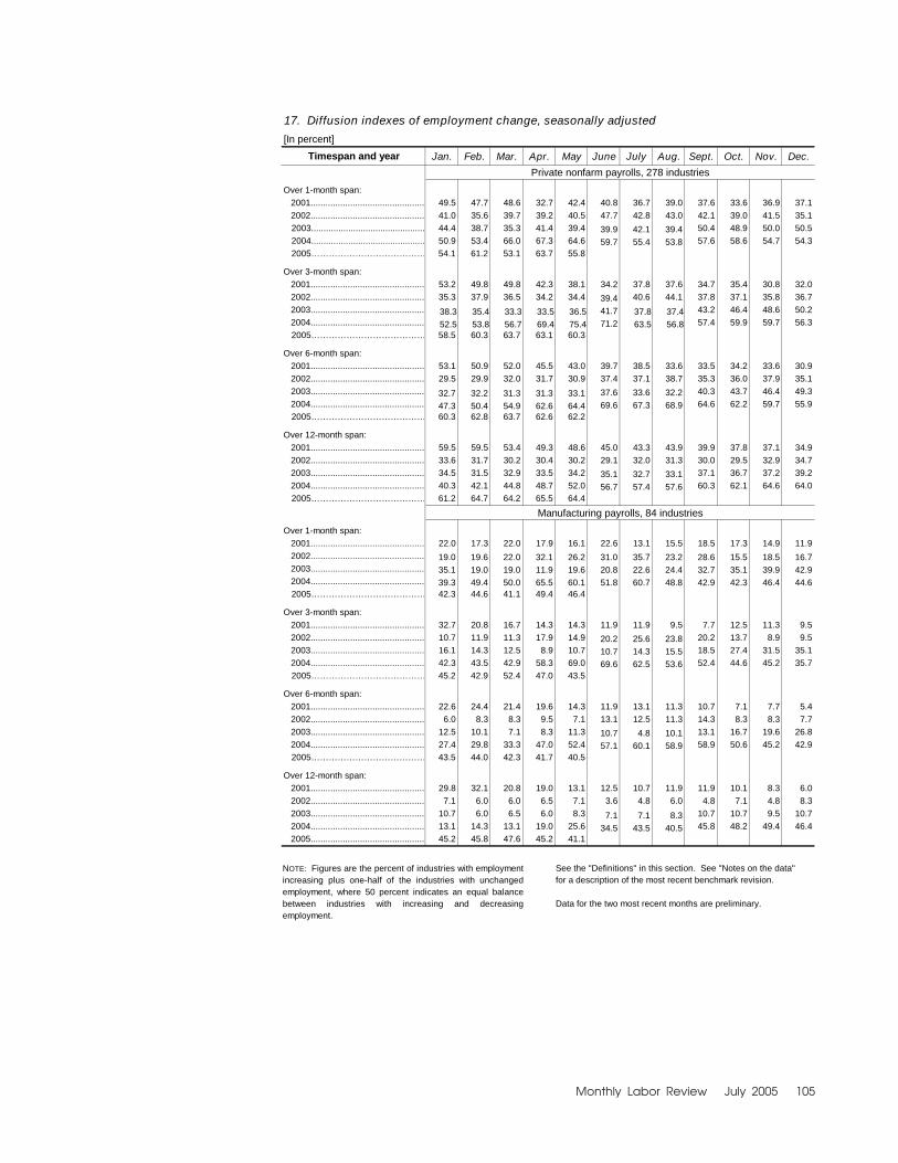
Monthly Labor Review July 2005 105
17. Diffusion indexes of employment change, seasonally adjusted
[In percent]Timespan and year Jan. Feb. Mar. Apr. May June July Aug. Sept. Oct. Nov. Dec.
Private nonfarm payrolls, 278 industries
Over 1-month span: 2001.............................................. 49.5 47.7 48.6 32.7 42.4 40.8 36.7 39.0 37.6 33.6 36.9 37.1 2002.............................................. 41.0 35.6 39.7 39.2 40.5 47.7 42.8 43.0 42.1 39.0 41.5 35.1 2003.............................................. 44.4 38.7 35.3 41.4 39.4 39.9 42.1 39.4 50.4 48.9 50.0 50.5 2004.............................................. 50.9 53.4 66.0 67.3 64.6 59.7 55.4 53.8 57.6 58.6 54.7 54.3 2005………………………………… 54.1 61.2 53.1 63.7 55.8
Over 3-month span: 2001.............................................. 53.2 49.8 49.8 42.3 38.1 34.2 37.8 37.6 34.7 35.4 30.8 32.0 2002.............................................. 35.3 37.9 36.5 34.2 34.4 39.4 40.6 44.1 37.8 37.1 35.8 36.7 2003.............................................. 38.3 35.4 33.3 33.5 36.5 41.7 37.8 37.4 43.2 46.4 48.6 50.2 2004.............................................. 52.5 53.8 56.7 69.4 75.4 71.2 63.5 56.8 57.4 59.9 59.7 56.3 2005………………………………… 58.5 60.3 63.7 63.1 60.3
Over 6-month span: 2001.............................................. 53.1 50.9 52.0 45.5 43.0 39.7 38.5 33.6 33.5 34.2 33.6 30.9 2002.............................................. 29.5 29.9 32.0 31.7 30.9 37.4 37.1 38.7 35.3 36.0 37.9 35.1 2003.............................................. 32.7 32.2 31.3 31.3 33.1 37.6 33.6 32.2 40.3 43.7 46.4 49.3 2004.............................................. 47.3 50.4 54.9 62.6 64.4 69.6 67.3 68.9 64.6 62.2 59.7 55.9 2005………………………………… 60.3 62.8 63.7 62.6 62.2
Over 12-month span: 2001.............................................. 59.5 59.5 53.4 49.3 48.6 45.0 43.3 43.9 39.9 37.8 37.1 34.9 2002.............................................. 33.6 31.7 30.2 30.4 30.2 29.1 32.0 31.3 30.0 29.5 32.9 34.7 2003.............................................. 34.5 31.5 32.9 33.5 34.2 35.1 32.7 33.1 37.1 36.7 37.2 39.2 2004.............................................. 40.3 42.1 44.8 48.7 52.0 56.7 57.4 57.6 60.3 62.1 64.6 64.0 2005………………………………… 61.2 64.7 64.2 65.5 64.4
Manufacturing payrolls, 84 industries
Over 1-month span: 2001.............................................. 22.0 17.3 22.0 17.9 16.1 22.6 13.1 15.5 18.5 17.3 14.9 11.9 2002.............................................. 19.0 19.6 22.0 32.1 26.2 31.0 35.7 23.2 28.6 15.5 18.5 16.7 2003.............................................. 35.1 19.0 19.0 11.9 19.6 20.8 22.6 24.4 32.7 35.1 39.9 42.9 2004.............................................. 39.3 49.4 50.0 65.5 60.1 51.8 60.7 48.8 42.9 42.3 46.4 44.6 2005………………………………… 42.3 44.6 41.1 49.4 46.4
Over 3-month span: 2001.............................................. 32.7 20.8 16.7 14.3 14.3 11.9 11.9 9.5 7.7 12.5 11.3 9.5 2002.............................................. 10.7 11.9 11.3 17.9 14.9 20.2 25.6 23.8 20.2 13.7 8.9 9.5 2003.............................................. 16.1 14.3 12.5 8.9 10.7 10.7 14.3 15.5 18.5 27.4 31.5 35.1 2004.............................................. 42.3 43.5 42.9 58.3 69.0 69.6 62.5 53.6 52.4 44.6 45.2 35.7 2005………………………………… 45.2 42.9 52.4 47.0 43.5
Over 6-month span: 2001.............................................. 22.6 24.4 21.4 19.6 14.3 11.9 13.1 11.3 10.7 7.1 7.7 5.4 2002.............................................. 6.0 8.3 8.3 9.5 7.1 13.1 12.5 11.3 14.3 8.3 8.3 7.7 2003.............................................. 12.5 10.1 7.1 8.3 11.3 10.7 4.8 10.1 13.1 16.7 19.6 26.8 2004.............................................. 27.4 29.8 33.3 47.0 52.4 57.1 60.1 58.9 58.9 50.6 45.2 42.9 2005………………………………… 43.5 44.0 42.3 41.7 40.5
Over 12-month span: 2001.............................................. 29.8 32.1 20.8 19.0 13.1 12.5 10.7 11.9 11.9 10.1 8.3 6.0 2002.............................................. 7.1 6.0 6.0 6.5 7.1 3.6 4.8 6.0 4.8 7.1 4.8 8.3 2003.............................................. 10.7 6.0 6.5 6.0 8.3 7.1 7.1 8.3 10.7 10.7 9.5 10.7 2004.............................................. 13.1 14.3 13.1 19.0 25.6 34.5 43.5 40.5 45.8 48.2 49.4 46.4 2005.............................................. 45.2 45.8 47.6 45.2 41.1
See the "Definitions" in this section. See "Notes on the data" for a description of the most recent benchmark revision.
Data for the two most recent months are preliminary.
NOTE: Figures are the percent of industries with employmentincreasing plus one-half of the industries with unchangedemployment, where 50 percent indicates an equal balancebetween industries with increasing and decreasingemployment.

Current Labor Statistics: Labor Force Data
106 Monthly Labor Review July 2005
18. Job openings levels and rates by industry and region, seasonally adjusted
Levels1 (in thousands)
Industry and region 2004 2005 2004 2005
Nov. Dec. Jan. Feb. Mar. Apr. Mayp Nov. Dec Jan. Feb. Mar. Apr. Mayp
Total2……………………………………………… 3,277 3,507 3,385 3,569 3,598 3,576 3,465 2.4 2.6 2.5 2.6 2.6 2.6 2.5
Industry
Total private2………………………………… 2,910 3,106 3,020 3,160 3,212 3,178 3,090 2.6 2.7 2.7 2.8 2.8 2.8 2.7
Construction……………………………… 118 132 127 133 170 113 111 1.6 1.8 1.8 1.8 2.3 1.5 1.5
Manufacturing…………………………… 248 266 252 252 258 259 236 1.7 1.8 1.7 1.7 1.8 1.8 1.6
Trade, transportation, and utilities……… 554 561 564 668 624 627 622 2.1 2.1 2.2 2.5 2.4 2.4 2.4
Professional and business services…… 620 699 682 607 646 691 645 3.6 4.0 3.9 3.5 3.7 3.9 3.7
Education and health services………… 543 557 560 602 616 608 604 3.1 3.1 3.2 3.4 3.5 3.4 3.4
Leisure and hospitality…………………… 411 450 434 447 440 457 465 3.2 3.4 3.3 3.4 3.4 3.5 3.5
Government………………………………… 369 396 346 404 383 396 374 1.7 1.8 1.6 1.8 1.7 1.8 1.7
Region3
Northeast………………………………… 560 620 602 606 615 602 548 2.2 2.4 2.3 2.3 2.4 2.3 2.1
South……………………………………… 1,250 1,329 1,342 1,399 1,447 1,414 1,335 2.6 2.8 2.8 2.9 3.0 2.9 2.7
Midwest…………………………………… 726 740 716 745 737 742 798 2.3 2.3 2.2 2.3 2.3 2.3 2.5
West……………………………………… 759 792 718 823 806 818 801 2.6 2.7 2.4 2.8 2.7 2.7 2.7
Percent
1 Detail will not necessarily add to totals because of the independent seasonal
adjustment of the various series.2 Includes natural resources and mining, information, financial activities, and other
services, not shown separately.3 Northeast: Connecticut, Maine, Massachusetts, New Hampshire, New Jersey,
New York, Pennsylvania, Rhode Island, Vermont; South: Alabama, Arkansas,
Delaware, District of Columbia, Florida, Georgia, Kentucky, Louisiana, Maryland,
Mississippi, North Carolina, Oklahoma, South Carolina, Tennessee, Texas, Virginia,
West Virginia; Midwest: Illinois, Indiana, Iowa, Kansas, Michigan, Minnesota,
Missouri, Nebraska, North Dakota, Ohio, South Dakota, Wisconsin; West: Alaska, Arizona,
California, Colorado, Hawaii, Idaho, Montana, Nevada, New Mexico, Oregon, Utah,
Washington, Wyoming.
NOTE: The job openings level is the number of job openings on the last business day of
the month; the job openings rate is the number of job openings on the last business day of
the month as a percent of total employment plus job openings. P = preliminary.
19. Hires levels and rates by industry and region, seasonally adjusted
Industry and region 2004 2005 2004 2005
Nov. Dec Jan. Feb. Mar. Apr. May.p Nov. Dec Jan. Feb. Mar. Apr. Mayp
Total2……………………………………………… 4,990 4,639 4,709 4,760 4,841 4,538 4,708 3.8 3.5 3.6 3.6 3.6 3.4 3.5
Industry
Total private2………………………………… 4,652 4,337 4,374 4,430 4,497 4,212 4,366 4.2 3.9 3.9 4.0 4.0 3.8 3.9
Construction……………………………… 373 368 339 430 414 412 422 5.3 5.2 4.8 6.0 5.8 5.7 5.8
Manufacturing…………………………… 386 324 307 336 334 319 345 2.7 2.3 2.1 2.3 2.3 2.2 2.4
Trade, transportation, and utilities……… 1,077 986 1,056 1,055 1,047 1,042 1,036 4.2 3.8 4.1 4.1 4.1 4.0 4.0
Professional and business services…… 935 878 882 853 895 792 834 5.6 5.3 5.3 5.1 5.3 4.7 5.0
Education and health services………… 447 452 445 500 472 487 460 2.6 2.6 2.6 2.9 2.7 2.8 2.7
Leisure and hospitality…………………… 858 834 826 771 798 742 750 6.8 6.6 6.6 6.1 6.3 5.8 5.9
Government………………………………… 335 307 341 329 336 329 338 1.5 1.4 1.6 1.5 1.5 1.5 1.6
Region3
Northeast………………………………… 851 858 762 820 856 825 768 3.4 3.4 3.0 3.2 3.4 3.3 3.0
South……………………………………… 1,903 1,770 1,880 1,867 1,922 1,701 1,834 4.1 3.8 4.0 4.0 4.1 3.6 3.9
Midwest…………………………………… 1,149 1,043 1,092 1,081 1,034 1,020 1,113 3.7 3.3 3.5 3.5 3.3 3.3 3.5
West……………………………………… 1,014 970 959 1,069 1,036 1,037 1,005 3.5 3.4 3.3 3.7 3.6 3.6 3.4
Levels1 (in thousands) Percent
1 Detail will not necessarily add to totals because of the independent seasonal
adjustment of the various series.2 Includes natural resources and mining, information, financial activities, and other
services, not shown separately.3 Northeast: Connecticut, Maine, Massachusetts, New Hampshire, New Jersey, New
York, Pennsylvania, Rhode Island, Vermont; South: Alabama, Arkansas, Delaware,
District of Columbia, Florida, Georgia, Kentucky, Louisiana, Maryland, Mississippi,
North Carolina, Oklahoma, South Carolina, Tennessee, Texas, Virginia, West Virginia;
Midwest: Illinois, Indiana, Iowa, Kansas, Michigan, Minnesota, Missouri,
Nebraska, North Dakota, Ohio, South Dakota, Wisconsin; West: Alaska, Arizona,
California, Colorado, Hawaii, Idaho, Montana, Nevada, New Mexico, Oregon, Utah,
Washington, Wyoming.
NOTE: The hires level is the number of hires during the entire month; the hires rate is
the number of hires during the entire month as a percent of total employment.
p = preliminary.

Monthly Labor Review July 2005 107
20. Total separations levels and rates by industry and region, seasonally adjusted
Industry and region 2004 2005 2004 2005
Nov. Dec. Jan. Feb. Mar. Apr. Mayp Nov. Dec. Jan. Feb. Mar. Apr. Mayp
Total2……………………………………………… 4,266 4,435 4,352 4,295 4,502 4,562 4,425 3.2 3.3 3.3 3.2 3.4 3.4 303.0
Industry
Total private2………………………………… 3,996 4,146 4,091 4,035 4,237 4,306 4,180 3.6 3.7 3.7 3.6 3.8 3.9 3.7
Construction……………………………… 351 355 417 3 303 421 393 5.0 5.0 5.9 5.7 4.2 5.8 5.4
Manufacturing…………………………… 327 353 361 341 360 369 357 2.3 2.5 2.5 2.4 2.5 2.6 2.5
Trade, transportation, and utilities……… 943 1,062 882 940 980 1,018 946 3.7 4.1 3.4 3.7 3.8 3.9 3.7
Professional and business services…… 822 833 836 772 924 869 924 4.9 5.0 5.0 4.6 5.5 5.2 4.9
Education and health services………… 408 375 356 389 445 433 413 2.4 2.2 2.1 2.3 2.6 2.5 2.4
Leisure and hospitality…………………… 727 758 832 790 743 709 746 5.8 6.0 6.6 6.3 5.9 5.6 5.9
Government………………………………… 275 274 258 260 267 256 251 1.3 1.3 1.2 1.2 1.2 1.2 1.2
Region3
Northeast………………………………… 756 773 773 732 802 807 685 3.0 3.0 3.1 2.9 3.2 3.2 2.7
South……………………………………… 1,594 1,707 1,747 1,647 1,763 1,766 1,728 3.4 3.6 3.7 3.5 3.7 3.7 3.6
Midwest…………………………………… 1,041 986 981 937 1,051 982 976 3.3 3.1 3.1 3.0 3.4 3.1 3.1
West……………………………………… 826 953 964 961 926 1,006 984 2.9 3.3 3.3 3.3 3.2 3.4 3.4
Level1 (in thousands) Percent
1 Detail will not necessarily add to totals because of the independent seasonal adjustment
of the various series.2 Includes natural resources and mining, information, financial activities, and other
services, not shown separately.3 Northeast: Connecticut, Maine, Massachusetts, New Hampshire, New Jersey, New
York, Pennsylvania, Rhode Island, Vermont; South: Alabama, Arkansas, Delaware,
District of Columbia, Florida, Georgia, Kentucky, Louisiana, Maryland, Mississippi,
North Carolina, Oklahoma, South Carolina, Tennessee, Texas, Virginia, West Virginia;
Midwest: Illinois, Indiana, Iowa, Kansas, Michigan, Minnesota, Missouri, Nebraska,
North Dakota, Ohio, South Dakota, Wisconsin; West: Alaska, Arizona, California,
Colorado, Hawaii, Idaho, Montana, Nevada, New Mexico, Oregon, Utah, Washington,
Wyoming.
NOTE: The total separations level is the number of total separations during the entire
month; the total separations rate is the number of total separations during the entire
month as a percent of total employment. p = preliminary.
21. Quits levels and rates by industry and region, seasonally adjusted
Percent
Industry and region 2005 2005
Nov. Dec. Jan. Feb. Mar. Apr. Mayp Nov. Dec. Jan. Feb. Mar. Apr. Mayp
Total2……………………………………………… 2,436 2,495 2,530 2,307 2,516 2,520 2,493 1.8 1.9 1.9 1.7 1.9 1.9 1.9
Industry
Total private2………………………………… 2,319 2,366 2,412 2,192 2,383 2,395 2,370 2.1 2.1 2.2 2.0 2.1 2.1 2.1
Construction……………………………… 159 162 171 139 150 146 151 2.2 2.3 2.4 2.0 2.1 2.0 2.1
Manufacturing…………………………… 185 194 185 181 186 178 168 1.3 1.4 1.3 1.3 1.3 1.2 1.2
Trade, transportation, and utilities……… 568 570 563 512 583 577 589 2.2 2.2 2.2 2.0 2.3 2.2 2.3
Professional and business services…… 401 415 417 410 424 417 413 2.4 2.5 2.5 2.4 2.5 2.5 2.5
Education and health services………… 250 232 230 259 280 277 260 1.5 1.4 1.3 1.5 1.6 1.6 1.5
Leisure and hospitality…………………… 499 506 516 474 458 506 494 4.0 4.0 4.1 3.8 3.6 4.0 3.9
Government………………………………… 118 129 124 117 124 125 122 .5 .6 .6 .5 .6 .6 .6
Region3
Northeast………………………………… 359 392 424 340 410 446 364 1.4 1.5 1.7 1.3 1.6 1.8 1.4
South……………………………………… 1,014 1,021 1,053 914 1,003 992 1,024 2.2 2.2 2.2 1.9 2.1 2.1 2.2
Midwest…………………………………… 551 544 539 509 561 540 556 1.8 1.7 1.7 1.6 1.8 1.7 1.8
West……………………………………… 492 536 530 550 562 573 544 1.7 1.9 1.8 1.9 1.9 2.0 1.9
Levels1 (in thousands)
2004 2004
1 Detail will not necessarily add to totals because of the independent seasonal adjustment
of the various series.2 Includes natural resources and mining, information, financial activities, and other
services, not shown separately.3 Northeast: Connecticut, Maine, Massachusetts, New Hampshire, New Jersey, New
York, Pennsylvania, Rhode Island, Vermont; South: Alabama, Arkansas, Delaware,
District of Columbia, Florida, Georgia, Kentucky, Louisiana, Maryland, Mississippi,
North Carolina, Oklahoma, South Carolina, Tennessee, Texas, Virginia, West Virginia;
Midwest: Illinois, Indiana, Iowa, Kansas, Michigan, Minnesota, Missouri,
Nebraska, North Dakota, Ohio, South Dakota, Wisconsin; West: Alaska, Arizona,
California, Colorado, Hawaii, Idaho, Montana, Nevada, New Mexico, Oregon,
Utah, Washington, Wyoming.
NOTE: The quits level is the number of quits during the entire month; the quits
rate is the number of quits during the entire month as a percent of total
employment. p = preliminary.

Current Labor Statistics: Labor Force Data
108 Monthly Labor Review July 2005
22. Quarterly Census of Employment and Wages: 10 largest counties, fourth quarter 2003.
County by NAICS supersector
Establishments,fourth quarter
2003(thousands)
Employment Average weekly wage1
December2003
(thousands)
Percent change,December2002-032
Fourthquarter
2003
Percent change,fourth quarter
2002-032
United States3 .............................................................................. 8,314.1 129,341.5 0.0 $767 3.6Private industry ........................................................................ 8,048.7 108,215.1 .0 769 3.9
Natural resources and mining .............................................. 123.7 1,557.8 .1 703 4.9Construction ......................................................................... 804.9 6,689.5 1.2 837 2.3Manufacturing ...................................................................... 376.8 14,307.8 -4.2 943 6.7Trade, transportation, and utilities ........................................ 1,853.6 25,957.3 -.3 665 3.4Information ........................................................................... 145.2 3,165.9 -4.0 1,139 3.9Financial activities ................................................................ 767.0 7,874.7 1.2 1,138 5.9Professional and business services ..................................... 1,329.4 16,113.2 .6 945 3.8Education and health services ............................................. 732.2 15,974.0 2.1 731 3.8Leisure and hospitality ......................................................... 669.9 12,042.8 1.7 335 3.4Other services ...................................................................... 1,080.6 4,274.1 -.1 494 3.1
Government ............................................................................. 265.3 21,126.3 -.2 757 2.4
Los Angeles, CA .......................................................................... 356.0 4,075.3 -.5 903 4.2Private industry ........................................................................ 352.2 3,486.3 -.2 898 4.2
Natural resources and mining .............................................. .6 11.0 .7 955 16.9Construction ......................................................................... 12.9 133.9 -1.1 883 1.7Manufacturing ...................................................................... 17.8 485.2 -7.1 900 6.5Trade, transportation, and utilities ........................................ 53.9 794.6 -1.2 735 2.7Information ........................................................................... 9.2 194.9 -2.0 1,627 5.2Financial activities ................................................................ 23.0 237.9 .9 1,258 7.0Professional and business services ..................................... 40.1 575.0 1.6 1,043 3.7Education and health services ............................................. 26.6 456.5 1.9 820 3.9Leisure and hospitality ......................................................... 25.6 375.9 5.6 766 6.5Other services ...................................................................... 142.1 220.7 3.5 422 5.0
Government ............................................................................. 3.8 589.0 -2.3 930 3.3
Cook, IL ........................................................................................ 126.7 2,539.8 -1.2 922 3.0Private industry ........................................................................ 125.5 2,221.9 -.9 929 3.2
Natural resources and mining .............................................. .1 1.3 -3.6 1,037 3.2Construction ......................................................................... 10.5 96.7 .0 1,169 -.8Manufacturing ...................................................................... 7.9 265.7 -5.1 975 6.3Trade, transportation, and utilities ........................................ 26.7 499.4 -.8 753 .4Information ........................................................................... 2.5 66.1 -4.1 1,164 .1Financial activities ................................................................ 13.8 219.4 -.8 1,471 8.1Professional and business services ..................................... 26.1 405.5 -1.3 1,206 4.1Education and health services ............................................. 12.3 350.8 1.0 791 3.7Leisure and hospitality ......................................................... 10.5 217.7 2.8 375 -.3Other services ...................................................................... 12.6 95.1 -2.0 655 3.0
Government ............................................................................. 1.2 317.9 -3.1 871 .9
New York, NY ............................................................................... 111.9 2,253.6 -1.0 1,480 7.2Private industry ........................................................................ 111.7 1,800.4 -.6 1,623 8.1
Natural resources and mining .............................................. .0 .1 .0 1,197 -6.5Construction ......................................................................... 2.2 30.0 -4.5 1,567 3.4Manufacturing ...................................................................... 3.5 46.6 -4.9 1,290 6.4Trade, transportation, and utilities ........................................ 22.1 247.6 -1.2 1,164 5.5Information ........................................................................... 4.3 130.6 -5.1 1,751 7.9Financial activities ................................................................ 16.7 352.0 -2.0 3,034 16.1Professional and business services ..................................... 22.6 439.7 .5 1,702 2.6Education and health services ............................................. 7.8 273.8 2.4 918 7.6Leisure and hospitality ......................................................... 10.1 188.2 .4 787 6.1Other services ...................................................................... 16.0 82.9 -1.1 871 6.1
Government ............................................................................. .2 453.2 -2.2 912 .1
Harris, TX ..................................................................................... 89.4 1,841.5 -.9 906 2.1Private industry ........................................................................ 89.0 1,595.2 -1.2 929 2.1
Natural resources and mining .............................................. 1.2 62.5 8.7 2,185 -.9Construction ......................................................................... 6.3 135.5 -5.0 919 2.6Manufacturing ...................................................................... 4.7 164.0 -4.9 1,106 2.3Trade, transportation, and utilities ........................................ 21.1 403.2 -2.1 821 1.0Information ........................................................................... 1.4 33.8 -3.9 1,098 .4Financial activities ................................................................ 9.7 113.1 1.7 1,181 4.9Professional and business services ..................................... 17.0 279.0 -1.7 1,073 3.2Education and health services ............................................. 8.8 188.3 1.5 812 1.8Leisure and hospitality ......................................................... 6.5 155.2 .7 335 -.9Other services ...................................................................... 10.3 56.3 -3.1 539 .4
Government ............................................................................. .4 246.3 1.1 759 3.1
Maricopa, AZ ................................................................................ 80.9 1,621.2 (4) 757 4.0Private industry ........................................................................ 80.5 1,401.8 2.2 755 3.9
Natural resources and mining .............................................. .5 9.8 -2.6 545 4.4Construction ......................................................................... 8.4 131.7 5.9 779 2.1Manufacturing ...................................................................... 3.3 128.0 -2.5 1,050 8.2Trade, transportation, and utilities ........................................ 18.6 336.4 1.5 712 3.2Information ........................................................................... 1.6 36.6 -4.1 872 .5Financial activities ................................................................ 9.5 133.3 1.5 933 3.7Professional and business services ..................................... 18.1 261.5 4.2 776 3.5Education and health services ............................................. 7.6 160.5 5.6 842 5.0Leisure and hospitality ......................................................... 5.6 155.8 .8 364 2.8Other services ...................................................................... 5.7 44.7 -2.6 500 2.2
Government ............................................................................. .5 219.4 1.6 766 3.7
See footnotes at end of table.

Monthly Labor Review July 2005 109
22. Continued�Quarterly Census of Employment and Wages: 10 largest counties, fourth quarter 2003.
County by NAICS supersector
Establishments,fourth quarter
2003(thousands)
Employment Average weekly wage1
December2003
(thousands)
Percent change,December2002-032
Fourthquarter
2003
Percent change,fourth quarter
2002-032
Dallas, TX ..................................................................................... 68.6 1,450.8 -1.4 $952 4.3Private industry ........................................................................ 68.2 1,294.6 -1.4 970 4.8
Natural resources and mining .............................................. .5 6.8 -20.5 2,680 22.7Construction ......................................................................... 4.5 73.0 -2.2 909 5.5Manufacturing ...................................................................... 3.5 144.9 -3.1 1,075 6.8Trade, transportation, and utilities ........................................ 15.8 326.1 -3.3 898 5.2Information ........................................................................... 1.9 64.0 -5.1 1,272 8.7Financial activities ................................................................ 8.6 140.0 1.2 1,215 2.9Professional and business services ..................................... 14.0 237.7 .0 1,152 4.2Education and health services ............................................. 6.3 131.4 2.4 887 2.7Leisure and hospitality ......................................................... 5.2 127.5 .0 432 4.3Other services ...................................................................... 6.7 40.5 -3.4 587 2.8
Government ............................................................................. .4 156.2 -1.8 800 -.1
Orange, CA .................................................................................. 88.8 1,436.6 1.3 874 5.3Private industry ........................................................................ 87.4 1,305.5 2.1 875 5.2
Natural resources and mining .............................................. .3 6.1 8.3 579 .2Construction ......................................................................... 6.4 85.5 4.4 969 5.9Manufacturing ...................................................................... 6.1 179.9 -3.0 1,036 11.4Trade, transportation, and utilities ........................................ 17.3 278.8 .6 802 2.7Information ........................................................................... 1.5 33.8 -4.4 1,152 5.3Financial activities ................................................................ 9.7 127.8 9.9 1,354 6.2Professional and business services ..................................... 17.4 261.0 1.0 942 2.8Education and health services ............................................. 9.1 126.6 6.1 849 3.7Leisure and hospitality ......................................................... 6.6 159.9 2.5 358 3.8Other services ...................................................................... 12.9 46.0 6.3 518 3.0
Government ............................................................................. 1.4 131.1 -5.7 859 6.0
San Diego, CA ............................................................................. 85.3 1,278.2 1.3 815 2.6Private industry ........................................................................ 83.9 1,060.2 1.5 809 2.5
Natural resources and mining .............................................. .9 11.0 -5.4 491 1.0Construction ......................................................................... 6.4 81.1 4.7 869 .7Manufacturing ...................................................................... 3.6 105.4 -4.2 1,129 11.5Trade, transportation, and utilities ........................................ 14.2 220.4 2.2 655 .9Information ........................................................................... 1.4 36.7 -4.5 1,582 -2.0Financial activities ................................................................ 8.8 81.6 4.8 1,058 .4Professional and business services ..................................... 14.9 208.1 1.5 989 2.8Education and health services ............................................. 7.6 122.6 1.6 778 5.7Leisure and hospitality ......................................................... 6.5 141.5 3.5 346 2.4Other services ...................................................................... 19.5 51.6 1.8 449 2.7
Government ............................................................................. 1.3 218.0 .1 843 2.9
King, WA ...................................................................................... 81.6 1,100.6 .2 935 .2Private industry ........................................................................ 81.0 945.5 .1 944 -.3
Natural resources and mining .............................................. .4 2.8 -11.3 1,109 .8Construction ......................................................................... 6.2 53.4 -.4 921 1.4Manufacturing ...................................................................... 2.7 101.9 -8.2 1,176 -2.1Trade, transportation, and utilities ........................................ 14.8 225.5 1.1 804 2.6Information ........................................................................... 1.5 69.2 .8 1,829 -15.7Financial activities ................................................................ 6.1 77.5 2.4 1,114 3.5Professional and business services ..................................... 11.7 158.3 .7 1,160 8.4Education and health services ............................................. 5.9 108.3 1.5 746 4.8Leisure and hospitality ......................................................... 5.4 100.5 2.9 390 3.7Other services ...................................................................... 26.4 48.1 1.2 463 .4
Government ............................................................................. .6 155.1 1.0 882 3.6
Miami-Dade, FL ............................................................................ 80.2 980.8 -.5 765 3.5Private industry ........................................................................ 79.9 827.5 -.7 742 3.6
Natural resources and mining .............................................. .5 9.9 -1.8 421 4.0Construction ......................................................................... 4.9 40.7 .3 788 2.7Manufacturing ...................................................................... 2.8 49.4 -9.8 695 5.8Trade, transportation, and utilities ........................................ 23.2 247.2 -1.7 689 4.2Information ........................................................................... 1.7 28.5 -3.2 990 1.7Financial activities ................................................................ 8.2 65.5 .7 1,062 -1.1Professional and business services ..................................... 15.9 132.0 -.2 948 5.2Education and health services ............................................. 7.8 123.4 1.4 748 2.3Leisure and hospitality ......................................................... 5.3 92.8 2.1 432 9.9Other services ...................................................................... 7.5 34.5 -1.8 450 3.0
Government ............................................................................. .3 153.3 .5 886 2.8
1 Average weekly wages were calculated using unrounded data.
2 Percent changes were computed from quarterly employment and pay dataadjusted for noneconomic county reclassifications. See Notes on Current LaborStatistics.
3 Totals for the United States do not include data for Puerto Rico or the
Virgin Islands.
4 Data do not meet BLS or State agency disclosure standards.
NOTE: Includes workers covered by Unemployment Insurance (UI) andUnemployment Compensation for Federal Employees (UCFE) programs. Data arepreliminary.

Current Labor Statistics: Labor Force Data
110 Monthly Labor Review July 2005
23. Quarterly Census of Employment and Wages: by State, fourth quarter 2003.
State
Establishments,fourth quarter
2003(thousands)
Employment Average weekly wage1
December2003
(thousands)
Percent change,December
2002-03
Fourthquarter
2003
Percent change,fourth quarter
2002-03
United States2 ................................... 8,314.1 129,341.5 0.0 $767 3.6
Alabama ............................................ 111.8 1,838.1 -.1 657 4.0Alaska ............................................... 20.0 282.7 1.1 746 1.1Arizona .............................................. 126.9 2,352.1 2.2 710 3.8Arkansas ........................................... 75.2 1,133.6 .5 587 4.1California ........................................... 1,190.8 14,922.3 .0 869 3.8Colorado ........................................... 160.0 2,134.6 -1.1 784 2.0Connecticut ....................................... 109.1 1,648.9 -.7 992 3.8Delaware ........................................... 27.1 408.4 .5 825 5.0District of Columbia ........................... 30.0 654.8 -.4 1,238 3.9Florida ............................................... 504.1 7,424.5 .8 685 3.8
Georgia ............................................. 245.6 3,845.6 .2 734 2.8Hawaii ............................................... 37.4 583.0 1.3 678 3.7Idaho ................................................. 48.5 577.5 .6 579 1.8Illinois ................................................ 325.7 5,738.7 -1.2 827 3.2Indiana .............................................. 152.1 2,852.2 -.3 675 3.5Iowa .................................................. 90.6 1,418.5 .0 626 4.7Kansas .............................................. 82.2 1,298.3 -.9 631 2.8Kentucky ........................................... 105.7 1,740.6 .3 645 3.5Louisiana ........................................... 114.0 1,870.9 .5 628 2.4Maine ................................................ 47.4 595.8 .7 631 4.6
Maryland ........................................... 150.4 2,466.4 .7 831 3.6Massachusetts .................................. 206.6 3,154.6 -1.9 954 5.2Michigan ............................................ 251.3 4,365.8 -1.1 806 3.9Minnesota ......................................... 159.0 2,591.9 -.5 777 3.2Mississippi ......................................... 65.6 1,108.1 .4 559 3.7Missouri ............................................. 165.4 2,633.6 -.7 676 2.4Montana ............................................ 42.0 396.6 1.1 549 4.0Nebraska ........................................... 55.3 884.4 .6 613 3.2Nevada .............................................. 60.3 1,111.2 4.4 721 5.1New Hampshire ................................ 47.0 614.9 .6 788 4.0
New Jersey ....................................... 268.1 3,912.8 .1 945 3.4New Mexico ...................................... 50.4 757.1 1.4 612 4.1New York .......................................... 550.3 8,379.2 -.4 959 5.2North Carolina ................................... 227.8 3,759.6 -.1 679 4.5North Dakota ..................................... 24.0 317.6 .9 563 4.3Ohio .................................................. 294.2 5,322.4 -.7 713 3.8Oklahoma .......................................... 91.6 1,423.4 -1.3 597 4.2Oregon .............................................. 118.8 1,579.8 .2 694 3.3Pennsylvania ..................................... 326.9 5,524.5 -.2 750 4.7Rhode Island ..................................... 34.7 480.5 1.2 738 5.1
South Carolina .................................. 108.4 1,781.0 .3 623 3.1South Dakota .................................... 28.1 365.4 .3 559 4.1Tennessee ........................................ 128.4 2,648.0 .4 689 4.2Texas ................................................ 505.3 9,300.1 -.3 754 3.1Utah .................................................. 73.9 1,066.2 1.2 630 2.3Vermont ............................................ 24.1 300.7 .3 661 5.1Virginia .............................................. 202.6 3,477.5 1.2 786 5.2Washington ....................................... 222.7 2,654.7 1.0 759 1.3West Virginia ..................................... 47.2 685.2 .1 587 2.1Wisconsin .......................................... 157.6 2,715.4 .0 683 4.1
Wyoming ........................................... 22.0 241.6 1.7 616 4.1
Puerto Rico ....................................... 50.2 1,074.1 3.5 450 4.7Virgin Islands .................................... 3.2 42.5 -.2 629 2.4
1 Average weekly wages were calculated using unrounded data.
2 Totals for the United States do not include data for Puerto Ricoor the Virgin Islands.
NOTE: Includes workers covered by Unemployment Insurance (UI)and Unemployment Compensation for Federal Employees (UCFE)programs. Data are preliminary.

Monthly Labor Review July 2005 111
24. Annual data: Quarterly Census of Employment and Wages, by ownership
Year Averageestablishments
Averageannual
employment
Total annual wages(in thousands)
Average annual wageper employee
Averageweeklywage
Total covered (UI and UCFE)
1993 .................................................. 6,679,934 109,422,571 $2,884,472,282 $26,361 $507 1994 .................................................. 6,826,677 112,611,287 3,033,676,678 26,939 518 1995 .................................................. 7,040,677 115,487,841 3,215,921,236 27,846 536 1996 .................................................. 7,189,168 117,963,132 3,414,514,808 28,946 557 1997 .................................................. 7,369,473 121,044,432 3,674,031,718 30,353 584 1998 .................................................. 7,634,018 124,183,549 3,967,072,423 31,945 614 1999 .................................................. 7,820,860 127,042,282 4,235,579,204 33,340 641 2000 .................................................. 7,879,116 129,877,063 4,587,708,584 35,323 679 2001 .................................................. 7,984,529 129,635,800 4,695,225,123 36,219 697 2002 .................................................. 8,101,872 128,233,919 4,714,374,741 36,764 707
UI covered
1993 .................................................. 6,632,221 106,351,431 $2,771,023,411 $26,055 $501 1994 .................................................. 6,778,300 109,588,189 2,918,684,128 26,633 512 1995 .................................................. 6,990,594 112,539,795 3,102,353,355 27,567 530 1996 .................................................. 7,137,644 115,081,246 3,298,045,286 28,658 551 1997 .................................................. 7,317,363 118,233,942 3,553,933,885 30,058 578 1998 .................................................. 7,586,767 121,400,660 3,845,494,089 31,676 609 1999 .................................................. 7,771,198 124,255,714 4,112,169,533 33,094 636 2000 .................................................. 7,828,861 127,005,574 4,454,966,824 35,077 675 2001 .................................................. 7,933,536 126,883,182 4,560,511,280 35,943 691 2002 .................................................. 8,051,117 125,475,293 4,570,787,218 36,428 701
Private industry covered
1993 .................................................. 6,454,381 91,202,971 $2,365,301,493 $25,934 $499 1994 .................................................. 6,596,158 94,146,344 2,494,458,555 26,496 510 1995 .................................................. 6,803,454 96,894,844 2,658,927,216 27,441 528 1996 .................................................. 6,946,858 99,268,446 2,837,334,217 28,582 550 1997 .................................................. 7,121,182 102,175,161 3,071,807,287 30,064 578 1998 .................................................. 7,381,518 105,082,368 3,337,621,699 31,762 611 1999 .................................................. 7,560,567 107,619,457 3,577,738,557 33,244 639 2000 .................................................. 7,622,274 110,015,333 3,887,626,769 35,337 680 2001 .................................................. 7,724,965 109,304,802 3,952,152,155 36,157 695 2002 .................................................. 7,839,903 107,577,281 3,930,767,025 36,539 703
State government covered
1993 .................................................. 59,185 4,088,075 $117,095,062 $28,643 $551 1994 .................................................. 60,686 4,162,944 122,879,977 29,518 568 1995 .................................................. 60,763 4,201,836 128,143,491 30,497 586 1996 .................................................. 62,146 4,191,726 131,605,800 31,397 604 1997 .................................................. 65,352 4,214,451 137,057,432 32,521 625 1998 .................................................. 67,347 4,240,779 142,512,445 33,605 646 1999 .................................................. 70,538 4,296,673 149,011,194 34,681 667 2000 .................................................. 65,096 4,370,160 158,618,365 36,296 698 2001 .................................................. 64,583 4,452,237 168,358,331 37,814 727 2002 .................................................. 64,447 4,485,071 175,866,492 39,212 754
Local government covered
1993 .................................................. 118,626 11,059,500 $288,594,697 $26,095 $502 1994 .................................................. 121,425 11,278,080 301,315,857 26,717 514 1995 .................................................. 126,342 11,442,238 315,252,346 27,552 530 1996 .................................................. 128,640 11,621,074 329,105,269 28,320 545 1997 .................................................. 130,829 11,844,330 345,069,166 29,134 560 1998 .................................................. 137,902 12,077,513 365,359,945 30,251 582 1999 .................................................. 140,093 12,339,584 385,419,781 31,234 601 2000 .................................................. 141,491 12,620,081 408,721,690 32,387 623 2001 .................................................. 143,989 13,126,143 440,000,795 33,521 645 2002 .................................................. 146,767 13,412,941 464,153,701 34,605 665
Federal Government covered (UCFE)
1993 .................................................. 47,714 3,071,140 $113,448,871 $36,940 $710 1994 .................................................. 48,377 3,023,098 114,992,550 38,038 731 1995 .................................................. 50,083 2,948,046 113,567,881 38,523 741 1996 .................................................. 51,524 2,881,887 116,469,523 40,414 777 1997 .................................................. 52,110 2,810,489 120,097,833 42,732 822 1998 .................................................. 47,252 2,782,888 121,578,334 43,688 840 1999 .................................................. 49,661 2,786,567 123,409,672 44,287 852 2000 .................................................. 50,256 2,871,489 132,741,760 46,228 889 2001 .................................................. 50,993 2,752,619 134,713,843 48,940 941 2002 .................................................. 50,755 2,758,627 143,587,523 52,050 1,001
NOTE: Detail may not add to totals due to rounding. Data reflect the movement of Indian Tribal Council establishments from private industry tothe public sector. See Notes on Current Labor Statistics.

Current Labor Statistics: Labor Force Data
112 Monthly Labor Review July 2005
25. Annual data: Quarterly Census of Employment and Wages, establishment size and employment, private ownership, bysupersector, first quarter 2003
Industry, establishments, andemployment Total
Size of establishments
Fewer than5 workers1
5 to 9workers
10 to 19workers
20 to 49workers
50 to 99workers
100 to 249workers
250 to 499workers
500 to 999workers
1,000 ormore
workers
Total all industries2
Establishments, first quarter .................. 7,933,974 4,768,812 1,331,834 872,241 597,662 203,030 115,598 28,856 10,454 5,487Employment, March ............................... 105,583,548 7,095,128 8,810,097 11,763,253 18,025,655 13,970,194 17,299,058 9,864,934 7,090,739 11,664,490
Natural resources and miningEstablishments, first quarter .................. 124,527 72,088 23,248 14,773 9,226 2,893 1,593 501 161 44Employment, March ............................... 1,526,176 110,155 153,629 198,895 275,811 198,122 241,559 171,063 108,563 68,379
Construction Establishments, first quarter .................. 795,029 523,747 129,201 76,215 46,096 12,837 5,604 1,006 262 61Employment, March ............................... 6,285,841 746,296 846,521 1,021,722 1,371,071 872,274 823,846 338,107 172,944 93,060
Manufacturing Establishments, first quarter .................. 381,159 148,469 65,027 57,354 54,261 25,927 19,813 6,506 2,565 1,237Employment, March ............................... 14,606,928 252,443 436,028 788,581 1,685,563 1,815,385 3,043,444 2,245,183 1,732,368 2,607,933
Trade, transportation, and utilitiesEstablishments, first quarter .................. 1,851,662 992,180 378,157 239,637 149,960 51,507 31,351 6,681 1,619 570Employment, March ............................... 24,683,356 1,646,304 2,514,548 3,204,840 4,527,709 3,564,316 4,661,898 2,277,121 1,070,141 1,216,479
InformationEstablishments, first quarter .................. 147,062 84,906 20,744 16,130 13,539 5,920 3,773 1,223 575 252Employment, March ............................... 3,208,667 112,409 138,076 220,618 416,670 410,513 576,674 418,113 399,366 516,228
Financial activitiesEstablishments, first quarter .................. 753,064 480,485 135,759 76,733 39,003 11,743 6,195 1,794 883 469Employment, March ............................... 7,753,717 788,607 892,451 1,017,662 1,162,498 801,140 934,618 620,183 601,549 935,009
Professional and business servicesEstablishments, first quarter .................. 1,307,697 887,875 180,458 111,532 73,599 28,471 17,856 5,153 1,919 834Employment, March ............................... 15,648,435 1,230,208 1,184,745 1,501,470 2,232,506 1,969,466 2,707,203 1,762,251 1,307,870 1,752,716
Education and health servicesEstablishments, first quarter .................. 720,207 338,139 164,622 103,683 65,173 24,086 17,122 3,929 1,761 1,692Employment, March ............................... 15,680,834 629,968 1,092,329 1,392,099 1,955,861 1,679,708 2,558,300 1,337,188 1,220,921 3,814,460
Leisure and hospitalityEstablishments, first quarter .................. 657,359 260,149 110,499 118,140 122,168 34,166 9,718 1,609 599 311Employment, March ............................... 11,731,379 411,192 744,144 1,653,470 3,683,448 2,285,550 1,372,780 545,304 404,831 630,660
Other servicesEstablishments, first quarter .................. 1,057,236 851,231 116,940 56,238 24,235 5,451 2,561 454 109 17Employment, March ............................... 4,243,633 1,037,360 761,518 740,752 703,957 371,774 376,832 150,421 71,453 29,566
1 Includes establishments that reported no workers in March 2003.
2 Includes data for unclassified establishments, not shown separately.
NOTE: Details may not add to totals due to rounding. Data are only produced forfirst quarter. Data are preliminary.

Monthly Labor Review July 2005 113
26. Annual data: Quarterly Census of Employment and Wages, bymetropolitan area, 2001-02
Metropolitan area1
Average annual wage2
2001 2002Percentchange,2001-02
Metropolitan areas3 .............................................................. $37,908 $38,423 1.4
Abilene, TX ............................................................................. 25,141 25,517 1.5Akron, OH ............................................................................... 32,930 34,037 3.4Albany, GA ............................................................................. 28,877 29,913 3.6Albany-Schenectady-Troy, NY ............................................... 35,355 35,994 1.8Albuquerque, NM .................................................................... 31,667 32,475 2.6Alexandria, LA ........................................................................ 26,296 27,300 3.8Allentown-Bethlehem-Easton, PA .......................................... 33,569 34,789 3.6Altoona, PA ............................................................................. 26,869 27,360 1.8Amarillo, TX ............................................................................ 27,422 28,274 3.1Anchorage, AK ....................................................................... 37,998 39,112 2.9
Ann Arbor, MI ......................................................................... 37,582 39,220 4.4Anniston, AL ........................................................................... 26,486 27,547 4.0Appleton-Oshkosh-Neenah, WI .............................................. 32,652 33,020 1.1Asheville, NC .......................................................................... 28,511 28,771 .9Athens, GA ............................................................................. 28,966 29,942 3.4Atlanta, GA ............................................................................. 40,559 41,123 1.4Atlantic-Cape May, NJ ............................................................ 31,268 32,201 3.0Auburn-Opelika, AL ................................................................ 25,753 26,405 2.5Augusta-Aiken, GA-SC ........................................................... 30,626 31,743 3.6Austin-San Marcos, TX ........................................................... 40,831 39,540 -3.2
Bakersfield, CA ....................................................................... 30,106 31,192 3.6Baltimore, MD ......................................................................... 37,495 38,718 3.3Bangor, ME ............................................................................. 27,850 28,446 2.1Barnstable-Yarmouth, MA ...................................................... 31,025 32,028 3.2Baton Rouge, LA .................................................................... 30,321 31,366 3.4Beaumont-Port Arthur, TX ...................................................... 31,798 32,577 2.4Bellingham, WA ...................................................................... 27,724 28,284 2.0Benton Harbor, MI .................................................................. 31,140 32,627 4.8Bergen-Passaic, NJ ................................................................ 44,701 45,185 1.1Billings, MT ............................................................................. 27,889 28,553 2.4
Biloxi-Gulfport-Pascagoula, MS .............................................. 28,351 28,515 .6Binghamton, NY ..................................................................... 31,187 31,832 2.1Birmingham, AL ...................................................................... 34,519 35,940 4.1Bismarck, ND .......................................................................... 27,116 27,993 3.2Bloomington, IN ...................................................................... 28,013 28,855 3.0Bloomington-Normal, IL .......................................................... 35,111 36,133 2.9Boise City, ID .......................................................................... 31,624 31,955 1.0Boston-Worcester-Lawrence-Lowell-Brockton, MA-NH ......... 45,766 45,685 -.2Boulder-Longmont, CO ........................................................... 44,310 44,037 -.6Brazoria, TX ............................................................................ 35,655 36,253 1.7
Bremerton, WA ....................................................................... 31,525 33,775 7.1Brownsville-Harlingen-San Benito, TX ................................... 22,142 22,892 3.4Bryan-College Station, TX ...................................................... 25,755 26,051 1.1Buffalo-Niagara Falls, NY ....................................................... 32,054 32,777 2.3Burlington, VT ......................................................................... 34,363 35,169 2.3Canton-Massillon, OH ............................................................ 29,020 29,689 2.3Casper, WY ............................................................................ 28,264 28,886 2.2Cedar Rapids, IA .................................................................... 34,649 34,730 .2Champaign-Urbana, IL ........................................................... 30,488 31,995 4.9Charleston-North Charleston, SC ........................................... 28,887 29,993 3.8
Charleston, WV ...................................................................... 31,530 32,136 1.9Charlotte-Gastonia-Rock Hill, NC-SC ..................................... 37,267 38,413 3.1Charlottesville, VA .................................................................. 32,427 33,328 2.8Chattanooga, TN-GA .............................................................. 29,981 30,631 2.2Cheyenne, WY ....................................................................... 27,579 28,827 4.5Chicago, IL ............................................................................. 42,685 43,239 1.3Chico-Paradise, CA ................................................................ 26,499 27,190 2.6Cincinnati, OH-KY-IN .............................................................. 36,050 37,168 3.1Clarksville-Hopkinsville, TN-KY .............................................. 25,567 26,940 5.4Cleveland-Lorain-Elyria, OH ................................................... 35,514 36,102 1.7
Colorado Springs, CO ............................................................ 34,391 34,681 .8Columbia, MO ......................................................................... 28,490 29,135 2.3Columbia, SC ......................................................................... 29,904 30,721 2.7Columbus, GA-AL ................................................................... 28,412 29,207 2.8Columbus, OH ........................................................................ 35,028 36,144 3.2Corpus Christi, TX .................................................................. 29,361 30,168 2.7Corvallis, OR .......................................................................... 35,525 36,766 3.5Cumberland, MD-WV ............................................................. 25,504 26,704 4.7Dallas, TX ............................................................................... 42,706 43,000 .7Danville, VA ............................................................................ 25,465 26,116 2.6
See footnotes at end of table.

Current Labor Statistics: Labor Force Data
114 Monthly Labor Review July 2005
26. Continued�Annual data: Quarterly Census of Employment andWages, by metropolitan area, 2001-02
Metropolitan area1
Average annual wage2
2001 2002Percentchange,2001-02
Davenport-Moline-Rock Island, IA-IL ...................................... $31,275 $32,118 2.7Dayton-Springfield, OH ........................................................... 33,619 34,327 2.1Daytona Beach, FL ................................................................. 25,953 26,898 3.6Decatur, AL ............................................................................. 30,891 30,370 -1.7Decatur, IL .............................................................................. 33,354 33,215 -.4Denver, CO ............................................................................. 42,351 42,133 -.5Des Moines, IA ....................................................................... 34,303 35,641 3.9Detroit, MI ............................................................................... 42,704 43,224 1.2Dothan, AL .............................................................................. 28,026 29,270 4.4Dover, DE ............................................................................... 27,754 29,818 7.4
Dubuque, IA ............................................................................ 28,402 29,208 2.8Duluth-Superior, MN-WI ......................................................... 29,415 30,581 4.0Dutchess County, NY ............................................................. 38,748 38,221 -1.4Eau Claire, WI ........................................................................ 27,680 28,760 3.9El Paso, TX ............................................................................. 25,847 26,604 2.9Elkhart-Goshen, IN ................................................................. 30,797 32,427 5.3Elmira, NY .............................................................................. 28,669 29,151 1.7Enid, OK ................................................................................. 24,836 25,507 2.7Erie, PA .................................................................................. 29,293 29,780 1.7Eugene-Springfield, OR .......................................................... 28,983 29,427 1.5
Evansville-Henderson, IN-KY ................................................. 31,042 31,977 3.0Fargo-Moorhead, ND-MN ....................................................... 27,899 29,053 4.1Fayetteville, NC ...................................................................... 26,981 28,298 4.9Fayetteville-Springdale-Rogers, AR ....................................... 29,940 31,090 3.8Flagstaff, AZ-UT ..................................................................... 25,890 26,846 3.7Flint, MI ................................................................................... 35,995 36,507 1.4Florence, AL ........................................................................... 25,639 26,591 3.7Florence, SC ........................................................................... 28,800 29,563 2.6Fort Collins-Loveland, CO ...................................................... 33,248 34,215 2.9Fort Lauderdale, FL ................................................................ 33,966 34,475 1.5
Fort Myers-Cape Coral, FL ..................................................... 29,432 30,324 3.0Fort Pierce-Port St. Lucie, FL ................................................. 27,742 29,152 5.1Fort Smith, AR-OK .................................................................. 26,755 27,075 1.2Fort Walton Beach, FL ............................................................ 26,151 27,242 4.2Fort Wayne, IN ....................................................................... 31,400 32,053 2.1Fort Worth-Arlington, TX ......................................................... 36,379 37,195 2.2Fresno, CA ............................................................................. 27,647 28,814 4.2Gadsden, AL ........................................................................... 25,760 26,214 1.8Gainesville, FL ........................................................................ 26,917 27,648 2.7Galveston-Texas City, TX ....................................................... 31,067 31,920 2.7
Gary, IN .................................................................................. 31,948 32,432 1.5Glens Falls, NY ....................................................................... 27,885 28,931 3.8Goldsboro, NC ........................................................................ 25,398 25,821 1.7Grand Forks, ND-MN .............................................................. 24,959 25,710 3.0Grand Junction, CO ................................................................ 27,426 28,331 3.3Grand Rapids-Muskegon-Holland, MI .................................... 33,431 34,214 2.3Great Falls, MT ....................................................................... 24,211 25,035 3.4Greeley, CO ............................................................................ 30,066 31,104 3.5Green Bay, WI ........................................................................ 32,631 33,698 3.3Greensboro--Winston-Salem--High Point, NC ........................ 31,730 32,369 2.0
Greenville, NC ........................................................................ 28,289 29,055 2.7Greenville-Spartanburg-Anderson, SC ................................... 30,940 31,726 2.5Hagerstown, MD ..................................................................... 29,020 30,034 3.5Hamilton-Middletown, OH ....................................................... 32,325 32,985 2.0Harrisburg-Lebanon-Carlisle, PA ............................................ 33,408 34,497 3.3Hartford, CT ............................................................................ 43,880 44,387 1.2Hattiesburg, MS ...................................................................... 25,145 26,051 3.6Hickory-Morganton-Lenoir, NC ............................................... 27,305 27,996 2.5Honolulu, HI ............................................................................ 32,531 33,978 4.4Houma, LA .............................................................................. 30,343 30,758 1.4
Houston, TX ............................................................................ 42,784 42,712 -.2Huntington-Ashland, WV-KY-OH ............................................ 27,478 28,321 3.1Huntsville, AL .......................................................................... 36,727 38,571 5.0Indianapolis, IN ....................................................................... 35,989 36,608 1.7Iowa City, IA ........................................................................... 31,663 32,567 2.9Jackson, MI ............................................................................ 32,454 33,251 2.5Jackson, MS ........................................................................... 29,813 30,537 2.4Jackson, TN ............................................................................ 29,414 30,443 3.5Jacksonville, FL ...................................................................... 32,367 33,722 4.2Jacksonville, NC ..................................................................... 21,395 22,269 4.1
See footnotes at end of table.

Monthly Labor Review July 2005 115
26. Continued�Annual data: Quarterly Census of Employment andWages, by metropolitan area, 2001-02
Metropolitan area1
Average annual wage2
2001 2002Percentchange,2001-02
Jamestown, NY ...................................................................... $25,913 $26,430 2.0Janesville-Beloit, WI ............................................................... 31,482 32,837 4.3Jersey City, NJ ....................................................................... 47,638 49,562 4.0Johnson City-Kingsport-Bristol, TN-VA .................................. 28,543 29,076 1.9Johnstown, PA ........................................................................ 25,569 26,161 2.3Jonesboro, AR ........................................................................ 25,337 26,165 3.3Joplin, MO .............................................................................. 26,011 26,594 2.2Kalamazoo-Battle Creek, MI ................................................... 32,905 34,237 4.0Kankakee, IL ........................................................................... 29,104 30,015 3.1Kansas City, MO-KS ............................................................... 35,794 36,731 2.6
Kenosha, WI ........................................................................... 31,562 32,473 2.9Killeen-Temple, TX ................................................................. 26,193 27,299 4.2Knoxville, TN .......................................................................... 30,422 31,338 3.0Kokomo, IN ............................................................................. 39,599 40,778 3.0La Crosse, WI-MN .................................................................. 27,774 28,719 3.4Lafayette, LA .......................................................................... 29,693 30,104 1.4Lafayette, IN ........................................................................... 31,484 31,700 .7Lake Charles, LA .................................................................... 29,782 30,346 1.9Lakeland-Winter Haven, FL .................................................... 28,890 29,505 2.1Lancaster, PA ......................................................................... 31,493 32,197 2.2
Lansing-East Lansing, MI ....................................................... 34,724 35,785 3.1Laredo, TX .............................................................................. 24,128 24,739 2.5Las Cruces, NM ...................................................................... 24,310 25,256 3.9Las Vegas, NV-AZ .................................................................. 32,239 33,280 3.2Lawrence, KS ......................................................................... 25,923 26,621 2.7Lawton, OK ............................................................................. 24,812 25,392 2.3Lewiston-Auburn, ME ............................................................. 27,092 28,435 5.0Lexington, KY ......................................................................... 31,593 32,776 3.7Lima, OH ................................................................................ 29,644 30,379 2.5Lincoln, NE ............................................................................. 29,352 30,614 4.3
Little Rock-North Little Rock, AR ............................................ 30,858 31,634 2.5Longview-Marshall, TX ........................................................... 28,029 28,172 .5Los Angeles-Long Beach, CA ................................................ 40,891 41,709 2.0Louisville, KY-IN ..................................................................... 33,058 33,901 2.6Lubbock, TX ........................................................................... 26,577 27,625 3.9Lynchburg, VA ........................................................................ 28,859 29,444 2.0Macon, GA .............................................................................. 30,595 31,884 4.2Madison, WI ............................................................................ 34,097 35,410 3.9Mansfield, OH ......................................................................... 28,808 30,104 4.5McAllen-Edinburg-Mission, TX ............................................... 22,313 23,179 3.9
Medford-Ashland, OR ............................................................. 27,224 28,098 3.2Melbourne-Titusville-Palm Bay, FL ......................................... 32,798 33,913 3.4Memphis, TN-AR-MS ............................................................. 34,603 35,922 3.8Merced, CA ............................................................................. 25,479 26,771 5.1Miami, FL ................................................................................ 34,524 35,694 3.4Middlesex-Somerset-Hunterdon, NJ ...................................... 49,950 50,457 1.0Milwaukee-Waukesha, WI ...................................................... 35,617 36,523 2.5Minneapolis-St. Paul, MN-WI ................................................. 40,868 41,722 2.1Missoula, MT .......................................................................... 26,181 27,249 4.1Mobile, AL ............................................................................... 28,129 28,742 2.2
Modesto, CA ........................................................................... 29,591 30,769 4.0Monmouth-Ocean, NJ ............................................................ 37,056 37,710 1.8Monroe, LA ............................................................................. 26,578 27,614 3.9Montgomery, AL ..................................................................... 29,150 30,525 4.7Muncie, IN .............................................................................. 28,374 29,017 2.3Myrtle Beach, SC .................................................................... 24,029 24,672 2.7Naples, FL .............................................................................. 30,839 31,507 2.2Nashville, TN .......................................................................... 33,989 35,036 3.1Nassau-Suffolk, NY ................................................................ 39,662 40,396 1.9New Haven-Bridgeport-Stamford-Waterbury-Danbury, CT .... 52,198 51,170 -2.0
New London-Norwich, CT ...................................................... 38,505 38,650 .4New Orleans, LA .................................................................... 31,089 32,407 4.2New York, NY ......................................................................... 59,097 57,708 -2.4Newark, NJ ............................................................................. 47,715 48,781 2.2Newburgh, NY-PA .................................................................. 29,827 30,920 3.7Norfolk-Virginia Beach-Newport News, VA-NC ...................... 29,875 30,823 3.2Oakland, CA ........................................................................... 45,920 46,877 2.1Ocala, FL ................................................................................ 26,012 26,628 2.4Odessa-Midland, TX ............................................................... 31,278 31,295 .1Oklahoma City, OK ................................................................. 28,915 29,850 3.2
See footnotes at end of table.
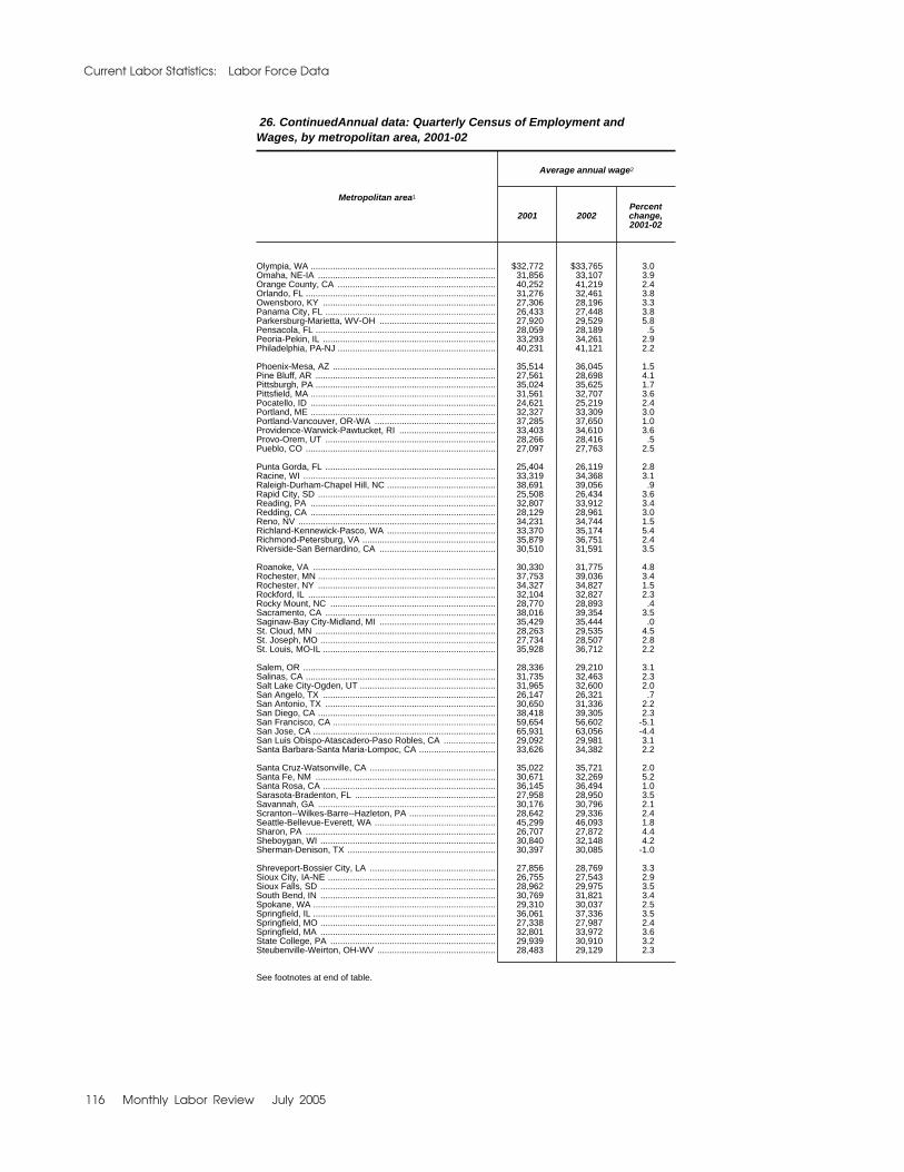
Current Labor Statistics: Labor Force Data
116 Monthly Labor Review July 2005
26. Continued�Annual data: Quarterly Census of Employment andWages, by metropolitan area, 2001-02
Metropolitan area1
Average annual wage2
2001 2002Percentchange,2001-02
Olympia, WA ........................................................................... $32,772 $33,765 3.0Omaha, NE-IA ........................................................................ 31,856 33,107 3.9Orange County, CA ................................................................ 40,252 41,219 2.4Orlando, FL ............................................................................. 31,276 32,461 3.8Owensboro, KY ...................................................................... 27,306 28,196 3.3Panama City, FL ..................................................................... 26,433 27,448 3.8Parkersburg-Marietta, WV-OH ............................................... 27,920 29,529 5.8Pensacola, FL ......................................................................... 28,059 28,189 .5Peoria-Pekin, IL ...................................................................... 33,293 34,261 2.9Philadelphia, PA-NJ ................................................................ 40,231 41,121 2.2
Phoenix-Mesa, AZ .................................................................. 35,514 36,045 1.5Pine Bluff, AR ......................................................................... 27,561 28,698 4.1Pittsburgh, PA ......................................................................... 35,024 35,625 1.7Pittsfield, MA ........................................................................... 31,561 32,707 3.6Pocatello, ID ........................................................................... 24,621 25,219 2.4Portland, ME ........................................................................... 32,327 33,309 3.0Portland-Vancouver, OR-WA ................................................. 37,285 37,650 1.0Providence-Warwick-Pawtucket, RI ....................................... 33,403 34,610 3.6Provo-Orem, UT ..................................................................... 28,266 28,416 .5Pueblo, CO ............................................................................. 27,097 27,763 2.5
Punta Gorda, FL ..................................................................... 25,404 26,119 2.8Racine, WI .............................................................................. 33,319 34,368 3.1Raleigh-Durham-Chapel Hill, NC ............................................ 38,691 39,056 .9Rapid City, SD ........................................................................ 25,508 26,434 3.6Reading, PA ........................................................................... 32,807 33,912 3.4Redding, CA ........................................................................... 28,129 28,961 3.0Reno, NV ................................................................................ 34,231 34,744 1.5Richland-Kennewick-Pasco, WA ............................................ 33,370 35,174 5.4Richmond-Petersburg, VA ...................................................... 35,879 36,751 2.4Riverside-San Bernardino, CA ............................................... 30,510 31,591 3.5
Roanoke, VA .......................................................................... 30,330 31,775 4.8Rochester, MN ........................................................................ 37,753 39,036 3.4Rochester, NY ........................................................................ 34,327 34,827 1.5Rockford, IL ............................................................................ 32,104 32,827 2.3Rocky Mount, NC ................................................................... 28,770 28,893 .4Sacramento, CA ..................................................................... 38,016 39,354 3.5Saginaw-Bay City-Midland, MI ............................................... 35,429 35,444 .0St. Cloud, MN ......................................................................... 28,263 29,535 4.5St. Joseph, MO ....................................................................... 27,734 28,507 2.8St. Louis, MO-IL ...................................................................... 35,928 36,712 2.2
Salem, OR .............................................................................. 28,336 29,210 3.1Salinas, CA ............................................................................. 31,735 32,463 2.3Salt Lake City-Ogden, UT ....................................................... 31,965 32,600 2.0San Angelo, TX ...................................................................... 26,147 26,321 .7San Antonio, TX ..................................................................... 30,650 31,336 2.2San Diego, CA ........................................................................ 38,418 39,305 2.3San Francisco, CA .................................................................. 59,654 56,602 -5.1San Jose, CA .......................................................................... 65,931 63,056 -4.4San Luis Obispo-Atascadero-Paso Robles, CA ..................... 29,092 29,981 3.1Santa Barbara-Santa Maria-Lompoc, CA ............................... 33,626 34,382 2.2
Santa Cruz-Watsonville, CA ................................................... 35,022 35,721 2.0Santa Fe, NM ......................................................................... 30,671 32,269 5.2Santa Rosa, CA ...................................................................... 36,145 36,494 1.0Sarasota-Bradenton, FL ......................................................... 27,958 28,950 3.5Savannah, GA ........................................................................ 30,176 30,796 2.1Scranton--Wilkes-Barre--Hazleton, PA ................................... 28,642 29,336 2.4Seattle-Bellevue-Everett, WA ................................................. 45,299 46,093 1.8Sharon, PA ............................................................................. 26,707 27,872 4.4Sheboygan, WI ....................................................................... 30,840 32,148 4.2Sherman-Denison, TX ............................................................ 30,397 30,085 -1.0
Shreveport-Bossier City, LA ................................................... 27,856 28,769 3.3Sioux City, IA-NE .................................................................... 26,755 27,543 2.9Sioux Falls, SD ....................................................................... 28,962 29,975 3.5South Bend, IN ....................................................................... 30,769 31,821 3.4Spokane, WA .......................................................................... 29,310 30,037 2.5Springfield, IL .......................................................................... 36,061 37,336 3.5Springfield, MO ....................................................................... 27,338 27,987 2.4Springfield, MA ....................................................................... 32,801 33,972 3.6State College, PA ................................................................... 29,939 30,910 3.2Steubenville-Weirton, OH-WV ................................................ 28,483 29,129 2.3
See footnotes at end of table.

Monthly Labor Review July 2005 117
26. Continued�Annual data: Quarterly Census of Employment andWages, by metropolitan area, 2001-02
Metropolitan area1
Average annual wage2
2001 2002Percentchange,2001-02
Stockton-Lodi, CA ................................................................... $30,818 $31,958 3.7Sumter, SC ............................................................................. 24,450 24,982 2.2Syracuse, NY .......................................................................... 32,254 33,752 4.6Tacoma, WA ........................................................................... 31,261 32,507 4.0Tallahassee, FL ...................................................................... 29,708 30,895 4.0Tampa-St. Petersburg-Clearwater, FL ................................... 31,678 32,458 2.5Terre Haute, IN ....................................................................... 27,334 28,415 4.0Texarkana, TX-Texarkana, AR ............................................... 26,492 27,717 4.6Toledo, OH ............................................................................. 32,299 33,513 3.8Topeka, KS ............................................................................. 30,513 31,707 3.9
Trenton, NJ ............................................................................. 46,831 47,969 2.4Tucson, AZ ............................................................................. 30,690 31,673 3.2Tulsa, OK ................................................................................ 31,904 32,241 1.1Tuscaloosa, AL ....................................................................... 29,972 30,745 2.6Tyler, TX ................................................................................. 30,551 31,050 1.6Utica-Rome, NY ...................................................................... 27,777 28,500 2.6Vallejo-Fairfield-Napa, CA ...................................................... 33,903 34,543 1.9Ventura, CA ............................................................................ 37,783 38,195 1.1Victoria, TX ............................................................................. 29,068 29,168 .3Vineland-Millville-Bridgeton, NJ .............................................. 32,571 33,625 3.2
Visalia-Tulare-Porterville, CA ................................................. 24,732 25,650 3.7Waco, TX ................................................................................ 28,245 28,885 2.3Washington, DC-MD-VA-WV .................................................. 47,589 48,430 1.8Waterloo-Cedar Falls, IA ........................................................ 29,119 29,916 2.7Wausau, WI ............................................................................ 29,402 30,292 3.0West Palm Beach-Boca Raton, FL ......................................... 35,957 36,550 1.6Wheeling, WV-OH .................................................................. 26,282 26,693 1.6Wichita, KS ............................................................................. 32,983 33,429 1.4Wichita Falls, TX ..................................................................... 25,557 26,387 3.2Williamsport, PA ..................................................................... 27,801 27,988 .7
Wilmington-Newark, DE-MD ................................................... 42,177 43,401 2.9Wilmington, NC ....................................................................... 29,287 29,157 -.4Yakima, WA ............................................................................ 24,204 24,934 3.0Yolo, CA ................................................................................. 35,352 35,591 .7York, PA ................................................................................. 31,936 32,609 2.1Youngstown-Warren, OH ....................................................... 28,789 29,799 3.5Yuba City, CA ......................................................................... 27,781 28,967 4.3Yuma, AZ ................................................................................ 22,415 23,429 4.5
Aguadilla, PR .......................................................................... 18,061 19,283 6.8Arecibo, PR ............................................................................ 16,600 18,063 8.8Caguas, PR ............................................................................ 18,655 19,706 5.6Mayaguez, PR ........................................................................ 17,101 17,500 2.3Ponce, PR .............................................................................. 17,397 18,187 4.5San Juan-Bayamon, PR ......................................................... 20,948 21,930 4.7
1 Includes data for Metropolitan Statistical Areas (MSA) and Primary Metropolitan Statistical Areas(PMSA) as defined by OMB Bulletin No. 99-04. In the New England areas, the New England CountyMetropolitan Area (NECMA) definitions were used.
2 Each year's total is based on the MSA definition for the specific year. Annual changes includedifferences resulting from changes in MSA definitions.
3 Totals do not include the six MSAs within Puerto Rico.
NOTE: Includes workers covered by Unemployment Insurance (UI) and Unemployment Compensationfor Federal Employees (UCFE) programs.

Current Labor Statistics: Labor Force Data
118 Monthly Labor Review July 2005
27. Annual data: Employment status of the population
[Numbers in thousands]Employment status 19941 1995 1996 19971 19981 19991 20001 2001 2002 2003 2004
Civilian noninstitutional population........... 196,814 198,584 200,591 203,133 205,220 207,753 212,577 215,092 217,570 221,168 223,357 Civilian labor force............................…… 131,056 132,304 133,943 136,297 137,673 139,368 142,583 143,734 144,863 146,510 147,401 Labor force participation rate.............. 66.6 66.6 66.8 67.1 67.1 67.1 67.1 66.8 66.6 66.2 66.0 Employed............................………… 123,060 124,900 126,708 129,558 131,463 133,488 136,891 136,933 136,485 137,736 139,252 Employment-population ratio......... 62.5 62.9 63.2 63.8 64.1 64.3 64.4 63.7 62.7 62.3 62.3 Unemployed............................……… 7,996 7,404 7,236 6,739 6,210 5,880 5,692 6,801 8,378 8,774 8,149 Unemployment rate........................ 6.1 5.6 5.4 4.9 4.5 4.2 4.0 4.7 5.8 6.0 5.5 Not in the labor force............................… 65,758 66,280 66,647 66,836 67,547 68,385 69,994 71,359 72,707 74,658 75,956
1 Not strictly comparable with prior years.
28. Annual data: Employment levels by industry
[In thousands]Industry 1994 1995 1996 1997 1998 1999 2000 2001 2002 2003 2004
Total private employment............................… 95,016 97,866 100,169 103,113 106,021 108,686 110,996 110,707 108,828 108,416 109,862
Total nonfarm employment…………………… 114,291 117,298 119,708 122,770 125,930 128,993 131,785 131,826 130,341 129,999 131,480 Goods-producing............................……… 22,774 23,156 23,410 23,886 24,354 24,465 24,649 23,873 22,557 21,816 21,884 Natural resources and mining................. 659 641 637 654 645 598 599 606 583 572 591 Construction............................…………… 5,095 5,274 5,536 5,813 6,149 6,545 6,787 6,826 6,716 6,735 6,964 Manufacturing............................………… 17,021 17,241 17,237 17,419 17,560 17,322 17,263 16,441 15,259 14,510 14,329
Private service-providing.......................... 72,242 74,710 76,759 79,227 81,667 84,221 86,346 86,834 86,271 86,599 87,978 Trade, transportation, and utilities.......... 23,128 23,834 24,239 24,700 25,186 25,771 26,225 25,983 25,497 25,287 25,510 Wholesale trade............................…… 5,247.3 5,433.1 5,522.0 5,663.9 5,795.2 5,892.5 5,933.2 5,772.7 5,652.3 5,607.5 5,654.9 Retail trade............................………… 13,490.8 13,896.7 14,142.5 14,388.9 14,609.3 14,970.1 15,279.8 15,238.6 15,025.1 14,917.3 15,034.7 Transportation and warehousing......... 3,701.0 3,837.8 3,935.3 4,026.5 4,168.0 4,300.3 4,410.3 4,372.0 4,223.6 4,185.4 4,250.0 Utilities............................……………… 689.3 666.2 639.6 620.9 613.4 608.5 601.3 599.4 596.2 577.0 570.2 Information............................…………… 2,738 2,843 2,940 3,084 3,218 3,419 3,631 3,629 3,395 3,188 3,138 Financial activities............................…… 6,867 6,827 6,969 7,178 7,462 7,648 7,687 7,807 7,847 7,977 8,052 Professional and business services…… 12,174 12,844 13,462 14,335 15,147 15,957 16,666 16,476 15,976 15,987 16,414 Education and health services………… 12,807 13,289 13,683 14,087 14,446 14,798 15,109 15,645 16,199 16,588 16,954 Leisure and hospitality…………………… 10,100 10,501 10,777 11,018 11,232 11,543 11,862 12,036 11,986 12,173 12,479 Other services…………………………… 4,428 4,572 4,690 4,825 4,976 5,087 5,168 5,258 5,372 5,401 5,431
Government…………………………………… 19,275 19,432 19,539 19,664 19,909 20,307 20,790 21,118 21,513 21,583 21,618

Monthly Labor Review July 2005 119
29. Annual data: Average hours and earnings of production or nonsupervisory workers on nonfarm payrolls, by industry
Industry 1994 1995 1996 1997 1998 1999 2000 2001 2002 2003 2004
Private sector: Average weekly hours.......……................................ 34.5 34.3 34.3 34.5 34.5 34.3 34.3 34.0 33.9 33.7 33.7 Average hourly earnings (in dollars)......................... 11.32 11.64 12.03 12.49 13.00 13.47 14.00 14.53 14.95 15.35 15.67 Average weekly earnings (in dollars)........................ 390.73 399.53 412.74 431.25 448.04 462.49 480.41 493.20 506.07 517.30 528.56
Goods-producing: Average weekly hours............................................ 41.1 40.8 40.8 41.1 40.8 40.8 40.7 39.9 39.9 39.8 40.0 Average hourly earnings (in dollars)....................... 12.63 12.96 13.38 13.82 14.23 14.71 15.27 15.78 16.33 16.80 17.19 Average weekly earnings (in dollars)...................... 519.58 528.62 546.48 568.43 580.99 599.99 621.86 630.04 651.61 669.13 688.03
Natural resources and mining Average weekly hours........................................... 45.3 45.3 46.0 46.2 44.9 44.2 44.4 44.6 43.2 43.6 44.5 Average hourly earnings (in dollars)...................... 14.41 14.78 15.10 15.57 16.20 16.33 16.55 17.00 17.19 17.56 18.08 Average weekly earnings (in dollars)..................... 653.14 670.32 695.07 720.11 727.28 721.74 734.92 757.92 741.97 765.94 804.03 Construction: Average weekly hours........................................... 38.8 38.8 38.9 38.9 38.8 39.0 39.2 38.7 38.4 38.4 38.3 Average hourly earnings (in dollars)...................... 14.38 14.73 15.11 15.67 16.23 16.80 17.48 18.00 18.52 18.95 19.23 Average weekly earnings (in dollars)..................... 558.53 571.57 588.48 609.48 629.75 655.11 685.78 695.89 711.82 726.83 735.70 Manufacturing: Average weekly hours........................................... 41.7 41.3 41.3 41.7 41.4 41.4 41.3 40.3 40.5 40.4 40.8 Average hourly earnings (in dollars)...................... 12.04 12.34 12.75 13.14 13.45 13.85 14.32 14.76 15.29 15.74 16.14 Average weekly earnings (in dollars)..................... 502.12 509.26 526.55 548.22 557.12 573.17 590.65 595.19 618.75 635.99 658.53
Private service-providing: Average weekly hours..………................................ 32.7 32.6 32.6 32.8 32.8 32.7 32.7 32.5 32.5 32.4 32.3 Average hourly earnings (in dollars)....................... 10.87 11.19 11.57 12.05 12.59 13.07 13.60 14.16 14.56 14.96 15.26 Average weekly earnings (in dollars)...................... 354.97 364.14 376.72 394.77 412.78 427.30 445.00 460.32 472.88 483.89 493.67
Trade, transportation, and utilities: Average weekly hours............................................ 34.3 34.1 34.1 34.3 34.2 33.9 33.8 33.5 33.6 33.6 33.5 Average hourly earnings (in dollars)....................... 10.80 11.10 11.46 11.90 12.39 12.82 13.31 13.70 14.02 14.34 14.59 Average weekly earnings (in dollars)...................... 370.38 378.79 390.64 407.57 423.30 434.31 449.88 459.53 471.27 481.14 488.58 Wholesale trade: Average weekly hours........................................ 38.8 38.6 38.6 38.8 38.6 38.6 38.8 38.4 38.0 37.9 37.8 Average hourly earnings (in dollars)................... 12.93 13.34 13.80 14.41 15.07 15.62 16.28 16.77 16.98 17.36 17.66 Average weekly earnings (in dollars).................. 501.17 515.14 533.29 559.39 582.21 602.77 631.40 643.45 644.38 657.29 666.93 Retail trade: Average weekly hours........................................ 30.9 30.8 30.7 30.9 30.9 30.8 30.7 30.7 30.9 30.9 30.7 Average hourly earnings (in dollars)................... 8.61 8.85 9.21 9.59 10.05 10.45 10.86 11.29 11.67 11.90 12.08 Average weekly earnings (in dollars).................. 501.17 515.14 533.29 559.39 582.21 602.77 631.40 643.45 644.38 657.29 666.93 Transportation and warehousing: Average weekly hours........................................ 39.5 38.9 39.1 39.4 38.7 37.6 37.4 36.7 36.8 36.8 37.2 Average hourly earnings (in dollars)................... 12.84 13.18 13.45 13.78 14.12 14.55 15.05 15.33 15.76 16.25 16.53 Average weekly earnings (in dollars).................. 507.27 513.37 525.60 542.55 546.86 547.97 562.31 562.70 579.75 598.41 614.90 Utilities: Average weekly hours........................................ 42.3 42.3 42.0 42.0 42.0 42.0 42.0 41.4 40.9 41.1 40.9 Average hourly earnings (in dollars)................... 18.66 19.19 19.78 20.59 21.48 22.03 22.75 23.58 23.96 24.77 25.62 Average weekly earnings (in dollars).................. 789.98 811.52 830.74 865.26 902.94 924.59 955.66 977.18 979.09 1,017.27 1,048.82 Information: Average weekly hours........................................ 36.0 36.0 36.4 36.3 36.6 36.7 36.8 36.9 36.5 36.2 36.3 Average hourly earnings (in dollars)................... 15.32 15.68 16.30 17.14 17.67 18.40 19.07 19.80 20.20 21.01 21.42 Average weekly earnings (in dollars).................. 551.28 564.98 592.68 622.40 646.52 675.32 700.89 731.11 738.17 760.81 777.42 Financial activities: Average weekly hours........................................ 35.5 35.5 35.5 35.7 36.0 35.8 35.9 35.8 35.6 35.5 35.5 Average hourly earnings (in dollars)................... 11.82 12.28 12.71 13.22 13.93 14.47 14.98 15.59 16.17 17.14 17.53 Average weekly earnings (in dollars).................. 419.20 436.12 451.49 472.37 500.95 517.57 537.37 558.02 575.51 609.08 622.99 Professional and business services: Average weekly hours........................................ 34.1 34.0 34.1 34.3 34.3 34.4 34.5 34.2 34.2 34.1 34.2 Average hourly earnings (in dollars)................... 12.15 12.53 13.00 13.57 14.27 14.85 15.52 16.33 16.81 17.21 17.46 Average weekly earnings (in dollars).................. 414.16 426.44 442.81 465.51 490.00 510.99 535.07 557.84 574.66 587.02 596.96 Education and health services: Average weekly hours........................................ 32.0 32.0 31.9 32.2 32.2 32.1 32.2 32.3 32.4 32.3 32.4 Average hourly earnings (in dollars)................... 11.50 11.80 12.17 12.56 13.00 13.44 13.95 14.64 15.21 15.64 16.16 Average weekly earnings (in dollars).................. 368.14 377.73 388.27 404.65 418.82 431.35 449.29 473.39 492.74 505.69 523.83 Leisure and hospitality: Average weekly hours........................................ 26.0 25.9 25.9 26.0 26.2 26.1 26.1 25.8 25.8 25.6 25.7 Average hourly earnings (in dollars)................... 6.46 6.62 6.82 7.13 7.48 7.76 8.11 8.35 8.58 8.76 8.91 Average weekly earnings (in dollars).................. 168.00 171.43 176.48 185.81 195.82 202.87 211.79 215.19 221.26 224.30 228.63 Other services: Average weekly hours........................................ 32.7 32.6 32.5 32.7 32.6 32.5 32.5 32.3 32.0 31.4 31.0 Average hourly earnings (in dollars)................... 10.18 10.51 10.85 11.29 11.79 12.26 12.73 13.27 13.72 13.84 13.98 Average weekly earnings (in dollars).................. 332.44 342.36 352.62 368.63 384.25 398.77 413.41 428.64 439.76 434.41 433.04
NOTE: Data reflect the conversion to the 2002 version of the North American Industry Classification System (NAICS), replacing the Standard Industrial Classification
(SIC) system. NAICS-based data by industry are not comparable with SIC-based data.
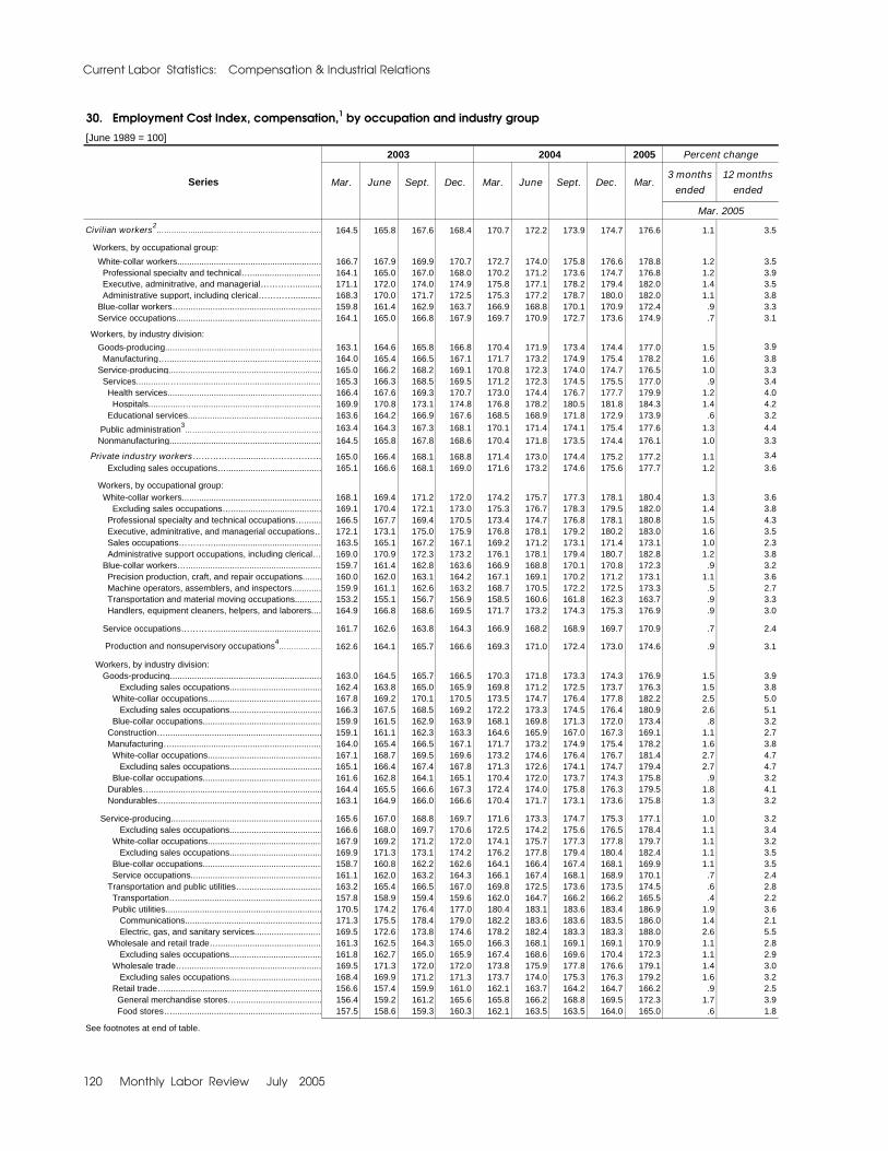
Current Labor Statistics: Compensation & Industrial Relations
120 Monthly Labor Review July 2005
30. Employment Cost Index, compensation,1 by occupation and industry group
[June 1989 = 100]
2003 2004 2005 Percent change
Series Mar. June Sept. Dec. Mar. June Sept. Dec. Mar.3 months
ended
12 months
ended
Mar. 2005
Civilian workers2……….…….........…………………………………….… 164.5 165.8 167.6 168.4 170.7 172.2 173.9 174.7 176.6 1.1 3.5
Workers, by occupational group:
White-collar workers........................................................... 166.7 167.9 169.9 170.7 172.7 174.0 175.8 176.6 178.8 1.2 3.5 Professional specialty and technical…............................. 164.1 165.0 167.0 168.0 170.2 171.2 173.6 174.7 176.8 1.2 3.9 Executive, adminitrative, and managerial…………........... 171.1 172.0 174.0 174.9 175.8 177.1 178.2 179.4 182.0 1.4 3.5 Administrative support, including clerical…………............ 168.3 170.0 171.7 172.5 175.3 177.2 178.7 180.0 182.0 1.1 3.8 Blue-collar workers….......................................................... 159.8 161.4 162.9 163.7 166.9 168.8 170.1 170.9 172.4 .9 3.3 Service occupations............................................................ 164.1 165.0 166.8 167.9 169.7 170.9 172.7 173.6 174.9 .7 3.1
Workers, by industry division:
Goods-producing................................................................ 163.1 164.6 165.8 166.8 170.4 171.9 173.4 174.4 177.0 1.5 3.9 Manufacturing…............................................................... 164.0 165.4 166.5 167.1 171.7 173.2 174.9 175.4 178.2 1.6 3.8 Service-producing............................................................... 165.0 166.2 168.2 169.1 170.8 172.3 174.0 174.7 176.5 1.0 3.3 Services..............….......................................................... 165.3 166.3 168.5 169.5 171.2 172.3 174.5 175.5 177.0 .9 3.4 Health services............................................................... 166.4 167.6 169.3 170.7 173.0 174.4 176.7 177.7 179.9 1.2 4.0 Hospitals..............…..................................................... 169.9 170.8 173.1 174.8 176.8 178.2 180.5 181.8 184.3 1.4 4.2 Educational services....................................................... 163.6 164.2 166.9 167.6 168.5 168.9 171.8 172.9 173.9 .6 3.2
Public administration3……….………………………………………… 163.4 164.3 167.3 168.1 170.1 171.4 174.1 175.4 177.6 1.3 4.4
Nonmanufacturing.............................................................. 164.5 165.8 167.8 168.6 170.4 171.8 173.5 174.4 176.1 1.0 3.3
Private industry workers……….…….........………………… 165.0 166.4 168.1 168.8 171.4 173.0 174.4 175.2 177.2 1.1 3.4
Excluding sales occupations…....................................... 165.1 166.6 168.1 169.0 171.6 173.2 174.6 175.6 177.7 1.2 3.6
Workers, by occupational group: White-collar workers......................................................... 168.1 169.4 171.2 172.0 174.2 175.7 177.3 178.1 180.4 1.3 3.6 Excluding sales occupations…..................................... 169.1 170.4 172.1 173.0 175.3 176.7 178.3 179.5 182.0 1.4 3.8 Professional specialty and technical occupations…....... 166.5 167.7 169.4 170.5 173.4 174.7 176.8 178.1 180.8 1.5 4.3 Executive, adminitrative, and managerial occupations… 172.1 173.1 175.0 175.9 176.8 178.1 179.2 180.2 183.0 1.6 3.5 Sales occupations…………............................................ 163.5 165.1 167.2 167.1 169.2 171.2 173.1 171.4 173.1 1.0 2.3 Administrative support occupations, including clerical… 169.0 170.9 172.3 173.2 176.1 178.1 179.4 180.7 182.8 1.2 3.8 Blue-collar workers…........................................................ 159.7 161.4 162.8 163.6 166.9 168.8 170.1 170.8 172.3 .9 3.2 Precision production, craft, and repair occupations........ 160.0 162.0 163.1 164.2 167.1 169.1 170.2 171.2 173.1 1.1 3.6 Machine operators, assemblers, and inspectors............ 159.9 161.1 162.6 163.2 168.7 170.5 172.2 172.5 173.3 .5 2.7 Transportation and material moving occupations........... 153.2 155.1 156.7 156.9 158.5 160.6 161.8 162.3 163.7 .9 3.3 Handlers, equipment cleaners, helpers, and laborers.... 164.9 166.8 168.6 169.5 171.7 173.2 174.3 175.3 176.9 .9 3.0
Service occupations…………........................................... 161.7 162.6 163.8 164.3 166.9 168.2 168.9 169.7 170.9 .7 2.4
Production and nonsupervisory occupations4……….……… 162.6 164.1 165.7 166.6 169.3 171.0 172.4 173.0 174.6 .9 3.1
Workers, by industry division: Goods-producing.............................................................. 163.0 164.5 165.7 166.5 170.3 171.8 173.3 174.3 176.9 1.5 3.9 Excluding sales occupations...................................... 162.4 163.8 165.0 165.9 169.8 171.2 172.5 173.7 176.3 1.5 3.8 White-collar occupations............................................... 167.8 169.2 170.1 170.5 173.5 174.7 176.4 177.8 182.2 2.5 5.0 Excluding sales occupations...................................... 166.3 167.5 168.5 169.2 172.2 173.3 174.5 176.4 180.9 2.6 5.1 Blue-collar occupations................................................. 159.9 161.5 162.9 163.9 168.1 169.8 171.3 172.0 173.4 .8 3.2 Construction…................................................................ 159.1 161.1 162.3 163.3 164.6 165.9 167.0 167.3 169.1 1.1 2.7 Manufacturing…............................................................. 164.0 165.4 166.5 167.1 171.7 173.2 174.9 175.4 178.2 1.6 3.8 White-collar occupations............................................... 167.1 168.7 169.5 169.6 173.2 174.6 176.4 176.7 181.4 2.7 4.7 Excluding sales occupations...................................... 165.1 166.4 167.4 167.8 171.3 172.6 174.1 174.7 179.4 2.7 4.7 Blue-collar occupations................................................. 161.6 162.8 164.1 165.1 170.4 172.0 173.7 174.3 175.8 .9 3.2 Durables…...................................................................... 164.4 165.5 166.6 167.3 172.4 174.0 175.8 176.3 179.5 1.8 4.1 Nondurables…................................................................ 163.1 164.9 166.0 166.6 170.4 171.7 173.1 173.6 175.8 1.3 3.2
Service-producing.............................................................. 165.6 167.0 168.8 169.7 171.6 173.3 174.7 175.3 177.1 1.0 3.2 Excluding sales occupations...................................... 166.6 168.0 169.7 170.6 172.5 174.2 175.6 176.5 178.4 1.1 3.4 White-collar occupations............................................... 167.9 169.2 171.2 172.0 174.1 175.7 177.3 177.8 179.7 1.1 3.2 Excluding sales occupations...................................... 169.9 171.3 173.1 174.2 176.2 177.8 179.4 180.4 182.4 1.1 3.5 Blue-collar occupations................................................. 158.7 160.8 162.2 162.6 164.1 166.4 167.4 168.1 169.9 1.1 3.5 Service occupations...................................................... 161.1 162.0 163.2 164.3 166.1 167.4 168.1 168.9 170.1 .7 2.4 Transportation and public utilities…................................ 163.2 165.4 166.5 167.0 169.8 172.5 173.6 173.5 174.5 .6 2.8 Transportation…........................................................... 157.8 158.9 159.4 159.6 162.0 164.7 166.2 166.2 165.5 .4 2.2 Public utilities................................................................ 170.5 174.2 176.4 177.0 180.4 183.1 183.6 183.4 186.9 1.9 3.6 Communications........................................................ 171.3 175.5 178.4 179.0 182.2 183.6 183.6 183.5 186.0 1.4 2.1 Electric, gas, and sanitary services............................ 169.5 172.6 173.8 174.6 178.2 182.4 183.3 183.3 188.0 2.6 5.5 Wholesale and retail trade….......................................... 161.3 162.5 164.3 165.0 166.3 168.1 169.1 169.1 170.9 1.1 2.8 Excluding sales occupations...................................... 161.8 162.7 165.0 165.9 167.4 168.6 169.6 170.4 172.3 1.1 2.9 Wholesale trade…........................................................ 169.5 171.3 172.0 172.0 173.8 175.9 177.8 176.6 179.1 1.4 3.0 Excluding sales occupations...................................... 168.4 169.9 171.2 171.3 173.7 174.0 175.3 176.3 179.2 1.6 3.2 Retail trade…................................................................ 156.6 157.4 159.9 161.0 162.1 163.7 164.2 164.7 166.2 .9 2.5 General merchandise stores…................................... 156.4 159.2 161.2 165.6 165.8 166.2 168.8 169.5 172.3 1.7 3.9 Food stores…............................................................. 157.5 158.6 159.3 160.3 162.1 163.5 163.5 164.0 165.0 .6 1.8
See footnotes at end of table.

Monthly Labor Review July 2005 121
30. Continued–Employment Cost Index, compensation,1 by occupation and industry group
[June 1989 = 100]
2003 2004 2005 Percent change
Series Mar. June Sept. Dec. Mar. June Sept. Dec. Mar.3 months
ended
12 months
ended
Mar. 2005
Finance, insurance, and real estate…............................ 176.7 178.3 180.2 180.9 182.5 183.6 184.8 186.0 188.9 1.6 3.5
Excluding sales occupations….................................. 182.0 184.0 1,853.0 186.1 186.6 188.7 190.9 191.2 194.3 1.6 4.1 Banking, savings and loan, and other credit agencies.. 204.3 206.3 207.6 209.0 207.2 208.9 210.5 212.3 213.7 .7 3.1 Insurance...................................................................... 172.1 173.9 175.1 176.2 177.8 180.5 182.1 183.6 186.3 1.5 4.8 Services.......................................................................... 167.1 168.4 170.4 171.4 173.5 175.1 176.9 177.9 179.7 1.0 3.6 Business services…...................................................... 168.5 169.2 171.9 172.6 174.8 176.9 178.5 179.1 180.1 .6 3.0 Health services............................................................. 166.5 167.9 169.4 170.8 173.3 174.8 177.0 178.0 180.3 1.3 4.0 Hospitals…................................................................. 170.8 171.9 173.9 175.9 178.1 179.7 181.8 183.2 185.8 1.4 4.3 Educational services..................................................... 176.3 177.1 180.2 181.3 183.1 184.2 187.0 188.5 190.0 .8 3.8 Colleges and universities…........................................ 174.5 175.4 178.4 179.4 181.2 182.5 185.2 186.2 187.6 .8 3.5
Nonmanufacturing.......................................................... 164.9 166.4 168.1 169.0 170.9 172.5 173.9 174.7 176.5 1.0 3.3
White-collar workers..................................................... 168.0 169.3 171.2 172.1 174.1 175.7 177.2 178.0 180.0 1.1 3.4 Excluding sales occupations…................................. 170.0 171.4 173.2 174.2 176.2 177.7 179.3 180.6 182.7 1.2 3.7 Blue-collar occupations…............................................. 157.5 159.7 161.1 161.7 163.4 165.5 166.4 167.3 168.8 .9 3.3 Service occupations…………....................................... 161.1 162.0 163.2 162.4 166.0 167.3 168.0 168.9 170.1 .7 2.5
State and local government workers................................... 162.6 163.2 165.9 166.8 168.0 168.7 171.5 172.6 174.1 .9 3.6
Workers, by occupational group:
White-collar workers........................................................... 161.7 162.2 164.9 165.7 166.8 167.5 170.0 171.2 172.6 .8 3.5 Professional specialty and technical…............................. 160.2 160.8 163.4 164.1 165.1 165.6 168.4 169.4 170.4 .6 3.2 Executive, administrative, and managerial…………......... 165.3 165.7 168.0 169.1 170.1 171.0 172.1 174.3 176.7 1.4 3.9 Administrative support, including clerical…………............ 163.8 164.4 167.9 168.5 170.4 171.8 174.3 175.5 177.2 1.0 4.0 Blue-collar workers….......................................................... 161.3 161.7 163.6 165.2 166.7 167.5 169.9 171.0 172.6 .9 3.5
Workers, by industry division:
Services............................................................................ 161.8 162.3 164.9 165.7 166.5 166.8 169.7 170.8 171.8 .6 3.2
Services excluding schools5……….……………………………… 164.0 164.2 166.8 168.2 169.4 170.1 173.0 173.8 175.6 1.0 3.7
Health services............................................................. 166.4 166.7 169.5 171.0 172.2 172.9 175.7 176.8 178.9 1.2 3.9 Hospitals.................................................................... 167.0 167.3 170.3 171.4 172.4 173.2 176.3 177.4 179.1 1.0 3.9 Educational services..................................................... 161.1 161.7 164.3 165.0 165.7 165.9 168.8 169.9 170.9 .6 3.1 Schools...................................................................... 161.4 162.0 164.7 165.3 166.0 166.3 169.2 170.3 171.2 .5 3.1 Elementary and secondary….................................. 159.4 160.0 163.0 163.7 164.4 164.6 168.0 169.2 169.8 .4 3.3 Colleges and universities…..................................... 167.0 167.5 169.2 170.0 170.7 171.0 172.4 173.2 175.1 1.1 2.6
Public administration3……….………………………………………… 163.4 164.3 167.3 168.1 170.1 171.4 174.1 175.4 177.6 1.3 4.4
1 Cost (cents per hour worked) measured in the Employment Cost Index consists ofwages, salaries, and employer cost of employee benefits.
2 Consists of private industry workers (excluding farm and household workers) andState and local government (excluding Federal Government) workers.
3 Consists of legislative, judicial, administrative, and regulatory activities.4 This series has the same industry and occupational coverage as the Hourly
Earnings index, which was discontinued in January 1989. 5 Includes, for example, library, social, and health services.

Current Labor Statistics: Compensation & Industrial Relations
122 Monthly Labor Review July 2005
31. Employment Cost Index, wages and salaries, by occupation and industry group[June 1989 = 100]
2003 2004 2005 Percent change
SeriesMar. June Sept. Dec. Mar. June Sept. Dec. Mar.
3 months
ended
12 months
ended
Mar. 2005
Civilian workers1……….…….........…………………………………….… 159.3 160.3 161.8 162.3 163.3 164.3 165.7 166.2 167.3 0.7 2.4
Workers, by occupational group: White-collar workers........................................................... 161.9 162.9 164.5 165.1 166.1 167.1 168.7 169.1 170.3 .7 2.5 Professional specialty and technical…............................. 159.3 160.1 161.8 162.5 163.8 164.4 166.5 167.0 168.1 .7 2.6 Executive, adminitrative, and managerial…………........... 167.9 169.0 170.5 171.2 171.4 172.4 173.4 174.4 175.9 .9 2.6 Administrative support, including clerical…………............ 161.8 163.1 164.3 164.9 166.3 167.5 168.8 169.7 170.9 .7 2.8 Blue-collar workers….......................................................... 153.8 154.8 155.8 156.3 157.3 158.4 159.7 160.0 161.0 .6 2.4 Service occupations............................................................ 158.0 158.7 159.8 160.6 161.2 161.9 162.8 163.6 164.4 .5 2.0
Workers, by industry division: Goods-producing................................................................ 156.3 157.5 158.3 160.6 159.9 161.0 162.3 162.4 163.8 .7 2.3 Manufacturing…............................................................... 158.0 159.0 159.7 160.1 161.3 162.4 163.8 164.0 165.3 .8 2.5 Service-producing............................................................... 160.5 161.4 163.0 163.6 164.6 165.5 167.0 167.5 168.6 .7 2.4 Services..............….......................................................... 161.9 162.8 164.7 165.4 166.5 167.4 167.3 170.1 171.2 .6 2.8 Health services............................................................... 162.0 163.2 164.7 165.9 167.7 168.6 170.8 171.7 173.2 .9 3.3 Hospitals..............…..................................................... 163.5 164.4 166.3 167.7 169.0 169.9 171.8 173.2 174.7 .9 3.4 Educational services....................................................... 160.4 160.7 162.7 163.2 163.6 163.8 166.0 166.8 167.5 .4 2.4
Public administration2……….………………………………………… 157.2 158.0 159.4 160.0 161.1 161.4 162.6 163.5 165.0 .9 2.4
Nonmanufacturing.............................................................. 159.6 160.5 162.1 162.7 163.7 164.6 166.0 166.5 167.6 .7 2.4
Private industry workers……….…….........………………… 159.3 160.4 161.7 162.3 163.4 164.5 165.9 166.2 167.4 .7 2.4 Excluding sales occupations…....................................... 159.4 160.5 161.7 162.4 163.5 164.5 165.8 166.5 167.6 .7 2.5
Workers, by occupational group: White-collar workers......................................................... 162.6 163.8 165.3 165.9 167.1 168.2 169.7 170.0 171.3 .8 2.5 Excluding sales occupations…..................................... 163.6 164.8 166.2 167.0 168.1 169.2 170.6 171.4 172.7 .8 2.7 Professional specialty and technical occupations…....... 159.5 160.5 162.1 163.0 164.7 165.5 167.6 168.0 169.4 .8 2.9 Executive, adminitrative, and managerial occupations… 169.1 170.3 171.8 172.5 172.7 173.9 174.9 175.7 177.2 .9 2.6 Sales occupations…………............................................ 158.1 159.3 161.6 161.1 162.6 163.9 165.9 164.0 164.9 .5 1.4 Administrative support occupations, including clerical… 162.6 164.0 165.1 165.7 167.2 168.6 169.7 170.8 172.0 .7 2.9 Blue-collar workers…........................................................ 153.6 154.6 155.6 156.1 157.2 158.3 159.5 159.9 160.8 .6 2.3 Precision production, craft, and repair occupations........ 153.4 154.7 155.5 156.2 157.1 158.3 159.3 159.7 160.4 .4 2.1 Machine operators, assemblers, and inspectors............ 154.7 155.3 156.8 156.9 158.6 159.8 161.6 161.6 162.6 .6 2.5 Transportation and material moving occupations........... 147.8 149.0 149.8 149.8 150.4 151.8 152.9 153.3 154.4 .7 2.7 Handlers, equipment cleaners, helpers, and laborers.... 158.4 159.0 159.9 160.6 161.8 162.7 163.6 164.5 165.6 .7 2.3
Service occupations…………........................................... 155.5 156.1 157.1 157.8 158.4 159.3 159.8 160.6 161.4 .5 1.9
Production and nonsupervisory occupations3……….……… 156.4 157.4 158.8 159.4 160.7 161.7 163.1 163.4 164.5 .7 2.4
Workers, by industry division: Goods-producing.............................................................. 156.3 157.4 158.3 158.7 159.9 160.9 162.3 162.4 163.6 .7 2.3 Excluding sales occupations...................................... 155.4 156.5 157.4 158.0 159.2 160.2 161.2 161.6 162.8 .7 2.3 White-collar occupations............................................... 160.0 161.4 161.9 162.1 163.2 164.5 166.0 165.9 167.3 .8 2.5 Excluding sales occupations...................................... 158.0 159.2 159.9 160.4 161.5 162.7 163.6 164.1 165.3 .7 2.4 Blue-collar occupations................................................. 153.8 154.8 155.9 156.4 157.7 158.6 159.8 160.1 161.2 .3 2.2 Construction…................................................................ 150.6 152.4 153.6 154.0 155.1 155.9 157.1 157.0 157.7 .4 1.7 Manufacturing…............................................................. 158.0 159.0 159.7 160.1 161.3 162.4 163.8 164.0 165.3 .8 2.5 White-collar occupations............................................... 160.1 161.6 162.0 162.1 163.3 164.7 166.1 166.1 167.6 .9 2.6 Excluding sales occupations...................................... 157.7 158.9 159.5 160.0 161.2 162.5 163.5 163.9 165.1 .7 2.4 Blue-collar occupations................................................. 156.3 156.9 157.9 158.5 159.8 160.6 162.1 162.4 163.6 .7 2.4 Durables…...................................................................... 158.8 159.7 160.6 160.9 161.9 162.9 164.5 164.7 165.9 .7 2.5 Nondurables…................................................................ 156.6 157.8 158.3 158.7 160.4 161.6 162.8 162.9 164.5 1.0 2.6
Service-producing.............................................................. 160.6 161.7 163.3 163.9 165.0 166.1 167.5 167.9 169.0 .7 2.4 Excluding sales occupations...................................... 161.7 162.8 164.2 165.0 166.0 167.1 168.5 169.3 170.4 .6 2.7 White-collar occupations............................................... 163.0 164.1 166.0 166.6 167.8 168.9 170.4 170.8 172.1 .8 2.6 Excluding sales occupations...................................... 165.3 166.5 168.2 169.0 170.2 171.2 172.8 173.6 175.0 .8 2.8 Blue-collar occupations................................................. 153.2 154.3 155.1 155.4 156.2 157.8 158.9 159.4 160.1 .4 2.5 Service occupations...................................................... 155.1 155.6 156.6 157.4 158.0 158.8 159.4 160.2 160.9 .4 1.8 Transportation and public utilities…................................ 154.8 155.6 156.0 156.5 157.6 159.1 160.4 160.5 159.8 –.4 1.4 Transportation…........................................................... 150.5 150.6 150.4 150.8 151.7 153.4 155.0 155.1 153.4 –1.1 1.1 Public utilities................................................................ 160.4 162.1 163.4 164.1 165.3 166.4 167.5 167.5 168.2 .4 1.8 Communications........................................................ 161.9 163.4 165.4 165.9 167.0 167.5 168.8 168.3 168.4 .1 .8 Electric, gas, and sanitary services............................ 158.6 160.4 161.0 161.8 163.3 165.1 165.9 166.6 167.9 .8 2.8 Wholesale and retail trade….......................................... 156.7 157.5 159.2 159.5 160.3 161.6 162.5 162.1 163.4 .8 1.9 Wholesale trade…........................................................ 163.4 164.7 164.8 165.3 166.2 167.8 169.7 167.5 169.5 1.2 2.0 Excluding sales occupations...................................... 163.9 165.2 165.7 166.3 167.8 167.6 168.6 168.9 171.5 1.5 2.2 Retail trade…................................................................ 153.1 153.8 156.3 156.5 157.3 158.4 158.7 159.3 160.3 .6 1.9 General merchandise stores…................................... 149.8 152.0 153.1 153.6 154.1 154.9 157.5 158.1 159.3 .8 3.4 Food stores…............................................................. 151.0 151.6 152.2 152.8 153.8 154.3 154.5 155.0 155.8 .5 1.3See footnotes at end of table.

Monthly Labor Review July 2005 123
31. Continued–Employment Cost Index, wages and salaries, by occupation and industry group[June 1989 = 100]
2003 2004 2005 Percent change
SeriesMar. June Sept. Dec. Mar. June Sept. Dec. Mar.
3 months
ended
12 months
ended
Mar. 2005
Finance, insurance, and real estate…............................ 171.1 172.4 174.1 174.5 175.2 175.3 176.5 177.7 179.2 0.8 2.3 Excluding sales occupations….................................. 176.7 178.5 179.2 210.2 179.2 180.5 181.8 182.9 184.6 .9 3.0 Banking, savings and loan, and other credit agencies.. 206.4 208.7 209.1 164.5 206.7 207.6 209.5 211.3 210.7 –.3 1.9 Insurance...................................................................... 161.6 163.0 163.9 164.5 165.1 167.2 168.9 170.4 171.7 .8 4.0 Services.......................................................................... 162.8 164.0 165.9 166.7 168.1 169.3 171.1 172.0 173.4 .8 3.2 Business services…...................................................... 165.6 166.4 169.1 169.8 171.0 172.7 174.3 175.0 175.5 .3 2.6 Health services............................................................. 161.9 163.2 164.6 135.8 167.8 168.8 170.9 171.9 173.4 .9 3.3 Hospitals…................................................................. 163.6 164.6 166.5 167.9 169.4 170.5 172.4 173.8 175.4 .9 3.5 Educational services..................................................... 167.1 167.5 170.3 171.0 171.9 172.6 175.5 176.8 177.9 .6 3.5 Colleges and universities…........................................ 164.4 165.1 167.6 168.4 169.5 170.0 172.9 173.6 174.6 .6 3.0
Nonmanufacturing.......................................................... 159.4 160.5 162.1 162.6 163.7 164.8 166.2 166.6 167.7 .7 2.4 White-collar workers..................................................... 162.8 163.9 165.7 166.3 167.5 168.6 170.1 170.5 171.7 .7 2.5 Excluding sales occupations…................................. 164.9 166.1 167.7 168.5 169.7 170.7 172.3 173.1 174.4 .8 2.8 Blue-collar occupations…............................................. 151.1 152.4 153.4 153.8 154.7 156.1 157.1 157.5 158.2 .4 2.3 Service occupations…………....................................... 155.0 155.5 156.5 157.3 157.9 158.7 159.2 160.1 160.8 .4 1.8
State and local government workers............………………… 162.6 163.2 165.9 166.8 168.0 168.7 171.5 172.6 174.1 .6 2.3
Workers, by occupational group: White-collar workers........................................................... 158.9 159.2 161.0 161.5 162.1 162.4 164.1 164.9 165.9 .6 2.3 Professional specialty and technical…............................. 158.8 159.1 161.0 161.4 162.1 162.3 164.4 165.0 165.7 .4 2.2 Executive, administrative, and managerial…………......... 160.9 161.0 162.5 163.3 163.5 163.8 164.3 166.1 168.2 1.3 2.9 Administrative support, including clerical…………............ 156.9 157.2 159.1 159.5 160.4 160.8 162.6 163.0 163.9 .6 2.2 Blue-collar workers….......................................................... 156.2 156.5 157.6 158.3 158.9 159.2 160.7 161.4 162.4 .6 2.2
Workers, by industry division: Services............................................................................ 159.5 159.8 161.6 162.1 162.6 162.7 164.8 165.5 166.2 .4 2.2
Services excluding schools4……….……………………………… 161.4 161.8 163.2 164.5 165.1 165.6 167.5 168.3 169.4 .7 2.6
Health services............................................................. 162.9 163.5 165.1 166.7 167.4 167.8 169.6 170.7 171.9 .7 2.7 Hospitals.................................................................... 163.1 163.8 165.5 166.7 167.4 167.9 169.9 171.0 172.0 .6 2.7 Educational services..................................................... 159.1 159.3 161.2 161.6 162.0 162.1 164.2 164.9 165.5 .4 2.2 Schools...................................................................... 159.2 159.5 161.4 161.8 162.1 162.3 164.3 165.0 165.6 .4 2.2 Elementary and secondary….................................. 158.2 158.5 160.6 160.9 161.3 161.5 163.8 164.5 164.8 .2 2.2 Colleges and universities…..................................... 162.1 162.1 163.5 164.0 164.3 164.4 165.4 166.3 167.9 1.0 2.2
Public administration2……….………………………………………… 157.2 158.0 159.4 160.0 161.1 161.4 162.6 163.5 165.0 .9 2.4
1 Consists of private industry workers (excluding farm and household workers) andState and local government (excluding Federal Government) workers. 2 Consists of legislative, judicial, administrative, and regulatory activities.
3 This series has the same industry and occupational coverage as the HourlyEarnings index, which was discontinued in January 1989. 4 Includes, for example, library, social, and health services.

Current Labor Statistics: Compensation & Industrial Relations
124 Monthly Labor Review July 2005
32. Employment Cost Index, benefits, private industry workers by occupation and industry group[June 1989 = 100]
2003 2004 2005 Percent change
SeriesMar. June Sept. Dec. Mar. June Sept. Dec. Mar.
3 months
ended
12 months
ended
Mar. 2005
Private industry workers...................................................... 179.6 182.0 184.3 185.8 192.2 195.3 196.9 198.7 203.3 2.3 5.8
Workers, by occupational group: White-collar workers........................................................... 183.6 185.5 187.7 189.2 194.4 197.4 199.1 201.1 206.8 2.8 6.4 Blue-collar workers….......................................................... 172.7 176.1 178.4 179.9 188.3 191.8 193.3 194.9 197.8 1.5 5.0
Workers, by industry division: Goods-producing................................................................ 178.0 180.2 182.3 183.8 193.7 196.2 198.1 201.2 207.0 2.9 6.9 Service-producing…........................................................... 179.9 182.3 184.7 186.2 190.6 194.1 195.5 196.5 200.5 2.0 5.2 Manufacturing..................................................................... 176.9 179.0 181.1 182.3 194.4 196.9 199.2 200.4 206.7 3.1 6.3 Nonmanufacturing…........................................................... 180.3 182.8 185.1 186.7 190.9 194.3 195.7 197.6 201.6 2.0 5.6

Monthly Labor Review July 2005 125
33. Employment Cost Index, private industry workers by bargaining status, region, and area size[June 1989 = 100]
2005 Percent change
SeriesMar. June Sept. Dec. Mar. June Sept. Dec. Mar.
3 months
ended
12 months
ended
Mar. 2005
COMPENSATION
Workers, by bargaining status1
Union....................................................................................... 162.1 164.1 165.7 166.8 171.4 173.9 175.3 176.2 177.5 0.7 3.6 Goods-producing................................................................. 161.4 163.4 164.7 165.9 172.3 174.6 176.0 176.7 178.2 .8 3.4 Service-producing…............................................................ 162.6 164.6 166.5 167.5 170.2 172.9 174.4 175.4 176.6 .7 3.8 Manufacturing...................................................................... 162.3 163.8 165.0 166.3 175.0 177.0 178.4 178.9 180.6 1.0 3.2 Nonmanufacturing…............................................................ 161.4 163.7 165.5 166.5 168.8 171.6 173.0 174.1 175.2 .6 3.8
Nonunion................................................................................. 165.4 166.8 168.4 169.1 171.3 172.7 174.2 174.9 177.1 1.3 3.4 Goods-producing................................................................. 163.6 164.9 166.1 166.7 169.7 170.9 172.4 173.5 176.5 1.7 4.0 Service-producing…............................................................ 165.9 167.2 169.0 169.8 171.6 173.2 174.6 175.1 177.0 1.1 3.1 Manufacturing...................................................................... 164.5 165.8 166.9 167.3 170.6 172.0 173.8 174.3 177.5 1.8 4.0 Nonmanufacturing…............................................................ 165.4 166.7 168.5 139.3 171.1 172.6 174.0 174.7 176.6 1.1 3.2
Workers, by region1
Northeast................................................................................ 163.8 165.2 166.9 167.9 170.2 172.3 173.7 174.2 176.1 1.1 3.5 South...................................................................................... 160.6 161.6 163.2 163.9 166.4 167.9 169.5 170.6 172.5 1.1 3.7 Midwest (formerly North Central)............................................ 169.0 170.4 171.7 172.5 174.7 176.2 177.6 177.9 180.0 1.2 3.0 West........................................................................................ 167.3 169.5 171.4 172.2 175.3 176.8 178.1 179.0 181.4 1.3 3.5
Workers, by area size1
Metropolitan areas.................................................................. 165.2 166.6 168.3 169.1 171.5 173.1 174.6 175.3 177.4 1.2 3.4 Other areas............................................................................. 163.5 165.0 166.1 166.9 170.2 172.1 173.3 174.3 176.4 1.2 3.6
WAGES AND SALARIES
Workers, by bargaining status1
Union....................................................................................... 153.3 154.3 155.3 156.2 157.2 158.7 160.0 160.6 160.8 .1 2.3 Goods-producing................................................................. 152.4 153.9 154.8 155.4 156.3 157.5 158.7 158.9 159.6 .4 2.1 Service-producing…............................................................ 154.6 155.1 156.3 157.3 158.5 160.3 161.7 162.6 162.3 –.2 2.4 Manufacturing...................................................................... 154.6 155.9 156.7 157.1 158.1 159.2 160.5 160.7 161.5 .5 2.2 Nonmanufacturing…............................................................ 152.5 153.5 154.6 155.6 156.6 158.4 159.6 160.4 160.3 –.1 2.4
Nonunion................................................................................. 160.4 161.5 163.0 163.4 164.6 165.6 167.0 167.3 168.6 .8 2.4 Goods-producing................................................................. 157.8 158.9 159.7 160.1 161.4 162.4 163.8 163.9 165.2 .8 2.4 Service-producing…............................................................ 161.2 162.3 164.0 164.5 165.6 166.6 168.0 168.4 169.7 .8 2.5 Manufacturing...................................................................... 159.3 160.2 160.9 161.3 162.6 163.7 165.2 165.3 166.8 .9 2.6 Nonmanufacturing…............................................................ 160.4 161.5 163.1 163.7 164.7 165.7 167.1 167.5 168.7 .7 2.4
Workers, by region1
Northeast................................................................................ 157.3 158.4 160.0 160.9 162.0 163.6 164.9 165.0 166.0 .6 2.5 South...................................................................................... 155.3 156.1 157.4 157.9 159.1 160.1 161.6 162.3 163.6 .8 2.8 Midwest (formerly North Central)............................................ 164.1 165.0 166.1 166.5 166.9 167.7 169.2 169.2 170.6 .8 2.2 West........................................................................................ 161.3 163.1 164.7 165.2 166.8 167.9 169.1 169.5 170.3 .5 2.1
Workers, by area size1
Metropolitan areas.................................................................. 159.6 160.7 162.2 162.7 163.8 164.9 163.3 166.6 167.7 .7 2.4 Other areas............................................................................. 156.8 158.0 158.9 159.5 160.8 162.1 162.1 163.8 165.1 .8 2.7
1 The indexes are calculated differently from those for the occupation and industry groups. For a detailed description of the index calculation, see the Monthly Labor Review Technical Note, "Estimation procedures for the Employment Cost Index," May 1982.
2003 2004

Current Labor Statistics: Compensation & Industrial Relations
126 Monthly Labor Review July 2005
34. Percent of full-time employees participating in employer-provided benefit plans, and in selected features within plans,medium and large private establishments, selected years, 1980—97
Item 1980 1982 1984 1986 1988 1989 1991 1993 1995 1997
Scope of survey (in 000's)…………………………….… 21,352 21,043 21,013 21,303 31,059 32,428 31,163 28,728 33,374 38,409Number of employees (in 000's): With medical care……...…………………………….… 20,711 20,412 20,383 20,238 27,953 29,834 25,865 23,519 25,546 29,340 With life insurance…………………………………..… 20,498 20,201 20,172 20,451 28,574 30,482 29,293 26,175 29,078 33,495 With defined benefit plan……………………………… 17,936 17,676 17,231 16,190 19,567 20,430 18,386 16,015 17,417 19,202
Time-off plansParticipants with: Paid lunch time………………………………………… 10 9 9 10 11 10 8 9 _ _ Average minutes per day…………………………… – 25 26 27 29 26 30 29 _ _ Paid rest time……………………………………….…. 75 76 73 72 72 71 67 68 _ _ Average minutes per day…………………………… – 25 26 26 26 26 28 26 _ _ Paid funeral leave…………………….………………… – – – 88 85 84 80 83 80 81 Average days per occurrence……………………… – – – 3.2 3.2 3.3 3.3 3.0 3.3 3.7 Paid holidays…………………………………..………… 99 99 99 99 96 97 92 91 89 89 Average days per year………………………………… 10.1 10.0 9.8 10.0 9.4 9.2 10.2 9.4 9.1 9.3 Paid personal leave…………………………………… 20 24 23 25 24 22 21 21 22 20 Average days per year………………………………… – 3.8 3.6 3.7 3.3 3.1 3.3 3.1 3.3 3.5 Paid vacations…………………………………………… 100 99 99 100 98 97 96 97 96 95
Paid sick leave 1………………………………………… 62 67 67 70 69 68 67 65 58 56 Unpaid maternity leave………………………………… – – – – 33 37 37 60 _ _ Unpaid paternity leave………………………………… – – – – 16 18 26 53 _ _ Unpaid family leave …………………………………… _ _ _ _ _ _ _ _ 84 93
Insurance plans Participants in medical care plans……………………… 97 97 97 95 90 92 83 82 77 76 Percent of participants with coverage for: Home health care……..................…………………… – – 46 66 76 75 81 86 78 85 Extended care facilities……………………………… 58 62 62 70 79 80 80 82 73 78 Physical exam…………….…………………………… – – 8 18 28 28 30 42 56 63
Percent of participants with employee contribution required for: Self coverage……….................................………… 26 27 36 43 44 47 51 61 67 69 Average monthly contribution……………………… – – $11.93 $12.80 $19.29 $25.31 $26.60 $31.55 $33.92 $39.14 Family coverage……………………………………… 46 51 58 63 64 66 69 76 78 80 Average monthly contribution……………………… – – $35.93 $41.40 $60.07 $72.10 $96.97 $107.42 $118.33 $130.07
Participants in life insurance plans……………………… 96 96 96 96 92 94 94 91 87 87 Percent of participants with: Accidental death and dismemberment insurance……………..........................……………… 69 72 74 72 78 71 71 76 77 74 Survivor income benefits……………………………… – – – 10 8 7 6 5 7 6 Retiree protection available…………………………… – 64 64 59 49 42 44 41 37 33Participants in long-term disability insurance plans………….............…………………… 40 43 47 48 42 45 40 41 42 43Participants in sickness and accident insurance plans…………....................………………… 54 51 51 49 46 43 45 44 _ _
Participants in short-term disability plans 1…………… _ _ _ _ _ _ _ _ 53 55
Retirement plans
Participants in defined benefit pension plans………… 84 84 82 76 63 63 59 56 52 50 Percent of participants with: Normal retirement prior to age 65……................... 55 58 63 64 59 62 55 52 52 52 Early retirement available…………………………… 98 97 97 98 98 97 98 95 96 95 Ad hoc pension increase in last 5 years………..…. – – 47 35 26 22 7 6 4 10 Terminal earnings formula…………………………… 53 52 54 57 55 64 56 61 58 56 Benefit coordinated with Social Security…………… 45 45 56 62 62 63 54 48 51 49
Participants in defined contribution plans……………… – – – 60 45 48 48 49 55 57Participants in plans with tax-deferred savings arrangements………..............………….................… – – – 33 36 41 44 43 54 55
Other benefits
Employees eligible for: Flexible benefits plans…………..…..........…………… – – – 2 5 9 10 12 12 13
Reimbursement accounts 2…………………………… – – – 5 12 23 36 52 38 32 Premium conversion plans…………………………… _ _ _ _ _ _ _ _ 5 71 The definitions for paid sick leave and short-term disability (previously sickness and
accident insurance) were changed for the 1995 survey. Paid sick leave now includes only
plans that specify either a maximum number of days per year or unlimited days. Short-
terms disability now includes all insured, self-insured, and State-mandated plans available
on a per-disability basis, as well as the unfunded per-disability plans previously reported as
sick leave. Sickness and accident insurance, reported in years prior to this survey, included
only insured, self-insured, and State-mandated plans providing per-disability bene-
fits at less than full pay.2 Prior to 1995, reimbursement accounts included premium conversion plans, which
specifically allow medical plan participants to pay required plan premiums with pretax
dollars. Also, reimbursement accounts that were part of flexible benefit plans were
tabulated separately.
NOTE: Dash indicates data not available.

Monthly Labor Review July 2005 127
35. Percent of full-time employees participating in employer-provided benefit plans, and in selected featureswithin plans, small private establishments and State and local governments, 1987, 1990, 1992, 1994, and 1996
Item Small private establishments State and local governments
1990 1992 1994 1996 1987 1990 1992 1994
Scope of survey (in 000's)…………………………….… 32,466 34,360 35,910 39,816 10,321 12,972 12,466 12,907
Number of employees (in 000's): With medical care……...…………………………….… 22,402 24,396 23,536 25,599 9,599 12,064 11,219 11,192 With life insurance…………………………………..… 20,778 21,990 21,955 24,635 8,773 11,415 11,095 11,194 With defined benefit plan……………………………… 6,493 7,559 5,480 5,883 9,599 11,675 10,845 11,708
Time-off plansParticipants with: Paid lunch time………………………………………… 8 9 – – 17 11 10 – Average minutes per day…………………………… 37 37 – – 34 36 34 – Paid rest time……………………………………….…. 48 49 – – 58 56 53 – Average minutes per day…………………………… 27 26 – – 29 29 29 – Paid funeral leave…………………….………………… 47 50 50 51 56 63 65 62 Average days per occurrence……………………… 2.9 3.0 3.1 3.0 3.7 3.7 3.7 3.7 Paid holidays…………………………………..………… 84 82 82 80 81 74 75 73
Average days per year1……………………………… 9.5 9.2 7.5 7.6 10.9 13.6 14.2 11.5 Paid personal leave…………………………………… 11 12 13 14 38 39 38 38 Average days per year………………………………… 2.8 2.6 2.6 3.0 2.7 2.9 2.9 3.0 Paid vacations…………………………………………… 88 88 88 86 72 67 67 66
Paid sick leave 2………………………………………… 47 53 50 50 97 95 95 94
Unpaid leave………………………….………………… 17 18 – – 57 51 59 – Unpaid paternity leave………………………………… 8 7 – – 30 33 44 – Unpaid family leave…………………………………… – – 47 48 – – – 93
Insurance plansParticipants in medical care plans……………………… 69 71 66 64 93 93 90 87 Percent of participants with coverage for: Home health care……..................…………………… 79 80 – – 76 82 87 84 Extended care facilities……………………………… 83 84 – – 78 79 84 81 Physical exam…………….…………………………… 26 28 – – 36 36 47 55
Percent of participants with employee contribution required for: Self coverage……….................................………… 42 47 52 52 35 38 43 47 Average monthly contribution……………………… $25.13 $36.51 $40.97 $42.63 $15.74 $25.53 $28.97 $30.20 Family coverage……………………………………… 67 73 76 75 71 65 72 71
Average monthly contribution……………………… $109.34 $150.54 $159.63 $181.53 $71.89 $117.59 $139.23 $149.70
Participants in life insurance plans……………………… 64 64 61 62 85 88 89 87 Percent of participants with: Accidental death and dismemberment insurance……………..........................……………… 78 76 79 77 67 67 74 64 Survivor income benefits……………………………… 1 1 2 1 1 1 1 2 Retiree protection available…………………………… 19 25 20 13 55 45 46 46Participants in long-term disability insurance plans………….............…………………… 19 23 20 22 31 27 28 30Participants in sickness and accident insurance plans…………....................………………… 6 26 26 _ 14 21 22 21
Participants in short-term disability plans 2…………… _ _ _ 29 _ _ _ _
Retirement plans
Participants in defined benefit pension plans………… 20 22 15 15 93 90 87 91 Percent of participants with: Normal retirement prior to age 65……................... 54 50 – 47 92 89 92 92 Early retirement available…………………………… 95 95 – 92 90 88 89 87 Ad hoc pension increase in last 5 years………..…. 7 4 – – 33 16 10 13 Terminal earnings formula…………………………… 58 54 – 53 100 100 100 99 Benefit coordinated with Social Security…………… 49 46 – 44 18 8 10 49
Participants in defined contribution plans……………… 31 33 34 38 9 9 9 9Participants in plans with tax-deferred savings arrangements………..............………….................… 17 24 23 28 28 45 45 24
Other benefits
Employees eligible for: Flexible benefits plans…………..…..........…………… 1 2 3 4 5 5 5 5
Reimbursement accounts 3…………………………… 8 14 19 12 5 31 50 64
Premium conversion plans ….………………………… _ _ _ 7 _ _ _ _
1 Methods used to calculate the average number of paid holidays were revised
in 1994 to count partial days more precisely. Average holidays for 1994 are
not comparable with those reported in 1990 and 1992.2 The definitions for paid sick leave and short-term disability (previously
sickness and accident insurance) were changed for the 1996 survey. Paid sick
leave now includes only plans that specify either a maximum number of days
per year or unlimited days. Short-term disability now includes all insured, self-
insured, and State-mandated plans available on a per-disability basis, as well
as the unfunded per-disability plans previously reported as sick leave.
Sickness and accident insurance, reported in years prior to this survey,
included only insured, self-insured, and State-mandated plans providing per-
disability benefits at less than full pay.3 Prior to 1996, reimbursement accounts included premium conversion plans,
which specifically allow medical plan participants to pay required plan
premiums with pretax dollars. Also, reimbursement accounts that were part of
flexible benefit plans were tabulated separately.
NOTE: Dash indicates data not available.

Current Labor Statistics: Compensation & Industrial Relations
128 Monthly Labor Review July 2005
36. Work stoppages involving 1,000 workers or more2004 2005
2003 2004 May June July Aug. Sept. Oct. Nov. Dec. Jan. Feb. Mar. Apr. Mayp
Number of stoppages: Beginning in period............................. 14 17 2 3 0 2 2 1 2 3 0 0 2 3 1 In effect during period…...................... 15 18 2 4 1 2 3 3 4 4 2 2 4 5 2
Workers involved: Beginning in period (in thousands)….. 129.2 170.7 103.0 27.6 .0 3.7 4.5 10.0 3.2 9.8 .0 .0 4.7 11.0 1.9 In effect during period (in thousands)… 130.5 316.5 103.0 28.6 1.6 3.7 6.5 16.1 16.1 8.5 2.5 2.6 7.3 14.0 3.2
Days idle: Number (in thousands)….................... 4,091.2 3,344.1 204.0 94.0 3.2 52.5 57.0 300.0 114.9 97.5 50.0 49.4 86.0 48.5 38.7
Percent of estimated working time1…… .01 .01 .01 (2) (2) (2) (2) .01 (2) (2) (2) (2) (2) (2) (2)
Annual totalsMeasure
1 Agricultural and government employees are included in the total employed and total
working time; private household, forestry, and fishery employees are excluded. An
explanation of the measurement of idleness as a percentage of the total time worked
is found in "Total economy measures of strike idleness,"
Monthly Labor Review , October 1968, pp. 54–56.2 Less than 0.005.
NOTE: P = preliminary.

Monthly Labor Review July 2005 129
37. Consumer Price Indexes for All Urban Consumers and for Urban Wage Earners and Clerical Workers: U.S. city average, by expenditure category and commodity or service group[1982–84 = 100, unless otherwise indicated]
2004 2005
2003 2004 May June July Aug. Sept. Oct. Nov. Dec. Jan. Feb. Mar. Apr. May
CONSUMER PRICE INDEXFOR ALL URBAN CONSUMERS
All items....................................................................... 184.0 188.9 189.1 189.7 189.4 189.5 189.9 190.9 191.0 190.3 190.7 191.8 193.3 194.6 194.4
All items (1967 = 100)................................................. 551.1 565.8 566.4 568.2 567.5 567.6 568.7 571.9 572.2 570.1 571.2 574.5 579.0 582.9 582.4
Food and beverages.................................................. 180.5 186.6 186.5 186.8 187.2 187.3 187.2 188.4 188.6 188.9 189.5 189.3 189.6 190.7 191.1
Food..................…..................................................... 180.0 186.2 186.1 186.3 186.8 186.8 186.7 187.9 188.2 188.5 189.1 188.8 189.1 190.2 190.6
Food at home…....................................................... 179.4 186.2 186.6 186.8 187.1 186.7 186.1 187.9 188.1 188.5 188.9 188.0 188.1 189.8 190.3
Cereals and bakery products…............................. 202.8 206.0 206.1 206.8 207.2 207.2 206.4 207.0 206.8 206.4 207.6 208.4 208.5 209.1 209.7
Meats, poultry, fish, and eggs…............................ 169.3 181.7 181.1 182.3 183.7 183.7 183.4 182.9 182.4 183.1 183.4 183.9 184.3 184.7 185.0
Dairy and related products1……….……………………… 167.9 180.2 185.9 188.8 187.7 184.9 181.6 182.1 180.9 180.1 183.3 181.8 181.4 182.2 183.3
Fruits and vegetables…......................................... 225.9 232.7 231.7 226.7 224.5 224.0 226.0 240.0 248.3 250.8 242.9 234.8 233.7 240.1 244.7
Nonalcoholic beverages and beverage
materials…......................................................... 139.8 140.4 169.9 139.8 140.5 140.3 140.3 140.6 139.6 140.4 142.2 142.5 143.6 144.8 144.3
Other foods at home….......................................... 162.6 164.9 165.4 165.8 166.0 166.2 165.2 165.4 164.4 163.6 165.6 165.3 165.7 167.5 166.3
Sugar and sweets…............................................ 162.0 163.2 163.5 162.8 163.8 164.4 163.5 162.6 163.1 161.3 163.0 164.2 162.6 164.9 163.3
Fats and oils…..................................................... 157.4 167.8 169.4 171.3 171.9 169.7 170.4 170.2 167.8 167.4 170.4 169.3 167.0 169.4 167.8
Other foods…...................................................... 178.8 179.7 180.1 180.5 180.3 180.9 179.4 180.1 178.9 178.3 180.3 179.7 181.3 183.0 182.0
Other miscellaneous foods1,2……….……………… 110.3 110.4 110.8 110.9 109.4 111.5 110.5 109.9 110.5 110.8 110.1 110.3 111.9 110.8 110.8
Food away from home1……….……………………………… 182.1 187.5 186.7 187.0 187.8 188.4 188.9 189.4 189.6 189.9 190.8 191.4 191.7 192.8 192.6
Other food away from home1,2……….………………… 121.3 125.3 124.8 124.8 125.1 125.4 125.9 126.8 126.7 127.0 127.5 128.7 129.4 129.6 130.3
Alcoholic beverages….............................................. 187.2 192.1 191.7 192.4 192.2 192.5 193.4 193.6 194.0 193.9 194.3 195.2 195.7 195.9 195.5
Housing...................................................................... 184.8 189.5 188.9 190.3 190.9 191.2 191.0 191.0 190.8 190.7 191.8 192.7 194.1 194.4 194.5
Shelter...............…................................................... 213.1 218.8 218.7 219.2 220.0 220.3 220.2 220.6 219.9 219.8 221.0 222.5 224.4 224.4 224.0
Rent of primary residence….................................. 205.5 211.0 210.2 210.7 211.2 211.9 212.4 212.8 213.2 213.9 214.5 215.0 215.5 216.0 216.4
Lodging away from home…………………………… 119.3 125.9 128.2 129.1 132.2 130.6 127.2 128.0 121.9 118.7 122.6 128.9 138.3 136.2 131.7
Owners' equivalent rent of primary residence3…… 219.9 224.9 224.3 224.7 225.1 225.7 226.1 226.5 226.8 227.2 227.8 228.4 228.7 229.0 229.4
Tenants' and household insurance1,2……….………… 114.8 116.2 116.1 116.2 116.1 116.3 116.6 116.3 117.7 118.7 118.5 118.7 119.0 118.2 118.0
Fuels and utilities….............................................. 154.5 161.9 158.1 165.5 166.6 167.7 166.7 162.8 165.6 165.7 166.9 166.4 166.7 169.6 171.7
Fuels...............…................................................. 138.2 144.4 140.4 148.5 149.5 150.5 149.3 144.9 147.8 148.0 149.0 148.1 148.4 151.5 153.7
Fuel oil and other fuels…................................... 139.5 160.5 150.4 150.7 151.1 157.4 161.6 177.3 186.6 183.7 181.2 188.5 195.5 199.5 193.9
Gas (piped) and electricity…............................. 145.0 150.6 146.8 155.8 156.9 157.6 156.0 150.0 152.7 153.0 154.3 152.9 152.7 155.9 158.7
Household furnishings and operations…............... 126.1 125.5 125.4 125.6 125.2 124.8 125.0 126.1 125.8 125.5 126.1 126.1 126.1 126.3 126.7
Apparel ...................................................................... 120.9 120.4 123.4 120.1 115.9 116.5 121.2 124.1 123.0 118.8 116.1 118.7 123.5 123.7 122.4
Men's and boys' apparel….................................... 118.0 117.5 120.3 117.7 115.2 113.8 116.2 118.3 118.9 116.3 115.0 116.3 119.6 120.4 119.7 Women's and girls' apparel…................................ 113.1 113.0 116.9 112.3 106.1 107.5 114.4 119.2 116.8 110.0 105.1 109.3 117.1 116.6 114.2
Infants' and toddlers' apparel1……….………………… 122.1 118.5 118.1 116.2 114.5 115.0 119.5 120.6 120.3 118.6 117.5 118.1 119.0 121.3 119.8
Footwear…............................................................ 119.6 119.3 120.3 118.4 115.1 117.3 121.7 122.1 121.8 120.3 119.4 121.1 122.8 123.8 123.2
Transportation............................................................ 157.6 163.1 165.2 165.7 164.0 162.9 162.9 166.4 167.2 164.8 164.0 166.1 168.8 173.2 172.1
Private transportation...............…............................ 153.6 159.4 161.5 161.9 160.0 159.1 159.4 162.9 163.6 161.3 160.5 162.6 165.2 169.6 168.3
New and used motor vehicles2……….………………… 96.5 94.2 94.0 93.6 93.5 93.4 93.9 94.3 95.2 95.4 95.8 95.9 95.6 95.6 95.7
New vehicles….................................................... 137.9 137.1 137.4 137.2 135.9 134.9 134.9 135.9 137.9 138.8 139.8 139.9 139.1 138.8 138.7
Used cars and trucks1……….…………………………… 142.9 133.3 131.8 130.6 132.1 133.8 136.5 136.8 136.7 137.3 137.5 137.6 137.7 138.1 138.8
Motor fuel…........................................................... 135.8 160.4 170.5 173.3 165.2 162.0 161.2 173.1 171.9 161.2 156.4 164.3 175.9 193.9 188.2
Gasoline (all types)….......................................... 135.1 159.7 169.8 172.7 164.5 161.2 160.5 172.2 171.0 160.4 155.6 163.4 175.0 193.9 187.3
Motor vehicle parts and equipment….................... 107.8 108.7 107.9 108.2 108.8 109.0 109.3 109.5 109.9 109.9 110.6 110.9 110.9 110.8 111.0 Motor vehicle maintenance and repair…............... 195.6 200.2 199.0 199.7 200.3 200.8 200.7 201.7 202.9 203.3 204.0 203.9 204.7 205.0 205.6
Public transportation...............…............................. 209.3 209.1 210.7 212.3 214.4 209.7 205.3 206.5 208.6 205.4 204.4 205.9 210.1 215.0 218.0
Medical care............................................................... 297.1 310.1 309.0 310.0 311.0 311.6 312.3 313.3 314.1 314.9 316.8 319.3 320.7 321.5 322.2
Medical care commodities...............….................... 262.8 269.3 269.1 269.6 269.9 270.0 270.9 271.7 271.2 270.8 271.6 272.8 273.2 273.5 274.6
Medical care services...............…........................... 306.0 321.3 319.8 321.0 322.3 323.1 323.7 324.8 326.0 327.3 329.5 332.5 334.3 335.2 335.9 Professional services…......................................... 261.2 271.5 270.9 271.6 272.3 273.3 273.3 273.7 274.2 274.6 276.2 278.6 279.7 281.0 281.6
Hospital and related services…............................. 394.8 417.9 414.6 416.9 419.1 418.8 420.3 422.5 425.0 428.0 431.0 434.7 437.3 437.1 437.3
Recreation2……….………………………………………….…… 107.5 108.6 108.8 108.9 108.7 108.5 108.6 108.7 108.7 108.5 108.9 109.0 109.0 109.2 109.5
Video and audio1,2……….…………………………………… 103.6 104.2 104.6 104.4 104.4 104.1 104.0 104.2 104.0 103.9 104.2 104.3 104.6 104.8 104.6
Education and communication2……….…………………… 109.8 111.6 110.6 110.8 110.9 111.7 112.9 112.5 112.7 112.6 112.7 112.8 112.7 112.9 112.7
Education2……….………………………………………….… 134.4 143.7 140.9 141.6 142.1 145.1 147.9 148.3 148.4 148.5 148.8 149.2 149.3 149.5 149.9
Educational books and supplies…...................... 335.4 351.0 349.6 350.6 349.5 353.3 352.8 353.8 354.4 355.9 357.4 359.9 360.6 361.3 362.3
Tuition, other school fees, and child care…........ 362.1 414.3 405.6 407.6 409.4 418.3 427.4 428.2 428.7 428.9 429.7 430.6 430.9 431.4 432.7
Communication1,2……….…………………………………… 89.7 86.7 86.9 86.8 86.5 86.1 86.2 85.5 85.6 85.4 85.4 85.4 85.2 85.4 84.9
Information and information processing1,2………. 87.8 84.6 84.8 84.7 84.5 84.0 84.1 83.4 83.5 83.3 83.2 83.3 83.1 83.2 82.7
Telephone services1,2……….………………………… 98.3 95.8 95.9 95.8 95.6 95.0 95.3 94.6 94.5 94.8 94.8 95.1 95.0 95.3 94.8
Information and information processing
other than telephone services1,4……….………… 16.1 14.8 14.9 14.9 14.8 14.7 14.7 14.5 14.3 14.2 14.2 14.0 14.0 13.9 13.8
Personal computers and peripheral
equipment1,2……….……………………………… 17.6 15.3 15.7 15.5 15.3 15.1 15.0 14.6 14.2 13.9 14.0 13.5 13.4 13.4 13.2
Other goods and services........................................... 298.7 304.7 303.8 304.1 305.1 305.5 306.3 306.8 307.0 307.8 309.3 310.8 311.2 311.5 312.5
Tobacco and smoking products...............…............ 469.0 478.0 473.5 476.0 480.5 481.6 482.9 482.3 481.7 484.8 493.9 496.1 496.6 497.0 498.0
Personal care1……….………………………………………… 178.0 181.7 181.4 181.4 181.7 181.9 182.3 182.8 83.0 183.3 183.5 184.4 184.7 184.9 185.5
Personal care products1……….………………………… 153.5 153.9 154.6 153.8 153.4 152.8 153.5 154.0 153.8 153.4 153.1 153.9 153.0 153.4 154.4
Personal care services1……….………………………… 193.2 197.6 196.6 196.9 197.5 198.9 199.1 199.4 200.0 201.2 201.9 202.9 203.3 203.3 202.8
See footnotes at end of table.
Annual averageSeries
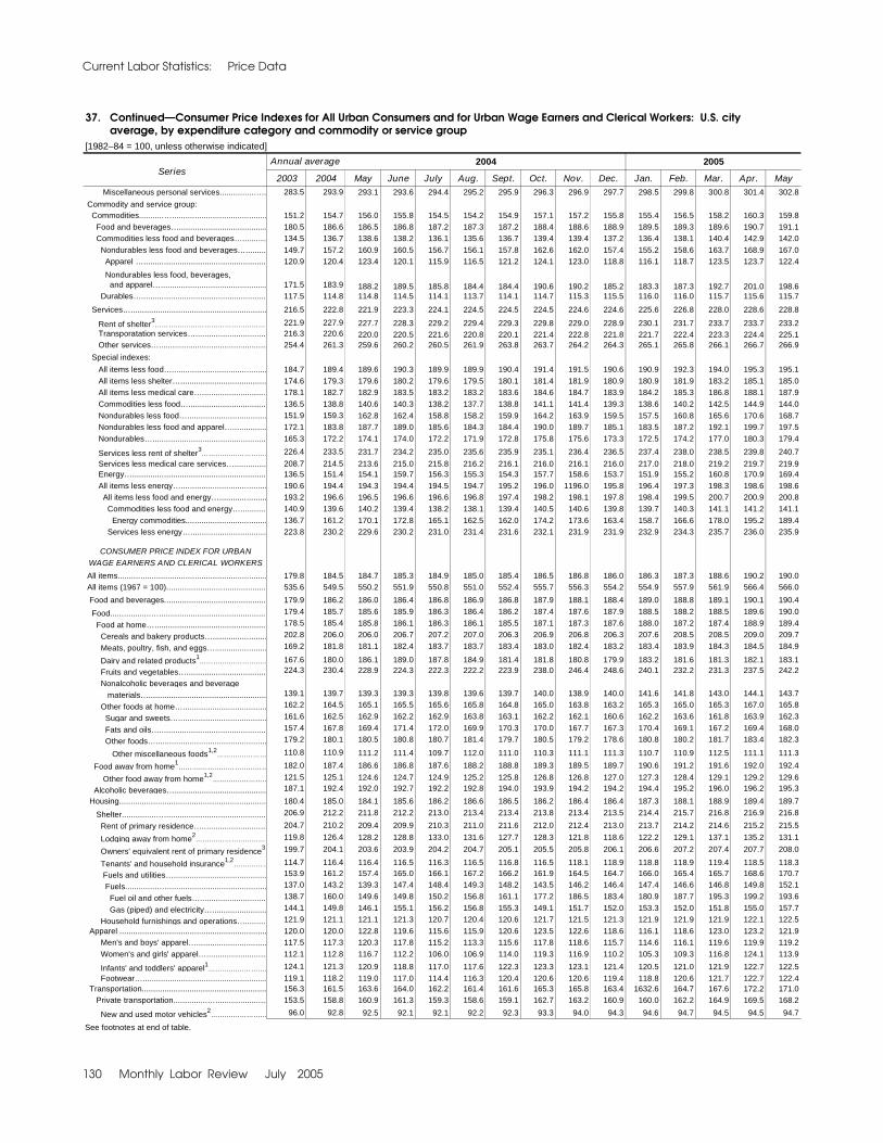
Current Labor Statistics: Price Data
130 Monthly Labor Review July 2005
37. Continued–Consumer Price Indexes for All Urban Consumers and for Urban Wage Earners and Clerical Workers: U.S. city average, by expenditure category and commodity or service group[1982–84 = 100, unless otherwise indicated]
2004 2005
2003 2004 May June July Aug. Sept. Oct. Nov. Dec. Jan. Feb. Mar. Apr. May Miscellaneous personal services...............….. 283.5 293.9 293.1 293.6 294.4 295.2 295.9 296.3 296.9 297.7 298.5 299.8 300.8 301.4 302.8
Commodity and service group: Commodities...........….......................................... 151.2 154.7 156.0 155.8 154.5 154.2 154.9 157.1 157.2 155.8 155.4 156.5 158.2 160.3 159.8
Food and beverages…....................................... 180.5 186.6 186.5 186.8 187.2 187.3 187.2 188.4 188.6 188.9 189.5 189.3 189.6 190.7 191.1 Commodities less food and beverages…........... 134.5 136.7 138.6 138.2 136.1 135.6 136.7 139.4 139.4 137.2 136.4 138.1 140.4 142.9 142.0
Nondurables less food and beverages…......... 149.7 157.2 160.9 160.5 156.7 156.1 157.8 162.6 162.0 157.4 155.2 158.6 163.7 168.9 167.0 Apparel …...................................................... 120.9 120.4 123.4 120.1 115.9 116.5 121.2 124.1 123.0 118.8 116.1 118.7 123.5 123.7 122.4
Nondurables less food, beverages, and apparel…............................................... 171.5 183.9 188.2 189.5 185.8 184.4 184.4 190.6 190.2 185.2 183.3 187.3 192.7 201.0 198.6 Durables…....................................................... 117.5 114.8 114.8 114.5 114.1 113.7 114.1 114.7 115.3 115.5 116.0 116.0 115.7 115.6 115.7
Services…............................................................ 216.5 222.8 221.9 223.3 224.1 224.5 224.5 224.5 224.6 224.6 225.6 226.8 228.0 228.6 228.8
Rent of shelter3……….…………………………………… 221.9 227.9 227.7 228.3 229.2 229.4 229.3 229.8 229.0 228.9 230.1 231.7 233.7 233.7 233.2
Transporatation services…............................... 216.3 220.6 220.0 220.5 221.6 220.8 220.1 221.4 222.8 221.8 221.7 222.4 223.3 224.4 225.1 Other services…................................................ 254.4 261.3 259.6 260.2 260.5 261.9 263.8 263.7 264.2 264.3 265.1 265.8 266.1 266.7 266.9
Special indexes:
All items less food….......................................... 184.7 189.4 189.6 190.3 189.9 189.9 190.4 191.4 191.5 190.6 190.9 192.3 194.0 195.3 195.1
All items less shelter…...................................... 174.6 179.3 179.6 180.2 179.6 179.5 180.1 181.4 181.9 180.9 180.9 181.9 183.2 185.1 185.0 All items less medical care…............................ 178.1 182.7 182.9 183.5 183.2 183.2 183.6 184.6 184.7 183.9 184.2 185.3 186.8 188.1 187.9
Commodities less food….................................. 136.5 138.8 140.6 140.3 138.2 137.7 138.8 141.1 141.4 139.3 138.6 140.2 142.5 144.9 144.0
Nondurables less food…................................... 151.9 159.3 162.8 162.4 158.8 158.2 159.9 164.2 163.9 159.5 157.5 160.8 165.6 170.6 168.7 Nondurables less food and apparel…............... 172.1 183.8 187.7 189.0 185.6 184.3 184.4 190.0 189.7 185.1 183.5 187.2 192.1 199.7 197.5
Nondurables….................................................. 165.3 172.2 174.1 174.0 172.2 171.9 172.8 175.8 175.6 173.3 172.5 174.2 177.0 180.3 179.4
Services less rent of shelter3……….………………… 226.4 233.5 231.7 234.2 235.0 235.6 235.9 235.1 236.4 236.5 237.4 238.0 238.5 239.8 240.7
Services less medical care services….............. 208.7 214.5 213.6 215.0 215.8 216.2 216.1 216.0 216.1 216.0 217.0 218.0 219.2 219.7 219.9 Energy…........................................................... 136.5 151.4 154.1 159.7 156.3 155.3 154.3 157.7 158.6 153.7 151.9 155.2 160.8 170.9 169.4
All items less energy…...................................... 190.6 194.4 194.3 194.4 194.5 194.7 195.2 196.0 1196.0 195.8 196.4 197.3 198.3 198.6 198.6 All items less food and energy…..................... 193.2 196.6 196.5 196.6 196.6 196.8 197.4 198.2 198.1 197.8 198.4 199.5 200.7 200.9 200.8
Commodities less food and energy…........... 140.9 139.6 140.2 139.4 138.2 138.1 139.4 140.5 140.6 139.8 139.7 140.3 141.1 141.2 141.1
Energy commodities.................................... 136.7 161.2 170.1 172.8 165.1 162.5 162.0 174.2 173.6 163.4 158.7 166.6 178.0 195.2 189.4 Services less energy….................................. 223.8 230.2 229.6 230.2 231.0 231.4 231.6 232.1 231.9 231.9 232.9 234.3 235.7 236.0 235.9
CONSUMER PRICE INDEX FOR URBANWAGE EARNERS AND CLERICAL WORKERS
All items.................................................................. 179.8 184.5 184.7 185.3 184.9 185.0 185.4 186.5 186.8 186.0 186.3 187.3 188.6 190.2 190.0 All items (1967 = 100)............................................ 535.6 549.5 550.2 551.9 550.8 551.0 552.4 555.7 556.3 554.2 554.9 557.9 561.9 566.4 566.0
Food and beverages............................................. 179.9 186.2 186.0 186.4 186.8 186.9 186.8 187.9 188.1 188.4 189.0 188.8 189.1 190.1 190.4
Food..................…............................................... 179.4 185.7 185.6 185.9 186.3 186.4 186.2 187.4 187.6 187.9 188.5 188.2 188.5 189.6 190.0
Food at home…................................................. 178.5 185.4 185.8 186.1 186.3 186.1 185.5 187.1 187.3 187.6 188.0 187.2 187.4 188.9 189.4
Cereals and bakery products…........................ 202.8 206.0 206.0 206.7 207.2 207.0 206.3 206.9 206.8 206.3 207.6 208.5 208.5 209.0 209.7
Meats, poultry, fish, and eggs…....................... 169.2 181.8 181.1 182.4 183.7 183.7 183.4 183.0 182.4 183.2 183.4 183.9 184.3 184.5 184.9
Dairy and related products1……….………………… 167.6 180.0 186.1 189.0 187.8 184.9 181.4 181.8 180.8 179.9 183.2 181.6 181.3 182.1 183.1
Fruits and vegetables…................................... 224.3 230.4 228.9 224.3 222.3 222.2 223.9 238.0 246.4 248.6 240.1 232.2 231.3 237.5 242.2
Nonalcoholic beverages and beverage
materials….................................................... 139.1 139.7 139.3 139.3 139.8 139.6 139.7 140.0 138.9 140.0 141.6 141.8 143.0 144.1 143.7
Other foods at home…..................................... 162.2 164.5 165.1 165.5 165.6 165.8 164.8 165.0 163.8 163.2 165.3 165.0 165.3 167.0 165.8
Sugar and sweets…....................................... 161.6 162.5 162.9 162.2 162.9 163.8 163.1 162.2 162.1 160.6 162.2 163.6 161.8 163.9 162.3
Fats and oils…............................................... 157.4 167.8 169.4 171.4 172.0 169.9 170.3 170.0 167.7 167.3 170.4 169.1 167.2 169.4 168.0
Other foods…................................................. 179.2 180.1 180.5 180.8 180.7 181.4 179.7 180.5 179.2 178.6 180.8 180.2 181.7 183.4 182.3
Other miscellaneous foods1,2……….………… 110.8 110.9 111.2 111.4 109.7 112.0 111.0 110.3 111.1 111.3 110.7 110.9 112.5 111.1 111.3
Food away from home1……….………………………… 182.0 187.4 186.6 186.8 187.6 188.2 188.8 189.3 189.5 189.7 190.6 191.2 191.6 192.0 192.4
Other food away from home1,2……….…………… 121.5 125.1 124.6 124.7 124.9 125.2 125.8 126.8 126.8 127.0 127.3 128.4 129.1 129.2 129.6
Alcoholic beverages…......................................... 187.1 192.4 192.0 192.7 192.2 192.8 194.0 193.9 194.2 194.2 194.4 195.2 196.0 196.2 195.3
Housing................................................................. 180.4 185.0 184.1 185.6 186.2 186.6 186.5 186.2 186.4 186.4 187.3 188.1 188.9 189.4 189.7
Shelter...............…............................................. 206.9 212.2 211.8 212.2 213.0 213.4 213.4 213.8 213.4 213.5 214.4 215.7 216.8 216.9 216.8
Rent of primary residence…............................. 204.7 210.2 209.4 209.9 210.3 211.0 211.6 212.0 212.4 213.0 213.7 214.2 214.6 215.2 215.5
Lodging away from home2……….………………… 119.8 126.4 128.2 128.8 133.0 131.6 127.7 128.3 121.8 118.6 122.2 129.1 137.1 135.2 131.1
Owners' equivalent rent of primary residence3… 199.7 204.1 203.6 203.9 204.2 204.7 205.1 205.5 205.8 206.1 206.6 207.2 207.4 207.7 208.0
Tenants' and household insurance1,2……….…… 114.7 116.4 116.4 116.5 116.3 116.5 116.8 116.5 118.1 118.9 118.8 118.9 119.4 118.5 118.3
Fuels and utilities…......................................... 153.9 161.2 157.4 165.0 166.1 167.2 166.2 161.9 164.5 164.7 166.0 165.4 165.7 168.6 170.7
Fuels...............…............................................ 137.0 143.2 139.3 147.4 148.4 149.3 148.2 143.5 146.2 146.4 147.4 146.6 146.8 149.8 152.1
Fuel oil and other fuels…............................. 138.7 160.0 149.6 149.8 150.2 156.8 161.1 177.2 186.5 183.4 180.9 187.7 195.3 199.2 193.6
Gas (piped) and electricity…........................ 144.1 149.8 146.1 155.1 156.2 156.8 155.3 149.1 151.7 152.0 153.3 152.0 151.8 155.0 157.7
Household furnishings and operations…......... 121.9 121.1 121.1 121.3 120.7 120.4 120.6 121.7 121.5 121.3 121.9 121.9 121.9 122.1 122.5
Apparel ................................................................. 120.0 120.0 122.8 119.6 115.6 115.9 120.6 123.5 122.6 118.6 116.1 118.6 123.0 123.2 121.9 Men's and boys' apparel…............................... 117.5 117.3 120.3 117.8 115.2 113.3 115.6 117.8 118.6 115.7 114.6 116.1 119.6 119.9 119.2
Women's and girls' apparel…........................... 112.1 112.8 116.7 112.2 106.0 106.9 114.0 119.3 116.9 110.2 105.3 109.3 116.8 124.1 113.9
Infants' and toddlers' apparel1……….……………… 124.1 121.3 120.9 118.8 117.0 117.6 122.3 123.3 123.1 121.4 120.5 121.0 121.9 122.7 122.5
Footwear…....................................................... 119.1 118.2 119.0 117.0 114.4 116.3 120.4 120.6 120.6 119.4 118.8 120.6 121.7 122.7 122.4 Transportation....................................................... 156.3 161.5 163.6 164.0 162.2 161.4 161.6 165.3 165.8 163.4 1632.6 164.7 167.6 172.2 171.0 Private transportation...............…....................... 153.5 158.8 160.9 161.3 159.3 158.6 159.1 162.7 163.2 160.9 160.0 162.2 164.9 169.5 168.2
New and used motor vehicles2……….…………… 96.0 92.8 92.5 92.1 92.1 92.2 92.3 93.3 94.0 94.3 94.6 94.7 94.5 94.5 94.7
See footnotes at end of table.
Annual average Series

Monthly Labor Review July 2005 131
37. Continued–Consumer Price Indexes for All Urban Consumers and for Urban Wage Earners and Clerical Workers: U.S. city average, by expenditure category and commodity or service group[1982–84 = 100, unless otherwise indicated]
2004 2005
2003 2004 May June July Aug. Sept. Oct. Nov. Dec. Jan. Feb. Mar. Apr. May
New vehicles…............................................... 139.0 138.1 138.5 138.2 137.0 136.0 136.0 136.9 138.9 139.8 140.7 140.7 140.0 139.7 139.6
Used cars and trucks1……….……………………… 143.7 134.1 132.6 131.4 133.0 134.6 137.3 137.6 137.5 138.1 138.3 138.4 138.5 138.9 139.6
Motor fuel…...................................................... 136.1 160.9 171.1 173.8 165.6 162.4 161.7 173.6 172.3 161.7 156.9 164.9 176.5 194.5 188.7 Gasoline (all types)…..................................... 135.5 160.2 170.4 173.2 165.0 161.7 161.0 172.9 171.6 160.9 156.1 164.1 175.7 193.7 187.9 Motor vehicle parts and equipment…............... 107.3 108.2 107.5 107.8 108.2 108.4 108.7 108.9 109.4 109.3 110.1 110.4 110.5 110.4 110.5 Motor vehicle maintenance and repair….......... 197.3 202.0 200.8 201.5 202.1 202.7 202.7 203.8 204.9 205.3 206.0 206.1 206.9 207.2 207.9
Public transportation...............…........................ 206.0 207.1 208.8 210.0 212.1 208.0 203.1 204.2 207.1 204.2 203.4 204.9 209.0 213.3 215.8
Medical care.......................................................... 296.3 309.5 308.4 309.4 310.4 311.0 311.7 312.7 313.6 314.4 316.3 318.9 320.3 321.1 321.9 Medical care commodities...............…............... 257.4 263.2 263.3 263.8 263.7 263.8 264.8 265.4 264.9 264.4 265.2 266.3 266.6 266.9 267.9 Medical care services...............…...................... 305.9 321.5 320.0 321.2 322.4 323.2 323.9 325.0 326.3 327.7 330.0 333.0 334.8 335.8 336.5 Professional services….................................... 263.4 274.0 273.5 274.1 274.8 275.8 275.9 276.3 276.9 277.2 278.9 281.2 282.3 283.6 284.3
Hospital and related services…........................ 391.2 414.0 410.7 413.0 415.2 414.9 416.4 418.5 421.0 424.2 427.4 430.9 433.6 433.4 433.7
Recreation2……….…………………………………………. 105.5 106.3 106.6 106.7 106.3 106.1 106.2 106.2 106.3 106.1 106.5 106.5 106.5 106.8 107.0
Video and audio1,2
……….……………………………… 102.9 103.4 103.9 103.7 103.7 103.4 103.3 103.5 103.3 103.2 103.4 103.5 103.9 104.0 103.9
Education and communication2……….……………… 109.0 110.0 109.2 109.4 109.4 109.9 110.8 110.5 110.6 110.5 110.6 110.7 110.7 110.8 110.6
Education2……….………………………………………… 133.8 142.5 139.9 140.6 141.0 143.6 146.3 146.7 146.8 147.0 147.3 147.7 147.8 148.0 148.5
Educational books and supplies…................. 336.5 352.2 350.4 351.5 350.4 354.7 354.8 355.6 356.1 357.6 359.0 361.5 362.4 363.1 364.0
Tuition, other school fees, and child care…... 377.3 402.5 394.6 396.7 398.1 405.8 414.0 415.2 415.6 415.8 416.8 417.6 418.0 418.5 419.8
Communication1,2
……….……………………………… 91.2 88.3 88..4 88.4 88.1 87.6 87.8 87.1 87.2 87.0 87.0 87.0 86.8 87.0 86.5
Information and information processing1,2
…… 89.9 86.8 87.0 86.9 86.7 86.2 86.3 85.6 85.7 85.5 85.5 85.5 85.3 85.5 85.0
Telephone services1,2
……….…………………… 98.5 96.0 96.1 96.1 95.8 95.2 95.5 94.8 95.1 95.0 94.9 95.3 95.1 95.4 94.9
Information and information processing
other than telephone services1,4
……….…… 16.7 15.3 15.4 15.4 15.3 15.3 15.2 15.0 14.9 14.8 14.8 14.6 14.5 14.5 14.3
Personal computers and peripheral
equipment1,2
……….…………………………… 17.3 15.0 15.4 15.2 15.0 14.9 14.8 14.3 13.9 13.7 13.7 13.3 13.2 13.2 13.0
Other goods and services..................................... 307.0 312.6 311.5 311.8 313.2 313.5 314.4 314.7 314.9 315.9 318.0 319.4 319.6 319.9 320.8 Tobacco and smoking products...............…....... 470.5 478.8 474.4 476.9 481.6 482.6 483.9 483.0 482.5 485.7 494.9 496.9 497.4 497.8 498.7
Personal care1……….…………………………………… 177.0 180.4 180.2 180.0 180.3 180.5 180.9 181.4 181.7 181.9 182.1 182.9 183.0 183.2 183.8
Personal care products1……….…………………… 154.2 154.4 155.1 154.3 153.9 153.1 154.0 154.3 154.3 153.8 153.3 154.2 153.3 153.6 154.5
Personal care services1……….……………………… 193.9 198.2 197.1 197.5 198.1 199.5 199.7 199.9 200.6 201.8 202.4 203.3 203.6 203.6 203.1
Miscellaneous personal services...............….. 283.3 294.0 293.1 293.5 294.7 295.4 296.2 296.6 297.5 298.4 299.2 299.8 300.8 301.5 303.2 Commodity and service group:
Commodities...........….......................................... 151.8 155.4 156.7 156.6 155.2 154.9 155.7 158.0 158.1 156.6 156.3 157.4 159.2 161.5 160.9 Food and beverages…....................................... 179.9 186.2 186.0 186.4 186.8 186.9 186.8 187.9 188.1 188.4 189.0 188.8 189.1 190.1 190.4 Commodities less food and beverages…........... 135.8 138.1 140.0 139.6 137.5 137.1 138.2 141.0 141.0 138.8 138.0 139.8 142.2 145.0 144.0 Nondurables less food and beverages…......... 152.1 160.6 164.7 164.4 160.4 159.5 161.2 166.5 165.9 160.9 158.8 162.5 167.8 173.6 171.5 Apparel …...................................................... 120.0 120.0 122.8 119.6 115.6 115.9 120.6 123.5 122.6 118.6 116.1 118.6 123.0 123.2 121.9 Nondurables less food, beverages,
and apparel…............................................... 175.6 189.6 194.5 196.0 191.8 190.2 190.1 196.9 196.5 190.8 188.8 193.3 199.4 208.9 206.0 Durables…....................................................... 117.4 114.0 113.9 113.5 113.2 113.1 113.7 114.3 114.8 115.1 115.5 115.5 115.3 115.3 115.5
Services…............................................................ 212.6 218.6 217.6 219.0 219.7 220.2 220.3 220.0 220.4 220.5 221.5 222.3 223.2 223.8 224.2
Rent of shelter3……….…………………………………… 199.2 204.3 203.9 204.4 205.1 205.5 205.5 205.9 205.5 205.6 206.5 207.7 208.8 208.9 208.8
Transporatation services…............................... 216.2 220.9 220.3 220.7 221.6 221.0 220.5 222.0 223.4 222.7 222.8 223.4 224.0 224.8 225.3 Other services…................................................ 248.5 254.1 252.7 253.3 253.5 254.4 256.0 255.9 256.3 256.5 257.2 257.8 258.1 258.7 258.9
Special indexes:
All items less food….......................................... 179.7 184.1 184.4 185.0 184.5 184.5 185.1 186.2 186.4 185.5 185.7 187.0 188.5 190.1 189.9 All items less shelter…...................................... 171.9 176.4 176.8 177.5 176.7 176.6 177.3 178.6 179.1 178.0 178.0 179.0 180.4 182.4 182.3
All items less medical care…............................. 174.8 179.1 179.4 180.0 179.6 179.6 180.0 181.1 181.3 180.6 180.8 181.7 183.1 184.6 184.4 Commodities less food….................................. 137.7 140.0 141.8 141.5 139.4 139.0 140.2 142.2 142.9 140.7 140.0 141.7 144.1 146.8 145.9 Nondurables less food…................................... 154.2 162.6 166.4 166.2 162.3 161.5 163.2 168.2 167.6 162.9 160.9 164.4 169.5 175.1 173.0 Nondurables less food and apparel…............... 175.9 189.0 193.5 194.8 191.0 189.6 189.7 195.6 195.4 190.3 188.5 192.7 198.3 206.9 204.2 Nondurables….................................................. 166.4 173.9 175.9 175.9 174.0 173.6 174.5 177.7 177.5 175.1 174.3 176.1 179.0 182.5 181.5
Services less rent of shelter3……….………………… 201.3 207.4 205.8 208.2 208.9 209.3 209.5 208.6 209.8 209.9 210.8 211.2 211.6 212.7 213.6
Services less medical care services….............. 205.2 210.6 209.7 211.1 211.8 212.2 212.3 212.0 212.3 212.4 213.2 214.0 214.7 215.4 215.7 Energy…........................................................... 135.9 151.3 154.5 159.9 156.2 155.1 154.2 157.8 158.5 153.3 151.4 155.0 160.9 171.4 169.6 All items less energy…...................................... 186.1 189.5 189.3 189.3 189.3 189.5 190.2 191.0 191.1 191.0 191.5 192.2 192.9 193.3 193.4 All items less food and energy…..................... 187.9 190.6 190.4 190.3 190.3 190.5 191.4 192.1 192.2 192.0 192.4 193.4 194.2 194.5 194.5
Commodities less food and energy…........... 141.1 139.4 139.9 139.0 138.0 138.0 139.5 140.5 140.6 139.9 139.9 140.5 141.3 141.4 141.3 Energy commodities.................................... 136.8 161.5 170.7 173.3 165.5 162.8 162.3 174.5 173.7 163.4 158.7 166.6 178.1 195.5 189.7 Services less energy….................................. 220.2 226.2 225.5 226.0 226.7 227.1 227.4 227.9 228.0 228.1 229.0 230.1 231.1 231.4 231.5
Annual averageSeries
1 Not seasonally adjusted.2 Indexes on a December 1997 = 100 base.3 Indexes on a December 1982 = 100 base.
4 Indexes on a December 1988 = 100 base.
NOTE: Index applied to a month as a whole, not to any specific date.

Current Labor Statistics: Price Data
132 Monthly Labor Review July 2005
38. Consumer Price Index: U.S. city average and available local area data: all items [1982–84 = 100, unless otherwise indicated]
Pricing
sched- 2004 2004
ule1 Dec. Jan. Feb. Mar. Apr. May Dec. Jan. Feb. Mar. Apr. May
U.S. city average…………………………………………… M 190.3 190.7 191.8 193.3 194.6 194.4 186.0 186.3 187.3 188.6 190.2 190.0
Region and area size2
Northeast urban……….………………………………………….……… M 201.9 202.6 203.6 206.0 206.9 206.2 198.7 199.0 200.0 201.8 202.9 202.5
Size A—More than 1,500,000.......................................... M 204.1 205.0 206.0 208.6 209.3 208.6 199.6 200.1 201.1 202.8 203.8 203.5
Size B/C—50,000 to 1,500,0003……….………………………… M 119.2 119.4 120.1 121.3 122.0 121.6 119.4 119.6 120.1 121.2 122.1 121.6
Midwest urban4……….………………………………………….………… M 183.8 184.1 185.2 186.3 187.7 187.4 178.8 179.1 180.2 181.2 182.8 182.4
Size A—More than 1,500,000.......................................... M 185.7 185.9 187.1 188.3 189.6 189.4 180.1 180.4 181.3 182.5 184.1 183.8
Size B/C—50,000 to 1,500,0003……….………………………… M 117.3 117.3 118.1 118.7 119.6 119.3 116.4 116.4 117.2 117.8 118.8 118.5
Size D—Nonmetropolitan (less than 50,000)…………..... M 177.2 178.2 179.2 179.9 181.7 181.6 174.9 175.7 176.5 177.3 179.1 178.8
South urban…….…............................................................. M 183.3 183.6 184.7 185.9 187.3 187.3 180.3 180.5 181.5 182.7 184.3 184.2
Size A—More than 1,500,000.......................................... M 184.9 185.2 186.6 187.9 189.9 189.2 182.4 182.6 184.0 185.3 186.7 186.8
Size B/C—50,000 to 1,500,0003……….………………………… M 117.1 117.1 117.7 118.4 119.3 119.4 115.6 115.7 116.3 117.0 117.9 117.9
Size D—Nonmetropolitan (less than 50,000)…………..... M 181.9 182.3 183.1 184.5 187.2 186.6 181.5 181.9 182.7 184.1 186.7 186.2
West urban…….….............................................................. M 194.2 194.5 195.7 197.1 198.6 198.8 189.4 189.5 190.5 192.0 193.7 193.9
Size A—More than 1,500,000.......................................... M 196.5 196.7 198.3 199.8 201.3 201.5 190.2 190.1 191.6 193.2 194.9 195.2
Size B/C—50,000 to 1,500,0003……….………………………… M 119.0 119.5 119.6 120.4 121.4 121.3 118.6 118.9 119.0 119.8 120.8 120.8
Size classes:
A5……….………………………………………….…………..…………… M 174.0 174.3 175.5 177.0 178.1 178.0 172.4 172.6 173.7 175.0 176.3 176.3
B/C3……………………….….………………………………………….… M 117.7 117.9 118.5 119.2 120.1 120.0 116.9 117.0 117.5 118.3 119.2 119.1
D…………….…………...................................................... M 182.4 183.0 183.7 184.8 186.9 186.9 180.6 181.0 181.7 182.9 185.1 185.0
Selected local areas6
Chicago–Gary–Kenosha, IL–IN–WI………………………….. M 189.6 189.9 190.5 191.3 193.2 193.3 183.1 183.5 184.2 184.8 186.9 186.8Los Angeles–Riverside–Orange County, CA……….………… M 195.2 195.4 197.4 199.2 201.1 201.5 188.5 188.5 190.3 192.1 194.2 194.6
New York, NY–Northern NJ–Long Island, NY–NJ–CT–PA… M 206.8 208.1 208.9 212.4 212.5 211.4 201.8 202.6 203.3 205.5 206.0 205.6
Boston–Brockton–Nashua, MA–NH–ME–CT……….………… 1 – 211.3 – 214.2 – 214.6 – 210.3 – 213.1 – 214.0
Cleveland–Akron, OH…………………………………………… 1 – 183.3 – 186.3 – 186.8 – 174.5 – 177.2 – 177.9
Dallas–Ft Worth, TX…….……………………………………… 1 – 180.0 – 181.3 – 183.5 – 180.3 – 181.6 – 184.1
Washington–Baltimore, DC–MD–VA–WV7……….……………… 1 – 121.3 – 122.7 – 123.6 – 120.7 – 122.3 – 123.2
Atlanta, GA……………………..………………………………… 2 183.2 – 185.3 – 188.0 – 181.5 – 183.4 – 186.0 –
Detroit–Ann Arbor–Flint, MI…………………………………… 2 185.3 – 187.8 – 189.8 – 180.7 – 182.6 – 185.2 –
Houston–Galveston–Brazoria, TX……………………………… 2 170.0 – 174.6 – 175.0 – 167.7 – 171.8 – 172.8 –
Miami–Ft. Lauderdale, FL……………...……………………… 2 188.6 – 190.6 – 193.2 – 186.6 – 188.3 – 191.2 –
Philadelphia–Wilmington–Atlantic City, PA–NJ–DE–MD…… 2 197.8 – 200.1 – 203.3 – 197.9 – 200.0 – 202.9 –
San Francisco–Oakland–San Jose, CA…….………………… 2 199.5 – 201.2 – 202.5 – 195.9 – 197.3 – 199.3 –
Seattle–Tacoma–Bremerton, WA………………...…………… 2 195.1 – 197.6 – 201.3 – 190.3 – 192.4 – 196.2 –
2005 2005
All Urban Consumers Urban Wage Earners
1 Foods, fuels, and several other items priced every month in all areas; most other
goods and services priced as indicated:
M—Every month.
1—January, March, May, July, September, and November.
2—February, April, June, August, October, and December.2 Regions defined as the four Census regions. 3 Indexes on a December 1996 = 100 base.4 The "North Central" region has been renamed the "Midwest" region by the
Census Bureau. It is composed of the same geographic entities.5 Indexes on a December 1986 = 100 base.6 In addition, the following metropolitan areas are published semiannually and
appear in tables 34 and 39 of the January and July issues of the CPI Detailed
Report: Anchorage, AK; Cincinnatti, OH–KY–IN; Kansas City, MO–KS; Milwaukee–Racine,
WI; Minneapolis–St. Paul, MN–WI; Pittsburgh, PA; Port-land–Salem, OR–WA; St Louis,
MO–IL; San Diego, CA; Tampa–St. Petersburg–Clearwater, FL.7 Indexes on a November 1996 = 100 base.
NOTE: Local area CPI indexes are byproducts of the national CPI program. Each local
index has a smaller sample size and is, therefore, subject to substantially more sampling
and other measurement error. As a result, local area indexes show greater volatility than
the national index, although their long-term trends are similar. Therefore, the Bureau of
Labor Statistics strongly urges users to consider adopting the national average CPI for use
in their escalator clauses. Index applies to a month as a whole, not to any specific date.
Dash indicates data not available.

Monthly Labor Review July 2005 133
39. Annual data: Consumer Price Index, U.S. city average, all items and major groups
[1982–84 = 100]
Series 1994 1995 1996 1997 1998 1999 2000 2001 2002 2003 2004
Consumer Price Index for All Urban Consumers: All items: Index..................……............................................... 148.2 152.4 156.9 160.5 163.0 166.6 172.2 177.1 179.9 184.0 188.9 Percent change............................…………………… 2.6 2.8 3.0 2.3 1.6 2.2 3.4 2.8 1.6 2.3 2.7 Food and beverages: Index................……................................................. 144.9 148.9 153.7 157.7 161.1 164.6 168.4 173.6 176.8 180.5 186.6 Percent change............................…………………… 2.3 2.8 3.2 2.6 2.2 2.2 2.3 3.1 1.8 2.1 3.3 Housing: Index....………………............................................... 144.8 148.5 152.8 156.8 160.4 163.9 169.6 176.4 180.3 184.8 189.5 Percent change............................…………………… 2.5 2.6 2.9 2.6 2.3 2.2 3.5 4.0 2.2 2.5 2.5 Apparel: Index........................……......................................... 133.4 132.0 131.7 132.9 133.0 131.3 129.6 127.3 124.0 120.9 120.4 Percent change............................…………………… –.2 –1.0 –.2 .9 .1 –1.3 –1.3 –1.8 –2.6 –2.5 –.4 Transportation: Index........................………..................................... 134.3 139.1 143.0 144.3 141.6 144.4 153.3 154.3 152.9 157.6 163.1 Percent change............................…………………… 3.0 3.6 2.8 0.9 –1.9 2.0 6.2 0.7 –.9 3.1 3.5 Medical care: Index................……................................................. 211.0 220.5 228.2 234.6 242.1 250.6 260.8 272.8 285.6 297.1 310.1 Percent change............................…………………… 4.8 4.5 3.5 2.8 3.2 3.5 4.1 4.6 4.7 4.0 4.4 Other goods and services: Index............……..................................................... 198.5 206.9 215.4 224.8 237.7 258.3 271.1 282.6 293.2 298.7 304.7 Percent change............................…………………… 2.9 4.2 4.1 4.4 5.7 8.7 5.0 4.2 3.8 1.9 2.0
Consumer Price Index for Urban Wage Earners and Clerical Workers: All items: Index....................…………….................................. 145.6 149.8 154.1 157.6 159.7 163.2 168.9 173.5 175.9 179.8 188.9 Percent change............................…………………… 2.5 2.9 2.9 2.3 1.3 2.2 3.5 2.7 1.4 2.2 5.1

Current Labor Statistics: Price Data
134 Monthly Labor Review July 2005
40. Producer Price Indexes, by stage of processing
[1982 = 100]
2004 2005
2003 2004 May June July Aug. Sept. Oct. Nov. Dec. Jan. Feb.p Mar.p Apr.p Mayp
Finished goods....…………………………… 143.3 148.5 148.9 148.7 148.5 148.5 148.7 152.0 151.7 150.6 151.4 152.2 153.5 154.4 154.1 Finished consumer goods........................ 145.3 151.6 152.5 152.0 151.9 151.8 152.1 155.7 155.4 153.8 154.8 155.8 157.5 158.7 158.3 Finished consumer foods....................... 145.9 152.6 155.5 155.0 152.3 152.2 152.7 155.1 154.7 154.9 154.2 155.6 156.2 156.5 156.8
Finshed consumer goods excluding foods.................................... 144.7 150.9 150.9 150.5 151.4 151.3 151.5 155.6 155.3 153.0 154.6 155.5 157.7 159.3 158.6 Nondurable goods less food................. 148.4 156.6 156.7 156.0 158.0 157.9 158.2 162.1 161.8 158.5 160.7 162.2 165.5 167.9 167.1 Durable goods...................................... 133.1 135.1 134.8 134.9 133.6 133.6 133.5 137.8 137.4 137.2 137.8 137.3 137.0 137.0 136.7 Capital equipment.................................. 139.5 141.5 140.8 141.1 140.7 141.2 141.2 143.4 143.4 143.6 144.1 144.0 144.3 144.5 144.4
Intermediate materials, supplies, and components........………… 133.7 142.5 142.0 142.8 143.5 144.8 145.3 146.5 147.7 146.9 148.0 148.9 150.4 151.7 151.0
Materials and components for manufacturing..................................... 129.7 137.9 137.4 137.7 138.1 139.4 140.6 141.5 142.0 142.8 143.9 144.5 145.2 145.3 144.9 Materials for food manufacturing.............. 134.4 145.0 152.2 152.0 147.3 144.9 144.3 144.2 143.9 145.2 145.7 146.0 146.6 146.6 147.6 Materials for nondurable manufacturing... 137.2 147.6 144.5 145.9 147.3 149.8 152.6 154.4 155.5 156.8 157.9 158.1 160.7 160.4 160.4 Materials for durable manufacturing......... 127.9 146.6 146.9 145.8 147.2 150.3 152.1 153.0 153.6 155.2 157.3 159.3 158.7 158.9 156.7 Components for manufacturing................ 125.9 127.4 127.3 127.6 127.4 127.7 128.0 128.2 128.3 128.5 129.2 129.6 129.5 129.9 129.7
Materials and components for construction......................................... 153.6 166.4 166.9 166.9 167.5 169.8 170.9 170.8 170.7 171.3 173.1 174.7 175.2 175.3 174.9 Processed fuels and lubricants................... 112.6 124.1 122.3 124.9 126.4 128.5 126.9 130.8 134.0 128.9 129.5 130.7 135.8 141.1 139.3 Containers.................................................. 153.7 159.2 156.7 158.9 159.7 162.0 162.5 164.6 164.9 165.2 165.5 166.8 166.8 167.0 167.1 Supplies...................................................... 141.5 146.7 147.2 147.3 148.0 147.6 147.9 147.9 147.9 148.5 149.6 150.0 150.6 151.2 151.4
Crude materials for further processing.......................………………… 135.3 159.0 161.8 163.0 162.5 162.2 154.4 160.5 171.5 165.7 163.0 162.2 169.4 174.1 171.7 Foodstuffs and feedstuffs........................... 113.5 126.9 141.1 137.4 130.9 124.8 122.0 120.1 119.5 121.5 123.8 121.3 127.6 125.0 126.2 Crude nonfood materials............................ 148.2 179.2 172.9 178.0 182.2 186.6 174.9 187.3 207.1 195.3 188.7 189.3 197.0 207.3 202.1
Special groupings: Finished goods, excluding foods................ 142.4 147.2 147.0 146.8 147.2 147.3 147.5 150.9 150.7 149.2 150.5 151.0 152.6 153.7 153.2 Finished energy goods............................... 102.0 113.0 113.6 112.5 115.4 115.0 115.1 121.1 120.1 114.5 116.4 118.2 123.4 126.9 125.2 Finished goods less energy........................ 149.0 152.4 152.7 152.7 151.7 151.9 152.1 154.5 154.4 154.6 155.1 155.5 155.7 155.9 156.0 Finished consumer goods less energy....... 153.1 157.2 158.0 157.9 156.5 156.6 156.9 159.3 159.2 159.4 159.9 160.6 160.7 160.9 161.1 Finished goods less food and energy......... 150.5 152.7 152.2 152.3 151.9 152.2 152.3 154.7 154.7 154.9 155.8 155.9 156.0 156.1 156.1
Finished consumer goods less food and energy............................................... 157.9 160.3 159.9 160.0 159.4 159.6 159.7 162.2 162.3 162.5 163.8 163.9 163.8 164.0 164.1
Consumer nondurable goods less food and energy............................................. 177.9 180.7 180.2 180.2 180.3 180.8 181.2 181.7 182.2 182.8 184.8 185.6 185.7 186.1 186.6
Intermediate materials less foods and feeds.................................................. 134.2 142.9 141.9 142.8 143.7 145.3 145.9 147.3 148.3 147.8 148.9 149.7 151.3 152.6 151.9 Intermediate foods and feeds..................... 125.9 137.0 147.7 144.9 142.3 136.3 134.4 131.2 130.7 131.0 132.0 132.1 133.3 134.2 135.2 Intermediate energy goods......................... 111.9 123.1 121.1 123.7 125.1 127.1 125.8 129.9 132.7 128.4 129.0 129.8 134.7 139.4 138.2 Intermediate goods less energy................. 137.7 145.8 145.7 146.0 146.4 147.5 148.5 149.0 149.4 149.9 151.1 151.9 152.5 152.9 152.4
Intermediate materials less foods and energy............................................... 138.5 146.5 145.7 146.2 146.8 148.3 149.5 150.1 150.6 151.1 152.3 153.2 153.8 154.1 153.6
Crude energy materials.............................. 147.2 174.7 172.1 180.0 177.9 181.9 166.6 181.8 208.3 192.7 183.9 186.3 196.5 210.6 206.7 Crude materials less energy....................... 123.4 143.9 150.1 147.0 147.5 144.6 141.6 141.9 142.7 143.3 144.5 141.7 146.8 145.3 144.0 Crude nonfood materials less energy......... 152.5 192.8 177.9 176.3 195.4 200.8 197.4 203.5 207.9 204.9 203.3 199.4 201.6 203.1 194.7
Annual averageGrouping
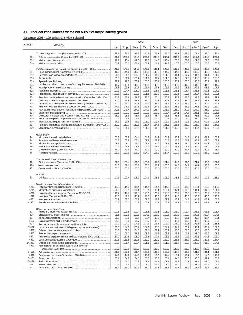
Monthly Labor Review July 2005 135
41. Producer Price Indexes for the net output of major industry groups
[December 2003 = 100, unless otherwise indicated]
July Aug. Sept. Oct. Nov. Dec. Jan. Feb.p Mar.p Apr.p Mayp
Total mining industries (December 1984=100)...................................... 155.6 159.3 149.6 160.6 179.1 169.2 163.3 165.9 173.4 183.0 179.1
211 Oil and gas extraction(December 1985=100) ........................................ 196.6 202.7 184.0 203.0 234.8 214.7 202.5 205.3 217.4 234.0 227.0 212 Mining, except oil and gas…………………………………………………… 110.2 110.4 112.3 112.8 114.0 116.4 120.2 120.2 121.8 122.3 122.8 213 Mining support activities……………………………………………………… 103.7 105.3 106.4 109.2 111.4 114.9 115.5 123.5 125.2 126.9 126.9
Total manufacturing industries (December 1984=100)......................... 143.2 143.7 144.2 146.5 146.1 145.0 146.2 147.2 148.9 149.7 149.3 311 Food manufacturing (December 1984=100)……………………………… 146.5 144.6 143.8 143.5 143.3 144.2 144.7 145.2 146.0 146.6 147.2 312 Beverage and tobacco manufacturing.................................................... 100.6 101.1 100.6 101.2 101.2 101.5 104.1 104.7 104.7 104.4 104.6 313 Textile mills............................................................................................. 101.5 101.2 101.4 101.6 101.7 101.5 102.3 102.5 103.0 103.2 103.7 315 Apparel manufacturing………………………………...……………………… 99.7 99.7 100.2 100.3 100.4 100.5 100.4 100.3 100.3 100.2 99.9
316 Leather and allied product manufacturing (December 1984=100)......... 143.7 143.6 143.6 143.5 143.8 143.9 143.8 144.3 144.6 144.5 144.5 321 Wood products manufacturing……………………………………………… 106.8 109.8 110.7 107.6 105.1 105.9 106.9 108.8 109.5 108.8 107.5 322 Paper manufacturing.............................................................................. 103.2 104.4 105.0 105.5 105.7 105.8 106.1 106.4 106.8 107.1 107.1 323 Printing and related support activities..................................................... 101.3 101.3 101.8 101.8 102.0 102.0 102.5 102.8 102.7 102.5 102.4
324 Petroleum and coal products manufacturing (December 1984=100)…… 152.3 155.6 158.9 176.7 170.4 150.3 155.9 163.6 182.5 189.3 183.3 325 Chemical manufacturing (December 1984=100)………………………… 172.2 173.8 175.5 177.2 179.3 180.5 182.7 184.0 185.2 186.5 186.4 326 Plastics and rubber products manufacturing (December 1984=100)…… 131.2 131.7 133.1 134.3 135.3 136.1 137.4 138.7 139.0 139.4 139.8 331 Primary metal manufacturing (December 1984=100)…………………… 144.7 148.3 150.8 152.9 154.2 155.5 158.6 159.2 158.1 157.9 156.0 332 Fabricated metal product manufacturing (December 1984=100)……… 142.5 143.4 144.2 144.9 145.4 145.7 146.9 147.7 147.9 148.9 149.0 333 Machinery manufacturing………………………..…………………………… 102.1 102.3 102.5 102.9 103.2 103.4 104.1 104.8 105.1 105.2 105.6 334 Computer and electronic products manufacturing…………………...…… 98.9 98.9 98.7 98.6 98.4 98.5 98.3 98.3 98.1 97.9 97.4 335 Electrical equipment, appliance, and components manufacturing……… 103.6 103.8 104.2 104.7 104.6 104.9 106.0 106.6 107.0 107.5 107.4 336 Transportation equipment manufacturing………………………………… 99.7 99.8 99.9 103.2 102.7 102.9 103.2 102.6 102.5 102.6 102.3 337 Furniture and related product manufacturing(December 1984=100)…… 152.0 152.7 152.8 153.4 154.6 155.1 155.5 156.0 155.9 156.8 157.1 339 Miscellaneous manufacturing………………………………………………… 101.2 101.4 101.8 101.3 101.3 101.6 102.2 102.5 102.7 102.7 102.8
Retail trade 441 Motor vehicle and parts dealers……………………………………………… 103.3 103.8 104.4 104.2 104.2 104.2 106.2 104.3 105.7 107.2 108.3 442 Furniture and home furnishings stores……………………………………… 102.6 102.8 103.4 103.8 103.7 104.6 105.6 106.8 106.9 107.0 108.2 443 Electronics and appliance stores…………………………………………… 98.6 98.7 99.2 98.4 97.9 93.6 98.3 96.9 102.3 101.1 102.9 446 Health and personal care stores…………………………………………… 101.3 105.6 105.1 104.1 106.8 107.2 106.5 105.1 107.9 106.2 107.6 447 Gasoline stations (June 2001=100)………………………………………… 48.3 48.6 46.3 43.1 53.3 59.8 49.0 46.4 48.3 49.5 51.9 454 Nonstore retailers……………………………………………………………… 103.6 102.0 105.6 104.7 111.5 117.4 117.5 121.9 119.6 121.6 123.2
Transportation and warehousing 481 Air transportation (December 1992=100)…………………………………… 163.9 163.4 159.8 160.9 162.2 161.4 164.9 166.5 171.1 169.6 167.0 483 Water transportation…………………………………………………………… 101.5 102.1 103.2 103.8 103.7 103.5 104.0 104.1 104.4 105.0 105.7 491 Postal service (June 1989=100)…………………………………………… 155.0 155.0 155.0 155.0 155.0 155.0 155.0 155.0 155.0 155.0 155.0
Utilities 221 Utilities………………………………………………………………………… 107.1 107.4 105.2 104.3 108.8 108.9 108.3 107.0 107.9 110.2 111.1
Health care and social assistance 6211 Office of physicians (December 1996=100)……………………………… 114.3 114.3 114.4 114.4 114.4 114.5 115.7 115.3 115.1 115.2 115.6 6215 Medical and diagnostic laboratories………………………………………… 100.0 100.1 100.1 100.1 100.1 100.1 102.4 100.5 104.4 104.3 104.3 6216 Home health care services (December 1996=100)……………………… 119.7 119.7 119.8 120.1 120.2 120.3 120.9 120.6 120.6 120.9 120.9 622 Hospitals (December 1992=100)…………………………………………… 141.6 141.6 141.7 143.3 143.5 143.8 144.8 145.3 145.3 145.5 145.8
6231 Nursing care facilities………………………………………………………… 102.9 103.0 103.2 103.7 103.9 103.9 105.3 104.5 104.9 105.1 105.7 62321 Residential mental retardation facilities…………………………………… 102.1 102.1 102.5 102.5 102.5 102.5 103.8 103.4 103.7 103.7 103.8
Other services industries 511 Publishing industries, except Internet …………………………………… 101.5 101.5 101.4 101.8 102.1 101.9 103.0 103.4 103.2 103.6 103.7 515 Broadcasting, except Internet……………………………………………… 99.6 100.9 100.8 104.3 103.2 100.8 100.2 100.0 100.8 102.4 104.2 517 Telecommunications………………………………………………………… 99.8 99.9 99.6 99.4 99.2 99.9 99.0 98.1 97.8 98.4 98.4 5182 Data processing and related services……………………………………… 99.0 99.0 98.7 98.7 98.6 98.6 98.7 98.8 98.6 98.7 98.6 523 Security, commodity contracts, and like activity…………………………… 103.2 104.1 104.5 104.3 105.8 106.0 108.0 111.8 109.8 110.1 111.4
53112 Lessors or nonresidental buildings (except miniwarehouse)…………… 103.5 104.0 103.9 104.6 103.0 104.2 104.2 103.2 103.4 105.2 104.2 5312 Offices of real estate agents and brokers………………………………… 101.0 101.0 104.0 103.1 103.1 105.9 106.0 106.0 106.0 106.0 105.9 5313 Real estate property managers……………………………………………… 101.4 101.0 99.8 101.5 101.2 102.3 103.2 103.1 101.0 102.6 101.6 5321 Automotive equipment rental and leasing (June 2001=100)…………… 110.0 110.8 108.0 107.8 107.7 108.1 105.2 107.9 109.1 104.8 106.0 5411 Legal services (December 1996=100)……………………………………… 131.6 131.5 131.8 132.0 132.0 132.0 136.8 136.7 136.9 137.3 137.7
541211 Offices of certified public accountants……………………………………… 101.3 101.4 101.4 101.6 101.7 101.3 101.8 101.9 102.0 101.9 104.3 5413 Architectural, engineering, and related services
(December 1996=100)…………………………………………………… 127.0 127.0 127.3 127.3 127.3 127.7 128.2 128.7 128.8 129.2 129.2 54181 Advertising agencies………………………………………………………… 100.0 100.3 100.4 100.3 100.5 100.5 100.8 101.0 101.0 101.1 101.0 5613 Employment services (December 1996=100)……………………………… 114.6 114.6 114.2 115.2 115.2 114.4 115.1 115.7 115.2 114.9 115.6
56151 Travel agencies……………………………………………………………… 95.1 94.7 94.5 95.8 95.2 96.1 94.5 95.0 96.2 97.1 95.9 56172 Janitorial services……………………………………………………………… 101.0 101.1 100.9 101.4 101.4 101.4 101.7 101.7 101.9 102.0 102.1 5621 Waste collection……………………………………………………………… 101.4 101.4 101.4 101.5 101.5 101.5 101.5 101.5 101.5 103.8 103.1 721 Accommodation (December 1996=100)…………………………………… 126.6 127.0 127.2 127.0 125.1 123.8 125.7 128.2 127.9 127.8 129.1
2004 2005IndustryNAICS
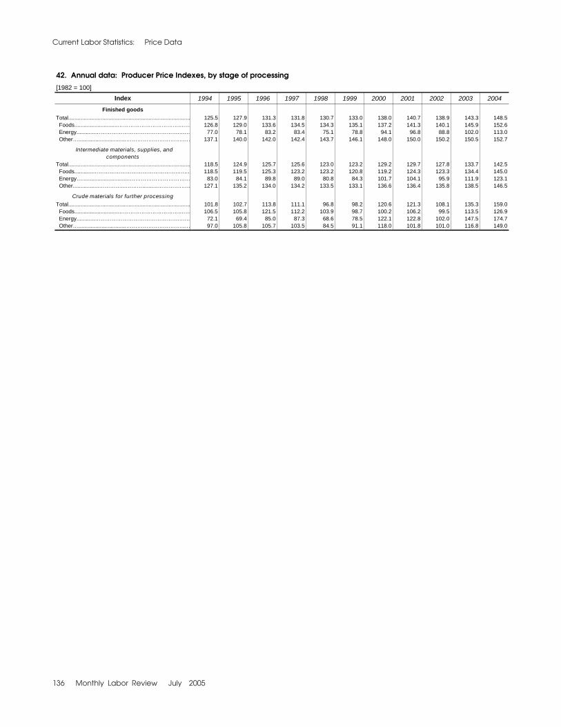
Current Labor Statistics: Price Data
136 Monthly Labor Review July 2005
42. Annual data: Producer Price Indexes, by stage of processing
[1982 = 100]Index 1994 1995 1996 1997 1998 1999 2000 2001 2002 2003 2004
Finished goodsTotal............................................................................... 125.5 127.9 131.3 131.8 130.7 133.0 138.0 140.7 138.9 143.3 148.5 Foods............................…………………………….…… 126.8 129.0 133.6 134.5 134.3 135.1 137.2 141.3 140.1 145.9 152.6 Energy............……………………………………….….… 77.0 78.1 83.2 83.4 75.1 78.8 94.1 96.8 88.8 102.0 113.0 Other…...............................………………………….…… 137.1 140.0 142.0 142.4 143.7 146.1 148.0 150.0 150.2 150.5 152.7
Intermediate materials, supplies, andcomponents
Total............................................................................... 118.5 124.9 125.7 125.6 123.0 123.2 129.2 129.7 127.8 133.7 142.5 Foods............……………………………………….….… 118.5 119.5 125.3 123.2 123.2 120.8 119.2 124.3 123.3 134.4 145.0 Energy…...............................………………………….… 83.0 84.1 89.8 89.0 80.8 84.3 101.7 104.1 95.9 111.9 123.1 Other.................…………...………..........………….…… 127.1 135.2 134.0 134.2 133.5 133.1 136.6 136.4 135.8 138.5 146.5
Crude materials for further processingTotal............................................................................... 101.8 102.7 113.8 111.1 96.8 98.2 120.6 121.3 108.1 135.3 159.0 Foods............................…………………………….…… 106.5 105.8 121.5 112.2 103.9 98.7 100.2 106.2 99.5 113.5 126.9 Energy............……………………………………….….… 72.1 69.4 85.0 87.3 68.6 78.5 122.1 122.8 102.0 147.5 174.7 Other…...............................………………………….…… 97.0 105.8 105.7 103.5 84.5 91.1 118.0 101.8 101.0 116.8 149.0

Monthly Labor Review July 2005 137
43. U.S. export price indexes by Standard International Trade Classification
[2000 = 100]
SITC 2004 2005Rev. 3 May June July Aug. Sept. Oct. Nov. Dec. Jan. Feb. Mar. Apr. May
0 Food and live animals………………………………………… 126.7 123.9 119.8 116.4 117.6 118.3 118.7 118.1 118.2 118.3 120.2 121.4 124.2 01 Meat and meat preparations........................................... 127.7 127.3 123.0 126.1 124.8 126.9 125.4 124.6 121.3 125.2 128.6 133.1 139.7 04 Cereals and cereal preparations..................................... 146.0 141.2 128.0 120.6 122.0 115.6 113.1 116.4 119.2 116.2 121.4 116.9 116.2 05 Vegetables, fruit, and nuts, prepared fresh or dry........... 113.3 111.1 110.0 113.2 119.8 130.6 137.2 129.9 127.4 128.1 125.2 130.5 137.4
2 Crude materials, inedible, except fuels........................... 132.5 125.7 132.1 118.0 119.4 118.2 119.5 119.4 123.1 122.1 127.5 129.3 128.5 22 Oilseeds and oleaginous fruits........................................ 199.0 168.5 184.5 117.4 125.1 109.1 110.3 111.1 115.2 109.7 128.9 124.6 127.7 24 Cork and wood................................................................ 98.2 98.3 98.9 98.8 99.1 99.1 98.4 98.8 98.7 98.9 99.2 98.7 97.0 25 Pulp and waste paper...................................................... 100.4 100.8 100.1 99.5 98.7 98.1 98.2 98.8 100.0 100.7 103.0 101.8 102.7 26 Textile fibers and their waste........................................... 114.9 108.7 102.9 101.1 102.1 100.2 97.5 96.4 98.4 98.7 104.1 104.8 103.3 28 Metalliferous ores and metal scrap.................................. 170.6 167.5 190.2 183.6 178.5 190.4 197.0 195.0 205.8 206.0 206.4 222.8 213.1
3 Mineral fuels, lubricants, and related products.............. 135.1 131.8 137.5 139.6 141.2 156.0 151.1 146.5 148.5 154.2 170.9 183.2 175.4 33 Petroleum, petroleum products, and related materials.... 135.0 129.7 134.5 136.2 138.0 156.4 151.0 144.6 147.3 155.7 177.1 192.1 179.1
5 Chemicals and related products, n.e.s. .......................... 105.6 105.8 107.0 108.6 109.7 111.6 112.9 114.0 116.1 116.3 116.9 117.8 116.5 54 Medicinal and pharmaceutical products.......................... 105.7 105.8 107.9 108.1 108.0 106.7 106.9 107.2 108.3 107.9 107.8 108.2 107.9 55 Essential oils; polishing and cleaning preparations......... 104.4 104.3 104.1 105.1 105.6 106.6 107.5 109.1 109.8 111.1 110.6 111.9 111.8 57 Plastics in primary forms ................................................ 102.9 103.2 104.8 107.3 109.9 113.2 117.2 118.9 126.6 127.5 128.2 127.7 123.7 58 Plastics in nonprimary forms........................................... 96.7 96.5 97.2 97.1 97.4 98.1 98.7 99.9 101.5 102.1 103.2 103.7 104.0 59 Chemical materials and products, n.e.s. ........................ 104.8 104.9 104.6 106.2 105.5 105.2 105.3 105.8 106.5 106.4 105.9 106.5 106.4
6 Manufactured goods classified chiefly by materials..... 106.6 107.0 108.5 109.6 110.5 111.3 111.8 112.2 113.0 113.5 113.6 114.3 114.2
62 Rubber manufactures, n.e.s. .......................................... 110.8 111.2 111.8 112.0 111.4 111.6 112.4 112.9 113.8 114.2 114.4 115.0 115.3 64 Paper, paperboard, and articles of paper, pulp,
and paperboard……………………………...………........ 99.0 99.2 101.2 101.9 102.7 104.0 103.7 104.2 104.1 104.1 103.8 103.8 103.7 66 Nonmetallic mineral manufactures, n.e.s. ...................... 99.5 99.9 99.9 100.2 100.4 101.1 101.3 101.6 101.9 102.0 102.2 102.4 102.3 68 Nonferrous metals........................................................... 97.6 95.4 95.4 96.5 99.0 99.1 100.6 101.5 103.4 105.6 107.2 109.5 108.6
7 Machinery and transport equipment............................... 98.4 98.2 98.2 98.2 98.2 98.4 98.4 98.5 98.7 98.7 98.7 98.7 98.7
71 Power generating machinery and equipment.................. 108.7 108.7 108.9 109.0 109.0 109.4 110.3 110.4 111.4 111.4 111.6 111.6 111.5 72 Machinery specialized for particular industries................ 105.4 105.4 105.7 105.9 106.1 107.3 107.6 108.0 109.3 109.2 109.4 110.6 110.6 74 General industrial machines and parts, n.e.s.,
and machine parts......................................................... 104.8 104.9 105.2 105.3 105.3 106.2 106.4 106.6 107.6 108.2 108.3 109.3 109.5 75 Computer equipment and office machines...................... 88.6 87.2 86.6 86.4 86.0 85.1 84.4 83.8 83.0 82.9 82.1 81.3 81.0 76 Telecommunications and sound recording and
reproducing apparatus and equipment.......................... 92.0 91.8 91.5 90.7 90.7 90.5 90.5 90.4 90.5 90.5 90.5 89.9 90.0 77 Electrical machinery and equipment................................ 88.6 88.2 88.3 88.2 88.1 87.9 87.7 87.9 87.8 87.6 87.6 87.5 87.4 78 Road vehicles.................................................................. 102.3 102.4 102.5 102.5 102.4 102.8 102.8 103.0 103.0 103.0 103.0 102.9 103.0
87 Professional, scientific, and controlling instruments and apparatus……………………………..… 102.1 102.0 101.7 101.9 101.8 102.2 102.3 102.6 103.4 103.4 103.4 103.5 103.1
Industry

Current Labor Statistics: Price Data
138 Monthly Labor Review July 2005
44. U.S. import price indexes by Standard International Trade Classification
[2000 = 100]
SITC 2004 2005Rev. 3 May June July Aug. Sept. Oct. Nov. Dec. Jan. Feb. Mar. Apr. May
0 Food and live animals………………………………………… 106.1 106.9 107.4 107.4 109.2 111.1 111.0 111.9 110.9 112.6 117.4 116.2 116.5
01 Meat and meat preparations........................................... 124.4 128.9 133.7 134.2 134.9 134.2 131.8 133.0 134.5 134.8 135.9 136.3 139.4 03 Fish and crustaceans, mollusks, and other
aquatic invertebrates…………………………................. 84.1 84.1 86.1 86.9 86.0 85.6 84.7 85.0 86.0 87.0 88.6 88.1 88.1 05 Vegetables, fruit, and nuts, prepared fresh or dry........... 106.1 105.9 102.1 100.6 109.2 114.5 116.3 112.2 107.0 107.5 121.6 117.6 116.9 07 Coffee, tea, cocoa, spices, and manufactures
thereof……………………..…………………………......... 102.4 107.0 102.7 103.4 105.6 104.5 108.9 114.4 118.9 122.8 130.2 128.9 126.2
1 Beverages and tobacco……………………………………… 105.4 105.3 105.9 106.1 106.2 106.5 106.7 107.1 107.5 107.7 107.7 107.9 107.9
11 Beverages……………..................................................... 105.7 105.6 106.4 106.6 106.7 106.9 107.1 107.6 107.9 108.1 108.2 108.3 108.4
2 Crude materials, inedible, except fuels........................... 127.3 125.8 125.7 134.0 135.1 125.1 121.7 125.5 129.6 135.7 135.0 134.8 130.7
24 Cork and wood................................................................ 139.0 136.1 132.1 148.9 151.1 126.3 117.1 124.7 127.0 132.0 136.9 132.5 121.4 25 Pulp and waste paper...................................................... 103.4 106.5 108.0 107.7 105.5 99.8 98.0 100.3 103.6 107.2 108.7 109.7 108.0 28 Metalliferous ores and metal scrap.................................. 143.5 140.4 145.3 160.8 162.6 166.2 167.0 167.3 170.8 169.6 176.9 185.7 183.0 29 Crude animal and vegetable materials, n.e.s. ................ 102.1 98.0 101.2 97.6 98.7 96.3 96.5 98.3 110.1 137.5 109.9 110.2 116.9
3 Mineral fuels, lubricants, and related products.............. 131.6 131.5 133.9 144.2 146.8 161.2 157.2 140.6 142.2 148.3 166.3 176.1 165.3 33 Petroleum, petroleum products, and related materials.... 131.5 130.0 133.0 144.8 149.5 165.7 155.3 137.0 140.4 148.6 168.7 177.5 166.7 34 Gas, natural and manufactured....................................... 129.5 140.0 134.8 136.3 121.9 124.1 166.2 163.5 150.8 143.3 145.8 161.0 150.3
5 Chemicals and related products, n.e.s. .......................... 103.5 103.8 104.6 105.1 106.7 108.4 108.9 109.6 110.2 111.8 112.0 113.7 112.4 52 Inorganic chemicals…..................................................... 117.5 119.8 122.2 123.8 124.1 125.5 126.8 126.7 127.6 128.5 130.2 133.0 133.1 53 Dying, tanning, and coloring materials............................ 100.8 100.3 98.3 98.4 98.4 98.5 98.7 98.7 97.9 98.6 98.6 99.8 101.0 54 Medicinal and pharmaceutical products.......................... 107.3 107.1 107.3 107.3 106.6 106.4 107.4 108.9 110.5 110.1 110.0 110.5 110.1 55 Essential oils; polishing and cleaning preparations......... 93.4 93.5 93.5 93.4 93.4 93.6 93.7 94.4 94.9 95.2 95.4 95.4 94.2 57 Plastics in primary forms................................................. 105.8 104.6 107.8 108.4 109.6 109.9 113.2 116.1 123.0 124.2 126.5 127.6 127.4 58 Plastics in nonprimary forms........................................... 102.9 102.3 103.0 103.2 103.8 104.4 105.1 105.7 106.7 106.4 106.3 106.8 106.6 59 Chemical materials and products, n.e.s. ........................ 95.1 95.2 94.7 94.1 94.4 95.3 95.8 96.1 96.2 97.7 97.8 99.5 99.1
6 Manufactured goods classified chiefly by materials..... 106.9 106.1 106.1 107.7 108.9 108.9 109.4 110.4 111.4 111.8 112.9 113.5 113.1
62 Rubber manufactures, n.e.s. .......................................... 100.0 100.5 100.5 100.8 100.8 101.0 101.3 101.9 102.2 102.6 103.6 104.1 103.8 64 Paper, paperboard, and articles of paper, pulp,
and paperboard…………………….…………….............. 95.5 95.5 96.4 96.9 97.9 99.2 99.4 99.0 100.0 99.9 100.3 102.1 102.2 66 Nonmetallic mineral manufactures, n.e.s. ...................... 99.4 99.4 99.3 100.2 100.4 100.5 100.5 100.7 100.9 100.8 100.9 101.0 101.0 68 Nonferrous metals........................................................... 106.1 101.6 102.3 105.6 106.3 106.6 108.6 111.0 112.1 114.1 116.2 118.6 119.3 69 Manufactures of metals, n.e.s. ....................................... 102.4 102.4 102.7 103.3 103.9 104.4 105.3 106.7 108.1 108.4 108.7 109.0 108.8
7 Machinery and transport equipment............................... 95.2 95.1 95.0 95.0 95.0 94.9 95.1 95.2 95.3 95.2 95.1 95.0 95.0
72 Machinery specialized for particular industries................ 106.7 106.6 107.2 107.6 107.4 107.8 108.5 109.5 110.5 110.6 110.8 111.2 111.1 74 General industrial machines and parts, n.e.s.,
and machine parts......................................................... 103.6 103.5 104.0 104.1 104.3 104.6 104.9 105.3 106.2 106.6 106.8 107.4 107.4 75 Computer equipment and office machines...................... 76.4 75.5 74.9 74.3 73.9 73.2 73.0 72.8 72.4 71.9 71.1 70.3 70.1 76 Telecommunications and sound recording and
reproducing apparatus and equipment.......................... 84.9 84.7 84.3 84.0 83.8 83.4 83.4 83.1 83.0 82.8 82.7 82.2 82.5 77 Electrical machinery and equipment................................ 94.8 94.7 94.6 94.7 94.6 94.3 94.4 94.6 94.6 94.4 94.5 94.5 94.5 78 Road vehicles.................................................................. 102.3 102.4 102.6 102.8 103.1 103.4 103.6 103.7 103.6 103.7 103.7 103.8 103.8
85 Footwear…………........................................................... 100.6 100.4 100.4 100.1 100.5 100.5 100.5 100.5 100.3 100.3 100.3 100.2 100.4
88 Photographic apparatus, equipment, and supplies, and optical goods, n.e.s. …........................................... 99.3 99.0 98.2 98.2 98.2 98.2 98.3 98.6 99.1 99.1 99.1 99.3 99.2
Industry

Monthly Labor Review July 2005 139
45. U.S. export price indexes by end-use category
[2000 = 100]
2004 2005
May June July Aug. Sept. Oct. Nov. Dec. Jan. Feb. Mar. Apr. May
ALL COMMODITIES……………................................... 104.1 103.4 103.9 103.4 103.8 104.4 104.7 104.8 105.6 105.7 106.4 107.0 106.9
Foods, feeds, and beverages……………...…………… 135.6 129.1 128.0 116.5 118.7 117.5 118.3 116.9 117.1 116.4 121.0 121.2 123.8 Agricultural foods, feeds, and beverages…............. 138.0 131.1 129.9 117.0 119.3 117.8 118.5 116.6 116.7 116.0 120.8 121.0 124.1 Nonagricultural (fish, beverages) food products…… 112.7 110.7 110.1 110.9 113.0 114.4 115.5 118.4 119.7 119.7 122.2 121.8 120.8
Industrial supplies and materials……………...………… 110.2 109.9 112.0 113.1 114.0 116.6 117.4 118.0 120.1 120.7 122.3 124.4 123.1
Agricultural industrial supplies and materials…....... 113.7 110.7 109.0 108.4 109.4 109.2 108.5 109.5 112.9 112.8 115.6 116.7 116.5
Fuels and lubricants…...............................………… 117.5 114.9 118.6 120.4 121.5 132.2 128.3 125.4 128.3 133.0 144.1 153.5 146.7 Nonagricultural supplies and materials, excluding fuel and building materials…………...… 109.9 110.0 112.4 113.5 114.4 116.4 117.9 118.9 121.0 121.0 121.3 122.7 121.9 Selected building materials…...............................… 103.9 103.4 102.8 103.3 104.0 103.9 104.0 104.4 104.6 104.8 105.3 105.2 105.3
Capital goods……………...…………………………….… 98.1 97.8 97.8 97.8 97.8 98.0 98.1 98.2 98.4 98.5 98.4 98.4 98.4 Electric and electrical generating equipment…........ 101.7 102.0 102.2 102.2 102.4 103.3 103.5 103.6 103.8 103.5 104.0 104.0 104.1 Nonelectrical machinery…...............................……… 94.6 94.1 94.0 94.0 93.9 93.9 93.8 93.9 94.0 94.0 93.8 93.8 93.7
Automotive vehicles, parts, and engines……………... 102.3 102.3 102.4 102.6 102.5 102.7 102.8 102.9 103.1 103.1 103.3 103.3 103.4
Consumer goods, excluding automotive……………... 100.5 100.4 100.9 101.1 101.0 100.9 101.0 101.2 101.7 101.6 101.6 102.0 102.0 Nondurables, manufactured…...............................… 100.1 100.0 100.8 101.0 101.0 100.5 100.6 101.0 101.6 101.5 101.5 101.9 101.9 Durables, manufactured…………...………..........…… 100.6 100.7 100.8 101.0 100.9 100.8 101.0 101.1 101.4 101.5 101.5 101.7 101.7
Agricultural commodities……………...………………… 133.7 127.4 126.1 115.5 117.6 116.3 116.7 115.4 116.1 115.5 119.9 120.3 122.7 Nonagricultural commodities……………...…………… 101.7 101.5 102.2 102.5 102.8 103.6 103.9 104.1 104.9 105.0 105.4 106.1 105.7
Category
46. U.S. import price indexes by end-use category
[2000 = 100]
2004 2005
May June July Aug. Sept. Oct. Nov. Dec. Jan. Feb. Mar. Apr. May
ALL COMMODITIES……………................................... 101.9 101.7 102.1 103.6 104.1 105.8 105.5 104.0 104.6 105.5 107.8 109.1 107.7
Foods, feeds, and beverages……………...…………… 106.8 106.9 107.5 107.3 108.7 110.0 110.3 111.5 111.1 112.2 115.8 115.3 115.6 Agricultural foods, feeds, and beverages…............. 114.0 114.3 114.5 114.1 116.4 118.4 119.1 120.7 119.6 120.8 125.6 125.2 125.6 Nonagricultural (fish, beverages) food products…… 90.6 90.3 91.8 92.3 91.4 91.1 90.7 91.0 92.0 92.8 94.0 93.2 93.2
Industrial supplies and materials……………...………… 119.7 119.3 120.6 126.6 128.5 134.9 133.2 126.4 127.9 130.7 139.8 145.0 139.2
Fuels and lubricants…...............................………… 131.0 130.9 133.2 143.4 146.2 160.8 157.0 141.0 142.5 148.0 165.4 175.4 164.3 Petroleum and petroleum products…………...…… 131.2 129.7 132.7 144.4 149.2 165.8 155.9 138.1 141.2 148.4 168.0 177.1 165.6
Paper and paper base stocks…............................... 98.2 99.0 100.0 100.4 101.1 101.4 101.1 101.3 102.4 103.0 103.8 105.7 105.4 Materials associated with nondurable supplies and materials…...............................……… 105.4 106.0 106.5 107.7 108.0 108.7 109.3 109.8 111.3 112.0 113.0 114.0 113.9 Selected building materials…...............................… 123.6 120.5 117.6 124.0 125.6 115.3 111.8 115.6 117.9 119.8 122.7 120.2 115.5 Unfinished metals associated with durable goods… 126.2 124.4 126.1 129.8 133.1 134.2 136.4 138.5 139.6 138.8 141.2 143.9 142.8 Nonmetals associated with durable goods…........... 99.1 98.7 98.5 98.5 98.8 98.9 99.2 99.7 100.9 100.9 100.8 101.1 100.9
Capital goods……………...…………………………….… 92.6 92.2 92.2 92.1 92.0 91.8 91.9 92.2 92.5 92.4 92.2 92.3 92.3 Electric and electrical generating equipment…........ 97.1 97.0 97.5 97.7 97.4 97.4 97.5 98.0 98.4 98.7 98.7 99.0 98.8 Nonelectrical machinery…...............................……… 90.5 90.1 90.0 89.9 89.8 89.5 89.6 89.9 90.1 90.0 89.7 89.7 89.8
Automotive vehicles, parts, and engines……………... 102.0 102.2 102.3 102.5 102.7 103.0 103.1 103.2 103.2 103.2 103.2 103.4 103.3
Consumer goods, excluding automotive……………... 98.5 98.5 98.5 98.4 98.4 98.5 98.7 99.0 99.6 100.1 99.8 99.8 99.9 Nondurables, manufactured…...............................… 101.0 100.9 101.0 100.9 100.8 100.9 101.1 101.4 102.2 102.8 102.8 102.8 102.6 Durables, manufactured…………...………..........…… 96.0 96.1 95.9 95.9 95.9 96.0 96.2 96.5 96.8 96.7 96.8 96.7 96.8 Nonmanufactured consumer goods…………...…… 97.3 96.8 97.4 97.9 97.9 97.9 98.0 98.2 100.1 105.0 100.3 100.7 102.2
Category
47. U.S. international price Indexes for selected categories of services [2000 = 100, unless indicated otherwise]
2003 2004 2005
Mar. June Sept. Dec. Mar. June Sept. Dec. Mar.
Air freight (inbound)……………..................................... 108.8 109.4 112.5 112.9 116.2 116.6 118.7 125.2 126.3 Air freight (outbound)……………...……………………… 97.2 95.4 95.5 94.9 96.1 99.0 100.7 104.7 103.7
Inbound air passenger fares (Dec. 2003 = 100)………… – – – 100.0 105.1 106.1 110.1 112.5 114.5 Outbound air passenger fares (Dec. 2003 = 100))…..... – – – 100.0 99.3 114.2 114.2 105.4 105.0 Ocean liner freight (inbound)…………...………..........… 94.0 116.1 116.2 117.7 119.1 121.1 120.3 122.7 121.2
NOTE: Dash indicates data not available.
Category
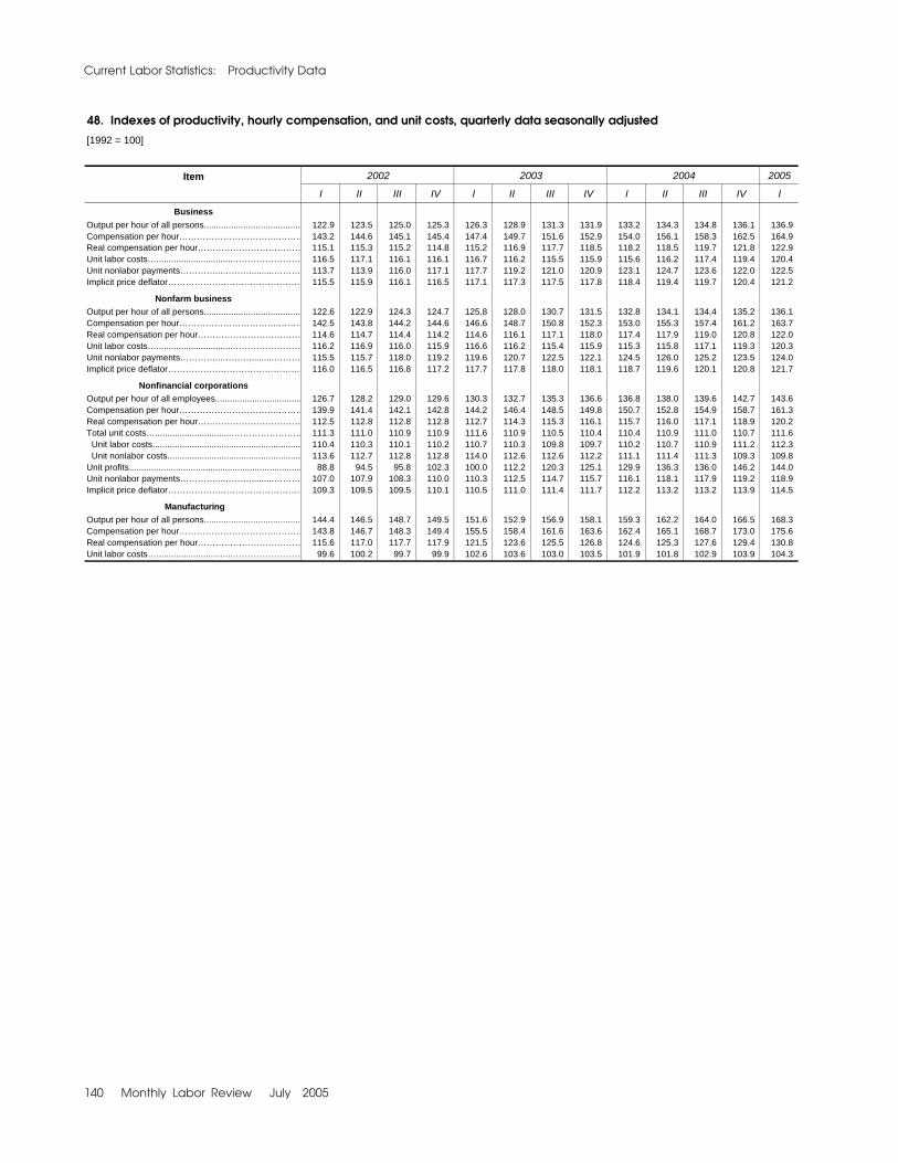
Current Labor Statistics: Productivity Data
140 Monthly Labor Review July 2005
48. Indexes of productivity, hourly compensation, and unit costs, quarterly data seasonally adjusted
[1992 = 100]
Item 2002 2003 2004 2005
I II III IV I II III IV I II III IV I
BusinessOutput per hour of all persons....................................... 122.9 123.5 125.0 125.3 126.3 128.9 131.3 131.9 133.2 134.3 134.8 136.1 136.9 Compensation per hour…………………………….……… 143.2 144.6 145.1 145.4 147.4 149.7 151.6 152.9 154.0 156.1 158.3 162.5 164.9 Real compensation per hour……………………………… 115.1 115.3 115.2 114.8 115.2 116.9 117.7 118.5 118.2 118.5 119.7 121.8 122.9 Unit labor costs…...............................…………………… 116.5 117.1 116.1 116.1 116.7 116.2 115.5 115.9 115.6 116.2 117.4 119.4 120.4 Unit nonlabor payments…………...………..........……… 113.7 113.9 116.0 117.1 117.7 119.2 121.0 120.9 123.1 124.7 123.6 122.0 122.5 Implicit price deflator……………………………………… 115.5 115.9 116.1 116.5 117.1 117.3 117.5 117.8 118.4 119.4 119.7 120.4 121.2
Nonfarm businessOutput per hour of all persons....................................... 122.6 122.9 124.3 124.7 125.8 128.0 130.7 131.5 132.8 134.1 134.4 135.2 136.1 Compensation per hour…………………………….……… 142.5 143.8 144.2 144.6 146.6 148.7 150.8 152.3 153.0 155.3 157.4 161.2 163.7 Real compensation per hour……………………………… 114.6 114.7 114.4 114.2 114.6 116.1 117.1 118.0 117.4 117.9 119.0 120.8 122.0 Unit labor costs…...............................…………………… 116.2 116.9 116.0 115.9 116.6 116.2 115.4 115.9 115.3 115.8 117.1 119.3 120.3 Unit nonlabor payments…………...………..........……… 115.5 115.7 118.0 119.2 119.6 120.7 122.5 122.1 124.5 126.0 125.2 123.5 124.0 Implicit price deflator……………………………………… 116.0 116.5 116.8 117.2 117.7 117.8 118.0 118.1 118.7 119.6 120.1 120.8 121.7
Nonfinancial corporationsOutput per hour of all employees................................... 126.7 128.2 129.0 129.6 130.3 132.7 135.3 136.6 136.8 138.0 139.6 142.7 143.6 Compensation per hour…………………………….……… 139.9 141.4 142.1 142.8 144.2 146.4 148.5 149.8 150.7 152.8 154.9 158.7 161.3 Real compensation per hour……………………………… 112.5 112.8 112.8 112.8 112.7 114.3 115.3 116.1 115.7 116.0 117.1 118.9 120.2 Total unit costs…...............................…………………… 111.3 111.0 110.9 110.9 111.6 110.9 110.5 110.4 110.4 110.9 111.0 110.7 111.6 Unit labor costs............................................................ 110.4 110.3 110.1 110.2 110.7 110.3 109.8 109.7 110.2 110.7 110.9 111.2 112.3 Unit nonlabor costs...................................................... 113.6 112.7 112.8 112.8 114.0 112.6 112.6 112.2 111.1 111.4 111.3 109.3 109.8 Unit profits...................................................................... 88.8 94.5 95.8 102.3 100.0 112.2 120.3 125.1 129.9 136.3 136.0 146.2 144.0 Unit nonlabor payments…………...………..........……… 107.0 107.9 108.3 110.0 110.3 112.5 114.7 115.7 116.1 118.1 117.9 119.2 118.9 Implicit price deflator……………………………………… 109.3 109.5 109.5 110.1 110.5 111.0 111.4 111.7 112.2 113.2 113.2 113.9 114.5
ManufacturingOutput per hour of all persons....................................... 144.4 146.5 148.7 149.5 151.6 152.9 156.9 158.1 159.3 162.2 164.0 166.5 168.3 Compensation per hour…………………………….……… 143.8 146.7 148.3 149.4 155.5 158.4 161.6 163.6 162.4 165.1 168.7 173.0 175.6 Real compensation per hour……………………………… 115.6 117.0 117.7 117.9 121.5 123.6 125.5 126.8 124.6 125.3 127.6 129.4 130.8 Unit labor costs…...............................…………………… 99.6 100.2 99.7 99.9 102.6 103.6 103.0 103.5 101.9 101.8 102.9 103.9 104.3

Monthly Labor Review July 2005 141
49. Annual indexes of multifactor productivity and related measures, selected years
[2000 = 100, unless otherwise indicated]
Item 1990 1991 1992 1993 1994 1995 1996 1997 1998 1999 2000 2001 2002
Private businessProductivity: Output per hour of all persons......……………............. 81.4 82.7 86.2 86.5 87.5 87.7 90.3 91.9 94.4 97.2 100.0 102.7 107.2 Output per unit of capital services……………………… 102.6 99.7 101.7 102.6 104.5 103.6 103.9 104.1 102.6 101.8 100.0 96.3 95.5 Multifactor productivity…………………………………… 90.9 90.3 92.7 93.1 94.1 93.8 95.5 96.3 97.4 98.7 100.0 100.1 102.0Output…...............................………………………….…… 68.6 68.1 70.9 73.2 76.9 79.1 82.8 87.2 91.5 96.2 100.0 100.4 102.3Inputs: Labor input................................................................... 80.1 79.1 80.0 82.4 86.1 88.5 90.4 94.0 96.2 99.0 100.0 98.6 97.4 Capital services…………...………..........………….…… 66.9 68.4 69.7 71.3 73.5 76.4 79.7 83.8 89.2 94.5 100.0 104.2 107.1 Combined units of labor and capital input……………… 75.5 75.4 76.5 78.6 81.7 84.3 86.7 90.5 93.9 97.5 100.0 100.4 100.3Capital per hour of all persons.......................…………… 79.3 83.0 84.8 84.4 83.7 84.6 86.9 88.3 92.0 95.4 100.0 106.6 112.2
Private nonfarm business
Productivity: Output per hour of all persons........……………………… 81.7 83.1 86.5 86.9 87.9 88.4 90.8 92.2 94.7 97.3 100.0 102.6 107.2 Output per unit of capital services……………………… 104.2 101.1 102.8 103.8 105.4 104.7 104.7 104.6 103.0 102.1 100.0 96.3 95.4 Multifactor productivity…………………………………… 91.5 91.0 93.2 93.6 94.5 94.6 96.0 96.6 97.7 98.8 100.0 100.0 102.0Output…...............................………………………….…… 68.6 68.1 70.8 73.2 76.7 79.3 82.9 87.2 91.5 96.3 100.0 100.5 102.4Inputs: Labor input................................................................... 79.8 78.7 79.6 82.2 85.6 88.0 90.0 93.7 96.0 99.0 100.0 98.8 97.3 Capital services…………...………..........………….…… 65.8 67.4 68.8 70.6 72.8 75.7 79.2 83.3 88.8 94.3 100.0 104.4 107.3 Combined units of labor and capital input……………… 75.0 74.8 75.9 78.2 81.2 83.8 86.3 90.2 93.7 97.5 100.0 100.5 100.3Capital per hour of all persons......………………………… 78.4 82.3 84.1 83.7 83.3 84.4 86.7 88.2 91.9 95.3 100.0 106.6 112.4
Manufacturing [1996 = 100]
Productivity: Output per hour of all persons...………………………… 82.2 84.1 88.6 90.2 93.0 96.5 100.0 103.8 108.9 114.0 118.3 119.7 – Output per unit of capital services……………………… 97.5 93.6 95.9 96.9 99.7 100.6 100.0 101.4 101.7 101.7 101.0 95.1 – Multifactor productivity…………………………………… 93.3 92.4 94.0 95.1 97.3 99.2 100.0 103.1 105.7 108.7 111.3 110.3 –Output…...............................………………………….…… 83.2 81.5 85.5 88.3 92.9 96.9 100.0 105.6 110.5 114.7 117.4 112.1 –Inputs: Hours of all persons..................................................... 101.1 96.9 96.5 97.8 99.9 100.4 100.0 101.7 101.5 100.7 99.2 93.6 – Capital services…………...………..........………….…… 85.3 87.1 89.1 91.1 93.2 96.4 100.0 104.1 108.7 112.8 116.2 117.9 – Energy……………….………........................................ 93.1 93.2 93.1 96.6 99.9 102.3 100.0 97.5 100.6 102.9 104.3 98.9 – Nonenergy materials.................................................... 77.5 78.5 83.5 86.5 90.3 93.1 100.0 101.9 107.5 107.9 106.9 105.5 – Purchased business services...................................... 84.7 84.6 92.0 92.9 96.0 100.4 100.0 103.9 103.1 105.4 106.5 97.7 – Combined units of all factor inputs…………...………... 89.1 88.3 90.9 92.8 95.5 97.7 100.0 102.4 104.6 105.5 105.5 101.6 –
NOTE: Dash indicates data not available.

Current Labor Statistics: Productivity Data
142 Monthly Labor Review July 2005
50. Annual indexes of productivity, hourly compensation, unit costs, and prices, selected years
[1992 = 100]Item 1960 1970 1980 1990 1996 1997 1998 1999 2000 2001 2002 2003 2004
BusinessOutput per hour of all persons....................................... 48.9 66.3 79.1 94.5 104.7 106.7 109.7 112.9 116.1 119.0 124.2 129.6 134.7Compensation per hour…………………………….……… 13.9 23.6 54.1 90.6 109.6 113.1 120.0 125.8 134.5 140.2 144.6 150.4 157.8Real compensation per hour……………………………… 60.8 78.8 89.1 96.3 99.6 100.6 105.3 108.1 111.9 113.4 115.1 117.1 119.6Unit labor costs…...............................…………………… 28.4 35.6 68.4 96.0 104.7 106.1 109.4 111.4 115.9 117.8 116.4 116.1 117.2Unit nonlabor payments…………...………..........……… 24.8 31.5 61.3 93.8 112.0 113.9 110.1 109.5 107.4 110.2 115.2 119.8 123.3Implicit price deflator……………………………………… 27.1 34.1 65.8 95.1 107.4 109.0 109.7 110.7 112.7 114.9 116.0 117.4 119.5
Nonfarm businessOutput per hour of all persons....................................... 51.9 68.0 80.6 94.5 104.9 106.6 109.5 112.6 115.6 118.5 123.6 129.0 134.2Compensation per hour…………………………….……… 14.5 23.7 54.4 90.4 109.5 112.9 119.6 125.2 134.0 139.3 143.8 149.6 156.8Real compensation per hour……………………………… 63.3 79.2 89.5 96.0 99.5 100.4 105.0 107.5 111.4 112.6 114.5 116.4 118.9Unit labor costs…...............................…………………… 27.9 34.9 67.5 95.7 104.5 105.9 109.3 111.2 115.9 117.5 116.3 116.0 116.9Unit nonlabor payments…………...………..........……… 24.3 31.2 60.4 93.5 112.2 114.6 111.1 111.1 108.9 111.8 117.1 121.3 124.8Implicit price deflator……………………………………… 26.6 33.5 64.9 94.9 107.3 109.1 109.9 111.1 113.3 115.4 116.6 117.9 119.8
Nonfinancial corporationsOutput per hour of all employees................................... 56.2 69.8 80.8 95.4 107.1 109.9 113.5 117.3 121.5 123.6 128.4 133.7 139.3Compensation per hour…………………………….……… 16.2 25.7 57.2 91.1 108.5 111.7 118.1 123.5 132.0 137.4 141.6 147.2 154.3Real compensation per hour……………………………… 70.8 85.9 94.1 96.8 98.5 99.4 103.6 106.2 109.7 111.1 112.7 114.6 116.9Total unit costs…...............................…………………… 27.3 35.6 69.2 96.0 100.9 101.1 102.9 104.0 107.4 111.6 111.0 110.8 110.8 Unit labor costs............................................................ 28.8 36.9 70.8 95.5 101.3 101.7 104.1 105.3 108.6 111.2 110.3 110.1 110.8 Unit nonlabor costs...................................................... 23.3 32.2 64.9 97.3 100.0 99.7 99.5 100.4 104.2 112.6 113.0 112.9 111.0Unit profits...................................................................... 50.2 44.4 66.9 96.9 150.0 154.3 137.0 129.1 108.7 82.2 95.4 114.6 137.5Unit nonlabor payments…………...………..........……… 30.5 35.4 65.5 97.2 113.3 114.3 109.5 108.0 105.4 104.5 108.3 113.3 117.8Implicit price deflator……………………………………… 29.4 36.4 69.0 96.1 105.3 105.9 105.9 106.2 107.5 108.9 109.6 111.2 113.1
ManufacturingOutput per hour of all persons....................................... 41.8 54.2 70.1 92.9 113.9 118.0 123.6 128.1 134.1 136.9 147.3 154.8 163.0Compensation per hour…………………………….……… 14.9 23.7 55.6 90.5 109.3 112.2 118.7 123.4 134.7 137.8 147.0 159.7 167.3Real compensation per hour……………………………… 65.0 79.2 91.4 96.1 99.3 99.8 104.2 106.0 112.0 111.5 117.0 124.3 126.8Unit labor costs…...............................…………………… 35.6 43.8 79.3 97.3 96.0 95.1 96.0 96.4 100.5 100.7 99.8 103.2 102.6Unit nonlabor payments…………...………..........……… 26.8 29.3 80.2 100.8 110.7 110.4 104.2 105.1 107.1 105.9 – – –Implicit price deflator……………………………………… 30.2 35.0 79.9 99.5 105.2 104.6 101.1 104.6 103.9 – – –
Dash indicates data not available.

Monthly Labor Review July 2005 143
51. Annual indexes of output per hour for selected NAICS industries, 1990-2002[1997=100]
NAICS Industry 1990 1991 1992 1993 1994 1995 1996 1997 1998 1999 2000 2001 2002
Mining21 Mining…………………………………………………… 86.0 86.8 95.2 96.2 99.6 101.8 101.7 100.0 103.4 111.1 109.5 107.7 112.3 211 Oil and gas extraction………………………………… 78.4 78.8 81.9 85.1 90.3 95.5 98.9 100.0 101.6 107.9 115.2 117.4 119.3 212 Mining, except oil and gas…………………………… 79.3 80.0 86.8 89.9 93.0 94.0 96.0 100.0 104.6 105.9 106.8 109.0 111.7 2121 Coal mining…………………………………………… 68.1 69.3 75.3 79.9 83.9 88.2 94.9 100.0 106.5 110.3 115.8 114.4 112.2 2122 Metal ore mining……………………………………… 79.9 82.7 91.7 102.2 104.1 98.5 95.3 100.0 109.5 112.7 124.4 131.8 143.9 2123 Nonmetallic mineral mining and quarrying………… 92.3 89.5 96.1 93.6 96.9 97.3 97.1 100.0 101.3 101.2 96.2 99.3 103.8
Utilities2211 Power generation and supply………………………… 71.2 73.8 74.2 78.7 83.0 88.6 95.5 100.0 103.8 104.1 107.0 106.4 102.4 2212 Natural gas distribution……………………………… 71.4 72.7 75.8 79.8 82.1 89.0 96.1 100.0 99.1 103.1 113.1 110.0 114.9
Manufacturing3111 Animal food…………………………………………… 90.1 89.3 90.2 90.2 87.3 94.0 87.5 100.0 109.4 109.5 109.7 127.2 –3112 Grain and oilseed milling……………………………… 89.0 91.2 91.1 93.8 94.7 99.1 91.3 100.0 107.5 114.2 112.5 117.3 –3113 Sugar and confectionery products…………………… 91.0 93.8 90.5 92.5 94.0 94.3 98.2 100.0 104.0 107.1 111.9 109.9 –3114 Fruit and vegetable preserving and specialty……… 86.4 89.7 90.7 93.8 94.9 97.1 98.2 100.0 106.8 108.4 109.8 117.0 –3115 Dairy products………………………………………… 90.8 92.1 95.4 93.9 95.4 98.7 98.0 100.0 99.1 94.5 96.0 96.2 –
3116 Animal slaughtering and processing………………… 94.5 96.8 101.5 100.9 97.4 98.5 94.3 100.0 99.9 100.3 101.9 102.7 –3117 Seafood product preparation and packaging……… 117.5 112.0 115.3 113.9 114.1 108.4 116.2 100.0 117.0 130.2 137.6 147.3 –3118 Bakeries and tortilla manufacturing………………… 92.6 92.3 95.6 96.0 96.7 99.7 97.7 100.0 103.8 105.4 105.3 106.3 –3119 Other food products…………………………………… 91.9 93.5 95.9 102.8 100.3 101.3 103.0 100.0 106.9 108.8 110.2 103.2 –3121 Beverages……………………………………………… 86.5 90.1 93.8 93.2 97.7 99.6 101.1 100.0 98.5 92.4 90.6 91.7 –
3122 Tobacco and tobacco products……………………… 81.4 77.3 79.6 73.7 89.8 97.5 99.4 100.0 98.1 92.1 98.0 100.0 –3131 Fiber, yarn, and thread mills………………………… 73.9 74.7 80.1 84.6 87.2 92.0 98.7 100.0 102.2 104.6 102.6 110.5 –3132 Fabric mills…………………………………………… 75.0 77.7 81.5 85.0 91.9 95.8 98.0 100.0 103.9 109.8 110.2 109.1 –3133 Textile and fabric finishing mills……………………… 81.7 80.4 83.7 86.0 87.8 84.5 85.0 100.0 100.6 101.7 104.0 109.7 –3141 Textile furnishings mills……………………………… 88.2 88.6 93.0 93.7 90.1 92.5 93.3 100.0 99.9 101.2 106.8 106.9 –
–3149 Other textile product millsv 91.1 90.0 92.0 90.3 94.5 95.9 96.3 100.0 97.0 110.4 110.4 105.0 –3151 Apparel knitting mills………………………………… 85.6 88.7 93.2 102.5 104.3 109.5 121.9 100.0 96.6 102.0 110.2 108.4 –3152 Cut and sew apparel………………………………… 70.1 72.0 73.1 76.6 80.5 85.5 90.5 100.0 104.0 118.8 127.7 131.7 –3159 Accessories and other apparel……………………… 100.9 97.3 98.7 99.0 104.6 112.4 112.6 100.0 110.8 103.3 104.9 114.8 –3161 Leather and hide tanning and finishing…………… 60.8 56.6 76.7 83.1 75.9 78.6 91.5 100.0 98.0 101.6 110.0 109.7 –
3162 Footwear……………………………………………… 77.1 74.7 83.1 81.7 90.4 95.6 103.4 100.0 100.9 116.8 124.1 142.7 –3169 Other leather products………………………………… 102.5 100.2 97.0 94.3 80.0 73.2 79.7 100.0 109.2 100.4 107.6 114.1 –3211 Sawmills and wood preservation…………………… 79.2 81.6 86.1 82.6 85.1 91.0 96.2 100.0 100.8 105.4 106.5 109.0 –3212 Plywood and engineered wood products…………… 102.3 107.4 114.7 108.9 105.8 101.8 101.2 100.0 105.6 99.9 100.5 105.0 –3219 Other wood products………………………………… 105.4 104.7 104.0 103.0 99.3 100.4 100.8 100.0 101.5 105.4 104.0 104.6 –
3221 Pulp, paper, and paperboard mills………………… 88.5 88.1 92.3 92.9 97.6 102.0 97.6 100.0 103.1 111.4 115.7 117.5 –3222 Converted paper products…………………………… 90.5 93.5 93.7 96.3 97.6 97.2 98.3 100.0 102.7 101.5 101.9 101.0 –3231 Printing and related support activities……………… 96.6 95.4 101.3 100.1 98.3 98.8 99.6 100.0 100.5 103.5 104.9 105.6 –3241 Petroleum and coal products………………………… 76.7 75.8 78.9 84.5 85.6 90.1 94.8 100.0 102.1 107.8 113.2 112.2 –3251 Basic chemicals……………………………………… 91.4 90.1 89.4 89.9 95.1 92.3 90.0 100.0 102.5 114.7 118.4 111.0 –
3252 Resin, rubber, and artificial fibers…………………… 75.8 74.7 80.6 83.8 93.5 95.9 93.3 100.0 105.5 108.8 108.1 103.8 –3253 Agricultural chemicals………………………………… 84.6 81.0 81.3 85.6 87.4 90.7 92.1 100.0 98.8 87.6 91.4 91.1 –3254 Pharmaceuticals and medicines…………………… 91.4 92.6 88.2 88.1 92.4 96.3 99.9 100.0 92.9 94.6 93.4 97.4 –3255 Paints, coatings, and adhesives…………………… 85.1 85.9 87.6 90.9 94.1 92.7 98.3 100.0 99.1 98.8 98.5 102.1 –3256 Soap, cleaning compounds, and toiletries………… 83.2 84.2 83.4 86.9 88.6 93.9 95.6 100.0 96.6 91.1 99.2 102.7 –
–3259 Other chemical products and preparations………… 76.6 78.0 84.7 90.6 92.6 94.4 94.2 100.0 99.4 109.2 120.0 111.3 –3261 Plastics products……………………………………… 84.7 86.3 90.3 91.9 94.4 94.5 97.0 100.0 103.5 109.3 111.2 113.3 –3262 Rubber products……………………………………… 83.0 83.8 84.9 90.4 90.3 92.8 94.4 100.0 100.5 101.4 103.9 104.2 –3271 Clay products and refractories……………………… 89.2 87.5 91.5 91.9 96.6 97.4 102.6 100.0 101.3 103.5 103.6 97.6 –3272 Glass and glass products…………………………… 80.0 79.1 84.3 86.1 87.5 88.8 96.5 100.0 102.7 108.6 109.7 105.2 –
3273 Cement and concrete products……………………… 94.8 93.7 94.8 96.5 95.0 98.2 100.6 100.0 103.5 104.1 100.4 97.1 –3274 Lime and gypsum products………………………… 84.1 82.7 88.5 90.1 87.8 88.8 92.4 100.0 113.1 102.7 97.0 100.1 –3279 Other nonmetallic mineral products………………… 79.8 81.4 90.2 89.3 90.5 91.7 96.5 100.0 98.8 95.5 95.6 96.8 –3311 Iron and steel mills and ferroalloy production……… 69.6 67.2 74.1 81.7 87.2 89.7 94.1 100.0 101.7 106.5 108.5 106.7 –3312 Steel products from purchased steel……………… 83.8 86.4 89.9 95.9 100.0 100.5 100.5 100.0 100.3 94.2 96.4 97.1 –
3313 Alumina and aluminum production………………… 91.9 93.3 96.8 96.0 100.3 96.8 95.9 100.0 101.1 104.3 97.8 96.9 –3314 Other nonferrous metal production………………… 95.6 95.8 98.8 101.8 105.1 102.9 105.7 100.0 111.2 108.9 103.1 100.5 –3315 Foundries……………………………………………… 85.3 84.5 85.8 89.8 91.4 93.1 96.2 100.0 101.6 104.9 104.0 109.3 –3321 Forging and stamping………………………………… 88.6 86.5 91.7 94.6 93.7 94.2 97.6 100.0 103.7 110.9 121.3 121.8 –3322 Cutlery and hand tools……………………………… 85.1 85.4 87.2 91.7 94.4 97.8 104.4 100.0 100.0 107.8 105.8 110.2 –
3323 Architectural and structural metals………………… 87.8 89.1 92.5 93.4 95.1 93.9 94.2 100.0 101.1 101.8 101.0 100.7 –3324 Boilers, tanks, and shipping containers…………… 90.4 92.6 95.3 94.8 100.5 97.8 100.7 100.0 101.3 98.9 97.7 98.2 –3325 Hardware……………………………………………… 84.4 83.8 86.9 89.6 95.7 97.3 102.6 100.0 101.0 106.5 115.8 114.6 –3326 Spring and wire products…………………………… 85.2 88.4 90.9 95.3 91.5 99.5 102.8 100.0 111.6 112.9 114.6 110.6 –3327 Machine shops and threaded products…………… 78.8 79.8 87.2 86.9 91.6 98.7 100.0 100.0 99.3 103.9 107.2 107.2 –

Current Labor Statistics: Productivity Data
144 Monthly Labor Review July 2005
51. Continued–Annual indexes of output per hour for selected NAICS industries, 1990-2002
[1997=100]
NAICS Industry 1990 1991 1992 1993 1994 1995 1996 1997 1998 1999 2000 2001 2002
3328 Coating, engraving, and heat treating metals……… 81.6 78.1 86.9 91.9 96.5 102.8 102.9 100.0 101.7 101.5 105.9 105.1 –3329 Other fabricated metal products…………………… 86.7 85.9 90.6 92.1 95.0 97.1 98.9 100.0 102.3 100.2 100.8 98.2 –3331 Agriculture, construction, and mining machinery 82.8 77.2 79.6 84.1 91.0 95.6 95.9 100.0 104.2 95.0 101.0 99.5 –3332 Industrial machinery…………………………………… 80.6 81.1 79.5 84.9 90.0 97.9 98.8 100.0 94.4 105.2 129.7 104.6 –3333 Commercial and service industry machinery……… 91.4 89.6 96.5 101.7 101.2 103.0 106.3 100.0 107.5 111.2 101.4 94.4 –
–3334 HVAC and commercial refrigeration equipment 88.8 88.2 90.8 93.8 97.3 96.6 97.8 100.0 106.6 110.4 108.3 110.8 –3335 Metalworking machinery……………………………… 85.3 82.3 89.3 89.3 94.0 99.1 98.1 100.0 99.1 100.5 106.4 102.0 –3336 Turbine and power transmission equipment……… 85.1 84.6 81.2 84.8 93.3 92.1 97.9 100.0 106.4 113.3 117.1 130.2 –3339 Other general purpose machinery…………………… 85.9 85.2 85.1 89.8 91.5 94.6 95.1 100.0 103.2 105.6 113.0 109.4 –
3341 Computer and peripheral equipment……………… 14.3 15.8 20.6 27.9 35.9 51.3 72.6 100.0 138.6 190.3 225.4 237.0 –
3342 Communications equipment………………………… 47.3 49.3 59.3 62.1 70.1 74.6 84.3 100.0 102.7 134.0 165.5 155.2 –3343 Audio and video equipment………………………… 75.5 82.8 92.1 98.8 108.5 140.0 104.7 100.0 103.1 116.2 123.3 126.3 –3344 Semiconductors and electronic components……… 21.4 24.5 29.6 34.1 43.1 63.4 81.8 100.0 125.2 174.5 233.3 231.6 –3345 Electronic instruments………………………………… 76.0 80.5 83.1 85.8 88.8 96.8 97.7 100.0 101.3 105.1 114.3 116.1 –3346 Magnetic media manufacturing and reproduction 86.6 91.2 93.0 96.8 106.1 106.7 103.8 100.0 105.4 106.8 104.0 98.6 –
3351 Electric lighting equipment…………………………… 87.3 88.5 93.6 90.8 94.5 92.2 95.6 100.0 103.8 102.5 101.9 105.4 –3352 Household appliances………………………………… 76.4 76.4 82.4 88.9 95.0 92.7 93.1 100.0 105.1 104.3 117.5 122.6 –3353 Electrical equipment…………………………………… 73.6 72.7 78.9 85.8 89.0 98.1 100.2 100.0 99.8 98.9 100.6 101.0 –3359 Other electrical equipment and components……… 75.3 74.2 81.6 86.8 89.4 92.0 96.0 100.0 105.5 114.8 120.5 113.5 –3361 Motor vehicles………………………………………… 86.0 82.4 91.2 89.8 90.3 88.6 91.0 100.0 113.3 123.3 110.4 108.7 –
3362 Motor vehicle bodies and trailers…………………… 75.8 71.8 88.3 96.3 97.7 97.3 98.4 100.0 102.7 103.1 98.4 99.4 –3363 Motor vehicle parts…………………………………… 75.7 74.5 82.4 88.5 91.8 92.3 93.1 100.0 104.8 110.4 112.7 114.8 –3364 Aerospace products and parts……………………… 87.7 92.1 94.1 98.2 93.8 93.7 98.1 100.0 118.5 118.0 101.0 114.7 –3365 Railroad rolling stock………………………………… 77.2 80.0 81.1 82.3 83.1 82.0 80.9 100.0 102.9 116.0 117.7 124.7 –3366 Ship and boat building………………………………… 99.6 92.6 98.5 101.3 99.0 93.1 94.1 100.0 100.3 112.2 120.1 119.8 –
3369 Other transportation equipment……………………… 62.6 62.0 88.4 99.8 93.4 93.1 99.8 100.0 110.8 113.3 130.9 146.9 –3371 Household and institutional furniture………………… 87.6 88.2 92.9 93.8 94.1 97.1 99.5 100.0 102.7 103.7 102.5 106.1 –3372 Office furniture and fixtures………………………… 80.8 78.8 86.2 87.9 83.4 84.3 85.6 100.0 100.1 98.5 100.2 97.1 –3379 Other furniture-related products…………………… 88.1 88.6 88.4 90.5 93.6 94.5 96.7 100.0 107.2 102.5 100.1 105.3 –3391 Medical equipment and supplies…………………… 81.2 83.1 88.1 91.1 90.8 95.0 100.0 100.0 108.9 109.6 114.2 119.0 –3399 Other miscellaneous manufacturing………………… 90.1 90.6 90.0 92.3 93.0 96.0 99.6 100.0 101.9 105.2 112.9 110.9 –
Wholesale trade42 Wholesale trade……………………………………… 77.8 79.1 86.2 89.5 91.3 93.3 96.2 100.0 104.4 110.9 114.1 117.1 123.6
423 Durable goods………………………………………… 65.7 66.1 75.0 80.5 84.5 88.9 94.0 100.0 105.6 115.3 119.6 120.3 127.7 4231 Motor vehicles and parts……………………………… 76.6 73.3 82.2 88.0 94.1 93.6 94.9 100.0 104.7 119.8 114.0 114.1 121.7 4232 Furniture and furnishings…………………………… 82.4 87.2 92.0 95.8 93.3 96.8 97.0 100.0 97.5 100.8 105.5 105.4 101.8 4233 Lumber and construction supplies…………………… 115.0 113.2 119.6 113.9 111.9 103.6 103.0 100.0 102.9 104.8 101.7 108.6 119.2
4234 Commercial equipment……………………………… 33.8 37.3 48.2 56.2 60.5 74.7 88.4 100.0 118.2 141.1 148.9 164.9 189.4 4235 Metals and minerals…………………………………… 101.6 102.6 109.1 111.7 110.1 101.2 102.7 100.0 102.4 96.0 99.2 102.2 102.2 4236 Electric goods………………………………………… 46.8 47.6 51.4 59.1 68.2 79.3 87.8 100.0 105.9 126.2 151.7 148.1 161.2 4237 Hardware and plumbing……………………………… 88.8 86.5 95.6 94.3 101.3 98.0 99.1 100.0 103.5 107.8 111.1 102.6 107.9 4238 Machinery and supplies……………………………… 78.9 74.2 79.7 84.3 85.4 89.7 93.9 100.0 104.2 101.4 104.1 102.7 100.2
4239 Miscellaneous durable goods………………………… 89.5 96.6 112.1 113.2 106.1 99.2 101.0 100.0 101.8 112.6 116.7 116.1 125.5 424 Nondurable goods…………………………………… 98.4 99.8 103.2 103.0 101.8 99.7 99.2 100.0 102.8 104.1 103.5 106.9 112.6
4241 Paper and paper products…………………………… 81.0 85.5 96.5 97.2 101.5 99.0 96.5 100.0 100.4 105.5 105.5 109.0 120.2 4242 Druggists' goods……………………………………… 81.8 86.6 91.8 89.3 92.8 95.4 98.3 100.0 99.6 101.7 96.8 101.2 116.0 4243 Apparel and piece goods…………………………… 103.9 103.3 100.1 97.7 103.8 92.2 99.0 100.0 104.1 103.5 102.7 102.4 111.5
4244 Grocery and related products………………………… 96.4 98.2 103.6 105.1 103.3 103.0 99.8 100.0 101.9 103.6 105.2 109.4 111.8 4245 Farm product raw materials………………………… 80.6 85.9 85.9 84.0 80.4 87.7 90.6 100.0 100.4 114.2 119.0 120.0 135.4 4246 Chemicals……………………………………………… 107.3 106.6 112.5 110.0 110.5 102.1 100.0 100.0 99.3 98.0 95.8 93.6 96.9 4247 Petroleum……………………………………………… 97.3 107.0 118.3 119.1 115.8 108.7 105.9 100.0 115.0 112.0 112.5 116.5 126.0 4248 Alcoholic beverages…………………………………… 109.4 111.2 107.4 105.6 105.9 102.5 104.5 100.0 109.7 110.1 111.0 111.6 117.3
4249 Miscellaneous nondurable goods…………………… 107.3 98.2 93.9 97.5 94.8 96.2 98.7 100.0 101.7 99.6 106.2 104.2 97.0 425 Electronic markets and agents and brokers……… 70.7 73.6 81.5 85.9 88.0 91.1 95.7 100.0 104.6 114.4 124.1 131.3 132.6
42511 Business to business electronic markets…………… 70.4 72.6 80.3 84.8 88.3 90.5 95.3 100.0 103.5 121.7 141.3 169.4 205.0 42512 Wholesale trade agents and brokers……………… 70.8 74.0 82.3 86.8 88.4 91.8 96.1 100.0 104.8 110.5 115.7 114.2 109.3
Retail trade44-45 Retail trade…………………………………………… 83.2 83.3 86.8 89.4 92.8 94.7 97.7 100.0 104.3 110.3 114.2 117.4 122.7 441 Motor vehicle and parts dealers……………………… 89.7 88.3 92.6 94.0 96.9 97.0 98.8 100.0 102.7 106.4 107.2 110.0 109.7
4411 Automobile dealers…………………………………… 92.1 90.8 94.8 96.0 98.0 97.2 98.9 100.0 102.7 106.4 106.6 109.1 106.0 4412 Other motor vehicle dealers………………………… 69.0 71.7 78.3 84.1 90.2 91.0 97.7 100.0 105.9 113.0 108.6 112.6 116.4 4413 Auto parts, accessories, and tire stores…………… 85.0 84.0 89.1 90.6 95.4 97.9 98.3 100.0 105.7 110.0 112.0 109.3 115.8
442 Furniture and home furnishings stores……………… 80.7 81.1 88.1 88.3 90.4 94.1 99.4 100.0 101.7 109.6 115.7 118.5 125.1 4421 Furniture stores……………………………………… 82.1 83.5 89.0 89.0 88.9 92.5 97.8 100.0 102.1 108.2 114.8 121.1 128.6 4422 Home furnishings stores……………………………… 78.5 77.6 86.8 87.2 92.1 95.9 101.3 100.0 101.3 111.4 116.8 115.6 121.4 443 Electronics and appliance stores…………………… 46.0 49.2 56.9 65.5 77.6 89.2 95.0 100.0 122.9 152.2 177.7 199.1 240.0 444 Building material and garden supply stores………… 81.8 80.2 84.0 88.0 93.7 93.7 97.5 100.0 106.7 112.3 113.1 115.8 119.9

Monthly Labor Review July 2005 145
51. Continued–-Annual indexes of output per hour for selected NAICS industries, 1990-2002
[1997=100]
NAICS Industry 1990 1991 1992 1993 1994 1995 1996 1997 1998 1999 2000 2001 2002
4441 Building material and supplies dealers……………… 83.2 80.7 84.7 89.1 94.8 94.8 97.6 100.0 107.6 113.7 113.8 115.3 119.8 4442 Lawn and garden equipment and supplies stores 74.5 77.5 80.2 81.5 86.9 87.0 97.1 100.0 101.2 103.5 108.2 119.4 121.2 445 Food and beverage stores…………………………… 107.1 106.6 106.9 105.4 104.3 102.5 100.3 100.0 99.9 103.7 105.1 107.6 110.3
4451 Grocery stores………………………………………… 106.5 106.6 106.7 105.9 104.9 103.0 100.8 100.0 100.3 104.3 104.9 107.5 110.3 4452 Specialty food stores………………………………… 122.9 115.0 111.4 107.6 104.5 101.1 95.5 100.0 95.0 99.6 105.6 110.8 114.2
4453 Beer, wine and liquor stores………………………… 100.1 100.2 101.0 94.4 92.9 96.2 103.1 100.0 105.8 99.8 111.1 110.4 111.8
446 Health and personal care stores…………………… 92.0 91.6 90.7 91.9 91.8 93.0 95.7 100.0 104.1 106.9 111.4 112.7 118.8 447 Gasoline stations……………………………………… 84.8 85.7 88.5 92.8 96.8 99.7 99.4 100.0 105.6 110.6 106.5 109.8 117.5 448 Clothing and clothing accessories stores…………… 69.5 70.5 75.3 78.9 83.3 91.2 97.9 100.0 105.4 112.8 120.3 123.5 129.0
4481 Clothing stores………………………………………… 68.9 71.4 77.1 79.2 81.9 90.1 97.1 100.0 106.7 113.3 120.9 125.2 132.7
4482 Shoe stores…………………………………………… 73.7 73.1 78.2 79.2 88.3 93.7 102.4 100.0 97.8 104.9 109.6 115.8 120.0 4483 Jewelry, luggage, and leather goods stores……… 68.6 64.5 65.0 77.1 85.0 94.1 97.3 100.0 107.0 118.3 128.0 122.5 121.5 451 Sporting goods, hobby, book, and music stores... 80.8 85.6 83.8 84.0 87.2 93.0 94.7 100.0 108.7 114.9 121.1 125.4 132.9
4511 Sporting goods and musical instrument stores…. 77.1 82.8 79.8 80.6 83.9 92.3 92.5 100.0 112.9 120.4 128.3 130.4 137.9 4512 Book, periodical, and music stores………………… 89.0 91.8 92.5 91.6 94.5 94.5 99.3 100.0 101.0 104.7 108.0 116.0 123.8
452 General merchandise stores………………………… 75.3 79.0 83.0 88.5 90.6 92.2 96.9 100.0 105.0 113.1 119.9 124.2 130.5 4521 Department stores…………………………………… 84.0 88.3 91.6 95.0 95.1 94.7 98.4 100.0 100.6 104.5 106.3 104.0 104.7 4529 Other general merchandise stores………………… 61.4 64.8 69.7 77.8 82.6 87.6 94.3 100.0 113.4 129.8 145.9 162.1 177.5 453 Miscellaneous store retailers………………………… 70.6 68.0 74.2 79.1 87.0 89.5 95.0 100.0 108.3 109.8 111.3 108.4 115.6
4531 Florists………………………………………………… 75.1 75.9 85.1 91.4 85.4 83.5 96.1 100.0 101.2 117.3 116.0 108.6 120.7
4532 Office supplies, stationery and gift stores………… 64.6 66.3 71.5 75.8 87.5 90.9 91.8 100.0 113.0 118.0 124.1 125.1 140.3 4533 Used merchandise stores…………………………… 84.9 83.1 89.7 88.9 87.3 90.2 97.4 100.0 113.5 109.8 115.7 115.0 121.4 4539 Other miscellaneous store retailers………………… 79.6 69.2 74.7 80.5 89.7 90.5 98.0 100.0 105.0 101.6 99.6 93.2 92.8 454 Nonstore retailers……………………………………… 54.4 55.0 63.4 66.7 73.8 80.9 91.6 100.0 111.3 125.4 142.8 146.9 169.6
4541 Electronic shopping and mail-order houses……… 43.5 46.7 50.6 58.3 62.9 71.9 84.4 100.0 118.2 141.5 159.8 177.5 209.8 4542 Vending machine operators………………………… 97.1 95.4 95.1 92.8 94.1 89.3 96.9 100.0 114.1 118.1 127.1 110.4 113.3 4543 Direct selling establishments………………………… 70.0 67.6 82.1 79.7 89.2 94.7 102.2 100.0 96.2 96.3 104.3 98.7 110.2
Transportation and warehousing481 Air transportation……………………………………… 77.5 78.2 81.4 84.7 90.8 95.3 98.8 100.0 97.6 98.2 98.2 91.9 103.2
482111 Line-haul railroads…………………………………… 69.8 75.3 82.3 85.7 88.6 92.0 98.4 100.0 102.1 105.5 114.3 121.9 131.9 48412 General freight trucking, long-distance……………… 88.5 92.4 97.5 95.6 98.1 95.4 95.7 100.0 99.1 102.0 105.5 104.2 109.4 491 U.S. Postal service…………………………………… 96.1 95.8 96.5 99.0 98.5 98.3 96.7 100.0 101.4 102.4 104.9 106.1 107.0
Information5111 Newspaper, book, and directory publishers……… 97.4 96.1 95.8 95.3 93.0 93.5 92.7 100.0 104.5 108.5 110.1 106.4 108.1 5112 Software publishers…………………………………… 28.6 30.6 42.7 51.7 64.6 73.0 88.0 100.0 115.9 113.0 103.9 101.9 106.7 51213 Motion picture and video exhibition………………… 109.4 108.9 104.1 104.6 103.4 99.9 100.0 100.0 99.9 102.0 106.5 104.7 104.4 5151 Radio and television broadcasting………………… 96.1 97.8 102.8 101.4 106.0 106.1 104.1 100.0 99.1 99.4 98.4 94.3 100.4 5152 Cable and other subscription programming………… 98.8 94.3 96.0 93.6 92.0 94.4 93.7 100.0 129.3 133.2 135.7 125.3 131.4 5171 Wired telecommunications carriers………………… 64.8 68.4 74.5 79.7 85.1 90.6 97.5 100.0 105.5 112.7 119.9 121.0 130.6 5172 Wireless telecommunications carriers……………… 76.3 73.8 85.6 94.8 97.1 98.3 103.0 100.0 114.2 134.3 139.0 172.7 192.0 5175 Cable and other program distribution……………… 99.1 94.3 95.9 93.5 91.9 94.2 93.5 100.0 95.7 94.5 90.4 87.6 93.5
Finance and insurance52211 Commercial banking………………………………… 80.5 83.2 83.3 90.3 92.9 96.0 99.3 100.0 98.0 101.5 104.2 101.6 103.8
Real estate and rental and leasing532111 Passenger car rental………………………………… 89.8 97.8 104.4 106.1 107.9 101.1 108.9 100.0 101.2 113.1 112.0 112.1 113.3 53212 Truck, trailer and RV rental and leasing…………… 70.7 71.7 69.5 75.8 82.0 90.3 96.7 100.0 93.7 97.8 95.9 93.6 91.4
Professional, scientific, and technical services
541213 Tax preparation services……………………………… 92.4 84.7 99.5 119.1 119.9 96.2 92.1 100.0 105.1 99.2 91.8 78.2 92.1 54181 Advertising agencies…………………………………… 105.0 99.7 111.9 111.3 106.8 101.4 102.1 100.0 95.8 110.1 116.6 116.7 123.9
Accomodation and food services7211 Traveler accommodations…………………………… 82.9 85.4 92.9 93.0 97.0 99.2 100.1 100.0 100.0 103.6 107.7 102.0 104.1 722 Food services and drinking places………………… 102.9 102.3 101.7 102.3 100.8 100.6 99.2 100.0 101.2 101.1 103.5 103.7 104.9
7221 Full-service restaurants……………………………… 99.1 98.3 97.5 97.7 97.8 96.6 96.3 100.0 100.0 99.2 100.8 100.8 102.0 7222 Limited-service eating places………………………… 103.3 103.3 102.7 105.6 103.6 104.7 102.2 100.0 102.4 102.5 105.1 106.6 107.1 7223 Special food services………………………………… 107.2 106.9 106.4 103.8 101.1 99.3 97.6 100.0 102.1 106.0 111.7 108.4 108.1 7224 Drinking places, alcoholic beverages……………… 125.7 121.2 121.5 112.7 102.6 104.4 102.4 100.0 100.0 99.4 100.4 98.2 107.2
Other services (except public administration)8111 Automotive repair and maintenance………………… 92.8 86.5 90.0 91.2 96.7 102.9 98.9 100.0 105.0 106.9 108.6 109.3 103.7 81211 Hair, nail and skin care services…………………… 81.6 79.8 85.6 84.3 88.7 92.4 97.1 100.0 102.7 103.6 103.0 109.5 104.2 81221 Funeral homes and funeral services………………… 96.1 94.3 104.7 100.4 103.6 100.4 97.9 100.0 103.8 100.4 94.5 93.9 90.9 8123 Drycleaning and laundry services…………………… 95.6 93.2 94.9 93.8 95.9 98.8 101.6 100.0 105.0 109.5 113.7 121.1 120.2 81292 Photofinishing………………………………………… 117.3 115.6 116.2 123.6 124.9 114.7 103.2 100.0 99.4 106.9 107.6 115.0 133.6
NOTE: Dash indicates data are not available.

Current Labor Statistics: International Comparison
146 Monthly Labor Review July 2005
52. Unemployment rates, approximating U.S. concepts, in nine countries, quarterly data seasonally adjusted
2003 2004 2005
Country 2003 2004 I II III IV I II III IV I
United States……… 6.0 5.5 5.8 6.1 6.1 5.9 5.6 5.6 5.5 5.4 5.3
Canada……………… 6.9 6.4 6.7 6.9 7.1 6.8 6.6 6.5 6.4 6.3 6.2
Australia…………… 6.1 5.5 6.2 6.2 6.0 5.8 5.7 5.6 5.6 5.2 5.1
Japan………………… 5.3 4.8 5.4 5.5 5.2 5.1 4.9 4.7 4.8 4.6 4.6
France……………… 9.6 9.8 9.3 9.5 9.7 9.8 9.7 9.8 9.8 9.8 9.9
Germany…………… 9.7 9.8 9.6 9.8 9.8 9.7 9.7 9.8 10.0 10.1 11.0Italy………………… 8.5 8.1 8.7 8.4 8.6 8.4 8.3 8.1 8.1 8.1 –
Sweden……………… 5.8 6.6 5.3 5.5 5.8 6.3 6.7 6.8 6.6 6.4 6.3
United Kingdom…… 5.0 4.8 5.1 5.0 5.0 4.9 4.8 4.8 4.7 4.7 –
Annual average
NOTE: Dash indicates data not available. Quarterly figures for
Japan, France, Germany, Italy, and Sweden are calculated by
applying annual adjustment factors to current published data, and
therefore should be viewed as less precise indicators of
unemployment under U.S. concepts than the annual figures. See
"Notes on the data" for information on breaks in series.
for further qualifications and historical data, see Comparative
Civilian Labor Force Statistics, Ten Countries, 1960-2004 (Bureau
of Labor Statistics, May 13, 2005), on the Internet at
http://www.bls.gov/fls/home.htm.
Monthly and quarterly unemployment rates, updated monthly, are
also on this site.

Monthly Labor Review July 2005 147
53. Annual data: employment status of the working-age population, approximating U.S. concepts, 10 countries[Numbers in thousands]
Employment status and country 1993 1994 1995 1996 1997 1998 1999 2000 2001 2002 2003 2004
Civilian labor forceUnited States………………………………………… 129,200 131,056 132,304 133,943 136,297 137,673 139,368 142,583 143,734 144,863 146,510 147,401Canada……………………………………………… 14,233 14,336 14,439 14,604 14,863 15,115 15,389 15,632 15,892 16,367 16,729 16,956Australia……………………………………………… 8,613 8,770 8,995 9,115 9,204 9,339 9,414 9,590 9,752 9,907 10,092 10,244Japan………………………………………………… 65,470 65,780 65,990 66,450 67,200 67,240 67,090 66,990 66,860 66,240 66,010 65,760France………………………………………………… 24,490 24,676 24,743 24,985 25,109 25,434 25,764 26,078 26,354 26,686 26,870 –Germany……………………………………………… 39,102 39,074 38,980 39,142 39,415 39,754 39,375 39,301 39,456 39,499 39,591 39,698Italy…………………………………………………… 22,771 22,592 22,574 22,674 22,749 23,000 23,172 23,357 23,520 23,728 24,021 24,065Netherlands………………………………………… 7,014 7,152 7,208 7,301 7,536 7,617 7,848 8,149 8,338 8,285 8,353 8,457Sweden……………………………………………… 4,444 4,418 4,460 4,459 4,418 4,402 4,430 4,489 4,530 4,544 4,567 4,576United Kingdom……………………………………… 28,094 28,124 28,135 28,243 28,406 28,478 28,782 28,957 29,090 29,340 29,562 29,748
Participation rate1
United States………………………………………… 66.3 66.6 66.6 66.8 67.1 67.1 67.1 67.1 66.8 66.6 66.2 66.0Canada……………………………………………… 65.5 65.1 64.8 64.6 64.9 65.3 65.7 65.8 65.9 66.7 67.3 67.3Australia……………………………………………… 63.5 63.9 64.5 64.6 64.3 64.3 64.0 64.4 64.4 64.4 64.6 64.7Japan………………………………………………… 63.3 63.1 62.9 63.0 63.2 62.8 62.4 62.0 61.6 60.8 60.3 60.0France………………………………………………… 55.4 55.6 55.4 55.7 55.6 55.9 56.3 56.6 56.9 57.2 57.4 –Germany……………………………………………… 57.8 57.4 57.1 57.1 57.3 57.7 56.9 56.7 56.7 56.5 56.4 –Italy…………………………………………………… 48.3 47.6 47.3 47.3 47.3 47.6 47.9 48.1 48.2 48.5 49.1 49.1Netherlands………………………………………… 57.9 58.6 58.8 59.2 60.8 61.1 62.6 64.5 65.6 64.7 64.9 65.5Sweden……………………………………………… 64.5 63.7 64.1 64.0 63.3 62.8 62.8 63.8 63.7 64.0 64.0 63.7United Kingdom……………………………………… 62.6 62.4 62.4 62.4 62.5 62.5 62.8 62.9 62.7 62.9 63.0 63.0
EmployedUnited States………………………………………… 120,259 123,060 124,900 126,708 129,558 131,463 133,488 136,891 136,933 136,485 137,736 139,252Canada……………………………………………… 12,694 12,960 13,185 13,309 13,607 13,946 14,314 14,676 14,866 15,221 15,579 15,864Australia……………………………………………… 7,699 7,942 8,256 8,364 8,444 8,618 8,762 8,989 9,091 9,271 9,481 9,677Japan………………………………………………… 63,820 63,860 63,900 64,200 64,900 64,450 63,920 63,790 63,460 62,650 62,510 62,630France………………………………………………… 21,714 21,750 21,956 22,039 22,169 22,597 23,053 23,693 24,128 24,293 24,293 –Germany……………………………………………… 35,989 35,756 35,780 35,637 35,508 36,061 36,042 36,236 36,346 36,061 35,754 35,796Italy…………………………………………………… 20,543 20,171 20,030 20,120 20,165 20,366 20,613 20,969 21,356 21,665 21,973 22,105Netherlands………………………………………… 6,572 6,664 6,730 6,858 7,163 7,321 7,595 7,912 8,130 8,059 8,035 8,061Sweden……………………………………………… 4,028 3,992 4,056 4,019 3,973 4,034 4,117 4,229 4,303 4,310 4,303 4,276United Kingdom……………………………………… 25,165 25,691 25,696 25,945 26,418 26,691 27,056 27,373 27,604 27,817 28,079 28,334
Employment-population ratio2
United States………………………………………… 61.7 62.5 62.9 63.2 63.8 64.1 64.3 64.4 63.7 62.7 62.3 62.3Canada……………………………………………… 58.4 58.9 59.2 59.0 59.5 60.3 61.2 61.9 61.9 62.4 63.0 63.4Australia……………………………………………… 56.8 57.8 59.2 59.3 59.0 59.3 59.6 60.3 60.1 60.3 60.7 61.2Japan………………………………………………… 61.7 61.3 60.9 60.9 61.0 60.2 59.4 59.0 58.4 57.5 57.1 57.1France………………………………………………… 49.2 49.0 49.2 49.1 49.1 49.7 50.4 51.5 52.1 52.1 51.9 –Germany……………………………………………… 53.2 52.6 52.4 52.0 51.6 52.3 52.1 52.2 52.2 51.6 51.0 –Italy…………………………………………………… 43.6 42.5 42.0 42.0 41.9 42.2 42.6 43.2 43.8 44.3 44.9 45.1Netherlands………………………………………… 54.3 54.6 54.9 55.6 57.8 58.7 60.6 62.7 63.9 62.9 62.4 62.4Sweden……………………………………………… 58.5 57.6 58.3 57.7 56.9 57.6 58.4 60.1 60.5 60.7 60.3 59.5United Kingdom……………………………………… 56.0 57.0 57.0 57.3 58.2 58.5 59.1 59.4 59.5 59.6 59.8 60.0
UnemployedUnited States………………………………………… 8,940 7,996 7,404 7,236 6,739 6,210 5,880 5,692 6,801 8,378 8,774 8,149Canada……………………………………………… 1,538 1,376 1,254 1,295 1,256 1,169 1,075 956 1,026 1,146 1,150 1,092Australia……………………………………………… 914 829 739 751 759 721 652 602 661 636 611 567Japan………………………………………………… 1,660 1,920 2,100 2,250 2,300 2,790 3,170 3,200 3,400 3,590 3,500 3,130France………………………………………………… 2,776 2,926 2,787 2,946 2,940 2,837 2,711 2,385 2,226 2,393 2,577 2,630Germany……………………………………………… 3,113 3,318 3,200 3,505 3,907 3,693 3,333 3,065 3,109 3,438 3,838 3,899Italy…………………………………………………… 2,227 2,421 2,544 2,555 2,584 2,634 2,559 2,388 2,164 2,062 2,048 1,960Netherlands………………………………………… 442 489 478 443 374 296 253 237 208 227 318 396Sweden……………………………………………… 416 426 404 440 445 368 313 260 227 234 264 300United Kingdom……………………………………… 2,930 2,433 2,439 2,298 1,987 1,788 1,726 1,584 1,486 1,524 1,484 1,414
Unemployment rateUnited States………………………………………… 6.9 6.1 5.6 5.4 4.9 4.5 4.2 4.0 4.7 5.8 6.0 5.5Canada……………………………………………… 10.8 9.6 8.7 8.9 8.4 7.7 7.0 6.1 6.5 7.0 6.9 6.4Australia……………………………………………… 10.6 9.4 8.2 8.2 8.3 7.7 6.9 6.3 6.8 6.4 6.1 5.5Japan………………………………………………… 2.5 2.9 3.2 3.4 3.4 4.1 4.7 4.8 5.1 5.4 5.3 4.8France………………………………………………… 11.3 11.9 11.3 11.8 11.7 11.2 10.5 9.1 8.4 9.0 9.6 9.8Germany……………………………………………… 8.0 8.5 8.2 9.0 9.9 9.3 8.5 7.8 7.9 8.7 9.7 9.8Italy…………………………………………………… 9.8 10.7 11.3 11.3 11.4 11.5 11.0 10.2 9.2 8.7 8.5 8.1Netherlands………………………………………… 6.3 6.8 6.6 6.1 5.0 3.9 3.2 2.9 2.5 2.7 3.8 4.7Sweden……………………………………………… 9.4 9.6 9.1 9.9 10.1 8.4 7.1 5.8 5.0 5.1 5.8 6.6United Kingdom……………………………………… 10.4 8.7 8.7 8.1 7.0 6.3 6.0 5.5 5.1 5.2 5.0 4.81 Labor force as a percent of the working-age population. For further qualifications and historical data, see Comparative Civilian Labor Force Statistics,2 Employment as a percent of the working-age population. 'Ten Countries, 1960–2004 (Bureau of Labor Statistics, May 13, 2005), on the Internet atNOTE: Dash indicates data not available. See "Notes on the data" for http://www.bls.gov/fls/home.htm.for information on breaks in series.

Current Labor Statistics: International Comparison
148 Monthly Labor Review July 2005
54. Annual indexes of manufacturing productivity and related measures, 15 economies
[1992 = 100]
Measure and economy 1960 1970 1980 1990 1991 1993 1994 1995 1996 1997 1998 1999 2000 2001 2002 2003
Output per hour United States……………………… – 0.0 70.5 96.9 97.9 102.1 107.3 113.8 117.0 121.3 126.5 132.8 143.5 145.2 160.0 171.0Canada……………………………… 37.8 54.9 72.9 93.4 95.3 105.8 110.8 112.4 109.7 113.5 115.5 122.1 129.3 127.0 130.5 132.1Australia……………………………… – – 69.5 91.6 96.4 106.1 104.9 105.8 113.6 115.2 118.5 119.9 128.0 132.4 136.2 140.7Japan………………………………… 13.9 37.7 63.6 94.4 99.0 101.7 103.3 111.0 116.1 121.0 121.2 126.7 135.9 135.9 139.9 146.2Korea………………………………… – – – 81.5 91.6 108.5 118.2 129.3 142.3 160.4 178.8 198.9 215.8 214.3 235.2 256.4Taiwan……………………………… – – 47.6 88.8 96.5 102.8 106.7 115.1 123.1 129.3 135.9 143.4 151.0 160.8 170.9 177.2Belgium……………………………… 18.0 32.9 65.4 96.8 99.1 102.5 108.4 113.2 116.3 125.5 126.9 125.5 130.8 132.6 141.7 146.2Denmark…………………………… 25.2 46.3 83.2 98.4 100.3 100.2 112.6 112.5 109.8 118.0 117.4 123.1 126.6 127.2 131.3 136.9France……………………………… 19.9 39.0 61.6 93.9 97.0 101.0 108.9 114.4 114.7 121.7 127.9 133.0 142.5 148.0 155.1 158.0Germany…………………………… 29.2 52.0 77.2 99.0 98.3 101.8 109.6 112.3 114.7 120.4 122.0 121.4 127.0 127.8 131.0 134.4Italy…………………………………… 24.6 46.2 78.6 96.6 96.1 101.2 104.8 107.9 108.3 110.3 110.8 110.6 113.5 114.0 112.1 110.9Netherlands………………………… 18.8 38.5 69.1 98.7 99.0 102.0 113.1 117.3 119.3 121.4 124.1 127.0 132.7 132.5 135.4 –Norway……………………………… 37.6 59.1 77.9 98.1 98.2 99.6 99.6 100.7 102.5 102.0 99.9 103.6 106.6 109.8 111.7 113.5Sweden……………………………… 27.3 52.2 73.1 94.6 95.5 107.3 117.8 124.5 129.5 141.0 149.5 162.7 175.5 170.3 185.6 196.5United Kingdom…………………… 30.0 43.2 54.3 89.2 93.9 103.8 108.0 106.2 105.4 106.9 108.4 113.6 121.0 125.1 127.7 134.8
Output United States……………………… – – 75.8 101.6 98.3 103.5 111.1 118.4 121.3 127.9 133.1 138.9 147.6 139.6 142.9 145.4Canada……………………………… 33.4 58.9 83.6 106.0 99.0 105.9 114.1 119.6 119.6 127.7 133.9 144.9 159.2 153.6 158.0 157.3Australia……………………………… – – 89.8 104.1 100.7 103.8 109.1 108.7 112.6 115.1 118.6 118.3 123.8 123.8 128.7 130.2Japan………………………………… 10.8 39.4 60.8 97.1 102.0 96.3 94.9 98.9 103.0 106.5 100.2 101.9 109.2 105.5 103.4 106.7Korea………………………………… – 7.0 29.9 86.7 95.0 105.4 116.8 129.9 138.3 145.0 133.5 162.6 190.2 194.3 209.1 219.1Taiwan……………………………… – 12.7 44.0 90.0 96.1 102.4 108.5 114.9 120.3 128.3 132.6 141.5 151.8 143.1 152.1 160.9Belgium……………………………… 30.7 57.6 78.2 101.0 100.7 97.0 101.4 104.2 105.9 112.7 114.4 114.4 119.9 120.4 121.6 120.9Denmark…………………………… 42.0 72.7 94.3 101.7 100.7 97.0 107.3 112.6 107.7 115.9 116.7 117.9 121.9 121.6 120.8 121.4France……………………………… 27.9 57.7 81.6 99.1 99.8 95.7 100.3 104.9 104.6 109.7 115.0 118.7 124.3 128.0 129.1 128.5Germany…………………………… 41.5 70.9 85.3 99.1 102.3 92.4 95.1 95.2 92.5 95.7 97.7 95.8 100.1 99.9 99.6 99.8Italy…………………………………… 23.0 48.1 84.4 99.4 99.3 96.5 102.4 107.2 105.4 108.8 110.7 110.3 113.6 113.0 111.7 110.2Netherlands………………………… 31.9 59.8 76.9 99.0 99.8 97.7 104.5 108.2 108.9 111.6 114.9 117.6 122.8 121.9 121.0 117.6Norway……………………………… 57.7 91.0 104.9 101.4 99.0 101.7 104.6 107.3 110.3 114.2 113.7 113.6 112.8 112.3 111.5 107.3Sweden……………………………… 45.9 80.7 90.7 110.1 104.1 101.9 117.0 131.9 136.4 146.5 158.3 172.5 188.3 183.1 190.6 194.4United Kingdom…………………… 67.5 90.2 87.2 105.3 100.1 101.5 106.2 107.8 108.6 110.7 111.3 112.1 115.0 113.4 109.9 110.3
Total hoursUnited States……………………… 92.1 104.4 107.5 104.8 100.4 101.4 103.6 104.0 103.6 105.4 105.2 104.6 102.9 96.2 89.3 85.0Canada……………………………… 88.3 107.1 114.6 113.5 103.9 100.1 103.0 106.4 109.0 112.4 115.9 118.7 123.1 120.9 121.1 119.1Australia……………………………… – – 129.2 113.6 104.4 97.8 103.9 102.8 99.1 100.0 100.1 98.7 96.7 93.5 94.5 92.5Japan………………………………… 77.8 104.3 95.5 102.9 103.1 94.7 91.9 89.1 88.7 88.0 82.7 80.4 80.3 77.7 74.0 73.0Korea………………………………… – – – 106.5 103.7 97.1 98.8 100.4 97.2 90.4 74.7 81.8 88.1 90.7 88.9 85.4Taiwan……………………………… – – 92.4 101.4 99.6 99.6 101.7 99.8 97.7 99.2 97.6 98.7 100.5 89.0 89.0 90.8Belgium……………………………… 170.7 174.7 119.7 104.3 101.5 94.7 93.6 92.0 91.0 89.8 90.2 91.2 91.7 90.8 85.8 82.7Denmark…………………………… 166.7 157.1 113.4 103.3 100.5 96.7 95.2 100.1 98.1 98.2 99.4 95.8 96.3 95.6 92.0 88.7France……………………………… 140.3 147.8 132.5 105.6 102.9 94.7 92.1 91.7 91.2 90.2 89.9 89.2 87.2 86.5 83.2 81.3Germany…………………………… 142.3 136.3 110.5 100.1 104.1 90.8 86.8 84.8 80.6 79.5 80.1 78.9 78.8 78.2 76.1 74.3Italy…………………………………… 93.5 104.0 107.4 102.9 103.3 95.4 97.7 99.4 97.3 98.6 99.9 99.8 100.1 99.1 99.7 99.3Netherlands………………………… 169.8 155.5 111.2 100.3 100.8 95.8 92.4 92.3 91.2 91.9 92.6 92.6 92.5 92.0 89.4 –Norway……………………………… 153.6 153.9 134.7 103.4 100.8 102.1 105.0 106.6 107.6 112.0 113.7 109.6 105.9 102.3 99.8 94.5Sweden……………………………… 168.3 154.7 124.0 116.4 109.0 94.9 99.4 105.9 105.3 103.9 105.9 106.0 107.3 107.5 102.7 98.9United Kingdom…………………… 224.6 208.8 160.5 118.1 106.6 97.7 98.4 101.5 103.1 103.5 102.7 98.7 95.0 90.7 86.0 81.9
Hourly compensation(national currency basis)
United States……………………… 14.9 23.7 55.6 90.8 95.6 102.7 105.6 107.9 109.4 111.5 117.4 122.0 133.2 136.3 145.4 157.8Canada……………………………… 10.0 17.1 47.5 88.3 95.0 102.0 103.7 106.0 107.0 109.3 111.7 115.8 119.6 123.7 126.8 131.4Australia……………………………… – – – 86.3 94.0 105.9 104.3 113.2 122.8 124.6 128.2 133.0 140.0 149.5 154.7 –Japan………………………………… 4.3 16.4 58.6 90.6 96.5 102.7 104.7 108.3 109.1 112.6 115.4 114.8 113.7 114.6 122.8 123.8Korea………………………………… – – – 68.6 86.2 114.3 129.8 158.3 184.3 200.3 218.2 219.4 234.2 241.7 266.1 290.9Taiwan……………………………… – – 29.6 85.2 93.5 105.9 111.1 120.2 128.2 132.4 140.3 144.3 146.6 150.0 145.8 146.7Belgium……………………………… 5.4 13.7 52.5 90.1 97.3 104.8 106.1 109.2 111.1 115.2 117.0 118.5 120.6 127.2 136.5 –Denmark…………………………… 3.9 11.1 45.1 93.5 97.9 102.4 106.0 108.1 112.8 116.6 119.6 127.3 130.2 136.5 143.2 150.0France……………………………… 4.3 10.5 41.2 90.9 96.4 103.1 106.5 110.4 112.2 111.8 112.7 116.6 122.8 128.3 135.2 139.1Germany…………………………… 8.1 20.7 53.6 89.4 91.5 106.4 111.8 117.6 123.3 125.7 127.6 130.6 137.4 142.0 145.5 148.9Italy…………………………………… 1.8 5.3 30.4 87.6 94.2 105.7 106.8 111.3 119.0 123.0 122.2 124.2 127.8 132.5 135.7 140.0Netherlands………………………… 6.2 19.4 60.5 89.8 94.8 104.5 109.0 112.1 114.4 117.2 122.0 126.0 132.0 138.2 147.3 –Norway……………………………… 4.7 11.8 39.0 92.3 97.5 101.5 104.4 109.2 113.6 118.7 125.7 133.0 140.5 148.9 157.9 164.6Sweden……………………………… 4.1 10.7 37.3 87.8 95.5 97.4 99.8 106.8 115.2 121.0 125.6 130.3 136.8 143.8 148.8 154.3United Kingdom…………………… 2.9 6.1 32.0 82.9 93.8 104.5 107.3 108.8 111.4 115.7 123.0 129.9 137.6 144.3 152.2 160.3 See notes at end of table.
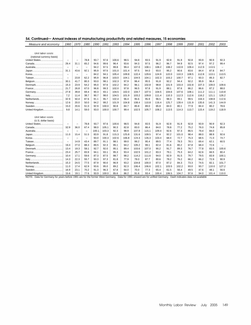
Monthly Labor Review July 2005 149
54. Continued– Annual indexes of manufacturing productivity and related measures, 15 economies
Measure and economy 1960 1970 1980 1990 1991 1993 1994 1995 1996 1997 1998 1999 2000 2001 2002 2003
Unit labor costs (national currency basis)
United States……………………… – – 78.8 93.7 97.6 100.6 98.5 94.8 93.5 91.9 92.8 91.9 92.8 93.9 90.9 92.3Canada……………………………… 26.4 31.1 65.2 94.6 99.6 96.4 93.6 94.3 97.5 96.2 96.7 94.9 92.5 97.4 97.2 99.4Australia……………………………… – – – 94.2 97.5 99.8 99.4 107.0 108.1 108.2 108.2 110.9 109.4 112.9 113.5 –Japan………………………………… 31.1 43.6 92.1 95.9 97.5 101.0 101.4 97.5 94.0 93.0 95.2 90.6 83.6 84.4 87.8 84.7Korea………………………………… – – – 84.2 94.1 105.4 109.8 122.4 129.6 124.9 122.0 110.3 108.5 112.8 113.1 113.5Taiwan……………………………… – 23.8 62.2 95.9 96.8 103.0 104.1 104.5 104.1 102.3 103.2 100.7 97.1 93.3 85.3 82.7Belgium……………………………… 30.1 41.7 80.3 93.0 98.1 102.3 97.9 96.4 95.5 91.8 92.2 94.4 92.2 95.9 96.4 –Denmark…………………………… 15.3 23.9 54.2 95.0 97.6 102.2 94.2 96.1 102.8 98.8 101.9 103.4 102.8 107.3 109.0 109.6France……………………………… 21.7 26.8 67.0 96.8 99.3 102.0 97.8 96.5 97.8 91.9 88.1 87.6 86.2 86.6 87.2 88.0Germany…………………………… 27.8 39.8 69.4 90.3 93.1 104.5 102.0 104.7 107.5 104.5 104.6 107.6 108.1 111.2 111.1 110.8Italy…………………………………… 7.2 11.4 38.7 90.7 98.0 104.5 101.9 103.2 109.8 111.4 110.3 112.3 112.6 116.2 121.1 126.2Netherlands………………………… 32.9 50.4 87.6 91.1 95.7 102.4 96.4 95.6 95.9 96.5 98.3 99.1 99.5 104.3 108.8 112.6Norway……………………………… 12.6 20.0 50.0 94.2 99.2 101.9 104.8 108.4 110.8 116.4 125.7 128.4 131.9 135.6 141.3 144.9Sweden……………………………… 15.0 20.6 51.0 92.9 100.0 90.8 84.7 85.8 89.0 85.8 84.0 80.1 77.9 84.4 80.2 78.6United Kingdom…………………… 9.8 14.1 59.0 93.0 100.0 100.7 99.4 102.5 105.7 108.2 113.5 114.3 113.7 115.4 119.2 118.9
Unit labor costs (U.S. dollar basis)
United States……………………… – – 78.8 93.7 97.6 100.6 98.5 94.8 93.5 91.9 92.8 91.9 92.8 93.9 90.9 92.3Canada……………………………… 32.9 36.0 67.4 98.0 105.1 90.3 82.8 83.0 86.4 84.0 78.8 77.2 75.2 76.0 74.8 85.8Australia……………………………… – – – 100.1 103.3 92.3 98.9 107.8 115.1 109.4 92.6 97.3 86.5 79.4 84.0 –Japan………………………………… 11.0 15.4 51.5 83.9 91.8 115.3 125.8 131.6 109.5 97.4 92.2 101.0 98.4 88.0 88.9 92.6Korea………………………………… – – – 93.0 100.3 102.6 106.8 124.3 126.3 103.4 68.4 72.7 75.3 68.5 71.0 74.7Taiwan……………………………… – 14.9 43.4 89.7 91.1 98.1 99.0 99.2 95.4 89.5 77.4 78.3 78.1 69.4 62.1 60.5Belgium……………………………… 19.4 27.0 88.3 89.5 92.3 95.1 94.2 105.2 99.1 82.4 81.6 80.2 67.8 68.4 72.6 –Denmark…………………………… 13.4 19.3 58.1 92.7 92.0 95.1 89.4 103.6 107.0 90.2 91.7 89.3 76.7 77.8 83.5 100.6France……………………………… 23.4 25.7 83.9 94.1 93.1 95.3 93.4 102.5 101.2 83.3 79.1 75.3 64.2 62.6 66.5 80.4Germany…………………………… 10.4 17.1 59.6 87.3 87.5 98.7 98.2 114.2 111.6 94.0 92.9 91.5 79.7 79.5 83.9 100.1Italy…………………………………… 14.3 22.3 55.7 93.3 97.3 81.8 77.9 78.0 87.7 80.6 78.2 76.2 66.2 66.2 72.9 90.9Netherlands………………………… 15.3 24.5 77.5 87.9 90.0 96.9 93.2 104.8 100.0 87.0 87.2 84.3 73.3 74.5 82.1 101.7Norway……………………………… 11.0 17.4 62.9 93.6 95.0 89.2 92.3 106.4 106.6 102.1 103.5 102.2 93.0 93.7 110.0 127.2Sweden……………………………… 16.9 23.1 70.2 91.3 96.3 67.8 64.0 70.0 77.3 65.4 61.5 56.4 49.5 47.6 48.1 56.6United Kingdom…………………… 15.6 19.1 77.6 93.9 100.0 85.6 86.2 91.6 93.4 100.4 106.5 104.7 97.6 94.0 101.4 110.0NOTE: Data for Germany for years before 1991 are for the former West Germany. Data for 1991 onward are for unified Germany. Dash indicates data not available

150 Monthly Labor Review July 2005
Current Labor Statistics: Injury and Illness
55. Occupational injury and illness rates by industry,1 United States
Incidence rates per 100 full-time workers3
1989 1 1990 1991 1992 1993 4 1994 4 1995 4 1996 4 1997 4 1998 4 1999 4 2000 4 2001 4
PRIVATE SECTOR5
Total cases ............................…………………………..…………… 8.6 8.8 8.4 8.9 8.5 8.4 8.1 7.4 7.1 6.7 6.3 6.1 5.7 Lost workday cases....................................................................... 4.0 4.1 3.9 3.9 3.8 3.8 3.6 3.4 3.3 3.1 3.0 3.0 2.8 Lost workdays........………............................................................. 78.7 84.0 86.5 93.8 – – – – – – – – –
Agriculture, forestry, and fishing5
Total cases ............................…………………………..…………… 10.9 11.6 10.8 11.6 11.2 10.0 9.7 8.7 8.4 7.9 7.3 7.1 7.3 Lost workday cases....................................................................... 5.7 5.9 5.4 5.4 5.0 4.7 4.3 3.9 4.1 3.9 3.4 3.6 3.6 Lost workdays........………............................................................. 100.9 112.2 108.3 126.9 – – – – – – – – –
Mining Total cases ............................…………………………..…………… 8.5 8.3 7.4 7.3 6.8 6.3 6.2 5.4 5.9 4.9 4.4 4.7 4.0
Lost workday cases....................................................................... 4.8 5.0 4.5 4.1 3.9 3.9 3.9 3.2 3.7 2.9 2.7 3.0 2.4 Lost workdays........………............................................................. 137.2 119.5 129.6 204.7 – – – – – – – – –
Construction Total cases ............................…………………………..…………… 14.3 14.2 13.0 13.1 12.2 11.8 10.6 9.9 9.5 8.8 8.6 8.3 7.9
Lost workday cases....................................................................... 6.8 6.7 6.1 5.8 5.5 5.5 4.9 4.5 4.4 4.0 4.2 4.1 4.0 Lost workdays........………............................................................. 143.3 147.9 148.1 161.9 – – – – – – – – – General building contractors: Total cases ............................…………………………..…………… 13.9 13.4 12.0 12.2 11.5 10.9 9.8 9.0 8.5 8.4 8.0 7.8 6.9
Lost workday cases....................................................................... 6.5 6.4 5.5 5.4 5.1 5.1 4.4 4.0 3.7 3.9 3.7 3.9 3.5 Lost workdays........………............................................................. 137.3 137.6 132.0 142.7 – – – – – – – – – Heavy construction, except building: Total cases ............................…………………………..…………… 13.8 13.8 12.8 12.1 11.1 10.2 9.9 9.0 8.7 8.2 7.8 7.6 7.8
Lost workday cases....................................................................... 6.5 6.3 6.0 5.4 5.1 5.0 4.8 4.3 4.3 4.1 3.8 3.7 4.0 Lost workdays........………............................................................. 147.1 144.6 160.1 165.8 – – – – – – – – – Special trades contractors: Total cases ............................…………………………..…………… 14.6 14.7 13.5 13.8 12.8 12.5 11.1 10.4 10.0 9.1 8.9 8.6 8.2
Lost workday cases....................................................................... 6.9 6.9 6.3 6.1 5.8 5.8 5.0 4.8 4.7 4.1 4.4 4.3 4.1 Lost workdays........………............................................................. 144.9 153.1 151.3 168.3 – – – – – – – – –
Manufacturing Total cases ............................…………………………..…………… 13.1 13.2 12.7 12.5 12.1 12.2 11.6 10.6 10.3 9.7 9.2 9.0 8.1
Lost workday cases....................................................................... 5.8 5.8 5.6 5.4 5.3 5.5 5.3 4.9 4.8 4.7 4.6 4.5 4.1 Lost workdays........………............................................................. 113.0 120.7 121.5 124.6 – – – – – – – – –
Durable goods: Total cases ............................…………………………..…………… 14.1 14.2 13.6 13.4 13.1 13.5 12.8 11.6 11.3 10.7 10.1 – 8.8
Lost workday cases....................................................................... 6.0 6.0 5.7 5.5 5.4 5.7 5.6 5.1 5.1 5.0 4.8 – 4.3 Lost workdays........………............................................................. 116.5 123.3 122.9 126.7 – – – – – – – – –
Lumber and wood products: Total cases ............................…………………………..………… 18.4 18.1 16.8 16.3 15.9 15.7 14.9 14.2 13.5 13.2 13.0 12.1 10.6
Lost workday cases.................................................................... 9.4 8.8 8.3 7.6 7.6 7.7 7.0 6.8 6.5 6.8 6.7 6.1 5.5 Lost workdays........……….......................................................... 177.5 172.5 172.0 165.8 – – – – – – – – – Furniture and fixtures: Total cases ............................…………………………..………… 16.1 16.9 15.9 14.8 14.6 15.0 13.9 12.2 12.0 11.4 11.5 11.2 11.0
Lost workday cases.................................................................... 7.2 7.8 7.2 6.6 6.5 7.0 6.4 5.4 5.8 5.7 5.9 5.9 5.7 Lost workdays........……….......................................................... – – – 128.4 – – – – – – – – – Stone, clay, and glass products: Total cases ............................…………………………..………… 15.5 15.4 14.8 13.6 13.8 13.2 12.3 12.4 11.8 11.8 10.7 10.4 10.1
Lost workday cases.................................................................... 7.4 7.3 6.8 6.1 6.3 6.5 5.7 6.0 5.7 6.0 5.4 5.5 5.1 Lost workdays........……….......................................................... 149.8 160.5 156.0 152.2 – – – – – – – – – Primary metal industries: Total cases ............................…………………………..………… 18.7 19.0 17.7 17.5 17.0 16.8 16.5 15.0 15.0 14.0 12.9 12.6 10.7
Lost workday cases.................................................................... 8.1 8.1 7.4 7.1 7.3 7.2 7.2 6.8 7.2 7.0 6.3 6.3 5.3 Lost workdays........……….......................................................... 168.3 180.2 169.1 175.5 – – – – – – – – 11.1 Fabricated metal products: Total cases ............................…………………………..………… 18.5 18.7 17.4 16.8 16.2 16.4 15.8 14.4 14.2 13.9 12.6 11.9 11.1
Lost workday cases.................................................................... 7.9 7.9 7.1 6.6 6.7 6.7 6.9 6.2 6.4 6.5 6.0 5.5 5.3 Lost workdays........……….......................................................... 147.6 155.7 146.6 144.0 – – – – – – – – –
Industrial machinery and equipment: Total cases ............................…………………………..………… 12.1 12.0 11.2 11.1 11.1 11.6 11.2 9.9 10.0 9.5 8.5 8.2 11.0
Lost workday cases.................................................................... 4.8 4.7 4.4 4.2 4.2 4.4 4.4 4.0 4.1 4.0 3.7 3.6 6.0 Lost workdays........……….......................................................... 86.8 88.9 86.6 87.7 – – – – – – – – – Electronic and other electrical equipment: Total cases ............................…………………………..………… 9.1 9.1 8.6 8.4 8.3 8.3 7.6 6.8 6.6 5.9 5.7 5.7 5.0
Lost workday cases.................................................................... 3.9 3.8 3.7 3.6 3.5 3.6 3.3 3.1 3.1 2.8 2.8 2.9 2.5 Lost workdays........……….......................................................... 77.5 79.4 83.0 81.2 – – – – – – – – – Transportation equipment: Total cases ............................…………………………..………… 17.7 17.8 18.3 18.7 18.5 19.6 18.6 16.3 15.4 14.6 13.7 13.7 12.6
Lost workday cases.................................................................... 6.8 6.9 7.0 7.1 7.1 7.8 7.9 7.0 6.6 6.6 6.4 6.3 6.0 Lost workdays........……….......................................................... 138.6 153.7 166.1 186.6 – – – – – – – – – Instruments and related products: Total cases ............................…………………………..………… 5.6 5.9 6.0 5.9 5.6 5.9 5.3 5.1 4.8 4.0 4.0 4.5 4.0
Lost workday cases.................................................................... 2.5 2.7 2.7 2.7 2.5 2.7 2.4 2.3 2.3 1.9 1.8 2.2 2.0 Lost workdays........……….......................................................... 55.4 57.8 64.4 65.3 – – – – – – – – – Miscellaneous manufacturing industries: Total cases ............................…………………………..………… 11.1 11.3 11.3 10.7 10.0 9.9 9.1 9.5 8.9 8.1 8.4 7.2 6.4
Lost workday cases.................................................................... 5.1 5.1 5.1 5.0 4.6 4.5 4.3 4.4 4.2 3.9 4.0 3.6 3.2 Lost workdays........……….......................................................... 97.6 113.1 104.0 108.2 – – – – – – – – –
See footnotes at end of table.
Industry and type of case2
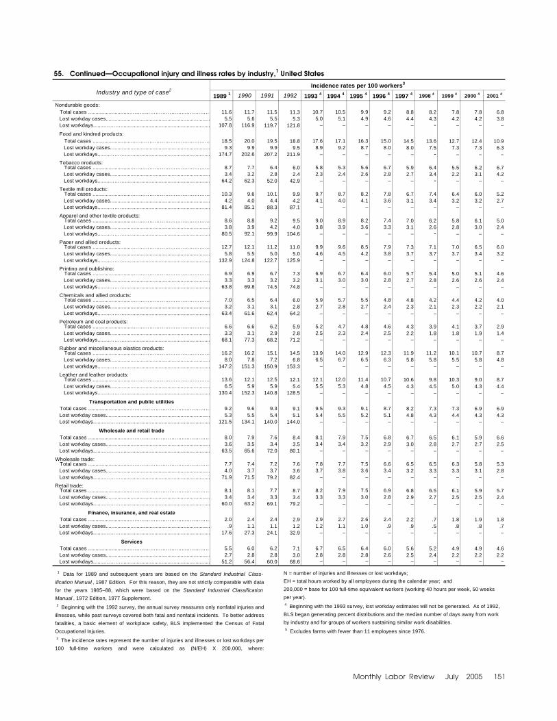
Monthly Labor Review July 2005 151
55. Continued–Occupational injury and illness rates by industry,1 United States
Incidence rates per 100 workers3
1989 1 1990 1991 1992 1993 4 1994 4 1995 4 1996 4 1997 4 1998 4 1999 4 2000 4 2001 4
Nondurable goods: Total cases ............................…………………………..…………… 11.6 11.7 11.5 11.3 10.7 10.5 9.9 9.2 8.8 8.2 7.8 7.8 6.8
Lost workday cases....................................................................... 5.5 5.6 5.5 5.3 5.0 5.1 4.9 4.6 4.4 4.3 4.2 4.2 3.8 Lost workdays........………............................................................. 107.8 116.9 119.7 121.8 – – – – – - – – –
Food and kindred products: Total cases ............................…………………………..………… 18.5 20.0 19.5 18.8 17.6 17.1 16.3 15.0 14.5 13.6 12.7 12.4 10.9
Lost workday cases.................................................................... 9.3 9.9 9.9 9.5 8.9 9.2 8.7 8.0 8.0 7.5 7.3 7.3 6.3 Lost workdays........……….......................................................... 174.7 202.6 207.2 211.9 – – – – – - – – – Tobacco products: Total cases ............................…………………………..………… 8.7 7.7 6.4 6.0 5.8 5.3 5.6 6.7 5.9 6.4 5.5 6.2 6.7
Lost workday cases.................................................................... 3.4 3.2 2.8 2.4 2.3 2.4 2.6 2.8 2.7 3.4 2.2 3.1 4.2 Lost workdays........……….......................................................... 64.2 62.3 52.0 42.9 – – – – – - – – – Textile mill products: Total cases ............................…………………………..………… 10.3 9.6 10.1 9.9 9.7 8.7 8.2 7.8 6.7 7.4 6.4 6.0 5.2
Lost workday cases.................................................................... 4.2 4.0 4.4 4.2 4.1 4.0 4.1 3.6 3.1 3.4 3.2 3.2 2.7 Lost workdays........……….......................................................... 81.4 85.1 88.3 87.1 – – – – – – – – – Apparel and other textile products: Total cases ............................…………………………..………… 8.6 8.8 9.2 9.5 9.0 8.9 8.2 7.4 7.0 6.2 5.8 6.1 5.0
Lost workday cases.................................................................... 3.8 3.9 4.2 4.0 3.8 3.9 3.6 3.3 3.1 2.6 2.8 3.0 2.4 Lost workdays........……….......................................................... 80.5 92.1 99.9 104.6 – – – – – - – – – Paper and allied products: Total cases ............................…………………………..………… 12.7 12.1 11.2 11.0 9.9 9.6 8.5 7.9 7.3 7.1 7.0 6.5 6.0
Lost workday cases.................................................................... 5.8 5.5 5.0 5.0 4.6 4.5 4.2 3.8 3.7 3.7 3.7 3.4 3.2 Lost workdays........……….......................................................... 132.9 124.8 122.7 125.9 – – – – – – – – – Printing and publishing: Total cases ............................…………………………..………… 6.9 6.9 6.7 7.3 6.9 6.7 6.4 6.0 5.7 5.4 5.0 5.1 4.6
Lost workday cases.................................................................... 3.3 3.3 3.2 3.2 3.1 3.0 3.0 2.8 2.7 2.8 2.6 2.6 2.4 Lost workdays........……….......................................................... 63.8 69.8 74.5 74.8 – – – – – – – – – Chemicals and allied products: Total cases ............................…………………………..………… 7.0 6.5 6.4 6.0 5.9 5.7 5.5 4.8 4.8 4.2 4.4 4.2 4.0
Lost workday cases.................................................................... 3.2 3.1 3.1 2.8 2.7 2.8 2.7 2.4 2.3 2.1 2.3 2.2 2.1 Lost workdays........……….......................................................... 63.4 61.6 62.4 64.2 – – – – – – – – – Petroleum and coal products: Total cases ............................…………………………..………… 6.6 6.6 6.2 5.9 5.2 4.7 4.8 4.6 4.3 3.9 4.1 3.7 2.9
Lost workday cases.................................................................... 3.3 3.1 2.9 2.8 2.5 2.3 2.4 2.5 2.2 1.8 1.8 1.9 1.4 Lost workdays........……….......................................................... 68.1 77.3 68.2 71.2 – – – – – – – – – Rubber and miscellaneous plastics products: Total cases ............................…………………………..………… 16.2 16.2 15.1 14.5 13.9 14.0 12.9 12.3 11.9 11.2 10.1 10.7 8.7
Lost workday cases.................................................................... 8.0 7.8 7.2 6.8 6.5 6.7 6.5 6.3 5.8 5.8 5.5 5.8 4.8 Lost workdays........……….......................................................... 147.2 151.3 150.9 153.3 – – – – – – – – – Leather and leather products: Total cases ............................…………………………..………… 13.6 12.1 12.5 12.1 12.1 12.0 11.4 10.7 10.6 9.8 10.3 9.0 8.7
Lost workday cases.................................................................... 6.5 5.9 5.9 5.4 5.5 5.3 4.8 4.5 4.3 4.5 5.0 4.3 4.4 Lost workdays........……….......................................................... 130.4 152.3 140.8 128.5 – – – – – – – – –
Transportation and public utilities Total cases ............................…………………………..…………… 9.2 9.6 9.3 9.1 9.5 9.3 9.1 8.7 8.2 7.3 7.3 6.9 6.9
Lost workday cases....................................................................... 5.3 5.5 5.4 5.1 5.4 5.5 5.2 5.1 4.8 4.3 4.4 4.3 4.3 Lost workdays........………............................................................. 121.5 134.1 140.0 144.0 – – – – – – – – –
Wholesale and retail trade Total cases ............................…………………………..…………… 8.0 7.9 7.6 8.4 8.1 7.9 7.5 6.8 6.7 6.5 6.1 5.9 6.6
Lost workday cases....................................................................... 3.6 3.5 3.4 3.5 3.4 3.4 3.2 2.9 3.0 2.8 2.7 2.7 2.5 Lost workdays........………............................................................. 63.5 65.6 72.0 80.1 – – – – – – – – – Wholesale trade: Total cases ............................…………………………..…………… 7.7 7.4 7.2 7.6 7.8 7.7 7.5 6.6 6.5 6.5 6.3 5.8 5.3
Lost workday cases....................................................................... 4.0 3.7 3.7 3.6 3.7 3.8 3.6 3.4 3.2 3.3 3.3 3.1 2.8 Lost workdays........………............................................................. 71.9 71.5 79.2 82.4 – – – – – – – – – Retail trade: Total cases ............................…………………………..…………… 8.1 8.1 7.7 8.7 8.2 7.9 7.5 6.9 6.8 6.5 6.1 5.9 5.7
Lost workday cases....................................................................... 3.4 3.4 3.3 3.4 3.3 3.3 3.0 2.8 2.9 2.7 2.5 2.5 2.4 Lost workdays........………............................................................. 60.0 63.2 69.1 79.2 – – – – – – – – –
Finance, insurance, and real estate Total cases ............................…………………………..…………… 2.0 2.4 2.4 2.9 2.9 2.7 2.6 2.4 2.2 .7 1.8 1.9 1.8
Lost workday cases....................................................................... .9 1.1 1.1 1.2 1.2 1.1 1.0 .9 .9 .5 .8 .8 .7 Lost workdays........………............................................................. 17.6 27.3 24.1 32.9 – – – – – – – – –
Services Total cases ............................…………………………..…………… 5.5 6.0 6.2 7.1 6.7 6.5 6.4 6.0 5.6 5.2 4.9 4.9 4.6
Lost workday cases....................................................................... 2.7 2.8 2.8 3.0 2.8 2.8 2.8 2.6 2.5 2.4 2.2 2.2 2.2 Lost workdays........………............................................................. 51.2 56.4 60.0 68.6 – – – – – – – – –
Industry and type of case2
1 Data for 1989 and subsequent years are based on the Standard Industrial Class-
ification Manual , 1987 Edition. For this reason, they are not strictly comparable with data
for the years 1985–88, which were based on the Standard Industrial Classification
Manual , 1972 Edition, 1977 Supplement.2 Beginning with the 1992 survey, the annual survey measures only nonfatal injuries and
illnesses, while past surveys covered both fatal and nonfatal incidents. To better address
fatalities, a basic element of workplace safety, BLS implemented the Census of Fatal
Occupational Injuries.3 The incidence rates represent the number of injuries and illnesses or lost workdays per
100 full-time workers and were calculated as (N/EH) X 200,000, where:
N = number of injuries and illnesses or lost workdays;
EH = total hours worked by all employees during the calendar year; and
200,000 = base for 100 full-time equivalent workers (working 40 hours per week, 50 weeks
per year). 4 Beginning with the 1993 survey, lost workday estimates will not be generated. As of 1992,
BLS began generating percent distributions and the median number of days away from work
by industry and for groups of workers sustaining similar work disabilities.
5 Excludes farms with fewer than 11 employees since 1976.

152 Monthly Labor Review July 2005
Current Labor Statistics: Injury and Illness
56. Fatal occupational injuries by event or exposure, 1998-2003
Fatalities
Event or exposure1 1998-2002 20023 2003
average2 Number Number Percent
Total……………..................................................................... 6,896 5,534 5,559 100
Transportation incidents............................................................... 2,549 2,385 2,367 42 Highway incident…….................................................................... 1,417 1,373 1,350 24 Collision between vehicles, mobile equipment…………............. 696 636 648 12 Moving in same direction…………........................................... 136 155 135 2 Moving in opposite directions, oncoming………….................. 249 202 269 5 Moving in intersection…………................................................ 148 146 123 2
Vehicle struck stationary object or equipment in roadway……… 27 33 17 (4) Vehicle struck stationary object, or equipment on side of road.................................................................. 281 293 324 6 Noncollision incident................................................................... 367 373 321 6 Jackknifed or overturned—no collision…………...................... 303 312 252 5 Nonhighway (farm, industrial premises) incident........................... 358 323 347 6 Overturned…………................................................................... 192 164 186 3 Worker struck by a vehicle…………………………………………… 380 356 336 6 Rail vehicle…….………….…...………………………………………… 63 64 43 1 Water vehicle …............................................................................ 92 71 68 1 Aircraft…………………………………………………………………… 235 194 208 4
Assaults and violent acts.............................................................. 910 840 901 16 Homicides…............………............................................................ 659 609 631 11 Shooting……………………………………………………………… 519 469 487 9 Stabbing……………………………………………………………… 61 58 58 1 Self-inflicted injuries............………................................................ 218 199 218 4
Contact with objects and equipment.…………............................ 963 872 911 16 Struck by object…............………................................................... 547 505 530 10 Struck by falling object…………................................................. 336 302 322 6 Struck by flying object…......…………......................................... 55 38 58 1 Caught in or compressed by equipment or objects…............…… 272 231 237 4 Caught in running equipment or machinery…………................. 141 110 121 2 Caught in or crushed in collapsing materials…............………....... 126 116 126 2
Falls..………………………............................................................... 738 719 691 12 Fall to lower level…............………................................................. 651 638 601 11 Fall from ladder…………............................................................ 113 126 113 2 Fall from roof…......…………...................................................... 152 143 127 2 Fall from scaffold, staging…......…………................................... 91 88 85 2 Fall on same level…............………............................................... 65 64 69 1
Exposure to harmful substances or environments..……………… 526 539 485 9 Contact with electric current…............………................................ 289 289 246 4 Contact with overhead power lines………….............................. 130 122 107 2 Contact with temperature extremes…............……….................... 45 60 42 1 Exposure to caustic, noxious, or allergenic substances…............… 102 99 121 2 Inhalation of substances…………............................................... 50 49 65 1 Oxygen deficiency…............………............................................... 89 90 73 1 Drowning, submersion………….................................................. 69 60 52 1
Fires and explosions ..………………………................................... 190 165 198 4
1 Based on the 1992 BLS Occupational Injury and Illness
Classification Manual . Includes other events and exposures,
such as bodily reaction, in addition to those shown separately.
2 Excludes fatalities from the Sept. 11, 2001, terrorist attacts.
3 The BLS news release of September 17, 2003, reported
a total of 5,524 fatal work injuries for calendar year 2003.
Since then, an additional 10 job-related fatalities were
identified, bringing the total job-related fatality count for
2002 to 5,534. 4 Equal to or greater than 0.5 percent.
NOTE: Totals for major categories may include sub-
categories not shown separately. Percentages may not add to
totals because of rounding.

U.S. BUREAU OF LABOR STATISTICSCOMPENSATION AND WORKING CONDITIONS
Page 1
Fatalities in the Ornamental Shrub and Tree Services Industry
by William J. WiatrowskiBureau of Labor Statistics
Originally Posted: July 26, 2005
While changes in industry classifications provide more detail on new and growing industries, less detail will be available for some smaller industries. Data on fatal injuries in the ornamental shrub and tree services industry for 2002 are the last such data available.As the U.S. economy continues to evolve, industry classifications evolve as well. In the past few decades, there have been declines in such industries as manufacturers of typewriters and vinyl records, while new industries have arisen, including Internet publishing, laser eye surgery, and cellular phone services.1 To keep up with these changes, the classification system used to categorize industries was revised in the mid-1990s; the former system, the Standard Industrial Classification (SIC) system, was replaced with the North American Industry Classification System (NAICS), which not only identifies and categorizes emerging industries but was designed to provide consistent classification between the U.S., Mexico, and Canada. And while NAICS has modernized the classification of industries, some smaller industries have been subsumed into broader categories that might not distinguish their unique character. The data presented here are from one such industry--ornamental shrub and tree services. This unique industry, classified separately under the SIC system (SIC 0783), is now part of the larger industry known as landscaping services under NAICS (NAICS 561730).2
The ornamental shrub and tree services industry was defined under the SIC system to include such activities as arborist services; ornamental tree and bush planting, pruning, bracing, spraying, removal, and surgery; and utility line tree trimming services. Under the new NAICS classification, organizations in the landscaping services industry comprise those providing landscape care and maintenance services and/or installing trees, shrubs, plants, lawns, or gardens; and those providing these services along with the design of landscape plans and/or the construction/installation of walkways, retaining walls, decks, fences, ponds, and similar structures. The addition of those involved in lawn and garden work and those involved in design and installation work, both previously in separate categories, results in the NAICS landscape services industry employing just over 1 million workers in 2003.3
There were 70 fatal occupational injuries in the ornamental shrub and tree services industry in 2002, the last year that such data are available. In the 11 years (1992-2002) for which data are available from the BLS Census of Fatal Occupational Injuries (CFOI), there were 637 fatalities in the industry--an average of about 58 fatalities per year.4 Beginning in 2003, CFOI began reporting fatalities for the larger NAICS-classified landscaping services industry. There were 156 fatal occupational injuries in that industry in 2003. (See table.) The fatality rate for this industry was 14.1 fatalities per 100,000 employed workers, compared with the overall rate of 4.0 for all workers.
The CFOI provides a glimpse into the demographics of the workers killed on the job and a categorization of the circumstances surrounding the incident. In the case of the ornamental shrub and tree services industry, all 70 decedents in 2002 were men. In fact, of the 637 fatalities in this industry over 11 years, only 5 were female. About two-thirds of the fatalities occurred among wage and salary workers--those employed by a firm in the shrub and tree service industry. The remaining one-third were self-employed individuals. While the NAICS landscaping services industry in 2003 employed more people and suffered more fatalities, the same patterns held true--most of the decedents were men and about two-thirds were wage and salary workers.
While the age of the fatally injured shrub and tree industry workers ranged from mid-teens to 65 and over, the majority were ages 25 to 54. The distribution of fatalities by age was very similar to the distribution of all fatalities by age, regardless of industry. Further, the age distribution in 2002 was little changed from the entire 11-year period for which data are available.
The number and proportion of fatally injured employees in the shrub and tree services industry who were identified as Hispanic has risen in recent years. In the first year of the Census, 1992, there were 4 decedents identified as Hispanic

U.S. BUREAU OF LABOR STATISTICSCOMPENSATION AND WORKING CONDITIONS
Page 2
among the 36 fatalities in the industry, or about 11 percent. In 1997, 6 Hispanics were killed among a total of 67, or about 9 percent. However, in 2001, 12 of the 75 fatalities (16 percent) were Hispanic and in 2002, 17 of 70 fatalities (24 percent) were Hispanic. (See chart.) This is consistent with the overall rise in fatalities among Hispanics in all industries.6 Looking at 2003 data for the larger landscaping services industry under NAICS, Hispanics represented about 28 percent of the total fatalities.
There were 4 types of events that led to most of the fatalities among workers in the shrub and tree services industry--struck by an object (typically a tree); fall to a lower level (typically out of a tree); contact with electric current (such as when a limb hits a live electrical wire); and a transportation incident (either a collision between vehicles or a worker struck by a vehicle).7
While these categories provide an overall view of the events leading to the fatality, some anecdotal evidence provides more details about the fatal events.8
• Those workers who were struck by a tree included cases where a tree they were cutting fell forward onto them. There were also instances where the tree that struck the decedent was being cut down by a co-worker.
• There were a number of cases where those cutting down trees were attempting to move from the path of a falling tree when they slipped or tripped and could not get out of the way in time.
• In several instances, fatally injured workers were described as wearing protective clothing or using protective equipment.
• Those who fell to their death included falls from ladders, roofs, and trees. In some cases, the incident occurred when the worker cut through a safety line.
• Electrocutions occurred when workers (or a branch, or a tool or other piece of equipment that the worker was touching) came in contact with high voltage lines or electric transformers.
• Some transportation incidents involved vehicles that were being used during a landscaping operation, such as a tractor being used to remove stumps overturning onto the driver.
• Other transportation incidents involved vehicles operated by others hitting the landscape worker, such as workers on the side of a road being struck by a vehicle.
The data presented here are examples of the variety of information available from the CFOI program, even for very small industries. While the change in industry classification system has resulted in the elimination of data for some smaller industries, such as ornamental shrub and tree services, it provides new data for other industries. For example, in the past, fatalities in the restaurant industry were all included in one category; now data are available separately for full-service restaurants, limited service restaurants (including fast food establishments), snack bars, and mobile food services (such as ice cream trucks). Beginning with the 2003 census, all future CFOI data will be presented under the new NAICS classifications, with data available for as many unique industries as possible.
William J. WiatrowskiEconomist, Office of Safety, Health, and Working Conditions, Bureau of Labor Statistics.Telephone: (202) 691-6305; E-mail: [email protected]
End Notes1 For a discussion of changes in employment by industry, see Teresa L. Morisi, "Recent changes in the national Current Employment Statistics survey," Monthly Labor Review, June 2003, pp. 3-13.
2 For a complete description of the Standard Industrial Classification system and the North American Industry Classification System, including a list of codes and definitions, go to www.bls.gov/bls/naics.htm.
3 Employment data are from the BLS Current Population Survey.
4 The Census of Fatal Occupational Injuries (CFOI) provides the nation’s most accurate count of fatal workplace injuries. Data are captured from multiple sources designed to confirm the work-related nature of the fatality and to verify the accuracy of data elements. Available data include demographic characteristics of the decedent, information about the occupation and industry in which the worker was employed, and descriptions of the event or exposure that led to the fatality. More information about the CFOI program is available at www.bls.gov/iif.
5 In addition to data on fatal work injuries, the Bureau of Labor Statistics also provides data on nonfatal workplace injuries and illnesses through the Survey of Occupational Injuries and Illnesses. These data also changed industry classification systems in 2003. While workplace

U.S. BUREAU OF LABOR STATISTICSCOMPENSATION AND WORKING CONDITIONS
Page 3
injury and illness data are available for many detailed industries, no data are available for the ornamental shrub and tree services industry (SIC 0783). Data are available for the broader landscape and horticultural services industry (SIC 078). Beginning in 2003, nonfatal workplace injury and illness data are available for the landscaping services industry (NAICS 561730). More information about the Survey of Occupational Injuries and Illnesses is available at www.bls.gov/iif.
6 For information on fatalities among foreign-born workers, see Katherine Loh and Scott Richardson, "Foreign-born workers: Trends in fatal occupational injuries, 1996-2001," Monthly Labor Review, June 2004, pp. 42-53.
7 CFOI classifies the fatal incident in a number of ways, including event or exposure (defined as the manner in which the injury was produced or inflicted by the source), primary source (defined as the object, substance, or exposure that directly produced or inflicted the injury), and secondary source (defined as the object, substance, or person that generated the source of injury or that contributed to the event or exposure). For example, in the case of a worker who is electrocuted, the event might be "contact with overhead power lines" (a component of "contact with electric current"), the primary source would be "electrical wiring" (a component of "machine, tool, and electric parts"), and the secondary source might be "trees, logs," if the tree came in contact with the electrical source.
8 In addition to the many data elements captured in the CFOI program, narrative descriptions of the incident are prepared. These descriptions are used to confirm the circumstances of the incident; they can also provide additional details of the fatality beyond those included in the CFOI data elements. Because these data are confidential, the information presented here includes summaries and highlights from numerous fatalities and does not refer to any one incident.
Table. Fatal occupational injuries by selected industry, 1992-2003
Characteristic Ornamental shrub and tree services (SIC 0783), 1992-2002
Ornamental shrub and tree services (SIC 0783), 2002
Landscaping services (NAICS 56173), 2003
Total: 637 70 156Employee status:
Wage and salary workers(1) 411 42 102Self-employed(2) 226 28 54
Sex:Men 632 70 154Women 5 -- --
Age:16 to 17 years 5 -- --18 to 19 years 17 3 --20 to 24 years 78 7 1925 to 34 years 176 14 3435 to 44 years 160 24 3645 to 54 years 110 11 2955 to 64 years 62 8 2265 years and over 25 3 10
Footnotes:(1) This category may include volunteers and other workers receiving compensation.(2) Includes paid and unpaid family workers, and may include owners of incorporated businesses, or members of partnerships.(3) In this study, the racial categories "White" and "Black or African American" do not include persons from the ethnic category "Hispanic or Latino." Hispanic or Latino persons may identify themselves racially as white, black, or another race category.(4) The primary source of injury identifies the object, substance, or exposure that directly produced or inflicted the injury.(5) The secondary source of injury, if any, identifies the object, substance, or person that generated the source of injury or that contributed to the event or exposure. For vehicle collisions, the deceased's vehicle is the primary source and the other object (truck, road divider, etc.) is the secondary source.
NOTE: Dashes indicate no data or data that do not meet publication criteria. Totals for major categories may include subcategories not shown separately.
SOURCE: U.S. Department of Labor, Bureau of Labor Statistics, Census of Fatal Occupational Injuries

U.S. BUREAU OF LABOR STATISTICSCOMPENSATION AND WORKING CONDITIONS
Page 4
Characteristic Ornamental shrub and tree services (SIC 0783), 1992-2002
Ornamental shrub and tree services (SIC 0783), 2002
Landscaping services (NAICS 56173), 2003
Race or ethnic origin:(3)White 489 49 87Black or African American 45 3 18Hispanic 83 17 44
Event or exposure:Contact with objects and equipment 225 22 52
Struck by object 197 21 45Struck by falling object 164 18 43
Caught in or compressed by equipment or objects 23 -- 4
Caught in running equipment or machinery 17 --
Falls 207 20 38Fall to lower level 204 19 38
Fall from ladder 17 4 3Fall from roof 3 --
Exposure to harmful substances or environments 119 13 23
Contact with electric current 112 13 17Exposure to caustic, noxious, or allergenic substances
3 --
Oxygen deficiency (including drowning) 4 -- 4
Transportation incidents 78 15 38Highway incidents 34 7 20
Collision between vehicles, mobile equipment
14 5 14
Non-collision incidents 12 -- 3Non-highway incident, except rail, air, water 15 -- 12
Overturned 9 -- 8
Footnotes:(1) This category may include volunteers and other workers receiving compensation.(2) Includes paid and unpaid family workers, and may include owners of incorporated businesses, or members of partnerships.(3) In this study, the racial categories "White" and "Black or African American" do not include persons from the ethnic category "Hispanic or Latino." Hispanic or Latino persons may identify themselves racially as white, black, or another race category.(4) The primary source of injury identifies the object, substance, or exposure that directly produced or inflicted the injury.(5) The secondary source of injury, if any, identifies the object, substance, or person that generated the source of injury or that contributed to the event or exposure. For vehicle collisions, the deceased's vehicle is the primary source and the other object (truck, road divider, etc.) is the secondary source.
NOTE: Dashes indicate no data or data that do not meet publication criteria. Totals for major categories may include subcategories not shown separately.
SOURCE: U.S. Department of Labor, Bureau of Labor Statistics, Census of Fatal Occupational Injuries

U.S. BUREAU OF LABOR STATISTICSCOMPENSATION AND WORKING CONDITIONS
Page 5
Characteristic Ornamental shrub and tree services (SIC 0783), 1992-2002
Ornamental shrub and tree services (SIC 0783), 2002
Landscaping services (NAICS 56173), 2003
Automobiles 10 --Trucks 55 12 16Tractors 8 -- 7
Worker struck by vehicle, mobile equipment 28 6 4
Assaults and violent acts 5 -- 4Primary source:(4)
Vehicles 79 14 30Highway vehicles 71 13 21Plant and industrial powered vehicles, tractors 8 -- 7
Structures and surfaces 199 18 38Floors, walkways, ground surfaces 191 18 37
Machinery 48 7 15Agriculture and garden machinery 5 -- 8
Construction, logging, and mining machinery 27 3 5
Material handling machinery 16 3Parts and materials 71 4 9
Machine, tool, and electric parts 61 3 6
Persons, plants, animals, and minerals 192 22 45
Trees, logs 185 22 44Tools, instruments, and equipment 41 5 6
Other 6 -- 12Bullets and pellets -- -- 3
Secondary source:(5)Vehicles 25 6 19
Highway vehicles 23 6 18Structures and surfaces 14 4 3
Footnotes:(1) This category may include volunteers and other workers receiving compensation.(2) Includes paid and unpaid family workers, and may include owners of incorporated businesses, or members of partnerships.(3) In this study, the racial categories "White" and "Black or African American" do not include persons from the ethnic category "Hispanic or Latino." Hispanic or Latino persons may identify themselves racially as white, black, or another race category.(4) The primary source of injury identifies the object, substance, or exposure that directly produced or inflicted the injury.(5) The secondary source of injury, if any, identifies the object, substance, or person that generated the source of injury or that contributed to the event or exposure. For vehicle collisions, the deceased's vehicle is the primary source and the other object (truck, road divider, etc.) is the secondary source.
NOTE: Dashes indicate no data or data that do not meet publication criteria. Totals for major categories may include subcategories not shown separately.
SOURCE: U.S. Department of Labor, Bureau of Labor Statistics, Census of Fatal Occupational Injuries

U.S. BUREAU OF LABOR STATISTICSCOMPENSATION AND WORKING CONDITIONS
Page 6
Characteristic Ornamental shrub and tree services (SIC 0783), 1992-2002
Ornamental shrub and tree services (SIC 0783), 2002
Landscaping services (NAICS 56173), 2003
Floors, walkways, ground surfaces 7 -- 3
Structures 4 --Machinery 43 -- 9Parts and materials 67 9 16
Machine, tool, and electric parts 57 9 9
Persons, plants, animals, and minerals 178 17 34
Trees, logs 173 16 29Tools, instruments, and equipment 35 3 11
Other 6 -- 5Liquids (including water) -- -- 3
No secondary source 266 27 59
Footnotes:(1) This category may include volunteers and other workers receiving compensation.(2) Includes paid and unpaid family workers, and may include owners of incorporated businesses, or members of partnerships.(3) In this study, the racial categories "White" and "Black or African American" do not include persons from the ethnic category "Hispanic or Latino." Hispanic or Latino persons may identify themselves racially as white, black, or another race category.(4) The primary source of injury identifies the object, substance, or exposure that directly produced or inflicted the injury.(5) The secondary source of injury, if any, identifies the object, substance, or person that generated the source of injury or that contributed to the event or exposure. For vehicle collisions, the deceased's vehicle is the primary source and the other object (truck, road divider, etc.) is the secondary source.
NOTE: Dashes indicate no data or data that do not meet publication criteria. Totals for major categories may include subcategories not shown separately.
SOURCE: U.S. Department of Labor, Bureau of Labor Statistics, Census of Fatal Occupational Injuries

U.S. BUREAU OF LABOR STATISTICSCOMPENSATION AND WORKING CONDITIONS
Page 7
Data for Chart. Fatal occupational injuries among Hispanic workers in the shrub and tree services industry, 1992-2002
Year Number of Fatalities Percent of total fatalities
1992 4 11%1993 6 11%1994 4 9%1995 7 18%1996 6 9%1997 6 9%1998 5 10%1999 8 13%2000 8 11%2001 12 16%2002 17 24%
U.S. Bureau of Labor Statistics | Division of Information and Marketing Services, PSB Suite 2850, 2 Massachusetts Avenue, NE Washington, DC 20212-0001 | www.bls.gov/OPUB | Telephone: 1-202-691-5200 | Contact Us

U.S. BUREAU OF LABOR STATISTICSCOMPENSATION AND WORKING CONDITIONS
Page 1
Older Workers and Severity of Occupational Injuries and Illnesses Involving Days Away from Work
by William J. WiatrowskiBureau of Labor Statistics
Originally Posted: July 26, 2005

U.S. BUREAU OF LABOR STATISTICSCOMPENSATION AND WORKING CONDITIONS
Page 2
• Injuries and illnesses among those aged 65 and older made up 1.9 percent of total days-away-from-work cases in private industry in 2003, while such employees worked 2.3 percent of all hours in the same period. (Days-away-from-work cases require recuperation away from work beyond the day of the incident.) Those aged 55 to 64 accounted for 10.2 percent of days-away-from-work injuries and illnesses and 10.7 percent of hours worked. (See charts 1 and 2.)
• In contrast to their lower incidence, lost-time injuries and illnesses among those aged 65 and older tended to be more severe than those among younger workers. Injured workers aged 65 and older were away from work a median of 18 days in 2003, compared with a median of 8 days for all workers and 12 days for workers aged 55 to 64. (See chart 3.)
• In addition, nearly 40 percent of the days-away-from-work injuries and illnesses among those aged 65 and older involved 31 or more days off the job. The proportion of all workers with days-away-from-work injuries involving 31 or more days off was about 26 percent, and among those aged 55 to 64, it was about 33 percent. (See chart 4.)
NOTE: For more information on these data, see the news release Lost-Worktime Injuries and Illnesses: Characteristics and Resulting Days Away From Work, 2003, USDL 05-521 (U.S. Department of Labor), March 30, 2005; available on the Internet at http://www.bls.gov/iif/oshwc/osh/case/osnr0022.pdf.

U.S. BUREAU OF LABOR STATISTICSCOMPENSATION AND WORKING CONDITIONS
Page 3
Source: Bureau of Labor Statistics, Survey of Occupational Injuries and Illnesses. Hours worked data are from the Current Population Survey.
William J. WiatrowskiEconomist, Office of Safety, Health, and Working Conditions, Bureau of Labor Statistics.Telephone: (202) 691-6305; E-mail: [email protected]
Data for Chart 1. Percent of injuries and illnesses with days away from work by age of worker, 2003
Age Percent of injuries and illnesses
16-19 3.3%20-24 11.1%25-34 24.2%35-44 27.5%45-54 21.9%55-64 10.2%65 and over 1.9%
Data for Chart 2. Percent of hours worked by age, 2003
Age Percent of hours worked
16-19 3.2%20-24 10.3%25-34 24.3%35-44 26.6%45-54 22.6%55-64 10.7%65 and over 2.3%
Data for Chart 3. Median days away from work due to occupational injury or illness, by age of worker, 2003
Age Median days
All ages 814-15 316-19 420-24 525-34 635-44 945-54 1155-64 1265 and over 18
Data for Chart 4. Percent of occupational injuries and illnesses involving 31 or more days away from work, by age of worker, 2003
Age Percent of cases with 31 or more days
All ages 26.2

U.S. BUREAU OF LABOR STATISTICSCOMPENSATION AND WORKING CONDITIONS
Page 4
Age Percent of cases with 31 or more days
16-19 1220-24 15.125-34 22.235-44 28.145-54 31.655-64 33.265 and over 39.1
U.S. Bureau of Labor Statistics | Division of Information and Marketing Services, PSB Suite 2850, 2 Massachusetts Avenue, NE Washington, DC 20212-0001 | www.bls.gov/OPUB | Telephone: 1-202-691-5200 | Contact Us