An adaptive finite element water column model using the Mellor–Yamada level 2.5 turbulence closure...

www.elsevier.com/locate/ocemod

Ocean Modelling 12 (2006) 205–223

An adaptive finite element water column model usingthe Mellor–Yamada level 2.5 turbulence closure scheme

Emmanuel Hanert a,b,*, Eric Deleersnijder a,b, Vincent Legat b

a Institut d’Astronomie et de Geophysique G. Lemaıtre, Universite catholique de Louvain,

2 Chemin du cyclotron, B-1348 Louvain-la-Neuve, Belgiumb Centre for Systems Engineering and Applied Mechanics, Universite catholique de Louvain,

4 Avenue Georges Lemaıtre, B-1348 Louvain-la-Neuve, Belgium

Received 31 January 2005; received in revised form 20 May 2005; accepted 20 May 2005Available online 29 June 2005

Abstract

A one-dimensional water column model using the Mellor and Yamada level 2.5 parameterization ofvertical turbulent fluxes is presented. The model equations are discretized with a mixed finite elementscheme. Details of the finite element discrete equations are given and adaptive mesh refinement strategiesare presented. The refinement criterion is an ‘‘a posteriori’’ error estimator based on stratification, shearand distance to surface. The model performances are assessed by studying the stress driven penetrationof a turbulent layer into a stratified fluid. This example illustrates the ability of the presented model tofollow some internal structures of the flow and paves the way for truly generalized vertical coordinates.� 2005 Elsevier Ltd. All rights reserved.

Keywords: Mellor and Yamada; Turbulence closure; Finite elements; Adaptivity; Mixed layer deepening

1463-5003/$ - see front matter � 2005 Elsevier Ltd. All rights reserved.doi:10.1016/j.ocemod.2005.05.003

* Corresponding author. Address: Institut d�Astronomie et de Geophysique G. Lemaıtre, Universite catholique deLouvain, 2 Chemin du cyclotron, B-1348 Louvain-la-Neuve, Belgium.E-mail address: [email protected] (E. Hanert).

mailto:[email protected]

206 E. Hanert et al. / Ocean Modelling 12 (2006) 205–223

1. Introduction

In many marine modelling applications, a reliable parameterization of eddy coefficients isneeded to accurately represent vertical turbulent fluxes. Nowadays, most ocean models useone- or two-equation turbulence closures. The most popular are the Mellor and Yamada(1982) level 2.5 model and the k–emodel (e.g., Rodi, 1987). A detailed comparison of both modelshas been performed by Burchard et al. (1998) and Burchard and Petersen (1999). Beside these twomodels, other two-equation models exist, like the k–x model, introduced by Wilcox (1988) andextended to buoyancy affected flows by Umlauf et al. (2003). Although all three models have verysimilar physical parameterizations (Umlauf and Burchard, 2003), only the model of Mellor andYamada took stratification into account since its inception. As a result, it has been usedfrequently in atmospheric and oceanic applications (e.g., Yamada, 1983; Blumberg and Mellor,1987; Rosati and Miyakoda, 1988; Timmermann and Beckmann, 2004).The numerical discretization of such turbulence closures is usually accomplished in finite differ-

ences, on a staggered or non-staggered grid. Details of the discretization of the turbulence energyequations, on different finite difference grids and with various time discretization have been given inDavies and Jones (1991) and Burchard (2002a). For problems in which the shape of eddy viscosityis constant in time, although its magnitude may change, functional approaches have been sug-gested (Davies, 1987). More recently, Burchard (2002b) proposed an energy-conserving discretiza-tion of the shear and production terms for the turbulent kinetic energy. The issue of non-uniformadaptive vertical grids has been studied by Burchard and Beckers (2004). They proposed a finitedifference scheme using a grid that can follow the relevant internal structures of the flow.Common to all the previous works is the use of the finite difference method to discretize the

hydrodynamic equations. However, over recent years other numerical methods have beencontemplated for simulating oceanic and coastal flows. These are mainly the finite element(e.g., Lynch et al., 1996; Le Roux et al., 2000; Danilov et al., 2004; Ford et al., 2004a,b; Hanertet al., 2005), the finite volume (e.g., Casulli and Walters, 2000; Chen et al., 2003) and the spectralelement (e.g., Iskandarani et al., 1995, 2003) methods. Their principal advantage is that they allowthe use of unstructured meshes. Such meshes have proved to be particularly well suited to repre-sent localized phenomena and complex geometries (Legrand et al., 2000). They also provide a nat-ural framework to perform dynamical mesh adaptation (Piggot et al., 2005). This seems to be avery promising tool for use in 3D ocean modelling as it permits to adapt the mesh in both spaceand time. Therefore, an optimal use of the computational power is always possible as the mesh‘‘follows’’ the dynamically active regions. Until now, most of the work on unstructured meshocean modelling has focused on horizontal processes while little interest has been paid to thediscretization of vertical ones.The purpose of this paper is to investigate the ability of the finite element method, combined

with adaptive mesh procedures, to discretize vertical oceanic processes. As a test problem, we sim-ulate the stress-driven deepening of the ocean mixed layer by using Mellor–Yamada level 2.5turbulence closure scheme. This phenomenon exhibits a transient dynamics and is therefore wellsuited to assess mesh adaptivity methods. All simulations have been performed with a MATLABsoftware, which is freely available at the following address: http://www.mema.ucl.ac.be/~hanert/FEMY25.html. This is a way to provide all numerical and technical tricks required to obtain anaccurate solution of this non-linear problem. While the MATLAB programming language is well

http://www.mema.ucl.ac.be/~hanert/FEMY25.html

http://www.mema.ucl.ac.be/~hanert/FEMY25.html

E. Hanert et al. / Ocean Modelling 12 (2006) 205–223 207

suited for educational purposes, it is not the most efficient for heavy computations. In thatrespect, the finite difference General Ocean Turbulence Model (GOTM, http://www.gotm.net)provides a comprehensive package of efficient turbulence models.

2. A simple water column model

For some very idealized situations where all variables are horizontally homogeneous, thefollowing one-dimensional water column model may be used:

ou

otþ f ez � u ¼ o

ozKu

ou

oz

� �; ð1Þ

obot

¼ o

ozKb

oboz

� �; ð2Þ

where f is the Coriolis factor, z is the vertical coordinate (increasing upward), ez is the vertical unitvector, Ku is the eddy viscosity and Kb is the eddy diffusivity. The unknowns are the horizontalvelocity u = (u,v) and the buoyancy b = �g(q � q0)/q0, where g is the gravitational acceleration,q is the water density and q0 is a reference value of the density. The model domain is a water col-umn that goes from z = �h to the sea surface (z = 0). The initial and boundary conditions dependon the problem under consideration and will be specified later.In Eqs. (1) and (2), eddy coefficients are parameterized with the Mellor–Yamada level 2.5 tur-

bulence closure:

Ku ¼ lqSu;

Kb ¼ lqSb;

where l and q are, respectively, an appropriate length scale, termed the turbulence macroscale, anda velocity scale, obtained from the turbulent kinetic energy k = q2/2. The stability functions Suand Sb are dimensionless functions of GM and GH:

ðGM ;GHÞ ¼l2

q2ðM2;�N 2Þ;

where M and N are the Prandtl and Brunt-Vaisala frequencies, i.e.,

ðM2;N 2Þ ¼ ou

oz

��2

;oboz

!.

The usual Eulerian norm is denoted kÆk.The velocity and length scales obey the following equations:

oq2

ot¼2KuM2 � 2KbN 2 �

2q3

16.6lþ o

ozKq

oq2

oz

� �; ð3Þ

oq2lot

¼1.8lKuM2 � 1.8lKbN 2 �Wq3

16.6þ o

ozKq

oq2loz

� �. ð4Þ

The eddy diffusivity of the turbulence model equations is Kq = 0.2lq. The physical meaning of thevarious terms in Eq. (3) is the following: KuM

2 is the shear production of turbulent kinetic energy

http://www.gotm.net


(TKE), KbN2 is the TKE conversion into potential energy and q3/(16.6l) represents the viscous

dissipation of TKE.To compute Ku and Kb, we use the stability functions designed by Galperin et al. (1988):

Su ¼0.393� 3.085GH

1� 40.803GH þ 212.469G2H;

Sb ¼0.494

1� 34.676GH.

In addition, the following constraints are necessary:

l2 60.28q2

maxð0;N 2Þ; �0.28 6 GH 6 0.0233. ð5Þ

All the empirical parameters used in the turbulence closure model are motivated by Mellor andYamada (1974, 1982) and Galperin et al. (1988).In addition, the Mellor–Yamada model requires the introduction of a wall proximity function,

W, to be able to represent the logarithmic layer near boundaries. In the standard implementationof the model, this function is defined as

W ¼ 1þ 1.33l2

ðjLÞ2;

where j ’ 0.4 is the von Karman constant and L is a function of the distance to the seabed, db,and of the distance to the sea surface, ds: L = dsdb/(ds + db). It should be noted that when the dis-tance to the sea bottom is assumed infinite, L = ds = jzj. In that case, the wall proximity functionmay be written as W ¼ 1þ 1.33l2

ðjzÞ2 . Other wall proximity functions have also been suggested(Burchard et al., 1998; Blumberg et al., 1992).Beside the necessity to use a wall proximity function, another shortcoming of the Mellor–Yam-

ada model is that the empirical coefficients for the buoyancy and for the shear production termsare the same. As a result, the turbulence closure does not take into account the limiting effects ofstable stratification on the size of turbulent eddies (Galperin et al., 1988). To overcome this issue,the length scale limitation (5) has been suggested. Another remedy is to properly calibrate thebuoyancy production term. In that case, the model works well without the length scale limitation(Burchard, 2001). Burchard and Bolding (2001) have also reported that the maximum value of theRichardson number, Ri = 0.2, that can be reached with the stability functions of Galperin et al.(1988) is too small. As a result, the model does not reach high turbulent Prandtl numbers. Theturbulence closure of Mellor–Yamada has been improved by several authors in recent years(e.g., Kantha and Clayson, 1994; Canuto et al., 2001).

3. Numerical scheme

3.1. Finite element spatial discretization

The derivation of the finite element discretization is based on a variational or weak formulation(Ciarlet, 1978; Johnson, 1990) of the model equations (1)–(4). If the model domain is X = [�h, 0],the weak formulation of Eq. (1) reads:


Z 0

�h

ou

ot udzþ

Z 0

�hf ðez � uÞ udz ¼

Z 0

�h

o

ozKu

ou

oz

� � udz

¼ �Z 0

�hKu

ou

oz ouozdzþ Ku

ou

oz u

� �z¼0z¼�h

; ð6Þ

where u is an arbitrary weighting function that belongs to the Sobolev space H1(X) andqKu

ouoz u

z¼zk(where zk = �h, 0) can be viewed as a momentum flux at the bottom and at the sur-

face respectively. It is readily seen that Neumann boundary conditions can be naturally enforcedin the weak formulation thanks to the integration by parts. The weak formulation of Eqs. (2)–(4)is derived in the same way.Afterwards, one has to build a discrete approximation of the exact solution u. The discrete

solution, denoted uh, is associated with a partition of the computational domain into NE non-overlapping elements or intervals Xe (1 6 e 6 NE):

�X ¼[NE

e¼1

�Xe and Xe \ Xf ¼ ; for e 6¼ f ;

where �X is the closure of X. The discrete solution can be expressed in terms of basis functions /i:

uhðt; zÞ ¼XNi¼1

uiðtÞ/iðzÞ; ð7Þ

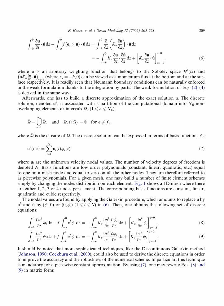
where ui are the unknown velocity nodal values. The number of velocity degrees of freedom isdenoted N. Basis functions are low order polynomials (constant, linear, quadratic, etc.) equalto one on a mesh node and equal to zero on all the other nodes. They are therefore referred toas piecewise polynomials. For a given mesh, one may build a number of finite element schemessimply by changing the nodes distribution on each element. Fig. 1 shows a 1D mesh where thereare either 1, 2, 3 or 4 nodes per element. The corresponding basis functions are constant, linear,quadratic and cubic respectively.The nodal values are found by applying the Galerkin procedure, which amounts to replace u by

uh and u by (/i, 0) or (0,/i) (1 6 i 6 N) in (6). Then, one obtains the following set of discreteequations:
Z 0
�h

ouh

ot/idz� f

Z 0

�hvh/idz ¼ �

Z 0

�hKu

ouh

ozo/i

ozdzþ Ku

ouh

oz/i

� �z¼0z¼�h

; ð8ÞZ 0

�h

ovh

ot/idzþ f

Z 0

�huh/idz ¼ �

Z 0

�hKu

ovh

ozo/i

ozdzþ Ku

ovh

oz/i

� �z¼0z¼�h

. ð9Þ

It should be noted that more sophisticated techniques, like the Discontinuous Galerkin method(Johnson, 1990; Cockburn et al., 2000), could also be used to derive the discrete equations in orderto improve the accuracy and the robustness of the numerical scheme. In particular, this techniqueis mandatory for a piecewise constant approximation. By using (7), one may rewrite Eqs. (8) and(9) in matrix form:

Fig. 1. Example of a 1D finite element mesh with different interpolations using, from the left to the right, constant,linear, quadratic and cubic basis functions. The model variables are computed on mesh nodes (represented by ‘‘d’’).For each mesh, the basis function associated with node i is represented. The three elements of the mesh are denotedXe�1, Xe and Xe+1.


Mijdujdt

� fvj

� �¼ Dijuj;

Mijdvjdt

þ fuj

� �¼ Dijvj;

whereMij ¼R 0�h /i/jdz is the mass matrix and Dij ¼ �

R 0�h Ku

o/ioz

o/j

oz dz is the stiffness matrix. Theseintegrals are easily computed as they only involve products of low order polynomials or productsof their derivatives. The derivation of the discrete formulation of Eqs. (2)–(4) is similar, althoughsome integrals may be more difficult to compute because of the non-linear terms in the turbulentvariables equations.In 1D, it is well known that finite element discrete equations are very close to those obtained

with the finite difference method. Indeed, a finite element scheme using nth order basis func-tions is similar to a (n + 1)th order finite difference scheme. It is possible to obtain exactlythe same discrete equations by using a Dirac delta as weighting function in formulation (6).This amounts to replace u by (d(x � xi), 0) or (0,d(x � xi)) (1 6 i 6 N). That method is usuallyreferred to as collocation. In 1D, the main advantage of the finite element method is that itmay accommodate uniform and non-uniform grids without any modifications. The accuracyof the method may also be easily changed by increasing or decreasing the order of the basisfunctions.In this work, we have used piecewise linear basis functions to approximate u, v, b, q2 and q2l.

Therefore, the slope of the velocity and buoyancy, as well as the Prandtl and Brunt-Vaisalafrequencies, are piecewise constant. The eddy coefficients are computed on the vertices and arelinearly interpolated on each element. Theoretically, the numerical scheme is second-order accu-rate in space.


3.2. Temporal discretization

Eqs. (1)–(4) are discretized in time by using the following scheme:

unþ1 � un

Dt¼ �f ez �

unþ1 þ un

2þ o

ozKn

u

ounþ1

oz

� �; ð10Þ

bnþ1 � bn

Dt¼ o

ozKn

b

obnþ1

oz

� �; ð11Þ

ðq2Þnþ1 � ðq2Þn

Dt¼ 2Kn

uðMnÞ2 � 2KnbðNnÞ2 � 2½ðq

2Þn�5=2

16.6ðq2lÞn þo

ozKn

q

oðq2Þnþ1

oz

!; ð12Þ

ðq2lÞnþ1 � ðq2lÞn

Dt¼ 1.8lnKn

uðMnÞ2 � 1.8lnKnbðNnÞ2

� W n½ðq2Þn�3=2

16.6þ o

ozKn

q

oðq2Þnþ1

oz

!. ð13Þ

All the non-linear terms are discretized explicitly in order to avoid solving a non-linear system.For the sake of clarity, we give in Appendix A the expression of Eqs. (12) and (13) where Kn

u, Knb,

Knq, M

n, Nn and Wn have been expressed in terms of un, bn, (q2)n and (q2l)n.When discretizing Eqs. (3) and (4) in time, use is often made of the pseudo-implicit discretiza-

tion of Patankar (1980) in order to avoid generating negative values of q2 and q2l (e.g., Deleersnij-der and Luyten, 1994; Burchard and Beckers, 2004). This scheme however still requires to imposethat l is bigger than a minimal value as it appears in the denominator of one of the terms in Eq.(3). However, in our implementation, better results were obtained by strongly imposing thefollowing constraints:

q2 > q2min and q2l > ðq2lÞmin

at the end of each time step rather than using a Patankar (1980) scheme. We therefore introduceq2min and (q

2l)min, the minimal values of q2 and q2l.

4. Numerical example: The Kato–Philips test case

The stress-driven penetration of a turbulent layer into a stratified fluid initially at rest is a clas-sical test case to assess turbulence closure schemes in the context of marine modelling (e.g.,Deleersnijder and Luyten, 1994; Burchard et al., 1998; Axell and Liungman, 2001; Burchardand Beckers, 2004). This experiment was first carried out in laboratory by Kato and Phillips(1969) with a non-rotating tank of fluid. The water column is considered sufficiently deep so thatthe only source of turbulence is the wind stress. Thus, the seabed has no influence on the flow andthe wall proximity function, W, may be assumed to depend only on the distance to the surface.


The following initial and boundary conditions are used:

u; b½ �t¼0 ¼ 0;N 20z� �

;

q2; q2l� �

t¼0 ¼ q2min; ðq2lÞmin� �

;

Kuou

oz;Kb

oboz

� �z¼0

¼ ku�ku�; 0½ �;

q2; q2l� �

z¼0 ¼ 6.5074u2�; 0� �

;

where N0 is the initial Brunt-Vaisala frequency and u* is the so-called surface friction velocity. Theminimal values of q2 and q2l are set to q2min ¼ 5� 10

�7 m2 s�2 and (q2l)min = 10�5 m3 s�2, respec-

tively. At the bottom of the computational domain, homogeneous Neumann boundary conditionsare enforced. As mentioned before, these conditions have no impact on the flow as the computa-tional domain is supposed to be sufficiently deep. Following Deleersnijder and Luyten (1994), wetransform this laboratory experiment to oceanic dimensions by setting ku*k = 10

�2 ms�1 andN0 = 10

�2 s�1. The Coriolis factor is set to zero.The convergence rate of the numerical scheme may be evaluated by computing the L2-error on

the numerical solution with respect to a high resolution solution computed on a mesh of 400elements. The error on the velocity and buoyancy fields are defined as follows:

eu ¼

ffiffiffiffiffiffiffiffiffiffiffiffiffiffiffiffiffiffiffiffiffiffiffiffiffiffiffiffiffiffiffiffiffiffiffiffiffiffiffiffiffiffiffiffiffiffiffiffiffiffiffiffiffiffiffiffiR 0�hður � uhÞ2 þ ðvr � vhÞ2 dz

qffiffiffiffiffiffiffiffiffiffiffiffiffiffiffiffiffiffiffiffiffiffiffiffiffiffiffiffiffiffiffiffiffiffiffiffiR 0�hðurÞ

2 þ ðvrÞ2 dzq ; eb ¼

ffiffiffiffiffiffiffiffiffiffiffiffiffiffiffiffiffiffiffiffiffiffiffiffiffiffiffiffiffiffiffiR 0�hðb

r � bhÞ2 dzq

ffiffiffiffiffiffiffiffiffiffiffiffiffiffiffiffiffiffiffiffiffiR 0�hðb

rÞ2 dzq ;

where the superscript r denotes the high-resolution reference solution. Both error measures arerepresented in Fig. 2 when using uniform meshes of 10, 20 and 40 elements and a time step of60 s. As expected, quadratic convergence rates are observed.For the case f = 0, Price (1979) suggested an analytical solution for the evolution of the mixed-

layer depth Dm based on a constant bulk Richardson number

DmðtÞ ¼ 1.05ku�kN�1=20 t1=2.

Fig. 3 shows the evolution of the mixed layer during 30 h of simulation. The computational do-main is 40 m deep, the time step is set to 60 s, the mesh is uniform and composed of 40 elements.The analytical solution of Price (1979) is compared to numerical results obtained by defining themixed layer depth as the depth at which the discrete TKE reaches values of 10�4 and 10�5 m2 s�2.Decreasing the TKE threshold value increases the accuracy. However, for threshold values smal-ler than 10�5 m2 s�2, the computed turbulent layer depth becomes noisy. Fig. 4 shows the profilesof buoyancy, velocity norm, TKE and mixing coefficients at the end of the simulation. Theseresults are totally in line with those obtained by Deleersnijder and Luyten (1994) with a finitedifference model.

5. Adaptive strategies

For applications like the deepening of the mixed layer under the influence of a wind stress, itis readily seen that better results could be obtained with non-uniform resolution. Indeed, the

0 5 10 15 20 25 300

5

10

15

20

25

30

35

40

Time [hours]

Mix

ed la

yer

dept

h [m

]

TKE = 10-5 m2s-2

TKE = 10-4 m2s-2

Price (79)

Fig. 3. Simulated mixed layer deepening compared to the algebraic solution of Price (1979). The numerical solutionsare obtained by taking TKE threshold values of 10�4 m2 s�2 ( ) and 10�5 m2s �2 (—). The mesh is uniform andcomposed of 40 elements.

10 20 40

10-2

10-1

Number of elements

L 2 e

rror

buoyancyvelocityquad. conv.

Fig. 2. L2-error on the discrete buoyancy (s) and velocity (·) fields with different uniform meshes. The convergencerate is quadratic in each case.


velocity and buoyancy solutions are quite smooth everywhere except near the surface and nearthe pycnocline (transition between the mixed and stratified layers). In these regions, the discrete

–4 –3 –2 –1 0

x10–3

–40

–35

–30

–25

–20

–15

–10

–5

0

Buoyancy [ms–2]

Dep

th [m

]

0 0.2 0.4 0.6–40

–35

–30

–25

–20

–15

–10

–5

0

Velocity norm [ms–1]

Dep

th [m

]

0 2 4 6–40

–35

–30

–25

–20

–15

–10

–5

0

TKE(q2/2) [m2s–2]

Dep

th [m

]

0 0.01 0.02 0.03–40

–35

–30

–25

–20

–15

–10

–5

0

Ku and Kb [m2s–1]

Dep

th [m

]

x10–4

Fig. 4. Profiles of buoyancy, velocity norm, TKE and mixing coefficients Ku (—) and Kb (– –) after 30 h for thesimulation of the Kato–Phillips experiment. The mesh is uniform and composed of 40 elements.


solutions exhibit stronger gradients. However, since the depth of the mixed layer continuouslyincreases, the resolution should also change accordingly. This can be achieved by using adaptivetechniques. Such methods allow to change the resolution dynamically and fit very nicely withinthe finite element formalism.The basic idea behind adaptivity is to compute, for a given discrete solution, an interpolation

error. This can be done by using either an ‘‘a priori’’ or an ‘‘a posteriori’’ estimator of the discret-ization error. For instance, an ‘‘a priori’’ estimator may be based on the convergence order of thenumerical method and an ‘‘a posteriori’’ estimator may be based on the knowledge of the physicalphenomenon. Once the interpolation error is computed, a new mesh is built in order to evenlydistribute the error on each element. In simple words, the resolution is increased where the erroris large and decreased where the error is small. Our point here is not to review all the theory onwhich adaptive methods stand. Instead, we refer to the paper by Piggot et al. (2005) and thereferences therein for more information.


In this work, we present a simple example of adaptivity based on an heuristic ‘‘a posteriori’’error measure. Following Burchard and Beckers (2004), we define the error on the numerical solu-tion as:

e ¼ eb þ eu þ ed þ ek ¼ cbmaxðN 2 � N 20; 0Þ

Dbþ cu

MDu

þ cd1

d þ d0þ ckdmax

; ð14Þ

where Db is a reference buoyancy difference, Du is a reference velocity difference, d is the distance tothe surface, d0 is a variable that permits to tune the near-surface grid zooming and dmax is the depthof the domain. The coefficients cb, cu, cd and ck allow to set the relative importance of the four com-ponents of the error. The error is expressed in meters. With this expression for e, one may increasethe resolution in region of strong shear, strong stratification and near the surface. The last compo-nent, ek, is a background error that prevents too coarse resolution in regions with no shear, nostratification and far away from the surface. Again, we have to stress that this error estimator isvery heuristic and only based on our knowledge of the physical phenomenon. Details on morerigorous ‘‘a posteriori’’ error estimates may be found in Strouboulis and Oden (1990), Cockburnand Gremaud (1996), Ainsworth and Oden (1997), Suli (1999) and Larson and Barth (2000).Once an error measure has been derived, the nodes may be redistributed accordingly. As the

accuracy of the finite element method depends both on the functional and geometrical discretiza-tions, several strategies exist to uniformly distribute the interpolation error. One is to locallyincrease or decrease the degree of the finite element approximation. In 1D, this is quite straight-forward as elements have at most one node in common. Reduction of the polynomial degree maybe useful not only to reduce the accuracy of the solution, but also to eliminate spurious oscilla-tions in the solution when non-smooth fields are present. Such an adaptive procedure is generallyreferred to as p-adaptivity. It is also possible to modify the numerical scheme accuracy by chang-ing the geometrical discretization. This might be achieved by either moving the nodes location orby locally changing the mesh and its connectivity. The former method, refered to as r-adaptivity,does not change the topology and keeps the number of elements constant while the latter, referedto as h-adaptivity, allows to add and remove elements. When the number of elements remains thesame, the movement of the grid may be taken into account by adding an advection term in theequations. The goal of this term is to counterbalance the movement of the mesh nodes and theadvection velocity is simply the opposite of the mesh velocity. When the number of elementschanges, mesh to mesh interpolation is required. It should be noted that it is possible to combinegeometrical and functional modifications. in that case, the method is called hp-adaptive. Someauthors also combine h and r methods to take advantage of both approaches (Piggot et al., 2005).In this work, we have used only r and h adaptive methods. The r-adaptive procedure requires

the introduction of a transport term in the discrete equations to compensate the motion of thegrid. If the grid nodes are denoted zi (t) (1 6 i 6 NE + 1), the vertical velocity at which a grid nodemoves is: ~wiðtÞ ¼ dzi

dt . A continuous velocity field ~wh may then be built by linearly interpolating be-tween vertical velocity nodal values. As an illustration of the modified equations, let us present theequation for the first component of the velocity:
Z 0
�h

ouh

ot/idzþ

Z 0

�h~wh ou

h

oz/i dz� f

Z 0

�hvh/idz ¼ �

Z 0

�hKu

ouh

ozo/i

ozdzþ ðsh0;x � sh�h;xÞ.


In matrix form, this yields:

Fig. 5using(botto

Mijdujdt

� fvj

� �þ Aijuj ¼ Dijuj;

where Aij ¼R 0�h ~w

h/io/j

oz dz. This advection operator is centered in space and second order accurateif /i and /j are piecewise linear. This finite element scheme is conservative but does not guaranteemonotonicity.An example of r-adaptation is shown in Fig. 5. We start with a mesh {xi, 1 6 i 6 NE + 1} and a

piecewise constant error field e(x). We compute the error integral on each element:Ei ¼

R xiþ1xi

eðxÞdx and on the whole domain: Etot ¼PNE

i¼1Ei. A new mesh fx�i ; 1 6 i 6 NE þ 1g isthen built by imposing the following constraints:

E�i ¼

Z x�iþ1

x�i

eðxÞdx ¼ EtotNE

;

x�0 ¼ x0;

x�NEþ1 ¼ xNEþ1.

This is achieved by successively moving the inner nodes of the initial mesh. When using a hmethod, one has to fix a priori an admissible error level per element: E*. In that case, thenew mesh is such that E�

i 6 E�. The number of elements may then change during the adaptationprocess.

. Example of mesh adaptation. The initial mesh {xi, 1 6 i 6 5} is composed of 4 elements of unit length (top). Byan r-adaptive procedure, a new mesh fx�i ; 1 6 i 6 5g is obtained where the error (e(x)) is evenly distributedm).


Fig. 6 shows the buoyancy field obtained with a r-adaptive scheme. The number of elementsremains equal to 20 and the time step is set to 60 s. The following parameters have been used:

Fig. 6numb

cb ¼ 1.2; cu ¼ 0.0; cd ¼ 0.3; ck ¼ 0.75;Db ¼ 0.002 ms�2; Du ¼ 0.2 ms�1; d0 ¼ 5.0 m; dmax ¼ 40.0 m.

It can be seen that the mesh accurately follows the pycnocline. With an adaptive finite elementscheme, the mixed layer deepens much more smoothly. This is illustrated in Fig. 7 where the meshis only composed of 20 elements instead of 40 in Fig. 3. Fig. 8 shows the results obtained with ah-adaptive scheme. The error level per element is set to E* = 0.12. The number of elements varies

–4 –2 0x 10–3

–40

–35

–30

–25

–20

–15

–10

–5

0

b [ms–2]

Dep

th [m

]

–4 –2 0–40

–35

–30

–25

–20

–15

–10

–5

0

Dep

th [m

]

–4 –2 0–40

–35

–30

–25

–20

–15

–10

–5

0

Dep

th [m

]

–4 –2 0–40

–35

–30

–25

–20

–15

–10

–5

0

Dep

th [m

]

x 10–3b [ms–2]

x 10–3b [ms–2]x 10–3b [ms–2]

. Discrete buoyancy field after 0, 10, 20 and 30 h (from left to right) obtained with a r-adaptive scheme. Theer of elements remains constant during the whole simulation. Mesh nodes are represented by ‘‘d’’.

0 5 10 15 20 25 300

5

10

15

20

25

30

35

40

Time [hours]

Mix

ed la

yer

dept

h [m

]

TKE = 10-5 m2s-2

TKE = 10-4 m2s-2

Price (79)

Fig. 7. Simulated mixed layer deepening compared to the algebraic solution of Price (1979). A r-adaptive scheme isused. The numerical solutions are obtained by taking TKE threshold values of 10�4 m2 s�2 ( ) and 10�5 m2 s�2 (—).The mesh is composed of 20 elements.


from 16 at the beginning to 23 by the end of the simulation and the average number of elements is19.3. The time step is still equal to 60 s. To interpolate the discrete fields from the old mesh to thenew one, we have used cubic Hermite interpolation scheme. This method preserves monotonicityand the shape of the data. It also has a slight smoothing effect that removes unwanted oscillations.The best accuracy could be obtained by using a least square projection as it minimizes the L2-errorbetween the initial and the interpolated fields. However, this method is not monotonous and maylead to negative buoyancy or velocity slope values.As pointed out by Burchard and Beckers (2004) and Piggot et al. (2005), adaptive vertical

meshes are expected to play a more important part in 3D ocean circulation models as they areable to achieve truly hybrid coordinates. Indeed, the free surface and bathymetry can be easilyresolved while, in the mid-ocean, the mesh is free to follow isopycnals. Within our adaptiveprocedure, hybrid vertical coordinates may be obtained by defining an error estimator thatdepends on the distance to the surface, on the distance to the bottom and on the stratification.One of the main advantages of this adaptive strategy is that any ‘‘a priori’’ knowledge of the flowis needed to place vertical coordinates. As the mesh evolves with the internal structure of the flow,coordinate surfaces are always located in an optimal way. This prevents coordinate surfaces fromvanishing when the flow becomes unstratified. It also prevents them from intersecting the sea sur-face or the sea bottom.Finally, it should be noted that, in a 3D finite element model using prismatic elements, adjacent

columns with a different number of elements may occur. These can result from the use of ah-adaptive scheme to move vertical coordinates or from bathymetry constraints. Indeed, changingthe number of vertical levels may be necessary to represent sharp bathymetry variations, like thosenear the shelf-break (Deleersnijder and Beckers, 1992). In that case, the 3D mesh becomesnon-conforming and a suitable numerical treatment should be performed.

–4 –2 0–40

–35

–30

–25

–20

–15

–10

–5

0

Dep

th [m

]

–4 –2 0–40

–35

–30

–25

–20

–15

–10

–5

0

Dep

th [m

]

–4 –2 0–40

–35

–30

–25

–20

–15

–10

–5

0

Dep

th [m

]

–4 –2 0–40

–35

–30

–25

–20

–15

–10

–5

0

Dep

th [m

]x 10–3b [ms–2] x 10–3b [ms–2]

x 10–3b [ms–2]x 10–3b [ms–2]

Fig. 8. Discrete buoyancy field after 0, 10, 20, 30 h (from left to right) obtained with a h-adaptive scheme. The meshesare composed of 16, 18, 20, 23 elements respectively. The mean number of elements over the whole simulation is 19.3.Mesh nodes are represented by ‘‘d’’.


6. Conclusions

We have built a simple finite element water column model using the Mellor and Yamada level2.5 turbulence closure. All variables are approximated by piecewise linear polynomials and theeddy coefficients are piecewise constant. The model has been assessed by simulating the deepeningof a stress driven turbulent layer into a stratified fluid. Results are comparable to those obtainedwith finite difference models.Some adaptive strategies have also been proposed. These permit to dynamically change the

mesh resolution. Hence, the physical phenomenon is always represented in an optimal way. In this


work, we have tested r- and h-adaptive schemes. The former keeps the number of elements con-stant and requires the addition of a transport term while the latter allows to change the number ofelements during the simulation at the cost of mesh to mesh interpolations. Both methods haveproved to be well suited to represent some internal structures of the flow, like the pycnocline posi-tion. Therefore, the finite element method with adaptive meshes seems to be a very promisingmethod to represent horizontal but also vertical oceanic processes. Compared to more traditionalnumerical methods, it offers an increased flexibility and efficiency, which allows to resolve abroader range of length scales.

Acknowledgements

Emmanuel Hanert and Eric Deleersnijder are Postdoctoral Researcher and ResearchAssociate, respectively, with the Belgian National Fund for Scientific Research (FNRS). Thepresent study was carried out within the scope of the project ‘‘A second-generation modelof the ocean system’’, which is funded by the Communaute Francaise de Belgique, as Actionsde Recherche Concertees, under the contract ARC 04/09-316. This work is a contribution tothe development of SLIM, the Second-generation Louvain-la-neuve Ice-ocean Model. Wewould like to thank Prof. Hans Burchard for providing detailed and insightful comments onour manuscript.

Appendix A. Expression of the model equations in terms of the primal variables

In this section, we present the expression of the model equations in terms of the primal variablesu, b, q2 and q2l. This permits to highlight the non-linearity of the Mellor–Yamada level 2.5turbulence closure. The equations for q2 and q2l may be written as:

ðq2Þnþ1 � ðq2Þn

Dt¼ 2Kn

u

oun

oz

��2

� 2Knb

obn

oz� 2½ðq

2Þn�5=2

16.6ðq2lÞn þo

ozKn

q

oðq2Þnþ1

oz

!; ðA:1Þ

ðq2lÞnþ1 � ðq2lÞn

Dt¼ 1.8 ðq

2lÞn

ðq2Þn Knu

oun

oz

��2

� 1.8 ðq2lÞn

ðq2Þn Knb

obn

oz

� 1þ 1.33½ðq2lÞn�2

ðjzÞ2½ðq2Þn�2

!½ðq2Þn�3=2

16.6þ o

ozKn

q

oðq2Þnþ1

oz

!; ðA:2Þ

where

Knu ¼

ðq2lÞnffiffiffiffiffiffiffiffiffiffiðq2Þn

p 0.393þ 3.085 ½ðq2lÞn�2

½ðq2Þn�3obn

oz

1þ 40.083 ½ðq2lÞn�2

½ðq2Þn�3obn

ozþ 212.469 ½ðq

2lÞn�4

½ðq2Þn�6obn

oz

� �2 ;


Knb ¼


p 0.494

1þ 34.676 ½ðq2lÞn�2

½ðq2Þn�3obn

oz

;

Knq ¼ 0.2


p .

References

Ainsworth, M., Oden, J.T., 1997. A posteriori error estimation in finite element analysis. Computer Methods in AppliedMechanics and Engineering 142, 1–88.

Axell, L.B., Liungman, O., 2001. A one-equation turbulence model for geophysical applications: Comparison with dataand the k–e model. Environmental Fluid Mechanics 1, 71–106.

Blumberg, A.F., Mellor, G.L., 1987. A description of a coastal ocean circulation model. In: Heaps, N.S. (Ed.), ThreeDimensional Ocean Models. American Geophysical Union Inc., Washington, DC, pp. 1–16.

Blumberg, A.F., Galperin, B., O�Connor, D.J., 1992. Modeling vertical structure of open-channel flows. Journal ofHydraulic Engineering 118 (H8), 1119–1134.

Burchard, H., 2001. Note on the q2l equation by Mellor and Yamada (1982). Journal of Physical Oceanography 31,1377–1387.

Burchard, H., 2002a. Applied turbulence modelling in marine waters. Lecture Notes in Earth Science, No. 100.Springer, Berlin.

Burchard, H., 2002b. Energy-conserving discretization of turbulent shear and buoyancy production. Ocean Modelling4, 347–361.

Burchard, H., Beckers, J.-M., 2004. Non-uniform adaptive vertical grids in one-dimensional numerical ocean models.Ocean Modelling 6, 51–81.

Burchard, H., Bolding, K., 2001. Comparative analysis of four second-moment turbulence closure models for theoceanic mixed layer. Journal of Physical Oceanography 31, 1943–1968.

Burchard, H., Petersen, O., 1999. Models of turbulence in the marine environment—A comparative study of two-equation turbulence models. Journal of Marine Systems 21, 29–53.

Burchard, H., Petersen, O., Rippeth, T., 1998. Comparing the performances of the Mellor–Yamada and the k–e two-equation turbulence models. Journal of Geophysical Research 103, 10543–10554.

Canuto, V.M., Howard, A., Cheng, Y., Dubovikov, M.S., 2001. Ocean turbulence. Part I: One point closure model.Momentum and heat vertical diffusivities. Journal of Physical Oceanography 31, 1413–1426.

Casulli, V., Walters, R.A., 2000. An unstructured grid, three-dimensional model based on the shallow water equations.International Journal for Numerical Methods in Fluids 32, 331–348.

Chen, C., Liu, H., Beardsley, R.C., 2003. An unstructured grid, finite-volume, three-dimensional, primitive equationsocean model: Applications to coastal ocean and estuaries. Journal of Atmospheric and Oceanic Technology 20, 159–186.

Ciarlet, P.G., 1978. The finite element method for elliptic problems. Studies in Mathematics and its Applications.North-Holland Publishing Company.

Cockburn, B., Gremaud, P.A., 1996. Error estimates for finite element methods for nonlinear conservation laws. SIAMJournal on Numerical Analysis 33, 522–554.

Cockburn, B., Karniadakis, G.E., Shu, C.W., 2000. Discontinuous Galerkin methods. Theory, computation andapplications. Lecture Notes in Computational Science and Engineering. Springer, Berlin.

Danilov, S., Kivman, G., Schroter, J., 2004. A finite element ocean model: Principles and evaluation. Ocean Modelling6, 125–150.

Davies, A.M., 1987. Spectral models in continental shelf sea oceanography. In: Heaps, N.S. (Ed.), Three-DimensionalCoastal Ocean Models, vol. 4. AGU, Washington DC, pp. 71–106.


Davies, A.M., Jones, J.E., 1991. On the numerical solution of the turbulence energy equations for wave and tidal flows.International Journal of Numerical Methods in Fluids 12, 17–41.

Deleersnijder, E., Beckers, J.-M., 1992. On the use of the r-coordinate system in regions of large bathymetric variations.Journal of Marine Systems 3, 381–390.

Deleersnijder, E., Luyten, P., 1994. On the practical advantages of the quasi-equilibrium version of the Mellor andYamada level 2.5 turbulence closure applied to marine modelling. Applied Mathematical Modelling 18, 281–287.

Ford, R., Pain, C.C., Piggot, M., Goddard, A., de Oliveira, C.R., Umpleby, A., 2004a. A non-hydrostatic finite elementmodel for three-dimensional stratified oceanic flows, Part I: Model formulation. Monthly Weather Review 132,2816–2831.

Ford, R., Pain, C.C., Piggot, M., Goddard, A., de Oliveira, C.R., Umpleby, A., 2004b. A non-hydrostatic finite elementmodel for three-dimensional stratified oceanic flows, Part II: Model validation. Monthly Weather Review 132, 2832–2844.

Galperin, B., Kantha, L.H., Hassid, S., Rosati, S., 1988. A quasi-equilibrium turbulent energy model for geophysicalflows. Journal of Atmospheric Sciences 45, 55–62.

Hanert, E., Le Roux, D.Y., Legat, V., Deleersnijder, E., 2005. An efficient Eulerian finite element method for theshallow water equations. Ocean Modelling 10, 115–136.

Iskandarani, M., Haidvogel, D.B., Boyd, J.B., 1995. A staggered spectral element model with application to the oceanicshallow water equations. International Journal for Numerical Methods in Fluids 20, 393–414.

Iskandarani, M., Haidvogel, D.B., Levin, J.C., 2003. A three-dimensional spectral element model for the solution of thehydrostatic primitive equations. Journal of Computational Physics 186, 397–425.

Johnson, C., 1990. Numerical Solution of Partial Differential Equations by the Finite Element Method. CambridgeUniversity Press, Cambridge, MA.

Kantha, L.H., Clayson, C.A., 1994. An improved mixed layer model for geophysical applications. Journal ofGeophysical Research 99, 25235–25266.

Kato, H., Phillips, O.M., 1969. On the penetration of a turbulent layer into stratified fluid. Journal of Fluid Mechanics37, 643–655.

Larson, M., Barth, T., 2000. A posteriori error estimation for discontinuous Galerkin approximations of hyperbolicsystems. In: Cockburn, B., Karniadakis, G., Shu, C.-W. (Eds.), Discontinuous Galerkin Methods. Theory,Computation and Applications. Springer, Berlin, pp. 363–368.

Le Roux, D.Y., Staniforth, A., Lin, C.A., 2000. A semi-implicit semi-Lagrangian finite-element shallow-water oceanmodel. Monthly Weather Review 128, 1384–1401.

Legrand, S., Legat, V., Deleersnijder, E., 2000. Delaunay mesh generation for an unstructured-grid ocean generalcirculation model. Ocean Modelling 2, 17–28.

Lynch, D.R., Ip, J.T.C., Naimie, C.E., Werner, F.E., 1996. Comprehensive coastal circulation model with applicationto the Gulf of Maine. Continental Shelf Research 16, 875–906.

Mellor, G.L., Yamada, T., 1974. A hierarchy of turbulence closure models for planetary boundary layers. Journal ofthe Atmospheric Sciences 31, 1791–1806.

Mellor, G.L., Yamada, T., 1982. Development of a turbulence closure model for geophysical fluids problems. Review ofGeophysics and Space Physics 20, 851–875.

Patankar, S.V., 1980. Numerical Heat Transfer and Fluid Flow. Hemisphere, New York.Piggot, M.D., Pain, C.C., Goreman, G.J., Power, P.W., Goddard, A.J.H., 2005. h, r and hr adaptivity with applicationsin numerical ocean modelling. Ocean Modelling 10, 95–113.

Price, J.F., 1979. On the scaling of stress-driven entrainment experiments. Journal of Fluid Mechanics 90, 509–529.Rodi, W., 1987. Examples of calculation methods for flow and mixing in stratified fluids. Journal of GeophysicalResearch 92 (C5), 5305–5328.

Rosati, A., Miyakoda, K., 1988. A general circulation model for upper ocean circulation. Journal of PhysicalOceanography 18, 1601–1626.

Strouboulis, T., Oden, J.T., 1990. A posteriori error estimation of finite element approximations in fluid mechanics.Computer Methods in Applied Mechanics and Engineering 78, 201–242.

Suli, E., 1999. A posteriori error analysis and adaptivity for finite element approximations of hyperbolic problems. In:An Introduction to Recent Developments in Theory and Numerics for Conservation Laws. In: Kroner, D.,


Ohlberger, Rhode, C. (Eds.), Lecture Notes in Computational Science and Engineering, vol. 5. Springer-Verlag,Berlin, pp. 123–194.

Timmermann, R., Beckmann, A., 2004. Parameterization of vertical mixing in the Weddell Sea. Ocean Modelling 6, 83–100.

Umlauf, L., Burchard, H., 2003. A generic length-scale equation for geophysical turbulence models. Journal of MarineResearch 61, 235–265.

Umlauf, L., Burchard, H., Hutter, K., 2003. Extending the k–x turbulence model towards oceanic applications. OceanModelling 5, 195–218.

Wilcox, D.C., 1988. Reassessment of the scale-determining equation for advanced turbulence models. AIAA Journal26, 1299–1310.

Yamada, T., 1983. Simulations of nocturnal drainage flows by a q2l turbulence closure model. Journal of theAtmospheric Sciences 40, 91–106.

An adaptive finite element water column model using the Mellor–Yamada level 2.5 turbulence closure...

Documents

Transcript of An adaptive finite element water column model using the Mellor–Yamada level 2.5 turbulence closure...