Applied Mathematics and Computation 218 (2011) 32–44

Contents lists available at ScienceDirect

Applied Mathematics and Computation

journal homepage: www.elsevier .com/ locate /amc

An adaptive domain-decomposition technique for parallelization of thefast marching method

Michael Breuß a, Emiliano Cristiani b,⇑, Pascal Gwosdek a, Oliver Vogel a

a Faculty of Mathematics and Computer Science, Saarland University, Building E1.1, 66041 Saarbrücken, Germanyb Dipartimento di Matematica, SAPIENZA - Università di Roma, Rome, Italy

a r t i c l e i n f o a b s t r a c t

Keywords:Parallel methodsEikonal equationHamilton–Jacobi equationsShape from Shading

0096-3003/$ - see front matter � 2011 Elsevier Incdoi:10.1016/j.amc.2011.05.041

⇑ Corresponding author.E-mail addresses: breuss@mia.uni-saarland.de (

vogel@mia.uni-saarland.de (O. Vogel).

The fast marching method (FMM) is an efficient technique to solve numerically the Eikonalequation. The parallelization of the FMM is not easy because of its intrinsic sequential nat-ure. In this paper we propose a novel approach to parallelize the FMM. It leads to an equa-tion-dependent domain decomposition and it turns out to be particularly suitable formachines with two or four cores that are in common use today. Compared to other tech-niques in the field, the proposed method is much simpler to implement and it gives aslightly better computational speed-up.

In order to test the new method on a real-world application, we solve the shape-from-shading problem based on a Hamilton–Jacobi equation. On a standard four-core machine,the method confirms the good properties. It shows a reasonable speedup factor of about2.5, and it reveals its potential to good performance if the arithmetic density of the problemis high.

� 2011 Elsevier Inc. All rights reserved.

1. Introduction

The fast marching method (FMM) is an efficient technique to solve numerically the Eikonal equation

f ðxÞjruðxÞj ¼ 1; x 2 Rd n C0

uðxÞ ¼ u0ðxÞ; x 2 C0;

(ð1Þ

where f(x) > 0 is a given Lipschitz continuous function, and C0 is a (d � 1)-dimensional manifold in Rd. Eq. (1) is well-posed inthe framework of viscosity solutions [1]. The unique viscosity solution u of (1) is in general not differentiable, even iff 2 C1ðRdÞ and C0 is smooth.

Eikonal and Eikonal-type equations appear in a number of different application fields [2], such as computer vision, imageprocessing, optics, geoscience, and medical image analysis. In some cases, the approximation of the solution must be carriedout on very large grids, requiring a significant computational time. For instance, this is the case of applications in computervision such as shape from shading [3], or in image processing tasks such as inpainting [4] on real-size digital images.Although the FMM is much faster than a classic iterative algorithm where all the grid nodes are visited iteratively in a pre-defined order [5,6], solving Eq. (1) on large grids in real-time is still out of reach. In order to obtain a significant potentialspeed-up of the algorithm, an interesting option is to parallelize it. This paper proposes a novel parallel algorithm forFMM, which is both fast and easy to implement.

. All rights reserved.

M. Breuß), emiliano.cristiani@gmail.com (E. Cristiani), gwosdek@mia.uni-saarland.de (P. Gwosdek),

M. Breuß et al. / Applied Mathematics and Computation 218 (2011) 32–44 33

Let us give a brief discussion of the FMM, restricting to the case of d = 2 to avoid cumbersome notations. FMM was intro-duced in [7–9], and it is based on Dijkstra’s classic shortest path algorithm for graphs [10]. A complete proof of convergencecan be found in [5], together with the right assumptions on the set-up that lets the method work in practice. First, a boundedcomputational domain X � C0 is introduced and discretized by a regular grid G = {(xi,yj);i = 1, . . . ,Nx; j = 1, . . . ,Ny}. Every cellis a square of side length Dx. Eq. (1) is then discretized by means of the usual upwind first-order finite-difference approx-imation introduced in [11]. uij denotes the approximation of the solution u at (xi,yj).

It can be shown that an iterative fixed-point algorithm based on this discretization converges, in a large number of iter-ations, to the viscosity solution [11]. The idea behind the FMM is to introduce an ordering in the selection of the grid nodes insuch a way that convergence is reached in just one iteration over the grid.

The FMM realizes this as follows. During the computation, the grid G is always partitioned in three sets named accepted,trial and far, respectively. The accepted nodes are those where the solution has been already computed; an accepted valuedoes not change any more. The trial nodes are the nodes where the computation actually takes place. Their value can stillchange as long as they are labelled as trial. Finally, the far nodes are the remaining nodes where an approximate solutionhas not been computed yet. For initialization, the nodes adjacent to C0 are labelled as accepted and their value is set tou0. All the values at non-accepted nodes adjacent to an accepted node are computed using the upwind scheme, and thesenodes are labelled as trial. All the remaining nodes are labelled as far and their value is set to infinity, or just to a very largevalue. At every step of the algorithm, the trial node with the minimal value is labelled as accepted, and all its far neighboursare labelled as trial. Only the non-accepted neighbours of the last accepted node are computed. The accept-the-minimum ruleis crucial, and it is based on the fact that a value can not be affected by other values larger than itself. The principle behindthe latter property is called causality principle. The algorithm ends when all the nodes are accepted.

The FMM has been the subject of many researches since its introduction, leading to a number of improvements. Papers[12–14] proposed modifications to speed up the method and drop the computational complexity. Papers [5,15–17] deal in-stead with modifications leading to a higher accuracy of the approximate solution. FMM can be also adapted to solve moregeneral Hamilton–Jacobi equations. This has been proven in [18], and then investigated in more detail in [19]. Meanwhile,several extensions of the FMM, such as in [18,20–24], were proposed.

Regarding parallelization techniques for the FMM the literature is quite scarce. This is due to the fact that the FMM worksin a highly sequential way. Indeed, only one node per iteration becomes accepted, and nodes must be computed in a specialorder so that the causality principle is respected. Until now, [25–27] have been the only three notable works that discussedparallelization of the FMM. [25] proposes a parallel algorithm based on a classical domain-decomposition method. [26]attempted modifying the method in technical detail. [27] focused on a parallel implementation using graphics processingunits (GPUs). However, while the algorithm presented in that paper is somewhat similar to the FMM, it is specifically tailoredto geodesic distance computation. In this paper, the method as applied in [25] is considered, since the algorithmic basis andthe assumed underlying computer architecture are identical to those of the proposed method.

There exist also other parallelization strategies for solving the Eikonal Eq. (1). One of these approaches is based on the FastSweeping Method [28] for which a parallelization was proposed in [29]. Another one is the Fast Iterative Method [30,31]which was parallelized on GPUs as described in the same papers.

This paper proposes a new parallelization technique for the FMM which creates automatically its own domain decompo-sition that depends on f, u0, and C0. The new method is much easier to implement than the one proposed in [25]. The ideaadopted is to split the set C0 (rather than X) among the processors since the very beginning of the computation. Then thesubsets of C0 resulting from this splitting are used by separate processors as starting points for parallel computations. Theprocess interaction is realized by a relatively simple procedure constructed to satisfy the causality principle. Some numericaltests validate the usefulness of the new approach. It turns out to be particularly useful for machines with two to four coresand computationally competitive to the domain-decomposition technique employed in [25]. In order to test the new methodon a real-world application, we solve a modern version of the shape-from-shading problem, which is a classic inverse prob-lem in computer vision. The mathematical model adopted in this paper is based on a Hamilton–Jacobi equation which can besolved by means of FMM.

2. Domain-decomposition method

In this section, the domain-decomposition method (DDM) introduced in [25] is discussed briefly. Initially, the domain X isdivided in P sub-domains D1; . . . ;DP , P being the number of processes to use in parallel. Each domain is extended by ghostnodes in the normal direction to the boundary, see Fig. 1. Ghost nodes are shared by neighbouring sub-domains and allowcommunication between corresponding processes.

The next step is to assign processes. After the usual initialization of the sequential FMM, each sub-domain is assigned toone process. Every process creates his own trial region, and starts working independently of the others. Basically, the loadbalance depends on the domain decomposition and the shape/position of C0. It is possible that only one sub-domaincontains C0, and then, at the beginning of the computation, all processes but one are idle.

An important issue is communication between sub-domains. Every time a process updates a ghost node, the informationis communicated to the sub-domain the node is shared with. In this way the information flowing along characteristics movesfrom a sub-domain to another, until the domain X is fully covered.

Fig. 1. Classic domain decomposition with overlapping regions to allow communication between processes. The ghost nodes are indicated by dashed lines.

34 M. Breuß et al. / Applied Mathematics and Computation 218 (2011) 32–44

The delicate and crucial point of the DDM is to define the correct response of a process in the case a new informationenters its sub-domain through a ghost node. Because of the relevance of this issue, we now give more details on it. We de-note by up

min the smallest value in the local trial zone and we assume that a ghost node of the sub-domain p is updated byanother process by the value �u. If �u P up

min, then the ghost node is simply labelled as trial so that information can start prop-agating from that node. On the contrary, if �u 6 up

min, then all values larger than �u might be wrong, since they could depend on�u. Hence, to allow for a consistent algorithm it is necessary to rollback to the status trial all the nodes whose value are largerthan �u, in such a way that they can be computed again. Of course, it may be necessary to perform the rollback operation formany times, even for the same nodes, depending of C0 and f.

Note that also the Fast Iterative Method [30,31] includes the rollback procedure, where it allows to ‘‘reactivate’’ nodesalready accepted.

The rollback procedure affects a lot the efficiency of the algorithm and must be restricted as much as possible. Besides thefact that it enables the re-computation of an accepted node, it also requires to visit all the nodes of a sub-domain to find thenodes to rollback. We define the rollback factor RF as in [25], i.e.

RF :¼ total number of rollback operationstotal number of nodes

: ð2Þ

The number RF greatly depends on the choice of the domain decomposition. In order to shed some light on the effect of thelatter, we consider the following toy example:

X ¼ ½�2;2�2; f ðxÞ � 1; C0 ¼ ½�2;2� � f�2g; u0ðx; yÞ ¼xþ 3

2: ð3Þ

The solution u of the equation and its level sets are depicted in Fig. 2. In the Eikonal equation, characteristic lines are orthog-onal to the level sets of the solution. Since information propagates along characteristics, it is easy to investigate the effect ofdifferent domain decompositions. If all the sub-domains’ boundaries coincide with characteristics, the decomposition is opti-mal in the sense that no information crosses these boundaries. As a consequence, RF is very small or zero, this situation isdepicted in Fig. 3-left. On the contrary, if all the sub-domain boundaries are orthogonal to the characteristics as inFig. 3-right, the computation becomes serial in practice, no matter how P is chosen. For decompositions like the one dis-played in Fig. 4, the number RF could be large. In such a case, the number RF grows as P increases.

3. An adaptive domain-decomposition method

In order to describe in detail the novel method, let us first present the theoretical foundations it is based on. For technicalterminology from the field of parallel computing see [32].

−2−1

01

2

−2−1

01

20

1

2

3

4

5

6

−2 −1 0 1 2−2

−1.5

−1

−0.5

0

0.5

1

1.5

2

Fig. 2. Solution of (1)–(3). Function u (left) and its level sets (right).

−2 −1 0 1 2−2

−1.5

−1

−0.5

0

0.5

1

1.5

2

−2 −1 0 1 2−2

−1.5

−1

−0.5

0

0.5

1

1.5

2

Fig. 3. Different domain decompositions for the problem (3), P = 4. A good choice (left), a bad choice (right).

M. Breuß et al. / Applied Mathematics and Computation 218 (2011) 32–44 35

3.1. Theoretical bases

It is well known that the solution u of the Eikonal equation has two important physical interpretations [2]:

� The t-level set of u

Ct ¼ fx 2 Rd : uðxÞ ¼ tg

represents a front (interface) at time t propagating in (outward) normal direction with velocity f, starting from the initialconfiguration C0.

� u(x) is the minimal time to reach the target C0 starting from the point x and moving with velocity f (any directionallowed). The optimal trajectories that are the paths of such movements correspond to the characteristic curves of theequation. These coincide with the gradient lines, i.e. the curves orthogonal to the level sets of u.

In the first case u0(n) denotes the time the initial front at n waits to start moving, while in the second case u0(n) is the priceto pay in terms of time units if the trajectory reaches the target at point n.

In order to realize the new parallelization idea, let the set C0 be partitioned into P > 1 subsets and let the correspondingfamily of sets Cp

0

� �p¼1;...;P be defined such that

−2 −1 0 1 2−2

−1.5

−1

−0.5

0

0.5

1

1.5

2

rollback

doublerollback

Fig. 4. A generic domain decomposition for the problem (3), P = 4. Here the rollback appears.

36 M. Breuß et al. / Applied Mathematics and Computation 218 (2011) 32–44

Cp0 � C0 8p ¼ 1; . . . ; P;

[Pp¼1

Cp0 ¼ C0; and

\Pp¼1

Cp0 ¼ ;: ð4Þ

For any specific p = 1, . . . ,P, this set-up leads to the sub-problem

f ðxÞjrupðxÞj ¼ 1; x 2 Rn n Cp0;

upðxÞ ¼ up0ðxÞ; x 2 Cp

0;

(ð5Þ

where up0 :¼ u0jCp

0. Following the minimal-arrival-time interpretation, it is easy to see that the solution u of Eq. (1) can be

obtained by means of the solutions of the sub-problems (5),

uðxÞ ¼ minp¼1...;P

upðxÞ for any x 2 Rn: ð6Þ

3.2. The algorithm

The algorithm stems on the theoretical considerations described above. First, every subset Cp0; p 2 f1; . . . ; Pg, is assigned to

a thread. Then, every thread runs the classic FMM to solve its corresponding sub-problem (5), thus computing an approxi-mation of the solution up. The solution of the main problem is then given by (6).

To make the method efficient, the equations to be solved and the memory allocated are not multiplied by P. This can beachieved by letting all threads have access to a shared memory area where the matrix containing the values {uij} is allocated.Whenever a thread is ready to write the value up

ij in the common matrix, two rules are followed:

R1. If some thread q – p already wrote a value uqij 6 up

ij in a previous iteration, the thread p refrains from writing its value,and does not enlarge the trial zone from the node (i, j).

R2. If some thread q – p already wrote a value uqij > up

ij in a previous iteration, or if the initial guess still holds at the node(i, j), the thread p substitutes the current value with the new one. It enlarges the trial zone, thereby ignoring the factthe thread q could have labelled that node as accepted.

R1 is crucial to avoid unnecessary computations: In a completely automatic way, every thread stops the others at theboundary of its own domain of competence.

Since multiple threads work concurrently on a common array of results in shared memory, two or more of them mightaccess one resource at the same time. This can not only invalidate the result in this specific point, but it can even have animmediate effect on a larger region: If reading, comparing, and updating one cell is not one atomic operation, a thread mightcontinue its evolution to a region which is already optimal. Then, it may deteriorate the existing results.

Thus, such critical sections need to be mutually exclusive, which is solved by one mutex flag for any data element in thesolution. This flag can be locked by one thread before it reads the current value at a point, and is unlocked after the new valuehas been written. In the meantime, no other thread is allowed to modify this cell, though we still allow pure read access. Byuse of this construction, all threads can thus work on a well-defined data set just like they would do in the single-threadedcase. Since no direct thread interaction takes place, it is even algorithmically irrelevant if there are other threads running,and how many of them.

M. Breuß et al. / Applied Mathematics and Computation 218 (2011) 32–44 37

For any thread, the computation ends when all local far and trial regions are empty. The algorithm ends when all threadscome to an end. The shared array then contains the desired solution.

3.3. Details on the management of labels

Differently to the sequential algorithm described in the introduction, the parallel algorithm needs a different understandingof which nodes are far, which are in the trial band, and which are accepted: The threads may disagree about the status of certainnodes, since the labelling always only applies to one particular front computed by one individual thread. Consequently, thelabelling information is kept thread-local.

As it turns out, the far state here takes a more restrictive role than in the original setting: A node is far with respect to thenew meaning, if

� it is far by the old definition, and� the particular thread can reach it.

The second point relates to the situation that a thread may stop the propagation of its front because another thread al-ready provided a better result. In such cases, the particular thread adapts to the global notion of acceptance. Unreachablenodes at which another thread is better can still be implemented to be flagged as far, while in practice they are implicitlytreated as accepted. This slight simplification saves complex algorithmic operations. If the second condition does not holdbut the first one does, the state of the particular node is comparable to an accepted state in the standard FMM.

By this proceeding, the local propagation is steered by the preliminary solution, which acts in favour of a globally optimalresult. In this respect, concrete runs of the algorithm might differ in their extent and run-time if threads do not run perfectlysynchronously.

3.4. Initialization

In order to ensure a fair load balancing among the threads, and thus a fast convergence of the algorithm, the sets Cp0

should be chosen in such a way that the emerging fronts ideally cover nearly the same portions of the computationaldomain. Obviously, this problem is intimately linked to the unknown solution and cannot be decided beforehand. Thissituation is tackled by taking clusters of neighbouring points within C0, and assigning them to the same subset Cp

0. Thisis achieved by applying a hierarchical domain decomposition scheme as it is known from the construction of kd-trees[33]. For the description of the procedure, consider a two-dimensional setting with x = (x1,x2)>.

Step1. Let o: = 0, n: = P. Furthermore, let C00 :¼ C0.

Step2. Compute the medians mx1 and mx2 of coordinates of all points c 2 Co0 in x1 and in x2 direction, respectively.

Step3. Let ðcx1 ; cx2 Þ> be the center of the current domain. The new direction to split in is then given by

i :¼ argmini¼1;2

jcxi�mxi

j: ð7Þ

Step4. Split mxiin direction i, meaning all points c 2 Co

0 are moved into Coþn=20 , if ci > mxi

, and stay in Co0 otherwise.

Step5. If n > 2, proceed recursively with� o o;n n=2;Co

0 Co0, and with

� o oþ n=2;n n=2;Co0 Coþn=2

0 ,by going back to Step 2 in both cases.

When this recursive algorithm comes to an end, then Cp0 is defined for all p 2 {1, . . . ,P}, which concludes the initialization

phase.

3.5. Other important aspects

As already indicated, a crucial task to obtain efficient parallel computations is to assure that every thread has the samecomputational load. This is one of the main issues of domain-decomposition-based methods as the one discussed in the pre-vious section, since it can happen that some threads are completely idle during the computation. In the proposed method theload is perfectly balanced at the beginning of the computation, since the set C0 is split in P equal parts. However, it is possiblethat after some time the threads are no longer perfectly balanced. To overcome this issue, parts of trial regions could beshifted to idle processes but this is a costly option and it turns out to be an efficient procedure only in the case of very largeproblems.

In the proposed method, R2 replaces the rollback procedure, since it allows to recompute a node already flagged asaccepted. In opposition to DDM, the procedure here is completely automatic and does not require to find in advance thenodes to be recomputed, nor store their labels at each iteration.

−2 −1 0 1 2−2

−1.5

−1

−0.5

0

0.5

1

1.5

2

Fig. 5. Regions of competence for problem (1)–(3), P = 4.

38 M. Breuß et al. / Applied Mathematics and Computation 218 (2011) 32–44

Let us consider again the test problem (1)–(3). Fig. 5 shows the decomposition of C0 for P = 4 and the resulting ’’natural’’decomposition of the domain X (not chosen by the user).

As it can be easily argued, the processes run side by side, stopping each others along the dashed lines by means ofthe values written by themselves. As a consequence, multiple computations are limited to a neighbourhood on the dashedlines.

4. Numerical experiments

Unless stated otherwise in the specific experiment, we choose f � 1 and u0 � 0. The computational domainX = [�10,10] � [�5,5] is divided in 2048 � 1024 nodes. The efficiency of the proposed method is shown by comparing itwith Herrmann’s DDM [25] in terms of CPU time, speedup and rollback operations.1 Note that the RF indicator defined in(2) can be also defined for the proposed method. It is the amount of pixels that are updated by more than one thread. Forexample, considering a set of 100 pixels and two threads, a rollback factor of 0.3 indicates that 30 pixels have been processedby both threads. So, this measure is an indicator for the communication overhead between threads. It shows if a reducedruntime behaviour is due to synchronisation issues, or due to a lack of parallelism.

The experiments were run on an octo-socket dual-core AMD Opteron setup clocked at 2.8 GHz. These 16 cores possess1 MB of L2 cache, each, and share a total amount of 32 GB of RAM. We used Pthread as parallelization tool.

It turns out that the proposed algorithm scales well on this machine using up to 8 threads, but often shows little or noimprovement when increasing the number to 16 threads. The reason for this behaviour can be attributed to the way thesethreads are scheduled onto the hardware. As long as only one core per processor is occupied, the memory bandwidth sufficesto provide fast updates. For two threads per processor, however, data cannot be loaded and stored quickly enough to keepthe caches valid. In turn, much higher memory latencies occur, which slow down the approach significantly.

4.1. Random points

In this case, 32 seed points were randomly chosen in the domain, i.e. C0 is given by 32 random points. This is very likelythe most relevant test case when it comes to real applications of the parallelization schemes, since in reality one hardly expe-riences nicely distributed seeds. Table 1 (see also Fig. 6) shows the speedups and the rollback factors. The CPU time on a sin-gle thread was around 15 s. The splitting is alternatingly performed in both directions, beginning with the x1-direction (asdescribed in [25]). The results in Table 1 showed nice speedups for both parallelization techniques, with the proposedmethod having a clear advantage with a growing number of threads. Remarkable speedups were obtained even for 16threads, since threads can run independent for a relatively long time. The rollback factors are also very reasonable in thiscase. Though the rollback for the proposed algorithm is higher than that of DDM, the proposed method is competitiveand even faster in some cases.

1 Results presented here are not directly comparable to the results in [25], since the latter do not seem to be conducted on a real architecture. Indeed, resultsin [25] do not show any hardware-specific overheads, so they are probably performed on simulated parallel architecture in which only parallelizationoverheads are considered, but no secondary run-time effects resulting therein.

Table 1Speedups and rollback factors for the random points test.

Method Threads Speedup RF

DDM Alternating 2 1.99 0.016DDM Alternating 4 3.84 0.012DDM Alternating 8 5.71 0.033DDM Alternating 16 7.10 0.044Proposed 2 2.06 0.226Proposed 4 3.14 0.339Proposed 8 5.87 0.497Proposed 16 8.65 0.568

0

1

2

3

4

5

6

7

8

9

10

0 2 4 6 8 10 12 14 16

Spee

dup

fact

or

CPU Cores

ProposedHerrmann

Fig. 6. Speedups for the random points experiment.

M. Breuß et al. / Applied Mathematics and Computation 218 (2011) 32–44 39

4.2. Wall test

In this test, C0 = [�10, � 9.99] � [�5 � 5], i.e. the leftmost node in every row was initialized with the value zero. CPU timeon a single thread was 9 s. This experiment evaluates a crucial property of the proposed method: The minor dependence ofits runtime from the underlying problem. By design, classic domain decomposition approaches such as the one by Herrmann[25] cannot satisfy this condition. Depending on whether the splitting is performed parallel or perpendicular to the propa-gation of the solution, a perfect parallelization or serialization will occur, respectively. In the first case, which corresponds toa splitting of the domain in horizontal stripes, a significant speedup can be observed. The second case, a splitting into verticalstripes, will be the worst-case setup and is expected to yield no speedup at all. In contrast, the proposed method is free ofsuch considerations and we conjecture that it behaves similar to the optimal case for Herrmann’s DDM. These expectationsare confirmed by numerical results, as reported in Table 2 and visualised in Fig. 7. Up to 8 threads, the proposed methodperforms equivalent to the optimal splitting of DDM. This indicates that all threads run fully parallel. For 16 threads, how-ever, there is a decrease in performance. This is due to the small domain employed in this academic experiment: Threads arelikely spread into the regions of neighbouring threads.

Table 2 shows that DDM has a larger rollback factor for a vertical splitting than for a horizontal one. This is immediatelyclear if what happens at domain boundaries is considered. In the case of the splitting in horizontal stripes, all fronts prop-agate equally fast and are resolved completely in parallel; no correction is necessary. However, vertical domain boundariescause threads to be unequally charged. At any given time, information can travel faster in one domain than in the otherwhich causes many updates along the boundary. This observation explains why the runtimes for a vertical splitting evendrop for a higher amount of threads rather than staying constant. The proposed parallelization strategy leads to higher roll-back factors. This is the prize to pay for splitting the domain during the computation rather than offline. Nevertheless, theruntime in this experiment is comparable to that of the optimal splitting for DDM.

4.3. Slope wall

In this test, X = [�2,2] � [�2,2] and it is divided in 2000 � 2000 nodes. The leftmost quarter of the domain was initializedassigning the value of the x2-coordinate. On the remaining parts of the domain, the Eikonal equation is solved as before. The

Table 2Speedups and rollback factors for the wall test.

Method Threads Speedup RF

DDM Vertical 2 1.00 0.00013DDM Vertical 4 1.00 0.00036DDM Vertical 8 0.99 0.00072DDM Vertical 16 0.91 0.00450DDM Horizontal 2 1.93 0DDM Horizontal 4 3.07 0DDM Horizontal 8 5.02 0.00025DDM Horizontal 16 5.143 0.00030Proposed 2 1.88 0.00025Proposed 4 3.63 0.00191Proposed 8 4.40 0.06077Proposed 16 3.24 0.24381

1

2

3

4

5

6

0 2 4 6 8 10 12 14 16

Spee

dup

fact

or

CPU Cores

ProposedHerrmann vHerrmann h

Fig. 7. Speedups for the wall experiment.

40 M. Breuß et al. / Applied Mathematics and Computation 218 (2011) 32–44

speedups and rollback factors can be found in Table 3. Only a horizontal splitting direction for DDM is considered, because itis likely the best one among the axis-aligned directions. Comparing the results with those of the Wall test (Section 4.2), itappears that the rollback factor plays a crucial role here. Indeed, DDM horizontal does not show a significant RF in the Walltest, while here RF increases as the number of threads increase. This leads to an important loss of speedup. On the contrary,the proposed method experiences a less severe increase of RF, which results in a better speedup, especially using 8 and 16threads. With around 15 s for a single thread, the run times are significantly larger than for the non-slope version of this test.

4.4. Circle in the centre

In this test, C0 is a circle at the centre of the domain. This is identical to the test scenario described in [25]. Computationtime on one CPU was around 10 s for this experiment. The speedups of both methods are shown in Table 4 and Fig. 8. Up to 4threads, DDM provides an optimal decomposition. Nevertheless, the speedup is not exactly 4, but quite a bit lower, which is

Table 3Speedups and rollback factors for the slope wall test.

Method Threads Speedup RF

DDM Horizontal 2 1.84 0.001DDM Horizontal 4 3.14 0.002DDM Horizontal 8 3.11 0.004DDM Horizontal 16 2.99 0.009Proposed 2 1.94 0.0285Proposed 4 2.35 0.065Proposed 8 4.37 0.087Proposed 16 6.84 0.138

M. Breuß et al. / Applied Mathematics and Computation 218 (2011) 32–44 41

caused by architecture-based as well as by synchronisation-related overheads. For only 2 threads, the overhead is so smallthat a perfect speedup is obtained. For the proposed method, the speedups at 2 and 4 threads are worse. On real hardware,threads do not run synchronously, therefore the proposed method does not guarantee for each thread computing exactly half(or a quarter for 4 threads) of the domain. Instead, some regions might be a bit larger, causing a worse speedup. However, theparallelization potential of DDM mostly stops at 4 cores here, since the additional split will create additional threads whichare idle for a certain time. The proposed method, instead, allows to split in more than four sections right from the beginning,and beats DDM at 8 threads. The result at 16 threads is, as before, suffering from architecture-specific problems.

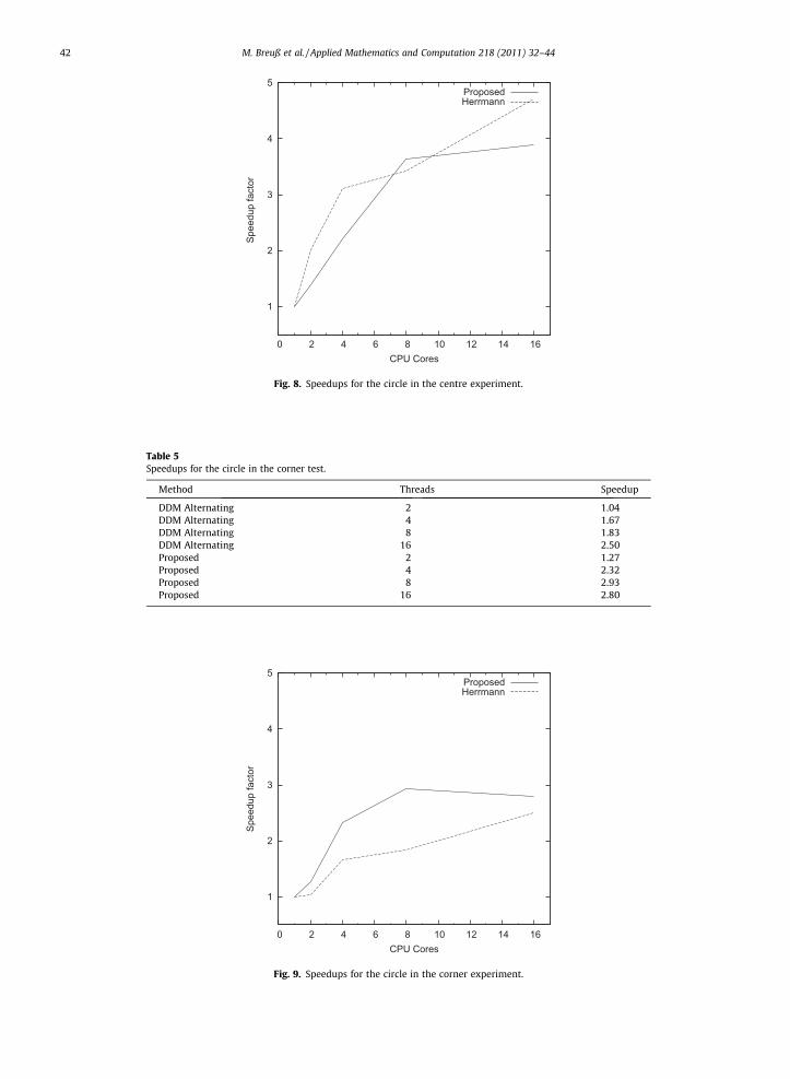
4.5. Circle in the corner

This experiment is similar to the test before, but this time we put a quarter of a circle in a corner of the domain. Table 5and Fig. 9 show the speedups of the different methods. Note that the speedups of the proposed method are generally betterthan the ones of DDM. This is caused by DDM running sequentially at the beginning, and only splitting into several threadswhen reaching the computational domain of another thread. In contrast, the proposed method splits the work to differentthreads right from the beginning, which makes it clearly superior in this case. CPU time on just one thread was around 9 s.

5. Application to the shape-from-shading problem

For a real-world application of the method, we consider the shape-from-shading (SfS) problem. This is a classic inverseproblem in the field of computer vision. It amounts to recover the 3D shape of an object from one given 2D grey-level pho-tograph of it, together with some assumptions on the illumination and the reflectance properties of the object. A survey car-ried out in [34] showed that SfS seemed a difficult task to achieve. Recently, the works [35–37] have improved upon theresults that could not be achieved earlier. As input images are usually taken with a digital camera with resolutions of severalmegapixels, the corresponding computational domain is quite large.

A mathematical model for SfS that gives adequate solutions for real-world images is the one proposed in [38]. We applythat method to a real-world image of three chess figures, shown in Fig. 10. This is quite a large image of around 8 megapixels.The computation time using a standard SfS method for such an image is several hours, while that of the FMM is in minutes[6].

Fig. 11 shows the reconstructions using this model. The accuracy of this reconstruction has been discussed in [6]. How-ever, this paper is directed towards the performance of the method under parallelization.

Table 6 shows the speedup factors of the proposed parallelization method for 1, 2, and 4 threads on a single Intel Core 2Quad Q8200, 2.33 GHz, with 2 � 2 MB L2 Cache and 4 GB RAM. The computation times on just a single thread was about86.5 s for the SfS model. Since the four cores on this machine share caches and a common memory interface, the computa-tion times are less meaningful than the ones obtained in the previous section. However, an architecture like this has becomevery popular in the recent years on home PCs, therefore this experiment has practical relevance. Table 6 shows that it is pos-sible to speed the computation up by almost a factor 2.5 on four threads, even on a shared cache architecture. This reducesthe computation time to about 35 s, which is very impressive for such a large input image.

6. Summary and conclusion

In this work we have described a new approach to parallelize the FMM in a way especially useful for machines with twoto four cores. The method is much easier to implement than existing approaches, and it gives better speedups in relevantexperimental settings. Following these attractive properties, this method can be a standard building block for future imple-mentations of the FMM.

The experiments reveal even better speedups if the arithmetic density of a computational problem, i.e. the ratio of arith-metic operations vs. memory interactions, is higher. As observable by the speedup obtained, more instructions are per-formed on a per-thread basis, i.e. on data that are already cached. Memory bottlenecks are hence less severe sincethreads are better occupied with available data which in turn grants a better parallelity.

Table 4Speedups for the circle in the centre test.

Method Threads Speedup

DDM Alternating 2 2.01DDM Alternating 4 3.11DDM Alternating 8 3.43DDM Alternating 16 4.72Proposed 2 1.39Proposed 4 2.22Proposed 8 3.64Proposed 16 3.89

1

2

3

4

5

0 2 4 6 8 10 12 14 16

Spee

dup

fact

or

CPU Cores

ProposedHerrmann

Fig. 8. Speedups for the circle in the centre experiment.

Table 5Speedups for the circle in the corner test.

Method Threads Speedup

DDM Alternating 2 1.04DDM Alternating 4 1.67DDM Alternating 8 1.83DDM Alternating 16 2.50Proposed 2 1.27Proposed 4 2.32Proposed 8 2.93Proposed 16 2.80

1

2

3

4

5

0 2 4 6 8 10 12 14 16

Spee

dup

fact

or

CPU Cores

ProposedHerrmann

Fig. 9. Speedups for the circle in the corner experiment.

42 M. Breuß et al. / Applied Mathematics and Computation 218 (2011) 32–44

Fig. 10. Real-world chess input image: Rook, knight, and pawn.

Fig. 11. Reconstruction of the chess figures using the parallel fast marching SfS method.

Table 6Speedups for the shape-from-shading test.

Threads Computation time (s) Speedup

1 86.532 12 64.133 1.354 35.764 2.42

M. Breuß et al. / Applied Mathematics and Computation 218 (2011) 32–44 43

Acknowledgments

The authors gratefully acknowledge partial funding by the Cluster of Excellence Multimodal Computing and Interaction andby the Deutsche Forschungsgemeinschaft.

References

[1] M. Bardi, I. Capuzzo Dolcetta, Optimal Control and Viscosity Solutions of Hamilton–Jacobi–Bellman Equations, Birkhäuser, Boston, Basel, Berlin, 1997.[2] J.A. Sethian, Level Set Methods and Fast Marching Methods, Cambridge University Press, Cambridge, UK, 1999.[3] R. Kimmel, J.A. Sethian, Optimal algorithm for shape from shading and path planning, J. Math. Imaging Vision 14 (2001) 237–244.[4] A. Telea, An image inpainting technique based on the fast marching method, J. Graph. GPU, Game Tools 9 (2004) 23–34.[5] E. Cristiani, M. Falcone, Fast semi-Lagrangian schemes for the Eikonal equation and applications, SIAM J. Numer. Anal. 45 (2007) 1979–2011.[6] O. Vogel, M. Breuß, T. Leichtweis, J. Weickert, Fast shape from shading for phong-type surfaces, in: X.-C. Tai, K. Mørken, M. Lysaker, K.-A. Lie (Eds.),

Scale space and variational methods in computer vision, Lecture Notes in Computer Science, vol. 5567, Springer, Berlin, 2009, pp. 733–744.

44 M. Breuß et al. / Applied Mathematics and Computation 218 (2011) 32–44

[7] J.A. Sethian, A fast marching level set method for monotonically advancing fronts, Proc. Natl. Acad. Sci. USA 93 (1996) 1591–1595.[8] J.N. Tsitsiklis, Efficient algorithms for globally optimal trajectories, IEEE Trans. Autom. Control 40 (1995) 1528–1538.[9] J. Helmsen, E.G. Puckett, P. Colella, M. Dorr, Two new methods for simulating photolithography development in 3D, in: Proceedings of SPIE, the

International Society of Optical Engineering 2726, 1996, pp. 253–261.[10] E.W. Dijkstra, A note on two problems in connection with graphs, Numer. Math. 1 (1959) 269–271.[11] E. Rouy, A. Tourin, A viscosity solutions approach to shape-from-shading, SIAM J. Numer. Anal. 29 (1992) 867–884.[12] E. Cristiani, M. Falcone, A characteristics driven fast marching method for the Eikonal equation, in: K. Kunisch, G. Of, O. Steinbach (Eds.), Numerical

Mathematics and Advanced Applications (ENUMATH 2007), Springer, Berlin, 2008, pp. 695–702.[13] S. Kim, An O(N) level set method for Eikonal equations, SIAM J. Sci. Comput. 22 (2001) 2178–2193.[14] L. Yatziv, A. Bartesaghi, G. Sapiro, O(N) implementation of the fast marching algorithm, J. Comput. Phys. 212 (2006) 393–399.[15] D.L. Chopp, Some improvements of the fast marching method, SIAM J. Sci. Comput. 23 (2001) 230–244.[16] P.-E. Danielsson, Q. Lin, A modified fast marching method, in: J. Bigun, T. Gustavsson (Eds.), Image Analysis, Lecture Notes in Computer Science, vol.

2749, Springer, Berlin, 2003, pp. 1154–1161.[17] M.S. Hassouna, A.A. Farag, Multistencil fast marching methods: a highly accurate solution to the Eikonal equation on Cartesian domains, IEEE Trans.

Pattern Anal. Mach. Intell. 29 (2007) 1563–1574.[18] J.A. Sethian, A. Vladimirsky, Ordered upwind methods for static Hamilton–Jacobi equations: theory and algorithms, SIAM J. Numer. Anal. 41 (2003)

325–363.[19] K. Alton, I.M. Mitchell, Fast marching methods for stationary Hamilton–Jacobi equations with axis-aligned anisotropy, SIAM J. Numer. Anal. 47 (2008)

363–385.[20] E. Cristiani, A fast marching method for Hamilton–Jacobi equations modeling monotone front propagations, J. Sci. Comput. 39 (2009) 189–205.[21] E. Carlini, E. Cristiani, N. Forcadel, A non-monotone fast marching scheme for a Hamilton–Jacobi equation modelling dislocation dynamics, in: A.

Bermúdez de Castro, D. Gómez, P. Quintela, P. Salgado (Eds.), Numerical Mathematics and Advanced Applications (ENUMATH 2005), Springer, Berlin,2006, pp. 723–731.

[22] E. Carlini, M. Falcone, N. Forcadel, R. Monneau, Convergence of a generalized fast marching method for an Eikonal equation with a velocity changingsign, SIAM J. Numer. Anal. 46 (2008) 2920–2952.

[23] E. Prados, S. Soatto, Fast marching method for generic shape from shading, in: N. Paragios, O. Faugeras, T. Chan, C. Schnörr (Eds.), Variational,geometric, and level set methods in computer vision, Lecture Notes in Computer Science, vol. 3752, Springer, Berlin, 2005, pp. 320–331.

[24] A. Vladimirsky, Static PDEs for time-dependent control problems, Interfaces Free Bound. 8 (2006) 281–300.[25] M. Herrmann, A domain decomposition parallelization of the fast marching method, Annual Research Briefs, Center for Turbulence Research, Stanford,

CA, USA, 2003.[26] M.C. Tugurlan, Fast marching methods: Parallel Implementation and Analysis, Ph.D. thesis, Louisiana State University, 2008.[27] O. Weber, Y.S. Devir, A.M. Bronstein, M.M. Bronstein, R. Kimmel, Parallel algorithms for approximation of distance maps on parametric surfaces, ACM

Trans. Graph. 27 (2008) 1–16.[28] H. Zhao, A fast sweeping method for Eikonal equations, Math. Comput. 74 (2005) 603–627.[29] H. Zhao, Parallel implementations of the fast sweeping method, J. Comput. Math. 25 (2007) 421–429.[30] W.-K. Jeong, R.T. Whitaker, A fast iterative method for Eikonal equations, SIAM J. Sci. Comput. 30 (2008) 2512–2534.[31] W.-K. Jeong, R.T. Whitaker, A Fast Iterative Method for a Class of Hamilton–Jacobi equations on parallel systems, Technical Report UUCS-07-010,

University of Utah, School of Computing, 2007.[32] D.R. Butenhof, Programming with POSIX Threads, Professional Computing Series, Addison-Wesley, 1997.[33] J.L. Bentley, Multidimensional binary search trees used for associative searching, Commun. ACM 18 (1975) 509–517.[34] R. Zhang, P.-S. Tsai, J.E. Cryer, M. Shah, Shape from shading: a survey, IEEE Trans. Pattern Anal. Mach. Intell. 21 (1999) 690–706.[35] E. Prados, O. Faugeras, Perspective shape from shading and viscosity solutions, Proceedings of Ninth International Conference on Computer Vision, vol.

2, IEEE Computer Society Press, Nice, France, 2003, pp. 826–831.[36] A. Tankus, N. Sochen, Y. Yeshurun, A new perspective [on] shape-from-shading, Proceedings of Ninth International Conference on Computer Vision,

vol. 2, IEEE Computer Society Press, Nice, France, 2003, pp. 862–869.[37] O. Vogel, L. Valgaerts, M. Breuß, J. Weickert, Making shape from shading work for real-world images, in: J. Denzler, G. Notni, H. Süße (Eds.), Pattern

Recognition, Lecture Notes in Computer Science, vol. 5748, Springer, Berlin, 2009, pp. 191–200.[38] O. Vogel, M. Breuß, J. Weickert, Perspective shape from shading with non-Lambertian reflectance, in: G. Rigoll (Ed.), Pattern recognition, Lecture Notes

in Computer Science, vol. 5096, Springer, Berlin, 2008, pp. 517–526.