An 18-year Timeseries of OH Rotational Temperatures and Middle Atmosphere Decadal Variations

Journal of Atmospheric and Solar-Terrestrial Physics 64 (2002) 1147–1166www.elsevier.com/locate/jastp

An 18-year time series of OH rotational temperatures andmiddle atmosphere decadal variations

M. Bittner a ;∗;1, D. O-ermanna, H.-H. Graef a ;2, M. Donnera, K. Hamiltonb;3aUniversity of Wuppertal, Germany

bGeophysical Fluid Dynamics Laboratory, Princeton, USA

Abstract

Rotational temperatures are derived from measurements of the (3-1) transitions of the OH Meinel bands. They are found tobe a reasonable proxy for atmospheric kinetic temperatures at an altitude of 3× 10−3 hPa (87 km). Measurements were takenin Wuppertal (51◦N=7◦E) from 1980 to 1998. A second (shorter) data set (1980–1991) is available for Northern Scandinavia(Andoya, 69◦N=16◦E, and Kiruna, 68◦N=21◦E). Data are analyzed for seasonal variations (annual, semi-annual, terannual) andfor long-term changes of the temperature. Furthermore atmospheric wave activity is studied by means of measured short-termtemperature =uctuations. Amplitudes and phases of the seasonal components do not change much during the measurementperiod. On the contrary annual mean temperatures and wave activity show strong long-term and even decadal variations.Similar decadal “episodes” are found in data from the Stratospheric Sounding Units (SSU) and from radiosondes at loweraltitudes (1 hPa=47 km and 10 hPa=31 km, respectively). Temperature variations during these episodes are rather large (10K)and need to be taken into account when using reference or standard atmospheres. Episodic variations of temperature and waveactivity are found to be correlated. They appear to be consistent with the “downward control principle” (Rev. Geophys. 33(1995) 403). c© 2002 Elsevier Science Ltd. All rights reserved.

Keywords: OH-temperatures; Atmospheric trends; Mesopause

1. Introduction

Temperature in the stratosphere and mesosphere is highlyvariable. Strong changes occur on all time scales fromhours to decades. Short-period oscillations (hours to days)are attributable to various kinds of waves (e.g. Forbes,1982a, b; Fritts et al., 1993; Fetzer and Gille, 1994; Bittneret al., 2000). Very large variations occur during thecourse of the year due to variations in energy budget and

∗ Corresponding author. Deutsches Fernerkundungsdatensen-trum, Postfach 1116 82230 Wessling, Germany. Fax: +49-81-53-28-1363.

E-mail address: [email protected] (M. Bittner).1 Now at DLR—German Remote Sensing Data Center, Oberp-

fa-enhofen, Germany.2 Now at SAP, Walldorf, Germany.3 Now at SOEST, University of Hawaii, Honolulu, USA.

dynamics (CIRA, 1986, Fig. 1). Multiannual to decadal vari-ations have also been shown to be of considerable magnitude(e.g. Van Loon and Labitzke, 1993; Keckhut et al., 1995;Taubenheim et al., 1997; Pawson et al., 1998). Middleatmosphere temperatures pose a challenge on the exper-imental as well as on the theoretical side. Temperaturemeasurement diJculties strongly increase with altitude.Theoretical investigations have shed some light on thenature of middle atmospheric temperature variations. Inparticular, variations in the long-term mean or zonal-meantemperature are related to wave forcing, which might beexpected to be re=ected in higher-frequency temperaturevariations (e.g. Fels, 1985; Andrews et al., 1987). Onecomplication is that the e-ects of eddy forcing on the meanis non-local, with mean circulation at some level dependenton the wave forcing at higher levels (e.g. Haynes et al.,1991; Holton et al., 1995).

Temperatures have been most diJcult to measure in theupper mesosphere and lower thermosphere, and continue

1364-6826/02/$ - see front matter c© 2002 Elsevier Science Ltd. All rights reserved.PII: S1364 -6826(02)00065 -2

1148 M. Bittner et al. / Journal of Atmospheric and Solar-Terrestrial Physics 64 (2002) 1147–1166

Fig. 1. Seasonal temperature variations in the middle atmo-sphere: (a) OH* temperatures (87 km, Wuppertal, 51◦N=7◦E), (b)SSU temperatures (1 hPa; 50◦N=5◦E), (c) Radiosonde tempera-tures (31 km, Hohenpeissenberg, 48◦N=11◦E). Seasonal variationshave been modeled by a three component harmonic Nt (annual,semi-annual, ter-annual). Residues of measured and modeled dataare given together with the seasonal variations. Data are from 1994.

to pose a problem there. Early data from grenade and pitotrocket experiments and ground based incoherent scatterdata are contained in the CIRA, 1986 model (CIRA, 1990).More recent in-situ measurements have been performed byrocket-borne instruments like falling spheres (active and,to some extent, also passive ones, Philbrick et al., 1985;Schmidlin et al., 1991), ion gauges, mass spectrometers (vonZahn et al., 1990; LPubken et al., 1994; Hillert et al., 1994),and by infrared radiometers and spectrometers (Grossmannet al., 1987, 1994; Ratkowski et al., 1994). Due to theircomplexity and costs, a relatively small number of suchmeasurements is available and presents a somewhat limitedbasis for a global climatology. Remote sensing from the

ground or from satellites o-ers extended time series and=orglobal coverage of measurements, in principle. Most lidars,however, are still limited to altitudes below 80 km. Only afew are presently exceeding this level (e.g. Hauchecorneet al., 1991; Philbrick and Chen, 1992; Leblanc et al.,1998), and the number of Na and Klidars is small (LPubkenand von Zahn, 1991; Bills et al., 1991; She et al., 1993,Bills and Gardner, 1993; von Zahn and HPo-ner, 1996). In-frared satellite measurements, on the other hand, are sparseabove 80 km and are hampered by non-LTE problems.This is a matter of active discussion presently (Sharma andWintersteiner, 1990; Rodgers et al., 1992; LQopez-Puertaset al., 1992; Grossmann et al., 1994; Ratkowski et al.,1994). Ultraviolet Rayleigh scatter measurements is yetanother satellite technique. A fairly large data set has beenobtained up to about 90 km by the Solar Mesospheric Ex-plorer (SME) satellite (Clancy and Rusch, 1989; Clancyet al., 1994). Satellite in-situ measurements are applicableat much higher altitudes only (Philbrick, 1976). However,Space Shuttle reentry measurements yielded a useful dataset (e.g. Fritts et al., 1993).

Because of the relative sparseness of data on upper meso-sphere temperatures, attempts are valuable that have beenmade in the past to derive temperatures from the emissionof excited OH molecules that occurs in a layer roughly 9 kmthick (half-power full-width) and centered at about 87 kmaltitude. Since the detection and identiNcation of this radi-ation by Meinel (1950a, b, c) various parts of its spectrumhave been used to derive rotational temperatures and thusestimate upper mesosphere kinetic temperatures. Such spec-troscopic measurements from the ground are straightforwardand relatively inexpensive.

A wealth of OH data have been measured in the recentyears which were used to intensely study:

• gravity waves and tides (e.g. Walterscheid et al., 1987;MyrabH et al., 1987; Scheer and Reisin, 1990; Tayloret al., 1991; Yee et al., 1991; Tarasick and Shepherd,1992; Dewan et al., 1992; Hickey et al., 1992; Tayloret al., 1993)

• variations due to season and latitude (MyrabH et al.,1984a; Clemeshea et al., 1990; O-ermann and Gerndt,1990)

• the solar cycle (Shefov, 1969)• changes during events like long period oscillations, ge-

omagnetic storms, aurorae, and stratospheric warmings(MyrabH et al., 1984b; Baker et al., 1985; O-ermannet al., 1987; Scheer et al., 1994; Bittner et al., 2000).

In the present work we analyze an 18-year time se-ries of ground-based OH∗ measurements for long-termchanges. The analysis yields considerable variations ofthis kind for temperature and other parameters. The dataseries also contains various short-period variations whichhave been analyzed by Bittner et al. (2000). The long-termresults are compared to temperature measurements at twolower altitudes. At 1 hPa (47 km) and at 10 hPa (31 km)

M. Bittner et al. / Journal of Atmospheric and Solar-Terrestrial Physics 64 (2002) 1147–1166 1149

Stratospheric Sounding Unit (SSU) satellite data are used(Bailey et al., 1993). At the lowest altitude (31 km) alsoradiosonde measurements are used. They were measuredat Hohenpeissenberg (47:8◦N; 11:0◦E), which is 477 kmaway from Wuppertal. Temperature variations at the dif-ferent altitudes show interesting structures and similaritiesthat are tentatively interpreted in terms of the downwardcontrol principle (Holton et al., 1995).

2. OH* measurements

2.1. Proxy temperatures

The OH emissions are chemically excited, and the ro-tational temperatures derived from them are only a proxyfor kinetic atmospheric temperatures. The usefulness of thisproxy encounters three diJculties: the question of local ther-modynamic equilibrium (LTE), the lack of vertical resolu-tion, and the vertical movements of the OH∗ layer. (Thishas recently been discussed by She and Lowe, 1998.)

Much work has gone into the analysis of the OH∗ spec-trum and the question as to which part of it is in LTE. Asurvey on the respective literature is contained in Pendle-ton et al. (1993). Substantial non-LTE components wereidentiNed by these authors. Only low-lying vibrational androtational levels=transitions appear to be suitable for temper-ature derivations (Baker, 1978; SivjQee, 1992; She and Lowe,1998). To avoid such problems we use the low-lying (3,1)OH∗ transitions. Non-LTE e-ects are of less importance ina relative analysis as the one presented here.

The lack of vertical resolution and the relatively largethickness of the OH∗ layer yields temperatures that areweighted means over a broad layer of the atmosphere. Thisis not a serious limitation under quiet conditions as the layeris in an atmospheric region, where temperature gradientsare relatively moderate. During disturbed conditions, on theother hand, it can be essential if the vertical scale of the dis-turbance is on the order of or even smaller than the layerthickness. It is, however, not believed to be too importantfor the present relative analysis.

Few ground-based temperature measurements have si-multaneous determinations of the OH∗ layer altitude Z0 (i.e.the altitude level of the layer maximum). Hence the alti-tude allocation of the measured temperature remains dubi-ous to some extent. This is unimportant for most relativeanalyses (e.g. for many wave studies). For other investiga-tions it could be important and needs to be analyzed on acase-to-case basis. Altitude Z0 and the shape of the OH∗

layer have been studied by a number of di-erent techniques.A large part of these data stem from rocket-borne radiome-ters or photometers. A compilation of these data was givenby Baker and Stair (1988). Additional Z0 values were morerecently derived from several orbital measurements: for theAtmospheric Explorer (AE)-E satellite by Abreu and Yee(1989), for the Solar Mesospheric Explorer (SME) satel-

lite by LeTexier et al. (1989), for the Space Shuttle STS37 by Mende et al. (1993), and for the WINDII experimenton the Upper Atmosphere Research Satellite (UARS) byLowe et al. (1996). A recent rocket experiment was per-formed by Takahashi et al. (1996). The data extend overmore than 30 years. They were analyzed for long-term vari-ations of Z0. A signiNcant trend could not be found. Themean altitude Z0 is 87:4 km ± 2:9 km. This is in excellentagreement with the result of 87 km recently derived from1 year (1993) of WINDII measurements (She and Lowe,1998). Quite recently an analysis of the layer Nne struc-ture (double peaks) was performed on the basis of WINDIIdata taken in 1991–1995 (Melo et al., 2000). In most casesa simple layer with a peak between 85 and 90 km wasobtained.

2.2. Time and location of measurements

Two near-infrared spectrometers were built, and at leastone of them was operated at the University of Wuppertal(51:3◦N; 7:2◦E) as often as possible to obtain ground-basedOH∗ measurements as complete as possible. Measurementsof the Nrst instrument started in autumn 1980, and those ofthe second spectrometer late in 1982. The instruments werealso used to complement temperature measurements in themesosphere and lower thermosphere taken by rockets andlidars. Hence the two instruments are mobile (includingthe calibration equipment) and participated in a number ofGBR campaigns (ground-based, Balloon, and Rocketmeasurements). As a result the measurement record atWuppertal has a few gaps, as is shown in Fig. 2. This ham-pers the long-term analysis to some extent. On the otherhand, this travel activity of the spectrometers yielded enoughdata in Northern Scandinavia (Andoya Rocket Range,69:3◦N; 16:0◦E; ESRANGE, 67:9◦N; 21:1◦E) to allowan independent high latitude analysis, which is also givenbelow.

2.3. Instruments

As discussed above, it may be that high-lying rotationaltransitions of OH are not in LTE. Therefore, the (3,1)transition lines P1(2); P1(3), and P1(4) near 1:5�m werechosen for measurements, to reduce NLTE e-ects as muchas possible (Baker, 1978; SivjQee, 1992). Typical spec-tra of the two grating spectrometers are shown in Fig. 3.The spectral resolution of the two spectrometers is highenough that spectral interferences from weak nearby lines(R branch) can be corrected for, and low enough thatmaximum measuring speed is obtained. The detectors areliquid nitrogen cooled intrinsic Ge crystals. Time resolutionof temperature measurements is 2–4min. The instrumentsare computer controlled. Details of optics, detectors, andelectronics are given by Gerndt (1986), Graef (1991),and Donner (1995). Instrumental data are summarized inTable 1.


Fig. 2. OH* temperature measurements in Wuppertal (51◦N=7◦E) from 1980 to 1998. Vertical dashed lines indicate the beginning of theyear. Data points are mean night temperatures (3139 values).

Fig. 3. Typical OH* spectra at 180 K rotational temperature: (a) Spectrometer 1 at KPuhlungsborn (54◦N=12◦E); (b) Spectrometer 2 atWuppertal (51◦N=7◦E).

Table 1Technical data of Wuppertal University Spectrometers

Spectrometer 1 Spectrometer 2

Type Ebert-Fastie Czerny-TurnerFocal length 0:5m 0:3mField of view 7:3◦ × 7:3◦ 13:5◦ × 13:5◦Etendue 0:007 cm2 sr 0:011 cm2 srGrating constant 1:2�m 3:5�mBlaze wavelength 1:2�m 3:5�mWavelength range 1.05–1:74�m 1.05–1:74�mScan time 4:5min 1:5minSpectral resolution (�=T�) 465 451Sample spacing 0:0841 nm 0:141 nmDetector Intrinsic Ge Intrinsic GeNEP 3× 10−16 W=

√Hz 5× 10−16 W=

√Hz


2.4. Accuracy

Rotational temperatures are derived from the semi-logarithmic relationship between the intensities of the threeP1 lines and their wavelengths (linear Nt, e.g. SivjQee, 1992;Bittner et al., 2000). It is important to note that only the rel-ative intensities of the three lines are needed for this deriva-tion. Hence, if there should be changes of the spectrometersensitivity, atmospheric transmission, or other factors thederived temperatures would not be a-ected unless suchchanges were wavelength dependent. Even in that case,in=uences would be small because the three lines are closetogether (1:524�m; 1:533�m; 1:543�m). For instancestratospheric aerosol from a volcanic eruption would notproduce a measurable change of our temperatures (Palmerand Williams, 1975). We have also checked whether watervapor and its variations could a-ect our results. This wasdone on the basis of transmissions presented by Espy andHammond (1995). No e-ects larger than 1K were found(summer and winter). Respective corrections were there-fore neglected in the present analysis of long-term relativetemperature variations.

Calibration of the infrared spectrometers was performedfrom time to time (i.e. about once per year on the mean).Spectral calibrations were performed by means of gas dis-charge lamps (Hg, Cd). The known line positions of ourthree OH lines were subsequently used to recalibrate the in-struments every night.

Calibrations of spectral sensitivity were performed bymeans of (two) black-body sources. Only the relative dif-ferences of the sensitivities at the positions of the threelines are needed for OH temperature derivation. It wasfound that these di-erences never varied by more than 0.6%(corresponding to 0:8K). Care was taken to guarantee thelong-term stability of the black-body sources. Comparisonof our temperatures with other techniques is discussed be-low. A close agreement with quite di-erent instruments(sodium lidar, SME, HRDI, potassium lidar) is obtainedover a long time interval (1982–1998). This agreementis in absolute temperatures and thus strongly supports thestability of our instruments.

Scattered light (Hg line from city lights, moon) ispresent in the spectra from time to time because of hazein the Neld of view. If the Hg signature shows up therespective spectrum is discarded. A background contin-uum is estimated and, if not too large, subtracted. This isdone by means of the intensity measured at 1:5474�m,which consists of the background and a known contri-bution from the nearby R line. It is assumed that thebackground is constant in our spectral range. If it is largerthan 10% of the P1 (4) line the respective spectra are dis-carded. (This criterion is applied separately from and inaddition to the criterion for low signal=noise ratio givenbelow.)

In the analysis presented below nightly mean rotationaltemperatures are used. These means result from 100–200

good spectra per night, depending on the spectrometer andthe time of the year. If a temperature is derived from eachspectrum, and subsequently a nightly mean is calculated byaveraging these temperatures an error is inevitably intro-duced because (1) the intensities contain some noise and (2)the dependence of temperatures on intensities is non-linear.This error could be reduced by averaging the line intensi-ties Nrst over some time interval, and then determining thetemperature from the three mean line intensities. Thisrequires, however, that the atmospheric temperature beconstant in that time interval. As the temperature =uctuatesconsiderably during the night, it is a diJcult task to estimatethe optimum time interval over which the intensities shouldbe averaged. We did a careful analysis and determinedthis optimum interval to be 0.5–1 h (Wiemert, 1993). Theresulting temperature bias is a second-order e-ect and thusrather small. It was found to be about 0:5K (based on a1 h interval). All measured data have been down-correctedaccordingly.

It should be emphasized again that, for the present anal-ysis, the absolute accuracy of the data, though important,is not as decisive as the data precision. This is becauseour analysis considers relative temperature variations only.We estimate the relative error of a nightly mean tempera-ture value to be 1–2K. This is derived from measurementstaken during the whole night (standard error of the mean),and therefore it still contains some atmospheric variability.Thus, the value must be considered as an upper limit for therelative error. The absolute temperature error is of the samemagnitude.

Ground-based optical experiments experience fairly triv-ial disturbances such as clouds in the Neld of view. Thesetime periods need to be excluded from the data analysis. Itturns out to be diJcult to identify such disturbances dur-ing fully automated measurements. We therefore chose asemi-automatic operation. This means that an instrumentis manually started in the evening (including cryogen Nll-ing), and manually stopped in the morning. Hence mostoperation irregularities are detected immediately becauseeach morning the spectra are checked visually for theirquality.

Spectra that are deteriorated by clouds, low OH∗ inten-sity (S=N ¡ 6), city stray light in combination with haze(Hg line), high background continuum, transition from highto low intensity (or vice versa), etc., are identiNed, andomitted from further analysis. Furthermore a nightly meantemperature is included to our data set only if it is basedon more than 2 h of measurement with normal accuracy(S=N ≈ 15) or 1 h with high accuracy (S=N¿ 25). Mea-surements were also routinely taken on the weekends andholidays. Thus, no spurious 7 day signatures appear in thespectral analyses. More than 3000 nights of data at Wupper-tal are analyzed below. This analysis is thus based on about250,000 spectra and temperature values, respectively. Twoof three nights on average yielded good data during the last10 years.


Fig. 4. Seasonal variation of temperatures derived from OH emis-sions in Wuppertal (51◦N=7◦E) and from SME measurementsat 86 km altitude (51◦ latitude). Measurements cover the period1981–1988 for the Wuppertal station, and 1982–1986 for SME.

2.5. Intercomparisons

One of the two spectrometers was always at Wuppertal toperform the long-term measurement series (except for thegaps 1985=86). The other instrument was either being refur-bished, participating in a measurement campaign elsewhere,or sitting beside the Nrst one in Wuppertal for compara-tive measurements. Short-term results of these simultaneousmeasurements show some di-erences which are attributedto the di-erent Nelds of view of the two spectrometers (seeTable 1) and to the high variability of the atmosphere. If,however, temperatures are averaged over several days oreven weeks, the two instruments agree to better than 1K.

Recently, one of the instruments was taken toKPuhlungsborn (54◦N; 12◦E, Institute of AtmosphericPhysics), and measured simultaneously with an all skyimager instrument (Aerospace Corporation, Los Angeles).Results will be presented elsewhere. Preliminary analy-sis of the data yields an agreement within a few degrees(Fricke-Begemann et al., 1998).

Several comparisons of OH∗ temperatures to rocket-bornein-situ measurements (falling spheres) or lidar observationswere performed during a number of measurement campaigns(mostly at high latitudes, O-ermann et al., 1987; Philbricket al., 1985; Schmidlin et al., 1991). Relatively coarse agree-ment was obtained (¡ 10K), which may be due to the fairlylarge errors of these techniques at high altitudes.

A comparison including much more data is o-ered bymesospheric temperatures derived from SME ultravioletand visible limb scattering observations that were taken in1982–1986 (Clancy and Rusch, 1989; Clancy et al., 1994).The respective seasonal variation for 51◦ latitude (Wupper-tal) and 86 km altitude is shown in Fig. 4. For comparisonthe Ngure also shows the OH temperatures at Wuppertal av-eraged from 1981 to 1988. Very close agreement between

the two data sets is found. (The agreement is slightly worsefor SME 87 km data. It needs to be remembered that theSME altitude resolution is 4 km.) The absolute error ofthe SME data is ±8K at this altitude. Assuming¡ 2K forthe OH proxy temperatures, the combined error is ¡ 10K.The di-erence between the two curves in Fig. 4 is much lessthan this except for January and February. When consideringthese di-erences it needs to be noted that the SME data arezonal means, whereas the OH∗ data are for a local station.Di-erences of a few Kelvin could arise from quasistation-ary planetary waves, for instance. Furthermore, part of theWuppertal data are from di-erent years. Finally the OH∗

data are nightly means whereas the SME data are for1400–1500LT. Tidal e-ects were observed to be strongestin January and February in Wuppertal (Wiemert, 1993).Temperatures at 14–15LT are estimated to be severalKelvin higher than the nightly mean temperatures. Hence,part of the di-erences in January=February in Fig. 4 can beexplained by tidal e-ects.

Recently, preliminary temperature results of the HighResolution Doppler Imager (HRDI) on the UARS satellitehave been published (Ortland et al., 1998). In July 1993=94these authors obtained a zonal mean temperature of 169K at87 km altitude and 51◦N. Our respective OH∗ temperatureis 173K. The di-erence of 4K is well within the combinederrors (7K for HRDI, ¡ 2K for OH∗).

High latitude OH∗ temperatures were compared to si-multaneous and co-located sodium lidar measurements(von Zahn et al., 1987). Mean temperature di-erence wasabout 2K (three nights). Most recently, one of the OH spec-trometers was taken to KPuhlungsborn as mentioned above.It sat beside of a potassium lidar and took data simultane-ously (Fricke-Begemann et al., 1998). The lidar absoluteaccuracy is on the order of 2K. The observed temperaturedi-erence (33 nights, 87 km altitude) of the two instrumentsis about 2K, and thus well within the combined error of(less than) 4K.

In summary it appears that our OH∗ temperatures do notdi-er from kinetic temperatures by more than a few de-grees. This should be suJcient for the subsequent analysis ofrelative variations.

3. Results

3.1. Seasonal variations

As is seen in Figs. 1 and 2 the OH∗ temperatures showlarge variations. Some of these appear to be systematic, andsome appear to be =uctuations. The variations are treatedaccordingly. The largest deviations from a constant temper-ature value appear to be seasonal variations. These need tobe eliminated Nrst, which is done by a multiple regressionprocedure. The remaining temperatures show pronouncedlow-frequency variations as well as strong high-frequency=uctuations. These are analyzed subsequently.


Fig. 5. Annual mean temperature T0 from Wuppertal OH data red circles: from multiple regression analysis blue circles: relative analysiswith respect to 1994 (see text) Volcano eruptions are indicated by dashed vertical lines.

The multiple regression scheme used allows for annual,semi-annual, and ter-annual oscillations. Amplitudes andphases of these and the mean annual temperature T0 areused as free parameters. The results are shown in Fig. 5(annual means, red circles) and Fig. 6 (spectral compo-nents). The time window of the analysis is one calendar year(January–December). This window is used for all the datafrom 1987 to 1998. In addition, the window is o--set by onehalf year (July–June), and the procedure is repeated in anattempt to improve the time resolution. Data measured be-fore 1987 in Wuppertal are not included in the analysis be-cause the data distribution is not homogeneous enough (seeFig. 2). Applying the procedure to the data of 1981–1984yields fairly similar results (as shown for 1982=83 and 1983in Fig. 5), but is not really reliable enough. Accuracy of theNt parameters is shown by the error bars. Increased errorsin 1989=90 are due to a 3 month data gap. The data analysisfollowed the lines given in Bittner et al. (2000), i.e. the datahave been processed using the maximum entropy method(MEM) to interpolate data gaps (see that paper for details).It is pointed out in that paper that this leads to an increaseof the number of data points of about of 35%. This froma statistical point of view—is the reason why the standarddeviation of the yearly temperature data is systematicallydecreased by about 0.5–1:0K.

The annual amplitude is by far the largest variation ob-tained from this analysis. It appears to decrease slightly dur-

ing the course of the 11 years shown. The amplitudes of thesemi-annual and ter-annual oscillations are much smaller.The semi-annual oscillation also indicates a small decrease.The Nt lines in Fig. 6a were calculated from the data pointsgiven for the middle of the years. The correlations are signif-icant at the 99% level for the annual and semi-annual ampli-tudes. (The slopes are −0:31 and −0:25K=a, respectively.)The gradient of the ter-annual oscillation is not signiNcant.The oscillation phases are shown in Fig. 6b. [The error barsof the phases were estimated as follows: for a given Nt andits standard deviation the phase under consideration wasshifted by T’ such that increased by 20% (which is aboutthe accuracy). Hence, T’ is a conservative upper bound-ary for the phase error, and is used as error bars in Fig. 6b.]The phases are fairly stable except after the Pinatubo erup-tion (see below). It is interesting to see that the amplitudes(as the phases) do not vary much in the time interval shown(2–3K), whereas the annual mean temperatures T0 showconsiderable variations (7–8K).

Hydroxyl temperature measurements are night measure-ments. Hence a tidal bias cannot be excluded. Furthermore,the e-ective length of the night varies between 4 h in sum-mer and 16 h in winter in Wuppertal (during clear weather).This can also contribute to a tidal bias. The mean annualtemperature as well as the Nt amplitudes could be a-ected.We have estimated these e-ects by means of tidal ampli-tudes taken from the Global Scale Wave Model (Hagan


Fig. 6. Multiple regression analysis of Wuppertal OH temperatures: (a) annual, semi-annual, ter-annual amplitudes; (b) phases (day of theyear when the maximum occurs). Dashed vertical lines indicate Pinatubo eruption.

et al., 1995; Hagan, private communication, 2001) and usingmean nightly measurement intervals available at Wuppertalfor the four di-erent seasons. Fit parameters were a-ectedby not more than about 1K.

We have tentatively included other geophysical parame-ters in our multi-regressional analysis in an attempt to Nndother sources of variations. We did not have much suc-cess in doing this. We did, for instance, not Nnd a clearsolar cycle signature. This may be due to the distributionof our data. It could, however, also be due to the fact thata solar cycle in=uence appears to be small at our altitudes(Keckhut et al., 1995). Furthermore, we did not Nnd clearin=uences of geomagnetic activity. We did not see an e-ectof the quasi-biannual oscillation (QBO), either, except rela-tively indirectly (Bittner et al., 2000). Much e-ort has beenspent in the literature to determine atmospheric temperaturechanges after the Pinatubo eruption. There are indicationsof some cooling in the upper mesosphere (Keckhut et al.,1995). In our data (Fig. 6) a Pinatubo signature in theseasonal amplitudes is barely visible. However, the meantemperatures appear to decrease steeply after the volcanoeruption (Fig. 5). To study this at higher time resolutionwe have calculated mean monthly temperatures in 1990 and1991. The temperature di-erences of corresponding monthsshow a temperature gradient that was positive before theeruption. Almost immediately after the eruption (i.e. about1 month later) this gradient became negative and remainedthat way except for 1 month (November). This leads to the

steep decrease of T0 seen in Fig. 5. This Nnding should,however, be considered with caution. There was a tendencyof decreasing gradient well before the eruption. It mighthave been just accidental that the gradient became nega-tive shortly after the eruption. The possibility cannot be ex-cluded that the mean temperatures in Fig. 5 would havedecreased by this time anyway, and that Pinatubo only con-tributed to this decrease, to some unknown extent. In fact,our data do not show any decrease after the eruption of ElChichon. Fig. 6b shows, on the other hand, that there isa clear Pinatubo signature in the phases of the Nt analy-sis. Phases of the annual and especially semi-annual com-ponents show considerable excursions about one half yearafter the Pinatubo eruption. It is remarkable, however, thatthis signature disappears again very soon (after another halfyear). Therefore, our results about atmospheric reactions tovolcanic eruptions are inconclusive.

She et al. (1998) and Krueger and She (1999) have an-alyzed lidar data above Ft. Collins, CO (41◦N; 105◦W)and found a strong temperature enhancement at 86 km (andsurroundings) 2 years after the Pinatubo eruption. This isnot in agreement with our data (Fig. 5) nor with those ofKeckhut et al. (1995). The only—and speculative—explanation we can presently o-er for this discrepancy arezonal asymmetries in atmospheric temperatures. Respectivestructures are well-known in the stratosphere and lowermesosphere, and might extend to the mesopause. Increasedwave activity (including planetary wave 1) are cited by


Keckhut et al. (1995) and by She et al. (1998) as a pos-sible cause of post-Pinatubo temperature signatures. Zonalasymmetries in this activity do not appear impossible. Dif-ferences at relatively small horizontal distances (24◦ inlongitude) have been discussed by She and Lowe (1998)and tentatively been attributed to di-erences in mountainwave activity.

If the three component harmonic Nt is subtracted fromthe data measured, =uctuations of considerable magnituderemain (residues in Fig. 1). We checked to see whether theirdistribution exhibits any peculiarities. In the time interval1988–1998, a total of 2459 nightly mean temperature valuesare available. A Gaussian curve was Ntted to these data. Itsstandard deviation is 5:6K (see also Fig. 9). The skewnessis 0.23. There is some time development of this distributionwhich is discussed below.

3.2. Long-term variations of annual mean temperatures

For a long-term analysis of the mean annual temperaturesT0 omission of the early part (1981–1984) of our data se-ries as in Fig. 6 would be detrimental. Since we cannot relyon the regression analysis here, we used the following pro-cedure. The seasonal variation of year 1994 is modeled asdescribed above. The Nt including annual, semi-annual, andter-annual variations and an annual mean is then used as areference curve, to be compared to all other years. Year 1994was selected because it is one of the more recent years thatshow fairly small variations in Fig. 6. In order to compare aspeciNc year to the reference year 1994, the reference curveis subtracted from the measured temperatures of the speciNcyear daily, and the mean di-erence is calculated. As a ba-sis for this procedure, we assume that the seasonal variationdoes not change much during the course of the years (seeFig. 6). If this assumption holds, any mean di-erence ob-tained (i.e. any residual deviation from the Nt 1994) wouldindicate a deviation of the mean annual temperature fromthat of year 1994, which would mean a temperature trendwith respect to year 1994. This applies even if there aredata gaps in the year under consideration. This proceduretherefore allows us to include years with larger data gaps(e.g. 1981–1984) in the analysis. We assume that all sea-sons contribute about equally to a mean temperature trend,if such a trend occurs. This was checked and appears to beapproximately the case.

If all data available in Wuppertal are referred to year1994 as described, mean temperature deviations are obtainedas shown in Fig. 5 by blue circles. (The gap in 1985 and1986 is when both spectrometers were at high latitudes inScandinavia.) The results of 1987 and following years arevery similar to those of the regression analysis given (redcircles). The blue circles now give additional results for theyears 1981–1984.

To estimate the reliability of the “relative temperatures”shown in Fig. 5 (blue circles), other years were used as ref-erence years. Every year that has full data coverage through-

out the course of the year was tried. In all cases the resultsagreed with those shown in Fig. 5 within about 0:5K forthe time span 1988–1997. In the earlier years (1981–1984)di-erences were occasionally somewhat larger and were ator above 1:5K in a few cases. Hence, the relative form ofthe blue curve shown in Fig. 5 (i.e. the relative variationsof the mean temperatures) is quite reliable.

The error bars of the red and blue circles in Fig. 5 areof di-erent magnitude because the circles have a di-erentmeaning: the red circles are annual mean temperatures ob-tained from a spectral analysis where data gaps have beeninterpolated by a maximum entropy method (MEM). Thisleads to small error bars (see above). The blue circles areannual relative temperatures (with reference to year 1994).In this analysis data gaps have not been interpolated. It isinteresting to note that the two data sets (red and blue) agreewell within the single smaller (red) error bars.

The “relative temperatures” in Fig. 5 show strong andrapid variations during part of the measurement period,which are believed to be real. During other parts of theperiod the temperatures are almost constant. The maxi-mum swing of variations is on the order 10K. This isrelatively large, if compared, for instance, to the seasonalanalysis. It is comparable to the semi-annual variation,and quite a bit larger than the ter-annual variation. Itwas tried to Nt a linear trend curve to the blue circles inFig. 5. The trend obtained is very small and not signif-icant. This is at least in part due to the large episodalvariations.

3.3. High latitude data

From 1980 to 1991 quite a number of rocket campaignswere performed in Northern Scandinavia (Andoya=Norwayand Kiruna=Sweden). During most of these one of theWuppertal NIR spectrometers was operated on the rocketrange. The duration of a measurement period ranged froma few weeks to 5 months. Therefore, only a scattered dataset of 22 monthly mean values is available in these 11years. It covers the winter season only, winter being de-Nned as the period from November to March. Since thetwo rocket ranges are fairly close together, the measure-ments from the two places are tentatively treated as onedata set. 355 nights of measurement are available. Thisis a valid data set which appears worth an attempt ofanalysis.

The data cannot, however, be treated as those atWuppertal, because a seasonal Nt is not possible. This isseen from Fig. 7, which shows all of the high latitude dataavailable. A seasonal Nt cannot be derived because of theshortness of the time series. Instead, polynomial curves havebeen tentatively Ntted to the data of winters 1981=82 and1983=84 (red line), and winters 1985=86 and 1986=87 (blueline), respectively. They give a suggestion of a seasonalvariation, indeed. However, they are not very trustworthy(especially not at their left and right ends). The two curves


Fig. 7. OH* temperature measurements in Northern Scandinavia (Andoya, 69◦N=16◦E, and Kiruna, 68◦N=21◦E) versus day of the year(DOY). Di-erent winters are labelled by di-erent colors. Data points are mean night temperatures (355 values) for the time period 1980to 1991. Solid lines are polynomial Nts to winters 1981=82 and 1983=84 (red) and winters 1985=86 and 1986=87 (blue). Dashed lines arecorresponding seasonal Nts from Wuppertal for comparison (red: winter 1982=83; blue: winter 1987=88).

are furthermore quite di-erent in shape, and thus suggestconsiderable changes in the form of the seasonal variations.This is supported by the two dashed lines which give theseasonal Nts to the Wuppertal data for the winters 1982=83(red), and 1987=88 (blue). These are the winters nearest tothe red and blue curves in Fig. 7. The two dashed lines indi-cate a substantial increase in temperature at Wuppertal from1983 to 1988. This was also suggested above in Fig. 5. Thetwo solid curves in Fig. 7 indicate a similar increase at highlatitudes. Hence a long-term variation appears to be presentin the high latitude data, too. However, neither a seasonalanalysis nor the polynomial Nts can be used to analyzethis.

In our search for long-term temperature variations we,therefore, performed a monthly analysis. We assumed thata trend would not only show up in the annual mean tem-peratures but in a similar manner in a series of monthlymeans as well (i.e. in a series of all Januarys available, forinstance). Five series of this kind were thus formed (see thevertical dashed lines in Fig. 7). For each of these monthlyseries a weighted mean value was calculated, and the devia-tions from that mean was determined for all years. Five rela-tive trend curves (November, December, January, February,March) are obtained for the 11 year time span. Each of these

curves consists of four or Nve data points (years) only, andis not really informative. It was therefore further assumedthat these Nve curves all contained the same long-term vari-ation, and that the 22 data points could be combined to formone common trend curve. This was done because all dataare from the winter season. (A similar assumption has alsobeen made above in the analysis of the Wuppertal data.)The trend curve obtained is shown in Fig. 8. It is deNned byseven data points in the time period of 11 years, which havebeen interpolated by a polynomial Nt. (The zero point of theordinate corresponds to 218:3K.) In the bottom of Fig. 8the number of measurements (nights) is given which con-tributed to each point of the curve. These numbers show thatthe points should be quite reliable. (The number of nightsavailable were used as weights in all means calculated inthe above-described procedure.) The error bars are relativelylarge. They show the error of the mean temperatures cal-culated from the monthly values available for that winter.(Data points without error bar result from 1 or 2 monthsonly.) The error bars indicate that other processes are activein the atmosphere in addition to the long-term variations.The polynomial Nt is therefore mainly meant to guide theeye and to indicate that temperatures are relatively lowerin the early 1980s and relatively higher in the later 1980s.


Fig. 8. Relative variations of mean winter temperatures in Northern Scandinavia (Andoya, 69◦N=16◦E, and Kiruna, 68◦N=21◦E, Novem-ber–March). Number of measurement nights is given at the bottom.

The curve thus shows that there are long-term temperaturevariations at high latitudes, indeed. Temperature variationsare similarly large (9K), as those for middle latitudes inFig. 5.

It should be mentioned that we do not see an in=uence ofauroral activity on our high latitude temperatures (Gerndt,1986). A search for correlation of our temperatures with themagnetic index Kp gave a negative result, too.

3.4. Short period temperature variations

3.4.1. Middle latitudesAs was mentioned above the OH∗ temperatures measured

on a daily basis appear quite noisy. If a Nt to the data ismade with annual, semi-annual, and ter-annual componentsand subtracted from the measured data, a noise-like residueremains (Fig. 1). The =uctuations are fairly large, and of-ten exceed ±10K. Thus, they are at least as large as thesemi-annual and ter-annual variations.

A detailed spectral analysis of these residues is given byBittner et al. (2000). The authors show that most of the =uc-tuations are not noise, but are due to atmospheric waves. Inthe present analysis, we study the overall magnitude of thisresidue and its variation with time. As a measure for thismagnitude we calculate the standard deviation of the OH∗

temperatures from the Nt function on a monthly basis. Fig. 1shows that the residues at the lower altitudes have a pro-nounced seasonal variation. In the upper mesosphere, how-ever, the =uctuation intensity appears almost constant. Totest this quantitatively the monthly standard deviations wereaveraged for all Wuppertal data from 1988 to 1998. Theresulting averaged seasonal variation is shown in Fig. 9a.The standard deviation is about 5–6K, and the curve hasno obvious seasonal structure. For comparison, respective

data at the two lower altitudes from Fig. 1 are also shown.At the stratopause we use SSU measurements (Baileyet al., 1993). SSU temperature variations are given at 1 hPaaltitude for 50◦N=5◦E (i.e. near to Wuppertal, Fig. 9b).The mean standard deviations are of a similar magnitude asthose in the upper mesosphere. However, they show a verystrong seasonal variation. The middle stratosphere (about10 hPa=31 km) is represented in Fig. 9c by radiosondedata measured at Hohenpeissenberg (47:8◦N=11◦E). Againthere is a strong seasonal variation, which is similar to thatat 1 hPa. At the lower altitudes (Fig. 9b and c) the stan-dard deviations are not calculated from di-erences toseasonal harmonic Nt curves, but to monthly mean temper-atures. (Seasonal harmonic analysis at these altitude doesnot yield useable results because of the strong erratic win-ter disturbances.) The two curves cover the time interval1980–1997.

The standard deviations of the OH∗ temperatures (i.e.the wave activity) are not the same in all years, but varyover time (Bittner et al., 2000). The whole data set from1981 until 1997 was used for more detailed analysis. Sincereliable seasonal Nt curves are not available for the years1981—1984, the standard deviations were calculated asthose in Fig. 9b and c (i.e. the monthly mean tempera-tures were used as reference). Calculations were done forall years available. Weighted annual means of these stan-dard deviations were calculated. The results are shown inFig. 10a. The average standard deviation is about 5:9K,and, thus, slightly higher than in Fig. 9a. This di-erence ispartly because the deviations are referred to the monthlymeans now. (We checked that the relative variations ofthe standard deviations in Fig. 10a over time are nearlythe same as if they had been calculated from the annual Ntcurves.) The data in Fig. 10a show fairly strong variations


Fig. 9. Mean seasonal variation of temperature standard deviations.(a) Wuppertal OH* temperatures (1988–1998); (b) SSU temper-atures at 1 hPa; 50◦N=5◦E (1980–1997); (c) Radiosonde temper-atures at Hohenpeissenberg at 31 km (1980–1997). (Bars are thestandard deviations of the mean values, i.e. they show the interan-nual scatter of the monthly values.)

during the time span given. There is a relatively steep de-crease in the early years, which is followed by a slowerincrease in the years after the data gap of 1985 to 1986.A polynomial Nt to the data was calculated and is alsoshown in Fig. 10a to guide the eye (dashed line). (Notethat the obvious contrast to Fig. 5 in Bittner et al. (2000)for 1982=83 is due to the fact that now older data havebeen processed and allow to calculate a standard deviationfor the year 1982 alone.) The earlier years incorporated inthis expanded analysis do not support the 0:8K per decadeincrease in standard deviations of the temperature residualsreported in Bittner et al. (2000) existing prior to 1983.

For comparison respective SSU data at 1 hPa are in-cluded in Fig. 10b. Annual mean data were calculated. Theyare dominated by the winter months (see Fig. 9b). Thedata show considerable variations. A long-term tendencyis seen also in these lower altitude data as shown by thepolynomial Nt.

Fig. 10. Long-term variations of temperature standard deviations at moderate latitudes: (a) OH* temperatures at Wuppertal; (b)SSU temperatures at 1 hPa (50◦N=5◦E).

3.4.2. High latitudesFor the OH∗ temperatures measured at Andoya

(69◦N=16◦E) and Kiruna (68◦N=21◦E) standard deviations were calculated with respect to the monthly mean values.

To analyze for a long-term trend in these data the 22standard deviation values were treated in the same way asdescribed above for the 22 monthly mean temperatures val-ues. The results are shown in Fig. 11a. The mean wasfound to be 5:8K and, thus, very similar to the Wuppertalvalue. There are strong time variations in this data set, too.An apparent long-term tendency is roughly indicated by thedashed line (polynomial Nt).

A =uctuation analysis at lower altitudes was also per-formed in order to compare the results to Fig. 11a. SSU dataat 1 hPa for 70◦N=15◦E were analyzed in the same way asfor the lower latitudes (Fig. 10b). The results are shownin Fig. 11b. Large data variations are obtained again. Con-siderable long-term variations appear to be present, too, asshown by the polynomial Nt.


Fig. 11. Long-term variations of temperature standard deviations at high latitudes: (a) OH* temperatures at Andoya (69◦N=16◦E)and Kiruna (68◦N=21◦E), relative values; (b) SSU temperaturesat 1 hPa (70◦N=15◦E).

4. Discussion

4.1. Seasonal parameters, high frequency variations, andtheir long-term changes

The seasonal amplitudes of the Wuppertal OH∗ tempera-tures are shown in Fig. 6. The annual amplitude is 22–24K.This is somewhat smaller than the respective value fromthe CIRA tables (CIRA, 1990), which is 28K. Part of thedi-erence is presumably due to the broadness of the OH∗

layer. The semi-annual amplitude of the OH∗ temperatures(5–6K) is quite a bit larger than that of CIRA (1K). As aconsequence the sum of the two amplitudes for the OH∗ tem-peratures and for CIRA is almost the same (29K). It shouldbe noted that the semi-annual oscillation of the SME tem-peratures is much stronger than that of CIRA, too (CIRA,1990). The phases of the annual and semi-annual oscilla-tions seen in the OH∗ temperatures are similar to those of

CIRA. The ter-annual oscillations are quite dissimilar. Theamplitude of the OH∗ temperatures in Fig. 6a is about 2Kin contrast to 0:36K in CIRA. Also, the phases are grosslydi-erent (almost opposite).

Data from two lidar stations in France (44◦N), that arenot too far away from Wuppertal, have been published byHauchecorne et al. (1991). For the time period 1984–1989and at 87 km altitude these authors Nnd an annual amplitudeof 20K, which is relatively close to our data. The di-er-ence can be explained mostly by the di-erence in latitudeof the two stations and by the broadness of the OH∗ layer.The semi-annual amplitude of the lidar data is 2:4K. Hy-droxyl temperatures have also been derived from OH (3-1)emissions by Niciejewski and Killeen (1995) and She andLowe (1998). Seasonal amplitudes derived are very similarto those discussed here.

The mean annual Nt temperature T0 of Hauchecorne et al.in the period 1984–1989 is 197K. Only part of that periodis covered in Fig. 5, with T0 ≈ 201K. This number neednot be representative as temperature variations could occurin the data gap (Golitsyn et al., 1996). The mean annualtemperature of CIRA (at 87 km; 51◦N) is 188K. Thus, it isconsiderably lower (9–17K) than our OH∗ temperatures inFig. 5. This Nnding is similar to the results of Clancy et al.(1994) above 80 km, who found CIRA to be 10–20K colderthan the temperature derived from the SME measurements.Too cold CIRA temperatures in the upper mesosphere werealso found by Hauchecorne et al. (1991) and by Leblancet al. (1998). A detailed discussion of CIRA temperaturedeNciencies was recently given by Leblanc et al. (1998).

The high-frequency variations of the OH∗ temperature (asrepresented by their standard deviation from the seasonalNt curve) shows little seasonal variations (Fig. 9). Compara-ble data from several lidar stations have recently been pub-lished by Leblanc et al. (1998) for the upper mesosphere.Two di-erences are observed: First, the absolute magnitudeof is 5–6K in our data, whereas it is around 10K in the li-dar data. This may be due to the broadness of the OH∗ layer,which brings about some inherent smoothing. Second, thelidar data shows a strong increase in winter (up to 14K).The reasons are not clear at present. One possibility is thedi-erence in length of the time series (11 years for the OH∗

data as compared to 4–8 years for the lidars).Local e-ects could also possibly play a role, since the

Table Mesa lidar appears not to see this strong increase.The seasonal amplitudes and phases of the OH∗ tempera-

tures do not change much over time, as was discussed above(Fig. 6). In contrast, there are strong variations of the meanannual temperatures T0 that amount to about 10K in Fig. 5.A signiNcant long-term trend in the T0 data, however, cannotbe found. This is diJcult to reconcile with relatively strongtrends obtained by Keckhut et al. (1995) for a station westof Wuppertal and by Golitsyn et al. (1996) and Lysenko etal. (1999) for a station east of Wuppertal (near Moscow).It should, however, be noted that either analysis yields a“neutral altitude”, i.e. an altitude at which the trend reverses


sign, and at which altitude it therefore is non-existent. Thisneutral altitude is slightly below 80 km for the western sta-tion, and somewhat below 100 km at the eastern station. TheWuppertal measurements are taken somewhat below 90 km(at 87 km), i.e. at an intermediate altitude. If such a “neutralaltitude” should exist above Wuppertal near 87 km, it wouldexplain the lack of trend in our data. Some more detaileddiscussion of such “neutral altitude layers” can be found inBittner et al. (1994).

The time series of annual mean OH∗ temperatures pub-lished by Golitsyn et al. (1996) and Lysenko et al. (1999)shows temperatures that are lower by more than 20K thanthe Wuppertal data, and their swing is a factor 3 larger. Thereason for this discrepancy is as yet unknown.

4.2. Comparison of wave activity and temperatureepisodes

The principle of wave-driven circulation (“downwardcontrol principle”) is often assumed to be one of the mainmechanisms controlling the middle atmosphere (for a sum-mary see Holton et al., 1995). According to this principle,in winter increased wave breaking at a given atmosphericlevel leads to temperature increases at some lower level. De-creased wave breaking should result in lower temperatures.If it is tentatively assumed that the temperature =uctuationsdiscussed here (in terms of their standard deviations) areindicative of atmospheric wave activity and hence wavebreaking, the episodic variations presented in Figs. 10 and11 o-er an interpretation in terms of the downward con-trol principle. The standard deviations analyzed are annualmean values except for the high latitude OH∗ data, whichare winter values. The stratospheric data are dominated bythe large winter values (see Fig. 9).

The variations seen in the two pictures, and especially thedecadal variations suggested by the dashed curves are rel-atively large. One should therefore expect some detectablecounterparts in temperature variations at lower altitude lev-els if the downward control principle holds. Comparabletemperature variations at the same altitude (OH layer) areseen, indeed, in Figs. 5 and 8. Temperatures at lower levelsare available from the SSU satellite instrument. Stratopausedata measured at 1 hPa altitude near Wuppertal and middlestratosphere Hohenpreissenberg temperatures (at 31 km) areshown in Fig. 12. Winter minimum data were used at thesealtitudes. This means that mean monthly temperatures werecalculated for November to March of a given winter, andthe lowest of these Nve values was used. This was done inorder to minimize the in=uences of stratospheric warmings.The two data sets show long-term temperature variations ofconsiderable magnitude, indeed. Decadal variations are sug-gested by polynomial Nt curves (dashed lines).

In the stratosphere a long-term temperature decrease hasbeen observed by several authors (for instance Hauchecorneet al., 1991; Dunkerton et al., 1998; Pawson et al., 1998). Ob-viously this trend is considerably modulated by the episodic

Fig. 12. Long-term temperature episodes at moderate latitudes: (a)SSU temperatures at 1 hPa; 50◦N=5◦E; (b) Radiosonde temper-atures at 31 km at Hohenpeissenberg. Data are winter minimumtemperatures (see text).

variations shown in Fig. 12. This may be due to the fact thatthe magnitude of the trend appears to be minimal near thealtitudes of 30 and 50 km (Hauchecorne et al., 1991).

High latitude data fromNorthern Scandinavia for the samealtitude levels as in Fig. 12 are shown in Fig. 13. Strato-spheric SSU data are for 70◦N=15◦E (at 1 and 10 hPa).Winter minimum data were used (November–March). Apolynomial was Ntted to the data to suggest the long-termvariations. The two data sets in Fig. 13 show episodic tem-perature variations similar to those at the lower latitudes.To test the downward control hypothesis we have corre-lated the wave activity seen in the Wuppertal OH∗ data(87 km) with lower altitude temperatures at the 1 hPa level(SSU data at the respective location). We assumed that waveamplitudes are proportional to temperature standard devi-ations, that wave forcing is approximately proportional tothe square of the wave amplitudes, and that the temperaturechanges are about proportional to the changes in forcing


Fig. 13. Long-term temperature episodes at high latitudes: (a)SSU temperatures at 1 hPa; 70◦N=15◦E; (b) SSU temperatures at10 hPa; 70◦N=15◦E. Data are winter minimum temperatures (seetext).

(Andrews et al., 1987). Hence the variances of OH∗ tem-peratures (squares 2 of the data shown in Fig. 10a) werecorrelated with the temperatures T at 1 hPa (Fig. 12a). Arespective scatter plot is shown in Fig. 14a. A correlationcoeJcient r = 0:51 is obtained if a time lag of 1.5 years isused. The signiNcance is 93%. The higher altitude variances2 lead the lower altitude temperatures T . The sensitivityof this correlation (TT=T2) is given by the slope b of therespective regression line. These results are summarized inTable 2 (If the standard deviation is correlated with thelower altitude temperatures r = 0:53 is obtained.) For thecalculation of the slope b accuracies of the input parametersT and 2 are needed. They were estimated from the datascatter about the polynominal Nts shown as dashed curvesin Figs. 10a and 12a, respectively.

Similar correlations were calculated for the high latitudeOH∗ data of Fig. 11a and the temperatures shown in Fig. 13a.The OH data were weighed by the number of measurements

Fig. 14. Scatter plot of annual values of temperatures T (at a lowerlevel) versus temperature variances 2 (at a higher level). Dashedlines show the regression curves. Correlation coeJcients r, slopesb, and lags are also given and are summarized in Table 2 (see text).(a) Variances at 87 km; 51◦N (from Fig. 10a), temperatures at1 hPa; 50◦N (from Fig. 12a), r=0:51; b=0:21 K=K2; lag=1:5a.(b) Variances at 87 km; 68◦=69◦N (from Fig. 11a), temperaturesat 1 hPa; 70◦N (from Fig. 13a), = 0:8; b= 0:32 K=K2; lag = 3a.(c) Variances at 1 hPa; 70◦N (from Fig. 11b), temperatures at10 hPa; 70◦N (from Fig. 13b), r=0:50; b=0:22 K=K2; lag=3a.

indicated in the bottom of Fig. 8. The scatter plot is shownin Fig. 14b. A positive correlation was obtained again, at asomewhat greater time lag (Table 2). At the high latitudesalso two lower altitude levels were compared: variances at1 hPa (see Fig. 11b) were correlated with the temperaturesat 10 hPa (Fig. 13b), and yielded a positive result at thesealtitudes, too (Table 2, scatter plot in Fig. 14c). The signif-icance level of these two correlations is 95%. The time lagfound in all cases is such that the wave activity parameter(2) at the higher altitude leads the temperature variation atthe lower altitude. The meaning of this lag remains to bedetermined.


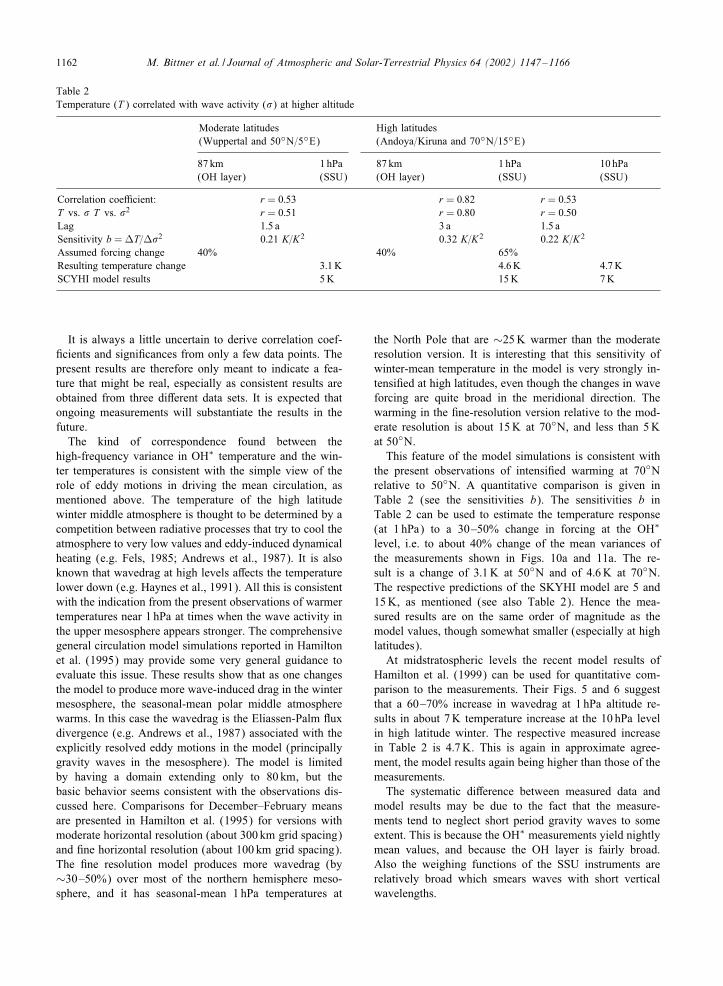
Table 2Temperature (T ) correlated with wave activity () at higher altitude

Moderate latitudes High latitudes(Wuppertal and 50◦N=5◦E) (Andoya=Kiruna and 70◦N=15◦E)

87 km 1hPa 87 km 1hPa 10 hPa(OH layer) (SSU) (OH layer) (SSU) (SSU)

Correlation coeJcient: r = 0:53 r = 0:82 r = 0:53T vs. T vs. 2 r = 0:51 r = 0:80 r = 0:50Lag 1:5 a 3 a 1:5 aSensitivity b =TT=T2 0:21 K=K2 0:32 K=K2 0:22 K=K2

Assumed forcing change 40% 40% 65%Resulting temperature change 3:1K 4:6K 4:7KSCYHI model results 5K 15K 7K

It is always a little uncertain to derive correlation coef-Ncients and signiNcances from only a few data points. Thepresent results are therefore only meant to indicate a fea-ture that might be real, especially as consistent results areobtained from three di-erent data sets. It is expected thatongoing measurements will substantiate the results in thefuture.

The kind of correspondence found between thehigh-frequency variance in OH∗ temperature and the win-ter temperatures is consistent with the simple view of therole of eddy motions in driving the mean circulation, asmentioned above. The temperature of the high latitudewinter middle atmosphere is thought to be determined by acompetition between radiative processes that try to cool theatmosphere to very low values and eddy-induced dynamicalheating (e.g. Fels, 1985; Andrews et al., 1987). It is alsoknown that wavedrag at high levels a-ects the temperaturelower down (e.g. Haynes et al., 1991). All this is consistentwith the indication from the present observations of warmertemperatures near 1 hPa at times when the wave activity inthe upper mesosphere appears stronger. The comprehensivegeneral circulation model simulations reported in Hamiltonet al. (1995) may provide some very general guidance toevaluate this issue. These results show that as one changesthe model to produce more wave-induced drag in the wintermesosphere, the seasonal-mean polar middle atmospherewarms. In this case the wavedrag is the Eliassen-Palm =uxdivergence (e.g. Andrews et al., 1987) associated with theexplicitly resolved eddy motions in the model (principallygravity waves in the mesosphere). The model is limitedby having a domain extending only to 80 km, but thebasic behavior seems consistent with the observations dis-cussed here. Comparisons for December–February meansare presented in Hamilton et al. (1995) for versions withmoderate horizontal resolution (about 300 km grid spacing)and Nne horizontal resolution (about 100 km grid spacing).The Nne resolution model produces more wavedrag (by∼30–50%) over most of the northern hemisphere meso-sphere, and it has seasonal-mean 1 hPa temperatures at

the North Pole that are ∼25K warmer than the moderateresolution version. It is interesting that this sensitivity ofwinter-mean temperature in the model is very strongly in-tensiNed at high latitudes, even though the changes in waveforcing are quite broad in the meridional direction. Thewarming in the Nne-resolution version relative to the mod-erate resolution is about 15K at 70◦N, and less than 5Kat 50◦N.

This feature of the model simulations is consistent withthe present observations of intensiNed warming at 70◦Nrelative to 50◦N. A quantitative comparison is given inTable 2 (see the sensitivities b). The sensitivities b inTable 2 can be used to estimate the temperature response(at 1 hPa) to a 30–50% change in forcing at the OH∗

level, i.e. to about 40% change of the mean variances ofthe measurements shown in Figs. 10a and 11a. The re-sult is a change of 3:1K at 50◦N and of 4:6K at 70◦N.The respective predictions of the SKYHI model are 5 and15K, as mentioned (see also Table 2). Hence the mea-sured results are on the same order of magnitude as themodel values, though somewhat smaller (especially at highlatitudes).

At midstratospheric levels the recent model results ofHamilton et al. (1999) can be used for quantitative com-parison to the measurements. Their Figs. 5 and 6 suggestthat a 60–70% increase in wavedrag at 1 hPa altitude re-sults in about 7K temperature increase at the 10 hPa levelin high latitude winter. The respective measured increasein Table 2 is 4:7K. This is again in approximate agree-ment, the model results again being higher than those of themeasurements.

The systematic di-erence between measured data andmodel results may be due to the fact that the measure-ments tend to neglect short period gravity waves to someextent. This is because the OH∗ measurements yield nightlymean values, and because the OH layer is fairly broad.Also the weighing functions of the SSU instruments arerelatively broad which smears waves with short verticalwavelengths.


5. Summary and conclusions

There is still a strong need for temperature data in thealtitude regime of the upper mesosphere. One relativelysimple and inexpensive method to obtain such temperaturesis the nightly measurement of the Meinel OH bands that areemitted from a relatively broad layer at around 87 km. Therotational temperatures derived from the relative line in-tensities can be used as proxy for the atmospheric kinetictemperatures. This proxy is found to be a reasonableapproximation (within a few Kelvin) if low-lying transi-tions in the near-infrared are used, as was done here. Thealtitude where the layer occurs is not measured simulta-neously, and thus poses an uncertainty. Quite a numberof special experiments by rockets or satellites have beenperformed during the course of the years to determine thisaltitude. Long-term changes of the layer altitude could beimportant for the present study. They are, however, notobvious from the data published to date. The thickness ofthe OH layer (9 km at half power) is a limitation for de-tailed vertical analyses. However, this is not the case for along-term study such as the present one.

Long-term OH measurements were performed for 18years (1980–1998) in Wuppertal (51◦N=7◦E), and fora shorter period (1980–1991) in Northern Scandinavia(Andoya, 69◦N=15◦E, and Kiruna, 68◦N=21◦E). Two near-infrared instruments were operated to obtain a time serieswith as few gaps as possible. Data from more than 3000nights are available fromWuppertal for the present analysis.

The Wuppertal data set was analyzed for seasonal vari-ations. An annual cycle with large amplitude was obtainedsimilar to those found in other measurements. Semi-annualand ter-annual variations of lesser amplitudes were alsofound. These amplitudes show only small variation duringthe years measured. The same holds true for the phases, withthe exception of the eruption of Pinatubo which caused ashort excursion of the phases.

Contrary to these Nndings, the mean annual temperaturesshow large variations during the observation period (10K).These variations are not easy to interpret. There are no ob-vious indications of a solar cycle, nor geomagnetic e-ects,nor an obvious reaction to volcano eruptions in these data.A signiNcant long-term trend (increase or decrease) of thetemperatures cannot be seen either. It appears that a timeseries of 18 years is still too short for a trend analysis if thedata variations are as large as were obtained. Another expla-nation may be a possible trend reversal at the altitude of ourmeasurements. Incidentally, it is obvious from these varia-tions that reference or standard atmospheres must be usedwith caution, if they do not include time variations longerthan the annual cycle. One speciNc Nnding is that the CIRA,1986 reference atmosphere is too cold by more than 10K atthe altitude of the OH∗ layer (at middle latitudes).

Considerable temperature variations are found in theOH∗ data on a time scale of several years to longer than adecade. This applies in the Wuppertal data as well as in the

Scandinavian data. Similar “temperature episodes” werelooked for and were indeed found at lower altitudes (SSUand radiosonde data at 1 hPa and around 10 hPa) when win-ter minimum temperatures were used. The variations areconsiderable at all three altitudes and at the two latitudes(10K and more). Considering the swing of the episodictemperature variations, the caveat concerning the referenceatmospheres must be applied to the lower altitudes, too.

Daily mean temperatures show considerable scatter whencompared to monthly mean values. Respective standard de-viations are used to describe this scatter. These short-termvariations are unlikely to occur at random, but are indica-tive of atmospheric waves. An annual mean of the standarddeviations was therefore used as an approximate measureof the wave activity in that year (at a given altitude andlatitude). These annual standard deviations were analyzedfor long-term variations. Episodic changes of considerablemagnitude were found, which resemble the mean tempera-ture episodes

Middle atmosphere winter temperatures and wave activityat moderate to high latitudes should be interrelated accord-ing to the concept of the wave-driven circulation (“down-ward control principle”). At a given geographic locationan increase or decrease in wave activity at a certain alti-tude level should result in a temperature increase or de-crease at a somewhat lower altitude. This is exactly whatwe observe at the three altitude levels and two latitudes an-alyzed here: a signiNcant correlation of the data sets is ob-tained (at time lags of 1.5–3 years). Thus, it appears thatthe long-term (“episodic”) changes found are compatiblewith the downward control principle. The present observa-tional results compare interestingly with a study of the sen-sitivity of mean circulation in a global simulation model(Hamilton et al., 1995,1999). In particular, when their modelwas altered and a∼30–50% increase in a mesospheric wave-drag in the northern hemisphere resulted, the 1 hPa zonalmean temperatures increased about 15K at 70◦N and 5Kat 50◦N, roughly comparable to the changes obtained fromthe present correlations analysis (Table 2). A similar resultis obtained for the lower altitudes (1 hPa=10 hPa) at highlatitudes. In all cases the measured temperature changes aresomewhat smaller than those of the model.

Acknowledgements

The SSU data were supplied by the UK MeteorologicalOJce under Contract ref. 097. We are grateful for the helpof the Stratospheric Research Group of the FU Berlin withthe handling of these data.

We thank H. Claude and the Ozone Group at Hohenpeis-senberg (DWD) for their radiosonde data of consistentlyhigh quality.

We also thank U. v. Zahn and C. Fricke-Begemann formaking available comparative K lidar temperatures beforepublication.


We acknowledge the untiring e-orts of the entireWuppertal atmospheric science team who operated the OH∗

instruments 365 days a year for a long time.

References

Abreu, V.J., Yee, J.H., 1989. Diurnal and seasonal variation ofthe nighttime OH (8-3) emissions at low latitudes. Journal ofGeophysical Research 94, 11,949–11,957.

Andrews, D.G., Holton, J.R., Leovy, C.B., 1987. MiddleAtmosphere Dynamics. Academic Press, New York.

Bailey, M.J., O’Neill, A., Pope, V.D., 1993. Stratospheric analysesproduced by the United Kingdom Meteorological OJce. Journalof Applied Meteorology 32, 1472–1482.

Baker, D.J., 1978. Studies of atmospheric infrared emissions.AFGL-TR-78-0251, Air Force Geophysics Laboratory,Hanscom AFB, MA 01731, USA.

Baker, D.J., Stair Jr., A.T., 1988. Rocket measurements of thealtitude distribution of the hydroxyl airglow. Physica Scripta 37,611–622.

Baker, D.J., Steed, A.J., Ware, G.A., O-ermann, D., Lange,G., Lauche, H., 1985. Ground-based atmospheric infrared andvisible emission measurements. Journal of Atmospheric andTerrestrial Physics 47, 133–145.

Bills, R.E., Gardner, Ch.S., 1993. Lidar observations of themesopause region temperature structure at Urbana. Journal ofGeophysical Research 98, 1011–1021.

Bills, R.E., Gardner, Ch.S., Franke, S.J., 1991. Na Doppler=temperature lidar:Initial mesopause region observations andcomparison with the Urbana medium frequency radar. Journalof Geophysical Research 96, 22,701–22,707.

Bittner, M., O-ermann, D., Graef, H.-H., 2000. Mesopausetemperature variability above a midlatitude station in Europe.Journal of Geophysical Research 105, 2045–2058.

Bittner, M., O-ermann, D., Bugaeva, I.V., Kokin, G.A.,Koshelkov, J.P., Krivolutsky, A., Tarasenko, D.A., Gil-Ojeda,M., Hauchecorne, A., Luebken, F.J., de la Morena, B.A.,Mourier, A., Nakane, H., Oyama, K.I., Schmidlin, F.J., Soule, I.,Thomas, L., Tsuda, T., 1994. Long period=large scale oscillationsof temperature during the DYANA campaign. Journal ofAtmospheric and Terrestrial Physics 56, 1675–1700.

CIRA, 1986. In: Rees, D., Barnett, J.J., Labitzke, K. (Eds.),COSPAR International Reference Atmosphere. Advances inSpace Research 10(12), 1990.

Clancy, R.T., Rusch, D.W., 1989. Climatology and trends ofmesospheric (58–90 km) temperatures based upon 1982–1986SME limb scattering proNles. Journal of Geophysical Research94, 3377–3393.

Clancy, R.T., Rusch, D.W., Callan, M.T., 1994. Temperatureminima in the average thermal structure of the middlemesosphere (70–80 km) from analysis of 40- to 92-km SMEglobal temperature proNles. Journal of Geophysical Research 99,19,001–19,020.

Clemeshea, B.R., Takahashi, H., Batista, P.P., 1990. Mesopausetemperatures at 23◦S. Journal of Geophysical Research 95,7677–7681.

Dewan, E.M., Pendleton, W., Grossbard, N., Espy, P., 1992.Mesospheric OH airglow temperature =uctuations: a spectralanalysis. Geophysical Research Letters 19, 597–600.

Donner, M., 1995. Langzeit-Variationen der Temperature in deroberen MesosphPare. Sci. Rep., WU D-95-44, University ofWuppertal, 42097 Wuppertal, Germany.

Dunkerton, T.J., Delisi, D.P., Baldwin, M.P., 1998. Middleatmosphere cooling trend in historical rocketsonde data.Geophysical Research Letters 25, 3371–3374.

Espy, P.J., Hammond, M.R., 1995. Atmospheric transmissioncoeJcients for hydroxyl rotational lines used in rotationaltemperature determinations. Journal of QuantitativeSpectroscopy and Radiative Transfer 54, 879–889.

Fels, S.B., 1985. Radiative-dynamical interactions in the middleatmosphere. Advances in Geophysics, vol. 28A. Academic Press,New York, pp. 277–300.

Fetzer, E.J., Gille, J.C., 1994. Gravity wave variance in LIMStemperatures, Part I: variability and comparison with backgroundwinds. Journal of Atmospheric Science 51, 2461–2483.

Forbes, J.M., 1982a. Atmospheric tides 1. Model description andresults for the solar diurnal component. Journal of GeophysicalResearch 87, 5222–5240.

Forbes, J.M., 1982b. Atmospheric tides 2. The solar and lunarsemidiurnal components. Journal of Geophysical Research 87,5241–5252.

Fricke-Begemann, C., von Zahn, U., Graef, H.-H., O-ermann,D., Hecht, J., 1998. Comparison of OH* layer temperaturewith potassium lidar measurements at 80–100 km altitude.International Workshop on Layered Phenomena, IAPKPuhlungsborn, Germany, September.

Fritts, D.C., Wang, D.-Y., Blanchard, R.C., 1993. Gravity waveand tidal structures between 60 and 140 km inferred fromSpace Shuttle reentry data. Journal of Atmospheric Science 50,837–849.

Gerndt, R., 1986. Untersuchung der Temperaturvariationen in deroberen MesosphPare mit Infrarot-Spektrometern. Ph.D. Thesis,University of Wuppertal, 42097 Wuppertal, Germany.

Golitsyn, G.S., Semenov, A.I., Shefov, N.N., Fishkova, L.M.,Lysenko, E.V., Perov, S.P., 1996. Long-term temperature trendsin the middle and upper atmosphere. Geophysical ResearchLetters 23, 1741–1744.

Graef, H.-H., 1991. Bestimmung der VariabilitPat der Mesopausen-temperatur aus OH*- Emissionen. Sci. Rep. WU D-91-23,University of Wuppertal, 42097 Wuppertal, Germany.

Grossmann, K.U., BrPuckelmann, H.G., O-ermann, D.,Schwabbauer, P., Gyger, R., KPunzi, K., Hartmann, G.K., Barth,C.A., Thomas, R., Chijov, A.F., Perov, S.P., Yushkov, V.A.,GlPode, P., Grasnik, K.H., 1987. Middle atmosphere abundancesof water vapor and ozone during MAP=WINE. Journal ofAtmospheric and Terrestrial Physics 49, 827–841.

Grossmann, K.U., Homann, D., Schulz, J., 1994. Lowerthermospheric infrared emissions from minor species duringhigh-latitude twilight—A. Experimental results. Journal ofAtmospheric and Terrestrial Physics 56, 1885–1897.

Hagan, M.E., Forbes, J.M., Vial, F., 1995. On modeling migratingsolar tides. Geophysical Research Letters 22, 893–896.

Hamilton, K., Wilson, R.J., Mahlman, J.D., Umschied, L.,1995. Climatology of the SKYHI troposphere–stratosphere–mesosphere general circulation model. Journal of AtmosphericScience 52, 5–43.

Hamilton, K., Wilson, R.J., Hemler, R.S., 1999. Middle atmospheresimulated with high vertical and horizontal resolution versionsof a GCM: Improvements in the cold pole bias and generationof a QBO-like oscillation in the tropics. Journal of AtmosphericScience 56, 3829–3846.


Hauchecorne, A., Chanin, M.-L., Keckhut, P., 1991. Climatologyand trends of the middle atmospheric temperature (33–87 km)as seen by Rayleigh lidar over the south of France. Journal ofGeophysical Research 96, 15,297–15,309.

Haynes, P.H., Marks, C.J., McIntyre, M.E., Shepherd, T.G., Shine,K.P., 1991. On the “downward control” of extratropical diabaticcirculations by eddy-induced mean zonal forces. Journal ofAtmospheric Science 48, 651–678.

Hickey, M.P., Schubert, G., Walterscheid, R.L., 1992. Seasonal andlatitudinal variations of gravity wave-driven =uctuations in OHnightglow. Journal of Geophysical Research 97, 14,911–14,922.

Hillert, W., LPubken, F.J., Lehmacher, G., 1994. Neutral airturbulence during DYANA as measured by the TOTALinstrument. Journal of Atmospheric and Terrestrial Physics 56,1835–1852.

Holton, J.R., Haynes, P.H., McIntyre, M.E., Douglass, A.E., Rood,R.B., PNster, L., 1995. Stratosphere–Troposphere exchange.Reviews of Geophysics 33, 403–439.

Keckhut, P., Hauchecorne, A., Chanin, M.L., 1995. Midlatitudelong-term variability of the middle atmosphere: trends and cyclicand episodic changes. Journal of Geophysical Research 100,18,887–18,897.

Krueger, D.A., She, C.Y., 1999. Observed “long-term” temperaturechange in a midlatitude mesopause region in response to externalperturbations. Earth, Planets and Space 51, 809–814.

Leblanc, T., McDermid, I.S., Keckhut, P., Hauchecorne, A.,She, C.Y., Krueger, D.A., 1998. Temperature climatology ofthe middle atmosphere from long-term lidar measurements atmiddle and low latitudes. Journal of Geophysical Research 103,17,191–17,204.

LeTexier, H., Solomon, S., Thomas, R.J., Garcia, R.R., 1989. OH∗(7-5) Meinel band dayglow and nightglow measured by theSME limb scanning near infrared spectrometer. Comparison ofthe observed seasonal variability with two-dimensional modelsimulations. Annals of Geophysics 7, 365–374.

LQopez-Puertas, M., LQopez-Valverde, M.A., Rinsland, C.P., Gunson,M.R., 1992. Analysis of upper atmosphere CO2 (�2) vibrationaltemperatures retrieved from ATMOS=Spacelab 3 observations.Journal of Geophysical Research 97, 20,469–20,478.

Lowe, R.P., LeBlanc, L.M., Gilbert, K.L., 1996. WINDII=UARSobservations of twilight behaviour of the hydroxyl airglow, atmid-latitude equinox. Journal of Atmospheric and TerrestrialPhysics 58, 1863–1869.

LPubken, F.J., von Zahn, U., 1991. Thermal structure of themesopause region at polar latitudes. Journal of GeophysicalResearch 96, 20,841–20,857.

LPubken, F.J., Hillert, W., Lehmacher, G., von Zahn, U., Bittner,M., O-ermann, D., Schmidlin, F.J., Hauchecorne, A., Mourier,M., Czechowsky, P., 1994. Intercomparison of density andtemperature proNles obtained by lidar, ionization gauges, fallingspheres, datasondes, and radiosondes during the DYANAcampaign. Journal of Atmospheric and Terrestrial Physics 56,1969–1984.

Lysenko, E.V., Perov, S.P., Semenov, A.I., Shefov, N.N.,Sukhodoev, V.A., Givishvili, G.V., Leshchenko, L.N., 1999.Long-term trends of the yearly mean temperature at heightsfrom 25 to 110 km. Izvestiya. Academy of Sciences, USSR.Atmospheric and Oceanic Physics 35, 393–400.

Meinel, A.B., 1950a. Hydride emission bands in the spectrum ofthe night sky. Astrophysical Journal 111, 207.

Meinel, A.B., 1950b. OH emission bands in the spectrum of thenight sky. I. Astrophysical Journal 111, 555–564.

Meinel, A.B., 1950c. OH emission bands in the spectrum of thenight sky. II, Astrophysical Journal 112, 120–130.

Melo, S.M.L., Lowe, R.P., Russell, J.P., 2000. Double-peakedhydroxyl airglow proNles observed from WINDII=UARS.Journal of Geophysical Research 105, 12,397–12,403.

Mende, S.B., Swenson, G.R., Geller, S.P., Viereck, R.A., Murad,E., Pike, C.P., 1993. Limb view spectrum of the Earth’s airglow.Journal of Geophyical Research 98, 19,117–19,125.

MyrabH, H.K., Romick, G.J., SivjQee, G.G., Deehr, C.S., 1984a.Night airglow OH (8-3) band rotational temperatures at PokerFlat, Alaska. Journal of Geophysical Research 89, 9153–9156.

MyrabH, H.K., Deehr, C.S., Lybekk, B., 1984b. Polar cap OHairglow rotational temperatures at the mesopause during astratospheric warming event. Planetary and Space Research 32,853–856.

MyrabH, H.K., Deehr, C.S., Viereck, R., Henriksen, K., 1987. Polarmesopause gravity wave activity in the sodium and hydroxylnight airglow. Journal of Geophysical Research 92, 2527–2534.

Niciejewski, R.J., Killeen, T.L., 1995. Annual and semi-annualtemperature oscillations in the upper mesosphere. GeophysicalResearch Letters 22, 3243–3246.

O-ermann, D., Gerndt, R., 1990. Upper mesosphere temperaturesfrom OH∗-emissions. Advances in Space Research 10, (12)217–(12) 221.

O-ermann, D., Gerndt, R., Kuechler, R., Baker, K., Pendleton,W.R., Meyer, W., von Zahn, U., Philbrick, C.R., Schmidlin,F.J., 1987. Mean state and long term variations of temperaturein the winter middle atmosphere above Northern Scandinavia.Journal of Atmospheric and Terrestrial Physics 49, 655–674.

Ortland, D.A., Hays, P.B., Skinner, W.R., Yee, J.-H., 1998. Remotesensing of mesospheric temperature and O2 (1�) band volumeemission rates with the high-resolution Doppler imager. Journalof Geophysical Research 103, 1821–1835.

Palmer, K.F., Williams, D., 1975. Optical constants of sulfuricacid: Applications to the clouds of Venus. Applied Optics 14,208–219.

Pawson, S., Labitzke, K., Leder, S., 1998. Stepwise changesin stratospheric temperature. Geophysical Research Letters 25,2157–2160.

Pendleton Jr., W.R., Espy, P.J., Hammond, M.R., 1993. Evidenceof non-local-thermodynamic-equilibrium rotation in the OHnightglow. Journal of Geophysical Research 98, 11,567–11,579.

Philbrick, C.R., 1976. Recent satellite measurements of upperatmospheric composition. Space Research XVI, 289–295.

Philbrick, C.R., Chen, B., 1992. Transmission of gravity wavesand planetary waves in the middle atmosphere based on lidarand rocket measurements. Advances in Space Research 12,(10)303–(10)306.

Philbrick, C.R., Schmidlin, F.J., Grossmann, K.U., Lange, G.,O-ermann, D., Baker, K.D., Krankowsky, D., von Zahn, U.,1985. Density and temperature structure over northern Europe.Journal of Atmospheric and Terrestrial Physics 47, 159–172.

Ratkowski, A.J., Picard, R.H., Winick, J.R., Grossmann, K.U.,Homann, D., Ulwick, J.C., Paboojian, A.J., 1994. Lowerthermospheric infrared emissions from minor species duringhigh-latitude twilight, Part B: analysis of 15�m emission andcomparison with non-LTE models. Journal of Atmospheric andTerrestrial Physics 56, 1899–1914.

Rodgers, C.D., Taylor, F.W., Muggeridge, A.H., LQopez-Puertas,M., LQopez-Vaverde, M.A., 1992. Local thermodynamicequilibrium of carbon dioxide in the upper atmosphere.Geophysical Research Letters 19, 589–592.


Scheer, J., Reisin, E.R., 1990. Rotational temperatures for OH andO2 airglow bands measured simultaneously form El Leoncito(31◦48′S). Journal of Atmospheric and Terrestrial Physics 52,47–57.

Scheer, J., Reisin, E.R., Espy, J.P., Bittner, M., Graef, H.-H.,O-ermann, D., Ammosov, P.P., Ignatyev, V.M., 1994.Large-scale structures in hydroxyl rotational temperatures duringDYANA. Journal of Atmospheric and Terrestrial Physics 56,1701–1715.

Schmidlin, F.J., Lee, H.S., Michel, W., 1991. The in=atablesphere: a technique for the accurate measurement of middleatmosphere temperatures. Journal of Geophysical Research 96,22,673–22,682.

Sharma, R.D., Wintersteiner, P.P., 1990. Role of carbon dioxide incooling planetary thermospheres. Geophysical Research Letters17, 2201–2204.

She, C.Y., Lowe, R.P., 1998. Seasonal temperature variations inthe mesopause region at mid-latitudes: Comparison of lidarand hydroxyl rotational temperatures using WINDII=UARS OHheight proNles. Journal of Atmospheric and Solar-TerrestrialPhysics 60, 1573–1583.

She, C.Y., Yu, J.R., Chen, H., 1993. Observed thermal structureof a midlatitude mesopause. Geophysical Research Letters 20,567–570.

She, C.Y., Thiel, S.W., Krueger, D.A., 1998. Observed episodicwarming at 86 and 100 km between 1990 and 1997: E-ectsof Mount Pinatubo eruption. Geophysical Research Letters 25,497–500.

Shefov, N.N., 1969. Hydroxyl emission of the upper atmosphere,I. Planetary and Space Science 17, 797.

SivjQee, G.G., 1992. Airglow hydroxyl emissions. Planetary andSpace Science 40, 235–242.

Takahashi, H., Clemesha, B.R., Simonich, D.M., Stella, ., Melo,M.L., Teixeira, N.R., Agnaldo Eras, ., Stegman, J., Witt,G., 1996. Rocket measurements of the equatorial airglow:MULTIPHOT 92 database. Journal of Atmospheric andTerrestrial Physics, 58, 1943–1961.

Tarasick, D.W., Shepherd, G.G., 1992. E-ects of gravity waveson complex airglow chemistries, 2. OH emission. Journal ofGeophysical Research 97, 3195–3208.

Taubenheim, J., Entzian, G., Berendorf, K., 1997. Long-termdecrease of meso-spheric temperature, 1963–1995, inferred fromradiowave re=ection heights. Advances in Space Research 20(11), 2059–2063.

Taylor, M.J., Turnbull, D.N., Lowe, R.P., 1991. Coincidentimaging and spectrometric observations of zenith OH nightglowstructure. Geophysical Research Letters 18, 1349–1352.

Taylor, M.J., Ryan, E.H., Tuan, T.F., Edwards, R., 1993. Evidenceof preferential directions for gravity wave propagation due towind Nltering in the middle atmosphere. Journal of GeophysicalResearch 98, 6047–6057.

Van Loon, H., Labitzke, K., 1993. Review of the decadal oscillationin the stratosphere of the northern hemisphere. Journal ofGeophysical Research 98, 18,919–18,922.

Walterscheid, R.L., Schubert, G., Straus, J.M., 1987. Adynamical-chemical model of wave-driven =uctuations in theOH nightglow. Journal of Geophysical Research 92, 1241–1254.

Wiemert, Th., 1993. Vergleichende Untersuchungen zumTemperaturverhalten der Mesopause. Sci. Rep. WU D-93-17,University of Wuppertal, 42097 Wuppertal, Germany.

Yee, J.H., Niciejewski, R., Luo, M.Z., 1991. Observations ofO2 (1�) and OH nightglow during the ALOHA-90 campaign.Geophysical Research Letters 18, 1357–1360.

von Zahn, U., HPo-ner, J., 1996. Mesopause temperatureproNling by potassium lidar. Geophysical Research Letters 23,141–144.

von Zahn, U., Fricke, K.H., Gerndt, R., Blix, T., 1987. Mesospherictemperatures and OH layer height as derived from ground-basedlidar and OH∗ spectrometry. Journal of Atmospheric andTerrestrial Physics 49, 863–869.

von Zahn, U., LPubken, F.J., PPutz, C., 1990. BUGATTI experiments:mass spectrometric studies of lower thermosphere eddymixing and turbulence. Journal of Geophysical Research 95,7443–7465.

An 18-year Timeseries of OH Rotational Temperatures and Middle Atmosphere Decadal Variations

Documents

Transcript of An 18-year Timeseries of OH Rotational Temperatures and Middle Atmosphere Decadal Variations