A Study of the Characteristics of Polymer Deposition

By Electrospraying

A thesis submitted in fulfilment of the requirements for the degree of

Doctor of Philosophy

Amit Arunchandra Jadhav

Dip. Text Mfg., B. Tech (Textile Technology), M.Sc. (Advanced Textiles)

School of Fashion and Textiles

Design and Social Context Portfolio

RMIT University

January 2014

ii | P a g e

Declaration

I, Amit Jadhav, certify that:

1) Except where due acknowledgement has been made, the work is that of the

candidate alone.

2) The work has not been submitted previously, in whole or in part, to qualify

for any other academic award.

3) The content of the thesis is the result of work which has been carried out in

the School of Fashion and Textiles, RMIT University.

4) Any editorial work, paid or unpaid, carried out by a third party has been

acknowledged.

5) Ethics procedures and guidelines have been followed.

--------------------------------------

Amit Jadhav

January 2014

iii | P a g e

Acknowledgements

Undertaking this PhD has been a truly life-changing experience for me and it would not

have been achievable to do without the support and guidance that I received from many

people.

I would like to express my sincere gratitude to my supervisors Associate Professor Dr.

Lijing Wang and Associate Professor Dr. Rajiv Padhye for all the support and

encouragement they gave me, during my entire doctoral studies at RMIT University. Dr.

Wang provided me with every bit of his valuable guidance, scholarly inputs, expertise

and consistent encouragement that I needed throughout my research work. This feat

was possible only because of the unconditional support provided by Dr. Padhye, A

person with an amicable and positive disposition; he has always made himself available

to clarify my doubts despite his busy schedules. He gave me the freedom to do whatever

I wanted, at the same time continuing to contribute valuable feedback and advice.

Many thanks also to Professor Carl Lawrence, University of Leeds (UK), Professor P. V.

Kadole, and Professor A. I. Wasif, D.K.T.E. Text & Engg. Institute (INDIA) for encouraging

me to pursue my doctoral degree. I am grateful to Mr. Keith Cowlishaw and Associate

Professor Robyn Healy, Head of School, who kindly provided a clear path regarding all

administrative matters.

I gratefully acknowledge the funding received through Endeavour Postgraduate

Scholarship towards my PhD from Department of Education, Australian Government.

Thanks to Ms. Valerie Hughes and Dr. Amanda Schiller from Austraining International,

for their encouragement and supervisory role during entire scholarship period.

I greatly appreciate the support received through the collaborative work undertaken

with Institute of Frontier Materials, Deakin University (Geelong), during the first phase

of my experimental work. Thank you to Professor Xungai Wang, Associate Professor

Tong Lin and Dr. Jian Fang for making those first few months of experimental work all

the more interesting.

This PhD study would not have been possible without the corporation and support

extended by the various staff members from RMIT University. Their patience during the

numerous experimental and analytical work is very much appreciated. I would like to

thank Mr. Mac Fergusson, Mr. Martin Gregory, Mr. Phil Francis, Dr. Muthu Panirselvem,

Ms. Trudie Orchard, Ms. Fiona Greygoose, and Ms. Christian Landolac.

iv | P a g e

I express my gratitude to Dr. Jenny Underwood, HDR co-ordinator and Ms. Fiona Gavens,

Administrative Officer, for assisting and guiding in regards to all HDR‒administration

related matters.

I am very grateful to Dr. Arun Vijayan who helped me in numerous ways during various

stages of my PhD. A very special thanks to Dr. Sinnappo Kanesalingam, for his invaluable

advice, feedback on my research and for always being so supportive to my work.

I am indebted to all my colleagues Dr. Rajkishor Nayak, Dr. Saminathan Ratnapadyan, Dr.

Saniyat Islam, Dr. Rajneesh Jaitlee, Mr. Farzad Mohaddes, Mr. Javed Jalvandi , Ms. Siti

Hana Nasir, Ms. Salwa Tashkandi, Ms. Nazia Nawaz, Ms. Rana Mahbub, Ms. Joesphine for

their kind support during this journey. Many thanks to Mr. Sarang & Mr. Rohit for their

friendship & the warmth extended to me and my family.

I would like to say a heartfelt thank you to my mother (Aai) & my father (Pappa) who

strived hard in their life to provide a decent education for me. I also like to thank my

brother Sachin, my sister-in-law Prachi & her family and my cute niece Shruti for always

believing in me and encouraging me to follow my dreams. I am thankful to my parents-

in-law Mummy, Pappa and my brothers-in-law Pushkar & Pawan for their unconditional

love and support during this challenging period. I thank my uncles Mr. Rajendra & his

family, Mr. Madan & his family and my all relatives for all the support and blessings

showered all these years.

And finally to my wife Gayatri, who has been by my side throughout this PhD, living

every single minute of it, and without whom, I would not have had the courage to

embark on this journey in the first place. And to my year old darling daughter Jiya for

being such a lovely little baby and making it possible for me to complete what I started.

Above all, I owe it all to Almighty God for granting me the wisdom, health and strength to

undertake this research task and enabling me to its completion.

v | P a g e

DEDICATION

This work is dedicated

To

My beloved parents

Sau. Vidya & Shri. Arunchandra

And

My beloved wife & daughter

Gayatri & Jiya

vi | P a g e

Contents

Declaration ................................................................................................................................. ii

Acknowledgements ............................................................................................................... iii

DEDICATION ............................................................................................................................... v

List of figures .......................................................................................................................... xii

List of tables ........................................................................................................................... xvi

Abstract .................................................................................................................................. xviii

Research output from the thesis ..................................................................................... xix

Chapter 1 Introduction and background ......................................................................... 1

1.1 Introduction ........................................................................................................................................ 1

1.2 Why this research? ........................................................................................................................... 3

1.3 Aims and objectives ......................................................................................................................... 4

1.4 Outline of the thesis ......................................................................................................................... 5

1.5 Background information ............................................................................................................... 6

Standard coating techniques ............................................................................................. 6 1.5.1

Electrospinning ..................................................................................................................... 15 1.5.2

Electrospraying ..................................................................................................................... 21 1.5.3

Chapter 2 Literature review .............................................................................................. 25

2.1 Chapter summary .......................................................................................................................... 25

2.2 Fundamentals of electrospraying .......................................................................................... 25

2.3 Jet initiation ...................................................................................................................................... 32

2.4 Jet instability .................................................................................................................................... 33

2.5 Effect of process parameters in electrospinning ............................................................ 36

2.5.1 Applied voltage ...................................................................................................................... 36

2.5.2 Nozzle-collector distance ................................................................................................. 39

vii | P a g e

2.5.3 Polymer flow rate ................................................................................................................. 39

2.5.4 Spinning environment ....................................................................................................... 40

2.6 Effect of solution parameters ................................................................................................... 40

2.6.1 Solution concentration ...................................................................................................... 40

2.6.2 Solution conductivity ......................................................................................................... 41

2.6.3 Volatility of solvent ............................................................................................................. 42

2.7 Applications of electrospraying in other fields ............................................................... 42

2.7.1 Thin solid film deposition ................................................................................................ 43

2.8 Advantages of electrospraying coating technique ......................................................... 46

Chapter 3 Materials and methods ................................................................................... 47

3.1 Introduction ..................................................................................................................................... 47

3.2 Materials............................................................................................................................................. 47

Thermoplastic polyurethane .......................................................................................... 47 3.2.1

Tetrahydrofluran (THF) .................................................................................................... 49 3.2.2

Chitosan .................................................................................................................................... 49 3.2.3

Fabric materials .................................................................................................................... 50 3.2.4

3.3 Methods .............................................................................................................................................. 51

Polymer solution preparation ........................................................................................ 51 3.3.1

Electrospraying apparatus .............................................................................................. 52 3.3.2

3.4 Experimental design ..................................................................................................................... 53

3.5 Scanning electron microscope (SEM) .................................................................................. 54

3.6 Contact angle measurement ..................................................................................................... 55

3.7 FTIR (Fourier transform infra-red) spectroscopy ......................................................... 57

viii | P a g e

3.8 Surface frictional properties .................................................................................................... 57

3.9 Moisture management testing (MMT) ................................................................................. 59

Chapter 4 Effect of process parameters on polymer aggregation ........................ 61

4.1 Introduction ..................................................................................................................................... 61

4.2 Experimental .................................................................................................................................... 63

Materials ................................................................................................................................... 63 4.2.1

Electrospraying ..................................................................................................................... 64 4.2.2

Polymer droplets aggregation analysis ..................................................................... 64 4.2.3

4.3 Results and discussions .............................................................................................................. 66

Effect of voltage on % polymer aggregation ........................................................... 66 4.3.1

Effect of nozzle collector distance polymer aggregation .................................. 67 4.3.2

Effect of solution flow rate on polymer aggregation ........................................... 69 4.3.3

Effect of concentration on polymer aggregation .................................................. 70 4.3.4

4.4 Conclusion ......................................................................................................................................... 71

Chapter 5 Effect of process parameters on jet length in electrospraying ......... 72

5.1 Introduction ..................................................................................................................................... 72

5.2 Experimental .................................................................................................................................... 74

Chemicals ................................................................................................................................. 74 5.2.1

Electrospraying equipment set up ............................................................................... 74 5.2.2

Jet length analysis: ............................................................................................................... 74 5.2.3

5.3 Results and Discussion ................................................................................................................ 75

Jet length formation during Electrospraying process ........................................ 75 5.3.1

Effect of polymer solution concentration on jet length ..................................... 76 5.3.2

ix | P a g e

Effect of applied voltage on jet length ........................................................................ 77 5.3.3

Effect of field strength on jet length ............................................................................ 78 5.3.4

5.4 Conclusion ......................................................................................................................................... 78

Chapter 6 Empirical modelling of polymer droplet aggregation by response

surface methodology ...................................................................................................... 80

6.1 Introduction ..................................................................................................................................... 80

6.2 Experimental .................................................................................................................................... 82

Response surface methodology .................................................................................... 82 6.2.1

Design of experiments ....................................................................................................... 84 6.2.2

Validation of DOE model ................................................................................................... 84 6.2.3

6.3 Results and discussions .............................................................................................................. 85

Summary of single factor parametric study ............................................................ 85 6.3.1

Determination of experimental design ...................................................................... 85 6.3.2

DOE-based analysis and experimental validation ................................................ 87 6.3.3

6.4 Conclusion .......................................................................................................................................105

Chapter 7 Influence of electrospraying process parameters on droplet size

distribution ...................................................................................................................... 106

7.1 Introduction ...................................................................................................................................106

7.2 Experimental ..................................................................................................................................107

Chemicals ...............................................................................................................................107 7.2.1

Electrospraying: ..................................................................................................................107 7.2.2

Polymer droplets size distribution analysis ..........................................................108 7.2.3

7.3 Results and discussion ..............................................................................................................108

x | P a g e

Effect of applied voltage ..................................................................................................108 7.3.1

Effect of flow rate ...............................................................................................................111 7.3.2

Effect of nozzle–collector distance ............................................................................113 7.3.3

7.4 Conclusion .......................................................................................................................................115

Chapter 8 Application of electrospraying coating on textile substrate ........... 116

8.1 Introduction ...................................................................................................................................116

8.2 Experimental ..................................................................................................................................117

Materials .................................................................................................................................117 8.2.1

Electrospraying ...................................................................................................................118 8.2.2

Scanning electron microscope (SEM) .......................................................................118 8.2.3

Contact angle measurement .........................................................................................118 8.2.4

FTIR (Fourier transform infra-red spectroscopy) .............................................119 8.2.5

Antimicrobial testing ........................................................................................................119 8.2.6

Moisture management testing (MMT) .....................................................................120 8.2.7

Surface frictional properties .........................................................................................120 8.2.8

8.3 Results and discussions ............................................................................................................121

Morphology of fabric coated with conventional technique ...........................121 8.3.1

Morphology of coated fabrics .......................................................................................122 8.3.2

FTIR analysis of TPU coated cotton fabrics ...........................................................123 8.3.3

Water contact–angle measurement ..........................................................................124 8.3.4

Moisture management testing .....................................................................................127 8.3.5

Surface roughness property ..........................................................................................130 8.3.6

xi | P a g e

Electrospraying of chitosan on wool substrate for antibacterial properties8.3.7

.........................................................................................................................................................132

FTIR spectra of chitosan coated wool substrate .................................................133 8.3.8

Antimicrobial efficacy ......................................................................................................134 8.3.9

8.4 Conclusion .......................................................................................................................................135

Chapter 9 Production of bicomponent droplets by electrospraying ................ 136

9.1 Introduction ...................................................................................................................................136

9.2 Experimental ..................................................................................................................................139

Chemicals ...............................................................................................................................139 9.2.1

EDS ............................................................................................................................................139 9.2.2

Electrospraying Device ....................................................................................................139 9.2.3

9.3 Results and Discussion ..............................................................................................................140

9.4 Conclusions .....................................................................................................................................145

Chapter 10 Summary of conclusions ............................................................................ 146

10.1 Introduction .................................................................................................................................146

10.2 Further work ...............................................................................................................................148

References ............................................................................................................................. 150

xii | P a g e

List of figures

Figure 1.1 Different types of knife coating: ....................................................................................... 7

Figure 1.2 Direct roll coating: ................................................................................................................... 8

Figure 1.3 Kiss roll coating: (1) pickup roll and (2) applicator roll [1]................................ 8

Figure 1.4 Direct Gravure coater: (1) gravure roll, (2) backup roll ...................................... 9

Figure 1.5 Offset gravure coater: (1) gravure roll, (2) rubber-covered offset roll, ..... 10

Figure 1.6 Dip coating: (1) squeeze rolls, (2) fabric ................................................................... 11

Figure 1.7 Layout of transfer-coating process: (1) release paper, ...................................... 12

Figure 1.8 Extrusion coating: (1) extruder, (2) die, (3) chill roll, ........................................ 13

Figure 1.9 Schematic of electrospinning process [2] ................................................................. 20

Figure 1.10 Schematic illustration of electrospraying [35] .................................................... 22

Figure 1.11 Electrospinning & electrospraying technique ..................................................... 22

Figure 2.1 Electroatomizer [37] ........................................................................................................... 26

Figure 2.2 Nomenclature of the labels used in equations ........................................................ 27

Figure 2.3 Schematic illustration of stresses and forces ......................................................... 28

Figure 2.4 Different modes in electrospraying [38] ................................................................... 30

Figure 3.1 Thermoplastic polyurethane (TPU) granules ......................................................... 48

Figure 3.2 Polyurethane chemical structure .................................................................................. 48

Figure 3.3 Chemical structure of chitin ............................................................................................ 50

Figure 3.4 Image of the apparatus used for melt electrospraying experiments .......... 53

Figure 3.5 FESEM Quanta Nova microscope .................................................................................. 54

xiii | P a g e

Figure 3.6 PsS OCA 20 contact angle instrument ......................................................................... 55

Figure 3.7 Measurement of contact angle [108] ......................................................................... 56

Figure 3.8 Contact angles for hydrophobic and hydrophilic surfaces ............................... 56

Figure 3.9 PerkinElmer Spectrum‒400 FTIR[109] .................................................................... 57

Figure 3.10 SDL Atlas MMT testing instrument ........................................................................... 60

Figure 4.1 Schematic illustration of electrospraying ................................................................. 62

Figure 4.2 Equipment setup for electrospraying Process ....................................................... 64

Figure 4.3 Optical micrograph image ............................................................................................... 65

Figure 4.4 Monochrome image ............................................................................................................ 65

Figure 4.5 Spray formation (a) spraying at 5kV (b) spraying at 30kV .............................. 66

Figure 4.6 Effect of applied voltage on % aggregation of polymer; ................................... 67

Figure 4.7 Electrospraying at nozzle-collector distance (15cm): ........................................ 68

Figure 4.8 Effect of nozzle-collector distance on % aggregation of polymer ................. 69

Figure 4.9 Effect of flow rate on % polymer aggregation ........................................................ 70

Figure 4.10 Effect of concentration on % polymer aggregation ........................................... 71

Figure 5.1 Jet Length formation during electrospraying.......................................................... 75

Figure 5.2 Effect of polymer solution concentration on jet length at applied voltage

20 kV, nozzle-collector distance 15 cm and 1mL/h flow rate ........................................ 76

Figure 5.3 Effect of applied voltage on jet length at 3.5% Concentration, nozzle-

collector distance 15cm and 1mL/h flow rate. ...................................................................... 77

Figure 5.4 Jet length VS field strength at 3.5% Conc., nozzle-collector ............................. 78

Figure 6.1 Half-normal plot of factor effects on response, % area of TPU aggregate 88

xiv | P a g e

Figure 6.2 Diagnostics of % area of TPU aggregate: ................................................................... 92

Figure 6.3 Half–Normal plot of standardised effect ................................................................... 95

Figure 6.4 Transformation diagnostics of % area of TPU aggregate .................................. 99

Figure 6.5 Contour plot for voltage vs. flow rate ......................................................................... 99

Figure 6.6 3D surface plot .....................................................................................................................100

Figure 6.7 Contour part of solution 1 ..............................................................................................102

Figure 6.8 3D surface plot of solution 1 .........................................................................................103

Figure 6.9 % TPU aggregation: predicted vs. experimental ................................................104

Figure 7.1 Monochrome images of droplets despersion at various..................................109

Figure 7.2 Droplet Size distribution at various applied voltages .......................................110

Figure 7.3 Effect of applied voltage on droplet diameter ......................................................111

Figure 7.4 Droplet size distribution at various flow rates ...................................................112

Figure 7.5 Effect of flow rate on droplet diameter ....................................................................113

Figure 7.6 Droplet size distribution at nozzle-collector distances: .................................114

Figure 7.7 Effect of nozzle-collector distance on droplet diameter ..................................115

Figure 8.1 Cotton fabric coated using roller coating technique: ........................................122

Figure 8.2 Cotton fabric: (a) uncoated and (b) coated at 20kV, 1mL/h flow rate, 10

cm nozzle-collector distance and 2.5% polymer concentration .................................122

Figure 8.3 Wool fabric: (a) uncoated and (b) coated at 20kV, 1mL/h flow rate, ......123

Figure 8.4 FTIR for uncoated and TPU–coated cotton fabrics .............................................124

Figure 8.5 Water droplet on cotton fabric: (a) uncoated (b) coated ...............................125

Figure 8.6 Cotton fabric contact angles: after 1 sec on (a) uncoated ...............................126

xv | P a g e

Figure 8.7 Water location vs. time: ..................................................................................................128

Figure 8.8 Fingerprints of moisture management properties (uncoated fabric) ......129

Figure 8.9 Finger print of moisture management properties (coated fabric) ............129

Figure 8.10 Coefficient of friction (MIU): (a) uncoated fabric (b) coated fabric .........131

Figure 8.11 Geometrical roughness (SMD): (a) uncoated fabric (b) coated fabric ...131

Figure 8.12 SEM images wool substrate: (a) uncoated (b) chitosan coated .................132

Figure 8.13 FTIR spectra of uncoated and chitosan coated wool substrate .................133

Figure 8.14 Agar plates showing (a) growth of bacteria with control sample ...........134

Figure 9.1 Equipment setup for bicomponent electrospraying: 1 ...................................140

Figure 9.2 SEM of bicomponent PVC (X) and TPU (Y) droplets deposition ..................142

Figure 9.3 Bicomponent droplets formation on textile substrate .....................................142

Figure 9.4 EDS of region X .....................................................................................................................143

Figure 9.5 EDS of region Y .....................................................................................................................143

xvi | P a g e

List of tables

Table 3.1 THF properties ......................................................................................................................... 49

Table 3.2 Fabric specifications .............................................................................................................. 50

Table 3.3 Needle–punched machine process parameters ....................................................... 51

Table 3.4 Solution properties ................................................................................................................ 52

Table 3.5 Different levels of process parameters used in experiments ............................ 53

Table 6.1 Experimental factor levels ................................................................................................. 85

Table 6.2 DOE summary ........................................................................................................................ 85

Table 6.3 The 24 design with two replications in two blocks ................................................ 86

Table 6.4 Experimental runs derived from DOE .......................................................................... 86

Table 6.5 List of effects on response, % area of TPU aggregate ........................................... 87

Table 6.6 Anova table ................................................................................................................................ 89

Table 6.7 List of effects on response after transform on % area of TPU aggregate .... 94

Table 6.8 Square root transformed Anova table ......................................................................... 96

Table 6.9 Solutions generated by Design Expert 8.0 ................................................................101

Table 6.10 Predication factor table ..................................................................................................103

Table 7.1 Experimental design ...........................................................................................................108

Table 8.1 FTIR bands of TPU coated cotton samples with assignments ........................124

Table 8.2 Contact angles for uncoated and coated fabrics ....................................................127

Table 8.3 MMT results in value of coated and uncoated fabrics ........................................127

Table 8.4 Surface roughness properties of coated and uncoated fabrics ......................130

xvii | P a g e

Table 8.5 FTIR bands of Chitosan coated substrate with assignments ...........................134

xviii | P a g e

Abstract

The electrospinning process is capable of producing fibres in the submicron range.

Electrospinning has gained much attention in the last decade not only due to its versatility in

spinning a wide variety of polymeric fibres, but also due to its consistency in producing

nanofibres. Instead of producing fibres if charged droplets are formed then the process is

called electrospraying or electrostatic spraying.

In this research, it has been attempted to apply electrostatic spraying in the textile field for

the coating of specialised textile surfaces. This process overcomes the disadvantages of the

standard coating techniques. In the standard coating process, the polymers are impregnated

into the interstices of the fibres/yarns, which results in alteration of the original properties

of the textile substrate. Also, coating thickness cannot be achieved at submicron level, which

increases the stiffness of the substrate. In electrospraying, the polymer droplets are

deposited at the submicron level, which facilitates a thinner coating on substrates.

Therefore, it is of interest to develop an understanding of spraying characteristics while a

polymer solution is subjected to electrospraying. This research study investigated the effect

of process parameters on polymer droplet diameter and its aggregation during

electrospraying. Response surface methodology was utilised to design the experiments and

evaluate the significance of process parameters on polymer aggregation. Applied voltage,

solution flow rate, nozzle-collector distance and polymer concentration significantly affected

the polymer aggregation and droplet diameter. Minimum polymer aggregation and smaller

droplet diameter were observed at higher applied voltage, higher field strength and lower

nozzle-collector distance. In addition, the development of a bicomponent polymer droplet

deposition technique was successfully demonstrated in this research study; this technique

can impart dual functionality to the textile substrate. This research contributes to the

knowledge established in the field of electrostatic spraying which leads to coating of

polymers at the submicron range on the textile substrate.

xix | P a g e

Research output from the thesis

Peer reviewed Journal Papers:

1. Jadhav, A, Wang, L and Padhye, R. 2013, Influence of applied voltage on

droplet size distribution in electrospraying of thermoplastic polyurethane

,International Journal of Materials, Mechanics and Manufacturing, vol. 1,

no. 3, pp. 287-289.

2. Jadhav, A, Wang, L and Padhye, R. 2013, Effect of field strength on polymer

aggregation in electrohydrodynamic spraying of thermoplastic

polyurethane, Applied Mechanics and Materials, vol. 328, pp. 895-900.

3. Jadhav, A, Wang, L and Padhye, R. 2012, Effect of applied voltage on

polymer aggregation in electrospraying of thermoplastic polymer,

Advanced Materials Research, vol. 535-537, pp. 2522-2525.

4. Jadhav, A, Wang, L, Lawrence, C and Padhye, R. 2012, Effect of process

parameters on jet length in electrospraying of thermoplastic polymer,

Advanced Materials Research, vol. 535-537, pp. 1146-1150.

5. Jadhav, A, Wang, L, Padhye, R and Lawrence, C. 2011, Study of

Electrospraying Characteristics of Polymer Solution Coating on Textile

Substrate, Advanced Materials Research, vol. 332-334, pp. 710-715.

6. Islam, S, Jadhav, A, Fang, J, Arnold, L, Wang, L, Padhye, R, Wang, X and Lin,

T. 2011, Surface deposition of chitosan on wool substrate by

electrospraying, Advanced Materials Research, vol. 331, pp. 165-170.

xx | P a g e

Research work presented in international conferences:

1. 2nd International Conference on Textile Engineering and Materials‒2011,

Tianjin, China

2. 2nd International Conference on Advanced Engineering Materials‒2012,

Zhuai, China

3. 3rd International conference on mechanical science and engineering

materials‒2013, Hong Kong China.

4. International conference on nano and materials engineering‒2013,

Bangkok, Thailand.

Manuscripts submitted for publication:

1. Effects of electrospraying parameters on thermoplastic polyurethane

droplet size: An investigation by response surface methodology

To Textile research journal

2. Application of electrospraying technique for surface coating on textile

substrate

To Journal of textile institute

1 | P a g e

Chapter 1

Introduction and background

1.1 Introduction

Coating is used on textile surfaces to impart additional functionality. Today’s,

coated fabrics are essentially polymer-coated textiles. Advances in polymer

science and textile technology have led to phenomenal growth in the application

of coated fabrics for many diverse end uses[1]. The production of synthetic

filaments using electrostatic forces has been known of for more than one

hundred years[2, 3]. The process of spinning fibres with electrostatic forces is

known as electrospinning. It has been shown recently that the electrospinning

process is capable of producing fibres in the submicron range. Electrospinning

has gained much attention in the last decade not only due to its versatility in

spinning a wide variety of polymeric fibres, but also due to its consistency in

producing fibres in the submicron range. If charged droplets are formed instead

of producing fibres, then the electrospinning process is transformed into

electrospraying or electrostatic spraying. In electrospraying droplets are formed

by electrical forces. Droplets obtained by this process are highly charged and can

be controlled by electrical field; hence the droplets deposition efficiency is higher

compared to other deposition techniques which is advantageous while surface

coating. Electrostatic spraying is quite successful in non-textile applications for

thin film deposition [4]. This spraying technique is applied in modern material

technologies, microelectronics, micromachining and automotive paint coating

2 | P a g e

[5]. In the present research work an attempt has been made to apply the

electrospraying concept in the textile field for coating of textile surfaces.

Coated fabrics find an important place among technical textiles and are one of the

most important technological processes in the modern textile industry. The

properties of a coated fabric depend on the type of polymer used and its

formulation, the nature of the textile substrate, and the coating process

employed. Currently, textile substrates are coated via standard coating

techniques such as knife coating, roller coating and hot-melt coating. The

alteration of bulk properties of the textile substrate, high consumption of the

coating polymers, limitations on the uses of a wide variety of polymers, thicker

coating and the clogging of polymer in the interstices of the yarns/fibres are the

disadvantages of the standard coating techniques. In the standard coating

process, fabric is passed through a series of rollers which compresses the fabric

substrate in order to remove excess coating material from the fabric. Therefore,

it is difficult to apply a coating on nonwoven fabric surfaces by this coating

process. Similarly, spacer fabrics, 3D fabric structures and medical sutures

cannot coated via the conventional coating process. With the electrospraying

method, the substrate is free from any kind of stress or strain. Hence

electrospraying method can be utilised to overcome the problems associated

with standard coating methods.

In regards to textile surface coating with electrospraying, the relationship

between process parameters and polymer aggregation and droplet diameter are

still not very well understood. It was of interest to investigate the effect of the

process parameters and properties of the polymer solution while electrospraying

3 | P a g e

on the textile substrate. A series of experiments were carried out employing

different settings of process parameters such as applied voltage, nozzle-collector

distance, polymer solution flow rate and polymer solution concentration.

Thermoplastic polyurethane (TPU) polymer was used to study the characteristics

of electrospraying. TPU is mostly used as a coating polymer on textile substrates

due to its excellent mechanical properties. Response surface methodology (RSM)

was employed to optimise the process parameters to obtain minimum polymer

aggregation on the target substrate. In this research a new equipment was also

designed and developed to produce bicomponent polymer droplets. Two distinct

polymers polyvinyl chloride (PVC) and thermoplastic polyurethane (TPU) were

electrosprayed on textile substrate to achieve dual functionality from the

respective polymers.

1.2 Why this research?

The disadvantages of conventional coating techniques are as follows:

• the coating range is 0.1 mm to 0.5 mm, which makes fabric stiff

• coating material consumption is substantially high

• limitation of the structure and thickness of the substrate e.g. Spacer

fabrics, thicker nonwovens, 3D fabrics structures cannot be coated

• limitation on the application of a wide variety of polymers

• increase in fabric shrinkage after coating

• bulk properties of the fabric does not remain the same

Due to the above disadvantages, new techniques like electrospraying technology

will play a significant role in the coating of textile materials rather than

4 | P a g e

conventional coating techniques. It was envisaged that electrospraying

technology could coat textile materials in the range of submicron thicknesses.

1.3 Aims and objectives

The aims and objectives of this research study were as follows:

A. to review the literature and understand the electrospinning and

electrospraying processes and also other commercially available coating

techniques

B. to gather the information available in the literature with respect to the

factors affecting the electrospraying process and its effect on coating

characteristics

C. to determine the effect of the following parameters on polymer

aggregation and droplet size in the electrospraying process:

1. applied voltage

2. solution flow rate

3. polymer concentration

4. nozzle- collector distance

D. to perform design of experiments (DOE) to identify the dominant process

parameters that govern the degree of polymer aggregation and develop

and validate the model with response surface methodology (RSM)

E. to identify potential applications of the electrospraying technique in

textiles

F. design and develop the equipment to coat polymer bicomponent droplets

5 | P a g e

1.4 Outline of the thesis

In chapter 1, relevant background information about various commercially

available textile surface coating techniques as well as the principles of the

electrospinning and electrospraying processes are discussed in detail.

In chapter 2, the published literature on the effect of process parameters on the

electrospinning process such as applied voltage, solution concentrations and

nozzle-collector distance are reviewed.

Chapter 3 covers the materials, experimental arrangement for electrospraying,

analytical techniques and various characterisation methods used in the present

research work.

Chapter 4 discusses the effect of process parameters such as applied voltage,

nozzle–collector distance, solution flow rate and polymer concentration on

polymer aggregation.

Electrospray jet formation and the interpretation of results including discussion

on effect of process parameters on jet length are reported in chapter 5.

In chapter 6, the DOE‒based model for TPU aggregation is evaluated for

optimisation of process parameters to achieve minimum droplet aggregation.

The effect of electrospraying process parameters on droplet size distribution is

reported in chapter 7.

Chapter 8 discusses the application of the electrospraying technique in textiles.

To achieve dual functionality, the coating of bicomponent polymer droplets is

highlighted in chapter 9.

A summary of the research conclusions is given in chapter 10.

6 | P a g e

1.5 Background information

Standard coating techniques 1.5.1

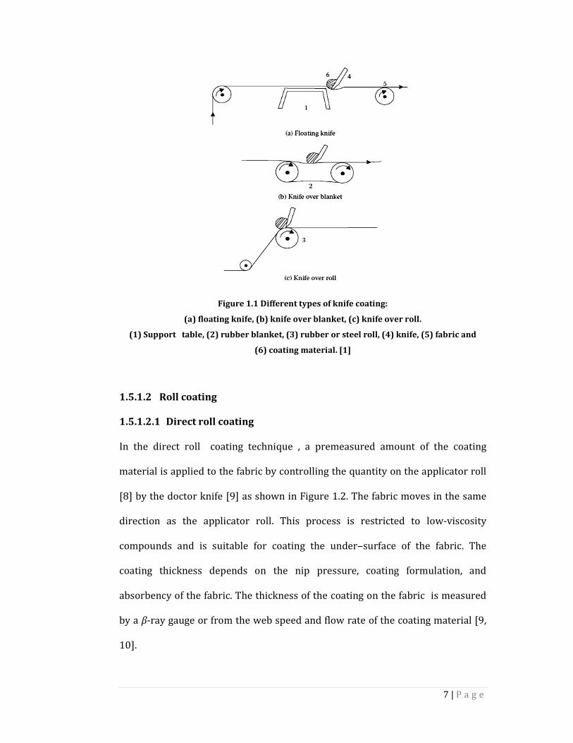
1.5.1.1 Knife coating

Knife coating is one of the oldest coating techniques and is also known as spread

coating. A dry, smooth fabric is fed over a bearer roll and under a knife, referred

to as a knife or doctor blade [6]. The coating material is poured in front of the

knife by a ladle or a pump over the entire width of the fabric [7]. As the fabric is

transported under the knife, the forward motion of the fabric and the fixed knife

barrier give the viscous mass of the coating material a rotatory motion [8]. This is

known as the rolling bank, which functions as a reservoir of the coating

compound in front of the knife. Two adjustable guards are used to prevent the

coating paste from spilling out from the edges of the fabric. Tension is applied on

the fabric to keep it tight under the knife. The majority of machines can coat

fabric widths up to 1.5 to 2.0 m, but specially designed machines can

accommodate widths up to 4 m. A coating material with adequate viscosity must

be used. The coated fabric then passes through a drying oven towards a winding

roll. The thickness of the coating is controlled by adjusting the gap between the

knife and the web [8]. Typical knife coating methods are shown in Figure 1.1.

7 | P a g e

Figure 1.1 Different types of knife coating:

(a) floating knife, (b) knife over blanket, (c) knife over roll.

(1) Support table, (2) rubber blanket, (3) rubber or steel roll, (4) knife, (5) fabric and

(6) coating material. [1]

1.5.1.2 Roll coating

1.5.1.2.1 Direct roll coating

In the direct roll coating technique , a premeasured amount of the coating

material is applied to the fabric by controlling the quantity on the applicator roll

[8] by the doctor knife [9] as shown in Figure 1.2. The fabric moves in the same

direction as the applicator roll. This process is restricted to low-viscosity

compounds and is suitable for coating the under‒surface of the fabric. The

coating thickness depends on the nip pressure, coating formulation, and

absorbency of the fabric. The thickness of the coating on the fabric is measured

by a β-ray gauge or from the web speed and flow rate of the coating material [9,

10].

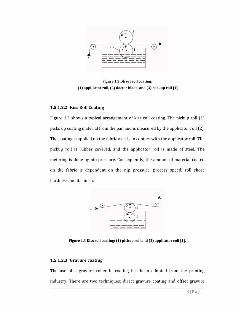
8 | P a g e

Figure 1.2 Direct roll coating:

(1) applicator roll, (2) doctor blade, and (3) backup roll [1]

1.5.1.2.2 Kiss Roll Coating

Figure 1.3 shows a typical arrangement of kiss roll coating. The pickup roll (1)

picks up coating material from the pan and is measured by the applicator roll (2).

The coating is applied on the fabric as it is in contact with the applicator roll. The

pickup roll is rubber covered, and the applicator roll is made of steel. The

metering is done by nip pressure. Consequently, the amount of material coated

on the fabric is dependent on the nip pressure, process speed, roll shore

hardness and its finish.

Figure 1.3 Kiss roll coating: (1) pickup roll and (2) applicator roll [1].

1.5.1.2.3 Gravure coating

The use of a gravure roller in coating has been adopted from the printing

industry. There are two techniques: direct gravure coating and offset gravure

9 | P a g e

coating. Engraved rollers are utilised in gravure coatings to coat a precise

amount of coating material on to the fabric. The amount of coating material is

usually controlled by the etched pattern and its fineness on the gravure roll.

There are a few standard patterns such as pyramid, quadrangular, and helical.

For lightweight coating, the pyramid pattern is mostly used. A direct gravure

coating method is shown in Figure 1.4. The coating material is picked up by the

gravure roll (1) and is transferred to the fabric as it passes between the nip of the

gravure roll and the backup roll (2) and then the coated fabric is passed between

smoothening rolls (4).

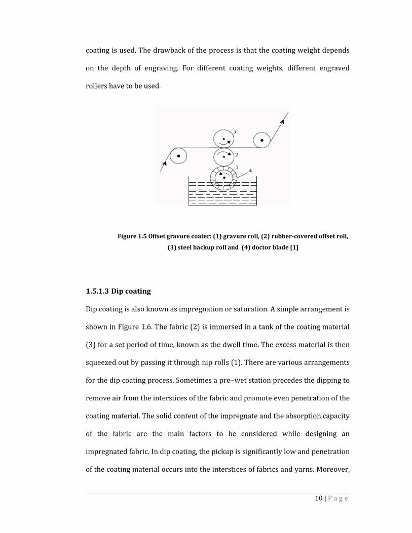
In an offset gravure coater (Figure 1.5), a steel backup roll (3) is added above the

direct gravure arrangement. The coating compound is first transferred onto an

offset roll (2) and then onto the fabric. The speed and direction of the gravure

and offset rollers can be varied independently. The arrangement is suitable for

extremely light coating (as low as 0.02 g/m2) and minimises the coating pattern.

This offset process can handle a higher-viscosity material (~10,000 cps) than can

the direct process. Hot-melt compounds are coated by heating the feed pan.

Generally for laminating adhesives or a top coat on a treated fabric, gravure

Figure 1.4 Direct Gravure coater: (1) gravure roll, (2) backup roll

(3) doctor blade, and (4) smoothening rolls [1]

10 | P a g e

coating is used. The drawback of the process is that the coating weight depends

on the depth of engraving. For different coating weights, different engraved

rollers have to be used.

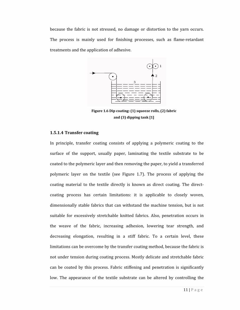
1.5.1.3 Dip coating

Dip coating is also known as impregnation or saturation. A simple arrangement is

shown in Figure 1.6. The fabric (2) is immersed in a tank of the coating material

(3) for a set period of time, known as the dwell time. The excess material is then

squeezed out by passing it through nip rolls (1). There are various arrangements

for the dip coating process. Sometimes a pre‒wet station precedes the dipping to

remove air from the interstices of the fabric and promote even penetration of the

coating material. The solid content of the impregnate and the absorption capacity

of the fabric are the main factors to be considered while designing an

impregnated fabric. In dip coating, the pickup is significantly low and penetration

of the coating material occurs into the interstices of fabrics and yarns. Moreover,

Figure 1.5 Offset gravure coater: (1) gravure roll, (2) rubber-covered offset roll,

(3) steel backup roll and (4) doctor blade [1]

11 | P a g e

because the fabric is not stressed, no damage or distortion to the yarn occurs.

The process is mainly used for finishing processes, such as flame-retardant

treatments and the application of adhesive.

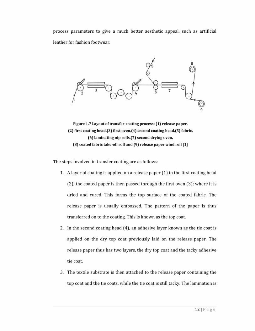
1.5.1.4 Transfer coating

In principle, transfer coating consists of applying a polymeric coating to the

surface of the support, usually paper, laminating the textile substrate to be

coated to the polymeric layer and then removing the paper, to yield a transferred

polymeric layer on the textile (see Figure 1.7). The process of applying the

coating material to the textile directly is known as direct coating. The direct-

coating process has certain limitations: it is applicable to closely woven,

dimensionally stable fabrics that can withstand the machine tension, but is not

suitable for excessively stretchable knitted fabrics. Also, penetration occurs in

the weave of the fabric, increasing adhesion, lowering tear strength, and

decreasing elongation, resulting in a stiff fabric. To a certain level, these

limitations can be overcome by the transfer coating method, because the fabric is

not under tension during coating process. Mostly delicate and stretchable fabric

can be coated by this process. Fabric stiffening and penetration is significantly

low. The appearance of the textile substrate can be altered by controlling the

Figure 1.6 Dip coating: (1) squeeze rolls, (2) fabric

and (3) dipping tank [1]

12 | P a g e

process parameters to give a much better aesthetic appeal, such as artificial

leather for fashion footwear.

The steps involved in transfer coating are as follows:

1. A layer of coating is applied on a release paper (1) in the first coating head

(2); the coated paper is then passed through the first oven (3); where it is

dried and cured. This forms the top surface of the coated fabric. The

release paper is usually embossed. The pattern of the paper is thus

transferred on to the coating. This is known as the top coat.

2. In the second coating head (4), an adhesive layer known as the tie coat is

applied on the dry top coat previously laid on the release paper. The

release paper thus has two layers, the dry top coat and the tacky adhesive

tie coat.

3. The textile substrate is then attached to the release paper containing the

top coat and the tie coats, while the tie coat is still tacky. The lamination is

Figure 1.7 Layout of transfer-coating process: (1) release paper,

(2) first coating head,(3) first oven,(4) second coating head,(5) fabric,

(6) laminating nip rolls,(7) second drying oven,

(8) coated fabric take-off roll and (9) release paper wind roll [1]

13 | P a g e

done by a set of nip rolls (6). The composite layer is then passed through

the second oven (7) to dry and cure the tie coat.

4. The release paper is finally stripped off, leaving the coated textile

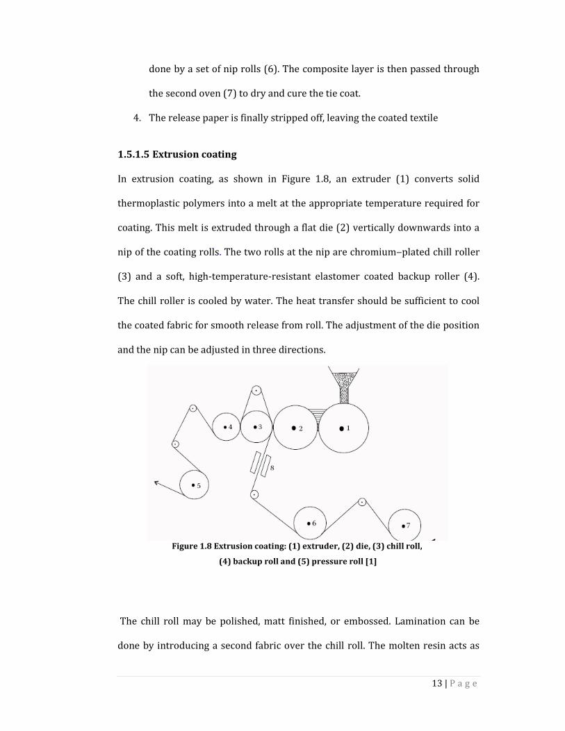
1.5.1.5 Extrusion coating

In extrusion coating, as shown in Figure 1.8, an extruder (1) converts solid

thermoplastic polymers into a melt at the appropriate temperature required for

coating. This melt is extruded through a flat die (2) vertically downwards into a

nip of the coating rolls. The two rolls at the nip are chromium‒plated chill roller

(3) and a soft, high-temperature-resistant elastomer coated backup roller (4).

The chill roller is cooled by water. The heat transfer should be sufficient to cool

the coated fabric for smooth release from roll. The adjustment of the die position

and the nip can be adjusted in three directions.

The chill roll may be polished, matt finished, or embossed. Lamination can be

done by introducing a second fabric over the chill roll. The molten resin acts as

Figure 1.8 Extrusion coating: (1) extruder, (2) die, (3) chill roll,

(4) backup roll and (5) pressure roll [1]

14 | P a g e

an adhesive. Extrusion coating is especially suitable for coating polyolefines on

different substrates. Because polyolefins can be brought down to low viscosity

without risk of decomposition, coating can be achieved at very high speed and

the process is highly economical. Regarding other polymeric coatings, including

poly vinyl chloride, polyurethane and butyl rubber, this process does not yield

uniform coating across the width, particularly at thicknesses below 0.5 mm [6] .

Conventional coating techniques have a few limitations:

• very fine coating (<0.2 mm) cannot be achieved by conventional coating

techniques

• a higher amount of coating material is required

• it is difficult to achieve uniform coating due to the fabric being under

tension during processing, which also leads to higher shrinkage of the

fabric after coating

• limited types of polymers can be used

• bulk properties of the fabric do not remain the same after coating

Due to the above disadvantages in conventional coating techniques there is a

need for modern coating techniques that have the ability to overcome these

disadvantages and achieve desired levels of coating on textile substrates.

15 | P a g e

Electrospinning 1.5.2

1.5.2.1 Introduction

The fabrication of synthetic fibres using electrostatic forces has been known for

more than one hundred years. The process of spinning fibres with electrostatic

forces is known as electrospinning. It has been shown recently that the

electrospinning process is capable of producing fibres in the submicron range

[11]. Due to the spinnability of a wide variety of polymeric fibres and consistency

in fibre production in the submicron range, electrospinning has gained much

attention.

In the fibre‒science‒related literature, fibres with diameters below 100 nm are

generally classified as nanofibres [12]. These fibres, with smaller pores and

higher surface area than regular fibres, have various applications in

nanocatalysis, tissue scaffolds, protective clothing, filtration and optical

electronics.

The electrospinning process uses a high‒voltage electric field to produce

electrically charged jets from a polymer solution or melts, which on drying by

means of evaporation of the solvent produces nanofibres. The highly charged

fibres are field directed towards the positively charged collector, which can be a

flat surface or rotating drum to collect the fibres. In standard spinning

techniques, the fibres are subjected to tensile, gravitational, aerodynamic,

rheological and inertial forces [13]. In electrospinning, tensile forces are created

in the axial direction of the flow of the polymer by the electric field to achieve the

spinning of the fibres.

16 | P a g e

1.5.2.2 History of electrospinning

The origin of electrospinning as a viable fibre spinning technique can be traced

back to the early 1930s. In 1934, Formhals patented his first invention relating to

the process and apparatus for producing artificial filaments using electric

charges [14]. Although the process of producing artificial threads using the

electric field had been experimented with for a long time, it had not gained

importance until Formhals’ invention due to some technical difficulties in earlier

spinning methods such as fibre drying and collection. Formhals used the spinning

drum to collect the fibres in a stretched condition and it was a movable drum.

This process was capable of producing threads which could be unwound

continuously. Formhals reported the spinning of cellulose acetate fibres using

acetone as the solvent [14].

Formhals’ first spinning method had some technical disadvantages. It was

difficult to dry the fibres after spinning due to the short distance between

spinning and collection zones, which resulted in a less aggregated web structure.

In a subsequent patent, Formhals refined his earlier approach to overcome the

aforementioned drawbacks [15]. In the refined process, the distance between the

feeding nozzle and the fibre‒collecting device was increased to give more drying

time for the electrospun fibres. Subsequently, in 1940, Formhals patented

another method for producing composite fibre webs from multiple polymer and

fibre substrates by electrostatically spinning polymer fibres on a moving base

substrate[16]. In the 1960s, fundamental studies on the jet forming process were

initiated by Taylor [17].

In 1969, Taylor studied the shape of the polymer droplet produced at the tip of

the needle when an electric field is applied and showed that it is a cone and the

17 | P a g e

jets are ejected from the vertices of the cone [17]. This conical shape of the jet

was later referred to by the researchers as the Taylor cone. By a detailed

examination of different viscous fluids, Taylor determined that an angle of 49.3

degrees is required to balance the surface tension of the polymer with the

electrostatic forces. The conical shape of the jet is important because it defines

the onset of the extensional velocity gradients in the fibre forming process [18].

In subsequent years, the focus shifted to studying the structural morphology of

nanofibres. To characterise structure of fibres and the relationship between the

structural features and process parameters, researchers used wide-angle x-ray

diffraction (WAXD), scanning electron microscopy (SEM), transmission electron

microscopy (TEM) and differential scanning calorimetry (DSC). In 1971,

Baumgarten reported the electrospinning of acrylic microfibres whose diameters

ranged from 500‒1100 nm [19]. Baumgarten determined the spinnability limits

of polyacrylonitrile/ dimethylformamide (PAN/DMF) solution and observed a

specific dependence of fibre diameter on the viscosity of the solution. He showed

that the diameter of the jet reached a minimum value after an initial increase in

the applied field and then became much larger with increasing electric fields.

Larrondo and Mandley produced polypropylene and polyethylene fibres from the

melt which were relatively larger in diameter than solvent spun fibres [20, 21].

They studied the relationship between the fibre diameters and melt temperature

and showed that the diameter decreased with increasing melt temperature.

According to them, fibre diameter reduced by 50% when the applied voltage

doubled, showing the significance of applied voltage on the fibre characteristics.

18 | P a g e

In 1987, Hayati et al. studied the effects of the electric field, experimental

conditions and the factors affecting fibre stability and atomisation. They

concluded that liquid conductivity plays a major role in the electrostatic

disruption of the liquid surfaces. Results showed that highly conducting fluids

with increasing applied voltage produced highly unstable streams that whipped

around in different directions. Relatively stable jets were produced with

semiconducting and insulating liquids such as paraffinic oil [22]. Results also

showed that unstable jets produced fibres with broader diameter distribution.

After a hiatus of a decade or so, a major upsurge in research on electrospinning

took place due to increased knowledge of the potential application of nanofibres

in other areas such as high efficiency filter media, catalyst substrates, protective

clothing and adsorbent materials. Research on nanofibres gained momentum due

to the work of Doshi and Reneker [11]. Doshi and Reneker studied the

characteristics of polyethylene oxide (PEO) nanofibres by varying the solution

concentration and applied electric potential [11]. Jet diameters were measured

as a function of distance from the apex of the cone, and they observed that the jet

diameter decreased with an increased in distance. They found that a PTO

solution with a viscosity less than 800 centipoise (cP) was too dilute to form a

stable jet and solutions with a viscosity more than 4000 cP were too thick to form

fibres.

Jaeger et al. studied the thinning of fibres as the extrusion progressed in PEO

water electrospun fibres and observed that the diameter of the flowing jet

decreased to 19 µm in travelling 1 cm from the orifice, 11 µm after travelling 2

cm and 9 µm after 3.5 cm [23]. Their experiment showed that solutions with

conductivities in the range of 1000‒1500 µs/cm heated up the jet due to the

19 | P a g e

electric current in the order of 1‒3 µA. Deitzel et al. showed that an increase in

the applied voltage changed the shape of the surface from which the jet

originated and the shape change has been correlated to the increase in the bead

defects [24]. They tried to control the deposition of fibres by using multiple field

electrospinning apparatus that provided an additional field of similar polarity on

the jets [25].

Warner et al. [26] and Moses et al. [27, 28] pursued rigorous work on the

evaluation of the fluid instabilities and experimental characterisation, which are

crucial for understanding of the electrospinning process. Shin et al. designed a

new apparatus that gave greater control over the experimental parameters in

order to enumerate the electrohydrodynamics of the process [29]. Spivak and

Dzenis showed that the Ostwaltde Waele power law could be applied to the

electrospinning process [30]. Gibson et al. studied the transport properties of

electrospun fibre mats, and they have concluded that nanofibre layers offer much

less resistance to moisture vapour diffusional transport [31]. Xin Wang et al.

produced hollow polyacrylonitrile (PAN)/Fe3O4 magnetic composite nanofibres

were fabricated through coaxial electrospinning[32]. Functionalised carbon

nanofibers (FCNF) coated with Ni-decorated MoS2 nanosheets were prepared by

Pinilla et al.[33].

20 | P a g e

1.5.2.3 Electrospinning theory and process

Electrospinning is a unique process to produce fine fibres using electrostatic

forces. Electrostatic precipitators and pesticide sprayers are some of the well-

known applications that work similar in a way to the electrospinning technique.

Fibre production using electrostatic forces has drawn attention due to its

potential to form fine fibres. Electrospun fibres have a small pore size and high

surface area. There is also evidence of sizable static charges in electrospun fibres

that could be effectively handled to produce three-dimensional structures [25].

Electrospinning is a process by which a polymer solution or melt can be spun

into small diameter fibres using a high potential electric field. This generic

description is appropriate as it covers a wide range of fibres with submicron

diameters that are normally produced by electrospinning. Based on earlier

research results, it is evident that the average diameter of electrospun fibres

ranges from 100 nm to 500 nm. In textile‒fibre‒science‒related scientific

literature, fibres with diameters in the range 100 nm to 500 nm are generally

referred to as nanofibres. The advantages of the electrospinning process are its

technical simplicity and its easy adaptability. A schematic of the electrospinning

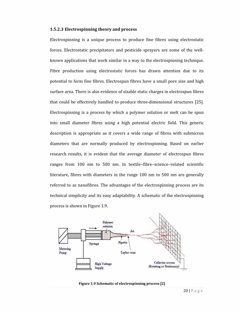
process is shown in Figure 1.9.

Figure 1.9 Schematic of electrospinning process [2]

21 | P a g e

Many previous researchers have used the similar apparatus with modifications,

depending on process conditions, to spin a wide variety of fine fibres. A polymer

solution is forced through a syringe pump to form a pendant drop of the polymer

at the tip of the nozzle. To induce free charges into the polymer solution a high

voltage potential is applied to the polymer solution inside the syringe through an

immersed electrode. These charged ions move in response to the applied electric

field towards the electrode of opposite polarity thereby transferring tensile

forces to the polymer liquid [13]. At the tip of the capillary, the pendant

hemispherical polymer drop takes a cone‒like projection in the presence of an

electric field. When the applied potential reaches a critical value required to

overcome the surface tension of the liquid, a jet of liquid is ejected from the cone

tip [17].

Most charge carriers in organic solvents and polymers have lower mobilities and

hence the charge will move through the liquid for large distances only if given

enough time. After the initiation from the cone, the jet undergoes a chaotic

motion or bending instability and is field directed towards the oppositely

charged collector, which collects the charged fibres [27]. As the jet travels

through the atmosphere, the solvent evaporates leaving behind a dry fibre on the

collecting device. For low viscosity solutions, the jet breaks up into droplets

while for high viscosity solutions it travels to the collector as fibre jets [34].

Electrospraying 1.5.3

Electrospraying is a method of generating a fine mist through electrostatic

charging. As the liquid passes through a nozzle, fine droplets are generated by

electrically charging the liquid to a very high voltage. The charged liquid in the

nozzle end charges up and forms a Taylor cone. Because the droplets are of the

22 | P a g e

same electrical charge, they repel each other very strongly. The liquid becomes

unstable due to more and more charge building up at the tip of the nozzle. When

the liquid can hold no more electrical charge, it disperses into numerous, micron-

sized, highly charged droplets at the tip of the nozzle (Figure 1.10). In general,

these tiny droplets are less than 10 μm in diameter and fly about searching for a

potential surface to land on that is opposite in charge to their own. As they fly

about, they shrink rapidly as solvent molecules evaporate from their surface [35].

Figure 1.10 Schematic illustration of electrospraying [35]

Figure 1.11 shows the difference between the electrospinning and

electrospraying technique. In electrospraying, the liquid flowing out of the

Figure 1.11 Electrospinning & electrospraying technique

23 | P a g e

capillary nozzle, which is maintained at high electric potential, is dispersed by

the electric field to be into fine droplets; instead of nanofibres in electrospinning.

Electrospraying systems have several advantages over mechanical atomisers.

The size of the electrosprayed droplets can range from micrometre to

nanometre. The size distribution of the droplets can be nearly monodisperse.

Droplet generation and droplet size can be controlled to some extent via the flow

rate of the liquid and the voltage at the capillary nozzle. The fact that the droplets

are electrically charged facilitates control of their motion (including their

deflection and focusing) by means of an electric field. Charged droplets are self-

dispersing in space, resulting in the absence of droplet coagulation. The

deposition efficiency of a charged spray on an object is higher than for an

uncharged spray. This feature can be advantageous, for example, in surface

coating, thin-film production and electroscrubbing. Electrospraying can be

widely applied to both industrial processes and scientific instrumentation [3].

The interest in industrial or laboratory applications has recently prompted the

search for new, more effective techniques which allow control of the droplet

production processes. Electrospraying has opened new routes to

nanotechnology. Electrospraying is used for micro- and nano-thin-film

deposition [36], micro- or nano-particle production, and micro- or nano-capsule

formation. Thin films and fine powders are (or potentially could be) used in

modern material technologies, microelectronics and medical technology.

Research in electro-microencapsulation and electro-emulsification is aimed at

developing new drug‒delivery systems, medicine production and ingredient

dosage in the cosmetic and food industries. Electrohydrodynamic spinning

(electrospinning) of viscous liquids facilitates the production of nanofibres for

24 | P a g e

masks, filters, scaffolds for biological tissue and intelligent garment

manufacturing [3].

This research work has studied the fundamentals of electrostatic spraying, and

the effect of various parameters on characteristics of electrospraying for the

deposition of polymer droplets at the submicron level on textile substrates.

25 | P a g e

Chapter 2

Literature review

2.1 Chapter summary

There is no significant research work conducted on electrospraying in the field of

textiles. As discussed in chapter 1, electrospinning and electrospraying are based

on the same principle so that research work carried out on the electrospinning

was useful during research on electrospraying, although some research workers

reported the work on electrospraying of liquids to produce dry nanoparticles in

powder form. This chapter throws light on the various attributes of

electrospinning and its effect on fibre characteristics. As electrospraying works

on the same fundamentals, the literature review helped to tune the process

parameters while doing the experiments.

2.2 Fundamentals of electrospraying

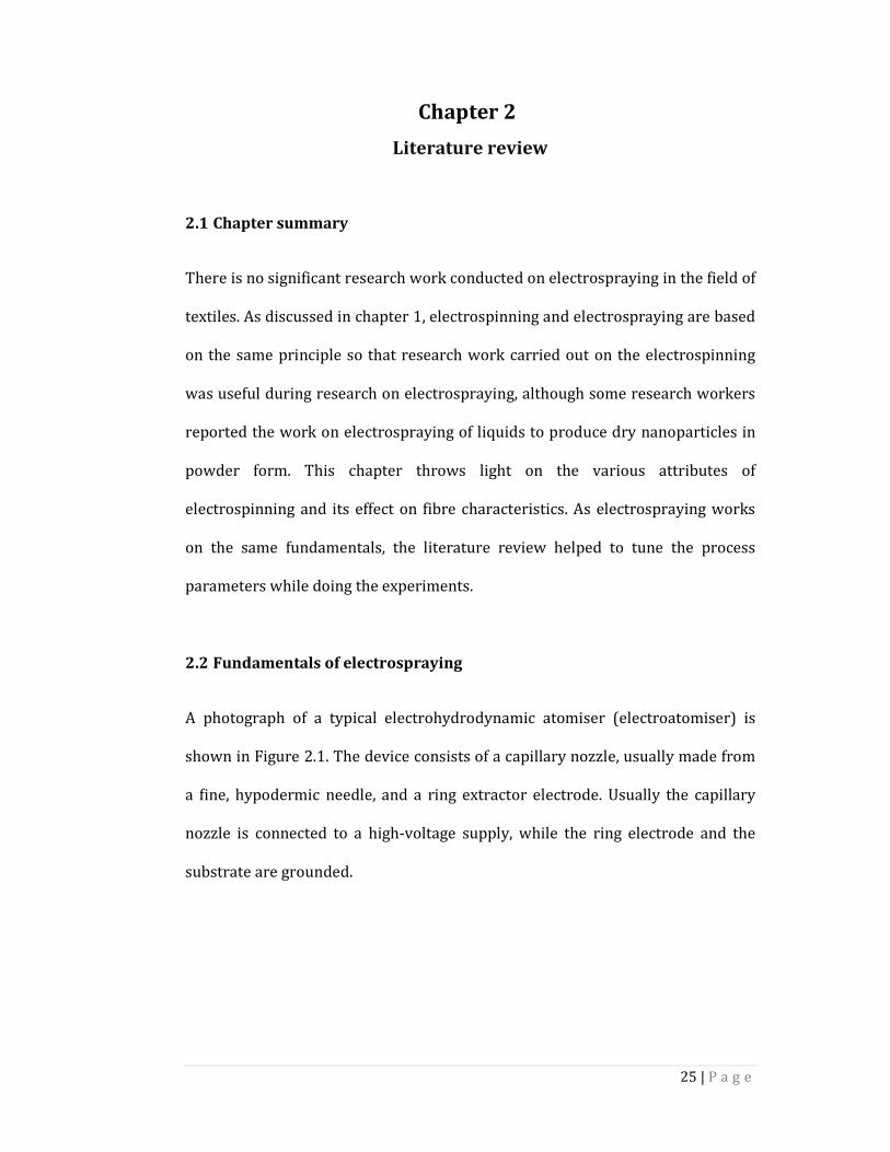
A photograph of a typical electrohydrodynamic atomiser (electroatomiser) is

shown in Figure 2.1. The device consists of a capillary nozzle, usually made from

a fine, hypodermic needle, and a ring extractor electrode. Usually the capillary

nozzle is connected to a high-voltage supply, while the ring electrode and the

substrate are grounded.

26 | P a g e

Figure 2.1 Electroatomizer [37]

In another configuration, the nozzle is grounded while the extractor electrode is

at high voltage. By this means, a strong electric field is built up at the capillary

outlet. Liquid flowing out from the nozzle forms a meniscus, which becomes

elongated in this electric field and disintegrates into droplets due to electrical

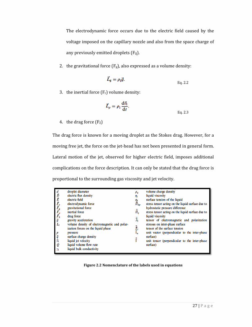
forces. There are two groups of forces which cause deformation and disruption of

the liquid jet (Fig. 2.3): bulk forces on the jet; and normal and tangential stresses

at the liquid surface. The bulk forces on the jet may be described as follows:

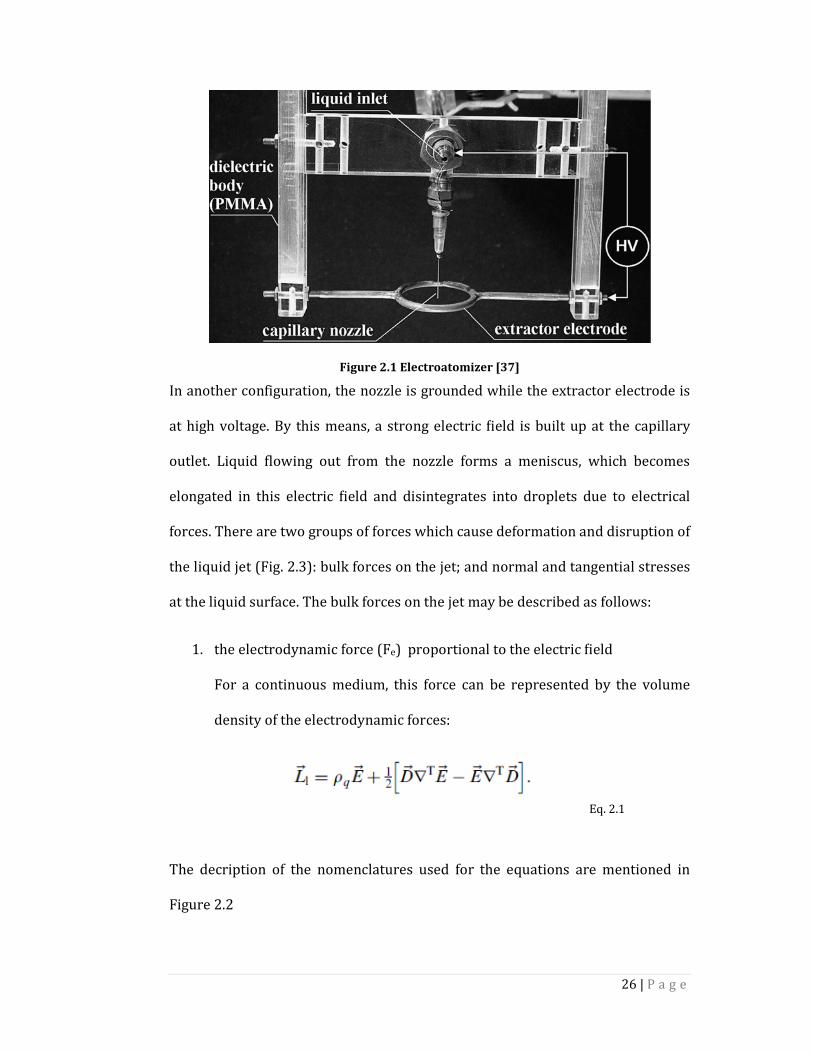
1. the electrodynamic force (Fe) proportional to the electric field

For a continuous medium, this force can be represented by the volume

density of the electrodynamic forces:

Eq. 2.1

The decription of the nomenclatures used for the equations are mentioned in

Figure 2.2

27 | P a g e

The electrodynamic force occurs due to the electric field caused by the

voltage imposed on the capillary nozzle and also from the space charge of

any previously emitted droplets (FQ).

2. the gravitational force (Fg), also expressed as a volume density:

Eq. 2.2

3. the inertial force (Fr) volume density:

Eq. 2.3

4. the drag force (FZ)

The drag force is known for a moving droplet as the Stokes drag. However, for a

moving free jet, the force on the jet-head has not been presented in general form.

Lateral motion of the jet, observed for higher electric field, imposes additional

complications on the force description. It can only be stated that the drag force is

proportional to the surrounding gas viscosity and jet velocity.

Figure 2.2 Nomenclature of the labels used in equations

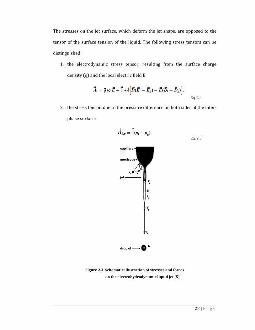
28 | P a g e

The stresses on the jet surface, which deform the jet shape, are opposed to the

tensor of the surface tension of the liquid. The following stress tensors can be

distinguished:

1. the electrodynamic stress tensor, resulting from the surface charge

density (q) and the local electric field E:

Eq. 2.4

2. the stress tensor, due to the pressure difference on both sides of the inter-

phase surface:

Eq. 2.5

Figure 2.3 Schematic illustration of stresses and forces

on the electrohydrodynamic liquid jet [5]

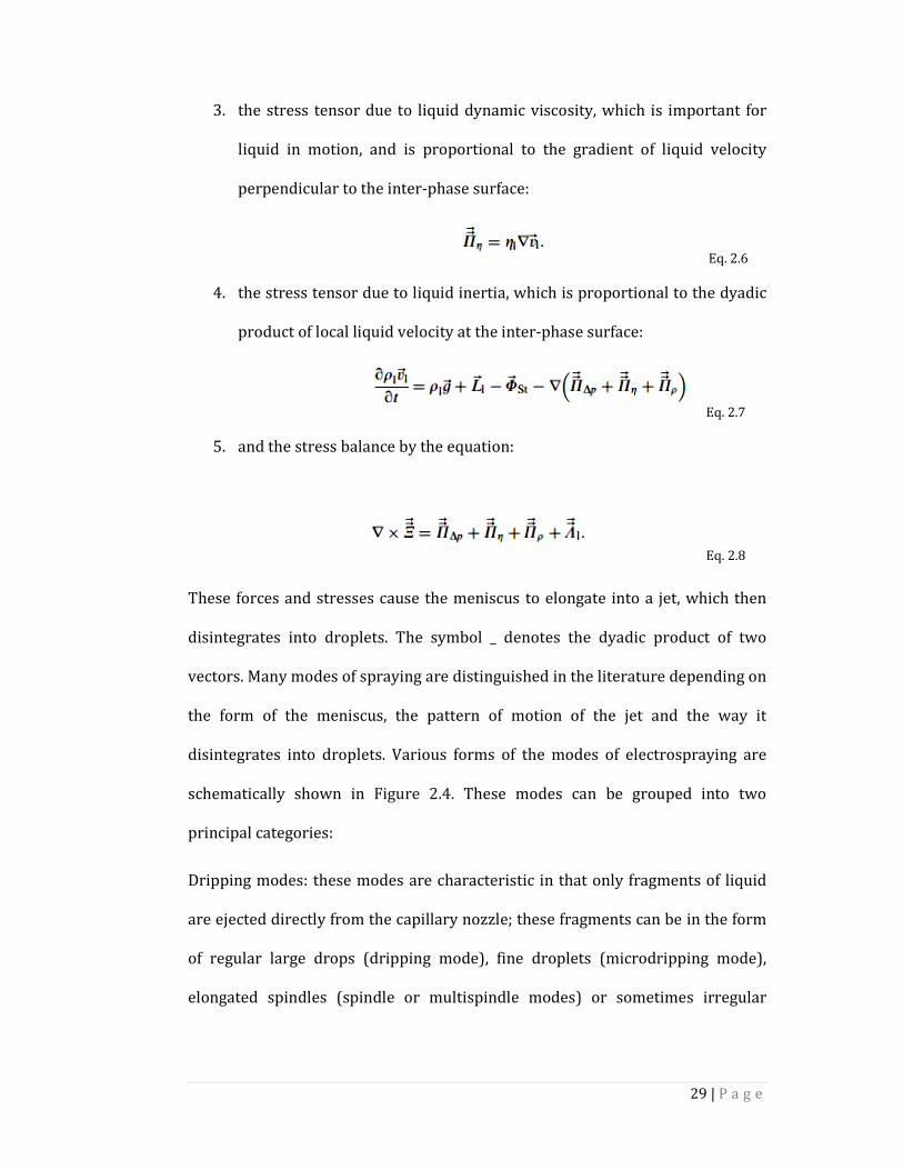
29 | P a g e

3. the stress tensor due to liquid dynamic viscosity, which is important for

liquid in motion, and is proportional to the gradient of liquid velocity

perpendicular to the inter-phase surface:

Eq. 2.6

4. the stress tensor due to liquid inertia, which is proportional to the dyadic

product of local liquid velocity at the inter-phase surface:

Eq. 2.7

5. and the stress balance by the equation:

Eq. 2.8

These forces and stresses cause the meniscus to elongate into a jet, which then

disintegrates into droplets. The symbol _ denotes the dyadic product of two

vectors. Many modes of spraying are distinguished in the literature depending on

the form of the meniscus, the pattern of motion of the jet and the way it

disintegrates into droplets. Various forms of the modes of electrospraying are

schematically shown in Figure 2.4. These modes can be grouped into two

principal categories:

Dripping modes: these modes are characteristic in that only fragments of liquid

are ejected directly from the capillary nozzle; these fragments can be in the form

of regular large drops (dripping mode), fine droplets (microdripping mode),

elongated spindles (spindle or multispindle modes) or sometimes irregular

30 | P a g e

fragments of liquid. At some distance from the nozzle outlet, however, these

fragments contract into spherical droplets.

Jet modes: in this case, the liquid is elongated into a long, fine jet, which can be

smooth and stable (cone-jet mode) or can move in any regular way. For example,

it may rotate around the capillary axis (precession mode) or oscillate in its plane

(oscillating mode). Sometimes, a few fine jets on the circumference of the

capillary can also be seen. This particular mode is known as the ‘multi-jet’ mode.

In each case, the jet disintegrates into droplets due to electrostatic forces.

Figure 2.4 Different modes in electrospraying [38]

The most important mode of spraying is the cone-jet mode. In this mode, the

liquid meniscus assumes the form of a regular, asymmetric cone with a thin jet

(100 mm in diameter) at its apex, stretching along the capillary axis. The end of

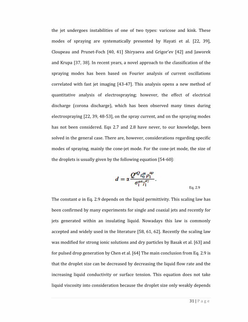
31 | P a g e

the jet undergoes instabilities of one of two types: varicose and kink. These

modes of spraying are systematically presented by Hayati et al. [22, 39],

Cloupeau and Prunet-Foch [40, 41] Shiryaeva and Grigor’ev [42] and Jaworek

and Krupa [37, 38]. In recent years, a novel approach to the classification of the

spraying modes has been based on Fourier analysis of current oscillations

correlated with fast jet imaging [43-47]. This analysis opens a new method of

quantitative analysis of electrospraying; however, the effect of electrical

discharge (corona discharge), which has been observed many times during

electrospraying [22, 39, 48-53], on the spray current, and on the spraying modes

has not been considered. Eqs 2.7 and 2.8 have never, to our knowledge, been

solved in the general case. There are, however, considerations regarding specific

modes of spraying, mainly the cone-jet mode. For the cone-jet mode, the size of

the droplets is usually given by the following equation [54-60]:

Eq. 2.9

The constant a in Eq. 2.9 depends on the liquid permittivity. This scaling law has

been confirmed by many experiments for single and coaxial jets and recently for

jets generated within an insulating liquid. Nowadays this law is commonly

accepted and widely used in the literature [58, 61, 62]. Recently the scaling law

was modified for strong ionic solutions and dry particles by Basak et al. [63] and

for pulsed drop generation by Chen et al. [64] The main conclusion from Eq. 2.9 is

that the droplet size can be decreased by decreasing the liquid flow rate and the

increasing liquid conductivity or surface tension. This equation does not take

liquid viscosity into consideration because the droplet size only weakly depends

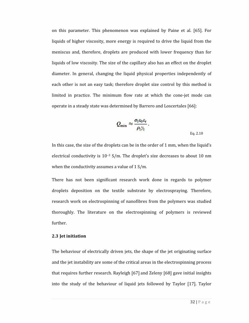
32 | P a g e

on this parameter. This phenomenon was explained by Paine et al. [65]. For

liquids of higher viscosity, more energy is required to drive the liquid from the

meniscus and, therefore, droplets are produced with lower frequency than for

liquids of low viscosity. The size of the capillary also has an effect on the droplet

diameter. In general, changing the liquid physical properties independently of

each other is not an easy task; therefore droplet size control by this method is

limited in practice. The minimum flow rate at which the cone-jet mode can

operate in a steady state was determined by Barrero and Loscertales [66]:

Eq. 2.10

In this case, the size of the droplets can be in the order of 1 mm, when the liquid’s

electrical conductivity is 10‒3 S/m. The droplet’s size decreases to about 10 nm

when the conductivity assumes a value of 1 S/m.

There has not been significant research work done in regards to polymer

droplets deposition on the textile substrate by electrospraying. Therefore,

research work on electrospinning of nanofibres from the polymers was studied

thoroughly. The literature on the electrospinning of polymers is reviewed

further.

2.3 Jet initiation

The behaviour of electrically driven jets, the shape of the jet originating surface

and the jet instability are some of the critical areas in the electrospinning process

that requires further research. Rayleigh [67] and Zeleny [68] gave initial insights

into the study of the behaviour of liquid jets followed by Taylor [17]. Taylor

33 | P a g e

showed that a conical shaped surface referred to as a Taylor cone, with an angle

of 49.3° is formed when a critical potential is reached to disturb the equilibrium

of the droplet at the tip of the capillary i.e. the initiating surface. When a high

potential is applied to the solution, electrical forces and the surface tension help

in creating a protrusion wherein the charges accumulate. The high charge per

unit area at the protrusion pulls the solution further to form a conical shape,

which on further increase in the potential initiates the electrospinning process by

jetting [13].

In a research study Yarin et al. have shown that the Taylor cone corresponds only

to a specific self-similar solution and there exists another shape corresponding to

nonself-similar solutions [69]. Taylor's work proposed a spheroidal

approximation of the initiating droplet shape, while Yarin et al. considered a

family of non‒self‒similar solutions for hyperboloidal shapes of electrified liquid

bodies and concluded that a cone sharper than the Taylor can precede the

initiation of the jet. It has been shown both experimentally and theoretically that

a liquid surface on application of a critical electric potential forms a conical shape

with an angle of 33.5° that is less than the typical Taylor cone angle of 49.3° [69].

The importance of the jet originating surface has been discussed by Cloupeau and

Prunet-Foch [40] and Grace and Marijnissen [70]. Different shapes of the jet

initiation have been associated with varying degrees of instability along the path

of the jet [28].

2.4 Jet instability

The jet ejected from the apex of the cone continues to thin down along the path of

its travel towards the collector and the jetting mode has been termed as the

34 | P a g e

electrohydrodynamic cone–jet [40]. The charges in the jet accelerate the polymer

solution in the direction of the electric field towards the collector thereby closing

the electrical circuit. The jet, while moving towards the collector undergoes a

chaotic motion or bending instability, as proposed by Yarin et al. due to the

repulsive forces originating from the charged ions within the electrospinning jet

[69]. The bending instability was originally thought to be occurring by a single jet

splitting into many thin fibre filaments due to radial charge repulsion, which was

termed splaying [11]. Doshi and Reneker argued that, due to the simultaneous

stretching of the jet and the evaporation of the solvent, the fibre diameter

decreases and therefore the increased charge density splits the jet into smaller

jets. This splitting is expected to occur repeatedly resulting in smaller diameter

fibres [11]. However, recent observations suggested that the rapid growth of a

non-axisymmetric or whipping instability causes the stretching and bending of

the jets [28]. Wamer et al. and Shin et al. used high-speed photography (with

exposure times down to 1 millisecond) to confirm that the unstable region of the

jet appears as an inverted cone, suggesting multiple splitting is in reality a single

rapidly whipping jet [26, 28]. They suggested that the whipping phenomena

occur so fast that the jet appears to be splitting into smaller fibre jets resulting in

ultra-fine fibres. A steady state model of the jets using nonlinear power law

constitutive equations (Oswald-deWaele model [71, 72]) was developed by

Spivak et al [73].

Reneker and his co-workers have contributed significantly to understanding of

the instability behaviour and developed a mathematical visco‒elastic model for

the rectilinear electrified jet. In their work, they mathematically modelled the jet

path, trajectory and velocity of the jet, area reduction ratio and longitudinal

35 | P a g e

strain of the jets [74]. They observed the onset of jetting instability from the

vertex of the envelope cone by imaging with a lens of focal length 86 mm and T

number 1.0. The image produced by this lens was observed on an electronic

camera with exposure time of 0.0125 ms and recording speed of 2000

frames/sec [74]. According to Reneker et al. a smooth surface with a slight

curvature suddenly develops an array of bends; on elongation the array of bends

becomes a series of spiralling loops with growing diameters and, as the

perimeter of the loop increases, the jets forming the loop start thinning. They

inferred that many cycles of instability repeat to form nanofibres [74].

Shin et al. [29], in their attempt to model the instability behaviour of electrically

forced jets, stressed the competition between different types of instabilities that

could occur due to the interactions between the charged ions and the electric

field. These instabilities were shown to vary along the path depending on the

fluid parameters and the operating conditions. Their work showcased the

possibility of three types of instabilities: (1) the classical Rayleigh mode

(asymmetric) instability; (2) the electric‒ field‒induced asymmetric conducting

mode; and (3) the whipping conducting mode instabilities. In order to have a

better understanding of the different instability modes, it is necessary to precise

modelling of the process. Shin et al. presented an approach to model the stability

of the jets as a function of fluid properties like viscosity and conductivity and

process variables like applied electric field and flow rate. They observed that the

whipping mode instability is dominant with high charge density in the jets, while

the asymmetric instability dominates at lower charge density.

36 | P a g e

The physical mechanisms of the instability and the development of asymptotic

approximations for modelling the instability behaviour were discussed

elsewhere in detail. Fridrikh et al. [75] re-examined the equations of motion

derived earlier for creating a model to derive the ultimate diameter of the jets by

accounting for the nonlinear instability of the jets at the final stage of whipping.

Their model assumed the charged fluid jet as Newtonian fluid and an empirical

model of the terminal diameter of the whipping jet was derived as a function of

flow rate, electric current and surface tension of the fluid. The model predicted

10‒fold variations in fibre diameter for varying flow rates and this 2/3 scaling

was experimentally verified for varying concentrations of polycaprolactone

(PCL) solution.

The production of nanofibres by the electrospinning process is influenced by

both the electrostatic forces and the viscoelastic behaviour of the polymer.

Process parameters like solution feed rate applied voltage, nozzle-collector

distance and spinning environment and material properties like solution

concentration, viscosity, surface tension, conductivity and solvent vapour

pressure affect the electrospraying.

2.5 Effect of process parameters in electrospinning

A detailed account is provided of the previous works dealing with the effects of

individual process parameters that influence the structure and morphology of

nanofibres.

2.5.1 Applied voltage

Various instability modes that occur during the fibre‒forming process are

expected to occur by the combined effect of both the electrostatic field and the

37 | P a g e

material properties of the polymer. It has been suggested that the onset of

different modes of instabilities in the electrospinning process depends on the

shape of the jet‒initiating surface and the degree of instability which efficiently

produces changes in the fibre morphology. In electrospinning, the charge

transport due to the applied voltage is mainly due to the flow of the polymer jet

towards the collector, and the increase or decrease in the current is attributed to

the mass flow of the polymer from the nozzle tip. Deitzel et al. have inferred that

the change in the spinning current is related to the change in the instability mode

[24]. They experimentally showed that an increase in applied voltage causes a

change in the shape of the jet‒initiating point and therefore the structure and

morphology of the fibres. Experimentation on the PEO/water system has shown

an increase in the spinning current with an increase in the voltage. It was also

observed that, for the PEO/water system, the fibre morphology changed from

defect‒free fibres at an initiating voltage of 5.5kV to a highly beaded structure at

a voltage of 9.0kV [24]. The occurrence of beaded morphology has been

correlated with a steep increase in the spinning current, which controls the bead

formation in the electrospinning process. Beaded structure reduces the surface

area, which ultimately influences the filtration abilities of nanofibres. Earlier in

1971, Baumgarten while carrying out experiments with acrylic fibres observed

an increase in the fibre length of approximately twice with small changes in fibre

diameter with an increase in applied voltage [19]. Megelski et al. investigated the

voltage dependence on the fibre diameter using polystyrene (PS). The PS fibre

size decreased from about 20 µm to l0 µm with an increase in voltage from 5kV

to 12kV; while there was no significant change observed in the pore size

distribution [76]. These results concur with the interpretation of Buchko et al.

38 | P a g e

[18], who observed a decrease in the fibre diameter with an increase in the

applied field while spinning silk‒like polymer fibre (SLPF) with fibronectin

functionality. Generally, it has been accepted that an increase in the applied

voltage increases the deposition rate due to higher mass flow from the needle tip.

Jaeger et al. used a two-electrode setup for electrospinning by introducing a ring

electrode between the nozzle and the collector [23]. The ring electrode was set at

the same potential as the electrode immersed in the polymer solution. This setup

was thought to produce a field-free space at the nozzle tip to avoid changes in the

shape of the jet initiating surface due to varied potential [23]. Although this setup

reduces the unstable jet behaviour at the initiation stage, bending instability is

still dominant at later stages of the process, causing an uneven chaotic motion of

the jet before depositing itself as a nonwoven matrix on the collector. Deitzel et

al. experimented with a new electrospinning apparatus by introducing eight

copper rings in a series between the nozzle and the collector for dampening the

bending instability [24]. The nozzle and the ring set were subjected to different

potentials (the ring set at a lower potential) of positive polarity while the

collector was subjected to a negative polarity. The idea behind this setup was to

change the shape of the macroscopic electric field from the jet initiation to the

collection target in such a way that the field lines converge to a centre line above

the collection target, caused by the applied potential to the ring electrodes. The

authors suggested that the bending instability of the fibres was dampened by the

effect of the converging field lines producing straight jets [25]. Controlled

deposition helps to produce specific deposition patterns and also yarn like fibres.

Deitzel et al. investigated the spinning of PEO in aqueous solution using multiple

electric fields, which resulted in fibres depositing over a reduced area due to the

39 | P a g e

dampening of bending instability. The multiple field technique was also shown to

produce fibres of lesser diameter than the traditional electrospinning method

[24].

2.5.2 Nozzle-collector distance

The structure and morphology of electrospun fibres could be easily affected by

the nozzle to collector distance because of their dependence on the deposition

time, evaporation rate and whipping or instability interval. Buchko et al.

examined the morphological changes in SLPF and nylon electrospun fibres with

variations in the distance between the nozzle and the collector screen. They

showed that, regardless of the concentration of the solution, lesser nozzle-

collector distance produced wet fibres and beaded structures. SLPF fibre

morphology changed from round to flat with a decrease in the nozzle collector

distance from 2 cm to 0.5 cm [18]. This result delineates the effect of the nozzle

collector distance on the fibre morphology. The work also showed that aqueous

polymer solutions require more distance for dry fibre formation than systems

that use highly volatile organic solvents. Megelski et al. observed the bead

formation in the electrospun PS fibres on reducing the nozzle‒collector distance

while preserving the ribbon shaped morphology with a reduction in the nozzle‒

collector distance [76].

2.5.3 Polymer flow rate

The flow rate of the polymer from the syringe is an important process parameter

as it influences the jet velocity and the material transfer rate. In the case of PS

fibres, Megelski et al. observed that the fibre diameter and the pore diameter

increased with an increase in the polymer flow rate [76]. As the flow rate

40 | P a g e

increased, fibres had pronounced beaded morphologies and the mean pore size

increased from 90 to 150 nm.

2.5.4 Spinning environment

The environmental conditions around the spinneret like the surrounding air, its

relative humidity (RH), vacuum conditions, surrounding gas etc. could influence

the fibre structure and morphology of electrospun fibres. Baumgarden observed

that acrylic fibres spun in an atmosphere of relative humidity more than 60% do

not dry properly and get entangled on the surface of the collector. The

breakdown voltage of the atmospheric gases is said to affect the charge‒retaining

capacity of the fibres [19]. Srinivasarao et al. proposed a new mechanism for

pore formation by evaporative cooling called breathe figures [77]. Breathe

figures occur on the fibre surfaces due to the imprints of condensed moisture

droplets caused by the evaporative cooling of moisture in the air surrounding the

spinneret. Megelski et al. investigated the pore characteristics of the PS fibres at

varied RH and emphasised the importance of phase separation mechanisms in

explaining the pore formation of electrospun fibres [77].

2.6 Effect of solution parameters

2.6.1 Solution concentration

Solution concentration decides the limiting boundaries for the formation of

electrospun fibres due to variations in the viscosity and surface tension [24].

Low‒concentration solution forms droplets due to the influence of surface

tension, while higher concentrations prohibit the fibre formation due to higher

viscosity. Previously published literature has documented the difficulties in

electrospinning polymers like poly-ethylene-oxide (PEO), poly-acrylonitrial

41 | P a g e

(PAN), poly-d-lactic acid (PDLA) [78] at certain concentration levels. By

increasing the concentration of polystyrene solution, the fibre diameter

increased and the pore size reduced to a narrow distribution [76]. In the case of

the PEO/water system, a bimodal distribution in fibre diameter was observed at

higher concentrations. In the PEO system, Dietzel et al. related the average fibre

diameter and the solution concentration by a power law relationship [25]. They

interpreted the variations in the fibre diameter and morphology as due to the

shape of the jet-originating surface, which concurred with the observations of

Zong et al. [78], undulating morphologies in fibres were attributed to the delayed

drying and the stress‒relaxation behaviour of the fibres at lower concentrations.

As is apparent from the discussion, the concentration of the polymer solution

influences the spinning of fibres and controls the fibre structure and morphology.

2.6.2 Solution conductivity

Polymers are mostly conductive, with a few exceptions among dielectric

materials and the charged ions in the polymer solution are highly influential in

jet formation. The ions increase the charge‒carrying capacity of the jet, thereby

subjecting it to higher tension with the applied electric field. Baumgarden

showed that the jet radius varied inversely as the cube root of the electrical

conductivity of the solution [19]. Zong et al. demonstrated the effect of ions by

the addition of ionic salt on the morphology and diameter of electrospun fibres

[78]. They found that PDIA fibres with the addition of ionic salts like KH2PO4,

NaH:P04 and NaCM produced headless fibres with relatively smaller diameters

ranging from 200 to 1000 nm.

42 | P a g e

2.6.3 Volatility of solvent

As electrospinning involves rapid solvent evaporation and phase separation due

to jet thinning, solvent vapour pressure critically determines the evaporation

rate and the drying time. Solvent volatility plays a major role in the formation of

nanostructures by influencing the phase separation process. Bognitzki et al.

found that the use of highly volatile solvents like dichloromethane yielded PLLA

fibres with pore sizes of l00 nm in width and 250nm in length along the fibre axis

[79]. Lee et al. evaluated the effect of volume ratio of the solvent on the fibre

diameter and morphology of electrospun PVC fibres [80]. Average fibre

diameters decreased with an increase in the amount of DMF in the THF/DMF

mixed solvent. Lee et al. found the electrolytic nature of the solvent to be an

important parameter in electrospinning [80]. Megelski et al. studied the

characteristics of electrospun fibres with respect to the physical properties of

solvents. The impact of vapour pressure was evident when PS fibres spun with

different THF/DMF combinations resulted in micro‒ and nanostructure

morphologies at higher solvent volatility and much diminished micro‒structures

at lower volatility [76].

2.7 Applications of electrospraying in other fields

Charged droplet sprays found application in the fields other than textiles such as

automotive painting or thin film deposition. Alternburg et al reported the

physical and chemical methods for thin and thick films deposition from gaseous,

solution, molten or solid states, but minor attention was given to electrospraying

[81]. Further Choy et al. reviewed the potential development of the chemical

43 | P a g e

vapour deposition process and its application to film deposition with a brief

discussion of electrospraying[82].

2.7.1 Thin solid film deposition

Thin solid films are used to improve the surface properties of mechanical

elements and scientific instruments [83]. Electrostatic deposition is the process

of depositing material on a substrate by electrical forces. Initially,

electrospraying was used to produce radioactive materials such as α and β

particle sources, or targets prepared for activation in particle accelerators or

nuclear reactors. Recently electrospraying being used for thin film deposition in

nanoelectronics. Its use in the textile field is still unexplored.

Electrospraying has been applied for painting, the production of pharmaceutical

and the production of foods. For example, nanocapsules and controlled drug

release were produced with electrospraying [84]. Other applications are for

nano-particle production [85], ionisation and characterisation of protein and

DNA in mass spectrometry, and respiratory drug delivery [86, 87].

2.7.1.1 Solar cells

Since the late 1990s, the electrospraying has been used for the production of

solar cells from TiO2, CdS and CdSe [88], or SnO2 [89]. Films produced by

electrospraying are homogeneous and composed of agglomerates built of

particles smaller than 1 µm, which are the dry powder particles used for

preparing a suspension. The structure and optical properties of CdSe films

depend on the temperature and deposition method. For electrospraying, CdSe

starts to crystallise at the substrate temperature of 300˚C, and the number of

crystals increases rapidly above 400˚C [90].

44 | P a g e

CdS and ZnS films are highly oriented in the electric field, but no preferred

orientation has been observed for CdSe films. Due to the grain orientation of CdS

and ZnS films in the electric field during precursors’ transformation to

nanocrystals, they have good optical and opto-electrical properties for solar cell

applications [91].

2.7.1.2 Lithium batteries:

Van Zomeren et al. were probably the first who used electrospraying to produce

electrodes for alkaline batteries [92]. The spraying system operates in the cone-

jet mode, generating droplets of a mean diameter of 4 µm. The film prepared by

this method is of low porosity, with crystallites of average size of 0.3 µm. Interest

in the production of electrodes for lithium microbatteries by ESD deposition has

grown in recent years. The demand for production of microbatteries is an effect

of the miniaturisation of electronic devices and the reduction of their power

consumption.

2.7.1.3 Micro and nano‒electronic devices

ZnO exhibits semiconducting, photoconductive and piezoelectric properties, and,

therefore, has found many applications in various fields of electronics, for

transducers or sensors manufacturing [93]. MgO is used in plasma displays as a

surface protection layer, as a buffer layer for high‒temperature superconductor

deposition and as with ovskite-type ferroelectric films [94, 95], PbTiO3 [96] and

BaZrO3 [97] are deposited on a substrate as piezoelectric materials in sensors

and microactuators. Ryu and Kim [94]reported that the ZnO film deposited on a

silicon wafer at a temperature ranging from 230 to 450°C was composed of

45 | P a g e

crystallites of a mean size of about 20 nm that were uniform, densely packed,

pinhole-free and predominantly c‒axis‒oriented.

2.7.1.4 Biotechnology

In biotechnology, electrospraying was used, for example, to deposit biomolecules

on a substrate for further studying them under a microscope or for medical

diagnostics. Moerman et al [98, 99] produced arrays of identical spots of 130–

350 µm in diameter consisting of biologically active substances, such as enzymes

or antibodies, for use in medical diagnosis, environmental research and

combinatorial chemistry.

2.7.1.5 The food industry

In foods, electrospraying has been evaluated to apply chocolate [100], smoke

flavour to meat, polishing and coating agent on sugar, confectionary and

chocolate products [101], flavour application on snacks and cocoa butter

microcapsules [102]. Further, lipid is sometimes used as a sticking agent for solid

ingredients.

2.7.1.6 Other applications:

Solid lubricating films of MoS2 were obtained by electrospraying of MoS2

dissolved in isopropanol, acetone, alcohol or toluene [103-105]. In this process,

the solvent evaporated when the droplets flow to a grounded substrate, and only

solid nanoparticles are deposited onto it. The film is composed of fine flat

particles about 120 nm thick and with a diameter up to 1000 nm. The film

thickness is between 0.28 and 1 µm. A cobaltite (NiCo2O4) electrocatalyst for

oxygen reduction has been fabricated by electrospraying from nickel and cobalt

46 | P a g e

nitrates by Lapham et al. [106]. Jayasinghe and Edirisinghe studied alumina

suspension in ethanol for the design of electrostatic printing on solid surfaces

[107].

2.8 Advantages of electrospraying coating technique

The electrospraying has the following advantages over conventional mechanical

spraying methods:

1. Droplet size is smaller than that available from conventional mechanical

atomisers and can be smaller than 1 mm.

2. The size distribution of the droplets is usually narrow, with a small

standard deviation that allows production of particles of nearly uniform

size.

3. The charged droplets are self-dispersing in space (due to their mutual

repulsion), resulting also in the absence of droplet coagulation.

4. The motion of the charged droplets can be easily controlled (including

deflection or focusing) by electric fields.

5. The deposition efficiency of a charged spray on an object is order of

magnitudes higher than for un-charged droplets.

These characteristics make electrospraying a versatile tool for micro- and nano-

thin-film deposition, or micro- and nano-particle production. From the reviewed

literature, it can be concluded that electrospraying facilitates the production of

extremely thin layers, which can be crack-free and more homogeneous than

those obtained by other methods. Therefore an attempt has been made to study

the electrospraying technique for polymer droplet deposition on textile

substrates.

47 | P a g e

Chapter 3

Materials and methods

3.1 Introduction

This chapter deals with the materials and equipment used and the processing

parameters applied in the electrospraying experiments. It also includes the

equipment and test conditions used for the characterisation of the polymer

droplets. The characterisation techniques include scanning electron microscopy

(SEM); optical microscopy (OM); energy dispersive spectroscopy (EDS); Fourier

transform infrared (FTIR) and mechanical characterisation. This also includes

image analysis tools like MATLAB® and DesignExpert® for empirical modelling.

Static contact angle and antimicrobial property analysis was performed to

understand the enhancement of the functionality of coated substrates. In

addition, moisture management testing of the samples was evaluated. The

specific methods followed are described in detail in experimental section of

respective chapters.

3.2 Materials

Thermoplastic polyurethane 3.2.1

Generally in coating of textiles, polyurethanes are widely used as a coating

polymer. Polyurethanes belong to a group of very durable plastic materials. The

main property of polyurethane is its wide application. It can be coated to textiles,

leather, in solution, dispersion, with a low solvent content or without it, as

granules or powder. Softness or hardness can be obtained by varying polymer

structures. Polyurethane has good washproofness and cleaning resistance, good

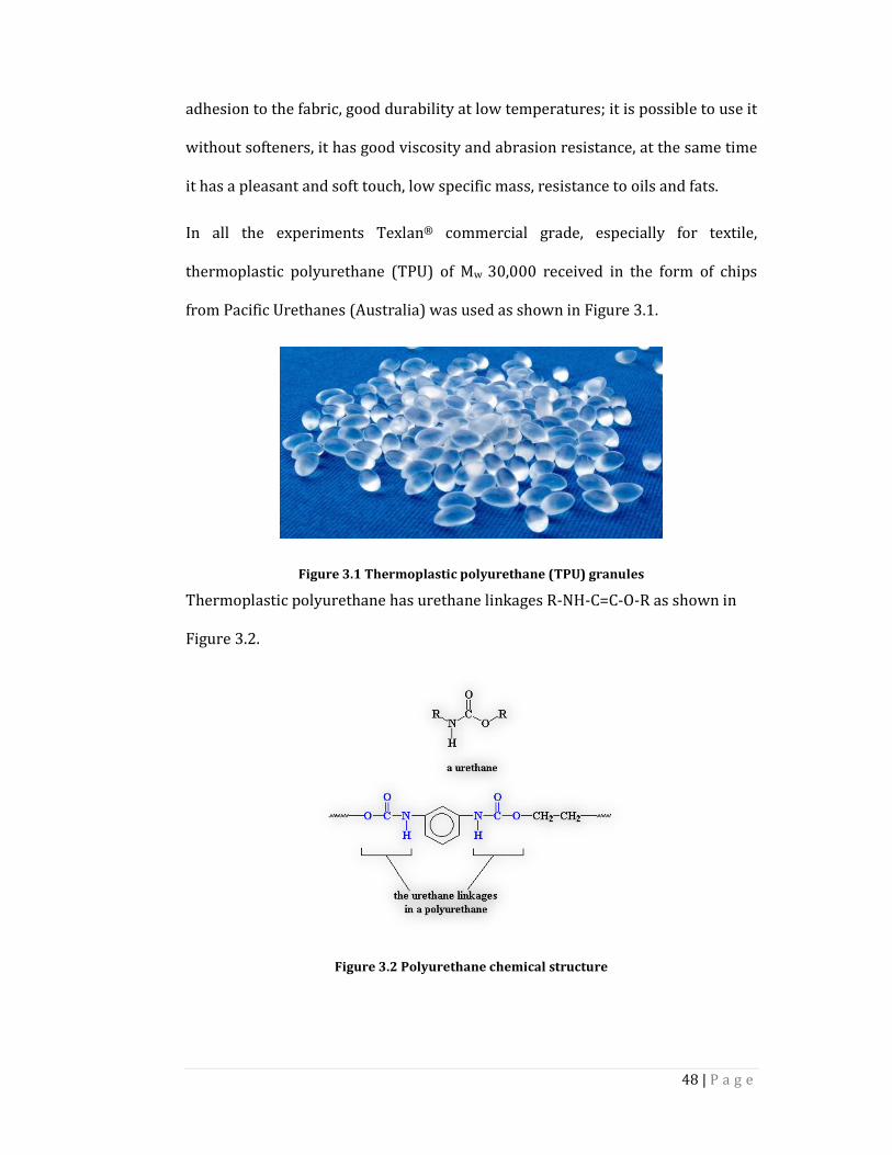
48 | P a g e

adhesion to the fabric, good durability at low temperatures; it is possible to use it

without softeners, it has good viscosity and abrasion resistance, at the same time

it has a pleasant and soft touch, low specific mass, resistance to oils and fats.

In all the experiments Texlan® commercial grade, especially for textile,

thermoplastic polyurethane (TPU) of Mw 30,000 received in the form of chips

from Pacific Urethanes (Australia) was used as shown in Figure 3.1.

Figure 3.1 Thermoplastic polyurethane (TPU) granules

Thermoplastic polyurethane has urethane linkages R-NH-C=C-O-R as shown in

Figure 3.2.

Figure 3.2 Polyurethane chemical structure

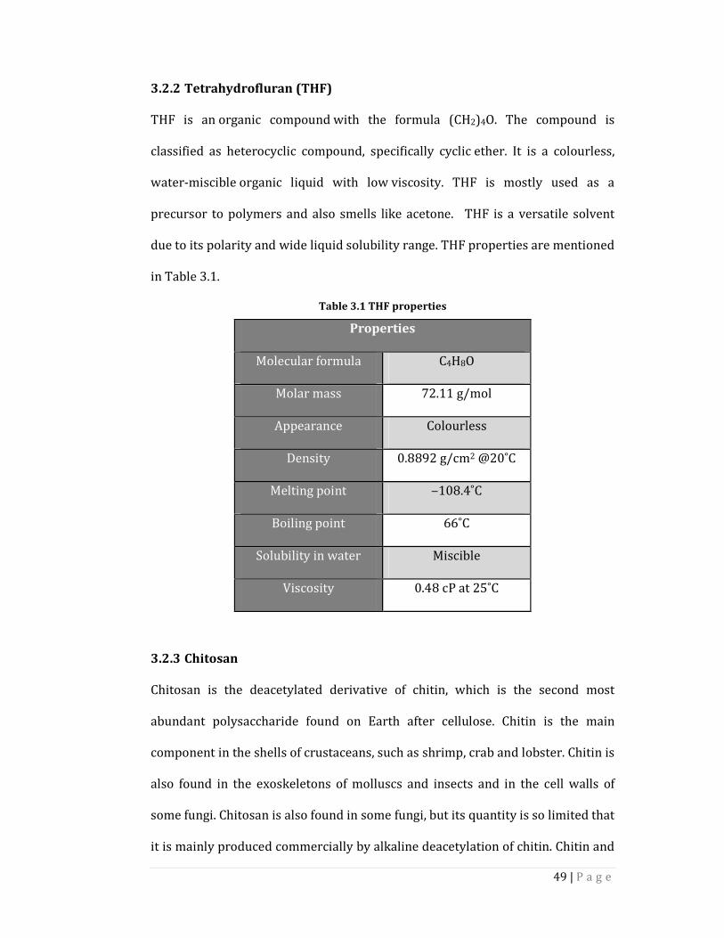
49 | P a g e

Tetrahydrofluran (THF) 3.2.2

THF is an organic compound with the formula (CH2)4O. The compound is

classified as heterocyclic compound, specifically cyclic ether. It is a colourless,

water-miscible organic liquid with low viscosity. THF is mostly used as a

precursor to polymers and also smells like acetone. THF is a versatile solvent

due to its polarity and wide liquid solubility range. THF properties are mentioned

in Table 3.1.

Table 3.1 THF properties

Properties

Molecular formula C4H8O

Molar mass 72.11 g/mol

Appearance Colourless

Density 0.8892 g/cm2 @20˚C

Melting point ‒108.4˚C

Boiling point 66˚C

Solubility in water Miscible

Viscosity 0.48 cP at 25˚C

Chitosan 3.2.3

Chitosan is the deacetylated derivative of chitin, which is the second most

abundant polysaccharide found on Earth after cellulose. Chitin is the main

component in the shells of crustaceans, such as shrimp, crab and lobster. Chitin is

also found in the exoskeletons of molluscs and insects and in the cell walls of

some fungi. Chitosan is also found in some fungi, but its quantity is so limited that

it is mainly produced commercially by alkaline deacetylation of chitin. Chitin and

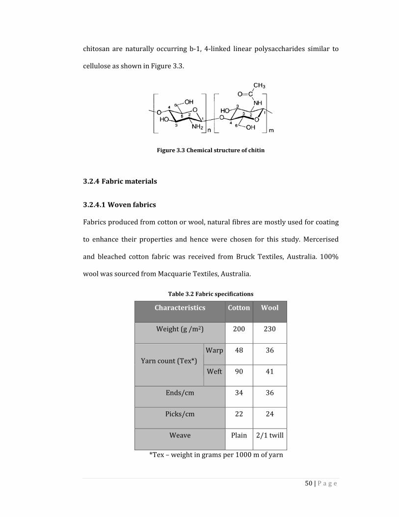
50 | P a g e

chitosan are naturally occurring b-1, 4-linked linear polysaccharides similar to

cellulose as shown in Figure 3.3.

Figure 3.3 Chemical structure of chitin

Fabric materials 3.2.4

3.2.4.1 Woven fabrics

Fabrics produced from cotton or wool, natural fibres are mostly used for coating

to enhance their properties and hence were chosen for this study. Mercerised

and bleached cotton fabric was received from Bruck Textiles, Australia. 100%

wool was sourced from Macquarie Textiles, Australia.

Table 3.2 Fabric specifications

Characteristics Cotton Wool

Weight (g /m2) 200 230

Yarn count (Tex*)

Warp 48 36

Weft 90 41

Ends/cm 34 36

Picks/cm 22 24

Weave Plain 2/1 twill

*Tex – weight in grams per 1000 m of yarn

51 | P a g e

Both fabrics were used as received without any further chemical treatments. The

fabric specifications are given in Table 3.2.

3.2.4.2 Nonwoven fabric

Wool nonwoven fabric was prepared using an integrated card–cross–lapper and

subsequent needle–punching. A SCG-600-60 model integrated card-crosslapper

from SHIN CHIANG Machinery Pty Ltd was used to prepare laps of 100% wool.

The prepared lap was subsequently needle–punched using SNP-50M-6, make

SHOOU SHYNG MACHINERY CO., LTD., It was a down-stroke needle–punching

machine. The machine process parameters and fabric specifications are given in

Table 3.3.

Table 3.3 Needle–punched machine process parameters

Parameters Values

Working area 500 mm X 296 mm

Needle type R22G3027

Needle penetration 11 mm

Strokes/min 400

Forward move step 1.80

Fabric thickness 10 mm

Fabric weight 400 g/m2

3.3 Methods

Polymer solution preparation 3.3.1

Polymer solutions were prepared by dissolving the TPU polymer granules in THF

solvent with constant stirring for 2 hrs. The Solution viscosity was measured

with a Brookfeild rheometer (USA) and solution conductivity was measured with

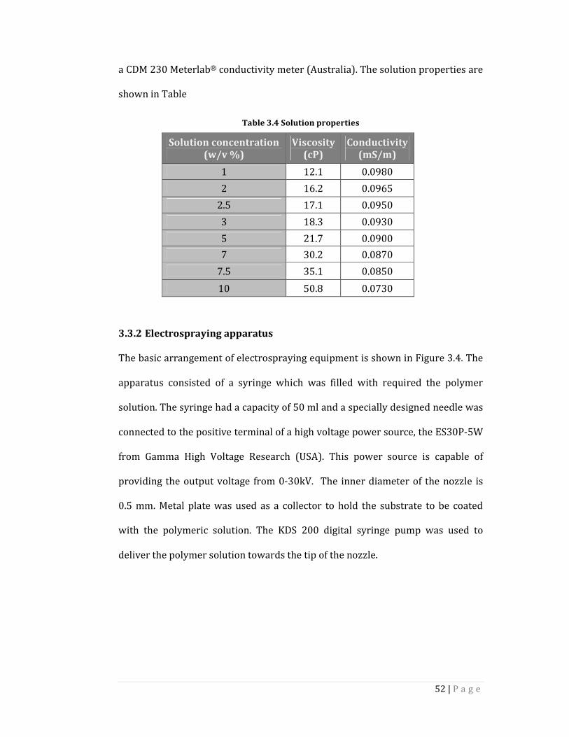
52 | P a g e

a CDM 230 Meterlab® conductivity meter (Australia). The solution properties are

shown in Table

Table 3.4 Solution properties

Solution concentration

(w/v %)

Viscosity

(cP)

Conductivity

(mS/m)

1 12.1 0.0980

2 16.2 0.0965

2.5 17.1 0.0950

3 18.3 0.0930

5 21.7 0.0900

7 30.2 0.0870

7.5 35.1 0.0850

10 50.8 0.0730

Electrospraying apparatus 3.3.2

The basic arrangement of electrospraying equipment is shown in Figure 3.4. The

apparatus consisted of a syringe which was filled with required the polymer

solution. The syringe had a capacity of 50 ml and a specially designed needle was

connected to the positive terminal of a high voltage power source, the ES30P-5W

from Gamma High Voltage Research (USA). This power source is capable of

providing the output voltage from 0-30kV. The inner diameter of the nozzle is

0.5 mm. Metal plate was used as a collector to hold the substrate to be coated

with the polymeric solution. The KDS 200 digital syringe pump was used to

deliver the polymer solution towards the tip of the nozzle.

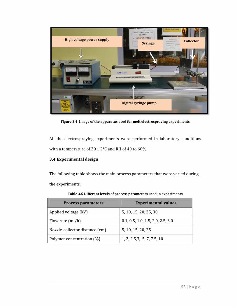
53 | P a g e

Figure 3.4 Image of the apparatus used for melt electrospraying experiments

All the electrospraying experiments were performed in laboratory conditions

with a temperature of 20 ± 2°C and RH of 40 to 60%.

3.4 Experimental design

The following table shows the main process parameters that were varied during

the experiments.

Table 3.5 Different levels of process parameters used in experiments

Process parameters Experimental values

Applied voltage (kV) 5, 10, 15, 20, 25, 30

Flow rate (ml/h) 0.1, 0.5, 1.0, 1.5, 2.0, 2.5, 3.0

Nozzle-collector distance (cm) 5, 10, 15, 20, 25

Polymer concentration (%) 1, 2, 2.5,3, 5, 7, 7.5, 10

High voltage power supply

Digital syringe pump

Collector Syringe

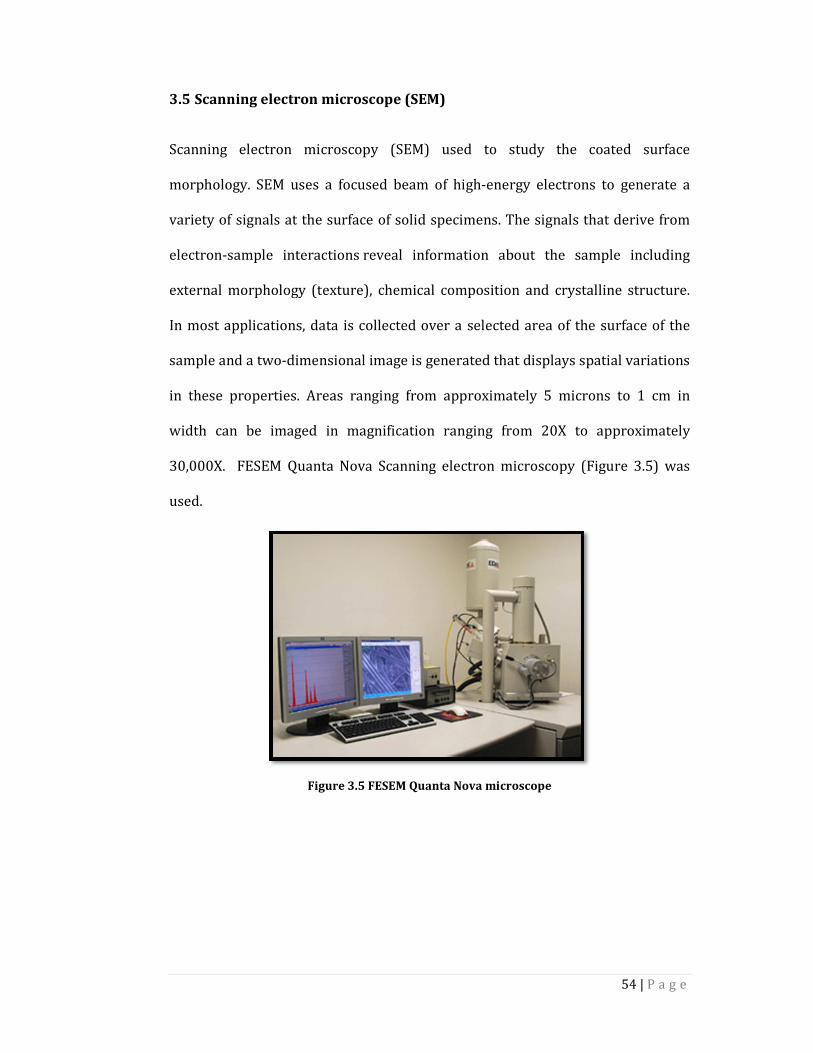
54 | P a g e

3.5 Scanning electron microscope (SEM)

Scanning electron microscopy (SEM) used to study the coated surface

morphology. SEM uses a focused beam of high-energy electrons to generate a

variety of signals at the surface of solid specimens. The signals that derive from

electron-sample interactions reveal information about the sample including

external morphology (texture), chemical composition and crystalline structure.

In most applications, data is collected over a selected area of the surface of the

sample and a two-dimensional image is generated that displays spatial variations

in these properties. Areas ranging from approximately 5 microns to 1 cm in

width can be imaged in magnification ranging from 20X to approximately

30,000X. FESEM Quanta Nova Scanning electron microscopy (Figure 3.5) was

used.

Figure 3.5 FESEM Quanta Nova microscope

55 | P a g e

3.6 Contact angle measurement

Contact angle measurement is important for assessing the hydrophobicity of the

textile material after polymer coating. A typical static contact angle

measurement instrument (PsS OCA 20) is shown in Figure 3.6.

Figure 3.6 PsS OCA 20 contact angle instrument

A contact angle can be measured by producing a drop of liquid on a solid surface.

The angle formed between the solid surface and liquid interfaces is referred to as

the contact angle. The most common method for measurement involves looking

at the profile of the drop and measuring two-dimensionally the angle formed

between the solid and the drop profile with the vertex at the three-phase line, as

shown in Figure 3.7. Young’s equation is used to describe the interaction

between the forces of cohesion and adhesion and measure what is referred to as

surface energy.

56 | P a g e

.

Figure 3.7 Measurement of contact angle [108]

If the contact angle is more than 90° then the surface is considered hydrophobic.

This condition is exemplified by poor wetting, poor adhesiveness and low solid

surface free energy and if the contact angle less than 90° then the surface is

considered as hydrophilic. This condition reflects better wetting, better

adhesiveness, and higher surface energy; both are shown in Figure 3.8.

Figure 3.8 Contact angles for hydrophobic and hydrophilic surfaces

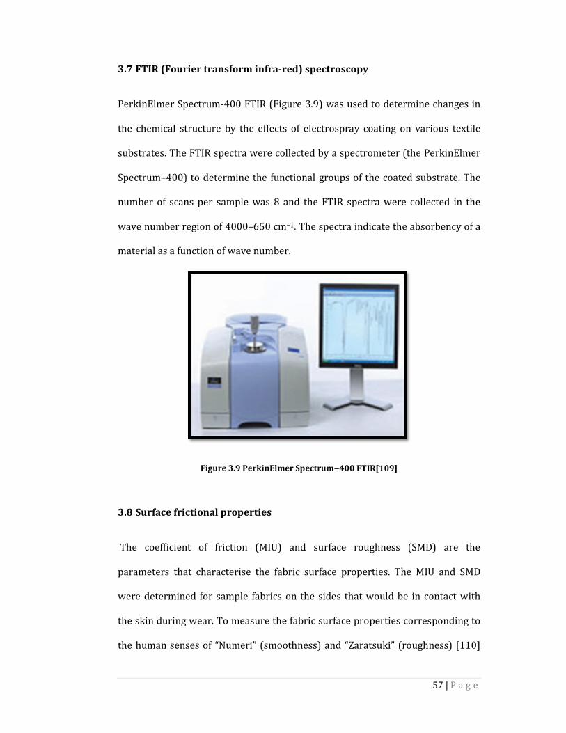
57 | P a g e

3.7 FTIR (Fourier transform infra-red) spectroscopy

PerkinElmer Spectrum-400 FTIR (Figure 3.9) was used to determine changes in

the chemical structure by the effects of electrospray coating on various textile

substrates. The FTIR spectra were collected by a spectrometer (the PerkinElmer

Spectrum–400) to determine the functional groups of the coated substrate. The

number of scans per sample was 8 and the FTIR spectra were collected in the

wave number region of 4000–650 cm–1. The spectra indicate the absorbency of a

material as a function of wave number.

Figure 3.9 PerkinElmer Spectrum‒400 FTIR[109]

3.8 Surface frictional properties

The coefficient of friction (MIU) and surface roughness (SMD) are the

parameters that characterise the fabric surface properties. The MIU and SMD

were determined for sample fabrics on the sides that would be in contact with

the skin during wear. To measure the fabric surface properties corresponding to

the human senses of “Numeri” (smoothness) and “Zaratsuki” (roughness) [110]

58 | P a g e

the KESFB4-A, Kato Tech Co. Ltd. Evaluation System was used. The system

acquires data from two sensors measuring the frictional coefficient and the

roughness of the fabric surface simultaneously in three different areas within a

fabric sample of 20 cm x20 cm. The frictional coefficient MIU is calculated by

averaging the output over the distance between 0 to 20 mm using an integrator.

The low-cut filter removes frequency components lower than 1mm/sec,

assuming that they are the signals that cannot be sensed by human skin. The

frictional coefficient is defined as:

��� = �/� Eq 3.1

where F is frictional force in N, P is sensor load in N

As the sample travels at a speed of 1 mm/sec in the same way as in the friction

test, the differential transformer detects the up-and-down movement of the

contact probe caused by the asperity of the fabric surface. The geometrical

surface roughness mean deviation (SMD) is the value obtained by eliminating the

low frequency harmonic wave by filtering the measurement curve through the

low-cut filter, extracting the frequency components higher than 1 mm/sec and

integrating over the absolute value of the distance moved from the standard

position along the path taken by the sensor.

Surface roughness (SMD) is expressed as follows:

SMD=1/Lmax � \� − �\ ����� Eq. 3.2

Where Lmax is the distance travelled by the sensor over the fabric, and Z0 is the

standard sensor position. The value of the friction coefficient (MIU), and the

59 | P a g e

roughness signal are recorded individually and simultaneously for the “go and

return” stroke. Measurements were taken in the warp and weft directions.

All the fabrics were tested on the side which is next to skin during the practical

use of the garments. The evaluation of the fabrics was carried out according to

the following:

• The value of MIU ranged from 0 to 1 and its approaching value of 1 was

interpreted as increasing friction and decreasing smoothness.

• The value of SMD ranged between 0 and 20 and its approaching value of

20 was interpreted as an increase in the surface roughness and surface

irregularities.

3.9 Moisture management testing (MMT)

SDL Atlas MMT instrument (Figure 3.10) was used for the experiments. MMT

utilises the electrical resistance technique, which is based on the substantial

difference in electrical conductivity of air (non-wetted fabrics) and water (wetted

fabrics): as the liquid wicks through and/or absorbs into the fabric sample, the

electrical resistance of the sample reduces. The MMT method assumes that the

value of the electrical resistance change depends on two factors: the components

of the water and the water content of the fabric; thus when the influence of the

water components is fixed, the electrical resistance measured is only related to

the water content in the fabric. [111, 112]. It is important to note that the

electrical resistance of wet textile fabrics also depends on the fabric fibre

composition and content, fibre polymer (where fibres themselves exhibit

different electrical conductivity or virtually no conductivity) and also different

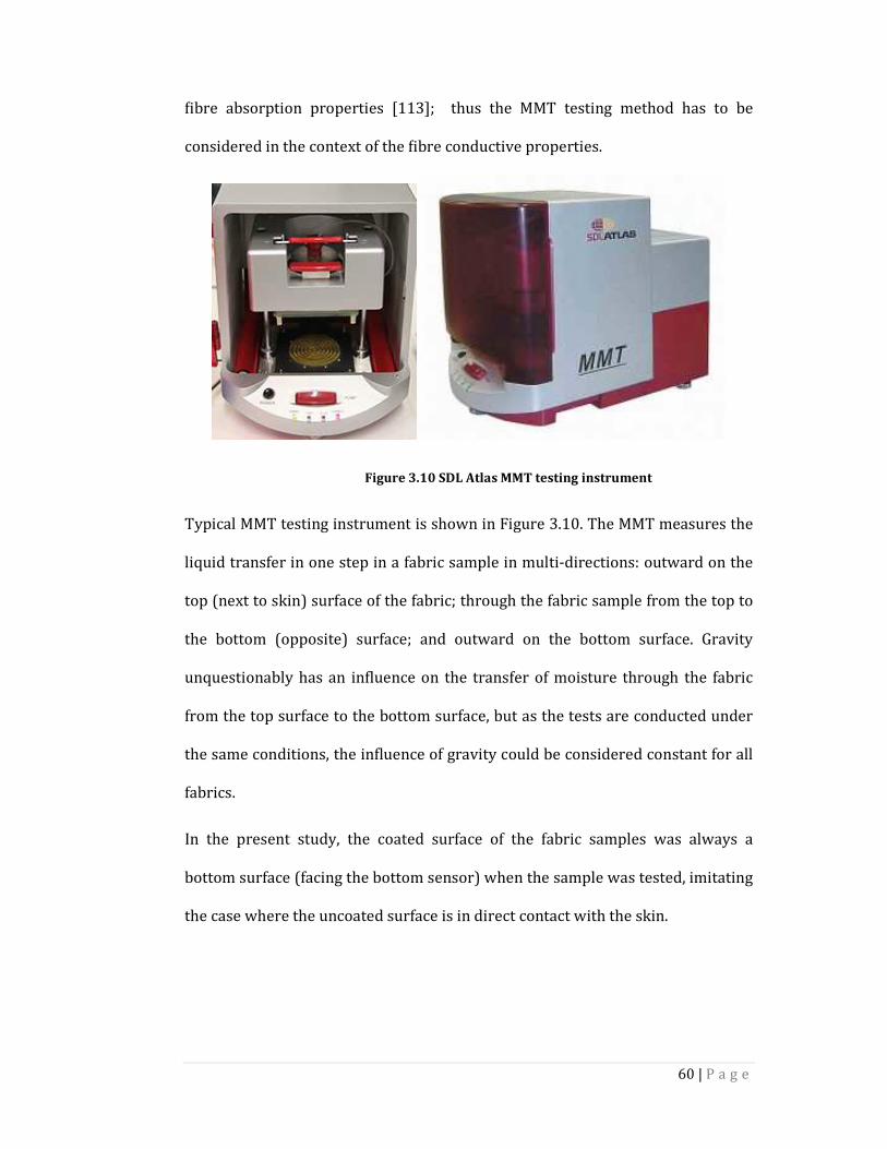
60 | P a g e

fibre absorption properties [113]; thus the MMT testing method has to be

considered in the context of the fibre conductive properties.

Typical MMT testing instrument is shown in Figure 3.10. The MMT measures the

liquid transfer in one step in a fabric sample in multi-directions: outward on the

top (next to skin) surface of the fabric; through the fabric sample from the top to

the bottom (opposite) surface; and outward on the bottom surface. Gravity

unquestionably has an influence on the transfer of moisture through the fabric

from the top surface to the bottom surface, but as the tests are conducted under

the same conditions, the influence of gravity could be considered constant for all

fabrics.

In the present study, the coated surface of the fabric samples was always a

bottom surface (facing the bottom sensor) when the sample was tested, imitating

the case where the uncoated surface is in direct contact with the skin.

Figure 3.10 SDL Atlas MMT testing instrument

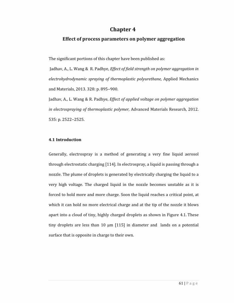
61 | P a g e

Chapter 4

Effect of process parameters on polymer aggregation

The significant portions of this chapter have been published as:

Jadhav, A., L. Wang & R. Padhye, Effect of field strength on polymer aggregation in

electrohydrodynamic spraying of thermoplastic polyurethane, Applied Mechanics

and Materials, 2013. 328: p. 895‒900.

Jadhav, A., L. Wang & R. Padhye, Effect of applied voltage on polymer aggregation

in electrospraying of thermoplastic polymer, Advanced Materials Research, 2012.

535: p. 2522‒2525.

4.1 Introduction

Generally, electrospray is a method of generating a very fine liquid aerosol

through electrostatic charging [114]. In electrospray, a liquid is passing through a

nozzle. The plume of droplets is generated by electrically charging the liquid to a

very high voltage. The charged liquid in the nozzle becomes unstable as it is

forced to hold more and more charge. Soon the liquid reaches a critical point, at

which it can hold no more electrical charge and at the tip of the nozzle it blows

apart into a cloud of tiny, highly charged droplets as shown in Figure 4.1. These

tiny droplets are less than 10 µm [115] in diameter and lands on a potential

surface that is opposite in charge to their own.

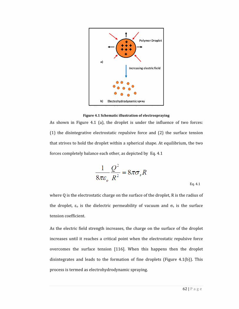
62 | P a g e

Figure 4.1 Schematic illustration of electrospraying

As shown in Figure 4.1 (a), the droplet is under the influence of two forces:

(1) the disintegrative electrostatic repulsive force and (2) the surface tension

that strives to hold the droplet within a spherical shape. At equilibrium, the two

forces completely balance each other, as depicted by Eq. 4.1

Eq. 4.1

where Q is the electrostatic charge on the surface of the droplet, R is the radius of

the droplet, εo is the dielectric permeability of vacuum and σs is the surface

tension coefficient.

As the electric field strength increases, the charge on the surface of the droplet

increases until it reaches a critical point when the electrostatic repulsive force

overcomes the surface tension [116]. When this happens then the droplet

disintegrates and leads to the formation of fine droplets (Figure 4.1(b)). This

process is termed as electrohydrodynamic spraying.

63 | P a g e

On the industrial scale, electrospray has been utilised in the application of paints

coatings on to metal surfaces extensively for automotive spray painting [117].

The fine spray results in very smooth and even films, with the paint actually

attracted to the metal, so the paint material is used more efficiently. The wastes

of coating chemicals are drastically reduced. This lowers the cost, cuts down on

the amount of organic solvents required and reduces environmental impact

[2]. Surface coating of polymer with electrospraying will be a promising

technology in many applications [118]. The polymer aggregation is important

while coating on the surface of any substrate. To get uniform coating on the

surface; the polymer droplets aggregation should be at minimum level [37]. So it

was important to study first the effect of the process parameters such as applied

voltage, nozzle-collector distance, solution flow rate and solution concentration

on polymer droplets aggregation on surface. This chapter discusses the effect of

dominant process parameters on polymer aggregation during electrospraying.

4.2 Experimental

The electrospraying was carried out by single factor parametric study, which

means by varying one parameter at a time and keeping other parameters

constant.

Materials 4.2.1

Thermoplastic polyurethane (TPU) was dissolved in THF solvent. And solutions

of 2%, 3%, 5% and 7 % were prepared on w/v basis.

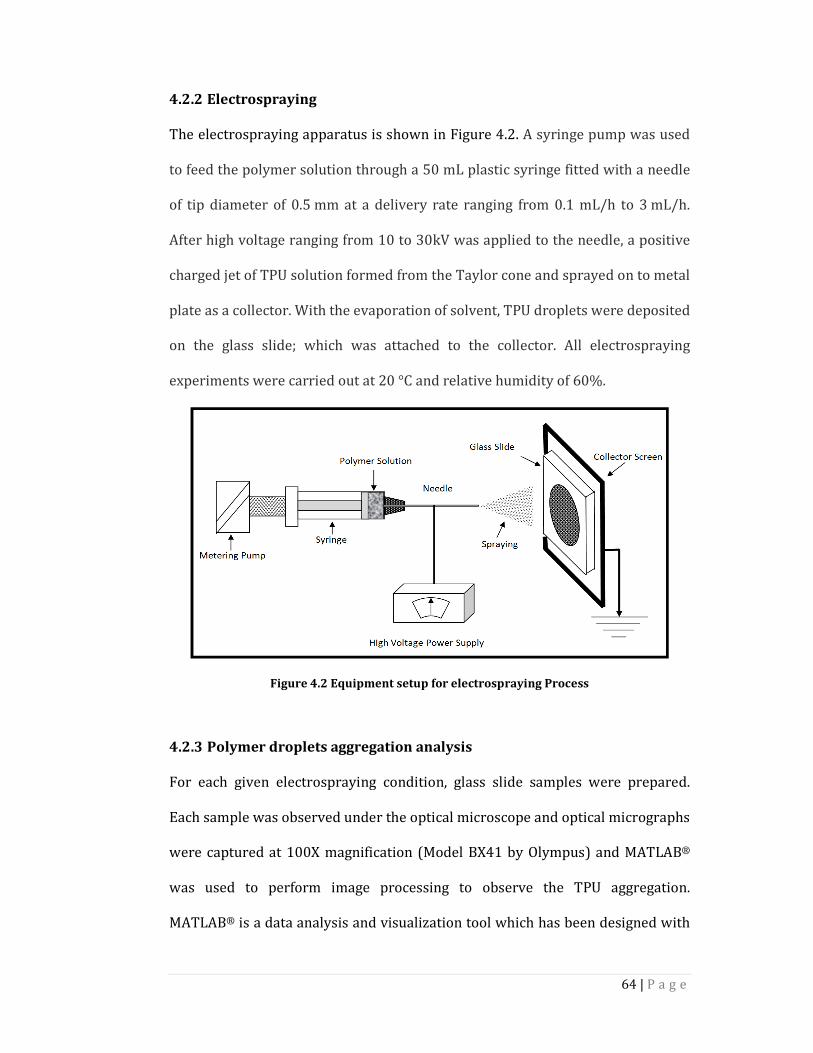
64 | P a g e

Electrospraying 4.2.2

The electrospraying apparatus is shown in Figure 4.2. A syringe pump was used

to feed the polymer solution through a 50 mL plastic syringe fitted with a needle

of tip diameter of 0.5 mm at a delivery rate ranging from 0.1 mL/h to 3 mL/h.

After high voltage ranging from 10 to 30kV was applied to the needle, a positive

charged jet of TPU solution formed from the Taylor cone and sprayed on to metal

plate as a collector. With the evaporation of solvent, TPU droplets were deposited

on the glass slide; which was attached to the collector. All electrospraying

experiments were carried out at 20 °C and relative humidity of 60%.

Figure 4.2 Equipment setup for electrospraying Process

Polymer droplets aggregation analysis 4.2.3

For each given electrospraying condition, glass slide samples were prepared.

Each sample was observed under the optical microscope and optical micrographs

were captured at 100X magnification (Model BX41 by Olympus) and MATLAB®

was used to perform image processing to observe the TPU aggregation.

MATLAB® is a data analysis and visualization tool which has been designed with

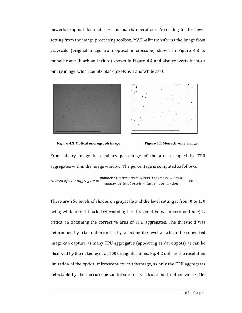
65 | P a g e

powerful support for matrices and matrix operations. According to the ‘level’

setting from the image processing toolbox, MATLAB® transforms the image from

grayscale (original image from optical microscope) shown in Figure 4.3 to

monochrome (black and white) shown in Figure 4.4 and also converts it into a

binary image, which counts black pixels as 1 and white as 0.

From binary image it calculates percentage of the area occupied by TPU

aggregates within the image window. The percentage is computed as follows:

%������������������ = � !"����"#�$%&'(�#)*'�+'��+�'!���*'�,�*� !"��������#&'(�#)*'�+'�'!���*'�,�* Eq. 4.2

There are 256 levels of shades on grayscale and the level setting is from 0 to 1, 0

being white and 1 black. Determining the threshold between zero and one) is

critical in obtaining the correct % area of TPU aggregates. The threshold was

determined by trial-and-error i.e. by selecting the level at which the converted

image can capture as many TPU aggregates (appearing as dark spots) as can be

observed by the naked eyes at 100X magnifications. Eq. 4.2 utilises the resolution

limitation of the optical microscope to its advantage, as only the TPU aggregates

detectable by the microscope contribute to its calculation. In other words, the

Figure 4.4 Monochrome image

Figure 4.3 Optical micrograph image

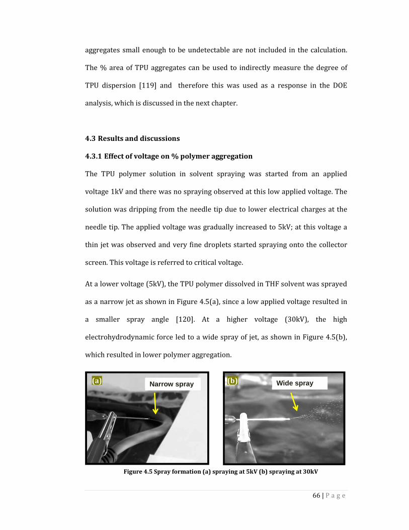
66 | P a g e

(a) (b)

aggregates small enough to be undetectable are not included in the calculation.

The % area of TPU aggregates can be used to indirectly measure the degree of

TPU dispersion [119] and therefore this was used as a response in the DOE

analysis, which is discussed in the next chapter.

4.3 Results and discussions

Effect of voltage on % polymer aggregation 4.3.1

The TPU polymer solution in solvent spraying was started from an applied

voltage 1kV and there was no spraying observed at this low applied voltage. The

solution was dripping from the needle tip due to lower electrical charges at the

needle tip. The applied voltage was gradually increased to 5kV; at this voltage a

thin jet was observed and very fine droplets started spraying onto the collector

screen. This voltage is referred to critical voltage.

At a lower voltage (5kV), the TPU polymer dissolved in THF solvent was sprayed

as a narrow jet as shown in Figure 4.5(a), since a low applied voltage resulted in

a smaller spray angle [120]. At a higher voltage (30kV), the high

electrohydrodynamic force led to a wide spray of jet, as shown in Figure 4.5(b),

which resulted in lower polymer aggregation.

Narrow spray Wide spray

Figure 4.5 Spray formation (a) spraying at 5kV (b) spraying at 30kV

(a) (b)

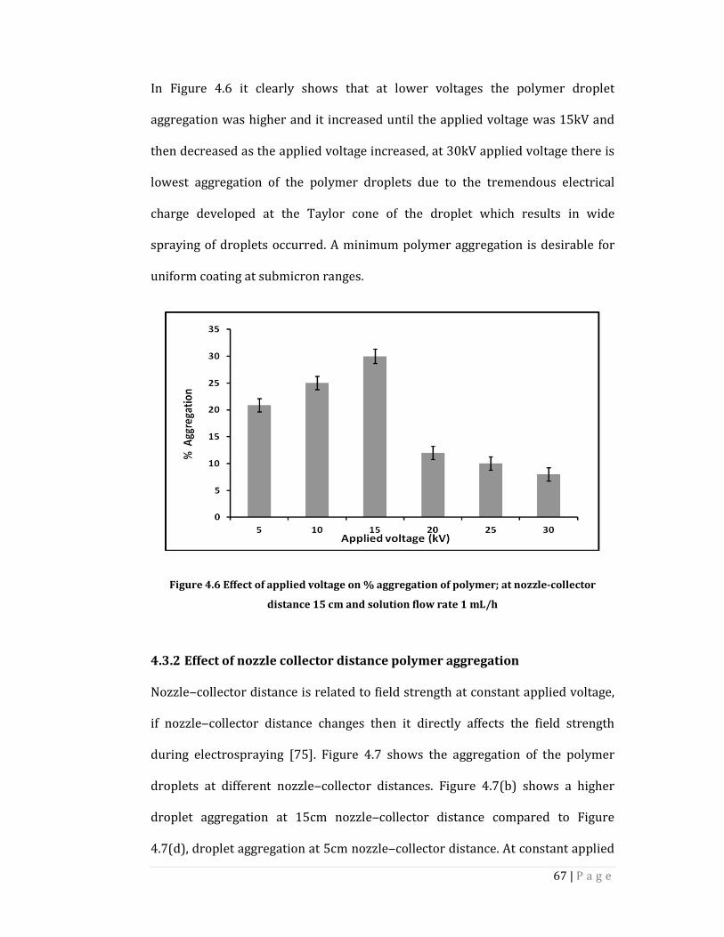
67 | P a g e

In Figure 4.6 it clearly shows that at lower voltages the polymer droplet

aggregation was higher and it increased until the applied voltage was 15kV and

then decreased as the applied voltage increased, at 30kV applied voltage there is

lowest aggregation of the polymer droplets due to the tremendous electrical

charge developed at the Taylor cone of the droplet which results in wide

spraying of droplets occurred. A minimum polymer aggregation is desirable for

uniform coating at submicron ranges.

Figure 4.6 Effect of applied voltage on % aggregation of polymer; at nozzle-collector

distance 15 cm and solution flow rate 1 mL/h

Effect of nozzle collector distance polymer aggregation 4.3.2

Nozzle‒collector distance is related to field strength at constant applied voltage,

if nozzle‒collector distance changes then it directly affects the field strength

during electrospraying [75]. Figure 4.7 shows the aggregation of the polymer

droplets at different nozzle‒collector distances. Figure 4.7(b) shows a higher

droplet aggregation at 15cm nozzle‒collector distance compared to Figure

4.7(d), droplet aggregation at 5cm nozzle‒collector distance. At constant applied

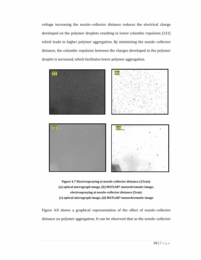
68 | P a g e

voltage increasing the nozzle‒collector distance reduces the electrical charge

developed on the polymer droplets resulting in lower columbic repulsion [121]

which leads to higher polymer aggregation. By minimising the nozzle‒collector

distance, the columbic repulsion between the charges developed in the polymer

droplet is increased, which facilitates lower polymer aggregation.

Figure 4.7 Electrospraying at nozzle-collector distance (15cm):

(a) optical micrograph image, (b) MATLAB® monochromatic image;

electrospraying at nozzle-collector distance (5cm):

(c) optical micrograph image, (d) MATLAB® monochromatic image

Figure 4.8 shows a graphical representation of the effect of nozzle‒collector

distance on polymer aggregation. It can be observed that as the nozzle‒collector

(a) (b)

(c) (d)

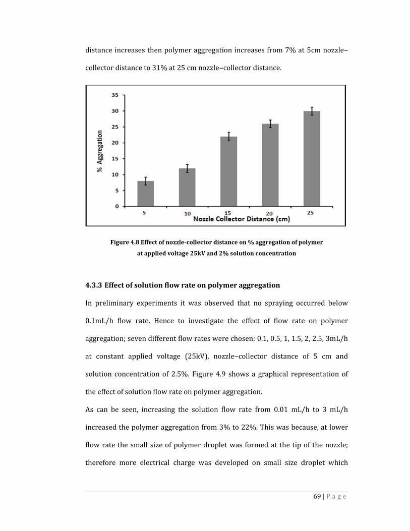
69 | P a g e

distance increases then polymer aggregation increases from 7% at 5cm nozzle‒

collector distance to 31% at 25 cm nozzle‒collector distance.

Figure 4.8 Effect of nozzle-collector distance on % aggregation of polymer

at applied voltage 25kV and 2% solution concentration

Effect of solution flow rate on polymer aggregation 4.3.3

In preliminary experiments it was observed that no spraying occurred below

0.1mL/h flow rate. Hence to investigate the effect of flow rate on polymer

aggregation; seven different flow rates were chosen: 0.1, 0.5, 1, 1.5, 2, 2.5, 3mL/h

at constant applied voltage (25kV), nozzle‒collector distance of 5 cm and

solution concentration of 2.5%. Figure 4.9 shows a graphical representation of

the effect of solution flow rate on polymer aggregation.

As can be seen, increasing the solution flow rate from 0.01 mL/h to 3 mL/h

increased the polymer aggregation from 3% to 22%. This was because, at lower

flow rate the small size of polymer droplet was formed at the tip of the nozzle;

therefore more electrical charge was developed on small size droplet which

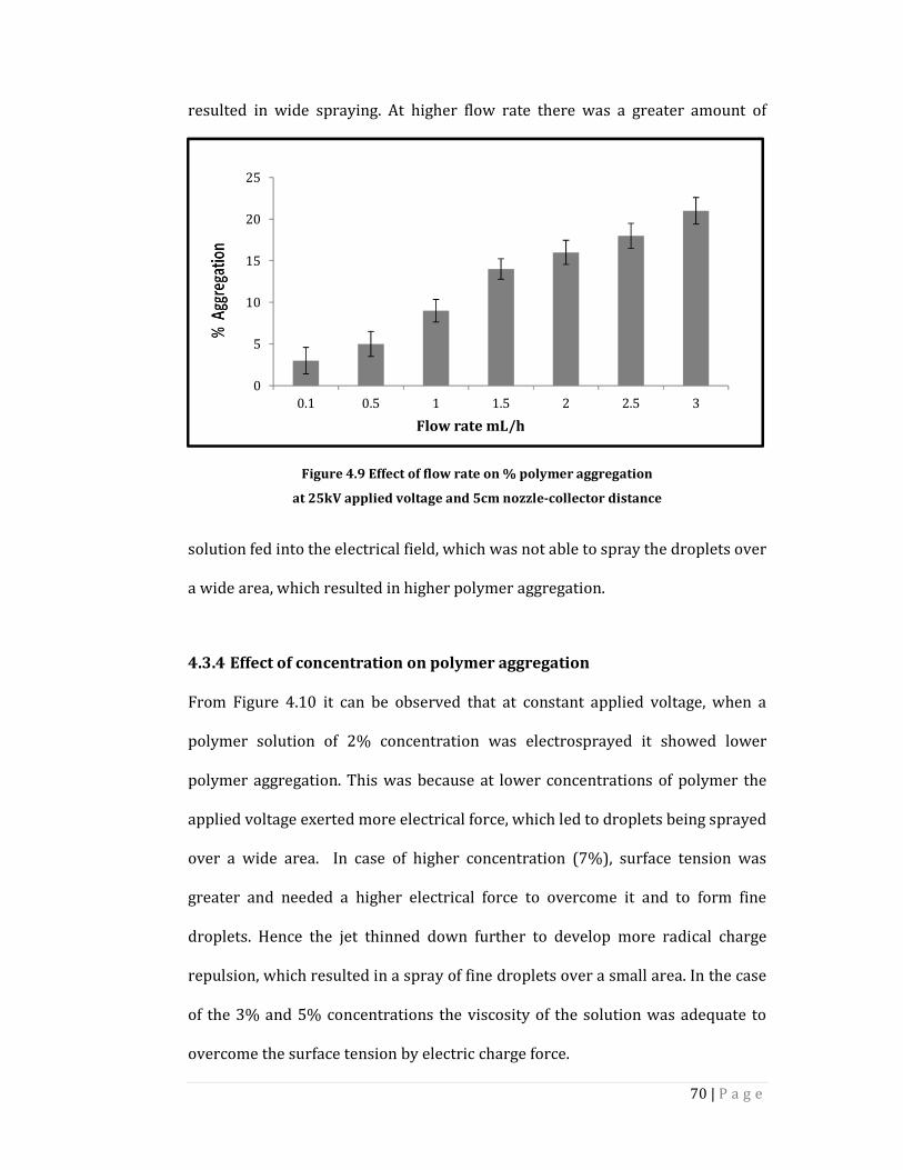
70 | P a g e

resulted in wide spraying. At higher flow rate there was a greater amount of

Figure 4.9 Effect of flow rate on % polymer aggregation

at 25kV applied voltage and 5cm nozzle-collector distance

solution fed into the electrical field, which was not able to spray the droplets over

a wide area, which resulted in higher polymer aggregation.

Effect of concentration on polymer aggregation 4.3.4

From Figure 4.10 it can be observed that at constant applied voltage, when a

polymer solution of 2% concentration was electrosprayed it showed lower

polymer aggregation. This was because at lower concentrations of polymer the

applied voltage exerted more electrical force, which led to droplets being sprayed

over a wide area. In case of higher concentration (7%), surface tension was

greater and needed a higher electrical force to overcome it and to form fine

droplets. Hence the jet thinned down further to develop more radical charge

repulsion, which resulted in a spray of fine droplets over a small area. In the case

of the 3% and 5% concentrations the viscosity of the solution was adequate to

overcome the surface tension by electric charge force.

0

5

10

15

20

25

0.1 0.5 1 1.5 2 2.5 3

Flow rate mL/h

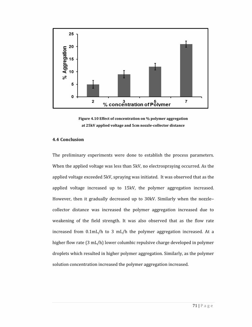
71 | P a g e

Figure 4.10 Effect of concentration on % polymer aggregation

at 25kV applied voltage and 5cm nozzle-collector distance

4.4 Conclusion

The preliminary experiments were done to establish the process parameters.

When the applied voltage was less than 5kV, no electrospraying occurred. As the

applied voltage exceeded 5kV, spraying was initiated. It was observed that as the

applied voltage increased up to 15kV, the polymer aggregation increased.

However, then it gradually decreased up to 30kV. Similarly when the nozzle‒

collector distance was increased the polymer aggregation increased due to

weakening of the field strength. It was also observed that as the flow rate

increased from 0.1mL/h to 3 mL/h the polymer aggregation increased. At a

higher flow rate (3 mL/h) lower columbic repulsive charge developed in polymer

droplets which resulted in higher polymer aggregation. Similarly, as the polymer

solution concentration increased the polymer aggregation increased.

72 | P a g e

Chapter 5

Effect of process parameters on jet length in electrospraying

The research work discussed in this chapter resulted in a refereed paper:

A. Jadhav, L.J. Wang, C. Lawrence, R. Padhye, Effect of process parameters on jet

length in electrospraying of thermoplastic polymer, Advanced Materials Research,

2012.

5.1 Introduction

Electrospraying is a method of form fine polymer particles through electrostatic

charging and attaching the particles to the target substrates. As a solvent based

liquid passes through a nozzle, fine droplets are generated by electrically

charging the liquid to a very high voltage. The charged liquid in the nozzle end

charges up and form a pendant droplet of the polymer solution at the tip of the

nozzle is deformed into conical shape, typically referred to as Taylor cone[122].

Because of the repulsive electric force due to the same electrical charge, the

charged liquid forms drops which repel strongly each other. At the tip of the

cone, the liquid becomes unstable as it is forced to hold more and more charge.

When the liquid can hold no more electrical charge, it disperses into numerous,

micron-sized, highly charged droplets at the tip of the nozzle [115]. In general,

these tiny droplets are less than 10μm in diameter, and fly and land on the

surface that is opposite in charge to their own. As they fly about, they rapidly

shrink as solvent molecules evaporate [115].

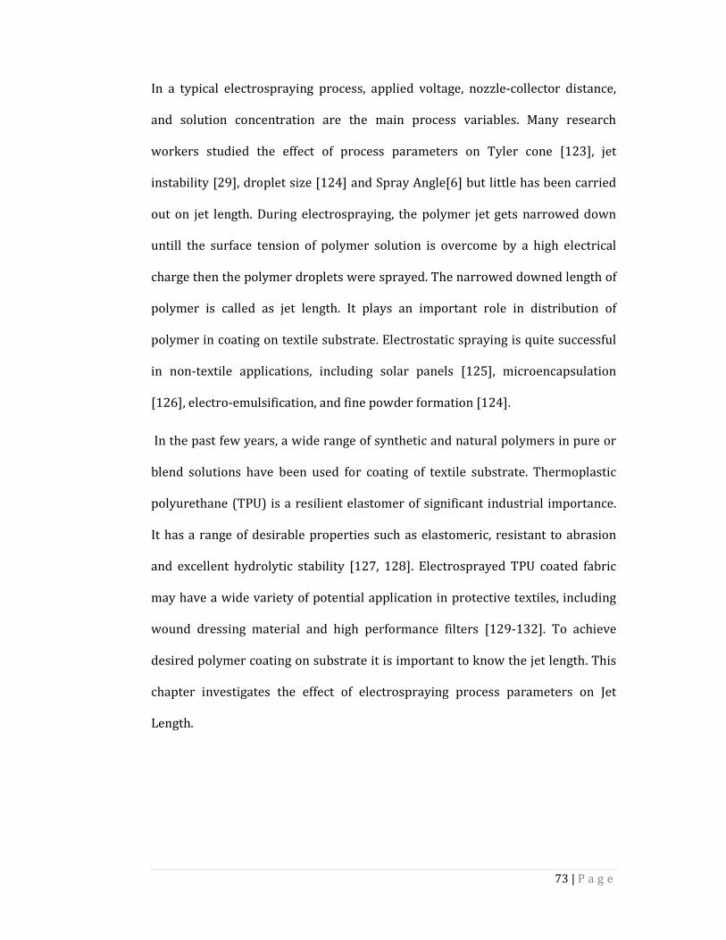
73 | P a g e

In a typical electrospraying process, applied voltage, nozzle-collector distance,

and solution concentration are the main process variables. Many research

workers studied the effect of process parameters on Tyler cone [123], jet

instability [29], droplet size [124] and Spray Angle[6] but little has been carried

out on jet length. During electrospraying, the polymer jet gets narrowed down

untill the surface tension of polymer solution is overcome by a high electrical

charge then the polymer droplets were sprayed. The narrowed downed length of

polymer is called as jet length. It plays an important role in distribution of

polymer in coating on textile substrate. Electrostatic spraying is quite successful

in non-textile applications, including solar panels [125], microencapsulation

[126], electro-emulsification, and fine powder formation [124].

In the past few years, a wide range of synthetic and natural polymers in pure or

blend solutions have been used for coating of textile substrate. Thermoplastic

polyurethane (TPU) is a resilient elastomer of significant industrial importance.

It has a range of desirable properties such as elastomeric, resistant to abrasion

and excellent hydrolytic stability [127, 128]. Electrosprayed TPU coated fabric

may have a wide variety of potential application in protective textiles, including

wound dressing material and high performance filters [129-132]. To achieve

desired polymer coating on substrate it is important to know the jet length. This

chapter investigates the effect of electrospraying process parameters on Jet

Length.

74 | P a g e

5.2 Experimental

Chemicals 5.2.1

The THF was used as the solvent for dissolving Polyurethane. Solutions of 1.5%,

2.5%, 3.5% polyurethane were prepared by dissolving the elastomer

homogenously in tetrahydrofluran for electrospraying.

Electrospraying equipment set up 5.2.2

Electrospraying arrangement was similar as described in section 3.3.1 of Chapter

3. The electrospraying was carried out by varying voltage, nozzle-collector

distance & concentration of polymer solution at a constant flow rate of 1 mL/h.

Jet length analysis: 5.2.3

5.2.3.1 High speed motion analyser

A high speed KODAK Max HS Motion Analyzer; Model 4540 was used to record

digital video up to 4,500 full frames per second, and up to 40,500 partial frames

per second for immediate playback and motion analysis of extremely rapid

events.

5.2.3.2 Image analysis by Image Pro-Plus 4.0

Images recorded by a high speed camera were analysed by Image Pro-Plus 4.0

software. The length of spray jet was measured by using various tools of

software.

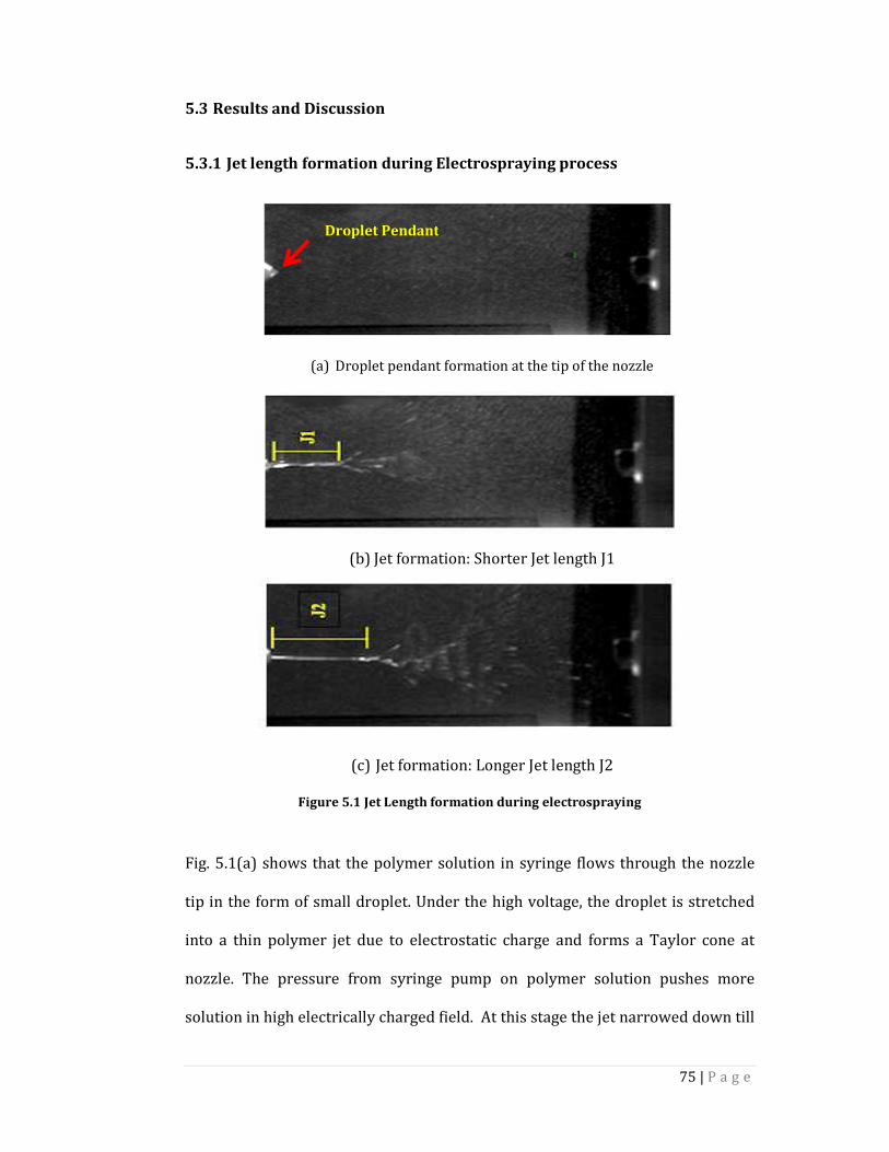
75 | P a g e

5.3 Results and Discussion

Jet length formation during Electrospraying process 5.3.1

(a) Droplet pendant formation at the tip of the nozzle

(b) Jet formation: Shorter Jet length J1

(c) Jet formation: Longer Jet length J2

Figure 5.1 Jet Length formation during electrospraying

Fig. 5.1(a) shows that the polymer solution in syringe flows through the nozzle

tip in the form of small droplet. Under the high voltage, the droplet is stretched

into a thin polymer jet due to electrostatic charge and forms a Taylor cone at

nozzle. The pressure from syringe pump on polymer solution pushes more

solution in high electrically charged field. At this stage the jet narrowed down till

Droplet Pendant

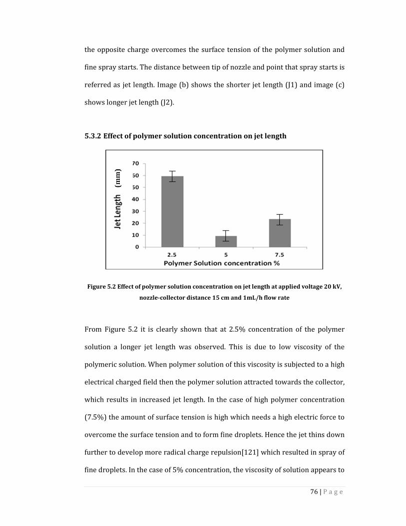
76 | P a g e

the opposite charge overcomes the surface tension of the polymer solution and

fine spray starts. The distance between tip of nozzle and point that spray starts is

referred as jet length. Image (b) shows the shorter jet length (J1) and image (c)

shows longer jet length (J2).

Effect of polymer solution concentration on jet length 5.3.2

Figure 5.2 Effect of polymer solution concentration on jet length at applied voltage 20 kV,

nozzle-collector distance 15 cm and 1mL/h flow rate

From Figure 5.2 it is clearly shown that at 2.5% concentration of the polymer

solution a longer jet length was observed. This is due to low viscosity of the

polymeric solution. When polymer solution of this viscosity is subjected to a high

electrical charged field then the polymer solution attracted towards the collector,

which results in increased jet length. In the case of high polymer concentration

(7.5%) the amount of surface tension is high which needs a high electric force to

overcome the surface tension and to form fine droplets. Hence the jet thins down

further to develop more radical charge repulsion[121] which resulted in spray of

fine droplets. In the case of 5% concentration, the viscosity of solution appears to

77 | P a g e

be adequate to overcome the surface tension by electric charge force at lower jet

length so that the spraying occurred at a lower jet length as compared to that of

2.5% and 7.5% polymer solutions.

Effect of applied voltage on jet length 5.3.3

The graphical representation of effect of applied voltage on jet length is shown in

Figure 5.3. At 10kV applied voltage the length of jet was observed to be 13 mm.

then it was slightly decreased to 10mm at the applied voltage 15kV, then again it

was gradually increased up to 25mm at applied voltage 25kv.

Figure 5.3 Effect of applied voltage on jet length at 3.5% Concentration, nozzle-collector

distance 15cm and 1mL/h flow rate.

Interestingly the jet length was reduced from 13 mm to 10 mm when applied

voltage increased from 10kV to 15kV, this is due to at 10kV the jet diameter was

observed higher than jet diameter of 15kV. Increase in jet length from 15kV to

25kV was due to high electrical charge developed in the polymer droplet at the

tip of the nozzle. Also at higher applied voltage the jet length was thinned down

towards the collector.

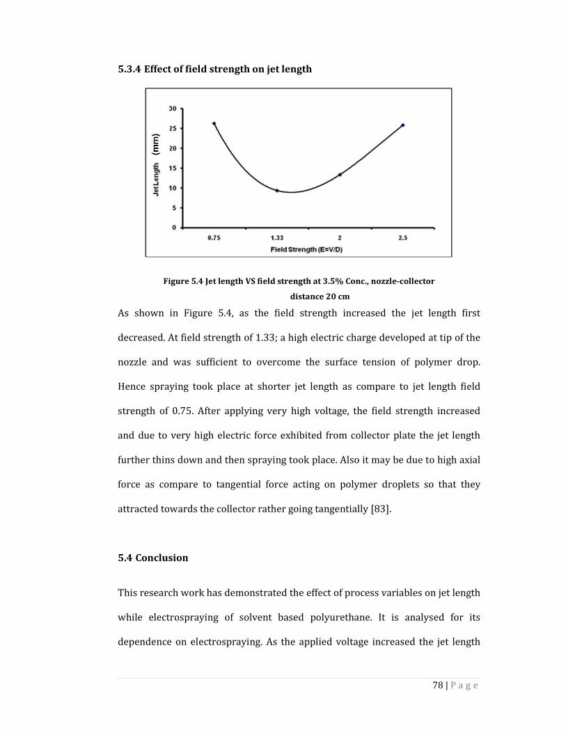
78 | P a g e

Effect of field strength on jet length 5.3.4

Figure 5.4 Jet length VS field strength at 3.5% Conc., nozzle-collector

distance 20 cm

As shown in Figure 5.4, as the field strength increased the jet length first

decreased. At field strength of 1.33; a high electric charge developed at tip of the

nozzle and was sufficient to overcome the surface tension of polymer drop.

Hence spraying took place at shorter jet length as compare to jet length field

strength of 0.75. After applying very high voltage, the field strength increased

and due to very high electric force exhibited from collector plate the jet length

further thins down and then spraying took place. Also it may be due to high axial

force as compare to tangential force acting on polymer droplets so that they

attracted towards the collector rather going tangentially [83].

5.4 Conclusion

This research work has demonstrated the effect of process variables on jet length

while electrospraying of solvent based polyurethane. It is analysed for its

dependence on electrospraying. As the applied voltage increased the jet length

79 | P a g e

initially increased up to 13mm and then slightly decreased to 10mm at 15kV

applied voltage. Then again it was gradually increased up to 25mm at applied

voltage 25kv due to higher electrical charge developed on polymer droplet. As

the polymer solution concentration increased from 5% to 7% the increase in jet

length was observed and at 2.5% polymer solution concentration shows

increased jet length. Effect of field strength on jet length shows negative

parabolic characteristics.

80 | P a g e

Chapter 6

Empirical modelling of polymer droplet aggregation by response

surface methodology

6.1 Introduction

Electrospraying has been recognised as an efficient technique for the fabrication

of submicron polymer droplets [83]. These droplets have attracted increasing

attention in the last ten years because of their very large surface area to volume

ratio, flexibility in surface functionalities and superior mechanical performance

compared with any other known form of materials. These outstanding properties

make electrosprayed polymer droplets optimal candidates for coating

applications in textiles.

Numerous studies have been carried out to gain deeper understanding of the

process for better control of droplet formation. Systematic investigations of the

effects of electrospraying variables on the diameter and morphology of the

polymer droplets are of great interest. Obviously, there is an important need to

produce polymer droplets of small and uniform size so that the electrospraying

process can be reproduced in large industrial applications. As discussed in

previous chapters, process parameters such as applied voltage, nozzle‒collector

distance, solution flow rate and polymer solution concentration affect the

aggregation and dimension of droplets. Other parameters such as polymer type

and its molecular weight, polymer concentration, solvent type and polymer

solution properties (viscosity, conductivity and surface tension) and ambient

81 | P a g e

parameters (temperature, humidity and air velocity) also affects the

electrospraying process [76, 133].

In chapter 4, for the deposition of polymer droplets, the conventional or classical

method of experimentation, which involves changing one of the independent

parameters while maintaining the others fixed at given values, has been

performed. As is well known, this conventional method of experimentation

involves many tests, which are time-consuming. It ignores interaction effects

between the operating parameters and induces low efficiency in optimisation.

These limitations can be avoided by applying the response surface methodology

(RSM) which involves statistical design of experiments (DOE) in which all factors

are varied together over a set of experimental runs [134, 135]. The statistical

method of experimental design offers several advantages over the conventional

method, being rapid and reliable, helping in understanding the interaction effects

between factors and reducing the total number of experiments tremendously

resulting in saving time and costs of experimentation. Moreover, RSM can be

used to evaluate the relative significance of several affecting factors even in the

presence of complex interactions [134-141].

In recent years, various statistical experimental designs and RSM have been

applied progressively to different processes like metal forming, chemical

vaporisation, and composite membrane fabrications [134-141]. However, among

them few reports have been dedicated to electrospinning [133, 142]. Yördem et

al. studied the effects of electrospinning parameters on polyacrylonitrile (PAN)

nanofibre diameter using RSM. Their investigations were carried out using only

two variables (applied voltage and solution concentration) but at several

82 | P a g e

collector distances. It was reported that the effect of the applied voltage on fibre

diameter was insignificant when the solution concentration and collector

distance were high [133]. Similarly, Gu et al. [142] applied RSM for PAN

nanofibres and also reported no significant effect of the voltage on the PAN

nanofibres. Both studies have been conducted considering two variables while

the third parameter was maintained fixed, and therefore possible interactions

between the three parameters were not studied [133, 142]. In the present study

a full factorial experimental design for the aggregation of TPU droplets on the

targeted substrate has been considered.

The polymer solution parameters (polymer type, molecular weight and solvent)

and the environmental conditions (temperature and humidity) were maintained

for all experiments. The main objective of this chapter is to investigate the

individual and mutual effects of the electrospraying variables (applied voltage,

polymer solution flow rate and distance between the needle tip and the collector)

on the TPU droplets aggregation. Furthermore, the optimum electrospraying

conditions to ensure minimum aggregation was determined.

6.2 Experimental

TPU polymer was used for the all the experiments and similar experimental

methods have been followed as discussed in detail in section 4.4 of chapter 4. The

electrospraying setup used was the same for all the experiments carried out.

Response surface methodology 6.2.1

The designs of response surface methodology (RSM) are those in which problems

are modelled and analysed; in these problems the response of interest is

influenced by different variables. RSM is widely used as an optimisation,

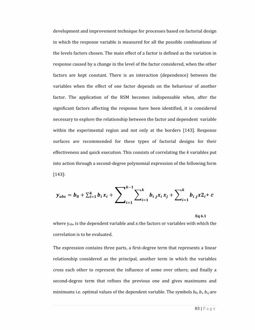
83 | P a g e

development and improvement technique for processes based on factorial design

in which the response variable is measured for all the possible combinations of

the levels factors chosen. The main effect of a factor is defined as the variation in

response caused by a change in the level of the factor considered, when the other

factors are kept constant. There is an interaction (dependence) between the

variables when the effect of one factor depends on the behaviour of another

factor. The application of the RSM becomes indispensable when, after the

significant factors affecting the response have been identified, it is considered

necessary to explore the relationship between the factor and dependent variable

within the experimental region and not only at the borders [143]. Response

surfaces are recommended for these types of factorial designs for their

effectiveness and quick execution. This consists of correlating the k variables put

into action through a second-degree polynomial expression of the following form

[143]:

2345 = 46 + ∑ 49�9:9;< += > 49,@�9:9;< �@

:A<

9;<+> 49,@�B9:

9;< + e

Eq 6.1

where yobs is the dependent variable and xi the factors or variables with which the

correlation is to be evaluated.

The expression contains three parts, a first-degree term that represents a linear

relationship considered as the principal, another term in which the variables

cross each other to represent the influence of some over others; and finally a

second-degree term that refines the previous one and gives maximums and

minimums i.e. optimal values of the dependent variable. The symbols b0, bi, bi,j are

84 | P a g e

constants and e a term of error or residual between the observed and calculated

values. The experimental values are adjusted to the above equation by a

polynomial regression. The usual statistics were used to determine the goodness

of fit.

Design of experiments 6.2.2

The dominant factors (process parameters) and their levels were determined

based on the minimum TPU aggregation observed from the results discussed in

chapter 4 section 4.5. The dominant factors and factor levels were utilised as a

precursor for DOE analysis. The DOE technique was employed to develop a

process model and validate the model experimentally.

DOE provides the following advantages:

1. DOE can provide a complete parametric study of the main factors and the

interaction of factors by means of the statistical data and charts.

2. DOE can allow optimisation of experiments, yielding the process conditions

under which minimum TPU droplet aggregation can be obtained.

In this study, commercial software Design Expert® (supplied by Stat-Ease) was

used to assist in DOE analysis.

Validation of DOE model 6.2.3

In order to prove the practical application of the model developed by DOE, the

new method was employed to validate derived DOE model. Optimised process

parameter combinations as predicted by Design Expert® were selected. Then,

electrospraying experiments based on those conditions were performed. The

experimental results or responses were compared with the predicted values.

85 | P a g e

6.3 Results and discussions

Summary of single factor parametric study 6.3.1

Dominant process parameters and their levels are mentioned in Table 6.1.

Table 6.1 Experimental factor levels

Factors Levels

Unit

‒ +

A: Applied voltage 10.00 25.00 kV

B: Flow rate 0.10 1.00 mL/h

C: Distance 5.00 20.00 cm

D: Concentration 20.00 50.00 g/l

Determination of experimental design 6.3.2

Based on the design factors, the experiment was a 24 factorial design. A 24 full

factional design was employed, consisting of 16 treatments. In order to obtain an

estimate of the experimental error and a more precise estimate of the sample

mean, four centre points were added. Table 6.2 is a DOE summary of

experiments, as generated by Design Expert®.

Table 6.2 DOE summary

Study type 2 level factorial design No. of runs 16

Factor Name Unit Min Max Coded Mean Std Dev.

A Voltage kV 10.00 25.00 ‒1 +1 17.50 7.50

B Flow rate mL/h 0.10 1.00 ‒1 +1 0.55 0.45

C Distance cm 5.00 20.00 ‒1 +1 12.50 7.50

D Concentration g/l 20.00 50.00 ‒1 +1 35.00 15.00

Response Name Unit Analysis Min Max Mean Std Dev.

Y1 TPU

aggregation % Factorial 0.5 18.0 6.26 5.21

Model R2FI

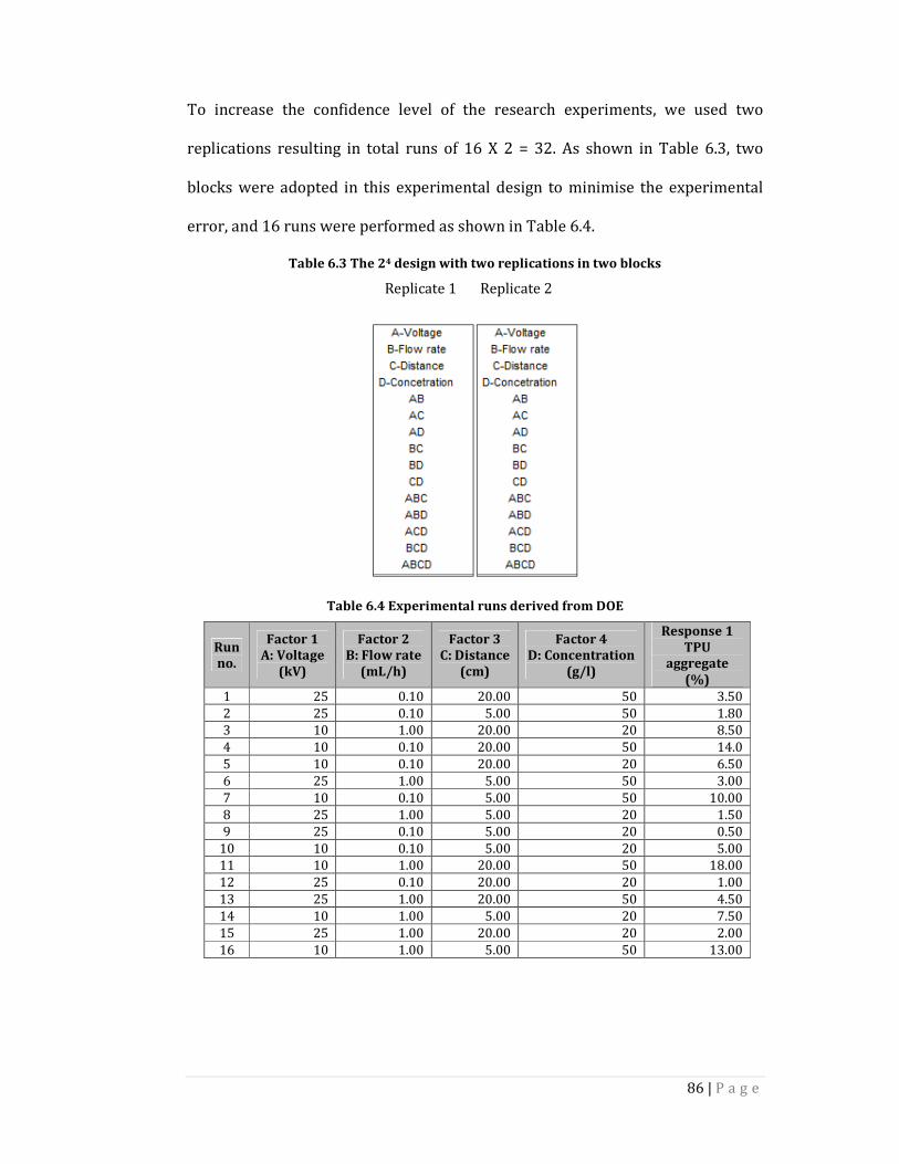
86 | P a g e

To increase the confidence level of the research experiments, we used two

replications resulting in total runs of 16 X 2 = 32. As shown in Table 6.3, two

blocks were adopted in this experimental design to minimise the experimental

error, and 16 runs were performed as shown in Table 6.4.

Table 6.3 The 24 design with two replications in two blocks

Replicate 1 Replicate 2

Table 6.4 Experimental runs derived from DOE

Run

no.

Factor 1

A: Voltage

(kV)

Factor 2

B: Flow rate

(mL/h)

Factor 3

C: Distance

(cm)

Factor 4

D: Concentration

(g/l)

Response 1

TPU

aggregate

(%)

1 25 0.10 20.00 50 3.50 2 25 0.10 5.00 50 1.80 3 10 1.00 20.00 20 8.50 4 10 0.10 20.00 50 14.0 5 10 0.10 20.00 20 6.50 6 25 1.00 5.00 50 3.00 7 10 0.10 5.00 50 10.00 8 25 1.00 5.00 20 1.50 9 25 0.10 5.00 20 0.50

10 10 0.10 5.00 20 5.00 11 10 1.00 20.00 50 18.00 12 25 0.10 20.00 20 1.00 13 25 1.00 20.00 50 4.50 14 10 1.00 5.00 20 7.50 15 25 1.00 20.00 20 2.00 16 10 1.00 5.00 50 13.00

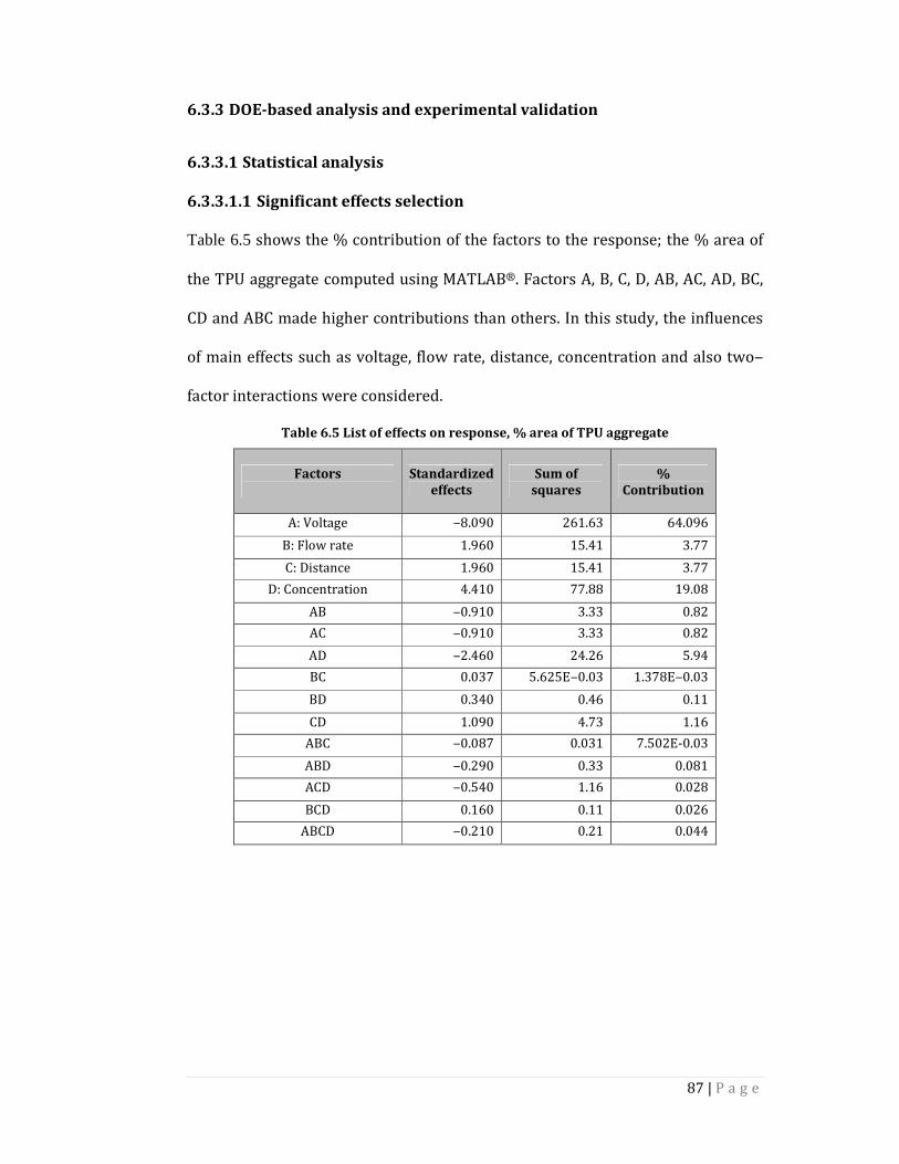
87 | P a g e

DOE-based analysis and experimental validation 6.3.3

6.3.3.1 Statistical analysis

6.3.3.1.1 Significant effects selection

Table 6.5 shows the % contribution of the factors to the response; the % area of

the TPU aggregate computed using MATLAB®. Factors A, B, C, D, AB, AC, AD, BC,

CD and ABC made higher contributions than others. In this study, the influences

of main effects such as voltage, flow rate, distance, concentration and also two‒

factor interactions were considered.

Table 6.5 List of effects on response, % area of TPU aggregate

Factors

Standardized

effects

Sum of

squares

%

Contribution

A: Voltage ‒8.090 261.63 64.096

B: Flow rate 1.960 15.41 3.77

C: Distance 1.960 15.41 3.77

D: Concentration 4.410 77.88 19.08

AB ‒0.910 3.33 0.82

AC ‒0.910 3.33 0.82

AD ‒2.460 24.26 5.94

BC 0.037 5.625E‒0.03 1.378E‒0.03

BD 0.340 0.46 0.11

CD 1.090 4.73 1.16

ABC ‒0.087 0.031 7.502E-0.03

ABD ‒0.290 0.33 0.081

ACD ‒0.540 1.16 0.028

BCD 0.160 0.11 0.026

ABCD ‒0.210 0.21 0.044

88 | P a g e

Figure 6.1 Half-normal plot of factor effects on response, % area of TPU aggregate

Figure 6.1 presents a half-normal probability plot of the effects estimated from

the model. The effects of A, B, C, D, AB, AC, AD and CD are significant because

their standardised effect was more than 0.9 and other factors were close to zero.

Therefore these factors were considered for further analysis. Figure 6.1 also

shows that factors A, D and AD were most important for the response.

6.3.3.1.2 ANOVA table and summary statistics

The ANOVA in Table 6.6 may be used to confirm the magnitude of the effect. The

Model F-value of 156.87 implies that the model is significant (as F-value >1).

There is only a 0.01% chance that this model could be insignificant due to noise.

In this case A, B, C, D, AB, AC, AD, BC, CD are significant model terms. It can be

concluded that the four main effects (A, B, C and D) are highly significant to the %

area of the TPU aggregate.

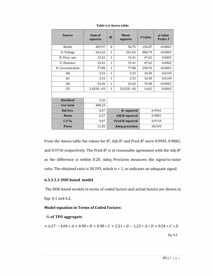
89 | P a g e

Table 6.6 Anova table

Source

Sum of

squares df

Mean

squares F value

p value

Prob> F

Model 405.97 8 50.75 156.87 <0.0001

A: Voltage 261.63 1 261.63 808.79 <0.0001

B: Flow rate 15.41 1 15.41 47.62 0.0002

C: Distance 15.41 1 15.41 47.62 0.0002

D: Concentration 77.88 1 77.88 240.76 <0.0001

AB 3.33 1 3.33 10.30 0.0149

AC 3.33 1 3.33 10.30 0.0149

AD 24.26 1 24.26 74.98 <0.0001

CD 5.625E‒.03 1 5.625E‒.03 14.62 0.0065

Residual 2.26

Cor total 408.23

Std Dev. 0.57 R- squared 0.9945

Mean 6.27 Adj R-squared 0.9881

C.V.% 9.07 Pred R-squared 0.9710

Press 11.83 Adeq precision 38.593

From the Anova table the values for R2, Adj-R2 and Pred-R2 were 0.9945, 0.9881,

and 0.9710 respectively. The Pred-R2 is in reasonable agreement with the Adj-R2

as the difference is within 0.20. Adeq Precision measures the signal-to-noise

ratio. The obtained ratio is 38.593, which is > 1, so indicates an adequate signal.

6.3.3.1.3 DOE based model

The DOE-based models in terms of coded factors and actual factors are shown in

Eqs. 6.1 and 6.2.

Model equation in Terms of Coded Factors:

%CDEFGHHIJHGKJ= 6.27 − 4.04 ∗ P + 0.98 ∗ S + 0.98 ∗ T + 2.21 ∗ V − 1.23 ∗ P ∗ V + 0.54 ∗ T ∗ V Eq. 6.2

90 | P a g e

Model equation in terms of actual factors:

%CDEFGHHIJHGKJ= 0.05717 + 0.01963 ∗ Y�#���� + 4.547 ∗ �#�*���� + 0.10 ∗ ,')���$�+ 0.278 ∗ $��$������'�� − 0.1354 ∗ Y�#���� ∗ $��$������'�� + 4.873∗ ,')���$� ∗ $��$������'��

Eq. 6.3

A sensitivity analysis can be performed using the DOE-based equation above. If

we do not calculate the interaction influence, then

Increase per 0.1 mL/h flow rate → % area of TPU aggregate increases by 4.36%

Increase per 100 mg/L concentration → % area of TPU aggregate increases by

1.09%

Increase per 1 cm distance → % area of TPU aggregate decreases by 2.17%

Increase per 1kV voltage → % area of TPU aggregate decreases by 1.64%.

6.3.3.1.4 Diagnostics

In the normal probability plot in Figure 6.2(a), the points lie reasonably close to a

straight line, which indicates that A, B, C, D, AB, AC, AD, BC and CD are the

significant effects. In the plot of the residuals versus the predicted value y^

Figure 6.2(b), it can be confirmed that the residuals have a constant variance.

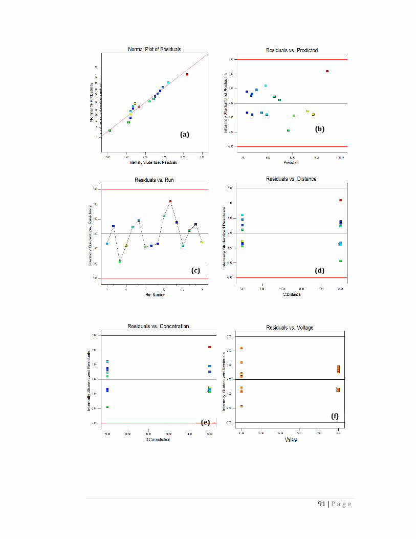
91 | P a g e

(a) (b)

(c) (d)

(e) (f)

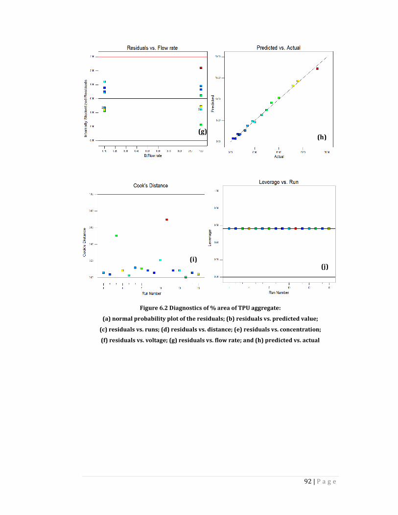
92 | P a g e

Figure 6.2 Diagnostics of % area of TPU aggregate:

(a) normal probability plot of the residuals; (b) residuals vs. predicted value;

(c) residuals vs. runs; (d) residuals vs. distance; (e) residuals vs. concentration;

(f) residuals vs. voltage; (g) residuals vs. flow rate; and (h) predicted vs. actual

(g) (h)

(i) (j)

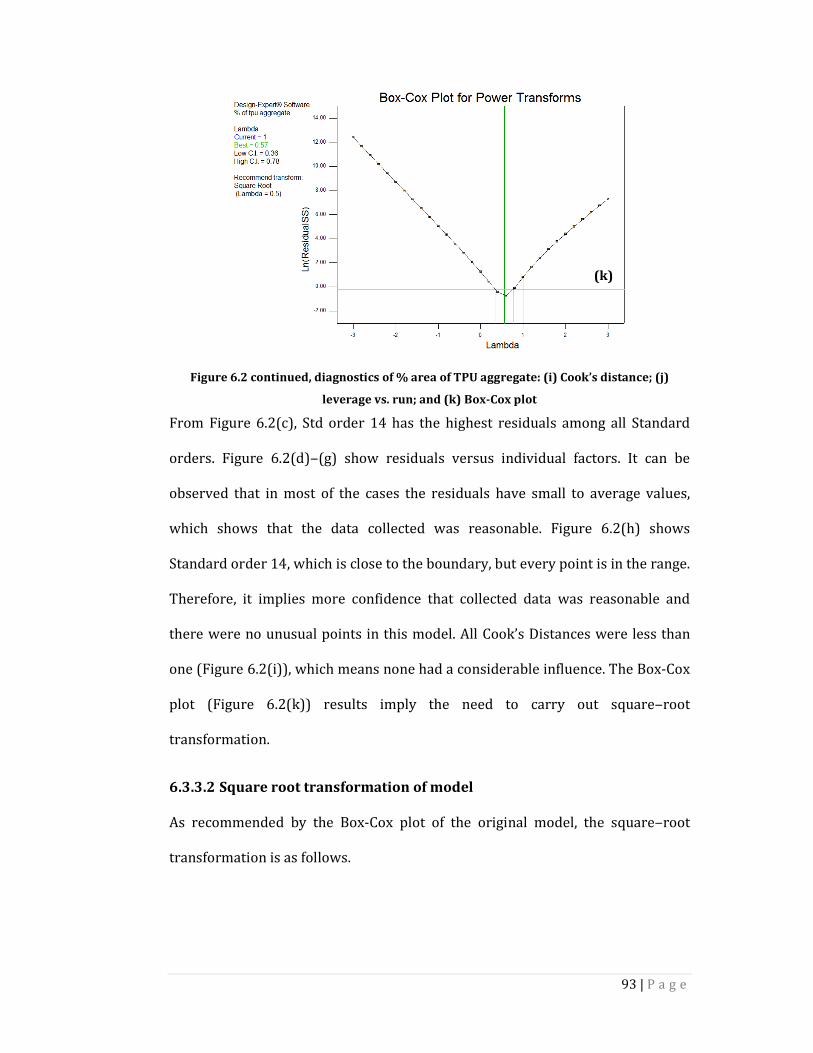
93 | P a g e

Figure 6.2 continued, diagnostics of % area of TPU aggregate: (i) Cook’s distance; (j)

leverage vs. run; and (k) Box-Cox plot

From Figure 6.2(c), Std order 14 has the highest residuals among all Standard

orders. Figure 6.2(d)‒(g) show residuals versus individual factors. It can be

observed that in most of the cases the residuals have small to average values,

which shows that the data collected was reasonable. Figure 6.2(h) shows

Standard order 14, which is close to the boundary, but every point is in the range.

Therefore, it implies more confidence that collected data was reasonable and

there were no unusual points in this model. All Cook’s Distances were less than

one (Figure 6.2(i)), which means none had a considerable influence. The Box-Cox

plot (Figure 6.2(k)) results imply the need to carry out square‒root

transformation.

6.3.3.2 Square root transformation of model

As recommended by the Box-Cox plot of the original model, the square‒root

transformation is as follows.

(k)

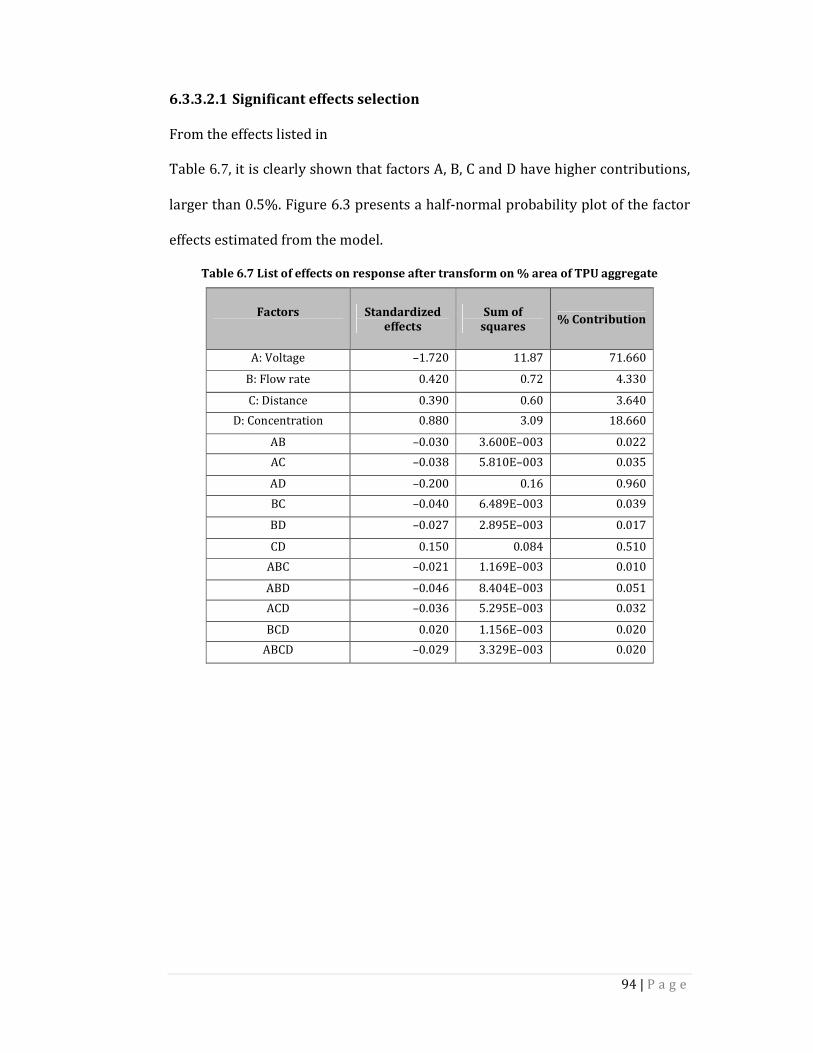
94 | P a g e

6.3.3.2.1 Significant effects selection

From the effects listed in

Table 6.7, it is clearly shown that factors A, B, C and D have higher contributions,

larger than 0.5%. Figure 6.3 presents a half-normal probability plot of the factor

effects estimated from the model.

Table 6.7 List of effects on response after transform on % area of TPU aggregate

Factors

Standardized

effects

Sum of

squares % Contribution

A: Voltage –1.720 11.87 71.660

B: Flow rate 0.420 0.72 4.330

C: Distance 0.390 0.60 3.640

D: Concentration 0.880 3.09 18.660

AB –0.030 3.600E–003 0.022

AC –0.038 5.810E–003 0.035

AD –0.200 0.16 0.960

BC –0.040 6.489E–003 0.039

BD –0.027 2.895E–003 0.017

CD 0.150 0.084 0.510

ABC –0.021 1.169E–003 0.010

ABD –0.046 8.404E–003 0.051

ACD –0.036 5.295E–003 0.032

BCD 0.020 1.156E–003 0.020

ABCD –0.029 3.329E–003 0.020

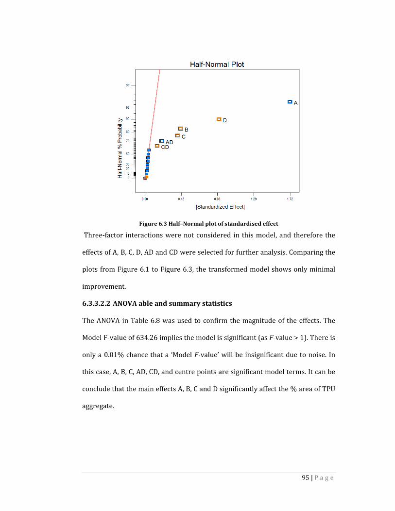
95 | P a g e

Figure 6.3 Half–Normal plot of standardised effect

Three-factor interactions were not considered in this model, and therefore the

effects of A, B, C, D, AD and CD were selected for further analysis. Comparing the

plots from Figure 6.1 to Figure 6.3, the transformed model shows only minimal

improvement.

6.3.3.2.2 ANOVA able and summary statistics

The ANOVA in Table 6.8 was used to confirm the magnitude of the effects. The

Model F-value of 634.26 implies the model is significant (as F-value > 1). There is

only a 0.01% chance that a ‘Model F-value’ will be insignificant due to noise. In

this case, A, B, C, AD, CD, and centre points are significant model terms. It can be

conclude that the main effects A, B, C and D significantly affect the % area of TPU

aggregate.

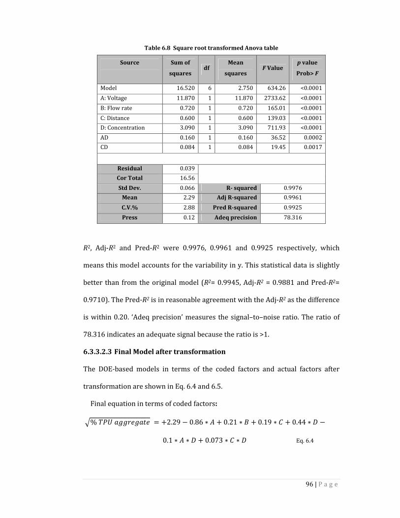
96 | P a g e

Table 6.8 Square root transformed Anova table

Source

Sum of

squares df

Mean

squares F Value

p value

Prob> F

Model 16.520 6 2.750 634.26 <0.0001

A: Voltage 11.870 1 11.870 2733.62 <0.0001

B: Flow rate 0.720 1 0.720 165.01 <0.0001

C: Distance 0.600 1 0.600 139.03 <0.0001

D: Concentration 3.090 1 3.090 711.93 <0.0001

AD 0.160 1 0.160 36.52 0.0002

CD 0.084 1 0.084 19.45 0.0017

Residual 0.039

Cor Total 16.56

Std Dev. 0.066 R- squared 0.9976

Mean 2.29 Adj R-squared 0.9961

C.V.% 2.88 Pred R-squared 0.9925

Press 0.12 Adeq precision 78.316

R2, Adj-R2 and Pred-R2 were 0.9976, 0.9961 and 0.9925 respectively, which

means this model accounts for the variability in y. This statistical data is slightly

better than from the original model (R2= 0.9945, Adj-R2 = 0.9881 and Pred-R2=

0.9710). The Pred-R2 is in reasonable agreement with the Adj-R2 as the difference

is within 0.20. ‘Adeq precision’ measures the signal–to–noise ratio. The ratio of

78.316 indicates an adequate signal because the ratio is >1.

6.3.3.2.3 Final Model after transformation

The DOE-based models in terms of the coded factors and actual factors after

transformation are shown in Eq. 6.4 and 6.5.

Final equation in terms of coded factors:

Z%������������ = +2.29 − 0.86 ∗ P + 0.21 ∗ S + 0.19 ∗ T + 0.44 ∗ V −0.1 ∗ P ∗ V + 0.073 ∗ T ∗ V Eq. 6.4

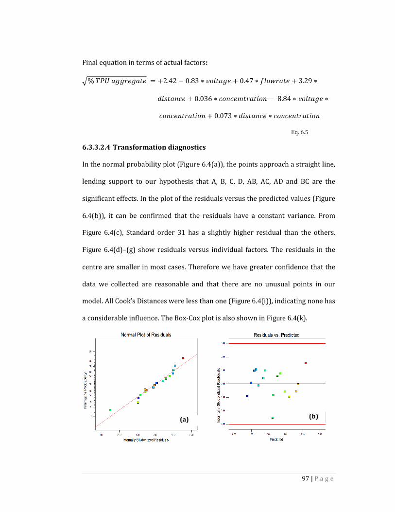
97 | P a g e

Final equation in terms of actual factors:

Z%������������ = +2.42 − 0.83 ∗ Y�#���� + 0.47 ∗ �#�*���� + 3.29 ∗,')���$� + 0.036 ∗ $��$�!����'�� − 8.84 ∗ Y�#���� ∗$��$������'�� + 0.073 ∗ ,')���$� ∗ $��$������'��

Eq. 6.5

6.3.3.2.4 Transformation diagnostics

In the normal probability plot (Figure 6.4(a)), the points approach a straight line,

lending support to our hypothesis that A, B, C, D, AB, AC, AD and BC are the

significant effects. In the plot of the residuals versus the predicted values (Figure

6.4(b)), it can be confirmed that the residuals have a constant variance. From

Figure 6.4(c), Standard order 31 has a slightly higher residual than the others.

Figure 6.4(d)–(g) show residuals versus individual factors. The residuals in the

centre are smaller in most cases. Therefore we have greater confidence that the

data we collected are reasonable and that there are no unusual points in our

model. All Cook’s Distances were less than one (Figure 6.4(i)), indicating none has

a considerable influence. The Box-Cox plot is also shown in Figure 6.4(k).

(a) (b)

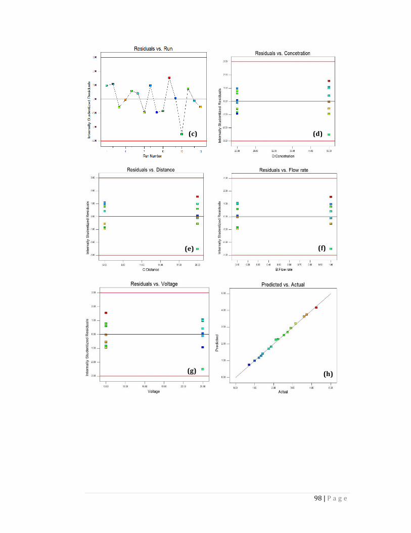
98 | P a g e

(c) (d)

(e) (f)

(g) (h)

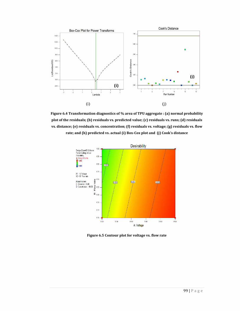
99 | P a g e

(i) (j)

Figure 6.4 Transformation diagnostics of % area of TPU aggregate : (a) normal probability

plot of the residuals; (b) residuals vs. predicted value; (c) residuals vs. runs; (d) residuals

vs. distance; (e) residuals vs. concentration; (f) residuals vs. voltage; (g) residuals vs. flow

rate; and (h) predicted vs. actual (i) Box-Cox plot and (j) Cook’s distance

Figure 6.5 Contour plot for voltage vs. flow rate

(i)

(j)

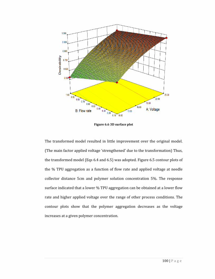
100 | P a g e

Figure 6.6 3D surface plot

The transformed model resulted in little improvement over the original model.

(The main factor applied voltage ‘strengthened’ due to the transformation) Thus,

the transformed model (Eqs 6.4 and 6.5) was adopted. Figure 6.5 contour plots of

the % TPU aggregation as a function of flow rate and applied voltage at needle

collector distance 5cm and polymer solution concentration 5%. The response

surface indicated that a lower % TPU aggregation can be obtained at a lower flow

rate and higher applied voltage over the range of other process conditions. The

contour plots show that the polymer aggregation decreases as the voltage

increases at a given polymer concentration.

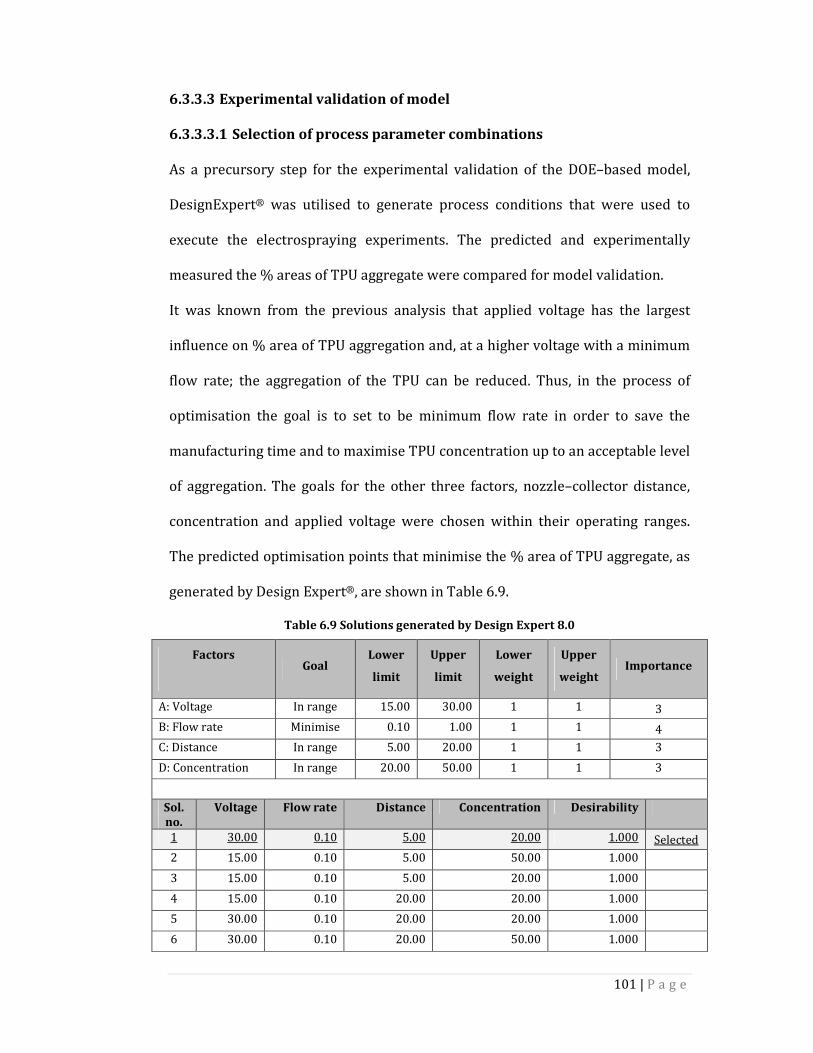
101 | P a g e

6.3.3.3 Experimental validation of model

6.3.3.3.1 Selection of process parameter combinations

As a precursory step for the experimental validation of the DOE–based model,

DesignExpert® was utilised to generate process conditions that were used to

execute the electrospraying experiments. The predicted and experimentally

measured the % areas of TPU aggregate were compared for model validation.

It was known from the previous analysis that applied voltage has the largest

influence on % area of TPU aggregation and, at a higher voltage with a minimum

flow rate; the aggregation of the TPU can be reduced. Thus, in the process of

optimisation the goal is to set to be minimum flow rate in order to save the

manufacturing time and to maximise TPU concentration up to an acceptable level

of aggregation. The goals for the other three factors, nozzle–collector distance,

concentration and applied voltage were chosen within their operating ranges.

The predicted optimisation points that minimise the % area of TPU aggregate, as

generated by Design Expert®, are shown in Table 6.9.

Table 6.9 Solutions generated by Design Expert 8.0

Factors

Goal

Lower

limit

Upper

limit

Lower

weight

Upper

weight Importance

A: Voltage In range 15.00 30.00 1 1 3

B: Flow rate Minimise 0.10 1.00 1 1 4

C: Distance In range 5.00 20.00 1 1 3

D: Concentration In range 20.00 50.00 1 1 3

Sol.

no.

Voltage Flow rate Distance Concentration Desirability

1 30.00 0.10 5.00 20.00 1.000 Selected

2 15.00 0.10 5.00 50.00 1.000

3 15.00 0.10 5.00 20.00 1.000

4 15.00 0.10 20.00 20.00 1.000

5 30.00 0.10 20.00 20.00 1.000

6 30.00 0.10 20.00 50.00 1.000

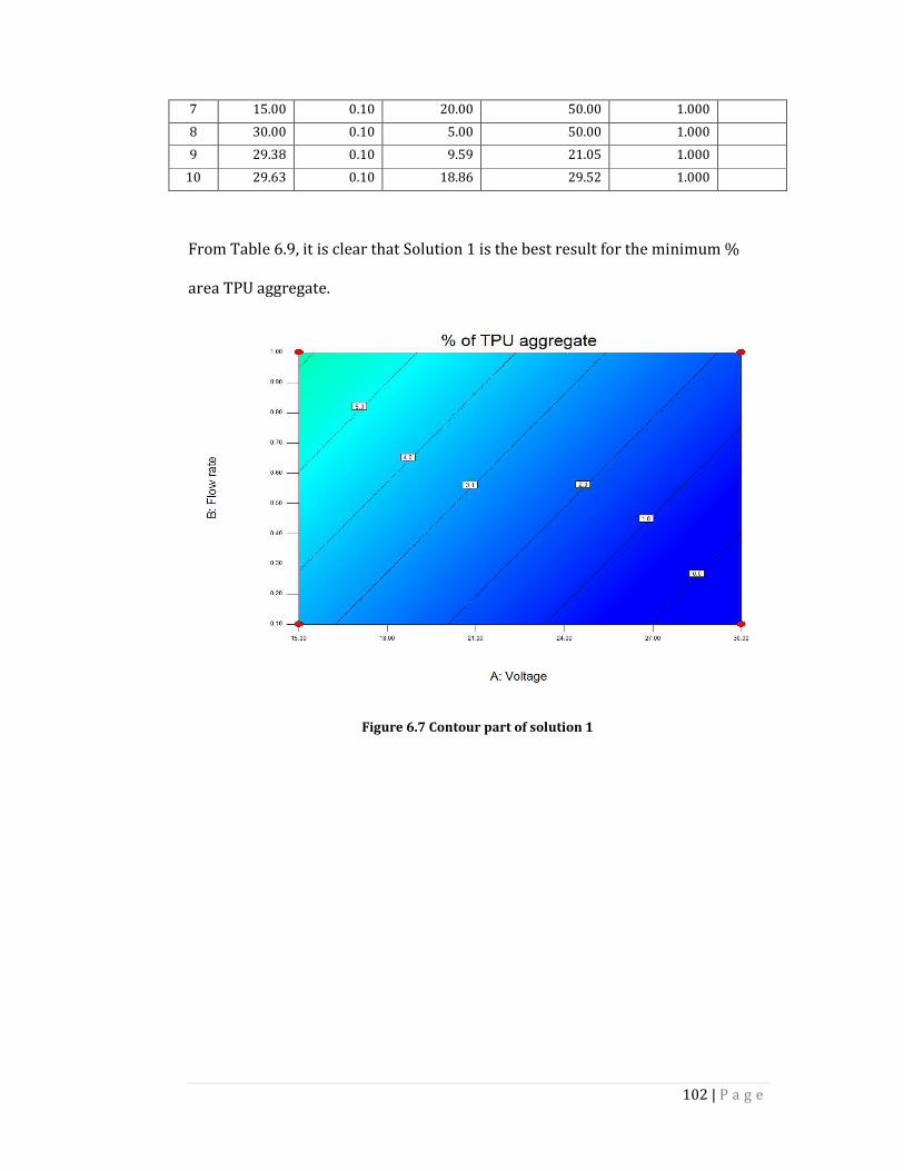
102 | P a g e

7 15.00 0.10 20.00 50.00 1.000

8 30.00 0.10 5.00 50.00 1.000

9 29.38 0.10 9.59 21.05 1.000

10 29.63 0.10 18.86 29.52 1.000

From Table 6.9, it is clear that Solution 1 is the best result for the minimum %

area TPU aggregate.

Figure 6.7 Contour part of solution 1

103 | P a g e

Figure 6.8 3D surface plot of solution 1

Contour and 3D surface plots (Figure 6.7 and Figure 6.8) provide the location of

the predicted optimisation solution of the model.

6.3.3.3.2 Point prediction

From Table 6.10, the confidence level of every response can be seen. This scale

can help to predict a new point, if new observation is to be added. It also provides

direction for predicting the confidence of entire data.

Table 6.10 Predication factor table

Factor Name Level Low

level

High

level Std Dev. Coding

A Voltage 17.50 5.00 30.00 0.00 Actual

B Flow rate 0.55 0.10 1.00 0.00 Actual

C Distance 12.50 5.00 20.00 0.00 Actual

D Concentration 35.00 20.00 50.00 0.00 Actual

Response Pred. Std Dev. 95% CI

low

95% CI

high

% TPU aggregation 5.2 % 5.1 5.4

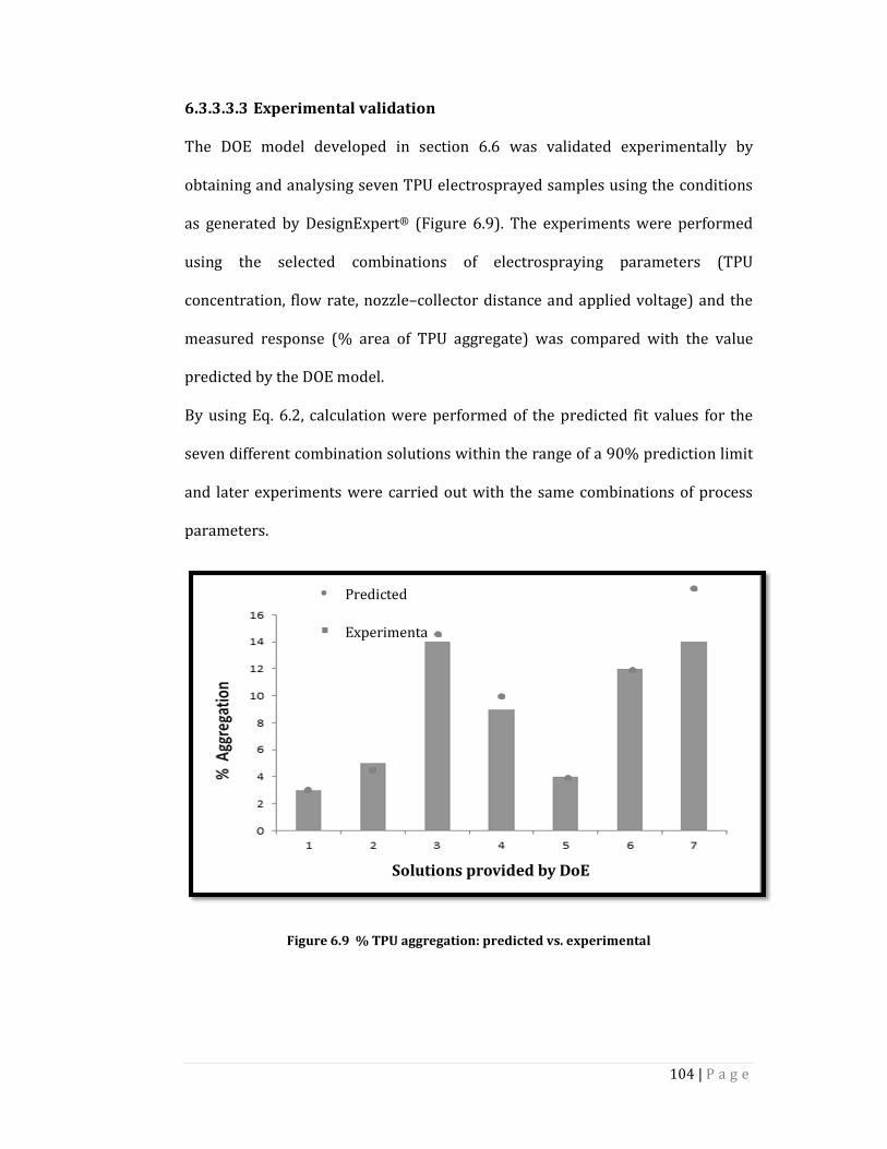
104 | P a g e

6.3.3.3.3 Experimental validation

The DOE model developed in section 6.6 was validated experimentally by

obtaining and analysing seven TPU electrosprayed samples using the conditions

as generated by DesignExpert® (Figure 6.9). The experiments were performed

using the selected combinations of electrospraying parameters (TPU

concentration, flow rate, nozzle–collector distance and applied voltage) and the

measured response (% area of TPU aggregate) was compared with the value

predicted by the DOE model.

By using Eq. 6.2, calculation were performed of the predicted fit values for the

seven different combination solutions within the range of a 90% prediction limit

and later experiments were carried out with the same combinations of process

parameters.

Figure 6.9 % TPU aggregation: predicted vs. experimental

Solutions provided by DoE

• Predicted

� Experimenta

105 | P a g e

From Figure 6.9 it can be observed that the values of responses obtained from

the experiments were within 90% prediction interval, which validates the

accuracy of the DOE model. There was significant difference observed between

actual and predicted value for run number 7 due to some noise.

6.4 Conclusion

From the two-way analysis of variance, it can be concluded that applied voltage

and concentration had the highest influence on the % area of TPU aggregate in

electrospraying, which suggests that setting a high voltage and minimise the

concentration are the key. From the half-normal plot of the factor effects of the

model, we can see that TPU flow rate and nozzle–collector distance are also the

main factors in our model. All four factors have some degrees of influence on the

% area of TPU aggregate. However, in the transformed model there is not much

difference in contribution of all factors compared to original model.

In this design of experiments, utilising two replications and two blocks greatly

improved model accuracy. From the blocks assigned (Figure 6.3), it can be seen

that blocks 1 and 2 ran the same combinations of factors, the full 24 model. This

compensated for potential experimental errors. The validation of the feasible

optimisation solutions proofs can be applied to the experimental model to

predict the % area of TPU aggregate, which can serve as an indirect method of

assessing the degree of TPU dispersion and can achieve a high quality TPU

dispersion using electrospraying.

106 | P a g e

Chapter 7

Influence of electrospraying process parameters on droplet

size distribution

The significant research work discussed in this chapter has been published:

Jadhav, A., L. Wang, and R. Padhye, Influence of applied voltage on droplet size

distribution in electrospraying of thermoplastic polyurethane. International

Journal of Applied Mechanics and Materials, 2013. 2(3): p. 64.

7.1 Introduction

Electrospraying is a one–step technique which can generate narrow size

distributions of submicron size droplets, with limited agglomeration of droplets

and high yield [144]. The principles of electrospraying are based on the

capability of an electric field to deform the interface of polymer drop, first

investigated by Lord Rayleigh in 1882 [67] and further investigated by Zeleny in

1917 [145] and Taylor in 1964 [114]. The theory of the charged droplet suggests

that if a very high electric field is applied to a polymer droplet, the electric charge

generates an electrical force inside the droplet, known as the Coulomb force,

which competes with the cohesive force intrinsic to the droplet. When the

applied Coulomb force overcomes the cohesive force of droplet manifested in the

surface tension, the polymer droplet explodes into very fine droplets in micro–

nano scales [146].

This activity happens at the Taylor cone, referring to the progressive shrinkage of

unstable, charged micro droplet into a cone from which the charged droplets are

ejected as soon as the surface tension is overcome by the Coulomb force.

Rayleigh predicted the limit for determining the breakup of the droplet, called

107 | P a g e

the Rayleigh Limit, LR, expressed in Eq. 7.1, where LR is a function of q, the surface

charge of the droplet, Ɛ, the permittivity of the surrounding medium, ϒ, the

surface tension of liquid and R, is the radius of the droplet. The maximum surface

charge of the droplet is given by Eq. 7.2 [67]. Based on these equations,

monodisperse electrosprayed droplets can be fabricated by using optimum

process parameters.

LR = q (64π2ƐϒR3) Eq. 7.1

Q= 8π √Ɛ0ϒR3 Eq. 7.2

During the electrospraying process, many parameters interdependently

influence on droplet size distribution [144]. In this research, the effect of process

parameters on the polymer droplet size distribution in electrospraying was

studied.

7.2 Experimental

Chemicals 7.2.1

A solution of 2.5% polyurethane was prepared by dissolving the TPU polymer

granules homogeneously in THF for the electrospraying.

Electrospraying: 7.2.2

A similar arrangement of the electrospraying apparatus was used as discussed in

chapter 3. The process parameters are described in Table 7.1.

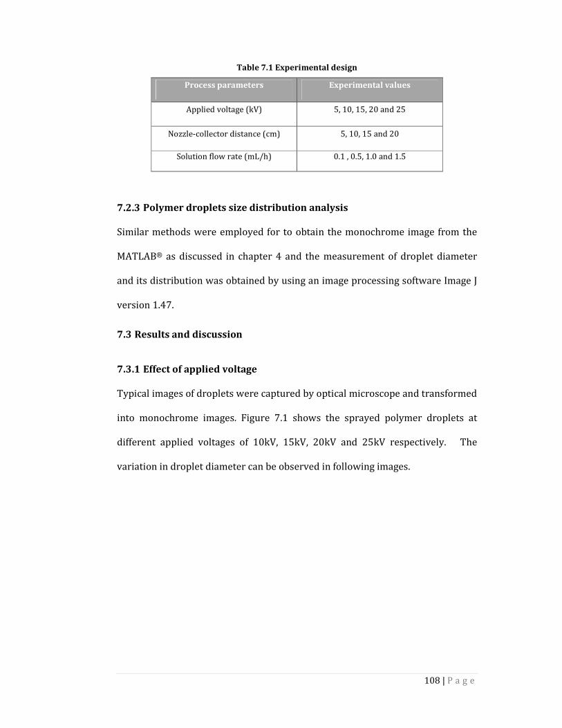
108 | P a g e

Table 7.1 Experimental design

Process parameters Experimental values

Applied voltage (kV) 5, 10, 15, 20 and 25

Nozzle-collector distance (cm) 5, 10, 15 and 20

Solution flow rate (mL/h) 0.1 , 0.5, 1.0 and 1.5

Polymer droplets size distribution analysis 7.2.3

Similar methods were employed for to obtain the monochrome image from the

MATLAB® as discussed in chapter 4 and the measurement of droplet diameter

and its distribution was obtained by using an image processing software Image J

version 1.47.

7.3 Results and discussion

Effect of applied voltage 7.3.1

Typical images of droplets were captured by optical microscope and transformed

into monochrome images. Figure 7.1 shows the sprayed polymer droplets at

different applied voltages of 10kV, 15kV, 20kV and 25kV respectively. The

variation in droplet diameter can be observed in following images.

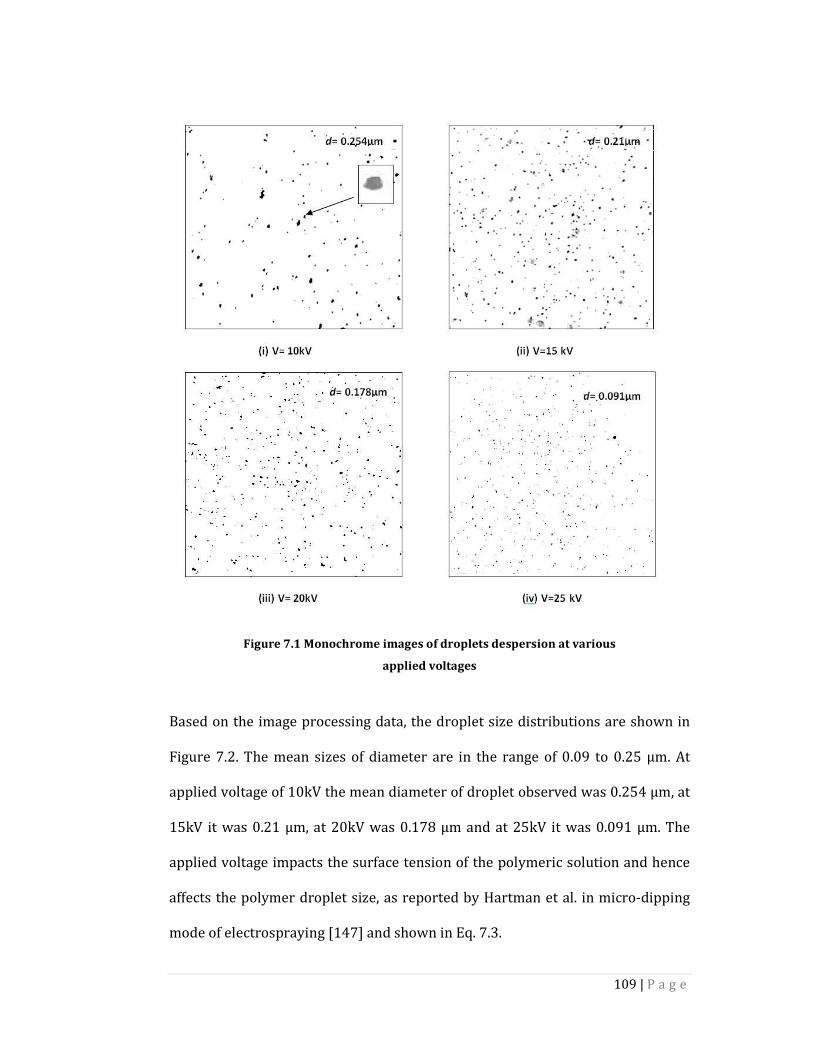
109 | P a g e

Figure 7.1 Monochrome images of droplets despersion at various

applied voltages

Based on the image processing data, the droplet size distributions are shown in

Figure 7.2. The mean sizes of diameter are in the range of 0.09 to 0.25 µm. At

applied voltage of 10kV the mean diameter of droplet observed was 0.254 µm, at

15kV it was 0.21 µm, at 20kV was 0.178 µm and at 25kV it was 0.091 µm. The

applied voltage impacts the surface tension of the polymeric solution and hence

affects the polymer droplet size, as reported by Hartman et al. in micro-dipping

mode of electrospraying [147] and shown in Eq. 7.3.

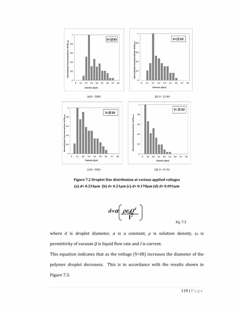
110 | P a g e

Figure 7.2 Droplet Size distribution at various applied voltages

(a) d= 0.254µm (b) d= 0.21µm (c) d= 0.178µm (d) d= 0.091µm

Eq. 7.3

where d is droplet diameter, α is a constant, ρ is solution density, ԑ0 is

permittivity of vacuum Q is liquid flow rate and I is current.

This equation indicates that as the voltage (V=IR) increases the diameter of the

polymer droplet decreases. This is in accordance with the results shown in

Figure 7.3.

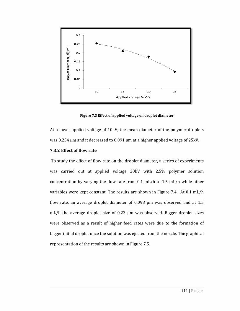
111 | P a g e

Figure 7.3 Effect of applied voltage on droplet diameter

At a lower applied voltage of 10kV, the mean diameter of the polymer droplets

was 0.254 µm and it decreased to 0.091 µm at a higher applied voltage of 25kV.

Effect of flow rate 7.3.2

To study the effect of flow rate on the droplet diameter, a series of experiments

was carried out at applied voltage 20kV with 2.5% polymer solution

concentration by varying the flow rate from 0.1 mL/h to 1.5 mL/h while other

variables were kept constant. The results are shown in Figure 7.4. At 0.1 mL/h

flow rate, an average droplet diameter of 0.098 µm was observed and at 1.5

mL/h the average droplet size of 0.23 µm was observed. Bigger droplet sizes

were observed as a result of higher feed rates were due to the formation of

bigger initial droplet once the solution was ejected from the nozzle. The graphical

representation of the results are shown in Figure 7.5.

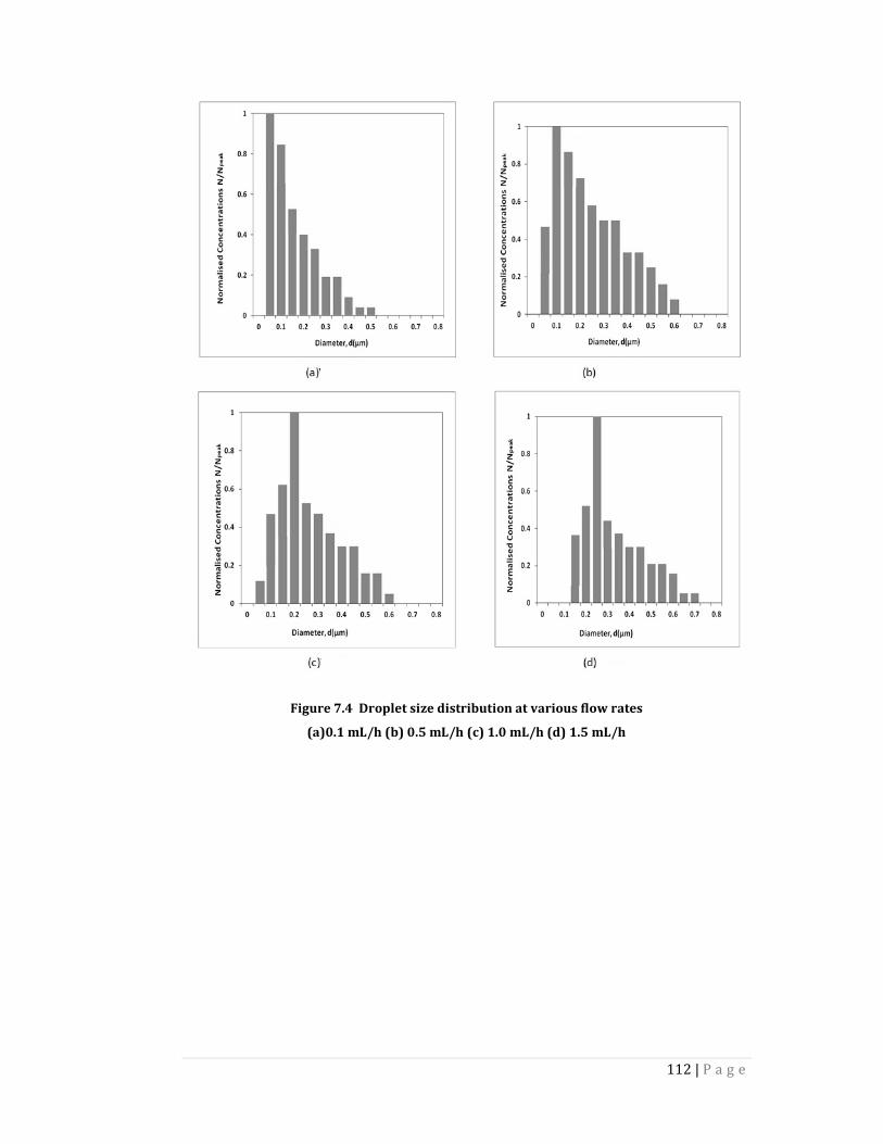
112 | P a g e

Figure 7.4 Droplet size distribution at various flow rates

(a)0.1 mL/h (b) 0.5 mL/h (c) 1.0 mL/h (d) 1.5 mL/h

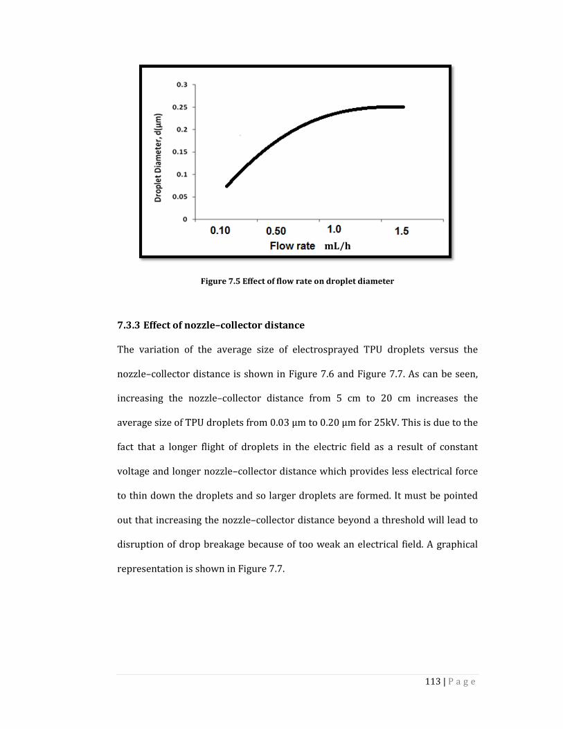
113 | P a g e

Figure 7.5 Effect of flow rate on droplet diameter

Effect of nozzle–collector distance 7.3.3

The variation of the average size of electrosprayed TPU droplets versus the

nozzle–collector distance is shown in Figure 7.6 and Figure 7.7. As can be seen,

increasing the nozzle–collector distance from 5 cm to 20 cm increases the

average size of TPU droplets from 0.03 µm to 0.20 µm for 25kV. This is due to the

fact that a longer flight of droplets in the electric field as a result of constant

voltage and longer nozzle–collector distance which provides less electrical force

to thin down the droplets and so larger droplets are formed. It must be pointed

out that increasing the nozzle–collector distance beyond a threshold will lead to

disruption of drop breakage because of too weak an electrical field. A graphical

representation is shown in Figure 7.7.

mL/h

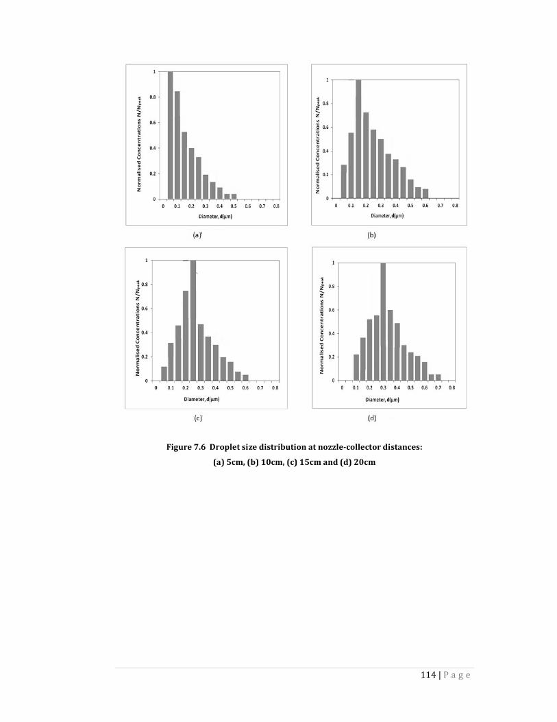
114 | P a g e

Figure 7.6 Droplet size distribution at nozzle-collector distances:

(a) 5cm, (b) 10cm, (c) 15cm and (d) 20cm

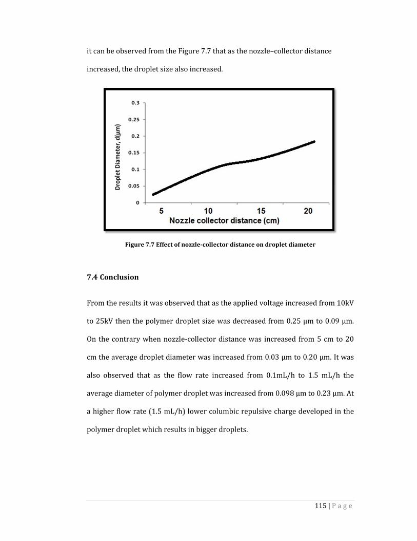
115 | P a g e

it can be observed from the Figure 7.7 that as the nozzle–collector distance

increased, the droplet size also increased.

Figure 7.7 Effect of nozzle-collector distance on droplet diameter

7.4 Conclusion

From the results it was observed that as the applied voltage increased from 10kV

to 25kV then the polymer droplet size was decreased from 0.25 µm to 0.09 µm.

On the contrary when nozzle-collector distance was increased from 5 cm to 20

cm the average droplet diameter was increased from 0.03 µm to 0.20 µm. It was

also observed that as the flow rate increased from 0.1mL/h to 1.5 mL/h the

average diameter of polymer droplet was increased from 0.098 µm to 0.23 µm. At

a higher flow rate (1.5 mL/h) lower columbic repulsive charge developed in the

polymer droplet which results in bigger droplets.

116 | P a g e

Chapter 8

Application of electrospraying coating on textile substrate

8.1 Introduction

The use of coated textiles for protective clothing, shelters, covers, liquid

containers etc. dates back to antiquity. Historically, the earliest recorded use of

coated textile was by the ancient people of Central and South America, who

applied latex to a fabric to render it waterproof [1]. Today, coated fabrics are

essentially polymer-coated textiles. Advances in polymer and textile technologies

have led to phenomenal growth in the application of coated fabrics for many

diverse end uses. Coated fabrics find an important place among technical textiles

and are one of the most important technological processes in the modern textile

industry.

The properties of a coated fabric depend on the type of polymer used and its

formulation, the nature of the textile substrate, and the coating method

employed. As reviewed in chapter 1, most coated textiles are produced by

conventional coating methods such as knife or roller coating. There are

problems associated with these coating methods, for example, impregnation of

the polymer into the yarn/fibre interstices, which alters the original properties of

the fabric. Electrospray coating has the ability to deposit polymer droplets at

submicron level due to electrostatic charging. The submicron level coating

facilitates the retention of the fabric’s original properties so that the fabric can

deliver additional functional properties depending on the polymer

characteristics.

117 | P a g e

In chapter 7 we studied the production of very fine TPU droplets through

electrostatic spraying. The fine spray of polymer droplets results in very smooth

and even coating. Surface coating of polymer with electrospraying is a promising

technology for the near future in the field of coating of materials [28].

Electrospraying has opened new routes to nanotechnology. Electrospraying is

used for micro– and nano–thinfilm deposition [36], micro– and nano–particle

production [148, 149], and micro– and nano–capsule formation. Thin films and

fine powders are (or potentially could be) used in modern material

technologies[150], microelectronics and medical technology [151, 152]. This

chapter discusses the potential applications of electrospraying as a coating

technique for textile substrates. Thermoplastic polyurethane was sprayed onto

cotton fabric to impart waterproof–breathable functionality. Chitosan was also

sprayed to impart antimicrobial properties to wool fabric.

8.2 Experimental

Materials 8.2.1

A solution of 2.5% TPU was prepared by dissolving the polymer granules

homogeneously in THF for the electrospraying. Chitosan was dissolved in 1%

(w/v) acetic acid until a clear solution was achieved. Freshly prepared solutions

were used for all the experiments.

Woven cotton and wool fabrics were chosen for this study to enhance their

properties. The fabric specifications are reported in chapter 3.

118 | P a g e

Electrospraying 8.2.2

A similar arrangement of the electrospraying apparatus was used as discussed in

chapter 3.

Scanning electron microscope (SEM) 8.2.3

Scanning electron microscopy (SEM) was used to study the coated surface

morphology. SEM uses a focused beam of high–energy electrons to generate a

variety of signals at the surface of solid specimens. The signals that derive from

electron–sample interaction reveal information about the sample including

external morphology (texture), chemical composition and crystalline structure.

In most applications, data is collected over a selected area of the surface of the

sample and a 2-dimensional image is generated that displays spatial variations in

these properties. Areas ranging from approximately 1 cm to 5 microns in width

can be imaged in magnification ranging from 20X to approximately 30,000X.

All the samples were coated with platinum in order to achieve high resolution images.

Contact angle measurement 8.2.4

Contact angle measurement is important for assessing the hydrophobicity of the

textile material after polymer coating. The contact angle measurement was done

using the PsS OCA 20 contact angle measurement instrument .The contact angle

was measured by producing a drop of liquid on a solid surface. The contact angle

was measured twice during the experiments, firstly 1 second after the droplet

formed on the surface and secondly after 120 seconds. The results were

compared before and after coating.

119 | P a g e

FTIR (Fourier transform infra-red spectroscopy) 8.2.5

FTIR was used to determine changes in the chemical structure by the effects of

electrospray coating on various textile substrates. The FTIR spectra were

obtained by a spectrometer (the PerkinElmer Spectrum–400) to determine the

functional groups of the coated substrate. The number of scans per sample was 8

and FTIR spectra were obtained in the wave number region of 4000–650 cm–1.

Antimicrobial testing 8.2.6

This test was carried out to evaluate the chitosan sprayed wool nonwoven

substrate. A modified AATCC TM 100-2004 (clause 10.2) test method was

followed to assess the antibacterial properties of electrosprayed fabrics.

Escherichia coli (E. coli) strain AATCC 11229, a gram-negative bacterium, was

used as the test organism. Bacterial inoculums were prepared to obtain a

suspension in an exponential growth of 108 colony forming units (CFU) mL-1 in 5

mL of modified tryptone soya nutrient broth. Uncoated fabrics were used as

negative control samples.

Antibacterial tests were conducted on each sample individually, as outlined by

Zhang et al [153]. In brief, 1 ml of inoculum, prepared as described above, was

added to a fabric swatch of 4 cm diameter in a conical flask. Immediately 100 ml

of distilled water was added to the flask and this was shaken vigorously for 1

minute. From this solution, a series of dilutions were prepared at 100, 101, 102

and 103 times with sterile distilled water. The dilutions were then plated in

triplicates and incubated for 18 hours at 37°C. After incubation, the control plates

exhibiting 30–300 CFU were taken as a reference. Test plates of a similar dilution

120 | P a g e

%100)( ×−

X

YX

were compared. The percentage reduction of bacteria was calculated with

Eq. 8.1.

Eq. 8.1

where, X is average number of bacterial colonies in the agar plate from control

fabric, Y is average number of bacterial colonies in the agar plates from fabric

coated with chitosan.

Moisture management testing (MMT) 8.2.7

To study the moisture management properties of TPU coated cotton fabric, MMT

instrument was used. The MMT measures the liquid transfer in one step on a

fabric sample in multi-directions. In the present study, the coated surface of the

fabric samples is always a bottom surface (facing the bottom sensor) when the

sample is tested, imitating the case where the uncoated surface is in direct

contact with the skin.

Surface frictional properties 8.2.8

The KESFB4-A, Kato Tech Co. Ltd. Evaluation System was used to study the

frictional properties of fabrics after electrospraying. The sensors measured the

frictional coefficient and the roughness of the fabric surface simultaneously in

three different areas within a fabric sample.

The evaluation of the fabrics was carried out having particulars that:

• The value of MIU ranges from 0 to 1 and its approaching value of 1 is

interpreted as increasing friction and decreasing smoothness.

121 | P a g e

• The value of SMD ranges between 0 and 20 and its approaching value of

20 is interpreted as an increase in surface roughness and surface

irregularities.

8.3 Results and discussions

Morphology of fabric coated with conventional technique 8.3.1

Figure 8.7 shows the surface morphology of the TPU coated cotton fabric with

the roller coating technique. As shown in Figure 8.1(a), the polymer is

impregnated into the interstices of the yarns and fibres. All the yarns/fibres were

bonded together with polymer. As seen in Figure 8.1(b), the cross section of the

coated fabric, the yarn crossover points are also bonded due to polymer

impregnation. This is due to the fact that, in roller coating, the fabric is immersed

into the polymer solution bath and then passed through the rollers to squeeze

out the excess polymer. The polymer impregnation into the yarn interstices

affects the original properties of the fabric including air permeability, moisture

management, colouration, extension, tearing strength etc.

The electrospraying technique could have an advantage over conventional

coating technique due to submicron–level polymer droplets deposition. There is

no mechanical action involved in the process. The deposition is taking place with

the help of electrostatic charging. Figure 8.2 shows scanning electron images of

uncoated and TPU–coated cotton fabric substrates. As shown in Figure 8.2(b) the

tiny droplets of TPU polymer were deposited on the fibre surface and attached

only to the fibre surface not in the interstices of the fibres or yarns. Due to this,

the original properties of the cotton fabric are unaltered and the added

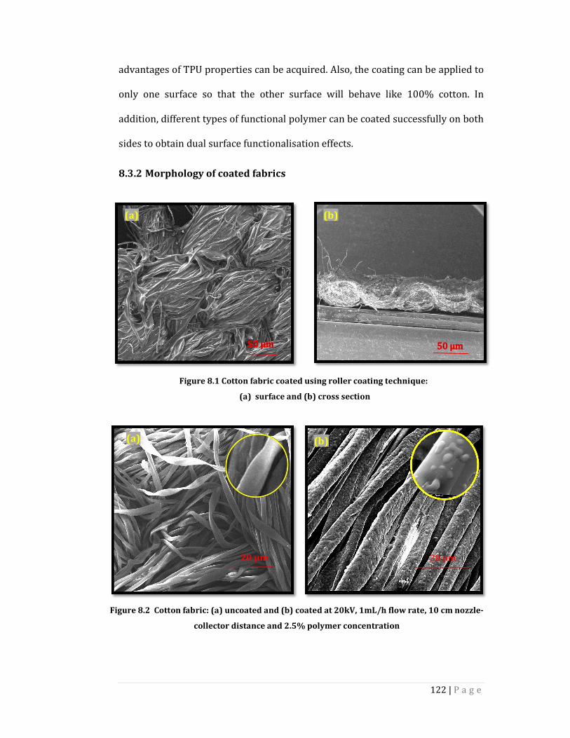
122 | P a g e

advantages of TPU properties can be acquired. Also, the coating can be applied to

only one surface so that the other surface will behave like 100% cotton. In

addition, different types of functional polymer can be coated successfully on both

sides to obtain dual surface functionalisation effects.

Morphology of coated fabrics 8.3.2

Figure 8.2 Cotton fabric: (a) uncoated and (b) coated at 20kV, 1mL/h flow rate, 10 cm nozzle-

collector distance and 2.5% polymer concentration

20 µm 20 µm

(a) (b)

(a) (b)

Figure 8.1 Cotton fabric coated using roller coating technique:

(a) surface and (b) cross section

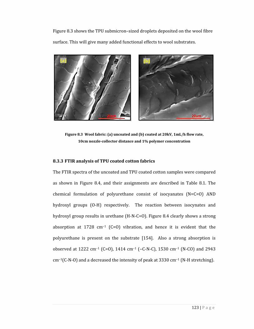
123 | P a g e

Figure 8.3 shows the TPU submicron–sized droplets deposited on the wool fibre

surface. This will give many added functional effects to wool substrates.

Figure 8.3 Wool fabric: (a) uncoated and (b) coated at 20kV, 1mL/h flow rate,

10cm nozzle-collector distance and 1% polymer concentration

FTIR analysis of TPU coated cotton fabrics 8.3.3

The FTIR spectra of the uncoated and TPU coated cotton samples were compared

as shown in Figure 8.4, and their assignments are described in Table 8.1. The

chemical formulation of polyurethane consist of isocyanates (N=C=O) AND

hydroxyl groups (O-H) respectively. The reaction between isocynates and

hydroxyl group results in urethane (H-N-C=O). Figure 8.4 clearly shows a strong

absorption at 1728 cm–1 (C=O) vibration, and hence it is evident that the

polyurethane is present on the substrate [154]. Also a strong absorption is

observed at 1222 cm–1 (C=O), 1414 cm–1 (‒C-N-C), 1530 cm–1 (N-CO) and 2943

cm–1(C-N-O) and a decreased the intensity of peak at 3330 cm–1 (N-H stretching).

(a) (b)

124 | P a g e

Figure 8.4 FTIR for uncoated and TPU–coated cotton fabrics

The presence of these peaks confirms that the TPU polymer droplets were

bonded to cotton fabric substrates.

Table 8.1 FTIR bands of TPU coated cotton samples with assignments

Wavenumber (cm–1) Vibrational assignments

1728 Strong C=O vibration

1414 C-N-C absorption

1530 Amide I N-C=O

2943 C-N-O vibration

3330 N-H stretching

Water contact–angle measurement 8.3.4

Water contact–angle measurements were made to observe any improvement in

hydrophobicity of the coated fabric after coating. The PsS OCA 20 static contact

angle measurement instrument was used to determine the contact angles. As

4000.0 3600 3200 2800 2400 2000 1800 1600 1400 1200 1000 800 650.0

62.5

64

66

68

70

72

74

76

78

80

82

84

86

88

90

92

94

96

98

99.0

Wavenumber cm-1

%T

3330.83

2943.82

1728.37

1597.12

1530.16

1311.04

1222.921105.31

TPU–coated Uncoated

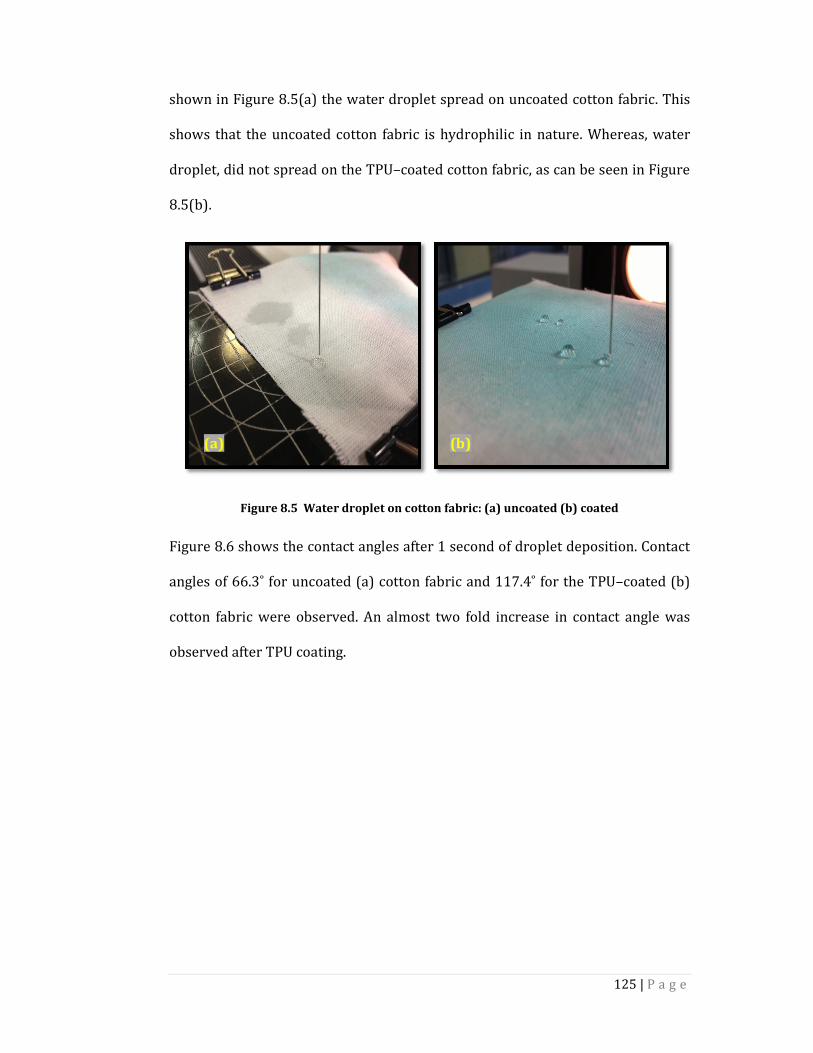
125 | P a g e

shown in Figure 8.5(a) the water droplet spread on uncoated cotton fabric. This

shows that the uncoated cotton fabric is hydrophilic in nature. Whereas, water

droplet, did not spread on the TPU–coated cotton fabric, as can be seen in Figure

8.5(b).

Figure 8.5 Water droplet on cotton fabric: (a) uncoated (b) coated

Figure 8.6 shows the contact angles after 1 second of droplet deposition. Contact

angles of 66.3˚ for uncoated (a) cotton fabric and 117.4˚ for the TPU–coated (b)

cotton fabric were observed. An almost two fold increase in contact angle was

observed after TPU coating.

(a) (b)

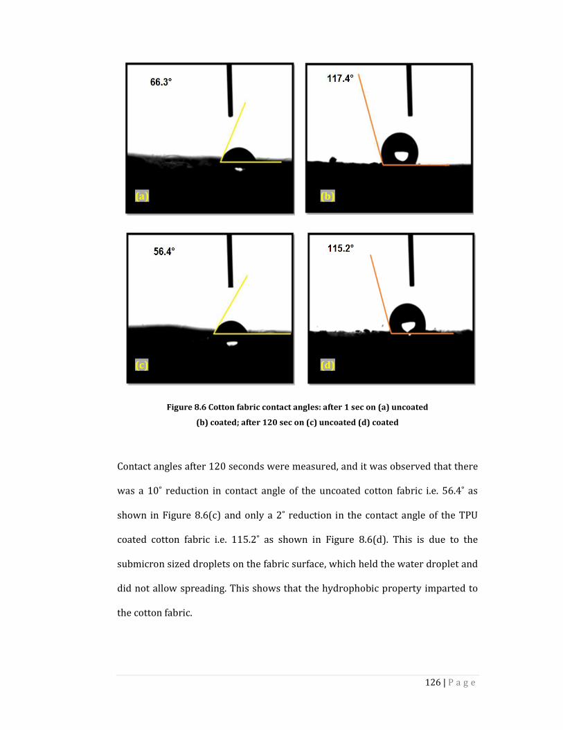
126 | P a g e

Figure 8.6 Cotton fabric contact angles: after 1 sec on (a) uncoated

(b) coated; after 120 sec on (c) uncoated (d) coated

Contact angles after 120 seconds were measured, and it was observed that there

was a 10˚ reduction in contact angle of the uncoated cotton fabric i.e. 56.4˚ as

shown in Figure 8.6(c) and only a 2˚ reduction in the contact angle of the TPU

coated cotton fabric i.e. 115.2˚ as shown in Figure 8.6(d). This is due to the

submicron sized droplets on the fabric surface, which held the water droplet and

did not allow spreading. This shows that the hydrophobic property imparted to

the cotton fabric.

(a) (b)

(c) (d)

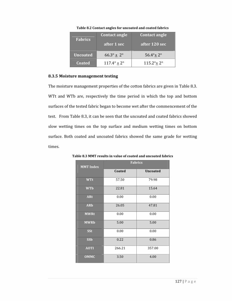
127 | P a g e

Table 8.2 Contact angles for uncoated and coated fabrics

Fabrics Contact angle

after 1 sec

Contact angle

after 120 sec

Uncoated 66.3° + 2° 56.4°+ 2°

Coated 117.4° + 2° 115.2°+ 2°

Moisture management testing 8.3.5

The moisture management properties of the cotton fabrics are given in Table 8.3.

WTt and WTb are, respectively the time period in which the top and bottom

surfaces of the tested fabric began to become wet after the commencement of the

test. From Table 8.3, it can be seen that the uncoated and coated fabrics showed

slow wetting times on the top surface and medium wetting times on bottom

surface. Both coated and uncoated fabrics showed the same grade for wetting

times.

Table 8.3 MMT results in value of coated and uncoated fabrics

MMT Index

Fabrics

Coated Uncoated

WTt 57.50 79.98

WTb 22.81 15.64

ARt 0.00 0.00

ARb 26.05 47.81

MWRt 0.00 0.00

MWRb 5.00 5.00

SSt 0.00 0.00

SSb 0.22 0.86

AOTI 266.21 357.00

OMMC 3.50 4.00

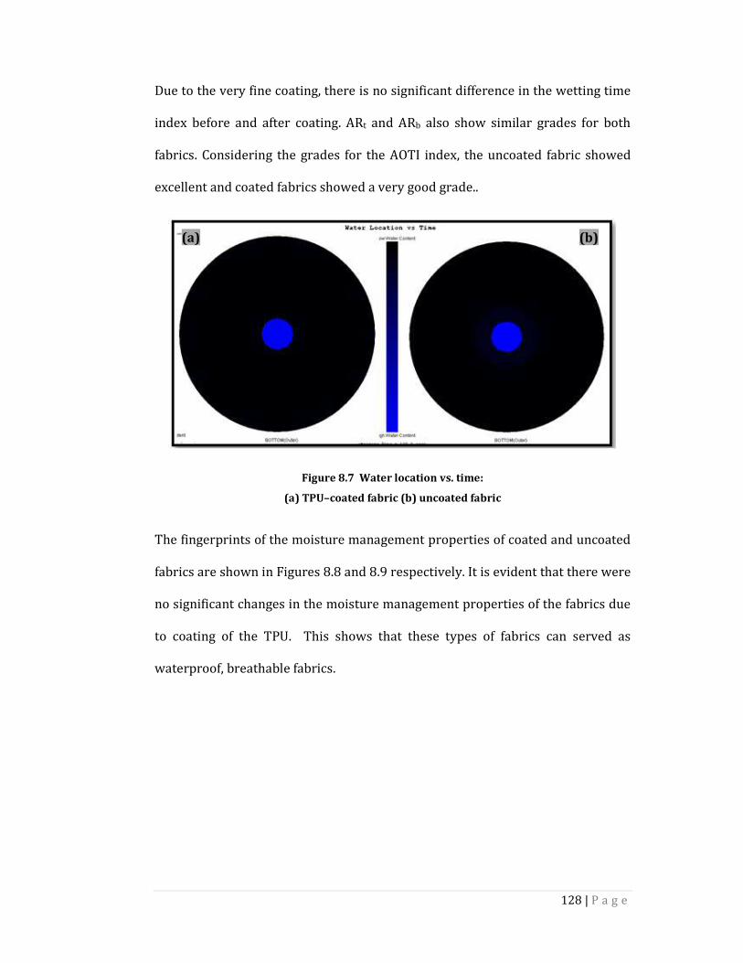
128 | P a g e

Due to the very fine coating, there is no significant difference in the wetting time

index before and after coating. ARt and ARb also show similar grades for both

fabrics. Considering the grades for the AOTI index, the uncoated fabric showed

excellent and coated fabrics showed a very good grade..

Figure 8.7 Water location vs. time:

(a) TPU–coated fabric (b) uncoated fabric

The fingerprints of the moisture management properties of coated and uncoated

fabrics are shown in Figures 8.8 and 8.9 respectively. It is evident that there were

no significant changes in the moisture management properties of the fabrics due

to coating of the TPU. This shows that these types of fabrics can served as

waterproof, breathable fabrics.

(a) (b)

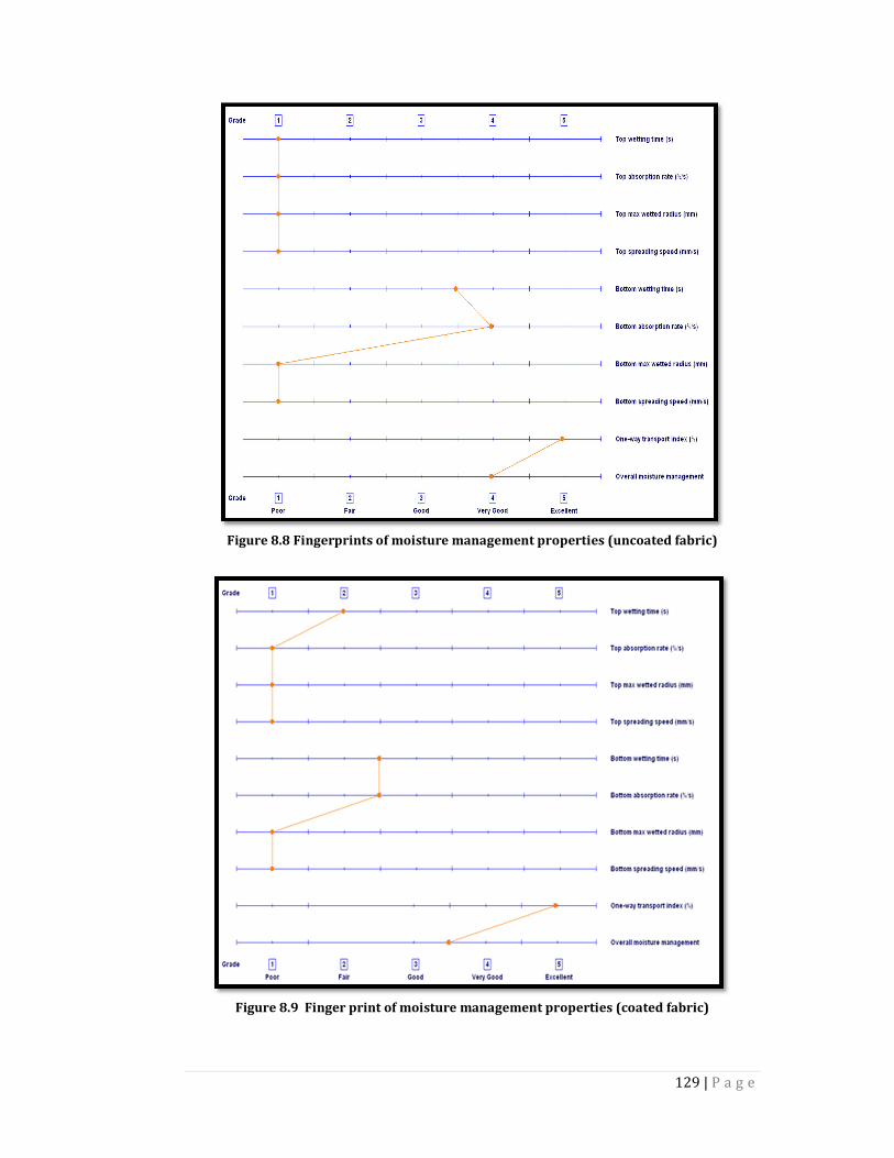
129 | P a g e

Figure 8.8 Fingerprints of moisture management properties (uncoated fabric)

Figure 8.9 Finger print of moisture management properties (coated fabric)

130 | P a g e

Surface roughness property 8.3.6

For the evaluation of fabric surface frictional properties, there are two main

attributes to be considered: coefficient of surface friction (MIU) and geometrical

roughness (SMD). In general, the frictional force is higher for fabric with a rough

surface and lower for fabric with a smooth surface. Table 8.4 demonstrates the

mean values of MIU and SMD for the coated and uncoated cotton fabric samples.

It can be observed that there was no significant change in surface frictional

properties. Figure 8.10 shows a graphical representation of the coefficient

friction (MIU) for uncoated and coated fabric surface. There was no significant

difference observed in MIU. Similarly, it can be observed from Figure 8.11 that

there was no significant difference in geometrical roughness of the coated and

uncoated fabric surfaces. This may be due to a very thin level of coating on the

surface which has not created any rough patterns on the fabric surface.

Table 8.4 Surface roughness properties of coated and uncoated fabrics

Surface roughness

Property Uncoated Fabric Coated Fabric

MIU 0.176 0.181

SMD 7.20 8.31

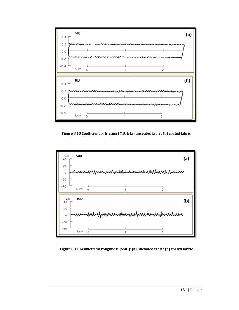
131 | P a g e

Figure 8.10 Coefficient of friction (MIU): (a) uncoated fabric (b) coated fabric

Figure 8.11 Geometrical roughness (SMD): (a) uncoated fabric (b) coated fabric

(a)

(b)

(a)

(b)

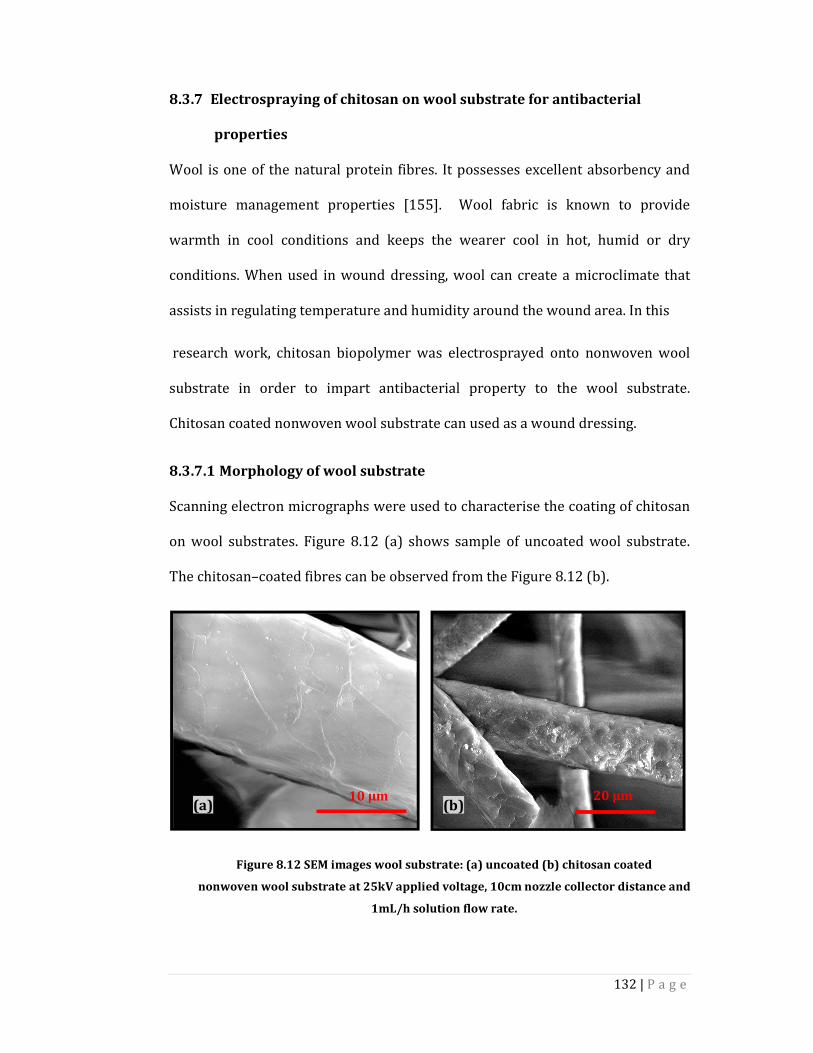
132 | P a g e

Electrospraying of chitosan on wool substrate for antibacterial 8.3.7

properties

Wool is one of the natural protein fibres. It possesses excellent absorbency and

moisture management properties [155]. Wool fabric is known to provide

warmth in cool conditions and keeps the wearer cool in hot, humid or dry

conditions. When used in wound dressing, wool can create a microclimate that

assists in regulating temperature and humidity around the wound area. In this

research work, chitosan biopolymer was electrosprayed onto nonwoven wool

substrate in order to impart antibacterial property to the wool substrate.

Chitosan coated nonwoven wool substrate can used as a wound dressing.

8.3.7.1 Morphology of wool substrate

Scanning electron micrographs were used to characterise the coating of chitosan

on wool substrates. Figure 8.12 (a) shows sample of uncoated wool substrate.

The chitosan–coated fibres can be observed from the Figure 8.12 (b).

Figure 8.12 SEM images wool substrate: (a) uncoated (b) chitosan coated

nonwoven wool substrate at 25kV applied voltage, 10cm nozzle collector distance and

1mL/h solution flow rate.

(a) (b) 20 µm 10 µm

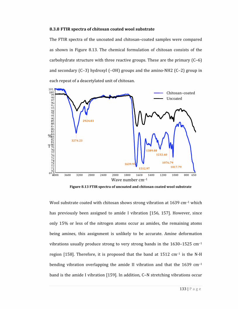
133 | P a g e

4000. 3600 3200 2800 2400 2000 1800 1600 1400 1200 1000 800 65069.3

707172737475767778798081828384858687888990919293949596979899

100101.1

Wave number cm–1

3274.23

2924.03

1639.95

1512.97

1389.08

1232.60

1076.79

1017.79

%

T

Chitosan–coated

Uncoated

FTIR spectra of chitosan coated wool substrate 8.3.8

The FTIR spectra of the uncoated and chitosan–coated samples were compared

as shown in Figure 8.13. The chemical formulation of chitosan consists of the

carbohydrate structure with three reactive groups. These are the primary (C‒6)

and secondary (C‒3) hydroxyl (‒OH) groups and the amino-NH2 (C‒2) group in

each repeat of a deacetylated unit of chitosan.

Wool substrate coated with chitosan shows strong vibration at 1639 cm–1 which

has previously been assigned to amide I vibration [156, 157]. However, since

only 15% or less of the nitrogen atoms occur as amides, the remaining atoms

being amines, this assignment is unlikely to be accurate. Amine deformation

vibrations usually produce strong to very strong bands in the 1630–1525 cm–1

region [158]. Therefore, it is proposed that the band at 1512 cm–1 is the N-H

bending vibration overlapping the amide II vibration and that the 1639 cm–1

band is the amide I vibration [159]. In addition, C‒N stretching vibrations occur

Figure 8.13 FTIR spectra of uncoated and chitosan coated wool substrate

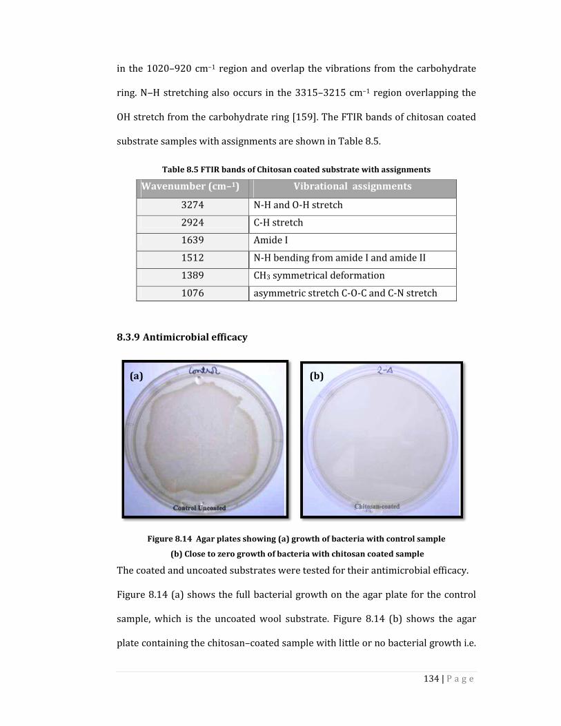
134 | P a g e

in the 1020–920 cm–1 region and overlap the vibrations from the carbohydrate

ring. N‒H stretching also occurs in the 3315–3215 cm–1 region overlapping the

OH stretch from the carbohydrate ring [159]. The FTIR bands of chitosan coated

substrate samples with assignments are shown in Table 8.5.

Table 8.5 FTIR bands of Chitosan coated substrate with assignments

Wavenumber (cm–1) Vibrational assignments

3274 N-H and O-H stretch

2924 C-H stretch

1639 Amide I

1512 N-H bending from amide I and amide II

1389 CH3 symmetrical deformation

1076 asymmetric stretch C-O-C and C-N stretch

Antimicrobial efficacy 8.3.9

Figure 8.14 Agar plates showing (a) growth of bacteria with control sample

(b) Close to zero growth of bacteria with chitosan coated sample

The coated and uncoated substrates were tested for their antimicrobial efficacy.

Figure 8.14 (a) shows the full bacterial growth on the agar plate for the control

sample, which is the uncoated wool substrate. Figure 8.14 (b) shows the agar

plate containing the chitosan–coated sample with little or no bacterial growth i.e.

(a) (b)

135 | P a g e

the bacterial reduction percentage was found close to 100%. The excellent

antimicrobial efficacy against the gram negative bacteria shows that chitosan–

coated wool nonwoven substrate can be a potential candidate for medical textiles

such as wound dressings.

8.4 Conclusion

This research investigated the successful applications of the electrospraying as a

coating process on textile substrates with waterproof breathable and

antimicrobial activity. TPU was used to coat the cotton fabric and results showed

that water contact angle of coated surface was improved significantly from 56° to

115° without significant change in the moisture management properties of the

fabric.. Also wool nonwoven fabric was coated with chitosan to impart the

antibacterial property to the substrate. A result showed that antibacterial activity

of wool coated nonwoven substrate was substantially higher. The agar plate

showed close to zero bacterial growth on the substrate. The presence of TPU &

chitosan on textile substrates was analysed by FTIR. The presence of strong

absorption at 1728 cm‒1 and N‒H stretching at 3330 cm‒1 confirmed the TPU

coating on substrate. Similarly presence of strong vibration of amide I at 1639

cm‒1 and N‒H stretching at 3274 cm‒1 confirmed the chitosan polymer coating

on substrate. Hence, electrospraying technique can be effectively used as a textile

coating technique to impart the functionality to textile substrate.

136 | P a g e

Chapter 9

Production of bicomponent droplets by electrospraying

9.1 Introduction

As discussed in earlier chapters, electrospraying is a unique process to produce

submicron polymeric droplets in the average diameter range of 0.2 μm to 10 μm.

The coating thickness produced by this method is at least one or two orders of

magnitude smaller than those produced by conventional coating methods like

roller coating or knife coating. The effects of several process parameters, such as

the applied voltage, electric field strength, flow rate, concentration and distance

between the nozzle and collector have, been explored in great detail for TPU.

Most of the bicomponent systems that have been investigated have utilised

electrospraying from a single polymer solution. Recently, a few systems have

blends of polymers (in the same solvent) and blends of polymer solutions (a

four–component system). Blends of polyaniline, a conducting polymer, with

polyethylene oxide (PEO) dissolve in chloroform were electrospun to produce

filaments in the range of 5–30 nm [160, 161] and examined for their magnetic

susceptibility behaviour. More specifically, PEO was blended with polyaniline to

increase the viscosity of the solution to achieve stable electrospinning. In another

research work, M13 viruses dispersed in 1,1,1,3,3,3-hexafluoro-2-propanol and

were blended with polyvinyl pyrrolidine (PVP) and nanofibres were electrospun.

The resulting electrospun virus-PVP nanofibres adjourned in a solution [162].

Regenerated silk was blended with polyethylene oxide (PEO) to eliminate the

137 | P a g e

expansion of brittle β-sheets of silk fibroin [163]. Hence utility of the resulting

electrospun mats were improved in vitro and in vivo conditions.

Many researchers have reported the feasibility of bicomponent electrospinning

systems, but there have been no reported studies regarding bicomponent

droplet fabrication by electrospraying. Hence an attempt has been made to

design and develop bicomponent electrospraying system. Some unique

characteristics must be considered when electrospraying performed from blends

of polymer solutions. For a blend of two polymers (in the same solvent or

different solvents), the mixture should be homogenous so that the resultant

droplets possesses a uniform spatial configuration. In addition to being

thermodynamically miscible, the interactions between the polymer and the

solvent of the opposing pair are of critical importance when two polymers

dissolved in two solvents respectively. Hence, during electrospraying of two

polymers, the thermodynamic and kinetic aspects of solution need to be

considered. Another way to produce electrosprayed droplets from two polymers

is to electrospraying of two polymers simultaneously in a side–by–side

arrangement.

In this research, the developed bicomponent system utilised was such that the

two polymer solutions do not come into physical contact until they reached the

end of the nozzle, where the process of droplet formation began. The

electrospraying device was designed in such way that two polymer solutions

were electrosprayed simultaneously in a side-by-side fashion. This allows for a

bicomponent electrospray coating that possesses properties from each of the

polymeric components. For instance, one of the polymers could contribute to

138 | P a g e

mechanical strength while the other could impart hydrophobic properties to the

resulting textile substrate. This could be useful for a protective textile

application. In fact by suitably choosing the constituent components based on

their respective properties, the potential of these bicomponent droplets to be

utilised in various applications becomes enhanced. These applications could

include medical, protective and technical textiles. This prime objective of this

study was to demonstrate the feasibility of this new methodology to produce

bicomponent droplets via electrospraying at submicron range.

In this chapter, the new bicomponent electrospraying device is described.

Preliminary results on TPU/PVC bicomponent droplets will be presented. It is

important to note here that TPU/PVC is a miscible system. PVC has a glass

transition temperature of 85˚C and is therefore a glassy and stiff material at room

temperature. The mechanical properties of PVC, especially toughness can be

enhanced by suitable plasticisation [164]. When blended with a thermoplastic

urethane polymer, it was expected that the resulting mechanical toughness and

hydrophobicity would be improved without scarifying, depending on the

composition ratio. It was expected that the resultant coating on the substrate will

possess characteristics of both the components. The main reason behind using

such a technique to enable easy identification of the two components easily in

each polymer pair by energy dispersive spectroscopy (EDS), thereby

demonstrating the feasibility of electrospraying a bicomponent droplet coating.

The EDS detector, which was a part of the scanning electron microscope (SEM)

was utilised in this study to investigate the morphology of the droplets. This

allowed characterisation of the local composition of the bicomponent droplets at

the submicron level.

139 | P a g e

9.2 Experimental

The electrospraying was carried out by varying voltage at a constant nozzle-

collector distance (15 cm) and solution flow rate (3 ml/h).

Chemicals 9.2.1

PVC of Mw, of 75,400 g/mol in the form of a fine powder and TPU of Mw 30,000 in

the form of chips received. The THF was used as solvent for dissolving TPU. N, N-

dimethylacetamide was used to dissolve PVC at different weight concentrations

ranging from 1% to 5% w/wt. All chemicals were used as received without any

purification.

EDS 9.2.2

EDS was performed on TPU/PVC electrosprayed substrates to calibrate the peak

intensities of oxygen (O) and chlorine (Cl) with the actual composition in the

blend. Energy dispersive x-ray spectroscopy (EDS, EDX) is a qualitative and

quantitative X-ray microanalytical technique that can provide information on the

chemical composition of a sample for elements with atomic number (Z) >3.

Electrospraying Device 9.2.3

Schematic arrangement of the component parts is shown in Figure 9.1.

The electrospraying apparatus consisted of a solutions container (1) which was

filled with the required polymer solutions (2). The container has a capacity of

150 ml and a specially designed nozzle (3) that was connected to the positive

terminal. The power source (8) was capable of providing output voltage from 0–

30kV. The inner diameter of nozzle (3) was 0.5 mm. A metal plate was used as a

collector (6) on which the fabric substrate (5) was placed to be coated with the

polymeric solution. Compressed nitrogen gas (9) was used to apply pressure

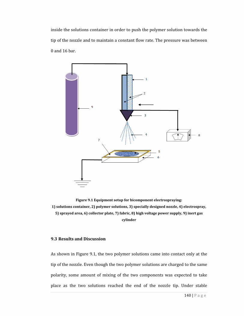
140 | P a g e

inside the solutions container in order to push the polymer solution towards the

tip of the nozzle and to maintain a constant flow rate. The pressure was between

0 and 16 bar.

Figure 9.1 Equipment setup for bicomponent electrospraying:

1) solutions container, 2) polymer solutions, 3) specially designed nozzle, 4) electrospray,

5) sprayed area, 6) collector plate, 7) fabric, 8) high voltage power supply, 9) inert gas

cylinder

9.3 Results and Discussion

As shown in Figure 9.1, the two polymer solutions came into contact only at the

tip of the nozzle. Even though the two polymer solutions are charged to the same

polarity, some amount of mixing of the two components was expected to take

place as the two solutions reached the end of the nozzle tip. Under stable

8

141 | P a g e

electrospraying conditions, a fluctuating jet was observed for TPU/PVC at 25kV, a

target distance of 20 cm and total flow rate of 3 ml/h at 10 bar pressure on the

cylinder. Interestingly, when the nozzle–collector distance was 10 cm or larger, a

single common Taylor cone was observed. From the surface of this Taylor cone, a

fluctuating jet was ejected. The position of ejection of the jet on the surface of the

Taylor cone changed very rapidly with time and led to a somewhat non-steady

flow of the polymer solution. These fluctuations likely influence the extent of

mixing of the two charged solutions when they came into contact at the tip of the

nozzle.

At distances larger than 20 cm, the jet was not continuous and the solutions were

dripped due to weak field strength that did not convey the jet to the collector. At

distances less than 10 cm, two Taylor cones were observed to emanate from each

of the two holes of nozzle. As a result, two jets were observed to eject form each

Taylor cone under these conditions. At such low distances (< 10 cm), the field

strength was relatively strong, thereby inducing a strong electrostatic repulsion

between the two polymer solutions emanating from each hole of nozzle. This

lead to the formation of two Taylor cones and subsequently two separate but

identically charged (in terms of polarity) jets causing the formation of two zones

of droplet collection on the target, each corresponding to only one of the two

respective polymer components. Hence, bicomponent electrospraying was

conducted at nozzle–collector distances of 10–20 cm in this study.

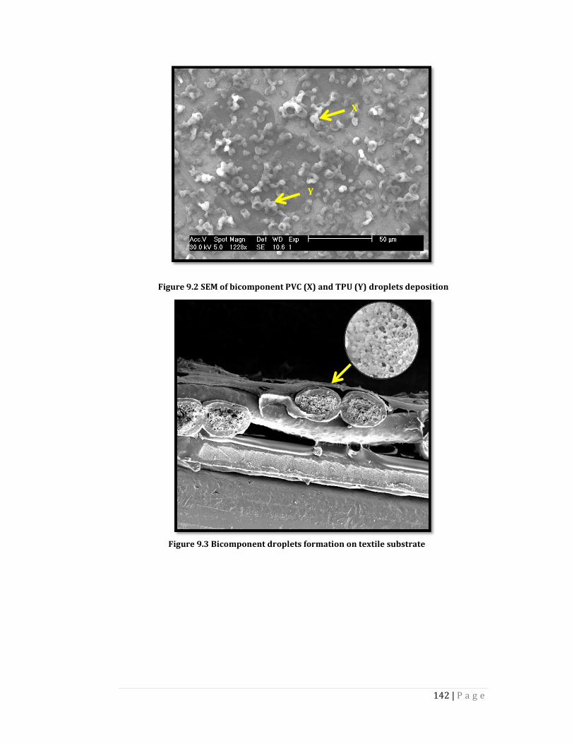
142 | P a g e

Figure 9.2 SEM of bicomponent PVC (X) and TPU (Y) droplets deposition

X

Y

Figure 9.3 Bicomponent droplets formation on textile substrate

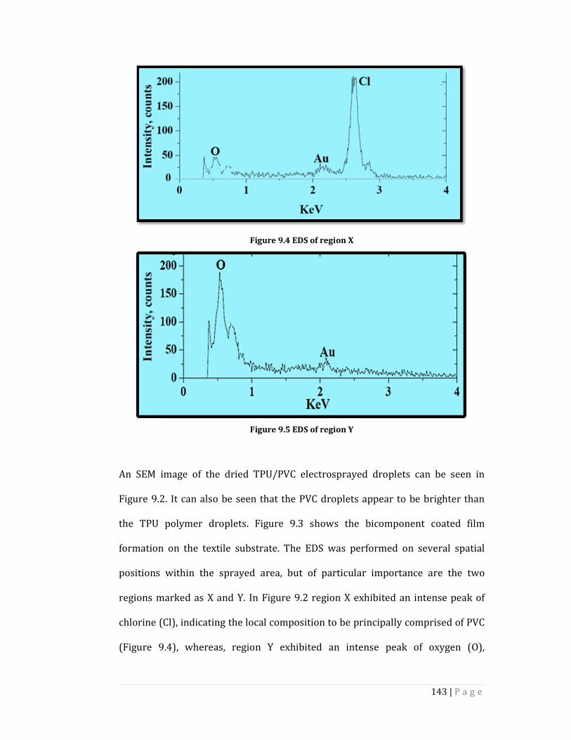
143 | P a g e

Figure 9.4 EDS of region X

Figure 9.5 EDS of region Y

An SEM image of the dried TPU/PVC electrosprayed droplets can be seen in

Figure 9.2. It can also be seen that the PVC droplets appear to be brighter than

the TPU polymer droplets. Figure 9.3 shows the bicomponent coated film

formation on the textile substrate. The EDS was performed on several spatial

positions within the sprayed area, but of particular importance are the two

regions marked as X and Y. In Figure 9.2 region X exhibited an intense peak of

chlorine (Cl), indicating the local composition to be principally comprised of PVC

(Figure 9.4), whereas, region Y exhibited an intense peak of oxygen (O),

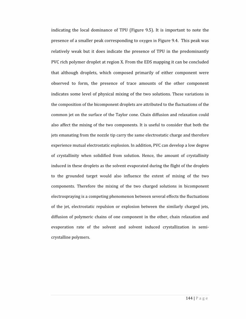
144 | P a g e

indicating the local dominance of TPU (Figure 9.5). It is important to note the

presence of a smaller peak corresponding to oxygen in Figure 9.4. This peak was

relatively weak but it does indicate the presence of TPU in the predominantly

PVC rich polymer droplet at region X. From the EDS mapping it can be concluded

that although droplets, which composed primarily of either component were

observed to form, the presence of trace amounts of the other component

indicates some level of physical mixing of the two solutions. These variations in

the composition of the bicomponent droplets are attributed to the fluctuations of the

common jet on the surface of the Taylor cone. Chain diffusion and relaxation could

also affect the mixing of the two components. It is useful to consider that both the

jets emanating from the nozzle tip carry the same electrostatic charge and therefore

experience mutual electrostatic explosion. In addition, PVC can develop a low degree

of crystallinity when solidified from solution. Hence, the amount of crystallinity

induced in these droplets as the solvent evaporated during the flight of the droplets

to the grounded target would also influence the extent of mixing of the two

components. Therefore the mixing of the two charged solutions in bicomponent

electrospraying is a competing phenomenon between several effects the fluctuations

of the jet, electrostatic repulsion or explosion between the similarly charged jets,

diffusion of polymeric chains of one component in the other, chain relaxation and

evaporation rate of the solvent and solvent induced crystallization in semi-

crystalline polymers.

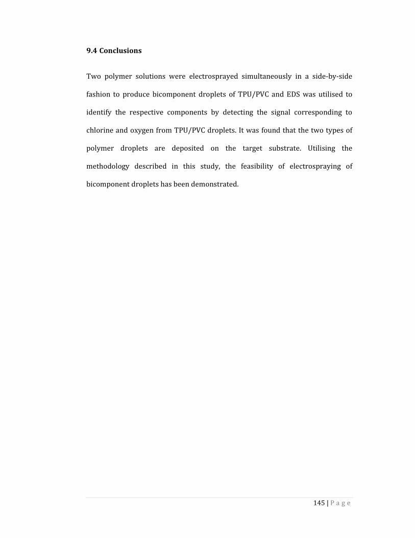
145 | P a g e

9.4 Conclusions

Two polymer solutions were electrosprayed simultaneously in a side-by-side

fashion to produce bicomponent droplets of TPU/PVC and EDS was utilised to

identify the respective components by detecting the signal corresponding to

chlorine and oxygen from TPU/PVC droplets. It was found that the two types of

polymer droplets are deposited on the target substrate. Utilising the

methodology described in this study, the feasibility of electrospraying of

bicomponent droplets has been demonstrated.

146 | P a g e

Chapter 10

Summary of conclusions

10.1 Introduction

This chapter summarises the conclusions from the investigations into

understanding the electrospraying process and its application to textile substrate

as a coating method. Based on the information found, further work could be

undertaken to increase the level of knowledge regarding the performance and

application of electrospraying technique using various polymers.

• This study suggests that applied voltage important parameter that governs

the polymer droplets aggregation in electrospraying process. Higher voltage

tends to result in lower polymer aggregation. This study suggests that field

strength is an important parameter that governs the polymer droplets aggregation

in electrohydrodynamic spraying process. Higher field strength tends to result in

higher polymer aggregation

• From the two-way analysis of variance, it can be concluded that Applied

voltage and concentration has the highest influence on % area of TPU

aggregate in electrospraying, which suggests the setting of high voltage and

minimising the concentration is the key. From the “half-normal plot of the

factor effects” of the model, we can see TPU flow rate and needle-target

distance are also the main factors in our model. All the four factors have

some degrees of influence on the % area of TPU aggregate

147 | P a g e

• As the applied voltage increased Jet length initially decreased up to certain

length and then starts increasing as voltage further increases due to higher

electrical charge.

• As the polymer solution concentration increased from 5% to 7% the increase

in jet length was observed. At 2.5% polymer solution concentration shows

higher jet length.

• Effect of field strength on jet length shows negative parabolic characteristics.

• The validation of the feasible optimization solutions proofs we can apply our

experiment model to predict the % area of TPU aggregate, which can serve as

an indirect method of assessing the degree of TPU dispersion and reach a

high quality TPU dispersion using electrospraying.

• From the results it was observed that as the applied voltage increased from

10kV to 25kV then the polymer droplet size was decreased from 0.25 µm to

0.09 µm. When nozzle-collector distance was increased from 5 cm to 20 cm

the average droplet diameter was increased from 0.03 µm to 0.20 µm. It was

also observed that as the flow rate increased from 0.1mL/h to 1.5 mL/h the

average diameter of polymer droplet was increased from 0.098 µm to 0.23

µm.

• From the experimental results shows that with electrospraying coating

technique can effectively utilise to as a textile coating technique. The textile

substrate can be coated without losing their original property compared to

conventional coating technique. The study demonstrated the production of

waterproof breathable coated cotton fabric and wool fabric consists of

antibacterial property which can effectively utilised in medical textiles

148 | P a g e

application. This coating technique just opens the door for novel textile

coating applications.

• Two polymer solutions were electrosprayed simultaneously in a side-by-side

fashion to produce bicomponent droplets that had diameters in the range of

1 µm to 10µm. TPU/PVC bicomponent droplets were electrosprayed. EDS

was utilized to identify the respective components by detecting the signal

corresponding to chlorine and oxygen from TPU/PVC droplets. It was found

that the two polymer droplets are deposited on the target substrate. Utilizing

the developed equipment described in this study, the feasibility of

electrospraying of bicomponent droplets has been demonstrated.

10.2 Further work

This research work contributes the understanding of the characteristics of

electrospraying technique as a coating method for textile substrates. It will be

interesting if the further research work carried out as per the following

recommendation:

• Suitable additives can be used to increase the conductivity of the polymeric

solution and its effect could be a worth studying.

• Optimisation of process parameters to achieve desired droplet size by

utilising RSM modelling could be interesting work.

• Combination of different polymers such as Poly-L-Lactic-acid (PLLA), Poly‒

acrylonitrile (PAN), Polypropylene (PP) and Poly‒tetrafluoroethylene

(PTFE) can be studied for production of bicomponent droplets.

149 | P a g e

• Use of other types of fabric substrates such as knitted fabric structures and

other fibres such as nylon, Kevlar and dyneem will be worth studying.

• Investigation on the adhesion properties of the coating on the textile

substrates.

150 | P a g e

References

1. Sen, A.K., Coated textiles: Principles and applications. 2007: Crc Press.

2. Pham, Q.P., U. Sharma, and A.G. Mikos, Electrospinning of polymeric

nanofibers for tissue engineering applications: a review. Tissue engineering,

2006. 12(5): p. 1197-1211.

3. Salata, O.V., Tools of nanotechnology: Electrospray. Current Nanoscience,

2005. 1(1): p. 25-33.

4. Jaworek, A., Electrostatic micro- and nanoencapsulation and

electroemulsification: a brief review. J Microencapsul, 2008. 25(7): p. 443-

68.

5. Jaworek, A. and A. Sobczyk, Electrospraying route to nanotechnology: An

overview. Journal of Electrostatics, 2008. 66(3): p. 197-219.

6. D. Zickler, Journal of Coated Fabrics, 1978. 8(October): p. 121-143.

7. R. Shinshoo, Coating of Textiles, 1995. 1(2): p. 190.

8. G. R. Lomax, Textiles 1992. 2(1): p. 18.

9. R. A. Park;H A Sarvetnick; VaNostrandeinhold, Spread Coating Processes, .

Plastisols and Organosols, 1972. 2(3): p. 143-181.

10. Stephens;, B.D.M.M.H.H.A., Coated fabrics. Rubber Products Manufacturing

Technology, 1994. 1(2): p. 154.

11. Doshi, J. and D.H. Reneker, Electrospinning process and applications of

electrospun fibers. Journal of electrostatics, 1995. 35(2): p. 151-160.

12. MacDiarmid, A., et al., Electrostatically-generated nanofibers of electronic

polymers. Synthetic Metals, 2001. 119(1-3): p. 27-30.

151 | P a g e

13. Reneker, D.H. and I. Chun, Nanometre diameter fibres of polymer, produced

by electrospinning. Nanotechnology, 1996. 7(3): p. 216.

14. Formhals, A., Process and apparatus fob pbepabing. 1934, Google Patents.

15. Formhals, A., Method and apparatus for spinning. 1939, Google Patents.

16. Formhals, A., A formhals. 1940, Google Patents.

17. Taylor, G., Electrically driven jets. Proceedings of the Royal Society of

London. A. Mathematical and Physical Sciences, 1969. 313(1515): p. 453-

475.

18. Buchko, C.J., et al., Processing and microstructural characterization of

porous biocompatible protein polymer thin films. Polymer, 1999. 40(26): p.

7397-7407.

19. Baumgarten, P.K., Electrostatic spinning of acrylic microfibers. Journal of

colloid and interface science, 1971. 36(1): p. 71-79.

20. Larrondo, L. and R. St John Manley, Electrostatic fiber spinning from

polymer melts. I. Experimental observations on fiber formation and

properties. Journal of Polymer Science: Polymer Physics Edition, 1981.

19(6): p. 909-920.

21. Larrondo, L. and R. St John Manley, Electrostatic fiber spinning from

polymer melts. II. Examination of the flow field in an electrically driven jet.

Journal of Polymer Science: Polymer Physics Edition, 1981. 19(6): p. 921-

932.

22. Hayati, I., A. Bailey, and T.F. Tadros, Investigations into the mechanisms of

electrohydrodynamic spraying of liquids: I. Effect of electric field and the

environment on pendant drops and factors affecting the formation of stable

jets and atomization. Journal of Colloid and Interface Science, 1987.

117(1): p. 205-221.

152 | P a g e

23. Jaeger, R., et al. Electrospinning of ultra‐thin polymer fibers. in

Macromolecular Symposia. 1998. Wiley Online Library.

24. Deitzel, J., et al., Controlled deposition of electrospun poly (ethylene oxide)

fibers. Polymer, 2001. 42(19): p. 8163-8170.

25. Deitzel, J., et al., Electrospinning of polymer nanofibers with specific surface

chemistry. Polymer, 2002. 43(3): p. 1025-1029.

26. Warner, S.B., et al., A fundamental investigation of the formation and

properties of electrospun fibers. National textile center annual report, 1998:

p. 83-90.

27. Hohman, M.M., et al., Electrospinning and electrically forced jets. I. Stability

theory. Physics of Fluids, 2001. 13: p. 2201.

28. Shin, Y., et al., Electrospinning: A whipping fluid jet generates submicron

polymer fibers. Applied Physics Letters, 2001. 78: p. 1149.

29. Shin, Y., et al., Experimental characterization of electrospinning: the

electrically forced jet and instabilities. Polymer, 2001. 42(25): p. 09955-

09967.

30. Spivak, A. and Y. Dzenis, Asymptotic decay of radius of a weakly conductive

viscous jet in an external electric field. Applied Physics Letters, 1998.

73(21): p. 3067-3069.

31. Gibson, P., H. Schreuder‐Gibson, and D. Rivin, Electrospun fiber mats:

transport properties. AIChE journal, 1999. 45(1): p. 190-195.

32. Wang, X., et al., Electromagnetic properties of hollow PAN/FeSo4 composite

nanofibres via coaxial electrospinning. International Journal of Materials

and Product Technology, 2013. 46(2): p. 95-105.

33. Pinilla, J.L., et al., Carbon nanofibres coated with Ni decorated MoS2

nanosheets as catalyst for vacuum residue hydroprocessing. Applied

Catalysis B: Environmental, 2014. 148–149(0): p. 357-365.

153 | P a g e

34. Deitzel, J., et al., The effect of processing variables on the morphology of

electrospun nanofibers and textiles. Polymer, 2001. 42(1): p. 261-272.

35. Objective, N. What is Electrospray 2000; Available from:

http://www.newobjective.com/electrospray/whatisESI.shtml.

36. Arya, N., et al., Electrospraying: a facile technique for synthesis of chitosan-

based micro/nanospheres for drug delivery applications. J Biomed Mater

Res B Appl Biomater, 2009. 88(1): p. 17-31.

37. Jaworek, A. and A. Krupa, Jet and drops formation in electrohydrodynamic

spraying of liquids. A systematic approach. Experiments in fluids, 1999.

27(1): p. 43-52.

38. Jaworek, A. and A. Krupa, Classification of the modes of EHD spraying.

Journal of Aerosol Science, 1999. 30(7): p. 873-893.

39. Hayati, I., A. Bailey, and T.F. Tadros, Investigations into the mechanism of

electrohydrodynamic spraying of liquids: II. Mechanism of stable jet

formation and electrical forces acting on a liquid cone. Journal of colloid

and interface science, 1987. 117(1): p. 222-230.

40. Cloupeau, M. and B. Prunet-Foch, Electrohydrodynamic spraying

functioning modes: a critical review. Journal of Aerosol Science, 1994.

25(6): p. 1021-1036.

41. Cloupeau, M. and B. Prunet-Foch, Electrostatic spraying of liquids: main

functioning modes. Journal of Electrostatics, 1990. 25(2): p. 165-184.

42. Shiryaeva, S. and A. Grigor'ev, The semiphenomenological classification of

the modes of electrostatic dispersion of liquids. Journal of

ELECTROSTATICS, 1995. 34(1): p. 51-59.

43. Marginean, I., et al., Flexing the electrified meniscus: the birth of a jet in

electrosprays. Analytical chemistry, 2004. 76(14): p. 4202-4207.

154 | P a g e

44. Parvin, L., et al., Electrospray diagnostics by Fourier analysis of current

oscillations and fast imaging. Analytical chemistry, 2005. 77(13): p. 3908-

3915.

45. Marginean, I., P. Nemes, and A. Vertes, Astable regime in electrosprays.

Physical Review E, 2007. 76(2): p. 026320.

46. Marginean, I., P. Nemes, and A. Vertes, Order-chaos-order transitions in

electrosprays: The electrified dripping faucet. Physical review letters, 2006.

97(6): p. 064502.

47. Marginean, I., et al., How much charge is there on a pulsating Taylor cone?

Applied physics letters, 2006. 89(6): p. 064104-064104-3.

48. Wiggers, H. and P. Walzel, Elektrostatisches Zerstäuben von Flüssigkeiten.

Chemie Ingenieur Technik, 1997. 69(8): p. 1066-1073.

49. Joffre, G.-H. and M. Cloupeau, Characteristic forms of electrified menisci

emitting charges. Journal of electrostatics, 1986. 18(2): p. 147-161.

50. Meesters, G., et al., Generation of micron-sized droplets from the Taylor

cone. Journal of aerosol science, 1992. 23(1): p. 37-49.

51. Jaworek, A. and A. Krupa, Studies of the corona discharge in ehd spraying.

Journal of electrostatics, 1997. 40: p. 173-178.

52. Borra, J.-P., P. Ehouarn, and D. Boulaud, Electrohydrodynamic atomisation

of water stabilised by glow discharge—operating range and droplet

properties. Journal of aerosol science, 2004. 35(11): p. 1313-1332.

53. Jaworek, A., et al., Spectroscopic studies of electric discharges in

electrospraying. Journal of electrostatics, 2005. 63(6): p. 635-641.

54. La Mora, D. and J. Fernandez, The current emitted by highly conducting

Taylor cones. Journal of Fluid Mechanics, 1994. 260(1): p. 155-184.

55. Hayati, I., A.I. Bailey, and T.F. Tadros, 1987. - 117(- 1): p. - 221.

155 | P a g e

56. De La Mora, J.F. and I.G. Loscertales, Current emitted by highly conducting

Taylor cones. Journal of Fluid Mechanics, 1994. 260: p. 155-184.

57. Fernández de la Mora, J., The fluid dynamics of Taylor Cones. Annual

Review of Fluid Mechanics, 2007. 39: p. 217-243.

58. Ganan-Calvo, A.M., New microfluidic technologies to generate respirable

aerosols for medical applications. Journal of Aerosol Science, 1999.

30(Suppl. 1): p. S541-S542.

59. Gañán-Calvo, A.M., J. Dávila, and A. Barrero, Current and droplet size in the

electrospraying of liquids. Scaling laws. Journal of Aerosol Science, 1997.

28(2): p. 249-275.

60. Hartman, R.P.A., et al., Jet break-up in electrohydrodynamic atomization in

the cone-jet mode. Journal of Aerosol Science, 2000. 31(1): p. 65-95.

61. López-Herrera, J.M., et al., Coaxial jets generated from electrified Taylor

cones. Scaling laws. Journal of Aerosol Science, 2003. 34(5): p. 535-552.

62. Barrero, A., et al., Steady cone-jet electrosprays in liquid insulator baths.

Journal of Colloid and Interface Science, 2004. 272(1): p. 104-108.

63. Basak, S., D.R. Chen, and P. Biswas, Electrospray of ionic precursor solutions

to synthesize iron oxide nanoparticles: Modified scaling law. Chemical

Engineering Science, 2007. 62(4): p. 1263-1268.

64. Chen, C.H., D.A. Seville, and I.A. Aksay, Scaling laws for pulsed

electrohydrodynamic drop formation. Applied Physics Letters, 2006.

89(12).

65. Paine, M.D., M.S. Alexander, and J.P.W. Stark, Nozzle and liquid effects on

the spray modes in nanoelectrospray. Journal of Colloid and Interface

Science, 2007. 305(1): p. 111-123.

66. Barrero, A. and I.G. Loscertales, Micro- and nanoparticles via capillary

flows. Annual Review of Fluid Mechanics, 2007. 39: p. 89-106.

156 | P a g e

67. Rayleigh, L., On the equilibrium of liquid conducting masses charged with

electricity Phil. Mag. Ser., 1882. 5(14): p. 184-186.

68. Zeleny, J., Instability of electrified liquid surfaces. Physical Review, 1917.

10(1): p. 1.

69. Yarin, A., S. Koombhongse, and D. Reneker, Taylor cone and jetting from

liquid droplets in electrospinning of nanofibers. Journal of Applied Physics,

2001. 90(9): p. 4836-4846.

70. Grace, J. and J. Marijnissen, A review of liquid atomization by electrical

means. Journal of aerosol science, 1994. 25(6): p. 1005-1019.

71. Darby, R., Chemical engineering fluid mechanics. 2001: CRC PressI Llc.

72. Yarin, A.L., Free liquid jets and films: hydrodynamics and rheology. 1993:

Longman Scientific & Technical.

73. Spivak, A., Y. Dzenis, and D. Reneker, A model of steady state jet in the

electrospinning process. Mechanics research communications, 2000. 27(1):

p. 37-42.

74. Reneker, D.H., et al., Bending instability of electrically charged liquid jets of

polymer solutions in electrospinning. Journal of Applied physics, 2000. 87:

p. 4531.

75. Fridrikh, S.V., et al., Controlling the fiber diameter during electrospinning.

Physical review letters, 2003. 90(14): p. 144502-144502.

76. Megelski, S., et al., Micro-and nanostructured surface morphology on

electrospun polymer fibers. Macromolecules, 2002. 35(22): p. 8456-8466.

77. Srinivasarao, M., et al., Three-dimensionally ordered array of air bubbles in

a polymer film. Science, 2001. 292(5514): p. 79-83.

78. Zong, X., et al., Structure and process relationship of electrospun

bioabsorbable nanofiber membranes. Polymer, 2002. 43(16): p. 4403-

4412.

157 | P a g e

79. Bognitzki, M., et al., Nanostructured fibers via electrospinning. Advanced

Materials, 2001. 13(1): p. 70-72.

80. Lee, K.H., et al., Influence of a mixing solvent with tetrahydrofuran and N,

N‐dimethylformamide on electrospun poly (vinyl chloride) nonwoven mats.

Journal of Polymer Science Part B: Polymer Physics, 2002. 40(19): p.

2259-2268.

81. Altenburg, H., et al., Thick films of ceramic superconducting, electro-ceramic

materials. Pure and applied chemistry, 2002. 74(11): p. 2083-2096.

82. Chandrasekhar, R. and K.L. Choy, Electrostatic spray assisted vapour

deposition of fluorine doped tin oxide. Journal of Crystal Growth, 2001.

231(1-2): p. 215-221.

83. Jaworek, A., Electrospray droplet sources for thin film deposition. Journal of

materials science, 2007. 42(1): p. 266-297.

84. Xie, J. and C.H. Wang, Encapsulation of proteins in biodegradable polymeric

microparticles using electrospray in the Taylor cone‐jet mode.

Biotechnology and bioengineering, 2007. 97(5): p. 1278-1290.

85. Loscertales, I.G., et al., Micro/nano encapsulation via electrified coaxial

liquid jets. Science, 2002. 295(5560): p. 1695-1698.

86. Ijsebaert, J.C., et al., Electro-hydrodynamic atomization of drug solutions for

inhalation purposes. Journal of Applied Physiology, 2001. 91(6): p. 2735-

2741.

87. Xu, Y., M. Skotak, and M. Hanna, Electrospray encapsulation of water-

soluble protein with polylactide. I. Effects of formulations and process on

morphology and particle size. Journal of microencapsulation, 2006. 23(1):

p. 69-78.

88. Choy, K., Progress in Mater. Sci, 2003. 48: p. 57.

158 | P a g e

89. Chandrasekhar, R. and K. Choy, Electrostatic spray assisted vapour

deposition of fluorine doped tin oxide. Journal of crystal growth, 2001.

231(1): p. 215-221.

90. Su, B. and K. Choy, Electrostatic assisted aerosol jet deposition of CdS, CdSe

and ZnS thin films. Thin Solid Films, 2000. 361: p. 102-106.

91. Su, B., M. Wei, and K. Choy, Microstructure of nanocrystalline CdS powders

and thin films by electrostatic assisted aerosol jet decomposition/deposition

method. Materials Letters, 2001. 47(1): p. 83-88.

92. Van Zomeren, A., et al., The production of thin films of LiMn< sub> 2</sub>

O< sub> 4</sub> by electrospraying. Journal of aerosol science, 1994.

25(6): p. 1229-1235.

93. Chon, U., et al., Fatigue-free samarium-modified bismuth titanate (BiSmTiO)

film capacitors having large spontaneous polarizations. Applied Physics

Letters, 2001. 79: p. 3137.

94. Kim, S.G., J.Y. Kim, and H.J. Kim, Deposition of MgO thin films by modified

electrostatic spray pyrolysis method. Thin Solid Films, 2000. 376(1): p.

110-114.

95. Rhee, S., et al., Low-temperature deposition of highly [100]-oriented MgO

films using charged liquid cluster beam. Thin Solid Films, 2001. 396(1): p.

23-28.

96. Chou, K.-S., K.-C. Huang, and H.-H. Lee, Fabrication and sintering effect on

the morphologies and conductivity of nano-Ag particle films by the spin

coating method. Nanotechnology, 2005. 16(6): p. 779.

97. Su, B. and K. Choy, Microstructure and properties of the CdS thin films

prepared by electrostatic spray assisted vapour deposition (ESAVD) method.

Thin solid films, 2000. 359(2): p. 160-164.

98. Moerman, R., et al., Picoliter dispensing in wells of a micro-array by means

of electrospraying. Journal of Aerosol Science, 1999. 30: p. S551-S552.

159 | P a g e

99. Moerman, R., et al., Miniaturized electrospraying as a technique for the

production of microarrays of reproducible micrometer-sized protein spots.

Analytical chemistry, 2001. 73(10): p. 2183-2189.

100. Gorty, A.V. and S.A. Barringer, Electrohydrodynamic spraying of chocolate.

Journal of Food Processing and Preservation, 2011. 35(4): p. 542-549.

101. Abu-Ali, J. and S. Barringer, Optimization of liquid electrostatic coating.

Journal of Electrostatics, 2008. 66(3): p. 184-189.

102. Bocanegra, R., et al., Production of cocoa butter microcapsules using an

electrospray process. Journal of food science, 2005. 70(8): p. e492-e497.

103. Musil, J., Hard and superhard nanocomposite coatings. Surface and coatings

technology, 2000. 125(1): p. 322-330.

104. Sobota, J. and G. Sorensen, Ion bombardment of solid lubricating

nanoparticle coatings. Nuclear Instruments and Methods in Physics

Research Section B: Beam Interactions with Materials and Atoms, 1997.

127: p. 945-948.

105. Jensen, H., et al., Reactive sputtering of nanostructured multilayer coatings

and their tribological properties. Surface and Coatings Technology, 1999.

116: p. 1070-1075.

106. Lapham, D., et al., The preparation of NiCo< sub> 2</sub> O< sub> 4</sub>

films by electrostatic spray deposition. Thin Solid Films, 2001. 391(1): p.

17-20.

107. Wang, D., S. Jayasinghe, and M. Edirisinghe, Instrument for

electrohydrodynamic print-patterning three-dimensional complex

structures. Review of scientific instruments, 2005. 76(7): p. 075105-

075105-5.

108. Information on Contact Angle Measurement 2013; Available from:

http://www.ramehart.com/contactangle.htm

160 | P a g e

109. Perking Elmer FTIR 400 Spectrum 2010; Available from:

http://www.rmit.edu.au/fashiontextiles/equipment/analytical.

110. Kawabata, S. and N.S.i.K. Gakki, The standardization and analysis of hand

evaluation. 1980: Textile Machinery Society of Japan.

111. Hu, J., Y. Li, and K. Yeung, Liquid moisture transfer. Clothing biosensory

engineering. Cambridge: Woodhead, 2006: p. 229-31.

112. Hu, J., et al., Moisture management tester: a method to characterize fabric

liquid moisture management properties. Textile Research Journal, 2005.

75(1): p. 57-62.

113. Morton, W.E. and J.W. Hearle, Physical properties of textile fibres. 1993:

Textile institute.

114. Taylor, G., Disintegration of water drops in an electric field. Phys. Sci. ,

1964(280): p. 383-397.

115. http://www.newobjective.com/electrospray>. 2004.

116. Shorey, J.D. and D. Michelson, On the mechanism of electrospraying. Nuclear

Instruments and Methods, 1970. 82(C): p. 295-296.

117. Spain, P.L. and K.L. Truog, Dry paint transfer product having high DOI

automotive paint coat. 1998, Google Patents.

118. Shin, Y.M.H., M.M.; Brenner, M.P.; Rutiedge, G.C. , Experimental Characterization of

Electrospinning: The Electrically Forced Jet and Instabilities,. Polymer, 2001. 42:

p. 9955-9967.

119. Mays, H., Dynamics and energetics of droplet aggregation in percolating

AOT water-in-oil microemulsions. The Journal of Physical Chemistry B,

1997. 101(49): p. 10271-10280.

120. al, A.J.e., Study of Electrospraying Characteristics of Polymer Solution

Coating on Textile Substrate. Adavanced Textiles Materials, 2011. 332-

334: p. 710-715.

161 | P a g e

121. Mit-uppatham, C., M. Nithitanakul, and P. Supaphol, Ultrafine Electrospun

Polyamide-6 Fibers: Effect of Solution Conditions on Morphology and

Average Fiber Diameter. Macromolecular Chemistry and Physics, 2004.

205(17): p. 2327-2338.

122. I, T.G., Proc. Roy. Soc. London 1969(A313): p. 448-453.

123. Renekar D.H., C., Nanometre Diameter Fibres Produced by Electrospinning.

Nanotechnology, 1996. 7: p. 216-233.

124. Jaworek, A. and A.T. Sobczyk, Electrospraying route to nanotechnology: An

overview. Journal of Electrostatics, 2008. 66(3-4): p. 197-219.

125. R. Chandrasekhar, K.L.C., Electrostatic spray assisted vapour deposition of

fluorine doped tin oxide. Journal of Crystal Growth, 2001. 231(1-2): p. 215-

221.

126. Ciach, T., Microencapsulation of drugs by electro-hydro-dynamic

atomization. International Journal of Pharmaceutics, 2006. 324(1): p. 51-

55.

127. W. Kuran, M.S., T. Listos, C. Debek and Z. Florjanczyk, New route to

oligocarbonate diols suitable for the synthesis of polyurethaneelastomers.

Polymers, 2000. 41: p. 8531.

128. D.M. Crawford, R.G.B.a.T.W.H., Strain effects on thermal transitions and

mechanical properties of thermoplastic polyurethaneelastomers.

Thermochim. Acta 1998. 323: p. 53.

129. J.H. Hong, E.H.J., H.S. Lee, D.H. Baik, S.W. Seo and J.H. Youk, , Electrospinning

of polyurethane/organically modified montmorillonite nanocomposites.

Journal of Polymer Science Part B: Polymer Physics, 2005. 43(22): p.

3171-3177.

130. S. Kidoaki, I.K.K.a.T.M., Structural features and mechanical properties of in

situ-bonded meshes of segmented polyurethane electrospun from mixed

solvents,. J. Biomed. Mater. Res. Part B: Appl. Biomater., 2006. 76.

162 | P a g e

131. T. Matsuda, M.I., H. Inoguchi, I.K. Kwon, K. Takamizawa and S. Kidoaki,,

Mechano-active scaffold design of small-diameter artificial graft made of

electrospun segmented polyurethane fabrics. J. Biomed. Mater. Res. Part A

2005. 73: p. 125.

132. D.I. Cha, H.Y.K., K.H. Lee, Y.C. Jung, J.W. Cho and B.C. Chun,, Electrospun

nonwovens of shape-memory polyurethane block copolymers. J. Appl. Polym.

Sci, 2005. 96: p. 460.

133. Yördem, O., M. Papila, and Y.Z. Menceloğlu, Effects of electrospinning

parameters on polyacrylonitrile nanofiber diameter: An investigation by

response surface methodology. Materials & design, 2008. 29(1): p. 34-44.

134. Wei, D., Z. Cui, and J. Chen, Optimization and tolerance prediction of sheet

metal forming process using response surface model. Computational

materials science, 2008. 42(2): p. 228-233.

135. Khayet, M., C. Cojocaru, and G. Zakrzewska-Trznadel, Response surface

modelling and optimization in pervaporation. Journal of Membrane Science,

2008. 321(2): p. 272-283.

136. Idris, A., F. Kormin, and M. Noordin, Application of response surface

methodology in describing the performance of thin film composite

membrane. Separation and purification technology, 2006. 49(3): p. 271-

280.

137. Khayet, M., C. Cojocaru, and C. García-Payo, Application of response surface

methodology and experimental design in direct contact membrane

distillation. Industrial & engineering chemistry research, 2007. 46(17): p.

5673-5685.

138. Ismail, A.F. and P. Lai, Development of defect-free asymmetric polysulfone

membranes for gas separation using response surface methodology.

Separation and purification technology, 2004. 40(2): p. 191-207.

163 | P a g e

139. Khayet, M., C. Cojocaru, and M. García-Payo, Experimental design and

optimization of asymmetric flat-sheet membranes prepared for direct

contact membrane distillation. Journal of Membrane Science, 2010. 351(1):

p. 234-245.

140. Khayet, M., M. Seman, and N. Hilal, Response surface modeling and

optimization of composite nanofiltration modified membranes. Journal of

Membrane Science, 2010. 349(1): p. 113-122.

141. Cui, W., et al., Investigation on process parameters of electrospinning system

through orthogonal experimental design. Journal of applied polymer

science, 2007. 103(5): p. 3105-3112.

142. Chae, H.G., et al., Carbon nanotube reinforced small diameter

polyacrylonitrile based carbon fiber. Composites Science and Technology,

2009. 69(3): p. 406-413.

143. Jiménez-Contreras, E., et al., Response Surface Methodology and its

application in evaluating scientific activity. Scientometrics, 2009. 79(1): p.

201-218.

144. C.H. Park, J.L., Electrosprayed polymer particles: Effect of solution properties.

Journal of Applied Polymer Science 2009. 114: p. 430-437.

145. Zeleny, J., The electrical discharge from liquid points, and a hydrostatic

method of measuring the electric intensity at their surfaces Phys. Rev. ,

1914. 3: p. 69-91.

146. Natali Bock, M.W.e.a., Electrospraying, a reproducible method for

production of polymeric Microspheres for biomedical applications Polymers

2011.

147. R.P.A. Hartman, D.J.B., D.M.A. Camelot,, Jet break up in electrohydrodynamic

atomisation in cone jet mode. Journal of Aerosol Sci., 2000. 31: p. 65-95.

148. Kumbar, S.G., et al., A preliminary report on a novel electrospray technique

for nanoparticle based biomedical implants coating: precision

164 | P a g e

electrospraying. J Biomed Mater Res B Appl Biomater, 2007. 81(1): p. 91-

103.

149. Bohr, A., et al., Application of Spray-Drying and

Electrospraying/Electospinning for Poorly Water-Soluble Drugs: A Particle

Engineering Approach. Current pharmaceutical design, 2013.

150. Peltonen, L., et al., Electrospraying, spray drying and related techniques for

production and formulation of drug nanoparticles. Expert Opin Drug Deliv,

2010. 7(6): p. 705-19.

151. Cavalli, R., et al., Poly(amidoamine)-Cholesterol Conjugate Nanoparticles

Obtained by Electrospraying as Novel Tamoxifen Delivery System. J Drug

Deliv, 2011. 2011: p. 587604.

152. Tavares Cardoso, M.A., et al., Functionalization of lactose as a biological

carrier for bovine serum albumin by electrospraying. Int J Pharm, 2011.

414(1-2): p. 1-5.

153. Zhang, F., et al., The antimicrobial activity of the cotton fabric grafted with

an amino-terminated hyperbranched polymer. Cellulose, 2009. 16(2): p.

281–88.

154. Mishra, A.K., et al., FT-IR and XPS studies of polyurethane-urea-imide

coatings. Progress in Organic Coatings, 2006. 55(3): p. 231-243.

155. Öner, E., et al., Evaluation of moisture management properties on knitted

fabrics. Journal of The Textile Institute, 2013(ahead-of-print): p. 1-9.

156. Osman, Z. and A. Arof, FTIR studies of chitosan acetate based polymer

electrolytes. Electrochimica Acta, 2003. 48(8): p. 993-999.

157. Smitha, B., S. Sridhar, and A. Khan, Chitosan–sodium alginate polyion

complexes as fuel cell membranes. European Polymer Journal, 2005. 41(8):

p. 1859-1866.

165 | P a g e

158. Nyquist, R.A., et al., The Handbook of Infrared and Raman Spectra of

Inorganic Compounds and Organic Salts: Infrared spectra of inorganic

compounds (3800-45 cm− 1). Vol. 4. 1997: Academic press.

159. Lawrie, G., et al., Interactions between alginate and chitosan biopolymers

characterized using FTIR and XPS. Biomacromolecules, 2007. 8(8): p.

2533-2541.

160. Pinto, N., et al., Electrospun polyaniline/polyethylene oxide nanofiber field-

effect transistor. Applied physics letters, 2003. 83(20): p. 4244-4246.

161. Kahol, P. and N. Pinto, An EPR investigation of electrospun polyaniline-

polyethylene oxide blends. Synthetic metals, 2004. 140(2): p. 269-272.

162. Lee, S.-W. and A.M. Belcher, Virus-based fabrication of micro-and nanofibers

using electrospinning. Nano letters, 2004. 4(3): p. 387-390.

163. Jin, H.-J., et al., Electrospinning Bombyx mori silk with poly (ethylene oxide).

Biomacromolecules, 2002. 3(6): p. 1233-1239.

164. Cano, J., et al., Determination of adipate plasticizers in poly (vinyl chloride)

by microwave-assisted extraction. Journal of Chromatography A, 2002.

963(1): p. 401-409.