Copyright and use of this thesis - CORE

Copyright and use of this thesis

This thesis must be used in accordance with the provisions of the Copyright Act 1968.

Reproduction of material protected by copyright may be an infringement of copyright and copyright owners may be entitled to take legal action against persons who infringe their copyright.

Section 51 (2) of the Copyright Act permits an authorized officer of a university library or archives to provide a copy (by communication or otherwise) of an unpublished thesis kept in the library or archives, to a person who satisfies the authorized officer that he or she requires the reproduction for the purposes of research or study.

The Copyright Act grants the creator of a work a number of moral rights, specifically the right of attribution, the right against false attribution and the right of integrity.

You may infringe the author’s moral rights if you:

- fail to acknowledge the author of this thesis if you quote sections from the work

- attribute this thesis to another author

- subject this thesis to derogatory treatment which may prejudice the author’s reputation

For further information contact the University’s Director of Copyright Services

sydney.edu.au/copyright

RESEARCH ON THE STRUCTURAL

DECOMPOSITION ANALYSIS OF GLOBAL

ENERGY AND GLOBAL CARBON FOOTPRINTS

A thesis submitted in fulfillment of the requirements for the degree of

Doctor of Philosophy in the School of Physics at The University of Sydney

Jun Lan

July 2015

1

@ Copyright by Jun Lan 2015

All Rights Reserved

2

CONTENT Abstract ............................................................................................................................................ 5

Acknowledgments ............................................................................................................................. 6

Publications ....................................................................................................................................... 7

Chapter 1 Introduction ................................................................................................................... 8

1.1 Overview on the relationships among marginal coefficients, consequential LCA and SDA......... 8

1.1.1 Marginal coefficients benefit consequential LCA in the framework of Input-Output

Analysis ..................................................................................................................................... 8

1.1.2 SDA as a downstream analytical tool for CLCA ................................................................. 11

1.2 Overview of thesis ................................................................................................................. 11

Chapter 2 An application of marginal coefficients – a case study of China’s production recipe and

CO2 emissions ................................................................................................................................. 13

2.1 Motivation and novelty .......................................................................................................... 13

2.2 Methodology ......................................................................................................................... 14

2.2.1 Dealing with variability .................................................................................................... 15

2.2.2 Distinguishing value added and intermediate inputs ....................................................... 16

2.2.3 Dealing with price changes .............................................................................................. 16

2.2.4 Economic interpretation ................................................................................................. 17

2.2.5 Generalizing marginal coefficients to incorporate CO2 emissions .................................... 19

2.2.6 Data sources ................................................................................................................... 21

2.3 Results ................................................................................................................................... 23

2.3.1 Average versus marginal coefficients............................................................................... 23

2.3.2 Distinguishing primary and intermediate inputs .............................................................. 25

2.3.3 Marginal change in CO2 emissions .................................................................................. 29

2.4 Conclusions of Chapter 2 ....................................................................................................... 32

2.5 Future development of marginal coefficients - Testing marginal coefficients for prospective

evaluations .................................................................................................................................. 33

2.5.1 Forecasting the gross outputs in t+1 ................................................................................ 34

2.5.2 Forecasting the gross outputs in t+2 ................................................................................ 35

3

2.5.3 Forecasting emissions ..................................................................................................... 35

2.5.4 Forecasting applications .................................................................................................. 36

Connecting Page .............................................................................................................................. 37

Chapter 3 A Structural Decomposition Analysis of Global Energy Footprints ................................. 38

3.1 Introduction ........................................................................................................................... 38

3.2 Methodology and data ........................................................................................................... 41

3.2.1 Construction of constant-price MRIO tables .................................................................... 41

3.2.2 Additive SDA methods ..................................................................................................... 42

3.2.3 MRIO-based Spatial decomposition ................................................................................. 43

3.2.4 Data sources ................................................................................................................... 45

3.2.5 SDA method selection ..................................................................................................... 46

3.3 Results and discussion ........................................................................................................... 47

3.3.1 Energy SDA for China, Russia and Japan .......................................................................... 49

3.3.2 Relations of different energy footprint measures ............................................................ 54

3.3.3 Outsourcing of energy-intensive production.................................................................... 57

3.3.4 Worldwide SDA ............................................................................................................... 59

3.3.5 Comparison with previous studies ................................................................................... 61

3.4 Conclusions of Chapter 3 ....................................................................................................... 63

3.5 Supporting Information.......................................................................................................... 64

3.5.1 Acronyms ........................................................................................................................ 64

3.5.2 TEFP-SDA results with raw data ....................................................................................... 65

Connecting page .............................................................................................................................. 67

Chapter 4 Consumption outpaces efficiency in driving global carbon emissions ............................ 68

4.1 Background ............................................................................................................................ 68

4.2 Dissecting the global carbon footprint.................................................................................... 69

4.3 Carbon leakage and outsourcing ............................................................................................ 73

4.4 Leaks and sinks ...................................................................................................................... 76

4.5 Policy implications ................................................................................................................. 77

4.6 Methods Summary ................................................................................................................ 78

4.7 Supporting Information.......................................................................................................... 78

4

4.7.1 Introduction of MRIO-based Input-output Analysis and Structure Decomposition Analysis

................................................................................................................................................ 78

4.7.2 Mathematical formulations of primary SDA methods ...................................................... 80

4.7.3 Literature review of MRIO-based SDA of carbon footprint ............................................... 82

4.7.4 Global levels of investment as a percentage of global GDP .............................................. 84

4.7.5 Construction procedures of constant-price IO tables ....................................................... 84

4.7.6 Explanation of increase or decrease in carbon emissions due to a change in production

recipe ...................................................................................................................................... 89

4.7.7 Carbon leakage ............................................................................................................. 100

4.7.8 Structural decomposition of carbon footprints for the former Soviet Republics (1990-2010)

.............................................................................................................................................. 102

4.7.9 Structural decomposition of carbon footprints for China, United States, United Kingdom

and Germany (2005-2010) ..................................................................................................... 104

4.7.10 Individual country information .................................................................................... 105

4.7.11 List of countries and sectors covered ........................................................................... 113

Connecting page ............................................................................................................................ 116

Chapter 5 Conclusion and outlook .............................................................................................. 118

5.1 Conclusion ........................................................................................................................... 118

5.2 Outlook................................................................................................................................ 119

References .................................................................................................................................... 120

5

Abstract Greenhouse gas emissions increased by 10.8 Gigagram (Gg) CO2 equivalent in 1990−2010.

Significant attention has been dedicated to the increase in emission transfers due to

international trade. However, questions remain unanswered about which key sectors are

stimulating the increase of CO2 emissions and whether changes in trade conditions have

affected global emissions.

To address the issue of increased emission transfers due to international trade, I used

input-output tables (IOTs) in constant prices extended with CO2 emissions to examine the

development of China. I calculated marginal coefficients – in monetary and CO2 terms – that

capture the additional (new) technology installed after that year. My work provides a first

overview of the magnitude and distribution of these coefficients in recent years across

China’s rapidly growing economy for which marginal coefficients could be expected to differ

greatly from average coefficients and are responsible for the substantial increase in CO2

emissions.

To answer the second question regarding which industries and trade conditions are

stimulating the increase in CO2 emissions, I first explore the countries and sectors recording

an increase or decrease in energy footprints during the decades from 1990-2010. I then

highlight the effect of international outsourcing of energy-intensive production processes by

decomposing the structural and spatial change in energy footprints. This energy data is then

further converted to CO2 emission data to disintegrate total CO2 emissions for each country

into contributions from various driving forces acting on the domestic economy and

international trade. The results reveal that consumption is outpacing efficiency by

accelerating energy consumption and CO2 emissions, and that a world-wide shifting of

energy-intensive and emissions-intensive production across borders has happened.

Keywords: marginal coefficient, Structural Decomposition Analysis, global energy footprint,

global carbon emissions

6

Acknowledgments

First and foremost I want to express my gratitude and thanks to my supervisor, Prof. Manfred

Lenzen. I have learned a lot from him as a researcher and also as a person par excellence.

This thesis would not have been completed without his guidance and encouragement.

I would also like to thank my friends and colleagues in the School of Physics, especially those

from the Integrated Sustainability Analysis (ISA) Research Group. Their support has been

invaluable throughout my PhD study, making my time both memorable and enjoyable. Other

special thanks go to Assistant Prof. Keiichiro Kanemoto at Institute of Decision Science for a

Sustainable Society, Kyushu University in Japan. His insights and help support my research at

a great magnitude.

My research is mainly supported by ENDEAVOUR Postgraduate Award from Minister for

Tertiary Education, Skills, Jobs and Workplace Relations. Some of the works presented in this

thesis is partially supported by Australian Research Council (ARC) through its Discovery

Project DP0985522.

Last but not least, I thank my husband, my son, my daughter and the other family members

for their unconditional love and support without which this journey would not have been

possible.

7

Publications

(1) Lan, Jun, M. Lenzen, E. Dietzenbacher, D. Moran, K. Kanemoto, J. Murray and A. Geschke

(2012) Structural Change and the Environment. Journal of Industrial Ecology 16, 623-635.

(2) Jun Lan and A. Malik (2013) Chapter 18: Structural Decomposition Analysis of the Energy

Consumption in China and Russia — An Application of the Eora MRIO Database. In: Joy

Murray and M. Lenzen (eds.) The sustainability practitioner's guide to multi-regional

input-output analysis. Champaign, Illinois, USA Common Ground Publishing LLC 178-187.

(3) Lan, Jun, M. Lenzen, D. McBain and K. Kanemoto (2014) A Structural Decomposition

Analysis of Global Energy Footprints. Applied Energy submitted.

(4) Jun Lan, A. Malik and M. Lenzen (2015) Consumption outpaces efficiency in driving global

carbon emissions. Intend to submit to the Journal of Global Environmental Change.

8

Chapter 1 Introduction

Growing giants are not only conceptualized by some mature industrial countries which have

reached a stage of high but stable metabolic rates (Krausmann et al. 2009;OECD 2008), but

also by the emerging economies – e.g. “BRIC” countries, referring to Brazil, Russia, India, and

China – and some countries marked with large populations and potentially high economic

growth (Group 2007). These countries are undergoing urbanization, technological change

and increasing international trade and are characterized by the scale and the pace of

changes. How such changes affect their influence on their energy footprints and carbon

footprints is an important question for decision makers. Understanding the implications of

changes often requires analyzing time-series data and identifying regional or sectoral

disparities throughout the supply chain (Hashimoto et al. 2012). Input-output analysis (IOA)

has been widely adopted by industrial ecology researchers in undertaking such analyses (Suh

and Kagawa 2005).

IOA provides a framework of analysis as well as basic data for modeling the interactions

between industries through the production and consumption of goods and services

(collectively, products). Coupling economic IOA with other statistics and models, researchers

have applied IOA to life cycle assessment (LCA) (Treloar 1997; Lenzen 2000; Suh et al. 2003).

IOA also uses time-series, interregional, or multiregional data and analytical techniques such

as structural decomposition analysis (SDA) to help answer some of the questions associated

with the changes that the growing giants are undergoing (Hashimoto et al. 2012).

1.1 Overview on the relationships among marginal coefficients,

consequential LCA and SDA

1.1.1 Marginal coefficients benefit consequential LCA in the framework of

Input-Output Analysis

Technological and structural change stimulates economic growth, but it also has a bearing

on environmental impacts. If a stimulus to the economy leads to increasing emissions, such

change will be a double-edged sword: new technologies and new production recipes can,

but do not necessarily result in cleaner production. This is particularly true for economies

recently experiencing economic growth, for example BRIC countries. Industrial changes in

9

such countries has a significant bearing on global emissions and climate change trajectories

(Peters et al. 2007;Guan et al. 2008; Wachsmann et al. 2009).

Technological and structural change has been monitored with the help of IOTs (Sato and

Ramachandran 1980; Sawyer 1992; Nielsen and Weidema 2001; Azid 2002). Indeed,

input-output theory provides for a so-called matrix of input coefficients (Leontief 1966).

These coefficients characterise the average technology installed, and the average input

structure operating throughout the reporting year of the IOT. A time series of such matrices

essentially traces the evolution of the production recipe of an economy over time. Another

variant of coefficients, so-called marginal input coefficients, describe the incremental inputs

necessary for the generation of an additional unit of gross output (Tilanus 1967).

Within the input-output discipline there is growing awareness of the need for different sets

of data and different methodologies if change-oriented (prospective) environmental

impacts of technological change in growing economies are to be estimated, instead of

descriptive (retrospective) impacts of existing technology. The input-output literature

contains many examples of studies where average input coefficients are used to quantify

the prospective impacts of new technologies, additional plants, or generally an altered

economic structure. A somewhat unrealistic assumption in such applications is that the

average economic structure present throughout the reporting year of the IOT is recruited

for the production of those new plants (Hamilton and Pongtanakorn 1983). In reality,

average input coefficients are likely to change throughout the current year through price

variations, wage and salary progressions, and technology changes alike (Sawyer 1992). Thus,

average input coefficients fail to indicate structural shifts in current economic activities (Azid

2002). Studies that have an explicit prospective focus would benefit from the use of

marginal input coefficients that better reflect the most recent technological changes taking

place (Tillman 2000; Finnveden and Moberg 2001).

Already a few decades ago, Middelhoek (1970) suggested that the use of marginal input

coefficients instead of average input coefficients would permit the use of IOTs for

medium-range planning. He argued that marginal input coefficients were not only stable

over time, but could also be used in the same elegant way of conventional IOA. Sato and

Ramachandran (1980) pointed out that changes of coefficients revealed by IOA can be an

indication of technical changes and their causes. Similarly, Hamilton and Pongtanakorn

(1983) showed that a Leontief matrix based on marginal input coefficients can be inverted,

and then used to describe the structural changes in an economy caused by an external

impact.

10

Technological and structural change must also be seen as facilitating changes in resource

use and environmental impacts. One of the most commonly used tools for assessment of

prospective environmental impacts (Ekvall et al. 2007) is LCA, which is aimed at quantifying

the resources used and the environmental impacts caused, throughout a product’s life cycle,

i.e., from raw material acquisition, via production and use phases, to waste management

(ISO 2006a). LCA can, and is being used to characterise the environmental consequences of

prospective investment in technologies, and to support strategic technological choice

(Sandén and Karlström 2007). Therefore, LCA can play an important role in steering the

future technological and structural trajectories of rapidly growing, large economies toward

environmentally benign outcomes. Based on pioneering work in the 1970s (Bullard et al.

1978) LCA has recently been operationalised in combination with IOA (Heijungs and Suh

2002; Suh et al. 2003; Suh 2004a; Suh and Huppes 2005; Guinee et al. 2010). The possibility

of combining process information and IOA at different resolutions in a consistent framework

offers a great advantage for both IOA and LCA practitioners (Nakamura et al. 2007).

There exist two methodological streams in LCA: attributional and consequential LCA,

depending on whether the LCA is used for descriptive (attributional) or change-orientated

(consequential) studies. Attributional LCA is characterised by its ex-post focus on describing

the environmentally relevant physical flows during the life cycle of a product or process.

Consequential LCA is defined by its aim to describe how environmentally relevant flows will

change in response to small changes in the production structure of an economy. “Small” in

this context means small enough so that it does not alter the overall production structure of

the economy. In mathematical parlance, such changes are often called “marginal”. Marginal

changes can arise out of decisions to create, expand, or otherwise alter, for example a

specific industrial plant, transport infrastructure, or health and education facility. As stated

by several scholars (Weidema 2003; Ekvall et al. 2005; Lundie et al. 2007), consequential

LCA is more relevant for decision-making and some attempts have been made to illustrate

its applicability, which in turn requires information about marginal structural change, which

– in principle – can be provided by input-output (IO) tables in a standard form, at a

comprehensive sector and country coverage. The application of consequential LCA has been

applied to electricity generation (Ekvall and Weidema 2004; Pehnt et al. 2008; Lund et al.

2010), lead-free solders (Ekvall and Andrae 2006), fuel cell bus investment (Sandén and

Karlström 2007), milk production (Thomassen et al. 2008), land use (Kløverpris et al. 2008),

biodiesel consumption (Reinhard and Zah 2009), and corn-based ethanol production (Abiola

et al. 2010).

The confluence of IOA and LCA offers new ground to be explored using marginal input

coefficients for consequential LCA. Nielsen and Weidema (2001) agree that the introduction

11

of dynamic and market-based (marginal) input coefficient modelling to IOA would be an

important improvement for (prospective) decision support and a topic for future research.

Marginal input coefficient models are more relevant for what-if scenario analysis than are

average input coefficients (Nielsen and Weidema 2001; Azid 2002). The routine and timely

provision in published IOTs of marginal coefficients along with the conventional average

coefficients could greatly improve the relevance of LCA under circumstances of rapid and

significant growth, for example in China.

1.1.2 SDA as a downstream analytical tool for CLCA

As the use of consequential LCA has been acted as one of the tools for decision and policy

making (Guinée et al. 2010, Zamagni et al. 2012) and the appraisal of efficient sustainable

consumption policies requires the assessment of the environmental consequences of

products and technologies at higher levels of analysis, input-output analysis (IOA) has been

combined to scale up LCA data and thus input-output (I/O)-LCA, environmentally extended

IOA (EIOA) and hybrid LCA (Suh 2009; Finnveden et al. 2009; Suh and Nakamura 2007) are

constructed.

The overall level of consumption of products can be determined in terms of consumption

activity and population growth. In this sense, a number of attempts have been made to

develop a methodological framework that integrates these two dimensions into LCA

(Hertwich 2005; Heijungs et al. 2009; Machida 2011). The matrix-based mathematical

structure of (I/O)-LCA framework combined with consumption activity and population

growth would allow for meaningful analyses on the contribution of each dimension

(technology, consumption activity, and population growth) to environmental impacts by

means of structural decomposition analysis (SDA). Moreover, because technological

changes can induce changes in consumption activity resulting from rebound effects, it is

theoretically possible to study the contribution of such changes both in terms of technology

and consumption activity (Jackson 2014; Vivanco et al. 2014). It is envisaged that SDA can

contribute both theoretically and empirically to the advancement of consequential LCA.

1.2 Overview of thesis

The thesis is structured as follows. In Chapter 2, I use the IOTs in constant prices extended

with CO2 emissions for examining the development of China in terms of marginal

coefficients – in monetary and CO2 terms – that capture the additional (new) technology

installed after that year. In Chapter 3, I use the Eora multi-regional input-output (MRIO)

database to conduct a SDA of global energy footprint and quantify the long-term drivers

12

that have led to the diversified energy footprint profiles of 186 countries around the world

from 1990 to 2010. In Chapter 4, I convert the energy data to CO2 emission data and employ

a well-established structural decomposition technique to disintegrate total CO2 emissions

for each country into contributions from various driving forces acting on the domestic

economy and international trade. In Chapter 5, I propose the outlook for IOA and SDA of a

port. In Chapter 6, I conclude by summarizing my work and offering an outlook for future

research.

This thesis is supported by my publications. Chapter 2 contains a copy of some parts in my

JIE paper, and Chapter 3 corresponds with the submitted Applied Energy paper and Chapter

4 with the intended GEC paper.

13

Chapter 2 An application of marginal

coefficients – a case study of China’s production

recipe and CO2 emissions

2.1 Motivation and novelty

The motivation for this study is as follows:

LCA can, and is being used to characterise the environmental consequences of

prospective investment in technologies, and to support strategic technological

choice (Sandén and Karlström 2007). Therefore, LCA can play an important role in

steering the future technological and structural trajectories of rapidly growing,

large economies toward environmentally benign outcomes.

The variant most relevant for prospective studies is consequential LCA, which in

turn requires information about marginal structural change, which – in principle –

can be provided by input-output tables in a standard form, at a comprehensive

sector and country coverage.

As a result, the routine and timely provision in published IOTs of marginal

coefficients along with the conventional average coefficients could greatly

improve the relevance of LCA under circumstances of rapid and significant growth,

for example in China.

Significant progress has been made in the use of marginal input coefficients for

consequential LCA. However, as far as I know, there exists no systematic review of these

coefficients and their stability on the basis of existing input-output data. My work seeks to

fill this knowledge gap by enumerating and comparing marginal and average input

coefficients for a range of periods, for the example of China. I will examine whether the

empirical evidence on marginal input coefficients is sufficiently sound to foster

understanding of structural change undergoing in China’s rapidly growing economy.

I extend the strict definition of the term “marginal” in that I allow marginal coefficients to

refer to multi-year periods, in order to be able to examine the structure of changes in

intermediate inputs over a multi-year period after the base year. I thus follow Middelhoek

(1970) in the understanding of marginal input coefficients supporting not only short-range,

but also medium-range planning.

Another novel aspect of my work is that I combine the conventional monetary marginal

input coefficients with those pertaining to CO2 emissions, expressed in units of tonnes of

14

CO2-equivalents. My aim here is to demonstrate the difference that marginal coefficients

would make compared to average coefficients, when utilised in LCA studies.

In the following I will first explain methodology and then present results on a range of

marginal input coefficients, which I compare with the corresponding average coefficients. In

the results I highlight examples in order to confirm whether marginal coefficients match

intuitive understanding of economic trends in China. I then continue by discussing the

meaning and usefulness of marginal coefficients in general, and in particular for

consequential LCA in rapidly growing economies. I conclude by summarising my work, and

offering the reader an outlook for future research.

2.2 Methodology

Input-output theory (Leontief 1966) defines a matrix of direct requirements, or average

input coefficients

𝐀 = 𝐓��−1 (2.1)

where

- x = T1N + y1K is a N1 vector holding the gross output xi of i=1,…,N sectors1 of an

economy in monetary units, and �� a diagonal matrix constructed from x,

- T is a NN matrix of intermediate demand transactions, describing the input 𝑇𝑖𝑗 from

sectors i=1,…,N into sectors j=1,…,N. In my calculations, T includes imported

commodities.

- y is a NK matrix of final demand transactions, describing the input 𝑦𝑖𝑘 from sectors

i=1,…,N into final demand categories2 k=1,…,K, including imported commodities, and

- 1N and 1K are N1 and K1 summation operators.

There are several variants of A, depending on whether or not T and x include imports and/or

gross fixed capital expenditure (Miller and Blair. 2009; Lenzen 2001). If at least imports are

included in T, A is also called a matrix of technical coefficients, because it reflects the

production recipe of the various commodities produced in the economy. Note that changes

in the elements of the A matrix can be caused by volume changes for the inputs into

production, but also by price changes. I will return to this issue further below, but I note

1 What constitutes a “sector” can be either a more or less broad grouping of industries, or the commodities

that these industries produce. All combinations exist in practice, with national statistical agencies issuing input-output tables in either industry-by-industry, commodity-by-commodity, or supply-use format (Rueda-Cantuche and Raa 2009; Rueda-Cantuche 2011; Suh et al. 2010). 2 Conventionally private (household) final consumption, government final consumption, gross fixed capital

expenditure, changes in inventories, and exports.

15

here that I include both volume and price effects when I use the terms “structural change”

and “production recipe”. In this work I examine the production recipes for a number of

countries with sector classifications varying between N = 20 and N = 500.

As explained in the introduction, A(t) represents the average production recipe for the

accounting year underlying the T matrix. In contrast, marginal input coefficients are defined

as

𝐴𝑖𝑗∗(𝑡)

=𝑇𝑖𝑗(𝑡+1)

−𝑇𝑖𝑗(𝑡)

𝑥𝑗(𝑡+1)

−𝑥𝑗(𝑡) (2.2)3

These coefficients are calculated only on the basis of additional technology installed

between years t and t+1.

2.2.1 Dealing with variability

Elements of coefficients matrices A, however defined, are normalised according to gross

output of the receiving sector, so that coefficients of small and large sectors alike range

between 0 and 1. Due to the nature of table updating methods used by statistical agencies,

the transaction values 𝑇𝑖𝑗 of sectors with small gross output 𝑥𝑗 fluctuate much more

over time than those coefficients of large sectors (Jensen 1980; Jensen and West 1980; Bon

1984; Wood 2011; ). The marginal coefficients A* of small sectors can therefore be expected

to be subject to similarly large fluctuations.

In order to avoid unwanted scatter in A*-A plots due to small sectors with highly fluctuating

transactions, I explore two approaches. First, I weight marginal input coefficients with the

absolute gross output 𝑥𝑗(𝑡)

of the earlier year, and plot

𝑇𝑖𝑗∗(𝑡)

= 𝐴𝑖𝑗∗(𝑡)𝑥𝑗(𝑡)=

(𝑇𝑖𝑗(𝑡+1)

−𝑇𝑖𝑗(𝑡))𝑥𝑗(𝑡)

𝑥𝑗(𝑡+1)

−𝑥𝑗(𝑡) versus 𝑇𝑖𝑗

(𝑡)= 𝐴𝑖𝑗

(𝑡)𝑥𝑗(𝑡)=𝑇𝑖𝑗(𝑡)𝑥𝑗(𝑡)

𝑥𝑗(𝑡) (2.3)

3 The difference term in the denominator means that marginal coefficients are not defined for invariant

outputs. However, a review of data from China, Brazil, India and South Africa did not yield a single case where

output was constant over two years. Note also that Equation 2.2 can be transformed into 𝐴𝑖𝑗∗(𝑡)(𝑥𝑗

(𝑡+1)−

𝑥𝑗(𝑡)) = 𝐴𝑖𝑗

(𝑡+1)𝑥𝑗(𝑡+1)

− 𝐴𝑖𝑗(𝑡)𝑥𝑗(𝑡)

𝐴𝑖𝑗(𝑡+1)

𝑥𝑗(𝑡+1)

= 𝐴𝑖𝑗(𝑡)𝑥𝑗(𝑡)+ (𝑥𝑗

(𝑡+1)− 𝑥𝑗

(𝑡))𝐴𝑖𝑗∗(𝑡)

𝐴𝑖𝑗(𝑡+1)

= 𝐴𝑖𝑗(𝑡)𝑤𝑗(𝑡)+

(1 −𝑤𝑗(𝑡))𝐴𝑖𝑗

∗(𝑡), where 𝑤𝑗

(𝑡)= 𝑥𝑗

(𝑡)𝑥𝑗(𝑡+1)

⁄ , meaning that the average coefficients in period t+1 can be

expressed as a weighted average of the average coefficients in period t and the marginal coefficients.

16

2.2.2 Distinguishing value added and intermediate inputs

Economic modeling often makes a distinction between intermediate inputs and primary

inputs (such as labor and capital), which are usually recorded in its aggregated form as value

added. Similarly, from an IO-LCA point of view, intermediate inputs differ from primary

inputs in that they facilitate environmental impacts. It should be noted that marginal input

coefficients and changes in average input coefficients do not always reflect the changes in

the mix on intermediate inputs. As an example, consider the case of a process innovation

where the same amount of each and every intermediate input generates additional output.

In that case, the share of value added increases and all average input coefficients decrease

whereas the mix of intermediate inputs remains unchanged. In order to focus on the

changes in the mix of intermediate inputs, average input ratios indicate the share of all

intermediate inputs of sector j that comes from sector i. They are defined in Eq. 2.4a and the

marginal input ratios are given in Eq. 2.4b.

𝛼𝑖𝑗(𝑡)=

𝑇𝑖𝑗(𝑡)

∑ 𝑇𝑖𝑗(𝑡)

𝑖

, and (2.4a)

𝛼𝑖𝑗∗(𝑡)

= 𝑇𝑖𝑗(𝑡+1)

−𝑇𝑖𝑗(𝑡)

∑ 𝑇𝑖𝑗(𝑡+1)

𝑖 −∑ 𝑇𝑖𝑗(𝑡)

𝑖

.4 (2.4b)

In essence, the difference between the 𝛂s and the As is that the 𝛂s refer to intermediate

inputs into sector j, and the As refer to total inputs into sector j.5 Similar to Eq. 2.3,

weighted and adjusted coefficients can be defined as

𝜏𝑖𝑗∗(𝑡)

= 𝛼𝑖𝑗∗(𝑡)∑ 𝑇𝑖𝑗

(𝑡)𝑖 =

(𝑇𝑖𝑗(𝑡+1)

−𝑇𝑖𝑗(𝑡))∑ 𝑇𝑖𝑗

(𝑡)𝑖



𝑖

versus 𝜏𝑖𝑗(𝑡)= 𝛼𝑖𝑗

(𝑡)∑ 𝑇𝑖𝑗(𝑡)

𝑖 = 𝑇𝑖𝑗(𝑡)

(2.5)

2.2.3 Dealing with price changes

Other immaterial changes in average coefficients can be brought about by inputs undergoing

relative price changes. For example, a decrease of the average input coefficients of

electronic components into other manufacturing may be due to a decrease in their price,

4 The 𝛼𝑖𝑗

(𝑡) and 𝛼𝑖𝑗

∗(𝑡) are normalized, ie ∑ 𝛼𝑖𝑗

(𝑡)𝑖 = ∑ 𝛼𝑖𝑗

∗(𝑡)𝑖 = 1.

5 The relationship between the αs and the As can be written as 𝐴𝑖𝑗(𝑡)= 𝛼𝑖𝑗

(𝑡)𝜙𝑖𝑗(𝑡)

and 𝐴𝑖𝑗∗(𝑡)

= 𝛼𝑖𝑗∗(𝑡)𝜙𝑖𝑗∗(𝑡)

, where

𝜙𝑖𝑗(𝑡)=

∑ 𝑇𝑖𝑗(𝑡)

𝑖

𝑥𝑗(𝑡) =

𝑥𝑗(𝑡)−𝑣𝑗

(𝑡)

𝑥𝑗(𝑡) , and 𝜙𝑖𝑗

∗(𝑡)=



𝑖

𝑥𝑗(𝑡+1)

−𝑥𝑗(𝑡) =

𝑥𝑗(𝑡+1)

−𝑣𝑗(𝑡+1)

−𝑥𝑗(𝑡)+𝑣𝑗

(𝑡)

𝑥𝑗(𝑡+1)

−𝑥𝑗(𝑡) = 1 −

𝑣𝑗(𝑡+1)

−𝑣𝑗(𝑡)

𝑥𝑗(𝑡+1)

−𝑥𝑗(𝑡) , where 𝑣𝑗

(𝑡)

gives the value added in sector j. Note that 𝑣𝑗(𝑡)

𝑥𝑗(𝑡) gives the average value added coefficient. Marginal effects due

to primary input (or value added) changes can hence be read from ratios 𝐴𝑖𝑗∗(𝑡)/𝛼𝑖𝑗

∗(𝑡).

17

and not due to a decrease in the overall volume of electronics used as inputs. Since

input-output tables are essentially monetary tables, there is in general no way to extract

volume changes from them, unless commodity price data are utilized to create a physical

input-output table6. However, such recipient-specific commodity price data are generally not

available in a consistent form across industries and over time.

When calculating marginal coefficients, it is important that the quantities relating to

different years are comparable. Therefore, in this work, I employ the input-output tables

expressed in constant prices to distinguish the effects of volume changes and relative

commodity price changes. In addition, I use physical satellite coefficients for converting

monetary input-output matrices into units of CO2 emissions.

2.2.4 Economic interpretation

In this work, I depict marginal and average input coefficients in scatter plots 𝐴𝑖𝑗∗(𝑡)

versus

𝐴𝑖𝑗(𝑡)

to analyze the variations of these coefficients. Growing and contracting economies are

depicted as mirror images on the right and left side of the plot, respectively. The

interpretation of these figures is as follows (see Figure 2.1):

Figure 2.1: A panorama of economic interpretation between average input coefficients A

6 For further reading on physical input-output tables consult Hubacek and Giljum 2003; Giljum et al. 2004;Suh

2004b;Dietzenbacher 2005; Hoekstra and van den Bergh 2006;Weisz and Duchin 2006.

18

and T (x-axis) and marginal input coefficients A* and T* (y-axis). To make the distinction

between economies under growth and contraction, Figure 2.1 is arranged as two mirror

images centered at the y-axis.

Growing economy, increasing inputs: In a growing economy (𝑥𝑗(𝑡+1)

> 𝑥𝑗(𝑡)

), sectors with

increasing inputs 𝑇𝑖𝑗 are situated in regions Ⅰ and Ⅱ . Among those, sectors with

increasing average input coefficients 𝐴𝑖𝑗 are situated above the diagonal (region Ⅰ). In

other words, if marginal and average coefficients are both positive but the marginal

coefficient is larger than the average coefficient, the average coefficient increases, ie the

average coefficient in year t+1 is larger than the one in year t. This means that input i is

becoming more important for the production of output j. On the other hand, sectors with

decreasing average input coefficients are situated below the diagonal (region Ⅱ). This

means that input i is becoming less important for the production of output j, for example

due to input-saving innovations. If for example, gas were gradually displacing coal as fuel for

new power plants, the marker for i = gas and j = electricity would lie in region Ⅰ, and the

marker for i = coal and j = electricity would lie in region Ⅱ. In the case of pure process

innovations, more output is produced with the same inputs, implying zero marginal

coefficients, decreasing average coefficients, and markers will be situated on the x axis of

Figure 2.1.

Growing economy, decreasing inputs: Sectors with decreasing inputs (and therefore also

decreasing input coefficients) are situated below the x axis (quadrant Ⅲ). If 𝐴𝑖𝑗∗(𝑡)

< 0 , an

increase in gross output of commodity j (𝑥𝑗(𝑡+1)

> 𝑥𝑗(𝑡)

) is accompanied by a decrease in the

input of commodity i (𝑇𝑖𝑗(𝑡+1)

< 𝑇𝑖𝑗(𝑡)

). Such a situation can occur when replacements save so

many inputs that even with growing outputs, less inputs are required overall. An example is

an electricity generation sector, where during a grid expansion, old coal-fired power plants

are replaced by new gas-fired or wind power plants. In this case, 𝑥𝑗=elec(𝑡+1)

− 𝑥𝑗=elec(𝑡)

> 0, but

𝑇𝑖=coal,𝑗=elec(𝑡+1)

− 𝑇𝑖=coal,𝑗=elec(𝑡)

< 0.

Contracting economy, increasing inputs: In a contracting economy (𝑥𝑗(𝑡+1)

< 𝑥𝑗(𝑡)

), sectors

with increasing inputs Tij are situated in quadrant Ⅳ. Such a situation can be due to

degrading technology, for example where leaks in gas pipelines require ever more gas to be

19

piped, but still less electricity is generated.

Contracting economy, decreasing inputs: Sectors with decreasing inputs Tij are situated in

region Ⅴ and Ⅵ. Among those, sectors with increasing average input coefficients Aij are

situated below the diagonal (region Ⅴ). In other words, if marginal and average coefficients

are both positive but the marginal coefficient is smaller than the average coefficient, the

average coefficient increases. This means that input i is becoming more important for the

production of output j. On the other hand, sectors with decreasing average input

coefficients are situated above the diagonal (region Ⅵ). This means that input i is becoming

less important for the production of output j. For example, assume a contracting economy

requiring less electricity. Assume further that during this contraction, proportionally more

coal-fired power plants were decommissioned than gas-fired power plants. Then the input

coefficient (ie the importance) of coal for electricity will decrease (region Ⅵ), and that of

gas for electricity will increase (region Ⅴ).7

The diagonal lines represent the situations of constant returns-to-scale. In other words, for

the sectors situated on the diagonal lines, increases in output require proportional increases

in intermediate inputs and the production recipe remains unchanged.8

These economic interpretations can also be applied to quadrant plots of 𝑇𝑖𝑗∗(𝑡)

versus 𝑇𝑖𝑗(𝑡)

,

𝛼𝑖𝑗∗ versus 𝛼𝑖𝑗 , and 𝜏𝑖𝑗

∗ versus 𝜏𝑖𝑗∗ . The diagonal lines in the quadrant plots of 𝛼𝑖𝑗

∗ versus

𝛼𝑖𝑗 and 𝜏𝑖𝑗∗ versus 𝜏𝑖𝑗

∗ indicate that no matter the total expenditure of intermediate

inputs increases or decreases, there is no change in the expenditure shares of the

intermediate inputs.

2.2.5 Generalizing marginal coefficients to incorporate CO2 emissions

Already in the 1970s, Leontief (1970) had extended the monetary input-output formalism so

it could deal with environmental externalities of economic production, and other production

factors expressed in non-monetary quantities (for example labour measured in hours for

7 This can be shown as follows: Assume 𝐴𝑖=coal,𝑗=elec∗(𝑡)

=𝑇𝑖=coal,𝑗=elec(𝑡+1)

−𝑇𝑖=coal,𝑗=elec(𝑡)

𝑥𝑗=elec(𝑡+1)

−𝑥𝑗=elec(𝑡) >

𝑇𝑖=coal,𝑗=elec(𝑡)

𝑥𝑗=elec(𝑡) = 𝐴𝑖=coal,𝑗=elec

(𝑡). Multiplying

by 𝑥𝑗=elec(𝑡+1)

− 𝑥𝑗=elec(𝑡) < 0 requires a sign switch, so that (𝑇𝑖=coal,𝑗=elec

(𝑡+1)− 𝑇𝑖=coal,𝑗=elec

(𝑡))𝑥𝑗=elec

(𝑡)< 𝑇𝑖=coal,𝑗=elec

(𝑡)(𝑥𝑗=elec

(𝑡+1)−

𝑥𝑗=elec(𝑡)

)⟺𝑇𝑖=coal,𝑗=elec(𝑡+1)

𝑥𝑗=elec(𝑡+1) <

𝑇𝑖=coal,𝑗=elec(𝑡)

𝑥𝑗=elec(𝑡) ⟺𝐴𝑖=coal,𝑗=elec

(𝑡+1) < 𝐴𝑖=coal,𝑗=elec(𝑡) . Similarly, 𝐴𝑖=gas,𝑗=elec

∗(𝑡)< 𝐴𝑖=gas,𝑗=elec

(𝑡)⟺

𝐴𝑖=gas,𝑗=elec(𝑡+1) > 𝐴𝑖=gas,𝑗=elec

(𝑡).

8 This can also be seen using footnote 3: If 𝐴𝑖𝑗(𝑡)= 𝐴𝑖𝑗

∗(𝑡), then 𝐴𝑖𝑗

(𝑡+1)= 𝐴𝑖𝑗

(𝑡)𝑤𝑗(𝑡)+ (1 −𝑤𝑗

(𝑡))𝐴𝑖𝑗(𝑡) = 𝐴𝑖𝑗

(𝑡).

20

various skill types or even occupations). It was Leontief’s idea to assemble such factors into

separate satellite accounts that are appended to the conventional monetary input-output

system below the value-added block. In the same fashion, emissions are appended in

environmental satellite accounts. In what follows we will focus on CO2 emissions, but the

analysis can be applied to handle any number of emissions and/or physical inputs

simultaneously. Like intermediate inputs, emissions can be expressed as average coefficients

𝐪 = 𝐐��−1 (2.6)

where Q is a 1N is a vector describing the CO2 emissions Qi of sector i=1,…,N9.

As with average input coefficients Aij, marginal emission coefficients10 can be defined as

𝑞𝑖∗(𝑡)

=𝑄𝑖(𝑡+1)

−𝑄𝑖(𝑡)

𝑥𝑖(𝑡+1)

−𝑥𝑖(𝑡) (2.7)

As with monetary marginal input coefficients, marginal emission coefficients describe

emissions into additional production between years t and t+1.

In order to separate the roles of 𝑞𝑖(𝑡)

and 𝐴𝑖𝑗(𝑡)

in these flow matrices, I finally construct

input-output flow variants 𝛘 expressed in kg CO2 per currency unit, with

𝜒𝑖𝑗(𝑡)= 𝑞𝑖

(𝑡)𝐴𝑖𝑗(𝑡)

, (2.8a)

𝜒𝑖𝑗∗(𝑡)

= 𝑞𝑖∗(𝑡)𝐴𝑖𝑗∗(𝑡)

. (2.8b)

Each term 𝑞𝑖𝐴𝑖𝑗 describes the absolute amount of emissions in sector i “embodied” in

the intermediate transaction 𝑇𝑖𝑗 to sector 𝑗, per unit of output of sector j. 𝛘 reflects

average technology with regard to the production recipe of sector j and the emission

intensity of its inputs 𝑖 . 𝛘∗ reflects additional technology with regard to both the

production recipe of sector j as well as the emission intensiveness of its inputs 𝑖. As the

original T and A matrices include imports, the assumption implicit in both cases is that

imports are characterized by the domestic emissions intensity. Whilst this is generally an

untenable assumption (Lenzen et al. 2004), it is reasonable in the case of China, because

emissions embodied in Chinese imports represent only around 5% of emissions from China’s

9 In input-output analysis, emission coefficients q are often used in order to quantify total emission impacts qLy, where L = (I – A)-1 is the well-known Leontief inverse, with I being the identity matrix. In this set-up, it is assumed that the emission coefficient qi of commodity i is constant across, or independent of, the receiving industries. Whilst this assumption is taken in virtually every input-output study, this may strictly speaking not necessary be the case. For example in Australia, emissions-intensive Queensland beef is used predominantly for exports, whilst less emissions-intensive beef supplies the domestic market. Such details may only be resolved by disaggregating and/or regionalizing the input-output system (Gallego and Lenzen 2009). 10 Note that emission coefficients (both average and marginal) are expressed in kg CO2 per currency unit.

21

territory.

2.2.6 Data sources

Four input-output tables (1992, 1997, 2002 and 2005) expressed in 2000-constant-price

(RMB) and in a 33-sector classification (Table2.1) are available from China Statistics Press

(Qiyun Liu and Zhilong Peng 2010). Data on sectoral CO2 emissions were taken from EORA

MRIO database (Lenzen et al. 2013) covering the data from EDGAR database (European

Commission 2011), CDIAC (Carbon Dioxide Information Analysis Center 2011), EIA (Energy

Information Administration 2011) and IEA (IEA 2011), and a number of national statistical

agencies.

Table 2.1: 33-sector Classification of China

Name Symbol in graphs

Agriculture, Forestry and Fishing *

Coal mining and processing +

Crude petroleum products and Natural gas products +

Ferrous ore mining +

Non-metal minerals mining +

Food & Beverages o

Textiles o

Wearing Apparel o

Wood products o

Paper products o

Petroleum refining and Coking o

Chemical products o

Non-metallic mineral products o

Metal smelting o

Metal products o

Electrical & Machinery o

Transport Equipment o

Electric machinery and equipment o

Electronic and communication equipment o

Instruments, meters and other measuring o

Other manufacturing products o

Scrap and waste o

Electricity and steam production and supply ◆

Gas production and supply ◆

Water production and supply ◆

22

Construction

Transport and Warehousing X

Post X

Wholesale and retail trade

Hotels and Restaurants

Finance and Insurance

Real estate

Other Services

23

2.3 Results

2.3.1 Average versus marginal coefficients

Figure 2.2 shows a typical comparison between average 1992 coefficients (x-axis) and

marginal 1992-2005 coefficients (y-axis) for the example of China. The plot is based on the

33-sector classification, and thus shows 3333 marker points, with the marker symbol

referring to the selling sector. I find a significant scatter of marginal coefficients around

diagram’s diagonal defining A = A*, thus clearly showing that average production recipes

may differ substantially from marginal production recipes. Indeed, most of the values lie

below the diagonal, indicating that, per unit of gross output, additional production has

involved, in monetary terms, less intermediate inputs than average production.

Figure 2.2: A comparison of average input coefficients A (x-axis) and marginal input

coefficients A* (y-axis) for China’s production recipe in 1992 and 2005, expressed in the

33-sector classification. Points for which A = A* lie on the diagonal dotted line. Each

sector-marker refers to the selling sector; the symbol concordance is shown in Table 2.1.

The broad sector grouping reveals many agricultural (), mining (+) and manufactured (o)

inputs that are characterized by high A and A* values, indicating that these inputs often

represent a major component (mostly up to 50%) of a particular production recipe. This

holds especially for transactions involving mining products, such as crude petroleum and

24

natural gas for petroleum refining and coking (75% for the outlier marker +1 in Figure 2.2).

Some typical transactions that need fewer inputs marginally than on average are metal

smelting for metal products (o2), agriculture for food and beverages (3) and textiles for

clothing (o4). This can be understood as input-saving changes, as explained in the section on

‘Economic interpretation’. In terms of transactions such as transport and warehousing for

wholesale and retail trade (X5), real estate for finance and insurance (6) and textiles for

other manufacturing products (o7), an increase in output was possible even with decreasing

inputs.

Figure 2.2 does not allow distinguishing small sectors (likely undergoing large data

fluctuations) from large sectors. In other words, an important input into a small sector (for

example sugar cane into sugar refining) appears in the same region of the diagram as an

important input into a large sector (for example non-metal mineral mining and cement into

construction). As explained in the methodology, I therefore scale the data according to Eq.

2.3. As a result, Figure 2.3 shows the same data set as Figure 2.2, but transformed into

average and marginal transactions T and T*.

Figure 2.3: A comparison of scaled average input coefficients T (x-axis) and scaled marginal

input coefficients T* (y-axis) for China’s production recipe in 1992 and 2005, expressed in

the 33-sector classification. Points for which T = T* lie on the diagonal dotted line. Each


I can now discern that agricultural (), mining (+) and manufactured (o) inputs feature

amongst the most important inputs, but some services () occur. The most important

25

transaction represents the intra-sectoral transaction in agriculture industry (1). Following

in importance are the intra-sectoral transaction in chemical products (o2) and textiles

industry (o3), crops for food & beverages (4). Once again, the finance and insurance sector

registered growth, but used less monetary inputs in form of real estate ( 5). This could be

due to sufficient offices being built primarily during a short boom period (which includes

1992), with little or no need for additional offices afterwards. The transaction of transport

and warehousing for wholesale and retail trade shows the same characteristic (X6). Due to

the scaled view in Figure 2.3, I can conclude that these transactions are not only important

relative to other inputs of these sectors, but also important in absolute terms in the Chinese

economy. Apart from this, the data shown in Figure 2.3 do not alter significantly the

conclusions gleaned from Figure 2.2. All sectors, whatever their broad grouping, may in

principle undergo significant technology changes.

2.3.2 Distinguishing primary and intermediate inputs

As described in Section ‘Distinguishing primary and intermediate inputs’, it is possible to

define marginal coefficients that apply to intermediate inputs only. Indeed, once

value-added is separated out, average and marginal production recipes are on average now

less similar to each other, which is visible in the points (Figure 2.4), and which is also evident

in the slopes of the regression lines (see Table 2.2). The regression slope in Figure 2.2 is 0.67

for 𝐴𝑖𝑗∗(𝑡)

vs 𝐴𝑖𝑗(𝑡)

and 0.86 for 𝑇ij∗(t)

vs 𝑇ij(t)

in Figure 2.3. In Figure 2.4 it is 0.62 for 𝛼𝑖𝑗∗(𝑡)

vs

𝛼𝑖𝑗(𝑡)

and 0.75 for 𝜏𝑖𝑗∗(𝑡)

vs 𝜏𝑖𝑗(𝑡)

in Figure 2.5. I explain this result by relative increases (in a

growing economy) in value added (for example in wages and salaries) being smaller than

relative increases in intermediate inputs. 11 In other words, intermediate inputs are

“catching up” in importance with value added.

11 Considering Eqs. 2.2-2.5, it can be shown that both 𝛼𝑖𝑗

∗(𝑡)𝛼𝑖𝑗(𝑡)

⁄ < 𝐴𝑖𝑗∗(𝑡)

𝐴𝑖𝑗(𝑡)

⁄ and 𝜏𝑖𝑗∗(𝑡)

𝜏𝑖𝑗(𝑡)

⁄ < 𝑇𝑖𝑗∗(𝑡)

𝑇𝑖𝑗(𝑡)

⁄

imply ∑ 𝑇𝑖𝑗(𝑡)

𝑖 (∑ 𝑇𝑖𝑗(𝑡+1)


𝑖 )⁄ < 𝑥𝑗(𝑡)

(𝑥𝑗(𝑡+1)

− 𝑥𝑗(𝑡))⁄ , which is equivalent to ∑ 𝑇𝑖𝑗

(𝑡+1)𝑖 ∑ 𝑇𝑖𝑗

(𝑡)𝑖⁄ >

𝑥𝑗(𝑡+1)

𝑥𝑗(𝑡)

⁄ . Substituting 𝑥𝑗(𝑡)= ∑ 𝑇𝑖𝑗

(𝑡)𝑖 + 𝑣𝑗

(𝑡), we find ∑ 𝑇𝑖𝑗

(𝑡+1)𝑖 ∑ 𝑇𝑖𝑗

(𝑡)𝑖⁄ > 𝑣𝑗

(𝑡+1)𝑣𝑗(𝑡)

⁄ .

26

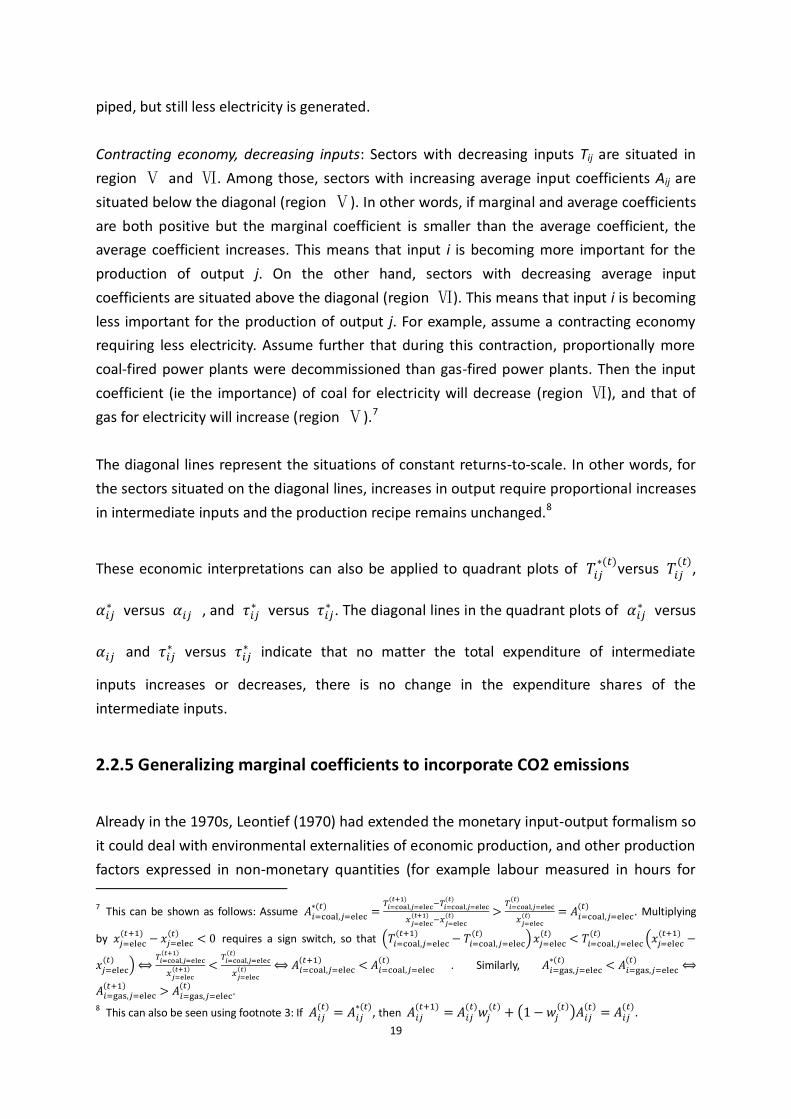
Figure 2.4: A comparison of average input coefficients (x-axis) and marginal input

coefficients * (y-axis) for China’s production recipe in 1992 and 2005, expressed in the

33-sector classification. Points for which = * lie on the diagonal dotted line. Each


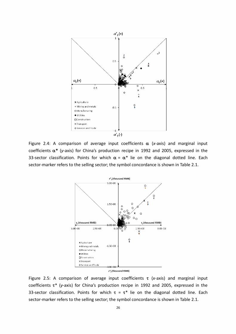
Figure 2.5: A comparison of average input coefficients (x-axis) and marginal input

coefficients * (y-axis) for China’s production recipe in 1992 and 2005, expressed in the

33-sector classification. Points for which = * lie on the diagonal dotted line. Each


27

Since and coefficients reference intermediate transactions 𝑇𝑖𝑗 to their sum ∑ 𝑇𝑖𝑗𝑗 , they

cannot all increase or decrease at the same time (see footnote 4). Therefore, when vs *

and vs * are depicted in a diagram, markers clouds must contain markers above and

below the diagonal, which is evident in Figure 2.4. Transactions represented by marker

points above the diagonal have become more important in the input mix of the production

recipe, and vice versa. As a consequence of value added being excluded in the and

coefficients, the transactions represented by marker points located above the diagonal are

the ones being displaced by the supplies of services () and manufactured products (o) to

sectors such as finance and insurance, material products, and transport. These transactions

have grown in importance in China’s economy at the expense of extractive industries.

Table 2.2 presents a comparison of findings of the kind shown in Figures 2.2-2.5, but instead

of showing diagrams for all years, I calculate the slopes b of the transactions’ marker point

“clouds” using linear regressions 𝐴𝑖𝑗∗ = b 𝐴𝑖𝑗 etc.

Table 2.2: Slope b and Student’s t from regressions of the data in Figures 2.2-2.5 for China,

but for various time intervals between 1992-2005

time interval A*-A T*-T

b t b t b t b t

1992-2005 0.67 16.8 0.62 11.8 0.86 19.8 0.75 19.7

1992-2002 0.69 13.2 0.63 4.2 0.77 12.9 0.66 3.3

1997-2005 0.94 29.9 0.87 22.6 0.94 28.6 0.88 29.0

1992-1997 0.67 6.3 0.58 4.9 0.79 4.9 0.58 4.5

1997-2002 0.80 13.5 0.63 4.1 0.77 16.8 0.73 8.9

2002-2005 1.04 28.7 1.04 21.9 1.10 23.0 1.01 19.1

Weighted average 0.86 ± 7.6% 0.83 ± 10 % 0.91 ± 5.7 % 0.84 ± 6.9 %

28

Figure 2.6: Slopes b from regressions of the data in Figures 2.2-2.5 for China, plotted against

the mean of the time intervals. For example, the A*-A slope 0.67 (see Table 2.2, column 1)

for the interval 1992-2005 was plotted at X = 1998.5.

Table 2.2 shows that marginal coefficients were smaller than average coefficients except for

2002-2005. Figure 2.6 reveals a clear upwards trend of slopes b, and hence of marginal

coefficients over time. For the years up to 2001, I see that the marginal coefficients are

smaller than the average coefficients. This implies that the average coefficients decrease

over time (for growing outputs).

The counterpart of the average A and T coefficients is the value added coefficient, which

hence increase over time. However, its growth slows down (marginal coefficients come

closer to the average coefficients, as reflected by the upward trend in the slope) and even

turns into a decline according to the observations for point 2003.5.

Slopes b < 1 show that there are more sectors with decreasing average coefficients than

increasing average and coefficients, meaning that the average coefficients of many

intermediate inputs (for example agriculture and mining, see Figures 2.4 and 2.5) decrease

at the cost of the coefficients of some intermediate inputs (for example services) increasing.

The are normalized (see footnote 4), so the many sectors with decreasing coefficients

must overall be sectors with smaller coefficients. The slopes have increased over time, and

hence the sectors with decreasing average and coefficients have become fewer, and/or

the decrease of their average and coefficients has slowed down. At the same time, the

sectors with increasing average and coefficients have become more numerous. By 2005,

the initial situation has reversed, with the average coefficients of as many intermediate

inputs decreasing and increasing.

29

2.3.3 Marginal change in CO2 emissions

Since this Special Issue is about “Greening Growing Giants”, I now focus on marginal change

in CO2 emissions. Figure 2.7 shows a comparison of marginal versus average CO2 coefficients

for China determined according to Eqs. 2.6 and 2.7. Markers on the diagonal line in Figure

2.7 show that new technology in these sectors had no increasing or decreasing effect on CO2

emission intensity. Given the logarithmic scale of the diagram, it becomes evident that

marginal and average intensities differ substantially, indicating a more pronounced change in

the CO2 intensity of production compared to the monetary production recipe. All sectors,

except petroleum refining and coking (o3), metal smelting (o4), real estate (5), scrap and

waste (o9), other manufacturing products (o14) and hotels and restaurants (15), have

registered marked decreases in CO2 intensity, especially in sectors of gas production and

supply (◆1) , ferrous ore mining (+12) and construction ( 16).

Figure 2.7: Comparison of average CO2 coefficients q versus marginal CO2 intensities q* for

China’s economy 2002 and 2005, expressed in 33-sector classification. The markers are

calculated from log10(q*)-log10(q).

The 𝝌 and 𝝌∗ introduced in Eqs. 2.8 combine CO2 intensities and monetary input

coefficients (expressed in kg of CO2 per RMB). In order to demonstrate a variation to the

30

kind of results I have presented so far, I plot in Figure 2.8 showing 𝝌 and 𝝌∗ for 33

Chinese sectors, but as with the q*-q comparison, I calculate the marginal coefficients over

the time interval 2002-2005. This allows us to identify nearest marginal changes in overall

CO2 flows between 2002 and 200512, and compare these to the 2002 average CO2 flows.

Note that the markers indicate the emissions embodied in the intermediate inputs that are

required for the production of 1 RMB in sector j (i.e. ∑ 𝜒𝑖𝑗 = ∑ 𝑞𝑖𝐴𝑖𝑗𝑖𝑖 ). Equivalently,

∑ 𝜒𝑖𝑗∗ = ∑ 𝑞𝑖

∗𝐴𝑖𝑗∗

𝑖𝑖 gives the additional emissions embodied in the additional intermediate

inputs that are required for 1 RMB of additional production in sector j.

Figure 2.8: 𝝌 and 𝝌∗ measures calculated for the interval 2002-2005, using China’s

33-sector classification and representing ∑ 𝝌𝑖𝑗𝒊 , ∑ 𝝌𝑖𝑗∗

𝒊 respectively.

Figure 2.8 shows clearly that the replacement of A* for A and q* for q sometimes result in

an increase of physical transactions, particularly for the sectors of coal mining and

processing (+7), crude petroleum products and natural gas products (+13), metal smelting

(o4), non-metal minerals mining (+10), electricity and steam production and supply (◆2),

chemical products (o8) and metal products (o11). This means that, during the past decade,

12 CO2 emission data are available from 2000. Therefore, we can only analyze the marginal changes in CO2 emissions between 2002 and 2005.

31

efforts to reduce CO2 emissions have concentrated more on decarbonizing production

processes rather than re-organizing the production recipe.

When comparing Figure 2.8 with Figure 2.7, it is notable that the sectors with labels

mentioned above are situated below diagonal line in Figure 2.7. After multiplied with

marginal coefficients, they show increase of physical transactions and are located above the

diagonal line in Figure 2.8. This means that even though technological change has brought

about reductions in CO2 emissions for these sectors, the CO2 emissions are partly offset by

structural changes in the production recipe.

It is worthwhile to note that not only technological innovation plays an important role in

reducing CO2 intensity, but also outsourcing of production chains contributes to the

reductions on CO2 intensity. As pointed out by the ‘physical flows’ study by Wiedmann et al.

(2007), China imports 50% of its natural gas and 30% of its iron ore in around 2005 and most

of its construction materials are sourced domestically. Typically the iron ore exported from

Australia to China increased dramatically from $12.8 million in 1995 to $30.2 billion in 2010.

The importing natural gas of China increased from $414 million in 1995 to $5.89 billion in

2010 (Simoes et al. 2015). The origin importing countries of natural gas for China in 1995

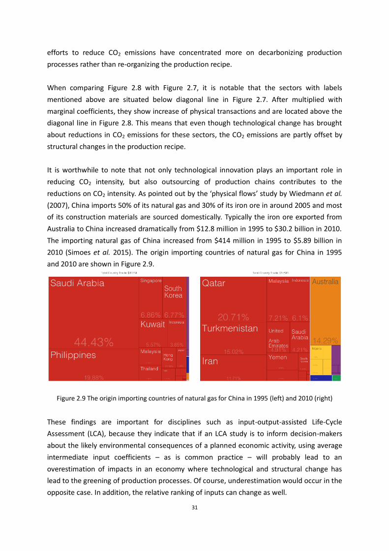
and 2010 are shown in Figure 2.9.

Figure 2.9 The origin importing countries of natural gas for China in 1995 (left) and 2010 (right)

These findings are important for disciplines such as input-output-assisted Life-Cycle

Assessment (LCA), because they indicate that if an LCA study is to inform decision-makers

about the likely environmental consequences of a planned economic activity, using average

intermediate input coefficients – as is common practice – will probably lead to an

overestimation of impacts in an economy where technological and structural change has

lead to the greening of production processes. Of course, underestimation would occur in the

opposite case. In addition, the relative ranking of inputs can change as well.

32

2.4 Conclusions of Chapter 2

I have used the input-output tables in constant price extended with CO2 emissions for

calculating marginal input coefficients in monetary as well as CO2 terms. Marginal

coefficients are increasingly mentioned in the literature, and recommended for applications

such as consequential Life-Cycle Assessment, where they are supposed to lead to more

realistic results especially in prospective analyses.

Despite their increased relevance for prospective studies, the use of marginal coefficients

also comes with methodological/theoretical drawbacks. First, negative marginal coefficients

cannot be understood in a causal sense, ie that an increase in output would causally lead to

a decrease in the amount of an input. Second, since marginal coefficients are derived from

differences in transactions and gross output, their relative standard deviations are often

much larger than those of the transactions and gross output, respectively13. This also means

that marginal coefficients can be subject to large variability, which may in some cases

preclude obtaining meaningful results. For example, I attempted a regression analysis of the

relationship between average and marginal coefficients for China over 13 years, however the

results show considerable scatter.

The use of marginal coefficients is not (yet) widespread, in general and also in consequential

Life-Cycle Assessment. My work provides a first, broad overview about the magnitude and

distribution of these coefficients across recent years, for which marginal coefficients could

be expected to differ greatly from average coefficients. Summarizing, I find that

- Marginal coefficients can differ substantially from average coefficients, thus lending

support to the need expressed in the literature for coining consequential LCA and

similar prospective assessments in marginal rather than average terms;

- In my analysis, marginal coefficients are smaller than average coefficients, indicating

(for most years) a declining share of intermediate inputs in the production recipe.

13

Error propagation shows that this is because

𝜎 (𝐴𝑖𝑗∗(𝑡)) = √[

𝜕𝐴𝑖𝑗∗(𝑡)

𝜕𝑇𝑖𝑗(𝑡+1) 𝜎 (𝑇𝑖𝑗

(𝑡+1))]

2

+ [𝜕𝐴

𝑖𝑗∗(𝑡)

𝜕𝑇𝑖𝑗(𝑡) 𝜎 (𝑇𝑖𝑗

(𝑡))]

2

+ [𝜕𝐴

𝑖𝑗∗(𝑡)

𝜕𝑥𝑗(𝑡+1)𝜎 (𝑥𝑗

(𝑡+1))]

2

+ [𝜕𝐴

𝑖𝑗∗(𝑡)

𝜕𝑥𝑗(𝑡) 𝜎 (𝑥𝑗

(𝑡))]

2

= √[𝜎 (𝑇

𝑖𝑗

(𝑡+1))

𝑥𝑗

(𝑡+1) − 𝑥𝑗

(𝑡)]

2

+ [𝜎(𝑇

𝑖𝑗

(𝑡))

𝑥𝑗

(𝑡+1) − 𝑥𝑗

(𝑡)]

2

+ [𝑇𝑖𝑗

(𝑡+1) − 𝑇𝑖𝑗

(𝑡)

(𝑥𝑗

(𝑡+1) − 𝑥𝑗

(𝑡))2 𝜎 (𝑥𝑗

(𝑡+1))]

2

+ [𝑇𝑖𝑗

(𝑡+1) −𝑇𝑖𝑗

(𝑡)

(𝑥𝑗

(𝑡+1) − 𝑥𝑗

(𝑡))2 𝜎 (𝑥𝑗

(𝑡))]

2

= 𝐴𝑖𝑗∗(𝑡)√[

𝜎(𝑇𝑖𝑗(𝑡+1)

)

𝑇𝑖𝑗(𝑡+1)

−𝑇𝑖𝑗(𝑡)]

2

+ [𝜎(𝑇

𝑖𝑗(𝑡))


−𝑇𝑖𝑗(𝑡)]

2

+ [𝜎(𝑥

𝑗(𝑡+1)

)

𝑥𝑗(𝑡+1)

−𝑥𝑗(𝑡)]

2

+ [𝜎(𝑥

𝑗(𝑡))

𝑥𝑗(𝑡+1)

−𝑥𝑗(𝑡)]

2

.

For each of the four terms I observe that in general 𝜎(𝑇𝑖𝑗

(𝑡+1))


−𝑇𝑖𝑗(𝑡) ≫


)

𝑇𝑖𝑗(𝑡+1) , and therefore

𝜎(𝐴𝑖𝑗∗(𝑡)

)

𝐴𝑖𝑗∗(𝑡) ≫


)

𝑇𝑖𝑗(𝑡+1) , etc.

33

- Similarly, the upwards trend of marginal coefficients indicate that: a) the growth of

value added relative to intermediate input has been slowing down, recently turning

into a decline; and b) inputs of service industries have increased increase at the cost

of some raw material industries;

- Marginal CO2 emissions coefficients differ more from their average counterparts than

marginal monetary coefficients, showing that for China, within-sector technological

solutions to emissions abatement have played a more important role than the

re-organisation of supply structures. Hence, in disciplines such as consequential LCA,

using marginal CO2 coefficients appears more essential than using marginal

monetary coefficients;

- There exists considerable scatter and variation of marginal coefficients across years,

which to a certain extent precludes the identification of clear temporal and sectoral

trends;

2.5 Future development of marginal coefficients - Testing marginal

coefficients for prospective evaluations

Consider the case where I have a time series of IO tables available. Suppose I use the tables

in periods t-1 and t for calculating an impact in periods t+1 and t+2. In order to test the

performance of using the marginal coefficients for this purpose, I will calculate the impact of

the true (and actually observed) final demands in periods t+1 and t+2. In other words, I

forecast the gross outputs in periods t+1 and t+2 on the basis of the IO tables for periods t-1

and t and projections for the final demands in periods t+1 and t+2.

Let 𝑍𝑡−1, 𝑍𝑡, 𝑍𝑡+1, and 𝑍𝑡+2 denote the matrices with intermediate deliveries in each

of the periods. Let 𝑥𝑡−1, 𝑥𝑡, 𝑥𝑡+1, and 𝑥𝑡+2 denote the corresponding vectors of gross

output and 𝑓𝑡−1, 𝑓𝑡 , 𝑓𝑡+1, and 𝑓𝑡+2 the vectors of final demands. The corresponding

matrices of average input coefficients are given by 𝐴𝑡−1 = 𝑍𝑡−1��𝑡−1−1 and, similarly, 𝐴𝑡,

𝐴𝑡+1, and 𝐴𝑡+2. The marginal input coefficients are defined as

𝑀𝑡,𝑡−1 = (𝑍𝑡 − 𝑍𝑡−1)(��𝑡−1 − ��𝑡−1

−1 ) (2.9)

For the IO models I start from the accounting equation 𝑥𝑡−1 = 𝑍𝑡−1𝑒 + 𝑓𝑡−1 where e

34

indicates the summation vector containing ones. Using the definition for the average input

coefficients yields 𝑥𝑡−1 = 𝐴𝑡−1𝑥𝑡−1 + 𝑓𝑡−1 which implies 𝑥𝑡−1 = (𝐼 − 𝐴𝑡−1)−1𝑓𝑡−1 =

𝐿𝑡−1𝑓𝑡−1 where 𝐿𝑡−1 = (𝐼 − 𝐴𝑡−1)−1 is the Leontief inverse. For the marginal input

coefficients I combine 𝑥𝑡−1 = 𝑍𝑡−1𝑒 + 𝑓𝑡−1 with 𝑥𝑡 = 𝑍𝑡𝑒 + 𝑓𝑡 into 𝑥𝑡 − 𝑥𝑡−1 = (𝑍𝑡 −

𝑍𝑡−1)𝑒 + (𝑓𝑡 − 𝑓𝑡−1). Using the definition of the marginal input coefficients gives 𝑥𝑡 −

𝑥𝑡−1 = 𝑀𝑡,𝑡−1(𝑥𝑡 − 𝑥𝑡−1) + (𝑓𝑡 − 𝑓𝑡−1). Its solution is given by

𝑥𝑡 − 𝑥𝑡−1 = (𝐼 −𝑀𝑡,𝑡−1)−1(𝑓𝑡 − 𝑓𝑡−1). (2.10)

2.5.1 Forecasting the gross outputs in t+1

Suppose I would like to forecast the gross outputs in period t+1. The available information is

the (correct) prognosis for the final demand vector in period t+1 (i.e. 𝑓𝑡+1) and the full IO

tables for the periods t and t-1. Because the prognosis for the final demand vector is

assumed to be correct, the correct forecast is 𝑥𝑡+1 which serves as the benchmark. Using

the most recent average input coefficients that are available, the forecast amounts to

𝑥𝑡+1𝑎𝑣𝑒 = (𝐼 − 𝐴𝑡)

−1𝑓𝑡+1 (2.11)

where the superscript ave indicates that the forecast is obtained from using average input

coefficients.

Using the marginal input coefficients, the true answer is obtained from the period t+1

equivalent of Eq. (2.9). That is, 𝑥𝑡+1 − 𝑥𝑡 = (𝐼 −𝑀𝑡+1,𝑡)−1(𝑓𝑡+1 − 𝑓𝑡). Because 𝑀𝑡+1,𝑡 is

not available in period t it is replaced in the forecast by its estimate 𝑀𝑡,𝑡−1. This yields

𝑥𝑡+1𝑚𝑎𝑟 = 𝑥𝑡 + (𝐼 −𝑀𝑡,𝑡−1)

−1(𝑓𝑡+1 − 𝑓𝑡). (2.12)

where the superscript mar indicates that the forecast is obtained from using marginal input

coefficients. Using the definition from Eq.(2.9), the forecast for the matrix of intermediate

deliveries yields

35

𝑍𝑡+1𝑚𝑎𝑟 = 𝑍𝑡 +𝑀𝑡,𝑡−1(��𝑡+1

𝑚𝑎𝑟 − ��𝑡) (2.13)

2.5.2 Forecasting the gross outputs in t+2

For the gross output in t+2 I have 𝑥𝑡+2 = 𝑥𝑡+1 + (𝐼 − 𝑀𝑡+2,𝑡+1)−1(𝑓𝑡+2 − 𝑓𝑡−1). Because

𝑥𝑡+1 is not known, it is estimated by its forecast 𝑥𝑡+1𝑚𝑎𝑟 in (4). Also the matrix 𝑀𝑡+2,𝑡+1 is

not known and is estimated by 𝑀𝑡+1,𝑡. In its turn, however, 𝑀𝑡+1,𝑡 is not known and is

itself estimated by 𝑀𝑡,𝑡−1. This yields

𝑥𝑡+2𝑚𝑎𝑟 = 𝑥𝑡+1

𝑚𝑎𝑟 + (𝐼 −𝑀𝑡,𝑡−1)−1(𝑓𝑡+2 − 𝑓𝑡−1) (2.14)

and substituting Eq.(2.11) gives

𝑥𝑡+2𝑚𝑎𝑟 = 𝑥𝑡 + (𝐼 − 𝑀𝑡,𝑡−1)

−1(𝑓𝑡+2 − 𝑓𝑡) (2.15)

When forecasting with the average input coefficients I arrive at

𝑥𝑡+2𝑎𝑣𝑒 = (𝐼 − 𝐴𝑡)

−1𝑓𝑡+2 (2.16)

The equations can be readily adapted for other forecasts.

2.5.3 Forecasting emissions

Let 𝑐𝑡−1, 𝑐𝑡, 𝑐𝑡+1, and 𝑐𝑡+2 denote the emissions in the years t, …, t+2. Let the average

emission coefficients (i.e. emissions per unit of gross output) be given by 𝑔𝑡−1 = ��𝑡−1−1 𝑐𝑡−1

and similar expressions for other years. This implies that I can write 𝑐𝑡−1 = ��𝑡−1𝑥𝑡−1. The

marginal emission coefficients are defined as

ℎ𝑡,𝑡−1 = (��𝑡−1 − ��𝑡−1

−1 )(𝑐𝑡 − 𝑐𝑡−1) (2.17)

In case of the average emission coefficients, the forecast for period t+2 would be obtained

from 𝑐𝑡+2 = ��𝑡+2𝑥𝑡+2 and using 𝑔𝑡 as an estimate for 𝑔𝑡+2 and using 𝑥𝑡+2𝑎𝑣𝑒 as an

estimate for 𝑥𝑡+2. This yields

36

𝑐𝑡+2𝑎𝑣𝑒 = ��𝑡(𝐼 − 𝐴𝑡)

−1𝑓𝑡+2 (2.18)

In case of the marginal emission coefficients, I have

𝑐𝑡+2 = 𝑐𝑡 + ℎ𝑡+2,𝑡+1(𝑥𝑡+2 − 𝑥𝑡+1) + ℎ𝑡+1,𝑡(𝑥𝑡+1 − 𝑥𝑡) (2.19)

Both vectors of marginal emission coefficients are now estimated by ℎ𝑡,𝑡−1 and 𝑥𝑡+2 is

estimated by 𝑥𝑡+2𝑚𝑎𝑟. This yields

𝑐𝑡+2𝑚𝑎𝑟 = 𝑐𝑡 + ℎ𝑡,𝑡−1(𝑥𝑡+2

𝑚𝑎𝑟 − 𝑥𝑡) (2.20)

Substituting Eq.(2.14) gives

𝑐𝑡+2𝑚𝑎𝑟 = 𝑐𝑡 + ℎ𝑡,𝑡−1(𝐼 − 𝑀𝑡,𝑡−1)

−1(𝑓𝑡+2 − 𝑓𝑡) (2.21)

2.5.4 Forecasting applications

Similar expressions can be given for forecasts further into the future. In terms of applications,

it would be interesting to consider one country with a time series of considerable length and

a cross country analysis (e.g. the OECD database covers 28 countries with IO tables for –at

least– years around 1995, 2000, and 2005).

37

Connecting Page

Marginal coefficients and Structure decomposition Analysis are analytical techniques based

on IO data. Marginal input coefficients can be extracted from IO tables to capture the

changes in technologies (and their combinations), while SDA technique can be applied to

compare two economic structures by using IO accounts as input data.

The results by these two research methods can be combined together to explain the

economic structure of one region for two different time periods, or a cross-sectional analysis

by comparing two different economies for the same time period.

38

Chapter 3 A Structural Decomposition Analysis

of Global Energy Footprints

3.1 Introduction

As globalization has blurred the lines between country border security and economic

interchange, new challenges have arisen. The concurrent and longer-term shifts in the global

economy are like movements of tectonic plates, with boosts in fossil fuel imports to

developing Asia offsetting flat or declining energy demand in the developed countries. These

shifts have major implications for long-standing security relationships as the producers in

the developed counties untangle themselves from historic dependencies. This process has

fanned the debate surrounding energy security. Developed countries are becoming

increasingly reliant on developing countries not only for their non-renewable energy

requirements (such as fossil fuels), but also for the energy embodied in the products they

import for domestic consumption. The increasing globalization of energy markets and supply

chains means that energy security has become a complex policy issue for governments in

particular, but also multinational organizations trading across multiple borders and

intergovernmental organizations working on energy, security, environmental protection and

quality of life issues. It is in this context that I seek to understand the driving forces of

regional and worldwide energy consumption through the development of a global energy

footprint.

To better understand how worldwide energy consumption has changed over time, I use

structural decomposition analysis (SDA). SDA is a technique that utilizes input-output (IO)

databases to break down observed changes in physical variables (such as energy footprint)

over time, into changes in their physical and economic determinants (e.g. energy intensity or

final demand structure). Using this methodology, I can also quantify the influence of these

determinants over the changes in energy consumption. The changes in these determinants

are understood to be driving the changes in the variables, either as accelerators or as

retardants. By using SDA to quantify determinants of changes in energy use the real drivers

of energy consumption can be discovered.

The use of SDA is now a widely accepted analytical tool for policymaking on energy issues at

a national level, and to develop understanding of the global energy footprint. Table 1

provides a summary of the key features and developments of energy SDA from a period of

39

1990 to 2010. Of the 31 energy SDA studies considered here, 75% represent decomposition

of changes in energy footprint over time in one or two single countries. Nine of the studies

include international trade between countries and regions in their SDA of the energy

footprint (Howarth et al. 1991; Howarth et al. 1993; Park et al. 1993; Sun 1998; Unander et

al. 1999; Sun and Ang 2000; de Nooij et al. 2003; Alcántara and Duarte 2004; Kagawa and

Inamura 2004). All of the studies considered used only single-region input-output

frameworks to carry out the SDA, even when the study involved groups of countries. Only

Kagawa and Inamura (Kagawa and Inamura 2004) used a multi-region input-output (MRIO)

framework in their study, using China-Japan inter-country IO tables to measure the effects of

the changes in energy demand. There is also a time lag between study publication date and

the data used. Since 2010 more studies using MRIO frameworks have been conducted, but

have not been included in this review.

Table 3.1 Specific features of SDA studies of energy footprint (1990-2010)

Publication Application Drivers

Decomposition

Method year authors area period

1990 Schipper et al. United States 1973-1987 3 ad hoc

1990 Chia-Yon et al. Taiwan 1971-1984

1991 Howarth et al. 8 OECD 1973-1987 4 LMDI

1991 Rose et al. United States 1972-1982 4 D&L

1992 Schipper et al. Norway 1973-1987 3 ad hoc

1992 Islam and Morison Australia 1974-1975

1980-1981 5 ad hoc

1992 Park Korea 1973-1989 3 D&L

1993 Park et al. 26 countries 1973-1980

1980-1988 3 D&L

1993 Howarth et al. 5 OECD 1973-1988 3 ad hoc

1994 Ang and Lee Singapore 1974-1990

3 D&L Taiwan 1971-1991

1994 Wilson et al. Australia 1973-1990 5 ad hoc

1994 Han and Lakshmanan Japan 1975-1985 4 ad hoc

1995 Lin and Polenske China 1981-1987 4 D&L

1997 Ang and Choi Korean 1981-1993 4 LMDI

1997 Campos Machado and

Miller United States 1963-1987 3 ad hoc

1998 Ang et al. Singapore,China,Korea 1985-1990 3 LMDI

1998 Sun Worldwide 1973-1990 3 SSA

1998 Wier Denmark 1966-1988 6 D&L

1999 Unander et al. 13 OECD 1971-1995 3 ad hoc

2000 Jacobsen Denmark 1966-1992 6 D&L

2000 Sun and Ang 15 European countries 1973-1995 4 SSA

40

* Methodology acronyms are listed in Section 3.5.1.

The novelties of my study are:

Detailed presentation of deflation procedure - when SDA is carried out over time, it is

vital to separate the quantity effects and the price effects that are aggregated in

current-price IO tables, and use IO tables with constant prices (Dietzenbacher and Hoen

1998). International comparative analysis requires the original aggregates in local

currency units to be deflated and converted into a common currency in a constant price

so they may be compared over time and across countries. Many SDA papers gloss over

this procedure. In Section 4.7.5, I present a detailed account of deflation procedure as a

contribution to greater understanding of this issue within the practice of SDA.

Exploration of SDA method selection - prevalent SDA methods are summarized by Su

and Ang (2012), who proposed a general additive decomposition framework to link

these SDA methods. However, their framework is only applied to China’s CO2 emission

analysis. I explore three SDA models and compare their applications on a worldwide

scale, contributing to existing recommendations for SDA method selection.

Analysis of energy footprint changes over time and geographies - although significant

work has been undertaken on the SDA of energy footprint, there is an obvious gap in

the existing literature because in most recent studies carbon emissions have been

chosen as the environmental indicator instead of energy footprint. My work seeks to fill

this knowledge gap by offering an MRIO-based SDA of the global energy footprint with

the aim of fostering understanding of worldwide energy use patterns and energy

security issues. Applying SDA to global energy footprint provides an effective way to

identify the determinants of countries’ and sectors’ changes in energy footprint.

However, due to lack of IO time series tables expressed in constant prices, geographical

(country or region) detail, and consistent environmental satellite accounts, much of the

prior work is limited to the study of only one country, one national currency unit and

the difference between two single years. As more MRIO databases with a global

2001 Shigemi and Hajime Japan 1985-1990 4 D&L

2003 Choi and Ang Singapore and Taiwan 1980-1990 2 LMDI

2003 de Nooij et al. 8 OECD 1990 5 D&L

2003 Zhang China 1991-1997 3 D&L

2004 Alcántara and Duarte 14 European countries 1994-1995 3 D&L

2004 Kagawa and Inamura China and Japan 1985-1990 6 ad hoc

2005 Cohen et al. Brazil 1995 -- ad hoc

2006 Ediger and Huvaz Turkish 1980-2000 3 LMDI

2008 Ma and Stern China 1980-2003 5 LMDI

2009 Wachsmann et al. Brazil 1970-1996 6 LMDI

41

coverage and environmental extensions, for example the GTAP (GTAP 2012; Andrew

and Peters 2013), EXIOBASE (EXIOPOL 2011; Wood et al. 2014), WIOD (WIOD 2012;

Dietzenbacher et al. 2013a), and the Eora databases (Lenzen et al. 2012; Lenzen et al.

2013) become available to the general public (Tukker and Dietzenbacher 2013),

researchers are able to apply SDA at the inter-country level and across multiple time

intervals. In this study, I employ the Eora MRIO database because it includes a long time

series (1990-2010) of spatially and sectorally detailed annual MRIO tables and

environmental satellite accounts.

Spatial SDA decomposition - existing SDA results mainly focus on revealing the temporal

driving forces of some physical variables. A SDA of the energy footprints for a large

number of countries with a MRIO framework, however, has not been carried out. In

addition, I spatially decompose SDA results, as Single Region Energy Footprints (SREFP),

Total Energy Footprints (TEFP), Domestic Energy Footprints (DEFP) and Rest-of-World

Energy Footprints (RoWEFP). This methodological innovation of SDA allows us to

examine the effect of international outsourcing of energy-intensive production

processes.

The paper is structured as follows. In Section 3.2 I will explain deflation procedure and then

compare prevalent SDA methods. In Section 3.3 I will provide the results and a discussion of

using the Eora MRIO database to conduct a SDA of global energy use. I also provide a

discussion and recommendations for SDA method selection. In Section 3.4 I conclude by

summarizing my work and offering the reader an outlook for future research.

3.2 Methodology and data

In the following section I describe the methods and data used for this study, focusing in

detail on novel contributions, and providing references where material has been extensively

dealt with in the existing literature. In particular I explain how I converted the Eora MRIO

time series data into constant prices (Section 3.2.1), the SDA decomposition form and

methods I apply (Section 3.2.2), how I used the MRIO structure to spatially decompose

international supply chains (Section 3.2.3), and the data sources utilised for this study

(Section 3.2.4).

3.2.1 Construction of constant-price MRIO tables

Constructing constant-price IO tables is undoubtedly important and necessary for any SDA

study. Obviously, in the process of converting national currency units into a constant-price

common-currency unit, the choice of an appropriate series of deflators and converters as

well as the procedure in which the series will be employed, will have a substantial effect on

42

the interpretation of resulting data series (Pardey et al. 1992).

Section 4.7.5 explains two prevailing procedures of constructing constant-price IO tables. I

follow the preference of most researchers by choosing the approach of “convert-first then

deflate” (Pardey et al. 1992; Fremdling et al. 2007; Hale and Arteta 2009; Li and Zhong 2009).

The rationale for this preference is that countries experience diverse stages of development

over a long time period resulting in a potentially large temporal variability of the relative

worth of their consumption baskets. This variability can be captured adequately by using

Purchasing Power Parity exchange rates (PPPs) in the conversion procedure, and by then

using Producer Price Indexes (PPIs) deflators. I adopt detailed sectoral deflators for the US

economy in the deflation procedure to convert the domestic currency into common US

dollars.

3.2.2 Additive SDA methods

The standard Leontief IO demand-pull model can be expressed as:

𝐱 = 𝐀𝐱 + 𝐘 = (𝐈 − 𝐀)−𝟏𝐘 = 𝐋𝐘 (3.1)

where

- 𝐱 = (𝑥𝑖)𝑛×1 is the vector of gross outputs by n industry sectors;

- 𝐀 = (𝐴𝑖𝑗)𝑛×𝑛 is the nn matrix of domestic technical coefficients 𝑎𝑖𝑗 = 𝑥𝑖𝑗/𝑥𝑗

representing monetary flows from industry i to industry j;

- 𝐘 = {𝑌𝑖}𝑛×1 is the vector of final demand from n industry sectors;

- L is the nn Leontief inverse matrix representing structural interdependencies.

SDA usually involves the generalization of the IO system from purely monetary terms to

incorporate environmental and resource measures. Energy footprint from production can be

formulated using the Leontief IO model in Eq. (3.1) as:

𝐐 = 𝐪𝐋𝐘 (3.2)

with Q being total energy requirements or energy footprint, and 𝐪 = {𝑞𝑖𝑗}𝑛×𝑛 being the

direct energy intensity vector representing the energy footprint in physical units per unit of

monetary output of each production sector (e.g., PJ/$). Here I define ‘energy requirements’

or ‘energy footprint’ as an indicator that can show clearly the effects of consumption-driven

actions on the energy use in production occurring elsewhere.

For further decomposition of the energy footprint, the vector of final demand y can be

43

subdivided into three drivers: final demand structure14 𝐮 = (𝑢𝑖𝑑)𝑛×𝑚 = 𝐹𝑖𝑑(𝐠−𝟏) , where

F is the nm flow matrix of final demand and 𝐠 = ∑ 𝐹𝑖𝑑𝑛𝑖=1 is the 1m matrix of total final

demand by category, representing the ratio of input 𝐹𝑖𝑑 from sectors i=1,…,n in total final

demand by category d=1,…,m (ie. commodity structure of final demand); final demand

destination 𝐯 = (𝑣𝑑)𝑚×1 = (𝐠(𝐘−1))′ , final demand/capita y (11) and population P(11),

resulting in

𝐐 = 𝐪𝐋𝐮𝐯𝐲𝐏 (3.3)

The central idea of SDA is that changes in Q are decomposed in changes of its determinants

resulting in an exhaustive sum of contributions from all changes in energy use within a

certain period (Wachsmann et al. 2009). Supposing the total amount of energy footprint

from production at time 0 and t are 𝐐0 and 𝐐𝑡 respectively, the change in energy

footprint ∆𝐐 is decomposed into following five effects15

∆𝐐 = ∆𝐪 + ∆𝐋 + ∆𝐮 + ∆𝐯 + ∆𝑦 + ∆𝑃 (3.4)

where ∆𝐪 is the energy intensity effect, ∆𝐋 is the Leontief structure effect, ∆𝐮 is the final

demand structure effect (product mix effect), ∆𝐯 is the final demand destination effect, ∆𝑦

is the level of GDP/capita effect (affluence effect), ∆𝑃 is the population effect16.

As summarized by Su and Ang (2012), the following three methods are the most prevalent

approaches: (1) the Dietzenbacher and Los (D&L) method (Dietzenbacher and Los 1998); (2)

the Logarithmic Mean Divisia Index (LMDI) method (Ang et al. 1998; Ang et al. 2003); and (3)

the Shapley-Sun-Albrecht (SSA) method (Sun 1998; Albrecht et al. 2002). The mathematical

formulations are summarised in Section 4.7.2. In this study, I compare the results given by

these three methods and propose recommendations for method selection.

3.2.3 MRIO-based Spatial decomposition

Having available a MRIO framework, it is possible to decompose change in energy footprint

not only structurally but also spatially to highlight the effect of international outsourcing of

energy-intensive production processes. To this end, I split the MRIO framework into a

domestic component and an international trade component for every country I appraise.

14 Conventionally private (household) final consumption, government final consumption, gross fixed capital expenditure, changes in inventories, and exports. Here, m = 6 and d = (1, … ,6). 15

In the case of energy decomposition studies, most authors choose additive over multiplicative decomposition form, because the former is generally easier to interpret. For a comparative review, see95 Hoekstra, R. & van den Bergh, J. C. J. M. Comparing structural and index decomposition analysis Energy Economics 25, 39-64, doi:10.1016/s0140-9883(02)00059-2 (2003)., Choi and Ang (2003), Su and Ang (2012). 16 Detailed explanation of the variables in the decomposition equation are referred to Wood and Lenzen (2009), Wachsmann et al.(2009), Rørmose (2011).

44

Figure 3.1 Schematic of MRIO-based spatial decomposition models for a 3-country economy, showing

components of the energy footprint of the United Kingdom of Great Britain and Northern Ireland (GBR)

as it relates to China (CHN) and Germany (DEU).

T – intermediate transactions (MRIO), Y – final demand (MRIO), Q – energy footprint (satellite). ‘GBR’, ‘CHN’ and ‘DEU’ are

ISO ALPHA-3 country codes issued by the United Nations UN 2014. Acms are listed in Section 3.5.1

First, by invoking only a part of final demand (for example GBR’s final demand YGBR in Figure

3.1), I can investigate spatially delineated patterns of energy footprint causation. Second, by

activating only a part of intermediate demand (for example GBR’s economy TGBR,GBR in Figure

1) I can exclude international trade feedback loops from footprint measures. Third, by

coupling only a part of the energy satellite to the MRIO framework (for example China’s and

SREFP TEFP

DEFP RoWEFP

45

Germany’s energy satellites QCHN and QDEU in Figure 3.1), I are able to separately account for

different energy origins. Proceeding as such, the single-region energy footprint (SREFP)

captures the energy footprint for a country facilitated only via domestic supply chains. This is

the traditional SDA setting in most of the recent literature on environmental SDA. The

domestic energy footprint (DEFP) measure extends the SREFP metric by including the energy

embodied within global supply chains. For example, a supply chain included in a DEFP but

not in a SREFP would be the energy used in the GBR for manufacturing gas turbines

exported to the Netherlands for generating power to supply dairy manufacturing

establishments that export cheese to the UK. As for the DEFP, the rest-of-world energy

footprint (RoWEFP) assumes global supply change coverage, however adds up only energy

initially used in countries other than the UK. Hence the RoWEFP would include components

such as the energy used for mining coal in Australia, exported to China for generating power

to manufacture household equipment exported to the UK. In unison, DEFP and RoWEFP

form a mutually exclusive and collectively exhaustive representation of the total energy

footprint (TEFP). Figure 3.1 offers a schematic three-region illustration of energy footprints

for the UK. Being a consumption-based measure, the UK’s energy footprint is driven solely

by the GBR’s final demand YGBR. Being able to occur anywhere in the world, the UK’s energy

footprint draws on energy footprint in the GBR (QGBR) as well in China (QCHN), Germany (QDEU)

and the other countries in the world (see also Figure 6 in Lenzen et al. 2012). The MRIO

table’s trade block (eg. TCHN,GBR, inputs from China into the UK) facilitates the embodiment of

the non-UK energy into the UK’s final demand. These three models can clearly interpret how

each country depends on its own as well as on foreign energy resources. Finally I am able to

reproduce single-region-based SDA results to demonstrate the advantage of a multi-regional

approach.

3.2.4 Data sources

The Eora MRIO database developed by Lenzen et al. (2013) provides a series of comparable

IO tables expressed in a common sector classification and in common monetary units (US$).

The data are available online at www.worldmrio.com (Moran 2013). The conversion of the IO

data for Eora’s 186 countries from the national currency to constant US$ can be achieved by

using PPPs published by the Organization for Economic Co-operation and Development

(OECD). PPIs published by the U.S. Bureau of Labor Statistics (Bureau of Labor Statistics 2014)

are applied as deflators. For those countries where PPPs are not available, market exchange

rates published by the International Monetary Fund (IMF 2014) can be used (see details in

Section 4.7.5). The energy consumption data were taken from International Energy Agency

(IEA 2012). In order to express the energy data in terms of the common Eora MRIO industry

sectors, I construct concordance matrices and transfer the energy data from domestic sector

http://www.worldmrio.com/

46

classification to 26 common sectors.

3.2.5 SDA method selection

As Ang (2004) pointed out, the criteria for evaluating the desirability of an SDA method

should take into account the (a) theoretical foundation, (b) adaptability, (c) ease of use, and

(d) ease of result interpretation. The D&L method, LMDI method and SSA method meet

these criteria for my study but have different characteristics. In respect of the theoretical

foundation, D&L is the most widely used SDA method for calculating an energy footprint in

the period 1990-2010 (11 out of 31 studies). n! equivalent exact decomposition forms are

calculated based on the concept of combinatorial reordering the sequence of n drivers in the

product form for exact decompositions. The SSA method shares a concept that is similar to

D&L method. In index decomposition analysis (IDA) research, many studies have proven that

the SSA method and the D&L method generate exactly the same results (Ang et al. 2003;

Ang et al. 2009). This identified similarity is supported by the results in Table 3.2. The LMDI

method is based on the index number theory (Ang et al. 2009) and has been applied more

often to SDA (7 out of 31 studies from 1990 to 2010 in the energy SDA field).

Regarding adaptability, researchers mainly considers the method’s practicality of handling

zero and negative values in the dataset. Many studies have proven that the D&L and LMDI

methods can handle these problems (Wood and Lenzen 2006; Ang and Liu 2007; De Boer

2008). D&L is theoretically zero-value robust and can handle zero values even if the data set

to be decomposed contains a large number of zeroes, while additional ‘analytical limits’ of

LMDI terms recommended by Ang and Liu (Ang and Liu 2007) were required to provide the

correct decomposition results. According to the equations of SSA method, the zero and

negative values have no impact on calculation procedures.

For ease of use, LMDI and D&L methods are preferred to SSA due to their relatively simple

formulae. My study covers 186 countries and considers 6 parameters. As MRIO settings

(TEFP, DEFP and RoWEFP) handle T block matrix (see section 3.2.3) with a dimension of 4650

4650, the expecting runtime of SSA methods for MRIO routines would be prohibitive.

As to ease of result interpretation, D&L, LMDI and SSA methods are ideal for exact

decomposition and to eliminate the unexplained residuals, thus reduce the complexity in

explanation of results. Sharing similar concepts with D&L, the SSA method generates exactly

the same results as D&L. Considering the calculation time, I only chose the TEFP-SDA results

for comparison.

To summarize, there is no preference among D&L, LMDI and SSA methods with respect to

47

the theoretical foundations, adaptability and ease of result interpretation. Considering the

number of parameters and ease of calculation, D&L and LMDI methods are recommended,

which is consistent with the conclusion given by Su and Ang (2012).

Table 3.2 TEFP-SDA results given by D&L, LMDI and SSA (PJ) (shown by the difference in percentage*)

D&L LMDI SSA

1990

-1995

1995

-2000

2000

-2005

2005

-2010

1990

-1995

1995

-2000

2000

-2005

2005

-2010

1990

-1995

1995

-2000

2000

-2005

2005

-2010

USA

∆𝒒 1 1 1 1 -6% -5% -4% -2% 1 1 1 1

∆𝑳 1 1 1 1 -10% -3% -3% 0% 1 1 1 1

∆𝒖 1 1 1 1 9% -4% -11% -3% 1 1 1 1

∆𝒗 1 1 1 1 -1% -7% -6% -2% 1 1 1 1

∆𝒀 1 1 1 1 -4% -1% -4% -2% 1 1 1 1

∆𝑷 1 1 1 1 -5% -2% -4% -2% 1 1 1 1

∆𝑸 1 1 1 1 -6% -5% -4% -2% 1 1 1 1

Wo

rld

∆𝒒 1 1 1 1 -2% -22% -6% -5% 1 1 1 1

∆𝑳 1 1 1 1 -7% -2% -39% 7% 1 1 1 1

∆𝒖 1 1 1 1 39% -3% 0% 1% 1 1 1 1

∆𝒗 1 1 1 1 -17% 0% -9% -8% 1 1 1 1

∆𝒀 1 1 1 1 -6% -2% -4% -4% 1 1 1 1

∆𝑷 1 1 1 1 -5% -2% -4% -4% 1 1 1 1

∆𝑸 1 1 1 1 -2% -22% -6% -5% 1 1 1 1

* Percentages in the table indicate the differences of results of LMDI and SSA compared with the results of D&L.

3.3 Results and discussion

In the following we first illustrate the utility and interpretation of our SDA approach by

examining three countries of interest: China, Russia and Japan. We select these countries

because their SDA results differ somewhat from the remaining countries, and thus warrant

special attention in the following Section 3.1. Whilst China’s growth rate in energy use by far

exceeds that of most other countries, Russia and Japan show unusual switches between

growth and decline in energy use. The remaining countries can be described well enough in

unison, in Sections 3.3 and 3.4. In Section 3.5 we will compare our results with those

obtained by other researchers.

49

3.3.1 Energy SDA for China, Russia and Japan

3.3.1.1 China

Figure 3.2 Contribution of six drivers to changes in energy use of China from 1990 to 2010 (PJ)

Between 1990 and 2010, China’s total energy footprint increased fourfold from 18.9 EJ to

79.9 EJ. Figure 3.2 (left panel) shows the contribution of six drivers for this significant

increase. The affluence effect (the changes in the level of economic activity measured in

GDP per capita; dy) is the driver responsible for almost the entire growth in energy footprint

(750%) within this period. The industrial structure effect (changes in energy use due to

changes in inter-sectoral dependencies; dL), population effect (dP) and final demand

categories effect (dv) are drivers which contribute to a 234%, 63% and 6.4% increase in

energy footprint, respectively. Although there was a significant increase in energy

consumption over this time, the growth was offset by improvements in energy intensity

(changes in energy use due to changes in direct energy intensity of industries; dq) and final

demand structure (du). The final demand structure only had a small influence.

Between 1990 and 2010 China experienced rapid economic growth, resulting in an increased

50

energy requirement. Over that time, productive processes in China became more complex,

with longer production and supply chains resulting in an increase of the mechanisation level

of the industry. The introduction of more equipment and machines has ultimately resulted in

an increase in embodied energy over all the production stages from mining through

manufacturing to distribution. In contrast, the intensity effect (dq) caused a decrease in

energy use over the entire period. Due to an increased focus on energy saving and emissions

reduction, the Chinese government has taken effective measures to decrease the energy

intensity of China’s industries. These measures include eliminating inefficient enterprises,

reducing out-dated capacity, monitoring the high-energy-consuming and high-emission

industries, promoting ecological compensation, intensifying efforts to reduce energy

footprint in high-energy-consuming industries, implementing a differential power pricing

policy and introducing natural resource tax reform (StateCouncil 2012). In conclusion, the

accelerating effects are significantly more dominating than retarding effects and therefore

the energy footprint of China has increased by nearly 61 EJ.

Significant events affecting China’s energy consumption policy occurred between 1990 and

2010. These include the political measures of the Chinese government to open the special

economic zone to the international market since 1990, the proposal for ‘energy saving and

emission reducing’ policy in 2005, the 2008 Beijing Olympic Games, and the Shanghai China

Expo 2010. To help assess the changes that occurred in China between 1990 and 2010, we

divided the period into sub-periods of five-years (Fig. 2, right panel). It can be observed that

within 21 years, the energy footprint increased in each sub-period because of the

accelerating effects of the determinants, with the exception of a slight decrease in the

sub-period of 1995-2000. The intensity effect (dq) contributed to footprint retarding in the

sub-periods, which is reflected in the SDA results for the total period (1990-2010). This

means that the sectors of China’s economy became more efficient in their energy use over

time, most likely due to a combination of factors such as continued efforts to implement the

energy saving and emission reducing policy and levying a resource tax across the whole

economy.

The industrial structure effect (dL) showed an opposite trend to dq, showing an increase in

all sub-periods and becoming more significant with time. The accelerating effect of dL can be

explained by the fact that production recipes changed to incorporate more energy-intensive

inputs (eg steel instead of wood). In the transportation sector, the development of public

transportation encouraged the investment into bus and subway infrastructure with

significant amount of energy embodied in metal and concrete components. Similarly, the

increase in buildings using intelligent air-conditioning systems for heating and cooling

required more electrical equipment. In both cases, increased non-energy inputs went

51

hand-in-hand with decreasing direct fuel usage: public transport replaced households’ fuel

purchases, and enhanced building temperature control made heating and cooling more

energy-efficient. Similar circumstances occurred throughout the manufacturing industry.

Although the government promoted technologies for saving energy and reducing emissions,

the rapid industrialization of China and increase in energy-intensive industries have resulted

in greater non-energy outputs, with significant energy embodied in mainly metallurgical

products, machines and equipment.

The affluence effect (dy) – measured in GDP per capita – was the most important

accelerating effect in total energy use. It can be observed that the evolution of dy and total

energy footprint dQ proceeded in a similar way, even though dQ showed a slight decreasing

trend from 1995 to 2000. This evolution can be explained by a significant increase in the

Chinese GDP since 1995 as a consequence of economic growth and the installation of more

energy-efficient projects (such as the China Utility-Based Energy Efficiency Finance Program

(CHUEE) project). After China became a member of the WTO in 2001, investment in heavy

industries, such as basic metals processing, expanded and an investment-led energy

footprint grew. In order to offset the shrinking foreign demand caused by the global financial

crisis in 2008, the Chinese government issued the famous four trillion-RMB stimulus

program (XinHuaNews 2008). This program promoted domestic final demand and thus

increased the energy footprint dramatically between 2005 and 2010.

During the entire period, final demand structure effect (du) and final demand destination

effect (dv) exerted no significant contribution to changes in energy use. As expected,

population growth (dP) accelerated energy consumption, although at a stable rate in each

period. This is consistent with historical population growth rates in China.

The results of our SDA show that changes in the energy use in China from 1990 to 2010 were

mainly influenced by changes in affluence, inter-sectoral dependencies, direct energy

intensity and population, rather than changes in final demand structure and final demand

destination. Considering the results of the SDA study on China, it is clear that government

actions and policies should focus on offsetting the strong energy footprint growth due to the

increasing level of individual wealth. This is the most important but also most difficult

challenge in the global climate change (Hertwich 2011) as governments tend to avoid

regulating consumption choices and levels (Beekman 2001a). Economic development is vital

and desirable in the view of Chinese decision-makers, mainly to achieve a more equitable

income distribution, which in turn increases directly and indirectly China’s total energy

footprint (Lenzen et al. 2006). The Chinese government will continue to focus on energy

efficiency in the sectors with significant energy requirements as well as high final demand in

52

monetary. The effect of population growth also impacts upon the energy footprint, and

slower population growth will have a retarding effect on China’s energy footprint.

Special attendance should also be paid to the energy rebound effect that ‘efficiency alone’

promotes. Although energy-saving technologies often improve energy efficiency, while the

existence of energy rebound effect may just offset its energy-saving effects. Energy

efficiencies will only have a ‘reducing and constraining’ policy effect when energy availability

is capped sector by sector. However, it is unreasonable to completely deny the impacts of

energy efficiency improvement on energy conservation. Murata et al. (2008) stated that

energy consumption of China would be reduced by 28% due to the improvement of terminal

equipment’s energy efficiency. The important thing is that we should understand the

limitations of efficiency improvement. In order to avoid the rebound effect, any cost savings

from efficiency gains would be taxed in order to keep the cost of use the same (Wackernagel

and Rees 1997). Some studies have noted that China’s low energy price policies contradict

the energy conservation efforts and add to the difficulty in achieving energy-saving and

emission reduction targets (Lin and Jiang 2012; Lin and Liu 2012; 2013). Combined with

market adjustment of prices, improving the energy efficiency by energy-saving technology is

still the effective method to satisfy the requirement for the pursuit of modern lifestyle and

achieve energy conservation. (Lin and Liu 2013). China’s energy pricing mechanism,

especially refined oil, has not achieved complete marketization because the government

frequently intervenes in energy pricing. Therefore, the energy-saving incentives of both

producers and consumers are weakened, causing that the ineffectually controlled increase in

energy demand largely offset the expected energy saving from energy efficiency promotion

and technological progress. Hence, a deeper marketization reform of energy price can play a

crucial role in abating the rebound (Shao et al. 2014).

3.3.1.2 Russia

Russia and Japan constitute unusual and therefore interesting cases, because the

decomposition of both countries’ energy footprints reveals that both the domestic and the

rest-of-world energy footprints switch trends around the year 2000. Whilst the Russian EFP

switched from a decline over 1990-2000 to an increase over 2000-2010, the Japanese EFP

showed the opposite behaviour (Fig.3.3).

53

Figure 3.3 Contribution of all effects to changes in Russia’s and Japan’s energy use from 1990 to 2010

(PJ). Legend identical to that in Figure 3.2.

Since 2000, the sectors of the Russian economy have become more efficient in their energy

use whereas relatively inefficient technology prevailed for nearly 10 years after the Former

Soviet Union (FSU) collapse in 1991 (Fig. 3.3). The negative effects in terms of affluence from

1990 to 2000 clearly highlight the economic downturn during the aftermath of the collapse.

Constructing new infrastructure aided in the recovery of the Russian economy from the

financial crisis in 1998 and consequently brought an increase of energy requirements in

Russia. After 2000, the SDA pattern of Russia resembles that of other resource-rich emerging

economies shown in Fig. 3.3.

54

3.3.1.3 Japan

For Japan, we find the reverse situation. Japan’s energy efficiency drive was only interrupted

between 1995 and 2000. Many regulations, laws and policies regarding energy saving were

introduced in this period, for example the Kyoto Protocol (1997), the Energy Conservation

Law (revised in 1998), the voluntary energy efficiency standards (1999), and the Voluntary

Action Plan on the Environment (from 1997). However, these energy efficiency initiatives

lagged behind Japan’s population attaining of higher levels of urbanization and living

standards, reflected in modern appliances and equipment, bigger houses and commercial

buildings, growth in vehicle ownership as well as increasing vehicle size Geller et al. 2006.

The decreasing levels of final demand were due to Japan’s decade-long economic stagnation

from 1995 to 2005. In the wake of the Heisei recession period that started from the

beginning of 1990s, the total energy footprint decreased. From 2005 onwards, the Japanese

economy started growing again. The newly enacted energy efficiency policies came into

force and the total energy footprint continued its declining trend, thereby contributing to

the achievement of Japan's energy footprint reduction target of approximately 2.2 EJ/year

by 2010.

3.3.2 Relations of different energy footprint measures

55

Figure 3.3 Four categories of SDA results for CHN and the GBR (PJ). Legend identical to that in Figure

3.2.

As shown in Figure 3.1, the use of an MRIO framework allows us to include the effects due

to international trade. Figure 3.3 reinforces the advantage of MRIO analysis: changes in total

energy footprints (TEFP, second column in Figure 3.3) are larger than changes in

single-region energy footprints (SREFP, first column in Figure 3.3) because the MRIO calculus

captures the feedbacks effects from international supply chains that are omitted in the

single-region calculation (compare with Lenzen et al. 2004)17 The difference between SRIO-

and MRIO-based SDA results is country-dependent, and increases with the importance of

imports relative to GDP.

Moreover, MRIO analysis allows us to separate effects due to changes in the domestic

economies from international trade. Examining domestic energy footprints (DEFP, third

column) and rest-of-world energy footprints (RoWEFP, fourth column) for China and the GBR

reveals that changes in the total energy footprint of the GBR are to a large extent

determined by the GBR’s rest-of-world energy footprint, in other words, by change in the

rest-of-world energy embodied in the GBR’s final demand. Whilst the GBR’s DEFP has

decreased from 5.67 Exajoule (EJ) in 1990 to 5.01 Exajoule (EJ) in 2010, the GBR’s RoWEFP

has continuously increased from 3.07 Exajoule (EJ) in 1990 to 5.93 Exajoule (EJ) in 2010.

Here I see a remarkable reversal of the energy sources for the GBR: whilst in 1990 two thirds

of total (embodied) energy needs were sourced from GBR territory, in 2010 the majority

(55%) of energy was ultimately sourced from abroad. This finding is consistent with a study

on the GBR’s carbon footprint (Lenzen et al. 2010; Wiedmann et al. 2010), concluding that

the decrease of the GBR’s domestic carbon emissions had been more than compensated by

the increase in its foreign carbon footprint. Cases like the GBR demonstrate how many

developed countries shift emissions- and resource-intensive production abroad to countries

with less stringent environmental legislation and/or cheaper resources (Barrett et al.

2013).18 In contrast, China is nowhere near as dependent on imports, as seen by its

comparatively small RoWEFP (always less than 10% of TEFP between 1990 and 2010), and by

the small differences between its DEFP and TEFP (and also SREFP). China’s DEFP has been

growing a breakneck pace, from 18 Exajoule (EJ) in 1990 to 73 Exajoule (EJ) in 2010, a

fourfold increase within 20 years. This development represents the other side of the picture

painted in the report on the UK’s carbon footprint 19 : a large part of the GBR’s

17

A fact long known from multiplier analyses, see Miller 1966, 1969; Gillen and Guccione 1980; Douglas and

MacMillan 1983; Round 1988; 2001. 18

The pollution haven or leakage effects, see Peters 2010a; Kanemoto et al. 2014. 19 See BBC News 2008; 2009.

56

energy-intensive production has in fact been shifted to China, thus increasing China’s energy

requirements for producing exports.

57

3.3.3 Outsourcing of energy-intensive production

Figure 3.4 Contribution of all effects to changes in energy footprint in 9 countries (PJ). Legend identical to that in Figure 3.2. The percentage in the brackets

stands for the ratio of DEFP and RoWEFP in TEFP.

58

The phenomenon of outsourced emissions as observed in the comparison of China

and the UK can be confirmed by examining the DEFP and RoWEFP of a number of

other countries. I selected nine countries typical for four economy types: i)

low-income developing nations (India, South Africa and Indonesia, GDP < $10k/cap),

ii) low-to-medium-income resource-rich emerging economies (Brazil and Mexico

$10k/cap < GDP < $15k/cap), iii) a high-income resource-rich nation (USA, GDP >

$30k), and iv) high-income resource-poor nations (Denmark, Germany and Italy, GDP >

$30k). The EFP trends shown for these countries also hold for many other countries

not shown in Figure 3.4, such as South Korea (ii), Australia and Canada (iii), and

France (iv).

Changes in the energy footprint of the countries in groups i) and ii) are dominated by

changes in their domestic energy footprint (larger than 80% and 60% of changes in

TEFP, respectively). Like China, these countries are major exporters of

energy-intensive commodities such as refined petroleum products (India, Brazil,

Indonesia, Mexico), iron ore (India, Brazil, South Africa), precious metals (South

Africa, Indonesia), and vehicles and machines (China, Brazil, Mexico). Group-iii)

countries (USA, Canada, Australia) register 50% or less of their TEFP changes abroad,

both exporting energy-intensive commodities such as vehicles and machinery (USA

and Canada) and petroleum products (Australia and Canada), as well as importing

energy-intensive commodities such as vehicles, machinery and crude oil. Group-iv)

countries feature changes in the RoWEFP that are larger than 70% of TEFP changes.

These countries predominantly host value-added industries that import

energy-intensive raw or semi-manufactured materials from groups i), ii) and iii), in

order to export specialized equipment and instruments (Germany and Italy) or food

products (Denmark, Italy).

I observe a general trend indicating that with increasing per-capita GDP, the TEFP is

increasingly concentrated on imports (Figure 3.5). This can be demonstrated by

applying a weighted least squares (WLS) regression of ΔRoWEFP/ΔTEFP against

per-capita GDP, with √Δ𝑇𝐸𝐹𝑃 used as regression weights in order to lend high

energy consumers (ie wealthy and/or populous countries) a more important weight

in the regression. Although I did not explore various functional regression forms

(neither in a theoretical nor empirical sense), I find a clear connection between

increasing per-capita GDP and increasing concentration of energy footprints on

imports.

59

Figure 3.5 Results from a weighted-least-squares (WLS) regression of ΔRoWEFP/ΔTEFP

against per-capita GDP. Circle sizes are proportional to √Δ𝐓𝐄𝐅𝐏, which was also used as a

weight in the WLS regression.

3.3.4 Worldwide SDA

Energy efficiency

(-550 EJ)

Production recipe

(+40EJ)

Final demand composition

(+56 EJ)

Final demand destination

(+11EJ)

Affluence

(+528 EJ)

Population

(+128 EJ)

60

Figure 3.6 Worldwide SDA results, with the legends indicating the percentage of the effect of

each driver in the total energy footprint change. Red stands for positive effect and green for

negative effect.

Figure 3.6 shows the first-ever global overview of drivers of increased energy

footprint. Between 1990 and 2010, the world’s energy footprint has increased by 211

Exajoule (EJ). Measured over the whole period, increased affluence (measured by the

per-capita consumption effect dy) has mostly driven this overall growth (increase of

528 Exajoule (EJ)). This remarkable affluence effect dominates across most countries,

except for some conflict-stricken African countries such as Somalia. Particularly

intensive growth centers are located in emerging economies such as Brazil, Thailand,

South Korea and Indonesia. The relatively weak demand structure (du with

increasing 11 Exajoule (EJ)) and demand destination effects (dv with increasing 56

Exajoule (EJ)) show that the affluence effect is not limited to certain commodities, or

certain demand segments (ie households, capital, or the government), but occurs

throughout all sectors of the economy. Growing affluence is offset by improved

technology (a decrease of 550 Exajoule (EJ), measured by the energy intensity effect

dq), mostly for industries such as electricity, gas and water supply, and also

petroleum, chemical and non-metallic mineral products manufactured in China,

Russia and the USA. Facilitated by international trade, energy-saving technology

penetrated almost all countries, again with the exception of some African countries

such as South Africa and Libya. As with affluence, population growth has also driven

up global energy footprint, albeit at a lower rate (128 Exajoule (EJ) between 1990

and 2010). The population effect is dominant in some African countries such as

Tanzania, Mozambique and Côte d’Ivoire. Production structure changes have had a

varying effect on overall energy footprint (a total of 40 Exajoule (EJ) between 1990

and 2010). In the USA, changes in the production structure have driven down energy

use, for example by decreasing the inputs of Financial Intermediation and Business

Activities sector into utilities (energy, gas and water) sectors and the transport sector.

In most other parts of the world, and notably China, restructuring of production

inputs have led to an increase in energy footprint. For example, in order to pursue

the development of secondary industries, more inputs from the ‘Electrical and

Machinery’, ‘Financial Intermediation and Business Activities’ and ‘Petroleum,

Chemical and Non-Metallic Mineral Products’ sectors were passed into utilities sector.

Similarly, as rural people migrated to urban areas due to modernization and

industrialization the energy footprint increased. By the end of 2010, urban residents

accounted for 50% of the total population for the first time in China’s history (NBS

2012a). This urbanization process has stimulated construction demand, particularly

for the construction of private households. The flourishing construction industry has

61

made an enormous contribution to the growing economy, leading to a higher energy

footprint.

3.3.5 Comparison with previous studies

In order to fully understand the features of our analysis, our study is compared with

the aforementioned studies in Section 1. As most of the studies were carried out

under the single-region IO framework, they did not estimate the intra- and

inter-country linkage effects. We are aware of only one case study by Kagawa and

Inamura 2004 using the China–Japan inter-country IO tables (1985 – 1990) and

revealing the relations between final demand shifts and primary energy requirement

in China and Japan. This study considered the fact that if energy-insensitive goods in

China were exported to Japan, the Japanese production system may absorb a

number of the energy-intensive goods and services from China as the inter-country

feedback effects. This study used different currency units to evaluate the embodied

energy requirements of China and Japan. The embodied energy requirements of

China were calculated in the currency of RMB whereas the embodied energy

requirements of Japan were calculated in the currency of YEN.

Compared with the study by Kagawa and Inamura and the other existing studies,

there are four main differences in our study. First, since our study is based on MRIO

framework expressed in common US$, it is possible to compare the absolute levels of

the fluctuation in the energy footprint internationally. Secondly, the maximum

number of countries involved in a SDA study prior to this was 40, as presented by Xu

and Dietzenbacher and the time series for most of the countries were not up to

date. The Eora MRIO enables us to expand the analysis to a range of 186 countries

and consider the economic status from 1990 to 2010. Thirdly, we test three

prevailing SDA methods and verify the advantages and disadvantage of each method

theoretically. Most researchers mainly used one method to carry out SDA by their

preferences and the method comparison is only presented in some comprehensive

SDA literature reviews, for example, by Su and Ang 2012. Fourthly, our analysis

reveals the worldwide energy outsourcing track by using MRIO framework. The Eora

MRIO provides an opportunity to look into the mechanism of energy flow around the

world and create truly global energy footprints.

Proops et.al Proops et al. 1999 pointed out the concept of “global sustainability” and

used a finite differences approach to determine various regional and structural

components of global sustainability between 1980 and 1990. They attributed the

most of global sustainability growth to Western Europe, Other Asia and Japan. The

USA, on the other hand, has made a very small net contribution to the growth in

62

global sustainability. Chen and Lin Chen and Lin 2008 analyzed China’s energy

consumption from 1953-2006 by using energy ecological footprint (EEF) method and

analyzed the fluctuation periods of annual China's per-capita EEF (EEFcpc) growth

rate by the empirical mode decomposition (EMD) method. They discussed main

trends for 37 factors that affect the annual growth rate of EEFcpc as well as three

obvious undulation cycles of the annual growth rate of EEFcpc. They pointed out that

China's energy policy-makers should pay attention to optimizing industrial structure,

regulating domestic petroleum exploitation and improving transportation efficiency.

Wiedmann Wiedmann 2009a compared the energy footprints embodied in trade of

the United Kingdom in 2002 by utilizing a Product Land Use Matrix (NFA-PLUM) with

the results from a recently developed multi-region input–output model (MRIO). This

study showed that a comprehensive Footprint account of trade can better be

achieved with an input–output based approach. That author pointed that once MRIO

models are fully developed, the energy footprints from their origin via inter-industry

linkages, international supply chains and multi-national trade flows could be tracked

by breaking down the results by economic sectors. Chen and Chen Chen and Chen

2015 compared the results of three approaches for energy consumption accounting

for Beijing in 2007: energy flow analysis (EFA), input–output analysis (IOA) and

ecological network analysis (ENA). The authors used input–output analysis (IOA) to

calculate the direct and indirect energy consumption of urban components or sectors.

Their IOA method indicated that the total embodied energy of the city was 202.9

Mtce based on 42-sector structure, including direct energy use and indirect

consumption from importing products from outside the city’s boundary. The authors

only used ENA to identify what drives urban energy consumption most, the control

and dependence relationships between economic sectors/component.

The results from these previous studies are not directly comparable to our results,

because of differences in the indicator definition, and the study area. There are also

methodological and data-related differences, in that in contrast to these studies, our

study (1) applies structural decomposition analysis underpinned by input-output

analysis; (2) covers a longer time series and is more up-to-date; (3) covers more

countries and economic sectors, and (4) offers an analysis of the outsourcing

phenomenon at the sectoral level by extracting information from the production

recipe reflected in the Leontief inverse matrix. We arrive at similar conclusions in

terms of the role of wealthy developed countries in driving the growth in global

energy consumption, and the importance of international trade facilitating this

growth, and we confirm these trends for a longer time period and virtually all world

countries. However we pinpoint individual sector and country relationships that are

63

top-ranking components in the energy growth trends, and that reveal clear

outsourcing behavior, and those results have not been reported before.

3.4 Conclusions of Chapter 3

In this study, I have decomposed and compared the energy footprint for 186

countries from 1990 to 2010. In total six drivers (∆𝐪 - energy intensity effect, ∆𝐋 -

structure effect, ∆𝐮 - final demand structure effect, ∆𝐯 - final demand destination

effect, ∆𝑦 - affluence effect, ∆𝑃 - population effect) are analyzed to provide unique

insights into the drivers of change in energy footprints for different countries. My

analysis shows that despite the status of various economies, increasing affluence is

the main driver of growth in energy footprints in the countries studied, both for

developing and developed countries. The increasing pressure on energy demand

associated with the increasing final demand was partly offset by the changes in

production technology and energy efficiency for most countries, which reduced the

total energy requirement per unit of goods and service. Clearly, increasing affluence

and demand are in conflict with targets to reduce national energy consumption.

The results also show that the proportion of the domestic energy footprint in the

total energy footprint of a country is related to its per-capita GDP. As the per capita

GDP increases, so does the geographical separation between the ‘production’ of

energy and the ‘consumption’ of energy. With increasing per-capita GDP, the total

energy footprint is increasingly concentrated within imports. This energy outsourcing

trend highlights the imbalance of energy consumption between developed and

emerging economies. This study demonstrates that developed countries did not play

the same role in world production of energy in 2010 as they did in 1990. At the same

time, some emerging economies (such as China and South Africa) have gained

importance in the world economy for their role in the production of energy and more

importantly for the embedding of energy in goods and services exported to the world.

As a result, developed countries with high per-capita GDP have become highly

dependent on developing countries with relatively low domestic energy needs. This

raises significant questions for both energy security in developed countries as well as

questions on the ethics of shifting energy-intensive production abroad to pollution

haven countries with less stringent environmental legislation and/or cheaper

resources or labor.

In summary, this study demonstrates that there is an increasing need for government

and intergovernmental actions and policies to be aimed at offsetting total energy

footprint growth. Domestically, the focus may be on increasing energy efficiency.

However, this study shows that increasing affluence plays a significant role in rapidly

64

increasing energy footprints. It is unclear from this study whether renewable energy

sources and energy efficiency alone can be effective enough to achieve a significant

reduction in energy footprint in an increasingly affluent economy (Trainer 1995;

Trainer 2010). Policies aimed at decreasing consumer demand are not well utilized

and often contradicted by a desire for sustained economic growth. Investment has

been a major factor in driving the economic growth for most of the countries studied

here. This paper also highlights the role for policy makers in understanding the

significance of energy embodied in imported products, and the need to take the

effects of trade on energy into consideration when formulating energy policies.

Energy is an essential part of life, contributing to the development of societies and

economies. Effective energy policies require an understanding of the drivers for

changes in energy consumption, as demonstrated by the global energy footprints in

this paper. The interdependence of global energy consumption on multiple countries

demonstrates that energy management cannot be solved easily or by one

government alone. Working together and recognizing the interdependence of energy

systems with international trade, governments and policy makers should work to

develop a market based economy and energy system that delivers on the energy

needs of the population, energy security and protection of the environment.

3.5 Supporting Information

3.5.1 Acronyms

SDA structural decomposition analysis

IO input-output

MRIO multi-region input-output

OECD Organization for Economic Co-operation and Development

GTAP Global Trade Analysis Project

EXIOPOL A New Environmental Accounting Framework Using Externality Data and

Input–Output Tools for Policy Analysis

WIOD World Input-Output Database

SREFP Single Region Energy Footprints

TEFP Total Energy Footprints

DEFP Domestic Energy Footprints

RoWEFP Rest-of-World Energy Footprints

PPP Purchasing Power Parity exchange rates

PPI Producer Price Indexes

D&L Dietzenbacher and Los method

LMDI Logarithmic Mean Divisia Index method

SSA Shapley-Sun-Albrecht method

IDA index decomposition analysis

65

EJ exajoule

PJ petajoule

GDP Gross Domestic Product

SRIO single region input output table

WLS weighted least squares

EFP energy foot print

MER market exchange rates

SNA United Nations System of National Account

SUT supply and use table framework ()

IC Intermediate consumption ()

FSU Former Soviet Union

GBR United Kingdom of Great Britain and Northern Ireland

CHN China

DEU Germany

USA United State

ZAF South Africa

IND India

IDN Indonesia

MEX Mexico

BRA Brazil

DNK Denmark

ITA Italy

DEU Germany

3.5.2 TEFP-SDA results with raw data

TEFP-SDA results given by D&L, LMDI and SSA (PJ) (shown by raw data)

D&L LMDI SSA

1990

-1995

1995

-2000

2000

-2005

2005

-2010

1990

-1995

1995

-2000

2000

-2005

2005

-2010

1990

-1995

1995

-2000

2000

-2005

2005

-2010

USA

∆𝒒 -15863 -6509 -29053 -27194 -14899 -6208 -27889 -26631 -15863 -6509 -29053 -27194

∆𝑳 -6747 384 -20365 -8765 -6059 374 -19717 -8771 -6747 384 -20365 -8765

∆𝒖 529 -1753 -777 430 575 -1691 -690 418 529 -1753 -777 430

∆𝒗 -284 174 -437 -259 -280 162 -411 -255 -284 174 -437 -259

∆𝒀 38225 26832 46589 23139 36709 26573 44867 22676 38225 26832 46589 23139

∆𝑷 3605 5475 5365 4625 3419 5391 5163 4540 3605 5475 5365 4625

∆𝑸 19465 24602 1322 -8023 19465 24602 1323 -8023 19465 24602 1322 -8023

Wo

rld

∆𝒒 -52067 -4805 -163667 -188352 -51066 -3727 -153191 -178535 -52067 -4805 -163667 -188352

∆𝑳 -13668 10633 1099 13929 -12698 10435 666 14929 -13668 10633 1099 13929

∆𝒖 18 -5765 3117 7035 25 -5582 3103 7135 18 -5765 3117 7035

66

∆𝒗 -39603 7056 27141 48583 -33001 7032 24727 44895 -39603 7056 27141 48583

∆𝒀 124345 24798 156684 150931 117038 24326 150231 144876 124345 24798 156684 150931

∆𝑷 24754 24556 26237 28187 23480 23989 25076 27013 24754 24556 26237 28187

∆𝑸 43778 56474 50611 60313 43778 56474 50611 60313 43778 56474 50611 60313

67

Connecting page

It is well known that total greenhouse gas emissions are caused by energy production,

energy use by the industry, services and households, and transport. Commonly

energy production involves nine categories: natural gas, coal, petroleum, nuclear

electricity, hydroelectric electricity, geothermal electricity, wind electricity, solar, tide

and wave electricity, biomass and waste electricity. In view of the immense pressure

to slow down global warming, more and more countries have joined into the carbon

reduction procession by shifting the share of energy consumption components in its

total energy consumption, such as generating more hydropower electricity and

switching fuel from solid to gaseous sources.

Recent studies have been directed towards examining the underlying CO2 emission

components to identify the driving forces influencing the variation of energy-induced

CO2 emissions by applying decomposition analysis techniques (Wang et al. 2005). By

using carbon content and carbon dioxide emission factors, energy consumption data

can be shifted to CO2 emission data, and hence the source of energy-related CO2

emissions can be identified. By comparing the global CO2 emission SDA results with

global energy footprint SDA results, Chapter 3 helps identify the ‘green energy’

countries using non-CO2-emission energy. Furthermore, using EORA MRIO as input

data enables the analysis of carbon leakage and outsourcing patterns through the

supply chain.

68

Chapter 4 Consumption outpaces efficiency

in driving global carbon emissions

4.1 Background

Due to anthropogenic greenhouse gas emissions, the Earth’s temperature has

increased by 0.85 °C between 1880 to 2012 (IPCC 2013), altering hydrological cycles,

leading to increased heat wave and flood frequency, disrupting marine ecosystems

and species lifecycles, and causing global habitat loss (Rosenzweig et al. 2008).

Economic losses associated with climate change have been estimated to be in the

order of billions of dollars (Great Britain. Treasury 2007).

Although the impacts of anthropogenic greenhouse gas emissions are reasonably

well understood, there is a lack of scientific studies investigating the societal forces

driving them. In order to design and implement strategies that will be effective in

mitigating climate change, policy mechanisms need to engage with the main

underlying causes, which in turn requires a thorough understanding of the key

drivers and trends of emissions (Ekins 2004). A well-established technique for

analyzing such drivers and trends is structural decomposition analysis.

Structural decomposition analysis (SDA) is based on macroeconomic input-output

theory (Leontief 1936). SDA can be used to break down changes in carbon dioxide

(CO2) emissions over time, into contributions from key physical and economic

determinants such as fuel efficiency, technological change, affluence and population

growth. These determinants can act as either accelerators or retardants of emissions

over time. SDA has been widely used for identifying drivers of change for a range of

environmental indicators, such as energy use in the USA (Weber 2009); CO2

emissions in Norway (Yamakawa and Peters 2011); air pollution in the Netherlands

(De Haan 2001); material flow in Australia (Wood et al. 2009); nitrogen emissions in

Denmark (Wier and Hasler 1999); and water use in Beijing (Zhang et al. 2012), to

name a few (see Section 4.7.3 for a detailed review of SDA-related literature).

All aforementioned studies have utilized a single-region input-output database, and

hence lack insight about international trade, which in turn is explicitly documented in

multi-regional input-output (MRIO) tables. Global MRIO databases include detailed

69

data on international trade between industry sectors of countries, and are therefore

acknowledged as a powerful cutting-edge tool for underpinning CO2 accounting from

a consumption perspective, widely known as carbon foot printing (Wiedmann 2009b;

Peters 2010b). More importantly, these databases have been used in real-world

policy-making aimed at reducing greenhouse gas emissions (Barrett et al. 2013;

Kokoni and Skea 2014). However, the compilation of MRIO data is a labor- and

resource-intensive task (Tukker and Dietzenbacher 2013), and as a consequence, only

the recent advent of advanced computation has enabled IO practitioners to

undertake MRIO-based structural decomposition analyses of carbon emissions

(Baiocchi and Minx 2010; Owen et al. 2014; Xu and Dietzenbacher 2014) (see Section

4.7.3 for a detailed account of MRIO-based SDA).

Whilst these studies demonstrate that MRIO databases are valuable for tracing

carbon emissions through global supply-chain networks, none of them offers a

comprehensive assessment of changes in carbon emissions across all individual

world countries. In particular, the most recent and detailed MRIO-based SDA of the

drivers of carbon emissions embodied in international trade, at the time of writing, is

available for only 40 world countries, distinguishing only 35 industries and 59

products, and using a relatively short (1995-2007) time series (Xu and Dietzenbacher

2014). Here I present a world-first MRIO-based SDA of global carbon emissions that is

novel in three ways: a) My analysis encompasses yet unsurpassed regional and

sectoral detail through the use of an MRIO table detailing 186 world countries

(representing 99.6% of global GDP) with a total sectoral resolution of 15,000 sectors

(Lenzen et al. 2012); b) I offer a long time series spanning from 1990-2010 and are

hence able to capture developments within the former Eastern Bloc and the financial

crisis of 2007-08; c) I split the carbon footprint for each country into contributions

from the domestic economy and from global imports, and analyze the drivers for

both components separately. This split allows us to unveil outsourcing of

carbon-intensive production and, for the first time, to quantify carbon leakage trends

for every individual country.

4.2 Dissecting the global carbon footprint

I decompose the change in global carbon dioxide emissions from fuel combustion

over a 20-year period, in accordance with previous SDA studies, into six causal

determinants:

- carbon efficiency (e.g. technological change leading to changes in emissions

per unit of output),

- production recipe (e.g. changes in the inputs of industries),

70

- final demand composition (e.g. changes in consumption baskets of

households),

- final demand destination (e.g. changes in the consumption-vs-investment

balance),

- affluence (e.g. changes in per-capita consumption) and

- and population.

Overall, I explain the 10.8 Petagram (Pg) increase between 1990 and 2010 by a 55.9

Petagram (Pg) increase due to the combined effect of changes in affluence,

population, final demand composition, production recipe and final demand

destination, which is only partially offset by a 45.1 Petagram (Pg) decrease due to

changes in carbon efficiency (Figure 4.1).

Figure 4.1: Global carbon footprint. Decomposition of changes in the world’s carbon

emissions between 1990-2010 into six key determinants. The percentage

contribution within the total change for each country is color-coded for each driver,

as either a accelerating (red) or retarding (green) effect.

For most world countries the carbon efficiency of their economy has improved over

time (Figure 4.1, top left panel), mostly due to key sectors becoming more

energy-efficient. For example, electricity sectors in countries such as China, United

States, Russia and India have shifted from coal to less carbon-intensive natural gas.

71

Metal manufacturers in the same countries have implemented energy-saving

strategies that have resulted in increased energy efficiency and in turn carbon

efficiency (EPA 2012) (see Section 4.7.10 for individual country information). On the

whole, improved energy-efficiency in vehicles, appliances and industrial processes

has been driving an ongoing decrease in emissions, facilitated by a range of policy

strategies such as providing financial incentives for accelerating the adoption of

energy efficiency measures (Geller and Attali 2005). For example, the Chinese

government has invested in measures aimed at eliminating carbon-intensive

industries by phasing out inefficient enterprises and reducing out-dated capacity

(StateCouncil 2012). Overall, analysis of the trends in global carbon emissions

indicates that carbon efficiency is the only driver that has shown a consistent

retarding effect. All other drivers have worked as accelerators of emissions.

Affluence has predominantly driven the staggering rise in carbon dioxide emissions

for almost all countries, except in war-stricken Somalia, Tanzania and Democratic

Republic of Congo (Figure 4.1). Affluence and population trends together have

cancelled out any emissions reductions achieved by improved carbon efficiency. Even

though this finding is consistent with other SDA studies (Baiocchi and Minx 2010),

quantitative evidence for the affluence phenomenon has never been reported for all

individual world countries. Representative results demonstrate that improvements in

technology are more than out-run by the combined effect of affluence and

population in each country (Figure 4.2). Interestingly, this is particularly true for

China where affluence has resulted in an almost eight-fold increase in emissions

between 1990 and 2010.

72

Figure 4.2: Affluence vs carbon efficiency. Relative increases in carbon dioxide

emissions due to affluence (marked red) are larger than reductions due to carbon

efficiency (marked green). Country acronyms are listed in Section 4.7.11.

These results point to the importance of addressing lifestyle and consumer demand

in policy-making (Jackson 2012). A direct link between household consumption and

environmental impacts has been shown for countries such as Germany, France, the

Netherlands (Weber and Perrels 2000), Australia, Brazil, India, Japan, Denmark

(Lenzen et al. 2006), and China (Wei et al. 2007). For example 80% of energy use and

carbon dioxide emissions in the US are due to consumer demand of goods and

services (Bin and Dowlatabadi 2005). There is at present a near-absence of policy

measures as governments are shying away from tackling unsustainable lifestyles

(Beekman 2001b). In principle, a shift towards a ‘steady’ or ‘zero-growth’ economy

would be effective in reducing emissions, however, this would require societies to

move away from status-driven consumerism towards radical conservationism

(Trainer 1995) through broad societal engagement and increased practicing of

sustainable living (Whitmarsh et al. 2011), whilst at the same time not compromising

quality of life (Jackson 2005). To facilitate such a shift, governments may need to

actively intervene in non-sustainable lifestyles (Beekman 2001b).

In addition to affluence, population growth has resulted in a 9.5 Petagram (Pg)

increase in emissions. The population driver is particularly strong throughout Africa,

but also for example in Pakistan and Bolivia. Global population growth is already a

well-discussed issue for food and resources security (Godfray et al. 2010), and here I

show that measures suggested for population control bears as well on climate

change mitigation. Changes in the consumption baskets of households (final demand

composition) have caused a 5.5 Petagram (Pg) increase in carbon dioxide emissions

over time, once again with particular significance throughout Africa, where economic

development entails the displacement of traditional fuels and foods with more

energy-intensive manufactured substitutes (Prasad 2008). Changes in the

consumption-vs-investment balance (final demand destination) have only had a

minor effect on carbon dioxide emissions, as global investments are made at a rather

constant level and on an ongoing bases, to compensate for depreciation and

facilitate capacity expansion (see Section 4.7.4).

Changes in industrial production recipes have resulted in an overall 0.4 Petagram (Pg)

increase in emissions, however this effect results from the cancelling out of

significant accelerating and retarding contributions that come about when industries

73

substitute their inputs into production with more or less carbon-intensive ones.

Examining the detailed sectoral composition of this effect (see Section 4.7.6), I find

that wide-ranging substitution with Chinese-made machinery and electrical

equipment as well as metal, chemical and mineral products accounts for the bulk of

the increases worldwide, because Chinese production is on the whole more

carbon-intensive than production elsewhere. Countries such as the USA, South Africa,

Namibia and Iraq have experienced a decrease in emissions due to a change in

production recipe. This is attributed to the use of less energy-intensive commodities

by major sectors, such as the electricity, gas & water and transport sectors of these

economies. For example, the USA’s domestic production recipe changes have

reduced carbon emissions, for example through improvements in the material

efficiency of basic metal refining and processing industries (Peck and Chipman 2007),

as well as in the textile and wood-to-paper supply chains. However at the same time,

the USA has substituted Chinese for Japanese imports of telecommunications and

sound equipment, electrical machinery and appliances, and office equipment, thus

offsetting the domestic reductions somewhat. More detailed results of the increase

or decrease in carbon emissions due to a change in production recipe are listed in

Section 4.7.6.

In a nutshell, global carbon emissions have increased over the 20-year period from

1990-2010, primarily driven by an increase in per-capita consumption, and aided by

changes in population, production recipes, final demand composition and final

demand destination. The implementation of energy-saving initiatives and

technologies has somewhat slowed this increase, but has so far been unable to effect

an overall decrease. Emissions will continue to rise, unless humans adopt sustainable

lifestyles to curb overconsumption.

4.3 Carbon leakage and outsourcing

In addition to structurally decomposing global carbon footprints, I split the total

carbon emissions of each country into contributions from domestic production and

global imports, and determine the drivers of each part (Figure 4.3). Note the column

diagram for Russia, where the effects of the Soviet Union breakup are clearly visible

as and disintegrating production structures and tumbling family incomes. I find

similar trends for other former Soviet Republics (see Section 4.7.8). The 2008-2009

financial crisis is also discernible as the columns labelled ’05-10’ are lower than

preceding columns for many developed nations that were primarily affected by the

turmoil Pincock 2010, but emissions growth is rather unaffected for strong exporters

such as China, Brazil, South Africa and India (see Section 4.7.9).

74

Figure 4.3: Structural decomposition of total carbon footprints. Domestic Carbon Footprint (DCEP, top panel) and Rest-of-World Carbon

Footprint (RoWCFP, bottom panel) in units of Tg for eleven selected countries, based on different economy types: low-income developing

nations (India, China and South Africa); low-to-medium-income resource-rich emerging economies (Brazil and Russia); high-income

resource-rich nations (Australia, USA and Japan); and high-income resource-poor nations (Germany, France and Great Britain).

75

Examining a sequence starting with low-income developing nations proceeding with

low-to-medium-income resource-rich emerging economies and high-income

resource-rich nations, and ending with high-income resource-poor nations, we find

an interesting transition in the relationship between Domestic Carbon Footprint

(DCFP) and the Rest-of-World Carbon Footprint (RoWCFP). Over the 20-year period,

low-income developing nations have experienced a strong growth in their DCFP,

whilst their RoWCFP has not grown significantly. As I move to the right of the figure

4.3, the RoWCFP increases in comparison to the domestic footprints. Changes in the

rest-of-world footprint of high-income resource-poor nations are much higher than

changes in their domestic footprint. In particular, the UK’s and Germany’s domestic

carbon footprint have continuously decreased at the cost of carbon embodied in

their imports. Moreover, the increase in the rest-of-the world footprint of Germany

and especially the UK is much larger than the decrease in their domestic carbon

footprint. This finding is consistent with previous work (Baiocchi and Minx 2010;

Lenzen et al. 2010; Wiedmann et al. 2010), but here, for the first time, I offer this

kind of evidence for the entire world.

My further investigation of individual international supply chains shows that the

cases of Germany and the UK constitute classic examples of outsourcing, where rich

countries shift emissions-intensive processes to pollution havens in developing

countries that do not have strict environmental legislation (Peters 2010a; Barrett et

al. 2013) (see Section 4.7.7 for more information on carbon leakage). A closer

analysis of the drivers of both the domestic and the rest-of-the world footprints

reveals interesting insights. For example, changes in the UK’s own production recipes

have had a retarding effect on its domestic carbon emissions. However, the opposite

is true for the rest-of-the world carbon footprint: the UK’s carbon-intensive imports

are sourced from countries where the change in production recipe is driving up

emissions (see the light blue column segments, Figure 4.3). This finding establishes

clear evidence for carbon leakage to be associated with input substitution. As I have

shown in Figure 4.1, this effect is predominantly occurring with trading partners such

as China and India, where input restructuring has led to an increase in emissions. In

addition, these “sinks” of carbon leakage also happen to be countries where

consumer baskets have become more carbon-intensive as these economies develop

(see the pink column segments).

The analysis of all 186 countries (see Section 4.7.11 for country and sector list)

demonstrates a statistically significant relationship between changes in the

rest-of-the world footprint and per-capita gross domestic product (GDP). I find that

countries with a high per-capita GDP tend to outsource carbon-intensive processes,

and that their carbon footprint is increasingly concentrated on imports.

76

4.4 Leaks and sinks

Some countries leaking carbon require others to absorb carbon, allowing to divide

the world into leaks (countries with RoWCFP growing stronger than their DFCP, see

red countries in Figure 4.4) and sinks (vice versa, green countries). Unsurprisingly,

China stands out as a sink - the country’s DCFP has grown stronger than the RoWCFP,

due to the rapid expansion of China’s domestic economy caused by rising population

and domestic affluence, but as I show in Section 4.7.10 caused mainly by the

increasing production of exports for countries such as the United Kingdom, Germany

and France. Similarly, carbon emissions in countries such as India, Brazil, Russia, and

certain Middle Eastern and African nations’ have grown domestically, but

predominantly because of a growth in exports of resources such as minerals, oil, and

agricultural commodities.

Figure 4.4: Leaks and sinks. Outsourcing trends can are indicated by comparing

changes in the domestic and rest-of-world carbon footprints, according to 𝜆 =Δ𝑅𝑜𝑊𝐶𝐹𝑃−Δ𝐷𝐶𝐹𝑃

𝑇𝐶𝐹𝑃 with 𝑇𝐶𝐹𝑃 =

𝑇𝐶𝐹𝑃1990+𝑇𝐶𝐹𝑃2010

2 being the average total carbon

footprint. Red and green colour coding represents negative and positive values of 𝜆,

indicating disproportionately high growth of the rest-of-world or domestic footprints,

respectively.

77

An escalation of the rest-of-the world carbon footprint in comparison to the

domestic footprint for countries colored red (Figure 4.4) is primarily due to any of the

following three reasons:

a) carbon leakage: outsourcing of carbon-intensive production to countries that have

laxer environmental legislation: For example I have shown high-income

resource-poor nations such as the United Kingdom, Germany and France (see also

Figure 4.3) to outsource carbon-intensive production to China.

b) shrinking of the domestic economy: For example Romania and Ukraine were hit

heavily by recession in the late 2000s. In particular, Ukraine’s economy shrunk by

almost 15% in 2009 leading to a decline in the country’s domestic carbon footprint;

and

c) accumulation of considerable debt due to ongoing trade deficit: The reasons of

this could either be continued war, such as in Congo; natural calamity such as the

drought in Mauritania; or a reduction in resource production such as in Zimbabwe

and Mongolia (see Section 4.7.10 for individual country information).

4.5 Policy implications

The results of this study have implications for any international agreement aimed at

imposing emission reduction targets on developed countries. For example the United

Kingdom (UK) is one of the prominent nations that are included in Annex B of the

Kyoto Protocol and thus were bound by an emissions reduction target. The UK’s

recent emission reductions and its meeting of targets have been the topic of criticism

(Baiocchi and Minx 2010; Kanemoto et al. 2014), because these have been achieved

mainly by outsourcing carbon-intensive production to developing countries

(non-Annex B) that do not face emission targets under the Kyoto Protocol. Since

policy-makers largely focus on reducing territorial emissions, they overlook the

important aspect that consumption-based emissions are generally greater than

territorial emissions. This holds true particularly for countries such as the UK (Peters

2010c). My results emphasize the need to report on the rest-of-the world carbon

emissions, in addition to the domestic emissions. Not only would this provide an

accurate assessment of a country’s total carbon responsibility, but would also

facilitate greater transparency and assist policy makers in devising effective emissions

abatement strategies. Under such a consumption-based reporting regime, the real

driver of global emissions – affluence – would clearly show up as in urgent need of

addressing.

78

4.6 Methods Summary

I undertake a SDA to break down the total change in CO2 emissions from fuel

combustion during the 1990–2010 period into contributions from six key

determinants – carbon efficiency, production recipe, final demand composition, final

demand destination, affluence and population. To this end, I first construct a

time-series of constant-price multi-regional input-output (MRIO) tables, which is a

key requirement for carrying out SDA (Dietzenbacher and Hoen 1998). I then

complement these constant-price MRIO tables with country- and sector-specific data

on carbon dioxide emissions. The integration of these two datasets enables us to

undertake an SDA of global CO2 emissions.

I build on Leontief’s multi-regional input-output (MRIO) theory (Leontief and Strout

1963) and use a high-resolution global MRIO database containing domestic and

international monetary transactions data for 186 world countries, over a continuous

time series from 1990 to 2010 (Lenzen et al. 2012). I convert time series data into

constant prices by following the ‘convert-first then deflate’ procedure (Fremdling et

al. 2007), which involves converting the monetary data for each country into a

common currency (typically US dollars), and then deflating the resulting current-price

IO tables to remove the effects of inflation over time. I then follow Leontief’s

generalization Leontief and Ford 1970 in linking these constant-price MRIO tables

with data on CO2 emissions, obtained by converting energy consumption data for

each country (IEA 2012), using carbon content and CO2 emission factors (IPCC

2002-present). Next, I select Dietzenbacher and Los’ SDA method (Dietzenbacher and

Los 1998), out of the three predominant approaches (Su and Ang 2012) because this

method has been shown to be exact, zero-robust and non-parametric (Lenzen 2006b.

For the first time, I also decompose the change in carbon dioxide emissions spatially

to highlight the phenomenon of carbon leakage and outsourcing. To this end, I split

the total carbon footprint for each of the 186 countries into contributions from

domestic production and international trade. This allows us to quantify the emissions

resulting from the domestic carbon footprint (DCEP) and the rest-of-the world

carbon footprint (RoWCFP). Further details on the methodology, along with the

mathematical formation of SDA, are available in Section 4.7.1, Section 4.7.2 and

Section 4.7.5.

4.7 Supporting Information 4.7.1 Introduction of MRIO-based Input-output Analysis and Structure Decomposition Analysis

In the research area of decomposition analysis, there are two lines of techniques:

index decomposition analysis (IDA) and the structural decomposition analysis (SDA).

79

They have been developed independently and applied extensively to study the

driving forces of changes of energy and emissions over time. Hoekstra and van den

Bergh (2003) and Su and Ang (2012) have explained in details the similarities as well

as differences between IDA and SDA in terms of study scope, method formulation,

data requirements and the results given.

In this work I utilize SDA, a technique commonly used for identifying the underlying

drivers of change in an economy over time (Rose and Casler 1996; Dietzenbacher

and Los 1998). It has been applied in numerous case studies on changes in economic

variables (Skolka 1989), energy consumption (Chen and Rose 1990), and nitrogen

flows (Wier and Hasler 1999), but more recently on changes in carbon dioxide

emissions (Casler and Rose 1998; De Haan 2001; Wood 2009; Yamakawa and Peters

2011). SDA requires at least a time series of input-output (IO) tables, but also works

on IO systems including physical satellite accounts (Hoekstra and van den Bergh

2002). A detailed introductory description of this technique can be found elsewhere

(Rose 1999).

The standard Leontief IO demand-pull model can be expressed as:

𝐱 = 𝐀𝐱 + 𝐘 = (𝐈 − 𝐀)−𝟏𝐘 = 𝐋𝐘 (4.1)

where

- 𝐱 = (𝑥𝑖)𝑛×1 is the vector of gross outputs by n industry sectors;

- 𝐀 = (𝐴𝑖𝑗)𝑛×𝑛 is the nn matrix of domestic technical coefficients 𝑎𝑖𝑗 =

𝑥𝑖𝑗/𝑥𝑗 representing monetary flows from industry i to industry j;

- 𝐘 = {𝑌𝑖}𝑛×1 is the vector of final demand from n industry sectors;

- L is the nn Leontief inverse matrix representing structural interdependencies.

SDA usually involves the generalization of the IO system from purely monetary terms

to incorporate environmental and resource measures. The carbon footprint from

production can be formulated using the Leontief IO model in Eq. (4.1) as:

𝐐 = 𝐪𝐋𝐘 (4.2)

with Q being the total carbon footprint, and 𝐪 = {𝑞𝑖𝑗}1×𝑛 being the direct CO2

emission intensity vector representing the carbon emissions in physical units per unit

of monetary output of each production sector (e.g., Gg/$).

For further decomposition of the carbon footprint, the vector of final demand y can

be subdivided into three components:

- final demand composition 𝐮 = (𝑢𝑖𝑑)𝑛×𝑚 = 𝐹𝑖𝑑(𝐠−𝟏) , where F is the nm

flow matrix of final demand and 𝐠 = ∑ 𝐹𝑖𝑑𝑛𝑖=1 is the 1m matrix of total final

demand by category, representing the ratio of input 𝐹𝑖𝑑 from sectors i=1,…,n

80

in total final demand by category d=1,…,m (ie. commodity structure of final

demand);

- final demand destination 𝐯 = (𝑣𝑑)𝑚×1 = (𝐠(𝐘−1))′ ,

- final demand/capita y (11) and

- population P(11), resulting in

𝐐 = 𝐪𝐋𝐮𝐯𝐲𝐏 (4.3)

Conventionally final demand includes private (household) final consumption,

government final consumption, gross fixed capital expenditure and changes in

inventories. Here, m = 5 and d = (1, … ,5).

The central idea of SDA is that changes in Q are decomposed into changes of its

determinants resulting in an exhaustive sum of contributions within a certain period

(Wachsmann et al. 2009). Supposing the total amount of carbon footprint from

production at time 0 and t are 𝐐0 and 𝐐𝑡 respectively, the change in carbon

footprint ∆𝐐 is decomposed into following five effects

∆𝑄 = ∆𝐪𝐋𝐮𝐯𝑦𝑃⏟ Efficiency

+ 𝐪∆𝐋𝐮𝐯𝑦𝑃⏟ Prod recipe

+ 𝐪𝐋∆𝐮𝐯𝑦𝑃⏟ Dem compos

+ 𝐪𝐋𝐮∆𝐯𝑦𝑃⏟ Dem destin

+ 𝐪𝐋𝐮𝐯∆𝑦𝑃⏟ Affluence

+ 𝐪𝐋𝐮𝐯𝑦∆𝑃⏟ Population

(4.4)

where

- ∆𝐪 is the carbon efficiency effect (eg due to technological progress),

- ∆𝐋 is the production recipe effect (eg due to re-organization of supply-chains and

industrial production recipes),

- ∆𝐮 is the final demand composition effect (eg due to shifts to more meat-based

diets),

- ∆𝐯 is the final demand destination effect (eg due to consumption – investment

shifts),

- ∆𝑦 is the affluence effect (eg due to increases in per-capita consumption

expenditure), and

- ∆𝑃 is the population effect (due to growth).

I use the SDA method described by Dietzenbacher and Los (Dietzenbacher and Los

1998), because it is exact (i.e. leaves no residual) and non-parametrical (Lenzen

2006b), as well as zero-robust (Wood and Lenzen 2004).

4.7.2 Mathematical formulations of primary SDA methods

Method A: Dietzenbacher and Los (D&L) method

When applying the D&L method in our study, it is obvious that the core of this

method is the existence of 6!=720 equivalent exact decomposition forms based on

81

the concept of reordering the sequence of 6 drivers (q, L, u, v, Y, P) in the product

terms contained within individual exact decompositions. Assuming no preference of

any particular form the full D&L method, more popular in recent studies after 2005

than the approximate D&L techniques (Su and Ang 2012), takes all the 6! = 720 exact

possibilities to address the non-arbitrary issues with respect to the factor-sequence

chosen as follows (Lenzen 2006a):

∆𝑄𝑒𝑘𝐷&𝐿 = ∑ (∏ 𝑒𝑘𝑆(𝑗)

0𝑘−1𝑗=1 ∏ 𝑒𝑘𝑆(𝑗)

𝑇6𝑗=𝑘+1 ∆𝑒𝑘𝑆(𝑘))，

6𝑘=1 (4.5)

where S(j) is any sequence of the numbers 1 to 6, prescribing the ordering of the

determinants (that is, the sequence of the integral path) in the sum in Eq. (4.5).

Method B: Logarithmic Mean Divisia index (LMDI) method

Applying the LMDI approach in SDA, the general formulae for the effect of the kth

factor on the right-hand side of Eq.(4.3) are respectively (Ang and Choi 1997;

Wachsmann et al. 2009,2001):

∆𝑄𝑞𝐿𝑀𝐷𝐼 = ∑

𝑞𝑚𝑖𝑇 𝐿𝑖𝑗

𝑇 𝑢𝑗𝑛𝑇 𝑣𝑛

𝑇𝑦𝑇𝑃𝑇 − 𝑞𝑚𝑖0 𝐿𝑖𝑗

0 𝑢𝑗𝑛0 𝑣𝑛

0𝑦0𝑃0

ln (𝑞𝑚𝑖𝑇 𝐿𝑖𝑗

𝑇 𝑢𝑗𝑛𝑇 𝑣𝑛𝑇𝑦𝑇𝑃𝑇) − ln (𝑞𝑚𝑖

0 𝐿𝑖𝑗0 𝑢𝑗𝑛

0 𝑣𝑛0𝑦0𝑃0)

𝑚𝑖𝑗𝑛

ln (𝑞𝑚𝑖𝑇

𝑞𝑚𝑖0 )

∆𝑄𝐿𝐿𝑀𝐷𝐼 = ∑





0𝑦0𝑃0





𝑚𝑖𝑗𝑛

ln (𝐿𝑖𝑗𝑇

𝐿𝑖𝑗0 )

∆𝑄𝑢𝐿𝑀𝐷𝐼 = ∑





0𝑦0𝑃0





𝑚𝑖𝑗𝑛

ln (𝑢𝑗𝑛𝑇

𝑢𝑗𝑛0 )

∆𝑄𝑣𝐿𝑀𝐷𝐼 = ∑





0𝑦0𝑃0





𝑚𝑖𝑗𝑛

ln(𝑣𝑛𝑇

𝑣𝑛0)

∆𝑄𝑦𝐿𝑀𝐷𝐼 = ∑





0𝑦0𝑃0





𝑚𝑖𝑗𝑛

ln (𝑦𝑇

𝑦0)

∆𝑄𝑃𝐿𝑀𝐷𝐼 = ∑





0𝑦0𝑃0





𝑚𝑖𝑗𝑛

ln (𝑃𝑇

𝑃0)

(4.6)

Method C: Shapley-Sun- Albrecht (SSA) method

The SSA method, first proposed by Sun (1998) and first applied in decomposition by

Albrecht et al. (2002) ,explains the effect from kth factor through the following

formula:

82

∆𝑄𝑒𝑘𝑆𝑆𝐴 = ∑

(𝑠 − 1)! (𝐾 − 𝑠)!

𝐾!

𝐾

𝑠=1

∑ [𝑣(𝑆) − 𝑣(𝑆 − 𝑒𝑘)]

𝐾

𝑒𝑘∈𝑆⊆𝑁

|𝑆|=𝑠

(4.7a)

and 𝑣(𝑆) is the characteristic function with detailed formula as

𝑣(𝑆) = ( ∏ 𝑒𝑘,𝑜𝑇 ∏ 𝑒𝑘,𝑝

0

𝑝∈𝑁|𝑆,𝑒𝑘,𝑝=𝑝𝑜∈𝑆,𝑒𝑘,𝑜=𝑜

− ∏𝑒𝑘0

𝐾

𝑘=1

)

(4.7b)

where N =e1,e2,e3,e4,e5 ,e6 and K =6.

The key point of the SSA method is the use of the Shapley value (Shapley 1953) in the

decomposition procedure. The formulae are demonstrated in detail by Ang et

al.(2003; 2009) and Ang (Ang 2004).

4.7.3 Literature review of MRIO-based SDA of carbon footprint

Structural decomposition analysis (SDA) has been widely used for identifying drivers

of change for a range of environmental indicators, such as energy use in the USA

(Weber 2009) and China (Ma and Stern 2008); air pollution in the Netherlands (De

Haan 2001) and Spain (Roca and Serrano 2007); CO2 emissions in Norway (Yamakawa

and Peters 2011), Australia (Wood 2009 and China (Peters et al. 2007); material flow

in Chile (Muñoz and Hubacek 2008) and Australia (Wood et al. 2009); nitrogen

emissions in Denmark (Wier and Hasler 1999); and water use in Beijing (Zhang et al.

2012), to name a few.

Changes in carbon dioxide (CO2) emissions either over time or across countries can

be monitored by SDA coupled with a multi-regional input output (MRIO) table with a

high sectoral disaggregation. The SDA technique utilizes IO databases to unravel the

roles of physical and economic determinants, such as technological change,

production structure and population growth, in driving up carbon dioxide (CO2)

emissions. Multi-region input-output (MRIO) analysis is acknowledged as a sound

and appropriate methodology to underpin trade-related CO2 accounting from a

consumption perspective (Wiedmann et al. 2007; Wiedmann 2009b; Peters 2010b).

Lenzen et al. (2012) pointed out that MRIO tables document thousands of

relationships between industry sectors (so-called “production recipes”) and are thus

able to trace carbon emissions through complex international trade and supply

chains networks. Benefiting from a number of global MRIO databases with coverage

and environmental extensions developed in recent years, the application of MRIO

tables to provide consumption-based CO2 emission accounts for various regions and

countries from the global perspective has been strengthened (Hertwich and Peters

83

2009; Wiedmann et al. 2011; Tukker and Dietzenbacher 2013). Five popular MRIO

databases are EXIOBASE (EXIOPOL 2011; Wood et al. 2014), GTAP (GTAP 2012;

Andrew and Peters 2013), Eora (Lenzen et al. 2013), AIIOT (Meng et al. 2013), WIOD

(WIOD 2012; Dietzenbacher et al. 2013a). More information on these global MRIO

databases can be found elsewhere (Lenzen et al. 2012, Wiedmann et al. 2011,Peters

et al. 2011, Dietzenbacher et al. 2013b, Tukker et al. 2013, Owen et al. 2014).

Geared up with the theoretical and empirical background of MRIO tables, a number

of studies ensued in calculating CO2 footprint and supporting the consumption-based

accounting perspective from a global scope. However, most of the studies are

restricted to calculate CO2 footprint in a single year (Davis and Caldeira 2010; Andrew

and Peters 2013). As far as I am aware, only three studies apply SDA technique to

explore the determinants of increasing CO2 emissions under the MRIO framework.

Baiocchi and Minx (2010) used an MRIO model covering UK, non-Europe OECD

countries and non-OECD countries to undertake structural decomposition analysis for

investigating the drivers of change in CO2 emissions from consumption in the UK

between 1992 and 2004. UK imports from all regions and region-specific production

structures and also CO2 intensities are considered. “Domestic” changes in efficiency

and production structure are quantified, offsetting CO2 emission increases from

changes in the global supply chain and from growing consumer demand. Owen et al.

(2014) investigate how source data, system structure, technical coefficients and final

demand contribute to variations in consumption-based CO2 emissions of countries

calculated by three different MRIO databases– Eora, GTAP and WIOD by applying the

SDA method. Xu and Dietzenbacher (2014) quantify the forces driving the growth in

CO2 emissions embodied in trade by utilizing the WIOD covering 40 countries during

1995 – 2007. The results show that the growth of emissions embodied in imports is

much higher than the growth of emissions embodied in exports in many developed

countries due to the change in the structure of trade, both in intermediate and in

final products. Emerging economies like the BRIC (Brazil, Russia, India and China)

countries have increased their share in production and trade. Furthermore, the

authors offer complementary insights both in terms of analysis and policy.

Although significant work has been undertaken on the SDA of CO2 emissions, most of

the studies specifically focus on how changes in trade affect total CO2 emissions in a

single country (Peters et al. 2007) by using a single-region input-output (SRIO)

framework with the limitation of one national currency unit and the difference

between two single years. Even though many researchers have used MRIO tables to

calculate CO2 emissions embodied in trade or associated with consumption

(Wiedmann 2009b), they mainly target on the analysis of a single country. Some

studies have shown global differences in CO2 emissions embodied in production and

consumption processes by employing MRIO (Davis and Caldeira 2010), however, the

84

analysis is restricted to one year and no SDA is carried out. Due to a lack of IO time

series tables expressed in constant prices, geographical (country or region) detail and

consistent environmental satellite accounts, SDA of CO2 emissions for a large number

of countries with a global MRIO model, however, has only been carried out by three

studies mentioned above. My work seeks to offer a MRIO-based SDA of the global

CO2 emissions with the aim of fostering understanding of worldwide CO2 emission

patterns. I employ the Eora MRIO database which includes a long time series

(1990-2010) of spatially and sectorally detailed annual MRIO tables and

environmental satellite accounts involving 186 countries.

4.7.4 Global levels of investment as a percentage of global GDP

Figure 4.5 Global levels of investment as a percentage of global GDP

4.7.5 Construction procedures of constant-price IO tables

There are two possible procedures: (i) first converting national currency values into a

common currency (by using convertors), typically U.S. dollars, and then applying

appropriate U.S. price indexes (deflators), which account for price level variability, to

express the data in constant price; or (ii) first deflating national currency values by

using appropriate price indexes (deflators) for the national currency, which account

for temporal variability in local price levels, and then converts them to a common

currency (by using convertors), say, U.S. dollars. Pardey et al. (1992) summarize the

strengths and weaknesses of these two algorithms as follows: ‘When using the

convert-first procedure, the volume measure will be biased unless the country's

aggregate is representative of all other countries in all years of the sample. The

deflate-first procedure will generate biases in the volume measure whenever the

base year basket within each country is not representative of that country for the

30%

40%

50%

60%

1970 1980 1990 2000 2010

Pe

rcen

tage

of

glo

ba

l GD

P

Year

85

time period under consideration. Therefore, in a particular application, the choice of

algorithm boils down to whether it is the temporal or cross-section composition of

the aggregate that is likely to vary most. In another word, whether a) the sectoral

output composition between countries or b) the sectoral output composition in one

country over 20 years varies most is the selection criterion.

For the convert-first procedure, when one aggregate deflator of US, which holds

uniformly within all sectors, is applied in the deflation stage, then the commodity

composition of the US should equal that of the original country. In practice, this

balance is hard to achieve. Since US sectoral deflators are available, the problem

poses itself in that the commodity composition of the output of the US’s sector (e.g.

the kinds of products manufacturing sector produces) should be the same as the

commodity composition of the output of the original country’s sector. Also, the

deflate-first procedure requires the same equation as mentioned above, but over

time, e.g. does the manufacturing sector of the original country in 1990 have the

same production structure as that in 2009? This opinion is also supported by

Fitzsimons et al.(1999). Researchers have shown a preference for the approach of

“convert-first then deflate” and I follow this practice in this paper.

Purchasing Power Parity exchange rates (PPPs) and official market exchange rates

(MERs) are two main kinds of convertors. As demonstrated by Heston, A. and R.

Summers (1988), PPPs are not driven by policy shifts in official market exchange rates

or by sudden swings in financial transactions and are more accurate converters than

exchange rates. Besides, MERs may carry little or no information about changes in

the relative purchasing power of different currencies and so will be inappropriate

converters for the purposes of international comparisons of long time series (Pardey

et al. 1992). Pardey et al. (1992) also proved that changes in PPPs over time should

do a better job of capturing changes in relative price levels between countries.

Therefore, the PPPs will be used in my work.

Another issue that needs to point out here is the procedure of deflation. In order to

achieve the table balance in constant-price, the approach of double deflation, ie

residual adjustment of value added, is adopted (Boer and Broesterhuizen 1991,

Durand 1994; 1996,Folloni and Miglierina 1994). The double-deflation method was

originally proposed and advocated by United Nations for the estimation of the value

added (or GDP) in constant prices (United Nations 1973). Under the assumption that

each sector produces a single homogeneous good, each sector's gross output and

intermediate and final deliveries are deflated by this sector's own price index. Each

sector's value-added can be obtained as the difference between this sector's deflated

gross output and the deflated intermediate inputs plus imports in constant prices. In

this method, the intermediate delivery deflator of each sector and import deflator

86

are assumed to be available. There are some inherent problems involved in applying

this method, for instance, the violation effects caused by the usage of a single price

index of the gross output that holds uniformly within the corresponding row of the

IO table (Sevaldson 1976; Statistics Canada 2001; Weisz and Duchin 2006), the total

measurement errors generated by the variables (deflated gross output, the deflated

intermediate inputs and imports in constant prices) those used for the value added

calculation (Wolff 1994), the effects of sector aggregation (de Mesnard and

Dietzenbacher 1995; Dietzenbacher and Temurshoev 2012), the choice of

aggregation-first or inversion-first procedure (Kymn 1990), and the choice of

aggregation-first or deflation-first method (Dietzenbacher and Hoen 1999). Despite

these drawbacks, the double deflated estimates of value added can guarantee the

consistency of corresponding estimates derived via supply-use balances in current

price, ie total output of an industry should equal its inputs (intermediate

consumption plus value added), which is one fundamental rule of constant price

compilation (Eurostat 2001). Therefore, in most cases, practitioners have still

predominantly advocated the double deflation method for the estimation of IO

tables in constant price, precisely for the purpose of estimating the total value added

(Mohr 1992; Ahmad 1999; Simpson 2005; WIOD 2012). An alternative method,

bi-proportional projection (or RAS) method, was introduced by Stone (1961). The

reader can refer to Miller and Blair (1985) for a detailed introduction, and to

Bacharach (1970) or Macgill (1977) for technical aspects. As demonstrated by

Dietzenbacher and Hoen (1998), the RAS method needs more exogenous information

than double deflation, particularly the total value added (or GDP) is required to be

known in constant prices. Therefore, the RAS method is used for the purpose of

estimating the intermediate deliveries in constant price.

There are three series of deflators: gross output deflators, final demand deflators

and cell-specific deflators. The former two series are available from the U.S. Bureau

of Labor Statistics, and the third series is computed from the IO tables in current and

constant price if these IO tables are available. Dietzenbacher and Temurshoev (2012)

used data for Denmark and proved that no matter whether IO tables are expressed

in current or constant price, the results of IO impact analysis are very similar as long

as one of the three series of deflators are available. This conclusion is caused by the

fact that the cell-specific deflators are fairly similar within each sector. In other

words, each sector applies a single price for all its sales in Denmark.

Although it has been well documented that a single deflator does not apply

uniformly within a row of the IO table and United States may not be specific case as

Denmark, I have no other choice but to choose the gross output deflators (which are

the reciprocal of the Producer Price Indexes (PPIs)), because only IO tables in current

price are available for United States.

87

One important step in deflation is to use double-deflation method to derive value

added. Though the double deflation method may be applied as a short cut for each

industry, it can only be consistently and systematically applied within the context of

the full SNA (United Nations System of National Accounts) supply and use table

framework (SUT) (United Nations 1999). The original IO tables from U.S. Bureau of

Economic Analysis U.S. Bureau of Economic Analysis and the IO tables from MRIO

are expressed in SUT format. They can meet the application requirement of

double-deflation.

As shown by Viet (2002), the usage of PPIs and the procedure of deflation is

demonstrated in Figure 4.6.

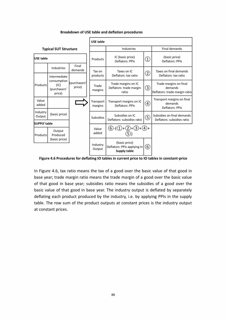
88

Figure 4.6 Procedures for deflating IO tables in current price to IO tables in constant-price

In Figure 4.6, tax ratio means the tax of a good over the basic value of that good in

base year; trade margin ratio means the trade margin of a good over the basic value

of that good in base year; subsidies ratio means the subsidies of a good over the

basic value of that good in base year. The industry output is deflated by separately

deflating each product produced by the industry, i.e. by applying PPIs in the supply

table. The row sum of the product outputs at constant prices is the industry output

at constant prices.

USE table

Industries Final demands

Products IC (basic price) Deflators: PPIs ①

(basic price) Deflators: PPIs

Tax on products

Taxes on IC Deflators: tax ratio ②

Taxes on final demands Deflators: tax ratio

Trade margins

Trade margins on IC Deflators: trade margin

ratio ③

Trade margins on final demands

Deflators: trade margin ratio

Transport margins

Transport margins on IC Deflators: PPIs ④

Transport margins on final demands

Deflators: PPIs

Subsidies Subsidies on IC

Deflators: subsidies ratio ⑤ Subsidies on final demands

Deflators: subsidies ratio

Value added

⑥-(①+②+③+④+⑤)

Industry Output

(basic price) Deflators: PPIs applying in

Supply table ⑥

USE table

Industries

Final demands

Products

Intermediate consumption

(IC) (purchasers’

price)

(purchasers’ price)

Value added

Industry Output

(basic price)

SUPPLY table

Products Output

Produced (basic price)

Breakdown of USE table and deflation procedures

Typical SUT Structure

89

4.7.6 Explanation of increase or decrease in carbon emissions due to a change in production recipe 4.7.6.1 India

Table 4.7.6.1 Selected positive and negative representative components of the production recipe of India (1990-2010)*

10 positive representative components 10 negative representative components

Exporting country

Sector of exporting country Importing country

Sector of importing country

Value(Gg) Exporting country

Sector of exporting country Importing

country Sector of importing

country Value(Gg)

CHN Electrical and Machinery IND Services to Private

Households 2.9E+05 USA Technical, Financial and Business Services IND

Services to Private Households

-6.6E+05

USA Electrical and Machinery IND Services to Private

Households 1.4E+05 USA Technical, Financial and Business Services IND Recycling -4.8E+05

CHN Petroleum, Chemical and

Non-Metallic Mineral Products IND


1.1E+05 TWN Electrical and Machinery IND Services to Private

Households -1.7E+03

JPN Electrical and Machinery IND Services to Private

Households 1.0E+05 DEU Construction IND


-1.2E+03

JPN Technical, Financial and Business

Services IND


7.0E+04 JPN Technical, Financial and Business Services IND Other Manufacturing -1.2E+03

DEU Technical, Financial and Business

Services IND


6.2E+04 GBR Public Administration IND Services to Private

Households -8.7E+02

CHN Technical, Financial and Business

Services IND


6.1E+04 GBR Retail Trade IND Services to Private

Households -7.7E+02

DEU Electrical and Machinery IND Services to Private

Households 5.0E+04 JPN Construction IND Recycling -6.9E+02

CHN Electrical and Machinery IND Recycling 4.8E+04 GBR Technical, Financial and Business Services IND Other Manufacturing -6.2E+02

CHN Metal Products IND Services to Private

Households 3.6E+04 JPN Technical, Financial and Business Services IND Metal Products -5.9E+02

* Country acronyms are listed in Section 4.7.11.

90

4.7.6.2 South Africa

Table 4.7.6.2 Selected positive and negative representative components of the production recipe of South Africa (1990-2010)*


Exporting country



country Value(Gg)

Exporting country


country Sector of importing country Value(Gg)

CHN Electrical and Machinery ZAF Services to Private

Households 3.3E+05 USA

Technical, Financial and Business Services

ZAF Services to Private

Households -4.6E+06

CHN Petroleum, Chemical and Non-Metallic

Mineral Products ZAF


1.1E+05 USA Technical, Financial and Business

Services ZAF Electricity, Gas and Water -1.6E+06

DEU Transport Equipment ZAF Services to Private

Households 1.1E+05 JPN Electrical and Machinery ZAF


-9.5E+04

DEU Technical, Financial and Business Services ZAF Services to Private

Households 9.8E+04 JPN Electrical and Machinery ZAF Electricity, Gas and Water -4.7E+04

AUS Technical, Financial and Business Services ZAF Services to Private

Households 3.4E+04 GBR


ZAF Electricity, Gas and Water -9.4E+03

GBR Technical, Financial and Business Services ZAF Services to Private

Households 1.6E+04 JPN Electrical and Machinery ZAF

Petroleum, Chemical and Non-Metallic Mineral

Products -7.8E+03

CHN Electrical and Machinery ZAF Transport 1.5E+04 FRA Technical, Financial and Business

Services ZAF Electricity, Gas and Water -5.4E+03


Mineral Products ZAF Fishing 1.5E+04 JPN Electrical and Machinery ZAF Maintenance and Repair -4.9E+03

BRA Technical, Financial and Business Services ZAF Services to Private

Households 1.3E+04 DEU Electrical and Machinery ZAF Electricity, Gas and Water -4.6E+03

DEU Transport Equipment ZAF Transport 1.1E+04 USA Petroleum, Chemical and Non-Metallic

Mineral Products ZAF Textiles and Wearing Apparel -4.6E+03


91

4.7.6.3 China

Table 4.7.6.3 Selected positive and negative representative components of the production recipe of China (1990-2010)*


Exporting country



country Value(Gg)

Exporting country



Value(Gg)

USA Electrical and Machinery CHN Electricity, Gas and

Water 9.1E+03 USA Technical, Financial and Business Services CHN Electricity, Gas and Water -2.0E+04

USA Petroleum, Chemical and Non-Metallic

Mineral Products CHN

Electricity, Gas and Water

3.1E+03 JPN Electrical and Machinery CHN Electricity, Gas and Water -1.1E+04

USA Electrical and Machinery CHN Public Administration 2.1E+03 USA Technical, Financial and Business Services CHN Petroleum, Chemical and

Non-Metallic Mineral Products

-1.0E+04


Mineral Products CHN


2.0E+03 JPN Technical, Financial and Business Services CHN Electricity, Gas and Water -4.2E+03

DEU Technical, Financial and Business Services CHN Electricity, Gas and

Water 1.8E+03 USA Technical, Financial and Business Services CHN Maintenance and Repair -3.3E+03

KOR Electrical and Machinery CHN Electricity, Gas and

Water 1.8E+03 USA Technical, Financial and Business Services CHN Transport -2.9E+03

JPN Electrical and Machinery CHN Services to Private

Households 1.7E+03 DEU Electrical and Machinery CHN Electricity, Gas and Water -1.7E+03

USA Electrical and Machinery CHN Maintenance and

Repair 1.6E+03 JPN Electrical and Machinery CHN Electrical and Machinery -1.3E+03

AUS Technical, Financial and Business Services CHN Electricity, Gas and

Water 1.0E+03 JPN Construction CHN Electricity, Gas and Water -8.8E+02

SGP Electrical and Machinery CHN Electricity, Gas and

Water 7.1E+02 TWN Electrical and Machinery CHN Electricity, Gas and Water -7.0E+02


92

4.7.6.4 Brazil

Table 4.7.6.4 Selected positive and negative representative components of the production recipe of Brazil (1990-2010)*


Exporting country



country Value(Gg)

Exporting country



Value(Gg)

CHN Electrical and Machinery BRA Fishing 1.1E+04 USA Technical, Financial and Business Services BRA Fishing -2.5E+05

CHN Electrical and Machinery BRA Post and

Telecommunications 2.6E+03 USA Technical, Financial and Business Services BRA Transport -5.9E+04 USA Technical, Financial and Business Services BRA Maintenance and Repair 1.9E+03 JPN Electrical and Machinery BRA Transport -7.4E+02 CHN Electrical and Machinery BRA Mining and Quarrying 1.3E+03 DEU Technical, Financial and Business Services BRA Transport -7.1E+02 USA Electrical and Machinery BRA Mining and Quarrying 1.2E+03 SAU Technical, Financial and Business Services BRA Fishing -5.8E+02


Mineral Products BRA Textiles and Wearing

Apparel 1.1E+03 JPN Technical, Financial and Business Services BRA Transport -5.2E+02 CHN Electrical and Machinery BRA Metal Products 9.8E+02 FRA Technical, Financial and Business Services BRA Transport -4.5E+02

AUS Technical, Financial and Business Services BRA Fishing

7.6E+02 USA Construction

BRA Textiles and Wearing

Apparel -4.5E+02 DEU Technical, Financial and Business Services BRA Mining and Quarrying 6.7E+02 DEU Electrical and Machinery BRA Transport -3.3E+02

JPN Technical, Financial and Business Services BRA Post and

Telecommunications 6.5E+02 USA Public Administration

BRA Agriculture

-2.9E+02


93

4.7.6.5 Russia

Table 4.7.6.5 Selected positive and negative representative components of the production recipe of Russia (1990-2010)*


Exporting country



country Value(Gg)

Exporting country



country Value(Gg)

CHN Electrical and Machinery RUS Services to Private

Households 2.4E+10 USA Post and Telecommunications RUS


-2.3E+08

USA Technical, Financial and Business Services RUS Services to Private

Households 9.9E+09 GBR Education, Health and Other Services RUS


-1.6E+08

CHN Electrical and Machinery RUS Transport Equipment 7.1E+05 USA Technical, Financial and Business Services RUS Transport Equipment -4.9E+07

CHN Textiles and Wearing Apparel RUS Textiles and Wearing

Apparel 1.4E+04 NZL Technical, Financial and Business Services RUS


-1.1E+07

CHN Electrical and Machinery RUS Hotels and Restaurants 3.1E+03 USA Construction RUS Transport Equipment -2.6E+06


Mineral Products RUS


Products 1.7E+03 USA Technical, Financial and Business Services RUS Electricity, Gas and Water -1.9E+06

CHN Construction RUS Electricity, Gas and Water 1.7E+03 GBR Technical, Financial and Business Services RUS Transport Equipment -1.7E+06 PRT Public Administration RUS Transport Equipment 1.0E+03 USA Electrical and Machinery RUS Electricity, Gas and Water -1.9E+05 CHN Retail Trade RUS Electricity, Gas and Water 7.0E+02 JPN Technical, Financial and Business Services RUS Electricity, Gas and Water -9.9E+04

GIN Transport RUS Services to Private

Households 7.0E+02 IND Agriculture RUS Transport Equipment -9.0E+04


94

4.7.6.6 Australia

Table 4.7.6.6 Selected positive and negative representative components of the production recipe of Australia (1990-2010)*


Exporting country



country Value(Gg)

Exporting country



country Value(Gg)

CHN Electrical and Machinery AUS Electricity, Gas and

Water 1.2E+04 USA Technical, Financial and Business Services AUS Electricity, Gas and Water -2.9E+05


Mineral Products AUS


5.3E+03 USA Technical, Financial and Business Services AUS Petroleum, Chemical and


-1.2E+05

CHN Construction AUS Electricity, Gas and

Water 4.6E+03 JPN Technical, Financial and Business Services AUS Metal Products -7.9E+02

USA Wholesale Trade AUS Transport 4.0E+03 JPN Electrical and Machinery AUS Electricity, Gas and Water -6.3E+02

DEU Technical, Financial and Business Services AUS Electricity, Gas and

Water 3.7E+03 JPN Construction AUS Electricity, Gas and Water -2.1E+02

GBR Technical, Financial and Business Services AUS Electricity, Gas and

Water 3.6E+03 USA Electrical and Machinery AUS Maintenance and Repair -2.1E+02

CHN Electrical and Machinery AUS Petroleum, Chemical and


3.3E+03 DEU Construction AUS Electricity, Gas and Water -8.1E+01

JPN Technical, Financial and Business Services AUS Transport 1.7E+03 GBR Public Administration AUS Electricity, Gas and Water -7.9E+01

CHN Transport Equipment AUS Electricity, Gas and

Water 9.8E+02 ESP Education, Health and Other Services AUS Electricity, Gas and Water -7.4E+01

USA Transport AUS Transport 9.0E+02 USA Transport AUS Wood and Paper -6.8E+01


95

4.7.6.7 United States

Table 4.7.6.7 Selected positive and negative representative components of the production recipe of United States (1990-2010)*


Exporting country



country Value(Gg) Exporting country Sector of exporting country

Importing country


Value(Gg)

CHN20

Electrical and Machinery USA Electricity, Gas and

Water 5.9E+03 JPN Electrical and Machinery USA Transport -6.4E+03

CHN Electrical and Machinery USA Transport 3.2E+03 JPN Electrical and Machinery USA Electricity, Gas and

Water -3.4E+03


Mineral Products USA


1.9E+03 JPN Electrical and Machinery USA Maintenance and Repair -1.4E+03


Mineral Products USA Transport 1.3E+03 DEU Electrical and Machinery USA Transport -6.2E+02

CHN Electrical and Machinery USA Wood and Paper 1.1E+03 GBR Technical, Financial and Business

Services USA Transport -4.4E+02

DEU Technical, Financial and Business Services USA Electricity, Gas and

Water 3.7E+02 FRA


USA Transport -3.8E+02

BRA Petroleum, Chemical and Non-Metallic

Mineral Products USA


2.9E+02 GBR Technical, Financial and Business

Services USA


-3.4E+02

DEU Electrical and Machinery USA Electricity, Gas and

Water 2.8E+02 CAN Transport Equipment USA Transport -2.6E+02

CHN Textiles and Wearing Apparel USA Textiles and Wearing

Apparel 2.4E+02 ITA Electrical and Machinery USA Transport -2.4E+02

AUS Technical, Financial and Business Services USA Electricity, Gas and

Water 2.2E+02 JPN Electrical and Machinery USA


Products -2.3E+02


20 The USA has substituted Chinese for Japanese imports of telecommunications and sound equipment, electrical machinery and appliances, and office equipment, thus offsetting the domestic reductions

somewhat89.

96

4.7.6.8 Japan

Table 4.7.6.8 Selected positive and negative representative components of the production recipe of Japan (1990-2010)*


Exporting country



Exporting country



country Value(Gg)

CHN Electrical and Machinery JPN Mining and Quarrying 1.7E+04 USA Technical, Financial and Business

Services JPN


-2.3E+04

CHN Petroleum, Chemical and Non-Metallic Mineral

Products JPN Mining and Quarrying 1.2E+04 USA Public Administration JPN Mining and Quarrying -8.9E+03

USA Wholesale Trade JPN Maintenance and Repair 4.3E+03 SAU Technical, Financial and Business

Services JPN Mining and Quarrying -8.8E+02

CHN Construction JPN Mining and Quarrying 3.6E+03 FRA Technical, Financial and Business


AUS Technical, Financial and Business Services JPN Mining and Quarrying 2.0E+03 CAN Technical, Financial and Business


KOR Petroleum, Chemical and Non-Metallic Mineral

Products JPN Mining and Quarrying 1.3E+03 SAU


JPN Electricity, Gas and

Water -1.9E+02

USA Transport JPN Transport 1.0E+03 USA Transport Equipment JPN Petroleum, Chemical and


-1.8E+02

AUS Technical, Financial and Business Services JPN Electricity, Gas and Water 7.1E+02 FRA Petroleum, Chemical and

Non-Metallic Mineral Products JPN Mining and Quarrying -1.6E+02

USA Electrical and Machinery JPN Electrical and Machinery 4.4E+02 GBR Education, Health and Other


KOR Petroleum, Chemical and Non-Metallic Mineral

Products JPN Electricity, Gas and Water 4.2E+02 FRA


JPN Electricity, Gas and

Water -9.6E+01


97

4.7.6.9 Germany

Table 4.7.6.9 Selected positive and negative representative components of the production recipe of Germany (1990-2010)*


Exporting country



country Value(Gg)

Exporting country



country Value(Gg)

CHN Electrical and Machinery DEU Electricity, Gas and

Water 7.4E+03 USA


DEU Electricity, Gas and

Water -2.3E+04

CHN Textiles and Wearing Apparel DEU Textiles and Wearing

Apparel 2.7E+03 USA


DEU Transport -9.6E+03


Products DEU


1.9E+03 USA Electrical and Machinery DEU Electricity, Gas and

Water -2.1E+03

CHN Technical, Financial and Business Services DEU Electricity, Gas and

Water 1.6E+03 USA Construction DEU


-2.1E+03

CHN Electrical and Machinery DEU Textiles and Wearing

Apparel 1.3E+03 GBR

Education, Health and Other Services

DEU Electricity, Gas and

Water -1.0E+02

CHN Electrical and Machinery DEU Transport 1.2E+03 USA Wholesale Trade DEU Petroleum, Chemical and


-1.0E+02

CHN Electrical and Machinery DEU Maintenance and Repair 1.2E+03 FRA Technical, Financial and Business

Services DEU


Products -9.2E+01

USA Transport DEU Transport 1.1E+03 GBR Education, Health and Other

Services DEU Transport -7.0E+01


Products DEU

Textiles and Wearing Apparel

9.6E+02 USA Construction DEU Mining and Quarrying -6.4E+01

JPN Technical, Financial and Business Services DEU Electricity, Gas and

Water 9.3E+02 GBR


DEU Petroleum, Chemical and


-5.1E+01


98

4.7.6.10 France

Table 4.7.6.10 Selected positive and negative representative components of the production recipe of France (1990-2010)*


Exporting country



country Value(Gg)

Exporting country



country Value(Gg)

CHN Electrical and Machinery FRA Electricity, Gas and Water 1.2E+03 USA Technical, Financial and Business

Services FRA


-9.3E+03

CHN Electrical and Machinery FRA Transport 1.1E+03 USA Education, Health and Other Services FRA Electricity, Gas and

Water -1.9E+03

DEU Technical, Financial and Business Services FRA Transport 6.6E+02 JPN Electrical and Machinery FRA Electricity, Gas and

Water -3.3E+02


Mineral Products FRA Transport 4.3E+02 JPN


FRA Electricity, Gas and

Water -2.3E+02

CHN Electrical and Machinery FRA Petroleum, Chemical and


4.2E+02 JPN Electrical and Machinery FRA Transport -2.1E+02

USA Transport FRA Transport 4.1E+02 ITA Technical, Financial and Business

Services FRA


-1.3E+02


Mineral Products FRA Electricity, Gas and Water 3.7E+02 ITA Electrical and Machinery FRA


-1.2E+02

DEU Transport Equipment FRA Transport 3.6E+02 GBR Technical, Financial and Business

Services FRA


Products -1.0E+02

CHN Technical, Financial and Business Services FRA Transport 3.1E+02 ITA Electrical and Machinery FRA Transport -9.6E+01


Mineral Products FRA


Products 2.9E+02 DEU Construction FRA


-7.5E+01


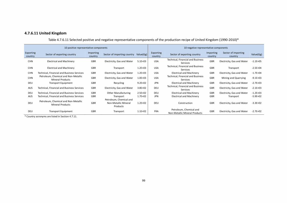
99

4.7.6.11 United Kingdom

Table 4.7.6.11 Selected positive and negative representative components of the production recipe of United Kingdom (1990-2010)*


Exporting country


Sector of importing country Value(Gg) Exporting country



country Value(Gg)

CHN Electrical and Machinery GBR Electricity, Gas and Water 5.1E+03 USA Technical, Financial and Business

Services GBR Electricity, Gas and Water -1.1E+05

CHN Electrical and Machinery GBR Transport 1.2E+03 USA Technical, Financial and Business

Services GBR Transport -2.5E+04

CHN Technical, Financial and Business Services GBR Electricity, Gas and Water 1.2E+03 USA Electrical and Machinery GBR Electricity, Gas and Water -1.7E+04


Mineral Products GBR Electricity, Gas and Water 1.0E+03 USA


GBR Mining and Quarrying -9.1E+03

DEU Transport Equipment GBR Recycling 9.2E+02 JPN Electrical and Machinery GBR Electricity, Gas and Water -2.7E+03

AUS Technical, Financial and Business Services GBR Electricity, Gas and Water 3.8E+02 DEU Technical, Financial and Business

Services GBR Electricity, Gas and Water -2.1E+03

DEU Technical, Financial and Business Services GBR Other Manufacturing 2.5E+02 DEU Electrical and Machinery GBR Electricity, Gas and Water -1.2E+03 AUS Technical, Financial and Business Services GBR Transport 1.7E+02 JPN Electrical and Machinery GBR Transport -5.9E+02

DEU Petroleum, Chemical and Non-Metallic

Mineral Products GBR


Products 1.2E+02 DEU Construction GBR Electricity, Gas and Water -3.3E+02

DEU Transport Equipment GBR Transport 1.1E+02 FRA Petroleum, Chemical and

Non-Metallic Mineral Products GBR Electricity, Gas and Water -2.7E+02


100

4.7.7 Carbon leakage

Table 4.7.7.1 Carbon leakage of Germany*

Exporting country Sector of exporting country Importing country Sector of importing country Value(Gg)

CHN Electrical and Machinery DEU Electricity, Gas and Water 7.44E+03 CHN Textiles and Wearing Apparel DEU Textiles and Wearing Apparel 2.74E+03 CHN Petroleum, Chemical and Non-Metallic Mineral Products DEU Electricity, Gas and Water 1.86E+03 CHN Technical, Financial and Business Services DEU Electricity, Gas and Water 1.57E+03 CHN Electrical and Machinery DEU Textiles and Wearing Apparel 1.28E+03 CHN Electrical and Machinery DEU Transport 1.22E+03 CHN Electrical and Machinery DEU Maintenance and Repair 1.21E+03 USA Transport DEU Transport 1.15E+03 CHN Petroleum, Chemical and Non-Metallic Mineral Products DEU Textiles and Wearing Apparel 9.56E+02 JPN Technical, Financial and Business Services DEU Electricity, Gas and Water 9.35E+02 GBR Technical, Financial and Business Services DEU Electricity, Gas and Water 9.25E+02 FRA Technical, Financial and Business Services DEU Electricity, Gas and Water 8.52E+02 CHN Construction DEU Electricity, Gas and Water 8.32E+02 USA Wholesale Trade DEU Maintenance and Repair 7.00E+02 CHN Education, Health and Other Services DEU Electricity, Gas and Water 6.04E+02 CHN Petroleum, Chemical and Non-Metallic Mineral Products DEU Transport 5.88E+02 CHN Electrical and Machinery DEU Petroleum, Chemical and Non-Metallic Mineral Products 5.67E+02 CHN Metal Products DEU Electricity, Gas and Water 5.59E+02 CHN Technical, Financial and Business Services DEU Textiles and Wearing Apparel 5.11E+02 JPN Electrical and Machinery DEU Electricity, Gas and Water 4.99E+02 CHN Petroleum, Chemical and Non-Metallic Mineral Products DEU Petroleum, Chemical and Non-Metallic Mineral Products 4.84E+02 CHN Technical, Financial and Business Services DEU Transport 4.70E+02 CHN Petroleum, Chemical and Non-Metallic Mineral Products DEU Maintenance and Repair 4.39E+02 CHN Technical, Financial and Business Services DEU Maintenance and Repair 4.32E+02 USA Wholesale Trade DEU Electricity, Gas and Water 4.27E+02 USA Petroleum, Chemical and Non-Metallic Mineral Products DEU Petroleum, Chemical and Non-Metallic Mineral Products 4.05E+02 CHN Transport DEU Electricity, Gas and Water 3.88E+02 CHN Retail Trade DEU Electricity, Gas and Water 3.75E+02 USA Petroleum, Chemical and Non-Metallic Mineral Products DEU Transport 3.64E+02 JPN Technical, Financial and Business Services DEU Maintenance and Repair 3.64E+02


101

Table 4.7.7.2 Carbon leakage of United Kingdom*

Exporting country Sector of exporting country Importing


CHN Electrical and Machinery GBR Electricity, Gas and Water 5.08E+03 CHN Electrical and Machinery GBR Recycling 2.62E+03 CHN Petroleum, Chemical and Non-Metallic Mineral Products GBR Recycling 1.72E+03 CHN Electrical and Machinery GBR Transport 1.25E+03 CHN Electrical and Machinery GBR Others 1.20E+03 CHN Technical, Financial and Business Services GBR Electricity, Gas and Water 1.17E+03 CHN Petroleum, Chemical and Non-Metallic Mineral Products GBR Electricity, Gas and Water 1.02E+03 DEU Technical, Financial and Business Services GBR Recycling 1.02E+03 CHN Technical, Financial and Business Services GBR Recycling 1.01E+03 CHN Electrical and Machinery GBR Petroleum, Chemical and Non-Metallic Mineral Products 9.81E+02 DEU Transport Equipment GBR Recycling 9.20E+02 CHN Electrical and Machinery GBR Other Manufacturing 8.02E+02 CHN Petroleum, Chemical and Non-Metallic Mineral Products GBR Petroleum, Chemical and Non-Metallic Mineral Products 6.15E+02 CHN Construction GBR Electricity, Gas and Water 5.83E+02 CHN Construction GBR Recycling 5.43E+02 CHN Education, Health and Other Services GBR Electricity, Gas and Water 5.36E+02 CHN Electrical and Machinery GBR Electrical and Machinery 5.00E+02 CHN Education, Health and Other Services GBR Recycling 4.78E+02 CHN Electrical and Machinery GBR Mining and Quarrying 4.78E+02 CHN Technical, Financial and Business Services GBR Transport 4.71E+02 CHN Petroleum, Chemical and Non-Metallic Mineral Products GBR Transport 4.45E+02 CHN Petroleum, Chemical and Non-Metallic Mineral Products GBR Others 4.42E+02 CHN Metal Products GBR Recycling 4.36E+02 DEU Technical, Financial and Business Services GBR Others 4.21E+02 CHN Petroleum, Chemical and Non-Metallic Mineral Products GBR Other Manufacturing 4.03E+02 CHN Textiles and Wearing Apparel GBR Textiles and Wearing Apparel 3.83E+02 AUS Technical, Financial and Business Services GBR Electricity, Gas and Water 3.81E+02 CHN Textiles and Wearing Apparel GBR Others 3.65E+02


102

4.7.8 Structural decomposition of carbon footprints for the former Soviet Republics (1990-2010)

Figure 4.7: Domestic Carbon Footprint (top panel) and Rest-of-World Carbon Footprint (bottom panel) for the former Soviet Republics.

103

Figure 4.8: Domestic Carbon Footprint (top panel) and Rest-of-World Carbon Footprint (bottom panel) for the former Soviet Republics.

104

4.7.9 Structural decomposition of carbon footprints for China, United States, United Kingdom and Germany (2005-2010)

Figure 4.9: Yearly Domestic Carbon Footprint (top panel) and Rest-of-World Carbon Footprint (bottom panel) for China, United States, United Kingdom and Germany from 2005 to 2010.

105

4.7.10 Individual country information

4.7.10.1 Mongolia

A large percentage of Mongolia’s economy relies on financial inflows from abroad to

finance her imports, especially after the country’s transition towards a market

economy and opening up to world markets. From 1990 to 2010, Mongolia had more

imports than exports in each year and made a trade deficit (Unstats 2013).

Mongolia’s foreign trade balance witnessed the worst historic deficit of $710 million

in 2008 that accounted for 14% of the country’s GDP Shagdar 2010.

4.7.10.2 Zimbabwe

Zimbabwe was the 18th largest recipient of official humanitarian assistance in 2012.

Total Official development assistance (ODA) of Zimbabwe in 2002 was US$305 million,

which increased to US$798 million in 2009 and US$783 million in 2010226.

Imports into Zimbabwe have increased from 17% in 1990 to 70% in 2010, leading to

excessive trade deficit and the shrinking of the country’s domestic economy.

4.7.10.3 South Africa, Namibia and Tanzania The economies of South Africa, Namibia and Tanzania have become carbon-intensive

over time because of a shift towards coal, and transport sectors having become more

carbon-intensive due to modal changes for example from road to air travel.

106

4.7.10.4 China, India, Brazil and certain Middle Eastern and African nations Table 4.7.10.4.1 20 representative components of the change in CO2 emissions due to domestic production and in international trade of China (1990-2010)*

CO2 emission in domestic production CO2 emission in international trade

Output sector Input sector Value (Gg)

Exporting country

Exporting sector Importing

country Importing sector

Value (Gg)

Electrical and Machinery Electricity, Gas and Water 5.8E+05 CHN Electrical and Machinery USA Electricity, Gas and Water 2.4E+10 Petroleum, Chemical and

Non-Metallic Mineral Products Electricity, Gas and Water 2.2E+05 CHN

Petroleum, Chemical and Non-Metallic Mineral Products

USA Electricity, Gas and Water 5.4E+09


Electricity, Gas and Water 2.1E+05 CHN Technical, Financial and Business Services DEU Electricity, Gas and Water 9.4E+08

Construction Services to Private

Households 1.9E+05 CHN Electrical and Machinery KOR Electricity, Gas and Water 9.0E+07

Electrical and Machinery Services to Private

Households 1.5E+05 CHN Electrical and Machinery JPN Services to Private Households 7.0E+07

Construction Electricity, Gas and Water 1.4E+05 CHN Electrical and Machinery USA Maintenance and Repair 6.1E+07 Education, Health and Other

Services Electricity, Gas and Water 1.4E+05 CHN Technical, Financial and Business Services DEU Services to Private Households 2.6E+07

Construction Public Administration 1.2E+05 CHN Electrical and Machinery USA Transport 1.0E+07 Electricity, Gas and Water Electricity, Gas and Water 1.1E+05 CHN Electrical and Machinery USA Other Manufacturing 7.9E+06



1.1E+05 CHN Electrical and Machinery USA Petroleum, Chemical and

Non-Metallic Mineral Products 5.3E+06



8.9E+04 CHN Food & Beverages AUS Food & Beverages 4.4E+06


Public Administration 8.8E+04 CHN Electrical and Machinery USA Mining and Quarrying 3.1E+06

Transport Equipment Electricity, Gas and Water 6.2E+04 CHN Transport Equipment USA Electricity, Gas and Water 3.0E+06

Textiles and Wearing Apparel Services to Private

Households 5.8E+04 CHN Electrical and Machinery DEU Services to Private Households 2.2E+06



5.5E+04 CHN Electrical and Machinery USA Metal Products 1.6E+06

Electrical and Machinery Maintenance and Repair 5.5E+04 CHN Electrical and Machinery SGP Electricity, Gas and Water 1.4E+06 Construction Transport 5.5E+04 CHN Electrical and Machinery KOR Services to Private Households 1.1E+06

Electrical and Machinery Public Administration 5.2E+04 CHN Technical, Financial and Business Services GBR Electricity, Gas and Water 7.1E+05 Transport Electricity, Gas and Water 5.1E+04 CHN Transport Equipment DEU Electricity, Gas and Water 5.6E+05

Metal Products Electricity, Gas and Water 4.5E+04 CHN Petroleum, Chemical and Non-Metallic Mineral

Products USA Other Manufacturing 4.5E+05


107

Table4.7.10.4.2 20 representative components of the change in CO2 emissions due to domestic production and in international trade of India (1990-2010)*



Exporting country



Value (Gg)

Transport Electricity, Gas and Water 8.6E+04 IND Electrical and Machinery CHN Services to Private Households 1.4E+08 Agriculture Electricity, Gas and Water 6.7E+04 IND Electrical and Machinery USA Services to Private Households 1.1E+08

Electrical and Machinery Electricity, Gas and Water 5.5E+04 IND Technical, Financial and Business Services CHN Services to Private Households 8.8E+07 Construction Electricity, Gas and Water 4.4E+04 IND Technical, Financial and Business Services DEU Services to Private Households 5.1E+07

Transport Maintenance and Repair 1.8E+04 IND Electrical and Machinery CHN Electricity, Gas and Water 7.1E+06

Transport Other Manufacturing 1.4E+04 IND Petroleum, Chemical and Non-Metallic Mineral

Products CHN


6.0E+06

Transport Metal Products 1.4E+04 IND Electrical and Machinery DEU Services to Private Households 4.9E+06 Retail Trade Electricity, Gas and Water 1.4E+04 IND Electrical and Machinery DEU Transport Equipment 3.9E+06

Transport Textiles and Wearing

Apparel 1.2E+04 IND Metal Products CHN Electrical and Machinery 2.4E+06

Transport Petroleum, Chemical and


1.2E+04 IND Petroleum, Chemical and Non-Metallic Mineral

Products GBR Services to Private Households 1.9E+06


Electricity, Gas and Water 1.2E+04 IND Electrical and Machinery CHN Electricity, Gas and Water 8.0E+05

Construction Post and

Telecommunications 1.1E+04 IND Technical, Financial and Business Services AUS Other Manufacturing 7.9E+05

Construction Transport 9.1E+03 IND Electrical and Machinery SGP Electrical and Machinery 7.7E+05

Transport Food & Beverages 8.9E+03 IND Petroleum, Chemical and Non-Metallic Mineral

Products CHN Electricity, Gas and Water 7.1E+05

Food & Beverages Food & Beverages 8.5E+03 IND Petroleum, Chemical and Non-Metallic Mineral

Products DEU Services to Private Households 7.0E+05

Transport Transport 8.5E+03 IND Electrical and Machinery ITA Services to Private Households 6.8E+05

Electrical and Machinery Post and

Telecommunications 8.4E+03 IND Electrical and Machinery CHN Textiles and Wearing Apparel 6.5E+05

Metal Products Electricity, Gas and Water 8.1E+03 IND Electrical and Machinery CHN Metal Products 6.5E+05

Construction Textiles and Wearing

Apparel 7.4E+03 IND


FRA Services to Private Households 6.4E+05

Transport Wood and Paper 7.3E+03 IND Textiles and Wearing Apparel CHN Textiles and Wearing Apparel 5.9E+05


108

Table 4.7.10.4.3 20 representative components of the change in CO2 emissions due to domestic production and in international trade of Brazil (1990-2010)*



Exporting country



Value (Gg)


Maintenance and Repair 6.1E+03 BRA Transport Equipment USA Petroleum, Chemical and Non-Metallic

Mineral Products 1.8E+08

Electrical and Machinery Fishing 5.5E+03 BRA Metal Products CHN Electrical and Machinery 8.7E+07 Technical, Financial and Business

Services Textiles and Wearing Apparel 3.7E+03 BRA Metal Products USA Electrical and Machinery 4.5E+07


Wood and Paper 2.5E+03 BRA Textiles and Wearing Apparel ARG Textiles and Wearing Apparel 9.5E+06

Electrical and Machinery Mining and Quarrying 2.4E+03 BRA Transport Equipment DEU Transport 4.9E+06 Textiles and Wearing Apparel Textiles and Wearing Apparel 1.7E+03 BRA Agriculture CHN Food & Beverages 1.7E+06

Transport Mining and Quarrying 1.6E+03 BRA Metal Products JPN Electrical and Machinery 1.6E+06 Hotels and Restaurants Recycling 1.5E+03 BRA Metal Products DEU Electrical and Machinery 8.7E+05

Transport Maintenance and Repair 1.0E+03 BRA Agriculture ARG Services to Private Households 4.5E+05

Electrical and Machinery Metal Products 1.0E+03 BRA Petroleum, Chemical and

Non-Metallic Mineral Products ARG Other Manufacturing 3.5E+05


Wholesale Trade 9.7E+02 BRA Technical, Financial and Business

Services ARG Other Manufacturing 9.5E+04


Textiles and Wearing Apparel 8.9E+02 BRA Transport Equipment NLD Transport 8.0E+04

Transport Textiles and Wearing Apparel 6.8E+02 BRA Mining and Quarrying CHN Metal Products 6.9E+04 Post and Telecommunications Post and Telecommunications 6.7E+02 BRA Metal Products DEU Transport Equipment 6.2E+04


Other Manufacturing 6.6E+02 BRA Electrical and Machinery NLD Services to Private Households 6.3E+04

Transport Metal Products 6.3E+02 BRA Metal Products CHN Transport Equipment 2.8E+04 Electrical and Machinery Textiles and Wearing Apparel 6.0E+02 BRA Textiles and Wearing Apparel NLD Wholesale Trade 2.6E+04

Transport Equipment Maintenance and Repair 5.4E+02 BRA Agriculture USA Food & Beverages 2.0E+04 Petroleum, Chemical and

Non-Metallic Mineral Products Wood and Paper 5.3E+02 BRA Food & Beverages AUS Electrical and Machinery 1.7E+04



4.7E+02 BRA Textiles and Wearing Apparel ITA Services to Private Households 1.6E+04


109

Table 4.7.10.4.4 20 representative components of the change in CO2 emissions due to domestic production and in international trade of Indonesia (1990-2010)*



Exporting country



Value (Gg)

Agriculture Other Manufacturing 1.3E+04 IDN Food & Beverages CHN Services to Private Households 1.8E+07 Technical, Financial and Business

Services Services to Private

Households 5.5E+03 IDN Technical, Financial and Business Services AUS Electricity, Gas and Water 1.2E+07

Mining and Quarrying Electricity, Gas and Water 5.4E+03 IDN Food & Beverages CHN Electricity, Gas and Water 9.6E+06 Food & Beverages Other Manufacturing 4.0E+03 IDN Electrical and Machinery KOR Transport 5.7E+06 Wood and Paper Other Manufacturing 3.1E+03 IDN Textiles and Wearing Apparel CHN Wood and Paper 2.2E+06


Electricity, Gas and Water 2.4E+03 IDN Textiles and Wearing Apparel MYS Other Manufacturing 9.7E+05


Other Manufacturing 2.3E+03 IDN Wood and Paper IRN Services to Private Households 5.3E+05

Mining and Quarrying Petroleum, Chemical and


1.6E+03 IDN Petroleum, Chemical and Non-Metallic Mineral

Products VNM Services to Private Households 3.3E+05



Products 1.0E+03 IDN


IND Textiles and Wearing Apparel 9.7E+04

Food & Beverages Transport 8.3E+02 IDN Mining and Quarrying KOR Electricity, Gas and Water 1.0E+04

Textiles and Wearing Apparel Textiles and Wearing

Apparel 8.1E+02 IDN Transport Equipment AUT Fishing 8.1E+03

Agriculture Wood and Paper 6.5E+02 IDN Petroleum, Chemical and Non-Metallic Mineral

Products VNM Other Manufacturing 6.3E+03


Other Manufacturing 5.7E+02 IDN Hotels and Restaurants CHN Other Manufacturing 5.3E+03

Food & Beverages Agriculture 5.3E+02 IDN Petroleum, Chemical and Non-Metallic Mineral

Products MYS Mining and Quarrying 4.1E+03

Food & Beverages Food & Beverages 5.2E+02 IDN Petroleum, Chemical and Non-Metallic Mineral

Products USA Electrical and Machinery 3.6E+03

Mining and Quarrying Other Manufacturing 4.5E+02 IDN Technical, Financial and Business Services AUS Fishing 3.5E+03

Food & Beverages Textiles and Wearing

Apparel 3.8E+02 IDN Mining and Quarrying TWN Electricity, Gas and Water 2.8E+03

Agriculture Textiles and Wearing

Apparel 2.8E+02 IDN


VNM Petroleum, Chemical and


Retail Trade Transport 2.8E+02 IDN Wood and Paper CHN Wood and Paper 1.0E+03

Mining and Quarrying Mining and Quarrying 2.8E+02 IDN Petroleum, Chemical and Non-Metallic Mineral

Products CHN


9.8E+02


110

Table 4.7.10.4.5 20 representative components of the change in CO2 emissions due to domestic production and in international trade of Iraq (1990-2010)*



Exporting country



Value (Gg)


Electricity, Gas and Water 1.6E+03 IRQ Electricity, Gas and Water CHN Electrical and Machinery 1.0E+06


Transport 9.1E+02 IRQ Petroleum, Chemical and Non-Metallic

Mineral Products CHN Electrical and Machinery 7.3E+04

Construction Electricity, Gas and Water 1.4E+02 IRQ Petroleum, Chemical and Non-Metallic

Mineral Products USA Electrical and Machinery 6.4E+04

Construction Transport 1.3E+02 IRQ Petroleum, Chemical and Non-Metallic

Mineral Products CHN Transport Equipment 4.2E+04

Construction Petroleum, Chemical and

Non-Metallic Mineral Products 1.2E+02 IRQ


CHN Construction 3.9E+04


Transport 9.0E+01 IRQ Petroleum, Chemical and Non-Metallic

Mineral Products IND Electrical and Machinery 3.5E+04

Transport Electricity, Gas and Water 6.9E+01 IRQ Electricity, Gas and Water KOR 1Electrical and Machinery 3.5E+04 Wholesale Trade Electricity, Gas and Water 5.1E+01 IRQ Mining and Quarrying USA Electricity, Gas and Water 2.4E+04

Post and Telecommunications Electricity, Gas and Water 4.2E+01 IRQ Electrical and Machinery IND Petroleum, Chemical and



Electricity, Gas and Water 3.6E+01 IRQ Wholesale Trade USA Agriculture 1.8E+04


Transport 3.2E+01 IRQ Electrical and Machinery IND Electrical and Machinery 1.1E+04


Services to Private Households 2.1E+01 IRQ Electrical and Machinery IND Electricity, Gas and Water 1.1E+04

Mining and Quarrying Electricity, Gas and Water 1.9E+01 IRQ Food & Beverages USA Services to Private Households 1.1E+04 Hotels and Restaurants Electricity, Gas and Water 1.7E+01 IRQ Electricity, Gas and Water CHN 1Electrical and Machinery 9.9E+03


Electricity, Gas and Water 1.6E+01 IRQ Petroleum, Chemical and Non-Metallic

Mineral Products CHN Transport Equipment 9.7E+03

Mining and Quarrying Petroleum, Chemical and

Non-Metallic Mineral Products 1.3E+01 IRQ Electricity, Gas and Water IND Construction 7.1E+03

Construction Electrical and Machinery 9.7E+00 IRQ Petroleum, Chemical and Non-Metallic

Mineral Products IRN Electricity, Gas and Water 6.2E+03

Agriculture Recycling 9.1E+00 IRQ Petroleum, Chemical and Non-Metallic

Mineral Products IND Construction 5.6E+03

Construction Other Manufacturing 8.5E+00 IRQ Agriculture USA Services to Private Households 4.8E+03 Transport Transport 7.2E+00 IRQ Mining and Quarrying UZB Services to Private Households 9.9E+02


111

Table 4.7.10.4.6 20 representative components of the change in CO2 emissions due to domestic production and in international trade of South Africa (1990-2010)*



Exporting country



Value (Gg)



2.4E+03 ZAF Metal Products CHN Private Households 3.2E+06

Retail Trade Education, Health and

Other Services 6.6E+02 ZAF Transport Equipment DEU Transport 1.0E+06



2.3E+02 ZAF Electrical and Machinery CHN Electricity, Gas and Water 5.3E+05

Post and Telecommunications Education, Health and

Other Services 2.1E+02 ZAF Mining and Quarrying CHN Electricity, Gas and Water 3.5E+05

Wholesale Trade Education, Health and

Other Services 1.3E+02 ZAF Construction USA Private Households 5.8E+04

Transport Education, Health and

Other Services 1.3E+02 ZAF Electrical and Machinery JPN Transport 1.6E+04

Construction Education, Health and

Other Services 1.1E+02 ZAF Electrical and Machinery USA Electrical and Machinery 1.6E+04

Electricity, Gas and Water Education, Health and

Other Services 2.5E+01 ZAF Electrical and Machinery CHN Textiles and Wearing Apparel 9.7E+03

Wood and Paper Education, Health and

Other Services 1.2E+01 ZAF Textiles and Wearing Apparel GBR Textiles and Wearing Apparel 8.0E+03

Maintenance and Repair Education, Health and

Other Services 8.0E-01 ZAF Electrical and Machinery IND Construction 7.8E+03


112

Table 4.7.10.4.7 20 representative components of the change in CO2 emissions due to domestic production and in international trade of Uzbekistan (1990-2010)*



Exporting country



Value (Gg)

Textiles and Wearing Apparel Other Manufacturing 3.6E+03 UZB Agriculture CHN Services to Private Households 1.4E+05 Food & Beverages Maintenance and Repair 2.3E+03 UZB Textiles and Wearing Apparel CHN Services to Private Households 1.0E+05

Agriculture Other Manufacturing 2.1E+03 UZB Agriculture RUS Services to Private Households 2.3E+04 Agriculture Maintenance and Repair 1.1E+03 UZB Electrical and Machinery TUR Electricity, Gas and Water 6.7E+03

Food & Beverages Other Manufacturing 8.5E+02 UZB Electrical and Machinery KAZ Maintenance and Repair 3.3E+03 Technical, Financial and Business

Services Electricity, Gas and Water 5.6E+02 UZB Transport Equipment CHN Electricity, Gas and Water 2.8E+03


Maintenance and Repair 5.2E+02 UZB Textiles and Wearing Apparel TUR Petroleum, Chemical and


Textiles and Wearing Apparel Hotels and Restaurants 5.1E+02 UZB Petroleum, Chemical and Non-Metallic Mineral

Products KAZ


1.0E+03

Textiles and Wearing Apparel Maintenance and Repair 3.6E+02 UZB Agriculture BGD Electricity, Gas and Water 8.3E+02

Food & Beverages Electricity, Gas and Water 2.8E+02 UZB Electrical and Machinery CHN Petroleum, Chemical and



Other Manufacturing 2.4E+02 UZB Electrical and Machinery TUR Transport 7.0E+02

Textiles and Wearing Apparel Electricity, Gas and Water 2.1E+02 UZB Agriculture ROU Services to Private Households 4.3E+02 Agriculture Hotels and Restaurants 1.8E+02 UZB Metal Products IRN Electrical and Machinery 3.9E+02

Food & Beverages Wholesale Trade 1.8E+02 UZB Technical, Financial and Business Services CHN Electricity, Gas and Water 2.6E+02 Education, Health and Other

Services Electricity, Gas and Water 1.7E+02 UZB


KGZ Hotels and Restaurants 2.1E+02


Hotels and Restaurants 1.7E+02 UZB Transport KGZ Transport 1.9E+02

Textiles and Wearing Apparel Petroleum, Chemical and


1.6E+02 UZB Metal Products RUS Other Manufacturing 1.3E+02

Food & Beverages Petroleum, Chemical and


1.4E+02 UZB Education, Health and Other Services KAZ Electricity, Gas and Water 1.1E+02

Other Manufacturing Hotels and Restaurants 1.3E+02 UZB Transport KAZ Electricity, Gas and Water 9.4E+01

Agriculture Textiles and Wearing

Apparel 1.2E+02 UZB


TUR Electricity, Gas and Water 8.9E+01


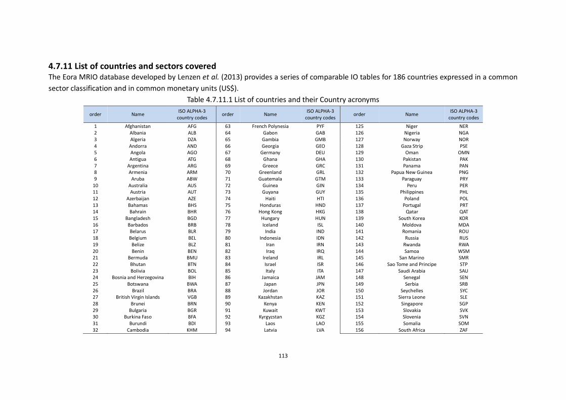
113

4.7.11 List of countries and sectors covered The Eora MRIO database developed by Lenzen et al. (2013) provides a series of comparable IO tables for 186 countries expressed in a common

sector classification and in common monetary units (US$).

Table 4.7.11.1 List of countries and their Country acronyms

order Name ISO ALPHA-3

country codes order Name

ISO ALPHA-3 country codes

order Name ISO ALPHA-3

country codes

1 Afghanistan AFG 63 French Polynesia PYF 125 Niger NER 2 Albania ALB 64 Gabon GAB 126 Nigeria NGA 3 Algeria DZA 65 Gambia GMB 127 Norway NOR 4 Andorra AND 66 Georgia GEO 128 Gaza Strip PSE 5 Angola AGO 67 Germany DEU 129 Oman OMN 6 Antigua ATG 68 Ghana GHA 130 Pakistan PAK 7 Argentina ARG 69 Greece GRC 131 Panama PAN 8 Armenia ARM 70 Greenland GRL 132 Papua New Guinea PNG 9 Aruba ABW 71 Guatemala GTM 133 Paraguay PRY

10 Australia AUS 72 Guinea GIN 134 Peru PER 11 Austria AUT 73 Guyana GUY 135 Philippines PHL 12 Azerbaijan AZE 74 Haiti HTI 136 Poland POL 13 Bahamas BHS 75 Honduras HND 137 Portugal PRT 14 Bahrain BHR 76 Hong Kong HKG 138 Qatar QAT 15 Bangladesh BGD 77 Hungary HUN 139 South Korea KOR 16 Barbados BRB 78 Iceland ISL 140 Moldova MDA 17 Belarus BLR 79 India IND 141 Romania ROU 18 Belgium BEL 80 Indonesia IDN 142 Russia RUS 19 Belize BLZ 81 Iran IRN 143 Rwanda RWA 20 Benin BEN 82 Iraq IRQ 144 Samoa WSM 21 Bermuda BMU 83 Ireland IRL 145 San Marino SMR 22 Bhutan BTN 84 Israel ISR 146 Sao Tome and Principe STP 23 Bolivia BOL 85 Italy ITA 147 Saudi Arabia SAU 24 Bosnia and Herzegovina BIH 86 Jamaica JAM 148 Senegal SEN 25 Botswana BWA 87 Japan JPN 149 Serbia SRB 26 Brazil BRA 88 Jordan JOR 150 Seychelles SYC 27 British Virgin Islands VGB 89 Kazakhstan KAZ 151 Sierra Leone SLE 28 Brunei BRN 90 Kenya KEN 152 Singapore SGP 29 Bulgaria BGR 91 Kuwait KWT 153 Slovakia SVK 30 Burkina Faso BFA 92 Kyrgyzstan KGZ 154 Slovenia SVN 31 Burundi BDI 93 Laos LAO 155 Somalia SOM 32 Cambodia KHM 94 Latvia LVA 156 South Africa ZAF

114

33 Cameroon CMR 95 Lebanon LBN 157 Spain ESP 34 Canada CAN 96 Lesotho LSO 158 Sri Lanka LKA 35 Cape Verde CPV 97 Liberia LBR 159 Suriname SUR 36 Cayman Islands CYM 98 Libya LBY 160 Swaziland SWZ 37 Central African Republic CAF 99 Liechtenstein LIE 161 Sweden SWE 38 Chad TCD 100 Lithuania LTU 162 Switzerland CHE 39 Chile CHL 101 Luxembourg LUX 163 Syria SYR 40 China CHN 102 Macao SAR MAC 164 Taiwan TWN 41 Colombia COL 103 Madagascar MDG 165 Tajikistan TJK 42 Congo COG 104 Malawi MWI 166 Thailand THA 43 Costa Rica CRI 105 Malaysia MYS 167 TFYR Macedonia MKD 44 Croatia HRV 106 Maldives MDV 168 Togo TGO 45 Cuba CUB 107 Mali MLI 169 Trinidad and Tobago TTO 46 Cyprus CYP 108 Malta MLT 170 Tunisia TUN 47 Czech Republic CZE 109 Mauritania MRT 171 Turkey TUR 48 Cote d’Ivoire CIV 110 Mauritius MUS 172 Turkmenistan TKM 49 North Korea PRK 111 Mexico MEX 173 Uganda UGA 50 DR Congo COD 112 Monaco MCO 174 Ukraine UKR 51 Denmark DNK 113 Mongolia MNG 175 United Arab Emirates ARE 52 Djibouti DJI 114 Montenegro MNE 176 UK GBR 53 Dominican Republic DOM 115 Morocco MAR 177 Tanzania TZA 54 Ecuador ECU 116 Mozambique MOZ 178 USA USA 55 Egypt EGY 117 Myanmar MMR 179 Uruguay URY 56 El Salvador SLV 118 Namibia NAM 180 Uzbekistan UZB 57 Eritrea ERI 119 Nepal NPL 181 Vanuatu VUT 58 Estonia EST 120 Netherlands NLD 182 Venezuela VEN 59 Ethiopia ETH 121 Netherlands Antilles ANT 183 Viet Nam VNM 60 Fiji FJI 122 New Caledonia NCL 184 Yemen YEM 61 Finland FIN 123 New Zealand NZL 185 Zambia ZMB 62 France FRA 124 Nicaragua NIC 186 Zimbabwe ZWE

115

Table 4.7.11.2 List of sectors covered

Sector Order Sector Name

1 Agriculture 2 Fishing 3 Mining and Quarrying 4 Food & Beverages 5 Textiles and Wearing Apparel 6 Wood and Paper 7 Petroleum, Chemical and Non-Metallic Mineral Products 8 Metal Products 9 Electrical and Machinery

10 Transport Equipment 11 Other Manufacturing 12 Recycling 13 Electricity, Gas and Water 14 Construction 15 Maintenance and Repair 16 Wholesale Trade 17 Retail Trade 18 Hotels and Restaurants 19 Transport 20 Post and Telecommunications 21 Technical, Financial and Business Services 22 Public Administration 23 Education, Health and Other Services 24 Private Households 25 Others 26 Re-export & Re-import

116

Connecting page

Ocean transport has the characteristics of large carriage and low energy consumption,

and is thus vital in foreign trade. Ocean transport is the link to economic globalization

and the ports are the key nodes on the chain, acting as distribution centers for

import and export materials.

With economic internationalization, the volume of foreign trade for countries with

ports grew consistently and the ports increasingly rely on the foreign trade. For the

1998 financial year, the port of Fremantle in Australia had a huge impact on the local

economy by creating US$ 0.728 billion of Gross Domestic Product (GDP), US$ 0.44

billion of value added, US$ 0.223 billion of resident income, 5792 jobs and US$ 0.125

billion of tax (Bureau of Transport Economics 2000). The research results for the

ports of Connecticut in USA (Fred V. Carstensen et al. 2001), Sydney in Australia

(EconSearch Pty 2003), Busan in Korea (Duk 2008)、and Canaveral in USA (Economists

2007) showed that the development of ports had an important impact on local

economy. Taking China as another example, 90% of foreign import and export

materials are run through ports. The GDP of 62 cities along a range of 200km

accounts for 42% of the national GDP. The sum of GDP of 35 cities in Yangtze River

Coastal occupies 27% of the national GDP. Ports create a GDP of 0.1 billion RMB by

handling 1 million Tonne throughout and 2000 jobs (National Bureau of Statistics

2014). The resources in China are dispersed in vast a territory and the industrial

structure demonstrates regional differences. Therefore, the domestic trade also

relies heavily on ports to transport coal from West to East China and from North to

South China. 90% of the coal transport in South China is supported by waterborne

transport and the ratio of East China is around 70% (Xing 2011).

The development of ports not only directly promotes regional economic

development, but also stimulates industry agglomeration in the port vicinity. In

recent years, the study of economic and environmental impacts of ports has drawn

increasing attention and has been the focus for researchers around the world.

Nevertheless, limited by the shortage of reliable data, research on ports is mainly

restricted to the study of their economic impact. The environmental impacts, such as

energy footprint and carbon footprint analysis, are analyzed by qualitative

description. Chapter 5 summarizes the economic impacts of ports by utilizing IOA,

exploring the methods of establishing environmental-extended IOTs of ports and

determining the driving forces of economic and environmental development. The

117

environmental-extended IOTs of ports are crucial for SDA and the results of port SDA

will provide important decision guidance for port company and administration

departments.

118

Chapter 5 Conclusion and outlook

5.1 Conclusion

In this thesis I have summarized the literature on IOA, marginal coefficients and SDA,

and extracted the links among them. Based on the prior research results, I

investigated China’s production recipe and CO2 emissions by combining IOA and

marginal coefficients. The SDA on global energy footprints and global CO2 footprints

was conducted by using the MRIO EORA database. Finally I propose a structure for

IOA and SDA of ports. The main conclusions are stated as follows:

(1) Marginal coefficients can differ substantially from average coefficients, thus

lending support to the need expressed in the literature for coining consequential LCA

and similar prospective assessment in marginal rather than average terms. Marginal

CO2 emissions coefficients differ more from their average counterparts than marginal

monetary coefficients, showing that for China within-sector technological solutions

to emissions abatement have played a more important role than the re-organization

of supply structures.

(2) In the SDA of global energy footprint, I use environmentally-extended

input-output tables provided by Eora Multi-Regional Input-Output database to

demonstrate that for most countries affluence and population growth increase a

country’s energy footprint, which is in part counteracted by the retarding effect of

decreased industrial energy intensity and changes in production structure. The

drivers for changes in the energy footprints of developed and developing countries

are different over time. In particular, with increasing per-capita GDP, the total energy

footprint of a country is increasingly concentrated on imports or consumption.

Developed countries with high per-capita GDP maintained high energy consumption

but had relatively low domestic energy needs at the expense of shifting

energy-intensive production abroad to ‘pollution haven’ countries with less stringent

environmental legislation and/or cheaper resources and labour. By considering the

global energy footprints of countries over time, policy makers need to concentrate

not only on improving energy efficiency within their countries, but also on reducing

the energy embodied in imported products to fully account for the effects of trade

on energy consumption.

(3) In the SDA of global carbon footprint, the results reveal that consumption is

outpacing efficiency in accelerating CO2 emissions. Additionally, I unveil carbon

leakage trends for all nations confirming a world-wide shifting of emissions-intensive

119

production across borders. Energy efficiency policies will not be effective unless

affluence is curbed, and emissions embodied in international trade are regularly

reported.

(4) The application of IOA in port economic impact analysis and port environmental

impacts analysis shows that it’s vital to establish the time-series IOTs for ports. IOA

can scientifically and precisely build horizontal association among the economic

indicators of port economic system, illustrate the relationships between port and the

other industries, and analyze the interaction between port and the city economic

system. IOTs of ports are integral to the SDA of environmental indicators for ports,

such as energy consumption and CO2 emission.

(5) The difficulty and complexity of the application from marginal coefficients to the

SDA of global energy footprint and then to the SDA of global carbon footprint proves

the validity for using MRIO to model the causes of changes of global energy

consumption and the carbon leakage embedded in the supply chain.

5.2 Outlook

In the process of applying marginal coefficients to explain the structural change in

industries, and in exploring the drivers of changes in energy consumption and CO2

emission, some deficiencies have been identified:

(1) There exists considerable scatter and variation of marginal coefficients across

years, which to a certain extent preclude the identification of clear temporal and

sectoral trends;

(2) A simple way to solve the problem of climate mitigation is to fulfill the best value

(i.e., the maximum reduction in energy consumption or CO2 emissions) for the

money spent. In other words, a dollar spent in the U.S. on further improving the

carbon intensity at home would generate a much larger effect if it were used to

improve the carbon intensity in China, for instance. The implementation of such a

solution is far from simple and would require a lot of investigation and international

political co-ordination;

The application of marginal coefficients and MRIO-based SDA has an important role

to play in determining the source of global CO2 emissions, and allocating

responsibility to producing and consuming nations. This study provides an excellent

basis for policy makers to better understand where the most effective policy focus

should be placed.

120

References Abiola, A., E.S. Fraga and P. Lettieri (2010) Multi-Objective Design for the Consequential Life Cycle

Assessment of Corn Ethanol Production. In: S. Pierucci and G.B. Ferraris (eds.) Computer Aided Chemical Engineering, Elsevier, 1309-1314.

Administration, E.I. (2011) International Energy Statistics. Ahmad, N. (1999) Experimental Constant Price Input-Output Supply-Use Balances: An approach to

improving the quality of the national accounts. Economic Trends 548, 29–36. Albrecht, J., D. François and K. Schoors (2002) A Shapley decomposition of carbon emissions without

residuals. Energy Policy 30, 727-736. Alcántara, V. and R. Duarte (2004) Comparison of energy intensities in European Union countries.

Results of a structural decomposition analysis. Energy Policy 32, 177-189. Andrew, R.M. and G.P. Peters (2013) A multi-region input–output table based on the global trade

analysis project database (GTAP-MRIO). Economic Systems Research 25, 99-121. Ang, B.W. (2004) Decomposition analysis for policymaking in energy: which is the preferred method?

Energy Policy 32, 1131-1139. Ang, B.W. and K.-H. Choi (1997) Decomposition of Aggregate Energy and Gas Emission Intensities for

Industry: A Refined Divisia Index Method. Energy Journal 18, 59-74. Ang, B.W., H.C. Huang and A.R. Mu (2009) Properties and linkages of some index decomposition

analysis methods. Energy Policy 37, 4624-4632. Ang, B.W. and F.L. Liu (2001) A new energy decomposition method: perfect in decomposition and

consistent in aggregation. Energy 26, 537-548. Ang, B.W., F.L. Liu and E.P. Chew (2003) Perfect decomposition techniques in energy and

environmental analysis. Energy Policy 31, 1561-1566. Ang, B.W. and N. Liu (2007) Handling zero values in the logarithmic mean Divisia index decomposition

approach. Energy Policy 35, 238-246. Ang, B.W., F.Q. Zhang and K.-H. Choi (1998) Factorizing changes in energy and environmental

indicators through decomposition. Energy 23, 489-495. Anonymous http://www.globalhumanitarianassistance.org/countryprofile/zimbabwe.

http://www.globalhumanitarianassistance.org/countryprofile/zimbabwe. Azid, T. (2002) Layers of Techniques, Marginal Input-Output Coefficients and Phillips Curve:A Case

Study of US Chemical Industry. 14th International Conference on Input-Output Techniques. Montréal, Canada.

Bacharach, M. (1970) Biproportional Matrices and Input-Output Change. London, Cambridge University Press.

Baiocchi, G. and J.C. Minx (2010) Understanding Changes in the UK’s CO2 Emissions: A Global Perspective. Environmental Science & Technology 44, 1177-1184.

Barrett, J., G. Peters, T. Wiedmann, K. Scott, M. Lenzen, K. Roelich and C. Le Quéré (2013) Consumption-based GHG emission accounting: a UK case study. Climate Policy 13, 451-470.

BBC News (2008) UK in 'delusion' over emissions. Internet site http://news.bbc.co.uk/today/hi/today/newsid_7536000/7536617.stm.

BBC News (2009) China seeks export carbon relief. Internet site http://news.bbc.co.uk/2/hi/science/nature/7947438.stm.

Beekman, V. (2001a) A green third way? : philosophical reflections on government intervention in non-sustainable lifestyles. PhD Thesis, Wageningen, Netherlands, Wageningen UR.

Beekman, V. (2001b) A green third way?: philosophical reflections on government intervention in non-sustainable lifestyles, Wageningen Universiteit.

Bin, S. and H. Dowlatabadi (2005) Consumer lifestyle approach to US energy use and the related CO2 emissions. Energy Policy 33, 197-208.

Boer, S.d. and G. Broesterhuizen (1991) The Simultaneous Compilation of Current Price and Deflated Input-Output Tables. In: W. Peterson (ed.) Advances in Input-Output Analysis. Oxford Oxford University Press, 53-65.

http://www.globalhumanitarianassistance.org/countryprofile/zimbabwe

http://www.globalhumanitarianassistance.org/countryprofile/zimbabwe

http://news.bbc.co.uk/today/hi/today/newsid_7536000/7536617.stm

http://news.bbc.co.uk/2/hi/science/nature/7947438.stm

121

Bon, R. (1984) Comparative Stability Analysis of Multiregional Input-Output Models: Column, Row, and Leontief-strout Gravity Coefficient Models. The Quarterly Journal of Economics 99, 791-815.

Bullard, C.W., P.S. Penner and D.A. Pilati (1978) Net energy analysis : Handbook for combining process and input-output analysis. Resources and Energy 1, 267-313.

Bureau of Labor Statistics, U.S. (2014) PPI Databases (1990-2010). http://www.bls.gov/ppi/data.htm. Bureau of Transport Economics, A. (2000) Fremantle Port : its economic impact : generating jobs and

economic wealth for Western Australia, stimulating trade, investment and growth. Casler, S.D. and A. Rose (1998) Structural decomposition analysis of changes in greenhouse gas

emissions in the U.S. Environmental and Resource Economics 11, 349-363. Center, C.D.I.A. (2011) National CO2 Emissions from Fossil-Fuel Burning, Cement Manufacture, and

Gas Flaring: 1751-2009. Chen, C.-Y. and A. Rose (1990) A structural decomposition analysis of changes in energy demand in

Taiwan: 1971-1984. Energy Journal 11, 127-146. Chen, C.-Z. and Z.-S. Lin (2008) Multiple timescale analysis and factor analysis of energy ecological

footprint growth in China 1953–2006. Energy Policy 36, 1666-1678. Chen, S. and B. Chen (2015) Urban energy consumption: Different insights from energy flow analysis,

input–output analysis and ecological network analysis. Applied Energy 138, 99-107. Choi, K.-H. and B.W. Ang (2003) Decomposition of aggregate energy intensity changes in two measures:

ratio and difference. Energy Economics 25, 615-624. Davis, S.J. and K. Caldeira (2010) Consumption-based accounting of CO2 emissions. Proceedings of the

National Academy of Sciences 107, 5687-5692. De Boer, P. (2008) Additive Structural Decomposition Analysis and Index Number Theory: An Empirical

Application of the Montgomery Decomposition. Economic Systems Research 20, 97-109. De Haan, M. (2001) A structural decomposition analysis of pollution in the Netherlands. Economic

Systems Research 13, 181-196. de Mesnard, L. and E. Dietzenbacher (1995) On the interpretation of fixed input coefficients under

aggregation. Journal of Regional Science 35, 233-243. de Nooij, M., R. van der Kruk and D.P. van Soest (2003) International comparisons of domestic energy

consumption. Energy Economics 25, 359-373. Dietzenbacher, E. (2005) Waste treatment in physical input–output analysis. Ecological Economics 55,

11-23. Dietzenbacher, E. and A.R. Hoen (1998) Deflation of input-output tables from the user’s point of view:

A heuristic approach. Review of Income and Wealth 44, 111-122. Dietzenbacher, E. and A.R. Hoen (1999) Double deflation and aggregation. Environment and Planning

A 31, 1695-1704. Dietzenbacher, E. and B. Los (1998) Structural Decomposition Techniques: Sense and Sensitivity.

Economic Systems Research 10, 307-324. Dietzenbacher, E., B. Los, R. Stehrer, M. Timmer and G. De Vries (2013a) The construction of world

input–output tables in the WIOD project. Economic Systems Research 25, 71-98. Dietzenbacher, E., B. Los, R. Stehrer, M. Timmer and G. de Vries (2013b) The Construction ofWorld

Input–Output Tables in the WIOD Project. Economic Systems Research 25, 71-98. Dietzenbacher, E. and U. Temurshoev (2012) Input-output impact analysis in current or constant prices:

does it matter? Journal of Economic Structures 1, 4. Douglas, G.W. and J.A. MacMillan (1983) Significance of interregional feedbacks for Canadian and

regional energy policy decisions. Canadian Journal of Regional Science 6, 251-258. Duk, L.J. (2008) Impact of Port and Port Related Industries on Busan Regional Economy.

한국항만경제학회지 24, 113-129. Durand, R. (1994) An Alternative to Double Deflation for Measuring Real Industry Value-Added.

Review of Income and Wealth 40, 303-316. Durand, R. (1996) Alternative Estimates of Real Value Added by Industry for Canada. Economic Systems

Research 8, 225-234. Economists, B.a.T. (2007) Economic Impact of Port Canaveral in FY 2006. EconSearch Pty, L. (2003) Economic Impact Study of Sydney’s Ports 2001/02 Sydney Ports Corporation. Ekins, P. (2004) Step changes for decarbonising the energy system: research needs for renewables,

energy efficiency and nuclear power. Energy Policy 32, 1891-1904. Ekvall, T. and A. Andrae (2006) Attributional and Consequential Environmental Assessment of the Shift

to Lead-Free Solders (10 pp). The International Journal of Life Cycle Assessment 11, 344-353.

http://www.bls.gov/ppi/data.htm

122

Ekvall, T., G. Assefa, A. Björklund, O. Eriksson and G. Finnveden (2007) What life-cycle assessment does and does not do in assessments of waste management. Waste Management 27, 989-996.

Ekvall, T., A.-M. Tillman and S. Molander (2005) Normative ethics and methodology for life cycle assessment. Journal of Cleaner Production 13, 1225-1234.

Ekvall, T. and B. Weidema (2004) System boundaries and input data in consequential life cycle inventory analysis. The International Journal of Life Cycle Assessment 9, 161-171.

EPA (2012) Available and Emerging Technologies for Reducing Greenhouse Gas Emissions from the Iron and Steel Industry. North Carolina, United States, U.S. Environmental Protection Agency.

European Commission, J.R.C.J.a.N.E.A.A.P. (2011) Emission Database for Global Atmospheric Research (EDGAR), release version 4.0., Internet site http://edgar.jrc.ec.europa.eu/.

Eurostat (2001) Handbook on price and volume measurement in national accounts. Luxembourg, Office for Official Publications of the European Communities.

EXIOPOL (2011) A New Environmental Accounting Framework Using Externality Data and Input-Output Tools for Policy Analysis, http://www.feem-project.net.

Finnveden, G., M.Z. Hauschild, T. Ekvall, J. Guinee, R. Heijungs, S. Hellweg, A. Koehler, D. Pennington and S. Suh (2009) Recent developments in life cycle assessment. Journal of Environmental Management 91, 1-21.

Finnveden, G. and Å. Moberg (2001) Environmental accounts and material flow analysis and other environmental systems analysis tools. Economic growth, material flows and environmental pressure. Stockholm.

Fitzsimons, E., V. Hogan and J.P. Neary (1999) Explaining the Volume of North-South Trade in Ireland: A Gravity Model Approach. Economic and Social Review 30(4), 381-401.

Folloni, G. and C. Miglierina (1994) Hypothesis of Price Formation in Input–Output Tables. Economic Systems Research 6, 249-264.

Fred V. Carstensen, William F. Lott, Stan McMillen and H. Shrestha (2001) The Economic Impact of Connecticut’s Deepwater Ports: An IMPLAN and REMI Analysis. Connecticut Center for Economic Analysis (CCEA).

Fremdling, R., H. De Jong and M.P. Timmer (2007) British and German Manufacturing Productivity Compared: A New Benchmark for 1935/36 Based on Double Deflated Value Added. The Journal of Economic History 67, 350-378.

Gallego, B. and M. Lenzen (2009) Estimating generalised regional input-output systems: A case study of Australia. The dynamics of regions and networks in industrial ecosystems, 55-82.

Geller, H. and S. Attali (2005) The experience with energy efficiency policies and programmes in IEA countries Paris, France, IEA.

Geller, H., P. Harrington, A.H. Rosenfeld, S. Tanishima and F. Unander (2006) Polices for increasing energy efficiency: Thirty years of experience in OECD countries. Energy Policy 34, 556-573.

Giljum, S., K. Hubacek and L. Sun (2004) Beyond the simple material balance: a reply to Sangwon Suh's note on physical input–output analysis. Ecological Economics 48, 19-22.

Gillen, W.J. and A. Guccione (1980) Interregional feedbacks in input-output models: some formal results. Journal of Regional Science 20, 477-482.

Godfray, H.C.J., J.R. Beddington, I.R. Crute, L. Haddad, D. Lawrence, J.F. Muir, J. Pretty, S. Robinson, S.M. Thomas and C. Toulmin (2010) Food security: the challenge of feeding 9 billion people. Science 327, 812-818.

Great Britain. Treasury (2007) The Economics of Climate Change: The Stern Review, Cambridge University Press.

Group, G.S.G.E. (2007) BRICS and beyond. http://www.goldmansachs.com/our-thinking/archive/BRICs-and-Beyond.html.

GTAP (2012) GTAP 8 Data Base. West Lafayette,USA, Department of Agricultural Economics, Purdue University.

Guan, D., K. Hubacek, C.L. Weber, G.P. Peters and D.M. Reiner (2008) The drivers of Chinese CO2 emissions from 1980 to 2030. Global Environmental Change 18, 626-634.

Guinée, J.B., R. Heijungs, G. Huppes, A. Zamagni, P. Masoni, R. Buonamici, T. Ekvall and T. Rydberg (2010) Life Cycle Assessment: Past, Present, and Future†. Environmental Science & Technology 45, 90-96.

Guinee, J.B., R. Heijungs, G. Huppes, A. Zamagni, P. Masoni, R. Buonamici, T. Ekvall and T. Rydberg (2010) Life Cycle Assessment: Past, Present, and Future. Environmental Science & Technology 45, 90-96.

http://edgar.jrc.ec.europa.eu/

http://www.feem-project.net/

http://www.goldmansachs.com/our-thinking/archive/BRICs-and-Beyond.html

123

Hale, G. and C. Arteta (2009) Currency crises and foreign credit in emerging markets: Credit crunch or demand effect? European Economic Review 53, 758-774.

Hamilton, J.R. and C. Pongtanakorn (1983) The economic impact of irrigation development in Idaho: An application of marginal input-output methods. The Annals of Regional Science 17, 60-70.

Hashimoto, S., M. Fischer-Kowalski, S. Suh and X. Bai (2012) Greening Growing Giants. Journal of Industrial Ecology 16, 459-466.

Heijungs, R., G. Huppes and J. Guinée (2009) A scientific framework for LCA. Deliverable (D15) of work package 2.

Heijungs, R. and S. Suh (2002) The computational structure of life cycle assessment. Dordrecht, Netherlands, Kluwer Academic Publishers.

Hertwich, E.G. (2005) Consumption and the rebound effect: an industrial ecology perspective. Journal of Industrial Ecology 9, 85-98.

Hertwich, E.G. (2011) The life cycle environmental impacts of consumption. Economic Systems Research 23, 27-47.

Hertwich, E.G. and G.P. Peters (2009) Carbon Footprint of Nations: A Global, Trade-Linked Analysis. Environmental Science & Technology 43, 6414-6420.

Heston, A. and R. Summers (1988) What We Have Learned about Prices and Quantities from International Comparisons: 1987. The American Economic Review 78, 467-473.

Hoekstra, R. and J.C. van den Bergh (2006) Constructing physical input–output tables for environmental modeling and accounting: Framework and illustrations. Ecological Economics 59, 375-393.

Hoekstra, R. and J.C.J.M. van den Bergh (2002) Structural decomposition analysis of physical flows in the economy. Environmental and Resource Economics 23, 357-378.

Hoekstra, R. and J.C.J.M. van den Bergh (2003) Comparing structural and index decomposition analysis Energy Economics 25, 39-64.

Howarth, R.B., L. Schipper and B. Andersson (1993) The Structure and Intensity of Energy Use: Trends in Five OECD Nations. The Energy Journal 14, 27-46.

Howarth, R.B., L. Schipper, P.A. Duerr and S. Strøm (1991) Manufacturing energy use in eight OECD countries: Decomposing the impacts of changes in output, industry structure and energy intensity. Energy Economics 13, 135-142.

Hubacek, K. and S. Giljum (2003) Applying physical input–output analysis to estimate land appropriation (ecological footprints) of international trade activities. Ecological Economics 44, 137-151.

IEA (2011) World Energy Statistics and Balances, Paris, France, SourceOECD. IEA (2012) Energy Balances of OECD Countries 2012, OECD Publishing. IMF (2014) Data and Statistics - Exchange Rate Data http://www.imf.org/external/data.htm. IPCC (2002-present) IPCC Emissions Factor Database, Intergovernmental Panel on Climate Change

(IPCC) [Available online: www.ipcc-nggip.iges.or.jp/EFDB/main.php]. IPCC (2013) Climate Change 2013: The Physical Science Basis. Contribution of Working Group I to the

Fifth Assessment Report of the Intergovernmental Panel on Climate Change [Stocker, T.F., D. Qin, G.-K. Plattner, M. Tignor, S.K. Allen, J. Boschung, A. Nauels, Y. Xia, V. Bex and P.M. Midgley (eds.)]. . Cambridge University Press, Cambridge, United Kingdom and New York, NY, USA.

ISO (2006a) Environmental management - life cycle assessment -principles and framework. Geneva, International Organisation for Standardisation.

Jackson, R. (2014) An Integrated Environmental and Economic Modeling Framework for Technological Transitions.

Jackson, T. (2005) Live Better by Consuming Less?: is there a “double dividend” in sustainable consumption? Journal of Industrial Ecology 9, 19-36.

Jackson, T. (2012) The challenge of sustainable lifestyles. Jensen, R.C. (1980) The Concept of Accuracy in Regional Input-Output Models. International Regional

Science Review 5, 139-154. Jensen, R.C. and G.R. West (1980) The effect of relative coefficient size on input - output multipliers.

Environment and Planning A 12, 659-670. Kagawa, S. and H. Inamura (2004) A Spatial Structural Decomposition Analysis of Chinese and

Japanese Energy Demand: 1985–1990. Economic Systems Research 16, 279-299. Kanemoto, K., D. Moran, M. Lenzen and A. Geschke (2014) International trade undermines national

http://www.imf.org/external/data.htm

http://www.ipcc-nggip.iges.or.jp/EFDB/main.php%5d

124

emission reduction targets: New evidence from air pollution. Global Environmental Change 24, 52-59.

Kløverpris, J., H. Wenzel and P. Nielsen (2008) Life cycle inventory modelling of land use induced by crop consumption. The International Journal of Life Cycle Assessment 13, 13-21.

Kokoni, S. and J. Skea (2014) Input–output and life-cycle emissions accounting: applications in the real world. Climate Policy 14, 372-396.

Krausmann, F., S. Gingrich, N. Eisenmenger, K.-H. Erb, H. Haberl and M. Fischer-Kowalski (2009) Growth in global materials use, GDP and population during the 20th century. Ecological Economics 68, 2696-2705.

Kymn, K.O. (1990) Aggregation in Input–Output Models: a Comprehensive Review, 1946–71. Economic Systems Research 2, 65-93.

Lenzen, M. (2000) Errors in Conventional and Input-Output—based Life—Cycle Inventories. Journal of Industrial Ecology 4, 127-148.

Lenzen, M. (2001) A generalised input-output multiplier calculus for Australia. Economic Systems Research 13, 65-92.

Lenzen, M. (2006a) Decomposition analysis and the mean-rate-of-change index. Applied Energy 83, 185-198.

Lenzen, M. (2006b) Structural Decomposition Analysis and the Mean-Rate-of-Change Index. Applied Energy 83, 185–198.

Lenzen, M., K. Kanemoto, D. Moran and A. Geschke (2012) Mapping the Structure of the World Economy. Environmental Science & Technology 46, 8374-8381.

Lenzen, M., D. Moran, K. Kanemoto and A. Geschke (2013) Building Eora: a global multi-region input–output database at high country and sector resolution. Economic Systems Research 25, 20-49.

Lenzen, M., L.-L. Pade and J. Munksgaard (2004) CO2 multipliers in multi-region input-output models. Economic Systems Research 16, 391-412.

Lenzen, M., M. Wier, C. Cohen, H. Hayami, S. Pachauri and R. Schaeffer (2006) A comparative multivariate analysis of household energy requirements in Australia, Brazil, Denmark, India and Japan. Energy 31, 181-207.

Lenzen, M., R. Wood and T. Wiedmann (2010) Uncertainty analysis for Multi-Region Input-Output models – a case study of the UK’s carbon footprint. Economic Systems Research 22, 43-63.

Leontief, W. (1936) Quantitative input and output relations in the economic system of the United States. Review of Economics and Statistics 18, 105-125.

Leontief, W. (1966) Input-Output Economics. New York, NY, USA, Oxford University Press. Leontief, W. (1970) Environmental Repercussions and the Economic Structure: An Input-Output

Approach. The Review of Economics and Statistics 52, 262-271. Leontief, W. and D. Ford (1970) Environmental repercussions and the economic structure: an

input-output approach. Review of Economics and Statistics 52, 262-271. Leontief, W.W. and A.A. Strout (1963) Multiregional input-output analysis. In: T. Barna (ed.) Structural

Interdependence and Economic Development. London, UK, Macmillan, 119-149. Li, Y. and M. Zhong (2009) International asset returns and exchange rates. The European Journal of

Finance 15, 263-285. Lin, B. and Z. Jiang (2012) Designation and influence of household increasing block electricity tariffs in

China. Energy Policy 42, 164-173. Lin, B. and X. Liu (2012) Dilemma between economic development and energy conservation: energy

rebound effect in China. Energy 45, 867-873. Lin, B. and X. Liu (2013) Reform of refined oil product pricing mechanism and energy rebound effect

for passenger transportation in China. Energy Policy 57, 329-337. Lund, H., B. Mathiesen, P. Christensen and J. Schmidt (2010) Energy system analysis of marginal

electricity supply in consequential LCA. The International Journal of Life Cycle Assessment 15, 260-271.

Lundie, S., A. Ciroth and G. Huppes (2007) Inventory Methods in LCA: Towards Consistency and Improvement- Final Report. Geneva, UNEP-SETAC.

Ma, C. and D.I. Stern (2008) China's changing energy intensity trend: A decomposition analysis. Energy Economics 30, 1037-1053.

Macgill, S.M. (1977) Theoretical properties of biproportional matrix adjustments. Environment and Planning A 9, 687-701.

125

Machida, W. (2011) IPAT equation, life cycle inventory analysis and dynamic Leontief model for critical thinking in industrial ecology: Decomposition, attribution and marginal analyses for innovative solutions.

Meng, B., Y. Zhang and S. Inomata (2013) Compilation and Applications of IDE-JETRO's International Input-Output Tables. Economic Systems Research 25, 122-142.

Middelhoek, A.J. (1970) Test of the Marginal Stability of Input-Output Coefficients. In: A.P. Carter and A. Brody (eds.) Applications of input-output analysis. Amsterdam,North-Holland, 261-279.

Miller, R.E. (1966) Interregional feedbacks in input-output models: some preliminary results. Papers in Regional Science 17, 105-125.

Miller, R.E. (1969) Interregional feedbacks in input-output models: some experimental results. Economic Inquiry 7, 41-50.

Miller, R.E. and P.D. Blair (1985) Input-Output Analysis: Foundations and Extensions. Englewood Cliffs,NJ, USA, Prentice-Hall.

Miller, R.E. and P.D. Blair. (2009) Input-Output Analysis : Foundations and Extensions, 2nd ed. , Cambridge University Press.

Mohr, M.F. (1992) Recent and Planned Improvements in the Measurement and Deflation of Services Outputs and Inputs in BEA's Gross Product Originating Estimates. Output Measurement in the Service Sectors University of Chicago Press, 25 - 71.

Moran, D. (2013) The Eora MRIO. In: J. Murray and M. Lenzen (eds.) The Sustainability Practitioner's Guide to Multi-Regional Input-Output Analysis. Urbana-Champaign, USA, Common Ground Publishing, 65-70.

Muñoz, J., Pablo and K. Hubacek (2008) Material implication of Chile's economic growth: Combining material flow accounting (MFA) and structural decomposition analysis (SDA). Ecological Economics 65, 136-144.

Murata, A., Y. Kondou, M. Hailin and Z. Weisheng (2008) Electricity demand in the Chinese urban household-sector. Applied Energy 85, 1113-1125.

Nakamura, S., K. Nakajima, Y. Kondo and T. Nagasaka (2007) The Waste Input-Output Approach to Materials Flow Analysis. Journal of Industrial Ecology 11, 50-63.

National Bureau of Statistics, C. (2014) China Staticstical Yearbook, China Statistics Press. NBS (2012a) China Statistical Yearbook 2012. Beijing, China Statistic Press. Nielsen, A.M. and B.P. Weidema (2001) Input/Output-Analysis - Shortcuts to life cycle data?

Copenhagen, Danish Environmental Protection Agency. OECD (2008) Measuring material flows and resource productivity - Synthesis report. Paris, France. Owen, A., K. Steen-Olsen, J. Barrett, T. Wiedmann and M. Lenzen (2014) A Structural Decomposition

Approach to Comparing MRIO Databases. Economic Systems Research 26, 262-283. Pardey, P.G., J. Roseboom and B.J. Craig (1992) A Yardstick for International Comparisons: An

Application to National Agricultural Research Expenditures. Economic Development and Cultural Change 40, 333-349.

Park, S.-H., B. Dissmann and K.-Y. Nam (1993) A cross-country decomposition analysis of manufacturing energy consumption. Energy 18, 843-858.

Peck, M. and R. Chipman (2007) Industrial energy and material efficiency: what role for policies? . Industrial Development for the 21st Century: Sustainable Development Perspectives Economic & social affairs, United Nations Publications.

Pehnt, M., M. Oeser and D.J. Swider (2008) Consequential environmental system analysis of expected offshore wind electricity production in Germany. Energy 33, 747-759.

Peters, G. (2010a) Managing carbon leakage. Carbon Management 1, 35-37. Peters, G.P. (2010b) Carbon footprints and embodied carbon at multiple scales. Current Opinion in

Environmental Sustainability 2, 245-250. Peters, G.P. (2010c) Policy update: managing carbon leakage. Carbon Management 1, 35-37. Peters, G.P., R. Andrew and J. Lennox (2011) Constructing an Environmentally-Extended Multi-Regional

Input–Output Table Using the Gtap Database. Economic Systems Research 23, 131-152. Peters, G.P., C.L. Weber, D. Guan and K. Hubacek (2007) China's Growing CO2 EmissionsA Race

between Increasing Consumption and Efficiency Gains. Environmental Science & Technology 41, 5939-5944.

Pincock, S. (2010) Financial crisis causes dip in CO2 levels. <http://www.abc.net.au/science/articles/2010/11/22/3071534.htm>. Accessed date: 10 November, 2014. ABC Science.

http://www.abc.net.au/science/articles/2010/11/22/3071534.htm%3e

126

Prasad, G. (2008) Energy sector reform, energy transitions and the poor in Africa. Energy Policy 36, 2806-2811.

Proops, J.L., G. Atkinson, B.F.v. Schlotheim and S. Simon (1999) International trade and the sustainability footprint: a practical criterion for its assessment. Ecological Economics 28, 75-97.

Qiyun Liu and Zhilong Peng (2010) The Constant Price Input-output Tables of China and Analysis (1992-2005). Beijing, China Statistics Press.

Reinhard, J. and R. Zah (2009) Global environmental consequences of increased biodiesel consumption in Switzerland: consequential life cycle assessment. Journal of Cleaner Production 17, S46-S56.

Roca, J. and M. Serrano (2007) Income growth and atmospheric pollution in Spain: An input–output approach. Ecological Economics 63, 230-242.

Rørmose, P. (2011) Structural Decomposition Analysis-Sense and Sensitivity. The 19th International Conference on Input-output Techniques. Alexandria, USA, 13-17 June, 2011.

Rose, A. (1999) Input-output structural decomposition analysis of energy and the environment. In: J.C.J.M. van den Bergh (ed.) Handbook of Environmental and Resource Economics. Cheltenham, UK, Edward Elgar, 1165-1179.

Rose, A. and S. Casler (1996) Input-output structural decomposition analysis: a critical appraisal. Economic Systems Research 8, 33-62.

Rosenzweig, C., D. Karoly, M. Vicarelli, P. Neofotis, Q. Wu, G. Casassa, A. Menzel, T.L. Root, N. Estrella and B. Seguin (2008) Attributing physical and biological impacts to anthropogenic climate change. Nature 453, 353-357.

Round, J.I. (1988) Multipliers and feedback effects in interregional input-output models. Ricerche Economiche XLII, 311-324.

Round, J.I. (2001) Feedback effects in interregional input-output models: what have we learned? In: Michael L. Lahr and Erik Dietzenbacher (eds.) Input-Output Analysis: Frontiers and Extensions, 54-70.

Rueda-Cantuche, J.M. (2011) The choice of type of input-output table revisited: moving towards the use of supply-use tables in impact analysis. Statistics and Operations Research Transactions 35, in press.

Rueda-Cantuche, J.M. and T.T. Raa (2009) The choice of model in the construction of industry coefficients matrices. Economic Systems Research 21, 363-376.

Sandén, B.A. and M. Karlström (2007) Positive and negative feedback in consequential life-cycle assessment. Journal of Cleaner Production 15, 1469-1481.

Sato, R. and R. Ramachandran (1980) Measuring the Impact of Technical Progress on the Demand for Intermediate Goods: A Survey. Journal of Economic Literature 18, 1003-1024.

Sawyer, J.A. (1992) Forecasting with Input–Output Matrices: Are the Coefficients Stationary? Economic Systems Research 4, 325 - 348.

Sevaldson, P. (1976) Price Changes as Causes of Variations in Input-Output Coefficients. In: K.R. Polenske; and J.V. Skolka (eds.) Advances in Input-Output Analysis. Ballinger, Cambridge,MA, 113-133.

Shagdar, E. (2010) Recent Trends in Mongolian Foreign Trade with Northeast Asian Countries ERINA REPORT 96, 41-52.

Shao, S., T. Huang and L. Yang (2014) Using latent variable approach to estimate China׳ s economy-wide energy rebound effect over 1954–2010. Energy Policy 72, 235-248.

Shapley, L.S. (1953) A value for n-person games. In: H.W. Kuhn and A.W. Tucker (eds.) Contributions to the Theory of Games, Vol. 2. Princeton, Princeton University Press, 307–317.

Simoes, A., D. Landry and C. Hidalgo (2015) observatory of economic complexity, https://atlas.media.mit.edu.

Simpson, L.H. (2005) Experience with Supply and Use and Input-Output Tables for Constant price Estimation of Annual National Accounts in Different Countries. the 15th International Input-Output Conference. Beijing, China.

Skolka, J. (1989) Input-output structural decomposition analysis for Austria. Journal of Policy Modeling 11, 45-66.

StateCouncil (2012) State Council (China): Issue the 12th Five Year Plan for Energy Saving and Emission Reduction.

Statistics Canada (2001) A guide to deflating the input-output accounts: sources and methods. System

127

of National Accounts, Catalogue no. 15F0077GIE. Stone, R. (1961) Input-output and national accounts. Paris, Organisation for European Economic

Co-operation. Su, B. and B.W. Ang (2012) Structural decomposition analysis applied to energy and emissions: Some

methodological developments. Energy Economics 34, 177-188. Suh, S. (2004a) Functions, commodities and environmental impacts in an ecological-economic model.

Ecological Economics 48, 451-467. Suh, S. (2004b) A note on the calculus for physical input-output analysis and its application to land

appropriation of international trade activities. Ecological Economics 48, 9-17. Suh, S. (2009) Handbook of input-output economics in industrial ecology, Springer. Suh, S. and G. Huppes (2005) Methods for Life Cycle Inventory of a product. Journal of Cleaner

Production 13, 687-697. Suh, S. and S. Kagawa (2005) Industrial ecology and input-output economics: an introduction.

Economic Systems Research 17, 349-364. Suh, S., M. Lenzen, G.J. Treloar, H. Hondo, A. Horvath, G. Huppes, O. Jolliet, U. Klann, W. Krewitt, Y.

Moriguchi, J. Munksgaard and G. Norris (2003) System Boundary Selection in Life-Cycle Inventories Using Hybrid Approaches. Environmental Science & Technology 38, 657-664.

Suh, S. and S. Nakamura (2007) Five years in the area of input-output and hybrid LCA. The International Journal of Life Cycle Assessment 12, 351-352.

Suh, S., B. Weidema, J.H. Schmidt and R. Heijungs (2010) Generalized Make and Use Framework for Allocation in Life Cycle Assessment. Journal of Industrial Ecology 14, 335-353.

Sun, J.W. (1998) Changes in energy consumption and energy intensity: A complete decomposition model. Energy Economics 20, 85-100.

Sun, J.W. and B.W. Ang (2000) Some properties of an exact energy decomposition model. Energy 25, 1177-1188.

Thomassen, M., R. Dalgaard, R. Heijungs and I. de Boer (2008) Attributional and consequential LCA of milk production. The International Journal of Life Cycle Assessment 13, 339-349.

Tilanus, C.B. (1967) Marginal Versus Average Input Coefficients in Input-Output Forecasting. The Quarterly Journal of Economics 81, 140-145.

Tillman, A.-M. (2000) Significance of decision-making for LCA methodology. Environmental Impact Assessment Review 20, 113-123.

Trainer, F.E. (1995) Can renewable energy sources sustain affluent society? Energy Policy 23, 1009-1026.

Trainer, T. (2010) Can renewables etc. solve the greenhouse problem? The negative case. Energy Policy 38, 4107-4114.

Treloar, G.J. (1997) Extracting Embodied Energy Paths from Input–Output Tables: Towards an Input–Output-based Hybrid Energy Analysis Method. Economic Systems Research 9, 375-391.

Tukker, A., A. de Koning, R. Wood, T. Hawkins, S. Lutter, J. Acosta, J.M. Rueda Cantuche, M. Bouwmeester, J. Oosterhaven, T. Drosdowski and J. Kuenen (2013) EXIOPOL – Development and Illustrative Analyses of a Detailed Global MR EE SUT/IOT. Economic Systems Research 25, 50-70.

Tukker, A. and E. Dietzenbacher (2013) Global Multiregional Input–Output Frameworks: An Introduction and Outlook. Economic Systems Research 25, 1-19.

U.S. Bureau of Economic Analysis http://www.bea.gov/. UN (2014) Countries or areas, codes and abbreviations. Internet site

http://unstats.un.org/unsd/methods/m49/m49alpha.htm, New York, USA, United Nations Statistics Division.

Unander, F., S. Karbuz, L. Schipper, M. Khrushch and M. Ting (1999) Manufacturing energy use in OECD countries: decomposition of long-term trends. Energy Policy 27, 769-778.

United Nations (1973) Input- Output Tables and Analysis. Studies in Methods-Handbook of National Accounting Series F, No. 14,revision 1.

United Nations (1999) Handbook of input-output table compilation and analysis. Studies in Methods-Handbook of National Accounting Series F, No. 74.

Unstats (2013) http://unstats.un.org/unsd/snaama/introduction.asp. Viet, V.Q. (2002) The role of the supply and use tables in double-deflation method.

UNESCAP/ECO/UNSD/SIS Subregional Workshop on Implementation of the 1993 System of National Accounts. Ankara, Turkey, 21-25 October

http://www.bea.gov/

http://unstats.un.org/unsd/methods/m49/m49alpha.htm

http://unstats.un.org/unsd/snaama/introduction.asp

128

Vivanco, D.F., R. Kemp, E. Voet and R. Heijungs (2014) Using LCA‐based Decomposition Analysis to Study the Multidimensional Contribution of Technological Innovation to Environmental Pressures. Journal of Industrial Ecology.

Wachsmann, U., R. Wood, M. Lenzen and R. Schaeffer (2009) Structural decomposition of energy use in Brazil from 1970 to 1996. Applied Energy 86, 578-587.

Wackernagel, M. and W.E. Rees (1997) Perceptual and structural barriers to investing in natural capital: Economics from an ecological footprint perspective. Ecological Economics 20, 3-24.

Wang, C., J. Chen and J. Zou (2005) Decomposition of energy-related CO2 emission in China: 1957–2000. Energy 30, 73-83.

Weber, C. and A. Perrels (2000) Modelling lifestyle effects on energy demand and related emissions. Energy Policy 28, 549-566.

Weber, C.L. (2009) Measuring structural change and energy use: Decomposition of the US economy from 1997 to 2002. Energy Policy 37, 1561-1570.

Wei, Y.-M., L.-C. Liu, Y. Fan and G. Wu (2007) The impact of lifestyle on energy use and CO2 emission: An empirical analysis of China's residents. Energy Policy 35, 247-257.

Weidema, B.P. (2003) Market information in life cycle assessment. Copenhagen, Danish Environmental Protection Agency.

Weisz, H. and F. Duchin (2006) Physical and monetary input–output analysis: What makes the difference? Ecological Economics 57, 534-541.

Whitmarsh, L., G. Seyfang and S. O’Neill (2011) Public engagement with carbon and climate change: To what extent is the public ‘carbon capable’? Global Environmental Change 21, 56-65.

Wiedmann, T. (2009a) A first empirical comparison of energy footprints embodied in trade—MRIO versus PLUM. Ecological Economics 68, 1975-1990.

Wiedmann, T. (2009b) A review of recent multi-region input–output models used for consumption-based emission and resource accounting. Ecological Economics 69, 211-222.

Wiedmann, T., M. Lenzen, K. Turner and J. Barrett (2007) Examining the global environmental impact of regional consumption activities — Part 2: Review of input–output models for the assessment of environmental impacts embodied in trade. Ecological Economics 61, 15-26.

Wiedmann, T., H.C. Wilting, M. Lenzen, S. Lutter and V. Palm (2011) Quo Vadis MRIO? Methodological, data and institutional requirements for multi-region input–output analysis. Ecological Economics 70, 1937-1945.

Wiedmann, T., R. Wood, M. Lenzen, J. Minx, D. Guan and J. Barrett (2010) The carbon footprint of the UK - Results from a Multi-Region Input-Output model. Economic Systems Research 22, 19-42.

Wier, M. and B. Hasler (1999) Accounting for nitrogen in Denmark—a structural decomposition analysis. Ecological Economics 30, 317-331.

WIOD (2012) The World Input-Output Database (WIOD): Contents, Sources and Methods. In: Marcel Timmer et al. (ed.), WIOD Background document available at www.wiod.org.

Wolff, E.N. (1994) Productivity measurement within an input-output framework. Regional Science and Urban Economics 24, 75-92.

Wood, R. (2009) Structural decomposition analysis of Australia's greenhouse gas emissions. Energy Policy 37, 4943-4948.

Wood, R. (2011) Construction, stability and predictability of an input–output time-series for Australia. Economic Systems Research 23, 175-211.

Wood, R. and M. Lenzen (2004) Zero-robustness of the Logarithmic Mean Divisia Index. Energy Policy 34, 1326-1331.

Wood, R. and M. Lenzen (2006) Zero-value problems of the logarithmic mean divisia index decomposition method. Energy Policy 34, 1326-1331.

Wood, R. and M. Lenzen (2009) Structural path decomposition. Energy Economics 31, 335-341. Wood, R., M. Lenzen and B. Foran (2009) A Material History of Australia. Journal of Industrial Ecology

13, 847-862. Wood, R., K. Stadler, T. Bulavskaya, S. Lutter, S. Giljum, A. de Koning, J. Kuenen, H. Schütz, J.

Acosta-Fernández and A. Usubiaga (2014) Global sustainability accounting—developing EXIOBASE for multi-regional footprint analysis. Sustainability 7, 138-163.

Xing, S. (2011) 天津港的区域经济贡献研究. 大连海事大学论文. XinHuaNews (2008) China's 4 trillion yuan stimulus to boost economy, demestic demand China's 4

trillion yuan stimulus to boost economy, demestic demand Xu, Y. and E. Dietzenbacher (2014) A structural decomposition analysis of the emissions embodied in

http://www.wiod.org/

129

trade. Ecological Economics 101, 10-20. Yamakawa, A. and G.P. Peters (2011) Structural Decomposition Analysis of greenhouse gas emissions

in Norway 1990-2002. Economic Systems Research 23, 303-318. Zamagni, A., J. Guinée, R. Heijungs, P. Masoni and A. Raggi (2012) Lights and shadows in consequential

LCA. The International Journal of Life Cycle Assessment 17, 904-918. Zhang, Z., M. Shi and H. Yang (2012) Understanding Beijing’s Water Challenge: A Decomposition

Analysis of Changes in Beijing’s Water Footprint between 1997 and 2007. Environmental Science & Technology 46, 12373-12380.

Copyright and use of this thesis - CORE

Documents

Transcript of Copyright and use of this thesis - CORE