
Thesis - commented - dgildfind - CORE
100
1
-
Upload
khangminh22 -
Category
Documents
-
view
0 -
download
0
Transcript of Thesis - commented - dgildfind - CORE

1

4

5
ABSTRACT
Since tennis became a professional sport in 1968, high levels of discussion have occurred regarding the presence of human error in line calls and ways to mitigate these errors. While many solutions have been produced in order to provide rulings where players doubt decisions made by linesmen, no solution to date has provided an affordable and accurate solution that is feasible at all levels of professional tennis. During the research period for this thesis, the literature showed that tennis balls would potentially leave a significant heat signature on the tennis court, which could potentially be detected by thermal imaging in order to determine whether a ball had landed on our outside of the line. The literature indicated that a typical tennis bounce across a tennis carpet surface could produce a 4.8 K temperature change across the mark of the bounce. Experimental testing was completed on a full size tennis court, with tennis balls fired under controlled conditions from a ball machine. A FLIR One thermal camera was used to image the heat transfer across the surface of the court, accurate to 0.1K. The experimental testing demonstrated a proof of concept for the use of the technology, with a small subset of the thermal images showing the existence of thermal transfer resulting from the bounce of the ball against the court surface. However, the majority of the results showed no results, which could have been the result of human error leading to the mark not being captured within the image frame, or through the thermal transfer being of a magnitude that is too low for the sensor to capture. A theoretical model, verified against experiments presented in the literature, demonstrated that the magnitude of thermal transfer was lower than expected and too low for the FLIR One camera to detect. Based on common ball flight trajectories in professional tennis, the testing rig was shown by the theoretical model to be incapable of detecting thermal marks for a significant proportion of flight trajectories, including those tested in earlier. A full-scale system is marginally viable, requiring further testing with high-resolution cameras. Two HRXCAM-2048 cameras placed above the court would be able to match the accuracy of the current Hawk-eye system, while reducing the cost of the system by approximately 66%. A limitation of the system is the high sensitivity required to measure the change in temperature and the potential noise in the raw data due to the natural variance in temperature across the court surface. A data processing technique has therefore been proposed which would involve calculating the derivative of the temperature between each time step, which would isolate the bounce marks, given stable ambient conditions.

6
Table Of Contents
ABSTRACT......................................................................................................................................3
TABLEOFFIGURES..........................................................................................................................9
TABLEOFTABLES..........................................................................................................................10
1 INTRODUCTION....................................................................................................................11
1.1 BACKGROUND.....................................................................................................................11
1.2 AIMS....................................................................................................................................11
1.3 REASONFORDEVELOPMENT..............................................................................................11
1.4 DESIGNREQUIREMENTS.....................................................................................................12
1.5 SUMMARYOFCHAPTERS....................................................................................................12
1.5.1 Literature........................................................................................................................12
1.5.2 FeasibilityStudy..............................................................................................................12
1.5.3 TechnologySelection......................................................................................................12
1.5.4 ExperimentalRig&Procedure........................................................................................12
1.5.5 ExperimentalTesting......................................................................................................13
1.5.6 TheoreticalModel...........................................................................................................13
1.5.7 FeasibilityofFull-ScaleSystem.......................................................................................13
1.5.8 Conclusions&Recommendations...................................................................................13
2 LITERATUREREVIEW............................................................................................................14
2.1 HAWK-EYETECHNOLOGY....................................................................................................14
2.2 CAIROSGOAL-LINETECHNOLOGY.......................................................................................18
2.3 ELECTRONICLINEJUDGE–GRANTANDNICKS....................................................................20
2.4 ELECTRONICLINEJUDGE–LYLEDAVID...............................................................................22
2.5 CYCLOPS..............................................................................................................................24
2.6 THERMALIMAGING............................................................................................................25
2.6.1 Background.....................................................................................................................25
2.6.2 ApplicationinTennis.......................................................................................................25
2.6.3 Cricket‘HotSpot’Technology.........................................................................................27
2.7 LOCALISEDPOSITIONINGSYSTEM.......................................................................................28
3 FEASIBILITYSTUDY...............................................................................................................30
3.1 VISUALTRACKING....................................................................................................................30
3.2 LOCALISEDPOSITIONINGSYSTEM(LPS).......................................................................................32

7
3.3 PRESSURESENSORS.................................................................................................................33
3.4 LASERMONITORING................................................................................................................34
3.5 THERMALIMAGING..................................................................................................................36
4 TECHNOLOGYSELECTION.....................................................................................................37
4.1 SERVICEABILITY.......................................................................................................................37
4.2 ACCURACY.............................................................................................................................37
4.3 LIMITATIONS...........................................................................................................................37
4.4 COST.....................................................................................................................................37
4.5 DYNAMICS.............................................................................................................................38
4.6 COMPARISONOFTECHNOLOGIES................................................................................................38
5 EXPERIMENTALRIG&PROCEDURE......................................................................................39
5.1 TESTINGRIG...........................................................................................................................39
5.1.1 FLIROneThermalCamera..............................................................................................39
5.1.2 LobsterEliteBallMachine..............................................................................................40
5.2 TESTINGPROCEDURE...............................................................................................................41
6 EXPERIMENTALTESTING......................................................................................................42
6.1 RESULTS................................................................................................................................42
6.2 DISCUSSION............................................................................................................................44
7 THEORETICALMODEL...........................................................................................................45
7.1 DERIVATIONOFEQUATIONS......................................................................................................45
7.1.1 Trajectory........................................................................................................................48
7.1.2 ChangeinEnergies.........................................................................................................51
7.2 VALIDATIONOFMODEL............................................................................................................52
7.3 RESULTS................................................................................................................................54
7.3.1 NoSpin............................................................................................................................54
7.3.2 TopSpin..........................................................................................................................55
7.3.3 BackSpin.........................................................................................................................56
7.3.4 DropShot........................................................................................................................57
7.3.5 Serves..............................................................................................................................58
7.4 DISCUSSION............................................................................................................................59
8 FEASIBILITYOFFULLSCALESYSTEM.....................................................................................60
8.1 PROPOSEDFULLSCALESYSTEM..................................................................................................63

8
9 CONCLUSIONS&RECOMMENDATIONS................................................................................66
10 RISKMANAGEMENT.............................................................................................................68
REFERENCES.................................................................................................................................69
APPENDICES.................................................................................................................................72
APPENDIXA–THEORETICALCODEANDRESULTS............................................................................72
RawCode–Mainsimulation.......................................................................................................72
RawCode–Iterativesolutionforrangesofvalues.....................................................................75
RawCode–Bounceenergiesgiveninitialconditions..................................................................78
Results-Flatgroundstrokes........................................................................................................79
Results-Topspingroundstrokes................................................................................................81
Results-Backspingroundstrokes...............................................................................................84
Results-Dropshot.......................................................................................................................86
Results-Flatserve.......................................................................................................................87
Results-Topspinserve................................................................................................................89
Results-Backspinserve..............................................................................................................90
Results–3Drelationshipbetweenvelocity,thetaandchangeintemperature..........................92
APPENDIXB–EXPERIMENTALRESULTS...........................................................................................94
Testingfortheexistenceofthermaltransferafteraforcedcollision..........................................94
Testingfortheexistenceofthermaltransferafternormalbounce.............................................94
Testingthecourttemperaturevariance......................................................................................98
APPENDIXC–PROJECTPLANNER...................................................................................................100
APPENDIXD–RISKMATRIXGUIDELINES........................................................................................101

9
TABLE OF FIGURES
Figure 1: Hawk-Eye Camera Configuration (Baodong, 2014) ................................................ 15
Figure 2: A camera detecting the ball and reference frame (Baodong, 2014) ........................ 15
Figure 3: Intersection of two beams to locate the ball position (Jean, 2009) .......................... 16
Figure 4: Hawk-Eye Demonstration of Ball Trajectory (Mohanty, 2014) .............................. 17
Figure 5: Hawk-Eye Ball Contact and Decision Output (Mohanty, 2014) .............................. 17
Figure 6: Areas of the soccer pitch with embedded electrical cables (FIFA, 2012) ............... 18
Figure 7: Electronic Circuit Embedded in the Ball (FIFA, 2012) ........................................... 19
Figure 8: The Mylar sensors used beneath the carpet to detect where the ball landed for the first
computerized, electronic line judge device (1 January 1976) .......................................... 20
Figure 9: The parallel configuration of steel wires in tennis lines (United States Patent No.
4071242, 1978) ................................................................................................................ 23
Figure 10: Schematic of areas where wires are laid on half of the tennis court (United States
Patent No. 4071242, 1978) .............................................................................................. 23
Figure 11: Beam placement of the Cyclops system (The Independent, 1995) ....................... 24
Figure 12: High speed images of tennis ball deformation at 87km/h (Vollmer, 2010) .......... 26
Figure 13: Thermal mark of a tennis ball at 0.1s (a) and 1.7s (b) after impact (Vollmer, 2010)
.......................................................................................................................................... 26
Figure 14: Decay of the temperature of a thermal mark on a tennis court (Vollmer, 2010) .. 27
Figure 15: An example of cricket's Hot Spot (Coverdale, 2012) ............................................. 27
Figure 16: Heat maps for a building with routers placed at different locations (Pritt, 2013) . 28
Figure 17: Heat map of geomagnetic strength in a building (Pritt, 2013) .............................. 29
Figure 18: OpenCV tracking highlights the position of two tennis balls (Rosebrock, 2015) . 31
Figure 19: FLIR One Thermal Camera (FLIR, 2016) ............................................................. 39
Figure 20: Lobster Elite ball machine (Lobster Sports, 2016) ................................................. 40
Figure 21: The raw visual and thermal image of a forced mark .............................................. 42
Figure 22: The processed thermal image of a forced mark ..................................................... 42
Figure 23: The raw visual and thermal image for a bouncing ball .......................................... 43
Figure 24: The processes thermal image for a bouncing ball .................................................. 43
Figure 25: ITF Court Pace Rating conversion chart (ITF, 2012) ............................................ 47
Figure 26: Forces acting on a tennis ball (Cross, 1998) .......................................................... 48
Figure 27: Specifications of velour tennis court (ITF, 2012) .................................................. 53

10
Figure 28: Trajectory of flat groundstroke (REF?) .................................................................. 54
Figure 29: Temperature rise relationships for flat groundstrokes ............................................ 55
Figure 30: Trajectory of topspin groundstroke ........................................................................ 56
Figure 31: Trajectory of backspin groundstroke ...................................................................... 56
Figure 32: Temperature rise versus spin .................................................................................. 57
Figure 33: Temperature variance across section of court ........................................................ 60
Figure 34: Temperature variances across a section of court lines ........................................... 61
Figure 35: Location of cameras in x,y plane ............................................................................ 62
TABLE OF TABLES
Table 1: Comparison of available technologies ....................................................................... 38
Table 2: FLIR ONE Specifications (FLIR, 2016) ................................................................... 40
Table 3: Lobster Elite ball machine specifications (Lobster Sports, 2016) ............................. 41
Table 4: Standard atmospheric conditions ............................................................................... 45
Table 5: Court Pace Ratings (ITF, 2012) ................................................................................. 45
Table 6: Selected coefficients for acrylic court surface ........................................................... 47
Table 7: Material specifications for acrylic court .................................................................... 47
Table 8: Comparison of the literature and simulation ............................................................. 53
Table 9: Typical range of variables in professional tennis (Honan, 2013) .............................. 54
Table 10: Minimum velocity relative to theta .......................................................................... 55
Table 11: Validation of expected scenarios ............................................................................. 59
Table 12: Technical specifications of thermal cameras ........................................................... 63
Table 13: Specifications of full scale system (INO, 2016) ...................................................... 64

11
1 INTRODUCTION
1.1 BACKGROUND
Tennis ball tracking has become a pivotal part of professional tennis since its introduction with
the Hawk-Eye system in 2008. The current technology uses up to ten cameras that track the
position of the ball and output a dataset that can deduce whether the ball was in or out at a
specific time. Whilst the technology has been accepted by most high-level professional
tournaments, it is not a widely used technology even at the professional level due to the high
installation and maintenance cost. The cost of the system starts at $60,000 per court (Mohanty,
2014). With some tournaments running up to 20 courts during a tournament (ITF, 2012), the
widespread use of the Hawk-Eye system is too expensive for widespread use.
Tracking technology is moving away from camera technology towards cheaper and more
accurate systems that are readily available to a wider demographic. For example, football has
begun to move away from camera technology in favour of in-ball systems, which produce an
accurate GPS position with relation to the entry of the goal mouth. This thesis project offers
the opportunity to complete research into the wide range of past, present and future
technologies – including cameras, sensors and 3D positioning technology.
1.2 AIMS
• Complete an extensive prior-art review considering the advantages and disadvantages of
current technologies in tennis along with other technologies in different sports being used and
considered for future use
• Produce a report regarding multiple alternatives to tennis ball tracking, with a benefit analysis
based on cost, effectiveness, feasibility and other parameters
• Produce a functional prototype that can demonstrate a proof of concept
• Produce a full CAD design for the proposed full-scale solution.
1.3 REASON FOR DEVELOPMENT
• Current systems are too expensive for implementation in scenarios outside of high revenue
tournaments
• No solution currently exists to compliment the increasing popularity of tennis racquet sensors
for the casual market.

12
1.4 DESIGN REQUIREMENTS
• Able to operate in wet weather conditions
• Dynamics of the game are not affected – i.e. dynamics of tennis ball, dynamic between tennis
ball and lines
• Able to conclude as to whether the ball made contact with the line
• Does not hinder the vision of the players on court
• Lower cost than the Hawk-Eye system.
1.5 SUMMARY OF CHAPTERS
1.5.1 Literature
The literature review provides a critical analysis of tested and emerging technologies,
discussing the background of the technology, how it works and its previous use in similar
applications. These technologies include past solutions to tennis ball tracking that have been
both accepted and rejected by the professional tour.
1.5.2 Feasibility Study
The feasibility study considers the most viable technologies when related back to the original
design requirements of the new system. Each technology is considered in the tennis ball
tracking application, discussing the potential configuration of the system, along with the
benefits and limitations.
1.5.3 Technology Selection
Based on the feasibility study, the technology selection section provides a direct comparison
between the viable technologies and the design requirements. Each technology is graded as a
pass, fail or inconclusive result based off of the technology’s ability to meet the design
requirements. As a result of the comparison, the most viable technology is selected.
1.5.4 Experimental Rig & Procedure
In the experimental rig and procedure section, the equipment used in the experimental testing
is explored, along with the procedure used to gather data. Each piece of equipment used is
described according to its manufacturer specifications, along with its observed limitations
during testing. The procedure is described in full, highlighting potential areas of limitation to
the accuracy of the results.
13
1.5.5 Experimental Testing
The experimental testing section presents the results of the on-court testing, along with a
critical discussion and implication of the results. The image processing technique is
demonstrated along with a discussion on the observed limitations of the experimental testing
conditions.
1.5.6 Theoretical Model
The theoretical model section details the analytical framework used to form the simplified
theoretical model used to estimate expected results. The theoretical model is tested in
conditions with known results in order to test the accuracy of the model, along with a critical
discussion as to why there may be deviations between the theoretical model and known results.
1.5.7 Feasibility of Full-Scale System
The full-scale feasibility section considers the results of the experimental and theoretical testing
and proposes the most viable full-scale solution, while also considering the potential limitations
of the system. In this section, equipment recommendations are made, along with the estimated
specifications of the system based on the manufacturer’s specifications.
1.5.8 Conclusions & Recommendations
Based on all of the information compiled throughout the previous sections, conclusions are
drawn as to the overall viability of the proposed design, along with recommendations towards
the future actions that would need to be taken to gain further confidence in the result.
14
2 LITERATURE REVIEW
2.1 HAWK-EYE TECHNOLOGY
When a tennis ball is in contact with the ground, the time of contact is on average 4 milliseconds
(Gangal, 2015). Due to the short contact time, the human eye is incapable of clearly seeing the
exact location of the tennis ball, requiring linesman to make decisions based on experience and
intuition.
To provide a more objective decision making basis, Hawk-Eye is the current technology used
by the Association of Tennis Professionals (ATP) to aid in the clarification of close line calls.
While the use of the technology is not mandatory in all ATP tournaments, the technology has
become widely accepted in top tier tournaments and is now a core part of top level matches.
The Hawk-Eye systems are designed on the basis of triangulation. Visual images and timing
data are provided by ten cameras placed around the circumference of the tennis stadium. The
video feeds from each camera are processed rapidly. The main data store contains a pre-set
model of the tennis court along with system rules that are defined by the rules of tennis
(Baodong, 2014).
The cameras are placed high in the stadiums in order to avoid the cameras’ views being blocked
by spectators or other foreign objects. While only three cameras are required, up to ten
cameras can be placed throughout the stadium in order to overcome the issue of the players
obstructing the cameras’ view of the ball at any one time. The cameras also are not
programmed to cover all of the court. With 10 cameras on one court, 5 of the cameras are
zoomed and adjusted to cover only the near side of the court (Baodong, 2014). These
adjustments create a more prominent picture of the ball in order to increase the accuracy of the
results.

15
Figure 1: Hawk-Eye Camera Configuration (Baodong, 2014)
A reference frame is created by the lines of the courts, which is used to merge the images from
the different cameras at a later stage in order to produce a singular 3D image of the ball’s
trajectory. The reference frame also defines the location of each camera within the frame.
The initiator of data acquirement for the system is through the cameras detecting the pixels
representing the tennis ball. The size and shape of the ball is pre-programmed into the system
in order to create an algorithm for the system to detect the ball.
Figure 2: A camera detecting the ball and reference frame (Baodong, 2014)
While this algorithm removes a significant portion of other foreign objects from being detected,
the main issue throughout the development of the system was the detection of the ball’s shadow
which present a similar shape. This is eliminated by the system accounting for the position of
the sun at each time that an image is taken along with the position of the ball in previous frames.
After this processing, each camera that has detected the ball outputs an x and y coordinate at

16
the centre of the tennis ball, relative to the image field of the camera. When the ball cannot be
located by the camera, that camera returns ‘Not Found’ to the system.
Triangulation is the process through which the location of the ball is determined through the
measurement of angles. Consider two cameras which have detected the presence of the ball
on the court. For camera one and two, the ball is known to be centred at (x1,y1) and (x2,y2)
respectively (Jean, 2009).
In an ideal case, consider the cameras to be at ground level. As a result, y1 and y2 would be
equal and represent the height of the ball above of the ground. We are aware of the position of
the cameras relative to the court. Based on the x location of the ball in each frame, the system
produces an output of possible locations on the court that the ball could be, given that the depth
of the ball is not known. With this process repeated on both cameras, the set of possible ball
locations are compared and produce one singular point of intersection, which represents the
location of the ball at the time that image was taken.
Figure 3: Intersection of two beams to locate the ball position (Jean, 2009)
In the real world situation, the cameras are not at the ground level and as a result, the same
process as above must be repeated in order to solve the height of the ball due to the varying
values of ‘y’. The system is then able to determine a 3D location of the tennis ball relative to
one of the reference cameras and the tennis court given the location of the camera is known
and the reference frame of the tennis court set. Each processed frame that produces a 3D
location for the tennis ball can then be collated with frames before and after that point in time
in order to create a trajectory of the ball over a set period of time.
17
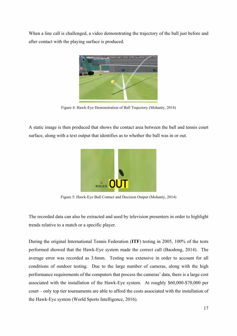
When a line call is challenged, a video demonstrating the trajectory of the ball just before and
after contact with the playing surface is produced.
Figure 4: Hawk-Eye Demonstration of Ball Trajectory (Mohanty, 2014)
A static image is then produced that shows the contact area between the ball and tennis court
surface, along with a text output that identifies as to whether the ball was in or out.
Figure 5: Hawk-Eye Ball Contact and Decision Output (Mohanty, 2014)
The recorded data can also be extracted and used by television presenters in order to highlight
trends relative to a match or a specific player.
During the original International Tennis Federation (ITF) testing in 2005, 100% of the tests
performed showed that the Hawk-Eye system made the correct call (Baodong, 2014). The
average error was recorded as 3.6mm. Testing was extensive in order to account for all
conditions of outdoor testing. Due to the large number of cameras, along with the high
performance requirements of the computers that process the cameras’ data, there is a large cost
associated with the installation of the Hawk-Eye system. At roughly $60,000-$70,000 per
court – only top tier tournaments are able to afford the costs associated with the installation of
the Hawk-Eye system (World Sports Intelligence, 2016).

18
2.2 CAIROS GOAL-LINE TECHNOLOGY
In football, goal line technology is a relatively new method used to determine whether the ball
has travelled completely across the face of the goal, between the goal posts and underneath the
crossbar. With the aid of electronic devices within the ball and the goal, the referee is instantly
notified by their watch as to when these conditions have been met.
Due to the $80,000 installation cost of the system (IOP Physics, 2016), the technology is
currently only in use in the upper echelons of professional football. As of January 2016, 78
stadia are listed as having licensed installations of goal-line technology (IOP Physics, 2016).
Thin cables are embedded in the ground underneath both the penalty area and inside of the
goal. Within the cables an electrical current runs through, which generates a magnetic field.
Figure 6: Areas of the soccer pitch with embedded electrical cables (FIFA, 2012)
Within the soccer ball sensor is suspended centrally, which measures the strength of the
magnetic fields surrounding it. When the sensor detects the presence of a magnetic field, the
ball’s location is transmitted to the receivers that are located behind the goal. Each cable has
a unique quantity of current running through it, resulting in a different strength of magnetic
field generated by each cable. The sensor, by measuring the magnetic field strength, can
therefore detect where within the electrical grid the ball is located.

19
Figure 7: Electronic Circuit Embedded in the Ball (FIFA, 2012)
When the sensor detects that the entire ball has passed the face of the goal based on the strength
of the magnetic field, the encrypted data is sent to the receiver which further transmits a signal
to the referee’s watch within a split second.
The sensor suspended within the soccer ball has been found to have no impact on the handling
characteristics of the ball (FIFA, 2012). During FIFA certification of the technology, the
players were unable to distinguish the difference between a ball with and without the chip
whilst performing the normal activities of a football match.
During testing at the 2005 Under 17 FIFA World Cup and 2007 FIFA Club World Cup, the
system was tested to have an accuracy of 100% and was approved by FIFA for implementation
in international competitive matches (FIFA, 2012).
The main concern during the introduction of the technology was the cost which stadia would
have to meet in order to implement the technology. However the company Cairos subsidised
the installation cost in exchange for sponsorship opportunities at each stadium.

20
2.3 ELECTRONIC LINE JUDGE – GRANT AND NICKS
Electronic Line Judge is a concept developed by Geoffrey Grant and Robert Nicks in 1974.
The system was initially used in the Men’s World Championship of Tennis in Dallas and
received positive reviews. However, the product was never commercialized. The system was
used underneath all of the court surface in order to produce additional capability in the detecting
of foot faults.
Figure 8: The Mylar sensors used beneath the carpet to detect where the ball landed for the first computerized,
electronic line judge device (1 January 1976)
Load cells and accelerometers are a common solution to many areas of force testing. With
correct positioning, the devices can provide accurate and valuable information regarding the
total forces resulting from an event. However, where the space available to position the sensors
is limited, the thickness of the sensors can limit the system to the point where data collection
is near impossible. A thin-film device was therefore required in order to map the force
distribution around an area whilst being able to be positioned within a size constrained space.
The key development of the Electronic Line Judge system was the use of thin Mylar film
laminate. With a final thickness of around 0.1 millimetres, the film can be produced in a variety
of shapes and sizes to meet the requirements of many applications (Hunston, 2002).

21
During manufacturing, silver electrodes are printed in a matrix onto a film (Pressure Profile,
2016). A layer of semi conductive ink is then added on top of the electrode matrix. The
pressure distribution can then be measured by the change in resistance of the ink given the
forces applied to the area. The film is then connected via cable to a computer and electrical
board that performs signal conditioning. Real time data collection or the recording of data over
a set period of time can be performed at a maximum rate of 125 frames per second (Hunston,
2002).
In order to produce films suitable for detecting a different range of pressures, different inks are
used and can be manufactured up to a maximum operating pressure of 175 Mega Pascals
(Pressure Profile, 2016).
The system, after processing the signal data, is able to present a 2D full colour display of the
pressure differences across the area being observed. The sensor film is also reusable indicating
that after use on a tennis court, the system can be salvaged and reused on another court.
In the tennis application, a playback of the impact of the tennis ball with the court could be
produced as the forces measured vary with time, with no limitations to the velocity of the shot
due to the high sensitivity of the system (Hunston, 2002). The rapid contact of a tennis ball
could be differentiated to a long contact with a human foot, allowing for the system to isolate
and identify only tennis ball impact.
The system also featured sensors in the immediate areas surrounding the lines on the court in
order to produce full visualisation of the tennis ball point of contact in the event that there was
only partial contact with the line. When the ball was registered as out, there was a buzz
produced in an earpiece worn by the linesman.

22
2.4 ELECTRONIC LINE JUDGE – LYLE DAVID
Following the successful proof of concept by Grant and Nicks, Lyle David invented a system
in 1977 which was first used in Edinburgh, Scotland. David’s design used electrically
conductive tennis balls, a micro-computer network system and wires along the boundaries of
the court. The design was able to determine the exact location of the tennis ball by the system
being programmed to register a band of voltages that only the tennis ball produced.
The system provides the umpire with automatic decisions where difficult and rapid judgements
are required. Issues with the system developed from players’ comments when it was noted that
the flight and feel of the tennis balls had been altered slightly due to the added metallic material
on the surface of the tennis ball. The system was later rejected by the players and scrapped.
The cloth originally used to manufacture a tennis ball was first cut into the patterns usually
performed during the manufacturing of a tennis ball. The ability to conduct electricity was
added to the tennis ball through the addition of a metallic material, usually stainless steel, that
was weaved into the cloth cut outs.
The cloth was weaved in a way to ensure that the electrical conductivity was uniform across
the surface area of the tennis ball. Other materials such as aluminium, copper or carbon fibres
were also considered in order to produce the electrical conductivity. Other methods of
introducing electrical conductivity such as needling or stitching were also considered.
The weaving on the cloth did not impair the playing characteristics of the ball. The balls are
designed in order to be more conductive than water, so that when water is present on the tennis
court there is no interference in the system. This also prevents water from causing false signals
as the sensitivity of the system is adjusted to only acknowledge the presence of contact with a
tennis ball.
Along the lines throughout the tennis court, a large amount of parallel steel wires were run
throughout the lines in either a zig-zag formation or in straight lines. The separation of the
wires was set to a quarter of an inch. At the edge of the tennis court, the wires from the lines
were connected to a source of potential energy and gave the system the capability to detect
when any two or more wires were short circuiting.

23
Figure 9: The parallel configuration of steel wires in tennis lines (United States Patent No. 4071242, 1978)
Figure 10: Schematic of areas where wires are laid on half of the tennis court (United States Patent No.
4071242, 1978)
When the electrically conductive tennis ball made contact with the upper surface of the line,
the balls would cause a short circuit between at least two wires and these interactions would be
detected by the system, resulting in the system being able to conclude that the ball touched the
line (United States Patent No. 4071242, 1978).
The system was extremely expensive to implement and experienced difficulties due to the
metal eyelets in shoes or metallic fibres in racquets frequently setting off the system.

24
2.5 CYCLOPS
Cyclops is an electronic line judge system developed by Bill Carlton and Margaret Parnis
England. The system was first introduced in the Wimbledon Championships in 1980, followed
by the U.S. Open in 1981 (Greenman, 2000). In 2008 it was removed and replaced by the
triangulation method used in Hawk-Eye.
During a serve, the umpire would activate a system of six infrared beams that are emitted from
one box. These beams are projected across the court at a height of 10 millimetres. One beam
is placed ahead of the service line in order to detect balls that just land short of the service line,
whilst the other beams are distributed behind of the service line to detect balls that land long
of the service line, up to a distance of 18 inches from the service line.
Figure 11: Beam placement of the Cyclops system (The Independent, 1995)
A second box is located on the other side of the court, which acts as a receiver and is connected
to the umpire’s central module. When a ball hits the ground short of the service line and
interferes with the infrared beam, the remaining beams are turned off. In the case where the
ball goes long of the service line and interferes with one of the other beams, the system
produces an audible signal. The system only accounts for a small amount of the area around
the service line as it is expected that balls that land in areas outside of this area are able to be
called by the linesman by eyesight alone.
Throughout its lifetime, the Cyclops system was found to have an accuracy of more than 99
percent (The Independent, 1995). However extreme temperature changes on the court led to
minor deviations in the court surface which could cause the system to fail. The system also
failed to gain implementation on other lines as both feet and racquets would consistently
interfere with lines and cause false activations of the system by breaking the infrared beams.

25
2.6 THERMAL IMAGING
2.6.1 Background
Thermographic cameras are used to form an image by detecting infrared radiation. Infrared
cameras detect wavelengths as long as 14,000nm, compared to common cameras that detect
visible light at 400-700nm (Vollmer, 2010).
All bodies emit black body radiation as a function of their temperature, when their temperature
is above absolute zero (Vollmer, 2010). The radiation is the result of the body’s conversion of
its thermal energy into electromagnetic energy. Emissivity is the material’s ability to emit
thermal radiation, ranging from fully emitting (1) to no emissions (0). In order for a
thermographic camera to accurately estimate the temperature of an object, the system needs to
know the emissivity of the surface. Generally, the thermographer will refer to an emissivity
table to find the emissivity value.
Modern thermal cameras are uncooled, using a sensor that operates at the ambient temperature.
All the sensors in the camera operate by the change of resistance, voltage or current when
heated by infrared radiation. The change in these variables is then measured and compared to
those at the ambient temperature.
2.6.2 Application in Tennis
In a lot of fast paced sports heat transfer is involved. Due to the small contact times with
playing surfaces in sports such as tennis, volleyball and squash, high-speed data acquisition is
required. In tennis, inelastic collisions occur between the tennis ball and the court surface,
which presents the opportunity to use infrared thermal imaging in order to map the temperature
changes on the court surface immediately following a collision between the ball and surface.
Tennis balls are fairly elastic and the ATP sets the requirement for the balls to be able to bounce
back to a height of at least 1.35 metres when dropped from a height of 2.5 metres (Vollmer,
2010). As the ball is bouncing back to a minimum of 54% of its original height, the
conservation of energy requires that the internal potential energy of the ball be transferred to
other forms of energy.

26
Immediately prior to colliding with the surface of the tennis court, the tennis ball has its highest
value of kinetic energy (Vollmer, 2010). When the ball bounces, the kinetic energy after the
collision however does not reach the same value. This is due to the deformation of the tennis
ball during its contact with the court surface. Some of the kinetic energy is converted to thermal
energy due to the deformation, which in turn creates a heat fingerprint on the surface of the
court that can potentially be mapped and utilised in order to detect the exact contact point of
the ball.
When tennis balls are used at the professional level, their collision speeds can reach 250
kilometres per hour and greater, which leads to significant deformation of the ball.
Figure 12: High speed images of tennis ball deformation at 87km/h (Vollmer, 2010)
In Figure 12 at a speed of 87 kilometres per hour, a typical tennis ball is compressed to half of
its normal volume whilst experiencing a contact time with the court of around 4 milliseconds.
The velocity of the ball is halved after colliding with the court surface. This change in velocity
leads to a change in kinetic energy, with the lost kinetic energy converted to thermal energy
(Vollmer, 2010).
Figure 13: Thermal mark of a tennis ball at 0.1s (a) and 1.7s (b) after impact (Vollmer, 2010)

27
Figure 14: Decay of the temperature of a thermal mark on a tennis court (Vollmer, 2010)
Even after 1.7 seconds in Figure 14, the point of contact still has a significant thermal
fingerprint that can be used to check whether the ball was in or out.
In these findings, the lines of the tennis court are dull and hard to compare against the mark of
the ball. However, the lines could be made more visible by using a large emissivity contrast.
2.6.3 Cricket ‘Hot Spot’ Technology
In the 2006-07 Ashes, the Hot Spot technology was first introduced in Brisbane, Australia. Hot
Spot is an infra-red imaging system that determines whether the bat of the player has struck
the ball or any other part of their body. Two cameras are placed at opposite ends of the ground,
normal to the direction of the pitch and analyse images for a rise in the temperature due to
contact with the cricket ball (Coverdale, 2012). Using a subtraction technique, a series of black
and white negative frames is generated in order to precisely locate the point of contact of the
ball, as shown in Figure 15.
Figure 15: An example of cricket's Hot Spot (Coverdale, 2012)
28
2.7 LOCALISED POSITIONING SYSTEM
Localised Positioning System, also known as an Indoor Positioning System (IPS), is a system
that to date has not been utilised in the tracking of tennis balls (Kotanen, 2012). IPS is primarily
used inside of buildings to locate positions through acoustic signals, magnetic fields and radio
waves (Pritt, 2013).
IPS systems are able to locate the position of an object by determining its distance relative to
at least three anchor nodes. Anchor nodes are objects in known positions that emit a wireless
signal (Pritt, 2013).
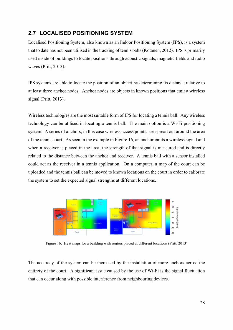
Wireless technologies are the most suitable form of IPS for locating a tennis ball. Any wireless
technology can be utilised in locating a tennis ball. The main option is a Wi-Fi positioning
system. A series of anchors, in this case wireless access points, are spread out around the area
of the tennis court. As seen in the example in Figure 16, an anchor emits a wireless signal and
when a receiver is placed in the area, the strength of that signal is measured and is directly
related to the distance between the anchor and receiver. A tennis ball with a sensor installed
could act as the receiver in a tennis application. On a computer, a map of the court can be
uploaded and the tennis ball can be moved to known locations on the court in order to calibrate
the system to set the expected signal strengths at different locations.
Figure 16: Heat maps for a building with routers placed at different locations (Pritt, 2013)
The accuracy of the system can be increased by the installation of more anchors across the
entirety of the court. A significant issue caused by the use of Wi-Fi is the signal fluctuation
that can occur along with possible interference from neighbouring devices.

29
To determine a location more accurately, there has been some success with the use of
geomagnetic anomalies. Ferrous objects like steel beams and metal cabinets disrupt the earth’s
natural magnetic field. As a result, within an area with ferrous objects there is a unique pattern
of magnetic variation, known as a magnetic fingerprint.
Figure 17: Heat map of geomagnetic strength in a building (Pritt, 2013)
At present, smartphones and tablets have both magnetic sensors and accelerometers which are
able to map the magnetic fingerprint of an area. For a geomagnetic fingerprint to be
successfully implemented, the two phases of training and positioning must be completed. A
fingerprint database is created during the training phase. At each reference point, the magnetic
field strength is measured and recorded in order to form unique strength identifications for each
point. This is then repeated along every reference point set by the user. During the positioning
phase, the device measures the strength of the magnetic field around the user and outputs the
most likely position of the device.

30
3 FEASIBILITY STUDY
3.1 VISUAL TRACKING
Visual tracking is the main technology used in present day applications through the Hawk-Eye
system. While the current system presents a highly accurate solution along with a high ease-
of-use, the system has a very high installation cost of $70,000 per court which restricts its use
to the upper echelons of professional tennis tournaments.
For visual tracking to be a viable solution given the scope of this problem, the costs must be
reduced significantly in order to make the system more accessible. Given that Hawk-Eye was
invented in 2001, the technology used at the time was limited and extremely expensive when
compared to options available today. The main technology used in Hawk-Eye has not been
altered significantly as it would result in the system requiring recertification which is a time
and resource consuming process. As a result, the cost of a visual tracking system could be
reduced by drawing on new and emerging technologies that present a low cost system similar
to that of Hawk-Eye.
Since 2001, the cost of a high speed camera with 1,000 frames per second has reduced from
$40,000 to $400 (Blain, 2014). Given this, major cost reductions can be made by first
introducing modern high speed cameras, while maintaining a high frame rate in order to
produce a smooth, accurate representation of the ball’s path.
The identification of the ball is the first step in the data processing. Simpler, more modern
methods can be used in order to identify the tennis ball through each camera. OpenCV ball
tracking methods could be used as an alternative to the current pixel algorithms used by
Hawkeye. A potential issue in the use of OpenCV tracking would be a possible reduction in
the accuracy of the system when identifying the tennis ball.

31
Figure 18: OpenCV tracking highlights the position of two tennis balls (Rosebrock, 2015)
While these two new additions would provide large cost cuts to the current visual tracking
solutions, the system would still need to perform a series of calculations during each frame in
order to produce an accurate representation of the travel of the ball and more importantly an
accurate image of the contact between the ball and the tennis court.
When the ball interacts with the tennis court, considerations have to be made in respect of the
deformation and skid of the ball, both of which alter the size and shape of the contact point
between the ball and tennis court. The Hawk-Eye system accounts for these dynamics and as
a result performs up to one billion calculations per second. In order to create an accurate
representation of the ball’s contact with the court, these calculations cannot be ignored and as
a result the cost of data processing still remains high.
The validation of the system would require testing in both laboratory and real-world examples
where the system is used to detect whether the ball has or has not made contact with the line
whilst a high speed camera or marker would be used to validate the results. These tests would
have to be extended to testing in low light conditions and poor weather.
As a result of these considerations, while we would be able to design a revised visual tracking
system that reduces costs through camera equipment and ball recognition, the data processing
needed to create an accurate depiction of the ball’s contact with the tennis court is so significant
that the overall costs of the system cannot be reduced in order to make a system that is
financially viable given the scope of the project.
32
3.2 LOCALISED POSITIONING SYSTEM (LPS)
Using Wi-Fi positioning or geomagnetic fingerprints alone would not provide the accuracy
required for the tennis ball tracking system. However, with the two systems combined, the
system could potentially present a solution with a high accuracy and low to moderate cost. Wi-
Fi signal generators could be placed around the border of the court and at the net posts. Given
that the lines of the tennis court are the key locations of interest, geomagnetic anomalies could
be created underneath the lines in order to create a unique fingerprint around the court.
Underneath the paint of the lines would require a thin layer of ferrous material that varies in
magnetic strength. The accuracy of the geomagnetic system increases proportionally to the
change of magnetic strength per unit length as it makes the system more sensitive to the change
in length and location.
Whilst this system would provide relatively accurate tracking of the ball, further considerations
are required towards the deformation and skid of the ball when it makes contact with the tennis
court. The system could be complimented by an embedded accelerometer in order to calculate
the forces of the ball and therefore calculate the deformation and skid to create an accurate
depiction of the ball’s contact with the line.
In order to validate the system, testing would have to be done initially on the use of wireless
signals, their locations and the expected signal fingerprint that they would produce on court.
Ferrous materials would have to be validated for use underneath of the tennis lines to ensure
that they do not significantly change the dynamics of the lines. A geomagnetic fingerprint
would then have to be evaluated.
Testing and validation of a dynamic model for the interactions between a tennis ball and the
court at various forces would have to be completed in order to create an accurate model of the
deformation and skid characteristics, along with ensuring that the sensors embedded within the
ball would be able to withstand the high forces experienced. An accuracy test would then have
to be completed in both a laboratory and in a real world situation where the system results are
compared with the actual results through either a high-speed camera or a marker.
The main concerns with this system is that both Wi-Fi positioning and geomagnetic anomalies
are designed for a two-dimensional system. The system would require Wi-Fi anchors to be

33
placed at various heights as well in order to accurately depict the impact of the tennis ball and
the mark left behind.
In professional matches, tennis balls are only used for up to nine service games and as a result,
plans would have to be made in order for the recuperation of the sensors inside of the ball if
they were expensive. The placement of the sensors would also have to guarantee that the
dynamics of the tennis ball were not affected in any way. Considerations would also have to
be made to ensure that no significant force interactions occur between any sensors within the
tennis ball and the ferrous materials underneath the surface of the court.
3.3 PRESSURE SENSORS
Pressure sensors were amongst the first solutions considered for electronic line judging. Due
to the cost of the technology at the time they were not further pursued.
The concept can be modernised into a low cost solution today through the use of the latest
tactile pressure indicating sensor film. Using pressure sensor arrays, high resolution images of
the forces experienced on a contact surface can be used in order to map the interactions between
two surfaces – in this case the tennis ball and the court lines.
Whilst the original concept placed sensors on and around the lines, a different approach could
be to use the sensors only underneath the lines of the tennis court. Whilst this only allows for
the mapping of the ball’s contact with the tennis court, it does allow for a simpler maintenance
in the case of a hard tennis court. The lines could be developed into a roll where the pressure
sensors are pre-glued to the line surface at the professional standard width. The lines could
then be rolled out and bonded to the court with a bonding agent.
A high resolution pressure sensor array would be recommended to have a margin of error equal
to or less than 3 millimetres, equal to that of Hawkeye. The system also requires a very low
film thickness whilst being able to operate. Some materials available for such an application
are conductive rubber, polyvinylidene fluoride, lead zirconate titanante and metallic capacitive
sensing elements (Pressure Profile, 2016).

34
A market-ready solution is the use of polyimide. With a thickness of 0.3 millimetres and
temperature range of -20 to 100 degrees Celsius (Pressure Profile, 2016), this material offers a
suitable solution for the system provided that the pressure range is suitable after having
completed an analysis of the interactions between the tennis ball and court. The system is
connected via USB to a visualisation and recording system which is then able to map the
pressure distributions to a resolution of two millimetres.
In order to validate the design, a dynamics analysis of tennis ball interactions with the tennis
court must first be completed in order to correctly evaluate the pressure range to be expected
across the surface of the court lines. The system would then have to be tested to ensure that
the court dynamics are not affected by the addition of the thin layer on sensors underneath of
the court lines. An accuracy test would then have to be completed in both a laboratory and in
a real world situation where the system results are compared with the actual results through
either a high-speed camera or a marker.
Concerns for the system surround the cost of maintenance. If part of the system were to fail,
the system would have to be shut down for the remainder of the day due to the need for the line
to be carefully separated from the court before being replaced with a new line. The court would
be unplayable while the bonding agent set between the lines and the court. Another concern is
the potential for the dynamics between the lines and ball to be altered by the addition of the
sensors underneath the line, which can be analysed during the laboratory and real-world testing.
3.4 LASER MONITORING
Laser monitoring was the main form of electronic line calling up until the adoption of Hawk-
Eye in 2007. Used in Wimbledon, the system has a high level of accuracy and reliability.
Whilst only used on service lines, the system could be expanded and modernised in order to
present a full court solution at a fraction of the cost of modern systems.
The system would work in a similar manner to the Cyclops system. In the Cyclops system,
each line has a set of lasers just before and after the line at a height of 10mm with a receiver
box on the opposite side of the line. Whilst this system detects when the ball lands just before
or after the line, a redesigned system could have a series of laser beams across the surface of
the line itself, ensuring that there is a beam on the upper and lower edge of the line. With this

35
system, when the receiver box detects that a laser beam has been blocked, it would signal that
the ball has touched the line.
The height of the lasers above of the ground would have to be reviewed to ensure that the
system can detect contact with the line regardless of the amount of deformation that the ball
exhibits on contact with the surface. A full analysis of the dynamics of the tennis ball and court
would have to be performed in order to derive this height. The height must also take into
consideration deviations in the height of the court, along with the possible blockages that may
occur due to dirt and insects.
Given that the system would be used in both doubles and singles matches, along with one set
of lasers and receivers being unable to operate from one side of the court to the other, the full
court system would require 14 sets of lasers and receivers in order to cover the entire court.
An issue with the design is the need for 10 receivers to be placed along the length of the net.
The receivers cannot be large in size due to the obstruction that they would present to play at
the net when the ball lands short. Given how rigid the professional tennis nets are, the design
could work to include receivers along the length of the base of the net. Instead of having a set
of individual receivers for each beam, a receiver strip could be set along the base which
registers the number of laser beams reaching the receiver. When one of the beams is blocked,
the system would register this and detect that the ball had touched the line. The system would
then present a visual message to the chair umpire informing them that the ball had touched the
line. The system could be further programmed in order to inform the umpire through a visual
display as to which line the ball had touched.
Another possible issue can arise if a blockage were to occur to a laser beam whilst the ball
crosses the line. There is a chance that whilst the ball touches the ground, a player’s foot may
obstruct the beam and therefore stop the system from making a line call on the position of the
ball. A statistical analysis of professional play over a set sample would have to be performed
in order to determine the significance of this issue. There is the third issue that whenever the
player’s foot blocked one of the beams, the umpire would receive a message saying that a ball
had touched the line. The system could be refined through the addition of a spectrometer or
similar device which would create a two-step mechanism for detecting that a tennis ball had

36
touched the line. The system would first detect a laser beam had been blocked, followed by
the spectrometer determining that the material was that of a tennis ball.
3.5 THERMAL IMAGING
A potential system could have at least four thermographic cameras in order to cover a quarter
of the court each. The system would register the thermal marking of a tennis ball after a
collision and keep an image of the mark. If a line call were to be challenged by a player, the
umpire would be able to select a point of collision that had occurred within the last 30 seconds.
The system would process the image and compare the location of the mark with the position
of the lines and determine if the mark overlaps the line at any point. The system would present
a visual demonstration of the location of the ball, along with a message as to whether the ball
was in or out.
The cameras could be in a top down view where they are suspended above the court at a height
significant enough in order to not obstruct play or create significant shadows on the court.
Alternatively, the cameras could be placed around the boundary of the court on lateral lines
such as service lines. This could lead to the possibility of parallax viewing errors that would
require programming in order to overcome.
A testing module for the proof of concept of the system could be created through the
acquirement of a low cost thermographic camera, along with a small sample of hard court
tennis surface and a tour level tennis ball. The system would require testing in order to test the
accuracy of the system and the minimum velocity of the tennis ball to which the system can
map a heat signature. Testing would also be required to find the optimal materials to use in the
tennis court lines to create a large emissivity contrast.
A computer program would also be developed in order to take a thermal image, register the
mark of the tennis ball, register the line of the tennis court and then decide as to whether the
ball was in or out with a visual feedback system.

37
4 TECHNOLOGY SELECTION
In order to pursue the most viable technology, the alternative technologies explored during the
feasibility study were compared in the following areas.
4.1 SERVICEABILITY
The ease in which repairs can be made to the system in the event of component or system
failure. A pass is awarded to systems where faulty components can be removed and replaced,
with the system returning to full operation while the faulty component is fixed. A fail is
awarded to systems which require significant downtime in the event of failure, potentially due
to the large time required to access and replace a faulty component. Another cause for failure
would be the need to remove the court surface in order to access faulty components.
4.2 ACCURACY
The margin of error of the technology. A pass is awarded to systems where the margin of error
is comparable to that of Hawk-eye. A fail is awarded to systems where the margin of error is
significantly worse than that of Hawk-eye.
4.3 LIMITATIONS
Any limitations that the system may have when installed in a professional tennis environment.
A pass is awarded to systems where the system has no practical limitations and is able to make
line calls for all scenarios in a professional tennis match. A fail is awarded to systems when
the system has limitations where a common scenario in a tennis match would cause the system
to fail.
4.4 COST
The current market cost of the technology. A pass is awarded to systems where the cost is less
than that of Hawk-eye. A fail is awarded to systems where the cost is the equal to or greater
than Hawk-eye.

38
4.5 DYNAMICS
The effect that the technology has on the dynamics of the tennis ball and court. A pass is
awarded to systems that have no effect on the balls or court. A fail is awarded to systems where
the dynamics of the ball or court are affected.
4.6 COMPARISON OF TECHNOLOGIES
As a result of these criteria, the available technologies were compared in the table below.
Table 1: Comparison of available technologies
Serviceability Accuracy Limitations Cost Dynamics Visual Tracking ü û û ü ü LPS ü o ü ü û Pressure Sensors û ü ü o o Lasers ü ü û ü ü Thermal ü ü ü ü ü
Key: ü Pass o Inconclusive û Fail As a result of the comparison between the alternative technologies, thermal imaging was
chosen as the most promising technology to pursue. Thermal imaging presents an accurate,
reliable and serviceable solution while not interfering with the dynamics of the sport, nor
creating a large cost of instalment.

39
5 EXPERIMENTAL RIG & PROCEDURE
5.1 TESTING RIG
A small scale testing rig was developed in order to test the broad feasibility of the system.
While previous literature had shown promising results with the technology in tennis
applications, the testing had been completed on a carpet surface, which has a significantly
higher coefficient of friction than that of the modern-day acrylic tennis surface.
The testing rig needed to be able to produce repeatable, controlled ball trajectories while also
generating thermal images showing the contact point between the tennis ball and court. Due
to the low availability of acrylic surface samples, the testing rig was designed for use on a full-
scale tennis court. The tennis balls were to be fired into the testing area using a controllable
tennis ball machine, with a thermographic camera suspended above the area recording the
thermal radiation levels in the test area.
5.1.1 FLIR One Thermal Camera
A low-cost thermal camera was required in order to provide the thermal image outputs during
the testing. The FLIR One camera was selected; a smartphone accessory that interacts with an
app in order to produce thermal images.
Figure 19: FLIR One Thermal Camera (FLIR, 2016)
The FLIR One system has two cameras – a visible and infrared camera. The visible camera
takes images at the same time as the infrared camera and detects the edges of objects in the
image. The processing software then merges the detected edges with the thermal images in
order to create a final image with enhanced detail and resolution (FLIR, 2016).

40
The FLIR One app allows the user to process the image at the end of testing, altering the
temperature range, thermal palette and material emissivity can be altered in order to produce
more suitable images for the application.
The specifications of the FLIR One system are shown below.
Table 2: FLIR ONE Specifications (FLIR, 2016)
Variable Value
Temperature detection range -20° to 120°C
Thermal resolution 160 x 120
Sensitivity 0.1°C
5.1.2 Lobster Elite Ball Machine
A ball machine was used in order to produce controlled and repeatable ball collisions with the
court surface. The ball machine is able to control the velocity, spin and elevation of the tennis
ball as it is launched.
Figure 20: Lobster Elite ball machine (Lobster Sports, 2016)
The machine shoots balls through two launch wheels, which are spun with programmed gears.
The two wheels spin in opposite directions in order to launch the balls (Lobster Sports, 2016).
When the spin on the ball is zero, the wheels spin at the same speed. When a spin is required,

41
the two wheels spin at different speeds in order to create either a topspin or backspin effect on
the ball.
The system is also able to change the elevation of the ball through a hydraulic leg at the front
of the machine that can raise and lower the angle of the ball machine, relative to the court
surface. The limitations of the ball machine are shown below.
Table 3: Lobster Elite ball machine specifications (Lobster Sports, 2016)
Variable Value
Speed 20 to 80 mph
Spin Top, flat, back
Elevation 0-60 degrees
5.2 TESTING PROCEDURE
The initial settings were provided to the ball machine, providing the spin, velocity and elevation
of the shot. The ball machine then fired three test shots in order to demonstrate that the ball
was correctly replicating the desired trajectory.
During the test shots, the testing area was chosen as a ~2m2 section of court surrounding the
area where the test shots had landed. The thermographic camera was manually held above the
test area and via remote, the ball machine started launching a test shot every four seconds. Just
after the time when the ball has bounced off of the court, a thermal image is taken and recorded
for data processing. This process is repeated and around 20 images are collected per test.
The images are then processed through the FLIR software, where the emissivity of the acrylic
court surface is supplied. The temperature range of the image is adjusted in order to locate and
highlight the thermal mark left by the collision between the tennis ball and court. A marker is
then placed across that mark in order to find the average temperature of the mark.
42
6 EXPERIMENTAL TESTING
6.1 RESULTS
Using the described procedure, experimental results were gathered using the tennis courts at
the University of Queensland Tennis Club. The tests were performed at sea level conditions,
with an assumed ambient temperature of 293.15K. During the testing, no part of the court was
shaded, which could have negatively affected the test results.
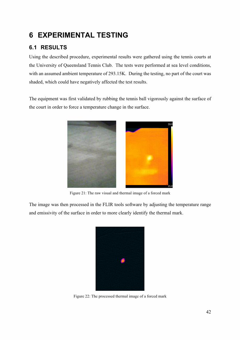
The equipment was first validated by rubbing the tennis ball vigorously against the surface of
the court in order to force a temperature change in the surface.
Figure 21: The raw visual and thermal image of a forced mark
The image was then processed in the FLIR tools software by adjusting the temperature range
and emissivity of the surface in order to more clearly identify the thermal mark.
Figure 22: The processed thermal image of a forced mark

43
As seen, the system clearly displays a change in temperature across the surface where the ball
was rubbed. The ball machine was then setup to fire tennis balls at 60 mph (96.5 kmph), with
no spin and an elevation setting of +3. As the ball machine began firing balls, the FLIR thermal
camera was held manually above the area where the balls were landing, taking photos just after
the time where the balls had bounced.
Figure 23: The raw visual and thermal image for a bouncing ball
As seen in the raw image, there is no discernible area in the court where it appears that a ball
has landed. The image has to be processed carefully in order to reduce the temperature range
and locate any mark on the court with a significantly raised temperature.
Figure 24: The processes thermal image for a bouncing ball

44
The processed image clearly shows the mark where the ball has landed, with the temperature
across the mark higher than any other temperature recorded on the court.
While this result was promising, the experimental testing only produced one result in around
30 tests.
6.2 DISCUSSION
While the results demonstrated a proof of concept for the use of the technology in tennis line
calls, the overwhelming majority of the results from the tests were inconclusive. The testing
was performed in similar ambient conditions to those performed by Vollmer in 2010, however
the fundamental difference was the coefficient of friction of the acrylic court in comparison to
the carpet used by Vollmer.
The low success in testing can be related to the procedure. The procedure relies on the user to
be able to take a photo of court area immediately after the ball has bounced. The first issue is
that due to human reaction times, by the time the user reacts and the photo is taken, the thermal
energy could have already dissipated from the surface if the magnitude of the energy was low.
Furthermore, due to the testing being outdoors, effects due to factors such as the wind can cause
the flight path of the ball to deviate and for the location of the bounce to deviate around the
testing area. As a result, some of the photos likely did not capture the area where the ball
landed.
It would be recommended for further experimental testing to be completed in a laboratory
environment, where more precise measurements of the ball’s velocity and angle of incidence
can be made.
In order to explain the results and to determine whether the results are due to experimental
error or a lack of heat transfer, a theoretical model was developed and run using similar
conditions to those seen at the University of Queensland Tennis Club.

45
7 THEORETICAL MODEL
As a result of the experimental results, a simulation of the system was developed in order to
estimate the expected temperature of a mark left after the collision between a tennis ball and
the court.
7.1 DERIVATION OF EQUATIONS
The simulation assumes sea level at standard atmospheric conditions.
Table 4: Standard atmospheric conditions
Density / kgm-3 Pressure / Pa Temperature / K g / ms-2
1.225 101350 293.15 9.81
The tennis ball used in the simulation was taken as the standard ball as defined by the
International Tennis Federation (ITF). The ball has a mass of 58.5 grams and a radius of 3.3
centimetres (ITF, 2016).
The tennis court used in the simulation was taken as a standard acrylic court, as defined by the
ITF. The ITF classifies courts based on their pace - the effect of the ball-surface interaction.
The ITF assigns a Court Pace Rating (CPR) to the court, derived from the theoretical model of
a ball/surface impact assuming that the ball slides through its contact with the surface. The
levels of CPR classifications by the ITF are shown below.
Table 5: Court Pace Ratings (ITF, 2012)
Category CPR
Slow < 30
Medium-Slow 30-34
Medium 35-39
Medium-Fast 40-44
Fast > 44
The target market for this design is professional hard courts, the majority of which are rated
with a CPR category of medium (ITF, 2012).
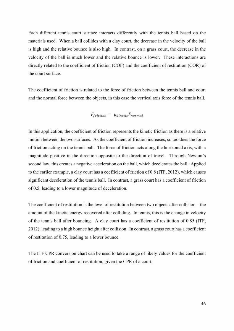
46
Each different tennis court surface interacts differently with the tennis ball based on the
materials used. When a ball collides with a clay court, the decrease in the velocity of the ball
is high and the relative bounce is also high. In contrast, on a grass court, the decrease in the
velocity of the ball is much lower and the relative bounce is lower. These interactions are
directly related to the coefficient of friction (COF) and the coefficient of restitution (COR) of
the court surface.
The coefficient of friction is related to the force of friction between the tennis ball and court
and the normal force between the objects, in this case the vertical axis force of the tennis ball.
!"#$%&$'( = +,$(-&$%!('#./0
In this application, the coefficient of friction represents the kinetic friction as there is a relative
motion between the two surfaces. As the coefficient of friction increases, so too does the force
of friction acting on the tennis ball. The force of friction acts along the horizontal axis, with a
magnitude positive in the direction opposite to the direction of travel. Through Newton’s
second law, this creates a negative acceleration on the ball, which decelerates the ball. Applied
to the earlier example, a clay court has a coefficient of friction of 0.8 (ITF, 2012), which causes
significant deceleration of the tennis ball. In contrast, a grass court has a coefficient of friction
of 0.5, leading to a lower magnitude of deceleration.
The coefficient of restitution is the level of restitution between two objects after collision – the
amount of the kinetic energy recovered after colliding. In tennis, this is the change in velocity
of the tennis ball after bouncing. A clay court has a coefficient of restitution of 0.85 (ITF,
2012), leading to a high bounce height after collision. In contrast, a grass court has a coefficient
of restitution of 0.75, leading to a lower bounce.
The ITF CPR conversion chart can be used to take a range of likely values for the coefficient
of friction and coefficient of restitution, given the CPR of a court.

47
Figure 25: ITF Court Pace Rating conversion chart (ITF, 2012)
Based on the system being designed for a court in the medium CPR category, the conversion
chart was used to select the following values for our acrylic court surface.
Table 6: Selected coefficients for acrylic court surface
Coefficient of Friction 0.63
Coefficient of Restitution 0.82
The following material specifications were applied based on an acrylic court surface used by
an ATP professional tournament in Auckland, New Zealand (APT Sports, 2016).
Table 7: Material specifications for acrylic court
Specific heat / J/kg-K 1630
Density / kgm-3 1130
In order to simplify the model, the kinetic energy lost during the collision between the ball and
court was taken to be completely converted to thermal energy, with the quantity of thermal
energy shared equally between the ball and the court. The contact time between the ball and

48
the court was taken to be the value found in the original literature, at a value of 4ms (Vollmer,
2010).
With these constants and assumptions, the process can begin to solve the trajectory of the ball
after being hit, given initial values for the velocity, spin, height of contact and angle of attack
relative to the horizontal axis.
7.1.1 Trajectory
A tennis ball has three primary forces acting on it – lift, drag and weight. The magnitude of
lift and drag is related to the magnitude of the spin, while the direction of the lift force is related
to the direction of spin.
Figure 26: Forces acting on a tennis ball (Cross, 1998)
At any time, a tennis ball travelling through the air has a drag force acting in the direction
opposite to the direction of travel. The coefficient of drag has a base value of 0.55 (Cross,
1998), however the value can change, relative to the magnitude of the spin of the ball.
12 = 0.55 +1
22.5 + 4.2 ∗;
;<=$(
>.?
@.A
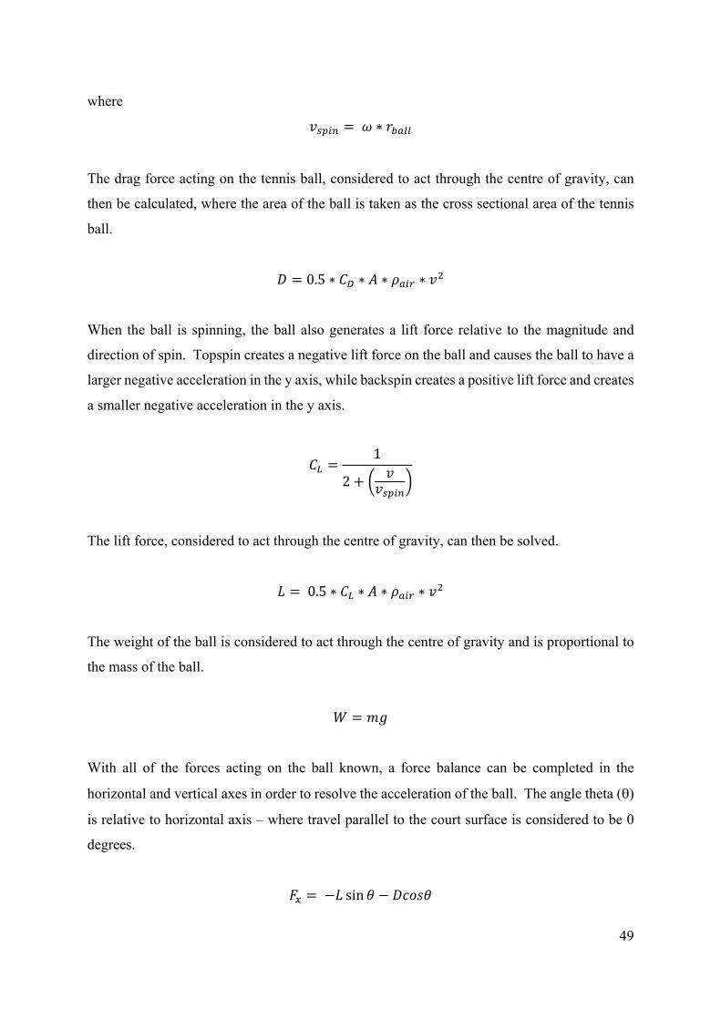
49
where
;<=$( = B ∗ CD/00
The drag force acting on the tennis ball, considered to act through the centre of gravity, can
then be calculated, where the area of the ball is taken as the cross sectional area of the tennis
ball.
E = 0.5 ∗ 12 ∗ F ∗ G/$# ∗ ;>
When the ball is spinning, the ball also generates a lift force relative to the magnitude and
direction of spin. Topspin creates a negative lift force on the ball and causes the ball to have a
larger negative acceleration in the y axis, while backspin creates a positive lift force and creates
a smaller negative acceleration in the y axis.
1H =1
2 +;
;<=$(
The lift force, considered to act through the centre of gravity, can then be solved.
I = 0.5 ∗ 1H ∗ F ∗ G/$# ∗ ;>
The weight of the ball is considered to act through the centre of gravity and is proportional to
the mass of the ball.
J = KL
With all of the forces acting on the ball known, a force balance can be completed in the
horizontal and vertical axes in order to resolve the acceleration of the ball. The angle theta (θ)
is relative to horizontal axis – where travel parallel to the court surface is considered to be 0
degrees.
!M = −I sin R − ESTUR

50
!V = −J + I cos R − EUYZR
Using Newton’s second law, the acceleration along each axis due to these forces can be
calculated.
[M =!MK
[V =!VK
The axial velocity of the ball can then be calculated.
;M = ;M,'0] + [M^
;V = ;V,'0] + [V^
The total velocity of the ball, along with the direction of travel can then be calculated.
; = ;M> + ;V>
R = tanab;V;M
Finally, the direction travelled in both the horizontal and vertical direction as a result of the
velocity can be solved at each time step.
c = c'0] + ;M^
d = d'0] + ;V^
Over a range of time-steps, the trajectory of the ball can be calculated and as the vertical height
reaches zero, indicating the start of the collision with the court, the velocity and angle can be
calculated in order to show the entry conditions for the collision.
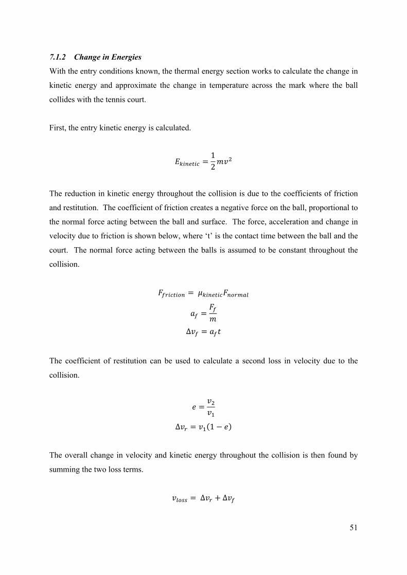
51
7.1.2 Change in Energies
With the entry conditions known, the thermal energy section works to calculate the change in
kinetic energy and approximate the change in temperature across the mark where the ball
collides with the tennis court.
First, the entry kinetic energy is calculated.
e,$(-&$% =1
2K;>
The reduction in kinetic energy throughout the collision is due to the coefficients of friction
and restitution. The coefficient of friction creates a negative force on the ball, proportional to
the normal force acting between the ball and surface. The force, acceleration and change in
velocity due to friction is shown below, where ‘t’ is the contact time between the ball and the
court. The normal force acting between the balls is assumed to be constant throughout the
collision.
!"#$%&$'( = +,$(-&$%!('#./0
[" =!"K
∆;" = ["^
The coefficient of restitution can be used to calculate a second loss in velocity due to the
collision.
g =;>;b
∆;# = ;b 1 − g
The overall change in velocity and kinetic energy throughout the collision is then found by
summing the two loss terms.
;0'<< = ∆;# + ∆;"

52
e,,0'<< =1
2K ;>
> − ;b>
Based on our assumptions, all of the lost kinetic energy is converted to thermal energy and
50% of this energy is transferred to the surface of the court. With these assumptions, a simple
calorimeter model can be used to estimate the temperature of the mark immediately after the
time of collision, assuming that the energy is initially transferred into the court material to a
depth of 1 millimetre.
To calculate the size of the mark, the contact area of the ball during collision is considered to
be the cross-sectional area of the ball at its widest point – the midpoint. With the contact time
assumed to be 4ms, the area of the mark can be estimated using the horizontal velocity term,
vx.
FD/00 = hC>
I./#, = ;M^%'00$<$'(
F./#, = FD/00 + C ∗ I./#,
The volume and mass of the court that is heated immediately after collision due to the gain in
thermal energy can be estimated, given our depth assumption of 1 millimetre for initial heating.
i<j#"/%- = F./#, ∗ kgl^ℎ
K%'j#& = G%'j#&i<j#"/%-
The change in temperature across the mark, immediately after the time of collision can then be
estimated.
∆n =
12e,,0'<<
K%'j#& ∗ S=,%'j#&
7.2 VALIDATION OF MODEL
In order to validate the theoretical model, the testing conditions used by Vollmer in 2010 were
replicated. However, the testing completed in the literature was performed on a carpet surface.

53
The following values were used for the specifications of a typical tennis carpet material,
Velour, as the specifications of the carpet used by Vollmer were not specified.
Figure 27: Specifications of velour tennis court (ITF, 2012)
Coefficient of friction 0.70
Coefficient of restitution 0.74
Specific Heat / J/kg-K 1400
Density / kg/m3 160
The literature provides the velocity used in their tests, but they make no mention of an angle
or spin rate. As a result, the simulation was run for a tennis ball that collides with the court at
86 km/h, with an assumed spin of zero and an entry angle of 45 degrees. The angle was chosen
due to the literature showing minor evidence of the ball skidding, insinuating that the ball was
not fired vertically, nor at a shallow angle. The results from the carpet simulation are shown
below.
Table 8: Comparison of the literature and simulation
Vollmer, 2010 Theoretical
Change in temperature / K 4.60 5.07
As shown, the theoretical model produces a similar change in temperature to that seen by
Vollmer. The theoretical model provides a slight overestimate; however, this is to be expected
based on the assumptions of the model. In reality, not all of the kinetic energy would be
converted to thermal energy, which would lower the temperature of the mark. Furthermore,
the assumption that only the top 1mm of the surface is heated immediately after the collision
is a simplification of the system which leads to an overestimation in the ∆T term.
Given the results and the implications of the assumptions in the model, the theoretical model
is considered valid and a reasonable method in order to estimate the heat transfer due to the
collision between a ball and court.

54
7.3 RESULTS
Using the specifications for the acrylic tennis court, the theoretical model was coded in
MATLAB and utilised in order to estimate the temperature change across the collision mark.
In the simulations, the three initial conditions were the velocity, angle and spin. The values
used were those typically seen in professional tennis, as shown below.
Table 9: Typical range of variables in professional tennis (Honan, 2013)
Variable Typical Range
Theta / deg 0 to 45
Velocity / kmph 20 to 140
Spin / RPM -5000 to 5000
7.3.1 No Spin
In the no spin model, the ball is hit at a typical contact height of one metre (APT Sports, 2016).
The spin of the ball was set to zero and the initial velocity and angle was varied across a range
of values. In one of the test cases, the ball is initially hit at 80kmph, 15 deg and 0RPM. The
trajectory of the ball is shown below, with the net and end of the court shown in red.
Figure 28: Trajectory of flat groundstroke (REF?)
For this scenario, the temperature of the court was raised by 0.17K across the area of the mark,
immediately after the collision. Overall, the simulation showed that most of the testing cases
had a minimum velocity, below which the thermographic camera would not be able to detect
the thermal mark. The full results are available in Appendix A.

55
Table 10: Minimum velocity relative to theta
Theta Minimum velocity (kmph)
0 40
15 50
30 55
45 55
The simulation also demonstrated two contrasting relationships. As the velocity increases with
a constant theta and spin, the temperature rise across the mark also increases. However, as the
value of theta rises with a constant velocity and spin, the temperature across the mark decreases.
As theta increases, the ball enters the point of collision at a sharper angle, reducing the
horizontal velocity term and the loss of kinetic energy due to the kinetic friction.
Figure 29: Temperature rise relationships for flat groundstrokes
Overall, the minimum velocity required to generate a significant thermal mark is 50 kmph.
This velocity is below the lower value expected velocities for flat groundstrokes and would
require further real-world testing to validate.
7.3.2 Top Spin
In the top spin model, the ball is hit at a contact height of one metre. The spin of the ball was
varied, along with the initial velocity and angle. In one of the test cases, the ball is initially hit
at 120kmph, 15 deg and 2000RPM. The trajectory of the ball is shown below, with the net and
end of the court shown in red.
0
0.05
0.1
0.15
0.2
0.25
0.3
0 50 100 150 200
ChangeinTem
perature(K)
Velocity(kmph)
Trisewithaconstanttheta
00.050.1
0.150.2
0.250.3
0 10 20 30 40 50
ChangeinTem
perature(K)
Theta(deg)
Trisewithaconstantvelocity

56
Figure 30: Trajectory of topspin groundstroke
For this scenario, the temperature of the court was raised by 0.31K across the area of the mark,
immediately after the collision. Overall, the simulation showed that most of the testing cases
produced a large enough temperature difference to be detected, however the minimum required
velocity for any combination of theta and spin was found to be 36.29 kmph. This is below the
typical range of top spin groundstroke velocities and validates the technology in this scenario.
7.3.3 Back Spin
In the back spin model, the ball is hit at a contact height of one metre. The spin of the ball was
varied along a range of negative values, along with the initial velocity and angle. In one of the
test cases, the ball is initially hit at 80kmph, 10 deg and -2000RPM. The trajectory of the ball
is shown below, with the net and end of the court shown in red.
Figure 31: Trajectory of backspin groundstroke
For this scenario, the temperature of the court was raised by 0.05K across the area of the mark,
immediately after the collision. Overall, the simulation showed that for all of the testing cases
the collision did not raise the temperature of the mark by a magnitude large enough to be
detected by the thermographic camera.
As the value of the spin becomes more negative, the magnitude of the lift force increases in the
positive y axis direction, which causes the ball to float. As a result, the ball bounces at a very
shallow angle, which reflects a low force acting on the ball normal to the surface of the court.

57
As a result, the kinetic energy lost due to friction is reduced along with the temperature change
across the court surface.
Figure 32: Temperature rise versus spin
7.3.4 Drop Shot
In the drop spin model, the ball is hit at a contact height of one metre. The spin of the ball was
varied, along with the initial velocity and angle. The drop shot is a special test case due to the
low velocity and high initial angle of the ball. In one of the test cases, the ball is initially hit at
20kmph, 60 deg and -2000RPM. The trajectory of the ball is shown below, with the net and
end of the court shown in red.
For this scenario, the temperature of the court was raised by 0.025K across the area of the mark,
immediately after the collision. Overall, the simulation showed that all test cases were unable
to produce a large enough temperature change to be detected by the thermographic camera.
This presents a significant limitation to the system. While drop shots are infrequently played
near the side-lines of a tennis court, if one were to occur and the line call was challenged, a
0.0405
0.041
0.0415
0.042
0.0425
0.043
0.0435
0.044
0.0445
-6000 -5000 -4000 -3000 -2000 -1000 0
ChangeinTem
perature(K)
Spin(RPM)
Temperaturerise- 15deg,50kmph

58
thermal imaging system would be unable to detect the mark at its current operating
specifications.
7.3.5 Serves
A special test case was created for serves, where three different types of serves were tested in
order to evaluate any limitations. Service challenges make up the majority of all challenges in
tennis due to the high velocity of the shot (Baodong, 2014). As a result, it is imperative that
the system is able to detect thermal marks caused by service collisions.
In the flat serve case, the ball is initially hit from a height of 3 metres, 200kmph, -8 deg and
0RPM.
For the simulations of the flat serve, the minimum velocity required to generate a significant
thermal mark is 42 kmph. This is well below the typical range of flat service speeds and
validates the technology in this scenario.
For the back spin serve case, the ball is initially hit from a height of 3 metres, 100kmph, -5 deg
and -1000RPM.
For the simulations of the back spin serve, the minimum velocity required to generate a
significant thermal mark is 112 kmph. This is below the typical range of backspin service
speeds and validates the technology in this scenario.

59
In the top spin serve case, the ball is initially hit from a height of 3 metres, 150kmph, -5 deg
and 3000RPM.
For the simulations of the top spin serve, the minimum velocity required to generate a
significant thermal mark is 104 kmph. This is below the typical range of top spin service
speeds and validates the technology in this scenario.
7.4 DISCUSSION
Overall, the theoretical results have provided an explanation for the results seen in the
experimental testing. A large portion of low velocity trajectories are unable to produce the
required change in temperature across the court surface in order to be detected by the
thermographic camera. During the experimental testing, the tennis ball machine was firing the
balls at these low velocities and therefore left no significant thermal mark for the camera to
image.
The theoretical model shows that in the majority of scenarios expected in professional tennis,
the current equipment would be valid for use.
Table 11: Validation of expected scenarios
Valid Further Testing Required Invalid
Top spin groundstroke
Flat serve
Top spin serve
Back spin serve
Flat groundstroke Back spin groundstroke
Drop shot
With the current technology and specifications used in the testing rig, the equipment would not
be suitable for a full-scale system due to its inability to detect back spin ground strokes and
drop shots.

60
8 FEASIBILITY OF FULL SCALE SYSTEM
In order for a full scale system to become feasible, the technology would have to overcome the
low temperature change caused by back spin groundstrokes and drop shots. The key parameter
to overcome this is the sensitivity of the camera.
A secondary issue presents itself due to the low temperature changes in some cases. While a
camera could be sourced with a high enough sensitivity in order to detect the temperature
change, there may be a variance in the temperature across the court due to inconsistencies in
the court material or environmental effects. These effects would be amplified when the system
attempts to detect a thermal mark, as the system would be required to significantly increase the
temperature sensitivity, which in turn amplifies any noise in the temperature of the court.
Across a section of a tennis court with an ambient temperature of 293.15K, the section was
shown to have a temperature variance of 3.0K. When attempting to measure temperature
differences in the magnitude of 0.02K, it would be difficult for the system to be able to locate
and accurately estimate the location of a bounce mark with that amount of variance across the
court.
Figure 33: Temperature variance across section of court

61
However, when you consider just the lines of the court, the temperature variance was found to
be 0.5K. Given that system is only designed to determine whether the ball has made contact
with the line and the variance of temperature across the line is relatively low, the use of highly
sensitive thermal imaging across the lines alone appears marginally feasible, with more testing
required.
Figure 34: Temperature variances across a section of court lines
In order to size and appropriately design a full scale system, we first have to consider the
operating environment and the optical requirements of the cameras. Based on the design
requirements, the system is required to have an accuracy comparable to that of Hawkeye -
3.6mm. The ideal system would have two cameras placed high above the court, unable to
interfere with common tennis shots. The placement of the cameras above the court with a
birds-eye view allows for the minimisation of any parallax viewing issues. An alternative
would see a series of six to ten cameras placed around the circumference of the tennis stadium,
however this would increase the total cost of the system and the chance of parallax errors.
In the two camera, top-down configuration, two cameras are required in order to provide
coverage for the entire court. The Hawk-eye system uses multiple cameras in order to mitigate
the risk of an object blocking a camera’s view of the ball, however the proposed configuration

62
with a birds-eye view of the court greatly reduces the risk of camera blockage as a result of the
camera’s perspective of the court.
The cameras have to be placed at a minimum height in order for the field of view to cover the
entire active area of the tennis court. Each camera covers half of the court, and the x and y axis
location of the camera is taken to be the centre of the half court.
Figure 35: Location of cameras in x,y plane
The minimum height of the camera can be found by calculating the dimensions of the field of
view for the camera, relating it to typical field of view angle values, along with basic
trigonometry to calculate the height. A typical thermographic camera has a field of view of 25
by 20 degrees (INO, 2016).
The court area being covered by each camera is 11.9 by 11 metres (ITF, 2012). As a result, we
consider the camera to have the 25-degree field of view aligned with the 11.9 metre length and
the 20-degree field of view aligned with the 11 metres, in order to reduce the minimum height.
Through trigonometry, the minimum height in the 25-degree case was found to be 26.84
metres, while the 20-degree case was found to be 31.20 metres. As a result, the minimum
height of the camera must be 31.20 metres. With this height, the 25-degree field of view images
a court width of 14.19 metres.
The required resolution of the camera can then be resolved by considering the desired accuracy
and the field of view. In the width case, the field of view is 14.19 metres, while the desired

63
accuracy is 3.6mm – the same as Hawk-eye. As a result, each pixel in the image must be
7.2mm wide. The field of view and pixel width can then be related to solve the number of
pixels.
o=$M-0< =J"$-0]'"p$-q
J/%%j#/%V
In the width case, the required resolution is 1970 pixels. In the length case where the width is
11 metres, the required resolution is 1528 pixels. As a result, the camera to be used in the
design requires a minimum resolution of 1970 x 1528 pixels.
There are many cameras that have the potential to be used in this full scale system. The cameras
have the following technical specifications.
Table 12: Technical specifications of thermal cameras
Model Resolution Sensitivity Cost
HRXCAM-2048 (INO, 2016) 2048 x 1536 0.001 K $10,500
IR-TCM HD 1024 RE (Sierra Olympic, 2016) 2048 x 1536 0.005 K $15,000
HRXCAM-16K (INO, 2016) 16348 x 12288 0.001 K $12,000
The recommended camera selection would be the HRXCAM-2048. If a user wished to
increase the accuracy of the system to a point that is superior than the Hawk-eye system, or to
increase the height of the cameras, the use of the HRXCAM-16K would be recommended.
The accuracy of the proposed configuration would be slightly better than Hawk-eye, due to the
number of pixels being larger than required.
8.1 PROPOSED FULL SCALE SYSTEM
With the considerations from above, the full scale system would have the following
specifications.

64
Table 13: Specifications of full scale system (INO, 2016)
Property Value
Resolution 2048 x 1536
Frame Rate 12 fps
Weight 1.6 kg
Size 11.4 x 27.6 cm
Power Supply 12V
Sensitivity 0.001 K
Accuracy 3.6 mm
Cost of Cameras $21,000
This system does present the potential as a viable alternative to the Hawk-eye technology. The
system is one third of the cost of the current technology, while still matching the accuracy of
3.6mm. The chosen thermal camera also has a proven track record in sports applications, used
in cricket, with a proven reliability and serviceability record.
A major concern for the system is the high temperature sensitivity required in order to
accurately map the ball-court interactions in all possible trajectories. While the proposed
camera is able to detect such small deviations in temperature, it has been shown that the court
surface experiences large deviations across the surface of the court to a magnitude of 3K. When
the sensitivity of the camera is adjusted to image such small changes in temperature, the
variance of the temperature across the court is amplified and it is possible that this noise in the
data would limit the system from identifying the collision mark.
An image processing technique could be developed in order to reduce the disruption caused by
the natural variance in the court temperature. While the temperature across the court
experiences significant variance, the change in temperature over a time period should be near
zero or varying smoothly with time. A system could be developed to take the thermal data and
create a database of the temperature at each pixel at each time step. The temperatures across a
range of time steps can then be compared in order to form a differential visual showing the
change in temperature at each time step. Assuming that the environmental conditions are
constant, deviations in the derivative of the court surface temperature should only be caused
by external factors of the players’ movements and the tennis ball colliding with the court.

65
In order to truly validate the technology and design configuration, testing should be completed
with the HEXCAM-2048 thermal camera and a image processing solution. The testing needs
to be completed across all the expected values of velocities, spins and angles for ball
trajectories as discussed in the theoretical model. The testing should also be expanded to cover
the temperature of the court and any potential limitations to the system, given that the on-court
temperature of the Australian Open can reach 60oC (ITF, 2016). Further considerations should
also be made towards the effects of partial shading of the court, and the potential for a player’s
movements to inhibit the functionality of the system, by either blocking one of the cameras or
by making direct contact with the thermal mark before a reading has been taken.

66
9 CONCLUSIONS & RECOMMENDATIONS
Thermal imaging as a technique for determining whether a ball was in or out has demonstrated
marginal feasibility. The experimental testing demonstrated that the thermal transfer was
observable on acrylic hard courts, however the lack of the results suggested that the magnitude
of the thermal transfer was significantly less than that of the literature. Under the same
conditions as the experimental tests, the theoretical model confirmed that the magnitude of
thermal transfer was far lower than initially expected based on the earlier paper’s example. and
was not being detected by the FLIR ONE thermal camera due to the magnitude being less than
the sensitivity of the camera.
For a full scale system, cameras are available which have a sensitivity much higher than that
required according to the theoretical estimates, however the primary issue becomes the
temperature variance across the court and whether the thermal mark from the ball would be
distinguishable from temperature noise across the court.
After further examination of the lines of the court, we saw that the painted lines do not display
the same variance that the court does, which leads us to the conclusion that while more testing
is required, the variation of temperature across the lines is of a small enough magnitude that a
highly sensitive thermal camera should be able to detect the mark where a ball bounced, even
at especially low temperature changes. Furthermore, the development of a data processing
technique that calculates the derivative of the temperature across a temperature range should
mitigate the noise across the surface of the court, assuming the ambient conditions do not
change rapidly.
Further testing is recommended in order to characterise the temperature variance across the
lines of the tennis court against a range of ambient temperatures and shade conditions. Testing
should then progress to a full-scale test with the recommended thermal camera in order to
determine any limitations to the system, along with the testing of the derivative data processing
technique and its ability to mitigate the effect of the temperature variance in the raw thermal
data.
Overall, the proposed solution has proven to be marginally feasible for this application,
pending further testing of the data processing technique. At the time of printing of this report,

67
the solution has reached four out of the five key design requirements. The system is able to
operate in wet weather conditions due to the manufacturer providing a waterproof body. The
system does not affect the dynamics of the game as neither the ball nor the court are altered in
material or design. The system does not hinder the vision of the players on court and has been
shown to have a lower cost per court than the Hawk-eye system. The system has not
conclusively been shown to be able to conclude as to whether the ball has made contact with
the line in all expected cases, however the recommended testing to be completed in the future
would be expected to resolve this, pending the ability of the temperature derivative model to
reduce the noise in the raw data.
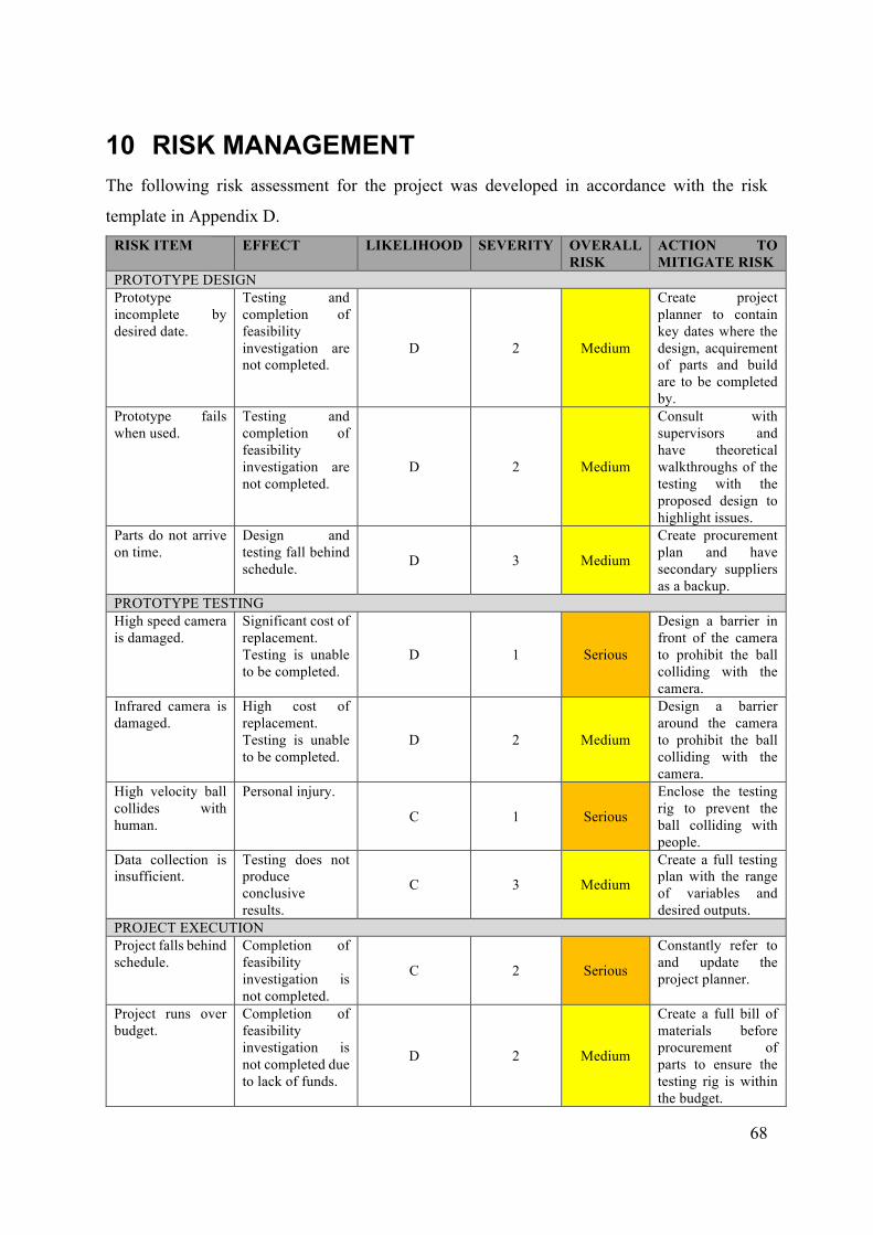
68
10 RISK MANAGEMENT
The following risk assessment for the project was developed in accordance with the risk
template in Appendix D. RISK ITEM EFFECT LIKELIHOOD SEVERITY OVERALL
RISK ACTION TO MITIGATE RISK
PROTOTYPE DESIGN Prototype incomplete by desired date.
Testing and completion of feasibility investigation are not completed.
D 2 Medium
Create project planner to contain key dates where the design, acquirement of parts and build are to be completed by.
Prototype fails when used.
Testing and completion of feasibility investigation are not completed.
D 2 Medium
Consult with supervisors and have theoretical walkthroughs of the testing with the proposed design to highlight issues.
Parts do not arrive on time.
Design and testing fall behind schedule. D 3 Medium
Create procurement plan and have secondary suppliers as a backup.
PROTOTYPE TESTING High speed camera is damaged.
Significant cost of replacement. Testing is unable to be completed.
D 1 Serious
Design a barrier in front of the camera to prohibit the ball colliding with the camera.
Infrared camera is damaged.
High cost of replacement. Testing is unable to be completed.
D 2 Medium
Design a barrier around the camera to prohibit the ball colliding with the camera.
High velocity ball collides with human.
Personal injury.
C 1 Serious
Enclose the testing rig to prevent the ball colliding with people.
Data collection is insufficient.
Testing does not produce conclusive results.
C 3 Medium
Create a full testing plan with the range of variables and desired outputs.
PROJECT EXECUTION Project falls behind schedule.
Completion of feasibility investigation is not completed.
C 2 Serious
Constantly refer to and update the project planner.
Project runs over budget.
Completion of feasibility investigation is not completed due to lack of funds.
D 2 Medium
Create a full bill of materials before procurement of parts to ensure the testing rig is within the budget.

69
REFERENCES
Advanced Diving Systems. (2016). Risk Assessment. Retrieved from Advanced Diving
Systems: http://www.advanceddivingsystems.com/RiskAssessment.aspx
APT Sports. (2016, October 14). Tennis Court Surfaces. Retrieved from APT Sports:
http://sportsbyapt.com/types-tennis-courts/
Baodong, Y. (2014). Hawkeye technology using tennis match. Yulin: Yulin University.
Blain, L. (2014, October 7). The low cost, high speed slow-mo camera. Retrieved from Gizmag:
http://www.gizmag.com/fps1000-affordable-slow-motion-camera/34161/
Coverdale, B. (2012, January 5). New cameras should capture faintest of edges. Retrieved from
ESPNcricinfo: http://www.espncricinfo.com/ci/content/story/548170.html
Cross, R. (1998, October 14). The bounce of a ball. Sydney: University of Sydney. Retrieved
from USYD: http://www.physics.usyd.edu.au/~cross/tennis.html
FIFA. (2012). Quality Program for Goal Line Technology. FIFA.
FLIR. (2016, October 14). FLIR ONE Technical Specifications. Retrieved from FLIR:
http://www.flir.com.hk/flirone/
Gangal, S. (2015). The Hawkeye Technology. Bombay: Indian Institute of Technology
Bombay.
Greenman, C. (2000, August 31). For U.S. Open Tennis, a Service Line Umpire That Never
Blinks. Retrieved from The New York Times:
http://www.nytimes.com/2000/08/31/technology/for-us-open-tennis-a-service-line-
umpire-that-never-blinks.html
Honan, D. (2013, November 2). The Physics of Federer-Nadal. Retrieved from Big Think:
http://bigthink.com/think-tank/anyone-for-physics-the-science-of-the-comeback
Hunston, M. (2002). Innovative thin-film pressure mapping sensors. Analogue and Digital
Services Ltd.
INO. (2016, October 14). HRXCAM High Resolution Infrared Camera Modules. Retrieved
from INO: http://www.ino.ca/en/products/hrxcam-high-resolution-infrared-camera-
modules/
IOP Physics. (2016, May 2). Goal Line Technology. Retrieved from IOP:
http://www.iop.org/resources/topic/archive/goal-line/

70
ITF. (2012, March 23). Court Pace Classification. Retrieved from ITF Tennis:
http://www.itftennis.com/technical/courts/classified-surfaces/about-court-pace-
classification.aspx
Jean, Y. (2009). Real Time Tracking for Enhanced Tennis Broadcasts. Murray Hill: Bell
Laboratories.
Kotanen, A. (2012). Experiments on Local Positioning with Bluetooth. Tampere: Tampere
University of Technology.
Lobster Sports. (2016, October 14). Lobster Elite Three Specifications. Retrieved from Lobster
Sports: http://www.lobstersports.com/products/el03.htm
Lyle, D. (1978). United States Patent No. 4071242.
Mohanty, A. (2014). Hawkeye Technology. Paralakhemundi: Centurion Institue for
Technology Paralakhemundi.
Pressure Profile. (2016). Tactarray Pressure Sensing Solutions. Retrieved from Pressure
Profile: http://www.pressureprofile.com/tact-array-sensors/
Pritt, N. (2013). Indoor Navigation with use of Geomagnetic Anomalies. Walkersville: Noah
Pritt.
Rosebrock, A. (2015, September 14). Ball Tracking with OpenCV. Retrieved from
Pyimagesearch: http://www.pyimagesearch.com/2015/09/14/ball-tracking-with-
opencv/
Sierra Olympic. (2016, October 14). IR-TCM HD 1024 LWIR Infrared Cameras. Retrieved
from Sierra Olympic:
https://www.sierraolympic.com/download/?file=/images/uploads/product-
drawings/IR-TCM_HD_1024_en_141107.pdf
The Independent. (1995, November 23). Cyclops has company as machine moves to replace
net cord judge. Retrieved from Independant:
http://www.independent.co.uk/sport/cyclops-has-company-as-machine-moves-to-
replace-net-cord-judge-1583317.html
University of NSW. (2013). Using Geomagnetic Field for Indoor Positioning. Sydney:
International Global Navigation Satellite Systems Society.
University of Strathclyde. (2008). Real-time Modeling of 3D Soccer Ball. Strathclyde:
University of Strathclyde.
Vollmer, M. (2010). Infrared Thermal Imaging: Fundamentals, Research and Applications.
Berkeley: Wiley.

71
World Sports Intelligence. (2016, 01 23). Tennis Hawk Eye – What is it and how does it work?
Retrieved 04 12, 2016, from World Sports Intelligence:
http://sportsworldintel.com/tennis-hawk-eye-what-is-it-and-how-does-it-work/
Yan, F. (2010). A Tennis Ball Tracking Algorithm for Automatic Annotation of Tennis Match .
Surrey: University of Surrey.
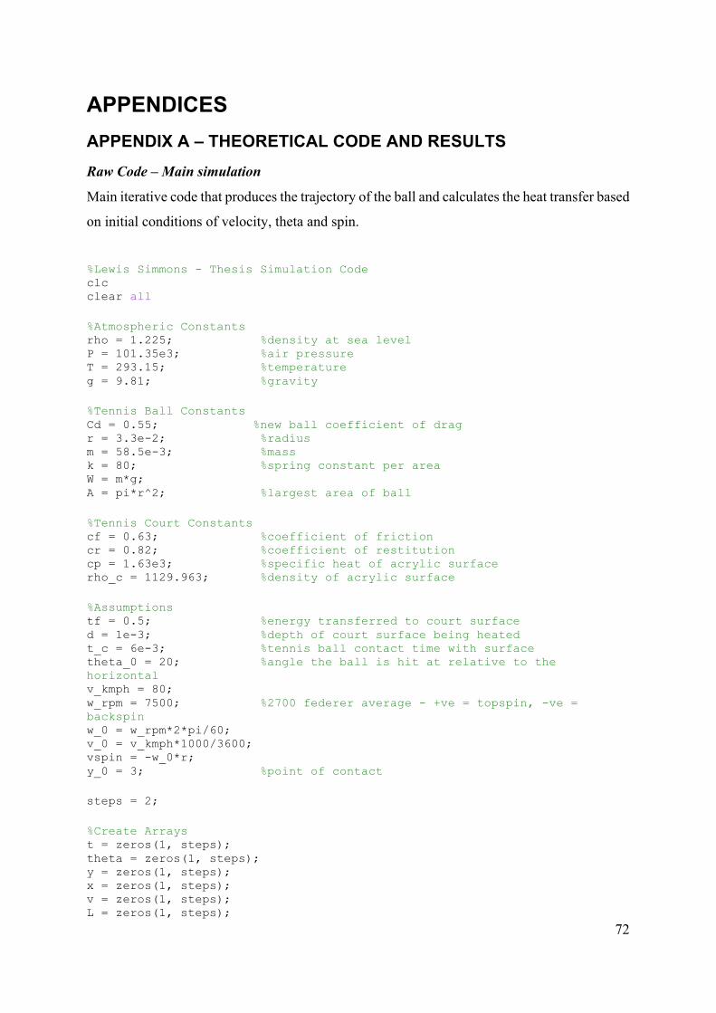
72
APPENDICES
APPENDIX A – THEORETICAL CODE AND RESULTS
Raw Code – Main simulation
Main iterative code that produces the trajectory of the ball and calculates the heat transfer based
on initial conditions of velocity, theta and spin.
%Lewis Simmons - Thesis Simulation Code clc clear all %Atmospheric Constants rho = 1.225; %density at sea level P = 101.35e3; %air pressure T = 293.15; %temperature g = 9.81; %gravity %Tennis Ball Constants Cd = 0.55; %new ball coefficient of drag r = 3.3e-2; %radius m = 58.5e-3; %mass k = 80; %spring constant per area W = m*g; A = pi*r^2; %largest area of ball %Tennis Court Constants cf = 0.63; %coefficient of friction cr = 0.82; %coefficient of restitution cp = 1.63e3; %specific heat of acrylic surface rho_c = 1129.963; %density of acrylic surface %Assumptions tf = 0.5; %energy transferred to court surface d = 1e-3; %depth of court surface being heated t_c = 6e-3; %tennis ball contact time with surface theta_0 = 20; %angle the ball is hit at relative to the horizontal v_kmph = 80; w_rpm = 7500; %2700 federer average - +ve = topspin, -ve = backspin w_0 = w_rpm*2*pi/60; v_0 = v_kmph*1000/3600; vspin = -w_0*r; y_0 = 3; %point of contact steps = 2; %Create Arrays t = zeros(1, steps); theta = zeros(1, steps); y = zeros(1, steps); x = zeros(1, steps); v = zeros(1, steps); L = zeros(1, steps);

73
D = zeros(1, steps); w = zeros(1, steps); Fx = zeros(1, steps); Fy = zeros(1, steps); ax = zeros(1, steps); ay = zeros(1, steps); vx = zeros(1, steps); vy = zeros(1, steps); %Initial Conditions t(1) = 0; theta(1) = theta_0; y(1) = y_0; x(1) = 0; v(1) = v_0; w(1) = w_0; Fx(1) = 0; Fy(1) = 0; ax(1) = 0; ay(1) = 0; vx(1) = v(1)*cosd(theta(1)); vy(1) = v(1)*sind(theta(1)); C_d(1) = 0.55+1/(22.5+4.2*(v(1)/vspin)^2.5)^0.4; C_l(1) = 1/(2+(v(1)/vspin)); D(1) = 0.5*C_d(1)*A*rho*v(1)^2; L(1) = 0.5*C_l(1)*A*rho*v(1)^2; %Iteration parameters t_step = 0.01; i = 1; % Initial time step %Trajectory Calculation while y(i) >= 0 % Run until ball hits the ground i = i+1; % Increment time step t(i)= (i-1)*t_step; C_d(i) = 0.55+1/(22.5+4.2*(abs(v(i-1)/vspin))^2.5)^0.4; %drag coefficient accounting for spin D(i) = 0.5*C_d(i)*A*rho*v(i-1)^2; %drag force C_l(i) = 1/(2+(v(i-1)/vspin)); %coefficient of lift L(i) = 0.5*C_l(i)*A*rho*v(i-1)^2; %lift force Fx(i) = -L(i)*sind(theta(i-1)) - D(i)*cosd(theta(i-1)); Fy(i) = -W + L(i)*cosd(theta(i-1)) - D(i)*sind(theta(i-1)); ax(i) = Fx(i)/m; ay(i) = Fy(i)/m; vx(i) = vx(i-1) + ax(i)*t_step; vy(i) = vy(i-1) + ay(i)*t_step; theta(i) = atand(vy(i)/vx(i)); v(i) = vx(i)/cosd(theta(i)); x(i) = x(i-1) + vx(i)*t_step;

74
y(i) = y(i-1) + vy(i)*t_step; end %% %BOUNCING %Entry Conditions v1 = v(end); theta1 = theta(end); alpha = 90+theta1; %angle relative to the court (the vertical) Fy1 = Fy(end); vx1 = vx(end); EK1 = 0.5*m*v1^2; %Restitution Component delta_v_r = v1*(1-cr); %change in velocity due to resititution %Friction component F_friction = cf*Fy1; a_friction = F_friction/m; delta_v_f = a_friction*t_c; %change in velocity due to friction %Compression of ball r_comp = r; %radius during compression A_comp = pi*r_comp^2; %area of ball during compression d_skid = vx1*t_c; %distance the ball skids %Exit Conditions v2 = v1-delta_v_f-delta_v_r; EK2 = 0.5*m*v2^2; delta_E = EK1-EK2; %loss in kinetic energy (gain in thermal) %Heat Transfer A_mark = 2*r_comp*d_skid+pi*r_comp^2; %total skid mark area by ball V_court = A_mark*d; %total volume of court affected m_court = V_court*rho_c; %total mass of court affected E_court = delta_E*tf; %energy transferred to court delta_T = E_court/m_court/cp %change in temperature of mark on court %Net for plot xnet = [12 12]; ynet = [0 1]; %End of court xcourt = [23 23]; ycourt = [0 0.25]; %Service box xserve = [18 18]; yserve = [0 0.25];

75
% %Trajectory Plot % figure(1) % hold on % plot(x,y) % axis equal % axis([0,25,0,5]) % xlabel('Distance (m)') % ylabel('Height (m)') % title('Trajectory of flat serve - -8 deg, 200 kmph, 0 rpm') % grid on % plot(xnet,ynet,'-r') % plot(xcourt,ycourt,'-r') % plot(xserve,yserve,'-r') % saveas(gcf,'flatserve.jpg') % Raw Code – Iterative solution for ranges of values
Iterative code that produces the trajectory of the ball and calculates the heat transfer based on
initial conditions of spin and theta, across a range of velocities. %Lewis Simmons - Thesis Simulation Code clc clear all %Initial Conditions vel(1) = 0 theta_test = 45; RPM_test = 6000; %Iteration parameters v_step = 30; j = 1; % Initial time step while vel <= 120 j=j+1; vel(j)= (j-1)*v_step; %Atmospheric Constants rho = 1.225; %density at sea level P = 101.35e3; %air pressure T = 293.15; %temperature g = 9.81; %gravity %Tennis Ball Constants Cd = 0.55; %new ball coefficient of drag r = 3.3e-2; %radius m = 58.5e-3; %mass k = 80; %spring constant per area W = m*g; A = pi*r^2; %largest area of ball %Tennis Court Constants

76
cf = 0.63; %coefficient of friction cr = 0.82; %coefficient of restitution cp = 1.63e3; %specific heat of acrylic surface rho_c = 1129.963; %density of acrylic surface %Assumptions tf = 0.5; %energy transferred to court surface d = 1e-3; %depth of court surface being heated t_c = 6e-3; %tennis ball contact time with surface theta_0 = theta_test; %angle the ball is hit at relative to the horizontal w_rpm = RPM_test; %2700 federer average - +ve = topspin, -ve = backspin w_0 = w_rpm*2*pi/60; v_kmph = 50; v_0 = vel(j)*1000/3600; vspin = -w_0*r; y_0 = 1; %point of contact steps = 2; %Create Arrays t = zeros(1, steps); theta = zeros(1, steps); y = zeros(1, steps); x = zeros(1, steps); v = zeros(1, steps); L = zeros(1, steps); D = zeros(1, steps); Fx = zeros(1, steps); Fy = zeros(1, steps); ax = zeros(1, steps); ay = zeros(1, steps); vx = zeros(1, steps); vy = zeros(1, steps); %Initial Conditions t(1) = 0; theta(1) = theta_0; y(1) = y_0; x(1) = 0; v(1) = v_0; Fx(1) = 0; Fy(1) = 0; ax(1) = 0; ay(1) = 0; w(1) = 0; vx(1) = v(1)*cosd(theta(1)); vy(1) = v(1)*sind(theta(1)); C_d(1) = 0.55+1/(22.5+4.2*(v(1)/vspin)^2.5)^0.4; C_l(1) = 1/(2+(v(1)/vspin)); D(1) = 0.5*C_d(1)*A*rho*v(1)^2; L(1) = 0.5*C_l(1)*A*rho*v(1)^2; %Iteration parameters t_step = 0.01; i = 1; % Initial time step %Trajectory Calculation

77
while y(i) >= 0 % Run until ball hits the ground i = i+1; % Increment time step t(i)= (i-1)*t_step; C_d(i) = 0.55+1/(22.5+4.2*(abs(v(i-1)/vspin))^2.5)^0.4; %drag coefficient accounting for spin D(i) = 0.5*C_d(i)*A*rho*v(i-1)^2; %drag force C_l(i) = 1/(2+(v(i-1)/vspin)); %coefficient of lift L(i) = 0.5*C_l(i)*A*rho*v(i-1)^2; %lift force Fx(i) = -L(i)*sind(theta(i-1)) - D(i)*cosd(theta(i-1)); Fy(i) = -W + L(i)*cosd(theta(i-1)) - D(i)*sind(theta(i-1)); ax(i) = Fx(i)/m; ay(i) = Fy(i)/m; vx(i) = vx(i-1) + ax(i)*t_step; vy(i) = vy(i-1) + ay(i)*t_step; theta(i) = atand(vy(i)/vx(i)); v(i) = vx(i)/cosd(theta(i)); x(i) = x(i-1) + vx(i)*t_step; y(i) = y(i-1) + vy(i)*t_step; end % %Trajectory Plot % plot(x,y) % axis equal % axis([0,inf,0,inf]) %% %BOUNCING %Entry Conditions v1 = v(end); theta1 = theta(end); alpha = 90+theta1; %angle relative to the court (the vertical) Fy1 = Fy(end); vx1 = vx(end); EK1 = 0.5*m*v1^2; %Restitution Component delta_v_r = v1*(1-cr); %change in velocity due to resititution %Friction component F_friction = cf*Fy1; a_friction = F_friction/m; delta_v_f = a_friction*t_c; %change in velocity due to friction %Compression of ball r_comp = r; %radius during compression A_comp = pi*r_comp^2; %area of ball during compression

78
d_skid = vx1*t_c; %distance the ball skids %Exit Conditions v2 = v1-delta_v_f-delta_v_r; EK2 = 0.5*m*v2^2; delta_E = EK1-EK2; %loss in kinetic energy (gain in thermal) %Heat Transfer A_mark = pi*r_comp^2; %total skid mark area by ball V_court = A_mark*d; %total volume of court affected m_court = V_court*rho_c; %total mass of court affected E_court = delta_E*tf; %energy transferred to court delta_T(j) = E_court/m_court/cp; %change in temperature of mark on court end vel delta_T Raw Code – Bounce energies given initial conditions
Code used to calculate the thermal transfer, given the bounce entry velocity and angle are
known. %Assume balanced case, acceleration only due to gravity. %BOUNCING clc clear all %Tennis Ball Constants Cd = 0.55; %new ball coefficient of drag r = 3.3e-2; %radius m = 58.5e-3; %mass k = 80; %spring constant per area g=9.81; W = m*g; A = pi*r^2; %largest area of ball %Entry Conditions v_kmph = 87; v1 = v_kmph*1000/3600; alpha = 15; %angle relative to the court (the vertical) Fy1 = W; %simplified model vx1 = v1*sind(alpha); %Assumptions tf = 0.5; %energy transferred to court surface d = 1e-3; %depth of court surface being heated t_c = 6e-3; %tennis ball contact time with surface

79
EK1 = 0.5*m*v1^2; %Tennis Court Constants - Velour Surface cf = 0.7; %coefficient of friction cr = 0.74; %coefficient of restitution cp = 1.4e3; %specific heat of surface rho_c = 160; %density of surface %Restitution Component delta_v_r = v1*(1-cr); %change in velocity due to resititution %Friction component F_friction = cf*Fy1; a_friction = F_friction/m; delta_v_f = a_friction*t_c; %change in velocity due to friction %Compression of ball r_comp = r; %radius during compression A_comp = pi*r_comp^2; %area of ball during compression d_skid = vx1*t_c; %distance the ball skids %Exit Conditions v2 = v1-delta_v_f-delta_v_r; EK2 = 0.5*m*v2^2; delta_E = EK1-EK2; %loss in kinetic energy (gain in thermal) %Heat Transfer A_mark = pi*r_comp^2; %total skid mark area by ball V_court = A_mark*d; %total volume of court affected m_court = V_court*rho_c; %total mass of court affected E_court = delta_E*tf; %energy transferred to court delta_T = E_court/m_court/cp %change in temperature of mark on court
Results - Flat ground strokes
The raw results from the flat ground stroke testing simulation, using the code provided.
Trajectory of shot
The spin was held constant at 0RPM.
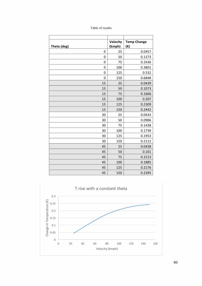
80
Table of results
Theta(deg)
Velocity
(kmph)
TempChange
(K)
0 25 0.04570 50 0.12730 75 0.24360 100 0.38010 125 0.5320 150 0.6848
15 25 0.043915 50 0.107315 75 0.166615 100 0.20715 125 0.230915 150 0.244230 25 0.043330 50 0.098630 75 0.143830 100 0.173930 125 0.195330 150 0.211245 25 0.043845 50 0.10145 75 0.151345 100 0.188545 125 0.217645 150 0.2395
0
0.05
0.1
0.15
0.2
0.25
0.3
0 20 40 60 80 100 120 140 160
ChangeinTem
perature(K)
Velocity(kmph)
Trisewithaconstanttheta

81
Change in temperature versus velocity with a constant angle and spin
Change in temperature versus velocity with a constant angle and spin
Results - Top spin ground strokes
The raw results from the top spin ground stroke testing simulation, using the code provided.
Trajectory of shot
Table of results
Theta(deg) Velocity(kmph) Omega(rpm)
TempChange
(K)
0 20 1000 0.0340 20 2000 0.03310 20 3000 0.03330 20 4000 0.03290 20 5000 0.03290 80 1000 0.26990 80 2000 0.2834
0
0.05
0.1
0.15
0.2
0.25
0.3
0 10 20 30 40 50
ChangeinTem
perature(K)
Theta(deg)
Trisewithaconstantvelocity

82
0 80 3000 0.32490 80 4000 0.09820 80 5000 0.09320 140 1000 0.66320 140 2000 0.70890 140 3000 0.76230 140 4000 0.82630 140 5000 0.8714
20 20 1000 0.032520 20 2000 0.032320 20 3000 0.032220 20 4000 0.032320 20 5000 0.031920 80 1000 0.165720 80 2000 0.2120 80 3000 0.325620 80 4000 0.123520 80 5000 0.111420 140 1000 0.234920 140 2000 0.31120 140 3000 0.448120 140 4000 0.626820 140 5000 0.864240 20 1000 0.032940 20 2000 0.031940 20 3000 0.032240 20 4000 0.032440 20 5000 0.032540 80 1000 0.144640 80 2000 0.190240 80 3000 0.340240 80 4000 0.143840 80 5000 0.135640 140 1000 0.202140 140 2000 0.239540 140 3000 0.432140 140 4000 0.690440 140 5000 0.9124
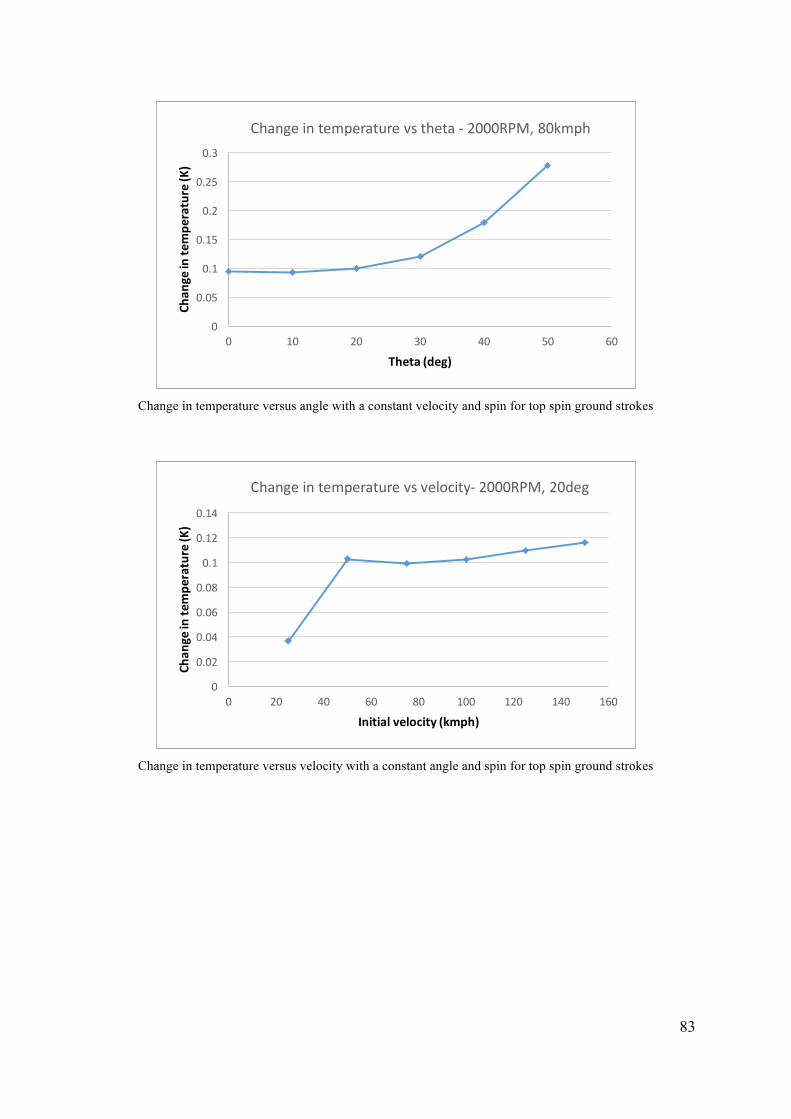
83
Change in temperature versus angle with a constant velocity and spin for top spin ground strokes
Change in temperature versus velocity with a constant angle and spin for top spin ground strokes
0
0.05
0.1
0.15
0.2
0.25
0.3
0 10 20 30 40 50 60
Changeintemperature(K
)
Theta(deg)
Changeintemperaturevstheta- 2000RPM,80kmph
0
0.02
0.04
0.06
0.08
0.1
0.12
0.14
0 20 40 60 80 100 120 140 160
Changeintemperature(K
)
Initialvelocity(kmph)
Changeintemperaturevsvelocity- 2000RPM,20deg
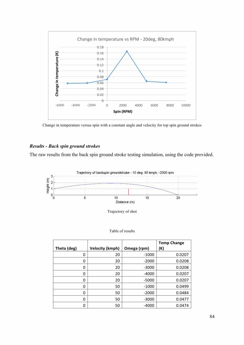
84
Change in temperature versus spin with a constant angle and velocity for top spin ground strokes
Results - Back spin ground strokes
The raw results from the back spin ground stroke testing simulation, using the code provided.
Trajectory of shot
Table of results
Theta(deg) Velocity(kmph) Omega(rpm)
TempChange
(K)
0 20 -1000 0.02070 20 -2000 0.02080 20 -3000 0.02080 20 -4000 0.02070 20 -5000 0.02070 50 -1000 0.04990 50 -2000 0.04840 50 -3000 0.04770 50 -4000 0.0474
00.020.040.060.080.1
0.120.140.160.18
-6000 -4000 -2000 0 2000 4000 6000 8000 10000
Changeintemperature(K
)
Spin(RPM)
ChangeintemperaturevsRPM- 20deg,80kmph

85
0 50 -5000 0.04720 80 -1000 0.08030 80 -2000 0.07550 80 -3000 0.07260 80 -4000 0.07080 80 -5000 0.0695
15 20 -1000 0.020915 20 -2000 0.020715 20 -3000 0.020615 20 -4000 0.020515 20 -5000 0.020515 50 -1000 0.044115 50 -2000 0.042215 50 -3000 0.041415 50 -4000 0.04115 50 -5000 0.040715 80 -1000 0.059215 80 -2000 0.054315 80 -3000 0.052215 80 -4000 0.05115 80 -5000 0.050430 20 -1000 0.021630 20 -2000 0.021330 20 -3000 0.021230 20 -4000 0.021130 20 -5000 0.021530 50 -1000 0.045130 50 -2000 0.043730 50 -3000 0.043130 50 -4000 0.043130 50 -5000 0.042930 80 -1000 0.062630 80 -2000 0.0630 80 -3000 0.059130 80 -4000 0.058730 80 -5000 0.0588
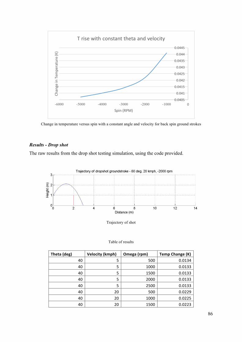
86
Change in temperature versus spin with a constant angle and velocity for back spin ground strokes
Results - Drop shot
The raw results from the drop shot testing simulation, using the code provided.
Trajectory of shot
Table of results
Theta(deg) Velocity(kmph) Omega(rpm) TempChange(K)
40 5 500 0.013440 5 1000 0.013340 5 1500 0.013340 5 2000 0.013340 5 2500 0.013340 20 500 0.022940 20 1000 0.022540 20 1500 0.0223
0.0405
0.041
0.0415
0.042
0.0425
0.043
0.0435
0.044
0.0445
-6000 -5000 -4000 -3000 -2000 -1000 0
ChangeinTem
perature(K)
Spin(RPM)
Trisewithconstantthetaandvelocity
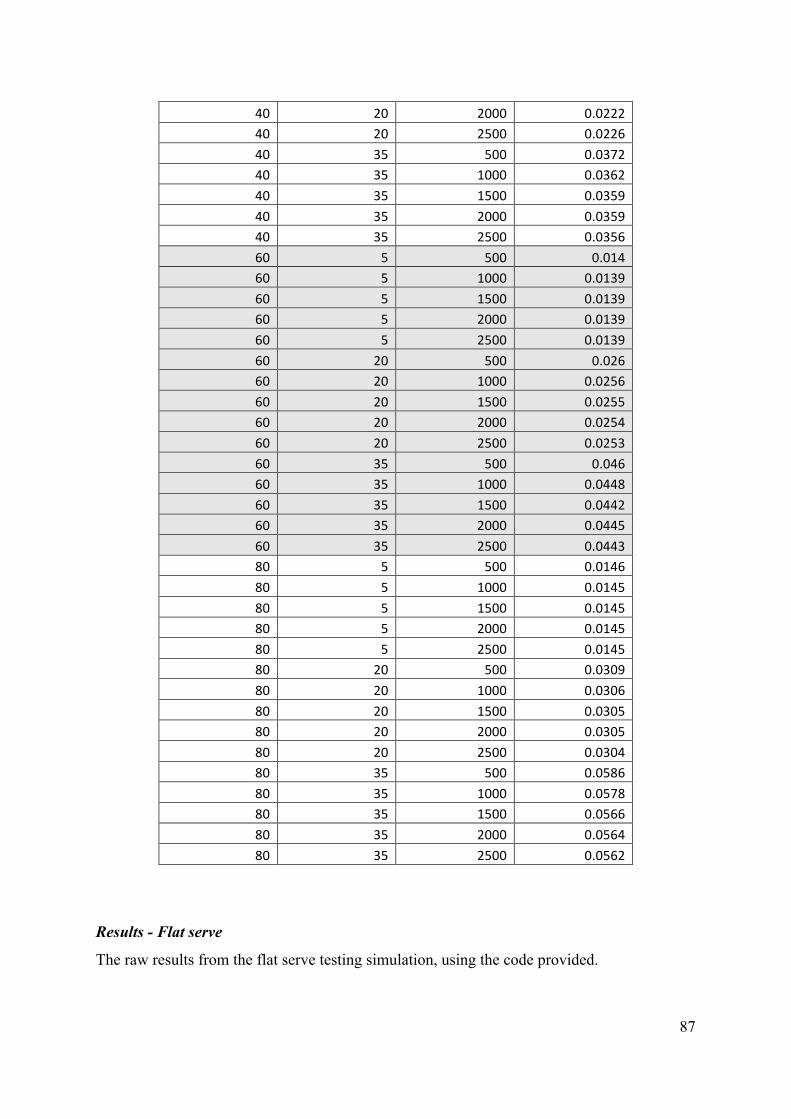
87
40 20 2000 0.022240 20 2500 0.022640 35 500 0.037240 35 1000 0.036240 35 1500 0.035940 35 2000 0.035940 35 2500 0.035660 5 500 0.01460 5 1000 0.013960 5 1500 0.013960 5 2000 0.013960 5 2500 0.013960 20 500 0.02660 20 1000 0.025660 20 1500 0.025560 20 2000 0.025460 20 2500 0.025360 35 500 0.04660 35 1000 0.044860 35 1500 0.044260 35 2000 0.044560 35 2500 0.044380 5 500 0.014680 5 1000 0.014580 5 1500 0.014580 5 2000 0.014580 5 2500 0.014580 20 500 0.030980 20 1000 0.030680 20 1500 0.030580 20 2000 0.030580 20 2500 0.030480 35 500 0.058680 35 1000 0.057880 35 1500 0.056680 35 2000 0.056480 35 2500 0.0562
Results - Flat serve
The raw results from the flat serve testing simulation, using the code provided.

88
Trajectory of shot
Table of results
Theta(deg) Velocity(kmph)
TempChange
(K)
-20 40 0.0983-20 80 0.3484-20 120 0.7658-20 160 1.3483-20 200 2.0861-20 240 3.0022-10 40 0.0949-10 80 0.3237-10 120 0.7015-10 160 1.2199-10 200 1.8786-10 240 2.71160 40 0.08970 80 0.26850 120 0.50080 160 0.74920 200 1.00920 240 1.2472
10 40 0.083510 80 0.199410 120 0.277210 160 0.312310 200 0.325110 240 0.3272

89
Results - Top spin serve
The raw results from the top spin serve testing simulation, using the code provided.
Trajectory of shot
Table of results
Theta(deg) Velocity(kmph) Omega(rpm)
TempChange
(K)
0 60 1000 0.0670 60 2000 0.09460 60 3000 0.04550 60 4000 0.04540 60 5000 0.04730 160 1000 0.1420 160 2000 0.15460 160 3000 0.17220 160 4000 0.20110 160 5000 0.28920 260 1000 0.19740 260 2000 0.22240 260 3000 0.24490 260 4000 0.26640 260 5000 0.2914
10 60 1000 0.06410 60 2000 0.101610 60 3000 0.050710 60 4000 0.047210 60 5000 0.047110 160 1000 0.105410 160 2000 0.125410 160 3000 0.155510 160 4000 0.208110 160 5000 0.3955

90
10 260 1000 0.118810 260 2000 0.148810 260 3000 0.184710 260 4000 0.224110 260 5000 0.269220 60 1000 0.063920 60 2000 0.117720 60 3000 0.056520 60 4000 0.052320 60 5000 0.051620 160 1000 0.095620 160 2000 0.11820 160 3000 0.170220 160 4000 0.297920 160 5000 1.044620 260 1000 0.108620 260 2000 0.134120 260 3000 0.185220 260 4000 0.261320 260 5000 0.3869
Results - Back spin serve
The raw results from the back spin serve testing simulation, using the code provided.
Trajectory of shot
Table of results
Theta(deg) Velocity(kmph) Omega(rpm)
TempChange
(K)
0 60 1000 0.06060 60 2000 0.0573

91
0 60 3000 0.05570 60 4000 0.05490 60 5000 0.05430 120 1000 0.0940 120 2000 0.08180 120 3000 0.07370 120 4000 0.06890 120 5000 0.06560 180 1000 0.11170 180 2000 0.08790 180 3000 0.07330 180 4000 0.06570 180 5000 0.0618
-10 60 1000 0.067-10 60 2000 0.0641-10 60 3000 0.0626-10 60 4000 0.0618-10 60 5000 0.0613-10 120 1000 0.1288-10 120 2000 0.1208-10 120 3000 0.1146-10 120 4000 0.1096-10 120 5000 0.1057-10 180 1000 0.1963-10 180 2000 0.1835-10 180 3000 0.1714-10 180 4000 0.1606-10 180 5000 0.1497-20 60 1000 0.0737-20 60 2000 0.0713-20 60 3000 0.07-20 60 4000 0.0693-20 60 5000 0.0689-20 120 1000 0.1539-20 120 2000 0.1491-20 120 3000 0.1451-20 120 4000 0.1429-20 120 5000 0.1402-20 180 1000 0.2437-20 180 2000 0.237-20 180 3000 0.2332-20 180 4000 0.2273-20 180 5000 0.2246

92
Results – 3D relationship between velocity, theta and change in temperature
The following three dimensional plots demonstrate the relationship between varied initial
angles and velocities, constant spins and the change in temperature.
Change in temperature versus theta and velocity at 0RPM
Change in temperature versus theta and velocity at 2000RPM

93
Change in temperature versus theta and velocity at 4000RPM
Change in temperature versus theta and velocity at 6000RPM

94
APPENDIX B – EXPERIMENTAL RESULTS
Testing for the existence of thermal transfer after a forced collision
Thermal transfer testing after the ball was rubbed against the surface of the court.
Testing for the existence of thermal transfer after normal bounce
Images of processed thermal data for testing at 60 mph, 0RPM and +3 elevation. Images have
been processed through the FLIR Tools application, with their temperature range reduced.
None of these thermal images produced noticeable thermal marks, as noted in the experimental
section with the lack of successful readings.

95

96

97
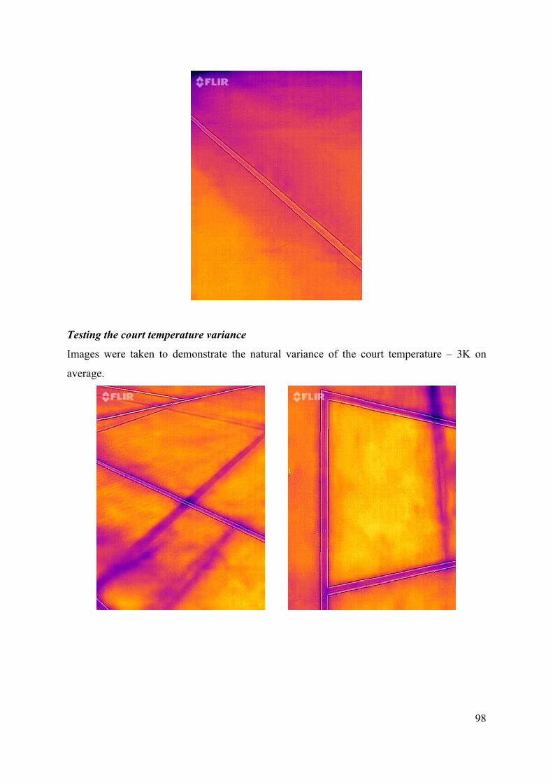
98
Testing the court temperature variance
Images were taken to demonstrate the natural variance of the court temperature – 3K on
average.

99

100
APPENDIX C – PROJECT PLANNER

101
APPENDIX D – RISK MATRIX GUIDELINES The following matrix is the risk assessment template used to classify the risks of the experiment
(Advanced Diving Systems, 2016).

102