W&M ScholarWorks W&M ScholarWorks

Dissertations, Theses, and Masters Projects Theses, Dissertations, & Master Projects

2010

Alternative substrates as a native oyster (Crassostrea virginica) Alternative substrates as a native oyster (Crassostrea virginica)

reef restoration strategy in Chesapeake Bay reef restoration strategy in Chesapeake Bay

Russell Paul Burke College of William and Mary - Virginia Institute of Marine Science

Follow this and additional works at: https://scholarworks.wm.edu/etd

Part of the Aquaculture and Fisheries Commons, Natural Resources and Conservation Commons, and

the Oceanography Commons

Recommended Citation Recommended Citation Burke, Russell Paul, "Alternative substrates as a native oyster (Crassostrea virginica) reef restoration strategy in Chesapeake Bay" (2010). Dissertations, Theses, and Masters Projects. Paper 1539616589. https://dx.doi.org/doi:10.25773/v5-qw1k-b793

This Dissertation is brought to you for free and open access by the Theses, Dissertations, & Master Projects at W&M ScholarWorks. It has been accepted for inclusion in Dissertations, Theses, and Masters Projects by an authorized administrator of W&M ScholarWorks. For more information, please contact scholarworks@wm.edu.

Alternative Substrates as a Native Oyster (Crassostrea virginica)

Reef Restoration Strategy in Chesapeake Bay

_____________

A Dissertation

Submitted to

The Faculty of the School of Marine Science

The College of William and Mary in Virginia

In Partial Fulfillment

of the Requirements for the Degree of

Doctor of Philosophy

_____________

by

Russell Paul Burke

2010

APPROVAL SHEET

This dissertation is submitted in partial fulfillment of the requirements for the degree of

Doctor of Philosophy

_________________________________ Russell P. Burke

Approved by the Committee, April 2010

_________________________________ Romuald N. Lipcius, Ph.D.

Chair of Advisory Committee

_________________________________ Mark W. Luckenbach, Ph.D.

_________________________________ Rochelle D. Seitz, Ph.D.

_________________________________ Harry V. Wang, Ph.D.

_________________________________ Jian Shen, Ph.D.

_________________________________ Sebastian J. Schreiber, Ph.D.

University of California, Davis

To my parents, Linda and Russ

iii

“Taken together, paleontological, archaeological, historical, geological and ecological evidence shows that oysters set, survive and grow better on elevated reefs with substantial ‘cores’ of oyster shells and ‘cinders’, and other suitable substrate, and healthy ‘veneers’ of living oysters than on beds near or on the bottom. Spatfall is better, growth is faster, predation effects are lower and disease-related effects reduced. Oysters lying flat on the bottom or partially submerged in the bottom do not fare nearly as well. Relative successes of ‘off-bottom culture’ efforts employing man-made structures to maintain the living oysters off of the bottom in disease- and predation-prone areas confirm this.”

Hargis WJ, Haven DS (1995) Chesapeake Bay oyster reefs, their importance, destruction and guidelines for restoring them. p. 329- 358 In: M. Luckenbach, R. Mann, and J. Wesson, eds. Virginia Institute of Marine Science Press, Gloucester Point, Virginia 23062

“Success can come only with realistic goals couched within comprehensive and quantitative analysis delineating planned actions in concert within the complex interplay between population dynamics and habitat maintenance.”

Mann R, Powell EN (2007) Why oyster restoration goals in the Chesapeake Bay are not and probably cannot be achieved. Journal of Shellfish Research, 26(4), 1-13

“Well-intentioned yet poorly ‘designed’ reefs, when monitored and appraised against original expectations, may lead the assessors to conclude that ‘reefs don’t work’ when, with the correct habitat requirement information for the target species, the end result would have been successful.”

Jensen AC, Collins KJ, Lockwood P (2000) Current issues relating to artificial reefs in European seas. p. 489–499 In: A.C. Jensen, K.J. Collins and A.P.M. Lockwood, eds. Artificial reefs in European seas. Kluwer Academics Publishers, London

iv

TABLE OF CONTENTS

Acknowledgments ............................................................................................................. ix List of Tables ................................................................................................................... xii List of Figures ................................................................................................................. xiv List of Appendices .......................................................................................................... xxi Abstract .......................................................................................................................... xxii Chapter 1: An Introduction to Native Oyster Reef Restoration and the Use of Alternative Substrates Abstract ........................................................................................................................................... 2 Introduction ..................................................................................................................................... 3 Chesapeake Bay oyster history ....................................................................................................... 4 Oyster diseases ................................................................................................................................ 5 Sanctuaries vs. harvest grounds ...................................................................................................... 7 Alternative vs. shell substrate ......................................................................................................... 8 Artificial reefs around the world ..................................................................................................... 9 Summary ....................................................................................................................................... 14 Chapter 2: Granite and Concrete Riprap as Intertidal Native Oyster (Crassostrea virginica) Reefs Abstract ......................................................................................................................................... 15 Introduction ................................................................................................................................... 16 Materials and methods .................................................................................................................. 18 Riprap field survey ........................................................................................................... 18 Restored oyster shell reef survey ..................................................................................... 25 Results ........................................................................................................................................... 26 Riprap oyster population structure ................................................................................... 26 Riprap oyster density ....................................................................................................... 26 Riprap oyster biomass ...................................................................................................... 29 Riprap oyster volume and reef accretion ......................................................................... 31 Riprap oyster condition index .......................................................................................... 31 Restored shell reef oyster population structure ................................................................ 32 Restored shell reef oyster density .................................................................................... 33

v

Restored shell reef oyster biomass ................................................................................................ 33 Restored shell reef oyster volume and reef accretion ................................................................... 35 Restored shell reef oyster condition index ....................................................................... 35 Discussion ..................................................................................................................................... 37 Acknowledgments.......................................................................................................................... 41 Chapter 3: Population Structure, Density and Biomass of the Eastern Oyster (Crassostrea virginica) on Artificial Oyster Reefs in the Rappahannock River, Chesapeake Bay Abstract ......................................................................................................................................... 42 Introduction ................................................................................................................................... 43 Materials and methods .................................................................................................................. 45 Concrete module reef ....................................................................................................... 45 Construction ........................................................................................................ 45 Sampling procedure and design .......................................................................... 46 Laboratory processing ......................................................................................... 47 Population structure ............................................................................................ 49 Density and abundance ........................................................................................ 50 Biomass ............................................................................................................... 51 Pathology ............................................................................................................ 51 Steamer Rock reef ............................................................................................................ 52 Sampling procedure and design .......................................................................... 52 Laboratory processing ......................................................................................... 54 Pathology ............................................................................................................ 55 Results ........................................................................................................................................... 55 Concrete module reef ....................................................................................................... 55 Population structure – 2005 ................................................................................. 55 Population structure – 2007, 1st sampling ........................................................... 59 Population structure – 2007, Resampling ........................................................... 59 Density – 2005 .................................................................................................... 59 Density – 2007, 1st sampling ............................................................................... 68 Density – 2007, Resampling ............................................................................... 70 Biomass – 2005 ................................................................................................... 72 Biomass – 2007, 1st sampling ............................................................................. 75 Biomass – 2007, Resampling .............................................................................. 75 Pathology – 2005 ................................................................................................. 78 Pathology – 2007 ................................................................................................ 78 Condition index ................................................................................................... 79 Steamer Rock reef ............................................................................................................ 79 Population structure ............................................................................................. 79 Density ................................................................................................................ 79 Biomass ............................................................................................................... 81

vi

Pathology ............................................................................................................ 81 Condition Index .................................................................................................. 82 Discussion ..................................................................................................................................... 85 Concrete module reef ....................................................................................................... 85 Population structure ............................................................................................. 85 Density and biomass ........................................................................................... 88 Pathology and condition ..................................................................................... 92 Steamer Rock reef ............................................................................................................ 94 Population structure ............................................................................................. 94 Density and biomass ........................................................................................... 95 Pathology and condition ..................................................................................... 96 Conclusions .................................................................................................................................... 99 Acknowledgments ....................................................................................................................... 102 Chapter 4: Eastern Oyster (Crassostrea virginica) Recruitment, Growth, and Survival on Alternative Reef Substrates Abstract ....................................................................................................................................... 103 Introduction ................................................................................................................................. 104 Materials and methods ................................................................................................................ 106 Sampling procedure and design ..................................................................................... 106 Density, biomass and condition index ........................................................................... 113 Oyster and substrate volume .......................................................................................... 116 Pathology and condition ................................................................................................ 116 Results ......................................................................................................................................... 118 Recruitment .................................................................................................................... 118 Density and biomass ....................................................................................................... 121 Populations structure ...................................................................................................... 137 Growth and survival ....................................................................................................... 138 Oyster volume and reef accretion .................................................................................. 143 Pathology and condition ................................................................................................ 144 Discussion ................................................................................................................................... 151 Recruitment .................................................................................................................... 151 Density, biomass and condition ...................................................................................... 153 Populations structure ...................................................................................................... 154 Growth and survival ....................................................................................................... 154 Oyster volume and reef accretion .................................................................................. 155 Pathology and condition ................................................................................................ 156 Conclusions .................................................................................................................................. 157 Acknowledgments ....................................................................................................................... 159

vii

Chapter 5: Living Oyster Reef Shorelines Using Shell and Alternative Structures in the Lynnhaven River, Chesapeake Bay Abstract ....................................................................................................................................... 160 Introduction ................................................................................................................................. 161 Materials and methods ................................................................................................................ 169 Sampling procedure and design ..................................................................................... 169 Recruitment .................................................................................................................... 172 Biomass and condition index ......................................................................................... 172 Oyster and substrate volume .......................................................................................... 173 Pathology and condition ................................................................................................ 173 Results ......................................................................................................................................... 174 Recruitment .................................................................................................................... 174 Density ........................................................................................................................... 177 Biomass .......................................................................................................................... 181 Population structure (PSS) .............................................................................................. 183 Survival ........................................................................................................................... 188 Oyster volume and reef accretion .................................................................................. 189 Pathology and condition ................................................................................................ 190 Discussion ................................................................................................................................... 198 Recruitment .................................................................................................................... 198 Density and biomass ....................................................................................................... 199 Populations structure (PSS) ........................................................................................... 200 Growth and survival ....................................................................................................... 200 Oyster volume and reef accretion .................................................................................. 201 Pathology and condition ................................................................................................ 202 Conclusions .................................................................................................................................. 203 Acknowledgments ....................................................................................................................... 205 Closing Thoughts ...................................................................................................................... 206 Appendices ................................................................................................................................. 207 Literature Cited ........................................................................................................................ 236 Vita ............................................................................................................................................. 264

viii

ACKNOWLEDGMENTS

I owe my utmost thanks to my parents, Linda and Russ Burke, and my wife, Candy Burke Huayhualla. Truly, there is no way I would have survived the many trials of my young adult life without their unconditional love and support. The best relationships I have seen, and been a part of, have had a healthy mix of independence and interdependence. I witnessed that balance between my parents and have found a similar dynamic relationship with my soul mate, Candy. I was seriously considering leaving graduate school in the fall of 2003. Meeting Candy changed me forever. . .she filled a hole in my heart and helped me discover real happiness. She has brought out the best in me; this degree is hers as much as it is mine. We’ll share it together.

I owe a special thanks to my advisor, Rom Lipcius. The reason I decided to come work with Rom in 2002 is the same reason I remained here for the duration of my graduate career – his heartfelt compassion, positive outlook on life and science, and his ability to recognize a real opportunity even if it was simply the result of serendipity. When my father passed away in June 2003, he gave me a wide berth as I grieved and searched my soul for direction and meaning. The flexibility afforded me was crucial to my recovery and integral in my growing as a scientist, as I also wrestled with finding a project that fit me. Fortunately, Rom reached out to Dave Schulte and Captain Bob Jensen, men who ended up shaping my academic path in ways none of us could have predicted. I am grateful for Rom’s willingness to trust my judgment and his support of my passion and ethics. I have learned much about science under Rom’s tutelage, but even more about how politics can shape the way that science is implemented at the local, state, and federal levels of government. Finally, I wish to thank Rom for keeping me funded through my degree extension and for supporting my travel to professional conferences in Connecticut, Canada, France, North Carolina, California, and South Carolina. He has made a commitment to the professional development of his students and staff, and we are all grateful.

I am especially thankful to my committee members for their support and understanding. My dissertation research came together in an unconventional way and did not follow the milestone schedule well. Sebastian Schreiber helped me to understand mathematical modeling in fall 2003 when I was really struggling. His enthusiasm for math and science was infectious and, I’m happy to admit, I got the bug. And, despite my inability to incorporate modeling into my dissertation due to time constraints, Harry Wang and Jian Shen helped educate me on how physical oceanography affects oyster larval dispersal and metapopulation connectivity, and how hydrodynamic modeling can integrate biological and physical data to produce practical tools.

When it came to field work, Rochelle Seitz guided me through my earliest field days, instructing me and the many students, interns, and summer aides “what lies beneath” in the benthos. Rochelle’s domain is secondary production and, during the years of my research, I have come to understand the value of benthic-pelagic coupling and importance of monitoring the benthic community before, during, and after implementing an experiment or survey.

ix

Harry and Mark Luckenbach both gave me something I needed but have always had a problem requesting – constructive criticism. A scientist is no good without an honest critique of his/her work. Harry reached out to me and, though we both were outside of our comfort zone, he challenged me and my track record. It was what I needed at the time and I am grateful for his courage and his candor. Mark’s critiques came in the form of detailed edits and comments in my prospectus and dissertation drafts. His thorough reviews of both documents contributed significantly (sorry, no p-value) to my progress through this degree program. In summary, my committee and moderators (Steve Kaattari and Jim Perry) made a positive difference for me. Looking back on my dissertation research and the other projects I found myself working on, or even running, I am proud of my commitment and accomplishments; I believe that I earned the respect of those with whom I worked.

The cast of characters of the five-act play that has been my graduate experience is long and incredibly diverse. Captain Bob Jensen (Reeftek-McLean), our own King Lear, inspired us with his vision and passion for the Chesapeake Bay and the eastern oyster. David Bushey (Commonwealth Pro Dive), the jack of all marine science trades (diver, reef builder, side scan sonar specialist, etc.), helped make Captain Bob’s vision of quantifying his reefs at Steamer Rock a reality and jumpstarted my research. Darryl Nixon (Getting It Done, Inc.), the self-taught scientist with an insatiable appetite for knowledge, conditioned and delivered reefballs for my final project, and stuck around to become a “shadow advisor” to these and potential future projects. The last character, but perhaps the most influential one, has been Dave Schulte (Army Corps/VIMS), our own Sisyphus, who carried the burden of designing and implementing a federal oyster restoration program that would solidify the paradigm shift from oyster harvest grounds to large-scale permanent oyster reef sanctuaries. Dave’s commitment to do the right thing by the environment and the taxpayer, despite the political and peer pressure to do otherwise, inspired me. Our working relationship and friendship have deep meaning for me. We have humbly dubbed ourselves the next Bill Hargis and Dexter Haven, partly because of how we have fought together to save this oyster restoration program in Virginia, and partly due to our great respect for what they achieved in their decades of service to the institute, the state, and science, in general; in no small way, I feel like the torch needed to be passed and we were just naïve and stubborn enough to continue the epic journey started by Hargis and Haven long ago. As they could not have achieved what they did at VIMS without considerable assistance from others, there are many people who deserve credit for their participation and support.

The Marine Conservation Biology and Marine Community Ecology lab groups were the backbone of my field research. Mike Seebo, Jacques van Montfrans, Katie Knick, Alison Smith and Danielle McCulloch always brought their “A” game for long, busy days on the Rappahannock and Lynnhaven Rivers. Jill Dowdy, Paul Gerdes, and Ryan Gill, along with Gina Ralph, Gabby Saluta, Cassie Bradley, Allison Colden, Liza Hernandez, Justin Falls, Diane Tulipani, James Douglass, Bryce Brylawski, Chris Long, Dave Hewitt, Deb Lambert, Amanda Lawless, Justine Woodward, Caitlin Bovery, Rachel Ward, Ethan Theuerkauf, Seth Theuerkauf, Jessica Showalter, Emily Kimminau, Katelynn Jenkins, and Elena Tenore all logged in hours on the Lynnhaven River projects, which speaks to the required manpower for some of this research.

x

On top of an incredible team of staff and students, other individuals and groups at VIMS have played an integral part in the successful completion of this research. David Evans mentored me as his Statistics Teaching Assistant, an experience that prepared me for teaching a graduate course of my own design at Christopher Newport University in fall 2008. Ryan Carnegie and Shellfish Pathology Lab are responsible for all we discovered about Dermo and MSX disease in oysters from 2005-2009. Stan Allen and the Aquaculture Genetics and Breeding Technology Center contributed oyster larval production, hatchery setting on various substrates, and oyster ploidy testing through flow cytometry. PG Ross and the Eastern Shore Lab spent two grueling days in the summer sun transporting and deploying the alternative substrate experiment in Lynnhaven. Sharon Miller, Susan Rollins, and the rest of the Vessel Operations crew worked closely with us over many years meeting our needs during high vessel demand, inclement weather, ceased engines, blown trailer tires, and unpredictable incidents (i.e. a broken leg on the Rappahannock River). Cindy Forrester, Gail Reardon, and Grace Walser of the Fisheries Sciences Department saved the day when freezers died, impromptu travel authorizations had to be processed, when we all struggled our way through the eVA procurement program for the first time, international travel plans needed to be made, and other fun quandaries. Kevin Kiley, Gary Anderson, Bob Polley and the rest of the Information Technology and Networking Services team helped me resolve computer issues, set up classes during my teaching assistantship, and prepare for teleconferences and seminars. The Customer Service Center and Communications and Publications departments contributed to the success of this work, often providing small miracles at a moment’s notice. Special thanks to Diane Perry, Fonda Powell, Sue Presson, and Louise Lawson for administrative support. Lastly, I wish to thank Tom Grose, Paul Nichols, and Gloria Rowe of the Safety Office and Howard Kator who all stuck by me through an incredible ordeal as I recovered from a field-related bacterial infection (MRSA) and fought insurance companies and prepared for Workmen’s Compensation appeal hearings over an 18-month period.

External agency and individual support rounded out the whole graduate experience. Special thanks to the US Army Corps of Engineers (Norfolk District) and the National Oceanic and Atmospheric Administration Chesapeake Bay Office who provided funding for some of this research. The Rappahannock Preservation Society, Lynnhaven River Now (Laurie Sorabella-Carroll, Richard Serpe, Cliff Love; Mr. and Mrs. Chalmers, Handeland, Clifton, Yopp, and Guion), and the Chesapeake Bay Foundation (Tommy Leggett, Claire Hudson, and Christy Everett) are non-profit organizations that contributed planning and field support on two major projects. Justin Worrell’s (Virginia Marine Resources Commission) patience and flexibility as I worked to submit two permit applications helped me tremendously.

I consider myself blessed to have had these years at the College of William and Mary and the Virginia Institute of Marine Science, and want everyone who has contributed to my life personally and professionally to know that I have carried you in my heart. When I was running on empty, the knowledge of your investment in me is what I called upon as my personal reserve. Thank you.

xi

LIST OF TABLES

Page

2.1 (A) Riprap sample site and (B) oyster and mussel data for Broad Bay, Long Creek and Lynnhaven ay (SH – shell height, SA – surface area, E – exposed, S – shaded) .......................... 21 2.2 Comparison of mean oyster count, shell height (SH), dry tissue mass (DM), ash-free dry tissue mass (AFDM), and oysters per unit surface area (SA) between concrete and granite riprap (+/- 1 SEM) ................................................................................................................................... 27 2.3 Linear regression models of oyster dry mass (DM) and ash-free dry mass (AFDM) for each site in Broad Bay, Long Creek and Lynnhaven Bay ..................................................................... 30 2.4 (A) Mean oyster density, shell height (SH), biomass (dry mass (DM), and ash-free dry mass (AFDM)) of Hume’s Marsh restored oyster shell reef and (B) condition indices (CI) across intertidal zones .............................................................................................................................. 36 2.5 Mean oyster density, shell height (SH), biomass (dry mass (DM), and ash-free dry mass (AFDM)), and condition indices (CI) of Hume’s Marsh and Keeling’s Drain high-density restored oyster shell reef sample, and mussel density across intertidal zones ............................................. 37 3.1 Surface area (SA) and SA-to-River Bottom (RB) ratios of the Steamer Rock (SR) and Concrete Module (CM) reefs ........................................................................................................ 51 3.2 (A) Percentage of oysters cohered to other oysters or mussels by Module Layer (ML)-face for undisturbed (1st Sampling) and (B) previously-denuded (Resampling) plots (May and November 2007) .............................................................................................................................................. 70 3.3 Density and surface area density metrics for the Concrete Module (2005, 2007) and Steamer Rock (2006) reef complexes ......................................................................................................... 97 4.1 A priori hypotheses for the Alternative Substrate Experiment (ASE) ................................... 109 4.2 The six substrate classes tested in the Alternative Substrate Experiment ............................. 111

xii

4.3 Field sampling protocols delineated by sampling period and tray quadrant ......................... 113 4.4 Regression models of log AFDM (g) versus log oyster shell height (mm) used for oyster biomass estimation of exterior and interior segments of experimental treatments ..................... 116 4.5 Dermo disease intensity ranking system for oysters ............................................................. 117 4.6 Nominal oyster recruitment ranking scale for lower Chesapeake Bay waters ...................... 120 4.7 Mean recruitment rankings (as defined in Table 4.6) for YC1, YC2, and YC3 by substrate-site, site, substrate, and caging effects (n = 108) ......................................................................... 122 4.8 Proportion of live oysters for the handled (Quad 1) and undisturbed (Quad 4) tray quadrants by site-substrate-exterior/interior for spring 2008 ....................................................................... 145 4.9 Dermo disease intensity data by (A) site-substrate, (B) site and (C) substrate. ..................... 149 5.1 A priori hypotheses for the Living Substrate Experiment (LSE) ........................................... 166 5.2 A priori hypotheses for the Remote Field Larval Setting Experiment (RFLSE), the corollary to the Living Shoreline Experiment ............................................................................................ 167

5.3 Regression models of log AFDM (g) versus log oyster shell height (mm) used for oyster biomass estimation for unseeded oyster shell, riprap, concrete module reefs, reefballs (unseeded and seeded), and cinder blocks (LB site only) at both sites in fall 2008 ...................................... 173 5.4 Oyster recruitment rankings for YC1 (fall 2006) and YC2 (fall 2007) by (A) site and (B) site-reef type, for seeded and unseeded oyster shell, riprap, concrete modules, reefballs, and cinder blocks ........................................................................................................................................... 175 5.5 Dermo disease intensity by (A) site-substrate-ploidy and (B) ploidy only (OS = oyster shell, RB = reefball) where Dermo disease intensity ranks are as follows: Heavy-Moderate-Light-Rare-Negative ...................................................................................................................................... 193

xiii

LIST OF FIGURES

Page

2.1 (A) Aerial map of the lower Lynnhaven River System containing markers for riprap shoreline sample sites; yellow = exposed, green = shaded (Map generated using Google EarthTM). (B) Riprap oyster reefs shaded beneath a wooden dock along Long Creek. (C) Collage of riprap oyster photographs taken in and around Broad Bay, 2005 ........................................................... 19 2.2 Regression model of log oyster AFDM (g) versus log oyster shell height (mm) used for oyster biomass estimation for riprap oysters (pooled across all sites) ..................................................... 24 2.3 (A) Population size structure of oysters on riprap in Lynnhaven River System (LRS). (B) LRS riprap oyster population size structure, by site ............................................................................. 28 2.4 Riprap oyster biomass estimates (g AFDM m-2 river bottom), by site, generated from regression models using pooled (gray bars) and site-specific data (black bars) ........................... 29 2.5 Separation of oyster shell length-frequency data from Hume’s Marsh restored oyster shell reef into individual oyster classes ........................................................................................................ 32 2.6 (A) Population size structure of oysters in Hume’s Marsh high-density oyster sample. (B) Population size structure of oysters in Keeling’s Drain high-density oyster sample .................... 34 3.1 Schematic design of a single concrete module (image credit: Harold Burrell, VIMS) ........... 48 3.2 (A) The five concrete modules (MLs) stacked pre-deployment, fall 2000 (image credits: Capt Robert Jensen), (B) The top three MLs on a barge in the Rappahannock River, May 2005, (C) ML 4 with the reef designer, Capt. Jensen (pictured far left), May 2005, (D) Close-up of the Top face of ML 2, May 2007 ........................................................................................................................ 49 3.3 (A) Bathymetic map of the lower Rappahannock River including (B) a mosaic of side scan sonar of the Concrete Module (CM) and Steamer Rock reefs (image credits: Gary Smith, Random Motion, LLC) ................................................................................................................................ 53

xiv

3.4 (A) Deployment of the first Steamer Rock reef stacks by McLean Contracting Co., September 1994, (B) Underwater image of an SR reef surface ~10 years post-deployment (image credits: Capt. Robert Jensen) ..................................................................................................................... 55 3.5 (A) Population size structure (PSS) of oysters on the concrete modular reef (May 2005) with separation of normal distributions using Bhattacharya’s method of decomposing composite distributions (FiSAT 2: FAO-ICLARM Stock Assessment Tools), (B) Oyster PSS by Module Layer (ML)-face (May 2005) ......................................................................................................... 57 3.6 (A) Population size structure (PSS) of mussels on the concrete modular reef (May 2005) with separation of normal distributions using Bhattacharya’s method (B) Mussel PSS by Module Layer (ML)-face (May 2005) .................................................................................................................. 58 3.7 (A) Population size structure (PSS) of oysters from undisturbed plots (1st Sampling) on the concrete modular reef (Module Layer – ML 4 – May 2007; MLs 1, 2, 3 – Nov. 2007), (B) PSS of adult oysters (Shell Height > 40.0 mm), otherwise obscured by strong 2007 oyster recruitment 60 3.8 Population size structure of oysters from previously-denuded plots (Resampling) on the concrete modular reef in (A) May 2007 (Module Layer – ML 4) and (B) Nov. 2007 (ML 3) ...... 61 3.9 Concrete module reef (A) oyster abundance, and (B) surface density, estimates (+ 95% confidence interval) by Module Layer (ML)-face (May 2005) ..................................................... 62 3.10 Concrete module reef (A) mussel abundance, and (B) surface density, estimates (+ 95% confidence interval) by Module Layer (ML)-face (May 2005) ..................................................... 64 3.11 Regression of live oysters per sample versus live mussels per sample on the concrete module reef (May 2005) ............................................................................................................................. 65 3.12 Concrete module reef (A) bivalve (oyster and mussel) volume, and (B) surface density, estimates (+ 95% confidence interval) by Module Layer (ML)-face (May 2005) ........................ 66 3.13 Concrete module reef (A) sponge volume, and (B) surface density, estimates (+ 95% confidence interval) by Module Layer (ML)-face (May 2005) ..................................................... 67 3.14 Concrete module reef (1st sampling) (A) oyster and (B) mussel abundance, (C) bivalve, (D) live oyster, and (E) sponge volume (L), and (F) mud crab abundance estimates (+ 95% confidence interval) by Module Layer (ML)-face (May and November 2007) ............................. 69 3.15 Concrete module reef (Resampling) (A) oyster and (B) mussel abundance, (C) bivalve, (D) live oyster, and (E) sponge volume (L), and (F) mud crab abundance estimates (+ 95% confidence interval) by Module Layer (ML)-face (May and November 2007) ............................. 71

xv

3.16 Regression models of log AFDM (g) versus log SH (mm) for (A) oyster and (B) mussel biomass estimation on the concrete module reef (May 2005) ...................................................... 73 3.17 Concrete module reef (A) oyster and (B) mussel biomass, and (C) oyster and (D) mussel biomass surface area density estimates (+ 95% confidence interval) by Module Layer (ML)-face (May 2005) ................................................................................................................................... 74 3.18 Concrete module reef (1st Sampling) (A) oyster abundance, and (B) surface density, estimates (+ 95% confidence interval) by Module Layer (ML)-face (May and November 2007) 76 3.19 Concrete module reef (Resampling) (A) oyster abundance, and (B) surface density, estimates (+ 95% confidence interval) by Module Layer (ML)-face (May and November 2007) ............... 77 3.20 Dermo intensity rank versus oyster shell height from the concrete module reef in (A) May 2005 and (B) November 2007 ........................................................................................................ 80 3.21 Population size structure of oysters on the Outer, Inner, and Intermediate Rings of the Steamer Rock reef complex (2006) .............................................................................................. 81 3.22 Oyster (A) density (m-2 river bottom - RB) and biomass (g AFDM m-2 RB), (B) live oyster, total oyster, and live mussel volume (L m-2 RB), and (C) mussel and mud crab density (m-2 RB) on the Outer, Inner, and Intermediate Rings of the Steamer Rock reef complex (2006) .............. 83 3.23 Regression models of log AFDM versus log SH for oyster biomass estimation on the (A) Outer, (B) Inner, and (C) Intermediate Rings of the Steamer Rock reef complex (2006) ............ 84 3.24 Steamer Rock oyster Dermo intensity rank versus oyster shell height (mm), August 2006 . 85 3.25 Rappahannock River discharge (ft3 s-1) at Fredericksburg, VA and oyster density (m-2) on Parrott’s Rock, Lower Rappahannock River, 2000-2004 (VMRC Annual Dive Survey) ............ 87 3.26 Total oyster (A) abundance and biomass (g AFDM m-2 RB), (B) live oyster, total oyster, and live mussel volume (L), and (C) mussel and mud crab abundance on the Outer, Inner, and Intermediate Rings of the Steamer Rock reef complex (2006) ..................................................... 98 4.1 The Lynnhaven River System (Chesapeake Bay, Virginia) contains the deployment sites for the Alternative Substrate Experiment trays in Long Creek ........................................................ 108 4.2 Long Creek Alternative Substrate Experiment design layout ............................................... 110 4.3 Images of experimental treatments (marsh site, fall 2006): (A) CVS, (B) CVS with spat (SC1/YC2), (C) OSU with small adult (SC2/YC1) oysters, (D) LML, (E) GL with large adult (SC3/YC1) oysters, (F) GL with spat, (G) GS (side view), (H) GS (bottom view) .................... 112

xvi

4.4 Regression model of log AFDM (g) versus log oyster shell height (mm) for biomass estimation of oysters measured in the Lynnhaven Riprap Survey (Dissertation Chapter 2) and used for oyster biomass estimation for this Alternative Substrate Experiment (ASE) from fall 2005 to fall 2007 .......................................................................................................................... 115 4.5 Population size structure of live and dead oysters in fall 2007, where YC1 = 2005, YC2 = 2006, YC3 = 2007; spat (SC1) < 30.0 mm, small adults (SC2) = 30.1 to 70.0 mm, large adults (SC3) > 70.0 mm ........................................................................................................................ 119 4.6 Mean live oyster density per unit area of river bottom (No. m-2) + 1 SEM by (A) substrate and (B) substrate-site from fall 2005 to spring 2008 ......................................................................... 123 4.7 Mean oyster biomass per unit area of river bottom (g AFDM m-2) + 1 SEM by (A) substrate and (B) substrate-site from fall 2005 to spring 2008 .................................................................. 126 4.8 Mean (A) exterior and (B) interior live oyster density per unit area of river bottom (No. m-2) + 1 SEM by substrate from fall 2005 to spring 2008 ...................................................................... 127 4.9 Mean (A) exterior and (B) interior oyster biomass per unit area of river bottom (g AFDM m-2) + 1 SEM by substrate from fall 2005 to spring 2008 ................................................................... 128 4.10 Mean (A) exterior and (B) interior live oyster density per unit area of river bottom (No. m-2) + 1 SEM by substrate-site from fall 2005 to spring 2008 ........................................................... 130 4.11 Mean (A) exterior and (B) interior oyster biomass per unit area of river bottom (g AFDM m-2) + 1 SEM by substrate-site from fall 2005 to spring 2008 ................................................... 131 4.12 Mean live oyster (A) density and (B) biomass per unit area of river bottom (No. m-2; g AFDM m-2) + 1 SEM by substrate-site for the exterior and interior segments of previously-handled (Quad 1) and undisturbed (Quad 4) quadrants of experimental trays (n = 72) sampled in spring 2008 ................................................................................................................................. 134 4.13 Mean live oyster (A) density and (B) biomass per unit area of river bottom (No. m-2; g AFDM m-2) + 1 SEM by substrate for the exterior and interior segments of previously-handled (Quad 1) and undisturbed (Quad 4) quadrants of experimental trays (n = 72) sampled in spring 2008 ............................................................................................................................................. 135 4.14 Regression models of (A) oyster shell height – SH (mm) at 1.0 g AFDM versus mean live oyster density, (B) exterior oyster SH at 1.0 g AFDM versus exterior live oyster density, (C) interior oyster SH at 1.0 g AFDM versus interior live oyster density, and (D) interior oyster SH at 1.0 g AFDM versus exterior live oyster density, three years after deployment .......................... 136

xvii

4.15 Population size structure (PSS) of oysters on (A) all substrates at each site separated by handled/undisturbed quadrants (Quads 1, 4) and live/dead in spring 2008. PSS at the (B) marsh, (C) oyster reef, and (D) riprap sites are separated by substrate and exterior/interior segments of each treatment in spring 2008. PSS on (E) large granite (GL), and (F) unconsolidated oyster shell (OSU) at the marsh site separated into caged/uncaged treatments from fall 2005 to fall 2007, which are representative of many of the treatments over time ................................................... 140 4.16 Population size structure (PSS) of oysters (A) across the entire Alternative Substrate Experiment (ASE) in spring 2007 and (B) on riprap in Lynnhaven Bay, Broad Bay and Long Creek (Lynnhaven Riprap Survey – Dissertation Chapter 2) ..................................................... 141 4.17 (A) Proportion of live and dead oysters present on other oysters in the exterior and interior reef segments, and exterior plus interior, by substrate-site. (B) Proportion of live oysters only on other oysters in the exterior and interior reef segments .............................................................. 146 4.18 (A) Live, dead, and total (live + dead) oyster volume (L m-2), and (B) exterior and interior oyster volume, by substrate-site .................................................................................................. 147 4.19 Mean oyster condition index (+ 1 SEM) for condition indices (CIs) 1-3 by site-substrate-exterior/interior ........................................................................................................................... 148 4.20 Dermo intensity rank versus oyster shell height by (A) site and (B) substrate ................... 150 5.1 Chesapeake Bay (inset) contains the deployment sites for the Living Shoreline Experiment reefs in Linkhorn Bay and the Eastern Branch of the Lynnhaven River (Virginia Beach, Virginia) ..................................................................................................................................................... 162 5.2 (A) General schematic of the Living Shoreline Experiment (LSE) located at two properties in the Lynnhaven River System. (B) Schematic of concrete module reef replicates (Proprietary Design: ReefTek Model 1105) in the Eastern Branch (EB) site of the Lynnhaven River. Note, modules labeled “B” were inoculated with triploid (3N) larvae via a remote field larval setting experiment; modules labeled, “A” and “C,” were both deployed barren (“A”: July 2006; “C”: August 2006). (C) The EB site, post-deployment ....................................................................... 163 5.3 (A) Captain Robert Jensen (Rappahannock Preservation Society; ReefTek) and his concrete module prototype. (B) A seeded reefball suspended by a crane prior to deployment. (C) An oyster cluster from an oyster shell reef. (D) Oysters (2.5 yrs old) from a seeded reefball with shell heights > 177 mm (7 inches). (E) Granite covered in oysters from a riprap reef. (F) Submerged concrete modules removed from a reef, with the seeded module at the top left. (G) Large oysters from an oyster shell reef at the EB site. (H) Oysters covering > 90 % of a seeded concrete module at the LB Site. (I) A seeded reefball (1.5 yrs post-deployment) with oysters thriving in every nook and cranny. (J) Oyster reef restoration ecologists on a mission .................................................. 164

xviii

5.4 Mean live oyster density per unit area of river bottom (No. m-2) + 1 SEM site-reef type from spring 2007 to fall 2008 for (A) unseeded reefs, and from fall 2006 to fall 2008 for (B) seeded reefs .............................................................................................................................................. 177 5.5 Mean oyster biomass per unit area of river bottom (g AFDM m-2) + 1 SEM by site-reef for (A) unseeded reefs from spring 2007 to fall 2008, and (B) seeded reefs in fall 2008 ................ 181 5.6 Regression models of log AFDM (g) versus log oyster shell height (mm) for biomass estimation of oysters on the unseeded oyster shell(A, B), riprap (C, D), and concrete module reefs (E, F), unseeded (G, H) and seeded reefballs (I, J), and unseeded cinder blocks (K, at LB site only) at the LB and EB sites, respectively ................................................................................... 183 5.7 Population size structure (PSS) on unseeded oyster shell, riprap, and concrete module reefs in (A) spring 2007, (B) fall 2007, and (C-D) fall 2008, where (C) LB and (D) EB sites include PSS of dead oysters. (E) PSS of live and dead oysters on unseeded reefballs in fall 2008. (F) PSS of live oysters on unseeded reefs, including cinder blocks, in fall 2008 .......................................... 185 5.8 (A) Population size structure (PSS) of live and dead oysters on seeded oyster shell (OS) and granite riprap (RR) at the LB and EB sites in fall 2006. (B) PSS of live oysters on seeded RR and concrete modules (CM) at both sites in spring 2007. PSS of live and dead oysters on (C) seeded OS, RR, CMs, and cinder blocks (CB) at the LB site and (D) seeded OS, RR, and CMs at the EB site in fall 2007. PSS of live and dead oysters on seeded OS, RR, and CMs at the (E) LB (including CBs) and (F) EB sites. (G) PSS of live and dead oysters on seeded reefballs at both sites in fall 2008 ........................................................................................................................... 186 5.9 Proportion of live oysters by site-reef type on (A) unseeded (spring 2007 – fall 2008) and (B) seeded (fall 2006 – fall 2008) oyster shell, riprap, concrete modules, reefballs, and cinder blocks ..................................................................................................................................................... 190 5.10 Proportion of live oysters on other oysters by site-reef type on (A) unseeded and (B) seeded oyster shell, riprap, concrete modules, reefballs, and cinder blocks in fall 2007 and fall 2008 .. 191 5.11 Oyster volume (L m-2) by site-reef type for unseeded and seeded oyster shell, riprap, concrete modules, reefballs, and cinder blocks in fall 2008 ....................................................... 192 5.12 Dermo intensity rank versus oyster shell height by site-reef type-ploidy ............................ 193 5.13 Mean oyster condition index – CI (+/- 1 SEM) by site-reef type for (A) diploid and (B) triploid oysters. CIs 1, 2, and 3 were calculated for all oysters processed for biomass ............. 195

xix

5.14 Regressions of mean oyster condition index (CI – for (A) CI 1, (B) CI 2, (C) CI 3) versus mean oyster density for unseeded oyster shell (OS), riprap (RR), concrete module (CM) reefs, reefballs (unseeded – U, seeded – S) at both sites (Linkhorn Bay – LB, Eastern Branch – EB) in fall 2008 (cinder blocks – CBs, at LB site only). Regression of mean oyster CI ((D) CI 1, (E) CI 2, (F) CI 3) versus mean oyster density for seeded (remotely-set) triploid oysters on OS, RR, CMs and CBs (at LB site only) in fall 2008 ........................................................................................ 196

xx

LIST OF APPENDICES

Page

1.1 A Discourse on the History and Politics of Chesapeake Bay Oyster Restoration ................ 205 2.1 Riprap oyster counts, oyster density, DM, AFDM, and surface area data ............................ 220 2.2 Population structure of oysters in the (A) upper, (B) mid and (C) lower intertidal zone on the Hume’s Marsh restored oyster shell reef ..................................................................................... 222 2.3 Long Creek restored oyster shell reef oyster and mussel counts, mean oyster SH and oyster density ......................................................................................................................................... 223 2.4 Hume’s Marsh restored oyster shell reef oyster and mussel counts, oyster density, mean SH, DMpooled, AFDM, DMsite-specific, and condition data ..................................................................... 224 3.1 Examples (Module Layer 3, all faces) of the stratified random sampling design used for the Concrete Module reef (Blue = plots sampled; yellow = unsampled interior Top/Bottom plots; purple = interstices) .................................................................................................................... 225 4.1 Recruitment rankings for YC1, YC2, and YC3 by site-substrate-cage control ..................... 228 4.2 The Information-Theoretic (I-T) Approach – Multi-Model Inference to test “candidate” statistical models – was used to examine the importance of hypotheses (Table 4.1). Linear mixed models, analyses of variance (ANOVAs), and regressions were the primary statistical analyses applied in the Alternative Substrate Experiment. The following is an outline as to how these statistics were completed and is included here since the I-T Approach is a newer tool in the field of Applied Ecology ...................................................................................................................... 229 5.1 Flow cytometry performed by the VIMS Aquaculture Genetics and Breeding Technology Center to determine the ploidy of oysters removed from seeded oyster shell and granite riprap in fall 2006, 12 wks post-deployment of triploid (3N) larvae as part of the Remote Field Larval Settling Experiment. The greater the percentage of 3N oysters detected, the more successful the experiment .................................................................................................................................. 231

xxi

ABSTRACT

Oyster shell for native oyster reef restoration is scarce in Chesapeake Bay and other estuaries (Chapter 1). Consequently, alternative substrates merit consideration in oyster restoration. This dissertation examines the suitability of shell alternatives, including granite, concrete, limestone marl, concrete modules and reefballs with reef surveys and experiments in the Rappahannock and Lynnhaven Rivers of Chesapeake Bay. Oyster recruitment, growth, survival, density, biomass, condition, and disease stress, as well as reef accretion and persistence, were measured. In the Lynnhaven River, intertidal riprap had a mean density of 978 oysters m-2 (165 g AFDM m-2) and peak densities > 2000 oysters m-2 (Chapter 2), which are among the highest abundances on alternative reefs, shell or otherwise. Riprap reefs supported a robust population size structure, signifying consistent annual recruitment and reef sustainability. Riprap age (older > younger) and location influenced reef performance; granite and concrete both supported dense oyster-mussel assemblages. In 2005 and 2007, oyster and mussel population structure, density and biomass were quantified on a novel, subtidal concrete modular reef deployed in 2000 in the Rappahannock River (Chapter 3). The reef was not seeded or harvested. Densities (m-2 river bottom) were very high for oysters (2005: 991 m-2; 2007: 2191 m-2) and mussels (2005: 8433 m-2; 2007: 6984 m-2) and comparable to the highest densities on shell reefs. An adjoining 0.44 ha array of concrete reefs (Steamer Rock) was deployed in 1994 and sampled in 2006. These reefs contained > 4 million oysters and > 30 million mussels. Oysters from both reef systems had low disease prevalence and intensity. In a field experiment (Chapter 4), treatments simulating oyster habitat were placed at three intertidal sites in Long Creek of the Lynnhaven River. Granite had highest oyster recruitment and abundance (density > 1500 m-2 and biomass > 200 g AFDM m-2). Many reefs reached a mature state after two years. By Year 3, some reefs had accreted 15-20 L of shell m-2 river bottom, and contained three year classes; some treatments had > 30 % of live oysters growing on other oysters. Large oysters (> 95 mm shell height) had lower intensities of Dermo infection than smaller (60-90 mm) oysters. These patterns indicate that oyster disease tolerance has developed in these high-salinity waters, and highlight the importance of substrate type and reef location in ecological oyster reef restoration. In summer 2006, nine reefs were constructed at two shoreline sites in the Lynnhaven River (Chapter 5), three each of oyster shell (OS), riprap (RR), and concrete modules (CM). Six reefballs were placed at each site, half pre-seeded with hatchery-reared oysters. Finally, in situ setting of triploid oyster larvae on OS, RR and CM reefs was attempted. After 2.5 yrs, all reefs had high oyster density and biomass (unseeded: 150-1200 m-2, 150-600 g AFDM m-2; seeded: 30-1800 oysters m-2), and sustainable accretion rates (8-15 L m-2 yr-1); diploid and triploid oysters had light Dermo infections. Consequently, alternative substrates can serve as effective oyster reefs under diverse conditions in subtidal and intertidal environments of Chesapeake Bay.

Alternative Substrates as a Native Oyster (Crassostrea virginica)

Reef Restoration Strategy in Chesapeake Bay

2

Chapter 1 An Introduction to Native Oyster Reef Restoration and the Use of Alternative Substrates ABSTRACT: Restoration efforts with native Eastern oyster (Crassostrea virginica) in Chesapeake Bay have been extensive, yet impeded by substrate and recruitment limitations along with numerous other environmental and political factors. Nearly 150 years of exhaustive and destructive oyster harvest techniques, combined with increased agricultural runoff, sedimentation, nutrient input and environmental pollution, have relegated the bay’s population to < 1 % its historic standing stock. Increasingly intensive and mechanized fishing contributed to leveling the profile of oyster reefs, forcing most of the remaining oysters to struggle for survival in and around the sediment-water interface where sedimentation, poor food supply, and low dissolved oxygen impeded the immune system of susceptible oysters. Under such conditions, parasites (Dermo – Perkinsus marinus and MSX – Haplosploridium nelsoni) have thrived and suppressed the immune systems of a weakened oyster population for nearly half a century. The demand for a disease-resistant oyster intensified as the public oyster fishery and its economic infrastructure struggled. Political pressure from the bay’s seafood industry led to efforts to selective breeding and consider the introduction of a nonnative oyster species with inherent resistance to Dermo and MSX. A critical, yet often overlooked, effect of the oyster fishery was the intense and systematic negative selection for slower-growing oysters. Those oysters best genetically-equipped to sustain the debilitating effects of disease were systematically removed from populations year after year, removing one of the native oyster’s last natural mitigating defenses to disease – the worst possible scenario given the persistent habitat destruction preceding these disease outbreaks. More recently, however, natural native oyster disease resistance has been detected among sanctuary oyster populations in the Lynnhaven, Elizabeth, Rappahannock and the Great Wicomico Rivers. If oyster condition (including the debilitating effects of disease) is influenced by its ambient living conditions, then reef architecture and substrate quality play an important role in oyster population recovery. With oyster shell in limited supply, alternative substrates must be considered part of adaptive management in oyster restoration. This dissertation addresses the suitability of shell alternatives, including granite, recycled concrete, limestone marl, concrete modules and reefballs, for the large-scale ecological restoration of native oyster reefs in the Chesapeake Bay and its tributaries.

3

Introduction. Temperate estuaries such as Chesapeake Bay have undergone profound

changes worldwide due to human exploitation and pollution, rendering them the most

degraded of marine ecosystems (Jackson et al. 2001). One of the most critical alterations

has been the near-complete eradication of oyster populations and their reefs (Rothschild

et al. 1994). Their destruction can be linked primarily to the surge of humans around the

bay and beyond and their demand for oysters and shells (Hargis and Haven 1999).

Benthic invertebrates such as the oyster are extremely important in nutrient recycling and

benthic pelagic coupling (Rhoads 1974, Boynton et al. 1980, Dame et al. 1980) and

molluscan suspension feeders may act as a natural control of the adverse effects of

eutrophication in estuaries (Cloern 1981, Cohen et al. 1984, Officer et al. 1982, Newell

1988). Thus, overfishing of oysters to the point of ecological extinction has dramatically

changed the health of the bay (Jackson et al. 2001).

An adaptive, ecosystem-based management program for the Chesapeake Bay and

the recovery of its oyster populations will require the application of diverse methods and

a variety of substrates to be successful. It is the goal of this dissertation research to

demonstrate the importance of alternative oyster reef substrates to the ongoing, large-

scale restoration.

Ecological and fishery restoration, though separate in many ways, share one

common thread – they both rely on the native eastern oyster (Crassostrea virginica) to be

successful. Furthermore, successful large-scale restoration of native oyster

metapopulations in Chesapeake Bay’s tributaries will provide secondary benefits to the

Bay oyster fishery as well as to general water quality. If, in fact, the Chesapeake Bay

cannot be restored without also restoring the native oyster, construction of extensive

4

permanent oyster sanctuary reef networks will be required. With shell availability at a

record low, other ‘alternative’ substrate options must be considered. This dissertation

addresses that problem directly through extensive field surveys and experiments in two

tributaries of Chesapeake Bay.

Chesapeake Bay oyster history. An expanded version of this historical depiction

integrating the political element is provided in Appendix 1.1. The following introductory

material emphasizes the scientific basis for the utility of alternative substrates in native

oyster reef restoration.

Oyster reefs in most ecoregions where they historically occurred are in poor

condition and at risk of extirpation as functional ecosystems (Kirby 2004, Lotze et al.

2006, Airoldi and Beck 2007, Coen and Grizzle 2007, Beck et al. 2009). The

Chesapeake Bay’s oyster population decline is amongst the most dramatic globally at less

than 1 % of its historic abundance. One of the earliest documented acknowledgments

that the Chesapeake Bay oyster fishery was in danger of damaging the plentiful reefs

occurred in 1858 when numerous Virginia residents, led by James G. Paxton, Esq.,

testified in front of the House of Delegates of Virginia that the ‘Oyster Fundum of

Virginia’ needed to be regulated and taxed (Paxton 1858). However, the committee

voted unanimously to leave the Commonwealth’s oyster fundum unregulated citing the

doctrine of Laissez-Faire capitalism. A few decades later (1880s), the foretold oyster

decline began due to extreme levels of harvesting and substrate removal (Ingersoll 1881,

Winslow 1881, Brooks 1891, Stevenson 1894, Kennedy and Breisch 1981, Rothschild et

al. 1994); despite long-term instability, the Chesapeake oyster fishery became the largest

5

in the world during the 1880s (MacKenzie 1981, NRC 2004). There was minimal

support to regulate such a bourgeoning fishery, especially with the oyster becoming

widely recognized as an important cultural symbol of the Chesapeake Bay region. And,

only a few decades later, the oyster fishery crashed (Haven et al. 1978, Andrews 1996),

ushering in the era of shell and oyster subsidies (state and federal) that perpetuated

through the 1980s. These subsidies protracted the period of intense fishing pressure,

accelerating the rate of oyster population decline and habitat destruction. Consequently,

the current state of shell availability in Chesapeake Bay is one of severe limitation, such

that alternative substrates must be considered for restoration efforts.

Oyster diseases. Another major contributing factor to this decline over the last half

century was the action of MSX and Dermo, diseases caused by pathogens

Haplosploridium nelsoni and Perkinsus marinus, respectively (Andrews 1988). The

oyster population and its habitat were in very poor condition by the time disease mortality

began taking its toll (Andrews 1996). The combined effect of both oyster diseases and

overharvesting has been the recent elimination of commercial oyster production from

essentially all waters in the Virginia portion of the bay with the exception of three oyster

bars in the upper James River and very limited areas of the upper Rappahannock River

(Mann et al. 1991).

Disease truly was ‘the last straw’ for the native oyster in Chesapeake Bay. The

increasingly intensive and mechanized fishing contributed to leveling the profile of oyster

reefs which, in turn, altered the flow regime over the reefs (Lenihan et al. 2001). In one

experiment, oysters with the highest proportion of individuals infected with Dermo,

6

highest intensity of infection, and highest mortality were located at the base of reefs,

where flow speeds and food quality were lowest and sedimentation rates highest (Lenihan

et al. 1996). The restoration of oyster reefs, whether made of shell or of alternative

substrates, with adequate reef height can improve flow, reduce sedimentation, and help

alleviate the negative effects of disease on resident oysters.

Natural disease resistance is, however, developing in many sub-populations of

native oysters in the lower Chesapeake Bay (Carnegie and Burreson 2009). Long-term

monitoring of Dermo and MSX in the lower portion of most of Virginia’s major Bay

tributaries (classified as Zone 3, high salinity, high disease-intense waters), has

uncovered significant populations of wild native oysters (Carnegie and Burreson 2009).

Natural disease resistance has apparently evolved in the Lynnhaven River (Dissertation

Chapters 3 and 4), Great Wicomico River (Carnegie and Burreson 2008, 2009),

Rappahannock River (Dissertation Chapter 2, Lipcius and Burke 2006), and Tangier

Sound (Encomio et al. 2005), where it was first documented. In most cases, these oysters

occur in sanctuaries (intentional or de facto) and in high-salinity, high-disease zones

where oysters are not expected to have persistent populations (Oyster Management Plan

2009).

Natural disease resistance in oysters benefits both ecological and fishery

restoration, as well as aquaculture. Disease-resistant strains have been used in restocking

programs for ecological restoration (Lynnhaven River, 2007-2009) and for hatchery-

based aquaculture, including private leasehold-based aquaculture. What appears to be

limiting is that these oysters do not exist in numbers sufficient to support a wild oyster

fishery. This will continue to be the case, given ongoing harvest damage and the poor

7

condition of the remnant oyster habitat, which suppresses recruitment and survival of

young oysters. Low recruitment due to low stock levels only compounds these problems,

and inhibits recovery to commercially acceptable stock size (MacKenzie 1981,

Southworth and Mann 2004).

Sanctuaries vs. harvest grounds. Leaving oysters undisturbed on constructed or natural

reefs in sanctuaries may be the only way to restore high-quality oyster bottom in

mesohaline Chesapeake Bay. Jordan and Coakley’s (2004) oyster population model led

them to conclude that harvest pressure must be curtailed before oyster stocks can recover.

Such a recovery will help restore the crucial ecological role oyster reefs play in benthic-

pelagic coupling (Newell 1988, Newell et al. 2005) and will provide hard substrate used

by many other species (Coen et al. 1999). Posey et al. (1999) suggested that the vertical

complexity of oyster reefs influences the degree to which reefs are utilized by benthic

organisms, particularly decapod crustaceans, because reefs with higher vertical

complexity contained higher abundances of epifaunal organisms. Soniat et al. (2004)

determined that horizontal surface was preferable to vertical surface for oyster larval

settlement under optimal conditions (low sedimentation, low predator pressure) but when

conditions degraded, vertical surfaces with refuge led to higher oyster survival than

horizontal and vertical surfaces without refuge. Thus, the restoration strategy of harvest

or managed grounds/reserves, which protects reefs for a period of 1-3 years before

exploitation, appears to be unsustainable. These reefs are eventually degraded by

reduction of their height, which reduces oyster growth rates and exposes them to

catastrophic mortality during hypoxic events (Lenihan and Peterson 1998). Alternative

8

substrate reefs can be built with the benefits of vertical complexity in mind (Nestlerode et

al. 2007), as well as protection from illegal poaching and cownose ray predation.

Vertical complexity of alternative substrate reefs also allows for greater flow and lower

overall sedimentation (Soniat et al. 2004, Dissertation Chapter 3).

Alternative substrates vs. shell. Traditionally, low-relief shell reefs (5-10 cm thick;

Smith et al. 2005) and oyster shell mounds (~1 m tall) have been created in an attempt to

mimic natural reef conditions and accelerate recruitment (Southworth et al. 2008b). To

date these efforts have met with limited success (Mann and Powell 2007).

Availability of good quality shell for oyster reef restoration projects has been a

growing problem. Equally serious are the documented limitations of using dredged,

fossil shell for such projects. Given the severe shortage of oyster shell for restoration

efforts and recognition that greater reef height or relief is an important characteristic of

successfully restored oyster reefs, the use of alternative substrates for restoration reefs

has received considerable attention. For example, the state of Maryland has teamed up

with the USACE (Baltimore District) to utilize substrates such as granite, concrete, and

steel slag as reef alternatives in the recent construction of a 5.4-ha reef in the lower

Severn River (Wood 2009). In addition, ecological oyster restoration efforts

(construction and monitoring) in Virginia in the Great Wicomico River (Schulte et al.

2009), Lynnhaven River (Lipcius et al. 2008; Dissertation Chapters 2, 4 and 5) and

Rappahannock River (Dissertation Chapter 3) provide evidence for the use of alternative

substrates, which has been an established oyster reef restoration technique in the

southeastern United States, including the Gulf of Mexico.

9

A restoration strategy only works if reefs are built at a biologically meaningful

scale, in optimized locations, with a durable substrate, and protected from physical

degradation (e.g. harvesting) and have sufficient recruitment. Well-intentioned yet

poorly ‘designed’ reefs, when monitored and appraised against original expectations, may

lead assessors to conclude that ‘reefs don’t work’ when, with the correct habitat

requirement information for the target species, the end result would have been successful

(Jensen et al. 2000).

Artificial reefs around the world. Since World War II national artificial reef programs

have been developed in Japan, the United States of America (US), Thailand, India,

Taiwan, Malaysia, Australia, and the South Pacific Islands. Countries of the European

Union (EU), including Italy, Spain, France, Portugal, the United Kingdom, and Monaco

also have artificial reef programs.

By far, the largest financial obligation of a federal government is in Japan, with

funding in recent years of billions of yen annually (Yamane 1989). Here, significant

government support for construction has led to establishment of an industrial

infrastructure, while a large research program has also evolved. Geographically, roughly

10 % of Japan’s ocean shelf has received what Yamane refers to as “improvements.” No

other federal government is as heavily involved as Japan (Stone et al. 1991). The

principal materials or structures used to enhance fishery species in Japan include: (1)

rocks (in layers, piles, or in cages), (2) substrate blocks (concrete), (3) breakwater blocks

(concrete), (4) chamber structures (concrete cubes and cylinders), (5) large chamber

structures (concrete, plastic, fiberglass, and steel frameworks), (6) longline, (7) plastic

10

seaweeds, (8) bamboo rafts, and (9) floating devices (Mottet 1981, Stone et al. 1991).

Though fish remain the principal focus of many of these reef projects, the rock (sea

urchins and abalone), substrate block (larval fishes and invertebrates), and breakwater

block (seagrass and clam culture grounds) reefs were deployed, in part, with shellfish

recovery in mind.

In many other nations, efforts have been made with a more limited geographic

range or on a feasibility basis. European countries have been experimenting with various

types of artificial reefs for over 30 years (Jensen 2002). Often, such reefs serve a dual

purpose, as habitat and as an outlet for excess materials produced by regional industry

(e.g. pelletized coal ash). Some of the oldest and best document reefs have been

deployed by Italy and other Mediterranean countries. At least 11 artificial reefs exist

along the Italian Adriatic coast (Bombace et al. 2000). Seven of these serve as the best

European examples to date of reefs that have provided successful commercial harvests,

especially of bivalves, and which are used both by fishers and in aquaculture (Jensen

2002). The first Italian reef to be planned scientifically was deployed in 1974 (Bombace

et al. 1989). The aims of the scheme were protection from illegal trawling, repopulation

of biota through the provision of habitat, and enhancement of harvestable sessile biomass,

especially mussels and oysters, through the introduction of suitable surfaces. The initial

costs were recovered three times over in about four years through small-scale fisheries

and collection of the mussels settled on the artificial substrata (Bombace et al. 1994).

One reef was used for experimental work on suspended shellfish culture (mussels and

oysters; Fabi and Fiorentini 1997, Fabi et al. 1986). On this oyster reef, species richness,

species diversity, and fish abundance increased after reef deployment (Fabi and Fiorentini

11

1994), particularly for reef-dwelling nekto-benthic species. Three years after

deployment, the increase in average catch weight for these species was 10–42 times the

initial values. In eutrophic waters, annual settlement of bivalves on these structures

provides mariculture opportunities for coastal communities; annual production was

measured as 8 kg of mussels per m of rope (Fabi and Fiorentini 1990).

Recently there has been a shift to deploy reef modules following baseline

assessment of fish diversity and biomass. In Portugal, reefs were deployed off the island

of Madeira and near the mainland (Neves dos Santos and Costa Monteiro 1997). On the

mainland, there were two reefs off the Ria Formosa, an estuarine system on the Algarve

coast. There were two reef types, a “production” reef and an “exploitation” reef. The

production reef (735 concrete lattice units each 2.7 m3) was deployed to provide shelter

for juveniles migrating from the lagoon to open coastal water. The exploitation reef (20

concrete structures in two sizes, 130 m3 and 174 m3) was placed farther from the lagoon

mouth to aggregate fish. The structures were physically stable, developed an epibiotic

community within months, and concentrated fish (Neves dos Santos and Costa Monteiro

1998, Costa Monteiro and Neves dos Santos 2000). The success of these reefs led to the

development of a much larger reef system for commercial exploitation, involving a 35-

km2 area of seabed off the Algarve coast, using more than 19,000 modules with a

combined weight of 66,690 t, which represented one of the largest artificial reef systems

in Europe.

Artificial habitats have been used for over 100 years in the US but have only

recently been recognized by fishery managers as a viable resource enhancement

technique (McGurrin et al. 1989, Stone et al. 1991). Artificial habitats have been

12

deployed throughout the US in a variety of temperature zones and in fresh, estuarine, and

saltwater environments. Their use is perhaps more ubiquitous than in Japan. They have

been deployed for many purposes such as recreational and commercial fishing, sport

diving, waste disposal, pollution control, and environmental mitigation.

Prior to 1984, only a few coastal states, including Virginia, had well-developed

programs directed at enhancing fisheries and fish habitat with artificial reef structures. In

1985, the USA developed its first National Artificial Reef Plan (NARP) under direction

of the National Fishing Enhancement Act of 1984 and with the participation of coastal

state artificial reef program managers (US Dept. of Commerce 1985). In 1986, the

Atlantic States Marine Fisheries Commission formed an Interstate Artificial Reef

Program to promote effective artificial reef fishery development and provide information

to satisfy present and upcoming reef management needs (McGurrin et al. 1989). A

similar program was soon developed by the Gulf States Marine Fisheries Commission

(Stone et al. 1991). Approximately half of the coastal state natural resources agencies in

the US have approved plans for construction of artificial fish habitats based on the

national plan (US Dept. of Commerce 2007). From 1986-1990, the states of North

Carolina (NCDMF 1988), Louisiana (Wilson 1986), New York, New Jersey, California,

and Texas (Stone et al. 1991) developed artificial reef management plans with guidance

from the NARP. The US NARP was amended in 2007 to reflect the progress and state of

knowledge surrounding guidelines for site selection, construction, development, and

assessment of artificial reefs (US Dept. of Commerce 2007).

Virginia's current Artificial Reef Program, which is managed by the Marine

Resources Commission, traces its roots back over 40 years. In the 1950s recreational

13

fishermen spearheaded efforts, resulting in the sinking of automobiles, tires and over 100

surplus U.S. Navy landing craft and pontoon barge sections off Virginia Beach. The

Marine Resources Commission became formally involved in reef building as the

authorized recipient of six World War II Liberty ships in the early 1970s. The vessels

were sunk in offshore waters to form the popular Triangle Reef off Virginia Beach and

the Parramore Reef off Wachapreague. During the 1970s and early 1980s, the Artificial

Reef Program primarily used "materials of opportunity" to create artificial reefs.

Concrete pipe, ships, and automobile tires were used most often. In addition to simple

deployments, attempts were made to use these materials to develop structures that

provided stability, durability and a maximum amount of surface area and interior space.

For example, tires were split and sunk vertically into concrete bases and concrete pipe

was bundled into pyramids (VMRC 2009).

Currently, the Virginia Artificial Reef Program is manufacturing all concrete

structures to augment the materials of opportunity which are still in use. High profile

structure is created with concrete "igloos.” These structures are 1.3 m in height with a

base spanning over 4 m and weigh approximately 5440 kg. Low profile habitat is created

with concrete tetrahedrons, which have a profile of approximately 1 m and a weight of

227 kg. The tetrahedron shape was chosen for its low center of gravity, which makes the

unit very stable (VMRC 2009).

In the arena of oyster restoration, one of the earliest and largest artificial reef

deployments took place in 1994 in the Rappahannock River, Virginia. The Steamer Rock

oyster sanctuary reef (~0.4-ha footprint) was made of a “material of opportunity”

(reinforced concrete bridge pieces), was of no cost to the state of Virginia, and is the

14

largest, most prolific artificial (alternative substrate) oyster reef ever built in the lower

Chesapeake Bay. Its popularity as a perennial fishing hotspot for recreational fishers

speaks to the resident and visiting fish populations it sustains. The strategy of stacking

the bridge material and its careful placement in concentric rings maximized its potential

as an oyster reef, and sets it apart from most other artificial reefs in the region. Dumping

haphazardly from the surface, though potentially adequate for recreational fish attraction,

appears to be much less effective for the construction of oyster reefs. A central goal of

this dissertation was to quantify features of alternative substrates that optimize the

effectiveness of restored native oyster reefs.

Summary. The preceding examples demonstrate that alternative reef structures can

provide the stability and complexity of natural reefs, and lead to higher abundance,

biomass and diversity of species under restoration. Alternative substrate reefs can serve

as the foundation from which natural oyster reefs can grow and reclaim their dominant

role as ecosystem engineers. The focus of this dissertation is to assess the performance of

alternative oyster reef substrates relative to unconsolidated oyster shell both subtidally

and intertidally within two Chesapeake Bay tributaries. In addition, the results of this

research will inform oyster restoration efforts by assisting federal, state, and local

agencies in Chesapeake Bay and beyond.

15

Chapter 2

Granite and concrete riprap as intertidal native oyster (Crassostrea virginica) reefs ABSTRACT: In recent years, oyster shell for native oyster restoration projects has been in short supply, requiring examination of alternative substrates useful in reef construction. In addition, "living shoreline" buffers that protect salt marsh and other coastal habitats from erosion may also be constructed from man-made materials. Consequently, we investigated the efficacy of alternative substrates to serve as oyster reefs along the intertidal zone of a subestuary in Chesapeake Bay. Intertidal shorelines comprised of granite and concrete riprap, built as revetments for erosion control, were sampled for oyster density, biomass (ash-free dry mass – AFDM), population structure, and condition at 17 locations throughout the Lynnhaven River System (LRS). For comparative purposes, restored oyster shell reefs were also sampled, including two high-density samples that represent peak reef productivity. The two high-density samples, 956 oysters m-2 for Hume’s Marsh and 776 oysters m-2 for Keeling’s Drain, were 8-10 times higher than the remainder of restored oyster shell reefs (97 +/- 16 (SEM) oysters m-2). With a mean density of 978 +/- 177 oysters m-2, and peak densities > 2000 oysters m-2, the intertidal riprap shorelines supported some of the highest abundances of oysters ever recorded for Chesapeake Bay manmade oyster reefs, shell or otherwise. Mean riprap oyster biomass was 165.02 +/- 24.63 g AFDM m-2. Five sites maintained > 295 g AFDM m-2, which far exceeds a stated restoration goal of 177 g AFDM m-2. Many of the riprap reefs supported a robust oyster population size structure which denotes consistent annual recruitment, a quality important for reef persistence. Riprap age (older > younger) and location (downriver > upriver) influenced oyster reef performance more so than composition (granite or concrete); both substrates supported dense oyster-mussel assemblages. Finally, despite being immersed in a high-salinity zone noted for high oyster disease pressure, many of these oysters had grown quite large indicating some level of disease tolerance. These results indicate that riprap reefs are effective in enhancing abundance of oysters and mussels, and serve as viable alternative substrates in oyster reef restoration and living shoreline construction to mitigate habitat degradation.

16

INTRODUCTION

Historically, natural marsh dominated Atlantic coastal shorelines and estuarine

tributaries of North America. As coastal communities became more developed, shallow-

graded marshes were filled in and steeper gradients were created at the water’s edge

(Komar and Holman 1986, Berman et al. 2000). Shoreline erosion became exacerbated

by forest and marsh development to the extent that considerable shorefront marshes and

forested buffers were lost. To control shoreline erosion along residential, commercial

and government-owned waterfront properties, numerous strategies were employed,

including creation of bulkheads (wooden, metal or concrete) and riprap revetments

(granite or concrete). More recently, conversion of natural marsh to riprap or bulkhead

has caused concerns about the effects of shoreline hardening and marsh loss on flora,

fauna, and estuarine water quality (Dauer et al. 2000). In response to these concerns, the

effects of shoreline development and oyster reefs on benthic (Lawless 2008) and riprap

(this study) communities were investigated in the Lynnhaven River System (LRS) in

Virginia Beach, Virginia.

Oysters are ecosystem engineers that provide habitat, influence population and

food web dynamics, maintain biodiversity, and affect nutrient cycling and other

ecosystem processes (Ruesink et al. 2005). The eastern oyster, Crassostrea virginica,

and its reefs can enhance several critical ecosystem functions by (1) reduction of water

turbidity through active filtration (Newell 1988, Nelson et al. 2004), (2) stabilization of

substrate, (3) erosion reduction (Meyer et al. 1997), (4) provision of habitat for many

marine organisms (Coen et al. 1999), and (5) alteration of current flow over the reefs

which, in turn, results in a reduction of susceptibility to disease (Lenihan et al. 1996,

17

Lenihan et al. 1999) and enhancement of larval recruitment (Abelson and Denny 1997).

Thus, the loss of oyster reefs through over-harvesting, disease, and pollution can cause

complex changes in coastal ecosystems.

The prospect that intertidal oyster communities on granite and concrete riprap

revetments can stabilize substrate and reduce erosion has only recently been considered

by proponents of ‘living shoreline’ projects and native oyster restoration (Erdle et al.

2006). From New England (Hardwick-Witman and Mathieson 1983, Capone et al. 2008)

to the Mid-Atlantic Bight (Baylor 1894, Taylor and Bushek 2008, Ross and Luckenbach

2009) to the South Atlantic (Harris 1980, Bahr and Lanier 1981, Burrell 1986, O’Beirn et

al. 1996, Coen et al. 1999, Manley et al. 2008) and Gulf Coasts (Ritter 1896, May 1971),

intertidal eastern oyster populations have persisted despite the species becoming

ecologically extinct throughout much of its range (Kirby 2004). Consequently, the

potential exists to combine shoreline protection and oyster reef construction to achieve

mutually beneficial goals.

The concept of using ‘alternative substrates,’ such as granite, concrete, gypsum,

clam shells, and limestone for the construction of fringing intertidal reefs for native

oyster restoration has been tested in the mid-Atlantic (Luckenbach and Ross 2006,

Nestlerode et al. 2007), South Atlantic (Powers et al. 2009) and Gulf states (Soniat et al.

1991, Haywood and Soniat 1992, LADWF 2004). In 2004, we observed that oysters

appeared to be thriving on intertidal riprap along the shorelines of the LRS, similar to the

recent discovery of thriving New England rocky intertidal oyster communities (Capone et

al. 2008). Consequently, we set out to quantify abundance of bivalves on granite and

concrete riprap to determine the viability of riprap as a restoration tool. In summer 2005,

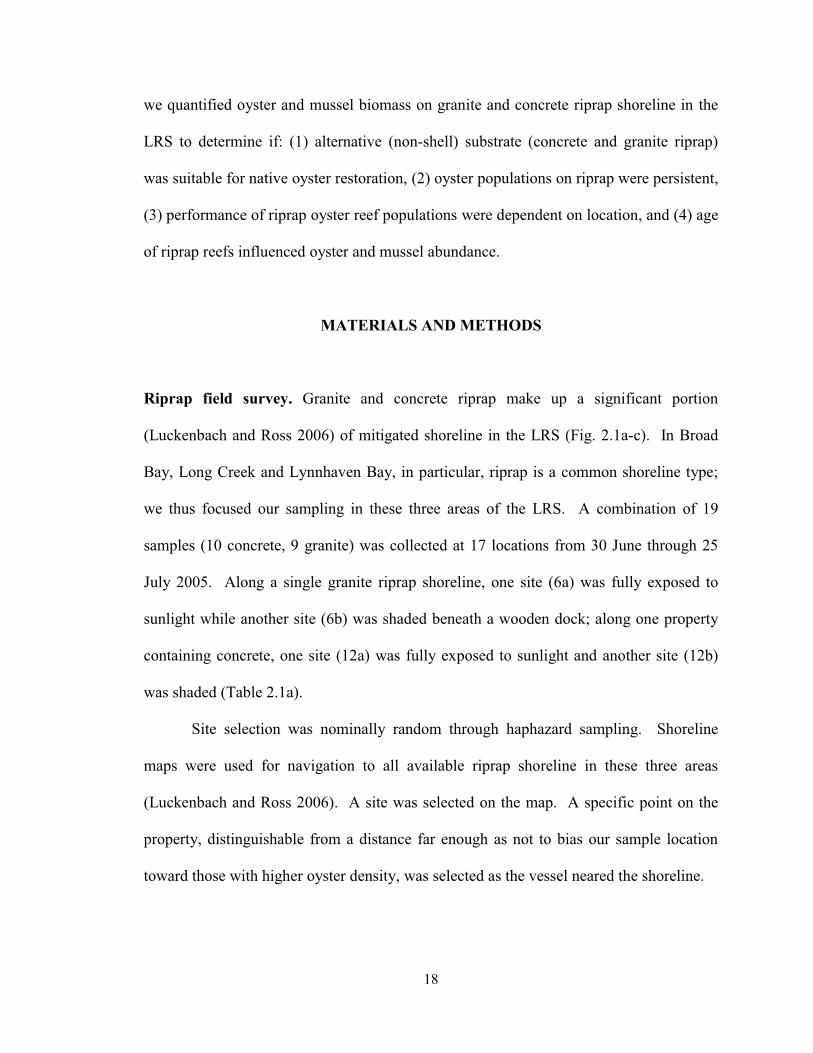
18

we quantified oyster and mussel biomass on granite and concrete riprap shoreline in the

LRS to determine if: (1) alternative (non-shell) substrate (concrete and granite riprap)

was suitable for native oyster restoration, (2) oyster populations on riprap were persistent,

(3) performance of riprap oyster reef populations were dependent on location, and (4) age

of riprap reefs influenced oyster and mussel abundance.

MATERIALS AND METHODS

Riprap field survey. Granite and concrete riprap make up a significant portion

(Luckenbach and Ross 2006) of mitigated shoreline in the LRS (Fig. 2.1a-c). In Broad

Bay, Long Creek and Lynnhaven Bay, in particular, riprap is a common shoreline type;

we thus focused our sampling in these three areas of the LRS. A combination of 19

samples (10 concrete, 9 granite) was collected at 17 locations from 30 June through 25

July 2005. Along a single granite riprap shoreline, one site (6a) was fully exposed to

sunlight while another site (6b) was shaded beneath a wooden dock; along one property

containing concrete, one site (12a) was fully exposed to sunlight and another site (12b)

was shaded (Table 2.1a).

Site selection was nominally random through haphazard sampling. Shoreline

maps were used for navigation to all available riprap shoreline in these three areas

(Luckenbach and Ross 2006). A site was selected on the map. A specific point on the

property, distinguishable from a distance far enough as not to bias our sample location

toward those with higher oyster density, was selected as the vessel neared the shoreline.

19

Figure 2.1 A-B.

20

Figure 2.1: (A) Aerial map of the lower Lynnhaven River System containing markers for riprap shoreline sample sites; yellow = exposed, green = shaded (Map generated using Google EarthTM). (B) Riprap oyster reefs shaded beneath a wooden dock along Long Creek. (C) Collage of riprap oyster photographs taken in and around Broad Bay, 2005.

21

Table 2.1: (A) Riprap sample site and (B) oyster and mussel data for Broad Bay, Long Creek and Lynnhaven Bay (SH – shell height, SA – surface area, E – exposed, S – shaded)

Region Site # Sample Date Latitude (oN) Longitude (oW) Riprap Type Sediment Type

N. Broad Bay 1 6/30/2005 36.90428 76.04892 Granite Muddy Sand

N. Broad Bay 2 6/30/2005 36.90419 76.05370 Granite Muddy Sand

Long Creek 3 7/6/2005 36.90957 76.04092 Concrete Muddy Sand

S. Broad Bay 4 7/8/2005 36.88950 76.02570 Concrete Muddy Sand

S. Broad Bay 5 7/8/2005 36.89040 76.02620 Granite Coarse Sand

Long Creek 6a – E 7/11/2005 36.91048 76.04602 Granite Mud

Long Creek 6b – S 7/11/2005 36.91048 76.04602 Granite Mud

Long Creek Yopp 7/11/2005 36.90873 76.03965 Concrete Mud

N. Broad Bay 7 7/19/2005 36.90371 76.05869 Concrete Muddy Sand

N. Broad Bay 8 7/19/2005 36.90332 76.05711 Granite Coarse Sand

S. Broad Bay 9 7/19/2005 36.89414 76.03976 Concrete Muddy Sand

S. Broad Bay 10 7/19/2005 36.89214 76.02883 Granite Coarse Sand

N. Broad Bay 11 7/21/2005 36.90231 76.06105 Concrete Coarse Sand

Lynnhaven Bay 12a – E 7/21/2005 36.89911 76.08601 Concrete Coarse Sand

Lynnhaven Bay 12b – S 7/25/2005 36.89911 76.08601 Concrete Coarse Sand

Lynnhaven Bay 13 7/25/2005 36.89164 76.07219 Concrete

Lynnhaven Bay 14 7/25/2005 36.89423 76.06588 Granite

Lynnhaven Bay 15 7/25/2005 36.89487 76.06493 Granite

Lynnhaven Bay 16 7/25/2005 36.89841 76.08545 Concrete

A.

22

Table 2.1 B.

Site # Oyster Density

(m-2

)

Oyster Biomass

(g AFDM m

-2)

Mean Oyster

SH (mm)

Oyster Volume (mL m

-2)

Mussel Density

(m-2

)

Mussel Volume (mL m

-2)

Riprap SA:

Bottom Area Ratio

Oyster Condition Index 1

Oyster Condition Index 2

Oyster Condition Index 3

1 260 58.03 43.2 2840 256 520 4.68 10.84 6.56 2.80

2 756 253.59 48.8 9932 1608 2200 6.23 10.38 7.66 3.71

3 1628 294.02 44.3 16500 308 360 7.40 7.17 5.03 2.21

4 32 0.17 24.2 28 264 100 2.78 -- -- --

5 112 12.95 37.1 340 216 80 2.46 12.54 9.70 2.36

6a – E 356 58.06 41.7 2600 140 320 4.81 8.66 6.42 2.49

6b – S 568 119.19 41.5 4800 152 520 3.56 9.23 6.61 2.71

Yopp 1328 285.02 46.7 15000 2048 4000 5.17 9.68 6.71 2.26

7 2028 216.81 40.7 12720 196 160 3.09 10.83 6.60 2.21

8 940 174.38 45.2 8000 480 600 2.17 11.02 7.31 2.25

9 224 48.65 46.0 984 428 100 1.32 9.64 8.10 4.24

10 928 143.12 41.0 6344 196 40 5.80 9.47 6.25 2.16

11 1228 175.46 38.9 7000 328 360 5.15 9.29 8.24 2.21

12a – E 2540 294.94 39.4 19980 1624 3820 4.16 10.05 8.04 2.31

12b – S 2000 236.39 33.7 8880 1088 2560 3.58 10.90 9.16 3.73

13 1092 249.44 44.2 10440 760 1188 1.24 8.98 7.40 2.97

14 432 105.82 47.4 6560 328 508 2.60 9.25 7.02 2.61

15 116 62.06 56.9 2560 44 60 1.86 13.63 10.75 3.74

16 2012 347.27 43.6 1640 1196 2000 2.05 8.20 6.40 2.82

Mean 978 165.02 42.3 7220 612 1028 3.69 9.99 7.44 2.76

SE Mean 177 24.63 1.5 1324 136 292 0.40 0.35 0.32 0.15

B.

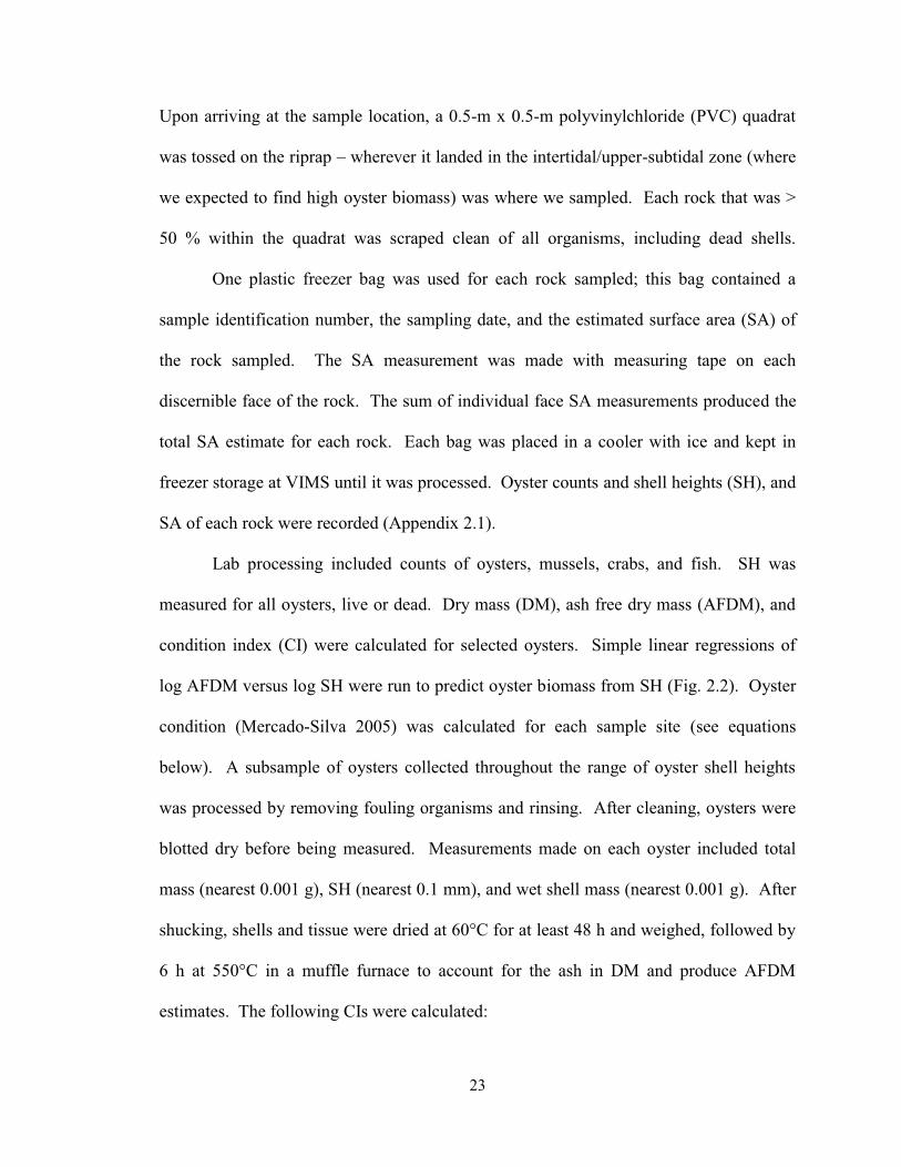
23

Upon arriving at the sample location, a 0.5-m x 0.5-m polyvinylchloride (PVC) quadrat

was tossed on the riprap – wherever it landed in the intertidal/upper-subtidal zone (where

we expected to find high oyster biomass) was where we sampled. Each rock that was >

50 % within the quadrat was scraped clean of all organisms, including dead shells.

One plastic freezer bag was used for each rock sampled; this bag contained a

sample identification number, the sampling date, and the estimated surface area (SA) of

the rock sampled. The SA measurement was made with measuring tape on each

discernible face of the rock. The sum of individual face SA measurements produced the

total SA estimate for each rock. Each bag was placed in a cooler with ice and kept in

freezer storage at VIMS until it was processed. Oyster counts and shell heights (SH), and

SA of each rock were recorded (Appendix 2.1).

Lab processing included counts of oysters, mussels, crabs, and fish. SH was

measured for all oysters, live or dead. Dry mass (DM), ash free dry mass (AFDM), and

condition index (CI) were calculated for selected oysters. Simple linear regressions of

log AFDM versus log SH were run to predict oyster biomass from SH (Fig. 2.2). Oyster

condition (Mercado-Silva 2005) was calculated for each sample site (see equations

below). A subsample of oysters collected throughout the range of oyster shell heights

was processed by removing fouling organisms and rinsing. After cleaning, oysters were

blotted dry before being measured. Measurements made on each oyster included total

mass (nearest 0.001 g), SH (nearest 0.1 mm), and wet shell mass (nearest 0.001 g). After

shucking, shells and tissue were dried at 60°C for at least 48 h and weighed, followed by

6 h at 550°C in a muffle furnace to account for the ash in DM and produce AFDM

estimates. The following CIs were calculated:

24

CI1 = [dry tissue weight (g) / shell cavity volume] x 100 (Abbe and Albright 2003)

CI2 = [dry tissue weight (g) / dry shell cavity volume] x 100 (Abbe and Sanders, 1988)

CI3 = [dry tissue weight (g) / dry shell weight (g)] x 100 (Rainer and Mann 1992)

Figure 2.2: Regression model of log oyster AFDM (g) versus log oyster shell height (mm) used

for oyster biomass estimation for riprap oysters (pooled across all sites).

These indices are considered to be the most accurate indicators of condition (Hickman

and Illingworth 1980, Davenport and Chen 1987). For CI1 and CI2, shell cavity volume

is equal to the difference between the mass of the whole oyster (g) and the mass of the

empty valves (g) (Abbe and Sanders 1988, Crosby and Gale 1990). CI1 considered the

mass of the empty shells immediately after shucking whereas CI2 used the mass of the

shells after a period of drying (Abbe and Albright 2003). For all analyses, condition

y = 2.3945x – 4.7812 R2 = 0.888

25

indices were used where shell volume was calculated by a gravimetric method. These

measures are linearly related to those where CI3 is calculated by a volumetric method

(i.e. by water displacement of the shells, Schumacker et al. 1998).

Restored oyster shell reef survey. Restored oyster shell reef samples were taken to

compare with metrics of oysters sampled on riprap. The site selection method was

identical to that used for riprap samples. For the restored oyster shell reefs, sets of

samples were taken from a reef in Long Creek and in Hume’s Marsh (Lynnhaven Bay),

as they appeared to represent the range from low to high oyster density. The oyster reef

samples were selected in a stratified random sampling design with location in the

intertidal zone (lower, mid, upper) as the stratum. The Hume’s Marsh Reef was sampled

completely with five samples from each intertidal zone. The Long Creek reef was not

fully sampled (insufficient number of samples: only 5 of 15 retrieved). A single high-

density sample was taken from the Keeling’s Drain reef (lower Eastern Branch of

Lynnhaven River) and another part of Hume’s Marsh Reef; both represent peak reef

productivity on restored oyster shell reefs.

The method for collection on a restored oyster shell reef was the excavation of a

selected sample down to a depth of 15 cm using a 0.5-m x 0.5-m quadrat. Only live

oysters, or dead shells with live oysters attached to them, were brought back and placed

in freezer storage. SH and shell volume were measured for all oysters and the number of

oysters per base shell was noted. A subset of 5-14 oysters was selected across the range

of SH to determine AFDM, and CI. Simple linear regressions of log AFDM versus log

SH were run to produce a model that could predict oyster biomass from SH alone.

26

In the analysis of size structure for oysters, peaks were analyzed with FISAT II

(Gayanilo et al. 2002) to delineate individual year classes. The peaks were separated

using Bhattacharya’s Method (Bhattacharya 1967). The program uses a set of equations

that yields mean lengths, population sizes, standard deviations and separation indices (SI)

for each year class, where SI is the difference between two successive means divided by

the difference between their estimated standard deviations. However, measurement of

peak height and width were secondary to the primary goal of distinguishing individual

peaks (size classes as proxies for age classes).

RESULTS

Riprap oyster population structure. In total, 4551 oysters were collected and used in

the size structure analysis (Fig. 2.3a). Oyster SH ranged from 1.4-133.4 mm, with some

variability in size structure across sites (Fig. 2.3b).

Riprap oyster density. Oyster counts ranged from 8-635 with a mean of 244 +/- 44

oysters (SE) sample-1. Mean oyster density was 978 +/- 177 oysters m-2 with a mean SH

of 42.3 +/- 1.5 mm (Table 2.1b). On average, concrete samples contained 219 more

oysters than granite samples (Table 2.2). Along a single granite riprap shoreline in Long

Creek, site 6a was fully exposed to sunlight while site 6b was shaded beneath a wooden

dock. At this site, the shaded sample contained 37 % more oysters and the oyster band

extended 6-7 cm higher in the intertidal zone than that of the exposed sample. In a

Lynnhaven Bay shoreline containing concrete riprap, site 12a was exposed and site 12b

27

was shaded. At this site, both samples had 2000 or more oysters m-2, and although the

shaded oyster band extended higher in the intertidal, the exposed sample contained 27 %

more oysters than the shaded sample.

Table 2.2: Comparison of mean oyster count, shell height (SH), dry tissue mass (DM), ash-free dry tissue mass (AFDM), and oysters per unit surface area (SA) between concrete and granite riprap (+/- 1 SEM).

Riprap Type

Oyster Density

(m-2

)

Oyster Biomass

(g AFDM m

-2)

Mean Oyster

SH (mm)

Oyster Volume (mL m

-2)

Mussel Density

(m-2

)

Mussel Volume (mL m

-2)

Riprap SA:

Bottom Area Ratio

Oyster Condition Index 1

Oyster Condition Index 2

Oyster Condition Index 3

Concrete 1411

(255)

214.82

(35.29)

40.2

(2.2)

9316

(2188)

824

(204)

1464

(488)

3.592

(0.612)

9.42

(0.40)

7.30

(0.41)

2.77

(0.25)

Granite 496

(107)

109.69

(24.46)

44.8

(1.9)

4888

(1024)

380

(160)

540

(220)

3.796

(0.544)

10.56

(0.55)

7.59

(0.53)

2.76

(0.20)

Oyster density clearly increased closer to the mouth of the LRS. In many cases,

there was an order of magnitude difference in oyster density between the upper bay sites

(1, 4, 5, 9) and the lower bay sites (7, 11, 12a, 12b, 13, 16). Overlaying the riprap sites

with the hydrodynamic and source-sink modeling results (Lipcius et al. 2008) allowed for

classification of each site as a: (1) source, (2) sink, (3) putative source, (4) self

replenishing, or (5) exporting sink (Table 2.1a). Sites 4, 5 and 9 (upper bay sites) were

designated sources while all six of the aforementioned lower bay sites were designated

sinks.

28

Figure 2.3: (A) Population size structure of oysters on riprap in Lynnhaven River System (LRS). (B) LRS riprap oyster population size structure, by site.

29

Riprap oyster biomass. Comparison of biomass estimates (total g AFDM m-2 bottom +/-

1 SEM) generated from regression equations using pooled and site-specific data (Fig. 2.4)

led to site-specific equations. Regressions from pooled data were robust (R2 > 0.83 for

AFDM), but regressions from the site-specific data were better (R2: 0.83 – 0.96). Thus,

site-specific regression equations were used (Table 2.3).

Figure 2.4: Riprap oyster biomass estimates (g AFDM m-2 river bottom), by site, generated from regression models using pooled (gray bars) and site-specific data (black bars).

30

Table 2.3: Linear regression models of oyster dry mass (DM) and ash-free dry mass (AFDM) derived for each site in Broad Bay, Long Creek and Lynnhaven Bay.

Site # Linear Regression Model Log DM (g) v. Log SH (mm) R

2 Linear Regression Model

Log AFDM (g) v. Log SH (mm) R2

1 y = 2.7195x - 5.2963 0.9437 y = 2.6913x - 5.2896 0.9443 2 y = 2.1542x - 4.1889 0.8787 y = 2.3667x - 4.629 0.9211 3 y = 2.9185x - 5.7011 0.9062 y = 2.8588x - 5.6484 0.9023 4 Used Pooled Model -- Used Pooled Model -- 5 y = 2.5548x - 4.9925 0.9183 y = 2.5029x - 4.9646 0.9196

6a – E y = 2.7465x - 5.3957 0.9578 y = 2.7378x - 5.4344 0.9561 6b – S y = 2.5372x - 4.905 0.9396 y = 2.5157x - 4.9229 0.9408 Yopp y = 2.3532x - 4.6608 0.9176 y = 2.276x - 4.5876 0.9121

7 y = 2.4237x - 4.9242 0.8524 y = 2.3351x - 4.8152 0.8341 8 y = 2.1328x - 4.3117 0.8810 y = 2.1163x - 4.3336 0.8833 9 y = 2.2899x - 4.4348 0.8703 y = 2.2186x - 4.4228 0.8625

10 y = 2.2822x - 4.5432 0.9556 y = 2.2231x - 4.4894 0.9566 11 y = 2.3766x - 4.7392 0.9356 y = 2.4556x - 4.9494 0.9421

12a – E y = 2.2607x - 4.5951 0.9224 y = 2.2991x - 4.7284 0.9247 12b – S y = 2.4562x - 4.7326 0.9240 y = 2.5183x - 4.9208 0.9233

13 y = 2.5461x - 4.9518 0.8726 y = 2.5789x - 5.1085 0.8744 14 y = 2.1531x - 4.2479 0.8633 y = 2.1614x - 4.3434 0.8536 15 y = 2.4052x - 4.5013 0.8744 y = 2.3727x - 4.5026 0.8712 16 y = 2.3708x - 4.6887 0.9325 y = 2.2385x - 4.5517 0.8920

Pooled Linear Regression Model y = 2.3984x - 4.7198 0.8849 y = 2.3945x - 4.7812 0.8880

31

Oyster biomass ranged from 0.17-347.27 g AFDM m-2 with a mean (+/- 1 SEM)

of 165.02 +/- 24.63 g AFDM m-2. In many cases, the age of the riprap shoreline

determined how developed the oyster reef had become. For example, riprap at sites #4

and #5 had been replaced within two years of sampling due to damage from Hurricane

Isabel (18 September 2003); granite and concrete take many months to obtain the

appropriate surface pH to support oyster settlement (Weiner et al. 1989, Bonar et al.

1990) and, in this case, we would not expect to find multiple year classes of oysters. In

contrast, some of the riprap sites were five or more years old and had thriving oyster

populations on and within them. We were informed by homeowners along Lynnhaven

Bay that concrete riprap at sites 12a-b and 16 were close to 30 years old; as might be

expected, riprap at these sites supported higher densities of small and large oysters, with

more than 1.5-2.0 times the oyster AFDM the Lynnhaven Decision Document expects for

unseeded restored oyster reefs five years or older.

Riprap oyster volume and reef accretion. Oyster volume (live and dead shell) ranged

from 0.03-19.98 L m-2, with a mean volume of 7.2 +/- 1.3 L m-2. The oldest riprap oyster

reefs accreted more shell than those deployed only a few years prior to this survey. On

rock reefs, such as these, shell accretion is an important oyster reef restoration metric.

Riprap oyster condition index. Mean CIs were calculated from all sites except site #4

(Table 2.2) because that site had low sample size. All three CIs are documented in the

literature (Rainer and Mann 1992) and assume that the oysters processed have both

valves. However, the process of removing oysters from riprap with hand scrapers left

32

some of the oysters with only a single valve. Thus, a correction factor was used to avoid

inflation of condition index for any oyster missing significant shell mass. For example,

an oyster with only one valve has its CI divided by two and an oyster with half of one

valve missing (1.5 valves remaining) had its CI divided by 1.5. Since in no case were all

oysters in a sample missing whole, or portions of their, valves, the mean ‘corrected CI’ is

not simply one half of the original CI. CI did vary amongst sites, but the means (+/- 1

SEM) of CI1 (9.99 +/- 0.35), CI2 (7.44 +/- 0.32) and CI3 (2.76 +/- 0.15) indicate that the

riprap oysters were healthy. There was no trend in the CIs among sites by region or

riprap type (p > 0.16 for all three CIs). Also, there was no distinct effect of concrete

versus granite on oyster CI (CI 1: R2 = 0.15; CI2: R2 = 0.01; CI3: R2 = 0.00).

Restored shell reef oyster population structure. In total, 362 oysters were collected

over 15 samples in the intertidal zone on the Hume’s Marsh restored oyster shell reef.

Oyster SH ranged from 8.9-116.3 mm, with three peaks representing two to three year

classes (Fig. 2.5).

Figure 2.5: Separation of oyster shell length-frequency data from Hume’s Marsh restored oyster shell reef into individual oyster classes.

33

The population size structure was similar for all three intertidal zones (Appendix 2.2),

thus allowing us to collapse across intertidal zone and provide for a robust analysis of the

entire reef. Although the Long Creek restored oyster shell reef (Appendix 2.3) was

incomplete, similar size structure patterns emerged. The two high-density oyster reef

samples (Fig. 2.6a-b) supported the full complement of oysters throughout the entire size

range observed in the LRS.

Restored shell reef oyster density. Mean oyster density on the Hume’s Marsh restored

oyster shell reef was 97 +/- 16 oysters m-2 with a mean SH of 46.0 +/- 2.6 mm and a

mean mussel density of 8 +/- 4 mussels m-2 (Table 2.4a). No trends were detected

amongst the individual samples or intertidal zones (Appendix 2.4).

The Hume’s Marsh high-density oyster shell reef sample had an oyster density of

956 oysters m-2, with a mean SH of 53.2 +/- 1.7 mm, and a mussel density of 300 mussels

m-2. The Keeling’s Drain high-density oyster reef sample had an oyster density of 776

oysters m-2, with a mean SH of 50.5 +/- 1.9 mm, and a mussel density of 68 mussels m-2.

Both samples were collected within the low- to mid-intertidal zone.

Restored shell reef oyster biomass. Oyster biomass was estimated for the Hume’s

Marsh restored oyster shell reef using separate regressions for each sample and a single

regression including all samples to determine the relative error associated with

regressions containing a small percentage of the total sample size. All regressions fit the

data well (r2 > 0.77). The Hume’s Marsh restored oyster shell reef mean oyster biomass

was 26.48 +/- 5.45 g AFDM m-2.

34

Figure 2.6: (A) Population size structure of oysters in Hume’s Marsh high-density oyster sample. (B) Population size structure of oysters in Keeling’s Drain high-density oyster sample.

A

B

35

A single oyster SH-biomass regression model for the whole reef (y = 2.8838x - 5.5426)

produced different mean oyster biomass estimates than three separate models for each

intertidal zone (Table 2.4a). Regardless of the method chosen, the mid intertidal zone

had the highest biomass.

The Hume’s Marsh high-density oyster reef sample (y = 2.1677x – 4.4791) had an

oyster biomass of 232.22 g AFDM m-2. The oyster biomass was equal to 58% of the sum

of all 15 samples taken from Hume’s Marsh restored oyster shell reef, which highlights

the variable productivity of previously deployed restored oyster shell reefs. The

Keeling’s Drain high-density oyster reef sample (y = 2.7219x - 5.3600) also had a high

oyster biomass of 251.54 g AFDM m-2.

Restored shell reef oyster volume and reef accretion. Oyster volume for the Hume’s

Marsh restored oyster shell reef, ranged from 0.0-6.0 L m-2, with a mean volume of 2.9

+/- 0.5 L m-2. This reef was built very high with large shucked oyster shells, which have

allowed it to persist for a number of years.

Restored shell reef oyster condition index. CIs were calculated for all samples on the

Hume’s Marsh restored oyster shell reef. Over the entire reef, the mean CI values for the

three indices (CIs 1-3) were 12.6 +/- 0.6, 10.1 +/- 0.6, and 3.4 +/- 0.3 while the mean

corrected CI values were 10.8 +/- 0.4, 8.6 +/- 1.7, and 2.7 +/- 0.2 (Table 2.4b), indicating

oysters in similar health to the average riprap oyster. Lower intertidal oysters had a

greater mean CI than those sampled from the upper intertidal zone. Note that no CIs

were calculated for the Long Creek reef because AFDM estimates were not available.

36

Table 2.4: (A) Mean oyster density, shell height (SH), biomass (dry mass (DM), and ash-free dry mass (AFDM)) of Hume’s Marsh restored oyster shell reef and (B) condition indices (CI) across intertidal zones

Intertidal Zone Depth

(cm) Oyster Density

(m-2

) Oyster

Biomass (g AFDM m

-2)

Oyster Biomass

(g DM m-2

) Mean

Oyster SH (mm)

Mussel Density

(m-2

)

Upper 0.8 (0.8) 88 (31) 23.25 (10.07) 26.71 (11.46) 44.8 (3.4) 8 (4) Mid 9.6 (2.3) 107 (25) 32.52 (11.56) 37.11 (13.01) 47.1 (3.8) 8 (4)

Lower 34.4 (5.3) 94 (31) 23.67 (7.95) 27.14 (9.05) 46.0 (6.5) 16 (12) A.

Intertidal Zone

Oyster Condition Index 1

Oyster Condition Index 2

Oyster Condition Index 3

Oyster CI 1 Corrected Oyster CI 2

Corrected Oyster CI 3 Corrected

Upper 10.9 (1.0) 8.6 (1.2) 2.9 (0.7) 9.1 (0.5) 7.0 (0.4) 2.3 (0.4) Mid 12.4 (0.7) 10.0 (0.8) 3.1 (0.2) 10.8 (0.6) 8.5 (0.6) 2.5 (0.1)

Lower 14.1 (0.8) 11.6 (0.8) 4.1 (0.6) 12.3 (0.5) 9.9 (0.6) 3.2 (0.3)

B.

The Hume’s Marsh high-density oyster reef sample had CIs (1-3) of 6.7 +/- 0.3,

5.1 +/- 0.2, and 2.1 +/- 0.1. The Keeling’s Drain high-density oyster reef sample had CIs

of 8.8 +/- 0.3, 7.3 +/- 0.3 and 2.3 +/- 0.1. The CIs were similar for both high-density

samples (Table 2.5). However, the mean oyster CI for the Hume’s Marsh high-density

sample was much less than the adjusted CIs for the Hume’s Marsh restored oyster shell

reef.

37

Table 2.5: Mean oyster density, shell height (SH), biomass (dry mass (DM), and ash-free dry mass (AFDM)), and condition indices (CI) of Hume’s Marsh and Keeling’s Drain high-density restored oyster shell reef sample, and mussel density across intertidal zones.

Sample ID

Oyster Density

(m-2

)

Oyster Biomass

(g DM m-2

)

Oyster Biomass

(g AFDM m-2

)

Mean Oyster

SH (mm)

Mussel Density

(m-2

)

Oyster Condition Index 1

Oyster Condition Index 2

Oyster Condition Index 3

Hume’s Marsh

956 289.20 232.22 53.2 (1.7) 300 6.7 (0.3) 5.1 (0.2) 2.1 (0.1)

Keeling’s Drain

776 287.12 251.54 50.5 (1.9) 68 8.8 (0.3) 7.3 (0.3) 2.3 (0.1)

DISCUSSION

The riprap oyster populations of Broad Bay, Long Creek and Lynnhaven Bay had

high condition index, biomass often exceeding 177 g AFDM m-2, and very high densities

averaging nearly 1000 oyster m-2 (978 +/- 177 SEM), which is among the top estimates

for intertidal artificial reef substrates in Chesapeake Bay (Nestlerode et al. 2007). Both

concrete and granite riprap supported robust oyster populations with a size structure

indicative of consistent annual recruitment, an important attribute for reef persistence.

The smooth curve of the single peak in size structure made it difficult to distinguish year

classes, and is usually characteristic of consistent recruitment from year to year. High

and variable growth rates and multiple spawning events could explain also the lack of

distinction between size classes.

We also compared the performance of the riprap reefs with the nearby Hume’s

marsh restored oyster shell reef. The Hume’s Marsh oyster shell reef harbored oysters

with a healthy condition index at a mean density of 97 +/- 16 (SEM) oysters m-2.

Moreover, oyster in the lower intertidal had a greater mean CI than those in the upper

intertidal zone. Bartol and Mann (1999) reported that oysters in the lower intertidal on a

38

constructed oyster shell reef had higher survival than those in the high intertidal. Lower

intertidal oysters experience less thermal and desiccation stress, and can continue to feed

during periods in the tidal cycle when upper intertidal oysters are exposed and unable to

feed. Apparently, indirect benefits of aerial exposure in the mid to upper intertidal zone,

such as reduced parasite load (Encomio and Chu 2007), fewer fouling organisms, and a

partial refuge from predation, do not overwhelm the disadvantage of reduced duration of

inundation in the high intertidal zone (Bishop and Peterson 2006).

Oyster reefs constructed of loose oyster shells offer a buffered, protected habitat

for oysters that settle and grow within the reef interstices, but only to a shallow depth of

10 cm (Bartol and Mann 1999). Riprap reefs provide much larger pore spaces and

supported oysters three to four rocks deep, greater than 50 cm deep, in many cases. The

considerable surface area, diversity of exposed and shaded surfaces, and good flow

within the reef interstices of concrete and granite riprap likely promote high oyster and

mussel densities.

The two high-density restored oyster shell reef samples represent peak values for

oyster density and biomass on such man-made reefs. These values were 8-10 times

higher than the Hume’s Marsh and Long Creek restored oyster shell reefs, and validate

claims that portions of constructed shell oyster reefs can perform well. The two high-

density samples each supported a robust oyster population size structure (Mann et al.

2009a); however, they had lower mean oyster condition than the rest of the Hume’s

Marsh restored oyster shell reef. This substantial difference in oyster condition suggests

that food competition became compounded with increased oyster and mussel density, a

phenomenon often exacerbated by low water flow over the reef (Wildish et al. 1987,

39

Eckman et al. 1989, Lenihan et al. 1996). This was likely the case as this sample was

collected on the lee side of the Hume’s Marsh restored oyster shell reef where buffering

of wind and wave action occurs due to the presence of Hume’s Marsh on one side and the

restored oyster shell reef on the other. The Keeling’s Drain high-density sample may

have fared better in this respect since it has marsh behind it, but open, unabated water

flow in front of it (mouth and channel of the Eastern Branch of the Lynnhaven River)

(Artabane 2006).

Finally, despite residing in a high salinity zone noted for high oyster disease

pressure (Carnegie and Burreson 2009), many of the oysters grew much larger than the

assumed size at which disease causes high mortality. Some possible explanations for the

high survival and growth are (1) evolved disease tolerance, (2) reduced pathogen

virulence or abundance, (3) high, but not complete disease mortality, and (4) oysters

grow fast in the LRS and give the impression of oyster disease resistance without really

expressing it. Unfortunately, this study did not test disease prevalence or intensity.

Beyond a lack of disease data, oysters in the LRS do often grow to 75 mm SH (market

size) faster than in many other parts of Chesapeake Bay, so assuming that a 75-mm oyster

is three years old would not be appropriate for the LRS. Thus, use of oyster SH alone as

a proxy for oyster disease resistance was not justified in this study. Disease-tolerant or

not, riprap oyster densities eclipsing 1000 m-2 with oyster biomass > 200 g AFDM m-2

indicate that concrete and granite riprap do serve as effective oyster reef habitat in the

LRS and should be considered for use in future native oyster restoration reef projects.

Furthermore, these alternative reefs can serve as “living shorelines” to mitigate erosion in

place of detrimental bulkheads (Meyer et al. 1997, Seitz et al. 2009).

40

In summary, alternative substrate reefs of granite and concrete supported some of

the highest abundances of healthy oysters ever recorded for Chesapeake Bay artificial

oyster reefs, shell or otherwise. Furthermore, the oyster population size structure was

indicative of consistent annual oyster recruitment, a quality critical for reef persistence.

Consequently, alternative oyster reefs constructed of concrete or granite riprap can

enhance ecological native oyster restoration efforts in the LRS and other high-salinity

Chesapeake Bay tributaries.

41

Acknowledgments. We express appreciation to students and staff of the Marine

Conservation Biology and Marine Community Ecology Programs at VIMS, particularly,

Katie Knick, Amanda Lawless, Alison Smith, and Justine Woodward for their assistance

in the lab and field. Special thanks to Dave Schulte for his field help and expertise.

Funding was provided by grants to R.N. Lipcius and R.D. Seitz from the Norfolk Office

of the USACE (D. Schulte, program manager). We wish to thank all waterfront property

owners who allowed us to sample their riprap and often provided us critical site-specific

background information. Finally, we have dedicated the name of one riprap sample site

as “Yopp” for the late Mr. Luther Yopp, who graciously welcomed our sampling of his

riprap and placement of an alternative substrate experiment outside his property along

Long Creek.

42

Chapter 3 Population structure, density and biomass of the Eastern oyster (Crassostrea virginica) and hooked mussel (Ischadium recurvum) on artificial oyster reefs in the Rappahannock River, Chesapeake Bay

ABSTRACT: Restored Eastern oyster (Crassostrea virginica) shell reefs have generally experienced marginal success and require reseeding to sustain populations in Chesapeake Bay. Many shell reefs vary significantly from natural reefs in having: (1) limited vertical complexity, (2) low reef stability, (3) reduced substrate area for larval settlement, and (4) diminished reef community structure. Some alternative reef structures may overcome these deficiencies and serve as effective oyster reefs. In 2005 and 2007, oyster and mussel population structure, density and biomass were quantified on a novel concrete modular reef deployed subtidally in the Rappahannock River, Chesapeake Bay. The modular reef was neither seeded artificially nor harvested. The reef was colonized heavily by oysters and mussels, which recruited and survived at high densities for the 5-7 years since reef deployment in 2000. Oyster and mussel biomass and density were among the highest recorded for natural and restored oyster reefs. Additionally, a large array of artificial concrete reefs known as ‘Steamer Rock’ (deployed in 1994, and located adjacent to the concrete modular reef), was sampled in 2006. We estimated that, within a subtidal footprint of < 0.4 ha, these reefs contained > 4 million oysters and > 30 million mussels. In disease prevalence and intensity tests, oysters from both reef systems were healthy. These artificial reefs support mature oyster communities, as they provide vertical structure and stability required to buffer environmental stress and predation pressure. We posit that the Steamer Rock reef system: (1) supports a significant fraction of the Rappahannock River oyster and mussel breeding stock, (2) is the largest, most successful artificial (alternative substrate) oyster reef in Chesapeake Bay, and (3) sustains a diverse assortment of fish and invertebrates. Thus, large-scale, subtidal, alternative substrate reefs are a viable native oyster restoration strategy.

43

INTRODUCTION

Restoration of the eastern oyster, Crassostrea virginica, in Chesapeake Bay has

traditionally relied on low-relief shell reefs (2-4 inches thick; Smith et al. 2005) and

oyster shell mounds (~1 m tall, personal observation) created in an attempt to mimic

natural reef conditions and accelerate recruitment (Mann 2001, Southworth et al. 2008b).

To date these efforts have met with limited success (Mann and Powell 2007), though

some recent restored oyster reefs in the Great Wicomico River (Schulte et al. 2009), and

Lynnhaven River (Lipcius et al. 2008) have been thriving.

Due to limitations in natural hard substrate, artificial habitats have been used for

various species over 100 years and recently recognized by fishery managers as a viable

enhancement technique (McGurrin et al. 1989, Stone et al. 1991). The utility of artificial

reefs led the United States to develop its a National Artificial Reef Plan (NARP) in 1985

(amended in 2007) under direction of the National Fishing Enhancement Act of 1984 and

with the participation of coastal state artificial reef program managers (US Dept. of

Commerce 1985, 2007). For instance, the Commonwealth of Virginia's Artificial Reef

Program, which is managed by the Marine Resources Commission, has a rich history,

using World War II Liberty ships in the early 1970s and “materials of opportunity” such

as demolished concrete bridges in the 1970s and as structures that provide stability,

durability and a maximum amount of surface area and interior space.

Traditional oyster repletion programs (those that condition harvest bottom to

receive natural spatset) and restoration projects (those that rehabilitate formerly

productive oyster bottom) have relied almost exclusively on supplies of oyster shell from

either processing houses or deposits of 3,000-4,000-year-old buried fossil shell.

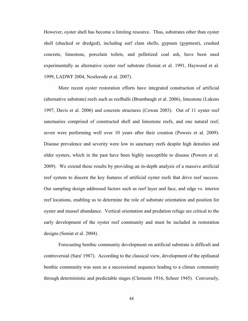
44

However, oyster shell has become a limiting resource. Thus, substrates other than oyster

shell (shucked or dredged), including surf clam shells, gypsum (gypment), crushed

concrete, limestone, porcelain toilets, and pelletized coal ash, have been used

experimentally as alternative oyster reef substrate (Soniat et al. 1991, Haywood et al.

1999, LADWF 2004, Nestlerode et al. 2007).

More recent oyster restoration efforts have integrated construction of artificial

(alternative substrate) reefs such as reefballs (Brumbaugh et al. 2006), limestone (Lukens

1997, Davis et al. 2006) and concrete structures (Cowan 2003). Out of 11 oyster reef

sanctuaries comprised of constructed shell and limestone reefs, and one natural reef,

seven were performing well over 10 years after their creation (Powers et al. 2009).

Disease prevalence and severity were low in sanctuary reefs despite high densities and

older oysters, which in the past have been highly susceptible to disease (Powers et al.

2009). We extend these results by providing an in-depth analysis of a massive artificial

reef system to discern the key features of artificial oyster reefs that drive reef success.

Our sampling design addressed factors such as reef layer and face, and edge vs. interior

reef locations, enabling us to determine the role of substrate orientation and position for

oyster and mussel abundance. Vertical orientation and predation refuge are critical to the

early development of the oyster reef community and must be included in restoration

designs (Soniat et al. 2004).

Forecasting benthic community development on artificial substrata is difficult and

controversial (Sara' 1987). According to the classical view, development of the epifaunal

benthic community was seen as a successional sequence leading to a climax community

through deterministic and predictable stages (Clements 1916, Scheer 1945). Conversely,

45

the community of a newly immersed artificial substratum is linked to stochastic larval

recruitment that is also characterized by seasonal and annual variability and by the

relative dominance of pioneer species, so that a classic succession cannot be determined

(Sutherland and Karlson 1977). In either case, five years is sufficient for a relatively

stable community to develop in waters other than the most oligotrophic waters (Jensen et

al. 2000). In our study, eastern oyster (C. virginica) and hooked mussel (Ischadium

recurvum) were quantitatively sampled on a concrete modular reef in 2005 and 2007

approximately 5 and 7 years after deployment, respectively. In 2006, the Steamer Rock

reef complex was similarly sampled, 11 years after deployment. Hence, both sets of reefs

had ample time for a mature oyster reef community to develop.

MATERIALS AND METHODS

Concrete Module Reef

Construction. In 1994, a non-profit organization (Rappahannock Preservation Society -

RPS) deployed 176 stacks (7 layers per stack) of recycled bridge pieces (materials of

opportunity) subtidally at 7 m depth on sand bottom at Steamer Rock (SR), near the

mouth of the Rappahannock River, a western-shore tributary of Chesapeake Bay.

Steamer Rock remains the largest (0.4-ha footprint) alternative oyster reef in lower

Chesapeake Bay. In October 2000, RPS deployed an experimental rebar-reinforced

concrete modular reef (CM) at the same depth and location. The designer of both reef

complexes, a retired engineer for the United States Navy (Captain Robert Jensen),

intended to provide suitable substrate for oysters in a high-flow, low-siltation habitat

(Abelson and Denny 1997) while testing his own design aimed at maximizing flow,

46

surface area and vertical structure (Baynes and Szmant 1989). The site selected met

Virginia state and federal artificial reef requirements (US Dept. of Commerce 1985,

2007) and benefited from strong tidal currents, ample depth assuring the tall reefs would

not pose a navigational hazard, and conservative distance from depths frequently

associated with hypoxia.

Sampling procedure and design. The CM reef (5.02-m2 footprint) consisted of five

Module Layers (ML, see one ML in Fig. 3.1) stacked on each other (Fig. 3.2a), with four

faces (Top, Side, Hole, Bottom) per ML (dimensions: 2.24 m x 2.24 m x 0.66 m). Due to

logistical constraints, we were only able to sample the top three layers (MLs 5, 4, and 3)

on 27 May 2005 (Fig. 3.2b-c). During reef retrieval, a commercial diver indicated that

the lowest two layers appeared similar in oyster and mussel abundance to the upper three

layers, when MLs 3, 2, and 1 were sampled (Fig. 3.2d). The three MLs were secured

simultaneously with straps by a commercial diver and brought to the surface by a crane

aboard a commercial barge for sampling (ML 4 was sampled in May 2007; technical

problems limited sampling to only one ML). To access all faces on each ML, the crane

on the commercial barge lifted one ML off the lower ML until all samples were collected.

Upon completion, the layers were stacked in order aboard the barge and returned to the

river bottom. Photographic and videographic documentation of each reef recovery and

sampling procedures were compiled the day of removal.

The CM reef was sampled using a stratified random sampling design (Appendix

3.1) following Cochran (1977) and Williams et al. (2002). Two types of strata were

defined, ML and face. The SA for each face was calculated using a schematic (Fig. 3.1)

47

provided by Reeftek-McLean (McLean constructed and deployed the CM reef). All

potential sample plots for each ML-face treatment (Appendix 3.1) were calculated with

Microsoft Excel®; sample plots were selected using random numbers generated by

Excel. On site, surface area of each sample was defined using a 25.4-cm x 25.4-cm

quadrat (2.54-cm x 2.54-cm Riverdale mesh). In 2005, a total of 120 samples were

collected over 7.250 m2 of concrete SA; 10 samples were taken from each of the 12 ML-

face treatments. In 2007, a total of 150 samples, over 8.048 m2 of concrete SA, were

collected from MLs 4, 3, 2 and 1 (ML 1 – Bottom was barren; no samples were taken).

Half of all samples collected from MLs 4 and 3 in 2007 were ML-face plots previously

sampled/cleared in 2005 to quantify oyster reef recovery, and are henceforth referred to

as ‘resamples’ in the ‘resampling’ sections. Careful attention was paid to the total SA

sampled since oyster and mussel density were ultimately calculated using recorded

sample plot areas.

Upon removal of the MLs, it became apparent the lifting straps had removed the

epifauna present at each strap-reef interface. Sample plots that were impacted by the

straps were discarded and the next random plot selected. Epifauna were removed from

each sample plot with hand scrapers, placed in large trays, stored in freezer bags, placed

in ice-filled coolers, and transported to freezers at the Virginia Institute of Marine

Science (VIMS).

Laboratory processing. Samples were processed in the laboratory in increments of 24

samples (3 MLs x 4 faces x 2 replicates). The first 24 samples were haphazardly selected

from freezer storage. Each sample was thawed and rinsed over a 1-mm mesh sieve.

48

Bivalve (oyster and mussel, live and dead) and sponge volume were measured using

volumetric displacement. Shell height (SH), width, and depth were measured for all

bivalves, living and dead. For oysters, SH was considered as the distance from the umbo

to the farthest posterior end of the shell. Additionally, all internal tissues were collected

for selected oyster in pre-weighed aluminum ‘weigh boats’ for dry mass (DM) and ash-

free dry mass (AFDM) measurements. Of the 924 mussels collected, 138 mussels

representing the full range of SH values were processed for DM and AFDM.

Condition Indices (CIs; Mercado-Silva 2005) were calculated for 66 of the 108

oysters from among the first 24 samples processed during the summer 2005. The oysters

were selected from all faces on all three MLs. For the remaining 96 samples, bivalve

volume was quantified and SH was measured for all oysters. Live and dead mussels were

counted but no SHs were measured. Details regarding laboratory biomass procedures

and condition index calculations can be found in the ‘Materials and Methods’ section of

Dissertation Chapter 2.

Figure 3.1: Schematic design of a single concrete module (image credit: Harold Burrell, VIMS).

49

Figure 3.2: (A) The five concrete module layers (MLs) stacked pre-deployment, fall 2000 (image credits: Capt. Robert Jensen), (B) The top three MLs on a barge in the Rappahannock River, May 2005, (C) ML 4 with the reef designer, Capt. Jensen (pictured far left), May 2005, (D) Close-up of the Top face of ML 2, May 2007.

Population structure. In the analysis of population size structure for oysters we used all

120 samples (523 oysters), whereas for mussels we used only the first 24 randomly-

selected (stratified by ML and face) samples (924 mussels). Peaks were analyzed with

FISAT II (Gayanilo et al. 2002) to delineate individual year classes (YCs). The peaks

were separated using Bhattacharya’s Method (Bhattacharya 1967). The program uses a

set of equations that yields mean lengths, population sizes (in numbers), standard

deviations and separation indices for each YC, where a ‘separation index’ is the

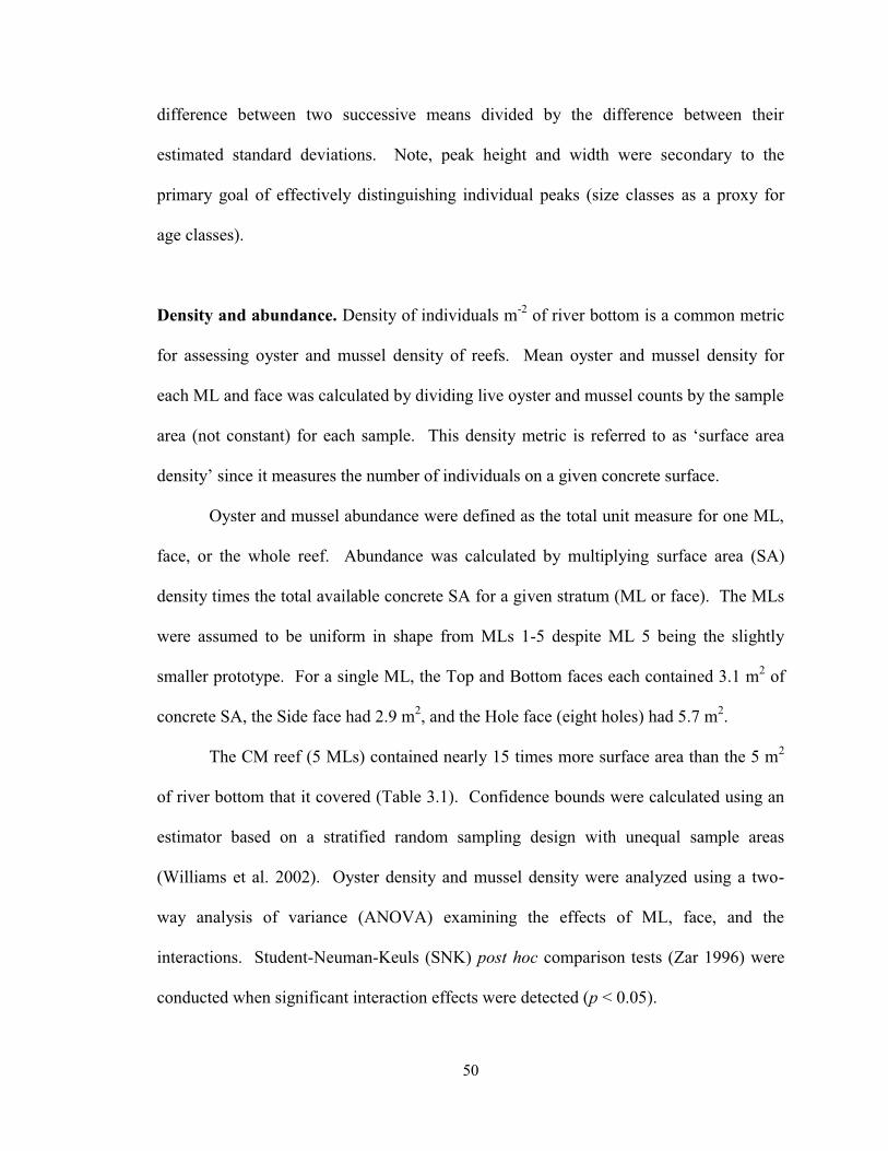
50

difference between two successive means divided by the difference between their

estimated standard deviations. Note, peak height and width were secondary to the

primary goal of effectively distinguishing individual peaks (size classes as a proxy for

age classes).

Density and abundance. Density of individuals m-2 of river bottom is a common metric

for assessing oyster and mussel density of reefs. Mean oyster and mussel density for

each ML and face was calculated by dividing live oyster and mussel counts by the sample

area (not constant) for each sample. This density metric is referred to as ‘surface area

density’ since it measures the number of individuals on a given concrete surface.

Oyster and mussel abundance were defined as the total unit measure for one ML,

face, or the whole reef. Abundance was calculated by multiplying surface area (SA)

density times the total available concrete SA for a given stratum (ML or face). The MLs

were assumed to be uniform in shape from MLs 1-5 despite ML 5 being the slightly

smaller prototype. For a single ML, the Top and Bottom faces each contained 3.1 m2 of

concrete SA, the Side face had 2.9 m2, and the Hole face (eight holes) had 5.7 m2.

The CM reef (5 MLs) contained nearly 15 times more surface area than the 5 m2

of river bottom that it covered (Table 3.1). Confidence bounds were calculated using an

estimator based on a stratified random sampling design with unequal sample areas

(Williams et al. 2002). Oyster density and mussel density were analyzed using a two-

way analysis of variance (ANOVA) examining the effects of ML, face, and the

interactions. Student-Neuman-Keuls (SNK) post hoc comparison tests (Zar 1996) were

conducted when significant interaction effects were detected (p < 0.05).

51

Biomass. The AFDM data for oysters and mussels were used in a length-weight

regression to estimate biomass over the entire CM reef, given that the size structure

produced from all 120 samples was consistent with the size structure produced from the

first 24 samples.

Pathology. A total of 30 (May 2005: 75.6-125.2 mm SH) and 25 (Nov. 2007: 51.4-153.8

mm SH) oysters were haphazardly sampled from the different ML faces for pathology

tests performed within two weeks of sampling. Samples were brought back live and on

ice. The VIMS Shellfish Pathology group processed the oysters and determined presence

and intensity of Dermo (Perkinsus marinus) and MSX (Haplosporidium nelsoni)

parasites. Two methods of Dermo analysis were conducted in 2007, histology and

RFTM (Ray fluid thioglycollate medium). The RFTM method has a lower detection

limit.

Table 3.1: Surface area (SA) and SA-to-River Bottom (RB) ratios of the Steamer Rock (SR) and Concrete Module (CM) reefs.

SR SA (m2) CM SA (m2) Top 16 3.1 Side 4 2.9 Hole --- 5.7

Bottom 16 3.1

Layer-1

36 14.8

Stack-1

236 74.2

SA:RB Ratio 14.75 14.78

52

Steamer Rock Reef

Sampling procedure and design. Adjacent to the CMs, the much larger SR concrete

reef was systematically sampled in April and August 2006. The layout of the reef (Fig.

3.3a-b) is a set of seven concentric rings consisting of 176 seven-layer stacks of bridge

sections (from the Rte. 3 Norris Bridge) covering 2816 m2 of river bottom within a 0.40-

ha footprint. The stacks (Fig. 3.4a) are about 4 m tall and were deployed in 1994 at

depths of 6-8 m in the Lower Rappahannock River off Mosquito Point (Lancaster

County, VA) to create sanctuary oyster and recreational fish reefs. Unlike the CM

survey, these stacks could not be lifted to the surface. Sample collection required

SCUBA diving over two sampling days. We expected that the intermediate concentric

rings (interior habitat) would be more similar to each other than the outer- and inner-most

rings (edge habitat).

The outer- and inner-most rings were sampled in April 2006; the intermediate

rings were sampled in August 2006. Diver safety prompted the decision to sample the

least obstructed (outer/innermost) rings first. Additionally, intense Dermo oyster

infections were more likely late in the summer (August) than in spring (April), especially

in the intermediate rings where bivalve densities were projected to be highest.

53

Figure 3.3: (A) Bathymetic map of the lower Rappahannock River including (B) a mosaic of side scan sonar of the Concrete Module (CM) and Steamer Rock reefs (images credit: Gary Smith, Random Motion, LLC).

54

The method of sample collection included the diver haphazardly selecting a

sample location visually from about 1 m away from the structure to avoid bias,

proceeding towards the location, setting a 0.3-m x 0.3-m sampling device flush against

the site, scraping all encrusted growth into a mesh bag until the concrete was fully

exposed, cinching the bag shut, and sending the sample to the surface using a dive bag

filled with air. For each sample, depth, GPS coordinates of the stack, concentric ring

identity, and the face of the structure (top, side, inner/between slabs) were recorded.

When moving to the next ring, GPS coordinates were once again recorded because

turbidity limited underwater visibility in August within the intermediate rings, increasing

the probability of diver disorientation. A color video camera mounted to the diver’s

helmet was used for quality control (Fig. 3.4b); we could confirm that the area sampled

was 0.3 m x 0.3 m. This video footage was also important because three different divers

conducted the sampling in April. In August, a single diver did the sampling, minimizing

individual-based sampling variance. Sample contents were removed from the mesh bags

into freezer bags, placed in ice-filled coolers, and transported to freezers at VIMS.

Laboratory processing. The same laboratory procedures used for the CM samples were

used for the SR survey, except that disease testing was only completed for the August

2006 samples. Measurements included oyster SH, mussel and mud crab counts, and

bivalve and sponge volume. Population size structure, density, biomass and CI estimates

were calculated as well. General linear models (GLMs) were conducted to test for

differences in oyster SH, abundance, biomass, and CI amongst concentric ring classes;

Kruskal-Wallis rank tests were conducted if tests of normality failed.

55

Figure 3.4: (A) Deployment of the first Steamer Rock reef stacks by McLean Contracting Co., September 1994, (B) Underwater image of an SR reef surface ~10 years post-deployment (image credits: Capt. Robert Jensen).

56

Pathology. A SCUBA diver haphazardly sampled 25 oysters (Aug. 2006: 73.3 – 141.3

mm SH) from the SR stacks for pathology tests. Samples were brought back to the

VIMS Pathology group live and on ice, and were performed within two weeks of

sampling. Presence and intensity of Dermo (Perkinsus marinus) and MSX

(Haplosporidium nelsoni) parasites were determined in the same manner as for the 2007

CM oysters – histology and RFTM (Dermo only).

RESULTS

Concrete Module Reef

Population structure – 2005. Oyster size structure was constructed using a length-

frequency histogram (Fig. 3.5a) that included SHs (mm) for 520 of the 523 live oysters

sampled. Oyster SHs ranged from 7.1-139.0 mm. Peaks were analyzed with FISAT II

(Gayanilo et al. 2002) to delineate individual year classes. Four distinct peaks were

distinguished from the composite distributions (Fig. 3.5a). The Top face of MLs 5 and 4

had the most pronounced oyster spat peak, while MLs 4 and 3 had more large oysters

(Fig. 3.5b). This trend of increasing oyster size with depth was confirmed by diver

observation for MLs 2 and 1. The mussel size structure (Fig. 3.6a) had 4-5 peaks with a

robust size distribution of mussel SHs (9.2-61.0 mm). ML 4 contained the most mussels,

many of which were > 30.0 mm (Fig. 3.6b). The Top face had more large mussels than

the other three faces combined (Fig. 3.6b).

57

Figure 3.5: (A) Population size structure (PSS) of oysters on the concrete modular reef (May 2005) with separation of normal distributions using Bhattacharya’s method of decomposing composite distributions (FiSAT 2: FAO-ICLARM Stock Assessment Tools), (B) Oyster PSS by Module Layer (ML)-face (May 2005).

58

Figure 3.6: (A) Population size structure (PSS) of mussels on the concrete modular reef (May 2005) with separation of normal distributions using Bhattacharya’s method (B) Mussel PSS by Module Layer (ML)-face (May 2005).

59

Population Structure – 2007, 1st Sampling. Oyster size structure (1230 oysters, SH:

3.0-148.4 mm) of undisturbed ML concrete surfaces (Fig. 3.7a) was dominated by the

2006 and 2007 year classes, a trend most pronounced on the Top and Side faces of MLs

3, 2, and 1. To resolve the older year classes, spat (SH < 40.0 mm) were removed,

revealing a size structure trend similar to that seen in 2005 with 3+ YCs present (Fig.

3.7b). Mussel SHs were not recorded in 2007, but ranged from small recruits to full-

sized adults (> 40 mm).

Population Structure – 2007, Resampling. Oyster size structure on concrete surfaces

previously sampled in 2005 (Fig. 3.8a-b) was predictably truncated (oyster SH < 50.0

mm). The Top and Side faces of ML 4 (24 oysters, SH: 15.0-47.3 mm) contained oysters

from the 2005 and 2006 year classes (Fig. 3.8a); ML 3 (430 oysters, SH: 4.0 to 43.0 mm),

although dominated by the Top face, contained oysters from YCs 2005-2007 on all faces

(Fig. 3.8b). Mussels SHs were not recorded in 2007, but were dominated by smaller size

classes.

Density – 2005. Oyster abundance and density differed significantly across face

(ANOVA, F = 30.91, p < 0.0005) with the highest densities on the Top face (Fig. 3.9a).

There was no effect of ML and no ML-face interaction effect. By SA density (Fig. 3.9b),

the Top face contained significantly more oyster than the other faces. For large adult

oysters (SH > 76 mm) there were significant ML (F = 3.56, p = 0.032), face (F = 13.59, p

< 0.0005), and ML-face interaction (F = 4.89, p < 0.0005) effects. Spat abundance varied

significantly only by face (F = 7.59, p < 0.0005).

60

Figure 3.7: (A) Population size structure (PSS) of oysters from undisturbed plots (1st Sampling) on the concrete modular reef (Module Layer (ML) 4 – May 2007; MLs 1, 2, 3 – Nov. 2007), (B) PSS of adult oysters (Shell Height > 40.0 mm), otherwise obscured by strong 2007 oyster recruitment.

61

Figure 3.8: Population size structure of oysters from previously-denuded plots (Resampling) on the concrete modular reef in (A) May 2007 (Module Layer – ML 4) and (B) Nov. 2007 (ML 3).

62

Figure 3.9: Concrete module reef (A) oyster abundance, and (B) surface density, estimates (+ 95% confidence interval) by Module Layer (ML)-face (May 2005).

63

Mussel abundance and density differed significantly across ML (ANOVA, F =

15.33, p < 0.0005), face (F = 233.59, p < 0.0005), and the ML-face (F = 12.07, p <

0.0005) interaction (Fig. 3.10a-b). ML 4 was mussel-dominated with the Top and Hole

faces maintaining much higher surface densities than the Side and Bottom faces (F =

96.63, p < 0.0005); ML 3 had the same relationship between faces (F = 45.86, p <

0.0005). On ML 5 (F = 100.50, p < 0.0005), however, the Hole face was statistically

similar to the Side and Bottom faces. Oyster density was strongly correlated (R2 = 0.54,

p < 0.0001) with mussel density (Fig. 3.11).

Bivalve volume (oyster and mussels) differed significantly across ML (ANOVA,

F = 6.12, p = 0.003), face (F = 102.04, p < 0.0005), and the ML-face (F = 4.32, p =

0.001) interaction. Bivalve volume was similar on ML 4 (F = 55.14, p < 0.0005) and ML

3 (F = 27.37, p < 0.0005); ML 4 > ML 5 (F = 25.83, p < 0.0005) (Fig. 3.12a). By face,

Top > Hole > Side = Bottom (Fig. 3.12a). By SA, the Side, Hole and Bottom faces were

similar; the Top face contained significantly higher bivalve volume (Fig. 3.12b).

Red beard sponge (Microciona prolifera) volume did not substantially vary

between MLs but was more abundant on the Hole and Bottom faces (Fig. 3.13a). By SA,

the Side, Hole and Bottom faces were similar; the Top face contained little to no sponge

(Fig. 3.13b). The sponge and oyster community contained mud crabs, juvenile clams

(Mya arenaria, Mercenaria mercenaria, Macoma balthica, Macoma mitchelli), mussels

(I. recurvum, Mytilus edilus), barnacles, amphipods, isopods, Nereid polychaete worms,

tunicates (Molgula manhattensis), and resident fish including oyster toadfish (Opsanus

tau), gobies (Gobiosoma sp.), blennies, and skilletfish (Gobiesox strumosus). Large

spadefish (Chaetodipterus faber) were also observed near the CM reef.

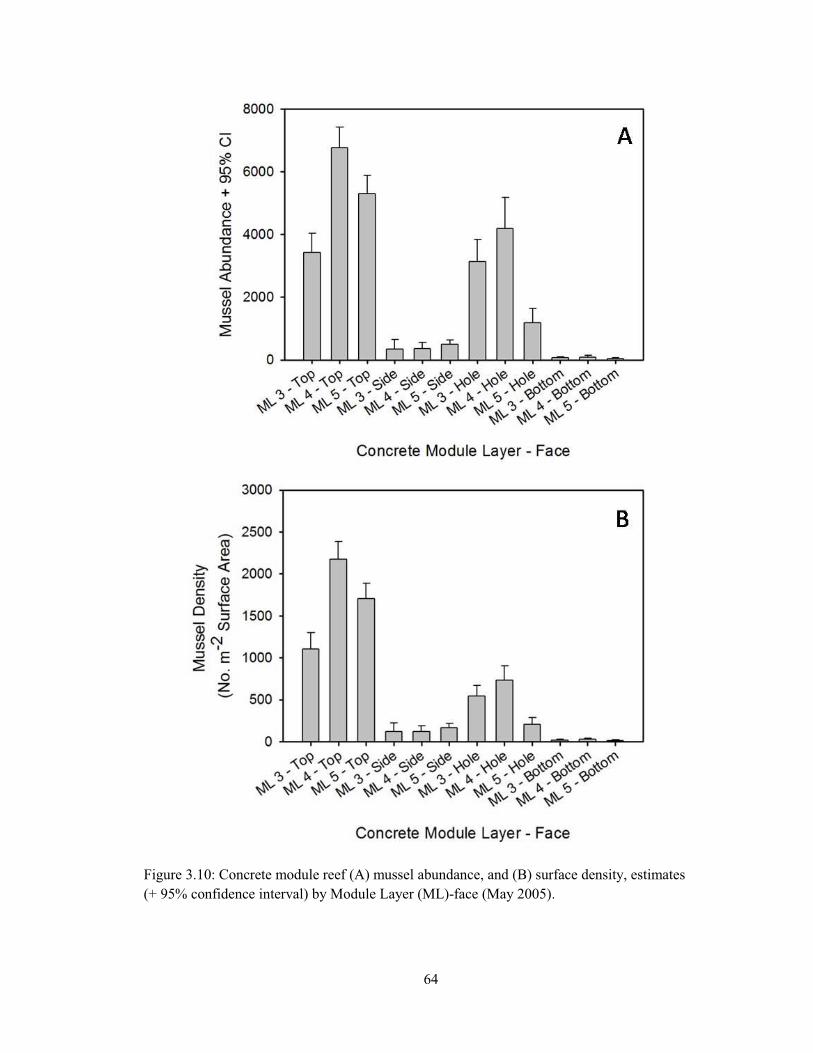
64

Figure 3.10: Concrete module reef (A) mussel abundance, and (B) surface density, estimates (+ 95% confidence interval) by Module Layer (ML)-face (May 2005).

65

Figure 3.11: Regression of live oysters per sample versus live mussels per sample on the concrete module reef (May 2005).

66

Figure 3.12: Concrete module reef (A) bivalve (oyster and mussel) volume, and (B) surface density, estimates (+ 95% confidence interval) by Module Layer (ML)-face (May 2005).

67

Figure 3.13: Concrete module reef (A) sponge volume, and (B) surface density, estimates (+ 95% confidence interval) by Module Layer (ML)-face (May 2005).

68

Density – 2007, 1st Sampling. ML 4 was sampled before the 2007 recruitment event;

MLs 3, 2, and 1 were sampled after that event and should be considered separate from

ML 4. Oyster density differed significantly across ML (ANOVA, F = 7.21, p = 0.001),

face (F = 17.54, p < 0.0005), and ML-face (F = 4.05, p = 0.001) interaction even with ML

4 excluded. The Top face of ML 3 was oyster-dominated with a density more than twice

any other ML-Top (Fig. 3.14a). Across all MLs, the other Top faces as well as the Side

and Hole faces maintained similar oyster densities; the Bottom faces contained the fewest

oysters. By SA, the trends were similar. Thirty-three percent of all oysters measured

were located on other oysters or mussels (Table 3.2a).

Mussel density (Fig. 3.14b) differed significantly across ML (ANOVA, F =

25.58, p < 0.0005), face (F = 64.77, p < 0.0005), and ML-face (F = 24.91, p < 0.0005)

interaction, and followed a similar trend to oyster density (ML 3-Top was more than

three times higher than other Top faces) except that the Top > Hole faces, and both Side

and Bottom faces maintained low densities. Also, mussel density of ML 3 was greater

than MLs 4, 2, and 1. By SA, the trends were similar.

Bivalve volume (oyster and mussels) differed by face only: Hole and Top faces

were greater than the Bottom and Side faces (Fig. 3.14c). By SA, the trends were similar.

Oyster volume (live oysters only) did not significantly differ by ML or face (Fig. 3.14d).

Sponge volume differed by face only with the Hole greater than the Top face (Fig. 3.14e).

By SA, there was no statistical difference by ML or face. Mud Crab density was higher

on MLs 2 and 3 than MLs 4 and 1; and higher in the Hole than the Top face (Fig. 3.14f).

By SA, there was no statistical difference by ML or face.

69

Figure 3.14: Concrete module reef (1st sampling) (A) oyster and (B) mussel abundance, (C) bivalve, (D) live oyster, and (E) sponge volume (L), and (F) mud crab abundance estimates (+ 95% confidence interval) by Module Layer (ML)-face (May and November 2007).

70

Table 3.2: (A) Percentage of oysters cohered to other oysters or mussels by Module Layer-face for undisturbed (1st Sampling) and (B) previously-denuded (Resampling) plots (May and November 2007).

2007 CM

1st Sampling Top Side Hole Bottom Total

ML 4 2/20 3/3 4/14 3/10 12/47; 25.5%

ML 3 38/219 3/81 19/54 6/22 66/376; 17.6%

ML 2 87/159 31/210 70/108 10/30 198/507; 39.1%

ML 1 69/123 61/173 4/11 0/0 134/307; 43.6%

Total 196/521; 37.6% 98/467; 21.0% 97/187; 51.9% 19/62; 30.6% 410/1237; 33.1%

A.

2007 CM

1st Sampling Top Side Hole Bottom Total

ML 4 8/11 0/0 1/11 1/2 10/24; 41.7% ML 3 41/260 4/95 29/50 2/14 76/419; 18.1% Total 49/271; 18.1% 4/95; 4.2% 30/61; 49.2% 3/16; 18.8% 86/443; 19.4%

B.

Density – 2007, Resampling. As ML 4 and 3 were resampled in May and Nov. 2007,

respectively, they are considered separately. For ML 3, the Top face recruited oyster spat

at a higher density than the Side and Bottom faces. The Top and Hole faces maintained

the bulk of ML 4’s oyster abundance, but at an order of magnitude lower than ML 3,

which emphasizes the strength of the 2007 oyster recruitment class (Fig. 3.15a). By SA,

the trends were similar. Of all oysters measured, 19 % were on other oysters or mussels

(Table 3.2b).

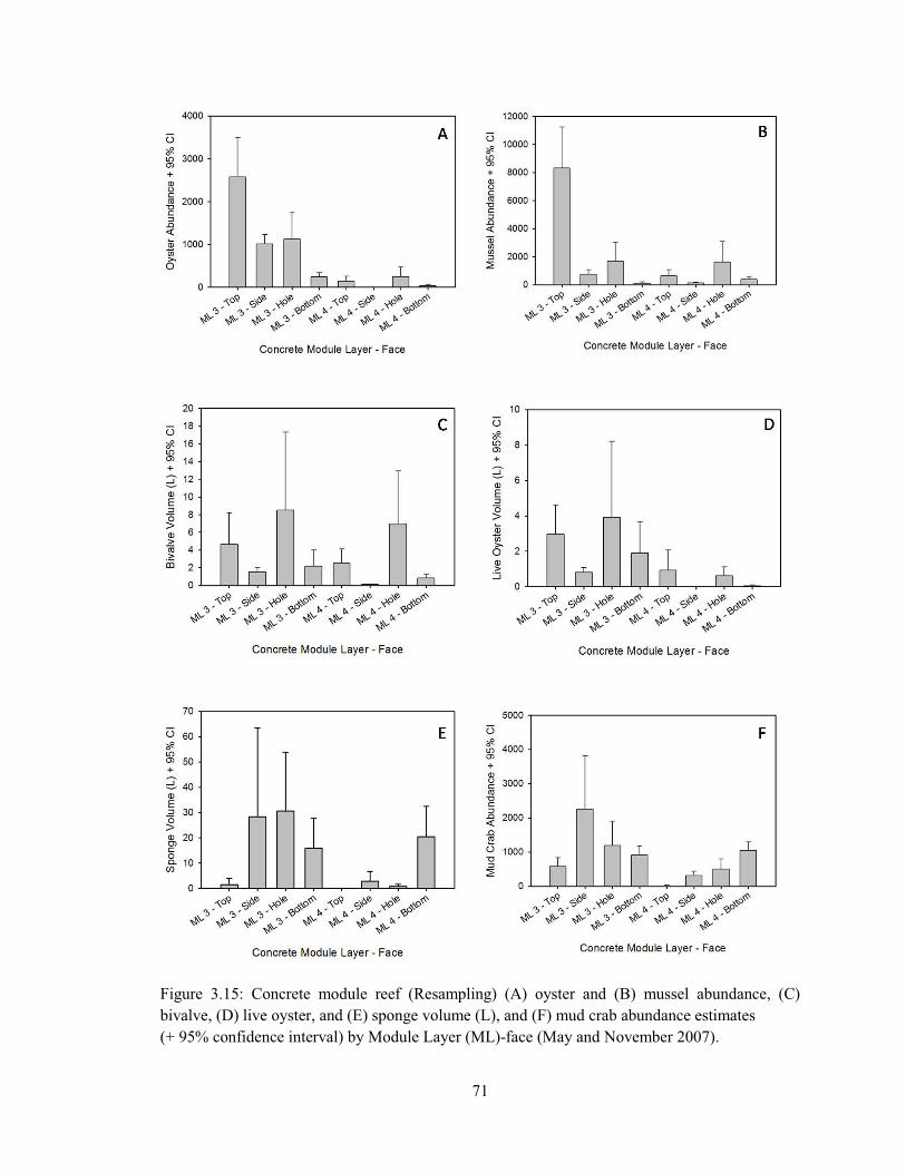
71

Figure 3.15: Concrete module reef (Resampling) (A) oyster and (B) mussel abundance, (C) bivalve, (D) live oyster, and (E) sponge volume (L), and (F) mud crab abundance estimates (+ 95% confidence interval) by Module Layer (ML)-face (May and November 2007).

72

Mussel recruitment/density (Fig. 3.15b) followed the same trend as oyster density,

similar to the trend observed in 2005. One notable similarity between MLs 4 and 3 was

the high mussel density on the Hole and Bottom faces, but not on the Top and Side faces.

By SA, the trends were similar.

Bivalve volume (Fig. 3.15c) of ML 3 was greater on the Top face; ML 4’s Hole

and Top faces were greater than the Side and Bottom faces (Side > Bottom). By SA, no

statistical difference was detected for ML 3; the Side face of ML 4 maintained lower

bivalve volume than the other faces. Oyster volume (live oysters only) followed the

same trends (Fig. 3.15d).

Sponge volume (Fig. 3.15e) was greater on the Hole face of ML 3 and Bottom

face of ML 4. By SA, no statistical difference was detected for ML 3; the Bottom face of

ML 4 maintained greater sponge volume than the other faces.

No statistical difference was detected for ML 3’s mud crab density (Fig. 3.15f).

For ML 4, the Bottom > Side > Top face; by SA, Bottom > Side = Hole > Top face.

Biomass – 2005. Sixty-two oysters and 138 mussels throughout the full size range (SH)

were processed to yield reliable estimates of oyster (Fig. 3.16a) and mussel (Fig. 3.16b)

biomass with the regression model of log AFDM versus log SH. Oyster biomass differed

significantly across ML (ANOVA, F = 4.06, p = 0.020), face (F = 10.51, p < 0.0005), and

ML-face (F = 2.81, p = 0.014) interaction with the highest densities on the Top and Hole

faces (Fig. 3.17a). ML 4 (F = 3.98, p = 0.015) and ML 3 (F = 7.00, p = 0.001) varied

significantly by face.

73

Figure 3.16: Regression models of log AFDM (g) versus log SH (mm) for (A) oyster and (B) mussel biomass estimation on the concrete module reef (May 2005).

y = 2.3713x – 4.6317 R2 = 0.846

y = 3.0402x – 5.5464 R2 = 0.948

74

Figure 3.17: Concrete module reef (A) oyster and (B) mussel biomass, and (C) oyster and (D) mussel biomass surface area density estimates (+ 95% confidence interval) by Module Layer (ML)-face (May 2005).

75

Mussel biomass (Fig. 3.17b) differed significantly across ML (ANOVA, F = 13.34, p =

0.001), face (F = 92.77, p < 0.0005), and ML-face (F = 6.07, p = 0.004) interaction. ML 5

(F = 18.31, p = 0.008), ML 4 (F = 103.31, p < 0.0005) and ML 3 (F = 13.20, p = 0.015)

varied significantly by face. Across all MLs, mussel biomass ranked the same: Top >

Hole > Side > Bottom. By SA, the Top face maintained much higher oyster and mussel

biomass than the other faces (Fig. 3.17c-d).

Biomass – 2007, 1st Sampling. Sample variance was much higher for oyster biomass

estimates than oyster density. The face (GLM, F = 4.27, p = 0.007), but not ML (F =

1.82, p = 0.167) or ML-face (F = 2.05, p = 0.067) interaction effects, significantly

influenced oyster biomass. Oyster biomass increased with depth, and biomass was higher

on Top and Hole faces (Fig. 3.18a-b). Higher oyster density on the Top face of ML 3 (>

2 times MLs 2 and 1) did not equate to higher oyster biomass; oyster biomass on ML 3’s

Top face was roughly half that of the Top faces of ML 2 and ML 1. Oyster size structure

for the three Top faces revealed a greater number of spat on ML 3 with fewer adults; ML

2 and ML 1 had half as many spat, but many more adults.

Biomass – 2007, Resampling. Oyster biomass on resampled plots of ML 3 varied by

face (Top > Side > Bottom; Top = Hole); undisturbed plots did not differ. Similarly, ML

4 maintained higher oyster biomass on the Hole and Top faces than on the Bottom and

Side faces (Fig. 3.19a). By SA, these trends shift slightly, but reflect variable oyster

recruitment patterns to recently denuded surfaces (Fig. 3.19b).

76

Figure 3.18: Concrete module reef (1st Sampling) (A) oyster abundance, and (B) surface density, estimates (+ 95% confidence interval) by Module Layer (ML)-face (May and November 2007).

77

Figure 3.19: Concrete module reef (Resampling) (A) oyster abundance, and (B) surface density, estimates (+ 95% confidence interval) by Module Layer (ML)-face (May and November 2007).

78

Pathology – 2005. Of the 30 large oysters processed for disease assessment, none were

infected with MSX and 30% were infected with Dermo. Of the infected with Dermo,

none had serious infections (4 infections were light, 5 were rare, 21 negative). There was

positive correlation (Regression, R2 = 0.14, p = 0.043) between individual oyster size and

Dermo intensity rank (Fig. 3.20a). The following pathogens were found in one or more

oysters: Nematopsis (1), Rickettsia-like organisms (1), Sphenophyra-like ciliates (11),

Stegotricha spp. ciliates (1), and viral gametocytic hypertrophy (1).

Pathology – 2007. Of the 25 oysters processed for disease assessment, six were infected

with MSX and 84% were infected with Dermo.

P. marinus, RFTM: 84% prevalence (21/25 positive), intensities: 0-16-3-2 (Heavy-Moderate-Light-Rare) P. marinus, histology: 56% prevalence (14/25 positive), intensities: 0-2-8-4 H. nelsoni, histology: 24% prevalence (6/25 positive), intensities: 1-1-2-2 The weighted prevalence of P. marinus, calculated from RFTM data, would be 2.08,

indicating that "serious mortality" should be occurring. Note however that no infections

were "heavy" by RFTM, and just 4 were of intensity greater than "light-moderate" – a

category collapsed together with the "moderates" in generating the 0-16-3-2 intensity

count, and the weighted prevalence value. By RFTM metrics, therefore, 21 of 25 oysters

were no more than "light-to-moderately" infected and so were probably generally

healthy. The histology data suggest the proportion of healthy (with respect to P.

marinus) oysters was probably even higher. Just one or two additional oysters, at most,

were detrimentally affected by H. nelsoni. There was no correlation (Regression, R2 =

0.07, p = 0.220) between individual oyster size and Dermo intensity rank (Fig. 3.20b)

across a very wide size range.

79

Condition index. Sixty-six oysters throughout the full range of SHs were processed to

yield three CIs that (Rainer and Mann 1992). CI results for the 2005 CM oysters were

CI1: 11.9 +/- 0.4; CI2: 8.4 +/- 0.3; CI3: 5.3 +/- 0.3 (+/- 1 SEMean)), indicating that these

oysters were healthy. Oyster condition was not tested by ML, but was significantly

influenced by face for CI3 (F = 4.81, p = 0.005) and not CI1 (F = 0.02, p =0.997) or CI2

(F = 0.07, p < 0.975). In addition, there was no correlation between oyster condition and

SH.

Steamer Rock Reef

Population structure. Steamer Rock oyster size structure (Fig. 3.21) was robust

throughout the full size range, containing a minimum of five year classes (2001-2005).

Oyster SHs ranged from 5.0-122.0 mm for the Outer Ring (132 oysters), 12.6-128.7 mm

for the Inner Ring (54 oysters), and 17.4-142.5 mm for the Intermediate Rings (171

oysters). Mussel SHs were not recorded in 2007, but ranged from small recruits to full-

sized adults (> 40 mm).

Density. Oyster density (ANOVA, F = 1.13, p = 0.336) (Fig. 3.22a) and live mussel

volume (F = 1.93, p = 0.162) (Fig. 3.22b) did not significantly differ between the

Intermediate, Outer or Inner rings of concrete stacks. Mussel (F = 6.69, p = 0.004) and

mud crab density (F = 8.71, p = 0.001) (Fig. 3.22c), as well as oyster volume (F = 7.68, p

= 0.002) (live oysters only; Fig. 3.22b), were greater on the Intermediate rings than the

Outer ring (Inner = Outer ring).

80

Figure 3.20: Dermo intensity rank versus oyster shell height from the concrete module reef in (A) May 2005 and (B) November 2007.

81

Biomass. Oyster biomass (Fig. 3.22b) did not significantly differ between the

Intermediate, Outer and Inner Ring strata (ANOVA, F = 0.11, p = 0.894). Two hundred

thirty nine oysters (Outer – 85; Inner – 51; Intermediate – 103 oysters, respectively)

throughout the full range of SHs were processed to yield reliable estimate of oyster

biomass (Fig. 3.23a-c) across all three strata.

Figure 3.21: Population size structure of oysters on the Outer, Inner, and Intermediate Rings of the Steamer Rock reef complex (2006).

Pathology. Of the 25 oysters processed for disease assessment, none were infected with

MSX and 96% were infected with Dermo.

P. marinus, RFTM: 96% prevalence (24/25 positive), intensities: 1-16-4-3 P. marinus, histology: 56% prevalence (14/25 positive), intensities: 0-1-4-9 H. nelsoni, histology: 0/25 positive

82

The weighted prevalence of P. marinus, calculated from RFTM data, would be 2.34,

indicating that "serious mortality" should be occurring. Note, however, that just one

infection was "heavy" by RFTM, and just 8 were of intensity greater than "light-

moderate.” By RFTM metrics, therefore, 17 of 25 oysters were no more than "light-

moderately" infected and so were probably generally healthy. The histology data suggest

the proportion of healthy oysters was probably even higher. There was no correlation

(Regression, F = 0.03, p = 0.873) between individual oyster size and Dermo intensity

rank (Fig. 3.24).

Condition index. Two hundred forty six oysters throughout the full range of SHs were

processed to yield three CIs across all three strata (Outer – 82; Inner – 62; Intermediate –

102 oysters). Oyster condition for the Outer (CI1: 11.7 +/- 0.3; CI2: 8.3 +/- 0.3; CI3: 3.5

+/- 0.1) and Inner (CI1: 11.1 +/- 0.4; CI2: 7.7 +/- 0.3; CI3: 3.6 +/- 0.2) stacks sampled in

April 2006 were similar to each other and to the 2005 CM reefs. The Intermediate stacks

sampled in August 2006 contained oyster with lower average condition (CI1: 9.0 +/- 0.3;

CI2: 6.6 +/- 0.2; CI3: 2.5 +/- 0.1).

83

Figure 3.22: Oyster (A) density (m-2 river bottom - RB) and biomass (g AFDM m-2 RB), (B) live oyster, total oyster, and live mussel volume (L m-2 RB), and (C) mussel and mud crab density (m-

2 RB ) on the Outer, Inner, and Intermediate Rings of the Steamer Rock reef complex (2006).

84

Figure 3.23: Regression models of AFDM (g) versus log SH (mm) for oyster biomass estimation on the (A) Outer, (B) Inner, and (C) Intermediate Rings of the Steamer Rock reef complex (2006).

y = 2.62x – 5.0146 R2 = 0.907

y = 2.5256x – 5.0062 R2 = 0.890

y = 2.7317x – 5.1797 R2 = 0.880

85

Figure 3.24: Steamer Rock oyster Dermo intensity rank versus oyster shell height (mm), August 2006.

DISCUSSION

Concrete Module Reef

Population structure. The 2005 CM oyster size structure could contain a maximum of

four year classes since the modular reef system had been deployed 4.5 years prior to

sampling. Upon plotting the size-frequency data, visual estimates suggested that there

were at least three, if not four, year classes present. To help interpret possible factors

affecting the patterns we observed, Rappahannock River discharge data, oyster density

estimates from the Commonwealth of Virginia’s Marine Resources Commission Dive

Survey, and data from the Virginia Dredge Survey (Southworth et al. 2003, Southworth

86

et al. 2002) were examined (Fig. 3.25). The discharge data showed low-flow, drought

(high salinity) conditions in 2001 and 2002 – good for oyster recruitment (larval retention

is protracted) but bad for disease-associated mortality (Albright et al. 2007). 2003 and

2004 were high flow (wet), low salinity years – conditions conducive to adult oyster

survival and lower oyster recruitment. In theory, two years of good recruitment with high

disease pressure would not be an issue for young oysters with Dermo; P. marinus does

not usually attack young oyster in Chesapeake Bay, in contrast to MSX, and natural

spatfall can be grown 1 or 2 years before the animals acquire the disease (Andrews and

Ray 1988). In order to thrive through adulthood, though, these growing oysters would

need a lower salinity environment or some level of disease resistance. Fortunately, 2003

and 2004 brought increased precipitation and, thus, diminished disease pressure. The two

peaks representing 2003 and 2004 are pronounced with the high peak for 2004 and

smaller peak for 2003, with oysters that had undergone an extra year of natural mortality.

Despite two years of recruitment failure in the rest of the Rappahannock River Estuary

(Wesson Dive Survey 2005 update; Fig. 3.25), the CMs experienced moderate

recruitment.

Although settlement throughout the Rappahannock River system was low from

2003-2005, 2006 and 2007 were good recruitment years, only slightly less than 2001 and

2002 (Southworth et al. 2008a). The CMs received these recruits on undisturbed and

denuded surfaces in very high numbers. Recovery of previously-cleared concrete

surfaces, as well as a persistent population of larger adults, was encouraging.

87

Figure 3.25: Rappahannock River discharge (ft3 s-1) at Fredericksburg, VA and oyster density (m-2) on Parrott’s Rock, Lower Rappahannock River, 2000-2004 (VMRC Annual Dive Survey).

At first glance, mussel size structure (2005) appeared to be one continuous

distribution possibly indicating successive year classes of similar levels of recruitment

and survival. However, closer scrutiny and the application of FISAT II revealed 4-5

separate size classes. The largest peak, however, was the 40-50 mm mussel size class.

Assuming that each peak represents one year class, this large peak coincides with the

2001 recruitment event noted within the CM oyster population as well as other surveyed

Rappahannock River populations (Southworth et al. 2008a). We did not see a large spike

of small mussels in spring of 2005 or 2007, but the Nov. 2007 sampling captured the

strong recruitment from preceding months.

88

Oyster and mussel size structure varied by ML and face. The protected Top faces

of MLs 4 and 3 in 2005, and the MLs 3, 2, and 1 in 2007, contained more oysters and

mussels throughout the full size range than the uppermost MLs. The Bottom faces

supported fewer mussels amongst a thriving sponge community. Hole and Side faces

contrasted more for mussels than oysters. The primary benefit of having a diversity of

concrete surface area (vertical/horizontal and protected/exposed) was that the oyster-

mussel-sponge community could develop under heterogeneous conditions, making the

reef community more diverse, stable, and resilient.

Density and biomass. The CM reef estimates of density were high for oysters (991 +/-

284 m-2 river bottom (+/- 95% confidence interval); 2191 +/- 777) and mussels (8433 +/-

1581; 6984 +/- 1822). These densities are comparable to the highest on restored oyster

shell reefs in Chesapeake Bay (Nestlerode et al. 2007, Schulte et al. 2009). The estimates

of biomass (g AFDM m-2 RB) were also high for oysters (1584 +/- 621; 715 +/- 443) and

mussels (1117 +/- 235; not available for 2007). Bivalve volume (L m-2 RB), an important

measure of reef growth and persistence, was very high for an oyster restoration reef (77.7

+/- 18.2; 34.5 +/- 11.8). Live oyster volume (12.9 +/- 8.0 L m-2 RB) and mud crab

density (3414 +/- 1292 m-2 RB) was also recorded in 2007. The apparent decline in the

oyster reef from ~78 L m-2 RB in 2005 to 34.5 L m-2 RB in 2007 has multiple possible

explanations: (1) Oyster density was actually higher in fall 2007 than in May 2005, but

increased adult oyster mortality and reduced oyster condition after two dry, disease-

intense years (relative to pre-spawned oysters sampled in May 2005 after two wet years)

exacerbated the difference in bivalve volume (Austin et al. 1993), (2) bivalve (oyster and

89

mussel) populations experience cycles related to salinity and temperature with a lag in

response time (Austin et al. 1996), and (3) the oyster-mussel reef has, in fact, entered a

regressive period from which it may not recover (Ardizzone et al. 1989).

As the oyster community structure developed on the CMs, a higher proportion of

the oyster population was found on live or dead oysters or mussels. The percentage of

oysters living on other oysters or mussels (Table 3.2a-b) increased with depth, likely due

to oyster larval tendency to settle towards the bottom where luminosity is lower and less

direct (Kennedy et al. 1996). By face, the Hole face had the highest proportion

(undisturbed: 52 %; denuded: 49 %) of oysters on other oyster or mussels. The Top faces

(38 %) and Bottom faces (31 %) of undisturbed plots, maintained a much higher

proportion of oysters on other oyster or mussels than the Top (18 %) and Bottom (19 %)

faces of denuded plots.

Sponge volume (L m-2 RB) was more variable (31.3 +/- 20.6; 34.2 +/- 26.7)

across the CM reef strata, with the majority present on the Hole and Bottom faces.

Sponge grew densest in close proximity to a crevice or crack and may gain a spatial

refuge when small and grow out from a strong foundation where even occasional high

current and abrasion by large fish would not cause them to be dislodged. Sponges

compete for space with oysters and mussels, though, in a defensive space utilization

strategy (Karlson 1978). Oysters can sustain some level of sponge overgrowth, but some

‘boxes’ (whole dead oyster shells) were found with a film of sponge on them. At the

very least, sponge inhibits settlement of competent oyster larvae where they have

overgrown suitable substrate (Gunter 1955). Only one oyster (spat, 2007) was found

growing on sponge. Alternative oyster settlement sites included live mussels, or their

90

byssal threads (only very small oysters). Mussels appear to be more easily overgrown

than oysters, but can, although in much lower density, adhere to a living sponge (byssal

thread attachment) and survive. A sponge has the highest surface area per individual of

all biota on the reef, but appears limited in its capacity to support many mussels.

One strong year class of oyster or mussel can dominate a population for years.

Broadcast spawning is most efficient when adults are at high densities (Mann and Evans

1998), populations are hydrodynamically linked (Lipcius et al. 2008), quality substrate is

available (Schulte et al. 2009), and ambient conditions, such as salinity (Kennedy et al.

1996), are optimized. Ctenophores can inhibit oyster larval abundance (Breitburg and

Fulford 2006). In 2006 and 2007, river conditions were the best they had been since

2001-2002 and the Rappahannock River adult oyster population (as well as populations

in many other subestuaries) responded (Southworth et al. 2002, 2003). In 2007,

settlement was relatively high and among the highest over the previous 15 years of

monitoring (Southworth et al. 2008a). In sampling the CM reefs in May and November

2007, distinctions between the 2006 and 2007 recruitment events were possible. Oyster

and mussel abundance were seven- and ~three-fold greater, respectively, on ML 3 than

ML 4. However, oyster and mussel biomass were equal between MLs 3 and 4, indicating

evidence that the abundance discrepancy was due, in large part, to the strong 2007

bivalve year classes.

The resampling (2007) of previously denuded surfaces (2005) provided additional

support for this hypothesis – oyster and mussel abundance were ten- and four-fold greater

on ML 3 than ML 4. Furthermore, the ratios of oyster (ML 3 – 1:1; ML 4 – 1.5:1) and

mussel (ML 3 – 1.3:1; ML 4 – 2:1) abundance on undisturbed versus previously-denuded

91

plots were positive indicators of recovery of cleared surfaces in fewer than three years.

The 3:1 ratio of oyster biomass (ML 3:ML 4) on previously-denuded surfaces highlights

the strong influence of the 2007 year class.

Large adult (> 75.0 mm SH) oyster abundance (2005) varied by face and ML,

with highest abundance on the middle layer (ML 3). Spat were significantly impacted by

face and covaried with juvenile abundance possibly indicating preferential oyster larval

settlement on surfaces occupied by conspecifics, and higher subsequent spat survival into

the young adult oyster (juvenile) size class (Bartol and Mann 1999, Bartol et al. 1999).

The resident oysters may have served as substrate, provided refuge, or both. However,

there was no covariance of large oysters with spat. Crowding as the reef matures in that

region of the reef, due to growth of oysters, mussels, sponges, bryozoans, and tunicates,

may limit settlement substrate, increase the probability of larval loss due to the high

density of filter feeders (Thorson 1966, Woodin 1976, Peterson and Black 1987, Osman

et al. 1992, Tamburri et al. 2007), or increase post-set mortality due to elevated predator

densities (Newell et al. 2000). Nevertheless, recruitment potential on these reefs may

decrease while still maintaining a high density of large adult oysters. Schulte et al.

(2009) showed a similar relationship between oyster adults and spat on the restored shell

reefs of the Great Wicomico River, whereby at high adult densities (> 800 oysters m-2

RB) the trend of increasing spat shifted downward.

A similar relationship exists between mussels and oysters. They share a

facilitative relationship at low to medium density (early stage of reef development) and

greater space and resource competition at higher densities (as the reef stabilizes and

matures) (Dittman 1990, Bruno and Bertness 2000, Witman and Dayton 2000). This

92

relationship was most pronounced on the Top faces. On some oyster grounds in

Chesapeake Bay, I. recurvum forms dense colonies attached to live oysters. Engle and

Chapman (1952) found that oysters with attached mussels were characteristically more

elongate than were mussel-free controls. More meat, relative to shell, was produced in

mussel-free oysters, with these oysters having a condition factor about 28 % better than

the oysters with attached mussels. Spatial competition occurs at high bivalve densities,

but the outward and upward growth of oysters and mussels can reduce this effect. These

findings support the assertion that the CMs had experienced the ‘pioneer stage’ of

succession and persisted through the stage of invertebrate (oyster and mussel) dominance

(Badalamenti et al. 2002).

The oyster and mussel community on the Top face of the uppermost ML (ML 5 in

2005; ML 4 in 2007) was the least productive. Conversely, the base ML’s Bottom face is

lost due to burial in the sediment, and the Top and Hole faces become buried in

pseudofeces over many years, eventually killing most of the organisms attached to them.

Overall, the base ML is not fully lost as an oyster-mussel community, but its lower

productivity should be factored into calculations of expected benefits from production of

such structures as restoration or mitigation reefs. Continued monitoring of the CMs will

reveal whether the bivalve assemblage has reached a stable state, will start to degrade, or

will continue to a more diverse, climax community.

Pathology and condition. MSX and Dermo were the two main pathogens of interest. By

2005, MSX had become relatively rare in the Chesapeake Bay after two years (2003-

2004) of heavy streamflows and depressed salinities (Carnegie and Burreson 2005)

93

indicating that neither parasite (P. marinus and H. nelsoni) was seriously impacting

oyster populations in the survey area (included the Rappahannock River), and that

mortality caused by these parasites in 2004 was probably low. In addition, disease

pressure and mortality should have been low until at least through summer 2005, and

perhaps longer if normal rainfall and streamflow conditions were slow to return. From a

disease-perspective, these oysters were healthy.

Condition indices of the 2005 CM oysters were high. Elevated oyster condition

following two years (2003-2004) of increased precipitation, with the resultant increase in

river discharge, had been also occurred in the Rappahannock River in the 1970s and

1980s, not far from where the SR reefs reside (Austin et al. 1993). These patterns were

further explained by a significant relation between spat count and the Palmer Drought

Index (PDI), which is published monthly by the Office of the Virginia State Climatologist

at University of Virginia (Austin et al. 1996). The drought index is a combination of

rainfall, soil type, and evapotranspiration. The responses of the spatfall to changes in the

PDI were reflected both in the 1960s, as conditions evolved from "damp" to "drought,"

and in the more prolonged "drying" period of the mid-1970s to mid-1980s, as the spatfall

reflected a short and a longer period of increased set. The cyclic nature of the PDI results

in rapid and cyclic changes in the spatfall (Austin et al. 1996).

Studies in the upper part of Chesapeake Bay (Engle 1951), in Canada (Medcoff

and Needler 1941), and in Louisiana (Hopkins et al. 1954) showed CI cycles similar to

those in the Rappahannock River (Austin et al. 1993). The finding of no difference

between face and ML may indicate that, although face can affect oyster density, the

influence of river discharge may overwhelm the anticipated effects of bivalve density on

94

oyster condition. Another possible explanation may be that water flow around, and

circulation through, the reef provides ample food delivery and sediment relief irrespective

of oyster location.

Disease assessment was conducted for 25 additional oysters from the 4 November

2007 sampling. Unlike the oysters tested from May 2005, these oysters had experienced

two seasons of relative drought, were in a post-spawning recovery state, and were

sampled at peak Dermo/MSX prevalence and intensity. By convention, these oysters

should have been in poor condition. However, the RFTM metrics and histology revealed

that 21 of 25 oysters were no more than "light-to-moderately" infected and so were

probably generally healthy. The histology data suggest the proportion of healthy (with

respect to P. marinus) oysters was probably even higher. Just one or two additional

oysters, at most, were detrimentally affected by H. nelsoni. Thus, the prognosis for the

CM oyster population’s sustainability is good.

Steamer Rock Reef

Population structure. Oyster size structure was robust throughout the full size range,

containing a minimum of five year classes (2001 – 2005). More than half of all oysters

sampled were large adult oysters (> 75 mm SH) which indicates: (1) a hardy broodstock

with some level of disease resistance, (2) adequate shell accretion (volume is the proxy

for reef persistence), and (3) longevity. The largest peak was between 80-100 mm SH

and represented the strong year classes of 2001 and 2002. The smaller peaks (< 80 mm)

represent the 2003-2005 year classes both the SR and CM reefs recruited oysters during

95

these years. Lighter recruitment during wet years was apparently important for oyster

reef stability.

An important observation for SR was that the 2006 oyster survey detected five

year classes (presumably 2001-2005). Since the reefs were deployed in 1994, an entire

generation of oyster likely recruited, had grown and died through the late 1990s. The

reefs persisted and grew. This finding of reef longevity and durability is critical. The

population quantified here was the second generation, indicating that alternative substrate

reefs can persist through years of poor recruitment and subsequent coverage by fouling

species and still flourish when more favorable conditions emerge.

Density and biomass. Oyster density, biomass, and bivalve volume did not significantly

differ between the Intermediate, Outer or Inner rings of concrete stacks. The

Intermediate stacks had higher densities and volumes. These differences were

exacerbated for estimates of total reef abundance since the Intermediate stacks made up

71 % of the SR reef. Across 176 stacks covering approximately 0.4 ha of river bottom,

we estimate a population of 4.818 +/- 0.927 million oysters (SEM), 30.055 +/- 6.116

million mussels, and 2.713 +/- 0.965 million mud crabs, with a total oyster biomass of

4242 +/- 1112 kg AFDM, a total oyster volume of 312,260 +/- 86,210 L, and a total

mussel volume of 113,360 +/- 24,890 L. The CM reef design is the more efficient use of

space (SA); however, the SR reef complex also supports a vibrant oyster reef community

comprised of high bivalve and sponge densities and volumes in an otherwise substrate-

limited system; these reef structures provide stable and heterogeneous settlement

surfaces.

96

By SA, the SR and CM reefs are both productive (Table 3.3), especially when

compared to other restored shell reef sites in the Rappahannock River (Drumming

Ground Reef, Parrot Rock Reef). These restored shell reefs experienced low (2005) to

marginal (2006/2007) oyster densities at least one order of magnitude lower than the

SR/CM reefs (Southworth et al. 2006, 2007, 2008a). Poaching of oysters is still a

problem on many Chesapeake Bay restored oyster shell reefs and may affect the recorded

densities for reefs such as Drumming Ground or Parrot Rock reefs. The benefit of large,

alternative concrete oyster reefs is the impracticality of poaching oysters off of them.

Thus, our population estimates are not confounded by a potential negative (poaching)

bias (a genuine concern for restored shell reefs) and the reefs are left to function and

progress naturally.

Pathology and condition. The effect of Dermo and MSX on SR oysters collected in

August 2006 was similar to oysters tested from the CM reefs in November 2007. By

RFTM metrics and histology, 17 of 25 oysters were no more than "light-to-moderately"

infected and so were probably generally healthy. Once again, the histology data suggest

the proportion of healthy (with respect to P. marinus) oysters was probably even higher.

No MSX infections were detected. The SR reef pathology data suggest that the

population of oysters living on these lower Rappahannock River reefs tolerate the effects

of disease, with greater than half of the oysters growing into the large oyster size class (>

75 mm SH). To date, this study is the first to document disease resistance on subtidal

alternative substrate oyster reefs. This emergence of disease resistance has been

documented in the Great Wicomico River (Carnegie et al. 2008, Schulte et al. 2009),

97

upper and lower Lynnhaven River (Dissertation Chapters 3 and 4), and Elizabeth River

(Burke and Schulte, unpublished data); each of these examples (including the SR and

CM reefs) have been fully-protected sanctuary oyster populations where harvest activities

cannot remove the largest, fastest-growing oysters. Selective premature harvest of

oysters on unprotected reefs may result in the suppression of disease resistance

development (Munch et al. 2005, Edeline et al. 2007).

Table 3.3: Density and surface area density metrics for the Concrete Module (2005, 2007) and Steamer Rock (2006) reef complexes.

Reef, Year (+/- 95% CI)

Oyster Density

(m-2

River Bottom)

Oyster Biomass

(g AFDM m-2

River Bottom)

Bivalve Volume

(L m-2

River Bottom)

Oyster SA

Density

(m-2

)

Oyster Biomass

SA Density

(g AFDM m-2

)

Bivalve Volume

SA Density

(L m-2

)

Concrete Modules,

2005 991 (284) 1584 (621) 77.7 (18.2) 284 (82) 439 (168) 21.8 (4.8)

Steamer Rock, 2006

1575 (386) 1459 (451) 126.1 (32.5) 107 (26) 99 (31) 8.6 (2.2)

Concrete Modules,

2007 2191 (777) 715 (443) 34.5 (11.8) 626 (214) 183 (112) 8.7 (3.0)

98

Figure 3.26: Total oyster (A) abundance and biomass (g AFDM m-2 RB), (B) live oyster, total oyster, and live mussel volume (L), and (C) mussel and mud crab abundance on the Outer, Inner, and Intermediate Rings of the Steamer Rock reef complex (2006).

99

CONCLUSIONS

Throughout the Chesapeake Bay, substrate limitation has been a considerable

issue. Many areas have also contended with significant recruitment limitation. Much of

the Rappahannock River is heavily silted, experiences annual summer hypoxia, and has

low recruitment. The SR and CM reef systems were deployed to a subtidal depth of 7 m

upon solid, sandy bottom at a location that experiences strong semidiurnal tidal currents.

These site-specific characteristics likely reduce siltation, reef subsidence, and hypoxic

stress, but increase flow of plankton-rich water, as well as increase exposure of oyster

and mussel larvae to the reef during periods of recruitment. In 1994, 176 seven-layer

stacks of concrete bridge ‘material of opportunity’ were deployed in concentric rings as a

new oyster reef restoration strategy. In October 2000, an experimental five-layer CM

reef was deployed adjacent to the larger reef complex. The experimental CM reef

increased settlement surface area by nearly 15 times that of the sediment bottom below it.

Its design makes it ideal for use as a sanctuary reef because it: (1) is difficult to harvest

on or around with patent tongs or dredges, (2) provides a plethora of niche spaces as

evidenced by its diverse community, (3) increases reef stability and, thus, the capacity for

increased vertical complexity, and (4) can act as a source reef in a metapopulation-based

restoration reef strategy. Other reefs were restored in the lower Rappahannock River and

have shown marginal success at the same time this reef has proven quite productive and

healthy.

A five-ML reef performed well. A taller reef may not be stable unless the MLs

are made wider; a shorter, three-ML reef may only contain one fully-functioning ML and

not be worth the investment. Given a fixed budget for CM reef construction (i.e.

100

maximum of 60 MLs) for a single project, the optimal allocation of MLs may be 12 five-

ML or 15 four-ML reefs rather than 20 three-ML or 30 two-ML reefs. Although single-

ML reefs would cover the most area, the strategy would result in the greatest loss of

concrete surface area for oyster and mussel settlement and the highest likelihood of

individual reef failure due to siltation or fouling. The internal spaces would quickly fill

with sediment and sponges; water flow along the estuary floor would likely bury the

whole structure in a few years, resulting in a considerable loss of a restoration program’s

investment.

We continue to see high survival ratios of multiple year classes on intertidal reefs

constructed of alternative substrates such as concrete and granite (Dissertation Chapters

2, 4). The results presented here make a convincing argument for the consideration of

subtidal deployment of alternative substrate reefs to supplement the current native oyster

restoration efforts in the Chesapeake Bay. Based on high oyster and mussel density (and

the resultant elevated fertilization efficiency), robust population structure, good oyster

condition and the detection of tolerance to Dermo and MSX diseases, we posit that

Steamer Rock is a significant contributor to the lower Rappahannock River oyster and

mussel larval pool each year and that this reef complex is the largest, most successful

artificial (alternative substrate) oyster reef built in the Chesapeake Bay. Its popularity as

a perennial fishing hotspot for recreational fishers speaks to the resident and visiting fish

populations it sustains. The CM reef design uses space efficiently and might be

economically viable considering the long-term production. The Steamer Rock reef is

made of a ‘material of opportunity’ and little, but requires careful placement.

101

Nonetheless it is clear that effectively-designed, alternative substrate reefs are a viable

restoration method for the native eastern oyster in subtidal habitats of Chesapeake Bay.

102

Acknowledgments. We express appreciation to Captain Robert W. Jensen, the

Rappahannock Preservation Society, Reeftek-McLean, Commonwealth Pro Dive, and the

VIMS Shellfish Pathology Group. Special thanks to the entire Marine Conservation

Biology and Marine Community Ecology groups at VIMS for their support of this

research in both the lab and field.

103

Chapter 4 Eastern oyster (Crassostrea virginica) recruitment, growth, and survival on alternative reef substrates

ABSTRACT: Reef restoration efforts with native Eastern oyster (Crassostrea virginica) in Chesapeake Bay have been extensive, yet impeded by predation and by substrate limitation due to the diminishing availability of oyster shell. Consequently, we experimentally tested the effects of large predators (e.g. cownose ray and blue crab) and the performance of various substrates as alternative intertidal oyster reefs in the Lynnhaven River System (LRS), a southern subestuary of Chesapeake Bay. In a three-year field experiment, treatments simulating intertidal oyster habitat were placed at three sites (marsh, riprap and restored oyster shell reef) within a tidal creek of the LRS. The two factors included (1) substrate type, involving granite, concrete, limestone marl, and oyster shell of various sizes and (2) predation, involving experimental plots either open or caged to exclude large predators. The response variables included native oyster recruitment, density, biomass, growth, survivorship, condition, and reef accretion. Across all sites, granite of two size classes had the highest oyster recruitment and long-term abundance (density > 1500 m-2 and biomass > 200 g ash-free dry mass m-2). Survival was high in most treatments. No significant caging or long-term handling effects were detected. Oyster weight-at-age and condition index decreased with increasing oyster density, indicating density-dependence. Many reefs reached a mature state after two years. By Year 3, some treatments accreted 15-20 L of shell m-2 of river bottom, and contained three strong oyster year classes; a few treatments had > 30 % of live oysters growing on other oysters. Exterior portions of the treatments maintained > 70 % of oyster density, biomass, and oyster shell volume indicating that exterior oyster density was a major control of oyster biomass. Disease (i.e. Dermo) intensity was lower in large oysters (> 95 mm shell length) than in smaller oysters (60-90 mm shell length). This trend was most pronounced in treatments with high oyster densities, suggesting that oyster disease tolerance had developed in these high salinity waters. These findings confirm that, in high-salinity intertidal habitats, (1) large predators such as blue crab and cownose ray do not control oyster population dynamics, (2) disease is not an absolute impediment to oyster recovery, and (3) alternative substrates can be extremely effective as native oyster reefs.

104

INTRODUCTION

Oyster reefs in most ecoregions where they historically occurred are in poor

condition and at risk of extirpation as functional ecosystems (Lotze et al. 2006, Airoldi

and Beck 2007, Beck et al. 2009). The Chesapeake Bay’s eastern oyster (Crassostrea

virginica) population decline is amongst the most dramatic globally, placing it at less

than 1 % of its historic abundance. The decline was due to extreme levels of harvesting

and substrate removal since the 1800s (Stevenson 1894, Kennedy and Breisch 1981,

Rothschild et al. 1994), and in the last half century due to the action of MSX or Dermo,

diseases caused by the pathogens Haplosploridium nelsoni and Perkinsus marinus,

respectively (Andrews 1988). The combined effect of disease and overharvesting has

been the elimination of the commercial oyster fishery from essentially all waters in the

lower bay with the exception of three oyster bars in the upper James River and very

limited areas of the upper Rappahannock River (Mann et al. 1991). Other areas that

appear to have self-sustaining populations are the lower Rappahannock River and the

Lynnhaven River, and, more recently, the Great Wicomico River (Schulte et al. 2009).

Oyster populations in these and other bay subestuaries have shown signs of recovery and

disease resistance (Encomio et al. 2005, Lipcius and Burke 2006, Carnegie and Burreson

2008, 2009, Dissertation Chapter 3).

In recent years, a dramatic shift away from unsustainable harvest ground (public

fishery subsidy) practices (Santopietro et al. 2009, Herberich 2006) towards the

reestablishment of large sanctuary reef networks has occurred. These sanctuary networks

are aimed at restoring oyster metapopulation structure that would provide the larvae for

ample recruitment to sanctuary reefs and public oyster grounds. Persistent harvesting of

105

most large oysters likely slowed the natural genetic rebound one would expect according

to Darwinian selection (Munch et al. 2005), but this sanctuary network strategy should

serve to dampen such effects. Ecological oyster reef restoration is now focused on a

tributary-by-tributary strategy to achieve sustainable oyster populations (Schulte et al.

2006).

The oyster shell necessary to build reefs has, unfortunately, diminished greatly,

requiring examination of substrates, either natural or artificial, to construct oyster reefs.

Alternative reefs may incorporate shells but are not made solely of dredged or shucked

oyster shells. Use of alternative reef materials for eastern oyster, restoration has been an

established technique in the southeastern United States, including many areas along the

Gulf of Mexico (Cowan 2003, LADWF 2004, Schulte and Ray 2009), and throughout

Europe for native and introduced oyster species (Jensen 2002). In Chesapeake Bay,

restored oyster reefs built of alternative substrates have shown promise in the

Rappahannock River, Lynnhaven River, and Fisherman’s Island (Lipcius and Burke

2006, Luckenbach and Ross 2006, Nestlerode et al. 2007, Dissertation Chapters 2, 3).

Disease, declines in water quality, and frequent shellfish closures shut down the

fishery in the Lynnhaven River System (LRS) in the early 1970s (Schulte et al. 2006).

More recently, the LRS has been the focus of oyster restoration because it was a

historical source of coveted oysters (“Lynnhaven Fancies”), it has supported natural

oyster populations in recent years (Brumbaugh et al. 2000), it had historical oyster

grounds delineated by the Baylor Survey in the late 1890s (Baylor 1894, Chipman 1948),

and it had a history of regular spat settlement and significant private oyster production

before the oyster disease MSX became established in the 1960s (Chipman 1948).

106

Given the impediments of predation by large predators and of substrate limitation

due to the lack of oyster shell, we experimentally tested the performance of various

substrates as alternative intertidal oyster reefs in the LRS. Specifically, in a three-year

field experiment, we examined the effects of substrate type (granite, concrete, limestone

marl and oyster shell of various sizes) and predation (caged and uncaged reefs) at three

sites (marsh, riprap and restored oyster shell reef) within a tidal creek of the LRS. Reef

performance was measured as native oyster recruitment, density, biomass, growth,

survivorship, condition, and reef accretion. We relied solely on natural settlement to the

substrates due to consistent recruitment in the LRS. The experiment took place in Long

Creek, a narrow creek connecting Broad Bay and Lynnhaven Bay in the LRS (Fig. 4.1).

Long Creek has a distinct intertidal oyster band, and there were several shoreline property

owners along its shores willing to allow us to deploy these oyster treatments for three

years. The area is also not prone to interference or tampering, nor does it experience

large boat wakes that might disturb experimental plots.

MATERIALS AND METHODS Sampling procedure and design. Experimental oyster trays (n = 108; L x W x H - 0.50

m x 0.50 m x 0.23 m; mesh size = 2.54 cm x 2.54 cm) were deployed in Long Creek in

late August 2005 (Fig. 4.1) in a replicated randomized block design (Fig. 4.2). The mesh

size of caged plots was selected to exclude large predators, but still allow water and small

predators to pass easily through the trays. Hypotheses (Table 4.1) were tested at three

sites: (1) a marsh fringe (36 trays), (2) the Long Creek restored oyster shell reef (36

trays), and (3) two stands of riprap revetments (12 trays on granite; 24 trays on concrete).

107

The fixed factors were substrate type and caging (caged/uncaged); site was a random

factor. There were six substrate classes (Table 4.2, Fig. 4.3a-h) including small pieces of

recycled concrete (CVS), large and small granite (GL, GS), large and small limestone

marl (LML, LMS), and unconsolidated, loose oyster shell (OSU) reclaimed from the

Long Creek restored oyster shell reef.

The trays were filled with each substrate class and deployed in replicate sets of 12

(6 caged trays and 6 uncaged trays) with 3 replicate sets per site. The uncaged trays did

not contain a mesh cover and were open to blue crabs, large fish (e.g. cownose ray and

oyster toadfish), birds (e.g. oystercatcher and seagulls), and mammals (e.g. raccoons and

muskrats). The caged trays were closed with the same material and mesh size using 8

cable ties (2 per side). Placement of the trays was adjacent to the marsh, on the Long

Creek restored oyster shell reef, and on the riprap. The riprap was the most variable in

terms of tray placement. The goal was uniform placement in the intertidal zone;

sometimes that meant placing them on the sediment (mud usually) or on the base of the

riprap. In extreme cases, pieces of riprap from the revetment were placed below the tray

to keep it from sinking into the mud; a few of these trays were half sunk in mud early in

the experiment which accounted for anoxic conditions in some lower tray portions.

108

Figure 4.1: The Lynnhaven River System (Chesapeake Bay, Virginia) contains the deployment sites for the Alternative Substrate Experiment trays in Long Creek.

109

Table 4.1: A priori hypotheses for the Alternative Substrate Experiment (ASE). Hypo-thesis

a priori Hypothesis Description followed by observation(s) and associated logic behind hypotheses

ASE #1 Oyster Recruitment differs across 1) substrate type and 2) caging (large predator exclusion) 1) Substrate Type: General hypothesis is that certain substrates perform better than others; more

specifically, large rocks will fare better than loose shells/small rocks. 2) Caging (Predator Exclusion): Mud crab predators will have a more detrimental impact on spat survival in closed rather than open trays; blue crabs and cownose rays can eat oysters in open trays.

ASE #2 Oyster Recruitment and survival increases on substrates with greater fractal dimension and interstitial

volume 1) Increasing fractal dimension equates to increasing surface area, which equates to more potential

settlement substrate and, thus, higher recruitment and lower post-set mortality 2) Interstitial Volume (Pore space): Increasing interstitial volume correlates to increased flushing or water flow (lower sedimentation & more available food) which results in increased settlement and survival.

ASE #3 Oyster Survival (%) differs across 1) substrate type and 2) caging (large predator exclusion)

Observation(s)/Logic outlined by ASE #1 and ASE #2.

ASE #4 Oyster Growth does not differ across site, substrate and/or caging (large predator exclusion) Water flow in Long Creek is similar amongst sample sites. HA: Increased Interstitial Volume (pore

space) equates to increased growth due to lower siltation stress and more available food.

ASE #5 Exterior > Interior for: Oyster 1) Recruitment, 2) Density, 3) Survival (%), and 4) Growth Exterior substrate surfaces are more readily available (higher larval encounter rate) than interior

surfaces deeper within treatments; food is more limiting on substrate types with low interstitial volume.

ASE #6 Good recruitment one year on a substrate facilitates relatively higher recruitment in subsequent years

on that substrate Studies have shown that oysters selectively settle on clean substrate, seemingly cued chemically by

presence of calcium carbonate (CaCO3) and live oysters (conspecifics). Thus, the presence of live oysters or their recently dead shells on a given substrate increases the probability of a higher oyster larval settlement rate compared to substrate unoccupied by oysters/shells.

ASE #7 Disease tolerance does exist and is detected in Dermo/MSX intensity data with the largest oysters

having lower intensity parasitic infections. The null hypothesis is that disease prevalence and intensity do not differ between site, substrate, or caging. An alternative hypothesis is oyster populations that experience the fewest metabolic stresses are expected to have the lowest intensity infections. Thus, site and caging are not expected to have a significant effect; larger substrates with high interstitial volume and good flow should perform best and favor oysters recruiting to them.

110

Figure 4.2: Long Creek Alternative Substrate Experiment design layout.

Caged

Uncaged

Substrate TypeOSU CVS GSGLLMSLML

Block 1 – Marsh SiteReplicate 1 Replicate 2 Replicate 3

Block 2 – Oyster Reef SiteReplicate 1 Replicate 2 Replicate 3

Block 3 – Riprap SiteReplicate 1 Replicate 2 Replicate 3

Caged

Uncaged

Substrate TypeOSU CVS GSGLLMSLML

Block 1 – Marsh SiteReplicate 1 Replicate 2 Replicate 3

Block 2 – Oyster Reef SiteReplicate 1 Replicate 2 Replicate 3

Block 3 – Riprap SiteReplicate 1 Replicate 2 Replicate 3

Block 1 – Marsh SiteReplicate 1 Replicate 2 Replicate 3

Block 1 – Marsh SiteReplicate 1 Replicate 2 Replicate 3

Block 2 – Oyster Reef SiteReplicate 1 Replicate 2 Replicate 3

Block 2 – Oyster Reef SiteReplicate 1 Replicate 2 Replicate 3

Block 3 – Riprap SiteReplicate 1 Replicate 2 Replicate 3

Block 3 – Riprap SiteReplicate 1 Replicate 2 Replicate 3

111

Sampling occurred in the spring and the fall of each year (fall 2005 - spring 2008)

and was non-destructive, except for the final sampling. All measurements were made on-

site (except for spring 2008). Trays were lifted out of the water onto adjacent rocks,

hauled into the boat with a davit winch, or sampled in situ when the tide was low enough.

Each tray was divided into 4 quadrants; each quadrant was systematically split into 4

categories – Top, Edge, Middle, and Bottom, with one quadrant sampled each time.

Quadrants were marked systematically with cable ties, where “Exterior” = Top + Edge,

and “Interior” = Middle + Bottom. The sampling regime (Table 4.3) was established to

address each hypothesis (Table 4.1) quantitatively throughout the experiment.

Table 4.2: The six substrate classes tested in the Alternative Substrate Experiment.

Substrate Acronym Size Dimensions

Demolished/Recycled Concrete Very Small CVS 2-3” diameter

Large Granite GL 10-14” L, 4-6” W, 4-6” H

Small Granite GS 4-6” diameter

Large Limestone Marl LML 12-16” L, 10-14” W, 6-8” H

Small Limestone Marl LMS 4-6” diameter

Unconsolidated Oyster Shell OSU 2-4” Shell Height

112

Figure 4.3: Images of experimental treatments (marsh site, fall 2006): (A) CVS, (B) CVS with spat (SC1/YC2), (C) OSU with small adult (SC2/YC1) oysters, (D) LML, (E) GL with large adult (SC3/YC1) oysters, (F) GL with spat, (G) GS (side view), (H) GS (bottom view).

113

Table 4.3: Field sampling protocols delineated by sampling period and tray quadrant.

Sampling Period Quad 1 Additional Quad

fall 2005 Oyster Count (live/dead); mud crab count; 1/3 trays from each site had oyster

SH measured

--

spring 2006 Resampled as before but measured SH

for all oysters in all 108 trays Quad 2: Selected randomly and

sampled same as Quad 1

fall 2006 Resampled as in spring 2006 Quad 3: Selected randomly and sampled same as Quad 1 except that oysters < ~10 mm were counted (not

measured) as YOY

spring 2007 Resampled as in spring 2006 --

fall 2007 Resampled as in spring 2006 --

spring 2008

Two thirds (72 Trays) resampled as in spring 2006; a subset of oysters from the

remaining 36 trays (12 from each site) were processed in the laboratory for

disease (Dermo, MSX)

Quad 4 (only Quad remaining): sampled same as Quad 1

YOY = Young-of-the-Year, also known as spat

Density, biomass and condition index. Oyster density and biomass are the primary

metrics of success in Chesapeake Bay native oyster restoration. A thorough description

of annual oyster recruitment can aid in determining the success of an oyster reef, but

density and biomass through time are important criteria for determining oyster reef

sustainability. Density – the number of live oysters per m2 of river bottom – is calculated

by multiplying the sum of all oysters in a tray quadrant (0.0625 m2) by 16.

Measures of biomass – grams of ash free dry mass (AFDM) of oyster tissue per

m2 of river bottom – were calculated from the pooled linear regression model of log

AFDM vs. log SH from the LRS Riprap Survey (Dissertation Chapter 2) for fall 2005

114

through fall 2007 (Fig. 4.4). The regression model (Log AFDM = 2.3945 * (Log SH) -

4.7812) predicts oyster biomass from oyster SH. In spring 2008, thirty separate

regressions (~1400 oysters) were generated for exterior and interior segments of all

treatments (Table 4.4). Individual oyster AFDM (g) estimates are summed for all live

oysters in a given category (i.e. one tray quadrant of CVS) and multiplied times 16 to

estimate oyster biomass per m2 of river bottom.

Shell height (SH), width, and depth were measured for all oysters, living and

dead. SH was considered as the distance from the umbo to the farthest posterior end of

the shell. Additionally, all internal tissues were collected for selected oyster in pre-

weighed aluminum ‘weigh boats’ for dry mass (DM) and AFDM measurements. More

than 1400 oysters representing the full range of SH values were processed to yield

reliable estimates of oyster biomass via regression of log AFDM (g) versus log SH (mm).

The oysters were selected across all factors, including site, substrate, caged/uncaged,

exterior/interior, and handled/undisturbed quadrants (Table 4.4). Details regarding

laboratory biomass procedures and condition index calculations can be found in the

‘Materials and Methods’ section of Dissertation Chapter 2.

Repeated Measures ANOVA tests were appropriate for this experimental design

but produced significant interaction effects for Sampling Period (fall 2005, spring 2006,

etc.) by caging or substrate type and, thus, required the use of Two-Way ANOVAs for

each site during each sampling period (Underwood 1997). Visual differences evident in

the associated tables and graphs were confirmed statistically using the Information-

Theoretic (I-T) approach (Burnham and Anderson 1998, Anderson 2008), which allowed

us to compare multiple candidate linear models (one- and two-way ANOVAs) and linear-

115

mixed models (general linear models with fixed and random factors) (Appendix 4.2).

Interaction effects between factors caused us to abandon the use of a Linear Mixed Model

(two fixed factors: Substrate and Caging; one random factor: Site) and turn to separate

Two-Way Analysis of Variance (ANOVA) tests for each site. Further interaction effects

were analyzed with Student-Newman-Keuls (SNK) post-hoc comparison tests

(Underwood 1997).

Figure 4.4: Regression model of log AFDM (g) versus log oyster shell height (mm) for biomass estimation of oysters measured in the Lynnhaven Riprap Survey (Dissertation Chapter 2) and used for oyster biomass estimation for this Alternative Substrate Experiment (ASE) from fall 2005 to fall 2007.

y = 2.3945x – 4.7812 R2 = 0.888

116

Table 4.4: Regression models of log AFDM (g) versus log oyster shell height (mm) used for oyster biomass estimation of exterior and interior segments of experimental treatments.

Site Substrate Exterior Sample Size (n)

Exterior Biomass Regression Equation

Interior Sample Size (n)

Interior Biomass Regression Equation

Marsh CVS 95 10^((2.1422*LOG10(SH))-4.2327) 21 10^((2.4203*LOG10(SH))-4.7906)

Marsh GL 69 10^((2.4141*LOG10(SH))-4.776) 36 10^((2.2811*LOG10(SH))-4.5101)

Marsh GS 65 10^((2.5047*LOG10(SH))-4.9667) 21 10^((1.9855*LOG10(SH))-4.1671)

Marsh LML 60 10^((2.3006*LOG10(SH))-4.5332) 33 10^((2.3213*LOG10(SH))-4.5216)

Marsh LMS 84 10^((2.3926*LOG10(SH))-4.7431) 17 10^((1.8781*LOG10(SH))-3.7813)

Marsh OSU 109 10^((2.2284*LOG10(SH))-4.4474) 35 10^((2.2449*LOG10(SH))-4.5365)

Oyster Reef CVS 57 10^((2.2091*LOG10(SH))-4.2808) 9 10^((2.1983*LOG10(SH))-4.2574)

Oyster Reef GL 44 10^((2.2695*LOG10(SH))-4.3963) 14 10^((2.6191*LOG10(SH))-4.9958)

Oyster Reef GS 71 10^((2.7227*LOG10(SH))-5.2603) 36 10^((2.7547*LOG10(SH))-5.3581)

Oyster Reef LML -- Use Riprap LMS Exterior -- Use Riprap LMS Exterior

Oyster Reef LMS -- Use Riprap LMS Exterior -- Use Riprap LMS Exterior

Oyster Reef OSU 54 10^((2.6867*LOG10(SH))-5.2135) 24 10^((2.247*LOG10(SH))-4.4636)

Riprap CVS 52 10^((2.4865*LOG10(SH))-4.8774) -- Use Riprap CVS Exterior

Riprap GL 104 10^((2.305*LOG10(SH))-4.4947) 13 10^((2.0862*LOG10(SH))-4.1763)

Riprap GS 106 10^((2.4224*LOG10(SH))-4.7282) 18 10^((1.8744*LOG10(SH))-3.9027)

Riprap LML 22 10^((2.539*LOG10(SH))-4.8159) 11 10^((3.0689*LOG10(SH))-5.7337)

Riprap LMS 13 10^((2.5017*LOG10(SH))-4.8094) -- Use Riprap LMS Exterior

Riprap OSU 70 10^((2.1952*LOG10(SH))-4.3076) 31 10^((2.3103*LOG10(SH))-4.6348)

Oyster and substrate volume. Oyster volume, a direct assay of oyster reef accretion,

was measured for live oysters and dead shells separately through volumetric

displacement. Oyster and substrate volume measurements were made for 72 of the 108

experimental trays in spring 2008 across all factors, including site, substrate,

caged/uncaged, exterior (Top, Edge)/interior (Middle, Bottom), and tray quadrant (Quads

1 and 4). Oysters (live and dead) and substrates were scraped clean of oysters, mussels,

large barnacle clusters and other fouling organisms to avoid overestimation.

Pathology and condition. Dermo (Perkinsus marinus) and MSX (Haplosploridium

nelsoni) prevalence and intensity were tested in 110 oysters. Oysters were collected in

117

early September since peak infection intensity occurs in September and October. Oysters

ranging in SH from 46.3-121.4 mm were haphazardly sampled from granite, limestone

marl, oyster shell, and recycled concrete at each site (n = 6-10 from each treatment). No

distinction was made between caged or uncaged treatments during oyster selection for

disease testing; nor were the large and small categories for granite and limestone marl

distinguished. Samples were brought back to the VIMS Shellfish Pathology group live

and on ice. Two methods of Dermo and MSX testing were conducted, histology and

RFTM (Ray fluid thioglycollate medium). The RFTM has a lower detection limit and,

thus, those data were selected for analysis. The oysters were assigned one of nine disease

ratings (Ray 1954, Table 4.5). SH and other condition metrics (i.e. emaciated tissue, thin

shell, presence of boring sponge, etc.) were noted for each oyster measured. A linear

mixed model (fixed factor = substrate type; random factor = site) with oyster SH as a

covariate and Dermo intensity rank as the response variable was used to determine if

oyster disease intensity varied by site or substrate type.

Table 4.5: Dermo disease intensity ranking system for oysters.

Dermo Disease Intensity Rank Nominal Rank

Negative (N; no cells detected) 0

Rare (R) 1

Very Light (VL) 2

Light (L) 3

Light to Moderate (LM) 4

Moderate (M) 5

Moderate to Heavy (MH) 6

Heavy (H) 7

Very Heavy (VH) 8

118

RESULTS Recruitment. At least one recruitment spike was detected during each fall sampling,

which produced three year classes (YC1 = 2005, YC2 = 2006, YC3 = 2007). We

classified three size classes by shell height: Spat (SC1) were < 30.0 mm SH, small adults

(SC2) were 30.1 - 70.0 mm, and large adults (SC3) were > 70.0 mm. Most new oyster

recruits were small (SC1), with only a small number of oysters – often those that settled

earliest in the season and almost exclusively on treatments at the marsh site – growing

large enough to be placed in SC2. For example, in fall 2007 (Fig. 4.5), YC1 was almost

entirely within SC3, YC2 in SC2, and YC3 in SC1, with minimal overlap. These

classifications were selected to assist in analyses and descriptions. To further simplify

comparisons of three years of recruitment across site, substrate type, and caging factors,

we adopted a ranking system from 0 to 8 (Table 4.6). Note that qualitative descriptors of

recruitment such as ‘Low’ and ‘Extremely High’ refer only to the Chesapeake Bay and its

subestuaries; locations outside of Chesapeake Bay could have different rankings.

The first recruitment event (YC1 - 2005) was deemed ‘average’ with a mean rank

value of 3.0 across all sites (Table 4.7, Appendix 4.1). Treatments at the oyster reef site

received the fewest recruits; treatments at the riprap and marsh sites received 2 and 3

times as many, respectively (Fig. 4.6b). Across the sites, limestone marl (LML and

LMS) treatments received the fewest recruits; the recycled concrete (CVS) and loose

oyster shell (OSU) treatments received 1.5 times as many recruits, while the granite (GL

and GS) treatments received nearly 2.5 times as many recruits as the limestone marl

treatments. Across all sites and substrates, there was no detectable caging effect (General

Linear Model – GLM, F = 5.77, p = 0.138). Significant effects of site (F = 26.33, p =

119

0.008) and substrate type (F = 7.82, p = 0.003) were detected; however, the trends were

fairly consistent between and within substrate types. For example, GL treatments had a

mean rank of 6.0 at the marsh site, 4.5 at the riprap site and 2.5 at the oyster reef site;

OSU treatments had a mean rank of 4.5 at the marsh site, 2.5 at the riprap site and 1.0 at

the oyster reef site. The between-substrate (i.e. GL vs. OSU) and within-substrate (e.g.

OSU, among sites) oyster recruitment trends were consistent across all factors. Further

analysis among the treatments is described in the ‘Density and biomass’ section.

Figure 4.5: Population size structure of live/dead oysters in fall 2007, where YC1 = 2005, YC2 = 2006, YC3 = 2007; spat (SC1) < 30.0 mm, small adults (SC2) = 30.1 to 70.0 mm, and large adults (SC3) > 70.0 mm.

120

Table 4.6: Nominal oyster recruitment ranking scale for lower Chesapeake Bay waters.

Recruitment Description Recruitment (Spat m-2) Nominal Rank

None 0 0

Very Low 1 – 50 1

Low 51 – 200 2

Average 201 – 400 3

Good 401 – 700 4

Very Good 701 – 1000 5

High 1001 – 1500 6

Very High 1501 – 2000 7

Extremely High > 2000 8

The second recruitment event (YC2 - 2006) ranked as ‘good’ with a mean value

of 3.7 across all sites. Treatments at the oyster reef and riprap sites received roughly the

same number of spat which, for treatments at the oyster reef site, was 2.3 times greater

than YC1 oyster recruitment. Treatments at the marsh site received 1.5 times as many

spat as the other two sites which was less than a 10 % increase relative to YC1. These

two successive years of high recruitment fostered considerable clustering of oysters into a

solid reef matrix on all treatments at the marsh site, and the granite treatments at the

riprap site.

Across sites, LML and LMS treatments attracted the fewest recruits. OSU and

CVS treatments received 2.2 and 2.5 times as many recruits, respectively. For GL and

GS treatments, YC2 was three times that of LML and LMS treatments, and was only

slightly higher (~1.2x) than YC1 recruitment on granite treatments. Although

statistically non-significant (p > 0.05), uncaged treatments often attracted > 25 % more

recruits than the caged treatments. Wherever this disparity between uncaged and caged

121

treatments emerged during this recruitment event (most pronounced in the granite

treatments), it tended to remain throughout the rest of the experiment.

Density and biomass. By site, mean oyster densities (+/- 1 SEM) and mean oyster

biomass estimates were: Marsh (759 +/- 92 m-2, 11.4 +/- 2.6 g m-2), Riprap (365 +/- 64 m-

2, 5.3 +/- 1.8 g m-2), and Oyster Reef (84 +/- 17 m-2, 0.4 +/- 0.2 g m-2), yielding ranks of

‘Very Good’, ‘Average’ and ‘Low’, respectively (Table 4.7). Here we compare Exterior

(reef surface) and Interior (substrate beneath the reef surface) treatment segments. By

substrate volume, the Exterior:Interior ratio was roughly 1:1; thus, we posited an

expected Exterior:Interior ratio of ~1:1 for oyster density and biomass as the null

hypothesis of no difference. However, mean Exterior and Interior oyster density and

biomass estimates, respectively, for the three sites were:

Site Exterior

Density (m-2) Interior

Density (m-2) Exterior Biomass

(g AFDM m-2) Interior Biomass (g AFDM m-2)

Marsh 541 (73) 228 (40) 7.5 (2.1) 4.0 (0.9)

Riprap 262 (47) 104 (22) 4.3 (1.5) 1.0 (0.4)

Oyster Reef 64 (14) 19 (5) 0.3 (0.2) 0.1 (0.1)

122

Table 4.7: Mean recruitment rankings (as defined in Table 4.6) for YC1, YC2, and YC3 by substrate-site, site, substrate, and caging effects (n = 108).

Substrate-Site YC1 YC2 YC3 Mean

CVS-Marsh 4.0 5.5 4.0 4.5

CVS-Oyster Reef 2.0 4.5 8.0 4.8

CVS-Riprap 2.5 3.5 2.5 2.8

GL-Marsh 6.0 6.5 4.0 5.5

GL-Oyster Reef 2.5 4.0 7.5 4.7

GL-Riprap 4.5 4.5 1.0 3.3

GS-Marsh 6.0 6.5 4.5 5.7

GS-Oyster Reef 2.5 5.0 8.0 5.2

GS-Riprap 5.0 4.5 2.0 3.8

LML-Marsh 3.0 2.5 3.0 2.8

LML-Oyster Reef 0.5 1.0 1.0 0.8

LML-Riprap 2.0 1.5 2.5 2.0

LMS-Marsh 3.5 3.0 2.5 3.0

LMS-Oyster Reef 0.0 1.0 2.0 1.0

LMS-Riprap 2.0 1.5 2.0 1.8

OSU-Marsh 4.5 4.5 6.0 5.0

OSU-Oyster Reef 1.0 3.5 6.0 3.5

OSU-Riprap 2.5 4.0 4.5 3.7

Site YC1 YC2 YC3 Mean

Marsh 4.5 4.8 4.0 4.4

Oyster Reef 1.4 3.2 5.4 3.3

Riprap 3.1 3.3 2.4 2.9

Substrate YC1 YC2 YC3 Mean

CVS 2.8 4.5 4.8 4.1

GL 4.3 5.0 4.2 4.5

GS 4.5 5.3 4.8 4.9

LML 1.8 1.7 2.2 1.9

LMS 1.8 1.8 2.2 1.9

OSU 2.7 4.0 5.5 4.1

Caging YC1 YC2 YC3 Mean

Caged 2.9 3.3 3.8 3.3

Uncaged 3.1 4.2 4.1 3.8

123

Figure 4.6: Mean live oyster density per unit area of river bottom (No. m-2) + 1 SEM by (A) substrate and (B) substrate-site from fall 2005 to spring 2008.

124

When comparing the different substrate types, site alone did not account for

differences in mean oyster density (Fig. 4.6a-b) and biomass (Fig. 4.7a-b):

Substrate Type Oyster

Density (m-2) Exterior Biomass

(g AFDM m-2) CVS 284 (99) 4.9 (2.2)

GL 747 (119) 41.3 (13.9)

GS 786 (140) 29.4 (10.5)

LML 137 (43) 6.2 (4.8)

LMS 143 (42) 7.4 (4.3)

OSU 318 (88) 13.8 (6.8)

The differences by substrate between mean Exterior and Interior oyster density (Fig.

4.8a-b) and between Exterior and Interior biomass (Fig. 4.9a-b) were:

Substrate Type Exterior

Density (m-2) Interior

Density (m-2) Exterior Biomass

(g AFDM m-2) Interior Biomass (g AFDM m-2)

CVS 227 (86) 58 (15) 1.3 (0.6) 0.4 (0.1)

GL 506 (96) 251 (69) 11.3 (3.9) 2.5 (0.9)

GS 567 (111) 219 (44) 6.0 (2.2) 3.8 (1.5)

LML 88 (30) 49 (19) 0.7 (0.5) 1.4 (1.1)

LMS 111 (33) 35 (11) 1.7 (1.1) 0.8 (0.4)

OSU 236 (62) 92 (38) 3.2 (1.4) 1.4 (1.4)

For the caging factor, mean oyster density and biomass estimates were:

Caging Oyster

Density (m-2) Oyster Biomass (g AFDM m-2)

Caged 343 (51) 5.1 (1.7)

Uncaged 463 (76) 6.3 (2.0)

125

The mean Exterior and Interior oyster density and biomass for caging were:

Caging Exterior

Density (m-2) Interior

Density (m-2) Exterior Biomass

(g AFDM m-2) Interior Biomass (g AFDM m-2)

Caged 220 (33) 129 (29) 4.0 (1.4) 1.7 (0.6)

Uncaged 358 (61) 106 (20) 4.0 (1.4) 1.7 (0.6)

Exterior treatment segments received many more recruits than the interior. Oyster

density (presented in ‘Recruitment’ section) and biomass both differed significantly by

site (GLM, F = 12.07, p = 0.008) and substrate type (F = 3.93, p = 0.031); oyster biomass

had a significant site x substrate interaction (F = 4.07, p = 0.018), which required separate

two-way ANOVAs for each site. Lower larval encounter rates with, or survival within,

interior treatment segments may have occurred due to lower water flow, less food, effects

of pore size, or sedimentation. Treatments at the marsh site had the highest oyster

density and biomass, but oyster density and biomass in the interior treatment segments

did not differ between substrate types or caging through spring 2008; the treatments at the

riprap site showed this same trend by spring 2008. Most of the exterior segment

treatments at the marsh site became so heavily encrusted with oysters that substrate type

(and caging, to an even lesser extent) within the treatment interior were not significant

factors.

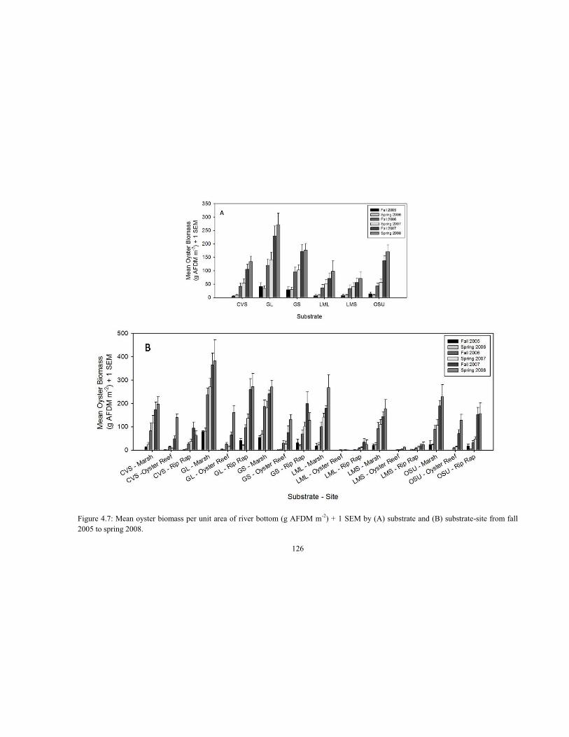
126

Figure 4.7: Mean oyster biomass per unit area of river bottom (g AFDM m-2) + 1 SEM by (A) substrate and (B) substrate-site from fall 2005 to spring 2008.

127

Figure 4.8: Mean (A) exterior and (B) interior live oyster density per unit area of river bottom (No. m-2) + 1 SEM by substrate from fall 2005 to spring 2008.

128

Figure 4.9: Mean (A) exterior and (B) interior oyster biomass per unit area of river bottom (g AFDM m-2) + 1 SEM by substrate from fall 2005 to spring 2008.

129

Consequently, the dominant mode of reef expansion (i.e. reef accretion) occurred at the

reef surface, as seen in comparisons of Exterior and Interior mean oyster density (Fig.

4.10a-b) and biomass (Fig. 4.11a-b) at the marsh site in fall 2007 (n = 36):

Substrate Type Exterior

Density (m-2) Interior

Density (m-2) Exterior Biomass

(g AFDM m-2) Interior Biomass (g AFDM m-2)

CVS 1429 (183) 619 (108) 137.5 (25.5) 35.6 (8.2)

GL 2059 (470) 467 (79) 292.5 (56.0) 72.1 (14.1)

GS 1803 (274) 517 (202) 195.3 (26.8) 45.3 (13.9)

LML 563 (53) 477 (65) 101.7 (21.4) 77.1 (17.1)

LMS 725 (83) 197 (60) 95.5 (19.8) 48.1 (33.0)

OSU 1688 (187) 480 (75) 153.9 (16.9) 35.9 (8.0)

and Spring 2008 (n = 24) using substrate-site-specific biomass regression models:

Substrate Type Exterior

Density (m-2) Interior

Density (m-2) Exterior Biomass

(g AFDM m-2) Interior Biomass (g AFDM m-2)

CVS 1728 (248) 444 (146) 178.2 (26.7) 19.0 (4.7)

GL 2280 (434) 584 (118) 321.0 (90.7) 60.7 (6.7)

GS 2672 (253) 360 (98) 244.6 (32.9) 26.0 (7.6)

LML 1284 (286) 548 (399) 196.2 (13.7) 71.6 (48.1)

LMS 1036 (113) 120 (52) 158.4 (28.9) 18.6 (14.4)

OSU 1144 (333) 444 (169) 184.3 (45.0) 44.0 (14.8)

130

Figure 4.10: Mean (A) exterior and (B) interior live oyster density per unit area of river bottom (No. m-2) + 1 SEM by substrate-site from fall 2005 to spring 2008.

131

Figure 4.11: Mean (A) exterior and (B) interior oyster biomass per unit area of river bottom (g AFDM m-2) + 1 SEM by substrate-site from fall 2005 to spring 2008.

132

By spring 2008, the interior oyster density and biomass estimates did not differ

significantly between treatments (GLM, p > 0.05), while in the within-substrate

comparisons, exterior surfaces had much higher oyster density (Paired t-tests, p < 0.0005)

and biomass (p < 0.0005) than interior treatment segments. Substrate-site (Fig. 4.12a-b)

and substrate only (Fig. 4.13a-b) oyster density and biomass comparisons between

previously-handled (Quad 1) and undisturbed (Quad 4) treatment quadrants (Paired t-

tests, p > 0.05) revealed no significant deviations. The first tests of this kind were

conducted in spring and fall 2006 where Quads 2 and 3, respectively, were sampled

alongside Quad 1. No apparent positive cleansing effects or destructive, handling effects

were realized by oysters in the handled quadrant in spring 2006 (Quad 1 vs. 2, n = 108, p

= 0.798). However, a handling effect was detected in fall 2006 (Quad 1 vs. 3, n = 108, p

= 0.016). Further analysis of exterior (p = 0.147) and interior (p = 0.002) portions of the

quadrants revealed that some benefits of cleansing may have been experienced by

substrates in the interior of the previously-handled treatment. But by spring 2008, no

differences between previously-handled (Quad 1) and undisturbed (Quad 4) treatment

quadrants were apparent for oyster density (n = 72, p = 0.739) and biomass (p = 0.146).

Linear regressions were conducted to determine the effect of oyster density on oyster

tissue mass at a given SH in exterior and interior treatment segments. Biomass data from

Quads 1 and 4 were combined to increase sample size, based on the absence of handling

effects in the spring 2008 sampling. There was a relationship between oyster density and

oyster AFDM at a given size (R2 = 0.39, p = 0.009); oysters of a given size decreased in

tissue mass with increasing oyster density (Fig. 4.14a). The trend was the same for the

effect of exterior oyster density on exterior oyster biomass (R2 = 0.42, p = 0.006; Fig.

133

4.14b), but no such trend existed in the interior locations (R2 = 0.008, p = 0.763; Fig.

4.14c). In fact, it was the exterior oyster density that drove the biomass of oysters present

in the interior of the treatments tested in this experiment (R2 = 0.23, p = 0.080; Fig.

4.14d). Effectively, the more developed, or mature, the face of an oyster reef (treatment)

becomes, the greater the influence of the exterior oyster density on the interior oyster

growth.

When exterior and interior treatment segments were combined, mean oyster

density and biomass estimates at the marsh site after 2+ years were:

Substrate Type Oyster

Density (m-2) Exterior Biomass

(g AFDM m-2) CVS 2048 (252) 173.1 (32.4)

GL 2525 (516) 364.6 (50.2)

GS 2320 (437) 240.7 (16.5)

LML 1040 (59) 178.8 (10.6)

LMS 923 (130) 143.6 (21.4)

OSU 2168 (219) 189.8 (22.4)

And, after 3 years, mean oyster density and biomass estimates in treatments at the

productive marsh site were:

Substrate Type Oyster

Density (m-2) Exterior Biomass

(g AFDM m-2) CVS 2172 (343) 197.2 (30.9)

GL 2760 (540) 381.7 (90.7)

GS 2952 (406) 270.6 (28.7)

LML 1832 (644) 267.7 (54.9)

LMS 1156 (138) 176.9 (39.0)

OSU 1588 (477) 228.4 (51.4)

134

Figure 4.12: Mean live oyster (A) density and (B) biomass per unit area of river bottom (No. m-2; g AFDM m-2) + 1 SEM by substrate-site for the exterior and interior segments of previously-handled (Quad 1) and undisturbed (Quad 4) quadrants of experimental trays (n = 72) sampled in spring 2008.

135

Figure 4.13: Mean live oyster (A) density and (B) biomass per unit area of river bottom (No. m-2; g AFDM m-2) + 1 SEM by substrate for the exterior and interior segments of previously-handled (Quad 1) and undisturbed (Quad 4) quadrants of experimental trays (n = 72) sampled in spring 2008.

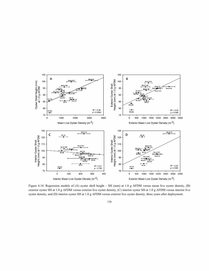
136

Figure 4.14: Regression models of (A) oyster shell height – SH (mm) at 1.0 g AFDM versus mean live oyster density, (B) exterior oyster SH at 1.0 g AFDM versus exterior live oyster density, (C) interior oyster SH at 1.0 g AFDM versus interior live oyster density, and (D) interior oyster SH at 1.0 g AFDM versus exterior live oyster density, three years after deployment.

137

The USACE’s Lynnhaven Decision Document (Schulte et al. 2006) set the 5-yr

mean oyster biomass benchmark at 177 g AFDM m-2 river bottom based on the best reef

information available at the time – some of the most productive, sustainable oyster reefs

located on Virginia’s eastern shore. Treatments at the marsh site (fall 2007: 215.1 +/-

16.4 g m-2; spring 2008: 253.8 +/- 23.8 g m-2) reached that oyster biomass benchmark in

just over 2 years; GL (fall 2007: 259.3 +/- 46.0 g m-2; spring 2008: 271.5 +/- 57.5 g m-2),

GS (fall 2007: 198.6 +/- 50.4 g m-2; spring 2008: 127.4 +/- 32.8 g m-2), and OSU (fall

2007: 151.8 +/- 31.1 g m-2; spring 2008: 156.2 +/- 46.0 g m-2) treatments also reached

similar oyster biomass levels at the riprap site.

Population structure. Population size structure (PSS) varied between site (Fig. 4.15a),

substrate (Fig. 4.15 b-d) and, to a lesser extent, caging (Fig. 4.15 e-f). PSS was most

“developed” on treatments at the marsh site, slightly less at the riprap site, and was

considerably less developed at the oyster reef site, where a “highly developed” PSS

means a mature oyster population with multiple size classes (proxy for year classes)

present and abundant. Notable, however, was the robust PSS across all sites (Fig. 4.16a)

after less than two years (spring 2007) and its similarity to the PSS for the entire LRS

Riprap Survey (Fig. 4.16b). This indicates that many of these experimental intertidal

treatments, particularly the granite treatments – across all sites, and all treatments at the

marsh site – reached a mature reef state in three years or less (Fig. 4.15a-b, e-f).

By fall 2007, we recorded three year classes (YC1 = 2005, YC2 = 2006, YC3 =

2007), as demarcated by three size classes in shell height (SH): Spat (SC1) were < 30.0

mm, small adults (SC2) were 30.1 - 70.0 mm, and large adults (SC3) were > 70.0 mm;

only a few oysters grew > 100.0 mm. We elected not to refer to oysters as ‘markets’

138

(market oysters are > 75 mm SH) because the break at 75 mm SH is economically, not

ecologically, defined. Oyster PSS confirmed trends observed in oyster density and

biomass analysis. Caging and handling effects were minimal, exterior treatment

segments contained > 70% of the oyster population, consistently attracting more recruits

than the interior of the treatments, and most importantly, alternative oyster reef substrates

performed as well or better than loose oyster shell in treatments at all three sites.

Growth and survival. In fall 2005, the proportion of live oysters was 0.92, which is

assumed to be the proportion of settled spat that survived the post-settlement mortality

period (~ 6 wks) and the time subsequent to that period. By spring 2006, the proportion

surviving dropped to 0.87, which provided an estimate of overwintering survivorship.

Fall 2006 was the first measure of mortality over the period of greatest predation

and disease stress. Since these oysters started as spat and very small adults in the spring,

significant disease-driven mortality was not anticipated. A quantitative estimate of

predation- vs. disease-related mortality was not realized; instead, we made qualitative

observations on mud crab, blue crab, and fish predation, or simply gaping, undamaged

valves. Some substrates were partially or totally covered by sediment; many oysters that

recruited to those substrates died due to siltation or burial, and their shells (and the

surrounding substrate) were a distinct black color typically associated with anoxia.

Spat recruitment and densities were high in fall 2006. These oysters grew quickly

such that some of the oysters reached shell heights > 70 mm in the first year, with most of

these occurring on exterior portions of granite treatments at the marsh site. The rapid

growth was likely due to the warm spring and fall of 2006, and may represent near-

139

maximum growth rate for oysters on intertidal reefs in the LRS. Those oysters that grew

into SC3 (YC1) had done so recently, so the proportion of live oysters was high (0.95).

For newly-recruited spat (YC2, SC1), the proportion live (0.77) was slightly higher than

that of the small adults (YC1, SC2) – 0.71. The proportion of live recruits may have been

slightly underestimated because all dead oysters were measured, not just those that had

died recently. Thus, some of the dead oysters may have died in the previous year.

Over the following winter a major mortality event occurred, presumably due to

the severe cold, which reduced the proportion live to 0.61. YC2 spat and small adults

suffered the highest relative mortality, especially at the oyster reef site, where many

treatments lost 50-70 % of their oysters. Mortality was generally restricted to the

substrates highest in the intertidal zone, so that treatments containing significant biomass

in the lower intertidal appeared to be less affected. Despite this major mortality event,

most oysters on oyster shell survived, possibly due to thermal buffering of the shell-

oyster matrix by reducing the substrate surface area exposed to the cold.

In fall 2007, most of YC1 had entered SC3 with a proportion live = 0.80. YC2

dominated SC2 with a proportion live = 0.77; YC3 was another good recruitment class

and had a proportion live = 0.74. These are underestimates of survival because of the

repetitive measurement of dead oysters that had died months to years earlier.

140

Figure 4.15: Population size structure (PSS) of oysters on (A) all substrates at each site separated by handled/undisturbed quadrants (Quads 1, 4) and live/dead in spring 2008. PSS at the (B) marsh, (C) oyster reef, and (D) riprap sites are separated by substrate and exterior/interior segments of each treatment in spring 2008. PSS on (E) large granite (GL), and (F) unconsolidated oyster shell (OSU) at the marsh site separated into caged/uncaged treatments from fall 2005 to fall 2007, which are representative of many of the treatments over time.

141

Figure 4.16: Population size structure (PSS) of oysters (A) across the entire Alternative Substrate Experiment (ASE) in spring 2007 and (B) on riprap in Lynnhaven Bay, Broad Bay and Long Creek (Lynnhaven Riprap Survey – Dissertation Chapter 2).

142

In spring 2008, the proportion of live oysters across all treatments was 0.52 and

0.54 for Quads 1 and 4, respectively. By site, experimental treatments at the oyster reef

(Q1: 0.59, Q4: 0.64) > marsh (Q1: 0.55, Q4: 0.56) > riprap (Q1: 0.46, Q4: 0.48); by

substrate, loose oyster shell (OSU – Q1: 0.61, Q4: 0.64) and limestone marl (LML – Q1:

0.58, Q4: 0.53; LMS – Q1: 0.53, Q4: 0.58) treatments had a higher proportion of live

oysters than the granite (GL – Q1: 0.49, Q4: 0.50; GS – Q1: 0.48, Q4: 0.52) and crushed

concrete (CVS – Q1: 0.49, Q4: 0.54) treatments. However, a site x substrate type

interaction effect (GLM, F = 2.57, p = 0.014) required separate one-way ANOVAs to be

conducted for each site. Although, no differences were detected among substrates at the

marsh and riprap sites, most substrates had higher mean oyster survival than the LML

treatment (F = 4.98, p = 0.005).

By site-substrate-exterior/interior for Quads 1 and 4 (Table 4.8), the proportion of

live oysters was much lower on the interior than the exterior treatment segments at the

riprap site (Paired t-test, p < 0.005) and the marsh site (p < 0.005). In contrast, the

proportion of live oysters on oyster reef site’s exterior and interior treatment segments

was similar (p = 0.612):

Site SC1 SC2 SC3 Marsh 0.52 0.56 0.69

Riprap 0.59 0.56 0.73

Oyster Reef 0.40 0.37 0.70

SC3 contained the fewest oysters but had the best survival; SC1 and SC2 (spat and

juveniles) remained the more vulnerable life stages, incurring a higher relative mortality.

After a second year of recruitment in fall 2006, younger oysters began to settle

and grow on older oysters. It became apparent that a test of substrate viability for oysters

143

would require the distinction between oysters recruiting to the base substrate or to other

oysters – live or dead – already present on the substrates. In fact, oysters recruited to

other oysters on the treatment exterior at higher proportions than on the treatment interior

(Fig. 4.17a). In spring 2008, the proportion of live oysters on other oysters on the

treatment exterior was equivalent or greater than that on the treatment interior (Fig.

4.17b). Thus, more oysters recruited to the treatment exterior AND a greater proportion

of those oysters survived. This trend was most pronounced in treatments at the riprap

site, where experimental tray subsidence was most dramatic. The vertical structure

provided by live and recently dead oysters represented some of the only viable settlement

surfaces as much of the available substrate in many treatments was covered in sediment

and algae.

Overall, considering this subestuary’s high salinity, high predator concentrations

during the warmer months, and the winter 2007 mortality event, survival and growth

rates were high. Oysters in treatments at the marsh and riprap sites consistently grew

faster with lower mortality than oysters in treatments at the oyster reef site.

Oyster volume and reef accretion. Oyster volume varied significantly (p < 0.020) by

substrate and site (Fig. 4.18a) with the highest accretion on treatments at the marsh site

(GL treatments exceeded 20 L m-2), reflecting trends of oyster density and biomass.

Total oyster volume was dominated by live oysters and, thus, the treatment exteriors (Fig.

4.18b), where > 70 % oysters were located. In three years, < 2 L m-2 yr-1 accreted on

treatments at the oyster reef site, treatments ranged from < 2 to 5 L m-2 yr-1 at the riprap

site, and 3-8 L m-2 yr-1 at the marsh site.

144

Pathology and condition. Mean oyster condition (+ 1 SEM) was calculated for CIs 1-3

by site-substrate-exterior/interior (Fig. 4.19). No handling effects on oyster condition

were detected (p > 0.05) between Quad 1 (n = 712) and Quad 4 (n = 695) and, thus,

samples were pooled. Treatments at the oyster reef site had the highest CI values. The

marsh and riprap treatments were similar to each other but maintained significantly lower

oyster condition.

Site CI1 CI2 CI3 Marsh 9.9 (0.2) 7.5 (0.1) 2.9 (0.1)

Riprap 9.6 (0.2) 7.4 (0.1) 2.7 (0.1)

Oyster Reef 13.5 (0.3) 10.5 (0.2) 3.1 (0.1)

Regarding disease (Dermo and MSX) condition, 93 % of the 110 tested oysters

contained Perkinsus cells, with weighted prevalence (WP) of 2.35 +/- 0.17 (Table 4.9a).

Only one oyster had Haplosploridium cells, and it was a rare infection (a few cells), so no

MSX analyses were conducted. Dermo WP varied by site (Table 4.9b) and substrate

(Table 4.9c). Dermo intensity varied significantly by site (ANOVA, F = 16.27, p =

0.003; Fig. 4.20a) and substrate (F = 4.97, p = 0.042; Fig. 4.20b) with no interaction (F =

0.41, p = 0.868). The marsh site had a mean Dermo intensity of ‘Moderate’ (4.68 +/-

0.25), the oyster reef site ‘Light-to-Moderate’ (3.91 +/- 0.28), and the riprap site ‘Light’

(3.29 +/- 0.30). The two smallest substrates – recycled concrete (mean rank = 4.31 +/-

0.32) and loose oyster shell (4.41 +/- 0.33) – maintained higher Dermo intensities than

the larger substrates – granite (3.83 +/- 0.28) and limestone marl (3.28 +/- 0.41).

145

Table 4.8: Proportion of live oysters for the handled (Quad 1) and undisturbed (Quad 4) tray quadrants by site-substrate-exterior/interior for spring 2008.

Site-Substrate-Exterior/Interior Quad 1 Quad 4 Marsh-CVS-Exterior 0.58 0.57 Marsh-CVS-Interior 0.28 0.33 Marsh-GL-Exterior 0.52 0.48 Marsh-GL-Interior 0.46 0.39 Marsh-GS-Exterior 0.53 0.53 Marsh-GS-Interior 0.37 0.41

Marsh-LML-Exterior 0.57 0.53 Marsh-LML-Interior 0.67 0.53 Marsh-LMS-Exterior 0.60 0.62 Marsh-LMS-Interior 0.31 0.41 Marsh-OSU-Exterior 0.60 0.71 Marsh-OSU-Interior 0.49 0.56

Oyster Reef-CVS-Exterior 0.60 0.66 Oyster Reef-CVS-Interior 0.58 0.65 Oyster Reef-GL-Exterior 0.52 0.61 Oyster Reef-GL-Interior 0.61 0.61 Oyster Reef-GS-Exterior 0.58 0.64 Oyster Reef-GS-Interior 0.55 0.56

Oyster Reef-LML-Exterior 0.29 0.59 Oyster Reef-LML-Interior 0.40 0.60 Oyster Reef-LMS-Exterior 0.54 0.63 Oyster Reef-LMS-Interior 0.73 0.83 Oyster Reef-OSU-Exterior 0.71 0.65 Oyster Reef-OSU-Interior 0.73 0.69

Riprap-CVS-Exterior 0.39 0.41 Riprap-CVS-Interior 0.15 0.27 Riprap-GL-Exterior 0.45 0.52 Riprap-GL-Interior 0.18 0.24 Riprap-GS-Exterior 0.41 0.46 Riprap-GS-Interior 0.12 0.28

Riprap-LML-Exterior 0.61 0.52 Riprap-LML-Interior 0.43 0.33 Riprap-LMS-Exterior 0.42 0.42 Riprap-LMS-Interior 0.00 0.23 Riprap-OSU-Exterior 0.63 0.57 Riprap-OSU-Interior 0.44 0.44

146

Figure 4.17: (A) Proportion of live and dead oysters present on other oysters in the exterior and interior reef segments, and exterior plus interior, by substrate-site. (B) Proportion of live oysters only on other oysters in the exterior and interior reef segments.

147

Figure 4.18: (A) Live, dead, and total (live + dead) oyster volume (L m-2), and (B) exterior and interior oyster volume, by substrate-site.

148

Figure 4.19: Mean oyster condition index – CI (+ 1 SEM) for CIs 1-3 by site-substrate-exterior/interior.

149

Table 4.9: Dermo disease intensity data by (A) site-substrate, (B) site and (C) substrate, where Dermo disease intensity ranks as follows: Heavy-Moderate-Light-Rare-Negative.

Site-Substrate Oysters Tested

Proportion Infected

Weighted Prevalence

Oyster Disease Intensity

Nominal Disease Intensity

Rank

Mean Oyster Density

(No. m-2

+/- 1 SEM)

Mean Oyster Biomass

(g AFDM m-2

+/- 1 SEM)

Marsh-CVS 10 1.00 3.20 3-5-2-0-0 5.2 2048 (252) 173.1 (32.4)

Marsh-Granite 10 1.00 2.60 2-4-4-0-0 4.4 2423 (477) 302.6 (33.3)

Marsh-LM 10 0.90 2.45 1-6-1-1-1 3.7 981 (89) 161.2 (16.0)

Marsh-OSU 10 1.00 3.60 5-3-2-0-0 5.4 2168 (219) 189.8 (22.4)

Oyster Reef-CVS 6 1.00 2.58 2-1-2-1-0 4 2467 (191) 48.8 (12.4)

Oyster Reef-Granite 10 0.90 1.90 1-3-5-0-1 3.6 2408 (306) 69.9 (20.6)

Oyster Reef-LM 6 1.00 2.00 0-3-3-0-0 3.8 93 (28) 2.5 (1.1)

Oyster Reef-OSU 10 1.00 2.40 1-5-4-0-0 4.2 1307 (130) 70.3 (17.5)

Riprap-CVS 10 1.00 1.95 0-5-4-1-0 3.6 901 (244) 48.8 (12.4)

Riprap-Granite 10 0.90 1.90 0-5-4-0-1 3.5 1741 (329) 229.0 (48.2)

Riprap-LM 9 0.56 1.67 2-1-2-0-4 2.4 260 (86) 26.5 (11.5)

Riprap-OSU 9 0.89 2.00 1-3-4-0-1 3.6 1560 (338) 151.8 (31.1)

A.

Substrate Oysters Tested

Proportion Infected

Weighted Prevalence

Disease Intensity

Nominal Disease Intensity

Rank

Mean Oyster Density

Fall 2007

(m-2

)

Mean Biomass Fall 2007

(g AFDM m-2

)

Recycled Concrete 26 1.00 2.58 5-11-8-2-0 4.3 1805 (203) 105.3 (18.4)

Granite 30 0.93 2.13 3-12-13-0-2 3.8 2191 (225) 200.5 (31.3)

Limestone Marl 25 0.80 2.04 3-10-6-1-5 3.3 445 (103) 63.4 (18.2)

Oyster Shell 29 0.97 2.67 7-11-10-0-1 4.4 1678 (159) 137.3 (17.9)

B.

Substrate Oysters Tested

Proportion Infected

Weighted Prevalence

Disease Intensity

Nominal Disease Intensity

Rank

Mean Oyster Density

Fall 2007 (m-2

)

Mean Biomass Fall 2007

(g AFDM m-2

)

Marsh 40 0.98 2.96 11-18-9-1-1 4.7 1837 (158) 215.1 (16.4)

Oyster Reef 32 0.97 2.22 4-12-14-1-1 3.9 1463 (195) 44.0 (7.8)

Riprap 38 0.84 1.88 3-14-14-1-6 3.3 1077 (148) 126.1 (19.2)

C.

150

Figure 4.20: Dermo intensity rank versus oyster shell height by (A) site and (B) substrate.

151

DISCUSSION

Recruitment. Restoration efforts with native eastern oyster (Crassostrea virginica) in

Chesapeake Bay have been extensive, yet impeded by substrate and recruitment

limitations along with other environmental factors. This experiment focused on

effectiveness of a number of substrates as oyster reef habitat and, over a 3-yr span,

yielded excellent results. Recruitment was not limiting during the lifetime of this

experiment; in fact, recruitment was good in all three years of the study (2005, 2006 and

2007), with the latter two years being exceptionally high. The YC1 recruitment was

important in determining substrate suitability for oyster settlement because all treatments

were vacant when they were deployed, devoid of oysters, mussels, sponges and any other

fouling organisms (e.g. barnacles and tunicates) that may have competed with oysters for

space.

Baywide, in summer and fall of 2006, oyster recruitment throughout lower

Chesapeake Bay was above the 14-yr average (Southworth et al. 2007). For example, in

the Great Wicomico River recruitment levels were the highest in decades (Southworth

and Mann, 2007). Recruitment in summer and fall of 2007 was not as high as in 2006

(Southworth et al. 2008a). However, YC3 in Long Creek was even larger than YC2, and

there were more recruits on the treatments at the oyster reef site than at the other two sites

– 2.3 times as many spat as at the riprap site and 1.4 times as many spat as at the marsh

site. Furthermore, YC3 on treatments at the oyster reef site reflected a 70 % increase

from YC2 recruitment and almost 300 % more recruits than in YC1, due in large part to

high recruitment to OSU and very high recruitment on GL, GS, and CVS. Across all

152

sites, OSU treatments had the most recruits, 2.5 times more than LML and LMS

treatments, 30 % more than GL treatments, and 15 % more than GS and CVS treatments.

The results at the oyster reef site were puzzling. How could treatments at the

oyster reef site do so much better after low recruitment during the first two years?

Moreover, cold temperatures in the previous winter had killed most of the spat that had

settled at the oyster reef site as YC2 in 2006, indicating that oyster densities at the oyster

reef site were unlikely to be high enough to attract the record number of settlers. Lastly,

why would the mature, high-oyster density treatments at the marsh site not continue to

attract the greatest number of recruits?

To explain these results, we adopted the following conceptual model. Reefs reach

a carrying capacity, whereby they cannot continue to support much higher densities of

filtering oysters; intraspecific competition becomes too great for new spat to survive and

thrive as they might in conditions of lower competitor or predator density. On Virginia’s

Eastern Shore, intertidal oyster reefs maintain this state and tend to be dominated by high

densities of small oysters that cover a smaller number of large oysters (B. Truitt, pers.

comm.). In this system, substrate is at a premium and is generally limiting. In Long

Creek, quality substrate is also limiting. However, the die-off only months earlier should

have opened up surface area for the oyster larvae that would eventually make up YC3.

Furthermore, the remaining shells of those recently dead spat and small adults, as well as

a number of surviving small and large adults, provided the physical and chemical cues –

calcium carbonate (Zimmer-Faust and Tamburri 1994) and oyster pseudofeces (Tamburri

et al. 1996, Turner et al. 1994), respectively – that can attract oyster larvae as they

prepare to settle out of the water column. These cues were undoubtedly stronger on

153

treatments at the riprap and marsh sites, but the major difference was the high percentage

of vacant substrate area within the treatments at the oyster reef site. The resulting density

of oyster recruits on treatments at the oyster reef site in 2007 was higher than any other

recorded throughout the entire experiment. We also dismiss the hypothesis that the water

flow favored the treatments at the oyster reef site over those at the marsh and riprap sites,

since (1) tidal flow in the narrow Long Creek is strong during each tidal cycle, and (2) the

LRS Riprap Survey (Dissertation Chapter 2) provided oyster size frequency data for both

stands of concrete and granite riprap as well as the Long Creek restored oyster shell reef,

which confirmed the presence of multiple year classes.

Much of the LRS oyster population exists in the intertidal and upper subtidal

zones (Luckenbach and Ross 2006, this study). This zonation may be partially due to

intense predation (Menge and Branch 2000, Witman and Dayton 2000), though reef

architecture, scale, and substrate quality may be equally or more critical to the success of

subtidal restored oyster reefs.

Density, biomass and condition. Density often exceeded 1000 oysters m-2 of river

bottom after one year and 2000 m-2 after three years. Biomass was similarly high on

most substrates, except limestone marl, and generally ranged from 150-300 g AFDM m-2

after 3 years. In particular, granite treatments at the marsh site generated very high

biomass (270-382 g AFDM m-2). As a comparison, a 75-mm SH oyster, which is

considered commercial (market) size, will weigh approximately 1 g AFDM. More than

70 % of oyster density and biomass was on the exterior segments, with that percentage

increasing over time as the reefs matured.

154

These oyster density and biomass estimates highlight the effectiveness of

alternative substrates for oyster reef restoration and the ability of oysters to survive and

persist at high density and biomass in high salinity waters of Chesapeake Bay.

Previously it was thought that oyster biomass would be too low at high salinity habitats,

particularly when compared to biomass in low-salinity sanctuaries (Paynter 1999). These

results refute that hypothesis. Moreover, the magnitude and frequency of recruitment

improve the chances that established reefs will be sustained by new recruits and persist

indefinitely. Comparably high density and biomass on oyster reefs has been achieved in

the high-salinity waters of coastal lagoons bordering Chesapeake Bay (Ross and

Luckenbach 2009).

Population structure. Oyster PSS varied between sites, substrates, location in the reef,

and, to a lesser extent, whether or not a plot was caged to exclude large predators. PSS

was most developed at the marsh site, slightly less at the riprap site, and considerably less

at the oyster reef site. Caging (large predator exclusion) was not necessary for

development of PSS on shell or non-shell substrates.

Growth and survival. Oyster growth was high at the marsh and riprap sites, and less so

at the oyster reef site. Growth was not significantly affected by location within the

treatment (exterior vs. interior), though we often observed the largest oysters on the

exterior segments. Oyster survival was high in all treatments except for limited mortality

due to anoxia, siltation and burial in some treatments, and due to the severe winter cold in

2007. The proportion of oysters settling and surviving on other previously-settled oysters

155

(live or dead) increased over time, with a greater number recruiting to the treatment

exterior. This trend indicates that underlying substrate becomes less important as the reef

matures above and around it; the developing shell reef becomes the main settlement

substrate. In areas of consistent, annual recruitment, substrate type may be less

important. However, where recruitment is infrequent or marginal, oyster reef substrate

quality may become critical. Additionally, if quality shell is limiting for large-scale

restoration and reef architecture is also deemed important, managers may consider using

less desirable materials of opportunity for the reef base with a veneer of higher-quality

substrate (Clarke et al. 1999, Priest et al. 1999, Nestlerode et al. 2007).

Oyster volume and reef accretion. A key feature of a thriving oyster reef is the rate of

shell accretion. Shell reefs must maintain a positive shell balance (Mann and Powell

2007). The durability structure of a substrate such as large granite likely lowers the

accretion threshold since the rocks themselves persist, even if the reef were denuded of

oysters by ice, storms, predation or poaching.

Historical records indicate that oyster reefs required about 5 L m-2 yr-1 of shell

accretion (Mann et al. 2009b) to balance natural sources of shell loss, including burial,

dissolution, and fouling (Smith et al. 2005). In a post-industrial Chesapeake Bay, the

necessary shell accretion to balance loss is likely higher. In three years, treatments at the

oyster reef site accreted < 2 L m-2 yr-1; treatments at the riprap site ranged from < 2 to 5 L

m-2 yr-1. Treatments at the marsh site (3-8 L m-2 yr-1) were all in a state of positive shell

balance with no apparent threat of being buried or lost. Intertidal oyster reefs do not

experience the same type of sedimentation, fouling and predation that many subtidal reefs

156

experience, but they do contend with more variable, often extreme, physical conditions

(Menge and Branch 2000).

Pathology and condition. Oyster condition at all three sites and all six substrate classes

decreased with increasing oyster density, similarly to that observed in oyster aquaculture

(Rheault and Rice 1996). The oyster reef site maintained the lowest oyster densities and

the highest mean CI values. Oysters recruited, grew, and survived well despite the heavy

disease challenge in these high-salinity waters, suggesting that oysters can express

disease resistance when afforded protection on reefs of high quality, whether shell or

alternative materials.

Previously it was hypothesized that disease would kill older oysters in high-

salinity areas, such that Dermo intensity would correlate positively with oyster shell

height, because the largest and oldest oysters contain the heaviest infections. Under the

contrasting hypothesis that disease tolerance exists in native oyster populations, some

large and old oysters could have significantly lower intensity infections than they should

have according to the former hypothesis. In this study, the largest oysters had light to

moderate infections, some with no infection at all, whereas many of the intermediate-

sized oysters had moderate to heavy infections. It is possible that some large oysters died

of Dermo infections and were thus not sampled, but we would still expect to sample

numerous large oysters with heavy infections. The densest populations of oysters with

the greatest Dermo prevalence (marsh site) also harbored some of the largest, most

Dermo-tolerant oysters. Consequently, we reject the hypothesis that disease tolerance

cannot be expressed in native oyster populations, and conclude instead that a percentage

157

of oysters can indeed survive, reproduce and persist under high disease challenge in high-

salinity areas. Along with the recent findings of disease tolerance in disease-challenged

(Dermo and MSX) oyster populations (Carnegie and Burreson 2009), these results

indicate that restoration efforts of native oyster populations in high-salinity, disease-

challenged areas can indeed succeed.

CONCLUSIONS

This experiment represents the most comprehensive quantitative test of

alternative, non-shell materials as intertidal oyster reef substrate in the Chesapeake Bay,

with emphasis on oyster recruitment success, growth, survival, and reef development.

The experimental treatments recruited ample oysters to distinguish subtle differences

between substrates in all three years of the study. The findings of this study were: (1)

density often exceeded 1000 oysters m-2 of river bottom after one year and 2000 m-2 after

2 ½ years, in many cases, (2) exterior treatment segments maintained > 70 % of oyster

density and biomass, (3) most treatments exceeded a biomass of 150 g AFDM m-2 after

three years, (4) caging (large predator exclusion) was not necessary for development of

oyster reefs on shell or non-shell substrates, (5) reef accretion rates were high, (6)

survival was high in all treatments except for limited mortality due to anoxia, siltation

and burial in some treatments, and due to the severe winter cold in 2007, and (7) oysters

recruited, grew and survived well despite heavy disease challenge. Throughout the entire

experiment, granite treatments performed as well as, or better than, oyster shell.

Moreover, rock reefs are easier to establish and more persistent than shells which can

158

degrade quickly and are more easily perturbed by storms and poaching. We conclude

that construction of intertidal oyster reefs with shell and alternative materials, such as

granite and concrete, is a viable restoration strategy in the high-salinity waters of

Chesapeake Bay.

159

Acknowledgments. We express appreciation to students and staff of the Marine

Conservation Biology and Marine Community Ecology Programs at VIMS, Mrs. Candy

Burke Huayhualla, and Mr. Darryl Nixon, for their assistance in the lab and field.

Special thanks to the VIMS Shellfish Pathology Lab for testing > 100 oysters for Dermo

and MSX. Funding was provided by grants to R.N. Lipcius and R.D. Seitz from the

Norfolk Office of the USACE (Norfolk District) and from the NOAA Chesapeake Bay

Office through the Blue Crab Advanced Research Consortium. Finally, we wish to thank

First Landing State Park, Mr. and Mrs. Robert Clifton, Mr. Jonathan and Laura Guion,

and recognize the late Mr. Luther Yopp, who welcomed our placement and sampling of

the Alternative Substrate Experiment alongside their properties on Long Creek.

160

Chapter 5 Living oyster reef shorelines using shell and alternative structures in the Lynnhaven River, Chesapeake Bay

ABSTRACT: Some physical barriers that protect shorelines from erosion are constructed of mollusk shell or alternative materials, which may also serve as reefs (i.e. "living shorelines") for ecological restoration of native bivalve species such as oysters and mussels. Despite their increasingly popular use, the efficacy of "living shoreline" reefs in enhancing bivalve abundance has rarely been tested. We experimentally examined the effectiveness of several types of living shoreline reef in augmenting abundance of Eastern oyster, Crassostrea virginica, at two locations in the Lynnhaven River System, a subestuary of lower Chesapeake Bay. In summer 2006, nine reef structures were constructed at two sites: three each of oyster shell (OS), riprap (RR), and concrete modular (CM) reefs. We also placed six reefballs (RBs) at each site, half of which had been seeded with oysters in culture tanks. In addition, we attempted in situ setting of triploid oyster larvae on OS, RR, and CM reefs. The primary objective of this construction was the development of vital oyster reef habitat as a living shoreline in the upper subtidal zone adjacent to natural marshes. The performance of unseeded and seeded reefs was assessed for oyster recruitment, density, biomass (ash-free dry mass – AFDM), condition, growth, survival, reef structural integrity, and disease. After 2.5 yrs: (1) mean oyster density and biomass were high on most unseeded (150-1200 m-2, 150-600 g AFDM m-2) and seeded (LB: 30 – 1800 oysters m-2) reefs, (2) most reefs reached a mature state, as indicated by population structure and high accretion rates (8-15 L m-2 yr-

1), (3) the proportion of live oysters was high (unseeded: 0.53- 0.77; seeded: 0.63-0.75), (4) reefs were covered with oysters, often obscuring the base substrate and causing subsequent oysters to recruit to the living portion of the reef (up to 44 % of oysters grew on other oysters), and (5) both diploid and triploid oysters tested for disease had below average Dermo (i.e. disease) infections, and were therefore healthy. Moreover, in situ setting of triploid oyster larvae was successful. These findings indicate that living shoreline reefs can serve both as physical barriers and as restoration reefs for native bivalve species, such as eastern oyster.

161

INTRODUCTION

Estuaries such as Chesapeake Bay have extensive shorelines lined with marshes,

beaches, and tidal mudflats that provide a rich habitat for plants and animals (VA CZM

2009). In many estuaries, however, shorelines are eroding at rapid rates (VA CZM

2009). For instance, in Chesapeake Bay, as much as one third of all shorelines have

eroded, with some areas losing as much as 20-40 cm of shoreline per year (Chesapeake

Bay Program 2005); an estimated 57 % of the sediment in the Bay comes from these

eroding shorelines (Langland and Cronin 2003). With the heavy industrial, agricultural,

and residential development of watersheds, including shorelines of rivers and estuaries,

the percentage of forested land has decreased. The increasing proportion of surfaces that

are impervious to drainage has exacerbated erosion problems and associated delivery of

pollutants to our coastal waters (NOAA 1998). The resultant increased sediment and

nutrient loads have numerous negative effects on estuarine flora and fauna by: (1)

blocking light required for submerged aquatic vegetation, (2) burying low-lying sessile

invertebrate reefs (e.g. oyster reefs) or clogging the filtration system of filter feeders, and

(3) increasing the frequency and intensity of harmful algal blooms that subsequently lead

to zones of low dissolved oxygen (NOAA 1998, Rabalais et al. 2001).

As coastal populations continue to grow, and as sea level continues to rise, the

need for shoreline stabilization has intensified. There is growing concern that erosion

control efforts that use “hardened” shoreline (e.g. rock revetments, wood or vinyl

bulkheads) are damaging natural, shoreline habitats (VA CZM 2009). Effective shoreline

protection may be achieved, however, with a technique called “living shorelines.” Living

shorelines incorporate materials such as marsh plantings, shrubs and trees, low profile

162

sills and breakwaters, and strategically placed organic material, which can recreate the

ecological functions of a natural shoreline (VA CZM 2009). Living shorelines also

promote local participation in “best management practices” with structures that do not

diminish environmental conditions while concurrently suiting the needs of the shoreline

property owner (Dept. Conservation and Recreation 2009). These benefits include: (1)

reduction of erosion and property loss, (2) lower erosion control construction costs, (3)

natural and aesthetically pleasing views, (4) restored marine habitat and spawning areas

for fish and invertebrates, and (5) improved water quality (VA CZM 2009).

Ecological restoration of the eastern oyster, Crassostrea virginica, in Chesapeake

Bay is one means of mitigating the effects of increased turbidity and phytoplankton

production, given suitable environmental conditions (Hargis and Haven 1999). Reefs

(i.e. "living shorelines") used for ecological restoration of native oyster may also serve as

physical barriers that protect shorelines from erosion. However, the efficacy of "living

shoreline" reefs in enhancing oyster abundance has not been tested. We experimentally

examined the effectiveness of several types of living shoreline reef in augmenting

abundance of eastern oyster, Crassostrea virginica, at two locations in the Lynnhaven

River System, a subestuary of lower Chesapeake Bay.

In early 2006, two homeowners in Virginia Beach’s LRS shoreline community

agreed to allow the construction of a living shoreline experiment adjacent to each of their

properties. In summer 2006, three oyster shell (OS), riprap (RR) and concrete module

(CM) reefs were constructed at these two subtidal sites in the upper reaches of the LRS,

one in Linkhorn Bay (LB) and one in the Upper Eastern Branch (EB) of the Lynnhaven

River (Fig. 5.1). In addition, we placed six reefballs (RB) at each site, half of which had

163

been seeded with oysters in controlled culture tanks two months prior to deployment.

The primary goal of this construction (Fig. 5.2a-c) was the development of healthy oyster

reef habitat as a living shoreline in the subtidal zone adjoining natural marshes. We

assessed the comparative success of the reef types (unseeded and seeded) with respect to

oyster recruitment, density, biomass, condition, growth, survival, disease intensity, and

reef structural integrity (Fig. 5.3a-j). The a priori hypotheses (Table 5.1) outline

expectations for this study.

Figure 5.1: Chesapeake Bay (inset) contains the deployment sites for the Living Shoreline Experiment reefs in Linkhorn Bay and the Eastern Branch of the Lynnhaven River (Virginia Beach, Virginia).

164

A

B

C

Figure 5.2: (A) General schematic of the Living Shoreline Experiment located at two properties in the Lynnhaven River System. (B) Schematic of concrete module reef replicates (Proprietary Design: ReefTek Model 1105) in the Eastern Branch (EB) site of the Lynnhaven River. Note, modules labeled “B” were inoculated with triploid (3N) larvae via a remote field larval setting experiment; modules labeled “A” and “C” were both deployed barren (“A”: July 2006; “C”: August 2006). (C) The EB site, post-deployment.

Riprap Reef

Concrete Module Reef Oyster Reef

Reefball

165

Figure 5.3 A-F.

166

Figure 5.3: (A) Captain Robert Jensen (Rappahannock Preservation Society; ReefTek) and his concrete module prototype. (B) A seeded reefball suspended by a crane prior to deployment. (C) An oyster cluster from an oyster shell reef. (D) Oysters (2.5 yrs old) from a seeded reefball with shell heights > 177 mm (7 inches). (E) Granite covered in oysters from a riprap reef. (F) Submerged concrete modules removed from a reef, with the seeded module at the top left. (G) Large oysters from an oyster shell reef at the EB site. (H) Oysters covering > 90 % of a seeded concrete module at the LB Site. (I) Seeded reefball (1.5 yrs post-deployment) with oysters thriving in every nook and cranny. (J) Oyster reef restoration ecologists on a mission.

167

Table 5.1: A priori hypotheses for the Living Shoreline Experiment (LSE).

Hypothesis a priori Hypothesis Description followed by the observation(s) and associated logic behind hypotheses

LSE #1 Year 1: Oyster Recruitment/Density is higher on restored oyster shell reefs than on riprap and concrete module reefs

Riprap and concrete modules were not conditioned prior to deployment; oyster shells, by definition, are conditioned to receive oyster larvae and had a distinct advantage in Year 1 of this experiment.

LSE #2 Year 2: Oyster Recruitment on riprap and concrete module reefs is equal to Recruitment on restored oyster shell reef from Year 1

The 1st sampling of the Alternative Substrate Experiment (Fall 2005) revealed alternative substrates recruited oysters as well or better than loose oyster shell.

LSE #3 Year 1: Oyster Survival (%) is higher on riprap and concrete module reefs than on restored oyster shell reef

Lower oyster density and higher interstitial volume on riprap and concrete module reefs equate to higher survival (%).

LSE #4 Oyster Growth does not differ across 1) substrate/reef type, and 2) site

There were no data available to suggest that one reef type or site would have oysters growing faster than any other.

LSE #5 Oyster Recruitment and Density are higher at the Eastern Branch (Lynnhaven River) site than at the Linkhorn Bay site.

The extant population at the Eastern Branch (Lynnhaven River) site was considerably larger than the Linkhorn Bay site.

168

Additionally, oyster larvae were set in situ on some modules, rocks and shell bags

to detect differences between seeded and barren substrates. This work is an expansion of

a study conducted by Coon and Fitt (1999) on unconsolidated (loose) OS reefs. To date,

this was the first attempt at deploying eyed-larvae on alternative substrates in situ. We

sought to determine the physical and economic feasibility of deploying larvae in situ (as

opposed to setting oyster larvae in tanks on land) on alternative oyster reef substrates.

The a priori hypotheses (Table 5.2) outline expectations for this corollary study.

Table 5.2: A priori hypotheses for the Remote Field Larval Setting Experiment (RFLSE), the corollary to the Living Shoreline Experiment.

Hypothesis a priori Hypothesis Description followed by the observation(s) and associated logic behind hypotheses

RFLSE #1 Oyster recruitment to oyster shells (in mesh bags) and conditioned granite rip rap is greater than on unconditioned concrete modules

Unconditioned rock and concrete surfaces are acidic and lack a biofilm that oyster larvae detect when landing on a substrate to test its viability for permanent settlement

RFLSE #2 Oyster growth and survival is high on all substrates since these larvae were triploid

Oyster growth and survival is higher on riprap and concrete modules than the oyster shells that are crowded in, and restricted by, mesh bags.

RFLSE #3 Triploid oysters set on riprap and concrete modules have higher survival and growth than diploid oysters that recruited naturally.

Triploid oysters do not have to expend energy for gamete production which frees up energy for shell and somatic growth, as well as energy to combat parasites and associate disease

RFLSE #4 Substrates set with triploid oyster larvae have higher recruitment in Year 2 than substrates with only diploid oysters present (excluding seeded reefballs).

A greater number of larger oysters equates to more fresh calcium carbonate shell surface available and stronger chemical cues for oyster larval attraction.

169

MATERIALS AND METHODS

Sampling procedure and design. After obtaining each homeowner’s consent to

construct the general design (Fig. 5.2a) of three replicates of the granite RR (0.91 m

diameter, 0.51 m height), loose OS (0.91 m diameter, 0.51 m height), and CM reefs

(bases: 1.22 m x 1.22 m x 0.13 m; mini-modules: 0.61 m x 0.61 m x 0.09 m), scale

drawings were constructed and submitted to the Commonwealth of Virginia as two joint

permit applications with the Chesapeake Bay Foundation. The official permits were

issued on 24 July 2006; we deployed the granite RR and OS reefs that same day. The

next day, 18 of 24 CM structures were deployed. Due to construction delays, the last six

modules were deployed a few weeks later. A permit addendum was sought and granted

for the addition of six RBs to each living shoreline. Half of the RBs were conditioned

and seeded with diploid oysters; the other RBs were devoid of oysters and unconditioned.

The RBs are called Mini-Bay Balls (dimensions: Base diameter – 0.71 m, Top diameter –

0.51 m, Height – 0.51 m, and estimated surface area of 2.74 m2). The RBs were

deployed on 26 September 2006 and likely missed the 2006 oyster larval recruitment

window.

Sampling of the reefs was conducted in July 2007, fall 2007, and September-

October 2008 (henceforth referenced as spring 2007, fall 2007, and fall 2008,

respectively) and was non-destructive, except for the final sampling. Oyster shell height

(SH) of live and dead oysters, as well as mud crab counts, were recorded from one of

four quadrants of each reef. One quarter of the granite RR and OS reefs were non-

destructively sampled in situ (except for fall 2008), recording the percent of substrate

present below the sediment line. Care was taken to return reef material to its original

170

orientation (i.e. rocks at the reef base were returned to the base position of the reef; oyster

clusters from shell reefs were placed on top of the empty, anoxic shell). This process was

important to the maintenance of reef integrity and ensuring that the shells and rocks that

were at the top, middle, or bottom were returned in that order to the reef. These

precautions were especially critical at the EB site where reef bases were buried in mud.

Any oysters that were accidentally placed at the bottom in the mud would have likely

died. One quarter of each CM layer was also non-destructively sampled noting its

position (upper/lower), condition, and locations of oysters measured (top, sides, holes or

bottom). Since one out of every four CMs on a reef was used in the RFLSE, the mean

(density, biomass, etc.) of the other three units was used to estimate the fourth. RBs were

photographed and notes taken regarding oyster reef progression (estimated growth,

density, and presence/absence of oyster recruits). At the close of the experiment (fall

2008), one quarter of each RB was destructively sampled. For all reef types, a fixed

number of oysters throughout the range of oyster SHs were retained for disease

(Dermo/MSX), biomass, and condition index analysis.

Approximately one million eyed-larvae were obtained from the VIMS

Aquaculture Genetics and Breeding Technology Center (ABC) and were deployed at the

two LSE sites on 7 August 2006. The objective was to set these larvae on three CMs

directly from the LSE, six pieces of conditioned granite RR from the adjacent shoreline,

and six mesh bags of OS. The modules were set on cinder blocks to maximize the

surface area for settlement and a silt fence enclosure built around them with the granite

and shell bags placed around the inside perimeter of the fence, to secure the bottom of the

fence to the sediment and avoid larval loss. Once larvae had warmed to room

171

temperature (~20 min), they were mixed in a pitcher filled will local river water, and

dispersed within the enclosure using a small cup. The silt fence was removed two days

later. Six weeks post-deployment, recruitment and post-set mortality were recorded. The

CMs were then returned to their respective reefs. The six granite pieces and three shell

bags were set near the LSE reefs of similar substrate, but not on them. Three shell bags

were recovered for sampling. The bags were broken down into four categories (top

exterior, top interior, bottom exterior and bottom interior) to detect patterns in

recruitment and post-set mortality. Oyster counts (live/dead) were recorded, noting the

face of the shell (inner/outer). Twelve weeks post-set, a single shell bag and three pieces

of granite from each site were recovered. The shell bags were broken down as before and

all oyster SHs were recorded. Oyster SHs were also recorded for the granite.

Subsequently, we determined the ploidy of a subset of the oysters. Since the larvae from

the VIMS ABC were triploid, we could distinguish them by their ploidy using flow

cytometry. A fixed number of oysters from both sites (½ from granite; ½ from OS, with

the shell half divided by the four sub-categories: top exterior, top interior, bottom

exterior, and bottom interior) were provided to the VIMS flow cytometry lab who

provided analytical results (Appendix 5.1).

Two shell bags, three pieces of granite, and three CMs remained at each site, so

progress of the triploid oysters and reef succession could be monitored with each

sampling of the LSE. One oyster bag was opened and the contents spread out in a 0.29-

m2 tray at each site during the spring 2007 LSE sampling. The second oyster bag was not

opened or sampled until the final sampling (fall 2008) to determine if growth and survival

were affected by the mesh bag.

172

We used a linear-mixed model design (General Linear Model: fixed factor: Reef

Type; random factor: Site) in the statistical analysis. Due to a significant interaction

effect, we tested the Reef Type effect with separate one-way ANOVA models for each

site (Underwood 1997).

Recruitment. To simplify comparisons of multiple years of oyster recruitment across

site, reef type, and seeding factors, a ranking system from 0 to 8 was adopted (Table 4.6).

Note that qualitative descriptors of oyster recruitment such as ‘Low’ and ‘Extremely

High’ refer only to the Chesapeake Bay and its subestuaries; locations outside of

Chesapeake Bay could have different rankings. Full-scale sampling of unseeded reefs

was first conducted in spring 2007. Though the live oysters were considerably larger

than they would have been in November 2006, it is appropriate to consider any oyster –

live or dead – greater than 5.0 mm (a SH that indicates survival past post-set mortality – 6

wks) as the 2006 YC (YC1 = 2006, YC2 = 2007). Distinct differences in size classes

between sites resulted in classification by YC only. The seeded substrates were measured

six weeks post-deployment (RFLSE). The cinder blocks were not measured during each

sampling; RBs were only measured during the last sampling. A different method, using

population size structure and notation of ‘newly-dead’ and ‘old dead’ oysters, was

employed to estimate YC1 and YC2; this method was validated using other data collected

in this study.

Biomass and condition index. SH, width, and depth were measured for all oysters,

living and dead. SH was considered as the distance from the umbo to the posterior end of

173

the shell. Additionally, all internal tissues were collected for selected oysters in pre-

weighed aluminum ‘weigh boats’ for dry mass (DM) and AFDM measurements. More

than 1200 oysters representing the full range of SH values were processed to yield

reliable estimates of oyster biomass via regression of log AFDM (g) versus log SH (mm).

The oysters were selected for unseeded RR, OS, CM reefs, RBs, cinder blocks, as well as

seeded (diploid) RBs and triploid (188) oysters from RR, OS, CM reefs and cinder blocks

(Table 5.3). Details regarding laboratory biomass procedures and calculation of oyster

condition indices can be found in the ‘Materials and Methods’ section of Dissertation

Chapter 2.

Oyster and substrate volume. Oyster volume, a direct assay of oyster reef accretion,

was measured for live oysters and dead shells separately through volumetric

displacement. Oyster volume measurements were made for all unseeded and most

seeded reefs/substrates in fall 2008. Oysters (live and dead) and substrates were scraped

clean of oysters, mussels, large barnacle clusters, etc., to avoid overestimation.

Pathology and condition. Dermo (Perkinsus marinus) and MSX (Haplosploridium

nelsoni) prevalence and intensity were tested in 59 oysters. Oysters were collected in

early November since peak infection intensity occurs in the fall. Oysters ranging in SH

from 59.0-176.8 mm were selected haphazardly from unseeded and seeded reefs at each

site; n = 10-15 from each treatment. Samples were brought back to the VIMS Pathology

group live and on ice. Dermo testing was conducted using RFTM (Ray fluid

thioglycollate medium). The RFTM has a lower detection limit than histology and, thus,

was selected for analysis. The oysters were assigned one of nine disease ratings (Ray

174

1954, Table 4.5). SH and other condition metrics (i.e. emaciated tissue, thin shell,

presence of boring sponge, etc.) were noted for each oyster tested.

Table 5.3: Regression models of log AFDM (g) versus log oyster shell height (mm) used for oyster biomass estimation for unseeded oyster shell, riprap and concrete module reefs, reefballs (unseeded and seeded), and cinder blocks (LB site only) at both sites in fall 2008.

Site Reef Type Sample Size (n) Biomass Regression Equations

LB Oyster Shell 131 10^((2.5868*LOG10(SH))-4.9846)

EB Oyster Shell 129 10^((2.0948*LOG10(SH))-3.9713)

LB Riprap 128 10^((2.5556*LOG10(SH))-4.8866)

EB Riprap 93 10^((2.0037*LOG10(SH))-4.0046)

LB Concrete Modules 121 10^((2.5612*LOG10(SH))-4.9126)

EB Concrete Modules 38 10^((2.9195*LOG10(SH))-5.4654)

LB Unseeded Reefballs 87 10^((2.3107*LOG10(SH))-4.5075)

EB Unseeded Reefballs 61 10^((1.8240*LOG10(SH))-3.6156)

LB Seeded Reefballs 86 10^((1.8242*LOG10(SH))-3.7435)

EB Seeded Reefballs 59 10^((1.6811*LOG10(SH))-3.4102)

LB Cinder Blocks 100 10^((2.0924*LOG10(SH))-4.0555)

RESULTS

Recruitment. In 2006, the unseeded granite RR reefs and CM reefs experienced low to

moderate recruitment; recruitment at the OS reefs was moderate at the LB site, and high

at the EB site (YC1). Across all reef types, the EB site outrecruited the LB site by an

order of magnitude (Table 5.4a). The unseeded and seeded RBs were deployed too late

in the season (late September) to receive more than a few oyster larvae, but the seeded

RBs (Fig. 5.3b) were uniformly packed with ~35-mm oysters, mimicking high natural

recruitment.

175

The release of triploid larvae within enclosures containing OS, RR, and CMs

resulted in oyster recruitment to those substrates. A site x substrate type interaction

(General Linear Model – GLM, F = 3.78, p = 0.032) required a separate one-way

ANOVA for each site. Triploid oyster recruitment was significantly higher (LB: F =

8.16, p = 0.008; EB: F = 20.76, p < 0.0005) on OS high) than on RR (low to moderate)

and CMs (low). Though not part of the initial experimental design, cinder blocks were

included due to low recruitment to seeded and unseeded blocks.

By fall 2007, unseeded reefs at both sites had experienced recruitment (YC2), but

the LB received more recruits than the EB site (Table 5.4b), a reversal from the previous

year. Unseeded reefs at both sites were developing well: OS reefs at the EB site were

beginning to cohere (cluster), a critical indicator of reef succession. Although OS reefs

received more recruits for the second year in a row (moderate to high), the other reef

types experienced much higher recruitment levels than in 2006 (moderate). Seeded

substrates at the LB site recruited well in 2007 (moderate to high); seeded OS at the EB

site also recruited well, but the RR and CMs experienced very low recruitment. The

cinder blocks had sunken in the mud and were no longer measured. The seeded RBs

recruited well (high) at both sites.

176

Table 5.4: Oyster recruitment rankings for YC1 (fall 2006) and YC2 (fall 2007) by (A) site and (B) site-reef type, for seeded and unseeded oyster shell, riprap, concrete modules, reefballs, and cinder blocks.

Site Seeded/Unseeded YC1 YC2 Mean

LB Unseeded 2.0 4.4 3.2

EB Unseeded 2.6 3.5 2.8

LB Seeded 4.6 5.0 4.8

EB Seeded 3.6 3.5 3.3

A.

Site Reef Type Seeded/Unseeded YC1 YC2 Mean

LB Oyster Shell Unseeded 3 6 4.5

EB Oyster Shell Unseeded 7 5 6.0

LB Riprap Unseeded 2 4 3.0

EB Riprap Unseeded 3 4 3.5

LB Concrete Module Unseeded 2 4 3.0

EB Concrete Module Unseeded 2 2 2.0

LB Reefball Unseeded 0 4 2.0

EB Reefball Unseeded 0 3 1.5

LB Cinder Block Unseeded 3 4 3.5

EB Cinder Block Unseeded 1 -- 1.0

LB Oyster Shell Seeded 8 5 6.5

EB Oyster Shell Seeded 6 5 5.5

LB Riprap Seeded 3 5 4.0

EB Riprap Seeded 2 1 1.5

LB Concrete Module Seeded 2 3 2.5

EB Concrete Module Seeded 1 1 1.0

LB Reefball Seeded 7 7 7.0

EB Reefball Seeded 8 7 7.5

LB Cinder Block Seeded 3 5 4.0

EB Cinder Block Seeded 1 -- 1.0

B.

177

Density. Unseeded oyster reefs were first sampled in spring 2007. Recruitment on these

reefs in 2006 – YC1 (Table 5.4a-b) was roughly equivalent to oyster density (Fig. 5.4a)

recorded the following spring, where the EB site maintained higher densities of live

oysters than the LB site. An interaction effect between site and reef type (F = 24.77, p <

0.0005) dictated the need to conduct separate one-way ANOVAs of reef type for each

site. At the EB site (F = 32.37, p = 0.001), oyster densities ranked: OS >> RR = CM,

with mean OS oyster density near 1000 m-2 and RR-CM densities of ~200 m-2 (Fig. 5.4a).

At the LB site (F = 11.62, p = 0.009), oyster densities ranked: OS > RR = CM, with mean

oyster densities less than 150 m-2 (Fig. 5.4a). Oyster densities on seeded substrates

commenced in fall 2006. As mentioned earlier, oyster recruitment to OS at both sites

was extremely high, exceeding 9000 spat m-2 at the LB site, and 2800 spat m-2 at the EB

site (Fig. 5.4b). RR recruited between 260 (EB site) and 530 spat m-2 (LB site); CMs

recruited between 40 (EB site) and 150 spat m-2 (LB site).

Across most seeded substrates in spring 2007, oyster densities were similar as in

fall 2006. RR oyster densities were lower, but this decrease was artificial; the rocks with

densest triploid settlement were recovered 12 wks post-deployment in 2006 for ploidy

testing to determine performance of the RFLSE (Appendix 5.1). Thus, the rocks left

behind for monitoring in spring 2007 and beyond had lower relative oyster density.

178

Figure 5.4: Mean live oyster density per unit area of river bottom (No. m-2) + 1 SEM site-reef type from spring 2007 to fall 2008 for (A) unseeded reefs, and from fall 2006 to fall 2008 for (B) seeded reefs.

179

By fall 2007, a second oyster recruitment event and a year of mortality (winter

and summer) reshaped oyster density on the unseeded and seeded reefs. The 2007

recruits (YC2) settled more heavily on unseeded reefs at the sandy, LB site – oyster

densities for OS, RR, and CM reefs were statistically equivalent (F = 5.13, p = 0.152)

between the sites (LB: 968 +/- 166; EB: 735 +/- 172 m-2 (+/- SE)) but varied significantly

between reef types (F = 33.45, p = 0.029). Oyster density ranks were: OS > RR = CM at

the LB site (F = 5.34, p = 0.009); OS > RR > CM at the EB site (F = 39.83, p < 0.0005)

(Fig. 5.4a). The most dramatic increases, in many cases > 10-fold, occurred on the OS

and CM reefs at the LB site, and RR at both sites.

Seeded OS densities declined from spring to fall 2007 (Fig. 5.4b) because oysters

removed from their mesh bags in spring 2007 were spread out, thus artificially decreasing

their densities. In an attempt to detect the benefits or disadvantages of long-term

enclosure in a mesh bag, one OS bag from each site was deconstructed and the remaining

one was left intact for the final sampling (fall 2008). For all other substrates, oyster

density increased in fall 2007 (GLM, site x substrate interaction effect, F = 5.57, p =

0.046), particularly at the LB site (one-way ANOVA, F = 9.48, p = 0.014): RR – 1295 +/-

140 m-2, CM – 514 +/- 200 m-2, and CB – 1398 +/- 120 m-2 (Fig. 5.4b). These oyster

assemblages were accreting at an impressive rate (1.5 yrs), especially the RBs (Fig. 5.3i)

where oysters were beginning to accrete laterally (reef expansion).

All unseeded and seeded reefs were destructively sampled and frozen in fall 2008,

to determine reef performance. This sampling occurred before most 2008 recruits (YC3)

could grow large enough to be measured and, thus, excluded estimates for YC3. By fall

2008, no significant differences were detected between sites (GLM, F = 14.47, p =

180

0.063), reef types (F = 4.64, p = 0.177), or due to the site x reef interaction (F = 3.33, p =

0.071). However, oyster density on unseeded reefs differed by reef type at each site

(ANOVA, LB: F = 10.83, p = 0.010; EB: F = 5.93, p = 0.038). When we included RB

reefs in the analysis, oyster density ranks for unseeded reef types at the EB site

(ANOVA, F = 11.74, p = 0.001) were: OS = RR > CM = RB, with no live oyster density

> 500 m-2; at the LB site (F = 11.55, p = 0.001), they were: OS (1216 +/- 123 m-2) > RR =

CM = RB, with all densities > 600 m-2 (Fig. 5.4a).

Excluding RBs (LB = EB site), seeded substrate oyster densities at the LB site

were twice those at the EB site (10:1 for CM), by fall 2008 (Fig. 5.4b). Note that the near

doubling of RR density at the EB site was artificial because one of the seeded rocks at

this site was not recovered and the resulting density was based on two samples instead of

three (Fig 5.4b). Oyster density ranks for seeded substrates at the LB site were: RB = OS

> RR = CM, with most densities > 750 m-2 (Fig. 5.4b). At the EB site, they were: RB >

OS > RR > CM, with most densities < 700 m-2 (Fig. 5.4b).

The OS bags opened during the final sampling had oyster densities of 3008 m-2

(LB site) and 2171 m-2 (EB site), given the small footprint (0.0645 m2); if these oysters

were spread across a 0.292-m2 tray in the manner the other OS samples had been, the

densities drop to 664 m-2 and 480 m-2, respectively. Compared to the previously spread

and seeded OS samples, densities were lower, with a smaller mean oyster SH at the LB

site (71.7 +/- 1.4 vs. 66.2 +/- 2.3 mm).

Seeded RB oyster densities were 1795 +/- 268 m-2 at the LB site and 1347 +/- 257

m-2 at the EB site (Fig. 5.4b). Oysters that had fallen off the RBs created a ring or ‘halo’

181

that was included in the RB density estimate. Nearly half of all RB oysters, including

some of the largest ones, were present in these halos.

Biomass. In spring 2007, unseeded oyster biomass followed the same trend as for density

(GLM, F = 26.91, p < 0.0005). The EB site (OS >> RR = CM; ANOVA, F = 44.07, p <

0.0005) contained > 10-fold more oyster biomass than the LB site (OS > RR = CM, F =

3.55, p = 0.096), 245.8 +/- 78.4 vs. 17.2 +/- 3.1 g AFDM m-2 (Fig. 5.5a).

In fall 2007, the difference in oyster biomass between the two sites was still

considerable but the GLM analysis was confounded by an interaction effect between site

and unseeded reef type (F = 13.17, p = 0.001); separate one-way ANOVAs of reef type

were conducted for each site. Oyster biomass ranks were: OS > RR = CM at the LB site

(F = 13.17, p = 0.017) and OS > RR > CM at the EB site (F = 13.17, p < 0.0005).

The interaction effect was not significant in fall 2008 (GLM, F = 2.22, p = 0.151),

but oyster biomass trends between sites on OS significantly differed from trends between

RR and CM among sites, leading to significant effects of both site (F = 16.75, p = 0.001)

and reef type (F= 14.86, p = 0.001). By fall 2008, most reef types contained high oyster

biomass (Fig 5.5a):

Site Oyster

Shell (OS)

Riprap

(RR)

Concrete

Modules (CM)

Reefballs

(RB)

Cinder

Blocks (CB)

Linkhorn Bay (LB) 616 (99) 413 (64) 443 (53) 380 (64) 603 (30)

Eastern Branch (EB) 554 (77) 156 (39) 122 (18) 156 (91) --

182

Figure 5.5: Mean oyster biomass per unit area of river bottom (g AFDM m-2) + 1 SEM by site-reef type for (A) unseeded reefs from spring 2007 to fall 2008, and (B) seeded reefs in fall 2008.

183

The unseeded oyster biomass regression models (Fig. 5.6a-k) were also used to

estimate the biomass of diploid oysters on seeded substrates. Additionally, 188 triploid

oysters were processed to estimate their contribution to the biomass of the seeded reefs at

both sites. The biomass regression models were not reliable (R2 values < 20%, with

many approaching zero) compared to those produced for diploid oysters (Table 5.3), so

individual biomass estimates were matched to each triploid oyster within each site-reef

type. For triploid oysters that were not processed, the site-reef type mean biomass was

used.

Population structure (PSS). PSS was similar across unseeded OS, RR and CM reefs in

spring 2007 (Fig. 5.7a). In fall 2007, a strong recruitment event (YC2) dwarfed YC1

across site and reef type (Fig. 5.7b). Oysters on reefs at the LB site must have settled

earlier in the season or grew faster after settlement; oyster SH was 25-30 mm larger on

reefs at the LB site. This trend was maintained through fall 2008 (Fig. 5.7c-d); RBs and

cinder blocks showed similar trends (Fig. 5.7e-f).

PSS of oysters was recorded for seeded substrates from fall 2006 through fall

2008 (Fig. 5.8a-g). Some oysters measured on OS and RR were diploid spat that had

settled after the deployment of the triploid larvae in August 2006. The triploid oysters

grew quickly (some > 60 mm) on both the OS and RR (Fig. 5.8a). By spring 2007, many

oysters on RR and CMs achieved SHs > 80 mm, with a mean SH near 70 mm (Fig. 5.8b).

The trend of larger oyster recruits at the LB site on unseeded reefs also occurred on

seeded substrates in fall 2007 (Fig. 5.8c-d). By fall 2008, oysters from YC1 were > 120

mm; oysters from YC2 were 50-75 mm at the LB site and 30-60 mm at the EB site (Fig.

184

5.8e-f). Oysters on the seeded RBs were < 150 mm at the LB site with peaks at 50 and

100 mm. Oyster SH exceeded 170 mm at the EB site with no obvious dominant size

class (Fig. 5.8g).

Figure 5.6 A-F.

y = 2.5868x – 4.9846 R2 = 0.863

y = 2.5556x – 4.8866 R2 = 0.809

y = 2.0037x – 4.0046 R2 = 0.773

y = 2.5612x – 4.9126 R2 = 0.836

y = 2.9195x – 5.4654 R2 = 0.785

y = 2.0948x – 3.9713 R2 = 0.841

185

Figure 5.6: Regression models of log AFDM (g) versus log oyster shell height (mm) for biomass estimation of oysters on the unseeded oyster shell(A, B), riprap (C, D), and concrete module reefs (E, F), unseeded (G, H) and seeded reefballs (I, J), and unseeded cinder blocks (K, at LB site only) at the LB and EB sites, respectively.

y = 2.3107x – 4.5075 R2 = 0.563

y = 1.824x – 3.6156 R2 = 0.617

y = 1.8242x – 3.7435 R2 = 0.672

y = 1.6811x – 3.4102 R2 = 0.656

y = 2.0924x – 4.0555 R2 = 0.605

186

Figure 5.7: Population size structure (PSS) on unseeded oyster shell, riprap, and concrete module reefs in (A) spring 2007, (B) fall 2007, and (C-D) fall 2008, where (C) LB and (D) EB sites include PSS of dead oysters. (E) PSS of live and dead oysters on unseeded reefballs in fall 2008. (F) PSS of live oysters on unseeded reefs, including cinder blocks, in fall 2008.

187

Figure 5.8: (A) Population size structure (PSS) of live and dead oysters on seeded oyster shell (OS) and granite riprap (RR) at the LB and EB sites in fall 2006. (B) PSS of live oysters on seeded RR and concrete modules (CM) at both sites in spring 2007. PSS of live and dead oysters on (C) seeded OS, RR, CMs, and cinder blocks (CB) at the LB site and (D) seeded OS, RR, and CMs at the EB site in fall 2007. PSS of live and dead oysters on seeded OS, RR, and CMs at the (E) LB (including CBs) and (F) EB site. (G) PSS of live and dead oysters on seeded reefballs at both sites in fall 2008.

188

Survival. In spring 2007, the mean proportion of live oysters across site and unseeded

reef type was 0.80 +/- 0.04. The ranked order at the LB site was: CM (0.96 +/- 0.04) =

OS > RR (0.61 +/- 0.13); at the EB site, CM (0.83 +/- 0.12) = OS = RR (Fig. 5.9a). By

fall 2007, the only change in the proportion of live oysters was at the LB site where CM

(0.94 +/- 0.02) > OS = RR (0.82 +/- 0.03). And by fall 2008 (GLM, site x reef type

effect, F = 4.53, p = 0.034), RB (0.86 +/- 0.03), CM, CB and RR were all > OS (0.68 +/-

0.02) at the LB site (ANOVA, F = 15.37, p = 0.004). The muddy, EB site (F = 10.24, p =

0.012) experienced the greatest mortalities with proportions of live oysters of 0.68 +/-

0.01 for CM reefs, 0.48 +/- 0.05 for OS reefs, and 0.42 +/- 0.05 for RR reefs (CM > OS =

RR); RB was 0.57 +/- 0.06 (Fig 5.9a). Overall, survivorship was high on the unseeded

reefs at the EB site and very high at the LB site.

On seeded substrates, oyster survival was similar at both site, but some reef types

differed from others. At the LB site in fall 2006, seeded CMs (0.99 +/- 0.01) and cinder

blocks (1.00 +/- 0.00) had near-zero mortality. RR (0.96 +/- 0.04) and OS (0.90 +/- 0.02)

had high survival as well (Fig. 5.9b). At the EB site, CM (0.98 +/- 0.02) > OS (0.84 +/-

0.00), and the proportion of live oysters on RR reefs was 0.89 +/- 0.03. In spring 2007,

the proportion live was similar to fall 2006 (CM > OS = RR, at both sites). By fall 2007,

survival was still high, but by fall 2008 (ANOVA, LB: F = 14.67, p = 0.001; EB: F =

32.73, p < 0.0005), survivorship dropped by 20 % or more on most seeded substrates (Fig

5.9b):

Site Oyster

Shell (OS)

Riprap

(RR)

Concrete Modules

(CM)

Reefballs

(RB)

Cinder

Blocks

Linkhorn Bay (LB) 0.63 (0.09) 0.80 (0.04) 0.79 (0.02) 0.41 (0.05) 0.77 (0.03)

Eastern Branch (EB) 0.56 (0.03) 0.63 (0.03) 0.67 (0.04) 0.23 (0.03) --

189

The proportions of oysters settling on other oysters (live or dead) were recorded

in fall 2007-2008. By fall 2007, OS (0.04 +/- 0.01) = RR (0.04 +/- 0.02) = CM (0.01 +/-

0.01) at the LB site (Fig. 5.10a) on unseeded substrates. The proportions were much

higher at the EB site: OS (0.44 +/- 0.01) > RR (0.28 +/- 0.02) > CM (0.04 +/- 0.04). By

fall 2008 (GLM, site x reef type, F = 37.29, p < 0.0005), these trends were maintained

except for RR (0.15 +/- 0.04) at the EB site (F = 48.82, p < 0.0005) where more oysters

recruited to the substrates, and CMs (0.09 +/- 0.02) at the LB site (F = 0.96, p = 0.433)

where more oysters recruited to live and dead oysters. Unseeded RBs had similar

proportions at each site (LB: 0.03 +/- 0.02; EB: 0.11 +/- 0.06), as did cinder blocks (0.02

+/- 0.00) at the LB site (Fig. 5.10a).

In fall 2007, proportions of oysters on other oysters on seeded substrates varied

between sites and substrates, but were similar by fall 2008 (Fig. 5.10b). In 2007, RR

(0.24 +/- 0.03) > CM (0.11 +/- 0.02) = OS (0.07) at the LB site. OS (0.46) > RR (0.08

+/- 0.06) = CM (0.00 +/- 0.00) at the EB site. By fall 2008, the proportions of oysters on

other oysters was (Fig. 5.10b):

Site Oyster

Shell (OS)

Riprap

(RR)

Concrete

Modules (CM)

Reefballs

(RB)

Cinder

Blocks

Linkhorn Bay (LB) 0.16 (0.03) 0.29 (0.05) 0.17 (0.02) 0.16 (0.02) 0.27 (0.08)

Eastern Branch (EB) 0.31 (0.17) 0.38 (0.18) 0.00 (0.00) 0.16 (0.03) --

Oyster volume and reef accretion. Oyster volume (L m-2 of live and dead oyster shell)

is an important reef feature because reefs must accrete at a rate high enough to combat

the loss of shell due to physical and chemical weathering, and outright removal (Mann

and Powell 2007, Powell and Klinck 2007). By fall 2008, many of the unseeded reefs

190

(GLM, F = 30.55, p = 0.009) at both sites (F = 12.79, p = 0.037) had accreted substantial

new shell (Fig. 5.11):

Site Oyster

Shell (OS)

Riprap

(RR)

Concrete

Modules (CM)

Reefballs

(RB)

Cinder

Blocks

Linkhorn Bay (LB) 38.4 (4.1) 13.4 (1.8) 15.7 (0.8) 14.0 (2.3) 19.5 (1.2)

Eastern Branch (EB) 28.9 (3.6) 9.9 (1.8) 3.7 (0.2) 9.7 (4.4) --

Note the similarities and extreme differences between some of the seeded substrates and

the unseeded reef types (ANOVA, LB: F = 12.30, p = 0.002; EB: F = 36.42, p = 0.002) in

the following seeded substrate oyster volumes (Fig. 5.11):

Site Oyster

Shell (OS)

Riprap

(RR)

Concrete

Modules (CM)

Reefballs

(RB)

Cinder

Blocks

Linkhorn Bay (LB) 39.8 30.9 (8.6) 20.2 (7.2) 77.2 (4.5) 45.6 (2.0)

Eastern Branch (EB) 36.9 1.2 (0.4) 1.2 (0.4) 102.5 (10.2) --

Pathology and condition. After 2.5 yrs, oysters from the LB and EB sites were tested for

Dermo disease. Of 59 oysters tested, 80 % contained Perkinsus cells, equating to a

weighted prevalence of 1.66 +/- 0.21 (Table 5.5a). No MSX analyses were conducted

because Haplosploridium was rare in the LRS (Dissertation Chapter 4). Oysters were

only tested from unseeded and seeded OS at both sites, and seeded RBs at the EB site

(Fig. 5.12, Table 5.5b). Dermo intensity differed somewhat by site (GLM: F = 5.35, p =

0.062) and oyster ploidy (F = 558.64, p = 0.141) with oyster SH as a covariate (F = 0.03,

p = 0.0853). Without the SH covariate, ploidy explained most of the variance (F =

164.08, p = 0.050). Without site as a factor, triploid DEBY oysters had significantly

lower Dermo intensity than diploid oysters (F = 6.35, p = 0.015).

191

Figure 5.9: Proportion of live oysters by site-reef type on (A) unseeded (spring 2007 – fall 2008) and (B) seeded (fall 2006 – fall 2008) oyster shell, riprap, concrete modules, reefballs, and cinder blocks.

192

Figure 5.10: Proportion of live oysters on other oysters by site-reef type on (A) unseeded and (B) seeded oyster shell, riprap, concrete modules, reefballs, and cinder blocks in fall 2007 and fall 2008.

193

Figure 5.11: Oyster volume (L m-2) by site-reef type for unseeded and seeded oyster shell, riprap, concrete modules, reefballs, and cinder blocks in fall 2008.

194

Table 5.5: Dermo disease intensity by (A) site-substrate-ploidy and (B) ploidy only (OS = oyster shell, RB = reefball), where Dermo disease intensity ranks are as follows: Heavy-Moderate-Light-Rare-Negative.

Site-Substrate-

Ploidy

Oysters Tested

Proportion Infected

Weighted Prevalence

Oyster Disease Intensity

Nominal Disease Intensity

Rank

Mean Oyster Density

(No. m-2

+/- 1 SEM)

Mean Oyster Biomass

(g AFDM m-2

+/- 1 SEM)

LB-OS-Diploid 10 1.00 1.95 0-5-4-1-0 3.3 1216 (123) 616.0 (99.2)

EB-OS-Diploid 10 0.80 1.80 0-5-3-0-2 2.8 483 (87) 553.6 (76.5)

EB-OS-Triploid

10 0.60 1.00 0-2-4-0-4 2.0 1339 848.4

LB-OS-Triploid 14 0.67 1.40 1-4-3-2-5 2.3 671 1376.9

EB-RB-Diploid

15 0.93 2.18 0-9-3-1-1 3.5 1347 (257) 1306.5 (341.0)

A.

Ploidy Sample Size (n) Disease Intensity Disease Intensity Description

Diploid 34 3.24 (0.24) Light

Triploid 25 2.16 (0.38) Very Light

B.

Figure 5.12: Dermo intensity rank versus oyster shell height by site-reef type-ploidy.

195

Mean oyster condition (CIs 1-3) was calculated for both diploid (Fig. 5.13a) and

triploid (Fig. 5.13b) oysters by site-reef type. For diploid oysters, similar trends existed

for CI1 (GLM, LB: F = 318.55, p < 0.0005; EB: F = 36.71, p < 0.0005) and CI2 (LB: F =

71.92, p < 0.0005; EB: F = 8.50, p < 0.0005), where CMs, and unseeded RBs at both sites

had significantly higher oyster condition than the RR, OS, and seeded RB oysters (Fig.

5.13a). For triploid oysters, similar trends also existed for CI1 (GLM, LB: F = 6.01, p =

0.001; EB: F = 26.07, p < 0.0005) and CI2 (LB: F = 4.84, p = 0.003; EB: F = 18.64, p <

0.0005), where OS had significantly lower CI than RR and CMs (LB site only). Oyster

density influenced the condition of both diploid (CI1: F = 2.89, p = 0.123; CI2: F =

11.62, p = 0.008) and triploid (CI1: F = 14.12, p = 0.013; CI2: F = 10.70, p = 0.022)

oysters, with the lowest-density reefs containing oysters with the highest mean CI values

(Fig. 5.14a-f).

196

Figure 5.13: Mean oyster condition index – CI (+/- 1 SEM) by site-reef type for (A) diploid and (B) triploid oysters. CIs 1, 2, and 3 were calculated for all oysters processed for biomass.

197

Figure 5.14: Regressions of mean oyster condition index (CI – for (A) CI 1, (B) CI 2, (C) CI 3) versus mean oyster density for unseeded oyster shell (OS), riprap (RR), concrete module (CM) reefs, reefballs (unseeded – U, seeded – S) at both sites (Linkhorn Bay – LB, Eastern Branch – EB) in fall 2008 (cinder blocks – CBs, at LB site only). Regression of mean oyster CI ((D) CI 1, (E) CI 2, (F) CI 3) versus mean oyster density for seeded (remotely-set) triploid oysters on OS, RR, CMs and CBs (at LB site only) in fall 2008.

198

DISCUSSION

Recruitment. In 2006, oyster recruitment was high in the Great Wicomico River,

Lynnhaven River, and other Chesapeake Bay subestuaries (Southworth et al. 2007). In

our study, recruitment was moderate to high in 2006 on OS reefs, but low on unseeded

granite RR and CM reefs. The apparent delay of substantial recruitment on RR and CM

reefs until 2007 was likely due to a need for protracted substrate conditioning.

Recruitment on reefs at the muddy, EB site was generally higher than recruitment at the

sandy, LB site by an order of magnitude. Similar differences were noted in oyster

population densities on granite and concrete riprap lining the shores of the two sites

before the experiment began. The unseeded and seeded RBs were deployed too late in

the season (late September) to receive significant recruitment, except for seeded RBs,

which had artificially high recruitment of hatchery-reared larvae, thereby mimicking high

natural recruitment.

The release of hatchery-reared triploid larvae within enclosures containing OS,

RR, and CMs produced different results at each site. Larvae recruited to substrates more

readily at the LB than the EB site. The difference was likely due to better larval retention

within the silt fence at the LB site than at the EB site, fence placement at LB was closer

to the shoreline, minimizing larval loss above the top of the fence during high tide. OS

had higher larval settlement than RR and CMs, probably because the RR and CMs were

either insufficiently conditioned or because they lacked a calcium carbonate cue, which is

liberated by the clean, shucked shell used in the OS treatments.

199

By the second year of oyster recruitment, unseeded reefs were recruiting at levels

similar to seeded substrates; this apparent increase is attributable to the conditioned state

of the substrates as well as the presence of live oysters from YC1. Only the seeded RBs

were significantly outrecruiting their unseeded counterparts. The main goal of the

RFLSE, to determine if setting oyster larvae on shells and alternative substrates in situ

was achievable, was met and should be considered as a viable tool in oyster restoration.

Our findings also demonstrate the value of reef seeding prior to deployment, as pre-

seeded reefs reached an advanced stage of reef development in less than two years, which

has previously been uncommon (Mann and Powell 2007).

Density and biomass. After one year post-deployment (July 2007), unseeded reefs at the

EB site ranged from 200 (CM and RR) to nearly 1000 oysters m-2 of river bottom (OS);

unseeded reefs at the LB site had mean oyster densities < 150 m-2. Seeded substrates,

such as RBs and OS, had mean oyster densities > 2000 m-2, while the unconditioned RR

and CMs had < 450 oysters m-2. By the end of the experiment (fall 2008), oyster density

and biomass were high on most unseeded (LB: 600-1200 oysters m-2, 400-600 g AFDM

m-2; EB: 150-480 oysters m-2, 120-550 g AFDM m-2) and seeded (LB: 540-1800 oysters

m-2, 525-1375 g AFDM m-2; EB: 30-1350 oysters m-2, 20-1300 g AFDM m-2) reef

substrates. Reef performance was excellent relative to that of most restored oyster reefs

in Chesapeake Bay (Nestlerode et al. 2007, Brumbaugh et al. 2009).

Reefs are suitable for oyster restoration and living shoreline production. Such

reefs serve as a buffer for adjoining salt marshes buffeted by storms and waves, and

promote marsh expansion towards the line of reefs, similarly to the function of historical

fringing oyster reefs (Winslow 1881, Hargis and Haven 1999). This was hypothesized to

200

be the mechanism by which the Chesapeake Bay’s early reefs first expanded, eventually

becoming the oyster rocks catalogued by early Colonial explorers.

The alternative substrate reefs performed well, but did not outperform OS reefs, in

contrast to our previous study (Dissertation Chapter 4), where granite RR had equal or

higher oyster biomass than OS after three years. In that study, all substrates were

conditioned at the outset of the experiment. In this study, conditioned (aged 1+ yrs)

shucking-house shell was used for the OS reefs, compared to unconditioned granite and

concrete reefs. This difference in conditioning likely explains the disparity between the

two studies. More importantly, though, both studies demonstrated that most shell and

non-shell substrates eventually reached high oyster biomass between 200 and 400 g

AFDM m-2, and were thus successful.

Population structure (PSS). By fall 2008, most of the unseeded and seeded reefs had

obtained a PSS generally associated with mature intertidal and upper subtidal oyster reefs

(Dissertation Chapters 2 and 4). Oyster PSS was more dependent on site than reef type

or seeding factors. Substrate conditioning and seeding did, however, provide a catalyst

for new reefs, which is particularly important in regions of low or inconsistent

recruitment. Moreover, oysters on muddy bottoms (EB site) trended toward the long,

thin growth form, whereas oysters on sandy, stable bottoms (LB site) tended to growth in

a more round, robust form.

Growth and survival. Oyster growth of naturally-recruiting diploid oysters and seeded

triploid oysters was high at both sites on nearly all substrates. Many oysters reached 70+

201

mm SH in one year. Triploid oysters grew to 50-60 mm in just three months after

deployment. In 2+ yrs, diploid and triploid oysters grew well beyond 120 mm, with

many > 150 mm. Oysters of this size are generally more fecund (diploid only) and attract

many other oyster larvae during their lives and post-mortem (Galtsoff 1930). The

proportion of live oysters on most unseeded (0.77-0.92 after 1 yr and 0.53-0.77 after 2

yrs) and seeded (0.92-0.95 after 1 yr and 0.63-0.75 after 2 yrs) reefs was above average

for this high-salinity, disease-intense subestuary (CRC 1999). Unusually low survival on

seeded RBs at the EB site was likely due to dislodgement of oysters which subsequently

died of anoxia in the mud, or space and resource competition due to the high initial oyster

densities on the RBs. In future oyster restoration efforts, a lower initial oyster density

may allow RBs to develop optimally. The higher proportion of oysters on other living or

dead oysters for seeded OS at the EB site was likely due to natural oyster recruitment in

2006 and 2007. In contrast, the RR and CMs at the EB site did not have high triploid

larval recruitment and were at an initial disadvantage due to lower concentrations of

chemical cues for recruitment (Turner et al. 1994, Tamburri et al. 1996).

Recruitment was often high on live and dead oysters that had previously recruited

to the reefs, a phenomenon previously documented for limestone marl along the marsh in

Long Creek, LRS (Dissertation Chapter 4). In that study, newly recruiting larvae

generally set on the few oysters that had previously recruited to the marl, and not on the

marl itself.

Oyster volume and reef accretion. Oyster volume (live and dead shell above the

sediment) is critical for reef persistence because reefs need sufficiently high accretion to

202

offset calcium carbonate (shell) loss due to natural or fishing mortality, and physical or

chemical weathering of shells (Mann and Powell 2007, Powell and Klinck 2007).

Unseeded and seeded reefs with the highest oyster densities and biomasses also

maintained the highest oyster volumes. The oyster shell accreted by all of the seeded

substrates at the LB site and the OS and RBs at the EB site was exceedingly high, with

unseeded reefs accreting 8-15 L m-2 yr-1, and seeded RBs accreting 25-34 L m-2 yr-1.

These accretion rates are well above the minimum necessary to maintain a positive shell

balance and assure reef persistence (Smith et al 2005, Mann et al. 2009b).

Pathology and condition. After nearly three years in a high-salinity subestuary of

Chesapeake Bay diploid and triploid oysters had relatively light Dermo infections. Not

only did oysters of the Lynnhaven River show signs of disease resistance, but many of

the triploid oysters had no Dermo cells present in their tissues (a character trait

selectively bred within the DEBY oyster strain). In addition, there was no relationship

between Dermo intensity and oyster SH (and presumably, age). This is inconsistent with

the hypothesis that oysters become more intensely infected with Dermo parasites as they

grow and reach 2-3 years of age (Andrews and Ray 1988). Instead, it appears that these

oysters have developed some level of disease resistance (Carnegie and Burreson 2009).

Similarly, oysters from Tangier Sound (Encomio et al. 2005), Lynnhaven River

(Carnegie and Burreson 2009, Dissertation Chapter 4), Rappahannock River (Dissertation

Chapter 3), and Great Wicomico River (Carnegie and Burreson 2008, 2009) have all

revealed the presence of disease (Dermo and MSX) resistance in the native eastern

oyster, when adverse selection (e.g. fishing) is absent (Hargis and Haven 1999). Oyster

203

condition diminished with increasing oyster density across all reef types and for

remotely-set triploid oysters on OS, RR and CM reefs, similar to that on shell and

alternative substrates in the LRS (Dissertation Chapter 2) and on experimental reefs in

Long Creek, LRS from 2005 to 2008 (Dissertation Chapter 4). In addition, oyster

condition seemed to be better on substrates elevated above the sediment, despite oyster

densities as high as 700 m-2. At similar densities, RR oysters closer to the sediment had

much lower oyster condition, possibly due to an effect of lower flow and sedimentation,

and suggesting that reef architecture mediates the effects of high oyster density and

sedimentation on oyster condition (Lenihan et al. 1999).

CONCLUSIONS

The major findings of this study were that: (1) oyster density, biomass, and reef

accretion were high on unseeded and seeded reef substrates, (2) unseeded alternative

substrates recruited fewer oysters and were less developed at a muddy site than at a sandy

site, (3) oyster condition varied by oyster density and reef type, and (4) diploid and

triploid oysters had light to moderate Dermo infections. Furthermore, in situ oyster larval

recruitment or pre-setting of oysters on reefs gave them a relative advantage over

unseeded reefs, especially when ambient physical conditions were stressful such as at the

heavily silted muddy site). Therefore, living shoreline reefs, which can minimize

shoreline erosion and loss of marsh, seagrass, and oyster habitat, can also serve as highly

effective native oyster reefs whether constructed of shell or alternative substrates.

204

Additionally, the in situ deployment of competent oyster larvae to various reef types was

successful, adding a tool for effective oyster restoration.

205

Acknowledgments. We express appreciation to students and staff of the Marine

Conservation Biology and Marine Community Ecology Programs at VIMS, Lynnhaven

River Now, Mr. Dave Schulte and the US Army Corps of Engineers, Captain Robert

Jensen and Reeftek for use of a proprietary concrete module reef design and assistance in

reef construction, the Chesapeake Bay Foundation for assistance in joint permitting and

reef deployment, Mr. Darryl Nixon and Sea Search, Inc. for the construction, seeding and

transportation of reefballs, Dr. Stan Allen and the VIMS Aquaculture Genetics and

Breeding Technology Center (ABC) for assistance in reefball seeding, oyster growout,

provision of larvae for remote field larval settlement, and oyster ploidy testing, Dr. Ryan

Carnegie and the VIMS Shellfish Pathology Lab for Dermo testing, and Capp’s Boat

Works in Virginia Beach, VA for substrate storage and use of their pier. Funding was

provided by grants to R.N. Lipcius and R.D. Seitz from the Norfolk Office of the USACE

(Norfolk District) and from the NOAA Chesapeake Bay Office through the Blue Crab

Advanced Research Consortium. Special thanks to Mr. Hap Chalmers and Dr. Wally

Handeland for permission to construct the living shoreline reefs adjacent to their

properties and moral support throughout the entire study.

206

Closing Thoughts

This dissertation explored the potential of alternative, non-oyster shell substrates

to serve as restored oyster reefs through an array of surveys (Chapters 2 and 3) and

experiments (Chapters 3, 4 and 5) in the Rappahannock and Lynnhaven Rivers,

subestuaries of lower Chesapeake Bay. Oyster restoration in this system has proven

challenging, with its fair share of scientific, logistical, fiscal, and political difficulties. It

became apparent that various issues required consideration when implementing oyster

restoration projects, including: (1) disease, (2) recruitment, (3) scale, and (4) reef design.

Despite these potential difficulties, the results of this dissertation demonstrated

conclusively that reefs constructed of shell and alternative materials were extremely

effective in native oyster restoration in intertidal and subtidal habitats, even in the high-

salinity waters of Chesapeake Bay where disease was thought to be insurmountable.

Consequently, alternative reef structures, including living shoreline reefs, should be

integrated into a comprehensive strategy to achieve successful native oyster restoration in

Chesapeake Bay.

207

Appendices

Appendix 1.1: A Discourse on the History and Politics of Chesapeake Bay Oyster Restoration

Chesapeake Bay oyster history. Overfishing of oysters to the point of ecological extinction

has dramatically changed the health of the Bay (Jackson et al. 2001), and led to the

realization amongst scientists and managers that: “The Chesapeake Bay will not be

restored without also restoring the native oyster.” This quotation may be one of the few

occasions where consensus is obtained amongst those involved in native oyster

restoration in Chesapeake Bay, but emphasizes the underlying importance of oyster

population recovery to the fate of the Bay in the 21st century.

The fate of the Chesapeake Bay ecosystem has been formally addressed by the

President of the United States. The Administration of President Barack H. Obama (May

12, 2009) released Executive Order 13508 – Chesapeake Bay Protection and Restoration

– declaring:

“The Chesapeake Bay is a national treasure constituting the largest estuary in the

United States and one of the largest and most biologically productive estuaries in

the world. Restoration of the health of the Chesapeake Bay will require a

renewed commitment to controlling pollution from all sources as well as

208

protecting and restoring habitat and living resources, conserving lands, and

improving management of natural resources, all of which contribute to improved

water quality and ecosystem health. The Federal Government should lead this

effort. Executive departments and agencies, working in collaboration, can use

their expertise and resources to contribute significantly to improving the health of

the Chesapeake Bay.”

The Executive Order includes a section on ‘Shared Federal Leadership, Planning and

Accountability’ which could set the modern precedent on how agencies interact on such

extensive restoration missions. The assessment, and potential use, of alternative

substrates for construction of native oyster restoration reefs is in direct alignment with the

Executive Order, Part 8 – Monitoring and Decision Support for Ecosystem Management:

Sec. 801(c): “using adaptive management to plan, monitor, evaluate, and adjust

environmental management actions.”

An adaptive, ecosystem-based management program for the Chesapeake Bay and the

recovery of its oyster populations will require the application of diverse methods and a

variety of substrates to be successful. It is the goal of this dissertation research to

contribute to the ongoing, large-scale restoration (1000s of acres, > $500 million over the

next 10 years) described in the Final Nonnative Oyster Programmatic Environmental

Impact Statement – PEIS (USACE 2009) and outlined by President Obama and his

administration.

Oyster reefs in most ecoregions where they historically occurred are in poor

condition and at risk of extirpation as functional ecosystems (Kirby 2004, Lotze et al.

2006, Airoldi and Beck 2007, Coen and Grizzle 2007, Beck et al. 2009). Oyster reef

209

restoration, protection, and construction are important to meeting harvest, water quality,

and fish habitat goals (Breitburg et al. 2000). By definition, a ‘sustainable oyster harvest’

is some level of oyster removal that can be sustained by oyster populations without

causing further decline of the populations. If, in fact, the goal of a sustainable harvest is

tenable, an unbiased quantification of such measures is necessary. Stock assessment

experts are the best qualified to take on such a task. However, Chesapeake Bay oyster

politics have been heavily skewed toward fishery interests for more than a century; thus,

control of the definition of sustainable oyster harvest has fallen to industry-dominated,

Blue- and Green-Ribbon oyster panels (BROP 2007). The conclusion reached by these

panels influenced the goals set by the recent nonnative oyster PEIS which stated:

“The purpose of this proposal is to establish an oyster population that reaches a

level of abundance in Chesapeake Bay that would support sustainable harvests

comparable to harvest levels during the period 1920-1970.”

To aim for harvest levels comparable to those of the period 1920-1970 may be

achievable. The greater concern is the claim that harvest levels from that period were

‘sustainable.’ The argument that has often been offered up by the oyster industry

supporting this notion of sustainable harvest is that there was “no economic cost” to

taxpayers/co-owners of the Commonwealth of Virginia’s shared oyster resources.

More recently, at the Sept. 10th, 2008 Congressional Subcommittee meeting on

Chesapeake Bay native oyster restoration, a representative from the Virginia Seafood

Council (VSC), testified that “sustainable oyster harvests” were, in fact, maintained for

the period 1920-1980 (Kellum 2008), but failed to mention that many of the spat

obtained for private oyster production over those years were harvested from public

210

grounds. Shells had been planted in Virginia waters of the Chesapeake Bay to replenish

depleted seed beds, as well as other beds, for many decades. The VSC representative’s

exact statement (Kellum 2008) was:

“tax revenues provided funding for replenishment along with only small amounts of State General Funds.”

This statement is not really true, considering the multi-million dollar annual operating

costs paid for by state general funds; amounts that far exceeded the tax revenue created

by the oyster fishery itself (Haven et al. 1978).

Taxes were first levied on harvests in 1926. Taxes remained at token levels

compared to the Commonwealth’s incurred direct costs of maintaining the fishery up

until 1962 (Haven et al. 1981) when a major change in the tax structure was initiated by a

special “Seafood Study Commission” (Commission to Study and Revise Title 28 of the

Code of Virginia: House Document No. 14, 1961) because, “prior to that time, the token

taxes required were totally inadequate” (Haven et al. 1978).

The following example emphasizes the extent of the subsidy provided to the

Virginia oyster fishery, public and private, during the period 1970-1975. All costs are

adjusted from Haven et al. (1978) and represent 2008 dollars:

Shells planted by repletion program cost – $ 10,076,772.00 Tax revenue generated by “repletion tax” – $ 1,203,254.00 Tax revenue generated by public ground fishery – $ 120,325.00 Tax revenue generated by tax on seed taken from public grounds – $ 168,312.00 The revenue shortfall was > $8.5 million. It is important to note that most of the

planted shells were planted to maintain “seed beds” that provided seed to the private

leasehold fishery, though a significant portion was planted on public grounds of the wild

oyster fishery to help maintain their integrity. What is clear here, though, is that the

211

public/private oyster fishery was not self-sustaining from a tax revenue standpoint and

that significant outlays of state general funds were used to keep it operational. Seed

removed from public grounds in the James, Great Wicomico, Piankatank and other

Rivers in both states resulted in: (1) loss of the oyster reproductive base (markets and

smalls), (2) habitat/reef damage (impacting oysters and most of the other species that

rely on them as part of their life cycle), and (3) depletion of oyster recruits (the next

generation of oysters, the spat).

Harvests were not ‘sustainable;’ they were ‘sustained’ as a “state-run farm” for

oyster fishermen paid for with state and, more recently, federal funds with massive

infusions of shell, seed, and money. Despite all this activity, it is important to note that

the oyster populations and habitat quality steadily declined throughout this period. An

honest accounting of the Chesapeake Bay oyster’s history enables oyster restoration

practitioners to set realistic goals with a clear understanding of what contributed to the

oyster fishery and population collapse, and what, if any, practices were sustainable.

The Norfolk District of the USACE has led a successful, large-scale restoration

effort for native oysters in Virginia’s Great Wicomico River (GWR) – the first of its kind

(Schulte et al. 2009). The distinct difference of the GWR and other native oyster

restoration efforts was a move away from two-dimensional low-relief reefs (LRRs) – 2

to 4 inches – to three-dimensional high-relief reefs (HRRs) – 12 to 18 inches (Schulte et

al. 2009). Since 1993, the Virginia Marine Resources Commission (VMRC), led by a

state mandate to support the oyster fishery, maintained a repletion program that included

LRRs and tall, mounded HRRs; however, limited funds and minimal industry support for

building large sanctuary reefs caused VMRC to avoid constructing larger, more gently

212

sloping HRRs such as those created by the USACE in the GWR. Major concerns were

raised regarding the direction of Chesapeake Bay native oyster restoration soon after the

signing of the 2000 Chesapeake Agreement. The following were a few of the major

issues revealed by a number of seminal ecological oyster restoration papers (VIMS 1996,

Lenihan and Peterson 1998, Breitburg 1999, CRC 1999, Coen et al. 1999, Eggleston

1999, Eggleston et al. 1999, Lenihan 1999, Allen et al. 2000, Coen and Luckenbach

2000, Peterson et al. 2003, Grabowski 2004, Newell 2004, Newell et al. 2004,

Luckenbach et al. 2005, Smith et al. 2005, Mann and Powell 2007, Powers et al. 2009,

Beck et al. 2009): (1) LRRs are generally not sustainable due to heavy siltation and

infrequent recruitment, (2) the scale of sanctuary reefs likely needs to be many tens of

acres, up to a few hundred acres in some tributaries, to boost or create a self-sustaining

oyster metapopulation, (3) both Maryland and Virginia have a severe shortage of

available dredged and shucked house shell, and (4) to attempt a bay-wide restoration

effort all at once too expensive (> $200 million). Oyster models (Smith et al. 2005,

Mann and Powell 2007) show that the limited annual areal extent of a LRR-centric

restoration program is ineffective in restoring oyster bottom at a rate commensurate with

its rate of degradation. Predictions from the models indicate that even greatly expanding

the scale of existing restoration activities will not be successful at restoring oyster habitat

unless other reef configurations and higher quality substrates are utilized. Ecological

oyster reef restoration is now focused on a tributary-by-tributary strategy, with a large-

scale investment in HRRs to achieve sustainable oyster populations.

213

Oyster diseases. After years of destructive overfishing, massive cultch removal, and

degrading water quality conditions (Rothschild et al. 1994), disease was the final insult

for the native oyster in Chesapeake Bay. This leads to another major point of refutation

with the VSC representative’s Congressional testimony (Kellum 2008):

“There is no scientific evidence that any significant disease resistance is occurring

naturally in the [Chesapeake] Bay.”

This quotation is wrong despite the frequency of similar statements in the media and

marine resource commission meetings.

First, the increasingly intensive and mechanized fishing contributed to leveling

the profile of oyster reefs which, in turn, altered the flow regime over the reefs (Lenihan

et al. 2001). In one experiment, oysters with the highest proportion of individuals

infected with Dermo, highest intensity of infection, and highest mortality were located at

the base of reefs, where flow speeds and food quality were lowest and sedimentation

rates highest (Lenihan et al. 1996). The restoration of oyster reefs of adequate reef height

can improve flow, reduce sedimentation, and help alleviate the negative effects of disease

on resident oysters.

Second, oyster pathology experts at the Virginia Institute of Marine Science

(VIMS) have presented oyster disease resistance data at meetings of the latest Virginia

Blue Ribbon Oyster Panel (BROP 2007); meetings that included the VSC representative

who testified before Congress. Natural disease resistance is developing in many sub-

populations of native oysters in the lower Chesapeake Bay. The long-term monitoring of

Dermo and MSX in Virginia’s native oysters have revealed that, in the lower portion of

most of Virginia’s major Bay tributaries (classified as Zone 3, high-salinity, high disease-

214

intense waters), there are significant populations of wild native oysters (Carnegie and

Burreson 2009). The systems where natural disease resistance has been documented

include the Lynnhaven River (Dissertation Chapters 4 and 5), Great Wicomico River

(Carnegie and Burreson 2008, 2009), Elizabeth River (Burke and Schulte unpublished

data), Rappahannock River (Dissertation Chapter 3, Lipcius and Burke 2006), and

Tangier Sound (Encomio et al. 2005), where it was first documented. In most cases,

these oysters have been found in sanctuaries (intentional or de facto) and in the high-

salinity, high-disease zones that are “not supposed to have any large, old oysters”; many

of these areas have not been fished in decades.

The Lynnhaven and Elizabeth Rivers have not had a public fishery in 30 and 50

years, respectively, due to fecal coliform levels, chemical/metal contamination, etc.

Large (4” and longer), wild oysters found in Lynnhaven River have been used as

hatchery broodstock for a ‘spat-on-shell’ program (paid with funds from the City of

Virginia Beach, ~$100,000 yr-1) designed to support ecological restoration headed by the

Norfolk District of the USACE in that system and serve as a model for future stocking

efforts with wild strains of native oysters with significant disease resistance. One

noteworthy find has been the monitoring of a group of oysters (2.5 years) from larval set

to > 177 mm (7 inches) in shell height (Dissertation Chapter 5). The VIMS Aquaculture

and Biotechnology Center and the Chesapeake Bay Foundation use large, wild, disease-

resistant oysters from various Bay tributaries as broodstock for their respective spat-on-

shell programs.

The lower Rappahannock River, below the Norris Bridge (Rte. 3), was maintained

as a no-harvest area for 20 years. For 15 of those 20 years, an artificial concrete reef

215

strategically-placed at a depth of 7 m on hard sand by the Rappahannock Preservation

Society (designed by Captain Robert Jensen, 1994) has been home to a natural oyster reef

with oysters as large as 127-152 mm (5-6 inches) in shell height (Dissertation Chapter 3).

Despite these and other examples of large healthy oysters in Virginia’s lower Bay

tributaries, claims that there is “no natural disease resistance in oysters” and that

“sanctuaries don’t work” have persisted.

At the 2008 Congressional Subcommittee hearing, the VSC representative

expounded upon the participation of watermen to deliver oysters that are > 4 inches to

sanctuary reefs in a buy-back program that has the intended outcome of enhancing

recruitment in the nearby fished areas. Acknowledging the presence of these oysters

recognizes that oysters do grow to that size; disease testing of such oysters as part of a

unique, 50-year dataset at the Virginia Institute of Marine Science has revealed that

oysters such as these have lower than average Dermo and MSX intensities, indicative of

the development of some level of disease resistance (Carnegie and Burreson 2009).

Additionally, the Commonwealth of Virginia spent $480,000 of general funds in 2007

and 2008 to purchase 40,000 bushels of spat-on-shell produced downriver of the USACE

Great Wicomico River sanctuary oyster reefs, conservatively estimated at roughly 75

million oyster spat. Justification for selecting these oysters over the traditional seed-

producing areas of the James River was the ‘presence of greater disease resistance

amongst the Great Wicomico River oysters.’ The promoters of this shift from the status

quo were representatives from the VSC and the Virginia Marine Resources Commission

(VMRC) staff oyster specialist, two of the most vocal opponents of the notion that natural

oyster disease resistance has emerged in native oyster populations (VMRC 2007, VMRC

216

2008). One important point of clarification is that this argument does not refer to naïve

stocks of oysters such as those located in the low-salinity reaches of the upper

Rappahannock River at Ross Rock versus downriver oyster populations consistently

exposed to Dermo/MSX disease intensity associated with higher salinities; the argument

here is that, within regions of perennial exposure to these disease parasites, Chesapeake

Bay oysters have started to develop resistance to both Dermo and MSX (Carnegie and

Burreson 2009).

Sanctuaries v. harvest grounds. A major component of an effective oyster restoration

strategy is its inherent ability to be scaled up to a level appropriate to the prescribed

estuary. Natural recovery of different Chesapeake Bay tributary oyster stocks (i.e. the

Lynnhaven strain, the Elizabeth River strain, etc.), especially to the extent documented

thus far, is particularly encouraging for those conducting ecological restoration at a large

scale in a tributary-by-tributary fashion. What we are learning from focusing intensely in

one tributary aids us when we begin a similar process of restoration in each subsequent

tributary. With limited funds to deploy and effectively monitor ecological oyster

restoration projects, this strategy has allowed the Norfolk District of the USACE to scale

up to a size that is biologically meaningful for the oyster stock in that tributary. For

example, prior to the Great Wicomico River Oyster Restoration Project, oyster

sanctuaries in Virginia were only built in one-acre plots and make up < 1 % of the

original oyster grounds of a given tributary and < 10 % of the total acreage restored in a

project, often in sub-estuaries with many 1,000s of acres of formerly productive oyster

reefs. Given the suggested scale of restoration in marine protected areas include up to

50% of the original population to hedge successfully against overfishing (Lauck et al.

217

1998), such small sanctuaries were likely ecologically trivial, and should not have been

expected to significantly influence the oyster stock where they were present. However,

the Great Wicomico River Project built sanctuary reefs on > 80 of the 480 acres of Baylor

(public) grounds available for restoration. This sanctuary reef network was the first built

large enough to significantly impact the local oyster population, and it has (Schulte et al.

manuscript in prep). The opportunity to build ‘sanctuaries exclusively’ emerged only

after an economic analysis revealed that the typical Maryland/Virginia strategy of

building harvest grounds/reserves for the ‘put-and-take’ public fishery was not in the

federal interest. Defining what the ‘federal interest’ means to oyster restoration is critical

in discerning how this paradigm shift occurred.

In 2003, the Norfolk District of the USACE conducted an in-house economic

analysis of harvest ground production in Virginia. To be in the ‘public interest’ and

allow the USACE to support a ‘put-and-take’ fishery, the benefit-to-cost ratio needs to be

a minimum of 1:1, with a preferred ratio of 3:1. The study revealed that harvest ground

production yielded only 7 cents for each dollar spent, or a ratio of 0.07:1. The USACE at

Norfolk District could not continue “put-and-take” fishery restoration and switched their

program to its current focus of population enhancement and recovery, tributary by

tributary.

More recent information has revealed that the Norfolk District economic analysis

was indeed accurate. An analysis entitled, “Estimated Return to Harvest due to the

Maryland Department of Natural Resources Repletion Activities 1990-2006” revealed

that the benefit-to-cost ratio was 0.05:1, or 5 cents to the dollar (Herberich 2006). In

2008, Maryland’s Oyster Advisory Commission (OAC) also stated that, despite their best

218

efforts, they could not show > 1:1 ratio of benefit-to-cost (OAC website) for their

managed reserve system; however, they remain hopeful that one day they will.

Smith et al. (2005), from 1999 to 2001, used an acoustic seabed classification

system and underwater videography to assess oyster habitat conditions throughout

Maryland’s portion of Chesapeake Bay relative to eastern oyster recruitment and habitat

restoration activities. They concluded that the majority of oyster bottom in Maryland is

extremely degraded and that no reasonable increase in the scale of present management

practices (i.e., restoration and harvest) will reverse this habitat decline. Their results

indicate that the ultimate fate of oyster shell spread by the Maryland Department of

Natural Resources over the last 40 years has been to revert to barren, sedimented bottom

covered by sand or mud. Thus, the program’s contribution to the enhancement of eastern

oyster populations and habitat has had minimal long-term benefit – a considerable

negative endorsement for harvest or managed reserves.

Finally, a recent study concluded that harvest grounds are not in the

Commonwealth of Virginia’s public interest (Santopietro et al. 2009). This fishery

restoration strategy, should it be continued, is a clear statement that the public fishery is

still being subsidized at the cost of taxpayer dollars and degrades the credibility of those

engaged in current and future Chesapeake Bay native oyster restoration activities.

Ecological oyster reef restoration efforts applying the strategy of large-scale sanctuaries

are preferable to the construction of more harvest grounds. It is clear that the past (and

for the most part current) approaches have failed to produce desired results.

Alternative vs. shell substrate. Native oyster restoration in Chesapeake Bay has

become a multi-agency effort with non-profit, local, state, and federal partners who have

219

committed > $50 million over the last 15 years and are poised to invest an estimated $500

million over the next ten years (USACE 2009). Ecological oyster reef restoration’s new

tributary-by-tributary strategy, focused on large-scale sanctuary reef production, is geared

toward achieving sustainable oyster populations, with the Great Wicomico River (Schulte

2003) serving as the first full-scale attempt; the Lynnhaven River System – LRS (Schulte

et al. 2006) is the second. The LRS was a well-known oyster-producing estuary and was

the source of the historically-coveted oysters, “Lynnhaven Fancies” (Chipman 1948),

until disease, declines in water quality, and frequent shellfish closures shut down the

fishery in the early 1970s (Schulte et al. 2006). Led by the Norfolk District of the

USACE, project partners have sought to revive the river’s oyster stocks through a

combination of reef construction and planting of disease-tolerant native oysters. The

LRS was selected for large-scale ecological oyster restoration because it has supported

natural oyster populations in recent years (Brumbaugh et al. 2000), had historical oyster

grounds delineated by the Baylor Survey in the late 1890s (Baylor 1894, Chipman 1948),

had engaged local non-profit organizations (i.e., Lynnhaven River NOW), and had a

history of regular spat settlement and significant private oyster production before the

oyster disease MSX became established in the 1960s (Chipman 1948). The USACE’s

projected overall investment in the LRS is $6.59 million to restore up to 111.3 acres of

oyster habitat and by Year 5 (2012) with an associated oyster biomass (predicted) of

approximately 130,000 kg on the restored habitat alone (Schulte et al. 2006). The

proposition to construct oyster habitat out of shells and/or alternative materials

represented an expansion of substrate options. Alternative materials/substrates are

natural or artificial structures that may be used to construct oyster reefs. Such reefs can

220

incorporate shells but are not made solely of dredged or shucked oyster shells. Use of

alternative materials as substrate for eastern oyster, C. virginica, recruitment and reef

accretion is an established oyster reef restoration technique in the southeastern United

States, including the Gulf of Mexico oyster-producing states. The USACE incorporated

alternative materials into this adaptive management plan because available shell

resources have been limited and recent research on alternative substrates for oyster reef

restoration in Chesapeake Bay has shown promise in the Rappahannock and Lynnhaven

River. Intertidal and subtidal oyster shell reefs were surveyed throughout the LRS since

2005 (Luckenbach and Ross 2006, Dissertation Chapter 2). Nestlerode et al. (2007)

found that small-scale intertidal and subtidal restored oyster reefs succeeded in high

salinity waters along Fisherman’s Island. Another subtidal oyster reef population in a

high salinity zone was quantified in 2005 at the mouth of the Rappahannock River in the

form of a prominent sustainable constructed concrete modular reef (Lipcius and Burke

2006, Dissertation Chapter 3).

Finally, the most convincing evidence of large-scale subtidal oyster populations

on restored oyster reefs has come from the Great Wicomico River with an oyster

metapopulation more than 50 times the river’s estimated oyster stock in 1994 (Schulte et

al. 2009). Within the Great Wicomico River system, as in the LRS, there is a thriving

intertidal band of oysters on the granite and concrete riprap revetments that line the

shores of many homeowners. The USACE applied lessons of success learned in the

Great Wicomico River native oyster restoration project, including reef scale (tens, instead

of tenths, of acres) and reef height (25-45 cm, instead of 8-12 cm), when it constructed

roughly 60 acres of subtidal high-relief oyster shell reefs (fall/winter of 2007 and 2008)

221

throughout the LRS. With a system-wide background oyster population of 10-20 million

oysters (Luckenbach and Ross 2006), the USACE restored reefs should not be

recruitment (spat) limited and, hopefully, will perform as well as the Great Wicomico

River restored oyster reefs. Underwater video monitoring of these reefs (June 2009)

confirmed that they are progressing in a trajectory similar to the Great Wicomico River

sanctuary reefs.

Final remarks. Alternative substrate reefs can serve as the foundation from which

natural oyster reefs can grow and reclaim their dominant role as ecosystem engineers. If

we heed the lessons of history and don’t become overwhelmed by the politics, Science

and Nature may prevail in a mutual partnership. The renewed commitment made by

President Obama’s administration, Congress, and the scientific community at large

presents us with hope for the future of the Chesapeake Bay ecosystem and the oysters

within it.

222

Appendix 2.1: Riprap oyster counts, oyster density, DM, AFDM, and surface area data.

No. of No. of Mean Oyster Oysters/SA DM (g) AFDM (g) DM (g) AFDM (g) DM/SA AFDM/SA DM/SA AFDM/SA Site Rock SA (m2) Oysters Mussels SH (mm) (No./m2) Pooled Pooled Ind. Site Ind. Site Pooled (g/m2) Pooled (g/m2) Ind. Site (g/m2) Ind. Site (g/m2)

1 1 0.145 7 64 Total 33.3 48 0.789 0.675 0.723 0.658 5.442 4.655 4.989 4.5401 2 0.036 5 -- 43.8 138 1.124 0.961 1.113 1.006 31.057 26.536 30.732 27.7921 3 0.360 9 -- 57.2 25 3.640 3.107 3.863 3.472 10.111 8.632 10.731 9.6451 4 0.202 5 -- 33.6 25 0.821 0.702 0.838 0.756 4.066 3.473 4.150 3.7411 5 0.041 8 -- 54.2 195 3.072 2.623 3.271 2.939 74.938 63.972 79.783 71.6911 6 0.036 8 -- 45.2 221 1.823 1.558 1.783 1.614 50.351 43.027 49.254 44.5901 7 0.160 13 -- 35.3 81 2.370 2.024 2.477 2.228 14.810 12.647 15.481 13.9241 8 0.106 5 -- 46.8 47 1.340 1.144 1.381 1.244 12.592 10.754 12.978 11.6911 9 0.054 4 -- 40.1 74 0.665 0.569 0.626 0.568 12.316 10.530 11.584 10.5221 10 0.030 1 -- 22.3 33 0.033 0.028 0.023 0.022 1.089 0.934 0.782 0.7282 1 0.111 2 3 22.8 18 0.120 0.103 0.183 0.133 1.079 0.924 1.648 1.1982 2 0.302 42 75 50.7 139 12.302 10.507 15.126 13.284 40.802 34.851 50.170 44.0602 3 0.049 1 7 73.3 20 0.567 0.484 0.674 0.610 11.498 9.816 13.679 12.3682 4 0.176 2 9 75.1 11 1.246 1.063 8.300 7.346 7.093 6.054 47.269 41.8342 5 0.080 2 0 64.4 25 6.449 5.508 1.460 1.337 80.615 68.854 18.246 16.7142 6 0.230 20 111 45.4 87 4.874 4.163 6.047 5.269 21.190 18.102 26.290 22.9072 7 0.300 73 0 47.1 243 18.532 15.832 23.032 20.039 61.773 52.772 76.772 66.7972 8 0.310 32 122 45.4 103 8.417 7.189 10.305 9.084 27.153 23.191 33.243 29.3052 9 0.093 15 75 58.9 161 5.837 4.985 7.084 6.294 62.699 53.544 76.086 67.6063 Dislodged 44 0 41.4 *** 8.694 7.429 7.656 6.755 *** *** *** ***3 1 0.395 38 1 44.3 96 8.790 7.510 7.837 6.909 22.252 19.012 19.840 17.4923 2 0.020 4 0 57.1 204 1.549 1.323 1.503 1.313 79.031 67.479 76.677 66.9653 3 0.050 34 10 48.5 680 8.970 7.663 8.120 7.144 179.400 153.263 162.401 142.8823 4 0.103 17 0 50.2 165 4.779 4.082 4.357 3.831 46.394 39.632 42.298 37.1913 5 0.099 37 2 40.1 375 7.021 6.000 6.162 5.439 71.210 60.851 62.491 55.1613 6 0.240 12 0 58.0 50 4.170 3.563 3.765 3.317 17.376 14.844 15.687 13.8203 7 0.147 11 13 54.4 75 3.884 3.316 3.695 3.234 26.419 22.561 25.135 22.0023 8 0.093 40 7 39.5 432 7.181 6.136 6.292 5.552 77.629 66.339 68.017 60.0193 9 0.043 6 1 42.8 138 1.112 0.950 0.899 0.802 25.616 21.901 20.704 18.4723 10 0.138 24 4 53.1 174 8.396 7.169 8.204 7.155 60.844 51.950 59.448 51.8463 11 0.113 14 0 32.7 124 1.409 1.206 1.033 0.931 12.528 10.719 9.183 8.2783 12 0.162 68 34 38.7 421 12.000 10.255 10.569 9.321 74.305 63.496 65.444 57.7163 13 0.011 1 1 33.5 92 0.087 0.074 0.056 0.051 7.951 6.809 5.156 4.7203 14 0.116 42 0 47.1 362 3.168 2.704 3.019 2.789 27.307 23.309 26.026 24.0473 15 0.094 12 3 42.6 127 0.642 0.548 0.616 0.499 6.811 5.820 6.538 5.3013 16 0.027 3 1 48.3 110 10.767 9.199 10.329 8.462 395.835 338.198 379.748 311.1074 1 0.171 4 0 25.8 23 0.197 0.169 0.197 0.169 1.152 0.987 1.152 0.9874 2 0.212 1 61 26.1 5 0.048 0.041 0.048 0.041 0.225 0.193 0.225 0.1934 3 0.169 1 0 15.6 6 0.014 0.012 0.014 0.012 0.082 0.071 0.082 0.0714 4 0.143 2 5 *** 14 *** *** *** *** *** *** *** ***5 1 0.022 7 11 34.7 324 0.723 0.618 0.683 0.602 33.453 28.632 31.605 27.8805 2 0.120 5 4 42.6 42 0.883 0.755 0.867 0.755 7.356 6.290 7.227 6.2935 3 0.010 1 3 59.4 96 0.342 0.293 0.346 0.299 32.917 28.125 33.276 28.7065 4 0.036 2 3 28.9 56 0.138 0.119 0.128 0.114 3.856 3.302 3.561 3.1655 5 0.069 1 21 63.4 14 0.400 0.342 0.409 0.351 5.801 4.955 5.924 5.0935 6 0.095 1 4 43.4 11 0.161 0.138 0.155 0.136 1.698 1.452 1.634 1.4335 7 0.120 5 8 31.3 42 0.505 0.432 0.489 0.427 4.204 3.596 4.071 3.5615 8 0.143 1 0 40.3 7 0.135 0.116 0.128 0.113 0.944 0.808 0.898 0.7915 Dislodged 5 0 32.7 Unconsolidated 0.522 0.447 0.502 0.440 *** *** *** ***

6a CE 1 0.270 15 4 38.2 56 2.681 2.291 2.364 2.086 9.930 8.485 8.755 7.7256a CE 2 0.212 7 2 45.4 33 1.359 1.162 1.115 0.986 6.410 5.481 5.259 4.6506a CE 3 0.226 3 2 31.2 13 0.254 0.218 0.189 0.167 1.124 0.962 0.835 0.7406a CE 4 0.358 48 23 43.3 134 11.170 9.540 10.210 9.001 31.244 26.686 28.558 25.1766a CE 5 0.040 1 0 39.3 25 0.198 0.170 0.160 0.142 4.956 4.238 4.002 3.5406a CE 6 0.098 5 2 47.3 51 1.079 0.922 0.962 0.849 10.974 9.375 9.786 8.6346a CE Dislodged 10 2 41.4 Unconsolidated 1.723 1.473 1.454 1.285 *** *** *** ***6b CS 1 0.136 24 18 44.2 176 5.896 5.036 6.897 6.046 43.352 37.027 50.715 44.4546b CS 2 0.293 24 9 40.4 82 4.591 3.923 5.269 4.632 15.696 13.413 18.012 15.8366b CS 3 0.460 94 11 41.1 204 18.856 16.111 21.768 19.120 40.992 35.024 47.322 41.564Yopp 1 0.138 20 9 52.6 145 6.405 5.471 6.071 5.202 46.585 39.787 44.155 37.832Yopp 2 0.147 14 50 49.7 95 4.116 3.516 3.905 3.351 28.002 23.918 26.565 22.795Yopp 3 0.115 7 27 45.2 61 1.431 1.223 1.371 1.196 12.497 10.684 11.972 10.443Yopp 4 0.170 37 45 43.9 218 10.874 9.285 10.272 8.753 63.965 54.615 60.423 51.490Yopp 5 0.114 37 74 47.4 325 11.650 9.949 11.030 9.431 102.197 87.276 96.752 82.724Yopp 6 0.030 2 9 50.0 67 0.622 0.531 0.593 0.514 20.721 17.707 19.771 17.125Yopp 7 0.157 30 97 57.1 191 7.337 6.268 6.978 6.015 46.734 39.927 44.448 38.310Yopp 8 0.390 124 84 46.0 318 29.044 24.812 27.611 23.783 74.472 63.621 70.796 60.982Yopp 9 0.032 2 1 44.7 63 0.220 0.188 0.213 0.188 6.884 5.889 6.647 5.878Yopp 10 0.150 5 12 32.6 33 1.165 0.994 1.111 0.931 7.765 6.629 7.405 6.209Yopp 11 0.155 5 40 73.8 32 1.427 1.220 1.371 1.181 9.207 7.868 8.847 7.616Yopp 12 0.105 2 20 54.1 19 1.193 1.019 1.145 0.981 11.330 9.681 10.872 9.317

223

Appendix 2.1 continued

No. of No. of Mean Oyster Oysters/SA DM (g) AFDM (g) DM (g) AFDM (g) DM/SA AFDM/SA DM/SA AFDM/SA Site Rock SA (m2) Oysters Mussels SH (mm) (No./m2) Pooled Pooled Ind. Site Ind. Site Pooled (g/m2) Pooled (g/m2) Ind. Site (g/m2) Ind. Site (g/m2)

7 1 0.145 114 5 39.1 786 16.662 14.250 11.519 10.493 114.909 98.277 79.442 72.3667 2 0.325 212 10 40.2 652 33.062 28.274 22.883 20.789 101.730 86.998 70.409 63.9687 3 0.303 181 34 42.3 598 36.930 31.556 25.569 22.920 122.002 104.249 84.471 75.7198 1 0.144 16 18 60.2 111 6.824 5.826 5.597 4.959 47.489 40.543 38.947 34.5108 2 0.165 63 46 43.3 382 14.241 12.166 12.219 10.860 86.311 73.733 74.054 65.8158 3 0.234 130 47 49.5 555 28.844 24.641 24.770 22.017 123.160 105.212 105.764 94.0088 Dislodged 26 9 43.2 Unconsolidated 7.714 6.588 6.488 5.759 *** *** *** ***9 1 0.330 47 69 47.5 142 11.419 9.758 14.160 10.901 34.604 29.569 42.910 33.0329 2 0.101 0 37 *** 0 0.000 0.000 0.000 0.000 0.000 0.000 0.000 0.0009 3 0.029 9 1 38.2 313 1.266 1.083 1.224 1.263 43.946 37.588 42.483 43.84710 1 0.380 51 11 37.2 134 3.865 3.305 3.725 3.367 10.170 8.699 9.802 8.86010 2 0.460 95 4 46.5 207 11.687 9.988 10.992 9.810 25.406 21.712 23.895 21.32710 3 0.460 51 4 42.5 111 19.897 17.000 18.598 16.554 43.253 36.957 40.431 35.98710 4 0.065 29 15 33.1 446 5.133 4.393 5.022 4.573 78.976 67.583 77.254 70.34710 5 0.085 6 15 53.3 70 1.779 1.520 1.707 1.476 20.883 17.843 20.036 17.32711 1 0.340 125 55 34.7 368 16.014 13.694 14.074 11.786 47.101 40.277 41.393 34.66411 2 0.068 8 2 27.5 118 0.485 0.416 0.431 0.348 7.136 6.113 6.331 5.12111 3 0.020 1 0 40.8 278 4.131 3.532 3.628 3.043 45.897 39.245 40.317 33.81311 4 0.069 8 0 36.4 117 0.248 0.212 0.217 0.183 3.610 3.086 3.168 2.66711 5 0.090 25 3 51.9 50 1.150 13.233 1.010 11.379 12.781 147.029 11.221 126.43211 Dislodged 21 2 51.1 Unconsolidated 15.595 0.983 13.710 0.849 *** *** *** ***11 6 0.234 49 9 46.3 209 11.719 10.013 10.251 8.731 50.082 42.791 43.806 37.31211 7 0.040 2 0 35.2 50 0.207 0.177 0.183 0.150 5.189 4.442 4.585 3.76311 8 0.426 68 11 38.2 160 10.042 8.587 8.823 7.396 23.573 20.157 20.710 17.361

12a BE Dislodged 140 65 37.8 Unconsolidated 23.599 20.167 18.038 15.490 *** *** *** ***12a BE 1 0.099 125 87 38.2 1266 22.162 18.936 16.858 14.495 224.535 191.851 170.800 146.86412a BE 2 0.195 173 155 38.9 887 28.121 24.041 21.782 18.638 144.212 123.286 111.704 95.58212a BE 3 0.028 13 0 49.6 464 3.941 3.365 2.933 2.538 140.749 120.189 104.764 90.64112a BE 4 0.054 2 5 17.7 37 0.045 0.039 0.040 0.033 0.842 0.723 0.736 0.60912a BE 5 0.072 1 6 26.7 14 0.050 0.043 0.043 0.036 0.701 0.601 0.595 0.49612a BE 6 0.102 48 9 46.2 471 11.601 9.912 8.790 7.568 113.739 97.174 86.175 74.19212a BE 7 0.040 34 5 44.1 850 6.958 5.947 5.349 4.587 173.949 148.677 133.716 114.66612a BE 8 0.069 33 5 42.1 478 6.402 5.472 4.914 4.215 92.788 79.304 71.212 61.09212a BE 9 0.158 3 22 46.9 19 0.725 0.620 0.551 0.474 4.599 3.929 3.495 3.00712a BE 10 0.051 4 4 63.4 78 1.868 1.595 1.374 1.193 36.625 31.265 26.950 23.39512a BE 11 0.070 34 38 34.3 486 3.986 3.410 3.151 2.681 56.944 48.709 45.010 38.29712a BE 12 0.058 13 3 36.4 224 1.534 1.313 1.226 1.040 26.450 22.632 21.132 17.92912a BE 13 0.029 4 0 42.1 138 0.711 0.608 0.553 0.473 24.531 20.974 19.061 16.29712a BE 14 0.017 8 2 25.1 476 0.391 0.335 0.329 0.275 23.299 19.965 19.574 16.37612b BS 1 0.423 268 96 35.1 633 32.102 27.460 38.824 31.883 75.856 64.887 91.740 75.33912b BS 2 0.160 118 101 31.0 738 11.890 10.170 14.386 11.823 74.310 63.563 89.915 73.89212b BS 3 0.136 99 41 32.9 728 12.664 10.826 15.464 12.835 93.119 79.603 113.709 94.37612b BS 4 0.176 15 34 36.5 85 2.489 2.127 3.058 2.556 14.149 12.090 17.388 14.530

13 1 0.110 66 65 40.2 600 10.796 9.231 11.283 11.283 98.149 83.921 102.574 102.57413 2 0.078 78 60 43.8 1006 15.976 13.654 16.970 16.970 206.140 176.180 218.967 218.96713 3 0.016 39 21 52.3 2500 12.014 10.262 13.065 13.065 770.144 657.807 837.468 837.46813 4 0.097 44 33 45.5 455 10.153 8.675 10.921 10.921 104.891 89.619 112.822 112.82213 5 0.010 8 5 32.1 800 0.731 0.625 0.734 0.734 73.058 62.532 73.383 73.38313 Dislodged 38 6 44.9 Unconsolidated 8.727 7.456 9.389 9.389 *** *** *** ***14 1 0.230 15 10 53.4 65 5.118 4.370 5.361 4.457 22.252 19.001 23.310 19.37614 2 0.260 20 16 62.1 77 10.777 9.194 10.680 8.895 41.449 35.361 41.078 34.21014 3 0.111 58 53 41.0 523 10.403 8.892 11.665 9.675 93.890 80.257 105.284 87.31614 4 0.051 15 3 46.8 296 3.832 3.273 4.130 3.430 75.728 64.692 81.615 67.77715 1 0.090 6 5 56.3 67 1.920 1.640 3.264 2.849 21.328 18.223 36.270 31.65415 2 0.086 5 0 68.4 58 2.848 2.430 4.853 4.192 32.998 28.158 56.238 48.57215 3 0.059 10 3 56.8 169 3.384 2.891 5.757 5.016 57.360 48.999 97.579 85.02515 4 0.100 5 0 41.9 50 0.844 0.722 1.433 1.260 8.441 7.218 14.331 12.60215 5 0.130 3 3 64.3 23 1.491 1.273 2.540 2.198 11.470 9.790 19.542 16.90716 1 0.075 22 10 42.0 293 3.886 3.323 3.746 3.060 51.816 44.302 49.953 40.79616 2 0.113 70 81 40.7 619 12.741 10.890 12.255 9.906 112.751 96.369 108.450 87.66116 Dislodged 76 13 40.3 Unconsolidated 14.215 12.147 13.653 10.963 *** *** *** ***16 3 0.152 169 144 39.9 1112 31.106 26.581 29.876 23.995 204.644 174.874 196.555 157.86416 4 0.173 166 51 50.2 958 52.124 44.506 49.779 38.893 300.774 256.813 287.239 224.425

224

Appendix 2.2: Population structure of oysters in the (A) upper, (B) mid and (C) lower intertidal zone on the Hume’s Marsh restored oyster shell reef.

225

Appendix 2.3: Long Creek restored oyster shell reef oyster and mussel counts, mean oyster SH and oyster density.

Intertidal Coordinates Depth No. of No. of Mean Oyster Density

Zone Length Width Latitude Longitude (cm) Mussels Oysters SH (mm) (m-2) Upper 14 4 36.91007°N 76.04079°W 0 65 3 28.9 (9.8) 12 Upper 2 5 36.91006°N 76.04066°W 0 61 0 -- 0

Mid 20.5 5 36.91010°N 76.04084°W 19 23 2 57.6 (1.8) 8 Mid 4 3 36.91022°N 76.04064°W 4 8 11 44.3 (6.3) 44

Lower 25 1 36.91007°N 76.04086°W 30 0 84 57.9 (2.2) 336

226

Appendix 2.4: Hume’s Marsh restored oyster shell reef oyster and mussel counts, oyster density, mean SH, DMpooled, AFDM, DMsite-specific, and condition data.

Hume's Marsh Oyster Reef Intertidal Coordinates Depth Total No. Total No. Mean Oyster Density

Zone Length Width Latitude (°N) Longitude (°W) (cm) Mussels Oysters SH (mm) (m-2) Upper 34 3 36.89745 76.08886 4 0 0 -- 0 Upper 37 7 36.89758 76.08876 0 6 37 49.2 (3.2) 148 Upper 21 3 36.89755 76.08874 0 0 9 35.8 (3.4) 36 Upper 14 4 36.89758 76.08868 0 1 24 43.7 (3.1) 96 Upper 7 3 36.89762 76.08860 0 3 40 50.6 (2.4) 160 Mid 21 4 36.89753 76.08875 17 3 8 46.4 (4.3) 32 Mid 12 2 36.89759 76.08868 4 3 20 32.9 (3.5) 80 Mid 20 4 36.89758 76.08823 10 2 42 53.9 (2.5) 168 Mid 32 7 36.89751 76.08885 6 0 25 49.7 (3.2) 100 Mid 15 7 36.89762 76.08869 11 0 39 52.6 (3.5) 156

Lower 24 11 36.89756 76.08882 33 0 10 59.8 (8.2) 40 Lower 34 6 36.89750 76.08886 23 3 37 53.5 (2.5) 148 Lower 33 7 36.89751 76.08885 28 1 20 56.0 (2.9) 80 Lower 35 8 36.89749 76.08889 54 0 5 30.5 (2.3) 20 Lower 11 2 36.89761 76.08868 34 15 46 30.0 (2.3) 184

Mean 2 (1) 24 (4) 46.0 (2.6) 97 (16)

Intertidal Total g Total g Total g Condition Condition Condition CI 1 CI 2 CI 3

Zone L W DMpooled AFDM DMsite Index 1 Index 2 Index 3 Corrected Corrected Corrected Upper 34 3 0.00 0.00 0.00 -- -- -- -- -- -- Upper 37 7 12.83 11.22 12.68 10.9 (0.9) 8.2 (0.8) 2.7 (0.2) 10.3 (0.9) 7.7 (0.7) 2.6 (0.2) Upper 21 3 1.13 0.93 1.27 13.7 (1.5) 12.0 (1.7) 4.9 (1.4) 9.0 (1.0) 7.7 (0.7) 3.1 (0.7) Upper 14 4 5.68 4.86 5.12 9.2 (0.6) 7.3 (0.6) 2.3 (0.3) 8.0 (0.8) 6.2 (0.5) 1.9 (0.2) Upper 7 3 13.74 12.05 8.31 9.8 (0.7) 6.8 (0.6) 1.7 (0.2) 9.2 (0.5) 6.3 (0.4) 1.6 (0.1) Mid 21 4 2.03 1.73 2.03 14.8 (1.3) 12.3 (1.1) 3.5 (0.3) 12.8 (1.2) 10.7 (1.1) 3.0 (0.2) Mid 12 2 2.59 2.16 2.99 13.0 (0.9) 11.1 (0.9) 3.3 (0.8) 10.5 (0.9) 8.9 (0.7) 2.3 (0.3) Mid 20 4 16.78 14.71 15.49 12.0 (0.8) 9.4 (0.8) 3.3 (0.4) 10.2 (0.7) 7.7 (0.5) 2.6 (0.2) Mid 32 7 8.19 7.13 10.48 11.7 (0.9) 8.9 (0.9) 2.7 (0.4) 10.9 (0.9) 8.3 (0.8) 2.4 (0.2) Mid 15 7 16.81 14.93 17.80 10.7 (0.6) 8.2 (0.4) 2.8 (0.4) 9.6 (0.9) 7.2 (0.5) 2.4 (0.1)

Lower 24 11 6.16 5.59 9.01 15.4 (1.3) 13.0 (0.5) 6.2 (1.7) 12.4 (0.9) 10.2 (0.6) 4.2 (0.8) Lower 34 6 14.23 12.43 12.12 12.1 (0.6) 9.5 (0.6) 3.1 (0.4) 10.8 (0.7) 8.4 (0.5) 2.6 (0.2) Lower 33 7 8.20 7.16 9.96 13.4 (0.6) 10.6 (0.5) 3.6 (0.5) 11.8 (1.3) 9.2 (0.9) 2.9 (0.2) Lower 35 8 0.37 0.29 0.37 16.4 (1.0) 13.8 (0.8) 4.6 (1.0) 13.9 (1.8) 11.7 (1.5) 3.6 (0.4) Lower 11 2 4.97 4.12 6.01 13.1 (0.9) 10.8 (0.7) 2.9 (0.3) 12.4 (1.0) 10.2 (0.8) 2.7 (0.2)

Mean 7.58

(1.54) 6.62

(1.36) 7.58

(1.45) 12.6 (0.6) 10.1 (0.6) 3.4 (0.3) 10.8 (0.4) 8.6 (1.7) 2.7 (0.2)

227

Appendix 3.1: Examples (Module Layer 3, all faces) of the stratified random sampling design used for the Concrete Module reef (Blue = plots sampled; yellow = unsampled interior Top/Bottom plots; purple = interstices).

Module 3 – Top face

1 2 3 4 5 6 7

8Hole #1 Hole #7

2 92 8

3 6 4 19

Hole #2 3 0 Hole #82 7

3 7 4 2 1 0

3 12 6 Hole #3 Hole #9

1 13 8 4 3

3 22 5

Hole #4 Hole #101 2

3 9 3 3 4 42 4

Hole #5 Hole #11 1 3

3 42 3 4 0 4 5

1 4Hole #6 3 5 Hole #12

2 2

2 1 2 0 1 9 1 8 1 7 1 6 1 5

Module 3 – Bottom face

1 2 3 4 5 6 7

8Hole #1 Hole #7

2 92 8

3 6 4 19

Hole #2 3 0 Hole #82 7

3 7 4 2 1 0

3 12 6 Hole #3 Hole #9

1 13 8 4 3

3 22 5

Hole #4 Hole #101 2

3 9 3 3 4 42 4

Hole #5 Hole #11 1 3

3 42 3 4 0 4 5

1 4Hole #6 3 5 Hole #12

2 2

2 1 2 0 1 9 1 8 1 7 1 6 1 5

228

Appendix 3.1 continued

Module 3 – Side face (North)

2 3 4 5 6 7 8

1 9

Module 3 – Side face (East)

1 1 1 2 1 3 1 4 1 5 1 6 1 7

1 0 1 8

Module 3 – Side face (South)

2 0 2 1 2 2 2 3 2 4 2 5 2 6

2 7

1 9

Module 3 – Side face (West)

2 9 3 0 3 1 3 2 3 3 3 4 3 5

3 62 8

229

Appendix 3.1 continued

Module 3 – Hole face

1 1 2 3 4 5 6 7 8

2 9 1 0 1 1 1 2 1 3 1 4 1 5 1 6

3 1 7 1 8 1 9 2 0 2 1 2 2 2 3 2 4

4 2 5 2 6 2 7 2 8 2 9 3 0 3 1 3 2

5 3 3 3 4 3 5 3 6 3 7 3 8 3 9 4 0

6 4 1 4 2 4 3 4 4 4 5 4 6 4 7 4 8

7 4 9 5 0 5 1 5 2 5 3 5 4 5 5 5 6

8 5 7 5 8 5 9 6 0 6 1 6 2 6 3 6 4

9 6 5 6 6 6 7 6 8 6 9 7 0 7 1 7 2

10 7 3 7 4 7 5 7 6 7 7 7 8 7 9 8 0

11 8 1 8 2 8 3 8 4 8 5 8 6 8 7 8 8

12 8 9 9 0 9 1 9 2 9 3 9 4 9 5 9 6

230

Appendix 4.1: Recruitment rankings for YC1, YC2, and YC3 by site-substrate-cage control.

Site Substrate Caging YC1 YC2 YC3 Mean Marsh CVS Caged 3 6 3 4.0 Marsh CVS Uncaged 5 5 5 5.0

Oyster Reef CVS Caged 2 4 8 4.7 Oyster Reef CVS Uncaged 2 5 8 5.0

Riprap CVS Caged 3 1 4 2.7 Riprap CVS Uncaged 2 6 1 3.0 Marsh GL Caged 6 5 4 5.0 Marsh GL Uncaged 6 8 4 6.0

Oyster Reef GL Caged 2 3 7 4.0 Oyster Reef GL Uncaged 3 5 8 5.3

Riprap GL Caged 4 5 1 3.3 Riprap GL Uncaged 5 4 1 3.3 Marsh GS Caged 5 6 4 5.0 Marsh GS Uncaged 7 7 5 6.3

Oyster Reef GS Caged 3 5 8 5.3 Oyster Reef GS Uncaged 2 5 8 5.0

Riprap GS Caged 4 5 1 3.3 Riprap GS Uncaged 6 4 3 4.3 Marsh LML Caged 3 3 3 3.0 Marsh LML Uncaged 3 2 3 2.7

Oyster Reef LML Caged 0 1 1 0.7 Oyster Reef LML Uncaged 1 1 1 1.0

Riprap LML Caged 2 1 2 1.7 Riprap LML Uncaged 2 2 3 2.3 Marsh LMS Caged 4 2 2 2.7 Marsh LMS Uncaged 3 4 3 3.3

Oyster Reef LMS Caged 0 1 2 1.0 Oyster Reef LMS Uncaged 0 1 2 1.0

Riprap LMS Caged 2 1 1 1.3 Riprap LMS Uncaged 2 2 3 2.3 Marsh OSU Caged 5 4 6 5.0 Marsh OSU Uncaged 4 5 6 5.0

Oyster Reef OSU Caged 1 3 6 3.3 Oyster Reef OSU Uncaged 1 4 6 3.7

Riprap OSU Caged 3 3 5 3.7 Riprap OSU Uncaged 2 5 4 3.7

Mean 3.0 3.7 3.9

231

Appendix 4.2: The Information-Theoretic (I-T) Approach – Multi-Model Inference to test “candidate” statistical models – was used to examine the importance of hypotheses (Table 4.1). Linear mixed models, analyses of variance (ANOVAs), and regressions were the primary statistical analyses applied in the Alternative Substrate Experiment. The following is an outline as to how these statistics were completed and is included here since the I-T Approach is a newer tool in the field of Applied Ecology.

232

Appendix 4.2 Continued

*Note: The highlighted rows represent viable models that do NOT contain significant interaction effects between a fixed factor (substrate/caging) and the random factor (site). Where there was a significant interaction between the random factor and the fixed treatments (linear mixed model), further analysis was done as comparisons of treatments at each site (three separate two-way ANOVAs) as in the following example where, for 1) Fall 2007 MLD, Model #’s 2 and 4 equally weighted, so both must be considered, and for 2) Fall 2007 AFDM/m2, Model #4 is the only viable statistical model.

233

Appendix 5.1: Flow cytometry performed by the VIMS Aquaculture Genetics and Breeding Technology Center to determine the ploidy of oysters removed from seeded oyster shell and granite riprap in fall 2006, 12 wks post-deployment of triploid (3N) larvae as part of the Remote Field Larval Settling Experiment. The greater the percentage of 3N oysters detected, the more successful the experiment.

234

Appendix 5.1 continued

235

Appendix 5.1 continued

236

Literature Cited

Abbe GR, Sanders JG (1988) Rapid decline in oyster condition in the Patuxent River,

Maryland. J Shellfish Res 7:57-59

Abbe GR, Albright BW (2003) An improvement to the determination of meat condition

index for the Eastern Oyster Crassostrea virginica (Gmelin 1791). J Shellfish Res

22:747-752

Abelson A, Denny M (1997) Settlement of marine organisms in flow. Ann Rev Ecol Syst

28:317-339

Administration of Barack H Obama (2009) Executive Order 13508—Chesapeake Bay

protection and restoration, May 12, 2009. Office of the Federal Register,

DCPD200900352

Airoldi L, Beck MW (2007) Loss, status and trends for coastal marine habitats of Europe.

Oceanogr Mar Biol Ann Rev 45:345-405

Albright BW, Abbe GR, McCollough CB, Barker LS, Dungan CF (2007) Growth and

mortality of Dermo-disease-free juvenile oysters (Crassostrea virginica) at three

salinity regimes in an enzootic area of Chesapeake Bay. J Shellfish Res

26(2):451-463

237

Allen SK, Brumbaugh RD, Fox JC (2000) A consensus report from the 2000 Chesapeake

Bay delegation to review French aquaculture: Oyster recovery strategy for the

Chesapeake Bay – Proactive recommendations

Anderson DR (2008) Model based inference in the life sciences: A primer on evidence.

Springer, New York, NY 10013

Andrews JD (1996) Epizootiology of the disease caused by the oyster pathogen,

Perkinsus marinus and its effects on the oyster industry. P. 47-63. In: (eds.) WS

Fisher. American Fisheries Society Special Publication No. 18, Bethesda, MD

Andrews JD, Ray SM (1988) Management strategies to control the disease caused by

Perkinsus marinus. P. 257-264. In: (eds.) WS Fisher. American Fisheries Society

Special Publication No. 18, Bethesda, MD

Ardizzone GD, Gravina MF, Belluscio A (1989) Temporal development of epibenthic

communities on artificial reefs in the central Mediterranean Sea. Bull Mar Sci

44(2):592-608

Artabane SJ (2006) The effects of proximity to a subtidal channel on habitat utilization of

intertidal oyster reefs. Master’s Thesis. University of North Carolina,

Wilmington, NC

Austin HM, Haven DS, Moustafa MS (1993) The relationship between trends in a

condition index of the American oyster, Crassostrea virginica, and environmental

parameters in three Virginia estuaries. Estuaries 16(2):362-374

Austin HM, Evans DA, Haven DS (1996) A retrospective time series analysis of oyster,

Crassostrea virginica, recruitment (1946-1993) J Shellfish Res 15(3):565-582

238

Badalamenti F, Chemello R, D'Anna G, Henriquez Ramos P, Riggio S (2002) Are

artificial reefs comparable to neighbouring natural rocky areas? A mollusc case

study in the Gulf of Castellammare (NW Sicily). ICES J Mar Sci 59:S127-S131

Bahr LN and Lanier WP (1981) The ecology of intertidal oyster reefs of the south

Atlantic coast: A community profile. US Fish and Wildlife Service, Office of

Biological Services, Washington DC. FWS/OBS-81/15. 105 pp

Bartol IK, Mann R (1999) Small-scale patterns of recruitment on a constructed intertidal

reef: the role of spatial refugia. p. 159-170. In: (eds.) MW Luckenbach, R Mann, J

Wesson. Virginia Institute of Marine Science Press, Gloucester Point, Virginia

23062

Bartol IK, Mann R, Luckenbach MW (1999) Growth and mortality of oysters

(Crassostrea virginica) on constructed intertidal reefs: Effects of tidal height and

substrate level. J Exp Mar Biol Ecol 237:157-184

Baylor JB (1894) Complete survey of the natural oyster beds, rocks, and shoals of

Virginia. Report to the Governor of Virginia, 1895. Superintendent of Public

Documents, Richmond

Baynes TW, Szmant AM (1989) Effect of current on the sessile benthic community

structure of an artificial reef. Bull Mar Sci 44(2):545-566

Beck MB, Brumbaugh RD, Airoldi L, Carranza A, Coen LD, Crawford C, Defeo O,

Edgar GJ, Hancock B, Kay M, Lenihan H, Luckenbach MW, Toropova CL,

Zhang G (2009) Shellfish reefs at risk: A global analysis of problems and

solutions. The Nature Conservancy, Arlington VA. 52 pp

239

Berman MR, Berquist H, Dewing S, Glover J, Hershner CH, Rudnicky T, Schatt DE,

Skunda K (2000) Mathews County shoreline situation report. Special Report in

Applied Marine and Ocean Engineering No. 364, Comprehensive Coastal

Inventory Program, Virginia Institute of Marine Science, College of William and

Mary, Virginia. 52 pp

Bhattacharya, CG (1967) A simple method of resolution of a distribution into Gaussian

components. Biometrics 23(1):115-135

Bishop MJ, Peterson CH (2006) Direct effects of physical stress can be counteracted by

indirect benefits: oyster growth on a tidal elevation gradient. Oecologia 147:426-

433

Blue Ribbon Oyster Panel (2007) Report and recommendations of the Blue Ribbon

Oyster Panel. Virginia Marine Resources Commission. Newport News, Virginia

23607

Bombace G (1989) Artificial reefs in the Mediterranean Sea. Bull Mar Sci 44:1023-1032

Bombace G, Fabi G, Fiorentini L, and Speranza S (1994) Analysis of the efficacy of

artificial reefs located in five different areas of the Adriatic Sea. Bull Mar Sci

55:559-580

Bombace G, Fabi G, Fiorentini L (2000) Artificial reefs in the Adriatic Sea. In Artificial

reefs in European Seas, 31-64. Ed. by AC Jensen, KJ Collins, and APM

Lockwood. Kluwer. 508 pp

Bonar DB, Coon SL, Walch M, Weiner RM, Fitt W (1990) Control of oyster settlement

and metamorphosis by endogenous and exogenous chemical cues. Bull Mar Sci

46(2):484-498

240

Boynton WR, Kemp WM, Osbourne CG (1980) Nutrient fluxes across the sediment-

water interface in the turbid zone of a coastal plain estuary. In: Estuarine

perspectives, p. 93-109 (ed) VS Kennedy, Academic Press, New York

Breitburg DL (1999) Are three-dimensional structure and healthy oyster populations the

keys to an ecologically interesting and important fish community? Pages 239-249.

In: Oyster reef habitat restoration: a synopsis and synthesis of approaches, (eds)

MW Luckenbach, R Mann, JA Wesson. Virginia Institute of Marine Science

Press. Gloucester Point, Virginia. 336 pp

Breitburg DL, Coen LD, Luckenbach MW, Mann R, Posey M, Wesson JA (2000) Oyster

reef restoration: Convergence of harvest and conservation strategies. J Shellfish

Res 19(1):371-377

Breitburg DL, Fulford RS (2006) Oyster-sea nettle interdependence and altered control

within the Chesapeake Bay ecosystem. Estuaries and Coasts 29(5):776-784

Brooks WK (1891) The oyster. The Johns Hopkins University Press, Baltimore,

Maryland 21218

Brumbaugh RD, Sorabella LA, Garcia CO, Goldsborough WJ, Wesson JA (2000)

Making a case for community-based oyster restoration: An example from

Hampton Roads, Virginia, U.S.A. J Shellfish Res 19(1):467-472

Brumbaugh RD, Beck MW, Coen LD, Craig L, Hicks P (2006) Practitioners’ guide to

design and monitoring of shellfish restoration projects: An ecosystem services

approach. The Nature Conservancy, Arlington, VA. 28 pp

241

Brumbaugh RD, Coen LD (2009) Contemporary approaches for small-scale oyster reef

restoration to address substrate versus recruitment limitation: A review and

comments relevant for the Olympia oyster, Ostrea lurida Carpenter 1864. J

Shellfish Res 28(1):147-161

Bruno JF, Bertness MD (2000) Habitat modification and facilitation in benthic marine

communities. In Marine Community Ecology. Sinauer Associates, Inc.

Sunderland, MA 01375-0407

Burnham KP, Anderson DR (1998) Model selection and multimodel inference: A

practical information-theoretic approach. 2nd Edition. Springer, New York, NY

10013

Burrell VG (1986) Species profiles: Life histories and environmental requirements of

coastal fishes and invertebrates (South Atlantic): American oyster. US Fish and

Wildlife Service Biological Report 82 (11.57). Coastal Ecology Group, US Army

Corps of Engineers, Waterways Experiment Station, Vicksburg, MS. TR

EL08204. 17 pp

Capone M, Grizzle R, Mathieson AC, Odell J (2008) Intertidal oysters in northern New

England. Northeastern Naturalist 15(2):209-214

Carnegie RB, Burreson EM (2005) Status of the major oyster diseases in Virginia 2004:

A summary of the annual monitoring program. Virginia Institute of Marine

Science. Gloucester Point, Virginia 23062

Carnegie RB, Burreson EM (2008) Gametogenesis and spawning in Crassostrea

virginica from disease-intense waters of Virginia, USA. 11th International

Conference on Shellfish Restoration, Charleston, South Carolina 29401

242

Carnegie RB, Burreson EM (2009) Status of the major oyster diseases in Virginia 2006-

2008: A summary of the annual oyster disease monitoring program. Virginia

Institute of Marine. Gloucester Point, Virginia 23062

Chesapeake Research Consortium (1999) Chesapeake Bay oyster restoration: Consensus

of a meeting of scientific experts. Virginia Institute of Marine Science.

Wachapreague, Virginia

Chipman, Jr. WA (1948) Conditions affecting shellfish production in Lynnhaven Bay,

Virginia, and the possibilities of improving them by increasing tidal flow. Special

Scientific Report No. 61. United States Dept. of the Interior, Washington, D.C.

Clarke D, Meyer D, Veishlow A, LaCroix M (1999) Dredged material as a substrate for

fisheries habitat establishment in coastal waters. pp 305-313. In: (eds) MW

Luckenbach, R Mann, JA Wesson. Oyster reef habitat restoration: a synopsis and

synthesis of approaches. Virginia Institute of Marine Science Press, Gloucester

Point, Virginia 23062

Clements FE (1916) Plant succession. Carnegie Inst. Wash. Publ. 242 pp

Cloern JE (1981) Does the benthos control phytoplankton biomass in South San

Francisco Bay? Mar Ecol Prog Ser 9:191-202

Cochran WG (1977) Sampling techniques. Wiley, New York

Coen LD, Luckenbach MW, Breitburg DL (1999) The role of oyster reefs as essential

fish habitat: a review of current knowledge and some new perspectives.

American Fisheries Society Symposium 22:438-454

243

Coen LD, Luckenbach MW (2000) Developing success criteria and goals for evaluating

oyster reef restoration: Ecological function or resource exploitation? Ecol Eng

15:323-343

Coen LD, Grizzle RE (2007) The importance of habitat created by molluscan shellfish to

Managed species along the Atlantic Coast of the United States. Atlantic States

Marine Fisheries Commission Habitat Management Series #8

Cohen RRH, Dresler PV, Philips EJP, Cory RL (1984) The effect of the Asiatic clam,

Corbicula Fluminea on phytoplankton of the Potomac River, Maryland. Limnol

Oceanogr 29:170-180

Coon S, Fitt WK (1999) Perspectives on induced settlement and metamorphosis as a tool

for oyster reef enhancement p. 171-178. In: (eds) MW Luckenbach, R Mann, JA

Wesson. Oyster reef habitat restoration: a synopsis and synthesis of approaches.

Virginia Institute of Marine Science Press, Gloucester Point, Virginia 23062

Costa Monteiro C, Neves dos Santos M (2000) Portuguese artificial reefs. In Artificial

reefs in European Seas, 249-262. Ed. by AC Jensen, KJ Collins, and APM

Lockwood. Kluwer. 508 pp

Cowan JLW (2003) Terrebonne Bay Shoreline Protection and Oyster Reef (DEMO).

Louisiana Department of Natural Resources

Crosby MP, Gale LD (1990) A review and evaluation of bivalve condition index

methodologies with a suggested standard method. J Shellfish Res 9:233-237

Dame R, Zingmark R, Stevenson H, Nelson D (1980) Filter feeding coupling between the

estuarine water column and benthic substrate, p. 521-526. In V.S. Kennedy (ed.),

Estuarine perspectives. Academic Press, New York

244

Dauer DM, Weisberg SB, Ranasinghe JA (2000) Relationships between benthic

community condition, water quality, sediment quality, nutrient loads, and land use

patterns in Chesapeake Bay. Estuaries 23:80–96

Davenport J, Chen X (1987) A comparison of methods for the assessment of condition in

the mussel (Mytilus edilus L.). J Moll Stud 53:293-297

Davis JLD, Takacs RL, Schnabel R (2006) Evaluating ecological impacts of living

shorelines and shoreline habitat elements: An example from the upper western

Chesapeake Bay. Proceedings of the 2006 Living Shoreline Summit. Gloucester

Point, VA 23062

Dittman S (1990) Mussel beds – amensalism or amelioration for intertidal fauna?

Helgolander Meeresunters 44:335-352

Eckman JE, Peterson CH, Cahalan JA (1989) Effects of flow speed, turbulence, and

orientation on growth of juvenile bay scallops, Argopecten irradians concentricus

(Say). J Exp Mar Biol Ecol 132(2):123-140

Edeline E, Carlson SM, Stige LC, Winfield IJ, Fletcher JM, James JB, Haugen TO,

Vollestad LA, Stenseth NC (2007) Trait changes in a harvested population are

driven by a dynamic tug-of-war between natural and harvest selection. Proc Nat

Acad Sci 104(40):15799-15804

Eggleston DB (1999) Application of landscape ecological principles to oyster reef habitat

restoration. p. 213-228. In: (eds.) MW Luckenbach, R Mann, and JA Wesson.

Virginia Institute of Marine Science Press, Gloucester Point, Virginia 23062

245

Eggleston DB, Elis WE, Etherington LL, Dahlgren CP, Posey MH (1999) Organism

responses to habitat fragmentation and diversity: Habitat colonization by estuarine

macrofauna. J Exp Mar Biol Ecol 236:107-132

Encomio VG, Stickler SM, Allen, Jr. SK, Chu F-L (2005) Performance of “natural

Dermo-resistant” oyster stocks—survival , disease, growth, condition and energy

reserves. J Shellfish Res 24(1):143-155

Encomio VG, Chu F-L (2007) Heat shock protein (hsp70) expression and thermal

tolerance in sublethally heat-shocked eastern oysters Crassostrea virginica

infected with the parasite Perkinsus marinus. Dis Aquat Org 76:251-260

Engle JB (1951) The condition of oysters as measured by the carbohydrate cycle, the

condition factor and the percent dry weight. Proc Nat Shellfisheries Assoc 41:20-

25

Engle JB, Chapman CR (1952) Oyster condition affected by attached mussels. Southern

Fisherman (August):28-30

Erdle SY, Davis JLD, Sellner KG (2006) Management, policy, science, and engineering

of nonstructural erosion control in the Chesapeake Bay. Proceedings of the 2006

Living Shoreline Summit. Chesapeake Research Consortium Publication No. 08-

164

Fabi G, Fiorentini L, Giannmi S (1986) Growth of Mytilus galloprovincalis Lamarck,

1891 on a suspended and immersed culture in the Bay of Portonovo (central

Adriatic Sea). FAO Fisheries Reports 357:144–154

Fabi G, Fiorentini L (1990) Shellfish culture associated with artificial reefs. FAO Fish

Rep 428:99-107

246

Fabi G, Fiorentini L (1994) Comparison of an artificial reef and a control site in the

Adriatic Sea. Bull Mar Sci 55:538-558

Fabi G, Fiorentini L (1997) Molluscan aquaculture on reefs. In European artificial reef

research, 123-140. Ed. by AC Jensen. Southampton Oceanography Centre. ISBN

0-904175-28-6. 449 pp

Galtsoff P (1930) The fecundity of the oyster. Science. 72:97-98

Gayanilo Jr. FC, Sparre P, Pauly D (2002) FISAT II version 1.2.0. Food and agriculture

Organization (FAO) of the United Nations, Rome

Grabowski JH (2004) Habitat complexity disrupts predator-prey interactions but not the

trophic cascade on oyster reefs. Ecology 85(4):995-1004

Gunter G (1955) Mortality of oysters and abundance of certain associates as related to

salinity. Ecology 36(4):601-605

Hardwick-Witman MN, Mathieson AC (1983) Intertidal macroalgae and

macroinvertebrates: Seasonal and spatial abundance patterns along an estuarine

gradient. Est Coast Shelf Sci 16:113-129

Hargis WJ, Haven DS (1999) Chesapeake oyster reefs, their importance, destruction and

guidelines for restoring them. p. 329-358. In: (eds) MW Luckenbach, R Mann,

and JA Wesson. Virginia Institute of Marine Science Press, Gloucester Point,

Virginia 23062

Harris DC (1980) Survey of the intertidal and subtidal oyster resources of the Georgia

coast. Georgia Department of Natural Resources Coastal Resources Division

(Project no. 2-234-R). Brunswick, Georgia, 44 pp

247

Haven DS, Whitcomb JP, Kendall PC (1981) The present and potential productivity of

the Baylor Grounds in Virginia. Special Report in Applied Marine Science and

Ocean Engineering No. 243. Virginia Institute of Marine Science, Gloucester

Point, VA 23062

Haven DS, Hargis WJ, Kendall PC (1978) The oyster industry of Virginia: its status,

problems and promise. VIMS special papers in marine science, Virginia Institute

of Marine Science, Gloucester Point, VA 23062

Haywood EL, Soniat TS (1992) The use of cement-stabilized gypsum as cultch for the

eastern oyster, Crassostrea virginica (Gmelin, 1791). J Shellfish Res 11(2):417-

419

Haywood EL, Soniat TM, Broadhurst RC (1999) Alternatives to clam and oyster shell as

cultch for eastern oysters. p. 295-304. In: (eds) M. Luckenbach, R. Mann, and

J.A. Wesson. Virginia Institute of Marine Science Press, Gloucester Point,

Virginia 23062

Herberich D (2006) Estimated return to harvest due to the Maryland Department of

Natural Resources repletion activities 1990-2006. College Park, MD 20742

Hickman RW, Illingworth J (1980) Condition cycle of the green-lipped mussel Perna

canaliculus in New Zealand. Mar Biol 60:27-38

Hopkins SH, Mackin JG, Menzel RW (1954) The annual cycle of reproduction growth,

and fattening. Proc Nat Shellfisheries Assoc 44:39-50

Ingersoll E (1881) 10th Census of the United States, the history and present condition of

the fishery industries. The oyster-industry. 251 pp

248

Jackson JBC, Kirby MX, Berger WH, Bjorndal KA, Botsford LW, Bourque BJ, Bradbury

RH, Cooke R, Erlandson J, Estes JA, Hughes TP, Kidwell S, Lange CB, Lenihan

HS, Pandolfi JM, Peterson CH, Steneck RS, Tegner MJ, Warner RR (2001).

Historical overfishing and the recent collapse of coastal ecosystems. Science

293:629-637

Jensen AC (2002) Artificial reefs of Europe: perspective and future. ICES J Mar Sci

59:S3-S13

Jensen AC, Collins KJ, Lockwood P (2000) Current issues relating to artificial reefs in

European seas. Pages 489–499 in A.C. Jensen, K.J. Collins and A.P.M.

Lockwood, eds. Artificial reefs in European seas. Kluwer Academics Publishers,

London

Jordan SJ, Coakley JM (2004) Long-term projections of eastern oyster populations under

various management scenarios. J Shellfish Res 23:63-72

Karlson R (1978) Predation and space utilization patterns in a marine epifaunal

community. J Exp Mar Biol Ecol 31(3):225-239

Kellum, T (2008) Written Testimony to the U.S. House of Representatives Committee on

Natural Resources Subcommittee on Fisheries, Wildlife, and Oceans: Oversight

Hearings on Past, Current, and Future Efforts to Restore Oysters in the

Chesapeake Bay. September 10, 2008

Kennedy VS, Breisch LL (1981) Maryland’s oysters: Research and management.

Maryland Sea Grant Publication UM-SG-TS-81-04, 286 pp

Kennedy VS, Newell RIE, Eble AF (1996) The Eastern Oyster, Crassostrea virginica

University of Maryland Sea Grant Press, College Park, MD. 734 pp

249

Kirby MX (2004) Fishing down the coast: historical expansion and collapse of oyster

fisheries along continental margins. Proc Nat Acad Sci 101(35):13096-13099

Komar PD, Holman RA (1986) Coastal processes and the development of shoreline

erosion. Ann Rev Earth Planet Sci 14:237-265

Langland M, Cronin T (2003) A summary report of sediment processes in Chesapeake

Bay and watershed. U.S. Geological Survey, WRI 03-4123, 109 pp

Lauck T, Clark CW, Mangel M, Munro GR (1998) Implementing the precautionary

principle in fisheries management through marine reserves. Ecol Appl 8(1):S72-

S78

Lawless AS (2008) Effects of shoreline development and oyster reefs on benthic

communities in Lynnhaven, Virginia. Master’s Thesis. The College of William

and Mary. Gloucester Point, Virginia 23062

Lenihan HS, Peterson CH, Allen JM (1996) Does flow speed also have a direct effect on

growth of active suspension feeders: An experimental test on oysters. Limnol

Oceanogr 41(6):1359-1366

Lenihan HS, Peterson CH (1998) How habitat degradation through fishery disturbance

enhances impacts of hypoxia on oyster reefs. Ecol Appl 11:128–40

Lenihan HS, Micheli F (1999) The influence of multiple environmental stressors on

susceptibility to parasites: An experimental determination with oysters. Limnol

Oceanog 44(3, part 2):910-924

Lenihan HS, Peterson CH, Byers JE, Grabowski JH, Thayer GW, Colby DR (2001)

Cascading of habitat degradation: Oyster reefs invaded by refugee fishes escaping

stress. Ecol Appl 11(3):764-782

250

Lipcius RN, Burke RP (2006) Abundance, biomass and size structure of eastern oyster

and hooked mussel on a modular artificial reef in the Rappahannock River,

Chesapeake Bay. Spec. Rept. Appl. Mar. Sci. Ocean Eng. No. 390, Virginia

Institute of Marine Science, The College of William and Mary, Gloucester Point,

VA 23062

Lipcius RN, Eggleston DB, Schreiber SJ, Seitz RD, Shen J, Sisson M, Stockhausen, WT,

Wang HV (2008) Importance of metapopulation connectivity to restocking and

restoration of marine species. Rev Fish Sci 16(1-3):101-110

Lotze HK, Lenihan HS, Bourque BJ, Bradbury, RH, Cooke RG, Kay MC, Kidwell SM,

Kirby MX, Peterson CH, Jackson JBC (2006) Depletion, degradation, and

recovery potential of estuaries and coastal seas. Science 312:1806-1809

Louisiana Department of Wildlife and Fisheries (2004) Louisiana’s oyster shell recovery

pilot project. Socioeconomics research and development section and marine

fisheries division

Luckenbach MW, Coen LD, Ross PG, Stephen JA (2005) Oyster reef habitat restoration:

Relationships between oyster abundance and community development based on

two studies in Virginia and South Carolina. J Coastal Res Special Issue 40:64-78

Luckenbach MW, Ross PG (2006) Lynnhaven River: Pre-deployment basin survey

(http://web.vims.edu/mollusc/NORM/NORMdatahub/NORMlysum.htm)

Lukens RR (1997) Guidelines for marine artificial reef materials. Artificial Reef

Subcommittee of the Technical Coordinating Committee, Gulf States Marine

Fisheries Commission

251

MacKenzie CL (1981) Biotic potential and environmental resistance in the American

oyster (Crassostrea virginica) in Long Island Sound. Aquaculture 22:229-268

McGurrin JM, Stone RB, Sousa RJ (1989) Profiling United States artificial reef

development. Bull Mar Sci 44:1004-1013

Manley J, Power A, Walker R (2008) Patterns of eastern oyster, Crassostrea virginica

(Gmelin, 1791), recruitment in Sapelo Sound, Georgia: Implications for

commercial oyster culture. Occasional papers of the University of Georgia Marine

Extension Service Vol. 3

Mann R, Burreson EM, Baker PK (1991) The decline of the Virginia oyster fishery in

Chesapeake Bay: considerations for introduction of a non-endemic species,

Crassostrea gigas (Thunberg, 1793). J Shellfish Res 10(2):379-388

Mann R, Evans DA (1998) Estimation of oyster, Crassostrea virginica, standing stock,

larval production and advective loss in relation to observed recruitment in the

James River, Virginia. J Shellfish Res 17(1):239-254

Mann R (2001) Restoration of the oyster resource in Chesapeake Bay: The role of oyster

Reefs in population enhancement, water quality improvement and support of

diverse species-rich communities. Bull Aquacul Assoc Canada 101(1):38-42

Mann R, Powell EN (2007) Why oyster restoration goals in the Chesapeake Bay are not

and probably cannot be achieved. J Shellfish Res 26(4):1-13

Mann R, Southworth M, Harding JM, Wesson JA (2009a) Populations studies of the

native eastern oyster, Crassostrea virginica, (Gmelin, 1791) in the James River,

Virginia, USA J Shellfish Res 28(2):193-220

252

Mann R, Harding JM, Southworth M (2009b) Reconstructing pre-colonial oyster

demographics in the Chesapeake Bay, USA. Est Coast Shelf Sci 85:217-222

May EB (1971) A survey of the oyster and oyster shell resources of Alabama. Ala Mar

Res Bull 3:1-14

Medcoff J, Needler AWH (1941) The influence of temperature and salinity on the

condition of oysters Ostrea virginica. J Fish Res Board Can 5:253-257

Menge BA, Branch GM (2000) Rocky intertidal communities. In Marine Community

Ecology. Sinauer Associates, Inc. Sunderland, MA 01375-0407

Mercado-Silva, N (2005) Condition index of the eastern oyster Crassostrea virginica

(Gmelin 1791) in Sapelo Island, Georgia—effects of site, position on bed and pea

crab parasitism. J Shellfish Res 24:121-126

Meyer DL, Townsend EC, Thayer GW (1997) Stabilization and erosion control value of

oyster cultch for intertidal marsh. Rest Ecol 5(1):93-99

Mottet MC (1981) Enhancement of the marine environment for fisheries and aquaculture

in Japan. Washington Dept. Fish., Tech. Rep. 7 pp

Munch SB, Walsh MR, Conover DO (2005) Harvest selection, genetic correlations, and

evolutionary changes in recruitment: one less thing to worry about? Can J Fish

Aquat Sci 62:802-810

National Oceanic and Atmospheric Administration (1998) Oxygen depletion in coastal

waters by Nancy N Rabalais. NOAA’s State of the coast report. Silver Spring,

Maryland:http://state_of_coast.noaa.gov/bulletins/html/hyp_09/hyp.html

National Oceanic and Atmospheric Administration (2009) Alternative substrates.

http://noaa.chesapeakebay.net/AlternativeSubstrates.aspx

253

National Research Council (2004) Non-native oysters in the Chesapeake Bay. National

Academy Press, Washington D.C.

Nelson KA, Leonard LA, Posey MH, Alphin TD, Mallin MA (2004) Transplanted oyster

(Crassostrea virginica) beds as self-sustaining mechanisms for water quality

improvement in small tidal creeks. J Exp Mar Biol Ecol 298:347-368

Nestlerode JA, Luckenbach MW, O’Beirn (2007) Settlement and survival of the oyster

Crassostrea virginica on created oyster reef habitats in Chesapeake Bay. Rest

Ecol 15(2):273-282

Neves dos Santos M, Costa Monteiro C (1997) The Olha˜o artificial reef system (south

Portugal): fish assemblages and fishing yield. Fish Res 30:33-41

Neves dos Santos M, Costa Monteiro C (1998) Comparison of the catch and fishing yield

from an artificial reef system and neighbouring areas off Faro (south Portugal).

Fish Res 39:55-65

Newell RIE (1988) Ecological changes in Chesapeake Bay: Are they the result of

overharvesting the eastern oyster (Crassostrea virginica)? Pages 536-546 In:

M.P. Lynch and E.C. Krome, (eds) Understanding the Estuary: Advances in

Chesapeake Bay Research. Chesapeake Research Consortium Publication 129

(CBP/TRS 24/88), Gloucester Point, VA

Newell RIE, Alspach GS, Kennedy VS, Jacobs D (2000) Mortality of newly

metamorphosed eastern oysters (Crassostrea virginica) in mesohaline

Chesapeake Bay. Mar Biol 136:665-676

Newell RIE (2004) Ecosystem influences of natural and cultivated populations of

suspension-feeding bivalve mollusks: A review. J Shellfish Res 23(1):51-61

254

Newell RIE, Fisher TR, Holyoke RR, Cornwell JC (2004) Influence of eastern oysters on

nitrogen and phosphorous regeneration in Chesapeake Bay, USA. In: The

comparative roles of suspension feeders in ecosystems (eds) R Dame, S Olenin.

NATO Science Series: IV – Earth and Environmental Sciences, Kluwer

Academic Publishers, Dordrecht, The Netherlands

Newell RIE, Fisher TR, Holyoke RR, Cornwell JC (2005) Influence of eastern oysters on

N and P regeneration in Chesapeake Bay, USA. Pages 93-120 in R. Dame and S.

Olenin, editors. The comparative roles of suspension feeders in ecosystems.

Springer, The Netherlands. Available: www.hpl.umces.edu/faculty/newellcv.html

North Carolina Division of Marine Fisheries (1988) North Carolina artificial reef master

plan. North Carolina Dept. of Natural Resources and Community Development

O’Beirn FX, Heffernan PB, Walker RL (1996) Recruitment of the eastern oyster in

coastal Georgia: Patterns and recommendations. N Am J Fish Man 16:413-426

Officer CB, Smayda TJ, Mann R (1982) Benthic filter feeding: A natural eutrophication

control. Mar Ecol Prog Ser 9:203-210

Osman RW, Whitlatch RB, Malatesta RJ (1992) Potential role of micropredators in

determining recruitment into a marine community. Mar Ecol Prog Ser 83:35-43

Oyster Advisory Commission (2008) http://www.dnr.state.md.us/fisheries/oysters/

Oyster Management Plan (2009) 2007 Oyster management plan workshop: Proceedings

and agreement statements. Chesapeake Bay Program, Environmental Protection

Agency

255

Paxton JG Esq (1858) Speech of James G. Paxton, Esq. of Rockbridge, relative to the

oyster fundum of Virginia. Delivered in the House of Delegates of Virginia,

March 26, 1858 Richmond, VA. Printed by Ritchie and Dunnavant

Paynter KT (1999) Managing around oyster diseases in Maryland and Maryland oyster

roundtable strategies. p. 317-328. In: (eds) MW Luckenbach, R Mann, and JA

Wesson. Virginia Institute of Marine Science Press, Gloucester Point, Virginia

23062

Peterson CH, Black R (1987) Resource depletion by active suspension feeders on tidal

flats: Influence of local density and tidal elevation. Limnol Oceanogr 32(1):143-

166

Peterson CP, Grabowski JH, Powers SP (2003) Estimated enhancement of fish

production resulting from restoring oyster reef habitat: Quantitative valuation.

Mar Ecol Prog Ser 264:249-264

Piazza BP, Banks PD, La Peyre MK (2005) The potential for created oyster shell reefs as

a sustainable shoreline protection strategy in Louisiana. Rest Ecol 13(3):499-506

Posey MH, Alphin TD, Powell CM, Townsend E (1999) Use of oyster reefs as habitat for

epibenthic fish and decapods. pp 229-237. In: (eds) MW Luckenbach, R Mann,

and JA Wesson. Oyster reef habitat restoration: a synopsis and synthesis of

approaches. Virginia Institute of Marine Science Press, Gloucester Point, Virginia

23062

Powell EN, Kraeuter JN, Ashton-Alcox KA (2006) How long does oyster shell last on an

oyster reef? Est Coast Shelf Sci 69:531-542

256

Powell EN, Klinck JM (2007) Is oyster shell a sustainable resource? J Shellfish Res

26(1):181-194

Powers SP, Peterson CH, Grabowski JH, Lenihan HS (2009) Success of constructed

oyster reefs in no-harvest sanctuaries: implications for restoration. Mar Ecol Prog

Ser 389:159-170

Priest WI, Nestlerode J, Frye CW (1999) Use of dredged material for oyster habitat

creation in coastal Virginia. pp 283-293. In: (eds) MW Luckenbach, R Mann, and

JA Wesson. Oyster reef habitat restoration: a synopsis and synthesis of

approaches. Virginia Institute of Marine Science Press, Gloucester Point, Virginia

23062

Rabalais NN, Turner RE, Wiseman WJ (2001) Hypoxia in the Gulf of Mexico. J Env

Qual 30:320-329

Rainer JS, Mann R (1992) A comparison of methods for calculating condition index in

eastern oysters Crassostrea virginica (Gmelin 1791). J Shellfish Res 11:55-58

Ray SM (1954) Studies on the occurrence of Dermocystidium marinum in young oysters.

Texas A & M Research Foundation.

Rheault RB, Rice MA (1996) Food-limited growth and condition index in the eastern

oyster, Crassostrea virginica (Gmelin 1791), and the bay scallop, Argopecten

irradians (Lamarck 1819). J Shellfish Res 15(2):271-283

Rhoads D (1974) Organism-sediment relations on the muddy sea floor. Oceanogr Mar

Biol Ann Rev 12:263-300

Ritter HP (1896) Report on a reconnaissance of the oyster beds of Mobile Bay and

Mississippi Sound, Alabama. Bull US Fish Comm for 1895:325-339

257

Ross PG, Luckenbach MW (2009) Population assessment of eastern oysters (Crassostrea

virginica) in the seaside coastal bays. Report to Coastal Zone Management

Program, Virginia Department of Environmental Quality, Richmond, VA

Rothschild BJ, Ault JS, Goulletquer P, Heral M (1994) Decline of the Chesapeake Bay

oyster population: a century of habitat destruction and overfishing. Mar Ecol Prog

Ser 111:29–39

Ruesink JL, Lenihan HS, Trimble AC, Heiman KW, Micheli F, Byers JE, Kay MC

(2005) Biotic resistance and facilitation of a non-native oyster on rocky shores.

Annual Review of Ecol Evol Syst 36:643-689

Santopietro GD, Stephenson K, Satyal VA, Wesson J (2009) A bioeconomic analysis of

management plans for the public oyster grounds of the Rappahannock River. J

Shellfish Res 28(2):235-241

Sara' M (1987) Persistence and changes in marine benthic communities. Nova Thalassia

3 suppl.:7-30

Scheer BT (1945) The development of marine fouling communities. Biol. Bull. 89:103-

121

Schulte DM (2003) Final Decision Document Amendment, Section 704B as Amended,

Chesapeake Bay Oyster Recovery Phase III, Great Wicomico River, Virginia.

Norfolk District – United States Army Corps of Engineers. Norfolk, Virginia

23510-1096

258

Schulte DM, Cleland M, Groth K (2006) Final Decision Document Amendment, Section

704B as Amended, Chesapeake Bay Oyster Recovery Phase IV, Lynnhaven

River, Virginia. Norfolk District – United States Army Corps of Engineers.

Norfolk, Virginia 23510-1096

Schulte DM, Burke RP, Lipcius RN (2009) Unprecedented restoration of a native oyster

metapopulation. Science 325:1124-1128

Schulte DM, Ray G (2009) Use of alternative materials for oyster reef construction.

Ecosystem management and restoration research program (EMRRP) Technical

Note

Schumacker EJ, Dumbauld BR, Kauffman BE (1998) Investigations using oyster

condition index to monitor the aquatic environment of Wilapa Bay Washington. J

Shellfish Res 17:338-339

Seitz RD, Lipcius RN, Olmstead NH, Seebo MS, Lambert DM (2006) Influence of

shallow-water habitats and shoreline development on abundance, biomass, and

diversity of benthic prey and predators in Chesapeake Bay. Mar Ecol Prog Ser

326:11-27

Seitz RD, Dauer DM, Llanso RJ, Long WC (2009) Broad-scale effects of hypoxia on

benthic community structure in Chesapeake Bay, USA. J Exp Mar Biol Ecol

381:S4-S12

Smith GF, Bruce DG, Roach EB, Hansen A, Newell RIE, McManus AM (2005)

Assessment of recent habitat conditions of eastern oyster Crassostrea virginica

bars in mesohaline Chesapeake Bay. N Am J Fish Man 25:1569-1590

259

Soniat TS, Broadhurst RC, Haywood EL (1991) Alternatives to clamshell as cultch for

oysters, and the use of gypsum for the production of cultchless oysters. J Shellfish

Res 10:405-410

Soniat TM, Finelli CM, Ruiz JT (2004) Vertical structure and predator refuge mediate

oyster reef development and community dynamics. J Exp Mar Biol Ecol 310:163-

182

Southworth M, Harding JM, Mann R (2002) The status of Virginia’s public oyster

resource 2001. Molluscan ecology program, Virginia Institute of Marine Science,

Gloucester Point, Virginia. 53 pp

Southworth M, Harding JM, Mann R (2003) The status of Virginia’s public oyster

resource 2002. Molluscan ecology program, Virginia Institute of Marine Science,

Gloucester Point, Virginia. 51 pp

Southworth M, Mann R (2004) Decadal scale changes in seasonal patterns of oyster

recruitment in the Virginia sub estuaries of the Chesapeake Bay. J Shellfish Res

23(2):391-402

Southworth M, Harding JM, Mann R (2006) The status of Virginia’s public oyster

resource 2005. Molluscan ecology program, Virginia Institute of Marine Science,

Gloucester Point, Virginia. 49 pp

Southworth M, Harding JM, Mann R (2007) The status of Virginia’s public oyster

resource 2006. Molluscan ecology program, Virginia Institute of Marine Science,

Gloucester Point, Virginia. 49 pp

260

Southworth M, Harding JM, Mann R (2008a) The status of Virginia’s public oyster

resource 2007. Molluscan ecology program, Virginia Institute of Marine Science,

Gloucester Point, Virginia. 49 pp

Southworth M, Mann R, Harding JM, Wesson JA (2008b) Multiyear recruitment patterns

of oysters (Crassostrea virginica) on constructed reefs in the Chesapeake Bay. J

Shellfish Res. 27:1053

Stevenson CH (1894) The oyster industry of Maryland. U.S. Fish Comm Bull 12:203-298

Stone RB, McGurrin JM, Sprague LM, Seaman W (1991) Artificial habitats of the world:

Synopsis and major trends. In Artificial habitats for marine and freshwater

fisheries. Eds W Seaman, Jr, LM Sprague. Academic Press, Inc. San Diego,

California 92101

Sutherland JP, Karlson RH (1977) Development and stability of the fouling community

at Beaufort, North Carolina. Ecol Monogr 47:425-446

Tamburri MN, Finelli CM, Wethey DS, Zimmer-Faust RK (1996) Chemical induction of

larval settlement behavior in flow. Biol Bull 191:367-373

Tamburri MN, Zimmer RK, Zimmer CA (2007) Mechanisms reconciling gregarious

larval settlement with adult cannibalism. Ecol Monogr 77(2):255-268

Taylor J, Bushek D (2008) Intertidal oyster reefs can persist and function in a temperate

North American Atlantic estuary. Mar Ecol Prog Ser 361:301-306

Thorson G (1966) Some factors influencing the recruitment and establishment of marine

benthic communities. Netherlands J Sea Res 3:267-293

261

Turner EJ, Zimmer-Faust RK, Palmer MA, Luckenbach MW, Pentcheff ND (1994)

Settlement of oyster (Crassostrea virginica) larvae: Effects of water flow and a

water soluble chemical cue. Limnol Oceanogr 39(7):1579-1593

Underwood AJ (1997) Experiments in ecology: Their logical design and interpretation

using analysis of variance. Cambridge University Press, United Kingdom. 504 pp

United States Army Corps of Engineers (2009) Final programmatic environmental impact

statement for oyster restoration in Chesapeake Bay including the use of a native

and/or nonnative oyster. Norfolk, VA 23510

United States Department of Commerce (1985) National artificial reef plan: Guidelines

for siting, construction, development, and assessment of artificial reefs

United States Department of Commerce (2007) National artificial reef plan (as amended):

Guidelines for siting, construction, development, and assessment of artificial reefs

Virginia Coastal Zone Management Program (2009) Living shorelines. . .the natural

approach to controlling shoreline erosion.

www.deq.state.va.us/coastal/livingshore.html

Virginia Commission to study and revise Title 28 of the code of Virginia relating to fish,

oysters and shellfish to the Governor and the General Assembly (1961) House

Document No. 14. Richmond, Virginia, 102 pp

Virginia Department of Conservation and Recreation (2009) Shoreline erosion problems?

Think Green. . .control shoreline erosion, help restore the Chesapeake Bay and

save money all at the same time. 8 pp

262

Virginia Institute of Marine Science (1996) Strategic plan for molluscan shellfish

research; including a rational plan for testing application of non-native oyster

species. Report to the Governor and the General Assembly of Virginia, House

Document No. 16, Richmond, Virginia

Virginia Marine Resources Commission (2007) January 23, 2007 Virginia Marine

Resource Commission meeting minutes item 17, Virginia oyster restoration:

approval of the 2007 program and approval of procurement procedures

Virginia Marine Resources Commission (2008) February 26, 2008 Virginia Marine

Resource Commission meeting minutes item 16, oyster restoration: approval of

the 2008 program and procurement procedures

Virginia Marine Resources Commission (2009) Virginia’s artificial reef program.

http://www.mrc.virginia.gov/vsrfdf/reef.shtm

Weiner RM, Walch M, Labare MP, Bonar DB, Colwell RR (1989) Effect of biofilms of

the marine bacterium Alteromonas colwelliana (LST) on set of the oysters

Crassostrea gigas (Thunberg) and C. virginica (Gmelin). J Shellfish Res 8:117-

123

Wildish DJ, Kristmanson DD, Hoar RL, DeCoste AM, McCormick SD, White AW

(1987) Giant scallop feeding and growth responses to flow. J Exp Mar Biol Ecol

113(3):207-220

Williams BK, Nichols JD, Conroy MJ (2002) Analysis and management of animal

populations. Academic Press. San Diego, California 92101-4495, USA

Wilson CA (1986) Development of an artificial reef plan for the State of Louisiana: A

statement of needs. CFI Publication No. 85-37. 23 pp

263

Winslow F (1881) Deterioration of American oyster beds. Popular Science Monthly

20:145-156

Witman JD, Dayton PK (2000) Rocky subtidal communities. In Marine Community

Ecology. Sinauer Associates, Inc. Sunderland, MA 01375-0407

Wood P (2009) Finding the right home for oysters. The Capital. 14 Dec 2009.

http://www.hometownannapolis.com/news/env/2009/12/14-26/Finding-the-right-

home-for-oysters.html

Woodin SA (1976) Adult-larval interactions in dense infaunal assemblages: patterns of

abundance. J Mar Res 34:25-41

Yamane T (1989) Status and future plans of artificial reef projects in Japan. Bull Mar Sci

44(2):1038-1040

Zar JH (1996) Biostatistical analyses. 3rd edition. Prentice Hall, Inc. Upper Saddle River,

NJ 07458

Zimmer-Faust RK, Tamburri MN (1994) Chemical identity and ecological implications

of a waterborne, larval settlement cue. Limnol Oceanogr 39(5):1075-1087

264

VITA

RUSSELL PAUL BURKE

Russ was born in Bay Shore, New York on 8 December 1979 to Russell and Linda Burke. He was raised in North Babylon and graduated from North Babylon High School in 1998. Russ studied marine and environmental science as an undergraduate at Rider University in Lawrenceville, New Jersey, and graduated with a B.S. in Marine Science and Environmental Science in the spring of 2002. Russ began his Ph.D. program at VIMS in the fall of 2002.