Aquatic Ecology31: 361–378, 1998. 361c 1998Kluwer Academic Publishers. Printed in the Netherlands.

Trophic capacity of Carlingford Lough for oyster culture – analysis byecological modelling

J.G. Ferreira1, P. Duarte2 and B. Ball31Universidade Nova de Lisboa, Fac. Ciencias e Tecnologia, DCEA, Quinta da Torre, 2825 Monte de Caparica,Portugal (web: http://tejo.dcea.fct.unl.pt);2Universidade Fernando Pessoa, Dep. de Ciencias e Tecnologia, Prac¸a9 de Abril, 349, 4200 Porto, Portugal (E-mail: nop57746@mail.telepac.pt);3The Martin Ryan Marine ScienceInstitute, University College Galway, Galway, Ireland (E-mail: brendan.ball@ucg.ie)

Accepted 16 January 1998

Key words:carrying capacity, oyster culture, demographic modelling

Abstract

A one-dimensional ecosystem box model is presented for carrying capacity assessment.The model includes physicaland biological processes. The physical processes are the transport of nutrients, suspended matter and phytoplanktonthrough the system boundaries and between model boxes. The biological processes are primary production andoyster (Crassostrea gigas) population dynamics and physiology. The model was implemented using an object-oriented approach. The model was employed to estimate the carrying capacity of Carlingford Lough (Ireland) foroyster culture. In the Lough, low water temperatures prevent the oysters from reproducing. Therefore, recruitmentis human-dependent. Small oyster spat is seeded every year during spring and harvested after the summer of thenext year. During this period oysters reach commercially harvestable weight. The results obtained indicate that thecarrying capacity of this system is approximately 0.45 g oysters (AFDW) m�3, determined more by the availabilityof particulate matter than by phytoplankton. It is suggested that a five-fold increase in oyster seeding may optimiseharvest yield.

Introduction

The carrying capacity may be defined as the stockdensity at which production levels are maximisedwithout negatively affecting growth rates (Carver &Mallet, 1990). Due to the lack of proper managementstrategies bivalve cultivation often exceeds the carry-ing capacity of the environment, therefore reducingharvest yields and potentially compromising sustain-ability. The importance of modelling for carrying capa-city assessment was discussed by Heral (1993); otherauthors (Bacher, 1989; Raillard & Menesguen, 1994)assessed carrying capacity in a macrotidal shellfish sys-tem (Marennes-Oleron Bay in France), by means of anecological model.

The previous authors used a physical and a biolo-gical sub-model. The physical sub-model simulated thetransport of dissolved and particulate matter whereasthe biological sub-model simulated the assimilation of

the latter by an oyster population. The model of Bacher(1989) did not simulate primary productivity,assumingthat the renewal of food by primary production is neg-ligible when compared to the inputs by tidal currentsat the ocean boundary. The oyster (Crassostrea gigas)population was the only biological variable explicitlysimulated. The model of Raillard & Menesguen (1994)simulated phytoplanktonand zooplanktongrowth. Thenitrogen cycle was also considered due to the roleplayed by primary production. However, the depos-ition and resuspension of sediments within the modelboxes were not considered.

The overall methodology in these models wasidentical. The ecosystem was assumed to be verticallyhomogeneous and divided into compartments (modelboxes). Although the number and shape of the chosencompartments differed, in both cases the models werebidimensional and the size of the compartments was

362

comparable to the tidal excursion (Bacher, 1989; Rail-lard & Menesguen,1994).

In the present study the system was also dividedinto ‘large’ ecological boxes (see Figure 1) withthe transport of particulate and dissolved substancesbetween boxes calculated using an upwind 1-D trans-port scheme. However, instead of using the classicalapproach of dividing the model into a physical and abiological sub-model each with their state variables, anobject-oriented approach was followed and the systemdivided in functional ecological units (objects), eachwith their state variables and forcing functions. Fordetails regarding object-oriented programming (OOP)see, e.g., Schildt (1995). Sekine et al. (1991), Silvert(1993) and Ferreira (1995) discuss the utility and someapplications of OOP in ecosystem modelling. The lat-ter paper gives a detailed description of the program-ming approach used in the development of the presentmodel (EcoWin). Some further details are given in themethods section.

The main objectives of the present work were thefollowing:

– To simulate oyster growth in Carlingford Lough bymeans of an ecological model.

– To assess the carrying capacity of CarlingfordLough for the cultivation of the Pacific Oyster,and examine different management strategies foraquaculture.

– To perform a mass balance for nitrogen in theLough, in order to understand the relative import-ance of physical and biological variables.

– To test and discuss the usefulness of the modelagainst the results obtained.

The study area

Carlingford Lough is a small embayment on the Irisheast coast, forming part of the border between theRepublic of Ireland and Northern Ireland (Figure 1). Itis 16.5 km long and 5.5 km wide at its widest point,withan area of approximately 40 km2 and an average depthof 5 m. The mean tidal prism corresponds to about 50%of the mean Lough volume. It has important intertidalareas in the north and south margins that correspondto almost half of the total area. The main freshwaterdischarge is from the Newry (Clanrye) river, with asmall flow rate that can vary from 1 m3 s�1 in Summerto 9 m3 s�1 in Winter (roughly 105–106 m3d�1).

In Carlingford Lough the oysters need approxim-ately 1.5 years to reach a commercially valuable size,which was the period required in Marennes-Oleron

when oyster culture was initiated, in clear contrastwith the present 4-year period (Raillard & Menesguen,1994). There are several possible reasons to explainthe differences in growth rates between both cultiva-tion areas and these will be discussed below. However,the most obvious seems to be the difference in oysterdensity, since it was demonstrated by Bacher (1989)and confirmed by Raillard & Menesguen (1994) thatdensity correlates negatively with individual growth. InMarennes-Oleron Bay the oyster density in the boxesused for cultivation is approximately6 individuals m�3

(calculated from Raillard & Menesguen, 1994) where-as in Carlingford Lough it is over 100 times lower(approximately 0.05 individuals m�3).

In Carlingford Lough the oyster recruitment ishuman-dependent. The oysters develop gametes butspawning does not occur, presumably because the tem-perature never reaches the required level. Oyster seed-ing takes place every year in the months of May andJune – approximately 5 tonnes of spat. After two sum-mers the oysters are harvested, by which time theirbiomass has increased to 300–400 tonnes. The oystercultivation areas are located in boxes 2 and 3 (Figure 1).Although box 1 seems to have good conditions foroyster growth, bacterial contamination from domest-ic and cattle effluents prevents its use as a cultivationarea.

Materials and methods

The modelling approach followed in the present studymay be divided in four parts:

(1) Data loading and exploration for model calibra-tion and validation by means of the database BarcaWin.

(2) Box definition with DifWin.(3) Application of the hydrodynamic model for

calculation of dispersion coefficients, and in order torefine box definition.

(4) Model development and simulations with Eco-Win.

BarcaWin is a relational database that includes aprogram for file conversion between different formats,the data files, and database software for analysis andexploration of the data. The BarcaWin database is writ-ten in Turbo Pascal for Windows and C++, and usesthe Borland Paradox Engine for all database-relatedfunctions. DifWin allows the interactive definition ofthe physical compartments in a box-model. The soft-ware is a tool allowing easy linkage between an eco-logical and a hydrodynamic model. It generates two

363

Figure 1. Carlingford Lough, showing the oyster cultivation areas and model boxes.

kinds of outputs: the compartment definition and itsmorphological parameters (areas and volumes). Forfurther details see Vicente (1994). It uses as input thebathymetry files defined for hydrodynamic modelling,which typically have a resolution one to two ordersof magnitude greater than the boxes used in ecolo-gical models. A digitised bathymetry for the system ofinterest must be obtained from existing charts or digitaldata. The definition of the compartments is made overthe hydrodynamicmodel grid and the output generatedconsists of the identification of which hydrodynamicgrid cells are contained in each ecological compart-ment. This information is used by the hydrodynamicmodel to calculate the dispersion coefficients betweenthe ecological model boxes. The second kind of output,the compartment’s morphological parameters, is useddirectly by the ecological model.

A 2-D finite difference, vertically integrated hydro-dynamic model with a 71m grid size was applied tothe Lough. The definition of the ecological boxes wasrefined depending on the advective patterns obtainedfrom the hydrodynamic model. Since the ecologicalmodel is tidally averaged, the hydrodynamic mod-el was used to compute the dispersion coefficientsfor the large boxes. A complementary methodologywas applied following the steady-state mean salinityapproach described in Barretta & Ruardij (1988), tak-

ing advantage of the 1-D formulation of the ecologicalmodel. Both methods gave good agreement.

The EcoWin ecological model is written in C++,and is based on the object-oriented paradigm. The eco-system is divided into objects that represent the differ-ent functional compartments in the model. The objectsencapsulate attributes (variables) and methods (pro-cedures and functions). Object properties are inheritedby descendants, making it possible to establish objecthierarchies which greatly improve code reusability andsecurity, and the sensitivity of different compartmentsin the model may easily be tested by switching theirobjects on or off.

The objects defined for Carlingford Lough in theEcoWin shell are the following:– Forcing functions.– Advection-dispersion.– Suspended particulate matter.– Phytoplankton.– Oysters.– Man.

Forcing function objects

The model is forced by river flow, temperature andlight. River flow is simulated by a flow object froman empirical relationship between time of the year andriver flow, established with field data. Photoperiod and

364

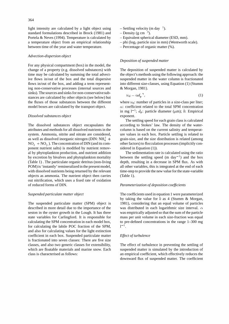
light intensity are calculated by a light object usingstandard formulations described in Brock (1981) andPortela & Neves (1994). Temperature is calculated bya temperature object from an empirical relationshipbetween time of the year and water temperature.

Advection-dispersion object

For any physical compartment (box) in the model, thechange of a property (e.g. dissolved substances) withtime may be calculated by summing the total advect-ive flows in/out of the box and the total dispersiveflows in/out of the box, and adding a term represent-ing non-conservative processes (internal sources andsinks). The sources and sinks for non-conservativesub-stances are calculated by other objects (see below) butthe fluxes of those substances between the differentmodel boxes are calculated by the transport object.

Dissolved substances object

The dissolved substances object encapsulates theattributes and methods for all dissolved nutrients in thesystem. Ammonia, nitrite and nitrate are considered,as well as dissolved inorganic nitrogen (DIN: NH+4 +NO�2 +NO�3 ). The concentration of DIN (and its com-ponent nutrient salts) is modified by nutrient remov-al by phytoplankton production, and nutrient additionby excretion by bivalves and phytoplankton mortality(Table 1) . The particulate organic detritus (non-livingPOM) is ‘instantly’ remineralized in the present model,with dissolved nutrients being returned by the relevantobjects as ammonia. The nutrient object then carriesout nitrification, which uses a fixed rate of oxidationof reduced forms of DIN.

Suspended particulate matter object

The suspended particulate matter (SPM) object isdescribed in more detail due to the importance of theseston in the oyster growth in the Lough. It has threestate variables for Carlingford. It is responsible forcalculating the SPM concentration in each model box,for calculating the labile POC fraction of the SPM,and also for calculating values for the light extinctioncoefficient in each box. Suspended particulate matteris fractionated into seven classes: There are five sizeclasses, and also two generic classes for extensibility,which are floatable materials and marine snow. Eachclass is characterised as follows:

– Settling velocity (m day�1).– Density (g cm�3).– Equivalent spherical diameter (ESD, mm).– phi (log2 particle size in mm) (Wentworth scale).– Percentage of organic matter (%).

Deposition of suspended matter

The deposition of suspended matter is calculated bythe object’s methods using the following approach: thesuspended matter in the water column is fractionatedinto different size-classes, using Equation (1) (Stumm& Morgan, 1981).

nd = �d�bp ; (1)

wherend: number of particles in a size-class per liter;�: coefficient related to the total SPM concentrationin mg l�1; dp: particle diameter (�m); b: Empiricalexponent.

The settling speed for each grain class is calculatedaccording to Stokes’ law. The density of the water-column is based on the current salinity and temperat-ure values in each box. Particle settling is related tograin-size, and the size distribution is related (amongother factors) to flocculation processes (implicitly con-sidered in Equation (1)).

The sedimentation rate is calculated using the ratiobetween the settling speed (m day�1) and the boxdepth, resulting in a decrease in SPM flux. As withall other variables, this is integrated at the end of eachtime-step to provide the new value for the state-variable(Table 1).

Parameterization of deposition coefficients

The coefficients used in equation 1 were parameterizedby taking the value forb as 4 (Stumm & Morgan,1981), considering that an equal volume of particleswas distributed in each logarithmic size interval.�

was empirically adjusted so that the sum of the particlemass per unit volume in each size-fraction was equalto pre-defined concentrations in the range 1–300 mgl�1.

Effect of turbulence

The effect of turbulence in preventing the settling ofsuspended matter is simulated by the introduction ofan empirical coefficient, which effectively reduces thedownward flux of suspended matter. The coefficient

365

Table 1. Main model equations and corresponding processes. These equations consider the sources andsinks for each model box. The transport equation calculates mass transfer between model boxes. Parametervalues were taken from the literature (e.g. Jørgensen et al., 1991) and tuned to calibrate the model

Suspended particulate matter (mg l�1) (5)@Spm

@t= Spmds � Resuspension

ds Suspended matter deposition rate Calculated from particle-

size distributions and

Stokes’ law (see text)

Dissolved mineral nitrogen (�mol l�1) (6)@N

@t= PhytppN +Oyse0

PpN Phytoplankton gross photosynthetic rate

calculated by eq. 14 and converted to

nitrogen units.

Phytoplankton (�g Chla l�1) (7)@Phyt

@t= Phyt(pp � ep � rp �mp � gOys) Carbon to Chlorophyll

Pp Phytoplankton gross photosynthetic rate h�1 (Eq. (14))

ep Phytoplankton exudation rate 0.3 ofpprp Phytoplankton respiration rate 0.3 ofppmp Phytoplankton mortality 0.002 h�1

gOys Oyster grazing pressure h�1

CarbonToChlorophyll Conversion factor 0.03

Oysters

Oyster number for each class (8)

@Oyss

@t=

nts��s

�ts��s

� nts�ts

�s� �tsn

ts (see text)

� Individual oyster scope for growth As in Raillard (1991) and

Raillard & Menesguen

(1994)

ms Oyster mortality of the sth class (See text)

Fresh weight to ash free dry weight 0.05

In the first class recruitment must also be added to eq. 8

For classes where oyster weight is above 65 g (FW) harvest may also occur, in which case it must

be subtracted from Equation (8).

used is 0.8, which effectively means that depositionmay only occur during a small part of the tidal cycle,i.e. on or about high and low water slack. This has beenvalidated by tests with a hydrodynamic model.

Resuspension

Resuspension depends on the shear-stress at thesediment-water interface, and on the nature and com-paction of the sediment. Based on the studies carriedout on the benthos, and on results from the existingdatabase on the nature of the sediment in the differentmodel boxes, a different sediment resuspension ratewas used for each box in the model.

Extinction coefficient

The light extinction coefficientk is estimated empiric-ally, using an empirical relationshipbetween SPM con-centration in the water column andk values, obtainedfrom measured data. The equation used for this is thefollowing:

k =1:7

exp(2:034)e0:723 ln(SPM)); (2)

wherek: light extinction coefficient (m�1); SPM: sus-pended particulate matter (mg l�1).

366

Particulate organic carbon

The proportion of SPM which is made up of particulateorganic carbon is estimated to vary between 0.03 and0.05 from field data gathered in Carlingford Lough.

Phytoplankton object

Primary production is estimated from light intensity,delivered by the respective forcing function object, andnutrient data, delivered by the dissolved substancesobject. If this object is not activated by the user thenprimary production is calculated solely as a functionof light. The light function is taken from Steele (1962),integrated over depth, and the nutrient limitation iscalculated by a Michaelis-Menten function (Table 2).Only nitrogen limitation is used, because an analysisof the Redfield ratio for dissolved nutrients indicatesthat nitrogen is the limiting factor.

The object also calculates exudation and respira-tion. In the literature, estimates of dissolved organiccarbon (DOC) losses are highly variable. Values ran-ging from almost zero to 90% of carbon fixed are giv-en by different authors (see Jørgensen et al., 1991).There is also variability in the literature concerningthe factors affecting DOC loss. Some authors referincreased losses with poor growth conditions (e.g.,Ittekot et al., 1981), and others have found greaterDOC exudation at high productivity rates. In this mod-el exudation is computed as a fixed fraction of grossproduction (0.1). Phytoplankton respiration is calib-rated to remove a constant proportion of the fixed car-bon, thus converting the phytoplankton gross primaryproduction (GPP) into net primary production (NPP).This has been defined as 0.3, based on a range of valuesfor algal respiration and primary production given byJørgensen et al. (1991).

Crassostrea gigas object

Due to the economic importance of this species, thereare already some models developed to simulate itsgrowth (Bacher, 1989; Bacher et al., 1991; Raillard,1991; Raillard & Menesguen, 1994). In the presentwork the simulation of oyster growth is carried outat two levels – the physiological level and the popu-lation level using a physiological and a demographicmodel. The demographic model is based on a seriesof weight classes. Oyster recruitment and harvest areman-controlled. At the physiological level the modelequations and parameters are those used earlier by Rail-

lard (1991) and Raillard & Menesguen (1994). Excre-tion rates are those reported in Bernard (1974). Scopefor growth is calculated by subtracting respiration andexcretion from assimilation, as described by the pre-vious authors. The demographic model is based on aconservation equation for the number of individuals:

@n(s; t)

@t= �

@[n(s; t)�(s; t)

@s� �((s)n(s; t); (3)

where,n: number of individuals of weights; �: scopefor growth (g day�1); � – mortality (day�1).

Equations of this type have been used in demo-graphic models for many years (see Sinko & Streifer,1967; Sinko & Streifer, 1969, Streifer, 1974). Equa-tion (3) was discretized following a upwind integra-tion scheme that seems to be the most appropriate intransport problems (in the present case it is transportof individuals between weight classes) (Press et al.,1995):

nt+�t

s=

�nt

s��s�ts��s

� nt

s�ts

�s� �t

snt

s

��

��t+ nt

s(4)

�s: class amplitude.In this equation the population is discretized in

size/weight classes ands refers to the weight of eachclass. The scope for growth calculated at the physiolo-gical level is then used in (4) to calculate transitionsof individuals between weight classes. A total of fortysize classes between 0.65 g (FW) and 97.75 g (FW)were used. The class amplitude was 2.5 g (FW). Thechoice of classes was made after running the modelwith various numbers of classes until the model solu-tion became stable taking always into consideration theCourant condition. The first class corresponds to thejuvenile oysters seeded in the Lough.

At every time step the biomass of the differentclasses is calculated as the product of the number ofindividuals they contain and the class weight. Seeding,natural mortality and harvesting mortality are calcu-lated and added/subtracted to the numbers and biomassof each class. Natural mortality was determined exper-imentally in Carlingford Lough for oysters of varioussizes (Douglas, 1992).

Man object

This object allows the simulation of different manage-ment strategies. Seeding and harvesting are carried outaccording to normal rates (Standard simulation) or to

367

Table 2. Rate equations for the biological processes and parameter values. Parameter values taken fromthe literature (e.g. Jørgensen et al., 1991) and tuned to calibrate the model

Phytoplankton

(9)

Pp = Pmaxe

kdepth(e�I=Iopt)

� e(�isup=Iopt))s(N)

f(N) =nlim

Kn + nlim(10)

Pmax Maximum photosynthesis 0.02 h�1

I Light intensity at box depth Calculated� � E m�2 s�1

Isup Surface light intensity Calculated� � E m�2 s�1

Iopt Optimum light intensity 400� E m�2 s�1

f(N) Nutrient limitation Calculated

nlim Nutrient concentration �mol N l�1 (delivered by

the dissolved substances

object)

Kn Half-saturation constant for limiting nutrient 1.19�mol N l�1

Oysters All equations and parameters as in Raillard

(1991) and Ralillard & Menesguen (1994)

Figure 2. Standard simulation. General scheme of stocks (rounded rectangles), fluxes (rectangles), sources and sinks of nitrogen in the model(all values in kg N yr�1).

different rates to estimate the carrying capacity of theLough. Normal seeding rates correspond to an averageof 0.08 tons of oysters per day during May and June.Harvest is carried out during autumn and in the modela constant rate of 4.6 tons per day is used. Whenevernecessary a higher rate is assumed in order to removeall the commercial sized oysters before the end of theyear. The model calibration and validation has beendescribed elsewhere (Ball et al., 1994), showing res-ults for measured data and simulations of pelagic statevariables and oysters. The model runs were performed

for a simulation period of four years, using a time stepof two hours. EcoWin has variables to save the inputsand outputs to the objects calculated at every time step.It also allows the storage of boundary fluxes due toadvection and dispersion of pelagic state variables. Itis thus possible to use the model to compute integratedproduction, average standing stocks and mass budgetsfor all state variables.

368

Figure 3. Standard simulation. Predicted and simulated phytoplankton biomass in model boxes 1, 2 and 3 (�g Chlorophyll l�1).

Results and discussion

Six model simulations were carried out in order toassess the carrying capacity of Carlingford Lough for

oyster culture and its sensitivity to different nutrientloads. The standard simulation represents the presentsituation in the Lough, both regarding nutrient loadsand oyster standing stocks. The next three simulations

369

Figure 4. Standard simulation. Predicted and simulated suspended matter (mg l�1) in model boxes 1, 2 and 3.

were carried out to test the effects of seeding increaseof small oyster spat by 5, 10 and 20 times the actualrate. In the last two simulations the nitrogen loads werechanged by�50% and+100%, keeping everything

else as in the standard simulation. In all simulationsthe man object interacts with the oyster object throughseeding and harvest of large (> 65 g FW) oysters.

370

Figure 5. Standard simulation. Growth simulation of an oyster with 20 g (FW) at the beginning of the year. Triangles and squares refer tomeasurements obtained in box 2 and 3, respectively (Douglas, 1992).

Figure 6. Standard simulation. Oyster biomass in box 2 as a function of time and individual weight. The drop in the biomass of large oysters atthe end of each year corresponds to harvest.

Seeding is simulated during May and harvest betweenthe beginning of fall and the end of the year.

In Figures 3 and 4 predicted and simulated chloro-phyll and suspended matter concentrations are shown.Because the observed data has a significant scatter, it

371

Figure 7. Standard simulation. Oyster biomass in box 3 as a function of time and individual weight. The drop in the biomass of large oysters atthe end of each year corresponds to harvest.

is very difficult to judge the quality of the model res-ults. However, the simulated values are well within therange of observed data. There is a chlorophyll peak atthe end of spring or beginning of summer. This peakresults from a combination of high light intensities withnitrogen concentrations ranging from 10 to 20�mol Nl�1 (Ball et al., 1994). Observed data on suspendedmatter do not follow any particular pattern. The mod-el results show average values that are close to thoseobserved in the Lough (between 20 and 30 mg l�1).

Mass balances

The execution of a mass balance is very useful both formodel analysis and in analysing the ecosystem beingmodelled:

– The role of physical (advection-dispersion) andbiological processes within each box may bedetermined, i.e. the role of internal processes maybe compared with the throughput of material.

– It allows an assessment of the relative importanceof the different biological state variables withineach box.

– Residence times may be calculated for differentmodel variables, allowing an analysis of turnoverof water relative to other variables such as DIN orphytoplankton.

– Inaccuracies in the mass balance closure are aneffective indicator of problems with the model,leading to improvements in the formulation. Theseare not always obvious in graphical output of res-ults, where errors may cancel each other out.

The mass balance for dissolved inorganic nitrogen(DIN), phytoplankton and particulate organic nitrogen(PON) is presented in Tables 3, 4 and 5. The resultswere obtained for the standard simulation, and are nor-malised per unit of surface area to allow a comparisonwith other systems.

The mass balances are presented separately forphysical inputs and outputs and biological sources andsinks. The Lough imports dissolved nitrogen both fromriverine sources and from the Irish Sea (Table 3). TheDIN is converted to particulate N by the phytoplank-ton, some of which is exported to the Irish Sea (0.29 gN m�2 yr�1) (Table 4). Internal sources of DIN in themodel are natural phytoplankton mortality and DIN

372

Figure 8. Average individual weight of the oyster population as a function of time and under different average standing stocks in box 2 (seetext for explanation).

Table 3. Standard simulation. Mass balance for DIN in Carling-ford Lough (all fluxes in g N m�2 yr�1)

Advection-dispersion Internal processes

Inputs Sources

Upstream 2.09 Phyto. mortality 1.58

Irish Sea 0.03 Oyster excretion 0.03

Sub-total 2.12 Sub-total 1.61

Outputs Sinks

Downstream – Gross primary prod. �3:73

Sub-total 0 Sub-total �3:73

Total 2.12 Total �2:12

Total 0 g m�2 y�1

Stock 0.52 gN m�2

excretion by the oysters. The natural mortality andfiltration by oysters of the phytoplankton are livingparticulate N sinks in the model (Table 4).

The PON mass balance (Table 5) shows that PONis exported from the Lough to the Irish Sea, and thatthe oyster filtration of seston is approximately oneorder of magnitude greater than that of phytoplankton.

373

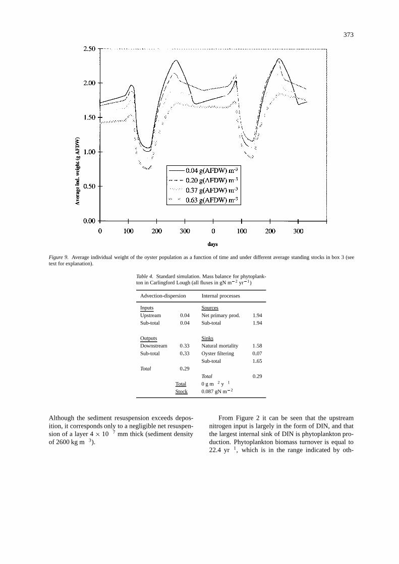
Figure 9. Average individual weight of the oyster population as a function of time and under different average standing stocks in box 3 (seetext for explanation).

Table 4. Standard simulation. Mass balance for phytoplank-ton in Carlingford Lough (all fluxes in gN m�2 yr�1)

Advection-dispersion Internal processes

Inputs Sources

Upstream 0.04 Net primary prod. 1.94

Sub-total 0.04 Sub-total 1.94

Outputs Sinks

Downstream �0:33 Natural mortality �1:58

Sub-total �0:33 Oyster filtering �0:07

Sub-total �1:65

Total �0:29

Total 0.29

Total 0 g m�2 y�1

Stock 0.087 gN m�2

Although the sediment resuspension exceeds depos-ition, it corresponds only to a negligible net resuspen-sion of a layer 4� 10�7 mm thick (sediment densityof 2600 kg m�3).

From Figure 2 it can be seen that the upstreamnitrogen input is largely in the form of DIN, and thatthe largest internal sink of DIN is phytoplankton pro-duction. Phytoplankton biomass turnover is equal to22.4 yr�1, which is in the range indicated by oth-

374

Figure 10. Oyster productivity as a function of average standing stock.

Figure 11. Time to reach a harvestable size as a function of seeding.

375

Figure 12. Oyster harvest as a function of seeding after the time necessary for the oysters to reach an harvestable size (see text).

Table 5. Standard simulation. Mass balance for PON inCarlingford Lough (all fluxes in gN m�2 yr�1)

Advection-dispersion Internal processes

Inputs Sources

Upstream 0.39 Resuspension 16.55

Sub-total 0.39 Sub-total 16.55

Outputs Sinks

Downstream �6:77 Deposition �9:61

Sub-total �6:77 Oyster filtering �0:57

Sub-total �10:18

Total �6:38

Total 6.37

Total 0.01 g m�2 y�1

Stock 0.72 gN m�2

er authors (e.g., Valiela, 1995). The oysters excreteabout 5% of their nitrogen uptake, and the nitrogenremoval due to them is relatively small compared tothe upstream inputs. The relation of biological inputsto physical inputs shows that for DIN mass flux, phys-ical processes are more important, whereas for phyto-plankton, biological processes dominate. As regardsoutputs, biological processes are far more important

than physical ones, both for DIN and phytoplankton.This contrasts with other ecosystems (e.g., Grillot &Ferreira, 1996), where the exchange of material acrossthe system boundaries plays a greater role than internalrecycling. Tables 3, 4 and 5 and Figure 2 show that theinfluence of the oysters in the processes of phytoplank-ton and particulate matter sinking and as a dissolvednitrogen source is negligible.

376

Oyster growth and production

In Figure 5 oyster growth predicted by the model andmeasured in field experiments are shown. The experi-mental data are described in Douglas (1992). The mod-el results tend to overestimate oyster growth in box 2.Since the same set of parameters is used to simulatethe oyster growth both in box 2 and 3, any parametertuning to improve box 2 results would tend to underes-timate oyster growth and production in box 3 beyondreasonable levels. Additionally, it was not possible todecrease oyster growth in box 2 and box 3, and atthe same time maintain the total biomass productionwithin the normal levels (ca. 400 tonnes year�1).

The oysters in Carlingford Lough do not exhibit anydiminishing trends in their individual weight over theannual cycle (Figure 5). This is because they do notreproduce and therefore do not lose weight throughgamete emission as in Marennes-Oleron Bay (Bach-er, 1989). The losses through respiration, the smalleramount of organic seston and the lower temperaturesprevent any significant growth during winter. Growthin box 2 is higher than in box 3 due to higher phyto-plankton concentrations in the former (Figure 3).

In Figures 6 and 7 the biomass dynamics of the fortyoyster weight classes is shown for a period of two years.Three cohorts can be observed in Figure 6 and four inFigure 7. The beginning of a cohort is located betweendays 120 and 180 (May and June) when seeding takesplace. The growth of the cohort may be followed tothe right of Figures 6 and 7. The growth acceleration isclearly seen during spring and summer. After day 265there is a sudden decrease in the biomass of the largeoysters due to harvest. All oysters above 65 g (FW)are harvested. By following the cohort from seeding toharvest it is possible to estimate the number of monthsit takes for the oysters to reach a commercial size –between about 12 months in box 2 and 17 months inbox 3. The sharp peaks observed in Figure 6 indicate agreater biomass concentration in the largest oysters inexcess of that observed in box 3. The model predictsa 325 tonnes (FW) harvest in box 2 and 42 tonnes(FW) in box 3 after two summers. Both results arewell within the real values (Douglas, pers. comm.).

The next figures synthesise results obtained withmodel simulations of different seeding rates. In Fig-ures 8 and 9 the average individual weight of the oystersis plotted against time for different average standingstocks in box 2 and 3. These standing stocks resul-ted from different seeding rates as explained earlier.All lines follow a similar pattern with a decreasing

trend after seeding, when a large number of small spatis introduced in the Lough and after harvest, whenthe largest oysters are removed from the system. Itis clearly seen that the larger the standing stock thesmaller tends to be the average individual weight. Thisnegative relationship suggests intraspecific competi-tion for food at higher than normal standing stocks.

The maximum value for oyster productivity wasobtained for the standard simulation correspondingto 1370 mg g�1 year�1 (Figure 10). These valueswere averaged for both boxes. It is clearly seen thatoyster productivity declines sharply as standing stockincreases. The time taken to reach a harvestable sizeincreases very fast with seeding (Figure 11). Whenseeding is increased to 10 times its normal value, thetime to reach an harvestable size is more than twoyears. In this hypothetical scenario the oysters seededduring the spring of one year would not grow fastenough to be harvested after the summer of the nextyear as is presently the case in Carlingford Lough. Itis important to note that the present model simulatescohorts based on weight rather than on age. The timeneeded to reach an harvestable size was determinedgraphically following the cohorts since their seeding.It is theoretically possible that animals of different agesappear in the same weight class. This may happen withtwo cohorts born in different years when the first onehad to survive through a period of poor growth condi-tions. In the present case this did not happen becausethe model forcing did not differ from one year to thenext. An important improvement in the demographicmodel would be the implementation of a age-weightequation as described in Sinko & Streifer (1967). Thiswould give the model more flexibility and utility inmanagement terms.

Harvest can be maximised by increasing the actu-al seeding rates approximately 5 times (Figure 12).Above these values the increase in harvest is very smalland according to the previous results the oysters willtake much more time to reach a harvestable size. Theseresults suggest a maximum sustainable yield around1300 tons of commercial sized oysters per year. Thesimulations with seeding increased 10 and 20 timesproduced a average oyster density of about 0.92 and1.6 individuals m�3. These values are still well belowthe 6 individuals m�3 of Marennes-Oleron Bay (Rail-lard & Menesguen, 1994) but growth depression isapparent. The differences between both systems maybe at least in part due to the higher productivity inMarennes-oleron bay (see paper in this volume).

377

In all model simulations oyster mortality was cal-culated solely as a function of individual weight usingthe experimental results described in Douglas (1992).According to Raillard & Menesguen (1994) oystermortality tends to increase with oyster density. If thisdependence was included in the model the differencesbetween the simulations would be even more pro-nounced.

The sensitivity of the model to changing nitrogenloads was not very noticeable in terms of oyster pro-duction . The model predicted that a decrease of 50%in the nitrogen load leads to an oyster productivity of1340 mg g�1 yr�1 whereas a 100% increase leads toa productivity of 1390 mg g�1 yr�1. These values arevery close to those obtained under the standard sim-ulation (1370 mg g�1 yr�1). This may be explainedbecause oyster growth in Carlingford Lough dependsmore on particulate matter, rather than on phytoplank-ton biomass.

A possible weakness of the model is in the wayscope for growth is calculated, because the equationsuse constant parameters over the all simulation period.However, as discussed by Bayne (1993) these para-meters change as a result of physiological and mor-phological adaptation of the filter-feeders at varioustime-scales. An important step in model refinementwould be the description of oyster feeding based onprinciples of optimality (Willows, 1992). It is import-ant to note that the usage of average exchange coeffi-cients between model compartments implies that partof the system dynamics, namely that resulting from thetide excursion, is lost. Considering the non-linearitiesbetween the biological processes and the environment-al conditions it is likely that these averaging proceduresmay lead to some distortion of the results.

Conclusions

Carrying capacity models are necessary to predictresponses of bivalve growth rate in relation to differ-ent management strategies (Heral, 1993). CarlingfordLough is an example of a system where bivalve cultiva-tion is still below the level where oyster growth beginsto be inhibited by stock density. Furthermore, since theoysters are not able to reproduce within the Lough dueto low water temperatures, it is easier to control thepopulation. According to the model results it seemslikely that a five-fold increase in seeding would max-imise oyster production in the Lough, allowing harvestto grow from the present 300–400 tonnes to a level

of 1300 tonnes year�1 without significantly affectingthe oyster growth rate. Further increases in seeding donot seem to lead to very significant increases in largeoysters. Therefore, according to the definition of car-rying capacity quoted previously, it may be stated thatthe carrying capacity of Carlingford Lough is approx-imately 0.44 g (AFDW) m�3 (see Figure 10) or 0.26oysters m�3.

In its present form, the model allows a fast andeasy simulation of different seeding and harvestingstrategies, with direct access to all model parametersand results. The model predictions generally show areasonable agreement with observed data, making it auseful tool for carrying capacity assessment. However,the small number of model boxes may cause some biason the results. The main oyster cultivation areas in box3 are located very close to the boundary between box2 and 3. For this reason it is likely that in this areathe environmental conditions may be closer to thoseof box 2 than predicted by the model. This could helpto reduce the differences in predicted oyster growth inboxes 2 and 3 (Figure 5).

The usage of a demographic model proved to beuseful in obtaining a detailed description of the biomassdynamics of the studied species. When the objectiveis to optimise a sustainable yield, it is important toknow the harvestable and non-harvestable classes andthe rate at which the population recovers from the har-vest (Usher, 1966). Although the usage of the demo-graphic model significantly increases the computingtime, the coupling between the physiological and thedemographic processes seem to be the best solution tosimulate biomass dynamics of a exploitable resource.This coupling allowed the advantages of the gener-al dynamic population models and analytical models(sensuHeral, 1993) to be synthesised in one model.

The combination of the three key componentsof, a large-scale coupled physical-ecological model,detailed physiological modelling of the target spe-cies, and the demographic aspects which are funda-mental to aid decision-making for management pur-poses, appears to be generally applicable to carryingcapacity assessment for bivalve species. This model-ling approach further benefits from the object-orientedmethodology used – it allows for easy developmentof the code to incorporate more species, and the pre-processing tools employed make it straightforward toapply the same model to different estuarine and coastalecosystems.

378

Acknowledgements

This work was supported by EU FAR project AQ-2-516 ‘Development of an Ecological Model for MolluscRearing Areas in Ireland and Greece’ and by EU Con-certed Action AIR3-CT94-2219 ‘Trophic capacity ofcoastal zones for rearing oysters, mussels and cockles’.The authors wish to thank two anonymous referees forhelpful suggestions.

References

Bacher C (1989) Capacite trophique du bassin de Marennes-Oleron:couplage d’un modele de transport particulaire et d’un modele decroissance de l’huitre Crassostrea gigas. Aquat Living Resour 2:199–214

Bacher C, Heral M, Deslous-Paoli and Razet D (1991) Modeleenergetique uniboite de la croissance des huitres (Crassostreagigas) dans le bassin de Marennes-Oleron. Can J Fish Aquat Sci48: 391–404

Ball B, Ferreira JG and Keegan B (1994) Development of a model todetermine the trophic capacity of mollusc rearing areas in Irelandand Greece. Final Report to the CEC for project FAR-AQ2516

Baretta J and Ruardij P (eds) (1988) Tidal flat estuaries. Simulationand analysis of the Ems Estuary. Springer-Verlag, Berlin

Bayne BL (1993) Feeding physiology of bivalves: Time dependenceand compensation for changes in food availability. In: RF Dame(ed.). Bivalve filter feeders in estuarine and coastal ecossystemprocesses. (pp. 1–24) Springer-Verlag, Berlin

Bernard FR (1974) Annual biodeposition and gross energy budgetof mature pacific oysters,Crassostrea gigas. J. Fish Res Bd Can.31: 185–190

Brock TD (1981) Calculating solar radiation for ecological studies.Ecol Modelling 14: 1–9

Carver CEA and Mallet AL (1990) Estimating carrying capacity ofa coastal inlet for mussel culture. Aquaculture 88: 39–53

Douglas DJ (1992) Environment and Mariculture (A study ofCarlingford Lough). Ryland Research Ltd., Ireland

Ferreira JG (1995) EcoWin – An Object-oriented Ecological Modelfor Aquatic Ecosystems. Ecol. Modelling 79: 21–34

Grillot N and Ferreira JG (1996). Ecological model of the Cala doNorte of the Tagus Estuary. ECOTEJO, Rel. A-8403-06-96-UNL,Ed. DCEA/FCT, New University of Lisbon

Heral M (1993) Why carrying capacity models are useful tools formanagement of bivalve molluscs culture. In: R.F. Dame (ed.).Bivalve filter feeders in estuarine and coastal ecossystem pro-cesses. (pp. 455–477) Springer-Verlag, Berlin

Ittekot V, Brockmann U, Michaelis W and Degens ET (1981) Dis-solved, free and combined carbon hydrates during a phytoplank-ton bloom in the Northern North Sea. Mar Ecol Progr Ser 4:259–305

Jørgensen SE, Nielsen S and Jørgensen L (1991) Handbook of Eco-logical Parameters and Ecotoxicology. Elsevier, Amsterdam

Portela LI and Neves R (1994) Modelling temperature distributionin the shallow Tejo estuary. In: Tsakiris & Santos (ed). Advancesin Water Resources Technology and Management. (pp. 457–463)Balkema, Rotterdam

Press WH, Teukolsky SA, Vetterling WT and Flannery BP (1995)Numerical recipes in C – The art of scientific computing. Cam-bridge University Press, Cambridge

Raillard O (1991) Etude des interactions entre les processusphysiques et biologiques intervenant dans la production del’huitre japonaiseCrassostrea gigasdu bassin de Marennes-Oleron: essais de modelisation. These doct. Oceanographie, Univ.Paris VI

Raillard O and Menesguen A (1994) An ecosystem box model forestimating the carrying capacity of a macrotidal shellfish system.Mar Ecol Prog Ser 115: 117–130

Schildt H (1995) C++, the complete reference, 2nd. Edition.Osborne

Sekine M, Nakanishi H, Ukita M and Murakami S (1991) A shallow-sea ecological model using an object-oriented programming lan-guage. Ecol Modelling 57: 221–236

Silvert W (1993) Object-oriented ecosystem modelling. Ecol Mod-elling 68: 91–118

Sinko JW and Streifer W (1967) A new model for age-size structureof a population. Ecology 48: 910–918

Sinko JW and Streifer W (1969). Applying models incorporatingage-size structure of a population toDaphnia. Ecology 50: 608–615

Steele JH (1962) Environmental control of photosynthesis in the sea.Limnol Oceanogr 7: 137–150

Streifer W (1974) Realistic models in population biology. Adv EcolRes 8: 199–266

Stumm W and Morgan J. (1981) Aquatic Chemistry, 2nd. Edition.Wiley-Interscience

Usher MB (1966) A matrix approach to the management of renew-able resources, with special reference to selection forests. J ApplEcol 3: 355–367

Valiela I (1995) Marine ecological processes, 2nd Edition. Springer-Verlag

Vicente P (1994) DifWin: A package for the definition of compart-ments and calculation of dispersion coefficients in box models– Application to the Carlingford Lough. In: Proceedings of theFirst International Conference on Hydroinformatics, Delft, TheNetherlands, 717–721

Willows RI (1992). Optimal digestive investment: A model for filter-feeders experiencing variable diets. Limnol Oceanogr 37: 829–847