Opt Quant Electron (2008) 40:943–956DOI 10.1007/s11082-009-9297-y

Alternative calculations of initial value problemfor electromagnetic field in dielectric waveguide

A. Nerukh · H. Semenova · N. Sakhnenko

Received: 30 August 2008 / Accepted: 14 April 2009 / Published online: 6 May 2009© Springer Science+Business Media, LLC. 2009

Abstract Two ways of solving an initial value problem in a dielectric waveguide ispresented. Each way describes one of two complementary approaches: a progressive orBrillouin waves approach and an oscillatory or eigenfrequency approach. The evolution of atransient electromagnetic field in the waveguide after an instant change of its permittivity isconsidered and calculated. The results of the approaches coincide completely, however, theBrillouin approach is more intuitive, visual, and less demanding computationally.

Keywords Dielectric waveguides · Initial electromagnetic problems ·Time-varying medium · Progressing · Oscillatory representations

Introduction

Guided-wave dynamics can be organized around two complementary approaches, progress-ing and oscillatory, that are closely related to local versus global descriptions (Felsen andMarcuvitz 1994). The progressing description operates with wave-fronts and it representspoint-to-point propagation during which the wave fronts interact with the physical envi-ronment locally along their trajectories. The oscillatory approach operates with modes orresonances which form standing waves over extended, often global portions of the physicalenvironment (Sevgi et al. 2007). These two approaches reveal the double nature of the oscil-lation and wave processes in the waveguide structures. However, it is important to emphasizethat the time variable has to enter in the progressive framework explicitly while the timedependence in the harmonic form is often enough for the oscillatory approach where theevolution of the electromagnetic phenomena has to be presented by the temporal Fourierseries that assumes infinite time axes. In contrast, the evolution process means the existenceof a beginning of this process. This, in turn, means that the evolution of the electromagneticphenomena has to be described as an initial and boundary value problem. The progressive

A. Nerukh (B) · H. Semenova · N. SakhnenkoKharkov National University of Radio Electronics, 14 Lenin Ave., Kharkov 61166, Ukrainee-mail: nerukh@ddan.kharkov.ua

123

944 A. Nerukh et al.

approach is more suitable for such problems because it describes in a natural way thosephenomena that develop from an initial time point. The progressive method is also morestraightforward and is used, for example, for the calculation of transient waves reflectionfrom multilayered media (Perry and Rothwell 2007). The oscillatory approach is more com-monly used when the process beginning does not play a role in the phenomenon.

There are many modern applications in quantum electronics, quantum computing, andoptical technology that rely on the interaction of electromagnetic waves and media withtime-varying, nonlinear, and/or anisotropic parameters. Example are the direct upconver-sion of the microwave signals into the optical domain by an electro-optical modulator ora microphotonic modulator (Cohen et al. 2001) that are the main phenomena in photonicfront-end microwave receiver architectures (Ilchenko et al. 2002, 2003) emerged as a newway of microwave and millimetre wave signal processing. To immunize electronic systemsagainst high power microwaves, a new radiofrequency front-end technology is constructedon a dielectric antenna coupled to an electro-optic resonator which converts the receivedelectromagnetic signal to a modulated optical signal carried away from the antenna front-endvia an optical fibre. To address this problem, all-dielectric photonic-assisted receivers havebeen proposed. The complete lack of metal and electronics in the front-end offers immunityagainst the damage from the intense electromagnetic radiation (Ayazi 2008).

In all these devices, one way or another, there is an interaction of an electromagneticfield with a time-varying medium. In practice temporal variation of the material’s refractiveindex can be caused by an external source current or a field source. For many applicationsthe frequency of the external source is much lower than that of the signal, which permits thesignal behaviour to be modelled using a slowly varying envelope to incorporate the effectsof the time-varying material. For example, modern modulators typically use an external 40GHz microwave signal whilst the frequency of the propagating optical signal is of the orderof few THz. However, the steadily increasing demand for higher bit rates requires the useof higher modulation frequencies and recently multiple quantum wells driven by terahertzfields have been investigated both analytically and experimentally for this purpose (Carteret al. 2005; Maslov and Citrin 2002). At such high modulation and switching speeds themodelling approaches based upon the slowly varying envelope paradigm such as the FiniteDifference Beam Propagation Method (Masoudi and Arnold 1995) are less appropriate andhence more rigorous modelling techniques need to be used. In particular, transient effectscannot be neglected with such high modulation rates and need to be properly accounted for(Bekker et al. 2007).

Dielectric waveguide tuning can be achieved by changing the material refractive indexwhich can be practically realized by varying the input signal in a non-linear waveguide (Blomet al. 1997), by voltage control (Savchenkov et al. 2005), or by free carrier plasma injection(Djordjiev et al. 2002). An enhanced frequency shift occurs in a slow wave photonic structurewith modulated permittivity (Morichetti et al. 2007). The reflection of a light pulse from ashock-like dielectric modulation propagating through a photonic crystal demonstrates thereverse Doppler effect (Reed et al. 2003a) and a frequency shift which is tuneable by adjust-ing the band gap size (Reed et al. 2003b). A dynamic photonic crystal whose properties aremodulated while a pulse is inside it can be used to stop, store, and time-reverse light pulses(Fan et al. 2007).

Surface plasmon polaritons have great potential as information carriers for next-generation, highly integrated nanophotonic devices. A number of techniques for control-ling the propagation of guided surface plasmon polariton signals have been demonstrated.However, with sub-microsecond or nanosecond response times at best, these techniques arelikely to be too slow for future applications in such fields as data transport and processing.

123

Alternative calculations of initial value problem for electromagnetic field in dielectric waveguide 945

In (Macdonald et al. 2009) it is reported that femtosecond optical frequency plasmon pulsescan propagate along a metal–dielectric waveguide and that they can be modulated on thefemtosecond timescale by direct ultrafast optical excitation of the metal, thereby offeringunprecedented terahertz modulation bandwidth—at speed at least five orders of magnitudefaster than existing technologies.

All these spatial-time processes can be described by the progressing as well as theoscillatory approaches. This paper elucidates the conceptual distinction between these twoapproaches by considering an initial-boundary value electromagnetic problem in a dielec-tric waveguide. The beginning of the electromagnetic wave evolution in the waveguide isinduced by the instant change of the core permittivity. It is a model problem for a wide rangeof nonstationary phenomena with applications shown above. The investigation of the wavetransformation is made by the oscillatory or the eigenwaves approach and the progressiveor the Brillouin waves approach. The calculation is made by the summation of generatedoscillatory modes in the former case and by tracing the Brillouin wave fronts in the latterone. The evolution of the electromagnetic field and its spectrum is considered and compared.

Mechanical analog

To obtain deeper understanding of the two representations we first consider a simple onedimensional problem in the form of longitudinal oscillations of an elastic rod fixed at oneend and subjected to a force F(t) at the other end. The oscillations are described by the onedimensional wave equation (Lavrentyev and Shabat 1987)

∂2u

∂t2 − a2 ∂2u

∂x2 = 0 (1)

where u = u(x, t) is the longitudinal displacement and a2 is a constant coefficient dependingon the rod material. If the harmonic force F = A sin(ωt)θ(t) begins to act at zero moment oftime (θ(t) is the Heaviside unit function) then the initial and boundary conditions turn intothe following:

u|t=0 = ∂u

∂t

∣∣∣∣t=0

= 0, u|x=0 = 0,∂u

∂x

∣∣∣∣x=l

= A

Esinωt (2)

where E is the modulus of elasticity and l is the length of the rod. The Laplace transform ofthis problem is given by the formula

U (p) = B

p(p2 + ω2)

sinh(xp/a)

cosh(lp/a), −1 ≤ x

l≤ 1 (3)

where p is the Laplace transform variable and B = Aaω/E . The function (3) has two polesp = ±iω and the infinite number of the poles pk = iωk, ωk = (2k + 1) πa/2l satisfyingthe equation cosh(lp/a) = 0 ⇒ e2lp/a = −1 and representing all eigenfrequencies of therod oscillations.

The inverse Laplace transformation can be found by the two ways described above: theoscillatory and the progressive approaches. The oscillatory approach uses all eigenfrequen-cies of the rod oscillations given by the poles. The calculation of all the residues at the polesgives the sum of the eigenwaves which frequencies are determined by the rod length only.If only 2K poles pk are used then the inverse Laplace transform has the form

123

946 A. Nerukh et al.

u1(t, K ) = B

2π i

σ+i∞∫

σ−i∞

1

p(p2 + ω2)

e(x+l)p/a − e−(x−l)p/a

e2lp/a + 1ept dp

= B

2ω2 cos(ωl/a)[cos(ω(t − x/a))θ(t − x/a)− cos(ω(t + x/a))θ(t + x/a)]

+ aB

l

K−1∑

k=0

1

ωk[

ω2k − ω2

]

{

sin

[

ωk

(

t + x + l

a

)]

θ

(

t + x + l

a

)

− sin

[

ωk

(

t − x − l

a

)]

θ

(

t − x − l

a

)}

− aB

2l

i

ωK[

ω2K − ω2

]

×{

eiωK

(

t+ x+la

)

θ

(

t + x + l

a

)

− eiωK

(

t− x−la

)

θ

(

t − x − l

a

)}

(4)

where σ > σa and σa is the abscissa of the absolute convergence of the Laplace transform.The progressive approach is obtained by expanding the fraction with hyperbolic functions

into the geometrical progression

sinh(xp/a)

cosh(lp/a)= e(x−l)p/a − e−(x+l)p/a

1 + e−2lp/a

=∞∑

n=0

(−1)n[

e(x−(1+2n)l)p/a − e(−x−(1+2n)l)p/a]

(5)

In this form all the poles of the oscillatory representation disappear and the remaining twopoles of the first fraction in (3) give re-reflected waves on the frequency of the driving force.Finally, it gives another representation of the inverse Laplace transform

u2(t, N ) = B

2π i

σ+i∞∫

σ−i∞

1

p(p2 + ω2)

e(x−l)p/a − e−(x+l)p/a

1 + e−2lp/aept dp

= B

ω2

N∑

n=0

(−1)n+1{

cos

[

ω

(

t + x − (1 + 2n)l

a

)]

θ

(

t + x − (1 + 2n)l

a

)

− cos

[

ω

(

t − x + (1 + 2n)l

a

)]

θ

(

t − x + (1 + 2n)l

a

)}

(6)

It is worth to note that for every given moment of time only a finite number Nof termsin u2(t, N ) are nonzero and this number is proportional to the moment of observation,N ∼ (t + (x − l)/a)/2. The difference between the two approaches is essential at the earlystage of the evolution, Fig. 1, when the progressive approach requires only two terms in thesum while the oscillatory one requires a few tens of terms for the same accuracy. For a longinterval both transforms give the same result asymptotically, Fig. 2, and in this case a fewterms of the oscillations give a good accuracy while the number of terms in the progressiverepresentation grows with time.

Thus, these two approaches give the same physically existing observed fields but for theinitial period of evolution the oscillatory approach requires a few tens of terms for a suitableaccuracy while only two terms of the progressive approach give the exact expression for thesame time interval. Concluding one can say that the oscillatory approach gives the indefinitesum of abstract eigenwaves. Only this sum can be observed directly, not the individual waves.

123

Alternative calculations of initial value problem for electromagnetic field in dielectric waveguide 947

-0,05

0,00

0,05

0,10

0,15

0,20

time

disp

lace

men

t

solid f(t,1)dash g(t,2)

0,00

0,05

0,10

0,15

0,20 solid f(t,3)dash g(t,2)

time

disp

lace

men

t

0,00

0,05

0,10

0,15

0,20 solid f(t,10)dash g(t,2)

time

disp

lace

men

t

0,0 0,1 0,2 0,3 0,4 0,5 0,0 0,1 0,2 0,3 0,4 0,5

0,0 0,1 0,2 0,3 0,4 0,5 0,0 0,1 0,2 0,3 0,4 0,5

0,00

0,05

0,10

0,15

0,20 solid f(t,30)dash g(t,2)

disp

lace

men

t

time

Fig. 1 The evolution of the field at early times calculated for various number of the expansion terms in (4)(the parameters are equal to: ωl/a = 2.7, x/ l = 0.7)

-1,0

-0,8

-0,6

-0,4

-0,2

0,0

0,2

0,4

0,6

0,8

1,0

disp

lace

men

t

time

dot f(t,5) solid g(t,5)

0 10 20 30 40 50 0 10 20 30 40 50-1,0

-0,8

-0,6

-0,4

-0,2

0,0

0,2

0,4

0,6

0,8

1,0

time

disp

lace

men

t

dot f(t,5) solid g(t,20)

Fig. 2 The agreement of the approaches asymptotically for long times (the same parameters as in Fig. 1)

Whereas the progressive approach gives the finite sum of really existing waves excited bythe driving force and their wave fronts can be detected separately.

Initial and boundary value electromagnetic problem in a dielectric waveguide

An electromagnetic problem in a general case has to be formulated as an initial and boundaryvalue problem. As an example of such a problem we consider here a two dimensional prob-lem on electromagnetic field evolution in a flat dielectric waveguide after an instant change

123

948 A. Nerukh et al.

Fig. 3 The problem geometry

0

b/2

Across waveguide, x

2

-b/2

1

10

E

E

0

Along waveguide, z

at t=0

of the core material parameters. The initial guiding wave propagates along the z axis and itselectric field is perpendicular to the propagation direction (along the y axis which is parallelto the waveguide walls), Fig. 3.

The boundary value problem considers the electromagnetic field in and out of the wave-guide with the requirement of continuity for the tangential components of the electric andmagnetic fields on the waveguides boundaries. The initial value problem arises from aninstant change of the core permittivity at zero moment, ε1 ⇒ ε2. Then the field evolution isinitiated by this change according to the initial conditions (Nerukh et al. 2001) which can beeasily obtained from the Maxwell’s equations:

Bz |t=−0 = Bz |t=+0 ; ε1 Ey∣∣t=−0 = ε2 Ey

∣∣t=+0 ; ∂t

(

ε1 Ey)∣∣t=−0 = ∂t

(

ε2 Ey)∣∣t=+0 (7)

and continuity of the tangential components of the electric and magnetic fields on the wave-guides boundaries. All these determine the spatial and temporal behaviour of the field. Theproblem as the initial one can also be considered in the two approaches as in the example ofthe mechanical problem above: the oscillatory and the progressive.

For certainty we consider the initial field as the TE eigenwave propagating along the z-axisof the dielectric waveguide:

E0y = A0 sin(k1x)eiωt−i�z, B0z = i (k1/ω) A0 cos(k1x)eiωt−i�z .

Here, �2 = ω2/v2 + s21 = ω2/v2

1 − k21 is the longitudinal wave number, v = c/

√ε,

v1 = c/√ε1 are the wave phase velocities, ε and ε1 are the cladding and core permittivities

respectively. The transverse wave numbers κ1 and s1,Re s1 > 0, satisfy the common disper-sion equation tan (κ1b/2) = −κ1/s1. The field outside the waveguide is represented by theevanescent waves E ′

0y = A′0eiωt−s1x − i�z, B ′

0z = −i(s1/ω)A′0eiωt−s1x−i�z .

After the moment of the core permittivity change the field inside the waveguide is con-trolled by the equations

{

∂2zz Ey + ∂2

xx Ey = v−22 ∂2

t Ey

∂x Ey = −∂t Bz(8)

Outside the waveguide the equations are similar

{

∂2zz Ey + ∂2

xx Ey = v−2∂2t Ey

∂x Ey = −∂t Bz(9)

123

Alternative calculations of initial value problem for electromagnetic field in dielectric waveguide 949

Fig. 4 The cuts for choosing ofthe branches of the square rootsin the function ϕ. The Riemannsurface corresponding toRe ϕ(p) > 0 is chosen.Analogous ones are for thefunction ϕ2

Re p

ivRe 0

Im p

Im < 0

iv

Im < 0Im < 0

integrationline

The solutions to these equations are found using Laplace transformation together withthe initial and boundary conditions that gives the Laplace transform of the field inside thewaveguide

E = v22

v21

A0

{

p + iω

p2 + ω22

sin(κ1x)−(

v21

v22

− 1

)

v2κ1 p2 (p + iω)

s1 (vs1 + ϕ)

cos(κ1b/2)

p2 + ω22

×2e−ϕ2b/2v2sinh(ϕ2x/v2)

D

}

(10)

Here, p is the Laplace transform variable, ϕ2 =√

p2 + v22�

2, ϕ = √

p2 + v2�2, R =v2ϕ−vϕ2v2ϕ+vϕ2

, v2 = c/√ε2, D = (v2ϕ + vϕ2) (1 − Re−ϕ2b/v2) and b is the waveguide width.

The frequency ω2 = ωv2/v1 is a new frequency which the transformed wave acquiresdue to the permittivity change (Morgenthaler 1958). The Riemann surface for the functionsϕ(p) and ϕ2(p) is chosen in such a way that the conditions Re ϕ(p) > 0 and Re ϕ2(p) > 0are satisfied. The corresponding branch cuts are shown in Fig. 4.

The field evolution in time is given by the inverse Laplace transform which is implementedin the oscillatory and the progressive ways. The oscillatory or eigenfrequency representa-tion of the inverse Laplace transform is given by the calculation of residues at the polesp± = ±iω2 and the poles pk which are zeros of the denominator D = 0 in the expression(10). The poles pk are the roots of the dispersion equation

tanh (ϕ2b/2v2) = − (vϕ2/v2ϕ) (11)

and represent the eigenwaves of the waveguide. The integration line for the calculationof the inverse Laplace transform shown in Fig. 4 is passing on the right from all thepoles.

The alternative, progressive representation is given by the expansion on the reflectiv-ity of the Brillouin waves R if the fraction in (10) is written in the form of geometricprogression

123

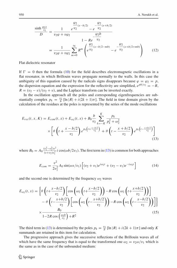
950 A. Nerukh et al.

sinh ϕ2xv2

D= 1

v2ϕ + vϕ2

e

ϕ2

v2(x−b/2)

− e−ϕ2

v2(x+b/2)

1 − Re−ϕ2b

v2

= 1

v2ϕ + vϕ2

∞∑

m=0

Rm

⎛

⎝e

ϕ2

v2(x−b/2−mb)

− e−ϕ2

v2(x+b/2+mb)

⎞

⎠ (12)

Flat dielectric resonator

If � = 0 then the formula (10) for the field describes electromagnetic oscillations in aflat resonator, in which Brillouin waves propagate normally to the walls. In this case theambiguity of this equation caused by the radicals signs disappears because ϕ = ϕ2 = p,the dispersion equation and the expression for the reflectivity are simplified, epb/v2 = −R,R = (v2 − v)/(v2 + v), and the Laplace transform can be inverted exactly.

In the oscillation approach all the poles and corresponding eigenfrequencies are sub-stantially complex pk = v2

b [ln |R| + i(2k + 1)π ]. The field in time domain given by thecalculation of the residues at the poles is represented by the series of the mode oscillations

Eres(t, x, K ) = Ecom(t, x)+ Eω2(t, x)+ B0b

v2

K∑

k=−K

pk

p2k + ω2

2

×[

θ

(

t + x − b/2

v2

)

epk

(

t+ x−b/2v2

)

+ θ

(

t − x + b/2

v2

)

epk

(

t− x+b/2v2

)]

(13)

where B0 = A0(v2

1−v22 )v

2

(v+v2)v31

i cos(ωb/2v1). The first term in (13) is common for both approaches

Ecom = v2

2v21

A0 sin(ωx/v1)[

(v2 + v1)eiω2t + (v2 − v1)e

−iω2t]

(14)

and the second one is determined by the frequency ω2 waves

Eω2(t, x) ={

θ

(

t+ x−b/2

v2

) [

cos

(

ω2

(

t+ x−b/2

v2

))

−R cos

(

ω2

(

t+ x+b/2

v2

))]

− θ

(

t− x+b/2

v2

) [

cos

(

ω2

(

t− x+b/2

v2

))

−R cos

(

ω2

(

t− x−b/2

v2

))]}

× B0

1−2R cos(ω2bv2

)

+R2(15)

The third term in (13) is determined by the poles pk = v2b [ln |R| + i(2k + 1)π ] and only K

summands are retained in this item for calculation.The progressive approach gives the successive reflections of the Brillouin waves all of

which have the same frequency that is equal to the transformed one ω2 = v2ω/v1 which isthe same as in the case of the unbounded medium:

123

Alternative calculations of initial value problem for electromagnetic field in dielectric waveguide 951

-0,4

-0,2

0,0

0,2

0,4

0,6

0,8

1,0

1,2(a) (b)

(d)(c)

Ele

ctric

fiel

d

tb/v

Eres

(t,0.4,5)

Eres

(t,0.4,100)

EBr

(t,0.4,3)

-1,4-1,2-1,0-0,8-0,6-0,4-0,20,00,20,40,60,8

Ele

ctric

fiel

d

tb/v

Eres

(t,0.4,5)

Eres

(t,0.4,100)

EBr

(t,0.4,3)

0,9

1,0

1,1

1,2

1,3

1,4

1,5

1,6

1,7

Ele

ctric

fiel

d

tb/v

Eres

(t,0.4,5)

Eres

(t,0.4,100)

EBr

(t,0.4,3)

0,06 0,08 0,10 0,12 0,14 0,56 0,58 0,60 0,62 0,64

0,68 0,69 0,70 0,71 0,72 0,73 0,74 0,75 -0,2 0,0 0,2 0,4 0,6 0,8 1,0 1,2 1,4 1,6

-2,0

-1,5

-1,0

-0,5

0,0

0,5

1,0

1,5

2,0

Ele

ctric

fiel

d

tb/v

Eres

(t,0.4,5)

Eres

(t,0.4,100)

EBr

(t,0.4,3)

Fig. 5 The electromagnetic oscillations in the flat resonator: (a, b, c) are for the early time and (d) forasymptotic behaviour (the parameters are ε = 3, ε1 = 3.5, ε2 = 3.8).

EBr (t, x,M) = Ecom(t, x)

+ B0

M∑

m=0

Rm[

θ

(

t + x − (m + 1/2)b

v2

)

cos

(

ω2t + ωx − (m + 1/2)b

v1

)

− θ

(

t − x + (m + 1/2)b

v2

)

cos

(

ω2t − ωx + (m + 1/2)b

v1

)]

(16)

In this case the field is given exactly by the finite sum of terms the number of which isdetermined by the moment of the observation.

The evolution of the field is given in Fig. 5. The calculations are made for the case when thepermittivity outside the flat resonator is equal to ε = 3. The inner permittivity changes fromε1 = 3.5 to ε2 = 3.8 at zero moment. The solid line in Fig. 5 corresponds to the approachexploiting reflections of the Brillouin waves with the reflectivity R = (v2 − v)/(v2 + v).The dash and dot lines give the results obtained by using the eigenfrequencies. The dash lineis for 5 terms of the series and the dot line is for 100 terms. It can be seen that the accuracyof the results based on the eigenfrequencies improves with the number of the terms for theearly time, Fig. 5a, b, c and practically does not depend on it for the asymptotic behaviour,Fig. 5d. At the same time interval it is enough to take into account only three reflectionsof the Brillouin waves that gives the exact solution. Thus, two representations of the fieldevolution differ at the early stage but coincide asymptotically.

As in the mechanical problem in the electromagnetic case the oscillatory approach givesthe infinite sum of abstract eigenwaves. Only the sum as a whole can be observed directly not

123

952 A. Nerukh et al.

the individual waves. Whereas the progressive approach gives the finite sum of really existingwaves initiated by the primary field and their wave fronts can be detected separately. Thesetwo approaches give the same physically existing observed field but for the initial period ofevolution the oscillatory approach requires hundreds of terms for a suitable accuracy whileonly three terms of the progressive approach give the exact expression for the same timeinterval.

Field evolution in a dielectric waveguide

When the propagation constant is not equal to zero, � �= 0, then the equation (10) describesthe evolution of the waves in the dielectric waveguides after the instant changes of the corepermittivity. In this case the ambiguity of the radical signs must be taken into account andthe equation besides the poles has a branch point. The presence of the radicals changesconsiderably the essence of the dispersion equation (11) and the form of its roots. Only thecontributions from the poles will be considered further as the contributions from the integralsalong the cut lines drawing from the branch points are negligible. Indeed, it is enough to makethe substitution p = qt in the integrand of the inverse Laplace transform of (10) to see thatthe integral over the branch cut tends to zero when time t tends to infinity (Lavrentyev andShabat 1987):

1

2π i

∫

C

eq

t

{

qt + iω

(qt)2 + ω22

sin(κ1x)−(

v21

v22

− 1

)

κ1(qt)2 (qt + iω)

v2s1 (vs1 + t ϕ̄)

cos(κ1b/2)

(qt)2 + ω22

× 2e−ϕ2b/2v2sinh(ϕ2x/v2)

D

}

dq (17)

So, the expression obtained by the eigenfrequency approach is equal to (without the integralsover the branch cuts)

Eres(t, x, K ) = Ecom(t, x)+ Eω2(t, x)

+ B1vv1

v22 − v2

K∑

m=1

pm (pm + iω)(

p2m + ω2

2

)ϕmϕ2m(v2ϕm + vϕ2m)

(vs1 + ϕm) (bp2mϕm − 2vv2

2�2)

×epm t(

eϕ2mv2(x+b/2)

θ [t + (x − b/2) /v2]

− e− ϕ2m

v2(x−b/2)

θ [t − (x + b/2) /v2]

)

(18)

where Ecom is as in (14),

Eω2 = B1v1 + v2

2v1ω2

×∑

±

sin(ω2t + κ1x)θ [t + (x − b/2)/v2] − sin(ω2t − κ1x)θ [t − (x + b/2)/v2]

(vs1 + ψ) [ψ sin (κ1b/2)+ vκ1 cos (κ1b/2)]

and B1 = A0(v2

1−v22 )vκ1

v31s1

cos(κ1b/2), ϕ2m =√

p2m + v2

2�2, ϕm = √

p2m + v2�2, ψ =

√

−ω22 + v2�2, andω2 = v2ω/v1 is the transformed frequency due to the change of the mate-

rial permittivity. The eigenfrequencies pm are the roots of the dispersion equation D(p) = 0which has a finite number of real roots and an infinite number of complex ones. For the

123

Alternative calculations of initial value problem for electromagnetic field in dielectric waveguide 953

Table 1 The lower eigenfrequencies (the first roots of the dispersion equations)

m 1 2 3 4 5 6 7 8

Re(pmb/v2) 0 0 0 −1, 79 −1, 91 −1, 99 −2, 04 −2, 14Im(pmb/v2) 5,46 10,90 16,04 34, 51 40, 81 47, 10 53, 39 72, 24

x /2= -v t+b

Time, t0

b/2

Across waveguide, x

2

x -b/2 = v t2

-b/2

Fig. 6 Re-reflection of the Brillouin waves in spatial-time coordinates

parameters as in the considered above case of the flat resonator the values for the lowereigenfrequencies are given in Table 1. It is seen that only a few roots are imagine and theother have negative real parts. It means that the corresponding waves will decay fast in time,so the contribution of the complex roots to the whole field is very small and, therefore, canbe neglected in this calculation.

The Brillouin approach gives the expression in the form of the expansion on the reflectivityof the Brillouin waves Re−ϕ2b/v2 = (v2ϕ − vϕ2)e−ϕ2b/v2/(v2ϕ + vϕ2). This formula givesthe re-reflections of the Brillouin waves at each moment

EBr (t,M) = Ecom + B1v2

2v1

∓v1−v2vs1+ψ∑

±e±iω2t

∞∑

m=0

(

R±)m

×[

e±iκ1(x−b/2−mb)θ [t + (x − b/2 − mb) /v2]

− e∓iκ1(x+b/2+mb)θ [t − (x + b/2 + mb) /v2]]

(19)

The formation of the transformed field is illustrated by the tracks of the Brillouin wavefronts as shown in the time-spatial diagram, Fig. 6. The progressive representation is a sumof a finite number of terms at each time moment. This number is equal to the number ofthe Brillouin wave re-reflections and is increasing with time. All re-reflected waves have thesame transformed frequency ω2 = ωv2/v1 as in the unbounded medium.

The initial and transformed fields on short time intervals are given in Fig. 7. There thecomplete coincidence for both ways of calculation is shown in detail in the early stage ofthe process immediately after the permittivity change, Fig. 7a, as well as after a long period,Fig. 7b, which equals to 70 periods of the initial wave marked by the dotted line in this

123

954 A. Nerukh et al.

-0,3

-0,2

-0,1

0,0

0,1

0,2

0,3(a) (b)

E0 E

res E

Bri

time interval from 0 to 2el

ectr

ic fi

eld

tb/v2

0,0 0,5 1,0 1,5 2,0 20,0 20,5 21,0 21,5 22,0 22,5 23,0

-0,3

-0,2

-0,1

0,0

0,1

0,2

0,3

tb/v2

time interval from 20 to 23

E0

Eres

EBr

elec

tric

fiel

d

Fig. 7 The comparison of calculations using the two approaches at different stages of the evolution

-0,3

-0,2

-0,1

0,0

0,1

0,2

0,3(a)(b)

tb/v2

E0

Eres

EBr

time interval from 15 to 20

elec

tric

fiel

d

15 16 17 18 19 20 0 2 4 6 8 100.0

0.2

0.4

0.6

0.8

1.0A

mpl

itude

(no

rmal

ized

)

dot - initialdash - residuessolid - brillouin

Frequency (normalized)

Fig. 8 The evolution of the electromagnetic wave on the long period (a) and the change of the spectrum (b)

diagram. These curves are calculated for seven terms in the oscillatory approach which cor-respond to the pure imaginary roots as the contribution of other terms with complex rootsis very small. The number of terms in the progressive approach increases with time as thegrowing number of the Brillouin wave re-reflections contribute to the whole field.

The wave evolution on the long time interval is shown in Fig. 8a and the spectra showclearly the shift of the frequency in Fig. 8b.

Thus, the two approaches give the same results but the progressive one seems to be lessexpensive because it does not require the solution of the dispersive equation that can be avery difficult problem. This difficulty arises, for example, in the investigations of the fieldevolution in a circular microcavity with time-varying medium (Sakhnenko et al. 2007).

Conclusions

The applicability of two alternative representations of wave evolution dynamics in a wave-guide (resonator) after the moment of the process beginning is shown. Examples of thisapplicability are considered, a dielectric waveguide with a time discontinuity of the corepermittivity among them. One of the representations is an expansion on the eigenmodes(oscillatory approach), another one is an expansion on Brillouin wave reflection coefficients(progressing approach). The Brillouin waves representation is a sum of a finite number ofterms at each time moment while the eigenmode representation is an infinite series. The

123

Alternative calculations of initial value problem for electromagnetic field in dielectric waveguide 955

progressing way turns out to be preferable because it does not require the calculation ofthe eigenfrequencies for the new modes that may be a rather difficult problem. Therewiththe Brillouin approach is more intuitive and visual and also less demanding to computationresources. This can be used in investigations of more complex problems, particularly withmore complex geometry, for example, the cylindrical or spherical ones.

Acknowledgment The authors thank the support from the NATO Reintegration Grant (CBP.EAP.RIG981996) and the Royal Society (2006/R2 IJP).

References

Ayazi, A., Hsu, R.C.J., Houshmand, B., Steier, W. H., Jalali, B.: All-dielectric photonic-assisted wirelessreceiver. Opt. Express 16, 1742–1747 (2008) doi:10.1364/OE.16.001742

Bekker, E.V., Vukovic, A., Sewell, P., Benson, T.M., Sakhnenko, N.K., Nerukh, A.G.: An assessment ofcoherent coupling through radiation fields in time varying slab waveguides. Opt. Quantum Electron. 39,533–551 (2007) doi:10.1007/s11082-007-9104-6

Blom, F.C., van Dijk, D.R., Hoekstra, H., Driessen, A., Popma, T.: Experimental study of integrated-opticsmicrocavity resonators: Toward an all-optical switching device. Appl. Phys. Lett. 71, 747–749 (1997)doi:10.1063/1.119633

Carter, S.G., Birkedal, V., Wang, C.S., Caldren, L.A., Maslov, A.V., Shevrin, M.S.: Quantum coherence in anoptical modulator. Science 310, 651–653 (2005) doi:10.1126/science.1116195

Cohen, D.A., Hossein-Zadeh, M., Levi, A.F.J.: High-Q micriphotonic electro-optic modulator. Solid-StateElectron. 45, 1577–1589 (2001) doi:10.1016/S0038-1101(01)00165-4

Djordjiev, K., Coi, S., Dapkus, P.: Microdisk tuneable resonant filters and switches. IEEE Photon. Technol.Lett. 14, 828–830 (2002) doi:10.1109/LPT.2002.1003107

Fan, S., Yanik, M., Povinelli, M., Sandhu, S.: Dynamic photonic crystals. Opt. Photonic News, 3, 42–45(2007).

Felsen, L.B., Marcuvitz, N.: Radiation and Scattering of Waves. IEEE Press Piscataway, New Jersy (1994)Ilchenko, V.S., Savchenkov, A.A., Matsko, A.B., Maleki, L.: Sub-micro watt photonic microwave receiver.

IEEE Photon. Technol. Lett. 14, 1602–1604 (2002) doi:10.1109/LPT.2002.803916Ilchenko, V.S., Savchenkov, A.A., Matsko, A.B., Maleki, L.: Whispering-gallery-mode electro-optic modu-

lator and photonic microwave receiver. J. Opt. Soc. Am. B 20, 333–342 (2003) doi:10.1364/JOSAB.20.000333

Lavrentyev, M.A., Shabat, B.V.: Methods of complex variable functions (in Russian). Nauka, Moscow (1987)Macdonald, K.F., Samson, Z.L., Stockman, M.I., Zheludev, N.I.: Ultrafast active plasmonics. Nat. Photon-

ics 3, 55–58 (2009)Maslov, A.V., Citrin, D.S.: Mutual transparency of coherent laser beams through a terahertz-field-driven quan-

tum well. J. Opt. Soc. Am. B 19, 1905–1909 (2002) doi:10.1364/JOSAB.19.001905Masoudi, H.M., Arnold, J.M.: Modelling second-order nonlinear effects in optical waveguides using a

parallel-processing beam propagation method. IEEE J. Quantum Electron. 31, 2107–2113 (1995) doi:10.1109/3.477734

Nerukh, A.G., Scherbatko, I.V., Marciniak, M.: Electromagnetics of Modulated Media with Applications toPhotonics. National Institute of Telecommunications Publishing House, Warsaw (2001)

Morgenthaler, F.R.: Velocity modulation of electromagnetic waves. IRE Trans. Microw. Theor. Tech. 6,167–172 (1958) doi:10.1109/TMTT.1958.1124533

Morichetti, F., Ferrari, C., Melloni, A.: Enhanced Frequency Shift in Optical Slow-Wave Structures. In ProcICTON 2007, Rome, Italy (2007)

Perry, B.T., Rothwell, E.J.: Calculation of the transient plane-wave reflection from an N-layer medium bythe method of subregions. IEEE Trans. Antennas Propag. 55, 3293–3299 (2007) doi:10.1109/TAP.2007.908793

Reed, E., Soljacic, M., Joannopoulos, J.: Reversed Doppler effect in photonic crystals. Phys. Rev. Lett.91(13), 133901 (2003a)

Reed, E., Soljacic, M., Joannopoulos, J.: Color shock waves photonic crystals. Phys. Rev. Lett.90(20), 203904 (2003b)

Sakhnenko, N., Nerukh, A., Benson, T., Sewell, P.: Investigation of 2-D electromagnetic transients in a circularcylinder with time discontinuity in permittivity vie the resolvent method. Opt. Quantum Electron. 39,825–836 (2007) doi:10.1007/s11082-007-9130-4

123

956 A. Nerukh et al.

Savchenkov, A., Ilchenko, V., Matsko, A., Maleki, L.: High-order tuneable filters based on a chain coupledcrystalline whispering gallery-mode resonators. IEEE Photon. Technol. Lett. 17, 136–139 (2005) doi:10.1109/LPT.2004.836906

Sevgi, L., Akleman, F., Felsen, L.B.: Visualization of wave dynamics in a wedge-waveguide with non-penetrable boundaries: Normal, adiabatic, and intrinsic mode representations. IEEE Antennas Propag.Mag. 49, 76–94 (2007) doi:10.1109/MAP.2007.4293938

123