Alliances and Risk Transfers in Intermodal Transportation

Carmen Juan∗, Fernando Olmos and Pedro Alfaro

Instituto de Economıa Internacional

Universidad de Valencia

Avda. de los Naranjos, s/n. 46022 Valencia.

Phone: +34963828369. Fax: +34963828370.

m.carmen.juan@uv.es, fernando.olmos@uv.es, pedro.al.fe@gmail.com

Rahim Ashkeboussi

Department of Marketing and Finance

Frostburg State University

101 Braddock Road

Frostburg, MD 21532-2303 (USA)

Phone: 204-527-2744. Fax: 240-527-2715

e-mail: ashkeboussi@frostburg.edu

Abstract

This paper addresses the problem of the strategic planning of an intermodal transporta-tion chain, and analyses potential risk transfers between agents in the chain derived from thereal options embedded in the underlying agreements for the operations of the chain. A plan-ning methodology is presented that enables the calculation of the Expanded Net Present Value(ENPV) when the material resources necessary to carry out the project (fleets and terminals)are not known a priori, and the choice of resources may change throughout the planning period.Based on the results of such planning, we propose methods to assess the transfers of risk amongagents in the chain. Specifically, we focus on risks transfers arising from clauses regulatingthe operation of a compensation fund that can refund those agents who are more exposed torisk derived from uncertainty concerning demand for the service. The article also discusses theterms of the mechanisms that regulate a possible departure of one of the agents. Such clausesare stated in terms of partial or total put and call options.

1 Introduction

Over the last decade problems inherent in the road transportation system (congestion, envi-ronmental impact, etc.) have prompted government authorities to consider the need to designmixed transport chains as an alternative to the difficulties currently posed by the sustainabilityof growth in road transportation over the short and medium-term ([3], [6], [7], [26]).

It is within this context that discussion has arisen about Motorways of the Sea (MoS). Theseare rapid connections between two ports, and are alternatives to highly congested road networks

∗Corresponding author: m.carmen.juan@uv.es

1

that cross areas already suffering severe environmental externalities. An MoS is the result ofcombined and interconnected operations managed by the following agents:

1. Two government authorities (of the same or different countries) responsible for efficientborder management and access;

2. Two Port Authorities (PAs) responsible for port management;

3. Two Terminal Operators (TOs) responsible for ground operations (loading and unloading);

4. One or more carriers responsible for maritime transportation (shipping companies);

5. One or more charter companies, which may participate in the formation of the fleet.

As an alternative mode of transport in competition with roads, an MoS must be competitivein two key areas: time and cost for the user. This coupled with the fact that large investments ininfrastructure (port terminals) and superstructure (terminal equipment and fleet) are requiredmeans that such a transport chain would be highly risky from a commercial point of view.

Moreover, taking into account the different risk borne by each agent, an MoS cannot be theresult of independent and uncoordinated activities by agents following their own business plans– because the failure of any of the agents inevitably leads to the failure of the chain.

Therefore, the operation of an MoS requires strategic planning, as well as the design ofa strategic alliance (SA). Strategic planning is required in order to determine the necessaryresources (fleet and terminals) for the operation, and its growth over time including economicprofitability criteria. From the viewpoint of real options, planning will present the problem ofdetermining the Expanded Net Present Value(ENPV) when resources are not known a priori,and may change at given moments during the planning period.

The purpose of the SA is to set a general framework that regulates sector agreements inthe land business and maritime business.1 The challenge is how to evaluate the strategic andoperational options included in these agreements, so that the transfer of risk among agents inthe chain can be quantified.

Specifically, this article focuses on risks transfers arising from clauses regulating the operationof a compensation fund that can refund those agents who are more exposed to risk derived fromuncertainty concerning demand for the service. These funds can absorb some of the possibleshortfalls with respect to initial expectations, but agents benefiting from them must repay anywithdrawals after the business has been consolidated.

The article also discusses the terms of the mechanisms that regulate a possible departure ofone of the agents. Such clauses are stated in terms of partial or total put and call options. Thearticle explains the structure of these terms and a methodology for the quantitative analysis ofrisk transfers by analyzing the embedded strategic real options.

The paper is structured as follows: section 2 discusses the methodology proposed for solvingthe problem of strategic planning. Section 3 discusses the design of the terms, and proposesalgorithms that enable an evaluation of the real embedded options; and the risk transfers arisingfrom these options.

2 Strategic planning of the intermodal (land-maritime)

transportation chain

The determining factor in the strategic planning of a land-maritime transportation chainis the determination of the fleet and its changes throughout the planning period. From this

1We understand the land operations business to include the ground operations, i.e. loading and unloading ships interminals and port related activities (access, customs, pilotage, etc). This activity involves Terminal Operators (TOs)and Port Authorities (PAs) in the relevant sector agreement. The maritime business refers to the shipping operations(fleet management) and includes several shippers if they jointly operate a single line, as well as chartering companies,and/or government authorities.

2

analysis, it is possible to also deduce the sequence of investment in port infrastructure andsuperstructure.

Let us consider a long-term planning period and assume that, due to variations in uncertaindemand, this period can be divided into sub-periods. Let’s also assume that the ships operatingin each of the sub-periods are chartered, which provides flexibility when matching the composi-tion of a fleet to an uncertain demand. The planning problem addressed in this section can bestated as follows: for each of the sub-periods a fleet mix (number and type of vessels) will beselected that meets demand and constraints frequency, and maximizes the NPV for the period.Since the planning period is long-term, we assume that certain relevant inputs of the problem(import and export demand and fuel prices) are stochastic and can be modelled using scenarios.

From the standpoint of operational research, the problem of planning is a scenarios opti-mization problem with multiple interconnected decision dates. Due to flexibility concerningthe mix fleet, from the viewpoint of real options, the problem to be solved is the equivalentto calculating an ENPV when the material resources necessary to carry out the project (fleetsand terminals) are unknown a priori. This requires the resolution of a series of optimizationproblems in various scenarios.

Moreover, as the fleet operates under charter, the different costs of contracts in the short,medium, and long-term requires that the decision regarding the composition of the fleet takesinto account future decisions. Therefore, planning should be made through a backward process.

The methodology proposed addresses the following points:

1. The generation of a multi-dimensional underlying scenarios tree for the problem. At eachdecision date, the tree provides the full probability distribution of the scenarios for thatdate. The tree also contains the corresponding transition probabilities between scenariosat consecutive dates.

2. For each of these scenarios in the tree, an optimization problem will be solved that providesthe optimal fleet mix, as well as the optimal value of the profits. Optimization problemssolved in final nodes (at expiry date) are distinguished from those related to intermediatenodes. For the latter, the objective function of the model incorporates the optimal solutionof the nodes related at a future consecutive date, as well as the corresponding transitionprobabilities.

3. The resolution of these optimization problems is made backwards, modifying the objectivefunction as indicated previously. By combining the optimal profits associated with eachscenario at each of the decision dates with its probability of occurrence, the expectedprofits of the business (ENPV) as well as the probability distribution of the ENPV areobtained. Risk measures can be deduced from this result. The fleet mix for each scenarioof the tree is also obtained.2

The research in this section is structured as follows: Section 2.1 describes the general al-gorithm for the generation of multinomial trees, both from the intuitive point of view foundin Section 2.1.1, and the formal approach found in Section 2.1.2. The implementation of thisalgorithm with a numeric example is shown in 2.1.3. Section 2.2 discusses the complete strategicplanning process. Construction of the base optimization problem begins in 2.2.1 and continuesin 2.2.2 with the structure of the backward planning process. In 2.2.3 the strategic planning ofthe fleet mix of an MoS.

2Obtaining a ‘robust’ solution for the scenario optimization problem does not make sense in a planning process ofthis type. This is because of the NPV associated with the ‘robust’ fleet for each period hides the risk of the projectprovided by the tree of optimal solutions, which is key to the evaluation of risk transfer. At the same time, a ‘robust’fleet has no meaning for the decision-maker, and hides valuable probabilistic information regarding the fleet mix.

3

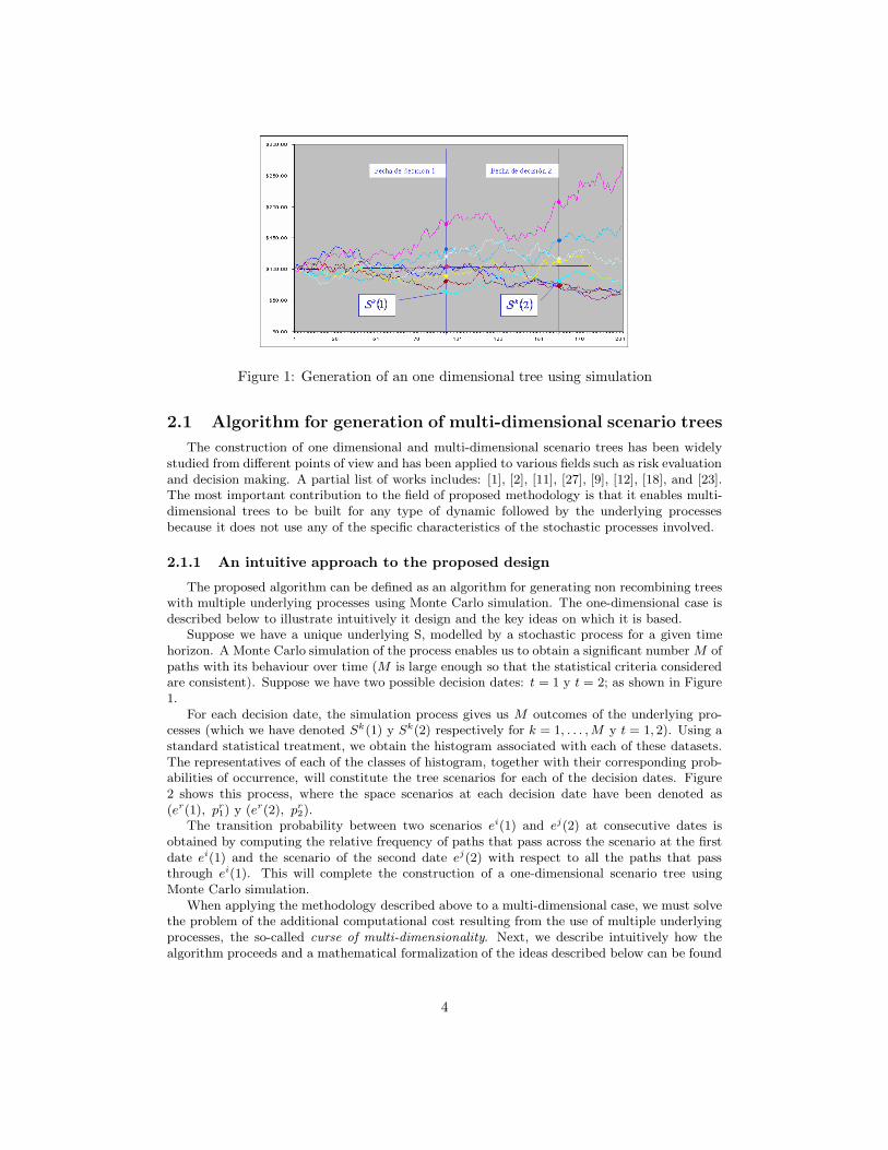
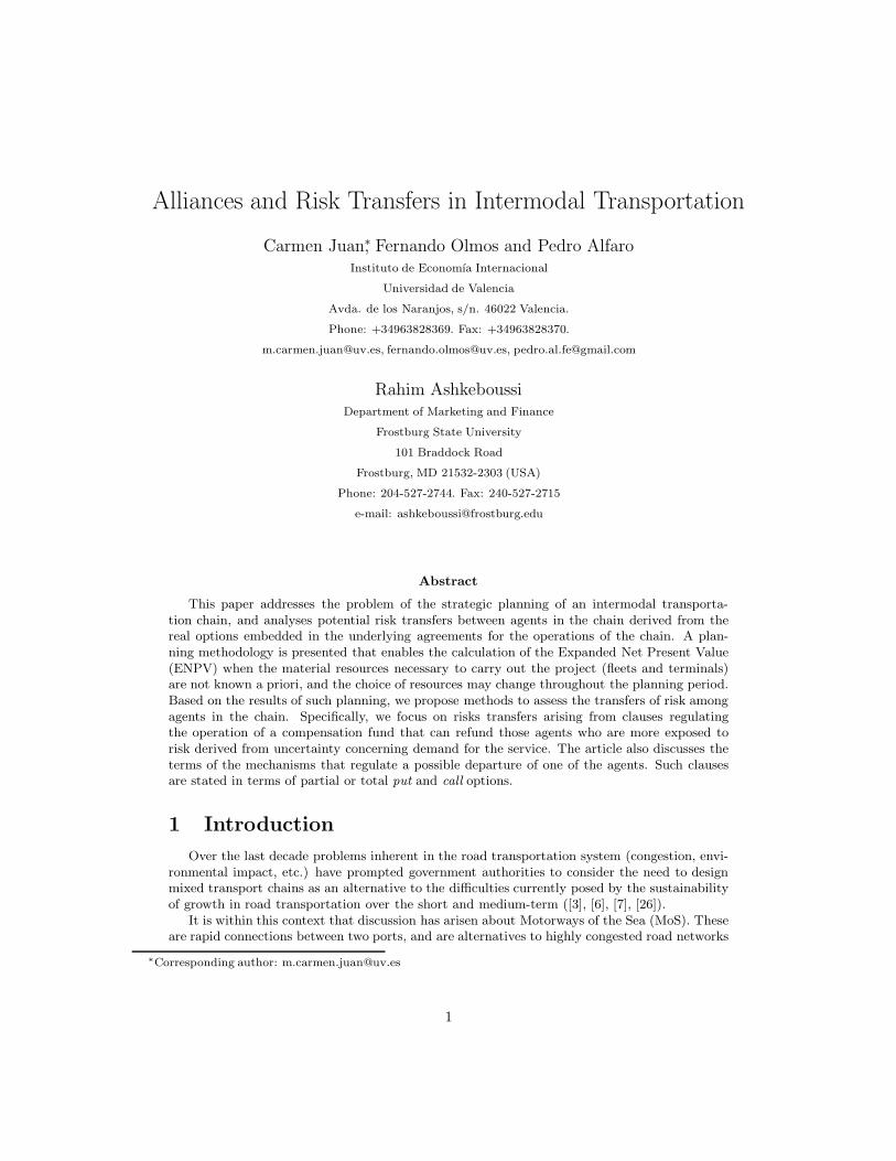
Figure 1: Generation of an one dimensional tree using simulation

2.1 Algorithm for generation of multi-dimensional scenario trees

The construction of one dimensional and multi-dimensional scenario trees has been widelystudied from different points of view and has been applied to various fields such as risk evaluationand decision making. A partial list of works includes: [1], [2], [11], [27], [9], [12], [18], and [23].The most important contribution to the field of proposed methodology is that it enables multi-dimensional trees to be built for any type of dynamic followed by the underlying processesbecause it does not use any of the specific characteristics of the stochastic processes involved.

2.1.1 An intuitive approach to the proposed design

The proposed algorithm can be defined as an algorithm for generating non recombining treeswith multiple underlying processes using Monte Carlo simulation. The one-dimensional case isdescribed below to illustrate intuitively it design and the key ideas on which it is based.

Suppose we have a unique underlying S, modelled by a stochastic process for a given timehorizon. A Monte Carlo simulation of the process enables us to obtain a significant number M ofpaths with its behaviour over time (M is large enough so that the statistical criteria consideredare consistent). Suppose we have two possible decision dates: t = 1 y t = 2; as shown in Figure1.

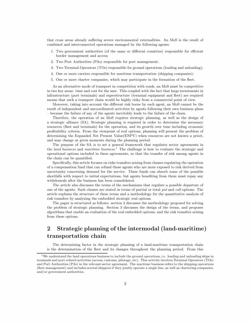
For each decision date, the simulation process gives us M outcomes of the underlying pro-cesses (which we have denoted Sk(1) y Sk(2) respectively for k = 1, . . . , M y t = 1, 2). Using astandard statistical treatment, we obtain the histogram associated with each of these datasets.The representatives of each of the classes of histogram, together with their corresponding prob-abilities of occurrence, will constitute the tree scenarios for each of the decision dates. Figure2 shows this process, where the space scenarios at each decision date have been denoted as(er(1), pr

1) y (er(2), pr2).

The transition probability between two scenarios ei(1) and ej(2) at consecutive dates isobtained by computing the relative frequency of paths that pass across the scenario at the firstdate ei(1) and the scenario of the second date ej(2) with respect to all the paths that passthrough ei(1). This will complete the construction of a one-dimensional scenario tree usingMonte Carlo simulation.

When applying the methodology described above to a multi-dimensional case, we must solvethe problem of the additional computational cost resulting from the use of multiple underlyingprocesses, the so-called curse of multi-dimensionality. Next, we describe intuitively how thealgorithm proceeds and a mathematical formalization of the ideas described below can be found

4

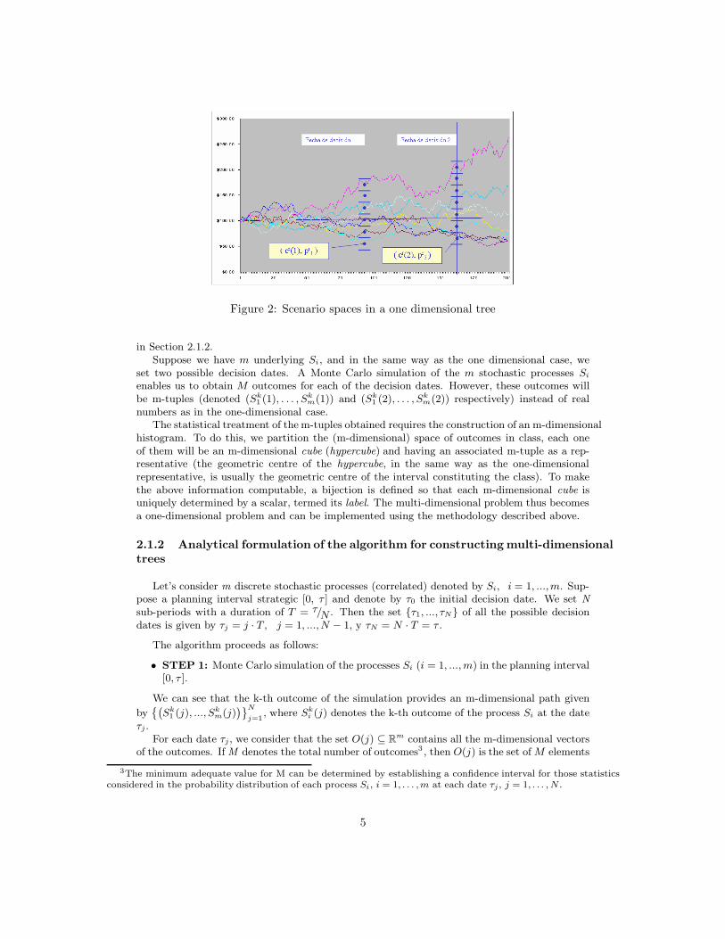
Figure 2: Scenario spaces in a one dimensional tree

in Section 2.1.2.Suppose we have m underlying Si, and in the same way as the one dimensional case, we

set two possible decision dates. A Monte Carlo simulation of the m stochastic processes Si

enables us to obtain M outcomes for each of the decision dates. However, these outcomes willbe m-tuples (denoted (Sk

1 (1), . . . , Skm(1)) and (Sk

1 (2), . . . , Skm(2)) respectively) instead of real

numbers as in the one-dimensional case.The statistical treatment of the m-tuples obtained requires the construction of an m-dimensional

histogram. To do this, we partition the (m-dimensional) space of outcomes in class, each oneof them will be an m-dimensional cube (hypercube) and having an associated m-tuple as a rep-resentative (the geometric centre of the hypercube, in the same way as the one-dimensionalrepresentative, is usually the geometric centre of the interval constituting the class). To makethe above information computable, a bijection is defined so that each m-dimensional cube isuniquely determined by a scalar, termed its label. The multi-dimensional problem thus becomesa one-dimensional problem and can be implemented using the methodology described above.

2.1.2 Analytical formulation of the algorithm for constructing multi-dimensional

trees

Let’s consider m discrete stochastic processes (correlated) denoted by Si, i = 1, ...,m. Sup-pose a planning interval strategic [0, τ ] and denote by τ0 the initial decision date. We set Nsub-periods with a duration of T = τ/N . Then the set τ1, ..., τN of all the possible decisiondates is given by τj = j · T, j = 1, ...,N − 1, y τN = N · T = τ .

The algorithm proceeds as follows:

• STEP 1: Monte Carlo simulation of the processes Si (i = 1, ..., m) in the planning interval[0, τ ].

We can see that the k-th outcome of the simulation provides an m-dimensional path given

by˘`

Sk1 (j), ..., Sk

m(j)´¯N

j=1, where Sk

i (j) denotes the k-th outcome of the process Si at the dateτj .

For each date τj , we consider that the set O(j) ⊆ Rm contains all the m-dimensional vectors

of the outcomes. If M denotes the total number of outcomes3 , then O(j) is the set of M elements

3The minimum adequate value for M can be determined by establishing a confidence interval for those statisticsconsidered in the probability distribution of each process Si, i = 1, . . . ,m at each date τj , j = 1, . . . , N .

5

given by

O(j) =n“

Sk1 (j), ..., Sk

m(j)”oM

k=1.

Thus, each set O(j) needs for memory storage a matrix sized M × m. In what follows, O(j)refers indiscriminately to all outcomes and their matrix representation. The three-dimensionalmatrix sized M × m × N , and given by O = (O(j))N

j=1, contains the complete information forthe simulation performed.

• STEP 2: Construction at each date τj (j = 1, . . . , N), of an m-dimensional interval C(j)containing the set of O(j) outcomes.

Let’s consider the interval given by C(j) = [a1(j), b1(j)] × · · · × [am(j), bm(j)], where

ai(j) = Minn

Ski (j) | k = 1, . . . , M

o

∀i = 1, ...,m

bi(j) = Maxn

Ski (j) | k = 1, . . . , M

o

∀i = 1, ...,m

Therefore, C(j) satisfies O(j) ⊆ C(j).

• STEP 3: Generation at each date τj (j = 1, . . . , N) of a disjointed partition P (j) of them-dimensional interval C(j).

For each i (i = 1, ...,m), consider a disjointed partition of the interval [ai(j), bi(j)] in δi(j)sub-intervals. An adequate value for δi(j) is determined establishing a 5% of acceptable discrep-ancy for certain statistics, which are obtained simultaneously as a result of the simulation, andin turn from the histogram of frequencies associated with the partition Pi(j) over [ai(j), bi(j)]which we will build below.

Denote by

n

a0i (j) = ai(j), a1

i (j), . . . , aδi(j)i (j) = bi(j)

o

i = 1, ...,m

all the points of the partition, and by Pi(j) (i = 1, ...,m) the corresponding set of parti-tion sub-intervals. For the sake of simplicity, we identify the partition of an interval with theset of generated sub-intervals. Thus, a multi-dimensional disjointed partition P (j) of an m-dimensional cube C(j) is defined as the Cartesian product of the sets of δi(j) elements Pi(j).An element of P (j) is an m-dimensional interval hr(j) given by

hr(j) =h

anr

1(j)−1

1 (j), anr

1(j)

1 (j)i

× · · · ×h

anr

m(j)−1

m (j), anr

m(j)

m (j)i

,

where r=1,. . . ,R(j), and R(j) =Qm

i=1 δi(j) being the cardinal of P (j).

• STEP 4: For each date τj(j = 1, . . . , N), the scenarios of the tree are defined as thecorresponding space of scenarios .

For each hr(j) ∈ P (j), the m-dimensional vector er(j) ∈ hr(j) whose components are thehalf-way points of each of the intervals of hr(j) is termed a scenario(or node)of the tree at

τj . The set E(j) = er(j) R(j)r=1 of all the scenarios or nodes in τj are termed the space of

scenarios at τj .

• STEP 5: Construction of a simple representation of each multi-dimensional partitionP (j) (j = 1, . . . , N).

Note that each m-dimensional interval hr(j) is uniquely determined by the m-tupla (nr1(j), . . . , n

rm(j)) ∈

Zm and so:

hr(j) =h

anr1(j)−1

1 (j), anr1(j)

1 (j)i

× · · · ×h

anr

m(j)−1

m (j), anr

m(j)

m (j)i

.

6

Therefore, we can establish a bijection4 so that each m-tupla (nr1(j), . . . , n

rm(j)) corresponds

to an integer lr(j) given by the expression

lr(j) =

m−1X

i=1

nri (j) · δi+1(j) · . . . · δm(j) + nr

m(j).

Consequently, hr(j) is uniquely determined by lr(j). We will call lr(j) the label of hr(j). The

set lr(j) R(j)l=1 of all the labels constitues a simple representation of P (j), and this set can be

stored in a matrix sized 1 × R(j).

• STEP 6: Construction of a simpe representation of the matrix M × m O(j), as wellas the corresponding simple representation of the matrix M × m × N O = (O(j))N

j=1

(j = 1, . . . , N).

For each`

Sk1 (j), ..., Sk

m(j)´

∈ O(j), there is a unique rk, 1 ≤ rk ≤ R(j), so that`

Sk1 (j), ..., Sk

m(j)´

∈hrk (j). In this way, it is possible to establish an injection so that each m-dimensional vector`

Sk1 (j), ..., Sk

m(j)´

∈ O(j) corresponds to a label lrk (j) associated with the corresponding hrk (j).Through this injection, the matrix M × m O(j) is replaced by the vector of integer numbersM × 1 L(j) and the matrix M ×m×N O = (O(j))N

j=1 is also replaced by the matrix of integer

numbers M × N L = (L(j))N

j=1.

• STEP 7: Construction of a complete probability distribution for the scenario space E(j)(j = 1, . . . , N).

For each date τj , let’s consider the discrete probability distribution where each er(j) ∈ E(j)has a probability pr

j given by the ratio between number of times the label lr(j) of er(j) appearsas a component of vector L(j), and the total of outcomes in the simulation M. If we denote withλs(j) (s = 1, . . . , M) the components of vector L(j), then pr

j is given by the expression:

prj =

0 si lr(j) /∈ Lj

| s | λs(j)=lr(j), s=1,...M |M

si lr(j) ∈ Lj

• STEP 8: Calculation of the transition probabilities between consecutive scenarios on thetree.

Suppose two consecutive decision dates τj y τj+1. Let’s consider the corresponding vectorsL(j) and L(j + 1). Let’s build the matrix M × 2 with columns L(j) and L(j + 1): L(j, j + 1) =(L(j) |L(j + 1) ). For each er(j) ∈ E(j) and each et(j + 1) ∈ E(j +1), the transition probabilitypr,t

j,j+1 between er(j) y et(j +1) is defined as the ratio between the number of rows of the matrix

L(j, j + 1) equal to`

lr(j), lt(j + 1)´

, and the number of rows of the matrix L(j, j + 1) whosefirst element equals lr(j). In this way, if λsu(j, j + 1) (s = 1, . . . , M ; u = 1, 2) denotes a genericelement of the element L(j, j + 1), then pr,t

j,j+1 is given by the expression:

pr,tj,j+1 =

(

0 si lr(j) /∈ L(j)| s | λs1(j,j+1)=lr (j), λs2(j,j+1)=lt(j), s=1,...M |

| s | λs1(j,j+1)=lr(j), s=1,...M |si lr(j) ∈ L(j)

4The bijection is established between the set (nr1(j), . . . , n

rm(j))

˛

˛ 1 ≤ nri (j) ≤ δi(j), i = 1, . . . ,m and the set

l ∈ Z˛

˛ L(j) ≤ l ≤ L(j) , where L(j) =Pm

i=2 δi · δi+1 · . . . · δm + 1 y L(j) =Pm

i=1 δi · δi+1 · . . . · δm + δm .

7

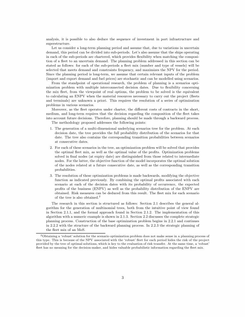
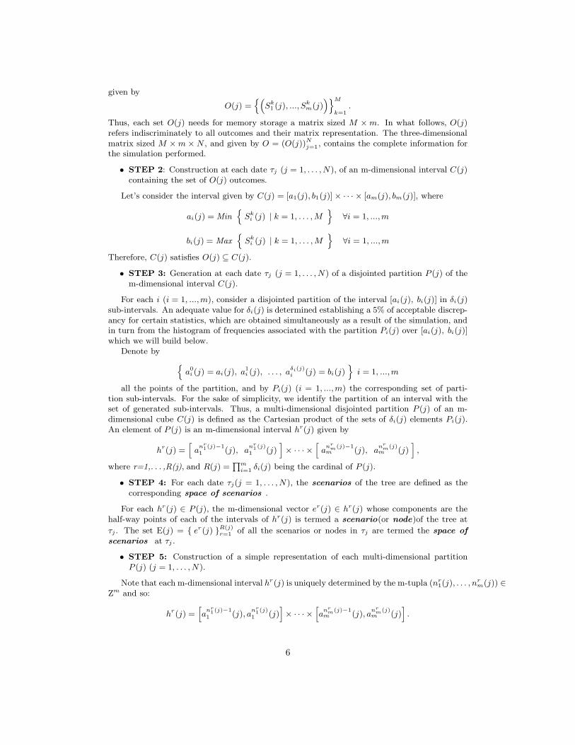
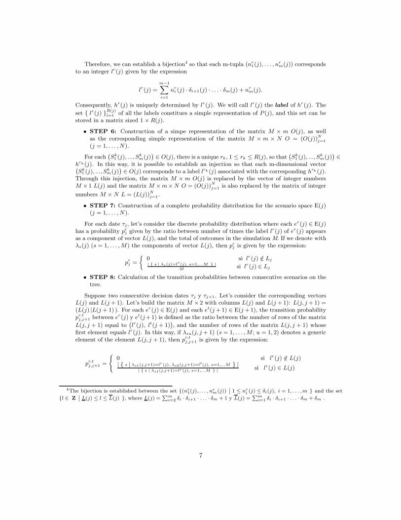
Figure 3: A section of the three-dimensional planning tree

2.1.3 Numerical example

The algorithm described in 2.1.1, and formalised in 2.1.2, has been implemented in VisualStudio.NET and C#. The program allows the number of decision dates and the intermediateperiods between these dates to be selected, as well as the number and structure of the underlyingprocesses.

Note that flexibility in deciding the decision dates and the dates between sub-periods isessential when applying this methodology to a real problem of strategic planning. Dependingon the behaviour of the underlying processes, it may be more advisable to shorten the timebetween decision dates, and even make the time period vary within the planning horizon.

For the sake of simplicity in presentation, in our case, a time horizon of 15 years is establishedwith two possible decision dates: at year 5 and year 10 respectively. The stochastic processesthat model the evolution of export demand, import demand, and the price of fuel for ships(bunker fuel)have been considered as underlying processes. These have been adjusted in thesame way as in models commonly used in studies of this type of demand ([5], [28], [29], [32])and models used for studying commodity prices such as fuel ([17], [22], [24], [33]).

The final tree resulting from the implementation of the algorithm consists of 64 scenarios onthe first decision date at year 5, and 100 scenarios on the second decision date at year 10. Amatrix of 64 × 100 includes the transition probabilities between the two decision dates, whereeach scenario has been replaced by its corresponding label.

Figure 3 illustrates a section of the tree which shows for each scenario (denoted by the label),the three-dimensional vector with the complete information of the underlying processes, itsprobability of occurrence, the transition probability of related scenarios, as well as the absoluteprobabilities of occurrence of these latter.

2.2 The problem of strategically planning the fleet

This section discusses the modelling of the optimization problem for determining the optimalfleet mix that should operate on the MoS for a certain planning period. Fleet mix and fleetschedulingproblems in the maritime sector have been studied for the deterministic case ([25],[10],[20], [21]). However, as noted in Section ??intro), the characteristics of the problem studied inthis article convert the problem into a stochastic problem with multiple and interrelated decision

8

dates. Therefore, a specific methodology for its resolution is developed below.

2.2.1 Description of the optimization problem

This section describes the basic problem to be solved, how to model each of its elements,and the peculiarities that require a specific approach. This problem will be properly modifiedin Section 2.2.2 when it is used to implement comprehensive strategic planning on the scenariotree.

The basic problem is to determine the mixed fleet of vessels for a container roro shippingline that maximizes profits. This shipping line covers a distance of δ miles between a singleport and a single destination. The fleet should operate without changing its composition duringthe period of T years between two consecutive decision dates. Therefore, capacity should besufficient to meet export and import demand generated during that period (indicated by Exl

and Iml respectively, for each year l of the period). For the shipping line to be competitivewith land transportation, it must offer a frequency of α sailings a day in both directions.

The fleet manager responsible for planning must first decide how many ships of each typewill be required, chosen from appropriate ships available on the market. Assuming that thechoice is between m different types of ships that meet these characteristics, then we can set thefollowing family of variables:

xk = number of type k ships k = 1, . . . , m.

Additionally, for each year of operation, the plan should establish how many sailings each typeof ship will make and what type of cargo will be carried in each sailing. In this way, the followingsets of variables will be incorporated into the problem:

ykl = number of sailings of a type k ship in year l, k = 1, . . . , m, l = 1, . . . , T.

zkl = cargo carried on each sailing by a type k ship in year l, k = 1, . . . , m, l = 1, . . . , T.

Note that it is not possible to work with aggregate capacity of the fleet, nevertheless it isnecessary to handle this level of detail when modelling the variables of the problem for thefollowing reasons:

• As they must comply with frequency constraints, the shipping line must offer a minimumnumber of sailings per year, regardless of demand.

• Fuel consumption is a significant share of the operating costs of a shipping line. Consump-tion is shown in tons of fuel per hour of navigation, and therefore depends directly on thenumber of sailings.

• The maximum number of annual sailings of a ship is a function of cargo. In fact, one ofthe factors that most affects efficiency for shipping lines is the time taken in loading andunloading. This, in turn, is determined by the technology of the ship and the terminal;and the volume of cargo transported. This technical relationship between the variables ykl

and zkl will be incorporated in a block of constraints indicated below.

In order to correctly select the fleet mix a manager needs to know a set of specifications foreach ship. These specifications will determine the parameters of the constraints, the objectivefunction of the problem, and therefore, the optimal fleet mix. Tables 1 and 2 contain thesespecifications, grouped into technical and financial aspects, respectively.

Taking into account the variables introduced earlier, as well as the inter-relationships betweenthe specifications in Tables 1 and 2, the constraints of the problem can be expressed as follows:

9

Technical specifications for a type-k ship

Capacity (standard cargo units) Ck

Speed (knots) vk

Number of maintenance days mdk

Fuel consumption (tons per navigation day) fk

Journey time (dıas) Tk = δ24·vk

Loading/unloading ratio (movements per hour) hrk

Time to load/unload a full ship Tcdk = 2 ·

(

ρ·Ck

24·hrk

)

Annual minimum sailings (number of sailings full load) Lk =[

365−mdk

Tk+γ+Tcdk

]

Maximum number of sailings (number of sailings empty load) Uk =[

365−mdk

Tk+γ

]

Table 1: Specifications for a type-k ship

Financial parameters for a type-k ship

Construction costs Pk

Annual crew costs l ϑkl

Annual insurance costs l ιkl

Annual maintenance costs l χkl

Depreciated value of ship at end of planning period Ωk

Annual charter costs Λk

Long-term charter rate rk

Short-term charter premium πk

Annual bonus for long-term charter bk

Table 2: Financial parameters for a type-k ship

10

Frequency constraints

mX

k=1

xk · ykl ≥ 2 · α · 365 ∀l = 1, . . . , T.

Demand constraintsmX

k=1

xk · ykl · zkl ≥ 2 · Max Exl, Iml ∀l = 1, . . . , T.

Technical relationship between number of sailings and cargo carried

ykl ≤365 − mdk

2·zkl ·ρ24·hrk

+ Tk + γ∀k = 1, . . . , m ∀l = 1, . . . , T.

Presence, or otherwise, of type k ships in the fleet If there are no type k ships inthe fleet, then in each year l of the planning period, the number of sailings ykl and the cargo zkl

should logically be 0. These constraints are included in the following way in the model (whereM denotes a large arbitrarily natural number):

ykl ≤ M · xk ∀k = 1, . . . , m ∀l = 1, . . . , T.

zkl ≤ M · xk ∀k = 1, . . . , m ∀l = 1, . . . , T.

zkl ≤ M · ykl ∀k = 1, . . . , m ∀l = 1, . . . , T.

Upper bounds for the variables xk An upper limit for the number of type k ships thatcan be part of the fleet is obtained assuming that only type k ships satisfy the shipping linefrequency and demand constraints. The relevant constraints would be expressed as follows:

xk ≤ Maxl bkl

where bkl is given by:

bkl = Max

»

2 · Max Exl, Iml

Lk · Ck

–

+ 1;

»

2 · α · 365

Lk

–

+ 1

ff

.

Upper bounds for the variables ykl

ykl ≤ Uk ∀k = 1, . . . , m ∀l = 1, . . . , T.

Upper bounds for the variables zkl

zkl ≤ Ck ∀k = 1, . . . , m ∀l = 1, . . . , T.

Once the constraints of the problem are established, the next step in modelling is to determinethe expression of the objective function. This function quantifies the profits arising from theshipping line operations for the T years of planning. Suppose a adjusted risk discount rate ofη. The various blocks involved in the final expression of the profits are shown below:

Income Income for the shipping operators comes from payments made by the users and theseare determined by tariffs set for each unit of cargo (known as freight rate). If we denote Frl

as the freight rate in the year l, then the total income during the planning year (Rev) will begiven by:

Rev =TX

l=1

((Exl + Iml) · Frl) · (1 + η)−l+1.

11

Operating costs Denote F ll as the price of fuel for the year l. From the financial parametersgiven in Table 2, the expression of the operating costs (Cop) will be given by:

Cop =

TX

l=1

mX

k=1

(xk · ϑkl + xk · ykl · Tk · fk · F ll + xk · ιkl + xk · χkl)

!

· (1 + η)−l+1.

Charter costs For a short-term charter contract lasting the planning period of T years arate r′k is used. This is the the base rate for a long-term contract rk , plus a premium πk for ashort-term charter. Therefore, the annual charter sum for a k type ship, Λk, should satisy thefollowing equation:

Pk − Ωk =

TX

l=1

Λk

(1 + r′k)l−1= Λk

1

r′k−

1

(1 + r′k)T · r′k

!

.

The total charter payments for the planning period (CΛ) can be shown as:

CΛ =

mX

k=1

xkΛk

„

1

η−

1

(1 + η)T η

«

.

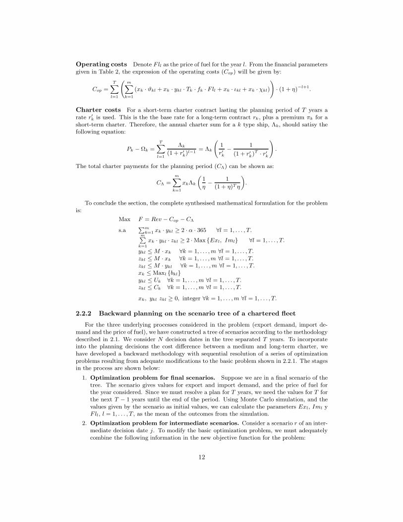
To conclude the section, the complete synthesised mathematical formulation for the problemis:

Max F = Rev − Cop − CΛ

s.aPm

k=1 xk · ykl ≥ 2 · α · 365 ∀l = 1, . . . , T.mP

k=1

xk · ykl · zkl ≥ 2 · Max Exl, Iml ∀l = 1, . . . , T.

ykl ≤ M · xk ∀k = 1, . . . , m ∀l = 1, . . . , T.zkl ≤ M · xk ∀k = 1, . . . , m ∀l = 1, . . . , T.zkl ≤ M · ykl ∀k = 1, . . . , m ∀l = 1, . . . , T.xk ≤ Maxl bklykl ≤ Uk ∀k = 1, . . . , m ∀l = 1, . . . , T.zkl ≤ Ck ∀k = 1, . . . , m ∀l = 1, . . . , T.

xk, ykl zkl ≥ 0, integer ∀k = 1, . . . , m ∀l = 1, . . . , T.

2.2.2 Backward planning on the scenario tree of a chartered fleet

For the three underlying processes considered in the problem (export demand, import de-mand and the price of fuel), we have constructed a tree of scenarios according to the methodologydescribed in 2.1. We consider N decision dates in the tree separated T years. To incorporateinto the planning decisions the cost difference between a medium and long-term charter, wehave developed a backward methodology with sequential resolution of a series of optimizationproblems resulting from adequate modifications to the basic problem shown in 2.2.1. The stagesin the process are shown below:

1. Optimization problem for final scenarios. Suppose we are in a final scenario of thetree. The scenario gives values for export and import demand, and the price of fuel forthe year considered. Since we must resolve a plan for T years, we need the values for T forthe next T − 1 years until the end of the period. Using Monte Carlo simulation, and thevalues given by the scenario as initial values, we can calculate the parameters Exl, Iml yF ll, l = 1, . . . , T , as the mean of the outcomes from the simulation.

2. Optimization problem for intermediate scenarios. Consider a scenario r of an inter-mediate decision date j. To modify the basic optimization problem, we must adequatelycombine the following information in the new objective function for the problem:

12

• From the backward process we have obtained the optimal planning for each scenario sof the next decision date j +1, i.e, we know how many ships of each type the line willoperate. Therefore, to determine the optimum fleet for the scenario r of j we knowhow many of the selected ships will continue to the next period, and therefore wouldbe entitled to a bonus for a long-term charter. The following expression formallymodels the bonus amount:

Bonus(r,s) =mX

k=1

Min x∗k(s), xk(r) · bk ·

„

1

η−

1

(1 + η)T η

«

,

where (x∗1(s), . . . , x

∗m(s)) denotes the optimal planning of ships obtained for s, bk

the annual bonus for each type k ship in the fleet that continues in the fleet, and(x1(r), . . . , xm(r)) is the possible plan for r.

• From the tree information, we know the transition probabilities from each scenario r ofj to each scenario s of j +1 (denoted as pr,s

j,j+1). Thus the following expression, whichcalculates the expected value of the bonus, must be incorporated in the objectivefunction:

Bonus(r) =

R(j+1)X

s=1

pr,sj,j+1 · Bonus(r,s).

Moreover, as was the case with the final nodes, it is necessary to determine the values ofthe parameters Exl, Iml and F ll, l = 1, . . . , T. This is achieved in the same way describedfor the final nodes.

3. Obtaining the final value of the profits associated with the MoS Suppose theearlier process of backward planning is finished. Then, for each scenario r of the decisiondate j, we have the optimum profits associated with the shipping line operations during thesubsequent planning T years(denoted as F ∗(r)). Moreover, from the information providedby the tree, we know the probability of each of the R(j) scenarios of j. Denote by pr theprobability of occurrence of the scenario r of j. Therefore, we can calculate the expectedvalue of the profits of the shipping line during the T years of operations between thedecision dates j and j + 1 using the following expression:

Rent(j) =

R(j)X

r=1

prj · F ∗r(j).

By discounting and accumulating the expected values for each of the possible N decisiondates, we obtain the expected profits for the planning period of (N + 1) · T years:

Rent =

NX

j=0

Rent(j)(1 + η)−jT .

2.2.3 Numerical example of strategic planning for an MoS

To illustrate the methodology proposed in sections 2.2.1 and 2.2.2, we will consider thetree obtained in 2.1.3, and an MoS with the characteristics described below. To develop thisexample, industry benchmarks have been used, as well as data from various studies on short seashipping in various countries ([4], [19], [26]).

Let’s look at an MoS designed to cover a distance between the port of origin and destinationof 350 miles at a rate of 3 daily sailings in each direction. We will make a strategic plan foroperations over 15 years, while setting two decision dates for the renewal of the fleet mix – at year5 and year 10 . A risk discount adjusted rate of 17% is set for the project. The charter market

13

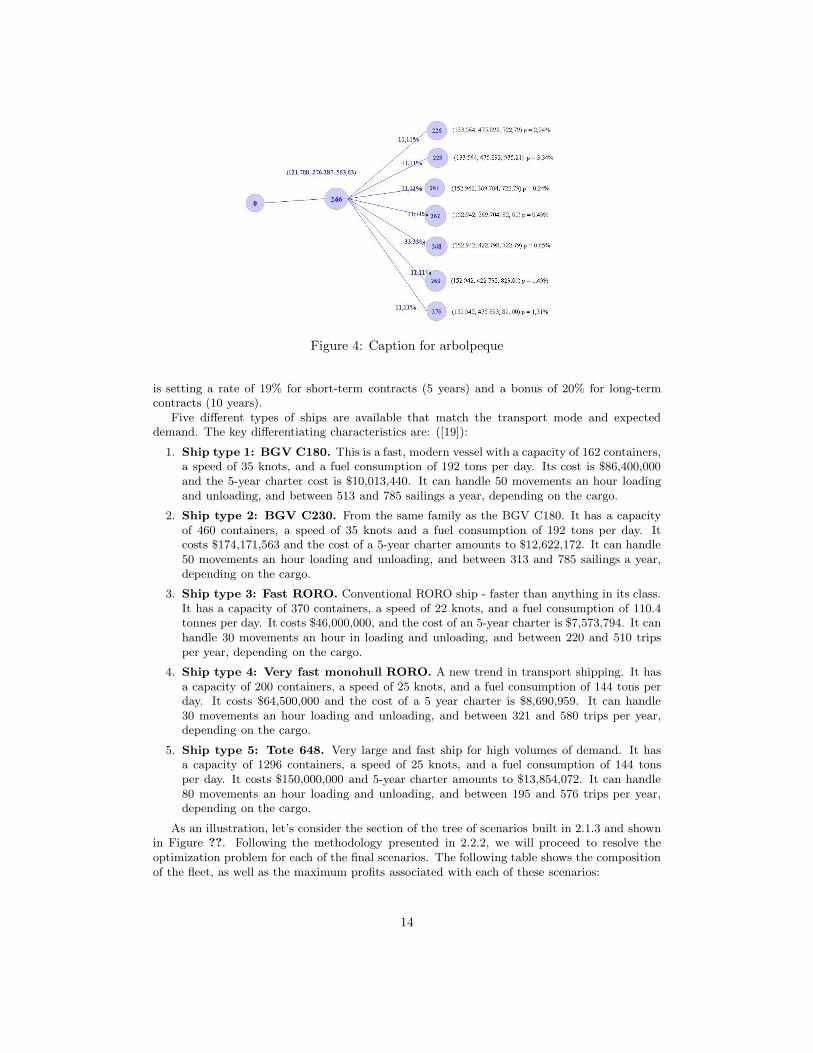
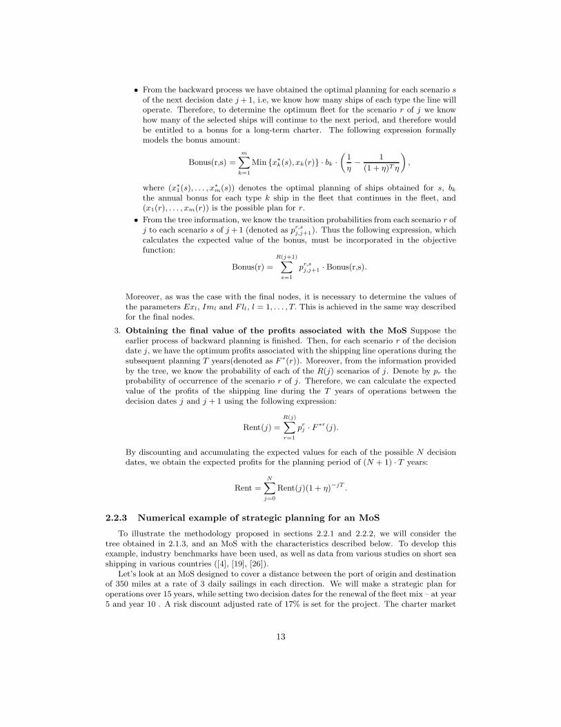
Figure 4: Caption for arbolpeque

is setting a rate of 19% for short-term contracts (5 years) and a bonus of 20% for long-termcontracts (10 years).

Five different types of ships are available that match the transport mode and expecteddemand. The key differentiating characteristics are: ([19]):

1. Ship type 1: BGV C180. This is a fast, modern vessel with a capacity of 162 containers,a speed of 35 knots, and a fuel consumption of 192 tons per day. Its cost is $86,400,000and the 5-year charter cost is $10,013,440. It can handle 50 movements an hour loadingand unloading, and between 513 and 785 sailings a year, depending on the cargo.

2. Ship type 2: BGV C230. From the same family as the BGV C180. It has a capacityof 460 containers, a speed of 35 knots and a fuel consumption of 192 tons per day. Itcosts $174,171,563 and the cost of a 5-year charter amounts to $12,622,172. It can handle50 movements an hour loading and unloading, and between 313 and 785 sailings a year,depending on the cargo.

3. Ship type 3: Fast RORO. Conventional RORO ship - faster than anything in its class.It has a capacity of 370 containers, a speed of 22 knots, and a fuel consumption of 110.4tonnes per day. It costs $46,000,000, and the cost of an 5-year charter is $7,573,794. It canhandle 30 movements an hour in loading and unloading, and between 220 and 510 tripsper year, depending on the cargo.

4. Ship type 4: Very fast monohull RORO. A new trend in transport shipping. It hasa capacity of 200 containers, a speed of 25 knots, and a fuel consumption of 144 tons perday. It costs $64,500,000 and the cost of a 5 year charter is $8,690,959. It can handle30 movements an hour loading and unloading, and between 321 and 580 trips per year,depending on the cargo.

5. Ship type 5: Tote 648. Very large and fast ship for high volumes of demand. It hasa capacity of 1296 containers, a speed of 25 knots, and a fuel consumption of 144 tonsper day. It costs $150,000,000 and 5-year charter amounts to $13,854,072. It can handle80 movements an hour loading and unloading, and between 195 and 576 trips per year,depending on the cargo.

As an illustration, let’s consider the section of the tree of scenarios built in 2.1.3 and shownin Figure ??. Following the methodology presented in 2.2.2, we will proceed to resolve theoptimization problem for each of the final scenarios. The following table shows the compositionof the fleet, as well as the maximum profits associated with each of these scenarios:

14

Figure 5: Caption for Solfin

Label node Maximum profits ($)) Optimum fleet

226 257,060,000 (0. 0. 6. 0. 3)

228 111,060,000 (0. 0. 6. 0. 3)

261 157,940,000 (0. 0. 7. 0. 2)

262 85,977,000 (0. 0. 7. 0. 2)

268 208,720,000 (0. 0. 8. 0. 2)

269 136,890,000 (0. 0. 8. 0. 2)

276 219,710,000 (0. 0. 6. 0. 3)

Using the previous solutions, let’s look at the problem of optimization for the intermediatenode 266, where the objective function incorporates the expexted charter bonus shown in 2.2.2.The resolution of this problem provides us with an optimal fleet consisting of 1 type-1 ship, and9 type-3 ships with maximum profits of $76, 482, 000. Figure ?? shows all the optimal solutionsobtained for this section of the tree.

The complete resolution on the tree of the corresponding optimization problems provides uswith a new scenario tree where, associated with each node, we have information on the optimalcomposition of the fleet and its derived maximum profits. This tree of fleets and profits will bekey in the methodologies for evaluating the transfers of risk associated with the clauses studiedin Section 3.

Note that obtaining the final level of profits associated with the project, as well as the corre-sponding optimal fleets for each scenario of the tree, has a high computational cost. Loops mustbe implemented to sequentially resolve the various optimization problems and automaticallyupdate the parameters. Therefore, the information provided by the algorithm for generating atree of scenarios described in 2.1, should be linked to the routine resolution of the correspondingoptimization problems.

The optimization problems in the example 2.2.3 have been resolved using the SBB solversupplied as part of the GAMS program; and which develops a type of nonlinear Branch andBound. A non-linear problem is resolved at each node of the Branch and Bound tree. Specifically,the SBB solver can use either the CONOPT or MINOS solvers and a combination of both hasbeen used to obtain the results of the numerical example.

2.2.4 Forward planning on the scenario tree of an owned fleet

For an owned fleet, planning must be done forward on the scenario tree, and the objectivefunction in the optimization problems associated with each node must be modified to incorporate

15

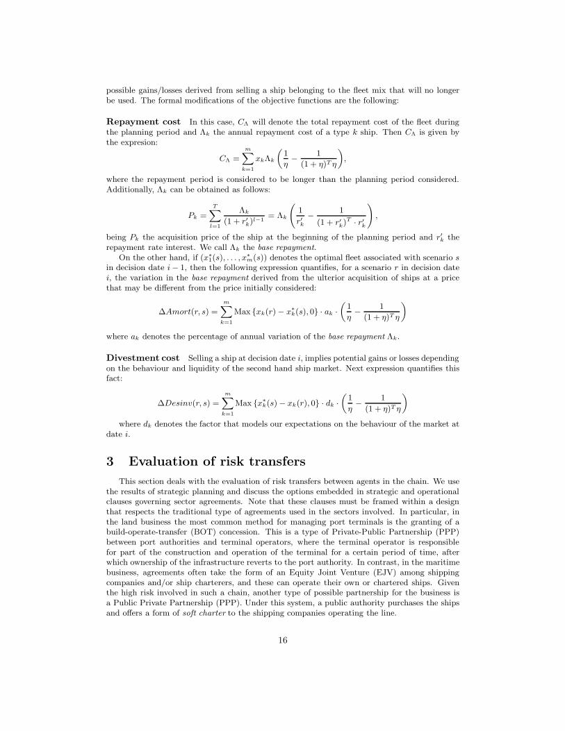
possible gains/losses derived from selling a ship belonging to the fleet mix that will no longerbe used. The formal modifications of the objective functions are the following:

Repayment cost In this case, CΛ will denote the total repayment cost of the fleet duringthe planning period and Λk the annual repayment cost of a type k ship. Then CΛ is given bythe expresion:

CΛ =

mX

k=1

xkΛk

„

1

η−

1

(1 + η)T η

«

,

where the repayment period is considered to be longer than the planning period considered.Additionally, Λk can be obtained as follows:

Pk =TX

l=1

Λk

(1 + r′k)l−1= Λk

1

r′k−

1

(1 + r′k)T · r′k

!

,

being Pk the acquisition price of the ship at the beginning of the planning period and r′k therepayment rate interest. We call Λk the base repayment.

On the other hand, if (x∗1(s), . . . , x

∗m(s)) denotes the optimal fleet associated with scenario s

in decision date i − 1, then the following expression quantifies, for a scenario r in decision datei, the variation in the base repayment derived from the ulterior acquisition of ships at a pricethat may be different from the price initially considered:

∆Amort(r, s) =

mX

k=1

Max xk(r) − x∗k(s), 0 · ak ·

„

1

η−

1

(1 + η)T η

«

where ak denotes the percentage of annual variation of the base repayment Λk.

Divestment cost Selling a ship at decision date i, implies potential gains or losses dependingon the behaviour and liquidity of the second hand ship market. Next expression quantifies thisfact:

∆Desinv(r, s) =

mX

k=1

Max x∗k(s) − xk(r), 0 · dk ·

„

1

η−

1

(1 + η)T η

«

where dk denotes the factor that models our expectations on the behaviour of the market atdate i.

3 Evaluation of risk transfers

This section deals with the evaluation of risk transfers between agents in the chain. We usethe results of strategic planning and discuss the options embedded in strategic and operationalclauses governing sector agreements. Note that these clauses must be framed within a designthat respects the traditional type of agreements used in the sectors involved. In particular, inthe land business the most common method for managing port terminals is the granting of abuild-operate-transfer (BOT) concession. This is a type of Private-Public Partnership (PPP)between port authorities and terminal operators, where the terminal operator is responsiblefor part of the construction and operation of the terminal for a certain period of time, afterwhich ownership of the infrastructure reverts to the port authority. In contrast, in the maritimebusiness, agreements often take the form of an Equity Joint Venture (EJV) among shippingcompanies and/or ship charterers, and these can operate their own or chartered ships. Giventhe high risk involved in such a chain, another type of possible partnership for the business isa Public Private Partnership (PPP). Under this system, a public authority purchases the shipsand offers a form of soft charter to the shipping companies operating the line.

16

3.1 Compensation clauses

The design of the compensation clauses under this section is based on the structure ofdynamic clauses for sharing profits and losses as used by joint ventures and strategic alliancesfor regulating transitional periods – in which one partner has losses in excess of their percentageof ownership in the joint venture, or over an amount stipulated in the agreement ([14], [15]). Inthe particular case of land-maritime transportation chains, we distinguish between the designof a compensation clause for the land business, and the corresponding clause for the maritimebusiness.

3.1.1 Compensation clauses for the land business

Structure of the clause The purpose of this clause is to prevent the failure of the trans-portation chain. To this end, the consortium ensures a TO a minimum income while the businessis in a consolidation phase through a compensation fund. It also provides a mechanism for therecovery of compensation funds paid when revenues of the TO are above the reference mini-mum (for a review of this clause in the context of economic-financial equilibrium of concessioncontracts for port terminals see [16]).

The system for determining the payment into a compensation fund or refunds will dependon the following conditions:

• Condition 1: If the accumulated revenues plus the funds received, less refunds contribu-tions made, is below the guaranteed minimum.

• Condition 2: If the compensation fund is exhausted.

• Condition 3: If the business is in a consolidation phase, or is already established.

• Condition 4: If the TO has outstanding debts with the consortium for funds previouslyreceived.

Figure ?? shows the flow diagram with the basic structure of the compensation clause ina given year j. We denote APVR(j) the current value of the accumulated present value ofrevenues of the TO until the year j. A floor is then set for APVR(j), whose value of Bj in eachyear j is established by the consortium (a certain percentage of the expected APVR(j) may besuitable as the floor in the clause). Additionally, the consortium sets a maximum $ for thecompensation fund and a number η ∈ N to better define what is regarded consolidated business :the TO business in the year j is assumed to be consolidated, if for η consecutive years prior toj, the accumulated present value of revenues is above the established minimum. That is to say,there is a year r < j that satisfies the following condition:

APVR(r + s) ≥ Br+s ∀s = 1, . . . , η.

Also, if we denote Φj as the amount of fund received in the year j and Ψj as the amountof the corresponding payment for the possible refund, then the present value of accumulatedfunds received by the TO in previous years will be denoted by APVΦ(j − 1) and, respectively,the refunds will be denoted by APVΨ(j − 1).

If the accumulated present value of revenues of the TO, together with the accumulatedpresent value of funds received, minus the accumulated present value of refunds made duringprevious years (APVR(j)+APVΦ(j-1)-APVΨ(j-1)) is below the floor Bj , then an evaluationshould be made as to whether the total compensation made exceeds the maximum amount $set for the fund. If so, the TO cannot receive a fund, and therefore Φj = 0. Otherwise, itmust be determined if the business is already established. If yes, then again Φj = 0. However,if the business is not established, the operator will receive a fund for the total deviation withrespect to the floor Bj : providing the fund does not exceed the amount of the balance of thecompensation fund at the date j given by $-APVΦ(j-1).

17

Figure 6: Caption for diagram

If, by contrast, the accumulated present value of revenues of the TO, plus the present value ofthe funds received, minus the present value of refunds made in previous years is above the floorBj , then the amount of outstanding debt must be computed as given by APVΦ(j-1)-APVΨ(j-1).If there is outstanding debt, the value of the refund Ψj is calculated as a γ percentage of theexcess of APVR(j)+APVΦ(j-1)-APVΨ(j-1) on the minimum Bj . Notice that the refunds aremade regardless of whether the business is consolidated, and are only linked to the behaviourof the accumulated revenues with respect to the set minimum.

Embedded options This clause provides rights to the consortium and the TO. From thestandpoint of the methodology of real options, this can be considered as a sequence of European-type, path-dependant options and whose number is uncertain because they are subject to com-pliance with the above conditions. These are European-type options because they can only beexercised on the dates considered in the plan. They are interrelated because either the TO hasthe option to receive funds, or the consortium has a corresponding option to receive a paymentrefund. These options are path-dependent because the amount of refund, and the determiningconditions, are depend on the record of receipts and payments previously made.

Risk transfer This clause establishes a transitional period of allocation of losses, so that theconsortium assumes 100% of the risk of deviations in the amount of the accumulated revenues ofthe TO with respect to the minimum. Thus, the direct risk that the TO is exposed to becauseof fluctuations in demand is transferred to the consortium. It also provides a transitional periodof allocation of profits, so the consortium can receive a percentage of the profits from the TO asa refund for the compensations previously received. However, a full recovery by the consortiumof funds made is not riskless, and there are scenarios where the total fund is lost. Thus, it isnecessary to evaluate the transfer of risk associated with the special design of this clause.

For this, we simulate the probability distribution of the random variable APV Φ(τ)−APV Ψ(τ),where APV Φ(τ) denotes the accumulated present value of funds received up to the termination

18

of the agreement at τ , and APV Ψ(τ) denotes the corresponding value of the repayments made.Once the probability distribution is known, the most appropriate risk measure can be cal-

culated (VAR, CVAR, ES).

Algorithm for risk evaluation

1. Monte Carlo simulation of the revenues of the TO to determine the values of Bj at eachdecision date j. The expected value of accumulated revenues untill the year j, or a percentileof its probability distribution, can be considered appropriate for the role of floor for theactivation of compensation rights.

2. Simulation of an m-dimensional path S(j) = (Sk1 (j), . . . , Sk

m(j)) of the underlying processesin the tree, and obtaining the corresponding path for accumulated revenues APVR(j),j = 1, . . . , τ .

3. Proceed forward on the path APVR(j) following the flow chart above to obtain the valuesof the variables Φj and Ψj in each of the decision dates j = 1, . . . , τ .

4. Calculate APVΦ(τ) y APVΨ(τ) and obtain the difference APVΦ(τ) − APVΨ(τ).

5. Repeat the process for each of the paths S(j) in the simulation, generating a completeprobability distribution of APVΦ(τ) − APVΨ(τ).

6. Calculate the most adequate risk measure (VAR, CVAR, ES).

Numerical example (In process)

3.1.2 Martime business compansation clauses

Note that the clause in 3.1.1 has been focussed on the revenues of the TO, and quantifiesdeviations of demand with respect to the expectations initially established in the overall planfor the MoS. The requirements of land operations do not make recommendable the wording ofthe clause in terms of (net) flows – this is due to the risk of moral hazard and opportunisticbehaviour on the part of the TO ([31], [8], [30]). However, the maritime business is differentand the effect of the factor of efficiency of operations on business results is lesser. Moreover,the uncertainty of price behaviour regarding the price of fuel must be taken into account whendetermining entitlement to any compensation in combination with demand. The first significantdifference between the model of compensation clause in the land business when compared withthis type of clause for the maritime business is seen by the use of accumulated present valueof (net) flows APV F (j); instead of the corresponding accumulated present value of revenuesAPV R(j).

Although the focus of the clause is the same as 3.1.1, the algorithm for the implementationand subsequent risk evaluation is different because it is phrased in terms of flows, and it mustnecessary look for information stored in the tree of scenarios so as to associate each simulatedpath with a fleet for each decision date; and consequently, with optimal flows derived from theoperation of the fleet. The resulting algorithm is shown below:

Algorithm for risk evaluation

1. We use the scenario tree to calculate for each decision date j, the probability distributionof the variable APV F (j). We establish the value of Bj which will act as a floor for thecompensation mechanism.

2. Simulate an m-dimensional path S(j) = (Sk1 (j), . . . , Sk

m(j)) of the underlying processes inthe tree. Then, for each date j we identify a scenario er(j) nearest to S(j) (Euclideandistance) and transform the original path S(j) into a path of nodes e(j) so that we thenhave the corresponding path of the business flows.

19

3. Proceed forward on the path e(j) following the sequence of steps described in the flowdiagram in ?? to obtain the values of the variables Φj and Ψj for each of decision datesj = 1, . . . , τ and, finally, the value of the variable APVΦ(τ) − APVΨ(τ).

4. By repeating the process for each of the paths S(j) of the simulation, we generate the fullprobability distribution APVΦ(τ) − APVΨ(τ).

5. Calculate the most adequate risk measure (VAR, CVAR, ES).

Numerical example (In process)

3.2 Restatement of ownership clauses and evaluation of associ-ated risk transfers

To ensure the continuity of an MoS it is necessary to regulate the eventual departure fromthe agreement of one of the agents through restatement of ownership clauses. Note that for landbusinesses these agreements mainly take the form of a concession contract, and especially a BOTcontract, as discussed in Section 1. The final distribution of property is clearly established insuch agreements and mechanisms for the eventual departure of a private agent are regulatedin terms of the concession, so that, if it occurs, it will necessarily lead to a new tender forthe concession. Therefore, it makes no sense to discuss the design of restatement of ownershipmechanisms for these agreements.

In the case of maritime business we will study how to handle this kind of provision using putand call options, and how to evaluate the associated risk in the following cases:

1. The maritime business adopts a form of an EJV in which one of the partners has a marketprice call option on another partner’s share in the EJV.

2. The maritime business adopts a form of an EJV in which one of the partners has a marketprice put option on another partner’s share in the EJV.

3. The maritime business adopts a form of PPP in which the public agent owns the shipsand also owns a market price put option on all, or part, of the fleet.

In the case of EJVs, when we discuss market price put and market price call options we arereferring to options whose exercise price is fixed as follows:

• The market price M of the shares is taken at the specified time after receiving a notificationfrom a partner who intends to exercise his rights.

• Three additional prices are obtained P1, P2 and P3 as determined by three independentvaluation companies (taken from a previously agreed list), as the result of an appraisalprocess.

• The highest and lowest prices are eliminated. Let’s call the remaining price A. During thesubsequent development, we consider that A is a proxy of the real value of the business -considering the resources available at the time of appraisal.

• For a call option, the price is set at max(M ; A). This ensures at least the market price ofthe shares, and removes the possibility of opportunistic advantage being taken of marketin a downward trend. Otherwise, when the value of M is higher than A, we shall see how– from the standpoint of risk assessment – the partner who has transferred his rights isfavoured.

• For a put option the price is set at min(M ; A). This will mean that the option will beexercised when the two prices are similar. For example, if price M is less than value A,then the holder of the put will receive for his part of the business a value less than theproxy of the real value A; and so he will wait until both values are closer together. In theopposite case, in which M is more than A, there is obviously no motivation for exercisingthe put option at the value of A when a higher price could be obtained in the share market.

20

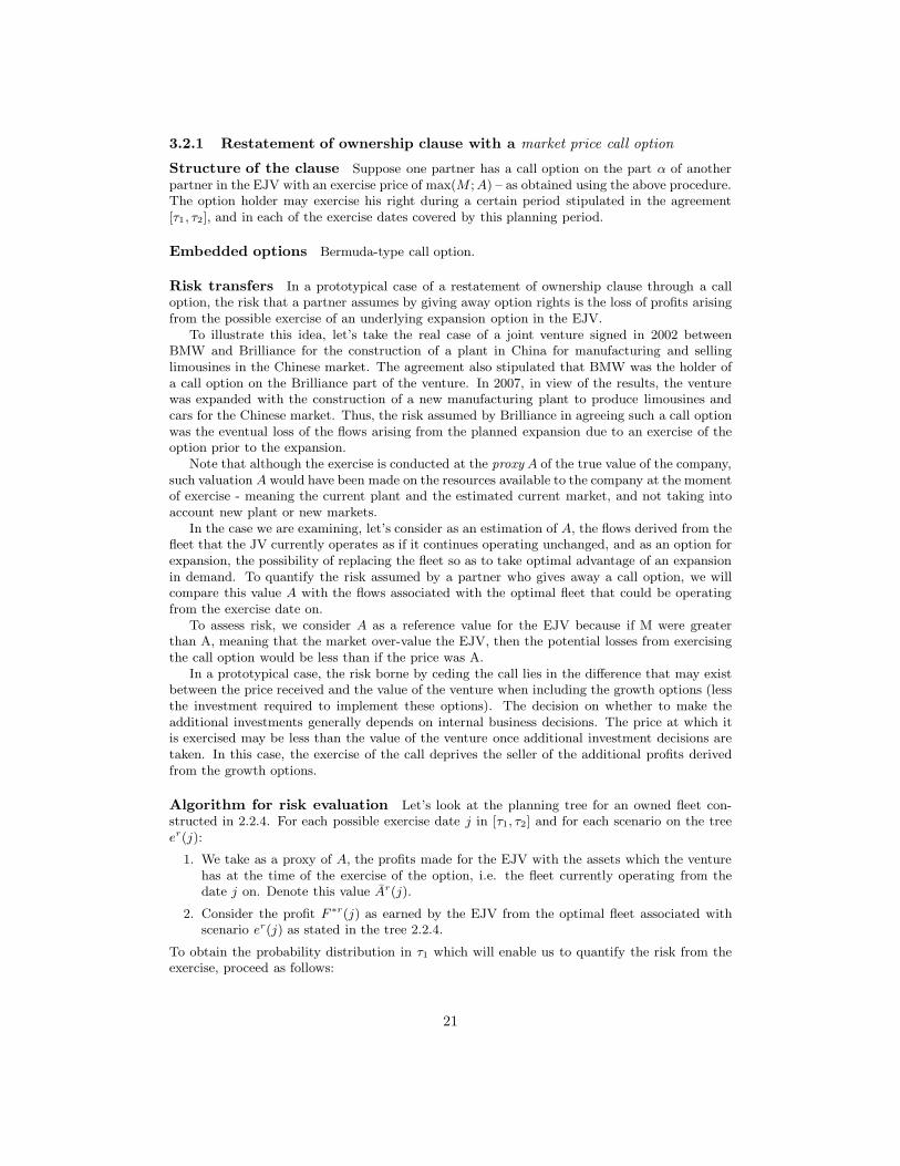
3.2.1 Restatement of ownership clause with a market price call option

Structure of the clause Suppose one partner has a call option on the part α of anotherpartner in the EJV with an exercise price of max(M ; A) – as obtained using the above procedure.The option holder may exercise his right during a certain period stipulated in the agreement[τ1, τ2], and in each of the exercise dates covered by this planning period.

Embedded options Bermuda-type call option.

Risk transfers In a prototypical case of a restatement of ownership clause through a calloption, the risk that a partner assumes by giving away option rights is the loss of profits arisingfrom the possible exercise of an underlying expansion option in the EJV.

To illustrate this idea, let’s take the real case of a joint venture signed in 2002 betweenBMW and Brilliance for the construction of a plant in China for manufacturing and sellinglimousines in the Chinese market. The agreement also stipulated that BMW was the holder ofa call option on the Brilliance part of the venture. In 2007, in view of the results, the venturewas expanded with the construction of a new manufacturing plant to produce limousines andcars for the Chinese market. Thus, the risk assumed by Brilliance in agreeing such a call optionwas the eventual loss of the flows arising from the planned expansion due to an exercise of theoption prior to the expansion.

Note that although the exercise is conducted at the proxy A of the true value of the company,such valuation A would have been made on the resources available to the company at the momentof exercise - meaning the current plant and the estimated current market, and not taking intoaccount new plant or new markets.

In the case we are examining, let’s consider as an estimation of A, the flows derived from thefleet that the JV currently operates as if it continues operating unchanged, and as an option forexpansion, the possibility of replacing the fleet so as to take optimal advantage of an expansionin demand. To quantify the risk assumed by a partner who gives away a call option, we willcompare this value A with the flows associated with the optimal fleet that could be operatingfrom the exercise date on.

To assess risk, we consider A as a reference value for the EJV because if M were greaterthan A, meaning that the market over-value the EJV, then the potential losses from exercisingthe call option would be less than if the price was A.

In a prototypical case, the risk borne by ceding the call lies in the difference that may existbetween the price received and the value of the venture when including the growth options (lessthe investment required to implement these options). The decision on whether to make theadditional investments generally depends on internal business decisions. The price at which itis exercised may be less than the value of the venture once additional investment decisions aretaken. In this case, the exercise of the call deprives the seller of the additional profits derivedfrom the growth options.

Algorithm for risk evaluation Let’s look at the planning tree for an owned fleet con-structed in 2.2.4. For each possible exercise date j in [τ1, τ2] and for each scenario on the treeer(j):

1. We take as a proxy of A, the profits made for the EJV with the assets which the venturehas at the time of the exercise of the option, i.e. the fleet currently operating from thedate j on. Denote this value Ar(j).

2. Consider the profit F ∗r(j) as earned by the EJV from the optimal fleet associated withscenario er(j) as stated in the tree 2.2.4.

To obtain the probability distribution in τ1 which will enable us to quantify the risk from theexercise, proceed as follows:

21

1. In the final scenarios of τ2, we calculate max α(F ∗r(j) − Ar(j)), 0.

2. In the intermediate nodes, we calculate max α(F ∗r(j) − Ar(j)), continuation value

Calculation of Ar(j) Note that there is no a single fleet currently associated with thescenario er(j). The tree provides us with a fleet operating in the period between j − 1 and j foreach scenario of j − 1 associated with er(j). Therefore, we must quantify the profits of usingeach of these fleets in er(j), and then weigh the results using transition probabilities to derivethe value of Ar(j).

Numerical example (In process)

3.2.2 Restatemnt of ownership clause with a market price put option

Structure of the clause Suppose one partner owns a put option on his part of an EJVwith exercise price min(M ; A) obtained by the above procedure. During a period stipulated inthe agreement [τ1, τ2] and in each of the dates stipulated in this period, the option holder mayexercise the right.

Embedded options Bermuda-type put option.

Risk transfers In a prototypical situation, the risk borne by the partner who cedes a marketprice put option results from the unfavourable position in which he may find himself afterthe option is exercised (strategic risk). To illustrate this idea, let’s take the real case of thejoint venture signed in 2000 by General Motors Corporation (GM) and Fiat S.p.A. (Fiat). Inthis alliance the two companies will partner in the European and South American automobilemarkets. As part of the agreement, GM cedes Fiat a put option so that, between the third anda half and the ninth year, on two occasions, Fiat may require a determination of the fair marketvalue of Fiat shares. Then Fiat may decide to exercise its option an sell its shares to GM.

Five years after the sighed of the agreement, Fiat announced GM its intention of exercisingits put option. The analysis of the different scenarios faced by GM led it to the conclusion that itsposition after the exercise would be strongly financially adverse. Then GM regarded two financialtransactions carried out by Fiat to be a material breach of section 6 of their agreement regulatingtransfers of shares with third parties. According to the termination provisions, General Motorswould have the legal right to terminate the agreement, prevailing the rules of liquidation overthe put option Fiat intended to exercise. This fact forced Fiat into negotiation to avoid a costlyand difficult legal process that would determine whether a material breach occurred. The resultof the negotiation was the payment by GM of 1.55 billion euros to Fiat in order to repurchasethe put option that was not finally exercised by Fiat.

As this example points out, a methodology for estimating the risk associated with this tyof clauses should take into account the potential losses from adverse market reactions followingthe exercise of the put (a reaction to the divestment), and the possible losses caused by thecontinuing activity without the partner (with or without additional investments) ([14]).

In our case of an MoS, we must highlight the fact that the SA provides a compensationmechanism that transfers the risk of the put option to the compensation clause described in ??.This is an example of how SAs and JVs often include a hierarchical structure of clauses, whichinteract among them. Therefore an evaluation of risk transfers associated with a given clausecan not be made by considering the clause as isolated but analyzing the complete agreement.

22

3.3 Resatement of ownership clauses in a PPP for a maritimebusiness

Structure of the clause Suppose that the public agent has a market price put option on allor part of the fleet. The exercise of the option is subject to a stability of demand, and thereforeto the consolidation of the business, and this stability will trigger the option. The exercise priceis set at the market value of the second-hand ships.

Embedded options European-type option with an uncertain exercise date depending on atrigger, which is path-dependant.

Risk transfers Note that the risk borne by the private operator when ceding the put optionto the public partner results from having to sell with possible losses (due to limited marketliquidity) several ships of the current fleet mix, as this current fleet mix differs from the optimalfleet able to handle future demand expectations.

If when the put option is exercised, a given ship is part of the optimal fleet, then there willbe no losses because the ship will continue operating. Otherwise, the ship must be sold and thecalculation of potential losses is a function of the sales strategy set by the private operator. Forexample, the operator may choose to continue using the ship until finding a buyer prepared topay a price equal to, or higher than, the price paid as exercising price of the put option. Theoperator may set a limit beyond which it should sell, even at a loss.

Algorithm for risk evaluation Let’s look at the planning tree for the case of a charteredfleet built in 2.2.2.

1. Simulation of an m-dimensional path S(j) = (Sk1 (j), . . . , Sk

m(j)) of the underlying processesin the tree. Then, for each date j we identify the scenario er(j) closest to S(j) (Euclideandistance) and transform the original path S(j) into a path of nodes e(j), so that we haveassociated with each node the corresponding maximum profits for the business.

2. We identify the first date j0 and the corresponding node of the tree on which the businessis consolidated.

3. Determine how many ships are not part of the optimal fleet for the following period.

4. Simulate the second-hand ship market.

5. Quantify the losses in terms of sales strategy. Consider the present value.

6. Repeating the process for each of the paths S(j) of the simulation, we generate the fullprobability distribution of losses, on which we calculate the most appropriate measure ofrisk (VAR, CVAR, ES).

Numerical example (In process)

Acknowledgment

This research has been sponsor by the Spanish government (Ministerio de Educacion yCiencia), research project number TRA2006-09939/TMAR.

23

References

[1] Barranquand, J., Martineau, D.(1995) Numerical Valuation of High- Dimensional Multi-variate American Securities. Journal of Financial and Quantitative Analysis, 30(3), 383-405.

[2] Brodie, M., Glasserman, P.(1997a) Pricing American-Style Securities using Simulation.Journal of Economic Dynamics and Control, 21, 1323-1352.

[3] Brooks, M.R., (2005). NAFTA and Short SeaShipping Corridors. The Atlantic Institute forMarket Studies. Halifax, Canada.

[4] Brooks, M.R., Hodgson, J.R. y Frost, J.D., (2006). Short Sea Shipping on the East Coastof North America: An analysis of opportunities and issues. Canada–Dalhousie UniversityTransportation Planning/Modal Integration Initiative. Project ACG-TPMI-AH08.

[5] Brownston, D., (2001). Discrete Choice Modelling for Transportation, en Hensher D. (ed)Travel Behaviour Research: The Leading Edge (97–124). Oxford: Pergamon Press.

[6] Cole, S. y Villa, A., (2005). Puertos e hinterlands: la intermodalidad para el transporte demercancıas en el espacio atlantico. Red Transnacional Atlantica. Nantes.

[7] Commission of the European Communities, (2007). An Integrated Maritime Policy for theEuropean Union. European Commission Maritime Affairs Documentation Center. Brussels.

[8] DeMonie, G., (1999). Guidelines for Port Authorities and Governments on the Privatizationof Port Facilities. Report by the UNCTAD secretariat. UNCTAD.

[9] Dupacova, J., Consigli, G. et al., (2000). Scenarios for multistage stochastic programs.Balzer Journals.

[10] Fagerholt, K. y Lindstad, H. (2007). TurboRouter: An Interactive Optimisation-BasedDecision Support System for Ship Routing and Scheduling. Maritime Economics &Logistics,9, 214–233.

[11] Fu, M.C, Laprise, S.B., Madan, D.B., Su, Y., Wu, R.,(2001) Pricing American Option: AComparison of Monte Carlo Simulation Approaches. Journal of Computational Finance,4,3, 39-88.

[12] Growe-Kuska, N., Heirsch, H. y W. Romisch (2003). Scenario Reduction and ScenarioTree Construction for Power Management Problems. IEEE Bologna POWER TECH 2003.Bologna, June 23-26.

[13] Gutterman, A., (2002). A Short Course in International Joint Ventures : Negotiating,Forming & Operating the International Joint Ventures. World Trade Press, Novato, CA,USA.

[14] Juan, C., Olmos, F. y R. Ashkeboussi, (2006). Termination Clauses in Joint Ventures andStratellic Alliances. Presented at 10th Annual International Conference on Real Options,New York.

[15] Juan, C., Olmos, F. y R. Ashkeboussi, (2007). Compensation Options in Joint Ventures. AReal Options Approach. The Engineering Economist, Vol. 52-1, 2007, pp. 67-94.

[16] Juan, C., Olmos, F. y R. Ashkeboussi, (2008). Private-Public Partnerships as StrategicAlliances. The Case of Concessions Contracts for Port Infrastructures. Transportation Re-search Record: Journal of the Transportation Research Board, 2062, pp. 1–9.

[17] Krichene, N., (2006). Recent Dynamics of Crude Oil Prices. International Monetary Fund.Working document.

[18] Mateo, A. (2005) Caracterizacion de los precios en mercados electricos competitivos medi-ante modelos ocultos de Markov de entrada salida (IOHMM). Aplicacion a la generacionde escenarios. Doctoral thesis. Universidad Pontificia Comillas de Madrid.

24

[19] National Ports and Waterways Institute Louisiana State University. High Speed Ferriesand Coastwise Vessels: Evaluation of Parameters and Markets for Application. Final Re-port submitted to Center for the Commercial Deployment of Transportation Technologies(CCDoTT).

[20] Perakis, A.N. y Jaramillo, D.I., (1991). Fleet deployment optimization for liner shippingPart 1. Background, problem formulation and solution approaches. Maritime Policy &Management, 18 (3), 183-200.

[21] Perakis, A.N. y Jaramillo, D.I., (1991). Fleet deployment optimization for liner shippingPart 2. Implementation and results. Maritime Policy & Management, 18 (4), 235-262.

[22] Pindyck, R.S., (2004). Volatility and Comodity Price Dynamics. The Journal of FuturesMarkets, Vol. 24, No. 11, 1029–1047.

[23] Plug, C.G. (2001). Scenario Tree Generation for multiperiod financial optimization byoptimal discretization. Mathematical Programing, 89, 251-271.

[24] Postali, F.A. y Picchetti, P., (2006). Geometric Brownian Motion and structural breaks inoil prices: A quantitative analysis. Energy Economics, 28 (4), 506-522.

[25] Powell, B.J. y Perkins, A.N., (1997). Fleet deployment optimization for liner shipping: aninteger programming model. Maritime Policy & Management, 24 (2), 183-192.

[26] Richemont, H., (2002). Un pavillon attractif, un cabotage credible. Report by senator HenriRichemont for the French prime minister. Paris, 2002.

[27] Tilley, J.A., (1993). Valuing American Options in a Path Simulation Model. Transactionsof the Society of Actuaries, 45, 83-104.

[28] Train, K., (2003). Discrete Choice Methods with Simulation. Ed. Cambridge UniversityPress.

[29] Vazquez, F.J. y Benitez, F.G., (2000). Reparto Modal Mediante Modelos de Eleccion Disc-reta Mixtos PR-PD. Calidad e Innovacion en los Transportes. Eds. J.V. Colomer and A.Garcia, pgs. 223-230.

[30] Vassallo, J.M. y J. Gallego, (2005). Risk Sharing in the New Public Works Concession Lawin Spain. Transportation Research Record: Journal of the Transportation Research Board,1932, pp. 1–8.

[31] Vassallo, J. M. y A. Sanchez, (2006). Minimum Income Guarantee in Transportation In-frastructure Concessions in Chile. Transportation Research Record: Journal of the Trans-portation Research Board, 1960, pp. 15–22.

[32] Vernimmen, B. y Witlox, F., (2003). The Inventory-Theoretic Approach to Modal Choice inFreight Transport: Literature Review and Case Study. Brussels Economic Journal/CahiersEconomiques de Bruxelles, 46 (2), 5-29.

[33] Schwarz, E.S., (1997). The stochastic behavior of commodity prices: Implications for val-uation and hedging. Journal of Finance, 52 (3), 923-973.

25