Alejandro Tommasi NTDS-Project IV ID: 200086 Practice IV: Design and analysis of a Latent Heat...

Alejandro Tommasi NTDS-Project IV ID: 200086

POLITECNICO DI TORINO

NUMERICAL DESIGN OF THERMAL SYSTEMS 2013/2014

Practice IV:

Design and analysis

of a Latent Heat Storage system


Introduction The aim of this project is to design and analyze a Latent heat storage system that consist in a metal shell and a

matrix of copper pipes that exchange heat with a phase change material (PCM) that is located in between the

shells and the tubes. This unit is used to store the heat delivered from the district heating network by means of

the PCM material in the form of sensible heat and latent heat, for the temperature and phase change

respectively. An analysis of the discharging process will be performed by considering a single tube with a

portion of PCM, in a 2D Axi-symetrical geometry problem. A conjugate heat transfer model will be studied in

which the stationary analysis will be the one for what regards the velocity field, and the transient problem for

the temperature evolution in time. All the calculations were performed by mean of COMSOL commercial code.

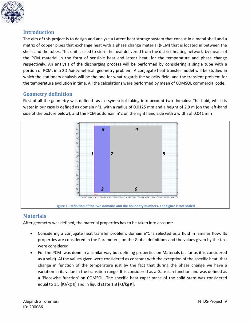
Geometry definition First of all the geometry was defined as axi-symetrical taking into account two domains: The fluid, which is

water in our case is defined as domain n°1, with a radius of 0.0125 mm and a height of 2.9 m (on the left-hand

side of the picture below), and the PCM as domain n°2 on the right hand side with a width of 0.041 mm

Figure 1: Definition of the two domains and the boundary numbers. The figure is not scaled

Materials After geometry was defined, the material properties has to be taken into account:

Considering a conjugate heat transfer problem, domain n°1 is selected as a fluid in laminar flow. Its

properties are considered in the Parameters, on the Global definitions and the values given by the text

were considered.

For the PCM was done in a similar way but defining properties on Materials (as far as it is considered

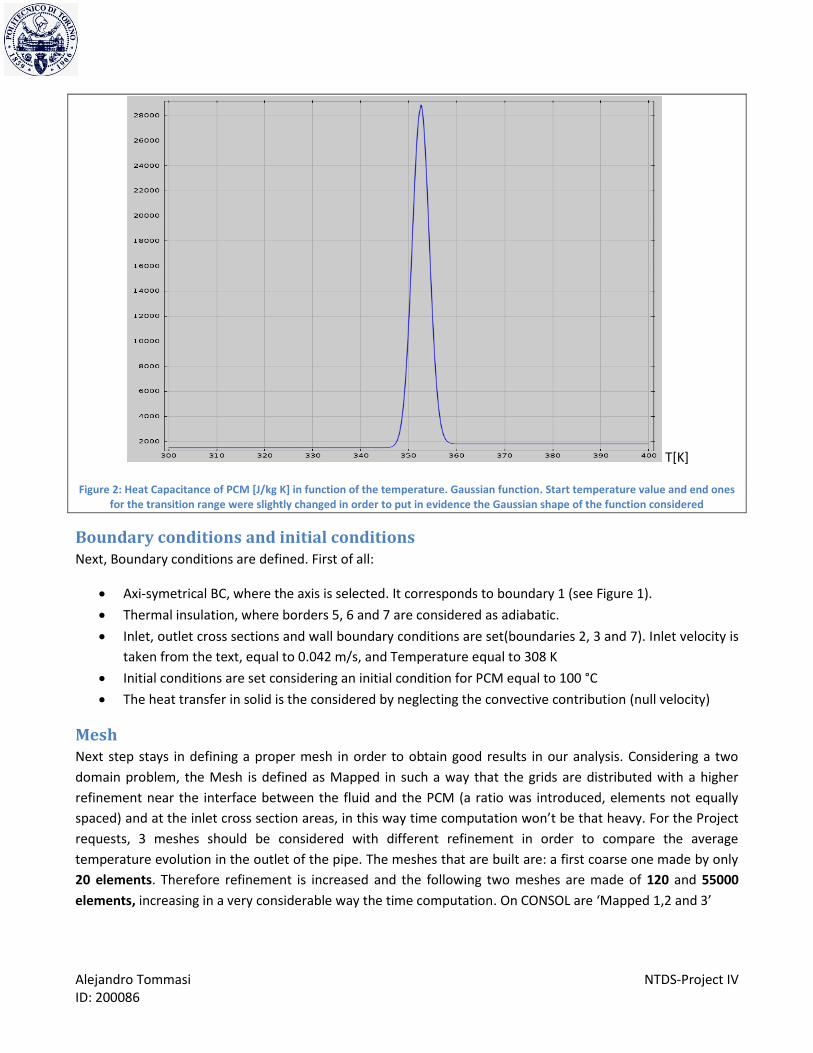
as a solid). Al the values given were considered as constant with the exception of the specific heat, that

change in function of the temperature just by the fact that during the phase change we have a

variation in its value in the transition range. It is considered as a Gaussian function and was defined as

a 'Piecewise function' on COMSOL. The specific heat capacitance of the solid state was considered

equal to 1.5 [KJ/kg K] and in liquid state 1.8 [KJ/kg K].


T[K]

Figure 2: Heat Capacitance of PCM [J/kg K] in function of the temperature. Gaussian function. Start temperature value and end ones for the transition range were slightly changed in order to put in evidence the Gaussian shape of the function considered

Boundary conditions and initial conditions Next, Boundary conditions are defined. First of all:

Axi-symetrical BC, where the axis is selected. It corresponds to boundary 1 (see Figure 1).

Thermal insulation, where borders 5, 6 and 7 are considered as adiabatic.

Inlet, outlet cross sections and wall boundary conditions are set(boundaries 2, 3 and 7). Inlet velocity is

taken from the text, equal to 0.042 m/s, and Temperature equal to 308 K

Initial conditions are set considering an initial condition for PCM equal to 100 °C

The heat transfer in solid is the considered by neglecting the convective contribution (null velocity)

Mesh Next step stays in defining a proper mesh in order to obtain good results in our analysis. Considering a two

domain problem, the Mesh is defined as Mapped in such a way that the grids are distributed with a higher

refinement near the interface between the fluid and the PCM (a ratio was introduced, elements not equally

spaced) and at the inlet cross section areas, in this way time computation won’t be that heavy. For the Project

requests, 3 meshes should be considered with different refinement in order to compare the average

temperature evolution in the outlet of the pipe. The meshes that are built are: a first coarse one made by only

20 elements. Therefore refinement is increased and the following two meshes are made of 120 and 55000

elements, increasing in a very considerable way the time computation. On CONSOL are ‘Mapped 1,2 and 3’


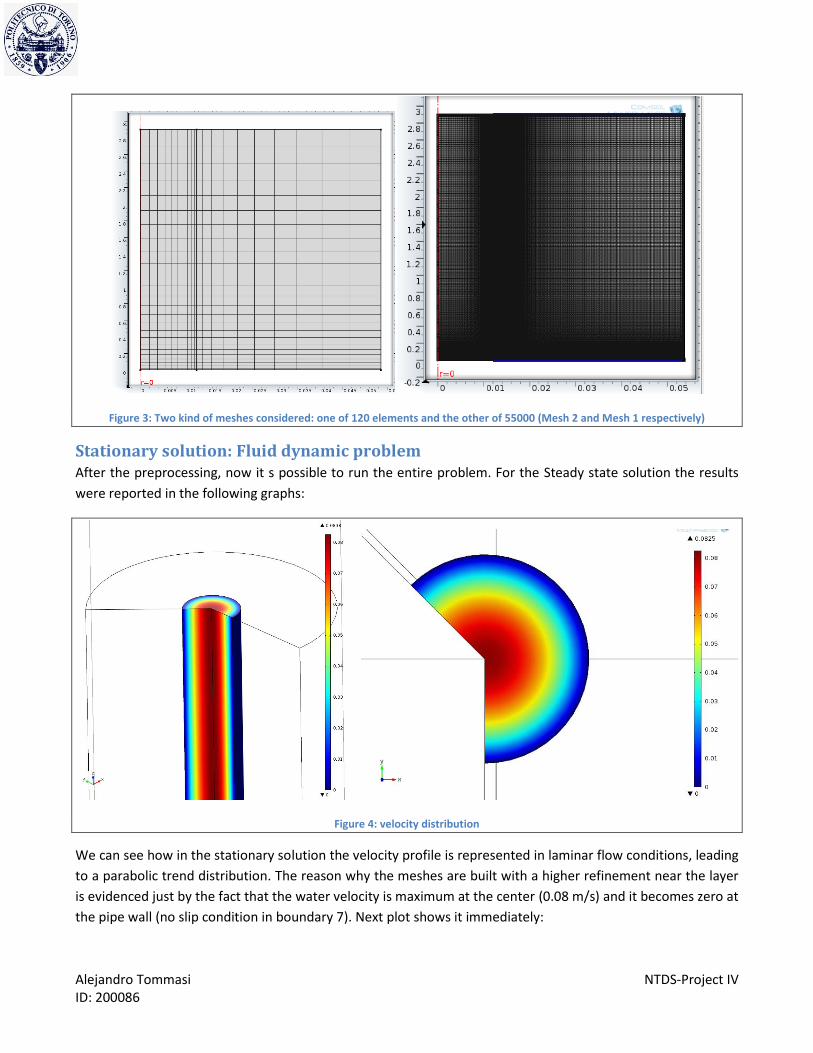
Figure 3: Two kind of meshes considered: one of 120 elements and the other of 55000 (Mesh 2 and Mesh 1 respectively)

Stationary solution: Fluid dynamic problem After the preprocessing, now it s possible to run the entire problem. For the Steady state solution the results

were reported in the following graphs:

Figure 4: velocity distribution

We can see how in the stationary solution the velocity profile is represented in laminar flow conditions, leading

to a parabolic trend distribution. The reason why the meshes are built with a higher refinement near the layer

is evidenced just by the fact that the water velocity is maximum at the center (0.08 m/s) and it becomes zero at

the pipe wall (no slip condition in boundary 7). Next plot shows it immediately:


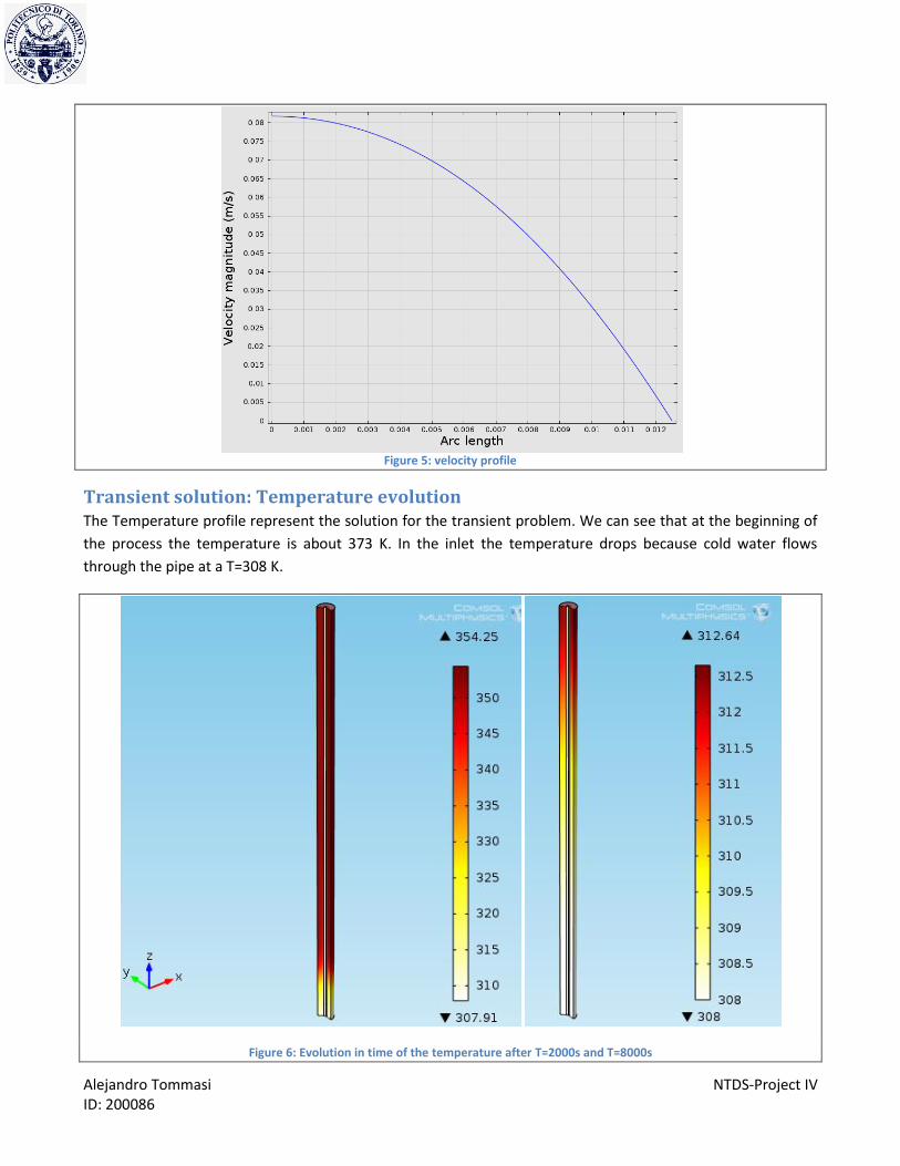
Figure 5: velocity profile

Transient solution: Temperature evolution The Temperature profile represent the solution for the transient problem. We can see that at the beginning of

the process the temperature is about 373 K. In the inlet the temperature drops because cold water flows

through the pipe at a T=308 K.

Figure 6: Evolution in time of the temperature after T=2000s and T=8000s


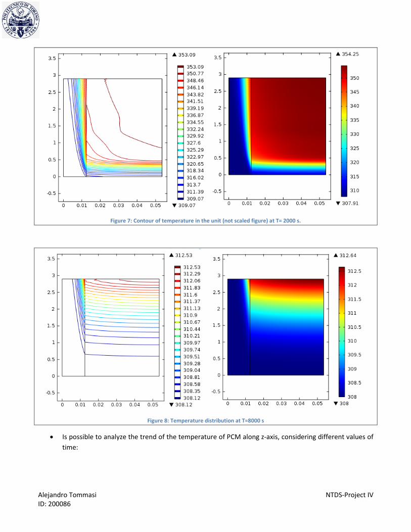
Figure 7: Contour of temperature in the unit (not scaled figure) at T= 2000 s.

Figure 8: Temperature distribution at T=8000 s

Is possible to analyze the trend of the temperature of PCM along z-axis, considering different values of

time:


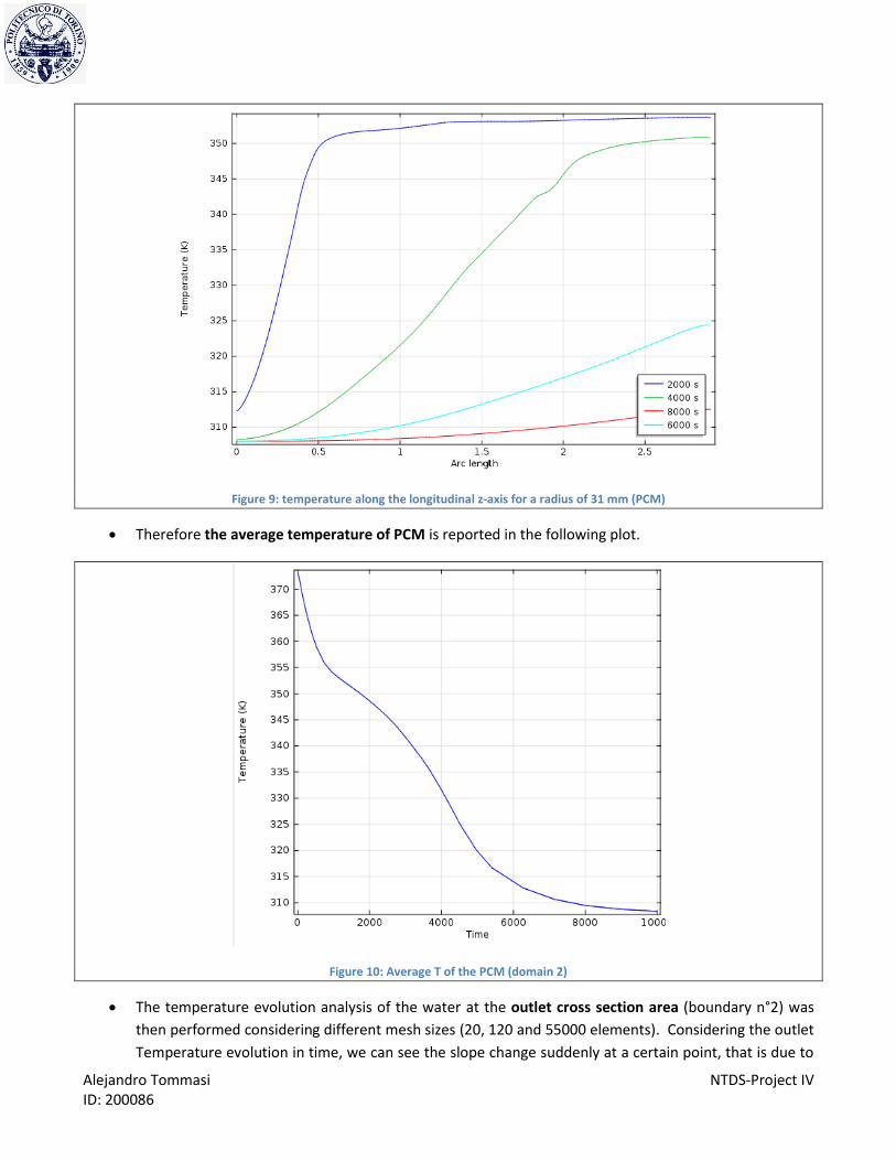
Figure 9: temperature along the longitudinal z-axis for a radius of 31 mm (PCM)

Therefore the average temperature of PCM is reported in the following plot.

Figure 10: Average T of the PCM (domain 2)

The temperature evolution analysis of the water at the outlet cross section area (boundary n°2) was

then performed considering different mesh sizes (20, 120 and 55000 elements). Considering the outlet

Temperature evolution in time, we can see the slope change suddenly at a certain point, that is due to


the PCM solidification which provides the heat to the water. The comparison between the 3 different

meshes has been done exporting the plot data from COMSOL on Matlab. The values has been

memorized as Matrices F, G and H and then plotted.

Figure 11: T outlet in function of time using different mesh sizes. Mesh 1= 55000 elements: Mesh 2= 120; Mesh 3=20. Between mesh 2 and 1, there is no evident change (only if zoomed), while for the third one it gives not accurate values.


The most evident changes for what concern the size of the mesh considered regards the computational time.

For the second mesh it took around 2 minutes and 15 seconds, for the third only 30 seconds. The most refined

one, the first, around 15 minutes (945 s).

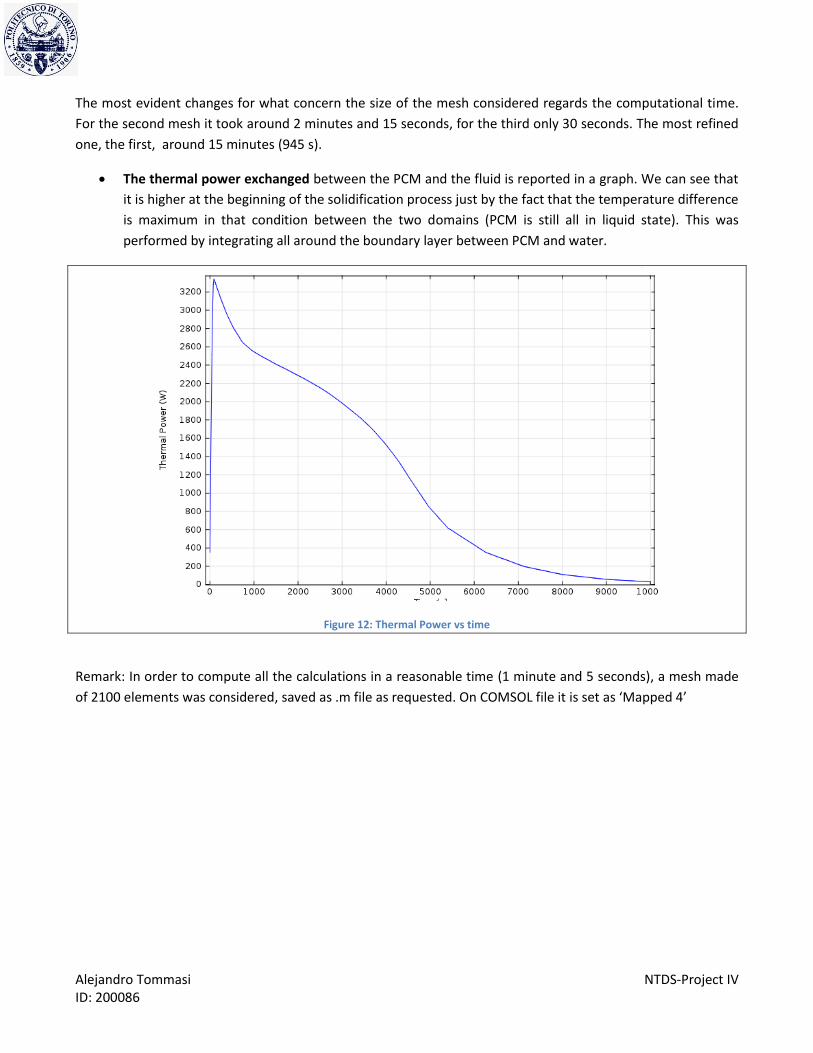
The thermal power exchanged between the PCM and the fluid is reported in a graph. We can see that

it is higher at the beginning of the solidification process just by the fact that the temperature difference

is maximum in that condition between the two domains (PCM is still all in liquid state). This was

performed by integrating all around the boundary layer between PCM and water.

Figure 12: Thermal Power vs time

Remark: In order to compute all the calculations in a reasonable time (1 minute and 5 seconds), a mesh made

of 2100 elements was considered, saved as .m file as requested. On COMSOL file it is set as ‘Mapped 4’

Alejandro Tommasi NTDS-Project IV ID: 200086 Practice IV: Design and analysis of a Latent Heat...

Documents

Transcript of Alejandro Tommasi NTDS-Project IV ID: 200086 Practice IV: Design and analysis of a Latent Heat...