Toxics 2014, 2, 1-x manuscripts; doi:10.3390/toxics20x000x

toxics ISSN 2305-6304

www.mdpi.com/journal/toxics Article

Water-air volatilization factors to determine Volatile Organic Compounds (VOCs) Reference Levels in water

Vicenç Martí 1,2,*, Joan De Pablo 1,2,†, Irene Jubany 2,† , Miquel Rovira 2,† and Emili Orejudo 3,†

1 Universitat Politècnica de Catalunya, Department of Chemical Engineering, ETSEIB, Av. Diagonal, 647, E-08028 Barcelona (Spain)

2 CTM, Centre Tecnològic Foundation, Environmental Technology Area, Plaça de la Ciència, 2 , E-08243 Manresa; E-Mails: joan.de.pablo@upc.edu; irene.jubany@ctm.com.es; miquel.rovira@ctm,com.es

3 Agència Catalana de l’Aigua , Departament de Territori i Sostenibilitat de la Generalitat de Catalunya, C/ Provença, 204-208, E-08036 Barcelona; E-Mail: eorejudo@gencat.cat

† These authors contributed equally to this work.

* Author to whom correspondence should be addressed; E-Mail: vicens.marti@upc.edu; Tel.: + 34 93 401 09 57; Fax: + 34 93 401 71 50.

Received: / Accepted: / Published:

Abstract: The calculation of Human Health Risk-Based Reference Levels (RLs) for the use of water with Volatile Organic Compounds (VOCs) need Volatilization Factors (VFs), which could be developed from mass-transfer concept from air to water. For a case study with five groups of risk scenarios and thirty VOCs, overall mass-transfer coefficients (Koverall) for flat and spherical surface geometries have been showing values close to KL when Henry’s law constant (KH) was high. In the case of spherical drops geometry, fraction of volatilization (fV) was asymptotical with KH with values also limited due to Koverall. VFs for flat surfaces were calculated from the emission flux of VOCs and results showed values close to KH for the most conservative indoor scenarios and almost constant values for outdoor scenarios. VFs for spherical geometry in indoor scenarios followed equal trend with KH than fV and, in outdoor scenarios, VFs were very far from KH and related to irrigation parameters.

OPEN ACCESS

Toxics 2014, 2 2

As a conclusion, VFs of several scenarios could be easily calculated applying flat and spherical geometries and allow modeling risk assessment cases where the water-air transfer of VOCs could be a key factor.

Keywords: Environmental contaminants; Volatile organic compounds; Water-air modeling; Human Health Risk Assessment; Exposure models; Volatilization Factors;

1. Introduction

As stated by Water Framework Directive 2000/60/CEE (WFD), contaminated water needs to decrease the concentration of its chemicals with time until reaching a total recovery of the good chemical status, indicating a minimum anthropogenic impact. Under this scope, long-term levels of concentration of contaminants in water as a function of uses cannot be defined.

The new policies derived from WFD need the development of sustainable water management solutions in order to satisfy the demand of uses of water from people and economic agents (agricultural, domestic, urban, industrial and recreational uses). The application of legislation to waters affected by chemical contamination (e.g. extracted groundwater) could ban its use, but the quality of the impacted water could be good enough for less stringent transitory uses under the scope of admissible risk for Human Health. In this situation, Risk Assessment methodologies could be used in order to establish protective Reference Levels (RLs) [1].

Risk-based soil management is a known methodology able to asess the contamination of a site and defines remediation goals using chemical risk assessment as a base. Methodology includes the exposure assessment, toxicity assessment and target carcinogenic risk and hazard indexes [1,2].

As a part of this methodology, protective levels for the safe use of water (RLs) could be derived by considering a multiple pathway exposure that includes oral pathway (direct ingestion of water or ingestion of vegetables irrigated with water), dermal pathways (direct dermal contact with water) and inhalation pathway (inhalation of VOCs in air coming from dissolved VOCs in water). [3,4]

As the calculation of RLs needs a concentration referred to water and inhalation pathway refers to air, the Volatilization Factors (VFs) must be introduced and have an important role in RLs of VOCs.

For soil contamination there are standard guidelines for Risk Assessment where subsurface soil-air, superficial soil-air or groundwater-air VFs have been calculated [5] (pp.23-30). These VFs assume a constant concentration of contaminant in water with time, equilibrium partitioning and steady-state transport, no loss of chemicals and steady and well-mixed hypothesis. The calculation of theses VFs start from the equilibrium concentration of contaminant is soil-gas phase, and models based on diffusion and advection allow obtaining a vertical flux of contaminants. By applying a mass balance in a hypothetical box or an enclosed space, the calculation of the inhalation concentration in outdoor or indoor scenarios is finally obtained.

In the case of VFs from water to air there is a lack of these official compilation guidelines to apply for risk assessment studies, but it could be developed with the same approach. The main difference to consider is that for these water-air pathway it must be integrated the transport of VOCs from water

Toxics 2014, 2 3

across the liquid and gas films and finally to air to model the overall mass transfer coefficient of these contaminants.

Looking at the water to air pathways that are more common in risk assessment, flat and spherical geometries could be chosen to define the transference of VOCs from flat surfaces (e.g. pools, bathrooms, water extended in soil) [6] (pp. 887-943) or droplets (sprinkler irrigation, shower) [7] (pp. G1-G9).

Several models for the calculation of mass transfer coefficients in water could be applied to calculate these VFs [6] (pp. 908-909). The film model states that the thickness of the limiting layer is independent of the substance. The Surface Renewal Model defines a constant time of renewal for all volatile compounds. The Boundary Layer Model, which is the most used model, introduces Schmidt Number. In the case of air mass transfer, models similar to Boundary Layer Model could be postulated.

Once the overall mass-transfer has been obtained, the second part of the VFs modeling could be developed in the same way that for soil contamination. Starting from the fluxes or the emission with time of contaminants, box models [5] (p. 35), [6] (pp. 945-981) could be applied to finally obtain VFs.

A final aspect to consider is the sensitivity of VFs linked to the parameters used to calculate it. Previous works have been focused mainly on several parameters of irrigation [8], but the role of volatility is crucial when considering new VOCs and must be investigated.

This paper develops these mentioned theoretical aspects and apply them to a specific case study that was used to calculate RLs in Catalonia [4] to obtain VFs for several VOCs and study its behavior as a function of volatility (KH) of the compounds. 2. Methodology

2.1. Mass transfer coefficients

The most used models consider that the equilibrium of water and air in the interface is given by Henry’s law. Around this interface it is considered a two-phase model as bottleneck boundaries with a constant gradient in the narrow zones close to the interface. In this model the overall mass transfer coefficient Koverall (m.s-1) for VOCs is given by the mass transfer coefficient for water KL (m-s-1) and the mass transfer coefficient air (KG (m.s-1) and KH, the non-dimensional Henry’s constant law [6] (p.893) ,[9] (p.64):

Koverall =1

� 1KL� + � 1

KG · KH� (1)

There are several models for mass-transfer coefficients in water and air [6] (p. 912) that could be

summarized in the following expression

𝐾 = 𝐾 𝑟𝑒𝑓𝑒𝑟𝑒𝑛𝑐𝑒 · �𝐷

𝐷𝑟𝑒𝑓𝑒𝑟𝑒𝑛𝑐𝑒�𝑎

(2)

D and Dreference are molecular diffusion coefficients (m2.s-1) and K and Kreference are the mass transfer coefficients. The most extended way to calculate values of KL and KG is starting from reference values

Toxics 2014, 2 4

obtained from evaporation of H2O in air or transport of CO2 in water and apply several models of proportionality between these reference compounds and each volatility.

An alternative of molecular diffusion coefficients ratios is to use molecular weight ratios M (g/mole), that roughly follow the expression [6] (pp. 803,813):

�𝐷

𝐷𝑟𝑒𝑓𝑒𝑟𝑒𝑛𝑐𝑒� = �

𝑀𝑀𝑟𝑒𝑓𝑒𝑟𝑒𝑛𝑐𝑒

�−0.5

(3)

The combination of expressions (2) and (3) allows the calculation in literature of overall mass transfer coefficients for flat and spherical surfaces (droplets). These values are adequate for the risk assessment scenarios and have been summarized in Table 1

Table 1. KL and KG values (m.s-1) for flat and spherical geometries

Geometry KL (m.s-1) KG (m.s-1)

Flat

[6] (p.915)

6.5 · 10−6 · �𝐷𝑤

1.488 · 10−9�0.67

(4) 𝐾𝐺,𝐻2𝑂 · �𝐷𝑎

2.6 · 10−5�0.67

u=0 KG,H2O=3·10-3 m.s-1

u=2.25 m·s-1 KG,H2O=8.5·10-3 m.s-1

(5)

Sphere

[10], [11]

[7] (p. G-2)

5.55 · 10−5 · �44𝑀�0.5

(6) 8.33 · 10−3 · �18𝑀�0.5

(7)

The values for flat geometry are based in the Boundary Layer Model (a=0.67 in expression (2)) and

consider several expressions reviewed in [6] (p. 915). In the case of KL, velocities of water bellow 4.2m.s-1 were considered and for KG the values depend on wind velocity. For spherical droplets, values are based in the film model (a=1 in expression (2)) and are independent of the velocity.

2.2. Summary of VFs

The appendix of the present articles calculates the values of VFs for flat and droplet geometry. The value Koverall must be calculated with the adequate values of KL and KG from table 1. In order to obtain VF values box models have been used (the room in the indoor scenario and a hypothetical box for outdoor scenarios) for the mass balance of the contaminant. The meaning of the parameters is detailed in appendix.

Toxics 2014, 2 5

Table 2. VFs models (L·m-3) for the type of scenarios considered

Geometry Indoor Outdoor

Flat 103 𝐿 · 𝑚−3

� 1KH

� + � f𝑅 · 𝑉A · Koverall

�

(8) 103 𝐿 · 𝑚−3

� 1KH� + � u · 𝐻

L · Koverall�

(9)

Sphere f𝑉 · 𝑄 · 𝑡𝑠ℎ · (103 𝐿 · 𝑚−3)𝑉

(10a)

f𝑉 · 𝑄 · (103 𝐿 · 𝑚−3)𝑢 · 𝐻 · 𝑊

(11)

f𝑉 · 𝑄 · (103 𝐿 · 𝑚−3)𝑓𝑅 · 𝑉

(10b)

2.2.3. Application to a case study

A case study about the calculation of RLs for the protective use of water in Catalonia is developed

in the present work. As a starting point, five groups of risk scenarios (1 agricultural, 2 domestic, 3 urban, 4 industrial and 5 recreational) were defined (table 3) [4] .

Table 3. Pathways included in all the scenarios considered

SCENARIOS

Vegetable Water Air

Ingestion Ingestion Dermal

contact

Inhalation

indoor

Inhalation

outdoor

E1A Crop Consumption Irrigated

E1B Indoor irrigation

(e.g. greenhouse) Irrigated direct Sprinkler (sphere)

E1C Exterior irrigation

(inundation and sprinkler) Irrigated direct

Sprinkler (sphere)

Puddle (flat)

E2A

Personal hygiene

(shower and hand cleaning) direct direct Shower (sphere)

E2B

Industrial cleaning

(e.g. cleaning pools) direct

From pool (flat)

Sprinkler (sphere)

E3A Domestic hygiene

(shower and hand cleaning) direct direct Shower (sphere)

E3B Private gardens

(irrigation with sprinkler) direct direct Sprinkler (sphere)

E4A Street cleaning (sprinkler) direct Sprinkler (sphere)

E4B Urban cleaning (splinker) direct Sprinkler(sphere)

E5A Recreational bath (pools ) direct direct From pool (flat)

Toxics 2014, 2 6

Each scenario was divided in several sub scenarios that included as pathways the ingestion of vegetables irrigated with water, the ingestion of water (shower, sprinkler), the inhalation of volatiles and the dermal contact with water (shower, contact with sprinklers).

In the last two columns of table 3 (indoor and outdoor), a detail of the type of geometry needed is included. Table 4 compiles the parameters for the indoor scenarios to calculate VF and table 5 the parameters for outdoor scenarios. In both cases references of these values are given.

Table 4. Volatilization parameters for indoor scenarios

Parameter E1B E2A E2B flat E2B sph

/E4B E3A E5A

Reference

fR (s-1) 2.3·10-3 - 2.3·10-3 2.3·10-3 - 1.4·10-3 10 more than

[5] (p. 28)

V (m3) 300 4.5 - 1250 4.5 - Calculated

V/A (m) - - 3 - - 2 [5] (p. 28)

t travel (s) 10 0.64 - 0.64 0.64 - [12]

d (m) 2·10-3 2·10-3 - 2·10-3 1·10-3 - [12]

Q·105 (m3·s-1) 5.55 16.6 - 50 16.6 - [7] [12]

tsh (s) - 600 - - 600 - [9]

Table 5. Volatilization parameters for outdoor scenarios

Parameter E1C flat E1C sph E3B E4A References

u (m.s-1) 2.25 2.25 2.25 2.25 [5] (p. 28)

H (m) 1.5 2.5 2 2 [5] (p. 28)

and calculated L (m) 15 - - - [5] (p. 28) t travel (s) - 10 0.64 0.64 [12] d (m) - 2·10-3 2·10-3 2·10-3 [12] Q·105 (m3·s-1) - 50 50 183 [7] [12] W (m) - 18 8 8 Local data

The VOCs considered and its chemical properties (M, dimensionless KH, Da and Dw) are shown in table 6 and have been obtained from the RAIS (Risk Assessment Information System) database [13] with the exception of MTBE, ETBE and tetrahydrofurane that were obtained from GSI database [14]. The rank of KH indicates the order of KH of the VOCs classified from lower to higher values and it will be helpful to identify individual VOCs in figures 1 to 5.

Toxics 2014, 2 7

Table 6. Properties of VOCs for VFs calculation

M (g.mole-1) KH Da (m2.s-1) Dw (m2·s-1) Rank KH

Acetone 5.81E+01 1.62E-03 1.24E-05 1.14E-09 2

Benzene 7.81E+01 2.27E-01 8.80E-06 9.80E-10 18

Bromoform 2.53E+02 2.19E-02 1.49E-06 1.03E-09 7

Butanone, 2- 7.21E+01 2.33E-03 8.08E-06 9.86E-10 3

CarbonTetrachloride 1.54E+02 1.13E+00 7.30E-06 8.70E-10 29

Chlorobenzene 1.13E+02 1.27E-01 1.04E-05 1.00E-09 13

Chloroform 1.19E+02 1.50E-01 1.04E-05 9.90E-10 15

Dichloroethylene, 1,1 9.69E+01 1.07E+00 1.01E-05 1.17E-09 28

Dichloroethylene, c-1,2 9.69E+01 1.67E-01 9.00E-06 1.04E-09 16

Dichloromethane 8.49E+01 1.33E-01 7.36E-06 1.13E-09 14

Dichlororethane, 1,2 9.90E+01 4.82E-02 7.07E-06 1.19E-09 10

Dichloroethylene, t-1,2 9.69E+01 3.83E-01 6.95E-06 7.34E-10 24

ETBE 1.02E+02 9.99E-02 7.50E-06 7.80E-10 12

Ethylbenzene 1.06E+02 3.22E-01 1.78E-05 1.98E-09 23

Formaldehyde 3.00E+01 1.38E-05 5.42E-06 5.91E-10 1

Hexachlorobenzene 2.85E+02 6.95E-02 7.92E-06 9.41E-09 11

MTBE 8.81E+01 2.44E-02 5.90E-06 7.50E-10 8

Naphtalene 1.28E+02 1.80E-02 7.10E-06 7.90E-10 6

Tetrachloroethane 1.68E+02 1.50E-02 7.20E-06 8.20E-10 5

Tetrachloroethylene 1.66E+02 7.24E-01 7.80E-06 8.80E-10 27

Tetrahydrofurane 7.21E+01 5.75E-03 9.30E-06 9.88E-10 4

Toluene 9.21E+01 2.71E-01 8.70E-06 8.60E-10 19

Trichloroethane, 1,1,1 1.33E+02 7.03E-01 7.80E-06 8.80E-10 26

Trichloroethane, 1,1,2 1.33E+02 3.37E-02 7.80E-06 8.80E-10 9

Trichloroethylene 1.31E+02 4.03E-01 7.90E-06 9.10E-10 25

Trichlorofluormethane 1.37E+02 3.97E+00 8.70E-06 9.70E-10 30

xylene, m- 1.06E+02 2.94E-01 7.00E-06 7.80E-10 22

xylene, o- 1.06E+02 2.12E-01 8.70E-06 1.00E-09 17

xylene, p- 1.06E+02 2.82E-01 7.69E-06 8.44E-10 21

xylenes (average) 1.06E+02 2.71E-01 7.14E-06 9.34E-10 20

3. Results and discussion

3.1. Mass-transfer coefficients

Toxics 2014, 2 8

Figure 1 shows the values of Koverall as a function of KH for the studied contaminants by using the models in table 1.

Figure 1. Overall mass-transfer coefficients as a function of KH

As it could be seen, as a general trend, VOCs with KH above 10-1 have an asymptotic value of Koverall. Expression (1) shows that for very volatile compounds, the water mass-transfer limits the overall mass-transfer, thus Koverall is approximately KL for most of the studied compounds.

As KL has the same model for flat geometry for outdoor and indoor scenarios, both type of values match. Most of the contaminants have also similar Dw value and thus an asymptotic value of 5·10-6 m.s-1 could be used as Koverall to assess these scenarios. The outlier in the graphic of flat models is MTBE, probably due to an error of Dw in the database.

In the case of spherical geometry, the overall transference is higher than in the flat surface due to the falling of the droplets. Asymptotical values are also close to KL, but the dependence now is due to M and values between 3·10-5 m.s-1 and 4·10-5 m.s-1.

3.2. Fraction of volatilization

In the case of spherical droplets, the fraction of volatilization (fV) for three groups of scenarios (E1B and E1C; a group formed by E2A, E2B, E3B, E4A and scenario E3A has been calculated. These groups are formed because share the same parameters than influence in fV (see tables 4 and 5). Results are shown in figure 2. As these scenarios have a limited Koverall, the fraction of volatilization is also limited to a maximum but never reaches 1. Agricultural scenarios, were the time of travel has been considered higher, show fractions around 60-70% for volatiles with KH greater than 10-2.

Toxics 2014, 2 9

Figure 2. Fraction of volatilization for droplets as a function of KH

In the case of showers and irrigation were it has been considered the dropping time from 2 meters (0.64 seconds) and diameter of 1mm (scenario E3A) or 2 mm (group 2,3,4) the fraction of volatilization is around 6 to 12%.

3.3. VFs for flat geometries

VFs for flat geometry (scenarios E2B, E5A and E1C) were calculated with the expressions of table 2 and data from tables 4, 5 and 6.

In figure 3, VFs are plotted as a function of KH and are compared with 1000 times KH that would have the equivalent units of L·m-3.

For indoor scenarios and KH below 10-2 VFs could be estimated as 1000KH. For higher values of KH the full expression has to be employed as asymptotic values are not yet reached. On the contrary, for outdoor scenarios the asymptotic value (around 2 L-m-3) is obtained for most of the compounds when KH is higher than 10-2. This concept of limited VFs for volatiles follows Andelman’s model [15], that establishes a VF=0.5 L·m-3 when KH exceeds 4·10-4.

3.4. VFs for spherical geometries

Figure 4 shows the VFs values for the indoor scenarios (E1B, E2A, E2B, E3A and E4B). In all cases, for volatilities greater than 10-2, asymptotical values (that correspond to asymptotical values of fv) were obtained. From the two indoor scenarios, the model without renovation of air is more conservative, because tsh is greater than the inverse of fR. Values equivalent to KH are only obtained when volatility is very low and for scenarios E2A and E3A. The flow rate, the volume of the room and the renovation or time of shower are, thus, the main parameters that will influence in these VFs.

Toxics 2014, 2 10

Figure 3. VFs as a function of KH for flat geometry

Figure 4. VFs for indoor scenarios as a function of KH for spherical droplets geometry

In the case of outdoor scenarios (E1C, E2B and E4A) figure 5 shows also steady values for high volatile compounds, but values are very far from KH values as renovation in outdoor is very high.

Toxics 2014, 2 11

Figure 5. VFs for outdoor scenarios as a function of KH for spherical droplets geometry

The flow rate, the fraction of volatilization and the width of the zone are important parameters that influence in VF, as it could be seen in table 2.

4. Conclusions

As a main conclusion, Koverall is limited to KL parameter when volatility (given by KH) is higher than 10-1-10-2. In the spherical droplet model, fV is also limited by this parameter in the same range. This situation implies that, as a general rule, VFs reach a limit value that is function of KL and thus the parameters of the models, excluding KH, become relevant to define VFs. On the contrary hand, low volatility VOCs in indoor scenarios could reach values equivalent to KH and parameters of the models of less relevance to define VFs.

Acknowledgments

Special thanks should be given to Agencia Catalana de l’Aigua for the funding received for the present work. Authors want to thank to David López Yuste all his support for the elaboration of results.

Conflicts of Interest

The authors declare no conflict of interest.

Toxics 2014, 2 12

Appendix. Theoretical expressions for VFs (table 2)

A.1. Flat surface

As this overall coefficient is referred to the resistances between the layers of water with a concentration C (mg·L-1 ), and the layer with an air concentration, Ca (mg·m-3), a flux of contaminant from a flat surface could be defined as [6] (p. 896):

This flux q (mg.m-2.s-1) is assumed to be constant with time (constant source concentration and

steady-state hypotheses). For the case of indoor scenario, a flat surface of contaminated water A (m2) in a perfectly-mixed

room of volume V (m3) that has a frequency of renovation of air fR (s-1) has been considered. Under these conditions the concentration CaFI is given by [5] (p. 35):

𝐶𝑎𝐹𝐼 =𝑞𝐹𝐼 · 𝐴𝑉 · 𝑓𝑅

(A.2.)

Combining expressions (A.1) and (A.2.), the volatilization factor for this case could be obtained and the final expression is compiled in table 2 (expression (8)).

In an outdoor scenario, the box model could be applied, and the maximum estimated concentration

in air inside the box is a function of L (m) , the length of contaminated water in the direction of the wind that blows with and speed u (m.s-1) and the height H (m) of the box [5] (p. 35).

𝐶𝑎𝐹𝐸 =q𝐹𝐸 · 𝐿𝑢 · 𝐻

(A.3)

Combining expressions (A.1) and (A-3), VF could be obtained for flat source and indoor scenario and the final expression is compiled in table 2 (expression (9)).

2.2.2. Spherical droplets

In the case of volatile release of VOCs from spherical droplets to air, the variation of concentration in the droplet is given by the first-order process that is function of the overall mass transfer coefficient given in (2) and a (m2.m-3) that is the specific surface of the droplet. For the spheres, a=6/d where d (m) is the diameter of the drop.

𝑑𝐶𝑑𝑡

= −𝐾′𝑜𝑣𝑒𝑟𝑎𝑙𝑙 · 𝑎 · 𝐶 (A.4)

𝑞 = Koverall · �1000𝐶 −𝐶𝑎𝐾𝐻� (A.1)

Toxics 2014, 2 13

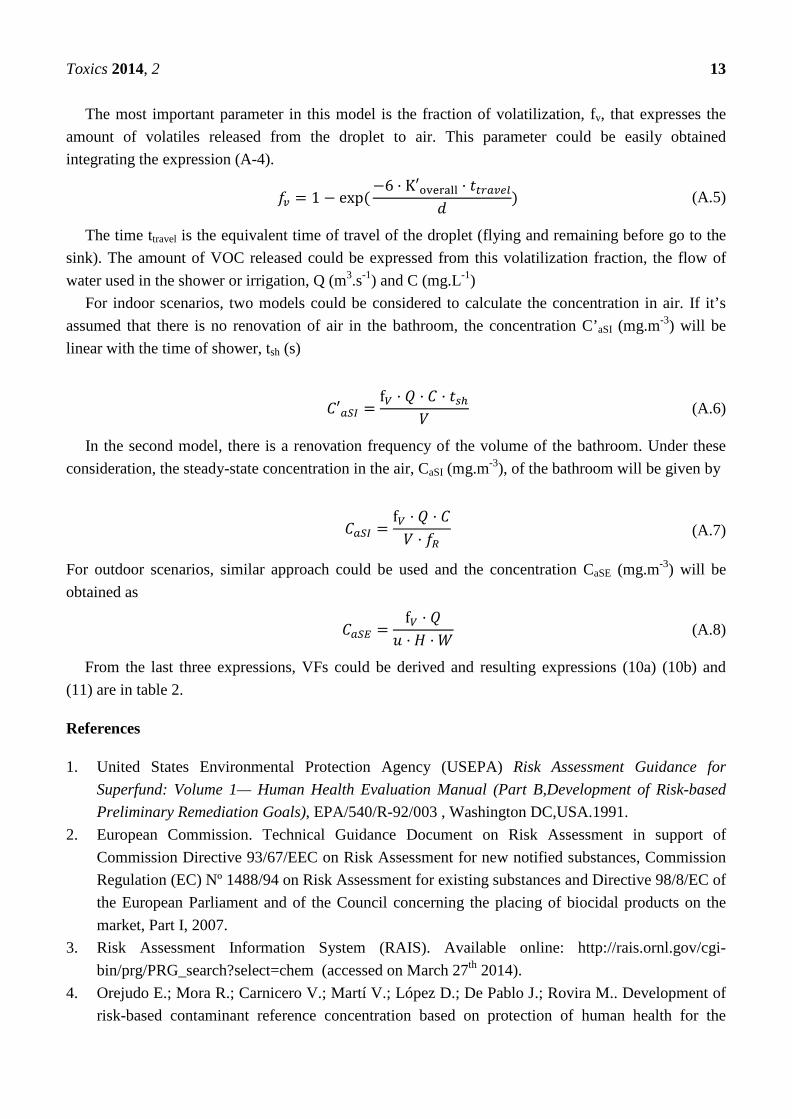
The most important parameter in this model is the fraction of volatilization, fv, that expresses the amount of volatiles released from the droplet to air. This parameter could be easily obtained integrating the expression (A-4).

𝑓𝑣 = 1 − exp(−6 · K′overall · 𝑡𝑡𝑟𝑎𝑣𝑒𝑙

𝑑) (A.5)

The time ttravel is the equivalent time of travel of the droplet (flying and remaining before go to the sink). The amount of VOC released could be expressed from this volatilization fraction, the flow of water used in the shower or irrigation, Q (m3.s-1) and C (mg.L-1)

For indoor scenarios, two models could be considered to calculate the concentration in air. If it’s assumed that there is no renovation of air in the bathroom, the concentration C’aSI (mg.m-3) will be linear with the time of shower, tsh (s)

𝐶′𝑎𝑆𝐼 =f𝑉 · 𝑄 · 𝐶 · 𝑡𝑠ℎ

𝑉 (A.6)

In the second model, there is a renovation frequency of the volume of the bathroom. Under these consideration, the steady-state concentration in the air, CaSI (mg.m-3), of the bathroom will be given by

𝐶𝑎𝑆𝐼 =f𝑉 · 𝑄 · 𝐶𝑉 · 𝑓𝑅

(A.7)

For outdoor scenarios, similar approach could be used and the concentration CaSE (mg.m-3) will be obtained as

𝐶𝑎𝑆𝐸 =f𝑉 · 𝑄

𝑢 · 𝐻 · 𝑊 (A.8)

From the last three expressions, VFs could be derived and resulting expressions (10a) (10b) and (11) are in table 2.

References

1. United States Environmental Protection Agency (USEPA) Risk Assessment Guidance for Superfund: Volume 1— Human Health Evaluation Manual (Part B,Development of Risk-based Preliminary Remediation Goals), EPA/540/R-92/003 , Washington DC,USA.1991.

2. European Commission. Technical Guidance Document on Risk Assessment in support of Commission Directive 93/67/EEC on Risk Assessment for new notified substances, Commission Regulation (EC) Nº 1488/94 on Risk Assessment for existing substances and Directive 98/8/EC of the European Parliament and of the Council concerning the placing of biocidal products on the market, Part I, 2007.

3. Risk Assessment Information System (RAIS). Available online: http://rais.ornl.gov/cgi-bin/prg/PRG_search?select=chem (accessed on March 27th 2014).

4. Orejudo E.; Mora R.; Carnicero V.; Martí V.; López D.; De Pablo J.; Rovira M.. Development of risk-based contaminant reference concentration based on protection of human health for the

Toxics 2014, 2 14

sustainable use of groundwater., Consoil 2008, 10th International UFZ/TNO Conference on Soil-Water Systems, Milano, Italy, 3-6 June 2008

5. American Society for Testing Materials. Standards Guide for Risk-Based Corrective Action

Applied at Pretroleum Release Sites, E 1739-95.; West Conshohocken, USA, 1995. 6. Schwarzenbach, R.P.; Gschwend, P.M.; Imboden D.M. Environmental Organic Chemistry, 2nd

ed.; Wiley Interscience: New York, USA, 2003. 7. Waterloo Hydrogeologic Inc. Risc WorkBench User´s Manual: Human Health Risk Assessment

Software for Contaminated Sites, v.4.0.; WHI: Waterloo, Canada, 2001 8. Orejudo E.; Mora R.; Carnicero V.; Martí V.; López D.; De Pablo J.; Rovira M.. Simplified

methodology for the sensitivity analysis of guideline values applied to water. D- Risks & Impacts. Consoil 2008, 10th International UFZ/TNO Conference on Soil-Water Systems, Milano, Italy, 3-6 June 2008

9. United States Environmental Protection Agency (USEPA) Water Quality Assessment, a screening procedure for toxic and conventional pollutants in surface and ground water (part I), EPA/600/6-85/002a , Washington, DC,USA.1985

10. Foster, S.A.; Chrostowski P.C.. Integrated Household Exposure Model for Use of Tap Water Contaminated with Volatile Organic Chemicals, 79th Annual Meeting of the Air Pollution Control Association, Minneapolis, USA, 1986

11. Carver, J.H., C.S. Seigneur, R.M. Block, T.M. Miller. Comparison of Exposure Models for Volatile Organics in Tap Water, Proceedings of Hazmacon, Santa Clara, USA, April 15, 1991.

12. Walden, J.T; Spence. L.R. Risk-Based BTEX Screening Criteria for a Groundwater Irrigation Scenario. Journal of Human and Ecological Risk Assessment 1997, 3, 699–722.

13. Risk Assessment Information System (RAIS). Available online: http://rais.ornl.gov/cgi-bin/tools/TOX_search?select=chem_spef (accessed on May 2006).

14. GSI Environmental, GSI chemical properties database. Available online: http://www.gsi-net.com/es/publicaciones/gsi-chemical-database/list.html (accessed on May 2006).

15. Andelman, J. B.. Total Exposure to volatile organic compounds in potable water, Chapter 20 in Significance and Treatment of Volatile Organic Compounds in Water Supplies, Lewis Publishers: Chelsea, USA, 1990; pp. 485-504.

© 2014 by the authors; licensee MDPI, Basel, Switzerland. This article is an open access article distributed under the terms and conditions of the Creative Commons Attribution license (http://creativecommons.org/licenses/by/3.0/).