AFRL/RW Technical Report Template - DTIC

AFRL-RW-EG-TR-2019-031

Novel Microstructures for Shock Survivability

David Lacina Christopher Neel Air Force Research Laboratory Munitions Directorate/Ordnance Division Energetic Materials Branch (AFRL/RWME) Eglin AFB, FL 32542-5910

May 2019

Final Report for period 3 February 2016 – 30 September 2018

Distribution A: Approved for public release; distribution unlimited. Approval Confirmation 96TW-2019-0136 dated 18 April 2019

AIR FORCE RESEARCH LABORATORY MUNITIONS DIRECTORATE

Air Force Materiel Command

United States Air Force Eglin Air Force Base, FL 32542

Distribution A

This page intentionally left blank

Distribution A

NOTICE AND SIGNATURE PAGE

Using Government drawings, specifications, or other data included in this document for any purpose other than Government procurement does not in any way obligate the U.S. Government. The fact that the Government formulated or supplied the drawings, specifications, or other data does not license the holder or any other person or corporation; or convey any rights or permission to manufacture, use, or sell any patented invention that may relate to them. Qualified requestors may obtain copies of this report from the Defense Technical Information Center (DTIC) (http://www.dtic.mil). AFRL-RW-EG-TR-2019-031 HAS BEEN REVIEWED AND IS APPROVED FOR PUBLICATION IN ACCORDANCE WITH ASSIGNED DISTRIBUTION STATEMENT. FOR THE DIRECTOR: ==Original Signed== ==Original Signed== ==Original Signed== JOHN D. CORLEY, PhD NYDEIA W. BOLDEN, PhD CHRISTOPHER H. NEEL, PhD Ordnance Sciences Core Technical Advisor Project Manager Technical Competency Lead Damage Mechanisms Branch Damage Mechanisms Branch Ordnance Division This report is published in the interest of scientific and technical information exchange, and its publication does not constitute the Government’s approval or disapproval of its ideas or findings.

Distribution A


Distribution A

REPORT DOCUMENTATION PAGE Form Approved OMB No. 0704-0188

Public reporting burden for this collection of information is estimated to average 1 hour per response, including the time for reviewing instructions, searching existing data sources, gathering and maintaining the data needed, and completing and reviewing this collection of information. Send comments regarding this burden estimate or any other aspect of this collection of information, including suggestions for reducing this burden to Department of Defense, Washington Headquarters Services, Directorate for Information Operations and Reports (0704-0188), 1215 Jefferson Davis Highway, Suite 1204, Arlington, VA 22202-4302. Respondents should be aware that notwithstanding any other provision of law, no person shall be subject to any penalty for failing to comply with a collection of information if it does not display a currently valid OMB control number. PLEASE DO NOT RETURN YOUR FORM TO THE ABOVE ADDRESS. 1. REPORT DATE (DD-MM-YYYY) 01 May2019

2. REPORT TYPE Final

3. DATES COVERED (From - To)3 February 2016 – 30 September 2018

4. TITLE AND SUBTITLE

Novel Microstructures for Shock Survivability

5a. CONTRACT NUMBER

5b. GRANT NUMBER

5c. PROGRAM ELEMENT NUMBER 61102F

6. AUTHOR(S)

David Lacina. Christopher Neel

5d. PROJECT NUMBER 3002HW16 5e. TASK NUMBER

5f. WORK UNIT NUMBER W10L

7. PERFORMING ORGANIZATION NAME(S) AND ADDRESS(ES)Air Force Research Laboratory, Munitions DirectorateOrdnance DivisionDamage Mechanisms Branch (AFRL/RWMW)Eglin AFB FL 32542-6810

8. PERFORMING ORGANIZATION REPORTNUMBER


9. SPONSORING / MONITORING AGENCY NAME(S) AND ADDRESS(ES)Air Force Research Laboratory, Munitions DirectorateOrdnance DivisionDamage Mechanisms Branch (AFRL/RWMW)Eglin AFB FL 32542-6810Technical Advisor: Nydeia W. Bolden, PhD

10. SPONSOR/MONITOR’S ACRONYM(S)AFRL-RW-EG

11. SPONSOR/MONITOR’S REPORTNUMBER(S)


12. DISTRIBUTION / AVAILABILITY STATEMENTDistribution A: Approved for public release; distribution unlimited. Approval Confirmation 96W-2019-0136 dated 18 April201913. SUPPLEMENTARY NOTES

14. ABSTRACTA series of plate impact experiments were conducted to measure the Hugoniot and unloading response of additivelymanufactured solid and porous polymer specimens, and to determine if the orientation along which a specimen is printedleads to a measurable effect on the shock response. This equation of state data was utilized to calibrate a finite element modelthat was used to study the propagation of compression waves through the porous polymer specimens. Comparisons of theexperimental and model results were used to study the effect of engineered porosity (i.e. different void geometries) on shockmitigation and attenuation. The results show that the polymer studied exhibits some viscoelastic response, and has aquadratic Us- up Hugoniot relation which could be reduced to a linear relation if a greater degree of uncertainty wasacceptable. The print orientation of the material does appear to affect the Hugoniot, but does not affect the unloadingbehavior. The finite element model was used to screen hundreds of potential geometries for their shock response andpotential use as a “shock diode”. The results of that screening indicate that pore (or void) geometry not only has ameasurable effect on the attenuation and propagation of compression waves, but that asymmetric void geometries can displaydirectional behavior. However, no true shock diode response was observed.15. SUBJECT TERMSShock, porosity, fractal, compaction, mitigation16. SECURITY CLASSIFICATION OF: 17. LIMITATION

OF ABSTRACT18. NUMBEROF PAGES

19a. NAME OF RESPONSIBLE PERSON Christopher Neel

a. REPORT

UNCLASSIFIED

b. ABSTRACT

UNCLASSIFIED

c. THIS PAGE

UNCLASSIFIED SAR 39

19b. TELEPHONE NUMBER (include area code)

Standard Form 298 (Rev. 8-98) Prescribed by ANSI Std. Z39.18

Distribution A


i Distribution A

Table of Contents

1. SUMMARY ......................................................................................................................................................... 1

2. INTRODUCTION .............................................................................................................................................. 1

3. METHODS, ASSUMPTIONS, AND PROCEDURES .................................................................................... 4 3.1 MATERIALS ................................................................................................................................................... 4 3.2 EXPERIMENTAL CONFIGURATION AND METHODOLOGY ............................................................................... 4 3.3 MODELING .................................................................................................................................................... 5

4. RESULTS AND DISCUSSION ......................................................................................................................... 7 4.1 EQUATION OF STATE MEASUREMENTS ......................................................................................................... 7 4.2 SHOCK RESPONSE ANISOTROPY .................................................................................................................. 10 4.3 SHOCK DIODE STUDIES ............................................................................................................................... 12 4.4 CORRELATION BETWEEN EXPERIMENTS AND SIMULATIONS ...................................................................... 16

5. CONCLUSIONS ............................................................................................................................................... 19

6. WORKS CITED ............................................................................................................................................... 20 APPENDIX ............................................................................................................................................................ 21 LIST OF SYMBOLS ................................................................................................................................................... 25 LIST OF ABBREVIATIONS AND ACRONYMS ............................................................................................................ 26

ii Distribution A

List of Figures Figure 1. (a) Example of 2-D Menger Sponge void geometries. Iteration of void geometries

follow a fractal pattern, as observed from left to right, and the voids decrease in size with iteration. (b) Example of regular grid void geometry, where all voids are the same size and vary in size uniformly. ...................................................................................................... 2

Figure 2. Schematic of the experimental configuration for plate impact experiments of engineered foam specimens (40 mm cubes and 40 mm×40 mm×13.3 mm slabs) incorporating high-speed video at 5,000,000 frames per second and four PDV probes (N, NE, C, E) on the back surface of the specimen. The specimen is minimally clamped in the fixture to minimize edge effects from the clamps. ........................................................ 5

Figure 3. Particle velocity histories for all gauges and trackers in FY17-06. Impact is zero time .......................................................................................................................................... 7

Figure 4. Depth vs time for shock wave arrival at each gauge and shock tracker in FY17-06. Impact is zero time. ................................................................................................................. 8

Figure 5. (a) Particle velocity vs. shock velocity data from initial FY17 experiments. Linear fit used to get Us- up relation. (b) 5(a) data where a quadratic fit was used to get Us- up relation. .................................................................................................................................... 9

Figure 6. Particle velocity vs. shock velocity data for experiments on all samples in Table 1. .. 10 Figure 7. Longitudinal and Transverse Print orientations ........................................................... 10 Figure 8. (a) Us- up data for all experiments listed in Tables 1 and 2, including Figure 6.

(b) Release (i.e. Unloading) wave speeds for the FY 18 experiments listed in Tables 1 and 2. ....................................................................................................................... 11

Figure 9. Particle velocity traces from PDV probes looking at the “back” face of specimen in Shot #3 in Table 2. ................................................................................................................. 12

Figure 10 40 mm width specimens used for some experiments. Menger geometries ranging in fractal iteration order from 0th to 4th. ................................................................................. 12

Figure 11. 13.33 mm width specimens used for some experiments. Note the 1nd and 2rd iterations in are parts of Figure 10. EVF1-3 signify equal dispersal of same size voids, with EVF3 being staggered, so that the void fraction is equivalent to Menger iteration. VF0-3 signify different arrangements of different sized voids in the specimen which are equivalent to the Menger iteration. ........................................................................................ 13

Figure 12. Compression of Menger 3rd order specimen in Shot #5 both (a) before impact, and (b) during compression after impact. Impact is occurring from the right. ........................... 14

Figure 13. Compression of VF2 and VF3 in Shot #14 and #16, respectively. Impact is occurring from the right. (a) When the shockwave impacts the large-to-small pore structure in moving to the left, no localized jets are formed. (b) The shockwave impacts the small-to-large pore structure in moving to the left, the structure results in the formation of jets on the downrange side. .............................................................................. 15

Figure 14. Correlation of measurements and models for 40 mm cubes, (a) test configuration, (b) section view of four items tested, (c) measured back-face velocity for solid cube, (d) predicted back-face velocity for solid cube, (e) measured back-face velocity for cube of 3rd –order shape, (d) predicted back-face velocity for cube of 3rd –order shape. Time is measured from impact. .......................................................................................................... 16

iii Distribution A

Figure 15. Contact pressure against stiff wall, (a) configuration assessed, (b) simulated peak contact pressures for fractal foam (2nd, 4th, and 6th cubes from the left) and regular grid (1st, 3rd, and 5th cubes from the left) void configurations. ..................................................... 17

iv Distribution A

List of Tables Table 1. Equation of State Experiments: lists the experimental configuration used, the

projectile velocity, the particle velocity, the shock velocity (average), and the calculated stress. ....................................................................................................................................... 7

Table 2. Shock Response Anisotropy Experiments: lists the experimental configuration used, the print orientation of the specimen, the projectile velocity, the particle velocity, the shock velocity (average), and the calculated stress. .............................................................. 11

Table 3. Shock Diode Experiments: lists the specimen thickness, the void geometry of the specimen, the impactor material used, and the projectile velocity. ....................................... 13

v Distribution A

Acknowledgements We thank Dr. Brittany Branch at LANL for performing PCI experiments at the advanced photon source to get results to aid the modeling effort at AFRL/RX. We thank Dr. Geoffrey Frank and Mr. Andrew Abbott for performing much of the FEA modeling analysis. We are also grateful to Jason Hipp, Leon Beck, and Joshua McKean for firing the gas and powder guns.

vi Distribution A


1 Distribution A

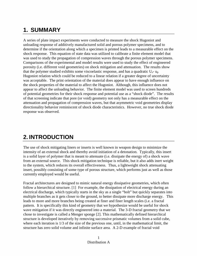
1. SUMMARY A series of plate impact experiments were conducted to measure the shock Hugoniot and unloading response of additively manufactured solid and porous polymer specimens, and to determine if the orientation along which a specimen is printed leads to a measurable effect on the shock response. This equation of state data was utilized to calibrate a finite element model that was used to study the propagation of compression waves through the porous polymer specimens. Comparisons of the experimental and model results were used to study the effect of engineered porosity (i.e. different void geometries) on shock mitigation and attenuation. The results show that the polymer studied exhibits some viscoelastic response, and has a quadratic Us- up Hugoniot relation which could be reduced to a linear relation if a greater degree of uncertainty was acceptable. The print orientation of the material does appear to have enough influence on the shock properties of the material to affect the Hugoniot. Although, this influence does not appear to affect the unloading behavior. The finite element model was used to screen hundreds of potential geometries for their shock response and potential use as a “shock diode”. The results of that screening indicate that pore (or void) geometry not only has a measurable effect on the attenuation and propagation of compression waves, but that asymmetric void geometries display directionality behavior reminiscent of shock diode characteristics. However, no true shock diode response was observed.

2. INTRODUCTION The use of shock mitigating liners or inserts is well known in weapon design to minimize the intensity of an external shock and thereby avoid initiation of a detonation. Typically, this insert is a solid layer of polymer that is meant to attenuate (i.e. dissipate the energy of) a shock wave from an external source. This shock mitigation technique is reliable, but it also adds inert weight to the system, which reduces its overall effectiveness. Thus, a lightweight shock attenuating insert, possibly consisting of some type of porous structure, which performs just as well as those currently employed would be useful. Fractal architectures are designed to mimic natural energy dissipative geometries, which often follow a hierarchical structure. [1] For example, the dissipation of electrical energy during an electrical discharge, which typically starts in the sky as a single “bolt” but quickly separates into multiple branches as it gets closer to the ground, to better dissipate more discharge energy. This leads to more and more branches being created at finer and finer length scales (i.e. a fractal pattern. It is specifically this kind of geometry that we hypothesize would be useful for shock wave mitigation if it was directly engineered into a material. The 3-D fractal geometry that we chose to investigate is called a Menger sponge [2]. This mathematically defined hierarchical structure is developed iteratively by removing successive prismatic volumes from a solid cube, where each iteration is 1/3 of the size of the previous one, until, in the mathematical limit, the structure has zero solid volume and infinite surface area. A 2-D example of fractal void

2 Distribution A

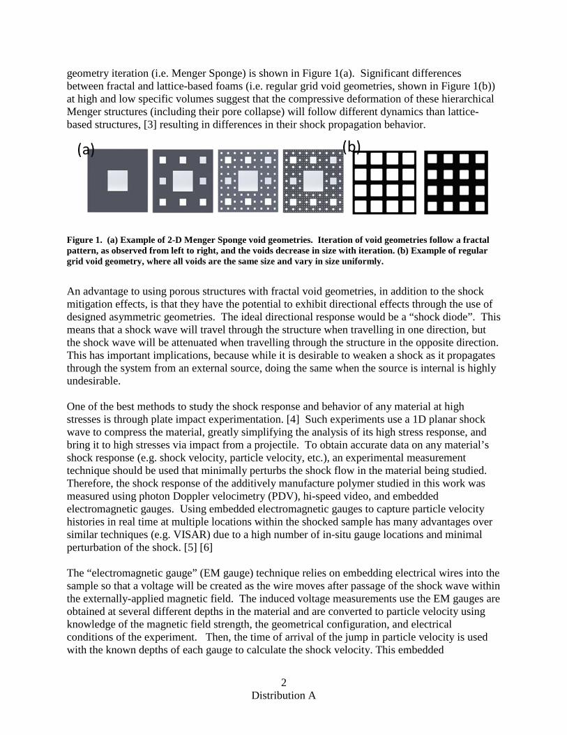
geometry iteration (i.e. Menger Sponge) is shown in Figure 1(a). Significant differences between fractal and lattice-based foams (i.e. regular grid void geometries, shown in Figure 1(b)) at high and low specific volumes suggest that the compressive deformation of these hierarchical Menger structures (including their pore collapse) will follow different dynamics than lattice-based structures, [3] resulting in differences in their shock propagation behavior.

Figure 1. (a) Example of 2-D Menger Sponge void geometries. Iteration of void geometries follow a fractal pattern, as observed from left to right, and the voids decrease in size with iteration. (b) Example of regular grid void geometry, where all voids are the same size and vary in size uniformly.

An advantage to using porous structures with fractal void geometries, in addition to the shock mitigation effects, is that they have the potential to exhibit directional effects through the use of designed asymmetric geometries. The ideal directional response would be a “shock diode”. This means that a shock wave will travel through the structure when travelling in one direction, but the shock wave will be attenuated when travelling through the structure in the opposite direction. This has important implications, because while it is desirable to weaken a shock as it propagates through the system from an external source, doing the same when the source is internal is highly undesirable. One of the best methods to study the shock response and behavior of any material at high stresses is through plate impact experimentation. [4] Such experiments use a 1D planar shock wave to compress the material, greatly simplifying the analysis of its high stress response, and bring it to high stresses via impact from a projectile. To obtain accurate data on any material’s shock response (e.g. shock velocity, particle velocity, etc.), an experimental measurement technique should be used that minimally perturbs the shock flow in the material being studied. Therefore, the shock response of the additively manufacture polymer studied in this work was measured using photon Doppler velocimetry (PDV), hi-speed video, and embedded electromagnetic gauges. Using embedded electromagnetic gauges to capture particle velocity histories in real time at multiple locations within the shocked sample has many advantages over similar techniques (e.g. VISAR) due to a high number of in-situ gauge locations and minimal perturbation of the shock. [5] [6] The “electromagnetic gauge” (EM gauge) technique relies on embedding electrical wires into the sample so that a voltage will be created as the wire moves after passage of the shock wave within the externally-applied magnetic field. The induced voltage measurements use the EM gauges are obtained at several different depths in the material and are converted to particle velocity using knowledge of the magnetic field strength, the geometrical configuration, and electrical conditions of the experiment. Then, the time of arrival of the jump in particle velocity is used with the known depths of each gauge to calculate the shock velocity. This embedded

3 Distribution A

electromagnetic gauge technique can provide data on particle velocities, shock velocities, unloading velocities for any nonmagnetic, non-conductive material. The embedded gauge technique has been refined over the past 50 years by researchers at Los Alamos National Laboratory (LANL) and elsewhere. [5] [6] The objectives for this work were as follows: (1) Measure the shock response and equation of state information for an additively manufactured polymer that is of interest for shock mitigation applications. (2) Determine if any anisotropy in the shock response exists due to how specimens were created during the additive manufacturing process. (3) Obtain measurements of the compression, via plate impact, of specimens possessing voids in various fractal geometries to calibrate constitutive models; which will eventually be used to evaluate the effectiveness of different void geometries without the need for experimentation. (4) Evaluate specimens with asymmetric void geometries to look for evidence of “shock diode” like behavior.

4 Distribution A

3. METHODS, ASSUMPTIONS, and PROCEDURES

3.1 Materials The material investigated in this work was an additively manufactured acrylonitrile butadiene styrene (ABS) polymer [7] provided by AFRL-RX. The measured acoustic longitudinal sound speed was 2.376+0.002 km/sec, the shear speed was 1.090+0.003 km/sec, and the bulk sound speed was 2.014+0.003 km/sec. The density, measured via weighing both in air and immersed in water, was 1.173 ± 0.002 g/cc. Experiments were performed using samples printed in separate batches. The two batches are identified in this work as either FY17 or FY18, signifying the printing year. Poly(methyl methacrylate) (PMMA) was used as an impactor material for many of the experiments. Typical parameters for PMMA longitudinal sound speed, shear speed, and bulk sound speed can be found elsewhere. [8]

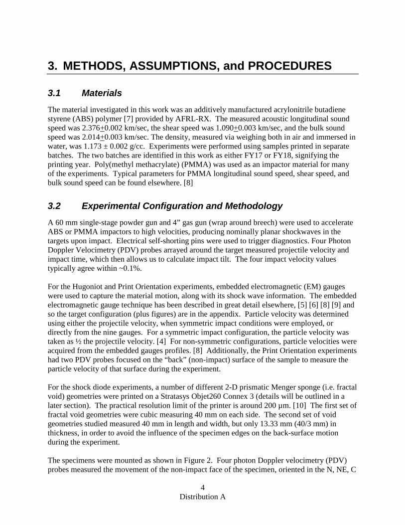
3.2 Experimental Configuration and Methodology A 60 mm single-stage powder gun and 4” gas gun (wrap around breech) were used to accelerate ABS or PMMA impactors to high velocities, producing nominally planar shockwaves in the targets upon impact. Electrical self-shorting pins were used to trigger diagnostics. Four Photon Doppler Velocimetry (PDV) probes arrayed around the target measured projectile velocity and impact time, which then allows us to calculate impact tilt. The four impact velocity values typically agree within ~0.1%. For the Hugoniot and Print Orientation experiments, embedded electromagnetic (EM) gauges were used to capture the material motion, along with its shock wave information. The embedded electromagnetic gauge technique has been described in great detail elsewhere, [5] [6] [8] [9] and so the target configuration (plus figures) are in the appendix. Particle velocity was determined using either the projectile velocity, when symmetric impact conditions were employed, or directly from the nine gauges. For a symmetric impact configuration, the particle velocity was taken as ½ the projectile velocity. [4] For non-symmetric configurations, particle velocities were acquired from the embedded gauges profiles. [8] Additionally, the Print Orientation experiments had two PDV probes focused on the “back” (non-impact) surface of the sample to measure the particle velocity of that surface during the experiment. For the shock diode experiments, a number of different 2-D prismatic Menger sponge (i.e. fractal void) geometries were printed on a Stratasys Objet260 Connex 3 (details will be outlined in a later section). The practical resolution limit of the printer is around 200 µm. [10] The first set of fractal void geometries were cubic measuring 40 mm on each side. The second set of void geometries studied measured 40 mm in length and width, but only 13.33 mm (40/3 mm) in thickness, in order to avoid the influence of the specimen edges on the back-surface motion during the experiment. The specimens were mounted as shown in Figure 2. Four photon Doppler velocimetry (PDV) probes measured the movement of the non-impact face of the specimen, oriented in the N, NE, C

5 Distribution A

and E positions shown in Figure 2. The specimens were sputter coated with a thin layer of Al to aid with the capture of PDV data. Hi-speed video of the impact and compression of the specimen was obtained at 5,000,000 frames per second, using a Xenon flash lamp for illumination. An exposure time of 100 ns was sufficient to avoid blurring of the images. The non-impact face PDV measurements were used in quantitative comparisons with constitutive model simulations, and the hi-speed video was used to perform comparisons, described in greater detail in a later section.

Figure 2. Schematic of the experimental configuration for plate impact experiments of engineered foam specimens (40 mm cubes and 40 mm×40 mm×13.3 mm slabs) incorporating high-speed video at 5,000,000 frames per second and four PDV probes (N, NE, C, E) on the back surface of the specimen. The specimen is minimally clamped in the fixture to minimize edge effects from the clamps.

3.3 Modeling To analyze the hi-speed video and PDV data acquired in the shock diode studies, finite element modeling of the configuration shown in Figure 2 was performed by AFRL/RX using Abaqus/Explicit. Only a brief summary and description of the modeling efforts will be explored in this work. These models have multiple contacting bodies, with impactors and specimens modeled as Lagrangian regions and a target lying in between the impactor and specimen modeled as an Eulerian region. Modeling practices followed standard Abaqus guidelines [11]. First-order, reduced integration hexahedral elements were used in Lagrangian regions. First-order multi-material, reduced integration hexahedral elements with hourglass control are used in Eulerian regions. Second-order advection is used in all Eulerian regions. All materials were modeled as isotropic. Boundary conditions representative of geometric symmetry were used wherever appropriate. Eulerian-Lagrangian contact is used at part-to-part interfaces, with a fiction coefficient of 1.0. Constitutive models for materials used in the FEA utilized an elastic-plastic model for deviatoric response and a Mie-Grüneisen equation of state (EOS) for dilatation response. For the printed ABS material, the EOS parameters used in the models were developed based on the Hugoniot experiments discussed in a later section. Shear modulus and yield strength were estimated based

6 Distribution A

on values in the literature [7] [12]. Spall strength was selected to match the predicted back-face velocity predicted by models with the velocity measured in testing of solid cubes. For the poly(methyl methacrylate) (PMMA) material the EOS parameters were adapted to the linear Us–up relationship used in the Mie-Grüneisen implementation in Abaqus based on quadratic model parameters from Ref. [13]. The shear modulus and yield strength were extrapolated to 5000/second rate based on response from lower rate testing [14].

7 Distribution A

4. RESULTS AND DISCUSSION

4.1 Equation of State Measurements

Figure 3. Particle velocity histories for all gauges and trackers in FY17-06. Impact is zero time

Figure 3 shows the particle velocity vs. time traces for an embedded gauge experiment (shot #5 in Table 1) after analysis. Aside from the initial symmetric configuration experiments, particle velocity (up) information (shown in Table 1) was obtained from the level part of the trace (i.e. the maximum particle velocity) after the rise. There was reasonable agreement between those values and particle velocities obtained from impedance matching calculations, using the Hugoniot curve. For symmetric configuration experiments, the particle velocities obtained from the embedded gauge traces yield values 2-4% below particle velocities calculated as ½ the projectile velocity. The reason for this slight discrepancy is unclear, but it seems to be a systemic issue. To compensate for this, all particle velocities, regardless of configuration, have had 3% of the measured value added to them. Table 1. Equation of State Experiments: lists the experimental configuration used, the projectile velocity, the particle velocity, the shock velocity (average), and the calculated stress.

Shot # Gun Configuration/ Impactor

Proj. Vel. (km/sec)

Part. Vel.

(km/sec)

Avg. Shock Vel.

(km/sec)

Stress (GPa)

1 (FY17-08) Gas Symmetric 0.2155+0.002 0.1078 2.576+0.030 0.33

2 (FY18-18) Gas Non-Symmetric/ PMMA 0.2053+0.002 0.1092 2.591+0.053 0.33

3 (FY17-07) Powder Symmetric 0.5233+0.003 0.2617 2.882+0.031 0.88

4 (FY18-24) Gas Non-Symmetric/ PMMA 0.4957+0.002 0.2590 2.889+0.045 0.88

5 (FY17-06) Powder Symmetric 0.9970+0.004 0.4985 3.297+0.023 1.93 6 (FY18-58) Powder Symmetric 0.9756+0.005 0.4878 3.249+0.040 1.86

8 Distribution A

The shock velocity was determined by assigning arrival times to each of the nine particle velocity gauges (corresponding to 50% of the rise), as well as to 50% of the rise/fall of every step of the three shock tracker gauges (i.e. center tracker, left tracker, right tracker). Next, the impact time and impactor tilt is determined from the PDV projectile measurements. The arrival times of the shock wave at the various gauge and tracker locations were corrected for the calculated impactor tilt. Finally, the corrected embedded gauge arrival times were plotted against the known depths of each gauge to generate an x-t plot, shown in Figure 4. To extract the shock velocity (Us), linear fits to each of the four data groups were performed. The shock velocity was found by averaging the slopes of the four fitted lines in the x-t plot, Us=3.295 km/s in Figure 4.

Figure 4. Depth vs time for shock wave arrival at each gauge and shock tracker in FY17-06. Impact is zero time.

The uncertainty in the shock velocity was determined from the standard deviation of the four Us values from the average. The uncertainty in particle velocity in symmetric impact experiments was very low due to the accuracy in the projectile velocity measurement. When the up was obtained through impedance matching, we applied a 2% uncertainty in the stress from the impactor Hugoniot, use the uncertainty in Us, and assume no uncertainty in projectile velocity to determine the particle velocity uncertainty. In Figure 3, the first gauge trace appears to be nearly discontinuous; however, traces for gauges deeper in the sample demonstrate a two-wave structure. This appears as an instantaneous jump in particle velocity followed by a smooth transition to a maximum particle velocity. This rounding behavior is likely due to the effects of viscoelasticity [15] and is evident to some degree in all acquired wave profiles. Therefore, a more accurate value for the stress would be determined by using an incremental application of the Hugoniot jump conditions (Δσ=Us*ρo*Δup). [16] Calculating the stress using this incremental application of the jump conditions was done for all experimental particle velocity histories for shots #2 and #3 (Table 1) as a way to account for the viscoelastic effects. The resultant stresses were a few percent (less than 5%) lower than those listed in Table 1. The small discrepancy is partly due to the particle velocity issue mentioned

9 Distribution A

earlier (the 3% increase was not applied) and partly due to the slower incremental shock speeds at the end of the rise. Since taking viscoelastic effects [15] into account had such a small impact on the calculated stress with a large added computational complexity, Table 1 shows the stresses that were calculated just using the maximum particle velocity. Since both the particle velocity and shock velocity are known, we can plot the Us- up points and determine the Hugoniot curve for this material. Figure 5 shows the Hugoniot curve that is obtained by only using the three samples from the initial (FY17) batch. A linear fit to all three points results in: Us=2.40+1.81up. [1] Due to the possible viscoelasticity of this material, as suggested by the traces for all three experiments, it is possible that the Hugoniot is not linear in this region, but slightly curved. Thus, the Us-up points might be better fit by a quadratic function, shown in Figure 5b:

Us= 2.349+2.273* up -0.744* up 2 [2]

Figure 5. (a) Particle velocity vs. shock velocity data from initial FY17 experiments. Linear fit used to get Us- up relation. (b) 5(a) data where a quadratic fit was used to get Us- up relation.

The Hugoniot curve that was determined using the results of all experiments listed in Table 1 is illustrated in Figure 6. The excellent agreement of the Hugoniot curve results between the two sample batches induces only a slight change to the quadratic Us- up relation. The Hugoniot curve for this material becomes:

Us=2.344+2.214* up -0.609* up

2. [3]

10 Distribution A

Figure 6. Particle velocity vs. shock velocity data for experiments on all samples in Table 1

4.2 Shock Response Anisotropy

Figure 7. Longitudinal and Transverse Print orientations

After determination of the Hugoniot for the material, it was of interest to determine whether the shock response (i.e. shock velocity) differed depending on the print orientation of the sample. Figure 7 illustrates what is meant by different print orientations. These different orientations are listed in Table 2 as transverse 1 or transverse 2. Further details regarding EM gauge sample and target assembly can be found in Appendix A.

Longitudinal

Transverse

11 Distribution A

Table 2. Shock Response Anisotropy Experiments: lists the experimental configuration used, the print orientation of the specimen, the projectile velocity, the particle velocity, the shock velocity (average), and the calculated stress.

Shot # Gun Print Orientation

Proj. Vel. (km/sec)

Part. Vel.

(km/sec)

Avg. Shock Vel.

(km/sec)

Stress (GPa)

1 (FY18-17) Gas Transverse 1 0.2023+0.002 0.1069 2.461+0.052 0.31 2 (FY18-23) Gas Transverse 1 0.4911+0.002 0.2550 2.957+0.033 0.88 3 (FY18-32) Powder Transverse 1 0.9730+0.005 0.4923 3.382+0.034 1.95 4 (FY18-57) Gas Transverse 2 0.2172+0.003 0.1086 2.457+0.033 0.31 5 (FY18-31) Powder Transverse 2 0.4917+0.003 0.2647 2.949+0.048 0.92 6 (FY18-33) Powder Transverse 2 0.9886+0.005 0.5003 3.414+0.050 2.00

Figure 8a shows the Figure 6 data with the additional results from other print orientations, listed in Table 2. As mentioned previously, the longitudinal shock velocities from FY18 samples are consistent with the FY17 results. Furthermore, the two transverse orientations have identical response, as expected. However, the transverse orientation(s) printed material exhibits noticeably different shock velocities on comparison with the longitudinal experiment results acquired at the same particle velocities. This indicates that the print orientation of the material could have a measurable influence on the shock properties of whatever material structure is being used. Although, the shock response of the samples printed in the two transverse orientations agree reasonably well with one another. These difference trends are also evident when plotting compression vs. stress, stress vs. strain, or compression vs. volume to varying degrees. Since these plots don’t show anything new beyond what has already been discussed for the Hugoniot curve, they aren’t included here. The information in this report, Tables 1 and 2, can be used to determine these parameters if desired. It is unknown if the Hugoniot differences continue to stresses beyond what was studied here.

Figure 8. (a) Us- up data for all experiments listed in Tables 1 and 2, including Figure 6. (b) Release (i.e. Unloading) wave speeds for the FY 18 experiments listed in Tables 1 and 2.

12 Distribution A

Figure 8b shows the release (unloading) wave speeds for the FY18 shots listed in Tables 1 and 2. The release wave speeds for the different orientation samples do not exhibit the differences which were apparent for the Hugoniot curve shock wave speeds. This isn’t surprising as the material differences caused by print orientation (e.g. arrangement of voids) would likely disappear upon compression by the initial shock wave. The release wave UR-up relation can be described with the following equation:

UR=2.307+5.482*up. [4]

Figure 9. Particle velocity traces from PDV probes looking at the “back” face of specimen in Shot #3 in Table 2.

Finally, Figure 9 shows the traces recorded by the two PDV probes focused at the rear (non-impact) surface of the samples. The traces are not stable enough for a proper PDV analysis, a fact that was true for all data from FY17 and FY18 experiments. These particle velocity traces of the rear surface are similar to those recorded for the additively manufactured cubes with fractal geometries. Specifically, the traces recorded from our wedge samples match those obtained for the solid cube case, discussed in the next section.

4.3 Shock Diode Studies

Figure 10. 40 mm width specimens used for some experiments. Menger geometries ranging in fractal iteration order from 0th to 4th.

13 Distribution A

Figure 11. 13.33 mm width specimens used for some experiments. Note the 1nd and 2rd iterations in are parts of Figure 10. EVF1-3 signify equal dispersal of same size voids, with EVF3 being staggered, so that the void fraction is equivalent to Menger iteration. VF0-3 signify different arrangements of different sized voids in the specimen which are equivalent to the Menger iteration.

Figures 10 and 11 show the various 2D Menger sponge (i.e. fractal void) geometries which were studied in this work. [17] Five fractal geometries were printed for the 40 mm specimens ranging from 0st-order to 4th-order as shown in Figure 10. The 0th-order (cube) served as a reference specimen for shock wave traversal time in the solid material, and for calibrating the material’s spall strength in the FEA models. Figure 11 illustrates the various 13.33 mm fractal void geometries studied in this work. In Figure 11, EVF specimens have voids of the same size, whereas VF specimens have voids of different sizes. Table 3 shows a list of the experiments that were performed as part of the shock diode studies. Table 3. Shock Diode Experiments: lists the specimen thickness, the void geometry of the specimen, the impactor material used, and the projectile velocity.

Shot # Specimen Thickness

(mm)

Menger Iteration Impactor

Projectile Velocity (mm/µs)

1 (FY17-49) 40 0 PMMA 252 2 (FY17-26) 40 0 PMMA 497 3 (FY17-27) 40 1 PMMA 491 4 (FY17-25) 40 2 PMMA 495 5 (FY17-28) 40 3 PMMA 496 6 (FY17-29) 40 4 PMMA 496 7 (FY17-51) 13 1 PMMA 502 8 (FY17-47) 13 2 PMMA 503 9 (FY17-48) 13 EVF1 PMMA 507 10 (FY17-50) 13 EVF2 PMMA 502 11 (FY17-52) 13 EVF3 PMMA 502 12 (FY17-56) 13 VF0 PMMA 506 13 (FY17-53) 13 VF1 PMMA 504 14 (FY17-54) 13 VF2 PMMA 505 15 (Fy18-8) 13 VF2 PMMA 490 16 (FY17-55) 13 VF3 PMMA 506 17 (FY18-7) 13 VF3 PMMA 496

Figure 12 shows two hi-speed video images of the 3rd order cube (Shot#5 in Table 3) both before and during compression. The collapse of the voids in Figure 12(b) demonstrates that the cube is not compressing uniformly. This would suggest that the compression wave input into the cube at

14 Distribution A

impact is likely being spread out in time and the wave speed is being slowed down, becoming a ramp wave. As the order of the cube reduces, the compression of the cube does appear to be more uniform. Although the PDV traces for these experiments demonstrate the effect of the void geometry on the compression wave, only phase contrast imaging will allow you to observe the compression wave in the specimen directly. [17]

Figure 12. Compression of Menger 3rd order specimen in Shot #5 both (a) before impact, and (b) during compression after impact. Impact is occurring from the right.

Figure 13 shows the compression of the VF2 and VF3 specimens from shots #14 and #16 (Table 3), respectively. Despite the fact that these experiments were conducted under the same conditions, the difference in the compression waves effect on the specimen is evident. When the compression wave collapses the geometry which goes from the small to large voids, the formation of jets can be observed from the back of the specimen, Figure 13(b). When compressing the geometry which goes from large to small, Figure 13(a), no jets are formed and the back face moves uniformly. This directionality is promising and can hopefully be exploited to develop a true “shock diode”. The FEA modeling efforts, briefly discussed later, will make that development process much quicker. However, the PDV traces show a ramp wave exiting the “back” face of both specimens, demonstrating that this approach is insufficient on its own.

15 Distribution A

Figure 13. Compression of VF2 and VF3 in Shot #14 and #16, respectively. Impact is occurring from the right. (a) When the shockwave impacts the VF2 large-to-small pore structure in moving to the left, no localized jets are formed. (b) The shockwave impacts the VF3 small-to-large pore structure in moving to the left, the structure results in the formation of jets on the downrange side.

The PDV results recorded for the 40 mm cubes show that the shock wave spreads out to a ramp wave as the degree of fractal iteration of the voids in the cube increases. This can be observed in Figure 14(c) and (e), which indicates that a true shock is transmitted by the solid cube, while a ramp wave reaches the back face for the 3rd order Menger cube. The PDV traces for the 1st–order Menger cube, not shown, indicate that a shock wave reaches the back face with a lower amplitude than that for the solid cube. The PDV results for the 2nd–order Menger cube continue this trend, showing a ramp wave with a steeper slope than what is shown for the 3rd–order Menger cube in Figure 14(e).

16 Distribution A

Figure 14 Correlation of measurements and models for 40 mm cubes, (a) test configuration, (b) section view of four items tested, (c) measured back-face velocity for solid cube, (d) predicted back-face velocity for solid cube, (e) measured back-face velocity for cube of 3rd –order shape, (d) predicted back-face velocity for cube of 3rd –order shape. Time is measured from impact.

4.4 Correlation Between Experiments and Simulations The finite element models that were utilized to simulate these experiments assumed the printed ABS cubes, 40 mm on each side, were normally impacted at nominally 500 m/s by a PMMA disk. Dimensions for the test and for the model are shown in Figure 14(a). Initially, FEA modeling was carried out using the four configurations shown in Figure 14(b). Measured velocities for the solid cube and 3rd order Menger configuration are shown in Figures 14(c) and 14(e), respectively. FEA predicted velocities for the same two configurations are shown in Figures 14(d) and 14(f). Good agreement is observed between the predictions and the measured data. In both cases, the model agrees well with the measured data. The reasonable correlation between the FEA model and the experimental results for the 40 mm cube specimens provided justification for an extensive modeling campaign to explore different fractal and non-fractal (regular) geometries under planar impact, both in the 40 mm and 13.3 mm specimen thicknesses. Over 100 different geometries, with various solid volume fractions and different arrangements of pores or voids were investigated in this way, which would have been

Dimensions in mm

12.2

NorthEastNorthCenterEastPMMA

Flyer

ABS Target

97.8 dia

-500

50100150200250300350400

14 16 18 20 22 24 26 28 30 32 34 36

free

surf

ace

velo

city

[m/s

]

time [us]

Predicted, Solid Cube

Center EastNorth N.E.

-500

50100150200250300350400

14 16 18 20 22 24 26 28 30 32 34 36

free

surf

ace

velo

city

[m/s

]

time [us]

Measured, Solid cube


-500

50100150200250300350400

14 16 18 20 22 24 26 28 30 32 34 36

free

surf

ace

velo

city

[m/s

]

time [us]

Measured, 3rd order cube


(a)

(b)

(c)

(d)

(e)

(f)

-500

50100150200250300350400

14 16 18 20 22 24 26 28 30 32 34 36

free

surf

ace

velo

city

[m/s

]

time [us]

Predicted, 3rd order cube


Solid 1st order

2nd order 3rd order

PDV locations

17 Distribution A

highly impractical if carried out experimentally. The experiments on the 13 mm specimens were used to validate the accuracy of the model’s simulations for the most promising cases. To assess the ability of these engineered porosity geometries to attenuate shocks, simulations were performed using the configuration illustrated in Figure 12(a). A PMMA flyer impacts the ABS target, which is in direct contact with a thin layer of PMMA that is backed by a stiff object. A single layer of elements in the Z-direction is modeled, with Z-direction constraints imposing plane strain conditions. Symmetry constraints are imposed on Y-normal sides of all parts. These constraints result in the model representing a flyer, target, and anvil of infinite dimension in the Y- and Z-directions, with finite thickness in the X-direction. The flyer and anvil are modeled as Lagrangian regions, with an element size of 0.2 mm. The target is modeled as an Eulerian region, with element sizes ranging from 0.2 to 0.1 mm, depending on the size of features in the voids. Frictionless contact is assumed.

Figure 15 Contact pressure against stiff wall, (a) configuration assessed, (b) simulated peak contact pressures for fractal foam (2nd, 4th, and 6th cubes from the left) and regular grid (1st, 3rd, and 5th cubes from the left) void configurations.

The first metric that was used to investigate shock mitigation effectiveness was peak contact pressure between the specimen and the projectile impactor. The peak pressure generally correlates to the time at which all voids in the specimen have collapsed. Simulated specimens ranged from completely solid ABS material to specimens with voids and less than 50% solid material. Voids were modeled as either fractal patterns of square voids, as with the experimental specimens in this work, or as circular voids. Time histories of the simulated contact pressure were computed by the FEA model and were spatially averaged over the entire contact surface. The results of the peak contact pressure simulations are illustrated in Figure 15(b). All configurations with voids had a lower peak contact pressure than a solid target. At any level of solid material volume fraction, the reduction in peak contact pressure for a specimen which has voids in a fractal geometry is greater than that for a regular grid target. A regular grid geometry is a pattern of same size voids, such as EVF1 and EVF2 in Figure 11 and Figure 15(b). These results provide some indication that fractal geometries may be more efficient at mitigating shock waves due to impact than other void geometries. However, neither the thickness nor the velocity of the impactor was varied during the modeling, the impact conditions were fixed. It is possible

0

400

800

1200

1600

0.4 0.5 0.6 0.7 0.8 0.9 1.0

Cont

act P

ress

ure

(MPa

)

Volume Fraction of Solid Material

SolidRegular GridFractal Foam

PMMAFlyer

Initial velocity500 mps

ABSTarget

PMM

A An

vil

40 mm 6mm

40 mm

Rigi

d Bo

unda

ry

19 mm

(a) (b)

18 Distribution A

that these engineered porosity structures would be less effective at mitigating longer pressure pulses. The second metric used to investigate shock mitigation was the nature of the stress change detected at the “back” face of the specimen (e.g. a shock wave or a ramp wave). In this work (Table 3), the nature of the pressure rise observed in the experimentally obtained PDV traces appears to be a ramp wave for specimens with any type of void geometry. This provides further evidence for shock mitigation by these structures rather than shock propagation. At some distance from the impact face, the incident shock wave is attenuated down to a ramp wave which generates a rising pressure pulse on the fixed specimen, the maximum of which is plotted in Figure 15(b). It is interesting to note that at a volume fraction of ~0.9, both the regular grid and fractal void geometry specimens show the same level of shock attenuation (roughly 50%). This is not surprising since the hierarchical nature of the fractal void geometries only becomes apparent at higher fractal orders. As such, it is only at volume fractions ~ 0.8 and below that the fractal void geometries exhibit greater shock attenuation than the regular grids, suggesting their suitability as low-density shock absorbing structures. The agreement between the experimental data and the FEA simulations indicate that there may be reductions in both the speed and the pressure for a disturbance exiting the “back” face of a fractal foam as compared to a regular (lattice-based) foam with the same volume fraction. Although figures of merit such as these can be subjective, and depend strongly on the loading and boundary conditions, it is possible that fractal foams may offer some advantage for shock mitigation over regular lattice structures. Furthermore, since such a structure might also be asked to be statically load bearing, the increased second moment of area of the fractal geometry – due to increased mass of material at a distance from the neutral axis – would also be a benefit, especially for structures loaded under in-plane bending.

19 Distribution A

5. CONCLUSIONS The ability to accurately manufacture 3-D printed objects for use in dynamic impact experiments was greatly beneficial when studying the effect of different void geometries on shock mitigation or attenuation. It allowed for multiple different geometries to be quickly printed and tested for their impact response. A series of plate impact experiments was conducted to measure the shock Hugoniot and unloading response of the solid printed material, and to determine if the orientation along which the sample is printed lead to a measurable effect on the shock response. The results show some viscoelastic response and a quadratic Us- up Hugoniot relation which could be reduced to a linear relation with a greater degree of uncertainty. The print orientation of the material does appear to have enough influence on the shock properties of the material to affect the Hugoniot. Although, this influence does not appear to affect the unloading behavior. Once this equation of state data was obtained, it allowed calibration of the finite element model used to study the propagation of compression waves through the ABS specimen and the effect-engineered porosity has on that propagation. Once established, this finite element model was used to screen hundreds of potential geometries for their shock response. The results of the current study indicates that pore (or void) geometry has a measurable effect on the attenuation and propagation of compression waves. This was determined using metrics such peak contact pressure and the nature of the compression wave input into the specimen. These metrics were analyzed because they both depend on lower-order microstructural details such as volume fraction of solid as well as higher-order features such as hierarchical arrangement of pores vs. simple lattice structures. It was determined that fractal void geometrics behaved more efficiently as shock mitigation structures than did lattice structures (regular grid geometries). However, the conditions under which these factors were studied is limited and further experiments are needed to ensure they apply over a wide range of conditions. Further, experimental results from asymmetric void geometry specimens suggest behavior somewhat similar to “shock diode” characteristics, where the propagation of true shocks can be accomplished in one direction but not in the opposite direction. However, clear evidence of such behavior has not been observed.

20 Distribution A

6. Works Cited [1] B. B. Mandelbrot, The Fractal Geometry of Nature, Macmillan, 1983. [2] "http://www.wolframalpha.com/input/?i=Menger+sponge," [Online]. Available:

http://www.wolframalpha.com/input/?i=Menger+sponge. [Accessed 2 February 2018]. [3] L. Gibson and M. Ashby, "Cellular Solids: Structure and Properties," Cambridge, UK,

Cambridge University Press. [4] J. Forbes, in Shock Wave Compression of Condensed Matter, New York, Springer Verlag,

2012, pp. 258-259. [5] S. Sheffield, R. Gustavsen and R. Alcon, "In-Situ Magnetic Gauging Technique used at

LANL-Method and Shock Information Obtained," in Shock Compression of Condensed Matter-1999, Snowbird, Utah, 2000.

[6] R. Gustavsen, S. Sheffield, R. Alcon and L. and Hill, "Shock Initiation of New and Aged PBX9501 measured with Embedded Electromagnetic Particle Velocity Gauges," LA-13634-MS, Los Alamos National Laboratory.

[7] A. Peterson, "Dynamic Evaluation of Acrylonitrile Butadiene Styrene Subjected to High-Strain-Rate Compressive Loads," Army Research Laboratory, 2014.

[8] D. Lacina, C. Neel and D. and Dattlebaum, "Shock Response of Poly[methyl methacrylate](PMMA)Measured with Embedded Electromagnetic Gauges," Journal of Applied Physics, vol. 123, no. 18, p. 185901, 2018.

[9] R. Alcon, S. Sheffield, A. Martinez and R. and Gustavsen, "AIP conference proceedings 429," 1998.

[10] [Online]. Available: https://www.stratasys.com/3d-printers/objet260-connex3. [11] Abaqus Analysis User's Guide Version 6.14, Dassault Systemes, 2014. [12] K. Nakai and T. and Yokoyama, "High Strain Rate Compressive Properties and

Constitutive Modeling of Selected Polymers," J. Solid Mechanics and Materials Engineering, vol. 6, no. 6, 2012.

[13] D. Steinberg, "Equation of State and Strength Properties of Selected Materials," Lawrence Livermore National Laboratory, 1996.

[14] G. Frank, "Analytic and Experimental Evaluation of the Effects of Temperature and Strain Rate on the Mechanical Response of Polymers," University of Dayton Research Institute, 1997.

[15] K. Schuler and J. Nunziato, "The dynamic mechanical bahavior of polymethylmethacrylate," Rhelogica Acta, vol. 13, no. 2, pp. 265-273, 1974.

[16] L. Barker and R. and Hollenbach, "Shock Wave Studies of PMMA, Fused silica, and sapphire," Journal of Applied Physics, vol. 41, no. 10, pp. 4208-4226, 1970.

[17] J. Spowart, D. Lacina, C. Neel, A. Abbott, Frank.G. and B. and Branch, "Shock Propagation and Deformation of Additively Manufactured Polymer Foams with Engineered Porosity," in Proceedings of 2018 SEM Annual Conference and Exposition on Experimental and Applied Mechanics, 2018.

21 Distribution A

APPENDIX: Figure A-1. a) Image of typical EM gauge film. The portion containing the gauge region

is circled in green. b) Detail of gauge region of the gauge package, showing particle velocity gauges 1-9 (numbered), as well as the left, right, and center shock trackers. Also note the horizontal “active elements” of each gauge, and the staggered loops of the trackers, where the length alternates along the loop. The vertical portions of the traces are inactive. ...............................................................................................................22

Figure A-2. Target assembly schematic. a) Exploded view of the small sample “top” wedge, the gauge package (see Figure 16 for details), and the larger sample “bottom” wedge prior to assembly. b) The assembled target, with the top wedge purposely extending past the surface of the bottom wedge. c) Detail of the assembled target after trimming excess gauge material and machining the impact (top) face just so that one surface is achieved. .......................................................................................................22

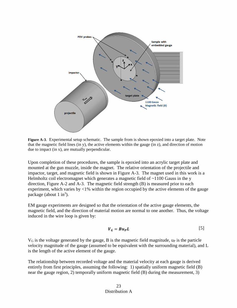
Figure A-3. Experimental setup schematic. The sample from is shown epoxied into a target plate. Note that the magnetic field lines (in y), the active elements within the gauge (in z), and direction of motion due to impact (in x), are mutually perpendicular. ....23

Embedded EM gauges operate based on Faraday’s Law, which states that a voltage is induced in a conductive wire loop which is moving in a magnetic field. The gauge package used in this work, shown in Figure A-1, consists of two layers of ~25 um thick FEP on either side of ~5 um aluminum deposited on the FEP. The gauge itself is twelve aluminum wires; nine separate “particle velocity” gauges (Figure A-1b “active elements 1-9”) and three gauges to capture progression of the shock, or detonation, wave with high spatial resolution (Figure A-1b “shock trackers”). The three shock trackers are identified as the left, right, and center trackers. The shock trackers work by essentially varying the effective length of the loop, and the voltage jumps up and down as a wavefront sweeps along the tracker. Since multiple gauge elements on a shock tracker are moving, the shock tracker cannot be used to determine particle velocity (uP), but it can track the shock wave arrival time at different depths in the material. Prior to target assembly, the gauge length is measured for each of the active elements.

22 Distribution A

a) b)

Figure A-1. a) Image of typical EM gauge film. The portion containing the gauge region is circled in green. b) Detail of gauge region of the gauge package, showing particle velocity gauges 1-9 (numbered), as well as the left, right, and center shock trackers. Also note the horizontal “active elements” of each gauge, and the staggered loops of the trackers, where the length alternates along the loop. The vertical portions of the traces are inactive.

Targets are assembled as illustrated in Figure A-2, where the gauge package is first epoxied onto the large wedge, followed by the small wedge onto the opposing side of the gauge package resulting in a short cylinder of material with the gauge package film embedded within. The top (impact) face of the sample is then machined down so that a single impact plane is achieved.

Figure A-2. Target assembly schematic. a) Exploded view of the small sample “top” wedge, the gauge package (see Figure A-1 for details), and the larger sample “bottom” wedge prior to assembly. b) The assembled target, with the top wedge purposely extending past the surface of the bottom wedge. c) Detail of the assembled target after trimming excess gauge material and machining the impact (top) face just so that one surface is achieved.

1

9

center tracker

2

active elements

left tracker

right tracker

Connector region

gauge region

4 3

5 6 7 8

L

inactive elements

a)

b

c)

23 Distribution A

Figure A-3. Experimental setup schematic. The sample from is shown epoxied into a target plate. Note that the magnetic field lines (in y), the active elements within the gauge (in z), and direction of motion due to impact (in x), are mutually perpendicular.

Upon completion of these procedures, the sample is epoxied into an acrylic target plate and mounted at the gun muzzle, inside the magnet. The relative orientation of the projectile and impactor, target, and magnetic field is shown in Figure A-3. The magnet used in this work is a Helmholtz coil electromagnet which generates a magnetic field of ~1100 Gauss in the y direction, Figure A-2 and A-3. The magnetic field strength (B) is measured prior to each experiment, which varies by <1% within the region occupied by the active elements of the gauge package (about 1 in3). EM gauge experiments are designed so that the orientation of the active gauge elements, the magnetic field, and the direction of material motion are normal to one another. Thus, the voltage induced in the wire loop is given by: 𝑽𝑽𝑮𝑮 = 𝑩𝑩𝒖𝒖𝑷𝑷𝑳𝑳 [5]

VG is the voltage generated by the gauge, B is the magnetic field magnitude, uP is the particle velocity magnitude of the gauge (assumed to be equivalent with the surrounding material), and L is the length of the active element of the gauge. The relationship between recorded voltage and the material velocity at each gauge is derived entirely from first principles, assuming the following: 1) spatially uniform magnetic field (B) near the gauge region, 2) temporally uniform magnetic field (B) during the measurement, 3)

24 Distribution A

gauge film and conductive traces move with the surrounding material, 4) geometry set up properly so that the active element of the particle velocity gauges, B field, and material motion are mutually perpendicular, and 5) that the inactive (side) gauge elements of the particle velocity gauges do not contribute to a change in projected loop area.

25 Distribution A

List of Symbols The following list describes all symbols used in this technical report.

Symbol Meaning

up Particle Velocity

Us Shock Velocity

σ Stress

ρo Density at ambient conditions

UR Release Wave Speed

26 Distribution A

List of Abbreviations and Acronyms The following list describes all abbreviations and acronyms used in this technical report.

Term Definition PDV Photon Doppler Velocimetry VISAR Velocity Interferometer System for Any

Reflector EM Gauge Electromagnetic Gauges ABS Acrylonitrile Butadiene Styrene PMMA Poly(methyl methacrylate) FEA FEP

Finite Element Analysis Fluorinated Ethylene Propylene

27 Distribution A

DISTRIBUTION LIST

AFRL-RW-EG-TR-2019-031 *Defense Technical Info Center AFRL/RWMW (1) 8725 John J. Kingman Rd Ste. 0944 AFRL/RWORR (STINFO Office) (1)

AFRL/RW Technical Report Template - DTIC

Documents

Transcript of AFRL/RW Technical Report Template - DTIC