i

Advances in Heap Leach Pad Surface Moisture Mapping

using Unmanned Aerial Vehicle Technology

and Aerial Remote Sensing Imagery

by

Mingliang Tang

A thesis submitted in conformity with the requirements

for the degree of Master of Applied Science

Graduate Department of Civil and Mineral Engineering

University of Toronto

© Copyright by Mingliang Tang 2020

ii

Advances in Heap Leach Pad Surface Moisture Mapping

using Unmanned Aerial Vehicle Technology

and Aerial Remote Sensing Imagery

Mingliang Tang

Master of Applied Science

Graduate Department of Civil and Mineral Engineering

University of Toronto

2020

Abstract

As easily accessible high-grade mineral reserves are depleting, heap leaching (HL) is gaining an

increased interest in the mining industry due to its economic feasibility for processing low-grade

ores. For HL operations, monitoring heap leach pad (HLP) surface moisture distribution is

essential to ensure optimal leaching conditions and to achieve a high metal recovery. Conventional

monitoring methods rely on manual sampling and naked-eye observation by technical staff, which

are labour-intensive and expose personnel to hazardous leaching reagents frequently. To

complement the conventional approaches, the use of unmanned aerial vehicles (UAVs) combined

with aerial imaging techniques can acquire representative data depicting the moisture status across

the HLP surface. This thesis presents a practical framework for HLP surface moisture monitoring,

consisting of UAV-based data collection and advanced data analytics to generate HLP surface

moisture maps, which provide direct visualization of the surface moisture distribution and are

effective tools to streamline the HLP monitoring process.

iii

Acknowledgments

The work presented in this thesis would not have been possible without the effort and support of

many brilliant and generous individuals. First, I would like to thank my supervisor, Professor

Kamran Esmaeili, for the constructive guidance and encouragement. Kamran, thank you so much

for granting me the opportunity to work on this exciting and meaningful project while giving me

the freedom in conducting my research. I have learned much from you and been inspired by your

high standards and professional integrity. To my co-supervisor, Professor Angela Schoellig, thank

you for sharing the laboratory for conducting my experiments and providing all the insightful and

helpful comments and suggestions. Special thanks to my colleagues, Thomas Bamford and Filip

Medinac, who have provided me tremendous assistance and support to my project. I am also

thankful to other members in the Mine Modeling & Analytics Lab and Dynamic Systems Lab for

providing ideas, support, and discussion.

I am grateful to McEwen Mining Inc. for supporting the project and making the site available for

field experiment and data collection. I would also like to thank the financial support provided by

Natural Science and Engineering Research Council of Canada (NSERC), University of Toronto,

and Vector Institute.

Last but not least, I sincerely appreciate and thank all the love, encouragement, and limitless

patience from my family and friends. Thank You!

iv

Table of Contents

Acknowledgments.......................................................................................................................... iii

Table of Contents ........................................................................................................................... iv

List of Tables ................................................................................................................................. vi

List of Figures ............................................................................................................................... vii

List of Abbreviations .......................................................................................................................x

Chapter 1 Introduction .....................................................................................................................1

Introduction and Motivation .......................................................................................................1

1.1 Research Objectives .............................................................................................................3

1.2 Thesis Outline ......................................................................................................................3

Chapter 2 Literature Review ............................................................................................................5

Background Information and Literature Review ........................................................................5

2.1 Heap Leaching .....................................................................................................................5

2.2 Data Acquisition Using Unmanned Aerial Vehicle in Mining Environments ..................12

2.3 Moisture Estimation Using Remote Sensing .....................................................................18

2.4 Thermal Infrared Remote Sensing .....................................................................................22

2.5 Deep Learning and Convolutional Neural Networks.........................................................32

2.6 Convolutional Neural Network Based Surface Water and Moisture Recognition and

Monitoring .........................................................................................................................53

Chapter 3 Field Data Collection ....................................................................................................56

Field Experiment and Data Acquisition ....................................................................................56

3.1 Site Information .................................................................................................................56

3.2 Equipment ..........................................................................................................................57

3.3 Field Experiment and Data Collection ...............................................................................59

Chapter 4 Surface Moisture Mapping Based on Thermal Imaging ...............................................62

Mapping Heap Leach Pad Surface Moisture Distribution Based on Thermal Imaging ...........62

v

4.1 Overview ............................................................................................................................62

4.2 Data Preprocessing.............................................................................................................63

4.3 Linear Regression Model Development ............................................................................64

4.4 Orthomosaics Generation...................................................................................................67

4.5 Moisture Maps Generation ................................................................................................67

4.6 Discussion and Conclusion ................................................................................................70

Chapter 5 Surface Moisture Mapping Using Convolutional Neural Networks .............................77

Mapping Heap Leach Pad Surface Moisture Distribution Using Convolutional Neural

Networks ...................................................................................................................................77

5.1 Overview and Methodology ..............................................................................................77

5.2 Data Preparation.................................................................................................................79

5.3 Classification-Based Heap Leach Pad Surface Moisture Mapping ...................................96

5.4 Segmentation-Based Heap Leach Pad Surface Moisture Mapping .................................118

5.5 Discussion and Conclusion ..............................................................................................127

Chapter 6 Conclusion ...................................................................................................................131

Conclusion, Recommendation, and Future Work ...................................................................131

6.1 Major Contributions .........................................................................................................134

6.2 Future Work .....................................................................................................................135

Bibliography ................................................................................................................................136

vi

List of Tables

Table 3-1: Thermal and digital cameras specifications ...............................................................................58

Table 3-2: Details of flight missions for phase two of the field experiment ...............................................59

Table 3-3: The number of colour and thermal collected during the field experiment*................................61

Table 5-1: The number of remote sensing data collected during the field experiment* ..............................79

Table 5-2: The number of tiles generated from each overview raster* ........................................................91

Table 5-3: Summarization of dataset statistics for the classification task ...................................................94

Table 5-4: Summarization of dataset statistics for the segmentation task ...................................................95

Table 5-5: Frequency and percentage of the number of classes contained per segmentation example* .....95

Table 5-6: Architecture of ResNet50 ........................................................................................................100

Table 5-7: The modified MobileNetV2 architecture employed in this study ............................................104

Table 5-8: Comparison of computer specifications ...................................................................................107

Table 5-9: Network architecture of MobileNetV2 A* ...............................................................................110

Table 5-10: Network architecture of MobileNetV2 B* .............................................................................111

Table 5-11: Evaluation results of the final classification models on the test set .......................................112

Table 5-12: Performance for the modified U-Net models on the segmentation dataset. ...........................123

Table 5-13: Evaluation results of the final segmentation model on the test set. .......................................123

vii

List of Figures

Figure 2-1: Illustration of a typical heap leach flow sheet. ...........................................................................6

Figure 2-2: Three main types of heap leach pad configurations. ..................................................................9

Figure 2-3: Illustration of overlaps and flight lines for heap leach pad photogrammetry data collection ...17

Figure 2-4: Blackbody radiation curves at various temperatures. ...............................................................24

Figure 2-5: Spectral radiant exitance of a) water, b) Granite, and c) Dunite in 0-25 μm region at 350 K

compared to a blackbody at the same temperature. .....................................................................................26

Figure 2-6: Atmospheric absorption effect in the 0-15 μm region of the electromagnetic spectrum. Notice

the existence of atmospheric windows in 3-5 μm and 8-14 μm regions. ....................................................27

Figure 2-7: Illustration of thermal crossovers and relative diurnal radiant temperature of water versus dry

soils and rocks. ............................................................................................................................................31

Figure 2-8: Typical relationship between model capacity and error. ..........................................................34

Figure 2-9: Summarization of the development of a deep learning model using supervised learning. .......34

Figure 2-10: Illustration of a one-hidden-layer multilayer perceptrons as a directed acyclic graph. ..........35

Figure 2-11: Illustration of a one-hidden-layer MLP with four units in the hidden layer. ..........................36

Figure 2-12: Illustration of the identity, rectified linear unit (ReLU), and leaky rectified linear unit

(LReLU, α = 0.1) activation functions. ......................................................................................................38

Figure 2-13: Illustration of a typical convolutional neural network (CNN) architecture. ...........................39

Figure 2-14: An example of 2D convolution followed by a nonlinear ReLU activation function. .............40

Figure 2-15: Comparison of the number of connections between a convolutional layer (top) and a fully

connected layer (bottom) with the same input and output dimensions.. .....................................................41

Figure 2-16: Illustration of spatial max pooling and average pooling. ........................................................43

Figure 2-17: Illustration of global minimum, local minimum and saddle point. ........................................46

Figure 2-18: Illustration of the forward propagation through a feedforward network using dropout. ........50

viii

Figure 3-1: Location of the El Gallo mine. .................................................................................................56

Figure 3-2: Material particle size distribution of the studied heap leach pad ..............................................57

Figure 3-3: Equipment used during the field experiment ............................................................................58

Figure 3-4: Flight mission 2 and locations of ground control points with respect to the heap leach pad. ..60

Figure 4-1: General workflow of the data processing and moisture map generation. .................................63

Figure 4-2: Visual comparison example between initial and processed thermal images. ...........................64

Figure 4-3: Determination of the remotely sensed surface temperature at a sampling location. ................65

Figure 4-4: (a) Empirically derived univariate linear regression between gravimetric moisture and

remotely sensed surface temperature; (b) Predicted vs. measured gravimetric moisture content (%). .......66

Figure 4-5: Generated orthomosaics of the HLP by using the acquired thermal image datasets. ...............68

Figure 4-6: Generated moisture maps by using the orthomosaics and the linear regression model. ...........69

Figure 4-7: Illustration of the Sun’s positions related to the HLP (not to scale). ........................................73

Figure 5-1: Schematic illustration of the moisture map generation workflow by using a classification

model (upper) and a segmentation model (lower). ......................................................................................78

Figure 5-2: (a) The generated point cloud without GPS information was not adequately oriented. (b) The

generated point cloud with GPS information was appropriately positioned. ..............................................82

Figure 5-3: Generated colour orthomosaics for the top two lifts of the HLP by using the acquired visible-

light image datasets. ....................................................................................................................................83

Figure 5-4: Generated colour orthomosaics for the whole HLP by using the visible-light image datasets.84

Figure 5-5: Generated thermal orthomosaics for the top two lifts of the HLP by using the acquired thermal

image datasets. .............................................................................................................................................85

Figure 5-6: Illustration of the feature correspondences over the colour and thermal orthomosaics. ..........87

Figure 5-7: Generation of a four-channel raster by overlaying a colour orthomosaic over a remotely

sensed surface temperature map of the heap leach pad. ..............................................................................89

ix

Figure 5-8: The three steps of the deep learning datasets construction process. .........................................90

Figure 5-9: The modified AlexNet architecture employed in this study. ....................................................97

Figure 5-10: (a) A plain convolutional (Conv) block with two Conv layers. (b) A basic building block of

residual learning. .........................................................................................................................................99

Figure 5-11: (a) An original residual block (b) A bottleneck residual block. ...........................................100

Figure 5-12: Illustration of the differences between a classical bottleneck residual block and an inverted

residual block with linear bottleneck. ........................................................................................................101

Figure 5-13: Comparison between regular, depthwise, and pointwise convolution. .................................103

Figure 5-14: : Inner structure of the inverted residual blocks. ..................................................................104

Figure 5-15: Training curves of the modified AlexNet, ResNet50, and modified MoblieNetV2. ............108

Figure 5-16: Comparison of learning performance of the modified MobileNetV2 (red), MobileNetV2 A

(magenta), and MobileNetV2 B (cyan) on the training and validation sets. .............................................112

Figure 5-17: Validation accuracy of the three employed architectures. ....................................................113

Figure 5-18: Moisture map generation using a convolutional neural network (CNN) classifier. .............115

Figure 5-19: A comparison of the generated moisture maps using the modified AlexNet, ResNet50, and

modified MobileNetV2 moisture classifiers..............................................................................................117

Figure 5-20: The modified U-Net architecture employed in this study. ....................................................120

Figure 5-21: Moisture map generation using CNN-based semantic segmentation. ..................................125

Figure 5-22: A comparison example between our generated moisture maps and the ground truth. .........126

Figure 5-23: Comparison examples between the HLP moisture maps generated by using classification and

segmentation CNN models. .......................................................................................................................129

x

List of Abbreviations

BLS Barren Leach Solution

BN Batch Normalization

CNN Convolutional Neural Network

CONV Convolutional

CP Control Point

CRS Coordinate Reference System

DL Deep Learning

ELU Exponential Linear Unit

EM Electromagnetic

ESA European Space Agency

FC Fully-Connected

FN False Negative

FP False Positive

GCP Ground Control Point

GD Gradient Descent

GPR Ground Penetrating Radar

GPS Global Positioning System

GSD Ground Sampling Distance

HDPE High-Density Polyethylene

HL Heap Leaching

HLP Heap Leach Pad

IFOV Instantaneous Field Of View

KNN K-Nearest Neighbours

LReLU Leaky Rectified Linear Unit

MIoU Mean Intersection Over Union

MLP Multilayer Perceptron

NN Neural Network

PGMs Platinum Group Metals

PLS Pregnant Leach Solution

PSD Particle Size Distribution

ReLU Rectified Linear Unit

RF Random Forest

RGB Red, Green, Blue

RMSE Root Mean Square Error

ROI Region Of Interest

ROM Run-Of-Mine

RS Remote Sensing

SGD Stochastic Gradient Descent

SIFT Scale-Invariant Feature Transform

SMOS Soil Moisture And Ocean Salinity

SSM Surface Soil Moisture

SVM Support Vector Machine

SVR Support Vector Regression

TF TensorFlow 2

TIR Thermal Infrared

TP True Positive

UAV Unmanned Aerial Vehicle

1

Chapter 1 Introduction

Introduction and Motivation

Depletion of high-grade ore reserves has led to an increasing interest in the extractive

hydrometallurgical technologies that are suitable for low-grade ore deposits. Heap leaching, as a

prominent option for processing low-grade ores, has been widely adopted in recent years due to

its easy implementation and high economic feasibility (Ghorbani et al., 2016). For heap leaching

operations, a high metal recovery requires a uniform leach solution coverage over the surface of

the heap leach pad (the facility that contains the ore material) because an uneven distribution of

moisture can lead to suboptimal leaching conditions and challenging operational problems

(Lankenau and Lake, 1973; Roman and Poruk, 1996). As heap leaching (HL) is a continuously

ongoing operation, monitoring plays a critical role in optimizing the production process and

providing sufficient feedback to the decision makers. Appropriate monitoring of HL operations

relies on the collection of high-quality data and the generation of informative analysis results based

on the acquired measurements. Hence, it is essential to have an efficient data collection routine

and advanced data analytics to optimize productivity and resolve technical challenges.

A good understanding of the spatial and temporal variations of surface moisture content over a

heap leach pad (HLP) is essential for HL production and to achieve a high metal recovery.

Therefore, a fundamental task in HL production optimization is to collect representative data from

the HLP to monitor production performance. However, the conventional data collection method

relies on manual sampling and naked-eye observation of the HLP by technical staff, which exposes

the personnel to the hazardous leaching reagent (e.g., cyanide solution) (Pyke, 1994). Moreover,

this labour-intensive method provides data with low spatial and temporal resolutions, resulting in

inefficient data analysis of the manually collected samples due to the cumbersome laboratory

experiment procedures. In contrast, using unmanned aerial vehicles (UAVs) combined with aerial

imaging techniques to obtain image data remotely can significantly improve the data acquisition

process in terms of time efficiency, data quality and quantity. The UAV-based approach is fast,

on-demand, and automated. It can also collect data with high temporal and spatial resolution. With

this approach, the regions inaccessible by human operators can be covered, and the obtained

images become a permanent record of the field conditions at a specific point of time, which can

2

be revisited in the future for various monitoring applications. In this work, a UAV platform

equipped with one digital camera and one thermal camera was used to acquire colour and thermal

images simultaneously over an HLP. The collected data were used to perform spatial analyses of

the moisture distribution over the HLP surface by using thermal remote sensing methods and

advanced computer vision techniques.

Thermal remote sensing has been widely utilized for terrestrial surface moisture estimation in a

vast variety of studies (Zhang and Zhou, 2016). It is shown that a strong relationship between

thermal measurements and material moisture content generally exists, and such a relationship can

be exploited to effectively estimate ground surface moisture (Kuenzer and Dech, 2013; Liang et

al., 2012). Among the various analytic methods, empirically derived correlations between

temperature measurements and material moisture content can be used to generate surface moisture

maps with high spatial resolution and adequate accuracy (Sugiura et al., 2007). The generated

moisture maps provide direct visualization of surface moisture variation over the surveyed area,

and such graphical results are effective tools for inspecting HL operations. From an HLP

monitoring perspective, surface moisture maps are useful for illustrating the moisture coverage

over the HLP surface and can be involved in the irrigation optimization process to depict the

performances of different solution application strategies quantitatively. Therefore, a framework

for generating HLP surface moisture maps based on thermal remote sensing data is introduced in

this thesis, and the proposed method can be utilized to streamline the HLP monitoring process.

Recent advances in deep learning-based computer vision techniques have shown promising

performance in a broad range of applications, including terrestrial surface moisture estimation

based on remote sensing imagery (Ge et al., 2018; Sobayo et al., 2018). One particular type of

deep leaching (DL) model that has shown remarkable performance on processing image data is

called convolutional neural network (CNN) (LeCun, 1989). CNN models have the capacity of

accommodating inputs with different modalities (e.g., images taken by different types of cameras),

and the models can extract latent information contained in the sensor data. Such property allows

the models to learn complex functions automatically without the need of feature engineering and

variable selection. To leverage the power of CNN models, this thesis proposes two CNN-based

moisture map generation approaches in which the acquired thermal and colour image data are used

as input simultaneously. Moisture maps are generated in an end-to-end fashion, and the proposed

methods have the potential to be further developed towards a fully automated data analysis process.

3

1.1 Research Objectives

The main goal of this thesis is to develop a practical and effective HLP surface moisture monitoring

workflow, starting from UAV-based data collection, followed by off-line data processing, and

ending with surface moisture map generation. To achieve this goal, the specific research objectives

include:

1) Designing and implementing a UAV-based data acquisition method to collect field data

from a heap leaching operation;

2) Conducting appropriate data preprocessing and preparation for moisture map generation;

3) Exploring a correlation between aerial thermal measurements and HLP surface material

moisture content;

4) Mapping heap leach pad surface moisture distribution using a thermal remote sensing

method; and

5) Developing frameworks that incorporate convolutional neural networks for generating

heap leach pad surface moisture maps.

1.2 Thesis Outline

This thesis consists of six chapters:

• Chapter 1: introduces the project motivation, research objectives, and thesis structure.

• Chapter 2: provides background information and literature review on the theory, concepts,

and recent applications relating to the data analyses performed in this work.

• Chapter 3: describes the field experiment conduced and the mine site in which the data

was collected. The details of surveying schedule, equipment specification, and data

collection campaigns are provided.

• Chapter 4: elaborates the process of empirical model development and moisture map

generation based on the acquired thermal images and in-situ moisture measurements. An

4

in-depth discussion about the advantages, limitations, and possible improvement of the

proposed method is included.

• Chapter 5: presents a thorough description of the two CNN-based moisture map

generation approaches. The explanation of both methods starts with data preparation,

followed by network construction, model training, and ends with model evaluation and

moisture map generation. A discussion comparing the two methods is included, and the

possible improvement of the proposed approaches is also outlined.

• Chapter 6: provides a summary of the thesis and outlines recommendations for future

work.

5

Chapter 2 Literature Review

Background Information and Literature Review

This chapter provides a review on the background information and related work associated with

the experiment and data analyses presented in this thesis. Section 2.1 outlines a brief review of the

heap leaching technology, followed by Section 2.2 in which the use of unmanned aerial vehicles

for data acquisition in mining environments is discussed. Section 2.3 presents a high-level

overview of the different remote sensing methods for soil moisture estimation, and Section 2.4

includes an explanation of the thermal remote sensing principles and concepts related to this work.

As convolutional neural networks (CNNs) are used for processing of the collected data, Section

2.5 summarizes the key deep learning theory and concepts, whilst Section 2.6 provides a review

on the CNN-based moisture recognition and monitoring applications presented in the literature.

2.1 Heap Leaching

Heap leaching (HL) is a mineral extraction technology that has been widely adopted in recent years

due to its high economic feasibility. HL operation is a hydrometallurgical recovery process where

metal-bearing ore is piled on an impermeable pad (i.e., an engineered liner), and a water-based

lixiviant, or leaching reagent, is irrigated on top of the heap surface (Ghorbani et al., 2016). The

leach solution flows through the pile and contact with the ore, such that the metal or mineral of

interest is extracted from the rock and dissolved into the solution (Kappes, 2002). Solution exits

the base of the heap through slotted pipes and a gravel drainage layer located above the liner (Pyper

et al., 2019). The metal-bearing pregnant leach solution (PLS) is collected in the PLS pond (i.e.,

pregnant pond) and then pumped to the processing facility for recovery of the extracted metal

(Ghorbani et al., 2016; Pyper et al., 2019). After the valuable metal is recovered from the PLS, the

barren leach solution (BLS) is pumped to the barren solution pond and reapplied to the heap after

refortifying with lixiviant chemicals (Pyper et al., 2019; Watling, 2006). A typical heap leaching

circuit is illustrated in Figure 2-1.

As described above, the technology of HL encompasses multiple scientific disciplines, including

physics, hydrology, geology, chemistry and biology (Bhappu et al., 1969; Pyper et al., 2019), and

there is a vast number of topics involved in the study area. In this section, we briefly introduce

6

several topics that are related to our experiment, where Ghorbani et al. (2016) provided an in-depth

and comprehensive review of the heap leaching technology, and Pyper et al. (2019) presented a

thorough introduction to the different operational components of dump and heap leaching. In the

literature, heap leaching can sometimes refer to both run-of-mine (ROM) dump leaching and

crushed ore heap leaching. In this section, we refer the term to crushed ore heap leaching, and our

emphasis is on HL of gold-bearing ore.

In practice, HL is most commonly used for low-grade ore deposits, although it is sometimes

applied to small high-grade deposits to control capital cost in higher-risk jurisdictions (Ghorbani

et al., 2016). Several advantages of HL as compared to milling ores include: low capital and

operating costs, quick up-front construction and installation, simple equipment and operation, no

liquid/solid separation step, less water requirement compared to flotation, no tailing disposal, and

most importantly, practical and effective for processing low-grade deposits (Kappes, 2002;

Ghorbani et al., 2016). Thanks to the high practicality and economic feasibility, HL has been

applied to extract a wide range of metals, such as gold, copper, silver, uranium, zinc, nickel, cobalt,

and platinum group metals (PGMs) (Mwase et al., 2012; Padilla et al., 2008; Pyper et al., 2019).

According to Marsden and House (2006), 10% of the world’s gold production was produced from

heap leaching in 2006, and HL is gaining an increased interest in the mining industry nowadays

(Ghorbani et al., 2016).

Figure 2-1: Illustration of a typical heap leach flow sheet. Extracted from Pyper et al. (2019).

7

In order to successfully extract the valuable metals from the stacked ore, the applied lixiviant

should first diffuse within the heap leach pad (HLP) and then chemically react with the target

mineral. The reaction should allow the solution to dissolve valuable metal while minimally

dissolve gangue material (Pyper et al., 2019). The metal-rich solution should then diffuse away

from the reaction site and finally percolate out from the bottom of the heap (Kappes, 2002).

However, this process is highly affected by the permeability within the HLP. Since different

regions within the heap may have different permeabilities, if a regional solution application rate

surpasses the permeability of the area, the solution will travel horizontally until a more permeable

zone is reached. A significant flow channelling can occur if large variations of permeability are in

concert with excessive solution application. The channelling of solution will result in unleached

areas within the heap and diluted PLS grades (Bouffard and Dixon, 2000; Ghorbani et al., 2016).

Moreover, solution over the impermeable zones tends to build up, resulting in surface ponding or

perched water table. If a large volume of solution is retained near the edge of the HLP, the solution

can blow out the heap slope, leading to potential stability issues (Pyper et al., 2019). Therefore,

heap permeability is crucial, and it is affected by the material particle size distribution (PSD) as

well as the ore preparation and stacking process.

2.1.1 Ore Preparation and Stacking

Ore preparation is often conducted before the placement of material onto the HLP. Several

common preparation steps for gold ore include: crushing of ROM, addition of lime for pH

adjustment, and agglomeration of the crushed rock. For crushed rock heap leaching, size reduction

of ROM is generally carried out through crushing at which the target mineral is liberated for leach

extraction (Pyper et al., 2019). The top sizes of the crushed rock usually range from 10 to 40 mm,

where a P80 is often desired to be greater than 6 mm to avoid permeability issues (Brierley and

Brierley, 2001; Ghorbani et al., 2016). The addition of lime or other pH modifiers is performed

during either crushing/stacking or agglomeration (Pyper et al., 2019). The preferred level of pH

for cyanide gold leaching is within 9.5 to 11 because below this range can increase cyanide

consumption while above this range will lead to a decrease in metal recovery (Ghorbani et al.,

2016). Although agglomeration is not always required, it can be used to mitigate segregation of

fines and reduce the chance of blinding (i.e., solution cannot flow downwards) (Pyper et al., 2019).

The purpose of agglomeration is to adhere the fines to each other or to larger particles so that a

more uniform heap can be resulted (Lewandowski and Kawatra, 2009; Velarde, 2007).

8

There are two principal methods for ore stacking: trucking stacking and conveyor stacking

(Ghorbani et al., 2016). Although some operations may use excavator stacking when the other two

options are not applicable due to accessibility issues (Pyper et al., 2019), it is less commonly used

than the other two approaches. For truck stacking, it is often used with competent ores with low

clay content. The heaps are generally constructed using the same techniques as waste dump

construction and maintenance (Pyper et al., 2019). The advantage of truck stacking is that it is

usually more flexible than conveyor stacking (Kappes, 2002). Nevertheless, the major

disadvantage of truck stacking is the compaction of ore due to the truck loads (Kappes, 2002).

Therefore, ripping is typically carried out to mitigate compaction prior to leaching (Pyper et al.,

2019).

Conveyor stacking system is commonly used for handling a large quantity of ore material, and it

can lead to a more uniform PSD across the heap (Ghorbani et al., 2016). In a typical conveyor

stacking system, one or more overland conveyors are used to connect the preparation plant (e.g.,

crushing plant) to the HLP. Multiple grasshopper conveyors are included across the active heap

area to feed a radial stacker conveyor, where the grasshopper conveyors are connected to the

overland conveyor through a tripper conveyor (Pyper et al., 2019). A stacker-follower conveyor

and a transverse conveyor, or horizontal indexing conveyor, are often involved in the system to

facilitate the material handling (Kappes, 2002; Pyper et al., 2019). One advantage of using

conveyor stacking system is that it allows gentle placement of ore, which reduce the amount of

compaction and segregation (Ghorbani et al., 2016).

2.1.2 Heap Leach Pad Configurations

Overall, there are three main types of HLP configurations (Figure 2-2): standard pad, valley fill

pad, and on/off pad (Ghorbani et al., 2016; Thiel and Smith, 2004). The selection of HLP

configuration has profound influences on capital and operation costs, leaching solution application

and collection, recovery plant sizing, stacking method, and heap closure (Pyper et al., 2019). An

HLP can consist of either one or multiple lifts, where a typical lift height ranges from 2 to 15 m

(John, 2011).

Standard pads (also refers to as traditional, conventional, flat or expanding pad in the literature)

require large ground areas for the pad construction and expansion (Lupo, 2010; Pyper et al., 2019;

Thiel and Smith, 2004). The ideal construction condition is on a flat topography with a slight slope

9

(e.g., 1-3% slope), although a pad can be also built in rougher terrain (Pyper et al., 2019). In

general, a standard pad requires low initial capital cost, and it is suitable for various ore types and

leach cycle time (Thiel and Smith, 2004). The construction requires relatively simple liner system,

and the pad offers flexibility for incremental pad expansion (Lupo, 2010; Pyper et al., 2019).

Figure 2-2: Three main types of heap leach pad configurations: (a) Standard pad; (b) Valley fill pad; (c)

On/off pad. Extracted from Lupo (2010).

10

Valley fill pads are constructed in steep topography (e.g., valley, basins), where the foundation

slope can often reach 40-50% (Ghorbani et al., 2016). A valley fill pad can often accommodate

variable ore production and leach cycle time, and it is suitable for hard and durable ores (Pyper et

al., 2019). Since a valley fill pad is constructed in steep terrain, a retaining structure (e.g., a dam)

is often required to be developed, and the cost of installation and construction is more expensive

than the other pad configurations. A valley fill pad generally has an internal solution storage pond

(Figure 2-2b), where leak detection and pumping systems are usually required for the internal pond

(Ghorbani et al., 2016).

On/off pads are often used to process soft ores that cannot be stacked to a large heap height

(Ghorbani et al., 2016; Thiel and Smith, 2004). The ore material is loaded and leached, followed

by removal at the end of the leach cycle. The pad is then recharged with fresh ore, and the spent

ore (ripios) is either abandoned or sent to a secondary leach pad for continuation leaching (Pyper

et al., 2019). An on/off pad is generally less expensive to construct compared to the other pad

configurations, but it has a higher operational cost due to the double handling of material (Ghorbani

et al., 2016). The leach cycle of ores in an on/off pad is relatively short (30 days or less), and the

configuration is useful in regions with limited ground areas (Pyper et al., 2019). Several

disadvantages of on/off pads include high maintenance cost, severe liner damage due to frequent

material handling, and requirement of multiple cells (at least three) for continuous operation

(Ghorbani et al., 2016).

2.1.3 Leaching

Following ore preparation and heap construction, leaching is conducted by applying a water-based

lixiviant over the heap surface. The leach solution application should have uniform surface

coverage because a maximal metal extraction requires optimum wetting uniformity (Pyper et al.,

2019). In addition, the solution application rate should be slower than the hydraulic conductivity

of the ore to prevent surface ponding. The existence of solution ponds on the heap surface can

become a threat to wildlife and a potential risk of heap stability issues (Franson, 2017; Marsden,

2019). According to Pyper et al. (2019), the solution application rates in practice vary from 2.4 to

19.6 L/h/m2, where a typical range is 8-12 L/h/m2.

Although there are various solution spreading devices employed in practice (e.g., wobbler

sprinklers, rotating impact sprinklers, D-ring sprinklers, misters, pressure drip emitters), irrigation

11

systems can be generally classified into sprinklers or drip emitters (Ghorbani et al., 2016). Dripper

lines are commonly made of high-density polyethylene (HDPE), and sprinkler systems are often

constructed using polyvinyl chloride or HDPE (Pyper et al., 2019). In general, a drip emitter

system can result in a gentle and precise solution application while diminishing evaporation losses

of solution and reagents. It has the advantages of easy installation and applicability to a wide range

of pressure conditions (Ghorbani et al., 2016; Pyper et al., 2019). However, drip emitters often

have small effective flow areas and do not provide continuous drip coverage, while channelling

and plugging problems make them difficult to accomplish sufficient solution/ore contact,

especially for the top one meter of the heap (Ghorbani et al., 2016; Kappes, 2002). In contrast,

sprinklers are easy to maintain, simple to conduct visual check, and convenient to adjust flow rate

while providing an uniform solution distribution pattern over the HLP surface (Ghorbani et al.,

2016). Nevertheless, sprinkler systems can increase the evaporation loss of reagents and might

lead to environmental and health hazards, especially in windy conditions (Ghorbani et al., 2016;

Pyper et al., 2019). Despite the pros and cons of sprinklers and drip emitters, both kinds of systems

have been successfully deployed in HL operations worldwide (Marsden, 2019).

In gold heap leaching, the commonly used water-based lixiviant is dilute cyanide solution. The

cyanidation process is proven to be effective for gold extraction, and cyanide is considered an

environmentally acceptable reagent among other alternatives (e.g., bromide, thiocyanate,

thiosulfate, iodide solutions) (Ghorbani et al., 2016; Grosse et al., 2003; Srithammavut, 2008).

Metals like gold and silver can be dissolved by a dilute alkaline sodium cyanide (NaCN) solution

at very low concentration (Marsden, 2019; Ghorbani et al., 2016), and the general reaction for gold

dissolution is expressed as:

4Au + 8CN− + O2 + 2H2O = 4Au(CN)2− + 4OH− (2.1)

The gold dissolution rate is affected by the NaCN concentration and alkalinity of the solution. The

desired range of solution pH is 9.5 to 11 (Ghorbani et al., 2016), and alkali may be added to the

leach solution for pH modification and control (Marsden, 2019). A typical range of cyanide level

within the heap ranges from 100 to 600 mg/L (or ppm) NaCN, and a maximized gold dissolution

rate may be achieved by maintaining the HLP runoff solution to have a concentration of

approximately 50-100 mg/L NaCN (Marsden, 2019; Ghorbani et al., 2016). Overall, the leaching

efficiency of a HLP is affected by several factors, including the chemistry of the applied solution,

12

the degree of gold liberation in the crashed ore material, the efficiency of ore-solution interaction,

and the amount of time allowed for the leaching reaction (Marsden, 2019). Precise control of the

abovementioned factors are hardly achievable in practice, but the HL performance may be tracked

by carefully monitoring the gold and cyanide concentration, pH, dissolved oxygen concentration,

and temperature of the process solutions (Marsden, 2019). In addition, maintaining a uniformity

of solution distribution across the HLP surface remains a critical monitoring task to ensure

sufficient contact between ore and leach solution while preventing surface ponding issues

(Marsden, 2019; Ghorbani et al., 2016).

In practice, leaching side slopes of an HLP is considered a challenging operational task (Pyper et

al., 2019). Neither sprinklers nor drip emitters provide promising options for addressing the

problem (Pyper et al., 2019), while the monitoring of side slope leaching also remains difficult due

to the inaccessibility by humans. Some operations found that the use of small sprinklers with gentle

spraying patterns offers a reasonable compromise for side slope leaching (Pyper et al., 2019). In

this study, we propose to use unmanned aerial vehicle equipped with remote sensing sensors to

constitute an effective and efficient option for HLP monitoring even for those human inaccessible

areas over the HLP.

2.2 Data Acquisition Using Unmanned Aerial Vehicle in Mining

Environments

Data acquisition using unmanned aerial vehicle (UAV) platforms has been adopted in almost every

study area that requires observed data from top or oblique views (Yao et al., 2019). Many studies

in mining (Bamford et al., 2020; Medinac et al., 2020), agriculture (Ivushkin et al., 2019), forestry

(Wallace et al., 2016), construction inspection (Lee et al., 2016) have demonstrated the practicality

and effectiveness of employing UAVs to perform various surveying and monitoring tasks.

Recently in the mining industry, Bamford et al. (2020) employed UAV systems to monitor blasting

process in four open pit mines, where visual data were collected during the pre-blasting, blasting

and post-blasting stages; Medinac et al. (2020) used a UAV system to perform haul road

monitoring to assess road conditions in an open pit mine; and Medinac and Esmaeili (2020)

collected UAV data to perform pit wall structural mapping and a design compliance audit of the

pit slope. Several other applications of UAVs in mining environments include dust monitoring

(Alvarado et al., 2015; Zwissler, 2016), drillhole alignment assessment (Valencia et al., 2019), pit

13

wall mapping (Francioni et al., 2015), particle size segregation analysis (Zhang and Liu, 2017),

and rock fragmentation analysis (Bamford et al., 2017a). However, not much attention in the

literature has been put on leveraging the power of UAV and sensing technology to perform heap

leach pad monitoring, especially HLP surface moisture mapping.

There are several advantages of using UAVs to conduct data acquisition in mining environments.

The data collected using UAV platforms are generally with high spatial and temporal resolutions,

which are hardly achievable by conventional point-measurement methods or even satellite-based

approaches. Meanwhile, UAV-based data acquisition reduces time effort in data collection and

increases the safety of personnel. The use of UAVs can survey a large field area within a short

duration while reducing the frequency of exposing technical staff to ongoing production

operations. The regions inaccessible by human operators can be covered, and the need for

personnel to collect data in hazardous environments (e.g., over an HLP with cyanide leaching) can

be diminished. In addition, if one or more imaging sensors are mounted on a UAV, the obtained

images with respect to the mining facility (e.g., a pit or an HLP) would become a permanent record

of the field conditions at a specific point of time, which can be revisited in the future as required

(Bamford et al., 2020). This is very useful for tasks like design compliance audit and change

detection. Also, many practitioners have devoted to developing real-time monitoring techniques

by incorporating computational devices or resources (e.g., onboard computer or cloud computing)

with UAVs, and the successful deployment of such systems can carry out real-time and on-demand

monitoring of production operations, which will be beneficial for timely decision making.

However, UAV-based data collection methods have their limitations. Different jurisdictions may

have different regulatory requirements, which can limit the use of UAVs in the mining

environments (Bamford et al., 2020). Moreover, weather, and environmental conditions have a

significant impact on both the data obtained by the UAV system as well as the UAV itself. The

variations of lighting conditions and cloud shadowing often have a large influence on the quality

of images. UAV platforms are generally not available to operate in extreme weather, such as rain,

snow, and storm. Also, consistently exposing a UAV system to a dusty and hot environment can

damage the UAV and wear the onboard sensors (Bamford et al., 2020). Therefore, appropriate

cleaning and maintenance of the UAV system after each data collection campaign is always

recommended to improve equipment durability.

14

The tremendous success and advantage of applying UAVs to conduct surveying and monitoring

tasks have contributed to the rapid development of UAV and sensing technologies in recent years

(Pajares, 2015). Various types of UAVs and sensors have been manufactured and commercialized

nowadays, which significantly advance the use of UAVs in different industries and working

environments. Overall, there are several categorization schemes for UAVs, and each

categorization method is based on one or multiple design attributes, including payload, endurance,

range, drone weight, flight speed, wing configurations, and flying altitude (Valavanis and

Vachtsevanos, 2015; Korchenko and Illyash, 2013; Yao et al., 2019). The data collection

conducted in our experiment was performed using a hexa-copter with a maximum gross takeoff

weight of approximately 15 kg (35 lbs). The detailed specification of our UAV system is described

in Chapter 3.

Although RGB cameras are the most used onboard sensors for UAV systems, there are other

imaging sensors that have been adopted for both academic and commercial applications, such as

multispectral, hyperspectral and thermal infrared cameras (Yao et al., 2019). For RGB cameras,

there are numerous options in the market, and some important specification parameters include

camera lens, resolution, and sensor chip quality. Cameras with better lenses and sensor chips can

result in less geometric distortions and higher signal-to-noise ratios than the worse ones (Yao et

al., 2019). A few RGB camera selection guidelines have been provided by Nex and Remondino

(2014), and Colomina and Molina (2014). Thermal infrared cameras are commonly used for

obtaining surface temperature and thermal emission measurements (Yao et al., 2019). These

measurements can be further processed to retrieve soil properties as well as material surface

moisture content (Ivushkin et al., 2019; Sobayo et al. 2018). Due to the payload limitation of

common commercial drones, UAV-based thermal cameras are generally without cooled detectors,

which result in lower sensitivity, spatial resolution, and capture rates than RGB cameras (Yao et

al., 2019). However, with properly designed flight height and image acquisition rate, the images

collected by a thermal camera can be integrated with data recorded in other spectral wavelengths

(e.g., RGB) to perform data analysis (see Chapter 5). For multispectral cameras, they are often

used for vegetation-related tasks as well as farming and hydrological applications (Calderón et al.,

2014; Candiago et al., 2015; Kemker et al., 2018; Kislik et al., 2018). As more and more data

processing packages and algorithms become available, data acquisition using UAV-based

multispectral cameras may become more common in the future (Yao et al., 2019). Although light-

15

weight hyperspectral cameras (e.g., Burkart et al., 2014; Suomalainen et al., 2014) are able to

capture images with a large number of narrow bands (e.g., a few hundred or even more than a

thousand bands with 5-10 nm bandwidth), they are usually expensive and not as mature as the

other camera sensors nowadays. Nevertheless, as the sensing technology is growing rapidly while

more and more data-driven algorithms are proposed in the literature (e.g., deep learning

techniques), the ability to capture a large amount of data by a single sensor within one flight can

become very appealing in the upcoming future. Besides the abovementioned sensors, Colomina

and Molina (2014) provided a review on the light-weight sensors that are available for low-payload

aerial platforms, and Pajares (2015) presented a thorough review on a wide range of sensors (e.g.,

camera, LiDAR, radar, sonar, gas detector) used for UAV-based data collection.

2.2.1 UAV Flight Planning

Despite the remarkable success of using UAV systems to acquire remote sensing data, there is no

universal guideline for UAV-based data collection. Data acquisition practices can vary

significantly even for the same or similar application, where different practitioners may develop

disparate practices through the learning-by-doing approach (Yao et al., 2019). One reason for such

phenomenon is because the different combinations of UAVs and sensors add flexibility and

complexity to the data acquisition process.

One practical flight planning method of UAV digital photogrammetry for geological surveys was

outlined by Tziavou et al. (2018), where the method was implemented and elaborated by Bamford

et al. (2020) for applications in the mining context. Bamford et al. (2020) adopted and applied the

method to collect photogrammetry data in multiple mining operations, demonstrating the

effectiveness and practicality of the approach in generating UAV flight plans. In this study, the

flight plans were generated following the practices employed by Tziavou et al. (2018) and Bamford

et al. (2020), and the implementation steps are described below.

Several factors should be considered to create a flight plan for photogrammetry data collection,

including image/photo overlaps, target distance, lighting and weather conditions, and camera’s

resolution, focal length and field of view (Bamford et al., 2020). In this study, the data collection

was performed by observing the HLP from a top-down view (i.e., the camera was tilted down to

the nadir), and the distance between the HLP surface and UAV system was considered the main

controllable parameter. To determine the appropriate distance from the HLP surface (i.e., flight

16

altitude in our case), the first step is to obtain knowledge about the dimension of the minimum

measurement target. For instance, in our experiment, the sprinkler spacing over the HLP was 3 m.

We decided to set the desired minimum measurement target to be approximately 1.5 m (i.e., half

of the sprinkler spacing), and this value was used to determine the objective ground sampling

distance (GSD). The GSD is defined as the ground distance covered between two adjacent pixel

centers. Bamford et al. (2020) suggested that the GSD should be at least an order of magnitude

smaller than the minimum measurement target, and thus we adopted a GSD varied from 10

cm/pixel to 15 cm/pixel. After determining the GSD, the flight altitude can be calculated by:

𝑧 = √GSD2𝑖𝑤𝑖ℎ

4 tan (𝑓ℎ

2) tan (

𝑓𝑣

2) (2.2)

where 𝑖𝑤 and 𝑖ℎ are the image width and height in pixels, respectively; 𝑓𝑣 and 𝑓ℎ are the lens

vertical and horizontal angle of view, respectively; GSD is the ground sample distance in meters

per pixel; and 𝑧 is the flight altitude in meters (Bamford et al., 2020; Langford et al., 2010).

Once the flight altitude is determined, the side and front spacing as well as the flight velocity can

be calculated as:

𝑠 = 2𝑧 tan (

𝑓ℎ

2) (1 − overlapside) (2.3)

𝑓 = 2𝑧 tan (

𝑓𝑣

2) (1 − overlapfront) (2.4)

𝑣𝑓 =

𝑓

𝑡𝑝 (2.5)

where 𝑠 is the side spacing between pictures in meters; 𝑓 is the front spacing between pictures in

meters; 𝑡𝑝 is the time between taking images (shutter interval) in seconds; 𝑣𝑓 is the flight velocity

in meter per second; 𝑓𝑣 and 𝑓ℎ are the lens vertical and horizontal angle of view, respectively; and

overlapside and overlapfront are the percentages of side and front overlap between images,

respectively (Bamford et al., 2020; Langford et al., 2010). In the literature, some studies

recommend the front overlap to be within the range of 30% to 85%, and 70% to 85% for side

overlap (Bamford et al., 2017; Dash et al., 2017; Francioni et al., 2015; Salvini et al., 2017; Tziavou

17

et al., 2018). Figure 2-3 schematically illustrates the concepts of front and side overlaps, where the

side spacing is the distance between the two flight lines, and the front spacing is the distance

between the two image centers on the same flight line (Bamford et al., 2020). In our field

experiment, the front and side overlap were designed to be 85% and 70%, respectively, where the

detailed flight plans are described in Chapter 3.

Beyond the creation of flight plans, the image georeference accuracy is also critical when the

acquired images are used to generate orthomosaics (also called true orthophotos, which are

generated based on an orthorectification process). Although some of the images captured by the

UAV system were georeferenced using onboard global positioning system (GPS), the GPS

coordinates recorded in the air are sometimes not as reliable as measurements made on the ground

(Bamford et al., 2020). In such cases, ground control points (GCPs) are often used to obtain better

positioning information. A GCP is an object or point in an image at which the real-world

coordinates are known (Linder, 2013). In this study, GCPs were placed over the HLP during the

field experiment, and the GPS coordinates of each GCP were measured using a portable GPS

device. The recorded positioning information was used to facilitate the data analyses described in

Chapter 4 and Chapter 5.

Figure 2-3: Illustration of overlaps and flight lines for heap leach pad photogrammetry data collection

18

2.3 Moisture Estimation Using Remote Sensing

This section presents a brief review of the different remote sensing methods for soil moisture

estimation proposed in the literature. The content covered in this section is largely extracted from

Tang and Esmaeili (2020).

In practice, two types of sensors are employed by remote sensing systems, namely, passive and

active sensors (Liang et al., 2012). A passive remote sensing system collects data through using

one or multiple passive sensors (e.g., digital cameras, thermal cameras, spectroradiometers), which

detect electromagnetic (EM) radiation that is either emitted or reflected from the target (Khorram

et al., 2012). In contrast, an active remote sensing system employs active sensors, such as radars,

to proactively release EM energy toward the target and record the amount of radiant flux scattered

back to the system (Jensen, 2009).

In remote sensing, a number of methods have been studied and applied to estimate surface soil

moisture (SSM) (Campbell and Wynne, 2011). Petropoulos et al. (2015) provided an in-depth

review of the principal foundations, advantages, drawbacks and current applications of different

soil moisture retrieval methods. According to Petropoulos et al. (2015), remote sensing-based SSM

retrieval methods can be grouped into three categories: microwave remote sensing, optical remote

sensing and synergistic methods, where synergistic methods are essentially data fusion techniques

developed to manage the complementarity between various types of data. Each of these categories

either uses one portion of the EM radiation spectrum or multiple regions of the spectrum as input

to estimate SSM.

In microwave remote sensing, the methods can be divided into passive and active microwave

sensing. Passive microwave sensors are designed to measure the naturally emitted microwave

emissions, with wavelengths ranging from 1 to 30 cm. The emitted EM signal at these wavelengths

is related to the soil dielectric properties closely associated with SSM (Chen et al., 2012). The

advantages of this method are that the data acquisition is not limited to daytime conditions, and

atmospheric effects become less significant when the detected EM wavelength is above 5 cm

(Petropoulos et al., 2015). However, the measurements from passive microwave systems are often

influenced by factors such as soil surface roughness and soil texture (Chai et al., 2010), as well as

being at a coarser spatial resolution as compared to other methods (Petropoulos et al., 2015).

Recent studies about using passive microwave remote sensing to estimate SSM are commonly

19

developed based on satellite measurements. The European Space Agency’s (ESA) Soil Moisture

and Ocean Salinity (SMOS) mission is a well-known program that uses on-board passive

microwave sensors to collect global-scale data. Similar to passive microwave remote sensing, the

measurements generated by active microwave sensors are related to SSM through the dielectric

properties of soil, and the measurement readings they produce are sensitive to soil surface

roughness. However, active microwave instruments also proactively release EM energy towards

the target surface, and the difference between the transmitted and received EM radiation,

commonly referred to as the backscatter coefficient, is subsequently measured (Petropoulos et al.,

2015). There are various empirical, semi-empirical and physically-based models that relate the

SSM to the backscatter coefficient. For example, Zribi and Dechambre (2002) developed an

empirical model to estimate the SSM by using the C-band radar measurements; Oh (2004)

proposed a semi-empirical model to directly retrieve both SSM and soil roughness using the

multipolarized radar measurements; and Shi et al. (1997) proposed a physically-based algorithm

to provide estimation on SSM and soil roughness using the L-band radar data. As compared to

passive microwave methods, the active methods can generate higher spatial resolution results, and

can thus be used in field experiments. Many investigations have been carried out to use ground

penetrating radar (GPR) to estimate soil moisture in both laboratory and field settings. For

instance, Ercoli et al. (2018) conducted both laboratory and field experiments to evaluate the

feasibility of using GPR to obtain SSM information for engineering and hydrogeological

applications; and Lunt et al. (2005) used GPR to estimate changes in soil moisture content under

different soil saturation conditions at a winery.

For optical remote sensing, Zhang and Zhou (2016) provided a review on the principal

foundations, advantages, limitations and practicalities of the existing optical methods. These

methods are categorized as optical because they utilize the properties of the optical wavelengths

of the EM spectrum, which extend from 0.3 to 15 μm, to estimate soil moisture (Swain and Davis,

1978). According to Petropoulos et al. (2015) and Zhang and Zhou (2016), optical remote sensing

methods can be further divided into reflectance-based and thermal infrared-based methods. The

wavelengths used by the reflectance-based methods include the reflective region of the EM

spectrum ranging from 0.4 to 3.0 μm, which covers the visible, near-infrared and shortwave

infrared wavelength regions (Jensen, 2009; Lillesand et al., 2015; Swain and Davis, 1978). These

methods relate the reflected EM radiation from the soil surface to SSM. It has been demonstrated

20

that surface reflectance decreases as SSM increases, and various relationships have been developed

to correlate soil surface reflectance to SSM (Liu et al., 2002; Wang et al., 2010). There are also a

large number of studies that correlate soil surface reflectance to SSM by using different types of

vegetation indices (Gao, 1996; Heim, 2002). In general, most of these correlations are empirically

derived, and these empirical relationships are often subject to challenges of low generality, fine-

tuning and weakness when describing physical processes. In addition, reflectance-based methods

are also influenced by numerous factors such as surface roughness, color of target surface, and

angles of measurement and incidence. Yet, these approaches are typically based on mature

instruments and technologies, and they can provide a high spatial resolution of SSM estimate

(Petropoulos et al., 2015).

In contrast, the thermal infrared (TIR) approaches estimate SSM through measuring the emitted

EM radiation from the soil surface with wavelengths ranging from 7 to 15 μm. These wavelengths

are commonly known as the thermal infrared region or less commonly far-infrared region of the

EM spectrum (Jensen, 2009; Swain and Davis, 1978). The measurements made by TIR sensors

can either directly provide an approximation to the soil surface temperature or be processed to

calculate the soil surface thermal properties. In this way, the TIR methods can be divided into two

groups. The first group refers to thermal inertia methods. Thermal inertia is a soil physical

property, defined by soil thermal conductivity, specific heat capacity, and soil bulk density, that

determines the resistance of soil to temperature variations (Minacapilli et al., 2012). The rationale

for thermal inertia methods is that SSM can affect the soil surface heating process by influencing

the thermal inertia (Zhao and Li, 2013); this is to say, an increase in SSM can result in an increase

in thermal inertia, and thus, lessen the diurnal temperature variation. Through this characteristic,

SSM can be estimated by measuring the diurnal temperature change, followed by solving a

relationship between SSM and temperature variation (Petropoulos et al., 2015). Applications on

using thermal inertia to estimate SSM have shown promising results in both laboratory

experiments (Minacapilli et al. 2012) and satellite-based remote sensing studies (Maltese et al.,

2013; Veroustraete et al., 2012; Verstraeten et al., 2006). Nevertheless, thermal inertia methods

often require ancillary data or up-front understanding of the soil properties (e.g., meteorological

factors or soil bulk density), which are sometimes difficult to obtain in practice (Zhang and Zhou,

2016). Besides the practicality challenges, thermal inertia methods are commonly unable to

provide on-demand SSM estimation and often limited to one estimation per day.

21

The second group of TIR methods employed in practice to estimate SSM is based on empirically

derived correlations between the remotely sensed soil surface temperature and SSM. Many studies

have empirically demonstrated that there exists strong correlations between moisture content and

surface temperatures, and these methods are often easy to implement while providing high spatial

and temporal resolution estimates (Petropoulos et al., 2015; Zhang and Zhou, 2016). Even though

these methods share the common drawbacks possessed by empirical approaches, they often

demonstrate high competency within the conditions in which they have been calibrated

(Petropoulos et al., 2015). In recent years, a number of applications have been carried out to use

UAV-based TIR methods to perform SSM retrievals in agriculture and mine tailing impoundment

monitoring. For instances, Chang and Hsu (2018) equipped a UAV with a thermal camera to

perform data acquisition over farm fields. Thermal images were taken during the field experiments,

and empirical relationships were employed to estimate SSM based on the remotely sensed TIR

data. Zwissler et al. (2016, 2017) conducted both laboratory and field studies to examine the

feasibility of SSM monitoring for mine tailings. In Zwissler’s studies, two empirical regression

models with respect to two different types of tailings were developed using the TIR data collected

in laboratory conditions. The performances of the models were tested in field experiments, and the

results provided meaningful insights.

In this study, a UAV-based passive remote sensing system equipped with one thermal and one

RGB camera was used to capture the emitted and reflected radiation from the heap surface. The

collected data can reveal thermal properties of the leach pad material which can be further used to

estimate the distribution of surface moisture over the HLP. Further details about the data

acquisition process is provided in Chapter 3, and the data analyses are elaborated in Chapter 4 and

Chapter 5.

22

2.4 Thermal Infrared Remote Sensing

As thermal images were acquired and used for the data analyses described in Chapter 4 and Chapter

5, it is beneficial to briefly review some fundamentals of thermal infrared remote sensing. This

section covers the basic concepts and principles that are related to our experiment, where for

further information about the subject may refer to Jensen (2009), Kuenzer and Dech (2013), and

Lillesand et al. (2015).

2.4.1 Thermal Infrared Radiation Principles and Concepts

As stated by Prakash (2000): “thermal remote sensing is the branch of remote sensing that deals

with the acquisition, processing and interpretation of data acquired primarily in the thermal

infrared (TIR) region of the electromagnetic (EM) spectrum.” Any object that has a temperature

greater than absolute zero (0 K) emits EM energy. Therefore, all terrestrial features, such as rock,

water, soil, and vegetation emit TIR radiation in the 3.0-14 𝜇m portion of the EM spectrum

(Jensen, 2009). Human eyes are not sensitive to TIR radiation, and we normally experience thermal

energy through the sense of touch (Jensen, 2009; Lillesand et al., 2015). However, it is possible to

design and engineer TIR sensors (e.g., infrared radiometer, thermal camera or imager) whose

detectors can capture and record the TIR energy, which allow human to sense the radiation

(Kuenzer and Dech, 2013; Lillesand et al., 2015). For thermal cameras, there is no “natural” way

to represent the thermal images because TIR radiation is not naturally visible by human eyes. A

common representation of thermal images is in grayscale, although one may use different colour

schemes (e.g., from red to blue) to deliver a feeling of hot and cold (Lillesand et al., 2015). Since

real-world objects continuously emit TIR radiation, thermal cameras can be operated at any time

of the day and night to obtain thermal images without the need of external light sources (Lillesand

et al., 2015; Prakash, 2000). The magnitude of TIR radiation emitted by an object is a function of

its temperature, and the measurements recorded by a thermal sensor with respect to the object is

dependent on multiple factors, which are discussed below.

Kinetic and Radiant Temperature

According to Lillesand et al. (2015), “kinetic temperature is an ‘internal’ manifestation of the

average translational energy of the molecules constituting a body.” It is the value measured by

using a thermometer in direct physical contact with an object. In contrast, the energy emitted from

23

an object is an “external” manifestation of its energy state (Lillesand et al., 2015). The emitted EM

radiation from the object is called radiant flux, and the concentration of the radiant flux’s

magnitude is known as the object’s radiant temperature (Jensen, 2009). Since kinetic and radiant

temperatures are positively interrelated for most ground objects, it is possible to use thermal

sensors, such as infrared radiometers and thermal imagers, to first sense the radiant temperature

remotely and then relate the measurements back to the object’s kinetic temperature (Kuenzer and

Dech, 2013; Jensen, 2009). The concepts and principles introduced in the remainder of this section

explain what the interrelationship between kinetic and radiant temperature is and how the object’s

temperature can be determined through the measurements from a thermal system.

Blackbody Radiation

A blackbody is a theoretical matter that absorbs and reemits all energy incident upon it (Kuenzer

and Dech, 2013). The amount of energy that a blackbody radiates (i.e., radiant exitance) is a

function of its surface temperature, and the mathematical expression is given by the Stefan-

Boltzmann law (Jensen, 2009),

𝑀black = 𝜎𝑇4 (2.6)

where 𝜎 is the Stefan-Boltzmann constant of 5.6697 × 10-8 (W m-2 K-4); 𝑇 is absolute temperature

(K); and 𝑀black is the total radiant exitance from the surface of a blackbody (W m-2). In addition

to radiant exitance, the spectral distribution of the emitted energy also varies with temperature

(Lillesand et al., 2015). Figure 2-4 illustrates the blackbody radiation curves at different

temperatures, where the area under a particular curve is equal to the total radiant exitance coming

from the surface of a blackbody at that specific temperature (Jensen, 2009). In this way, the

expanded form of the Stefan-Boltzmann law is defined as (Lillesand et al., 2015):

𝑀black = ∫ 𝑀black(𝜆)

∞

0

𝑑𝜆 = 𝜎𝑇4 (2.7)

where 𝑀black(𝜆) is the spectral radiant exitance at wavelength 𝜆 (W m-2 𝜇m-1); and the other terms

have the same definitions as in equation (2.6). The above mathematical expressions imply that the

higher the blackbody’s temperature, the greater the total amount of emitted radiation. This property

can be easily observed by comparing the radiation curves shown in Figure 2-4. Moreover, the

radiation curves also show that the dominant wavelength, which is the peak of a radiation

24

distribution, will shift towards a shorter wavelength as the blackbody’s temperature increases. The

determination of the dominant wavelength for a blackbody at a particular temperature is defined

by Wien’s displacement law,

𝜆max =

𝐴

𝑇 (2.8)

where, A is a constant of 2898 (𝜇m K); T is absolute temperature (K); and 𝜆max (𝜇m) is the

dominant wavelength at which the maximum spectral radiant exitance occurs (Jensen, 2009;

Lillesand et al., 2015). Wien’s displacement law can be used to determine the wavelength at which

the most information can be captured by a sensor with respect to an object. For instance, the

temperature of surface materials on the earth, such as rock, soil, and water, is approximately 300

K (Lillesand et al., 2015). Based on equation (2.8), the dominant wavelength from earth features

is at approximately 9.7 𝜇m. Therefore, a TIR sensor operating in the 8-14 𝜇m region can be used

to detect the radiation emitted from the earth surface with strong responses (Jensen, 2009).

Figure 2-4: Blackbody radiation curves at various temperatures. The area under each curve is the total

radiant exitance of a blackbody at that specific temperature. Extracted from Lillesand et al. (2015).

25

Emissivity

Although the notion of blackbody is convenient for describing radiation principles, there is no

natural object on the earth that acts as a perfect blackbody (Lillesand et al., 2015). Ground

materials are selectively radiating bodies, or selective radiators, where the amount of radiated

energy is always less than the energy emitted from a blackbody at the equivalent temperature

(Jensen, 2009; Lillesand et al., 2015). To measure the “emitting ability” of a real-world material,

emissivity (𝜀) is defined as (Lillesand et al., 2015):

𝜀(𝜆) =

radiant exitance of an object at a given temperature

radiant exitance of a blackbody at the same temperature (2.9)

The value of emissivity ranges between zero and one, and different materials have distinct

emissivity at different wavelengths (Jensen, 2009). Figure 2-5 provides an example depicting the

behaviours of three selective radiators in the 0-25 𝜇m region of the EM spectrum. As shown in

Figure 2-5, water behaves similar to a blackbody in the 0-25 𝜇m region, whereas Granite and

Dunite have a varying spectral radiant exitance at different wavelengths (Jensen, 2009). In general,

the emissivity of an object is influenced by several factors, including colour, compaction,

wavelength, chemical composition, moisture content, observation angle, surface roughness, and

field of view (Jensen, 2009; Schmugge et al., 2002; Weng et al., 2004). Salisbury and D’Aria

(1992) provided a list of emissivity of various terrestrial materials in the 8-14 𝜇m region, while

Jensen (2009), Kuenzer and Dech (2013), and Lillesand et al. (2015) summarized the emissivity

values of some typical materials.

Atmospheric Effects

The atmosphere directly determines what infrared energy can be transmitted from the terrain to a

thermal remote sensing system (Jensen, 2009). The energy with certain wavelengths would be

greatly absorbed by the atmosphere, and these regions of the EM spectrum are called absorption

bands (Jensen, 2009). Conversely, the regions that are less affected by the atmosphere are called

atmospheric windows (Jensen, 2009). Figure 2-6 illustrates the atmospheric absorption effect in

the 0-15 𝜇m region of the EM spectrum, where the grayish areas in the figure indicate the

atmosphere “closes down” the energy transmission (Lillesand et al., 2015). As shown in Figure

2-6, two typical atmospheric windows of the TIR regions are 3-5 𝜇m and 8-14 𝜇m. The other

26

wavelengths within the TIR region are significantly absorbed by carbon dioxide, water vapour,

and ozone contained in the atmosphere (Jensen, 2009).

In addition to the absorption effect, many other atmospheric constituents can significantly

influence the thermal remote sensing measurements (Lillesand et al., 2015). For instance,

suspended particles can scatter EM radiation resulting in an attenuation of the signal magnitude;

gases in the atmosphere can emit their radiation, which strengthens the energy detected by the

sensor; and the various environmental and weather conditions, such as aerosol, clouds, dust, fog,

smoke, and water droplets can all introduce noises and complexity into the data acquisition process

(Lillesand et al., 2015). Therefore, the data interpretation should take atmospheric effects into

account, and certain data cleaning and compensation strategies may be performed before the data

analysis (Jensen, 2009; Kuenzer and Dech, 2013; Lillesand et al., 2015).

Figure 2-5: Spectral radiant exitance of a) water, b) Granite, and c) Dunite in 0-25 𝜇m region at 350 K

temperature compared to a blackbody at the same temperature. Extracted from Jensen (2009).

27

Kirchhoff’s Radiation Law

The EM energy radiated from a terrain feature is often the result of the energy incident upon it

(Lillesand et al., 2015). There are three possible interactions between the object and the incident

energy, which are reflection, absorption, and transmission (Kuenzer and Dech, 2013). By using

the principle of conservation of energy, the relationship can be stated as

𝐸I(𝜆) = 𝐸A(𝜆) + 𝐸R(𝜆) + 𝐸T(𝜆) (2.10)

where 𝐸I(𝜆) is the energy incident on the object surface; and 𝐸A(𝜆), 𝐸R(𝜆), and 𝐸T(𝜆) are the

energy components absorbed, reflected, and transmitted by the object, respectively (Lillesand et

al., 2015). Equation (2.10) can be modified through dividing both sides by 𝐸I(𝜆), which gives

𝐸I(𝜆)

𝐸I(𝜆)=

𝐸A(𝜆)

𝐸I(𝜆)+

𝐸R(𝜆)

𝐸I(𝜆)+

𝐸T(𝜆)

𝐸I(𝜆) (2.11)

To simplify the notation in equation (2.11), we can further define the following:

𝛼(𝜆) =

𝐸A(𝜆)

𝐸I(𝜆), 𝑟(𝜆) =

𝐸R(𝜆)

𝐸I(𝜆), 𝜏(𝜆) =

𝐸T(𝜆)

𝐸I(𝜆) (2.12)

Figure 2-6: Atmospheric absorption effect in the 0-15 𝜇m region of the electromagnetic spectrum.

Notice the existence of atmospheric windows in 3-5 𝜇m and 8-14 𝜇m regions. Extracted from Lillesand

et al. (2015).

28

where 𝛼(𝜆) , 𝑟(𝜆) , and 𝜏(𝜆) are absorptance, reflectance, and transmittance of the object,

respectively (Jensen, 2009; Lillesand et al., 2015). By substituting equation (2.12) into equation

(2.11), the relationship becomes

1 = 𝛼(𝜆) + 𝑟(𝜆) + 𝜏(𝜆) (2.13)

which defines the absorbing, reflecting, and transmitting properties of an object under the principle

of conservation of energy (Lillesand et al., 2015; Slater, 1980).

According to the Kirchhoff’s radiation law, the spectral emissivity of an object equals to its

spectral absorptance at thermal equilibrium:

𝛼(𝜆) = 𝜀(𝜆) (2.14)

This relationship holds true in most conditions, and it is often phrased as “good absorbed are good

emitters” (Gupta, 2017; Jensen, 2009; Kuenzer and Dech, 2013; Lillesand et al., 2015).

Furthermore, real-world materials in remote sensing applications are usually assumed to be opaque

to TIR radiation, meaning that the radiant flux exits from the other side of the object is negligible,

i.e., 𝜏(𝜆) = 0 (Jensen, 2009; Lillesand et al., 2015). Hence, we can substitute equation (2.14) into

equation (2.13) and set the transmittance term to zero, resulting in

1 = 𝜀(𝜆) + 𝑟(𝜆) (2.15)

Equation (2.15) describes the important relationship between an object’s emissivity and

reflectance in the infrared region of the EM spectrum, where the higher the emissivity, the lower

the reflectance, and vice versa. For instance, water is a substance that has an emissivity close to

one, thus it absorbs almost all the incident energy and reflects very little back to the surroundings

(Jensen, 2009). Conversely, many metallic materials (e.g., aluminum foil) often have a low

emissivity, which means they absorb little and reflect most of the incident thermal energy

(Lillesand et al., 2015).

Knowing the emissivity of an object has a significant implication for relating the object’s radiant

temperature to its kinetic temperature. Recall the Stefan-Boltzmann law, i.e., equation (2.6), stated

that 𝑀 = 𝜎𝑇4. When we point a thermal sensor at a real object, the measurement we obtain is the

total radiant exitance from the surface of the object (i.e., M in the Stefan-Boltzmann law). This

measurement is made based on the object’s radiant temperature (Trad) because the radiant

29

temperature is the “external” manifestation of the object’s energy state (Jensen, 2009). The remote

sensor can only detect the external manifestation because it is not in direct contact with the

substance. In this way, we have

𝑀sensor = 𝜎𝑇rad4 (2.16)

where 𝜎 is the Stefan-Boltzmann constant of 5.6697 × 10-8 (W m-2 K-4); 𝑇rad is the radiant

temperature of the object (K); and 𝑀sensor is the total radiant exitance measured by the sensor (W

m-2) (Jensen, 2009). We can determine the object’s radiant temperature, Trad, by inverting equation

(2.16). However, the determined Trad is not equal to the object’s kinetic temperature, Tkin, mainly

due to the effect of emissivity (Lillesand et al., 2015). Therefore, we can modify the Stefan-

Boltzmann law by incorporating the emissivity of the object to the following form (Jensen, 2009;

Kuenzer and Dech, 2013; Lillesand et al., 2015):

𝑀object = 𝜀𝜎𝑇kin4 (2.17)

where 𝜀 is the object’s emissivity; 𝜎 is the Stefan-Boltzmann constant; 𝑇kin is the kinetic

temperature of the object (K); and 𝑀object is the total radiant exitance from the surface of the object

(W m-2). It is often assumed that the incorporation of emissivity can lead to equality between

equation (2.16) and equation (2.17), hence the relationship between the object’s kinetic

temperature and radiant temperature is given as (Gupta, 2017; Jensen, 2009; Kuenzer and Dech,

2013; Lillesand et al., 2015; Sabins, 1987):

𝑇rad = 𝜀1 4⁄ 𝑇kin (2.18)

This relationship demonstrates that an object’s radiant temperature reported by a remote sensor is

always less than the substance’s kinetic temperature due to the effect of emissivity (Lillesand et

al., 2015). Many thermal infrared cameras nowadays allow users to explicitly enter the material’s

emissivity to account for the abovementioned discrepancy. In this study, a typical emissivity value

of 0.95 for wet soil surface was set in the thermal system during the data acquisition, where further

information about the data collection process is elaborated in Chapter 3.

2.4.2 Considerations for Thermal Imagery Collection and Interpretation

Although thermal cameras can be operated at any time of the day and night to obtain thermal

images, the selection of optimal times for field data acquisition should consider various factors.

30

One critical element that should be considered is the diurnal temperature cycle of ground materials.

Figure 2-7 illustrates a typical 24-hour diurnal temperature variation of water and dry soil/rock

(Lillesand et al., 2015). If the relative temperature curves intersect with each other, then there is

no radiant temperature difference exists between the materials, which will result in minimal

contrast in the acquired thermal imagery (Jensen, 2009). These points are called thermal

crossovers, and there are two time periods within a day (shortly after dawn and around sunset)

when several ground materials, such as soil, water, rock, vegetation, have similar radiant

temperature (Jensen, 2009; Lillesand et al., 2015). In general, obtaining thermal infrared data at

the thermal crossovers should be avoided because the collected data provide limited information

about the different types and conditions of the objects.

In contrast, there are two favourable times for field TIR data acquisition within a diurnal cycle.

The first time period is the predawn hours. As shown in Figure 2-7, the terrestrial materials have

relatively stable temperatures during this period (4 - 5 a.m.), where the change of terrain

temperature is approaching zero (Jensen, 2009). It is often considered that a quasi-equilibrium

condition is reached during this time period, where the slopes of the radiant temperature curves

are relatively flat (Lillesand et al., 2015). In addition to the predawn, another preferable time for

thermal imagery acquisition is the early afternoon (around 2 - 3 p.m.). As shown in Figure 2-7, the

two material types have distinct behaviours under solar heating. Water has a small temperature

fluctuation across the 24-hour period, whereas dry soils and rocks have a large temperature

difference between the afternoon and predawn. The solar radiation can warm up bare soils and

rocks significantly, and the maximum temperature is often reached in the early afternoon. If a

terrain mainly consists of soil, rock, and water, the maximum scene contrast normally occurs in

these hours, and the data obtained in the early afternoon can furnish significant information for

distinguishing different materials (Lillesand et al., 2015).

Besides the diurnal effects, some other factors should also take into consideration during the data

collection and interpretation. UAV-based thermal imagery acquisition, in particular, is influenced

by various meteorological and logistic elements. For instance, the early afternoon is generally more

windy than other times within a day (Gupta, 2017), and using UAV to obtain data can encounter

inaccurate flight lines and drone instability. Also, the effects of heat dissipation and moisture

evaporation caused by the high wind speed can introduce uncertainties in the captured data (Gupta,

2017). For the predawn hours, although the convective wind currents are usually gentle in the

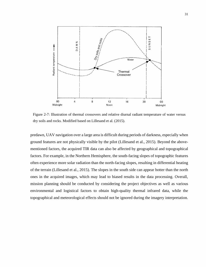
31

predawn, UAV navigation over a large area is difficult during periods of darkness, especially when

ground features are not physically visible by the pilot (Lillesand et al., 2015). Beyond the above-

mentioned factors, the acquired TIR data can also be affected by geographical and topographical

factors. For example, in the Northern Hemisphere, the south-facing slopes of topographic features

often experience more solar radiation than the north-facing slopes, resulting in differential heating

of the terrain (Lillesand et al., 2015). The slopes in the south side can appear hotter than the north

ones in the acquired images, which may lead to biased results in the data processing. Overall,

mission planning should be conducted by considering the project objectives as well as various

environmental and logistical factors to obtain high-quality thermal infrared data, while the

topographical and meteorological effects should not be ignored during the imagery interpretation.

Figure 2-7: Illustration of thermal crossovers and relative diurnal radiant temperature of water versus

dry soils and rocks. Modified based on Lillesand et al. (2015).

32

2.5 Deep Learning and Convolutional Neural Networks

This section provides a brief overview of the core concepts in deep learning and convolutional

neural networks that are related to the data analyses elaborated in Chapter 5 of this thesis. The field

of deep learning is a new field division of machine learning, which is rapidly evolving thanks to

the appearances of large datasets, efficient algorithms and powerful computational hardware in

recent years (Rawat and Wang, 2017; Lateef and Ruichek, 2019). The ever-changing state of the

deep learning field makes difficult to keep up with its evolution pace, and thus, only the topics and

methods that are relative to the conducted experiments are covered and explained. The interested

readers may refer to Goodfellow et al. (2016) and Aggarwal (2018) for a more thorough discussion

of deep learning theory and practice.

Over the past several years, deep learning (DL) has accomplished tremendous success in a vast

variety of application domains including computer vision (Rawat and Wang, 2017), autonomous

robotics (Pierson and Gashler, 2017), agriculture sciences (Kamilaris and Prenafeta-boldú, 2018),

medical sciences (Shen et al., 2017), remote sensing (Zhu et al., 2017), and mining (Zhang and

Liu, 2017), to name a few. It is spawned by a subfield of machine learning called Neural Network

(NN) (Alom et al., 2019), and a deep learning model is consisted of a NN with multiple layers

(Aggarwal, 2018). The term deep often refers to the number of layers involved in state-of-the-art

models, and neural originated from the loose biological similarity to human nervous system

(Aggarwal, 2018). One of the key reasons for DL to become popular is its ability to effectively

decompose latent information contained in data into a hierarchical structure, where a hierarchy of

features or patterns with different levels of abstractions can be learned at different layers of a NN

(Peretroukhin, 2020). For instance, an image of a cat may have local textures (e.g., fur) that

compose primitive(s) (e.g., tail), which belongs to a semantic object (i.e., cat). The layers that are

close to the input are empirically proved to learn low-level features (e.g., local textures), and layers

that are close to the output have the capability to capture high-level abstractions (e.g., semantics)

(Zeiler and Fergus, 2014). In this way, many practical tasks, such as image classification, object

detection, can be handled by NNs, and many state-of-the-art DL models have surpassed human-

level performance in real-world applications (e.g., He et al., 2015; Silver et al., 2017).

Depending on the specific task to be addressed, DL approaches employed in an application can

often be categorized into one of the following types: Supervised, Semi-supervised, Unsupervised

33

and Reinforcement Learning (Alom et al., 2019). Among the abovementioned categories, the

Supervised Learning technique has been widely used to develop models (algorithms) for tasks

involving perception and recognition (e.g., moisture detection, image classification), where

models are trained to learn how to associate an input with an output, given a set of examples of

inputs and labelled outputs (Goodfellow et al., 2016). The labelled outputs, 𝐲train∗ (also known as

targets), and the input examples, 𝐱train , together compose a training set (i.e., 𝒮train ≜

{𝐱train, 𝐲train∗ }). To train a DL model using supervised learning, we iteratively feed the model with

𝐱train and obtain estimated targets 𝐲train . For every iteration, we compute difference measure

between 𝐲train and 𝐲train∗ , which is called the training loss. The objective is to successively reduce

this training loss so that a mapping function, 𝐟(∙), between the input and output is learned by the

model. This process is called optimization. Ideally, we want this learned function to generalize to

new data that are not included in 𝒮train. However, this is usually not true in practice, where the

model tends to perform well on the data that it has seen during training, but not necessarily on the

previously unseen inputs. Such a phenomenon is called overfitting, and the ability for a model to

perform well on previously unobserved inputs is called generalization (Goodfellow et al., 2016).

In order to keep track on the generalization ability of the model, we need to incorporate a validation

set (𝒮val ≜ {𝐱val, 𝐲val∗ }) of examples that the model does not experience during training. This

validation set should be periodically visited by the model at training time, so that some validation

loss can be computed. Note that the validation set is not used for training the model, but for

assessing how well the model performs when encountering points outside the training set.

Typically, both the training and validation losses decrease at the early stage of a training process,

until a critical stage would be reached. After the optimal point, the training loss keeps decreasing

onward, while the validation loss starts increasing (Goodfellow et al., 2016). Figure 2-8 graphically

depicts this relationship. One may stop training the model when the loss on the validation set

reaches its minimum, and this type of training strategy is known as early stopping. A formal

definition of early stopping and some other training strategies that can be used to prevent

overfitting are described by Goodfellow et al. (2016) and Aggarwal (2018).

After the training has completed, the final performance of the trained model should be evaluated

by using a held-out test set (𝒮test ≜ {𝐱test, 𝐲test∗ }). The test set shall never be used in any way

during the learning process, and the data in test set should not contain any repeated entry in the

34

training and validation sets (Goodfellow et al., 2016). Figure 2-9 summarizes the relationships

between the three sets of data (i.e., training, validation, and test sets) and provides a roadmap of

the development process for DL models, which are designed for image classification and

segmentation tasks, using supervised learning. The topics within the green blocks are discussed in

this section, and the remaining topics are covered in later chapters of this thesis. All models

Figure 2-8: Typical relationship between model capacity and error. After reaching the optimal capacity,

the generalization error starts increasing, while the training error keeps decreasing. Modified based on

Goodfellow et al. (2016).

Figure 2-9: Summarization of the development workflow of a deep learning model using supervised

learning.

35

developed in this study are following the procedure depicted in Figure 2-9. The data preparation,

network construction, model training and evaluation, and moisture map generation processes are

elaborated in Chapter 5.

2.5.1 Deep Feedforward Networks

Deep feedforward networks, also known as feedforward neural networks, or multilayer

perceptrons (MLPs), are a typical type of deep learning model, which are designed to approximate

an arbitrary function 𝐟∗ by defining a parameterized mapping 𝐲 = 𝐟(𝐱; 𝜽) (Clement, 2020). The

values of parameters, 𝜽, are learned from data with an intent to result in the best approximation of

𝐟∗ (Goodfellow et al., 2016). The term feedforward refers to the direction of information flow

inside the model, where an input, 𝐱 ∈ ℝ𝑀, flows through the intermediate computations toward

the corresponding output, 𝐲 ∈ ℝ𝑁 , without any feedback connections during the forward

propagation of information. Feedforward neural networks are called networks because multiple

functions are chained together in the intermediate computations, and the length of the chain defines

the depth of the network (Goodfellow et al., 2016). For instance, a two-layer network may include

two functions, 𝐟1 and 𝐟2, chained together such that 𝐲 = 𝐟2 ∘ 𝐟1(𝐱) = 𝐟2(𝐟1(𝐱)). Equivalently, the

computation can be expressed as 𝐡 = 𝐟1(𝐱), and 𝐲 = 𝐟2(𝐡). In this expression, 𝐟1(𝐱) is called a

hidden layer, where 𝐡 is an intermediate result which would not be reported as an output by the

network. In contrast, 𝐟2(𝐡) is called the output layer because it is the last layer of the network, and

the output y is what would be obtained by a user. Therefore, we can call the network a two-layer

feedforward network, or a one-hidden-layer MLP (Goodfellow et al., 2016). Figure 2-10 illustrates

this one-hidden-layer MLP as a directed acyclic graph.

Figure 2-10: Illustration of a one-hidden-layer multilayer perceptrons (MLP) as a directed acyclic graph

describing the mapping 𝐲 = 𝐟2 ∘ 𝐟1(𝐱) , where 𝐱 and 𝐲 are the input and output of the network,

respectively; 𝐡 is the hidden layer; and 𝐟1 and 𝐟2 are two functions mapping a layer onto the next.

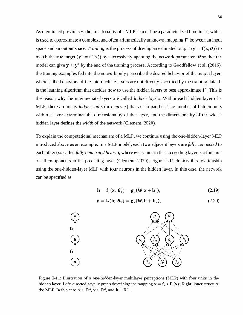
36

As mentioned previously, the functionality of a MLP is to define a parameterized function 𝐟, which

is used to approximate a complex, and often arithmetically unknown, mapping 𝐟∗ between an input

space and an output space. Training is the process of driving an estimated output (𝐲 = 𝐟(𝐱; 𝜽)) to

match the true target (𝐲∗ = 𝐟∗(𝐱)) by successively updating the network parameters 𝜽 so that the

model can give 𝐲 ≈ 𝐲∗ by the end of the training process. According to Goodfellow et al. (2016),

the training examples fed into the network only prescribe the desired behavior of the output layer,

whereas the behaviors of the intermediate layers are not directly specified by the training data. It

is the learning algorithm that decides how to use the hidden layers to best approximate 𝐟∗. This is

the reason why the intermediate layers are called hidden layers. Within each hidden layer of a

MLP, there are many hidden units (or neurons) that act in parallel. The number of hidden units

within a layer determines the dimensionality of that layer, and the dimensionality of the widest

hidden layer defines the width of the network (Clement, 2020).

To explain the computational mechanism of a MLP, we continue using the one-hidden-layer MLP

introduced above as an example. In a MLP model, each two adjacent layers are fully connected to

each other (so called fully connected layers), where every unit in the succeeding layer is a function

of all components in the preceding layer (Clement, 2020). Figure 2-11 depicts this relationship

using the one-hidden-layer MLP with four neurons in the hidden layer. In this case, the network

can be specified as

𝐡 = 𝐟1(𝐱; 𝜽1) = 𝐠1(𝐖1𝐱 + 𝐛1), (2.19)

𝐲 = 𝐟2(𝐡; 𝜽2) = 𝐠2(𝐖2𝐡 + 𝐛2), (2.20)

Figure 2-11: Illustration of a one-hidden-layer multilayer perceptrons (MLP) with four units in the

hidden layer. Left: directed acyclic graph describing the mapping 𝐲 = 𝐟2 ∘ 𝐟1(𝐱); Right: inner structure

the MLP. In this case, 𝐱 ∈ ℝ3, 𝐲 ∈ ℝ2, and 𝐡 ∈ ℝ4.

37

where 𝜽1 = {𝐖1, 𝐛1} and 𝜽2 = {𝐖2, 𝐛2} are parameters of the hidden layer and output layer,

respectively; 𝐖1 ∈ ℝ4×3 and 𝐖2 ∈ ℝ2×4 are weight matrices; 𝐛1 ∈ ℝ4 and 𝐛2 ∈ ℝ2 are bias

vectors; and 𝐠1(∙) and 𝐠2(∙) are element-wise activation functions. It is important to note that if

𝐠𝟏(∙) and 𝐠2(∙) are both linear functions, then the composition of 𝐟2 ∘ 𝐟1 is also linear, which

means the model would not be able to approximate any nonlinear mapping. Therefore, at least one

of the two activation functions must be nonlinear in order to introduce some nonlinearity into the

model. As a common practice, we often choose the activation function of the hidden layer(s) (i.e.,

𝐠1(∙) in this case) to be nonlinear and leave the output layer to be linear. By doing so, the MLP is

capable to learn a nonlinear mapping between the input, 𝐱, and output, 𝐲.

Activation Functions

The selection of activation function is an area of active research. There are a number of nonlinear

activation functions which have been proposed in the literature and implemented in state-of-the-

art models. It has been shown that the choice of activation function has significant influence on

both the performance and required training time of a NN (Glorot et al. 2011; Krizhevsky et al.,

2012). Thorough reviews on activation functions employed in deep learning models are provided

by Rawat and Wang (2017), and Nwankpa et al. (2018).

Recent practices in deep learning often employ the rectified linear unit (ReLU) introduced by Nair

and Hinton (2010) at the hidden layers of feedforward networks (Goodfellow et al., 2016). The

mathematical expression of ReLU is defined as

𝑔(𝑧) = max(0, 𝑧), (2.21)

which only retains the positive part of the activation and set the negative part to zero. Some

researchers also proposed several generalized forms of rectified linear unit such as leaky rectified

linear unit (LReLU) by Maas et al. (2013), parametric rectified linear unit (PReLU) by He et al.

(2015), and exponential linear unit (ELU) by Clevert et al. (2016). The expressions are given as

𝑔(𝑧) = {

max(0, 𝑧) + 𝛼 min(0, 𝑧) LReLUmax(0, 𝑧𝑘) + 𝛼𝑘 min(0, 𝑧𝑘) PReLU

max(0, 𝑧) + min(0, 𝛼(𝑒𝑧 − 1)) ELU (2.22)

38

where 𝛼’s are adjustable parameters, which are used to control the shapes of the functions. One

common property of these rectified linear unit variants is that they allow the activations to be

negative values so that the robustness of the models are improved (Rawat and Wang, 2017).

As mentioned in the one-hidden-layer MLP example, the output layer is often left as linear, which

means an identity activation is employed. The identity activation is defined as

𝑔(𝑧) = 𝑧. (2.23)

Figure 2-12 provides an illustration of the identity, ReLU and LReLU activation functions.

2.5.2 Convolutional Neural Networks

Convolutional networks, (LeCun, 1989) or convolutional neural networks (CNNs), are a particular

form of feedforward network that is commonly used for processing data with a grid-like topology,

such as images and time-series data (Goodfellow et al., 2016). The key distinction between CNNs

and MLPs is that typical CNNs employ not only fully connected layers in their architectures, but

also convolutional and pooling (or subsampling) layers. The convolutional and pooling layers are

often grouped into modules, and multiple modules are stacked together followed by one or more

fully connected layers to form a deep model. Figure 2-13 graphically illustrates a typical CNN

architecture, where the depicted model is designed for an image classification task (Rawat and

Wang, 2017). In the remaining of this section, the image classification task is used as an example

to facilitate the explanation of key concepts in CNN.

Figure 2-12: Illustration of the identity, rectified linear unit (ReLU), and leaky rectified linear unit

(LReLU, 𝛼 = 0.1) activation functions.

39

Fully Connected Layers

Fully connected layers are usually placed at the end of a CNN architecture to perform the function

of high-level reasoning such as identifying the corresponding class of an input image (Rawat and

Wang, 2017). As introduced in Section 2.5.1, neurons between two adjacent layers are pairwise

connected to each other, while there is no connection among units within a single layer. The

computation of a fully connected layer can be interpreted as a dense matrix-vector multiplication

followed by passing through an element-wise activation function. The computational results

contained in the output layer are often taken to represent the class scores (e.g., in classification) or

some real-valued targets (e.g., in regression).

Convolutional Layers

The convolutional (CONV) layer is the core building block of CNNs. The CONV layers serve as

feature extractors, which learn the feature representations of an input and arrange the extracted

information into feature maps (Rawat and Wang, 2017). The process of generating feature maps

is called convolution, which is an operation of using kernels to convolve over the input. Because

convolution is a linear operation, some additional nonlinearity would be required to enable a

CONV layer to learn a nonlinear mapping between the input and the output. This is achieved by

Figure 2-13: Illustration of a typical convolutional neural network (CNN) architecture designed for an

image classification task, which includes convolutional layers, pooling layers and fully connected

layers. Extracted from Rawat and Wang (2017).

40

including a nonlinear activation function (e.g., ReLU) after each convolution operation (Clement,

2020). To graphically depict this process, Figure 2-14 provides an example of a 2D convolution

followed by a ReLU nonlinearity. In Figure 2-14, each pixel (unit) in the feature map is associated

with a 2 × 2 area of the input. Each of these 2 × 2 areas is called the receptive field of its

corresponding pixel in the feature map. The size of the receptive field reflects the amount of

information that is used to obtain a result. In this case, the generated feature map has a size of 2 ×

3, which is dependent on how much the kernel moves at each step. The spatial interval of the kernel

movement is called the stride. In general, the greater the stride, the smaller the feature map would

be, if a padding strategy is not employed to extend the input data (Aggarwal, 2018).

In the example shown in Figure 2-14, the input to the CONV layer is a set of discrete data, which

are represented as a two-dimensional array. This kind of input is very common in deep learning

applications, where images are prominent examples. When working with such input, the

convolution operation can be expressed as

𝐒(𝑖, 𝑗) = (𝐈 ∗ 𝐊)(𝑖, 𝑗) = ∑ ∑ 𝐈(𝑖 − 𝑚, 𝑗 − 𝑛) 𝐊(𝑚, 𝑛)

𝑛𝑚

(2.24)

Figure 2-14: An example of 2D convolution followed by a nonlinear ReLU activation function. The

kernel is restricted to lie within the input, which is called a “valid” convolution in some contexts. The

kernel size is 2 × 2, and the input can be thought of as a 3 × 4 single-channel image. The dimension of

the generated feature map is 2 × 3, which is smaller than the input. In practice, some padding strategies

may be used to force the output to match the input’s dimension. Modified based on Clement (2020).

41

where 𝐈 is the 2D discrete input data; 𝐊 is a discrete 2D kernel; 𝐒 is the generated feature map;

symbol ∗ denotes the convolution operation; 𝑖 and 𝑗 are indices indicating the pixel location inside

the 2D input; and 𝑚 and 𝑛 are indices specifying a position within the kernel 𝐊 (Goodfellow et al.,

2016). In equation (2.24), only the weights in kernel 𝐊 are learnable entries, while the others are

either fixed values, or results computed based on 𝐊. Hence, the goal of the learning algorithm is

to search for optimal values of kernel 𝐊 for all the convolutional layers. An in-depth explanation

about the convolution arithmetic is elaborated by Dumoulin and Visin (2016).

Overall, there are three factors that have contributed to the extensive use of convolutional layers

in CNNs, namely sparse interactions, parameter sharing and equivariant representations

(Goodfellow et al., 2016). To visualize the concept of sparse interactions (also referred to as sparse

connectivity), Figure 2-15 provides a comparison between a CONV layer and a fully connected

layer with the same input and output dimensions. As demonstrated in Figure 2-15, the CONV layer

Figure 2-15: Comparison of the number of connections between a convolutional layer (top) and a fully

connected layer (bottom) with the same input and output dimensions. The convolutional layer

significantly reduces the number of connections. Top: each color of the connections represents one

kernel, and thus, three kernels are employed (i.e., orange, purple and green). Each input unit only

connects to three output units, hence a sparse connectivity. Bottom: every input unit has pairwise

connections to all the output units.

42

has sparse interactions between the input and output as compared to the fully connected layer. The

CONV layer significantly reduces the number of connections, which means it requires much fewer

computational operations to obtain the output. In addition, the CONV layer has fewer parameters,

and thus, less memory requirements. The importance of these properties become prominent when

the inputs are large images with millions of pixels. The concept of parameter sharing is shown in

Figure 2-14, where one single convolutional kernel is used to compute the entire feature map. The

parameters contained in the kernel is shared across all spatial locations of the input data. This

property of CONV layer also contributes to its small memory requirement and efficient

computation. Finally, the property of equivariant representations is actually a consequence of

parameter sharing. Due to the fact that the kernels are learned to pick up local features of the data,

and the parameters are shared across the spatial locations of the input, the same set of features can

be extracted even if the input has undergone some translation (i.e., shifting). The generated feature

maps would be translated by the same amount due to the equivariance to translation property,

which adds robustness to the feature extractors (Goodfellow et al., 2016).

Pooling Layers

A pooling layer is often located after a composition of one or multiple CONV layers to reduce the

spatial resolution of the generated feature maps. By performing the pooling operation, the resultant

output can achieve spatial invariant to input distortions and translations (Rawat and Wang, 2017).

Such a property is accomplished because the pooling layer summarizes the input data and outputs

a summary statistic of the input representations (Goodfellow et al., 2016). To visualize this

process, Figure 2-16 depicts two types of pooling, namely max pooling and average pooling,

applied to a 4 × 4 two-dimensional array. In the example shown in Figure 2-16, the pooling

operations are implemented over non-overlapping 2 × 2 areas (labelled with dotted lines) with

stride of two, and the output dimension is 2 × 2 for both cases. In max pooling, for instance, the

maximum value within each non-overlapping area is determined and reported, and the output can

be seen as a recapitulation of the input data.

Pooling layers that perform max pooling operations are commonly used in recent practice to

diminish computational burden and memory requirement of a CNN model (Rawat and Wang,

2017). Some studies have shown that the max pooling operation can help improve model

generalization and increase convergence speed when compared to conventional subsampling

43

techniques, such as average pooling, which suffers from cancellation effects between neighboring

outputs (Jarrett et al., 2009; Scherer et al., 2010; Rawat and Wang, 2017). However, one of the

biggest drawbacks of max pooling and many other pooling techniques is that the downsampling

nature of a pooling operation would result in loss of spatial knowledge of input features. Such

spatial information becomes important when precise localizations of features are required, such as

in image segmentation and object detection tasks. One alternative to pooling layers is strided

convolution, which can preserve spatial context when downsampling features (Clement, 2020).

Although max pooling is the most commonly used pooling technique in practice (Goodfellow et

al., 2016), there are many other pooling strategies which have been used and proposed in the

literature, such as Lp pooling (Sermanet et al., 2012), stochastic pooling (Zeiler and Fergus, 2013),

fractional max pooling (Graham, 2014), mixed pooling (Yu et al., 2014), spectral pooling (Rippel

et al., 2015), and transformation invariant pooling (Laptev et al., 2016). Each of these pooling

strategies has strengths and inadequacies, and additional details of different pooling methods are

discussed by Rawat and Wang (2017).

Figure 2-16: Illustration of spatial max pooling and average pooling applied to a 4 × 4 two-dimensional

array. In this example, both pooling techniques are operated over non-overlapping 2 × 2 windows

(labelled with dotted lines) with stride of two, and thus, the output dimension is 2 × 2 in both cases.

44

2.5.3 Supervised Training

Given a NN with a set of parameters 𝜽 (where 𝜽 may include, but not limited to, kernel parameters,

𝐊, and weight and bias parameters, 𝐖 and 𝐛), the objective of the training process is to find an

optimal parameter set such that a task-specific loss function is minimized. The process of

minimizing the loss function is called optimization, and it is achieved by iteratively updating the

model parameters. In recent practice, NNs are commonly trained using gradient-based

optimization algorithms (e.g., gradient descent or its variants), accompanied by the batch

normalization technique during the training process. In order to increase the generalization ability

of the model, some regularization mechanisms are often adopted in the learning algorithm to add

robustness to the trained model. It has also been found that an appropriate parameter initialization

scheme can help increase the success rate of network convergence and reduce the required training

time. In this subsection, we briefly discuss each of these supervision components, where further

information may refer to Goodfellow et al. (2016), and Rawat and Wang (2017).

Loss Function

A loss function measures the magnitude of error between the true target and the result estimated

by a given model. The choice of loss function determines how estimation error is penalized, and

thus, influence how the parameters are updated at each optimization step. Loss functions are often

task-specific and can have many different forms. For multi-class image classification, for instance,

the Categorical Cross-Entropy loss (a.k.a. Softmax loss) is the most commonly used thanks to its

simplicity and probabilistic interpretation. There are some other loss functions such as the Hinge

loss and the Triplet Ranking loss, which are also suitable for an image classification task depending

on the problem setup (Rawat and Wang, 2017). In this thesis, the Softmax loss is employed for the

image classification task described in Chapter 5, and the Softmax loss is written as

𝐿 =1

𝑁∑ 𝐿𝑖

𝑁

𝑖=1

=1

𝑁∑ −log (

𝑒𝑠𝑦𝑖

∑ 𝑒𝑠𝑗𝑗

)

𝑁

𝑖=1

, (2.25)

where 𝐿 is a scalar representing the full loss for the entire dataset; 𝑁 is the number of examples

contained in the dataset; index 𝑖 indicates the 𝑖th example of the data; 𝐿𝑖 is a scalar representing

the loss for the 𝑖th example; 𝑦𝑖 represents the true label of the 𝑖th example; 𝒔 is a vector (ℝ𝐶 , 𝐶 is

the number of classes) containing the class scores for each output class; and, 𝑠𝑗 denotes the 𝑗th

45

element (𝑗 ∈ [1, 𝐶]) of the vector of class scores 𝒔. In equation (2.25), the vector of class scores 𝐬

is usually the output of a fully connected layer, which has weights matrix, 𝐖, and bias vector, 𝐛,

as shown in Figure 2-13. Therefore, 𝑠𝑦𝑖 can be denoted as 𝑠𝑦𝑖

= 𝐖𝑦𝑖

𝑇 𝐱𝑖 + b𝑦𝑖, where 𝐱𝑖 is a vector

representing the input feature associated with the 𝑖th example; 𝐖𝑦𝑖

𝑇 is a vector denoting the

transpose of the 𝑦𝑖th column of 𝐖; and, b𝑦𝑖

is a scalar indicating the 𝑦𝑖th element of vector 𝐛.

Further details about the other loss functions may refer to Goodfellow et al. (2016) and Aggarwal

(2018).

Optimization

In the context of training a deep learning model, optimization refers to the process of minimizing

a loss function by altering the model parameters (Goodfellow et al., 2016). Modern optimization

approaches are often built on top of the gradient descent algorithm, which involves computing the

gradient of the loss function with respect to the model parameters. Gradient, in this context, is the

generalized notion of derivative, which is a vector that contains the partial derivatives of the loss

function with respect to every model parameter, denoted by ∇𝜽𝐿(𝜽) (Goodfellow et al., 2016). The

computed gradient points to the direction of steepest ascent, and thus, the negative gradient is

pointing toward the steepest descent direction. One can take a small step each time along the

negative gradient to move toward a critical point (i.e., ∇𝜽𝐿(𝜽) = 0) in the parameter space. This

process can be expressed as

𝜽 ← 𝜽 − 𝜂 ∙ ∇𝜽𝐿(𝜽), (2.26)

where 𝜂 is the step size, which is commonly called the learning rate; and symbol “←” denotes an

operation that the parameters are updated by a set of new parameter values. In this way, equation

(2.26) can be applied iteratively to the parameters until the update become sufficiently small (i.e.,

𝜂 ∙ ∇𝜽𝐿(𝜽) ≈ 0). It is important to note that the gradient descent algorithm does not guarantee to

find a set of parameters that can reach the absolute lowest value (i.e., global minimum) of the loss

function. The optimization problem is often operated in a high-dimensional space, which may have

many local minima and saddle points surrounded by flat regions (Goodfellow et al., 2016).

Therefore, the training is often stopped when the parameter configuration has led to a small loss

value but not necessarily the minimal. Figure 2-17 provides an illustration of the three types of

critical points, namely global minimum, local minimum, and saddle point.

46

In order to perform parameter updates, the back-propagation (often simply called backprop)

algorithm is employed to flow information backward through the network to compute the gradients

with respect to the model parameters by using the chain rule of calculus. For instance, if a system

has 𝐡 = 𝝍(𝐱) , 𝐬 = 𝐠(𝐡) , and 𝐳 = 𝝓(𝐬) = 𝝓(𝐠(𝐡)) = 𝝓(𝐠(𝝍(𝐱))) , where 𝐳 can be either a

scalar or a vector; 𝐱, 𝐡, and 𝐬 are vectors; and, 𝝍(∙), 𝐠(∙) and 𝝓(∙) are functions operating with

vectors and matrices, then the chain rule states that

∇𝐡𝐳 = (∂𝐬

∂𝐡)

𝑇

∇𝐬𝐳,

∇𝐱𝐳 = (∂𝐡

∂𝐱)

𝑇

∇𝐡𝐳.

(2.27)

Equation (2.27) implies that the gradient of the output 𝐳 with respect to the input x can be obtained

simply by multiplying the gradient of the succeeding layer, ∇𝐡𝐳, by the partial derivative of the

succeeding result, 𝐡, with respect to 𝐱, which is actually a Jacobian matrix, i.e., (∂𝐡

∂𝐱)

𝑇

. In this way,

Figure 2-17: Illustration of global minimum, local minimum and saddle point in an optimization

problem. Optimization algorithm does not guarantee to reach the global minimum in many cases,

because of the existence of local minima and saddle points. It is often acceptable when the algorithm

results in a reasonably small loss value. Reproduced from Goodfellow et al. (2016).

47

for each step of the backward gradient computation, we only need to compute one new component,

i.e., the Jacobian matrix of the current layer. Then the gradient of the current layer can be easily

computed by multiplying the newly computed Jacobian by the already computed gradient from the

previous step. This process is recursively performed until the gradients for all of the layers are

determined. Further details about the backprop algorithm may refer to Rumelhart et al. (1986), and

Goodfellow et al. (2016).

At this point, it is possible to use the gradient descent approach to update the model parameters

and implement the back-propagation algorithm to efficiently compute the gradients, but there is

another challenge that is required to be addressed. In practice, the number of examples contained

in a training set is usually large. Benchmark datasets often contain several thousands to several

millions of training examples (Everingham et al., 2010; Geiger et al., 2012; Lin et al., 2014; Zhou

et al., 2019), and even many custom datasets can contains a tremendous number of data points. It

is often impossible for present computational hardware to perform training over the whole training

set due to the limited memory and computational power. To encounter this challenge, the strategy

is to divide the entire dataset into non-overlapping minibatches. Each minibatch is a small subset

randomly sampled from the dataset without replacement, and only one minibatch is sent to the

model for each iteration of training. The model parameters are updated based on an incoming

minibatch at every iteration, and the method of updating parameters is called minibatch stochastic

gradient descent (SGD) if equation (2.26) is used. Every time the training set is fully sampled, it

represents that one epoch of training has elapsed. One issue associated with this stochastic

optimization process is that the minibatches sampled from the training set may have different

statistics as compared to the dataset as a whole. This can lead to the computed gradients become

noisy, which may increase the possibility of model divergence. In order to increase the success

rate of model convergence and to add robustness to the optimization process, many improved

optimization algorithms have been proposed, such as RMSprop (Hinton et al., 2012b),

ADADELTA (Zeiler, 2012), and Adam (Kingma and Ba, 2014). Further information about the

frequently used optimization algorithms for machine learning may refer to Sun et al. (2019).

Batch Normalization

Batch Normalization (BN) introduced by Ioffe and Szegedy (2015) is an adaptive

reparameterization method that is commonly used in practice. One significant reason that makes

48

BN popular is because it effectively tackles one of the fundamental challenges when training NNs

using gradient descent (GD). As mentioned above, the model parameters are updated based on the

update directions (i.e., gradients) determined by the back-propagation algorithm. The gradient of

a parameter computed by using backprop indicates the direction of steepest ascent when all other

parameters stay unchanged. Nevertheless, in practice, all the model parameters are updated

simultaneously at every iteration, and unexpected results may be observed due to the simultaneous

changes of many interdependent parameters (Clement, 2020). Batch normalization tackles this

problem by reparametrizing some layers of the model to always have standardized outputs with

zero mean and unit standard deviation (Goodfellow et al., 2016). In this way, the BN technique

reduces the severe consequences of internal covariate shift (i.e., parameter changes in early layers

result in changes of input distributions for later layers) (Rawat and Wang, 2017).

To show the reparameterization of BN, let matrix 𝐇 contains a minibatch of inputs with a

dimension of 𝑀 × 𝑁, where each row of 𝐇 represents one training example, and the number of

columns denotes the dimensionality of the inputs. To normalize the minibatch, we replace the

entries in 𝐇 by

𝐻𝑖𝑗 ←𝐻𝑖𝑗 − 𝜇𝑗

𝜎𝑗, (2.28)

where 𝑖 is the row index of 𝐇 indicating the 𝑖𝑡ℎ input in the minibatch (𝑖 ∈ [1, 𝑀]); 𝑗 is the column

index of 𝐇 indicating the 𝑗𝑡ℎ dimension of the input (𝑗 ∈ [1, 𝑁]); 𝜇𝑗 is a scalar representing the

mean of the 𝑗𝑡ℎ column; 𝜎𝑗 is a scalar denoting the standard deviation of the 𝑗𝑡ℎ column; and 𝐻𝑖𝑗

is a scalar indicating the entry of 𝐇 located at the 𝑖th row and the 𝑗th column. It is important to

note that the definitions of 𝜇𝑗 and 𝜎𝑗 are different at training time and at test time. At training time,

the column mean and standard deviation are given by

𝜇𝑗 =

1

𝑀∑ 𝐻𝑖𝑗

𝑀

𝑖=1

(2.29)

𝜎𝑗 = √1

𝑀∑ (𝐻𝑖𝑗 − 𝜇𝑗)

2+ 𝜖

𝑀

𝑖=1

(2.30)

49

where 𝜖 is a small scalar (e.g., 10−5) added to avoid the denominator in equation (2.28) being zero.

The running averages of 𝜇𝑗 and 𝜎𝑗 are recorded during training, and the values are locked once the

training is finished. At test time, the locked values of 𝜇𝑗 and 𝜎𝑗 are applied to the test input in the

same fashion as in equation (2.28), which allows the model to be evaluated at individual data points

(Clement, 2020).

As mentioned by Goodfellow et al. (2016), and Ioffe and Szegedy (2015), simply normalizing the

data to have zero mean and unit standard deviation can reduce the expressive power of the network.

Therefore, it is common to use an additional linear transformation to enhance the representation

such that

𝐻𝑖𝑗 ← 𝛾𝑗 (

𝐻𝑖𝑗 − 𝜇𝑗

𝜎𝑗) + 𝛽𝑗, (2.31)

where 𝛾𝑗 and 𝛽𝑗 (𝑗 ∈ [1, 𝑁]) are learnable parameters that are used to scale and shift the output.

Batch Normalization has been successfully applied in many state-of-the-art deep learning models

to accelerate the training process and increase the model performance (Santurkar et al., 2018).

Besides BN, there are also other normalization techniques that are proposed in the literature such

as Layer Normalization by Ba et al. (2016), Instance Normalization by Ulyanov et al. (2016), and

Group Normalization by Wu and He (2018). Each of these techniques has its strengths and

appropriate use cases, and many models developed with these methods have shown promising

results.

Regularization

Regularization refers to a broad class of strategies that are used to increase the generalization

ability of machine learning models. In practice, regularization techniques can be applied at every

stage of the model development process, including data preparation (e.g., data augmentation

techniques), model construction (e.g., pooling layers, restrictions on the parameter values), model

training (e.g., dropout, loss penalties), and even prediction stage (e.g., ensemble methods). In this

section, we focus on a regularization technique that is commonly used during the training process

of deep models, called dropout (Hinton et al., 2012a; Srivastavaet al., 2014). Further details about

the other frequently used regularization strategies for deep models may refer to the survey study

given by Moradi et al. (2019).

50

The key idea of dropout is that at each training iteration, individual units in one or more layers are

either dropped out of the model with some probability 𝑝 , or retained in the network with

probability 1 − 𝑝. In this way the incoming and outgoing connections of the dropped units are also

removed for the iteration. Model parameters are then updated only for those retained units. This

process can be thought of as training a random subnetwork of the base network at each iteration

by stochastically dropping some of the computational units. It is important to note that the

subnetworks sampled from the base model are not independent because they share the parameters.

Each of the subnetworks has a reduced capacity as compared to the base network, where the base

model after training is similar to an ensemble of all the sub-models (Goodfellow et al., 2016).

Figure 2-18 provides an illustration of dropout applied to a feedforward network during training.

At test time (i.e., after the training process), the entire base network is used, and there is no dropout

implemented.

Dropout has been proved to significantly diminish overfitting by preventing feature coadaptation

and possess an implicit bagging effect (Rawat and Wang, 2017). It can be easily integrated with

other regularization techniques such as weight decay and early stopping. Many studies have

provided profound explanations and analyses on the rationale and mechanism of dropout, and

several variants of dropout have been proposed in the literature to adapt different problem setups

(Baldi and Sadowski, 2014; Goodfellow et al., 2016; Rawat and Wang, 2017; Moradi et al., 2019).

Figure 2-18: Illustration of the forward propagation through a feedforward network using dropout.

During training, dropout can be interpreted as sampling a random subnetwork from the base network.

Left: the forward pass of the base network; Right: dropout applied to the network at training time.

51

Parameter Initialization

Parameter initialization plays a critical role in the training process of NNs. Although it occurs only

once per network at the beginning of learning, a poor initialization can lead to problems like

vanishing/exploding gradient, which can significantly hinder network convergence (Bengio et al.,

1994). In general, there are two groups of initialization approaches. The first group refers to

transfer learning, where the parameters values of a successful model developed for a proxy

application are used as the starting point for a model designed for another application. For example,

a CNN that is designed to classify images of cats and dogs may use the parameters from an already

trained animal classifier as its starting point. A secondary training stage can then be performed to

fine-tune the model based on a specialized dataset, which mainly contains photos of cats and dogs

in this case. Numerous studies have shown that transfer learning can be used to resolve the problem

of insufficient training data, increase the success rate of model convergence and shorten the

required training time of NNs (e.g., Huang et al., 2017; Tan et al., 2018). Thanks to the existence

of many benchmark datasets for general vision tasks, a lot of successful models have been

developed, and the model parameters are made available to be used (Lin et al., 2014; Everingham

et al., 2010).

Many research-oriented tasks need to train models from scratch, and the second group of

initialization approaches aim to provide robust initialization schemes for deep NNs. As shown in

equation (2.19) and (2.20), the parameters of a network often consist of weights and biases, as well

as some operation-specific parameters (e.g., learnable parameters in batch normalization and

PReLU). Most of the studies regarding parameter initialization focus on initialization of weights,

where biases are commonly set to zeros at the beginning of the training process. Among the

proposed initialization methods in the literature, two techniques are popular and often used in

practice, namely Glorot initialization (a.k.a. Xavier initialization, Glorot and Bengio, 2010) and

He initialization (a.k.a. Kaiming initialization, He et al., 2015). In Xavier initialization, the initial

weights of a layer are drawn from either a uniform distribution or a normal distribution. In the case

of uniform distribution, each entry of the weight matrix would have

𝑊𝑖𝑗𝑙 ~𝒰 [−√

6

𝑛𝑙 + 𝑛𝑙+1, √

6

𝑛𝑙 + 𝑛𝑙+1], (2.32)

52

where 𝒰[−𝑎, 𝑎] is the uniform distribution in the interval (−𝑎, 𝑎); 𝑙 is an index indicating the 𝑙𝑡ℎ

layer of the network; 𝑊𝑖𝑗𝑙 denotes the entry located at the 𝑖𝑡ℎ row and the 𝑗𝑡ℎ column of the weight

matrix for the 𝑙𝑡ℎ layer; and, 𝑛𝑙 and 𝑛𝑙+1 are called fan-in and fan-out, which are the number of

neurons within the 𝑙𝑡ℎ and the 𝑙 + 1𝑡ℎ layer, respectively. In contrast, if a normal distribution is

employed, the weights should follow

𝑊𝑖𝑗

𝑙 ~𝒩 (0,2

𝑛𝑙 + 𝑛𝑙+1), (2.33)

where 𝒩(0, 𝜎2) is a zero-mean normal distribution with a variance of 𝜎2. It is important to note

that all the weights are independent and identically distributed regardless of the distribution from

which they are drawn. It has been shown that Xavier initialization can increase convergence speed

and reduce the risk of vanishing gradient when training NNs (Glorot and Bengio, 2010). However,

the main limitation of Xavier initialization is that its derivation is based on a linear activation,

which might not be optimal when used jointly with nonlinear activation functions (Rawat and

Wang, 2017).

To improve Xavier initialization, He et al. (2015) derived a theoretically sound initialization,

known as Kaiming initialization, which is compatible with the commonly used ReLU and PReLU

nonlinear activation functions. The initial weights under Kaiming initialization follow

𝑊𝑖𝑗

𝑙 ~𝒩 (0,2

𝑛𝑙), (2.34)

where all the terms have the same definitions as in Xavier initialization. It can be easily observed

that Kaiming initialization is similar to the Xavier method, except that the weights are drawn from

a normal distribution whose variance is calculated based on only the number of neurons within the

current layer. Due to the extensive use of ReLU activation in modern deep learning models,

Kaiming initialization has been widely adopted in the literature, and it has shown its suitability for

training extremely deep networks (He et al., 2015; Rawat & Wang, 2017).

53

2.6 Convolutional Neural Network Based Surface Water and Moisture

Recognition and Monitoring

To the best of our knowledge, not much attention in the literature has been put on utilizing

convolutional neural networks (CNNs) for heap leach pad (HLP) monitoring, especially HLP

surface moisture mapping. However, CNNs have been widely adopted in agriculture, remote

sensing, and several other study areas thanks to their ability to generate accurate and precise

predictions (Ball et al., 2017; Kamilaris and Prenafeta-boldú, 2018a; Li et al., 2018; Ma et al.,

2019; Zhu et al., 2017).

CNNs are most commonly used to process data with grid-like topology (e.g., images, video and

time-series data), where the multilayer structure allow the models to extract low-, mid- and high-

level features from the data and provide a hierarchical representation of the model input (Garcia-

Garcia et al., 2017; Goodfellow et al., 2016; Kamilaris and Prenafeta-boldú, 2018a). The key

advantage of CNN is that the extracted features are learned automatically from the data through

the training process. There is no hand-engineered feature required, which significantly improves

the models’ generalization ability when applied to data within the same problem domain but

previously unobserved by the models (Goodfellow et al., 2016; Pan and Yang, 2010; Weiss et al.,

2016; Zhu et al., 2017). Beyond the capacity of learning features automatically, CNNs are often

robust against challenging image conditions, including complex background, different resolution,

illumination variation, and orientation changes (Amara et al., 2017). In contrast, many traditional

signal and image processing approaches rely on hand-engineered features, where the feature

engineering is not only time-consuming and tedious but also dataset specific, which is often subject

to generalization issues (Kamilaris and Prenafeta-boldú, 2018a; Li et al., 2018). Xia et al. (2017)

and Li et al. (2018) conducted comparative studies regarding the performance of different image

classification methods, which use low-level (e.g., SIFT), mid-level (e.g., Bag of Visual Words),

and high-level (i.e., CNN) image features, on multiple datasets, such as RSSCN7 (Zou et al., 2015),

AID (Xia et al., 2017), and UC-Merced (Yang and Newsam, 2010). The experimental results

demonstrated that CNN models, as high-level feature extractors, surpass the performance of

traditional handcrafted feature-based methods by a significant margin (Xia et al., 2017).

In addition, CNNs are shown to achieve comparable and usually more efficient and accurate

inference performance than other machine learning algorithms, such as support vector machine

54

(SVM), k-nearest neighbours (KNN), and random forest (Kemker et al., 2018; Paisitkriangkrai et

al., 2016; Zhang et al., 2018). Kemker et al. (2018) introduced a semantic segmentation dataset

(called RIT-18) and compared the performance of two CNNs and several machine learning

algorithms (e.g., KNN, SVM, multiscale independent component analysis) on RIT-18. The

experimental results showed that the CNN models significantly outperformed the other algorithms

in terms of prediction accuracy, and Kemker el al. (2018) mentioned that the deep features learned

by CNNs can generalize better than handcrafted features across different datasets. Kussul et al.

(2017) carried out an application of land cover and crop type classification using one multilayer

perceptron (MLP), one random forest (RF), and two CNN models based on satellite imagery. The

two CNN models consistently accomplished higher accuracy in classifying water body and the

various crop types than the RF and MLP models. Kussul et al. (2017) concluded that the CNN

models were able to build a hierarchy of sparse and local features, which contributed to their better

performance over the other two methods in their experiment.

There are many studies that utilize CNNs for surface water and moisture recognition. Isikdogan et

al. (2017) proposed a CNN named DeepWaterMap, which was used to generate surface water

maps on a global scale based on Landsat satellite imagery. The experiment was formulated as a

semantic segmentation task (known as image classification in remote sensing), and the network

architecture of DeepWaterMap had a typical encoder-decoder structure (Hinton and

Salakhutdinov, 2006). Isikdogan et al. (2017) stated that the trained DeepWaterMap model was

capable of learning the shape, texture and spectral response of surface water, cloud, and several

other land cover types, where the generated results from their experiment demonstrated the

model’s ability to discriminate water from surrounding land cover. Rather than using satellite

imagery, Fu et al. (2018) performed a land use classification application based on remotely sensed

visible-light (RGB) images acquired by aerial platforms. The three datasets employed in the study

covered agriculture and urban areas, and they proposed a blocks-based object-based image

classification method that embedded a CNN model to determine the types of land use (e.g., water,

building, road). Fu et al. (2018) highlighted that the high-level features extracted by the CNN

model were effective for complex image pattern descriptions, which facilitated their method to

achieve an end-to-end land use classification without the time-consuming design process of

handcrafted features. Moreover, CNNs can be also applied to grid-like data derived from other

types of signals. Wang et al. (2018) collected soil echoes using an ultra-wideband radar sensor

55

over an approximately 50 m2 bare soil field. The recorded soil echoes were transformed into time-

frequency distribution patterns, and two CNN architectures, AlexNet (Krizhevsky et al., 2012) and

Visual Geometry Group (Simonyan and Zisserman, 2014), were employed to classify the time-

frequency patterns with different moisture levels. Besides the applications in remote sensing and

agriculture, Zhao et al. (2020) applied a CNN model to detect potential water leakage in a metro

tunnel by locating moisture marks of shield tunnel lining. They mentioned that moisture marks are

caused by water ingress through cracks in concrete, and early notice of such defects has significant

meaning for avoiding ground failure. They acquired RGB images through a platform called

Moving Tunnel Inspection equipment, and a CNN architecture, Mask R-CNN (He et al., 2017),

was employed to perform instance segmentation on their obtained images. The experimental

results demonstrated that the trained model was able to locate and segment the moisture marks in

the images accurately and efficiently (Zhao et al., 2020).

In addition to recognizing the existence of surface water and moisture, a number of studies in the

literature have applied CNNs to perform soil moisture estimation. Ge et al. (2018) adopted a CNN

model with 1-D convolutions to estimate soil moisture on a global scale based on satellite data.

They combined information from four different sources to generate input vectors and compared

the model’s performance against a fully connected feedforward NN. The experimental results

indicated that the CNN model produced reasonable moisture estimates and achieved a better

performance than the NN on their custom dataset (Ge et al., 2018). Similarly, Hu et al. (2018)

employed a CNN model to retrieve global soil moisture based on passive microwave satellite

imagery. They used the Advanced Microwave Scanning Radiometer - Earth Observing System

(AMSR-E) brightness temperatures as input data and compared the performance of a CNN model

(with a linear output layer) against a support vector regression (SVR) model. The experimental

results showed that the CNN model could produce more accurate moisture estimates than their

SVR model. Besides using satellite data to estimate soil moisture on a large scale, Sobayo et al.

(2018) collected in-situ moisture measurements in three farm areas and acquired thermal images

by attaching a thermal infrared camera to an unmanned aerial vehicle. They trained a CNN-based

regression model to learn the correlation between the remotely sensed soil temperature and the in-

situ moisture measurements. The experimental results demonstrated the effectiveness of using the

CNN model to generate relatively accurate soil moisture estimates based on the custom dataset

(Sobayo et al., 2018).

56

Chapter 3 Field Data Collection

Field Experiment and Data Acquisition

Field experiment and data acquisition were conducted over a sprinkler-irrigated heap leach pad at

McEwen Mining’s El Gallo gold mine located in Sinaloa State, Mexico, from March 5th to 8th,

2019. This chapter provides an overview of the mine site where the data were collected, the

equipment used, and the methodology for collecting the data. The content covered in the chapter

is largely reproduced from Section 3 of the author’s conference publication (Tang and Esmaeili,

2020).

3.1 Site Information

The McEwen Mining’s El Gallo gold mine is located in Sinaloa State, Mexico, approximately 350

km northwest of Mazatlán, 100 km northwest of Culiacan, and 40 km northeast of Guamúchil

(Figure 3-1). The mine is resided in the Lower Volcanic Series of the Sierra Madre Occidental,

dominated by rocks of andesitic composition (Medinac, 2019). The mineralization is hosted within

a northeast structural trend with numerous sub-structures (Bamford et al., 2020). Gold was the

primary metal produced, and heap leaching (HL) was used to extract the metal from the crushed

ores.

Figure 3-1: Location of the El Gallo mine.

57

The heap leach pad (HLP) was located north of the mine site and the footprint of the HLP was

approximately 22 hectares. The HLP adopted a sprinkler irrigation system with a sprinkler spacing

of 3 m, and dilute cyanide solution was applied continuously during the field experiment. The flow

rate of the HLP was 600 m3/hr, and an average irrigation rate of 8 L/hr/m2 was used for the

irrigation system. The designed lift height of the HLP was 10 m and the overall heap height was

80 m. The HLP material was crushed gold-bearing rock with a particle size distribution (PSD) as

illustrated in Figure 3-2. The PSD curves in Figure 3-2 were generated from both on-site mesh

sieving and laboratory sieving results. Based on the PSD, the HLP material had an 80% passing

size (P80) of 8 to 10 mm, and the material was treated as coarse-grained soil (ASTM, 2017).

3.2 Equipment

During the field data collection, a commercially available UAV platform, DJI Matrice 600 Pro,

was equipped with one thermal camera, DJI Zenmuse XT 13 mm, and one digital camera, DJI

Zenmuse X5, in a dual gimbal setup. The specifications of the cameras are listed in Table 3-1. The

dual gimbal system consisted of a front gimbal, which was installed with a global positioning

system (GPS), and a bottom gimbal (without a GPS), which was located at the geometric center

of the UAV platform. This dual gimbal setup allowed for the acquisition of both thermal and

regular RGB images simultaneously. The UAV was selected because it had sufficient payload

Figure 3-2: Material particle size distribution of the studied heap leach pad

58

capacity to carry the dual gimbal system during the experiment. The two cameras were selected

because they could take images with high resolutions while easily integrating with the existing

gimbal system. It is worthwhile to mention that the spectral band captured by the thermal camera

was 7.5–13.5 μm, which is known as the commonly used atmospheric window for aerial sensing

within the TIR region of the EM spectrum (Gupta, 2017). Figure 3-3 shows the equipment used

during the field experiment. The other equipment used included one BIKOTROIC BTH Portable

Sand Moisture Meter, one Dr. Meter LX 1330B digital light meter, and one Protmex MS 6508

Digital Thermo-hygrometer.

Table 3-1: Thermal and digital cameras specifications

Specifications DJI Zenmuse XT 13 mm DJI Zenmuse X5

Dimension 103 mm x 74 mm x 102 mm 120 mm × 135 mm × 140 mm

Weight 270 g 530 g

Maximum Resolution 640 × 512 4608 × 3456

Angle of View 45o × 37o 72o

Gimbal Accuracy ±0.03o ±0.02o

Spectral Band 7.5 – 13.5 μm RGB

Source: DJI 2019a, 2019b

Figure 3-3: Equipment used during the field experiment

59

3.3 Field Experiment and Data Collection

The duration of the field experiment was from March 5 to March 8, 2019. There were two phases

of the field experiment. The first phase focused on generating a detailed survey plan and placing

ground control points (GCPs) within the study area. The second phase (Mar. 6 to Mar. 8, 2019)

included data acquisition using the generated survey plan. In phase one, a flight was conducted

using the UAV platform equipped with the dual camera system to acquire images that covered the

entire HLP. An orthomosaic (or true orthophoto, which is generated based on an orthorectification

process), of the HLP was then generated by using the OpenDroneMap software to help facilitate

the survey planning. Using the orthomosaic of the HLP, the locations of the GCPs were determined

based on their accessibility over the HLP. A detailed survey plan, which included the mission

count, take-off location, flight altitudes, and flight times and durations, was then generated. In the

second phase of the field experiment, two data collection campaigns were conducted in each

surveying day, one in the morning (10 a.m.) and the other in the afternoon (2 p.m.). This survey

schedule was adopted to comply with the mine site’s shift schedule and safety policies, although

the predawn hours were considered as best for thermal infrared surveys because of the minimal

temperature variation caused by differential solar heating and logistic reasons (Gupta, 2017).

During each data collection campaign, two flight missions were carried out, and Table 3-2

summarizes the details of the flight plans. Twelve GCPs were placed at the designated locations

by on-site technical staff, and the GPS coordinates of the GCPs were recorded by a portable GPS

device. Figure 3-4 illustrates the GCP locations with respect to the HLP. It is worthwhile to note

that five of the twelve GCP locations were selected to be the sampling locations, where samples

were collected near these GCPs.

Table 3-2: Details of flight missions for phase two of the field experiment

Flight Mission Parameters Flight Mission 1 Flight Mission 2

Area of study Top two lifts of the HLP Entire HLP

Footprint of studied area 4 hectares 22 hectares

Flight altitude* 90 m 120 m

Ground sampling distance** 12 cm/pixel 15 cm/pixel

Flight time 7 min/mission 24 min/mission

Number of RGB images 80 images/mission 280 images/mission

Number of thermal images 170 images/mission 620 images/mission * The flight altitude is with respect to the take-off location ** The ground sampling distance is with respect to the thermal images

60

For each data collection campaign, five ground samples were collected at the sampling locations

during the time of flights. These samples were sent to the on-site laboratory to measure specific

gravity and gravimetric moisture content. These measurements were used as ground truth to

facilitate and validate the remote sensing results. Care was taken during the sampling process to

collect only the surface material (top 5 to 10 cm) from the HLP.

There were five members involved in each surveying campaign. Two technical staff for ground

sample collection and three members for UAV data acquisition. Due to the large extent of the

study area, the time spent by the technical staff to collect ground samples at the selected locations

was approximately the same as the total flight time of the two flight missions.

During each UAV data collection campaign, the following setup was used to acquire the aerial

images: the thermal and RGB cameras were operated by using the DJI GO and DJI Ground Station

Pro applications, respectively, where the gimbal pitch angles were both set to 90o downward to

face the HLP surface; the image acquisition rates were set to two seconds per thermal image and

Figure 3-4: Flight mission 2 (light yellow) and locations of ground control points (GCPs) with respect

to the heap leach pad. Five sampling locations are shown as green circles.

61

five seconds per RGB image, where the thermal image format was set to R-JPEG (Radiometric

JPEG) format, and the colour image was set to JPEG format; and for each pair of adjacent images,

the front and side overlap were designed to be 85% and 70%, respectively. The user-defined

external parameters in the DJI GO application were set based on the field conditions at the time

of image acquisition, where the scene emissivity for all missions was set to 0.95, which is a typical

value for wet soil surface (Jensen, 2009). The atmospheric temperature and relative humidity were

measured using a thermohygrometer, and the corresponding values were inputted into the

application. The parameter of reflected apparent temperature was set to the same as the

atmospheric temperature, and the external optics temperature and transmittance were set to 1.0

(Zwissler, 2016). The acquired images were presented in 8-bit grayscale JPEG files when exported

to computing devices, where the remotely sensed surface temperature at each pixel location was

stored in the metadata of the image. The surface temperature sensed by the thermal camera can

then be extracted by using external software tools such as FLIR Atlas SDK for MATLAB. In this

study, we used the remotely sensed surface temperature (TRS) acquired by the thermal camera as

an approximation of the actual HLP surface temperature to perform data analysis.

By the end of the field experiment, twenty-four sets of data with approximately 6,900 images were

collected in total. This included 12 sets of colour images and 12 sets of thermal images. Table 3-3

summarizes the number of data collected at each flight mission, where the thermal and RGB colour

images are reported separately.

Table 3-3: The number of colour and thermal collected during the field experiment*

March 6, 2019 March 7, 2019 March 8, 2019

Morning Afternoon Morning Afternoon Morning Afternoon

Whole HLP** T: 620

C: 273

T: 618

C: 281

T: 618

C: 270

T: 621

C: 289

T: 618

C: 290

T: 619

C: 275

Top two lifts** T: 178

C: 58

T: 170

C: 74

T: 174

C: 74

T: 169

C: 81

T: 170

C: 73

T: 173

C: 76

* Overall, there were 24 sets of data collected, where 12 sets were colour images and the other 12 sets were thermal images

** T: number of thermal images; C: number of colour (RGB) images

62

Chapter 4 Surface Moisture Mapping Based on Thermal Imaging

Mapping Heap Leach Pad Surface Moisture Distribution

Based on Thermal Imaging

Chapter 3 provided a description of the studied heap leach pad (HLP) and depicted the data

acquisition using the UAV system. This chapter outlines how the acquired thermal images are used

to create surface moisture maps and includes a discussion on the effectiveness and limitations of

the proposed method. The data analysis presented in this chapter focuses on analyzing the six sets

of thermal images covering the whole HLP (approximately 3,700 image), and the results of

processing the rest of the data are elaborated in Chapter 5. The material contained in this chapter

is largely reproduced from the author’s paper: “Mapping Surface Moisture of a Gold Heap Leach

Pad at the El Gallo Mine Using an UAV and Thermal Imaging”, which has been submitted to the

Mining, Metallurgy & Exploration Journal for publication.

4.1 Overview

After acquiring data from the field experiment, data processing and moisture map generation were

conducted off-line. As mentioned previously, the heap leach pad material was treated as coarse

grained soil according to its particle size distribution (ASTM, 2017). It would be adequate to apply

a remote sensing based surface soil moisture (SSM) retrieval method to estimate the surface

moisture distribution over the HLP. Therefore, the acquired thermal images and in-situ moisture

measurements from the collected samples were first used to derive an empirical relationship

between the surface moisture content and the remotely sensed surface temperature using linear

regression. Moisture distribution maps were then generated by using the regression model to

visualize the moisture variation over the HLP.

A general workflow of the data analysis process is illustrated in Figure 4-1. The remainder of this

chapter provides the implementation details of each data processing step, and the generated

orthomosaics and moisture maps are presented to illustrate the analysis results.

63

4.2 Data Preprocessing

As mentioned above, there were six sets of thermal images with respect to the whole HLP, and the

preprocessing of data was independently performed for each of these six datasets in two different

procedures. The first procedure is referred to as a data cleansing step, where the corrupted and

low-quality (i.e., inappropriately exposed) images were manually removed from each of the

datasets. In the second procedure, an intensity transformation and mapping script written in

MATLAB using the FLIR Atlas SDK was run to first determine the highest and lowest remotely

sensed surface temperature (denoted as Tmax and Tmin, respectively) within each dataset. In this

way, there were six pairs of Tmax and Tmin determined, where each pair was associated with one of

the thermal datasets. By using the maximum and minimum surface temperatures, the pixel

intensity values of the thermal images were then mapped by using equation (4.1).

𝐼𝑥,𝑦

(𝑖)= 𝑟𝑜𝑢𝑛𝑑(

𝑇𝑥,𝑦(𝑖)

− 𝑇min

𝑇max − 𝑇min× 255) (4.1)

In equation (4.1), 𝑟𝑜𝑢𝑛𝑑(∙) is the rounding operator that returns an integer pixel intensity value

ranging from 0 to 255, which is the bit-depth range for an 8-bit image; Tmax and Tmin are the highest

and lowest remotely sensed surface temperature in degree Celsius of the current dataset,

respectively; the superscript (i) denotes the ith image in the current dataset; 𝑇𝑥,𝑦(𝑖)

is the remotely

sensed surface temperature in degree Celsius at the 𝑥th row and 𝑦th column pixel location of the

ith image; and 𝐼𝑥,𝑦(𝑖)

is the output pixel intensity value at the (𝑥, 𝑦) pixel location of the ith image in

the current dataset. The outputs of this process were a set of single-channel 8-bit raster data in

matrices format. For each matrix, the single-channel raster data were replicated three times to

Figure 4-1: General workflow of the data processing and moisture map generation.

64

generate an RGB image with three channels having the same intensity values. By following the

above procedure, six sets of grayscale images were generated with the same number of images as

the input thermal image datasets. Figure 4-2 provides a visual comparison example between the

initial and processed images. The images included in Figure 4-2 were four thermal images taken

in a successive order. As seen in Figure 4-2, the initial images undergo rapid intensity changes due

to the camera’s built-in exposure adjustment. Therefore, this pre-processing step was performed

to ensure that the images used to generate orthomosaics were following a consistent intensity scale.

4.3 Linear Regression Model Development

A linear relationship between the HLP surface temperature and material gravimetric moisture

content, 𝜔, was derived based on the acquired data. Several assumptions were made during the

data analysis process in order to facilitate the regression model development. It was assumed that

the chemical composition and material roughness were relatively uniform for the top 5 cm of the

HLP surface, and the remotely sensed surface temperature captured by the thermal camera could

be used as an approximation to the HLP surface temperature. It was also assumed that the sensor

noises of the camera were independent and identically distributed (IID) random variables. Under

Figure 4-2: Visual comparison example between initial and processed thermal images taken in a

successive order: (a) Output images after the preprocessing step; (b) Initial thermal images taken by

thermal camera.

65

these assumptions, the linear regression model was developed based on the remotely sensed

surface temperature values (TRS) and the measured gravimetric moisture contents at the sampling

locations. To determine the TRS values at the sampling locations, the following steps were

employed independently for each of the thermal datasets:

1) The thermal images that covered the sampling locations were manually identified;

2) The pixel coordinates associated with the sampling locations were then pinpointed by using

the GIMP software within the images that were identified in the previous step;

3) After determining the pixel coordinates at which the sampling locations were located, a 5

× 5 average kernel was applied at these pixel locations to calculate the TRS values. An

illustration of the temperature determination step is depicted in Figure 4-3.

Note that a 5 pixels by 5 pixels area on the image plane represents approximately a 75 cm by 75

cm area on the HLP surface. It was assumed that the measured moisture content from the collected

samples represents the average surface moisture of the 75 cm by 75 cm area. The above process

Figure 4-3: Determination of the remotely sensed surface temperature at a sampling location. The pixel

coordinate associated with the sampling location (labeled in green) was first pinpointed within the

thermal image on the left. The average temperature of a 5 pixels by 5 pixels area (labeled in blue on the

right) was then calculated to represent the TRS at this sampling location.

66

would result in multiple TRS values associated with each of the sampling locations. The average of

the values corresponding to the same location was used to represent the approximate surface

temperature at that sampling point. In this way, 30 pairs of TRS and moisture measurements (i.e.,

five from each dataset) were determined, and a univariate linear regression model was developed

based on these 30 data points. The resultant linear relationship is expressed as equation (4.2).

𝜔 = −0.5103(TRS) + 23.77 (4.2)

In equation (4.2), 𝜔 is the HLP surface material gravimetric moisture content (%); and TRS is the

remotely sensed surface temperature (oC). Figure 4-4 illustrates the linear relationship between 𝜔

and TRS, and Figure 4-4 compares the measured moisture content to the predicted values calculated

using equation (4.2). Overall, the model demonstrates a good agreement between the predicted

and measured moisture contents with a R2 of 0.7409, and a root mean square error (RMSE) of

1.28%.

Figure 4-4: (a) Empirically derived univariate linear regression between gravimetric moisture and

remotely sensed surface temperature; (b) Predicted vs. measured gravimetric moisture content (%).

There were five samples (one from each sampling location) collected for every data collection campaign.

The surveying team conducted two campaigns per day for three successive days. Therefore, there are

30 data points (i.e., groundtruth samples) involved in both (a) and (b).

67

4.4 Orthomosaics Generation

Orthomosaics were generated in the Agisoft Metashape software by using the preprocessed

images. Software parameters were set to generate orthomosaics with the highest possible spatial

resolution. The generated orthomosaics had a ground sampling distance of approximately 10

cm/pixel, and the outputs were in 8-bit image format. Overall, six orthomosaics were generated,

where each one was associated with one of the thermal datasets with respect to the entire HLP.

During the orthomosaic generation process, after the importation of the images into the software,

the images were automatically registered based on their georeference information (i.e., GPS

information) from the images’ metadata. The image and camera alignment functions were used to

generate sparse point cloud, followed by dense point cloud generation. The GCP coordinates were

also imported during the point cloud generation step to increase the accuracy of the dense point

cloud. After generating the dense point cloud, the orthomosaic was generated and exported as an

image in TIFF format. This process was repeated using the same software settings for the six sets

of preprocessed images. The generated orthomosaics from each of the datasets are shown in Figure

4-5.

4.5 Moisture Maps Generation

Moisture maps were generated by using the orthomosaics and the linear regression model. Each

orthomosaic was first imported into the QGIS software, and the “Raster Calculator” function was

used to map the pixel intensity values to surface temperature values through equation (4.3).

𝑇𝑥,𝑦 = 𝑇min + (𝑇max − 𝑇min)

𝐼𝑥,𝑦 − 𝐼min

𝐼max − 𝐼min (4.3)

In equation (4.3), 𝑇𝑥,𝑦 is the remotely sensed surface temperature (oC) at the 𝑥th row and 𝑦th

column pixel location of the current orthomosaic; Tmin and Tmax are, respectively, the highest and

lowest remotely sensed surface temperatures (oC) of the current thermal dataset, which have been

determined in the image pre-processing step; 𝐼max and 𝐼min are the maximum and minimum pixel

intensity values; and 𝐼𝑥,𝑦 is the pixel intensity value at the (𝑥, 𝑦) pixel location of the current

orthomosaic. By doing so, every pixel location of the orthomosaics would have its corresponding

TRS, and thus, moisture maps can be generated by applying equation (4.2) to each pixel in the

orthomosaics. The generated moisture maps for the thermal datasets are illustrated in Figure 4-6.

68

Figure 4-5: Generated orthomosaics of the HLP by using the acquired thermal image datasets.

69

Figure 4-6: Generated moisture maps of the HLP by using the orthomosaics and the linear regression

model.

70

4.6 Discussion and Conclusion

The results shown in Figure 4-5 and Figure 4-6 demonstrate the feasibility of mapping HLP surface

moisture distribution using remotely sensed thermal images. The generated HLP surface moisture

maps have a temporal and spatial resolution hardly achievable by conventional point-measurement

methods. In addition, the proposed method is highly practical, which makes it beneficial to HL

monitoring.

The proposed method is practical for its efficient product generation process and the adequate

accuracy of the generated results. As mentioned previously, the linear model directly relates

material surface moisture content to remotely sensed surface temperature, which does not require

further effort to collect additional ancillary data. As soon as the model is developed, a moisture

map can be generated within an hour of the data acquisition, and the spatial distribution of the

material moisture over the HLP can be intuitively visualized.

From the results shown in Figure 4-6, we can directly acquire an understanding of the spatial

distribution of surface moisture over the HLP. This allows a mine manager to make decisions

based on the generated results, and the moisture maps can be used as a guide to evaluate the

performance of the irrigation system. In our case, we can conclude that the solution application in

the west is more abundant than in the east. A relatively poor moisture coverage can be consistently

observed in the southeast area of the HLP, and particular attention should be paid to identify the

possible operational issues in this region. One may also notice that there is one region in the north

showing less moisture coverage as compared to the surrounding area (i.e., the orange stripe

surrounded by blue colour at the upper part of each moisture map). This region was actually the

toe of the ore pile, and there was no sprinkler installed at the location, thus, the dryness was

expected. In addition to providing overviews of the HLP surface, the spatial resolution of the

moisture maps is high enough to even show the performances of individual sprinklers. By looking

at the center portion of the HLP, it can be found that several sprinklers result in smaller areas of

influence as compared to the others. This may indicate a requirement for sprinkler replacement or

descaling.

From an HLP monitoring perspective, it would be difficult for the HLP manager to precisely

control the surface wetness for every inch of the pile. Instead, a more practical strategy is to

maintain the majority of the surface moisture falling within an acceptable range (this range should

71

be defined based on site-specific operational practice), while avoiding the creation of solution

ponds and extremely dry areas over the HLP. In our case, if we define the area with a moisture

level below 3% as dry and above 9% as wet, we can quickly pinpoint the regions associated with

extreme moisture conditions; for example, the northwest and the southeast regions in the March

6, Morning dataset. These areas might arise operational concerns because the extremely dry

regions may imply sprinkler defects or ineffective leaching conditions, while the regions that show

an extremely high moisture level may be subject to ponding issues. Actions can be taken by

technical staff to further investigate these regions with the help from the generated moisture maps.

This increases the efficiency and effectiveness in resolving operational issues and streamlines the

entire monitoring process. In addition, since the moisture maps provide direct visualization of the

spatial variation in material surface moisture, they can be involved in the irrigation optimization

process to quantitatively depict the performances of different solution application strategies.

Despite the benefits discussed above, the empirically derived linear model has its imperfections.

Thus, it is important to understand the principal foundation, limitation, and possible improvement

of the proposed method. In general, remote sensing (RS) approaches are essentially approximation

techniques that inevitably include errors in their estimated results. Assumptions and/or

simplifications are commonly employed up to a certain extent during the RS model development

process to balance accuracy, efficiency, and practicality. As shown in Figure 4-6, there are

inconsistencies between datasets regarding the estimated surface moisture content from one dataset

to another. This is due to the inability of the linear model to take the effects of all the influential

factors into account when relating the remotely sensed surface temperature to the surface moisture

content of the HLP material. In the remainder of this section, some of the factors that may have

contributed to the generated results are discussed, and several recommendations regarding model

improvement are also provided.

The basis of TIR remote sensing is to use a thermal sensor placed at some distance from an object

to measure the EM energy emitted from the object’s surface (Jensen, 2009). A material that has a

temperature higher than absolute zero (0 K) emits thermal infrared EM radiation, and the amount

of the emitted energy is a function of its true surface temperature (i.e., kinetic temperature) and

emissivity. The kinetic temperature of any ground feature on the earth is affected by the heat

sources, atmospheric effects, and material thermal properties; while the emissivity of the object is

the result of its composition and surface geometry (Gupta, 2017). It is important to note that some

72

of these factors are interdependent, for example, the composition of an object also affects its

physical and thermal properties.

In this study, the primary heat source of the HLP surface was the Sun, and the spatial and temporal

surface temperature variation was mainly due to solar heating. The energy from the incoming sun

rays led to changes in the kinetic temperature of the leach pad surface, and the maximum surface

temperature was expected to occur in the early afternoon (around 2 p.m.) (Gupta, 2017). In general,

the amount of incident solar energy over the HLP was not spatially uniform. The amount of solar

radiation received by an area on the HLP depended on several parameters such as topographical

relief, slope aspect, as well as solar zenith and azimuth angles. The solar angles were functions of

the latitude of the site and time of day and month (Kalogirou, 2013). Also, slopes with different

orientations underwent differential heating, and the magnitude of heat energy received was

affected by sun position and surface orientation. The differential heating that occurs at different

times of the day can be easily observed when comparing the morning datasets to the afternoon

datasets in Figure 4-5 and Figure 4-6. Because the site was located in the northern hemisphere, the

sunrise occurred in the southeast, and thus more solar radiation was incident toward the southeast

corner of the HLP in the morning hours. This resulted in a higher remotely sensed surface

temperature in the area. In contrast, ground materials generally reach their maximum temperature

in the early afternoon (Gupta, 2017; Jensen, 2009; Lillesand et al., 2015), and the detected surface

temperature was more uniform as shown in the afternoon datasets. To graphically depict the

different positions of the Sun related to the HLP, an illustration of the Sun’s daily path from sunrise

to sunset is shown in Figure 4-7 (Kalogirou, 2013). According to Lillesand et al. (2015), south-

facing slopes in the northern hemisphere generally receive more solar heating than the north-facing

ones. This phenomenon can be intuitively recognized from Figure 4-7, and the influence of the

differential heating on the HLP surface can also be observed in Figure 4-5 and Figure 4-6. One

may develop a moisture estimation approach that incorporates the site latitude and solar angles to

enhance estimation accuracy and model generalizability (Liu and Zhao, 2006).

Another factor that can influence the kinetic temperature of the ground surface is active thermal

sources. For HLPs that involve extensive exothermic reactions (e.g., rapid sulfide-to-sulfur and

sulfur-to-sulfate oxidation of sulfide minerals), the chemical reactions can result in self-heating of

the leach pad material, and the heat generated in the HLP can be transferred to the surface via

convection of fluid and/or conduction through solid. Remote sensing models that are developed

73

based on surface data may be incapable of explaining the sophisticated patterns of heat generation

and transportation inside the HLP. Although the heat energy introduced by chemical reactions was

considered insignificant in this study, future improvement of the proposed method may incorporate

the results provided by numerical programs that can model the internal behaviours of the HLP to

complement the estimation of surface moisture content.

In addition to the heat sources, the atmosphere plays a critical role in both downwelling and

upwelling energy transfer. It affects not only the magnitude and spectral composition of the solar

radiation received by the ground surface but also the intensity and components of the energy

recorded by a thermal remote sensing system (Lillesand et al., 2015). Gases and suspended

particles in the atmosphere can absorb, scatter, and emit radiation during the energy transfer, which

may attenuate, strengthen, or transform the radiation emitted from ground objects before reaching

the thermal camera (Lillesand et al., 2015). Water vapour, in particular, may absorb radiation

emitted from the material surface, leading to a decrease in the energy detected by the sensor

(Lillesand et al., 2015). Several studies in agriculture and mine tailing impoundment monitoring

have shown that the effect of atmospheric humidity during the data collection should be considered

when the remotely sensed thermal data are used for estimation of material surface moisture (Liu

and Zhao, 2006; Sugiura et al., 2007; Zwissler et al., 2017). In our case, the measured relative

Figure 4-7: Illustration of the Sun’s positions related to the HLP (not to scale). The mine site is located

in the northern hemisphere, and thus the south-facing slopes receive more solar heating than the north-

facing ones. The solar zenith angle, 𝚽, and solar azimuth angle, 𝜶, change overtime from sunrise to

sunset. Figure modified based on (Kalogirou, 2013).

74

humidity was approximately 25% (±2%) throughout the entire field experiment, which was

considered as consistent. Nevertheless, the data acquisition was performed in three successive days

with similar weather conditions, and thus the collected data may not be representative to explain

the effect of humidity. Future improvement of the predictive model may be achieved by

incorporating a humidity term in the regression after collecting more representative data in

different seasons and weather conditions.

Besides the gases and suspended particles contained in the atmosphere, meteorological conditions

ought to be considered for remote sensing studies, especially for surveys conducted using UAV

based remote sensing platforms. Wind, for instance, can dissipate surface heat and accelerate

moisture evaporation, which results in cooling of the ground material. This cooling effect often

varies spatially and temporally, and thus introduces complexity and difficulty when using the

remotely sensed thermal data to estimate surface moisture. Moreover, wind speed and direction

are usually capricious in the local area, which may result in instability issues of the UAV platform

such as inaccurate flightpath (i.e., deviating from the pre-set flight routes) and tilted observation

angles of the onboard sensors (Jensen, 2009). During our field experiment, it was observed that

the wind speed was generally higher in the afternoon than in the morning. Also, the wind directions

were often inconsistent during the data acquisition, which had contributed to variations in the

flightpath accuracy and drone battery consumption. Some studies in the literature have proposed

parameterized models that include wind velocity to take the influence of wind into account when

relating material surface moisture to thermal data (Liu and Zhao, 2006; Scheidt et al., 2009; Zhao

and Li, 2013). In addition to wind velocity, another important meteorological component that may

have affected our results was cloud cover. The amount of cloud cover at each data collection

campaign was considerably different, and it was expected that the cloud cover had contributed to

differential heating and shadowing over the HLP, which led to patchy appearances on some of the

collected thermal images. It is important to bear in mind the potential influence of the

meteorological conditions when interpreting the generated results. To improve our method, a more

sophisticated model that involves meteorological variables may be developed in future studies to

account for the influences of meteorological conditions on the moisture estimation.

The amount of radiation emitted by an object is a function of its emissivity (Lillesand et al., 2015).

The greater the emissivity, the more radiance is emitted by the radiating body at a given kinetic

temperature (Jensen, 2009). It is important to notice that a cooler ground feature can emit the same

75

amount of radiation as a warmer body due to the discrepancy between their emissivity (Gupta,

2017). There are a number of factors that can influence the emissivity of an object, such as

chemical composition, surface roughness, moisture content, colour, and viewing angle (Jensen,

2009; Weng et al., 2004). In general, rocks with high silica content have a low emissivity, and

coarse particle surfaces relate to a high emissivity (Gupta, 2017). In this study, it was assumed that

the chemical composition and material roughness were uniform for the top 5 cm of the HLP

surface. However, if the material composition and roughness varied significantly across the

surface, then the estimated results would be biased toward the data on which the linear model was

derived. In our case, the mineralization at El Gallo mine has occurred in a volcanic series,

dominated by rocks of andesitic composition. Moreover, the ores were subjected to crushing before

they were dumped within the HLP. Thus assuming a consistent rock composition and roughness

surface for the HLP should be conceivably appropriate. Besides the effects of material composition

and roughness, darker-coloured particles are better emitters than the lighter-coloured ones; and the

more moisture a rock contains, the higher its ability to emit radiation (Gupta, 2017). These

relationships imply that the correlation between the material moisture content and the remotely

sensed data may not be a univariate linear function, and an improved model may be developed in

future studies to account for the abovementioned variables.

Observing the same surface from different viewing angles would obtain different thermal

measurements. This is because the emissivity of an object varies with the sensor viewing angle

(Jensen, 2009). Moreover, the distance between the sensor and the observed surface affects the

accuracy of the recorded data. The further the distance from the sensor to the target surface, the

more noise would be introduced into the remotely sensed thermal images (Sugiura et al., 2007). In

this study, the thermal images were acquired by pointing the thermal camera vertically downward

so that the central axis of the camera’s instantaneous field of view (IFOV) aligns with the normal

of the top surface. Such a strategy would result in a uniform observation distance between the

sensor and the horizontal surfaces at the expense of observing the slopes at oblique angles. The

reason for adopting such configuration was because ponding issues were more likely to occur on

the flat terrains rather than on the slopes of the HLP. Hence, more emphasis was put on the flat

regions over the HLP. Furthermore, the flight altitudes of the data collection campaigns were

selected based on the considerations of image resolution, flight duration and drone battery

consumption so that a balance between accuracy, efficiency and practicality was achieved.

76

In conclusion, this chapter elaborated on the methodology and implementation details of using the

acquired thermal images and in-situ moisture measurements to generate HLP surface moisture

maps. An empirical linear relationship between the remotely sensed surface temperature and the

HLP surface moisture content was first derived, and the moisture maps were generated using the

linear model. The empirical model showed a good agreement with the ground-truth moisture

measurements, and the generated moisture maps possessed a temporal and spatial resolution hardly

achievable by conventional point-measurement methods. The benefits and limitations of the

proposed method were discussed, and possible improvement of the moisture estimation step was

also outlined. Overall, the results have demonstrated the feasibility and practicality of the proposed

approach, and the products created from the data analysis process can be useful for HLP

monitoring applications.

77

Chapter 5 Surface Moisture Mapping Using Convolutional Neural Networks

Mapping Heap Leach Pad Surface Moisture Distribution

Using Convolutional Neural Networks

Chapter 4 described a framework for producing HLP surface moisture maps based on the obtained

thermal images. This chapter introduces how the acquired colour and thermal images can be

utilized simultaneously during the data analysis to generate surface moisture maps using

convolutional neural networks (CNNs). The proposed approaches create moisture maps in an end-

to-end fashion after the necessary data preparation procedures, and the methods can be further

developed towards a fully automated data analysis process for HLP surface moisture monitoring.

5.1 Overview and Methodology

Convolutional neural networks (CNNs) are a particular type of neural networks (NNs), which has

shown remarkable performance in processing data with a grid-like topology, such as images and

time-series data (Rawat and Wang, 2017). CNN models typically consist of multiple layers (e.g.,

a few tens or hundreds of layers), which endow them with the ability to extract hierarchical features

from the model input (Bengio, 2009; LeCun et al., 2015). Layers that are close to the input can

extract low- and mid-level features, while later layers can learn high-level (i.e., more abstract and

semantically meaningful) representations, which are the combinations of lower-level abstractions

(Alom et al., 2019; Zhu et al., 2017). Such a feature extraction ability allows predictive CNN

models to exploit spatial and/or temporal correlations in the data when making predictions, which

contributes to the tremendous success of CNNs in computer vision tasks, including image

classification and semantic segmentation (Khan et al., 2020; Lateef and Ruichek, 2019). Image

classification, known as scene classification in remote sensing, refers to categorizing a model input

(e.g., an image) into one of several predefined classes (Ma et al., 2019; Rawat and Wang, 2017);

and semantic segmentation, known as image classification in remote sensing, refers to assigning a

semantic class to every pixel of the input (Kemker et al., 2018; Zhu et al., 2017). To avoid

confusion, we adopt computer vision terms throughout this chapter unless otherwise specified.

In this study, we propose two approaches for generating heap leach pad (HLP) surface moisture

maps using CNNs, where the first method embeds a moisture classification model, and the second

78

utilizes a semantic segmentation network. The general workflow of the two methods is illustrated

in Figure 5-1. Since the input of CNN models must be raster tiles with a fixed height and width,

we designed the models to adapt a small input size (32 × 32 for classification, and 64 × 64 for

segmentation). In this way, if an input based on which a moisture map should be generated has a

large height and width, we first subdivide the input into multiple tiles with the same size, followed

by using the predictive CNN models to produce the corresponding prediction for each tile and

finally combine all of the model predictions to generate the moisture map output (Figure 5-1).

All the employed models in this work were trained using supervised learning, and the data used

for model development were derived from the colour (RGB) and thermal images obtained during

the field experiment described in Chapter 3. Since the two types of networks require different kinds

of training, validation, and testing data, we prepared the classification and segmentation datasets

separately based on the same set of remote sensing imagery (i.e., the raw data). The details of data

preparation are elaborated in Section 5.2. The model development and moisture map generation

for the classification and segmentation CNNs are presented in Section 5.3 and Section 5.4,

respectively. Methodology and implementation details are explained throughout the sections,

while discussions and visualization examples are provided to clarify the important concepts and

experimental results. Finally, Section 5.5 concludes the chapter and outlines the future direction

of this research work.

Figure 5-1: Schematic illustration of the moisture map generation workflow by using a classification

model (upper) and a segmentation model (lower). The input of the workflow should be a four-channel

raster with a height and width no less than the designated tile size of the corresponding model (i.e., 32

× 32 for classification, and 64 × 64 for segmentation). The classification model returns a moisture class

for each tile, while the segmentation model provides pixel-wise prediction.

79

5.2 Data Preparation

This section provides a detailed description of the data preparation process. The overall workflow

consisted of four parts, namely, data preprocessing, orthomosaic generation, orthomosaic co-

registration, and datasets construction. The resultant outputs were two sets of training, validation,

and testing data, which were later used for the development of convolutional neural networks.

During the field experiment, there were 24 sets of data collected, which contained approximately

4,750 thermal images and 2,115 visible-light (colour) images. Among the 24 sets of data, half of

the datasets were for the whole studied area, and the other half were collected only for the top two

lifts of the HLP. Table 5-1 summarizes the number of data collected at each flight mission, where

the thermal and visible-light data are reported separately. The data preparation process started with

preprocessing the colour and thermal images (Section 5.2.1). Then, the preprocessed data were

used to create 24 orthomosaics, followed by dividing the generated outputs into 12 groups

according to their studied area and time of data acquisition (Section 5.2.2). In this way, each group

consisted of one thermal and one colour orthomosaic that covered the same studied area (i.e., either

the whole facility or the top two lifts of the HLP). Afterwards, the colour orthomosaic within each

group was registered with its thermal counterpart such that 12 four-channel rasters (called overview

rasters) were generated (Section 5.2.3). Lastly, the datasets construction process, which involved

three steps, was performed to generate appropriate training and evaluation data for the deep

learning models (Section 5.2.4).

There were various types of data used and generated during the data preparation process, thus, it

is necessary to clarify the naming convention employed in the remainder of this section. In this

study, images were taken using digital and thermal cameras. Therefore, we use the term colour

image (or sometimes visible-light image) to indicate the data collected by the digital camera and

thermal image to denote the information recorded by the thermal sensor. In general, a colour image

Table 5-1: The number of remote sensing data collected during the field experiment*

March 6, 2019 March 7, 2019 March 8, 2019

Morning Afternoon Morning Afternoon Morning Afternoon

Whole HLP** T: 620

C: 273

T: 618

C: 281

T: 618

C: 270

T: 621

C: 289

T: 618

C: 290

T: 619

C: 275

Top two lifts** T: 178

C: 58

T: 170

C: 74

T: 174

C: 74

T: 169

C: 81

T: 170

C: 73

T: 173

C: 76

* Overall, there were 24 sets of data collected, where 12 sets were colour images and the other 12 sets were thermal images

** T: number of thermal images; C: number of colour images

80

has three channels, which means every pixel of the image has a red, green, and blue colour intensity

value associated with it. In contrast, the thermal images are single-channel images because there

is only one digital number at each pixel location. For those data involving more than three channels

of values (e.g., four channels in our case), we call them raster data, or simply rasters. We adopted

the abovementioned naming convention to avoid confusion, although a raster image, by definition,

can represent any data that are stored in a 2D array-like pattern (Marschner and Shirley, 2015).

5.2.1 Data Preprocessing

The preprocessing of data was performed independently for the colour and thermal datasets. It is

important to note that the colour images were not georeferenced by default because the GPS device

was installed at the front gimbal on which the thermal camera was attached. Therefore, only the

raw thermal images were initially georeferenced. For the 12 colour image sets, the corrupted and

inappropriately exposed images were manually removed from the dataset. There were four (out of

2114) colour images removed in total. The colour images that cover one or multiple ground control

points (GCPs) within the field of view were recorded manually so that the GPS coordinates of

these GCPs could be used in the orthomosaics generation step to georeference the images.

The method used to preprocess the 12 thermal image sets was described in Section 4.2. In short,

the preprocessing of thermal images consisted of two procedures. The first procedure was to

remove the poor-quality data by manual inspection, which resulted in a removal of 47 (out of 4748)

images from the dataset. The second procedure was to run an intensity transformation and mapping

script written in MATLAB to ensure that the images within the same dataset had a consistent

intensity scale. By the end of the preprocessing step, every thermal dataset would have one pair of

highest and lowest remotely sensed surface temperature (denoted as Tmax and Tmin, respectively)

associated with it, where these Tmax and Tmin values would be later used to map the pixel

intensities of thermal orthomosaics into surface temperature values (see Section 4.2 for details).

5.2.2 Orthomosaics Generation

After completing the data preprocessing step, orthomosaics were generated in the Agisoft

Metashape software by using the preprocessed images. For the visible-light image sets, the

generated colour orthomosaics had a ground sampling distance (GSD) of 2 cm/pixel, and the

outputs were in 24-bit image format (8-bit for each red, green, and blue channel). Overall, twelve

81

colour orthomosaics were generated, where half of these orthomosaics were related to the whole

HLP facility, and the other half were associated with the top two lifts of the HLP. It is worth noting

that the highest possible GSD for the top two lifts datasets could be finer than 2 cm/pixel due to

the high image resolution resulting from the low flight altitude. However, a coarser spatial

resolution was selected to match with the datasets for the whole HLP so that the inputs to the deep

learning models are consistent in spatial scale.

The colour orthomosaic generation process started with importing the visible-light images into the

Agisoft Metashape software. The visible-light images were not georeferenced, and thus, the

images would not be automatically registered after importation. A preliminary image alignment

was then performed by using the “Align Photos” function, where the software would compute a

sparse point cloud and a set of preliminary positions of the images. However, the generated sparse

point cloud and preliminary positions were neither accurate nor orientated adequately due to the

lack of elevation and global positioning information. An example of the preliminary camera

positions and sparse point cloud computed by the software is illustrated in Figure 5-2(a). In order

to refine the image alignment, the locations of the GCPs were manually pinpointed within the

software interface, and the corresponding GPS coordinates of the GCPs were inputted into the

software. In this way, the appropriately positioned image alignment and sparse point cloud could

be generated by using the “Optimize Camera” function. An example of the adequately positioned

sparse point cloud created by incorporating the GCP coordinates is shown in Figure 5-2(b). The

refined spare point cloud was then used to create a dense point cloud, followed by the final

orthomosaic generation. This process was repeated using the same software settings for the 12

colour image sets. Figure 5-3 shows the six colour orthomosaics for the top two lifts of the HLP,

while Figure 5-4 depicts the orthomosaics with respect to the whole HLP facility.

The thermal orthomosaics for the 12 sets of thermal images were generated following the

procedures described in Section 4.4. The overall procedures for thermal and colour orthomosaic

generation was similar, except that the thermal images were georeferenced by default. Hence, the

thermal images would be automatically registered based on their georeference information after

importation. The generated thermal orthomosaics had a GSD of approximately 10 cm/pixel for all

12 datasets, and the outputs were in 8-bit (i.e., single-channel grayscale) image format. The

generated thermal orthomosaics for the whole facility are shown in Figure 4-5, and the

orthomosaics with respect to the top two lifts of the HLP are provided in Figure 5-5.

82

By following the procedures described above, there were 24 orthomosaics created based on the

Figure 5-2: (a) The generated point cloud without GPS information was not adequately oriented. (b)

The generated point cloud with GPS information was appropriately positioned. The x- and y-axis are

denoting the east-west and the north-south directions, respectively. The blue rectangles represent the

estimated image plane positions of the input images.

83

acquired visible-light and thermal image sets. The orthomosaics were then divided into 12 groups

according to their studied area and time of data acquisition, such that each group involved one

thermal and one colour orthomosaic. For instance, the first group would involve the thermal and

colour orthomosaics generated based on the data collected on the morning of March 6, and both

orthomosaics were for the whole HLP. In this way, we can superimpose the colour orthomosaics

onto the thermal ones to produce 12 four-channel rasters, where the first three channels contain

the intensity values for the red, green, and blue colours, followed by the fourth channel containing

Figure 5-3: Generated colour orthomosaics for the top two lifts of the HLP by using the acquired visible-

light image datasets.

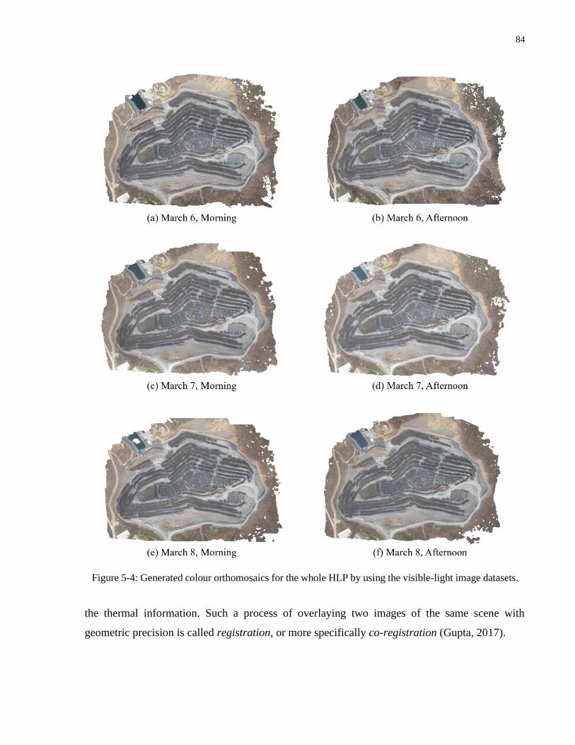
84

the thermal information. Such a process of overlaying two images of the same scene with

geometric precision is called registration, or more specifically co-registration (Gupta, 2017).

Figure 5-4: Generated colour orthomosaics for the whole HLP by using the visible-light image datasets.

85

5.2.3 Orthomosaics Registration & Multichannel Rasters Generation

Overlaying the colour and thermal orthomosaics with geometric precision can allow the resultant

raster data to simultaneously contain information acquired from both visible-light and thermal

cameras. However, the generated orthomosaics were inevitably subject to image distortion, which

resulted in geometric misalignments when directly superimposed over each other. In other words,

if a colour orthomosaic was directly superimposed onto a thermal one, the same pixel location of

the two orthomosaics would not refer to the same location over the HLP due to image distortion

and variations (Gupta, 2017). To adequately align the orthomosaics within the same group, the

Figure 5-5: Generated thermal orthomosaics for the top two lifts of the HLP by using the acquired

thermal image datasets.

86

“Georeferencer” function in the QGIS software was used to perform orthomosaics alignment. It is

important to clarify that we were not truly georeferencing the orthomosaics to a geodetic reference

system (e.g., WGS-84); instead, we were selecting one of the two orthomosaics within a group to

be a reference and registering the other one onto the reference image. In the literature, the reference

image is also called the base or master image, while the images to be registered are referred to as

sensed or slave images (Gupta, 2017; Zitova and Flusser, 2003).

In this study, the thermal orthomosaic within each group was selected to be the reference, and the

goal was to align the colour orthomosaic with the thermal one such that the geometric

misalignment between the two would fall below a tolerance limit. This tolerance limit should be

set based on the application’s objective, and we adopted a threshold of three pixels (equivalently

0.3 m over the HLP surface), which is an order of magnitude smaller than the three-meter sprinkler

spacing of the HLP’s irrigation system. We consider that this precision is sufficient for the

application of HLP surface moisture map generation.

For each group of orthomosaics, the alignment process started with importing both images into the

QGIS software. After the importation, the colour orthomosaic was used as the image to be

registered (i.e., the slave image), and the thermal orthomosaic was used as the master image. A set

of feature correspondences was then manually identified between the two images, where these

correspondences were used to compute an image transformation that mapped the pixel locations

in the slave image onto the coordinate system of the master image. In this process, the user-defined

software parameters were set as follows: the “Polynomial 3” option was selected to be the

“Transformation type”, and the “Cubic” interpolation technique was picked as the “Resampling

method”. The reason for selecting the third-order polynomial transformation was because it has

the ability to correct complex and nonlinear image distortions, while it is one of the most

commonly used transformation types in practice (Kurt et al., 2016). Similarly, the “Cubic”

resampling method was selected because the cubic interpolation technique is commonly used when

processing aerial images, and it has the ability to preserve edges and produce sharp image outputs

(Kurt et al., 2016; Lehmann et al., 1999) .

In the above procedure, the number of identified feature correspondences depended on the studied

area. If the orthomosaics covered the whole HLP, then 150 pairs of features were manually

determined on the images. An example of the identified feature correspondences on one group of

87

the orthomosaics is shown in Figure 5-6. As depicted in the figure, the identified features were

spread over the images, and every feature (i.e., red dot) on the left image had one corresponding

feature on the right. These identified features are called control points (CPs) in the literature, where

one may refer to them as postmarked CPs because they were determined after the data collection

(Hackeloeer et al., 2014; Zitova and Flusser, 2003). In contrast, if the studied area was the top two

lifts of the HLP, then 60 pairs of CPs were used for the alignment.

As mentioned previously, the goal of the above process was to align the orthomosaics such that

the misalignment between the thermal and colour data fell below a tolerance limit. To evaluate the

alignment accuracy, an additional set of feature correspondences were manually identified, where

the CPs contained in this additional set were mutually exclusive from the ones that were used to

compute the image transformation (i.e., there was no repeating entry between the two sets of

features). The numbers of additional feature correspondences used for the whole area and the top

two lifts of the HLP were 25 and 15, respectively. In this way, the coordinates of these additional

CPs on the master image and the transformed slave image could be recorded, and the overall

alignment error was calculated by averaging the root mean square errors between the

corresponding coordinate pairs (Zitova and Flusser, 2003). As mentioned above, we set the

tolerance limit for the alignment error to be 0.3 m, or equivalently the ground distance represented

by three pixels of the thermal orthomosaic. If the alignment error were greater than the threshold,

Figure 5-6: Illustration of the selected 150 feature correspondences over the colour and thermal

orthomosaics. The two orthomosaics were generated based on the March 6, Morning datasets. Every

red dot on the colour orthomosaic (left) has a unique corresponding feature on the thermal orthomosaic

(right). There were 150 correspondences identified for every pairs of orthomosaics for the whole HLP.

88

then another round of image transformation would be performed until the averaged error went

below the tolerance.

After performing the image alignment described above, the thermal and transformed colour

orthomosaics were positioned adequately, and the next step was to regularize the spatial resolution

(i.e., GSD) of the data so that every pixel of the colour and thermal orthomosaics could represent

the same real-world dimension over the HLP. As mentioned in Section 5.2.2, the GSDs of the

thermal and colour orthomosaics were 10 cm/pixel and 2 cm/pixel, respectively. Since we selected

the thermal data as the reference, the colour orthomosaics would be downsampled to the same

resolution as its thermal counterpart. The downsampling was carried out by using the “Align

Raster” function in the QGIS software. The downsampling operation started with importing a

transformed colour orthomosaic and its thermal counterpart into the software. The thermal

orthomosaic was then selected to be the reference layer, and the output size was set to be the same

as the thermal data. The “Average” algorithm was selected to be the resampling method, and the

generated output would be saved in TIFF file format. By using these settings, the resultant output

would be a downsampled colour orthomosaic with the same GSD as the thermal input. This

downsampling operation was repeated for all 12 groups such that the spatial resolutions of all

orthomosaics were appropriately regularized.

The final step of the registration process was to superimpose the transformed and regularized

visible-light orthomosaics over the thermal data to generate four-channel rasters containing both

colour and temperature information. Figure 5-7 graphically depicts this step, and the same

procedure was repeated for every group of the data. To generate a four-channel raster, a thermal

orthomosaic was first imported into the QGIS software. After the importation, the “Raster

Calculator” function was used to map the pixel intensity values to surface temperature values by

using equation (4.3). The output of this operation would be a surface temperature map, where each

pixel would have an associated remotely sensed surface temperature value in degree Celsius. Once

the temperature map was created, the final product was generated using the “Merge” function in

QGIS to overlay the colour orthomosaic with the temperature map. The resultant output would be

a four-channel raster with all data values being single-precision floating-point numbers. In this

way, the 12 groups of orthomosaics were converted into 12 four-channel rasters (called the

overview rasters in the remainder of this chapter), which were used to prepare the datasets for the

development of convolutional neural networks.

89

5.2.4 Datasets Construction

The datasets construction process consists of three steps, which are graphically summarized in

Figure 5-8. In this study, we designed CNNs for two different tasks, namely image classification

and semantic segmentation, that required different types of model inputs. Therefore, the datasets

used to develop the classification and segmentation models were separately prepared as shown in

Figure 5-8. Overall, the first step of the datasets construction was to subdivide the 12 overview

rasters into a large number of small tiles such that each tile covered a small area of the HLP surface.

Secondly, the small raster tiles were partitioned into training, validation, and test sets, which would

be used in the CNN training and evaluation processes. Lastly, a label creation step was performed

to label all the examples (i.e., the small raster tiles) contained in the datasets so that the labelled

examples could be used to train the NNs in a supervised learning paradigm. The remainder of this

subsection provides the implementation details of each datasets construction step, followed by a

summarization of the datasets statistics.

Figure 5-7: Generation of a four-channel raster by overlaying a colour orthomosaic over a remotely

sensed surface temperature map of the heap leach pad. The output is a four-channel raster, where the

first three channels contain intensity values of the red, green, and blue colour, and the fourth channel

contains the remotely sensed surface temperature in degree Celsius. All data values in the output raster

are single-precision floating-point numbers.

90

Figure 5-8: The three steps of the deep learning datasets construction process.

91

At this point, the 24 sets of images were converted into 12 overview rasters containing both visible-

light and temperature information. The rasters that covered the top two lifts of the HLP had

approximately 4,100 × 2,050 (width × height) pixels, while the raster size for the whole HLP

facility was approximately 7,000 × 5,500 pixels. To subdivide a large raster into small tiles, the

raster to be subdivided was first imported into the QGIS software, followed by running the “Save

Raster Layer as” function. The “Create VRT” option was selected, and the output files were

designated to be in the TIFF file format. The raster height and width of the resultant outputs were

both set to 64 pixels, while the coordinate reference system (CRS) was set to be the same as the

input raster. The same settings were used for all 12 overview rasters, and the generated outputs

were a set of raster tiles that had a dimension of 64 × 64 × 4 (height × width × channels). Since

the region of interest (ROI) in this study is the HLP, thus, the raster tiles that covered areas outside

the ROI were manually removed. In this way, there were 31,313 raster tiles created, and these

raster tiles would be used for the segmentation task. Table 5-2 summarizes the number of raster

tiles generated by each of the overview rasters.

As shown in Figure 5-8, the classification data were obtained by splitting each of the raster tiles in

the segmentation dataset into four equal-area portions (i.e., top-left, top-right, bottom-left and

bottom-right portions) through running a MATLAB script. By doing so, there were 125,252 rasters

contained in the classification dataset (i.e., four times the segmentation dataset), and each

classification example had a dimension of 32 × 32 × 4 (height × width × channels). It is

important to note that the image resolution of 32 × 32 pixels is one of the commonly used image

sizes in computer vision and image processing for the image classification task (Krizhevsky and

Hinton, 2009). Moreover, the generated rasters had a GSD of 10 cm/pixel, and thus, every

classification example represented approximately a 3.2 m by 3.2 m area on the HLP surface. This

matches with the sprinkler spacing of 3 m of the HLP’s irrigation system (see Section 3.1).

Table 5-2: The number of tiles generated from each overview raster*

March 6, 2019 March 7, 2019 March 8, 2019

Morning Afternoon Morning Afternoon Morning Afternoon

Whole HLP 4,794 4,854 4,881 4,905 4,656 4,770

Top two lifts 401 415 433 434 361 409

* In total, there were 31,313 raster tiles generated, where every raster tile had a dimension of 64×64×4 (height ×

width × channels). These raster tiles were used as the inputs for the semantic segmentation task.

92

After obtaining the classification and segmentation rasters, the next step was to group the data into

training, validation, and test sets. In practice, there is no universal standard regarding the

percentages by which the data should be partitioned. Machine learning practitioners employ

different ratios between training, validation and test sets, which is true even for benchmark

databases (Deng et al., 2009; Geiger et al., 2012; Lin et al., 2014). In this study, we decided to

adopt an 80/10/10 split (i.e., the training, validation and test sets contain approximately 80%, 10%

and 10% of the total number of data, respectively). The data partition was performed stochastically,

and the detailed procedures were as follows:

1) Assigning a unique file index to each raster in the dataset. For instance, the first raster in

the classification dataset had a file index of “000001”, while the last file had an index of

“125252”.

2) Creating two lists of random numbers (one for segmentation, and the other for

classification) by using the random number generator in MATLAB to sort the file indices

stochastically. It is worthwhile to note that a random seed of “44” was used to anchor the

permutation of file indices.

3) Grouping the first 80% of the indices to be the training set, while the last 10% to be the test

set, and the remaining 10% to be the validation set.

In this way, the classification dataset was partitioned into a training set including 101,252 rasters,

a validation set containing 12,000 rasters, and a test set of 12,000 rasters Similarly, the

segmentation dataset was also divided into a training set (25,313 rasters), a validation set (3,000

rasters), and a test set (3,000 rasters) through the same procedures.

After partitioning the datasets, the final step was to create labels for all the classification and

segmentation examples. It is important to note that the example labels are the expected outputs

that the deep learning models should learn to produce. In this study, we wanted the classification

models to estimate the moisture status of the ground area covered by an input raster. The estimated

moisture status should be given in one of the three classes, namely “Wet”, “Moderate”, and “Dry”.

In other words, the models should learn the correlation between pixel values and moisture levels

and return a class estimate that best describes the moisture status of a given area over the HLP.

Therefore, we annotated each classification example with one of the three moisture classes, and

93

the created labels were stored in a text file, including the file indices and their corresponding

moisture class. To annotate a classification example, a moisture map was first created by applying

equation (4.2) to every pixel over the temperature channel of the raster (see Figure 5-8). Secondly,

the mean moisture content of the moisture map for each raster tile was calculated, followed by a

thresholding operation. In this study, we defined the “Wet” class to be greater than 8% of moisture

content, the “Dry” class to be smaller than 4% of moisture content, and the “Moderate” class to be

any moisture value falling within the range of 4% to 8%. In this way, every classification example

was annotated by a text string, which denoted its moisture status. The annotation process above

was performed by running a script written in MATLAB.

Similarly, for semantic segmentation, we wanted the models to classify a given moisture value

into one of the three moisture classes; however, the classification should be carried out at a pixel

level, and one may treat the segmentation task as a pixel-wise classification problem (see Figure

5-8). To annotate a segmentation example, a MATLAB script was run to first apply equation (4.2)

to every pixel over the temperature channel of the raster to create an estimated moisture map. A

pixel-wise thresholding operation was then conducted to categorize the moisture values into one

of the three moisture classes (i.e., “Wet”, “Moderate”, and “Dry”), where the same definitions of

the moisture classes were used as in the classification case. The resultant output of the annotation

process was a 2D array with the same height (64 pixels) and width (64 pixels) as the input raster.

Every element (pixel) of the 2D array contained a text string denoting the moisture class at the

pixel location (i.e., pixel-wise labelling). In order to make it easier for data handling, we further

converted the text strings into numbers, such that “0” denoted the “Dry” class, “1” represented the

“Moderate” class, and “2” indicated the “Wet” class. In this way, we could save the created label

as a single-channel image and name the file using the file index of the corresponding segmentation

example. By following the above procedures, every segmentation example (in the training,

validation, and test sets) had its corresponding label image, and the prepared data were then used

for the development of convolutional neural networks.

At this point, all the data were prepared appropriately, and it is important to obtain an

understanding on the datasets statistics. Table 5-3 summarizes the frequencies and percentages of

each moisture class present in the classification dataset. Overall, we can conclude that the majority

of the data (60.7%) were labelled with a “Moderate” moisture class, and the “Wet” moisture class

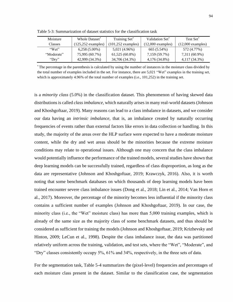
94

is a minority class (5.0%) in the classification dataset. This phenomenon of having skewed data

distributions is called class imbalance, which naturally arises in many real-world datasets (Johnson

and Khoshgoftaar, 2019). Many reasons can lead to a class imbalance in datasets, and we consider

our data having an intrinsic imbalance, that is, an imbalance created by naturally occurring

frequencies of events rather than external factors like errors in data collection or handling. In this

study, the majority of the areas over the HLP surface were expected to have a moderate moisture

content, while the dry and wet areas should be the minorities because the extreme moisture

conditions may relate to operational issues. Although one may concern that the class imbalance

would potentially influence the performance of the trained models, several studies have shown that

deep learning models can be successfully trained, regardless of class disproportion, as long as the

data are representative (Johnson and Khoshgoftaar, 2019; Krawczyk, 2016). Also, it is worth

noting that some benchmark databases on which thousands of deep learning models have been

trained encounter severe class imbalance issues (Dong et al., 2018; Lin et al., 2014; Van Horn et

al., 2017). Moreover, the percentage of the minority becomes less influential if the minority class

contains a sufficient number of examples (Johnson and Khoshgoftaar, 2019). In our case, the

minority class (i.e., the “Wet” moisture class) has more than 5,000 training examples, which is

already of the same size as the majority class of some benchmark datasets, and thus should be

considered as sufficient for training the models (Johnson and Khoshgoftaar, 2019; Krizhevsky and

Hinton, 2009; LeCun et al., 1998). Despite the class imbalance issue, the data was partitioned

relatively uniform across the training, validation, and test sets, where the “Wet”, “Moderate”, and

“Dry” classes consistently occupy 5%, 61% and 34%, respectively, in the three sets of data.

For the segmentation task, Table 5-4 summarizes the (pixel-level) frequencies and percentages of

each moisture class present in the dataset. Similar to the classification case, the segmentation

Table 5-3: Summarization of dataset statistics for the classification task

Moisture

Classes

Whole Dataset*

(125,252 examples)

Training Set*

(101,252 examples)

Validation Set*

(12,000 examples)

Test Set*

(12,000 examples)

“Wet” 6,258 (5.00%) 5,021 (4.96%) 665 (5.54%) 572 (4.77%)

“Moderate” 75,995 (60.7%) 61,525 (60.8%) 7,159 (59.7%) 7,311 (60.9%)

“Dry” 42,999 (34.3%) 34,706 (34.3%) 4,176 (34.8%) 4,117 (34.3%)

* The percentage in the parenthesis is calculated by using the number of instances in the moisture class divided by

the total number of examples included in the set. For instance, there are 5,021 “Wet” examples in the training set,

which is approximately 4.96% of the total number of examples (i.e., 101,252) in the training set.

95

examples also encounter the class imbalance issue, where the “Wet”, “Moderate”, and “Dry”

classes occupy approximately 6%, 58% and 36%, respectively, in the training, validation and test

sets. Additional attention should be paid when tracking the model performance because a model

that identifies all the pixels as “Moderate” moisture class can still achieve a pixel-wise accuracy

of approximately 58%. As shown in Table 5-5, approximately 59% of the rasters contained two

moisture classes, while 36% of the segmentation examples involve only one class, and 5% of the

data include all three classes simultaneously. These statistics imply that the moisture distribution

across the HLP surface is not overall uniform. Most areas over the HLP surface have moisture

contents vary from one class to another even within the small surface area represented by one

raster. Nevertheless, the variations in moisture classes within individual rasters are actually

beneficial for training segmentation models since they provide more contextual information than

those data involving only one class per example (Lin et al., 2014).

In summary, the data preparation process converted the 24 image sets (i.e., the raw data) into one

classification and one segmentation dataset, which were used for the development of convolutional

neural networks. The entire process took approximately 300 hours for someone who possessed

familiarities with the software and programming language used. The data preparation was arguably

the most time-consuming and labour-intensive part in this study, and future works will devote to

automate the process with intents to minimize human intervention and increase workflow

efficiency.

Table 5-4: Summarization of dataset statistics for the segmentation task

Moisture

Classes

Whole Dataset

(128.3 M pixels)

Training Set

(103.7 M pixels)

Validation Set

(12.3 M pixels)

Test Set

(12.3 M pixels)

“Wet” 6.04% 6.00% 6.61% 5.81%

“Moderate” 58.5% 58.6% 57.7% 58.8%

“Dry” 35.4% 35.4% 35.7% 35.4%

Table 5-5: Frequency and percentage of the number of classes contained per segmentation example*

Number of

classes present

Whole Dataset

(31,313 examples)

Training Set

(25,313 examples)

Validation Set

(3,000 examples)

Test Set

(3000 examples)

One class 11,289 (36.1%) 9,159 (36.2%) 1,057 (35.2%) 1,073 (35.8%)

Two classes 18,448 (58.9%) 14,889 (58.8%) 1,792 (59.7%) 1,767 (58.9%)

Three classes 1,576 (5.03%) 1,265 (5.00%) 151 (5.03%) 160 (5.33%)

* On average the segmentation dataset contains 1.7 classes per example.

96

5.3 Classification-Based Heap Leach Pad Surface Moisture Mapping

In this section, we introduce our methodology for using CNN-based moisture classifiers to

generate moisture maps for the studied HLP. We first define the three CNN architectures that we

employed in the experiment, followed by providing the implementation details of the model

training and model evaluation process. We end the section with a description of the workflow that

we adopted to generate the moisture maps, where a brief conclusion about the performance of our

method is included. To the best of our knowledge, not much attention in the literature has been put

on leveraging the power of CNNs to perform HLP surface moisture mapping. Therefore, the focus

of this section is to showcase how a CNN classifier can be incorporated into the moisture map

generation workflow and to study the behaviours and performances of the proposed method.

5.3.1 Network Architectures

Convolutional neural networks have become the most prominent solution for the image

classification task in recent years, demonstrating superhuman performance in real-world

applications (He et al., 2015; Rawat and Wang, 2017). While lots of breakthroughs have been

made in the past decade (Ciresan et al., 2011; He et al., 2016a; Howard et al., 2017; Krizhevsky

et al., 2012; Sermanet et al., 2013), exploring powerful and efficient architectures of CNNs remains

as an active area of research nowadays (Howard et al., 2019; Sandler et al., 2018; Tan and Le,

2019; Zhang et al., 2020). Among the vast number of proposed CNN models in the literature, we

employed three well-studied architectures, AlexNet (Krizhevsky et al., 2012), ResNet (He et al.,

2016a), and MobileNetV2 (Sandler et al., 2018), to study their behaviours when using the prepared

data as inputs to perform a moisture classification task. The trained models were further used to

produce moisture maps for the HLP, and their performances were compared against each other.

AlexNet was first proposed by Krizhevsky, Sutskever and Hinton in 2012, which has

revolutionized the field of computer vision and is one of the key contributors to the recent

renaissance of neural networks (Krizhevsky et al., 2012; Rawat and Wang, 2017). AlexNet and its

variants have been extensively used as base models in many research studies (Rawat and Wang,

2017; Wang et al., 2018). In this work, we employ a modified version of AlexNet to learn the

correlation between the raster input and the moisture class output. The network architecture

contains eight layers with weights, where the first five layers are convolutional, and the reminders

97

are three fully-connected (FC) layers. There are also two max pooling layers without weights

involved in the architecture to downsample the intermediate feature maps (a.k.a. activation maps).

The modified version of AlexNet is graphically depicted in Figure 5-9. The inputs to the models

are the 32 × 32 × 4 (height × width × channels) raster data in the classification dataset (see

Section 5.2.4). All of the convolutional layers in the network adopt 3 × 3 kernels with a stride of

one. The first and the second layers do not use zero padding to adjust the layer’s input dimension,

whereas the third to the fifth convolutional layers adopt a zero padding to ensure that the layer’s

input and output have the same height and width. Max pooling layers with 2 × 2 non-overlapping

windows and a stride of two are used to downsample the feature maps such that the height and

width become one half after each pooling operation. The last three layers are FC layers, where the

first two have 1024 neurons each, and the final layer is a three-way FC layer with softmax. The

final output of the network is a 3 × 1 vector containing the predicted probabilities for each of the

three moisture classes (i.e., “Wet”, “Moderate”, and “Dry”). The ReLU activation function is

applied in all convolutional and fully-connected layers except for the output in which a softmax is

used (Krizhevsky et al., 2012). The dimensionalities of the intermediate feature maps are clearly

Figure 5-9: The modified AlexNet architecture employed in this study. The input to the network has a

dimension of 32 × 32 × 4 (height × width × channels), and the output is a 3 × 1 vector containing the

corresponding probabilities for each of the three moisture classes. The numbers in the figure indicate

the corresponding dimension of the input, feature maps and output; while “Conv 3×3” represents a

convolutional layer with a kernel size of 3 × 3; “Max pool 2×2” indicates a max pooling layer operating

with 2 × 2 non-overlapping windows; “Fully connected” means a fully-connected layer; letter “s” stands

for stride; and letter “p” denotes the number of zeros padded to each side of feature maps.

98

labelled in Figure 5-9, and the whole network includes 17.2 million parameters, which are all

trainable entries.

ResNet (or Residual Network) is another groundbreaking architecture proposed by He et al.

(2016a) that has significantly improved the performance of CNNs in image recognition tasks (i.e.,

classification, detection, segmentation). Many advanced models are developed and fostered based

on the ideas and concepts introduced by ResNet (Alom et al., 2019; Khan et al., 2020). One

important reason for the network’s popularity is that ResNet simultaneously addresses two critical

challenges during the training of CNNs: vanishing/exploding gradients and degradation. He et al.

(2016a) addressed the vanishing/exploding gradients problem by 1) employing a normalized

weight initialization technique, and 2) using batch normalization extensively in the network (He

et al., 2015; Ioffe and Szegedy, 2015). By doing so, information can effectively flow through the

network in both forward and backward directions, and the model can converge by using stochastic

gradient descent (SGD) with backpropagation (He et al., 2016a). However, the degradation

problem makes the training of deep CNN difficult. The network performance starts saturating and

then degrades as more layers are directly stacked over each other in the architecture. Such

degradation is undesirable because deeper models (i.e., more layers stacked together) should result

in greater capacity and are expected to obtain better performance than the shallower ones (He et

al., 2016a; Simonyan and Zisserman, 2014; Szegedy et al., 2015).

To address the degradation problem, He et al. (2016a) introduced a deep residual learning

framework. A basic building block of residual learning with convolutional layers is shown in

Figure 5-10(b). In this framework, the residual block includes a shortcut connection that skips two

convolutional layers and performs an identity mapping. One copy of the input first passes through

the two stacked convolutional layers, followed by adding another copy of the input from the

shortcut to generate the final output. The ReLU activation function is used for introducing

nonlinearity to the process. As a comparison, Figure 5-10(a) shows a block in a plain network

without a shortcut connection. The notion of residual learning has been found quite useful for

training deep neural networks, where He et al. (2016a, 2016b) demonstrated that a network with

more than one thousand layers could be successfully trained with residual learning (Alom et al.,

2019; Khan et al., 2020).

99

In practice, deploying deep networks requires a significant amount of computational power and

computer memory. Training a network made of a stack of multiple residual blocks shown in Figure

5-10(b) can require long training time. Therefore, He et al. (2016a) proposed a bottleneck design

of the residual block to make the training of ResNet less computationally expensive. Figure 5-11

provides a comparison example between an original residual block and the bottleneck design (He

et al., 2016a). As shown in Figure 5-11, the original residual unit consists of two convolutional

layers with 3 × 3 kernels. In contrast, the bottleneck residual unit replaces the two convolutional

layers with three layers: a 1 × 1 layer for dimension reduction, a 3 × 3 layer of regular

convolution, and a 1 × 1 layer for dimension restoration (He et al., 2016b). Such a bottleneck

design can result in a more efficient training process, and thus it is used in our experiment.

In this study, we employ a 50-layer ResNet (ResNet50) architecture, which is one of the most

widely used versions of the network in practical applications (Alom et al., 2019). Overall,

ResNet50 consists of 50 layers with weights, including 49 convolutional layers and one FC layer.

There is also one max pooling and one global average pooling layer, which does not have trainable

entries. Batch normalization is used after every convolutional layer, and the ReLU nonlinearity is

used as the activation function except for the output layer. The architecture of ResNet50 is

summarized in Table 5-6, and the final output of the network is a 3 × 1 vector containing the

predicted probabilities for each of the three moisture classes. The network includes 23.6 million

parameters consisting of 23.5 million trainable and 53 thousand non-trainable parameters.

Figure 5-10: (a) A plain convolutional (Conv) block with two Conv layers. (b) A basic building block

of residual learning. The ⊕ symbol denotes an element-wise addition operation. In this case, the

shortcut connection performs identity mapping. Modified based on He et al. (2016a).

100

The last network that we have adopted is MobileNetV2 proposed by Sandler et al. (2018). As

mentioned previously, modern state-of-the-art CNNs have demonstrated their abilities to surpass

human-level performance in visual recognition tasks. Nevertheless, many of these networks

require high computational resources, and they are not compatible with portable devices, such as

on-board computers or smartphones, especially when real-time performance is desired (Howard et

Figure 5-11: (a) An original residual block (b) A bottleneck residual block. The ⊕ symbol denotes an

element-wise addition operation. In this case, the shortcut connection performs identity mapping. BN

stands for batch normalization. Modified based on He et al. (2016a).

Table 5-6: Architecture of ResNet50 (He et al., 2016a)

Layer/block Name Layer/block output dimension ResNet50*

Input 32 × 32 × 4 -

Conv1 16 × 16 × 64 7 × 7, 64, stride 2

Conv2_x 8 × 8 × 256

3 × 3 max pool, stride 2

[1 × 1, 643 × 3, 64

1 × 1, 256] × 3

Conv3_x 4 × 4 × 512 [1 × 1, 1283 × 3, 1281 × 1, 512

] × 4

Conv4_x 2 × 2 × 1024 [1 × 1, 2563 × 3, 256

1 × 1, 1024] × 6

Conv5_x 1 × 1 × 2048 [1 × 1, 5123 × 3, 512

1 × 1, 2048] × 3

FC 1 × 1 × 3 global average pool, three-way FC, softmax

* Each square bracket represents a bottleneck residual block, with the numbers of block stacked. Every row in a

bracket denotes one layer of operation. For instance, “7 × 7, 64, stride 2” means a convolution operated with 64

kernels, where each kernel has a size of 7 × 7, and the convolutional operations are operated with a stride of two.

Batch normalization is applied after every convolutional operation. Downsampling is performed in Conv3_1,

Conv4_1, and Conv5_1 with a stride of two.

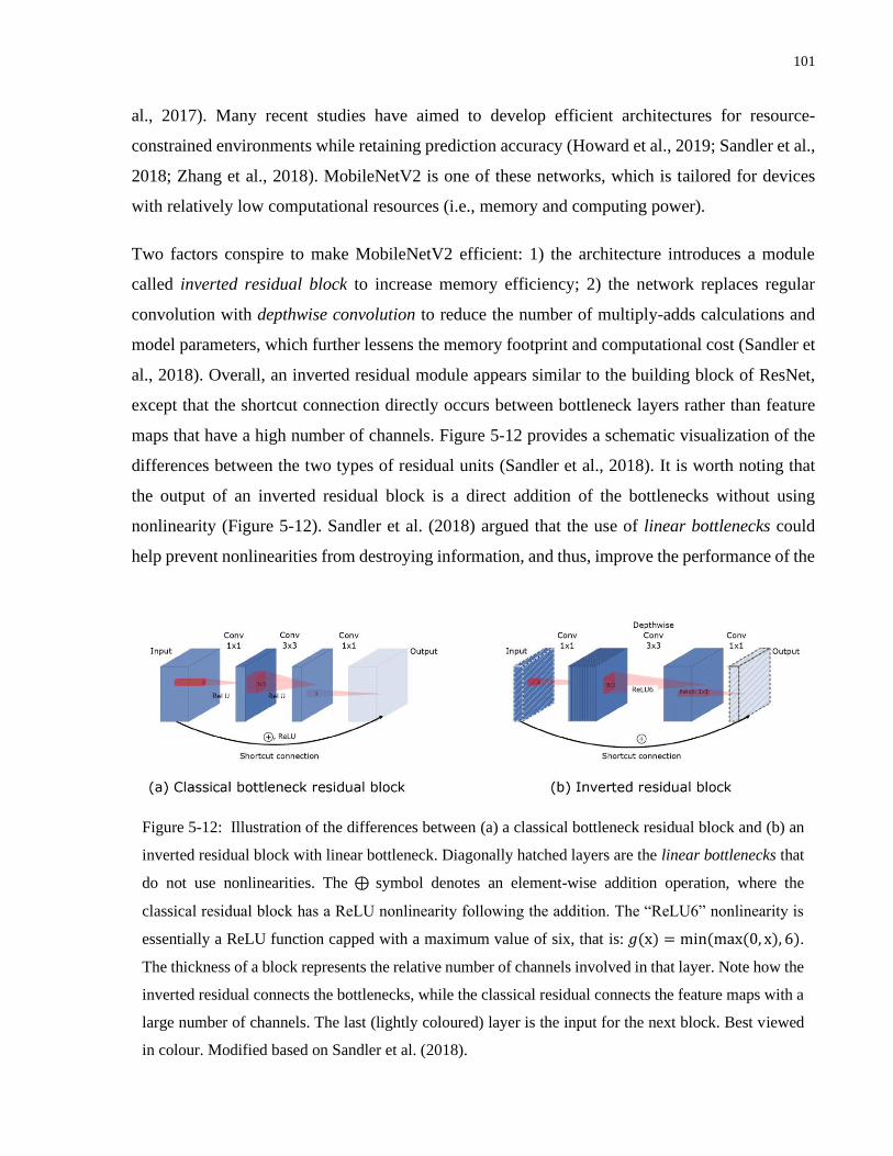
101

al., 2017). Many recent studies have aimed to develop efficient architectures for resource-

constrained environments while retaining prediction accuracy (Howard et al., 2019; Sandler et al.,

2018; Zhang et al., 2018). MobileNetV2 is one of these networks, which is tailored for devices

with relatively low computational resources (i.e., memory and computing power).

Two factors conspire to make MobileNetV2 efficient: 1) the architecture introduces a module

called inverted residual block to increase memory efficiency; 2) the network replaces regular

convolution with depthwise convolution to reduce the number of multiply-adds calculations and

model parameters, which further lessens the memory footprint and computational cost (Sandler et

al., 2018). Overall, an inverted residual module appears similar to the building block of ResNet,

except that the shortcut connection directly occurs between bottleneck layers rather than feature

maps that have a high number of channels. Figure 5-12 provides a schematic visualization of the

differences between the two types of residual units (Sandler et al., 2018). It is worth noting that

the output of an inverted residual block is a direct addition of the bottlenecks without using

nonlinearity (Figure 5-12). Sandler et al. (2018) argued that the use of linear bottlenecks could

help prevent nonlinearities from destroying information, and thus, improve the performance of the

Figure 5-12: Illustration of the differences between (a) a classical bottleneck residual block and (b) an

inverted residual block with linear bottleneck. Diagonally hatched layers are the linear bottlenecks that

do not use nonlinearities. The ⊕ symbol denotes an element-wise addition operation, where the

classical residual block has a ReLU nonlinearity following the addition. The “ReLU6” nonlinearity is

essentially a ReLU function capped with a maximum value of six, that is: 𝑔(x) = min(max(0, x), 6).

The thickness of a block represents the relative number of channels involved in that layer. Note how the

inverted residual connects the bottlenecks, while the classical residual connects the feature maps with a

large number of channels. The last (lightly coloured) layer is the input for the next block. Best viewed

in colour. Modified based on Sandler et al. (2018).

102

trained models. It has been shown that the use of inverted residual block can result in memory-

efficient models while maintaining the prediction accuracy. Furthermore, MobileNetV2 uses

depthwise convolutions and 1 × 1 convolutions (a.k.a. pointwise convolution) extensively in the

network. This significantly reduces the number of mathematical operations and the number of

trainable weights as compared to the use of regular convolution (Howard et al., 2017; Ye et al.,

2019). Sandler et al. (2018) and Bai et al. (2018) provided detailed calculations quantifying the

amount of computational resources required by the three types of convolutional layers. Figure 5-13

provides a visual comparison between the regular convolution, depthwise convolution, and

pointwise convolution (Bai et al., 2018) .

In this study, a modified version of MobileNetV2 was employed to make the model compatible

with our input rasters. We modified the network to have a shallower depth (i.e., fewer layers) than

the original architecture. The modification is made because the prepared classification examples

have a height and width of 32 pixels, which is smaller than the input of the original model (224

pixels). Directly using the original architecture would shrink the size of intermediate feature maps

to have a width and height of one pixel before reaching the output layer. This could be suboptimal

because we have observed that the network performance deteriorates if the size of feature maps

become smaller than 4 × 4 (see Section 5.3.3). The deterioration may be due to the kernel size (3

× 3) used by the network, which means padding would be needed in order to perform the

convolution when a feature map has a small height and width. For instance, if we perform a 3 × 3

convolution over a 2 × 2 feature map, then five zeros (or other artificial values) would be padded

at the perimeter of the feature map. Note that the feature map has only four pixels in total, which

means the convolution would be performed over mostly artificial numbers. To avoid the

intermediate feature maps becoming too small, we reduced the number of inverted residual blocks

used by the original architecture and stopped stacking residual module when the feature maps have

a height and width of four pixels.

The architecture of the modified MobileNetV2 is summarized in Table 5-7, and the final output of

the network is a 3 × 1 vector containing the predicted probabilities for each of the three moisture

classes. Overall, the modified MobileNetV2 architecture starts with a regular 3 × 3 convolution

with 32 filters, followed by six inverted residual blocks, and ends with a global average pooling, a

three-way fully-connected layer, and a softmax. Note that the inverted residual blocks with

different stride values have different inner structures. For “Block1” to “Block5” (excluding

103

“Block0”) in Table 5-7, the stride of each block is provided in the last column of the table, and the

corresponding inner structures are depicted in Figure 5-14. The network has 109 thousand

parameters in total, which includes 103 thousand trainable and six thousand non-trainable

parameters. It is worth noting that this model is considered small (in terms of the number of

parameters involved) in modern practice, but we have observed that the network’s performance is

comparable to ResNet50 and consistently better than AlexNet on the prepared dataset.

Figure 5-13: Comparison between (a) regular convolution, (b) depthwise convolution and (c) pointwise

convolution. In the figure, symbol ⊛ represents a convolutional operator; K denotes the kernel size; H,

W, and D are the height, width and depth of the input, respectively; and Dout is the number of channels

of the output feature maps, which is equal to the depth of the input, D, in this case. Best viewed in

colour. Modified based on Bai et al. (2018).

104

Figure 5-14: : Inner structure of the inverted residual blocks in the modified MobileNetV2 architecture.

(a) Inverted residual block with stride of one. (b) Block with stride of two. The shortcut connection

performs identity mapping. BN stands for batch normalization. Dwise means depthwise convolution.

Table 5-7: The modified MobileNetV2 architecture employed in this study

Layer/block name Layer/block output dimension Operator* Stride for 3 × 3

Convolution

Input 32 × 32 × 4 - -

Conv1 16 × 16 × 32 3 × 3, 32 2

Block0 16 × 16 × 16 [1 × 1, 32

3 × 3 Dwise, 321 × 1, 16

] 1

Block1 8 × 8 × 24 [1 × 1, 96

3 × 3 Dwise, 961 × 1, 24

] 2

Block2 8 × 8 × 24 [1 × 1, 144

3 × 3 Dwise, 1441 × 1, 24

] 1

Block3 4 × 4 × 32 [1 × 1, 144

3 × 3 Dwise, 1441 × 1, 32

] 2

Block4 4 × 4 × 32 [1 × 1, 192

3 × 3 Dwise, 1921 × 1, 32

] 1

Block5 4 × 4 × 32 [1 × 1, 192

3 × 3 Dwise, 1921 × 1, 32

] 1

Conv2 4 × 4 × 1280 1 × 1, 1280 1

FC 1 × 1 × 3 avg. pool, three-way FC, softmax -

* Each square bracket represents an inverted residual block. Every row in the bracket denotes one layer of operation. For

instance, “3 × 3 Dwise, 32” means a 3 × 3 depthwise convolution operated with 64 kernels. The “avg. pool, three-way

FC, softmax” refers to a global average pooling, followed by a three-way fully-connected layer with softmax. Batch

normalization is applied after every convolutional operation, including regular, depthwise and pointwise convolution.

105

5.3.2 Training Setup

We implemented all three networks in TensorFlow 2 (TF) and deployed model training using

TensorFlow’s Keras API (Abadi et al., 2016; Chollet et al., 2015). All models were trained from

scratch using RMSProp optimizer with a learning rate of 0.001, a momentum of zero, and a decay

(named rho in TF) of 0.9 (Hinton et al., 2012). There was no extra learning rate decay used during

the training, and the cross-entropy loss (named sparse categorical crossentropy in TF) was used

as the loss function. We normalized the training data to have zero mean and unit standard deviation

for every channel. The normalization started with calculating the per-channel means of the whole

training set (i.e., four mean values for the entire training set, one for each channel), followed by

subtracting every training example by the per-channel means. After obtaining the zero-mean data,

we calculated the per-channel standard deviations (i.e., four values, one for each channel) and

ended the normalization process by using every training example to divide the per-channel

standard deviations. We did not perform any data augmentation during the training process

because we considered the number of rasters in our training set (101,252 examples) sufficient for

training classifiers for only three classes. The training set statistics (i.e., the means and standard

deviations) were also used to normalize the validation and testing data following the

abovementioned procedure (He et al., 2016a; Simonyan and Zisserman, 2014) .

We included dropout with a dropout probability of 0.5 in the first two FC layers of the modified

AlexNet architecture, whereas there was no batch normalization (BN) used in the network

(Krizhevsky et al., 2012). In contract, no dropout was used in the ResNet50 architecture, but we

adopted BN with a momentum of 0.99 right after every convolution and before activation (He et

al., 2016a). Similarly, we did not adopt dropout for the modified MobileNetV2, while BN with a

momentum of 0.999 was applied after every convolutional operation including regular, depthwise

and pointwise convolution (Sandler et al., 2018).

To train a model, we started with initializing the model using the Kaiming initialization proposed

by He et al. (2015). We then trained the model for 20 epochs with a minibatch size of 68 examples.

It is worth noting that the training set contained 101,252 examples which can be divided by 68

with no remainder. In this way, each epoch consisted of 1489 steps (or iterations), where each step

was for one minibatch. After completing the 20 epochs of training, the trained model was examined

106

against the validation set, and the validation accuracy was used to represent the prediction accuracy

of that model.

In order to conduct a fair comparison regarding the performance of the three employed

architectures, we trained 30 copies of each network (i.e., 30 models for each architecture, 90

models in total) with different initialization of the network parameters. Since different initialization

for the weights of a network can lead to variations in the model performance, we chose the one

(out of 30) that resulted in the best prediction accuracy on the validation set to be the final model.

In this way, there were three final models determined (one for each architecture) based on their

performances on the validation set. We then evaluated the three final models on the test set to

compare the three architectures’ classification accuracy. It is important to note that we did not use

any ensemble technique to combine multiple models together in this study.

Since the Kaiming initialization randomly samples model weights from a zero-mean (truncated)

Gaussian distribution (He et al., 2015), the model will have a different initial state after each

initialization process. To improve the reproductivity of our training results, we explicitly defined

30 seeds1 for the random number generator in TF to initialize the 30 models for each architecture

(i.e., one seed for one model). The same list of seeds was used for all three architectures, such that

the initialization of weights can be reproduced.

The model training was carried out on a “workstation” computer, while the development and

coding were performed on a “laptop” computer. Table 5-8 provides a comparison between the

specifications of the laptop and workstation computers. It is worth noting that the ResNet50

architecture could not be efficiently trained on the laptop computer due to its large memory

footprint, while both the modified AlexNet and MobileNetV2 could be trained on the laptop with

the setup described above. Training of the modified AlexNet, ResNet50, and modified

MobileNetV2 on the workstation computer required approximately 7 hours, 20 hours, and 8 hours,

respectively, for 600 epochs (i.e., 20 epochs per model × 30 models per architecture).

1 The list of random seeds for model initialization: {0, 4, 5, 9, 40, 44, 45, 49, 50, 54, 55, 59, 90, 94, 95, 99, 400, 444, 459, 499, 500, 540, 549, 550,

599, 900, 949, 959, 995, 999}.

107

5.3.3 Model Evaluation

The training curves of the networks are shown in Figure 5-15. The classification accuracy of the

models on the training and validation sets was recorded after each epoch of training. Each solid

line in Figure 5-15(a) is a curve of mean training accuracy, determined by averaging the prediction

accuracy of the 30 models with the same network architecture. Similarly, every curve in Figure

5-15(b) represents the mean classification accuracy on the validation examples for the models with

the same architecture. The shaded regions in Figure 5-15(a) indicate the ranges of training accuracy

for the three networks, where the upper and lower bounds of the shaded areas are the maximum

and minimum accuracy values that were resulted from the models. The ranges of validation

accuracy for the three network architectures significantly overlapped with each other and thus are

not shown in Figure 5-15(b).

Overall, we have five major observations from Figure 5-15. First, the modified MobileNetV2 and

ResNet50 models that we have trained possess an ability to fit the training data better than the

modified AlexNet models. The former two architectures consistently resulted in higher training

accuracy than the modified AlexNet. This result is expected because several studies have shown

that ResNet and MobileNetV2 generally have better performance than AlexNet (Canziani et al.,

2016; Howard et al., 2017; Khan et al., 2020). Second, we observe that although performances on

the training set vary among the three architectures, all models were able to converge, and more

importantly, they could fit the training set at a high classification accuracy (higher than 97% as

shown in Figure 5-15(a)). Third, the range of accuracy for the modified AlexNet in Figure 5-15(a)

appears wider than the other two architectures. One possible reason for this phenomenon is because

we have included dropout in the modified AlexNet but not in the modified MobileNetV2 and

ResNet50 models. The randomness introduced by dropout during the training process could result

Table 5-8: Comparison of computer specifications

Component Workstation Laptop

Central processing unit

(CPU)

Intel Core i9 12-Core/24-Thread

Processor, 2.90 GHz Base/4.3 GHz

Max Turbo

Intel(R) Core(TM) i7-7700HQ CPU

@ 2.80GHz

Graphics processing unit

(GPU) NVIDIA RTX 2080 Ti 11 GB NVIDIA GeForce GTX 1050 Ti 4 GB

DDR RAM 64 GB 16 GB

108

in some misclassification by the modified AlexNet models on the training examples. Fourth, we

can conclude that, on average, the trained models are generalizable to the validation data. As shown

in Figure 5-15(b), the models from all three architectures were able to achieve a validation

accuracy close to the training accuracy. The high generalization ability of the trained models may

imply that the data in the training and validation sets have a similar distribution, and thus the

features learned from the training examples can be well generalized to the validation rasters.

Last, we notice that the modified MobileNetV2 performed marginally better than the ResNet50

models on the dataset. However, it is important to note that the training curves are not supportive

evidence for arguing that the modified MobileNetV2 is a better network architecture than

ResNet50. The results only imply that our training data can be better fitted by the modified

MobileNetV2 models given the specific training setup and data preparation process described in

previous sections. Moreover, the small height and width of the intermediate feature maps could

have impacted the ResNet50 models’ performance on our dataset. As shown in Table 5-6, the

feature maps are shrunk to 1 × 1 (height × width) before reaching the output layer, and the loss of

spatial information may have led to a deterioration of network performance. Since ResNet was

Figure 5-15: Training curves of the modified AlexNet (blue), ResNet50 (green), and the modified

MoblieNetV2 (red). (a) Training accuracy of the three networks. Each solid line represents the mean

training accuracy of the 30 models with the same architecture. The upper and lower bounds of the shaded

areas are the maximum and minimum training accuracy among the 30 models, respectively. (b) Mean

prediction accuracy on the validation set of the three networks. Each line was determined by averaging

the validation accuracy of the 30 models with the same architecture. The validation accuracy of the first

and second epoch for the modified MobileNetV2 were 60% and 79%, respectively.

109

initially proposed for images with higher resolutions (e.g., 224 × 224) than our data (32 × 32),

future studies may incorporate rasters with higher resolution or adopt some padding techniques to

avoid the intermediate feature maps in the network becoming too small in size.

To further explore the influence of height and width of intermediate feature maps on the model

performance, we compared our modified MobileNetV2 architecture with two other versions of the

network: (A) a version that shrinks the feature maps to 1 × 1 (height × width) before reaching the

output layer; and (B) a version that has a minimum size of intermediate feature map of 2 × 2. Table

5-9 and Table 5-10 summarize the two network architectures, and we denote A and B as

MobileNetV2 A and MobileNetV2 B, respectively, in the remainder of this section. As shown in

Table 5-9 and Table 5-10, MobileNetV2 A and MobileNetV2 B are both deeper and have more

parameters than the network that we have employed (Table 5-7), while all three versions are

constructed based on the same inverted residual blocks (Figure 5-14). We trained 30 models for

each of the MobileNetV2 A and B following the same setup described in Section 5.3.2. In general,

the two deeper networks should result in higher training accuracy (i.e., less misclassification on

the training examples) than our shallower version due to their stronger representational abilities

(He et al., 2016a).

However, as depicted in Figure 5-16, MobileNetV2 A and B consistently performed worse than

our version on both the training and validation sets. Also, the ranges of prediction accuracy for A

and B were wider than our version, which indicates that they were more sensitive to initialization

and less stable in performance. Besides, we observed that MobileNetV2 A, which is the deepest

but shrinks the feature maps to 1 × 1 (height × width), had the worst classification accuracy. As

already mentioned in Section 5.3.1, many studies have shown that batch normalization and residual

learning can effectively address the vanishing/exploding gradient and degradation problems (He

et al., 2016a; Ioffe and Szegedy, 2015; Santurkar et al., 2018). The three architectures involved in

the comparison all used BN and inverted residual blocks extensively. Hence, the deterioration of

the two deeper networks’ performance should not be caused by the vanishing gradient or

degradation problem. We consider that the small size of intermediate feature maps for A and B

may have led to a significant loss of local and global spatial information during the forward

information flow, which is one of the crucial contributors to the reduced performance from

MobileNetV2 A and B. Therefore, we employed the modified MobileNetV2 described in Section

5.3.1 in our analysis presented below.

110

Table 5-9: Network architecture of MobileNetV2 A*

Layer/block name Layer/block output dimension Operator** Stride for 3 × 3

Convolution

Input 32 × 32 × 4 - -

A_Conv1 16 × 16 × 32 3 × 3, 32 2

A_Block0 16 × 16 × 16 [1 × 1, 32

3 × 3 Dwise, 321 × 1, 16

] 1

A_Block1 8 × 8 × 24 [1 × 1, 96

3 × 3 Dwise, 961 × 1, 24

] 2

A_Block2 8 × 8 × 24 [1 × 1, 144

3 × 3 Dwise, 1441 × 1, 24

] 1

A_Block3 4 × 4 × 32 [1 × 1, 144

3 × 3 Dwise, 1441 × 1, 32

] 2

A_Block4 4 × 4 × 32 [1 × 1, 192

3 × 3 Dwise, 1921 × 1, 32

] × 2 1

A_Block5 2 × 2 × 64 [1 × 1, 192

3 × 3 Dwise, 1921 × 1, 64

] 2

A_Block6 2 × 2 × 64 [1 × 1, 384

3 × 3 Dwise, 3841 × 1, 64

] × 3 1

A_Block7 2 × 2 × 96 [1 × 1, 384

3 × 3 Dwise, 3841 × 1, 96

] 1

A_Block8 2 × 2 × 96 [1 × 1, 576

3 × 3 Dwise, 5761 × 1, 96

] × 2 1

A_Block9 1 × 1 × 160 [1 × 1, 576

3 × 3 Dwise, 5761 × 1, 160

] 2

A_Block10 1 × 1 × 160 [1 × 1, 960

3 × 3 Dwise, 9601 × 1, 160

] × 2 1

A_Block11 1 × 1 × 320 [1 × 1, 960

3 × 3 Dwise, 9601 × 1, 320

] 1

A_Conv2 1 × 1 × 1280 1 × 1, 1280 1

A_FC 1 × 1 × 3 avg. pool, three-way FC, softmax -

* This network has 2.26 million parameters, where 2.23 million are trainable and 34 thousand are non-trainable.

** Each square bracket represents an inverted residual block. Every row in the bracket denotes one layer of

operation. For instance, “3 × 3 Dwise, 32” means a 3 × 3 depthwise convolution operated with 64 kernels. The

“avg. pool, three-way FC, softmax” refers to a global average pooling, followed by a three-way fully-connected layer

with softmax. Batch normalization is applied after every convolutional operation, including regular, depthwise

and pointwise convolution.

111

For each of the modified AlexNet, ResNet50 and modified MobileNetV2, we compared the

validation accuracy of the 30 trained models and chose the one with the highest accuracy to be the

final model (i.e., three models, one from each architecture). The box plots in Figure 5-17

summarize the model performance on the validation set after 20 epochs of training. Each box plot

represents the accuracy of the 30 models with the same architecture, except that one model (with

a validation accuracy of 92.1%) for ResNet50 was considered an outlier and excluded from the

box plot. The best classifiers for the modified AlexNet, ResNet50, and modified MobileNetV2

Table 5-10: Network architecture of MobileNetV2 B*

Layer/block name Layer/block output dimension Operator** Stride for 3 × 3

Convolution

Input 32 × 32 × 4 - -

B_Conv1 16 × 16 × 32 3 × 3, 32 2

B_Block0 16 × 16 × 16 [1 × 1, 32

3 × 3 Dwise, 321 × 1, 16

] 1

B_Block1 8 × 8 × 24 [1 × 1, 96

3 × 3 Dwise, 961 × 1, 24

] 2

B_Block2 8 × 8 × 24 [1 × 1, 144

3 × 3 Dwise, 1441 × 1, 24

] 1

B_Block3 4 × 4 × 32 [1 × 1, 144

3 × 3 Dwise, 1441 × 1, 32

] 2

B_Block4 4 × 4 × 32 [1 × 1, 192

3 × 3 Dwise, 1921 × 1, 32

] 1

B_Block5 4 × 4 × 32 [1 × 1, 192

3 × 3 Dwise, 1921 × 1, 32

] 1

B_Block6 2 × 2 × 64 [1 × 1, 384

3 × 3 Dwise, 3841 × 1, 64

] × 3 1

B_Block7 2 × 2 × 96 [1 × 1, 384

3 × 3 Dwise, 3841 × 1, 96

] 1

B_Block8 2 × 2 × 96 [1 × 1, 576

3 × 3 Dwise, 5761 × 1, 96

] × 2 1

B_Conv2 2 × 2 × 1280 1 × 1, 1280 1

B_FC 1 × 1 × 3 avg. pool, three-way FC, softmax -

* This network has 691 thousand parameters, where 672 thousand are trainable and 19 thousand are non-trainable. ** Each square bracket represents an inverted residual block. Every row in the bracket denotes one layer of

operation. For instance, “3 × 3 Dwise, 32” means a 3 × 3 depthwise convolution operated with 64 kernels. The

“avg. pool, three-way FC, softmax” refers to a global average pooling, followed by a three-way fully-connected layer

with softmax. Batch normalization is applied after every convolutional operation, including regular, depthwise

and pointwise convolution.

112

had a validation accuracy of 98.3%, 99.1%, and 99.0%, respectively. These three best classifiers

were chosen to be the final models for moisture map generation, and they were also evaluated

against the test set. It is worth noticing that although the modified MobileNetV2 models had the

highest mean and median accuracy, the best performance was achieved by a ResNet50 model,

which correctly classified 99.1% of the validation rasters (i.e., 11,891 out of 12,000 examples were

classified correctly). This variation in model performance reveals the inherent randomness and

uncertainty involved in the model training process.

The performances of the three final models on the test set (12,000 testing examples) are reported

in Table 5-11. The highest classification accuracy was 99.2% from the ResNet50 model.

Nonetheless, the computational time (with a batch size = 1) for the model is approximately three

Figure 5-16: Comparison of learning performance of the modified MobileNetV2 (red), MobileNetV2 A

(magenta), and MobileNetV2 B (cyan) on the training and validation sets. The upper and lower bounds

of the shaded areas are the maximum and minimum values among the 30 models, respectively. Notice

the different scale in y-axes of the two plots. (a) Training accuracy curves of the three architectures.

Each solid line represents the mean training accuracy of the 30 models with the same architecture. (b)

Validation accuracy curves of the three architectures. Best viewed in colour.

Table 5-11: Evaluation results of the final classification models on the test set (12,000 testing examples)

Metrics Modified AlexNet ResNet50 Modified MobileNetV2

Classification Accuracy 98.1% 99.2% 99.0%

Runtime (batch size = 1)

on NVIDIA GeForce

GTX 1050 Ti 4 GB

6 ms/example 17 ms/example 4 ms/example

113

times the modified AlexNet and four times the modified MobileNetV2 on the “laptop” computer

(Table 5-8). The high accuracy came with the cost of long execution time and a large memory

footprint. In contrast, the modified MobileNetV2 model achieved a high prediction accuracy

(99.0%) and the shortest runtime (4 ms/example); thus, provided the best balance between

classification accuracy and computational efficiency.

Figure 5-17: Validation accuracy of the three employed architectures. Each boxplot represents the

distribution of validation accuracy for the 30 models with the same architecture. An outlier (with a

validation accuracy of 92.1%) for the ResNet50 is not shown.

114

5.3.4 Moisture Map Generation

The moisture map generation process consists of three steps, which are graphically summarized in

Figure 5-18. The entire workflow was implemented in Python 3, and there is no human

intervention required after specifying the input raster based on which a moisture map should be

generated. In this study, the inputs to the workflow were the overview rasters of the HLP that had

been produced during the data preparation (see Section 5.2.3). However, the process can be applied

to any input data that fulfill the following requirements. The input of the process should be a four-

channel raster with a height and width of at least 32 pixels. The first three channels of the raster

ought to be red, green, and blue colour channels, respectively, while the fourth should be a

temperature channel. All pixel values contained in the input raster should be floating-point

numbers, where every intensity value in the colour channels should be within the range of [0, 255].

The temperature values in the temperature channel should be expressed in degrees Celsius, and

thus the digital numbers generally fell within the range of 10 to 70 in our case.

Since every overview raster covered a large ground area and had several thousand of pixels for

both height and width, the first step was to subdivide an input raster into non-overlapping tiles

such that each tile corresponds to a small area over the HLP. As mentioned in Section 5.2, the

moisture classifiers were designed for data with an input dimension of 32 × 32 × 4. Therefore,

each raster tile after subdivision had a height and width of 32 pixels. If the size of an input is not

divisible by 32 for either its height, width or both, we omitted the right-most columns and/or

bottom-most rows to avoid resizing and transforming the input during the process such that the

generated moisture map (i.e., the output) had the same GSD as the input raster. In this way, the

number of created raster tiles could be calculated as 𝑁tiles = ⌊𝐻in

32⌋ ∙ ⌊

𝑊in

32⌋ , where ⌊∙⌋ is the floor

operator; Hin and Win are the height and width of the input raster, respectively; and Ntiles is the

number of tiles obtained after the subdivision. Afterwards, the second step of the process was to

use a moisture classification model that had been developed to identify and assign a moisture class

to each tile (Figure 5-18). The CNN classifier used in this procedure could be any one of the three

final models described in Section 5.3.3.

The final step of the workflow was to colour code and combine all the tiles to produce the moisture

map. The colour coding was performed based on the moisture class of a tile, and every pixel within

the same tile was assigned with the same colour. We denoted the “wet” (> 8% moisture content),

115

“moderate” (4% to 8%), and “dry” (< 4%) class by using a blue, greenish, and red colour,

respectively, as shown in Figure 5-18. It is worth noting that the GSD of each raster was

approximately 10 cm/pixel, which means each tile represented an area of 3.2 m × 3.2 m on the

HLP surface. In this way, the colour coding assumed that the moisture status was uniform within

Figure 5-18: Moisture map generation using a convolutional neural network (CNN) classifier.

116

the area covered by each raster tile. Lastly, we arranged all the colour-coded tiles according to

their initial positions in the input raster and combined them to generate the final output. A

comparison example of the generated moisture maps using the modified AlexNet, ResNet50, and

modified MobileNetV2 classifiers is provided in Figure 5-19. The ground-truth moisture maps in

Figure 5-19 were generated by following the same process used to prepare the training, validation,

and testing data (Section 5.2.4). In short, a ground-truth moisture map for an overview raster was

created by first applying equation (4.2) to every digital number in the temperature channel,

followed by performing a threshold operation to categorize the pixels that had an estimated

moisture content greater than 8% to be the “wet” class, those smaller than 4% as the “dry” class,

and the remaining as the “moderate” moisture class.

Overall, we can conclude that HLP surface moisture maps were efficiently and accurately

generated using the CNN-based moisture classifiers. Correlation between the input rasters and

their corresponding moisture classes were effectively learned by the trained networks, where the

error rates were below 2% for the final models. Meanwhile, the three employed CNN architectures

produced comparable results against each other, and only minor differences were observed in the

resultant output. The ResNet50 model achieved the highest classification accuracy, but the

execution time was relatively slow. Both the modified AlexNet and MobileNetV2 models had

short inference time, where the modified MobileNetV2 provided the best balance between

classification accuracy and computational efficiency. However, despite the effectiveness of using

CNN classifiers to identify the average moisture status of a given area, the prediction output from

the classification models was in coarse resolution. It did not preserve sufficient details for depicting

a fine-grained moisture distribution over a local region. As mentioned previously, the workflow

described in Figure 5-18 assumed that the moisture content was constant across the 3.2 m × 3.2 m

area represented by each raster tile. This assumption is acceptable if an overview of a large study

area is required (e.g., the moisture maps for the whole HLP shown in Figure 5-19). Nevertheless,

some monitoring tasks in practice, such as pinpointing malfunctioning sprinklers, may require the

moisture maps to provide information with a sub-meter level resolution. Given the dataset we have,

CNN classifiers are incompetent for such tasks because, by definition, classification performs

coarse inference that makes a prediction for a whole input. To achieve fine-grained inference, we

developed a semantic segmentation model in the next section (Section 5.4) to perform per-pixel

moisture prediction, so that moisture maps with fine details can be generated.

117

Figure 5-19: A comparison of the generated moisture maps using the modified AlexNet, ResNet50, and

modified MobileNetV2 moisture classifiers. The top two lifts moisture maps were generated based on

March 8, Afternoon dataset, and the moisture maps for the whole HLP were created based on March 7,

Morning dataset.

118

5.4 Segmentation-Based Heap Leach Pad Surface Moisture Mapping

This section presents our methodology for using a semantic segmentation CNN to generate fine-

grained moisture maps based on our prepared rasters for the HLP. We first illustrate the semantic

segmentation network that we have adopted in the experiment, followed by elaborating on the

model training and evaluation process. The section ends with depicting the moisture map

generation workflow, while several examples of the generated moisture maps by our method are

also provided.

5.4.1 Network Architecture

Semantic segmentation is a natural step towards fine-grained inference after image classification,

object detection and boundary localization (Garcia-Garcia et al., 2017; Lateef and Ruichek, 2019).

The goal of semantic segmentation is to accurately provide pixel-wise labelling for an input raster

such that the pixels correspond to different objects or regions within the raster can be correctly

classified and localized (Ulku and Akagunduz, 2020). The semantic segmentation task has long

been a hot and challenging topic in computer vision due to its broad range of applications, such as

autonomous robotics (Zhang et al., 2018), medical image analysis (Ronneberger et al., 2015),

ground moisture estimation (Zhang et al., 2020), and agriculture and industrial inspection (Kemker

et al., 2018; Sharifzadeh et al., 2020). Despite the accomplishments that have been achieved by

various traditional techniques (Zaitoun and Aqel, 2015; Ulku and Akagunduz, 2020), CNNs have

demonstrated their ability to surpass the traditional methods by a large margin in prediction

accuracy and sometimes computational efficiency (Garcia-Garcia et al., 2017). There are a large

number of semantic segmentation architectures proposed in the literature, where Lateef and

Ruichek (2019), and Ulku and Akagunduz (2020) provided thorough reviews on the

categorizations of different networks as well as the evolution of semantic segmentation CNNs.

U-Net is a popular semantic segmentation CNN proposed by Ronneberger et al. (2015) that has a

typical encoder-decode structure. The network architecture is comprised of two parts: the encoder

part (also called contracting path or compression stage in the literature) that convolves an input

raster and gradually reduces the spatial size of the feature maps; and the decoder part (also called

expansive path or decompression stage) which gradually recovers the spatial dimension of the

intermediate features and produces an output raster with the same or a similar height and width as

the input (Clement and Kelly, 2018; Ronneberger et al., 2015). The encoder and decoder parts are

119

more or less symmetric, and the network appears as a U shape leading to the name of the

architecture (Ronneberger et al., 2015). Many studies have shown that U-Net-based models can

be used to perform segmentation for different applications, including radio signal processing

(Akeret et al., 2017), image appearance transformation (Clement and Kelly, 2018), vegetation

detection (Ulku et al., 2019), and biomedical image processing (Ronneberger et al., 2015).

In this study, we employ a modified version of the original U-Net to perform pixel-wise moisture

classification over the prepared raster data. Overall, our modified U-Net involves four levels of

depth as shown in Figure 5-20. Every level in the encoding part consists of two 3 × 3 convolutions

(with zero padding and a stride of one), each followed by a ReLU nonlinearity. The downsampling

from one level to the next is performed using a 2 × 2 max pooling with a stride of two such that

the height and width of the feature map are halved after the pooling operation. Within each level

of the encoder part, we double the number of feature channels, and the feature maps at the fourth

level (i.e., the bottom level) have 512 channels (see Figure 5-20). In the decoder part of the

network, every preceding level is connected to the succeeding one through a transposed

convolution (also called up-convolution or sometimes deconvolution in the literature) that halves

the number of channels and doubles the height and width of the feature map. Meanwhile, a skip

connection is used to copy and concatenate the feature map at the same level of the encoder part

to the corresponding upsampled decoder feature so that the model can learn to create well-localized

hierarchical features and assemble precise output (Ronneberger et al., 2015; Ulku and Akagunduz,

2020). Every level of the decoder part consists of two 3 × 3 convolutions (with zero padding and

a stride of one), each followed by a ReLU nonlinearity. To generate the output, we use a 1 × 1

convolution with softmax to map the 64-channel features to the final three-channel feature map,

where each channel contains the predicted probabilities for the corresponding moisture class at

each pixel (i.e., the first channel at a pixel contains the probability for the “dry” class, and the

second and third channels are for the “moderate” and “wet” classes, respectively). The single-

channel segmentation map can then be created by applying a pixel-wise argmax operation over

the three-channel feature such that the moisture class with the highest probability is used to

represent the moisture status at each pixel location. In total, the network has 7.7 million parameters,

which are all trainable entries.

120

Figure 5-20: The modified U-Net architecture employed in this study. There are four levels of depth in

the architecture, where the bottom level is the fourth level, and the input and output are at level one.

Each box represents a multi-channel feature map, and the number of channels is labeled at either top or

bottom of the box. The height × width of the feature maps are denoted at the lower-left corners of the

boxes. The green boxes correspond to the feature maps generated in the encoder part of the network,

where the red boxes belong to the decoder part. The arrows with different colours represent different

operations. For the convolutional operations (Conv), letter “s” and “p” stand for stride and zero padding,

respectively. Best viewed in colour. Modified based on Ronneberger et al. (2015).

121

5.4.2 Training Setup

We implemented our modified U-Net2 in TensorFlow 2 (Abadi et al., 2016), and the models were

trained, evaluated, and tested using the raster data in the segmentation dataset described in Section

5.2. All models were trained from scratch using RMSProp optimizer with a learning rate of 0.001,

a momentum of zero, and a decay of 0.9 (Hinton et al., 2012). We did not use any extra learning

rate decay during the training, and neither dropout nor batch normalization was used in the

network. We normalized the training data to have zero mean and unit standard deviation for every

channel, and the data normalization procedure is described in Section 5.3.2. We did not perform

any data augmentation during the training process because we considered our training set (25,313

training examples) sufficiently large to train a semantic segmentation CNN.

Similar to the training setup for the classification models (Section 5.3.2), we trained 30 models of

our modified U-Net in which each model has a different initialization of the network parameters.

We initialized the models using the Kaiming initialization (He et al., 2015), where each

initialization adopted a designated seed for the random number generator in TF (i.e., one seed for

one model). The 30 seeds that were used for the model initialization is provided in Section 5.3.2.

Since models with different initialization resulted in different prediction accuracy, we selected the

one that returned the best performance on the validation set to be the final model, and the final

model was evaluated against the test set. We trained each model for 20 epochs with a minibatch

size of 32 and used the cross-entropy loss (sparse categorical crossentropy in TF) as the loss

function. The model training was carried out on the “workstation” computer with an NVIDIA RTX

2080 Ti 11 GB GPU (Table 5-8), and the training for the 30 models took approximately 12.5 hours

in total (i.e., 25 mins for every 20 epochs).

5.4.3 Model Evaluation

In this study, we adopted two commonly used accuracy metrics for semantic segmentation, Pixel

Accuracy (a.k.a. global accuracy) and Mean Intersection over Union (MIoU), to assess the trained

models. Pixel accuracy is a simple metric that calculates the ratio between the number of correctly

2 Our implementation was modified mainly based on https://github.com/zhixuhao/unet and https://github.com

/jakeret/unet, whilst the original implementation by Ronneberger et al. (2015) was in Caffe and is available at

https://lmb.informatik.uni-freiburg.de/people/ronneber/u-net/.

122

classified pixels and the total number of pixels (Garcia-Garcia et al., 2017; Ulku and Akagunduz,

2020). The formula of pixel accuracy is defined as

𝑃𝐴 =

∑ 𝑛𝑖𝑖𝑁cls𝑖=1

𝑁pixel, (5.1)

where PA is the pixel accuracy expressed in percentage; 𝑁cls is the total number of the classes,

which is equal to three in our case for the three moisture classes; 𝑛𝑖𝑖 denotes the number of pixels

that are both predicted and labelled as the ith class (i.e., true positive, TP); and 𝑁pixel is the total

number of pixels involved. The pixel accuracy metric is commonly used due to its simplicity, but

it may not be a good measure of the model performance when the dataset has a class imbalance

issue. A model that consistently biases toward the majority class can still result in a relatively high

pixel accuracy because of the class imbalance. Therefore, we also assessed the trained model using

MIoU, which is the most widely used and considered the standard metric for evaluating

segmentation techniques (Garcia-Garcia et al., 2017; Lateef and Ruichek, 2019). The expression

of MIoU is given as

𝑀𝐼𝑜𝑈 =1

𝑁cls∑

𝑛𝑖𝑖

𝑛𝑖𝑗 + 𝑛𝑗𝑖 + 𝑛𝑖𝑖

𝑁cls

𝑖=1

, 𝑖 ≠ 𝑗 (5.2)

where 𝑁cls is the total number of the classes; subscript i and j are indices denoting different classes;

𝑛𝑖𝑖 indicates the number of pixels that are both predicted and labelled as the ith class; 𝑛𝑖𝑗 is the

number of pixels that are predicted as the ith class, but the true label is the jth class (i.e., false

positive, FP); and 𝑛𝑗𝑖 is the number of pixels that are predicted as the jth class, but the true label is

the ith class (i.e., false negative, FN). In short, the MIoU metric is the ratio between true positive

(i.e., intersection) and the sum of TP, FP, and FN (i.e., union) averaged over the number of classes

involved (Lateef and Ruichek, 2019; Ulku and Akagunduz, 2020).

The performances of the 30 models on the training and validation sets after 20 epochs of training

are summarized in Table 5-12. Most of the trained models resulted in high pixel accuracy and

MIoU scores, and the best performer on the validation set was selected as the final model to

examine against the test set. It is worth noting that the highest pixel accuracy (99.7%) and MIoU

(98.9%) on the validation data were achieved by the same model in our experiment. However, in

practice, the highest scores on different metrics may be accomplished by different models, so a

123

weighted average of the scores may be used as a synthetic metric for evaluating the trained models.

Despite the successful ones, five of the models failed to converge and lead to unsatisfactory

performance as shown in Table 5-12. Future studies may adopt a learning rate warmup strategy to

improve the success of convergence by avoiding optimization difficulties in the early stage of the

training process (Goyal et al., 2017; He et al., 2016a).

The performance of the final model on the test set is presented in Table 5-13. Overall, the final

model achieved similar performance on the test set compared to the validation set, and the model

demonstrated a good competency and generalizability in creating accurate segmentation maps

based on our prepared data. Although the inference speed of the model is not fast compared to

many recent networks (Poudel et al., 2019; Zhuang et al., 2019), the model runtime is considered

acceptable because the key focus in this study is on prediction accuracy rather than running speed

of the model. Moreover, the average runtime on each input raster can be shortened by using a

larger batch size as shown in Table 5-13. This final model was then used in the moisture map

generation process to perform per-pixel moisture prediction.

Table 5-12: Performance for the modified U-Net models on the segmentation dataset (30 models).

Data Training Set (25,313 rasters) Validation Set (3,000 rasters)

Metric Pixel Accuracy MIoU Pixel Accuracy MIoU

Highest 99.3% 96.4% 99.7%* 98.9%*

Upper Quartile 99.1% 95.6% 98.9% 93.8%

Median 98.5% 93.2% 98.3% 92.3%

Lower Quartile 93.2% 61.0% 92.5% 60.3%

Lowest 35.4% 11.8% 35.7% 11.9%

* The highest pixel accuracy and MIoU were achieved by the same model in our experiment, and thus, the model

was used as the final model for moisture map generation. In practice, the two metrics can be combined to form a

synthetic metric to determine the best performing model.

Table 5-13: Evaluation results of the final segmentation model on the test set.

Metric Test Set

(3,000 rasters, 64 × 64 × 4)

Pixel Accuracy 99.7%

MIoU 98.6%

Runtime* (batch size = 1) 67 ms/example

Runtime* (batch size = 32) 5 ms/example * The model runtime was measured on a NVIDIA GeForce GTX 1050 Ti 4 GB GPU (Table 5-8).

124

5.4.4 Moisture Map Generation

The semantic segmentation-based moisture map generation process consisted of three steps

(Figure 5-21), and the whole workflow was automated in a script written in Python 3. The input to

the process should be a four-channel raster with at least 64 pixels in both height and width. The

four channels should be sequentially red, green, blue, and temperature channels, while all the

digital numbers should be floating-point values. In this study, the inputs to the workflow were the

overview rasters of the HLP, and the outputs were the generated moisture maps that had the same

GSD as the inputs.

The first step of the moisture map generation process was to subdivide an input raster into non-

overlapping small tiles such that each tile had a dimension of 64 × 64 × 4 (height × width ×

channel). If the input size was not divisible by 64 for its height, width, or both, we omitted the

right-most columns and/or bottom-most rows to avoid geometrically transforming the input raster.

In this way, the number of created raster tiles could be calculated as 𝑁tiles = ⌊𝐻in

64⌋ ∙ ⌊

𝑊in

64⌋, where ⌊∙⌋ is

the floor operator; 𝐻in and 𝑊in are height and width of the input raster, respectively; and 𝑁tiles is the

number of tiles after the subdivision. The second step of the process was to utilize the modified U-

Net model to create a segmentation map for each raster tile, such that every pixel of the raster tiles

was assigned with a moisture class. The “dry”, “moderate”, and “wet” moisture classes were

denoted by using red, greenish, and blue colour, respectively, as shown in Figure 5-21. Finally,

the individual segmentation maps were combined based on their corresponding positions in the

input raster to generate the output moisture map. An example of the generated moisture maps for

the HLP is provided in Figure 5-22.

Overall, the moisture maps generated by our method shown in Figure 5-22 were approximately

the same as the ground-truth thanks to the high prediction accuracy of the modified U-Net model.

The ground-truth moisture maps were generated by following the same process used to prepare

the training, validation, and testing segmentation data (Section 5.2.4). In short, a ground-truth

moisture map for an overview raster was created by first applying equation (4.2) to every digital

number in the temperature channel, followed by performing a threshold operation to categorize

the pixels that had an estimated moisture content greater than 8% to be the “wet” class, those

smaller than 4% as the “dry” class, and the remaining as the “moderate” moisture class. The results

125

depicted in Figure 5-22 demonstrate that the pixel-wise mapping between the input rasters and the

output segmentation maps were effectively learned by the trained network, and the generated

moisture maps had the same GSD (10 cm/pixel) as the model input. In this way, a fine-grained

visualization of the HLP surface moisture distribution could be produced by following the

workflow illustrated in Figure 5-21.

Figure 5-21: Moisture map generation using CNN-based semantic segmentation.

126

Figure 5-22: A comparison example between our generated moisture maps (right) and the ground-truth

(left). The ground-truth moisture maps are generated following the same method in which the

segmentation dataset is prepared (Section 5.2.4). (a) Generated moisture maps for the whole HLP

(March 7, Morning dataset). (b) Generated moisture map for the top two lifts of the HLP (March 8,

Afternoon dataset). (c) Created segmentation (moisture) map based on a test set example (ID_00017)

with a height and width of 64 pixels.

127

5.5 Discussion and Conclusion

The results shown in Figure 5-19 and Figure 5-22 demonstrate the feasibility of using

convolutional neural networks to generate HLP surface moisture maps based on the acquired

remote sensing data. All the classification and segmentation CNNs employed in our experiments

were capable of learning correlations between the four-channel input rasters and the corresponding

output moisture classes. Most of the trained models manifested high prediction accuracy on our

prepared dataset, and the training scheme that we adopted was effective for training the model to

converge successfully. One significant advantage of CNNs is their ability to extract hierarchical

knowledge from the input while accommodating data from various sources with different

modalities (e.g., data acquired from visible-light and thermal cameras) (Gómez-Chova et al.,

2015). Such capacity allows CNN models to adapt to practical applications that include multiple

sensors, and many studies have demonstrated that CNNs can be deployed in automated systems to

perform real-time prediction (Burnett et al., 2020; Wei et al., 2018). In our case, since the data

processing and moisture map generation were conducted offline, the execution speeds of the

predictive models were not considered a crucial metric when evaluating the model performance.

However, the future progress of this project will emphasize onboard data analysis, and the ultimate

goal is to develop a system that is capable of real-time and on-demand HLP surface moisture

monitoring. Therefore, future studies will devote to integrating efficient and accurate CNN models

into the existing UAV platform to for real-time performance.

In this study, the data preparation process described in Section 5.2 was used to create adequate

datasets for training, validating, and testing CNN models. The workflow produced multichannel

raster data with geometric precision, and the resultant rasters contained colour and temperature

information derived from the visible and thermal images. Although we used only visible-light and

thermal infrared imagery in our experiment, the proposed method can be utilized to combine raw

image data captured in other spectral regions (e.g., near-infrared). Despite the effectiveness of our

approach, the time-consuming data preprocessing and association process remains a critical

challenge, especially if efficient data analysis is desired. The image registration, for instance, was

performed manually to co-register the colour and thermal orthomosaics. Such a process was

labour-intensive, and the resultant product was subject to reproducibility issues due to the

extensive human intervention. A number of studies in the literature have proposed various area-

based approaches (e.g., Fourier methods, mutual information methods) and feature-based

128

approaches (e.g., using image feature extractors combined with the random sample consensus

algorithm to compute image transformation) to automate the registration of data with

multimodality (Aganj and Fischl, 2017; Kemker et al., 2018; Liu et al., 2018; Raza et al., 2015).

Our future studies will incorporate and implement several of these methods to streamline and to

automate the data processing for a more efficient data analysis workflow.

The classification and segmentation models generate moisture maps with a different resolution of

spatial details, where the distinction is less significant when the input raster covers a large studied

area but more prominent when the input size (height and width) is relatively small. Figure 5-23

provides comparison examples of the generated moisture maps by the two types of models using

input rasters with different sizes. As shown in Figure 5-23(a), the two maps display the same

moisture distribution pattern across the whole HLP, and thus both versions are suitable to provide

an overview of the moisture status of the HLP surface. However, the distinction becomes apparent

when the ground area covered by the input is relatively small. The generated result by the

classification model in Figure 5-23(b) appears pixelated, and the wetted area (or wetted radius) of

each sprinkler is not noticeable in the classification moisture map. In contrast, the segmentation

moisture map preserves fine-grained details, and the sprinklers that were not working at their full

capacity can be easily pinpointed (e.g., those at the bottom-right corner and several at the center

of the studied region). Moreover, if an input raster has a size of 64 × 64 (i.e., representing

approximately 6.4 m × 6.4 m over the HLP), the results generated by the classification model are

at coarse resolution (Figure 5-23(c)), which are not particularly useful for studying the moisture

distribution within the area. Conversely, the semantic segmentation model performs pixel-wise

prediction, and thus the boundaries of different moisture zones are clearly outlined in the generated

moisture maps.

Although moisture maps generated by the segmentation model preserve fine-grained details, the

model has a larger number of parameters and require more multiply-adds calculations than its

classification counterpart. This implies that the segmentation model requires more computational

resources (i.e., memory footprint and computational operations), and the computational burden

may become a crucial challenge if an efficient data analysis process is required. Therefore, the

decision on which CNN model to use should consider not only the amount of detail required from

the output but also the amount of time and computational resources available for the inference.

129

Figure 5-23: Comparison examples between the HLP moisture maps generated by using classification

and segmentation CNN models. The “dry”, “moderate”, and “wet” moisture classes are denoted by red,

greenish, blue colour, respectively. The classification- and segmentation-based moisture maps were

generated using the modified MobileNetV2 and modified U-Net models, respectively. (a) Generated

moisture maps for the whole HLP using classification (left) and segmentation (right) models. The input

raster had a height × width of 4800 × 6848. (b) Generated moisture maps for top two lifts of the HLP

using classification (left) and segmentation (right) models. (c) Generated moisture maps based on

examples from the segmentation dataset (one from each training, validation, and test set). The upper

rows are the input to the models, and the bottom rows are the output moisture maps. The top-left are the

RGB channels of the input rasters, and the top-right are the temperature channel (shown in grayscale

images) of the input. The bottom-left and bottom-right are the moisture maps generated using

classification and segmentation models, respectively. Each input had a size of 64 × 64.

130

In conclusion, this chapter presented our methodology for generating HLP surface moisture maps

using classification and segmentation CNNs based on visible-light and thermal infrared data

acquired by an unmanned aerial vehicle. The full process consisted of multiple stages, starting

with image preprocessing and data preparation, followed by CNN model development, training

and evaluation, and ending with moisture map generation. Each stage involved a sequence of steps,

and the implementation details of each step were elaborated throughout the chapter. Overall, the

most time-consuming and labour-intensive stage was the data preparation, where future studies

will devote to automate the process and to generate a more efficient data processing workflow. In

addition, the workflow for creating moisture maps with classification and segmentation models

were separately provided, and the proposed method can be deployed to perform HLP monitoring

as well as other applications. Future works will focus on incorporating more efficient CNN models

into the workflow and designing capable systems for conducting real-time data analysis.

131

Chapter 6 Conclusion

Conclusion, Recommendation, and Future Work

This thesis presented a thorough case study of implementing the general workflow for HLP surface

moisture monitoring, starting from UAV-based data collection, followed by off-line data

processing, and ending with surface moisture map generation. Methodology and implementation

details were explained throughout the thesis, and the benefits and limitations of the proposed

methods were discussed. The results have demonstrated the feasibility and practicality of the

proposed data acquisition and data analysis approaches. Overall, the practicality of the proposed

HLP surface moisture monitoring workflow resides in two factors: the improved data acquisition

process by using a UAV system; and the direct visualization of surface moisture variation through

the informative and intuitive moisture maps.

The main advantages of data acquisition using UAV-based remote sensing techniques are the

reduced time effort in data collection and the increased safety of personnel. By employing a UAV

system, a large survey area can be mapped without disrupting ongoing production operations, and

the regions inaccessible by human operators can also be covered. This leads to an on-demand and

nearly real-time data acquisition, which provides high-resolution data. In the field experiment

conducted at El Gallo gold mine’s HLP (Chapter 3), the time spent by the technical staff to collect

five ground samples at the sampling locations was approximately the same as the total flight times

of the two flight missions. The flight missions not only covered the entire HLP with high image

resolution, but also the top two lifts of the HLP with even finer resolution. In this way, flight

altitude was adjusted to target different regions over the HLP. This can become useful when

investigating regions inaccessible to humans. In addition, UAV-based data acquisition avoids

directly exposing technical staff to hazardous material (i.e., dilute cyanide solution), which

increases workplace safety. The collected data become permanent records of the HLP, which can

be used not only for generating surface moisture maps but also for change detection and

monitoring, HLP volume estimation, material particle size analysis, and HLP slope stability

analysis (Bamford et al., 2017; Medinac and Esmaeili, 2020; Zhang and Liu, 2017).

In general, several recommendations can be made for the deployment of UAV-based data

acquisition over HLPs. The selection of flight altitude and viewing angle should be decided based

132

on the surveying objective. If an overview of a large area is required, a flight mission with a high

flight altitude can be conducted to cover the entire area within the battery constraints. In contrast,

if a local region over the HLP (e.g., a slope) is to be investigated, a low flight altitude with an

oblique camera angle can be adopted to collect high-resolution and representative thermal

measurements. In general, the predawn time (around 4 a.m.) is the best for conducting thermal

infrared data collection because the differential heating effect is minimized. However, UAV

navigation over a large study area is difficult during periods of darkness, especially when both the

drone and the ground features are not physically visible by the pilot (Lillesand et al., 2015). Other

logistic issues, such as accessibility of the mine site during the midnight shift, can become

additional difficulties for the surveying team to acquire data in the predawn hours. Therefore, a

good alternative is to conduct field data collection in the early afternoon (2 – 3 p.m.), where most

of the ground features are at their maximum temperature (Gupta, 2017; Jensen, 2009; Sugiura et

al., 2007). In the case of rain, a common practice for data collection after rains is to delay the flight

by up to one day so that the influence of rain on moisture content becomes less significant on the

ground surface (Gupta, 2017). Lastly, appropriate cleaning and maintenance of the UAV system

after each data collection campaign is always recommended to improve equipment durability.

In Chapter 4, a framework for generating HLP surface moisture maps by using the acquired

thermal images and in-situ moisture measurements was proposed. The obtained data were first

used to derive an empirical relationship between the surface moisture content and the remotely

sensed surface temperature using linear regression. The thermal images were then used to generate

thermal orthomosaics representing the surface temperature across the HLP. The moisture maps

were lastly created by applying the linear relationship over the orthomosaics such that the HLP’s

surface moisture content was estimated. This framework is practical because of its efficient

product generation process and the adequate accuracy of the generated results. As soon as the

empirical model is developed, a moisture map can be generated within an hour of the data

acquisition, and the spatial distribution of the material moisture over the HLP can be intuitively

visualized. The produced moisture maps have a GSD of approximately 10 cm/pixel, and this

spatial resolution is hardly achievable by conventional point-measurement manual methods. The

limitations and possible improvements of the proposed method were carefully discussed in Section

4.6. Overall, future improvement of the moisture estimation step should take the various influential

factors into consideration, including meteorological and environmental conditions, material

133

properties, solar angles, geographical locations, and active heat sources. These factors often have

profound effects on the moisture estimates, and the ability for a model to account for these

components can increase the estimate accuracy. Despite what moisture estimation model is used,

one important recommendation is to regularly validate and calibrate the model with newly

collected data and always consider the site-specific operational and meteorological conditions

when interpreting the generated results.

Chapter 5 elaborated on the methodology for generating HLP surface moisture maps using two

kinds of convolutional neural networks based on the acquired colour and thermal images. The

explanation of the two approaches started with data preparation, followed by network construction,

model training, and ended with model evaluation and moisture map generation. Two custom

datasets were prepared based on the collected aerial remote sensing images, and the dataset

statistics were summarized and presented. Implementation details were provided throughout the

chapter, and a discussion comparing the two approaches was also outlined. Overall, the results

generated by both methods demonstrated the feasibility of using CNNs to produce surface moisture

maps, and the advanced computer vision techniques can bring values into the HLP monitoring

process. One significant advantage of CNNs is their ability to accommodate data taken from

different sensors simultaneously while learning complex functions automatically without the need

for feature engineering and variable selection. However, one remaining challenge was the time-

consuming and labour-intensive data preparation stage, where future studies will devote to

automate the process and to generate a more efficient data processing workflow. Regarding the

proposed approaches, the two methods generate moisture maps with a different resolution of

spatial details, where the distinction is more prominent when the input size is relatively small but

less significant when the input covers a large studied area. The selection between the two should

consider the resources available for computation and the amount of detail required from the

generated moisture maps.

To sum up, this thesis demonstrated that UAV-based data collection increases workplace safety

and the quality and quantity of acquired data. The proposed data analysis methods generate

informative surface moisture maps, which bring significant value to the HLP monitoring process.

134

6.1 Major Contributions

The main contributions of this work were:

• Emphasizing the importance of heap leach pad surface moisture monitoring and promoting

a complementary framework to the conventional monitoring techniques.

• Presenting a general workflow for HLP surface moisture mapping, starting from UAV-

based data collection, followed by off-line data processing, and ending with surface

moisture map generation.

• Providing a thorough case study for the implementation of the proposed monitoring

approach at an operating gold heap leach pad. The methodology and implementation steps

were described and explained in great detail, where recommendations for the deployment

of the proposed method were also outlined.

• Deriving a regression model that correlates remotely sensed surface temperature to material

surface moisture content.

• Incorporating advanced deep learning-based computer vision techniques into the moisture

map generation process. The results demonstrated the feasibility of using CNN models for

moisture map generation.

• Constructing two custom datasets, which can be used for the development of image

classification and semantic segmentation CNN models. The data involved in each dataset

were four-channel rasters, where the first three channels were sequentially red, green, and

blue colours, and the fourth one was a temperature channel.

• Discussing the various factors that can potentially influence the aerial remote sensing

measurements and the generated moisture maps in the context of HLP monitoring.

135

6.2 Future Work

Overall, the application of UAV technology in HLP monitoring has not yet been fully appreciated.

There exist many areas for future research and improvement:

• The future progress of this project should emphasize onboard data analysis, and the

ultimate goal is to develop a system that is capable of real-time and on-demand HLP

surface moisture monitoring. The entire data processing pipeline should move towards

fully automated to minimize human intervention. Such improvement can increase the

reproductivity of the generated results as well as reduce time effort for data processing.

• The empirical univariate model (equation (4.2)) developed in this work has an inability to

explain the effects of all the influential factors when relating the remotely sensed surface

temperature to the surface moisture content of the HLP material. To improve the proposed

method, a more sophisticated model that involves more variables may be developed in

future studies to account for the influences of meteorological, environmental, and

geographical factors on the moisture estimation.

• In this work, the field experiment and data acquisition were conducted at only one mine

site during a three-day duration. Future studies should conduct more field experiments and

collect more representative data to further improve and refine the proposed workflow for

HLP monitoring. Particular attention should be put on investigating HLPs that involve

extensive exothermic reactions (e.g., leaching of sulfide minerals).

• In this study, thermal and colour images were acquired by equipping an UAV platform

with one thermal and one RGB camera. Future studies may explore the feasibility of using

UAV systems to collect multispectral or hyperspectral data for HLP monitoring. The

collected information will be beneficial for various monitoring tasks because the remote

sensing data captured in different wavelengths can reveal different properties of the HLP

material. This direction will result in a new set of data analytic methods, which will

complement the proposed approaches in this work.

136

Bibliography

Abadi, M., Agarwal, A., Barham, P., Brevdo, E., Chen, Z., Citro, C., … Zheng, X. (2016).

TensorFlow: Large-Scale Machine Learning on Heterogeneous Distributed Systems. ArXiv

Preprint ArXiv:1603.04467.

Aganj, I., & Fischl, B. (2017). Multimodal image registration through simultaneous

segmentation. IEEE Signal Processing Letters, 24(11), 1661–1665.

Aggarwal, C. (2018). Neural Networks and Deep Learning. Springer.

Akeret, J., Chang, C., Lucchi, A., & Refregier, A. (2017). Radio frequency interference

mitigation using deep convolutional neural networks. Astronomy and Computing, 18, 35–

39. https://doi.org/10.1016/j.ascom.2017.01.002

Alom, Z., Taha, T. M., Yakopcic, C., Westberg, S., Sidike, P., Nasrin, M. S., … Asari, V. K.

(2019). A State-of-the-Art Survey on Deep Learning Theory and Architectures. Electronics,

8, 292. https://doi.org/10.3390/electronics8030292

Alvarado, M., Gonzalez, F., Fletcher, A., & Doshi, A. (2015). Towards the Development of a

Low Cost Airborne Sensing System to Monitor Dust Particles after Blasting at Open-Pit

Mine Sites. Sensors, 15(8), 19667–19687. https://doi.org/10.3390/s150819667

Amara, J., Bouaziz, B., & Algergawy, A. (2017). A Deep Learning-based Approach for Banana

Leaf Diseases Classification. Datenbanksysteme Für Business, Technologie Und Web, 79–

88.

ASTM. (2017). D2487-17. https://doi.org/10.1520/D2487-17.

Ba, J. L., Kiros, J. R., & Hinton, G. E. (2016). Layer Normalization. ArXiv Preprint

ArXiv:1607.06450.

Bai, L., Zhao, Y., & Huang, X. (2018). A CNN Accelerator on FPGA Using Depthwise

Separable Convolution. IEEE Transactions on Circuits and Systems II: Express Briefs,

65(10), 1415–1419.

Baldi, P., & Sadowski, P. (2014). The dropout learning algorithm. Artificial Intelligence, 210,

78–122. https://doi.org/10.1016/j.artint.2014.02.004

Ball, J. E., Anderson, D. T., & Chan, C. S. (2017). Comprehensive survey of deep learning in

remote sensing: theories, tools, and challenges for the community. Journal of Applied

Remote Sensing, 11(4), 042609. https://doi.org/10.1117/1.JRS.11.042609

Bamford, T., Esmaeili, K., & Schoellig, A. P. (2017a). A real-time analysis of post-blast rock

fragmentation using UAV technology. International Journal of Mining, Reclamation and

Environment, 31(6), 1–18. https://doi.org/10.1080/17480930.2017.1339170

Bamford, T., Esmaeili, K., & Schoellig, A. P. (2017b). Aerial Rock Fragmentation Analysis in

137

Low-Light Condition Using UAV Technology. In Application of Computers and

Operations Research in Mining Industry.

Bamford, T., Medinac, F., & Esmaeili, K. (2020). Continuous Monitoring and Improvement of

the Blasting Process in Open Pit Mines Using Unmanned Aerial Vehicle Techniques.

Remote Sensing, 12(17), 2801. https://doi.org/10.3390/rs12172801

Bengio, Y. (2009). Learning deep architectures for AI. Now Publishers Inc.

Bengio, Y., Simard, P., & Frasconi, P. (1994). Learning Long-Term Dependencies with Gradient

Descent is Difficult. IEEE Transactions on Neural Networks, 5(2), 157–166.

Bhappu, R. B., Johnson, P., Brierley, J., & Reynolds, D. (1969). Theoretical and practical studies

on dump leaching. AIME Trans, 244(September), 307--320.

Bouffard, S. C., & Dixon, D. G. (2000). Investigative study into the hydrodynamics of heap

leaching processes. Metallurgical and Materials Transactions B, 32(5), 763--776.

Brierley, J. A., & Brierley, C. L. (2001). Present and future commercial applications of

biohydrometallurgy. Hydrometallurgy, 59, 233–239.

Burkart, A., Cogliati, S., Schickling, A., & Rascher, U. (2014). A Novel UAV-Based Ultra-Light

Weight Spectrometer for Field Spectroscopy. IEEE Sensors Journal, 14(1), 62–67.

Burnett, K., Qian, J., Du, X., Liu, L., Yoon, D. J., Shen, T., … Barfoot, T. D. (2020). Zeus : A

system description of the two ‐ time winner of the collegiate SAE autodrive competition.

Journal of Field Robotics, (April). https://doi.org/10.1002/rob.21958

Calderón, R., Montes-Borrego, M., Landa, B. B., Navas-Cortés, J. A., & Zarco-Tejada, P. J.

(2014). Detection of downy mildew of opium poppy using high-resolution multi-spectral

and thermal imagery acquired with an unmanned aerial vehicle. Precision Agriculture,

15(6), 639–661. https://doi.org/10.1007/s11119-014-9360-y

Campbell, J. B., & Wynne, R. H. (2011). Introduction to remote sensing. Guilford Press.

Candiago, S., Remondino, F., Giglio, M. De, Dubbini, M., & Gattelli, M. (2015). Evaluating

Multispectral Images and Vegetation Indices for Precision Farming Applications from UAV

Images. Remote Sensing, 7(Vi), 4026–4047. https://doi.org/10.3390/rs70404026

Canziani, A., Paszke, A., & Culurciello, E. (2016). An analysis of deep neural network models

for practical applications. ArXiv Preprint ArXiv:1605.07678.

Chai, S., Walker, J. P., Makarynskyy, O., Kuhn, M., Veenendaal, B., & West, G. (2010). Use of

Soil Moisture Variability in Artificial Neural Network. Remote Sensing, 166–190.

https://doi.org/10.3390/rs2010166

Chang, K. T., & Hsu, W. L. (2018). Estimating soil moisture content using unmanned aerial

vehicles equipped with thermal infrared sensors. Proceedings of 4th IEEE International

Conference on Applied System Innovation 2018, ICASI 2018, 168–171.

138

https://doi.org/10.1109/ICASI.2018.8394559

Chen, X., Chen, S., Zhong, R., Su, Y., Liao, J., Li, D., … Li, X. (2012). A semi-empirical

inversion model for assessing surface soil moisture using AMSR-E brightness temperatures.

Journal of Hydrology, 456–457, 1–11. https://doi.org/10.1016/j.jhydrol.2012.05.022

Chollet, F., & and others. (2015). Keras. Retrieved from https://keras.io

Ciresan, D. C., Meier, U., Masci, J., Gambardella, L. M., & Schmidhuber, J. (2011). Flexible,

high performance convolutional neural networks for image classification. In Twenty-second

international joint conference on artificial intelligence (pp. 1237–1242).

Clement, L. (2020). On Learning Models of Apperance For Robst Long-term Visual Navigation.

University of Toronto.

Clement, L., & Kelly, J. (2018). How to Train a CAT : Learning Canonical Appearance

Transformations for Direct Visual Localization Under Illumination Change. IEEE Robotics

and Automation Letters, 3(3), 2447--2454.

Clevert, D.-A., Unterthiner, T., & Hochreiter, S. (2016). Fast and Accurate Deep Network

Learning by Exponential Linear Units (ELUs). In ICLR (pp. 1–14).

Colomina, I., & Molina, P. (2014). Unmanned aerial systems for photogrammetry and remote

sensing: A review. ISPRS Journal of Photogrammetry and Remote Sensing, 92, 79–97.

https://doi.org/10.1016/j.isprsjprs.2014.02.013

Dash, J. P., Watt, M. S., Pearse, G. D., Heaphy, M., & Dungey, H. S. (2017). Assessing very

high resolution UAV imagery for monitoring forest health during a simulated disease

outbreak. ISPRS Journal of Photogrammetry and Remote Sensing, 131, 1–14.

https://doi.org/10.1016/j.isprsjprs.2017.07.007

Deng, J., Dong, W., Socher, R., Li, L.-J., Li, K., & Fei-Fei, L. (2009). Imagenet: A large-scale

hierarchical image database. In 2009 IEEE conference on computer vision and pattern

recognition (pp. 248–255). IEEE. https://doi.org/10.1109/CVPR.2009.5206848

DJI. (2019a). ZENMUSE X5 Aerial imaging evolved. Retrieved from

https://www.dji.com/ca/zenmuse-x5

DJI. (2019b). ZENMUSE XT Unlock The Possibilities of Sight. Retrieved from

https://www.dji.com/ca/zenmuse-xt

Dong, Q., Gong, S., & Zhu, X. (2018). Imbalanced deep learning by minority class incremental

rectification. IEEE Transactions on Pattern Analysis and Machine Intelligence, 41(6),

1367–1381.

Dumoulin, V., & Visin, F. (2016). A guide to convolution arithmetic for deep learning. ArXiv

Preprint ArXiv:1603.07285, 1–31.

Ercoli, M., Di Matteo, L., Pauselli, C., Mancinelli, P., Frapiccini, S., Talegalli, L., & Cannata, A.

139

(2018). Integrated GPR and laboratory water content measures of sandy soils: From

laboratory to field scale. Construction and Building Materials, 159, 734–744.

https://doi.org/10.1016/j.conbuildmat.2017.11.082

Everingham, M., Gool, L. Van, Williams, C. K. I., Winn, J., & Zisserman, A. (2010). The

PASCAL Visual Object Classes (VOC) Challenge. Int J Comput Vis, 303–338.

https://doi.org/10.1007/s11263-009-0275-4

Francioni, M., Salvini, R., Stead, D., Giovannini, R., Riccucci, S., Vanneschi, C., & Gullì, D.

(2015). An integrated remote sensing-GIS approach for the analysis of an open pit in the

Carrara marble district , Italy: Slope stability assessment through kinematic and numerical

methods. Computers and Geotechnics, 67, 46–63.

https://doi.org/10.1016/j.compgeo.2015.02.009

Franson, J. C. (2017). Cyanide poisoning of a Cooper’s hawk (Accipiter cooperii). Journal of

Veterinary Diagnostic Investigation, 29(2), 258–260.

https://doi.org/10.1177/1040638716687604

Fu, T., Ma, L., Li, M., & Johnson, B. A. (2018). Using convolutional neural network to identify

irregular segmentation objects from very high-resolution remote sensing imagery. Journal

of Applied Remote Sensing, 12(2), 025010. https://doi.org/10.1117/1.JRS.12.025010

Gao, B. (1996). NDWI-A Normalized Difference Water Index for Remote Sensing of Vegetation

Liquid Water From Space. Remote Sensing of Environment, 266(April), 257–266.

Garcia-Garcia, A., Orts-Escolano, S., Oprea, S., Villena-Martinez, V., & Garcia-Rodriguez, J.

(2017). A Review on Deep Learning Techniques Applied to Semantic Segmentation. ArXiv

Preprint ArXiv:1704.06857.

Ge, L., Hang, R., Liu, Y., & Liu, Q. (2018). Comparing the Performance of Neural Network and

Deep Convolutional Neural Network in Estimating Soil Moisture from Satellite

Observations. Remote Sensing, 10(9), 1327.

Geiger, A., Lenz, P., & Urtasun, R. (2012). Are we ready for Autonomous Driving? The KITTI

Vision Benchmark Suite. In 2012 IEEE Conference on Computer Vision and Pattern

Recognition (pp. 3354–3361).

Ghorbani, Y., Franzidis, J.-P., & Petersen, J. (2016). Heap Leaching Technology — Current

State , Innovations , and Future Directions : A Review. Mineral Processing and Extractive

Metallurgy Review, 37(2), 73–119. https://doi.org/10.1080/08827508.2015.1115990

Glorot, X., & Bengio, Y. (2010). Understanding the difficulty of training deep feedforward

neural networks. In Proceedings of the thirteenth international conference on artificial

intelligence and statistics (Vol. 9, pp. 249–256).

Glorot, X., Bordes, A., & Bengio, Y. (2011). Deep Sparse Rectifier Neural Networks. In

International Conference on Artificial Intelligence and Statistics (Vol. 15, pp. 315–323).

Gómez-Chova, L., Tuia, D., Moser, G., & Camps-Valls, G. (2015). Multimodal Classification of

140

Remote Sensing Images : A Review and Future Directions. Proceedings of the IEEE,

103(September), 1560--1584. https://doi.org/10.1109/JPROC.2015.2449668

Goodfellow, I., Bengio, Y., & Courville, A. (2016). Deep Learning. MIT press.

Goyal, P., Dollár, P., Girshick, R., Noordhuis, P., Wesolowski, L., Kyrola, A., … He, K. (2017).

Accurate, Large Minibatch SGD: Training ImageNet in 1 Hour. ArXiv Preprint

ArXiv:1706.02677.

Graham, B. (2014). Fractional Max-Pooling. CoRR, abs/1412.6, 1–10.

Grosse, A. C., Dicinoski, G. W., Shaw, M. J., & Haddad, P. R. (2003). Leaching and recovery of

gold using ammoniacal thiosulfate leach liquors ( a review ). Hydrometallurgy, 69, 1–21.

https://doi.org/10.1016/S0304-386X(02)00169-X

Gupta, R. P. (2017). Remote Sensing Geology. Springer.

Hackeloeer, A., Klasing, K., Krisp, J. M., & Meng, L. (2014). Georeferencing: a review of

methods and applications. Annals of GIS, 20(1), 61–69.

https://doi.org/10.1080/19475683.2013.868826

He, K., Gkioxari, G., Dollár, P., & Girshick, R. (2017). Mask R-CNN. In Proceedings of the

IEEE international conference on computer vision (pp. 2961--2969).

He, K., Zhang, X., Ren, S., & Sun, J. (2015). Delving Deep into Rectifiers : Surpassing Human-

Level Performance on ImageNet Classification. In International Conference on Computer

Vision (pp. 1026--1034).

He, K., Zhang, X., Ren, S., & Sun, J. (2016a). Deep residual learning for image recognition. In

Proceedings of the IEEE conference on computer vision and pattern recognition (pp. 770--

778).

He, K., Zhang, X., Ren, S., & Sun, J. (2016b). Identity mappings in deep residual networks. In

European conference on computer vision (pp. 630--645). Springer.

Heim, R. R. (2002). A Review of Twentieth-Century Drought Indices Used in the United States.

Bulletin of the American Meteorological Society, 83(August), 1149–1166. Retrieved from

https://doi.org/10.1175/1520-0477-83.8.1149

Hinton, G. E., & Salakhutdinov, R. R. (2006). Reducing the dimensionality of data with neural

networks. Science, 313(5786), 504--507.

Hinton, G., Srivastava, N., Krizhevsky, A., Sutskever, I., & Salakhutdinov, R. R. (2012).

Improving neural networks by preventing co-adaptation of feature detectors. CoRR,

abs/1207.0, 1–18.

Hinton, G., Srivastava, N., & Swersky, K. (2012). Neural networks for machine learning lecture

6a overview of mini-batch gradient descent.

141

Howard, A. G., Zhu, M., Chen, B., Kalenichenko, D., Wang, W., Weyand, T., … Adam, H.

(2017). Mobilenets: Efficient convolutional neural networks for mobile vision applications.

ArXiv Preprint ArXiv:1704.04861.

Howard, A., Sandler, M., Chu, G., Chen, L.-C., Chen, B., Tan, M., … Vasudevan, V. and others.

(2019). Searching for MobileNetV3. In Proceedings of the IEEE International Conference

on Computer Vision (pp. 1314--1324).

Hu, Z., Xu, L., & Yu, B. (2018). SOIL MOISTURE RETRIEVAL USING CONVOLUTIONAL

NEURAL NETWORKS: APPLICATION TO PASSIVE MICROWAVE REMOTE

SENSING. International Archives of the Photogrammetry, Remote Sensing & Spatial

Information Sciences, 42(3).

Huang, Z., Pan, Z., & Lei, B. (2017). Transfer Learning with Deep Convolutional Neural

Network for SAR Target Classification with Limited Labeled Data. Remote Sensing, 9.

https://doi.org/10.3390/rs9090907

Ioffe, S., & Szegedy, C. (2015). Batch Normalization : Accelerating Deep Network Training by

Reducing Internal Covariate Shift. CoRR, abs/1502.0.

Isikdogan, F., Bovik, A. C., & Passalacqua, P. (2017). Surface Water Mapping by Deep

Learning. IEEE Journal of Selected Topics in Applied Earth Observations and Remote

Sensing, 10(11), 4909–4918.

Ivushkin, K., Bartholomeus, H., Bregt, A. K., Pulatov, A., Franceschini, M. H., Kramer, H., …

Finkers, R. (2019). UAV based soil salinity assessment of cropland. Geoderma, 338, 502–

512. https://doi.org/10.1016/j.geoderma.2018.09.046

Jarrett, K., Kavukcuoglu, K., Ranzato, M. A., & Lecun, Y. (2009). What is the Best Multi-Stage

Architecture for Object Recognition? In 2009 IEEE 12th International Conference on

Computer Vision (pp. 2146–2153).

Jensen, J. R. (2009). Remote Sensing of the Environment: An Earth Resource Perspective (2/e).

Pearson Education India.

John, L. W. (2011). The art of heap leaching-The fundamentals. Percolation Leaching: The

Status Globally and in Southern Africa. Misty Hills: The Southern African Institute of

Mining and Metallurgy (SAIMM), 17–42.

Johnson, J. M., & Khoshgoftaar, T. (2019). Survey on deep learning with class imbalance.

Journal of Big Data, 6, 27. https://doi.org/10.1186/s40537-019-0192-5

Kalogirou, S. A. (2013). Solar energy engineering: processes and systems (2nd ed.). Academic

Press. https://doi.org/10.1016/B978-0-12-397270-5.01001-3

Kamilaris, A., & Prenafeta-boldú, F. X. (2018a). A review of the use of convolutional neural

networks in agriculture. The Journal of Agricultural Science, 156(3), 312–322.

Kamilaris, A., & Prenafeta-boldú, F. X. (2018b). Deep learning in agriculture : A survey.

142

Computers and Electronics in Agriculture, 147(July 2017), 70–90.

https://doi.org/10.1016/j.compag.2018.02.016

Kappes, D. W. (2002). Precious Metal Heap Leach Design and Practice. In Proceedings of the

Mineral Processing Plant Design, Practice, and Control 1 (pp. 1606–1630). Retrieved from

http://www.kcareno.com/pdfs/mpd_heap_leach_desn_and_practice_07apr02.pdf

Kemker, R., Salvaggio, C., & Kanan, C. (2018). Algorithms for semantic segmentation of

multispectral remote sensing imagery using deep learning. ISPRS Journal of

Photogrammetry and Remote Sensing, 145(April), 60–77.

https://doi.org/10.1016/j.isprsjprs.2018.04.014

Khan, A., Sohail, A., Zahoora, U., & Qureshi, A. S. (2020). A survey of the recent architectures

of deep convolutional neural networks. Artificial Intelligence Review, 1–70.

Khorram, S., Koch, F. H., van der Wiele, C. F., & Nelson, S. A. (2012). Remote sensing.

Springer Science & Business Media.

Kingma, D. P., & Ba, J. L. (2014). Adam: A method for stochastic optimization. ArXiv Preprint

ArXiv:1412.6980, 1–15.

Kislik, C., Dronova, I., & Kelly, M. (2018). UAVs in Support of Algal Bloom Research : A

Review of Current Applications and Future Opportunities. Drones, 2(4), 1–14.

https://doi.org/10.3390/drones2040035

Korchenko, A. G., & Illyash, O. S. (2013). The Generalized Classification of Unmanned Air

Vehicles. In 2013 IEEE 2nd International Conference Actual Problems of Unmanned Air

Vehicles Developments Proceedings (APUAVD) (pp. 28–34). IEEE.

Krawczyk, B. (2016). Learning from imbalanced data: open challenges and future directions.

Progress in Artificial Intelligence, 5(4), 221–232. https://doi.org/10.1007/s13748-016-0094-

0

Krizhevsky, A., & Hinton, G. (2009). Learning multiple layers of features from tiny images.

Krizhevsky, A., Sutskever, I., & Hinton, G. E. (2012). ImageNet Classification with Deep

Convolutional Neural Networks. In Advances in neural information processing systems (pp.

1097–1105).

Kuenzer, C., & Dech, S. (2013). Thermal Infrared Remote Sensing.

Kurt, M., Richard, S. J., Luigi, P., & Van, H. J. (2016). Mastering QGIS. Packt Publishing Ltd.

Kussul, N., Lavreniuk, M., Skakun, S., & Shelestov, A. (2017). Deep Learning Classification of

Land Cover and Crop Types Using Remote Sensing Data. IEEE Geoscience and Remote

Sensing Letters, 14(5), 778–782. https://doi.org/10.1109/LGRS.2017.2681128

Langford, M., Fox, A., & Smith, R. S. (2010). Chapter 5 - Using different focal length lenses,

camera kits. In Langford’s Basic Photography (Ninth Edition) (pp. 92–113).

143

https://doi.org/10.1016/B978-0-240-52168-8.10005-7

Laptev, D., Savinov, N., Buhmann, J. M., & Pollefeys, M. (2016). TI- POOLING :

transformation-invariant pooling for feature learning in Convolutional Neural Networks. In

The IEEE Conference on Computer Vision and Pattern Recognition (pp. 289–297).

Lateef, F., & Ruichek, Y. (2019). Survey on semantic segmentation using deep learning

techniques. Neurocomputing, 338, 321–348. https://doi.org/10.1016/j.neucom.2019.02.003

LeCun, Y. (1989). Generalization and Network Design Strategies. Connectionism in Perspective,

19, 143–155.

LeCun, Y., Bengio, Y., & Hinton, G. (2015). Deep learning. Nature, 436–444.

https://doi.org/10.1038/nature14539

LeCun, Y., Bottou, L., Bengio, Y., & Haffner, P. (1998). Gradient-based learning applied to

document recognition. Proceedings of the IEEE, 86(11), 2278--2324.

Lee, E. J., Shin, S. Y., Ko, B. C., & Chang, C. (2016). Early sinkhole detection using a drone-

based thermal camera and image processing. Infrared Physics and Technology, 78(August),

223–232. https://doi.org/10.1016/j.infrared.2016.08.009

Lehmann, T. M., Gonner, C., & Spitzer, K. (1999). Survey: Interpolation methods in medical

image processing. IEEE Transactions on Medical Imaging, 18(11), 1049–1075.

Lewandowski, K. A., & Kawatra, S. K. (2009). Binders for heap leaching agglomeration.

Mining, Metallurgy & Exploration, 26(1), 1–24.

Li, Y., Zhang, H., Xue, X., Jiang, Y., & Shen, Q. (2018). Deep learning for remote sensing

image classification: A survey. Wiley Interdisciplinary Reviews: Data Mining and

Knowledge Discovery, 8(April), 1–17.

Liang, S., Li, X., & Wang, J. (2012). Advanced remote sensing: terrestrial information

extraction and applications. Academic Press. https://doi.org/10.1016/B978-0-12-385954-

9.01001-7

Lillesand, T. M., Kiefer, R. W., & Chipman, J. W. (2015). Remote Sensing and Image

Interpretation (Seventh Ed). WILEY.

Lin, T.-Y., Maire, M., Belongie, S., Bourdev, L., Girshick, R., Hays, J., … Dollár, P. (2014).

Microsoft COCO : Common Objects in Context. CoRR, abs/1405.0, 1–15.

Linder, W. (2013). Digital photogrammetry: theory and applications. Springer Science and

Business Media.

Liu, G., Liu, Z., Liu, S., Ma, J., & Wang, F. (2018). Registration of infrared and visible light

image based on visual saliency and scale invariant feature transform. EURASIP Journal on

Image and Video Processing.

144

Liu, W., Baret, F., Xingfa, G., Qingxi, T., Lanfen, Z., & Bing, Z. (2002). Relating soil surface

moisture to reflectance. Remote Sensing of Environment, 81, 238–246.

Liu, Z., & Zhao, Y. (2006). Research on the method for retrieving soil moisture using thermal

inertia model. Science in China, Series D: Earth Sciences, 49(5), 539–545.

https://doi.org/10.1007/s11430-006-0539-6

Lunt, I. A., Hubbard, S. S., & Rubin, Y. (2005). Soil moisture content estimation using ground-

penetrating radar reflection data. Journal of Hydrology, 307, 254–269.

https://doi.org/10.1016/j.jhydrol.2004.10.014

Lupo, J. F. (2010). Geotextiles and Geomembranes Liner system design for heap leach pads.

Geotextiles and Geomembranes, 28(2), 163–173.

https://doi.org/10.1016/j.geotexmem.2009.10.006

Ma, L., Liu, Y., Zhang, X., Ye, Y., Yin, G., & Johnson, B. A. (2019). Deep learning in remote

sensing applications: A meta-analysis and review. ISPRS Journal of Photogrammetry and

Remote Sensing, 152(March), 166–177. https://doi.org/10.1016/j.isprsjprs.2019.04.015

Maas, A. L., Hannun, A. Y., & Ng, A. Y. (2013). Rectifier Nonlinearities Improve Neural

Network Acoustic Models. In ICML (Vol. 30, p. 3).

Maltese, A., Capodici, F., Ciraolo, G., & La Loggia, G. (2013). Mapping soil water content

under sparse vegetation and changeable sky conditions: comparison of two thermal inertia

approaches. Journal of Applied Remote Sensing, 7(1), 079997.

https://doi.org/10.1117/1.jrs.7.079997

Marschner, S., & Shirley, P. (2015). Fundamentals of computer graphics. CRC Press.

Marsden, J. O. (2019). Gold and Silver. In R. C. Dunne, S. K. Kawatra, & C. A. Young (Eds.),

SME Mineral Processing and Extractive Metallurgy Handbook (pp. 1689–1728).

Medinac, F. (2019). Advances in Pit Wall Mapping and Slope Assessment using Unmanned

Aerial Vehicle Technology. Univeristy of Toronto.

Medinac, F., Bamford, T., Hart, M., Kowalczyk, M., & Esmaeili, K. (2020). Haul road

monitoring in open pit mines using unmanned aerial vehicles. Mining, Metallurgy &

Exploration, (1), 20–27.

Medinac, F., & Esmaeili, K. (2020). Integrating unmanned aerial vehicle photogrammetry in

design compliance audits and structural modelling of pit walls. In Proceedings of the 2020

International Symposium on Slope Stability in Open Pit Mining and Civil Engineering (pp.

1439–1454). https://doi.org/10.36487/ACG

Minacapilli, M., Cammalleri, C., Ciraolo, G., D’Asaro, F., Iovino, M., & Maltese, A. (2012).

Thermal inertia modeling for soil surface water content estimation: A laboratory

experiment. Soil Science Society of America Journal, 76(August 2016), 92–100.

https://doi.org/10.2136/sssaj

145

Moradi, R., Berangi, R., & Minaei, B. (2019). A survey of regularization strategies for deep

models. Artificial Intelligence Review, 1–40. https://doi.org/10.1007/s10462-019-09784-7

Mwase, J. M., Petersen, J., & Eksteen, J. J. (2012). A conceptual fl owsheet for heap leaching of

platinum group metals ( PGMs ) from a low-grade ore concentrate. Hydrometallurgy, 111–

112, 129–135. https://doi.org/10.1016/j.hydromet.2011.11.012

Nair, V., & Hinton, G. E. (2010). Rectified Linear Units Improve Restricted Boltzmann

Machines. In ICML (pp. 807–814).

Nex, F., & Remondino, F. (2014). UAV for 3D mapping applications : a review. Applied

Geomatics, 6(1), 1–15. https://doi.org/10.1007/s12518-013-0120-x

Nwankpa, C. E., Ijomah, W., Gachagan, A., & Marshall, S. (2018). Activation Functions :

Comparison of Trends in Practice and Research for Deep Learning. CoRR, abs/1811.0.

Oh, Y. (2004). Quantitative Retrieval of Soil Moisture Content and Surface Roughness From

Multipolarized Radar Observations of Bare Soil Surfaces. IEEE Transactions on

Geoscience and Remote Sensing, 42(3), 596–601.

Padilla, G. A., Cisternas, L. A., & Cueto, J. Y. (2008). On the optimization of heap leaching.

Minerals Engineering, 21(9), 673–678. https://doi.org/10.1016/j.mineng.2008.01.002

Paisitkriangkrai, S., Sherrah, J., Janney, P., & Hengel, A. Van Den. (2016). Semantic Labeling of

Aerial and Satellite Imagery. IEEE Journal of Selected Topics in Applied Earth

Observations and Remote Sensing, 9(7), 2868–2881.

Pajares, G. (2015). Overview and Current Status of Remote Sensing Applications Based on

Unmanned Aerial Vehicles ( UAVs ). Photogrammetric Engineering and Remote Sensing,

81(4), 281–330. https://doi.org/10.14358/PERS.81.4.281

Pan, S. J., & Yang, Q. (2010). A Survey on Transfer Learning. IEEE Transactions on Knowledge

and Data Engineering, 22(10), 1345--1359.

Peretroukhin, V. (2020). Learned Improvement to the Visual Egomotion Pipeline. University of

Toronto.

Petropoulos, G. P., Ireland, G., & Barrett, B. (2015). Surface soil moisture retrievals from remote

sensing : Current status , products & future trends. Physics and Chemistry of the Earth, 83–

84, 36–56. https://doi.org/10.1016/j.pce.2015.02.009

Pierson, H. A., & Gashler, M. S. (2017). Deep learning in robotics : a review of recent research.

Advanced Robotics, 31(16), 821–835. https://doi.org/10.1080/01691864.2017.1365009

Poudel, R. P., Liwicki, S., & Cipolla, R. (2019). Fast-SCNN : Fast Semantic Segmentation

Network. ArXiv Preprint ArXiv:1902.04502.

Prakash, A. (2000). Thermal remote sensing: concepts, issues and applications. International

Archives of Photogrammetry and Remote Sensing, 33, 239–243.

146

Pyper, R., Seal, T., Uhrie, J. L., & Miller, G. C. (2019). Dump and Heap Leaching. In R. C.

Dunne, S. K. Kawatra, & C. A. Young (Eds.), SME Mineral Processing and Extractive

Metallurgy Handbook (pp. 1207–1224).

Rawat, W., & Wang, Z. (2017). Deep Convolutional Neural Networks for Image Classification :

A Comprehensive Review. Neural Computation, 2449, 2352–2449.

https://doi.org/10.1162/NECO

Raza, S., Sanchez, V., Prince, G., Clarkson, J. P., & Rajpoot, N. M. (2015). Registration of

thermal and visible light images of diseased plants using silhouette extraction in the wavelet

domain. Pattern Recognition, 48(7), 2119–2128.

https://doi.org/10.1016/j.patcog.2015.01.027

Rippel, O., Snoek, J., & Adams, R. P. (2015). Spectral Representations for Convolutional Neural

Networks. Advances in Neural Information Processing Systems, 2449–2457.

Ronneberger, O., Fischer, P., & Brox, T. (2015). U-Net: Convolutional Networks for Biomedical

Image Segmentation. In Medical Image Computing and Computer-Assisted Intervention --

MICCAI 2015 (pp. 234--241).

Rumelhart, D. E., Hintont, G. E., & Williams, R. J. (1986). Learning representations by back-

propagating errors. Nature, (323), 533–536.

Sabins, F. F. (1987). Remote sensing--principles and interpretation. WH Freeman and company.

Salisbury, J. W., & D’Aria, D. M. (1992). Emissivity of terrestrial materials in the 8–14 μm

atmospheric window. Remote Sensing of Environment, 42(2), 83–106.

Salvini, R., Mastrorocco, G., Seddaiu, M., Rossi, D., Salvini, R., Mastrorocco, G., … Rossi, D.

(2017). The use of an unmanned aerial vehicle for fracture mapping within a marble quarry

( Carrara , Italy ): photogrammetry and discrete fracture network modelling discrete fracture

network modelling. Geomatics, Natural Hazards and Risk, 8(1), 34–52.

https://doi.org/10.1080/19475705.2016.1199053

Sandler, M., Zhu, M., Zhmoginov, A., & Mar, C. V. (2018). MobileNetV2: Inverted Residuals

and Linear Bottlenecks. In Proceedings of the IEEE conference on computer vision and

pattern recognition (pp. 4510--4520).

Santurkar, S., Tsipras, D., & Ilyas, A. (2018). How Does Batch Normalization Help

Optimization? In Advances in Neural Information Processing Systems (pp. 2483–2493).

Scheidt, S., Ramsey, M., & Lancaster, N. (2009). Determining soil moisture and sediment

availability at White Sands Dune Field, NM from apparent thermal inertia data, (412).

Scherer, D., Müller, A., & Behnke, S. (2010). Evaluation of Pooling Operations in Convolutional

Architectures for Object Recognition. In 20th International Conference on Artificial Neural

Networks (pp. 92–101).

Schmugge, T., French, A., Ritchie, J. C., Rango, A., & Pelgrum, H. (2002). Temperature and

147

emissivity separation from multispectral thermal infrared observations. Remote Sensing of

Environment, 79(2–3), 189–198.

Sermanet, P., Chintala, S., & Lecun, Y. (2012). Convolutional neural networks applied to house

numbers digit classification. In Proceedings of the 21st International Conference on Pattern

Recognition (pp. 3288–3291).

Sermanet, P., Eigen, D., Zhang, X., Mathieu, M., Fergus, R., & LeCun, Y. (2013). OverFeat:

Integrated Recognition, Localization and Detection using Convolutional Networks. ArXiv.

Sharifzadeh, S., Tata, J., Sharifzadeh, H., & Tan, B. (2020). Farm Area Segmentation in Satellite

Images Using DeepLabv3 + Neural Networks. In International Conference on Data

Management Technologies and Applications (Vol. 1, pp. 115–135).

https://doi.org/10.1007/978-3-030-54595-6

Shen, D., Wu, G., & Suk, H. (2017). Deep Learning in Medical Image Analysis. Annual Review

of Biomedical Engineering, 19, 221–248.

Shi, J., Wang, J., Hsu, A. Y., Neill, P. E. O., & Engman, E. T. (1997). Estimation of Bare

Surface Soil Moisture and Surface Roughness Parameter Using L-band SAR Image Data.

IEEE Transactions on Geoscience and Remote Sensing, 35(5), 1254–1266.

Silver, D., Schrittwieser, J., Simonyan, K., Antonoglou, I., Huang, A., Guez, A., … Hassabis, D.

(2017). Article Mastering the game of Go without human knowledge. Nature, 550(7676),

354–359. https://doi.org/10.1038/nature24270

Simonyan, K., & Zisserman, A. (2014). Very deep convolutional networks for large-scale image

recognition. ArXiv Preprint ArXiv:1409.1556, 1–14.

Slater, P. N. (1980). Remote sensing: optics and optical systems. Addison-Wesley Pub. Co.

Sobayo, R., Wu, H., Ray, R. L., & Qian, L. (2018). Integration of Convolutional Neural Network

and Thermal Images into Soil Moisture Estimation. 2018 1st International Conference on

Data Intelligence and Security (ICDIS), 207–210.

https://doi.org/10.1109/ICDIS.2018.00041

Srithammavut, W. (2008). Modeling of gold cyanidation.

Srivastava, N., Hinton, G., Krizhevsky, A., Sutskever, I., & Salakhutdinov, R. (2014). Dropout :

A Simple Way to Prevent Neural Networks from Overfitting. J. Mach. Learn. Res., 15,

1929–1958.

Sugiura, R., Noguchi, N., & Ishii, K. (2007). Correction of Low-altitude Thermal Images applied

to estimating Soil Water Status. Biosystems Engineering, 96(3), 301–313.

https://doi.org/10.1016/j.biosystemseng.2006.11.006

Sun, S., Cao, Z., Zhu, H., & Zhao, J. (2019). A Survey of Optimization Methods from a Machine

Learning Perspective. CoRR, abs/1906.0, 1–30.

148

Suomalainen, J., Anders, N., Iqbal, S., Roerink, G., Franke, J., Wenting, P., … Kooistra, L.

(2014). A lightweight hyperspectral mapping system and photogrammetric processing chain

for unmanned aerial vehicles. Remote Sensing, 6(11), 11013–11030.

https://doi.org/10.3390/rs61111013

Swain, P. H., & Davis, S. M. (1978). Remote Sensing: The Quantitative Approach. New York:

McGraw-Hill.

Szegedy, C., Liu, W., Jia, Y., Sermanet, P., Reed, S., Anguelov, D., … Rabinovich, A. (2015).

Going Deeper with Convolutions. In Proceedings of the IEEE conference on computer

vision and pattern recognition.

Tan, C., Sun, F., Kong, T., Zhang, W., Yang, C., & Liu, C. (2018). A Survey on Deep Transfer

Learning. In International Conference on Artificial Neural Networks (pp. 1–10).

Tan, M., & Le, Q. V. (2019). EfficientNet : Rethinking Model Scaling for Convolutional Neural

Networks. ArXiv Preprint ArXiv:1905.11946.

Tang, M., & Esmaeili, K. (2020). Mapping Surface Moisture Distribution of Heap Leach Pad

using Unmanned Aerial Vehicle. In MineXchange 2020 SME Annual Conference.

Thiel, R., & Smith, M. E. (2004). State of the practice review of heap leach pad design issues.

Geotextiles and Geomembranes, 22(6), 555–568.

https://doi.org/10.1016/j.geotexmem.2004.05.002

Tziavou, O., Pytharouli, S., & Souter, J. (2018). Unmanned Aerial Vehicle ( UAV ) based

mapping in engineering geological surveys : Considerations for optimum results.

Engineering Geology, 232, 12–21. https://doi.org/10.1016/j.enggeo.2017.11.004

Ulku, I., & Akagunduz, E. (2020). A Survey on Deep Learning-based Architectures for Semantic

Segmentation on 2D images. ArXiv Preprint ArXiv:1912.10230.

Ulku, I., Barmpoutis, P., Stathaki, T., & Akagunduz, E. (2019). Comparison of single channel

indices for U-Net based segmentation of vegetation in satellite images. In Twelfth

International Conference on Machine Vision (ICMV 2019) (Vol. 11433).

https://doi.org/10.1117/12.2556374

Ulyanov, D., Vedaldi, A., & Lempitsky, V. S. (2016). Instance Normalization: The Missing

Ingredient for Fast Stylization. ArXiv Preprint ArXiv:1607.08022. Retrieved from

http://arxiv.org/abs/1607.08022

Valavanis, K. P., & Vachtsevanos, G. J. (2015). Handbook of Unmanned Aerial Vehicles.

Valencia, J., Battulwar, R., Naghadehi, M. Z., & Sattarvand, J. (2019). Enhancement of

explosive energy distribution using UAVs and machine learning. In Mining goes Digital

(pp. 671–677).

Van Horn, G., Mac Aodha, O., Song, Y., Cui, Y., Sun, C., Shepard, A., … Belongie, S. (2017).

The iNaturalist Species Classification and Detection Dataset. In Proceedings of the IEEE

149

conference on computer vision and pattern recognition (pp. 8769--8778).

Velarde, G. (2007). Agglomeration control for heap leaching processes. Mineral Processing and

Extractive Metallurgy Review, 219–231. https://doi.org/10.1080/08827500590943974

Veroustraete, F., Li, Q., Verstraeten, W. W., Chen, X., Bao, A., Dong, Q., … Willems, P. (2012).

Soil moisture content retrieval based on apparent thermal inertia for Xinjiang province in

China. International Journal of Remote Sensing, 33(12), 3870–3885.

https://doi.org/10.1080/01431161.2011.636080

Verstraeten, W. W., Veroustraete, F., Van Der Sande, C. J., Grootaers, I., & Feyen, J. (2006).

Soil moisture retrieval using thermal inertia, determined with visible and thermal

spaceborne data, validated for European forests. Remote Sensing of Environment, 101(3),

299–314. https://doi.org/10.1016/j.rse.2005.12.016

Wallace, L., Lucieer, A., Malenovský, Z., Turner, D., & Vopěnka, P. (2016). Assessment of

Forest Structure Using Two UAV Techniques : A Comparison of Airborne Laser Scanning

and Structure from Motion ( SfM ) Point Clouds. Forests, 7(3).

https://doi.org/10.3390/f7030062

Wang, H., Li, X., Long, H., Xu, X., & Bao, Y. (2010). Monitoring the effects of land use and

cover type changes on soil moisture using remote-sensing data : A case study in China’s

Yongding River basin. Catena, 82, 135–145. https://doi.org/10.1016/j.catena.2010.05.008

Wang, T., Liang, J., & Liu, X. (2018). Soil Moisture Retrieval Algorithm Based on TFA and

CNN. IEEE Access, 7, 597–604. https://doi.org/10.1109/ACCESS.2018.2885565

Watling, H. (2006). The bioleaching of sulphide minerals with emphasis on copper sulphides —

A review. Hydrometallurgy, 84, 81–108. https://doi.org/10.1016/j.hydromet.2006.05.001

Wei, P., Cagle, L., Reza, T., Ball, J., & Gafford, J. (2018). LiDAR and Camera Detection Fusion

in a Real-Time Industrial Multi-Sensor Collision Avoidance System. Electronics, 7(6).

https://doi.org/10.3390/electronics7060084

Weiss, K., Khoshgoftaar, T. M., & Wang, D. (2016). A survey of transfer learning. Journal of

Big Data, 3(1), 9.

Weng, Q., Lu, D., & Schubring, J. (2004). Estimation of land surface temperature – vegetation

abundance relationship for urban heat island studies. Remote Sensing of Environment, 89(4),

467–483. https://doi.org/10.1016/j.rse.2003.11.005

Wu, Y., & He, K. (2018). Group Normalization. In The European Conference on Computer

Vision (ECCV) (pp. 3–19).

Xia, G.-S., Hu, J., Hu, F., Shi, B., Bai, X., Zhong, Y., … Lu, X. (2017). AID : A Benchmark

Data Set for Performance Evaluation of Aerial Scene Classification. IEEE Transactions on

Geoscience and Remote Sensing, 55(7), 3965–3981.

https://doi.org/10.1109/TGRS.2017.2685945

150

Yang, Y., & Newsam, S. (2010). Bag-Of-Visual-Words and Spatial Extensions for Land-Use

Classification. In Proceedings of the 18th SIGSPATIAL international conference on

advances in geographic information systems (pp. 270–279).

https://doi.org/10.1145/1869790.1869829

Yao, H., Qin, R., & Chen, X. (2019). Unmanned Aerial Vehicle for Remote Sensing

Applications — A Review. Remote Sensing, 11(12), 1–22.

Ye, R., Liu, F., & Zhang, L. (2019). 3D depthwise convolution: Reducing model parameters in

3D vision tasks. In Canadian Conference on Artificial Intelligence (pp. 186--199).

Yu, D., Wang, H., Chen, P., & Wei, Z. (2014). Mixed Pooling for Convolutional Neural

Networks. In International Conference on Rough Sets and Knowledge Technology (pp.

364–375). https://doi.org/10.1007/978-3-319-11740-9

Zaitoun, N. M., & Aqel, M. J. (2015). Survey on Image Segmentation Techniques. Procedia

Computer Science, 65, 797–806. https://doi.org/10.1016/j.procs.2015.09.027

Zeiler, M. D. (2012). ADADELTA: An Adaptive Learning Rate Method. CoRR, abs/1212.5.

Zeiler, M. D., & Fergus, R. (2013). Stochastic pooling for regularization of deep convolutional

neural networks. ArXiv Preprint ArXiv:1301.3557., 1–9.

Zeiler, M. D., & Fergus, R. (2014). Visualizing and Understanding Convolutional Networks. In

European Conference on Computer Vision (pp. 818–833). Springer.

Zhang, C., Sargent, I., Pan, X., Li, H., Gardiner, A., Hare, J., & Atkinson, P. M. (2018). An

object-based convolutional neural network (OCNN) for urban land use classification.

Remote Sensing of Environment, 216(July), 57–70.

https://doi.org/10.1016/j.rse.2018.06.034

Zhang, D., & Zhou, G. (2016). Estimation of soil moisture from optical and thermal remote

sensing: A review. Sensors (Switzerland), 16(8). https://doi.org/10.3390/s16081308

Zhang, H., Wu, C., Zhang, Z., Zhu, Y., Zhang, Z., Lin, H., … Manmatha, R. and others. (2020).

ResNeSt: Split-Attention Networks. ArXiv Preprint ArXiv:2004.08955.

Zhang, J., Yang, X., Li, W., Zhang, S., & Jia, Y. (2020). Automatic detection of moisture

damages in asphalt pavements from GPR data with deep CNN and IRS method. Automation

in Construction, 113(September 2019), 103119.

https://doi.org/10.1016/j.autcon.2020.103119

Zhang, S., & Liu, W. (2017). Application of aerial image analysis for assessing particle size

segregation in dump leaching. Hydrometallurgy, 171(February), 99–105.

https://doi.org/10.1016/j.hydromet.2017.05.001

Zhang, X., Zhou, X., Lin, M., & Sun, J. (2018). ShuffleNet : An Extremely Efficient

Convolutional Neural Network for Mobile Devices. In Proceedings of the IEEE conference

on computer vision and pattern recognition (pp. 6848–6856).

151

Zhang, Y., Chen, H., He, Y., Ye, M., Cai, X., & Zhang, D. (2018). Road segmentation for all-

day outdoor robot navigation. Neurocomputing, 314, 316–325.

https://doi.org/10.1016/j.neucom.2018.06.059

Zhao, S., Zhang, D. M., & Huang, H. W. (2020). Deep learning – based image instance

segmentation for moisture marks of shield tunnel lining. Tunnelling and Underground

Space Technology, 95(October 2019), 103156. https://doi.org/10.1016/j.tust.2019.103156

Zhao, W., & Li, Z. (2013). Sensitivity study of soil moisture on the temporal evolution of surface

temperature over bare surfaces. International Journal of Remote Sensing, 1161, 3314–3331.

https://doi.org/10.1080/01431161.2012.716532

Zhou, B., Zhao, H., Puig, X., Xiao, T., Fidler, S., Barriuso, A., & Torralba, A. (2019). Semantic

Understanding of Scenes Through the ADE20K Dataset. International Journal of Computer

Vision, 127(3), 302–321. https://doi.org/10.1007/s11263-018-1140-0

Zhu, X. X., Tuia, D., Mou, L., Xia, G., Zhang, L., Xu, F., & Fraundorfer, F. (2017). Deep

learning in remote sensing: A comprehensive review and list of resources. IEEE Geoscience

and Remote Sensing Magazine, 5(4), 8–36.

Zhuang, J., Yang, J., Gu, L., & Dvornek, N. (2019). ShelfNet for Fast Semantic Segmentation. In

Proceedings of the IEEE International Conference on Computer Vision Workshops.

Zitova, B., & Flusser, J. (2003). Image registration methods: a survey. Image and Vision

Computing, 21, 977–1000. https://doi.org/10.1016/S0262-8856(03)00137-9

Zou, Q., Ni, L., Zhang, T., & Wang, Q. (2015). Deep learning based feature selection for remote

sensing scene classification. IEEE Geoscience and Remote Sensing Letters, 12(11), 2321–

2325.

Zribi, M., & Dechambre, M. (2002). A new empirical model to retrieve soil moisture and

roughness from C-band radar data. Remote Sensing of Environment, 84, 42–52.

Zwissler, B. (2016). Dust Susceptibility at Mine Tailings Impoundments : Thermal Remote

Sensing for Dust Susceptibility Characterization and Biological Soil Crusts for Dust

Susceptibility Reduction. Michigan Technological University.

Zwissler, B., Oommen, T., Vitton, S., & Seagren, E. A. (2017). Thermal remote sensing for

moisture content monitoring of mine tailings: laboratory study. Environmental &

Engineering Geoscience, XXIII(4), 299–312. https://doi.org/10.2113/eeg-1953