Advances in examining preferences for similarity in seating:Revisiting the aggregation index

Ivan Hernandez

Published online: 27 November 2014# Psychonomic Society, Inc. 2014

Abstract Past research finds that people prefer to sit next toothers who are similar to them in a variety of dimensions suchas race, sex, and physical appearance. This preference forsimilarity in seating arrangements is called aggregation andis most commonly measured with the aggregation index(Campbell, Kruskal, & Wallace, Sociometry 29, 1–15,1966). The aggregation index compares the observed dissim-ilarity in seating with the amount of dissimilarity that wouldbe expected if seats were chosen randomly. However, thecurrent closed-form equations for this method limit the ease,flexibility, and inferences that researchers have. This paperpresents a new approach for studying aggregation that usesbootstrapped resampling of the seating environment to esti-mate the aggregation index parameters. This method, com-piled as an executable program, SocialAggregation, reads aseating chart matrix provided by the researcher and automat-ically computes the observed number of dissimilar adjacen-cies, and simulates random seating preferences. The currentmethod’s estimates not only converge with those of the orig-inal method, but it also handles a wider variety of situationsand also allows for more precise hypothesis testing by directlymodeling the distribution of the seating arrangements.Developing a better measure of aggregation opens new pos-sibilities for understanding intergroup biases, and allows re-searchers to examine aggregation more efficiently.

Keywords Similarity . Seating . Aggregation . Intergroupbias . Software

Introduction

The expression “birds of a feather flock together” suggeststhat people prefer being around similar others. One commonway to measure this preference for similarity in an environ-ment, or “aggregation,” is by examining people’s seatingchoice. Sitting next to a person expresses a liking towards thatperson and, therefore, choosing to sit next to some people butnot others can reveal what traits we value (Holland et al.,2004). Indeed, research finds that people prefer to sit next toother people who are similar on a variety of traits includingrace, sex, and physical appearance (Batson, Flink,Schoenrade, Fultz, & Pych, 1986; Sriram, 2002). This prefer-ence to sit next to similar others leads to less contact betweengroups (e.g., races, sexes), which can promote further separa-tion and prejudice (Campbell, Kruskal, & Wallace, 1966).Although studying aggregation is important, the current meth-od for studying aggregation is difficult to implement, unableto accommodate many situations, and provides limited statis-tical information. This paper presents a new method for study-ing aggregation that addresses these limitations and allowsresearchers more opportunities to understand intergroupbiases.

Seat choice and preference for similarity

Even without explicitly stating their attitudes, people oftenreveal their biases towards others with subtle non-verbal cues,such as how near or far they are sitting from them. A person,or group of people, may not admit on self-reports to likingpeople who are similar to them on some dimension (e.g.,race), but their non-verbal behavior, such as whether theychoose to sit next to them, could indicate a preference(Snyder, Kleck, Strenta, & Mentzer, 1979). A variety of pastresearch has used seating patterns to understand the dynamics

I. Hernandez (*)Department of Psychology, University of Illinois atUrbana-Champaign, 603 East Daniel Street, Champaign, IL 61820,USAe-mail: hernan27@illinois.edu

Behav Res (2015) 47:1328–1342DOI 10.3758/s13428-014-0541-4

between groups and the diversity of a setting. Campbell,Kruskal, &Wallace (1966) found that students tend to sit nextto students of the same race and sex. Further, when examiningseveral different schools, how much a school’s White studentspreferred to sit next to others of the same race, on average,predicted students’ average level of positivity towards Blackstudents within that school. This association between group-level seating preferences and group-level attitudes was foundfor both direct attitude survey measures and indirect measuresof attitude such as projection tests and electrodermal response.More recently, seating aggregation has helped examine racialrelations in areas with strong racial divisions such as SouthAfrica (Koen & Durrheim, 2010) and Singapore (Sriram,2002). By unobtrusively examining seating behavior, thesestudies showed how a population’s underlying intergroupbiases manifest in daily life. In addition to revealing prefer-ences for well known individual differences, studying seatingaggregation also allows researchers to understand very subtlepreferences people hold that are less immediately obvious,such as liking those whom they physically resemble(Mackinnon, Jordan, & Wilson, 2011). People with glassesare more likely to sit next to people who wear glasses and viceversa. Therefore, measuring aggregation is important becauseit allows researchers to understand how integrated a settingcurrently is, and study sensitive or subtle attitudes towardsothers that are often difficult to assess merely through self-reports.

Current measure of seating aggregation

The most widely used measure of seating preference is the“aggregation index” (Campbell, Kruskal, & Wallace, 1966).This procedure examines whether the number of dissimilargroup pairings observed (e.g., a White person sitting next aBlack person) in a given location (e.g., a classroom) differsfrom what the dissimilar group pairings would be if peoplechose their seats randomly. Thus, the aggregation index issimilar to a z-score, where an observed value is compared tosome null criterion and this difference is divided by thevariability. Large differences relative to the variability suggestthat seating preferences are unlikely to be random, but arebased on some systematic preference. It is important to notethat, in the equation, a group can be defined in any way by theresearcher as long as it is dichotomous (e.g., Black/White,male/female, Northerner/Southerner). Thus, a researcher canapply the aggregation index to the same setting multiple timesby examining the seating patterns of different types of groups.

Aggregation index

The overall index value, I, is the difference between theobserved and the expected number of adjacent seat parings

between members of two different groups, all divided by thestandard deviation of the expected number of dissimilar adja-cencies. Negative values of I indicate that people prefer sittingby similar others (i.e., aggregation), while positive values of Iindicate that people favor sitting next to dissimilar others (i.e.,segregation).

The following formula expresses the aggregation index:

I ¼ A−EAσA

ð1Þ

In Eq. 1, variable A represents the observed number ofpairs of dissimilar group members who are adjacent. Thisvariable is determined by examining how many of pairs ofrow-wise adjacent seats contain members of different groups(e.g., how many times a White student is sitting next to aBlack student).

Variable EA represents the expected number of dissimilaradjacencies the room would have if people chose their seatsrandomly. EA is calculated using a formula that takes intoaccount the number of members from each group, numberof contiguous rows of people (i.e., clusters of people who arealongside each other), and the total number of people in theroom. The formula for expected adjacencies is

EA ¼ 2M N−Mð ÞN N−1ð Þ N−Kð Þ ð2Þ

where N is the total number of people in a room, M is thenumber of people in the reference group (e.g., Black students),andK is the number of groups of row-wise contiguous people,including isolates. Another way to define K is that it is thenumber of uninterrupted chains of adjacent people in theroom, as well as people sitting by themselves.

Variable σA represents the standard deviation of the num-ber of dissimilar adjacencies under randomness. It is derivedfrom the assumption that seats were randomly chosen withregard to group status, but that the pattern of occupied seatswas fixed.

The following is the formula for the standard deviation ofadjacencies under randomness:

σA ¼ 2M N−Mð ÞN N−1ð Þ 2N−3K þ K1ð Þ þ 4

M M−1ð Þ N−Mð Þ N−M−1ð ÞN N−1ð Þ N−2ð Þ N−3ð Þ

N−Kð Þ N−K−1ð Þ−2�N−2K þ K1ð Þ

h i−4

M 2 N−Mð Þ2N2 N−1ð Þ2 N−Kð Þ

ð3Þ

The variables in the standard deviation formula are thesame as those in the expected value formula, with the additionofK1, which is the number of people with no-one next to them(i.e., isolates).

Behav Res (2015) 47:1328–1342 1329

Limitations of current seating aggregation measure

The aggregation index proposed by Campbell et al. (1966)provided a useful tool for researchers studying intergrouprelations, but many aspects of the method are problematic.One often mentioned issue with the Campbell et al. method isthat the equations are difficult to implement. Many authorshave commented on the complexity of the equations given,specifically the calculation of the variance term (McCauley,Plummer, Moskalenko, & Mordkoff, 2001; Schofield &Sagar, 1977). The equations are so complex that Campbellet al. issued a correction to the variance equation due to atypographical error they made in the original paper (AmericanSociological Association, 1967). This correction may haveadded to the confusion of future users of the technique, whom,if not aware of the correction, may mistakenly use the wrongformula. Even with the correct formulas, the technique stillrequires researchers to visually inspect the seating chart, andenter the relevant variables into the equations. To calculate thethree components of the aggregation index, a researcher mustmanually count the total number of people, the individualgroup sizes, the number of isolates, and the number of row-wise contiguous groups. This visual inspection is subject tohuman error and is also time-consuming for larger seatingcharts. As the size of the room or number of seating chartsincreases, the potential to miscount one of the needed compo-nents also increases. Therefore, a large limitation of the cur-rent technique for calculating aggregation is the difficulty inimplementing it.

Another weakness of the Campbell et al. formulas is thatthey are only able to address a narrow range of seatingsituations. Specifically, their equations restrict the definitionof adjacency to only one direction. That is, the formulas givenfor the method only examine adjacencies along one spatialaxis at a time. This limitation is due to the formulas requiringthe number of groups of row-wise contiguous people (i.e. K),which is not possible when you are interested in both rows(i.e., side-by-side) and column (i.e., front-and-back) adjacen-cies. However, researchers may conceptualize being next to aperson as not just sitting side-by-side, but also as sitting acrossfrom a person or occupying any space that touches the person.Looking at only one dimension does not capture their intendedconstruct. In the past, researchers have needed to performseparate tests for each axis (Ramiah, Schmid, Hewstone, &Floe, 2014; Schoofield & Sagar, 1977). Performing multiplecomparisons, though, comes at the expense of increasing thetype I error rate. For every dimension a researcher analyzes,he/she increases the probability that sampling variation willhave produced an extreme result and he/she may erroneouslyconclude that the finding is systematic and able to be replicat-ed (Simmons, Nelson, & Simonsohn, 2011). Also, conductingseparate tests along multiple axes disregards information fromthe other axes by treating each dimension in isolation.

Researchers may want to combine the adjacencies from allof the axes to have a more powerful test. For these situationswhere a researcher prefers to conduct a single test of aggrega-tion along all axes, the Campbell et al. method offers no clearsolution.

Another technical limitation of the Campbell et al. methodis that it can only examine aggregation between two groups.However, groups in real-life are sometimes more complexthan binary categories, and take the form of ethnicities, class,and religions, among others. Group differences may not evenbe nominal. Theories of aggregation suggest that preferencesfor similarity go beyond groups and for variables that occuralong a continuum. Many important variables such as age,attractiveness, and skin color that past research has studied inaggregation are naturally continuous. Dichotomizing physicalsimilarity variables reduces power by discarding informationthat would otherwise be available in a continuous variable.Therefore, using a continuous similarity variable can poten-tially provide greater generalizability and statistical power. Amore appropriate method of measuring seating aggregationshould be able to take into account the continuous nature ofthe data.

An additional limitation of the current method is the lack ofinferential statistics available to the researcher. With theCampbell et al. method, the only way to determine the prob-ability of observing aggregation at least as extreme as whatwas currently observed assuming no true underlying prefer-ence (i.e., a p-value) is by collecting data frommultiple roomsand then running a statistical test such as a one-sample t-test,using each room as an observation. Thus, the current methodrequires a great deal of resources (e.g., time, participants, etc.)for researchers to know how reliable their estimates are. Thisrestriction therefore favors research designs measuring manysmall rooms/locations. Situations involving large areas, suchas lecture halls, and infrequent events, such as ceremonies, aretherefore difficult to study. However, these situations may stillbe meaningful to the research question or theory. Further,despite not being able to resample the seating setting, thenumber of participants could still be large (e.g., a stadium),and therefore still provide more information than multipleobservations on smaller settings (e.g, four classrooms of tenpeople). Therefore, the current method limits the amount ofinformation that researchers can infer from a setting, andplaces pressures on researchers to uses designs that involverepeated settings.

Despite offering insight to researchers interested in study-ing aggregation, the current aggregation technique has roomfor improvement. Solutions to this problem must address thelimitations discussed by being (1) simpler to understand, (2)easier to and implement, and (3) more flexible in the types ofanalyses. The present paper describes a technique based onbootstrapped simulation of seating charts that can estimate theparameters in the aggregation index more simply and

1330 Behav Res (2015) 47:1328–1342

intuitively, while also providing a greater variety of analysesthan the original closed-form method allowed.

Proposed simulation method

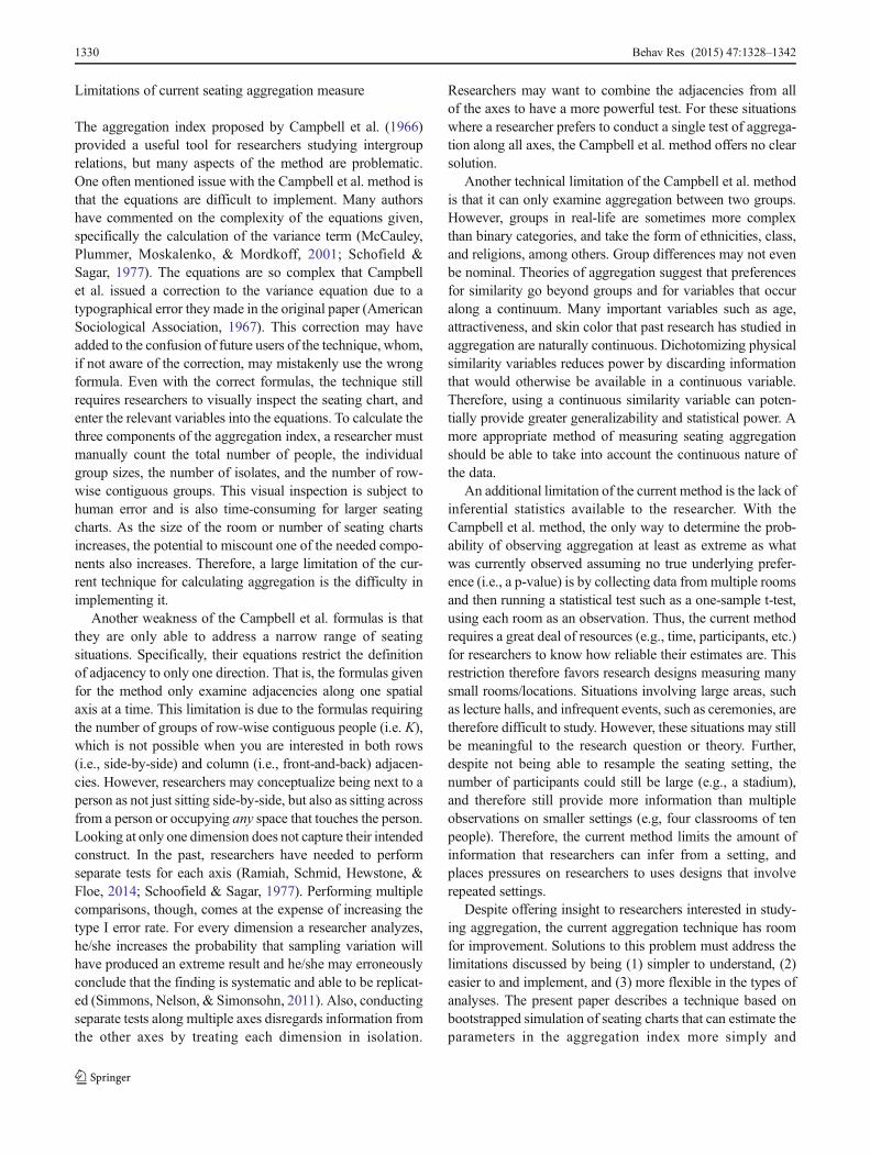
Rather than using deterministic formulas to estimate the ag-gregation index parameters, this paper proposes usingbootstrapped simulations to calculate the otherwise complexparameters of the aggregation index (for a more in-depthtutorial see: Efron & Tibshirani, 1994; Simonsohn, 2013).Themethod follows the intuition behind the aggregation indexof Campbell et al., where I is the difference between thecurrent aggregation and what would be expected by randomseating, divided by the standard deviation. However, thismethod calculates the expected value of aggregation and thevariability of aggregation by simulating people choosing seatsrandomly in the specified space. This method, which has beencompiled into an executable program (SocialAggregation.exe;Fig. 1), iteratively simulates a room whose occupied seatswere chosen at random to get values for expected adjacenciesand variability of those adjacencies. Specifically the programis given a row-by-column seating chart (either in an Excel,comma separated, tab-delimited file, or entered directly intothe program), which is then represented as a two-dimensionalmatrix. In this matrix, all empty seats or spaces that nostudents occupy are set as null values, and all occupied seatsare represented as an integer representing a specific group(e.g., 1=White, 2=Black). The program then calculates thenumber of dissimilar adjacencies by searching through thechart, and counts the number of instances where two positiveintegers are next to each other and are not equal to each other.This search obtains the first value needed for the aggregationindex: the observed number of dissimilar adjacencies.

To calculate the second parameter—the average number ofadjacencies that would be expected by chance, assuming theseat choices are fixed—the program un-assigns the peoplefrom their seats (by temporarily removing their values fromthe seating matrix) and then randomly assigns each person,without replacement, to a seat that was previously occupied.The program then counts the number of dissimilar adjacenciesin this random seating and appends that value to a list. Afternumerous iterations, the program then takes the mean of thatlist, which is equivalent to the expected value of dissimilaradjacencies, assuming random seating. Further, the standarddeviation of that list represents the last parameter of the index,which is the variability of dissimilar adjacencies under ran-dom seating conditions. With those three values, the programcan compute the aggregation index.

Example of the proposed method

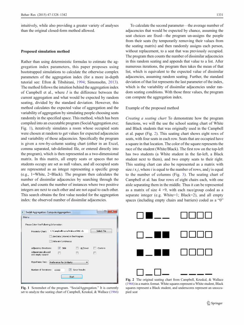
Creating a seating chart To demonstrate how the programfunctions, we will the use the school seating chart of Whiteand Black students that was originally used in the Campbellet al. paper (Fig. 2). This seating chart shows eight rows ofseats, with four seats in each row. Seats that are occupied havea square in that location. The color of the square represents therace of the student (White/Black). The first row on the top-lefthas two students (a White student in the far-left, a Blackstudent next to them), and two empty seats to their right.This seating chart can also be represented as a matrix withsize i x j, where i is equal to the number of rows, and j is equalto the number of columns (Fig. 3). The seating chart ofCampbell et al. has four rows of eight chairs each, with oneaisle separating them in the middle. Thus it can be representedas a matrix of size 4 ×9, with each race/group coded as aseparate integer (e.g. White=1; Black=2), and all emptyspaces (including empty chairs and barriers) coded as a “0”

Fig. 1 Screenshot of the program. “SocialAggregation.” It is currentlyset to analyze the seating chart of Campbell, Kruskal, & Wallace (1966)

Fig. 2 The original seating chart from Campbell, Kruskal, & Wallace(1966) in a matrix format. White squares represent aWhite student, Blacksquares represent a Black student, and underscores represent an unoccu-pied seat

Behav Res (2015) 47:1328–1342 1331

(Fig. 3). This matrix representation of a seating chart can beeasily created by a researcher using a text/spreadsheet editor,and then read into the program (Fig. 4).

Because unoccupied space is irrelevant for the calculationof the aggregation index, any two-dimensional setting can berepresented in the matrix format. The examples previouslydiscussed involve a naturally rectangular environment (e.g., aclassroom). However, as long as blank space and unoccupiedchairs are represented as 0s in the chart, the environment canstill be represented in a spreadsheet. Figure 5 shows an exam-ple of how circular seating arrangements or open spaces thatdo not have clearly defined seats can be translated into aspreadsheet. In irregular seating patterns, the dimensions ofadjacency become especially important to consider. For cir-cular seating arrangements, adjacencies should probably in-clude a corner dimension to include those sitting where thecircle bends. Also, for areas where seats are not clearly defined(e.g., a mall or a park), it is important to use spaces of equalsize to represent a possible seating location.

It is important to note that Campbell et al.’s method (andthus the proposed method) assumes that seat choice possibil-ities are fixed. That is, the method Campbell et al. introducedassumes that the places people chose to sit are the only spotsavailable for others to choose to sit. Therefore, empty space,

barriers, and unoccupied seats are all irrelevant to the calcu-lation. It is important to keep in mind that the technique makesthis assumption, but it does not seem to be particularly prob-lematic for many researchers as the aggregation index hasshown predictive validity and convergent validity with otherintergroup research, as discussed in the “Introduction” section.This assumption is also important because it allows all seatingcharts to be represented in the matrix form described in theabove paragraph. Regardless of the room shape, obstructions,and chair placement, the matrix notation only requires re-searchers to specify where the people are currently sitting inrelation to another (i.e., are they next to each other or is therespace or another person between them). Even irregularlyshaped rooms can be represented because any area where aperson is not currently siting is represented by a 0. Whether ornot a 0 is between two people is a decision left up to theresearcher who decides if the empty space is small/insignificant enough for those two people to be consideredadjacent or not.

Calculat ing the observed number of diss imi laradjacencies The program allows researchers to define adjacen-cy along different dimensions. Researchers can specify that anadjacency is only when two people are sitting side-by-side (i.e.,to the left or right of each other on a seating chart). The programcan also have adjacency specified as front-and-back, or on thecorners of a person. For this example, we will use the definitionCampbell et al. used, which was side-by-side. When the matrixis loaded, and the adjacency is specified, the program can berun. When the program analyzes the data, it computes the threeparameters in the aggregation index.

To compute the observed number of adjacencies, the pro-gram sets a variable that represents the starting number ofadjacencies to 0. The program then looks at the cells in the ith

row, and jth column, starting at i=1 and j=1. The value of theinteger, in this case “1”, is compared to the cells adjacent to it.If an adjacency is defined as side-by-side, then the program

Fig. 3 A matrix representation of the seating chart from Campbell,Kruskal, & Wallace (1966). Values of 1 represent a White student,values of 2 represent a Black student, and values of 0 represent anempty area, such as an aisle, or an unoccupied seat

Fig 4 A sample spreadsheet and a sample comma-separated text file thatrecreate the seating chart from Campbell, Kruskal, & Wallace (1966).Values of 1 represent a White student, values of 2 represent a Blackstudent, and values of 0 represent an empty area, such as an aisle, or anunoccupied seat

Fig. 5 Sample spreadsheets for environments with irregular location/seating arrangements. Values of 1 represent a person from one group,while values of 2 represent a person from another group, and values of 0represent an empty area. The panel on the left is a room with a circularseating arrangement. The panel on the right would be similar to an openmall or park where each cell represents a patch of land of the same squaresize (e.g, 1 m ×1 m)

1332 Behav Res (2015) 47:1328–1342

looks at the cell in the ith row and j+1st column. In this case,the adjacent cell has a value of “2.” The two values arecompared, and if the both cells are not 0, and the value ofthe second is not equal to the first, then the number of totaldissimilar adjacencies for that room is incremented by 1. Theprocess continues for the next column, until all seats in the roware analyzed. The program then moves to the next row anddoes the same calculation. After all rows have been examinedthe number of adjacencies counted is stored. The comparativeprocess is illustrated in pseudo-code (see Appendix 1).

If researchers wish to define adjacencies as not only side-by-side but also as people sitting in the front and back of theperson, the program can calculate these special cases in asimilar way. Rather than looking only at the j+1st column insame row, the search for adjacencies would also include i+1strow in the same column. Therefore a person sitting in the 1strow (i=1) and 4th column (j=4), would be counted as beingadjacent to a person who was a in the 2nd row, and 4th column.Related, dissimilar adjacencies can be calculated by looking atnot only the next seat, but also two seats ahead in case norms ofpersonal space dictate that an extra seat should always be leftempty between people sitting side-by-side. If adjacency isdefined in this way, then, in addition to the normal adjacencycalculation, the program can also look at the seat in the j+1stposition to see if it is empty, and the j+2nd position to see if aperson is there and if they are similar (see Appendix 2). In priorresearch, the decision of how to define an “adjacent seat” hasbeen left up to the individual researcher. Some researchersprefer to count only the seats immediately next to a person astheir definition. This definition is consistent with howCampbellet al. originally presented the method. Other researchers preferto count two people as adjacent if they are next to each other orif there is one empty seat in between them. As mentioned, onejustification given for this procedure is social norms. That is,society dictates that a seat be left between people, even if theyhave a shared relation. Thus, a researcher interested in examin-ing people’s preferences will add imprecision to the measure bymissing many instances relevant to the construct. Anotherjustification given is that including people separated by an openseat reduces the number of people sitting alone (i.e., “isolates”).As seen in the Campbell et al. equations, rooms with greaternumbers of isolates increase the standard deviation, and thusmake it more difficult to detect an effect (i.e., reducing thepower of the measure). There does not seem to be a clear wayto assess the relative merits of each reason, and it is importantfor researchers to understand the benefits and the limitations tomake the most informed decision.

Calculating the expected number of dissimilar adjacenciesand its variance After all of the observed number of adjacen-cies in the specified seating chart are counted, the programthen calculates the number of adjacencies that would beexpected by random seating. To assign random seating, the

program creates an array of length N, with each entry corre-sponding to an individual person in the room, represented bytheir group’s assigned integer. For example, in our seatingchart, there are 22 total people in the room. Of those 22, 16 areWhite and six are Black. Because our seating chart assignedthe integer, “1”, to the White group, and “2” to the Blackgroup, the programwould create an array of length 22, with 161s and six 2s. The list would then be randomly shuffled. Eachcurrently filled seat (i.e. a cell in the seating chart not set to 0)would be assigned the next entry in the shuffled list.Therefore, we would have a new seating chart with the peoplerandomly placed in the seats that were previously occupied.

The program would then perform the same adjacencycounting calculation previously described and append the num-ber of adjacencies counted into an observed adjacency list. Thisprocess of randomly assigning people and counting adjacencieswould repeat for a large number of iterations (e.g., 10,000). Afterthe final iteration, the mean of the observed adjacency list wouldindicate the expected number of adjacencies if the studentsoccupied the seats without preference for race/group status.The standard deviation of that list would represent the variabilityfrom random seating. Now, using the observed number of dis-similar adjacencies, and the simulated estimates for the expectednumber of adjacencies and the associated standard deviation, theprogram can compute the aggregation index using equation 1.

Optimal number of iterations: A simulation study

When using an iterative estimation procedure, such asbootstrapping, it is important to determine the number ofiterations needed to obtain both accurate and stable parameterestimates. The parameters estimated in the proposed methodare the expected number of adjacencies for a room (EA), thestandard deviation of expected number of adjacencies (σA)for the room, and from those parameters, the program thencomputes the aggregation index (I). Therefore, a simulationstudy was conducted for different room sizes and variations ofnumber of iterations used by the bootstrap routine. Then theestimated parameter values (EA, σA, and I) for each simula-tion were compared to the closed-form equations. These com-parisons provide the expected error for different settings anditeration values. It is important to note that because Campbellet al. only provide estimates for adjacencies along a singledimension, the current simulations can only address optimal-ity for side-by-side situations.

Simulation program

A separate programwas conducted for simulating rooms. Thisprogram generated a square (N × N) matrix, where the roomsize (N) was set to be either: 5, 10, 15, or 20. Thus, weexamined rooms containing between 25 and 400 seats. The

Behav Res (2015) 47:1328–1342 1333

choice of room sizes was arbitrary, but was intended to repre-sent a realistic spectrum of rooms encountered in life. Notethat room size is defined by number of possible seats, and notby space. Therefore a setting with large square footage, butwith a few seats close to one another, is more similar to asmaller room size in these simulations than a room with littlespace, but with the many separated seats. These rooms werepopulated with two separate groups of “people” in equalproportion (represented as 1s and 2s in the matrix). Thesparseness of the room was set to be 50 % (e.g., if the roomhad 100 seats, it contained 50 people: 25 people from group 1and 25 people from group 2). For odd-numbered room sizes,the number of people was rounded up to the nearest integerthat was closest to 50 % of the room size. Each simulationrandomly assigned each person to an empty seat.

Once the roomwas constructed, the Campbell et al. method(coded as a separate program that measures the parameters inthe equations) was used to obtain closed-form (i.e., absolute)values for the expected number of left-right adjacencies (EA)as well as the standard deviation of the expected number ofadjacencies (σA). The bootstrapped estimates were obtainedby having the bootstrapping program count the number ofsimilar side-by-side adjacencies, and perform the bootstraproutine to estimate the EA and σA parameters for that room.The number of iterations used to calculate those estimateswere: 1,000, 5,000, 10,000, 50,000, 100,000, 500,000.These numbers were chosen because prior informal simula-tions by the researcher suggested that 500,000 iterations weresufficient to obtain accuracy and reliability, and thereforeserved as an upper limit for the possible values.

Because people were randomly assigned to seats, there maybe variability in the number of adjacencies for each room type,and, therefore, each room was re-simulated 1,000 times to min-imize the standard error of the estimates. Although the resam-pling value can be any arbitrarily large number, 1,000 waschosen for computational practicality as the time needed forany order of magnitude larger would be extremely time intensive(e.g., months, years). Therefore, these simulations will provide ameasure of how much error, on average, there is between themethods for varying room sizes and iteration values.

Measuring estimate accuracy

Following the simulations, the estimates between the twomethods (e.g., formula-derived EA and bootstrapped EA)were subtracted from each other, and then the absolute valueof that difference was computed. For each room size anditeration value, the average of this error was computed. Thismean absolute error represents how much the simulationswere off from the closed-form answer and serves as a measureof how imprecise the estimates obtained from the program are.All statistics are reported in Table 5, including the associatedstandard deviation of these values that show how much

variability the parameter estimates have for each iterationand room size.

Results

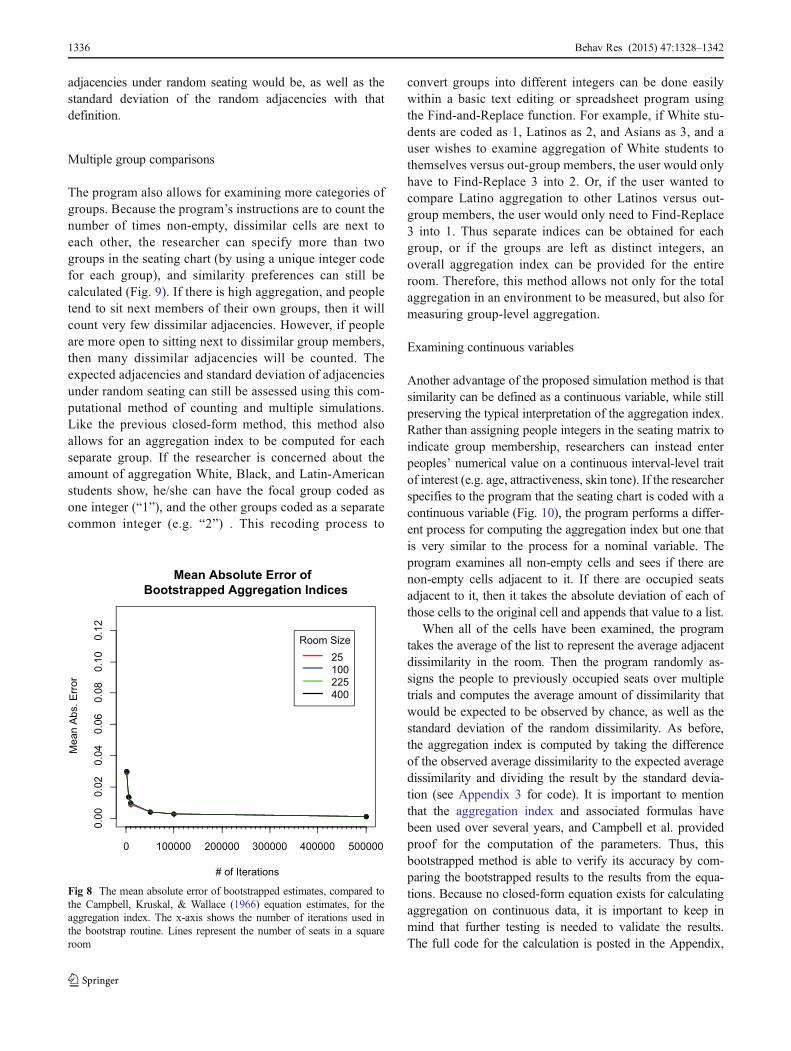
The results of this simulation study are shown in Figures 6, 7,and 8. For all simulations, the error rates are all relatively low.As might be expected, the best parameter estimates are ob-tained with the largest iteration values and in the smallestroom (i.e., a room with 25 seats). The least accurate estimatesare obtained when only 1,000 iterations are used for a roomsize of 400 (see Tables 1, 2, and 3). However, when thenumber of iterations is 50,000 or greater, the estimates differfrom the true value by only .002 on average and thereforesufficient for reporting the statistic to a precision of two digits.

When examining room size, larger rooms tend to createmore error in the estimates. This finding is not unexpectedgiven the parameters in the original Campbell et al.equations,which suggest that the number of occupants asnumber of non-contiguous blocks of people will increase thevariability of adjacencies. However, when estimating the trueaggregation index (Fig. 8), room size does not seem to makeas much of difference in the error rates, and all iterationmethods will produce roughly the same error rate for theaggregation indices in larger rooms as they do in smallerroom.

0 100000 200000 300000 400000 500000

0.00

0.02

0.04

0.06

0.08

0.10

0.12

Mean Absolute Error of Bootstrapped Expected Adjacencies

# of Iterations

Mea

n A

bs. E

rror

Room Size25100225400

Fig. 6 The mean absolute error of bootstrapped estimates, compared tothe Campbell, Kruskal, & Wallace (1966) equation estimates, for theexpected number of dissimilar seating adjacencies in a room. The x-axisshows the number of iterations used in the bootstrap routine. Linesrepresent the number of seats in a square room

1334 Behav Res (2015) 47:1328–1342

Another important property of the bootstrap method toexamine is when does the error rate experience diminishingreturns for increased iterations. That is, a researcher may beinterested in knowing the iteration value when accuracy stopsincreasing to an appreciable level. One method to assess thisquestion is scree analysis (Cattell, 1966). This method exam-ines variance/error plots for “elbows.” These elbows can oftenbe seen visually, though there are also quantitative methods tosuggest the appropriate value (Cng: Gorsuch & Nelson, 1981;mReg: Zoski & Jurs, 1993). From visual inspection, in allthree plots the elbow occurs between the 10,000th and50,000th iteration. That is, after about 50,000 iterations, theestimates see very slow improvement. This visual analysisshowing that between 10,000 and 50,000 iterations is the pointof diminishing returns was also confirmed by quantitativescree analysis methods. For all estimates, the mReg methodsuggests the 50,000th iteration, while the Cng method sug-gests the 10,000th iteration. Thus, this paper recommendsusing 50,000 iterations when conducting research, and at least500,000 iterations for atypical situations not examined in thissimulation study.

Comparison with results from previous studies

To assess the validity of the simulation method at estimatingthe aggregation index’s parameters, six published and unpub-lished seating charts from papers examining aggregation wereanalyzed with both the Campbell et al. and the current

simulation method. Equations 2 and 3 were used to calculatethe parameter values of the aggregation index for theCampbell et al. method. To estimate the values using thesimulation methods, the seating chart was converted to thematrix format (in an Excel spreadsheet) using the procedurespreviously discussed. These seating matrices were enteredinto the program, and each chart’s parameters were computedfrom a simulation using 500,000 iterations (to reduce thestandard error as much as possible) of random seatassignment.

The first parameter calculated was the observed number ofdissimilar adjacencies. For the Campbell et al. method, thisparameter has to be visually calculated, while the simulationmethod automates the counting. The results of this compari-son showed no differences between visually counting thenumber of observed adjacencies and having them countedwith the SocialAggregation program. Because the number ofadjacencies counted is equivalent to visual inspection, it sug-gests that the adjacency counting algorithm is functioning asexpected. Table 4 compares the methods’ estimates for theexpected number of adjacencies. The bootstrap method showshigh convergence with the closed-form equations. The largestdeviation between the simulated estimates and the closed-form solution was .0027. Similarly, Table 5 shows how theestimates of the standard deviation compare betweenmethods. The bootstrap estimates were never more than ap-proximately .0031 off from the estimates of the closed-formequations. This similarity between parameters suggests thatthe aggregation index parameter estimates from the simulationare comparable for previous investigations of seat preference.The parameter estimates between methods are all within twodecimal places of each other, and greater accuracy may po-tentially be achieved with a greater number of iterations.

Advantages and extensions

Simultaneous analysis of adjacencies

By using simulations to estimate the parameters, this boot-strap method offers several improvements over theCampbell et al. method due it being more flexible in thetypes of analyses, simpler to understand, and easier to use.The previous method could only compute an aggregationindex concerning adjacencies along one dimension (e.g,leftside-rightside) at a single time. If more dimensions wereof interest (e.g., front and back), the researchers wouldhave to conduct a separate test for that dimension.However, this proposed bootstrap method offers users theability to examine the different types of adjacenciessimultaneously. The program, as usual, would then countthe number of those types of adjacencies in the providedseating chart, and compute what the expected number of

0 100000 200000 300000 400000 500000

0.00

0.02

0.04

0.06

0.08

0.10

0.12

Mean Absolute Error of Bootstrapped Standard Devations

# of Iterations

Mea

n A

bs. E

rror

Room Size25100225400

Fig. 7 The mean absolute error of bootstrapped estimates, compared tothe Campbell, Kruskal, & Wallace (1966) equation estimates, for thestandard deviation of the expected number of dissimilar seating adjacen-cies in a room. The x-axis shows the number of iterations used in thebootstrap routine. Lines represent the number of seats in a square room

Behav Res (2015) 47:1328–1342 1335

adjacencies under random seating would be, as well as thestandard deviation of the random adjacencies with thatdefinition.

Multiple group comparisons

The program also allows for examining more categories ofgroups. Because the program’s instructions are to count thenumber of times non-empty, dissimilar cells are next toeach other, the researcher can specify more than twogroups in the seating chart (by using a unique integer codefor each group), and similarity preferences can still becalculated (Fig. 9). If there is high aggregation, and peopletend to sit next members of their own groups, then it willcount very few dissimilar adjacencies. However, if peopleare more open to sitting next to dissimilar group members,then many dissimilar adjacencies will be counted. Theexpected adjacencies and standard deviation of adjacenciesunder random seating can still be assessed using this com-putational method of counting and multiple simulations.Like the previous closed-form method, this method alsoallows for an aggregation index to be computed for eachseparate group. If the researcher is concerned about theamount of aggregation White, Black, and Latin-Americanstudents show, he/she can have the focal group coded asone integer (“1”), and the other groups coded as a separatecommon integer (e.g. “2”) . This recoding process to

convert groups into different integers can be done easilywithin a basic text editing or spreadsheet program usingthe Find-and-Replace function. For example, if White stu-dents are coded as 1, Latinos as 2, and Asians as 3, and auser wishes to examine aggregation of White students tothemselves versus out-group members, the user would onlyhave to Find-Replace 3 into 2. Or, if the user wanted tocompare Latino aggregation to other Latinos versus out-group members, the user would only need to Find-Replace3 into 1. Thus separate indices can be obtained for eachgroup, or if the groups are left as distinct integers, anoverall aggregation index can be provided for the entireroom. Therefore, this method allows not only for the totalaggregation in an environment to be measured, but also formeasuring group-level aggregation.

Examining continuous variables

Another advantage of the proposed simulation method is thatsimilarity can be defined as a continuous variable, while stillpreserving the typical interpretation of the aggregation index.Rather than assigning people integers in the seating matrix toindicate group membership, researchers can instead enterpeoples’ numerical value on a continuous interval-level traitof interest (e.g. age, attractiveness, skin tone). If the researcherspecifies to the program that the seating chart is coded with acontinuous variable (Fig. 10), the program performs a differ-ent process for computing the aggregation index but one thatis very similar to the process for a nominal variable. Theprogram examines all non-empty cells and sees if there arenon-empty cells adjacent to it. If there are occupied seatsadjacent to it, then it takes the absolute deviation of each ofthose cells to the original cell and appends that value to a list.

When all of the cells have been examined, the programtakes the average of the list to represent the average adjacentdissimilarity in the room. Then the program randomly as-signs the people to previously occupied seats over multipletrials and computes the average amount of dissimilarity thatwould be expected to be observed by chance, as well as thestandard deviation of the random dissimilarity. As before,the aggregation index is computed by taking the differenceof the observed average dissimilarity to the expected averagedissimilarity and dividing the result by the standard devia-tion (see Appendix 3 for code). It is important to mentionthat the aggregation index and associated formulas havebeen used over several years, and Campbell et al. providedproof for the computation of the parameters. Thus, thisbootstrapped method is able to verify its accuracy by com-paring the bootstrapped results to the results from the equa-tions. Because no closed-form equation exists for calculatingaggregation on continuous data, it is important to keep inmind that further testing is needed to validate the results.The full code for the calculation is posted in the Appendix,

0 100000 200000 300000 400000 500000

0.00

0.02

0.04

0.06

0.08

0.10

0.12

Mean Absolute Error of Bootstrapped Aggregation Indices

# of Iterations

Mea

n A

bs. E

rror

Room Size25100225400

Fig 8 The mean absolute error of bootstrapped estimates, compared tothe Campbell, Kruskal, & Wallace (1966) equation estimates, for theaggregation index. The x-axis shows the number of iterations used inthe bootstrap routine. Lines represent the number of seats in a squareroom

1336 Behav Res (2015) 47:1328–1342

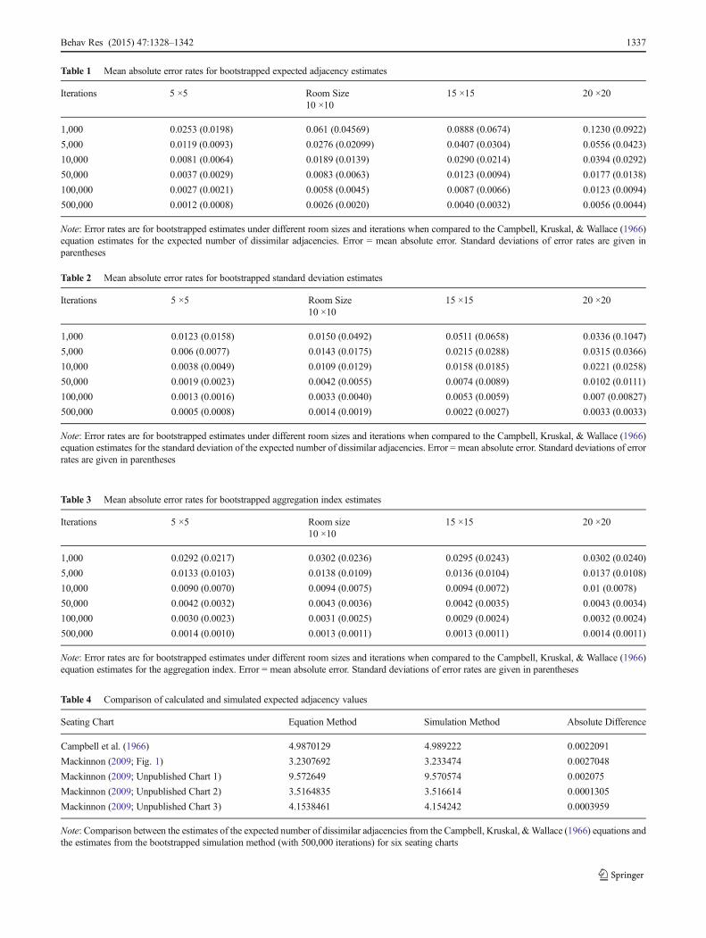
Table 1 Mean absolute error rates for bootstrapped expected adjacency estimates

Iterations 5 ×5 Room Size10 ×10

15 ×15 20 ×20

1,000 0.0253 (0.0198) 0.061 (0.04569) 0.0888 (0.0674) 0.1230 (0.0922)

5,000 0.0119 (0.0093) 0.0276 (0.02099) 0.0407 (0.0304) 0.0556 (0.0423)

10,000 0.0081 (0.0064) 0.0189 (0.0139) 0.0290 (0.0214) 0.0394 (0.0292)

50,000 0.0037 (0.0029) 0.0083 (0.0063) 0.0123 (0.0094) 0.0177 (0.0138)

100,000 0.0027 (0.0021) 0.0058 (0.0045) 0.0087 (0.0066) 0.0123 (0.0094)

500,000 0.0012 (0.0008) 0.0026 (0.0020) 0.0040 (0.0032) 0.0056 (0.0044)

Note: Error rates are for bootstrapped estimates under different room sizes and iterations when compared to the Campbell, Kruskal, & Wallace (1966)equation estimates for the expected number of dissimilar adjacencies. Error = mean absolute error. Standard deviations of error rates are given inparentheses

Table 2 Mean absolute error rates for bootstrapped standard deviation estimates

Iterations 5 ×5 Room Size10 ×10

15 ×15 20 ×20

1,000 0.0123 (0.0158) 0.0150 (0.0492) 0.0511 (0.0658) 0.0336 (0.1047)

5,000 0.006 (0.0077) 0.0143 (0.0175) 0.0215 (0.0288) 0.0315 (0.0366)

10,000 0.0038 (0.0049) 0.0109 (0.0129) 0.0158 (0.0185) 0.0221 (0.0258)

50,000 0.0019 (0.0023) 0.0042 (0.0055) 0.0074 (0.0089) 0.0102 (0.0111)

100,000 0.0013 (0.0016) 0.0033 (0.0040) 0.0053 (0.0059) 0.007 (0.00827)

500,000 0.0005 (0.0008) 0.0014 (0.0019) 0.0022 (0.0027) 0.0033 (0.0033)

Note: Error rates are for bootstrapped estimates under different room sizes and iterations when compared to the Campbell, Kruskal, & Wallace (1966)equation estimates for the standard deviation of the expected number of dissimilar adjacencies. Error = mean absolute error. Standard deviations of errorrates are given in parentheses

Table 3 Mean absolute error rates for bootstrapped aggregation index estimates

Iterations 5 ×5 Room size10 ×10

15 ×15 20 ×20

1,000 0.0292 (0.0217) 0.0302 (0.0236) 0.0295 (0.0243) 0.0302 (0.0240)

5,000 0.0133 (0.0103) 0.0138 (0.0109) 0.0136 (0.0104) 0.0137 (0.0108)

10,000 0.0090 (0.0070) 0.0094 (0.0075) 0.0094 (0.0072) 0.01 (0.0078)

50,000 0.0042 (0.0032) 0.0043 (0.0036) 0.0042 (0.0035) 0.0043 (0.0034)

100,000 0.0030 (0.0023) 0.0031 (0.0025) 0.0029 (0.0024) 0.0032 (0.0024)

500,000 0.0014 (0.0010) 0.0013 (0.0011) 0.0013 (0.0011) 0.0014 (0.0011)

Note: Error rates are for bootstrapped estimates under different room sizes and iterations when compared to the Campbell, Kruskal, & Wallace (1966)equation estimates for the aggregation index. Error = mean absolute error. Standard deviations of error rates are given in parentheses

Table 4 Comparison of calculated and simulated expected adjacency values

Seating Chart Equation Method Simulation Method Absolute Difference

Campbell et al. (1966) 4.9870129 4.989222 0.0022091

Mackinnon (2009; Fig. 1) 3.2307692 3.233474 0.0027048

Mackinnon (2009; Unpublished Chart 1) 9.572649 9.570574 0.002075

Mackinnon (2009; Unpublished Chart 2) 3.5164835 3.516614 0.0001305

Mackinnon (2009; Unpublished Chart 3) 4.1538461 4.154242 0.0003959

Note: Comparison between the estimates of the expected number of dissimilar adjacencies from the Campbell, Kruskal, &Wallace (1966) equations andthe estimates from the bootstrapped simulation method (with 500,000 iterations) for six seating charts

Behav Res (2015) 47:1328–1342 1337

and can be reviewed by any researcher interested in usingthis experimental calculation.

Non-parametric inferential statistics

Because the program computes the amount of aggregation inthe room under random seating conditions, researchers canknow more precisely the probability of observing aggregationas extreme as the amount they found.With the prior Campbellet al. method, a researcher could only compute p-values whenhe/she had measured many seating charts, and had multipleaggregation indices. With this method, the researcher onlyneeds to observe one setting to know how often he/she wouldobserve aggregation at least as extreme as the amount in thepresent chart if seating were chosen at random. For example, ifa researcher observes 12 dissimilar adjacencies in his/herstudy, and out of 10,000 simulations with random seating,only three of those simulations have dissimilar adjacencies≥12, then there is approximately a 3/10,000 chance that theresearcher would have observed that much aggregation ifseating is being chosen at random (p = .0003). Therefore,researchers can test directional hypotheses with the proposedbootstrap method.

In addition to p-values, the program also provides confi-dence intervals for the mean value of the expected number ofadjacencies. That is, researchers are able to understand moreabout the setting they are examining, and know how many

adjacencies would be expected under randomness 95 % of thetime, thereby giving the researcher further information notattainable with the previous Campbell et al. method. To com-pute these confidence intervals, after each simulation of ran-dom seating, the number of adjacencies in that randomlyseated room is counted and added to a list. Once all iterationshave finished, the program then computes bootstrapped con-fidence intervals from that list using the bias-corrected andaccelerated bootstrap suggested by Efron (1987), which ad-justs for both bias and skewness in the bootstrap distribution.This bias-corrected procedure for confidence intervals tends to

Table 5 Comparison of calculated and simulated standard deviation values

Seating Chart Equation Method Simulation Method Absolute Difference

Campbell et al. (1966) 1.51518927 1.51514729 0.00004198

Mackinnon (2009; Fig. 1) 1.21926441 1.21777609 0.00148832

Mackinnon (2009; Unpublished Chart 1) 1.90059027 1.89754428 0.00304599

Mackinnon (2009; Unpublished Chart 2) 1.2744106 1.27293270 0.00147790

Mackinnon (2009; Unpublished Chart 3) 1.32384105 1.32250610 0.00133495

Note: Comparison between the estimates of the standard deviation of dissimilar adjacencies from the Campbell, Kruskal, &Wallace (1966) equations andthe estimates from the bootstrapped simulation method for six seating charts

Fig. 9 A sample spreadsheet that examines students belonging to fourdistinct groups (e.g., White=1, Black=2, Latino=3, and Asian=4)

Fig. 10 A sample spreadsheet that uses a continuous measure ofsimilarity (i.e., numbers from 1–10) for each student. The program hasa special option that must be selected when the entries in the seating chartare a continuous-level variable (e.g. height, attractiveness, age)

1338 Behav Res (2015) 47:1328–1342

produce more accurate/narrow estimations then the more sim-ple percentile bootstrapped confidence method of removingthe first and last 1 – α/2 entries from the sorted list.

This confidence interval provides the range of observablevalues at the specified confidence for the expected number ofdissimilar adjacencies. Therefore, this interval can be com-pared to the observed number of adjacencies to determine ifthe observed dissimilar adjacencies overlap or are outside therange of the interval. The program also provides bias-correctedconfidence intervals for the estimated aggregation index usinga similar process, and therefore researchers can report theconfidence interval for this effect size measure. With theseconfidence intervals, it possible for researchers to conduct theirown pre-study power analysis. Researchers who anticipatecertain room sizes, total number of persons, group distribu-tions, and isolates can submit hypothetical seating charts to theprogram and discover the range of dissimilar adjacencies thatare probable (i.e., the confidence interval for EA), as well asthe standard deviation of the expected adjacencies. With theseestimates, the researcher knows how much aggregation theywould need to observe to obtain a certain effect size, and cantherefore plan studies accordingly and know the feasibility ofthose studies finding extreme levels of aggregation.

New measures of aggregation

Because of the bootstrapped nature of the method, moreinformation about the room and the individuals can be pro-vided that go beyond the information provided by theCampbell et al. equations. One limitation of the closed-formequations is that they provide very little individual levelinformation. That is, the parameters EA, σA, and I reflectwhat happens at an aggregate level, but say nothing about theexperience of an individual group member. With the bootstrapmethod, it is possible to compute different statistics aboutindividual level behavior and experiences.

One statistic this paper proposes is the proportion of dis-similar adjacencies for a person (p-DAP). This statistic isintended to provide a more easily interpretable measure ofaggregation by describing the daily experience of a typicalgroup member. Specifically, it describes what percent of peo-ple next to a person are members of a different group. Thisstatistic thus offers an easy-to-describe picture of intergroupcontact that can be communicated to a non-technical audiencemore clearly. It can also be expressed as raw counts (e.g., forevery eight people a White person is next to, roughly two ofthem are going be Black), which research suggests is one of themost understandable ways to convey statistical information tothe public (Gigerenzer, Gaissmaier, Kurz-Milcke, Schwartz, &Woloshin, 2007). To compute the statistic, during the initialcounting phase (where the number of observed adjacencies are

counted), each group receives its own empty dictionary wherethe entries are the group members. When a person is adjacentto a person from a different group their dictionary valueincrements by 1. Thus, all people in a room are assigned avalue representing the number of dissimilar people next tothem. Further, each seat on the matrix has a value for howmany adjacencies are possible (e.g., a person in the top-leftcorner has only one side-by-side adjacency possible, but twopossible adjacencies if adjacent is defined as side-by-side andfront-and-back). To obtain an individual’s probability of hav-ing an adjacent person next to them, each person’s dissimilaradjacency count is divided by the total possible adjacencies forthat seat. For example, if a person is next to only one dissimilarperson, and their seat has two total possible adjacencies, thenthe proportion of people next to them that are dissimilar is .50or 50 %. In other words, 50 % of the people this person willencounter at their seat are of from a different group. Theseprobabilities are computed for each person in the seating chart.Next, all probabilities are then averaged. This average indicatesthe probability that an individual of a certain group (e.g.,White) will have a dissimilar group member next to them. Itis important to note that each group receives its own p-DAPestimate. Further, with this statistic, it is possible to computethe expected proportion of dissimilar adjacencies of a groupmember for a given room. By computing the p-DAP statisticsfor each group during the bootstrapped randomization process,it is possible to show how conducive a room is to havingintergroup contact at an individual level. Thus, the p-DAPinforms researchers of how much experience with other groupmembers an individual has, and also how often these dissimilarencounters will even take place by chance alone given thenature of the room and proportions of group members. Thesestatistics provide a richer picture of intergroup relations andstructural barriers to contact as they give an immediatelyinterpretable description of what a group member will experi-ence in a room as well as an exact measure of environmentalencouragement that is directly comparable to other environ-ments. While the prior Campbell et al. method does detail theexpected dissimilar adjacencies of the environment, this inte-ger is difficult to compare across settings, and therefore maynot be particularly helpful for researchers who want to under-stand how much an environment facilitates intergroup contactat the individual level.

The aggregation index, however, still serves an importantmetric for researchers. This index, which shows the magnitudeof a difference between an observed and null hypothesisvalue, standardized by the variability, provides an overallrepresentation of group preferences. As a standardized differ-ence between two mean values, it meets the requirements ofmany different definitions given for an effect size (Kazis,Anderson, & Meenan, 1989; Kelley & Preacher, 2012;

Behav Res (2015) 47:1328–1342 1339

NCES, 2002; Olejnik & Algina, 2003; Thompson, 2004).Further, this specific definition of effect size is analogous tothe definition provided for Cohen’s d (1988), and thereforetypical interpretations of effect size magnitude are applicable.Journals are placing an increasing emphasis on reportingeffect size instead of null-hypothesis tests (Cumming, 2014),and therefore it represents a preferred way of expressingresults and communicating the extent of a finding. Further,this effect size is directly comparable to other effect sizes,which makes it especially useful for being included in meta-analyses (not only for meta-analayses of seating studies butalso meta-analyses of attitudes or in-group bias). The alterna-tive statistic proposed, p-DAP, is probably better suited forresearchers interested in a real-life implication of group-member contact and the pressures a particular environmentplaces on group interactions. Thus, the aggregation index andp-DAP can be seen as complementary and not competingmeasures of aggregation.

Conclusion

The method originally proposed by Campbell et al. was animportant contribution to the social sciences, and offered aclosed-form method of analyzing aggregation. However, ad-vances in computing speed offer the opportunity to improve

upon the method’s limitations. Using bootstrap simulations toestimate the various parameters of the aggregation indexallows researchers to analyze more types of situations, learnmore information about the index, and do this analysis moreefficiently.

This new approach makes it possible to develop intuitiveexaminations of seating preferences that are more flexible, andallow for a greater variety of analyses, than is currently pos-sible with the Campbell et al. closed-form equations. Further,this method still maintains a high degree of accuracy inparameter estimation, and converges with the previousmethod’s estimates. Therefore, the bootstrapped simulationmethod is recommended as an alternative to analyzing howmuch preference for similarity exists in a social setting.

Author Note The author would like to thank Sean Mackinnon forproviding seating chart data, and for his suggestions of features for theprogram. He would also like to thank Ryan Ritter for his comments on anearly version of the paper. A copy of the SocialAggregation program andsample seating charts can be downloaded from http://ivanhernandez.com/software/SocialAggregation.zip

Appendix 1

Source code for counting the number of dissimilar groupmembers who are adjacent (side-by-side) to one another in aroom

Appendix 2

Source code for counting the number of dissimilar groupmembers who are adjacent to one another in a room, where

adjacent is defined as either side-by-side or front-and-back toanother person

1340 Behav Res (2015) 47:1328–1342

Appendix 3

Code to compute aggregation index for continuous data

Behav Res (2015) 47:1328–1342 1341

References

American Sociological Association. (1967). Erratum: Seating aggrega-tion as an index of attitude. Sociometry, 30, 104.

Batson, C. D., Flink, C. H., Schoenrade, P. A., Fultz, J., & Pych, V.(1986). Religious orientation and overt versus covert racial preju-dice. Journal of Personality and Social Psychology, 50, 175.

Campbell, D. T., Kruskal, W. H., & Wallace, W. P. (1966). Seatingaggregation as an index of attitude. Sociometry, 29, 1–15.

Cattell, R. B. (1966). The scree test for the number of factors.Multivariate behavioral research, 1, 245–276.

Cohen, J. (1988). Statistical power analysis for the behavioral sciences(2nd ed.). Hillsdale, N.J: L. Erlbaum Associates.

Cumming, G. (2014). The new statistics: Why and how. PsychologicalScience, 25, 7–29.

Efron, B. (1987). Better bootstrap confidence intervals. Journal of theAmerican Statistical Association, 82, 171.

Efron, B., & Tibshirani, R. (1994). An introduction to the bootstrap. NewYork: Chapman & Hall.

Gigerenzer, G., Gaissmaier, W., Kurz-Milcke, E., Schwartz, L. M., &Woloshin, S. (2007). Helping doctors and patients make sense ofhealth statistics. Psychological Science in the Public Interest, 8, 53–96.

Gorsuch, R. L. & Nelson, J. (1981). CNG scree test: an objectiveprocedure for determining the number of factors. Presented at theannual meeting of the Society for multivariate experimentalpsychology.

Holland, R. W., Roeder, U. R., Brandt, A. C., & Hannover, B. (2004).Don’t stand so close to me the effects of self-construal on interper-sonal closeness. Psychological Science, 15(4), 237–242.

Kazis, L. E., Anderson, J. J., & Meenan, R. F. (1989). Effect sizes forinterpret ing changes in health status. Medical Care,27(Supplement), S178–S189.

Kelley, K., & Preacher, K. J. (2012). On effect size. PsychologicalMethods, 17, 137–152.

Koen, J., & Durrheim, K. (2010). A naturalistic observational study ofinformal segregation: Seating patterns in lectures. Environment andBehavior, 42, 448–468.

Mackinnon, S. (2009). Birds of a feather sit together: Physical similaritypredicts seating choice. Theses and Dissertations (Comprehensive).Paper 941. http://scholars.wlu.ca/etd/941

Mackinnon, S. P., Jordan, C. H., & Wilson, A. E. (2011). Birds of afeather sit together: Physical similarity predicts seating choice.Personality and Social Psychology Bulletin, 37, 879–892.

McCauley, C., Plummer, M., Moskalenko, S., & Mordkoff, J. T. (2001).The exposure index: A measure of intergroup contact. Peace andConflict: Journal of Peace Psychology, 7, 321–336.

National Center for Education Statistics. (2002). NCES statisticalstandards (recth ed.). Washington, DC: Department of Education.

Olejnik, S., & Algina, J. (2003). Generalized eta and omega squaredstatistics: Measures of effect size for some common researchsesigns. Psychological Methods, 8, 434–447.

Ramiah, A. A., Schmid, K., Hewstone, M., & Floe, C. (2014).Why are all the White (Asian) kids sitting together in thecafeteria? Resegregation and the role of intergroup attribu-tions and norms. British Journal of Social Psychology. doi:10.1111/bjso.12064

Schofield, J. W., & Sagar, H. A. (1977). Peer interaction patterns in anintegrated middle school. Sociometry, 40, 130–138.

Simmons, J. P., Nelson, L. D., & Simonsohn, U. (2011). False-positivepsychology: Undisclosed flexibility in data collection and analysisallows presenting anything as significant. Psychological Science,22, 1359–1366.

Simonsohn. (2013). Just post it: The lesson from two cases of fabricateddata detected by statistics alone. Psychological Science, 24, 1875–1888.

Snyder, M. L., Kleck, R. E., Strenta, A., & Mentzer, S. J. (1979).Avoidance of the handicapped: An attributional ambiguity analysis.Journal of Personality and Social Psychology, 37, 22–97.

Sriram, N. (2002). The role of gender, ethnicity, and age in inter-group behavior in a naturalistic setting. Applied Psychology, 51,251–265.

Thompson, B. (2004). The “significance” crisis in psychology and edu-cation. The Journal of Socio-Economics, 33, 607–613.

Zoski, K., & Jurs, S. (1993). Using multiple regression to determine thenumber of factors to retain in factor analysis. Multiple LinearRegression Viewpoints, 20, 5–9.

1342 Behav Res (2015) 47:1328–1342