Advanced human body modelling to support designing ...
254
Advanced human body modelling to support designing products for physical interaction
-
Upload
khangminh22 -
Category
Documents
-
view
3 -
download
0
Transcript of Advanced human body modelling to support designing ...

Advanced human body modelling
to support designing products for
physical interaction

ii

Advanced human body modelling
to support designing products for
physical interaction
Proefschrift
ter verkrijging van de graad van doctoraan de Technische Universiteit Delft,
op gezag van de Rector Magnificus prof. dr. ir. J.T. Fokkema,in het openbaar te verdedigen ten overstaan van een commissie,
door het College voor Promoties aangewezen,op maandag 13 december 2004 te 10.30 uur
door
Cornelis Christiaan Marie MOES
natuurkundig ingenieur
iii

Dit proefschrift is goedgekeurd door de promotoren:
Prof. dr. I. HorvathProf. W.S. Green
Samenstelling promotie commissie:
Rector magnificus voorzitterProf. dr. I. Horvath Technische Universiteit Delft, promotorProf W.S. Green Technische Universiteit Delft, promotorProf. dr. J. Duhovnik Univerza v LjubljaniProf. dr. ir. F.J.A.M. van Houten University of TwenteProf. dr. ir. I.S. Sariyildiz Technische Universiteit DelftProf. dr. P. Vink Technische Universiteit DelftProf. ir. K.H.J. Robers Technische Universiteit DelftProf. dr. ir. J.C. Brezet Technische Universiteit Delft, (reservelid)
Niels CCM Moes
Advanced human body modelling to support designing products forphysical interaction,
Ph.D. Thesis, Delft University of Technology.ISBN 90-9018829-0
Keywords advanced human body modelling, ergonomics, physical interaction, computeraided design, conceptual design, shape conceptualization, vague modelling,finite elements modelling, human tissues, knowledge engineering.
Typesetting: plain TEX, eplain, apalike.
Copyright c© by Niels CCM Moes. All rights reserved. No part of materials protected bythis copyright notice may be reproduced or utilized in any form or by any means electronicor mechanical, including photocopying, recording or by any information storage and retrievalsystem, without written permission from the author.
iv

Voor Els,mijn lieve vrouw
v

vi

AcknowledgementsThis research has been carried out with the support of the Faculty of Industrial DesignEngineering. The research started when I was still a member of the ergonomicsdepartment. The main part of the research has been done in the CADE section,where I entered in the year 2000. I want to express my gratitude to the faculty,and particularly to my current department for the opportunity to accomplish thisthesis, and for the means that were needed. I realize that my colleagues have hadconsideration with me, and that they have taken other tasks from me.
Special gratitude I want to give to my professor, Imre Horvath. Imre taught me realscientific thinking, to persevere, to be patient, and to cooperate. He showed so muchwarmth, patience and involvement, his critics were always sharp and clear, and provedto be a great help to deepen in and to progress with the project.
Many other people have helped me. I would like to mention them all, but I can justmention a few of them. In the first stage of my research Hans Houtkamp was of agreat help for me in the study of pressure distribution, as well as in the project for thecalibration of the pressure distribution measuring device. His significant contributionwas related to the development of the calibration device. Adrie Kooijman also gave mesupport when computer help was needed. Henk Lok constructed the mirror box andthe pressure distribution measuring device; he was of great help in the preparation ofthe ergonomic measurements. Peter Pesch greatly supported the computations relatedto the calibration needed for the pressure measurements. Zoltan Rusak did many ofthe computations related to VDIM. Willem Smit introduced the great TEX systemto me. Erik Ulijn was my guru for TEX and Linux. Many students contributed inthe routine measurements as part of their education, and by participating as patientsubjects during the measurements of pressure distribution, body shape and pelvicangle. Michelle Williams, from the university of Bath (UK), was of a great help duringthe measurements of the rotation of the pelvis. Cynthia Smeets and AnnemariekeMoes contributed by doing a good part of the data analysis of the mirror box results,and Thelma Oskam and Sarah Los assisted in the shape measurements.
I want to express my special gratitude to the members of the Promotion Committee.They invested their precious time to reading and commenting the concept thesis.
My good friends helped me during the difficult years of the project of the thesis. Wimvan den Boogaard, my great friend and music companion, was always willing to givean ear for my struggles, and helped me time after time to open my eyes for seeingthings clearly. Hans and Yolanda Lebbe always knew how to give comfort after thehectic weeks with a glass of their excellent wines and a good, relaxing talk. Carlovan Nierop taught me associative thinking, and was of a great help to survive severalturbulent years.
Last but certainly not least I want to say “thank you so much” to my family. Mywife Els has been missing her husband for a long time. She showed an unbelievablepatience during the years of research and thesis writing, and was always the wisewife of a chaotic husband. She always knew how to let me feel the earth below myoften airborne feet. Together with our children, Annemarieke, Michiel, Janneke andJeroen, she kept on encouraging me to go on, and was careful to take only limitedattempt on my energy. To her I owe most of my thesis work. I am also grateful tomy children for their patience, criticism, optimism, realism, love and humour. Theywere a significant support and helped me to persevere.
vii

GlossaryAHBM Advanced Human Body Model
CACD Computer Aided Conceptual Design
CSG Constructive Solid Geometry
dof degrees of freedom
FBD Free Body Diagram
FE Finite Elements
FEA Finite Elements Analysis
FEM Finite Elements Model
HBM conventional human body model
HCD Human Centred Design
ifp interstitial fluid pressure
lfp lymph fluid pressure
MCS measuring coordinate system
pdf probability distribution function
SCI spinal cord injury
SI sacro-iliac
SIAS Spina Iliaca Anterior Superior
SIPS Spina Iliaca Posterior Superior
TOL tolerance
VDIM Vague Discrete Interval Modelling
WCS working coordinate system
caudal in the direction of the feet
contact area the surface that is shared by the user and the product
cranial in the direction of the headdermis the deeper layer of the skin, containing blood vessels, nerves,
etc.decubitus ulcers caused by prolonged pressure or rubbing on vulnerable
areas of the body.
dorsal in the direction of the backepidermis the set of outward layers of the skin from the germinative layer
to the stratum corneum.
fibroblast cell that generates fibres.
hypoxia unsufficient oxygen
interstitial fluid a type of extracellular fluid.
lateral in left-right direction
lymph a colorless, watery fluid originating from interstitial fluid.necrosis the death of one part or area of tissue, especially of bone or
an organ, in a living organism.oncotic pressure the difference between the osmotic pressures of the blood and
the interstitial fluid.osmotic pressure the pressure that can build in a space that is enclosed by a
membrane that is permeable to a solvent such as water butnot to solutes.
viii

Photoplethysmography infrared light is emitted into the skin. More or less light isabsorbed, depending on the blood volume in the skin. Thebackscattered or transmitted light corresponds with the vari-ation of the blood volume.
sagittal in forward direction.
Legend of symbolsecto ectomorphic index
endo endomorphic index
meso mesomorphic index
A magnitude of area
b vector of body characteristics
C coefficient of the Mooney constitutive equationscdf regression coefficient for factor f and distribution trajectory
dd skin thickness
Eaverage average strain energy of the elements
Ei adaptive error criterion for element iEtotal sum of the strain energy of the elements
E Lagrangian strain tensor
F deformation gradient tensor
fbf coefficient of the b-th body characteristic for the f -th factor
Fsf f -th underlying body factor for the s-th subject
f force
Fsf f -th underlying factor for the s-th subject
FG body weight
F S sitting force
G gradient of pressure distribution
h stature
H Hermann pressure variable
H hyper surface
I strain invariant
J Jacobian of matrix
K bulk modulus
K stiffness matrix
m midpoint of ischial tuberosities
M body mass
n direction cosine of vector
n normal vector
N eigen vector
n eigen value
NA number of adaptive elements
NC number of contact nodes
ix

NF number of underlying statistical factors
NP number of postures
NS number of subjects
NT number of distribution trajectories
p hydraulic pressure
P particle
P first Piola-Kirchhoff stress tensor
Rxy operator for rotation around the x and the y axes
r coefficient of correlation
r reference vector
S second Piola-Kirchhoff stress tensor
S shape
t traction pressure
u displacement vector
v velocity
V volume
w weight factor
W strain energy
W virtual work
x point (unslanted italic)
X material vector
x space vector
yf front depth
greek symbols
αa antenna angle
αp angle of the rotation of the pelvis
βαpx derivative of x with respect to the pelvis tilt
γ lateral angle between ischial tuberosities
Γ reference frame
Γ gradient for search
Ξ point cloud
ε metric occurrence
ε vector of strain components
ζ location index
ζ estimation location index
η viscosity
λ stretch ratio
µ coefficient of friction
µ coefficient of friction
ρ radius of a curvature
σ Cauchy stress tensor
τ Kirchhoff stress tensor
Φv volume flow
x

Contents
1.1 Background of promotion research . . . . . . . . . . .
"!#"$%&'(")+*,-.'("%)%$%/01%,234 '5*,768")9:.;<9%) 4-= >?:@A/
B B C@&D = @%,2 34 '5*,768")9:E>?:@A/AE =F4 99")9FG@:*,9 =
IH J KL"!#"$M@N%,2O'(%)"$$A/5*P 4 '5*,QD%)0RTS1.2 Human body modelling . . . . . . . . . . . . . . . . . . . . . . U1.3 Contribution of this promotion research . . . . . . V1.4 Problem description . . . . . . . . . . . . . . . . . . . . . . . .
"W1.5 Research hypotheses . . . . . . . . . . . . . . . . . . . . . . . .
:B1.6 Research Methodics . . . . . . . . . . . . . . . . . . . . . . . .
FH1.7 Structure of the thesis . . . . . . . . . . . . . . . . . . . . . .
:X1.8 Own publications related to the research . . . .
YSZ [.\]<^N ]`_a]Ob ]Oc V
2.1 Introduction . . . . . . . . . . . . . . . . . . . . . . . . . . . . . . . . V
2.2 Reasoning model . . . . . . . . . . . . . . . . . . . . . . . . . . . V
2.3 Advancements in Human Body Modelling . . . VB J d?"%'("9A = 9"&9:@")*,A%(%,2+% 4 feN*,9(@-*,&D+%,2QD%)0 . V
gh i)hkj#hkjmlonpFqsr:tvuxwntyzY|O~Du"qhhhhhhhhhhhhhhhhhhhhhhhhhhh B,Wgh i)hkj#h gnDux y-wMzY|Nt~q?~Du"q1qFu,:,rqs1qsnt1qxt~z)hhhhhhhhh BBgh i)hkj#h iwTwq:51z)qsMahhhhhhhhhhhhhhhhhhhhhhhhhhhhhh Bgh i)hkj#h IzY(wnDuxo1z)qsMLhhhhhhhhhhhhhhhhhhhhhhhhhhhhhhhh BXgh i)hkj#h O#Luxnq:51z)qsMRhhhhhhhhhhhhhhhhhhhhhhhhhhhhhh BXB J B C@&D = @+%,2OAM@@ 4 I'(%)"$$A/(-(B#Sgh i)h ghkjnDutzY(wpux~Du"qIuxn:tr:)pYt,rq hhhhhhhhhhhhhhhhhhh B#Sgh i)h gh g<~#y-wzYz:,yzY|twM:q(hhhhhhhhhhhhhhhhhhhhhhhhhhhh B#S
xi

gh i)h gh iIwnqsutwpsuxn)wnqxtwps hhhhhhhhhhhhhhhhhhhhhhhhh B Ugh i)h gh z),y7pFzYntvupYt 1hhhhhhhhhhhhhhhhhhhhhhhhhhhhhhhhh B UB J J E%)"$$A/*,-*,%'(A = *,$LAM@@ 4 :@ (B Vgh i)h i)hkj)wn7hhhhhhhhhhhhhhhhhhhhhhhhhhhhhhhhhhhhhhhhh B Vgh i)h i)h g#w zxqPtwM:q(hhhhhhhhhhhhhhhhhhhhhhhhhhhhhhhhh J,Wgh i)h i)h i Fpq hhhhhhhhhhhhhhhhhhhhhhhhhhhhhhhhhhhhhhh J,Wgh i)h i)h rsuxn-zYr:tvutwzYnEfy-:tqs5Nh)hhhhhhhhhhhhhhhhhhhhhhhhh Jgh i)h i)h zz)1fy-:tqs hhhhhhhhhhhhhhhhhhhhhhhhhhhhhhhhhh JBgh i)h i)h yT~Dutwpfy-:tqs hhhhhhhhhhhhhhhhhhhhhhhhhhhhhh JJgh i)h i)h Iqsrxq?fy-:tqs hhhhhhhhhhhhhhhhhhhhhhhhhhhhhhhhhh JxHgh i)h i)h zYnqhhhhhhhhhhhhhhhhhhhhhhhhhhhhhhhhhhhhhhhh JxHgh i)h i)h ntqsr:twvtw uxo,whhhhhhhhhhhhhhhhhhhhhhhhhhhhhhhh JB J H A%'( = -*,A = *,$LQD"-*Y!)A% 4 9N%,2O$%#*:.QD%)0 (JXgh i)h hkjutqsrw ux)qs~DuYwz),r hhhhhhhhhhhhhhhhhhhhhhhhhhhhh JXgh i)h h g wvttwn rq:,rq(hhhhhhhhhhhhhhhhhhhhhhhhhhhhhhhh J#Sgh i)h h ioq:pYt ?zY|:trqzYn~#y-wzYz:#wpux|\,npYtwzYnwn hhhhhhhhh H#Wgh i)h h p"pFq\OtvuxqI:trqqxqsM?hhhhhhhhhhhhhhhhhhhhhhhhhh HB2.4 Finite elements modelling . . . . . . . . . . . . . . . . . . .
HBB H- )9%) 4-= A% HBB H- B d?"%'("9A = *@&D = @+%,2"!-A"$"'(")@+'(%)"$$A/ HHgh h ghkjz),n)uxrfy.1q~.qsnqsrsutwzYnahhhhhhhhhhhhhhhhhhhhhhh HHgh h gh g #zYv,1qxtrwp1q~.qsnqsrsutwzYn hhhhhhhhhhhhhhhhhhhhhh HHgh h gh i)u"Otw$xq1q~1qsnqsrsutwzYn(h-hhhhhhhhhhhhhhhhhhhhhhh Hgh h gh <rz)pFqwn5nwvtqqsqs1qsntO1q~q hhhhhhhhhhhhhhhhhh HB H- J 3 *,-$A/ = %)* = @%)$%#*@%*,-@ 4 &&D%9@ Hgh h i)hkj7z)qswnEpFzYntvupYt '&Owvt~Enwvtqqsqs1qsnt N1q~qhhhhhhh Hgh h i)h g( z,uuxn5z,u#wnpFzYn#wvtwzYn- hhhhhhhhhhhhhhhhhhhhh HXgh h i)h i:zYr:t uxn51z)qswnzY|O::zYr:t Phhhhhhhhhhhhhhhh HXB H- H ) = A+* 4 :@82%9,!-A"$"'(")@+*,-*,$0@AM@ HXgh h hkjutqsrw uxrzFqsr:twq?zY|OzY|\tNtwM:q?hhhhhhhhhhhhhhhhhh HXgh h h g( LwnqFuxr tq:p\~nw.-qahhhhhhhhhhhhhhhhhhhhhhhhhhhhhh H Ugh h h iIzYn0/wnqFuxrTtq:p\~nw.-q7hhhhhhhhhhhhhhhhhhhhhhhhhhh H Ugh h h 1wk#~ ynzYn0/wnqFuxr tq:p\~nw.-q8hhhhhhhhhhhhhhhhhhhhhh H VB H- &D"EAM@@ 4 :@%,2<*!,*, = :2!-A"$"'(")@N'(%)"$$A/P H Vgh h )hkj3#DuYDqnwvtqqsqs1qsnt +1z)qswn hhhhhhhhhhhhhhhhhhh H Vgh h )h g(7z)qswnzYr\)uxnwpIz465Fq:pYt (hhhhhhhhhhhhhhhhhhhhhhhh ,Wgh h )h i0FuxnpFq:tq:p\~nw.-qzY|8qs|vzYrutwzYnpFzYTOtvutwzYn hhhhh ,W2.5 Ergonomics and Human Centred Product
Design. . .
,WB ;<A$%#@%&)0%,2 34 '5*,68")9:;<9%) 4-= >?:@A/ (
xii

B B E"%)%$%/A:@+2%9 34 '5*,768")9:;<9%) 4-= >?:@A/ (B J C&&$A = *,A%-@+%,2 34 '5*,68")9:;<9%) 4-= >?:@A/ (B2.6 Conclusions . . . . . . . . . . . . . . . . . . . . . . . . . . . . . . . . .
B O]T ^D J
3.1 Introduction of the concepts . . . . . . . . . . . . . . . .J
J d?""9*,$L&9% = :@@I(xHJ B 4 9"9*,9A =F4 $M*,A%%,2'(%)"$M@ (xHi)hkj#h ghkj7zYr~zYz:#wpuxo1z)qshhhhhhhhhhhhhhhhhhhhhhhhhhhh i)hkj#h gh g(qs~DuYwz),rsux1z)qs hhhhhhhhhhhhhhhhhhhhhhhhhhhhh Xi)hkj#h gh i qwk#n.1z)qsh-hhhhhhhhhhhhhhhhhhhhhhhhhhhhhhhhh XJ J $%xe %,2<*,*(*,- )%xe+$:/(#S3.2 Morphological modelling of the human body
UJ B E%)"$$A/5!,*,9AM*,A%A)"9!,*,$2%9@AA/1( Ui)h ghkj#hkjIwnqsutwpuxL1z)qswn hhhhhhhhhhhhhhhhhhhhhhhhhh X,Wi)h ghkj#h g(Iwnqxtwps hhhhhhhhhhhhhhhhhhhhhhhhhhhhhhhhhhhhhh XBJ B B 4 -*,'(")*,$ = % = "&@+%,2!,*,/ 4 /"%'("9A = '(%)"$$A/ (XJJ B J 689:*,A/5*P!,*,/ 4 '(%)"$L29%' &D%A) = $% 4 @5(XxHi)h gh i)hkj<rq:pwMwzYnzY|Nt~q )utvu1hhhhhhhhhhhhhhhhhhhhhhhhhhhh Xi)h gh i)h g zxwvtwzYnwn t~qLzYwntpz))own u?pFzY(1zYn rqs|vqsrqsnpFq|rsux1q hhhhh XJ B H * = 9%,G@-*,&D '(%)"$$A/ (X Ui)h gh hkjnnqsruxn.z)tqsrIpzx:,rqThhhhhhhhhhhhhhhhhhhhhhhhhh X Ui)h gh h g?q\rqqsntwnt~q?~Du"qzY|t~q? )wn Fy.z)putwzYnwn#wpFqhh X Ui)h gh h itvutwM:twpuxOqFprw OtwzYnzY|t~qz)putwzYnEwnq hhhhhhhhhh X Vi)h gh h <rq:#wpYtwzYn7zY|t~qz)putwzYnEwnq.|vzYrNnq& wn-:tvuxnpFq5hhhhh SxWJ B EA = 9%@-*,&D'(%)"$$A/ 5SxWJ B X E:@%,G@-*,&D'(%)"$$A/5S)J B S %)01'(%)"$$A/15S,BJ B U 68% = $ 4 @A%-@ 5S,B3.3 Non-linear finite elements model of the hu-
man body. . .
S,JJ J d?"%'("9A = *@&D = @+%,2 !-A"$"'(")@+'(%)"$$A/`5S,i)h i)hkj#hkjq"zY1qxtrwpwTwputwzYn- hhhhhhhhhhhhhhhhhhhhhhhh S,i)h i)hkj#h g(7q~wnPhhhhhhhhhhhhhhhhhhhhhhhhhhhhhhhhhhhhhh SSi)h i)hkj#h i<qs1qsnt+tyqhhhhhhhhhhhhhhhhhhhhhhhhhhhhhhhhhh U W
xiii

J J B E = -*,A = *,$L&9%&D"9A:@%,2AM@@ 4 :@ U Wi)h i)h ghkjutqsrw uxrzFqsr:twq?zY|NtwM:q hhhhhhhhhhhhhhhhhhhhh U Wi)h i)h gh g<zYTrqs~qsn-w$xqpFzYn-:twvttwzYnDuxL1z)qsM+|vzYrt~q twM:q hhh U Bi)h i)h gh ittwn t~q(pFzYn-:twvttwzYnDuxO1z)qsMIwntzpFzYntqLt+zY| 1 , hhhhh U BJ J J 68%)* = = %-AA%-@ U Bi)h i)h i)hkj qsnwvtwzYnzY|8pFzYntvupYtPhhhhhhhhhhhhhhhhhhhhhhhhhhhh U Ji)h i)h i)h g-rwpYtwzYn hhhhhhhhhhhhhhhhhhhhhhhhhhhhhhhhhhhhhh U JJ J H % 4 -*,90 = %-AA%-@T U Hi)h i)h hkj<zYn-:trsuxwnt tz )qIu"wq: hhhhhhhhhhhhhhhhhhhhhhhh U HJ J AA"$"'(")@+*,-*,$0@AM@ U J J X d?"A/( *,*(%,2%Q-@"9!,*,Q$ *,-.%,2O%\Gv%Q-@"9!,*,Q$
= -*,/:@ U X
i)h i)h#hkj1?uxn#wn zY|P)utvu7rqs utq: tz7wntqsrnDux )wnqsutwpuxp\~Duxnq hhhhh U Xi)h i)h#h g(1?uxn#wnzY| )utvu rqs utq:tzTwntqsrnDux)wnqxtwpp\~Duxnq hhh V Wi)h i)h#h i1?uxn#wn7zY|)utvu1rqs utq: tzqLtqsrnDux y z4,qsrFuxqp\~Duxnq hhhhh V i)h i)h#h <~#y-wzYz:#wpuxp\~DuxnqRhhhhhhhhhhhhhhhhhhhhhhhhhhh V J J S 68% = $ 4 @A%-@ VV3.4 Generation of product shapes . . . . . . . . . . . . . . . VVJ H- 9* = A% %,2 F2%9'5*,A%I29%' !-A "$"'(")@'(%)"$ 7"WJ H- B >?AM@9AQ 4 A%9*\ = %9A:@+*,-.A-@*, = /""9*,A%E7"WJ H- J % 4 -*,9A:@+%,29"/A%-@+%,2A)"9:@7"W#BJ H- H 4 $Q-*@:.A-@*,)AM*,A%.%,2O&9%) 4-= @-*,&DE7"W,HJ H- 68% = $ 4 @A%-@ 7"W,H3.5 Discussion and projections to the imple-
mentation. .
"W,HJ 689AA = *,$o*,-*,$0@AM@N%,2OQD%)01%,2)%xe+$:/?2%9C 3 , 7"W#J B ;<9%&D%#@*,$L2%9N!,*,9A% 4 @N 4 '5*,QD%)01'(%)"$M@7"W#J J 9 4-= 4 9A/( )%xe+$:/I2%9N *!,*, = :.'(%)"$E7"W#
]<^DP \ ^ P N ] ]<^N "WS
4.1 Introduction . . . . . . . . . . . . . . . . . . . . . . . . . . . . . . ."WS
4.2 Implementation of vague geometric model-ling
. ."W
H- B C$/%9A'5@N2%9+!,*,/ 4 '(%)"$$A/(%,2O @ )A@-*,&D 7"W
xiv

h ghkj#hkjkzYrwvt~`|vzYrt~qIuxwk#n1qsnt8zY|Nt~qNzYwntpz))hhhhhh h ghkj#h gkzYrwvt~5|vzYrt~qNpFzYTOtvutwzYn5zY|ot~qN#wM:trw twzYntrsu65Fq:pYtzYrwq hhhh :h ghkj#h ikzYrwvt~5 tz5pFzYTOtqPt~q FuYDq~Du"q1z)qs hhhhhh :Xh ghkj#h <zYTOtvutwzYnzY|O~Du"qwn-:tvuxnpFq(hhhhhhhhhhhhhhhhhh UH- B B C@@"' Q$A/PQD% '(%)"$oA @ )A.'(%)"$ 7 V4.3 Implementation of behavioural modelling . . .
:BH- J AA"$"'(")@N'(%)"$$A/5%,2 QD%)0 7:BBh i)hkj#hkjrqFutwnt~q1q~.hhhhhhhhhhhhhhhhhhhhhhhhhhhhh :BBh i)hkj#h gwk#n1qsnt zY|Oqxt Lhhhhhhhhhhhhhhhhhhhhhhhhhhhhh :B#Sh i)hkj#h iwk#n1qsnt zY| )z),n)uxrfy7pFzYn#wvtwzYn- hhhhhhhhhhhhhhh :B Uh i)hkj#h <zYn-:tr:)pYtwzYnzY|OurzFqsrpFzYn-:twvttw$xq1z)qs hhhhhhhh :B Vh i)hkj#h wk#n1qsnt zY|<u)u"Otw$xqIqsqs1qsnt hhhhhhhhhhhhhhhhh :J,WH- J B E%)"$$A/5%,2O @ 4 &&D%97:J,WH- J J E%)"$$A/5%,2OA)"9* = A% 7:Jh i)h i)hkj<zYntvupYt )z)#wqahhhhhhhhhhhhhhhhhhhhhhhhhhhhhhh :Jh i)h i)h g<zYntvupYtpFzYn#wvtwzYn- hhhhhhhhhhhhhhhhhhhhhhhhhhhh :Jh i)h i)h iwputwzYn7zY||vzYrFpFq Dq tz )z),y &<qswk#~t<hhhhhhhhhhhh :JH- J H "A/(%&A%-@N2%9 C 7:JJh i)h hkj3#wM:#uxwMsutwzYnuxn rqqsntvutwzYnzY|Nt~qrq:,vt hhhhhhhh :J4.4 Implementation of product modelling . . . . . .
:J#SH- H- 9* = A%%,2OQD% 4 -*,901%):@+%,2 = %)* = *,9:* 7:J#SH- H- B C$/%9A' 2%9N/""9*,A/5&9%) 4-= @-*,&DN7:J#S
O^N ^ bN^ ^N :J V5.1 Introduction . . . . . . . . . . . . . . . . . . . . . . . . . . . . . . .
:J V5.2 Applying the model in the investigation of
sitting on a flat support. .
FH#W
B ;<9"&-*,9*,A%E%,2'(:*@ 4 9"'(")@17FH- B B ;<9"&-*,9*,A%E%,2A& 4 *,*7FHB)h gh ghkj tvuxwnwnt~q )z),y p\~DuxrsupYtqsrwM:twpshhhhhhhhhhhhhhhh FHB)h gh gh g(7qFu,:,rwnt~q?~Du"qzY|Nt~q? )wn hhhhhhhhhhhhhhhhhh FHX B J 689:*,A%%,2O!,*,/ 4 /"%'("9A = '(%)"$)7FH U)h gh i)hkjwk#n1qsnt8zY|Nt~qNzYwntpz))?zY|t~q? )wnhhhhhhhhhhh FH V)h gh i)h g<zYTOtvutwzYnzY|Nt~qwnnqsruxn.z)tqsrIpzx:,rqEhhhhhhhh :,W)h gh i)h i <zYTOtwnt~q #wM:trw twzYn trsu65Fq:pYtzYrwqhhhhhhhhhhhh :)h gh i)h <zYTOtvutwzYnzY|Nt~qz)putwzYnEwnq hhhhhhhhhhhhhhhh :B)h gh i)h O# uxwnwnt~qz)putwzYnEwnq7wn5rq#rqwzYn7hhhhhhh :xH
xv

)h gh i)h?#uxntwvtvutw$xq Fuxw)utwzYnzY|t~qrq#rqwzYnrq:,vt <hhhhhh :)h gh i)h q"zY1qxtrwp1z)qswnzY|,)zYnqNhhhhhhhhhhhhhhhhhhhh :X B H 689:*,A/ * !-A"$"'(")@1'(%)"$%,2T&D"$!)AM@*,-
4 &&D"9$"/7: U
)h gh hkjrqFutwn:,r| upFqIqsqs1qsnt ?zY| )wnEuxn )zYnqohhhhhhhhh : V)h gh h gqs xwn )zYnq?1z)qsLwn )wn.1z)qs hhhhhhhhhhhhh :X,W)h gh h i rqFutwn1uPzYw51q~ahhhhhhhhhhhhhhhhhhhhhhhhhh :XB)h gh h ?q:D)pYtwzYn7zY|t~q?wxqzY|t~qnwvtq qsqs1qsnt N1z)qsThhhh :XxH)h gh h <uxrsux1qxtqsrqxttwnN|vzYrt~q?zYw51q~wn?hhhhhhhhhhh :X)h gh hz),n)uxrfypFzYn#wvtwzYn- hhhhhhhhhhhhhhhhhhhhhhhhhhh :X#S)h gh h qsq:pYtwzYnzY|Nt~qqsqs1qsnt+tyq hhhhhhhhhhhhhhhhhhhh :X#S)h gh h ywnpFzYntvupYtpFzYn#wvtwzYn-hhhhhhhhhhhhhhhhhhhhh :X U)h gh h <zYn-:twvttw$xq1z)qswn hhhhhhhhhhhhhhhhhhhhhhhhh :X U B 68-*,/A/(A)"9-*,$L$%#*A/#@+Q)01@-*,&D'(%)A! = *,A% 7YS,)h gh )hkjuYw., rq:,rqwn t~q pFzYntvupYt uxrqFu hhhhhhhhhhhhh YS U)h gh )h gnDux y-wMzY|Nt~q?zY|\tNtwM:qTt~wp )nq+uxntwM:qrq /z)putwzYn hhhh YS U)h gh )h i~qFuxr:trquxn~qFuxr:trsuxwnhhhhhhhhhhhhhhhhhhhhh YS V)h gh )h <zYnpvwzYn(hhhhhhhhhhhhhhhhhhhhhhhhhhhhhhhhhhh YS V B X @A/(9:@ 4 $@N%,2 CaAE@-*,&D :@A/7 U B)h gh#hkjOLtrsupYtwzYnzY|Nt~q?~Du"q )utvu hhhhhhhhhhhhhhhhhhhh U J)h gh#h g ywnt~q?~Du"q )utvuzYnup\~Duxwr hhhhhhhhhhhhhhh U H5.3 Conclusion. . . . . . . . . . . . . . . . . . . . . . . . . . . . . . . . .
U X DO D ^ O D U S
6.1 Problems and hypotheses . . . . . . . . . . . . . . . . . . U S
6.2 Conceptual solutions . . . . . . . . . . . . . . . . . . . . . . . UU
6.3 Feasibility of the conceptual solutions . . . . . . V W
6.4 Verification and validation of the pilot im-plementation
. . V
6.5 Final evaluation of the promotion researchand the results
. . V J
_a]"]<]< O] V R ^ BYS
] B U
xvi

List of FiguresFig. 1-1 Reach of Human Centred Product Design . . . . . . . . . . . . . . . . . . . 2Fig. 1-2 Subdisciplines Human entred design . . . . . . . . . . . . . . . . . . . . . . . 5Fig. 1-3 Efforts for knowledge incorporation . . . . . . . . . . . . . . . . . . . . . . . 7Fig. 1-4 Design for physical interaction . . . . . . . . . . . . . . . . . . . . . . . . . . 13Fig. 1-5 Knowledge in advanced human body model . . . . . . . . . . . . . . . . 14Fig. 2-1 Reasoning model literature study . . . . . . . . . . . . . . . . . . . . . . . . 19Fig. 2-2 Sources of uncertainty . . . . . . . . . . . . . . . . . . . . . . . . . . . . . . . . 20Fig. 2-3 shape measurement methods . . . . . . . . . . . . . . . . . . . . . . . . . . . 22Fig. 2-4 hydraulic pressure in transportation tissues . . . . . . . . . . . . . . . . 32Fig. 2-5 Tubular structure lymph system . . . . . . . . . . . . . . . . . . . . . . . . 33Fig. 2-6 Cross section spinal nerve . . . . . . . . . . . . . . . . . . . . . . . . . . . . . 34Fig. 2-7 Front view female pelvis . . . . . . . . . . . . . . . . . . . . . . . . . . . . . . 34Fig. 2-8 Aspects of tissue load . . . . . . . . . . . . . . . . . . . . . . . . . . . . . . . . 36Fig. 3-1 Principle conceptual solution . . . . . . . . . . . . . . . . . . . . . . . . . . . 53Fig. 3-2 general process diagram . . . . . . . . . . . . . . . . . . . . . . . . . . . . . . 54Fig. 3-3 Basic submodels AHBM . . . . . . . . . . . . . . . . . . . . . . . . . . . . . . 54Fig. 3-4 Formation morphological model . . . . . . . . . . . . . . . . . . . . . . . . . 55Fig. 3-5 knowledge structure basic models . . . . . . . . . . . . . . . . . . . . . . . . 56Fig. 3-7 Assembly levels . . . . . . . . . . . . . . . . . . . . . . . . . . . . . . . . . . . . . 58Fig. 3-6 Flow diagram shape instantiation . . . . . . . . . . . . . . . . . . . . . . . 58Fig. 3-8 Lumbar curvature . . . . . . . . . . . . . . . . . . . . . . . . . . . . . . . . . . . 60Fig. 3-9 Pelvis rotation . . . . . . . . . . . . . . . . . . . . . . . . . . . . . . . . . . . . . 60Fig. 3-10 Circular disc model ischial tuberosities . . . . . . . . . . . . . . . . . . . . 61Fig. 3-11 Hamstrings and quadriceps . . . . . . . . . . . . . . . . . . . . . . . . . . . . 62Fig. 3-12 Distribution interval . . . . . . . . . . . . . . . . . . . . . . . . . . . . . . . . . 63Fig. 3-13 Generating minimal and maximal closure . . . . . . . . . . . . . . . . . . 63Fig. 3-14 Generation of distribution trajectories . . . . . . . . . . . . . . . . . . . . 64Fig. 3-15 Uncertainty of generated interval . . . . . . . . . . . . . . . . . . . . . . . . 65Fig. 3-16 Rotation for vertical alignment . . . . . . . . . . . . . . . . . . . . . . . . . 66Fig. 3-17 Translation for common origin . . . . . . . . . . . . . . . . . . . . . . . . . . 67Fig. 3-18 Projecting measured points on distribution trajectory . . . . . . . . . 68Fig. 3-19 Computation of location index . . . . . . . . . . . . . . . . . . . . . . . . . . 68Fig. 3-20 morphological types of muscle . . . . . . . . . . . . . . . . . . . . . . . . . . 71Fig. 3-21 FE process for internal loadings . . . . . . . . . . . . . . . . . . . . . . . . . 73Fig. 3-22 Scheme for behavioural modelling . . . . . . . . . . . . . . . . . . . . . . . 73Fig. 3-23 simplification of geometry . . . . . . . . . . . . . . . . . . . . . . . . . . . . . 75Fig. 3-24 Three levels of simplification . . . . . . . . . . . . . . . . . . . . . . . . . . . 75Fig. 3-25 Strong deformations may reduce the resolution . . . . . . . . . . . . . . 78Fig. 3-26 Meshed micro structure for muscle . . . . . . . . . . . . . . . . . . . . . . . 78Fig. 3-27 Micro structure for skin . . . . . . . . . . . . . . . . . . . . . . . . . . . . . . . 78Fig. 3-28 Cross section of a vessel . . . . . . . . . . . . . . . . . . . . . . . . . . . . . . 79Fig. 3-29 Modelling micro-pore transport . . . . . . . . . . . . . . . . . . . . . . . . . 79Fig. 3-30 Kelvin – Maxwell models . . . . . . . . . . . . . . . . . . . . . . . . . . . . . . 81Fig. 3-31 Contact tolerance . . . . . . . . . . . . . . . . . . . . . . . . . . . . . . . . . . . 83Fig. 3-32 Vessel forces . . . . . . . . . . . . . . . . . . . . . . . . . . . . . . . . . . . . . . . 84Fig. 3-33 Foundation . . . . . . . . . . . . . . . . . . . . . . . . . . . . . . . . . . . . . . . . 85Fig. 3-34 Assessment of the physiological effects and criteria . . . . . . . . . . . 86Fig. 3-35 Particle position vector . . . . . . . . . . . . . . . . . . . . . . . . . . . . . . . 86Fig. 3-36 Extracting changes from FEA data . . . . . . . . . . . . . . . . . . . . . . 86
xvii

Fig. 3-37 Displacements in sitting region . . . . . . . . . . . . . . . . . . . . . . . . . 89Fig. 3-38 Semantic scheme blood flow . . . . . . . . . . . . . . . . . . . . . . . . . . . . 91Fig. 3-39 Blood circulation . . . . . . . . . . . . . . . . . . . . . . . . . . . . . . . . . . . 93Fig. 3-40 Interstitial and lymphatic pressure . . . . . . . . . . . . . . . . . . . . . . . 94Fig. 3-41 Five compartment model . . . . . . . . . . . . . . . . . . . . . . . . . . . . . . 94Fig. 3-42 Tissue viability . . . . . . . . . . . . . . . . . . . . . . . . . . . . . . . . . . . . . 96Fig. 3-43 Tissue viability of skin . . . . . . . . . . . . . . . . . . . . . . . . . . . . . . . 96Fig. 3-44 Physiological effects for muscles . . . . . . . . . . . . . . . . . . . . . . . . . 98Fig. 3-45 Physiological effects for nerves . . . . . . . . . . . . . . . . . . . . . . . . . . 98Fig. 3-46 Procedures shape generation artefact . . . . . . . . . . . . . . . . . . . . . 99Fig. 3-47 Transformation nodes to vague model . . . . . . . . . . . . . . . . . . . . 99Fig. 3-48 Trajectories of contact nodes . . . . . . . . . . . . . . . . . . . . . . . . . . . 101Fig. 3-49 Vague domain of subjects . . . . . . . . . . . . . . . . . . . . . . . . . . . . . 101Fig. 3-50 Regions of interest . . . . . . . . . . . . . . . . . . . . . . . . . . . . . . . . . . 102Fig. 3-51 Shape instantiation . . . . . . . . . . . . . . . . . . . . . . . . . . . . . . . . . . 103Fig. 4-1 Feasibility testing and tool development . . . . . . . . . . . . . . . . . . . 108Fig. 4-2 omputation of vague geometric model . . . . . . . . . . . . . . . . . . . . 110Fig. 4-3 Example measured shape data . . . . . . . . . . . . . . . . . . . . . . . . . . 111Fig. 4-4 Projecting a data point . . . . . . . . . . . . . . . . . . . . . . . . . . . . . . . 115Fig. 4-5 Positioning knee midpoints . . . . . . . . . . . . . . . . . . . . . . . . . . . . 121Fig. 4-6 Connecting two bones . . . . . . . . . . . . . . . . . . . . . . . . . . . . . . . . 122Fig. 4-7 Closing distal end . . . . . . . . . . . . . . . . . . . . . . . . . . . . . . . . . . . 123Fig. 4-8 Holes in mesh . . . . . . . . . . . . . . . . . . . . . . . . . . . . . . . . . . . . . . 125Fig. 4-9 Gap parameter . . . . . . . . . . . . . . . . . . . . . . . . . . . . . . . . . . . . . 125Fig. 4-10 Wedge elements . . . . . . . . . . . . . . . . . . . . . . . . . . . . . . . . . . . . 126Fig. 4-11 Initial contact body and support . . . . . . . . . . . . . . . . . . . . . . . . 131Fig. 4-12 Load cases . . . . . . . . . . . . . . . . . . . . . . . . . . . . . . . . . . . . . . . . 133Fig. 5-1 Measuring skin fold thickness . . . . . . . . . . . . . . . . . . . . . . . . . . . 142Fig. 5-2 Measuring width and girth . . . . . . . . . . . . . . . . . . . . . . . . . . . . 142Fig. 5-3 Measuring bony landmarks . . . . . . . . . . . . . . . . . . . . . . . . . . . . 143Fig. 5-4 Mirror box . . . . . . . . . . . . . . . . . . . . . . . . . . . . . . . . . . . . . . . . 143Fig. 5-5 Noise reduction . . . . . . . . . . . . . . . . . . . . . . . . . . . . . . . . . . . . . 145Fig. 5-6 Alignment trochanter and epicondyle . . . . . . . . . . . . . . . . . . . . . 147Fig. 5-7 MicroScribe . . . . . . . . . . . . . . . . . . . . . . . . . . . . . . . . . . . . . . . 147Fig. 5-8 Visual grid on skin . . . . . . . . . . . . . . . . . . . . . . . . . . . . . . . . . . 148Fig. 5-11 Maximum and minimum of measured data . . . . . . . . . . . . . . . . . 149Fig. 5-9 Not aligned geometric data . . . . . . . . . . . . . . . . . . . . . . . . . . . . 149Fig. 5-10 Aligned geometric data . . . . . . . . . . . . . . . . . . . . . . . . . . . . . . . 149Fig. 5-12 Closures and distribution trajectories . . . . . . . . . . . . . . . . . . . . . 151Fig. 5-13 Length and angle metric occurrence . . . . . . . . . . . . . . . . . . . . . . 151Fig. 5-14 length and caudal distance metric occurrence . . . . . . . . . . . . . . . 151Fig. 5-15 Generated minimal and maximal closures . . . . . . . . . . . . . . . . . . 152Fig. 5-16 Location index: best and worst . . . . . . . . . . . . . . . . . . . . . . . . . 153Fig. 5-17 Average location index . . . . . . . . . . . . . . . . . . . . . . . . . . . . . . . 154Fig. 5-18 Location index: frequency distribution . . . . . . . . . . . . . . . . . . . . 155Fig. 5-19 Relative distance . . . . . . . . . . . . . . . . . . . . . . . . . . . . . . . . . . . . 156Fig. 5-20 Scanning anatomical images . . . . . . . . . . . . . . . . . . . . . . . . . . . 156Fig. 5-21 Scanning anatomical images: ischial tuberosity . . . . . . . . . . . . . . 156Fig. 5-22 Bones: scanned contours . . . . . . . . . . . . . . . . . . . . . . . . . . . . . . 158Fig. 5-23 Bones: surface elements . . . . . . . . . . . . . . . . . . . . . . . . . . . . . . . 159Fig. 5-24 Bones: assembled surface elements . . . . . . . . . . . . . . . . . . . . . . . 160
xviii

Fig. 5-25 Connection pelvis femur . . . . . . . . . . . . . . . . . . . . . . . . . . . . . . 160Fig. 5-26 Assembly bone-skin . . . . . . . . . . . . . . . . . . . . . . . . . . . . . . . . . . 160Fig. 5-27 Auxilliary elements . . . . . . . . . . . . . . . . . . . . . . . . . . . . . . . . . . 160Fig. 5-28 Hexmeshing . . . . . . . . . . . . . . . . . . . . . . . . . . . . . . . . . . . . . . . 163Fig. 5-29 Hexmeshed model . . . . . . . . . . . . . . . . . . . . . . . . . . . . . . . . . . . 164Fig. 5-30 Surface finite elements mesh . . . . . . . . . . . . . . . . . . . . . . . . . . . 165Fig. 5-31 Solid finite elements mesh . . . . . . . . . . . . . . . . . . . . . . . . . . . . . 165Fig. 5-32 Continuity conditions for non-uniform load . . . . . . . . . . . . . . . . . 167Fig. 5-33 Measuring pressure distribution and pelvis angle . . . . . . . . . . . . . 170Fig. 5-34 Maximum pressure and tissue thickness . . . . . . . . . . . . . . . . . . . 173Fig. 5-35 Search for best elasticity . . . . . . . . . . . . . . . . . . . . . . . . . . . . . . 174Fig. 5-36 Relationship constitutive coefficient and Cauchy stress . . . . . . . . 175Fig. 5-37 Applied surfaces . . . . . . . . . . . . . . . . . . . . . . . . . . . . . . . . . . . . 176Fig. 5-38 Maximum interface pressure and curvedness . . . . . . . . . . . . . . . . 176Fig. 5-39 Deformed body shape . . . . . . . . . . . . . . . . . . . . . . . . . . . . . . . . 176Fig. 5-40 Displacement of nodes . . . . . . . . . . . . . . . . . . . . . . . . . . . . . . . . 179Fig. 5-41 Total shear stress . . . . . . . . . . . . . . . . . . . . . . . . . . . . . . . . . . . 179Fig. 5-42 Iterative shape design . . . . . . . . . . . . . . . . . . . . . . . . . . . . . . . . 182Fig. 5-43 Extracted point cloud for decreased curvedness . . . . . . . . . . . . . . 183Fig. 5-44 Extracted point cloud for modal curvedness . . . . . . . . . . . . . . . . 183Fig. 5-45 Extracted point cloud for increased curvedness . . . . . . . . . . . . . . 183Fig. 5-46 Rendered view extracted point clouds . . . . . . . . . . . . . . . . . . . . 183Fig. 5-47 Rendered basic chair . . . . . . . . . . . . . . . . . . . . . . . . . . . . . . . . . 184Fig. 5-48 Customized seats . . . . . . . . . . . . . . . . . . . . . . . . . . . . . . . . . . . 184Fig. 5-49 Customized seats: rendered . . . . . . . . . . . . . . . . . . . . . . . . . . . . 185
xix

List of TablesTable 2-1 Physical contact between the internal tissues . . . . . . . . . . . . . . 28Table 2-2 Aspects for physiologically acceptable pressure distribution . . . . 42Table 2-3 Overview FE models . . . . . . . . . . . . . . . . . . . . . . . . . . . . . . . . 43Table 3-1 Properties human body models . . . . . . . . . . . . . . . . . . . . . . . . 76Table 3-2 Aspects constitutive models . . . . . . . . . . . . . . . . . . . . . . . . . . 81Table 5-1 Body characteristics: statistics . . . . . . . . . . . . . . . . . . . . . . . . 146Table 5-2 Body characteristics: factor loadings . . . . . . . . . . . . . . . . . . . . 146Table 5-3 Properties finite elements model . . . . . . . . . . . . . . . . . . . . . . . 166Table 5-4 Sitting force and maximum pressure . . . . . . . . . . . . . . . . . . . . 171Table 5-5 Regression results force and maximum pressure . . . . . . . . . . . . 171Table 5-6 Mooney-Rivlin coefficients . . . . . . . . . . . . . . . . . . . . . . . . . . . . 172
List of algorithmsAlgorithm 1 Alignment of point clouds . . . . . . . . . . . . . . . . . . . . . . . . . . . 111Algorithm 2 Conversion point cloud to distribution trajectories . . . . . . . . . 114Algorithm 3 Building a vague shape model . . . . . . . . . . . . . . . . . . . . . . . . 115Algorithm 4 Computation of shape instances . . . . . . . . . . . . . . . . . . . . . . 118Algorithm 5 Assembling bone in skin . . . . . . . . . . . . . . . . . . . . . . . . . . . . 119Algorithm 6 Algorithm to create a solid mesh . . . . . . . . . . . . . . . . . . . . . . 122Algorithm 7 Assignment of sets . . . . . . . . . . . . . . . . . . . . . . . . . . . . . . . . 126Algorithm 8 Assignment of boundary conditions . . . . . . . . . . . . . . . . . . . . 128Algorithm 9 Implementation of constitutive modelling . . . . . . . . . . . . . . . . 128Algorithm 10 Assignment of adaptive elements . . . . . . . . . . . . . . . . . . . . . . 130Algorithm 11 Application of force . . . . . . . . . . . . . . . . . . . . . . . . . . . . . . . 131Algorithm 12 Product modelling . . . . . . . . . . . . . . . . . . . . . . . . . . . . . . . . 135
xx

SummaryWe are using many designed artefacts in our daily life. These artefacts are typicallyin physical interaction with the human body, and cause stresses and deformationsinside the tissues. When these stresses exceed a given level, the proper physiologicalfunctioning of the tissues is limited, and ergonomics discomfort or even medical com-plications can appear. It is important to consider these effects in designing artefacts.However, consideration of these effects is not straightforward, because we need moreknowledge about the mechanisms of human-product physical interaction, about thebehaviour of the tissues in the contact region, and about the opportunities to influencethe interaction in a positive way. There are no means available to directly study theinternal effects that appear inside the body of the user when a particular artefact isused. Therefore we have to use a mechanical-physiological model of the human bodyto generate the information needed for an ergonomically proper designing of artefacts.Apart from the simulation of the internal loads, this model is supposed to be able tomodel the physiological functioning. In the past several efforts have been made todevelop combined anthropometric and mechanical models, that can approximate thebehaviour of the human body. However, these models are not able to represent com-plex biomechanical properties, anthropometric variability, tissue relocation, complexmechanical properties, and physiological functioning of the involved tissues.
The goal of this thesis is to explore knowledge, and to develop and verify concep-tual solutions for complex behavioural modelling of various human bodies and partsof it. The research hypothesis was that this goal can be achieved by the developmentof a knowledge intensive, multi-representational model of the human body, which hasbeen called ‘advanced human body model’. This advanced model (i) considers the an-thropometric variability of the whole body and its constituents, (ii) is able to computethe effects of the external loads on the internal structures and tissues of the body,(iii) provides information about the deformed shape of the body when it interactswith the used artefact, and (iv) integrates these aspects into one consistent system ofknowledge and processing algorithms. In addition to collecting and structuring theknowledge needed for an advanced human body model, algorithms and procedureshave been developed. The knowledge structures and the algorithms have been testedand validated in a pilot application. Commercial software tools were used togetherwith newly developed programs to operationalise the advanced human body model.The software tools are able to support the consideration of anthropometric variability,to represent a cluster of shapes of the human body, to generate instances, to representthe mechanical and biophysical properties, to analyse the restructuring and loadingof the internal tissues, to determine the physical deformation of the body being incontact with the artefact, and to facilitate using this information in an ergonomicallyproper designing of the artefact. In our application the artefacts were various sittingsupports.
The results obtained with the pilot implementation show that (i) useful shapemodels can be developed based on a small set of descriptive parameters, (ii) the simu-lation of the material properties based on the generalised Mooney-Rivlin constitutiveequations provides no adequate results, and asks for further research, (iii) the currentfinite element based simulation packages can not sufficiently cope with the complex-ities of human body modelling, and (iv) advanced human body models open up newopportunities in optimising the shape of products according to ergonomics criteria.
xxi

Samenvatting
In het dagelijks leven gebruiken wij vele ontworpen gebruiksgoederen. Kenmerkendvoor het gebruik van dergelijke producten is een fysieke interactie met het menselijklichaam. Dit veroorzaakt spanningen en vervormingen in de zachte weefsels van hetlichaam. Wanneer deze spanningen een bepaald niveau overschrijden, kunnen dezeweefsels hun normale fysiologische functies niet meer vervullen. Dit heeft een vermind-ering van ergonomisch comfort tot gevolg, en er kunnen zelfs medische complicatiesoptreden. Alhoewel het belangrijk is dergelijke effecten te betrekken bij het ontwerpenvan producten, is dit gemakkelijker gezegd dan gedaan. De belangrijkste reden hier-voor is en gebrek aan voldoende kennis van de mechanismen die een rol spelen in defysieke interactie tussen mens en product, van het gedrag van de menselijke weefselsin de regio waar het contact plaats vindt, en van de mogelijkheden om deze interactieop een gunstige manier te kunnen beınvloeden. Er is geen reele mogelijkheid omtijdens de mens-product interactie de interne gevolgen te bestuderen in het inwendigevan het lichaam van de gebruiker. Dit vraagt om een mechanisch-fysiologisch modelvan het menselijk lichaam teneinde die informatie te genereren, welke nodig is voorhet ergonomisch ontwerpen van producten. Een dergelijk model moet niet alleen debelasting binnen het lichaam simuleren, maar ook het fysiologisch functioneren. Inhet verleden zijn verschillende pogingen gedaan om gecombineerde antropometrische-mechanische modellen te ontwikkelen, die het gedrag van het menselijk lichaam inmeer of mindere mate kunnen benaderen. Deze modellen waren echter niet in staatde complexe biomechanische eigenschappen, de antropometrische variaties, het ver-schuiven van weefsels, de complexe mechanische eigenschappen, en het fysiologischfunctioneren van de betrokken weefsels te representeren.
De doelstelling van dit proefschrift ligt zowel in het navorsen van benodigde ken-nis, als in het ontwikkelen en verifieren van conceptuele oplossingen ten teneinde hetmodelleren van het complexe gedrag van delen van het menselijk lichaam en van hetlichaam als geheel mogelijk te maken. In de onderzoeks-hypothese werd geformuleerddat dit doel kan worden bereikt door het ontwikkelen van een model, dat kennis-intensief is, en het lichaam vanuit verschillende benaderingen kan representeren. Zo’nmodel werd hebben wij een ‘geavanceerd model van het menselijk lichaam’ (advancedhuman body model) genoemd. Dit geavanceerde model moet het mogelijk maken(i) de antropometrische variabiliteit van het lichaam en de samenstellende delen tebeschrijven, (ii) de gevolgen van externe belastingen op de structuren en weefselsbinnen het lichaam te berekenen, (iii) de gegevens met betrekking tot het vervormdelichaam tijdens de interactie met een product te produceren, en (iv) deze aspec-ten te integreren in een enkel consistent systeem van ingebouwde kennis en proces-algoritmen. In dit onderzoek is niet alleen de kennis verzameld en gestructureerdteneinde een geavanceerd model te kunnen maken; ook de benodigde algoritmen enprocedures werden ontwikkeld. Deze kennis-structuren en algoritmen werden getesten gevalideerd met een proeftoepassing. Om het geavanceerde model te operation-aliseren werd commercieel verkrijgbare programmatuur gebruikt, gecombineerd metprogrammatuur die in het kader van dit onderzoek werd ontwikkeld. De synergie vandeze programmatuur maakt het mogelijk de diverse aspecten van deoprationalisatiete ondersteunen: de antropometrische variabiliteit, de representatie van clusters vanlichaamsvormen, het generen van specifieke lichaamsvormen, van de representatie vande mechanische en biofysische weefseleigenschappen, het analyseren van het herstruc-tureren en het belasten van de weefsels, het vaststellen van de fysieke vervorming van
xxii

het lichaam terwijl het in contact is met het product, en de toepassing van deze in-formatie in het ontwerpen van een ergonomisch correct product. Onze proeftoepassingbetrof verschillende zittingen.
De resultaten, die met deze proeftoepassing werden verkregen, laten zien dat(i) bruikbare vorm-modellen kunnen worden ontwikkeld op basis van een klein groepbeschrijvende parameters, (ii) het simuleren van de materiaaleigenschappen op basisvan de vaak gebruikte gegeneralizeerde Mooney-Rivlin vergelijkingen voor het gedragvan materialen geen adequate resultaten opleveren, en aanleiding geven voor vervolg-onderzoek, (iii) de huidige generatie simulatie-programmatuur, die is gebaseerd opde eindige elementen technologie, onvoldoende in staat is de complexiteiten van demenselijk lichaam te simuleren, en (iv) geavanceerde modellen van het menselijklichaam nieuwe mogelijkheden bieden om de vorm van producten te verbeteren, rek-ening houdend met ergonomische criteria.
xxiii


Chapter 1Introduction
1.1 Background of promotion research
To achieve certain goals a person usually has to interact with the environment. Inthe interaction with the environment, artefacts are typically used. As it is generallyknown, an artefact is any non-natural, i.e., human made, physical ‘thing’ that is alsocalled product. The nature of the used artefact depends on the goals to be achieved.The type of interaction can be physical (defined by the transmission of force), semi-physical (processing or exchange of information), or non-physical (perception of theenvironment and physiological reactions). The interaction is called physical if there isa transmission of force through a contact area. A typical example is when a chair ora hand tool is used. The goal of use as well as the functionality of the artefacts maybe completely different. Some of the products are for extending the human physicalcapacities (orthoses or exoskeletons, e.g. hand tools), others for increased well-being(e.g. supports, protective means), and often a combination of these two (a tool withprotective part). The interaction is called semi-physical if generation and exchangeof information is the dominant activity. In this case there is no contact by touchand, consequently, there is no physical contact area. This is the case when someonereads a scale for temperature. If no artefact is used at all, as it is for instance, in thecase of the perception of temperature, light and sound, or more general, the wholeenvironment, then the interaction is called non-physical. Many physiological effectscan be perceived this way.
We use artefacts of different functionality and usability. For instance, whenchop-sticks are used, it is handy, fully functional, but might not provide the bestinteraction for an inexperienced user. Furthermore, when we use a multi-functionalartefact, typically very sophisticated interaction is needed, that should be designedin a purposeful way. The design of such interaction requires sufficient knowledgeof the human capabilities and characteristics. The increasing level of complexity ofartefacts as well as the increasing expectations towards usability, require more andmore knowledge about the rules of designing products for interaction and usability.The knowledge should extend to the human perception and cognition of the artefact,the environment and the use situation. Having recognised all these necessities, therelated research has to make intensive efforts to discover and apply such knowledge.
This endeavour is high in the field of Ergonomics or Human Factors Research.Ergonomics has been decomposed according to the types of interaction to the sub-disciplines of physical, informational, and sensory ergonomics. A current trend is tocombine the scientific and practical methods of the sub-disciplines of ergonomics andcomputer-aided design and engineering, which has given rise to the rapidly growingsub-disciplines of Human Centered Product Design (HCPD). The intention of the pro-motion research, reported on in this thesis, was to contribute to the methodological

2 Introduction — Ch. 1
further development of HCPD in a specific field of attention. As its title implies,this thesis summarises the process of research, the achieved results, and the drawnconclusions related to advanced modelling of the human body for HCPD. The object-ives of the research were to understand the knowledge that is needed to generate aquasi-organic, multi-functional human body model, that is capable to support therepresentation of not only the anthropometric (geometric) aspects, but also to sup-port the simulation of the behaviour of the human body in interaction. The ultimategoal is to use this sophisticated model in HCPD with a special attention to designingbody supports.
In the following section we first explain the issues related to HCPD, then discussthe requirements for an advanced human body model together with the technicalquestions related to its implementation.
1.1.1 On the development and the methodology ofHuman Centred Product Design
HCPD is an integral methodology of designing products for people. Although HumanCentred Design covers designing for people in general, including products, environ-ments, services, and systems, we confine ourselves to designing physical products.According to (Nemeth, 2004), from which reference several concepts will be usedin this section, HCPD considers both the human and the technical subsystems in abroader context. Historically, ergonomics provided the knowledge for human orienteddevelopment of artefacts and workplaces (Sanders and McCormick, 1993, ch. 1). Inthe context of HCPD, the body of knowledge, the modelling techniques, and the meth-ods of design support, new requirements emerged for ergonomics. Actually, HCPD ismulti-disciplinary (Green, 2002). It amalgamates not only the traditional methodsand means of ergonomics, but also modern design science, research methods, know-ledge of aesthetics, materials science, the relevant technologies of applied informationtechnology, manufacturing, etc.
The flow diagram in figure 1 shows the stages of a typical HCPD-process1. Thefirst stage is to define the global design problem, based on an analysis of a practicalproblematic situation. Inherent to the problem definition is the global formulation ofthe solution elements as the basic functionalities, or the goal the product has to fulfil.The basic functionalities are analysed for design-relevant aspects such as physicalinteraction, exchange of information and the aesthetical appeal; this is conform theobjectives as defined by. The stage ends with the formulation of a set of functionaland human-oriented requirements or criteria (in this place we will not discuss the‘other’, not human-oriented requirements).
In the second stage, ergonomics knowledge is collected about the relevant hu-man characteristics and capacities, the aspects of person-product interaction, theergonomical concerns of safety, efficiency, effectivity, comfort and aesthetics, togetherwith the human conditioning factors, such as motivation, fixation, etc. This ergonom-ics knowledge is needed for the conversion and extension of the global human-centredrequirements to more concrete terms.
In the third stage, conceptual solutions are concieved by interrelating and com-bining the filtered pieces of knowledge, including opposing views and synergic views.A conceptual solution, or a principle of a solution, contains the synthesised knowledgeand is still considered on a non-material level. Practically, a conceptual solution canbe created by the investigation of the possibilities of an actual implementation, and
1 This diagram does not show the regular contacts between the designer and thestakeholders.

Sec. 1.1 — Background of promotion research 3
other requirements
design of physical product
usage
quality of performance
physical informational aesthetic
gath
erin
g hu
man
cent
red
know
ledg
eor
ient
atio
n on
the
prob
lem
inte
ract
ion
conc
eptu
al s
olut
ion
and
impl
emen
tatio
nde
sign
con
cept
s detailed humancentred requirements
other detailedrequirements
person-productinteraction- anticipation of usage
safetyefficiencyeffectivitycomfortaestheticsapplication filter
- motivation- social context
humancapacities- social- emotion- cognition- association- force exertion
application filter- motivation- social context
humancharacteristics- anthropologic- anthropometric- physiological- psychological- behaviour
human conditioning- motivation- social context- laziness- emotion- fixation- attractiveness- experience- use strategies- (not) intended usage- association
rough productdesign problem
physical prototypeof product
implementationof knowledge
no
yes
manufacturing
basic functionalitiesof artefact
rough formulation ofhuman centred requirements
provisional overview of usage aspectsand rough formulation of requirements
knowledge synthesis fora conceptual solution
sufficient performanceof basic functionalities?
emotionalresponses
cognitiveresponses
physicaleffects
Figure 1-1. Overview of the scope of Human Centred Product Design

4 Introduction — Ch. 1
the elaboration of the human centred product requirements, which express the de-signer’s vision on the product and how the product is intended to be used. Using theserequirements, a designer develops design concepts of the physical product, which res-ults in the end in a physical prototype of the product.
In the fourth stage, the physical, emotional and cognitive effects of the productusage are evaluated by user trials and the assessment of responses of product usage,the quality of the performance, based on the ergonomical concepts of safety, efficiency,etc. Such trials must take into consideration the human conditions and the totalenvironment of the system. If the trials show that the performance2 agrees with theformulated basic functionalities, that were derived from the global design problem,then the artefact can be manufactured. Otherwise the design process must be iterated.
This HCPD scheme has been developed in a slightly comparable way by (Nemeth,2004). He discusses in depth the human factors aspects, especially on the first twostages and the last stage of the scheme of figure 1.
1.1.2 Aspects of Human Centred Design in the current research
For the purpose of our discussion on advanced human body modelling to supportdesigning product for physical interaction, we need a part of the reach of the field ofHCPD, that has been described in subsection 1.1.1. In the remainder of this work weconsider HCPD in the specific context of designing products for physical interaction.Therefore we will discuss the integration of specific sub-disciplines and aspects. Thesources of the knowledge for HCPD are ergonomics, industrial design engineering,computer science and research methodologies.
It became known that there are several subfields of ergonomics where the cur-rently available knowledge is not in all cases sufficient for optimum design of artefactsfor physical or semi-physical interaction with humans. The research in physical inter-action has explored that in order to develop the artefacts according to the satisfactionof the users, comprehensive modelling of the human body is needed (Dirken, 1997).However, the overwhelming majority of current human body models manifests inmorphological and mechanical representations (Jones and Rioux, 1997).
The disciplines of ergonomics and Industrial Design Engineering overlap in cer-tain respects. The knowledge about artefacts and design processes is delivered byindustrial design engineering (Roozenburg and Eekels, 1995). With other words,industrial design engineering gives the methodological and technological frameworkof HCPD by pursuing a synergism of knowledge of marketing and innovation, formand colour design, aesthetics, ergonomics, materials and technologies, and informa-tion and knowledge (Mital and Karwowski, 1991)(Wilson and Corlett, 1995)(Dirken,1997). Industrial design has recently been extended with the concepts and tech-nologies of Global Product Realization in collaborative virtual design environments(Horvath et al., 2003).
Due to the complexity of the design tasks and to the distributed nature of productdevelopment, computer-based design support systems are indispensable in the prac-tice of industrial design engineering. Computer science and applied information tech-nology offer methods and tools based on which the challenging problems of HCPDcan be treated and solved in a efficient way (McMahon and Browne, 1998). Certaindesign tasks can not be performed efficiently by humans (Sanders and McCormick,1993). As far as HCPD is concerned, the modelling, simulation, data management, andknowledge representation means of applied information technology play a, especially
2 The performance has been defined as the sum of all elements’ activities andinteractions in the context of the total environment.

Sec. 1.1 — Background of promotion research 5
significant role. As the first results indicate, a completely new approach can be de-veloped to organic modelling of human bodies (Rusak, 2003) by combining the abovementioned elements. One remarkable new concept is resource integrated modelling ofhumans, products, and environments (van der Vegte and Horvath, 2003).
Research in ergonomics and design explores new knowledge about the relation-ship of humans and artefacts and about the realization of artefacts with the view tothe users. The methods of research vary in a wide range, involving literature study,observational studies, experimental investigations, comparative analysis, model basedinterpretations, statistical processing, system implementation, participatory sessions,to mention just the most important ones. HCPD is currently considered as a combin-ation of activities of explorative research and activities of product development. Ifsufficient knowledge is not available related to a design problem, various combinationsof research methods are needed such as the empirical explorative research includinga literary survey (Wijvekate, 1971)(Meerling, 1989).
Within HCPD various methodics3 have been developed, for instance, design forinteraction with physical artefacts, design for transmission of information, and designfor controlling the environment. The applicable methodics always depends on thedesign problem at hand. Various aspects of the methodological development can beseen in figure 2, which illustrates how the different disciplines aggregate the know-ledge needed for design for physical artefact interaction as well as for the other fieldsof interest of HCPD, and how this knowledge is utilised in applications. This thesisconcentrates on the knowledge aggregation and the model development issues relatedto design for physical artefact interaction with the aim of achieving optimum inter-action between the human body and the body supporting artefact from a physicalergonomics point of view.
ergonomics
physical ergon.inform./cognitive ergonomicssensory ergon....
physical artefactinteraction
informationtransmission
environmentalcontrol
...
...climatecontrollers
informationalinterfaces
supportstoolsprotective meansloads
computer science
programming languagesprocess controlgeometric modellingfinite elements modelling...
research methodologies
fundamental researchapplied researchoperational researchliterature review...
...industrial design engin.
product definitionproduct realizationservice design...
Figure 1-2. Associations among the sub-disciplines, aspects of HCPD and the fieldsof applications. The keywords that are relevant for this promotion research are shownin bold.
3 A methodics is a purposefully arranged set of methods (Eekels, 1982); accordingto (Wikipedia, 2004): a methodic is a way of solving a problem.

6 Introduction — Ch. 1
A great deal of the physical ergonomics knowledge is available for HCPD in theform of guidelines, statistical tables, mathematical relationships (Rodgers, 1983), andergonomic design methods (Wilson and Corlett, 1995). In addition, descriptive in-formation carried by invariant data and properties is also at the disposal of designers.However, designers often lack information, especially related to the application of thelatest computer technologies, and about the specific ergonomics methods and the useof highly specialised knowledge.
Whenever knowledge is needed within the context of an ergonomics design prob-lem, concerning the human body, individual body properties, or internal physiologicalprocesses, the direct access to the knowledge is not in all cases possible. This highlyspecialised knowledge is typically indispensable when designers need to model thephysiological processes within the human body, for instance to describe the beha-viour of the body under extreme external loads.
The risk of disfunctioning was recognised within the context of long term sittingor lying a few decades ago. This is typical for wheelchair users and bed ridden people(Kosiak et al., 1958)(Kosiak, 1961)(Kett and Levine, 1987). Such physical interac-tion induces high interface loads and internal stresses, as well as large deformations.Sitting is indeed a typical representative of a kind of physical interaction involvingsevere mechanical loadings and showing far reaching medical consequences (Brienzaet al., 2002). When the problem of designing optimum shapes for sitting supports isconsidered in HCPD, designers need knowledge about the physiological and mechan-ical processes inside the body. Although a lot is known about the physiology of thehuman tissues and the mechanical behaviour, which is usually expressed in terms ofstresses and strains in the tissues, no theory has until now been developed, which couldquantitatively describe these processes. Therefore this knowledge must be obtaineddifferently.
In ergonomics, physiology and medical research, information about the humanbody can be obtained ‘in vitro’, ‘in vivo’, or by simulation. Measuring the biomechan-ical properties, the physiological processes, and the stress and strain conditions of thetissues in vitro can not be considered in our case. The reason is that the in vitro bodyproperties significantly differ from the in vivo properties of the tissues (Stidham et al.,1997). For instance the Young’s modulus is significantly different when measured invivo or in vitro. As a consequence, the results of the in vitro measurements can notbe considered as a proper representative of the living tissues. Moreover, it is our goalto measure and obtain data from living interaction between a person and the sittingsupport used. The mechanical loading of the concerned tissues has consequences forthe physiological functioning. This requires in vivo gauging of the stresses and thedeformations inside the tissues, and the monitoring the conduct of the physiologicalprocesses. Since such processes do not happen on the surface of the body only, butalso in the deeper structures, the measurements would require penetration throughthe skin. Obviously, using such kind of intrusive means is out of the scope of a non-medical research. Also in this research we did not count on it. At the same time, theneed has emerged for a fully featured simulation of the integral behaviour of complexorganic systems.
Due to the nature of real life experimentation and investigation, it seems to benecessary to develop substituting computer based solutions. This is the reason why wehave considered the exploration of the theoretical fundamentals in this thesis togetherwith the development of an advanced human body model. These are importantconstituents of the realization of HCPD in our specific field of application. Through aknowledge intensive human body model the behaviour in physical interaction can besimulated as it happens with true organic bodies.

Sec. 1.1 — Background of promotion research 7
1.1.3 Levels of modelling a human body
We have seen that HCPD relies on a wide area of disciplines, and covers in principle anyaspect of the functioning of the human body and mind. An ideal model would simulateall properties and their relationships. Building such a holistic model, which is able torepresent all above aspects, requires (i) sufficient data that describes the functioningquantitatively, (ii) interpretative skills of the model builders, (iii) specialised modellingskills and computational tools, (iv) the skills to handle the inherent complexity, (v)the validation of such model for validity and robustness, and (vi) the knowledge,the skills and the power to use the model in an application. Although such a modelwould make a perfect simulation possible, there are two reasons to refrain from such aknowledge and work explosion. First, the modelling effort would exceed the typicallyavailable reach of human capabilities. Second it will definitely never be needed fordesign purposes.
effort
knowledge
optimal
ideal
advancedsimple
0% 100%
Figure 1-3. Graphical presentation of the relationship between the incorporatedamount of knowledge and the required efforts for data gathering, modelling, etc.
The major issues for computational model generation and processing are com-plexity, fidelity, robustness and validation. Complexity originates from the need (i)to aggregate a large body of knowledge for multiple applications, (ii) to structure theknowledge consistence for a computational and interactive use, and (iii) to validatethe model for all aspects and problems of application. Having this in mind, we hadto consider a possible reduction of the knowledge, incorporated in the model. Onthe basis of the extent of reduction, we can talk about models of various levels. Forinstance, we could build a model that were able to simulate all relevant aspects ofa particular person-product interaction, and to deliver all knowledge, necessary fordesigners and engineers. This model could be called an optimal model. However,practically speaking, for most applications this is remaining a dream. The next levelof modelling could offer the knowledge that (i) is available or can be obtained withoutunreasonable efforts, (ii) can be interpreted with respect to the application, (iii) canbe effectively used in a sufficiently precise modelling of the human body, and (iv)can offer a solution for handling reasonable complexities. This level of complexity ofmodels makes sense and the validation of these models is also sensible. Such a modelhas been called an advanced model. Besides these we can also consider a less perfectmodel, that must be suited to test the feasibility of just one or more aspects of the

8 Introduction — Ch. 1
interaction, without considering a wider spectrum. This requires less amount of know-ledge, but offers a limited functionality. This level of a model has been called a simplemodel. Figure 3 gives a graphical presentation of the various levels of implementationand the required modelling efforts.
1.2 Human body modelling
In HCPD there is a need for a ‘simulated looking’ inside the human body to knowthe internal stresses and deformations, due to interaction with products. Severalattempts have been made to create various human body models. One class of thesemodels are shape models which are focusing on the geometrical and the structuralcharacteristics of the measured human body. Typically they describe only one singlebody shape, and can not consider any distributed phenomena which goes beyondthe capacity of parameterised models. A second class of models tries to combinethe modelling of the shape with the representation of the mechanical properties andbehaviour. These models are capable to represent deformation, stresses, kinematicaland kinetic changes of the body, but are typically based on low order mechanicaltheories. However, they are not capable to represent biomechanical and physiologicalcharacteristics or behaviour. This can be expected from a third class of models whichare referred to as quasi-organic human body models. These models can simulate notonly the distribution and the functioning of the tissues inside the body but also theinternal stresses and the deformations when the body is in action or is in interactionwith an artefact. These quasi-organic human body models are supposed to reflect themost important tissues and processes inside the body with sufficient fidelity.
There have already been some specific requirements already identified for thiskind of human body modelling.
(i) The human body model has to reflect the geometry and the structure of thehuman body in various situations (postures) and under various circumstances.
(ii) It has to describe the internal anatomical structure and the distribution of thetissues inside the human body.
(iii) It has to represent the relevant physiological and biomechanical functions andprocesses of the structures.
(iv) It should support the calculation of the internal stresses and deformations whicharise in a given situation.
(v) It should allow to evaluate the effects of the internal mechanical stresses on thephysiological functioning of the concerned tissues.
(vi) It has to facilitate obtaining information about the changes of the shape ininteraction for the human centred design of artefacts such as sitting supports.
Unfortunately, the conventional human body models are neither able to meetmany of the above requirements, nor to support studying various interactions. Theyhave been developed for other purposes and lack the potential of being used as fullyfeatured behavioural simulation models. The more sophisticated computer modelswhich completely fulfil these requirements will be referred to as an Advanced HumanBody Model (AHBM). To generate a computer model of the human body which meetsthe formulated requirements the following steps should be taken.
- The knowledge from the corresponding sub-disciplines should be aggregated,structured and represented in a homogeneous form.
- The global functionality of the computer model has to be defined and the com-ponent technologies have to be integrated accordingly.

Sec. 1.3 — Contribution of this promotion research 9
- The computer model must be prepared for the simulation of the biomechanicaland the physiological behaviour of the human body, which incorporates instanti-ation of the observable external and internal shapes, assignments of the materialproperties and application of loading conditions.
- The results obtained by the simulation have to be compared with experimentaldata in order to validate the AHBM.
- The validated model has to be applied in a multiple situations to study theinfluences on the formation of the shape of the human body in interaction.
- As a last step, the shape deformation information has to be extracted from theAHBM, and transferred to a product design system.
Although this process seems to be straightforward, we have to encounter manydifficulties in its practical implementation. The problems may originate from threesources, namely from the complexity of the model, the preciseness of the modelling,and the trade-offs of application. The complexity is caused mainly by the fact thattoo many types of tissues and materials are included in the human body, whose be-haviour and interaction can not be treated in other manner than only with significantapproximations. The problems, related the preciseness, originate in the simplifica-tions that we have to apply in order to have a manageable model. The neglects andthe reductions unfavourably influence the representative power and the preciseness ofthe simulations. The computational trade-off and the related problems concern whatcan be computed and for what price. With simple words, it means that generation ofa more precise model might need extreme efforts, which might not be justified withthe improvements of the preciseness of the results.
We note that the current trend is to integrate human, product, and environmentmodels based on shared resources (van der Vegte et al., 2001). However, this thesisfocuses on the issues of advanced modelling of human bodies only, neglecting thecognitive and intellectual aspects of model creation.
In the promotion research, we concentrated on a comprehensive solution for amulti-functional model, on the elaboration to the level of being operational, and on thetesting for validity. In the remainder of the manuscript this model will be indicatedas AHBM.
1.3 Contribution of this promotion research
The contribution of this promotion research is twofold. On the one hand, it explores,aggregates and generates knowledge from the corresponding disciplines. On the otherhand, it created new opportunities for the implementation of HCPD. Actually thesetwo are amalgamated in the target AHBM. As far as the contribution to the bodyof knowledge of the corresponding scientific areas is concerned, the following can beclaimed.
- The knowledge that will be generated in this research project can be used inphysical ergonomics to support (i) the measurement and the description of theanthropometric variability of the shape of the human body, and (ii) to establishthe relationships between external mechanical loads and internal biomechanicaland physiological effects inside the body.
- It overcomes the limitations of the conventional models of the human body (Bur-andt, 1978)(Steenbekkers, 1993)(Molenbroek, 1994)(Jones and Rioux, 1997), bywhich the anthropometric variability can only be simulated by statistical tech-niques, such as percentiles and stratification (Sanders and McCormick, 1993),on a few specific dimensions, or by linear scaling (Lewis et al., 1980)(Richts-meyer, 1989). By following the latest concepts in cluster oriented representation

10 Introduction — Ch. 1
of shapes this research proposes a new alternative to represent multiple shapesin one interval model, which allows a rule based instantiation (Rusak et al.,2000a)(Rusak and Horvath, year) of specific shapes.
- New knowledge will be provided for computer aided modelling in terms of the ap-plicability of a comprehensive, physically based morphological modelling (Rusak,2003) of organic objects and systems, with the consideration of ergonomics know-ledge.
- The promotion research will go beyond the current practice of setting criteriafor ergonomics oriented design of artefacts by formulating the functional limitsfor quantities, that can be observed from outside the body (Bullinger and Solf,1979) or by subjective responses from the participants (le Carpentier, 1969)(Shenand Galer, 1993; Frusti and Hoffman, 1994). It is important since the grossinternal behaviour can only partially be deduced from such observations, e.g., bybiomechanical methods, but eventually they do not reflect the internal mechanicaland physiological processes.
- It seems to be possible to represent biomechanical and physiological processesinside the body through the application of AHBM-s and extending it with ergo-nomics implied criteria for proper shape generation (Moes, 2001b).
- In the field of industrial design engineering, a direct coupling will be establishedbetween the ergonomics data and the shape of a family of artefacts.
- Instead of creating an ergonomic comfortable shape of artefacts by trial and error,the AHBMling makes it possible to shorten the development time and to spareefforts in the design process along with the elimination of the need for multipleuser trials.
1.4 Problem description
Based on the discussion in the previous section it is obvious to conclude that inorder to realize an adequate computational support of HCPD, we can not miss AHBM-s. They are supposed to provide much more functionality for supporting design andbehavioural simulation than the conventional shape models or the mechanical models.An organic body model can simulate the behaviour of the human body in physicalinteraction and can support the study of physical interaction processes between anindividual and an sitting support. Such an advanced model can also be supposedto better support the design and development of customer durables of all kinds. Toobtain a sufficient level of fidelity in the model the relevant ergonomics knowledge mustbe included in a computational model, which has to be specialised for the simulationof the mechanical interaction with the seating support. In addition to it, it has toallow the analysis of the internal effects due to externally applied loads in varioussituations. Such a model has not yet been fully elaborated. For this reason, thegeneral problem of the research work reported in this thesis has been formulated asfollows.
How can a quasi-organic model of the human body be build based on thegeometric, anatomical, physiological and biomechanical knowledge?
The chunks of knowledge that are needed to build the AHBM either belong tothe field of physical ergonomics or to the field of applied information technology:
- the anatomical and anthropometrical properties of the concerned body parts,- the physiological properties, that describes the metabolic processes,- the biomechanics of stresses and deformations of the body structures, and re-
spectively

Sec. 1.4 — Problem description 11
- the geometric and structural modelling methods, that are needed to describe theshape of the body and its components.
In a concrete design case, the information about the deformation of the AHBMcan be used as an input for the artefact modelling. After having formulated the designcriteria and the type of usage, the designer can optimise the interaction and hencethe shape of the artefact.
On a more detailed level the following specific problems were observed.
1 Representation of a cluster of shapes To create an AHBM with anthropomet-ric adaptability, an interval oriented geometric model must be developed toreflect the variability of the shape of the various body components and allowthe generation of specific instances of the shape. It concerns the shape ofthe visible and the non-visible components. For some human tissues (forinstance, for the bone, muscle, skin, blood vessels) research has been doneto describe and model the geometry and structural characteristics. However,in most of the cases, fuzzy representations were applied, which are not themost adequate ones to model internal geometries. Related to the geometryand the structure of other tissues, for instance, to adipose tissue, tendons,useful research results could not be found.
2 Consideration of human tissues It must be investigated which are anatom-ical tissues that significantly contribute to the transmission of the sittingforce and whose physiological functioning can possibly be influenced by theforce transmission.
3 Understanding and simulation of physiological functioning Although a lot ofresearch has been reported on several physiological aspects of the behaviourof the human body, there are still open issues. One of them is the quantific-ation of the physiological threshold, which is a kind of limit from the pointof view of adequate functioning of certain tissues. The research related tothis physiological threshold did not reach the level, which would allow us toinclude any physiological threshold in the AHBM. The same is true for therestructuring process of the anatomical tissues under varying loading con-ditions. Therefore, a substituting method has to be found, which is able torelate the stress and the deformation of the tissues according to the physiolo-gical threshold.
4 Consideration of organic material properties The biomechanical behaviour ofthe organic tissues must be represented by a constitutive material model. Ithas to be included in the AHBM in order to relate the internal stresses andstrains. Substantial research has been done in the mechanical properties ofspecific human tissues, such as muscle, bone and skin. However, these arefor small deformations and for specific loading conditions. Only a very lim-ited research for large deformations accompanied by large internal structuralrearrangement. For the biomechanical behaviour of the other tissues, suchas the adipose tissue, no research was found.
Due to the diversity of the morphological, mechanical, physiological and anatomicalknowledge, the integration of pieces of disciplinary knowledge into one consistentknowledge structure is far not easy. Nevertheless, to be able to construct a quasi-organic model of the human body, finding solutions for the above mentioned four sub-problems seems to be inevitable . In addition, representational and incompatibility
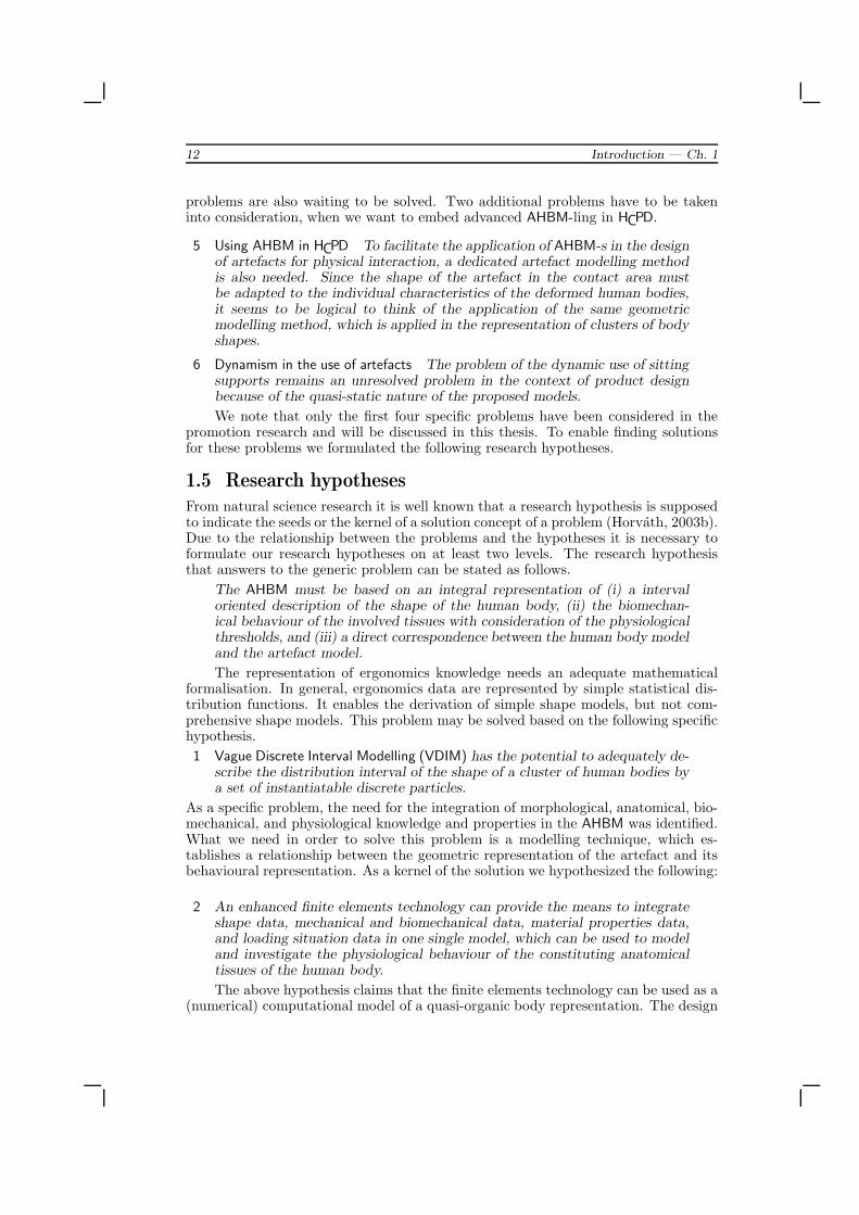
12 Introduction — Ch. 1
problems are also waiting to be solved. Two additional problems have to be takeninto consideration, when we want to embed advanced AHBM-ling in HCPD.
5 Using AHBM in HCPD To facilitate the application of AHBM-s in the designof artefacts for physical interaction, a dedicated artefact modelling methodis also needed. Since the shape of the artefact in the contact area mustbe adapted to the individual characteristics of the deformed human bodies,it seems to be logical to think of the application of the same geometricmodelling method, which is applied in the representation of clusters of bodyshapes.
6 Dynamism in the use of artefacts The problem of the dynamic use of sittingsupports remains an unresolved problem in the context of product designbecause of the quasi-static nature of the proposed models.
We note that only the first four specific problems have been considered in thepromotion research and will be discussed in this thesis. To enable finding solutionsfor these problems we formulated the following research hypotheses.
1.5 Research hypotheses
From natural science research it is well known that a research hypothesis is supposedto indicate the seeds or the kernel of a solution concept of a problem (Horvath, 2003b).Due to the relationship between the problems and the hypotheses it is necessary toformulate our research hypotheses on at least two levels. The research hypothesisthat answers to the generic problem can be stated as follows.
The AHBM must be based on an integral representation of (i) a intervaloriented description of the shape of the human body, (ii) the biomechan-ical behaviour of the involved tissues with consideration of the physiologicalthresholds, and (iii) a direct correspondence between the human body modeland the artefact model.
The representation of ergonomics knowledge needs an adequate mathematicalformalisation. In general, ergonomics data are represented by simple statistical dis-tribution functions. It enables the derivation of simple shape models, but not com-prehensive shape models. This problem may be solved based on the following specifichypothesis.
1 Vague Discrete Interval Modelling (VDIM) has the potential to adequately de-scribe the distribution interval of the shape of a cluster of human bodies bya set of instantiatable discrete particles.
As a specific problem, the need for the integration of morphological, anatomical, bio-mechanical, and physiological knowledge and properties in the AHBM was identified.What we need in order to solve this problem is a modelling technique, which es-tablishes a relationship between the geometric representation of the artefact and itsbehavioural representation. As a kernel of the solution we hypothesized the following:
2 An enhanced finite elements technology can provide the means to integrateshape data, mechanical and biomechanical data, material properties data,and loading situation data in one single model, which can be used to modeland investigate the physiological behaviour of the constituting anatomicaltissues of the human body.
The above hypothesis claims that the finite elements technology can be used as a(numerical) computational model of a quasi-organic body representation. The design

Sec. 1.5 — Research hypotheses 13
of the proper shape of an artefact for physical interaction has to consider the internalstresses and deformations arising in the body due to the external mechanical effects.It should enable to compute the large deformations and the consequences. For thisreason we need robust methods to compute the distribution of the stresses and strainsin the loaded body. Based on these considerations we can hypothesize the following.
3 The principle of the highly non-linear finite elements modelling and analysiscan be used to model biomechanical behaviour of the human body and toadequately compute the stresses and strains in the tissues with the consider-ation of internal restructuring and changes in the biomechanical propertiesdue to large deformation and rearrangements of the loads.
The potentialities of the highly non-linear finite elements modelling are knownbased on the latest results of the related research. Open issues are how much therepresentation of the highly non-linear properties can approximate the real behaviourof organic structures, how the complexity of the model can be rationalised from aconstruction and computational point of view, and how correctly the internal re-structuring and the changes of the biomechanical properties can be described withthis kind of model. A next point is the manipulation of the model in order to ex-plore extra information about the physical interaction and the physiological aspectsof the interaction. A potential solution to this last problem is offered by the followinghypothesis.
4 The finite elements model makes it possible to modify the distribution of theinternal stresses so that their effects on the physiological functioning of theconcerned tissues can be optimised according to some ergonomics criteria.
Based on a non-conventional finite elements model, which provides a balance interms of the distribution of the internal stresses in an AHBM and the physiologicalcomfort of the person represented by this model, the observable body deformationscan be computed. The deformed shape of the finite elements model based AHBMserves as a basis of deriving the best fitting shape of the artefact. This shape caninherit the deformation of the supported region of the body of an individual to theproduct model and in principle can provide the highest comfort for the user of theartefact, i.e. of a sitting support. Based on this reasoning we can formulate our lasthypothesis.
5 The shape of the deformed body model can be used to derive the shape ofthe contact region of an artefact and used as the approximate geometry ofa sitting support.
These hypotheses project ahead a knowledge intensive modelling framework,in which organic modelling of the human body is directly connected with to non-conventional modelling of the shape of the designed artefact (figure 4). Actually, thecoupling between the two kinds of models is established through the simulation ofthe physical interaction that is optimised for user comfort. As hypothesized above,the AHBM encapsulates all kinds of information and knowledge, that are needed tosimulate the real life behaviour, that is, the highly non-linear deformation, internalrestructuring, and rearrangement of loads, of a particular human body. The sourcesof knowledge are physical ergonomics, applied information technology, and productuse. The benefits appear in product design, that is, in the designing of comfortablesitting supports.
The most characteristic feature of an AHBM is knowledge intensiveness. Withsimple words, it integrates knowledge from the concerned disciplines and makes itpossible to simulate biomechanical behaviour. Figure 5 shows the various classes ofknowledge that are used to construct an AHBM. There were two inherent challenges

14 Introduction — Ch. 1
advanced humanbody model
virtual modelof the artefact
physicalinteraction
physical prototype
geometry of theanatomical structures
biomechanics andmechanical properties
physiology andphysiological criteria
physicalergonomics
appliedinformationtechnology
vague geometricmodelling
finite elementsmodelling
artefact design
uses of artefacts
Figure 1-4. The scheme of design for physical interaction based on a AHBM.
to take: (i) complexity of the knowledge structure that has to be overcome by apurposeful structuring of the AHBM, and (ii) the diversity of the representation formsof the knowledge that was managed by following the concept of frame-working.
A lot of knowledge has been explored for the realization of the objectives. How-ever, in many domains and aspects, the available knowledge was not sufficient ordid not yet exist. For this reason an intensive research work had to be completedaccording to a specific research methodics, which will be presented below.
1.6 Research MethodicsIn an ideal case the solution of the presented sub-problems could be achieved by ap-plying a theoretical well supported methodology. However, due to the complexity ofthe problem, which originates from the multi-disciplinarity and knowledge intensive-ness, such a comprehensive methodology does not exist. Instead, what we could doin the research program to solve the sub-problems was to find, evaluate and combineknown methods and techniques with the new methods and techniques, that has beenpurposefully developed in the promotion research. On this basis we applied a goaloriented methodics in our research rather than a fully consistent methodology. Ina chronological order the research program was completed through an exploratory,empirical, implementation, and evaluation part.
was done to find possible solutions for modelling the humanbody and quantify the descriptive parameters of the body.
- The relevant aspects of the functional anatomy of the human body and thephysiological properties of the concerned tissues were studied in a literary review.
- In order to support the development of a quasi-organic model of the humanbody, shape, anatomical, mechanical, biomechanical and physiological modellingtechniques were studied.
- To model the constitutive behaviour of the complex soft tissues a study of theliterature was done to find empirically tested stress-deformation relationships

Sec. 1.6 — Research Methodics 15
advanced HBM
constitutivemodelling
material properties: elasticity viscosity plasticitydrainage of fluids
physiology
bloodlymphnervesinterstitial fluidoxygennutrients
anthropometry
dimensions
shape
vagueness
interval modelling and instantiation
anatomyof tissues
biomechanicalrelationships
forces and momentsconnectivityfrictionrearrangement
skinadipose tissuemusclestendonsblood vesselslymph vesselsnerve fibresbonesjoints
Figure 1-5. Overview of the knowledge incorporated in an advanced human bodymodel.
for highly non-linear behaviour, and the possible constitutive models for themechanical behaviour of the tissues were investigated.
After the exploratory study some information was still missing: (i) no dedicatedgeometric representation of organic and cluster shapes was found, (ii) the constitutivemodels presented in the literature mainly considered the regions of the upper leg inthe context of designing prostheses, and showed conflicting results, (iii) no consistentdata were found on the biomechanical conditions, in particular, on the relationship ofvarying external load and the posture of a person, just to mention the most importantones.
was undertaken to complete the information that was neededfor building the target AHBM. It included the research in the adaptation of intervaloriented geometric modelling, and in the constitutive modelling of the body parts.As a result of the empirical study it was decided to apply finite elements modellingtechniques.
- The research in geometric modelling involved the consideration of three tech-niques for: (i) measuring the shape of the body, (ii) clustering the measuredgeometric data for interval oriented representation, and (iii) generating instancesbased on the interval representation of the shape of the body.
- The research in the constitutive modelling was oriented to the development ofthree methods, namely (i) measuring the interface pressure distribution, (ii)measuring the posture of the body simultaneously with the interface pressuredistribution, and (iii) elaborating the constitutive model as a basis of the finiteelements model. As far as the finite elements model is concerned we had to takeinto consideration the fact that a quasi-organic model with highly non-linearbehavioural characteristics was the target. This is the reason why we neededspecial, non-conventional techniques.

16 Introduction — Ch. 1
was conducted to investigate how the shape model, the
finite elements model, and the artefact model could be implemented in an integ-ral way. Vague Discrete Interval Modelling (VDIM) was used to represent clusters ofshapes and instantiate concrete body shapes. The discrete geometric data represent-ing the instance shape was converted to the input of a finite elements model, andwith the consideration of the internal anatomic structure a compound finite elementsmesh model was generated. The constitutive model was applied to the finite ele-ments model together with the support and the loading conditions. An investigationwas conducted to model the process of internal restructuring, large deformations andloading rearrangement by means of the finite elements model. The interface pressuredistribution was computed and compared to the measured data. The computed in-ternal stresses and deformations were empirically evaluated with a view to medicalrelevance. It was also studied how the information about the deformed body shapecan be extracted from the finite elements model and imported to the VDIM envir-onment for the purpose of physical interaction oriented designing the shape of theartefact.
was completed in order to test and evaluate both the morpho-logical and the finite elements model in various applications and assess the fidelityand reliability of the results. Conclusions were drawn about the strong and the weakpoints of the presented approach. The whole approach to the organic human bodymodelling has been evaluated to see what kind of improvements can be introduced infuture research.
As the above discussion indicates, we had to apply dedicated techniques for eachspecific problem. The cohesion between the techniques does not go beyond the levelneeded by usefulness. For the reason that the disjunct methods could not be mademore integral, the whole research methodology is actually a purposeful methodics ofcreating an AHBM.
1.7 Structure of the thesisChapter 1 has introduced the reader to the main issues of HCPD and the role an AHBMplays in it. It also discussed the specific problems and the research hypotheses of thepromotion research. In chapter 2, the results of the literary study will be presentedincluding the aspects of the human body modelling, the finite elements modelling,and human centred artefact design. Actually, this chapter concludes about whatis available and what knowledge is missing for an AHBM. The conceptual solutionsof the subproblems, together with the theoretical fundamentals and the analysis ofthe feasibility are presented in chapter 3. Apart from the mathematical details, theexperimental setups, and the empirical collection of information are also detailed. Theimplementation of the shape modelling, the finite elements based body model and theresults of the measurements are given in chapter 4. The whole of the research workand the value of the results are discussed in chapter 6. Together with the recognitionsof the shortcoming, suggestions for improvement and the further elaboration are alsoincluded.

Sec. 1.8 — Own publications related to the research 17
1.8 Own publications related to the research
The first ideas of using an AHBM to improve the shapes of body supports have beenconsidered many years ago. These early investigations concerned only the directmodification of the shape of body supports to improve the interface pressure distribu-tion (Moes and Horvath, 1999b). An algorithmic framework to guide a computationtowards this improvement has been introduced in (Moes and Horvath, 1999a). Itwas further elaborated in (Moes, 2001b). The possibility to apply a finite elementsmodel for this purpose, and two concrete computational models to use the finite ele-ments model for improving the shape were presented in (Moes, 1999b). In (Moes andHorvath, 2002a) the concept of an objective functional for the shape improvementwas elaborated. However, this material has not been presented in this thesis, due tothe lack of exhaustive experimental validation.
In this early stage of the research the need to represent the vagueness of the bodydid already appear in the promotion research. The measurements of the shape of thebody, that were needed to build a vague interval model, have been presented in (Moes,2000b). The application of vague interval modelling resulted in a generic shape model(Moes, 2001a). As a conclusion of these investigations, the concept of non-linear finiteelements modelling was adapted as a vehicle for the behavioural modelling aspects ofAHBM-s.
A detailed discussion of using a cluster of shapes to form a generic shape model,and to apply them as a base for the geometric information of a finite elements modelwas introduced in (Moes et al., 2001). The geometric aspects of the finite elementsmodel, and the basic idea of assigning the most simple, neo-Hookean non-linear con-stitutive behaviour to the elements, was discussed in (Moes and Horvath, 2002b).Since this model showed a lack of correspondence, the further research focused onthe use of the more complex, Mooney-type of constitutive modelling (Moes, 2002a).Although some improvement was observed, the results were not yet satisfying, so thata third, even more complex model was tested (Moes and Horvath, 2002). The lastresults showed again that the model still needed further modification to improve itsfidelity. Proposals for such improvement were presented in (Moes, 2003).
The research in constitutive modelling covered the interface pressure distribution(Moes, 2000c), location of the regions with the maximum interface pressure (Moes,2000a), and posture of a sitting person (Moes, 1998a). An in-depth discussion ofthe reference data on the pressure distribution in the contact area was presented in(Moes, 2002b).
Although it is clear that the finite elements model needs further elaboration,the model has been applied to get first impressions on the internal stresses and de-formations for a 3D simulation of the deformations in sitting interaction, which werecompared to the available medical reports (Moes, 2003).


Chapter 2Literature Review
2.1 IntroductionThe knowledge that is needed to solve the problems that were introduced in sec-tion 1.4, covers a range of disciplines such as physics, anatomy, physiology, mechanicalengineering and ergonomics. This is the reason why we needed a broadly-based liter-ature study with the aim of finding useful knowledge, methods and tools. To presentthe studied material and the results in a consistent and logical way this chapter hasbeen build around a reasoning model, presented in section 2.2.
2.2 Reasoning model
The reasoning model for the literature review has been organised in three main areas:(i) the knowledge that is basically needed to elaborate a Human Body Model (HBM),(ii) the knowledge of FE related techniques, and (iii) the considerations for the imple-mentation in HCPD. Figure 1 gives a schematic view of these fields and their subfields.
The knowledge that is related to human body modelling will be presented insection 2.3. It includes the research on modelling the geometry of the body, thebiomechanical properties, and the biomechanical behaviour of loaded body parts.The knowledge that is needed for the finite elements modelling will be surveyed insection 2.4. It includes the aspects of geometric modelling, handling of boundaryconditions, the techniques of FEA, and some open issues related to the use of advancedfinite elements modelling techniques. The various aspects of implementation of HCPDwill be discussed in section 2.5. It includes the basic considerations, the proposedmethodologies, and the fields of application of HCPD.
Whenever we need more depth in our analysis, and to compare and classify theresults of the investigations, we will introduce a specific reasoning model.
2.3 Advancements in Human Body Modelling
This section explores the literature on the geometric models, physiological models,and biomechanical models of the human body.
2.3.1 Geometric representation of the outward shape of the body
A geometric or morphological model of the human body always has a certain degree ofcompleteness from a representational point of view. Based on the carried informationwe can talk about simplified, nominal and expanded shape models. A nominal modelcontains all relevant information for an instance shape. A simplified model containsless, and an expanded model contains more information than needed for a singleinstance shape, such as the spatial distribution of a cluster of shapes and the rules

20 Literature Review — Ch. 2
mor
pholo
gical
body
mod
elling
finite elements modelling
human centred design
applications
methodologies
basicconsiderations
geometry
boundaryconditions FEA
advancedtechniques
geometry
biomechanicalproperties
biomechanicalbehaviour
AHBM
Figure 2-1. The reasoning model of the literature study.
to generate shape instances. First the approaches to handle uncertainty of the shapewill be discussed in 2.3.1.1. A review of the techniques to measure the shape of thehuman body is given in 2.3.1.2. The methods of generating geometric models of thehuman body are analysed in 2.3.1.3 to 2.3.1.5. Having considered which tissues shouldbe included in the HBM, in 2.3.2 a review is given of the properties and modellingaspects of these tissues.
2.3.1.1 Uncertainty of shapes
Uncertainty stems from (i) inaccurate measurements, (ii) in-completeness of the data, and (iii) the variability of the original quantities. With aview to the nature of ergonomics measurement, such kind of uncertainties are inevit-able. Figure 2 gives an overview of the main factors that lead to uncertainty.
The left part of figure 2 shows the decomposition of the uncertainty of meas-urement, the difference between the observed value and the true value, which canbe caused by the inaccuracy of the device, rounding errors, measurement errors, andmeasuring artefacts (Bevington, 1969) (Meerling, 1989). The middle part shows thesources of incompleteness, which is related to the resolution of the measurements. Itdepends on the measuring technique (device) and the measurement procedure (ac-tions). In ergonomics the variability of the true values includes the intra-variabilityand the inter-variability. The inter-variability is the variation among different people

Sec. 2.3 — Advancements in Human Body Modelling 21
uncertainty ofmeasurement
anthropometricvariability
resolution ofmeasurements
incomplete data statistical distributionof the measured data
uncertain data
measuringinaccuracy
measuringerrors
measuringartefacts
measurementtechnique
measuringprocedure
inter-variability
intra-variability
seculargrowth shift
inaccuracy of a virtual shape
Figure 2-2. The sources of uncertainty of the virtual shape.
or groups of people. According to (Tanner, 1981) inter-variability is explained byethnicity, age, gender and somatotype. The inter-variability of anthropometric datahas been reported within the fields of physical anthropology (Knußman, 1988a), ergo-nomics design (NASA, 1978) (Molenbroek, 1994), design for children (Tanner, 1981)(Steenbekkers, 1993), design for the elderly (Steenbekkers and van Beijsterveldt,1998), and design for the disabled (van de Weijgert and Molenbroek, 1991). Theintra-variability of the shape refers to the variation that happens for each individualduring his life (Dirken, 1997). It is a natural phenomenon, explained by time, age,nutrition, health, posture, pregnancy, etc (Molenbroek, 1994). The secular growthshift is the systematic change of anthropometric dimensions during the stages of de-velopment of the human race (van Wieringen, 1972) (van Wieringen, 1986) (Voskamp,1996). Summaries and practical compilations of the anthropometric variability havebeen reported in numerous publications e.g., (Burandt, 1978) (Bullinger and Solf,1979) (Molenbroek, 1994) and (Pheasant, 1996).
Since the human shape usually shows a large variability, the geometric modelsof the body, that have been derived from measured data sets, are often incomplete(Varady et al., 1997). A virtual shape representation of the human body, or a partof the body, always has an uncertainty. The simplified and the nominal models cannot have the potential needed to describe the uncertain shape of the human body. Tothis end we have to consider the various forms of expanded or vague models.
According to (Varady et al., 1997), handling uncertainty canbe done by (i) eliminating measurement noise by filtering, (ii) repairing of missingdata, and (iii) applying statistical models and selection techniques for the variabilityof shape. The elimination of the noise by filtering can be accomplished by fittingshape functions such as B-splines (Arlt and Marach, 1998) (Ruiter, 2000), contours(Hertzberg et al., 1957) or superquadrics (Gu et al., 1998). The repair of missing datacan be done with a generic shape model of sufficient validity (Ko et al., 1994) (Dobsonet al., 1995) (Au and Yuen, 1999), for instance finite elements scaling methods (Lewiset al., 1980)(Richtsmeyer, 1989). These techniques require a detailed knowledge of thelocal anatomy. (Allen et al., 2003) developed a statistical model of the shape of thehuman body. However, this model does not explain shapes related to, for instance,gender or somatotype. Each of these methods has its drawbacks. The eliminationof noise and the repair of missing data have the risk of obscuring relevant details.A generic statistical model creates a new shape by using, for instance, the principal

22 Literature Review — Ch. 2
shape components (Allen et al., 2003), without considering the independent humancharacteristics.
fringes phasestepped
anthropometricmeasurements
probing
stereo-photography
opticalcontours
laser scanning Moirescanner laserrange finder
vertical bars
deformationstrips
ultrasound
passive active
contact non-contact
unloaded loaded
3D body measurement techniques
Figure 2-3. The 3D shape measurement methods.
2.3.1.2 Analysis of the shape measurement methods
Shape measurements are needed in medicine, industry, biomechanics, ergonomics, etc.The required accuracy depends on the fields of application (Gu et al., 1998). Someapplications require modelling of a specific human subject with spatial accuracy beingthe prime concern, such as mannequin modelling for garment design (Simmons, 2002).Other applications require modelling of a general human body, and visual realismdominates over spatial accuracy. This section gives a review of the shape measurementtechniques applicable to the human body. First, the methods for measuring the shapeof the unloaded body, then the methods for the loaded body will be surveyed (figure 3).
To measure the shape of the unloadedhuman body we have found two categories of methods: the contact methods and thenon-contact methods. Using a contact method implies that the body is physicallycontacted by an anthropometric measuring device, or by a probe. In the case ofnon-contact methods, a scattered beam of light or ultra-sound image a subject. Thisimage can be detected and analysed. Either ambient light conditions are used, or acontrolled beam of energy (light or ultrasound) is projected onto the subject.
In the category of the contact methods two measurement typescan be distinguished: (i) traditional anthropometric techniques, for instance, theanthropometer, callipers, sliding compass and tape measure (Steenbekkers, 1993),(ii) touching probe based techniques. The traditional devices can be used to measurethe characteristics of specific features of the shape, for instance, the distance betweentwo landmarks or the circumference of a body part. The operational techniques andthe required statistics for application in physical anthropology have been discussed in(Knußman, 1988b).
The touching probe based techniques can be used to measure spatial locationsof the points of a shape. The probe is usually mounted at the end of a multi-limbrobot arm (Pronk and van der Helm, 1991) (Microscribe, 2002), but air born 3Dmeasuring devices were also reported (Moulia and Sinoquet, 1993) (Vannah et al.,1997) (Bussiere et al., 2002).

Sec. 2.3 — Advancements in Human Body Modelling 23
Since the contact methods are based on physical touching of the measured object,they offer the possibility to obtain the location of palpable bony landmarks. However,contact methods may induce specific problems. (i) Palpating landmarks requires adetailed knowledge of the human anatomy (Backhouse and Hutchings, 1989) and welldeveloped tactile and palpation skills (Field, 1994). (ii) Handling possible emotionalreactions of the subjects requires a relationship of trust and respect (usually thepresence of a second observer is an advantage) (Field, 1994). (iii) The degrees offreedom of movement of the subject must be reduced, and the measurements shouldbe done as fast as possible (Hertzberg et al., 1957) (Moes, 2000b). (iv) Since thetiredness of the observer may result in slight movements of the hand and, thus, ininaccurate data regular periods of relaxation are needed (Moes, 2000b).
The non-contact methods analyse the light that is scatteredby the body (Varady et al., 1997). In a passive system the body is illuminated byambient light, in an active system by artificial light or ultrasound. Some applicationscombine the ambient and the projected light (Schmitz and Whiteford, 2001). (Mor-ing et al., 1989) made distinction between monocular and binocular systems, andintroduced a measure to compare the performance of 3D shape measuring devices
as (resolution/√
measurement rate). Monocular devices derive ‘shape from X ’,where X includes shading, texture, contours, etc. Binocular devices derive the surfacecoordinates based on triangulation techniques.
The use of passive systems enables capturing additional information such as thelocation of special surface markers (Gu et al., 1998). A well known method is thestereo-photogrammetry (Moulia and Sinoquet, 1993), that can be applied if sufficientsurface details are visible. It has been applied in the measurement of the morphometryof the trunk (Kovats, 1985) (Kovats et al., 1988), and for the shape of the human body(Sheffer and Herron, 1989). Although this method enables high resolution imagingand fast measurement sessions, the analysis of the pictures requires intensive cpu usage(Siebert and Marshall, 2000). If the analysis must be done by hand, it is extremelytime consuming (Sheffer and Herron, 1989). Automated analysis requires statisticalcorrelation techniques (Remondino, 2002). In ideal circumstances, an uncertainty ofless than 1% of the size of a pixel can be obtained (Sjodahl, 1994). Electronic specklephotography applied an additional pattern of speckles (Urquhart and Siebert, 1993)(Siebert and Marshall, 2000).
(Hertzberg et al., 1957) developed a technique using the optical contours of thebody, viewed from a set of circumferentially located cameras. Specific problems oc-cur when the surface is reconstructed, such as the triangulation problem (Keppel,1975), the correspondence problem, the tiling problem, the branching problem andthe surface fitting problem (Keppel, 1975) (Meyers et al., 1992). Applying deformablesuperquadrics enables a 3D parametric model (Gu et al., 1998).
The active methods project light on the body. The scattered light is analysedusing goniometric triangulation (Ko et al., 1994). The projected light originates froma laser or from an integral light projection system. The use of a state of the art laserallows a recording time of about twenty seconds for a high resolution 3D image of afull size standing body. This method allows almost real time representation of theshape (Gourlay et al., 1984) (Lewis and Sopwith, 1986). If normal light is projected,it is either a raster of spots (Frobin and Hierholzer, 1981) (Lewis and Sopwith, 1986),a projection of fringes along a line (Lalor et al., 1993) (McCallum et al., 1996), ora grating (Lewis and Sopwith, 1986) (Gourlay et al., 1984) (Ko et al., 1994). Thismethod has been used to study the lung function (Morgan et al., 1985) (Gourlayet al., 1984), and to map the shape of the chest during breathing (Peacock et al.,1985). Further developments have been reported for improved resolution (Rioux,

24 Literature Review — Ch. 2
1984), rotation of the object (Coombes et al., 1991) (Asundi et al., 2002), rotation ofthe light beam (Reid et al., 1988) (Uesugi, 1991) (LaserScanning, 2002), and rotationof the complete projector-camera unit (Turner-Smith, 1982). (Srinavasan et al., 1984)achieved a resolution of the surface ‘height’ better than 10 µm using phase analysisof the deformed projected grating.
The scanning laser range finder (Moring et al., 1989) is an active monoculardevice. This technique uses no triangulation, but the time delay of scattered light tocompute the distance in a certain direction (shape from distance). It was applied by(Allen et al., 2003) within the CAESAR project (Robinette, 2000) to represent thecomplete human body by CAD models. An improved camera setup and a detailedmathematical discussion have been reported in (Takeda and Mutoh, 1983).
A projected grating can be analysed with the Moire fringes method that filtersthe scattered light with a second grating (Meadows et al., 1970) (Takasaki, 1970)(Takasaki, 1973) (Duncan et al., 1980). Advanced developments, using the phaseanalysis of the fringes (Reid et al., 1984) (Lalor et al., 1993) or the Moire phasestepped method, that uses the fast Fourier transform algorithms (Takeda et al., 1982),increased the resolution dramatically (Moire. WWW-Report, 2002). Further clinicalapplications of the Moire methods were reported for the management of scoliosis(Sahlstrand, 1986) (Turner-Smith and Harris, 1985).
Instead of light, it is possible to project ultrasound. The elapsed time betweenthe excitation of the sound and the moment of arrival at a microphone is a measureof the distance. It has been investigated for clinical application (Mauritzson et al.,1985), and to obtain the digitised shape of plants (Sinoquet et al., 1991) (Bussiereet al., 2002).
To measure the shape of a loaded humanbody (a sitting person), three methods have been developed. The first is based on thedisplacement of vertical bars mounted through holes in the seat (Setyabudhy et al.,1997). This system can be combined with force sensors to simultaneously measurethe interface pressure distribution (Reger et al., 1985) (Brienza et al., 1996a) (Brienzaand Karg, 1998a) (Brienza et al., 1989).
The second method measures the deformation of a strip using build-in straingauges (Yamazaki, 2002) (Brodeur and Reynolds, 2001). It deforms together withthe contact area. A drawback is the reduced accuracy when surface irregularitiesexist. This method has been elaborated for seats (Yamazaki, 2002) (Brodeur andReynolds, 2001).
The third method uses ultrasound to measure the shape of the cushion-personinterface (Kadaba et al., 1984). This method does not allow the usage of a multi-material cushion, since it makes use of the specific velocity of sound for the cushionof a homogeneous gel substance.
Point cloud data can be used to fit a parametric shape
model, that gives the basic features for a specific application (Ko et al., 1994) (Dob-son et al., 1995) (Au and Yuen, 1999). The Finite Elements Scaling Analysis method(Lewis et al., 1980) has been developed to study the evolutionary shape, where theword ‘evolutionary’ refers to evolution, growth, inter- and intra-variability (Richts-meyer, 1989). Lewis developed a system of geometric elements, which he coined ‘finiteelements’, for a specific basic biological shape that can be scaled to fit the measuredlandmark data. The specific application is to quantify differences between forms,but a further elaboration towards vague modelling would need profound anatomicalknowledge (Richtsmeyer, 1989).

Sec. 2.3 — Advancements in Human Body Modelling 25
Simple anthropometric data can be obtained using conventional anthro-
pometric measuring devices, or they can be derived from virtual 3D models. If palp-ation of subcutaneous structures is required, then to build a 3D model of the bodyshape, a contact method must typically be applied.
The choice of the technique to be used depends on several requirements. The mostimportant one is the size of the body (large sizes call for stereo-photogrammetry), theexistence of ‘shadows’ or undercuts (which favours contact techniques), the movementsof the subject (fast recording possible with stereo-photogrammetry), the resolution(contact methods give lower resolution), the accuracy (depends on many circum-stances), and the refresh rate of the representation (fast refreshing requires lowerresolution).
2.3.1.3 Simplified models
Simplified models were developed as statistical anthropometrical, biomechanical, vir-tual anthropometric, and finite elements models.
Statistical anthropometric models provide the basic statistical descriptors ofmeasures of the human body, which either characterise the type of the human body(Carter and Heath, 1990), or define the ergonomics requirements for the design ofartefacts (Rodgers, 1983) (Sanders and McCormick, 1993). Comprehensive data setswere reported for the american population (Churchill et al., 1976) (NASA, 1978),children (Steenbekkers, 1993) and the elderly (Steenbekkers and van Beijsterveldt,1998), to mention only a few. Compilations of several sources were published forindustrial design applications (Rodgers, 1983), and for human engineering in artefactdesign (Burandt, 1978) (Bullinger and Solf, 1979) (Molenbroek, 1994).
Biomechanical models include the kinematic and the kinetic models. The kin-ematic models describe the movements of the body during a task (van der Vaart,1995), or support the implementation of avataers (Luciano et al., 2001). The kineticmodels apply free body diagrams (Nordin and Frankel, 1989), and are used to com-pute forces and accelerations of body segments. Applications include a wide area,for instance the load on the sacro-iliac joint during manual materials handling (Mitalet al., 1997) (Mital and Karwowski, 1991) (Tichauer, 1973) (Tichauer and Gage,1977)(Tichauer, 1978) (Anderson et al., 1985), the load on the seat (Goossens, 1994),or the stress inside a sitting person (Staarink, 1995).
Simplified virtual models include geometric models and finite elements models.The simplified-anthropometric models are virtual models based on a set of anthropo-metric measures (Ruiter, 2000, ADAPS), where the simulated shape of the integumenthas an assumed polynomial degree (Arlt and Marach, 1998). These models includestatistical percentiles and were developed for a set of body types. Nevertheless, theycan not be called expanded models, since the correlation of measures is not considered.Within the area of animation and avataers (Wilhelms and van Gelder, 1997), subcu-taneous tissues such as muscles have been included in body models. The simplifiedfinite elements models are based on simple mathematical functions such as spheresor cylinders. They show no direct correspondence to the measured data sets. Mostof them are axisymmetric models of the buttock and ischial tuberosity (Chow andOdell, 1978) (Dabnichki et al., 1994) (Bidar et al., 2000). Other models were used toinvestigate the impression made by a separate indenter as a simulation of the ischialtuberosity (Brunski et al., 1980). (Setyabudhy et al., 1997) modelled a cross sectionof the upper leg to load it by a soft foundation.
Simplified models are useful for a global evaluation of the usage of artefacts inthe first stages of design with the aim to get an impression of the effects of the designparameters.

26 Literature Review — Ch. 2
2.3.1.4 Nominal models
Nominal geometric models in general contain sufficient information to describe theshape of an instance of the body. They have been developed as physical-anatomicalmodels, geometric models, finite elements models, and kinematic models. A physicalanatomical model is a non-virtual, materialised 3D model of the human body. It con-tains the anatomical structures, and is used for medical demonstration and practice,and for demonstrating anthropometric aspects of product design (Dirken, 1997).
Nominal virtual models have been created for various purposes. Geometric mod-els, derived from 3D scanned data sets, served purely geometry oriented applicationssuch as medical imaging and industrial applications (clothing) (Siebert and Marshall,2000) (Simmons, 2002). (Jones and Rioux, 1997) gave an overview of the state ofthe art and an inventory of the possible applications. (Wang et al., 2003) reporteda detailed procedure to create a shape of the upright standing human body fromlaser scanned data using fuzzy logic. A geometric modelling method was developedto generate 3D models for principal components of the vertices of the scanned models(Allen et al., 2003). However, they reported no relationship between these principalcomponents and body characteristics, so that the rules for the generation of valid in-stances are missing. This is why their model can not be considered to be an expandedmodel.
The geometry of nominal 2D and 3D finite elements models must be based onthe geometry of real subjects. 2D models of the buttock were based on MRI scans(Todd et al., 1990) (Todd and Tacker, 1994). 3D models were created using differentscanning techniques. Models of the legs (Steege and Childress, 1988) (Steege et al.,1987) (Sanders and Daly, 1993) and the head (Koch et al., 1996) (Koch et al., 1998)were based on digitised CT slices. Models of the arm (Chen and Zeltzer, 1992) andthe female breast (Azar et al., 1999) (Azar et al., 2000) were based on digitised MRIslices. (Todd and Wang, 1996) developed an automated system to create geometricmodels from MRI scans. If no CT or MRI scans were available, the VHP data set(VHP, 1997) was used (Bro-Nielsen and Cotin, 1996a) (Koch et al., 1996).
(Nußbaum and Chaffin, 1996) developed a kinematic model of the bones of thespine, the pelvis and the rib cage, for fitting to measured landmarks. This modelallows the computation of the loads in any region of the spine for any posture, butit reflects no relationship between movements of the bony part and the surroundingsoft tissues.
Creating avataers requires visual realism of the kinematics of the outward shape(Luciano et al., 2001). (Oliveira et al., 2003) extracted features from high resolutionscanned 3D data to generate an assumed skeleton from surface landmarks and thesurface itself. In general, it seems that the avataer technology is not yet able to handlehuman variability with sufficient spatial accuracy.
2.3.1.5 Expanded models
An expanded model describes the variation interval of the uncertain shape, the dis-tribution of the shape inside the interval, and the rules how to generate a shapeinstance. By generating an intervals it is possible to handle families of shapes. How-ever, building expanded models requires the data for a set of bodies (Varady et al.,1997). Although simplified statistical models exist for anthropometric dimensions ofthe human body, generic vague models of the shape of the human body or the in-ternal tissues have not yet been reported in the literature. A categorisation of virtualshape models includes (i) parametric shape models (solid and feature models), (ii)the shape interval oriented models (interval, statistical, fuzzy, α shapes and fractalmodels) and (iii) physically based expanded models (physically based vague models)

Sec. 2.3 — Advancements in Human Body Modelling 27
(Rusak, 2003). The mathematics for such models has been explored and elaboratedin a series of publications (Horvath and Vergeest, 1998) (Horvath et al., 1999) (Rusaket al., 2000b)(Rusak et al., 2000a) (Rusak and Horvath, year). These investigationsprovided us with a sound foundation that enables the development of a more specificmodel suited for specific applications.
2.3.2 Aspects of tissue modelling
To model the anatomical structures for a simulation of the biomechanical behaviour,first of all, knowledge is needed about major properties of the tissues. The propertiesinclude the anatomical structure and shape, the physiology, the kinematics, the kin-etics, the material properties, and the contact properties, which will be discussed inthis section. The microscopic aspects of modelling of the tissues will be discussed insection 2.3.3
2.3.2.1 Anatomical shape and structure
Each tissue has an external shape and an internal structure, which are globally equalfor all people, but in detail they are different for everyone. For this reason, biomech-anical modelling of a tissue needs individual data. The reported geometric modelsof body tissues were derived using different measuring methods or basic availabledata. (Chow and Odell, 1978) (Brunski et al., 1980) (Todd et al., 1990) (Dabnichkiet al., 1994) and (Bidar et al., 2000) used simple anthropometric estimations for thecore measures of the tissue models, and reduced the actual shape to simple geometricprimitives. (Schock et al., 1982) and (Oomens et al., 1987) used the dimensions ofexcised tissues. Since these tissues had to be removed from their natural environment,the connectivity information was lost. Moreover, the interaction with the surroundingtissues was also lost and the in vitro tissue characteristics may be different from invivo tissue characteristics. (Koch et al., 1996) (Koch et al., 1998) derived part of thetissue shape data from the Visible Human Project (VHP) data (VHP, 1997). Thesedata represent, however, the shape of only two individuals, lying on their back so thatthe dorsal tissues are compressed. CT scans (Steege et al., 1987) (Steege and Chil-dress, 1988) (Vannah and Childress, 1996), and MRI scans (Chen and Zeltzer, 1992)(Todd and Tacker, 1994) (Todd and Wang, 1996) (Azar et al., 1999) and (Azar et al.,2000) seem to be promising for accurate geometric models. But these techniques arestill slow and allow only a restricted number of postures. Moreover, like in the caseof the VHP project, some tissues will inevitably be compressed during the scanningprocess. (Todd and Tacker, 1994) managed to obtain an MRI scan of the undeformedshape of the buttock by supporting the back and the thighs. (Koch et al., 1996) and(Koch et al., 1998) used a combination of CT and VHP data.
2.3.2.2 Physiology of tissues
Physiological functioning of tissues includes metabolism, vascularisation, innervation,and similar biological processes. (Oomens et al., 1987) explained that physiologicalmeasurements inside the tissues can easily create measuring artefacts (see for instancethe literature on measuring the hydraulic pressure inside tissues).

28 Literature Review — Ch. 2
2.3.2.3 Kinematics and kinetics
The kinematics of the tissues describes the movements without considering the forces.The kinetic behaviour of tissues is usually modelled as stress-strain (in solids) or aspressure gradient-flow relationships. The deformation of the surface has been meas-ured with displacement transducers, and the internal deformation using ultrasound.(Malinauskas et al., 1989) recognised the complex, non-linear continuum propertiesof organic tissues. They further elaborated the basic work on ultrasound techniquesof (Krouskop et al., 1987a) to obtain a linear approach of the Young’s modulus (forsmall displacements) using ultrasound. (Cespedes et al., 1993) developed a systemfor elasticity imaging of muscle and breast tissues using ultrasound.
The kinetics of human tissue includes (i) the modelling of the movement of awhole tissue, and (ii) the modelling of the deformation of a tissue. The first is usuallysolved by applying a Free Body Diagram (FBD) (Nordin and Frankel, 1989). Thesecond requires the knowledge about the distribution of the stress throughout thetissue, which is provided by continuum mechanics.
Table 2-1. Physical contact between the internal tissues.
bone tendon muscle adipose tissue skin
bone X X X X X
tendon X X X
muscle X X
adipose tissue X
support X
2.3.2.4 Body contacts
Table 1 shows possible contacts of anatomical entities. Each connection has its degreesof freedom. Contact between bodies has been modelled by finite elements models.(Todd et al., 1990) (Todd and Tacker, 1994) (Bidar et al., 2000) modelled the bodyand the support as a continuous structure by applying common interface nodes. Not-connected neighbouring bodies were applied by (Chow and Odell, 1978) (Brunskiet al., 1980) and (Schock et al., 1982). (Koch et al., 1996) and (Koch et al., 1998)modelled the skin as a thin layer kept at a distance from the skull by linear springs.(Setyabudhy et al., 1997) modelled the thigh as a soft tissue rigidly connected to thebone, but the type of contact between the thigh and the cushion was not mentioned.(Dabnichki et al., 1994) modelled the contact between body and cushion as a fixedtrajectory that was followed by the nodes of the skin to the nodes of an otherwise rigidsupport. To represent connections in a morphological skeleton model (Horvath et al.,1998) developed a technique by which the in-ports, the out-ports, the connections(con-ports) and the internal centres of entities (mid-port) could be specified. Designparameters can be assigned to the mid-ports, the in-ports and the out-ports of theskeleton model. The design parameters of a con-port include, among other things, (i)the geometric shape, (ii) the mechanical friction, and (iii) the hardness of the entity.
Reports on modelling the contact between internal tissues were not found; theknowledge about the frictional freedom of movement of coupled anatomical surfacesis sparse.

Sec. 2.3 — Advancements in Human Body Modelling 29
2.3.3 Modelling anatomical tissues
Anatomical tissues include skin, muscle, adipose tissue, bone and the transportationsystems (blood, lymph, nerves, interstitial fluid).
2.3.3.1 Skin
Integral skin models were mainly developed for application in finite elements models.The techniques include modelling as a membrane (Ziegert and Lewis, 1978) and (Toddet al., 1990), a C1 surface connected to the skull by a system of springs to simulatethickness (Koch et al., 1996), and a layer (Brunski et al., 1980) (Schock et al., 1982).(Koch et al., 1998) used extra springs to simulate facial musculature. The thicknessof the modelled skin was constant, although it has been shown to be dependent onage (Vogel, 1987a) and location (Marks, 1983) (Rushmer et al., 1966) (Brunski et al.,1980).
Despite the large number of reports on the functions and the physiology of theskin (Montagna and Parakkal, 1974) (Goldsmith and Sterner, 1983), research on thecontribution of the epidermis and the dermis to the overall mechanical properties ofthe skin, or on the physiological behaviour were not found. Yet such data are neededfor building a finite elements model. The papillary layer of the dermis (Horstmann,1952) hosts the cutaneous blood capillaries for the nutrition of the epidermis (Williamset al., 1989), which is firmly connected to the papillary layer of the dermis (Felsher,1947). The deeper reticular layer contains e.g., the larger blood vessels and thecutaneous lymph system, and it gives the dermis mechanical strength and elasticity(Rushmer et al., 1966).
The skin shows non-linear elastic (Rollhauser, 1950) (Bader and Bowker, 1983)(Manschot and Brakkee, 1986b) (Manschot and Brakkee, 1987a), visco-elastic (Man-schot and Brakkee, 1986a), anisotropic (Manschot and Brakkee, 1987a), and loca-tion dependent (Bader and Bowker, 1983) (Grebenyuk and Uten’kin, 1994) mechan-ical properties, including the shear stiffness (Grebenyuk and Uten’kin, 1994). Theseproperties are dependent on season (Manschot and Brakkee, 1987b), age (Kirk andChieffi, 1962) (Bader and Bowker, 1983) (Vogel, 1987a) (Grebenyuk and Uten’kin,1994), pre-conditioning (Marks, 1983), gender (Kirk and Chieffi, 1962) (Bader andBowker, 1983), and on the history of the load (hysteresis) (Vogel, 1987b). (Oomenset al., 1987) found that skin and fat behave like solid/fluid mixtures.
Nevertheless, linear behaviour was often applied to reduce complexity and com-putational demands (Sanders and Daly, 1993).
No reports were found about the kinematics of the skin, but it has been shownthat the shape of the skin of the gluteal and the thigh regions vary with the shapeof a sitting support (Levine et al., 1990b) (Brienza and Chung, 1993) (Brienza et al.,1996a) (Brienza et al., 1996b), with (experimental) electrical stimulation of the glu-teus maximus (Levine et al., 1990a), and with posture (Hobson, 1988) (Staarink,1995) (Brodeur and Reynolds, 2001). To simulate the skin deformations for muscleactivation (Schock et al., 1982) applied a subcutaneous soft layer.
Since the skin hosts many tissues whose functioning depends essentially on mech-anical loads (hydraulic pressure, osmotic pressure, etc.), its physiological functioningis sensitive to external loads.

30 Literature Review — Ch. 2
2.3.3.2 Adipose tissue
The human body consists of 10 to 25% of adipose tissue . Adipose tissue occurs inabundance inside the body (around the kidneys, in the female breast, behind theeye ball) and in subcutaneous tissue (Williams et al., 1989) where its distributionis characteristic for age, gender and body type (Carter and Heath, 1990) (Tortoraand Grabowski, 2003), and depends on nutrition, physical constitution, gender andhealth. The amount of soft tissue below the ischial tuberosities shows a large range(5.0–60 mm) (Zacharkow, 1988), citing (Daniel and Faibisoff, 1982) and (Helbig,1978). Reports on geometric modelling of adipose tissue were not found.
The subcutaneous adipose tissue functions as a thermal insulator, as a cushionfor the skin and the deeper internal tissues (Rushmer et al., 1966) (Ferguson-Pell,1990) (Remsburg and Bennett, 1997), and as the main source of energy for the basalmetabolism or low intensity physical activity (Lehmann, 1962) (Astrand and Rodahl,1986) (Tortora and Grabowski, 2003). Although it has been described as a ‘looseconnective tissue’ (Williams et al., 1989) (Tortora and Grabowski, 2003), neither theactual meaning and a quantification of this ‘looseness’, nor the biomechanical prop-erties and coherence have been explained in the literature. Likewise, no explanationon the separation forces of this type of connective tissue were found. (Durnin andWomersley, 1974b) claimed that the compressibility of skin folds is related to thecompressibility and to the deformation of the underlying adipose tissue, in particularto the drainage of the contained water, and therefore decreases with age.
To estimate the amount of fat in the body severalmethods have been developed (Booth et al., 1966), including density measurements(Siri, 1956) (Brozek et al., 1963), using ultrasound (Clark et al., 1989) and (Ramirez,1992), the electric impedance of the body (Roubenoff et al., 1995) (Edlinger, 2002),and a set of skin fold thickness measurements (Durnin and Rahaman, 1967) (Durninand Womersley, 1974a) (Durnin and Womersley, 1974b).
2.3.3.3 Muscle
Skeletal muscular tissue forms the main volumetric part of the buttock and the upperleg regions. The shape and the internal structure are related with function, lengthand location of attachment (Hill, 1956) (Elftman, 1966) (Lohman, 1967) (Gas andGaunt, 1991). Reported geometric models of muscles were derived from scanned data(MRI, CT or VHP). (Chen and Zeltzer, 1992) made MRI based models of severalmuscles, for application in finite elements models. (Zhu et al., 1998) constructed avoxel based model from the VHP data set for application in finite elements modelling.Such geometric modelling techniques can be used for modelling the hamstrings andthe quadriceps group, but for the gluteal group this approach seems to be inadequatebecause of the lateral displacement (Minami et al., 1977). However, since these modelsinvolve crisp geometric representations of individuals, they are not robust enough forapplication in advanced HBM.
The kinematics of muscles (Hill, 1970) includes the deformation (length and dia-meter) (Pitman and Peterson, 1989) (Zhu et al., 1998) (Chen and Zeltzer, 1992),the longitudinal translation (Chen and Zeltzer, 1992), and the lateral translation(Daniel and Faibisoff, 1982) during rotation of joints or under externally appliedload. If a sitting person rotates his pelvis (forward/backward) the hamstring/glu-teal groups are passively elongated/shortened, and the quadriceps group shortened/elongated (Kapandji, 1993b). A muscle exposes lateral movement (sideway sliding) ifit results in a shortening of the muscle and in positive work by the muscle tone andthe elastic force (minimising potential energy). The gluteus maximus muscle moves

Sec. 2.3 — Advancements in Human Body Modelling 31
in superolateral direction off the ischial tuberosity if the hip is flexed (Minami et al.,1977) (Daniel and Faibisoff, 1982) Therefore, no muscle tissue is found below theischial tuberosities of a sitting person.
The actual microscopic mechanical functioning of muscle (Hill, 1970) is accom-plished by the microscopic filaments, the contractile sarcomeres of the myofibrils, andthe visco-elastic sheaths that surround the muscle fibres, the fascicles and the muscleas a whole. Therefore a kinetic model of muscle must include passive and activeelements. Although these elements have been investigated in depth, their mechanicalproperties and geometry are insufficiently known for application in a finite elementsmodel.
Contractive muscle forces depend on (i) the physiological cross section of themuscle (Neu et al., 2002), (ii) the amount of the intra-muscular connective tissue(no contribution to active forces), (iii) the size of the activated motor units (whichare small for precise motor control) and (iv) the number of activated motor units(Williams et al., 1989). (Neu et al., 2002) found no significant gender difference ofthe maximum force for equal physiological cross section area. (Tortora and Grabow-ski, 2003) argues that a decrease of muscle strength is caused by a reduction of thephysiological cross sectional area.
Kinetic modelling of a muscle considers (i) the relations between the sites of theattachments and the morphological adaptation of the muscle4 to speed and strength(Lohman, 1967) (Stern, 1974) (Gas and Gaunt, 1991) (Chen and Zeltzer, 1992), (ii)the dynamic behaviour of the muscle contraction (Hill, 1970) (Pitman and Peterson,1989), and (iii) the relation of the contracting muscle with the surrounding soft tis-sue (Levine et al., 1990a). According to (Pitman and Peterson, 1989) four types of(active) contraction exist: (i) isotonic (the exerted force is constant), (ii) isometricor iso-inertial (length is constant), (iii) concentric (positive work), and (iv) eccentric(negative work). When a muscle is passively elongated beyond the resting length,then the reaction force is based on the muscle elasticity and muscle tone.
Several kinetic models of isolated muscles have been reported. (Zajac et al.,1986) developed a dimensionless muscle model with only four parameters. (Chenand Zeltzer, 1992) refined the Zajac-model to a finite elements model of muscles andincluded active force elements. (Lemos et al., 2001) considered the typical musclemorphology, the mechanical behavioural characteristics and the geometrical config-uration for the muscles of the calf on a basic and simplified level, claiming sufficientgenerality for wider applications. However, they included no active elements. (Zhuet al., 1998) modelled the deformation of muscle for varying voxel-density.
Constitutional models for muscles have been derived from indenter tests of the up-per and lower leg. The force-impression relationships reflect the properties of muscletissue since this forms the main volumetric part of the soft tissue (Krouskop et al.,1987b) (Vannah and Childress, 1988) (Vannah and Childress, 1996).
2.3.3.4 Transportation systems
The transportation systems of the human body are vitally important for supplyingnutrients, to remove waste, and to transfer information. The functional relationshipbetween the transportation systems and the organs implies a spatial relationship.Therefore the kinematic behaviour of the transportation systems is strongly connec-ted to that of the corresponding organ (Montagna and Parakkal, 1974) (Nordin andFrankel, 1989) (Tortora and Grabowski, 2003).
4 This morphological adaptation refers to shape, the pennation angle, the fibrelength, and the gross fascicular architecture.

32 Literature Review — Ch. 2
The transportation of blood and lymph occurs in tubular structures. The propul-sion is maintained by the hydraulic pressure gradient, and supported by a system ofinternal valves. The diameter of the vessels and the thickness of the walls dependson the function (transport or exchange of nutrients and waste). Transport vesselshave a larger diameter and thicker walls. Exchange vessels have a smaller diameterand thinner walls to allow the diffusion of substances. A delicate pressure balanceenables the exchange and prevent a lateral collapse (Williams et al., 1989) (Tortoraand Grabowski, 2003). Under the assumption of collapsible tubular structures (Holt,1959) developed a model that relates the shape, the pressure gradient inside the tubeand the flow of liquid. This model can be applied to fluid transportation systems withlow internal hydrostatic pressure with respect to the pressure of the environment. Thisis typically the case with the venous system, where the pressure eventually drops tozero.
nerve
blood
lymph
interstitial fluid
-1 0 1 2 3 4 5
(kPa)
(10/16)capillary pressure
Figure 2-4. The hydraulic pressure inside the transportation tissues.
An overview of the pressure values inside the transportation tissues is summarisedin figure 4. The next sections discuss the modelling aspects of the concerned tissues.
2.3.3.5 Blood system
The flow of blood is maintained by three mechanisms: (i) the pumping action ofthe heart, (ii) the skeletal muscle pump, and (iii) the respiratory pump (Tortora andGrabowski, 2003). It is controlled by the anastomotic mechanisms of the cutaneousblood system, the venous valves, the smooth muscles of the walls of the vessels, gravity,and external pressure. The diameter of the capillaries depends on circumstances (vas-odilatation, -constriction), for instance temperature (Montagna and Parakkal, 1974),pressure (Bennet et al., 1979) (Yamaguchi et al., 1986) or vibration (van Drimmelen,1979; van Drimmelen et al., 1985) (Taylor, 1989).
The blood has a maximum, pulsating diastolic/systolic pressure inside the aorta(Astrand and Rodahl, 1986). The pulsation diminishes in the arteries and the capil-laries, and drops to zero in vena cavae and the right ventricle. The hydraulic pressurein the blood capillaries has been investigated by (Landis, 1930) and (Bennet et al.,1979). (Humphreys and Lind, 1963) found that the intramuscular pressure duringcontraction can not occlude the blood flow.
The kinetic mechanisms of filtration and resorption5 depend on the pressuredifference over the wall of the vessel. Inside the capillary the hydraulic pressure is
5 Filtration is the pressure driven relocation of fluid and solutes from a capillaryinto the interstitial fluid. The reverse mechanism is called resorption (Tortora andGrabowski, 2003).

Sec. 2.3 — Advancements in Human Body Modelling 33
ca. 4.0 kPa (arterial) and 2.7 kPa (venous), and the osmotic pressure ca. −25 kPa inboth.
hydraulic pressure osmotic pressure In the surrounding tissues the hydraulic pres-sure and the osmotic pressure are ca. −2 kPa (compare with the pressure of the inter-stitial fluid, ca. −0.5 kPa) and +4 kPa (Leduc, 1982). Since an advanced HBM mustreflect the effects of load on the physiological functioning of tissues, these pressurevalues must be considered.
(Intaglietta and de Plomb, 1973) investigated the ratio of the blood flow and theexchange based on a rheologic model and on Starling’s law6 (Starling, 1896). Theyincluded the geometry, the permeability of the capillary wall and the viscosity of theblood. (Holt, 1959) developed a geometric and physical model of a vein system using‘collapsible tubes’. These tubes can be completely closed, but take an elliptical shapewith increasing cross-section if the blood flow increases.
Based on the literature it was concluded that the mechanisms of blood flow andof the exchange of fluids and nutrients form a physiological system of such complex-ity, that the consideration of these aspects in a HBM needs further research. Thementioned models represent important physiological aspects, and the elaboration ofeach of them to a finite elements model would require enormous research effort. Inaddition, the specific quantitative data for model building are still missing.
2.3.3.6 Lymphatic system
When the interstitial pressure exceeds the lymph pressure, mini-valves in the wallsof the lymph capillaries (terminals) open, so that soft tissue waste products are ab-sorbed together with the interstitial fluid. When the interstitial fluid has entered thelymphatic system it is called lymph. A normal, healthy adult has about three litresof lymph. The lymph that has been collected by the lymph terminals, flows to thelymphangion system (pre-collectors provided with valves), and via the lymph collect-ors to the lymph nodes, where it is cleaned. Figure 5 give a schematic drawing of thecollection of lymph. This flow is facilitated by the activation of smooth muscle in thewalls of the lymphatic vessels, by the lymph valves, the osmotic pressure inside thelymphatics, the pressure of the interstitial fluid, the respiratory pump, the arterialpulse, the muscle pump, and the movements of the surrounding tissues (Leduc, 1982)(Tortora and Grabowski, 2003).
precollector
lymphangioncollector
lymph
valve
lymph terminal
muscle cells
Figure 2-5. The tubular structure of the lymph system.
(Reddy et al., 1975) have built a simplified mathematical model of the lymphflow into the terminal lymphatics using the internal hydraulic pressure, the externaltissue pressure, the geometry and the mechanical properties of the vessels. (Millerand Seale, 1981) measured the lymphatic clearance for increasing external pressure.They found that for increasing external pressure the lymphatic drainage increases
6 Starling’s law states that the filtration and the absorption are in near balance.

34 Literature Review — Ch. 2
until a critical pressure. Continued increase of the pressure resulted in occlusion ofthe vessels, reducing the clearance to zero. (Miller and Seale, 1985) used these resultsto elaborate a mathematical model of a system of blood capillaries, interstitial fluid,terminal lymphatics and deep lymphatics. Based on the literature we can concludethat the lymph dynamics depends on a large number of factors, particularly on theexternal pressure. Therefore, if the lymph system is included in a HBM, it must atleast simulate the lymph dynamics. For an adequate model more knowledge aboutthese factors is needed.
spinal nerve
epineurium aroundspinal nerve
blood vessel
axon, individualnerve fibre
endoneuriumaround axon
perineuriumaround fascicle
fascicle
Figure 2-6. Cross section of a spinal nerve.
2.3.3.7 Nerve system
The nerve system (Voorhoeve et al., 1974) takes care of the transportation of sensory(generated by a receptor) and motory information (generated by the central nervesystem) in the form of a pulse train of action potentials (Iggo, 1977) (Sinclair, 1981)using electro-chemical processes within the nerve fibres (Schmidt, 1985) (Schmidt,1986). Each type of corpuscle is mainly sensitive for a specific type of stimulus(Quilliam and Armstrong, 1963). A detailed exposition of tactility is given in (Ludel,1970) (Geldard, 1972) (Iggo and Muir, 1969) (Sinclair, 1981). A cross section of anerve fibre is shown in figure 6. (Myers et al., 1978) and (Lundborg et al., 1983) foundthat the fluid within the nerve fascicles, that are surrounded by the endoneurium,shows a pressure of 0.2(0.1) kPa. No research results were found on the biomechanicalmodelling of nerve tissue, or on the influence of the hydraulic and the osmotic tissuepressure on nerve functioning.
2.3.3.8 Bones
The pelvis region includes the femur, the sacrum and the pelvis (pubic bone, ischiumand ala), figure 7, that articulate in the sacro-iliac (SI) joint, the hip joint and thepubic symphysis. The mobility of the SI joint can be translation or nutation7. No datawas found on the translation, but (Vleeming, 1990) found that the maximum nutationand contra-nutation together was 4. The transversal axis is dorsal to the auricularsurfaces (Egund et al., 1978). This rotation is probably insufficient to include as aparameter of a HBM.
7 Nutation is the rotation of the sacrum towards ventral.

Sec. 2.3 — Advancements in Human Body Modelling 35
Figure 2-7. Front view of the female pelvis.
The hip joint has three axes of rotation. The maximum excursion (circumduc-tion) for a standing person is a curve on a sphere with its midpoint in the centre ofthe joint (Kapandji, 1993b). This envelop is much smaller for a sitting person.
The symphyseal mobility is small. It was shown that during walking and max-imum abduction of the hip joint the translations of the left and the right aspect ofthe symphysis have the order of magnitude of 1 mm, while rotations do not exceed1.5 (Walheim et al., 1984).
The pelvis of a seated person can rotate around a lateral axis. Since the axis ofrotation does not necessarily coincide with the centre of mass of the pelvis, the pelvismay exhibit a translation of its centre of mass. No research was found on these pelvismovements.
Since for normal sitting the deformation of the femur or the pelvis is considered ir-relevant, only FBD modelling (Tichauer, 1978) (Nordin and Frankel, 1989) (Kapandji,1993a) needs to be considered. With respect to sitting (Snijders et al., 1995) reportedFBD-modelling for healthy, and (Hobson, 1988) for disabled persons. No data wasfound on a FBDs, that explains the articulation of the pelvis and the femur.
2.3.3.9 Interstitial fluid
The interstitial fluid (i) takes care of the transportation of nutrients, oxygen, waste etc,(ii) functions as a viscous cushion for external load (Reddy et al., 1981b) (Reddy et al.,1981a), (iii) prevents friction between neighbouring cells, and (iv) has an importanthomoeostatic8 function (Tortora and Grabowski, 2003). It comprises 17% of a healthybody (Guyton et al., 1966). Mechanical load and tissue deformation have a significantinfluence on the interstitial fluid dynamics (Kosiak, 1961). Since the interstitial fluidis bound to the organic intercellular structures such as fibres, its mobility is low(Guyton et al., 1966). Normally tissues show a negative interstitial fluid pressure
8 Homoeostasis is the tendency of organisms to maintain internal balance, espe-cially with concern of temperature, pulse, blood pressure, the hormonal ratios, thewater and mineral balance, and the numerous biophysical functions (Hilfman, 1984).

36 Literature Review — Ch. 2
(Guyton et al., 1960) (Guyton, 1965b) (Guyton, 1965a), which is maintained by theinflow of the interstitial fluid into the lymph terminals (subsection 2.3.3.6). Whenthis inflow is reduced, the interstitial fluid pressure increases. For zero and positivepressures the interstitial volume increases and more interstitial fluid is present thanthe organically bound fluid. This increases its mobility, and results in oedematousconditions (Guyton, 1963).
This reasoning agrees with a mechanical model of the lymphatic flow (Reddyet al., 1975) based on negative pressure differences between the lymph capillariesand the interstitial fluid and the the lymphangions and the lymph capillaries. Inoedematous conditions, and if the flow has been blocked by external pressure orother, medical causes, the interstitial fluid pressure increases indeed (Reddy et al.,1981a) (Reddy et al., 1981b).
Since the interstitial fluid has such an important function for the transportationof fluids, nutrients and waste, it must be modelled in an advanced HBM. However,more research is needed to quantify the behavioural determinants.
2.3.4 Biomechanical behaviour of the loaded body
After the discussion of the body tissues, we turn our attention to the behaviour of thewhole body. Kinematic aspects of sitting do not consider the transmission of forces.In a review (Grieco, 1986) discussed the problem of ‘postural fixity’ in the context ofdifferent work processes. He concentrated on the risk postural fixity for defects of theosteo-muscular system. (Fleischer et al., 1987) found that the kinematic behaviour ofsitting during positioning tasks shows individual patterns.
Kinetic aspects of sitting considered, among other things, the interface forces(Stumbaum, 1983) (Goossens, 1994), muscular load and intra-abdominal pressure(Boudrifa and Davies, 1987), the loads on the SI-joint and the spine (Akerblom, 1948)(Snijders et al., 1995), the effects of a back rest and arm rests (Stumbaum, 1983), andthe circumstances or occupation, for instance office work, working on a running belt,sitting for dentists (Tichauer, 1978), and sitting in automobiles (Zacharkow, 1988).
Modelling the behaviour of the body tissues loaded during sitting, needs know-ledge about (i) the material behaviour and restructuring of tissues, (ii) the distributionof the stresses and the strains at the interface and inside the body, (iii) the effects ofloads on the physiological functioning and the criteria for maximum loads.
2.3.4.1 Material behaviour
(Levine et al., 1990b) measured the in vivo deformation of the softtissues of the buttocks for additional electric stimulation of muscle while the subjectwas sitting. (Staarink, 1995) implanted stress sensors in an artificial buttock toinvestigate the relationships between internal stresses and tissue deformation. Thevertical compression hamstrings, based on a finite elements model, has been reportedby (Setyabudhy et al., 1997).
Rearrangement of tissues during sitting happens for the gluteus
maximus muscle, that slides off the ischial tuberosity when changing from standingto sitting posture (Daniel and Faibisoff, 1982).
Although observations during palpation suggested that subcutaneousadipose tissue shows internal separation below the ischial tuberosities, no report wasfound on this subject.

Sec. 2.3 — Advancements in Human Body Modelling 37
load at the interface
force
contact areapressure distribution
internal load
stressdeformation
relationships of press. distr. with
body support
Figure 2-8. Aspects of the tissue load.
2.3.4.2 Sitting pressure
To discuss the tissue load during sitting the reasoning model shown in figure 8 is used.
Reports were found about the force on the seat. This force is referred to asthe sitting force. (Aissaoui et al., 2001) found that the sitting force was in the rangeof 240 N to 410 N, and a lower force for the disabled. The difference can possiblybe explained by the using of additional surfaces (backrest) or by a reduced bodyweight. The concept of the shear force on the seat as a result of using a backrest,and the consequences for the comfort of sitting have been discussed by (Akerblom,1948). (Hobson, 1988) elaborated this concept for wheelchairs of severely handicappedpersons, and (Goossens, 1994) for office chairs.
(Swearingen et al., 1962) found that the contact area varied between651 cm2 and 1729 cm2 with a maximum for the age of 20 to 29 years. Above that agethe contact area decreased by about -4.4 cm2/year. The same report mentioned anincrease of the body mass of 4.22 cm2/kg. A smaller range, but with the same lowerlimit, was reported by (Aissaoui et al., 2001), who found that the magnitude of thecontact area is smaller for the disabled than for the healthy subjects, 650 cm2 and770 cm2. From these figures it can be concluded that 650 cm2 is close to the smallestcontact area that is needed for sitting.
Research in the optimisation of the shape of the contact area was reported withinthe context of rehabilitation, where long term contact is common. Usually the aimwas the reduction of the maximum interface pressure. The final, optimised shape wasmanufactured by molding individually adapted seat shells (Hobson, 1988) (Brienzaand Karg, 1998a), or by cushioning (Kang and Mak, 1997).
(Kosiak, 1976) claimed that low average pressure enables a redis-tribution of relatively high pressure values over regions of lower pressure. Thereforethe average pressure seems to be an important determinant for the maximum attain-able improvement of the shape of the seat in terms of reducing unacceptable high peakvalues. The relevance of such improvement is typically high for wheelchair users.
(Swearingen et al., 1962) (Bader and Hawken, 1986) and (Maltais et al., 1999)found that for healthy persons the average pressure varied between 6 to 10 kPa. Norelationship with posture, constitution or support characteristics was given. (Kosiak,1976) claimed that (i) the average pressure is essentially higher than the capillaryblood pressure, and (ii) it is therefore impossible to sit for very long periods of timewithout developing pressure sores.
A particular difficulty of the measurement of the maximumpressure is caused by the facts that (i) pressure measuring sensors have a finite size,and (ii) usually a gap exists between neighbouring elements. In most reports thisfact has been left undiscussed, while the maximum pressure was simply defined as themaximum recorded value.

38 Literature Review — Ch. 2
he reported maximum pressure values show a large variation from 5 kPa to248 kPa (Houle, 1969; Garber et al., 1978; Minns et al., 1984; Bader and Hawken,1986; Henderson et al., 1994; Maltais et al., 1999; Aissaoui et al., 2001; Brienzaand Karg, 1998b; Brienza et al., 1996a; Hobson, 1988; Riley and Bader, 1988). Thehighest values were found for disabled subjects sitting on a flat, hard support (Minnset al., 1984), and the lowest values for healthy subjects, who were sitting on a curvedsupport and used a backrest (Riley and Bader, 1988). A few investigations measuredhealthy and disables persons using the same setup, where a higher maximum pres-sure was found for the disabled subjects (Minns et al., 1984) (Hobson, 1988) (Aissaouiet al., 2001).
The behaviour of the pressure gradient can be compared with the maximumpressure. The range was from 0.23 kPa/m to 6 kPa/m, with the higher values forthe disabled (Maltais et al., 1999) (Brienza and Karg, 1998b) (Hobson, 1988) (Baderand Hawken, 1986). The computation of the pressure gradient was always linear.The importance of the pressure gradient for seat comfort was argued by (Gross et al.,1994), who developed a scale for comfort rating, but did not quantify the relationshipsof comfort and pressure distribution.
(Maltais et al., 1999) found values of the mean pressure of 7.1(0.3) kPa
and 6.2(0.3) kPa for the left and right sides. (Minns et al., 1984) compared the sittingpressure distribution, including laterality of healthy and disabled subjects. For thehealthy subjects they found 65.2(28.0) kPa; the left/right ratio was slightly in favourof the left side. For the disabled group the left/right ratio showed a comparable shiftto a range of 0.43 to 1.78. Left-right balance within the distribution of the sittingforce over the skin of healthy subjects was investigated by (Drummond et al., 1982)(Drummond et al., 1985). Absolute pressure values were not reported, but significantdeviations from unity were found for the ratio left/right and for the sagittal location ofthe maximum pressure values for disabled subjects compared to the results of healthysubjects.
(Akerblom, 1948) measured the ‘distance between the
midpoints of the ischial tuberosities’. For the male subjects they found 11.5(1) cm,for the females 13.0(1) cm. (Diffrient et al., 1981) measured the ‘bi-ischial distance’for male subjects: 13.2(0.5) cm. (Kira, 1976, cited in Zacharow, 1988) gives a rangefrom 12.1 cm to 15.9 cm. (Kuboki et al., 2001) found that the distance betweenthe high pressure points depends on stature and gender, but gave no quantification.(Williams et al., 1989) and (Kira, 1976) mention that the ischial spines are closer,and being more in-turned in males. No research was found on the relationship withposture (bending forward or backward). Possibly the pelvis type (Williams et al.,1989) has also a relationship with this distance. Apparently the actual definition ofthis distance varies among the investigators, so that the comparison of the results isdifficult.
Since the ischial tuberosities converge in the sagittal direction, the distancebetween the high pressure areas must depend on the lateral rotation of the pelvis.Furthermore, if the pelvis is rotated forward, a larger part of the sitting force is trans-mitted via the hamstring muscle group, thus reducing the maximum pressure belowthe ischial tuberosities. When the pelvis is rotated backward, the same occurs forthe gluteal muscle group. To investigate such hypotheses the angle of the rotation ofthe pelvis should be included as an independent variable. Nevertheless (Stumbaum,1983) found no significant relationship of the distance between the high pressurepoints with gender or with rotation of the backrest. For upright sitting this distancewas 121(14) mm. (van Engelen, 1988) measured the distance between the ischium

Sec. 2.3 — Advancements in Human Body Modelling 39
impressions on bicycle saddles. He found a range between 90 mm and 120 mm, butdid not explore the results to find explaining variables.
The internal load of the buttocks or the upper legs during sitting hasbeen computed for simplified models, showing homogeneous, isotropic, etc. mechan-ical properties, without differentiation for internal tissues, and extremely simplifiedbony parts, usually the ischial tuberosities (Reddy et al., 1982; Parks, 1969). Theinvestigated aspects of the internal load were the hydraulic pressure, the shear stressand the von Mises stress criterion for several types of the support. Their results showinteresting distributions of the load in a vertical cross section. The magnitude of thestresses and the deformations were only be qualitatively compared, since the materialproperties do reflect real material behaviour.
Only limited quantitative re-search was found on relationships between posture, body characteristics and pressuredistribution. (Garber and Krouskop, 1982) and (Kernozek et al., 2000) found thattypically ectomorph people are more prone to painful sitting on a hard and flat chairthan people showing different body type. Several authors have investigated the de-pendencies of the pressure distribution. According to (Brienza and Karg, 1998b) thebody mass index9 is correlated 0.56< r <0.76. (Stumbaum, 1983) found no sig-nificant correlation with individual body measures. Women showed a tendency forreduced maximum pressure (Stumbaum, 1983). (Garber and Krouskop, 1982) foundthat the frequency of the occurrence of the maximum pressure below a bony area de-creased from thin to obese (in a scale from thin to average to obese), but they foundno dependency on gender. (Treaster, 1987) reported no absolute pressure values, butfitted a Weibull distribution function with location parameter Θ and shape parameterΛ to a histograms of measured pressure values of healthy subjects. The variation ofthe values of Θ and Λ was significant for the subjects and could be attributed to theamount of subcutaneous fat and the degree of musculature.
(Souther et al., 1974) found asignificant dependency of the average maximum pressure on the type of wheelchaircushion. (Stumbaum, 1983) related the sitting force, the magnitude of the contactarea and the maximum pressure to weight, cushion and gender. In the un-cushionedsituation the maximum pressure varied between 40 and 180 kPa, for men about 10 kPalarger than for women. The average contact area was 880 cm2, for women ca. 50cm2
larger than for men. The coefficient of correlation between maximum pressure andbody weight was -0.37/-0.47 for men/women, which shows that the maximum pressureis inversely related with body mass. An average of 65% of the weight was transmittedvia 20% of the contact area. Using a cushion, 40 mm PU foam 40kg/m3, reduced themaximum pressure to 15–30 kPa and increased the contact area by 15%. (Shvartset al., 1980) reported the influence of a ‘massage cushion’ on various physiologicalparameters. Such massage was the result of repeated interface pressure fluctuation.They found, among other things, that the main beneficial effect an increased exchangeof stagnant blood in thigh and calf during prolonged sitting. Such effects can also bereached by regularly pushing up the upper body, as it is advised in rehabilitation forwheelchair users (Patterson and Fisher, 1986).
It can be concluded that a relationship between the pressure distribution para-meters and the properties of a support does certainly exist. However, a useful quan-tification has not been developed.
9 BMI = mass/stature2

40 Literature Review — Ch. 2
2.3.4.3 Effects of stress on physiological functioning
This section reviews the literature of the general effects of load, and the effects of loadon specific tissues including pressure sores.
(Levine et al., 1990b) claimed that the hydrostatic,compressive pressure is not very harmful for tissue functioning. Non-uniform pressureapplication results in strain and risk for tissue damage (Brienza et al., 2002). (Hobson,1988) argued that a gradient of the hydraulic pressure causes migration of body fluids.
For sitting, the normal surface pressure constitutes the main mechanical inter-action between the body and the seat, but also shear exists depending on posture(Reichel, 1958). Using a FBD, (Akerblom, 1948) argued that the seat inclinationangle influences the interface shear, which has been confirmed by experimental data(Goossens, 1994). (Bennett, 1972) developed a mechanical model of soft tissue to ana-lyse the internal shear for external pressure applied by several indenter shapes. (Zhangand Roberts, 1993) elaborated a comparable model, but included the directional as-pects of the effects of external shear on the internal tissue load. They empiricallyverified that the magnitude of the resultant of the shear and normal forces determinethe maximum internal stress and strain.
Without external pressure the interstitial fluid pressureis about −0.5 kPa for healthy persons (subsection 2.3.3.9). (Reddy et al., 1981a)and (Krouskop, 1983) suggested that the tissue breakdown, that happens in situ-ations with prolonged external pressure, is a result of (i) drainage of the interstitialfluid causing direct cell to cell contact which induces contact stress, and (ii) capil-lary bursting after removal of the load, when the interstitial fluid pressure has beenreduced. Such contact stress between, e.g, fibroblasts, should suffice to rupture thecell membranes so that the synthesis of collagen is interrupted. For patients with lossof collagen network integrity (as a consequence of e.g, SCI10) these processes may beamplified.
Using a cranially placed cuff, the interstitial fluid pressure reaches a stable pres-sure of 65-75% of the external pressure (Reddy et al., 1981b) after a few minutes.However, (Kenyon, 1979, cited in Reddy:1981a) investigated the flow of the combina-tion of the interstitial fluid and the ground substance due to external pressure. Theyfound a characteristic time of the order of a few hours. In a follow-up research (Reddyet al., 1981a) applied a mathematical model to study the effects of external pressureon the interstitial fluid dynamics. Assuming literature based values for the hydraulicconductivity, They found an inverse relationship between the applied pressure andthe time to reach a given fraction of the original volume of the interstitial fluid space.This was similar to the relationship found in ulcer creation studies (Reswick andRogers, 1976).
The conclusion can be drawn that the external pressure has a significant influenceon the flow of the interstitial fluid, and that serious medical consequences may happen.It seems therefore important to include the interstitial fluid behaviour in an ideal HBM.
Mechanical load reduces the blood flow if the resultantinternal stress approaches the capillary blood pressure, or if venae become compressed.The blood pressure of the capillaries (Landis, 1930) and the venae has been discussedin section 2.3.3.5. The external pressure is applied by a device that presses on the skin(Bennet et al., 1979), or by a cuff or a bandage that encloses a limb (Yamaguchi et al.,
10 Spinal Cord Injury

Sec. 2.3 — Advancements in Human Body Modelling 41
1986). The effect on the blood flow was obtained by photoplethysmography11 (Ben-nett et al., 1981), by measuring the partial oxygen in the underlying tissue (Newsonet al., 1981), or by the rate of removal of injected isotopes (Daly et al., 1976). (Dalyet al., 1976) found that the response of the blood flow in a pressure loaded regionreaches a steady state condition within minutes.
(Yamaguchi et al., 1986) found that if a bandage pressure, applied on the calf,increases from 40 kPa to 92 kPa, then a decrease of the pulse amplitude of the toesfrom 100% to 40% was found. (Bennett et al., 1981) applied an increasing externalpressure below an ischial tuberosity of a geriatric group and a control group untilthe pulse was reduced to zero. For the control group flow cessation required at least16 kPa, for the geriatric group less than 5.3 kPa, while values of 2.7 kPa were notexceptional.
(Zhang and Roberts, 1993) found that the application of a shear force equal tothe normal force reduces the blood flow by 45% from the flow without shear. (Bennetet al., 1979) found that the pressure necessary to produce occlusion was reduced bya factor of two when sufficient shear was exerted, and that 2.6 units of shear areequivalent to one unit of normal pressure.
(Krouskop et al., 1978; Krouskop, 1983) argued that the propulsionof lymph is largely dependent on the contractility of the lymphatic smooth muscles.The contractility is sensitive for specific chemicals and hypoxia; a reduced lymphaticfunctionality may result in tissue necrosis. Since external pressure may reduce thesupply of oxygen, the consequence can be necrosis because of inhibited lymph func-tioning. (Miller and Seale, 1981) found that external compressive loading influencesthe lymphatic clearance. If the applied pressure increases until 8.0 kPa, then theclearance increases, possibly due to increased pressure gradient. Further increase ofthe pressure until 10.0 kPa reduces the clearance to zero, leaving only a very smalldiffusive component. (Lindan, 1961) found that below 8.0 kPa the effects of pressureload are reversible, but above this level permanent necrosis may occur. Thus externalpressure may reduce the lymphatic clearance. If the limit of 8.0 kPa is expected, thenthe lymphatic system must be included in an ideal HBM.
The frequency of the pulsesof a pulse train is related to the intensity of the stimulus. Pressure exertion on thenerve bundle, that have normally an internal pressure of 0.2 kPa (2 cm H2O) (Myerset al., 1978) and (Lundborg et al., 1983), modifies the permeability of the endo-neuralmicro-vessels and introduce endo-neural oedema. Relief of this endo-neural oedemaby drainage is not easy since (i) the endo-neural space lacks lymphatic channels, and(ii) the perineurium forms a highly effective diffusion barrier (Lundborg et al., 1983).Thus a compression of peripheral nerves may induce an impairment of the nervefunction and cause damage. (Dahlin et al., 1986) reported that a load of 10.6 kPa(80 mmHg) applied for two hours decreases the conduction velocity to 86%, followedby a further decrease, instead of a recovery, during another two hours. The amplitudeof the action potential decreased to 48%, not followed by recovery either. (Rydevikand Nordborg, 1980) found that applying a load of 53.2 kPa during 15 minutes on anerve fibre reduced the conduction speed to 70%, followed by a slight recovery duringthe next two hours; the action potential dropped to 48%, also followed by slightrecovery. If the 53.2 kPa load was applied for two hours, then after 45 minutes bothactions were reduced to zero, not followed by any recovery during another 30 minutes.
11 Plethysmographic determination in which the intensity of light reflected from theskin surface and the red cells below is measured to determine the blood volume of therespective area. There are two types, transmission and reflectance.

42 Literature Review — Ch. 2
2.3.4.4 Acceptable stress levels
In section 2.3.4.3 the influence of pressure on the tissues was reviewed. As a next stepwe investigate the values of the maximum internal stress that are supposed to be notharmful. Although suffering from incompleteness and uncertainty, some recommend-ations do exist for externally applied pressure. However, no recommendations werefound for the maximum internal stress distribution. Table 2 gives an overview of theaspects to be considered when the effects of load must be known.
Table 2-2. Aspects of the factors to be considered for the physiologically acceptablepressure distribution.
Internal stress = f (organ system, conditions, location)
where
organ system =
skinmusclefatbonenerve fibrelymph systemblood vesselinterstitial fluidsensory organ
conditions =
temperaturephysical constitutionphysical conditiongendertimeagemoisturesocial lifecharacternutrition
In this multidimensional field some data was found in literature, which will bediscussed below.
From the experiments of (Rydevik and Nordborg, 1980) it can be concludedthat applying a compressive pressure of 6.7 kPa on a nerve had almost no effect onnerve conduction. An increase of the compressive pressure to 26.6mm or above didseverely affect the conduction.
(Landis, 1930) measured 4.3 kPa in the blood pressure in
arterial, and 1.6 kPa in the venous capillaries. These values are possibly the firstapproximations for the limits of the maximum internal stress that does not cause acollapse of the capillaries.
In normal, healthy circumstances the subcutaneous inter-stitial fluid pressure is slightly negative, −0.52(0.19) kPa, compared to the atmo-spheric pressure. As soon as this pressure reaches positive values, oedema may occur.
2.4 Finite elements modelling
2.4.1 Introduction
Finite element models of the human body have been reported for various body parts,dimensionality, element type and material properties. For qualification12 the finite
12 (Knowles, 1984) defines the terms ‘verification’ and ‘qualification’. Verificationhas to do with the correctly performing computer code in a mathematical and syn-tactical sense; qualification deals with the ability to represent adequately the realphysical world.

Sec. 2.4 — Finite elements modelling 43
elements model computations have been compared with measurements on body partsin vivo and in vitro, and on sectioned parts of animals. Although many authors re-cognised the non-linear behaviour of the human body tissues, most of the models werebased on linear material properties and small deformations. In table 3 an overviewof the main reports is given. The first data column specifies the part of the bodythat was modelled, and the second the type of tissue. The geometry column givesthe technique of obtaining the geometry of the model, and the dimension column thedimensional extent of the model. The last two columns give the element type and thetype of the attributed material properties.
Table 2-3. Overview of FE models. The element type ‘brick’ means eight nodehexahedral element type, ‘qlat’ the quadri-lateral, ‘ohed’ octahedral. In the columnof the material properties, ‘lin’ means linear, ‘M’ Mooney, ‘O’ Ogden, ‘nlin’ non-linear,and ‘v-el’ visco-elastic.
body tissue geometry dimens. elem. mat.
(Chow and Odell, 1978) buttock integral rot qlat lin
(Brunski et al., 1980) buttock skin/ ? rot ohed lin
fat/muscle
(Schock et al., 1982) back pig skin photogr. 2D qlat lin
fat
muscle
(Krouskop et al., 1987b) leg soft/bone mech. sens. 3D brick lin
(Steege et al., 1987) leg integral CT 3D brick lin
(Steege and Childress, 1988) leg integral CT 3D brick lin
(Todd et al., 1990) buttock soft/bone MRI 2.5D (?)
(Todd and Tacker, 1994) buttock soft/bone MRI 3D brick lin
(Chen and Zeltzer, 1992) muscle MRI 3D 20-brick v-el
dissection nlin
(Sanders and Daly, 1993) knee bone/soft MRI 3D brick lin
(Dabnichki et al., 1994) buttock soft 2D M
(Koch et al., 1996) head bone/soft CT/VHP 3D truss lin
(Koch et al., 1998) head id.+muscle CT/VHP 3D. truss lin
(Setyabudhy et al., 1997) thigh soft wires 2D quad O
(Zhu et al., 1998) arm muscle VHP 3D brick lin
(Bidar et al., 2000) buttock soft rot quad lin
(Azar et al., 1999) breast soft/tumour MR 2D qlat
(Azar et al., 2000) breast soft/tumour MR 3D brick M
In other fields of finite elements modelling, such as plastics materials modelling,the modelling of large constructions or the modelling of the behaviour of the earth,non-linear and highly non-linear modelling techniques have often been applied. Alsohybrid modelling of the material properties of human tissue was reported in (Oomenset al., 1987). Nevertheless, it was not before the nineties when the first non-linearmodels have been worked out (Chen and Zeltzer, 1992).

44 Literature Review — Ch. 2
2.4.2 Geometric aspects of finite elements modelling
This subsection discusses the techniques and possibilities to create a nominal 3D meshfrom a nominal geometric model (MARC, 2001g).
Actually, several techniques were already used to generate a nominal geometricmodel. Some authors applied simplified models of geometric primitives (Chow andOdell, 1978) (Brunski et al., 1980) (Schock et al., 1982) (Bidar et al., 2000). Suchmodelling technique is cheap and fast, and suited for getting first impressions of thebehaviour of the model under load. However, to achieve increased fidelity with thefinite elements analysis (FEA), the geometry must reflect the real, free form geometryof the body and its tissues. (Steege et al., 1987) (Steege and Childress, 1988) (Kochet al., 1996) (Koch et al., 1998) used CT scans. MRI scan were used by (Todd et al.,1990) (Chen and Zeltzer, 1992) (Todd and Tacker, 1994) (Azar et al., 1999) and (Azaret al., 2000). When such scans were not available, the archive of the Visible HumanProject (VHP, 1997) was used, but these data are from one subject.
2.4.2.1 Boundary mesh generation
A solid finite elements mesh is usually created from surface data. Although thesesurface data, which can be a boundary mesh or a geometric shape, are of crucialimportance for the accuracy that can be reached for the volumetric mesh of a scannedbody tissue, none of the authors (table 3) reported the details of the surface mesh andhow it was created. The size of the boundary elements is related to the accuracy ofthe curvature that can be reached for the boundary of the solid mesh. A preprocessorto aid the conversion of MRI data into a surface mesh of quadrilateral elements wasdeveloped by (Todd and Wang, 1996), but to create the volumetric mesh they usedcommercial software packages.
2.4.2.2 Volumetric mesh generation
Solid meshing is usually based on tetragonal (pyramid) and hexahedral (brick) ele-ments. According to (MARC, 2001f), a mesh with hexahedral elements is generallymore accurate, and requires fewer elements than tetrahedral meshes. The main partof the finite elements models of the sitting region of the body were two-dimensional(or 2.5D) and rotation symmetric meshes (Brunski et al., 1980; Schock et al., 1982;Dabnichki et al., 1994; Setyabudhy et al., 1997; Bidar et al., 2000).
Three dimensional meshes can be generated by hand, which is time consumingespecially if the number of elements is high (Steege and Childress, 1988). One of thefirst attempts to create a free form volumetric model of a body tissue was reportedin 1987 by (Krouskop et al., 1987b). They used brick elements to generate a finiteelements model of the upper leg. A 3D free form model of the buttock region wasreported by (Todd and Tacker, 1994). (Chen and Zeltzer, 1992) constructed an iso-parametric model of muscle using a small number of 20-node brick elements; (Zhuet al., 1998) explored the effects of a series of subdivisions of 8-node brick elementsfor the anconeus muscle. Several finite elements models of the human body weremade in the field of surgery simulation. (Bro-Nielsen and Cotin, 1996b) created a 3Dmodel of the lower leg, based on the VHP data set. Within the field of rehabilitationseveral models of a stump were build, for instance (Sanders and Daly, 1993), whoused brick elements. The currently available automated meshing engines can createmeshes under several initial conditions such as the element size, connection to theboundary mesh, alignment to specific nodes, etc. (MARC, 2001f).

Sec. 2.4 — Finite elements modelling 45
2.4.2.3 Adaptive mesh generation
During behavioural analysis adaptive re-meshing can be applied to adapt the mesh tothe current, local conditions of load such as high pressure gradients of high deforma-tions (MARC, 2001d). The available techniques are capable to (i) relocate nodes, (ii)subdivide selected elements, (iii) increase the polynomial order of selected elements,and (iv) define new mesh topology with an improved distribution of elements (Shep-hard et al., 1988). These techniques can be applied if a discretisation error indicatorexceeds a preset limit. For the FEA of the sitting loads and deformations no reportswere found on mesh refinement during the analysis.
2.4.2.4 Processing finite element meshes
The size of the finite elements is related to the required accuracy of the results. Afiner mesh, or elements with increased polynomial order (extra nodes along the edgese.g., 20-node brick elements) increase the accuracy (MARC, 2001g; MARC, 2001h).If internal tissue rearrangement is expected, then type of connections between theboundary elements of the neighbouring tissues must provide the required degrees offreedom for the concerned motion (subsection 2.3.2.4). No report was found thatdiscussed or modelled such tissue rearrangement for sitting.
Tissue continuity on the cut faces of a slice can be simulated by the immobil-isation of the nodes in the direction perpendicular to the faces. Closely connectedto tissue continuity is the aspect of symmetry, which can be simulated by immobil-ising the transversal motion of the nodes along the plane or axis of symmetry e.g.,(Todd and Tacker, 1994) (Bidar et al., 2000). (Dabnichki et al., 1994) defined a ver-tical plane of symmetry in the mid of a model by disabling the lateral movement ofthe corresponding nodes, thus avoiding buckling and preventing tissue from passingthrough the axis of symmetry. Modelling tissue continuity at moving planes is moredifficult. Therefore (Todd and Tacker, 1994) applied an elastic foundation of a seriesof oblong elements that were restrained from motion on the free endings.
2.4.3 Handling contacts, loads, and supports
This section discusses how the contact between the body and artefacts, were modelled.This includes the application of the external load and setting the contact conditions.
2.4.3.1 Modelling contacts with finite elements meshes
During the computation of the effects of a seat in the internal loadings of the bodymodel, the FE analyser must know (i) which nodes can contact the seat, and (ii) thetype of contact and friction (MARC, 2001e). (Todd and Tacker, 1994) and (Bidaret al., 2000) modelled a buttock-cushion system without separating the buttock andthe cushion. The contacting nodes of the buttock coincided with the contacting nodesof the cushion. The same idea of coinciding nodes was used by (Chow and Odell, 1978)(Todd and Tacker, 1994) and (Bidar et al., 2000) for the contact area between boneand soft tissue.
When the bodies are treated separately, friction can be modelled. Zero frictionwas applied between the indenter and the skin by (Brunski et al., 1980) and (Schocket al., 1982). (Setyabudhy et al., 1997) gave no specification of the contact propertiesbetween a thigh and the support13. (Dabnichki et al., 1994; Chow and Odell, 1978)applied varying friction, allowing respectively free and restricted tissue rearrangementalong the interface.
13 Probably they used frictionless weak springs to avoid free (air borne) bodies.

46 Literature Review — Ch. 2
2.4.3.2 Loads and loading conditions
When the loading is applied, the equilibrium of forces and moments must be satisfied,otherwise the body will move as a free object, which can not be managed by staticFEA systems.
When forces are applied on a finite elements model, they need a body to act on.In finite elements models of a buttock and a seat they can be applied (i) on the seatingbone, in which case the lower aspect of the support is usually fixed (Dabnichki et al.,1994) (Todd and Tacker, 1994) (Setyabudhy et al., 1997) and (Bidar et al., 2000),or (ii) on the lower aspect of the cushion or the support, in which case the force hasan upward direction. For the last type of force application no references were found.(Chow and Odell, 1978) applied loads exerted by fluids, thus always perpendicularto the skin surface. In the case that FEA that is applied to compute the materialproperties using force-impression relationships, indenter tests are modelled. In thesecases the forces are usually applied on the indenter (Brunski et al., 1980) (Schocket al., 1982).
Automatic balancing of forces can be achieved by fixing the nodes of the support,for instance on the lower side of a cushion (Dabnichki et al., 1994) (Todd and Tacker,1994) (Setyabudhy et al., 1997) and (Bidar et al., 2000), or the boundary nodes of abone (Brunski et al., 1980) and (Schock et al., 1982).
2.4.3.3 Supports and modelling of supports
If the support is a cushion, it can be modelled with a flat initial surface (Dabnichkiet al., 1994) (Setyabudhy et al., 1997) (Bidar et al., 2000), or with a curved surface(Todd and Tacker, 1994). An undeformable support can be simulated by fixing nodesof the upper surface of a flat cushion (Chow and Odell, 1978), or by using a geometricsurface, for which no literature was found. (Chow and Odell, 1978) also investigatedthe effects of the support by fluids, considering a hydraulic pressure that increaseswith the depth, and which is normal to the skin surface.
2.4.4 Techniques for finite elements analysis
For linear models, a solution can be obtained by a direct solver, since the problemis not dependent on the history of the force application. For non-linear problems,several non-linear procedures have been developed (MARC, 2001a). The choice ofthe solver can strongly influence the accuracy, the convergence and the computationalcosts of the solution (Knowles, 1984). The best known are the ‘Newton-Raphson’method, that updates the stiffness matrix after each iteration, and the ‘ModifiedNewton-Raphson method’, that updates the stiffness matrix only with each increment(or time step) (MARC, 2001c). Apart from (Dabnichki et al., 1994), who appliedthe Newton-Raphson iterative procedure, no reference was found about the appliedequation solver. Neither procedure guarantees convergence. This depends on theconstitutive model and the degree of deformation, and more on experience than onmathematical analysis (Knowles, 1984).
2.4.4.1 Material properties of soft tissues
Building a finite elements model of the human body and human tissues requirescareful consideration of possible simplifications of highly complex structures. Realisticcomputations of externally loaded tissues (Schock et al., 1982) mentioned seriousdifficulties such as geometric and material non-linearities, friction, sliding betweendifferent tissue layers, tissue anisotropy, inhomogeneity and visco-elasticity. We hadto conclude, that analytical solutions for such problems are not available.

Sec. 2.4 — Finite elements modelling 47
All reports on finite elements models of the buttock region or other
soft tissue parts of the human body claim that the soft tissue is practically incom-pressible. The Poisson’s ratio is close to 0.5. In the practice a value of 0.49 is oftenused, since otherwise the stiffness matrix can become unstable. (Setyabudhy et al.,1997) allowed for compressibility by using the Ogden constitutive equation, but theyassumed small volume change. Incompressibility of specific tissues such as muscleincompressibility was also assumed (Chen and Zeltzer, 1992). Bone tissue, however,is compressible; (Todd and Tacker, 1994) assumed a Poisson’s ratio of 0.31.
Although most authors recognise the non-linear material proper-
ties of organic tissues, linear material properties have often been allocated to avoidingcomputational complexity or to save computation time. A linear elastic model alloc-ated one single Young’s modulus, possibly anisotropic, to the material. For smalldeformation this is a common and acceptable approach.
(Schock et al., 1982) applied linear elasticity in a FE model of a layered specimenof skin, fat and muscle for various combination of the Young’s modulus of the differenttissues, extracted from other reports. After comparison with experimental indenta-tion measurements they concluded that for large deformations the linear model wasinappropriate. (Bader and Bowker, 1983) (Steege et al., 1987) and (Grebenyuk andUten’kin, 1994) showed that the linear Young’s modulus for indentation depends onlocation and age. (Todd and Tacker, 1994) described a method to obtain an estima-tion of the effective normal Young’s modulus for the sitting load of the tissues belowthe ischial tuberosities. They found that the Young’s modulus depends on postureand gender. In the modelling research for breast tumours, (Azar et al., 1999) choosedthe material stiffness for breast tissue within the range 70–250 kPa, approximately10 times that of fat, but gave no argument. (Krouskop et al., 1987a) measured thematerial properties within the tissue for relaxed muscles, mild and maximum muscleactivation. They found that the Young’s modulus increased with the activation.
Linear normal stiffness was assumed in many finite elements models of the humanbody, for example (Steege et al., 1987) (Bader and Bowker, 1983) (Todd and Tacker,1994) (Azar et al., 1999) (Krouskop et al., 1987a) and (Malinauskas et al., 1989).Linear shear stiffness was assumed by (Grebenyuk and Uten’kin, 1994).
(Chow and Odell, 1978) refined the soft tissue stiffness for large
deformation in a two step approach. After the internal load reached a critical value,the Young’s modulus was increased by a factor of 20, which prevented that the com-pressed tissue would be of zero thickness.
(Rollhauser, 1950) (Manschot and Brakkee, 1987b) and (Man-schot and Brakkee, 1987a) claimed that the stress-strain relationships of the skin arestrongly non-linear, and depend on age, the relative humidity, the direction of theapplied load and even on the season. Within the context of modelling incompressiblebulk muscular tissue in vivo, (Vannah and Childress, 1996) applied multiple regressionfor different combinations of the 5-term James-Green-Simpson strain energy model(MARC, 2000) to experimental data. The first three terms gave sufficient correlationwith the experimental stress-strain data. (Steege and Childress, 1988) developed aFE model of the below-knee stump for the design of a prosthesis. They applied thethree term, extended Mooney material model (Mooney, 1940). (Azar et al., 1999) and(Azar et al., 2000) made a rubber model of the breast with an inclusion to simulatea tumour, and applied increasing stiffness. They used the two-term Mooney materialmodel for the soft tissue, but gave no explanation for the chosen values. (Nakamuraet al., 1981) investigated the soft tissue below the foot using a FE model. Strongly

48 Literature Review — Ch. 2
non-linear values of the Young’s modulus were found from stress-strain measurementswith differences up to a factor of 200.
Based on findings of (Reswick and Rogers, 1976)and (Kosiak, 1961), who investigated the time dependent effects of the externallyapplied mechanical load, (Kett and Levine, 1987) developed a visco-elastic model ofthe tissue at the seating interface. They recognised that such a soft tissue model mustinclude a matrix of soft tissue, the blood vessels, and the lymph vessels. (Oomenset al., 1987) hypothesized that skin and fat behave like solid/fluid mixtures. In orderto prove this assumption they compared the results of FEA of a model, consistingof mixture elements, with the in vitro measurements of indenter displacements andinterstitial fluid pressures.
2.4.4.2 Linear techniques
For very small deformations of incompressible materials the Hookean constitutivematerial model can be used with ν set to 0.5:
σ = 2(1 + ν)Gε and τ = Gγ (1)
2.4.4.3 Non-linear techniques
No non-linear constitutive models were found in our research for relevant publicationsabout organic tissues. Researchers reported on the non-linear behaviour of organic tis-sues applied one of the available constitutive models for elastomeric materials. For thedifferent levels of deformation of elastomeric materials, several nonlinear constitutivemodels have been developed (MARC, 2000; MARC, 2001b). Such models establisha relationship between the strain energy function, W , and the deformation. Thedeformation is expressed by the stretch ratio’s (λ1, λ1, λ1) or the strain invariants,(I1, I2, I3). The most promising approaches are: (i) a power series of the invariantsfor incompressible elastomers (Mooney, 1940) and (Makino et al., 1993):
W (I1, I2) =
∞∑
i=0,j=0
Cij(I1 − 3)i(I2 − 3)j (2)
and (ii) the Ogden model, that allows compressibility (Ogden, 1972):
W =
N∑
k=1
µk
αk
[J
−αk3 (λαk
1 + λαk2 + λαk
3 )− 3
]+ 4.5K
(J
1
3 − 1)2
(3)
Optionally, incompressibility can be modelled by setting the Jacobian
J = λ1λ2λ3 (4)
of the deformation tensor equal to one. In this case we only have the deviatoriccomponent of the Ogden strain energy function. µk and αk , which are not necessar-ily integers (Makino et al., 1993), are material constants, and K is the initial bulkmodulus.
In practice, equation Eq. (2) is reduced to one or more terms. To representsmall deformations of incompressible elastomeric materials only C10 is used, so thatW = C10(I1 − 3), which after some substitution can be brought to the form of theneo-Hookean model:

Sec. 2.4 — Finite elements modelling 49
σ = G((1 + ε)− (1 + ε)−2
)and τ = Gγ (5)
However, for large deformations the neo-Hookean model shows serious imperfec-tions. (Mooney, 1940) argued that using the first two terms reproduces the behaviourof most rubbers for moderate deformations (λ ≈ 4). This reduced form has beencalled the Mooney-Rivlin formulation:
W (I1, I2) = C10(I1 − 3) + C01(I2 − 3) (6)
The strain energy function that was adopted by (James et al., 1975), defines amore general behaviour by using the third order deformation form of equation Eq. (2),that can be applied for extreme deformations:
W = C10(I1 − 3) + C01(I2 − 3) + C11(I1 − 3)(I2 − 3)
+ C20(I1 − 3)2 + C30(I1 − 3)3(7)
This formula is called the 5-term James-Green-Simpson strain energy model. (Vannahand Childress, 1996) applied multiple regression for different combinations of thecoefficients with experimental stress-strain data of the upper thigh tissue, and theyfound that three terms already gave satisfactory fit.
2.4.4.4 Highly non-linear techniques
Techniques that consider (i) rearrangement of tissue, and (ii) hybrid or multi-phasemodelling are called highly non-linear (Horvath, 2003a). The FEA systems imple-ment the tissue rearrangement by (i) introducing different contacting tissues, that areweakly connected (MARC, 2001e), or (ii) introducing separation forces, that allowstissues to ‘split’ (MARC, 2001g). Multiphase modelling is usually implemented aslarge strain visco-elastic behaviour (MARC, 2000).
Each anatomical tissue comprises a number of constituents. Finite elementsmodelling of human soft tissue as an elastic-plastic matrix, (such as cells and fibres)combined with the flow of fluids (such as blood, lymph and interstitial fluid) needsexact knowledge about the rheologic properties of the matrix and the fluids, andabout their interactions. Even if such values could be obtained in vitro, then thequestion remains whether they are valid in vivo. As a matter of fact, such propertiesare extremely heterogeneous and show a substantial variability not only betweenindividuals, but also within a single person. The non-linear behaviour and the largedeformations only increase the modelling problem. As previous research showed,the computation times of simple geological multi-phase models are drastically high(Gerritsen, 2000).
2.4.5 Open issues of advanced finite elements modelling
Several issues of non-linear modelling of living organic materials have not yet beenclarified. These include, among other things, vague modelling and the constitutivebehaviour.
2.4.5.1 Vague finite elements modelling
In geometric modelling research, vague modelling has been explored, elaborated andapplied (Rusak, 2003), and in ergonomics research the statistical distribution of hu-man bound variables is common use. However, in the field of finite elements modellingand FEA each model and computation is of a crisp nature. That is, the current state

50 Literature Review — Ch. 2
of the art does not allow the incorporation of uncertainty in the stiffness matrix.In principle, vague modelling might be applied to represent large deformations andinternal restructuring inside materials.
2.4.5.2 Modelling organic objects
Obtaining the shape of humans or of parts of the human body and the conversion toa finite elements model has been worked out for individuals, and has become quitesuccessful (Vannah et al., 1997). However, representation of the shape of a cluster ofindividuals is yet in its infancy. It is even more true for the finite elements model ofthe whole or parts of the human body.
Obtaining valid models of the material properties of living human tissues needsenormous further research. So far, useful results have been reported on creating mech-anical models of the skin and the underlying subcutaneous tissue (Kirk and Kvorning,1949) and (Kirk and Chieffi, 1962; Grebenyuk and Uten’kin, 1994), the interstitialfluid flow (Reddy et al., 1981b), the leg (Steege et al., 1987) (Vannah and Childress,1988) and (Vannah and Childress, 1996), the lymph flow (Reddy et al., 1975) (Millerand Seale, 1981) (Miller and Seale, 1985) and (Krouskop et al., 1987a), the bloodflow and the diffusion through the blood vessel walls (Holt, 1959) (Intaglietta andde Plomb, 1973) (Daly et al., 1976) and (Kenyon, 1979), the breast (Azar et al.,1999) and (Azar et al., 2000), and muscle (Hill, 1970) (Stern, 1974) (Zajac et al.,1986) and (Lemos et al., 2001). No results were found about the constitutive mod-elling of nerve tissue. Some authors reported the building of a finite elements modelbased on their proprietary constitutive model (Lemos et al., 2001), but the conversionof such knowledge to application in constitutive models for FEA for HBM has not yetproceeded to a level of valid representations of human tissues.
2.4.5.3 Advanced techniques of deformation computation
If the material properties are non-linear and the deformations are large, then theanalysis is usually done in several load cases. The magnitude of the load cases, eachof which is responsible for a part of the total load, is based on experience or on trialand error. Each load case is processed in a series of linearised time steps. The size ofa time step must be determined experimentally. To achieve convergence a time stepmay be subdivided on the run in multiple iterations (MARC, 2001a).
2.5 Ergonomics and Human Centred Product Design
First of all, the philosophy behind HCPD and the related methodologies should beunderstood from the point of view of Ergonomics. The term Ergonomics refers toa relatively young discipline. Ergonomists have struggled for several decades for aproper definition. Three of them will be given here.According to the International Ergonomics Association (IEA, 2003):
Ergonomics (or human factors) is the scientific discipline concerned with theunderstanding of interactions among humans and other elements of a system,and the profession that applies theory, principles, data and methods to designin order to optimise human well-being and overall system performance.
According to (Chapanis, 1985):Ergonomics discovers and applies information about human capabilities, lim-itations, and other characteristics to the design of tools, machines, systems,tasks, jobs and environments for safe, comfortable and effective human use.
(Sanders and McCormick, 1993) defined Ergonomics in terms of the following pecu-liarities:

Sec. 2.5 — Ergonomics and Human Centred Product Design 51
(i) the focus is on human beings and their interaction with artefacts, (ii)the objectives are to enhance the effectiveness and the efficiency of work,and to enhance certain desirable human values, (iii) systematically appliedergonomics knowledge about human capabilities, limitations, etc., is for thedesign of artefacts, procedures and environments.Each of these definitions includes knowledge about (i) humans, (ii) the interaction
between a person and the artefact, and (iii) the application in the design of artefacts.
2.5.1 Philosophy of Human Centred Product Design
The starting point for HCPD is the central positioning of the user during the designprocess. Generally speaking, the involvement of the user means, on the one hand,gaining knowledge about (i) the user’s tasks and goals, (ii) user’s behaviour andcontext of use, (iii) user’s characteristics, and on the other hand (iv) consultationwith users during the whole design process, and (v) taking design decisions withinthe context of users, their work and environment (Rogers et al., 2002). Within thecontext of designing physical artefacts (for instance, sitting supports) this knowledgemust specifically be collected.
2.5.2 Methodologies for Human Centred Product Design
Basically HCPD relies on four principles: (i) focusing on users, (ii) empirical researchon human capabilities and properties, (iii) research on interaction and usability, and(iv) the iterative approach (Rogers et al., 2002). Although these principles wereformulated for human-computer interaction, they are relevant to the physical person-product interaction as well. They appear in most of the methodologies that weredeveloped for the design of physical artefacts, software, etc.
The methodologies of HCPD can be classified as conventional or advanced meth-odologies. Conventional methodologies, theories and techniques, (Bullinger and Solf,1979) (Mital and Karwowski, 1991) (Roozenburg and Eekels, 1995) and (Mochimaruet al., 2000) apply knowledge to design artefacts, which are the results of severaltreatises on ergonomics (Sanders and McCormick, 1993) (Rodgers, 1983) and (Muller,1998). Such knowledge is either already available (Burandt, 1978) (Bullinger and Solf,1979) and (Rodgers, 1983), or it can be collected by empirical research (Wilson andCorlett, 1995).
Advanced methodologies endeavour to support the designers reasoning by model-ling various human-product-environment combinations to integrate all relevant know-ledge in processes that can be supported by computers, and synthesise the intelligencehow to handle this widespread and complex knowledge. The proposed HBM-s appearin different forms, for instance, as finite elements model or avataers. They have incommon that they can be modified with respect to, for instance, the shape or theexternal load, and that they can simulate the effects of such modifications. First de-velopments of such model-based human centred product design methodologies havebeen reported in various fields and stages of development. Focusing on the field ofseat design we can discerned two trends. The first trend considers the mapping ofknowledge (Brienza et al., 1996a), which is, ideally, a linear one-step mapping ofknowledge onto the shape of an artefact. The second trend considers optimisationprocesses, which has an inherent iterative nature (Krouskop et al., 1987b) (Derbyshireand Platts, 1989) (Sprigle et al., 1990) and (Heller et al., 1999).

52 Literature Review — Ch. 2
2.5.3 Applications of Human Centred Product Design
In each definition of ergonomics, the domain of application of ergonomics knowledge isan essential concern. Such domains are broadly the following (IEA, 2003): (i) Physicalergonomics is concerned with human anatomical, anthropometric, physiological andbiomechanical characteristics as they relate to physical activity (Rodgers, 1983) and(Dirken, 1997). (ii) Cognitive ergonomics is concerned with mental processes, suchas perception, memory, reasoning, and motor response, as they affect interactionsamong humans and other elements of a system (Rodgers, 1983). (iii) Organisationalergonomics is concerned with the optimisation of socio-technical systems, includingtheir organisational structures, policies, and processes (Dul, 2003).
2.6 ConclusionsAn extensive literature review was conducted to explore the recent developments of,and the possibilities for advanced HBMthat include (i) the integral representationof shape, biomechanical behaviour, physiological thresholds and the correspondencebetween HBM and artefact, (ii) handling the uncertainty of shape, material properties,etc., in expanded models, and (iii) using finite elements models with integrated shapedata of several internal tissues, their correspondences, and specific material properties.Though a lot of information was found on these individual items, the total pictureshows a lack of consistency and incompleteness. These fundamental problems havelarge influence on the opportunities in the field of advanced human body modelling.From a purely technical point of view, however, creating an integral nominal finiteelements model does not seem impossible under the condition that the necessary datais available.
In our review we dealt with the reported measurements and computations of thestresses and strains at the buttock-seat interface and inside the body. It turned outthat the assumption of linear material properties was inadequate to correctly describethe relationships between loads and large deformations. The reports on highly non-linear modelling and behaviour were inconsistent.
As a next step in our literature study, we investigated if the computed internalstresses could be modified in the process of FEA. The main problem is that theactual optimisation criterion has many aspects to be considered, and a single, validformulation was not found.
Although in principle it is not a problem to extract and convert shape data,included in a finite elements model for geometry-based downstream processes, therewas no publication found on this particular modelling problem.

Chapter 3Conceptual solutions and knowledgesynthesis for advanced HBM
3.1 Introduction of the concepts
Our general idea is that the measured shape data are combined in one vague intervalmodel, rather than in multiple concrete models, which offers the possibility for gener-ating various shape instances. These will be characterised for the assumed mechanicaland biomechanical behaviour. Based on these models information is obtained on theshape of the deformed human body and used to derive the optimum shape of theproduct for a particular user. The manufactured shape of the product can be takenfor clusters of users or for an individual user.
This chapter introduces the conceptual solution for the human body modellingproblem and the synthesis of the knowledge that is necessary for creating varioushuman body models. The general solution will be presented in subsection 3.1.1. Re-ferring to the research hypothesis, given in section 1.5, that states that an AHBM (i)is an integral representation of a vague description of the shape, (ii) the biomechanicaland physiological behaviour of the tissues of the body, and (iii) has a direct corres-pondence with the model of the designed artefact, three basic models constituting acomputer based HBM will be introduced: the morphological model, that describes theshape aspects, the behavioural model, that describes the internal effects of externallyapplied loads and the relationships between stresses and strains, and the design modelthat produces the actual shape of the artefact (figure 1).
loads
input
morphologybehaviour
design model
Figure 3-1. The principle of combining the fundamental sets of knowledge in acomprehensive modelling framework.
A decomposition of the three basic models will be discussed in subsection 3.1.2. Theknowledge that is needed to build the basic models, and the data flow between themare introduced in subsection 3.1.3.

54 Conceptual solutions — Ch. 3
3.1.1 General process
Figure 2 shows the process of linking the generation and processing of the basicmodels in a comprehensive modelling process. The morphological model synthesisesthe initial knowledge and data on the morphology of the tissues into a vague shapemodel. The behavioural model synthesises the knowledge of the mechanical behaviourof the tissues. The design model synthesises the knowledge of generating the shape ofa contact area based on a loaded and deformed HBM, according to some physiologicalcriteria. The input knowledge and data are shown on the left side of figure 2, and theoutput data that are used to generate partial shapes of the designed structures on theright side. The AHBM is not a linear transformation of input to output. Rather it isan iterative process, in which additional knowledge is used to optimise the shape ofthe product for physical criteria. The modelling procedures and the related knowledgeare called an AHBM.
HBM
morphologicalmodelling
behaviouralmodelling
designmodelling
optimizationcriteria
optimization
product shapedata
initi
al k
now
ledg
ean
d da
ta
Figure 3-2. The general process diagram of generating and optimising the productshape.
3.1.2 Further articulation of the models
The development of the basic models was done in phases, each with its own sub-models. Figure 3 gives a further detailing of the basic models. The morphologicalmodelling needs (i) a vague shape model to describe the variance, uncertainties andincompleteness of the domain of the outward body shape and the anatomical tissues,and (ii) an instance from this domain. The behavioural model needs (i) a simplifica-tion of the geometry to balance between complexity and usability, (ii) a discretisationof the internal space in order to reduce the amount of information that must be pro-cessed, (iii) a material modelling to simulate the material properties of the tissues,(iv) the application of external loads to simulate using products, and (v) the pos-sibility to record and export changes of several quantities, for instance of the shape.The design model (i) needs the changed shape of several users, user groups or typesof product usage, (ii) creates a vague model of the product shape, and (iii) generatesa specific shape for further manufacturing. To create these sub-models, mathematicsand algorithms are needed as well as tools for the operationalisation. The flow ofknowledge and data between the sub-models is discussed in subsection 3.1.3.

Sec. 3.1 — Introduction of the concepts 55
deformedshape data
vagueshape model
highly non-linear finite elements model
behaviouralmodel
morphologicalmodel
designmodel
algorithms/methods
HBMA
meshgeometry
materialproperties
loads/supports
geometricsimplification
changesof shape
product shapeinstantiation
instanceshape model
vagueshape model
anatomicalmicro structuremodel
VDIM based product model
algorithms/methods
VDIM - statistics
algorithms/methods
Figure 3-3. The sub-models of the three basic models of the AHBM.
3.1.2.1 Morphological model
A morphological model of the human body is based on measured point data, fig-ure 4(a), which are positioned in a common reference frame, figure 4(b), and convertedto a vague shape model, figure 4(c). From this vague shape model instances can begenerated by, for instance, rule based instantiation, figure 4(d). The instance shapesof a set of tissues, which are considered the macro geometric models, figure 4(e), andthe physiological substructures of the tissues, figure 4(f), are composed in a body part,figure 4(g). The degrees of freedom among contacting tissues, for instance joints andattachments of tendon and bone, and which are called surface relations, are shownas grey regions in figure 4(h). The spatial geometric constraints, for instance slidingof a muscle along a bone, which are called contact relations, as the grey region infigure 4(i).
The existing VDIM (Rusak, 2003) is a system to generate a domain description ofa point cloud in terms of reference vectors and metric occurrences. It offers the possib-ility to generate instances by applying rules. These rules are, as a matter of fact, notincluded in the system, since they are different among specific applications. Thereforean extension to VDIM is needed, that defined the rules for the instantiation. In thesection dealing with the morphological modelling of the human body (section 3.2),we will concentrate on the modelling of the static geometry of the unloaded body fora specific posture. To model the unloaded body the VDIM technique was applied,that enables (i) the conversion of an assembled set of point clouds, representing theshape of tissues, into a shape domain, (ii) the creation of a generic vague model,(iii) assembling into a model of the human body, (iv) generating body models usingselection rules.

56 Conceptual solutions — Ch. 3
(e) (g) (i)
macro structure assembly contact relations
(f)
micro structure
(h)
surface relation
measuredpoint data
positionedshape data
vague genericshape model
generatedshape instance
(a) (b) (c) (d)
Figure 3-4. The stages of the formation of the morphological model. The cross inthe upper row represents the origin of the common reference frame.
3.1.2.2 Behavioural model
The behavioural modelling (section 3.3) is generated to support the computation of (i)the mechanical effects caused by the external loads and deformations on the internalloads, and (ii) the physiological effects such as the flow of body fluids. For such com-putations finite elements modelling technology was found the best alternative. Thegeometric aspects of generating the behavioural model involved the geometry of theinstance shape (subsection 3.3.1), the geometrical simplifications (subsection 3.3.1.1),and the finite elements meshing (subsection 3.3.1.2). The mechanical aspects includethe constitutional modelling (subsection 3.3.2), the application of loads and supports(subsection 3.3.4), and modelling of changes (subsection 3.3.6). After the implement-ation of the geometric aspects nd the mechanical aspects we have a deformable finiteelements model. The external boundary conditions, such as deformation, gravity andsupports, are applied to the unloaded, undeformed body.
3.1.2.3 Design model
In the stage of designing the optimal shape of a product, the shape information isextracted from the deformed finite elements model, and analysed to determine thebest fitting shape of the designed product. If the contact shape fulfils the qualitycriteria, then the deformed shape is extracted from the finite elements model andreused in shape design. Otherwise the deformations and internal stresses must beoptimised based on the finite elements model.

Sec. 3.1 — Introduction of the concepts 57
data contact area
HBM
shape instance data
deformed shape model,physiological functioning
optim
izat
ion
post
ure
dom
ain
varia
tion
dom
ain
measured shape datameasured body charact.assumed body charact.
reference frame dataVDIM
statisticsposture
meshing techniquesmaterial properties
constitutional modelsmaterial distribution
external loadsexternal support
external deformationcontact conditions
medical knowl. & criteriaphysiol. knowl. & criteriaergon. knowl. & criteria
optimization criteriadesign rules
designmodel
morphologicalmodel
behaviouralmodel
Figure 3-5. The knowledge structure for the basic models.
3.1.3 Flow of data and knowledge
Figure 5 summarises the pieces of knowledge and data that are needed to operation-alise the three basic models that are constituents of the AHBM. The morphologicalmodel needs data of the generated point clouds and manipulation of point clouds.The posture domain was introduced to VDIM to account a unified description of pos-sible changes of the shape, that are due to posture. The output of morphologicalmodelling is a shape instance. Since current FE techniques are not able to handleinterval shape data, crisp shape instances must be generated. In certain cases theinstance shape can be generated as a representative of an instance set, produced e.g.,using stratification. If future FE developments allow us to work with vague shapes,then the instances can be vague.
The input data for the behavioural model, which is based on FE technologies,include the applied external forces and deformations, the constitutional model, andthe data on internal effects in terms of stresses, deformations, and their spatial gradi-ents. Meshing techniques are needed to discretise the macro and micro structuresof the body tissues into finite elements. The results of behavioural modelling is thedeformed model, and the distribution of stresses.

58 Conceptual solutions — Ch. 3
The design model is used to (i) judge the resulting internal loads in terms of med-ical, physiological and ergonomics criteria, (ii) optimise the model, and (iii) extractthe final shape. The design rules include the generation of the shape for a particularsub-domain of the user population and the variation domain. These dependencies areshown by the feedback arrows in figure 5.
3.2 Morphological modelling of the human body
This section presents the formal means for building the morphological model. Thisincludes the mathematical description of the kinematics and the kinetics of sitting, thefundamental concepts that are used in vague modelling (3.2.2), generating and hand-ling point clouds for interval shape models (3.2.3), modelling tissue substructures(subsection 3.2.5), tissues (3.2.4), body parts (3.2.6), and the total body (subsec-tion 3.2.7). Figure 7 shows the process of assembling these structures in a total bodystructure. The undecomposable level represents the smallest structures that build upthe tissues models. These tissues are assembled in a body part, representing a macrolevel, and body parts in a total body or holonic model.
undecomposablelevel: micro structures
tissue level:meso structures
total body: holonic levelbody part level:macro structures
mic
ro a
ssem
bly
mic
ro a
ssem
bly
mes
o as
sem
bly
mes
o as
sem
bly
mac
ro a
ssem
bly
Figure 3-7. Micro, meso and macro level assembly of the components of the humanbody model.
A flow diagram of the procedures, intermediate and final results for the develop-ment of the morphological model is shown in figure 6. The left part shows the actionsfor the generation of the tissue models, and the right part for the assembly.
3.2.1 Modelling the variation interval for sitting
The variation interval is needed to represent (i) the kinematical changes of the bodyposture, and (ii) the kinetics of the body. The kinematical changes are supposed todescribe (i) to the lumbar curvature of the back, (ii) the lateral rotation of the pelvis,and (iii) the position of the legs.
The lordotic curvature and the lateral rotation of the pelvis are closely related.The rotation of the pelvis is an important factor for the pressure distribution in thecontact area with the support. The effect of the pelvis on the location of the highpressure region depends the shape of the ischial tuberosities, and the rotation angle.

Sec. 3.2 — Morphological modelling of the human body 59
poin
t clo
uds
mac
ro-s
hape
mod
ellin
g
generatingdistributiontrajectories
referenceframe data
assumedbody chrs.
VDIM:physical
operators
VDIM:position
operators
mountedbodies
reshapingtissues
attachmentsbetween tissues
spatial arrangementof tissues
aggregationof point clouds
positioning ofpoint clouds
conversionof shape data
measuredbody chrs.
input data and knowledge
VDIMhulloperators
VDIMmetricoccurrenceoperators
statistics
pointclouds
vague shapemodel of tissues
shape instancegeneration
vaguemodels of
tissues
anatomical &physiologicalknowledge
macrolevel
microlevel
mic
ro-s
hape
mod
ellin
gof
tiss
ues
body
inst
ance
gen
erat
ion
posture interval( =1, ..., )ip np
tissue level body level
macro levelinstance (1)
macro levelinstance (nt )
generationmicro level
components(nt )
body
mod
ellin
g
vague shapemodel of body
generation ofshape instance
of body
shape instanceof the body
(1)
shape instanceof the body
( )np
measuredshape data
ip
shape intervalgeneration
computation oflocation indices
behaviouralmodel
macro + microlevel components
(nt )
generationmicro level
components(1)
macro + microlevel components
(1)
Figure 3-6. Flow diagram of the input data and knowledge, the procedures, andthe intermediate results that are needed for an instance of a body.

60 Conceptual solutions — Ch. 3
3.2.1.1 Kinematical modelling
In this subsection we will discuss the kinematical aspects that should be modelledin an optimal AHBM. Although the study of the sitting kinematics covers a widearea of external and internal movements, we will concentrate of the aspects that canbe relevant for inclusion in an optimal finite elements model. These aspects are themovement and the posture of the legs, the lumbar lordotic curvature and the rotationof the pelvis.
If the legs are allowed to move, then the hip joint must allow rotation, and theline of action of the support force must be allowed to translate accordingly. Since theposition of the legs is not a domain on some interval or absolute scale, but consists ofseveral possible postures, it must be described as a nominal variable.
In figure 8 it is shown that the lumbar lordosis is associated with the rotationof the pelvis. Since the natural mobility of a sitting person goes together with amodification of the lumbar lordosis, the kinematical modelling of the pelvis must payattention to the forward/backward (lateral) rotation, which is shown in figure 8 as arotation of the sacrum, and should be included in an optimal model. The muscular andthe tendinous structures, that span the lumbo-sacral joint, must allow deformationand relocation, which is shown as the change of the length of the muscle (L1 → L2)and its spatial relocation.
increased lordosis
L1
L2
lumbar spine
sacrum
Ft
FtFr
FrMLSL-S joint
Figure 3-8. The increase in the lumbar curvature causes a rotation of the pelvis(sacrum is shown), and a muscular (grey area: m. multifidus) relocation and deform-ation. Modelling ft represents the traction forces of the muscle.
If the pelvis rotates along a lateral axis, then the spheroidal hip joint allowslateral rotation. This kinematical mechanism should be included in a sophisticatedbody model. The helical axis of the pelvis rotation, also called the screw axis, can beused to describe the rotation and the translation of the pelvis bones. In addition, theAHBM must allow modelling the contact regions of the ischial tuberosities and theadaptation of the inner aspect of the skin below these bones to such circumstances.
The effect of pelvis rotation on the reaction force arising on the seat dependson (i) the angle of rotation, (ii) the distance between the ischial tuberosities, (iii)the curvature of the ischial tuberosities, and (iv) the contact properties of the ischialtuberosities with respect to the underlying soft tissue (adipose tissue and skin). Con-centrating on the kinematics, and assuming that the shape of the lower part of theischial tuberosities can be represented as half-circular discs, the relationship betweenthe radius of the ischial tuberosities, ρ, the rotation of the pelvis, αp, and the distance,t, between the locations of maximum pressure (assuming a correspondence with theischial tuberosities) can be quantified (figure 9).
When the pelvis rotates, the region of the ischial tuberosities, which contactsthe inner aspect of the skin, is shifted accordingly. Since the ischial tuberosities

Sec. 3.2 — Morphological modelling of the human body 61
rolling
sliding
femur
pelvis
skin
not rotated
αp
αp
Figure 3-9. Lateral rotation of the pelvis causes rotation of the hip joint, and, ifaccompanied by sliding, a relocation of the ischial tuberosity with respect to the skin.
converge in sagittal direction, t decreases with forward pelvis rotation, ∆αp > 0, andincreases with backward pelvis rotation. The relationship between ∆t and ∆αp canbe quantified.
Let us consider the ischial bones as radial sections of a cylinder with radius ρ(figure 10). The two sections enclose an angle γ. Points A and B are the loweraspects of the right and left discs. If the discs roll over an angle ∆αp their lower
aspects move from A to A′ and from B to B′. The length ∆s of the path along thelegs a or b is ∆s = ρ ∆αp. The distance between the lower projections of the discschanges accordingly:
βαp
t =∆t
∆αp= −2ρ× ∆αp × sin(γ/2)
∆αp= −2ρsin(γ/2) (8)
Since ρ >0 and sin(γ/2) >0, βαp
t must be negative: when the pelvis rotatesforward, the points of maximum pressure approach one another.
t
a
b
B
B’
left
A A’
right
r
∆s
γ
∆αp
Figure 3-10. The circular disc model of the ischial tuberosities.

62 Conceptual solutions — Ch. 3
If no sliding takes place over the inner aspect of the skin, γ can be calculated fromthe trajectories of the maximum pressure points. Since ∆t and αp can be obtainedfrom measurement, ρ can be computed. But if sliding does take place, then onlyρsin(γ/2) can be computed. Whether sliding of the ischial tuberosities over the innerside of the skin takes place or not depends on several factors. Specific anatomical,mechanical and motor characteristics of a subject determine which mechanisms ofmotion take place. However, the friction between the ischial tuberosities and theinner skin surface is unknown.
The occurrence of sliding can be judged roughly from the sagittal displacementof the points of maximum pressure. In case of pure rolling, the relation between thefront depth (the distance between the front edge of the sitting support and the pointsof maximum pressure) and αp is a monotonously decreasing function. The reverse isnot necessarily true; a monotonously decreasing relation is not a proof for the absenceof sliding. If sliding happens, then this relationship can be of different forms, such asincreasing, decreasing, flat, or even a local minimum or maximum.
3.2.1.2 Kinetics
A change of the posture, i.e. a change of the legs or a tilt of the pelvis, implies a changein the forces, in the pressure distribution in the contact area, and in the distributionsof the internal stress and deformation. This means that, when modelling the tissuesand their mechanical relationships, we have to consider that the corresponding loadscan shift along the line of action. It has to definitely be considered in the followingsituations.
- If the shape of the lumbar spine varies, then the muscles and tendons, thatspan the lumbo-sacral joint (erector spinae, multifidus, muscles of the abdominalwall, etc.), exert varying traction forces accordingly. Therefore, the FBD14 ofthe model must include the traction forces (the arrows Ft in figure 8), and thereaction forces and moments that are exerted via the lumbo-sacral joint.
- The same is true for a rotation of the pelvis. If the pelvis has a rotationaldegree of freedom, the anatomical structures, that span the hip joint (quadriceps,hamstrings, etc., figure 11) have to be modelled for traction forces.
femur
pelvis
hamstrings
quadriceps
Figure 3-11. The hamstrings and the quadriceps.
- If the legs are allowed to move, then the hip joint must allow rotation, and itmust be possible that the line of action of the support force is moved.
14 Free Body Diagram.

Sec. 3.2 — Morphological modelling of the human body 63
3.2.2 Fundamental concepts of vague geometric modelling
A vague geometric model includes the representation of the distribution interval ofa shape. In the practice it means an explicit description of the minimal and themaximal closures and a representation of possible shapes by points located alongthe distribution trajectories (Rusak, 2003). The first step is the construction of theclosures, which is based on a vector space model. The mathematical fundamentalshave been introduced in (Rusak et al., 2000a), and have been illustrated in figure 12.Rusak considered a discrete representation of a vague shape, and assumed that thisvague shape is known or can be composed by aggregating shapes. in the current workthe latter procedure is followed: the vague shape is derived from measured point sets,that are incomplete and uncertain.
(a) (b) (c)
inner closure
outer closure
x
z
v
y
ε
o
ε1ε 2
1ε
y1
y2
z1z2
y2
y1
z1
z2
x
v1v2
v1v22i
ε
ε1i
Figure 3-12. Representation of the vagueness of a shape by a distribution intervalon the basis of vector spaces. The metric occurrences of the reference points areshown as finite vector spaces.
Figure 12 shows the following quantities. A geometric point, for instance x, isa position in 3D space: x = (x, y, z). A localised geometric vector, e.g. v = y − x,is a vector from a point x to a point y, is fixed in space, and has a magnitude anda direction. But a geometric vector has no fixed location. A vector space is a set ofvectors that is closed under vector addition and vector multiplication. A vague vector,vv , is a localised geometric vector, r, with an attached vector space, ε = zi − y.This vector space is called the metric occurrence. The point y ∈ <3 coincides with theend point of the vague vector, so that vv = (y,ε) (figure 12a). The vector r = (y−o),where o is the origin of the coordinate system, is called the reference vector of vv .Figure (b) shows two vague vectors with a circular and a general metric occurrence.In figure 12(c) the metric occurrence is a vector space where sign(v · εi) is constant.A crisp vector is a vague vector with zero metric occurrence.
A vague model of an object is a set of vague vectors that describe the spatialdomain of all possible shape instances of an object. It is defined by following inter-connected entities: (i) the distribution domain, which is given by the closures of themetric occurrences, (ii) a set of localised crisp reference vectors, and (iii) the metricoccurrences, or vector spaces at the end points of the reference vectors. An instancecan be derived from a distribution interval by, for instance, a statistical distributionfunction. distribution function
The vector space of the metric occurrence is defined by supporting vectors andboundary vectors. A supporting vector is a localised vector which end point serves asan approximation point for a closure (figure 14). A closure is an overlaying surface

64 Conceptual solutions — Ch. 3
Discrete domain generation fromtwo point sets
Discrete domain modification byadding a new point set
(b)(a)
maximalclosure v1
v12
v2
meaningless
minimalclosure
surface normal
n2
n1
modified maximalclosure
area between theouter closure and the
added shape
area between theinner closure andthe added shape modified
minimal closure
Figure 3-13. A graphical representation of generating the minimal and the max-imal closure.
that connects the supporting vectors. When the point cloud of each of the closuresis determined, lines are drawn from the points of one closure to the closest points ofthe other closure. A distribution trajectory is a line-piece from a supporting point onthe inner closure to the matching supporting point on the outer closure (figure 14).A supporting point is a point at the average location of end points of the supportingvectors of one reference point. A reference point is associated with a supporting pointon the outer closure and a supporting point on the inner closure, figure 14.
outer hull
inner hull
reference vectorsfor metric occurences
reference vectors fordistribution trajectories
supporting points anddistributiontrajectories (vectors)
supporting vectorsboundary vectorssupporting points
Figure 3-14. Generation of distribution trajectories.
These concepts, that have been developed within the context of vague shapemodelling, will actually be applied in the creation of the vague model of the body.
3.2.3 Creating a vague model from point clouds
To build a generic shape model of the tissues and the body for a particular population,we need the knowledge on the distribution of the shapes. The input knowledge to buildthe shape interval models of the tissues and the body can be obtained by measuringthe bodies and converting the measured data to point clouds. The shape data areobtained from subjects having their body in a position that causes no mechanical loadon the parts in question. The tissues of importance include the skin, the subcutaneous

Sec. 3.2 — Morphological modelling of the human body 65
adipose tissue, the muscles, the bones, and the transportation systems. To reflect therelevant shape features of the tissues, such as dimples and protrusions, a certainmeasurement accuracy and completeness of the data is needed.
3.2.3.1 Precision of the data
What measurement uncertainty can be accepted? The answer to this question has twoaspects. First, what comfort tolerance can be accepted in the final shape? Secondly,what minimal uncertainty is inherent due to the fact that the measured object is ahuman being? These questions can not be answered without further analysis of thephysiological behaviour of the human body, and the tolerance for comfort.
The shape variations within the intended user population determines the extent ofthe generated shape interval. The uncertainty of this extent depends on completenessof the measures data figure 15, assuming the instrumental errors can be neglected.
uncertainty frommovements
uncertainty fromshape variations
uncertain point cloudsand vague model
uncertainty of thesize of the generatedshape interval
shape measurementsbody characteristics
body characteristics
Figure 3-15. Uncertainty of the generated interval.
Due to the facts that (i) living persons show natural movements, and (ii) theshape of a person shows natural variation, uncertainty of the data can not be avoided.Since these variations depend on many factors, exact figures can not be given. Becauseof the large number of influencing factors, the inter-person and the intra-person vari-abilities have a statistical nature. Therefore the shape domain must be described by astatistical model. This approach is actually an extension to previously available meansof the VDIM methodology. In (Rusak, 2003) a different approach was proposed andused for deriving the distribution interval, trajectories and shape instances. Basedon the fore-running reasoning, we have found statistical instance generation a betterfitting alternative.
Additional sources of uncertainty are (i) observer errors, systematic and random(reading errors, lack of skill errors, movement errors, inter-observer errors), (ii) in-strumental errors, systematic and random, (device-bias, device inaccuracy), and (iii)errors inherent to the measurement setup (measuring artefacts, incomplete data).During the application the actual shape measurements have been done, see chapter 5.In the measurement setup for the various experiments the procedures to minimisethe uncertainties have been developed. In the next section, which discusses how tohandle the point clouds in order to create a vague shape model, it was assumed thatthe shape measurements data are available.
3.2.3.2 Positioning the point clouds in a common reference frame
During the measurements the reference frame may differ among the subjects. Theorigin is usually defined some inside the measuring device, and the direction of theCartesian axes depends on the orientation of the device. However, to create the vagueshape model the point clouds must be defined in the same reference frame. Thereforewe first define a common reference frame, Γ. Then the measured point clouds aretransformed to fit in Γ.

66 Conceptual solutions — Ch. 3
The choice of Γ is in principle irrelevant, but a practical definition will make thetransformation computations easier. It has been decided to define the origin on themidpoint of the ischial tuberosities. The z-axis runs in the vertical direction (towardsthe head). During the measurement a vertical vector has been measured. The x- andthe y-axis run to the right and in frontal direction. The right direction is defined torun from the left SIAS to the right SIAS. Since this reference frame does not dependon soft, deformable tissues, but is based on easily palpable bony landmarks and onstandard lateral and frontal orientations, it forms a stable and convenient basis forthe Working Coordinate System (WCS).
In the following paragraphs the transformations are described, that are appliedon the point clouds. These transformations include three rotations, a 3D translation,and a fine tuning. Two rotations with respect to the x- and the y-axis are neededto align the measured vertical vector along the positive z-axis. One rotation withrespect to the z-axis is needed to align the SIAS-line parallel to the y = 0 plane. Theremaining three degrees of freedom of translation are used to position the midpointof the ischial tuberosities in the origin.
The measured vertical direction is represented as the
vector vMCS = (xv, yv, zv)T , figure 16(a). This vector is aligned with the z-axis ofthe Working Coordinate System (WCS) by applying a rotation αx = atan (xv/zv)around the x-axis, followed by a rotation αy = atan (yv/zv) around the y-axis
Rxy =
cos(αy) 0 −sin(αy)
−sin(αx) sin(αy) cos(αx) −sin(αx) cos(αy)
cos(αx) sin(αy) sin(αx) cos(αx) cos(αy)
(9)
x
y
αz
rightSIAS
leftSIAS
y
x
z
αx
αy
(a) (b)
vMCS
Figure 3-16. The angles αx, αy and αx. The thick arrow is the vector vMCS .
The measured line that connects the SIAS-es is ad-justed parallel to the xz-plane, figure 16(b). Therefore the point cloud is rotated over
the angle αz = atan(∆yS/∆xS
)
Rz =
cos(αz) −sin(αz) 0
sin(αz) cos(αz) 0
0 0 1
(10)

Sec. 3.2 — Morphological modelling of the human body 67
Since the location of the two ischial tuberosities can
not be measured simultaneously when the subjects are using the sitting posturewithout loading the buttocks, the distance, t between the ischial tuberosities is meas-ured separately (see the next chapter). A graphical representation is given in fig-ure 17. The point cloud is translated in three steps. First the point of the rightischial tuberosity, xTr , is translated to the origin. Secondly the location of the leftischial tuberosity is computed by subtracting their distance, t, from xTl : xTl = xTr−t
where t = (t, 0, 0)T . Thirdly the midpoint, m, is translated to the origin, followed by
a translation over d = (0, 0,−d)T to correct for the skin thickness, d.
t
midpoint
pelvis
ischialtuberosities
ox
z
WCS
Figure 3-17. Translation of the midpoint of the ischial tuberosities to the originof the WCS. One half of pelvis (dashed) is obtained via symmetry assumptions.
Summarising, the point cloud is transformed so that for each point
xi,WCS = Rz
(Rxy
(xi,MCS − x
Tr
i
))+ 1/2 t− d (11)
During the data collection the body must be in a standard posture. This
is not always possible because of the variability of the angle ‘between the legs’; thelegs are not always parallel. This would introduce an artificial domain of existencefor the shape of the leg. Therefore a correction must be applied. The introducedmeasures are demonstrated in figure 3, where the end point is defined based on thebounding box of the distal measuring point of the upper leg. Since the TL-line isalmost parallel to the y-axis, the tilt of the line from the ischial tuberosity to theend point is small. Thus, the angles which must be corrected are αz ≈ ∆ze/ and
αx ≈ ∆xe/ , where ` ≈ ye. The fine tuned points are then computed as
xfi = Rxz(xi + d)− d
Rxz =
cos(αz) −sin(αz) 0
cos(αx) sin(αz) cos(αx) cos(αz) −sin(αx)
sin(αx) sin(αz) sin(αx) cos(αz) cos(αx)
(12)
This fine tuning improves the alignment of the legs, but the alignment of theSIAS lines is not perfect any more. For the reason that the distance of the SIAS line

68 Conceptual solutions — Ch. 3
to the rotation centre is much smaller than that of the end point, the overall effect isan improvement.
3.2.4 Macro-shape modelling
The creation of a generic vague interval model of the shape of the tissues consists of thefollowing steps. (i) The inner and the outer closures are computed (3.2.4.1). (ii) Thereference vectors and metric occurrences are computed (3.2.4.2). (iii) The locationindices are computed for all subjects and distribution trajectories (3.2.4.2). (iv) Thelocation index is described as a statistically distributed variable which depends on thebody characteristics and the location on the body (3.2.4.3), and it is used to defineinstances of the shape. (v) In the generic vague interval model statistics is used tocompute shape instances for specific subjects, that are characterised by their bodycharacteristics (3.2.4.4).
3.2.4.1 Inner and outer closure
By definition, the interval model represents the range of variation of the cluster ofshapes that can be instantiated from the interval. The minimal and the maximalextents of the interval are the inner and the outer closures. The corresponding pointsof the inner and the outer closures are connected by the distribution trajectories.When an instance is to be derived, the distribution trajectories. The distributiontrajectories quantify the extent of the interval in terms of location, magnitude anddirection. The location index, ζ, shows the place of the occurrence of a measuredpoint along a distribution trajectory. The total set of location indices, ζ, reflectsthe shape of a measured instance along the set of distribution trajectories. The innerclosure and the outer closure are obtained according to (Rusak et al., 2000b)(Rusaket al., 2000a).
First, the closures are computed for two point clouds. Although starting with thelargest and the smallest sample is advantageous for reducing the computation time (ifan added point lies within the current vague domain no action is needed to extend thedomain), it is not an essential issue. To determine if a point to be added modifies theinner or the outer closure, containment computations are made. Figure 13(a) showsthe points and the surface normal vectors of two shapes and the principle of extensionof the distribution interval. The metric occurrence is shown by the lines running fromthe inner closure to the outer closure. The sampled point clouds are added one byone, and the closures recomputed for each added point cloud. The mathematics ofthis method is discussed in detail in (Rusak et al., 2000a).
3.2.4.2 Representing the shape of the skin by location indices
The shape of the skin can be described as a set of locations on the distribution tra-jectories. For each distribution trajectory the intersection points with the measuredshape has to be determined. To compute the location indices the original, measureddata points have to be projected to the closest distribution trajectories, figure 18.
The location of the projected points on the distribution trajectory is expressedas a distance from the inner closure. Actually, the ratio of this distance and the totallength of the distribution trajectory is called the location index: ζ = k/l (figure 19),where l is the length of the trajectory and k the length of the intersected part.

Sec. 3.2 — Morphological modelling of the human body 69
ζ>1
ζ=1
0<ζ<1
line of application of thedistribution trajectory
measureddata points
ζ=0 point of inner closure
point of outer closureouter closure
inner closure
ζ<0
Figure 3-18. Projecting measured points on a distribution trajectory. The thickarrow is the distribution trajectory.
l
k
distribution trajectory
point on innerclosure
point on outer closure
intersectionpoint
Figure 3-19. Computation of the location index along a distribution trajectory.
3.2.4.3 Statistical description of the location index
If it is possible to relate the location index to body characteristics, then a statisticaldescriptive model of the location index can be created.
The relationship of the location indices with the body characteristics such asstature, body mass, somatotype15 (Carter and Heath, 1990), the amount of bodyfat as a fraction of body mass (Durnin and Womersley, 1974a) and gender, can beinvestigated using multiple linear regression. Since human body characteristics areusually correlated, the underlying factors16 can be found by factor analysis. If bbis the b-th body characteristics, then the f -th underlying factor, Fsf , for the s-thsubject is defined as
15 (Carter and Heath, 1990) used the endomorphic, mesomorphic and ectomorphicindices to indicate the type of body build.
16 Factor analysis of a set of quantifications of different variables seeks for the maindirections in the space that is spanned by these variables. The first factor is definedin the direction that represents the largest amount of total variance. The secondfactor is orthogonal to the first and represents the maximum variance in a directionperpendicular the the first, etc. Each factor, also called underlying factor, is a linearcombination of the primary quantities. The corresponding weight factors are calledthe respective loadings.

70 Conceptual solutions — Ch. 3
Fsf =∑
b
fbfbsb (13)
where fbf is the coefficient of the b-th body characteristic for the f -th factor, Ff .The results of the multiple regression analysis are given as a set of linear regressioncoefficients, cdf and a set of constant terms cd, for the d-th distribution trajectory
ζsd = cd +∑
f
cdfFsf (14)
3.2.4.4 Prediction of the location index for new instances
The distribution of ζ over the distribution trajectories can be described by multipleregression of ζ with respect to a set of measured body characteristics, bM . Thisenables us to predict ζ for new subjects from the same population (if the sample was
representative). The set of the estimated ζ defines the point cloud of a new instanceshape of a subject with the assumed body characteristics, bA, or for a subpopulationwith the assumed range of body characteristics.
Suppose that an imaginary subject has body characteristics bsbb and corres-ponding underlying factors Fsff . The instance corresponding to this subject can be
generated by the estimations, ζsdd, of ζsdd for the set of distribution trajectoriesd:
ζsd = cd +
∑
f
cdfFsf
d
(15)
For each distribution trajectory the dependency of ζsd on the factors, Fsf , is quantified
by applying multiple linear regression of ζsd to the factors. Thus for each distributiontrajectory a linear regression equation (eq.15) is generated. The explained fraction ofthe total variance is given by the correlation statistic r2. A perfect regression gives
r2 = 1, a perfect non-regression gives r2 = 0. The values of ζ and ζ should ideallybe within the range [0,1]. Because of the assumed convex global curvature and theapplied projection procedure some instances of ζ are inevitably larger than 1, which
is transferred to the values of ζ via the regression procedures. In concave regions ζcan get a negative value. Ideally the fit results in a zero intercept, and a slope andcorrelation equal to one.
3.2.5 Micro shape modelling
Micro-shape modelling concerns the internal structure of the tissues (the micro-structure). For each type of tissue the specific anatomical characteristics and themechanical and physiological effects of loads and deformations have to be taken intoaccount.
- In the internal structure of the skin two layers are distinguished: the epidermisand the dermis. Since the natural toughness and resilience of the skin is mainlydue to the fibrous constituents of the dermis, enmeshed in a gel-like matrix,the micro-structure has to represent such elements. The dermis supports, bindsand elaborates the epidermis, so that it conforms to the underlying bones andmuscles. If the physiological functioning of the skin is a design criterion, then

Sec. 3.2 — Morphological modelling of the human body 71
the transportation systems, that are sensitive for pressure and deformation, haveto be also included as micro-structures.
- The gross internal structure of muscles is mainly composed of contractive musclefibres spanning the length of the muscle, fasciae, adipose tissue and blood vessels.To reflect natural muscle contraction, the mechanically active elements can bemodelled as contractive fibres, for instance, by highly deforming truss or beamelements. The freedom of lateral expansion of the tendons is reduced to almostzero, but they show low bending stiffness. An even more precise micro-structurecan also represent the muscle type, for instance, pennate or fusiform.
unipennate tendon
muscle
bone
fusiform
tendon
tend
on
muscle
bone
Figure 3-20. Two examples of the morphological types of muscle.
- If large deformations are expected on the adipose tissue, then the possibility oftissue separation must be considered. The tissue can be modelled by spheroidalelements with separation forces, and interspersed with blood vessels.
- Large deformations and stresses inside the tissues can result in inhibited provisionof nutrients, oxygen, etc, as well as in the removal of waste products. Therefore,in a precise micro-shape model the small blood and lymph vessels, includingcapillaries, must be considered.
3.2.6 Meso-shape modelling
Meso-shape modelling concerns the positioning of the 3D tissue models and definingthe relationships. If the tissue models are derived from one subject (as a crisp model),then we can use the bony landmarks for positioning. If they are derived from a genericinterval model, the landmarks will probably not coincide. In this case additionalscaling operations are needed. If the vague model includes the assembly of the tissues,then the correspondence of landmarks is guaranteed.
In order to be able to assemble the vague tissue models, many conditions haveto be fulfilled. The conditions include the surface relations and contact conditions(Rusak, 2003). Assume that tissues A and B have the nominal shapes SA and SBwith boundaries b(SA) and b(SB). The surface relations express the positional re-lationships. For example all point of SA are outside SB (for instance the epidermisand the adipose tissue), touching if there is at least one point of b(SA) that coincideswith one point of b(SB) (for instance skin and adipose tissue), and containing if allpoint of SA are inside b(SB) (for instance a blood vessel inside a muscle).
The contact conditions specify the type of touch. Examples are friction or rigidconnections. To connect two tissues, for instance a muscle with two bones, the effect

72 Conceptual solutions — Ch. 3
regions must be known. For each effect region a transformation matrix must bedefined. Such matrices can define, for instance, a sliding contact, a spheroidal hingecontact, or a rigidly fixed contact. Using such transformations, the different tissuescan be assembled in a body part or in a whole body.
The connection of the tendon of the muscle and the bone is a fix contact, whichcan be described by:
FF = T RxRyRz =
1 0 0 0
0 1 0 0
0 0 1 0
(16)
where T is a translation matrix and R is a rotation matrix. The connection of themuscle belly and the bone(s) can be modelled as a slide contact, that leaves twodegrees of freedom:
FS =
1 0 0 [−∞, +∞]
0 1 0 [−∞, +∞]
0 0 1 0
(17)
It is assumed that the sliding takes place in the local xy plane. This type ofcontact is in between the human body and a chair, but also at the hip joint. Althoughthe head and the acetabulum are not perfectly congruent, it can be considered aspheroidal joint with three degrees of freedom for rotation, and zero degrees of freedomfor translation. So, the transformation matrix is:
Fhip =
[−1, +1] [−1, +1] [−1, +1] 0
[−1, +1] [−1, +1] [−1, +1] 0
[−1, +1] [−1, +1] [−1, +1] 0
(18)
3.2.7 Body modelling
The vague discrete interval model (VDIM) can describe the shape of the entire bodyas well as of a specific region of the body. As a matter of fact, any derived new shapemust reflect a person who belongs to the population from which the representativesample of the measured subjects was drawn. By statistical techniques the statisticaluncertainty of the generated shape can be quantified. The statistical uncertaintyis covered by the interval representation, which is based on the metric occurrencecomputations.
3.2.8 Conclusions
In principle it is possible to build an advanced morphological model of the humanbody for a particular population and to consider the physical interaction with anartefact. This model includes the geometric descriptions of the tissues that make upthe body or, in our case, the buttock region. The model can also be called ‘advanced’,since it is based on vague geometry and applies rules to generate shape instances foran individual or for a subpopulation.
Collecting the input data does not impose technical difficulties, but much hasyet to be elaborated from an instrumental point of view. Though the basic principlesare understood and well formulated from a mathematical point of view, the actualalgorithmisation still needs a lot of effort.

Sec. 3.3 — Non-linear finite elements model of the human body 73
Setting up the procedures to collect the input data needs (i) measuring the ex-ternal shape of the body and the internal tissues, (ii) conversion of the measureddata into generic shape models using extended VDIM, and (iii) assembling the vaguemodels in a partial or a complete human body which can again be done by VDIM.
3.3 Non-linear finite elements model of the human body
The new behavioural model differs from the traditional models in that it can handletypical biomechanical and physiological behaviour. According to our hypothesis, itcan be based on highly non-linear FE technology. It synthesises (i) the geometry ofthe AHBM, (ii) the mechanical behaviour of the tissues, (iii) the contact propertiesbetween macro structures, micro structures, and between the pair of the body andthe support, and (iv) the boundary conditions. The FEA algorithms are supposedto compute (i) the mechanical effects of the interaction of body and artefact underenvironmental and usage conditions, and (ii) the physiological effects of the stressesand strains inside the body in terms of the flow of the fluid body components. Fig-ure 21 gives an overview of the processes of forming the basis of the finite elementsmodel and computations.
FEM
boundary conditions
elementmatrix
internal deformation
interface pressure distributionmesh
constitutivemodels
interface deformation
internal stress
FEA
internal hydraulic pressure
resistance for fluid flow
draining behaviour
Figure 3-21. The FE process to obtain the internal stresses, strains, and physiolo-gical quantities related to fluid flow.
Figure 22 shows the input data and the conditions, how they are applied inthe behavioural model, and the results of the FEA in terms of the external and theinternal effects. These can be used as input data for the design model, since theycarry information about the changes before and after the load application.
The finite elements model must be highly non-linear since the various linear mod-els were already shown to be inadequate for handling large deformations and viscousbehaviour. Non-linear, but elastic models can cope with large deformations, but notwith non-elastic behaviour. Highly non-linear models can handle large deformationsand rheologic behaviour simultaneously.
Under the assumption of having (i) an assembly of complete, accurate geometricmodels of the body tissues, (ii) adequate highly non-linear constitutional models forthe tissues, (iii) models for the connectivity of the tissues, and (iv) models for thephysiologic behaviour of the tissues under loading, an ideal finite elements modelis possible. A further question for implementation considers what can actually beincluded in the finite elements model.
This section discusses the components for the finite elements model, including thegeometric aspects (3.3.1), the mechanical properties (3.3.2), the contact conditions(3.3.3), the boundary conditions (3.3.4), the FEA (3.3.5), and the modelling of thebehavioural changes 3.3.6.

74 Conceptual solutions — Ch. 3
assignmentof mechanical
properties
assignment ofelement types
mec
hani
cal p
rope
rtie
s
geometricmodel ofsupport
FEA
modelling of the changes
translation rotation deformationphysical:
physiological:change offluid flow
static changes:transformationof the tissues
dynamic changes:flow of fluids
loaded FEM(iv=1, ..., nv)
assignmentof loadingconditions
assignmentof contactconditions
FEAanalysis
conditions
FEAmethods
undeformablesupport
externaldeformations
externalforces
contactproperties
constitutionalmodels
materialproperties
force/deformationmeasurements
expecteddeformations
results of the FE computation
contactconditions
expectedstress
gradients
unloadedFEM (iv)
boundaryconditions
assignmentof deformation
conditions
internal stresses,deformations,
and flow (i)( =1 , ..., nv )iv
external deformedshape and pressure
distribution (i)( =1 , ..., nv )iv
input data &input knowledgemeshing
techniques
meshing
meshesof tissues
geom
etry
of F
EM
geometricsimplification
simplifiedmodel
advancedmodel
body instance( =1, ..., nv)iv
idealmodel
vague geometricmodel
Figure 3-22. A global scheme representing the input data and knowledge, the pro-cedures, and the intermediate results that are needed for generating the deformedshape of a loaded body, and the internal stresses and deformations.

Sec. 3.3 — Non-linear finite elements model of the human body 75
3.3.1 Geometric aspects of the finite elements modelling
The result of the morphological modelling is a vague interval body model, that consistsof body parts, macro structures, and possibly elementary micro structures. Consid-ering far future FE systems, we can assume that they will be able to handle vaguegeometric and other properties. That is, the vague body model can be converted tovague finite elements. The nodes will be defined by crisp reference points with metricoccurrences.
However, this functionality was not available at the time of completing this pro-motion research. Therefore we concentrated on crisp FE geometries, exactly locatednodes, exact material properties etc., handling inaccuracy and uncertainty as it wasdescribed in subsection 3.2.3.1.
As a first step, the previously generated shape model must be converted to aFE geometric model, more precisely to a 3D solid mesh. Since the content of themodel depends simultaneously on the purpose of application and on the technicalpossibilities, certain simplifications can be introduced in the finite elements model.
FEMsimplificationcomplete
geometric model
application of:- feasibility testing- internal loads- physiological aspects
requirements for- completeness- computation- preciseness
Figure 3-23. The process of geometry simplification.
3.3.1.1 Geometric simplifications
An ideal geometric model is supposed to represent (i) the details of the macro, themeso and the micro structures and the integral body structure, and (ii) the geometricrelationships of neighbouring structures. It is complete in the sense of the number ofrepresented tissues and has sufficient resolution to represent typical shape features.Such level of modelling is not always a prerequisite for a meaningful analysis anddrawing conclusions about the behaviour. Reduced complexity can, depending onthe context, give valuable results as well, and simplifications can be advantageous oreven needed, see figure 23. In this context three types of study can be distinguishedthat call for respective levels of model simplification: (i) the ideal model, (ii) theadvanced model, and (iii) the simple model (figure 24).
- If the effects of applied loads on the physiological behaviour must be evaluated,then an ideal, fully detailed, model must be used.
- If the purpose is to get an impression of the distribution of the stresses and thestrains, without considering the basic physiological effects, then several aspects

76 Conceptual solutions — Ch. 3
minimally detailed
fully detailed ideal model
simple model
advancedmodel
Figure 3-24. Three levels of simplification.
can be left out from the implementation of the model, such as fluid behaviour.depending on the omissions, advanced models of various fidelities can be con-structed. The level of detailing of the advanced model is not sharply described;it depends on the purpose of the application.
- If the purpose is to support testing a specific modelling aspect or a detail of theanalysis, a simple model may be satisfactory.
Applying geometric simplification influences not only the geometry, but also thebehavioural modelling. The legacy of the simplification always depends on the inten-ded application. In the practice, simplification may concern the following:
- Reduction of the resolution to omit non-relevant details of the geometry.- Reduction of degrees of freedom of the kinematic relationships of contacting
tissues, such as the joint between two bony parts.- Merging different tissues into one common tissue.- Reduction of the complexity of the shape, which is typically applied when the
reduction of the time is more important than the optimal fidelity of the model.- Consideration of only a specific part of the body.
These simplifications can be incorporated in the model by dedicated techniquesthat depend on the type of simplification.
- Reduction of the resolution can be achieved by applying a coarse triangulationor α-complexes. In practice, one natural simplification is the one which happenswhen shapes are measured.
- Reduction of the degrees of freedom can be achieved by rigid joints, excludingsliding between neighbouring tissues, or by making the relatively stiffest tissuesrigid, for instance, by applying fixed, zero displacements as boundary conditions.
- Reduction of the number of tissues can be implemented by merging, for instance,the skin, the subcutaneous adipose tissue, and the muscle tissues into one com-mon soft tissue.
- The complexity can be reduced by replacing organic shapes by geometric prim-itives, for instance the ischial tuberosities, by half spheres.
- In case of the shape of a sitting support, the representation of the body parts ‘ata distance’, for instance the head or the back, can be ignored. In our research itwas chosen that only the upper leg and the buttock regions have been includedin the model building.

Sec. 3.3 — Non-linear finite elements model of the human body 77
Table 3-1. The properties of the human body models for different applications. A‘0’ means not implemented, a ‘1’ means implemented, and an ‘X’ means implement-ation for testing.
Investigations ofpure mechanical non-linear physiologicalfeasibility study stress/strain consequences
↓ ↓ ↓simplified model advanced model ideal model
geometric propertiesmulti tissues X 0 1relocation of tissues X 0 1natural shape X 1 1large deformations X 1 1
material propertiesanisotropy X 0 1multi phase modelling X 0 1physiological behav. 0 0 1
3.3.1.2 Meshing
Meshing is substituting the nominal geometric model of an object by a given structureof finite elements. What constitutes a good mesh? According to the developers of theMarc FE system: this question can only be answered after completion of the analysis,and convergency has been proved (MARC, 2001g). Creating a 3D solid FE mesh usu-ally starts with a surface mesh of the generated geometric instances. Several methodscan be applied for the surface meshing, such as the Delaunay triangulation, which canbe applied for triangular meshes, and the advancing front algorithm, which can beapplied for both triangular and quadrilateral meshes. The solid meshing starts witha triangular mesh, a quadrilateral surface mesh, or with a mix of them. Tetrahedralelements are generated with a closed triangular mesh, while a hexahedral mesh canbe generated from any closed surface mesh. A mesh with hexahedral elements isgenerally more accurate and requires fewer elements than a meshes that contains tet-rahedral elements (MARC, 2001f). For complex geometries, hexahedral meshes areeasier to edit and to visualise than the tetrahedral meshes. Therefore, a solid meshof the geometrically complex human body should preferably be constructed by usinghexahedral elements.
For extremely large deformations, the finite element mesh must be designed sothat it is able to simulate these deformations without degeneration of the elements(coinciding nodes). This requires re-zoning (MARC, 2001g).
The density of the elements over the model must support effi-ciency and accuracy. Using a finer mesh, the FEA approaches the exact solution ofthe engineering problem, but the computation time and the memory load increase.The maximum size has to be determined with a view to the overall size of the struc-ture, and the magnitude and gradients of the internal stresses and deformations. Thesmallest element size must be applied in the regions with maximum deformation. Togive an example: in case of upright sitting it happens below the ischial tuberosities.To get a first estimation of the gradient, at least two layers of elements should beimplemented in that region, so that three values of the local stress/strain can be

78 Conceptual solutions — Ch. 3
computed. More layers (more elements) increase the accuracy, but reduce the com-putation speed. If the magnitude of the gradients is known, then the mesh size canbe adjusted during the initial mesh generation.
However, since such data are not always available, adaptive re-meshing mustprobably be applied during the analysis. To control the mesh, the refinement criteriacan be applied for several quantities: the residuals of strain or stress, the strain,geometrical considerations, or invariants of the stress and strain tensors (MARC,2001e). Since, in our case, the exact solution and the invariants are not known, thestrain energy criterion was chosen for the adaptive re-meshing. The average strainenergy is computed as the sum of the strain energy of the elements (MARC, 2001e)
Eaverage =Etotal
NA=
1
NA
i=1∑
NA
Ei =1
NA
NA∑
i=1
∫
Ωi
1
2σT εdΩ
(19)
where σ is the vector of stress components, ε is the vector of strain components, Ωi
is the domain of element i, and NA is the number of elements for which the criterionis active. For element i the error criterion is Ei > f1Eaverage, where f1 is a userdefined value.
For the macro meshing without micro structures, someiterative trials have to be done for the tissue in question, in order to find the optimummesh size distribution. For hexahedral elements the loads and the deformations aredefined at the nodes. We have to take care of the loaded and deformed elements notto become too flattened. To this end we have to increase the density of the nodes ofthe deformed finite elements model, see figure 25.
normal resolution(horizontal)
reduced resolution(horizontal)
FEA
Figure 3-25. Strong deformations may reduce the resolution.
(i) To represent the micro structure of the muscles, the muscle fibres can be mod-elled as longitudinal series of elements. Figure 26 shows a 2D example with onefibre elaborated by a set of contiguous elements.
Figure 3-26. Applying a meshed micro structure to muscle.
(ii) To apply sub-layers for the skin, the skin shell layer has to be split. In figure 27an example is given for the splitting of the skin in an epidermal and a dermal

Sec. 3.3 — Non-linear finite elements model of the human body 79
epidermis
dermisskin
Figure 3-27. Applying a micro structure to skin. The grey surface is the skin. Theelements are quadrilaterals.
part. It can also be seen that a low resolution mesh is unable to follow the smallshape singularities.
(iii) The micro modelling of adipose tissue can be implemented with cubic elementsfor the fat globules, with a view to separation forces.
(iv) The micro modelling of the vessels represents the vessels as a series of cubicelements. In figure 28 an example is given for a 2D cross section. The vesselelements are shaded grey, and the surrounding tissue is unshaded.
surrounding tissue(e.g., muscle)
vessel wall
Figure 3-28. A cross section of a vessel, 2D modelled by quadrilateral elements.
(v) We can implement the micro modelling of the capillary system by using diffusiveelements, or possibly finite volume elements . In figure 29 the diffusive solutionis sketched. The capillary system, which transports nutrients, fluids, oxygen,waste, etc., is modelled as a thin wall of diffusive elements. No direct solverhas been developed for the diffusion problem through the capillary walls in theMarc system. A coupled analysis of fluid and soil can probably be applied tosolve the problem of diffusivity of the capillaries, since it seems to be a naturalsolution for the flow through the lymphatic walls17.
17 As far as we can see now, the flow of the blood as well as the diffusive flow can,in future, be modelled using finite volume elements. Assuming incompressibility, wecould then apply an integral approach based on the conservation of fluxes of mass,momentum, and energy. Finite volume elements modelling is based on (i) the con-struction of a suitable computational grid (using for instance, the Voronoi neighbourcriterion), and (ii) the approximation of the integral forms of the conservation equa-

80 Conceptual solutions — Ch. 3
diffusion, modelled bymicro-pore transport
capillary wall
capillary interior
supply of nutrientsand removal of waste
Figure 3-29. A capillary structure for micro-pore transport can be modelled byusing fluid-soil elements.
3.3.1.3 Element type
Our literature review provided evidence that the soft tissues, in particular belowthe ischial tuberosities, can become severely strained as a result of (i) deformation oftissues, (ii) separation between macro structures and between micro structures, whichcan be modelled by applying separation forces, (iii) draining of fluid components suchas blood, lymph and interstitial fluid. On the other hand it is generally acceptedthat the soft tissues can be considered incompressible, mainly because of the nearlyincompressible water content. A constant volume can be achieved through the use of aperturbed Lagrangian variational principle in the basis of the Herrmann formulation:H = σpp/(2G0(1+ν0)), where H is the Hermann pressure variable (MARC, 2001g).These elements allow large deformations, and are included in the standard finiteelement libraries.
3.3.2 Mechanical properties of tissues
This section discusses the main considerations for the modelling of the physical-mechanical properties of the tissues by constitutive models.
3.3.2.1 Material properties of tissues
We first investigate which material properties can be or necessarily have to be includedin the model. Afterwards, the actual physical properties that must be modelled byconstitutive equations will be discussed.
The material properties that were considered inthe past for various tissues include elasticity (E), compressibility (C), viscosity (V),plasticity (P) and anisotropy (I).
Table 2 shows which material properties should be taken into consideration forthe tissues. The set of properties to be actually included in the model depends on thelevel of the model. For a simple model, developed for simplicity, it is usually sufficient
tions on finite cells, or 3D volumes. The conservation equations describe the totalfluxes of mass, momentum and energy over the surfaces of the finite volume elements.The method is based on the integration of fluxes across boundary layers, compar-able with the finite difference approach. It provides the advantage of simplicity andcomputational efficiency. It is often applied as an accurate and simple approach toEuler and Navier-Stokes equations of, for instance, laminar flows (Loyd and Murman,1986).

Sec. 3.3 — Non-linear finite elements model of the human body 81
to use linear elasticity for the overall soft tissue, and possibly incompressibility. But iflarge deformations have to be modelled, it gives a realistic view of the internal stressesand strains, if non-linear elasticity and incompressibility are taken into consideration.For the ideal model all material properties are important.
Table 3-2. The aspects of the approximative constitutive model: E (elasticity), C((in)compressibility), V (viscosity), P (plastic deformation), I (anisotropy).
E C V P I
bone Xskin X X X Xmuscle X X X X Xadipose tissue X X Xblood, lymph vessels X X Xblood, lymph, interst. fluid Xoverall soft tissue X X
The properties that we are going to model by constitutive equa-
tions are elasticity, viscosity, and anisotropy.- A simple model can support linear analysis, for which the material behaviour is
defined by the Young’s modulus and the Poisson’s ratio, ν. This analysis modelis relatively simple since the superposition principle holds for linear analysis. Theforce vector is f = Ku, where K is the stiffness matrix and u the displacementvector.Large deformations require non-linear modelling. In the case of non-linear mod-elling, the stiffness matrix, K, depends on the current state: f = K(f, u)u.
- Large deformation combined with viscoelastic, incompressible behaviour, canbe modelled using hyper elastic models with large-strain viscoelastic properties.These were proposed by (Mooney, 1940) and (Ogden, 1972).Another way to model viscoelastic behaviour is using the Kelvin or the Maxwellspring-damper systems (figure 30).
Kelvin model Maxwell model
Figure 3-30. The Kelvin and the Maxwell models for viscoelastic behaviour.
- Integrated non-linear, anisotropic and viscous modelling are technically possible,but the mathematical and the practical implementations could not be found bythe author. The current generation of fluid modellers normally apply incompress-ibility and zero viscosity (MARC, 2001g).

82 Conceptual solutions — Ch. 3
3.3.2.2 Comprehensive constitutional models for the tissues
Several constitutive models exist to describe non-linear elastic behaviour. The con-ventional tissue models were able to reflect the elastic tissue properties only by non-linear elastic models of soft rubber materials. Typical examples are: the simpleMooney model, the generalised Mooney model, and the Ogden model. The Mooney-type models express the strain energy, W , as a function of the strain invariants Ii.The generalised Mooney model, which was developed for incompressible elastomericmaterials, was often used for modelling soft living tissues. Mathematically, it is for-mulated as:
W =
∞∑
i=0,j=0
Cij(I1 − 3)i(I2 − 3)j (20)
where i = j = 1 for the simple Mooney model. The neo-Hookean non-linear approachcan be obtained by setting i = 1, j = 0.
The Ogden model is also frequently applied for slightly compressible materials(∆V/V < 0.01):
W =
N∑
k=1
µk
αk
[J
−αk3 (λαk
1 + λαk2 + λαk
3 )− 3
]+ 4.5K
(J
1
3 − 1)2
(21)
It will allow us to model incompressibility by setting the Jacobian, J = λ1λ2λ3, ofthe deformation tensor to one. In this case we get only the deviatoric component ofthe Ogden strain energy function. In the afore mentioned equation, µk and αk arematerial constants, which are not necessarily integers. K is the initial bulk modulus(Makino et al., 1993).
To perform an incompressible, single phase and laminar fluid flow ana-
lysis, the Navier-Stokes equations have to be solved for fluid behaviour and fluid-solidcoupled behaviour (MARC, 2001g). Solving fluid-solid FE systems goes together withsome problems. (i) Fluid problems, especially in three dimensions, can only be solvedwith a very large system of equations. (ii) Processing fluid flow systems always re-quires the solution of a non symmetric system. (iii) When using an iterative solver,which is inevitable for large deformations, the strongly coupled structure will resultin an ill-conditioned system, which lends itself to a poor convergence (MARC, 2001g).
3.3.2.3 Putting the constitutional models into context of AHBM
The constitutive models must be assigned to each element of the finite elements modelto make the computation of the stresses, the strains and the flow inside the body andin the contact area possible (figure 21).
The internal loads must be assessed in terms of the acceptable levels for physiolo-gical tissue functioning. If this evaluation shows that critical levels are exceeded(which would result in, for instance, reduced supply of nutrients), then the load mustbe redistributed. This aspect of optimisation to be discussed in section 3.4.
3.3.3 Contact conditions
This subsection discusses the aspects of contact and friction according to the docu-mentation of the FEA software.

Sec. 3.3 — Non-linear finite elements model of the human body 83
3.3.3.1 Definition of contact
During the FEA the motion of the nodes that belong to the boundary of two tissues,or to the region between the body and the sitting supports, is checked to see ifpenetration is taking place. Since it is not very likely that exact touching will occur,the penetration must be defined in terms of a tolerance and a bias (MARC, 2001g,ch.8). The tolerance is the magnitude of the region within which a node is consideredto be in contact. As an illustrative example, see nodes B, C and D in figure 31(a).Node A is neither contacting nor penetrating, and node E has penetrated the body.
bias
(1-bias)tolerance
(1+bias)tolerance
A
B
CD
E
contact
outside
penetration
(a)
2 toler. A Bn
(b)
Figure 3-31. The definition of the contact tolerance and the bias for the contact.(a) Normal gap between potentially contacting bodies. (b) Direction cosine of a vectorbetween points.
These can be mathematically formalised as (uA − uB) · n < TOL, where A andB are points on the bodies, n is the direction cosine of a vector between the points,see figure 31(b), and TOL is the tolerance. This constraint problem can be solved inseveral ways, for instance by using (i) Lagrange multipliers in the minimisation of the
virtual work functional, Ψ, that assembles the elastic energy, 12uT Ku, the work of the
applied forces, f, in uT f, and the Lagrange term for the constraint conditions (CU =
0), so that Ψ = 12uT Ku− uT f + λT Cu. (ii) Penalty methods in which a penalty is
applied to the amount of penetration. (iii) Hybrid and Mixed methods, which applythe principles of complementary energy resulting from continuity conditions on thecontact surface and contact forces. (iv) The method of Direct Constraints, whichreduces the degrees of kinematic freedom as soon as contact is determined (whichresults in nodal forces). This method is implemented in the MARC analyser fordeformable-rigid contacts and for deformable-deformable contacts. The deformable-rigid contact, that can describe the seat-body contact, transforms the degrees offreedom of the contacting node to a local system so that ∆unormal = v · n, where vis the velocity of the rigid surface. This allows sliding. If the type of contact is ‘glue’,then ∆utang = v · t (MARC, 2001g).
3.3.3.2 Friction
If two bodies slide along each other, friction occurs. Friction is in general a com-plicated phenomenon, but in our research Coulomb friction (the simplest form) wasadopted. The Coulomb friction is formally expressed as σfr ≤ −µσn · et, whereσfr is the friction stress, µ the friction coefficient, σn the normal stress, and etthe unit tangential vector in the direction of the relative velocity, vt. Because ofthe discontinuity at vt = 0, the representative step function is modified to σfr ≤−µσn ·
(2π tan−1(c · vt)
)et, which smoothes the transition.

84 Conceptual solutions — Ch. 3
3.3.4 Boundary conditions
The model can be related to the embedding world by imposing boundary conditions.Forces are exerted on the nodes, pressures (uniform or non-uniform) on faces, forcefields act on elements, spatial constraints on nodes, and ties on nodes. Since the modelis build for large deformations, the history of loading has to be taken into account:df = K(f, ε) df dε. Therefore the boundary conditions must be applied in time steps.
3.3.4.1 Constraints to be applied
The micro level structures are contained by the macro structures. Therefore mutualcontact conditions are to be represented. Apart from the conservative force fields,such as gravity, the internal micro structures have no direct contact with the externalforces. Therefore, the only internal boundary conditions are the active force exertionby the muscle fibres and the gravity18. An active muscle can be simulated by initialpre-stressing, and by pre-stressing during the time steps. This includes the applicationof constrictive forces in the walls of vessels (figure 32).
c
f
f
f
ff
f f
f
Figure 3-32. The forces, f, exerted by the smooth muscles, and the effect by thecentripetal forces fc. Due to the contraction of the vessels at low temperature, T ,vibration (A,ω) will be produced by the smooth muscles in the vessel walls, F .Their effect can be modelled as centripetal forces, fc. To model these forces, therelationship f = f (T,A, ω, . . .) must be known.
In macro level modelling, the tissues have already their connections with othertissues, which are defined by the contact conditions. The geometric boundary condi-tions are usually not applied on macro tissues, but for loads it can occur, for instancedue to gravity.
On the meso level of modelling the decision on the size of the model has con-sequences for the boundary conditions on the end faces, since tissue continuity mustbe simulated. On the end faces the tissues are virtually cross sectioned, so that thetissue continuity is lost. This can be solved by applying tissue continuity boundaryconditions in the form of removing the freedom of movement perpendicular to thecross section.
Rigid body motion is to be avoided in order to prevent free floating of a body. Tothis end at least three independent spatial boundary conditions are needed. This canbe obtained variously. (i) One or more nodes, belonging to, for instance, bony parts,can be fixed in space. (ii) A support can counteract gravity, for instance a seat. (iii)Tyings can be applied to anchor one or more nodes to a set of retained nodes, forinstance ur = aiuri (servo links), and (iv) symmetry and continuity conditions canbe applied.
18 Gravity is applied as a uniform force applied on the central integration point ofthe elements that have mass.

Sec. 3.3 — Non-linear finite elements model of the human body 85
The external deformations and loads are considered on the body level.
This includes (i) the force exerted by a body support, which is converted into apressure distribution in the contact area, and (ii) deformation caused by the support.A support with a cushion can be modelled by the involvement of foundation layers(figure 33), which include spring and damper support.
Figure 3-33. The application of a foundation. The foundation elements containelastic and/or damping elements.
3.3.5 Finite elements analysis
To solve the basic equations for non-linear problems, several solution schemes areavailable (MARC, 2001g). The incremental type of solution is inherent to non-linearproblems, and can be expressed as Kδu = r, where K is the stiffness matrix, δu thecorrection of the incremental displacement, and r is the correction for the incrementalforce vector. For most strongly non-linear, non-velocity 3D problems, which neces-sitates back substitution for the assessment of the updated stiffness matrix, the fullNewton-Raphson algorithm is the best option. This is a default for most iterativesolvers. It is used to obtain the equilibrium of the following set of equations:
K(u)δu = f− R(u)
R =∑
elem
∫
V
βT σdv
(22)
where f if the external nodal load vector and R the internal nodal load vector. Theprescribed iterative steps are executed by a set of increments.
The increments have to be provided as input data for the FE analyser. Since theexpected deformations are strongly non-linear, controlling the increment size can leftto the computer, or controlled. If it is left to the computer, it is usually done as aseries of constant time steps. If controlled, it must be decided upon a series of loadcases, that are analysed successively. In our case it was decided to divide the total loadtraject of the force exerted by the support (from zero load to the weight of the body)in n sub-trajects of equal change of deformation (δu). The output data of the FEAare the external and internal reaction data, which are explained in subsections 3.3.6.3and 3.3.6.1.

86 Conceptual solutions — Ch. 3
3.3.6 Getting the data of observable and of not-observable changes
The effects of applying supports, the existence of gravity and a variation of the postureintroduce changes in the loads and the deformations. More specifically, the changesappear in the externally observable pressure distribution, deformation and internaldistribution of loads and deformations. Here, ‘external’ means measurable at thesurface of the skin. ‘Internal’ means inside the body, and not directly measurable.The external data can, in principle, be (i) verified by empirical research, (ii) used formodel validation, and (iii) used to derive the shape of the artefact (the morphologicaldata of the contact area). The internal data can be used to estimate the tissueload and, if the corresponding criteria are quantified, to assess whether the effectscan be allowed on the physiological functioning of tissues. This section discusses (i)how the internal and the external data can be obtained from the FEA results, (ii)how the changes are modelled, and (iii) how the AHBM is implemented. Since thefinite elements model is in our case not a dynamic model, the stress rates and thecorresponding dynamics will not be discussed.
Figure 34 shows the input data and how the dependent quantities are computed asa semantic scheme. The dependent quantities include the kinematical and the kineticbehaviour (loads and deformations), and the physiological effects. The physiologicaleffects can be compared with the physiological criteria for healthy tissue functioningunder the condition that the same types of dependent quantities are applied. Figure 34can be used as a reference for the next subsections. The implementation of thedeformation and load quantities will be discussed in more detail in subsection 3.3.6.4.
3.3.6.1 Handling of data related to internal kinematical changes
The internal changes are of a kinematical and a kinetic nature. This section dis-cusses how to obtain the data that describe the kinematical changes. The kinemat-ical changes include the translation of tissues, the general strain, the distortion, therotation and the stretch, and the change of the volume.
The kinematic changes inside the body result from varying external loads andpostural changes. Modelling the kinematic variation of the posture includes
(i) a nominal19 classification of the postures, and(ii) the variation within each classified posture.
The classification of the postures covers
(i) the positions of the back (upright, relaxed),(ii) the rotation of the pelvis (forward, mid position, backward),(iii) the position of the legs (parallel, crossed), and(iv) the variation within these classes of postures.
The kinematic changes inside the body are computed from the displacements ofthe nodes. They cover the aspects of rotation and translation, and the various aspectsof deformation: the strain, the change of the volume, the stretch and the distortion.Deformations of larger regions, for instance bending, will be judged from relationshipsof the deformation of regions of nodes.
From a continuum mechanics point of view the changes of the shape of the tissuecan be defined using the material vector, X, and the spatial vector, x, which represent
19 When the siatistical classification of objects is based on symbols, that representmeasurements at its weakest (nominal) level, then these symbols constitute a nominalor categorical scale (Siegel and Castellan, 1988).

Sec. 3.3 — Non-linear finite elements model of the human body 87
surfacenormalvector
N
spatialcoordinates
x
elementalspatialvolume
dv
spatialboundaryvectors
dx
Lagrangianstrain tensorE=1/2(C-I)
stretchtensor
U
rotationtensor
R
hydraulicpressure
p=1/3 tr(σ)
deviatoricstress
σ’=σ - p I
materialcoordinates
X
elementalmaterialvolume
dV
Cauchystress
σ
materialboundaryvectors
dX
volumechangeJ=dv/dV
translationvector
t = x - X
test
right Cauchy-Greendeformation tensor
C=F FT
Lagrangianstrain scalar
εG=1/2 N.(EN)
deformationgradient
F = Xx
displacementtrajectoriesx = f (X, t) =seq(ti)
eigenvectorsN1,2,3
eigenvaluesλ1,2,3
phys
iolo
gica
l effe
cts
flow of blood, lymph
vessel
nerve
interstitial fluid
muscle
skin
adipose tissue
p, η
p
p, posm , η
p, σ’, M, εG
innervationattachment: xdeformation: U, Elength: xoptimum length: L0
p, σ’
p, σ’, εG, U
physiological criteria
flow of blood, lymph
vessel
nerve
interstitial fluid
muscle
skin
adipose tissue
p, η
p
p, pif (int. fluid press.)
deformation: U, Elength: xoptimum length: L0
p, σ’, εG, U
p, σ’, εG, U
p, σ’, M, εG
loadsand
deformations
FEM/FEA
Figure 3-34. Scheme showing the use of the kinematical and the kinetic quantitiesfor the assessment of the physiological effects and criteria. The (thick) arrows shows(multiple) dependencies.

88 Conceptual solutions — Ch. 3
y
φ
x
zXP
xp
dx1
dx2
dX2
dX1
P
pt
Figure 3-35. The change of the position of a particle P and its neighbourhood. φis the mapping function, t is the transformation vector. dXi and dxi are the particlevectors for the environment of the particles P and p.
translationvolumestretchdistortionrotation
FEA data
Xi
(xi)n
Fn Cn
Figure 3-36. The scheme how to extract the changes from the FEA data.
the original and the displaced locations, see figure 35. In the following reasoning thenot-discussed details can be found in (Bonet and Wood, 1997).
Figure 36 shows how the morphological changes are derived from the FEA results.The basic quantity is the deformation gradient tensor, F,
F = ∂x/∂X =
∂x1
∂X1
∂x1
∂X2
∂x1
∂X3
∂x2
∂X1
∂x2
∂X2
∂x2
∂X3
∂x3
∂X1
∂x3
∂X2
∂x3
∂X3
(23)
The deformation is defined by the change of the scalar product dx1 · dx1 →dX1 · dX1, which includes a stretch (change in length) and a change in the enclosedangle. The local deformation around particle P at time t is computed using the rightCauchy-Green deformation tensor C = FT F in dx1 · dx2 = dX1 · (C dX2). The actualchange in the length, dS2, of dX is computed using the Lagrangian strain tensor,E = 1/2(C− I), in ds2−dS2 = 2 dX · (E dX), where ds2 = dx ·dx and dS2 = dX ·dX,

Sec. 3.3 — Non-linear finite elements model of the human body 89
so that the Green’s strain scalar for a vector in the environment of particle P
εG =1
2
ds2 − dS2
dS2=
dX
dS· EdX
dS(24)
where dXdS
is the unit vector, N, in the direction of dX: εG = N · (EN). This enables
us to compute the change of the length of a boundary vector of the metric occurrenceof P in any direction.
The Green’s strain scalar must be implemented to compute the of deformabletissues (blood vessels, muscle, adipose tissue), and to express the physiological limitfor overall deformation, see figure 34.
The tissue relocation is defined by the translation of the geometric centre
of mass of that tissue. Since tissue relocation typically does not happen withoutdeformation, the relocation is considered in cross sections. A cross section is definedby a set of nodes, so that the translation of the cross section can be traced during theload application. For the current application the location of the nodes of an elementbelow the ischial tuberosities can be represented by the set of the displacements ofthe geometric centres of mass cmi = 1
2
∑j(xij − Xij) where the index i refers to
the cross section and the index j to the nodes of the cross section. The resultingpattern of displacement can be shown graphically, see figure 37. The translationvector, t = x−X, is used to define the relocation of the nodes. Linearised trajectoriesare used to describe the paths of the nodes, (for instance the attachments of nodesof the muscle tendons at the bones). They are defined as a sequence of successivetranslation vectors, t← seq(ti) (figure 35 and the semantic scheme in figure 34).
undeformed
deformed
ischial tuberosityvertical displacement: x3 - X3
horizontal displacement: x1,2 - X1,2
support
displacement trajectory: x = f (X, t) = seq(ti)
Figure 3-37. The horizontal (x1,2−X1,2) and the vertical (x3−X3) displacementsin a cross section of the sitting region.
The general expression for the strain of an element is given by the Lagrangianstrain scalar, eq. 24, which has been discussed before. The strain scalar enables us todefine the deformation of an element without consideration of translation, rotation oranisotropy, which are left for later analyses.
For each element the deformation gradient tensor, F, is com-
puted as it has been described above. F can be expressed as the product of anorthogonal (RT R = I) rotation tensor, R, and a symmetric (UT = U) stretch tensor,U, so that the deformation gradient tensor can be written as F = RU. Then, sinceC = FT F = (RU)T RU = UT RT RU = UT U, the right C-G deformation tensor
C = U2. After expressing in eigenvectors, C =∑3
i=1 n2i Ni⊗Ni, which can be solved

90 Conceptual solutions — Ch. 3
by det(C − n2 I) = 0, the stretch tensor follows from U =∑3
i=1 ni Ni⊗Ni, and the
rotation from R = FU−1, which are normal output quantities of current FE analysers.This enables us to compute (i) the distribution of the stretch type of deformation
over the tissue, with eigenvalues n1, n2, n3 (which can in this context be interpreted
as stretch ratios), along the eigenvectors, N1, N2, N3 (principle stretch directions),and (ii) the overall rotation of the tissue and the distribution of the rotation withinthe tissue.
The change of the volume of an element, dV → dv, is ob-served by dv = JdV , where dV = dX1 dX2 dX3 and dv = dx1 dx2 dx3. The factor
J is computed by J = det(F). The purely distortional component, F, of an element
is then computed by F = J1/3 F. These quantities are less relevant since (i) the soft
tissues are usually considered to be practically incompressible, and (ii) the overalldeformation is represented by the Lagrangian strain scalar and the stretch tensor.
3.3.6.2 Handling of data related to internal kinetic changes
The internal stress can be expressed by several quantities, such as the Cauchy stressand the Piola-Kirchhoff stress tensors. In order to be able to decide for the stresstensor, a comparison is with physiological quantities is needed.
The traction pressure vector, which is defined as the ratio of a force vector, f, andthe magnitude of the contacted area, A, giving t(n) = limA→0 (f/A), correspondingto the surface normal, n, can be expressed by the Cauchy stress tensor: t(n) = σn.
The Cauchy stress tensor, σ =∑3
i,j=1 σij ei ⊗ ej (where the components of the two
dimensional tensor product are expressed as (u⊗ v)ij = uivj) gives the componentsof the traction vectors for the three Cartesian directions in the global, unrotatedcoordinate system (Bonet and Wood, 1997).
Equilibrium of surface (∂V ) forces and volume (V ) forces (for instance, thegravity force f) requires
∫∂V t dA+
∫V f dV = 0, which can be reworked to (div)σ+f =
0. This conversion (t→ σ) relates the externally applied forces to the body surfaceforces. An out-of-balance condition gives a residual force r = divσ + f, which is usedin the FEA to control the convergency. The equilibrium of moments requires that σ
is a symmetric tensor (σ = σT ).In the case of an out-of-balance condition, the residual force exerts internal virtual
work (per unit of time and unit of volume), δW , during the virtual motion, δv: δW =rδv. For the total volume of the body: δW =
∫v(divσ + f ) δv dv. To represent the
residual force several measures have been developed. These measures will be describedbriefly. Then the selection for our research will be made. The Cauchy stress tensor, σ,expresses the spatial stress based on spatial coordinates. The Kirchhoff stress tensor,τ = Jσ, expresses the spatial stress based on the original, material coordinates.The first Piola-Kirchhoff stress tensor, P = JσF−T , expresses the stress as thecurrent force per unit of undeformed area. The second Piola-Kirchhoff stress tensor,S = RT σR, can be considered as the Cauchy stress tensor expressed in the local setof orthogonal coordinate axes that result from the rotation of the global Cartesianaxes. The respective expressions for the virtual work are then δWint =
∫V τ : δd dV ,
δWint =∫V P : δF dV , and δWint =
∫V S : δE dV .
The last important quantity that is derived from the internal stress data is thehydraulic pressure, p, that is computed from either the decomposed Cauchy, the firstor the second Piola-Kirchhoff tensors:

Sec. 3.3 — Non-linear finite elements model of the human body 91
σ = σ′ + p I and p = 13σ : I
P = P′ + pJF−T and p = 13J−1P : F
S = S′ + pJC−1 and p = 13J−1S : C
(25)
We are mainly interested in the current, local stress
circumstances, that influence the physiological behaviour. Therefore the first Piola-Kirchhoff stress tensor does not seem very useful. If the FE mesh is completelyparallel to the coordinate axes, using the second Piola-Kirchhoff stress formulationwould be appropriate. However, it can not be expected that a geometrically complexhuman body can be meshed completely parallel to the coordinate axes. Therefore theCauchy stress tensor seems to be the right choice for further analysis. The Cauchystress tensor will be applied to compute the total Cauchy stress scalar, the hydraulicpressure and the deviatoric stress (figure 34).
When the changes of the internal and the external quantities are known, they canbe related to the loading process and to the body postures. During the loading process,the nodes follow the trajectories that are characteristic for the type of load (sitting)and the body type. The types of deformation and stress, as they were describedbefore, can be plotted versus the time steps of the FEA. These relationships shouldthen be analysed to explore possible explanations. The relationships with posturemust be analysed based on non-parametric nominal statistical methods.
3.3.6.3 Handling of data related to externally observable changes
The externally observable data relate to (i) the changes of the shape of the contactarea, and (ii) the pressure distribution in the contact area. The word ‘externally’refers to the fact that these data can be empirically verified without penetration ofthe skin. Based on our literature review and on our anatomical knowledge of thehuman shape, the following aspects of the pressure distribution of a seated personare considered to be relevant: (i) the absolute pressure and pressure gradient values,which can be derived from the Cauchy stress tensor or the second Piola-Kirchhoffstress tensor at the contact nodes, (ii) the magnitude of the contact area, and (iii)the distance between the locations of the maximum pressure, which can be derivedfrom the spatial distribution of the contact nodes.
3.3.6.4 Physiological changes
This subsection presents the basic algorithms for modelling the physiological func-tioning of the tissues, including the changes of functioning and the physiological cri-teria. Modelling the physiological criteria, needed for setting up the boundary condi-tions of the shape optimisation, requires the knowledge of the critical limits. Beyondthese limits the physiological functioning becomes insufficient, and discomfort or evenpathological consequences can arise.
In the discussions of the non-transportation systems, a distinction will be madebetween the tissue functionality (force exertion by muscles, protection by the skin,etc) and the viability of a tissue, which is assumed to be explained sufficiently by theworking conditions of the local transportation systems.

92 Conceptual solutions — Ch. 3
blood volume flowΦv = −(πR4/8η) ∂p/∂x
ext. hydr.pressure
pext
contraction bysmooth muscles
Fmuscle
material propertiesvessel wall
M
systolicpressure
psyst
unstressed pressin venae cavae
punstr
internal hydr.pressure
p
vessel shapefunctions
R0=f(x, vessel)
external dev.stress
σ’
thicknessvessel wall
d
viscosityof blood
η
inner radiusof vessel
R=f(R0, pint, pext, σ’, M, d, Fmuscle)
location alongcirculatory path
x
aortaarteries
arteriolescapillaries
venulesveins
venae
major controlmechanism
for blood flow
temperaturevibrationchemicalsemotions. . .
heart function
peripheral resistance(vaso-dilatation)
lack of oxygenbuild-up CO2
decreased pH
intrinsic control
extrinsic control
autonomousnervous system
exercise (incr.oxygen demand)
vasomotorcontrol centre
Figure 3-38. Semantic scheme of the volume blood flow for a circular vessel.
Modelling the blood flow through tubular vessels requires knowledge
of hemodynamics20. For a vessel with a circular cross section the Hagen-Poisseuilleequation describes the volume flow, Φv ,
Φv =πR4
8η
∂p
∂x(26)
where 2R is the inner diameter of the vessel, η is the viscosity of the fluid, p is theinternal hydraulic pressure, and x the axial location along the vessel. The local drivingforce is the gradient of the hydraulic pressure, ∂p/∂x. The expressions ‘internal’ and‘external’ refer in this context to inside and outside the blood vessel.
The inner radius depends on several variables.
20 Hemodynamics studies the forces generated by the heart and the motion of bloodthrough the cardiovascular system.

Sec. 3.3 — Non-linear finite elements model of the human body 93
(i) The inner radius is maximal for the aorta and the venae cava, and minimal forthe capillaries, and does possibly vary between adjacent vessel nodes (figure 39).This dependency is expressed as: R0 = f (x, vessel type) (figure 38).
(ii) The internal and external pressure components. The internal pressure equalsthe hydraulic blood pressure. The external pressure is composed of (i) the hy-draulic pressure, that is caused by surrounding tissue fluids, such as interstitialfluid, and (ii) the deviatoric stress, that is caused by the deformation of thesurrounding tissue, such as muscle or skin.
(iii) The material properties and the thickness of the wall of the vessel.(iv) The contraction of the smooth muscle tissue, that happens as a result of, for
instance low temperature or vibration. To compensate for the increase of flowresistance, anastomoses may open.
For larger vessels such as the aorta and the venae cava the inner diameter exceedsthat of the smaller vessels, but the total cross section at a specific level (figure 39),shows the opposite behaviour. The maximum total cross section for the blood flow isat the capillary level. The wall thickness, the wall material properties, and the activ-ation of the smooth muscles in the walls determine the compressibility of a capillary.A vessel can be compressed by out-of-balance conditions of (i) the external hydraulicpressure or contact forces from other tissues, (ii) the internal hydraulic pressure, and(iii) smooth muscle activation in the vessel wall. When that happens, the capillaryblood flow is reduced (eq.26).
Since the path is composed of several types of vessels (figure 39), it should bedecided what vessels will be modelled and incorporated in the AHBM, and whatproperties it is supposed to show. A model of a vessel must represent at least thefollowing attributes: the inner diameter, the wall thickness, contractive forces of thesmooth muscles of the vessel wall, and a shape function. The model must allowthe application of external hydraulic pressure and external deviatoric stresses. Thematerial properties of the vessel wall and the internal blood pressure are needed tocompute the deformation of a cross section of the vessel, and thus the modified flow.
The viscosity of the blood21 depends on the inner diameter of the blood vessel.Blood is a non-Newtonian22 fluid: η = f (v). At a high speed it is almost as fluidas water, but for low speeds, like in the larger arteries, the viscosity may increaseby a factor up to five (Boss and Kensey, 2002). Possible reasons for this behaviouris that the blood particles are mainly transported in the middle of the blood streamand the plasma on the periphery (Reinis, 2004). Also the existence of coagulationsof the blood particles, which occurs at low speed, may significantly contribute to themodification of the viscosity.
The hydraulic blood pressure decreases along the flow path, ∂p/∂x < 0. Theblood velocity depends on the magnitude of the hydraulic pressure gradient, ∂p/∂x,which is the driving force for the flow. Since the main function of the blood is tomaintain the metabolic processes, the physiological functioning can only be exertedif the blood has a certain velocity, v = Φv/A, where A is the area of a cross section.
For a laminar flow in a circular tube: v = R2
8η∂p∂x .
21 A mature human body contains 5 to 6 litres of blood. Blood is considered to bea connective tissue with dissolved fibrous components. 45% of the blood consists ofthe platelets and the blood cells (haematocrit). 55% (ca. 3 litres) is the blood plasmathat reflects the water balance of the body. It contains dissolved solutes: ions, gasesand organic molecules.
22 A fluid is non-Newtonian if the viscosity depends and the flow velocity.

94 Conceptual solutions — Ch. 3
aorta
arteries
arteriolescapillaries
venules
veins
venae cavae
max
imum
pre
ssur
e minim
um pressure
+ lo
wes
t vel
ocity
+ m
axim
um
cros
s se
ctio
n,+
min
imum
w
all t
hick
ness
max
imum
resi
stan
ce
heart pump
vessel node
heart pump
lung function
lymph system(2-4 l/d)tissue level
(7200 l/d)
anastomose
Figure 3-39. Scheme of the blood circulation.
The interstitial fluid23 constitutes the me-
dium to transport nutrients and oxygen to the tissue cells. As such a disfunctioningof the interstitial fluid has serious consequences for the health. Therefore the criteriafor the shape optimisation, that will be discussed in section 3.4, must be essentiallybased on the effects of the artefact use on the status of the exchange of such sub-stances.
Figure 40 shows a semantic scheme of the dependencies of the interstitial fluidpressure (ifp) and the lymph fluid pressure (lfp). These two systems show an intricatecooperation and mutual dependency. This scheme is based on the findings of (Guyton,1963), who argued that (i) the average capillary blood pressure throughout the tissueis considerably lower than the plasma colloid osmotic pressure, and (ii) there is acontinual movement of the interstitial fluid, caused by pulsations of the arteries andby contractile tissue movements.
The model is supposed to describe (i) the relationships between the hydraulicinterstitial fluid pressure (ifp) with the osmotic ifp, the hydraulic pressure of thesurrounding tissues, and the protein lymph inflow, and (ii) the relationships betweenthe lymph pressure and the existence of the uni-directional transportation, that isfacilitated by the valves of the lymphangions.
Essentially, the interstitial fluid transports fluid, ions and proteins from the bloodcapillaries to the interstitial cells (for instance muscle cells), and to the lymph system,
23 The mature, healthy human body contains ca. 40 litres of water. It is distributedas intra-cellular fluid (ca. 25 litres), interstitial fluid (ca. 12 litres), and blood plasma(ca. 3 litres).

Sec. 3.3 — Non-linear finite elements model of the human body 95
capillaryblood
pressure
osmotic interstitialfluid pressure
posm
grossbody
movements
arterialpressure
pulsations
hydraulic pressuresurrounding tissue
pext
negative hydrauliclymph pressure
plymph
unidirectionaltransportation
within lymphangions
lymphangion valves
negative pressureinterstitial fluid
pif
protein lymphinflow
proteinconcentration
Figure 3-40. Scheme of the interstitial pressure and the lymphatic pressure.
blood compartment (5-6 l)
interstitial fluidcompartment (12 l)
interstitial cellcompartment (25 l)
lymphcompartment
F
P
I
F P I
red blood cell compartmentF
I
F I
infusioninto theblood
FI
FPI
urinaryloss
FI
perspirationloss
FPI
muscles
intestinesbones
adipose tissue
nervesskinbrains
cell membrane
capillary membrane
Figure 3-41. Scheme of the transport of fluid, proteins and ions related to the fivecompartment model. The semi-permeable membrane functions are shown by dashedlines. The bold capitals represent the transfer of fluid, proteins and ions.

96 Conceptual solutions — Ch. 3
which transfers it back to the blood system. Based on the findings of (Gyenge et al.,1999), figure 41 shows these transfers for the five compartments of blood, red bloodcells, interstitial fluid, interstitial cells and lymph.
The relationships between (i) the hydraulic pressures, (ii) the oncotic24 pressures,(iii) the concentrations of proteins and ions, (iv) the reflection coefficients25, and (v)the transfer of fluid (F), ions (I) and proteins (P), were mathematically modelled bya set of differential equations, that enables the dynamic simulation of, among otherthings, (i) the transfers through the capillary membrane, (ii) changes of osmolarity,(iii) distribution and transport of substances for each of the compartments, (iv) thetrans-cellular potential, (v) changes of volume of the compartments, and (vi) theinfusion influx and the out-flux via the perspiration system and the urinary system(Gyenge et al., 1999). The overall compartment model is based on 20 ordinary dif-ferential equations, that describe the balance of fluid volumes, ions and proteins, twoimplicit non-linear algebraic equations, that describe the cellular trans-membrane po-tential, and two explicit algebraic equations, that describe the changes in cellularvolume, several auxiliary algebraic equations for the compliance relationships, theosmotic pressures.
The incorporation of these factors in the AHBM enables the evaluation of thephysiological effects, that result from externally applied loads, and from internalpulsations. These factors, together with the blood volume flow, are essential fortissue viability (Kosiak, 1961). Since the negative pressure values are so important,they should be the main criteria for a shape optimisation of the contact area betweenskin and product.
The exertion of external pressure may cause disturbances of the tissue viability.Figure 42 gives possible causes, among which the applied pressure by artefacts. Suchpressure decreases the distance, d, between the cells, which may result in inter-cellularfriction and damage of the cell membranes and reduced flow of the interstitial fluidbetween the cells. If this flow is considered as a plane Poisseuille flow, then theinfluence of d is to the third power: Φv = 1
8η (∂p/∂x)d3. Although no information
was found about the influence of external pressure (artefact) on the functioning ofthe lymph system, evidence for such effects follows from the fact that lymphaticfunctioning can be stimulated by special types of lymphatic drainage massage, or byapplying pressure bandages. Other influences of the pressure balances are factors ofdisease such as loss of protein or blocked lymphatics (figure 42), which can result inincreased ifp and oedema.
The physiological effects of the external mechanical loading have a significantinfluence on the viability of the skin. The factors are shown in figure 43. Here thecutaneous blood flow, the ifp and the lfp are considered to be the most importantquantities, while extreme, physiological effects such as the formation of blisters (fromvery large loads that lead to epidermal-dermal rupture, damage of the cells of the
24 The osmotic pressure for a substance equals posm = σrRT (ci− co), where σr isthe reflection coefficient, and ci and co the inside and outside concentrations of thesubstance. The osmotic pressure of the blood is as high as 800 kPa (6000 mmHg).However, the difference between the osmotic pressures of the blood and the interstitialfluid determines the transfers of substances. This difference is called the oncoticpressure, which has an order of 25 mmHg.
25 The reflection coefficient is the relative impediment to the passage of a substancethrough the capillary membrane. For water it is zero (no resistance), for albumin itis zero (impermeable).

Sec. 3.3 — Non-linear finite elements model of the human body 97
d
d
R
increased arterialcapillary pressure heart failure
decreased capillaryosmotic pressure
loss ofprotein
increased interstitialfluid osmotic pressure inflammation
increased lymphpressure
blockedlymphatics
capillaryvolume flow
interstitialfluid pressure
frictionbetween cells
interstitial fluidvolume flow
external pressuredisturbancestissueviability
lymphvolume flow
Figure 3-42. Scheme of the causes for disturbances of the tissue viability.
cutaneous volumeblood flow
cutaneousifp
cutaneouslfp
mat. propertiesof the skin
externalpressure
modelling entitiesof the skin
viabilityof the skin
temperatureof the skin surface
Figure 3-43. Scheme of the factors for the viability of the skin.
stratum spinosum, etc) are not included in this scheme. Such loads significantly ex-ceed the loads that are considered for the viability factors, which have to be optimisedin first instance.
Modelling of the transportation systems has been discussed before. These sys-tems should be included in the skin model to enable the viability criterion. In addition,the remaining skin tissue is characterised by the constitutive properties (the materialproperties) of a matrix of isotropic connective tissue. Figure 43 shows also that theviability factors must be related to the external pressure and, particularly for thevascularisation, with the outside temperature.

98 Conceptual solutions — Ch. 3
Such modelling is of course not complete. But we do not strive after the perfectAHBM, but after a model that allows further extensions when more data is available.
musclefunctioning
muscleifp
musclelfp
mat. propertiesof the muscle
externalpressure
muscle viability
tirednessCLA
pretensionf0
elongationL, L0
physiologicalcross section
A, A0
blood flowin the muscle
mod
ellin
g en
titie
sof
a m
uscl
e
muscle forcefmuscle=f(L, L0, A, A0, f0, CLA)
Figure 3-44. Scheme of the factors for the physiological effects for muscles.
When a load is exerted on a muscle, its physiological functioning can beinfluenced, especially the maximum force exertion, and the viability of the muscle(figure 44). The maximum muscle force depends on (i) the physiological cross sec-tion26, which may change during deformation, (ii) the accumulated lactic acid as aresult of past exertion of force, (iii) the muscle elongation, that results from changingbone positions, and (iv) the pre-tension. The tissue viability for applied externalpressure is considered equal to the skin viability (showing high relevance in the causeand treatment of decubitus) and will not be repeated in this place. No evidence forthe effects of externally applied pressure on muscle force exertion was found, so thatthis effect has been omitted from the scheme.
Like the skin and the muscle tissues, the nervous tissue can also be consideredfrom the point of physiological functioning and the point of tissue viability. Thelast is predicted by the status of the transportation systems and can in a way becompared with skin tissue and muscle tissue, although with different magnitudes.The physiological functioning reflects the transfer of information along the nerve. Theproperties of the fired pulse train that result from the arousal of a specific receptorfor a specific type of nerve fibre can be expressed by the amplitude of the pulses, thefrequency and the number of pulses. The dependency of the transfer function withexternally applied pressure has been presented in the literature chapter. Figure 45gives a semantic scheme of the factors that build up the physiologic functioning of anerve, including the externally applied artefact pressure.
26 The physiological cross section of a muscle is the size of the area of the muscleperpendicular to the direction of the muscle fibres, reduced with the amount of adiposetissue.

Sec. 3.4 — Generation of product shapes 99
characteristics of pulse train(amplitude, number of pulses, propagation velocity)
viability
nerve functioning
information transport
mat. propertiesof the nerve
externalpressure
blood flowin nerve
nervelfp
nerveifp
compression of nerve
intensity and type ofstimulation
(force, deformation, pain,temperature, chemicals,
vibration)type of nerve
type of receptor(initiation pulse train)
mod
ellin
g en
titie
sof
a n
erve
Figure 3-45. Semantic scheme of the factors for the physiological effects for nerves.
3.3.7 Conclusions
In principle it is possible to create a knowledge-intensive finite elements model ofthe human body, that (i) incorporates the knowledge of geometry and the materialproperties, (ii) has the knowledge to handle the contact conditions and the boundaryconditions, and (iii) allows the extraction of the observable kinematical, kinetic andphysiological changes. Depending on the complexity of the model the mesh generationis done for the total matrix or for the different tissues. The material properties are def-initely non-linear, which leads to high computational costs and memory requirements.The contact conditions and the boundary conditions refer to the contact between tis-sues, which, for instance, can be implemented using the contact algorithms of VDIM,and to the applied forces, that must be applied in a series of time steps. Neverthe-less many algorithms have still to be elaborated, and much quantified physiologicalknowledge is missing.
3.4 Generation of product shapes
Assuming that an adequate AHBM has been build that fulfils the physiological con-ditions for healthy tissue functioning by a favourable internal distribution of stressesand deformations, the shape of the contact area can be derived from the locations ofthe contact nodes of the AHBM.
Figure 46 summarises the procedures for the instance generation of a shape ofthe artefact. First a representative sample of the user group is selected (user 1 touser m). The geometric data and the body characteristics are measured and processedinto a VDIM (Rusak, 2003) (Rusak and Horvath, 2004). The instances are generated,and converted into finite elements models. The result of the FEA is a set of crispnodes. The nodes of the contact area are selected to be processed for further shapeconceptualisation of shape of the artefact.
If only one instance has been analysed, the nodes can be noisy (uncertain), ornon-noisy (negligible uncertainty), see figures 47a and b. If they are non-noisy, they

100 Conceptual solutions — Ch. 3
geom.data
bodydata
VDIM
instancegeneration
user 1
user mcrisp pointcloud 1
crisp pointcloud n
VDIM k
instancegeneration
(1)
shapeartefact (1)
support
supportusergroup k (same procedures)
instancegeneration
(k)
shapeartefact (k)
assumedusers 1-n instance n
instance 1FEM/FEA
1
FEM/FEAn
VDIM 1
usergroup 1
Figure 3-46. The procedures for the generation of the shape of an artefact to beused by a specific user group. For different circumstances or a different posture theprocedures must be repeated.
one noisy setof crisp nodes
(a) (b) (c) (e)(d)
one non-noisyset of crispnodes
stratified set oftwo noisy setsof crisp nodes
stratified set oftwo non-noisysets of crispnodes
one set ofvague nodes
one set of nodes
stratified sets of nodesFEM
noisy
non noisy
noisy
non noisy
VDIM of shape
VDIM of shape
VDIM of shape
shape
crisp nodes
vague nodes
Figure 3-47. Transformation of node information to vague model.

Sec. 3.4 — Generation of product shapes 101
can be transferred to physical prototyping without further analysis. If they are noisy,a VDIM must be build to generate instances, using regression, of the shape, to beused for the artefact.
If more instances were analysed, see figures 47c and d, the contact nodes of thesubjects of the sample are converted to a second VDIM. If the nodes are noisy, addi-tional regression must be performed, like the one instance case. If more user groupshave to be provided with the artefact, the procedure must be repeated accordingly(user group 1 to k).
If the data is a set of vague nodes, then each node consists of a reference vector anda region of occurrence, see figure 47e, which can be defined variously (subsection 3.2.2).In this figure the metric occurrence is shown as a reference point with a circular vectorspace. Such happens in the (currently unavailable) case that the finite elementstechniques are able to handle vague data.
If the vagueness originates from varying circumstances and usage, for instancedifferent postures of one person or different body weights among persons, then theclosures are obtained in the same way.
3.4.1 Extraction of the deformation from the finite elements model
The nodes that are used for the shape generation are extracted from the deformedfinite elements model. Figure 48 shows the unloaded and the loaded shape and thecurves along which the displacement of the contact nodes for one instance takes place.This applies for the deformation of the skin shape, as well as for the deformation ofthe internal tissues, but for the generation of the shape of the artefact only the contactnodes of the skin surface are used.
regions of the contact nodes
trajectories boundary/contact nodessupport
trajectories boundary nodes
Figure 3-48. The trajectories of the contact nodes from the unloaded to the loadedcondition. The dashed line represents the support. Although it is drawn as a flatplane, the physiological optimum shape will certainly show curvature.
3.4.2 Distribution trajectories and instance generation
When the analysis has been done for (i) one instance, resulting in a noisy data set, or(ii) a sample of instances from a user group, the vague domain is defined by the spacebetween the closures. Figure 49 shows the inner (thick line) and the outer closure(thin line) of the point cloud of the combines set of contact nodes of the deformedbodies of the analysed virtual subjects (cross section of the AHBM).
The grey region is the vague domain, containing the distribution trajectories.The distribution trajectories are computed according to the methods explained insubsection 3.2.4.2. A virtual subject is defined by a specific set of body characterist-ics. For this virtual subject a shape instance can be created. The location indices can

102 Conceptual solutions — Ch. 3
Figure 3-49. The vague domain (grey) of several subjects. The figure shows theinner and the outer closure. For reasons of visibility the support (dashed line) ismoved slightly downward.
be computed using the same regression techniques as for the VDIM of the unloadedgeometry. Then the instance selection rules are known based on body characteristics,which means that, under the condition of the limits of the user group (representativ-ity), we are able to predict the deformed shape of the body for any combination ofbody characteristics as far as they were included in the regression equation.
3.4.3 Boundaries of the regions of interest
The computation of the location index, ζ, is the core task for the instance generation,see the subsections 3.2.4.2, 3.2.4.3 and 3.2.4.4. (Rusak and Horvath, 2004) introduceda more general approach, relying on three concepts: the effect function, the morphingcharacteristic, and the level of regionality.
The region of interest is a subset of the point cloud that can be instantiatedwith one mathematical transformation function (effect function). The body, which isrepresented by a point cloud, can often be divided into several parts. For instance, thedorsal region of the upper leg can show a unified behaviour, that is different the regionbelow the ischial tuberosities, which results in two regions of interest. Figure 50(a)shows an hypothetical example of an object that has a circular shape in unloadedcondition. After it has been loaded by the forces with index 1 it takes up a deformedshape shown by the corresponding curve. This figure also shows the deformation forthe loading by different forces with index 2. The vague region that is formed by thesetwo forces is shown by the figure 50(b). Depending on the application several regionsof interest, A, B and C, can be distinguished that can be described by the same effectfunction.
The effect function, e(sx, sy), is defined to compute the location index for aregion of interest. The reference point of the effect function can be chosen arbitrarilyfor each region.
e(sx, sy)|(p,x)=A s3x + B s3
y + C s2xsy + D sxs2
y +E s2x + F s2
y +G sxsy +H sx + I sy +J (27)
In this equation the values sx and sy are the distance from the reference point ofthe effect function. The effect parameters, A to J , determine the morphologicalcharacteristics of the instantiation. For instance, J defines purely translation, whileH and I define the linear stretch.
The concept of morphing is introduced to show the dependency of the transform-ation on the length of the distribution trajectories. Two possibilities are distinguished.The instantiation with morphing takes into account the length of a distribution tra-jectory, p = r + ζτ, while the instantiation without morphing applies the transform-ation without considering the length of the distribution trajectory, p = r +ζ(τ/|τ|).In the current context the morphing is essential from the point of view of the compu-tation of the instance using the regression analysis. In the original text the value if ζis limited to 0 ≤ ζ ≤ 1. However, the statistical description of the location index that

Sec. 3.4 — Generation of product shapes 103
A B
C
A, B and C are theregions of interest
distribution trajectories
inner hullouter hull
F1aF1b
F2a F2b
unloaded shape
(a) (b)
Figure 3-50. VDIM: shapes under different loads, and regions of interest.
is used in the current research, requires the interval to be defined by a continuous,for instance a normal distribution function, in order to cover the total user group.
The concept of level of regionality was introduced to handle the complexity ofthe body. The generation of instances is called ‘simple’, if one effect function issufficient for the whole point cloud. It is called ‘compound’, if several regions needdifferent effect functions. It is called ‘constraint for multiple particle clouds’, if severalparts exist, that have their own effect functions, and moreover have mutual geometricrelationships. For instance, the body contains muscles as separate entities, that aretouching bone and adipose tissue, but show no overlap. Therefore, an instance of amuscle and an instance of a bone should be constrained with respect to their mutuallocation and orientation.
In our case ‘extremely compound’ instance generation will be applied, whichmeans that each distribution trajectory is considered a region in itself, which is con-form the instance generation as it was introduced in the development of the morpho-logical model.
metric occurrence
distribution trajectory
generated instance
inner hull
outer hull
Figure 3-51. The closures, the distribution trajectories and a generated instance.

104 Conceptual solutions — Ch. 3
3.4.4 Rule based instantiation of the product shape
Applying Eq. (27) can be used to generate an instance of the shape from the vaguedomain, see figure 51. Although Eq. (27) allows the generation of a wide range ofclasses of shape, it does not consider the criteria that represent the physiologicalcriteria for healthy tissue functioning. This requires the development of the relation-ships between the coefficients A to J and the effect of a modification on the internalstresses. Since such knowledge is as yet out of reach, we do not have the possibilitiesto develop such analytical rules, so that the instance generation must be based ondifferent techniques, which will be touched in the discussion and application chapter.Experimental verification must be left for future research.
Building the rules to generate a shape instance or a solution domain for theintended user or group of users is based on the following two procedures.
- For one user, the procedure depends on the noisiness of the data set. Provisionalcheck for noisiness can be done by the comparison of the ‘severeness’ of thesharp and the phantom singularities with the existing ergonomics guidelines forshape irregularities. If the point set turns out to be noisy, then a VDIM must becreated, otherwise the point set represents the instance to be generated for thetested subject of the sample.
- For a group of users the vague domain for the group is computed. If the shapes ofthe generated instances from the domain differ too much to meet the ergonomicrequirements, it can be decided to select (i) one crisp shape, which has the drawback that for a part of the user group there is reduced comfort, (ii) several crispsizes of the shape (within the domain), which has a reduced level of discomfort,or (iii) an adaptive shape, for instance by applying cushioning.
3.4.5 Conclusions
The methods that have been developed for VDIM can be applied to convert the geo-metric data of the nodes to shape data of the artefact. It has been shown that thecurrent development of VDIM needs further elaboration to generate instances accord-ing to ergonomic and physiological criteria. Depending on the range of the solutionsfor a given user domain, it can be decided on the set of the artefact sizes (modularcopies of the artefact).
3.5 Discussion and projections to the implementation
This chapter proposed solutions for synthesising the knowledge, that is needed forbuilding an AHBM, which allows the computation of the internal strains and stressesof the human body tissues, and the physiological effects of such loads. In the idealcase, (i) the user group is geometrically sufficiently described, (ii) all relevant bodycharacteristics of the user group are known, (iii) the physiological data are known,(iv) sufficient programming power and the software for the modelling and the com-putations are available, (v) VDIM is fully operational, and (vi) sufficient computingpower and computer memory are available. Then an ideal AHBM can be build andoperationalised. However, the real situations defers seriously from the ideal, and wehave to critically review the real possibilities to build a model.

Sec. 3.5 — Discussion and projections to the implementation 105
3.5.1 Critical analysis of the body of knowledge for AHBM
The knowledge that is actually needed depends on the level of modelling.- For the simple model, a rough shape description without use of vague modelling
techniques can be sufficient. The material properties can be linear or non-linearfor respectively small or large deformations. For a simple model the hardwareand the software requirements are not very high.
- For an advanced model, the geometric data of the outer shape of the body andthe shape of the bones is needed. Since the outcome of the stress and straincomputations will be used to derive the internal loadings, and compared withglobally formulated physiological criteria, the material properties of the overallsoft tissue must be known from force-deflection data, that have been obtainedfor a whole body part (not for single tissues). These material properties shouldbe assigned to the tissue between the body surface and the bones.
- For the ideal model, the data of the advanced model, and the physiological be-haviour as well as the physiological criteria for healthy tissue functioning have tobe synthesised. The changes of the stresses and the strains can be related to thephysiological functioning. The main physiological quantities relate to the pro-cesses that take care of the exchange of nutrients between the blood capillariesvia the interstitial fluid. Such processes turned out to be sensitive to externallyapplied loads.
3.5.2 Proposal for various human body models
In the last section we concluded that including all knowledge in a HBM would enableto compute the loads at every location in the model. The physiological effects wouldbe known, and the physiological thresholds implemented. This model has been calledthe ideal model. However, due to the current lack of knowledge, implementationtechniques, and sufficient computation power, such a model can only be dreamed of.
A model that contains sufficient knowledge to get results that are practicallyuseful is called the advanced model. The amount of detail to be incorporated dependson the purpose of the model. The required knowledge is a subset of the knowledge ofthe ideal model.
A model that contains the minimal knowledge for, for instance, rough impressionsof the internal load or for assessing the feasibility of certain modelling aspects, iscalled the simplified model. The required knowledge is a subset of the knowledge ofthe advanced model. Most models that were reported in the past, can be categorisedas simplified.
3.5.3 Structuring the knowledge for the advanced model
This includes (i) the possibilities to create a vague model of the shape of the humanbody and the involved tissues, (ii) to generate valid geometric instances of the body,(iii) to create a mesh of finite elements of the tissues and the body, (iv) to assignthe constitutive behaviour to the elements, (v) to apply the load of a support tothe body, (vi) to compute and analyse the internal stresses and strains, and (vii) torelate the results to available ergonomics and physiological data. The decision onwhat shall be practically implemented is the result of the consideration of (i) theavailable knowledge, (ii) the objectives, and (iii) the possibilities. In the next chapterthe feasibility of the several aspects of the advanced AHBM will reviewed, and, wherepossible, experimentally investigated.


Chapter 4Investigation of the feasibility andpilot implementation
4.1 IntroductionIn chapter 2 we found that several Human Body Models (HBMs) have been developed inthe past. Most of these were proposed to cover one or a very limited number of aspectsof human body modelling. Therefore they typically embodied only a limited amountof specialised knowledge. For instance, they provided a 2D or 3D purely geometricrepresentation, compute mostly linear and small deformations without applying ad-aptive re-meshing. They could handle and analyse the changes of non-organic bodyshapes and single tissues, but they did not support, for instance, the computationof tissue relocations and effective product modelling. This is the reason why we callthem simple models27.
Nowadays, much more knowledge and technological achievements are availablethan what has been included in simple models. For this reason we propose the im-plementation of advanced human body modelling. According to our understanding itmust be an adaptive, multi-aspect framework that can incorporate more knowledge,when it is available, together with the requested processing means. It is importantto consider what fidelity an AHBM should and can achieve in order to be by allmeans useful, which is obviously an issue of consensus, or a trade off in terms of theinvestments and the advantages to be gained.
Having analysed the knowledge, that can be considered in the development ofHBM, and the various computational opportunities for an all embracing modellingof human bodies, we had to conclude two things at the end of chapter 3. First,building an ideal model, that contains all knowledge and makes use of all modellingopportunities, is currently not yet possible since the knowledge about many things isstill missing or has not yet been expressed in an adequate format. Secondly, even if thisknowledge would be available we would immediately face the enormous complexityissues of knowledge representation, structuring, processing and application, as it wasmentioned in chapter 1.
We hypothesized and formed a conceptual solution of what knowledge, and inwhich form, can be synthesised in a knowledge intensive HBM. According to our reas-oning, a purposeful and dexterous combination of geometric and behavioural model-ling of the human body can provide sufficient information for designing products for
27 This does not mean, however, that analysing and computing these models issimple; actually, it is usually far from simple. The meaning of the word simple isrelated to the low knowledge content.

108 Feasibility and pilot implementation — Ch. 4
supporting the human body. In the preferred geometric model, that is oriented to acluster of shapes, we applied (i) the concept of vagueness, and (ii) the instantiationof a shapes or a shape domain. In the behavioural model we applied theories thatprovide us with the opportunity of handling large deformations and of representingthe organic mechanisms of the body. Finally, in the product model we converted thedeformed body shape, derived from the behavioural model, to a description of theshape of the contact area of the product. These models form the main constituentsof our advanced approach.
When we are talking about the implementation of AHBM, we are aware of thefact that knowledge management is just one part of the business. The other is thedevelopment of the computational means that operationalise the knowledge model.It means that certain actions have to be done (i) to convert the knowledge and (ii) todefine and gradually develop the processing means such as algorithms and programs.When the ‘active components’ of AHBM are to be realized, it can be based on re-usableexisting software components (directly or after adaptation) or on the development ofnew components from scratch.
Figures 5, 6, 22, and 46 show the knowledge structure and the knowledge man-agement for an AHBM. In this chapter the algorithms and the software tools to op-erationalise the various parts of the knowledge (in geometric modelling, behaviouralmodelling and product-modelling) are presented. The algorithms together form a pi-lot implementation for AHBM. The geometric model needs input data about the shapeand the body characteristics of a sample of subjects. Based on these data a genericshape model is created. The behavioural model requires (i) converting the geometricdata of a generated instance to a solid finite elements model, (ii) a finite elementsmodel of a support, (iii) an adequate constitutive model for the concerned tissues, (iv)the integration of these models into a comprehensive finite elements model, (v) theapplication of loads, and (vi) enabling of the computation of the internal effects. Theproduct model needs (i) the extraction of the location of the nodes, that are labelledwith the contact attribute, and (ii) the conversion of these points to a surface modelthat can be used for testing, verification and manufacturing.
KEA 2:mathematicalformalization
KEA 1:preliminary
studies
KEA 3:algorithmic
developmentand complexity
control
KEA 4:software
developm.
KEA 5:performance
evaluation andoptimization ofcomponents
KEA 6:integration ofcomponents
relevantcomponent
software toolsKEA 3a:selection
componentsoftware tools
conceptual solution
feasibility testing andimplementation of
selected tools
pilotimplem. ofsoftware tools
aggr.knowl.
formal theoriesand procedures
algorithmsandconstructs
dedicatedcomponentsoftware tools
adapted andoptimizedcomponents
red. andstructuralknowl.
Figure 4-1. The procedural model for feasibility testing and tool development.

Sec. 4.1 — Introduction 109
The development of the algorithms is done as a series of actions, presented infigure 1. Should these actions be presented as an ordered set of mathematical in-structions, they can be elaborated as algorithms28. In order to be able to develop theproper algorithms, the feasibility29 must be tested. Such testing activities are calledthe knowledge engineering actions (KEA’s).
The feasibility is investigated in a series of steps, as shown in figure 1. Inherentto a step is a reduction of the knowledge content by increased abstraction. The firststage is a pre-study to identify the nature and structure of the knowledge, the requiredinput state of knowledge, the resulting knowledge state, and a global formulation ofthe algorithm. This stage of knowledge processing was actually reached in chapter 3.The aggregated knowledge had to be reduced because not all knowledge could beconsidered for reasons of complexity or quantitativeness. For instance, if it is presentedin informal formats such as pictures, text, video, experience, etc, which can typicallynot be formalised in mathematical expressions, or by a logical or symbolic reasoningscheme. The remaining knowledge can in principle be formalised, and converted tothe second knowledge state, which is the expression by mathematical operations.
In this chapter we will investigate if the informally expressed algorithms can befurther elaborated according to the steps mentioned in figure 1. The goal is to providethe proper algorithms for the morphological model, the behavioural model and theproduct model. The first step is to construct mathematical expressions related tothe algorithms. This step may require intermediate stages of creating a measurementsetup and doing measurements, for instance, in the case of the shape of the bodyor of specific interaction parameters (pressure distribution). If this stage has beenrealized, then basis of the algorithms is expressed by mathematical formulas and thealgorithms can be coded and the appropriate software programs selected.
Assuming that the algorithms can individually be expressed by mathematicalrelationships, we can investigate the related representational and computational com-plexities and manage the synergy. For instance, the individual operations that to-gether constitute the exchange of nutrients, waste and oxygen via the interstitialfluid, each can be expressed by differential equations and computed. But the com-bined actions, that can be expressed as a combination of mathematical expressions,can be so complex that extreme simplifications are needed to combine the differentialequations (which has been described in chapter 3).
When it has been proved that the complexity can be managed, and realisablemathematical constructs have been build, the next step creating the components ofa pilot implementation. It can be done in two steps. The first is the search foravailable, relevant physical and software tools. If they are not found an in housebased development must be considered. The second step is the investigation if thetools can be applied with reasonable performance indices such as time, costs, andefforts.
The last stage is the integration in a comprehensive pilot implementation, whichis actually the AHBM system. This includes all computational tools needed to processthe reduced set of knowledge. It must be mentioned that the AHBM is not a visibleor tangible model. It is a knowledge and computational system with brainware andsoftware components. It is a composition of efficient algorithms and a set of processesthat should be followed, starting with initial processing of the shape data, material
28 An algorithm is a set of instructions which are carried out in a fixed order toconvert the knowledge content from one stage to the next (Procter, 1984)
29 Feasibility is the ability to be carried out or done (Procter, 1984).

110 Feasibility and pilot implementation — Ch. 4
properties, definition of purpose, etc. These must be executed with concrete numericaldata about a specific user group and a specific product in mind in mind.
When existing software tools, that provide identical functionalities as the reques-ted algorithms, have been selected, and the not existing component algorithms havebeen programmed and incorporated in a pilot implementation, we are ready to testand verify the whole AHBM. For the testing no predefined solutions are available.One important test is the verification of the external stresses and deformations bycomparison with in vivo obtained data (for instance, the measured contact pressuredistribution). Another test is the comparison of the internal stresses and deformationswith the internal sites where medical problems such as decubitus originally developbefore they extend towards the body surface. These issues will be discussed furtherin chapter 5.
The following sections present the process of development and testing the com-ponents of the pilot implementation, and their integration, as they have been elab-orated in this research project. The feasibility investigations and the details of theimplementation of the geometric model will be discussed in section 4.2, of the beha-vioural model in section 4.3, and of the product model in section 4.4.
4.2 Implementation of vague geometric modelling
In this section we discuss the pilot implementation of the geometric model. Practicallythis means the development of the algorithms and the software tools to process themathematically formulated knowledge, introduced in chapter 3. The procedural partof the geometric model will process knowledge about both the soft tissues and thebones. The soft tissue part actually includes all non-bone tissues between the skinsurface and the bone surface. It represents the muscles, the transportation systems,the subcutaneous adipose tissue, the skin, etc, by one homogeneous matrix of softtissue. The bones will be processed based on their surfaces (boundaries), whichactually constitute the inner surface of the soft tissue.
The pilot implementation of the vague geometric modelling involves the adapt-ation and the development the algorithms for (i) the domain representation of theshape (the inner and the outer closure, and the distribution trajectories), and (ii) therules to generate instances of the shape, based on a set of body characteristics.
For the shape of the bone a special computational strategy must be developedsince it is not yet possible, within reasonable terms, to create a representative setof shape data, that is needed to build a vague model by non-obtrusive methods.Therefore, a scalable representation of the bony parts will be developed, that means,that the model needs be geometrically transformed fit a set of bony landmarks of theskin shape model.
4.2.1 Algorithms for vague modelling of the skin shape
Figure 2 shows the computational procedures which also reflect the algorithms neededfor processing the knowledge related to geometric modelling. This structure is basedon the results of the knowledge synthesis that was discussed in figure 6. The al-gorithms are arranged in the shown five groups of activities. Groups A to E corres-pond to the vague model generation, the group F to the instance generation. Group Ashows the procedures for the data collection and the algorithms to transform the datainto a common reference frame. Group B is the basis for the algorithms for the finetuning, see p. 67, that is needed to compensate for the deviation from the ideal pos-ture. Group C covers the process of the generation of the inner and the outer closuresand the distribution trajectories. In group D the procedures for the projection of

Sec. 4.2 — Implementation of vague geometric modelling 111
factors ofartif. subject
genericfactorization
model
E
end lines
set ofpoint clouds
transformedpoint cloud
aligned point cloud
aligned point clouds
definition workingcoordinate system
in measurementcoordinate system
inner and outerclosures
distributiontrajectories
A
B
factors ofall subjects
factor loadings
descriptivefactorization
model
body charsmeasured subjects
D=
transformation forcommon reference frame
bonylandmarks
vertical
measuredpoint cloud
doing measurementsand putting point clouds
in common reference frame
C
F
computationlocation index
computation of thedistribution trajectories
descriptive linearregression model
generic linearregression model
=
fine tuningof the alignedpoint clouds
computation ofdistribution trajectories computation
of the locationindices
vagueshape model
shape generation
fine tuningtransformation
computation ofclosures
body charsartif. subject
body charsartif. subject
estimationlocation index
estimation of locationartificial point
location indicesof all subjects
generatedcrisp point
cloud
generatedvague point
cloud
Figure 4-2. The computational procedures, that are needed to create a vague geo-metric model of the shape of the skin based on the geometric and body characteristicsof a representative sample of subjects.
the measured data points on the distribution trajectories, and the computation ofthe location indices are shown. Group E shows the framework of the algorithms thatwere developed to generate the location index by linear regression as a function thebody characteristics for each distribution trajectory. Group F contains those processelements, that the algorithms for building the generic model for a shape instancefor a specific set of body characteristics, which can be crisp or vague, should cover.The algorithms that have been constructed for the groups A and B of figure 2, arepresented symbolically in algorithm 1, for the group C in algorithm 2, group D inalgorithm 3, and E and F in algorithm 4.
4.2.1.1 Algorithm for the alignment of the point clouds
Algorithm 1 converts the input data (shape, coordinate systems, landmark data,skin thickness, distance between the lower aspects of the ischial tuberosities) into anordered single point cloud. This algorithm has three functional units: (i) the globalalignment, (ii) the fine tuning, and (iii) the assembling.
The global alignment algorithm transforms themeasurement coordinate system (MCS) into the working coordinate system (WCS).In the WCS, the x-axis runs from left to right, the y-axis in the sagittal direction,and the z-axis coincides with the upward vertical direction. The origin of the WCSis defined as the midpoint of the ischial tuberosities.
The required three rotations and three translations are performed in three steps.(i) Make the vertical in the MCS coincident with the vertical in the WCS (Eq. (9)). (ii)

112 Feasibility and pilot implementation — Ch. 4
(b)x
y
z
(c)
x
y
z
Figure 4-3. Example of the measured shape data (chapter 5). (a) Visualisation ofthe scan lines, the landmarks and the auxiliary geometric elements in the WCS. Alsothe distal poly-line and the bounding box for the distal endings and the end pointof the scan lines is shown. (b) The solid filled markers are the end points, es, of thesubjects, the open marker the average end point, e, and the line is the end line, thatruns through the average end point and is parallel to the y-axis. (c) The location ofthe end points after the fine tuning.
Align the SIAS-line parallel to the y = 0 plane (Eq. (10)). (iii) Align the midpoint ofthe ischial tuberosities with the origin of the WCS. The midpoint is computed from thelocation of the right ischial tuberosity, the distance between the ischial tuberosities,and the skin thickness (Eq. (11)).
These transformation algorithms have already been incorporated in CAD sys-tems. Therefore we used an appropriate CAD system, rather than develop themagain. For our purpose, we selected the Rhinoceros software package (McNeel, 1999),which allows us to visually control the matrix multiplications and vector operations.Figure 3(a) shows the terminology that is used in the global alignment algorithms, asshown in the formal specification.
The concept of fine tuning was introduced earlier to
correct for deviations from the ideal posture while the measurements are done (seep. 67). The fine tuning is based on the vertical and the lateral distances between theend points and the average location of the end points.
The end points are computed as follows. The distal points of the scanned linesspan a bounding box, bb, which is computed for each subject. Figure 3(a) shows the

Sec. 4.2 — Implementation of vague geometric modelling 113
Algorithm 1 Alignment and assembly of point clouds of skin shape
Global alignment of the point clouds
do for s = 1, NS, where NS = number of point clouds (subjects):
Vertical alignment of ΞMCSs using vMCS
s = (xv, yx, zv)T
compute αx = atan(xv/zv), αy = atan(yv/zv) and Rxy (see eq.9)
compute Ξv1
s = Rxy
(ΞMCS
s
)
Lateral alignment of Ξv1
s using SIAS-es
compute αz = atan(∆ys/∆xs) and Rz (see eq.10)
compute Ξv2
s = Rz (Ξv1
s )
Translation of Ξv2
s using xTr, t = (t, 0, 0)T and d = (0, 0,−d)T .
compute Ξts = Ξv2
s − xTr + 1/2t− d (see eq.11)
enddo
Fine tuning ofΞt
s
using end points es and skin thickness d
do for all point clouds, s:
compute bounding box distal points[(x, y, z)Tmin,s → (x, y, z)Tmax,s
]
compute end point es =(
xmax,s−xmin,s
2, ymax,s, zmax,s
)T
enddo
compute e = 1NS
∑es
do for all point clouds,s:
compute ∆zs = zes − ze and ∆xs = xes − xe
compute αz = atan∆z/` and αx = atan∆x/`
compute ΞWCSs = Rxz
(Ξt
s + d)− d (see eq.12)
enddo
Assembling the point clouds
Ξ = ∪ΞWCSs
poly-line that connects the distal points, and the corresponding bb. The faces of thebb are parallel to the planes of the coordinate system, so that it can be defined bythe two extreme points:
bbs = (x, y, z)Tmin,s → (x, y, z)Tmax,s (28)
Again, algorithms for the computation of such a bounding box are included in manyCAD software packages. The bounding box is used to compute the end point, es, foreach subject:
es =
(xmax,s − xmin,s
2, ymax,s, zmax,s
)T
(29)
The average end point, e, is computed as e = 1NS
∑es, where NS is the number of

114 Feasibility and pilot implementation — Ch. 4
subjects. The end line is a straight line, that is parallel to the y-axis and intersects theaverage end point. In figure 3-upper-right the individual end points and the averageend point are demonstrated.
The actual fine tuning is defined by Eq. (12). It is a combined xz-rotation ofthe individual point clouds, Ξs, so that the individual end points will coincide withthe end line. The rotation centre is the point of the right ischial tuberosity, and therotation angles are defined by the deviations of the end points from the end line. Theresult is that all end point are aligned along the end line, see figure 3(c).
After these transformations the point clouds, ΞWCSs ,
have a common reference frame. In the following text, the assembly, Ξ = ∪ΞWCSs ,
is called the point cloud.
Algorithm 2 Conversion point cloud to distribution trajectories
Computation inner and outer closures (see figures 13a and b, p. 64)
do for shape 1 and shape 2 (randomly chosen)
define the initial distribution interval
compute the initial set of distribution trajectories
do for all points of inner closure
compute closest point of outer closure
define distribution trajectory from inner to outer point
enddo
do for all points of outer closure
compute closest point of inner closure
define distribution trajectory from inner to outer point
enddo
do for all distribution trajectories
if two or more distr. trajectories coincide, reduce to one
enddo
define NT = the number of distribution trajectories
enddo
do for the remaining s = 3, NS point clouds
add Ξs
if an added point is outside the distribution interval
modify the interval
modify the set of distribution trajectories
redefine NT = the number of distribution trajectories
if an added point is inside the distribution interval
leave the set of distribution trajectories as it is
enddo

Sec. 4.2 — Implementation of vague geometric modelling 115
4.2.1.2 Algorithms for the computation of the distribution trajectories
The computation of the distribution trajectories is done in two steps. The first stepis the computation of an initial set of distribution trajectories, based on two pointclouds. The second step is the modification of the set of distribution trajectories,when additional points are to be combined with the original ones.
For each of the first two point clouds the normal vectors are computed, based on theneighbouring points. These normal vectors are used to determine if a point belongsto the inner or to the outer closure. To compute the distribution trajectories, foreach point of the inner closure the closest point of the outer closure is searched.Then a straight line is computed from the inner point, s
innerd , to the corresponding
outer point, souterd . The index d refers to a distribution trajectory. This procedure
is repeated for all points of the outer closure towards the points of the inner closure.The result is a set of lines connecting the points of the inner and the outer closure.It is probable that a subset of these lines coincide. If this is the case, each set ofcoinciding lines is reduced to one line. The remaining lines are called distributiontrajectories.
Then a new point cloud can be added, step by step. For each point of the addedpoint cloud it is computed if it is inside or outside the distribution interval. The no-tions of inside/outside are based on linear interpolation between neighbouring points.If the added point is inside, it is not considered in this run anymore. Otherwise thealgorithm modifies the inner or the outer closure, and redefines the set of distributiontrajectories. The computation of the distribution interval, and the inner and outerclosures of the combined set of point clouds, and the distribution trajectories hasbeen implemented in the VDIM software package (Rusak, 2003). However, as it willbe seen later, several adaptations has to be made as well as extensions introduced.
data point
innerpoint
outerpoint
d
k
l
projectedpoint
Figure 4-4. Projecting a data point on the closest trajectory (shown by the thickline).

116 Feasibility and pilot implementation — Ch. 4
Algorithm 3 Building a vague shape model
Computation of location indices
do for all points of the assembled point cloud, Ξ,
find the geometrically closest distribution trajectory
compute geom. projection of points on distribution trajectory
compute ζ = k/l (see figure 4)
enddo
arrange ζds in matrix Z (see eq.14)
Representing a measured shape by a set of location indices
each subject is now defined by the discrete shape
Ss =sinnerd + ζds(s
outerd − s
innerd )
d
Representing a subject, s, by a set of body factors, Fs
arrange the bs in a table
compute coefficients for underlying factors, C = cfbfb
do for all subjects, s = 1, NS:
compute the body factors Fs = Cbs (compare eq.13)
select the significant factors, f = 1, NF
Representing a shape using body characteristics
do for all distribution trajectories, d
compute regr. coeff. (rd, rd) of ζds vs. Fs,(
f=1,NF
s=1,NS
)
enddo
do for all subjects, s
compute the body factors, F
do for all distribution trajectories, d
compute location index: ζsd = rd + rd · Fs
compute shape, S, as function of location indices
enddo
enddo
4.2.1.3 Algorithms to compute the vague shape model
The algorithms for computing the vague shape model are based on the the relation-ships between the location indices of the points included in the clouds, ΞWCS
s ,and the body characteristics of the subjects, bs. The algorithm is composed of fourparts: (i) computing the location index, (ii) representing the measured shapes by aset of location indices, (iii) representing the set of body characteristics by a smallerset of statistical factors, the body factors, and (iv) computing the location index asa function of the body factors, so that the measured shapes can be represented usingonly the body factors.

Sec. 4.2 — Implementation of vague geometric modelling 117
This algorithm quantifies the place of the
considered point on the distribution trajectory. For each point of Ξ a location index iscomputed in two steps. First the closest distribution trajectory determined by com-puting the distance d for the set of distribution trajectories inside a binary partitionedspace30 using triangulation trigonometry (figure 4). Once the closest distribution tra-jectory has been found, the second step is to compute the location index, ζsd, for theconcerned point using the method that has been described in subsection 3.2.4.2.
This procedure has been implemented as an add-on for the VDIM modellingpackage, which initially was not capable of handling location indices to incorporatemeasured instances in the vague interval model.
Assuming that each point
cloud ΞWCSs has been projected on the distribution trajectories, we can describe the
inner and the outer points of the distribution trajectories and the location indices:
Ss =sinnerd + ζds(s
outerd − s
innerd )
d
(30)
In Eq. (30) the location index is the independent variable to determine the pointsof an instant shape for a set of distribution trajectories. The location indices aredefined as a function of the body characteristics, which enabled us to derive theshape model of a specific person or a group of persons.
Since many body
characteristics (stature, mass, gender, somatotype, subcutaneous fat, pelvis width,pelvis depth, thigh depth) show a significant correlation, the principle components,or underlying statistical factors (see footnote p. 69), are needed to obtain an ortho-gonal set of independent, representative variables. These factors were computed bythe statistical factor analysis. To this end, factor analysis with varimax rotation wasapplied. The resultant statistical factors, Fs, were used as the independent variablesof multiple linear regression. Since the option of defining a shape using statistical re-gression techniques has not been implemented in the VDIM, the inner and outer points,sinner
d , souterd , and the location indices, ζsd were exported in ASCII format for
statistical multiple regression analysis. Because the number of distribution traject-ories was large, and the computations of the linear regression coefficients had to beroutinely repeated, it was necessary to use a statistical software package, that wasequipped with macro writing capabilities. For this purpose the Splus package31 wasused.
Eq. (31) gives the components for all factors as a matrix of coefficients, C. Eachrow corresponds to a factor, and gives the coefficients (weights, see footnote p. 69) fora particular factor. The columns show how the body characteristics have differentweights for different factors.
C =
1st body ch. last (NB) body ch.
factor 1 c11 · · · c1NB
......
. . ....
factor NF cNF 1 · · · cNF NB
(31)
30 Binary space partitioning divides the bounding box of a point set into a numberof sub-boxes, where each sub-box has a specific number of points.
31 Splus is a language for statistical analysis. WEB: http://www.insightful.com

118 Feasibility and pilot implementation — Ch. 4
The results of the factor analysis can be represented as a matrix of coefficients,see Eq. (31). The columns represent the body characteristics, and the rows the coef-ficients of the body characteristics for a particular factor. As it was explained earlier,the factors are essentially orthogonal, so that the number of significant factors isprobably smaller than the number of body characteristics, NF < NB (if the body
characteristics are independent, then NF = NB). The factors were used in the re-
gression analysis when they sufficiently explained the variance of the NB-dimensionalspace in a certain direction. The row elements in Eq. (31) are the coefficients of thecorresponding body characteristics for one factor. Thus the factors can be easilyexpressed as Fs = Cbs.
Knowing the underlying stat-
istical factors, the dependency of the location index on these factors can be computedusing linear multiple regression. This computation delivers the intercept, rd, and vec-tor of coefficients, rd, for each distribution trajectory. Each measured point of ΞWCS
scan then be represented by a computed location (with a hat accent) on a distribution
trajectory. The points of the original point cloud, ΞWCSs , were represented by a set
of points located at the distribution trajectories:
ζsd = rd + rd · Fs
Ss =sinnerd + ζsd(s
outerd − s
innerd )
d
(32)
where Ss is the computed discrete shape of subject s.
Algorithm 4 Computation of shape instances
assume the set of body characteristics: b
compute C with Eq. (31)
compute underlying statistical factors: f = C b
assume set of distribution trajectories: sinnerd , souter
d compute ζ for each distribution trajectory: ζd = rd + rd · fcompute points on distr. traj.: S =
sinnerd + ζsd(s
outerd − s
innerd )
d
4.2.1.4 Computation of shape instances
Having completed the former preparatory steps, the instance shape of a subject with
an assumed set of body characteristics, b, can be computed using algorithm 4. Onecondition is that, for validity reasons, the set of body characteristics is drawn from theprobability region of the measured population. That is, the distribution trajectories(with index d), the factor coefficients, C, and the regression coefficients, (r, r), mustbe valid for the assumed subject. The underlying statistical factors, F , are computedas described earlier. The set of the distribution trajectories is the same as before.The location indices and the new discrete shape are computed according to Eq. (32).
To compute the results in real time the distribution trajectories, the coefficients ofthe statistical factors, and the regression coefficients were taken over to a spreadsheetprogram. This enables us to quickly modify the body characteristics and visualise

Sec. 4.2 — Implementation of vague geometric modelling 119
the newly generated shape. The Open-Office spreadsheet software package32, whichprovided the needed operations such as linear interpolation along the distributiontrajectories, and graphical representation of the resulting shape, was selected.
4.2.2 Assembling the bone model in the skin model
The point clouds of the bone model had to be translated, rotated, scaled, and skewedto fit with the landmarks.
To transform the point cloud, representing the bone,to fit to the bony landmarks of the skin model, first the WCS of the skin model waschanged so that simple mathematics could be used. The re-orientation (i) translatedthe ischial tuberosity to the origin and fixes this location, (ii) transforms the greatertrochanter to the x-axis, and (iii) rotated the mid-knee point33 to the z = 0 plane.
The right ischial tuberosityis translated to the origin. This means that forthe whole point cloud of the skin: Ξs,0 = Ξs − xTr ,s. The invariance axis forthe transformations of the bone model was the line through the ischial tuberos-ity and the greater trochanter. Hence the skin model was rotated according to:Ξs,1 = RΞs,0 = RzRy Ξs,0, where αy = atan(z/x) and αz = atan(y/x), with(x, y, z) the coordinates of the greater trochanter. Finally, the point cloud was ro-tated around the lateral (x) axis, using αx = atan(z/y), until the mid-knee pointwas located in the z = 0 plane.
One transformation of the point
cloud of the bone model, Ξb, was a translation of the ischial tuberosity of the bone
to the ischial tuberosity of the skin model (thus to the origin): Ξb,1 = Ξb − xTr,b,
where xTr ,b is the vector (xTr ,b, 0, 0) of the right ischial tuberosity of the bone. The
translated point cloud was denoted by Ξb,1.Afterwards the greater trochanter was rotated in the same way as described above
for the point cloud of the skin. The transformed point cloud was denoted by Ξb,1a.However, the two greater trochanters have different x coordinates, which was resolvedby a linear scaling. Linear scaling applied a scaling for all points of Ξb,1a so that thedistance between the ischial tuberosity and the greater trochanter of the bone wasequal to the distance between the ischial tuberosity and the greater trochanter of the
skin model: xGT,b = xGT,s. This was computed by Ξb.1b =(
xGT,s
xGT,b
)Ξb,1a.
The next transformation adjusted the right mid-knee point,
mk, to the corresponding landmark. This was done using rotation, stretching, andskewing with respect to the fixed tuber-trochanter line. This transformation was donein three steps.
First, the point cloud of the bone model was rotated along the x-axis, so that
mbk coincided with the plane z = 0: Ξb,1c = RxΞb,1b, with αx = atan(zmk
/ymk),
and (y, z) refer to the knee points.Second, the point cloud was scaled, so that ymb
k= yms
k(figure 5). The scaled
point cloud was computed as Ξb,1d = S Ξb,1c =
1 0 00 yms
k/mb
k0
0 0 1
Ξb,1c. This
32 http://www.openoffice.org/33 The mid-knee point is defined as the midpoint of the medial and the lateral
epicondyles of the femur.

120 Feasibility and pilot implementation — Ch. 4
Algorithm 5 Assembling bone point cloud in skin point cloud
Setting the temporary WCS
Translate skin point cloud, Ξs
locate right ischial tuberosity, xTr ,s, of skin in origin
Ξs,1 = Ξs − xTr
Rotate skin point cloud for trochanter (X,Y,Z) to x-axis
compute αy = atan(Z/X) → Ry
compute αz = atan(Y/X) → Rz
compute Ξs,1a = Rtroch Ξs,1 = RzRy Ξs,1
Rotate skin point cloud for msk (X,Y,Z) to z = 0 plane
compute αx = atan(Z/Y ) → Rx
compute αz = atan(X/Y ) → Rz
compute Ξs,1b = Rknee Ξs,1a = RzRy Ξs,1a
Setting the ischial tuberosity and the gr. troch. of the bone point cloud
Translate point cloud, Ξb, for right isch. tub. to origin
Ξb,1 = Ξb − xTr ,b
Rotate bone for greater trochanter (X,Y,Z) on x-axis
compute αy = atan(Z/X) → Ry
compute αz = atan(Y/X) → Rz
compute Ξb,1a = Rz ,Ry Ξb,1
Scale the model for coinciding greater trochanter and landmark
compute Ξb,1b =(
xGT,s
xGT,b
)Ξb,1a
Transform point cloud for coinciding mid knee points, mk
Rotate mbk to z = 0 plane
assume mid knee point bone id (X,Y,Z)
compute αx = atan(Z/Y ) → Rx
compute Ξb,1c = Rx Ξb,1b
Scale point cloud for ymbk
= ymsk
compute ymsk/ymb
k→ S
compute Ξb,1d = S Ξb,1c
Skew point cloud for xmbk
= xmsk
compute 1 + d yyk, where d = xms
k− xmb
k→ S ′
compute Ξb,2 = S ′ Ξb,1d
Apply reverse skin transformations to restore original WCS
Ξb,s = R−1kneeR−1
troch Ξb,2 ∪ Ξs,1b + xTr ,s

Sec. 4.3 — Implementation of behavioural modelling 121
scaling relocated all point of the point cloud parallel to the y-axis.Third, the point cloud was skewed, so that xmb
k= xms
k(figure 5). The skewing
of the point cloud is computed as Ξb,2 = S ′ Ξb,1d =
1 + d yyk
0 00 1 00 0 1
Ξb,1d. By
these transformations the point cloud of the bones was adapted to the point cloud ofthe skin.
mk,bone
mk,skin
ischialtuberosity
greatertrochanter
stretchin z=0 plane
invariantline
y
x
skew inplane
y knee pointskin
y knee pointbone
Figure 4-5. Visual interpretation of the applied scaling and skewing to position
the knee midpoint of the bone, mbk at the knee midpoint of the skin model, ms
k. Theischial tuberosity is already positioned in the origin and the greater trochanter on thex axis.
The point cloud of the bone was located insidethe point cloud of the skin to coincidence with a set of bony landmarks. To achievean easy interpretation of a visual representation of the point clouds, they were trans-formed so that the midpoint is again in the origin, and the y and z axes refer againto the sagittal and the vertical direction. To restore the original WCS an inversetransformation had to be done. This included the rotations R−1
knee and R−1troch, and
a translation over xTr , so that the combined point cloud of the skin and the bones,
which was denoted by Ξb,s, was obtained by Ξb,s = R−1kneeR−1
troch Ξb,2∪Ξs,1b+xTr ,s.
The transformation algorithms, in-troduced above, were available in the Rhinoceros CAD package, which enabled avisually controlled manipulation of the point clouds. Since in our pilot implementa-tion, the shape model of the bone was based on different anatomical data than theshape model of the skin, fitting it into the skin model gave rise to some inconsisten-cies. Such inconsistencies had to be resolved by hand, using specific modifications ofthe geometry and applying auxiliary surfaces. These modifications had to be definedfor each individual case.
4.3 Implementation of behavioural modelling
Behavioural modelling was based on non-linear finite elements modelling that required(i) finite elements modelling of the body (subsection 4.3.1), (ii) finite elements model-ling of the designed artefact (subsection 4.3.2), (iii) modelling the interaction betweenthe seat and the body (subsection 4.3.3), and (iv) setting the conditions for the FEA(subsection 4.3.4).

122 Feasibility and pilot implementation — Ch. 4
4.3.1 Finite elements modelling of the body
The algorithms, needed for the creation of a finite elements model of the body, wereavailable in software packages. The software tool, used for the FE preprocessing(mesh generation, boundary conditions, material properties, contact conditions, ana-lysis options, output results, etc.), was the Mentat2001/Mentat2003 (MSC-software)package. To reveal the various considerations and actions related to the applicationof these algorithms, they will be discussed in the following five groups. (i) The al-gorithms for the creation of a solid mesh, which cover the conversion of the generatedpoint cloud to a surface mesh, checking of the surface mesh, and conversion of thesurface mesh to a solid mesh. (ii) The algorithms for the definition of sets, which arerelated to the material properties, the boundary conditions and the contact condi-tions. (iii) The algorithms to handle the boundary conditions, which are related tothe undeformability of bony tissue, rigid body motions, tissue continuity and bodysymmetry. (iv) The algorithms to process the material properties of the soft tissues,including the selection of the coefficients in the generalised Mooney-Rivlin formula-tion for elastomeric rubber materials, and the procedure to find the optimum valueof the concerned coefficients. (v) The algorithms to select the elements that allowedadaptive re-meshing, and to assign the involved parameters.
4.3.1.1 Creating the mesh
The algorithm for creating a solid mesh is summarised in algorithm 6. It consists ofthree parts: (i) converting point clouds of skin and bone to a surface mesh, (ii) check-ing the surface mesh for errors and inconsistencies, and (iii) converting the surfacemesh to a solid mesh.
The input data was a point cloud instan-tiated from the geometric model. This point cloud contained the points that belongedto the bony parts, and the points of the skin surface. These points were distinguishedfrom each other by appropriate labelling. The surface mesh was created in threestages: (i) building the surface model of the skin, (ii) building the surface model ofthe bone, and (iii) closing the combined surface models by auxiliary surfaces.
Although several automated surface mesh generators have been developed, thecomplex surface of the bone (head of femur, pelvis, sacrum) had to be triangulated byhand. The surface model of the unloaded skin, however, showed much less variationin its curvedness and the measured curvedness was in general low. Therefore an auto-mated triangulation could be applied. Nevertheless, manual checking and correctionswere inevitable. The size of the surface patches and the surface elements was notrelevant, since the hexmesh engine used the surface only as an aid for generating thehexahedral elements.
After the surface meshing of the skin and the bone, the surfaces were not com-pletely closed. Gaps existed (i) between the articulating surfaces of bones (since therelative position of the bones had to be adjusted, they were assembled as separatebodies), and (ii) between the skin and the bones (since these originated from differentexperiments namely, the skin shape measurements and from the VHP data). Theprocedure of connecting two bones is shown in figure 6. The connection could beestablished in two steps. (i) Removing the elements that were opposite in the ac-tual joint between the bones (elements A-D, figure 6(a-b)). (ii) Connecting the openboundaries using quadrilateral or triangular elements (see figure 6(c)). In this figureonly quadrilateral elements are used.
In our research the concerned joints were the hip joint (femur and iliac bone), andthe SI joint (sacrum and iliac bone). Connecting of the skin and bone by auxiliary

Sec. 4.3 — Implementation of behavioural modelling 123
Algorithm 6 Algorithm to create a solid mesh
Conversion of point clouds to surface mesh
Create geometric surface of skin
convert discrete point cloud of shape instance to surface
convert triangular and quadrilateral surfaces to meshes
convert skin surfaces of the skin to surface finite elements
Create geometric surface of bone
convert bone contours to triang. and quadrilat. elements
Close the surface mesh
Connect femur and iliac bone
remove opposite elements of femur and acetabulum
connect femur head and iliac bone at their open boundaries
Connect iliac bone and sacrum
remove opposite elements of iliac bone and sacrum
connect iliac bone and sacrum at their open boundaries
Applying auxiliary surfaces
Checking the surface mesh
Check for inside/outside elements
Check for zero volume elements
Check for cross elements
Check for degenerated elements
Check for holes
Converting surface mesh to solid mesh
Specify element size
Specify edges for forced mesh geometry
Specify edge sensitivity
Specify size of the initial gap between inner elements and surface
Specify mesh enhancement for improved potential energy of nodes
Specify allowed coarsening
Specify allowance of wedge elements for crossing geometric edges
Apply hexmeshing
Checking the hexmesh
surface elements had to be done at the distal end of the upper leg (where the crosssection between the femur and the skin was missing), in the upper pelvis region, andin the sagitto-medial region of the pelvis (figure 7). Since the applied hexmesher wasable to accept any surface element, such gaps could be filled with either triangular orquadrilateral elements.

124 Feasibility and pilot implementation — Ch. 4
(a) articulating elementsof two bones
(b) articulating elementsare removed
(c) auxillary elementsfill the gap
A B
DC
Figure 4-6. Connecting two bones. (a) Two articulating bones. (b) The openboundaries after removal of the articulating surfaces. (c) The connecting auxiliaryelements.
Figure 4-7. Example of the distal end. Auxiliary surface elements (black) at thedistal endings of the skin and the femur (grey). Triangular elements are needed tore-mesh larger quadrilateral elements in smaller ones.
The surface mesh that had been created, was typically
not yet ready for solid meshing. At least the following checks and corrections werenecessary.
(i) Checking for inside-outside elements. If a two-dimensional element has a negat-ive Jacobian, the direction of the associated normal vector has to be reversed.The checking and reverting were completed by the software package.
(ii) Checking for zero volume. If certain elements have zero volume, they have to beremoved from the mesh, as well as the remaining free nodes. The remaining ele-ments and nodes have to be renumbered. Also these operations were supportedby the software.
(iii) Checking for cross elements. This check is necessary to see if shell elements wereintersecting or not. If one edge of an element enters the interior area of anotherelement, the two elements presumably cross each other. If two elements stayco-planar, and one edge of an element intersects the edge of the other element,they really cross each other. A surface mesh model can not be hexmeshed if itcontains crossing elements. The problem of crossing elements had to be resolvedby relocating the concerned nodes so that the nodes of common edges coincided.Then the coinciding nodes had to be replaced by a single node, and the meshhad to be renumbered.
(iv) Checking for degenerated elements. It had to be checked if four-node elementshad two coinciding nodes. Since the software package had no means to find

Sec. 4.3 — Implementation of behavioural modelling 125
degenerated elements, they had to be found by visual observation and correctedby hand. The steps of the procedure were (i) marking the three and the fournode elements with different colours, (ii) visual inspection, and (iii) correctionby transforming the degenerated quadrilateral elements into triangular ones. Asurface mesh model can not be hexmeshed if it contains degenerated elements.
(v) Checking for holes. Neighbouring elements, that are not correctly connec-ted, can form a hole between them (figure 8). A surface mesh model can nothexmeshed if it contained holes.
AB
CD
Figure 4-8. Forming holes by badly connected elements. The surface elements, Aand B, whose nodes are badly connected, form a hole. The elements C and D arecorrectly connected and have no hole.
When the surface mesh is checked andno errors left, then the various setting for the solid hexmeshing can be decided upon:the regarded the size of the elements, edges and edge sensitivity, initial gap, reductionof potential energy, mesh coarsening, wedge formation and mesh processing.
(i) Element size. The regions of highest stress-strain gradients determine thehighest spatial resolution. Based on experimental data (Moes, 1998b) (Moes,2000c) such regions were expected around the ischial tuberosities. It was as-sumed that, in order to evaluate the internal loadings in terms of values of thestress-strain and their gradients along specific trajectories, at least three ele-ments were needed. Since the distance between the lower aspects of the ischialtuberosities and the skin surface below them was in the order of centimetres,an trial element size of 1 cm3 cube was applied. A smaller element size wouldunnecessarily increase the requirements on CPU-time and physical memory. Alarger element size may be advantageous for first evaluations, but (i) give insuf-ficient detailed information about the internal loadings, and (ii) the mesh canshow gaps in regions of high curvature.
(ii) Edges and edge sensitivity. When it is known in advance that the mesh creationmust follow specific contours (edges), this can be specified in the software. Thismay happen for geometric reasons, for instance, when sharp singularities occur,or due to the expected gradient trajectories along the known edges. Providedby the Marc system, the edge sensitivity parameter determines how severe theseedges are prescribed. Since in the current status of the research such gradientdata were not sufficiently known, and the maximum curvatures of the skin andthe bones surfaces were expected to be larger than ca. 1 cm, this parameter hasnot been involved in the investigations.
(iii) Initial gap. First, a mesh is generated in the inner region of the closed surface.Afterwards, it is connected to the boundary. The initial gap, together with theallowed mesh coarsening (see below), that is allowed for the connecting region,determine the accuracy of the boundary discretisation. Therefore we set thegap parameter equal to the preferred edge size of the elements.

126 Feasibility and pilot implementation — Ch. 4
gap=-0.5
gap=0
gap=1
Figure 4-9. The effect of different values of the gap parameter.
(iv) Reduction of potential energy of the elements. Micro-relocations of the internalnodes (shaking) can be applied to reduce the differences of the shape of theelements, which is expressed as the potential energy of the mesh. The parametervalue to be set is the number of times to shake the mesh to enhance the globalmesh. A value of 10 was recommended for a test mesh, and 100 for a final mesh.Without further experience to make us aware of increasing these figures, thesedefault values were used in our investigation.
(v) Mesh coarsening levels. To reduce the number of generated elements, it ispossible to produce larger elements in the interior of the mesh. Tying equationsare used to maintain compatibility with the neighbouring elements. The Marc-Mentat package accepts the values 0, 1, and 2. A zero value indicates that nocoarsening would occur, while a value of two indicates that the elements in theinterior can be up to four times larger on each side than elements on the surface.
(vi) Allow wedges. This meshing option allows the creation of wedge elements (fig-ure 10) if an edge crosses the diagonal of a face of the hexahedral element. Sincethis improved the quality of the resulting mesh (MARC, 2001f), we applied thisoption in mesh generation.

Sec. 4.3 — Implementation of behavioural modelling 127
Figure 4-10. The effect of allowing the formation of wedge elements.
Algorithm 7 Assignment of sets
Assign subsets for constitutive modelling
select soft tissue elements
label ‘elements-soft-material’
select skin elements
label ‘elements-skin-material’
Assign subsets for boundary conditions
select nodes on bony surfaces
label ‘nodes-bone-surface-bound’
select nodes on medial plane
label ‘nodes-medial-plane-bound’
select nodes on upper surface
label ‘nodes-upper-surface-bound’
Assign subsets for adaptive re-meshing
label ‘elements-adaptive-remeshing’
Assign subset for contact conditions
select nodes for contact with support
label ‘elements-contact’
label ‘nodes-contact’
4.3.1.2 Assignment of sets
The subsets of elements or nodes that have a common property were labelled witha particular name. The concerned properties were: material properties, boundaryconditions, contact elements, element type, and adaptive re-meshing. Since the geo-metry of the model was supposed to reflect the organic nature of the modelled partsof the human body, selecting the subsets had to be done by hand. This task requiresselective visibility of the elements and the nodes, which was achieved by using subsets.

128 Feasibility and pilot implementation — Ch. 4
Below, the list of the names of the sets are given.
(i) Material properties have to be assigned to the soft tissue elements. Since allelements (N.B. not all nodes!) represent soft tissue, we simply selected allelements and assigned the name ‘elements-soft-material’. In the case of theskin, different material properties were assigned. Therefore, the elements thatcorresponded to the outer closure, were labelled with the name ‘elements-skin-material’.
(ii) Various boundary conditions were assigned (see below), which were groupedin corresponding subsets. The subset of nodes of the bony parts were named‘nodes-bone-surface-bound’, the nodes of the medial plane ‘nodes-medial-plane-bound’, the boundary nodes of the elements, forming the upper surface ‘nodes-upper-surface-bound’, and the nodes of the auxiliary surface at the distal endof the upper leg were called ‘nodes-distal-surface-bound’.
(iii) The elements that were involved in re-meshing were indicated as ‘elements-adaptive-remeshing’.
(iv) The elements containing the nodes of the contact area were labelled ‘elements-contact’.
(v) The nodes which could initially be in contact with the support or which wereadded during the application of load, were labelled ‘nodes-contact’.
Algorithm 8 Assignment of boundary conditions
Rigid nature of bones and avoiding floating rigid bodies
Select ‘nodes-bone-surface-bound’
set x = 0
Tissue continuity at tissue cross sections
Select ‘nodes-medial-plane-bound’
set x = 0
Select ‘nodes-upper-surface-bound’
set z = 0
Select ‘nodes-distal-surface-bound’
set y = 0
4.3.1.3 Assignment of boundary conditions
To avoid rigid body motion, the nodes of the bones were fixed in a given location(x, y, z). This meant that rigid body motions were disabled for the FEA. To ensurethe tissue continuity in perpendicular cross sections, the motion of the nodes of thecorresponding surfaces had to be restricted in a direction that is perpendicular to thatsurface. Since the medial plane separates the left and the right halves of the partialbody model, the ‘nodes-medial-plane-bound’ were restricted from lateral movement(∆x = 0). The upper sectioned boundary of the FEM formed the connection betweenthe volume of the pelvis and the abdominal cavity. Therefore the ‘nodes-upper-surface-bound’ were restricted to move vertically (∆z = 0). The ‘nodes-distal-surface-bound’ were at the cross section between the knee part and the thigh part of the femur.Tissue continuity was simulated here by allowing no relocation in the longitudinaldirection of the upper leg (∆y = 0).

Sec. 4.3 — Implementation of behavioural modelling 129
Algorithm 9 Implementation of constitutive modelling
Select ‘elements-soft-material’ and/or ‘elements-skin-material’
Assume gener. Mooney-Rivlin strain energy model
apply James-Green-Simpson coefficients c10, c01, c11, c20, c30
discard c20 and c30
optimise coefficients using experimental press. distr. data
using neo-Hookean approach (c10)
apply stepwise reduction of c10
if agreement, then stop optimisation
using Mooney approach (c10, c01)
apply stepwise reduction of c10 and c01
if agreement, then stop optimisation
using the JGS three parameter approach (c10, c01, c11)
apply stepwise reduction of c10, c01 and c11
if agreement, then stop
if no agreement, repeat algorithm using other const. models
4.3.1.4 Construction of a proper constitutive model
Based on the experiences with the past implementations of the Mooney-Rivlin for-mulation (Mooney, 1940) for soft, elastomeric, incompressible materials (Vannah andChildress, 1988) and (Vannah and Childress, 1996), we employed this constitutivemodel to describe the mechanical properties of the soft tissues (Eq. (20) in subsec-tion 3.3.2.2). Since this model (James et al., 1975) was also implemented in the ap-plied Marc software (MARC, 2000), there was no need to write additional software.the Marc software package allowed us to define the values of all included coefficients(c10, c01, c11, c20, c30). For each coefficient, the concrete values and their combina-tions could be chosen with a large freedom. The obtained results could be comparedwith, for instance, the maximum pressure and the pressure gradients, and adjustedaccordingly.
The mentioned two papers used this model to investigate the behaviour of muscletissue, which is actually only a part of the total matrix of soft tissue. Hoping that,in our case, a more simple model with a reduced number of coefficients was sufficientto describe the soft tissue, the model was optimised as shown in algorithm 9. Ourapproach made it apparent, that the initial search values were extremely high. Thetissue seemed to be almost undeformable, and caused very high maximum pressurevalues. Then we reduced the values of the coefficients step by step until the min-imum of the maximum pressure was found. Finally the values of the coefficients weredecreased further until there was an agreement with the measured results.
First the neo-Hookean approach (considering c10) was tested. If agreement isreached with the pressure distribution parameter (maximum pressure), the procedureis stopped. Otherwise one coefficient was added (c01), causing an increase of thenon-linear nature of the constitutive equation. In order to handle the complexity ofthe search and to limit CPU-time, needed for the search for the optimum values ofthe coefficients, the coefficients were given a fixed ratio. For instance, according to(Steege and Childress, 1988): c01 = 0.25 c10. If agreement is reached, then the search

130 Feasibility and pilot implementation — Ch. 4
procedure is stopped. Otherwise a third coefficient was added (c11), for which againa fixed ratio was introduced, according to (Vannah and Childress, 1988) and (Vannahand Childress, 1996) : c10 = 4 c01 = 0.5 c11. This way, the degrees of freedom wereagain set to one34.
Algorithm 10 Assignment of adaptive elements
Select ‘elements-adaptive-remeshing’
Assign re-meshing parameters
define level for re-meshing
define criterion, f1, for re-meshing
Apply FEA
Determine regions with high stress/strain gradients
If highly deformed elements (f1) are not included in subset:
add concerned elements to ‘elements-adaptive-remeshing’
repeat FEA
otherwise ‘elements-adaptive-remeshing’ is complete
4.3.1.5 Assignment of adaptive elements
The elaboration of the model for adaptive re-meshing required (i) a subset of elements,(ii) a re-meshing level, which defined the number of the allowed re-meshing for eachelement from the subset, and (iii) a criterion for starting the re-meshing (see subsec-tion 3.3.1.2). The process of assigning adaptive elements is sketched in algorithm 10The procedure started with the selection of the subset ‘elements-adaptive-remeshing’.These attributes of these elements were as follows: (i) the level parameter was set toone, which means that adaptive re-meshing could take place only once per element,and (ii) the parameter f1 was set in relation to the local strain energy, Ei, and the av-erage strain energy, Eaverage, (compare Eq. (19)). In our case, based on pilot studies,we selected f1 = 5.
4.3.2 Modelling of the support
Assuming that it is an undeformable surface, the Marc/Mentat system allows themodelling of the support as a geometric surface. In our research, the initially assumedbody support is a flat plane. Thus, four equi-planar points are sufficient to define thesurface.
The nominal size of the support had to be such that it covered the boundarypoly-line of the subset of the contact nodes (‘nodes-contact’). Afterwards, it had tobe enlarged by 10% to allow lateral motions of the contact nodes. In the Marc-Mentatsystem it is necessary to link a node to the surface for the exertion of translations,rotations, forces and moments.
34 Although (Dabnichki et al., 1994) used the four-coefficient Mooney-Rivlin con-stitutive model according to the interpretation of the ABAQUES FE-modeller, theyactually introduced two dependency relations, so that the model had effectively twocoefficients. However, for the above mentioned complexity reasons, in this researchwe could apply only one degree of freedom.

Sec. 4.3 — Implementation of behavioural modelling 131
4.3.3 Modelling of the interaction
The interaction between the considered part of the human body and the support ismodelled by (i) defining the contact bodies, (ii) defining the contact conditions, and(iii) the application of the body weight.
4.3.3.1 Contact bodies
The contact situation was based on the deformable finite elements model of the humanbody and the rigid geometric surface, representing the support. A deformable contactbody (a connected entity), was a set of elements that together formed a body in acontact analysis. A deformable contact body can touch other bodies including itselfand can be touched by other deformable bodies (MARC, 2001g). Although the contactwith a deformable body can be mechanical, thermal, electrical, etc., in the context ofthis research only the mechanical contacts were investigated.
Since a deformable body can also be in contact with itself, the selection of thecontact elements was quite crucial. To be at the safe side, we decided to include allelements in the contact body.
4.3.3.2 Contact conditions
The contact conditions include the type of the contact and the detection of contact.The possible contact types include ‘touching’ and ‘glue’. If ‘touching’ is applied, anda node is found to be in contact, it is constrained in the direction normal to thecontacted body. When ‘glue’ is selected, and a node is found to be in contact, it isconstrained in the directions normal and tangential to the contacted body.
The Marc/Mentat system offers four methods for detection. The ‘default’ optionmeans that there is first a check completed for the nodes of the first body withrespect to the second body, and then for the nodes of the second body with respectto the first body. When the ‘single-sided’ option is activated, there is only a check oncontact on the nodes of the first body with respect to the nodes of the second body.The ‘automatic’ option means that the program first computes which one of the twodeformable contact bodies has the smallest element edge at the outer boundary. Thenit only checked if there is a contact for the nodes of this body with respect to the otherbody. The ‘first→second’ option means that there is only a check for the nodes of thefirst body with respect to the second body. The ‘second→first’ option means thatthere is only a check for the nodes of the second body with respect to the first. Sincethe second contact body was an undeformable geometric surface, and had no elementsand nodes, we decided to apply the ‘first→second’ contact detection method.
The other parameters of the contact conditions are the tolerance and the bias,(subsection 3.3.3 and figure 31). The default tolerance in the Mentat-Marc softwareequals to 5%, the default bias equals to zero, which values were applied in our analysis.
4.3.3.3 Application of force due to body weight
The support, modelled as an undeformable object, can be characterised by position,velocity and load, which can be introduced into the model of the body part via acontrol node. However, in our analysis velocity and positional control was not takeninto consideration. The load, representing the sitting force, was the only controlledfactor. It has two attributes: the applied force and the initial velocity. When aninitial velocity is given to the rigid body, it moves in this direction until it contactsan object (figure 11). The control node has three translational degrees of freedom.
The maximum force was the half of the (estimated) weight of the upper body. Tocompute this force the regression equations of (Moes, 2000c) were applied. However,

132 Feasibility and pilot implementation — Ch. 4
Algorithm 11 Application of force
Compute maximum force, Fmax
compute upper body weight, G
Fmax = G/2
Apply Fmax in nlc load cases
define a single load case
define a provisional number of time steps (100)
run pilot FEA
define, based on experience and/or pilot computations, nlc
distribute Fmax over the load cases → ∆F1,...nlc
Define the number of time steps, nlcts, of each load case
run pilot FEA computations
multiply nlcts by the average number of recycles
deformable body
support
F=0v=v(initial)no contactundeformed body
F=0v=0initial contactundeformed body
F=Fmax
v=0deformed body
(a) (b) (c)
Figure 4-11. First contact between support and body. The empty square is thecontrol node. (a) The starting situation, (b) the initial contact situation, and (c) thefinal situation.
because of the highly non-linear material properties, the load had to be applied in aseries of load cases, where each load case is decomposed in a number of steps, whichformed a ‘time series’. Each time step was linearly analysed assuming a quasi-staticbehaviour.
To optimise the load cases, experimental FEA runs were needed. In the optim-isation we considered (i) the number of load cases, nlc, (ii) the range of the increase ofthe force in each load case, ∆Flc, (iii) the number of time steps, nts, in each load case.The number of load cases, nlc, could only be defined after running the experimentalFEA with a provisional overall nts, and studying the obtained load cases, time stepsand numbers of recycles. However, no exact rules were found to compute nlc, so ithad to be done based on intuition and experience. We assumed, as a rule of thumb,

Sec. 4.3 — Implementation of behavioural modelling 133
that the number of recycles must be minimised, and uniformly distributed over thetime steps. The minimisation of the number of recycles was important since a largenumber decreases the convergency of the analysis, and possibly results in sub-timesteps that are so small that the computation proceeded almost infinitely. The number
of time steps was estimated by computing nlcts ≈ nts × nrc, where nrc is the average
number of recycles. An example of the application of a force in four load cases isshown in figure 12. Note that this figure does not show the time steps.
F (1E8)3
00 1
12
3
4
5
Figure 4-12. Application of the maximum force in four load cases. The time andthe force ratios are (0.4 : 0.3 : 0.2 : 0.1) and (0.05 : 0.15 : 0.30 : 0.50), respectively.
4.3.4 Setting the options for FEA
The Marc system offers several options for the execution of the FEA. These optionsare taken into consideration either during the actual computations (analysis options)or between the computations to guide the progress of the iterative computations(solution options). The options are set for each load case separately as follows:
(i) In general not all load cases should always be included in the analysis. However,in our research all load cases were considered one after the other.
(ii) For each load case, it must be decided which boundary conditions are applied.In our research all boundary conditions were considered for all load cases.
(iii) The contact conditions are to be applied for all load cases. In our case thecoefficient of friction was set to zero.
(iv) The progress of the solution is controlled by (i) the settings related to the timesteps, and (ii) the iterative procedure for the non-linear analysis.Controlling the time steps involves the following parameters: (i) the total timeof the load cases, (ii) the time of the individual load cases, (iii) the number ofincrements, (iv) the number of recycles, and (v) the cut back settings. In ourresearch, the total loading ‘time’ was set to one. Therefore the times of theindividual load cases had to add to one. After a few experiments the ratio of

134 Feasibility and pilot implementation — Ch. 4
the four load case times was set to 0.4 : 0.3 : 0.2 : 0.1, and the number ofincrements was set to 25 for each load case. Thus the complete load applicationwas done in 100 increments (but probably more cycles). The allowed numberof recycles becomes relevant in case of a lack of convergence, where a recycledivides a time step by two, and restarts the computation of that time step.When this halved time step has converged, then the second halve is computed.The maximum number of recycles was set to 10. The ‘time step cut back’ optionspecifies if the automatically reducing of the time step and starting again fromthe beginning of the current increment is enabled. Each time, that cutting backis applied, the time step is divided by two. The cut-back is repeated until aconverged solution is obtained or until the maximum allowed number of timesis reached. We set a maximum number of cut backs to 25 (but in practice thisnumber was never reached).The default iterative procedure for non-linear analyses of the Marc-FEA system(MARC, 2001g) is the ‘full Newton-Raphson’ method (Kammer, 1977). ‘Full’means that after each cycle the stiffness matrix is updated. Since this updat-ing requires CPU-time, the Marc software offers the possibility to update thestiffness matrix only once per increment (time step). This method is referredto as the ‘modified N-R’. However, due to the risk of slower convergence, wepreferred the full N-R method.
(v) The convergence testing is based on the ratio of the residual load and the max-imum reaction load. When this ratio is smaller than a predefined tolerancevalue, the system initiated the next increment. Three options were available.The ‘relative convergence testing’ was capable to check if the residuals, dis-placements, or energy were scaled appropriately so that a relative tolerance wasgiven. The ‘absolute convergence tolerances’ assessed the absolute values ofresiduals or displacements. In ‘relative/Absolute convergence testing’ relativetolerances were used unless the reactions or the incremental displacements werebelow a specified cutoff value. In this case the absolute testing is applied. Be-cause the behaviour of the convergency was not known, it was decided to applythe relative convergence checking with a tolerance value of 0.1.
(vi) The contact control parameters for penetration include the tolerance and thebias (figure 31). The ‘tolerance’ defines the size of the contact tolerance zone,i.e. the distance below which a node is considered to touch a surface. Weselected as default value 5% of the smallest element side. The ‘tolerance bias’takes up values between -1 and 1 to control the position of the contact tolerancezone. In our case the bias factor was set to 0.95 so that a 5% penetration canbe detected. A penetration check is always done at the end of each increment.When penetration occurs, then the concerned node is positioned at the surface,and the degrees of freedom reduced by one.
(vii) The mesh adaptivity options set the maximum number of nodes and elementsthat can be generated by adaptive element splitting. This option may cause anincrease of analysis time and memory requirements.
(viii) The analysis can be controlled by several options, but in our case only the‘rubber elasticity procedure’ was appropriate. The rubber elasticity procedurescan be of various types such as: (i) the small strain procedure, (ii) the largestrain-total Lagrange procedure, and (iii) the large strain updated Lagr. pro-cedure. The choice between the total and updated formulations is relevant forthe Mooney-Rivlin constitutive model. For these models the total Lagrangianformulation is the default approach. In the updated formulation, the elementquantities are evaluated with respect to a reference system that is updated by

Sec. 4.3 — Implementation of behavioural modelling 135
the current displacements. Because of the large deformations, the large strain-update Lagrange formulation was preferred by us.
(ix) Domain decomposition can be used in case of parallel computing. Althoughthis would definitely be an advantage, it is unfortunately not operational fornon-linear analysis, so that this option remains unused.
(x) The required job results have to be specified in advance, otherwise the com-putation of the derived quantities must be done afterwards. The basic outputdata of the FEA are (i) the location of the nodes, and (ii) the forces on thenodes. The derived quantities of our FEA included (i) the Cauchy stress andits components, (ii) the von Mises stress and its components, (iii) the totalstrain and its components, and (iv) the engineering stress and its components.
4.3.4.1 Visualisation and presentation of the results
After the FEA the loaded and deformed finite elements model was first visualisedfor a qualitative inspection and to study the results of the FEA. Based on the visualinspection we determined which quantified data had to be extracted from the finiteelements model. After extraction, the data were be processed by other systems. Theywere exported in a generally accepted format.
The change of the mechanical quantities in the soft tissues can be shown in‘cutting planes’. For instance, a set of vertical planes parallel to the lowest bone nodealong or across the ischial tuberosity was used.
Actually, the visualisation and representation were done for the following reasons.
(i) The visualisation of the distribution of the strain over the increments showed ifthe changes of the strain were reasonably uniformly distributed. For instance,if the location is shown by a graph, the non-linearity can be tested. When it isnecessary, the load cases can be modified and the analysis repeated.
(ii) The visualisation of the adaptive re-meshing showed what has happened duringthe increments. When it was necessary, a different setting for the compositionand the parameters of the adaptive subset could be created.
(iii) The evaluation of tissue relocations was not yet possible since the analysedmodel did not contain separate tissues. Nevertheless the relocations of thenodes can be analysed with the Marc system. A visual inspection can be doneusing cutting planes.
(iv) To compare the computational results with the empirically found maximumpressure values, the Cauchy(33) stress component was extracted. Note that forother pressure distribution parameters, the corresponding components can alsobe extracted.
(v) In order to compare the computational results with medical data on the arisingof decubitus below the ischial tuberosities of sitting people, the maximum strainregions were determined visually. Then the corresponding values were extrac-ted.
(vi) Since the high gradient of hydraulic pressure was recognised as an importantfactor for the drainage of tissue fluids, the hydraulic pressure was also visualisedin a set of cutting planes.

136 Feasibility and pilot implementation — Ch. 4
Algorithm 12 Algorithm for product modelling
Preparative analyses
select number of subjects, NS, for the product modelling
select number of postures, NP , for the product modelling
characterise subjects by factors, F
characterise postures by measured aspects, p =
aspect 1...
aspect n
determine the optimum shape for NS ∪NP
Extract ‘points-contact’ from finite elements model
do for s = 1, NS or for p = 1, NP
do for nc = 1, NC
export table, x(t), of nodes nc for time series, t
enddo
combine tables in a single table, X = xnclast row = coordinates of points of deformed body
enddo
compile 6D table of point data:
[p
s
], nc, x, y, z, t
Create vague product model
compute inner-outer closure (VDIM)
compute distribution trajectories (VDIM)
compute location indices (VDIM)
compute regression coefficients (S+), using
first:
[stat. factors (F )
posture (p)
]
second: location index
Generate point cloud of product surface
define
[b
p
]
compute point cloud of product surface
apply multiple regression for b or p → location indices
compute point cloud
Create surface from point cloud
apply surface fitting function
feed surface data into prototyping device

Sec. 4.4 — Implementation of product modelling 137
4.4 Implementation of product modelling
The modelling of a body support is based on the following assumptions. If the internalloadings of the human body, caused by a particular shape of the support duringsitting, are acceptable, then the locations of the nodes-contact can be used for anacceptable shape of a contact surface of the body support. As a matter of fact,finding the acceptable loadings requires an optimisation procedure in terms of theshape of the support. In chapter 5 we will propose an interactive method for such ashape optimisation.
Implementation of the product modelling this way requires (i) extracting thedata on the contact area, (ii) creating a vague product model, (iii) generating a pointcloud for the contact surface of a product, (iv) generating a surface from the pointcloud, and (v) making this surface suited for prototyping.
If the data are extracted from more than one finite elements model, which hap-pens typically if more than one model was computed (NS > 1, or NP > 1), thenvague modelling must be applied. On the other hand, it enables us to generate furthershape instances. The involved algorithm is the same what was described for the vaguegeometric modelling of the shape of the skin for a set of subjects. This means that theproducts’ shape is represented as a distribution interval. The computation of shapeinstances is based on the distribution trajectories and a set of multiple regressionequations, and the actual shape is derived from the computed location indices. Thedistribution trajectories represent either the shape interval of a target group, or theshape interval for a group of postures.
4.4.1 Extraction of boundary nodes of contact area
Since the contact-nodes are labelled as a set, they can be extracted by referring to thename of this subset. The coordinate system of the finite elements model was conformwith the coordinate system that was introduced in subsection 4.2.1.1.
4.4.2 Algorithm for generating the product shape
The algorithm for the generation of the product shape has two parts. One part is forsimple cases that only one analysis was conducted. The other part is for those caseswhen more than one analysis was completed (NS > 1 ∪NP > 1).
When there is one point cloud, that represents the shape of the
contact surface of the product, the manufacturable shape can be obtained by applyinga surface fitting function to the points (such as NURBS or B-splines).
When there was more than one point cloud, a vagueproduct model was created by computing (i) the inner and the outer closures, (ii) thedistribution trajectories, (iii) the location indices, and (iv) the regression between thelocation indices and the independent variables (see algorithms 3 and 4).
When the point clouds represents a sample of subjects, the independent variablesof the regression equation are the statistical factors that represent the body charac-teristics. If the point clouds represent different postures, then the posture must bequantified, so that it can be used as an independent variable for the regression ana-lysis35. These equations provided us with the location index for a specific subject orposture. After conversion of the set of location indices to spatial points, the surfacecan be defined by a fitting function.
35 If it is necessary, the posture aspects can also be represented by factors.

138 Feasibility and pilot implementation — Ch. 4
Such instances are determined by either the assumed body characteristics or bythe posture. As a matter of fact, the assumed body characteristics or posture mustbe inside the region of representativity of the initial body characteristics or postures.

Chapter 5Application and validation
5.1 IntroductionIn chapter 3, the knowledge needed for building an AHBM, was gathered, structured,analysed and logically reduced for an effective algorithmic processing. In chapter 4 theactive components of the human body model, the algorithms, have been developed.In this chapter we put the algorithms into application in order to be able to test theapplicability, to check if the results are indeed useful for designers, and to assess theend results from the viewpoint of the end users. In the end of this chapter we showhow designers can benefit from the proposed approach in designing body supports,more precisely, chairs.
The investigation of the validity of the model for the represented target group ofusers may cover many different aspects, such as the completeness of covering the realworld situation (contents validity), the face validity of the computed quantities (orrepresentational validity), and if the measured construct really reflects the requiredquantity without contamination by not-relevant quantities or by measuring artefacts(construct validity). The related issues have been studied in (Sanders and McCormick,1993). The validity testing can be done using several means: (i) comparison of thecomputed results with empirical data, and (ii) comparison of the global behaviourof the model with the behaviour of the real world system that is represented by themodel, which can be known from observation or from reasoning. In our case thevalidation will include both.
Our application example will be a typical example from the research area ofthe of decubitus prevention for sitting people. As it was demonstrated in chapter 2,it is very much needed to know the spatial distribution of the internal strains anddeformations. Once these are known, a therapist and a designer of a sitting device canstart modifying the shape towards an optimum shape, which causes physiologicallyacceptable loadings inside the body. In this application case the body support is aflat, horizontal seat, which will be described in more detail in section 5.2.
This chapter is structured as follows.
(i) Description of the application case, including the practical context, formulationof the design problem, and specification of the functionalities of the humanbody model, that enables us to solve the problem within the proper context.
(ii) Description of the process of data collection, including the practical (experi-mental) issues and the measurement setup.
(iii) Discussion of the computational issues concerning model building.(iv) Validation of the results for appropriateness for the purpose of product design.(v) Conclusion.

140 Application and validation — Ch. 5
5.2 Applying the model in the investigation of sitting on aflat support
In our application case study we focus on the problem that for people, for instancewheelchair users, long term sitting together with high internal tissue loadings mayinduce severe personal discomfort or even medical complications (Hobson, 1988). Inorder to eliminate these problems we to take the internal loadings into considerationat designing the shape of the support. Since it is not possible to measure the internalstress and deformations without introducing measuring artefacts (reduced constructvalidity), the only possibility is the computation of these quantities, by using anAHBM.
In the past, HBMs were used to investigate the regions of high stresses which wereassumed to initiate severe tissue deformation, tissue anaemia and tissue necrosis. Sucheffects were shown to start deep inside the body, typically at the surface of the ischialtuberosities. Within the aim to prevent decubitus, the maximum interface pressurewas first measured, and then it was used as a criterion for the improvement of theshape of the support. In general, however, the relationship between the location andthe value of the maximum pressure in the interface domain and the distribution ofinternal loadings were unknown. To investigate and formalise these relationships,simple36 finite elements models were developed in order to be able to ‘look insidethe body’. Most of these models were build from geometric primitives, and showedplane symmetry or rotational symmetry. It has been recognised that such models canonly be used to get a rough estimation of the general formation of internal loadings(merely on a qualitative way). To actually improve the shape of the body support,the individual body shape has to be precisely defined. Furthermore, the materialproperties of the soft tissues must be described by adequate non-linear constitutiveequations. For these reasons, an advanced human body model is needed, which is ableto compute the internal stresses and strain with sufficient fidelity. Having computedthese quantities, we can modify the initial shape of the product towards optimalresults. This way, better comfort and physiological conditions for tissue viability canbe achieved.
The above mentioned requirements can be fulfilled by a correctly defined quasi-organic AHBM having the following characteristics: (i) the articulations of the bonesare reduced to zero, (ii) the spatial position of the bones is fixed, (iii) the support is aflat, horizontal and undeformable plane, (iv) the sitting force is simulated by a verticalload of the support on the body model. To realize the geometric component of theAHBM we obviously need geometric input data and body characteristics. Then thesedata must be processed by a VDIM, resulting in a generic shape model. To implementthe behavioural part of the model we need to build a finite elements model, whichrequires the input geometric data from the generic shape model and the referencedata to set up the constitutive equations. After applying the external load the modeldelivers the internal and external loadings. For the design of the shape of the product,we need the contact nodes, which will processed by VDIM.
In order to solve these problems, the following assumptions for the AHBM aremade.
(i) The data describing the surface of the soft tissues and the bones must allow thegeneration of a correct shape for any subject from the target group. This meansthat a vague geometric model, that is representative for the target group, hasto be build.
36 See footnote on p. 107

Sec. 5.2 — Application case 141
(ii) The constitutive equations must be representative of the (unknown) materialproperties of the target group. Based on our preliminary studies, we adapted theso called ‘generalised Mooney model’ with three coefficients. The very reason isthat it was reported in several publications as reasonably fitting to experimentaldata obtained for human tissues (Vannah and Childress, 1996). We have tomention, however, that the reported data were not about the soft buttock tissue.Because of the unknown material properties, the coefficients of the constitutiveequations of the behavioural component model must be adaptable to varyinginput data.
(iii) The analysis of the interaction between the human body model and a seatingsupport must deliver the internal and external loads for any location in theupper leg and buttock regions.
In this section we present (i) the concrete experimental setup for the measure-ments of the shape of the human body, particularly the upper leg and the buttockregions, (ii) the actual processing of these data using VDIM and statistics, resultingin a vague generic shape model of the body, (iii) the search for the values of thecoefficients of the constitutive model that fit best to the reference data, and (iv) theresults of the computations.
5.2.1 Preparation of the measurements
The preparation of the subjects for the measuring the body shape included (i) anexplanation of the goal of the experiments and the procedures to be followed, (ii)measuring the body characteristics, (iii) drawing the scan lines on the skin, and (iv)positioning the subject and fixating the posture. During the measurement sessionsthe subjects had to keep the measurement position as long as it was possible withoutmoving37, which was not longer than five minutes in the practice. This reduced thenumber of lines that could be scanned. To afterward detect possible motions thathappened during the scanning, the SIAS-es were measured as first and as last. If thedifference was too much (> 1cm) that subject was excluded from the analysis (threeout of the 43 subjects). The average of the SIAS lines was defined as the SIAS lineto be used in analysis.
The tiredness of the investigator was also a factor to be considered in the max-imum time that was available for scanning. The end point of the MicroScribe devicehad to slide along the skin, causing no impression. After some time, however, the un-comfortable posture of the measurer caused tiredness, resulting in a slight tremblingof the hand and the arm, which resulted in a reduction of the available measuringtime. The construction of the scanning device did not allow to scan each line in onesingle movement without a collision of a limb of the robot arm and the body. De-pending on the position of the device some lines had to be scanned in two or eventhree parts.
37 During the measurements the participants make not only natural movementsbut also movements which result from the forces that are inevitably exerted by thepalpating investigator. These uncertainties were minimised by careful palpation andaccording to personal observation no movement was detected, but no objective meas-urement of these effects has been done.

142 Application and validation — Ch. 5
5.2.2 Preparation of the input data
We used the developed algorithms to build a finite elements model by using thegeometric model of the human body and the non-linear constitutive equations for thephysical interaction with a flat and horizontal support. The model will be used tocompute the distribution of the internal loads and the pressure distribution in thecontact area. The data and the processes used for vague modelling of the skin willbe presented in subsections 5.2.2.2 to 5.2.3.6. The process of building an adaptivemodel of the bones is presented in subsection 5.2.3.7, the assembly of the bones andthe skin is presented in subsection 5.2.4.2. The steps of building the finite elementsmodel will be explained in subsection 5.2.4.
5.2.2.1 Obtaining the body characteristics
The body characteristics have been used as the independent variables for the vari-ous regression analyses. Since such characteristics are often correlated, we have usedfactor analysis to create independent underlying variables. The following body char-acteristics have been considered to be important to distinguish between individuals.
Stature, h, has been measured using a standard anthropometer. The sub-jects were standing upright with their back against a wall, while the Frankfurter planewas kept horizontal (the Frankfurter plane is a plane running through the lower sur-face of the eye-socket and the auditory canal). They wore no shoes, and their heels,buttocks, shoulders and back of the head were lightly touching the wall.
The body mass, M , has been measured using electronic scales (1 N).
(The subject wore their underwear).
The BMI was computed as BMI = M/h2, where Mis the body mass and h the stature.
The percentage of subcutaneous fat was determined accordingto the method published by (Vos and Telkamp, 1986). The sum of the skin foldthicknesses (left body site), taken at the m. biceps brachii, the m. triceps brachii(figure 1(b), below the apex scapulae (figure 1(a)), and immediately above the iliaccrest, was used to compute the percentage fat.
(a) (b)
Figure 5-1. Taking the skinfold thickness at the subscapular (a) and the triceps(b) sites.

Sec. 5.2 — Application case 143
(a) (b)
Figure 5-2. Measuring the epicondylar width of the humerus (a) and the upperarm girth (b).
The anthropometric somatotype of the subjects was obtained according
to the method of (Carter and Heath, 1990). It consists of three quantities: theendomorphic index, endo, the mesomorphic index, meso, and the ectomorphic index,ecto. These quantities are computed from 10 anthropometric dimensions (eq.33):
stature, h, body weight, F G, 4 right side skinfolds (triceps (stf ), subscapular (ssc
f ),
supraspinale (sspf ) and medial calf (sc
f )), two measures of a girth (flexed upper arm
(ga, right figure 2), and calf (gc)), and two measures of a breadth (bi-epicondular ofhumerus (bh, left figure 2), and femur (bf )). The values of the numerical constantsin the equations have been motivated in (Carter and Heath, 1990).
sf =(stf + ssc
f + sspf )/3 sf,c = sf
(170.18
h
)hw =
h3√
FG
endo = − 0.7182 + 0.1451sf,c − 0.00068s2f,c + 0.0000014s3
f,c
meso =0.858 ∗ bh + 0.601 ∗ bf + 0.188 ∗ (ga − stf )+
0.161 ∗ (gc − scf )− 0.131 ∗ h + 4.5
ecto =
0.1hw, if hw < 38.25;
hw 0.732− 28.58, if hw > 40.75;
hw 0.463− 17.63, otherwise.
(33)
Three distances between various bony landmarks were
taken to characterise the width and the depth of the pelvis. The distance between theleft and the right SIAS/SIPS is measured using a standard anthropometer, figure 3.The SIAS-es as well as the SIPS-es were palpated from the lower aspect until themaximum protuberance was found. The sagittal distance between the SIAS and theSIPS was computed as the average distance of the values, measured at the right andthe left side.
To make it possible to measure the dis-
tance between the ischial tuberosities we constructed a device called the mirror box,which is a modified type of a paedobarograph (Chodera and Lord, 1979; Treaster,

144 Application and validation — Ch. 5
(a) (b)
(c)
Figure 5-3. The measurements of the distance of some bony landmarks of thepelvis, that are used to characterise the width and the depth of the pelvis. (a)Measurement the distance between the SIAS-es (marked black). (b) The same for theSIPS-es. (c) Measuring the sagittal distance.
front
opaquewhite foil glass plate
referenceboard
fluor. tube
back
polished end
mirror
camera 1
back board
mirror box
foot rest
back
front
camera 2
camera 1
(a) (b)
Figure 5-4. The mirror box device that was used to obtain the distance betweenthe lower aspects of the ischial tuberosities.

Sec. 5.2 — Application case 145
1987). It contained a 40×40 cm glass plate of 1 cm thickness38, figure 4(a). Oneside of the glass plate was polished and illuminated by a fluorescent tube. The lightentered the glass and remained inside due to total reflection. A roughly corrugatedsheet of white opaque silicon rubber of 1 mm thickness, covered the top of the glassplate. When pressure was exerted at the top of the sheet, the light entered the rubberand locally illuminated it. A pressure of 0.01 N/cm2 was detected as a bright spot.If a person is sitting on top of the sheet, the image of varying brightness is recordedby camera 1, figure 5(a). Figure 4(b) shows a top view. The second camera was toobserve the posture and the pelvis rotation of the subject. The foot rest was a rollersupported platform so that the horizontal shear force was avoided.
(a) (b)
(c)
Figure 5-5. Three stages of image processing. Figure (a) gives the image fromthe mirror box, figure (b) the same image after application of noise reduction, andfigure (c) showing only maximum pressure areas.
The actual analysis was done with the SigmaScan-Pro image analysis program(Fox and Ulrich, 1995). Because of the brightness resolution of the images, the bright-est areas were not shown as small spots, but as an area around the actual, but un-known point of maximum pressure (figure 5(a). To find the brightest spots (i) thenoise, that resulted from the corrugated structure of the sheet, was reduced, (ii) thecontrast was increased, and (iii) the brightness was decreased39, (figures 5(b) and5(c)). To compute the point of maximum pressure, (i) the pixels of high intens-
ity were selected, and (ii) the average location computed as xc = 1n
∑np
i=1 xi and
38 The glass plate and the illuminating tube were commercially available as a deviceto observe the foot pressure distribution while standing.
39 Noise reduction was obtained by applying Gaussian blur over circular regions of5 pixels. The software package was the GIMP (GNU Image Manipulation Program)version 1.2.5

146 Application and validation — Ch. 5
yc = 1n
∑np
i=1 yi. np is the number of pixels in the selected area, and the point of co-ordinates (xc, yc) was considered to coincide with the point of maximum pressure (Foxand Ulrich, 1995). The distance between the ischial tuberosities, t, is computed byusing the distance between the left and right points: t2 = (xc,l−xc,r)
2+(yc,l−yc,r)2.
The depth of the thigh was estimated with a view to the amount of
fat in the region of the buttock. The depth was measured in standing posture as thesagittal depth at the lower aspect of the buttock.
5.2.2.2 Measuring the shape of the skin
In this section we present the method, that we developed to obtain the surface shapeof the pelvis and the upper leg as a point cloud. It was argued earlier that we haveto apply a contact method, and to reject the faster methods such as laser scanning orstereo-photogrammetry. The total time of a measurement session was ca. 30 minutesper subject, including preparation, drawing the scan lines on the skin (see below),etc. This means that special attention had to be paid to tiredness and to the min-imisation of the measuring time. Since the body is not supposed to move during themeasurements, a special setup was required to reduce the degrees of freedom. Sincewe needed the shape data of the unloaded body in a sitting posture, attention waspaid to taking the right posture for the measurements (see below).
The body characteristics of the subjects40 are shown in table 1
and the coefficients of the factors, that were computed using the factor analysis, intable 2. Three factors explained 85% of the total variance of the body characteristics.The first factor (33%) is strongly related to the mesomorphic index, the second one(28%) to the amount of fat, and the third one (24%) to the overall size of the body41.
Table 5-1. The average and the standarddeviation of the body characteristics.
max min average st. dev. var. coeff.
age 28 18 21.6 2.17 0.10
stature (cm) 194 156 172.7 8.3 0.05
mass (kg) 88.0 50.7 65.4 9.3 0.14
quet. (kg/m2) 33.7 17.2 22.0 3.3 0.15
% fat 40.0 8.5 24.5 7.0 0.29endo 8.1 1.8 4.0 1.5 0.38meso 6.2 1.5 3.5 1.0 0.29ecto 6.5 1.0 3.2 1.3 0.41
t (cm) 15.3 9.5 12.8 1.4 0.11
Table 5-2. The loadings ofthe underlying factors, fkm,of the body characteristics.The variable ‘gender’ is 1for male and 0 for female.
factor 1 factor 2 factor 3
gender 0. 200 -0. 706 0. 556stature -0. 376 -0. 179 0. 909mass 0. 612 0. 246 0. 699
% fat 0. 302 0. 916 -0. 186endo 0. 662 0. 666 -0. 155meso 0. 948ecto -0. 594 -0. 244 0. 134
It was already mentioned on p. 142, that these factors are used as the independentvariables for the regression equations to generate instances.
40 The subjects (7 , 36 ) were free to participate, completely informed about themeasuring procedures and they had no objection to physical palpation. Three sub-jects were excluded from the analysis because of excessive movements during themeasurements or incomplete measurements.
41 Mesomorphic: the degree of being a typical ‘body builder’. Fat: % fat, genderand endomorphic index. Overall magnitude: stature, body mass.

Sec. 5.2 — Application case 147
We need the skin geometry for the sample of subjects taking the sitting
posture, but without force exertion by a support. However, since in practice a postureis never fixed, it was assumed that in the sitting posture the upper body was uprightand the right upper leg horizontal. This was controlled by the line through thepalpated landmarks of the greater trochanter and the lateral epicondyle of the knee(figure 6), which was assumed horizontal (TL-line.). The left leg was straight andvertical (figure 7(a)).
Figure 5-6. Adjusting the height of the greater trochanter (left black spot) andthe lateral epicondyle of the knee (right black spot) to the same vertical level.
It can easily be observed that for an upright sitting person, the triangle, formedby the left and the right SIAS-es and the upper border of the symphysis of the pubicbone has a vertical tilt of ca. 30, but for an upright standing person this angleis ca. 0. However, in the case of the assumed posture this angle is somewhere inbetween. Therefore the SIAS-es were measured separately. The position of the pubicbone was obtained during the shape measurements.
(a) (b) (c)
Figure 5-7. The Microscibe device. Figure (a) shows the overall measuring setup,and (b) the device mounted on a stand. Figure (c) shows a close-up of the shaperecording with the end point of the MicroScribe device.

148 Application and validation — Ch. 5
During shape measurements the subjects were supposed to
stand still. Since it is difficult to maintain the posture for longer than ca. 2 minutes,the subject had to be stabilised. The reduction of possible movements was achievedby (i) reducing the freedom of the knee (see the white tape in figure 7(a)), and (ii) po-sitioning the spine against a ridge of the wall. During the measurements, the subjectskept their back to the ridge. The arms were folded before the chest.
The shape was measured by a (figure 7(c))using the MicroScribe device (Microscribe, 2002) (figure 7(b) and (c)). The Rhino-ceros-1.1 software was used for visualisation and for further processing of the data.The erroneous data points were removed and the problem of crossed scanning lineswas solved.
To facilitate MicroScribe based scanning a measuring grid was
drawn on the skin (figure 8). The SIAS-line (figure 3(a)) was perpendicular to thefemur. The direction of the femur was defined by the TL-line from the trochanter tothe lateral epicondyle (see the line in figure 6).
(a) (b)
Figure 5-8. To facilitate the shape measurements a grid was drawn on the skin.(a) Shows a lateral view of trhese grid lines and the curve for the distal border forscanning. (b) Shows a dorsal view.
The following landmarks were measured: (i) the lateral and the medial epicon-dyles of the knee, (ii) the greater trochanter, (iii) the right ischial tuberosity, and (iv)the SIAS-es. The epicondyles and the greater trochanter were defined as the locallymost protrusive facets of the femur. The ischial tuberosity landmark was definedby its lowest point. The SIAS-es were palpated in upward direction until the actualbeginning of the iliac crest was found.
The scanned data were collected for all subjects. Figure 3 shows one of the
data sets as an example of the measurements. In the next section these data will beused in the computations that were needed for building the vague geometric model.
5.2.3 Creation of the vague geometric model
In the creation of a vague geometric model, we employed the algorithms that weredeveloped for the alignment (algorithm 1, p. 113), the computation of the distributiontrajectories (algorithm 2, p. 114), and for the computations related to the locationindex (algorithm 3, p. 116).

Sec. 5.2 — Application case 149
5.2.3.1 Alignment of the point clouds of the skin
Figure 9 shows the result of the ap-plication of algorithm 1 for global alignment of the point clouds of the measuredshapes. The common orientation was obtained based on the vertical and the SIAS-lines. The common origin was obtained by taking into account the inter-tuber dis-tance, t, the location of the right ischial tuberosity, and the skin thickness. Figure 3shows the locations of the bony landmarks. The data points of the skin are not shown.Now the ischial tuberosities are still positioned too heigh because of the skin thick-ness. To compensate for this thickness, the ischial tuberosities were positioned alongthe line z=-0.3 cm, which corresponds to the assumed skin thickness. The SIAS-linesare set parallel to the x-axis. The knee lines, that connect the lateral and the medialepicondyle of the knee, were not used in the analysis. They give just an indication ofthe position of the knee.
In figure 9 the end points are scattered in 3D space42.
After the application of the fine tuning according to algorithm 1, the end points havebecome aligned along a straight line, that is parallel to the y-axis and runs throughthe average end point, e, (figure 10).
Since the fine tuning compensates for the postural variation, caused by deviationsfrom the mentioned 90 angle, a side effect is a decrease of the extent of the domainof the knee lines and the SIAS lines (compare figures 9 and 10). It is not immediatelyevident from this figure, but the distal points have a certain extent along the y-axis,because the length of the upper leg varies for subjects. It should be mentioned,however, that this only gives an indication of the extent of the domain. To computethe actual domain, the closures for the union of the shape data of all subjects haveto be computed, and not for only the smallest and the largest individual shapes.
Figure 5-11. A rendered view of the maximum and minimum width (left) and themaximum and minimum height (right) of the measured data.
42 The reason for this misalignment is that the vertical distance between the ischialtuberosities, the end points, and the angle between the SIAS line and the TL-line,which was originally set to 90, show interpersonal variation.

150 Application and validation — Ch. 5
Figure 5-9. The original geometric data. The scan lines have been removed fromthe figure. The not aligned end points are shown.
Figure 5-10. The end point-aligned original data sets without the scan lines. Tohave a reference for the size of the point cloud, the length of the coordinate axes areshown in the figure.
5.2.3.2 Computation of the inner and outer closures
The inner and the outer closures were generated by applying algorithm 2. Figure 11shows a surface oriented representation of the boundaries of the different components

Sec. 5.2 — Application case 151
of the buttock region. Figure 11(a) presents the samples with maximum and minimumwidth, and figure 11(b) the maximum and minimum height of the distal poly line.The distal poly lines are marked as white curves. Figures 12(a) and (b) show a top-lateral view of the point sets of the outer and the inner hull, that were computed bythe VDIM software.
5.2.3.3 Computing the distribution trajectories
It was discussed in chapter 3, that the relevant points of shape instances are supposedto lay on distribution trajectories between the minimal and maximal closures. Inthe concept of the VDIM-based geometry representation this means that the metricoccurrence vector space is defined by the set of vectors that run from the inner closureto the outer closure. Figure 12(c) shows the distribution trajectories, as they havebeen computed by the VDIM software. The right part of the three images is the distalend (towards the knee), and the left part is the caudal end (buttock region).
Figure 5-12. A top-lateral view of the maximal closure, the minimal closure andthe distribution trajectories of the measured samples.
Figures 13 and 14 show the length of the
vectors representing the distribution trajectories as a function of the angle with thez-axis (φ = arctan ∆z/∆x, φ in radians), and as a function of the y-coordinate inscatterplots. The lateral aspect of the (right) leg is represented by φ = 0 rad, the

152 Application and validation — Ch. 5
10
8
6
4
2
00
x-z angle (radians)
length distribution trajectory (cm)
lateral upper medial lower lateral
2πππ/2 3π/2
Figure 5-13. The length and the angleof the vectorial metric occurrence.
length distribution trajectory (cm)
0 10 20 30 40 50 60
10
8
6
4
2
0
y (cm)
Figure 5-14. The length and the caudaldistance (y) of the vectorial metric occur-rence.
upper aspect with φ = 0.5π rad, etc. The maximum width of the vague intervalis at the lateral border, corresponding to φ = 0, while the minimum length is, asa consequence of the alignment procedure, on the upper side of the leg. Figure 14shows that the length decreases if y increases. Apparently the extent of the vagueinterval has a maximum value at the lateral aspect of the buttocks, which decreasestowards the knee, and has a minimum value in the region of the end points. Thiscan be explained by the facts that (i) the soft tissues, such as muscle and adiposetissue, are the main contributors to the variation of the shape, (ii) the subcutaneousfat and the muscle volume are not distributed equally over the human body, (iii) themain portions of fat and muscle are usually larger in the buttock region compared tothe region of the knee, (iv) the volumes of subcutaneous fat and muscle are the mainresponsible factors for the variation of the body characteristics (compare %fat, endo,meso and ecto in table 2).
Figure 15(a) shows the closures and their bounding boxes together in top view,and figure 15(b) in lateral view. The red dots represent the minimal closure and theyellow dots the maximal closure. It must be mentioned that it is difficult to discernarbitrary samples in the vague model, especially if there is a large number of samples.Without colour rendering it is almost impossible.
5.2.3.4 Computation of the location index
The location index, ζsd determines the position of an intersection point of the bound-ary of a shape on a distribution trajectory with respect to the start point. We considerit to be an effective shape descriptor for each individual shape. In our applicationcase, the location indices were computed for all measured shapes and distributiontrajectories. Small values of ζ indicate a location close to the inner closure, while

Sec. 5.2 — Application case 153
(a) (b)
Figure 5-15. Different views of the generated minimal and maximal closures. (a)top view, (b) lateral view.
larger values point towards the outer closure. The range of the location index shouldideally be between zero and one. However, the average fraction of occurrences ex-ceeding 1 was 0.0214 with standard deviation 0.0207 (average per subject). Therewere no observations for the location index less than zero. Thus about 2% of theobservations were outside the distribution trajectory (exceeding values). The verticalaxis in the figures 16(a) and (b) gives the location indices for two subjects (‘original’values) on the vertical axis (the values on the horizontal axes will be explained later).The exceeding values are shown above the line y = 1.0.
(a) (b)
Figure 5-16. The ‘original’ location index (of the measured data points) is givenon the y-axis, and the estimated on the x-axis. (a) the best results and (b) the worstresults.
If the location index is a constant (with small standard deviation) for each sub-ject, then the computation of a shape would be very easy. In that case the shape ofthe subjects can be defined by a simple linear interpolation between the inner andthe outer closures using a single interpolation factor. Therefore it is interesting tocompute the distribution of the location index for the individual subjects. In physical,anthropometric ergonomics a two-sided 10% uncertainty level is usually acceptable.Adopting this value for the current situation, the corresponding standard deviation
can easily be computer by s = (ζ− ζ)/z, where z is found in any lookup tableof the standard normal distribution for the 5%–95% level, so that z = 1.645, ands = 0.03. In figure 17 the standard deviation is given as a function of the averagelocation index for each subject. From this graph it can be seen that the standarddeviation s 0.03. Apparently the location index has a significant variability overthe distribution trajectories. Therefore the adoption of a one parameter approach is

154 Application and validation — Ch. 5
not realistic. Based on these results we decided that the explanation of the locationindex must be done using the multiple regression technique.
stan
dard
dev
iatio
n lo
c in
dex
average location index
0.1
0.2
0.3
0.4
0.2 0.3 0.4 0.5 0.6 0.7
Figure 5-17. The average location index and its standard deviation for each sub-ject.
5.2.3.5 Explaining the location index using regression
Multiple regression analysis was applied with respect to the factors Fs, see algorithm 3and table 2. The result is a set of coefficients, C, for each distribution trajectory,described by a vector, d:
ζsd = rd +∑
m
rdFs (34)
where rd is the intercept for distribution trajectory d, rd the regression coefficients forthe body factors, Fs of subject s, and m the number of factors. Since the factors 1
and 2 together explained 85% of the variance of ζ, and factor 3 had no significantinfluence, the last factor was left out from further analysis. The resulting regressionequation is as follows:
ζ = −0.070 + 0.0088× Fs1 + 0.0031× Fs2 (r2 = 0.85) (35)
For the s-th subject, the ideal correspondence between ζsd and ζsd is such that
ζsd=ζsd. However, in practice the data are spread. Figure 16(a) shows the bestresult (highest coefficient of correlation). The solid line gives the ideal fit between ζd
and ζd; the computed regression was ζd = 0.074 + 0.71ζd, r = 0.90. In figure 16(b)
the worst result is given; the computed regression was ζd = 0.39 + 0.12ζd, r = 0.22.The results of the regression analysis for all subjects is shown in figures 18. Figure
18(a) shows a histogram of the distribution of the average location index for each sub-
ject, ζi. This figure shows a trend for low values of the location index (< 0.5). Basedon this fact we concluded that, the ‘thin body’ is found more often than the thickerone within the group of participating subjects. The most important quantity for thevalidation of the vague model is the coefficient of correlation between the original

Sec. 5.2 — Application case 155
location index and the computed location index for the distribution trajectories. Infigure 18(b) the distribution of the squared coefficient of correlation43 is shown forall distribution trajectories. The average is about 0.4, which means that 40% of the
variance of ζ is explained by ζ, and 60% by other factors.Based on these data we concluded that the shape of the measured body parts
of the participating subjects can not fully be explained by the current definition ofthe location index. This can be caused by several factors. (i) It is possible thatthe set of selected body characteristics is not the optimal one. A different set wouldmodify the factors and consequently the regression coefficients. (ii) We applied linearregression based on Gaussian distribution functions of the factors, which could be awrong approach. Re-computation using parameter free regression has not been done.We may conclude from these figures that further research is needed to find the bestpredicting variables for the computation of the location index.
20
15
10
5
00.30 0.40 0.50 0.60
frequency of ζ
0 0.2 0.4 0.6 0.80
50
100
150
200frequency of r2
d
(a) (b)
Figure 5-18. (a) Frequency distribution of ζ for the subjects (n = 40). (b): Fre-quency distribution of r2 for the distribution vectors.
5.2.3.6 Quantitative validation of the regression results
The validity of the method to describe the shape in this way has been investigated bycomparing the location indices that were obtained from the projection of the distri-bution trajectories with the location indices that were obtained from the regressionapproach. For each measured subject a shape instance was generated using the re-gression equation (eq.32). The distance between the projections of the original dataand the estimated data was computed. This distance, which ideally equals zero, wasdivided by the length of the corresponding distribution trajectory. This ratio wascalled the relative distance. For each subject the average relative distance was com-puted for all distribution trajectories. The measure for the variation of the relativedistance was expressed as its standard deviation. Figure 19 shows a scatter diagramof the relative distance and the standard deviation for all subjects. Based on these
43 The squared coefficient of correlation is the proportion of the variance in the de-pendent variable (computed location index), that is accounted for by the independentvariable (original location index). Ideally it equals one or 100%.

156 Application and validation — Ch. 5
data we concluded that (i) no significant relation exists between the relative distanceand its standard deviation, and (ii) the range of the standard deviation [0.11, 0.32]exceeds significantly the range of the relative distance [-0.09, 0.14] for each subject.Thus the relative distance does not differ significantly from zero.
Figure 5-19. The average relative distance and the corresponding standard devi-ation.
5.2.3.7 Geometric modelling of bones
The shape of the femur, the sacrum and the pelvis were obtained from the VisibleHuman Project (VHP) data set (VHP, 1997). The VHP data set gives the images ofthe sliced cross sections of the body. The scanning software was used to select thelongitudinal location, to scan the boundary of the surface of the tissue in question, tocorrect the scanned data, to simultaneously scan different tissues in a single image,to align the scanned contours correctly and to export the data in a suitable formatfor the FE preprocessor (Moody and Lozanoff, 1999).
Figure 20 shows an example of a cross section at the level of the ala of the sacrum.The selected slice (#AVM1809), which is shown in figure 20, was at the level of thepromontorium. The points (called ‘vertices’ in the software) are shown by the blackopen squares. The blue and the green contours show the ilium, the red contour thesacrum. Details that are less relevant for this research, such as the shape of the dorsalvertebral processes, are left out.
To ensure sufficient anatomical details we have to control (i) the distance betweenthe contours (or the selection of the slices), and (ii) the density of the vertices thatcontrol the contour of the tissue.
The distance between the contours must allow the reproduction of relevant lon-gitudinal shape singularities and anatomical shape characteristics. For the femur:the greater trochanter, the femur head and the femur shaft. For the pelvis bones:the lower curvature of the ischial tuberosities, the pubic angle, the acetabulumand the iliac bones.The point density along a contour must enable the reproduction of the relevantshape singularities. In figure 20 the vertices of a scan are shown as black opensquares.

Sec. 5.2 — Application case 157
Figure 5-20. Scanning the ilium and the sacrum using the SurfDriver package.
Figure 5-21. Relevant contour details of the shape of the ischial tuberosity.
The density of the scanned vertices was a compromise between (i) the accuracyof the shape of a tissue, and (ii) the element size that will be used for the generationof the solid mesh of the finite elements model. Although the accuracy can be raisedto any level, such details will be lost during the meshing process. Based on earlierpublished finite elements models of the human buttock region, it was assumed thatan order of magnitude of 1 cm would be sufficient. Therefore the smallest scanneddetails had the order of magnitude of a few millimetres. The scanned vertices of thelower aspect of the ischial tuberosity is shown in figure 21. This figure, which is anenlarged part of a slice, shows that during the scanning the selection of the verticesdetermines the detailedness of the contour.

158 Application and validation — Ch. 5
The sacrum and the pelvis were scanned with 5 mm contour intervals, the headof the femur with 1 mm interval and the femur shaft with lower density, varying from1 to 7 cm interval, depending on the longitudinal curvature.
Figure 22 shows samples of 2D projections of
the scanned contours of the femur, the pelvis and the sacrum. Because of the adaptivescan density, the density of the contours is significantly higher at the strongly curvedregions than at the regions of low curvature (compare for instance the head and theshaft of the femur). The ilium and the sacrum were scanned with constant contourdensity.
Y
XZ
1
Z
YX
1
XY
Z
1(a) (b) (c)
Figure 5-22. The scanned contours of the femur, the pelvis and the sacrum (sub-section 5.2.3.7).
The contour representations of the shape of the bones will be used to createthe corresponding surface elements models. These models will then be fitted intothe model of the skin using the landmark data and the algorithms presented in al-gorithm 5.
5.2.4 Creating a finite elements model of the pelvis and upper leg
A finite elements model of the pelvis and the upper leg will be created44 for a malesubject with body mass 78 kg and ectomorphic index ect = 6 (a rather arbitrarychoice, intended as a carrier for the application). Building the model follows the FEalgorithm algorithm 6.
(i) Importing the contours of the scanned VHP-slices and the geometric skin datain the FE preprocessor.
(ii) Conversion of the geometric data of skin and bone into finite surface elements.(iii) Assembling and aligning the surface elements to form one coherent surface
model that is suited for meshing with hexagonal brick elements.
44 The computations were done with the Mentat/Marc2003 running on a Linux2.4.21 kernel on a Pentium 4, 2.4 GHz system.

Sec. 5.2 — Application case 159
(iv) Checking the surface mesh for upside-down elements, inside-outside elements,cross elements, and degenerated elements.
(v) Meshing the resulting closed surface with hexagonal elements.(vi) Assigning constitutive equations to simulate the material properties.(vii) Assigning boundary and contact conditions to simulate tissue continuity and
body symmetry, to avoid rigid body motions, and to model the type of frictionbetween support and body.
5.2.4.1 Creating surface elements of skin and bones
First the bones are scaled so that their size is in accordance with the skin model, andthe surface elements have a size of the same order of magnitude. The quadrilateral andtriangular elements for the model of the skin were created using the automatic mesherof the Mentat system. The elements of the bones were created by hand because ofthe irregularities and the complexity of the shape. The nodes of the surface elementswere attached to the measured points. Figure 23 shows the resulting surface elementmodels of the bones. The surface element model of the skin is shown, together withthe bone models in figure 24(b).
It was already mentioned before, that a vague model of the bones is not yetpossible. Therefore the idea of the generation of instances using the VDIM has nomeaning for the bone model. Yet we need bone models for created shape instances.The solution for this problem is to consider the bone model as an adaptive model, thatcan be transformed by scaling, translation, rotation and deformation to fit in the skinmodels. Although the validity of the geometric model is reduced by this approach, wecan nevertheless continue with the validation of the developed methodics using thecurrent application.
Y
XZ
1
Z
YX
1
XY
Z
1(a) (b) (c)
Figure 5-23. The surface elements of the femur, the pelvis and the sacrum.

160 Application and validation — Ch. 5
5.2.4.2 Assembling bone model in skin model
The transformation of the bones, that is needed in order to be able to put them inthe skin model, consisted of the following actions:
(i) Application of algorithm 5 to mount the bone surface elements in the skin modelby using the measured bone landmarks and the articulative relationships of thejoints.
(ii) Connecting the bones to eliminate the degrees of freedom that is inherent tothe joints.
It is of course difficult to validate the resulting bone model, since the data do notstem from the participants of the skin shape measurement project, simply because ofa lack of non-intrusive methods to measure the shape of the bones of living people.When such techniques should be available, than the methods that have been developedto create a vague model of the skin, can be applied equally for vague models of thebones.
(a) (b)
Figure 5-24. (a) Assembled surface elements model of the bones. (b) The samemodel as (a) plus the skin surface elements model.
To arrive at a manageable complexity of the FEM, the bony parts must be madecontinuous at the joints45. This implies the need to eliminate the degrees of freedomof the hip joint and the sacro-iliac joint (figure 6). In the simplest way, the bones canbe joined with C1 continuity. Then it is sufficient to remove the opposing faces of thejoints and to add auxiliary elements in between the newly created boundaries to fillthe gaps. In figure 25(a) the connection between the femur and the pelvis is shown.Triangular elements are used (i) when the size of neighbouring quadrilateral elementsshows too much difference, (ii) when a shape singularity within a quadrilateral elementmust be made explicit, or (iii) when the density of the quadrilateral elements changesover a small region.
The ilium-sacrum assembly is shown in figure 25(b). The sacrum has been separ-ated in left and right parts. Actually, only the right half is shown and included in themodel. The upper regions have already been opened for continuity with the auxiliarysurfaces. The border with the removed elements are marked by the black poly line.
45 If the joint itself would be modelled, the internal gap, the friction and the kin-ematic restrictions would also need modelling, which in turn would increase the modelcomplexity.

Sec. 5.2 — Application case 161
pelvis(lateral) sacrum
(dorsal)
sacrum(ventral)
pelvis(medial)
ischium
X
Z
Y
(a) (b)
Figure 5-25. (a) Lateral view of the connection of the surface elements of thepelvis (green) and the femur (orange) at the acetabulum. The auxiliary elements arecoloured yellow. (b) The assembly of the pelvis and the sacrum at the SI-joint.
Figure 5-26. The assembly of the bone and the skin without auxiliary surfaces.
(a) (b)
Figure 5-27. The auxiliary elements; (a) shows a sagittal, and (b) a lateral view.

162 Application and validation — Ch. 5
As a result of the above mentioned steps two surfaces are available: the bound-aries of the bones and the boundary of the skin. The assembly of these is shown infigure 26. The skin is rendered dark green with the two most caudal rows of the ele-ments purple and blue. The pelvis, the sacrum and the femur are shown light green,middle green, and blue. The femur head and the connection with the acetabulum arehidden by the medial surface of the pelvis.
The surface of the bone and the surface of the skinare not connected since (i) the skin and the femur were measured until a cross sectionjust above the knee, so that at that location a gap exists between the skin and thebone, (ii) the skin model and the bone model originate from different subjects, and(iii) the assumed angle between the femur line and the pelvis plane is only statisticallycorrect, so that individual values may be different. However, the generation of solidfinite elements needs a closed surface. Therefore auxiliary surfaces were added. (i)A distal surface to connect the femur and the skin (orange elements in figure 27).(ii) A surface that fills the gap between the skin and the curve running through thepubic crest, the inguinal ligament (running from the SIAS to the pubic tubercle), theiliac crest and the upper border of the sacrum (yellow elements in figure 27). (iii)A transversal surface that forms the border between the inner pelvis region and theabdominal region (purple elements in figure 27)46. (iv) A medial surface to simulatethe left-right symmetry of the body (blue elements in figure 27).
Now the skin surface, the bone surface and the auxiliary surfaces are combinedin a single, closed surface model. This model consists of quadrilateral and triangularelements. The next step is the creation of a solid model by filling the volume of theclosed model with solid elements, which will be presented in subsection 5.2.4.3.
5.2.4.3 Creating a solid mesh
In order to create a solid mesh that fills the closed volume of the surface model, itmust be free of defects. Therefore the surface mesh must first be checked for defects.If necessary, these defects must be repaired. When that (i) the surface mesh consistsof three- or four-node elements, (ii) the surface mesh and the geometry are withoutdefects, the hexahedral elements can be generated. With the consideration of a fewparameters the process of generating hexahedral finite elements can be executed.
The automatic generation of hexahedral ele-ments requires a surface mesh without defects. A defect exists if any of the followingconditions is not fulfilled.
(i) The surface must be completely closed, showing no gaps. This means that theoutline length47 of the surface mesh must be zero. The Mentat preprocessorhas a routine to compute the outline length. In case of a non-zero value thefree edges must be found (by hand), and corrected by removing (if they are notconnected to a face), or by combining with other edges (if they form the edgeof a face).
(ii) The surface normals must point outward. A routine is available to select thefinite surface elements that are ‘inside-out’.
(iii) If degenerated surface elements exist (an edge has zero length), then it must bedefined as a lower class. For instance, a quadrilateral to a trilateral element,
46 This surface is located in line with the pelvic brim (see also figure 7). Creatingthis surface required opening the upper part of the pelvis bone, which was accom-plished by removing the surface elements between the iliac crest and the pelvis brim.
47 The outline length is the total length of the free edges.

Sec. 5.2 — Application case 163
and one of the nodes must be swept. The existence of degenerated elementscan in the current version of the software only be observed by assigning specificcolours to the element geometries, followed by visual inspection if the numberof visible nodes corresponds with the element geometry.
(iv) No crossing elements may exist (one edge of an element goes through the interiorarea or crosses an edge of another element.) The preprocessor has a routine toselect crossing elements.
(v) The elements must have a positive Jacobian (check for upside-down elements).When such defects are repaired and no defects remain, then the hexmeshing
procedure can be started.
(a) (b)
(c) (d)
Figure 5-28. Applying hexmeshing with four different element sizes. Model (a)has been meshed with 5mm, (b) with 10mm, (c) with 20mm, and (d) with 30mm.
The determination of the size of the elements goes withcompromises. First the size and a few characteristic distances of the overall objectare considered. The distance between the ischial tuberosity and the skin below it wasconsidered the most important characteristic measure, since at that place the higheststresses and deformations can be reasonably expected. Moreover, this distance is thesmallest soft tissue thickness of the model (order of magnitude of 1 cm). Thereforetrial meshes have been generated for four different element sizes, with equal lengthof the edges: 0.5 cm, 1 cm, 2 cm and 3 cm. In figures 28(a)–(c) examples of solid

164 Application and validation — Ch. 5
meshed bodies using four different sizes are shown. The largest size (30mm) can notfill the complete body, while 20mm cubes still show some holes. On the other hand,the 5mm mesh has about 143,000 elements. This model shows a fine detailing of allgeometric details. A size of 10×10×10 mm was adopted as a good compromise.
However, provisional runs with non-linear material properties showed that (i) thecomputation time of the analysis would required several days to analyse a single con-figuration, and (ii) the amount of required computer physical memory would largelyexceed the maximum that is available on a regular personal computer. Therefore itwas necessary to reduce the overall size of the model. This reduction will be discussedin subsection 5.2.4.4.
(a)
(b)
Figure 5-29. (a) The complete hexmesh model. (b) The model has been madeincomplete by removing volume and surface elements to show the interior.
5.2.4.4 Reduction of the size of the finite elements model
In order to achieve computational efficiency with respect to CPU time and memorymanagement, it was decided to reduce the finite elements model. We reduced thegeometric model to the most essential part, located around the ischial tuberosities.The reduction consisted of the removal of the upper leg and the upper part of thepelvis. The medial boundary coincides with the y = 0 plane or medio-sagittal plane.A surface finite elements model was generated using quad and triangular elements.After checking for defects, a solid mesh of hexagonal and pentagonal (wedge elements)

Sec. 5.2 — Application case 165
was created. Figure 30 shows a lateral-dorsal view of the surface finite elements model.The medial plane was positioned at x = 0, the distal plane at y = 240mm, and theupper plane at z = 83mm (blue). The skin elements are rendered green, and thecavity for the ischial tuberosity orange. The bone thickening in the upper part of thefigure is a part of the pubis. The encircled area shows the region between the frontpart of the ischial tuberosity and the medial plane, which is the most critical regionfor the solid meshing.
Figure 5-30. The surface finite elements mesh.
Figure 5-31. The solid model of hexahedral and pentagonal elements. The penta-gonal wedge elements are coloured green.
5.2.4.5 Parameters settings for the solid meshing
In order to create an optimal mesh, the Mentat system offers a number of parametersto control the meshing procedure.
The element size was set to 9mm, which wasthe largest size that did not introduce unmeshed regions, such as between the ischialtuberosity and the medial plane, see the marked area in figure 30.

166 Application and validation — Ch. 5
Hexahedral elements are usually less suited to
represent sharp edges, especially when the gap area in relatively small. In that caseit can be advantageous to allow pentagonal wedge elements. This parameter was setto allow wedge elements during the mesh generation. Figure 31 shows the resultingwedge elements (green).
The edge sensitivity parameter (range [0,1]) is used to control thedegree to which the edges between the faces of the finite elements must be reproduced.This parameter was set to 0.5, which turned out to be sufficient four our model. Usingvalues closer to 1 showed no improvement of the mesh.
The mesh generator createsfirst an overlay mesh, that completely fills the volume. The elements that penetratethe outer surface are removed, which leaves a gap between the overlay mesh and theboundary. The number of elements that will be removed depends on the tolerateddistance from the surface. In the Mentat system this tolerance is characterised by thegap parameter (range [-1,+1]). Finally the gap space is filled with hexagonal elementswith a shape that deviates from the standard cubic shape. The gap parameter wasset to the default value, 0, which turned out to mesh the boundary elements withapproximately the same size as the inner elements.
Usually the element size must be smaller inregions showing shape singularities or in the surface region. To enable this, a so-calledcoarsening has been introduced, which allows for difference in size, and usually reducesthe number of elements. When the coarsening is activated during the mesh generation,links are created to avoid crossing elements. However, any modification of the modelin terms of adaptive re-meshing or removing elements creates inconsistencies in theset of links. In our model the coarseness was disabled. The result is that all elementsof the initial grid (before the application of the gap parameter) have the same size.
When the mesh has been created according to theabove mentioned parameters, It can still be improved by adjusting the position of thenodes to places of less potential energy, which process is called shaking . The numberof shakes was set to 10 for the trial meshes, but increased to 100 for the final mesh.This setting was according to the guidelines in the Mentat manual.
The resulting mesh is shown in figure 31. Most of the finiteelements are hexagonal. Since pentagonal, wedge elements were allowed, pentagonalelements are found at the edges of the model (orange elements).
Some properties of the model are important for the further processing. The softtissue thickness is computed as the vertical (z) distance between the lowest bone nodeand the lowest soft tissue node, table 3. Since (i) the element size was 9× 9× 9 mmduring meshing, and (ii) the number of shakes was set to 100, the actual size of thehexagonal elements can slightly deviate from 9 mm. Table 3 summaries.
Table 5-3. Some properties of the solid finite elements model.
# hexagonal elements 14,149# wedge elements 186# nodes 16,478lowest node of the soft tissue (mm) (100.68, 29.61,−51.12)lowest node of the bone (mm) (100.25,−25.80, 3.06)x medial plane (mm) 0initial thickness of the soft tissue(mm) 54.18

Sec. 5.2 — Application case 167
5.2.4.6 Boundary conditions
The boundary conditions serve to ‘relate’ the model with its environment. They areapplied as given in algorithm 8 (p. 128) to define the spatial and deformation condi-tions of the bones, to ensure left-right symmetry, and to simulate tissue continuitywith the abdominal and the distal regions.
To simulate biomechanical equilibrium, avoid rigid body motions, and infinite
stiffness of the bones, they were fixed in space. Therefore, each node of the surface ofthe boundary of the bones has zero degrees of freedom (∆x = ∆y = ∆z = 0).
The medial plane (y = 0) has a zero displacement in the x-direction,(∆x = 0), which simulates tissue continuity between the left and the right parts ofthe pelvis.
The conditions for the upper plane, subsection 5.2.4.6, refer to the
tissue continuity at the pelvis inlet plane: ∆z = 0. However, because of the reductionof the model the upper plane is lower than it was in case with the complete model,where the condition ∆z = 0 was fully legal. The current height of the upper planeis much lower than the pelvis inlet plane. It even crosses the ischium. Thereforethe volume, that is available for deformations of the soft tissue, is largely decreasedcompared to the complete model. As a consequence there is a reduced ‘buffer space’for changes of the shape of the elements around the ischial tuberosity48. For thisreason the upper plane boundary conditions are not applied to the current model49.
The distal plane was introduced to simulate longitudinal tissue con-
tinuity along the upper leg. The distal plane was initially defined by the nodes ofthe auxiliary surface that connects the distal femur boundary and the distal skinboundary. Since the size of the model has been reduced this plane has been shiftedtowards the pelvis, so that it is located close to the ischium. The boundary condition(∆y = 0) assures tissue continuity in the y-direction of the upper leg.
However, in case of more or less uniform pressure distribution in the contactarea, this setup would have been reasonable indeed, but if the pressure distributionis strongly non-uniform, as is in our application case, then these boundary conditionsare erroneous. The reason is that the matrix of soft tissues must be able to movethrough the cross section (figure 32). Therefore this boundary condition will not beapplied.
5.2.4.7 Selection of the element type
The element type of the soft tissue and the skin must allow (i) incompressibility,(ii) the computation of the components of the shear and normal stress, and (iii) thecomponents of the shear and normal deformations. According to (MARC, 2001h) suchelements must obey the Hermann formulation, which applies a central node inside thefinite element to integrate the forces for the computation of the hydraulic pressure50.
48 Remember that the Poisson’s ratio ν ≈ 0.549 In a later stage a foundation layer can be applied. A foundation layer consists
of elongated finite elements with low Young’s modulus. Such a layer enables thesimulation of a non-infinite resistance against displacements.
50 This elements type is found in the Marc/Mentat element library as #84 for thehexagonal elements and as #7 for the wedge elements.

168 Application and validation — Ch. 5
y
z
Figure 5-32. The effects of uniform and non-uniform external load (arrows) onthe continuity condition (line inside the model). In case of a non-uniform load thecontinuity condition may not be represented by a fixed y-displacement.
5.2.4.8 Applying contact conditions
The contact conditions were applied to model the friction between the body model andthe support. If the coefficient of friction ν = 0, there is no friction at all; maximumfriction is obtained if ν = 0.5. In between several type of friction can be defined(MARC, 2001e). We applied the ‘touch’ type of contact, which means that a nodewill remain at the location of its first incidence of contact with the support. Thereason for this choice is, that (i) modelling the friction with organic, living tissues isfar from trivial (Mossel, 1998), (ii) we have not considered the existence of clothingbetween seat and skin, (iii) modelling the real-world behaviour of friction requires theknowledge of the transition equations that describe the frictional behaviour for regionwith low shear stress, and (iv) we did not find sources for this knowledge.
5.2.4.9 Constitutive modelling
The decision has been made to use incompressible, isotropic, single phase finite ele-ments. As a next step of putting the AHBM into application the material properties ofthe tissues must be modelled by constitutive equation. Based on the literature review(chapter 2), we formulated three criteria for the assignment of the coefficients of theMooney-Rivlin constitutive equations. These criteria refer to the order of magnitudeof the elasticity of the soft tissue, of the total impression of the soft tissue, and theexternally observable pressure distribution.
(i) According to (Todd et al., 1990) and (Azar et al., 2000) the Young’s modulusof the soft tissue is in the order of 50 kPa for small deformations (the initialstiffness).
(ii) The thickness of the soft tissue below the ischial tuberosity of a person sittingupright on a flat, horizontal support, is not known in the literature. (Toddet al., 1990) computed the displacement of the ischial tuberosity, but they (i)did not account for the impression of the soft cushion below the buttock, and(ii) allowed only small deformations because of the assumed linear materialproperties. Unpublished observations51 showed that this tissue thickness shouldbe of the magnitude of the skin thickness (≈ 3mm).
(iii) The computed pressure distribution in the contact area must agree with empir-ically obtained pressure distribution, particularly the maximum pressure.
51 These observations were done during the measurement sessions for the geometricmodel. In order to measure the location of the ischial tuberosity it was necessary topalpate this landmark.

Sec. 5.2 — Application case 169
These criteria have been used in the search for the coefficients in the constitutiveequation.
We have elaborated the generalised Mooney-Rivlin (M-R) constitutive equation(Eq. (2)) to enable the computation of the Young’s modulus, and applied it to small,middle and large deformations52. The order of the coefficients in the M-R equationrepresent increasing non-linearity for stretch and for shear. Then the above mentionedcriteria were specified. Finally the research was done to find the best coefficients forthe constitutive model. After setting the model properties for the initial stiffness,the search for the maximum pressure and the thickness has been carried out. It wasdecided, from a practical point, to investigate the options for the coefficients usingthe neo-Hookean model (only the first coefficient), the two coefficient Mooney model,and one higher order model (three coefficients). For these models the computedresults have been compared with the reference values, that come from the criteria,particularly the maximum pressure and the tissue thickness. If this approach is notsuccessful, then one criterion must be dropped, and another type of search formulated.
The strain energy, W , of soft deformable, incompressible53 materials can expressedusing the generalised Mooney-Rivlin constitutive equation. The strain invariants canbe expressed in terms of the stretch ratios:
I1 =λ21 + λ2
2 + λ23
I2 =λ21λ
22 + λ2
2λ23 + λ2
3λ21
I3 =λ21λ
22λ
23
(36)
where I3 = 1.
If we restrict to the case of a one dimensional load along the third axis, so that
λ3 = λ, then λ1 = λ2 = λ−1/2, I1 = λ2 + 2/λ, and I2 = 2λ + 1/λ2. The strainenergy can now be computed as:
W = C10
(2
λ+ λ2 − 3
)+ C01
(2λ +
1
λ2− 3
)+
C11
(2λ3 − 3λ3 − 6λ + 12− 6
λ+
3
λ2− 2
λ3
)+
C20
(λ4 − 6λ2 + 4λ + 9− 12
λ+
4
λ2
)+
C30
(λ6 − 9λ4 + 6λ3 + 27λ2 − 36λ− 15 +
54
λ− 36
λ2+
8
λ3
)
(37)
In Eq. (37) we have only shown the coefficients that are available in the Men-tat/Marc software. Now, if t is the engineering stress and ε the deformation, theYoung’s Modulus can be computed as a function of the deformation:
52 If λ is the stretch ratio, then small deformation means λ ≈ 1, medium λ ≈ 0.5,and large λ ↓ 0.
53 For an incompressible material I3 = λ21λ
22λ
23 = 1.

170 Application and validation — Ch. 5
E(Cij , λ) =∂t
∂ε=
∂
∂λλ
∂W
∂λ=
C10
(4λ +
2
λ2
)+ 2C01
(2
λ3+ 1
)+
6C11
(3λ2 − 2λ− 1− 1
λ2− 2
λ3+
3
λ4
)+
4C20
(4λ3 − 6λ + 1− 3
λ2+
4
λ3
)+
18C30
(2λ5 − 8λ3 + 3λ2 + 6λ− 2 +
3
λ2− 8
λ3+
4
λ4
)
(38)
For low deformation, for medium deformation, and for large compression, allapplied uni-axial, equation Eq. (38) can be reduced to:
E(λ↑1) = 6(C10 + C01) (39)
E(λ≈0.5) = 10C10 + 34C01 + 161C11 + 74C20 + 231C30 (40)
E(λ↓0) =C11 + 24C30
3λ4(41)
These equations are used for the initial stiffness and to decide which coefficientare used to explain the stress-strain relationship for large deformation.
(Todd and Tacker, 1994) measured im-pression curves for the seated, unloaded buttock in the region below the ischial tuber-osities. They found initial (λ ≈ 1) stiffness values of 47.5 kPa for women and 64.8 kPafor men. For large deformations no data were found. Therefore, based on the dataof (Todd and Tacker, 1994) and (Azar et al., 1999), the Young’s modulus for verysmall deformations is assumed to be in the order of 50kPa. Since for small deform-ations (λ ↑ 1), and assuming C01 = 1/4C10, E ≈ 6(C10 + C01) = 7.5 C10 (eq.39),we can set C10 = 6.7 kPa for the Mooney and the higher order equations. In caseof the neo-Hookean approach, equation Eq. (39) reduces to E ≈ 6 C10, which setsC10 = 8.3 kPa.
Since the non-linearity increases the differential Young’s modulus for large de-formations. Therefore, the maximum deformation must be reached before the influ-ence of the higher order coefficients comes into effect. This calls for minimal stiffnessfor low deformations, which is in contrast with the requirement of a constant valueC10 = 6.7 kPa.
The search for the best fitting set of coefficients will be started with these initialvalues. The next step is to elaborate the criterion for the maximum pressure on thecontact area.
Research was undertaken to measurethe pressure distribution for subjects sitting on a flat, horizontal support, for varyingtilt of the pelvis. The development and the calibration of the measuring device havebeen reported in (Moes, 1999a).
The construction of the pressure distribution measuring device and its calibrationare reported in (Moes, 1999a). The device (figure 33(a)) is based on the capacitivemethod. It has an overall uncertainty of 10%. It consists of a 24×36 rectangular

Sec. 5.2 — Application case 171
(a) (b)
Figure 5-33. Figure (a) shows the pressure distribution measuring device, moun-ted on top of the Kistler platform. Figure (b) shows the antenna arrangement formeasuring the angle of the pelvis rotation.
array of 1 cm2 elements, spaced at 2 mm intervals, so that the distance between twoneighbouring elements in a row or a column is 1.2 cm. Its upper limit of calibrationwas 350 kPa. Values that exceed this maximum were set to 350 kPa. It is placed ontop of a Kistler measuring platform that records the sitting force and the location ofthe line of action. A vertical removable board is mounted for correct and reproduciblepositioning of the subjects. Before the actual pressure distribution measurements itis removed so that the pelvis can rotate freely.
The output of the measuring system is a matrix of pressure values, representingthe pressure distribution in the contact area. This pressure distribution was convertedin a few parameters, such as the maximum pressure, the pressure gradient, the locationof the points of maximum pressure, and the shape and the magnitude of the contactarea. These parameters have been statistically explained by using multiple regressionwith respect to a set of measured body characteristics such as somato type, gender andbody mass. The results of this research have been published in (Moes, 2000c; Moes,2000a). Here the results for only the maximum pressure in the contact area and theforce that was transmitted via the seat are given. Table 4 summarises the statisticaldescriptors of the sitting force and the maximum pressure. Table 5 gives the resultsof the computation of the multiple regression with respect to the body characteristicsthat have a significant contribution to the sitting force and the maximum pressure.
Table 5-4. Summary of the sitting force on the seat and the maximum pressure.
variable min max x sx s V skew
sitting force (N) 303 647 508 18 79 0.16 -0.72max. pressure (kPa) 71 350 170 19 78 0.46 0.60
Applying the regression for the computation of the maximum pressure for thesubject that was chosen for the geometric modelling (subsection 5.2.4) gives:
pmax = (38.6 + 42.2× ect).103 = 290kPa (42)

172 Application and validation — Ch. 5
Table 5-5. Coefficients of the regression results.
const ecto mass mult. r
sitting force (N) -25.5 7.98 0.91max. pressure (kPa) 38.6 42.2 0.73
The angle of the pelvis rotation was measured
according to the antenna method, which has been reported in (Moes, 1998a). A smallrod (antenna) is mounted at the sacral skin, so that the pelvis rotation is reflectedby the antenna rotation. Figure 33b shows the location the antenna on the sacralskin. A laterally placed camera records the rotation of the antenna, see camera (2) infigure 4(b). The angle of the pelvis rotation, αp, is computed from the angle of theantenna rotation, αa with respect to the reference position as: αp = 1.1× αa. Thestandard deviation of the coefficient is 10%.
It is generally known that upright sitting on a flat, horizontalsurface can be painful. This can be the result of (i) lateral movement of adipose tissuecells, (ii) strong deformation of the adipose tissue, or (iii) both. Medical specialistsgave opposing opinions about the behaviour of the adipose tissue under the severesitting forces. The consequences of the two options for the finite elements modellingof the soft tissue are different. In case of the first option, neighbouring finite elementswould require spring elements between their nodes. In case of the second option, thesmall thickness of the soft tissue below the ischial tuberosities is obtained by extremeflattening of the soft tissue finite elements. Since the knowledge on such couplings islacking, we had no choice but adopting the second option. This means that (i) thedifferential stiffness (∂t/∂ε) must allow the uni-axial deformation for low and mediumstrain levels, and (ii) the effects of the coefficients for large deformation come in effectonly after sufficient compression has taken place. Table 6 summarises the influenceof the coefficients for the low, medium and high deformation regions (Eq. (39) toEq. (41)).
Table 5-6. The Mooney-Rivlin coefficients that are relevant for specific deformationregions.
λ ≈ 1 C10 C01
λ ≈ 0.5 C11 C30
λ ≈ 0 C11 C20 C30
The coefficients C10 and C01 determine the initial stiffness, and are includedin the neo-Hookean and the Mooney models. C11 and C30 determine the middlestiffness, which should be low, because a large deformation must be obtained beforethe Young’s modulus for large deformations stiffness comes into effect.
If the criteria can not be fulfilled with the first two coefficients, the large stiffnesscoefficients must be used. According to Eq. (41) for larger deformations the Young’smodulus can be described by considering C11, C20 and C30. To keep the mediumYoung’s modulus low, C11 was not used. Since C20 contributes to an increase of themedium Young’s modulus, and its influence on large deformations is about 30% ofC30, it was not included either. The result is that not more than three coefficientsare considered in the constitutive equation: C10, C01 and C30.

Sec. 5.2 — Application case 173
The first computations have been done using the neo-
Hookean model with one coefficient C10 = 8.3 kPa. Based on the results of the FEAthe initial Young’s modulus, the maximum interface pressure and the soft tissue thick-ness below the ischial tuberosity have been computed. The initial Young’s moduluswas computed by:
E(λ↑1) =σ33
ε33
(43)
for the first increment (time step, see algorithm 11). The result of this computa-tion was E = 49.8 kPa, which is close to the criterion of E = 50 kPa. The maximumcontact pressure was computed as the component σmax
33 of the Cauchy stress. Theresult was 44.9 kPa, about 15% of the requested value, compare Eq. (42). The endthickness was computed subtracting the z-displacement of the lowest skin node (inunloaded condition) from the initial thickness. The initial thickness was computedby subtracting the z coordinate of the lowest skin node from the z coordinate of thelowest bone node. The result was 27 mm, which is about 10 times the requestedvalue. Because of this bad agreement with the empirical data, it was decided to stepover to the Mooney model with increased non-linearity.
The value of C10 was set to 6.7 kPa. The results was an
initial Young’s modulus of E = 51.3 kPa, slightly more than in the neo-Hookeanmodel. The maximum contact pressure was slightly increased to 48.2 kPa, which wasstill too low. Finally, the end thickness was 28 mm, even more than we found inthe neo-Hookean approach. Apparently the Mooney model did not give a significantimprovement. Therefore the non-linearity of the Young’s modulus had to be increasedfurther. In the next experiment the search for an adequate constitutive model wascontinued by adding the coefficient C30 to the constitutive equation.
Since no literature data were available as a
first estimation of C30, a series of computations was done for varying C30. The firstvalue was extremely high, 2.4 MPa. Then a series of decreasing values was applieduntil C30 = 0 Pa. Figures 34a and b give the maximum interface pressure (kPa) andthe soft tissue thickness (mm) of the loaded tissue for C10 = 4C01 = 6.7 kPa, and0 ≤ C30 ≤ 2.4 MPa.
(a) (b)
Figure 5-34. (a) The maximum interface pressure and (b) the soft tissue thicknessfor varying C30.

174 Application and validation — Ch. 5
The value σmax33 = 290 kPa was reached for C30 = 2.0 MPa. However, reach-
ing this high pressure was the result of extremely high Young’s modulus of the softtissue, which was concluded from the corresponding soft tissue thickness of 41 mm.Apparently the increase of the Young’s modulus starts ‘too early’. When C30 wasdecreased, the maximum pressure decreases accordingly until a stationary value ofσmax
33 = 49 kPa was reached. It can also be seen in figure 34 that the final thicknessof the tissue between the ischial tuberosity and the skin still exceeded the criterionvalue (ca. 3mm) for the whole range of C30. Based on these data we concluded that (i)using C30 did not lead to the fulfilment of the criteria, and (ii) that new experimentmust be carried out where one of the criteria has been removed.
It was shown that the M-R model is not
able to cope fully with the formulated criteria. Therefore it was necessary to removeone criterion, and redefine the search procedure, based on the following considerations.(i) The data on the initial Young’s modulus were obtained from measurements usinga small indenter that impressed the skin. We did not investigate the results fordifferent indenter sizes (a seat can be considered as a very large indenter). (ii) Theinvolved tissues were skin, muscular tissue, female breast tissue, and buttock tissue fora reclined person. The stress-strain relationships for buttock tissue in sitting postureare not known (iii) The thickness of the soft tissue was in the order of 3 mm whenpalpated. (iv) The high maximum contact pressures have been measured.
Based on these considerations we decided to remove the criterion of the initialYoung’s modulus, because it shows the largest empirical uncertainty. However, futureresearch can investigate the effects of removing other criteria.
To find the best value for the coefficients, the following reasoning model has beendeveloped, see figure 35(a). Consider a finite elements model, where the support hasa flat geometry. For high values of the Young’s modulus, the body can be deformedonly slightly Then the sitting force must be distributed over a relatively small contactarea. Consequently, the maximum contact pressure is high, and shows no or almostno relationship with the shape of the ischial tuberosities. If the Young’s modulus ofthe model is decreased, then the contact area increases, the force is spread over alarger area, and the maximum pressure as well as the pressure gradient around themaximum pressure point are decreased.
On the other hand, If the Young’s modulus is extremely low , the body canbe impressed easily and the maximum pressure is caused by extremely decreasedsoft tissue thickness. Consequently, the shape of the ischial tuberosity is the maindeterminant for the location and the magnitude of the maximum pressure and thepressure gradient.
From this reasoning we stated that the maximum pressure as a function of theYoung’s modulus of the soft tissue must show a minimum, see figure 35(b).
The maximum reference pressure was computed using the regression eq.5
pmax = (38.6 + 42.2× ect).103 = 290kPa (44)
This value must be searched for in the left part of the curve, because the large de-formation and the high pressure regions are caused by the ischial tuberosities.
The computations were started with high value, C10 = 100 kPa, of the coefficientof the Mooney model figure 35(a). The value of the second coefficient was C01 =0.25C10. Then it was decreased to find the minimum value of σmax
33 , and continuedfor even further decrease until the predicted value of 290 kPa was found. The analysiswas done for the neo-Hookean model and the Mooney model, see figure 36a and b.
The neo-Hookean model with one coefficient showed insufficient non-linear powerto reach the reference pressure on the left side of the graph, figure 36(a). For values

Sec. 5.2 — Application case 175
referencepressure
σmax33
optC 10 C 10
∣∣∣∣∣∣∣∣∣∣∣∣
yes
no
FEA Π agreement?
∆M
M
M i
flatsupport
(a) (b)
Figure 5-35. (a) The search for the optimum value, Copt10 for the elasticity. (b)
Graphical representation of the minimum in the relationship between the maximuminterface pressure and the Young’s modulus of the soft tissue.
below 500 Pa the system became unstable, since the changes in the re-iterations duringthe increments became in the order of the machine uncertainty. As a consequencethe convergency was extremely or even zero. However, using the Mooney model thereference pressure was reached for C10 = 4C01 = 125 Pa, figure 36(b).
(a) (b)
Figure 5-36. The relationship between C10 and σmax33 . (a) The results for the
neo-Hookean model. (b) The results for the Mooney model.
Based on these results we conclude that the best fitting to the criteriahas been found for the two-coefficient Mooney model. The next parts of this researchhave been done with this constitutive equation. Nevertheless, further research isneeded to investigate other constitutive models in order to agree with all criteria.
5.2.5 Changing the internal loadings by shape modification
Referring back to the main goal of this research, which is to achieve improved physicalinteraction between a product and a person, we assumed that it is possible to actuallycontrol the internal loadings by using supports of different shape. When the humanbody model is loaded by the supports, it is deformed. Based on the deformed shape,a product shape can be conceptualised.
To prove this assumption, we applied four different rigid support shapes withincreasing curvedness, see figure 37. The first is the flat shape, that was used in untilnow (a). The second is a surface that conforms the shape of the unloaded body (b,

176 Application and validation — Ch. 5
the ‘1 curvedness surface’). Based on the second surface, two additional surfaces werecreated by the following transformation:
XYZ
=
xyαz
(45)
where the capital symbols represent the deformed coordinates, and the lower case sym-bols the original coordinates. The coefficient α, which is a measure for the curvedness,was set to 0.5 for the third surface with decreased curvedness, figure 37(c), and to1.25 for increased curvedness, figure 37(d). These values are rather arbitrarily chosenwith the only intention to create different surfaces. The fact that they are derived bylinear scaling has the advantage that the differences of the resulting loading can beconsidered in an ordered sequence. The curvedness values must be not be consideredon an interval or a ratio scale, but on an ordinal scale.
Figure 5-37. The surfaces that were applied to show the dependency of the internalloadings on the curvedness of the shape. In the top of the figure the finite elementsmodel is shown. Surfaces (a), (d), (b) and (c) show increasing curvedness. Surface (b)was chosen to fit closely to the model of the unloaded body.
These support surfaces were applied to the deformable body model the same wayas the flat surface in the foregoing experiments. The same control node, point load Fz,and boundary conditions for lateral movement have been applied. The experimentthat applied the 1 curvedness surface on the deformable body conforms with theexperiments of (Brienza and Chung, 1993), who used the unloaded body shape asa starting point for the reshaping of wheelchair cushions54, based on the currentYoung’s modulus, measured in a vertical direction (not necessarily perpendicular tothe boundary surface of the body). Since the contact type has been defined as ‘touch’(subsection 5.2.4.8), in case of the 1 curvedness support, the loaded surface of the
54 . . . although during the shape measurements a small pressure was exerted, whichinevitably must have caused a deformation.

Sec. 5.2 — Application case 177
(a) (b)
Figure 5-38. (a) The computed maximum interface pressure as a function of thecurvedness. (b) The shift of the location as projected in a horizontal plane as afunction of the curvedness.
(a) (b)
(c) (d)
Figure 5-39. The contours of these figures show the deformed body shape in thealong-cutting-plane for increasing curvedness. The left side is the frontal part of theischial tuberosity, and the right side the dorsal part. The colours refer to the shearstrain (subsection 5.2.5.3).

178 Application and validation — Ch. 5
body must be exactly the same as the unloaded surface. It can be expected thatfor increasing curvedness an increasing part of the sitting force is transmitted to theregions that are more peripheral to the ischial tuberosity. However, since a largepart of the ischial tuberosity is now ‘surrounded’ by the support, predicting the newlocation of the maximum pressure point on the bone and on the skin has becomedifficult.
In subsection 5.2.5.1 the results will be presented, including the maximum pres-sure in the contact area and its location, the soft tissue thickness, the tissue relocation,and the shear stress and strain. The figures in the following sections will show thesequantities related to the undeformed body; only the soft tissue thickness is shown forthe deformed body (otherwise it can not be visually shown).
5.2.5.1 Maximum pressure in the contact area
The highest pressure in the contact area was found for the flat surface. The value was287 kPa, which is close to the reference value (290 kPa), that has been computed usingeq.Eq. (44). With the increased curvedness, the maximum pressure was decreased to134 kPa for the surface with the highest curvedness, see figure 38(a). This is asexpected since the curved surface will transfer a larger part of the sitting force viathe peripheral parts.
In figure 38(b) the shift of the projected location (x and y coordinates) of max-imum pressure on a horizontal plane is shown. For the 0.5 curvedness surface thepoint is still close to the lowest bone point of the ischial tuberosity, but for increasingcurvature a tendency of a dorso-lateral movement (∆x > 0, ∆y < 0) can be observed.On top of the figure, indicated by the arrow, the lowest skin point is also shown. Thehorizontal distance between the location of the maximum pressure point and the loc-ation of the lowest bone point was computed to be within 7 mm for the flat surface.For the 0.5 curvedness surface this distance is even smaller, but then it increaseswith curvedness. It must be mentioned that the computation of the location of themaximum pressure is based on the nodes of the strongly flattened elements belowthe ischial tuberosity. Since the unloaded element size is ca. 9 mm, and the elementsare extremely flattened (subsection 5.2.5.2), the lateral distance between the nodes isincreased accordingly, so that the resolution of the stress is reduced. However, sincethe mentioned distance of 7 mm is still closer to the lowest bone point than the sizeof the original elements, we concluded that the location of the point of maximumpressure is quite accurate.
5.2.5.2 Analysis of the soft tissue thickness and tissue relocation
The figures 39(a) to (d) show the shape of the deformed body in the ‘along cuttingplane’. This plane was defined such that it (i) runs in the length direction of theischial tuberosity, and (ii) does not touch the walls of the ischial tuberosity. Theseconditions were reached for the intersection point (66.5, 4.50, 19.57) and normal vector(2, 2,−1). The line of view in the figure is in dorso-medial direction: the y-axis pointsto the left and the x-axis to the right side of the body. For increasing curvedness thelocation of the region of minimum soft tissue thickness shifts from the lowest regionto the dorsal region of the ischial tuberosity. A significant change of the minimumthickness for varying curvature could not be observed.
The relocation of the soft tissue can be represented by the relocation of the nodesof the finite elements. The figure 40(a) to (d) show the movement of the nodes, thatare close to the along-cutting-plane, in the x-direction for increasing curvedness. Theorange zone is the region with zero x-displacement. The yellow zones show a lateral

Sec. 5.2 — Application case 179
shift (∆x ∼ 15 mm, or to the right side of the body, since the model represents theright buttock), and the blue regions a medial shift (∆x ∼ −37 mm, or to the medio-sagittal plane). The forward-backward shift of the nodes are not shown here, butthey show comparable patterns.
The displacement of the flat surface in the z-direction is shown in figure 40(e),and for the maximum curvedness surface in figure 40(f). The maximum displacementswere +15mm (yellow) and −37 mm. The figures (e) and (f) show the displacementsin the z-direction. Here the dark-blue zone shows the regions with less than 0.8 mmdisplacement, and the bright-yellow zone a displacement of ca. 8 mm. In both picturesthe bone nodes did not move because of the boundary conditions (blue). In the case ofthe flat support surface, the compression below the ischial tuberosities is the cause ofthe main z-relocation. In case of the maximum curvedness surface, the z-displacementpattern is different. The increase of the height of the nodes was more pronounced atthe dorsal aspect of the buttock (right part of figure 40(f)).
5.2.5.3 Shear stress and shear strain
The total shear stress, which is considered an important factor for the viability ofmechanically loaded soft tissues (see chapter 2), is shown in figures 41(a) to (d). Itincludes the vectorial sum of the σij (i 6= j) components of the Cauchy stress tensor,σ. The low strain regions are coloured blue. For both support surfaces, the stress isconcentrated on the bony surface, where the yellow and the grey regions are subject toshear stresses exceeding 50 kPa. For the flat surface the shear stress is concentrated onthe lowest part of the ischial tuberosity(figure 41(a)). The curvedness of the surfacescause a shift of the location of the maximum shear stress towards the dorsal aspectof the bone.
Although the shear stress is shown concentrated on a small location, the shearstrain is more evenly distributed (figure 39). Figures 41(e) and (f) show an enlargedpart of the region with the maximum stress and the corresponding strain. The dif-ferent patterns are caused by the strong non-linearity of the constitutive equations.
The fact that the shear stress is concentrated on the bony surface agrees with themedical evidence that decubitus problems during long term sitting, which happense.g., for wheelchair users, are usually not initiated on the skin surface, but rather deepinside the tissue, and mostly on the surface of the ischial tuberosity.
5.2.5.4 Conclusion
The application of supports with different shapes on the deformable AHBM can showthe changes in the internal deformations and stresses of the supported region of thebody. This is a fundamental observation since it opens up a dimension for the designerto use AHBM to design the best suited support surface for their products from theergonomics and medical points of view. Especially in the area of designing body sup-ports for long lasting contacts (wheelchair users or bed-ridden people) the distributionof the internal shear stress is a major issue for tissue viability and personal comfort.Since the above described computational procedure is not a fully automated (closed)procedure, there is an opportunity to include designers’ decisions and to employ thetools in an interactive support surface enhancement procedure. This can be used bythe product designer to assess and control the ergonomics and medical consequencesof the different product shapes. In the next session we will give an example how toapply this observation and to use it in shape design.

180 Application and validation — Ch. 5
(a) (b)
(c) (d)
(e) (f)
Figure 5-40. Figures (a) to (d) show the displacement of the nodes in the x-direction for varying curvedness of the support, shown in the along-cutting-plane.

Sec. 5.2 — Application case 181
(a) (b)
(c) (d)
(e) (f)
Figure 5-41. Figures (a) to (d) show the total shear stress in the along-cutting-plane for the flat support surface and the surfaces with increasing curvedness. Themaximum shear stress occurs at the surface of the bones. Figures (e) and (f) showan enlarged part of the location of maximum stress.

182 Application and validation — Ch. 5
5.2.6 Using the results of FEA in shape design
The finite element based behavioural analysis makes it possible for the designer toobserve the internal and the external effects of a load, that is externally applied onthe human body, in terms of the deformation pattern of the human body as well asthe distribution of stresses. By changing the shape of the contacting surface of theproduct, the designer can interactively modify the internal deformations and stressesas well as the deformations and pressure distribution in the regions of contact. Sincethe final shape of the product is influenced not only by these ergonomics aspects, butalso by aesthetical, economical and technological ones, an interactive design meth-odology seems to be a better alternative than a fully automated shape optimisa-tion, which would raise serious knowledge management, computational efficiency anddesign methodological problems. These are the main reasons for proposing a intuitionbased procedure, which is actually based on the reuse of the body deformation datain shape design. We assume that the designer indeed wants to optimise the shape ofa sitting support rather than just to accept the result of a first iteration.
As mentioned above, such optimisation could be a mathematically controlledautomated search, in which case an initial configuration is optimised using an ob-jective optimisation functional (Haftka and Gurdal, 1992), based on ergonomics andmedical criteria, and a search procedure (Gosavi, 2003). Alternatively, the designercan apply the trial and error method by generating several shapes, and looking whathappens inside the body. Our proposal is an in between solution, providing effectivecomputational tools and methods, but leaving the design decisions on the designer.
ergonomics anddesign evaluation
decision onthe requestedchanges of thesupport shape
finite elementsmodel
externalloads
supportconditions
initialundeformedbody shape
initial shapeof the
body support
finite elementsanalysis engine
optimalsupport shape
stressdistribution
insidethe body
deformedshape ofthe body
Figure 5-42. The scheme of iterative shape design.
Figure 42 shows the process scheme of iterative shape design that the designer canfollow to optimise the contact shape of his product, under the consideration of otherdesign aspects. The procedure starts with the definition of the finite elements model,the application of the external loads and the FEA conditions. The output data of theanalysis contain the deformed shape of the human body and the internal and externalstress distributions. As a post-processing, the designer can evaluate these data andjudge if they are acceptable or not for the application at hand. If he is not satisfied,he can decide on a next iteration, otherwise he accept the support shape as the semi-optimal shape. When the pattern of the deformation and the stress distribution are

Sec. 5.2 — Application case 183
acceptable, he can extract the shape of the skin nodes from the finite elements model,and convert them to define the shape of a real product (body support).
In order to prove that this approach is practical, in this section we discuss howthe model can be used for interactive shape design. We will present the methods to (i)extract the coordinates of the skin nodes, (ii) import these data in the VDIM software,and (iii) manipulate the shape using the means that are incorporated in the VDIMsoftware. The technologies for transferring the shape to a numerically controlledmanufacturing tools, that are able to produce the physical model of a product aregenerally well known, so there is no need to discuss them in this context. We willillustrate this process of shape enhancement by a limited number of iterations.
5.2.6.1 Extraction of the shape data
Assume that a designer must design a seat for three groups of people, and that thegroups show an increasing sensitivity for stresses and deformations. He starts withthe flat support, computes the internal loadings, and finds that these loadings areexceeding the limits for any of the groups. Therefore he decides that a next iterationmust be done, for which purpose he tries the surface of 0.5 curvedness, execute thecomputation, and analyses the results. Now he decides that for a particular usergroup the loadings are acceptable, but not for the other two. Therefore he extractsthe shape for the first group (figure 43). In order to give an impression of a completeshape, a copy of the shape was mirrored with respect to the medio-sagittal plane, andglued with the original one, so that a symmetric shape was obtained.
Figure 5-43. The point cloud that was extracted from the deformed shape of 0.5curvedness.
Then the designer does another iteration with the shape of 1.0 curvedness. Theresults of the analysis are fine for the second group, but not for the third, the mostsensitive group. Hence the designer can extract the shape data for the second group(figure 44).
Figure 5-44. The point cloud that was extracted from the deformed shape of 1.0curvedness.
He continues with a third iteration for the third group. For this iteration he usesthe shape of 1.25 curvedness. After the analysis of the internal loadings he decidesthat these are acceptable for the last, most sensitive group, and extract the shapedata from this finite elements model(figure 45). This way he can select the bestfitting shape for each group based on their stress sensitivity.
The VDIM system was used to determine the surface normal vectors of the tri-angulated shape, and to render the surface. In figure 46 the shape with the lowestcurvedness (0.5) is shown in the right image and with the highest curvedness (1.25)in the left image.
dball
Onderstreping

184 Application and validation — Ch. 5
Figure 5-45. The point cloud that was extracted from the deformed surface of 1.25curvedness.
Figure 5-46. The rendered point clouds of the chosen contact surfaces for the seats.
5.2.6.2 Applying the shape data on a chair
The next step is the inclusion of these contact surface shapes in the seat of a chair. Forthe purpose of demonstrating the subtraction of a functional shape (an individuallycustomized shape) from a chair of standard shape, a point cloud for a basic chair hasbeen created within the VDIM project. The point clouds of the standard chair andthe customised surfaces are combined in the VDIM system. The designer still hasthe possibilities to apply smoothing or any other ‘cosmetics’ to the point clouds. Infigure 47, a rendered view of the geometric model of a standard chair is shown55
Figure 5-47. The rendered chair without surface modification (Image: Z. Rusak).
Now the extracted point clouds of the customised contact surface shapes mustbe positioned with respect to the seat of the basic chair. Of course, this positioningrequires more consideration about the existence of ridges, the orientation of the shape,the relationship with the location, the shape and the orientation of the backrest, theheight of the seat, etc. Though we have to be aware of, these aspects will not bediscussed here. Assuming that the designer is satisfied with the positioning of the
55 This chair was not designed from an ergonomics point of view. Therefore itshould not be subject to ergonomics evaluation.

Sec. 5.2 — Application case 185
Figure 5-48. The point clouds of the chairs with the customised seats. (Image: Z.Rusak)
point clouds of the contact surfaces relative to the seat, he can subtract them fromthe point cloud of the standard chair.
Figure 48 shows the point clouds of the three chairs after the volumetric subtrac-tion of the contact surface shapes, derived from the deformed buttocks. Figure 49shows a rendered view of these chairs. It must be mentioned that, in order to createa chair according to all ergonomics criteria, it is not sufficient to subtract the pointclouds derived from the buttock region only. Actually, a larger part of the humanbody should be modelled, that includes the upper legs, so that the edges at the frontpart can also be customised.
Figure 5-49. A rendered view of the three final seats (Image: Z. Rusak).
In the same way as described above, the designer can compute other deformedbuttock shapes under different loading conditions and can ‘play’ with different typesof product usage. We mention two demonstrative examples (which have however not

186 Application and validation — Ch. 5
been elaborated in this research). The first example is a combination of a verticalload and a horizontal (forward or backward) load, that mimics a tilt of the seat. Thesecond is with the consideration of a series of loads that shifts in lateral direction.This simulates a quasi-static change of sitting posture. In the first example it ispossible to compute the extra shear that is caused by the tilt. To compensate for thisshear extra loads have to be applied on the model (boundary conditions). These loadsreflect the ways of compensating the shear in practice, for example via the lower legs(balance chair). To be able to correctly model this situation, the body model mustbe extended to include the femur. In the second example it is possible to computethe asymmetry of the internal loadings.
5.3 ConclusionIn this chapter we have shown that applied software packages and the developedalgorithms together can be operationalised and successfully used in the creation of ashape of a chair. First a vague model of the human body was created. This modelcan embed the shape variance of a group of people, and offers the potential to createinstances, which are valid for the user group. It was shown that the shape of thegeneric bony model can be transformed to fit in the skin model using measured bonylandmark data.
A finite elements model was created to investigate the deformations and thestresses caused by the loads during the contact of the human body with the support.The geometry of this model was based on real shape data of the surface of the body andof the bony parts. The constitutive equations that represent the material propertiesof the soft tissue could not be set to fulfil all criteria. Therefore the criterion of theinitial stiffness was loosened.
In the FEA the deformable model was loaded with a flat surface and three surfacesof different curvedness, which resulted in deformed shapes and the internal loadings.The pattern of the internal loadings was in agreement with medical data on arisingof pressure wounds that are mainly subject to shear instead of normal pressure, andusually start on the bone surfaces. We also showed that by simulating the interactionsbetween the human body and varying contact surfaces, the designer can find theoptimal stress distribution and deformation patterns for groups of product users, oreven for particular individuals.

Chapter 6Discussion and conclusions
6.1 Problems and hypotheses
In this chapter we will discuss the research, following the scheme of this manuscript.As it was introduced in chapter 1, the generic problem of this promotion researchwas how to build a quasi-organic model of the human body that can be used indesign products for physical interaction. This problem was decomposed to a set ofsub-problems, each concerning different chunks of knowledge: geometric, anatomical,physiological and biomechanical. Looking at the current state of the art research wecan state, that the problems addressed are still in the focus of the research. To findsolutions for the sub-problems we have to gather the relevant knowledge, put thisknowledge into a conceptual solution, and synthesise to a meaningful pilot imple-mentation. The usefulness of the implementation was validated in a typical practicalapplication.
After the classification of the sub-problems and the investigation of the condi-tions, research hypotheses were formulated. The global hypothesis considered howto (i) represent the geometry of the body, (ii) model the biomechanical behaviour inrelation with the physiological functioning of the tissues, (iii) connect the geometryof the deformed human body model on the shape of a sitting support. The researchfor solutions was guided and scoped by five specific hypotheses.
The first hypothesis considered using VDIM for interval modelling of the shape ofvarious human bodies and to generate new shapes. The possibilities offered by VDIMwere extended through the application of statistical multiple regression techniques.The measured shape data were converted to a cloud of particles. Regression analysiswas applied to generate a shape instance for a particular set of body characteristics.This vague modelling, however, could not be used for the internal tissues. The mainreason is that no data were available on the shape of the tissues and the connectionsamong the tissues.
The second hypothesis assumed that the component models could be integratedin one model. This model was also supposed to enable the analysis of the mechanicaland physiological interactions. Therefore it was needed to integrate the shape data,biomechanical and physiological data, material properties, the external loads, andvarious algorithmic procedures to facilitate the modelling of sitting support. Apartfrom an exhaustive incorporation of the physiological aspects, this integration wassuccessful.
The third hypothesis concerned the modelling of the highly non-linear mechanicalbehaviour of the human body by constitutive equations, and of the relocation of tissueelements during the loading. Criteria were formulated to construct the constitutive

188 Discussion and conclusions — Ch. 6
equations and to assign the correct constitutive parameters (coefficients). These cri-teria were based on empirical observations. It turned out that the constitutive equa-tions, that were used in the past, could not correctly approximate the extremely largedeformations and the physical changes. It was also investigated if specific tissues,such as the adipose tissue, could adequately be described by solid eight-nodes brickelements that were rigidly connected at their common nodes. Within the currentproject it was decided to restrict the attention to non-linear, but otherwise purelyelastic modelling.
The fourth hypothesis, which gave the basis for the computation of the internalmechanical loadings, led to a good solution for the problem of ‘virtual observation’of the mechanical loadings that are caused inside the body. The characteristic valuesstress and strain components could easily be retrieved from the model. Some datawere provided by the FE software without additional effort, but in certain casesspecific user subroutines had to be written to obtain other data.
The fifth and last hypothesis stated that the shape of the contact area, represen-ted by the external contact nodes of the deformed body, could be used as a basis forgenerating the geometry of the sitting support to be designed. This solution was em-pirically tested and proved feasible. Moreover, it was shown that a designer can playaround with shapes of his own choice, compute the effects on the internal loadings,and decide upon the preferred shape.
6.2 Conceptual solutions
The conceptual solutions for the sub-problems were developed on the basis of theabove summarised hypotheses. The concrete solutions were first mathematically form-alised. The advanced human body model had been constructed from three aspectmodels, namely, from the morphological model, a behavioural model and a design (orproduct) model.
A morphological model of the body was developed to describethe outward body shape and the internal tissues. The conceptual solution was basedon the application of three techniques: (i) vague shape modelling to represent theshape of a tissue in terms of a set of vague particles, (ii) statistical regression tocreate shape instances from the vague interval, (iii) shape composition to describethe internal structures of the tissues and their interrelationships. The principles ofhow to apply these techniques were discussed in chapter 3. It was also shown thatconcessions could not be avoided because much knowledge is still missing.
The vague interval model could be generated for the skin only, due to the lackof concrete data and adequate measuring methods for the bones and the internaltissues. Because of the importance of the bone shape, an adaptive model was buildfrom the VHP data set. The vague model of the skin was build based on (i) themeasured shape data, and how the problems of how to compensate for the bodymovements during the measurements, and how to handle the inter-person variationin the reference posture. Utilising the opportunities provided by our VDIM software,an additional transformation of the point cloud was developed, which was referred toas ‘fine tuning’.
The location indices of a measured data points were computed using a simpleprojection technique. This made it possible to include any measured body data inthe vague interval model. The location indices and the connected statistics allowedus (i) to describe individual shapes within the vague interval, and (ii) to generatenew instances from this interval. To ensure independency in the data-space of thebody characteristics, orthogonal factors were introduced, that substitute the bodycharacteristics.

Sec. 6.2 — Conceptual solutions 189
The micro modelling of the individual tissues and the meso modelling to combinethese tissues into a consistent organic body have also been investigated. However, ithas been found that any practical information on shape, connectivity and boundaryconditions were missing in the literature. This is one of the fields, where furtherresearch is needed.
Using particle based vague geometric modelling is, as far as we know, a realnovelty in the field of ergonomics and design. Although it can be applied not only tothe buttock region of the human body, but also to any region, e.g. hands or legs, it canbe considered as a new dimension in anthropometry. It offers a set of instruments forthe representation of the shape of a cluster of human bodies (and parts of them) in amuch more flexible way than what is possible with the conventional tools. Moreover,it can be used as a generic model for new shapes. Provided that more research onthe internal anthropometry of the human body is carried out, it can be an effectivetool to model the musculo-skeletal system and other organ systems.
The behavioural model was a composition of the surface-, solid-,
and constitutive finite elements models.The surface finite elements model was created from an input shape, that was
imported from a vague interval model. Ideally, it would contain all relevant tissuesand their interconnections. Simplifications allowed us to build a finite elements modelthat consisted of two components: soft tissue and bony tissue. A further simplificationwas the removal of a number of degrees of freedom of movements, such as those in thesynovial joints between bones, and between the fascia of soft tissues (e.g., muscles)and the periosteum of bones.
When the separation of tissues appears as an effect of external loads, the cohe-sion, or inter-connectivity, of the elements of the soft tissue must be reconsidered.Although medical experts took up different views on this phenomenon, the modelshould preferably take care of this effect. However, for practical reasons, which weremainly related to the complexity of the model, this phenomenon was not consideredin the current model.
The material properties of the elements should ideally reflect the extremely com-plex mechanical behaviour of the human body tissues including, among other things,the type of elastic behaviour, the plastic deformation, the flow of fluids, the com-pressibility of the tissues, and the anisotropic properties. In principle such kind ofmodelling can be developed (as was shown for the behaviour of wet soil (Gerritsen,2000)), but at the cost of (i) extremely long computing times, (ii) huge amounts ofrequired physical memory, and (iii) very complex programming. On the other hand,this is not only a computational issue, but also a knowledge engineering problem. Atthis time we miss a lot of knowledge about the non-elastic behaviour of compositehuman tissue as well as about the biophysical behaviour. Consequently it was decidedto start the model building with purely elastic elements and simple constitutive equa-tions, that were already included in the standard version of the used FE software.Considering the aforementioned limitations, two constitutive models could be used:the slightly compressible Ogden model and the incompressible generalised Mooney-Rivlin model. These models were actually designed to simulate the elastic behaviourof elastomeric materials such as soft rubbers. In the end, the Mooney-Rivlin modelwas selected since we assumed incompressibility of the tissues.
Based on the delicate equilibrium of the pressure of tissue fluids, the flow offluids through the walls of cells and tissues, and the exchange of waste and nutrients,it was investigated what stress/strain quantities were the most influential and musttherefore be extracted from the FEA. We left the incorporation of such relationshipsin the model for future research.

190 Discussion and conclusions — Ch. 6
The design model was developed to facilitate the generation of the
contact shape of a product based on the deformed body shape provided by the FEbased behavioural model. The basic idea was to (i) select an intended user group,(ii) take a stratified sample from the group, (iii) find the shape that causes, froma physiological point of view, the optimum internal loadings for the particular usergroup, (iv) compute a vague shape model based on the resulting shapes, and (v) applyrule-based instance generation to derive one or more shape instances for the contactregions of interest. The body posture was introduced as an independent variable,forming a challenge for future research.
6.3 Feasibility of the conceptual solutions
Testing the feasibility of implementation involved the following questions. (i) Canthe developed mathematical formalisation be computed? (ii) Are the computationaltools available? (iii) Can the complexity be handled? (iv) Is the implementationreasonable from the point of view of time, hardware and personal investment? (v)Can the component computations and tools be integrated into a synergic system? Inthe end positive answers could be given to all these questions.
Selecting appropriate commercial software tools and development of new al-gorithms for computation problems were not concerned by these tools.
The algorithms for the alignment of the measured data setsof the skin showed three serious problems. The first problem concerned the factthat a person can not remain motionless for a longer period of time. Even for lasertechnology based systems, which currently need only 20 seconds to make a body scan,the problem of a moving subject crops up regularly, even in relatively comfortablepostures. So we had to accept the fact that during the measurement sessions the bodymoves. The problem how to cope with these movements was solved by the doubleSIAS measurements.
The second problem concerned the posture, especially the assumed right anglebetween the lateral body axis and the femur, or actually the trochanter-femur line.This problem was controlled by the fine tuning of the data.
The third problem concerned the shape of the bony parts of the body. Ideallywe would have built a vague model of the bones, but for practical reasons this wasnot possible without using intrusive means. Therefore an adaptable bone model wasdeveloped that could be matched to fit a generated skin instance. However, fittingthe bone to the measured bony landmarks was not possible without the applicationof non-linear scaling and deformation techniques.
Algorithms were needed for building a finite elements model,
based on the generated shape and the assumed material properties. The algorithmshad to cover (i) the creation of a solid mesh, (ii) the assignment of the boundaryand contact conditions, (iii) the constitutive equations, and (iv) the application ofadaptive re-meshing. These computational tools were available in the Mentat/Marcsoftware, but not without limitations.
The definition of the constitutive equations was the most difficult part of the finiteelements modelling. Three criteria were formulated for an acceptable approximation.Based on the literature review it was assumed that the first two or three coefficients ofthe generalised Mooney-Rivlin equation would be sufficient to simulate the materialproperties. However, our application related research showed that the Mooney-Rivlinequation could not cope with all criteria. It meant that a different solution had to befound for the constitutive equation.

Sec. 6.4 — Verification and validation of the pilot implementation 191
Initially we assigned the adaptive re-meshing conditions for a set of elementsaround the ischial tuberosity. However, it cropped up in the application study, thatthe simultaneous application of coarse meshing, adaptive re-meshing and reduction ofthe size of the model introduced errors in the integrity of the solid mesh. It was themajor reason why we decided to test various finite elements models, to use a smallerelement size, and to omit the coarse meshing condition as well as the adaptive re-meshing conditions. Future research will focus on these issues.
The integration of the solution elements
is based on a serial flow of information, starting from the measured shape data, andending with a proposal of the product shape in contact. So this AHBM is actually not amodel that is ready for use, but rather a process of gathering knowledge, building sub-models, analysing and verifying these models, and applying these models in productdesign.
6.4 Verification and validation of the pilot implementation
In order to validate the implementation, we considered a practical application case.It was about the modelling of the body for sitting upright on a flat, horizontal seat,with the aim to know the internal loadings. In this application, numerous technicalproblems popped up, such as how to stabilise a subject without hurting, the transferof geometric models between different software programs, the determination of thefirst contact between support and body in the first stage of the FEA, instability ofthe element matrix, or extremely long computation times.
Most of them were solved ‘on the run’. For other problems, doing concessionswas necessary. In this section the main problems will be discussed together with theway they were handled.
The measurements of theshape and the palpable bony landmarks were subject to uncertainties resulting fromthe sample of subjects, tiredness, the measuring device, the force exertion, and theskills of the experimenter. These uncertainties will be discussed in order.
The vague model was created based on a small sample of subjects, which repres-ented a specific user group. The selection of the group of subjects was random andnot a stratified sample, for instance with respect to the ratio between male and femalesubjects. Therefore the results may not be generalised. For more accurate results: (i)the number of subjects must be increased, and (ii) the ratio between male and femalesubjects must be more balanced. For a perfect stratified sample, the distributionfunctions of the body characteristics and their correlations must be known.
Palpation for finding anatomical structures and landmarks required specific skills.The investigator who performed the palpation and positioned the top of the measuringdevice, had to first find the global location of the bony landmark. Then he couldfind smaller sub-landmarks. These sub-landmarks, which were actually used for thepositioning of the sensor, could only be found by tactile perception and were thereforesubject to the personal judgement of the investigator. Nevertheless, it was sometimesdifficult to find reproducible marks on an otherwise readily palpable landmark becauseof the variation of the thickness of the adipose tissue layer among subjects.
For the alignment procedure the following assumptions were made.
(i) The body is considered left-right symmetric.(ii) The thickness of the soft tissue layer at the end point of the leg, which includes
the skin, subcutaneous fat, and the quadriceps tendon shows a slight variationamong subjects.

192 Discussion and conclusions — Ch. 6
(iii) The location of a maximum pressure point was defined and computed as the‘geometric centre’ of the region of maximum possible intensity. Since it is anestimation, it is also subject to uncertainty.
The regression analysis of the location index with respect to the
factors of the body characteristics showed a substantial spread of the coefficient ofcorrelation. To increase the coefficient of correlation, it should be investigated whatbody characteristics are related to the body shape. This means that further researchis needed to find an extension to the currently defined set of body characteristics.It seems reasonable to search for such characteristics in the region of the pelvis andupper leg. However, other type of characteristics, such as of the way of living, foodconsumption, and physical exercising, should not be overlooked.
The geometry of the finite elements modelshould be based on a generated instance of the vague interval shape model. However,at the time of the research, the mathematics of the VDIM were still in development,and the computation of the distribution trajectories showed imperfections, especiallyfor surfaces that contain convex and concave curvatures simultaneously. Therefore, itwas decided to use the measured shape data of one of the subjects as the input shapefor the finite elements model. One consequence of this decision is that the spatialresolution of the surface points is reduced, resulting in lower detailing of the surfacesingularities than would be possible with the vague model.
Although the point clouds of the bony parts were carefully scaled and positionedin the point cloud of the skin, they were nevertheless derived from a different subject.This meant that the shape of specific bones, for instance the ischial tuberosity, couldbe different from the shape that would have been instantiated from a vague shapeinterval model of the bones, created for the same population of people as was donefor the vague shape model of the skin. This inevitably had an effect on the externaland internal stresses and strains.
It was assumed (p. 147) that in the upright sitting posture the angle of the planethrough the upper front edge of the pubis and the two SIAS-es had a backward inclin-ation of 30 with respect to the (horizontal) femur (Moes, 1998a). A deviation fromthis angle implies that (i) a different part of the lower aspect of the ischial tuberosityis responsible for the local maximum pressure, and (ii) it requires an increased de-formation of the point cloud of the bones to position them in the skin model usingthe bony land marks.
Another consequence of the imperfect fitting of bone and skin was the introduc-tion of holes (figure 26). In order to close the surface model that created using theskin and the bone models, which was a requirement for solid meshing, it was necessaryto create auxiliary surfaces (figure 27). The meshing itself was effectively controlledby a small set of parameters.
A first version of the finite elements model, which
has not been discussed in this manuscript, was generated using maximum coarsenessfor the whole model, as well as adaptive re-meshing for a subset of the elements. Thisresulted in a large number of links between the nodes of the elements. The number ofelements of the resulting model was ca. 30,000. Pilot experiments showed that the sizeof the model was too large for processing in a personal computer with one processorand 1 GB physical memory. A solution would have been to use a super computerwith the possibility of parallel processing, but this could not be realized. The mainreason was that the combination of non-linear analysis and adaptive re-meshing wasnot supported by parallel processing in the current version of the FEA software. Theonly solution was to reduce the size of the finite elements model. This was achieved

Sec. 6.5 — Final evaluation of the promotion research and the results 193
through removal of the elements that were not in the immediate vicinity of the ischialtuberosity, so that ca. 3000 elements remained. This reduction removed a numberof links and created incomplete links, hence caused instability of the model, even forsmall deformations.
With this in mind it was decided to build a second finite elements model. Thismodel was actually presented and analysed in chapter 5. The size of the overall modelwas now reduced in the phase of the geometric modelling of the surfaces, rather thanin the phase of the generation of the solid elements.
Although the Mooney-Rivlin constitutiveequation was used in several reports, it proved to be useful only for small deform-ations. For large deformations (adding higher order non-linearities) it did not givesatisfying results. We found that the right equations could be derived by considering(i) the complex stress-strain relationships of the tissues and of their substructures,and (ii) the interactions between the tissues, including among other things frictionand attachments. Since this knowledge was not available, it was not possible to designa system of absolutely correct constitutive equations. Therefore we had to rely onthese constitutive models, that were incorporated in the used software system.
The ultimate goal of an AHBM was to provide an interactive ap-
plication methodology which enables designers to adjust the contact shape of theproduct to the predictable deformable contact shape of the user. This is the reasonwhy a method for importing the information from the finite elements model to ashape model was elaborated. We showed how the designer can choose the best fit-ting shapes, apply them in the model, compute the internal loadings, and evaluatethe results. When he has got sufficient insight in the physiological conditions, func-tions and thresholds of the body, he can to compare the internal loadings with thephysiologically acceptable thresholds.
In principle, it is possible to design a fully automated optimisation procedureto modify the shape in such a way that the internal loadings cause less discomfort.The first idea for such a procedure has been presented in (Moes and Horvath, 2002a;Moes and Horvath, 2002b). However, there are severe complexity problems. Cur-rently, an all embracing optimisation is in its infancy, and needs more theoretical andexperimental elaboration and verification.
6.5 Final evaluation of the promotion research and the results
The proposal has been a new type of product modellingfor physical interaction and has been implemented as an integration of a knowledgesub-model and a procedural sub-model. These two together was called ‘advancedhuman body model’.
A weak point of the implementation was the diversity of the software. We usedcommercial software (Mentat/Marc, Rhinoceros, S-plus), freeware software (Open-Office), newly developed software (VDIM), and own-written software (statistics, sub-routines). It would be better if all these functionalities and models could be mergedin a single, stand-alone piece of software.
An important application problem is the effects of physical palpation of the bonylandmarks. This can, as far as we can see, not be automated, and will always requirepersonal judgement. Although other, quasi-automated systems have been developed(usually based on laser scanning techniques, that give the location of externally visiblemarkers (bony or externally applied)), the skillful actions of an investigator, goodanatomical knowledge, and expertise and educated skills in physical palpation, aredefinitely needed.

194 Discussion and conclusions — Ch. 6
When we project ahead to the actual usage of the model in product design, theproblem we will face will be finding the best shape in harmony with the physiologicaleffects. Assuming that a future model can approach the ideal model better, we willstill need an effective objective optimisation functional as the criterion to judge ashape, and an intelligent search procedure to find the optimum shape. As far as wecan see now, the current status of computing power is insufficient to carry out suchjobs, since it will require a large number of interrelated analyses for a series of smallvariations of the applied load (Moes and Horvath, 2002a)(Moes and Horvath, 2002b).
The results, that were achieved in the application, relate to (i) usinga new geometric modelling technique for modelling the shape of the human body,(ii) conversion of a generated shape instance into a finite elements surface model,(iii) the creation of a free-form, non-linear finite elements model of the human bodythat can be used to support product design, and (iv) providing a set of tools for aninteractive methodology for industrial designers. Obviously, our results are not readyfor commercial exploitation, but they prove the feasibility and the usability of theproposal.
The main limitations of the model are (i) the large computing times, (ii)
the requirements for the physical computer memory, (iii) the limited knowledge on thematerial properties of human tissues and the corresponding constitutive equations,(iv) the post-processing times to see and assess the results. The size of the finiteelements model is still limited, but appropriate reasonably sized applications thatconsider the complete pelvis and the upper leg during sitting.
The proposed AHBM can be used to investigate the internal
loadings in the human buttocks where no dynamics is involved, and where the postureis constant and upright. This means that, based on the current implementation of theAHBM, quasi-static analyses can be done. Cases such as slowly changing body postureor seat orientation can be modelled. An example of changing posture is bending thetrunk to the left and to the right. The change in the seat meant the application of atilt so that the person has to rotate the pelvis forward or backward.
The proposed geometric, behavioural and design modelling approacheshave not been used for modelling of the contact between the human body and sittingsupports, to the best knowledge of the author. Though it is just a first step in thispromising new direction, the proposal has both significant academic and practicalvalue, especially in the field of designing products for handicapped and body-injuredindividuals.
This research project offers
a wide spectrum of possibilities for (i) a refinement of the data gathering, includingshape measurements and material properties, (ii) a refinement of the model, includ-ing varying finite element sizes, element types, and constitutive behaviours, (iii) theapplication of the model to other ergonomics situations, (iv) extending the modelfor contents and completeness, including physiology, fluid flow, increased part of thebody, tissues and substructures, (v) testing different support shapes so that a designercan see the effects of his actions, and (vi) the application of different external pressuredistribution patterns instead of loading the model by a shape. Exploration of moreknowledge, the development of methods and techniques, the integration of all toolsinto one system may form a large future project. It poses new challenges to scientists,and offers new benefits for the designers of consumer goods.

References
Aissaoui R, Kauffmann C, Dansereau J and de Guise JA (2001). Analysis of pressuredistribution at the body-seat interface in able-bodies and paraplegic subjects usinga deformable active contour algorithm. Medical Engin and Physics, 23:369–367.
Akerblom B (1948). Standing and sitting posture. Nordiska Bokhandeln, Stockholm.
Allen B, Curless B and Popovic Z (2003). The space of human shapes: reconstructionand parametrization from range scans. In: ACM SIGGRAPH, pages 1–10, SanDiego, CA.
Anderson CK, Chaffin DB and Herrin GD (1985). A biomechanical model of thelumbosacral joint during lifting activities. J Biomech, 18(8):571–584.
Arlt F and Marach A (1998). CAD modelling of a human 3D child body. Int J ofIndustrial Ergonomics, 22:333–341.
Astrand P and Rodahl K (1986). Textbook of Work Physiology. McGraw-Hill, Inc.
Asundi A, Chan CS and Sajan MR (2002). 360 Degree Profilometry – New Tech-niques for Display and Acquisition, University of Hongkong, Department ofMechanical Engineering. url=http://www.ntu.edu.sg/ mpe/ Research/ Groups/Digital–Imaging/ ddv/ 3dpaper/ 3dpaper.html.
Au CK and Yuen MMF (1999). Feature-based reverse engineering of mannequin forgarment design. Computer-Aided Design, 31(12):751–759.
Azar FS, Metaxas DN, Miller RT and Schnall MD (2000). Methods for PredictingMechanical Deformations in the Breast During Clinical Breast Biopsy. In: Pro-ceedings of the 26th IEEE Northeast Bioengineering Conference, page ?, U ofConnecticut.
Azar FS, Metaxas DN and Schnall MD (1999). A Finite Element Model of the Breastfor Predicting Mechanical Deformation during Interventional Procedures. In: Pro-ceedings of the Seventh Scientific Meeting for Magnetic Resonance Imaging inMedicine, pages 1084–1085, Philadelphia.
Backhouse KM and Hutchings RT (1989). A Colour Atlas of Surface Anatomy, clin-ically and applied. Wolfe Medical Publications, first edition.
Bader DL and Bowker P (1983). Mechanical characteristics of skin and underlyingtissues in vivo. Biomaterials, 4:305–308.
Bader DL and Hawken MB (1986). Pressure Distribution under the Ischium of NormalSubjects. J of Biomedical Engin, 8:353–357.
Bennet L, Kavner D, Lee BK and Trainor FA (1979). Shear vs Pressure as CausativeFactors in Skin Blood Flow Occlusion. Arch Phys Med Rehabil, 60:309–314.
Bennett L (1972). Transferring Load to Flesh; Part III. Analysis of Shear Stress. Bullof Prosthetics Research, pages 38–51.

196 References
Bennett L, Kavner D, Lee BY, Trainor FS and Lewis JM (1981). Skin Blood Flow inSeated Geriatric Patients. Arch Phys Med Rehabil, 62:392–398.
Bevington PR (1969). Data Reduction an Error Analysis for the Physical Sciences.McGraw-Hill, Inc.
Bidar M, Ragan R, Kernozek T and Matheson JW (2000). Finite element calculationof seat-interface pressures for various wheelchair cushion thicknesses, Chicago,Illinois.
Bonet J and Wood RD (1997). Nonlinear continuum mechanics for finite elementanalysis. Camebridge University Press, 1st edition.
Booth RAD, Goddard BA and Paton A (1966). Measurement of fat thickness in man:a comparison of ultrasound, Harpenden calipers and electrical conductivity. Br JNutr, 20:719–725.
Boss AH and Kensey KR (2002). Blood viscosity, measurement and intervention.Pharmaceutical Visions(?), pages 1–5(?). (Incomplete bibliographic information).
Boudrifa H and Davies BT (1987). The effect of bending and rotation of the trunkon the intra-abdominal pressure and the erector spinae muscle when lifting whilesitting. Ergonomics, 30(1):103–109.
Brienza DM and Chung K (1993). Seat Support Surface Optimization AlgorithmDevelopment. In: Tarbell JM, editor, Advances in Bioengineering, volume BED-Vol. 26, pages 495–498. ASME.
Brienza DM, Chung KC, Brubaker CE, Wang J, Karg TE and Lin CT (1996a). ASystem for the Analysis of Seat Support Surfaces Using Surface Shape Controland Simultaneous Measurement of Applied Pressures. IEEE Transactions onRehabil Engin, 4(2):103–113.
Brienza DM, Geyer MJ and Karg P (2002). White Paper on Pressure Management,http://www.rercwm.pitt.edu/RERCWM PDF.
Brienza D, Gordon J and Thacker J (1989). A comparison of force transducers suitablefor an automatic body support contouring system. In: Proc. RESNA 12th AnnualConference, pages 238–239, New Orleans, Louisiane.
Brienza DM and Karg PE (1998a). A method for contoured cushion design usingpressure measurements. In: Sprigle S, editor, Proc RESNA’98 Annual Conf,pages 125–127.
Brienza DM and Karg PE (1998b). Seat Cushion Optimization: A Comparison ofInterface Pressure and Tissue Stiffness Characteristics for Spinal Cord Injuredand Elderly Patients. Arch Phys Med Rehabil, 79:388–394.
Brienza DM, Karg PE and Brubaker CE (1996b). Seat Cushion Design for Eld-erly Wheelchair Users Based on Minimization of Soft Tissue Deformation UsingStiffness and Pressure Measurements. IEEE Trans Rehabil Engin, 4(4):320–327.
Bro-Nielsen M and Cotin S (1996a). Real-Time Volumetric Deformable Models forSurgery Simulation using Finite Elements and Condensation. Eurographics,Computer Graphics Forum, 15(3):C57–C66.
Bro-Nielsen Morten and Cotin Stephane (1996b). Real-time volumetric deformablemodels for surgery simulation using finite elements and condensation. ComputerGraphics Forum, 15(3):57–66.

References 197
Brodeur RR and Reynolds HM (2001). Digital Definition of the Deflected Shape of theHuman Body in Seated Postures for Ergonomic Design in CAD Models. In: Pro-ceedings of the Digital Human Modelling for Design and Engineering Conference:Human Form and Shape Metrics, volume 2001-01-2106 of SAE Transactions.
Brozek J, Grande F, Anderson JT and Keys A (1963). Densitometric analysis of bodycomposition: revision of some quantitative assumptions. Annals of the New YorkAcademy of Science, 110:113–140.
Brunski JB, Roth V, Reddy N and Cochran GVB (1980). Finite element stress ana-lysis of a contact problem pertaining to formation of pressure sores. In: ASME:Advances in Bioengineering, pages 53–56.
Bullinger HJ and Solf JJ (1979). Ergonomische Arbeitsmittelgestaltung I, Systematik.Bundesanstalt fur Arbeitsschutz und Unfallforschung, Dortmund. In german.
Burandt U (1978). Ergonomie fur Design und Entwicklung. Dr. Otto Schmidt KG,Koln. In german.
Bussiere F, Solmon F and Fouere A (2002). Implementation and evaluation of DROP,a model for the simulation of rainfall distribution below plants described in 3D.Agronomie, 22:93–103.
Carter JEL and Heath BH (1990). Somatotyping – development and applications.Cambridge University Press.
Cespedes I, Ophir J, Ponnekanti H and Maklad N (1993). Elastography: elasticityimaging using ultrasound with application to muscle and breast in vivo. UltrasonicImaging, 15:73–88.
Chapanis A (1985). Some reflections on progress. In: Proceeding Human FactorsSociety, 29th annual meeting, pages 1–8.
Chen DT and Zeltzer D (1992). Pump It Up: Computer Animation of a Biomech-anically Based Model of Muscle Using the Finite Element Method. ComputerGraphics, 26(2):89–98.
Chodera JD and Lord M (1979). Paedobarographic Foot Pressure Measurements andtheir Applications. In: Kenedi, editor, Proceedings of the Strathclyde bioengin.seminar on Disability, pages 173–181, Glasgow. McMillan Press.
Chow WW and Odell EI (1978). Deformations and Stresses in Soft Body Tissues ofa Sitting Person. J of Biomedical Engin, 100(may):79–87.
Churchill E, Kikta P and Churchill T (1976). Intercorrelations of anthropometricmeasurements: a source book for USA data. Aerospace Medical Research Labor-atory, AFSC, Yellow Springs, Ohio.
Clark M, Rowland LB, Wood HA and Crow RA (1989). Measurement of soft tissuethickness over the sacrum of elderly hospital patients using B-mode Ultrasound.J of Biomedical Engin, 11(may):200–202.
Coombes AM, Moss JP, Linney AD, Richards R and James DR (1991). A mathemat-ical method for the comparison of three-dimensional changes in the facial surface.European J of Orthodontics, 13:95–110.
Dabnichki PA, Crocombe AD and Hughes SC (1994). Deformation and stress analysisof supported buttock contact. In: Proceedings of the Institution of MechanicalEngineers, volume 208, pages 9–17.

198 References
Dahlin LB, Danielson N, Ehira T, Lundborg G and Rydevik B (1986). Mechan-ical effects of compression of peripheral nerves. J Biomech Engin, 108:120–122.Transactions of the ASME.
Daly CH, Chimoskey JE, Holloway GA and Kennedy D (1976). The effect of pressureloading on the blood flow rate in human skin. In: Kenedi RM and Cowden JM,editors, Bedsore Biomechanics, pages 69–77. University Park Press, London.
Daniel RK and Faibisoff B (1982). Muscle Coverage of Pressure Points – The Roleof Myocutaneous Flaps. Annals of Plastic Surgery, 8(6):446–452.
Derbyshire B and Platts RGS (1989). A shapeable foot-pressure measuring device. Jof Biomedical Engin, 11:258–264.
Diffrient N, Tilley AR and Harman D (1981). Humanscale 7/8/9, Cambridge. MITPr.
Dirken H (1997). Product-ergonomie. Delft University Press, 1st edition. in dutch.
Dobson GT, Waggenspack WN and Lamousin HJ (1995). Feature based models foranatomical fitting. Computer-Aided Design, 27(2):139–146.
Drummond DS, Breed AL and Narechania RG (1985). Relationship of Spine Deform-ity and Pelvic Obliquity on Sitting Pressure Distributions and Decubitus Ulcera-tion. J of Pediatric Orthopedics, 5:396–402.
Drummond DS, Narechania RG, Rosenthal AN, Breed AL, Lange TA and DrummondDK (1982). A Study of Pressure Distributions Measured during Balanced andUnbalanced Sitting. J of Bone and Joint Surgery, 64-A(7):1034–1039.
Dul J (2003). De mens is de maat van alle dingen. Over Mensgericht Ontwerpen vanProducten en Processen. Delft University of Technology, Faculty of IndustrialDesign Engineering. Inaugural Speech.
Duncan JP, Dean DP and Pate GC (1980). Moire contourography and computer-aidedreplication of human anatomy. Engin in Medicine - IMechE, 9(1):29–36.
Durnin JVGA and Rahaman MM (1967). The assessment of the amount of fat in thehuman body from measurements of the skinfold thickness. Br J Nutr, 21:681–689.
Durnin JVGA and Womersley J (1974a). Body fat assessment from total body densityand its estimation from skinfold thickness. Br J Nutr, 21(21):681.
Durnin JVGA and Womersley J (1974b). Body fat assessment from total body densityand its estimation from skinfold thickness: measurements on 481 men and womenaged from 16 to 72 years. Br J Nutr, 32:77–97.
Edlinger E (2002). Die Bedeutung der bioelektrischen Impedanzanalyze (BIA) imgeriatrischen Bereich. J Ernahrungsmed, 4(4):24–25.
Eekels J (1982). Industriele doelontwikkeling, een filosofische-methodologische analyse.Delftse Universitaire Pers, 2nd edition. in dutch.
Egund N, Olsson TH, Schmid H and Selvik G (1978). Movements in the sacroiliacjoints demonstrated with rontgen stereophotogrammetry. Acta Radiologica Dia-gnosis, 19:833–846.
Elftman H (1966). Biomechanics of Muscle. J of Bone and Joint Surgery, 48-A(2):363–377.

References 199
Felsher Z (1947). Studies on the adherence of the epidermis to the corium. J ofinvestigative dermatology, 8:35–47.
Ferguson-Pell MW (1990). Seat Cushion Selection. J of Rehabil Research and Devel-opment, Supplement 2:49–73.
Field D (1994). Anatomy, palpation & Surface Markings. Butterworth-Heinemann,first edition.
Fleischer AG, Rademacher U and Windberg H-J (1987). Individual characteristics ofsitting behaviour. Ergonomics, 30(4):703–709.
Fox E and Ulrich CG (1995). SigmaScan & SigmaScan Pro 2.0, Image. User’s manual,Jandel Scientific Software Development, Jandel GmbH, Erkrath, Germany.
Frobin W and Hierholzer E (1981). Rasterstereography: A Photogrammetric Methodfor Measurement of Body Surfaces. Photogrammetric Engin and Remote Sensing,47(12):1717–1724.
Frusti TM and Hoffman DJ (1994). Quantifying The Comfortable Seat DevelopingMeasurable Parameters Relating To Subjective Comfort. In: Automotive BodyInterior & Safety Systems, pages 14–18. IBEC’94.
Garber SL and Krouskop TA (1982). Body Build and Its Relationship to PressureDistribution in the Seated Wheelchair Patient. Arch Phys Med Rehabil, 63:17–20.
Garber SL, Krouskop TA and Carter RE (1978). A system for Clinically EvaluatingWheelchair Pressure-Relief Cushions. Amer J Occup Ther, 39(9):565–570.
Gas C and Gaunt AS (1991). Muscle architecture in relation to function. J Biomech,24(Suppl. 1):53–65.
Geldard FA (1972). The Human Senses. Wiley & Sons, 2 edition.
Gerritsen B (2000). B Gerritsen, personal communication.
Goldsmith LA and Sterner JH, editors (1983). Biochemistry and Physiology of theSkin, volume I and II. Oxford University Press.
Goossens RHM (1994). Biomechanics of Body Support. PhD thesis, Erasmus Univer-steit, Rotterdam, the Netherlands.
Gosavi A (2003). Simulation Based Optimization: Parametric Optimization Tech-niques and Reinforcement Learning. Kluwer Academic Publishers.
Gourlay AR, Kaye G, Denison DM, Peacock AJ and Morgan MDL (1984). Analysisof an optical mapping technique for lung function studies. Computers in Biologyand Medicine, 14(1):47–58.
Grebenyuk LA and Uten’kin AA (1994). Mechanical Properties of the Human Skin.Human Physiology, 20(2):149–151.
Green WS (2002). Design for the whole person: Integrating physical, cognitive andsocial ergonomics. In: HF 2002, Melbourne. keynote address.
Grieco A (1986). Sitting posture: an old problem and a new one. Ergonomics,29(3):345–362.

200 References
Gross CM, Goonetilleke RS, Menon KK, Banaag JCN and Nair CM (1994). Thebiomechanical assessment and prediction of seat comfort. In: Lueder R and NoroK, editors, Hard facts about Machines: the Ergonomics of seating, chapter VII-18,pages 231–253. Taylor & Francis.
Gu J, Chang T, Mak I, Gopalsamy S, Shen HC and Yuen MMF (1998). A 3D Re-construction System for Human Body Modelling. Modelling and Motion CaptureTechniques for Virtual Environments, Lecture Notes in Artificial Intelligence,1537:229–241.
Guyton AC (1963). A Concept of Negative Interstitial Pressure Based on Pressuresin Implanted Perforated Capsules. Circulation Research, XII:399–414.
Guyton AC (1965a). A Concept of Negative Interstitial Pressure Based on Pressuresin Implanted Perforated Capsules. Circulation Research, XII:399–414.
Guyton AC (1965b). Interstitial Fluid Pressure: II. Pressure-Volume Curves of In-terstitial Space. Circulation Research, 16:452–460.
Guyton AC, Armstrong CG and Crowell JW (1960). Negative pressures in the inter-stitial spaces. The Physiologist, 3:70.
Guyton AC, Scheel K and Murphree D (1966). Interstitial Fluid Pressure: III ItsEffect on Resistance to Tissue Fluid Mobility. Circulation Research, XIX:412–419.
Gyenge CC, Bowen BD, Reed RK and Bert JL (1999). Transport of fluid and solutesin the body, i, formulation of a mathematical model. Am J Physiol Heart CircPhysiol, 277(3):H1215 – 1227.
Haftka RT and Gurdal Z (1992). Elements of Structural Optimization, volume 11 ofSolid mechanics and its applications. Kluwer Academic Publishers, 3rd edition.
Helbig K (1978). Sitzdruckverteilung beim ungepolsterten Sitz. AnthropologischerAnzieger, 36(3):194–202.
Heller M, Kaye R and Rose LRF (1999). A gradientless finite element procedure forshape optimization. J of Strain Analysis, 34(5):323–336.
Henderson JL, Price SH, Brandstater ME and Mandac BR (1994). Efficacy of ThreeMeasures to Relieve Pressure in Seated Persons with Spinal Cord Injury. ArchPhys Med Rehabil, 75:535–539.
Hertzberg HTE, Dupertuis CW and Emanuel I (1957). Stereophotogrammetry as anAnthropometric Tool. Photogrammetric Engineering, 23:942–947.
Hilfman MM (1984). Geneeskundig woordenboek. Bohn, Scheltame en Holkema,Utrecht, the Netherlands. in dutch.
Hill AV (1956). The design of muscles. Brit Med Bull, 12(3):165–166.
Hill AV (1970). First and last experiments in muscle mechanics. Cambridge UniversityPress.
Hobson DA (1988). Contributions of posture and deformity to the body-seat inter-face conditions of a person with spinal cord injuries. PhD thesis, University ofStrathclyde, Glasgow, Scotland.

References 201
Holt JP (1959). Flow of Liquids Through “Collapsible” Tubes. Circulation Research,7:342–353.
Horstmann E (1952). Uber den Papillarkorper der menschlichen Haut und seineregionalen Unterschiede. Acta anatomica, 14(1/2):23–42.
Horvath I (2003a). personal communication.
Horvath I (2003b). Engineering Design Research: From Seeing it Through the Eyesto Seeing it with the Mind. In: Proceeding of the AED2003, page 234, Prague.
Horvath I, Duhovnil J and Xirouchakis P (2003). Learning the methods and the skillsof global product realization in an academic virtual enterprise. European J ofEngin Education, 28(1):83–102.
Horvath I, Kuscogi G and Vergeest JSM (1998). Development and application ofdesign concept ontologies for contextual conceptualization. In: DETC98/CIE-5701 CD-ROM:, editor, Proceedings of 1998 ASME Design Engineering TechnicalConferences DETC98, page 1, Atlanta, Georgia. ASME, NewYork.
Horvath I and Vergeest JSM (1998). Theoretical Fundamentals of Natural Repres-entation of Shapes Generated with Gestural Devices. In: Horvath I and Taleb-Bendiab A, editors, Proceeding of the 2nd Int. Symp. on TMCE, pages 393–409,Manchester, UK.
Horvath I, Vergeest JS, Rusak Z and Kooijman A (1999). A Fuzzified Geometric Modelto Support Conceptual Design: Mathematical and Methodological Fundamentals.In: Lindemann U, Birkhofer H, Meerkamm H and Vajna S, editors, Proceed-ings of the Int Conference on Engineering Design ICED ’99, pages 2/667–2/672,Munchen. Technisch Universitat Munchen.
Houle RR (1969). Evaluation of seat devices designed to prevent ischemic ulcers inparaplegic patients. Arch Phys Med Rehabil, 50:587–594.
Humphreys PW and Lind AR (1963). The blood flow through active and inactivemuscles of the forearm during sustained hand-grip contractions. J Physiology,166:120–135.
IEA Int Ergonomics Association (2003). http://www.iea.cc/ergonomics.
Iggo A (1977). Cutaneous and subcutaneous sense organs. Br Med bull, 33(2):97–102.
Iggo A and Muir AR (1969). The structure and function of a slowly adapting touchcorpuscle in hairy skin. J of Physiology, 200(3):763–796.
Intaglietta M and de Plomb EP (1973). Fluid Exchange in Tunnel and Tube Capil-laries. Microvascular Research, 6:153–168.
James AG, Green A and Simpson GM (1975). Strain Energy Functions of Rubber. I.Characterization of Gum Vulcanizates. J of Applied Polymer Science, 19:2033–2058.
Jones PRM and Rioux M (1997). Three-dimensional Surface Anthropometry: Applic-ations to the Human Body. Optics and Lasers in Engineering, 28:28–117.
Kadaba MP, Ferguson-Pell MW, Palmieri VR and Cochran GVB (1984). UltrasoundMapping of the Buttock-Cushion Interface Contour. Arch Phys Med Rehabil,65(August):467–469.

202 References
Kammer R (1977). Numerieke methoden voor technici. Elsevier, Amsterdam, 2ndedition.
Kang TET and Mak AFT (1997). Evaluation of a Simple Approach to Modify theSupporting Property of Seating Foam Cushion for Pressure Relief. Assistive Tech-nology, 9(1):48–54.
Kapandji IA (1993a). Bewegingsleer, volume I, II and III. Bohn Stafleu Van Loghum,Houten, the Netherlands. In dutch.
Kapandji IA (1993b). Bewegingsleer II, de onderste extremiteit. Bohn Stafleu VanLoghum, Houten, the Netherlands. In dutch.
Kenyon DE (1979). A mathematical model of water flux through aortic tissue. Bullof Mathematical Biology, 41:79–90.
Keppel E (1975). Approximating Complex Surfaces by Triangulation of Contour Lines.IBM J Res Dev, january:2–10.
Kernozek TW, Amundson A, Hummer J and Wilder P (2000). Effects of Body MassIndex on Seat Interface Pressures of Elderly that were Institutionalized, Chicago,Illinois.
Kett RL and Levine SP (1987). A dynamic model of tissue deflection in a seatedindividual. In: Proc. 10th Annual RESNA Conference, pages 524–526.
Kira A (1976). The bathroom. Viking Press, New York. Cited in Zacharkow 1988.
Kirk E and Kvorning SA (1949). Quantitative Measurements of the Elastic Prop-erties of the Skin and Subcutaneous Tissue in Young and Old Individuals. JGerontology, 4(4):273–284.
Kirk JE and Chieffi M (1962). Variation with age in elasticity of skin and subcutaneoustissue in human individuals. J Gerontology, 17:373–380.
Knowles NC (1984). Finite element analysis. Computer Aided Design, 16(3):134–140.
Knußman R (1988a). Anthropologie, Band I: Wesen und Methoden de Anthropologie.Gustav Fischer Verlag, Stuttgart, 4 edition. in german.
Knußman R (1988b). Anthropologie, Band I: Wesen und Methoden de Anthropologie,volume 2: Physiologische, psychologische, genetische und mathematische Meth-oden. Gustav Fischer Verlag, Stuttgart, 4 edition. in german.
Ko H, Kim MS, Park HG and Kim SW (1994). Face sculpturing robot with recognitioncapability. Computer Aided Design, 26(11):814–821.
Koch RM, Gross MH and Bosshard AA (1998). Emotion Editing using Finite Ele-ments. In: Ferreira N and Gobel M, editors, Eurographics, volume 17(3), pagesC–296–C–302, Oxford. Blackwell Publishers.
Koch RM, Gross MH, Carls FR, von Buren DF, Frankhauser G and Parish YIH(1996). Simulating facial surgery using finite element models. In: ComputerGraphics Proceedings, Annual Conference Series, pages 421–428. SIGGRAPH 96,New Orleans.
Kosiak M (1961). Etiology of decubitus ulcers. Arch Phys Med Rehabil, 42:19–29.
Kosiak M (1976). A Mechanical Resting Surface: Its Effect on Pressure Distribution.Arch Phys Med Rehabil, 57(october):481–484.

References 203
Kosiak M, Kubicek WG, Olson M, Danz JN and Kottke FJ (1958). Evaluation ofPressure as a Factor in the Production of Ischial Ulcers. Arch Phys Med Rehabil,39:623–629.
Kovats F (1985). Age and Chest-wall Physiology. SPIE Biostereometrics, 602:257–261.
Kovats F, Boszormenyi-Nagy G, Nagy GG and Ordog L (1988). Morphometry of theupright trunk during breathing. SPIE Biostereometrics, 1030:255–262.
Krouskop TA (1983). A synthesis of the factors that contribute to pressure soreformation. Medical Hypotheses, 11:255–267.
Krouskop TA, Dougherty DR and Vinson FS (1987a). A pulsed Doppler ultrasonicsystem for making noninvasive measurements of the mechanical properties of softtissue. J Rehabil Res Dev, 24(2):1–8.
Krouskop TA, Muilenberg AL, Doughtery DR and Winningham DJ (1987b). Com-puter aided design of a prosthetic socket for an above-knee amputee. J RehabilRes Dev, 24(2):31–38.
Krouskop TA, Reddy NP, Spencer WA and Secor JW (1978). Mecanisms of decubitusulcer formation – an hypothesis. Medical Hypotheses, 4(1):37–39.
Kuboki N, Okamura H, Enomonto T, Nishimoto T, Ohue T and Ando K (2001). AnOccupant Sensing System for Automobiles Using a Flexible Tactile Force Sensor.Furukawa Review, 20:89–94.
Lalor MJ, Atkinson JT, Burton DR and Barton P (1993). A Fibre Optic Com-puter Controlled Fringe Projection Interferometer for Surface Measurement. In:Juptner W and Osten W, editors, Proceedings of the 2nd Int Workshop on Auto-mated Processing of Fringe Patterns, pages 242–247, Bremen. Akademie Verlag.
Landis EM (1930). Micro injection studies of capillary blood pressure in human skin.Heart, 15:209–228.
LaserScanning (2002). Laser Scanning. url=http://faraday.dcs.gla.ac.uk/laser.htm.
le Carpentier EF (1969). Easy Chair Dimensions for Comfort – A Subjective Ap-proach. Ergonomics, 12(2):328–337.
Leduc A (1982). Lymfdrainage. De Tijdstroom, Lochem-Poperinge. In dutch, trans-lated from french.
Lehmann G (1962). Praktische Arbeitsphysiologie. Georg Thieme Verlag, Stuttgart,2nd edition.
Lemos R, Epstein M, Herzog W and Wyvill B (2001). Realistic Skeletal Muscle De-formation using Finite Element Analysis. In: Proceedings of the 14th BrazilianSymposium on Computer Graphics and Image Processing, pages 192–199, Flori-anopolis, Brazil.
Levine SP, Kett RL, Cederna PS and Brooks SV (1990a). Electric Muscle Stimulationfor Pressure Sore Prevention: Tissue Shape Variation. Arch Phys Med Rehabil,71:210–215.
Levine SP, Kett RL and Ferguson-Pell M (1990b). Tissue Shape and DeformationVersus Pressure as a Characterization of the Seating Interface. Assistive Tech-nology, 2(3):93–99.

204 References
Lewis JL, Lew WD and Zimmerman JR (1980). A nonhomogeneous anthropometricscaling method based on finite element principles. J Biomech, 13:815–824.
Lewis JRT and Sopwith T (1986). Three-dimensional surface measurement by micro-computer. Image and Vision Computing, 4(3):159–166.
Lindan O (1961). Etiology of Decubitus Ulcers: An Experimental Study. Arch PhysMed Rehabil, november:774–783.
Lohman AHM (1967). Vorm en beweging. Oosthoeks Uitgeversmaatschappij, Utrecht,the Netherlands.
Loyd B and Murman EM (1986). Finite Volume Solution of the CompressibleBoundary-Layer Equations. Technical Report NASA Contractor Report 4013,NASA.
Luciano CJ, Banerjee P and Mehrotra S (2001). 3D Animation of TelecollaborativeAnthropomorpic Avatars. Communications of the ACM, 44(12):64–67.
Ludel J (1970). Introduction to Sensory Processes. A Series of books in psychology.WH Freeman and Company, San Francisco.
Lundborg G, Myers R and Powell H (1983). Nerve compression injury and increasedendoneurial fluid pressure: a “miniature compartment syndrome”. J of Neurology,Neurosurgery, and Psychiatry, 46:1119–1124.
Makino A, Hamburgen WR and Fitch JS (1993). Fluoroelastomer Pressure PadDesign for Microelectronic Applications. Technical Report WRL-93-7, WesternResarch Laboratory, Palo Alto, California 94301 USA.
Malinauskas M, Krouskop TA and Berry PA (1989). Noninvasive measurement ofthe stiffness of tissue in the above-knee amputation limb. J Rehabil Res Dev,26(3):45–52.
Maltais C, Dansereau J, Aissaoui R and Lacoste M (1999). Assessment of Geometricand Mechanical Parameters in Wheelchair Seating: A Variability Study. IEEETransactions on Rehabil Res, 7(1):91–98.
Manschot JFM and Brakkee AJM (1986a). The measurement and modelling of themechanical properties of the human skin in vivo — I. The measurement. J Bio-mech, 19(7):511–515.
Manschot JFM and Brakkee AJM (1986b). The measurement and modelling of themechanical properties of the human skin in vivo — II. The model. J Biomech,19(7):517–521.
Manschot JFM and Brakkee AJM (1987a). Characterization of in vivo mechanicalskin properties independent of measuring configuration. Bioengin and the Skin,3:1–10.
Manschot JFM and Brakkee AJM (1987b). Seasonal variations in the mechanicalproperties of the human skin. Bioengin and the Skin, 3:25–33.
MARC (2000). MSC.Marc Advanced Course. Course material, MSC Software,Munchen, Germany.
MARC (2001a). Analysis of Non-Linear Material Behaviour Using the MARC FiniteElements Program. MARC Analysis Research Corporation, Palo Alto, CA 94306USA.

References 205
MARC (2001b). Analysis of Visco-Elastic and Elastomeric Materials. MARC Ana-lysis Research Corporation, Palo Alto, CA 94306 USA.
MARC (2001c). Automatic load and time stepping. MARC Analysis Research Cor-poration, Palo Alto, CA 94306 USA.
MARC (2001d). Automatic Mesh Refinement. In: MSC.MARC Advanced Course,chapter 9. MARC Analysis Research Corporation.
MARC (2001e). Enhanced Contact Analysis using Adaptive Techniques. MARC Ana-lysis Research Corporation, Palo Alto, CA 94306 USA.
MARC (2001f). HexMesh User Reference. In: MSC.User’s Guide. MARC AnalysisResearch Corporation.
MARC (2001g). MARC Volume A: Theory and Users Guide. MARC Analysis Re-search Corporation, Palo Alto, CA 94306 USA, version 2001 edition.
MARC (2001h). MARC Volume B: Element Library. MARC Analysis ResearchCorporation, Palo Alto, CA 94306 USA, version 2001 edition.
Marks R (1983). Mechanical Properties of the Skin. In: Goldsmith LA and SternerJH, editors, Biochemistry and Physiology of the Skin, pages 1237–1254. OxfordUniversity Press.
Mauritzson L, Benoni G, Lindstrom K and Willner S (1985). Imaging the Form ofthe Back with Airborne Ultrasound. In: Sayers B McA and Hoffman JIE, editors,Biomechanical Measurement in Orthopaedic Practice, volume 5 of Oxford MedicalEngineering Series, pages 87–91, Oxford, UK. Clarendon Press.
McCallum BC, Fright WR, Nixon MA and Price NB (1996). A Feasibility Study ofHand-held Laser Surface Scanning. In: Proceedings Image and Vision Computing,pages 103–108, Lower Hutt, New Zealand.
McMahon C and Browne J (1998). CADCAM, principles, practice and manufacturingmanagement. Addison-Wesley, 2nd edition.
McNeel R (1999). Rhinoceros, NURBS modelling. Robert McNeel & Associates,Seattle. version 1.1.
Meadows DM, Johnson WO and Allen JB (1970). Generation of Surface Contoursby Moire Patterns. Applied Optics, 9(4):942–947.
Meerling (1989). Methoden en technieken van psychologisch onderzoek, deel 1. Boom,Amsterdam, 4th edition. in dutch.
Meyers D, Skinner S and Sloan K (1992). Surfaces from Contours. ACM Transactionson Graphics, 11(3):228–258.
Microscribe (2002). url=www.immersion.com/products/3d/capture/msinfo.shtml.
Miller GE and Seale JL (1981). Lymphatic Clearance during Compressive Loading.Lymphology, 14:161–166.
Miller GE and Seale JL (1985). The Mechanics of Terminal Lymph Flow. J BiomechEngin, 107(november):376–380.
Minami RT, Mills R and Pardoe R (1977). Gluteus Maximus myocutaneous flaps forrepair of pressure sores. Plastic and Reconstructive Surgery, 60(2):242–249.

206 References
Minns RJ, Sutton RA, Duffus A and Mattinson R (1984). Underseat pressure distri-bution in the sitting spinal injury patient. Paraplegia, 22:297–304.
Mital A and Karwowski W, editors (1991). Workspace, Equipment and Tool Design.Number 15 in Advances in Human Factors/Ergonomics. Elsevier, Amsterdam.
Mital A, Nicholson AS and Ayoub MM (1997). A guide to manual materials handling.Taylor and Francis, London.
Mochimaru M, Kouchi M and Dohi M (2000). Analysis of 3-D human foot formsusing the Free Form Deformation method and its application in grading shoelasts. Ergonomics, 43(9):1301–1313.
Moire. WWW-Report (2002). Moire Fringe Contouring. url=faraday.dcs.gla.ac.uk/moire.htm.
Molenbroek JFM (1994). Op maat gemaakt. PhD thesis, Delft University of Techno-logy, Delft, the Netherlands. in dutch.
Montagna W and Parakkal PF (1974). The Structure and Function of Skin. AcademicPress, Orlando.
Moody D. and Lozanoff S. (1999). Surf Driver, Rapid and Reliable 3-D Reconstruc-tion. version 3.5.5, http://www.surfdriver.com.
Mooney M (1940). A Theory of Large Elastic Deformation. J Applied Physics, 11:582–592.
Morgan MDL, Peacock AJ, Gourlay AR and Denison DM (1985). The Application ofOptical Contour Mapping to the Recumbent Patient. In: Sayers B McA and Hoff-man JIE, editors, Biomechanical Measurement in Orthopaedic Practice, volume 5of Oxford Medical Engineering Series, pages 102–108, Oxford, UK. ClarendonPress.
Moring I, Heikkinen T and Myllyla R (1989). Acquisition of three-dimensional imagedata by a scanning laser range finder. Optical Engineering, 28(8):897–902.
Mossel WP (1998). Modelling skin friction. In: Scott PA, Bridger RS and CharterisJ, editors, Global Ergonomics, Proceedings of the Ergonomics Conference, pages429–435, Cape Town (South Africa). Elsevier Science Ltd, Oxford (UK).
Moulia B and Sinoquet H (1993). Three-dimensional digitizing systems for plantcanopy geometrical structure: a review. In: Varlet-Grancher C, Bonhomme Rand Sinoquet H, editors, Crop structure and light microclimate, pages 183–193.Science update, INRA, Paris.
Muller W (1998). Vormgeven. Lemma, Utrecht, the Netherlands. In Dutch.
Myers RR, Powell HC, Costello ML, Lampert PW and Zweifach BW (1978). En-doneurial fluid pressure: direct measurement with micropipettes. Brain Research,148:510–515.
Nakamura S, Crowninshield RD and Cooper RR (1981). An Analysis of Soft TissueLoading in the Foot – A Preliminary Report. Bull Prosth Res, 18 (10-35)(1):27–34.
NASA (1978). Anthropometric Source Book, Part II: A Handbook of AnthropometricData. National Aeronautics and Space Administration, Staff of Anthropology Re-search Project, Webb Associates, Yellow Springs, Ohio. Publication N79-13711.

References 207
Nemeth CP (2004). Human Factors Methods for Design, Making Systems Human-Centred. CRC, 1st edition.
Neu CM, Rauch F, Rittweger J, Manz F and Schoenau E (2002). Influence of pubertyon muscle development at the forearm. Am J Physiol Endocrinol Metab, 283:103–107.
Newson TP, Rearcy MJ and Rolfe P (1981). Skin Surface PO2 Measurement and theEffect of Externally Applied Pressure. Arch Phys Med Rehabil, 62:390–392.
Nordin M and Frankel VH (1989). Basic Biomechanics of the Musculoskeletal System.Lea & Febiger, London, 2nd edition.
Nußbaum MA and Chaffin DB (1996). Development and evaluation of a scalableand deformable geometric model of the human torso. Clinical Biomechanics,11(1):25–34.
Ogden RW (1972). Large deformation isotropic elasticity — on the correlation oftheory and experiment for incompressible rubberlike solids. Proc R Soc Lond,326:565–584.
Oliveira JF, Zhang D and Spanlang B (2003). Animating Scanned Human Models. Jof WSCG, 11(2):362–369.
Oomens CWJ, van Campen DH and Grootenboer HJ (1987). In Vitro Compression ofa Soft Tissue Layer on a Rigid Foundation. J of Biomechanics, 20(10):923–935.
Parks VJ (1969). The Grid method. Experimental Mechanics, 9:27N–33N.
Patterson RP and Fisher SV (1986). Sitting Pressure-Time Patterns In Patients withQuadriplegia. Arch Phys Med Rehabil, 67:812–814.
Peacock AJ, Morgan MDL, Gourlay AR and Denison DM (1985). An Optical Tech-nique of Mapping the Change in Shape of the Chest Wall with Breathing. In:Sayers B McA and Hoffman JIE, editors, Biomechanical Measurement in Ortho-paedic Practice, volume 5 of Oxford Medical Engineering Series, pages 109–113,Oxford, UK. Clarendon Press.
Pheasant S (1996). Bodyspace. Taylor and Francis, London, 2nd edition.
Pitman MI and Peterson L (1989). Biomechanics of the skeletal muscle. In: NordinM and Frankel VH, editors, Basic Biomechanics of the Musculoskeletal System,chapter 5, pages 89–114. Lea & Febiger, London, 2nd edition.
Procter P, editor (1984). Longman Disctionary of Contemporary English. LongmanGroup Limited, Essex, UK.
Pronk GM and van der Helm FCT (1991). The palpator: an instrument for meas-uring the positions of bones in three dimensions. J of Medical Engineering andTechnology, 15:15–20.
Quilliam TA and Armstrong J (1963). Mechanoreceptors. Endeavour, 22:55–60.
Ramirez ME (1992). Measurement of Subcutaneous Adipose Tissue Using UltrasoundImages. American J of Physical Anthropology, 89:347–357.
Reddy NR, Cochran GvB and Krouskop TA (1981a). Interstitial Fluid Flow as aFactor in Decubitus Ulcer Formation. J Biomech, 14(12):879–881.

208 References
Reddy NR, Krouskop TA and Newell PH (1975). A Note on the Mechanisms of LymphFlow Through the Terminal Lymphatics. Microvascular Research, 10:214–216.
Reddy NR, Palmieri V and Cochran GvB (1981b). Subcutaneous interstitial fluidpressure during external loading. Am J Physiol, 240:R327–R329, annote=ica–tissues–0008.
Reddy NP, Patel H and Brunski GVB Cochran JB (1982). Model experiments tostudy the stress distributions in a seated buttock. J Biomech, 15(7):493–504.
Reger SI, Adams T, Chung KC and McLaurin CA (1985). Instrumentedm adjustableseat for evaluating posture and body conditions. In: Proc. RESNA 8th Conference,pages 335–337.
Reichel SM (1958). Shearing force as a factor in decubitus ulcers in paraplegics. J ofthe American Medical Association, 166(7):762–763.
Reid GT, Rixon RC and Messer HI (1984). Absolute and comparative measurementsof three-dimensional shape by phase measuring moire topography. Optics andLaser Technology, 16:315–319.
Reid GT, Rixon RC and Stewart H (1988). Stripe scanning for engineering. SensorReview, 8(2):67–71.
Reinis S (2004). Metabolism and properties of the myocardium. arterial andvenous hemodynamics, University of Waterloo, Waterloo, Ontario, Canada.http://www.uwaterloo.ca/.
Remondino F (2002). Human Body Reconstruction from Image Sequences. In: vanGool L, editor, Proceedings of the annual symposium for Pattern Recognition ofthe DAGM e.V., pages 50–57, Zurich, Switzerland. Springer Verlag.
Remsburg RE and Bennett RG (1997). Pressure-relieving strategies for preventingand treating pressure sores. Pressure Ulcers, 13(3):513–529.
Reswick JB and Rogers JE (1976). Experience at Rancho los Amigos Hospital withDevicesband Techniques to Prevent Pressure Sores. In: Kenedi RM, Cowdwn JMand Scales JT, editors, Bedsore Biomechanics, Proceeding of a seminar on tissueviability and clinical applications, pages 301–310, London. Macmillan.
Richtsmeyer JT (1989). Applications of Finite-Element Scaling Analysis in Primato-logy. Folia Primatology, 53:50–64.
Riley S and Bader DL (1988). Biomechanical measurements of back shape and inter-face pressures in unsupported sitting. Clinical Biomechanics, 3(2):114–117.
Rioux M (1984). Laser range finder based on synchronized scanners. Applied Optics,23(21):3837–3844.
Robinette KM (2000). CAESAR Measures Up. Ergonomics in Design, pages 17–23.
Rodgers SH, editor (1983). Ergonomics design for people at work, I and II. vanNostrand Reinhold, New York.
Rogers Y, Sharp H and Preece J (2002). Interaction Design. John Wiley & Sons, 1stedition.
Rollhauser H (1950). Die Zugfestigkeit der Menschlichen Haut. Gegenbaurs morphJb, 90:249–261.

References 209
Roozenburg NFM and Eekels J (1995). Productontwerpen, structuur en methoden.Lemma, Utrecht, the Netherlands. in dutch.
Roubenoff R, Dallal GE and Wilson PWF (1995). Predicting Body fatness: The BodyMass Index vs Estimation by Electrical Impedance. American J of Public Health,85(5):726–728.
Ruiter IA (2000). Using an anthropometric man-model, what goes wrong? In:Podgorski D. and Karwowski W., editors, Ergonomics and Safety for GlobalBusiness Quality and Productivity, Proceedings of the Second Int ConferenceERGON-AXIA 2000, pages 379–382, Central Institute for Labour Protection,Warsawa (Poland). ISBN 83-87354-54-6.
Rusak Z (2003). Vague Discrete Interval Modelling for Product Conceptualizationin Collaborative Virtual Design Environments. PhD thesis, Delft University ofTechnology, Fac. Industrial Design Engineering.
Rusak Z and Horvath I (2004). Deriving product variances by rule based instantiationof vague discrete interval models. In: Horvath I and Xirouchakis P, editors,Proceedings of the TMCE2004, Lausanne,Switzerland.
Rusak Z and Horvath I (year=?). A study of shape modelling techniques with a viewto conceptual design of artifacts. Accepted for J Computing and InformationScience in Engineering.
Rusak Z, Horvath I, Kuczogi G, Vergeest JSM and Jansson J (2000a). DiscreteDomain Representation for Shape Conceptualization. In: Parsaei Hamid R., GenMitsuo, Leep Herman R. and Wong Julius P., editors, Proceedings of the 4TH IntConference of Engineering Design and Automation - EDA 2000, pages 228–233,Orlando, Florida. CD-rom; Integrated Technology Systems, Inc.
Rusak Z, Horvath I, Kuczogi G, Vergeest JSM and Jansson J (2000b). First Results OfThe Development Of Particle System Modelling For Shape Conceptualisation. In:Marjanovic D, editor, Proceedings of the 6th Int Design Conference DESIGN2000,pages 339–346, Zagreb. University of Zagreb.
Rushmer RF, Buttner KJK, Short JM and Odland GF (1966). The skin. Science,154:343–348.
Rydevik B and Nordborg C (1980). Changes in nerve function and nerve fibre struc-ture induced by acute, graded compression. J of Neurology, Neurosurgery, andPsychiatry, 43:1070–1082.
Sahlstrand T (1986). The Clinical Value of Moire Topography in the Managemnentof Scoliosis. Spine, 11(5):409–417.
Sanders JE and Daly CH (1993). Normal and shear stresses on a residual limb ina prosthetic socket during ambulation: Comparison of finite element results withexperimental results. J of Rehabilitaion Research and Development, 30(2):191–204.
Sanders MS and McCormick EJ (1993). Human Factors in Engineering and Design.Psychology Series. McGraw-Hill, Inc., seventh edition.
Schmidt RF, editor (1985). Neurophysiology. Springer-Verlag, 3 edition.
Schmidt RF, editor (1986). Fundamentals of Sensory Physiology. Springer-Verlag, 3edition.

210 References
Schmitz S and Whiteford DN (2001). 3D whole body scanning using photogrammetrictechniques. In: ?, editor, Proc. Rendez-vous Europeen Annuel de la NumerisationSixieme Edition, pages 1–13, Paris, France.
Schock RB, Brunski JB and Cochran GVB (1982). In Vivo Experiments on PressureSore Biomechanics: Stresses and Strains in Indented Tissues. In: Advances inBioengineering; Winter Annual Meeting, pages 88–91.
Setyabudhy RH, Ali A, Hubbard RP, Beckett C and Averill RC (1997). Measuringand Modeling of Human Soft Tissue and Seat Interaction. In: SAE Transactions,pages 1058–1065.
Sheffer DB and Herron RE (1989). Biostereometrics. In: Karara HM and Adams LP,editors, Non-Topographic Photogrammetry, chapter 21. Falls Church: AmericanSociety for Photogrammetry and Remote Sensing.
Shen W and Galer IAR (1993). Development of a pressure related assessment modelof seating discomfort. In: Proceedings of the Human Factors and ErgonomicsSociety 37th Annual Meeting, pages 831–835, Seattle, WA.
Shephard MS, Baehmann PL, Lambropoulos ND and Grice KR (1988). Finite elementmodelling advancements. In: Spilker RL and Simon BR, editors, Computationalmethods in bioengineering, volume 9 of BED, pages 41–52, Chicago, Ill. TheAmericam Society of Mechanical Engineers.
Shvarts E, Guame JG, Wight RT, Riebold RC and Glasford EJ (1980). Effect of thecircutone seat on hemodynamic, subjective and thermal response during prolongedsitting. In: Proceedings of the Human factors Society 24th Annual Meeting, pages639–642.
Siebert JP and Marshall SJ (2000). Human body 3D imaging by speckle texture pro-jection photogrammetry. Sensor Review, 20(3):218–226.
Siegel S and Castellan NJ (1988). Nonparametric statistics for the behavioural sci-ences. McGraw-Hill, Inc., 2nd edition.
Simmons KP (2002). Body Measurements Techniques: A Comparison of Three-Dimensional Body Scanning and Physical Anthropometric Techniques. PhDthesis, TTM Graduate Faculty. College of Textiles, North Carolina State Uni-versity.
Sinclair D (1981). Mechanisms of Cutaneous Sensation. Oxford University Press,Oxford.
Sinoquet H, Moulia B and Bonhomme R (1991). Estimating the three-dimensionalgeometry of a maize crop as an input of radiation models: comparison betweenthree-dimensional digitizing and plant profiles. Agricultural and Forest Meteoro-logy, 55:233–249.
Siri WE (1956). Body composition from fluid spaces and density: analysis of methods.Univ calif radiat lab publ ucrl-3349, U.S. Atomic Energy Commission, RadiationLaboratory Berkeley, California.
Sjodahl M (1994). Electronic speckle photography: increased accuracy by nonintegralpixel shifting. Applied Optics, 33(28):6667–6673.
Snijders CJ, Nordin M and Frankel VH (1995). Biomechanica van het spier-skeletstelsel; grondslagen en toepassingenl. Lemma, Utrecht, the Netherlands,2 edition. in dutch.

References 211
Souther SG, Carr SD and Vistness LM (1974). Wheelchair cushions to reduce pressureunder bony promenences. Arch Phys Med Rehabil, 55:460–464.
Sprigle S, Faisant TE and Chung KC (1990). Clinical Evaluation of Custom-ContouredCushions for the Spinal Cord Injured. Arch Phys Med Rehabil, 71:655–658.
Srinavasan V, Liu HC and Halioua M (1984). Automated phase-measuring profilo-metry of 3-D diffuse objects. Applied Optics, 23(18).
Staarink HAM (1995). Sitting Posture, Comfort and Pressure. PhD thesis, DelftUniversity of Technology, Delft, the Netherlands.
Starling EH (1896). On the absorption of fluids from the connective tissue spaces. JPhysiol, 19:312–326.
Steege JW and Childress DS (1988). Finite Element Modeling of the Below-KneeSocket and Limb: Phase II. In: ASME Modelling and Control Issues in Biomech-anical Systems, volume BED-4, pages 121–129.
Steege JW, Schnur DS and Childress DS (1987). Prediction of Pressure at theBelow-Knee Socket Interface by Finite Element Analysis. In: Stein JL, editor,ASME Symposium on Biomechanics of Normal and Prosthetic Gait, volume B10-7B,BED-4,DSC-7, pages 39–43.
Steenbekkers LPA (1993). Child development, design implications and accident pre-vention. PhD thesis, Delft University of Technology, Delft, the Netherlands.
Steenbekkers LPA and van Beijsterveldt CEM, editors (1998). Design-relevant char-acteristics of ageing users. Number 1 in Ageing and Ergonomics. Delft UniversityPress, Delft, the Netherlands.
Stern J (1974). Computer Modeling of Gross Muscle Dynamics. J of Biomechanics,7:411–428.
Stidham DB, Stager DR, Kamm KE and Grange RW (1997). Stiffness of the inferioroblique neurofibrovascular bundle. Invest Ophthalmol Vis Sci, 38(7):1314–1320.
Stumbaum F (1983). Experimentelle Untersuchung und mathematische Simulationder Sitzhaltung auf Arbeitsstuhlen. PhD thesis, Lehrstuhl und Institut fur Ar-beitsphysiologie, Technische Universitat Munchen.
Swearingen JJ, Wheelwright CD and Garner JD (1962). An analysis of sitting areasand pressures of man. Technical Report 62-1, Civil Aero medical research Insti-tute, Federal aviation agancy, Aeronautical centre, Oklahoma City.
Takasaki H (1970). Moire Topography. Applied Optics, 9(6):1467–1472.
Takasaki H (1973). Moire Topography. Applied Optics, 12(4):845–850.
Takeda M, Ina H and Kobayashi S (1982). Fourier-transform method of fringe-patternanalysis for computer-based topography and interferometry. J Opt Soc Am, 72(1).
Takeda M and Mutoh K (1983). Fourier transform profilometry for the automaticmeasurement of 3-D object shapes. Applied Optics, 22(24):3977–3982.
Tanner JM (1981). A history of the study of human growth, chapter 14, pages 380–396.Camebridge University Press, Camebridge.
Taylor B (1989). Bad vibrations. New scientist, 14:41–47. NM8845.

212 References
Tichauer ER (1973). Ergonomics Aspects of Biomechanics. In: The Industrial Envir-onment, its Evaluation and Control, pages 431–492, Washingtin D.C. NIOSH,Superintendent of Documents.
Tichauer ER (1978). The Biomechanical Basis of Ergonomics. John Wiley & Sons,New York.
Tichauer ER and Gage H (1977). Ergonomic principles basic to hand tool design.American Industrial Hygiene Association Journal, 38(11):622–634.
Todd BA and Tacker JG (1994). Three-dimensional computer model of the humanbuttocks, in vivo. J of Rehabilitation Research and Development, 31(2):111–119.
Todd BA, Thacker JG and Chung KC (1990). Finite Element Model of the HumanButtock. In: Proceedings of the Resna 13th annual conference, pages 417–418,Washington DC.
Todd BA and Wang H (1996). A visual basic program to pre-process mri data forfinite elements modelling. Comput Biol Med, 26(6):489–495.
Tortora GJ and Grabowski SR (2003). Principles of anatomy and physiology. JohnWiley, 10 edition.
Treaster D (1987). Measurement of seat pressure distributions. Human Factors,29(5):563–575.
Turner-Smith AR (1982). Television scanning technique for topographic body meas-urements. SPIE Biostereometrics, 361:1–5.
Turner-Smith AR and Harris D (1985). Shape Measurement in the Scoliosis Clinic.In: Sayers B McA and Hoffman JIE, editors, Biomechanical Measurement inOrthopaedic Practice, volume 5 of Oxford Medical Engineering Series, pages 92–101, Oxford, UK. Clarendon Press.
Uesugi M (1991). Three-Dimensional Curved Shape Measuring System Using ImageEncoder. J of Robotics and Mechatronics, 3(3):190–195.
Urquhart CW and Siebert JP (1993). Towards real-time dynamic close range photo-grammetry. In: SPIE: Videometrics II, volume 2067, pages 240–251.
van de Weijgert ECM and Molenbroek JFM (1991). Ontwerpen Voor Ouderen EnGehandicapten. Technical report, Delft University of Technology, Fac. IndustrialDesign Engineering. in dutch.
van der Vaart AJM (1995). Arm movements in operating rotary controls. PhD thesis,Delft University of Technology, Delft, the Netherlands.
van der Vegte WF and Horvath I (2003). Nucleus-based product conceptualization –application in designing for use. In: Proceedings of the 14th Int Conference onEngineering Design, pages 1–10, Stockholm, Sweden.
van der Vegte WF, Vergeest JSM and Horvath I (2001). Towards a unified descriptionof product related processes. Transactions of the SDPS - J of Integrated Design& Process Science, 5(2).
van Drimmelen D (1979). Trillen en schokken tijdens je werk. Technical report,Industriebond F.N.V. Stichting Arbeid & Gezondheid, Amsterdam. in dutch.

References 213
van Drimmelen D, Boshuizen H, Musson Y and Gerlings P Oortman (1985). Werkenmet hamers. Technical report, Delft University of Technology, fac. W&M. indutch.
van Engelen E (1988). Comfortonderzoek fietszadels. Master’s thesis, Fac. of Indus-trial Design Engineering, Delft University of Technology. in dutch.
van Wieringen JC (1972). Seculaire groeiverschuiving. Ph.d. dissertation, Rijksuni-versiteit Leiden, Leiden, the Netherlands. In dutch.
van Wieringen JC (1986). Secular growth changes. In: Falkner F and Tanner JM,editors, Human Growth, pages 307–331. Plenum, New York, 2nd edition.
Vannah WM and Childress DS (1988). An investigation of the three-dimensionalmechanical response of bulk muscular tissue: experimental methods and results.In: ASME Symposium on Computational Methods in Biomechanics, pages 492–503.
Vannah WM and Childress DS (1996). Indentor tests and finite element modeling ofbulk muscular tissue in vivo. J of Rehab Res and Devel, 33(3):239–252.
Vannah WM, Drvaric DM, Stand JA and Hastings JA (1997). Performance of a Con-tinuously Sampling Hand-Held Digitizer for Residual-Limb Shape Measurement.J of Prosthetics and Orthotics, 9(4):157–162.
Varady T, Martin R and Cox J (1997). Reverse engineering of geometric models –an introduction. Computer-Aided Design, 29(4):255–268.
VHP (1997). The Visible Human Project. URL: http:// www.nlm.nih.gov/ research/visible/ visible–human.html.
Vleeming A (1990). The sacro-iliac joint. PhD thesis, Erasmus University, Rotterdam.
Vogel HG (1987a). Age dependence of mechanical and biochemical properties of humanskin. Part I: stress-strain experiments, skin thickness and biochemical analysis.Bioeng Skin, 3:67–91.
Vogel HG (1987b). Age dependence of mechanical and biochemical properties of hu-man skin. Part II: Hysteresis, relaxation, creep and repeated strain experiments.Bioeng Skin, 3:141–176.
Voorhoeve PE, Walter WG and van den Brink G (1974). Physiologie van het centralezenuwstelsel en de zintuigen. Agon Elsevier, 3 edition. in dutch.
Vos JA and Telkamp IHK (1986). Het meten van lichaamssamenstelling en algemeenuithoudingsvermogen. Pim Mulier stichting, Amersfoort, the Netherlands. indutch.
Voskamp P (1996). Antropometrie. In: Voskamp P, editor, Handboek Ergonomie,pages 23–35. Samson BedrijfsInfirmatie, Alphen aan de Rijn/Diegen. In dutch.
Walheim G, Olerud S and Ribbe T (1984). Mobility of the pubic symphysis. ActaOrthop Scand, 55:203–208.
Wang CCL, Chang TKK and Yuen MMF (2003). From laser-scanned data to featurehuman model: a system based on fuzzy logic concept. Computer-Aided Design,35:241–253.

214 References
Wijvekate ML (1971). Methoden van onderzoek. Aula. Spectrum, Utrecht, the Neth-erlands, 2nd edition. in dutch.
Wikipedia (2004). Wikipedia, the free encyclopedia. http://en.wikipedia.org. Wiki-pedia is a free encyclopedia that is being written collaboratively by contributorsfrom all around the world. Every day hundreds of contributors from around theworld make thousands of edits and create lots of new articles. All of the site’scontent is covered by the GNU Free Documentation License. Contributions re-main the property of their creators, while the copyleft licensing ensures that thecontent will always remain freely distributable and reproducible.
Wilhelms J and van Gelder A (1997). Anatomically Based Modelling. In: ComputerGraphics Proceedings, Annual Conference Series, pages 172–180.
Williams PL, Warwick R, Dyson M and Bannister LH, editors (1989). Gray’s Anat-omy. Churchill Livingstone, Edinburgh, 37 edition.
Wilson JR and Corlett EN, editors (1995). Evaluation of Human Work, London.Taylor & Francis.
Yamaguchi RN, Gans H, Yamaguchi S and Hagisawa RN (1986). External Compres-sion with Elastic Bandages: Its Effect on the Peripheral Blood Circulation DuringSkin Traction. Arch Phys Med Rehabil, 67:326–331.
Yamazaki N (2002). Analysis of sitting comfortability of driver’s seat by contact shape.Ergonomics, 35(5/6):677–692.
Zacharkow D (1988). Posture: Sitting, Standing, Chair Design and exercise. CharlesC Thomas, Springfield, Ill.
Zajac FE, Topp EL and Stevenson PJ (1986). A dimensionless musculotendon model.In: IEEE Eighth Annual Conference of the Engineering in Medicine and BiologySociety, pages 601–604.
Zhang M and Roberts VC (1993). The effect of shear forces externally applied to skinsurface on underlying tissues. J of Biomedical Engin, 15:451–456.
Zhu Q, Chen Y and Kaufman A (1998). Real-time Biomechanically-based MuscleVolume Deformation using FEM. Eurographics, 17(3):275–284.
Ziegert JC and Lewis JL (1978). In-Vivo Mechanical Properties of Soft Tissue Cov-ering Bony Prominences. J Biomech Engin, 100:194–201.

Own publications
Moes CCM (1998a). Measuring the Tilt of the Pelvis. Ergonomics, 41(12):1821–1831.
Moes CCM (1998b). Pressure distribution. In: et al. M Soede, editor, ConferenceBook IXth World Congress ISPO, pages 195–198, Amsterdam. Int Society forProsthetics and Orthotics.
Moes CCM (1999a). Calibration of a Pressure Distribution Measuring Device. Tech-nical report, Delft Univ. of Technol, Fac. of Ind. Design Engin, Delft, the Neth-erlands.
Moes CCM (1999b). Computer Support for Pressure Distribution Controlled ShapeDesign. In: Roller D, editor, 32nd ISATA Conference on Automotive Mechatron-ics Design & Engineering, pages 483–492, Vienna, Austria.
Moes CCM (2000a). Distance Between the Points of Maximum Pressure for SittingSubjects. In: Marjanovic D, editor, Proceedings of the 6th Int Design ConferenceDESIGN2000, pages 227–232, Zagreb. University of Zagreb.
Moes CCM (2000b). Geometric Model of the Human Body. In: Horvath Imre, MedlandAnthony J. and Vergeest Joris S.M., editors, Proceedings of the TMCE2000, pages79–92, Delft, the Netherlands. Third Int Symposium on Tools and Methods ofCompetitive Engineering, Delft University Press.
Moes CCM (2000c). Pressure Distribution and Ergonomics Shape Conceptualiza-tion. In: Marjanovic D, editor, Proceedings of the 6th Int Design ConferenceDESIGN2000, pages 233–240, Zagreb. University of Zagreb.
Moes CCM (2001a). Generation of Shape Instances for FE Modelling of the HumanBody. In: Culley S, Duffy A, McMahon C and Wallace K, editors, Design Methodsfor Performance and Sustainability, Proceedings of the 13th Int Conference onEngineering Design, ICED01, pages 131–138, Glasgow. Professional EngineeringPublishing, Bury St Edmunds, UK.
Moes CCM (2001b). Mathematics and Algorithms for Pressure Distribution Con-trolled Shape Design. In: Culley S, Duffy A, McMahon C and Wallace K, editors,Design Methods for Performance and Sustainability, Proceedings of the 13th IntConference on Engineering Design, ICED01, pages 99–106, Glasgow. ProfessionalEngineering Publishing, Bury St Edmunds, UK.
Moes CCM (2002a). Estimation of the Nonlinear Material Properties for a FiniteElements Model of the Human Body. In: Horvath Imre, Peigen L and VergeestJoris S.M., editors, Proceedings of the TMCE2002, pages 451–467, HuazhongUniv. of Science and Techn, Wuhan, Hubei, P.R. China. HUST Press.
Moes CCM (2002b). Modelling the Sitting Pressure Distribution and the Location ofthe Points of Maximum Pressure for Body Characteristics and Rotation of thePelvis. Ergonomics, 1(1):1–10. Status: accepted for revision.

216 Own publications
Moes CCM (2003). Sitting stresses inside the body. In: McCabe Paul T., editor,Contemporary Ergonomics 2003, pages 549–554. The Ergonomics society, Taylor& Francis.
Moes CCM and Horvath I (1999a). Consideration of Pressure Distribution in Con-ceptualization of the Shape of Body Supports. In: Lindemann U, Birkhofer H,Meerkamm H and Vajna S, editors, Proceedings of the Int Conference on Engin-eering Design ICED ’99, pages 457–460, Munich. Technisch Universitat Munchen.
Moes CCM and Horvath I (1999b). Ergonomics considerations for the conceptu-alization of the shape of body supports. In: Kals H and v Houten F, editors,Integration of Process Knowledge into Design Support Systems; Proceedings ofthe 1999 Int Design Seminar, pages 435–448, University of Twente, Enschede,the Netherlands. Kluwer Academis Publishers.
Moes CCM and Horvath I (2002). Estimation of the non-linear material properties fora finite elements model of the human body parts involved in sitting. In: Lee DE,editor, ASME/DETC/CIE 2002 proceedings, pages (CDROM:DETC2002/CIE–34484), Montreal, Canada. ASME 2002.
Moes CCM and Horvath I (2002a). Optimizing the Product Shape for ErgonomicsGoodness Index. Part I: Conceptual Solution. In: McCabe Paul T., editor, Con-temporary Ergonomics 2002, pages 314–318. The Ergonomics society, Taylor &Francis.
Moes CCM and Horvath I (2002b). Optimizing the Product Shape for ErgonomicsGoodness Index. Part II: Elaboration for material properties. In: McCabe Paul T.,editor, Contemporary Ergonomics 2002, pages 319–322. The Ergonomics society,Taylor & Francis.
Moes CCM, Rusak Z and Horvath I (2001). Application of vague geometric rep-resentation for shape instance generation of the human body. In: Mook DTand Balachandran B, editors, Proceedings of DETC’01, Computers and Inform-ation in Engineering Conference, pages (CDROM:DETC2001/CIE–21298), Pitt-sburgh, Pennsylvania. ASME 2001.

Biography
Niels Moes werd geboren op 27 augustus 1950 te Maastricht. In 1968 verkreeg hijhet HBS diploma aan het Henric van Veldeke college te Maastricht. Zijn academi-sche opleiding voor Technische Natuurkunde genoot hij aan de Technische HogeschoolEindhoven. Hij specialiseerde zich in het gebied van de biomedische techniek, en volg-de een opleiding voor functionele anatomie aan de medische faculteit van de KatholiekeUniversiteit in Nijmegen. Hij studeerde in 1976 af met een scriptie over een nieuwontwikkelde technologie om scoliosis operatief te corrigeren. Daarna trad hij in dienstbij zowel de faculteit Tandheelkunde aan de Rijksuniversiteit Utrecht, waar hij zichvooral bezig hield met onderwijs en onderzoek op gebied van tandheelkundige ma-terialen, als de Hogere Technische School van Utrecht, waar hij wis- en natuurkundedoceerde aan de faculteiten electrotechniek en technische natuurkunde. In 1985 kwamhij in aanraking met de faculteit Industrieel Ontwerpen van de Technische UniversiteitDelft, waar zijn onderzoeks- en onderwijsinteresses de ergonomische aspecten van hetontwerpen van producten betroffen. Hij hield zich voornamelijk bezig met het gebiedvan de fysieke ergonomie, biomechanica, statistiek en de toepassing van deze special-ismen in het ontwerpen van consumenten producten. Zijn onderzoek betrof de fysiekeinteractie tussen lichaam en product, met name het verband tussen de uitgeoefendekracht van een product en de fysiologische gevolgen. In het jaar 2000 kwam hij indienst van de vakgroep Computer Aided Design Engineering (CADE) van de faculteitIndustrieel Ontwerpen. Zijn belangrijkste taak was de verbinding te leggen tussen hetgebied van CAD en ergonomie, hetgeen resulteerde in het huidige proefschrift overgeavanceerde computermodellen van het menselijk lichaam.
Niels Moes was born on August 27, 1950 at Maastricht, the Netherlands. After hissecondary school he visited the University of Technology of Eindhoven. His principleinterests concerned the field of biomedical engineering. He deepened his knowledge ofthe functional anatomy of the human body at the faculty of medicine of the CatholicUniversity of Nijmegen, the Netherlands. Within the context of a newly developedtechnology to correct for a scoliosis he graduated in 1976 on the rheological aspectsof the human spine. On leave from the Technical University he decided to apply for aprofessional career at the Faculty of Dentistry of the Rijksuniverseit of Utrecht, wherehis principle concern was the education and research in the field of dental materials,and simultaneously at the Technical Highschool of Utrecht where he teached appliedmathematics and technical physics. In 1985 he shifted his concern to the field ofapplied ergonomics for product design at the faculty of Industrial Engineering ofthe University of Technology in Delft, the Netherlands. He became a specialist ofthe fysical aspects of ergonomics, biomechanics, statistics, and the application in thedesign of consumer products. His research was focused on the aspects of physicalinteraction between human body and product, in particular the relationship betweenapplied mechanical loads and the physiological effects the internal tissues of the humanbody. It was in 2000 that he entered the department of Computer Aided DesignEngineering (CADE). His main concern was to build a bridge between the fieldsof CAD and ergonomics, which naturally led to the field of vague modelling of thehuman variability, and to building behavioural models of the body. The result of thisassignment was the compilation of this thesis.

Index
absolute convergence tolerances, 134
abstraction, 109
acceptable stress levelsblood, 42interstitial fluid pressure, 42nerves, 42overview, 42
adaptive re-meshing, 130assigning elements, 130criterion, 130level, 130
adipose tissue, 71, 172amount of, 30below ischial tuberosities, 30cell separation, 30compressibility, 30deformation, 172distribution, 30functions, 30lateral movement, 172properties of, 30
Advanced Human Body Model, 54,109active components, 108assumptions, 140behavioural part, 140classes of knowledge, 13computational means, 108constituents, 108definition product shape, 140geometric part, 140implementation, 108knowledge intensiveness, 13knowledge management, 108knowledge structure, 108quasi-organic, 140testing, 110
advanced human body modelling, 107
advanced model, 75, 105
AHBM, See Advanced Human BodyModel
algorithms, 54alignment of point clouds, 111, 113assembly of point clouds, 113, 114assignment of boundary conditions,
128assignment of sets, 127body characteristics, 116, 117body factors, 116, 117checking surface mesh, 123, 124closires, 114coding of, 109computation of shape, 116, 118computation of shape instances, 118constitutive modelling, 129constructing math. expressions, 109creation solid mesh, 123creation surface mesh, 122, 123development, 109distribution trajectories, 114, 115fine tuning, 112, 113location index, 116, 117product modelling, 136, 137solid meshing, 125tools for implementation, 109vague domain, 115vague geometric modelling, 110vague shape model, 116
along cutting plane, 178amount of fat, 146antenna method, 172anthropometer, 142anthropometric variability, 9aorta, 93artefact, 1, See productauricular surface, 34avataers, 51average end point, 113behavioural model, 54, 56, 57, 73, 108
contained knowledge, 54behavioural modelling
implementation, 121bias, 83, 131binary space partitioning, 117blisters, 96

Index 219
bloodcapillaries, 32collapse of vessel, 32constituents, 93contraction of vessels, 93control of flow, 32diastolic/systolic pressure, 32external pressure, 93filtration, 32hydraulic pressure, 32, 93hydraulic pressure in capillaries, 32internal pressure, 93maximum cross section, 93osmotic pressure, 32, 96physiological functioning, 93properties of vessel wall, 93resorption, 32rheologic model, 33transportation system, 31velocity, 93vessel diameter, 92viscosity, 93wall diameter, 32
bodybiomechanics, 36kinematics, 36kinetics, 36
body characteristics, 39, 68, 69, 101,142, 146, 171underlying factors, 69
body factors, 154body mass, 142, 171Body Mass Index, 142body modelling, 72body symmetry, 159bone
pelvis region, 34bony landmarks, 71boundary conditions, 99, 167
body level, 85conservative force field, 84force, 84gravity, 84macro level, 84meso level, 84micro level, 84pre-stressing, 84pressure, 84spatial constraints, 84support, 85time steps, 84
boundary poly-line, 130
boundary vectors, 63
bounding box, 67, 112, 152
buffer space, 167
bulk modulus, 48
buttock, 30, 141amount of fat, 146artificial, 36compressibility, 47deformed, 185Finite Elements Model, 25, 44, 157impression curves, 170in vivo deformation, 36interaction with seat, 46internal load, 39shape, 27, 185shape domain, 152shape region, 151
capillaries, 29average pressure, 94
caudal end, 151
chair, 184
changesexternal, 91internal, 86kinematical, 86kinetic, 88morphological, 88physiological, 91volume, 90
circumduction, 35
closure, 63, 68, 101, 152computation, 68inner, 64, 68, 150modification, 68outer, 64, 68, 150
clothing, 168
coagulation, 93
common reference frame, 65
complementary energy, 83
complexity, 9, 99, 160of design tasks, 4reduction, 76
computation time, 68, 77
computational means, 108
conceptual solution, 107
connective tissue, 97

220 Index
constitutive model, 168adding coefficients, 129bi-linear, 47coefficients, 169, 172criteria for, 168elastomers, 48extended non-linearity approach,
173Hookean, 48incompressibility, 82initial stiffness, 170James-Green-Simpson, 47, 49large deformations, 170linear, 47Mooney, 47, 48, 82, 169, 173Mooney-Rivlin, 49, 130multi-phase, 48muscle, 47neo-Hookean, 48, 82, 129, 169, 173non-linear, 47, 48of breast tumour, 47Ogden, 47, 48, 82representatitivity, 140rheologic, 48search for best model, 129small deformations, 170soft tissues, 129
contact, 83Coulomb friction, 83deformable-deformable, 83deformable-rigid, 83friction, 83glue, 83step function, 83
contact area, 58, 62, 91contact bodies, 131contact conditions, 71, 99, 168
fix contact, 72slide contact, 72type of touch, 71
contact elements, 131contact nodes, 130contact relations,, 55contact tolerance zone, 134contacting bodies
degrees of freedom, 28morphological contact model, 28
continuity conditions, 83continuum mechanics, 28, 86contours, 158convergence, 50
coordinate system, 65transformation, 66
correlation, 70, 154CPU time, 164crisp, 57crisp vector, 63cross elements, 159cushion, 45, 85cutting planes, 135decubitus, 98
research for prevention, 139deformable bodies, 131deformation, 36, 48, 50, 86
definition, 88extraction from deformed FEM, 101extremely large, 77input for artefact modelling, 11internal, 62internal tissues, 101physiological limit, 89right Cauchy-Green, 88skin, 101total, 89
deformation gradient tensor, 88, 89deformation of tissue, 36deformation tensor, 48degenerated elements, 159degree of freedom, 62degrees of freedom, 160
reduction, 76dermis, 29, 70design model, 54, 56, 58design task, 4deviatoric component, 48differential stiffness, 172diffusive element, 79displacement vector, 81distal end, 151distal plane, 167distal point, 113distal poly line, 151distal surface, 162distortion, 90distribution domain, 63distribution interval, 65, 114
extension of, 68distribution trajectory, 63, 64, 68, 151
computation, 101direction, 151length, 102, 151
domain description, 55ectomorph, 39

Index 221
ectomorphic index, 143, 158effect function, 102
computation, 102effects of loads
acceptable stress levels, 42blood flow, 40general, 40interstitial fluid, 40lymph, 41nerves, 41
eigenvalues, 90eigenvectors, 89, 90elastic energy, 83elasticity
imaging, using ultrasound, 28end line, 114end point, 112, 149endomorphic index, 143epicondyle, 148epidermis, 29, 70ergonomics, 2, 50
definition, 50Euler, 80expanded model
parametric, 26physically based, 26shape interval, 26
external, 86factor analysis, 69, 142feasibility, 109femur, 34, 148femur line, 162fine tuning, 66, 67, 114finite elements
adaptive re-meshing, 130advantages of hexahedral, 77auxiliary, 160, 162contact conditions, 168deformation, 80flattened, 78Herrmann, 80hexahedral, 44, 77, 78, 159integration point, 84maximum size, 77minimal size, 77nodes, 159preprocessor, 122quadrilateral, 159re-zoning, 77separation, 80size, 77, 163
tetrahedral, 44, 77triangular, 159type of element, 80, 167
Finite Elements Analysis(modified) Newton-Raphson, 46adaptive re-meshing, 45, 78boundary conditions, 133contact conditions, 133contact control, 134convergence testing, 134convergency, 90CPU time, 49cut backs, 134domain decomposition, 135fluid systems, 82fluid-solid systems, 82increment, 46increment size, 85incremental solutions, 85increments, 134iterative procedure, 134iterative solver, 82load case, 85load cases, 133mesh adaptivity options, 134Newton-Raphson, 85, 134output data, 85, 135penetration check, 134recycles, 134rubber elasticity procedure, 134solver, 46time step, 85total loading time, 133updating stiffness matrix, 85vague, 101visualisation of results, 135
Finite Elements Modelling, 56, 1582D/2.5D, 443D, 44advanced, 49bi-linear elasticity, 47boundary mesh, 44brick element, See hexahedralbuttock, 44cluster, 50components, 73contact bodies, 131contact conditions, 131contact nodes, 45crisp vs. vague, 49degree of polynomial order, 45elastic foundation, 45

222 Index
force application, 46, 132foundation layer, 85free form geometry, 44friction, 45geometric primitives, 44geometric simplification, 75geometry, 75highly non-linear, 49, 73ideal, 73, 75in rehabilitation research, 44indenter test, 46input data, 73interaction, 131linear elasticity, 47load cases, 50lower leg, 44material properties, 46meshing engine, 44multi-phase, 49muscle, 44organic objects, 50overview of reports, 43preprocessor, 44rigid body motion, 46rotation symmetric, 44simple, 140soft tissues, 49, 50solid mesh, 44support, 130supports, 46tissue continuity, 45tissue rearrangement, 45, 49upper leg, 44vague, 75
finite volume elements, 79flat support, 183force
gravity, 90residual, 90surface, 90volume, 90
foundation layer, 85, 167Frankfurter plane, 142free body diagram, 28, 35, 62free edges, 162friction, 168gap, 162Gaussian blur, 145gender, 171generic shape model, 64geometric centre of mass, 89
geometric model, 108bones, 156skin, 148
geometric point, 63geometric primitives, 27, 44, 76, 140geometric simplification, 75geometric vector, 63GIMP, 145Global Product Realization, 4glue, 131gravity, 84, 90greater trochanter, 119, 148Hagen-Poisseuille, 92helical axis, 60hemodynamics, 92Hermann pressure variable, 80Herrmann formulation, 80hip joint, 35, 60, 62homoeostasis, 35Human Body Model
advanced, 7behavioural, 53classes of, 8complexity of, 7computational aspects, 7conventional, 8design, 53expanded geometric, See expanded
modelgeometric, 19holistic, 7knowledge intensive, 107levels, 7mechanical, 8morphological, 53nominal geometric, See nominal
modeloptimal, 7quasi-organic, 8requirements for advanced, 8simple, 8simplified geometric, See simplified
modelstructural/geometric, 8
Human Body Modelling, 8general process, 54knowledge management, 54problem sources, 9requirements, 8

Index 223
Human Centred Product Design, 2–6,50fields of application, 52methodologies, 51model based, 51philosophy, 51
Human Factors Research, 1hypothesis
applying FEM, 12generic, 12highly non-linear FEA, 13model optimisation, 13modelling the product shape, 13representation cluster of shapes, 12
ideal model, 75, 105, 107iliac crest, 148implementation, 73increment, 85, 173Industrial Design Engineering, 4initial configuration, 182initial stiffness, 169initial velocity, 131inlet plane, 167inside-outside elements, 124, 159instance generation, 99instance selection rules, 102instance shape, 55instantiation, 55
compound, 103constraints for multiple particle
clouds, 103extremely compound, 103rule based, 104simple, 103statistical, 65
instrumental errors, 65inter-cellular friction, 96inter-observer errors, 65interaction, 1, 6
non-physical, 1physical, 1semi-physical, 1
internal, 86internal load, 82
during sitting, 39output data of FEA, 86
internal stress, 90internal structure, 70intersection point, 68
interstitial fluid, 33dynamics, 35flow, 94functions, 35, 94hydraulic pressure, 94increase of pressure, 36influence from product use, 94mathematical physical modelling, 96mechanical model, 36negative pressure, 35, 96oedematous conditions, 36osmotic pressure, 94properties, 94relation with lymph inflow, 36volume, 35
interval model, 10
intra-abdominal pressure, 36
ischial tuberosities, 38, 149angle, 62distance, 60, 67, 91, 143friction, 62radius, 62shape, 58, 60sliding, 62
ischial tuberosity, 66, 148anatomical slice, 157distance with skin, 163location, 149scanning, 157
iscial tuberosityfinite elements, 165
iterative shape design, 182
Jacobian, 48, 82
James-Green-Simpson, 47
Kelvin, 81
kinematics, 60body, 36muscle, 30sitting, 58tissue modelling, 29transportation system, 31
kinetics, 62blood, 32body, 36muscle, 31sitting, 36, 58tissue modelling, 28

224 Index
knowledgeadvanced model, 105application, 9available, 6flow, 54flow of, 57formalised, 109format, 109format of, 107highly specialised, 6ideal model, 105in human body model, 99level of modelling, 105missing, 107morphological model, 55needed, 1, 105obtaining, 6obtaining, in vitro, 6obtaining, in vivo, 6processing, 109reduction of, 7, 109simple model, 105sources, 13structuring, 105
Knowledge Engineering Actions, 109
knowledge management, 108
Lagrange multiplier, 83
Lagrangian formulation, 134
laminar flow, 80, 93
landmarks, 148
large strain updated Lagr. procedure,134
large strain-total Lagrange procedure,134
lateral epicondyle, 148
lateral rotation, 58
leg, 60
level of regionality, 103
linear analysis, 81
linear scaling, 9, 119
load case, 50, 132
load casesnumber of, 132number of time steps, 132range, 132
localised geometric vector, 63
location index, 68, 152, 154average, 154computation, 101definition, 68prediction, 70statistical distribution, 102statistics, 69
lordosis, 60lordotic curvature, 58lumbo-sacral joint, 62lymph
flow, 33functioning, 96hydraulic pressure, 32lymphangion, collectors, nodes, 33pressure, 33transportation system, 31volume, 33wall diameter, 32
lymph system, 29, 96lymphangion, 94material properties, 99
adipose tissue, 30anisotropy, 29compressibility, 47dependencies, 29elasticity, 29muscle, 31organic tissues, 28Poisson’s ratio, 47skin, 29variability, 49
material vector, 86maximum deformation, 170maximum pressure, 145Maxwell, 81measurement
in vivo vs. in vitro, 27, 49of amount of subcutaneous fat, 30of body characteristics, 146of deformation, 36of internal stress, 36of shape, See shape measurementof tissue deformation, 28uncertainty, 65
measuring artefacts, 65medial boundary, 164medial plane, 165, 167medial surface, 162medio-sagittal plane, 164memory load, 77

Index 225
memory management, 164Mentat/Marc2003, 158mesh, 77
optimum size, 78quadrilateral, 77triangular, 77
meshing, 77adipose tissue, 79automated mesh generators, 122auxiliary surface elements, 122capillary system, 79coarseness, 166coarsening, 126cross element, 124degenerated elements, 124edge sensitivity, 125element size, 125errors surface mesh, 122gap, 166holes, 125initial gap, 125inside-outside elements, 124macro level, 78muscle, 78refinement criteria, 78shaking, 125, 166size, 165skin, 78solid, 162type of elements, 166vessels, 79wedge elements, 126zero volume, 124
mesomorphic index, 143, 146methodics, 5metric occurrence, 55, 63, 68, 101,
151MicroScribe, 141, 148mid-knee point, 119midpoint, 67mirror box, 143morphing, 102morphing characteristic, 102morphological model, 54, 57, 58
input knowledge, 55instance generation, 55vagueness, 54
movement errors, 65multiple linear regression, 69
independent variables, 117
multiple regression, 154, 171validation, 155
muscleabdominal, 62active and passive elements, 31constitutive model, 47contraction, 31effects of external loads, 98erector spinae, 62geometric modelling, 30gluteus maximus, 30hamstrings, 62kinematics, 30kinetic modelling, 31kinetic models, 31lateral displacement, 30material properties, 31modelling, 71models, 30multifidus, 62physiological cross section, 98physiological functioning, 71quadriceps, 62shape, 30viability, 98
natural mobility, 60natural movements, 65natural variation, 65Navier-Stokes, 80Navier-Stokes equations, 82nerve
anatomy, 34effects of external loads, 98function, 34physiologic functioning, 98properties of pulse, 98sensors, 34tactility, 34
nodenoisy, 99non-noisy, 99vague, 101
nodes, See Finite Elements Modellingnoise reduction, 145nominal model
avataers, 26geometric, 19, 26kinematic, 26physical anatomical, 26
normal vector, 68, 115nutation, 34

226 Index
objective optimisation functional, 182observer errors, 65oedema, 96Ogden strain energy function, 48optimisation, 51origin, 65outline length, 162overlaying surface, 63paedobarograph, 143palpation, 143papillary layer, 29pelvis, 34
angle of rotation, 172deformation during sitting, 35degrees of freedom, 35depth, 144rotation, 38, 58, 60, 62scanning, 157width, 144
pelvis plane, 162penalty, 83penetration, 83, 91, 134percentage fat, 142percentiles, 9physical prototyping, 101physiologic functioning, 98physiological functioning
blood, 93critical levels, 82, 91
physiological threshold, 11pilot implementation, 109point, 63point cloud, 55, 57, 64, 65, 146
extracted, 184point clouds
assembling skin and bone, 119, 120bone, 120common origin, 149fine tuning, 149global alignment, 149greater trochanter, 119knee points, 119mid-knee point, 120modification, 121tools for transformation, 121volumetric subtraction, 185WCS, 119
point setincomplete, 63uncertain, 63
Poisseuille, 96
Poisson’s ratio, 167postural variation, 149posture, 39, 57, 60, 62, 147, 186
domain, 57preciseness, 9pressure
absolute, 91average, 37capillaries, 94contact area, 37distribution, 37, 39gradient, 38, 91hydraulic, 90hydraulic interstitial fluid, 94ischial tuberosities, 38location of maximum, 60oncotic, 96plasma colloid, 94reduction maximum pressure, 38
pressure distribution, 58, 62, 86, 91and properties support, 39location of maximum pressure, 178maximum interface pressure, 170maximum pressure, 174, 178measuring device, 170parameters, 171relationships with . . . , 39sitting force, 171
probability region, 118problem
dynamic product use, 12general, 10organic material properties, 11product modelling, 12representing a cluster of shapes, 11selection of tissues, 11simulation physiol. functioning, 11
product, 1shape, 101
product model, 108product modelling
crisp model, 137extracting coordinates, 136extraction boundary nodes, 137point cloud of product surface, 136preparative analyses, 136product surface, 136vague model, 136, 137
projected point, 68protein lymph inflow, 94pulse train, 98qualification, 42

Index 227
Quetelet, 142
random errors, 65
re-zoning, 77
rearrangement of tissuesgluteus maximus, 36
reasoning modelfor literature review, 19
receptor, 98
recycles, 132
reference frame, 65
reference point, 64, 101
reference vector, 55, 63, 68, 101
reflection coefficient, 96
region of interest, 102
region of occurrence, 101
regionality, 102
regression analysis, 142
regression coefficients, 154
relative convergence testing, 134
relative distance, 155
representativity, 102
researchhypotheses, 12–14methodics, 14–16methods of, 5problems, 10–12
resolution, 76reduction, 76
reticular layer, 29
Rhinoceros, 148
rigid body, 131
rigid body motion, 84, 159
rotation, 60, 66
rotation angle, 58
rotation tensor, 89
rule based instantiation, 10
sacrum, 34scanning, 157
scaling operations, 71
screw axis, 60
seat, 184tilt, 186
selection rules, 55
separation adipose tissue, 36, 71
separation forces, 49
shape, 101aggregation, 63back, 60cluster oriented representation, 9distribution, 64distribution interval, 63extraction of shape data, 183fuzzy representation, 11interval, 65ischial tuberosities, 60lumbar spine, 62new discrete, 118noisy, 101of deformed body, 178optimisation, 182prediction, 102singularities, 79unloaded body, 64vague, 63
shape instance, 57, 63, 101shape measurement, 22
active systems, 23binocular methods, 23choice of method, 25contact methods, 22CT, 44deformation of strip method, 24finite elements scaling, 24methods using ultrasound, 24Moire methods, 24monocular methods, 23MRI, 44non-contact methods, 23of loaded body, 24of unloaded body, 22, 146optical contours methods, 23passive systems, 23preparation for, 141scanning laser range finder, 24set up, 146speckle photography, 23stabilising the body, 148stereo-photogrammetry, 23uncertainty, 20using vertical bars, 24VHP, 44
shape optimisation, 175minimizing of maximum contact
pressure, 37

228 Index
shape uncertainty, 20handling uncertainty, 21human variability, 20incompleteness, 20measurement uncertainty, 20secular growth shift, 21sources of, 65
shear stiffness, 29SIAS, 66, 67, 144, 148SIAS-lines, 149SigmaScan-Pro, 145simple model, 75, 107simplifications, 9simplified model, 105
anthropometric, 25biomechanical, 25geometric, 19simplified virtual, 25
simulation, 6singularities, 104SIPS, 144sitting
average pressure, 37contact area, 37force, 37high-pressure regions, 38kinetics, 36laterality, 38pressure, 37pressure distribution, 37pressure gradient, 38shape optimisation, 37shear force, 37
sitting force, 131skin, 70
dermis, 70effects of external loads, 96epidermis, 70material properties, 29micro structure, 70modelling, 29non-linear elasticity, 29physiological functioning, 70thickness, 29viability, 96
skin fold thicknesses, 142skin thickness, 67, 149sliding, 83small strain procedure, 134somato type, 171somatotype, 143
spatial domain, 63
spatial gradient, 57
spatial vector, 86
standard posture, 67
statistical factor coefficients, 117
statistics, 63correlation, 70distribution of location index, 68generic vague interval model, 68inter-person variability, 65intra-person variability, 65non-parametric, 91statistical model, 65
stature, 142
stiffness matrix, 81
strain, 53Lagrangian strain scalar, 89total, 135
strain energyaverage, 78criterion, 78function, 48
strain energy function, 49
strain invariant, 48, 169
stratification, 9, 57
stress, 53Cauchy, 90, 91, 135, 179deviatoric, 91distribution, 57engineering, 135, 169friction, 83hydraulic, 91internal, 62, 90normal, 83Piola-Kirchhoff, 90shear, 179von Mises, 135
stretch ratio, 48, 90, 169
stretch tensor, 89
subcutaneous fat, 142
superposition principle, 81
support, 130curvedness, 176
support force, 60
supporting point, 64
supporting vectors, 63
surface elements, 159

Index 229
surface meshcrossing elements, 163degenerated, 162gaps, 162Jacobian, 163normal vector, 162outline length, 162
surface relations, 71symphysis
mobility, 35systematic errors, 65tactility, 34tensor
Cauchy, 90deformation, 82, 88deformation gradient, 89first Piola-Kirchhoff, 90Kirchhoff, 90Lagrangian, 88Piola-Kirchhoff, 90Piola-Kirchhoff, first, 90Piola-Kirchhoff, second, 90right Cauchy-Green, 88, 89rotation, 89second Piola-Kirchhoff, 90strain, 78stress, 78stretch, 89symmetric, 90
thigh depth, 146time series, 132time step, 50, 173tiredness, 141tissue
functionality, 91viability, 91, 96
tissue continuity, 84, 159, 167tissue modelling
anatomical, 27anthropometric estimations, 27assumed linear behaviour, 29blood flow, 92CT – MRI, 27dynamics transportation system, 36FEM skin, 29in vivo vs. in vitro, 27kinematics, 29kinetics, 28large deformations, 81linear elasticity, 81lymph, 33
macro, 68meso, 71micro, 70, 71muscle, See musclenon-linear behaviour, 29non-linear elasticity, 81of body during sitting, 36physiological functioning, 91physiology, 27reduction of lymphatic drainage, 33rheologic, 81skin, 29VHP, 30
tissuescross section, 89material properties, 80reduction of number of, 76relocation, 89
TL-line, 67tolerance, 83, 131, 134, 166tolerance bias, 134touching, 131traditional model, 73transfer function, 98transition equations, 168translation vector, 89transportation system
blood, 31complexity, 33hydraulic pressure, 32interstitial fluid, 33, 35lymph, 31mathematical model, 34nerve, 34
transportation systemsof skin, 70
transversal axis, 34transversal surface, 162triangulation, 117
advancing front, 77Delaunay, 77
tyings, 84unloaded body, 55upper plane, 167upper surface, 162upside-down elements, 159Vague Discrete Interval Modelling, See
VDIMvague domain, 101, 104vague geometric modelling, 63
implementation, 110vague interval, 152

230 Index
vague model, 63generic, 68
vague modellingshape of the skin, 110
vague modelsassembly of, 71
vague shapediscrete representation, 63needed data, 64
vague vector, 63vagueness, 101validity, 155
of the model, 139testing, 139
variation, 58, 65factors that influence, 65inter, 65intra, 65
varimax rotation, 117VDIM, 55, 58, 72, 104, 115, 151, 183
extension, 55vector, 66
addition, 63boundary, 63, 89crisp, 63direction, 83displacement, 81external nodal load, 85force, 81, 85geometric, 63internal nodal load, 85localised geometric, 63material, 86multiplication, 63normal, 68particle, 88
reference, 55, 68spatial, 86strain components, 78stress components, 78supporting, 63surface normal, 90tangential, 83traction pressure, 90transformation, 88translation, 89unit, 89vague, 63vector space, 63vertical, 66
vector setclosed, 63
vector space, 63circular, 101
venae cava, 93Verification, 42vertical vector, 66viability, 179virtual work, 83, 90viscosity
non-Newtonian, 93Visible Human Project, 27, 156WCS, 119–121
origin, 119Working Coordinate System, 66Young’s modulus
dependency, 47inappropriateness of non-linear, 47linear, 47of soft tissues, 47soft tissue, 168