Adaptive estimation of EEG-rhythms for optimal band identification in BCI

G

N

A

KS

a

ARRA

KETAB

1

tbmenvpMAa2iu

qagffrpa2d

0d

ARTICLE IN PRESS Model

SM-6119; No. of Pages 10

Journal of Neuroscience Methods xxx (2011) xxx– xxx

Contents lists available at SciVerse ScienceDirect

Journal of Neuroscience Methods

jou rna l h om epa ge: www.elsev ier .com/ locate / jneumeth

daptive estimation of EEG-rhythms for optimal band identification in BCI

alyana C. Veluvolu ∗, Yubo Wang, Swathi S. Kavurichool of Electronics Engineering, College of IT Engineering, Kyungpook National University, Daegu 702-701, Republic of Korea

r t i c l e i n f o

rticle history:eceived 4 February 2011eceived in revised form 23 August 2011ccepted 23 August 2011

a b s t r a c t

The amplitude of EEG �-rhythm is large when the subject does not perform or imagine movement andattenuates when the subject either performs or imagines movement. The knowledge of EEG individualfrequency components in the time-domain provides useful insight into the classification process. Iden-

eywords:EG classificationime-frequency analysisdaptive estimation

tification of subject-specific reactive band is crucial for accurate event classification in brain–computerinterfaces (BCI). This work develops a simple time-frequency decomposition method for EEG � rhythmby adaptive modeling. With the time-domain decomposition of the signal, subject-specific reactive bandidentification method is proposed. Study is conducted on 30 subjects for optimal band selection for fourmovement classes. Our results show that over 93% the subjects have an optimal band and selection ofthis band improves the relative power spectral density by 200% with respect to normalized power.
CI
. Introduction

The brain–computer interface (BCI) is an emergent technologyhat provides a new pathway for communication by allowing therain to control a computer directly, without any physical move-ent achieved through normal neuromuscular pathways (Wolpaw

t al., 2000; Comment, 2006). Non-invasive EEG-based BCIs foreuroprosthesis control has been an attractive control method forarious applications ranging from cursor control to robotic neuro-rosthesis (Wolpaw et al., 2000; Graimann et al., 2010; Schalk andellinger, 2010; Mueller-Putz et al., 2006, 2000; Sun et al., 2000).

mong the various ways to acquire brain signals, EEG still remainss the most viable option (Wolpaw et al., 2000; Curran and Strokes,003; Vaughan, 2000). The analysis for EEG signal can be performed

n both time and frequency domains. Both forms of analysis can besed for EEG-based communication (Wolpaw et al., 2000).

Spatial filters (Blankertz et al., 2008) that match the spatial fre-uencies of the users � or ̌ rhythms, autoregressive frequencynalysis (McFarland et al., 2008; McFarland and Wolpaw, 2008) thatives higher resolution than fast Fourier transform (FFT) analysisor short time segments to permit rapid device control are popularor BCI applications. Frequency-domain control based on � and ˇhythms can be combined with time-domain control based on slowotentials to yield better EEG-based communication (McFarland etl., 1997; Krusienski et al., 2007; Brunner et al., 2010; Guger et al.,

Please cite this article in press as: Veluvolu KC, et al. Adaptive estimatioMethods (2011), doi:10.1016/j.jneumeth.2011.08.035

003). If the data is available for short time segments, the frequencyomain classification via band-power may not accurate.

∗ Corresponding author. Tel.: +82 539507232.E-mail address: [email protected] (K.C. Veluvolu).

165-0270/$ – see front matter © 2011 Elsevier B.V. All rights reserved.oi:10.1016/j.jneumeth.2011.08.035

© 2011 Elsevier B.V. All rights reserved.

In Neuper et al. (2000), it was shown that by estimating the bandpower in the frequency band (15–19 Hz) and by applying simplethreshold classification, the foot motor imagery related brain pat-tern could be detected with 100% accuracy. The amplitude of the� rhythm is largest when the subject is not moving or not imagin-ing any movement, and attenuates when the subject is moving orimagines movement (Wolpaw et al., 2000; Birbaumer et al., 1999;Pfurtscheller et al., 2000; Pineda et al., 2000; Lotte et al., 2007).Movement-based BCI’s recognize changes in the human � rhythmfrom the central region of the scalp overlying the sensorimotorcortices (Comment, 2006; Mueller-Putz et al., 2006; Pineda et al.,2000). The free-running EEG shows characteristic changes in �-activity, which are unique for the movement of different limbs(Pfurtscheller and Neuper, 2000). Studies that show that peoplecan learn to regulate EEG �-rhythm (Mueller-Putz et al., 2000;Pfurtscheller and Neuper, 2000; McFarland et al., 1997).

In general, the collected EEG signal is then divided into smallsegments, and the � (8–13 Hz) and ̌ (18–27 Hz) powers in eachsegment are calculated using frequency domain methods such asfast-Fourier-transform (FFT), autoregressive spectral analysis tocalculate band-power for event classification. These methods relyon band power to classify the � rhythm in the range of 8–13 Hz.A threshold is set for classifying the type of activity based on therhythm (Guger et al., 2003; Neuper et al., 2000). As the band remainsfixed for all subjects, large data sets are required for setting thethreshold for classification.

Instead of using the complete � or ̌ spectral bands, nar-rowed subject-specific frequency bands are selected to achieve

n of EEG-rhythms for optimal band identification in BCI. J Neurosci

higher accuracy in classification (McFarland and Wolpaw, 2008;McFarland et al., 2010; Royer et al., 2000; Schalk and Mellinger,2010). In McFarland and Wolpaw (2008), spectral bands with mul-tiple 3 Hz-bins are selected for feature extraction to control cursor

dx.doi.org/10.1016/j.jneumeth.2011.08.035


http://www.sciencedirect.com/science/journal/01650270

http://www.elsevier.com/locate/jneumeth

mailto:[email protected]


ARTICLE IN PRESSG Model

NSM-6119; No. of Pages 10

2 K.C. Veluvolu et al. / Journal of Neuroscience Methods xxx (2011) xxx– xxx

d tim

mdRaHlb(gsatbbist

pt2tfitpttSca2lb

aim(AFrtif

ddetmrtmtWm

C4(LH) (shown in Fig. 1) from 30 s to 55 s is considered for analy-sis. For rest, C4(R) or C3(R) segment data from time 140 s to 165 sis considered. Among 34 subjects, only 30 subjects (10 female, 20male) data was used in the study. An observer stationed behind the

Fig. 1. EEG recording sequence an

ovements. Recently, similar approach was adopted for three-imensional movement in virtual space (McFarland et al., 2010;oyer et al., 2000). Tools to customize frequency band for subjectsre readily available with BCI2000 (Schalk and Mellinger, 2010).owever, in order to identify the subject specific reactive bands,

arge number of trials/training sessions are needed to identify theands for electrode locations. These methods rely on higher-ordere.g. 16-order McFarland et al., 2010; Royer et al., 2000) autore-ressive algorithm to model the EEG data. The data in short-timeegments is processed and logarithmic amplitudes are employeds commands for control. In Blankertz et al. (2008), a heuris-ic approach was adopted for selection of discriminative spectraland. Methods that on auto-regressive spectral analysis or FFTased spectral estimation methods that does not provide temporal

nformation. Time-domain (temporal) information of the dominantpectral bands is necessary for customizing subject-specific reac-ive band for a given electrode location.

Several time-frequency decomposition methods, such as band-ass filtering, short time Fourier transform and continuous waveletransform, are analyzed for EEG analysis (Allen and MacKinnon,010; McFarland et al., 2008). In the band-pass filtering approach,he temporal resolution mainly depends on the filter type and thelter complexity increases with the spectral resolution. In the shortime Fourier transform, the spectral and temporal resolution isair of contradictory which depends on the time window selec-ion. Recently, it was demonstrated in Allen and MacKinnon (2010)hat continuous wavelet transform (CWT) is not superior to theTFT in terms of spectral and temporal resolution. Also its high-omputation requirement remains as a barrier for real-time BCIpplications. Auto-regressive methods (McFarland and Wolpaw,008; Bashashati et al., 2007) and Fourier transform (FFT) are popu-

ar for EEG spectral analysis that only provides spectral informationut lack temporal resolution.

A simple and efficient method that provides optimal temporalnd spectral resolution is required for real-time feature extractionn BCI. This paper develops a time-domain analysis method by esti-

ation of bandlimited EEG �-rhythm through adaptive filteringVeluvolu and Ang, 2000). The method developed in (Veluvolu andng, 2000) is adopted to model the EEG signal through multipleourier series as individual frequency components with LMS algo-ithm. Compared to FFT, the proposed method does not rely onransformation and provides the individual frequency componentsn time-domain with optimal temporal resolution and user-definedrequency resolution.

With time-frequency decomposition obtained, a study is con-ucted on 30 subjects for optimal band identification thatemonstrates the significant change in amplitude for accuratevent classification. The study also aims to identify the characteris-ics of reactive band for different electrode locations for various

ovement classes. The time-domain characteristics of subjectseactive band for different movement classes will be crucial to iden-ify an optimal band (common reactive band) for the subject. A

easure is formulated based on the average energy distribution in


he reactive band for 30 subjects with different movement classes.ith this measure, a procedure to automatically identify the opti-al band is presented. The study shows that selecting the optimal

ings of the 5 classes in each trial.

band for the subject increased the relative power spectral densityby 200%.

2. Methods

Three channels EEG data were recorded monopolarly from C3,C4 and Cz corresponding to the international 10/20 system (Jasper,1958), with the right mastoid as ground and left mastoid as ref-erence. Analog-to-digital conversion and amplification of the EEGdata was done by LXE3204 of LAXTHA (www.laxtha.com) whichcan provide 4 channels EEG data recording with one reference andone ground additionally. The data was sampled at 512 Hz.

34 subjects (12 female, 22 male) aged between 22 and 27 par-ticipated in the research study. All of the subjects are healthy andnone of them has prior knowledge about EEG data collection. Thesubjects sat on a comfortable chair to make sure their limbs were inrest position. All participants gave written informed consent priorto study procedures. The study was approved by the KyungpookNational University Ethical Committee.

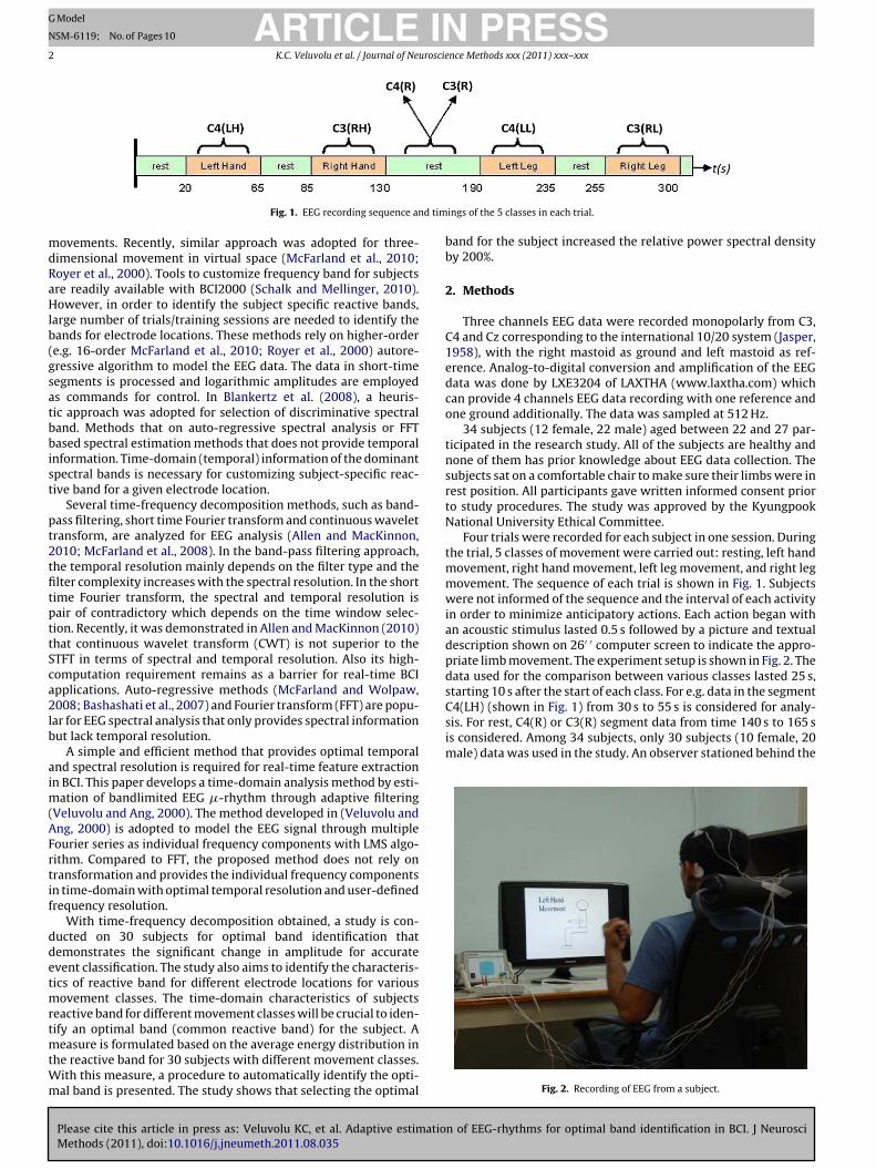
Four trials were recorded for each subject in one session. Duringthe trial, 5 classes of movement were carried out: resting, left handmovement, right hand movement, left leg movement, and right legmovement. The sequence of each trial is shown in Fig. 1. Subjectswere not informed of the sequence and the interval of each activityin order to minimize anticipatory actions. Each action began withan acoustic stimulus lasted 0.5 s followed by a picture and textualdescription shown on 26′ ′ computer screen to indicate the appro-priate limb movement. The experiment setup is shown in Fig. 2. Thedata used for the comparison between various classes lasted 25 s,starting 10 s after the start of each class. For e.g. data in the segment


Fig. 2. Recording of EEG from a subject.


ING Model

N

uroscie

ssttatetmi

(

(

2

nt2ias

blaoFLst

ststf

y

wbωt(paipa

x

y

�

w

ARTICLESM-6119; No. of Pages 10

K.C. Veluvolu et al. / Journal of Ne

ubject verified whether the desired movement instructed on thecreen was performed by the subject. No feedback was providedo the subject about the movement performed. Four subjects failedo perform the required movement or performed no movement int least two trials. When a subject fails to perform a minimum of 2rials correctly, the subject data was excluded from the study. How-ver, in the 30 subjects data chosen for analysis, 5 subjects in one orwo trials failed to follow the instruction and performed a wrong

ovement or no movement. These trials were identified and themproper segments were removed from the data for analysis.

Subjects participated in two conditions:

1) Rest: in which subjects sat in a chair comfortably and placedtheir hands on the table; a blank screen was shown, and theywere instructed not to think of anything.

2) Self-generated movement: subjects were cued to move hisleft/right hand or left/right leg at their own pace with a beepand on screen instructions.

.1. Bandlimited multiple Fourier linear combiner (BMFLC)

Since EEG is comprised of quasi-periodic or quasi-sinusoidal sig-als characterized by coupled, harmonically related frequencies,here have been several Fourier based works (Akim and Kiymik,000; Krusienski et al., 2007; Brunner et al., 2010). A parameter-

zed �-rhythm model has been formulated with a matched filter forccurate tracking with harmonically related phase-coupled sinu-oidal components (Krusienski et al., 2007; Brunner et al., 2010).

In this paper, we focus on bandlimited Fourier linear combinerased on LMS algorithm to estimate/track the �-rhythm. Fourier

inear combiner (FLC) (Vaz and Thakor, 2000; Vaz et al., 2000) is andaptive filter that forms a dynamic truncated Fourier series modelf an input signal. The FLC operates by adaptively estimating theourier coefficients of the known frequency model according to theMS algorithm. To overcome the drawbacks in tracking bandlimitedignals, the band limited multiple Fourier combiner is developed torack modulated signals (Veluvolu and Ang, 2000).

In order to estimate the unknown �-rhythm, we consider theignal to be distributed in the band of [ω1 − ωn] and then dividehe frequency band of interest into ‘n’ finite number of divisions ashown in Fig. 3(b). For the estimation of the unknown signal, wehen choose a series comprising of sine and cosine components toorm band-limited multiple-Fourier linear combiner (BMFLC):

k =n∑

r=1

ark sin(ωrk) + brk cos(ωrk) (1)

here yk denotes the estimated signal at sampling instant k. ark,rk represents the adaptive weights corresponding to the frequencyr at instant k. The following series only considers ‘n’ fundamen-

al frequencies in the band. The division of the band, step size �ωin Fig. 3(b)) and selection of the fundamental frequencies will beresented in the later part of the section. We then adopt the LMSlgorithm (Widrow and Stearns, 1985) to adapt the weights ark, brkn (1) to the incoming unknown signal. The architecture of the pro-osed algorithm is shown in Fig. 3(a). The algorithm can be stateds follows:

k ={

[ sin(ω1k) sin(ω2k) . . . sin(ωnk) ]T

[ cos(ω1k) cos(ω2k) . . . cos(ωnk) ]T

}(2)

= wT x (3)


k k k

k = sk − yk (4)

k+1 = wk + 2�xk�k (5)

PRESSnce Methods xxx (2011) xxx– xxx 3

where

wk = [ a1k . . . ank b1k . . . bnk ]T (6)

and xk are the adaptive weight vector and reference input vectorrespectively. sk is the reference signal, �k represents the error termand � is an adaptive gain parameter. Input signal amplitude andphase are estimated by the adaptive vector wk.

From the architecture, it is clear that n-FLC’s are combined toform BMFLC to estimate bandlimited signal. Since we select a bandof frequencies, the corresponding weights adapt to the frequenciespresent in the input signal. Due to the LMS algorithm, the corre-sponding weights adapt to the change in frequency of the incomingsignal. The adaptive gain parameter � can be chosen to have fastconvergence without loosing stability. The stability of the algorithmcan be established similar to (Vaz and Thakor, 2000). As the func-tions in xk (2) are orthogonal with a mean power of 1/2 for eachfunction, the autocorrelation matrix of xk becomes diagonal andcan be obtained as

R = E[ xk xTk ] = 1

2I (7)

According to Widrow and Stearns (1985), the practical bound forconvergence is given by

0 < � <1

tr[R]= 1/n (8)

where tr[·] represents the trace of the matrix. Hence, for the BMFLCalgorithm the adaptive gain parameter � should be less than 1/n toachieve convergence.

Since the objective is to identify the optimum band of the EEG�-rhythm, we estimate the whole range of �-rhythm by choos-ing f1 = 8 Hz, w1 = 2�f1 and fn = 14 Hz, wn = 2�fn. The adaptive gainparameter � decides the adaptive rate of the algorithm. The accu-racy of estimation also depends on the frequency spacing �ω/2�.A small �ω will increase the number of fundamental frequencies(i.e. weights wk) and the estimation process will be highly accurate.A very small �ω also increases the computational complexity. Anappropriate value of � should be selected according to (8) for theconvergence of the algorithm. The accuracy for various values of�ω/2� and � are analyzed and the findings are presented in Section3.

2.2. Analysis with BMFLC

In this section, we first present the proposed method for time-frequency decomposition of the rest-EEG and movement-EEGfollowed by identification of optimal band. The identified optimalband will be later used for better event classification. The block dia-gram of the procedure is given in Fig. 4. The three steps A, B andC shown in Fig. 4 are organized as three sub-sections for ease ofanalysis.

2.2.1. Time-frequency decompositionBy construction of BMFLC, the weight vectors wk represents

the amplitude information of each frequency component at timeinstant k. This information forms the basis for time-frequencydecomposition of the signal. Each amplitude weight representsthe magnitude of the corresponding frequency in the signal. Themodelled signal with BMFLC at time instant k is given by


yk = wTk xk (9)

Since the reference vectors xk are pre-defined and constant, ouranalysis will be focused on the weight vector wk. From (5) and





) frequ

at

w

cc

w

wpt

D

To

Fig. 3. (a) BMFLC architecture and (b

rchitecture in Fig. 3, wk contains both the sine and cosine vectorerms and so the weight vectors can be re-expressed as

wsk

= [ a1k . . . ank ]T

wck

= [ b1k . . . bnk ]T

here wk = [ wsk

wck ]

T, ws

kand wc

kare sine and cosine weights.

In order to evaluate the individual frequency components, weompute the square-root of the sum of squares of the sine andosine components to obtain

fk

=[ √

a21k

+ b21k

2. . .

√a2

nk+ b2

nk

2

]T

(10)

here wfk

is the absolute weight vector of the frequency com-onents at instant k. The time-frequency decomposition matrixermed D can be obtained for the signal with m samples as

= [ wf1 . . . wf

k. . . wf

m ]

(11)

=

⎡⎢⎢⎢⎢⎢⎢⎢⎢⎢⎢⎣

√a2

11 + b211

2

√a2

12 + b212

2. . .

√a2

1m + b21m

2√a2

21 + b221

2

√a2

22 + b222

2. . .

√a2

2m + b22m

2...

.... . .

...√a2 + b2

√a2 + b2

√2 2

⎤⎥⎥⎥⎥⎥⎥⎥⎥⎥⎥⎦

(11)


n1 n1

2n2 n2

2. . .

anm + bnm

2

his time-frequency decomposition contains the absolute valuesf all the frequency components with spacing �ω. These weights

Fig. 4. Flowchart of

ency distribution for multiple FLC’s.

are useful to extract the time-frequency characteristics of the EEGsignal.

2.2.2. Optimal band selectionThe reactive band can be clearly visualized from the time-

frequency decomposition of the signal. To quantify the optimalband for the subject, we first analyze spectra power distributionin all the frequency components for rest and each movement class.The square of all the amplitudes of individual frequency compo-nents will provide power distribution in each class of a trial and aregiven by

Prest = Drest ⊕ Drest

Pmov = Dmov ⊕ Dmov(12)

where Prest and Pmov represent the power distribution matrices forrest and movement. Dmov and Drest represents the time-frequencydecomposition matrix (11) corresponding to rest and movementof the subject. The operator ⊕ represents the element by elementmultiplication of the matrix.

To identify the dominant frequency components, we analyzethe average power of all the frequency components. For the abovematrices Prest and Pmov, the average power can be obtained bycomputing the mean of all the rows as each row corresponds to aspecific frequency. The difference of the average power distributionbetween the two matrices will identify the dominant frequencycomponents between two classes (e.g. C3(R) and C3(RH) in a singletrial). The difference of the average power can be obtained as


PDiff = avg{Prest} − avg{Pmov} (13)

where avg(·) is a row operation to compute the mean of every rowthat corresponds to frequency components ωi. PDiff will be a vec-tor with elements corresponding to the power difference of all the

EEG analysis.


IN PRESSG Model

N

uroscience Methods xxx (2011) xxx– xxx 5

fic

ewmbbS

2

bnIfqto

sc

wci

i

wii

wamo(wt

3

Ebm

s

0 0.5 1 1.5 2 2.5 3−10

−5

0

5

10

15

Time (sec)

μ V

EEG(C4(LH))Modeled EEG (Δω/2π=0.5 Hz, η=0.03)Model Error

Fig. 5. Subject #1, actual and modeled EEG � rhythm.

0 5 10 15 20 25−5

0

5x 10

−3

μ V

Mean square error

TA


K.C. Veluvolu et al. / Journal of Ne

requency components. This measure will provide power variationn all the frequency components in the �-band between the twolasses under consideration.

The area under the curve PDiff will provide information aboutnergy distribution between the two movement classes. The regionith the maximum energy distribution can be identified for all theovement classes and trials separately and an optimal band can

e selected for the subject. The measure to identify the optimaland will be discussed together with the analysis of 30 subjects inection 3 later.

.3. Normalized power between events

The classification accuracy depends on the accurate reactiveand selection. By considering the most reactive frequency compo-ents for each subject the classification accuracy can be improved.

n Neuper et al. (2000), it was shown that selection of optimumrequency bands for subjects when compared with standard fre-uency bands has higher success rate. In this section, we employhe optimum band identified in the previous section for calculationf normalized power.

We first calculate the normalized power (�V2/Hz) or powerpectral density (PSD) with respect to time for the signal in theomplete �-band (8–14 Hz) during rest and movement as follows:

Crest = sum(Prest)BW

Cmov = sum(Pmov)BW

(14)

here the bandwidth BW = 14 − 8 = 6 Hz and sum(·) represents theolumn operation to compute the sum of all components power atnstant k.

Similarly, for the EEG signal in the optimum band, the normal-zed power can be obtained as

C+rest = sum(P+

rest)BW+

C+mov = sum(P+

mov)BW+

(15)

here P+rest only contains the rows of Prest that corresponds to the

dentified optimum band of the subject and BW+ represents thedentified optimum bandwidth.

To quantify the effect of optimal band selection for all subjects,e analyze the relative power-spectral density. This is necessary

s some subjects may have large power (large EEG amplitude) anday lead to bias in the analysis. To accurately quantify the effect of

ptimal band on the normalized power (PSD) between two eventse.g. C4(LH) and C4(R)), we divide the normalized power (�V2)/Hzith the average power of the two events (e.g. C4(LH) and C4(R))

o form relative power spectral density (rP/Hz).

. Results

In this section, we first analyze the accuracy of BMFLC for EEG


stimation. In order to estimate the �-rhythm, all the data wasandpass filtered in the band of 8–14 Hz. To evaluate the perfor-ance of EEG estimation with BMFLC, we employ the root mean

quare (RMS) defined as RMS(s) =√

(∑m

k=1(sk)2)/m where m is the

able 1ccuracy with BMFLC.

30 Subjects × 4 trials �ω/2� = 0.1 Hz �ω/2� =(% Accuracy) � = 0.007 � = 0.015

Average (±STD) 98.85 (±0.03) 98.62 (±

Time (sec)

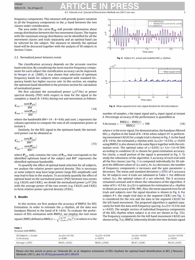
Fig. 6. Mean-squared error over signal duration for all trials/subjects.

number of samples, s the input signal and sk input signal at instantk. Percentage accuracy of the performance is quantified as

% Accuracy = RMS(s) − RMS(�)RMS(s)

× 100 (16)

where � is the error signal. For demonstration, the bandpass filteredEEG � rhythm in the band of 8–14 Hz when subject #1 is perform-ing movement C4(LH) for a single trial is shown in Fig. 5. In the bandof 8–14 Hz, the estimated � rhythm with �ω/2� = 0.5 Hz, � = 0.035using BMFLC is also shown in the same figure together with the esti-mation error. The optimal value of � = 0.035 (� < 1/n = 1/n =0.769)according to condition (8) is chosen for good estimation accuracy.For clarity, a small portion of the signal is presented in Fig. 5. Tostudy the robustness of the algorithm, % accuracy of each trial withall the five classes (see Fig. 1) is computed individually for 30 sub-jects for different values of �ω and �. As �ω decreases, the numberof frequency components n increases and the gain parameter �decreases. The mean and standard deviation (±STD) of % accuracyfor 30 subjects over 4 trials are tabulated in Table 1. For differentvalues �ω, the optimal values of � are selected. The % accuracyremained constant and it shows the robustness of the algorithm. Avalue of 0.1–0.5 for �ω/2� is optimum for estimation of �-rhythmto obtain an accuracy of 96–98%. Also, the mean squared error for alltrials and subjects over the signal duration is shown in Fig. 6. Forsubject # 1, the single trial data in the segment C4(R) (see Fig. 1)is considered for the rest and the data in the segment C4(LH) forthe left hand movement. The proposed algorithm is applied sepa-rately for both the data with frequency spacing �ω/2�= 0.5 Hz and


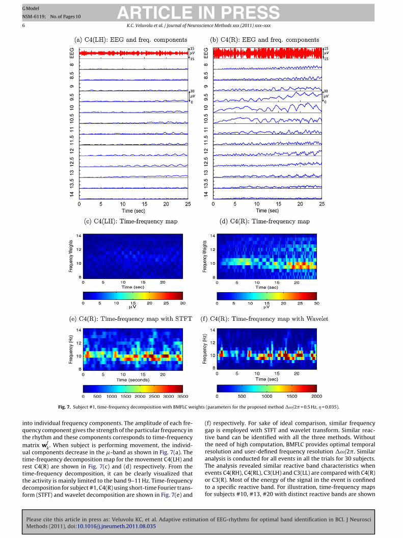
� = 0.035. The weight vectors of individual frequency componentsof the EEG rhythm when subject is at rest are shown in Fig. 7(b).The frequency components for the left hand movement C4(LH) areshown in Fig. 7(a). BMFLC inherently divides the time domain signal

0.2 Hz �ω/2� = 0.4 Hz �ω/2� = 0.5 Hz � = 0.03 � = 0.035

0.04) 98.47 (±0.06) 98.34 (±0.05)





ights

iqtmutrttdf

Fig. 7. Subject #1, time-frequency decomposition with BMFLC we

nto individual frequency components. The amplitude of each fre-uency component gives the strength of the particular frequency inhe rhythm and these components corresponds to time-frequency

atrix wfk. When subject is performing movement, the individ-

al components decrease in the �-band as shown in Fig. 7(a). Theime-frequency decomposition map for the movement C4(LH) andest C4(R) are shown in Fig. 7(c) and (d) respectively. From theime-frequency decomposition, it can be clearly visualized that


he activity is mainly limited to the band 9–11 Hz. Time-frequencyecomposition for subject #1, C4(R) using short-time Fourier trans-orm (STFT) and wavelet decomposition are shown in Fig. 7(e) and

(parameters for the proposed method �ω/2� = 0.5 Hz, � = 0.035).

(f) respectively. For sake of ideal comparison, similar frequencygap is employed with STFT and wavelet transform. Similar reac-tive band can be identified with all the three methods. Withoutthe need of high computation, BMFLC provides optimal temporalresolution and user-defined frequency resolution �ω/2�. Similaranalysis is conducted for all events in all the trials for 30 subjects.The analysis revealed similar reactive band characteristics whenevents C4(RH), C4(RL), C3(LH) and C3(LL) are compared with C4(R)


or C3(R). Most of the energy of the signal in the event is confinedto a specific reactive band. For illustration, time-frequency mapsfor subjects #10, #13, #20 with distinct reactive bands are shown




K.C. Veluvolu et al. / Journal of Neuroscience Methods xxx (2011) xxx– xxx 7

mposi

itrimsrodtfi�c

P

wbeabr

aastb(ti

TS

Fig. 8. Time-frequency deco

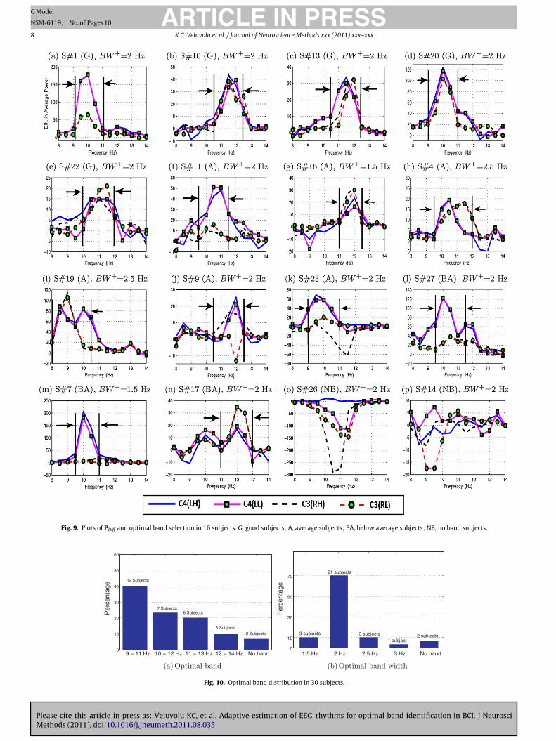
n Fig. 8 for rest and movement. To identify the optimal band forhe subject, PDiff for all the four movement classes with respect toest are evaluated for all four trials as discussed in Section 2.2.2. Forllustration, the plot of the PDiff for subject # 1 with all four move-

ent classes with respect to the frequency for a single trial data ishown in Fig. 9(a). From the plot, it is clear that the 9–11 Hz band iseactive for the subject # 1 for all the four movement classes. Plotsf PDiff for 16 subjects for all four movement classes for single trialata are shown in Fig. 9. Most subjects exhibited a distinctive reac-ive band. To quantify the band and bandwidth for the subject, werst evaluate the distribution (area under the PDiff curve) for the-band and the reactive band. The power ratio % for a movement

lass in a single trial is defined as

R = Aopt

A�× 100 (17)

here Aopt is the area under the PDiff curve for the selected reactiveand and A� is the total positive area under the PDiff curve for thentire �-band. Since PDiff vector represents the average power over

period of time, Aopt represents the average power in the optimaland and A� represents the average power in the �-band. PR alsoepresents % average energy ratio of optimal band to �-band.

For a selected reactive bandwidth BW+, the PR is computed forll the movement classes in all the four trials for the subject. Theverage PR resulting from various movement classes and trials for aubject provides the measure of average energy % associated withhe selected reactive band and bandwidth. To analyze the effect of


andwidth on PR, the average PR for subjects for various bandwidths2 Hz, 2.5 Hz and 3 Hz) are tabulated in Table 2. The distribution ofhe subjects in the table reveals that the average PR of 60–80% existsn most subjects. For only few subjects, an increase in BW+ increased

able 2ubjects with the optimal band % energy.

Band width No. of subjects with PR

50–60% 60–70% 70–80% 80–85%BW+ = 2 Hz 3 16 8 1BW+ = 2.5 Hz 2 13 11 2BW+ = 3 Hz 2 12 10 4

tion for movement and rest.

the energy %. The table shows that most subjects have an averagePR close to 70%. Hence in this study the average PR = 70% is chosen asthe basis to identify the optimal band for the subject. The identifiedoptimal bands for 16 subjects are shown in Fig. 9. The optimal bandsshown in Fig. 9 are average of four trials for all movement classes. InFig. 9, subjects are grouped as good, average, below average and noband subjects. Subjects who displayed a very distinctive commonband in all trials are considered as good subjects. In Fig. 9(a)–(e)are marked as good subjects. In Fig. 9(f)–(k) represent the aver-age subjects and all subjects have a common band. However somesubjects in one or two trials, a movement class failed to follow theother movement classes (for e.g. Fig. 9(j)–(k)). For some subjectsthe energy and frequency band depended on the electrode location.For e.g. subject #4 has separate peaks for both electrode locations.However a common band was selected as shown in Fig. 9(h). Forsome subjects, a large energy difference existed between electrodelocations C3 and C4. For e.g. subjects #27 and #7 (see Fig. 9(k)–(m))show a large difference in power in electrode locations. For sub-jects #14, #26 a band was not identified in at least 3 trials. Carefulobservation revealed that the subjects had a power decrease in the�-band as opposed to power increase as shown in Fig. 9(k)–(m)and are grouped as no band subjects. Few subjects have a reactivebandwidth greater than 2 Hz. For e.g. subject #4 has a reactive bandof 9.5–12 Hz.

For some subjects, there was a slight mismatch in the bandbetween two electrode locations C3 and C4. Most subjects dis-played a common band for both the C3 and C4 locations. For agiven subject, as the reactive band is mainly dependent on the restC3(R) or C4(R), the band remained constant during all the trials. Thereactive band varied from subject to subject, but remained fixedirrespective of the event performed as shown in Fig. 9.

The distribution of optimal band for 30 subjects is shown inFig. 10(a). Over 93% of the subjects has a distinct reactive bandwith bandwidth 2 Hz. The study also shows that 40% of the sub-jects has a reactive band in the range of 9–11 Hz whereas only 8%of the subjects has the reactive band in the range of 12–14 Hz. In


Fig. 10(b), the distribution of subjects with different bandwidthsis shown. 70% of subjects have a bandwidth of 2 Hz, where as 10%subjects have 2.5 Hz bandwidth. One has to note that the distri-bution is likely to change with the change of basis measure 70%.


Please cite this article in press as: Veluvolu KC, et al. Adaptive estimation of EEG-rhythms for optimal band identification in BCI. J NeurosciMethods (2011), doi:10.1016/j.jneumeth.2011.08.035




Fig. 9. Plots of PDiff and optimal band selection in 16 subjects. G, good subjects; A, average subjects; BA, below average subjects; NB, no band subjects.

9 − 11 Hz 10 − 12 Hz 11 − 13 Hz 12 − 14 Hz No band0

10

20

30

40

50

60

Per

cent

age

7 Subjects6 Subjects

12 Subjects

2 Subjects3 Subjects

1.5 Hz 2 Hz 2.5 Hz 3 Hz No band0

10

30

50

70

Per

cent

age

3 subjects1 subject

21 subjects

3 subjects 2 subjects

Fig. 10. Optimal band distribution in 30 subjects.




K.C. Veluvolu et al. / Journal of Neuroscience Methods xxx (2011) xxx– xxx 9

0 5 10 15 20 250

100

200

300

400

Time (sec)

μV

2 /H

zμ Band (8 Hz − 14 Hz)

Subject#1 C4(LL)

Subject#1 C4(R)

0 5 10 15 20 25

0

20

40

60

80

Time (sec)

μ Band (8 Hz − 14 Hz)

Subject#10 C3(RH)

Subject#10 C3(R)

0 5 10 15 20 25

0

20

40

60

Time (sec)


Subject#13 C3(RH)

Subject#13 C3(R)

0 5 10 15 20 250

50

100

150

200

Time (sec)


Subject#20 C4(LH)

Subject#20 C4(R)

0 5 10 15 20 250

100

200

300

400

Time (sec)

μV

2 /H

z

Optimal Band (9 Hz − 11 Hz)

Subject#1 C4(LL)

Subject#1 C4(R)

0 5 10 15 20 25

0

20

40

60

80

Time (sec)

Optimal Band (10.5 Hz − 12.5 Hz)

Subject#10 C3(RH)

Subject#10 C3(R)

0 5 10 15 20 25

0

20

40

60

Time (sec)

Optimal Band (10.5 Hz − 12.5 Hz)

Subject#13 C3(RH)

Subject#13 C3(R)

0 5 10 15 20 250

50

100

150

200

Time (sec)

Optimal Band (9 Hz − 11 Hz)

Subject#20 C4(LH)

Subject#20 C4(R)

Fig. 11. Normalized power for the �-band vs. optimal band for single trial data.

Table 3Comparison of r-power spectral density (rP/Hz) in �-band and optimal band.

30 subjects× 4 trials Average of r-power spectral density (rP/Hz)

�-Band (8–14 Hz) Optimal band % Increase withoptimal band

Event Rest Movement Diff. Rest Movement Diff.

LH (C4) 11.78 ± 2.1 4.71 ± 2.12 7.06 ± 4.21 31.57 ± 5.61 8.37 ± 4.02 23.19 ± 8.4 228%

AtCt�iftwFtdt(Fndssmda

4

oc

LL (C4) 11.62 ± 1.87 4.8 ± 1.87 6.81 ± 3.74RH (C3) 11.14 ± 2.54 5.28 ± 2.56 5.85 ± 5.1

RL (C3) 11.5 ± 1.84 4.94 ± 1.78 6.53 ± 3.62

s discussed in Section 2.3, the normalized power or power spec-ral density (PSD) variations are computed for subject #1 C4(R) and4(LL) events for a single trial and are shown in Fig. 11(a1). The dis-inction between the rest and left hand motion can be seen in the

band. With the identified optimal band (9–11 Hz), the differencen normalized power increased as shown in Fig. 11(a2). The dif-erence in normalized power increases by 200% across time withhe selection of optimal band. The normalized power variationsith optimal bands for subjects #10, #13 and #20 are presented in

ig. 11. The distinction between rest and activity are not very dis-inct as the characteristics vary from subject to subject. Subject #10oes not have a very clear distinction between C3(RH) and C3(R) inhe �-band as shown in Fig. 11(b1). Selection of the optimal band10.5–12.5 Hz) increases the power difference by 200% as shown inig. 11(b2). To further quantify the effect of optimal band on theormalized power (PSD) we analyze the relative power spectralensity (rP/Hz) for all the subjects. The analysis conducted for 30ubjects for four events (LH, LL, RH and RL) in all trials and mean ±tandard deviation is tabulated in Table 3. It reveals that the opti-um band improves the difference in the relative power spectral

ensity by a minimum 200% with respect to normalized power onn average across the time.

. Discussion


For many subjects, a significant change in �-rhythm does existver the entire band 8–14 Hz. However, closer examination of spe-ific narrower frequency bands for a subject may provide good

31.13 ± 4.84 8.78 ± 4.19 22.34 ± 7.4 227%30.06 ± 4.6 9.15 ± 4.31 20.91 ± 7.96 257%29.12 ± 3.99 9.37 ± 3.94 19.75 ± 7.9 202%

difference in the activity with the dominant frequency components.Time-frequency decomposition provides more insight about thecharacteristics of the EEG and dominant frequency components,their time-domain characteristics. The amplitude weights of indi-vidual frequency components provide extra information about thesubject when compared to conventional methods of calculating theband power using FFT or STFT. The frequency gap �ω/2� in the pro-posed method can be varied according to the requirement. A small�ω/2� can be selected for high time-frequency resolution. Basedon the amplitudes of individual frequency components, the mostreactive frequencies for a subject can be identified to improve thethreshold level for event classification. This method also providesoptimal temporal and user-defined frequency resolution and canbe employed for feature extraction in BCI.

Earlier methods for identifying the subject specific reactivebands relied on heuristic based methods and require large num-ber of trials to train the subjects. The proposed method can clearlyidentify the subjects optimal band for an electrode location withfewer number of trials. A period of 25 s for identification of the bandfor a movement class was considered to analyze the time-domaincharacteristics of the reactive band. It was evident from the time-frequency maps that the reactive band indeed remained constantthrough out the entire time-period.

For most subjects a common optimal band existed for all move-


ment classes. Fig. 9 shows that all the four movement classes havea common band. In most of the earlier studies, bandwidth of 3 Hzwas employed to customize the reactive band based on heuristicmethods. The selection of proper optimal band depends on the


ING Model

N

1 uroscie

sttesafBmcp

euammesm�tlm

caatcdp

A

vo

R

A

A

B

B

B


0 K.C. Veluvolu et al. / Journal of Ne

ubject’s energy distribution and an exact band cannot be quan-ified directly. In this paper, a basis measure of 70% is employedo identify the subject-specific optimal band. A larger band can bemployed for all subjects, but it will eventually decrease the powerpectral density. Although the analysis in the paper is limited toctual movement-related data, the proposed method will be usefulor identifying the optimal band related to movement-imagery forCI applications. Similar results may not be obtained with imaginedovement, however a good difference in power spectral density

an be obtained with a proper selection of optimal band with theroposed method.

The proposed method of optimal band identification can bemployed for identifying users with a narrow reactive band. Thesers with a narrow frequency band will operate BCI with higherccuracy compared to subjects without a band. The proposedethod in combination with spatial filtering will provide opti-al temporal, spatial and time-resolution for real-time feature

xtraction in BCI’s. Identifying the optimal bands in � and ˇ-bandseparately for each electrode location will improve the perfor-ance of classifiers. Although the analysis has been limited to-band in this paper, the same approach can be extended to ˇ-band

o identify the optimal band in ˇ-band for electrode locations. Simi-ar optimal bands for subjects can also be identified with traditional

ethods like STFT and Wavelet transform.Results are illustrated for 16 subjects for optimal band identifi-

ation. Our study reveals that optimal band exists in most subjectsnd it improves the spectral power density difference between restnd movement. The study clearly identified the optimal band forhe subjects and the optimal band can be selected for better eventlassification. An average of 200% improvement in power spectralensity with respect to normalized power can be obtained with theroposed method.

cknowledgements

Authors would like to thank anonymous reviewers for theiraluable suggestions/comments that largely improved the qualityf the paper.

eferences

kim M, Kiymik M. Application of periodogram and ar spectral analysis to eeg sig-nals. J Med Syst 2000;24(4):247–56.

llen DP, MacKinnon CD. Time-frequency analysis of movement-related spectralpower in eeg during repetitive movements: a comparison of methods. J NeurosciMeth 2010;186:107–15.

ashashati A, Fatourechi M, Ward RK. A survey of signal processing algorithmsin brain–computer interfaces based on electrical signals. J Neural Eng 2007;4:R03.

irbaumer N, Ghanayim N, Hinterberger T, Iversen I, Kotchoubey B, Kübler A, et al.


Guest editorial brain–computer interface technology: a review of the secondinternational meeting. Nature 1999;398(6725):297–8.

lankertz B, Tomioka R, Lemma S, Kawanabe M, Muller KR. Optimizing spatialfilters for robust eeg single-trial analysis. IEEE Signal Proc Mag 2008;25(1):41–56.

PRESSnce Methods xxx (2011) xxx– xxx

Brunner C, Allison BZ, Krusienski DJ, Vera Kaiser, Mller-Putz GR, Pfurtscheller G,et al. Improved signal processing approaches in an offline simulation of a hybridbrain–computer interface. J Neurosci Meth 2010;188(1):165–73.

Editorial comment. Is this the bionic man? Nature 2006;442(7099):109.Curran EA, Strokes MJ. Learning to control brain activity: a review of the produc-

tion and control of eeg components for driving brain–computer interface (bci)systems. Brain Cogn 2003;51:326–36.

Graimann B, Allison B, Pfurscheller G. Brain–computer interfaces. London, UK:Springer; 2010.

Guger C, Edlinger G, Harkam W, Niedermayer I, Pfurtscheller G. How many peopleare able to operate an eeg-based brain–computer interface (bci)? IEEE TransNeural Syst Rehabil Eng 2003;11(2):99–110.

Jasper HH. The ten–twenty electrode system of the international federation. Elec-troen Clin Neuro 1958;10:371–5.

Krusienski DJ, Schalk G, McFarland DJ, Wolpaw JR. A mu-rhythm matched filterfor continuous control of a brain–computer interface. IEEE Trans Biomed Eng2007;54(2):273–80.

Lotte F, Congedo M, Lecuyer A, Lamarche F, Arnaldil B. A review of classification algo-rithms for EEG-based brain–computer interfaces. J Neural Eng 2007;4:R1–13.

McFarland DJ, Lefkowicz AT, Wolpaw JR. Design and operation of an eeg-basedbrain–computer interface (bci) with digital signal processing technology. BehavRes Meth Instrum Comput 1997;29:337–45.

McFarland DJ, Wolpaw JR. Sensorimotor rhythm-based brain–computer interface(bci): model order selection for autoregressive spectral analysis. J Neural Eng2008;5:6.

McFarland DJ, Anderson CW, Muller KR, Schlogl A, Krusienski DJ. Bci meeting 2005– workshop on bci signal processing: feature extraction and translation. IEEETrans Neural Syst Rehabil Eng 2008;14(2):135–8.

McFarland DJ, Sarnacki WA, Wolpaw JR. Electroencephalographic (eeg) control ofthree-dimensional movement. J Neural Eng 2010;7:36007.

Mueller-Putz GR, Scherer R, Pfurtscheller G, Rupp R. Eeg-based neuroprosthesiscontrol: a step towards clinical practice. Neurosci Lett 2000;382:169–74.

Mueller-Putz GR, Scherer R, Pfurtscheller G, Rupp R. Brain–computer interfacesfor control of neuroprosthesis: from sysnchronous to asynchronous mode ofoperation. Biomed Eng 2006;51(2):57–63.

Neuper C, Mueller-Putz GR, Scherer R, Pfurtscheller G. Motor imagery andeeg-based control of spelling devices and neuroprostheses. Prog Brain Res2000:159393–409.

Pfurtscheller G, Neuper C. Motor imagery activates primary sensorimotor area inhumans. Neurosci Lett 2000;239:65–8.

Pfurtscheller G, Neuper C, Andrew C, Edlinger G. Foot and hand area mu rhythms.Int J Psychophysiol 2000;26(1–3):121–35.

Pineda AJ, Allison BZ, Vankov A. The effects of self-movement, observation and imag-ination on � rhythms and readiness potentials (rp’s): toward a brain–computerinterface (bci). IEEE Trans Rehabil Eng 2000;8(2):219–22.

Royer SA, Doud AJ, Rose ML, Bin He. Eeg control of a virtual helicopter in 3-dimensional space using intelligent control strategies. IEEE Trans Neural SystRehabil Eng 2000;18(6):581–9.

Schalk G, Mellinger J. A practical guide to brain–computer intefacing with BCI2000.London, UK: Springer; 2010.

Sun S, Zhang C, Lu Y. The random electrode selection ensemble for eeg signal classi-fication. Pattern Rcogn 2000;41:1663–75.

Vaughan TM. Guest editorial brain–computer interface technology: a reviewof the second international meeting. IEEE Trans Neural Syst Rehabil Eng2000;11(2):94–109.

Vaz C, Thakor N. Adaptive fourier estimation of time-varying evoked potentials. IEEETrans Biomed Eng 2000;36(4):448–55.

Vaz C, Kong X, Thakor N. An adaptive estimation of periodic signals using a fourierlinear combiner. IEEE Trans Signal Process 2000;42(1):1–10.

Veluvolu KC, Ang WT. Estimation and filtering of physiological tremor for surgicalrobotics applications. Int J Med Robot Comput Assist Surg 2000;6(3):334–42.

Widrow B, Stearns SD. Adaptive signal processing. Englewood Cliffs, NJ: Prentice-Hall; 1985.


Wolpaw JR, McFarland DJ, Vaughan TM. Brain–computer interface research at thewadsworth center. IEEE Trans Rehabil Eng 2000;8(2):222–6.

Wolpaw JR, Birbaumer N, McFarland DJ, Pfurtscheller G, Vaughan TM.Brain–computer interfaces for communication and control. Clin Neurophysiol2000;113:767–91.


Adaptive estimation of EEG-rhythms for optimal band identification in BCI

Documents

Transcript of Adaptive estimation of EEG-rhythms for optimal band identification in BCI