Actionable Information in Vision

Stefano Soatto

University of California, Los Angeleshttp://vision.ucla.edu; soatto@ucla.edu

AbstractI propose a notion of visual information as the complex-

ity not of the raw images, but of the images after the effects

of nuisance factors such as viewpoint and illumination are

discounted. It is rooted in ideas of J. J. Gibson, and stands

in contrast to traditional information as entropy or coding

length of the data regardless of its use, and regardless of

the nuisance factors affecting it. The non-invertibility of

nuisances such as occlusion and quantization induces an

“information gap” that can only be bridged by controlling

the data acquisition process. Measuring visual information

entails early vision operations, tailored to the structure of

the nuisances so as to be “lossless” with respect to visual

decision and control tasks (as opposed to data transmission

and storage tasks implicit in traditional Information The-

ory). I illustrate these ideas on visual exploration, whereby

a “Shannonian Explorer” guided by the entropy of the data

navigates unaware of the structure of the physical space

surrounding it, while a “Gibsonian Explorer” is guided by

the topology of the environment, despite measuring only

images of it, without performing 3D reconstruction. The

operational definition of visual information suggests desir-

able properties that a visual representation should possess

to best accomplish vision-based decision and control tasks.

1. IntroductionMore than sixty years ago, Norbert Wiener stormed into

his students’ office enunciating “entropy is information!”

before immediately storming out. Claude Shannon latermade this idea the centerpiece of his Mathematical Theoryof Communication, formalizing and unifying the wide va-riety of methods that practitioners had been using to trans-mit signals. The influence of Shannon’s theory has sincespread beyond the transmission and compression of data,and is now broadly known as Information Theory. But isthe entropy of the data really “information”? There is nodoubt that the more complex the data, the more costly it is

to store and transmit. But what if we want to use the datafor tasks other than storage or transmission? What is the“information” that an image contains about the scene it por-trays? What is the value of an image if we are to recognize

objects in the scene, or navigate through it? Despite itspervasive reach today, Shannon’s notion of information hadearly critics, among who James J. Gibson. Already in thefifties he was convinced that data is not information, andthe value of data should depend on what one can do with it,i.e. the task. Much of the complexity in an image is due tonuisance factors, such as illumination, viewpoint and clut-ter, that have little to do with the decision (perception) andcontrol (action) task at hand.

The goal of this manuscript is to define an operational

notion of “information” that is relevant to visual decision

and control tasks, as opposed to the transmission and stor-age of image data. Following Gibson’s lead, I define Ac-

tionable Information to be the complexity (coding length)of a maximal statistic that is invariant to the nuisances asso-ciated to a given task.1 I show that, according to this defi-nition, the Actionable Information in an image depends not

just on the complexity of the data, but also on the struc-

ture of the scene it portrays. I illustrate this on a simpleenvironmental exploration task, that is central to Gibson’secological approach to perception. A robot seeking to max-imize Shannon’s information is drifting along unaware ofthe structure of the environment, while one seeking to max-imize Actionable Information is driven by the topology ofthe surrounding space. Both measure the same data (im-ages), but the second is using it to accomplish spatial tasks.An expanded version of this manuscript, with more detailsand discussion in relation to existing literature, is availableat [25].

1It is tempting to write off this idea on grounds that neither viewpointnor illumination invariants exist [7, 8]. But this would be simplistic: [30]shows that non-trivial viewpoint invariants exist for Lambertian objectsof general shape. Similarly, [8] considers complex illumination fields, butinvariants can be constructed for simpler illumination models, such as con-trast transformations [2], even though these are valid only locally.

1

2. PreliminariesI represent an image as a function I : D ⊂ R2 →

Rk+; x → I(x) that is L2-integrable, but not necessarily

continuous, taking positive values in k bands, e.g. k = 3 forcolor, and k = 1 for grayscale. A time-indexed image is in-dicated by I(x, t), t ∈ Z+ and a sequence by I(x, t)T

t=1,or simply I. The image relates to the scene, which I rep-resent as a shape S ⊂ R3, made of piecewise continuoussurfaces parameterized by x, S : D → R3; x → S(x),and a reflectance ρ : S → Rk, which I also parameter-ize as ρ(x) .= ρ(S(x)). I model illumination changes bycontrast transformations, i.e. monotonically increasing con-tinuous functions h : R+ → R+. Changes of viewpoint arerepresented by a translation vector T ∈ R3 and a rotationmatrix R ∈ SO(3), indicated by g = (R, T ). As a result ofa viewpoint change, points in the image domain x ∈ D aretransformed (warped) via x → π(g−1(π−1

S (x))) .= w(x),where π : R3 → P2; X → x = λX is an ideal perspectiveprojection and λ−1 = [0 0 1]X ∈ R+ is the depth along theprojection ray [x] .= X ∈ R3 | ∃ λ ∈ R+, x = λX; π−1

Sis the point of first intersection of the projection ray [x] withthe scene S. I use the notation w(x;S, g) when emphasizingthe dependency of w on viewpoint and shape. Without lossof generality [26], changes of viewpoint are modeled withdiffeomorphic domain deformations w : D ⊂ R2 → R2.All un-modeled phenomena (deviation from Lambertian re-flection, complex illumination effects etc.) are lumped intoan additive “noise” term n : R2 → Rk. We finally have theimage formation model:

I(x) = h(ρ(X)) + n(x)x = π(g(X)), X ∈ S.

(1)

I further call the scene ξ, the collection of (three-dimensional, 3D) shape and reflectance ξ

.= ρ, S, andthe nuisance ν, the collection of viewpoint and illuminationν

.= g, h. In short-hand notation, substituting X in thefirst equation above with g−1(π−1

S (x)), I write (1) as

I(x) = h ρ w(x;S, g) + n(x) .= f(ρ, S; g, h, n) (2)

or, with an abuse of notation, as I = f(ξ; ν) + n.

2.1. Visibility and QuantizationThe model (1) is only valid away from visibility artifacts

such as occlusions and cast shadows. I will not deal withcast shadows, and assume that they are either detected fromthe multiple spectral channels k ≥ 3, or that illumination isconstant and therefore they cannot be told apart from ma-terial transitions (i.e. spatial changes in the reflectance ρ).Based on natural intensity and range statistics [22], I modelocclusions as the “replacement” of f , in a portion of thedomain Ω ⊂ D, by another function β having the samestatistics:

I(x) =

f(ρ, S; g, h, n) x ∈ D\Ωβ(x) x ∈ Ω.

(3)

Digital images are quantized into a discrete lattice, witheach element averaging the function I over a small regionwhere the quantization error is lumped into the additivenoise n.

2.2. Invariant and Sufficient StatisticsA statistic, or “feature,” is a deterministic function φ

of the data I(x), x ∈ D, taking values in some vec-tor space, φ(I) ∈ RK . A statistic is invariant if it doesnot depend to the nuisance, i.e. for any ν, ν, we haveφ(f(ξ, ν)) = φ(f(ξ, ν)). A trivial example is a constantφ(I) = c ∀ I. Among all invariant statistics, we are mostinterested in the largest

2, also called maximal invariant

φν(I). A statistic is sufficient for a particular task, speci-fied by a risk functional R associated to a control or decisionpolicy u and loss function L, R(u|I) .=

L(u, u)dP (u|I),

R(u) .=

R(u|I)dP (I), if the risk from a policy based onsuch a statistic is the same as one based on the raw data,i.e. R(u|I) = R(u|φ(I)). A trivial example is the iden-tity φ(I) = I . Among all sufficient statistics, of particularinterest is the smallest2, or minimal, one φ∨(I). When anuisance acts as a group on the data, it is always possibleto construct invariant sufficient statistics (the orbits, or thequotient of the data under the group).

3. Placing the Ecological Approach to VisualPerception onto Computational Grounds

3.1. Actionable InformationI define Actionable Information to be the complexity H

(coding length) of a maximal invariant,

H(I) .= H(φν(I)). (4)

When the maximal invariant is also a sufficient statistic, wehave complete information H(I) = H(φ∨(I)). In this case,the Actionable Information measures all and only the por-tion of the data that is relevant to the task, and discountsthe complexity in the data due to the nuisances. As I dis-cuss in Sect. 3.3, invariant and sufficient statistics are, ingeneral, different sets, so we have an “information gap.”

In Sect. 4 I show how to compute Actionable Information,which for unknown environments requires spatial integra-tion of the information gap.

3.2. Invertible and Non-invertible NuisancesViewpoint g and contrast h act on the image as groups,

away from occlusions and cast shadows, and therefore can2In the sense of inclusion of sigma-algebras.

be inverted [26]. In other words, the effects of a viewpointand contrast change, away from visibility artifacts, can be“neutralized” in a single image, and an invariant sufficientstatistic can, at least in principle, be computed [26]. Unfor-tunately, this is of little help, as visibility and quantizationare not groups, and once composed with changes of view-point and contrast, the composition cannot be inverted.

When a nuisance is not a group, it must bedealt with as part of the decision or control pro-cess: The risk functional R depends on the nuisance,R(u|f(ξ; ν)), which can be eliminated either by extrem-ization (ML), maxν R(u|f(ξ; ν)), or by marginalization(MAP)

R(u|f(ξ, ν))dP (ν), if a probability measure on

the nuisance dP (ν) is available. In either case, an optimaldecision cannot be based on direct comparison of two in-variant statistics, φ(I1) = φ(I2) computed separately onthe training/template data I1 and on the testing/target dataI2 in a pre-processing stage. The most one can hope frompre-processing is to pre-compute as much of the optimiza-tion or marginalization functional as possible. For the caseof occlusion and quantization, this leads to the notion oftexture segmentation as follows.Segmentation as Redundant Lossless CodingAn occlusion Ω ⊂ D is a region that exhibits the same(piece-wise spatially stationary [22]) statistics of the unoc-cluded scene (3). It can be multiply-connected, generallyhas piecewise smooth boundaries, and is possibly attachedto the ground. In the absence of quantization and noise, onewould simply detect all possible discontinuities, store theentire set f(ξ, ν), ∀ ν, leaving the last decision bit (oc-clusion vs. material or illumination boundary) to the laststage of the decision or control process. Occluders connect-ing to the ground where no occlusion boundary is presentwould have to be “completed”, leading to a segmentation, orpartitioning, of the image domain into regions with smoothstatistics. Unfortunately, quantized signals are everywherediscontinuous, making the otherwise trivial detection of dis-continuities all but impossible. One could, as customary invision, set up a cost functional (a statistic) ψΩ(I), that im-plicitly defines a notion of “discrete continuity” within Ωbut not across its boundary, making the problem of segmen-tation self-referential (i.e. defined by its solution). But whileno single segmentation is “right” or “wrong,” the set of all

possible segmentations is a sufficient statistic. It does notreduce the complexity of the image, but it may reduce therun-time cost of the decision or control task, by rendering ita choice of regions and scales that match across images.Quantization and TextureFor any scale s ∈ R+, minimizing ψΩ(I|s) yields a dif-ferent segmentation Ω(s) .= arg minΩ ψΩ(I|s). Becauseimage “structures” (extrema and discontinuities) can ap-pear and disappear at the same location at different scales,3

3Two-dimensional signals do not obey the “causality principle” of one-

one would have to store the entire continuum Ω(s)s∈R+ .In practice, ψΩ(·|s) will have multiple extrema (critical

scales) that can be stored in lieu of the entire scale-space.In between such critical scales, structures become part ofaggregate statistics that we call textures. To be more pre-cise, a texture is a region Ω ⊂ D within which some im-age statistic ψ, aggregated on a subset ω ⊂ Ω, is spa-tially stationary. Thus a texture is defined by two (un-known) regions, small ω and big Ω, an (unknown) statisticψω(I) .= ψ(I(y), y ∈ ω), under the following conditionsof stationarity and non-triviality:

ψω(I(x + v)) = ψω(I(x)), ∀ v | x ∈ ω ⇒ x + v ∈ ΩΩ\Ω = ∅ ⇒ ψΩ(I) = ψΩ(I). (5)

The region ω, that defines the intrinsic scale s = |ω|, isminimal in the sense of inclusion: If ω satisfies the station-arity condition, then ∃ v | x ∈ ω ⇒ x + v ∈ ω. Note that,by definition, ψω(I) = ψΩ(I). A texture segmentation isthus defined, for every quantization scale s, as the solutionof the following optimization with respect to the unknownsΩi

Ni=1, ωi

Ni=1, ψi

Ni=1, N(s)

minN(s)

i=1

Ωi

ψωi(I(x))− ψi2dx + Γ(Ωi, ωi) (6)

where Γ denotes a regularization functional.4As described in Sect. 3.1, in general one cannot compute

statistics that are at the same time invariant and sufficient,

because occlusion and quantization nuisances are not in-

vertible. Or are they?

3.3. The Actionable Information GapAs I have hinted at in Sect. 2.1, whether a nuisance is

invertible depends on the image formation process: Castshadows are detectable (hence invertible) if one has accessto different spectral bands. Similarly, occluding boundariescan be detected if one can control accommodation or van-tage point. So, if the sensing process involves control of thesensing platform (for instance accommodation and view-point), then both occlusion and quantization become invert-

ible nuisances.5 This simple observation is the key to Gib-son’s approach to ecological perception, whereby “the oc-

cluded becomes unoccluded” in the process of “InformationPickup” [12].

dimensional scale-space, whereby structure cannot be created with increas-ing scale [20].

4 A bare-bone version pre-computes the statistics ψi on a fixed domainω, and aggregates statistics using a mode-seeking algorithm [31] that en-ables model selection with respect to scale s. The downside is that bound-aries between regions Ωi are only resolved to within the radius of ω, gen-erating spurious “thin regions” around texture boundaries. For the purposeof this study, this is a consequence we can live with, so long as we knowthat a sound model exists, albeit computationally challenging.

5Want to remove the effect of an occlusion? Move around it. Want toresolve the fine-structure of a texture, removing the effects of quantization?Move closer.

To make this concrete, recall from Sect. 3.1 the defini-tion of complete information and note that – because of thenon-invertible action of the nuisances – it must now dependon the scene ξ. I indicate this with I

.= H(φ∨ξ (I)). Whena sequence of images I capturing the entire light-field ofthe scene is available, it can be used in lieu of the sceneto compute the complete information I

.= H(φ∨(I)). Idefine the Actionable Information Gap (AIG) as the differ-ence between the Complete Information and the ActionableInformation

G(I) .= I −H(I). (7)

Note that, in the presence of occlusion and quantization,the gap can be only be reduced by moving within the en-

vironment. In order to move, however, the agent must beable to compute the effects of its motion on the AIG, ide-ally without having to know the complete information I,even if the data I or the statistics φ∨(I) were avail-able from memory of previous explorations. To this end,I define an incremental occlusion Ω(t) ⊂ D between twoimages I(x, t), I(x, t + dt) as a region which is visible inone image but not the other. Letting dt → 0, given theassumptions implicit in the model (1), we have

Ω(t) = arg minΩ

D\Ω

∇Iw(x, t) +

∂I

∂t(x, t)

2

dx+

D∇w1dx +

Ω∇I2dx. (8)

Once an incremental occlusion has been found, the De-crease in Actionable Information Gap (DAIG) can be mea-sured by the Actionable Information it unveils:

δG(I, t) = H(I(x, t)|x∈Ω(t)). (9)

The aim of environmental exploration is to maximize theDAIG, until a stopping time T is reached when, ideally, T

0δG(I, t)dt = −H

φ∨(IT

t=0)

= H

φν(I)T

t=0

(10)and therefore G(I) = 0. We have developed a variationaltechnique for detecting occlusions based on the solution ofa partial differential equation (PDE) that has the minimumof (8) as its fixed point. However, a hurried man’s solutionto (8), and the ensuing computation of (9), can be foundby block matching followed by run-length encoding of theresidual, as customary in MPEG. The shortcoming of thisapproach is that, in general, it yields a loss of actionableinformation, so that G(I) > 0, whereas the optimal solutionto (8) guarantees that no actionable information is lost, atleast in theory, asymptotycally for T →∞.

3.4. Information PickupTo study the process of “Information Pickup” by means

of closing the Actionable Information Gap, I specify a sim-

ple model of an “agent,” i.e. a viewpoint g(t) moving underthe action of a control, which I assume can specify the in-stantaneous velocity u(t) ∈ R6 so that g(t) = u(t)g(t)starting from some initial position, which for convenience Iassume to be the origin g(0) = e. 6 The agent measures animage at each instant of time, I(x, t):

g(t) = u(t)g(t) g(0) = e

I(x, t) = f (ρ(x), S(x); g(t), h(t), n(x, t)) .(11)

A myopic control would simply maximize the DAIG:

u(t) = arg maxu

δG(I, t) subject to (11) (12)

and quickly converge to local minima of the Actionable In-formation Gap: The agent would stop at “interesting places”forever. To release it, one can introduce a “boredom func-tion” that increases with the time spent at any given loca-tion. Still, the agent can get trapped by his own trajectories,as soon as he is surrounded by spots it has already visited.A simple “forgetting factor” can restore the reward expo-nentially over time.

A more sophisticated controller, or explorer, would at-tempt to close the information gap by planning an entiretrajectory:

u(t)Tt=1 = arg max

u(·)

T

0δG(I, t)dt subject to (11)

(13)until (10) is satisfied. This would require knowledge of thecomplete information I. Our goal is to study instantaneouscontrol strategies (12) that converge to I in an efficient man-ner (a dumb observer with only contact sensors can explorethe space eventually, Sect. 5).

If the models are sensible, the explorer would attempt togo around occlusions, and resolve the structure in texturedregions. Thus, when placed in an unknown environment, itsmotion would be guided by the structure of the scene, notby the structure of the image, despite only measuring thelatter. This would not be the case for an explorer who isunaware of the structure of the nuisances, and instead treatsas “information” the complexity of the raw data. I test thishypothesis in the experimental section 5.

4. The Representational StructuresI now describe the computation of Actionable Informa-

tion and the representation it suggests. For each image, Iperform texture segmentation at all scales: Starting froma 5-dimensional vector of color channels and positions, Iuse Quick Shift [31] to construct in one shot the tree ofall possible segmentations (Fig. 1 top). I then consider

6Here bu indicates the operator that transforms a linear and angular ve-locity vector u into a twist bu ∈ se(3) [21].

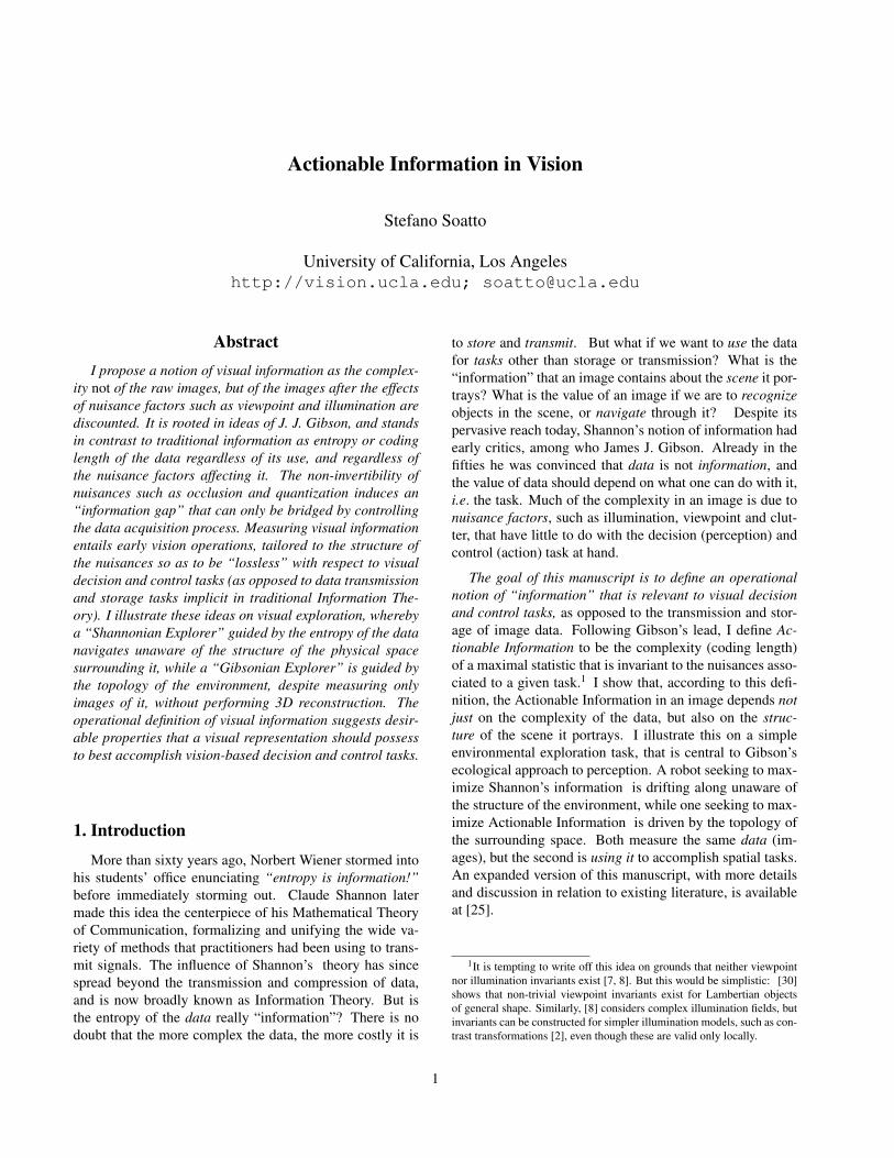
the finest partition (a.k.a. “superpixels”), and construct theadjacency graph, then aggregate nodes based on the his-togram of vector-quantized intensity levels and gradient di-rections in a region ω of 8 × 8 pixels and arrive at thetexture adjacency graph (TAG) (Fig. 2 top-right). Two-dimensional regions with homogeneous texture (or color)are represented as nodes in the TAG. I then represent one-dimensional boundaries between texture regions as edgesin the TAG, (Fig. 1 top-right and Fig. 2 bottom-left).Ridges sometimes appear as boundaries between texturedregions, or as elongated superpixels. Finally, I representzero-dimensional structures, such as junctions or blobs (Fig.1 bottom), as faces of the TAG (Fig. 2 bottom). This struc-ture, computed at all critical scales, is the Representational

Graph, R, whose coding length measures Actionable Infor-mation.

I compute the DAIG (9) by solving, at each time instant,(8) starting from a generic initialization, and using the bestestimate at time t as initialization for the optimization attime t + dt. On the occluded region Ω(t), I compute theactionable information as described above.

5. ExperimentsIn the first indoor experiment (Fig. 3), a simu-

lated robot is given limited control authority u =[uX , uY , 0, 0, 0, 0]T to translate on a plane inside a(real) room, while capturing (real) color images with fixedheading and a field-of-view of 90o. The robot is capableof computing both Entropy and the AIG at the current po-sition as well as at immediately neighboring ones. Therobot is also able of computing the DAIG. Under these con-ditions, the agent reduces to a point g = (Id, T ) whereT = [TX , Ty, 0]T . I indicate the vantage point with X =[TX , TY ]T , and the control with V = [uX , uY ]T .

In the second outdoor experiment (Fig. 5), the robot isGoogle’s StretView car, over which we have no control au-thority. Instead, we assume that it has an intelligent (Gibso-nian) driver aboard, who has selected a path close to the op-timal one. In this case, we cannot test independent controlstrategies. Nevertheless, we can still test the hypothesis thattraditional information, computed throughout the sequence,bears no relation to the structure of the environment, un-like actionable information, and in particular the DAIG. Forthe purpose of validation, standard tools from multiple-viewgeometry have been used to reconstruct the trajectory of thevehicle and its relation with the 3D structure of the environ-ment (Fig. 6).5.1. Exploration via Information Pickup

The “ground truth” Entropy Map (Fig. 3 top) and Com-plete Information Map (Fig. 3 middle) are computed from(real) images regularly sampled on a 20cm grid and up-sampled/interpolated to a 40× 110 mesh (sample views are

50 100 150 200 250 300 350 400 450 500

50

100

150

200

250

300

350

Figure 1. Representational structures: Superpixel tree (top),

dimension-two structures (color/texture regions), dimension-one

structures (edges, ridges), dimension-zero structures (Harris junc-

tions, Difference-of-Gaussian blobs). Structures are computed at

all scales, and a representative subset of (multiple) scales are se-

lected based on the local extrema of their respective detector oper-

ators (scale is color-coded in the top figure, red=coarse, blue=fine).

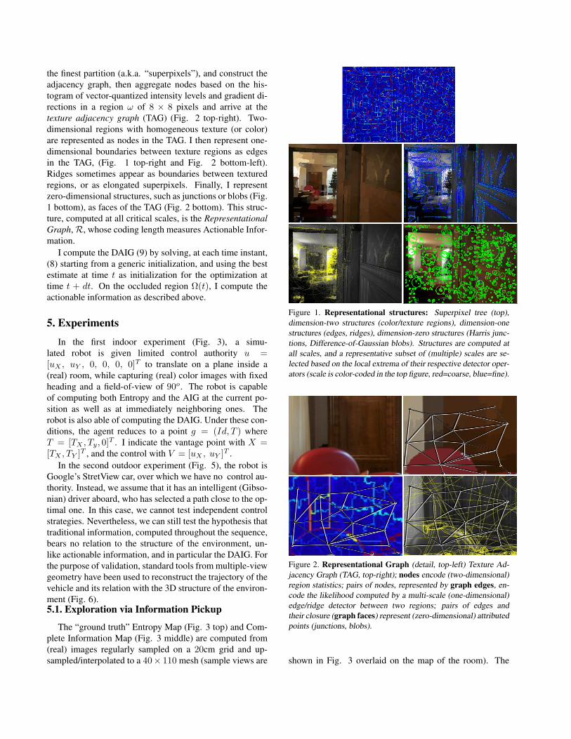
Figure 2. Representational Graph (detail, top-left) Texture Ad-

jacency Graph (TAG, top-right); nodes encode (two-dimensional)

region statistics; pairs of nodes, represented by graph edges, en-

code the likelihood computed by a multi-scale (one-dimensional)

edge/ridge detector between two regions; pairs of edges and

their closure (graph faces) represent (zero-dimensional) attributed

points (junctions, blobs).

shown in Fig. 3 overlaid on the map of the room). The

Figure 3. Entropy vs. Actionable Information (first and second

from the top) displayed as a function of position for a mobile agent

with constant heading and 90ofield-of-view (bright = high; dark =

low). Entropy relates to the structure of the image, without regard

to the three-dimensional structure of the environment: It is high in

the presence of complex textures (wallpaper and wood wainscot-

ing) in the near field as well as complex scenes in the distance.

Actionable Information, on the other hand, discounts periodic and

stochastic textures, and prefers apertures (doors and windows), as

well as specular highlights. Note the region on the right-hand side

shows high levels of Actionable Information, proportional to the

percentage of the field of view that intercepts the door aperture.

first agent I consider is a Brownian Explorer, that followsa random walk governed by

X(t + dt) = X(t) + V (t)dt; X(0) ∼ U(S ⊂ R2)V (t + dt) = V (t) + W (t)dt; W (t) iid

∼ N (0, σ2I)(14)

with V (0) = 0. The trajectory charted is shown in Fig. 4(top). Clearly, one can do better with vision. For the Shan-nonian Explorer I consider the discrete-time model, with atemporal evolution of the entropy H(I(x, t)|g(t) = X) ofthe image I captured at time t in position X , which I indi-cate in short form with H(X, t) .= [H(X, 0) − B(X, t)]+

X(t + dt) = X(t) +∇H(X(t), t)dt

B(X, t + dt) = αB(X, t) + βN (X|X(t), σ2)dt(15)

where N (x|m, σ2) is a Gaussian kernel with mean m andisotropic variance σ2I; the coefficients β > 0 and 0 < α ≤1 trade off boredom and forgetfulness respectively.The Gibsonian Explorer seeks to maximize ActionableInformation H(I(x, t)|g(t) = X) .= G(X, t), tradingoff boredom and forgetfulness in G(X, t) .= [G(X, 0) −B(X, t)]+

X(t + dt) = X(t) +∇G(X, t)dt

B(X, t + dt) = as in (15).(16)

Figure 4. Brownian (top), Shannonian (left) and Gibsonian(right) Information Pickup Representative samples of explo-

ration runs are shown. The Shannonian Explorer (left column)

is attracted by wallpaper (top edge of each plot) and the foliage

outside the window (bottom-left corner of each plot). The Gib-

sonian Explorer (right column), aims for the window (bottom-left

corner of the room) or the door (top-right corner of the room) like

a trapped fly, and is similarly repelled by the control law that pro-

hibits escape.

Representative sample explorations are shown in Fig. 4 (leftand right column respectively).

5.2. Exploration via Minimization of the DAIG

Figure 5. Google StreetView Dataset Linear panorama, 2, 560×905 pixels RGB. Entropy (left) and Entropy gradient along the

path is shown color-coded at the bottom. Neither bear any relation

to the geometry of the scene.

It is patent in Fig. 5 that neither Entropy nor its gradi-ent bear any relation to the structure of the scene. In Fig.6, I show the top view of a 250 frame-long detail. Thecolor-coded trajectory on the bottom shows the entropy gra-dient, with enhanced color-coding (red is high, blue is low).On the top I show the same for the Actionable Informa-tion Gap. It shows peaks at turns and intersections, whenlarge swaths of the scene suddenly become visible. Notethat the peaks are both before and after the intersection, asthe omni-directional viewing geometry makes the sequencesymmetric with respect to forward and backward directions.Trees, and vegetation in general, attract both the Shannon-ian and the Gibsonian explorers, as they are photometri-cally complex, but also geometrically complex because ofthe fine-scale occlusion structure, visible in the last part ofthe sequence (right-hand side of the plot; images are shownin Fig. 5). Similar considerations hold for highly specularobjects such as cars and glass windows.

6. DiscussionThe goal of this work is to define and characterize a

notion of visual information tailored to decision and con-trol tasks, as opposed to transmission and storage tasks.It relates to visual navigation or robotic localization andplanning [14]. In particular, [32, 6] propose “information-based” strategies, although by “information” they mean lo-calization and mapping uncertainty based on range data.There is a significant literature on vision-based navigation[27, 24, 11, 9, 23, 17]. However, in most of the liter-ature, stereo or motion are exploited to provide a three-dimensional map of the environment, which is then handedoff to a path planner, separating the photometric from thegeometric and topological aspect of the problem. Not onlyis this separation unnecessary, it is also ill-advised, as theregions that are most informative are precisely those wherestereo provides no disparity. The navigation experimentsalso relate to Saliency and Visual Attention [15], althoughthere the focus is on navigating the image, whereas we areinterested in navigating the scene, based on image data.

Although the problem of visual recognition is not tack-led directly, the computation of actionable information im-plicitly suggests a representational structure that integratesimage features of various dimensions into a unified repre-sentation that can, in principle, be exploited for recogni-tion. In this sense, it presents an alternative to [13, 29],that could also be used to compute Actionable Information.This work also relates to the vast literature on segmenta-tion, particularly texture-structure transitions [33]. It alsorelates to Active Learning and Active Vision [1, 5, 4, 18],also [10, 3, 19].

This work also relates to other attempts to formalize “in-formation” including [16, 28], and can be understood as aspecial case tailored to the statistics and invariance classes

Figure 6. Navigation via Minimization of the Actionable Infor-mation Gap Actionable Information gap (top) vs. Data Entropy

gradient (bottom) color-coded (blue=small, red=large) for a 250-

frame long detail of the Google Street View dataset, overlaid with

the top-view of the point-wise 3D reconstruction computed us-

ing standard multiple-view geometry. For reference, the top-view

from Google Earth is shown, together with push-pins correspond-

ing to “ground truth” coordinates. The Entropy gradient (bottom)

shows no relation with the 3D structure of the scene. Actionable

Information (top), on the other hand, has peaks at turns and inter-

sections, when large portions of the scene become visible (getting

into the intersection) and thence disappear (getting out of the in-

tersection).

of interest, that are task-specific, sensor-specific, and con-trol authority-specific. These ideas can be seen as seeds ofa theory of “Controlled Sensing” that generalizes ActiveVision to different modalities whereby the purpose of thecontrol is to counteract the effect of nuisances. This is dif-ferent than Active Sensing, that usually entails broadcastinga known or structured probing signal into the environment.

The operational definition of information introduced,and the mechanisms by which it is computed, suggest somesort of “manifesto of visual representation” for the purposeof viewpoint- and illumination-independent tasks (Sect. 4),

discussed in detail in [25]. Whether the representationalstructure R implied by the computation of Actionable In-formation will be useful for visual recognition will dependon the availability of efficient (hyper-)graph matching algo-rithms that can handle topological changes (missing nodes,links or faces).

Acknowledgments

Thanks to T. Lee for processing StreetView, B. Fulkersonand J. Meltzer for examples, and AFOSR FA9550-09-1-0427 and ONR N00014-08-1-0414 for support.

References[1] J. Aloimonos, I. Weiss, and A. Bandyopadhyay. Active vi-

sion. International Journal of Computer Vision, 1(4):333–356, 1988.

[2] L. Alvarez, F. Guichard, P. L. Lions, and J. M. Morel. Ax-ioms and fundamental equations of image processing. Arch.

Rational Mechanics, 123, 1993.[3] T. Arbel and F. Ferrie. Informative views and sequential

recognition. In Conference on Computer Vision and Pattern

Recognition, 1995.[4] R. Bajcsy. Active perception. Proceedings of the IEEE,

76(8):966–1005, 1988.[5] A. Blake and A. Yuille. Active vision. MIT Press Cambridge,

MA, USA, 1993.[6] F. Bourgault, A. Makarenko, S. Williams, B. Grocholsky,

and H. Durrant-Whyte. Information based adaptive roboticexploration. In Proc. of the IEEE/RSJ Int. Conf. on Intelli-

gent Robots and Systems (IROS), volume 1, 2002.[7] J. B. Burns, R. S. Weiss, and E. M. Riseman. The non-

existence of general-case view-invariants. In Geometric In-

variance in Computer Vision, pages 120–131, 1992.[8] H. F. Chen, P. N. Belhumeur, and D. W. Jacobs. In search

of illumination invariants. In Proc. IEEE Conf. on Comp.

Vision and Pattern Recogn., 2000.[9] A. J. Davison and D. W. Murray. Simultaneous localization

and map-building using active vision. IEEE Transactions on

Pattern Analysis and Machine Intelligence, 24(7):865–880,2002.

[10] J. Denzler and C. Brown. Information theoretic sensor dataselection for active object recognition and state estimation.IEEE Transactions on Pattern Analysis and Machine Intelli-

gence, 24(2):145–157, 2002.[11] M. Franz, B. Scholkopf, H. Mallot, and H. Bulthoff. Learn-

ing view graphs for robot navigation. Autonomous robots,5(1):111–125, 1998.

[12] J. J. Gibson. The theory of information pickup. Contemp.

Theory and Res. in Visual Perception, page 662, 1968.[13] C. Guo, S. Zhu, and Y. N. Wu. Toward a mathematical theory

of primal sketch and sketchability. In Proc. 9th

Int. Conf. on

Computer Vision, 2003.[14] S. Hughes and M. Lewis. Task-driven camera operations for

robotic exploration. IEEE Transactions on Systems, Man and

Cybernetics, Part A, 35(4):513–522, 2005.

[15] L. Itti and C. Koch. Computational modelling of visual at-tention. Nature Rev. Neuroscience, 2(3):194–203, 2001.

[16] N. Jojic, B. Frey, and A. Kannan. Epitomic analysis of ap-perance and shape. In Proc. ICCV, 2003.

[17] S. Jones, C. Andersen, and J. Crowley. Appearance basedprocesses for visual navigation. In Processings of the

5th International Symposium on Intelligent Robotic Systems

(SIRS’97), pages 551–557, 1997.[18] K. Kutulakos and C. Dyer. Occluding contour detection us-

ing affine invariants and purposive viewpoint control. In Pro-

ceedings CVPR’94., pages 323–330, 1994.[19] K. Kutulakos and C. Dyer. Global surface reconstruction by

purposive control of observer motion. Artificial Intelligence,78(1-2):147–177, 1995.

[20] T. Lindeberg. Principles for automatic scale selection. Tech-nical report, KTH, Stockholm, CVAP, 1998.

[21] Y. Ma, S. Soatto, J. Kosecka, and S. Sastry. An invitation

to 3D vision, from images to geometric models. SpringerVerlag, 2003.

[22] D. Mumford and B. Gidas. Stochastic models for genericimages. Quarterly of Applied Mathematics, 54(1):85–111,2001.

[23] S. Se, D. Lowe, and J. Little. Vision-based mobile robotlocalization and mapping using scale-invariant features. InIn Proceedings of the IEEE International Conference on

Robotics and Automation (ICRA), 2001.[24] R. Sim and G. Dudek. Effective exploration strategies for the

construction of visual maps. In 2003 IEEE/RSJ International

Conference on Intelligent Robots and Systems, 2003.(IROS

2003). Proceedings, volume 4, 2003.[25] S. Soatto. Actionable information in vision. Technical Re-

port UCLA-CSD-090007, March 10, 2009.[26] G. Sundaramoorthi, P. Petersen, V. S. Varadarajan, and

S. Soatto. On the set of images modulo viewpoint and con-trast changes. In Proc. IEEE Conf. on Comp. Vision and

Pattern Recogn., June 2009.[27] C. Taylor and D. Kriegman. Vision-based motion planning

and exploration algorithms for mobile robots. IEEE Trans.

on Robotics and Automation, 14(3):417–426, 1998.[28] N. Tishby, F. C. Pereira, and W. Bialek. The information

bottleneck method. In Proc. of the Allerton Conf., 2000.[29] S. Todorovic and N. Ahuja. Extracting subimages of an un-

known category from a set of images. In Proc. IEEE Conf.

on Comp. Vis. and Patt. Recog., 2006.[30] A. Vedaldi and S. Soatto. Features for recognition: viewpoint

invariance for non-planar scenes. In Proc. of the Intl. Conf.

of Comp. Vision, pages 1474–1481, October 2005.[31] A. Vedaldi and S. Soatto. Quick shift and kernel methods

for mode seeking. In Proc. of the Eur. Conf. on Comp. Vis.

(ECCV), October 2008.[32] P. Whaite and F. Ferrie. From uncertainty to visual explo-

ration. IEEE Transactions on Pattern Analysis and Machine

Intelligence, 13(10):1038–1049, 1991.[33] Y. N. Wu, C. Guo, and S. C. Zhu. From information scaling

of natural images to regimes of statistical models. Quarterly

of Applied Mathematics, 66:81–122, 2008.