Acoustic properties of a 5G Telecom Equipment Shroud ...

IN DEGREE PROJECT ENGINEERING PHYSICS,SECOND CYCLE, 30 CREDITS

, STOCKHOLM SWEDEN 2021

Acoustic properties of a 5G Telecom Equipment Shroud Design for Noise suppression

DAVID ANDERSSON

KTH ROYAL INSTITUTE OF TECHNOLOGYSCHOOL OF ENGINEERING SCIENCES

Acoustic properties of a 5G Telecom EquipmentShroud Design for Noise suppression

DAVID ANDERSSON

Master Thesis at SCISupervisor: Mats ÅbomExaminer: Mats Åbom

TRITA-SCI-GRU 2021:163

Abstract

As technology moves forward it has a tendency to consumemore and more power that needs to be cooled by bigger andlouder fans, this is especially true for the new generationof 5G radio equipment. This Master thesis is a collabo-ration with Ericsson and attempts to construct a shroudfor containing a number of 5G radio units whilst attenuat-ing the fan noise of the units as effectively as possible. Inthis project are air ducts used and at the ends silencers arecreated utilizing the Cremer impedance; the optimal wallimpedance for damping an acoustic mode of a propagatingwave. To predict the result, a simplified model in an acous-tic FEM program was also explored and compared to thesound level of the constructed shroud.The finished shroud successfully reduces the noise of the ra-dio units by 13 dB(A) while causing an increase in temper-ature of between 2.8oC to 5.9oC. This result was deemedto be a success and the Cremer impedance approach of re-ducing noise is therefore advised for future development.

Keywords:- Acoustics- 5G- Shroud- Telecom- Noise reduction

ReferatHuvdesign för ljudämpning till 5G

Teleutrustning

Allt eftersom tekniken går framåt tenderar den att ocksåförbruka mer och mer energi som i sin tur måste kylas avkraftigare och mer högljudda fläktar, detta fenomen är sär-skilt påtagligt när det kommer till den senaste generatio-nens radioutrustning för 5G. Detta examensarbete är ettsamarbete mellan KTH och Ericsson med avsikt att ska-pa en kåpa som är designad för att innesluta ett bestämtantal 5G radiomoduler. Denna kåpa ska i så stor utsträck-ning som möjligt dämpa det fläktinducerade bullret. I dethär projektet nyttjas kanaler med ljuddämpare vid ändar-na som dämpar ljudet med hjälp av Cremerimpedans, dvs:den väggimpedans som optimalt dämpar en akustisk mod.För att kunna förutspå resultatet skapades en förenkladakustisk modell i ett FEM program. Resultatet från dennamodell jämförs sedan med ljudeffektnivån från slutmätning-en av den färdiga kåpan.Resultatet från slutmätningen visar att kåpan lyckas sänkaradioenheternas totala ljudeffektnivå med 13 dB(A) samti-digt som en temperaturökning på mellan 2.8oC och 5.9oCerhålls. Det här resultatet bedöms vara en framgång, vilketleder till slutsatsen att ljuddämpning med användning avCremerimpedans rekommenderas för vidare arbete.

Nyckelord:- Akustik- 5G- Kåpa- Teleutrustning- Ljudisolering

Acknowledgements

This project would not have been possible if not for the help and support by myEricsson supervisors Stefan Skoglund and Sven Sjögren aswell as my KTH supervisorMats Åbom especially for helping me understand the nature of Cremer impedance.I would also like to present a thank you to Ralf Corin of Sontech for providing theAcustimet MPP sheets and for other help in regards to this. My colleague; PerRundström also deserves credit for putting up with my shenanigans.

Contents

1 Introduction 11.1 Background . . . . . . . . . . . . . . . . . . . . . . . . . . . . . . . . 11.2 Purpose . . . . . . . . . . . . . . . . . . . . . . . . . . . . . . . . . . 21.3 Scope . . . . . . . . . . . . . . . . . . . . . . . . . . . . . . . . . . . 31.4 Method . . . . . . . . . . . . . . . . . . . . . . . . . . . . . . . . . . 3

2 Theory 42.1 Cremer impedance . . . . . . . . . . . . . . . . . . . . . . . . . . . . 42.2 Micro perforated plates . . . . . . . . . . . . . . . . . . . . . . . . . 6

2.2.1 MPP impedance calculation . . . . . . . . . . . . . . . . . . . 72.3 Cremer silencer . . . . . . . . . . . . . . . . . . . . . . . . . . . . . . 8

2.3.1 Chunky chamber . . . . . . . . . . . . . . . . . . . . . . . . . 112.3.2 Sidelong chamber . . . . . . . . . . . . . . . . . . . . . . . . . 12

3 Noise Characterization Measurement 153.1 Separated intake/exhaust measurement . . . . . . . . . . . . . . . . 153.2 Whole radio measurement . . . . . . . . . . . . . . . . . . . . . . . . 173.3 Sound recording . . . . . . . . . . . . . . . . . . . . . . . . . . . . . 173.4 Measurement results . . . . . . . . . . . . . . . . . . . . . . . . . . . 18

4 Simulation 224.1 Radio model . . . . . . . . . . . . . . . . . . . . . . . . . . . . . . . 224.2 Shroud model . . . . . . . . . . . . . . . . . . . . . . . . . . . . . . . 244.3 Simulation Results . . . . . . . . . . . . . . . . . . . . . . . . . . . . 26

5 Demonstrator 315.1 Ducts . . . . . . . . . . . . . . . . . . . . . . . . . . . . . . . . . . . 325.2 Acoustical chambers . . . . . . . . . . . . . . . . . . . . . . . . . . . 34

5.2.1 The expansion chambers used . . . . . . . . . . . . . . . . . . 385.2.2 Validation of expansion chambers used . . . . . . . . . . . . . 39

5.3 Micro perforated plates . . . . . . . . . . . . . . . . . . . . . . . . . 425.4 The dimensions and specifications used . . . . . . . . . . . . . . . . . 44

6 Results 46

6.1 Measurement procedure . . . . . . . . . . . . . . . . . . . . . . . . . 466.2 Measurement Results . . . . . . . . . . . . . . . . . . . . . . . . . . . 506.3 Simulation Results . . . . . . . . . . . . . . . . . . . . . . . . . . . . 526.4 Thermal testing results . . . . . . . . . . . . . . . . . . . . . . . . . . 55

7 Discussion and Conclusion 567.1 Conclusion . . . . . . . . . . . . . . . . . . . . . . . . . . . . . . . . 567.2 Discussion . . . . . . . . . . . . . . . . . . . . . . . . . . . . . . . . . 567.3 Future work . . . . . . . . . . . . . . . . . . . . . . . . . . . . . . . . 57

Bibliography 59

Appendices 61

A Matlab code for Impedance calculation 61

B Expansion chamber correction factor 64

C Test duct 65

D Non local reaction test 66

E Ducts used 67

List of Figures

2.1 Sketch of the pressure profile of the 2 first modes in a rectangular ductfor both a hard wall case and a single sided soft wall case . . . . . . . . 5

2.2 One of the Acustimet® slit style MPP sheets used in this project . . . . 72.3 The resulting silencer from [1], the arrow marked 1 is pointing at the

MPP sheet used in the silencer . . . . . . . . . . . . . . . . . . . . . . . 92.4 Sketch showing a simple type of expansion chamber (Created in paint.net[2]) 102.5 Sketch showing a wide version of the expansion chamber (Created in

paint.net[2]) . . . . . . . . . . . . . . . . . . . . . . . . . . . . . . . . . . 112.6 Sketch showing a type of expansion chamber protruding parallel to the

permeable wall (Created in paint.net[2]) . . . . . . . . . . . . . . . . . . 12

3.1 An illustration of test setup (Created in Paint.net [2]) . . . . . . . . . . 163.2 Images taken when preparing the measurement of how the radio was

mounted . . . . . . . . . . . . . . . . . . . . . . . . . . . . . . . . . . . . 163.3 Image taken before the Sound power measurement of the whole radio

was performed . . . . . . . . . . . . . . . . . . . . . . . . . . . . . . . . 173.4 Image taken before one of the sound recordings . . . . . . . . . . . . . . 183.5 Third octave band spectra of the radio intake for different percentages

of the maximum fan speed . . . . . . . . . . . . . . . . . . . . . . . . . . 193.6 Third octave band spectra of the radio exhaust for different percentages

of the maximum fan speed . . . . . . . . . . . . . . . . . . . . . . . . . . 19

4.1 Image showing intake (blue) and the exhaust (red) position on the radio(Exported from COMSOL multiphysics [3]) . . . . . . . . . . . . . . . . 23

4.2 Simulation model of the shroud (Exported from COMSOL multiphysics[3]) . . . . . . . . . . . . . . . . . . . . . . . . . . . . . . . . . . . . . . . 24

4.3 The simplified intake space used in the simulation (Exported from COM-SOL multiphysics [3]) . . . . . . . . . . . . . . . . . . . . . . . . . . . . 25

4.4 Simulation example of the shroud (Exported from COMSOLmultiphysics[3]) . . . . . . . . . . . . . . . . . . . . . . . . . . . . . . . . . . . . . . . 26

4.5 The simulation of only one radio (Exported from COMSOL multiphysics[3]) . . . . . . . . . . . . . . . . . . . . . . . . . . . . . . . . . . . . . . . 27

4.6 The result from the measurement minus the simulation results (Exportedfrom COMSOL multiphysics [3]) . . . . . . . . . . . . . . . . . . . . . . 28

4.7 Convergence analysis of two different maximum element sizes (Exportedfrom COMSOL multiphysics [3]) . . . . . . . . . . . . . . . . . . . . . . 29

5.1 Picture showing the outside of the shroud . . . . . . . . . . . . . . . . . 315.2 Picture with the lid of the shroud removed . . . . . . . . . . . . . . . . 325.3 Sketch of a duct solution (Created in Paint.net [2]) . . . . . . . . . . . . 325.4 Simplification of the airflow (Created in Paint.net [2]) . . . . . . . . . . 335.5 Model of the airflow in the Shroud . . . . . . . . . . . . . . . . . . . . . 345.6 A photo taken looking into the intake duct . . . . . . . . . . . . . . . . 355.7 A photo taken looking into the low frequency intake expansion chamber 365.8 Image showing the proposed 2-sided Cremer damper sliced at one point

along the length of the duct (Created in Paint.net [2]) . . . . . . . . . . 365.9 Image showing the used 2-sided Cremer damper sliced at one point along

the length of the duct (Created in Paint.net [2]) . . . . . . . . . . . . . 375.10 Image showing another used 2-sided Cremer damper sliced at one point

along the length of the duct (Created in Paint.net [2]) . . . . . . . . . . 375.11 Sliced CAD model of the intake silencer (Created in Solid Edge [4]) . . 385.12 Sliced CAD model of the exhaust silencer (Created in Solid Edge [4]) . . 385.13 Comparison between one sided and two sided damper (exported from

COMSOL multiphysics [3]) . . . . . . . . . . . . . . . . . . . . . . . . . 405.14 The sound attenuation from using different division distances (Exported

from COMSOL multiphysics [3]) . . . . . . . . . . . . . . . . . . . . . . 415.15 Example graph showing an optimized MPP impedance corresponding to

the real part of the Cremer impedance at 1246 Hz . . . . . . . . . . . . 435.16 Example graph showing an optimized total wall impedance after the

expansion chamber is added corresponding to the Cremer impedance at1246 Hz . . . . . . . . . . . . . . . . . . . . . . . . . . . . . . . . . . . . 43

5.17 Drawing of the cross section of the intake duct silencer (Created inPaint.net[2]) . . . . . . . . . . . . . . . . . . . . . . . . . . . . . . . . . . 45

5.18 Drawing of the cross section of the exhaust duct silencer (Created inPaint.net[2]) . . . . . . . . . . . . . . . . . . . . . . . . . . . . . . . . . . 45

6.1 The test object setup without and with the shroud . . . . . . . . . . . . 476.2 The 2+1 configuration . . . . . . . . . . . . . . . . . . . . . . . . . . . . 486.3 The improvised mitigation for the plate vibrations . . . . . . . . . . . . 496.4 The reduction of the sound power level for each fan speed for the new

Cremer based shroud design (Created in Matlab [5]) . . . . . . . . . . . 506.5 The reduction in A-weighted total sound power level for each fan speed

(Created in Matlab [5]) . . . . . . . . . . . . . . . . . . . . . . . . . . . 516.6 Simulated and measured attenuation in sound power level (Created in

Matlab [5]) . . . . . . . . . . . . . . . . . . . . . . . . . . . . . . . . . . 526.7 Simulated and measured normalized shroud sound power level for 39%

fanspeed (Created in Matlab [5]) . . . . . . . . . . . . . . . . . . . . . . 53

6.8 Simulated and measured normalized shroud sound power level for 59%fanspeed (Created in Matlab [5]) . . . . . . . . . . . . . . . . . . . . . . 53

6.9 Simulated and measured normalized shroud sound power level for 100%fanspeed (Created in Matlab [5]) . . . . . . . . . . . . . . . . . . . . . . 54

6.10 Temperature difference of radios heatsink with and without casing (Cre-ated in Matlab [5]) . . . . . . . . . . . . . . . . . . . . . . . . . . . . . . 55

C.1 Images showing the test duct used (Exported from COMSOL multi-physics [3]) . . . . . . . . . . . . . . . . . . . . . . . . . . . . . . . . . . 65

D.1 Images showing the inserted hard wall divider in the high frequencydamper as well as the result (Exported from COMSOL multiphysics [3]) 66

E.1 CAD from [6] showing one of the exhaust ducts with silencers (Left) andthe intake duct with silencers (Right) . . . . . . . . . . . . . . . . . . . 67

E.2 CAD from [6] showing the intake and the exhausts as they are mountedinside the shroud . . . . . . . . . . . . . . . . . . . . . . . . . . . . . . . 68

Introduction

1.1 Background

5G has been on the news for many years now, and while it is (as of writing thisreport) now possible to enjoy some of the promises that has been cleverly marketedby smartphone manufacturers and cell service providers, this is limited to a handfulof places in some cities.

A globe spanning mobile network is however not built in a day.

The main advantages of 5G are to allow higher communication bandwidth as wellas lower latencies. These advantages do however come with some disadvantages.Firstly, do the increase in data throughput cause a much higher load on the telecomhardware that talks to your phone. This causes higher thermal load which causesincreased cooling requirements which often results in an increase in fan noise.

This would not have been as much of a problem if not for the second disadvan-tage of 5G.Due to the increase in radio frequency, the 5G signal has a much shorter range thanprevious standards. To solve this, the cell towers previously built ontop of buildingroofs, must instead be closer to ground level.

The combination of these two disadvantages is that the fan noise is now audibleto people on the streets or to residents through an open window. This is the back-ground of this project.Since designing 5G equipment is a long process, this project will instead be lookingat constructing a shroud that is meant to house a number of telecom radio unitsand reduce the noise they emit.

1

CHAPTER 1. INTRODUCTION

1.2 PurposeThe purpose of this project is to create a housing that is designed to contain 3Ericsson specific radio units.This shroud should be designed to at a fixed component and ambient temperaturereduce the noise as much as possible.This housing is meant to supply the radio with cold ambient air and expel the hotexhaust air whilst reducing the fan induced noise of the radio units cooling system.It should be noted that the shroud/housing itself in this project should not containany additional fans.

This project is therefore an optimization problem where both the acoustic and thethermal/fluid dynamic aspect must be considered. It was therefore organized to bea collaboration between two master thesis students each writing a separate reportaddressing the two different aspects of the problem.The other report written by Per Rundström [6] focuses on the thermal aspect aswell as the construction of the shroud. This report is about the acoustic aspect ofthe problem but will contain reasoning based on the result from the other report.

From preliminary measurement using a sound pressure measurement device, it wasclear that a high amount of low frequency noise caused by the blade pass frequencyof the fans existed around 500 Hz.Since such low frequencies are difficult to attenuate using common resistive dampingin a small space [7] and since both the intake and the exhaust should be dampened,reflective damping is ineffective also, it was decided that a form of Cremer dampingin ducts should be used.Cremer damping has in previous reports [8] been shown to achieve a high amountof low to mid frequency resistive damping.

This report will aim to answer the following questions:

• How can Micro perforated plates and Cremer impedance be used within anenclosure to eliminate noise?

• Can a complex source be properly characterized by measurements to be in-serted into a Finite Element Method (or FEM) acoustical model?

2

CHAPTER 1. INTRODUCTION

1.3 ScopeSince the purpose of this report is to assess the strategy of utilizing air ducts withCremer damping for a shroud use case, will the conclusion be focusing on whetherthis is viable or not.A set of goals was however set for the project:

• For a certain fan speed should the total sound power level decrease at least10dB by using the shroud.

• The increase in fan noise required for the radio to maintain a constant temper-ature when using the shroud should be much smaller than the total reductionof noise by the shroud.

Since the FEM simulation aspect in this report is of a concept testing nature, wasno goals set for how accurately the simulated results correlate to the measurement.

1.4 MethodTo make the project more manageable and ease planning, it was in an early stagedivided into a number of steps.

• Perform a sound characterization measurement of the radio units.

• Create a theoretical model of Cremer damping and calculate the best dimen-sions to attenuate the noise from the previous step.

• Using the result of the previous step, build a model in a FEM program andperform acoustic simulations and realize and optimize the model dimensionsfrom the previous step.

• Build a demonstrator of the optimized model.

• Perform a final acoustic measurement of the radio mounted in the shroud.

• Draw conclusions on how well the theory and simulations coincide with themeasurement.

3

Theory

2.1 Cremer impedanceCremer impedance is the theoretical optimal wall impedance for attenuating a wavetraveling in a duct, developed in in 1953 by Cremer [9] and expanded upon by Testerin 1973 [10].Typically, this impedance is created for the least damped mode in a duct sinceother modes already have a higher degree of dissipation assuming non-hard bound-ary. This is especially true in small ducts where the plane wave (0,0) mode isdominant.

The theory is that this optimal wall impedance makes the next order duct modemerge with the propagating plane wave, resulting in optimal attenuation of themerged mode pair.The model used in this report merges the plane wave (0,0) mode in the duct witha (0,1) mode. The (0,1) mode described has its node line parallel to the liner wall.A single sided liner model can be described with the following sketch:

4

CHAPTER 2. THEORY

Figure 2.1: Sketch of the pressure profile of the 2 first modes in a rectangular ductfor both a hard wall case and a single sided soft wall case

As can be seen in figure 2.1 when the wall impedance moves away from infinite(hard wall), the (0,0) and (0,1) pressure profile will approach each other.According to Tester [10] for a wall impedance where these two modes meet in thecomplex wave number plane there is an attenuation peak for these modes travelingin the duct.

For such a rectangular duct with negligible flow speeds 1, the branch point equationcan be expressed as [11]:

H = (β̄1 + β̄2)kyh · kh cos(kyh) + i

[(kyh)2 + β̄1β̄2(kh)2

]sin(kyh) = 0 (2.1)

Where the β̄1 and β̄2 is the normalized admittance for two opposing liner walls witha duct width of h.Converting the admittance β to impedance Z for the liner wall as well as settingthe admittance for the other wall to 0, the following equation is received:

H = −iZkyh · kh cos(kyh) + i(kyh)2sin(kyh) = 0 (2.2)

1The typical flow speed in this project does not exceed 4.2 m/s, corresponding to M<0.013

5

CHAPTER 2. THEORY

To find the wall impedance that corresponds to the smallest sum of the waves,equation 2.2 is therefore derivated in respect to the normalized transverse wavenumber:

∂H

∂(kyh) = −iZkh(cos(kyh)− kyh · sin(kyh)) + i(2kyhsin(kyh) + (kyh)2cos(kyh)) = 0

(2.3)

Using equation 2.2 and 2.3 this can be simplified to:

∂H

∂(kyh) = kyh+ sin(kyh)cos(kyh)cos2(kyh) = 0 (2.4)

This can be solved to:kyh = 2.106 + 1.125i

The wall impedance Z in equation 2.2 can be written as:

Z = −1kyh tan(kyh) · kh (2.5)

Using the solution from equation 2.4, the normalized wall impedance becomes:

Z = (0.9288− 0.7442i)khπ

(2.6)

This is what is known as the Cremer impedance.

2.2 Micro perforated plates

A Micro perforated plate (or MPP) is a metal sheet with a dense pattern of smallholes through it. These holes are designed to be impermeable to a flowing fluidwhilst have the ability to absorb sound waves. The intended use case for MPP:sare to replace traditional porous damping material such as mineral wool while alsohave the ability to be a structural part of the design [12]. While circular hole MPPexist as well, in this project slit style MPP as seen in figure 2.2 are used instead.

6

CHAPTER 2. THEORY

Figure 2.2: One of the Acustimet® slit style MPP sheets used in this project

2.2.1 MPP impedance calculationTo properly implement the usage of MPP in a model, the equivalent transferimpedance caused by a MPP wall is required. Such a model for the slit styletype of MPP has been described before in an overview by Guo et al. [13] and canbe presented as:

rs = Re

{iωt

σc

[1− tanh(ks

√i)

ks√i

]−1}+ 4Rsσρc

+ |uh|σc

+ γM

σ(2.7)

xs = Im

{iωt

σc

[1− tanh(ks

√i)

ks√i

]−1}(2.8)

Where:rs is the normalized resistancexs is the normalized reactanceω is the angular frequencyt is the thickness of the micro perforated plateσ is the porosity of the micro perforated platec is the speed of sound of the mediumρ is the density of the mediumuh is the peak particle velocity in the aperturesγ is a factor for grazing flow effects

7

CHAPTER 2. THEORY

M is the Mach number of the grazing flow

Rs is the surface resistance:Rs = 0.5

√2ρη (2.9)

Where η is the dynamic viscosity of the medium

ks is the shear wave number:ks = d

√ω

4ν (2.10)

Where d is the slit width of the micro perforated plate andν is the kinematic viscosity of the medium.

If M and uh are assumed small, equation 2.7 can be written:

rs = Re

{iωt

σc

[1− tanh(ks

√i)

ks√i

]−1}+ 4Rsσρc

(2.11)

Using the result from equation 2.7 and 2.8 the total normalized transfer impedanceof the MPP can then be expressed by:

Zn = rs + xs (2.12)

2.3 Cremer silencerWhen building a Cremer silencer the wall impedance should be optimized to beas close to the Cremer optimum as possible at the frequency that the silencer isdesigned to attenuate.

8

CHAPTER 2. THEORY

Figure 2.3: The resulting silencer from [1], the arrow marked 1 is pointing at theMPP sheet used in the silencer

For example, a silencer described in [1] achieves the Cremer impedance by utilizingan Acustimet MPP [12] as well as a chamber behind this plate to perfectly matchthe Cremer impedance at one frequency.

The idea is that the resulting wall impedance can be expressed as [1]:

Ztot = Zwall + Zchamber (2.13)

The wall impedance Zwall is the impedance of the material used as a separatingwall between the duct and the chamber, for example an MPP sheet.The chamber impedance Zchamber can be calculated by assuming an incident waveas well as a reflected wave from an outer wall as:

pin = p̂eiωt (2.14)

pre = p̂eiωt+ik×2h (2.15)

Where pin is the incident wave and pre is the reflected wave, note that the reflectedwave is phase shifted 2 times the depth of the chamber h.

9

CHAPTER 2. THEORY

Impedance is defined by dividing sound pressure with sound velocity [7] whichresults in:

Zchamber = p

u= pin + pre−uin + ure

(2.16)

By using formula 2.14 and 2.15 aswell as the plane wave relationship between thepressure and velocity of a wave:

Z0 = p+

u+x

(2.17)

Formula 2.16 can be written:

Zchamber = p

u= p̂eiωt + p̂eiωt+ik×2h

p̂Z0eiωt+ik×2h − p̂

Z0eiωt

(2.18)

This can be simplified to:

Zchamber = Z01 + eik×2h

eik×2h − 1 (2.19)

Figure 2.4: Sketch showing a simple type of expansion chamber (Created inpaint.net[2])

Where b is the height of the duct and the expansion chamber and h is the depth ofthe expansion chamber. In figure 2.4, the sound waves enter the expansion chamberthrough the permeable wall (marked red in figure 2.4, 2.5 and 2.6) and is reflectedat the outer wall.The dotted lines represent the position of the air duct relative to the expansionchamber.

10

CHAPTER 2. THEORY

2.3.1 Chunky chamberIf the height (b) of the expansion chamber is larger than the height of the duct, theimpedance calculated in equation 2.19 is no longer correct.For low Helmholtz numbers, the particle velocity ux needs to be proportionallyhigher to achieve the same sound pressure in the expansion chamber. This can beexpressed by modifying equation 2.17 to be:

Z0 = pSchamberSduct

∗ ux(2.20)

Where Schamber is the constant area of the expansion chamber and Sduct in the areaof the incident wave.

Figure 2.5: Sketch showing a wide version of the expansion chamber (Created inpaint.net[2])

For a continuous duct case, equation 2.20 becomes:

Z0 = pbchamberbduct

∗ ux(2.21)

Where bchamber is the height of the expansion chamber and bduct is the height of theduct.

Calculating the impedance using the steps from earlier yields:

Zchamber = Z0bduct

bchamber× 1 + eik×2h

eik×2h − 1 (2.22)

11

CHAPTER 2. THEORY

2.3.2 Sidelong chamberThe last type of chamber design used was the following:

Figure 2.6: Sketch showing a type of expansion chamber protruding parallel to thepermeable wall (Created in paint.net[2])

In this type of chamber, the assumption that the soundwave travels to the opposingwall and reflects, no longer holds as the wave will instead bend as can be seen infigure 2.6.For low Helmholtz numbers, this type of expansion chamber can be expressed asthe chambers previously discussed with an equivalent length. This length can be

12

CHAPTER 2. THEORY

expressed as:L′ = L+ ∆L (2.23)

Where L′ is the equivalent length, L is set to the width of the chamber not occupiedby the entrance (red in figure 2.6), and ∆L is the length needed in order to correctfor the bend. Using the figure nomenclature, this is:

L′ = (h− bduct) + C · bduct (2.24)

Where C is a correction factor that is applied to the width of the entrance.A simulation as well as a calculation was performed and can be found in Appendix B.The resulting equivalent length of the camber was calculated to: L’=0.1403m, yield-ing a correction factor C=0.71.The impedance can be calculated with this version of equation 2.22

Zchamber = Z0bduct

bchamber× 1 + eik×2L′

eik×2L′ − 1 (2.25)

13

Noise Characterization Measure-ment

In order to develop a strategy to reduce the noise, measurements need to be per-formed to find which frequencies contribute most to the total emitted sound power.

The measurements where deigned to answer what the emitted sound power of thestandalone radio is, as well as separating the intake of the radio from the exhaustin order to more properly be able to use the results in a FEM simulation.

The next 3 subchapters describe the different kinds of measurements used in theproject.

3.1 Separated intake/exhaust measurementThe goal of this measurement is know how much of the sound power radiates fromthe radio intake and how much radiates from the exhaust.The result of this is meant to be used as a sound source in the FEM simulationmodel, placed on the surfaces representing the intake as well as the exhausts of theradio.The measurement utilizes the ISO 3741:2010 standard; Sound pressure method us-ing a reference sound source, and was performed at the Marcus Wallenberg Labora-tory (or MWL) using the Anechoic room and the Reverberation room. A separatingMedium Density Fibreboard (or MDF) wall was placed in the 920 mm x 1010 mmrectangular hole between the rooms.

A simple illustration of the setup is as follows:

15

CHAPTER 3. NOISE CHARACTERIZATION MEASUREMENT

Figure 3.1: An illustration of test setup (Created in Paint.net [2])

In figure 3.1 is the blue part of the radio representing the intake and the red partrepresenting the exhaust. The radio was flipped when the sound power level of theexhaust was measured.In practice the separating board was constructed of 16mm thick MDF. To avoidvibrations from the radio radiating into the MDF, the hole in the board was about0.5cm larger on each side than the radio and the gaps filled in with latex. To supportthe weight of the radio, it was placed on a small screw jack.

Figure 3.2: Images taken when preparing the measurement of how the radio wasmounted

Note that in figure 3.2 the left image was taken while preparing for the intake

16


measurement and the right was taken while preparing for the exhaust measurement.

3.2 Whole radio measurementThe goal of this measurement is to acquire the sound power of the whole radio.The result of this was firstly requested by Ericsson, however is also meant to beused as validation of the FEM simulation results.

Figure 3.3: Image taken before the Sound power measurement of the whole radiowas performed

The measurement utilizes the ISO 3741:2010 standard; Sound pressure methodusing a reference sound source, and was performed at MWL in the Reverberationroom. The radio was placed on two rolls of tape in the middle of the room.

3.3 Sound recordingThe goal of this measurement is to record the sound emitted from the radio atdifferent angles.The result is meant to be used as a reference of playing back the sound emitted bythe radio, providing the possibility of illustrating the difference to the sound beforeand after applying the attenuation from the simulation results.This measurement was performed 3 times, on top of the radio, in front of the intake(as in 3.4) and in front of the exhaust. In all cases the microphone was placed at adistance on 1m from the surface being measured.

17


Figure 3.4: Image taken before one of the sound recordings

3.4 Measurement resultsThis section aims to display the relevant results of the measurements performed inthe previous sections.

To better illustrate the sound spectra for each fan speed tested, the third octaveband sound power levels has been normalized using the following formula:

LW (A),3bandnorm,n = LW (A),3band,n − LW (A),tot,n (3.1)

Where LW (A),3bandnorm,n is the normalized A-weighted third octave band soundpower level for the fan speed n.The LW (A),3band,n is the measured A-weighted third octave band sound power levelfor the fan speed n and LW (A),tot,n is the measured total A-weighted sound powerlevel for the fan speed n.

18


Figure 3.5: Third octave band spectra of the radio intake for different percentagesof the maximum fan speed

Figure 3.6: Third octave band spectra of the radio exhaust for different percentagesof the maximum fan speed

As can be seen in both figure 3.5 and 3.6, there is some variations in the radiatedsound as the fan speed increases. Below 50% fan speed, frequencies below 1000Hz

19


contain relatively less power, while at higher speeds the noise spectra is more uni-form. As the noise of the device is most problematic at higher fan speeds was thethird octave band curves for > 50% chosen as the reference for the need of attenu-ation.When comparing the intake and the exhaust do the intake contain stronger highfrequency content and it was suggested that the relevant span of damping for itshould be from 400Hz to 2500Hz.The exhaust has more uniform sound power levels and the relevant span of dampingfor it was suggested to be from 315Hz to 2500Hz.The difference in total A-weighted sound power level between the intake and theexhaust is for relevant frequencies about 3 dB higher for the intake than the ex-haust. The conclusion drawn from this was that both the intake and the exhaust isin need of noise reduction.

20

Simulation

The main goal of the simulation is to anticipate the sound power spectra of theentire shroud and tweak the dimensions to avoid strong resonances. Another goal isto optimize the attenuation peaks of the Cremer dampers to achieve a total soundpower level as low as possible, the idea being that if two attenuation peaks are toospread apart, the frequencies in between will have little damping possibly causinga higher total sound power level than the optimum.The simulations in this report are performed in the commercial software COMSOLmultiphysics [3].The frequency sweep in the simulation was set to logarithmic steps from 100 Hzto 5000 Hz with a step density of 5 steps per third octave band. The simulatedthird octave band sound power level results is therefore an average of 5 points perfrequency band.

4.1 Radio modelThe radio unit was input into the simulation as a "black box" utilizing the measure-ment results from chapter 3.4 as the sound power emitted from the intake and theexhausts respectively.Since the measurement did not contain information on the pressure distribution onthe surface of the fans, it was assumed even. This assumption holds true at lowHelmholtz numbers compared to the diameter of the fan.

22

CHAPTER 4. SIMULATION

Figure 4.1: Image showing intake (blue) and the exhaust (red) position on the radio(Exported from COMSOL multiphysics [3])

Note that in figure 4.1 there is a second exhaust at the same location on the otherside not shown.

The intake was modelled as a pressure source and the following equation was used[7]:

W/S = p̃2/(ρ0 c) (4.1)

Where ρ0 is the air density, c is the sound velocity and S is the area of the surface.This was modified and inserted as:

p̂intake =√

2

√ρ0 c

Wref ∗ 10(LW /10)

hintake ∗ bintake(4.2)

Where Wref is the reference sound power which is 10−12W [7], hintake and bintakeis the height and width of the intake respectively.Since the measurement method performed when characterizing the intake and ex-haust does not account for the phase information, the phase of the exhaust needsto be approximated in the model.

It was approximated that the fans of the radio in located 90mm from the intakeand the airpath from the fans to the exhaust was 270mm. Because of the dipolenature of a fan noise source, the phase was also shifted π radians. The resultingphase shift was expressed as:

φ = (0.27− 0.09)2π fc

+ π (4.3)

Where f is the frequency.Since in the measurement the sound power of both the exhausts where measured,the sound power from each of the exhaust must be divided by 2, this is based onthe assumption that the exhausts are uncorrelated.

23


The following modification of equation 4.2 with equation 4.3 was inserted as apressure source for each exhaust:

p̂exhaust =

√ρ0 c

Wref ∗ 10(LW /10)

hexhaustbexhaustei(0.27−0.09) 2π f

c+π (4.4)

Where hexhaust and bexhaust is the height and width of one exhaust respectively.

The result of this is that both exhausts exhibit the same phase. In reality howeverare the exhausts uncorrelated because of the use of multiple fans combined with theinterior layout of the radio.

4.2 Shroud modelThis portion aims to demonstrate how the shroud was implemented into the simu-lation. This section will also include the area around the shroud which the soundradiates into after escaping the shroud.

Figure 4.2: Simulation model of the shroud (Exported from COMSOL multiphysics[3])

In figure 4.2 the radio units (colored grey) have their intakes facing towards theright.

24


Note that both the intake duct and the exhaust duct utilizes the Cremer wallimpedance on 2 perpendicular sides of the duct. For more details see section 5.2.

In the model, the MPP was inserted as a surface with an interior impedance condi-tion with the impedance from equation 2.12. Other surfaces which in the demon-strator are constructed of sheet metal were set to interior hard boundaries.

As can be seen in figure 4.2 is the complete shroud not modelled. This has beendone to make the computation time smaller.While in the demonstrator, the intake of the radio can radiate sound to most of theinside of the shroud, has in the model, a cuboid between the radio intake and theentrance to the intake duct been used. The effect of the exterior shroud and theexterior flow guides has been assumed small and has been omitted.

Figure 4.3: The simplified intake space used in the simulation (Exported fromCOMSOL multiphysics [3])

In figure 4.3 the radio intake marked dark blue radiates into the intake space markedorange. The intake space can freely radiate into the intake duct marked light bluewhilst all other of its surfaces were set to interior hard boundaries.Note that in figure 4.3 has the left exhaust duct and silencer been removed for bettervisibility.

25


Figure 4.4: Simulation example of the shroud (Exported from COMSOL multi-physics [3])

To derive the sound power level of the model, the average sound pressure rms valuewas taken on a surface of the surrounding spheroid seen in figure 4.4 and using thefollowing formula converted into sound power level:

LW = 10 ∗ log10(p2rms

p2ref

) + 10 ∗ log10(AspheroidAref

) (4.5)

Where pref is the reference sound pressure (2 ∗ 10−5 Pa) and Aref is the referencearea (1m2) [7]The spheroid has the dimensions 0.7 m x 0.7 m x 1.7 m, resulting inAspheroid = 3.121m2.

4.3 Simulation ResultsThis section aims to validate the results yielded from the simulation.The simulation results for the entire shroud will be presented in the result section,instead will this chapter compare the measurement results of the sound power levelof the whole radio, detailed in section 3.2, to the simulated radio radiating into thespheroid.

26


Figure 4.5: The simulation of only one radio (Exported from COMSOL multiphysics[3])

27


Figure 4.6: The result from the measurement minus the simulation results (Exportedfrom COMSOL multiphysics [3])

28


As can be seen in figure 4.6 are the results of the simulated radio mostly within 6dBfor frequencies considered to be an issue in figure 3.5 and 3.6. The deviance fromthe 0dB mark is also reduced at frequencies above the 630Hz third octave band.

Figure 4.7: Convergence analysis of two different maximum element sizes (Exportedfrom COMSOL multiphysics [3])

As can be seen in figure 4.7, the maximum element size used (0.12m) is sufficientto accurately predict the sound power level within 1dB at frequencies up until the2500Hz octave band.

29

Demonstrator

This section seeks to give an overview of the design in order to present the readerwith a clear picture of the finished shroud.

Figure 5.1: Picture showing the outside of the shroud

31

CHAPTER 5. DEMONSTRATOR

Figure 5.2: Picture with the lid of the shroud removed

The beige middle radio in figure 5.2 is the dummy radio used. Some areas wherefilled with foam plastic to make the shroud more consistent with the simulationmodel shown in section 4.2

5.1 DuctsTo be able to realize a solution based on Cremer damping the sound must passthrough a cross section with walls that realizes the Cremer optimum. To achievethis, it was decided to implement some sort of duct solution. A duct solution wouldbe as the image below:

Figure 5.3: Sketch of a duct solution (Created in Paint.net [2])

In figure 5.3 cool air is supplied to the radio through an intake duct and the hotexhaust is expelled through an exhaust duct.This solution also enabled the exhaust and intake damper to have a different design

32


based on the noise spectra emitted, as demonstrated in section 3.4.The finalized duct solution can be simplified to:

Figure 5.4: Simplification of the airflow (Created in Paint.net [2])

In figure 5.4 cool air is supplied to all of the radio units through an intake duct andthe hot exhausts are expelled through an exhaust duct.

The demonstrator built contains two exhaust ducts on either side of the radio unitsand one larger intake duct behind the units.A more accurate model is therefore the following:

33


Figure 5.5: Model of the airflow in the Shroud

The left image in figure 5.5 corresponds to the duct on the left side of the radiounits in figure 5.4, and the right image in 5.5 corresponds to the duct on the rightside of the radio units in figure 5.4.

A Computer Aided Design (or CAD) of the ducts used aswell as them assembledcan be seen in Appendix E

5.2 Acoustical chambersTo realize the Cremer impedance, acoustical chambers with certain dimensions areused and are fitted behind the MPP. To make more efficient use of the space, itwas decided to implement the impedance on 2 perpendicular walls for 2 differentfrequencies and thus creating higher broad band attenuation. This is based on theassumption that the wave guide profile created in the x direction of the duct cross-section would have little impact on the optimal wave guide profile in the y directionand can achieve optimal attenuation irregardless of each other.As can be seen in the third octave band plots in figure 3.5 and 3.6 might such an

34


approach be helpful because of the broadband nature of the noise. Although theattenuation peak of a single sided Cremer damper is usually wide [1] it was deemednot wide enough for this application.

Figure 5.6: A photo taken looking into the intake duct

As can be seen in figure 5.6 the silencer itself make up the last 30 cm of the ductand is on two walls covered with Acustimet [12] micro perforated plate.

To seal off the gaps in the construction since leakage has been shown [14] can havea large impact on the result, a latex seal was placed on some seams, however ascan be seen figure 5.6 some spillage was present in the finished shroud (top rightcorner). This might have an impact on the result however was a revised model notexplored.

Since the impedance model used as seen in section 2.3 is based upon the assumptionof local wall reaction were the chambers divided. The implementation of this can beseen in the following picture taken from before the silencers where riveted together:

35


Figure 5.7: A photo taken looking into the low frequency intake expansion chamber

As can be seen in figure 5.7 are the 300 mm long silencers divided into 6 sub cham-bers, each 50 mm long.

A two sided damper solution can be illustrated in the image below:

Figure 5.8: Image showing the proposed 2-sided Cremer damper sliced at one pointalong the length of the duct (Created in Paint.net [2])

In the image above is the blue section the air duct, the green lines represent theMPP sheets and the two red parts represent the two different expansion chambers,each targeting one frequency different from the other. The proper impedance foreach chamber is calculated with equation 2.19, 2.22 and 2.25 by altering the dis-tance from the MPP to the opposite wall in the expansion chamber.

36


To make better use of space, another version of the right most chamber in figure5.8 was designed. This design was used in the demonstrator for the intake silencers,and the proper impedance of this expansion chamber can be calculated by usingequation 2.22.

Figure 5.9: Image showing the used 2-sided Cremer damper sliced at one pointalong the length of the duct (Created in Paint.net [2])

Another type of chamber was also created to be used in the exhaust silencers dueto size constraints. This type of silencer replaces the right most damper with asidelong chamber and the impedance of this expansion chamber can be calculatedusing equation 2.25.

Figure 5.10: Image showing another used 2-sided Cremer damper sliced at one pointalong the length of the duct (Created in Paint.net [2])

37


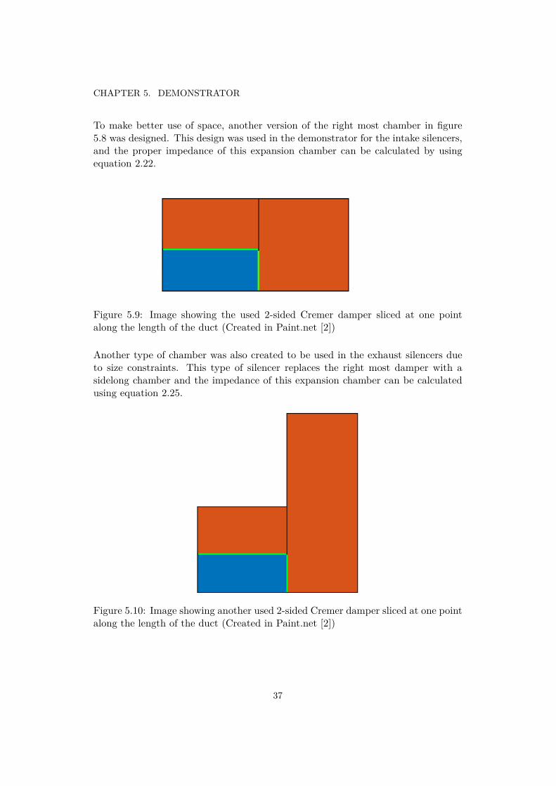
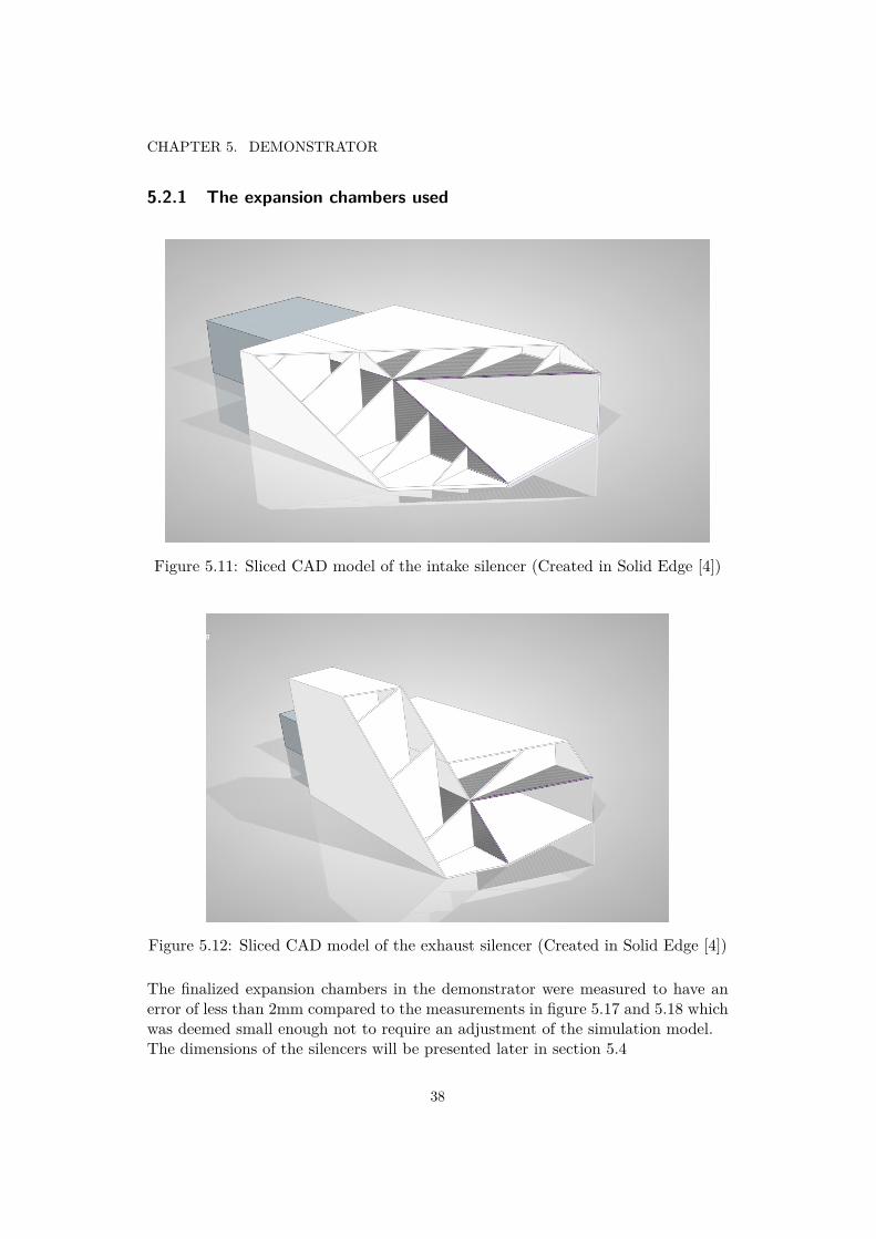
5.2.1 The expansion chambers used

Figure 5.11: Sliced CAD model of the intake silencer (Created in Solid Edge [4])

Figure 5.12: Sliced CAD model of the exhaust silencer (Created in Solid Edge [4])

The finalized expansion chambers in the demonstrator were measured to have anerror of less than 2mm compared to the measurements in figure 5.17 and 5.18 whichwas deemed small enough not to require an adjustment of the simulation model.The dimensions of the silencers will be presented later in section 5.4

38


5.2.2 Validation of expansion chambers usedTo test the method of using a two-sided Cremer damper, a FEM simulation wasperformed using the Acoustic module in COMSOL multiphysics [3]. This simula-tion utilizes the test duct specified in Appendix C, where the ducts and expansionchambers used for the demonstrator was built.The goal of this exercise is to validate the theory that the Cremer damping waveprofile in the x direction is unaffected by the perpendicular wave profile caused bythe other liner wall in the duct in the y direction.

39


Figure 5.13: Comparison between one sided and two sided damper (exported fromCOMSOL multiphysics [3])

As can be seen in figure 5.13 does the total damping match the attenuation curvesof the separate dampers added up until about 1100Hz.Where after this, the resulting attenuation diverges from the result of the individualdampers. The reason for this is believed to be because of first the cut on frequency

40


of the duct and expansion chambers. At 1100Hz half of a wavelength is 15.6cm,which is starting to reach a characteristic length in the cross-section of the duct.A scenario where the high frequency damper of the intake was divided can befound in Appendix D, the result of which lead to the conclusion that the lower thanexpected attenuation of the intake in figure 5.13 is a result of non local wall reaction.

Since the resulting damping did not impact the broadband damping negatively, thiswas however accepted.

Since the formula for calculating the expansion chamber impedance is based uponthe assumption of a local reaction was a simulation verifying that the division ofthe chambers in the axial direction is sufficiently small performed.

Figure 5.14: The sound attenuation from using different division distances (Ex-ported from COMSOL multiphysics [3])

The conclusion drawn from figure 5.14 was that a dividing wall every 50mm realizesthe theory to a sufficient degree. It should however be noted that a non locally re-acting solution as is the 100mm case might prove to give a higher total attenuation,this was however not further explored in this report since it is no longer a solutionbased on the Cremer impedance.

41


5.3 Micro perforated plates

As is discussed in [1] a good practice of optimizing the wall impedance to match theCremer optimum is to firstly choose a duct width (between MPP and other wall)and then change the specification for a micro perforated plate to match the realpart of the Cremer optimum at the target frequency.After this, a chamber behind the wall is created. Since the point impedance ofsuch a chamber would have a purely reactive part, the real part of the total wallimpedance will not be affected by adding the chamber.

If equation 2.22 is rewritten to solve for h the following formula can be used tocalculate the required chamber depth:

hchamber = i

2k ln( bchamber

bduct(ZCremer − ZMPP )− 1

bchamberbduct

(ZCremer − ZMPP ) + 1

)(5.1)

In equation 5.1 the impedance is expressed as the difference between the Cremerimpedance and the MPP impedance. Note that if the MPP is optimized correctlyin the previous step, ZCremer − ZMPP should be purely imaginary.

(The following graphs are received from the code in Appendix A)

42


Figure 5.15: Example graph showing an optimized MPP impedance correspondingto the real part of the Cremer impedance at 1246 Hz

Figure 5.16: Example graph showing an optimized total wall impedance after theexpansion chamber is added corresponding to the Cremer impedance at 1246 Hz

43


5.4 The dimensions and specifications used

To realize the Cremer impedance the Matlab [5] code in appendix A was used. Thecode needs the specifications of the MPP used as well as the distance between theMPP and the opposite wall in the duct.These parameters was then tweaked in order to receive damping maxima at frequen-cies that was desired in the iterative progress of receiving the lowest sound level inthe simulation model detailed in section 4.2, whilst still fulfilling the minimum ductsize requirements from the thermal part of this project [6].The resulting duct dimensions used was 150 mm x 70 mm for the intake and120 mm x 50 mm for each exhaust.

Note that instead of the Cremer impedance specified by Tester [10] as seen inequation 2.6, the following approximate result calculated earlier by Cremer [9] wasused:

Z = (0.91− 0.76i)khπ

(5.2)

This is however believed not to have a significant impact on the broadband dampingproperties of the silencer.

Intake silencer Exhaust silencerLow freq dampertarget frequency 496Hz 401Hz

High freq dampertarget frequency 1384Hz 1246Hz

MPP slit width 0.3mm 0.3mmMPP perforationratio 2% 3%

MPP thickness 1mm 1mm

Table 5.1: Table of the MPP dimensions used and the target frequencies for thesilencers

The sizes and specifications of slit width, thickness and perforation ratios of theAcustimet MPPs needed were requested to be provided by Sontech.

Using equation 5.1 in the Matlab code, the following dimensions was decided upon.These are the dimensions used both in the simulation as well as the demonstrator:

44


Figure 5.17: Drawing of the cross section of the intake duct silencer (Created inPaint.net[2])

Figure 5.18: Drawing of the cross section of the exhaust duct silencer (Created inPaint.net[2])

In figure 5.17 and 5.18 the shallow expansion chamber on the top of the duct arethe high frequency dampers and the larger chambers on the left side are the lowfrequency dampers.

45

Results

6.1 Measurement procedureTo validate the resulting demonstrator, the shroud needs to be measured in order toasses the effectiveness of it. The chosen comparison is to measure the Sound powerlevel before and after the Shroud is applied.This is done by mounting the radio units on only the spine in the shroud lying on astool, whereafter the radio units where mounted in the shroud for the "with shroud"measurement.

46

CHAPTER 6. RESULTS

Figure 6.1: The test object setup without and with the shroud

Since only 2 radio units where available at the time of measurement, the units wheremeasured in a 2+1 configuration. Please observe the following figure:

47

CHAPTER 6. RESULTS

Figure 6.2: The 2+1 configuration

As can be seen in figure 6.2, the first case consists of 2 radios plugged in to the powersupply, for the next case the top radio switches places with the wooden dummy radioseen in figure 6.1 and the bottom radio is unplugged from the power supply.Since the fans of the radios are controlled irrespectively of each other and thesound sources are therefore uncorrelated, the sound power level for a theoreticalmeasurement of 3 radio units can be expressed as:

LW, 3 radio units = 10 ∗ log10(10LW,Case 1/10 + 10LW,Case 2/10) (6.1)

During the measurement of the shroud, a humming noise was discerned coming froma vibrating metal sheet on the bottom of the shroud. From an analysis done usinga simple frequency analyser this was discovered to correspond to the fundamentalrotating frequency of the fans. This discrepancy will appear later on in the resultsection to have an impact on the total shroud noise reduction.Since the airborne sound emanating from the radio carries little energy at this fre-quency as can be seen in figure 3.5 and 3.6, was this believed to be caused by aninstability in the fan causing structural vibrations. These vibrations have a firmlymounted path to travel through the spine of the radio seen in figure 6.1 to thismetal sheet.

48

CHAPTER 6. RESULTS

Figure 6.3: The improvised mitigation for the plate vibrations

This was attempted to be dampened by attaching rubber mats as well as foam onthe plate where by touch the vibrations felt the strongest as can be seen in figure6.3.The added absorption area in the room caused by this mitigation was deemed tobe negligible.

49

CHAPTER 6. RESULTS

6.2 Measurement ResultsThis section aims to display the results gathered from the previous section.In the following graphs has the result from equation 6.1 been calculated for boththe case with the radio mounted on only the spine as can be seen in the top imagein figure 6.1, as well as the case with the radio units mounted in the shroud. TheA-weighted sound power level of 3 radio units without shroud minus the A-weightedsound power level of 3 radio units with shroud is presented here as the attenuation:

Figure 6.4: The reduction of the sound power level for each fan speed for the newCremer based shroud design (Created in Matlab [5])

As can be seen in figure 6.4 is strong attenuation received starting at the 400Hz thirdoctave band, this corresponds to where the silencers was designed to have their lowfrequency attenuation peak. Above the 1250Hz third octave band, the attenuationrises and remains at a level of about 15 dB until the 6300Hz third octave band.Strong amplification at low frequencies was found at 50%, 59% and 60% fan speed,this is believed correspond to the structural vibrations discussed in the previoussection.

50

CHAPTER 6. RESULTS

Figure 6.5: The reduction in A-weighted total sound power level for each fan speed(Created in Matlab [5])

As can be seen in figure 6.5 do the blue curve correspond to the reduction in total A-weighted sound power level from the measurement. It gives an average attenuationof 12.8dB.Since the third octave bands below 200Hz originally carry very little energy as canbe seen in figure 3.5 and 3.6 is the orange curve created. It is meant to represent acase where the structural vibrations are controlled and thus the octave bands below200Hz are set to 0dB for this curve, since they are about 25dB lower in the withoutshroud case than the total A-weighted sound power level and therefore assumednegligible.The average attenuation of this case is 12.9dB with the largest improvement overthe previous case at 59% fan speed, likely corresponding with the strong resonanceat this fan speed seen in figure 6.4.

51

CHAPTER 6. RESULTS

6.3 Simulation ResultsThis section aims to present the results from the simulation performed in chapter4. This is meant to give an answer to if a simulation of the shroud as detailed istrustworthy enough to base conclusions upon.

Figure 6.6: Simulated and measured attenuation in sound power level (Created inMatlab [5])

In figure 6.6 has the mean third octave band reduction in measured sound powerlevel from figure 6.4 been compared to the reduction in sound power level betweenthe simulation of the shroud and a simulation of 3 freely radiating radio units.

As can be seen are the attenuation peaks lower in the measurement curve as wellas has been shifted towards higher frequencies than the simulation curve.

In figure 6.6 the simulation shows an increase in attenuation below 200 Hz. Sincethe radio noise at these frequencies was close to the background noise of the mea-surement, as well as an increase in measurement uncertainties at low frequencies,no conclusion could be made as to whether this behavior was a simulation error ornot.

The normalized third octave band sound power levels of the simulated compared tothe measured shroud are as follows:

52

CHAPTER 6. RESULTS

Figure 6.7: Simulated and measured normalized shroud sound power level for 39%fanspeed (Created in Matlab [5])


53

CHAPTER 6. RESULTS


Note that both the simulated and the measured third octave band sound powerlevels was normalized using the measured total A-weighted sound power level.

54

CHAPTER 6. RESULTS

6.4 Thermal testing results

The following measurements results have been provided by Per Rundström [6] andare more thoroughly detailed in his report.The "without casing" test was performed on a standalone radio unit equipped withheating elements as well as thermal probes. The "with casing" test was performedusing 2 radio units with controlled fan speed as well as a dummy unit mountedin the shroud. One of the radios was equipped with heating elements as well asthermal probes yielding the following results.

Figure 6.10: Temperature difference of radios heatsink with and without casing(Created in Matlab [5])

55

Discussion and Conclusion

7.1 ConclusionThe resulting Shroud does quite noticeably reduce the emitted sound from the radio.The average reduction in A-weighted sound power level is 13 dB, which fulfills thescope of this project of at least 10dB sound power level reduction. The reductionnever falls below this value at any fan speed either.

The temperature of the radio units increased between 2.8◦C to 5.9◦C depending onfan speed.If the temperature is held constant through interpolation, the sound power leveldecreases between 8dB and 10dB depending on fan speed when the shroud is used.

It is therefore the opinion of the author of this report that this technology holdssignificant promise for future development of this type of shroud solution.

7.2 DiscussionThis project is based on a number of assumptions, one of which is; the Mach-numberof the flow is negligible. It has been shown [14] that even at low Mach speeds, theflow can have an impact on the impedance calculation, which would affect the valueof the MPP resistance as well as the Cremer impedance possibly resulting in a non-optimal wall impedance.

Another factor that might have a small impact is that the air in the exhaust duct ina real scenario have an above ambient temperature. Since the acoustic measurementin this project was performed without heating elements was this not considered inthis report.

It was discovered that while the attenuation peaks of the silencers used did notreach the simulated results as well as the attenuation curve was shifted upwards infrequency did they yield strong broadband reduction from the 400Hz third octave

56

CHAPTER 7. DISCUSSION AND CONCLUSION

band and upwards.One theory on why this discrepancy occurred is the seal material in the demon-strator causing some of the micro perforated plate holes to be filled. This wouldhave an impact on the impedance calculation failing to match the exact Cremerimpedance. The lower than expected attenuation peaks might however also be aresult of flanking transmission.

The characterization measurement showed that there was much acoustic energy atthe 5kHz and 6.3kHz octave band. It was however believed that the shroud solutionwould have high frequency reduction due to losses at walls, therefore was this notconsidered in the silencer design. As can be seen in figure 6.4, high frequenciesexhibit a strong level of attenuation.Another reason for the high frequency reduction may be because of the fans radi-ated sound pressure profile exiting more damped duct modes at higher frequenciesthan the simulated case, since the simulation assumed an even pressure source dis-tribution for the fans.

When looking at the simulated results of the shroud verses the measurement (figure6.7, 6.8 and 6.9), while the third octave bands follow roughly the same curve, thereare discrepancies at many frequencies which leads to the conclusion that the simu-lation model as described needs improvement before it can be used for other shroudscenarios for approximating the total sound power level. Since silencers based onCremer impedance show good consistency between measurement and simulationresults [14] is the errors most likely due to other aspects of the simulation model;such as the correlated radio exhausts as well as the simplified space between theradio intake and the intake duct.

7.3 Future workWhile the project described in this report produced a functioning shroud solution,there is always possible improvements that could be made.

Since the theory behind this project only focused on the attenuation of the emittedairborne sound from the radio, was the vibration of the radio units disregarded. Afuture improvement is thus to vibration isolate the spine in the shroud aimed at thefundamental rotation frequency of the fans.

The silencers used in this project were decided to both have a fixed length of 30cmfor balancing attenuation and overall length of the shroud. It was however not in-vestigated to optimise the length of the intake and exhaust silencers separately. Thereason why this may be relevant is because of the somewhat higher sound powerlevel of the intake.

57

CHAPTER 7. DISCUSSION AND CONCLUSION

Secondly, since the intake duct also is larger than the exhaust duct, the Helmholtznumber will be slightly larger. It can be shown that, at a fixed frequency, the Cre-mer impedance attenuation per wavelength decreases when the Helmholtz numberincreases [15].Since it for user cases when the shroud in mounted on a pole or facing away froma wall may be more aesthetically pleasing to have a taller back section than frontmay a longer intake duct silencer be a reasonable solution.

When it comes to the simulation aspect is a more detailed study required. It isbelieved that the largest source of error in the model was the sound source model.It was assumed in section 4.1 that the free field sound power level measured couldbe expressed as plane wave pressure sources. The sound source model also uses thesimplification that the exhausts are correlated. The reason why a non correlatedapproach through superposition of two simulations was not used in this report, isthat for a simulation of 3 radio units, this requires a superposition of 6 simulations,which was deemed too computationally costly. For such a project, it is howeversuggested that for the radio units used, the intake is also split in two halves corre-sponding to each exhaust.

58

Bibliography

[1] R. Kabral, L. Du, M. Åbom, and M. Knutsson, “A compact silencer for thecontrol of compressor noise,” SAE International Journal of Engines, vol. 7,no. 3, pp. 1572–1578, 2014.

[2] dotPDN, “Paint.net.” [Online]. Available: https://www.getpaint.net/

[3] COMSOL AB, “Comsol multiphysics 5.6.” [Online]. Available: https://www.comsol.com/comsol-multiphysics

[4] Siemens, “Solid edge st10.” [Online]. Available: https://solidedge.siemens.com/en/

[5] Mathworks, “Matlab 2018b.” [Online]. Available: https://www.mathworks.com/products/matlab.html

[6] P. Rundström, “Thermal properties of a 5g telecom equipment casing designfor noise suppression,” M. Sc. Eng. thesis, KTH, Tech. Rep., 2021. [Online].Available: http://www.diva-portal.org

[7] H. Wallin, H. Bodén, U. Carlsson, M. Åbom, and R. Glav, Ljud och vibrationer,2017.

[8] S. Sack and M. Åbom, “Modal filters for mitigation of in-duct sound,” Pro-ceedings of Meetings on Acoustics, vol. 29, 2016.

[9] L. Cremer, “Theory regarding the attenuation of sound transmitted by airin a rectangular duct with an absorbing wall, and the maximum attenuationconstant produced during this process,” Acustica, vol. 3, no. supplement 2, pp.249–263, 1953.

[10] B. J. Tester, “The optimization of modal sound attenuation in ducts, in theabsence of mean flow,” Journal of Sound and Vibration, vol. 27, no. 4, pp.477–513, 1973.

[11] Z. Zhang, M. Åbom, and H. Bodén, “The cremer impedance for double-linedrectangular ducts,” International Congress and Exhibition on Noise ControlEngineering, INTER-NOISE 2019 MADRID, vol. 48, 2019.

59

https://www.getpaint.net/

https://www.comsol.com/comsol-multiphysics

https://www.comsol.com/comsol-multiphysics

https://solidedge.siemens.com/en/

https://solidedge.siemens.com/en/

https://www.mathworks.com/products/matlab.html

https://www.mathworks.com/products/matlab.html

http://www.diva-portal.org

BIBLIOGRAPHY

[12] Sontech, “Acustimet.” [Online]. Available: https://www.sontech.se/product-page/acustimet

[13] Y. Guo, S. Allan, and M. Åbom, “Micro-perforated plates for vehicle applica-tions,” 37th International Congress and Exhibition on Noise Control Engineer-ing 2008, vol. 37, no. 2, pp. 773–791, 2008.

[14] Z. Zhang, M. Åbom, H. Tiikoja, and L. Peerlings, “Experimental analysison the ‘exact’ cremer impedance in rectangular ducts,” International StyrianNoise, Vibration Harshness Congress: The European Automotive Noise Con-ference, vol. 10, 2018.

[15] Z. Zhang, M. Åbom, R. Kabral, and B. Nilsson, “Revisiting the cremerimpedance,” Proceedings of meetings on acoustics, vol. 30, 2017.

60

https://www.sontech.se/product-page/acustimet

https://www.sontech.se/product-page/acustimet

Matlab code for Impedance cal-culation

%close all

%−−−−−−−−−−Medium specs (Air)−−−−−−−−−kinv=1.516*10^−5;

dynv=1.825*10^−5;

rho=1.204;

c0=343;

%−−−−−−−−−−−−−−−−−−−−−−−−−−−−−−−−−−−−−%−−−−−−−−−−−MPP specs−−−−−−−−−−t=0.001*1; %Thickness of the MPP

sig=3*0.01; %The perforation ratio

slitw=0.001*0.3; %The slitwidth

%−−−−−−−−−−−−−−−−−−−−−−−−−−−−−−

Zcrem=0.91−0.76i; %The cremer impedance divided by k*h/pi

wid=0.05; %The duct width (from the MPP wall to hard wall)

S2dS1=1; %The relationship between duct height and the height of

the expansion chamber

f=1:20000; %Frequencies used

w=2*pi*f; %Converted into angular frequency

Res=0.5*sqrt(2*rho*w*dynv); %Surface resistance

ks=slitw*sqrt(w/(4*kinv)); %Shear wave number

%Calculate the normalized acoustic resistance:

rspr=real((1i*w*t/(sig*c0))./(1−tanh(ks*sqrt(1i))./(ks*sqrt(1i))))+4*Res/(sig*rho*c0);

61

APPENDIX A. MATLAB CODE FOR IMPEDANCE CALCULATION

%Check at which frequency the acoustic resistance match the real part

of the cremer impedance:

[imr,frq]=min(abs(rspr−(real(Zcrem)*w*wid/pi/c0)))

%Calculate the normalized acoustic reactance at this frequency:

xspr=imag((1i*2*pi*frq*t/(sig*c0))./(1−tanh(ks(frq)*sqrt(1i))./(ks(frq

)*sqrt(1i))));

imagimp=xspr; %The acoustic reactance caused by the MPP wall

targimp=Zcrem*2*pi*frq*wid/pi/c0; %The imaginary part of the Cremer

impedance

% Calculate the needed depth of an expansion chamber for the wall+

chamber reactance to match the imaginary part of the Cremer

impendace:

h=(1i/(2*2*pi*frq/c0))*log((S2dS1*(imag(targimp)−imagimp)*1i−1)/(1+S2dS1*(imag(targimp)−imagimp)*1i))

%Calculate MPP resistance (redundant) and the reactance for all

frequencies:

rs=real((1i*w*t/(sig*c0))./(1−tanh(ks*sqrt(1i))./(ks*sqrt(1i))))+4*Res

/(sig*rho*c0);

xs=imag((1i*w*t/(sig*c0))./(1−tanh(ks*sqrt(1i))./(ks*sqrt(1i))));

Zmpp=rs+1i*xs; %The total impendance of the MPP

%The impedance caused by the expansion chamber (purely imaginary):

Z=1/S2dS1*(1+exp(−2*1i*w*h/c0))./(1−exp(−2*1i*w*h/c0));

Ztot=Z+Zmpp; %Total wall impedance;

alf=1−abs((Ztot−1)./(Ztot+1)).^2; %Absorbtion coefficient

62

APPENDIX A. MATLAB CODE FOR IMPEDANCE CALCULATION

%%

%−−−−Plot of the Real and Imaginary part of the MPP impedance−−−figure

plot(f,rs)

hold on

plot(f,xs)

plot(f,real(Zcrem*w*wid/pi/c0))

plot(f,imag(Zcrem*w*wid/pi/c0))

axis([−inf 2000 −1 1])

xline(frq,'green')

plot(frq,rs(frq),'.','MarkerSize',20,'color','green')

xlabel('Frequency (Hz)')

ylabel('Normalized impedance (Z/Z0)')

grid on

grid minor

legend({'MPP resistance','MPP reactance','Real part of Cremer

impedance','Imaginary part of Cremer impedance'},'location','

southwest')

%−−−−−−−−−−−−−−−−−−−−−−−−−−−−−−−−−−−−−−−−−−−−−−−−−−−−−−−−−−−−−−−−−−

%−−−−−−−−Plot of the Imnpedance curves of the Wall+expansion chamber

and the Cremer impedance−−−−−−−

figure

plot(f,real(Ztot))

hold on

plot(f,imag(Ztot))

plot(f,real(Zcrem*w*wid/pi/c0))

plot(f,imag(Zcrem*w*wid/pi/c0))

xline(frq,'green')

plot(frq,real(Ztot(frq)),'.','MarkerSize',20,'color','green')

plot(frq,imag(Ztot(frq)),'.','MarkerSize',20,'color','green')

axis([−inf 2000 −1 1])

grid on

grid minor

xlabel('Frequency (Hz)')

ylabel('Normalized impedance (Z/Z0)')

legend({'Total wall resistance','Total wall reactance','Real part of

Cremer impedance','Imaginary part of Cremer impedance'},'location',

'southwest')

%−−−−−−−−−−−−−−−−−−−−−−−−−

63

Expansion chamber correction fac-tor

A simulated model of a 2-mic impedance measurement, the blue line is a vibratingsurface and the rightmost wall is reflection free. The two lines in the middle-leftpart of the figure is where the pressure measurement points (here average over lines)are.

The parameters are: chamber height=0.15m, chamber width=0.057m and ductheight=0.05m

k=2*pi*400/343; % Wave number for the excited frequency

d=0.1; % Length between pressure points

L=0.143; % Length from the leftmost pressure point to the

entrance of the expansion chamber

pm=(p2*exp(1i*k*L)−p1*exp(1i*k*(d+L)))/(−exp(1i*k*d)+exp(−1i*k*d)) % Reflected wave at the entrance point

pp=p1*exp(−1i*k*L)−pm*exp(−2i*k*L) % Incoming wave at the

entrance point

Zn=1i*imag((pp+pm)/(pp−pm)) % The normalized impedance at the

entrance

h=log((1+Zn*5.7/5)/(Zn*5.7/5−1))/(i*k*2) % the length is

calculated from the impedance

64

Test duct

Figure C.1: Images showing the test duct used (Exported from COMSOL multi-physics [3])

The top image show the source surface, set as a velocity source. The bottom imageshow the two surfaces used as the 2 points from which the attenuation is receivedby using the difference in mean sound pressure level.

65

Non local reaction test

Figure D.1: Images showing the inserted hard wall divider in the high frequencydamper as well as the result (Exported from COMSOL multiphysics [3])

66

Ducts used

Figure E.1: CAD from [6] showing one of the exhaust ducts with silencers (Left)and the intake duct with silencers (Right)

67

APPENDIX E. DUCTS USED

Figure E.2: CAD from [6] showing the intake and the exhausts as they are mountedinside the shroud

68

TRITA -SCI-GRU 2021:163

www.kth.se

Acoustic properties of a 5G Telecom Equipment Shroud ...

Documents

Transcript of Acoustic properties of a 5G Telecom Equipment Shroud ...