J. Appl. Phys. 129, 171103 (2021); https://doi.org/10.1063/5.0046878 129, 171103

© 2021 Author(s).

Acoustic metamaterials

Cite as: J. Appl. Phys. 129, 171103 (2021); https://doi.org/10.1063/5.0046878Submitted: 08 February 2021 . Accepted: 12 April 2021 . Published Online: 05 May 2021

Jensen Li, Xinhua Wen, and Ping Sheng

COLLECTIONS

This paper was selected as an Editor’s Pick

Acoustic metamaterials

Cite as: J. Appl. Phys. 129, 171103 (2021); doi: 10.1063/5.0046878

View Online Export Citation CrossMarkSubmitted: 8 February 2021 · Accepted: 12 April 2021 ·Published Online: 5 May 2021

Jensen Li,a) Xinhua Wen, and Ping Shengb)

AFFILIATIONS

Department of Physics, HKUST, Clear Water Bay, Kowloon, Hong Kong, China

a)Email: jensenli@ust.hkb)Author to whom correspondence should be addressed: sheng@ust.hk

ABSTRACT

Waves are generally characterized by angular frequency ω and wavevector k. Accordingly, this tutorial is structured into two parts,one on resonance-based acoustic metamaterials, in the frequency domain, and one on topological acoustics, based on the wavevectordomain as topological structures inherently involve spatial configurations that are a step beyond the simple periodic lattices. Eachpart will begin with a brief introduction of the basic principles, followed by two examples described in detail. In the first part, wepresent decorated membrane resonators and the broadband optimal acoustic absorption structures, the latter being crucial for thepotential applications of acoustic metamaterials. In the second part, we discuss how to construct the Dirac cone, a special type ofdispersion from either accidental degeneracy or symmetry protection, which can be shown to lead to negative, zero, or positiverefractive indices. The shifting and gapping of these Dirac cones in the reciprocal space can result in effects on acoustic wavessimilar to that of a magnetic field on an electron. More generally, they lead to edge states resulting from a real-space gauge field aswell as topological bandgaps.

Published under an exclusive license by AIP Publishing. https://doi.org/10.1063/5.0046878

I. INTRODUCTION

Acoustic waves in air satisfy the scalar wave equation

1v2

@2p(t, x)@t2

� ∇2p(t, x) ¼ 0, (1)

where v denotes the wave speed, which has the value v0 ¼ ffiffiffiffiffiffiffiffiffiffiffiffiffiγP0/ρ0

p¼ 340m/s in air, where P0 ¼ 1:01� 105 Pa is the atmosphericpressure, ρ0 ¼ 1:21 kg/m3 is the air density, and γ ¼ 1:4 is the adi-abatic index of air. In Eq. (1), p ¼ P � P0 represents the pressuremodulation of sound, where P is the instantaneous pressure.Solution to Eq. (1) has the general functional form p(ωt + k � x)with the dispersion relation

jkj2 ¼ k2 ¼ ω2

v2, (2)

as can be easily verified through differentiation. Among all the possi-ble wave functional forms, the plane wave exp[�i(ωt + k � x)] is themost common. To supplement Eqs. (1) and (2), we also haveNewton’s law that relates the pressure modulation and displacement(particle) velocity u ¼ @ξ/@t, where ξ denotes the air displacement ofthe sound wave,

�∇p ¼ ρ0@u@t

, (3)

and the continuity equation

@ρ

@tþ ρ0∇ � u ¼ 0, (4)

where ρ denotes the instantaneous density. In what follows, we willtreat those cases in which the metamaterial sample has a planar inter-face with air. Hence, we will regard both the displacement and dis-placement velocity as complex scalar quantities, ξ and u, thatrepresent the components of the two vectors normal to the interface.

The ω and k characterization of the acoustic waves foreshad-ows the development of acoustic metamaterials, initially in therealm of resonance-based structures that can display sample charac-teristics such as the subwavelength sample size, together with theirwave manipulation characteristics not found in naturally occurringmaterials. More recently, the advent of topological quantum phe-nomena has propelled a new direction based on novel spatial struc-tures, i.e., in the wavevector domain, that have topological featuresdistinct from the periodic structures. This tutorial is accordinglydivided into two sections, each with two examples. For the

Journal ofApplied Physics TUTORIAL scitation.org/journal/jap

J. Appl. Phys. 129, 171103 (2021); doi: 10.1063/5.0046878 129, 171103-1

Published under an exclusive license by AIP Publishing.

resonance-based acoustic metamaterials,1–17 membrane-typeacoustic metamaterials will be used as the first example since itinvolves several general concepts that can be applied in manyother contexts. The second example is the optimal acousticabsorption structure, which can display tunable absorptionspectrum over arbitrarily broad frequency band and therebyeliminates one of the major drawbacks of metamaterials forpotential applications. For the second part, we will discuss pho-nonic crystals in the diffraction regime, which can be utilizedto make special types of dispersions, such as negative andzero indices as the first example. It is related to Dirac cone dis-persion from an accidental degeneracy. In the second example,we will move to another type of Dirac cone dispersion enabledby symmetry protection—by lowering spatial or lattice symme-tries to induce gauge field or topological bandgap in whichquantum-Hall-like edge states or topological one-way edgestates can be realized and observed. These principles do not relyon resonance and are generic to both acoustic and elastic wavesin solid. Rather than trying to cover a broad swath of thisgrowing field, our intention here is to use examples to elucidatethe basic concepts underlying the acoustic metamaterials, hope-fully to lay the groundwork for the readers to further explorethis rapidly evolving area.

II. RESONANCE-BASED METAMATERIALS

Resonance-based metamaterials can manipulate waves with sub-wavelength sample sizes, in contrast to phononic crystals whose wavecharacteristics are only apparent when sample’s structural periodicityis comparable to the relevant wavelength. In this section, we detailtwo examples with emphasis on explaining the relevant conceptstogether with the pertinent mathematics involved.

A. Preliminaries

In an acoustically resonant system with resonance frequencyΩ, the magnitude of displacement response ξ(ω) of the system to apressure modulation p(ω) has the general form

ξ ¼ p(A/m)

Ω2 � ω2 � iβω, (5)

where p is the actual pressure on the sample that includes the pres-sure from both the incident and reflected waves, A and m denotethe relevant area and inertial mass of the resonator, respectively,and β is a dissipation coefficient in units of frequency. The Greenfunction is defined as

G ¼ ξ

p¼ A

m1

Ω2 � ω2 � iβω

� �: (6)

The quantity in the bracket has the functional form denotedas a “Lorentzian,” which characterizes almost all the resonances. Inacoustics, an important parameter is the impedance,

Z ¼ pu¼ p

�iωξ¼ 1

�iωG: (7)

For a plane wave in air, Z0 ¼ ρ0v0. The real part of the Green func-tion is non-dissipative; its dissipative imaginary part correspondsto the real part of impedance. Equation (7) is generally true forsamples with subwavelength lateral dimensions so that diffractionis not a concern. The inverse relationship between the Greenfunction and impedance is especially convenient for evaluatingthe impedance of resonance-based metamaterials since the Greenfunction can always be written as the sum of Lorentzians for reso-nators with different resonance frequencies, which can always beobtained, in conjunction with the eigenfunction configurations,either analytically or through numerical simulations for resona-tors with complex geometries.

We note here some special properties of the Lorentzian that canbe useful for later developments. In the limit of vanishing β, we have

limβ!0

1

Ω2 � ω2 � iβω

� �¼ P

1

Ω2 � ω2þ i

π

2ωδ(Ω� ω), (8)

where P denotes taking the principal value of the quantity thatfollows. It might appear puzzling why there can be an imaginarypart, which represents dissipation, even when the dissipation coeffi-cient β is zero. The reason is that as β diminishes, the resonancepeak becomes sharper, implying an increasing Q factor of the reso-nator. As Q approaches infinity, the lifetime of the resonance alsoapproaches infinity; hence even with an infinitesimal dissipationcoefficient there can be finite dissipation over an infinite duration.This is the meaning of the delta function imaginary part, which canalso be regarded as the density of resonant mode per unit frequency,localized at Ω.

B. Decorated membrane resonator

A decorated membrane resonator (DMR) consists of a thinpolymeric membrane, such as Latex, slightly stretched over afixed boundary with one or multiple pieces of solid weight gluedon top.6 The solid piece(s) can be in different shapes. Here, weconsider the simplest case of a circular membrane with a circularweight in the center. Such a resonator can have multiple resonan-ces; here we will be concerned with only the two lowest frequencyresonance eigenmodes whose profiles, ξ1(2)(xjj), are depictedschematically in Fig. 1. Here, xjj denotes the coordinate in theplane of the membrane, whereas the displacement ξ is normal tothe plane as noted earlier and generally much smaller than thewavelength. The resonance frequencies of the DMR can be espe-cially low, because the restoring force of the membrane is weak.Hence, the relevant wavelength can be order(s) of magnitudelarger than the size of the DMR.

A resonator can be classified to have a dipolar symmetry if itsresonance involves center of mass motion. DMR is a dipolar reso-nator. In contrast, Helmholtz resonator5 is monopolar in symmetrysince at its resonances involves no center of mass movement.

1. Anti-resonance and the effective dynamicmass density

If we denote Ω1 and Ω2 as the two lowest resonance frequenciesof a DMR, then the sample area-averaged displacement response canbe written as

Journal ofApplied Physics TUTORIAL scitation.org/journal/jap

J. Appl. Phys. 129, 171103 (2021); doi: 10.1063/5.0046878 129, 171103-2

Published under an exclusive license by AIP Publishing.

ξ(ω)h i ¼ α1

Ω21 � ω2 � iβ1ω

þ α2

Ω22 � ω2 � iβ2ω

(9)

by neglecting the higher order resonant modes. Here, α1,2 are positiveconstants and the angular brackets hi denote area averaging. For anincident acoustic wave with frequency ω that is intermediate betweenΩ1 and Ω2 the first term on the right-hand side of Eq. (9) is negativein its real part, whereas the second term is positive. The net behavioris illustrated in Fig. 2. It is inevitable that there is always a pointwhere Rehξ(ω)i vanishes, denoting the anti-resonance frequency. Ifwe define a dynamic mass density1–3,7–9 as

ρd ¼fh i

�ω2Re ξh i , (10)

where fh i denotes the area averaged force density, and the denomi-nator is recognized to be the area-averaged acceleration. The behaviorof ρd is also illustrated in Fig. 2, which is seen to display a nearlydivergent behavior followed by a negative dynamic mass densityregion in which the acceleration is opposite to the force.

Can the divergence of the dynamic mass density have a realeffect, in the sense of exhibiting consequences that imitate theeffect of a large mass at the anti-resonance frequency? We showbelow that indeed, the dynamic mass density effect is real.

2. Coupling with propagating waves and evanescentwaves—Total reflection at anti-resonance

Anti-resonance is associated with a special wave manipula-tion functionality of DMR.6 To understand this functionality, wehave to examine DMR’s coupling to the incident and reflectedwaves. The basis of this consideration is a propagating wave’s dis-persion relation

k2 ¼ jkjjj2 þ k2? ¼ ω2

v20¼ 2π

λ

� �2

, (11)

where λ denotes the wavelength in air, and subscripts || and ?denote wavevector’s components parallel and perpendicular toDMR’s surface, respectively. The basis of our considerations isthat the lateral dimension d of the DMR is subwavelength, i.e.,d � λ. For the resonance mode profiles depicted in Fig. 1, if weFourier transform the two-dimensional mode profile to the trans-verse wavevector domain, then it is clear that except for one com-ponent of the transverse wavevector component that will beselected out for special note below, the other components mustsatisfy the inequality

jkjjj . 2πd

� 2πλ, (12)

because all the lateral features of the resonance profile are smallerthan d, and displacement is continuous across the membrane/airinterface. That means in order to satisfy Eq. (11), the associated k?must be purely imaginary, i.e., decaying away from the DMR surfaceexponentially and hence decoupled from the propagating waves. Theone exception is the jkjjj ¼ 0 component associated with the centerof mass motion. Since jkjjj ¼ 0 delineates a mode in which thewhole DMR moves up and down in unison, we denote such a modeas the “piston mode.” Hence for the DMR with subwavelengthlateral dimensions, only the piston mode couples to the propagatingmodes since in that case we have k? ¼ k ¼ 2π/λ.

Because at anti-resonance ξh i ¼ 0, there is no piston mode andhence the DMR is decoupled from the propagating mode, i.e., it actslike a rigid wall and can totally reflect the acoustic wave at this fre-quency even though the DMR is a flimsy membrane. This effect hasbeen experimentally demonstrated5 as well as numerically simulatedas shown in Fig. 3.

The total reflection behavior is consistent with the divergenceof dynamic mass density as required by Eq. (10), i.e., at anti-resonance the DMR seems to acquire a very large mass density. Inaccordance to the mass density law, the transmission amplitude T

FIG. 2. An illustration of the displacement plotted as a function of frequency forthe DMR. At a frequency intermediate between the two resonance frequencies,there is a point at which the displacement is zero. That point is denoted the anti-resonance frequency. The dynamic mass density as defined by Eq. (10) isplotted as the solid red line.

FIG. 1. A schematic illustration of the lowest frequency eigenmode, in blue color,and the second lowest frequency eigenmode, in red color, for the decoratedmembrane resonator (DMR). The rectangle indicates the solid platelet. Here xdenotes the coordinate axis in middle of the DMR’s plane, and ξ1,2 denotes thedisplacement normal to the plane for the two eigenmodes. Adapted from Ref. 13.

Journal ofApplied Physics TUTORIAL scitation.org/journal/jap

J. Appl. Phys. 129, 171103 (2021); doi: 10.1063/5.0046878 129, 171103-3

Published under an exclusive license by AIP Publishing.

of an acoustic wave through a solid wall with mass density ρ andthickness h is given by

T ¼ i2Z0

ωρh, (13)

independent of solid wall’s bulk modulus. Hence, DMR’s near-totalreflection at anti-resonance is in agreement with the mass densitylaw, by replacing the static mass density by the dynamic massdensity in Eq. (13). Another manifestation of the large dynamicmass density at anti-resonance is the use of a very light-weightDMR in being able to successfully suppress vibration that is tunedto the antiresonance frequency.4 As to the negative dynamic massdensity, its effect was demonstrated in the first publication onlocally resonant sonic materials.1–3,7

3. Acoustic absorption by DMR and its upper bound

Polymeric membranes usually have a low dissipation coeffi-cient. However, absorption per unit volume is the product ofenergy density multiplied by the dissipation coefficient. In acousticmetamaterials, high absorption relies on a high energy density asthe result of resonance, rather than the magnitude of the dissipa-tion coefficient. In fact, a large dissipation coefficient can causeimpedance mismatch with air, leading to increased reflection andreduced absorption as a result. In this context, a low dissipationcoefficient may offer an advantage if properly utilized.

For the DMR, the largest energy density at resonance islocated at the perimeter(s) of the solid mass, where there is a kinkin the mode profile due to the large rigidity contrast between thesolid and the membrane, as seen in Fig. 1. In this case, there can bea very large curvature energy density, localized at the perimeter(s),that is proportional to the square of the second derivative along thelateral direction, i.e., ε/ (∇2

jjξ)2. Since a kink implies a discontinu-

ity in the first derivative, the second derivative would resemble a

delta function. The delta function can be integrated to a finitevalue, but the square of the delta function implies a very largevalue even when integrated. A detailed finite element simulationhas indeed confirmed this fact.11 Hence, significant acousticabsorption by the DMR occurs at resonances through the curvatureenergy density enhancement by the resonant mode profile.

While the absorption by DMR can be significant, there existsan upper bound owing to the thin membrane thickness.12 In orderto see the inevitability of such a bound, let us consider two counter-propagating incoming waves incident from two sides on the DMRwith pressure modulation amplitudes pi� and piþ. Upon reflection,they are converted into two outgoing waves with the relevant ampli-tudes po� and poþ. The subscripts – and + denote the left- and right-hand side regions, respectively, and superscripts i and o stand forincoming and outgoing waves, respectively. In Fig. 4, we illustratethis incident and scattering configuration. At the surface of theDMR, the net pressure modulation is the sum of the incoming andoutgoing pressure modulations. The time-averaged acoustic energyflux in air is given by pu/2 ¼ +p2/(2Z0), opposite in direction forthe incident and outgoing waves. Owing to the small thickness ofthe membrane, we must have u�h i ¼ uþh i, i.e., the membranethickness does not change since the membrane’s thickness-varyingresonance has a much higher frequency and, therefore, “frozen” inthe relevant low frequency regime. As only the piston mode couplesto the propagating waves and the displacement velocity is continuousbetween the coupling mode and air, we must have

u�h i ¼ pi� � po�Z0

¼ poþ � piþZ0

¼ uþh i: (14)

As a note on the side, for a stationary solid boundary pi� ¼ po�so that the displacement velocity has a node, such as the case atanti-resonance. The total pressure on the solid boundary, on theother hand, is given by pi� þ po�. Hence, for a stationary wall thepressure exerted on the boundary is twice that of the incident wave.

4. Conservation law in analogy to momentumconservation

Equation (14) leads directly to the conservation law for themean pressure modulation �p,12

�p ¼ 12(piþ þ pi�) ¼

12(poþ þ po�): (15)

FIG. 3. Results of a full-waveform simulation on the DMR, with transmissioncoefficient shown as the black solid line. Full transmission is seen at the tworesonances, with near-zero transmission at anti-resonance. The divergence ofthe dynamic mass density at anti-resonance is shown by solid red circles, asevaluated from Eq. (10) using simulated values for ξ. Adapted from Ref. 8.

FIG. 4. An illustration of the incoming and outgoing acoustic waves on the twosides of the DMR, in terms of the pressure modulation. Here k0 ¼ ω/v0.

Journal ofApplied Physics TUTORIAL scitation.org/journal/jap

J. Appl. Phys. 129, 171103 (2021); doi: 10.1063/5.0046878 129, 171103-4

Published under an exclusive license by AIP Publishing.

Equation (15) is completely similar to the momentum conser-vation law before and after the collision between two identical par-ticles. Here, we treat pi(o)þ(�) as complex numbers, or phasors, i.e., 2Dvectors in the complex plane. The analog to the kinetic energy isthe energy flux p2/(2Z0).

It follows from analogy to classical mechanics that a wave inci-dent from one side is just like the collision between a moving particleand a stationary one, with equal mass. In that case, half of the inci-dent kinetic energy is the conserved center of mass energy and,therefore, not available for dissipation. Hence, the upper bound forDMR dissipation is 50%.

5. Hybrid structure and total absorption

From the simple argument that leads to the absorption upperbound for incidence from one side, it also becomes clear that if thereare incident waves from both sides of the membrane, then 100%absorption is entirely possible. However, even if we have incidenceonly from one side, it is still possible to have backscattered wave froma reflecting surface on the other side. Hybrid resonance is the resultof such considerations when the reflecting surface is placed in thenear-field region (i.e., at a very subwavelength distance) to the DMRso that the resonance pattern of the DMR is altered as well.13 InFig. 5(a), we show such a configuration, denoted the hybrid structure,in which the DMR is subject to incident and scattered waves on theright, piþ and poþ, as well as similar waves on the left, pi� and po�.However, the two waves on the right are subject to the reflectingboundary condition imposed by the hard wall placed at a distance saway from the DMR. Due to the hard wall boundary condition, thedisplacement velocity must have a node at the reflecting boundary.That means at the position of the DMR, the two waves on the rightmust have equal amplitude, i.e., jpiþj ¼ jpoþj, with a phase differencepiþ/p

oþ ¼ 2δ ¼ 2k0s, where k0 ¼ ω/v0. The phase of poþ can be taken

to be zero as the reference.

6. Imposition of the no-reflection condition

We wish to see if it is possible to achieve total absorption bythe hybrid structure. Total absorption implies po� ¼ 0. Hence from

Eq. (15), we have

pi� ¼ poþ � piþ, (16)

which can be represented by a phasor diagram as shown inFig. 5(b) in which Eq. (16) is regarded as a two-dimensional vectorequation in the complex plane, forming a closed triangle. Here, thephase is treated as giving the relative angle(s) between the vectors.

The net area-averaged pressure on the DMR is given by thedifference between the two sides of the DMR: ptoth i ¼ pi��(poþ þ piþ). From Fig. 5(b), it is clear that poþ þ piþ ¼ ipi�cotδ.Hence, ptoth i ¼ pi�(1� icotδ), and it follows that with the imped-ance condition imposed by po� ¼ 0, i.e., no reflection, the DMRimpedance for total absorption needs to be

ZDMR ¼ ptoth iu

¼ pi�u

(1� icotδ) ¼ Z0(1� icotδ): (17)

At the same time, we recognize that the impedance at the+side of the DMR, representative of the air cavity impedance that isin series with the DMR impedance, is precisely given by

Zcav ¼poþ þ piþ

u¼ iZ0cotδ: (18)

When δ ! 0, Zcav ! i1 in agreement with that of a hard reflect-ing wall. It follows from Eqs. (17) and (18) that the total impedanceof the hybrid structure is given by

Zhybrid ¼ ZDMR þ Zcav ¼ Z0: (19)

Since the reflection coefficient at normal incidence is given by

R ¼ Z � Z0

Z þ Z0, (20)

hence consistency is achieved with the imposed no-reflection con-dition. We also note that from energy conservation the absorptionis given by A ¼ 1� jRj2 when there is no transmission, it followsthat Z ¼ Z0 implies total absorption.

7. Emergence of hybrid resonance

A special situation occurs at δ ¼ (2nþ 1)π/2, with n = 0,1,…,or s ¼ (2nþ 1)λ/4. This is the “drum resonance” condition.However, if the reflecting wall is very close to the DMR, then itmay seem impossible for total absorption to occur, unless DMRcan exhibit an impedance that has a very large negative imaginarypart. It turns out that precisely such an impedance can occur forthe DMR at a frequency that is slightly less than the anti-resonancefrequency. Just to make this point intuitively obvious, we note thatfrom Eqs. (7) and (10), near the anti-resonance the impedance ofthe DMR can be expressed as

ZDMR /�iωρd , (21)

apart from some constants. Since the dynamic mass density at fre-quencies less than the anti-resonance frequency can be very large

FIG. 5. (a) A pictorial illustration of the hybrid resonator structure. (b) A phasordiagram that illustrates Eq. (16) geometrically. Figure (a) adapted from Ref. 13.

Journal ofApplied Physics TUTORIAL scitation.org/journal/jap

J. Appl. Phys. 129, 171103 (2021); doi: 10.1063/5.0046878 129, 171103-5

Published under an exclusive license by AIP Publishing.

and positive, it follows that the condition imposed by the totalabsorption may indeed be realized close to the anti-resonance fre-quency. Such total absorption can be realized with significantlysubwavelength sample thickness, thereby realizing the advantage ofresonance-type acoustic metamaterials.

What is special and somewhat anti-intuitive about the hybridresonance, is that there can be large membrane displacement evenwhen the membrane is placed very close to a hard reflecting wall,which is always associated with a displacement velocity node. Atlow frequencies, any significant displacement velocity has to be atleast a quarter of a wavelength away from the hard boundary,hence intuition would tell us that a membrane placed very close toa hard wall should have no displacement velocity at low frequen-cies. This intuition turns out to be wrong when the membrane hasmultiple resonance modes, with anti-resonances in-between anytwo resonances.

8. Mathematics of the hybrid mode

In a hybrid structure, the vibration modes of the DMR arealtered in a manner such that the original modes are replaced bythe hybrid resonances.13 To see how the hybrid resonance actuallyemerge, we recall that the Green function can be expanded interms of the eigenfunctions of the system. In the vicinity of theanti-resonance the Green function can be expressed as the sum oftwo Lorentzians,

Gh i ¼Xn¼1,2

j ξnh ij2mn(Ω2

n � ω2 � iβnω), (22)

where ξn(xjj) denotes the displacement profile of the nth eigen-function,

mn ¼ 1

jξnj2� � ð

A

ρa(xjj)jξn(xjj)j2dxjj: (23)

Here A denotes the area of the membrane, and ρa(xjj) is thearea mass density, i.e., mass per unit area as a function of theplanar coordinate. Consider the case where β1,2/ω ,, 1 in the rel-evant frequency range, and for simplicity let β1 ¼ β2. Then we canexpand Eq. (22) as

Gh i ¼Xn¼1,2

j ξnh ij2mn(Ω2

n � ω2)þ 2iβ

Xn¼1,2

j ξnh ij2ωmn(Ω2

n � ω2)2: (24)

This expansion is to facilitate the consideration that at theanti-resonance frequency ~ω, Re Gh i ¼ 0. If we express the hybridresonance frequency to be at ω ¼ ~ω� Δω, where Δω/~ω � 1, then

Gh i ffi 2Ξ(iβ � Δω), (25)

where

Ξ ¼Xn¼1,2

j ξnh ij2~ωmn(Ω2

n � ~ω2)2: (26)

From Eq. (7), we obtain from Eq. (25)

Z ¼ 12βΞ

β � iΔω

β2 þ Δω2: (27)

If β ! 0, then the impedance diverges toward negative infinitywhen Δω ! 0. What we want, however, is for the real and imagi-nary parts of Eq. (27) to agree with those of Eq. (17),

Z0 ¼ 12βΞ

β

β2 þ Δω2, (28a)

Z0cotδ ¼ 12βΞ

Δω

β2 þ Δω2: (28b)

These two conditions can certainly be satisfied since there arethree adjustable parameters: β, Δω, and δ. Since β is a materialparameter set by the material used, usually the tuning is carried outby adjusting the other two.

9. Profile of the hybrid resonance mode

At anti-resonance frequency we have the conditionRe ξ1h i þ ξ2h i½ � ¼ 0. Since the hybrid resonance frequency is onlyslightly less than ~ω, at the hybrid resonance we must haveξ1h ij j . ξ2h ij j but ξ2h ij j/ ξ1h ij j 1. If in addition we impose the

condition that the hybrid resonance’s piston component amplitudemust match that of the incident wave, ξs, in order to achieve imped-ance matching, then the following condition should hold:

ξhh ij jξ1h ij j ¼ 1� ξ2h ij j

ξ1h ij j ¼ξsξ1h ij j : (29)

As the right-hand side of Eq. (29) is a small number, itfollows that ξ1h ij j, ξ2h ij j � ξhh ij j, the piston mode amplitude ofthe hybrid mode. The implication is that the evanescent compo-nent of the hybrid resonance has a much larger displacementamplitude than that of the piston mode. In other words, for thehybrid resonance the variance of the displacement can be very large,

i.e., jξhj2� �� ξhh ij j2� �1/2� ξhh ij j. This has indeed been verified

experimentally as seen in Fig. 6(a), together with the total absorptionat hybrid resonance frequency of 152Hz as shown in Fig. 6(b), bothin excellent agreement with the theory simulation predictions.13

In the experiment, the sample thickness is noted to be more thantwo orders of magnitude smaller than the wavelength at 152Hz, 2.3m.

C. Broadband optimal acoustic absorption structures

Resonance is inherently a dispersive, narrow frequency-widtheffect. In considering the practical applications of resonance-typeacoustic metamaterials, this feature is a drawback since for mostapplications broadband functionality is a necessity. Therefore, how toachieve broadband functionality by integrating resonators with differ-ent resonance frequencies is a crucial concern for the development ofacoustic metamaterials into useful products. Associated with thisissue is the question whether acoustic metamaterials can still retain itsadvantage of subwavelength sample size in the broadband regime.We will see in this section that in regard to broadband acoustic

Journal ofApplied Physics TUTORIAL scitation.org/journal/jap

J. Appl. Phys. 129, 171103 (2021); doi: 10.1063/5.0046878 129, 171103-6

Published under an exclusive license by AIP Publishing.

absorption functionality, the definition of metamaterial’s advantage,as compared to the conventional absorption materials, is altered fromthe previous “subwavelength sample size.” We elaborate below.

Noise absorption is one of the most important applicationareas for acoustic metamaterials.16 A thick-enough conventionalacoustic absorbing materials, such as those used in anechoicchambers, can absorb acoustic waves of all frequencies; but thebulky unwieldiness limits their broad applications. In this regardan optimally integrated acoustic resonator structure can displaythe advantage of being able to target the spectrum range of peaknoise, with a minimum sample thickness allowed by a law ofnature—the causality constraint on minimum sample thicknessassociated with a given absorption spectrum.

1. Causality constraint on minimum sample thickness

Reflection and transmission of an incident wave are denotedthe sample response to an incident wave. Since the incident wavevaries as a function of time, the sample response will similarlyacquire a time dependence. Causality is defined to mean that theresponse at any given moment can only depend on what transpiredprior to that moment, but not on anything that happens after thatmoment, i.e., the future cannot affect what is happening now. Whentranslated into mathematical language, this simple and intuitive state-ment led to some marvellous results. The most famous one is theKramers–Kronig relation, taught in almost all the standard electrody-namics textbooks, that relates the real and imaginary parts of theelectromagnetic dielectric constant in the frequency domain. A less-known consequence is the inequality constraint that relates theabsorption spectrum to a minimum sample thickness. Since its deri-vation can be found in the literature14 and is beyond the scope ofthis tutorial, we just state it below as a simple inequality,

d 14π2

Beff

B0

ð10ln[1� A(λ)]dλ

¼ dmin, (30)

where d is the sample thickness, A(λ) is the absorption spectrum, Beff

denotes the effective bulk modulus of the sound absorbing structurein the static limit, and B0 is the bulk modulus of air. Two implica-tions of Eq. (30) are (a) low frequency absorption inherently requiresa larger sample thickness as compared to absorption at higher fre-quencies, and (b) any given absorption spectrum is associated with aminimum sample thickness. We denote “optimal” those absorptionstructures or materials that can nearly attain equality with dmin.

The causality constraint serves as the reference for judging the“degree of success” of a broadband absorption material/structure. Italso tells us that for a given sample thickness, there is only a finiteamount of wave absorption resources available. Hence how toallocate the absorption resources, in the form of an absorptionspectrum, is an issue of importance. If the aim is to absorb noise,then the best allocation strategy is naturally to match the absorp-tion spectrum with the noise spectrum. The freedom offered by anintegrated array of acoustic resonators in realizing a target absorp-tion spectrum is therefore the main advantage over the conven-tional absorption materials, which are otherwise excellent in theiracoustic absorption capabilities. Since the low frequency noise inthe range of less than 500–1000 Hz is the most difficult to absorbwith a reasonable sample thickness, it is in this range that acousticmetamaterial can be most effective.

2. Fabry–Pérot resonators

An acoustic Fabry–Pérot (FP) resonator is just a hollow pipewith subwavelength cross sectional dimension. One end of the pipeis closed with a hard reflecting boundary; the other end is open.The boundary condition at the closed end—displacement velocitynode—means that the displacement velocity has the following func-tional form:

u(z) ¼ u0sinω

v0(‘� z)

�, (31a)

FIG. 6. (a) Numerical simulation of the hybrid mode,shown as the black line, plotted together with the laservibrometer measurement of the hybrid mode’s displace-ment, shown as empty red circles. It is seen that the ratioof the displacement to the incident wave’s particle dis-placement, ξs, can be more than a factor of 20. Sincehybrid resonance mode is impedance-matched to that ofair, ξs is approximately equal to the piston mode compo-nent of the hybrid resonance’s displacement profile. (b)Measured (plotted as red circles) and simulated (plottedas black line) absorption as a function of frequency. Totalabsorption is seen at 152 Hz. The solid arrow on the leftindicates the frequency of the lowest resonance, the arrowwith dashed line on the right indicates the anti-resonancefrequency. Adapted from Ref. 13.

Journal ofApplied Physics TUTORIAL scitation.org/journal/jap

J. Appl. Phys. 129, 171103 (2021); doi: 10.1063/5.0046878 129, 171103-7

Published under an exclusive license by AIP Publishing.

where ‘ is the length of the FP resonator, u0 is the amplitude ofincident wave’s displacement velocity, and z = 0 is taken to be theposition of the open mouth end of the resonator. Here the timedependence, exp(�iωt), is always implied. From Eq. (31a) andEq. (3), we obtain the pressure modulation as

p(z) ¼ iZ0u0cosω

v0(‘� z)

�: (31b)

The impedance at the mouth of the FP resonator as perceivedby the incident wave, is given by

z ¼ p(0)u(0)

¼ iZ0cotω

v0‘

� �, (32a)

which is identical to Eq. (18) with δ ¼ ω‘/v0. Here we use thelower-case z to denote the impedance of a single FP resonator, inanticipation of later development below where we use Z to denotethe impedance of a sample comprising an array of integrated FPresonators. Similarly, we use lower-case g to denote the Green func-tion of a single resonator so that

z ¼ 1�iωg

: (32b)

The upper-case G will be used for the Green function of anintegrated array of FP resonators.

The fact that a hollow pipe can be a resonator, i.e., with theLorentzian form, becomes clear with the following mathematicalidentity:

tanπx2

� ¼ 4x

π

X1m¼1

1

(2m� 1)2 � x2: (33)

By comparing the arguments of cotangent in Eq. (32) withthe tangent in Eq. (33), we obtain x ¼ 4‘/λ. In Eq. (33)x ¼ 2m� 1 indicates the condition for a resonance, henceΩ(m) ¼ (2m� 1)(πv0/2‘) ¼ (2m� 1)Ω are the FP resonance fre-quencies. The lowest resonance frequency Ω, with m = 1, corre-sponds with the condition ‘ ¼ λ/4, i.e.,

‘ ¼ πv02Ω

: (34)

By adding a vanishingly small imaginary part in the denominatorof Eq. (33), we obtain after some re-arrangement the followingexpression:

Z0

z¼ �i lim

β!0

X1m¼1

4ωΩ/π

(2m� 1)2Ω2 � ω2 � iβω, (35)

which is in full accordance with the Lorentzian expression formultiple resonances in a FP resonator. From Eqs. (8) and (35)

can be further reduced to the form

Z0

z¼ �iP

X1m¼1

4ωΩ/π

(2m� 1)2Ω2 � ω2þX1m¼1

2Ωδ[(2m� 1)Ω� ω]: (36)

3. Integration schemewith a continuum of FP resonatorsto achieve tunable absorption spectrum

In order to obtain broadband absorption, integration by usingan array of FP resonators is a necessity. However, using FP resona-tors with equally spaced (lowest order) frequencies is not the beststrategy to obtain, for example, a flat absorption spectrum. Instead,there is an integration strategy14,15 that can best achieve a targetabsorption spectrum, shown below.

Consider a continuum of Ω in an idealized FP resonatorarray. The lateral size of the array will be assumed to be smallerthan the relevant wavelength in the following discussion. Sincethese resonators are arranged in parallel, the array impedance isthe sum of the inverse of the individual impedances. In addition,we assume that the FP resonators are separated by hard reflectingsurfaces that occupy a fraction 1� w of the total surface areaexposed to the incident wave. Since the inverse of the hard reflect-ing surface impedance is zero, hence the FP resonator array has areal part of the inverse impedance given by

Z0

Z¼ð1ΩC

X1m¼1

2ΩwD(Ω)δ[(2m� 1)Ω� ω]dΩ, (37)

where ΩC is a lower cut-off frequency as required by the causalityconstraint in order for the array to have a finite sample thickness.Here, we have inserted a mode density

D(Ω) ¼ dndΩ

, Ω . ΩC , (38a)

D(Ω) ¼ 0, Ω � ΩC (38b)

in the integral. Here, n is treated as a continuous real number thatcan be viewed as the index ~n of N resonators to span a finite,fixed frequency range. As N approaches infinity, ~n/N ! n. Wewill see that the determination of the mode density is the centraltask of the integration scheme, with the goal of attaining thetarget absorption spectrum.

In Eq. (37), we have purposely ignored the imaginary part ofthe inverse impedance because that part is oscillatory as a func-tion of Ω and, therefore, its integrated effect will be minimal.However, the imaginary part of the inverse impedance will befully taken into account after the mode density is determined sothat the full integration of the Lorentzian form can be carried outwith the complex denominator. It will be seen that the effect ofincluding the imaginary part is to introduce a smooth transitionregion above the cutoff that tends exponentially to the designedabsorption spectrum.

Journal ofApplied Physics TUTORIAL scitation.org/journal/jap

J. Appl. Phys. 129, 171103 (2021); doi: 10.1063/5.0046878 129, 171103-8

Published under an exclusive license by AIP Publishing.

By carrying out the integration in Eq. (37), we obtain a simpleexpression

Z0

Z(ω)¼X1m¼1

2wΩD(Ω)2mþ 1

�Ω¼ ω

2m�1

, Ω . ΩC: (39)

At this point, it is instructive to first illustrate the determina-tion of mode density from the target absorption spectrum byignoring all terms on the right-hand side of Eq. (39) with m 2,i.e., retaining only the lowest-order FP resonances. From Eq. (38a)and the condition Ω ¼ ω, we have

dΩdn

¼ 2wΩZZ0

� �, (40)

where the quantity (Z/Z0) is treated as the known input, determinedfrom the target absorption spectrum A(ω) ¼ 1� j[Z(ω)� Z0]/[Z(ω)þ Z0]j2. Here, we would like to treat the simplest case of totalabsorption above the cutoff frequency, by letting Z/Z0 ¼ 1. In thatcase, the solution of Eq. (40) is an exponential

Ω ¼ ΩCexp[2wn], (41)

where we used the initial condition Ω ¼ ΩC at n = 0. It should benoted that in accordance to the inverse relationship between Ωand ‘, Eq. (41) or its improved version by including all thehigher-order FP resonances (see below), determines FP resona-tors’ length distribution provided w is known. In anticipation oflater development, here we mention that there is indeed anoptimal value of w, fixed by using the causality constraint’sminimum sample thickness dmin.

It should be noted that if the target absorption spectrum isnot total absorption, then Eq. (40) represents a somewhat more dif-ficult differential equation to solve, but should be able to be solvednumerically if the given Z/Z0 is frequency dependent.

4. Correction to the resonator frequency distributionby including higher-order FP resonances

Equation (39) can be written in the form of

Z0

Z¼X1m¼1

a[ω/(2m� 1)]2m� 1

¼ a(ω)þ 13a

ω

3

� þ 15a

ω

5

� þ � � � , (42a)

where the left-hand side is treated as known. By comparison withEq. (39), it can be seen that

aω

2m� 1

� ¼ 2Ωw

dndΩ

�Ω¼ ω

2m�1

, (42b)

and since there is no mode density belowΩC, we have the condition

aω

2m� 1

� ¼ 0, if

ω

2m� 1, ΩC: (42c)

Provided that the left-hand side of Eq. (42b) can be solved interms of the input (Z0/Z), then the distribution of resonator fre-quencies can be solved in terms of a first order differential equa-tion. Below, we illustrate the solution of this problem in the case oftotal absorption, i.e., Z0/Z ¼ 1.

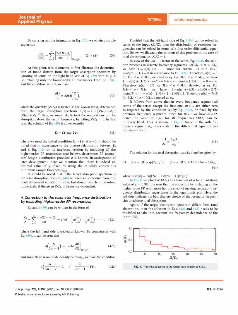
In view of the 2m� 1 factor in the series, Eq. (42a), the solu-tion proceeds in discrete frequency segments. For ΩC , ω , 3ΩC ,we have 1 ¼ a(ω)þ 0þ � � � since for ω/(2m� 1) with m > 1a(ω/(2m� 1)) ¼ 0 in accordance to Eq. (42c). Therefore, a(ω) ¼ 1for ΩC , ω , 3ΩC , denoted as a1. For 3ΩC , ω , 5ΩC , we have1 ¼ a(ω)þ (1/3)� a(ω/3)þ 0þ � � � ¼ a(ω)þ (1/3)� 1þ 0þ � � �.Therefore, a(ω) ¼ 2/3 for 3ΩC , ω , 5ΩC , denoted as a2. For5ΩC , ω , 7ΩC we have 1¼ a(ω)þ (1/3)� a(ω/3)þ (1/5)�a(ω/5)þ�� � ¼ a(ω)þ (1/3)� 1þ (1/5)� 1. Therefore a(ω)¼ 7/15for 5ΩC , ω , 7ΩC , denoted as a3.

It follows from above that in every frequency segment allterms of the series except the first one, m = 1, are either zeroas required by the condition set by Eq. (42c), or fixed by theprevious frequency segments. Since for m = 1 we have ω ¼ Ω,hence the value of a(Ω) for all frequencies Ω/ΩC can beuniquely fixed. This is shown in Fig. 7. Since in the mth fre-quency segment am is a constant, the differential equation hasthe simple form

dΩdn

¼ 2wΩam

: (43)

The solution for the total absorption case is, therefore, given by

Ω ¼ (2m� 1)ΩCexp[2wa�1m n], (2m� 1)ΩC , Ω , (2mþ 1)ΩC ,

(44)

where max[n] ¼ ‘n[(2mþ 1)/(2m� 1)]/2wa�1m .

In Fig. 8, we plot ‘n(Ω/ΩC) as a function of n for an arbitraryvalue of w ¼ 0:98. It is seen that the correction by including all thehigher order FP resonances has the effect of making resonator’s fre-quency distribution super-linear in the logarithmic plot. Here, thered dots indicate the best discrete choice of the resonator frequen-cies to achieve total absorption.

Again, if the target absorption spectrum differs from totalabsorption, then the solution to Eqs. (42) and (43) needs to bemodified to take into account the frequency dependence of theinput Z/Z0.

FIG. 7. The value of solved a(Ω) plotted as a function of Ω/Ωc .

Journal ofApplied Physics TUTORIAL scitation.org/journal/jap

J. Appl. Phys. 129, 171103 (2021); doi: 10.1063/5.0046878 129, 171103-9

Published under an exclusive license by AIP Publishing.

5. Inclusion of the imaginary part of the impedance

In the pursuit of the best design for the resonator integration,we have so far ignored the imaginary part of the impedance aspointed out above. Here, we return to Eq. (35) to carry out the inte-gration over Ω,

Z0

Z¼ �i

2ωπ

limβ!0

ð1ΩC

P1m¼1

2ΩwD(Ω)/(2m� 1)

~Ω2 � ω2 � iβω

d ~Ω, (45)

where ~Ω ¼ (2m� 1)Ω and by the definition of a lower cutoff,~ΩC ¼ ΩC . For the total absorption case, the numerator inside theintegral is equal to 1 in accordance to the designed resonance fre-quency distribution. By using Eq. (8), the resulting integration canbe done exactly to yield the impedance expression

Z(ω)Z0

¼ 1� 2iπarctanh

ΩC

ω

� � ��1

, ω . ΩC , (46a)

Z(ω)Z0

¼ iπ ‘nΩC þ ω

ΩC � ω

� � ��1

, ω , ΩC: (46b)

In Eq. (46b), we have taken ‘n(�1) ¼ �i in order to cancelout the real part of the impedance as it should vanish, since thereis no mode density below the cutoff frequency. The real andimaginary parts of the impedance are plotted in Fig. 9(a). Theresulting absorption spectrum is plotted in Fig. 9(b), whereA(ω) ¼ 1� j(Z(ω)/Z0 � 1)/(Z(ω)/Z0 þ 1)j2. It is seen that indeedthe effect of the imaginary part decays quickly above the cutofffrequency as stated earlier but induces a smooth exponentialapproach to the target absorption spectrum.

6. Circle of consistency and the determinationof optimal w

In the above, sample thickness is only implicitly implied bythe distribution of Ω, as the FP resonator’s length is specified byEq. (34). If the longer FP resonators can be folded so that theoverall shape of the sample is a compact cuboid, then its thicknessshould be given by the average of all the FP resonator lengths asdictated by volume conservation. We denote the average as �‘. Asw is present in the Ω distribution, Eqs. (41) or (44), �‘ is, therefore,a function of w. By equating �‘ ¼ dmin, the value of w can beexplicitly determined. We illustrate below this process in thesimple case of Eq. (41) where only the lowest-order FP resonancesare taken into account. From Eqs. (34) and (41), we obtain from�‘ ¼ dmin the following condition:

dmin ¼ �‘ ¼ πv02NΩc

XN~n¼1

exp[�2w(~n� 1)/N] ffi πv04fΩc

[1� exp(�2w)]:

(47)

On the other hand, we can use Eqs. (46) and (30) to calculatedmin ¼ 2v0/πwΩC , where we have used the effective medium

FIG. 8. Logarithm of the resonator frequency plotted as a function of n. Thedashed line indicates the exponential relation obtained by ignoring all the higherorder FP resonances. The solid red circles indicate the best choice for the(lowest order) FP resonator frequencies for a 3 by 3 array.

FIG. 9. (a) The real (in red) and imaginary (in blue) parts of the impedance, plotted as a function of frequency. (b) Absorption coefficient evaluated from the impedanceshown in (a). Imaginary part of the impedance is shown to have a minor effect above the cutoff frequency. Adapted from Ref. 14.

Journal ofApplied Physics TUTORIAL scitation.org/journal/jap

J. Appl. Phys. 129, 171103 (2021); doi: 10.1063/5.0046878 129, 171103-10

Published under an exclusive license by AIP Publishing.

expression Beff ¼ B0/w. This leads to the optimal value

w ¼ � 12‘n(1� 8/π2) ¼ 0:832: (48)

A similar optimal value of w ¼ 0:982 may be obtained by con-sidering the correction due to the higher order FP resonances. Thisfinal piece of design strategy completes the “circle of consistency”depicted by Fig. 10.

7. Self-energy correction

Consider a square array of a finite number of FP resonators,each with a different Ω. Let g~n denote the Green function of the ~n thresonator. The pressure at the mouth of the resonators must be dif-ferent in accordance with Eq. (31b) when excited, e.g., at a frequencyintermediate between two (lowest order) resonances. With a pressuredifference, there must be lateral air flow. This implies the differentresonators to be essentially interacting with each other, i.e., they con-stitute an interacting system. When that happens, the Green functionof each resonator will be renormalized with the consequence that theresonance frequency of each resonator is shifted downward some-what. The kernel of such interaction renormalization is called self-energy,14 adapted from the Dyson equation terminology for a multi-entity interacting system. Also, the lateral oscillating air flow impliesevanescent waves that decay away from the array surface, and suchevanescent waves with their attendant lateral air flows can be utilizedto smooth out the absorption spectrum of an array with an insuffi-cient, finite number of resonators; e.g., by putting a thin layer ofacoustic sponge over the surface of the array.

To obtain an explicit expression for the self-energy, weobserve that the displacement velocity u~n at the mouth of the ~nthresonator can be expressed as

u~n ¼ �iωg~n( ph i þ δp~n), (50)

where ph i is the modulation pressure averaged over the arraysurface, and δp~n denotes the local deviation from the average,arising from the evanescent modes. Hence, δp~nh i ¼ 0. Since col-lectively δp0~ns are associated with evanescent waves that exponen-tially decay away from the array surface, one should be able toexpress δp~n ¼ δp(x(~n)jj ) in the wavevector domain by using the

normalized Fourier basis γα(xjj) ¼ exp(�ik(α)jj � xjj). Effectively,

that means δp(xjj) ¼Pαδp(kαjj)γα(xjj). Here, the wavevectors k(α)jj

are discretized by the condition that γα(xjj) integrated over thearray surface must vanish, with index α ¼ (αx , αy),

αx , αy ¼ +1, + 2, . . .. That means jk(α)jj j ¼ (2π/L)ffiffiffiffiffiffiffiffiffiffiffiffiffiffiffiffiα2x þ α2

y

q,

where L denotes the side length of the square array. The reasonfor expressing δp in the wavevector domain is to obtain the zvariation of the evanescent mode. Since the lateral size ofthe array is smaller than the relevant incident wavelength, wemust have jk(α)jj j . ω/v0. Hence, it follows from Eq. (11) that

k? ¼ffiffiffiffiffiffiffiffiffiffiffiffiffiffiffiffiffiffiffiffiffiffiffiffiffiffiffiffiffiffiffijk(α)jj j2 � (ω/v0)

2q

is indicative of the exponential decay

length of the evanescent wave. It follows that

δp(xjj, z) ¼Xα

δp(kαjj)γα(xjj)exp �ffiffiffiffiffiffiffiffiffiffiffiffiffiffiffiffiffiffiffiffiffiffiffiffiffiffiffiffiffiffiffijk(α)jj j2 � (ω/v0)

2q

jzj�

: (51)

The z variation of pressure modulation implies that from Eq. (3),we have at z = 0,

Xα

δp(kαjj)γα(x0jj)

ffiffiffiffiffiffiffiffiffiffiffiffiffiffiffiffiffiffiffiffiffiffiffiffiffiffiffiffiffiffiffijk(α)jj j2 � (ω/v0)

2q

¼ iωρ0δu(x0jj), (52)

where δu(x0jj) ¼ u(x0jj)� u(x0jj)D E

. The Fourier component δp(kβjj)

can be solved in terms of δu(xjj) by using the orthogonality propertyof the Fourier basis. The result is

δp(kαjj) ¼ iωρ0

1L2

ðsurface

u(x0jj)γ*α(x

0jj)dx

0jj

ffiffiffiffiffiffiffiffiffiffiffiffiffiffiffiffiffiffiffiffiffiffiffiffiffiffiffiffiffiffiffijk(α)jj j2 � (ω/v0)

2q : (53)

We observe that the integral of u(x0jj)D E

γ*α(x0jj) must vanish,

owing to the condition imposed on the Fourier basis, hence δu(x0jj)can be replaced by u(x0jj) in Eq. (53). By substituting Eq. (53) into

Eq. (51) and setting z = 0, we obtain

δp(xjj, z ¼ 0) ¼ iωρ0L2

ðsurface

Xα

γα(xjj)γ*α(x0jj)ffiffiffiffiffiffiffiffiffiffiffiffiffiffiffiffiffiffiffiffiffiffiffiffiffiffiffiffiffiffiffi

jk(α)jj j2 � (ω/v0)2

q0B@

1CAu(x0jj)dx

0jj

¼ iωρ0L2

ðsurface

Λ(xjj, x0jj)u(x0jj)dx

0jj: (54)

FIG. 10. The circle of consistency that closes the loop. Adapted from Ref. 15.

Journal ofApplied Physics TUTORIAL scitation.org/journal/jap

J. Appl. Phys. 129, 171103 (2021); doi: 10.1063/5.0046878 129, 171103-11

Published under an exclusive license by AIP Publishing.

Equation (54) can be easily expressed in a discretized form as

δp~n ¼ iωρ0X~m

Λ~n~mu~m, (55)

with ~n, ~m being the discrete indices of the resonators in the array.Just to be self-contained, we give below the expression for Λ~n~m,

Λ~n~m ¼ 1N

1σ~n

ðσ~n

γα(xjj)dxjj

0@

1A 1

σ ~m

ðσ ~m

γα(x0jj)dx

0jj

0@

1A

jkαj , (56)

where N is the total number of resonators in the array, and theintegrals are to be carried out over the cross-sectional areas of themouths for resonators ~n and ~m, with x(~n)jj , x(~m)

jj being their respec-tive center positions. Here, σ~n denotes the mouth area of resonator~n, and we have assumed jkαj � ω/v0. By carrying out the integra-tions, we obtain

Λ~n~m ¼ NXα

sin2 αxπ/ffiffiffiffiN

p� �sin2 αyπ/

ffiffiffiffiN

p� �π4α2

xα2y jkαj

exp[ikα � (x(~n)jj � x(~m)jj )]:

(57)

Equations (50) and (55) are the starting point of an infiniteseries as can be seen as follows. By substituting Eq. (55) into Eq. (50),one obtains

u~n ¼ �iωg~n( ph i þ iωρ0X~m

Λ~n~mu~m): (58)

But, then one can substitute Eq. (50) into the right-hand side ofEq. (58) to obtain

u~n ¼ �iωg~n ph i þ ω2ρ0X~m

Λ~n~mg~m( ph i þ δp~m)

!: (59)

At this point, it is already clear that by repeated, alternatingsubstitutions, one can obtain the following series:

u~n ¼ �iω g~n þ (ω2ρ0g2~nΛ~n~n þ ω4ρ20g

3~nΛ

2~n~n þ�� )þ

X~m

Π~n~m

!" #

� ph i,(60)

where we have separated out the diagonal terms in the {Λ~n~m}matrix. The off-diagonal terms are grouped into the term Π~n~m,with ~n not equal to ~m. It is found that Π~n~m is order(s) of magni-tude smaller than the diagonal terms due to the summation overthe oscillation phase factors, hence it can be neglected. By retainingonly the diagonal terms, we obtain

u~n ¼� iω g~n þ ω2ρ0g2~nΛ~n~n

1� ω2ρ0g~nΛ~n~n

� �ph i

¼ � iωg~n

1� ω2ρ0g~nΛ~n~n

� �ph i

¼ � iω1

g�1~n � ω2ρ0Λ~n~n

ph i:

(61)

For the incident wave, the perceived effective impedance forthe ~n th oscillator is given by

z~n ¼ ph iu~n

¼ 1

�iωg(e)~n

, (62)

where we have defined g(e)~n to be the renormalized effective Greenfunction for the ~n th oscillator. Comparison of Eq. (62) to Eq. (61)leads to the Dyson equation

(g(e)~n )�1 ¼ g�1

~n � ω2ρ0Λ~n~n, (63)

from which we identify the self-energy correction to be ω2ρ0Λ~n~n.Since the resonance frequency is generally identified by the van-ishing of the real part of g�1

~n , it follows that the self-energyrenormalization has the effect of shifting the resonance frequencyto where the real part of (g(e)~n )

�1vanishes. It should be noted that

in accordance to Eq. (57), if N ! 1, then Λ~n~n ! 0. Therefore,the self-energy correction is inherently an effect associated with afinite number of resonators.

Since the resonators’ impedances are in parallel, the sampleimpedance for the array is given by

1Z¼X~n

f~nz~n

¼X~n

f~n(�iωg(e)~n ), (64)

where f~n is the area fraction occupied by the mouth area of the res-onator, with

P~n

f~n ¼ w. If the resonators have the same cross-sectional area, then f~n ¼ w/N so that

Z ¼ iω

w

N

XN~n¼1

g(e)~n

!�1

: (65)

8. Experimental verification

In Fig. 11(a), we show a schematic picture and a photo imageof the sample. The array has 16 resonators whose Ω’s are designedin accordance with the total absorption target spectrum with acutoff frequency set at 345 Hz. The photo image actually showsfour such arrays, each one in the shape of a compact cuboid that is10.6 cm in thickness and approximately 2.3 cm by 2.3 cm in cross-sectional dimension. The longer FP channels were folded so thatthe cuboid thickness is very close to �‘. Since 16 resonators wereinsufficient to produce a flat absorption spectrum, a 3 mm thicksponge was put on top of the array surface in order to utilize thelateral air flows of the evanescent modes for filling the dips in the

Journal ofApplied Physics TUTORIAL scitation.org/journal/jap

J. Appl. Phys. 129, 171103 (2021); doi: 10.1063/5.0046878 129, 171103-12

Published under an exclusive license by AIP Publishing.

absorption spectrum. The absorption results measured by usingthe impedance tube are shown as open circles in Fig. 11(b). Theidealized target spectrum is shown by the red dashed line, and thetheory prediction from Eq. (65), by using parameter valuesdetailed in Ref. 14, is shown as the solid red line. Excellent agree-ment is seen. From the experimental absorption spectrum, theminimum sample thickness predicted by Eq. (30) is 10.55 cm (byusing the effective medium expression for Be ¼ B0/w), which isonly about 3 mm less than the actual sample thickness (includingthe acoustic sponge). It should be noted that while the ideal valueof w is 0.982 as mentioned previously, the actual value for thesample shown is 0.8. However, in the design of the FP channellengths, the 0.982 value was used, and this turned out to be themost important. The lower actual value of w only has the effect ofreducing the reflection loss from 20 dB to 15 to 17 dB in the fre-quency range of 1500–3000 Hz.

As a further example to demonstrate the tunability of the absorp-tion spectrum, we select a target spectrum as shown by the dashed linein Fig. 12, with a reflection window extending from 560 to 1000Hz.The FP resonator length is now designed by solving Eqs. (42) and (43)with an input that is different from that for total absorption. Thisparticular sample also has 16 FP resonators. Experimentally mea-sured results and theory predictions by Eq. (65) are shown inFig. 12 by open circles and solid lines, respectively. It is apparentthat 16 resonators in an array are insufficient to closely mimic thetarget spectrum, but the resemblance is clear. In the present casethe designed w ¼ 0:81, and the causal minimum thickness is 9 cm,which is 3 mm less than the actual sample thickness of 9.33 mm.

9. Heuristic understanding of total absorption byresonator arrays

In the experimental results presented above, the array has only16 resonators, far from the idealized continuum model. In this

array, a single resonator occupies a small fraction of the total areaexposed to the incident wave. It follows that at its resonance fre-quency, only that area fraction is absorbing. The question is: Ifthat is the case, how can total absorption be achieved? Theanswer to this question can have two different aspects. In Fig. 13,we show the physical picture aspect of the answer. Similar to theflow streamline in a water sink, the Poynting vector of the inci-dent acoustic wave energy starts to deviate from the incidentwavevector at a distance above the array’s surface and convergestoward the resonant FP resonator. The underlying reason for thisphysical picture is that a discrete resonance always has highdensity of states to accommodate the wave energy at that fre-quency. Below we show the second, heuristic mathematical aspectof the answer to this question.

In accordance to Eq. (64), total absorption at the frequency ofthe resonator ~n is given by the condition Z�1

0 ¼ Cf~nIm[g(e)~n ], whereC denotes some constant. The imaginary part of the Green func-tion has a peaked shape as illustrated schematically in Fig. 14,where the red dashed line indicates the impedance matching condi-tion for total absorption. If the frequency of the intersection point

FIG. 11. (a) A pictorial illustration of the sample (left panel) and a photo image of the actual 3D-printed sample with four arrays. (b) Measured (shown by empty redcircles) and theory (shown by black solid line) absorption spectrum of the sample shown in (a). The dashed red line indicates the target absorption spectrum used todesign the sample. Deviation from the target spectrum can be attributed to the finite number (16 in the present case) of FP resonators. The sample thickness, 10.9 cm, isonly ∼3 mm over the causality minimum. Adapted from Ref. 15.

FIG. 12. Measured (shown by empty red circles) and theory (shown by blacksolid line) absorption spectrum design in accordance to the target absorptionspectrum indicated by the red dashed line, using 16 FP resonators. Here thesample thickness, 9.33 cm, is only 3 mm over the causality minimum. Adaptedfrom Ref. 15.

Journal ofApplied Physics TUTORIAL scitation.org/journal/jap

J. Appl. Phys. 129, 171103 (2021); doi: 10.1063/5.0046878 129, 171103-13

Published under an exclusive license by AIP Publishing.

between CIm[g(e)~n ] and Z�10 is denoted by ωs as delineated by a

cross, then due to the presence of the f~n factor total absorptionobviously can only be achieved at another frequency ωσ indicatedby an open circle, so that when the magnitude of CIm[g(e)~n ] at ωσ ismultiplied by f~n, the result exactly meets the red dashed line. Onecan see that obviously if f~n is too small, i.e., the number of resona-tors is very large so that each occupies only a very small fraction ofthe total exposed area, then such a “mechanism” of frequency shift(from ωs to ωσ) would not work. However, in that case the fre-quency difference between the resonators becomes small. Hence,when one resonator is excited by the incident wave, it is inevitablethat some other resonators with resonance frequencies in the

vicinity of the incident wave frequency will also be excited in accor-dance to the Lorentzian form. When that happens, total absorptionat a particular frequency is no longer shouldered by a single resona-tor. Rather, it is achieved by a collection of resonators, each withsome degree of “frequency shift.”

D. Further challenges in resonance-based acousticmetamaterials

Just as in any research topic, achieving broadband acousticabsorption also opens up some further challenges. Below wemention a few.

Challenge 1: It is easy to deduce from Eq. (30) that the absorp-tion of air-borne acoustic waves at frequencies below 200 Hz wouldrequire sample’s thicknesses that are not practical for most applica-tions. Hence, the first challenge for resonance-based acoustic meta-materials is to find a way to circumvent the causality limitation, soas to attain near-total absorption with a sample thicknesses thatcan “break” the causal limit.

Challenge 2: Some low frequency noise is caused by machinevibrations that can reach over 120 dB. Since it is usually not possi-ble to have an acoustic absorber with a 60 dB absorption perfor-mance, a reasonable way to remediate such problem is to firstabsorb the vibrational energy, so as to reduce the sound emissionintensity. Vibration suppression is a well-studied field, but toabsorb low frequency vibrational energy by using resonators canalways be a problem, since low frequency resonators can be heavyand bulky in themselves. In this respect, a second challenge is torealize compact and light-weight low frequency resonators, withfrequencies in the 10–200 Hz range that can be easily applied tosuppress vibrations and maybe harvest the energy as well.

Challenge 3: Using resonance-based acoustic metamaterials forunderwater acoustic absorption/sensing still represents a relativelyun-explored area. Acoustic waves in water have wavelengths ∼5times longer than that in air. The design of thin underwater acous-tic absorbers, with a sample thickness that approaches the causalityconstrained limiting thickness, can represent a third challenge.

III. TOWARD TOPOLOGICAL ACOUSTICS AND ONE-WAYEDGE STATES

In the last section, we have been using the concept ofimpedance, effective density and bulk modulus to discuss absorp-tion properties by using acoustic metamaterials, which can workin the regime where the wavelength is much larger than thelattice constant, in conjunction with resonance. On the otherhand, when we go up in frequency to the diffraction regime, wehave to use band structure or dispersion diagram to describe thewave properties or a structure. Special dispersion structures, suchas Dirac cones, can be constructed. Taking the Dirac cone as atypical example, below we examine different ways to constructthem by using accidental degeneracy or symmetry protection.These Dirac cones can occur in both the long wavelength regimeas well as the diffraction regime. It allows us to have a wide rangeof counter-intuitive phenomena in wave manipulation, such asnegative refraction, zero-index tunneling, quantum Hall-like edgestates and topological bandgaps.

FIG. 13. A pictorial illustration of the Poynting vector of the incident wave at theresonance frequency of one of the resonators in the array. Close to the surfaceof the array, the power flow converges onto the resonating unit, leading to totalabsorption.

FIG. 14. A pictorial illustration of the slight frequency shift that can lead to theimpedance matching condition as described in the text.

Journal ofApplied Physics TUTORIAL scitation.org/journal/jap

J. Appl. Phys. 129, 171103 (2021); doi: 10.1063/5.0046878 129, 171103-14

Published under an exclusive license by AIP Publishing.

A. Space-coiling structures

Acoustic metamaterials, while sharing similar concept withelectromagnetic wave metamaterials, need different design strategiesand realizations. In particular, for airborne acoustics, one veryessential difference is that it is difficult to realize a large refractiveindex but easy to realize a small refractive index since sound travelsmuch faster in any solid, fluid than in air. It is in contrary to thecase of electromagnetic waves, in which index larger than that ofair is easy but index smaller than air is not possible without reso-nance. In acoustic metamaterials, it is very usual to employ resonat-ing structures to achieve different indices. On the other hand,inspired by how solid slows down light by a dielectric in creatingmultiple scatterings and phase delay, we can also create high indexby delaying the sound in curled channels. Figure 15(a) shows theconcept of this phase delay of sound within a curled channel acrossa straight-line distance a.18 The factor of elongation in the path,comparing to a, is the effective refractive index n1D along this direc-tion. By assembling this curled channels into a two-dimensionalnetwork [Fig. 15(b)], it becomes the basis for constructing acousticmetamaterials with very flexibly tuned dispersion or refractiveindices working both in the long wavelength and the diffractionregime, without invoking local resonances.

1. From negative to positive refractive indices

When the unit cells in Fig. 15(b) are assembled in a squarelattice, its band structure can be solved numerically (COMSOLMultiphysics) and is plotted in Fig. 16(a). As we see from the firstband, it has a much lower slope (scaled by a factor of around 5, thenumber of turns within each sub-unit of the curled channels) com-pared to the slope of the background sound line (plotted in dashedline). It means that the refractive index of such a 2D acoustic meta-material can be easily tuned to any large value without employingany resonance. More interestingly, it will form the so-called Dirac

cones at the M point at around ωa/(2πc) ffi 0:11 and at the Γ pointat around ωa/(2πc) ffi 0:22. There is a very tiny bandgap opened atthe center of the cone due to a small practical impedance mismatchas the Dirac cone is formed based on accidental degeneracy in thiscase. Anyway the dispersion is approximately linear around theseDirac cones, e.g., the cone at Γ point, from the band structure andthis linear dispersion is isotropic near the cone center frequency, asdepicted from Fig. 16(c). There is also a flatband occurring at thesame frequency, which can be associated to the acoustic death band(colored green) at which the effective density is zero, to be extractedin the next section.

2. Effective medium extraction of wave parameters

As the dispersion returns to the Γ point at a low normalizedfrequency (wavelength in air being at least five times the size ofunit cell), we expect the dispersion can also be described by aneffective medium (which is also true for resonance-based metama-terials). For simplicity, rather than an analytic formulation of thedetailed mechanism in creating the acoustic response, we can adopta generic approach in extracting the effective medium parametersby using the so-called S-parameter retrieval method.19 From anygiven set of scattering S-parameters either from full-wave simula-tions (such as COMSOL Multiphysics) or from an experimentalmeasured set, the method can be used to extract effective densityand bulk modulus of any acoustic metamaterials. In fact, the samecan be applied to extract other constitutive parameters, such as therecently found Willis coupling parameters in analogy to electro-magnetic bianisotropic constitutive parameters.20

The starting point of the method is to assume a homogeneousslab of material with density ρ and bulk modulus B (we normalizethem to the values of background air for mathematical conveniencehere). The complex transmission coefficient t and reflection coeffi-cient r can be easily proved by transfer matrix method to satisfy the

FIG. 15. (a) Coiling up space to allow sound to propagate within a curled channel with hard solid boundary to achieve a high refractive index n1D for each channel. (b)Curled channels to form a 2D network as an acoustic metamaterial.

Journal ofApplied Physics TUTORIAL scitation.org/journal/jap

J. Appl. Phys. 129, 171103 (2021); doi: 10.1063/5.0046878 129, 171103-15

Published under an exclusive license by AIP Publishing.

following relations for a slab of thickness a:

i1� r � t1þ r þ t

¼ 1Ztan

nk0a2

� �, (66a)

i1þ r � t1� r þ t

¼ Ztannk0a2

� �, (66b)

where n and Z are the refractive index and impedance of the mate-rial, given by n ¼ ffiffiffi

ρp ffiffiffiffiffiffiffi

1/Bp

and Z ¼ ffiffiffiρ

p/ffiffiffiffiffiffiffi1/B

p(with normalized

definition as well). k0 is the wavenumber in the backgroundmedium air. The S-parameter retrieval method basically inverts

Eq. (66) to get its solution of n and Z as

Z ¼ffiffiffiffiffiffiffiffiffiffiffiffiffiffiffiffiffiffi1þ r � t1� r þ t

r/

ffiffiffiffiffiffiffiffiffiffiffiffiffiffiffiffiffiffi1� r � t1þ r þ t

r, (67a)

nk0a ¼ 2tan�1 i

ffiffiffiffiffiffiffiffiffiffiffiffiffiffiffiffiffiffi1þ r � t1� r þ t

r ffiffiffiffiffiffiffiffiffiffiffiffiffiffiffiffiffiffi1� r � t1þ r þ t

r !, (67b)

except that now we use the r and t from full-wave simulations withmicrostructures or experimental results. The inversion takes a con-vention in the square roots so that the real part of impedance Z ispositive to satisfy the requirement of causality. There is also a

FIG. 16. (a) Band structure of a space-coiling metamaterial in square lattice (with lattice cell constant 2:33 cm for later realization) while each space-coiling unit has a5-times folding in each channel. (b), (c), (d). Equi-frequency contour in the long wavelength limit, below, and above the Dirac cone at Γ-point. Adapted from Ref. 18.

Journal ofApplied Physics TUTORIAL scitation.org/journal/jap

J. Appl. Phys. 129, 171103 (2021); doi: 10.1063/5.0046878 129, 171103-16

Published under an exclusive license by AIP Publishing.

branch taking in evaluating tan�1 (adding multiple integer of 2π tonk0a gives the same tangent value). For a thin slab, we can just takethe first branch while for a thick slab, one must consider theanalytic continuity when we obtain n as a function of frequency.Then, the effective ρeff and Beff can be obtained as ρeff ¼ nZ,1/Beff ¼ n/Z. For the mentioned design of space-coiling metamate-rial (with lattice constant set as a ¼ 2:33 cm), Fig. 17 shows itseffective medium results from such S-parameter retrieval methodbeing applied on either full-wave simulation results (solid lines)or experimental results (open symbols) with excellent agreement.We have plotted the real part of the refractive index n, effectivedensity and reciprocal of effective bulk modulus in the first threepanels. All of them cross the horizontal axis at a frequencyaround 3.12 kHz [corresponding to the normalized frequencyωa/(2πc) ¼ 0:22], verifying the Dirac cone as indicated in Fig. 16at this center frequency.

Through the relationship n ¼ ffiffiffiρ

p ffiffiffiffiffiffiffi1/B

p, the index approaches

zero at the center frequency. In fact, it is called “double-zero” dueto the Dirac-cone (or linear dispersion) feature. On the other hand,below the center frequency, both the density and bulk modulusbecome negative. In this regime, it is called the double negativemetamaterial or simply negative refractive index. It becomes avalue −1 at around 2.7 kHz, which is usually associated with theimaging lens to do subwavelength imaging.22,23

To ensure the metamaterial to be useful for manipulatingpropagating waves (e.g., at the frequency having index of −1, incontrast to the previous part of this article on sound absorption),we have also extracted from the effective medium approach theimaginary part of the effective material parameters. Absorptioncomes from the viscosity of the air channels. More turns we curlthe path, the narrower the channels become with respect to thewavelength in air, thereby inducing more contact between thesound and the solid with dissociation through the viscosity or thefriction on the solid surfaces. To have an estimation on the loss, wehave adopted Ref. 24 in estimating the attenuation coefficient, i.e.,by adopting the form of sound amplitude /exp(�αx) for a straightchannel along x with rectangular cross section (w� h), given by

α ¼ 1þ γ � 1ffiffiffiffiffiPr

p� �

wþ hwh

1v0

ffiffiffiffiffiffiffiffiffiffi4πηfρ0

s, (68)

where ρ0 and v0 are the density of sound speed in air, η is thedynamic viscosity of air and Pr = 0.71 is the Prandtl number inrelating the contribution of attenuation from viscosity and thermalconduction. In our case, we add an imaginary part to n1D, therefractive index of a single curled channel, by Im(n1D) ¼ α/(2k0)before assembling into the 2D metamaterial with resultant effective

FIG. 17. Effective medium extracted from the space-coiling metamaterial in Fig. 16. Solid lines show the refractive index n (a), effective density (b), reciprocal of effectivebulk modulus (c) and the imaginary part of the index (d). The open symbols are the corresponding results extracted from experimental data. Adapted from Ref. 21.

Journal ofApplied Physics TUTORIAL scitation.org/journal/jap

J. Appl. Phys. 129, 171103 (2021); doi: 10.1063/5.0046878 129, 171103-17

Published under an exclusive license by AIP Publishing.

index n. The imaginary part of refractive index of n is foundnumerically to be around 20% of the real part at that frequency(agreeing with the direct measurement of attenuation for the meta-material), which is not easy to achieve for metamaterials based onresonating mechanism for a negative refractive index. It is alsoworth to note on what we previously mentioned about zerodensity. At zero effective density, the acoustic wave equation forplane wave solution becomes simply k � v ¼ 0, where v is the veloc-ity field. It means that it supports transverse polarizations (ratherthan longitudinal) being perpendicular to the wave vector. It is theorigin of the flatband at the center frequency in the band structure(Fig. 16).25 This argument also implies that the band is doublydegenerate. Such a situation is well known in electromagneticwaves in which the longitudinal plasma mode exists at the fre-quency with zero permittivity.

3. Negative refraction and zero index tunneling

A direct consequence of the broadened domain of refractiveindex values for the acoustic metamaterial is to allow a directdemonstration of negative refraction at a negative index, as wellas zero index-tunnelling at the frequency having zero refractiveindex (also the center frequency of the Dirac cone). Figure 18shows a simulation to demonstrate negative refraction from a45° right-angle prism (schematically shown in the same figure)made of unit cells with curled channels. When wave impingeson one interface at normal incidence, it enters the prism andhits another interface (metamaterial-to-air) at 45°. Then, therefractive angle θ is governed by the Snell’s law sinθ ¼ nsin45�,with θ being positive (negative) above (below) the surfacenormal which is shown as a dashed straight line in the figure.The full-wave simulation results in Fig. 18(b) shows sound waveintensity measured at different angles at different frequencies. Atan individual frequency, the resultant angular profile is normal-ized to its highest intensity, which can be defined as the refrac-tion angle. It is obvious to note that the refraction angle variesfrom negative to positive in the interested frequency regime(2.6–3.8 kHz), verifying negative refraction is achieved and isassociated with negative refractive indices below 3.1 kHz (thezero index frequency).

It has been pointed out and later realized (first proposed inelectromagnetism and later in acoustics) that a zero refractiveindex26–30 can be used for tunneling in a waveguide with anobstacle. This occurs at the center frequency of the Dirac cone.In Fig. 18(c), we have simulated this situation when we wrap ahard solid obstacle in such a waveguide (also with hard solid astop and bottom boundary) by 28 layers of the current acousticmetamaterial unit cells. When a wave at 3.2 kHz impinges fromthe left of the waveguide with an incident amplitude of 1, thewave tunnels through the waveguide with nearly unit transmit-tance and nearly flat wavefront. The small reflection is seen, dueto the imperfect mini gap opened around the center frequencyof the Dirac cone. As the Dirac cone is constructed by accidentaldegeneracy, any imperfections in the design due to the imped-ance mismatch of the channels to the background can open atiny bandgap [with a width of ∼0.2 kHz in this case, as shown inFigs. 18(b) and 18(c)].

B. Pseudo-magnetic field and edge states

Dirac cone, a conic dispersion originally described by theDirac equation,31 has attracted great attention in electronic32,33

and classical wave systems,34–38 due to the associated rich physicssuch as one-way edge modes,35,36,39 Zitterbewegung oscillations,40

extremal transmissions,41,42 and Klein tunneling.43 Historically,the existence of Dirac cones is closely related to the crystal sym-metry.44 High crystal symmetry supports deterministic Diracdegeneracies at high symmetry points of the Brillouin zone (BZ).While in the case of without high enough crystal symmetry, e.g.,the accidental degeneracies described in the last section, can alsobe generated by fine-tuning the parameters. Due to the advent ofstate-of-the-art fabrication technologies, the artificial crystals forclassical waves can now provide a versatile platform for studyingthe Dirac cones and associated physical phenomena.

Inspired by recent works45–52 in distorting the underlyinglattice in supporting the Dirac cones (originally considered in thecontext of strained graphene), pseudo-magnetic field can be gen-erated and it provides new ways to manipulate wave and ray tra-jectories. The concept of a pseudo-magnetic field comes from theanalogy to Lorentz force acting on an electron, which consists of aconservative part due to the electric potential and electric field,and a non-conservative part associated with the magnetic field. Inacoustics or any other scalar waves, the similar concept can beformulated by modifying the harmonic wave equation (in twodimensions for simplicity) as

(∇þ ik0A) � 1n (∇þ ik0A)pþ k20np ¼ 0: (69)

Compared to the usual Helmholtz wave equation, a fictitious 2Dreal vector A ¼ Axx þ Ayy is introduced into the wave equation.While its realization is described in the next section, its meaningis intuitive in terms of ray dynamics, which can be considered bywriting down the Hamiltonian, or dispersion relationship, as

H(k, r) ¼ 12k0n

(jk þ k0Aj2 � k20n2) ¼ 0: (70)

Then, the ray position (r) as the rate change of path length s isgoverned by Hamilton’s equations

drds

¼ @H@k

¼ k þ k0Ak0n

, (71a)

dkds

¼ � @H@r

¼ jk þ k0Aj2 þ k20n2

2k0n2∇n� k0(∇A) � drds , (71b)

which implies the ray equation

dds

ndrds

� �¼ ∇n� s� ∇� A: (72)

Equation (72) can be regarded as Newton’s second law for raydynamics, with the right-hand side being the Lorentz force actingon electronic motion.53 The first term is conservative, where the

Journal ofApplied Physics TUTORIAL scitation.org/journal/jap

J. Appl. Phys. 129, 171103 (2021); doi: 10.1063/5.0046878 129, 171103-18

Published under an exclusive license by AIP Publishing.

index corresponds to the scalar potential, and ∇n corresponds tothe electric field. The second term, as a “force” perpendicular tothe ray direction s, can be regarded as the magnetic force, where Acorresponds to the vector potential, also denoted as the gauge field,and ∇� A corresponds to the magnetic field. It makes sense todefine a pseudo-magnetic field as

B ¼ Bz ¼ ∇� A: (73)

The immediate impact of the pseudo-magnetic field, in cor-respondence to the magnetic force acting on an electron, is theanalogy of cyclotron motion. Suppose we consider a constantpseudo-magnetic field B within a circular region r � r0. To simu-late the propagation of a beam with pseudo-magnetic field withEq. (69), we impose a spatial profile of gauge field A as

A ¼r2Bf, r � r0,

r202r

B f, r . r0:

8><>: (74)

The vector potential A is not unique for a fixed profile of B, asalso suggested by its name “gauge” field. The gauge can be fixed,e.g., by the Coulomb gauge (∇ � A ¼ 0). Figure 18(a) shows a beampropagating in such a region, which is bent in the counterclockwisedirection in a circular motion. When the sign of B flips, thebending direction will change to clockwise. When the magnitudeof B increases, the radius of the circular motion decreases. Due tothe preferential bending direction within the region of non-zero Bfield, the B-field profile can be arranged into a setting with oppositesign on the opposite sides of an interface. In such a case, the ray islocalized on such interface by the bending mechanism. This isshown in full-wave simulation for this localized state propagatesfrom the left in Fig. 19(b). The red arrow shows the ray trajectoriesin bending along the interface. Even though such a localized stateencounter a corner of the interface, it still bends around it and goesforward. As the bending mechanism is not compatible with propa-gation in the reverse direction, reflection of such state around thecorner is forbidden. That is, if we imagine the ray trajectory of sucha state is in the reverse direction, it would require clockwise (coun-terclockwise) bending in the lower (upper) medium, but this is not

FIG. 18. (a) Simulated negative refraction for a prism made of space-coiling metamaterial. Outgoing beam below/above the dashed straight line indicates negative/positiverefraction angle. (b) Simulation results of refraction angle θ for an impinging wave normally hitting on one interface of the prism across different frequencies. Negativerefraction (θ , 0) is found below 3 kHz. (c) Experimental results verifying negative-to-positive refraction across the zero-index frequency. (d) zero index tunnelling aroundan obstacle made of hard solid (white region). Adapted from Refs. 18 and 21.

Journal ofApplied Physics TUTORIAL scitation.org/journal/jap

J. Appl. Phys. 129, 171103 (2021); doi: 10.1063/5.0046878 129, 171103-19

Published under an exclusive license by AIP Publishing.

the case of cyclotron motion in Fig. 19(a). Such a state is called theone-way edge mode and the same mechanism, together with thecyclotron motion, is associated with the quantum Hall effect.Unlike electron motion, the mentioned magnetic-force bending isnot readily available in classical wave systems. One way to realizesuch pseudo-magnetic field is through the strained grapheneapproach.45 Such a synthetic or pseudo-field approach opens thedoor to explore magnetic phenomena in classical wave systems butwithout actually employing any physical magnetic field.54–56

1. Shifting Dirac cones at high symmetry points

In this section, we describe how a pseudo-magnetic field, gen-erated by the gauge field A, can be materialized. In the domain ofelectromagnetic waves, the gauge field A can be conceptually real-ized in the effective medium regime by using metamaterials withtiled anisotropy together with the concept of pseudo-spin.53 Thewave equation for a particular pseudo-spin becomes Eq. (69). Inacoustics, we have to look for an appropriate design of phononiccrystals, working in the diffraction regime, in which the dispersionsurface satisfies effectively the description of Eq. (70) around a sym-metry point in the Brillouin zone, and the ray dynamics will be gov-erned by Eq. (72). In particular, we can start from a 2D phononiccrystal with a triangular lattice, schematically shown in Table I. Itconsists of a triangular array of circular rigid cylinders in air (withradius of cylinders r being 9 mm and lattice constant a being25mm), carrying point group symmetry C6v.

57 In the reciprocalspace, the phononic crystal supports six Dirac cones at K or K 0

points in BZ. When the circular cylinders are deformed into ellipti-cal ones, where p and q represent the semi-major and semi-minoraxes, respectively, with fixed filling fraction [Fig. 20(a)], the pointgroup symmetry is reduced to C2v , which results in the shifting ofDirac points along the kx direction, as schematically shown inFig. 20(b). Due to the time reversal symmetry, the Dirac cones at K 0

points shift in opposite directions to that of Dirac cones at K points,as indicated by the blue and red arrows. Below, we focus onthe Dirac cones at K points only. For elliptical deformationswith p , q, these Dirac cones, originally with dispersion ω� ωD

¼ vD(kxσx þ kyσy) measured from the cone center K and Diracfrequency ωD ¼ 6:97 kHz, shift to the right by δkx. Here, σx andσy are the first two Pauli matrices. On the other hand, the conesshift in the reverse direction for p . q, as shown in Fig. 20(c),numerically found to satisfy δkx ¼ 0:59π(q� p)/( pa). It is worthyto mention that, the shape deformation shifts Dirac cones buthardly affects Dirac frequency ωD. The shifting of the Dirac conescan now be written as k ! k þ A, where A is now interpreted asthe gauge field (or pseudo-vector potential) and a spatiallyvarying profile of such A can be used to generate pseudo-magnetic field and edge states. Such a gauge field approach issummarized in the first row in Table I. A complementaryapproach to generate the edge state is to adopt the mentionedgauge field A and pseudo-magnetic field B to the reciprocal spaceinstead of the real space. It involves opening topologically non-trivial bandgap (second row in Table I). One way to construct theappropriate phononic crystal is gapping the double Dirac cone,but its discussion will be postponed to a latter section.

2. Acoustic Landau levels

The linear relationship between the momentum shift and theshape factor can be used to construct a phononic crystal with alinear gauge field in the y direction. By linearly varying the shapefactors of scatterers along the y direction through a relationshipξ(y) ¼ �Bzy/cγ where cγ ¼ 0:59π/a, and ξ ¼ (q� p)/p is thedimensionless shape parameter governing the elliptical cross sec-tional shape of the cylinders, a linearly gradient gauge fieldAx(y) ¼ �Bzy can be constructed in the phononic crystal, wherethe constant Bz defines the strength of acoustic pseudo-magnetic

FIG. 19. (a) a beam propagating with constant pseudo magnetic field B ¼ 0:1 within a circular region of radius 6.5.(b) a one-way edge state propagating along a cornerwith B ¼ 2 (−2) on the inner (outer) region.

Journal ofApplied Physics TUTORIAL scitation.org/journal/jap

J. Appl. Phys. 129, 171103 (2021); doi: 10.1063/5.0046878 129, 171103-20

Published under an exclusive license by AIP Publishing.

field orientated in the z direction. The inset in Fig. 21(a) sche-matically shows a gradient 91-layer (�45 � ny � 45) phononiccrystal ribbon, which can be used to construct the 2D gradientphononic crystal by periodically arranging in the x direction.According to B ¼ ∇� A, Bz ¼ � @Ax

@y ¼ �0:013a�2 (the minus

sign indicates �z direction). In analogy to electron undergoingcyclotron motion and quantization into Landau levels, the linearDirac cones here also quantizes into a sequence of discrete acous-tic Landau levels (LLs), which is clearly observed in the spectrumaround the K point (set as the original point) for the 91-layer gradi-ent ribbon in Fig. 21(b). Clearly, the spectrum exhibits discrete flatLandau plateaus centered by the Dirac frequency ωD ¼ 6:97 kHz,

which is the hallmark of Landau quantization for massless Diracsystems. The analytical LLs (at frequencies Δn with respect to theDirac frequency) calculated from the effective Dirac HamiltonianH ¼ vD((Px þ Ax)σx þ Pyσy) with Px,y being the momentum oper-ator,58 which can be written as

Δn ¼ sign(n)ffiffiffiffiffiffijnj

pωc, (75)

where ωc ¼ vDffiffiffiffiffiffiffiffiffiffi2jBzj

p ¼ 200Hz is an acoustic analog of the cyclo-tron frequency, with vD ¼ @ω/@k ¼ 1241:4a being obtained fromthe Dirac dispersion. In Fig. 21(b), the bold lines representing ana-lytical LLs (with the Dirac frequency as the center frequency),

TABLE I. Summarizing the approaches to realize the pseudo-magnetic field in real space and reciprocal space with a triangular lattice, corresponding to the upper and lowerrows, respectively.

Unit-cell Brillouin zonePerturbationon unit cell

Pseudo-magneticfield

Edge modesrequired

Triangular lattice

Primitive unit cell Dirac cones at K and K0

Lowering pointgroup symmetry

In real space Spatially varyinggauge field

Extended unit cell

Double Dirac cone at Γ

Lowering latticesymmetry

In reciprocal space Topologicallynon-trivialbandgap

FIG. 20. (a) The unit-cell of the triangular phononic crystals with cylinder being deformed into an elliptical one. (b) With reduced crystal symmetry, the Dirac cones at thecorner of BZ shifts along kx direction in momentum space. (c) The band structures for three uniform phononic crystals with different shape of cylinders. The location ofDirac cone (indicated with vertical gray lines) shifts for the deformed cylinders but with almost the same Dirac frequency (indicated with horizontal gray line).

Journal ofApplied Physics TUTORIAL scitation.org/journal/jap

J. Appl. Phys. 129, 171103 (2021); doi: 10.1063/5.0046878 129, 171103-21

Published under an exclusive license by AIP Publishing.

match perfectly with the simulated results for the first 11 LLs. Thestates in each Landau plateau are accidentally degenerated, as theyshare the same energy but their wave functions center at differenty-coordinates. The high degeneracy in discrete LLs results in thehigh density of states, which will be reflected by the mode profileand excitation spectrum.

Here, we demonstrate a bulk state and two edge states in thezeroth LL for the 91-layer phononic crystal [marked with blackdots in Fig. 21(b)], whose eigen-mode profiles (normalized by thelargest value) are shown in Fig. 21(c). For the bulk states in Landau

plateau (middle panel), the pressure field situates at the center ofthe sample, and spreads over a length scale of the effective mag-netic length lB ¼ 1/

ffiffiffiffiffiffiffiffijBzjp ¼ 8:8a (marked with the black arrow).

However, for the edge state in the gap between n ¼ 0 and n ¼ 1LLs, the pressure field localizes at lower boundaries, as shown inthe left panel. In contrast, the edge state in the gap between n ¼ 0and n ¼ �1 LLs corresponds to the upper edge states, as shown inthe right panel. Physically, the edge states arise from the openedacoustic cyclotron orbits (green arrow) near a ribbon edge, in con-trast to the complete cyclotron orbit for the bulk states (middle

FIG. 21. (a) Simulated momentum shifts δkx or Ax with a linear dependence (line) on the deformation shape factor ξ ¼ (q� p)/p, which is used to construct the a linearprofile of Ax in a gradient 91-layer phononic crystal consisting of a periodic array of the ribbon (inset) in x direction. (b) Landau level spectrum center around the Dirac fre-quency around K point, simulated for the ribbon in (a), where the bold lines represent the analytically predicted LLs. Adapted from Ref. 57. (c) The normalized pressureamplitude distributions for bulk (s2) and edge (s1 and s3) states in a gradient 91-layer phononic crystals. The direction of the trajectories of the states are schematicallyindicated by the green arrows. Insets: the zoom-in field pattern within the black frame. (d) The first 11 LLs for phononic crystals with different magnetic strength Bz(achieved by adjusting the number of layers in phononic crystal), where the symbols and dashed lines represent the simulated and analytical results respectively.

Journal ofApplied Physics TUTORIAL scitation.org/journal/jap

J. Appl. Phys. 129, 171103 (2021); doi: 10.1063/5.0046878 129, 171103-22

Published under an exclusive license by AIP Publishing.

panel). For edge states, the frequencies deviate gradually from the LLvalues, as these states become more and more localized at the edge.In addition, the bulk-state vibrations behave strikingly different at thetwo sublattices: the field concentrates around the A sublattice butvanishes at the B sublattice, as the inset shows. This is a direct conse-quence of the graphene-like Dirac systems, where the zeroth LL statesare sublattice polarized (the eigenvector for the zeroth LL obtainedfrom the effective Hamiltonian is zero for B sublattice), in contrast tothe states in other LLs that occupy both sublattices. The polarizationweakens as the state departs from the Landau plateau due to theinteraction with the physical boundary (see insets).

For the phononic crystal with macroscopic controllability, it iseasy to achieve stronger uniform pseudo-magnetic field. WithAx(y) ¼ �Bzy, for example, we can simply decrease the number oflayers, that is, decrease y to increase the gradient to achieve strongerpseudo-magnetic field as exemplified in Fig. 21(d). Here, we takeBz ¼ �0:013a�2 achieved in the 91-layer gradient phononic crystal asthe baseline B0. By decreasing the number of layers of the gradientphononic crystal to 46 layers and 31 layers, we can achieve the double(Bz/B0 ¼ 2) and triple value (Bz/B0 ¼ 3). The symbols represent thesimulated results for the first 11 LLs (jnj � 5), and consistent with theanalytical results obtained from Eq. (75) (dashed lines), even for stron-ger pseudo-magnetic field. In addition, the Dirac LLs in phononiccrystals show a square-root dependence on the pseudo-magnetic field,in contrast to the equally spaced LLs with a linearly dependence onmagnetic field for free 2D electrons in a real magnetic field.

3. Experimental realization

As high degeneracy in discrete LLs leads directly to highdensity of states, we can experimentally observe the quantized

acoustic LLs through the peak structure of the excitation spectrum.To facilitate the experimental demonstration of the quantizedacoustic LLs well separated in the frequency spectrum (larger sepa-rations between different Δn), a higher pseudo-magnetic field Bz ispreferred according to Eq. (75). In our case, the pseudo-magneticfield is constructed from a linear gradient of Ax (δkx of the Diraccones) in the y-direction, which in turns comes from the deforma-tion of the unit cells across the whole phononic crystal, describedin Fig. 21(a). Therefore, we further decrease the number of layersfrom 91 to 16 layers, corresponding to a six-fold increase ofthe pseudo-magnetic field of the theory simulation in Fig. 21(Bz ¼ �0:078a�2) to achieve separations of the LLs. The experi-mental setup is shown in Fig. 22(a). Due to the sublattice polariza-tion nature of the zeroth LL state, the location of the sound source(A-sublattice or B-sublattice) can profoundly affect the excitationspectrum. For comparison, a point-like sound source is placed atone A-sublattice and one B-sublattice near the sample center forexcitation, and the measured frequency spectra for the total soundenergy are plotted as red and blue circles in Fig. 22(b), respectively,and the red and blue solid lines represent the respective simulatedresults. For the A-site spectrum (red), three discrete peaks corre-sponding to the first three LLs are clearly observed, dramaticallydifferent from the quadratic background spectrum (black dashedline) simulated for a 16-layer sample with zero pseudo-magneticfield. Specifically, the primary peak, corresponding to the zerothLL, is a key feature of the Landau quantization in a relativisticDirac system. However, for B-site excitation spectrum (blue), thezeroth LL cannot be excited effectively because the zeroth LL livesentirely on the A-sublattice [as shown in the inset of Fig. 21(c)],while the n ¼ �1 and n ¼ 1 LLs without sublattice polarizationcan be excited by B-site excitation. The quantization peak locations

FIG. 22. (a) The experimental setup, a 16-layer 2D phononic crystal is covered by a transparent holey plate to form a 2D acoustic waveguide for measurement. The pre-served holes are sealed by plugs colored in red and blue respectively for A and B sublattices of each unit-cell [as shown in Fig. 19(a)], will be opened one-by-one forsound detection, where the inset shows a zoom-in image indicating the sound source and detector. (b) The frequency spectra of the total intensity for A and B sublatticeexcitation are plotted with red and blue open circles respectively, agrees well with the numerical results (solid lines), whose peak structures follow the model prediction(purple arrows). Adapted from Ref. 57.

Journal ofApplied Physics TUTORIAL scitation.org/journal/jap

J. Appl. Phys. 129, 171103 (2021); doi: 10.1063/5.0046878 129, 171103-23

Published under an exclusive license by AIP Publishing.

in the excitation spectra that result from the acoustic pseudo-magnetic field, match well with the expected positions (indicatedwith purple arrows) calculated by Eq. (75).

In addition to the above, we can observe the quantum-hall-likeedge modes in the gaps between two neighboring acoustic LLs byusing a similar experimental setup shown in Fig. 22(a) but withrigid strips attached at the upper and lower boundaries to preventsound leakage. Here, we exemplify the measurement of edge stateslocalized at the bottom boundary with a frequency at 7.3 kHz,which falls into the gap between n ¼ 0 and n ¼ 1 LLs. For theobservation of edge states that propagate along the bottom boun-dary, a sound source (green star) is positioned at the bottom left ofthe sample to excite the edge mode that travels to the right direc-tion. The measured pressure distributions for bottom edge states isshown in Fig. 23(a), a well-confined edge state appears in thebottom boundary and propagates rightwards, consistent with thesimulation results in Fig. 23(b). Similarly, the rightward-propagating upper edge states which falls into the gap between then ¼ 0 and n ¼ �1 LLs can also be measured with an excitationsource located at the upper left of the sample (not shown).

4. Topologically non-trivial bandgap and topologicaledge states

Another approach to generate edge states is through a topolog-ical non-trivial bandgap. In this approach, the concepts about thegauge field and pseudo-magnetic field are directly related to theBerry connection A(k) and Berry curvature Ω(k) in the reciprocalspace, respectively. The non-zero Berry curvature Ω(k) in the recip-rocal space gives rise to topological properties of the bands. Inturns, a topological edge state can be generated within a topologi-cally non-trivial bandgap from the Dirac cone as the result. As atypical example, we start from the same triangular lattice, exceptthat we now purposely use an extended unit-cell (rather than theoriginal primitive one) with a lattice constant a0 ¼ ffiffiffi

3p

a. Then, thecorresponding Brillouin zone is reduced. From band folding, adouble Dirac cone appears at the Γ point, as shown in the secondrow in Table I and the relevant band structure is shown in Fig. 24(b).Such an approach has been used to generate double Dirac conesfor both the electromagnetic and acoustic waves and the consider-ation of topological nontrivial bandgap.59–63 Here, we lower thelattice symmetry by introducing a perturbation only in the central

FIG. 23. (a) Measured field pattern for a bottom edge state in a 16-layer phononic crystal with a strong pseudo magnetic field. (b) Simulated field pattern from ComsolMultiphysics. Adapted from Ref. 57.

FIG. 24. Band structures for three phononic crystals with different radius r0 of the central cylinder. (b) With r0 ¼ r , the lattice symmetry allows zone folding to achieve adoubly degenerated Dirac cone at Γ point. With a reduced (a) or enlarged radius r0(c), the lattice symmetry lowers and a band gap (indicated by gray regions) opens at Γpoint. The insets show the pressure field distribution for four modes at Γ point.

Journal ofApplied Physics TUTORIAL scitation.org/journal/jap

J. Appl. Phys. 129, 171103 (2021); doi: 10.1063/5.0046878 129, 171103-24

Published under an exclusive license by AIP Publishing.

cylinder in the extended unit cell. By adjusting the radius r0 of thecentral cylinder to deviate from the original radius r, the originaltranslational symmetry is broken (lowered), thereby a bandgapcan be opened and tailored flexibly at the Dirac cone. For areduced radius (r0 ¼ 0:65r) in Fig. 24(a), the bandgap opens andtwo twofold degenerated modes are located on the upper andlower sides of the bandgap. The inset shows the pressure field pat-terns for the modes at Γ point, which can be classified into thepx/py (lower two modes) and dx2�y2 /d2xy (upper two modes) byfollowing the convention in topological photonics.59,60 In contrast,for an enlarged radius (r0 ¼ 1:4r) in Fig. 24(c), the frequency ofpx/py modes is higher than that of dx2�y2 /d2xy modes, which char-acterizes the band inversion and topological phase transition.Consequently, by adjusting the radius r0, we achieve two topologi-cal distinct phases. To understand such topological non-trivialbandgap, it is intuitive to adopt a spring-mass model in the hex-agonal lattice.64 The waves of pseudo-spin up state, defined bypx þ ipy and dx2�y2 þ i d2xy , are approximately decoupled near thezone center from those of pseudo-spin down defined by px � ipyand dx2�y2 � i d2xy . The corresponding Hamiltonian near thebandgap can be written in the form of

Heff ¼ M þ Bk2 A(kx þ iky)A*(kx � iky) �M � Bk2

� �, (76)

which gives you the quality of the bandgap (and eigenmodes) nearzone center in Fig. 24(a) (with BM . 0 for the trivial case) andFig. 24(c) (with BM , 0 for the non-trivial case). It shares similarfeatures with the Hamiltonian of the quantum spin Hall effect.59,61

Combining two phononic crystals with different topologicallydistinct phases, we construct an A-B type supercell ribbon, as sche-matically shown in the inset of Fig. 25(a). As a result, a pair of

topological edge states appear at the bulk bandgap (gray region), asshown in the band structure of the supercell in Fig. 25(a). InFig. 25(b), we demonstrate the pressure field distribution of twotopological edge states [marked with red dots in Fig. 25(a)] with afrequency at 7.32 kHz, which is localized at the interface and decayquickly along the normal direction of the interface. In Fig. 25(c),we have simulated the edge state running along on an interfacewhen B is enclosed by A. A point-type source is excited in themiddle on the interface to excite with only one single spin edgestate which goes around the corner in the counterclockwise direc-tion almost without reflection.

While the acoustic properties of the metamaterials in thisarticle on absorption and topological acoustics are mainly driven byresonating physical structures, it is worthwhile to note that there isrecently a direction in constructing acoustic metamaterials based oninterconnected loudspeakers and microphones, or piezoelectrictransducers with external feedback circuits, to give rise to more arbi-trarily defined response of the acoustic metamaterials.65–67 It allowsus to have more flexibility to explore material loss (and also gain) innon-Hermitian or topological metamaterials and also allows us tohave dynamical tunability and time-varying metamaterials.68–71

ACKNOWLEDGMENTS

P.S. would like to thank Sichao Qu for help with the figures.We would also like to thank Yan Meng for his helpful discussionwhen the article was prepared. This work is supported by RGCgrant (No. AoE/P-02/12).

DATA AVAILABILITY

The data that support the findings of this study are availablewithin the article.

FIG. 25. (a) Simulated band structure for a ribbon consisting of two phononic crystals with distinct topological phase (A-B type suppercell shown in the inset). Topologicaledge states appear at the band gap (gray region). (b) The pressure field pattern for the edge state indicated by the red dots at 7.32 kHz. (c) Topological edge state at7.24 kHz in circulating the interface in counter-clockwise direction.

Journal ofApplied Physics TUTORIAL scitation.org/journal/jap

J. Appl. Phys. 129, 171103 (2021); doi: 10.1063/5.0046878 129, 171103-25

Published under an exclusive license by AIP Publishing.

REFERENCES

1Z. Liu, X. Zhang, Y. Mao, Y. Y. Zhu, Z. Yang, C. T. Chan, and P. Sheng,“Locally resonant sonic materials,” Science 289, 1734–1736 (2000). It should benoted that in this initial publication, the novel effect was mis-attributed to thenegative modulus rather than to the dynamic mass dispersion. It was subse-quently corrected in Refs. 2 and 3.2P. Sheng, X. X. Zhang, Z. Liu, and C. T. Chan, “Locally resonant sonic materi-als,” Phys. B: Condens. Matter 338, 201–205 (2003).3Z. Liu, C. T. Chan, and P. Sheng, “Analytic model of phononic crystals withlocal resonances,” Phys. Rev. B 71, 014103 (2005).4L. Sun, K. Y. Au-Yeung, M. Yang, S. T. Tang, Z. Yang, and P. Sheng,“Membrane-type resonator as an effective miniaturized tuned vibration massdamper,” AIP Adv. 6, 085212 (2016).5N. Fang, D. Xi, J. Xu, M. Ambati, W. Srituravanich, C. Sun, and X. Zhang,“Ultrasonic metamaterials with negative modulus,” Nat. Mater. 5, 452–456(2006).6Z. Yang, J. Mei, M. Yang, N. H. Chan, and P. Sheng, “Membrane-type acous-tic metamaterial with negative dynamic mass,” Phys. Rev. Lett. 101, 204301(2008).7S. H. Lee, C. M. Park, Y. M. Seo, Z. G. Wang, and C. K. Kim, “Acoustic meta-material with negative density,” Phys. Lett. A 373, 4464–4469 (2009).8P. Sheng, J. Mei, Z. Liu, and W. Wen, “Dynamic mass density and acousticmetamaterials,” Phys. B: Condens. Matter 394, 256–261 (2007).9J. Mei, Z. Liu, W. Wen, and P. Sheng, “Effective dynamic mass density of com-posites,” Phys. Rev. B 76, 134205 (2007).10D.-Y. Maa, “Potential of microperforated panel absorber,” J. Acoust. Soc. Am.104, 2861–2866 (1998).11J. Mei, G. Ma, M. Yang, Z. Yang, W. Wen, and P. Sheng, “Dark acousticmetamaterials as super absorber for low-frequency sound,” Nat. Commun. 3,756 (2012).12M. Yang, Y. Li, C. Meng, C. Fu, J. Mei, Z. Yang, and P. Sheng, “Sound absorp-tion by subwavelength membrane structures: A geometric perspective,” Comp.Rend. Mécanique 343, 635–644 (2015).13G. Ma, M. Yang, S. Xiao, Z. Yang, and P. Sheng, “Acoustic metasurface withhybrid resonances,” Nat. Mater. 13, 873–878 (2014).14M. Yang, S. Chen, C. Fu, and P. Sheng, “Optimal sound-absorbing structures,”Mater. Horiz. 4, 673–680 (2017).15M. Yang and P. Sheng, “An integration strategy for acoustic metamaterials toachieve absorption by design,” Appl. Sci. 8, 1247 (2018).16M. Yang and P. Sheng, “Sound absorption structures: From porous media toacoustic metamaterials,” Annu. Rev. Mater. Res. 47, 83–114 (2017).17G. C. Ma and P. Sheng, “Acoustic metamaterials: From local resonances tobroad horizons,” Sci. Adv. 2, 83–114 (2016).18Z. Liang and J. Li, “Extreme acoustic metamaterial by coiling up space,” Phys.Rev. Lett. 108, 114301 (2012).19D. R. Smith, S. Schultz, P. Markoš, and C. M. Soukoulis, “Determination ofeffective permittivity and permeability of metamaterials from reflection andtransmission coefficients,” Phys. Rev. B 65, 195104 (2002).20Y. Liu, Z. Liang, J. Zhu, L. Xia, O. Mondain-Monval, T. Brunet, A. Alù,and J. Li, “Willis metamaterial on a structured beam,” Phys. Rev. X 9,011040 (2019).21Z. Liang, T. Feng, S. Lok, F. Liu, K. B. Ng, C. H. Chan, J. Wang, S. Han, S. Lee,and J. Li, “Space-coiling metamaterials with double negativity and conical disper-sion,” Sci. Rep. 3, 1–6 (2013).22J. B. Pendry, “Negative refraction makes a perfect lens,” Phys. Rev. Lett. 85,3966 (2000).23S. Zhang, L. Yin, and N. Fang, “Focusing ultrasound with an acoustic metama-terial network,” Phys. Rev. Lett. 102, 194301 (2009).24L. E. Kinsler, R. A. Frey, A. B. Coppens, and J. V. Sanders, Fundamentals ofAcoustics (Wiley, New York, 1999).25I. E. Psarobas, A. Modinos, R. Sainidou, and N. Stefanou, “Acoustic propertiesof colloidal crystals,” Phys. Rev. B 65, 064307 (2002).

26M. Silveirinha and N. Engheta, “Tunneling of electromagnetic energy throughsubwavelength channels and bends using ϵ-near-zero materials,” Phys. Rev. Lett.97, 157403 (2006).27B. Edwards, A. Alù, M. E. Young, M. Silveirinha, and N. Engheta, “Experimentalverification of epsilon-near-zero metamaterial coupling and energy squeezing usinga microwave waveguide,” Phys. Rev. Lett. 100, 033903 (2008).28I. Liberal, M. Lobet, Y. Li, and N. Engheta, “Near-zero-index media as electro-magnetic ideal fluids,” Proc. Natl. Acad. Sci. U.S.A. 117, 24050–24054 (2020).29F. Liu, X. Huang, and C. T. Chan, “Dirac cones at k = 0 in acoustic crystals andzero refractive index acoustic materials,” Appl. Phys. Lett. 100, 071911 (2012).30C. Xu, G. Ma, Z.-G. Chen, J. Luo, J. Shi, Y. Lai, and Y. Wu, “Three-dimensionalacoustic double-zero-index medium with a fourfold degenerate Dirac-like point,”Phys. Rev. Lett. 124, 074501 (2020).31J. D. Bjorken and S. D. Drell, Relativistic Quantum Mechanics (McGraw-Hill,New York, 1964).32H. Zhang, C.-X. Liu, X.-L. Qi, X. Dai, Z. Fang, and S.-C. Zhang, “Topologicalinsulators in Bi2Se3, Bi2Te3 and Sb2Te3 with a single dirac cone on the surface,”Nat. Phys. 5, 438–442 (2009).33S. Q. Shen, Topological Insulators (Springer, Berlin, 2012), Vol. 174.34L. Lu, J. D. Joannopoulos, and M. Soljačić, “Topological photonics,” Nat.Photon. 8, 821–829 (2014).35Z. Yang, F. Gao, X. Shi, X. Lin, Z. Gao, Y. Chong, and B. Zhang, “Topologicalacoustics,” Phys. Rev. Lett. 114, 114301 (2015).36J. Lu, C. Qiu, L. Ye, X. Fan, M. Ke, F. Zhang, and Z. Liu, “Observation oftopological valley transport of sound in sonic crystals,” Nat. Phys. 13,369–374 (2017).37J. Lu, C. Qiu, M. Ke, and Z. Liu, “Valley vortex states in sonic crystals,” Phys.Rev. Lett. 116, 093901 (2016).38S.-Y. Yu, C. He, Z. Wang et al., “Elastic pseudospin transport for integratabletopological phononic circuits,” Nat. Commun. 9, 3072 (2018).39Y. Poo, R. Wu, Z. Lin, Y. Yang, and C. T. Chan, “Experimental realization ofself-guiding unidirectional electromagnetic edge states,” Phys. Rev. Lett. 106,093903 (2011).40X. Zhang, “Observing zitterbewegung for photons near the Dirac point of atwo-dimensional photonic crystal,” Phys. Rev. Lett. 100, 113903 (2008).41R. A. Sepkhanov, Y. B. Bazaliy, and C. W. J. Beenakker, “Extremal trans-mission at the dirac point of a photonic band structure,” Phys. Rev. A 75,063813 (2007).42X. Zhang and Z. Liu, “Extremal transmission and beating effect of acousticwaves in two-dimensional sonic crystals,” Phys. Rev. Lett. 101, 264303 (2008).43C. Shi, Z. Li, X. Li, S. Wang, Y. Wang et al., “Direct observation of Klein tun-neling in phononic crystals,” Science 370, 1447–1450 (2020).44J. Lu, C. Qiu, S. Xu, Y. Ye, M. Ke, and Z. Liu, “Dirac cones in two-dimensionalartificial crystals for classical waves,” Phys. Rev. B 89, 134302 (2014).45F. Guinea, M. I. Katsnelson, and A. K. Geim, “Energy gaps and a zero-fieldquantum hall effect in graphene by strain engineering,” Nat. Phys. 6, 30–33(2010).46K. K. Gomes, W. Mar, W. Ko, F. Guinea, and H. C. Manoharan, “Designerdirac fermions and topological phases in molecular graphene,” Nature 483,306–310 (2012).47M. Hafezi, E. A. Demler, M. D. Lukin, and J. M. Taylor, “Robust optical delaylines with topological protection,” Nat. Phys. 7, 907 (2011).48M. Hafezi, S. Mittal, J. Fan, A. Migdall, and J. M. Taylor, “Imaging topologicaledge state in silicon photonics,” Nat. Photon. 7, 1001 (2013).49K. Fang, Z. Yu, and S. Fan, “Photonic Aharonov-Bohm effect based ondynamic modulation,” Phys. Rev. Lett. 108, 153901 (2012).50K. Fang, Z. Yu, and S. Fan, “Realizing effective magnetic field for photons bycontrolling the phase of dynamic modulation,” Nat. Photon. 6, 782 (2012).51M. C. Rechtsman, J. M. Zeuner, Y. Plotnik, Y. Lumer, D. Podolsky, F. Dreisow,S. Nolte, M. Segev, and A. Szameit, “Photonic floquet topological insulators,”Nature 496, 196 (2013).52L. D. Tzuang, K. Fang, P. Nussenzveig, S. Fan, and M. Lipson, “Non-reciprocalphase shift induced by an effective magnetic flux for light,” Nat. Photon. 8, 701 (2014).

Journal ofApplied Physics TUTORIAL scitation.org/journal/jap

J. Appl. Phys. 129, 171103 (2021); doi: 10.1063/5.0046878 129, 171103-26

Published under an exclusive license by AIP Publishing.

53F. Liu and J. Li, “Gauge field optics with anisotropic media,” Phys. Rev. Lett.114, 103902 (2015).54M. C. Rechtsman, J. M. Zeuner, A. Tünnermann, S. Nolte, M. Segev, andA. Szameit, “Strain-induced pseudo magnetic field and photonic landau levels indielectric structures,” Nat. Photon. 7, 153–158 (2013).55H. Schomerus and N. Y. Halpern, “Parity anomaly and Landau-level lasing instrained photonic honeycomb lattices,” Phys. Rev. Lett. 110, 013903 (2013).56H. Abbaszadeh, A. Souslov, J. Paulose, H. Schomerus, and V. Vitelli, “SonicLandau levels and synthetic gauge fields in mechanical metamaterials,” Phys.Rev. Lett. 119, 195502 (2017).57X. Wen, C. Qiu, Y. Qi, L. Ye, M. Ke, F. Zhang, and Z. Liu, “Acoustic Landauquantization and quantum-Hall-like edge states,” Nat. Phys. 15, 352–356 (2019).58D. L. Miller, K. D. Kubista, G. M. Rutter, M. Ruan, W. A. de Heer, P. N. First,and J. A. Stroscio, “Observing the quantization of zero mass carriers in gra-phene,” Science 324, 924–927 (2009).59L.-H. Wu and X. Hu, “Scheme for achieving a topological photonic crystal byusing dielectric material,” Phys. Rev. Lett. 114, 223901 (2015).60Y. Deng, H. Ge, Y. Tian, M. Lu, and Y. Jing, “Observation of zone foldinginduced acoustic topological insulators and the role of spin-mixing defects,”Phys. Rev. B 96, 184305 (2017).61C. He et al., “Acoustic topological insulator and robust one-way sound trans-port,” Nat. Phys. 12, 1124–1129 (2016).

62X. Zhang, M. Xiao, Y. Cheng, M. H. Lu, and J. Christensen, “Topologicalsound,” Commun. Phys. 1, 97 (2018).63G. Ma, M. Xiao, and C. T. Chan, “Topological phases in acoustic and mechan-ical systems,” Nat. Rev. Phys. 1, 281–294 (2019).64Y. Zhou, P. R. Bandaru, and D. F. Sievenpiper, “Quantum-spin-hall topologicalinsulator in a spring-mass system,” New J. Phys. 20, 123011 (2018).65R. Fleury, D. Sounas, and A. Alu, “An invisible acoustic sensor based onparity-time symmetry,” Nat. Commun. 6, 1–7 (2015).66B.-I. Popa, Y. Zhai, and H.-S. Kwon, “Broadband sound barriers with bianiso-tropic metasurfaces,” Nat. Commun. 9, 5299 (2018).67C. Cho, X. Wen, N. Park, and J. Li, “Digitally virtualized atoms for acousticmetamaterials,” Nat. Commun. 11, 251 (2020).68J.-P. Xia, D. Jia, H.-X. Sun, S.-Q. Yuan, Y. Ge, Q.-R. Si, and X.-J. Liu,“Programmable coding acoustic topological insulator,” Adv. Mater. 30,1805002 (2018).69Y. Chen, X. Li, G. Hu, M. R. Haberman, and G. Huang, “An active mechanicalWillis meta-layer with asymmetric polarizabilities,” Nat. Commun. 11, 3681 (2020).70C. Caloz and Z.-L. Deck-Léger, “Spacetime metamaterials—Part I: Generalconcepts,” IEEE Trans. Antennas Propag. 68, 1569 (2020).71X. Wen, X. Zhu, A. Fan, W. Y. Tam, J. Zhu, F. Lemoult, and J. Li,“Asymmetric frequency conversion with acoustic non-Hermitian space-timevarying metamaterial,” arXiv:2011.01006 (2020).

Journal ofApplied Physics TUTORIAL scitation.org/journal/jap

J. Appl. Phys. 129, 171103 (2021); doi: 10.1063/5.0046878 129, 171103-27

Published under an exclusive license by AIP Publishing.