Acoustic Daylight at Scripps Institution of ... - DTIC

fDEPARTMENT OF DEFENCEI ACT A DEFENCE SCIENCE & TECHNOLOGY ORGANISATION I Utf I V

.M

.

^lÄfSS*

ji^SääiSt ^^ s? fe. jm

j/ s / ::- dm jmmämiiB-

/ y

r»iCT5f*flijJCi!l|B|Blfl« ~Wttll

illllSl» \ \ ^k:mm

[■ ■ "

Acoustic Daylight at Scripps Institution of Oceanography

Mark Readhead

DSTO-RR-0136

m

DISTRIBUTION STATEMENT A Approved for Public Release

Distribution Unlimited


Mark Readhead

Maritime Operations Division Aeronautical and Maritime Research Laboratory

DSTO-RR-0136

ABSTRACT

Acoustic daylight uses ambient noise in the ocean for target imaging. This technique is introduced and compared to traditional active and passive sonar. Theoretical studies of the method are summarised and the first experiment is described. An acoustic daylight imaging system, called ADONIS, is described in detail. It was constructed at Scripps Institution of Oceanography and consisted of a 130 element hydrophone array at the focal plane of a 3 m reflecting dish. The array elements were sensitive between 8-80 kHz. Amplification of the signal from each element was done in three stages and filtered into 16 frequency bins. The data was processed by a surface computer to produce two dimensional images displayed on a screen with a 25 Hz update rate.

The device was deployed at a number of sites, with most measurements done in San Diego Bay. During some of these deployments ancillary equipment was used, including omnidirectional hydrophones. These are described, as well as measurements of the noise field in the vicinity of ADONIS. A series of targets were imaged, being planar, cylindrical and spherical in shape, at ranges of 15-40 m. Acoustic daylight images of these targets are presented under varying ensonification conditions.

ADONIS was able to image all targets, with varying resolution and contrast between the target and background. In some cases it was able to distinguish between different target compositions through the reflected spectral content.

RELEASE LIMITATION

Approved for public release

DEPARTMENT OF DEFENC

DEFENCE SCIENCE & TECHNOLOGY ORGANISATION ̂ DSTO

Published by

DSTO Aeronautical and Maritime Research Laboratory PO Box 4331 . Melbourne Victoria 3001 Australia

Telephone: (03) 9626 7000 Fax: (03) 9626 7999 © Commonwealth of Australia 1998 AR-010-595 July 1998

APPROVED FOR PUBLIC RELEASE


Executive Summary

Detection of targets in the ocean using sound is traditionally achieved with either passive or active techniques. Passive techniques rely on sound emission from the target itself, whereas an active acoustic system transmits a pulse and listens for the returning echo. A third technique, acoustic daylight, relies on the ambient noise in the ocean to provide the acoustic ensonification necessary to detect a target. A target scatters some of the incident sound which can be collected by a suitable acoustic lens to produce an image of the target.

This report describes the technique, lists potential sources of ambient noise and summarises theoretical studies of the method. The studies consider the acoustic contrast between targets, usually spherical, and the background, under various noise source scenarios. The first experiment into the method, conducted in 1991 by a group of researchers at the Scripps Institution of Oceanography, established that the presence of a target altered the ambient noise field.

The Scripps researchers then constructed an acoustic daylight imaging system, called ADONIS, and this apparatus is described in detail. It consisted of an approximately planar array at the focal plane of a 3 m reflecting dish. The dish was comprised of neoprene foam on a fibreglass base and provided approximately 18 dB gain. Beamwidths varied from 3.4° at the lowest frequencies, to 0.6° at the highest frequencies. The field of view was 10° in the horizontal and 8° in the vertical. The array had 130 square elements in an elliptical pattern, spaced 2 cm apart. Between 8- 80 kHz their sensitivity was approximately -188.8 dB re 1 V/uPa. Amplification of the signal from each element was done in three stages and filtered into 16 frequency bins. The data was processed by a surface computer to produce images displayed on a screen with a 25 Hz update rate. The calibration of ADONIS and various signal processing procedures are discussed.

The device was deployed at a number of sites, with most measurements done in San Diego Bay. The noise field in the bay in the vicinity of ADONIS was recorded with omnidirectional hydrophones. The dominant source was snapping shrimp. It was realised after the deployments that the quality of the images was compromised by the design of ADONIS, in which noise arriving directly at the array from the sources often exceeded that reflected from targets.

A series of targets was imaged, being planar, cylindrical and spherical. The planar targets were mostly 1 m x 1 m panels of neoprene on aluminium, arranged to

form a bar or fenestrated cross. Other panels were of wood. The cylindrical targets were 113 I polyethylene drums of 76 cm height, 50 cm diameter, and filled with foam, sand and water. An air-filled 70 cm diameter titanium sphere was also used. The targets were deployed in the water column at ranges of 20-40 m. The drums were also lowered to the floor of the bay.

Targets could be seen under front and back ensonification, with the resolution and contrast between the target and background depending on the frequency and noise conditions. At the higher frequencies the hole in the fenestrated cross could be resolved. The drums could be clearly seen against the mud. It was also possible to distinguish target composition based on the frequency content of the reflected signals.

The acoustic daylight concept has considerable potential in naval applications. It does not require the surveillance platform to radiate acoustic energy and so is entirely covert, but unlike passive acoustic techniques it can detect targets that do not themselves emit sound. The technique provides a new capability for detecting and classifying underwater objects and vessels. Although the method is at an early stage of development, potential applications of interest to the RAN include harbour surveillance and mine hunting. In the longer term the method may also have an ASW role.

Author

Mark Readhead Maritime Operations Division

Mark Readhead obtained a BSc(Hons) in Physics from the University of Western Australia in 1979, and a PhD in Physics from the Australian National University in 1984. After lecturing in Physics and holding the position of Postdoctoral Research Associate at the University of Washington, he joined DSTO in 1989. He xuorks in the Maritime Operations Division and has conducted research into the performance of fluid-filled spherical shells, target strengths of sea mines, the absorption of sound by sea ivater, and the distribution of undenoater noise sources. In 1995 he was awarded the inaugral RAN Science Scholarship to study acoustic daylight at Scripps Insititution of Oceanography. This report summarises the research done there.

Contents

1. INTRODUCTION 1

2. ACOUSTIC DAYLIGHT 1

3. AMBIENT NOISE 3

4. THEORECTICAL STUDIES 4

5. FIRST EXPERIMENT 11

6. ADONIS 18

6.1 DESIGN CONSTRAINTS 18

6.2 COMPUTATIONAL CONSTRAINTS 19

6.3 REFLECTOR 21

6.3.1 Design 21

6.3.2 Focal point 22

6.3.3 Depth of field 28

6.3.4 Beam patterns 29

6.3.5 Gain 30

6.3.6 Fabrication 31

6.4 ADONIS ASSEMBLY 33

6.5 ARRAY 35

6.6 ARRAY PREAMPLIFIERS 40

6.7 CABLES 40

6.8 DATA ACQUISITION OVERVIEW 42

6.9 WET-END ELECTRONICS 44

6.9.1 Analogue 44

6.9.2 Digital 51

6.9.3 Power 55

6.10 SURFACE ACQUISITION 55

6.11 SCREEN DISPLAY 59

6.12 DATASTORAGE 59

6.13 ANCILLARY SENSORS 60

6.14 OMNIDIRECTIONAL HYDROPHONES 61

6.15 DEFECTS 64

6.15.1 Manufacturing 64

6.15.2 Grounding 64

6.15.3 Dead channels 66

6.15.4 Bad frames 66

6.15.5 Nonlinearity 66

6.16 SYSTEM NOISE 67

6.17 EQUALISATION 68

6.18 CALIBRATION 70

6.19 DATA PROCESSING 74

6.19.1 Averaging 74

6.19.2 Colour mapping 77

6.19.3 Software 81

7. DEPLOYMENTS 82

7.1 ORB1 82

7.2 CORDOVA CHANNEL 85

7.3 SEA WORLD 87

7.4 FLIP1 88

7.5 ORB2 90

7.6 FLIP2 93

8. AMBIENT NOISE AT DEPLOYMENT SITES 95

8.1 SOURCES 95

8.2 HORIZONTAL ANISOTROPY 97

8.3 TEMPORAL FLUCTUATIONS 98

8.4 BREAKING WAVES 110

9. IMAGES 111

9.1 BAR TARGET 111

9.2 FENESTRATED CROSS 114

9.3 WOODEN PANELS 117

9.4 MULTI-METAL PANELS 119

9.5 SUSPENDED DRUMS 121

9.6 SUSPENDED SPHERE 123

9.7 BOTTOM DRUMS 123

9.8 SWIMMING DrVER 126

10. FUTURE WORK 126

11. OPERATIONAL IMPLICATIONS 129

12. ACKNOWLEDGMENTS 130

13. REFERENCES 130

DSTO-RR-0136

1. INTRODUCTION

Traditionally the search for underwater targets by sound has been performed with passive or active sonar. In active techniques sound is projected into the water by the listening platform, and a target in the vicinity scatters some of this sound energy back towards the listener. Passive sonar, on the other hand, relies upon the emission of sound by the target, which can be picked up by the listener. Each method has application in certain operational circumstances, depending upon the target being searched for and the platform doing the searching.

Passive sonar is inherently a covert method. The listener does not emit any sound and so does not provide any acoustic signal by which the target can detect its presence. Since it relies upon sound being emitted by the target, it cannot be used for targets which are inherently silent, such as mines. As modern submarines become quieter, its utility for anti-submarine warfare also diminishes.

Active sonar by its nature flags the position of the searching platform to the target. In some cases, such as when sonar buoys are being used, this may not be a problem, although there may be power constraints limiting the intensity of the projected signal, and hence the range out to which targets can be detected. On board a submarine the commander is usually reluctant to actively transmit for fear of giving away his position and hence tactical advantage. Since mines don't emit sound, active sonar is the only acoustic method currently available for mine hunting. In theory the mine could use the incoming acoustic signal to calculate a range and bearing to the mine hunter and destroy or disable the mine hunting platform. At present there are no mines which do this, but since the technique is already in use in the field of radar, it is not unreasonable to expect manufacturers to incorporate such an ability into future mines.

In both active and passive sonar the presence of background noise degrades the performance of the detection equipment and so lowers detection ranges. If a submarine is sufficiently quiet, it can hide from the hunting platform in the background noise. The returns from active transmissions can also be masked by background noise. This is particularly noticeable in mine hunting in warm waters where the sonar screen displays not only the returns from mines, but also flashes from hundreds of snapping shrimp. The sonar operator is required to distinguish the target's return from amongst all the false ones.

2. ACOUSTIC DAYLIGHT

In optics there are three ways by which one commonly observes an object. In the first instance, it might emit light. This is how we see the stars. If it isn't a light emitter, but the observer is in dark surroundings, he can shine a torch and thereby see the target from the light it reflects. However, most commonly there is already sunlight present and objects are perceived when they scatter this light. The observer can distinguish between different objects because of the frequencies of light they scatter and/or the intensity of the light scattered by each. We call the first property colour and the second contrast.

In underwater acoustics, passive sonar is analogous to the first optical case. In this instance the object emits sound rather than light. Active sonar is like the second technique in which a torch is replaced by a sound projector. However, at present there

DSTO-RR-0136

is no acoustic equivalent to the most common optical method which utilises scattered light. Such a method would use ambient noise in place of ambient light.

There are similarities between sunlight in the atmosphere and ambient noise in the ocean: both fields generally consist of random incoherent radiation propagating in all directions. There are also notable differences. The wavelength of green light is around 500 nm, and the diameter of the pupil of the human eye is some 20,000 greater, leading to excellent resolution. On the other hand, the wavelength of 50 kHz sound in water is about 3 cm, so an equivalent resolution would require an aperture of 600 m, which is not practical. However, image enhancing techniques might improve the resolution attained with a much smaller aperture. Another difference between the optical and acoustic cases is absorption. In the atmosphere the absorption of 500 nm light is only about 0.04 dB/km, but for 50 kHz sound in 20°C sea water it is approximately 13 dB/km and increases sharply with frequency. This places a restriction on the range over which the ambient noise scattered by objects can be detected.

At the suggestion of Allen Ellinthorpe, Flatte and Munk (1985) theoretically studied the detection of a submarine by the acoustic contrast between it and the noise field. At about the same time Buckingham suggested imaging with the background noise. He proposed that an acoustic movie camera could be constructed which would operate in much the same way as a traditional optical movie camera which produces moving images of the focal plane. In the acoustic equivalent, ambient sound would replace the daylight and the optical lens would be replaced by an acoustic lens consisting of some sort of array of hydrophones. The incoming acoustic signals would be converted to electrical signals and processed to form moving images displayed on a computer screen. By analogy with optics the proposed method was called "acoustic daylight".

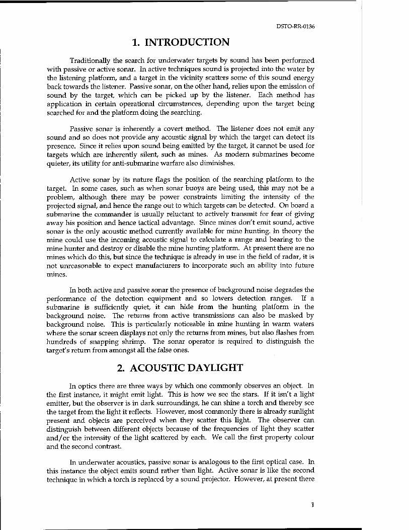
Figure 1 displays the principle behind the method. Sound is generated by a variety of sources such as breaking waves and snapping shrimp. Some of this sound scatters off underwater objects and is reflected towards the acoustic camera, in this case

Fig. 1. Acoustic daylight concept.

DSTO-RR-0136

a hydrophone array on an underwater vehicle, where it is collected and processed to yield an image on a computer screen. Just as one can use front or back lighting in photography, so the sources of sound can be in front of or behind the object. In the latter case the object would appear in acoustic silhouette.

The intensity of sound scattered by different objects would result in a contrast between them. On a grey scale image on a computer screen the good sound reflectors would be drawn in white and the poor reflectors would appear black. False colour could also be added to the images by recording the frequencies of sound scattered by the objects. Certain frequencies of sound could be mapped into optical colour on a computer screen.

3. AMBIENT NOISE

Ambient noise is generated in the ocean by several mechanisms (Urick 1983; 1984). Seismic disturbances produce noise from less than 1 Hz to 100 Hz. The hydrostatic pressure changes induced by tides and surface waves produce noise of just a few hertz. Turbulence of deep ocean currents and swifter oceanic streams is thought to produce noise from 0.1 to 100 Hz. It is also thought that standing waves caused by the interaction of travelling surface waves produce low frequency noise.

Between 50 and 500 Hz distance shipping is the dominant source of ambient noise. The noise consists of two components: tones associated with shaft and propeller blade rotation rates, which are overlain on a continuous spectrum extending to several kilohertz, produced by cavitation. The noise predominantly arrives within ±15° to the horizontal. For shipping close by, the noise is both variable in direction and highly non-stationary.

Between 500 Hz and 30 kHz the ambient noise has a high dependence on wind speed. Breaking surface gravity waves, small-scale spilling breakers and breaking capillary waves inject bubbles into the ocean. The bubbles oscillate at their natural frequency of oscillation, radiating sound into the ocean. As the wind speed increases, breaking waves inject more bubbles into the ocean, leading to more noise. Thus, as the ambient noise becomes less dominated by distant shipping and more by overhead breaking waves, it displays increasing vertical directionality. However, little is known about the horizontal directionality. As the frequency of sound increases, the noise intensity level falls by approximately 17 dB/decade.

Some types of fish, shellfish and marine mammals produce sounds which add to the ambient noise in the ocean. Marine mammals produce clicks, whistles, chirps, grunts, groans, yelps, barks and songs with spectral content to 150 kHz. Some fish, such as the croakers found in Chesapeake Bay, USA, produce a tapping noise, which forms a nearly continuous background noise from the superposition of the tapping of many individuals. Snapping shrimp, which are ubiquitous in shallow warm waters having a bottom offering some concealment, make a snapping sound extending from 500 Hz to more than 200 kHz. In this case the superposition of sounds from many individuals produces a frying sound.

Falling rain and hail can produce an increase in the noise level of up to 30 dB, primarily in the range from 1 to 20 kHz. Some of the sound is made by the impact itself; the rest by the entrainment and subsequent ringing of bubbles produced. Along the shoreline surf generates noise in the low kilohertz range. Because of the location of the generation sites, it is highly directional.

DSTO-RR-0136

14*

30

■ Traffic noise Wind dependent noise at wind speeds shown

10

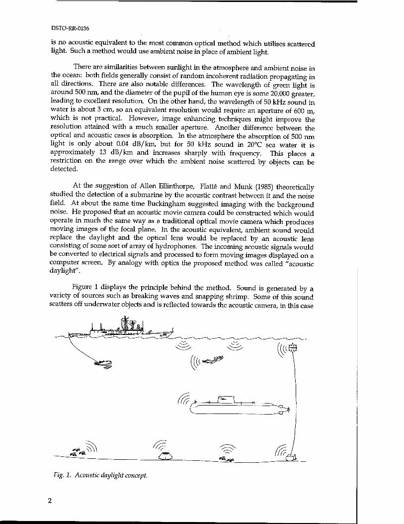
Fig. 2.

100 1000 Frequency (Hz)

Ambient sea noise prediction curves for Australian waters, after Cato (1997)

10000

Below 10 kHz the noise field in the ocean has been widely studied. Frequency spectra have been published and information about depth, temporal and directional variations are known to some extent. The coherence of the noise has also been studied at the lower frequencies. Cato (1997) has published noise curves (Fig. 2) for the Australian underwater environment which plot the intensity of sound versus frequency and identify many of the sources of sound.

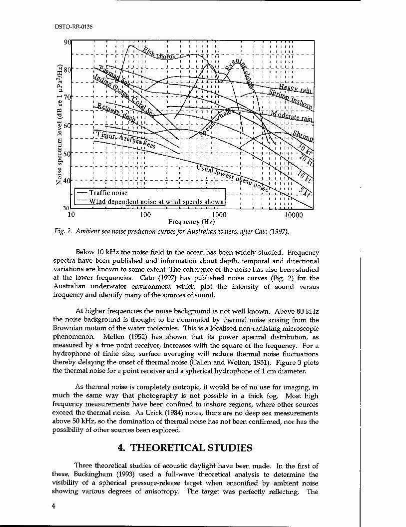
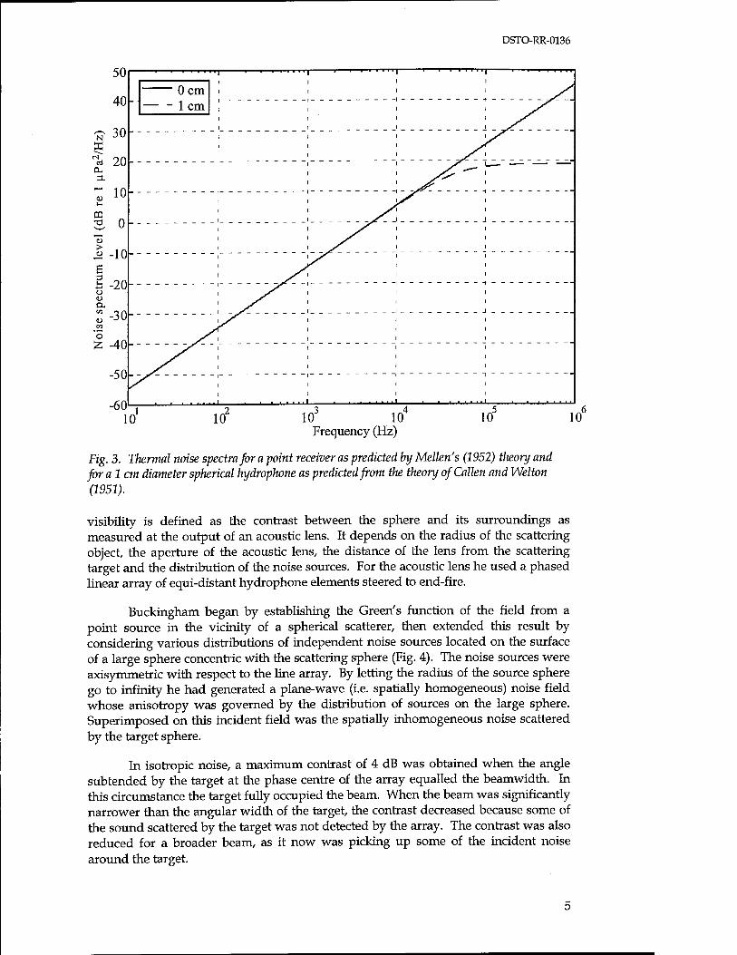
At higher frequencies the noise background is not well known. Above 80 kHz the noise background is thought to be dominated by thermal noise arising from the Brownian motion of the water molecules. This is a localised non-radiating microscopic phenomenon. Meilen (1952) has shown that its power spectral distribution, as measured by a true point receiver, increases with the square of the frequency. For a hydrophone of finite size, surface averaging will reduce thermal noise fluctuations thereby delaying the onset of thermal noise (Callen and Welton, 1951). Figure 3 plots the thermal noise for a point receiver and a spherical hydrophone of 1 cm diameter.

As thermal noise is completely isotropic, it would be of no use for imaging, in much the same way that photography is not possible in a thick fog. Most high frequency measurements have been confined to inshore regions, where other sources exceed the thermal noise. As Urick (1984) notes, there are no deep sea measurements above 50 kHz, so the domination of thermal noise has not been confirmed, nor has the possibility of other sources been explored.

4. THEORETICAL STUDIES

Three theoretical studies of acoustic daylight have been made. In the first of these, Buckingham (1993) used a full-wave theoretical analysis to determine the visibility of a spherical pressure-release target when ensonified by ambient noise showing various degrees of anisotropy. The target was perfectly reflecting. The

DSTO-RR-0136

N ffi a

CL,

o

CO

O

50

40

30

20

10

0

-10

-20

-30

-40

-50

-60

| 1 1 1 i i i i i

-■

0 cm — - 1 cm

y>^

"

10 10 10 10 Frequency (Hz)

10 10

Fig. 3. Thermal noise spectra for a point receiver as predicted by Meilen's (1952) theory and for a lcm diameter spherical hydrophone as predicted from the theory ofCallen and Welton (1951).

visibility is defined as the contrast between the sphere and its surroundings as measured at the output of an acoustic lens. It depends on the radius of the scattering object, the aperture of the acoustic lens, the distance of the lens from the scattering target and the distribution of the noise sources. For the acoustic lens he used a phased linear array of equi-distant hydrophone elements steered to end-fire.

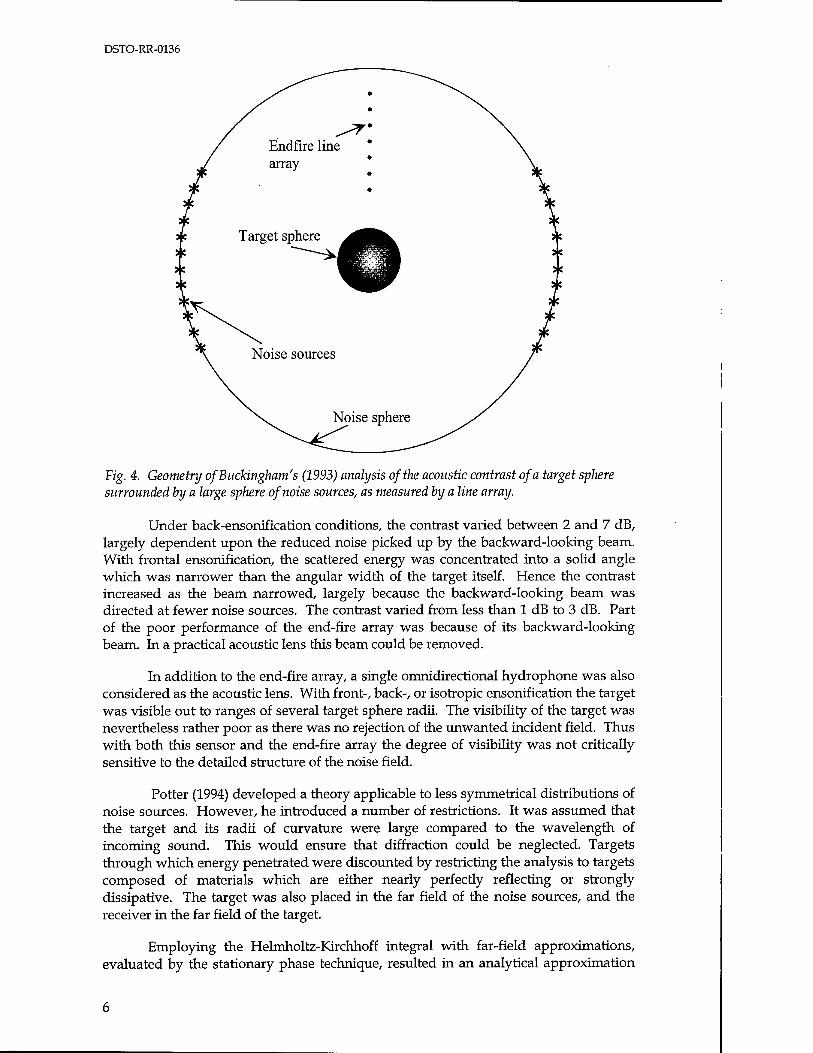
Buckingham began by establishing the Green's function of the field from a point source in the vicinity of a spherical scatterer, then extended this result by considering various distributions of independent noise sources located on the surface of a large sphere concentric with the scattering sphere (Fig. 4). The noise sources were axisymmetric with respect to the line array. By letting the radius of the source sphere go to infinity he had generated a plane-wave (i.e. spatially homogeneous) noise field whose anisotropy was governed by the distribution of sources on the large sphere. Superimposed on this incident field was the spatially inhomogeneous noise scattered by the target sphere.

In isotropic noise, a maximum contrast of 4 dB was obtained when the angle subtended by the target at the phase centre of the array equalled the beamwidth. In this circumstance the target fully occupied the beam. When the beam was significantly narrower than the angular width of the target, the contrast decreased because some of the sound scattered by the target was not detected by the array. The contrast was also reduced for a broader beam, as it now was picking up some of the incident noise around the target.

DSTO-RR-0136

Fig. 4. Geometry of Buckingham's (1993) analysis of the acoustic contrast of a target sphere surrounded by a large sphere of noise sources, as measured by a line array.

Under back-ensonification conditions, the contrast varied between 2 and 7 dB, largely dependent upon the reduced noise picked up by the backward-looking beam. With frontal ensonification, the scattered energy was concentrated into a solid angle which was narrower than the angular width of the target itself. Hence the contrast increased as the beam narrowed, largely because the backward-looking beam was directed at fewer noise sources. The contrast varied from less than 1 dB to 3 dB. Part of the poor performance of the end-fire array was because of its backward-looking beam. In a practical acoustic lens this beam could be removed.

In addition to the end-fire array, a single omnidirectional hydrophone was also considered as the acoustic lens. With front-, back-, or isotropic ensonification the target was visible out to ranges of several target sphere radii. The visibility of the target was nevertheless rather poor as there was no rejection of the unwanted incident field. Thus with both this sensor and the end-fire array the degree of visibility was not critically sensitive to the detailed structure of the noise field.

Potter (1994) developed a theory applicable to less symmetrical distributions of noise sources. However, he introduced a number of restrictions. It was assumed that the target and its radii of curvature were large compared to the wavelength of incoming sound. This would ensure that diffraction could be neglected. Targets through which energy penetrated were discounted by restricting the analysis to targets composed of materials which are either nearly perfectly reflecting or strongly dissipative. The target was also placed in the far field of the noise sources, and the receiver in the far field of the target.

Employing the Helmholtz-Kirchhoff integral with far-field approximations, evaluated by the stationary phase technique, resulted in an analytical approximation

DSTO-RR-0136

for die energy density scattered by the target near the specular angle for the case of a single noise source. The expression was summed over many noise sources and segments of the target to yield the total field.

The first case studied was a rigid sphere in isotropic noise. The noise field was modelled by a large number of incoherent noise sources placed on the surface of a very large spherical shell centred on the spherical target. The result, which was independent of beamwidth of a receiver, was that there would be no contrast difference between the target and the background. Hence the target would be invisible. This result differed from Buckingham's exact full wave analysis, which had found a 4-6 dB contrast for an end-fire array whose beam was just filled by the target. It was noted that to obtain a sufficiently narrow beam, Buckingham required a linear array whose length was 40% of the separation between the array phase centre and the target. Thus Buckingham's result applied to the near field. In the far field both theories agreed - the target would be invisible.

To study more complicated noise source distributions, Potter used a ray tracing technique. He summed eigenrays back-propagating from die receiver to die target and tiience to the noise sources, or directly to the noise sources. This geometrical approach assumed a homogeneous propagation medium. The receiver modelled was the almost planar ADONIS hydrophone array (described below), consisting of 126 elements spaced 20 mm apart and operating at 75 kHz. The beamwidths were 0.76°. Two similar but more highly resolving systems were also considered, with 9 and 900 times die resolution.

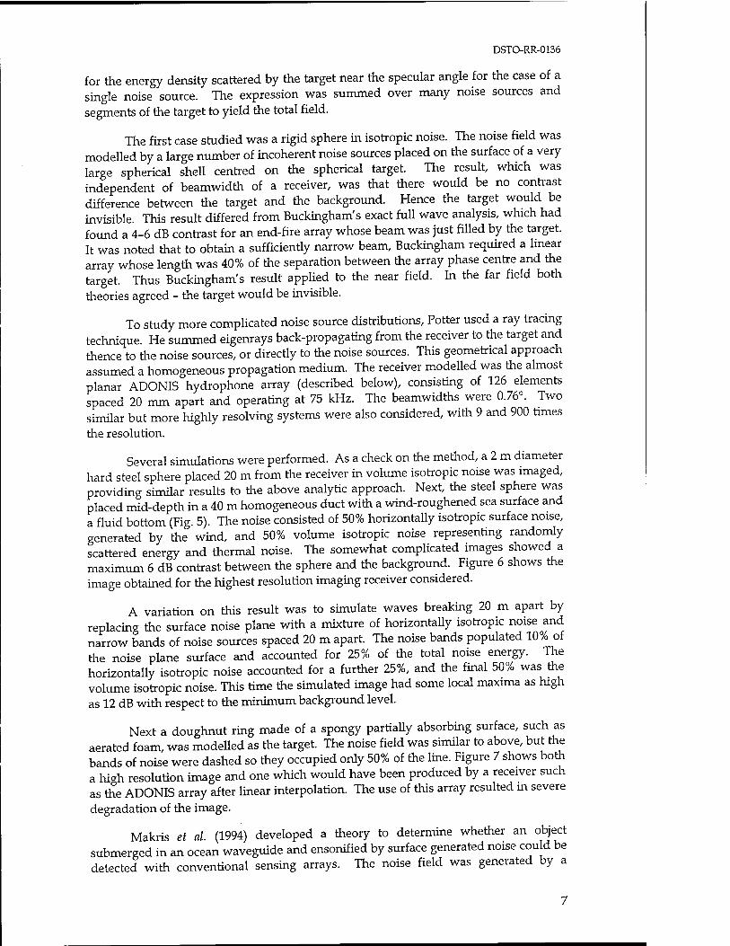
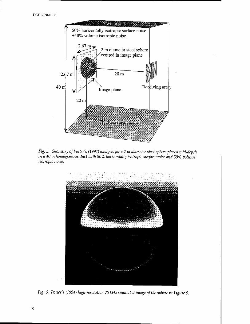
Several simulations were performed. As a check on the metiiod, a 2 m diameter hard steel sphere placed 20 m from die receiver in volume isotropic noise was imaged, providing similar results to the above analytic approach. Next, the steel sphere was placed mid-depth in a 40 m homogeneous duct with a wind-roughened sea surface and a fluid bottom (Fig. 5). The noise consisted of 50% horizontally isotropic surface noise, generated by the wind, and 50% volume isotropic noise representing randomly scattered energy and thermal noise. The somewhat complicated images showed a maximum 6 dB contrast between the sphere and the background. Figure 6 shows the image obtained for the highest resolution imaging receiver considered.

A variation on this result was to simulate waves breaking 20 m apart by replacing the surface noise plane with a mixture of horizontally isotropic noise and narrow bands of noise sources spaced 20 m apart. The noise bands populated 10% of die noise plane surface and accounted for 25% of the total noise energy. The horizontally isotropic noise accounted for a further 25%, and the final 50% was the volume isotropic noise. This time the simulated image had some local maxima as high as 12 dB with respect to the minimum background level.

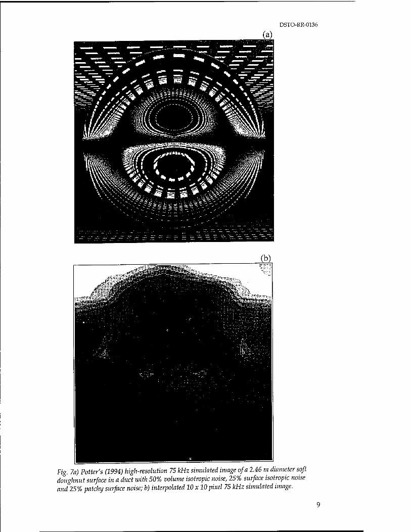
Next a doughnut ring made of a spongy partially absorbing surface, such as aerated foam, was modelled as the target. The noise field was similar to above, but the bands of noise were dashed so they occupied only 50% of the line. Figure 7 shows both a high resolution image and one which would have been produced by a receiver such as the ADONIS array after linear interpolation. The use of this array resulted m severe

degradation of the image.

Makris et al (1994) developed a theory to determine whether an object submerged in an ocean waveguide and ensonified by surface generated noise could be detected with conventional sensing arrays. The noise field was generated by a

7

DSTO-RR-0136

Water surface

50% horizontally +50% volume

isotropic surface noise isotropic noise

2 m diameter steel sphere centred in image plane

Fluid basement plane

Fig. 5. Geometry of Potter's (1994) analysis for aim diameter steel spliere placed mid-depth in a 40 m homogeneous duct with 50% horizontally isotropic surface noise and 50% volume isotropic noise.

Fig. 6. Potter's (1994) high-resolution 75 kHz simulated image of the sphere in Figure 5.

DSTO-RR-0136

Fig. 7a) Potter's (1994) high-resolution 75 kHz simulated image of a 2.46 m diameter soft doughnut surface in a duct with 50% volume isotropic noise, 25% surface isotropic noise and 25% patchy surface noise; b) interpolated 10 x 10 pixel 75 kHz simulated image.

DSTO-RR-0136

continuous sheet of stochastic sources submerged within a quarter wavelength of the free surface and extended uniformly in range and azimuth from the object. The simulated sensing array was an upright, filled, 7 x 7-element, planar array, with the individual hydrophone elements at half wavelength spacing, leading to a broadside beamwidth of 38° for all simulations. Using full-field wave theory they derived an expression for the total noise field covariance of a stratified shallow waveguide with a submerged pressure-release sphere present at the centre of the water column. This was evaluated by numerical wavenumber integration at 50,300 and 10,000 Hz.

In the first simulation they attempted to detect a 20 m diameter sphere at 50 Hz. The array spanned the full 100 m water column. At a range of 100 m the detection level was 1.4 dB, decreasing to 0.1 dB at 500 m range. They then tried to detect the same sphere at 300 Hz, for which the array spanned 15 m of the water column, and obtained similar detection levels. Finally they attempted to detect a 0.5 m diameter sphere at 10 kHz, for which the array occupied 0.45 m of the water column. At 2 m range from the sphere the detection level was 3.6 dB, but it was not detectable at 10 m range. They concluded that detecting objects using ambient noise presses the limits of current technology for azimuthally homogeneous noise, but .that high resolution imaging is more effective within the deep shadow range of the object.

The acoustic contrasts reported by Makris et al. were significantly lower than those calculated by Buckingham (1993) or Potter (1994). The reason was the insufficient angular resolution used. In the first simulation, the angle subtended by the 20 m diameter sphere at 100 m range was 11.4°, which was only 30% of the 38° beamwidth. In the final example the angle subtended by the 0.5 m diameter sphere at 10 m range was 2.8°, which was only 8% of the beamwidth. Since the angle subtended by the sphere was smaller than the beamwidth, background noise leaked into the beam, reducing the acoustic contrast. A second factor contributing to the poor contrast was the omission of a baffle behind the array to eliminate unwanted noise arriving at the rear.

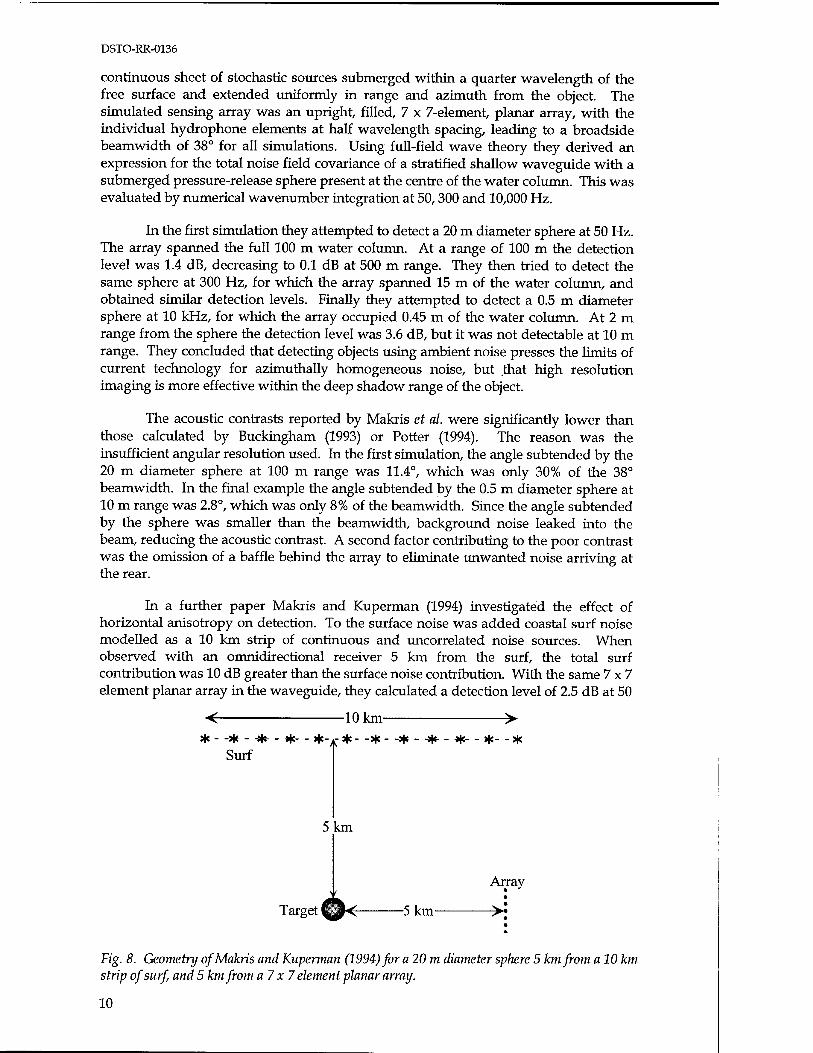
In a further paper Makris and Kuperman (1994) investigated the effect of horizontal anisotropy on detection. To the surface noise was added coastal surf noise modelled as a 10 km strip of continuous and uncorrelated noise sources. When observed with an omnidirectional receiver 5 km from the surf, the total surf contribution was 10 dB greater than the surface noise contribution. With the same 7 x7 element planar array in the waveguide, they calculated a detection level of 2.5 dB at 50

< 10 km > sk - -sk - -9fc- - -9k- - >k~ A- sk - ->k - -sk - -sk- - -94c-

Surf

Km

Array

Target EK 5 km >•

Fig. 8. Geometry of Makris and Kuperman (1994) for a 20 m diameter sphere 5 km from a 10 km strip of surf and 5 km from a 7 x 7 element planar array.

10

DSTO-RR-0136

Hz for a 20 m diameter sphere located with the geometry shown in Figure 8. They concluded that horizontal anisotropy might significantly improve the detectability of a target and thereby increase the maximum detection range.

In these four theoretical studies a number of simplifying assumptions were made, which in many cases are not applicable to target detection. Firstly, it was assumed that many noise sources simultaneously contributed to the ambient noise. However, in coastal waters where the noise from snapping shrimp dominate, the more intense ensonification events come predominantly from one snap at a time. A second assumption was that reflections from the target were assumed to be specular. Thirdly, no penetration of sound into the target was considered.

5. FIRST EXPERIMENT

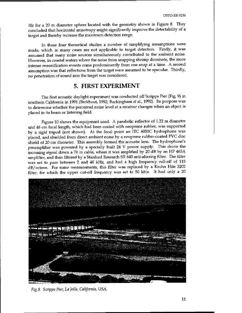
The first acoustic daylight experiment was conducted off Scripps Pier (Fig. 9) in southern California in 1991 (Berkhout, 1992; Buckingham et al.t 1992). Its purpose was to determine whether the perceived noise level at a receiver changes when an object is placed in its beam or listening field.

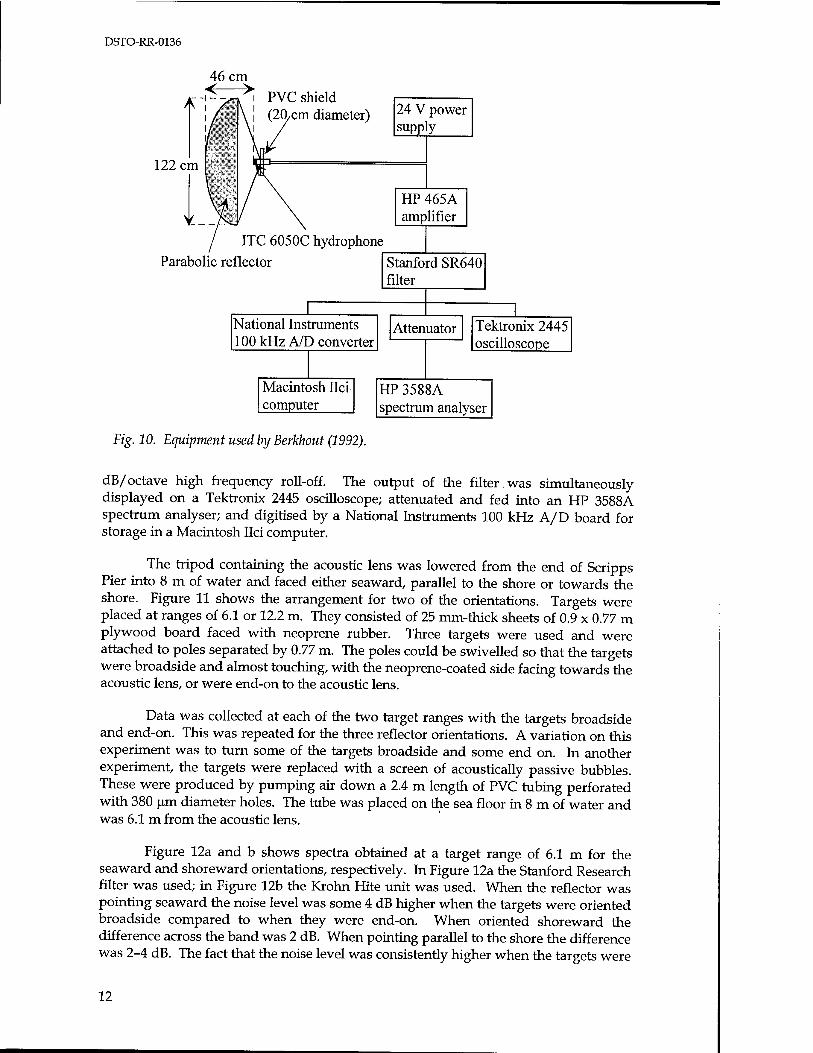
Figure 10 shows the equipment used. A parabolic reflector of 1.22 m diameter and 46 cm focal length, which had been coated with neoprene rubber, was supported by a rigid tripod (not shown). At the focal point an ITC 6050C hydrophone was placed, and shielded from direct ambient noise by a neoprene rubber-coated PVC disc shield of 20 cm diameter. This assembly formed the acoustic lens. The hydrophone's preamplifier was powered by a specially built 24 V power supply. This drove the incoming signal down a 76 m cable, where it was amplified by 20 dB by an HP 465A amplifier, and then filtered by a Stanford Research SR 640 anti-aliasing filter. The filter was set to pass between 2 and 40 kHz, and had a high frequency roll-off of 115 dB/octave. For some measurements, this filter was replaced by a Krohn Hite 3202 filter, for which the upper cut-off frequency was set to 50 kHz. It had only a 20

Fig.9. Scripps Pier, La]olla, California, USA.

11

DSTO-RR-0136

122 cm

PVC shield (20,cm diameter) 24 V power

supply

HP 465A amplifier

ITC 6050C hydrophone

Parabolic reflector Stanford SR640 filter

National Instruments 100 kHz A/D converter

Attenuator

Macintosh Ilci computer

Tektronix 2445 oscilloscope

HP 3588A spectrum analyser

Fig. 10. Equipment used by Berkhout (1992).

dB/octave high frequency roll-off. The output of the filter was simultaneously displayed on a Tektronix 2445 oscilloscope; attenuated and fed into an HP 3588A spectrum analyser; and digitised by a National Instruments 100 kHz A/D board for storage in a Macintosh Ilci computer.

The tripod containing the acoustic lens was lowered from the end of Scripps Pier into 8 m of water and faced either seaward, parallel to the shore or towards the shore. Figure 11 shows the arrangement for two of the orientations. Targets were placed at ranges of 6.1 or 12.2 m. They consisted of 25 mm-thick sheets of 0.9 x 0.77 m plywood board faced with neoprene rubber. Three targets were used and were attached to poles separated by 0.77 m. The poles could be swivelled so that the targets were broadside and almost touching, with the neoprene-coated side facing towards the acoustic lens, or were end-on to the acoustic lens.

Data was collected at each of the two target ranges with the targets broadside and end-on. This was repeated for the three reflector orientations. A variation on this experiment was to turn some of the targets broadside and some end on. In another experiment, the targets were replaced with a screen of acoustically passive bubbles. These were produced by pumping air down a 2.4 m length of PVC tubing perforated with 380 urn diameter holes. The tube was placed on the sea floor in 8 m of water and was 6.1 m from the acoustic lens.

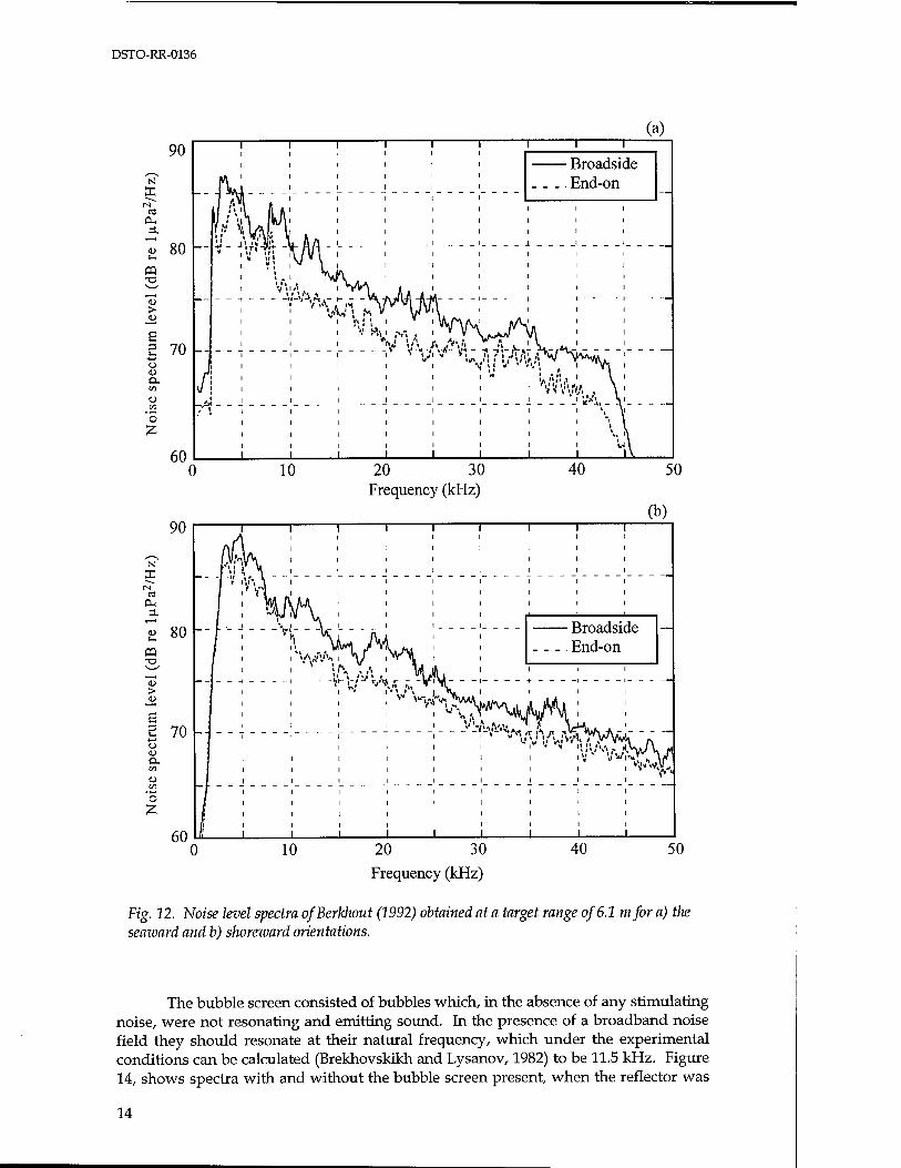
Figure 12a and b shows spectra obtained at a target range of 6.1 m for the seaward and shoreward orientations, respectively. In Figure 12a the Stanford Research filter was used; in Figure 12b the Krohn Hite unit was used. When the reflector was pointing seaward the noise level was some 4 dB higher when the targets were oriented broadside compared to when they were end-on. When oriented shoreward the difference across the band was 2 dB. When pointing parallel to the shore the difference was 2-4 dB. The fact that the noise level was consistently higher when the targets were

12

DSTO-RR-0136

Scripps Pier

Fig. 11. Experimental configuration ofBerkhout (1992), shozving the seaward and shoreward orientation of the targets.

broadside indicated that the source of ambient noise was coming from behind the reflector, amongst the pier pilings.

At a range of 12.2 m, similar results were obtained at frequencies above 15 kHz, for which frequency the targets still occupied the beam. At lower frequencies the beam also imaged the area behind the targets, so the contrast was lessened. Contrast diminished to negligible levels below 5 kHz. Figure 13 plots the relative intensity normalised to the ambient noise field when the reflector was pointing parallel to the shore. The difference between broadside and end-on orientations in clear. There is also a difference between an absence of the targets altogether and when they were end-on. In the latter case the supporting poles were making a contribution. Another noticeable feature of the spectrogram are the bands of high intensity centred at 10, 22, 33 and 48 kHz, providing evidence for acoustic colour.

The experiments with various target panels broadside and end-on were consistent with the above results. The acoustic lens was able to distinguish between the different target configurations at a range of 6.1 m.

13

DSTO-RR-0136

(a) 90 1— 1 1 1 1 1 1 ■-

! ] 1

1

Broadside . End-on

17M A 1 •v'l Aft

y-4*n i ?!

1 1 1 ..

t 1 I v. - - -t - - - -i

1

1

1

a P-c a.

« 80 J-H

CQ

w

1 1

1 1

1 1

: MI*

1 1

1 1

1 1

e sp

ectr

um l

eve

o

1 1 1

' i» ; »

vA —

1

1

1

■ \?

'o Z

60 C

1

1

]

1 1 1

i i

i i

i i

i i

i " iV

) 10 20 30 40 5< Frequency (kHz)

(b) 90

II Jl

i 1

1

1

1

i i

i

i

i

i 1

ts

CM

I 1 V v. i

\ 1

i

Broadside . End-on

— 2 80 CQ T3

v '.ft, ,.* i

\A lA '

I

i

e sp

ectr

um l

eve

o

1 1 "* ,, Nu..»' i

1

1

1

1

1

1

1 1 l > »n-\ 1 1 1

'S

1 I 1

1 1 1

1 1 1 1

1 1 1 1

1 1 1 1

1 1 1 1

1 1 1 1 1

10 20 30 40 50

Frequency (kHz)

Fig. 12. Noise level spectra ofBerkhout (1992) obtained at a target range of 6.1 mfor a) tlte seaward and b) shoreward orientations.

The bubble screen consisted of bubbles which, in the absence of any stimulating noise, were not resonating and emitting sound. In the presence of a broadband noise field they should resonate at their natural frequency, which under the experimental conditions can be calculated (Brekhovskikh and Lysanov, 1982) to be 11.5 kHz. Figure 14, shows spectra with and without the bubble screen present, when the reflector was

14

DSTO-RR-0136

Acoustic intensity normalised by the ambient noise level (dB) 0 2 4 6

20 30 Frequency (kHz)

Fig. 13. Acoustic intensity normalised by the ambient noise field obtained by Berkhout (1992) when the reflector was pointing parallel to the shore. The targets were at 12.2 m range and were either absent, broadside or end-on.

90

u 80 « T3

>

e H70 o <u a. C/3

o

60

- —1 1 1 1 1— 1 1 1 1 1

- i" 1 r 1— ■ i i i

1 1 1 1 1

1 1 1 1 1 1 1 1 1 1

.... , , ... ■ With bubble screen Without bubble screen

|J ! V /s ' ' ' ' ' ' ' ' .-I "»JUl/u1 - ' '- '- ' -' ' - -'

W ' *V *\ ' ' ' ' iii 1 ' V \ » ' ' i i i i i

1 y ,W\A !!,,!!, 1 I i I \ i i i i i i i 1 *» \

1 '«'• •• WvAA ' ' ' ' ' ' I i Y\". i IMC ~ V I i i i i i ,v,w' , l.vVk/*i

II 1 1 Ir "\ 1 1 1 1 1 - -J T _!_ !_ T ^jo._ -jy_ _(_ _r T , | 1 1 1 1 XSfW* "\ ,'-..>J _ ,M 1 1 1 P i i i I i vVU*Äv i ,«.,( i i

/; i i i i i i ^* iv. i

-

/ r ~ i_" i" "" r " ~ i ~ "i ~r ~ " r*» vw"i " i " ■ i i i i i i i I^MJ i ■ i i i i i i i i V i ; i i i i i i i i o i

i i i i i i i i L i

10 20 30 Frequency (kHz)

40 50

Fig. 14. Noise level spectrum of Berkhout (1992) for a bubble screen at 6.1m range for the seaward orientation.

pointing seaward. Over a band between 9 and 14 kHz the difference is 5 dB; elsewhere it is negligible. Similar results were obtained when the reflector was pointing parallel to the shore. The results indicate that the bubbles are excited at their resonant frequency by ambient noise, and so are visible to acoustic daylight.

Before these experiments were undertaken, it had been anticipated that the primary source of ambient noise would come from the surf zone. The targets would

15

DSTO-RR-0136

s below Joise spectrum level (dB re 1 uPa2/Hz) v ^ fa ■ % Ml

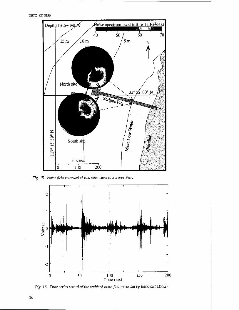
Fig. 15. Noise field recorded at two sites close to Scripps Pier.

T

50 100 150 200 Time (ms)

Fig. 16. Time series record of the ambient noise field recorded by Berkhout (1992).

16

DSTO-RR-0136

20 30 Frequency (kHz)

(b)

N

? 90

pa

> 0)

80

o a, en

'S

70

1 1 1 1 I 1 1— 1 .... 1—

ttroaasiae End-on

V,I\IV VV

i i

i i

fa 1 k\ * r - - -

i

l 1

l l

1 1 1

0 10 40 50 20 30 Frequency (kHz)

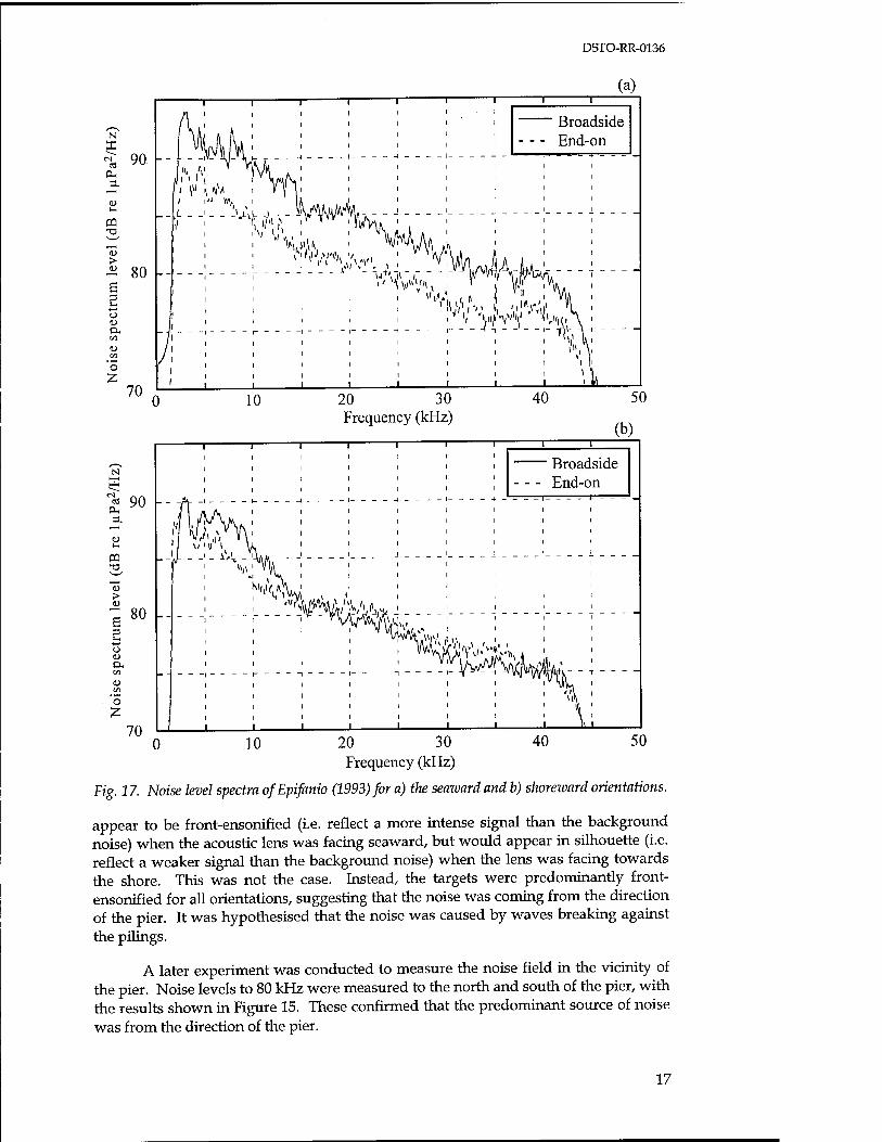
Fig. 17. Noise level spectra ofEpifanio (1993) for a) the seaward and b) shoreward orientations.

appear to be front-ensonified (i.e. reflect a more intense signal than the background noise) when the acoustic lens was facing seaward, but would appear in silhouette (i.e. reflect a weaker signal than the background noise) when the lens was facing towards the shore. This was not the case. Instead, the targets were predominantly front- ensonified for all orientations, suggesting that the noise was coming from the direction of the pier. It was hypothesised that the noise was caused by waves breaking against the pilings.

A later experiment was conducted to measure the noise field in the vicinity of the pier. Noise levels to 80 kHz were measured to the north and south of the pier, with the results shown in Figure 15. These confirmed that the predominant source of noise was from the direction of the pier.

17

DSTO-RR-0136

On inspecting time series of the data (Fig. 16) Epifanio (1993) noted that the noise consisted of loud noise events and a quieter background noise. Postulating that the loud events were coming from the pilings, he removed the latter and recomputed the noise spectra, as shown in Figure 17. This time there was a discernible difference: in the seaward orientation the targets reflected more intensely than the background, as before, but for the shoreward orientation the targets reflected more weakly than the background above 18 kHz. In this orientation the targets were now in silhouette.

The overall result of this first acoustic daylight experiment was to show that a target can alter the noise field, but being a parabolic reflector with a single hydrophone at its focus, it formed a single beam and so corresponded to just one pixel of an image. To build up an image a multi-beam acoustic lens is necessary. If the system was broadband, it would be able to make use of the acoustic colour characteristic.

6. ADONIS

The first operational acoustic daylight system was designed and built at Scripps Institution of Oceanography, in a research group headed by Mike Buckingham. Key participants included Chad Epifanio and John Potter. The acoustic camera was called 'ADONIS', which stands for Acoustic Daylight Ocean Noise Imaging System.

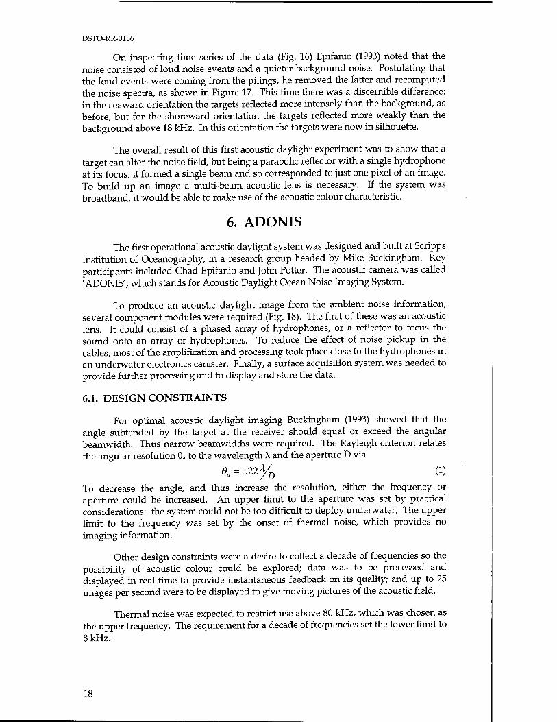
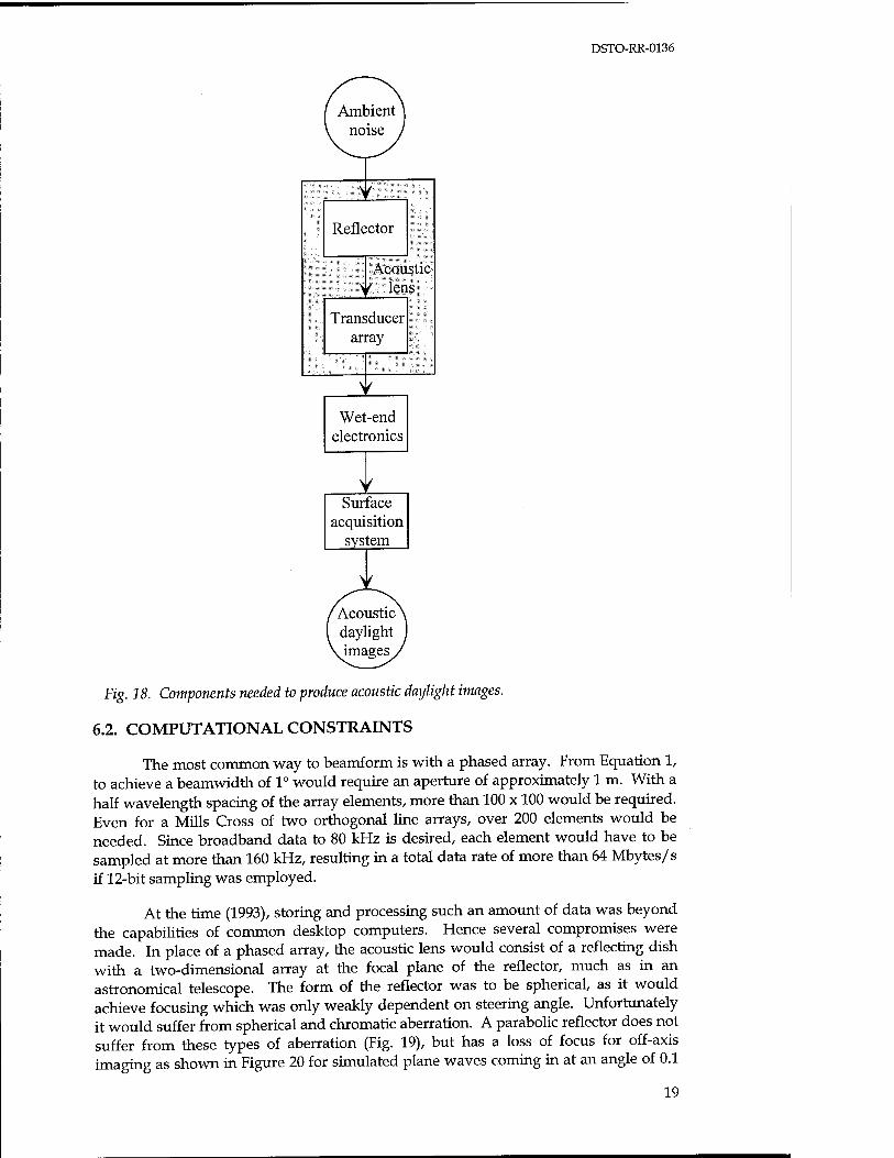
To produce an acoustic daylight image from the ambient noise information, several component modules were required (Fig. 18). The first of these was an acoustic lens. It could consist of a phased array of hydrophones, or a reflector to focus the sound onto an array of hydrophones. To reduce the effect of noise pickup in the cables, most of the amplification and processing took place close to the hydrophones in an underwater electronics canister. Finally, a surface acquisition system was needed to provide further processing and to display and store the data.

6.1. DESIGN CONSTRAINTS

For optimal acoustic daylight imaging Buckingham (1993) showed that the angle subtended by the target at the receiver should equal or exceed the angular beamwidth. Thus narrow beamwidths were required. The Rayleigh criterion relates the angular resolution 0a to the wavelength A, and the aperture D via

0,=1.22% (1)

To decrease the angle, and thus increase the resolution, either the frequency or aperture could be increased. An upper limit to the aperture was set by practical considerations: the system could not be too difficult to deploy underwater. The upper limit to the frequency was set by the onset of thermal noise, which provides no imaging information.

Other design constraints were a desire to collect a decade of frequencies so the possibility of acoustic colour could be explored; data was to be processed and displayed in real time to provide instantaneous feedback on its quality; and up to 25 images per second were to be displayed to give moving pictures of the acoustic field.

Thermal noise was expected to restrict use above 80 kHz, which was chosen as the upper frequency. The requirement for a decade of frequencies set the lower limit to 8 kHz.

18

DSTO-RR-0136

Reflector

Acoustic y lens

Transducer array

Wet-end electronics

Surface acquisition

system

Fig. 18. Components needed to produce acoustic daylight images.

6.2. COMPUTATIONAL CONSTRAINTS

The most common way to beamform is with a phased array. From Equation 1, to achieve a beamwidth of 1° would require an aperture of approximately 1 m. With a half wavelength spacing of the array elements, more than 100 x 100 would be required. Even for a Mills Cross of two orthogonal line arrays, over 200 elements would be needed. Since broadband data to 80 kHz is desired, each element would have to be sampled at more than 160 kHz, resulting in a total data rate of more than 64 Mbytes/s if 12-bit sampling was employed.

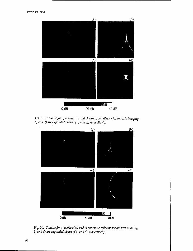
At the time (1993), storing and processing such an amount of data was beyond the capabilities of common desktop computers. Hence several compromises were made. In place of a phased array, the acoustic lens would consist of a reflecting dish with a two-dimensional array at the focal plane of the reflector, much as in an astronomical telescope. The form of the reflector was to be spherical, as it would achieve focusing which was only weakly dependent on steering angle. Unfortunately it would suffer from spherical and chromatic aberration. A parabolic reflector does not suffer from these types of aberration (Fig. 19), but has a loss of focus for off-axis imaging as shown in Figure 20 for simulated plane waves coming in at an angle of 0.1

19

DSTO-RR-0136

OdB 20 dB 40 dB

Fig. 19. Caustic for a) a spherical and c) parabolic reflector for on-axis imaging, b) and d) are expanded views of a) and c), respectively.

OdB 20 dB 40 dB

Fig. 20. Caustic for a) a spherical and c) parabolic reflector for off-axis imaging, b) and d) are expanded views of a) and c), respectively.

20

DSTO-RR-0136

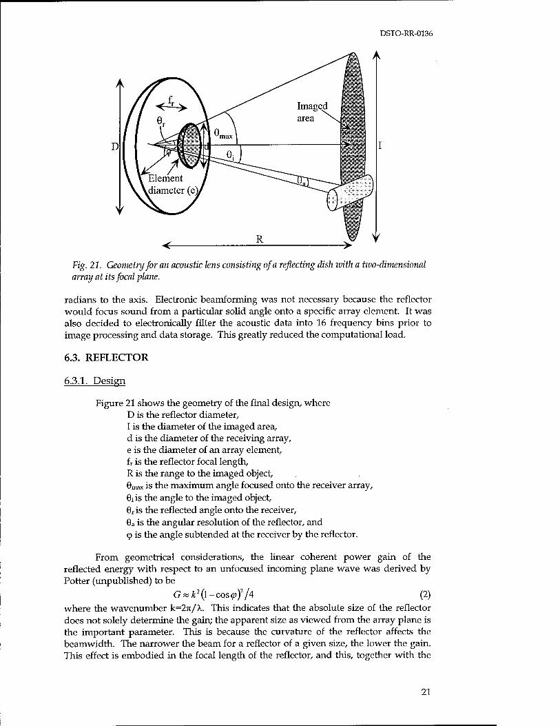
Fig. 21. Geometry for an acoustic lens consisting of a reflecting dish ivith a two-dimensional array at its focal plane.

radians to the axis. Electronic beamforming was not necessary because the reflector would focus sound from a particular solid angle onto a specific array element. It was also decided to electronically filter the acoustic data into 16 frequency bins prior to image processing and data storage. This greatly reduced the computational load.

6.3. REFLECTOR

6.3.1. Design

Figure 21 shows the geometry of the final design, where D is the reflector diameter, I is the diameter of the imaged area, d is the diameter of the receiving array, e is the diameter of an array element, fr is the reflector focal length, R is the range to the imaged object, Gmax is the maximum angle focused onto the receiver array, 0i is the angle to the imaged object, 0r is the reflected angle onto the receiver, 9a is the angular resolution of the reflector, and (p is the angle subtended at the receiver by the reflector.

From geometrical considerations, the linear coherent power gain of the reflected energy with respect to an unfocused incoming plane wave was derived by Potter (unpublished) to be

G«£2(l-cos^)2/4 (2) where the wavenumber k=27t/A,. This indicates that the absolute size of the reflector does not solely determine the gain; the apparent size as viewed from the array plane is the important parameter. This is because the curvature of the reflector affects the beamwidth. The narrower the beam for a reflector of a given size, the lower the gain. This effect is embodied in the focal length of the reflector, and this, together with the

21

DSTO-RR-0136

physical size of the reflector, is contained in the apparent size viewed from the receiver point, 9. For acceptable geometric focusing from a spherical reflector, 9 < 1.

Two design constraints on the acoustic lens were the decision to image a region defined by Qmax = 0.1 radians, and a restriction on the physical size of the reflector to 3 m. The first constraint defined the total imaged area to be

I-TtiRB^)2 (3)

or 78 m2 at 50 m range. With a beamwidth resolution given approximately by RX/D, targets would need to be about 1 m2 to be resolved at 50 m range at 25 kHz, the logarithmic mid-point of the frequency range 8-80 kHz. The second design constraint was set by the anticipated manageability of the lens underwater. To satisfy the restriction on 9, and at the same time to achieve maximum gain, the radius of rotation of the spherical reflector was set to 3 m. According to Equation 2, the gain at 25 kHz would be 27 dB. This gain will not be realised in practice, since the spherical reflector does not focus either coherently or without aberration.

6.3.2. Focal point

The focal point can be estimated using the optical mirror equation

.1 = 1 — rc~R + fr

(4)

where rc is the radius of curvature of the reflector. Based on this, the focal point is 1.5

Intensity (dB re 1 (j.Pa2)

>z

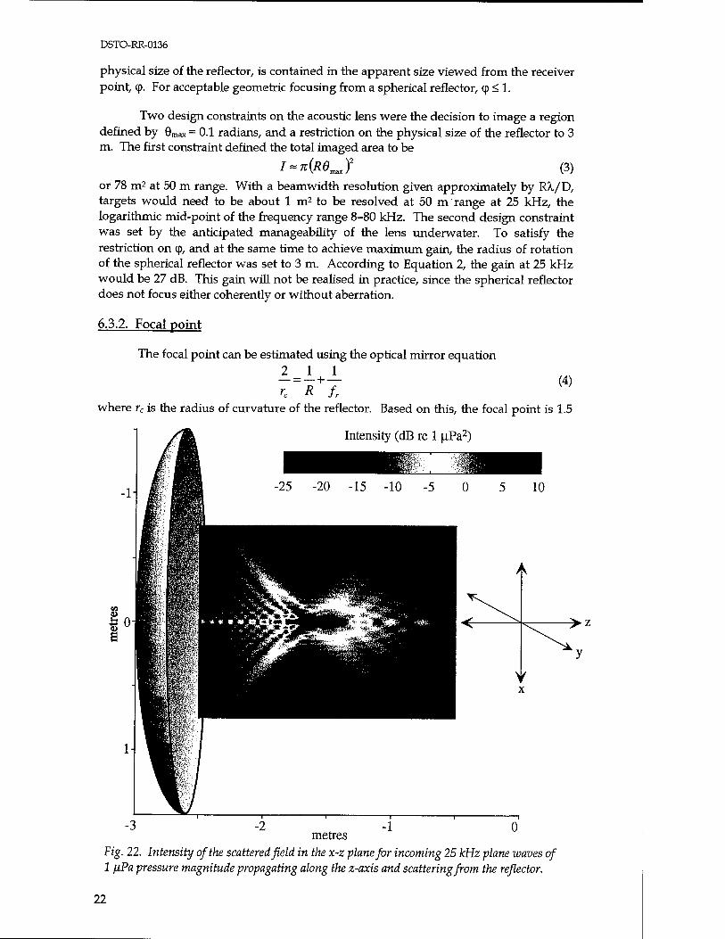
metres Fig. 22. Intensity of the scattered field in the x-z plane for incoming 25 kHz plane waves of 1 ßPa pressure magnitude propagating along the z-axis and scattering from the reflector.

22

DSTO-RR-0136

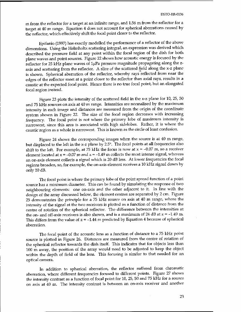
m from the reflector for a target at an infinite range, and 1.56 m from the reflector for a target at 40 m range. Equation 4 does not account for spherical aberrations caused by the reflector, which effectively shift the focal point closer to the reflector.

Epifanio (1997) has exactly modelled the performance of a reflector of the above dimensions. Using the Helmholtz scattering integral, an expression was derived which described the pressure field at any point within the focal region of the dish for both plane waves and point sources. Figure 22 shows how acoustic energy is focused by the reflector for 25 kHz plane waves of lyPa pressure magnitude propagating along the z- axis and scattering from the reflector. A slice of the scattered field along the x-z plane is shown. Spherical aberration of the reflector, whereby rays reflected from near the edges of the reflector meet at a point closer to the reflector than axial rays, results in a caustic at the expected focal point. Hence there is no true focal point, but an elongated focal region instead.

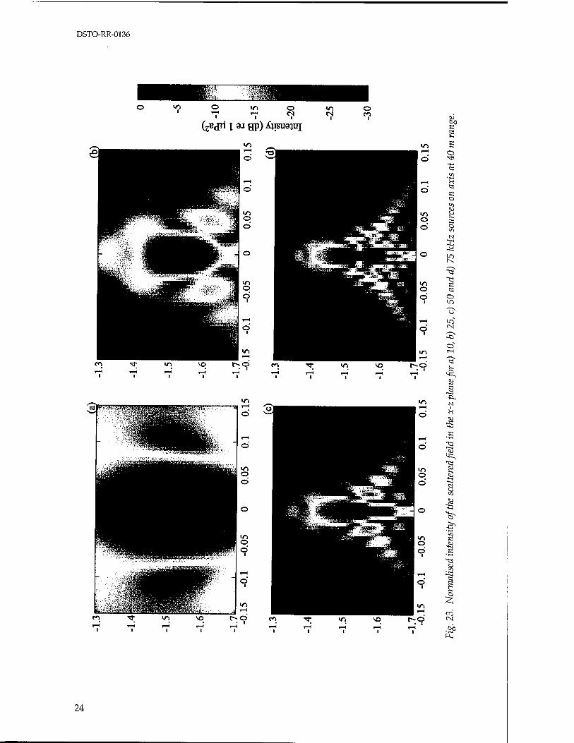
Figure 23 plots the intensity of the scattered field in the x-z plane for 10, 25, 50 and 75 kHz sources on axis at 40 m range. Intensities are normalised by the maximum intensity in each image and distances are measured from the origin of the coordinate system shown in Figure 22. The size of the focal region decreases with increasing frequency. The focal point is not where the primary lobe of maximum intensity is narrowest, since this area is associated with high sidelobes. Rather, it is where the caustic region as a whole is narrowest. This is known as the circle of least confusion.

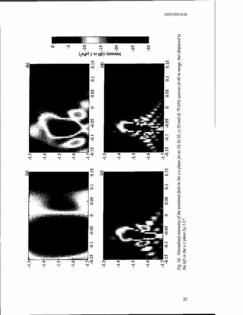
Figure 24 shows the corresponding images when the source is at 40 m range, but displaced to the left in the x-z plane by 2.5°. The focal points at all frequencies also shift to the left. For example, at 75 kHz the focus is now at x = -0.07 m, so a receiver element located at x = -0.07 m and z = -1.49 m collects the most intense signal, whereas an on-axis element collects a signal which is 20 dB less. At lower frequencies the focal regions broaden, so, for example, the on-axis element receives a 10 kHz signal down by only 10 dB.

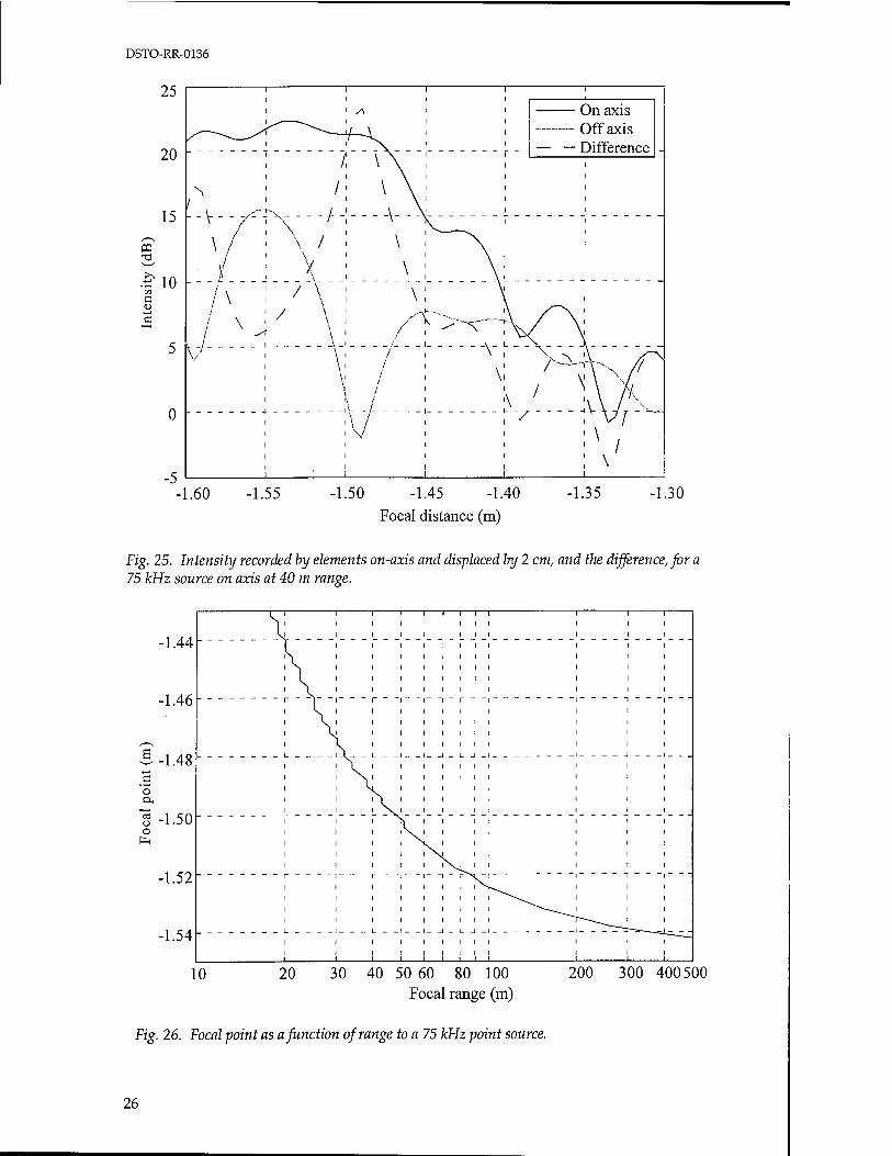
The focal point is where the primary lobe of the point spread function of a point source has a minimum diameter. This can be found by simulating the response of two neighbouring elements: one on-axis and the other adjacent to it. In line with the design of the array discussed below, the element centres are separated by 2 cm. Figure 25 demonstrates the principle for a 75 kHz source on axis at 40 m range, where the intensity of the signal at the two receivers is plotted as a function of distance from the centre of rotation of the spherical reflector. The difference between the intensities at the on- and off-axis receivers is also shown, and is a maximum of 24 dB at z = -1.49 m. This differs from the value of z = -1.44 m predicted by Equation 4 because of spherical aberration.

The focal point of the acoustic lens as a function of distance to a 75 kHz point source is plotted in Figure 26. Distances are measured from the centre of rotation of the spherical reflector towards the dish itself. This indicates that for objects less than 100 m away, the position of the array would need to be adjusted to keep the object within the depth of field of the lens. This focusing is similar to that needed for an optical camera.

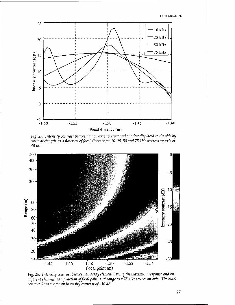
In addition to spherical aberration, the reflector suffered from chromatic aberration, where different frequencies focused to different points. Figure 27 shows the intensity contrast as a function of focal point for 10, 25, 50 and 75 kHz for a source on axis at 40 m. The intensity contrast is between an on-axis receiver and another

23

DSTO-RR-0136

(zB<rrt taj ap) tystrajui g

X « R o

O

R «

N i

J*

»—a

IS

s

•a to

R

24

DSTO-RR-0136

(ru<p11 ai gp) XJISUSIUI s

s s o

s o to

I e « o

in CN

ST o"

'S"

K « 1—4

ft. N

l

Ja

s

^ o •

CN

o >> o ■5 S *« «

ft. I—1 i-S •^ o

R X V. J&

i

CN ^T>

25

DSTO-RR-0136

ff) T3

■1.60 -1.50 -1.45 -1.40

Focal distance (m)

Fig. 25. Intensity recorded by elements on-axis and displaced by 2 cm, and the difference, for a 75 kHz source on axis at 40 m range.

-1.44

-1.46

-1.48

o

g -1.50 o

-1.52

-1.54

p - _,_ _,_ _ _ , _, !_ _, _ r _, _!- _ - _,_ -,

L _ „ _ _ I _L_ _l_ _ _|__|_ _|_ U -1-1- _ - _-_ _ -I- - -- -1

! , , , , , _^- -, , ,

L____|___U__I__I__I_U-J-I---- ----!-- -~~^~~~3

10 20 30 40 50 60 80 100 Focal range (m)

200 300 400500

Fig. 26. Focal point as a function of range to a 75 kHz point source.

26

DSTO-RR-0136

25

20

15 -

a o o >>

-4->

a

10

c 5 -

1 "T" |

—10 kHz

— 25 kHz

— 50 kHz

— 75 kHz

■-

\ ——' """ ,—'y t * ■**", *i-—1 _ .

1 i i ■1.60 ■1.55 -1.50

Focal distance (m)

-1.45 -1.40

Fig. 27. Intensity contrast between an on-axis receiver and another dis-placed to the side by one wavelength, as a function of focal distance for 10, 25, 50 and 75 kHz sources on axis at 40 m.

-1.44 -1.46 -1.52 -1.54 -1.48 -1.50 Focal point (m)

Fig. 28. Intensity contrast between an array element having the maximum response and an adjacent element, as a function of focal point and range to a 75 kHz source on axis. The black contour lines are for an intensity contrast of-10 dB.

27

DSTO-RR-0136

displaced to the side by one wavelength. The focal points are at -1.515, -1.51, -1.50 and -1.49 m, respectively. This poses a problem when using the reflector for a broad band of frequencies. The focal point was usually set for the higher frequencies, which gave higher spatial resolution.

6.3.3. Depth of field

The depth of field is the region beyond which the image of a source shows significant blurring. For ADONIS the F number, given by/r /D, is approximately 0.5, making the lens extremely wide angle but with a small depth of field. The depth of field was calculated by fixing the array distance and varying the range to a point source. Figure 28 plots the intensity contrast between an array element having the maximum response and an adjacent element, for a 75 kHz source on axis at the ranges shown, and for the array adjusted to focal points between -1.43 and -1.54 m. When the intensity difference decreased to -10 dB, indicating significant spreading of the source image, the system was said to have reached its depth of field. The contour lines indicate this level. Thus for a focal point of -1.46 m, corresponding to focusing on an

« T3

Ö

s u o

4 5 6 Angle (°)

9 10

4 5 6 Angle (°)

9 10

Fig.29. Normalised beam patterns for 10, 25, 50 and 75 kHz sources at a) 25 and V) 500 m range. In each case the source is in focus by locating the array element on-axis at focal points of-1.45 and -1.538 m, respectively. A line corresponding to the -3 dB point is plotted.

28

DSTO-RR-0136

object at 25 m range, any other objects between 18 and 33 m would be in focus too. When focusing on 80 m, the depth of field varies from 41 m to infinity.

6.3.4. Beam patterns

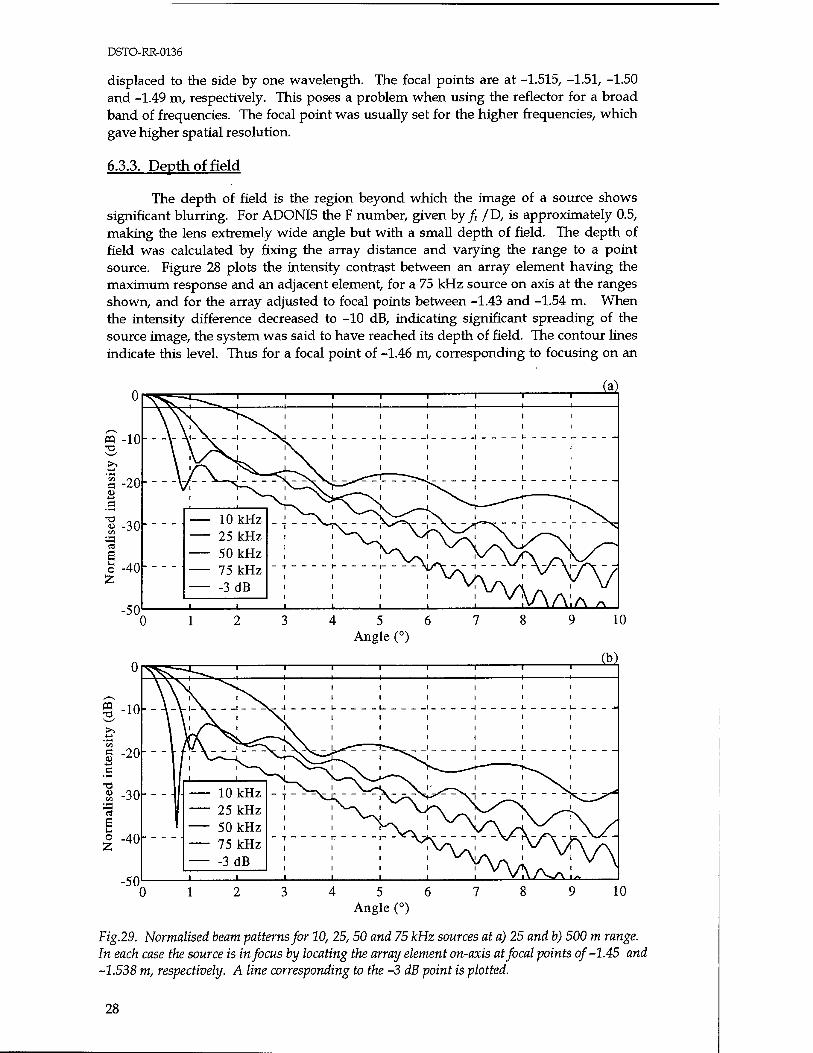
During two of the major deployments in San Diego Bay, called ORB1 and ORB2, the focal point was set at -1.45 m. Beam patterns (Epifanio, 1977) for an on-axis array element receiver at a focal point of -1.45 m are shown in Figure 29a for sources of 10, 25, 50 and 75 kHz at 25 m range. All curves have been normalised to the same response at 0° and a line corresponding to the -3 dB point is plotted. Since the source is on axis the beam patterns are symmetric about 0°, so only positive angles are shown. The beamwidths are 3.36°, 1.48°, 1.2° and 0.68°, with nearest sidelobes down by -18, - 18, -13 and -16 dB, respectively. Figure 29b plots the corresponding beam patterns for an on-axis element at -1.538 m so a source at 500 m range would be in focus. The beamwidths are 3.1°, 1.38°, 1.04° and 0.58° with nearest sidelobes down by -18, -16, -13 and -16 dB at 10,25,50 and 75 kHz.

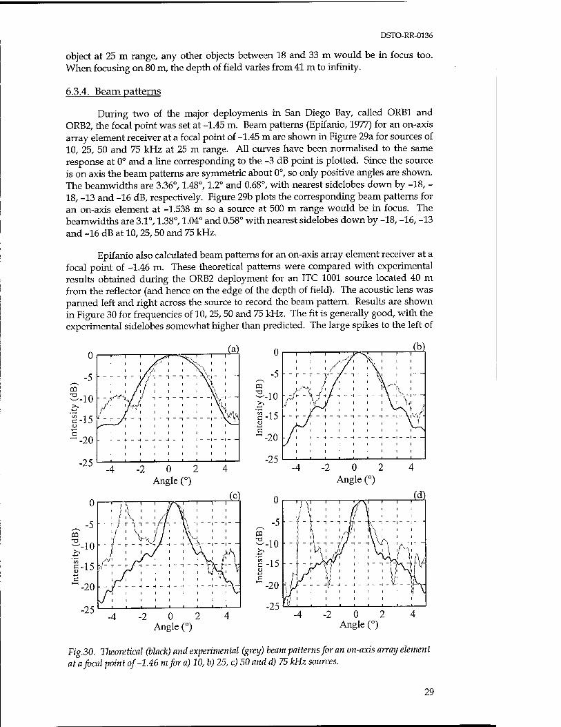
Epifanio also calculated beam patterns for an on-axis array element receiver at a focal point of -1.46 m. These theoretical patterns were compared with experimental results obtained during the ORB2 deployment for an ITC 1001 source located 40 m from the reflector (and hence on the edge of the depth of field). The acoustic lens was panned left and right across the source to record the beam pattern. Results are shown in Figure 30 for frequencies of 10, 25, 50 and 75 kHz. The fit is generally good, with the experimental sidelobes somewhat higher than predicted. The large spikes to the left of

0 (a) 1 I

I

m -5 • - r - r

i

~ 1

■10 ':/

^%j F -f - -i - "1 - -i - -i - -

on c • ■15 i - r ~/r

~^^ i

i I

- -r - -i - -i - -i - -i - -

c -20 • -

i

h - ■»-

i

i

» ■

i i

- -+ - H - -i

1 1

1 1

- -i - H - - — 1 —

PQ T3

0

-5

-10

M

£-15 0)

'-20

-25

I 1

1

1 ! '"""V^X

■ /7-X ■ •

y ' t -t -t i- -i - -i - -i - -i -\ -1 -\ -1 - —

1 r* ■ ■ ■ ■ ^s\J - - r - / - - t - i - -i - -i - -i- -i- ViVii—

i i i i i ' \ '

k-4--(-H-H-H- -1- -1- —

1 1 1 1 1 II

1 1 1 1 1 II ■ ■■II 11

-2 0 2 Angle (°)

-2 0 2 Angle (°)

-2 0 2 Angle (°)

-4 -2 0 2 Angle (°)

Fig.30. Tlieoretical (black) and experimental (grey) beam patterns for an on-axis array element at a focal point of-1.46 mfor a) 10, b) 25, c) 50 and d) 75 kHz sources.

29

DSTO-RR-0136

CQ

0 ,(a) 1 1 A/ 1 ! ^^ 1 1

i

-5 ■ - r _ Tff i - i - "i - "i " \ " " i ~ -i —

-10 1 / 1 1 1 1 1 1 \

-15 1 / t 1 1 1 1 1 l\

T-7- i- — -t — -t — —i — —i — —i — —i — \-i- _

-20 11 1 1 1 J I 1

--4---t---l--t--l--l--H--l-

11 1 1 1 1 I 1

11 1 1 1 1 1 1

-i-\

M

CQ T3

G

4 6 Angle (°)

10

-5

-10

-15

-20

-25

i i i df i Xi i 1 ' ' / ' V ' i— T - -[ jh ~ -i - nr i - _

rA\ r Xy -!--!- -I -\-I - -

1 1 1 1 1 1 1 \

1 ■"

1 1 1 1 1 1 1 1 1 1 1 1 1 1 ■ I 1 1

-5 ■ P3 T3 -10 >> •*-t

CO

C -15 0)

-4-» c 1—1

-20

-25

(c) i i i i /-^V ' i i

VV\ )! i Ay i i i v i i —

11 V. 1,1 ll11 '\

0 2 4 6 Angle (°)

8 10

(d)

4 6 Angle (°)

10 4 6 Angle (°)

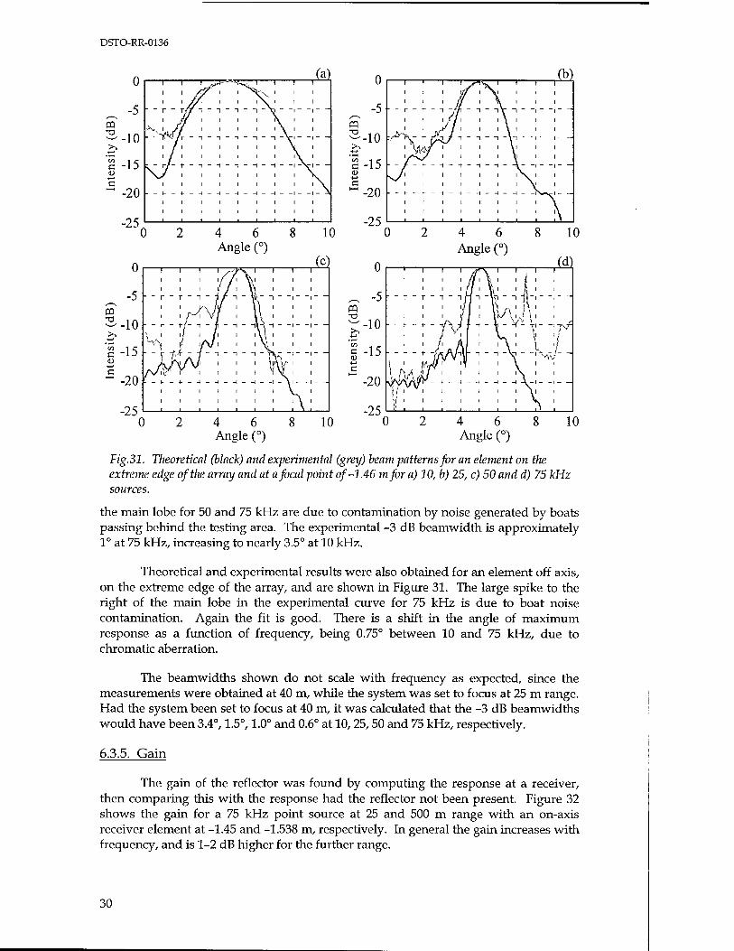
Fig.31. Tlieoretical (black) and experimental (grey) beam patterns for an element on tlie extreme edge oftlie array and at a focal point of-1.46 mfor a) 10, b) 25, c) 50 and d) 75 kHz sources.

the main lobe for 50 and 75 kHz are due to contamination by noise generated by boats passing behind the testing area. The experimental -3 dB beamwidth is approximately 1° at 75 kHz, increasing to nearly 3.5° at 10 kHz.

Theoretical and experimental results were also obtained for an element off axis, on the extreme edge of the array, and are shown in Figure 31. The large spike to the right of the main lobe in the experimental curve for 75 kHz is due to boat noise contamination. Again the fit is good. There is a shift in the angle of maximum response as a function of frequency, being 0.75° between 10 and 75 kHz, due to chromatic aberration.

The beamwidths shown do not scale with frequency as expected, since the measurements were obtained at 40 m, while the system was set to focus at 25 m range. Had the system been set to focus at 40 m, it was calculated that the -3 dB beamwidths would have been 3.4°, 1.5°, 1.0° and 0.6° at 10, 25,50 and 75 kHz, respectively.

6.3.5. Gain

The gain of the reflector was found by computing the response at a receiver, then comparing this with the response had the reflector not been present. Figure 32 shows the gain for a 75 kHz point source at 25 and 500 m range with an on-axis receiver element at -1.45 and -1.538 m, respectively. In general the gain increases with frequency, and is 1-2 dB higher for the further range.

30

DSTO-RR-0136

25

20

15

ü 10

1 1 TC „. i i i

i i i

1 >- "r" ZJ 111

500 m

___ -—■ -T"

* J*^

//

10 20 30 40 50 60 Frequency (kHz)

80 100

Fig.32. Gain oftlte reflector for a 75 kHz source in focus at 25 and 500 m range.

6.3.6. Fabrication

Is was intended to deploy the reflector in water depths of 10-50 m in the open ocean. The most severe hydraulic forces were expected to be encountered at shallow depths, where wave surge and turbulence predominate. Maximum surge forcing on the concave side of the reflector was expected to be 5 kN, spread smoothly over the surface. Turbulence might result in considerable shear in the water flow onto and around the reflector. Turbulence forces were expected to cause peak variations of 5 kN in the mean stress. Locally, the stress might then attain 10 kN with gradients of 10 kNm1. Under these expected stresses the reflector had to deform within its elastic limits and sustain no fracturing, permanent deformation or other damage. For stresses of 50% of these maximum anticipated values, the strain (displacement) of any part of the front reflecting surface had to be less than 12.5 mm.

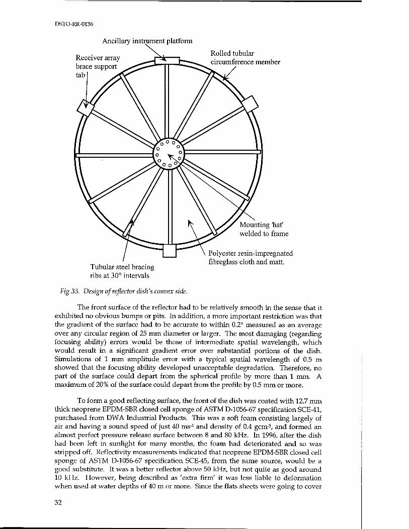
The reflector was fabricated from fibreglass and resin, with steel stiffeners for structural rigidity. The concave side was smooth. The convex side of the reflector had an undulating shape, caused by steel reinforcing ribs placed at 30° intervals. It was anticipated that the undulation would serve to break up the boundary layer flow and prevent the formation of periodic vortex shedding from the rear of the dish. This was important, as vortex shedding can cause large oscillatory forces which would drive the dish into flexural oscillations. The reflector was equipped with three equidistant (at 120°) mounting tabs of side 100 x 100 mm on the perimeter for the tubular array supports. In addition there was a further perimeter tab of size 150 x 150 mm which acted as a multi-purpose instrument platform. All tabs were welded to the structural steel internal frame. The reflector mounting to its support frame was by means of a 'top-hat' flange, also welded to the steel frame. The reflector could contain no voids and had to be impermeable to water ingress up to 6 bar absolute pressure. Figure 33 shows the reflector design, as seen on the convex side.

31

DSTO-RR-0136

Ancillary instrument platform

Receiver array brace support tab

Rolled tubular circumference member

Mounting 'hat' welded to frame

Polyester resin-impregnated ,, . fibreglass cloth and matt.

Tubular steel bracing ribs at 30° intervals

Fig.33. Design of reflector dish's convex side.

The front surface of the reflector had to be relatively smooth in the sense that it exhibited no obvious bumps or pits. In addition, a more important restriction was that the gradient of the surface had to be accurate to within 0.2° measured as an average over any circular region of 25 mm diameter or larger. The most damaging (regarding focusing ability) errors would be those of intermediate spatial wavelength, which would result in a significant gradient error over substantial portions of the dish. Simulations of 1 mm amplitude error with a typical spatial wavelength of 0.5 m showed that the focusing ability developed unacceptable degradation. Therefore, no part of the surface could depart from the spherical profile by more than 1 mm. A maximum of 20% of the surface could depart from the profile by 0.5 mm or more.

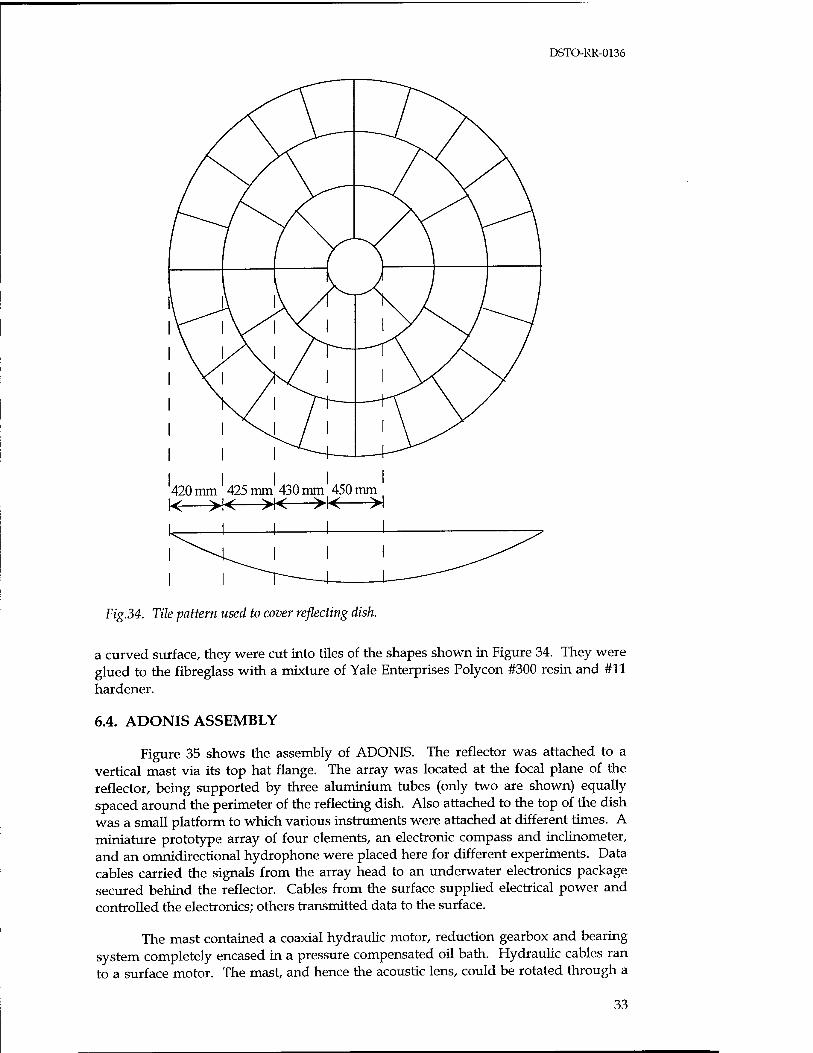
To form a good reflecting surface, the front of the dish was coated with 12.7 mm thick neoprene EPDM-SBR closed cell sponge of ASTM D-1056-67 specification SCE-41, purchased from DWA Industrial Products. This was a soft foam consisting largely of air and having a sound speed of just 40 ms-1 and density of 0.4 gem-3, and formed an almost perfect pressure release surface between 8 and 80 kHz. In 1996, after the dish had been left in sunlight for many months, the foam had deteriorated and so was stripped off. Reflectivity measurements indicated that neoprene EPDM-SBR closed cell sponge of ASTM D-1056-67 specification SCE-45, from the same source, would be a good substitute. It was a better reflector above 50 kHz, but not quite as good around 10 kHz. However, being described as 'extra firm' it was less liable to deformation when used at water depths of 40 m or more. Since the flats sheets were going to cover

32

DSTO-RR-0136

I I I I 420 mm 425 mm 430 mm 450 mm < >K—>K >K >l

Fig.34. Tile pattern used to cover reflecting dish.

a curved surface, they were cut into tiles of the shapes shown in Figure 34. They were glued to the fibreglass with a mixture of Yale Enterprises Polycon #300 resin and #11 hardener.

6.4. ADONIS ASSEMBLY

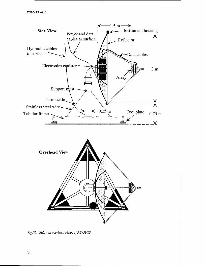
Figure 35 shows the assembly of ADONIS. The reflector was attached to a vertical mast via its top hat flange. The array was located at the focal plane of the reflector, being supported by three aluminium tubes (only two are shown) equally spaced around the perimeter of the reflecting dish. Also attached to the top of the dish was a small platform to which various instruments were attached at different times. A miniature prototype array of four elements, an electronic compass and inclinometer, and an omnidirectional hydrophone were placed here for different experiments. Data cables carried the signals from the array head to an underwater electronics package secured behind the reflector. Cables from the surface supplied electrical power and controlled the electronics; others transmitted data to the surface.

The mast contained a coaxial hydraulic motor, reduction gearbox and bearing system completely encased in a pressure compensated oil bath. Hydraulic cables ran to a surface motor. The mast, and hence the acoustic lens, could be rotated through a

33

DSTO-RR-0136

Side View

Hydraulic cables to surface

Electronics c:

Power and data cables to surface

—1.5 m >| ■ ^—— Instrument housing

Turnbuckle^

Stainless steel wire-

Tubular frame Foot plate Q y r

Overhead View

Fig.35. Side and overhead views of ADONIS.

34

DSTO-RR-0136

full 360° around the vertical axis. The mast was held perpendicular to a frame with stainless steel wires adjusted with turnbuckles. The whole system was placed on a triangular platform made of tubular pipes and had three foot plates. The distance between the feet and frame could be adjusted, thereby tilting the whole acoustic lens by a maximum of 10°.

6.5. ARRAY

From the geometry of the spherical reflector (Fig. 21), 0r = 6i, which leads to

tan(0=4 2/, (5)

The diameter of the array becomes 0.3 m. For independent array element output, e > X/2 at the maximum frequency. Therefore the element diameter had to exceed 18.75 mm. It was set at 20 mm. The number n of elements used to 'tile' the array area is found from the approximate relationship, assuming a planar receiver,

7tdl ne (6)

leading to n=l 77. In practice n was limited to 130, thereby Hmiting the steering angle

It was anticipated that the acoustic lens would be tested in shallow waters where the depth would limit imaging in the vertical direction. Hence, rather than using a circular array an elliptical one was chosen, with major and minor dimensions of 280 and 220 mm respectively. The layout is shown in Figure 36. Although it consisted of 130 elements, only 126 were used. To maintain a spacing of 20 mm between elements, but also to provide decoupling between individual elements, pressure release spacers were located between each element. The elements were oblong in shape, being 17.8 x 17.8 x 19 mm, with 2.3 mm thick spacers between them. To best match the focal surface of the reflector the elements were formed into a smooth

Shaded elements included in the physical array but not used in data processing

22.2 cm

28.0 cm-

Fig.36. Layout of ADONIS array elements.

35

DSTO-RR-0136

Potting

Cable connectors

Fig.37. Cross section through tlie ADONIS array.

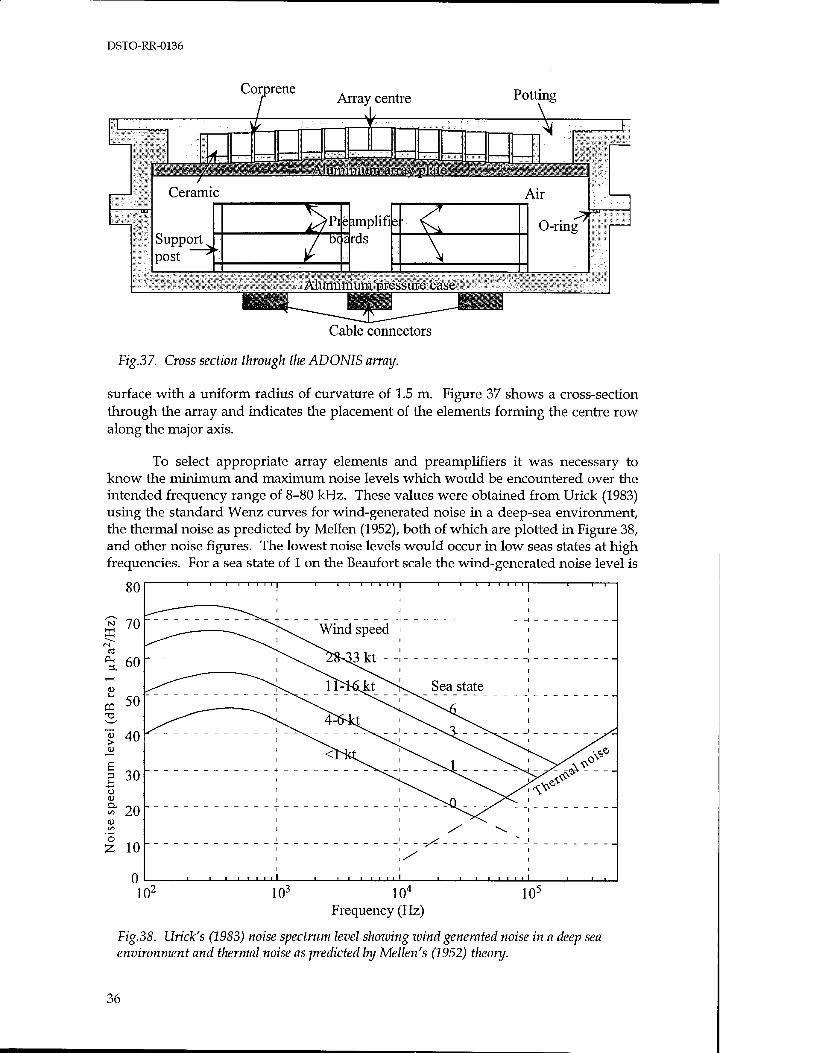
surface with a uniform radius of curvature of 1.5 m. Figure 37 shows a cross-section through the array and indicates the placement of the elements forming the centre row along the major axis.

To select appropriate array elements and preamplifiers it was necessary to know the minimum and maximum noise levels which would be encountered over the intended frequency range of 8-80 kHz. These values were obtained from Urick (1983) using the standard Wenz curves for wind-generated noise in a deep-sea environment, the thermal noise as predicted by Meilen (1952), both of which are plotted in Figure 38, and other noise figures. The lowest noise levels would occur in low seas states at high frequencies. For a sea state of 1 on the Beaufort scale the wind-generated noise level is

80

N 70 ffi

CO

60 T-^

<D

CQ 50

> 40 <D

F= 30

o ^

i

i

i

i

i

<hkt

t

i

■ i ■ i i ■ i i 1 i i i ■ i i i i § i i 111111 i II

w 103 104

Frequency (Hz) 105

Fig.38. Urick's (1983) noise spectrum level showing wind generated noise in a deep sea environment and thermal noise as predicted by Mellen's (1952) theory.

36

DSTO-RR-0136

20 dB re 1 uPa2/Hz at 80 kHz, but the thermal noise is 25 dB re 1 uPa2/Hz. In such quiet conditions the highest useable frequency is 65 kHz, where the thermal noise equals the wind-generated noise at about 22 dB re 1 uPa2/Hz. This value was taken as the lowest noise level which would be encountered.

The noisiest measurements would occur at low frequencies in high sea states, or in the presence of rain or snapping shrimp. The highest sea state in which the equipment could be deployed is 4, for which the wind-generated noise is 50 dB re 1 uPa2/Hz at 8 kHz. This is exceeded by rain-generated noise, being 80, 72 and 62 dB re 1 uPa2/Hz for heavy, moderate and light rain, respectively. At this frequency the snapping shrimp noise was taken to be 68 dB re 1 uPa2/Hz. It was decided that the system could not encompass this entire range of noise levels, and so the upper operational limit was set at 70 dB re 1 uPa2/Hz. Thus the dynamic range would be 48 dB.

The array elements had to operate over the frequency range 8-80 kHz and vary by no more than +6 dB over this frequency range. Further, it was specified that the inter-element variability not exceed 1 dB. Given an assumed reflector gain of 18 dB, they had to be sensitive to sound pressure levels of 40-88 dB re 1 |jPa2/Hz.

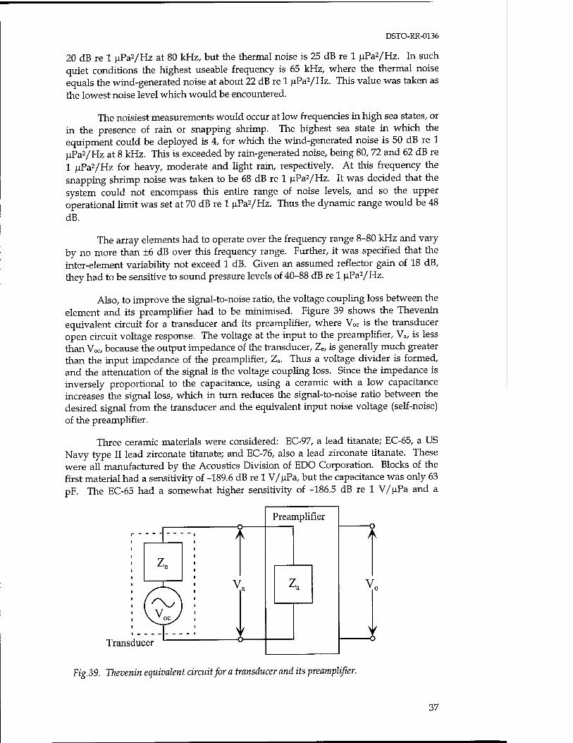
Also, to improve the signal-to-noise ratio, the voltage coupling loss between the element and its preamplifier had to be minimised. Figure 39 shows the Thevenin equivalent circuit for a transducer and its preamplifier, where Voc is the transducer open circuit voltage response. The voltage at the input to the preamplifier, Va/ is less than Voc, because the output impedance of the transducer, Ze, is generally much greater than the input impedance of the preamplifier, Za. Thus a voltage divider is formed, and the attenuation of the signal is the voltage coupling loss. Since the impedance is inversely proportional to the capacitance, using a ceramic with a low capacitance increases the signal loss, which in turn reduces the signal-to-noise ratio between the desired signal from the transducer and the equivalent input noise voltage (self-noise) of the preamplifier.

Three ceramic materials were considered: EC-97, a lead titanate; EC-65, a US Navy type II lead zirconate titanate; and EC-76, also a lead zirconate titanate. These were all manufactured by the Acoustics Division of EDO Corporation. Blocks of the first material had a sensitivity of -189.6 dB re 1 V/uPa, but the capacitance was only 63 pF. The EC-65 had a somewhat higher sensitivity of -186.5 dB re 1 V/uPa and a

Transducer

Fig.39. Tlievenin equivalent circuit for a transducer and its preamplifier.

37

DSTO-RR-0136

-170 OH

>

£-180 <D

a ■*-»

"o > 3 o

C a. O

■190

1 1 1 1 1 1 1 1 1 1 1 1 1 1

MM! i ■ MM j/ivA --]-|ii[----i---L--J---i-i-]4-[I-

L J \ IIJ L 1 1 Llllll.

I I I I I I 1 I llllll -200 5 6 7 8 9 10

Fig.40. Sensitivity curve of ADONIS array element.

20 30 40 50 60 70 80 100 Frequency (kHz)

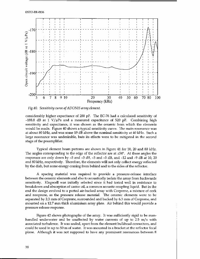
considerably higher capacitance of 288 pF. The EC-76 had a calculated sensitivity of -188.8 dB re 1 V/uPa and a measured capacitance of 520 pF. Combining high sensitivity and capacitance, it was chosen as the ceramic from which the elements would be made. Figure 40 shows a typical sensitivity curve. The main resonance was at about 80 kHz, and was some 19 dB above the nominal sensitivity at 40 kHz. Such a large resonance was undesirable, buts its effects were to be mitigated in the second stage of the preamplifier.

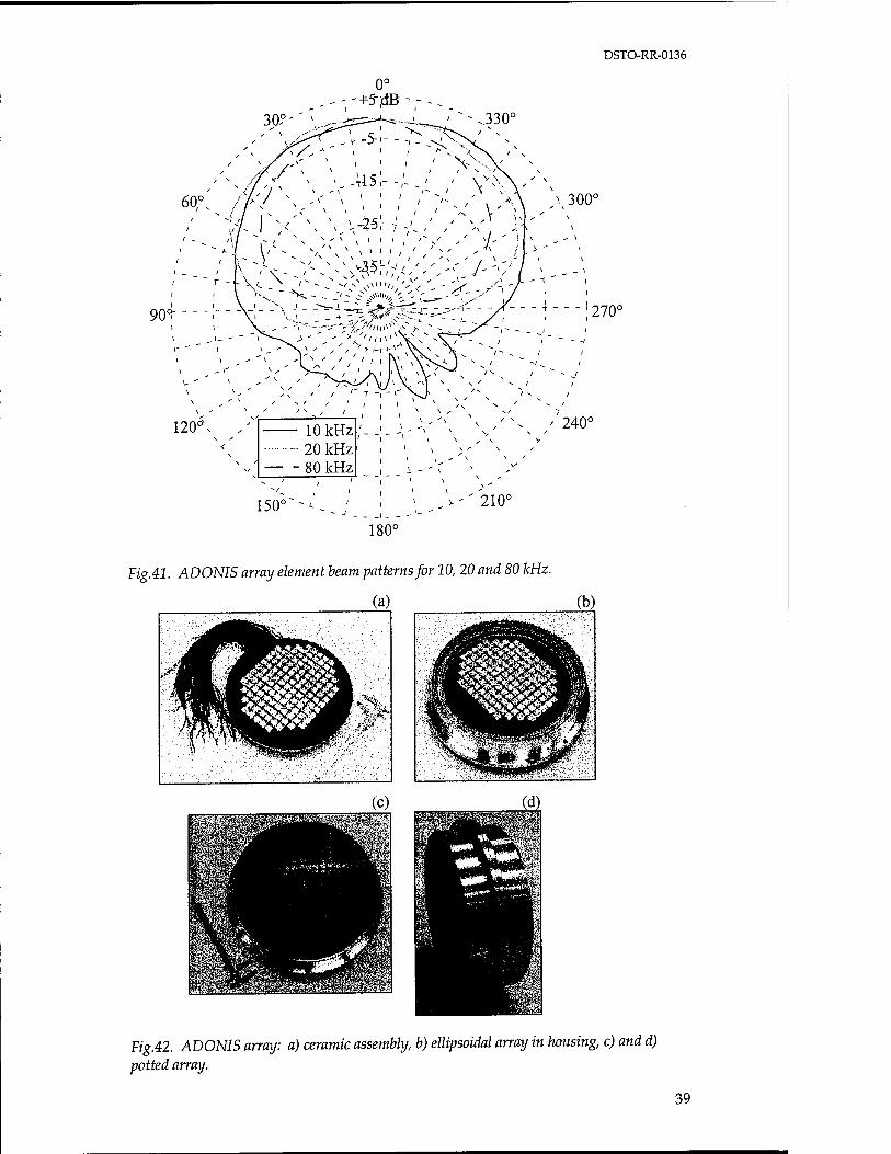
Typical element beam patterns are shown in Figure 41 for 10, 20 and 80 kHz. The angles corresponding to the edge of the reflector are at ±54°. At these angles the responses are only down by -5 and -3 dB, -3 and -5 dB, and -12 and -9 dB at 10, 20 and 80 kHz, respectively. Therefore, the elements will not only collect energy reflected by the dish, but some energy coming from behind and to the sides of the reflector.

A spacing material was required to provide a pressure-release interface between the ceramic elements and also to acoustically isolate the array from backwards sensitivity. Klegecell was initially selected since it had tested well in resistance to breakdown and absorption of castor oil, a common acoustic coupling liquid. But in the end the design evolved to a potted air-backed array with Corprene, a mixture of cork and neoprene, as the pressure release material. The ceramic elements were to be separated by 2.3 mm of Corprene, surrounded and backed by 6.3 mm of Corprene, and mounted on a 12.7 mm thick aluminium array plate. Air behind this would provide a pressure release response.

Figure 42 shows photographs of the array. It was sufficiently rigid to be man- handled underwater and be unaffected by water currents of up to 2.5 m/s with associated turbulence. It was sealed, apart from the element bulkhead connectors, and could be used in up to 50 m of water. It was mounted in a bracket at the reflector focal plane. Although it was not supposed to have any prominent resonances between 8

38

DSTO-RR-0136

30?- .330°

/ / \ v>,\ ' "

60° /A/ \ -< * 300°

90c '270°

120°\ . 10 kHz -20 kHz 80 kHz

' ' ' ' '" V

, _ I -''

\ \ ,^' 210°

180°

240°

Fig.41. ADONIS array element beam patterns for 10, 20 and 80 kHz.

(a) (b)

Fig.42. ADONIS array: a) ceramic assembly, b) ellipsoidal array in housing, c) and d) potted array.

39

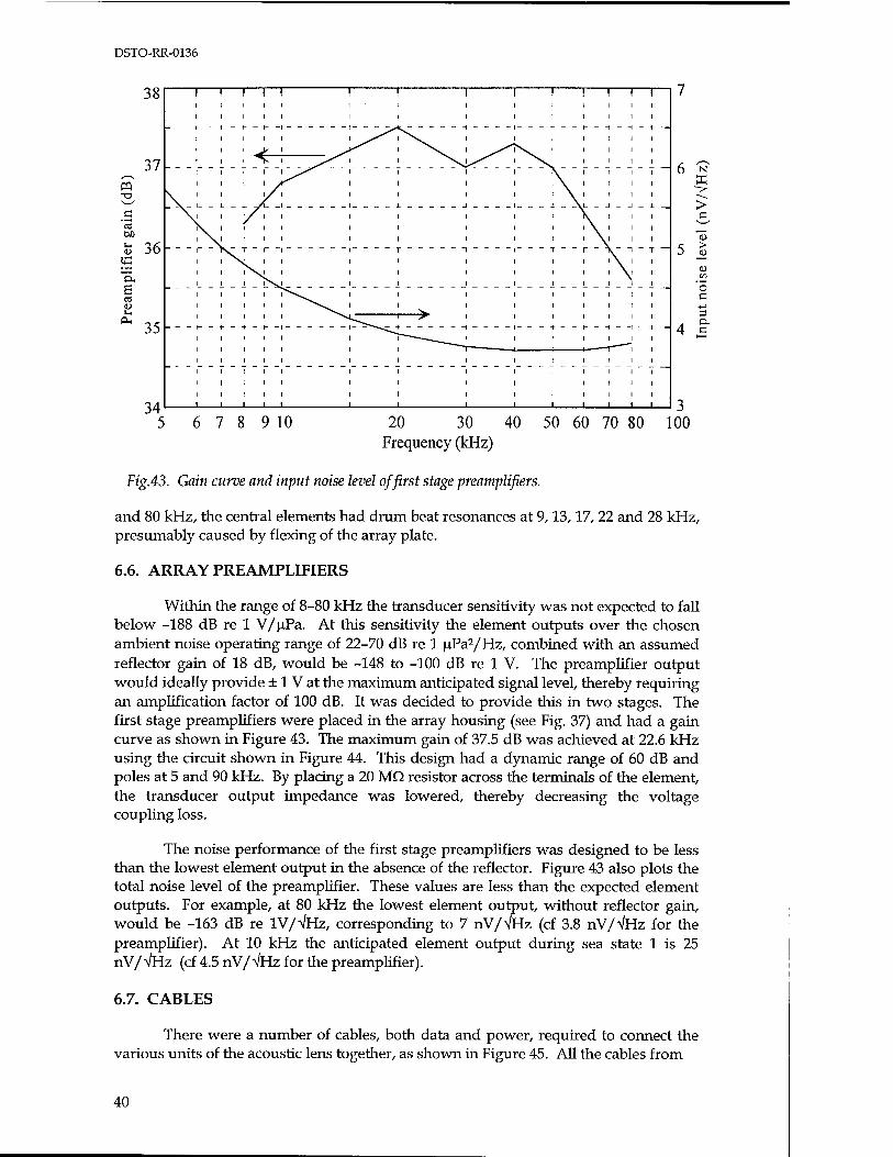
DSTO-RR-0136

38 1 ! 1

--t--i--|--

1 1 1

1 1 J,

i I

i i

37 m T3

1 *V

" \

1 1 1

1 I 1 /

i i \X i \ i i ii

i \ i i ii

ream

plif

ier

gain

\ 1 1 1

Tv T r

1 ' ' is

r ~\ i i

i i i

i i i •> i iiit

i iiii ___.f__e.__,__<_ + __ i i i i i

* 35 l^^ ~

i i i i i

1A

i i i

i i i

i i i i i

i i i i i

i IIII

i IIII

6 N

> c

- 5

- 4

> 4>

o a 3 CU G

6 7 8 9 10 20 30 40 50 60 70 80 Frequency (kHz)

3 100

Fig.43. Gain curve and input noise level of first stage preamplifiers.

and 80 kHz, the central elements had drum beat resonances at 9,13,17, 22 and 28 kHz, presumably caused by flexing of the array plate.

6.6. ARRAY PREAMPLIFIERS

Within the range of 8-80 kHz the transducer sensitivity was not expected to fall below -188 dB re 1 V/pPa. At this sensitivity the element outputs over the chosen ambient noise operating range of 22-70 dB re 1 uPa2/Hz, combined with an assumed reflector gain of 18 dB, would be -148 to -100 dB re 1 V. The preamplifier output would ideally provide ± 1 V at the maximum anticipated signal level, thereby requiring an amplification factor of 100 dB. It was decided to provide this in two stages. The first stage preamplifiers were placed in the array housing (see Fig. 37) and had a gain curve as shown in Figure 43. The maximum gain of 37.5 dB was achieved at 22.6 kHz using the circuit shown in Figure 44. This design had a dynamic range of 60 dB and poles at 5 and 90 kHz. By placing a 20 MQ resistor across the terminals of the element, the transducer output impedance was lowered, thereby decreasing the voltage coupling loss.

The noise performance of the first stage preamplifiers was designed to be less than the lowest element output in the absence of the reflector. Figure 43 also plots the total noise level of the preamplifier. These values are less than the expected element outputs. For example, at 80 kHz the lowest element output, without reflector gain, would be -163 dB re IV/VHZ, corresponding to 7 nV/VHz (cf 3.8 nV/VHz for the preamplifier). At 10 kHz the anticipated element output during sea state 1 is 25 nV/VHz (cf 4.5 nV/VHz for the preamplifier).

6.7. CABLES

There were a number of cables, both data and power, required to connect the various units of the acoustic lens together, as shown in Figure 45. All the cables from

40

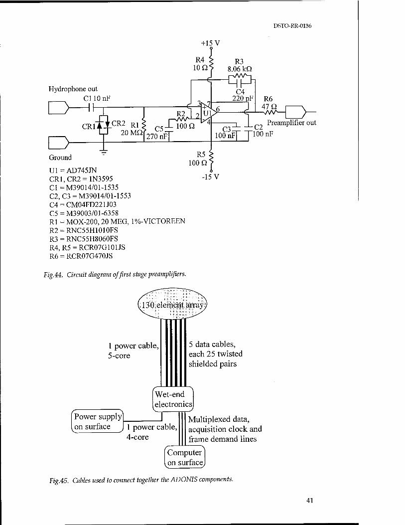
DSTO-RR-0136

+ 15 V

Hydrophone out CllOnF

■N/W—

Preamplifier out C3

lOOnFfT1001117

Ground

U1-AD745JN CR1,CR2=1N3595 C1=M39014/01-1535 C2,C3 = M39014/01-1553 C4 = CM04FD221J03 C5 = M39003/01-6358 Rl = MOX-200, 20 MEG, 1%-VICTOREEN R2 = RNC55H1010FS R3 = RNC55H8060FS R4,R5 = RCR07G101JS R6 = RCR07G470JS

R5 100 Q

-15 V

Fig.44. Circuit diagram of first stage preamplifiers.

1 power cable, 5-core

5 data cables, each 25 twisted shielded pairs

Wet-end electronics

Power supply on surface 1 power cable,

4-core

Multiplexed data, acquisition clock and frame demand lines

Computer on surface

Fig.45. Cables used to connect togetlier tlie ADONIS components.

41

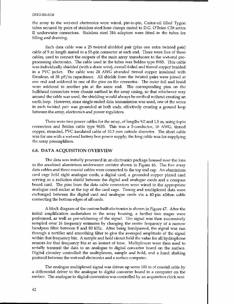
DSTO-RR-0136

the array to the wet-end electronics were wired, pin-to-pin, Castor-oil filled Tygon tubes secured by pairs of stainless steel hose clamps mated to D.G. O'Brien C28 series II underwater connectors. Stainless steel 316 adaptors were fitted in the tubes for filling and draining.

Each data cable was a 25 twisted shielded pair (plus one extra twisted pair) cable of 9 m length mated to a 55-pin connector at each end. There were five of these cables, used to connect the outputs of the main array transducers to the wet-end pre- processing electronics. The cable used in the tubes was Beiden type 8185. This cable was individually shielded (with a drain wire), overall foiled and tinned copper braided in a PVC jacket. The cable was 24 AWG stranded tinned copper insulated with Datalene, of 38 pF/m capacitance. All shields from the twisted pairs were joined at one end and soldered to one of the pins on the connector. The outer foil and braid were soldered to another pin at the same end. The corresponding pins on the bulkhead connectors were chassis earthed in the array casing, so that whichever way around the cable was used, the shielding would always be earthed without creating an earth loop. However, since single-ended data transmission was used, one of the wires in each twisted pair was grounded at both ends, effectively creating a ground loop between the array, electronics and power regulators.

There were two power cables for the array, of lengths 9.0 and 1.5 m, using 6-pin connectors and Beiden cable type 9620. This was a 5-conductor, 16 AWG, tinned copper, stranded, PVC insulated cable of 10.3 mm outside diameter. The short cable was for use with a wet-end battery box power supply; the long cable was for supplying the array preamplifiers.

6.8. DATA ACQUISITION OVERVIEW

The data was initially processed in an electronics package housed near the lens in the anodised aluminium underwater canister shown in Figure 46. The five array data cables and three coaxial cables were connected to the top end cap. An aluminium card cage held eight analogue cards, a digital card, a grounded copper plated card serving as a radiation shield between the digital and analogue cards and a compass board card. The pins from the data cable connectors were wired to the appropriate analogue card socket at the top of the card cage. Timing and multiplexed data were exchanged between the digital card and analogue cards via a 40-pin ribbon cable connecting the bottom edges of all cards.

A block diagram of the custom built electronics is shown in Figure 47. After the initial amplification undertaken in the array housing, a further two stages were performed, as well as pre-whitening of the signal. The signal was then successively sampled over 16 frequency estimates by changing the centre frequency of a narrow bandpass filter between 8 and 80 kHz. After being bandpassed, the signal was run through a rectifier and smoothing filter to give the averaged amplitude of the signal within that frequency bin. A sample and hold circuit held the value for all hydrophone sensors for that frequency bin at an instant of time. Multiplexers were then used to serially transmit the data to an analogue to digital converter board on the surface. Digital circuitry controlled the multiplexers, sample and hold, and a hand shaking protocol between the wet-end electronics and a surface computer.

The analogue multiplexed signal was driven up some 100 m of coaxial cable by a differential driver to the analogue to digital converter board in a computer on the surface. The analogue to digital conversion was controlled by an acquisition clock sent

42

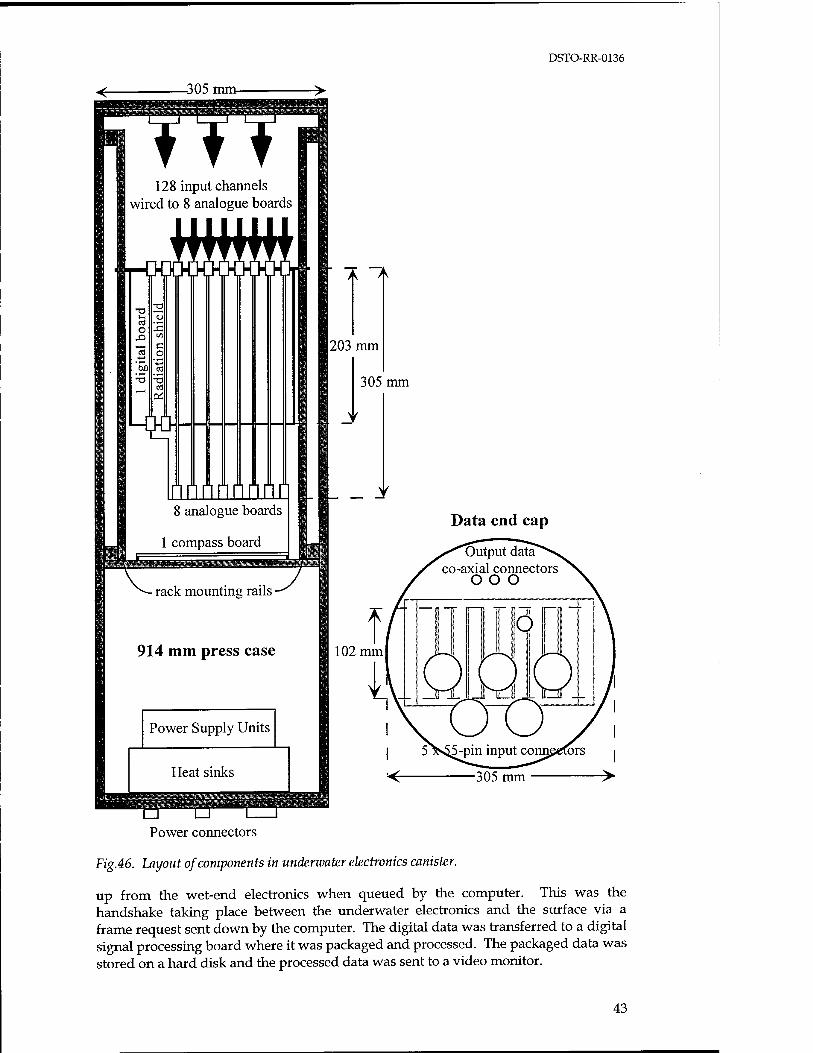
DSTO-RR-0136

305 mm-

11J 128 input channels

wired to 8 analogue boards

HW

nnnnnnnri 8 analogue boards

1 compass board

Ä ~>r-

203 mm

305 mm

~~

Data end cap

rack mounting rails •

914 mm press case

Power Supply Units

Heat sinks

102 mm I

52N$5-pin input connpefors

■305 mm >

Power connectors

Fig.46. Layout of components in undenvater electronics canister.

up from the wet-end electronics when queued by the computer. This was the handshake taking place between the underwater electronics and the surface via a frame request sent down by the computer. The digital data was transferred to a digital signal processing board where it was packaged and processed. The packaged data was stored on a hard disk and the processed data was sent to a video monitor.

43

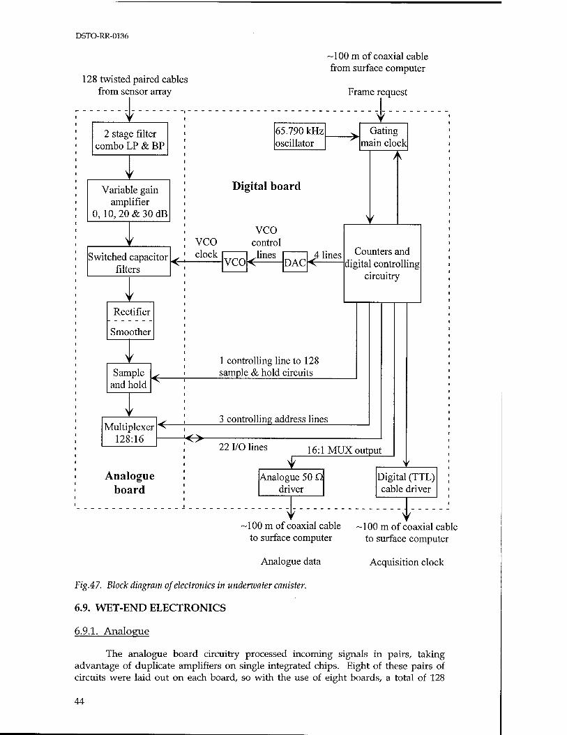
DSTO-RR-0136

128 twisted paired cables from sensor array

-100 m of coaxial cable from surface computer

Frame request

2 stage filter combo LP & BP

65.790 kHz oscillator

Gating main clock

Variable gain amplifier

0, 10,20 & 30 dB

Switched capacitor filters

VCO clock

Digital board

VCO control Jines

VCO DAC 4 lines

Rectifier

Smoother

Counters and digital controlling

circuitry

Sample and hold

1 controlling line to 128 sample & hold circuits

Multiplexer 128:16

3 controlling address lines lO-

22 I/O lines

Analogue board

16:1 MUX output

Analogue 50 Q driver

Digital (TTL) cable driver

400 m of coaxial cable to surface computer

Acquisition clock

-100 m of coaxial cable to surface computer

Analogue data

Fig.47. Block diagram of electronics in underwater canister.

6.9. WET-END ELECTRONICS

6.9.1. Analogue

The analogue board circuitry processed incoming signals in pairs, taking advantage of duplicate amplifiers on single integrated chips. Eight of these pairs of circuits were laid out on each board, so with the use of eight boards, a total of 128

44

$%

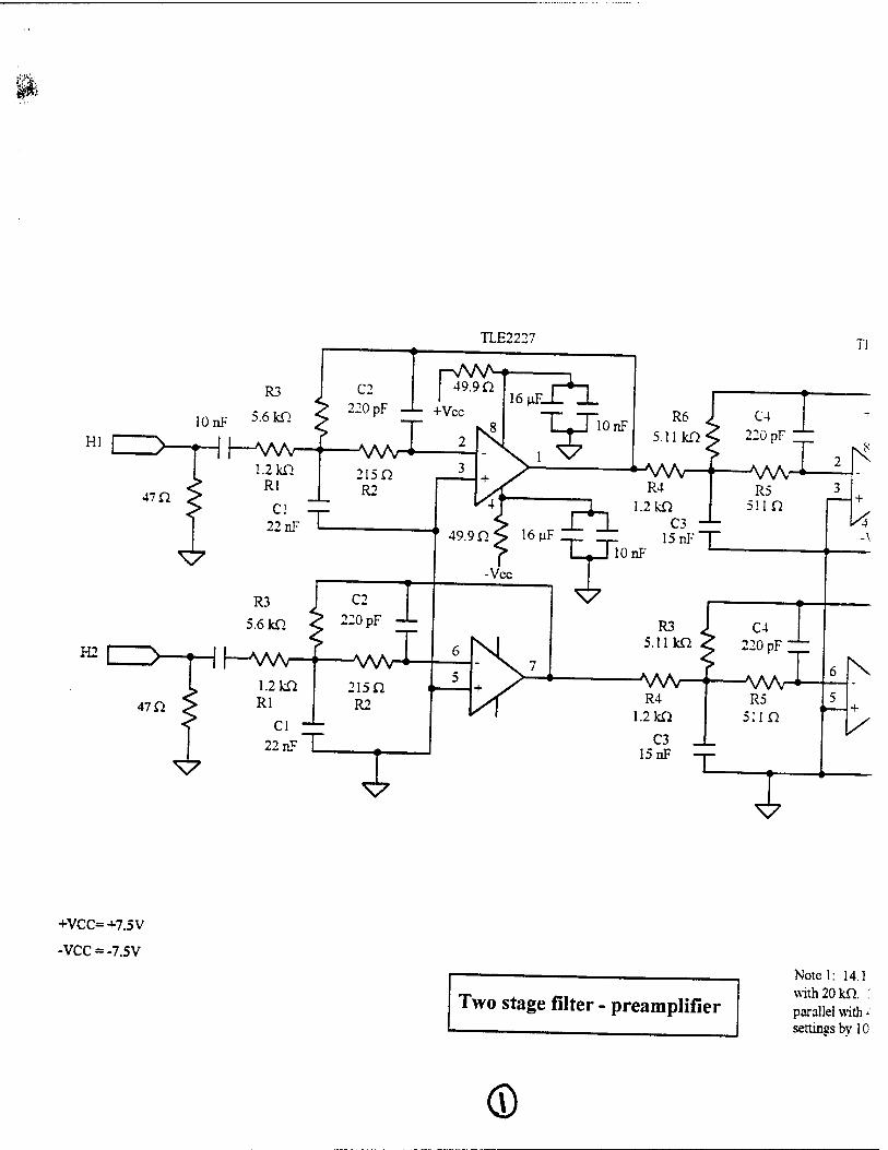
TLE2227

Hl

H2

47 D.

10 nF

R3

5.6 ldl

C2

220 PF -L. +Vcc

pAAA-f , I 499n 16MZT1

> •—| |—VA—" V\Ar

TI

47 n

>—Hi—Wv—f VW

+VCC=+7.5V

-VCC = -7.5V

Two stage filter - preamplifier

Notel: 14.1 with 20 kn. : parallel with - settings by 10

CD

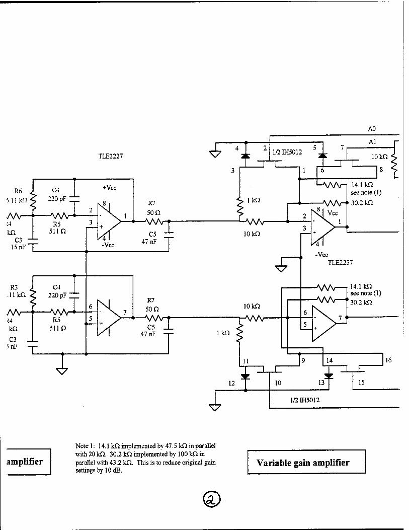
amplifier

Note 1: 14.1 kQ implemented by 47.5 kQ in parallel with 20 kn. 30.2 kft implemented by 100 kQ in parallel with 43.2 kQ. This is to reduce original gain settings by 10 dB.

Variable gain amplifier

©

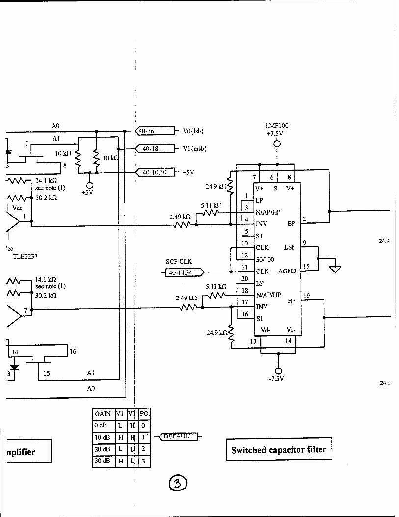
LMF100 +7.5V

6

nplifier

GAIN VI V0 PO.

OdB L ri 0

10 dB H H 1

20 dB L M 2

30 dB H L: 3

-< DEFAULT

Switched capacitor filter

®

24.9

24.9

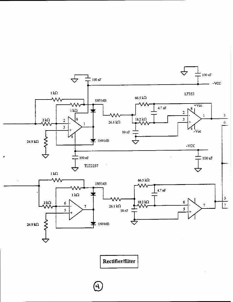
lOOnF

24.9 kO

24.9 kn

Rectifier/filter

©

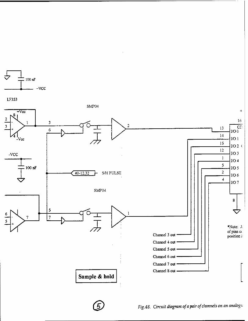
100 nF

-vcc

LF353

SMP04 +Vcc

-Vcc

-VCC

T -p-lOOnF

> r°

Z

< 40-12.32 h S/H PULSE

SMP04

<° ^

Sample & hold

Channel 3 out ■

Channel 4 out ■

Channel 5 out ■

Channel 6 out ■

Channel 7 out ■ Channel 8 out ■

14

15

16

CD I/O0

I/O 1

1/0 2 (

1/0 3

1/0 4

1/0 5

1/0 6

1/0 7

8

\7

♦Note: Ji of pins cc position i:

a> Fig.48. Circuit diagram of a pair ofclmnnels on an analogu

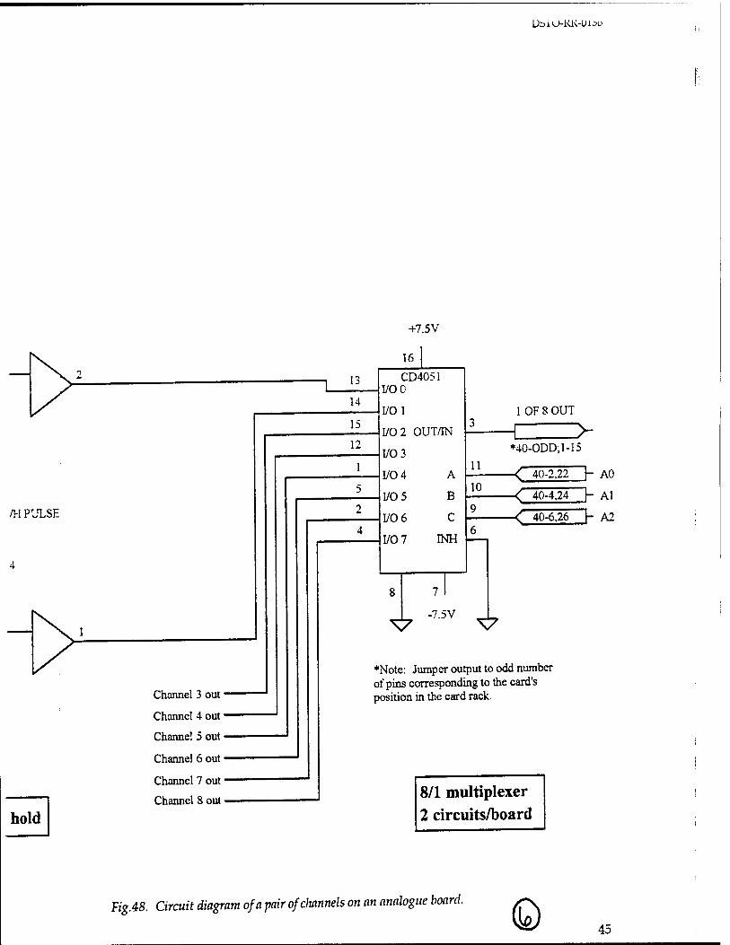
DbiU-KK-Ulou

/H PULSE

hold

Channel 3 out ■

Channel 4 out ■

Channel 5 out ■

Channel 6 out ■

Channel 7 out ■

Channel 8 out ■

13

14

15

+7.5V

16

CD4051 I/OO

I/O 1

1/0 2 OUT/IN

1/0 3

1/0 4

1/0 5

1/0 6

1/0 7

A

B

C

INH

8 7 I

-7.5V

11

10

1 OF 8 OUT

> *40-ODD;1-15

-< 40-2,22 h AO

-< 40-4,24 h Al

■< 40-6,26 h A2

\7

♦Note: Jumper output to odd number of pins corresponding to the card's position in the card rack.

8/1 multiplexer 2 circuits/board

Fig.48. Circuit diagram of a pair of channels on an analogue board. © 45

DSTO-RR-0136

THIS PAGE LEFT INTENTIONALLY BLANK

%

DSTO-RR-0136

incoming signals could be processed. Figure 48 shows the analogue circuit used to process the data coming from a pair of hydrophones.

As noted above, a total gain of 100 dB would be needed to raise the maximum element outputs to ± 1 V. 37.5 dB of this was provided by the preamplifiers housed with the hydrophones; the remainder was supplied by the amplifiers on the analogue boards. Thus the first portion of the circuit was another preamplifier, built with a filter. The amplification was in two stages to provide the requisite gain. It incorporated a local power supply so transient signals would not cause a voltage drop; the 10 nF and 16 uF capacitors in parallel covered both low and high frequencies. TLE2227 operational amplifiers were used because of their large open loop gain and low noise. The filter had the purpose of pre-whitening the incoming signal, to some extent correcting the resonance peak of the hydrophone. To achieve this, lowpass and bandpass filters were convolved. Figure 49 shows the response of this unit, where the fall-off in response above 50 kHz is most noticeable.

To achieve the desired total gain of 100 dB, further amplification was needed. Since the intensity of the ambient noise field is very dependent on sea state and can vary considerably with location, a variable gain amplifier (VGA) was used to maximise the dynamic range of the system. The gain was varied by changing the input resistance and/or feedback resistance of a linear gain amplifier. Two junction field effect transistors (JFET), acting as analogue switches, were used to add or remove resistance in the circuit. Applying a low voltage (0 V) to the JFET gate caused the switch to open, preventing current from flowing through the parallel resistance. When a high voltage (5 V) was applied to the JFET gate, the gate was closed, allowing current to flow through the parallel resistor. When the switch in the feedback path was closed the feedback resistance was lowered, which increased the gain of the amplifier. When the switch in the input path was closed the intput resistance was lowered, which decreased the gain of the amplifier. Gains of 0, 10, 20 or 30 dB could be selected by manipulating the analogue switches. The switches were controlled by signals from the digital circuitry, and were normally set at the start of data acquisition, with the default

40

35

m •a c

Ü

30

25

20

_ J__I._I-_I-LJ.I_I '-y^''— L.j-iii-u.

4 5 6 8 10 20 30 40 60 80 100 Frequency (kHz)

Fig.49. Gain of second stage preamplifier and pre-whitening filter.

47

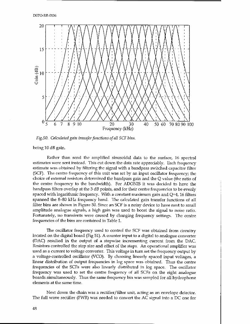
DSTO-RR-0136

20

15

C "c3 Ü

10

0 5 6 7 8 9 10 20 30 Frequency (kHz)

40 50 60 70 80 90 100

Fig.50. Calculated gain transfer functions of all SCF bins.

being 10 dB gain.

Rather than send the amplified sinusoidal data to the surface, 16 spectral estimates were sent instead. This cut down the data rate appreciably. Each frequency estimate was obtained by filtering the signal with a bandpass switched capacitor filter (SCF). The centre frequency of this unit was set by an input oscillator frequency; the choice of external resistors determined the bandpass gain and the Q value (the ratio of the centre frequency to the bandwidth). For ADONIS it was decided to have the bandpass filters overlap at the 3 dB points, and for their centre frequencies to be evenly spaced with logarithmic frequency. With a constant maximum gain and Q=4,16 filters spanned the 8-80 kHz frequency band. The calculated gain transfer functions of all filter bins are shown in Figure 50. Since an SCF is a noisy device to have next to small amplitude analogue signals, a high gain was used to boost the signal to noise ratio. Fortunately, no transients were caused by changing frequency settings. The centre frequencies of the bins are contained in Table 1.

The oscillator frequency used to control the SCF was obtained from circuitry located on the digital board (Fig 51). A counter input to a digital to analogue converter (DAC) resulted in the output of a stepwise incrementing current from the DAC. Resistors controlled the step size and offset of the steps. An operational amplifier was used as a current to voltage converter. This voltage in turn set the frequency output by a voltage-controlled oscillator (VCO). By choosing linearly spaced input voltages, a linear distribution of output frequencies in log space was obtained. Thus the centre frequencies of the SCFs were also linearly distributed in log space. The oscillator frequency was used to set the centre frequency of all SCFs on the eight analogue boards simultaneously. Thus the same frequency bin was sampled for all hydrophone elements at the same time.

Next down the chain was a rectifier/filter unit, acting as an envelope detector. The full wave rectifier (FWR) was needed to convert the AC signal into a DC one for

48

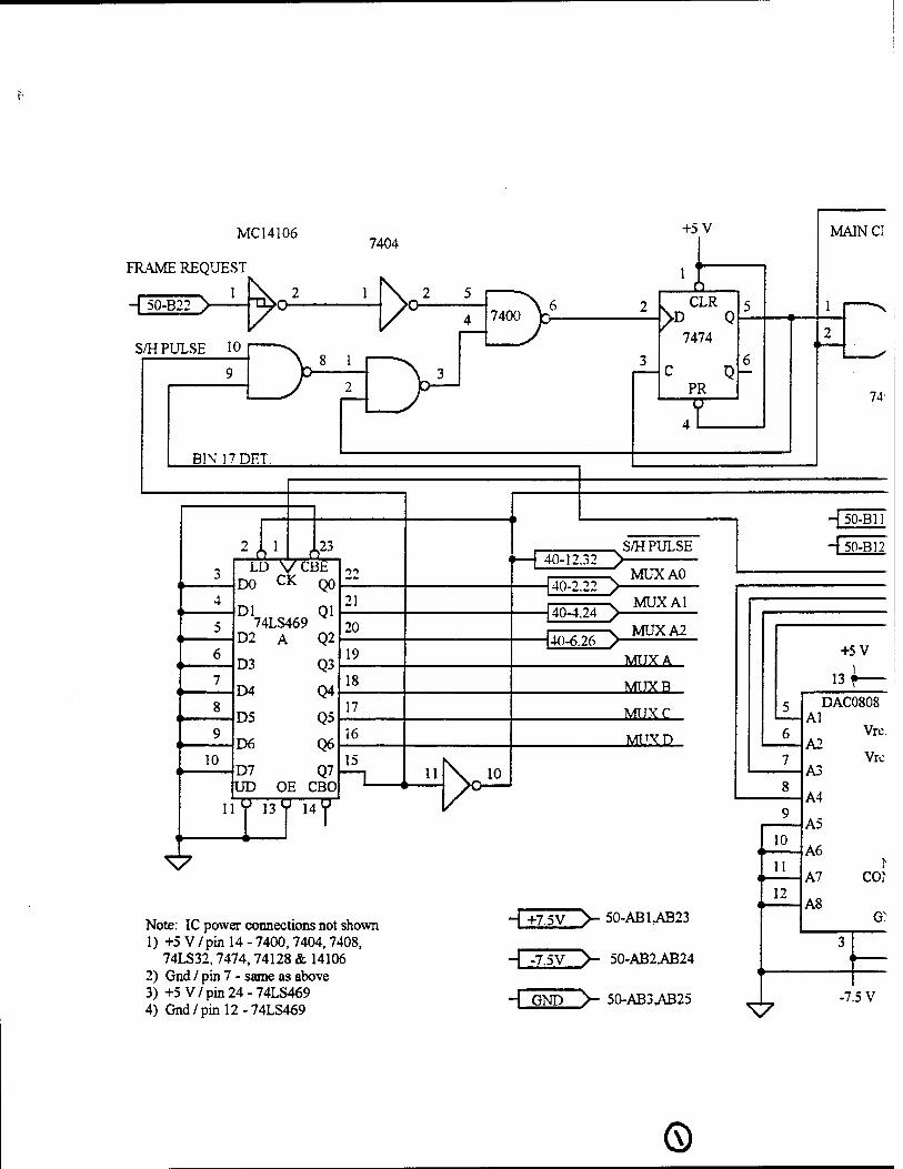
MC14106

FRAME REQUEST

I v. l

H 50-B22 >

10

2A] ., ... 0

LD VCBE DO CK

Dl

QO

Ql 74LS469

D2 A Q2

D3

D4

D5

D6

D7

Q3

Q4

Q5

Q6

Q7 UD OE CBO

11 y is y i4 y

22

21

20_

19

18

n_ 16

15

Note: IC power connections not shown 1) +5 V / pin 14 - 7400,7404,7408,

74LS32,7474,74128 & 14106 2) Gnd / pin 7 - same as above 3) +5V/pin24-74LS469 4) Gnd/pinl2-74LS469

40-12.32 > S/H PULSE

40-2.22 >

40-4.24 >

40-6.26 >

MUXAO

MUX Al

MUXA2

MUX A

MUXB

MTTXr

MUXD

- +7.3V >- 50-AB1.AB23

- -7.5V >- 50-AB2AB24

H GND >- 50-AB3AB25

H 50-B12

10

11

12

\7

+5V

13 J-

Al

A2

A3

A4

A5

A6

A7

A8

DAC0808

Vre.

Vrc

1 CO?

G:

-7.5 V

©

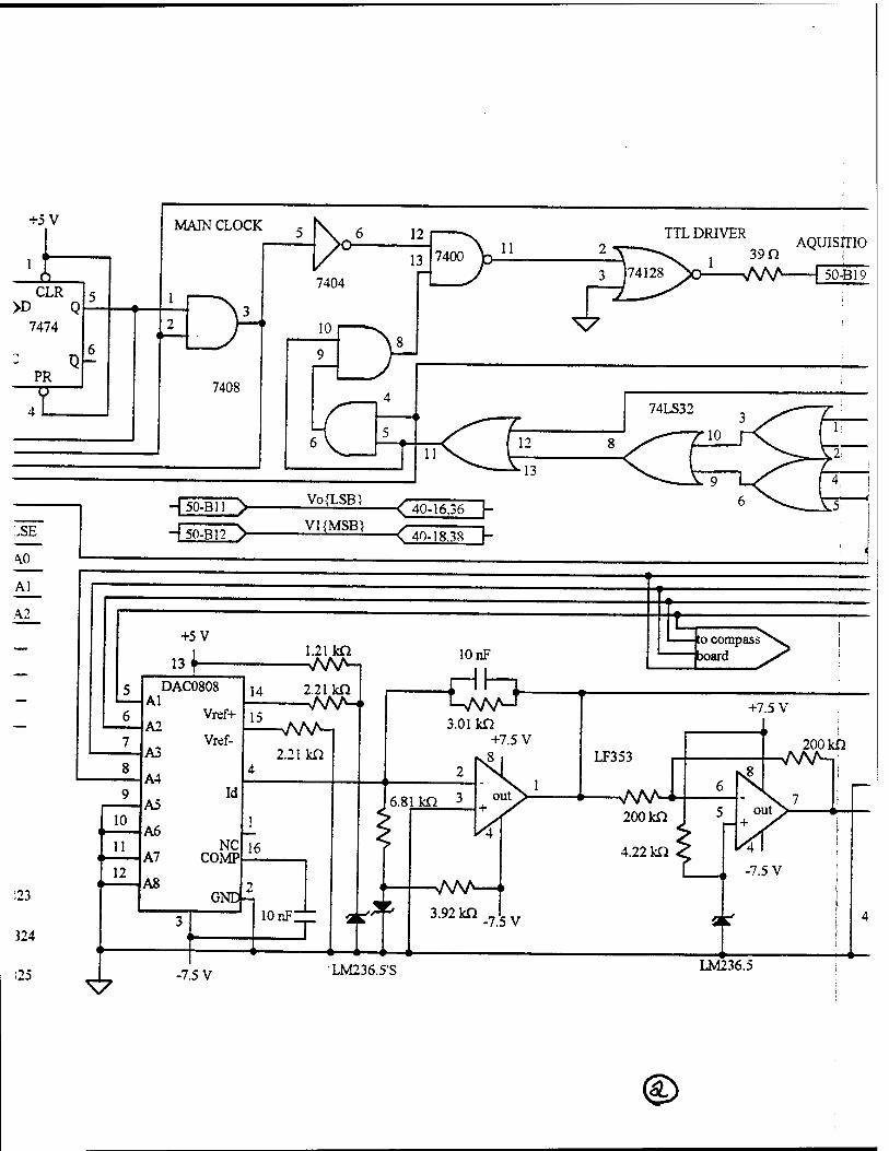
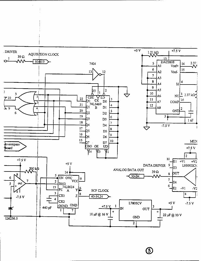
ACQUISITION CLOCK DRIVER

1 39n -*_ VW \ 50-B19 V

+5V

>o

1.21 kfi X KKK

+7.5 V T

n 5 DAC0808

Al Vref+

A2 Vref-

A3

A4 Id

A5

A6 NC

A7 COMP AC

14 2.37

6 15

< 7 i

8 4 i

9 J 1 2.37 kf2<: 10

11 16 <

12

GNDj 1 -1 U _J

InF

S7 -7.5 V i

-7.5 V

22 pF @ 10 V

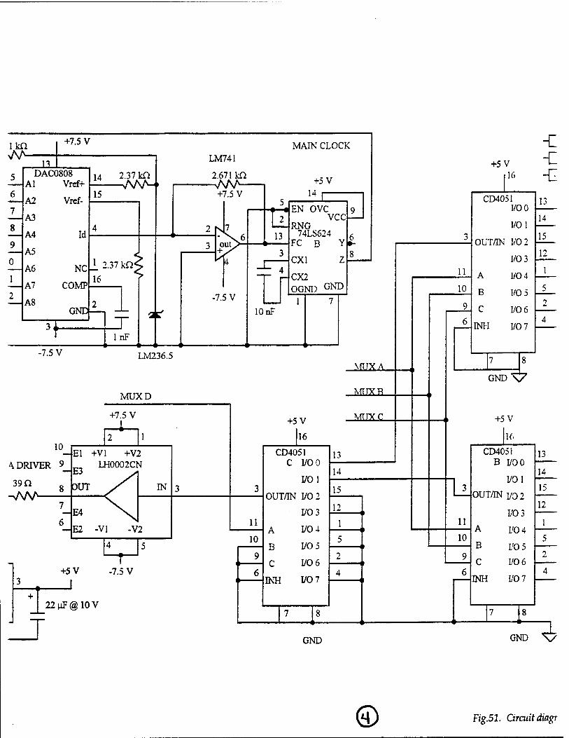
<VDRIVER 9

39 n

-7.5 V

22nF@10V

GND

© Fig.51. Grcuitdiagr

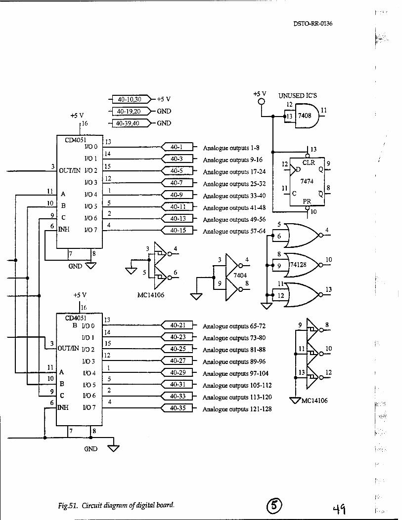
DSTO-RR-0136

+5V 16

11

10

CD4051 I/O0

1/0 1

OUT/IN 1/0 2

1/0 3

A

B

C

INH

1/0 4

1/0 5

1/0 6

1/0 7

GND*\7

+5V

lit.

11

10

CD4051 B I/OO

I/O 1

OUT/IN yo2

1/03

A

B

C

INH

I/O 4

1/0 5

1/06

1/0 7

40-10,30 >-+5V

40-19,20 >-GND

+5V

I UNUSED IC'S

12

- 40-39,40 "V-GND

14

15

12

13

14

15

12

-K 40-1 h Analogue outputs 1-8

"C 40-3 h Analogue outputs 9-16

-C 40-5 h Analogue outputs 17-24

\ 40-7 h Analogue outputs 25-32

< 40-9 h Analogue outputs 33-40


-< 40-13 \- Analogue outputs 49-56

~C 40-15 h Analogue outputs 57-64

MC14106 13

11

-< 40-21 h Analogue outputs 65-72






< 4°-33 >" Analogue outputs 113-120 ^7MC14106

■< 40-35 h Analogue outputs 121-128

13

GND \7

Fig.51. Circuit diagram of digital board. <s> n't

DSTO-RR-0136

r

THIS PAGE LEFT INTENTIONALLY BLANK

50

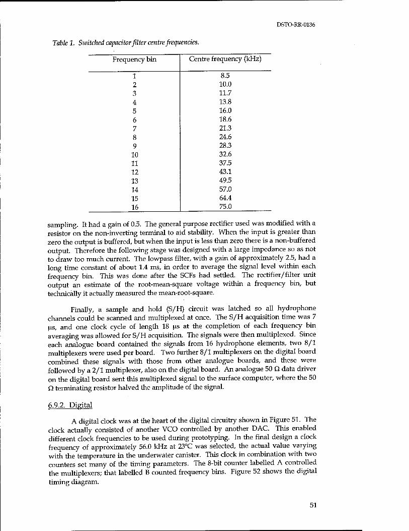
DSTO-RR-0136

Table 1. Szuitched capacitor filter centre frequencies.

Frequency bin Centre frequency (kHz)

1 8.5 2 10.0 3 11.7 4 13.8 5 16.0 6 18.6 7 21.3 8 24.6 9 28.3

10 32.6 11 37.5 12 43.1 13 49.5 14 57.0 15 64.4 16 75.0

sampling. It had a gain of 0.5. The general purpose rectifier used was modified with a resistor on the non-inverting terminal to aid stability. When the input is greater than zero the output is buffered, but when the input is less than zero there is a non-buffered output. Therefore the following stage was designed with a large impedance so as not to draw too much current. The lowpass filter, with a gain of approximately 2.5, had a long time constant of about 1.4 ms, in order to average the signal level within each frequency bin. This was done after the SCFs had settled. The rectifier/filter unit output an estimate of the root-mean-square voltage within a frequency bin, but technically it actually measured the mean-root-square.

Finally, a sample and hold (S/H) circuit was latched so all hydrophone channels could be scanned and multiplexed at once. The S/H acquisition time was 7 j^s, and one clock cycle of length 18 us at the completion of each frequency bin averaging was allowed for S/H acquisition. The signals were then multiplexed. Since each analogue board contained the signals from 16 hydrophone elements, two 8/1 multiplexers were used per board. Two further 8/1 multiplexers on the digital board combined these signals with those from other analogue boards, and these were followed by a 2/1 multiplexer, also on the digital board. An analogue 50 Q. data driver on the digital board sent this multiplexed signal to the surface computer, where the 50 Q terminating resistor halved the amplitude of the signal.

6.9.2. Digital

A digital clock was at the heart of the digital circuitry shown in Figure 51. The clock actually consisted of another VCO controlled by another DAC. This enabled different clock frequencies to be used during prototyping. In the final design a clock frequency of approximately 56.0 kHz at 23°C was selected, the actual value varying with the temperature in the underwater canister. This clock in combination with two counters set many of the timing parameters. The 8-bit counter labelled A controlled the multiplexers; that labelled B counted frequency bins. Figure 52 shows the digital timing diagram.

51

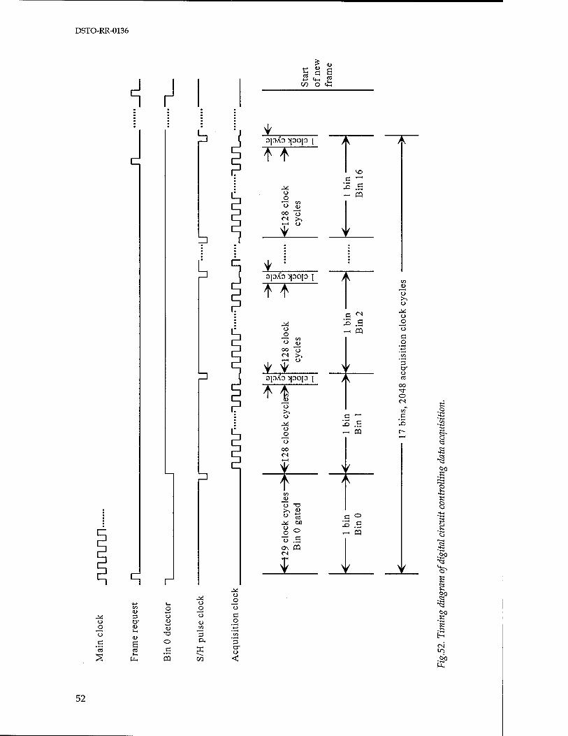
DSTO-RR-0136

r

b

L

o

ü

"S

h

3 W

P-,

<a

<D T3 O

5

o _o o

in 3 OH

O

"o c

3 W o <

+-» 4> «-H

«3 c I C/3 O lH

spfo ypop \

TJ o o o %

3J0/(0 >[00[0 [

TT ^ Ü O O (1)

00 o (N p^

3J0A0 3J0Op I

o >^ o

o _o "o 00

"o "O

go

ON PQ

£ .5

(N

PQ

X) .5 — 03

J=> .3 ~ pq

o

Ü 44 o o

c o

3 cr o <z

oo

o

c IS

s •2 ,5? 'S «

H O

..a

.§0

S s

in

52

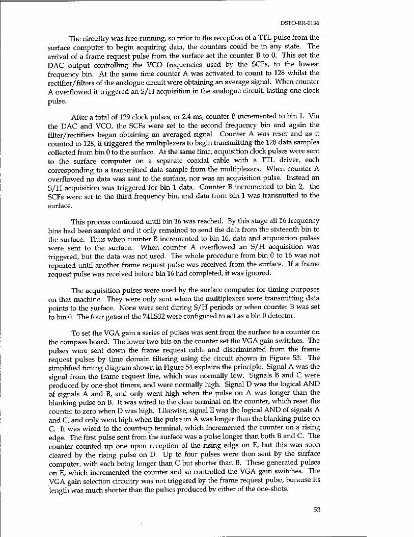
DSTO-RR-0136

The circuitry was free-running, so prior to the reception of a TTL pulse from the surface computer to begin acquiring data, the counters could be in any state. The arrival of a frame request pulse from the surface set the counter B to 0. This set the DAC output controlling the VCO frequencies used by the SCFs, to the lowest frequency bin. At the same time counter A was activated to count to 128 whilst the rectifier/filters of the analogue circuit were obtaining an average signal. When counter A overflowed it triggered an S/H acquisition in the analogue circuit, lasting one clock pulse.

After a total of 129 clock pulses, or 2.4 ms, counter B incremented to bin 1. Via the DAC and VCO, the SCFs were set to the second frequency bin and again the filter/rectifiers began obtaining an averaged signal. Counter A was reset and as it counted to 128, it triggered the multiplexers to begin transmitting the 128 data samples collected from bin 0 to the surface. At the same time, acquisition clock pulses were sent to the surface computer on a separate coaxial cable with a TTL driver, each corresponding to a transmitted data sample from the multiplexers. When counter A overflowed no data was sent to the surface, nor was an acquisition pulse. Instead an S/H acquisition was triggered for bin 1 data. Counter B incremented to bin 2, the SCFs were set to the third frequency bin, and data from bin 1 was transmitted to the surface.

This process continued until bin 16 was reached. By this stage all 16 frequency bins had been sampled and it only remained to send the data from the sixteenth bin to the surface. Thus when counter B incremented to bin 16, data and acquisition pulses were sent to the surface. When counter A overflowed an S/H acquisition was triggered, but the data was not used. The whole procedure from bin 0 to 16 was not repeated until another frame request pulse was received from the surface. If a frame request pulse was received before bin 16 had completed, it was ignored.

The acquisition pulses were used by the surface computer for timing purposes on that machine. They were only sent when the multiplexers were transmitting data points to the surface. None were sent during S/H periods or when counter B was set to bin 0. The four gates of the 74LS32 were configured to act as a bin 0 detector.

To set the VGA gain a series of pulses was sent from the surface to a counter on the compass board. The lower two bits on the counter set the VGA gain switches. The pulses were sent down the frame request cable and discriminated from the frame request pulses by time domain filtering using the circuit shown in Figure 53. The simplified timing diagram shown in Figure 54 explains the principle. Signal A was the signal from the frame request line, which was normally low. Signals B and C were produced by one-shot timers, and were normally high. Signal D was the logical AND of signals A and B, and only went high when the pulse on A was longer than the blanking pulse on B. It was wired to the clear terminal on the counter, which reset the counter to zero when D was high. Likewise, signal E was the logical AND of signals A and C, and only went high when the pulse on A was longer than the blanking pulse on C. It was wired to the count-up terminal, which incremented the counter on a rising edge. The first pulse sent from the surface was a pulse longer than both B and C. The counter counted up one upon reception of the rising edge on E, but this was soon cleared by the rising pulse on D. Up to four pulses were then sent by the surface computer, with each being longer than C but shorter than B. These generated pulses on E, which incremented the counter and so controlled the VGA gain switches. The VGA gain selection circuitry was not triggered by the frame request pulse, because its length was much shorter than the pulses produced by either of the one-shots.

53

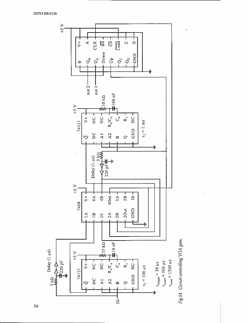
DSTO-RR-0136

Q

> U~) +

1 + < pi |o IO i-o

1 i n

> j 'm to g

« < o ex u D m a a Q P a

i o

1

Hi-

CN •4-J •*-» 3 3 O O IX,

G c ^ o o o

> m vWV I II 1 + 1 1 1 1 1

CN j s s M: «« pi

r- O — <N

rH

II

\<y z, < < m o> a H

1 1 1 i 1 I ' i

^^> *■ ^jHHi- C <7fe >> Y °* rt n o <D V CN

>

Q CN

1 ( I i

H M ffl 3 < P5 o

00 o

>■ Tt Tf Q CO CO

^t- r-

< 3

C PQ o < CQ O H r-H .—I CN CN C ■^ O

1 Hi'

G to •5 ^ c &0 in o ^

:> »—1 ' ' u L

\ ex o

i CN

in + i/WV—Hh too

/ l l 1 1

Z 1

u » - 1 i o § o

( / \ CN CN e* o ^ ° £ Ä

HHi' •* Q O II || —' - " II uJ r~-

O - CN Z II M 1 t 5

CO "* IC y ^ < < ffl c y Ü

e H H (-> 1 i i 1 Q 1 1

M" CO

1- 7j .00

54

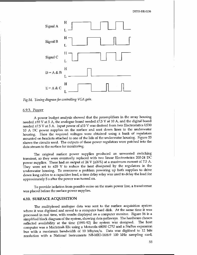
DSTO-RR-0136

H Signal A

Signal B

Signal C

D = A&B

E = A&C

L —'

H—i

L

H-

L

H

L -

H

L -

Fig.54. Timing diagram for controlling VGA gain.

6.9.3. Power

A power budget analysis showed that the preamplifiers in the array housing needed ±10 V at 5 A, the analogue board needed ±7.5 V at 10 A, and the digital board needed ±7.5 V at 5 A. Input power of ±15 V was derived from two Electrostatics LS30 10 A DC power supplies on the surface and sent down lines to the underwater housing. Here the required voltages were obtained using a bank of regulators mounted on brackets attached to one of the lids of the underwater housing. Figure 55 shows the circuits used. The outputs of these power regulators were patched into the data stream to the surface for monitoring.

The original surface power supplies produced an unwanted switching transient, so they were eventually replaced with two linear Electrostatics 200-24 DC power supplies. These had an output of 24 V (±20%) at a maximum current of 7.5 A. They were set to ±20 V to reduce the heat dissipated by the regulators in the underwater housing. To overcome a problem powering up both supplies to drive down long cables to a capacitive load, a time delay relay was used to delay the load for approximately 5 s after the power was turned on.

To provide isolation from possible noise on the main power line, a transformer was placed before the surface power supplies.

6.10. SURFACE ACQUISITION

The multiplexed analogue data was sent to the surface acquisition system where it was digitised and saved to a computer hard disk. At the same time it was processed in real time, with results displayed on a computer monitor. Figure 56 is a simplified block diagram of the system, showing data pathways. The hardware chosen reflected availability at the time (1991-92) the system was designed. The host computer was a Macintosh Ilfx using a Motorola 68030 CPU and a NuBus expansion bus with a maximum bandwidth of 10 Mbytes/s. Data was digitised to 12 bits resolution with a National Instruments NB-MIO-16H-9 100 kHz sampling card,

55

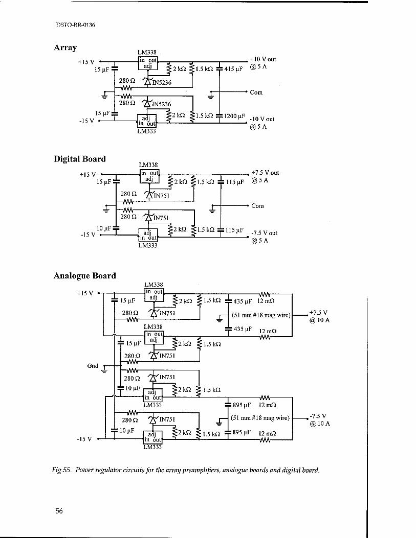
DSTO-RR-0136

Array LM338

+15 V - 15 nF!

15 ^iF^s -15 V «—

in out, adj

j£±

____+10 Vout

; 2 kQ ^ 1.5 kD Ä 415 uF @ 5 A

280 Q 7^5236 -VW\r -iMAr

» 280 Q 7VIN5236

adj '•in out1

Com

LM333

;2kQ |l.5kQ^1200^F ,1QVout

@5A

Digital Board LM338

+15 V •- 15 uF!

-15 V 10 UF:

in outr adj

^ 280 Q '/YIN751 HAMr

* Hwv- 280 Q 7TIN751 "^

,. adj 'in out* LM333

_ +7.5 V out

i2kQ |l.5kQ :{:115uF @5A

Com

[2kQ |l.5kQJ:il5nF .75Vout

@5A

Analogue Board

+15 V *

LM338

280 Q I 1/WV-

, in outj. adj

ffilN751

i/vw- ;2kQ ^1.5kQ :£:435uF 12 mQ

LM338

Gnd J^

-15 V -

S:i5uF

280 Q _-\ZWV- ~-\/WV-

280 Q

ilOuF

, in out „ adj

ffilN751

'IN751

.adj m outl

LM333 —i/WV- 280 Q

SriOuF .adj in outl

LM333

(51 mm # 18 mag wire)

:j=435uF ,2mQ

(MA ;2kQ ^1.5kQ

=2kQ < 1.5 kQ \MA

1^895^ 12 mQ

'IN751 I—I (51 mm #18 mag wire)

;2 kQ ^ i 5 kQ =7=895 ^F 12 mQ M/V—

,+7.5V @ 10 A

.-7.5V @10A

Fig.55. Power regulator circuits for tlte array preamplifiers, analogue boards and digital board.

56

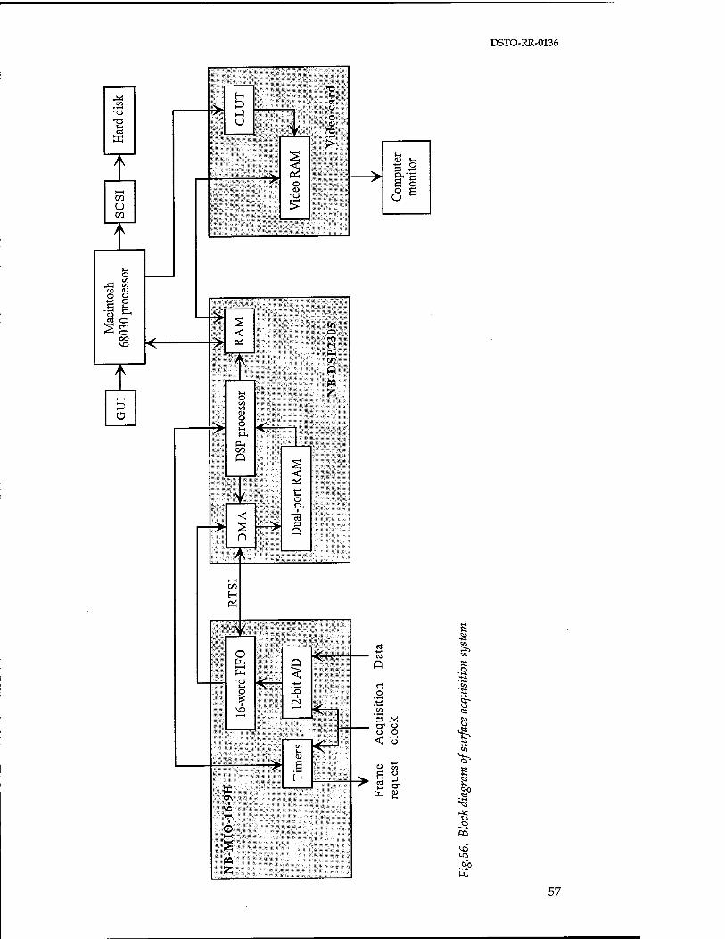
DSTO-RR-0136

IL'-: s- « u o «a

>

>

V

o

>

—>

Com

pute

r m

onito

r > <

t—<

CO

U GO

r

> <

Mac

into

sh

6803

0 pr

oces

sor

eft n

i

M

^

< P4 s

V all / \

/ <

i;>v

o

 "V

>w

O i

*c3 3 P

> f

.!;B|

Q ■iihil r

K /

GO

H

> <

^ O Hi Pi

O 4

Q

1-»

■4-»

V Q

^

rf' .J2

=> " o Ü

>w

CO

<L)

e

"^ o V

-. -4-»

X ■

l

c 1—1

s 1

ea

r > !

CO

-^ Ü w l-c

K O

a U e

S en

!> 'a

o CQ

57

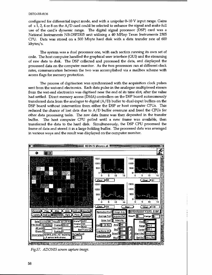
DSTO-RR-0136

configured for differential input mode, and with a unipolar 0-10 V input range. Gains of x 1, 2, 4 or 8 on the A/D card could be selected to enhance the signal and make full use of the card's dynamic range. The digital signal processor (DSP) card was a National Instruments NB-DSP2305 unit utilising a 40 MFlop Texas Instruments 2305 CPU. Data was stored on a 500 Mbyte hard disk with a data transfer rate of 600 kbytes/s.

The system was a dual processor one, with each section running its own set of code. The host computer handled the graphical user interface (GUI) and the stieaming of raw data to disk. The DSP collected and processed the data, and displayed the processed data on the computer monitor. As the two processors ran at different clock rates, communication between the two was accomplished via a mailbox scheme with access flags for memory protection.

The process of digitisation was synchronised with the acquisition clock pulses sent from the wet-end electronics. Each data pulse in the analogue multiplexed stream from the wet-end electronics was digitised near the end of its time slot, after the value had settled. Direct memory access (DMA) controllers on the DSP board autonomously transferred data from the analogue to digital (A/D) buffer to dual-input buffers on the DSP board without intervention from either the DSP or host computer CPUs. This reduced the chance of lost data due to A/D buffer overruns and freed the CPUs for other data processing tasks. The raw data frame was then deposited in the transfer buffer. The host computer CPU polled until a new frame was available, then transferred the data to the hard disk. Simultaneously, the DSP CPU processed the frame of data and stored it in a large holding buffer. The processed data was averaged in various ways and the result was displayed on the computer monitor.

Date! 11/14/95

File Sizell 146^80862

ADgainllä

Channel

Desoriptioni

Time||4:44:25PM Frames 35412

VGA Ga1n|

Packing! AD0NIS_DAQ_V2: Scanning L,R aoross both drums.

frame* time(s) curFrm

5457 224 3642

Bad Frame!

Delaarfms) UMWMMH

Normalize Fcn[|| Image Avg | ||BottomSandAir.4.dat| STOP

Average Fcn[ jj exponential || Small g)o | Large 3cT

Color Fcnlfj intensity

\ Redl|50 Log Norm Off) —'äa '■■'■"' * R ISfcn

, Log Color Off) Blue!

wmmmmmmmmmmmmmmmMMmmMKm mm.

Fig.57. ADONIS screen capture image.

58

DSTO-RR-0136

6.11. SCREEN DISPLAY

Figure 57 displays a screen capture image from ADONIS. The actual acoustic daylight image is shown in the upper left quadrant, where each pixel corresponded to one array element, and hence to a unique look direction. For each element there were 16 frequency estimates, but the data was processed so as to yield a single value. In this case the colour represented the intensity averaged over the upper three frequency bins, and was mapped into a "jet" colour scale. As well as this spatial information, the frequency content of up to four elements could also be displayed by using a mouse to select pixels in the image. The spectra could be plotted to the right as raw data or normalised in some way. Most of the other details on the screen contained information relevant to the raw data or processing used for the screen display.

To paint an area of screen 320 x 240 pixels at a 25 Hz refresh rate would require a data rate of 11.5 Mbytes/s. As this exceeded the total bandwidth of the NuBus, the images were displayed by direct manipulation of the Macintosh colour look-up table (GLUT). The CLUT is a mapping from an 8-bit number into an associated set of three 16-bit (or higher) numbers that specify the three colour components (usually red, green and blue) necessary to form a colour. In this way up to 256 colours could be displayed on the screen at any time, and a colour was selected by writing a single byte to the video RAM. This first step reduced the data rate to 1.9 Mbytes/s.

The ADONIS image was painted once at the start of the program. All the screen pixels forming an element pixel were assigned their own slot in the CLUT. When the exact 6-byte colour associated with that slot in the CLUT was changed, all screen pixels associated with that CLUT slot were updated to the new colour. Since the uninterpolated ADONIS image of 320 x 240 screen pixels only consisted of 126 large pixels, corresponding to the 126 array elements, only 126 6-byte values needed to be written to the CLUT to change the colour of all the element pixels. This reduced the data bandwidth by another two orders of magnitude, to 18.9 kbytes/s for a 25 Hz image refresh rate.

6.12. DATASTORAGE

The ADONIS data was stored in a series of files on a hard disk, each corresponding to a particular target being viewed, or some other experimental detail. At the beginning of each file was a file header of variable length. This contained such details as the file header size, the file size, the number of frames collected, the date and time, the version of software used, the A/D card channel used for digitising, the gain of that channel, the VGA gain of the wet-end electronics, the data packing format, and a trial description of variable length. After the file header, each frame was stored.

Each frame began with a frame header of fixed size. This started with the frame number and time elapsed from the start of the file, a bad frame conversion pulse count, and details about the screen display settings. These latter enabled a later reconstruction of the data seen by the experimentalist when first collected. Then followed the data associated with each frame. The data was not stored in the way it was sent to the surface. Rather, the data from each frequency bin of a channel was stored together, as [chO,bin0][ch0,binl]...[ch0,binl5][chl,bin0][chl,binl]...[chl,binl5]... [chl26, bin0][chl26, binl]...[chl26, binl5]. The order of the data channels was not in the proper order to make an image, but ordered according to the pin and connector they were assigned in the array hardware.

59

DSTO-RR-0136

It was a simple matter to convert each multiplexed channel number to its corresponding array element in any processing software.

A single frame of ADONIS data contained 16 spectral estimates for 126 channels, with each 12-bit data point occupying two bytes. At a 25 Hz frame rate, this translated to a data bandwidth of 100 kbytes/s. To save hard disk storage space, 12-bit packing was used. The data was sampled at 12-bits resolution, but being unipolar the four most significant bits of each 16-bit samples were always zero. By stripping the unused bits from four data samples, and shifting the remaining bits to fill in the space, four 12-bit data samples were packed into 6 bytes, leading to a space, and bandwidth, reduction of 25%.

As the hard disk filled up every couple of hours, the files were transferred to tape and finally written to CD-ROM disks for final storage. In this way well over a million frames of ADONIS data, each with 126 x 16 data points, were gathered.

6.13. ANCILLARY SENSORS

Although the circuitry had provision for 128 channels of data, only 126 were used by the array elements. Two further elements and preamplifiers, identical to those in the array, were housed in a canister mounted on top of the reflector (see Fig. 35), with the beams facing in the same direction as the central array beams. Because of their small size, their beamwidths were wide. Their signals were processed in the same way as for the array elements, using the spare two data channels. These hydrophones were intended to provide a spatially averaged estimate of the noise field in front of the acoustic lens for the purpose of normalising the signals from the main array. Because they were mounted outside the focal region of the reflector, they possessed different gain and frequency characteristics from the main array, and their use was discontinued.

A KVH C100 digital compass was mounted in the underwater canister, giving the sine and cosine of ADONIS' heading. It was run from the +15 V supply line. The outputs were patched into the analogue multiplexed data stream to the surface using additional multiplexers and digital timing circuitry. Although it was accurate to ±0.5°, it was sensitive to local masses of steel, including the platform from which the acoustic daylight measurements were collected. It was calibrated by pointing the acoustic lens in a known direction and rotating it through 360° in a horizontal plane at a constant speed.

A Spectron SSY0090 dual-axis inclinometer was also mounted in the underwater canister, with its outputs patched into the multiplexed data stream. Each axis had a range of ±20° with respect to the horizontal, and an accuracy of 0.01°. Using the compass and inclinometer together, the orientation of ADONIS throughout the measurements was known completely.

The wet-end electronics was convection cooled through direct contact with sea water. Two AD22100 voltage output temperature sensors with in-built signal conditioning were mounted inside the canister, and their outputs patched into the data stream to the surface for monitoring. No moisture sensor was used. The underwater canister was always mounted vertically, with the electronic cards at the top and the power regulators at the bottom. When the canister began to flood, which happened twice, the water first shorted out the regulators. This caused a sudden increase in current, which blew fuses in the power supplies on the surface, effectively cutting power to the electronics and saving the cards from arc-induced corrosion.

60

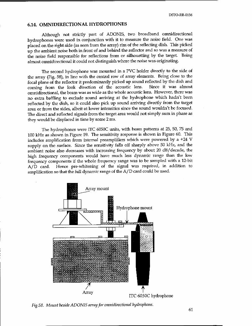
DSTO-RR-0136

6.14. OMNIDIRECTIONAL HYDROPHONES

Although not strictly part of ADONIS, two broadband omnidirectional hydrophones were used in conjunction with it to measure the noise field. One was placed on the right side (as seen from the array) rim of the reflecting dish. This picked up the ambient noise both in front of and behind the reflector and so was a measure of the noise field responsible for reflections from or silhouetting by the target. Being almost omnidirectional it could not distinguish where the noise was originating.

The second hydrophone was mounted in a PVC holder directly to the side of the array (Fig. 58), in line with the central row of array elements. Being close to the focal plane of the reflector it predominantly picked up sound reflected by the dish and coming from the look direction of the acoustic lens. Since it was almost omnidirectional, the beam was as wide as the whole acoustic lens. However, there was no extra baffling to exclude sound arriving at the hydrophone which hadn't been reflected by the dish, so it could also pick up sound arriving directly from the target area or from the sides, albeit at lower intensities since the sound wouldn't be focused. The direct and reflected signals from the target area would not simply sum in phase as they would be displaced in time by some 2 ms.

The hydrophones were ITC 6050C units, with beam patterns at 25, 50, 75 and 100 kHz as shown in Figure 59. The sensitivity response is shown in Figure 60. This includes amplification from internal preamplifiers which were powered by a +24 V supply on the surface. Since the sensitivity falls off sharply above 50 kHz, and the ambient noise also decreases with increasing frequency by about 20 dB/decade, the high frequency components would have much less dynamic range than the low frequency components if the whole frequency range was to be sampled with a 12-bit A/D card. Hence pre-whitening of the signal was required, in addition to amplification so that the full dynamic range of the A/D card could be used.

Array mount

Hydrophone mount

XLff°-..y~

ITC 6050C hydrophone

Fig.58. Mount beside ADONIS array for omnidirectional hydrophone. 61

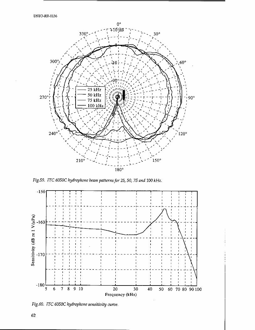
DSTO-RR-0136

0° -,--<-+! (HE

330>'r ' '

270° r ■• 90°

240°

180°

Fig.59. ITC 6050C hydrophone beam patterns for 25, 50, 75 and 100 kHz.

-150

% -160

03 •a

I -170 t/j a

-180

i 1 —i —1- + 1 1- 1 1 i i 1 —i —1__

I 1 1 I - +• 1 1 | S | I-^\H 1 1 - -

I 1 1 1 - +• 1 -t I 1 | | 1 _\_| 1 _ .

1 1 1 l-J- 1 J. I I I I I I A _1

I 1 1 1 - + 1 \ I 1 i | 1 1 iA_

5 6 7 8 9 10 20 30 40 50 60 70 80 90100 Frequency (kHz)

Fig.60. ITC 6050C hydrophone sensitivity curve.

62

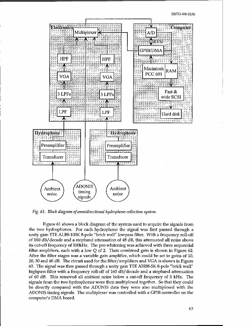
DSTO-RR-0136

Electronics Multiplexer

HPF

VGA

3LPFs

LPF

Hydrophone

Preamplifier 31

Transducer

HPF

VGA

3LPFs

LPF

A/D Computer

'RTSI

GPIB/DMA

Macintosh PCC 601

RAM

Fast& wide SCSI

Hard disk

Hydrophone

Preamplifier ü

Transducer

'ADONIS timing

^signals

Fig. 61. Block diagram of omnidirectional hydrophone collection system.

Figure 61 shows a block diagram of the system used to acquire the signals from the two hydrophones. For each hydrophone the signal was first passed through a unity gain TTE ALB8-100K 8-pole "brick wall" lowpass filter. With a frequency roll-off of 160 dB/decade and a stopband attenuation of 48 dB, this attenuated all noise above its cut-off frequency of 100kHz. The pre-whitening was achieved with three sequential filter amplifiers, each with a low Q of 2. Their combined gain is shown in Figure 62. After the filter stages was a variable gain amplifier, which could be set to gains of 10, 20,30 and 40 dB. The circuit used for the filter/amplifiers and VGA is shown in Figure 63. The signal was then passed through a unity gain TTE AHB8-5K 8-pole "brick wall" highpass filter with a frequency roll-off of 160 dB/decade and a stopband attenuation of 60 dB. This removed all ambient noise below a cut-off frequency of 5 kHz. The signals from the two hydrophones were then multiplexed together. So that they could be directly compared with the ADONIS data they were also multiplexed with the ADONIS timing signals. The multiplexer was controlled with a GPIB controller on the computer's DMA board.

63

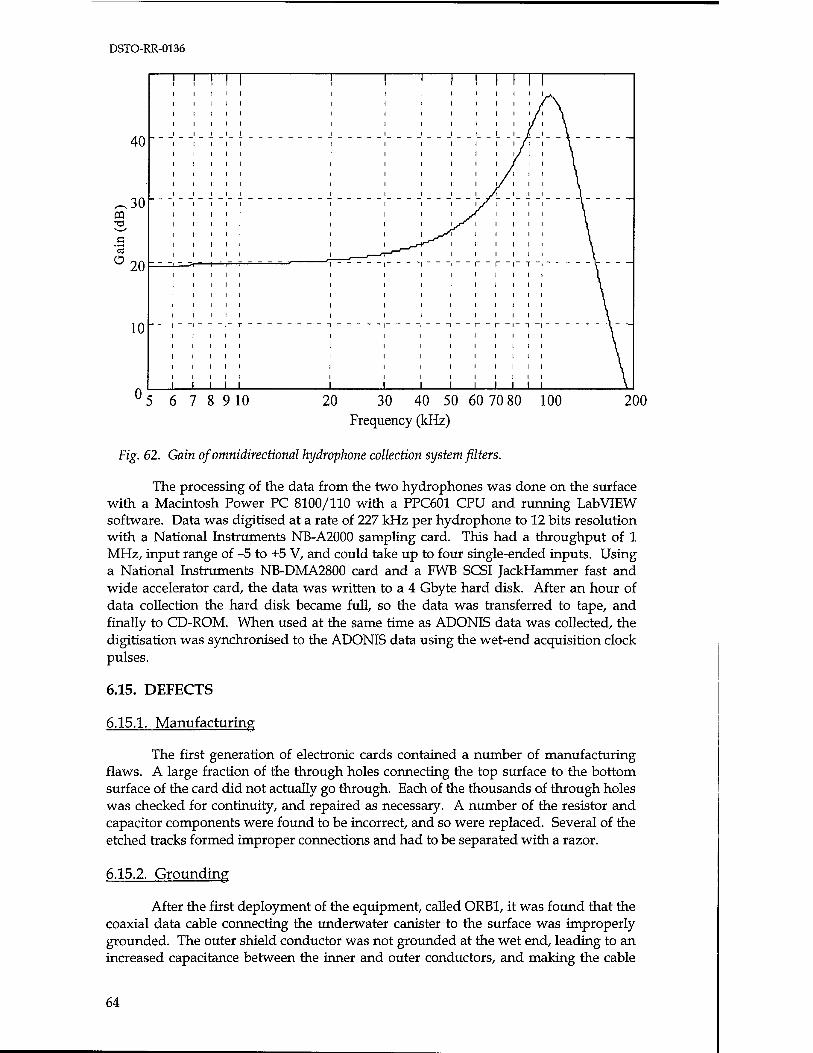
DSTO-RR-0136

40

30 m v—'

a

O 20

10

1 - -i —r - i- T ■» 'i - - - — i -i — -i — r_r-|-T_i — - — V

— -|--|--t-|-T---------j-----i----|---|--r-r-|--r-|------4- —

5 6 7 8 910 20 30 40 50 Frequency (kHz)

60 70 80 100 200

Fig. 62. Gain of omnidirectional hydrophone collection system filters.

The processing of the data from the two hydrophones was done on the surface with a Macintosh Power PC 8100/110 with a PPC601 CPU and running LabVIEW software. Data was digitised at a rate of 227 kHz per hydrophone to 12 bits resolution with a National Instruments NB-A2000 sampling card. This had a throughput of 1 MHz, input range of -5 to +5 V, and could take up to four single-ended inputs. Using a National Instruments NB-DMA2800 card and a FWB SCSI JackHammer fast and wide accelerator card, the data was written to a 4 Gbyte hard disk. After an hour of data collection the hard disk became full, so the data was transferred to tape, and finally to CD-ROM. When used at the same time as ADONIS data was collected, the digitisation was synchronised to the ADONIS data using the wet-end acquisition clock pulses.

6.15. DEFECTS

6.15.1. Manufacturing

The first generation of electronic cards contained a number of manufacturing flaws. A large fraction of the through holes connecting the top surface to the bottom surface of the card did not actually go through. Each of the thousands of through holes was checked for continuity, and repaired as necessary. A number of the resistor and capacitor components were found to be incorrect, and so were replaced. Several of the etched tracks formed improper connections and had to be separated with a razor.

6.15.2. Grounding

After the first deployment of the equipment, called ORB1, it was found that the coaxial data cable connecting the underwater canister to the surface was improperly grounded. The outer shield conductor was not grounded at the wet end, leading to an increased capacitance between the inner and outer conductors, and making the cable

64

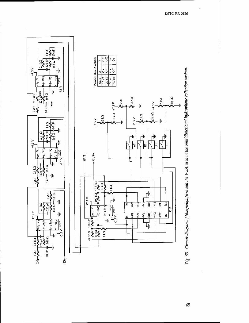
DSTO-RR-0136

l- a>

tc 03 o O Ü Ü

<f c ta d ta < O o Ü o

CQ CQ CQ CQ

'5 ■o T) -o T>

«3 o O C (N m Tf

> R o ••c u

a

H P O

^-ww^-t-ww—|l

-vwv-r^wv—||i

rt es

P O

-VWirf^WV—||i

^-vÄV-f-WW—I!'

rri \

r4'^ \

■r-* ~ — <N £< £1 ^ c 3 ~ ~ 3 C

^

R o

1- 1 « R o

•-G

R

R CS «

S

Q en

65

DSTO-RR-0136

act as a lowpass filter. This in turn caused successive data pulses to run into each other, a particularly serious problem when a low amplitude pulse followed a high amplitude pulse. The level of the low amplitude pulse was then raised.

The array head had a sea water ground, whereas the power regulators were grounded at the surface. This resulted in a ground loop which was not resolved.

6.15.3. Dead channels

During ORB1 one of the thick data cables from the array to the wet-end electronics was twisted, so that two of the internal conductor wires detached from the conductor pins. Thus two of the 126 channels provided no data. In the second major deployment, called ORB2, a short on one of the electronic cards caused another channel to fail.

6.15.4. Bad frames

The National Instruments cards used in the surface acquisition system made use of their real-time system integration (RTSI) bus, which was a flat ribbon cable directly connecting National Instruments boards to allow inter-board communication without the overhead of using the system bus. As soon as a conversion was available from the A/D converter, a signal was sent over the RTSI bus to the DMA controller on the DSP board. The DMA then transferred the digital word from the A/D buffer to a memory location on the DSP board. Noise on the RTSI bus, perhaps due to impedance mismatches on either end of the RTSI cable, occasionally triggered the DMA to attempt to transfer a data point before its conversion was available. This inserted a spurious data point into the multiplexed data stream, but did not trigger a hardware error flag. Since each frequency estimate for each channel was expected to be in a specific multiplexer time slot, all the following data points were offset from their expected locations, leading to a bad frame.

To detect these bad frames the number of data transfers made by the DMA was compared to the number of acquisition clock pulses received from the wet-end electronics. The acquisition clock pulses were counted with one of the spare counter/timers on the A/D card, and this value was compared to the DMA transfer count register. If these numbers were different, a spurious data point had been inserted and the frame was flagged as bad.

Initially these bad frames, which accounted for 10-20% of the total, were discarded. Later it was noted that these spurious data points always had the same value, equivalent to -60 in decimal notation, whereas the ADONIS data lay between 0- 4095. Thus the identified spurious data points were simply removed and the following data points shifted back. Only the last data point in the frame was lost. The rest of the data frame could be recovered.

6.15.5. Nonlinearity

Only after the completion of ORB2 was it noted that the input impedance of the FWR was 2 kQ, an order of magnitude too low. This lowered the output voltage swing of the SCFs to a maximum of 3.5 V, instead of the intended voltage swing of 5 V. Therefore the system was linear from 0 to 3.5 V, after which it became increasingly nonlinear. Figure 64 plots the system response for a 50 kHz sinusoid applied to the input of channel 1 of the underwater electronics package, as measured at the output of the electronics for frequency bin 13. The output becomes nonlinear beyond 3.5 V.

66

DSTO-RR-0136

> 3

3

* 2 - 3

O

! ! j- L^^^^rr^T- _ -i -i i '

',- - y~ -', -t i 1 ' f ' '

0 1 4 5 6 Input amplitude (mV)

10

Fig. 64. System response of frequency bin 13 of channel 1 ofunderwater electronics to 50 kHz input.

Due to the nature of the electronics, this flaw could not be readily corrected. The system had a frequency dependent gain such that the higher frequency bins would be in saturation whilst the lower frequency bins were still in the linear region. When the SCF saturated, significant amounts of noise were injected into the power bus and ground. This bus noise induced a corresponding noise into the first stage amplifiers, which then amplified the noise and fed it back into the SCFs, completing the positive feedback loop and driving the other bins into saturation. The increased system noise skewed all outputs towards high amplitudes. In Heu of a solution, all nonlinear data was discarded.

6.16. SYSTEM NOISE

In the description of the electronics above, mention has been made of some sources of electronic noise. This was quantified by measuring the self noise of the whole system. The array was placed in a tank of water, and connected to the wet-end electronics and surface acquisition system. Without injecting any acoustic noise into the tank, the system was run to collect data in the usual way. This gave the self noise of each channel for each frequency bin, from the array elements to the input of the computer A/D card. Results were recorded for VGA gains of 0,10 and 20 dB, and are plotted in Figure 65 as the voltage into the A/D card. As to be expected, the self noise increased with gain. The noise was particularly intense at all gains for frequency bin 13, reaching more than 0.1 V for a 20 dB VGA gain. The source of this noise is pickup of the digital board clock frequency. This was subsequently ameliorated by heavy bypassing where it was generated; re-routing power to some chips to isolate the source; and by placing two capacitors on the power leads coming into the boards.

67

DSTO-RR-0136

9 10 20 30 40 50 60 70 Frequency (kHz)

Fig. 65. Self noise from array to input of the A/D card for VGA gains ofO, 10 and 20 dB.

6.17. EQUALISATION

The first acoustic daylight experiment had shown acoustic contrast differences between the target and background of approximately 4 dB. Therefore, in order to successfully image targets, the differences between channels had to be considerably less than this figure. Any variations caused by the reflector, array element sensitivities or electronic gain needed to be measured to derive a correction factor for each channel, resulting in channel equalisation.

The reflector was so large it could not be put into a calibration pool, so initially equalisation excluded the effect of the reflector. EDO, who built the array, measured the sensitivity of all elements at 40 kHz. They also measured the sensitivity of 19 of the elements, in 1 kHz increments from 5 to 100 kHz, using different projectors for frequencies above and below 50 kHz. At 50 kHz there was a discontinuity of 1-3 dB. Figure 66 plots the sensitivity of element 70, including the gain of the array preamplifiers.

Another attempt at measuring the sensitivities of the elements was made at the Transdec naval calibration facility at Pt Loma, San Diego. Twenty-eight of the elements were measured in 250 Hz increments from 5 to 30 kHz using one projector, and 500 Hz increments from 30 to 100 kHz using another projector. There was no discontinuity at 30 kHz, but there was no consistent correlation between the EDO and Transdec sensitivity measurements. Over part of the frequency range, the Transdec results were some 3-4 dB less than those made by EDO, as seen by the comparison for element 70 in Figure 66.

It had been hoped that the element response might vary in a smooth and predictable way across the face of the array, so the response of those elements not calibrated could be inferred from those that were. This was not the case. The elements on the outer edge of the array, which were not bordered on all sides by other elements,

68

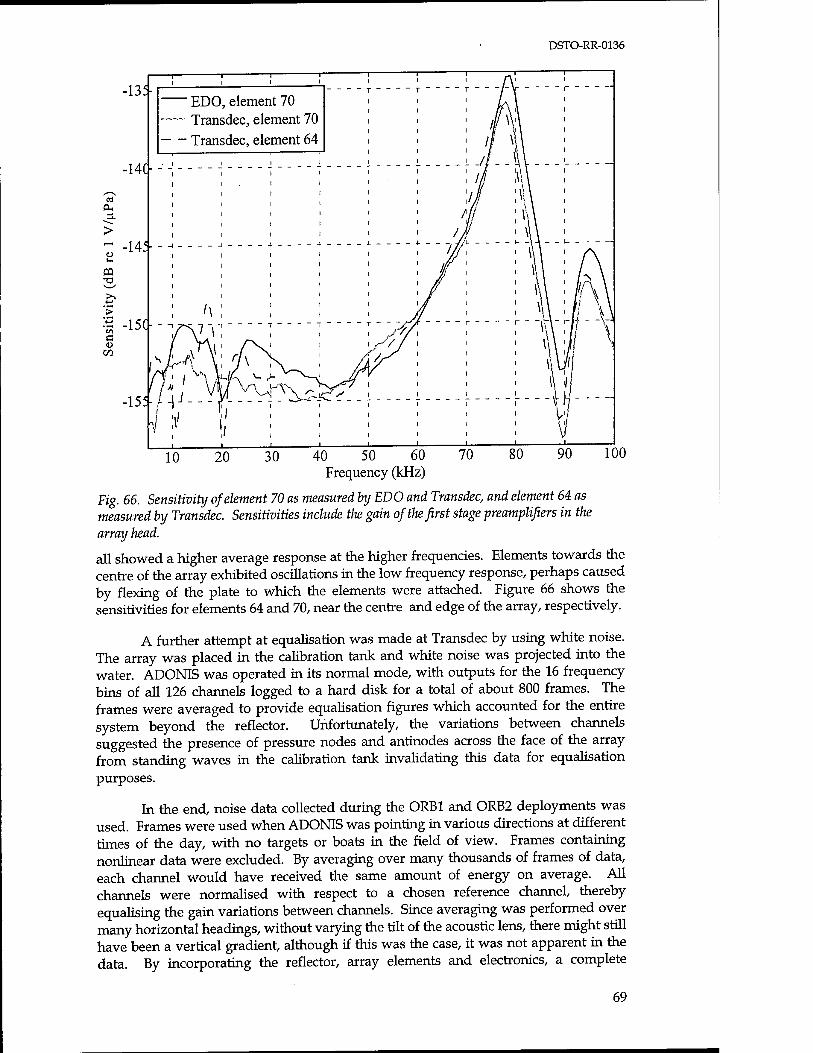
DSTO-RR-0136

a PL,

>

'>


Fig. 66. Sensitivity of element 70 as measured by EDO and Transdec, and element 64 as measured by Transdec. Sensitivities include the gain of the first stage preamplifiers in the array head.

all showed a higher average response at the higher frequencies. Elements towards the centre of the array exhibited oscillations in the low frequency response, perhaps caused by flexing of the plate to which the elements were attached. Figure 66 shows the sensitivities for elements 64 and 70, near the centre and edge of the array, respectively.

A further attempt at equalisation was made at Transdec by using white noise. The array was placed in the calibration tank and white noise was projected into the water. ADONIS was operated in its normal mode, with outputs for the 16 frequency bins of all 126 channels logged to a hard disk for a total of about 800 frames. The frames were averaged to provide equalisation figures which accounted for the entire system beyond the reflector. Unfortunately, the variations between channels suggested the presence of pressure nodes and antinodes across the face of the array from standing waves in the calibration tank invalidating this data for equalisation purposes.

In the end, noise data collected during the ORB1 and ORB2 deployments was used. Frames were used when ADONIS was pointing in various directions at different times of the day, with no targets or boats in the field of view. Frames containing nonlinear data were excluded. By averaging over many thousands of frames of data, each channel would have received the same amount of energy on average. All channels were normalised with respect to a chosen reference channel, thereby equalising the gain variations between channels. Since averaging was performed over many horizontal headings, without varying the tilt of the acoustic lens, there might still have been a vertical gradient, although if this was the case, it was not apparent in the data. By incorporating the reflector, array elements and electronics, a complete

69

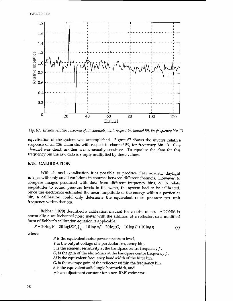
DSTO-RR-0136

1.8

1.6

1.4

•S 1-2 3 +-»

| 1.0

> 0.8

Pi 0.6

0.4

0.2

0

fV\| IrWV^vAK^w^rt ̂ . --Y- ___.^___| I

r — -

1 1 1 1

20 40 60 Channel

80 100 120

Fig. 67. Inverse relative response of all channels, with, respect to channel 59, for frequency bin 13.

equalisation of the system was accomplished. Figure 67 shows the inverse relative response of all 126 channels, with respect to channel 59, for frequency bin 13. One channel was dead; another was unusually sensitive. To equalise the data for this frequency bin the raw data is simply multiplied by these values.

6.18. CALIBRATION

With channel equalisation it is possible to produce clear acoustic daylight images with only small variations in contrast between different channels. However, to compare images produced with data from different frequency bins, or to relate amplitudes to sound pressure levels in the water, the system had to be calibrated. Since the electronics estimated the mean amplitude of the energy within a particular bin, a calibration could only determine the equivalent noise pressure per unit frequency within that bin.

Bobber (1970) described a calibration method for a noise meter. ADONIS is essentially a multichannel noise meter with the addition of a reflector, so a modified form of Bobber's calibration equation is applicable:

P = 201ogF-201og(S'Ge)|/e -101ogA/-201ogG,-101og5 + 101og77 (7)

where P is the equivalent noise power spectrum level, V is the output voltage of a particular frequency bin, S is the element sensitivity at the bandpass centre frequency fc, Ge is the gain of the electronics at the bandpass centre frequency fc, A/is the equivalent frequency bandwidth of the filter bin, Gr is the average gain of the reflector within the frequency bin, B is the equivalent solid angle beamwidth, and rj is an adjustment constant for a non-RMS estimator.

70

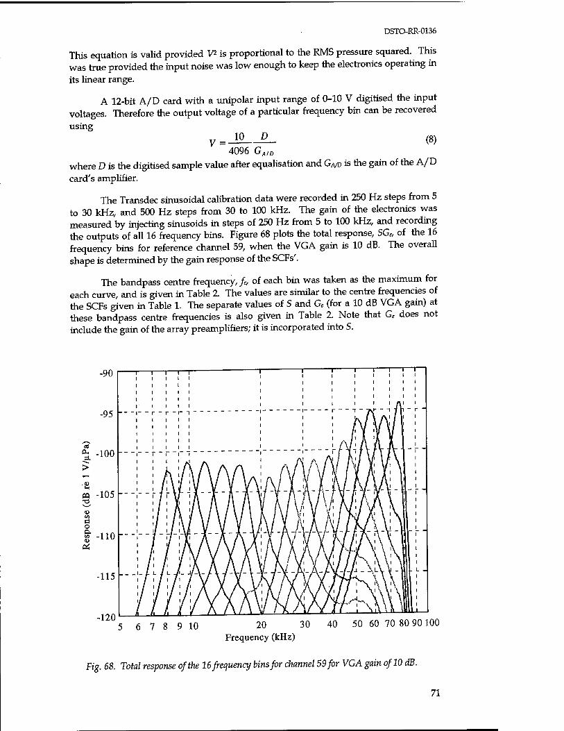
DSTO-RR-0136

This equation is valid provided V* is proportional to the RMS pressure squared. This was true provided the input noise was low enough to keep the electronics operating in its linear range.

A 12-bit A/D card with a unipolar input range of 0-10 V digitised the input voltages. Therefore the output voltage of a particular frequency bin can be recovered

using 10 D

V = (8) 4096 GAID

where D is the digitised sample value after equalisation and GVD is the gain of the A/D card's amplifier.

The Transdec sinusoidal calibration data were recorded in 250 Hz steps from 5 to 30 kHz, and 500 Hz steps from 30 to 100 kHz. The gain of the electronics was measured by injecting sinusoids in steps of 250 Hz from 5 to 100 kHz, and recording the outputs of all 16 frequency bins. Figure 68 plots the total response, SGe, of the 16 frequency bins for reference channel 59, when the VGA gain is 10 dB. The overall shape is determined by the gain response of the SCFs'.

The bandpass centre frequency, fC/ of each bin was taken as the maximum for each curve, and is given in Table 2. The values are similar to the centre frequencies of the SCFs given in Table 1. The separate values of S and Ge (for a 10 dB VGA gain) at these bandpass centre frequencies is also given in Table 2. Note that Ge does not include the gain of the array preamplifiers; it is incorporated into S.

-120 5 6 7 8 9 10 20 30 40 50 60 70 80 90100

Frequency (kHz)

Fig. 68. Total response of the 16 frequency bins for channel 59 for VGA gain of 10 dB.

71

DSTO-RR-0136

t3 K CS

O CM

00

CS

'S,

es too

tu

ts

13 K CS

-O

>, U K tu 3 Cr- tu

cs

•5 3 Cj-

too ^

K K CS

*- <-> ,° tu •O u r. a

-Si P3

-*-» cs to tu

•+J rO

V5 tu

e too tu en CS

>s 13 u »d S o tu Ui

a »*-l

Cr- F1

tu tu

^ CS tu Ö *. ■*j 3 K cr- tu tu u "«

K CM CS

tu E"

CS c-> t-H ^H

f-i

"0 w s CO CO in CO SO o IN m Os Os rH CO SO Os in rt<

JC •4-t

o CO o CO SO in in rt* Tt* CO CM CM rH rH o Os CO

"o CM CM lH rH rH rH rH rH rH rH rH rH rH rH o o <n T3 o o o O O O O O O O O O O O o o

£ OJ a (8 « > 0>

«W •Q 3 CT1

m (U e Os in o CO O CO in in CO rH in o in o "tf Os

CM o\ tN ■* CO rH o Os CO CO IN IN SO SO in -^ 00 o CM r-i i-l rH rH rH rH o o o O O o O o o

CM O O o O O O O o o o o o o o o o

o CO

so CM

00

CO

Os

CO

o O

rH rH

IN

rH

o CM

CO

CM

CO

CM

in o CO rl<

CO Os rH rH

SO IN

c rH rH rH rH rH rH rH rH rH rH rH rH rH

(Ö oo

o •*-> u HI

SU*

m s CM C\ CM SO Os CO O O CO SO ttf CM O CO IN SO

o CM

IN CO o rH CM CO in SO so IN CO Os O O rH CM r-i rH rH rH r-i rH rH T-H rH rH CM CM CM CM

^-^ N

^ X c >^ ^ 0) u *■—'

(8 H-> r-i CM IN rH SO ■* CO IN ■* in 3^ in o 1 5 > 3 TS so CT\ CO ON CO ttf CM CO O IN ■<* OS

'3 cr1

cr1

01 £ rH r-i CM CM CO ■* in in SO IN <*S OS Os rH »

W MH

c (Ö

C •t-H

(0 bo u ^^ '2 o

pa ■d *# ■* "* CO o CM Os in CO •<*< OS TJH CO rH so in

O O o o rH rH rH CM CO -* in IN CO IN CM in «4-< m in in in in in in in in in in in in in in rt< ttJ

w

^ rt

•4-» •*H •x^

> • 1—( > IN \o IN in CO m CM CO •* SO IN CM ■^ CM in so ■ i-H CM TH rH CM CM ■* in ■* •^ in SO SO t* CM CO Os <n r-< in in in m in in in in in in in in in in Ttl CO C 0) rH T-H r-t rH rH rH rH rH T-H rH rH rH rH rH rH rH 0) I-i i t l i i l l l 1 1 l ■ l i l l

c/5

3-

>, o> u

C <L)

^^ N

X O CO in CO CO in CO CO o CO in co O CO in co

c 3 00 ON rH CO SO CO rH in Os CO 00 Tt< rH IN SO so

a> cr1 ^ rH rH rH rH CM CM CM CO CO Tt< in in so IN U 01

"HH

>-. u C 01 3 •iH r-i CM CO Ttf in SO IN CO Os o

rH rH CM rH rH

CO rH rH

in so rH rH

cr <u u

V-,

72

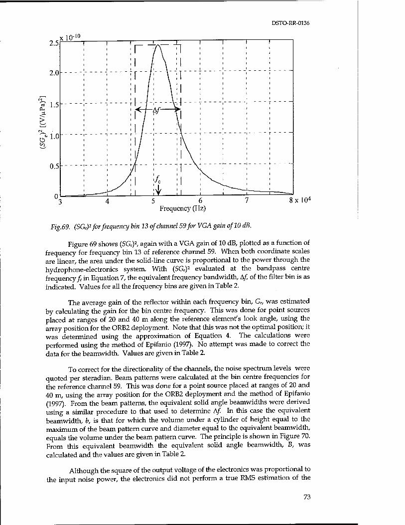
DSTO-RR-0136

5 6 7 8xl04

Frequency (Hz)

Fig.69. (SGe)2 for frequency bin 13 of channel 59 for VGA gain of 10 dB.

Figure 69 shows {SGe)2, again with a VGA gain of 10 dB, plotted as a function of frequency for frequency bin 13 of reference channel 59. When both coordinate scales are linear, the area under the solid-line curve is proportional to the power through the hydrophone-electronics system. With (SGe)

2 evaluated at the bandpass centre frequency fc in Equation 7, the equivalent frequency bandwidth, A/, of the filter bin is as indicated. Values for all the frequency bins are given in Table 2.

The average gain of the reflector within each frequency bin, G„ was estimated by calculating the gain for the bin centre frequency. This was done for point sources placed at ranges of 20 and 40 m along the reference element's look angle, using the array position for the ORB2 deployment. Note that this was not the optimal position; it was determined using the approximation of Equation 4. The calculations were performed using the method of Epifanio (1997). No attempt was made to correct the data for the beamwidth. Values are given in Table 2.

To correct for the directionality of the channels, the noise spectrum levels were quoted per steradian. Beam patterns were calculated at the bin centre frequencies for the reference channel 59. This was done for a point source placed at ranges of 20 and 40 m, using the array position for the ORB2 deployment and the method of Epifanio (1997). From the beam patterns, the equivalent solid angle beamwidths were derived using a similar procedure to that used to determine A/. In this case the equivalent beamwidth, b, is that for which the volume under a cylinder of height equal to the maximum of the beam pattern curve and diameter equal to the equivalent beamwidth, equals the volume under the beam pattern curve. The principle is shown in Figure 70. From this equivalent beamwidth the equivalent solid angle beamwidth, B, was calculated and the values are given in Table 2.

Although the square of the output voltage of the electronics was proportional to the input noise power, the electronics did not perform a true RMS estimation of the

73

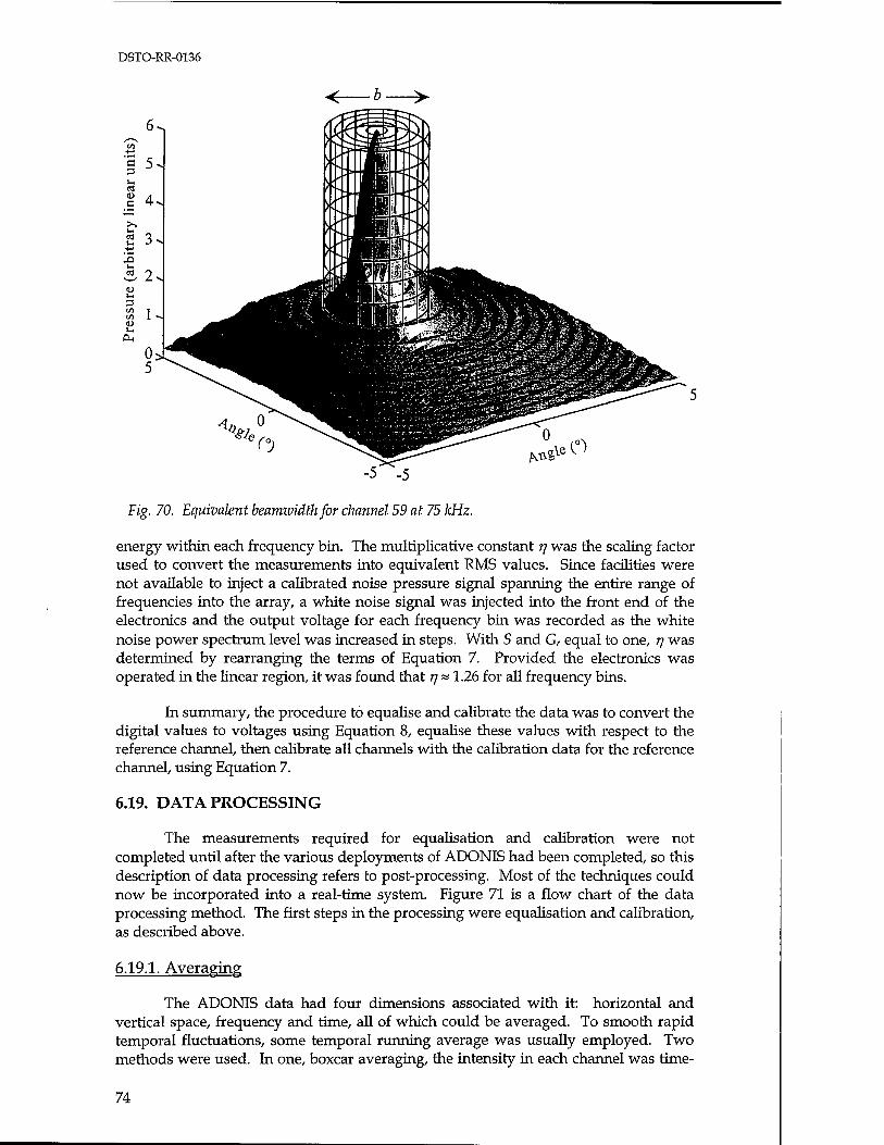
DSTO-RR-0136

-5 -5

Fig. 70. Equivalent beamzuidth for channel 59 at 75 kHz.

energy within each frequency bin. The multiplicative constant rj was the scaling factor used to convert the measurements into equivalent RMS values. Since facilities were not available to inject a calibrated noise pressure signal spanning the entire range of frequencies into the array, a white noise signal was injected into the front end of the electronics and the output voltage for each frequency bin was recorded as the white noise power spectrum level was increased in steps. With S and Gr equal to one, 77 was determined by rearranging the terms of Equation 7. Provided the electronics was operated in the linear region, it was found that 77« 1.26 for all frequency bins.

In summary, the procedure to equalise and calibrate the data was to convert the digital values to voltages using Equation 8, equalise these values with respect to the reference channel, then calibrate all channels with the calibration data for the reference channel, using Equation 7.

6.19. DATA PROCESSING

The measurements required for equalisation and calibration were not completed until after the various deployments of ADONIS had been completed, so this description of data processing refers to post-processing. Most of the techniques could now be incorporated into a real-time system. Figure 71 is a flow chart of the data processing method. The first steps in the processing were equalisation and calibration, as described above.

6.19.1. Averaging

The ADONIS data had four dimensions associated with it: horizontal and vertical space, frequency and time, all of which could be averaged. To smooth rapid temporal fluctuations, some temporal running average was usually employed. Two methods were used. In one, boxcar averaging, the intensity in each channel was time-

74

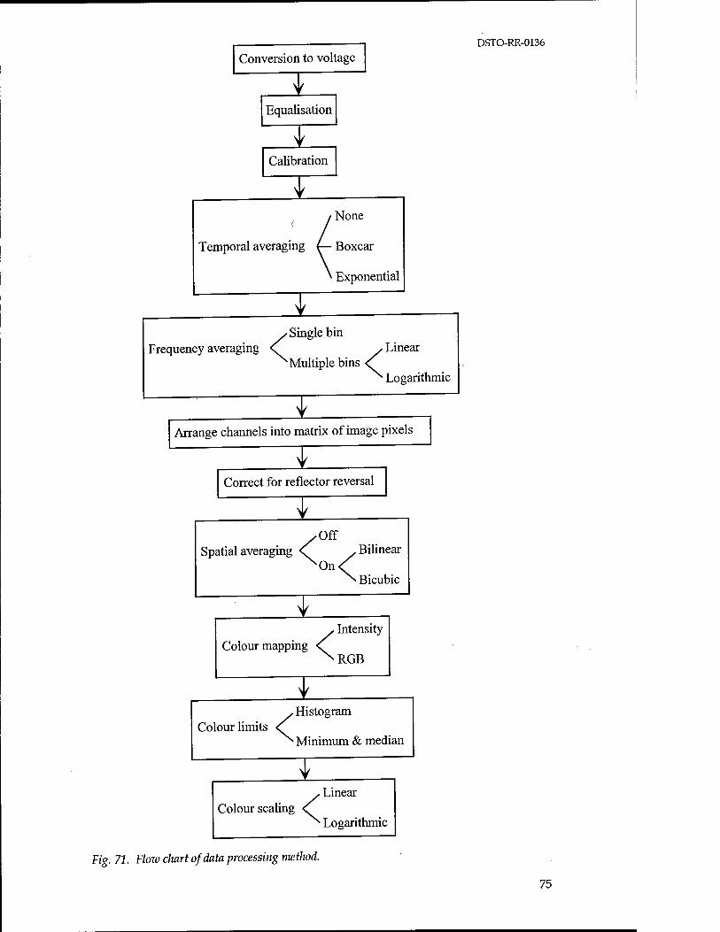
Conversion to voltage DSTO-RR-0136

Equalisation

Calibration

None

Temporal averaging £— Boxcar

Exponential

Frequency averaging Single bin

Multiple bins <

Linear

Logarithmic

Arrange channels into matrix of image pixels

± , Correct for reflector reversal

Off Spatial averaging <f .Bilinear

XOn<^ ^ Bicubic

Colour mapping Intensity

RGB

Colour limits Histogram

Minimum & median

Colour scaling Linear

Logarithmic

Fig. 71. Flow chart of data processing metlwd.

75

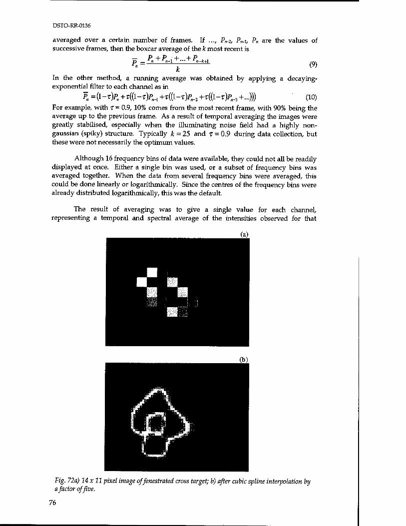
DSTO-RR-0136

averaged over a certain number of frames. If ..., P„-2, Pn-i, Pn are the values of successive frames, then the boxcar average of the k most recent is

p — -Si + "n-1 + — + "n-fe+1 (9)

In the other method, a running average was obtained by applying a decaying- exponential filter to each channel as in

P„ =(1-T)P„+T((1-T)P„,+T((1-T)P„.2+T((1-T)?„.3+...))) (10)

For example, with x - 0.9,10% comes from the most recent frame, with 90% being the average up to the previous frame. As a result of temporal averaging the images were greatly stabilised, especially when the illuminating noise field had a highly non- gaussian (spiky) structure. Typically k = 25 and T = 0.9 during data collection, but these were not necessarily the optimum values.

Although 16 frequency bins of data were available, they could not all be readily displayed at once. Either a single bin was used, or a subset of frequency bins was averaged together. When the data from several frequency bins were averaged, this could be done linearly or logarithmically. Since the centres of the frequency bins were already distributed logarithmically, this was the default.

The result of averaging was to give a single value for each channel, representing a temporal and spectral average of the intensities observed for that

Fig. 72a) 14x11 pixel image offenestrated cross target; b) after cubic spline interpolation by a factor of five.

76

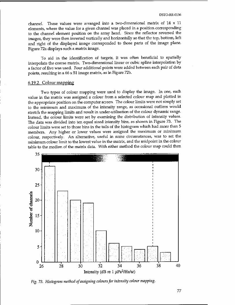
DSTO-RR-0136

channel. These values were arranged into a two-dimensional matrix of 14 x 11 elements, where the value for a given channel was placed in a position corresponding to the channel element position on the array head. Since the reflector reversed the images, they were then inverted vertically and horizontally so that the top, bottom, left and right of the displayed image corresponded to those parts of the image plane. Figure 72a displays such a matrix image.

To aid in the identification of targets, it was often beneficial to spatially interpolate the coarse matrix. Two-dimensional linear or cubic spline interpolation by a factor of five was used. Four additional points were added between each pair of data points, resulting in a 66 x 51 image matrix, as in Figure 72b.

6.19.2. Colour mapping

Two types of colour mapping were used to display the image. In one, each value in the matrix was assigned a colour from a selected colour map and plotted in the appropriate position on the computer screen. The colour limits were not simply set to the minimum and maximum of the intensity range, as occasional outliers would stretch the mapping limits and result in under-utilisation of the colour dynamic range. Instead, the colour limits were set by examining the distribution of intensity values. The data was divided into ten equal sized intensity bins, as shown in Figure 73. The colour limits were set to those bins in the tails of the histogram which had more than 5 members. Any higher or lower values were assigned the maximum or minimum colour, respectively. An alternative, useful in some circumstances, was to set the minimum colour limit to the lowest value in the matrix, and the midpoint in the colour table to the median of the matrix data. With either method the colour map could then

35 m ■

30-

25

"a?

o CM O

I 20-

15-

10

26 28 30 32 T

34 —t—

36 38 40 Intensity (dB re 1 |oPa2/Hz/sr)

Fig. 73. Histogram method of assigning colours for intensity colour mapping.

77

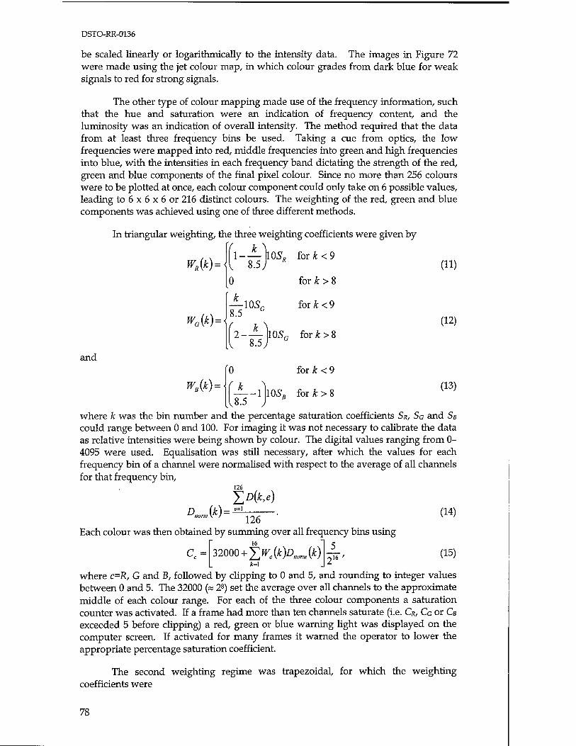
DSTO-RR-0136

be scaled linearly or logarithmically to the intensity data. The images in Figure 72 were made using the jet colour map, in which colour grades from dark blue for weak signals to red for strong signals.

The other type of colour mapping made use of the frequency information, such that the hue and saturation were an indication of frequency content, and the luminosity was an indication of overall intensity. The method required that the data from at least three frequency bins be used. Taking a cue from optics, the low frequencies were mapped into red, middle frequencies into green and high frequencies into blue, with the intensities in each frequency band dictating the strength of the red, green and blue components of the final pixel colour. Since no more than 256 colours were to be plotted at once, each colour component could only take on 6 possible values, leading to 6 x 6 x 6 or 216 distinct colours. The weighting of the red, green and blue components was achieved using one of three different methods.

In triangular weighting, the three weighting coefficients were given by

V k\ 1-— 10Sß for£<9

WR{k) =

WG(k) =

and

WB(k) =

V

0

8.5 G

( 2-

lv

0

for k > 8

for&<9

10S„ for£>8

for k < 9

(11)

(12)

\

iv 8.5 -1 10SR for k > 8

(13)

J where k was the bin number and the percentage saturation coefficients SR, SG and SB

could range between 0 and 100. For imaging it was not necessary to calibrate the data as relative intensities were being shown by colour. The digital values ranging from 0- 4095 were used. Equalisation was still necessary, after which the values for each frequency bin of a channel were normalised with respect to the average of all channels for that frequency bin,

126

DnormV0)- '

E^M 126

Each colour was then obtained by summing over all frequency bins using

a tu

32000+ 2K(k)Dnorm(k) k=\

(14)

(15)

where c=R, G and B, followed by clipping to 0 and 5, and rounding to integer values between 0 and 5. The 32000 (« 28) set the average over all channels to the approximate middle of each colour range. For each of the three colour components a saturation counter was activated. If a frame had more than ten channels saturate (i.e. CR, CG or CB

exceeded 5 before clipping) a red, green or blue warning light was displayed on the computer screen. If activated for many frames it warned the operator to lower the appropriate percentage saturation coefficient.

The second weighting regime was trapezoidal, for which the weighting coefficients were

78

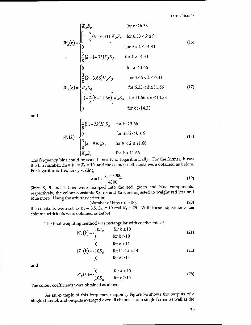
WR(k)-

WG(k) =

and

WB(k) =

DSTO-RR-0136

KRSR for k< 6.33

I--(k-6.33) KRSR for6.33<£<9 8 J

0 for 9 < k < 14.33 (16)

-{k-\A.33)KRSR for k> 14.33 8 0 for k < 3.66

-(£-3.66)£GSG for 3.66 < k < 6.33

KGSG for 6.33 < k < 11.66 (17)

1-—(Jt-11.66) £GSG for 11.66 <k< 14.33

0 for £> 14.33

-(ll-3A;)i:A for k< 3.66

0 for3.66<Ä:<9 (18)

l(k-9)KBSB for 9 < A: < 11.66 \ /

KBSB for k > 11.66

The frequency bins could be scaled linearly or logarithmically. For the former, k was the bin number, KR = KG = KB = 10, and the colour coefficients were obtained as before. For logarithmic frequency scaling

/c-8000 & = ! + •

4300 Since 9, 5 and 2 bins were mapped into the red, green and blue components, respectively, the colour constants KR, KG and KB were adjusted to weight red less and blue more. Using the arbitrary criterion

Number of bins x K = 50, (20) the constants were set to KR = 5.5, KG = 10 and KB = 25. With these adjustments the colour coefficients were obtained as before.

The final weighting method was rectangular with coefficients of for£<10

forA:>10

and

WG(k) =

WB(k) = -

\0SG

\osn

for Ä: < 11

forll<A:<14

for k > 14

for k < 15

forÄ:>15

(21)

(22)

(23)

The colour coefficients were obtained as above.

As an example of this frequency mapping, Figure 74 shows the outputs of a single channel, and outputs averaged over all channels for a single frame, as well as the

79

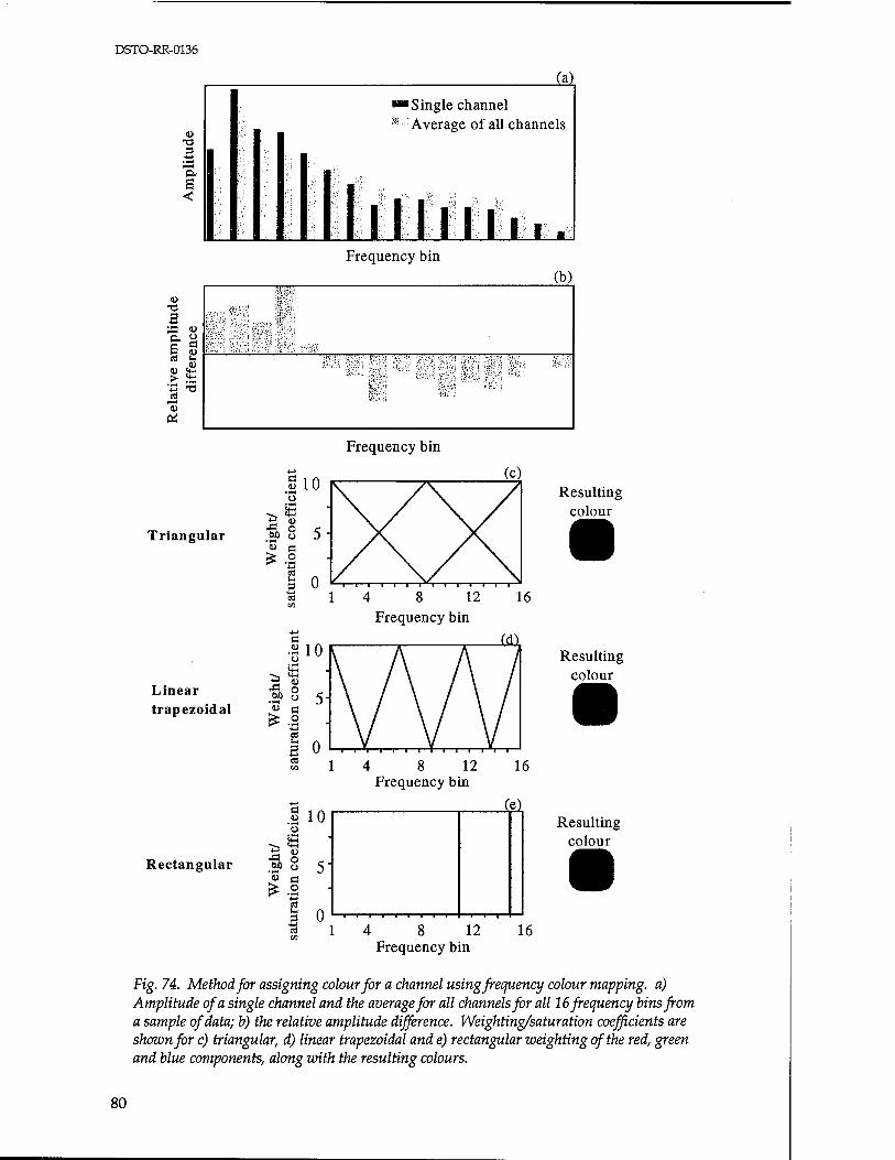
DSTO-RR-0136

M

u a

a

£ ■■Single channel ;« Average of all channels

mi 1 1 i i i r«; . Frequency bin

(b) apai

<D T3 3 3 -:■■>: ^'v.Jo-:- V''-; & O V.--Y-, r-./'i ££./; ;,;>.>!

S ■

4) - i, <'; '' ' ' •'$-/* £-<.■

U. A,....

**-> 'O i • &fo »-H u c*

Frequency bin

Triangular

Linear trapezoidal

Resulting colour

Resulting colour

12 Frequency bin

Rectangular

Resulting colour

a CO

14 8 12 16 Frequency bin

Fig. 74. Method for assigning colour for a channel using frequency colour mapping, a) Amplitude of a single channel and the average for all channels for all 16 frequency bins from a sample of data; b) the relative amplitude difference. Weighting/saturation coefficients are shown for c) triangular, d) linear trapezoidal and e) rectangular weighting of the red, green and blue components, along with the resulting colours.

80

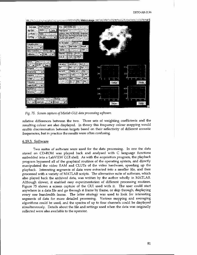
DSTO-RR-0136

Fig. 75. Screen capture ofMatlab GUI data processing software.

relative differences between the two. Three sets of weighting coefficients and the resulting colour are also displayed. In theory this frequency colour mapping would enable discrimination between targets based on their reflectivity of different acoustic frequencies, but in practice the results were often confusing.

6.19.3. Software

Two suites of software were used for the data processing. In one the data stored on CD-ROM was played back and analysed with C language functions embedded into a Lab VIEW GUI shell. As with the acquisition program, the playback program bypassed all of the graphical routines of the operating system, and directly manipulated the video RAM and CLUTs of the video hardware, speeding up the playback. Interesting segments of data were extracted into a smaller file, and then processed with a variety of MATLAB scripts. The alternative suite of software, which also played back the archived data, was written by the author wholly in MATLAB. Although slower, it enabled easy experimentation of different processing routines. Figure 75 shows a screen capture of the GUI used with it. The user could start anywhere in a data file and go through it frame by frame, or skip through, displaying every one hundredth frame. The latter strategy was used to look for interesting segments of data for more detailed processing. Various mapping and averaging algorithms could be used, and the spectra of up to four channels could be displayed simultaneously. Details about the file and settings used when the data was originally collected were also available to the operator.

81

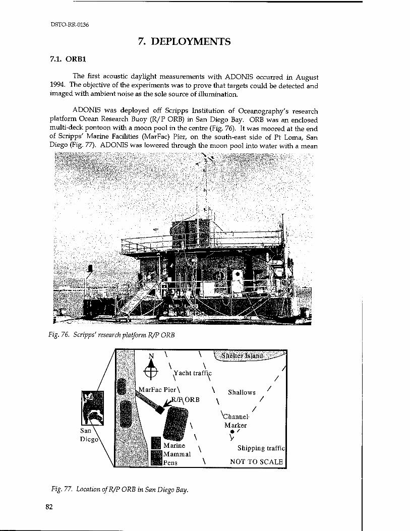
DSTO-RR-0136

7.1. ORB1

7. DEPLOYMENTS

The first acoustic daylight measurements with ADONIS occurred in August 1994. The objective of the experiments was to prove that targets could be detected and imaged with ambient noise as the sole source of illumination.

ADONIS was deployed off Scripps Institution of Oceanography's research platform Ocean Research Buoy (R/P ORB) in San Diego Bay. ORB was an enclosed multi-deck pontoon with a moon pool in the centre (Fig. 76). It was moored at the end of Scripps' Marine Facilities (MarFac) Pier, on the south-east side of Pt Loma, San Diego (Fig. 77). ADONIS was lowered through the moon pool into water with a mean

;',-■: '*■■:': ■■"'. ■■'■ '■■■'■"■'■''■ '■.''■■:^ ':'•: >-v«.' :C^^äSfs^^^:P;:i::-X'-;-'-

Fig. 76. Scripps' research platform R/P ORB

\ ^Shelter Island_

\ \ Yacht traffic

MarFac Pier\ ^R/I\ORB

/

/

/

* Shallows \ /

^Channel- Marker

V

/

\ Marine Mammal Pens \

Shipping traffic

NOT TO SCALE

Fig. 77. Location of R/P ORB in San Diego Bay.

82

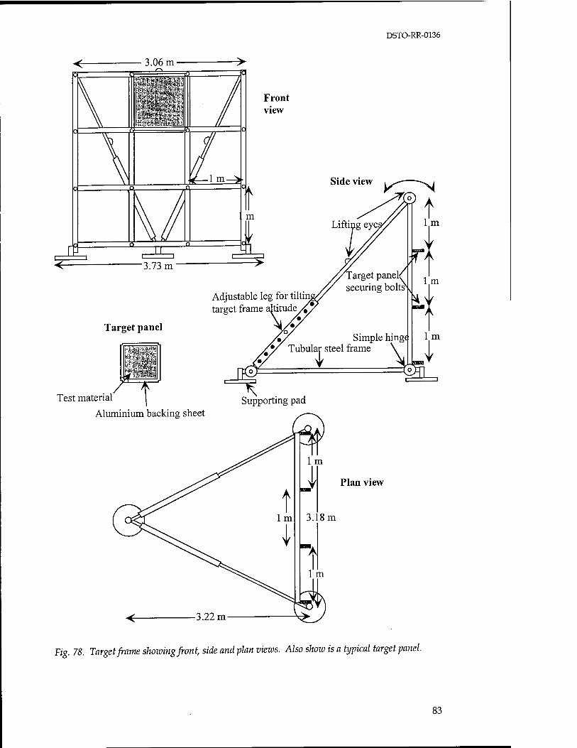
DSTO-RR-0136

Test material

Aluminium backing sheet

Fig. 78. Target frame showing front, side and plan vieios. Also show is a typical target panel.

83

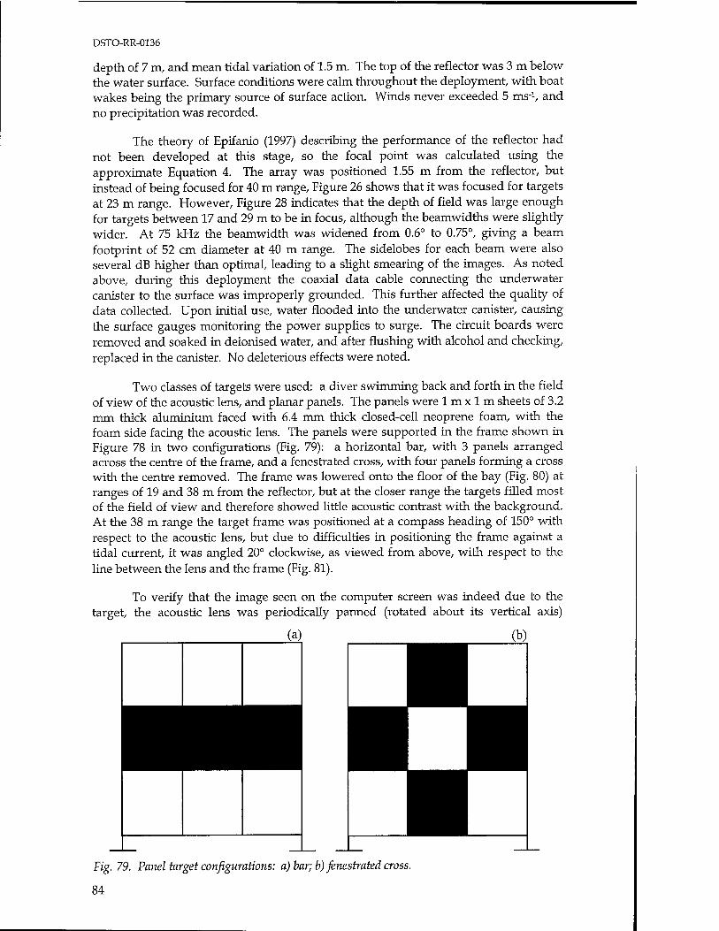
DSTO-RR-0136

depth of 7 m, and mean tidal variation of 1.5 m. The top of the reflector was 3 m below the water surface. Surface conditions were calm throughout the deployment, with boat wakes being the primary source of surface action. Winds never exceeded 5 ms4, and no precipitation was recorded.

The theory of Epifanio (1997) describing the performance of the reflector had not been developed at this stage, so the focal point was calculated using the approximate Equation 4. The array was positioned 1.55 m from the reflector, but instead of being focused for 40 m range, Figure 26 shows that it was focused for targets at 23 m range. However, Figure 28 indicates that the depth of field was large enough for targets between 17 and 29 m to be in focus, although the beamwidths were slightly wider. At 75 kHz the beamwidth was widened from 0.6° to 0.75°, giving a beam footprint of 52 cm diameter at 40 m range. The sidelobes for each beam were also several dB higher than optimal, leading to a slight smearing of the images. As noted above, during this deployment the coaxial data cable connecting the underwater canister to the surface was improperly grounded. This further affected the quality of data collected. Upon initial use, water flooded into the underwater canister, causing the surface gauges monitoring the power supplies to surge. The circuit boards were removed and soaked in deionised water, and after flushing with alcohol and checking, replaced in the canister. No deleterious effects were noted.

Two classes of targets were used: a diver swimming back and forth in the field of view of the acoustic lens, and planar panels. The panels were lmxlm sheets of 3.2 mm thick aluminium faced with 6.4 mm thick closed-cell neoprene foam, with the foam side facing the acoustic lens. The panels were supported in the frame shown in Figure 78 in two configurations (Fig. 79): a horizontal bar, with 3 panels arranged across the centre of the frame, and a fenestrated cross, with four panels forming a cross with the centre removed. The frame was lowered onto the floor of the bay (Fig. 80) at ranges of 19 and 38 m from the reflector, but at the closer range the targets filled most of the field of view and therefore showed little acoustic contrast with the background. At the 38 m range the target frame was positioned at a compass heading of 150° with respect to the acoustic lens, but due to difficulties in positioning the frame against a tidal current, it was angled 20° clockwise, as viewed from above, with respect to the line between the lens and the frame (Fig. 81).

To verify that the image seen on the computer screen was indeed due to the target, the acoustic lens was periodically panned (rotated about its vertical axis)

(a) (b)

Fig. 79. Panel target configurations: a) bar; b) fenestrated cross.

84

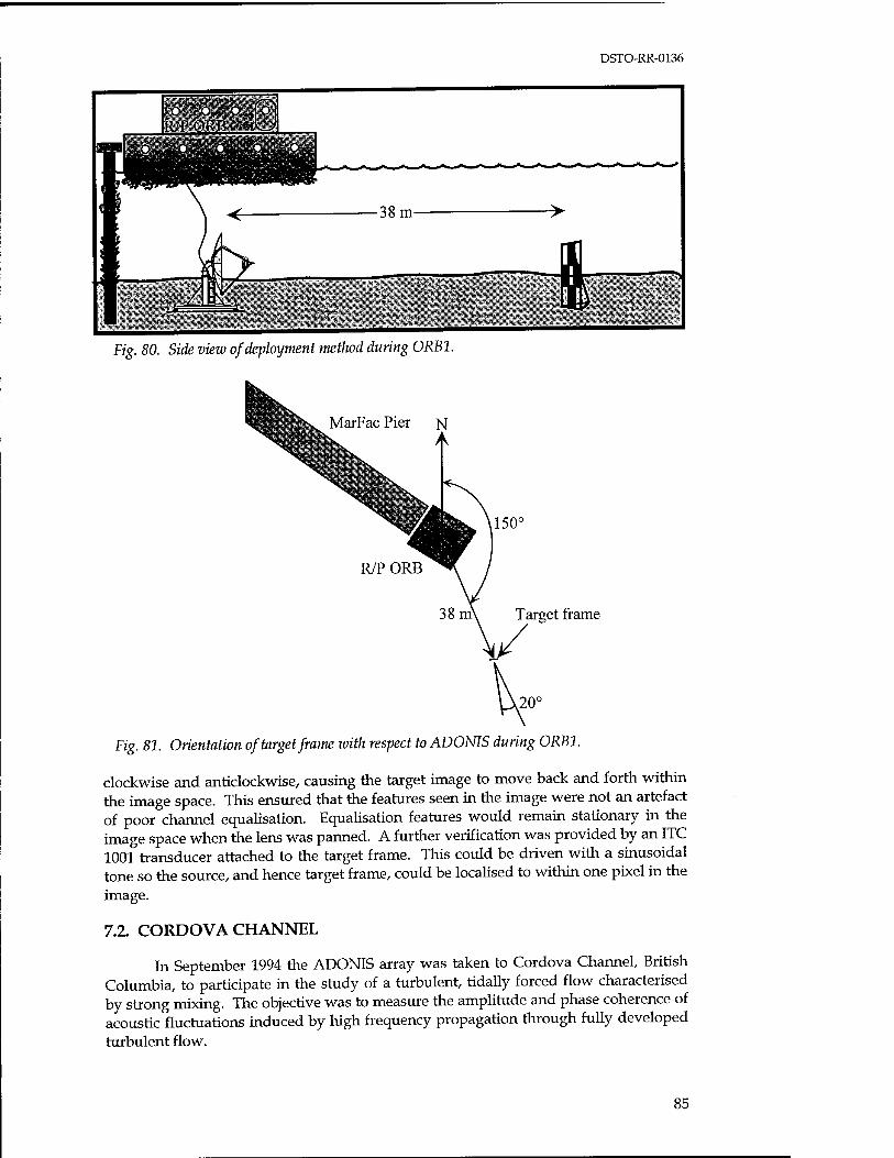
DSTO-RR-0136

K.POR» -4

Fig. 80. Side view of deployment method during 0RB1.

MarFac Pier N A

Target frame

Fig. 81. Orientation of target frame with respect to ADONIS during 0RB1.

clockwise and anticlockwise, causing the target image to move back and forth within the image space. This ensured that the features seen in the image were not an artefact of poor channel equalisation. Equalisation features would remain stationary in the image space when the lens was panned. A further verification was provided by an ITC 1001 transducer attached to the target frame. This could be driven with a sinusoidal tone so the source, and hence target frame, could be localised to within one pixel in the image.

7.2. CORDOVA CHANNEL

In September 1994 the ADONIS array was taken to Cordova Channel, British Columbia, to participate in the study of a turbulent, tidally forced flow characterised by strong mixing. The objective was to measure the amplitude and phase coherence of acoustic fluctuations induced by high frequency propagation through fully developed turbulent flow.

85

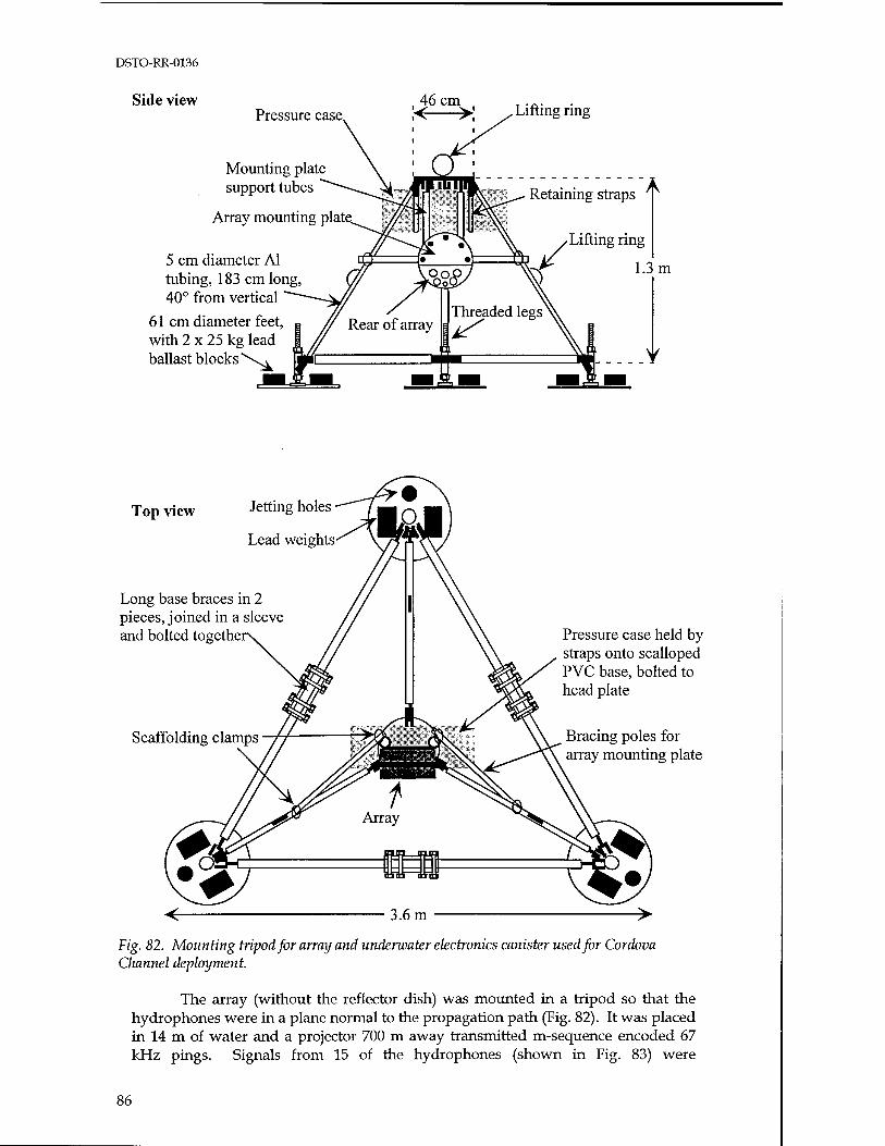
DSTO-RR-0136

Side view Pressure case,

Mounting plate support tubes

Array mounting plate.

5 cm diameter Al tubing, 183 cm long, 40° from vertical

61 cm diameter feet, with 2 x 25 kg lead ballast blocks \^

1.3 m

Top view Jetting holes

Lead weights

Long base braces in 2 pieces, joined in a sleeve and bolted togethe: Pressure case held by

straps onto scalloped PVC base, bolted to head plate

Scaffolding clamps Bracing poles for array mounting plate

Fig. 82. Mounting tripod for array and underwater electronics canister used for Cordova Channel deployment.

The array (without the reflector dish) was mounted in a tripod so that the hydrophones were in a plane normal to the propagation path (Fig. 82). It was placed in 14 m of water and a projector 700 m away transmitted m-sequence encoded 67 kHz pings. Signals from 15 of the hydrophones (shown in Fig. 83) were

86

DSTO-RR-0136

22.2 cm

28.0 cm

Fig. 83. Array elements, filled in grey, used for Cordova Channel deployment.

preamplified and complex demodulated by electronics housed in the pressure casing attached to the tripod. The resultant quadrature and in-phase components of the data stream from each hydrophone were time division multiplexed and transmitted down 300m of cable to the acquisition electronics on Cordova Spit. Both a data cable splice failed and a power supply cable became severed, but once repaired, data was collected. The data stream was analysed by correlating the complex de-multiplexed signal from a hydrophone with the m-sequence replica signal.

7.3. SEA WORLD

In February 1995 ADONIS was taken to Sea World, San Diego, in an attempt to image moving marine mammals. The mammals dislike intrusive active systems and are virtually silent when not vocalising, so normal passive systems are of limited use. It was perceived that there would be a need to develop expertise in covert location and tracking of marine mammals for environmental impact studies, monitoring of endangered species, etc., in addition to a need for improved methods of studying specific natural social behaviour. Sea World presented an opportunity to image killer whales (Orcinus orca) under controlled conditions, with simultaneous video and acoustic measurements for comparison.

ADONIS was mounted down one corner of the main 11.4 Ml tank as shown in Figure 84. It was tilted upwards by 6° and could rotate around its vertical axis as usual. The ambient noise was provided by pumps and other machinery, which brought the noise in the tanks to levels comparable to those in the ocean. Continual recirculation of the water (turned over every 4 hours) ensured a homogeneous propagation medium. Images of the killer whales were seen, and three hydrophone monitors in the tank confirmed that the whales themselves were not transmitting the sound.

With a refresh rate of 25 Hz, ADONIS was also capable of detecting the transients of both communication and echolocation signals from the killer whales, which were typically 15 dB above the background noise levels. These transmissions

87

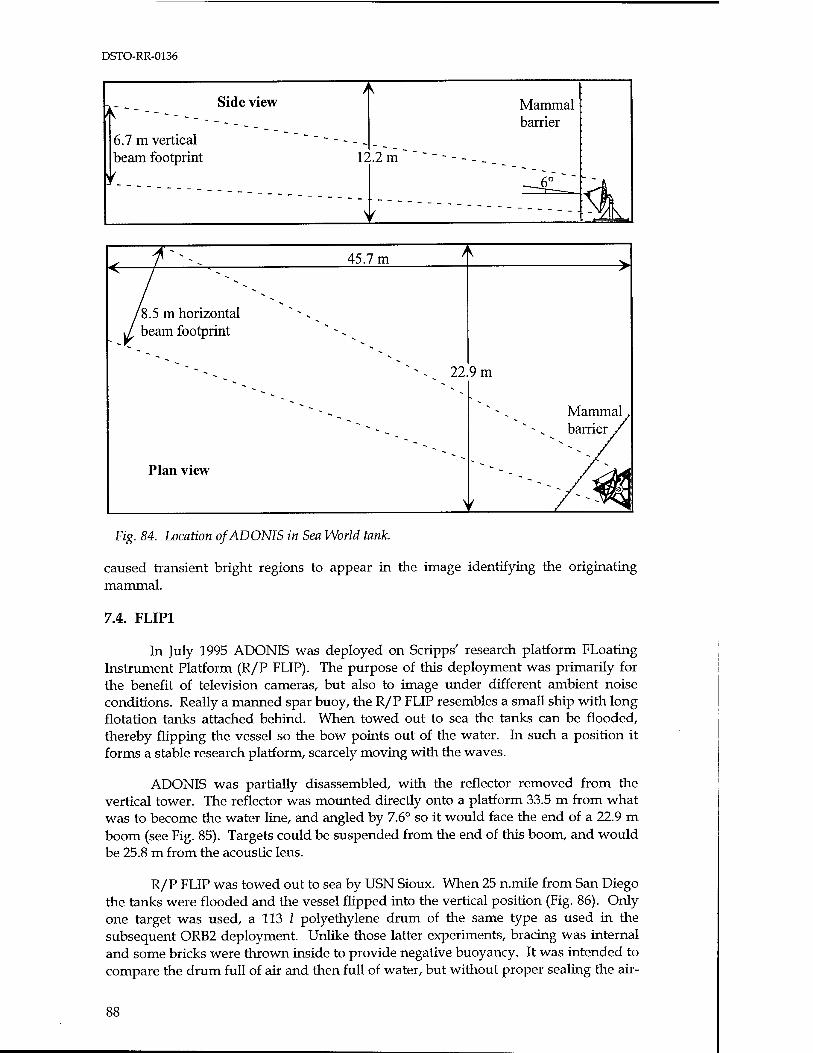
DSTO-RR-0136

A Side view Mammal

barrier 6.7 m vertical " ~ - - _

beam footprint 12.2 m "" _ ~ - - - - _ _

y< --411" 

1 ^

/ /8.5m horizontal

J beam footprint " - -,

** ^ ^ 22. 9m

Mammal, barrier /

Plan view *~

/*M V /--^|

Fig. 84. Location of ADONIS in Sea World tank.

caused transient bright regions to appear in the image identifying the originating mammal.

7.4. FLIP1

In July 1995 ADONIS was deployed on Scripps' research platform FLoating Instrument Platform (R/P FLIP). The purpose of this deployment was primarily for the benefit of television cameras, but also to image under different ambient noise conditions. Really a manned spar buoy, the R/P FLIP resembles a small ship with long flotation tanks attached behind. When towed out to sea the tanks can be flooded, thereby flipping the vessel so the bow points out of the water. In such a position it forms a stable research platform, scarcely moving with the waves.

ADONIS was partially disassembled, with the reflector removed from the vertical tower. The reflector was mounted directly onto a platform 33.5 m from what was to become the water line, and angled by 7.6° so it would face the end of a 22.9 m boom (see Fig. 85). Targets could be suspended from the end of this boom, and would be 25.8 m from the acoustic lens.

R/P FLIP was towed out to sea by USN Sioux. When 25 n.mile from San Diego the tanks were flooded and the vessel flipped into the vertical position (Fig. 86). Only one target was used, a 113 I polyethylene drum of the same type as used in the subsequent ORB2 deployment. Unlike those latter experiments, bracing was internal and some bricks were thrown inside to provide negative buoyancy. It was intended to compare the drum full of air and then full of water, but without proper sealing the air-

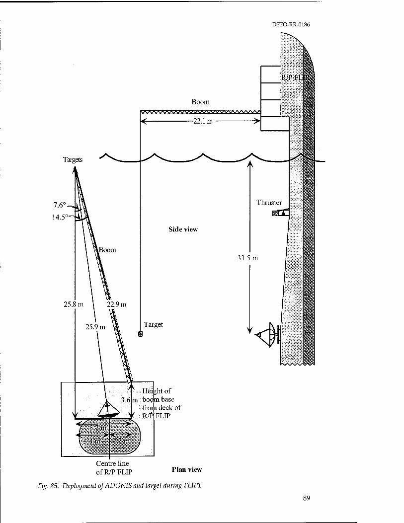
DSTO-RR-0136

Centre line of R/P FLIP Plan view

Fig. 85. Deployment of ADONIS and target during FLIP1.

89

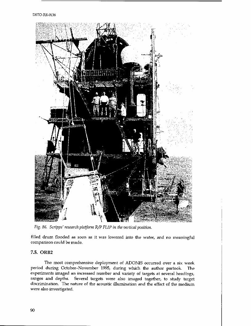
DSTO-RR-0136

Fig. 86. Scripps' research platform R/P FLIP in the vertical position.

filled drum flooded as soon as it was lowered into the water, and no meaningful comparison could be made.

7.5. ORB2

The most comprehensive deployment of ADONIS occurred over a six week period during October-November 1995, during which the author partook. The experiments imaged an increased number and variety of targets at several headings, ranges and depths. Several targets were also imaged together, to study target discrimination. The nature of the acoustic illumination and the effect of the medium were also investigated.

90

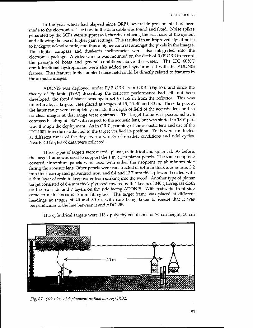
DSTO-RR-0136

In the year which had elapsed since ORB1, several improvements had been made to the electronics. The flaw in the data cable was found and fixed. Noise spikes generated by the SCFs were suppressed, thereby reducing the self noise of the system and allowing the use of higher gain settings. This resulted in an improved signal-noise to background-noise ratio, and thus a higher contrast amongst the pixels in the images. The digital compass and dual-axis inclinometer were also integrated into the electronics package. A video camera was mounted on the deck of R/P ORB to record the passage of boats and general conditions above the water. The ITC 6050C omnidirectional hydrophones were also added and synchronised with the ADONIS frames. Thus features in the ambient noise field could be directly related to features in the acoustic images.

ADONIS was deployed under R/P ORB as in ORB1 (Fig 87), and since the theory of Epifanio (1997) describing the reflector performance had still not been developed, the focal distance was again set to 1.55 m from the reflector. This was unfortunate, as targets were placed at ranges of 15, 20, 40 and 80 m. Those targets at the latter range were completely outside the depth of field of the acoustic lens and so no clear images at that range were obtained. The target frame was positioned at a compass heading of 145° with respect to the acoustic lens, but was shifted to 135° part way through the deployment. As in ORB1, panning of the acoustic lens and use of the ITC 1001 transducer attached to the target verified its position. Trials were conducted at different times of the day, over a variety of weather conditions and tidal cycles. Nearly 40 Gbytes of data were collected.

Three types of targets were tested: planar, cylindrical and spherical. As before, the target frame was used to support the 1 m x 1 m planar panels. The same neoprene covered aluminium panels were used with either the neoprene or aluminium side facing the acoustic lens. Other panels were constructed of 6.4 mm thick aluminium, 3.2 mm thick corrugated galvanised iron, and 6.4 and 12.7 mm thick plywood coated with a thin layer of resin to keep water from soaking into the wood. Another type of planar target consisted of 6.4 mm thick plywood covered with 4 layers of 340 g fibreglass cloth on the rear side and 7 layers on the side facing ADONIS. With resin, the front side came to a thickness of 5 mm fibreglass. The target frame was placed at different headings at ranges of 40 and 80 m, with care being taken to ensure that it was perpendicular to the line between it and ADONIS.

The cylindrical targets were 113 I polyethylene drums of 76 cm height, 50 cm

Fig. 87. Side view of deployment metlwd during ORB2.

91

DSTO-RR-0136

diameter, and with a wall thickness of 5 mm. These drums were filled with wet sand with a density of approximately 1900 kg.m3, sea water or syntactic foam with a density of approximately 290 kg.m-3. Each drum was clamped with 6.4 mm diameter threaded connecting rods between 6.4 mm thick steel endplates. Lead weights were tied with hemp chord to the connecting rods of the foam-filled drum to make it negatively buoyant. The drums were suspended individually in the water column with plastic surface floats, or equidistantly spaced along a 4 m wooden beam, at ranges of 20, 40 or 80 m from ADONIS (Fig. 88). The beam was supported with floats and fixed in orientation and range from ADONIS with anchors at either end, and with the order of the drums, as seen by ADONIS, as shown in the diagram. The heading chosen was approximately 125°. The depth of the drums was adjusted so that at mid-tide the centre of each was 2 m above the sea floor. In other measurements the foam and sand- filled drums were dropped onto the sea floor 13 and 15 m, respectively, from ADONIS, becoming partially buried (30-50%) in the silty sediment (Fig. 88). The sand-filled drum landed askew, angled down into the mud by about 45°. For these sea floor measurements ADONIS was tilted downwards by 10° to keep the targets in the field of view (Fig. 89).

Fig. 88. Suspension method for drums and sphere during ORB2.

Fig. 89. Side view of deployment method for drum on the bottom during ORB2.

92

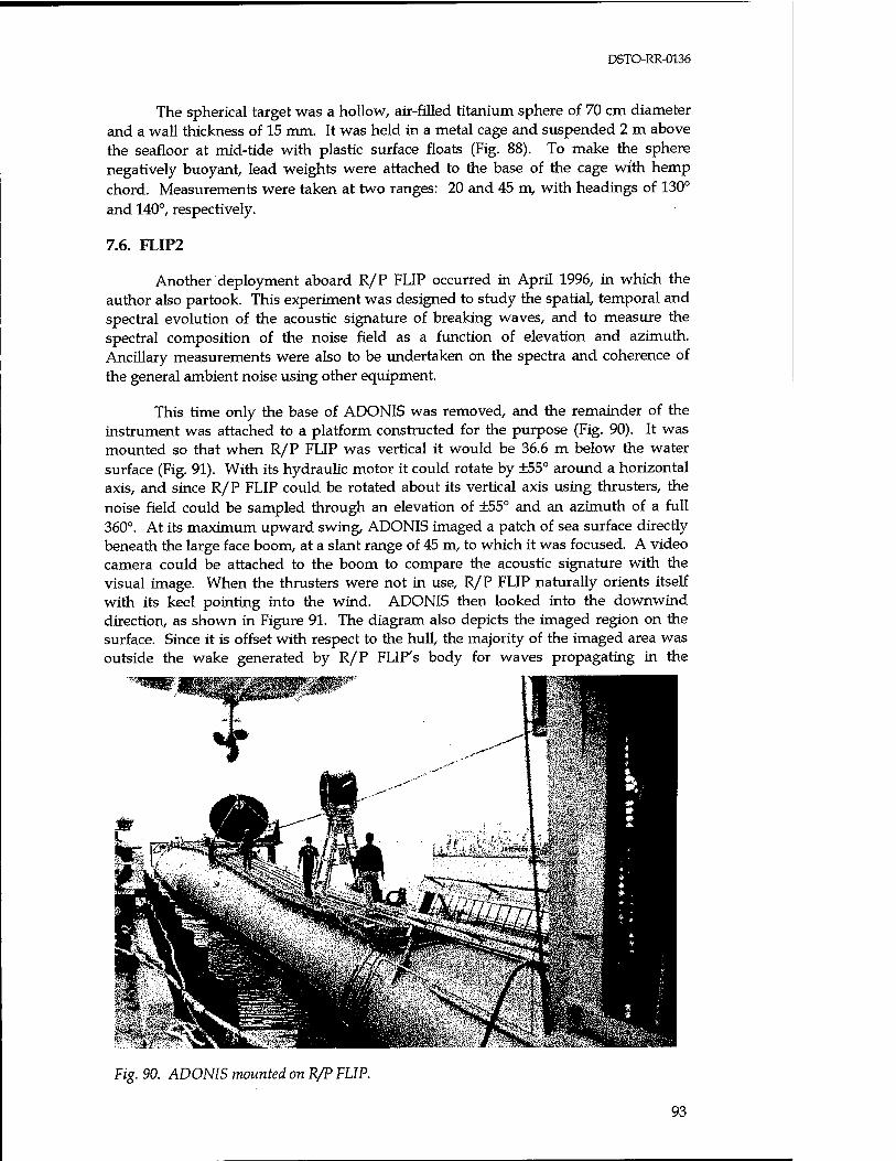
DSTO-RR-0136

The spherical target was a hollow, air-filled titanium sphere of 70 cm diameter and a wall thickness of 15 mm. It was held in a metal cage and suspended 2 m above the seafloor at mid-tide with plastic surface floats (Fig. 88). To make the sphere negatively buoyant, lead weights were attached to the base of the cage with hemp chord. Measurements were taken at two ranges: 20 and 45 m, with headings of 130° and 140°, respectively.

7.6. FLIP2

Another deployment aboard R/P FLIP occurred in April 1996, in which the author also partook. This experiment was designed to study the spatial, temporal and spectral evolution of the acoustic signature of breaking waves, and to measure the spectral composition of the noise field as a function of elevation and azimuth. Ancillary measurements were also to be undertaken on the spectra and coherence of the general ambient noise using other equipment.

This time only the base of ADONIS was removed, and the remainder of the instrument was attached to a platform constructed for the purpose (Fig. 90). It was mounted so that when R/P FLIP was vertical it would be 36.6 m below the water surface (Fig. 91). With its hydraulic motor it could rotate by ±55° around a horizontal axis, and since R/P FLIP could be rotated about its vertical axis using thrusters, the noise field could be sampled through an elevation of ±55° and an azimuth of a full 360°. At its maximum upward swing, ADONIS imaged a patch of sea surface directly beneath the large face boom, at a slant range of 45 m, to which it was focused. A video camera could be attached to the boom to compare the acoustic signature with the visual image. When the thrusters were not in use, R/P FLIP naturally orients itself with its keel pointing into the wind. ADONIS then looked into the downwind direction, as shown in Figure 91. The diagram also depicts the imaged region on the surface. Since it is offset with respect to the hull, the majority of the imaged area was outside the wake generated by R/P FLIP's body for waves propagating in the

Fig. 90. ADONIS mounted on R/P FLIP.

93

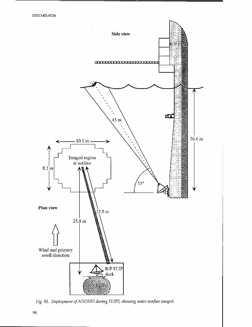
DSTO-RR-0136

8.2 m

Plan view

A

Side view

Wind and primary swell direction

Imaged region at surface

Fig. 91. Deployment of ADONIS during FLIP2, shoxoing water surface imaged.

94

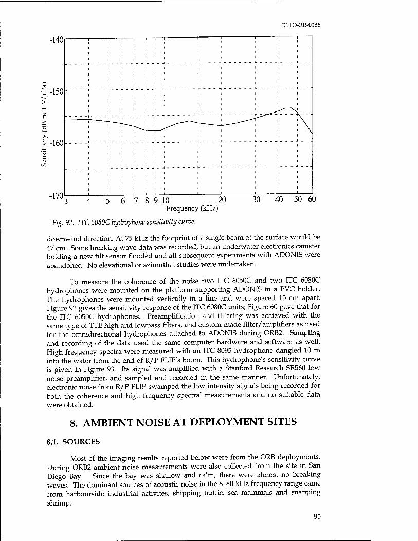
DSTO-RR-0136

-140

5-150

m

f-160 c

C/3

-170 , , 1 1 1 1 1——

4 5 6 7 8 9 10 20 Frequency (kHz)

30 40 50 60

Fig. 92. ITC 6080C hydrophone sensitivity curve.

downwind direction. At 75 kHz the footprint of a single beam at the surface would be 47 cm. Some breaking wave data was recorded, but an underwater electronics canister holding a new tilt sensor flooded and all subsequent experiments with ADONIS were abandoned. No elevational or azimuthal studies were undertaken.

To measure the coherence of the noise two ITC 6050C and two ITC 6080C hydrophones were mounted on the platform supporting ADONIS in a PVC holder. The hydrophones were mounted vertically in a line and were spaced 15 cm apart. Figure 92 gives the sensitivity response of the ITC 6080C units; Figure 60 gave that for the ITC 6050C hydrophones. Preamplification and filtering was achieved with the same type of TTE high and lowpass filters, and custom-made filter/amplifiers as used for the omnidirectional hydrophones attached to ADONIS during ORB2. Sampling and recording of the data used the same computer hardware and software as well. High frequency spectra were measured with an ITC 8095 hydrophone dangled 10 m into the water from the end of R/P FLIP'S boom. This hydrophone's sensitivity curve is given in Figure 93. Its signal was amplified with a Stanford Research SR560 low noise preamplifier, and sampled and recorded in the same manner. Unfortunately, electronic noise from R/P FLIP swamped the low intensity signals being recorded for both the coherence and high frequency spectral measurements and no suitable data were obtained.

8. AMBIENT NOISE AT DEPLOYMENT SITES

8.1. SOURCES

Most of the imaging results reported below were from the ORB deployments. During ORB2 ambient noise measurements were also collected from the site in San Diego Bay. Since the bay was shallow and calm, there were almost no breaking waves. The dominant sources of acoustic noise in the 8-80 kHz frequency range came from harbourside industrial activites, shipping traffic, sea mammals and snapping shrimp.

95

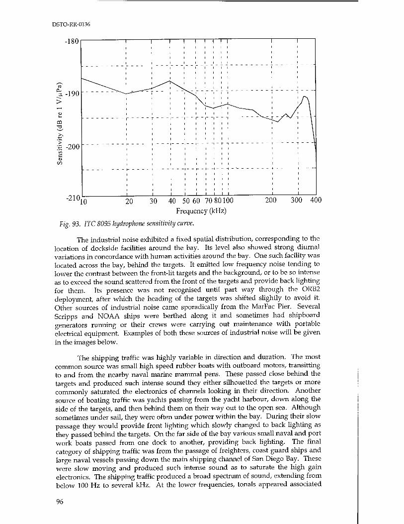
DSTO-RR-0136

-180

cd eu ■190

:§ -200 CO

C

-210

- 1 1 1 1 1 1 1 I 1 1 1

^f^y. i i i i i i—i—i_i 1 1

10 20 30 200 300 400 40 50 60 70 80100

Frequency (kHz)

Fig. 93. ITC 8095 hijdrophone sensitivity curve.

The industrial noise exhibited a fixed spatial distribution, corresponding to the location of dockside facilities around the bay. Its level also showed strong diurnal variations in concordance with human activities around the bay. One such facility was located across the bay, behind the targets. It emitted low frequency noise tending to lower the contrast between the front-lit targets and the background, or to be so intense as to exceed the sound scattered from the front of the targets and provide back lighting for them. Its presence was not recognised until part way through the ORB2 deployment, after which the heading of the targets was shifted slightly to avoid it. Other sources of industrial noise came sporadically from the MarFac Pier. Several Scripps and NOAA ships were berthed along it and sometimes had shipboard generators running or their crews were carrying out maintenance with portable electrical equipment. Examples of both these sources of industrial noise will be given in the images below.

The shipping traffic was highly variable in direction and duration. The most common source was small high speed rubber boats with outboard motors, transitting to and from the nearby naval marine mammal pens. These passed close behind the targets and produced such intense sound they either silhouetted the targets or more commonly saturated the electronics of channels looking in their direction. Another source of boating traffic was yachts passing from the yacht harbour, down along the side of the targets, and then behind them on their way out to the open sea. Although sometimes under sail, they were often under power within the bay. During their slow passage they would provide front lighting which slowly changed to back lighting as they passed behind the targets. On the far side of the bay various small naval and port work boats passed from one dock to another, providing back lighting. The final category of shipping traffic was from the passage of freighters, coast guard ships and large naval vessels passing down the main shipping channel of San Diego Bay. These were slow moving and produced such intense sound as to saturate the high gain electronics. The shipping traffic produced a broad spectrum of sound, extending from below 100 Hz to several kHz. At the lower frequencies, tonals appeared associated

96

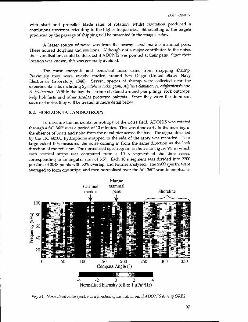
DSTO-RR-0136

with shaft and propeller blade rates of rotation, whilst cavitation produced a continuous spectrum extending to the higher frequencies. Silhouetting of the targets produced by the passage of shipping will be presented in the images below.

A lesser source of noise was from the nearby naval marine mammal pens. These housed dolphins and sea lions. Although not a major contributor to the noise, their vocalisations could be detected if ADONIS was pointed at their pens. Since their location was known, this was generally avoided.

The most energetic and persistent noise came from snapping shrimp. Previously they were widely studied around San Diego (United States Navy Electronics Laboratory, 1946). Several species of shrimp were collected near the experimental site, including Synalpheus lockingtoni, Alpheus clamator, A. californiensis and A. bellimanus. Within the bay the shrimp clustered around pier pilings, rock outcrops, kelp holdfasts and other similar protected habitats. Since they were the dominant source of noise, they will be treated in more detail below.

8.2. HORIZONTAL ANISOTROPY

To measure the horizontal anisotropy of the noise field, ADONIS was rotated through a full 360° over a period of 10 minutes. This was done early in the morning in the absence of boats and noise from the naval pier across the bay. The signal detected by the ITC 6050C hydrophone strapped to the side of the array was recorded. To a large extent this measured the noise coming in from the same direction as the look direction of the reflector. The normalised spectrogram is shown in Figure 94, in which each vertical stripe was computed from a 10 s segment of the time series, corresponding to an angular scan of 5.5°. Each 10 s segment was divided into 2200 portions of 2048 points with 50% overlap, and Fourier analysed. The 2200 spectra were averaged to form one stripe, and then normalised over the full 360° scan to emphasise

Channel marker

Marine mammal

pens Shoreline

50 150 200 Compass Angle (°)

-4-2024 Normalised intensity (dB re 1 (iPa2/Hz)

Fig. 94. Normalised noise spectra as a function of azimuth around ADONIS during ORB2.

97

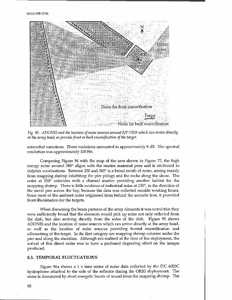
DSTO-RR-0136

Direct noise

" vMarFac Pier xxS Direct noise

Noise for front ensonification

Target

Noise for back ensonification

Fig. 95. ADONIS and tlte location of noise sources around R/P ORB which can arrive directly at tin array head, or -provide front or back ensonification of the target.

azimuthal variations. These variations amounted to approximately 8 dB. The spectral resolution was approximately 100 Hz.

Comparing Figure 94 with the map of the area shown in Figure 77, the high energy noise around 180° aligns with the marine mammal pens and is attributed to dolphin vocalisations. Between 250 and 360° is a broad swath of noise, arising mainly from snapping shrimp inhabiting the pier pilings and the rocks along the shore. The noise at 110° coincides with a channel marker providing another habitat for the snapping shrimp. There is little evidence of industrial noise at 150°, in the direction of the naval pier across the bay, because the data was collected outside working hours. Since most of the ambient noise originated from behind the acoustic lens, it provided front illumination for the targets.

When discussing the beam patterns of the array elements it was noted that they were sufficiently broad that the elements would pick up noise not only reflected from the dish, but also arriving directly from the sides of the dish. Figure 95 shows ADONIS and the location of noise sources which can arrive directly at the array head, as well as the location of noise sources providing frontal ensonification and silhouetting of the target. In the first category are snapping shrimp colonies under the pier and along the shoreline. Although not realised at the time of the deployment, the arrival of this direct noise was to have a profound degrading effect on the images produced.

8.3. TEMPORAL FLUCTUATIONS

Figure 96a shows als time series of noise data collected by the ITC 6050C hydrophone attached to the side of the reflector during the ORB2 deployment. The noise is dominated by short energetic bursts of sound from the snapping shrimp. The

98

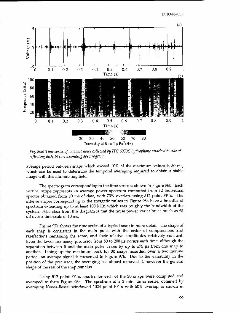
DSTO-RR-0136

(a)

So 0 a o >

-5

11 ' }> m* I ►+HH*" ^[..^iLii,}.«..»,!,!,,,

0 0.1 0.2 0.3 0.4 0.5 0. Time (s)

0.5 0.6 Time (s)

20 30 40 50 60 70 Intensity (dB re 1 ^Pa2/Hz)

80

Fig. 96a) Time series of ambient noise collected by ITC 6050C hydrophone attached to side of reflecting dish; b) corresponding spectrogram.

average period between snaps which exceed 10% of the maximum values is 30 ms, which can be used to determine the temporal averaging required to obtain a stable image with this iUuminating field.

The spectrogram corresponding to the time series is shown in Figure 96b. Each vertical stripe represents an average power spectrum computed from 12 individual spectra obtained from 10 ms of data, with 70% overlap, using 512 point FFTs. The intense stripes corresponding to the energetic pulses in Figure 96a have a broadband spectrum extending up to at least 100 kHz, which was roughly the bandwidth of the system. Also clear from this diagram is that the noise power varies by as much as 65 dB over a time scale of 10 ms.

Figure 97a shows the time series of a typical snap in more detail. The shape of each snap is consistent in the main pulse with the order of compressions and rarefactions remaining the same, and their relative amplitudes relatively constant. Even the lower frequency precursor from 50 to 200 |is occurs each time, although the separation between it and the main pulse varies by up to ±75 |is from one snap to another. Lining up the maximum peak for 30 snaps recorded over a two minute period, an average signal is presented in Figure 97b. Due to the variability in the position of the precursor, the averaging has almost removed it, however the general shape of the rest of the snap remains.

Using 512 point FFTs, spectra for each of the 30 snaps were computed and averaged to form Figure 98a. The spectrum of a 2 min. times series, obtained by averaging Keiser-Bessel windowed 1024 point FFTs with 50% overlap, is shown in

99

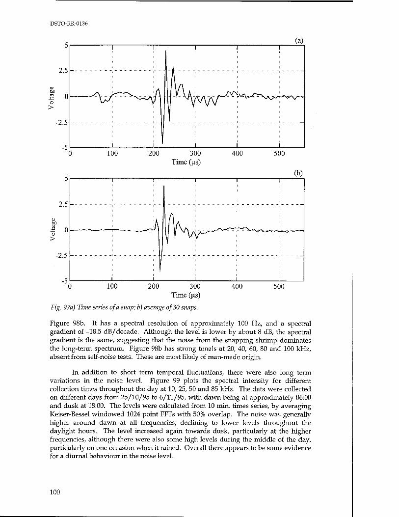
DSTO-RR-0136

(a)

o

o >

-2.5 -

2.5-

* 0 o >

-2.5 -

0

1 1 1 1 1

t | VvNr7^^^

1 1 1 1 1

100 200 300 Time (|o.s)

400 500

(b)

100 200 400 500 300 Time (us)

Fig. 97a) Time series of a snap; b) average of 30 snaps.

Figure 98b. It has a spectral resolution of approximately 100 Hz, and a spectral gradient of -18.5 dB/decade. Although the level is lower by about 8 dB, the spectral gradient is the same, suggesting that the noise from the snapping shrimp dominates the long-term spectrum. Figure 98b has strong tonals at 20, 40, 60, 80 and 100 kHz, absent from self-noise tests. These are most likely of man-made origin.

In addition to short term temporal fluctuations, there were also long term variations in the noise level. Figure 99 plots the spectral intensity for different collection times throughout the day at 10, 25, 50 and 85 kHz. The data were collected on different days from 25/10/95 to 6/11/95, with dawn being at approximately 06:00 and dusk at 18:00. The levels were calculated from 10 min. times series, by averaging Keiser-Bessel windowed 1024 point FFTs with 50% overlap. The noise was generally higher around dawn at all frequencies, declining to lower levels throughout the daylight hours. The level increased again towards dusk, particularly at the higher frequencies, although there were also some high levels during the middle of the day, particularly on one occasion when it rained. Overall there appears to be some evidence for a diurnal behaviour in the noise level.

100

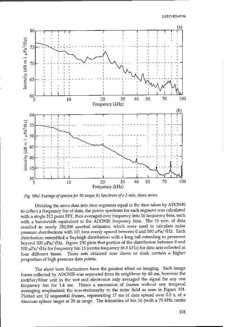
DSTO-RR-0136


40 50 70


100

Fig. 98a) Average of spectra for 30 snaps; b) Spectrum of a 2 min. times series.

Dividing the same data into time segments equal to the time taken by ADONIS to collect a frequency bin of data, the power spectrum for each segment was calculated with a single 512 point FFT, then averaged over frequency into 16 frequency bins, each with a bandwidth equivalent to the ADONIS frequency bins. The 10 min. of data resulted in nearly 250,000 spectral estimates, which were used to calculate noise pressure distributions with 101 bins evenly spaced between 0 and 500 uPa/VHz. Each distribution resembled a Rayleigh distribution with a long tail extending to pressures beyond 500 uPa/VHz. Figure 100 plots that portion of the distribution between 0 and 100 uPa/VHz for frequency bin 15 (centre frequency 66.5 kHz) for data sets collected at four different times. Those sets obtained near dawn or dusk contain a higher proportion of high pressure data points.

The short term fluctuations have the greatest effect on imaging. Each image frame collected by ADONIS was separated from its neighbour by 40 ms, however the rectifier/filter unit in the wet end electronics only averaged the signal for any one frequency bin for 1.4 ms. Hence a succession of frames without any temporal averaging emphasised the non-stationarity in the noise field as seen in Figure 101. Plotted are 12 sequential frames, representing 17 ms of data spread over 0.5 s, of a titanium sphere target at 20 m range. The intensities of bin 16 (with a 75 kHz centre

101

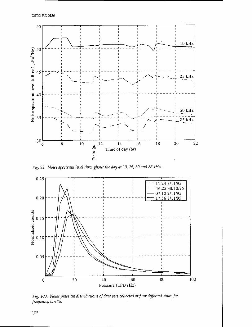
DSTO-RR-0136

55

U 50

0-,

»- 45 PQ

6 40

o OH

o 35

30

1 i 1—

10 kHz /K r^- «_— -

__ 25 kHz

! \

i

_ _r _ - r \ : / i N~1—

— —

50 kHz

_~8~5kHz~

10 . 12 14 16 18 20 22

ö

OH

Time of day (hr)

Fig. 99. Noise spectrum level throughout the day at 10, 25, 50 and 85 kHz.

40 60 Pressure (uPa/VHz)

100

Fig. 100. Noise pressure distributions of data sets collected at four different times for frequency bin 15.

102

DSTO-RR-0136

|pr-TT^|

15 20 25 30 Intensity (dB re 1 |jPa2/Hz/sr)

Fig. 101. 12 sequential images of the suspended sphere using frequency bin 16 data without any temporal averaging.

103

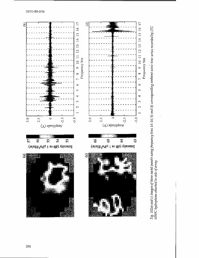
DSTO-RR-0136

e ; F T—I

en r—I

CN

o x> (—1

>1

o ON c

 m »/"> in >n

(js/zH7zB«p1 i 3J gp) Xjisuajui

o in (N (N

O in

(A) spmnduiy

■sf en

(JS/ZH/^£T1 x 3J gp) Xjisuajui

r- 1—1

C ) VÜ H

i—i

in >> »—<

■vl- 1 Q

co O

Si CN 1 '

S3 t—< to ^ c cu

O JD

>i - ^H oj « ü1 o U tt a o f? K

T^ CN f-si O U

o 00 8 £ ^o

104

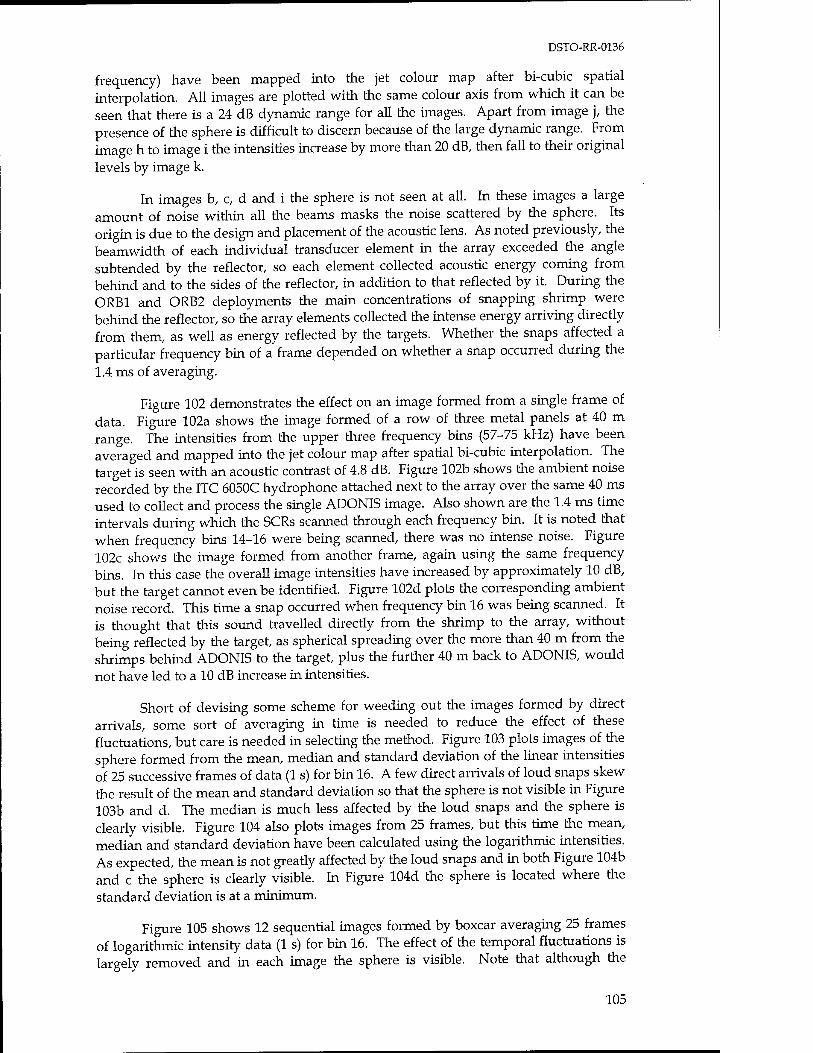
DSTO-RR-0136

frequency) have been mapped into the jet colour map after bi-cubic spatial interpolation. All images are plotted with the same colour axis from which it can be seen that there is a 24 dB dynamic range for all the images. Apart from image j, the presence of the sphere is difficult to discern because of the large dynamic range. From image h to image i the intensities increase by more than 20 dB, then fall to their original levels by image k.

In images b, c, d and i the sphere is not seen at all. In these images a large amount of noise within all the beams masks the noise scattered by the sphere. Its origin is due to the design and placement of the acoustic lens. As noted previously, the beamwidth of each individual transducer element in the array exceeded the angle subtended by the reflector, so each element collected acoustic energy coming from behind and to the sides of the reflector, in addition to that reflected by it. During the ORB1 and ORB2 deployments the main concentrations of snapping shrimp were behind the reflector, so the array elements collected the intense energy arriving directly from them, as well as energy reflected by the targets. Whether the snaps affected a particular frequency bin of a frame depended on whether a snap occurred during the 1.4 ms of averaging.

Figure 102 demonstrates the effect on an image formed from a single frame of data. Figure 102a shows the image formed of a row of three metal panels at 40 m range. The intensities from the upper three frequency bins (57-75 kHz) have been averaged and mapped into the jet colour map after spatial bi-cubic interpolation. The target is seen with an acoustic contrast of 4.8 dB. Figure 102b shows the ambient noise recorded by the ITC 6050C hydrophone attached next to the array over the same 40 ms used to collect and process the single ADONIS image. Also shown are the 1.4 ms time intervals during which the SCRs scanned through each frequency bin. It is noted that when frequency bins 14-16 were being scanned, there was no intense noise. Figure 102c shows the image formed from another frame, again using the same frequency bins. In this case the overall image intensities have increased by approximately 10 dB, but the target cannot even be identified. Figure 102d plots the corresponding ambient noise record. This time a snap occurred when frequency bin 16 was being scanned. It is thought that this sound travelled directly from the shrimp to the array, without being reflected by the target, as spherical spreading over the more than 40 m from the shrimps behind ADONIS to the target, plus the further 40 m back to ADONIS, would not have led to a 10 dB increase in intensities.

Short of devising some scheme for weeding out the images formed by direct arrivals, some sort of averaging in time is needed to reduce the effect of these fluctuations, but care is needed in selecting the method. Figure 103 plots images of the sphere formed from the mean, median and standard deviation of the linear intensities of 25 successive frames of data (1 s) for bin 16. A few direct arrivals of loud snaps skew the result of the mean and standard deviation so that the sphere is not visible in Figure 103b and d. The median is much less affected by the loud snaps and the sphere is clearly visible. Figure 104 also plots images from 25 frames, but this time the mean, median and standard deviation have been calculated using the logarithmic intensities. As expected, the mean is not greatly affected by the loud snaps and in both Figure 104b and c the sphere is clearly visible. In Figure 104d the sphere is located where the standard deviation is at a minimum.

Figure 105 shows 12 sequential images formed by boxcar averaging 25 frames of logarithmic intensity data (1 s) for bin 16. The effect of the temporal fluctuations is largely removed and in each image the sphere is visible. Note that although the

105

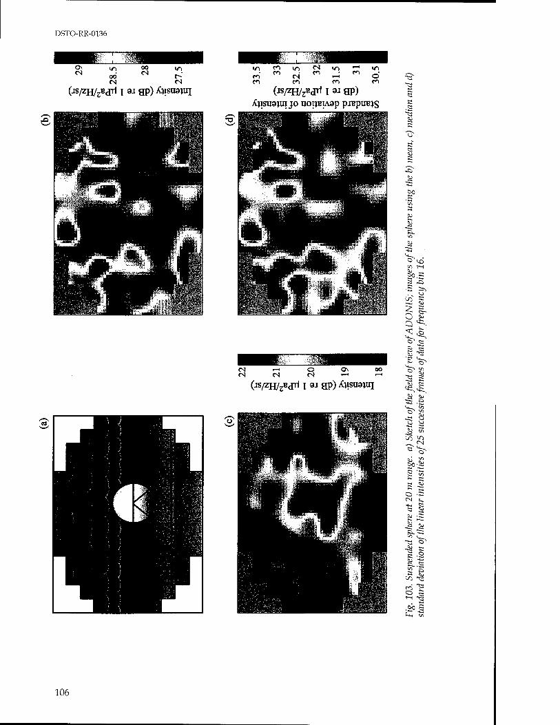
DSTO-RR-0136

(js/zH/3Bdii i ai gp) Ajisirajui (js/zH/^dtl i 9J gp)

Xjisuajui jo uotiBiAap pj^ptrejs

(js/2H/rBdTl t aJ ap) Xjisuaiiq

fflBBSS

-a

Si •4-1

«>0

CU

«> «1 « w

-+-J

^ VO

V> t—1 t\> &n a -a

■~ er <-r> K >—< ^J

Q ^ ^ ^ ̂

ct

•§ £• ^> ^ 0) "W p; i) w ^«■fc,



5) s> V ) u

u-\ in fM

es ^

et tn »r* 5)

~ o •£2 CN ^. •+-» Ci « cu Ju ^ 'tJ o «I •c BL e « B

to ^ m' T o f! 1-H "ft

<50 « U.

106

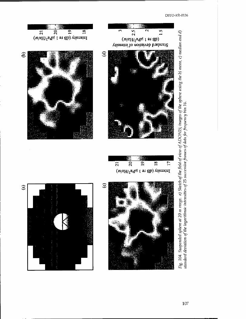
DSTO-RR-0136

<S <N *-i "-1

(js/zu/^^ri i 9i gp) Xjistrajiq (JS/ZH/^ jrl i 3i HP)

Äjisaajui jo uoijBiAap pjupuins

(jS/ZH/jBjrl l 3J gp) ÄJISU9JUI

13

ü8

107

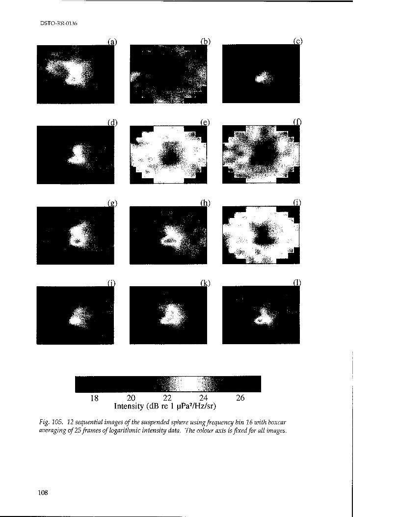
DSTO-RR-0136

18 20 22 24 Intensity (dB re 1 (jPa2/Hz/sr)

Fig. 105. 12 sequential images of the suspended spltere using frequency bin 16 with boxcar averaging of 25 frames of logarithmic intensity data. The colour axis is fixed for all images.

108

DSTO-RR-0136

(C)

20 21 22 24 25 26 20 21 22 Intensity (dB re 1 |iPa2/Hz/sr) Intensity (dB re 1 |iPa2/Hz/sr) Intensity (dB re 1 ^iPa2/Hz/sr)

20 22 22.5 23 23.5 24 25 26 Intensity (dB re 1 (iPa2/Hz/sr) Intensity (dB re 1 |uPa2/Hz/sr) Intensity (dB re 1 |iPa2/Hz/sr)

20.5 21 21.5 22 22.5 20 22 22 24 Intensity (dB re 1 |iPa2/Hz/sr) Intensity (dB re 1 |iPa2/Hz/sr) Intensity (dB re 1 |iPa2/Hz/sr)

19 20 21 20 22 20 20.5 21 21.5 Intensity (dB re 1 |iiPa2/Hz/sr) Intensity (dB re 1 |iPa2/Hz/sr) Intensity (dB re 1 |jPa2/Hz/sr)

Fig. 106. As for Figure 105, but with the colour axis scaled for each image.

109

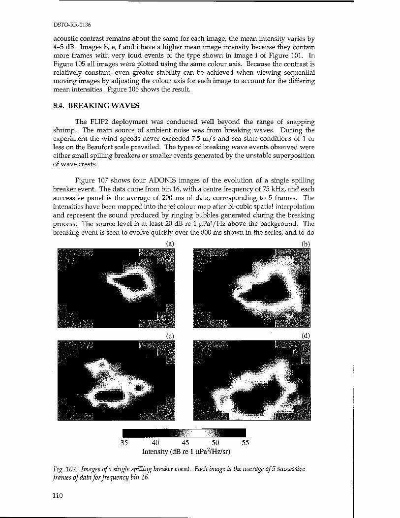
DSTO-RR-0136

acoustic contrast remains about the same for each image, the mean intensity varies by 4-5 dB. Images b, e, f and i have a higher mean image intensity because they contain more frames with very loud events of the type shown in image i of Figure 101. In Figure 105 all images were plotted using the same colour axis. Because the contrast is relatively constant even greater stability can be achieved when viewing sequential moving images by adjusting the colour axis for each image to account for the differing mean intensities. Figure 106 shows the result.

8.4. BREAKING WAVES

The FLIP2 deployment was conducted well beyond the range of snapping shrimp. The main source of ambient noise was from breaking waves. During the experiment the wind speeds never exceeded 7.5 m/s and sea state conditions of 1 or less on the Beaufort scale prevailed. The types of breaking wave events observed were either small spilling breakers or smaller events generated by the unstable superposition of wave crests.

Figure 107 shows four ADONIS images of the evolution of a single spilling breaker event. The data come from bin 16, with a centre frequency of 75 kHz, and each successive panel is the average of 200 ms of data, corresponding to 5 frames. The intensities have been mapped into the jet colour map after bi-cubic spatial interpolation and represent the sound produced by ringing bubbles generated during the breaking process. The source level is at least 20 dB re 1 |jPa2/Hz above the background. The breaking event is seen to evolve quickly over the 800 ms shown in the series, and to do

(a) (b) HÜHÜ

40 45 50 55 Intensity (dB re 1 |aPa2/Hz/sr)

Fig. 107. Images of a single spilling breaker event. Each image is the average of 5 successive frames of data for frequency bin 16.

110

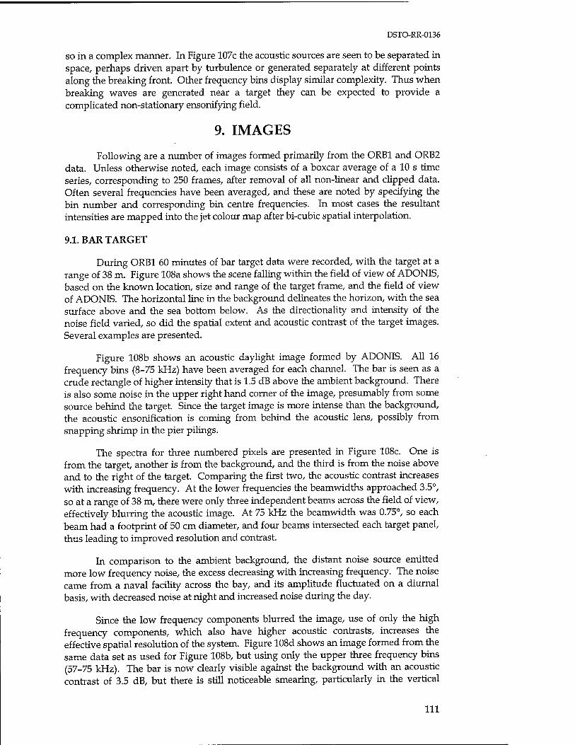
DSTO-RR-0136

so in a complex manner. In Figure 107c the acoustic sources are seen to be separated in space, perhaps driven apart by turbulence or generated separately at different points along the breaking front. Other frequency bins display similar complexity. Thus when breaking waves are generated near a target they can be expected to provide a complicated non-stationary ensonifying field.

9. IMAGES

Following are a number of images formed primarily from the ORB1 and ORB2 data. Unless otherwise noted, each image consists of a boxcar average of a 10 s time series, corresponding to 250 frames, after removal of all non-linear and clipped data. Often several frequencies have been averaged, and these are noted by specifying the bin number and corresponding bin centre frequencies. In most cases the resultant intensities are mapped into the jet colour map after bi-cubic spatial interpolation.

9.1. BAR TARGET

During ORB1 60 minutes of bar target data were recorded, with the target at a range of 38 m. Figure 108a shows the scene falling within the field of view of ADONIS, based on the known location, size and range of the target frame, and the field of view of ADONIS. The horizontal line in the background delineates the horizon, with the sea surface above and the sea bottom below. As the directionality and intensity of the noise field varied, so did the spatial extent and acoustic contrast of the target images. Several examples are presented.

Figure 108b shows an acoustic daylight image formed by ADONIS. All 16 frequency bins (8-75 kHz) have been averaged for each channel. The bar is seen as a crude rectangle of higher intensity that is 1.5 dB above the ambient background. There is also some noise in the upper right hand corner of the image, presumably from some source behind the target. Since the target image is more intense than the background, the acoustic ensonification is coming from behind the acoustic lens, possibly from snapping shrimp in the pier pilings.

The spectra for three numbered pixels are presented in Figure 108c. One is from the target, another is from the background, and the third is from the noise above and to the right of the target. Comparing the first two, the acoustic contrast increases with increasing frequency. At the lower frequencies the beamwidths approached 3.5°, so at a range of 38 m, there were only three independent beams across the field of view, effectively blurring the acoustic image. At 75 kHz the beamwidth was 0.75°, so each beam had a footprint of 50 cm diameter, and four beams intersected each target panel, thus leading to improved resolution and contrast.

In comparison to the ambient background, the distant noise source emitted more low frequency noise, the excess decreasing with increasing frequency. The noise came from a naval facility across the bay, and its amplitude fluctuated on a diurnal basis, with decreased noise at night and increased noise during the day.

Since the low frequency components blurred the image, use of only the high frequency components, which also have higher acoustic contrasts, increases the effective spatial resolution of the system. Figure 108d shows an image formed from the same data set as used for Figure 108b, but using only the upper three frequency bins (57-75 kHz). The bar is now clearly visible against the background with an acoustic contrast of 3.5 dB, but there is still noticeable smearing, particularly in the vertical

111

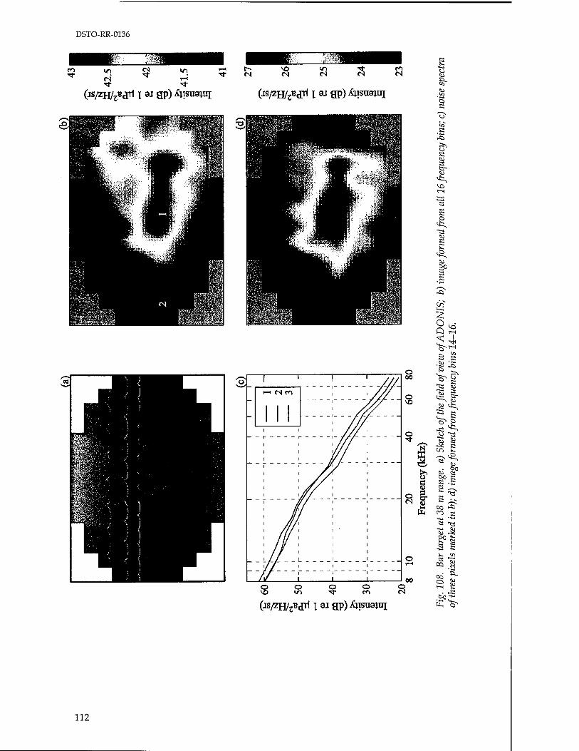
DSTO-RR-0136

(js/zH/zB,irl i ai gp) Xjisuaiui (js/zH/2Bjrl i 9J gp) ^xsua;ui a.

1 I 1 ! ///

- HNCO -V/A --

- I i

//ill

© VO

o If)

o "3-

o CO

o

G> K S cr-

<3

S

(JS/ZH/JB jrl i aj ap) ^isusjui

Q Ä

*3 3 g

■~ -a o 00

o VO

hoft

lief

ie

from

freq

i

o s-> ta T /«"»>

a) S

ket

e for

me

£ . «50

öo ss a K .5

o 0) m

ra

);d)

VH OO A HH

r ta

rget

at 3

s

mar

ked

in

o &% T—1

00 ) 1

Fig. 1

08.

of th

ree

p

112

DSTO-RR-0136

direction. This may be due to the target not being at the focal range, or could be reflections from the metal target frame.

Images from another data set of the bar target are shown in Figure 109. The target was still at 38 m range, but ADONIS had been rotated a few degrees to the right, so that the bar was in the centre of the field of view. Figurel09a is an image formed by the lowest three frequency bins (8-12 kHz) and Figure 109b is the corresponding image from the same frames of data, but using the upper three frequency bins (57-75 kHz).

Since only low frequencies are used in Figure 109a, the spatial resolution is poor, but the noise from the naval pier across the bay is still evident. The target blocks some of the noise from the pier, leading to an apparent hole in the noise field. The target appears in a crude silhouette. In Figure 109b the target scatters more noise than the background and appears front-ensonified by high frequency noise. However, this high frequency image is inferior to that shown in Figure 108d, and the bar shape is not discernible.

Figure 109 shows that the anisotropy of the noise field has reversed over the frequency band from 8 to 80 kHz. The target is front-ensonified in one spectral band and simultaneously back-ensonified in another spectral band, an effect that is rarely observed in optical photography.

27.51

^26.5

e 26m 8

25.5

25

24.51

Fig. 109. Bar target at 38 m range. Images formed from frequency bins a) 1-3; b) 14-16, shoiuing back and front ensonification, respectively.

113

DSTO-RR-0136

55.5'

£ 32

§ 30

8 28 i •f 26

1 I £ 24

Fzg. 220. Bar target at 38 m range, with, noise generated on the pier providing front ensonification. Images formed from frequency bins a) 1-3; b) 14-16.

Figure 110 presents images from a third data set, with Figure 110a being for the low frequencies (8-12 kHz), and Figure 110b being for the high frequencies (57-75 kHz). The data corresponded in time to the use of an angle grinder for hull maintenance on a vessel moored along the MarFac Pier. Acoustic noise was injected into the water for several seconds at a time, greatly increasing the ambient noise level. The acoustic contrast of the images also increased, from the usual 3.5 dB to 9 dB at the higher frequencies. Under these conditions the system operated like a bi-static sonar.

9.2. FENESTRATED CROSS

During ORB1 60 minutes of data were also collected for the fenestrated cross. This presented a more complicated target and the object of the experiment was to see whether the hole in the centre could be resolved. At 75 kHz four beams would fall within the hole, but only under favourable alignment. More typically only one beam will fall in the hole, while the surrounding beams will contain both the edge of a panel and part of the hole. At substantially lower frequencies the hole would not be resolved. Figure Ilia shows the scene in ADONIS' field of view.

Figure 111b shows the image formed from a typical data set, averaged over all frequency bins (8-75 kHz). The target can be seen as a rough square with an acoustic contrast of 1.5 dB, but the hole has not been resolved. The inability to resolve the hole is due to the contribution of the lower frequencies.

114

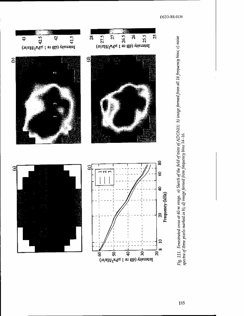
DSTO-RR-0136

m >/■> a "d- "3-

^f 00 es <s «n ô V)

vn es in es es

>n

(js/ZH/jBdTl i aj gp) îsuajiq (js/zH/^d^ i ai gp) îsuajui o

ff K 3

IP

rS)

V)

(js/2H/rB jrl i si gp) Aisuajui

o <d Q TH

^ ^H ^

=> P cu A fo ff

S ^> *cs 3

*~ o o ^ ts

tJ !U

3 C ^~ ^ w <S)

00

s s « ^.^N. iw. ts s ^v

fS"l o ^H £

^3 (ft & <J5 V. O ct s

IT! (ß

J" <u « H -fa B cn <u S £

U, '*s

r-i ^ r-i B i—I H-i

I.) «X !" £

115

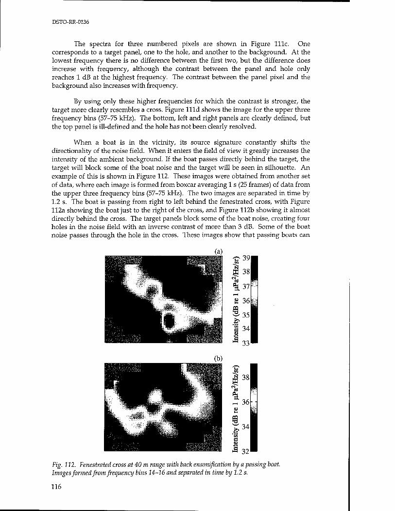
DSTO-RR-0136

The spectra for three numbered pixels are shown in Figure 111c. One corresponds to a target panel, one to the hole, and another to the background. At the lowest frequency there is no difference between the first two, but the difference does increase with frequency, although the contrast between the panel and hole only reaches 1 dB at the highest frequency. The contrast between the panel pixel and the background also increases with frequency.

By using only these higher frequencies for which the contrast is stronger, the target more clearly resembles a cross. Figure llld shows the image for the upper three frequency bins (57-75 kHz). The bottom, left and right panels are clearly defined, but the top panel is ill-defined and the hole has not been clearly resolved.

When a boat is in the vicinity, its source signature constantly shifts the directionality of the noise field. When it enters the field of view it greatly increases the intensity of the ambient background. If the boat passes directly behind the target, the target will block some of the boat noise and the target will be seen in silhouette. An example of this is shown in Figure 112. These images were obtained from another set of data, where each image is formed from boxcar averaging 1 s (25 frames) of data from the upper three frequency bins (57-75 kHz). The two images are separated in time by 1.2 s. The boat is passing from right to left behind the fenestrated cross, with Figure 112a showing the boat just to the right of the cross, and Figure 112b showing it almost directly behind the cross. The target panels block some of the boat noise, creating four holes in the noise field with an inverse contrast of more than 3 dB. Some of the boat noise passes through the hole in the cross. These images show that passing boats can

Fig. 112. Fenestrated cross at 40 m range zuith back ensonification by a passing boat. Images formed from frequency bins 14-16 and separated in time by 1.2 s.

116

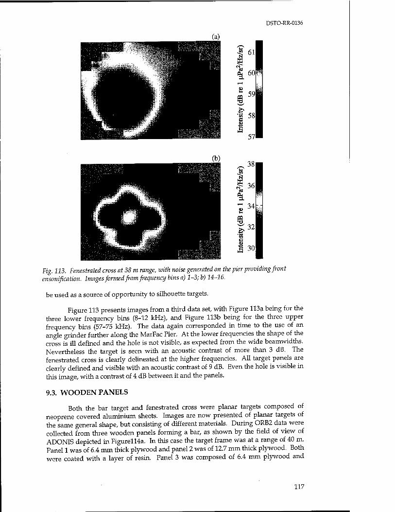
DSTO-RR-0136

-^ 611

"Id 60 i—<

p 59

^«-»' * •a 5X 0

57l

38|

36

34

32

1 30

Fig. 213. Fenestrated cross at 38 m range, with noise generated on the pier providing front ensonification. Images formed from frequency Uns a) 1-3; b) 14-16.

be used as a source of opportunity to silhouette targets.

Figure 113 presents images from a third data set with Figure 113a being for the three lower frequency bins (8-12 kHz), and Figure 113b being for the three upper frequency bins (57-75 kHz). The data again corresponded in time to the use of an angle grinder further along the MarFac Pier. At the lower frequencies the shape of the cross is ill defined and the hole is not visible, as expected from the wide beamwidths. Nevertheless the target is seen with an acoustic contrast of more than 3 dB. The fenestrated cross is clearly delineated at the higher frequencies. All target panels are clearly defined and visible with an acoustic contrast of 9 dB. Even the hole is visible in this image, with a contrast of 4 dB between it and the panels.

9.3. WOODEN PANELS

Both the bar target and fenestrated cross were planar targets composed of neoprene covered aluminium sheets. Images are now presented of planar targets of the same general shape, but consisting of different materials. During ORB2 data were collected from three wooden panels forming a bar, as shown by the field of view of ADONIS depicted in Figurell4a. In this case the target frame was at a range of 40 m. Panel 1 was of 6.4 mm thick plywood and panel 2 was of 12.7 mm thick plywood. Both were coated with a layer of resin. Panel 3 was composed of 6.4 mm plywood and

117

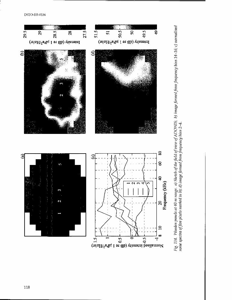
DSTO-RR-0136

in .—i

«n

m o <n <* o m c^ •sf «n ■*■

(js/zH/rB jri i aj gp) /fystrajui (iS/zH/^^ i ai gp) jfysirajtq

1 | .. I X 1 1/

^ 7 >^\ -'-(--' v

\ PyY \

/ ' 1 ^^L'

—< CS en "frVn

--

/ ' JT '

/ ' >y ' / ' /' y^ 1 ^-i^^ 1 >v 1 / 1

/ i \'s"",,,,,'> ^S ' J ' \. 1 / ' / / ' / '

1 /^ ^^^x ^J / '

y' i i ys. i Y i / i i \_iS(A i

\ ' ' 1' \1 ' \ i i t i j\ i

o 00

©

00

© ©

"a

K Si r-i

p

5XJ

-O

to

•Si S

s s

55 W

to

o 'S

8 .8

£ ■* a.

(js/zH/rBjti i ai gp) vfystrajui psspuuojsi .ÖO-?

118

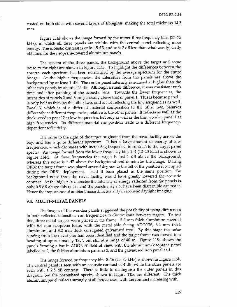
DSTO-RR-0136

coated on both sides with several layers of fibreglass, making the total thickness 14.3 mm.

Figure 114b shows the image formed by the upper three frequency bins (57-75 kHz), in which all three panels are visible, with the central panel reflecting more energy. The acoustic contrast is only 1.5 dB, and so is 2 dB less than what was typically obtained for the neoprene-covered aluminium panels.

The spectra of the three panels, the background above the target and some noise to the right are shown in Figure 114c. To highlight the differences between the spectra, each spectrum has been normalised by the average spectrum for the entire image. At the higher frequencies, the intensities from the panels are above the background by at least 1 dB. The centre panel intensity is somewhat higher than the other two panels by about 0.25 dB. Although a small difference, it was consistent with time and after panning of the acoustic lens. Towards the lower frequencies, the intensities of panels 2 and 3 are generally above that of panel 1. This is because panel 1 is only half as thick as the other two, and is not reflecting the low frequencies as well. Panel 3, which is of a different material composition to the other two, behaves differently at different frequencies, relative to the other panels. It reflects as well as the thick wooden panel 2 at low frequencies, but only as well as the thin wooden panel 1 at high frequencies. Its different material composition leads to a different frequency- dependent reflectivity.

The noise to the right of the target originated from the naval facility across the bay, and has a quite different spectrum. It has a large amount of energy at low frequencies, which decreases with increasing frequency, in contrast to the target panel spectra. An image formed from the lower frequency bins 2-4 (10-13 kHz) is shown in Figure 114d. At these frequencies the target is just 1 dB above the background, whereas this noise is 2 dB above the background and dominates the image. During ORB2 the target frame was placed several degrees to the left of the position it occupied during the ORB1 deployment. Had it been placed in the same position, the background noise from the naval facility would have greatly lowered the acoustic contrast. At the higher frequencies the intensity of energy reflected from the panels is only 0.5 dB above this noise, and the panels may not have been discernible against it. Hence the importance of ambient noise directionality in acoustic daylight imaging.

9.4. MULTI-METAL PANELS

The images of the wooden panels suggested the possibility of using differences in both reflected intensities and frequencies to discriminate between targets. To test this, three metal targets were placed in the frame: 3.2 mm thick aluminium covered with 6.4 mm neoprene foam, with the metal side facing ADONIS, 6.4 mm thick aluminium, and 3.2 mm thick corrugated galvanised iron. By this stage the noise coming from the naval pier had been identified and the target frame was moved to a heading of approximately 135°, but still at a range of 40 m. Figure 115a shows the panels forming a bar in ADONIS' field of view, with the aluminium/neoprene panel labelled as 2, the thicker aluminium panel as 3, and the galvanised iron panel as 4.

The image formed by frequency bins 8-16 (25-75 kHz) is shown in Figure 115b. The central panel is seen with an acoustic contrast of 4 dB, while the other panels are seen with a 2.5 dB contrast. There is little to distinguish the outer panels in this diagram, but the normalised spectra shown in Figure 115c are different. The thick aluminium panel reflects strongly at all frequencies, with the contrast increasing with

119

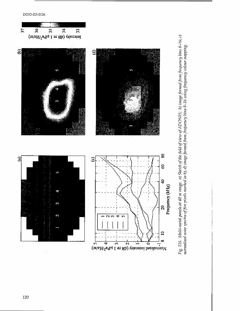
DSTO-RR-0136

p- vo m ■*r r<-> m m m ro f>

(IS/ZH/ZB jri t 3J gp) A4ISU91UI

- \\J 1 1 V 1 1 j

^\S. r ' V T ' n

-

*• 1 Nn

1 -> -^r <r>

! 1 1

1 i 1 \ / \' /

_i.. 1 1 ihV

o 00

o

_ O

00 —< O «-H »/"> Tf rn cS

(JS/ZH/^jrl x ai gp) vtysirajui pasijBiuio^

I—I I

00 bo

sa- cs

p s

C 00

bo rt

S ^° •~ I

* w

O s Q SJ ^ §- 0^

-w P S <-CL

^•«

^^ w tu « g> ^1

-a

bo"?1

e 5

s * o a ^ "B.

Si s.

s 8

2 « .bo

120

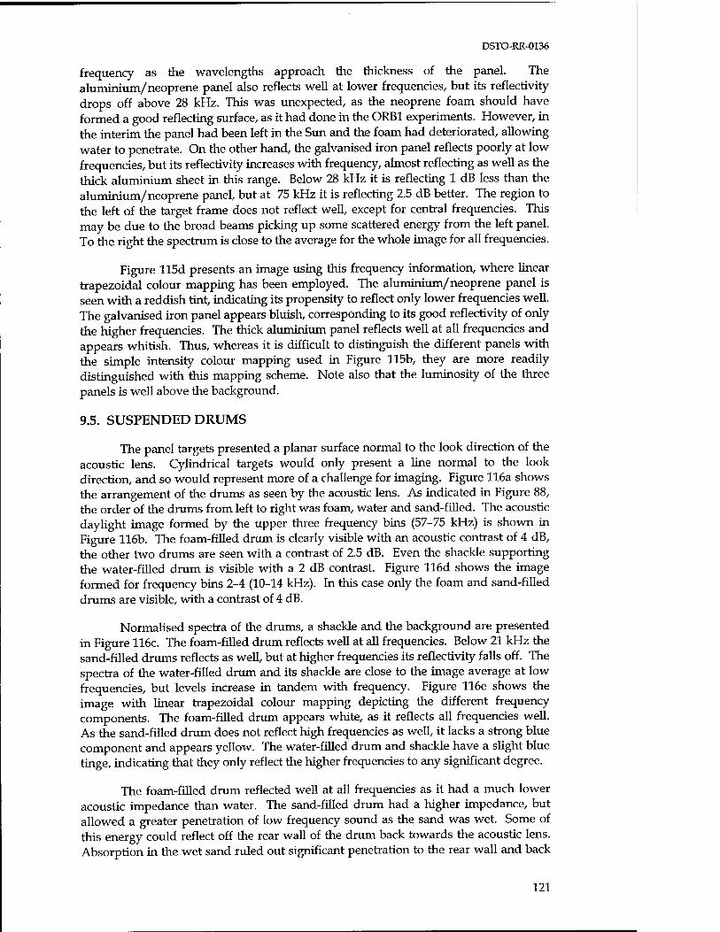
DSTO-RR-0136

frequency as the wavelengths approach the thickness of the panel. The aluminium/neoprene panel also reflects well at lower frequencies, but its reflectivity drops off above 28 kHz. This was unexpected, as the neoprene foam should have formed a good reflecting surface, as it had done in the ORB1 experiments. However, in the interim the panel had been left in the Sun and the foam had deteriorated, allowing water to penetrate. On the other hand, the galvanised iron panel reflects poorly at low frequencies, but its reflectivity increases with frequency, almost reflecting as well as the thick aluminium sheet in this range. Below 28 kHz it is reflecting 1 dB less than the aluminium/neoprene panel, but at 75 kHz it is reflecting 2.5 dB better. The region to the left of the target frame does not reflect well, except for central frequencies. This may be due to the broad beams picking up some scattered energy from the left panel. To the right the spectrum is close to the average for the whole image for all frequencies.

Figure 115d presents an image using this frequency information, where linear trapezoidal colour mapping has been employed. The aluminium/neoprene panel is seen with a reddish tint, indicating its propensity to reflect only lower frequencies well. The galvanised iron panel appears bluish, corresponding to its good reflectivity of only the higher frequencies. The thick aluminium panel reflects well at all frequencies and appears whitish. Thus, whereas it is difficult to distinguish the different panels with the simple intensity colour mapping used in Figure 115b, they are more readily distinguished with this mapping scheme. Note also that the luminosity of the three panels is well above the background.

9.5. SUSPENDED DRUMS

The panel targets presented a planar surface normal to the look direction of the acoustic lens. Cylindrical targets would only present a line normal to the look direction, and so would represent more of a challenge for imaging. Figure 116a shows the arrangement of the drums as seen by the acoustic lens. As indicated in Figure 88, the order of the drums from left to right was foam, water and sand-filled. The acoustic daylight image formed by the upper three frequency bins (57-75 kHz) is shown in Figure 116b. The foam-filled drum is clearly visible with an acoustic contrast of 4 dB, the other two drums are seen with a contrast of 2.5 dB. Even the shackle supporting the water-filled drum is visible with a 2 dB contrast. Figure 116d shows the image formed for frequency bins 2-4 (10-14 kHz). In this case only the foam and sand-filled drums are visible, with a contrast of 4 dB.

Normalised spectra of the drums, a shackle and the background are presented in Figure 116c. The foam-filled drum reflects well at all frequencies. Below 21 kHz the sand-filled drums reflects as well, but at higher frequencies its reflectivity falls off. The spectra of the water-filled drum and its shackle are close to the image average at low frequencies, but levels increase in tandem with frequency. Figure 116e shows the image with linear trapezoidal colour mapping depicting the different frequency components. The foam-filled drum appears white, as it reflects all frequencies well. As the sand-filled drum does not reflect high frequencies as well, it lacks a strong blue component and appears yellow. The water-filled drum and shackle have a slight blue tinge, indicating that they only reflect the higher frequencies to any significant degree.

The foam-filled drum reflected well at all frequencies as it had a much lower acoustic impedance than water. The sand-filled drum had a higher impedance, but allowed a greater penetration of low frequency sound as the sand was wet. Some of this energy could reflect off the rear wall of the drum back towards the acoustic lens. Absorption in the wet sand ruled out significant penetration to the rear wall and back

121

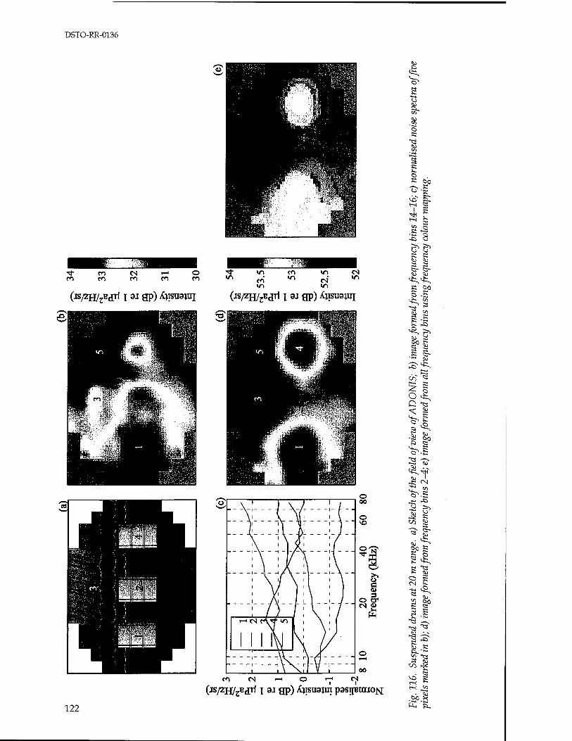
DSTO-RR-0136

■<fr CO cs 1—< O ■<*• f> en >r> CN en en CO en en v> en m

in v>

(JS/ZH/ZB jrl i aj gp) Xjisuajui (is/2H/rB jri i ai gp) Xjisua;ui

Jl H Ip^^^^H

I 9 tfi^^^^^^^^^l

iw^j IB

(JS/2H/3Bjrl x aj gp) Äjisua;ui paspraio^

S 55.

O K

us

o S

*o I

■S

f a, a. <3

e e S 3 er- <s-

If £ -S

ef Si £ §-

i—^ *-*

O <fc, Q is

It? ^ £ *G —N

*J ■ -

-s; "^

•$ ? to Si »-^

"*. rj £*§ o CN

•3 ts

122 .00

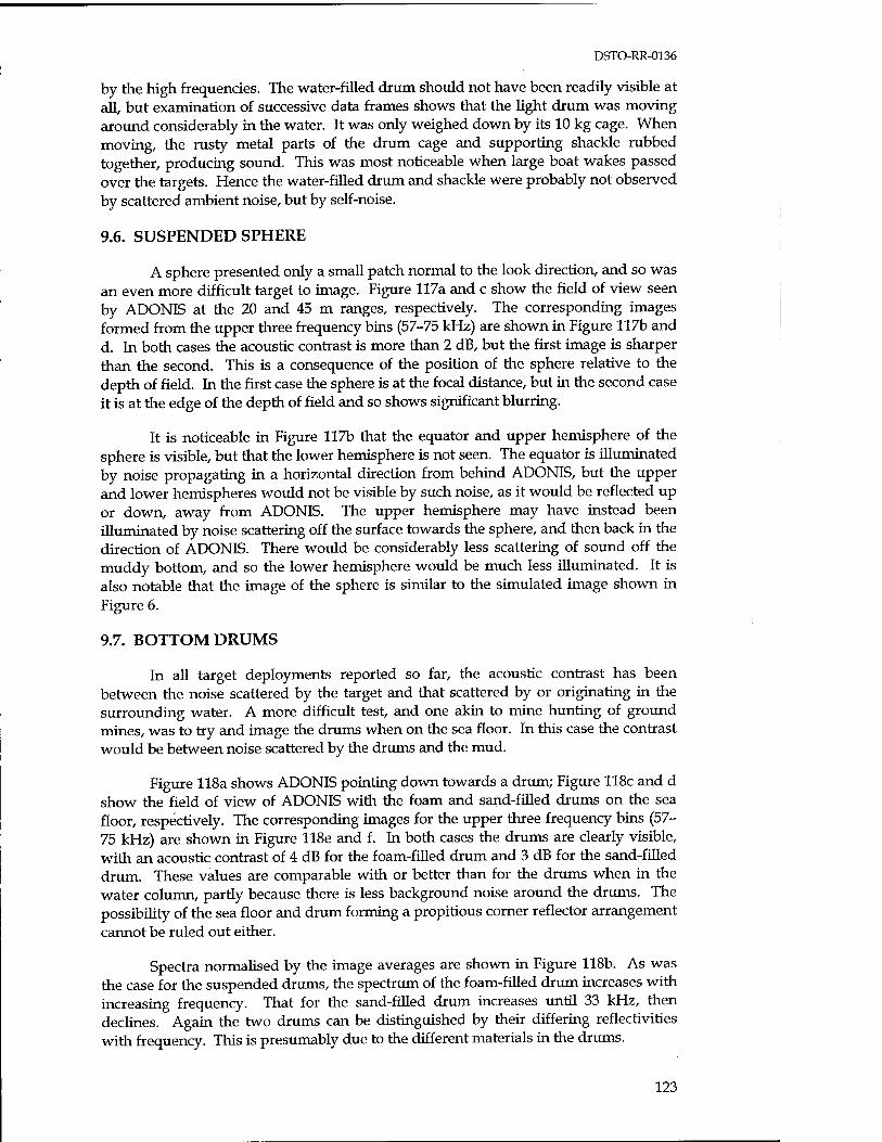
DSTO-RR-0136

by the high frequencies. The water-filled drum should not have been readily visible at all, but examination of successive data frames shows that the light drum was moving around considerably in the water. It was only weighed down by its 10 kg cage. When moving, the rusty metal parts of the drum cage and supporting shackle rubbed together, producing sound. This was most noticeable when large boat wakes passed over the targets. Hence the water-filled drum and shackle were probably not observed by scattered ambient noise, but by self-noise.

9.6. SUSPENDED SPHERE

A sphere presented only a small patch normal to the look direction, and so was an even more difficult target to image. Figure 117a and c show the field of view seen by ADONIS at the 20 and 45 m ranges, respectively. The corresponding images formed from the upper three frequency bins (57-75 kHz) are shown in Figure 117b and d. In both cases the acoustic contrast is more than 2 dB, but the first image is sharper than the second. This is a consequence of the position of the sphere relative to the depth of field. In the first case the sphere is at the focal distance, but in the second case it is at the edge of the depth of field and so shows significant blurring.

It is noticeable in Figure 117b that the equator and upper hemisphere of the sphere is visible, but that the lower hemisphere is not seen. The equator is illuminated by noise propagating in a horizontal direction from behind ADONIS, but the upper and lower hemispheres would not be visible by such noise, as it would be reflected up or down, away from ADONIS. The upper hemisphere may have instead been illuminated by noise scattering off the surface towards the sphere, and then back in the direction of ADONIS. There would be considerably less scattering of sound off the muddy bottom, and so the lower hemisphere would be much less illuminated. It is also notable that the image of the sphere is similar to the simulated image shown in Figure 6.

9.7. BOTTOM DRUMS

In all target deployments reported so far, the acoustic contrast has been between the noise scattered by the target and that scattered by or originating in the surrounding water. A more difficult test, and one akin to mine hunting of ground mines, was to try and image the drums when on the sea floor. In this case the contrast would be between noise scattered by the drums and the mud.

Figure 118a shows ADONIS pointing down towards a drum; Figure 118c and d show the field of view of ADONIS with the foam and sand-filled drums on the sea floor, respectively. The corresponding images for the upper three frequency bins (57- 75 kHz) are shown in Figure 118e and f. In both cases the drums are clearly visible, with an acoustic contrast of 4 dB for the foam-filled drum and 3 dB for the sand-filled drum. These values are comparable with or better than for the drums when in the water column, partly because there is less background noise around the drums. The possibility of the sea floor and drum forming a propitious corner reflector arrangement cannot be ruled out either.

Spectra normalised by the image averages are shown in Figure 118b. As was the case for the suspended drums, the spectrum of the foam-filled drum increases with increasing frequency. That for the sand-filled drum increases until 33 kHz, then declines. Again the two drums can be distinguished by their differing reflectivities with frequency. This is presumably due to the different materials in the drums.

123

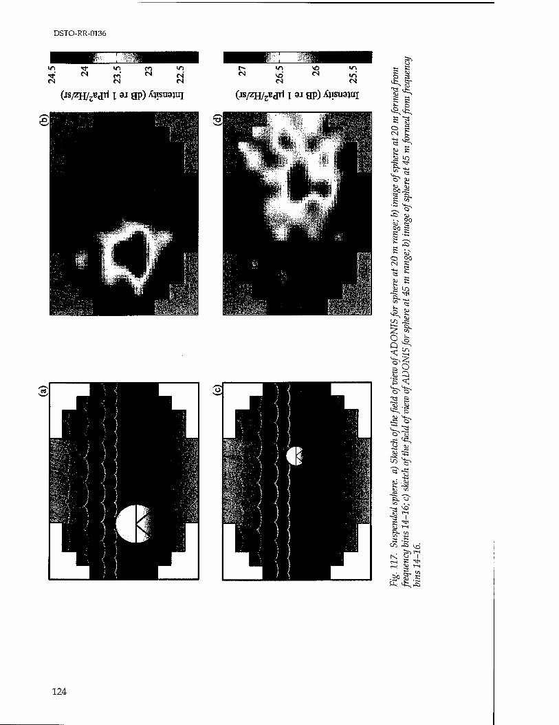
DSTO-RR-0136

>/■> "* «D en V"> "t CM en ts <s es <S ts

(js/zn/^jjri i aj gp) Xjxsuajiq (js/zH/^dti i 9i gp) X;isuajui

S § e> s

£ s !- O

s *«

cs ^ 82 £ SJ ^

s ^> •s £ x^ &. s

1^

- s 82 £

<-o ^

"I 'B ^ ^^

a.

*4J

 -5

124

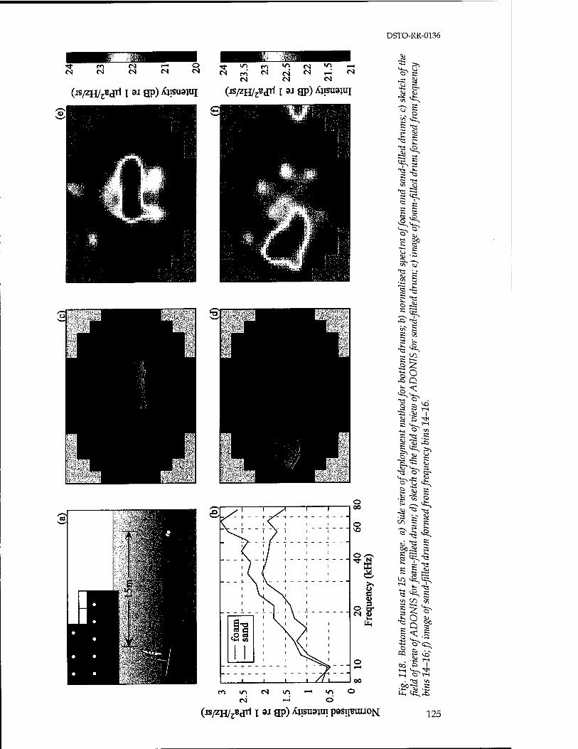
^ ifl n m M m .-H

e^ r*i C* oi f «-< ^ (S cs ts

(JS/ZH/JB jrl i aj gp) Xjrcuajui (JS/ZH/^ jri i SJ gp) Xjxsuajui

cs <-• o

(JS/ZH/^JTI x ai gp) Xjisuajm pasrpniuoN;

DSTO-RR-0136

^

^ Ö1

Cl)

u r-i -*-i <3-

Tj p « ^ *W

3 CO

TS ~ ^

T—-»

ts <3 "C"? « ^ "a >-—* s ^ c JS cs

offo

a e

offo

e 00 s^ W u -, rH u U3

R t-i R

0

SJ A ^ i* 5>

R £x. £ < 52 -2 •*~. *** -+-1

O 0' ^

CQ ■o

00 rO 1 r-H V ■sd t-H O r-H

Ti « .<* .« R U-, ^ Ä

125

DSTO-RR-0136

9.8. SWIMMING DIVER

All targets presented so far have been stationary, although an illusion of target movement could be created by panning with the acoustic lens whilst the target remained fixed. During the ORB1 deployment, an experiment was conducted in which a diver swam in front of ADONIS at a range of approximately 18 m. He was wearing a neoprene wetsuit and had an aqualung, however he refrained from exhaling during the crossing, as the noise created by the bubbles was sufficient to saturate the ADONIS electronics. He had an underwater acoustic communication device operating at a carrier frequency of about 30 kHz. Although not is use, it emitted a soft quiescent hum at the carrier frequency. This could be detected by ADONIS as it fell within frequency bin 9, which had a centre frequency of 29 kHz. Thus images based on bin 9 would have a true passive component from which the position of the diver could be tracked.

Figure 119 shows images formed from 0.5 s (12 frames) of data. Figure 119a and b use data from frequency bin 9. Figure 119a shows the diver just to the left of the centre, and Figure 119b shows him 2 s later, near the left edge of the image. These are compared with actual acoustic daylight images in Figure 119c and d for the same temporal segments of data averaged over the upper three frequency bins (57-75 kHz). The diver is seen in identical positions with an acoustic contrast of some 2.5 dB. Since ADONIS was focused for 25 m during ORB1, the diver fell well within the depth of field of the system, and is in sharp focus. On the other hand, at the bottom and right of the images there is some unknown noise that presumably originates some distance behind the diver and so appears blurred.

10. FUTURE WORK

Although impressive images were obtained with ADONIS in its current configuration, the potential was marred by the direct arrival at the array of noise coming from behind and to the sides of the reflecting dish. This masked noise originating from behind the targets or reflected by them. If realised at the time, this flaw could have been corrected by die use of a baffle around the dish, in much the same way that optical telescopes use a tube around the mirror to remove local stray light.

The next stage in the development of acoustic daylight imaging is to build a more sophisticated system. Staying with the current design principle of using a reflecting dish to do the beamforming, an array with more elements and operating to higher frequencies would increase the resolution. The use of SCFs to measure the energy in each frequency band sequentially simplifies the data acquisition, but with a penalty of the loss of most of the data. The alternative is to measure the energy in each frequency band simultaneously or send all the broadband data from all elements to the surface for processing. The first option can be implemented by modifying the electronics in the underwater canister. The latter option places a heavy computational load on the system.

The alternative approach is to scrap the reflecting dish and build a more conventional phased array. As noted above, to achieve a beamwidth of 1° requires a filled array of 10,000 elements, or a Mills Cross with 200 elements. The latter has large sidelobes in the orientation of the cross arms. A random sparse array of the same number of elements has the same total sidelobe energy, but it is more evenly spread in all directions (Steinberg, 1976). The computational load is high, since 64 Mbytes/s of data is acquired if 12-bit sampling is used for frequencies to 80 kHz. However, with

126

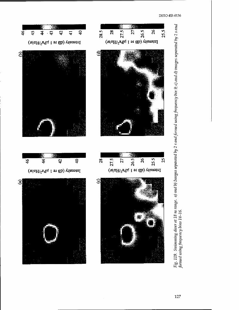
DSTO-RR-0136

(js/zH/zB,p11 9J gp) Xjisuajui (js/zH/zB<irl i ai ap) jtysuajui

5

«a a.

"a

5

•5 IS

e

•« «J

s

CN

(js/zH/rB jri \ 9i gp) Xjisuajui (js/zH/jB.jrl i 8J ap) X;isuajui en

5 'S"

2

•S ^ S ■

s

cr»

127

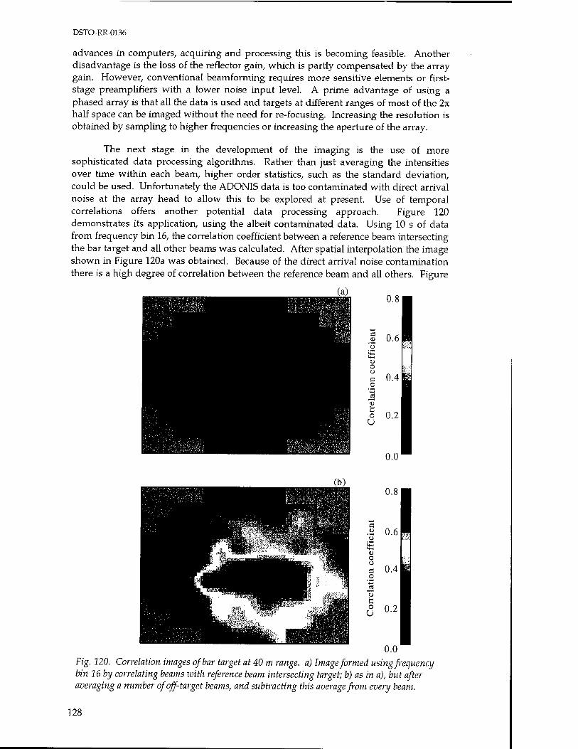
DSTO-RR-0136

advances in computers, acquiring and processing this is becoming feasible. Another disadvantage is the loss of the reflector gain, which is partly compensated by the array gain. However, conventional beamforming requires more sensitive elements or first- stage preamplifiers with a lower noise input level. A prime advantage of using a phased array is that all the data is used and targets at different ranges of most of the 2rc half space can be imaged without the need for re-focusing. Increasing the resolution is obtained by sampling to higher frequencies or increasing the aperture of the array.

The next stage in the development of the imaging is the use of more sophisticated data processing algorithms. Rather than just averaging the intensities over time within each beam, higher order statistics, such as the standard deviation, could be used. Unfortunately the ADONIS data is too contaminated with direct arrival noise at the array head to allow this to be explored at present. Use of temporal correlations offers another potential data processing approach. Figure 120 demonstrates its application, using the albeit contaminated data. Using 10 s of data from frequency bin 16, the correlation coefficient between a reference beam intersecting the bar target and all other beams was calculated. After spatial interpolation the image shown in Figure 120a was obtained. Because of the direct arrival noise contamination there is a high degree of correlation between the reference beam and all others. Figure

o o c

_o ca

'S o U

0.8

0.6 I 0.4

0.2

0.0'

0.8

.a 0.6

«4-1

o o ö o

h o U

I 0.4

0.2

0.0 Fig. 120. Correlation images of bar target at 40 m range, a) Image formed using frequency bin 16 by correlating beams with reference beam intersecting target; b) as in a), but after averaging a number of off-target beams, and subtracting this average from every beam.

128

DSTO-RR-0136

120b shows the improvement obtained by averaging a number of off-target beams, and subtracting this average from every beam. Now the bar target is clearly seen, with the reference beam (the dark brown circle) being well correlated with all beams intersectingthe target, but only poorly correlated with the off-target beams.

In addition to improvements in hardware and software algorithms, some more fundamental studies of the noise field and targets are required. Measurements of higher frequency spectra in shallow and deeper waters are needed, particularly to see whether thermal noise provides a limitation to high frequency imaging, and to see whether other higher frequency sources of noise are available for imaging. Knowledge of the azimuthal and elevational distribution of the noise is needed to determine likely contrast values; measurements of the coherence of the noise and that reflected from targets would give a measure of the expected array gain. A broader knowledge of the temporal fluctuations would aid potential signal processing approaches. To provide some quantitative indication of the success of imaging, a measure of probability of recognition is needed, along with reflectivity measurements on the various targets as a function of frequency and source direction.

11. OPERATIONAL IMPLICATIONS

Acoustic daylight potentially has a number of advantages over conventional active and passive sonar. Like a passive sonar, it can look for specific signals within one of its beams. It can also look for silent targets and does not have a degraded performance in regions of high ambient noise. In fact, since it uses the ambient noise, it should have an enhanced performance in such regions. Since it does not produce its own sound, it should have a lower power consumption than an active sonar, and so is suited to use on an underwater remotely operated vehicle. Its covert nature has important tactical advantages. Since it produces a pictorial image, with sufficient resolution it should be easier to interpret than current sonar system displays, which require trained operators. The introduction of false colour to the images should ease discrimination between different targets.

Since acoustic daylight uses ambient noise, it works best where there is plenty of noise. Snapping shrimp are ubiquitous in Australia's coastal waters to the north of Bass Strait, so an acoustic daylight system should work well in most shallow water environments. It could be used for the mine hunting of moored and ground mines. Because ADONIS was mostly used out of focus, its focal point not readily changed, and was of low resolution, it is not yet clear over what range it can detect mine-like targets. Certainly it can image over short ranges of less than 40 m. The reflecting dish is cumbersome to use, but if replaced by a phased array conformal with an underwater vehicle's front surface, it could be deployed on such a vehicle for mine hunting purposes. If a higher resolution system could be built it might be deployable in a hull- mounted configuration. It could also be used for harbour surveillance and with its ability to provide real-time moving images, could warn of the presence of divers in the vicinity of naval installations.

Based on their theoretical study, Flatte and Munk (1985) thought acoustic daylight could be used for submarine detection, however it has not yet been tried experimentally over long ranges. To get sufficient resolution, a system would need a huge aperture at low frequencies, such as might be provided by multiple towed arrays. It is not clear whether there is sufficient high frequency ambient noise in the deep ocean for imaging purposes, or whether thermal noise will be an insuperable obstacle

129

DSTO-RR-0136

to high frequency imaging. If there is enough non-thermal high frequency noise, a less cumbersome system operating at high frequencies might be devised.

12. ACKNOWLEDGMENTS

The author wishes to express his gratitude to Prof. Michael Buckingham for hosting visits to his acoustic daylight laboratory at the Scripps Institution of Oceanography, and allowing him access to all facilities and staff. Throughout the visits the author worked on a daily basis with Prof. Buckingham's PhD student Mr (now Dr) Chad Epifanio, who willingly passed on all the accumulated knowledge on acoustic daylight, as well as some of the diagrams used in this report. Many months were spent together performing experiments, analysing data and holding stimulating discussions on acoustic daylight. Others who assisted in the attachment at Scripps included Mr Mark Brentnall, Prof. Grant Deane, Mr Gene King, and Mr Fernando Simonet.

These visits to Scripps were made possible through the awarding to the author of the inaugural Royal Australian Navy Science Scholarship. The author thanks Dr Roger Creaser, Chief of the Maritime Operations Division of DSTO, for nominating him, and the Royal Australian Navy for selecting him for the scholarship.

13. REFERENCES

Berkhout, B.V. (1992). Acoustic daylight: imaging tJie ocean with ambient noise, unpublished MS thesis, University of California, San Diego, 86 pp.

Brekhovskikh, L. and Lysanov, Yu. (1982). Fundamentals of ocean acoustics, Springer- Verlag, New York, 250 pp.

Bobber, R.J. (1970). Undenvater electroacoustic measurements, Naval Research Laboratory, Washington, 333 pp.

Buckingham, M.J. (1993). "Theory of acoustic imaging in the ocean with ambient noise", Journal of Computational Acoustics 1,117-140.

Buckingham, M.J., Berkhout, B.V. and Glegg, A.L. (1992). "Acoustic daylight: imaging the ocean with ambient noise", Nature 356,327-329.

Callen, H.B., and Welton, T.A. (1951). "Irreversibility and generalized noise," Physical Review 83(1), 34-40.

Cato, D.H. (1997). "Features of ambient noise in shallow water," In Shallow-Water Acoustics, (R. Zhang and J. Zhou, Eds), China Ocean Press, Beijing, 634 pp.

Epifanio, C.L. (1993). Analysis of the noise field in the vicinity of Scripts Pier as determined by tlie acoustic daylight experiment, unpublished midterm project report, University of California, San Diego, 19 pp.

Epifanio, C.L. (1997). Acoustic daylight: passive acoustic imaging using ambient noise, unpublished PhD thesis, University of San Diego, 311 pp.

Flatte, S. and Munk, W. (1985). Submarine detection: acoustic contrast versus acoustic glow, JASON Report JSR-85-108, MITRE Corp., McLean, Virginia.

130

DSTO-RR-0136

Makris, N.C., Ingenito, F., and Kuperman, W.A. (1994). "Detection of a submerged object insonified by surface noise in an ocean waveguide", Journal of the Acoustical Society of America 96,1703-1724.

Makris, N.C. and Kuperman, W.A. (1994). "Bounds on the detection of a submerged object insonified by surface noise in a shallow water waveguide". In Sea Surface Sound '94, (M.J. Buckingham and J.R. Potter, Eds), World Scientific, University of California, Lake Arrowhead, 494 pp.

Meilen, R.H. (1952). "The thermal-noise limit in the detection of underwater acoustic signals", Journal oftlie Acoustical Society of America 24,478-480.

Potter, J.R. (1994). "Acoustic imaging using ambient noise: some theory and simulation results", Journal of the Acoustical Society of America 95,21-33.

Steinberg, B.D. (1976). Principles of aperture and array system design: including random and adaptive arrays, Wiley, New York, 356 pp.

United States Navy Electronics Laboratory (1946). Undenoater noise caused by snapping shrimp, University of California Division of War Research publication no. U337, San Diego, 74 pp.

Urick, R.J. (1983). Principles of undenoater sound, 3rd ed. McGraw-Hill Book Co., New York, 423 pp.

Urick, R.J. (1984). Ambient noise in tlie sea, Peninsula Publishing, Los Altos, California, various pagings.

131

DISTRIBUTION LIST


Mark Readhead

AUSTRALIA

DEFENCE ORGANISATION

Task Sponsor Naval Scientific Advisor

S&T Program Chief Defence Scientist ]

FAS Science Policy f- shared copy AS Science Corporate Management J Director General Science Policy Development Counsellor Defence Science, London (Doc Data Sheet) Counsellor Defence Science, Washington (Doc Data Sheet) Scientific Adviser to MRDC Thailand (Doc Data Sheet) Director General Scientific Advisers and Trials/Scientific Adviser Policy and

Command (shared copy) Scientific Adviser - Army (Doc Data Sheet and distribution list only) Air Force Scientific Adviser Director Trials

Aeronautical and Maritime Research Laboratory Director

Chief of Maritime Operations Division Chief of Maritime Platforms Division Dr Stuart Anstee Dr David Blair Dr Doug Cato Mr Ian Cox Mr Manuel de Sousa Dr Brain Ferguson Dr Bryan Jessup Dr Daryl McMahon Dr Mark Readhead

Electronics and Surveillance Research Laboratory Director (1 copy)

DSTO Library Library Fishermens Bend Library Maribyrnong

Library Salisbury (2 copies) Australian Archives Library, MOD, Pyrmont (2 copies) Library, MOD, HMAS Stirling

Capability Development Division Director General Maritime Development Director General Land Development (Doc Data Sheet only) Director General C3I Development (Doc Data Sheet only)

Navy SO (Science), Director of Naval Warfare, Maritime Headquarters Annex,

Garden Island, NSW 2000 Deputy Director Mine Warfare Development

Army ABCA Office, G-l-34, Russell Offices, Canberra (4 copies) SO (Science), DJFHQ(L), MILPO Enoggera, Queensland 4051 (Doc Data Sheet

only) NAPOC QWG Engineer NBCD c/- DENGRS-A, HQ Engineer Centre Liverpool

Military Area, NSW 2174 (Doc Data Sheet only)

Intelligence Program DGSTA Defence Intelligence Organisation

Corporate Support Program (libraries) OIC TRS, Defence Regional Library, Canberra Officer in Charge, Document Exchange Centre (DEC), 1 copy *US Defence Technical Information Center, 2 copies *UK Defence Research Information Centre, 2 copies "Canada Defence Scientific Information Service, 1 copy *NZ Defence Information Centre, 1 copy National Library of Australia, 1 copy

UNrvERsrriES AND COLLEGES

Australian Defence Force Academy Library Head of Aerospace and Mechanical Engineering

Deakin University, Serials Section (M list), Deakin University Library, Geelong, 3217

Senior Librarian, Hargrave Library, Monash University Librarian, Flinders University

OTHER ORGANISATIONS NASA (Canberra) AGPS

OUTSIDE AUSTRALIA

ABSTRACTING AND INFORMATION ORGANISATIONS INSPEC: Acquisitions Section Institution of Electrical Engineers Library, Chemical Abstracts Reference Service Engineering Societies Library, US Materials Information, Cambridge Scientific Abstracts, US Documents Librarian, The Center for Research Libraries, US

INFORMATION EXCHANGE AGREEMENT PARTNERS Acquisitions Unit, Science Reference and Information Service, UK Library - Exchange Desk, National Institute of Standards and Technology, US

SCRIPPS INSTITUTION OF OCEANOGRAPHY Prof Michael Buckingham Prof Grant Deane Dr Chad Epifanio Mr Gene King Mr Fernando Simonet

SPARES (20 copies)

Total number of copies: 85

Page classification: UNCLASSIFIED

DEFENCE SCIENCE AND TECHNOLOGY ORGANISATION DOCUMENT CONTROL DATA 1. PRIVACY MARKING/CAVEAT (OF

DOCUMENT)

2. TITLE


3. SECURITY CLASSIFICATION (FOR UNCLASSIFIED REPORTS THAT ARE LIMITED RELEASE USE (L) NEXT TO DOCUMENT CLASSIFICATION)

Document Title Abstract

(U) (U) (U)

4. AUTHOR(S)

Mark Readhead

5. CORPORATE AUTHOR

Aeronautical and Maritime Research Laboratory PO Box 4331 Melbourne Vic 3001 Australia

6a. DSTO NUMBER DSTO-RR-0136

6b. AR NUMBER AR-010-595

6c. TYPE OF REPORT Research Report

7. DOCUMENT DATE July 1988

8. FILE NUMBER 510/207/0874

9. TASK NUMBER NAV 95/235

10. TASK SPONSOR NSA

11. NO. OF PAGES 136

12. NO. OF REFERENCES 19

13. DOWNGRADING/DELIMITING INSTRUCTIONS 14. RELEASE AUTHORITY

Chief, Maritime Operations Division

15. SECONDARY RELEASE STATEMENT OF THIS DOCUMENT

Approved for public release

OVERSEAS ENQUIRIES OUTSIDE STATED LIMITATIONS SHOULD BE REFERRED THROUGH DOCUMENT EXCHANGE CENTRE, DIS NETWORK OFFICE, DEFT OF DEFENCE, CAMPBELL PARK OFFICES, CANBERRA ACT 2600 16. DELIBERATE ANNOUNCEMENT

No Limitations

17. CASUAL ANNOUNCEMENT Yes 18. DEFTEST DESCRIPTORS

Acoustic array, acoustic daylight (free Term), acoustic detection, acoustic imaging, acoustic lenses, ADONIS (Acoustic Daylight Ocean Noise Imaging System) (free Term), underwater ambient noise

19. ABSTRACT

Acoustic daylight uses ambient noise in the ocean for target imaging. This technique is introduced and compared to traditional active and passive sonar. Theoretical studies of the method are summarised and the first experiment is described. An acoustic daylight imaging system, called ADONIS, is described in detail. It was constructed at Scripps Institution of Oceanography and consisted of a 130 element hydrophone array at the focal plane of a 3 m reflecting dish. The array elements were sensitive between 8-80 kHz. Amplification of the signal from each element was done in three stages and filtered into 16 frequency bins. The data was processed by a surface computer to produce two dimensional images displayed on a screen with a 25 Hz update rate.

The device was deployed at a number of sites, with most measurements done in San Diego Bay. During some of these deployments ancillary equipment was used, including omnidirectional hydrophones. These are described, as well as measurements of the noise field in the vicinity of ADONIS. A series of targets were imaged, being planar, cylindrical and spherical in shape, at ranges of 15-40 m. Acoustic daylight images of these targets are presented under varying ensonification conditions.

ADONIS was able to image all targets, with varying resolution and contrast between the target and background. In some cases it was able to distinguish between different target compositions through the reflected spectral content.

Page classification: UNCLASSIFIED

Acoustic Daylight at Scripps Institution of ... - DTIC

Documents

Transcript of Acoustic Daylight at Scripps Institution of ... - DTIC