Achievement and maintenance of dominance in male crested ...
171
Achievement and maintenance of dominance in male crested macaques (Macaca nigra ) Von der Fakult¨at f¨ ur Biowissenschaften, Pharmazie und Psychologie der Universit¨ at Leipzig genehmigte DISSERTATION zur Erlangung des akademischen Grades Doctor rerum naturalium Dr. rer. nat. vorgelegt von Dipl. Biol. Christof Neumann geboren am 4. April 1981 in Meiningen Dekanin: Prof. Dr. Andrea Robitzki Gutachter: Prof. Dr. Anja Widdig Prof. Dr. Carel van Schaik Dr. Antje Engelhardt Tag der Verteidigung: 25. Oktober 2013
-
Upload
khangminh22 -
Category
Documents
-
view
0 -
download
0
Transcript of Achievement and maintenance of dominance in male crested ...
Achievement and maintenance ofdominance in male crestedmacaques (Macaca nigra)
Von der Fakultat fur Biowissenschaften, Pharmazie undPsychologie der Universitat Leipzig genehmigte
DISSERTATION
zur Erlangung des akademischen Grades
Doctor rerum naturalium
Dr. rer. nat.
vorgelegt von
Dipl. Biol. Christof Neumann
geboren am 4. April 1981 in Meiningen
Dekanin: Prof. Dr. Andrea Robitzki
Gutachter: Prof. Dr. Anja Widdig
Prof. Dr. Carel van Schaik
Dr. Antje Engelhardt
Tag der Verteidigung: 25. Oktober 2013


Bibliographische Darstellung
Christof Neumann
Achievement and maintenance of dominance in male crested macaques(Macaca nigra)
Erzielen und Erhalten von Dominanz bei mannlichen Schopfmakaken (Macacanigra)
Fakultat fur Biowissenschaften, Pharmazie und Psychologie
Universitat Leipzig
Dissertation
171 Seiten, 311 Literaturangaben, 18 Abbildungen, 22 Tabellen
Dominance rank often determines the share of reproduction an individual malecan secure in group-living animals (i.e. dominance rank-based reproductive skew).However, our knowledge of the interplay between individual and social factors indetermining rank trajectories of males is still limited. The overall aim of this the-sis was therefore to investigate mechanisms that underlie individual dominancerank trajectories in male crested macaques (Macaca nigra) and to highlight po-tential individual and social determinants of how males can achieve and maintainthe highest rank possible. Data for this thesis were collected on 37 males duringa field study on a natural population of crested macaques living in the Tangkoko-Batuangus Nature Reserve in Indonesia. In study 1, I validate Elo-rating asa particularly well suited method to quantify dominance hierarchies in animalspecies with dynamic dominance relationships. In studies 2 and 3, I suggest apersonality structure for crested macaque males consisting of five distinct factorsand further demonstrate that two personality factors determine whether maleswill rise or fall in rank. Finally, in study 4, I present results on how males utilizecoalitions to increase their future rank. Together, these results shed light on howindividual attributes and social environment both can impact male careers. Ul-timately, in order to understand what determines rank-based reproductive skew,we need to consider the complexity and likely diversity of the mechanisms under-lying rank trajectories of individual males which are likely to differ across differentspecies.


Contents
Contents i
List of Figures iii
List of Tables vii
Summary ix
Zusammenfassung xiii
1 General Introduction 1
1.1 The relationship between dominance and fitness . . . . . . . . . . . . . . 2
1.2 What is dominance (rank)? . . . . . . . . . . . . . . . . . . . . . . . . . 4
1.3 Determinants of dominance (rank): the interplay between individualtraits and social environment . . . . . . . . . . . . . . . . . . . . . . . . 5
1.4 Dynamics in rank relationships . . . . . . . . . . . . . . . . . . . . . . . 7
1.5 Crested macaques as study species . . . . . . . . . . . . . . . . . . . . . 8
1.6 Aims of this thesis . . . . . . . . . . . . . . . . . . . . . . . . . . . . . . 8
2 Assessing dominance hierarchies: validation and advantages of pro-gressive evaluation with Elo-rating 9
2.1 Abstract . . . . . . . . . . . . . . . . . . . . . . . . . . . . . . . . . . . . 10
2.2 Introduction . . . . . . . . . . . . . . . . . . . . . . . . . . . . . . . . . . 10
2.3 Elo-Rating Procedure . . . . . . . . . . . . . . . . . . . . . . . . . . . . 11
2.4 Advantages of Elo-Rating over Matrix Based Methods . . . . . . . . . . 12
2.5 Testing the Reliability and Robustness of Elo-Rating . . . . . . . . . . . 21
2.6 Using Elo-Rating – an Example . . . . . . . . . . . . . . . . . . . . . . . 27
2.7 General Discussion . . . . . . . . . . . . . . . . . . . . . . . . . . . . . . 27
3 Personality in wild male crested macaques Macaca nigra 29
3.1 Abstract . . . . . . . . . . . . . . . . . . . . . . . . . . . . . . . . . . . . 30
3.2 Introduction . . . . . . . . . . . . . . . . . . . . . . . . . . . . . . . . . . 30
3.3 Methods . . . . . . . . . . . . . . . . . . . . . . . . . . . . . . . . . . . . 32
3.4 Results . . . . . . . . . . . . . . . . . . . . . . . . . . . . . . . . . . . . . 37
3.5 Discussion . . . . . . . . . . . . . . . . . . . . . . . . . . . . . . . . . . . 40
4 Personality factors predict future male dominance rank in a socialmammal 47
4.1 Abstract . . . . . . . . . . . . . . . . . . . . . . . . . . . . . . . . . . . . 48
4.2 Introduction . . . . . . . . . . . . . . . . . . . . . . . . . . . . . . . . . . 48
i

ii Contents
4.3 Results . . . . . . . . . . . . . . . . . . . . . . . . . . . . . . . . . . . . . 494.4 Discussion . . . . . . . . . . . . . . . . . . . . . . . . . . . . . . . . . . . 50
5 Coalitions and dominance rank in wild male crested macaques(Macaca nigra) 555.1 Abstract . . . . . . . . . . . . . . . . . . . . . . . . . . . . . . . . . . . . 565.2 Introduction . . . . . . . . . . . . . . . . . . . . . . . . . . . . . . . . . . 565.3 Methods . . . . . . . . . . . . . . . . . . . . . . . . . . . . . . . . . . . . 595.4 Results . . . . . . . . . . . . . . . . . . . . . . . . . . . . . . . . . . . . . 655.5 Discussion . . . . . . . . . . . . . . . . . . . . . . . . . . . . . . . . . . . 69
6 General Discussion 756.1 Competitive abilities . . . . . . . . . . . . . . . . . . . . . . . . . . . . . 766.2 The complexity of dominance determinants . . . . . . . . . . . . . . . . 776.3 Other benefits of personality and coalitions . . . . . . . . . . . . . . . . 806.4 Conclusions and Outlook . . . . . . . . . . . . . . . . . . . . . . . . . . 81
A Example of Elo-rating principles 83
Appendices 83
B Details on the stability index S 85
C R functions to calculate Elo-ratings 87
D Manual to calculate Elo-ratings 97D.1 Before starting . . . . . . . . . . . . . . . . . . . . . . . . . . . . . . . . 97D.2 A worked example . . . . . . . . . . . . . . . . . . . . . . . . . . . . . . 98D.3 Your own data . . . . . . . . . . . . . . . . . . . . . . . . . . . . . . . . 103
E Example data to calculate Elo-ratings 105
F Details on methods and results for Chapter 4 107F.1 Study subjects and site . . . . . . . . . . . . . . . . . . . . . . . . . . . 107F.2 Personality assessment . . . . . . . . . . . . . . . . . . . . . . . . . . . . 107F.3 Data analysis . . . . . . . . . . . . . . . . . . . . . . . . . . . . . . . . . 108F.4 Model results and figures . . . . . . . . . . . . . . . . . . . . . . . . . . 109
Bibliography 121
Acknowledgments 145
Contributions of co-authors 147
Publications and conference contributions 149
Selbststandigkeitserklarung 151

List of Figures
1.1 Dominance as intervening variable. Individual traits listed under inde-pendent interact with each other to form the ability to become domi-nant or subordinate given the opponent’s expressions of the same traits.Traits that follow from becoming dominant in a given dyad are listedunder dependent. Note that the traits listed under dependent are fromthe perspective of the dominant individual. Redrawn and modified fromHinde and Datta (1981). . . . . . . . . . . . . . . . . . . . . . . . . . . . 5
2.1 Graphical illustration of Elo-rating principles. Two individuals A(squares) and B (circles) interact four times of which the first three inter-actions are won by A and the fourth is won by B. The number of pointsgained/lost depends on the probability that the higher-rated individualwins the interaction (see text for details). The winning probability (p) isa function of the difference in Elo-ratings before the interaction (dottedvertical lines). As the difference in ratings increases with each interac-tion so does the chance of A winning. A graphical way to obtain thewinning chance is depicted in the inset figures. A detailed description ofthis example can be found in Appendix A. . . . . . . . . . . . . . . . . . 13
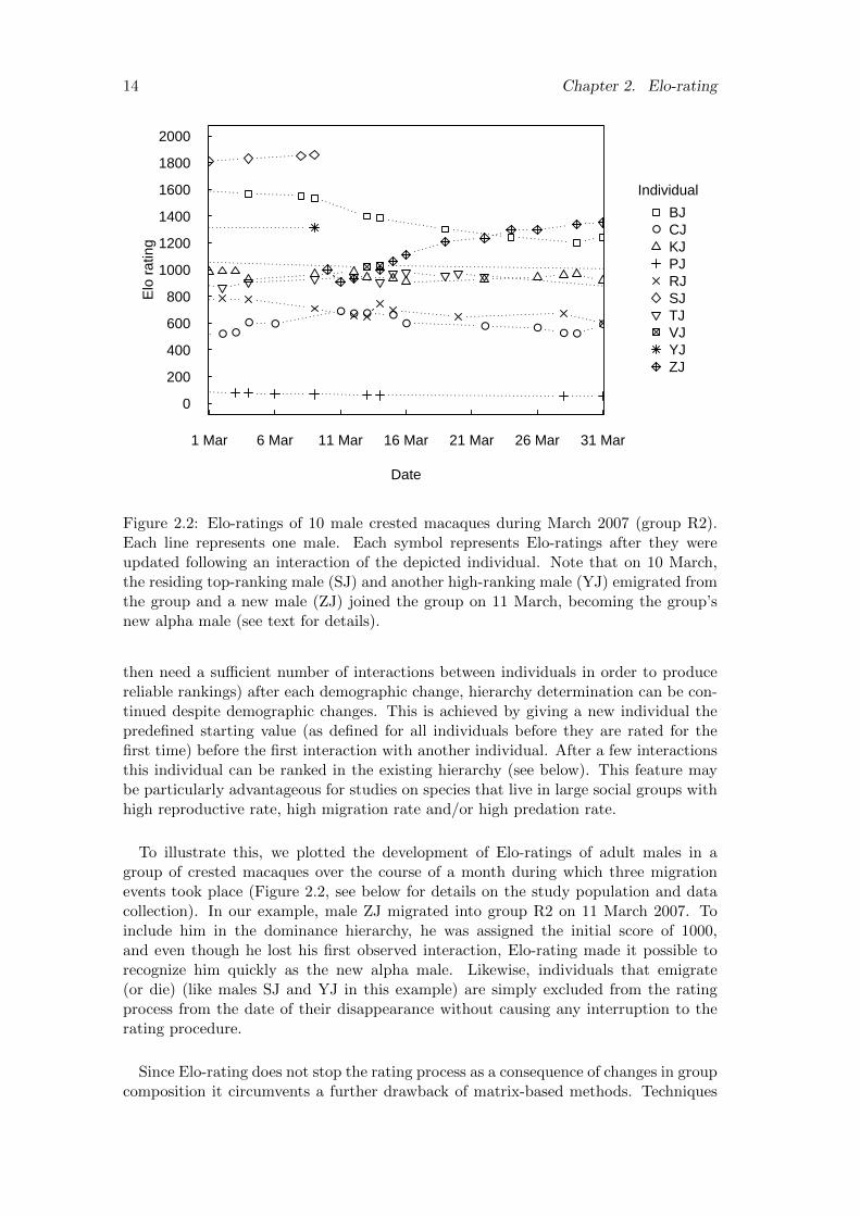
2.2 Elo-ratings of 10 male crested macaques during March 2007 (group R2).Each line represents one male. Each symbol represents Elo-ratings afterthey were updated following an interaction of the depicted individual.Note that on 10 March, the residing top-ranking male (SJ) and anotherhigh-ranking male (YJ) emigrated from the group and a new male (ZJ)joined the group on 11 March, becoming the group’s new alpha male(see text for details). . . . . . . . . . . . . . . . . . . . . . . . . . . . . . 14
2.3 Elo-ratings of 11 male crested macaques between June and August 2007(group R2). Note that the timescale differs from Figure 2.2 and for allmales except KJ, symbols represent every fifth interaction (see text fordetails). . . . . . . . . . . . . . . . . . . . . . . . . . . . . . . . . . . . . 16
2.4 The development of dominance status of 16 natal male crested macaquesduring the 6 months before their emigration. Whereas using David’sscore only suggests an increase in status over time (a), Elo-rating in-dicates a clear linear increase (b). Elo-rating in addition allows a re-finement of the time resolution, thereby suggesting a noticeable surge inratings about 3 months before emigration (c, see text for details) . . . . 18
iii

iv List of Figures
2.5 Correlation between the increase in unknown relationships and the per-formance of (a) Elo-rating, (b) David’s score and (c) I&SI. The increasein unknown relationships was induced by randomly removing 50% ofdata points and performance is expressed as the correlation coefficientbetween rankings from the full and reduced data sets. Elo-ratings andI&SI ranks are not influenced by higher percentages of unknown relation-ships, whereas the performance of David’s score decreases when unknownrelationships increase. . . . . . . . . . . . . . . . . . . . . . . . . . . . . 26
5.1 Pure coalitions lead to higher future Elo-ratings than mixed coalitions.Open circles depict parameter estimates with associated standard er-rors. Note that these parameter estimates reflect the difference betweenmixed and pure coalitions at the reference levels of the remaining cate-gorical factors in the model (role = participant, age = middle) and atthe numerical predictor variables being at their means, i.e. 0. . . . . . . 66
5.2 Effects of the interaction between role and coalition configuration on fu-ture Elo-rating. (a) middle-aged males, (b) young males, and (c) oldmales. Circles depict parameter estimates with associated standard er-rors. Parameter estimates above the horizontal line indicate a rise inElo-ratings while those below indicate a drop. Note that the panels areseparated by age because age is the only remaining categorical predictorin the model. All other numerical predictor variables are at their means(i.e. zero). . . . . . . . . . . . . . . . . . . . . . . . . . . . . . . . . . . . 68
5.3 Effects of feasibility on future Elo-ratings for participants and targetsof coalitions. Note that the plot reflects again the effects of the testvariable (here: interaction between feasibility and role) at the referencelevels of the remaining categorical factors and the means of the numericalvariables (see text). . . . . . . . . . . . . . . . . . . . . . . . . . . . . . . 69
5.4 The time course over which coalitions influence future Elo-ratings ofmales. Note that the plot reflects again the effects of the test variable(here: interaction between feasibility and role) at the reference levels ofthe remaining categorical factors and the means of the numerical vari-ables (see text). . . . . . . . . . . . . . . . . . . . . . . . . . . . . . . . . 70
D.1 Data layout necessary for the R functions to work. . . . . . . . . . . . . 99
D.2 Elo-ratings over time from seven individuals. . . . . . . . . . . . . . . . 102
D.3 Elo-ratings over time from three individuals during a subset of the ob-servation time. . . . . . . . . . . . . . . . . . . . . . . . . . . . . . . . . 103
F.1 (a) and (b) depict the relationships between current and past Elo-ratingdifference and Connectedness score. (c) and (d) show the relation-ships between Connectedness score and current Elo-rating and futureElo-rating difference. . . . . . . . . . . . . . . . . . . . . . . . . . . . . . 115
F.2 (a) and (b) depict the relationships between current and past Elo-ratingdifference and Sociability score. (c) and (d) show the relationshipsbetween Sociability score and current Elo-rating and future Elo-ratingdifference. . . . . . . . . . . . . . . . . . . . . . . . . . . . . . . . . . . . 116

List of Figures v
F.3 (a) and (b) depict the relationships between current and past Elo-ratingdifference and Aggressiveness score. (c) and (d) show the relation-ships between Aggressiveness score and current Elo-rating and futureElo-rating difference. . . . . . . . . . . . . . . . . . . . . . . . . . . . . . 117
F.4 (a) and (b) depict the relationships between current and past Elo-ratingdifference and Anxiety score. (c) and (d) show the relationships be-tween Anxiety score and current Elo-rating and future Elo-rating differ-ence. . . . . . . . . . . . . . . . . . . . . . . . . . . . . . . . . . . . . . . 118
F.5 (a) and (b) depict the relationships between current and past Elo-ratingdifference and Boldness score. (c) and (d) show the relationships be-tween Boldness score and current Elo-rating and future Elo-rating dif-ference. . . . . . . . . . . . . . . . . . . . . . . . . . . . . . . . . . . . . 119

vi List of Figures

List of Tables
2.1 General description of the time periods and dominance matrices used inthe analysis. . . . . . . . . . . . . . . . . . . . . . . . . . . . . . . . . . . 23
2.2 Robustness analysis. Correlation coefficients (rs) between rankings fromfull and reduced data sets. (Median and inter-quartile range). . . . . . . 25
3.1 Definitions of 22 behavioral variables. . . . . . . . . . . . . . . . . . . . 34
3.2 Repeatabilities and confidence intervals of behavioral variables. Vari-ables for which the confidence interval included zero (bold) were excludedfrom the subsequent factor analysis. . . . . . . . . . . . . . . . . . . . . 38
3.3 Loadings of the four extracted personality factors after oblimin rotation.Only loadings with absolute values ≥ 0.40 and communalities (h2) arereported. Values in brackets were not interpreted as belonging to thisfactor as they loaded higher on a different factor. . . . . . . . . . . . . . 39
3.4 Pearson correlation coefficients between personality factors and the re-sponses to the donkey playback. . . . . . . . . . . . . . . . . . . . . . . . 40
3.5 Summary of personality factors for crested macaque males. Descriptionsrefer to animals scoring high on the respective factor. . . . . . . . . . . . 41
4.1 Effect of current Elo-rating and past rating differences on five personalitytraits. Response variables are the single personality traits. . . . . . . . . 51
4.2 Effect of five personality traits on differences between current and futureElo-ratings. . . . . . . . . . . . . . . . . . . . . . . . . . . . . . . . . . . 52
5.1 Results of the LMM testing for the effects of coalition composition onfuture Elo-ratings. For categorical predictor variables, the factor levelsnot included in the intercept are given in parentheses. Two predictors(configuration and feasibility) included in model 2 (see Table 5.2) areomitted here because they could not be measured for mixed coalitions. . 66
5.2 Results of the LMM testing for the effects of configuration, feasibility,role in a coalition and the time distance that passed from the originalevent on future Elo-ratings. For categorical predictor variables, the fac-tor levels not included in the intercept are given in parentheses. . . . . . 67
E.1 Example data to calculate Elo-ratings . . . . . . . . . . . . . . . . . . . 106
F.1 Connectedness as a function of current status and past status differ-ence. Likelihood ratio test: autocorrelation, χ2 = 2.06, df = 1, p =0.1511. Likelihood ratio test: full model vs null model, χ2 = 13.24, df =2, p = 0.0013. . . . . . . . . . . . . . . . . . . . . . . . . . . . . . . . . . 110
vii
viii List of Tables
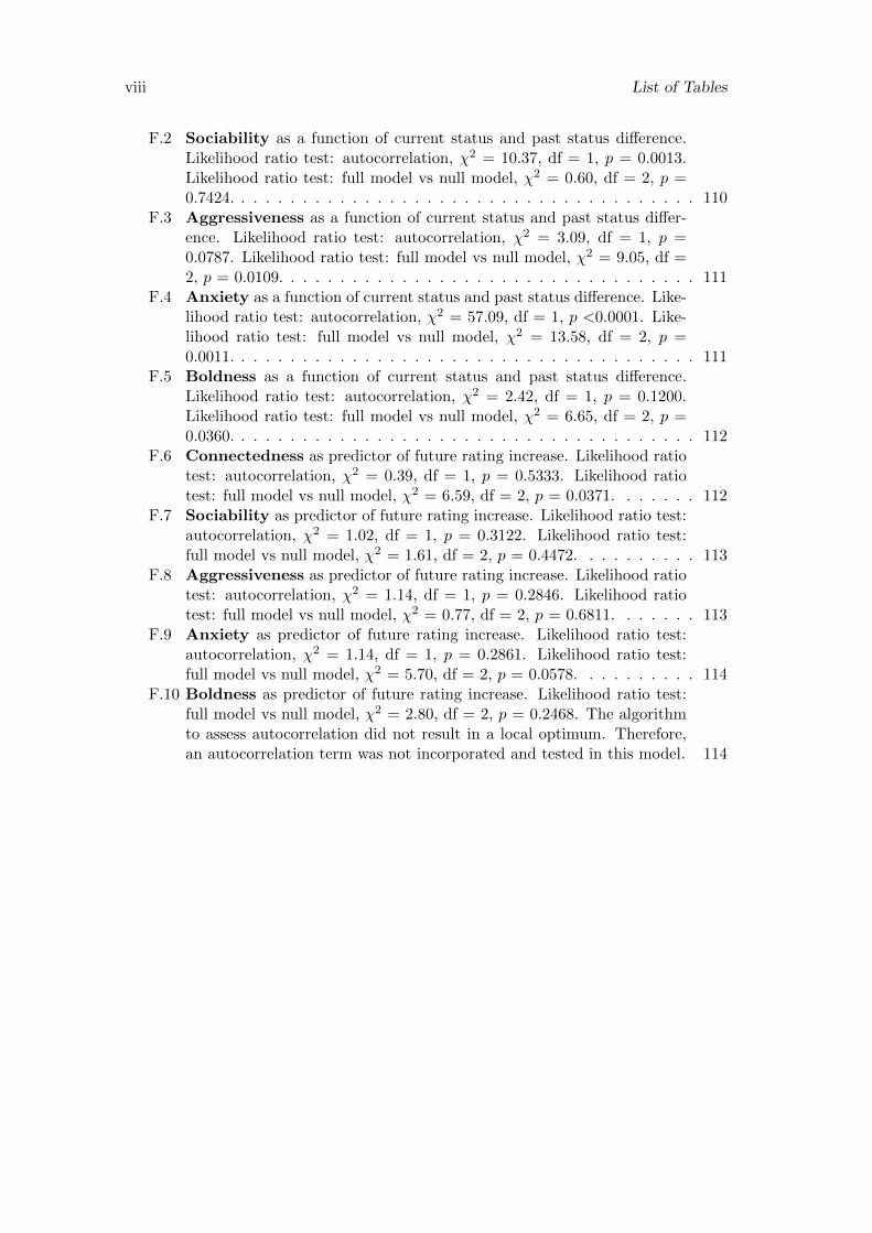
F.2 Sociability as a function of current status and past status difference.Likelihood ratio test: autocorrelation, χ2 = 10.37, df = 1, p = 0.0013.Likelihood ratio test: full model vs null model, χ2 = 0.60, df = 2, p =0.7424. . . . . . . . . . . . . . . . . . . . . . . . . . . . . . . . . . . . . . 110
F.3 Aggressiveness as a function of current status and past status differ-ence. Likelihood ratio test: autocorrelation, χ2 = 3.09, df = 1, p =0.0787. Likelihood ratio test: full model vs null model, χ2 = 9.05, df =2, p = 0.0109. . . . . . . . . . . . . . . . . . . . . . . . . . . . . . . . . . 111
F.4 Anxiety as a function of current status and past status difference. Like-lihood ratio test: autocorrelation, χ2 = 57.09, df = 1, p <0.0001. Like-lihood ratio test: full model vs null model, χ2 = 13.58, df = 2, p =0.0011. . . . . . . . . . . . . . . . . . . . . . . . . . . . . . . . . . . . . . 111
F.5 Boldness as a function of current status and past status difference.Likelihood ratio test: autocorrelation, χ2 = 2.42, df = 1, p = 0.1200.Likelihood ratio test: full model vs null model, χ2 = 6.65, df = 2, p =0.0360. . . . . . . . . . . . . . . . . . . . . . . . . . . . . . . . . . . . . . 112
F.6 Connectedness as predictor of future rating increase. Likelihood ratiotest: autocorrelation, χ2 = 0.39, df = 1, p = 0.5333. Likelihood ratiotest: full model vs null model, χ2 = 6.59, df = 2, p = 0.0371. . . . . . . 112
F.7 Sociability as predictor of future rating increase. Likelihood ratio test:autocorrelation, χ2 = 1.02, df = 1, p = 0.3122. Likelihood ratio test:full model vs null model, χ2 = 1.61, df = 2, p = 0.4472. . . . . . . . . . 113
F.8 Aggressiveness as predictor of future rating increase. Likelihood ratiotest: autocorrelation, χ2 = 1.14, df = 1, p = 0.2846. Likelihood ratiotest: full model vs null model, χ2 = 0.77, df = 2, p = 0.6811. . . . . . . 113
F.9 Anxiety as predictor of future rating increase. Likelihood ratio test:autocorrelation, χ2 = 1.14, df = 1, p = 0.2861. Likelihood ratio test:full model vs null model, χ2 = 5.70, df = 2, p = 0.0578. . . . . . . . . . 114
F.10 Boldness as predictor of future rating increase. Likelihood ratio test:full model vs null model, χ2 = 2.80, df = 2, p = 0.2468. The algorithmto assess autocorrelation did not result in a local optimum. Therefore,an autocorrelation term was not incorporated and tested in this model. 114

Summary
Competition for access to females is the major principle governing the differentialreproductive success observed among males in most animal species. Dominance hi-erarchies arise from differences in competitive abilities between individual males andoften translate into reproductive benefits for high-ranking males (i.e. rank-based re-productive skew). Frequently, dominance hierarchies correspond to relatively simplevariables that describe general physical abilities of individuals, such as body size ordevelopment of weaponry. In many species, however, the determinants of dominancestatus are more complex than that, and represent interactions between a variety ofindividual attributes, which collectively determine the ability to become dominant.Primates represent an interesting taxon to study this phenomenon because they livein complex social systems and further display elaborate cognitive abilities. Thus, themakeup of traits that determine which individuals will achieve high status is expectedto be particularly complex in primates.
For several reasons, crested macaques (Macaca nigra) are a well suited taxon to studythe mechanisms that underlie differential dominance achievement and maintenancebetween individual males. First, high dominance rank is associated with high matingand reproductive success, highlighting the importance of becoming as high-ranking aspossible with regard to fitness. Second, male dominance hierarchies in crested macaquescan be described as very dynamic in both, the level of males commonly migrating inand out of groups, and rank changes within the group that frequently occur outsidethe context of migration.
The overall aim of this thesis was therefore to investigate mechanisms underlyingindividual dominance rank trajectories in male crested macaques and to highlight pos-sible, individual and social, determinants of how males can achieve and maintain thehighest rank possible. In study 1, I address the problem of how dominance hierarchiescan be reliably estimated even when conditions such as frequent migration events andchanges within the hierarchy make the application of traditional approaches difficult,if not impossible. Studies 2 and 3 describe how male personality as an example of anintrinsic property can contribute to rank trajectories. Finally, in study 4, I investigatehow coalitions, as an example for influences of the social environment, impact rankdynamics.
The data for this study were collected between 2009 and 2011 in the Tangkoko-Batuangus Nature Reserve in the north of Sulawesi, Indonesia. Study subjects werethe 37 adult males residing in two social groups during this time. During focal animalsampling on these males, continuous data were recorded on social, aggressive and self-directed behaviour. In addition, the identities of adult individuals in spatial proximity
ix

x Summary
were noted at regular intervals, as well as the focal animals’ position with respect tothe core of the social group. In total, more than 2,000 hours of focal animal data werecollected (mean = 66.1h, range = 0.6 – 130.0h per male, total = 2447.2h). Finally,two playback experiments were conducted to supplement the observational study ofpersonality. With the presentation of dog bark bouts, I tested whether males differ inboldness, while neophilia was measured as the response to donkey brays. Statisticalmethods employed during data analysis include non-parametric tests, factor analysisand linear mixed models.
In study 1, I validate Elo-rating as a useful method to quantify dominance hierar-chies. Elo-rating is rooted in the rating of competitive chess players and has a rangeof hitherto overlooked advantages over more commonly used methods of measuringdominance hierarchies in animals. These advantages are particularly important withrespect to obtaining dominance measures in the context of overly dynamic relationsbetween individuals. The applicability of standard ranking algorithms is limited tosituations in which group composition is relatively stable and in which the majority ofrelationships between any pair of individuals are known. Elo-rating, in contrast, usesa relatively simple algorithm, during which an individual’s Elo-rating is updated aftereach single interaction this individual was involved in. The underlying principle of howratings change reflects the expected as compared to the observed outcome of singledominance interactions. In this way, Elo-rating allows the estimation of dominancestatus on a very fine-grained time scale, without the need to aggregate dominance dataover substantial periods of time. In addition, Elo-rating results in dominance hierar-chies that closely match those derived from commonly used methods – given the dataallow the application of these methods. Elo-rating therefore provides the necessary toolfor reliable assessment of dominance status in dynamic systems, such as male crestedmacaque hierarchies. Furthermore, it allows to address conveniently questions relatedto individual rank trajectories.
In study 2, I suggest a personality structure for crested macaque males that con-sists of five personality factors: connectedness, sociability, anxiety, aggressiveness, andboldness. Connected males spent their time with a high diversity of female and malegroup members in spatial proximity. Sociable males spent more time grooming andhad more diverse grooming partners. Anxious males were inactive, approached femalesrarely and showed high frequencies of self-directed behaviors. Aggressive males exhib-ited high rates of aggressive and threat behaviors towards other group members, withthe notable exception of other adult males. Finally, bold males showed consistentlystronger responses to the playback of dogs. The general makeup of crested macaquepersonality resembles to a high degree that of other macaque species. Yet, a notabledifference to other macaques is the presence of connectedness, which covers aspects ofsocial network diversity. These results not only contribute to our understanding of theevolution of personality structure in primates, they further set the grounds to investi-gate the possible adaptive value of differential expression of specific personality factorswith regards to dominance rank – the topic of the subsequent study.
In study 3, I tested the relationships between the five personality factors determinedin study 2 and dominance rank as determined with Elo-ratings. For this, I divided thestudy period into two-month blocks (necessary to obtain repeated personality scoresfor each male), for which I gathered corresponding current rank (Elo-rating), past rank
xi
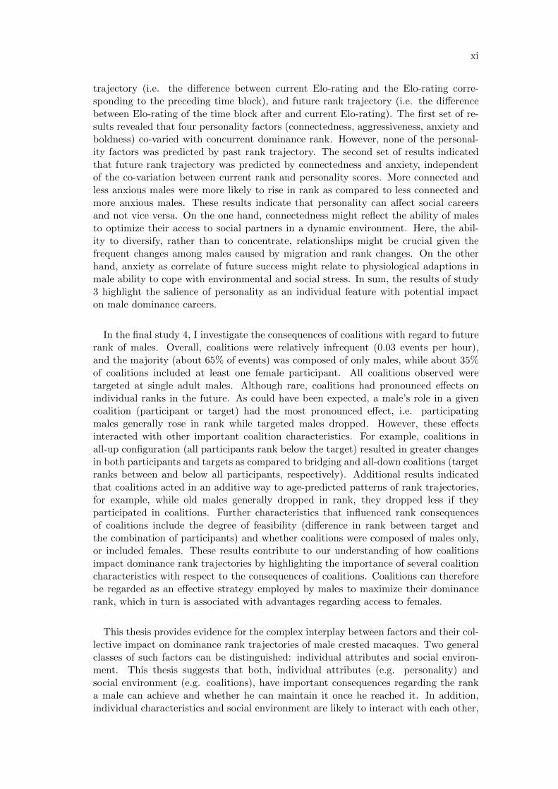
trajectory (i.e. the difference between current Elo-rating and the Elo-rating corre-sponding to the preceding time block), and future rank trajectory (i.e. the differencebetween Elo-rating of the time block after and current Elo-rating). The first set of re-sults revealed that four personality factors (connectedness, aggressiveness, anxiety andboldness) co-varied with concurrent dominance rank. However, none of the personal-ity factors was predicted by past rank trajectory. The second set of results indicatedthat future rank trajectory was predicted by connectedness and anxiety, independentof the co-variation between current rank and personality scores. More connected andless anxious males were more likely to rise in rank as compared to less connected andmore anxious males. These results indicate that personality can affect social careersand not vice versa. On the one hand, connectedness might reflect the ability of malesto optimize their access to social partners in a dynamic environment. Here, the abil-ity to diversify, rather than to concentrate, relationships might be crucial given thefrequent changes among males caused by migration and rank changes. On the otherhand, anxiety as correlate of future success might relate to physiological adaptions inmale ability to cope with environmental and social stress. In sum, the results of study3 highlight the salience of personality as an individual feature with potential impacton male dominance careers.
In the final study 4, I investigate the consequences of coalitions with regard to futurerank of males. Overall, coalitions were relatively infrequent (0.03 events per hour),and the majority (about 65% of events) was composed of only males, while about 35%of coalitions included at least one female participant. All coalitions observed weretargeted at single adult males. Although rare, coalitions had pronounced effects onindividual ranks in the future. As could have been expected, a male’s role in a givencoalition (participant or target) had the most pronounced effect, i.e. participatingmales generally rose in rank while targeted males dropped. However, these effectsinteracted with other important coalition characteristics. For example, coalitions inall-up configuration (all participants rank below the target) resulted in greater changesin both participants and targets as compared to bridging and all-down coalitions (targetranks between and below all participants, respectively). Additional results indicatedthat coalitions acted in an additive way to age-predicted patterns of rank trajectories,for example, while old males generally dropped in rank, they dropped less if theyparticipated in coalitions. Further characteristics that influenced rank consequencesof coalitions include the degree of feasibility (difference in rank between target andthe combination of participants) and whether coalitions were composed of males only,or included females. These results contribute to our understanding of how coalitionsimpact dominance rank trajectories by highlighting the importance of several coalitioncharacteristics with respect to the consequences of coalitions. Coalitions can thereforebe regarded as an effective strategy employed by males to maximize their dominancerank, which in turn is associated with advantages regarding access to females.
This thesis provides evidence for the complex interplay between factors and their col-lective impact on dominance rank trajectories of male crested macaques. Two generalclasses of such factors can be distinguished: individual attributes and social environ-ment. This thesis suggests that both, individual attributes (e.g. personality) andsocial environment (e.g. coalitions), have important consequences regarding the ranka male can achieve and whether he can maintain it once he reached it. In addition,individual characteristics and social environment are likely to interact with each other,

xii Summary
for example by personalities that facilitate the formation of bonds and/or coalitions.Ultimately, if we want to understand what determines rank-based reproductive skew,we need to consider the complexity of mechanisms that govern rank trajectories thatindividual males will follow and we further have to take into account the likely diversityand cross-species differences of these mechanisms.

Zusammenfassung
Der Wettkampf um Zugang zu Weibchen ist eines der wichtigsten Prinzipien umdie Variation im individuellen Reproduktionserfolg von Mannchen in vielen Tier-arten zu erklaren. Durch inter-individuelle Unterschiede in kompetitiven Fahigkeitenzwischen Individuen entstehen Dominanzhierarchien, in denen hochrangige Mannchenoft Vorteile im Hinblick auf Reproduktion haben (rang-basierter reproductive skew).Haufig korrespondieren solche Hierarchien mit relativ einfachen individuellen Merk-malen, welche die allgemeine physische Erscheinung beschreiben, wie beispielsweiseKorpergroße oder die Ausbildung von Waffen. Allerdings sind die Determinanten vonDominanzstatus oft komplexer und konnen als Interaktionen zwischen verschiedenenindividuellen und sozialen Merkmalen betrachtet werden, die in ihrer Gesamtheit dieFahigkeit eines Individuums beschreiben dominant zu werden. Primaten stellen eingeeignetes Taxon dar um dieses Phanomen zu untersuchen, da sie in komplexen Sozial-systemen leben und ihre kognitiven Fahigkeiten den Einfluss von sozialen Komponen-ten auf Dominanzstatus wahrscheinlich machen. Es kann daher erwartet werden, dassdie Zusammensetzung der Merkmale, die in ihrere Kombination bestimmen welchesMannchen einen hohen Rang erreicht, in Primaten außerst komplex ist.
Zwei Grunde machen Schopfmakaken (Macaca nigra) zu einer sehr geeigneten Artdie Mechanismen zu untersuchen, die dem zwischen individuellen Mannchen vari-ierenden Erreichen und Erhalten von Dominanz zugrunde liegen. Zum einen ist ho-her Dominanzrang mit hohem Paarungs- und Fortpflanzungserfolg assoziiert, was dieWichtigkeit, so hochrangig wie moglich zu werden, in Hinblick auf Fitnessvorteile un-terstreicht. Zum anderen sind die Dominanzhierarchien mannlicher Schopfmakakenaußerst dynamisch; sowohl mit Blick auf immigrierende und emigrierende Mannchen,als auch durch regelmaßige Rangwechsel wahrend stabiler Gruppenzusammensetzung.
Ziel dieser Arbeit war daher, jene Mechanismen zu untersuchen, die individuellenRangdynamiken mannlicher Schopfmakaken zugrunde liegen und dabei mogliche indi-viduelle und soziale Determinanten zu identifizieren, die Erreichen und Erhalten deshochstmoglichen Ranges der Mannchen bestimmen. In Studie 1 untersuche ich dieProblematik der zuverlassigen Quantifizierung von Dominanzhierarchien im Angesichthaufiger Migration und Rangwechsel, welche die Anwendung herkommlicher Methodenerschweren. In Studien 2 und 3 beschreibe ich, als Beispiel fur individuelle Merkmale,wie die Personlichkeit von Mannchen Rangdynamiken beeinflussen kann. In der ab-schließenden Studie 4 untersuche ich Koalitionen, als Beispiel fur soziale Faktoren, aufihre Auswirkungen auf Dominanzrang.
Fur diese Studie wurden zwischen 2009 und 2011 im Tangkoko-Batuangus Natur-reservat in Nordsulawesi, Indonesien, Daten von jenen 37 Mannchen gesammelt, die
xiii

xiv Zusammenfassung
wahrend dieser Zeit in zwei sozialen Gruppen lebten. Mittels Fokustierbeobachtungenwurden kontinuierliche Daten uber soziales, aggressives und selbst-gerichtetes Verhal-ten aufgenommen. Zusatzlich wurde regelmaßig notiert welche anderen adulten Tieresich in der Nahe des Fokustieres aufhielten, und wo sich das Fokustier in Relation zumraumlichen Kern der Gruppe befand. Auf diese Weise wurden mehr als 2.000 Stun-den Fokustierdaten aufgenommen (Mittelwert pro Mannchen = 66,1h, min = 0,6h,max = 130,0h, total = 2.447,2h). Um die Personlichkeitsstudie zu erganzen, wurdenzudem zwei Vorspielexperimente durchgefuhrt. Mittels Hundegebell wurde getestet,inwiefern Mannchen unterschiedlich mutig sind, und der Schrei eines Esels diente demTest ob Schopfmakaken einen Personlichkeitsfaktor Neugierde besitzen. Die wichtig-sten statistischen Methoden die in dieser Arbeit angewendet wurden, umfassen nicht-parametrische Tests, Faktoranalyse und gemischte Regressionsmodelle.
In Studie 1 validiere ich Elo-rating als zuverlassige Methode um Dominanzhierar-chien zu bestimmen. Elo-rating hat seine Wurzeln in der Bewertung von Schachspielernund besitzt eine Reihe von Vorteilen gegenuber herkommlichen Methoden, die einge-setzt werden um Dominanzhierarchien zu messen. Diese Vorteile kommen vor allemdann zum Tragen wenn das System, fur das eine Dominanzhierarchie bestimmt wer-den soll, sehr dynamisch ist. Traditionell verwendete Methoden setzen voraus, dass dieBeziehungen zwischen den meisten Paaren von Tieren bekannt sein mussen und dass dieGruppenzusammensetzung stabil ist. Im Gegensatz dazu verwendet Elo-rating einenrelativ simplen Algorithmus, in dem nach jeder einzelnen Interaktion, in die ein Tierverwickelt war, die Elo-rating Punktzahl der involvierten Tiere neu berechnet wird. DasPrinzip, nach dem eine Anderung in der individuellen Punktzahl berechnet wird, basiertauf dem Vergleich von zu erwartendem und tatsachlichem Ausgang der jeweiligen In-teraktion. Dies erlaubt die Bestimmung von Dominanz mit sehr feiner Zeitauflosung.Daruber hinaus stimmen mit Elo-rating berechnete Hierarchien sehr gut uberein mitden Ergebnissen von herkommlichen Algorithmen – sofern die Bedingungen fur derenAnwendungen gegeben sind. Elo-rating kann daher als das notwendige Werkzeug di-enen um in dynamischen Systemen, wie den Hierarchien mannlicher Schopfmakaken,Dominanz verlasslich zu quantifizieren.
In Studie 2 schlage ich eine Personlichkeitsstruktur fur Schopfmakaken vor, die aus 5Faktoren besteht: Vernetztheit, Sozialitat, Angstlichkeit, Aggressivitat und Mut. Ver-netzte Mannchen besaßen ein diverses Netzwerk von anderen Mannchen und Weibchenin deren Nahe sie sich aufhielten. Soziale Mannchen verbrachten mehr Zeit mit sozialerFellpflege und besaßen ein diverses Netzwerk von Partnern fur diese. AngstlicheMannchen waren inaktiv, naherten sich selten Weibchen an und verbrachten viel Zeitmit selbst-gerichtetem Verhalten. Aggressive Mannchen zeigten anderen Gruppenmit-gliedern gegenuber haufig aggressives Verhalten, mit der Ausnahme anderer adulterMannchen. Mutige Mannchen zeigten gegenuber dem Vorspielexperiment konsistentstarkere Reaktionen. Damit entspricht die Personlichkeitsstruktur von Schopfmakakenim Allgemeinen der anderer Arten der Gattung, mit der Ausnahme des Faktors Vernet-ztheit. Die Ergebnisse dieser Studie tragen nicht nur zum Verstandnis der Evolutionvon Personlichkeitsstrukturen innerhalb der Primaten bei, sondern sind daruber hinausauch die notwendige Grundlage fur Studien zum adaptiven Wert von Personlichkeit beiSchopfmakaken – dem Thema der folgenden Studie.

xv
Der Zusammenhang zwischen Personlichkeitsfaktoren und Dominanzrang ist Inhaltvon Studie 3. Um wiederholte Messwerte innerhalb eines Mannchens fur die funf inStudie 2 beschriebenen Personlichkeitsfaktoren zu erhalten, unterteilte ich die Gesamt-studienzeit in Blocke zu je zwei Monaten. Fur jeden dieser Blocke und fur jedesanwesende Mannchen wurden ebenfalls (1) der gegenwartige Rang (Elo-rating Punk-tzahl innerhalb des Blocks), (2) die vergangene Rangentwicklung (Differenz zwischengegenwartiger Elo-rating Punktzahl und der Punktzahl im vorausgehenden Block), und(3) die zukunftige Rangentwicklung (Differenz zwischen der Punktzahl im nachfolgen-den Block und gegenwartiger Punktzahl) berechnet. Ein erstes Ergebnisset zeigte,dass vier Personlichkeitsfaktoren mit gegenwartigem Dominanzrang kovariierten: Ver-netztheit, Aggressivitat, Angstlichkeit und Mut. Im Gegensatz dazu gab es keinenZusammenhang zwischen vergangener Rangentwicklung und Personlichkeitsfaktoren.Im zweiten Ergebnisset konnte gezeigt werden, dass Vernetztheit und Angstlichkeitdie zukunftige Rangentwicklung voraussagen – unabhangig von der eben genan-nten Kovarianz zwischen Personlichkeit und gegenwartigem Rang. Vernetztere undweniger angstliche Mannchen stiegen eher im Rang, verglichen mit weniger vernetztenund angstlicheren Mannchen. Diese Ergebnisse zeigen, dass es wahrscheinlicher ist,dass Personlichkeit Rangentwicklung beeinflusst, und nicht umgekehrt, namlich dassPersonlichkeit von Rangentwicklung abhangt. Die Vorteile von Vernetztheit konntenmit der Fahigkeit im Zusammenhang stehen, den Zugang zu sozialen Partnern in einerdynamischen Umgebung zu optimieren. Angstlichkeit konnte eine physiologische An-passung im Umgang mit (sozialem) Stress widerspiegeln. Insgesamt unterstreichen dieErgebnisse dieser Studie die potentielle Wichtigkeit, die Personlichkeit, als individuellesAttribut, auf Rangentwicklung haben kann.
In der abschließenden Studie 4 untersuchte ich die Konsequenzen von Koalitionenauf Rangentwicklung. Insgesamt waren Koalitionen relativ seltene Ereignisse (0.03Ereignisse pro Stunde), wobei die Mehrheit der beobachteten Koalitionen nur ausMannchen bestand (etwa 65% aller Ereignisse), wahrend an 35% aller Koalitionen min-destens ein Weibchen beteiligt war. Alle Koalitionen waren gegen einzelne Mannchengerichtet. Trotz ihrer Seltenheit hatten Koalitionen deutliche Konsequenzen fur denDominanzrang. Allem Voran hatte die Rolle, die ein Mannchen in einer Koalition hatte,den großten Einfluss auf zukunftigen Rang, d.h. Teilnehmer profitierten von Koalitio-nen wahrend Opfer im Rang sanken. Der Einfluss von Rolle interagierte jedoch mit einerReihe weiterer Charakteristika von Koalitionen. Beispielsweise waren Ranganderun-gen am starksten ausgepragt nach revolutionaren Koalitionen (alle Teilnehmer sindniedriger im Rang als das Opfer), verglichen mit konservativen und uberbruckendenKoalitionen (Opfer ist im Rang unter, beziehungsweise zwischen den Teilnehmern).Weitere Ergebnisse zeigten, dass Koalitionen einen additiven Effekt auf altersbed-ingte Ranganderungen hatten. Beispielsweise sanken alte Mannchen im Allgemeinenim Rang, allerdings weniger, nachdem sie Teilnehmer einer Koalition waren. WeitereEigenschaften von Koalitionen mit Rangeinfluss beinhalten die
”Machbarkeit“ (feasi-
bility, der Unterschied zwischen Rang des Opfers und der Summe der Range aller Teil-nehmer) und die Geschlechterzusammensetzung der Koalitionen. Diese Ergebnisse tra-gen zu unserem Verstandnis bei wie Koalitionen Rangentwicklung beeinflussen konnen,indem sie aufzeigen, dass eine Reihe von Koalitionsparametern in ihrem Einfluss aufRangentwicklung interagieren. Insgesamt konnen Koalitionen als effektive Strategiebetrachtet werden, die von Mannchen verfolgt wird um ihren Dominanzrang zu op-timieren, was wiederum mit Vorteilen in Bezug auf Zugang zu Weibchen verbunden
xvi Zusammenfassung
ist.
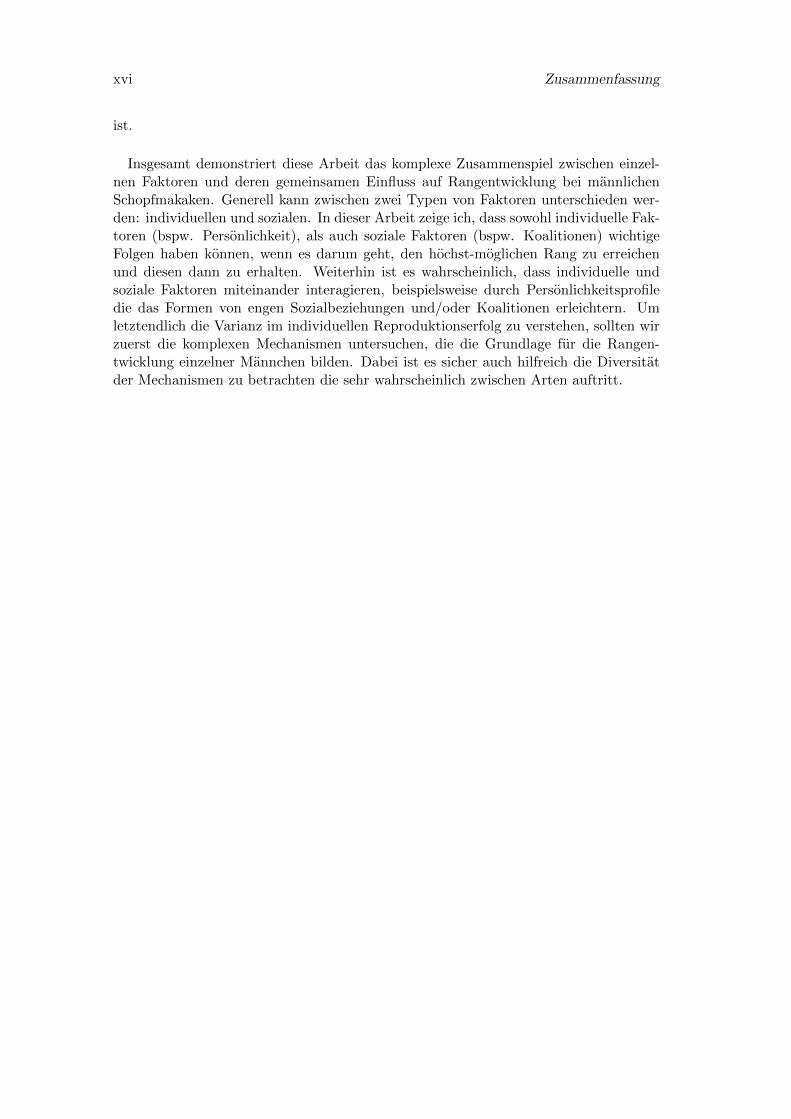
Insgesamt demonstriert diese Arbeit das komplexe Zusammenspiel zwischen einzel-nen Faktoren und deren gemeinsamen Einfluss auf Rangentwicklung bei mannlichenSchopfmakaken. Generell kann zwischen zwei Typen von Faktoren unterschieden wer-den: individuellen und sozialen. In dieser Arbeit zeige ich, dass sowohl individuelle Fak-toren (bspw. Personlichkeit), als auch soziale Faktoren (bspw. Koalitionen) wichtigeFolgen haben konnen, wenn es darum geht, den hochst-moglichen Rang zu erreichenund diesen dann zu erhalten. Weiterhin ist es wahrscheinlich, dass individuelle undsoziale Faktoren miteinander interagieren, beispielsweise durch Personlichkeitsprofiledie das Formen von engen Sozialbeziehungen und/oder Koalitionen erleichtern. Umletztendlich die Varianz im individuellen Reproduktionserfolg zu verstehen, sollten wirzuerst die komplexen Mechanismen untersuchen, die die Grundlage fur die Rangen-twicklung einzelner Mannchen bilden. Dabei ist es sicher auch hilfreich die Diversitatder Mechanismen zu betrachten die sehr wahrscheinlich zwischen Arten auftritt.

Chapter 1
General Introduction
1
2 Chapter 1. General Introduction
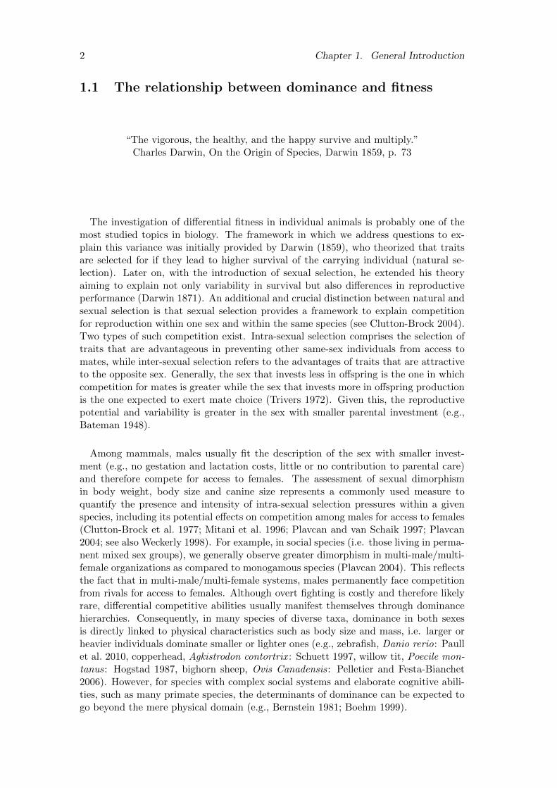
1.1 The relationship between dominance and fitness
“The vigorous, the healthy, and the happy survive and multiply.”Charles Darwin, On the Origin of Species, Darwin 1859, p. 73
The investigation of differential fitness in individual animals is probably one of themost studied topics in biology. The framework in which we address questions to ex-plain this variance was initially provided by Darwin (1859), who theorized that traitsare selected for if they lead to higher survival of the carrying individual (natural se-lection). Later on, with the introduction of sexual selection, he extended his theoryaiming to explain not only variability in survival but also differences in reproductiveperformance (Darwin 1871). An additional and crucial distinction between natural andsexual selection is that sexual selection provides a framework to explain competitionfor reproduction within one sex and within the same species (see Clutton-Brock 2004).Two types of such competition exist. Intra-sexual selection comprises the selection oftraits that are advantageous in preventing other same-sex individuals from access tomates, while inter-sexual selection refers to the advantages of traits that are attractiveto the opposite sex. Generally, the sex that invests less in offspring is the one in whichcompetition for mates is greater while the sex that invests more in offspring productionis the one expected to exert mate choice (Trivers 1972). Given this, the reproductivepotential and variability is greater in the sex with smaller parental investment (e.g.,Bateman 1948).
Among mammals, males usually fit the description of the sex with smaller invest-ment (e.g., no gestation and lactation costs, little or no contribution to parental care)and therefore compete for access to females. The assessment of sexual dimorphismin body weight, body size and canine size represents a commonly used measure toquantify the presence and intensity of intra-sexual selection pressures within a givenspecies, including its potential effects on competition among males for access to females(Clutton-Brock et al. 1977; Mitani et al. 1996; Plavcan and van Schaik 1997; Plavcan2004; see also Weckerly 1998). For example, in social species (i.e. those living in perma-nent mixed sex groups), we generally observe greater dimorphism in multi-male/multi-female organizations as compared to monogamous species (Plavcan 2004). This reflectsthe fact that in multi-male/multi-female systems, males permanently face competitionfrom rivals for access to females. Although overt fighting is costly and therefore likelyrare, differential competitive abilities usually manifest themselves through dominancehierarchies. Consequently, in many species of diverse taxa, dominance in both sexesis directly linked to physical characteristics such as body size and mass, i.e. larger orheavier individuals dominate smaller or lighter ones (e.g., zebrafish, Danio rerio: Paullet al. 2010, copperhead, Agkistrodon contortrix : Schuett 1997, willow tit, Poecile mon-tanus: Hogstad 1987, bighorn sheep, Ovis Canadensis: Pelletier and Festa-Bianchet2006). However, for species with complex social systems and elaborate cognitive abili-ties, such as many primate species, the determinants of dominance can be expected togo beyond the mere physical domain (e.g., Bernstein 1981; Boehm 1999).

1.1. The relationship between dominance and fitness 3
In the light of sexual selection theory, it is not surprising that we observe variancein reproductive performance among males with regards to the ability to exclude rivalsfrom reproducing (e.g., Setchell et al. 2005). Variation between individuals in matingand reproductive success is one of the most studied topics in behavioural biology, withhundreds of studies having been published on primates alone (Dewsbury 1982; Ellis1995; Alberts 2012). One of the major determinants of this observed variance is indi-vidual dominance rank (see below for the definition of dominance). One major modelto explain the link between dominance rank and variance in mating success (skew) isthe priority of access model (PoA, Altmann 1962; Alberts et al. 2003). This PoA modelposits that if there is exactly one fertile female present, an alpha male will be able tomonopolize mating with her by preventing all other males present from mating andtherefore secure paternity of that female’s offspring. Obviously, the ability of a maleto monopolize matings with fertile females is constrained by the number of femalesbeing fertile at the same time. Accordingly, if there are two fertile females present, thebeta male will be able to secure access to this second female. Summarized, the PoAmodel predicts male mating, and implicitly reproductive success, dependent on maledominance rank and synchrony in fertility of females (i.e. how many females are fertileat the same time). Though the PoA model generally fits well with observed matingdistributions, some considerable amount of variance in the mating distribution usuallyremains unexplained by male dominance rank (e.g., Kutsukake and Nunn 2006; Ostneret al. 2008; Dubuc et al. 2011; see also Gogarten and Koenig 2013).
Nevertheless, the overall consensus is that dominance rank and mating/reproductivesuccess correlate positively with each other in male primates. That being said, thereis substantial evidence that this relationship is quite variable. A number of reviewsidentified overall positive relationships (e.g., Fedigan 1983; Berenstain and Wade 1983;Cowlishaw and Dunbar 1991; Bulger 1993; Ellis 1995; Rodriguez-Llanes et al. 2009;Majolo et al. 2012), though evidence for variation can be found across species, butalso within genus and species, and even within groups of the same species across time(Smith 1994; Altmann and Alberts 2003; Alberts et al. 2003; Alberts 2012).
This led to identifying additional factors, other than male rank and its consequencesof monopolizing access to females, to affect reproductive skew and more generally,reproductive and life-history decisions (e.g., Altmann and Alberts 2003; van Noordwijkand van Schaik 2004). For instance, males might try to circumvent direct competitionwith each other by seeking out sneak copulations that can occur with or without thecooperation of females (e.g., Berard et al. 1994; Crockford et al. 2007). Likewise,females might have preferences for specific mating partners, but this preference doesnot necessarily need to be synonymous with male rank (e.g., Dubuc et al. 2011). Anadditional alternative strategy might be for males to form coalitions. In such cases,two or more males aggressively displace a male from a female that the target of thecoalition is monopolizing (Pandit and van Schaik 2003). Finally, paternities can alsobe determined on a post-copulatory level (e.g., Harcourt et al. 1981; Birkhead andKappeler 2004). Males might face sperm competition if a female mated with morethan one male during her fertile period (regardless of how this came about), so thesperm of the males are competing for the actual fertilization of the female’s egg. At thesame time, females might (also) exhibit choice after copulations with multiple maleshave occurred, i.e. females might have a preference for the sperm of a specific male(cryptic female choice, e.g., Thornhill 1983).

4 Chapter 1. General Introduction
1.2 What is dominance (rank)?
Despite such alternative strategies available to males, dominance is an overall usefulconcept to explain a great portion of the variance in reproductive success among maleprimates. So far though, I used the terms dominance and dominance rank withoutdefining them. As Seyfarth (1981, p. 447) stated, one might consider the attempt tofind a universal definition for dominance “a fairly sterile intellectual exercise”, yet it isimportant to point out that dominance and dominance rank are relational properties(within dyads or groups of individuals) that have no meaning as absolute individualproperties when seen outside the context of interactions with other individuals (Bern-stein 1981; Barrette 1993; Drews 1993). I therefore follow Drews (1993, p. 283) andconsider dominance as “an attribute of the pattern of repeated, agonistic interactionsbetween two individuals, characterized by a consistent outcome in favour of the samedyad member and a default yielding response of its opponent rather than escalation”.An individual is not dominant per se; rather it is dominant over another individualwithin a dyad in which the other individual is subordinate (Bernstein 1981; Drews1993). Dominance rank extends the concept of dyadic dominance into groups of ani-mals, where an individual that is dominant over many others is considered to have ahigh rank, and an individual that is dominant over few or no others is considered tobe low-ranking. The resulting order of individuals in descending rank is then referredto as dominance hierarchy. As with dyadic dominance, dominance rank in a hierarchyis only meaningful as an individual property with respect to the other individuals (andtheir ranks) that are included in the hierarchy.
Given the reproductive benefits of dominance or high dominance rank, the questionarises whether dominance (rank) as defined above and in the sense it is generally usedin behavioural biology can be under (sexual) selection pressure. The simple answeris: no, dominance cannot be selected. As outlined above, dominance is an attributeof a relationship between two individuals and as such is not heritable and thereforenot selectable. This discussion has received a lot of attention (Bernstein 1981 andcomments therein; Barrette 1987, 1993; Drews 1993, see also Dewsbury 1990; Moore1990), and starting with Hinde and Datta’s (1981, see also Hinde 1978) stance ofconsidering dominance as an intervening variable, a general understanding emerged thatnot dominance itself but the ability to become dominant is the trait that can be selected.The idea here being that a variety of individual traits (e.g. body size, personality,experience) interact with each other and result in a theoretically quantifiable propensityto become dominant over another individual whose trait combination amounts to asmaller ability to become dominant (Figure 1.1). This argument is not new and hasalready been hinted at by Kawai (1958), who distinguished between an individual’sbasic rank which is a purely dyadic measure based on the individual differences betweentwo opponents and an individual’s dependent rank in which the dyadic relationshipis influenced by the social situation. It is these individual traits which collectivelydetermine dominance, or rather the ability to dominate, and which should be the focusof trying to understand rank-based reproductive skew. Overall, most of these individualtraits are heritable and can therefore be selected for.

1.3. Determinants of dominance (rank) 5
Figure 1.1: Dominance as intervening variable. Individual traits listed under indepen-dent interact with each other to form the ability to become dominant or subordinategiven the opponent’s expressions of the same traits. Traits that follow from becomingdominant in a given dyad are listed under dependent. Note that the traits listed underdependent are from the perspective of the dominant individual. Redrawn and modifiedfrom Hinde and Datta (1981).
1.3 Determinants of dominance (rank): the interplay be-tween individual traits and social environment
A variety of factors influences the ability of an individual to achieve the highestrank possible (see Figure 1.1 for a non-exhaustive selection of such factors). Perhapsthe most obvious trait that determines which individual will win a fight is weaponry.There is evidence from a wide range of taxa, that individuals with bigger weaponsare more likely to win contests (e.g., dung beetles, Euoniticellus intermedius: Pomfretand Knell 2006; red deer, Cervus elaphus: Clutton-Brock et al. 1979). Similarly, bodysize and weight often determine contest outcome in favour of the larger and/or heavierindividual (e.g., Anolis lizard, Anolis aeneus: Stamps and Krishnan 1994; red deer:Clutton-Brock et al. 1979). What determines the outcome of dyadic contests amongprimates, however, is less clear. For example, to my knowledge, there is no evidencein primates for the often stated assumption that males with larger canines (primates’primary weapons) are more likely to win fights. One reason for this lack of data might bethat experiments, i.e. staged conflicts, are difficult to conduct in primates due to ethicalconcerns (though see, for example, Bissonnette et al. (2009b) for a mild experimentalapproach, and Alexander and Hughes (1971) for a quasi-experiment involving removalof canines).
In contrast, numerous studies on primates looked at the relationship between domi-nance rank as measure of contest outcome and various individual traits. For example,age is a very important predictor of dominance rank in various species. This reflectsthe relationship between general physical prowess and age, i.e. males reach their primephysical condition at some point after becoming adult, after which it declines with age(Setchell and Lee 2004). Age is therefore often considered as an indirect measure ofgeneral male fighting ability (e.g., long-tailed macaques, Macaca fascicularis: van No-

6 Chapter 1. General Introduction
ordwijk and van Schaik 2001; rhesus macaques, Macaca mulatta: Bercovitch et al. 2003;Widdig et al. 2004; mandrill, Mandrillus sphinx : Setchell et al. 2005; yellow baboons,Papio cynocephalus: Alberts et al. 2006; for a counter example: Assamese macaques,Macaca assamensis: Schulke et al. 2010). Complicating the relationship between ageand rank is the observation that sometimes tenure in the group confounds this link. InJapanese (Macaca fuscata) and rhesus macaques, males often attain a very low rankupon immigration into a new group, and rise passively as other male above them inthe hierarchy emigrate or die (Drickamer and Vessey 1973; Hill 1987; Sprague et al.1996; Sprague 1998). It was argued, however, that the relationship between tenure andrank stems from the fact that the populations in which this pattern was observed wereprovisioned and contained very large groups with high number of males (Manson 1998).Whether such tenure-based mechanisms of rank achievement exist in nature remainsto be seen.
Following from this it appears that age as proxy for general physical condition andprowess is a very important determinant of rank for male primates because rank oftenfollows fairly predictable trajectories of a male’s life. The question that follows fromthis is, what determines rank among males of similar age, or in other words, what arethe predictors of residual rank (e.g., Schulke et al. 2010)? This question can only beanswered with analyses that test relationships between individual variables and rank,while controlling for age. A study nicely demonstrating such an approach comes fromchacma baboons (Papio ursinus). Male rank was related to faecal testosterone levels,but after controlling for age this relationship disappeared (Beehner et al. 2006). How-ever, testosterone levels predicted rank changes in the future, and this relationship wasindependent of age, suggesting that testosterone production can be regarded as an indi-vidual trait, that explains some of the remaining variation between age and dominancerank (Beehner et al. 2006). In contrast, many other studies that report simply rela-tionships between individual traits and rank while not controlling for age as the mostlikely confounding variable provide us with little information about the determinantsof male rank (e.g., canine size: Bercovitch 1993; body weight/size: Kitchen et al. 2003;Neumann et al. 2010; personality factors: Konecna et al. 2012).
In addition to the individual properties that I have mentioned so far, the social envi-ronment is likely to play a prominent role in rank achievement and maintenance (Har-court 1989). Already in 1958, Kawai realized that among female Japanese macaquesthe continued support of other individuals is crucial for females to maintain their ranks.The importance of such alliances that preferentially occur among kin has since beenconfirmed for females in many primate species (e.g., Datta 1983; Chapais 1988; re-viewed in Chapais 1992, see also Silk 2007). In contrast, our knowledge about theconsequences of alliances (or coalitions) occurring between male primates is much morelimited. In general, the preferential coalitionary support often occurring between re-lated females is less likely to explain coalition formation among adult males, given thatin many primate species males are the dispersing sex (Pusey and Packer 1987). How-ever, there is some evidence that coalitions between males influence the rank of theparticipants, and therefore serve a similar function as coalitions between females (e.g.,Schulke et al. 2010; Gilby et al. 2013; see Silk (1993) for the absence of such an effect).Models of coalition formation among males support the idea that coalitions can servefunctions related to dominance rank trajectories, though other important functions arealso possible (Noe 1994; Pandit and van Schaik 2003; van Schaik et al. 2004, 2006).

1.4. Dynamics in rank relationships 7
As becomes clear from the arguments above, the determinants of dominance rankin male primates are particularly complex. A variety of individual properties, such asage, and social influences, such as coalitions, are likely to interact in varying magnitudewith regard to their ultimate contribution to a male’s ability to achieve the highest rankpossible and thereby maximizing his reproductive success and fitness.
1.4 Dynamics in rank relationships
Dominance relationships and the resulting hierarchies among females in many, partic-ularly cercopithecine, primate species have been shown to be very stable over extendedperiods of time, due to the matrilineal organization in which females usually attainranks just below their mothers (e.g., Hausfater et al. 1982; Samuels et al. 1987; Datta1989). Rank changes in females therefore mostly occur only as females are born andmature or die. In contrast, hierarchies of male primates are much more dynamic. Notonly do males in cercopithecines usually migrate between groups repeatedly over theirlifetime and upon successful immigration into a new group attain a rank in the exist-ing hierarchy, but rank changes also occur among males within groups (e.g., Samuelset al. 1984; Zhao 1994; van Noordwijk and van Schaik 2001; Kutsukake and Hasegawa2005; Setchell et al. 2006; Beehner et al. 2006; reviewed in van Noordwijk and vanSchaik 2004). Though differences between and within species exist regarding to whatthe degree of stability in a hierarchy is, such dynamics are the prerequisite to studymechanisms of how males achieve and maintain their ranks.
It is here that a general methodological issue arises. A myriad of methods is avail-able to quantify dominance hierarchies (e.g., Boyd and Silk 1983; Martin and Bateson1993; de Vries 1998; Gammell et al. 2003; reviewed in de Vries 1998; Whitehead 2008),yet they all present researchers with substantial challenges when aiming at measuringdynamics in dominance relationships. All commonly used methods rely on dyadic inter-actions as the initial data. The spectrum of interaction types usually considered rangesfrom physical fights, threat-and-leave interactions, displacements (also, make room orsupplant) to signals of submission (e.g., the silent-bared teeth display of many macaquespecies, e.g., de Waal and Luttrell 1985; Preuschoft and van Schaik 2000). Though thelatter is strictly speaking not a dyadic interaction (though the signal is considered tobe directed at another individual), all have in common that the dominance relation-ship between the dyad members can be inferred if a “winner” and a “loser” can beidentified. Here, a problematic issue with regards to dynamics arises because dyadicinteractions are aggregated over time and arranged in a matrix, on which the currentlymost important methods considered by primatologists work. A concern resulting fromthis method is that the obtained dominance ranks will be an aggregate over the ap-plied time period. As such, with these static methods, dynamics (changes in ranks ofindividuals) cannot readily be detected as they might disappear in data noise, and itis up to the investigator as to whether rank changes are recognized as such. A methodthat is able to adequately deal with issues of dynamics in rank relationships is thereforegreatly needed if we want to understand the mechanisms underlying rank dynamics inmore detail.
8 Chapter 1. General Introduction
1.5 Crested macaques as study species
A suitable taxon in which to study the determinants and dynamics of male domi-nance rank ideally meets two expectations. First, high dominance rank translates intohigh fitness, and second, the hierarchy is dynamic enough so that observations of rankchanges are possible. Crested macaques (Macaca nigra) meet both criteria in as muchas male dominance rank is positively correlated to mating success during the periods inwhich females are most likely to conceive (Engelhardt et al. in prep; see also Reed et al.1997) and male reproductive success is skewed towards high-ranking males (Engelhardtet al., unpublished data). At the same time, males frequently migrate and rank changeswithin groups occur on a regular basis (Neumann et al. 2010; Marty and Engelhardt,in prep).
The crested macaque is one of seven species of macaques endemic to the Indone-sian island of Sulawesi (Riley 2010, see also Abegg and Thierry (2002) and Ziegler etal. (2007) for information on phylo-geography and phylogenetic history of macaqueswith special reference to the Sulawesi species). Crested macaques follow the typicalsocial organization found in cercopithecine monkeys, i.e. they live in permanent multi-male/multi-female groups, comprising up to 90 individuals (Thierry 2011; Cords 2012;Duboscq et al. 2013), in which adults of both sexes form linear dominance hierar-chies (e.g., Reed et al. 1997; Duboscq et al. 2013). Most of our knowledge on crestedmacaque behavior comes from studies in captivity (e.g., Hadidian 1980; Bernstein andBaker 1988; Petit et al. 1997; see O’Brien and Kinnaird (1997) and Reed et al. (1997)for the only field-based study on their behaviour and ecology up until recently). In2006, the Macaca-Nigra-Project was initiated in the Tangkoko-Batuangus Nature Re-serve (www.macaca-nigra.org) to study the behavior, ecology and reproductivebiology of crested macaques. Given that there is only one small viable population leftin their natural range (Palacios et al. 2012), fundamental data on their biology arecrucial not only from a purely scientific point of view, but perhaps even more so toensure that appropriate conservation efforts can be undertaken to facilitate the species’survival in the wild.
1.6 Aims of this thesis
The overall aim of this thesis is to investigate mechanisms that underlie individualdominance rank trajectories in male crested macaques and to highlight different pos-sible, individual and social, determinants of how males can achieve and maintain thehighest rank available to them. In Chapter 2, I address the problem of how dom-inance hierarchies can be reliably estimated even when conditions such as frequentmigration events and changes within the hierarchy make the application of traditionalapproaches difficult, if not impossible. Chapter 3 and 4 describe how male personalityas an example of an intrinsic property can contribute to rank trajectories. One par-ticular personality factor is highlighted, given that it bridges an individual propertywith sociality more generally. Finally, in Chapter 5, I investigate how coalitions, as anexample for influences of the social environment, impact rank dynamics.

Chapter 2
Assessing dominance hierarchies:validation and advantages ofprogressive evaluation withElo-rating
with
Julie Duboscq, Constance Dubuc, Andri Ginting, Ade Maulana Irwan,Muhammad Agil, Anja Widdig, Antje Engelhardt
Published in Animal Behaviour 82 (2011): 911-921.
9

10 Chapter 2. Elo-rating
2.1 Abstract
Whereas dominance hierarchies are used in a wide range of behavioural studies, theirassessment with commonly used methods is often impeded by several factors such assparse data sets or dynamics in rank relationships and unit composition. In this studywe validate Elo-rating as a tool to reliably assess dominance hierarchies. In contrastto methods commonly used, Elo-ratings are calculated based on the sequence in whichdominance interactions occur without tabulating these interactions in matrix form. Us-ing data on dominance interactions from five groups of free-ranging crested and rhesusmacaques (Macaca nigra and M. mulatta, respectively), we show that Elo-rating resultsin rankings that are in strong agreement with commonly used methods. We furtherdemonstrate that Elo-rating provides several advantages over matrix-based methodssince it is capable of tracking dynamics in dominance relationships, it is less affected bythe negative effects of sparse data, and it can comfortably deal with changes in groupcomposition. This, in combination with a straight-forward way to visualize dominancerelationships, makes Elo-rating a very promising alternative to methods commonly usedto assess dominance hierarchies, particularly in dynamic animal societies.
2.2 Introduction
Dominance is one of the most important concepts in the study of animal socialbehaviour. Dominance hierarchies in groups arise from dyadic relationships betweendominant and subordinate individuals present in a social group (Drews 1993). Highhierarchical rank or social status is often associated with fitness benefits for individuals(e.g., Cote and Festa-Bianchet 2001; von Holst et al. 2002; Widdig et al. 2004; Engel-hardt et al. 2006), and hierarchies can be found in most animal taxa including insects(e.g., Kolmer and Heinze 2000), birds (e.g., Kurvers et al. 2009) and mammals (e.g.,Keiper and Receveur 1992).
The analysis of dominance has a long-standing history (Schjelderup-Ebbe 1922; Lan-dau 1951), and a great number of methods to assess hierarchies in animal societiesare currently available (reviewed in de Vries 1998; Bayly et al. 2006; Whitehead 2008).Though differing in calculation complexity, all ranking methods presently used in stud-ies of behavioural ecology are based on interaction matrices. For this, a specific typeof behaviour or interaction, from which the dominance/subordinance relationship of agiven dyad can be deduced, is tabulated across all individuals (see for example, Ver-vaecke et al. 2007). This matrix can either be reorganized as a whole in order tooptimize a numerical criterion (e.g., I&SI: de Vries 1998; minimizing entries below thematrix diagonal: Martin and Bateson 1993), or alternatively, an individual measureof success calculated for each animal present (e.g., David’s score: David 1987; CBI:Clutton-Brock et al. 1979). In the latter case, a ranking can be generated by orderingthe obtained individual scores.
Although calculations of dominance hierarchies are routinely undertaken in manystudies of behavioural ecology, and although there have been numerous methodologicaldevelopments in this area (e.g. Clutton-Brock et al. 1979; David 1987; de Vries 1998),there are still a number of obstacles and limitations scientists have to tackle whenanalysing dominance relationships. This is mainly due to the fact that the methodscommonly used can often not be applied to highly dynamic animal societies, or to
2.3. Elo-Rating Procedure 11
sparse data sets, and because methods based on interaction matrices need to fulfilcertain criteria in order to generate reliable results. Generally, many researchers maynot be aware of some of the problems that are associated with the application of suchmethods to their data sets, which may in the worst case lead to the misinterpretationof results.
An alternative method that can overcome the shortcomings of matrix-based methodsis Elo-rating. Developed by and named after Arpad Elo (Elo 1978), it is used for ratingsin chess and other sports (e.g., Hvattum and Arntzen 2010), but has been rarely usedin behavioural ecology (but see Rusu and Krackow 2004; Porschmann et al. 2010).The major difference to commonly used ranking methods is that Elo-rating is based onthe sequence in which interactions occur, and continuously updates ratings by lookingat interactions sequentially. As a consequence, there is no need to build up completeinteraction matrices and to restrict analysis to defined time periods. Ratings (after agiven start-up time) can be obtained at any point in time, thus allowing monitoring ofdominance ranks on the desired time scale.
The major aim of this paper is to promote Elo-rating amongst behavioural ecologistsby illustrating its advantages over common methods, and by validating its reliabilityfor assessing dominance rank orders, particularly in highly dynamic social systems. Byproviding the necessary computational tools along with an example (Appendices D - E),we also make Elo-rating user-friendly. In the following, we start with an introductioninto the procedures of Elo-rating. We then show that with Elo-rating it is easy to trackchanges in social hierarchies, which may be overlooked with matrix based methods,and point out several general advantages of Elo-rating over matrix based methods. Inorder to demonstrate the benefits of Elo-rating empirically, we present the results ofa reanalysis of one of our own previously published datasets. Finally, we validate thereliability and robustness of Elo-rating by comparing the performance of this methodwith those of two currently widely used ranking methods, the I&SI method and theDavid’s score, using empirical data and reduced data sets that mimic sparse data.
2.3 Elo-Rating Procedure
Elo-rating, in contrast to commonly used methods, is not based on an interactionmatrix, but on the sequence in which interactions occur. At the beginning of the ratingprocess, each individual starts with a predefined rating, for example a value of 1000.The amount chosen here has no effect on the differences in ratings later: the relativedistances between individual ratings will remain identical (Albers and de Vries 2001).After each interaction, the ratings of the two participants are updated according tothe outcome of the interaction: the winner gains points, the loser loses points. Theamount of points gained and lost during one interaction depends on the expectationof the outcome (i.e., the probability that the higher rated individual wins, Elo 1978)prior to this interaction. Expected outcomes lead to smaller changes in ratings thanunexpected outcomes (Figure 2.1). Depending on whether the higher rated individualwins or loses an interaction, ratings are updated according to the following formulae:
Higher-rated individual wins:
WinnerRatingnew = WinnerRatingold + (1 − p) × k (2.1)
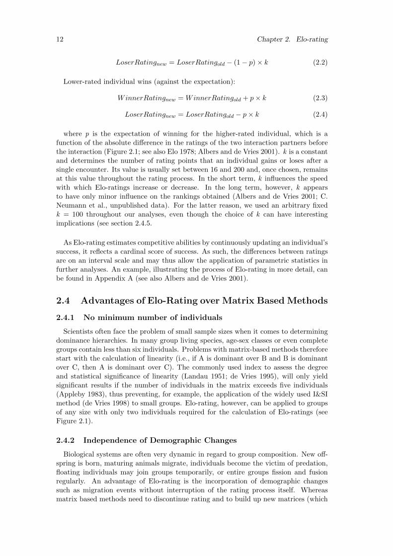
12 Chapter 2. Elo-rating
LoserRatingnew = LoserRatingold − (1 − p) × k (2.2)
Lower-rated individual wins (against the expectation):
WinnerRatingnew = WinnerRatingold + p× k (2.3)
LoserRatingnew = LoserRatingold − p× k (2.4)
where p is the expectation of winning for the higher-rated individual, which is afunction of the absolute difference in the ratings of the two interaction partners beforethe interaction (Figure 2.1; see also Elo 1978; Albers and de Vries 2001). k is a constantand determines the number of rating points that an individual gains or loses after asingle encounter. Its value is usually set between 16 and 200 and, once chosen, remainsat this value throughout the rating process. In the short term, k influences the speedwith which Elo-ratings increase or decrease. In the long term, however, k appearsto have only minor influence on the rankings obtained (Albers and de Vries 2001; C.Neumann et al., unpublished data). For the latter reason, we used an arbitrary fixedk = 100 throughout our analyses, even though the choice of k can have interestingimplications (see section 2.4.5.
As Elo-rating estimates competitive abilities by continuously updating an individual’ssuccess, it reflects a cardinal score of success. As such, the differences between ratingsare on an interval scale and may thus allow the application of parametric statistics infurther analyses. An example, illustrating the process of Elo-rating in more detail, canbe found in Appendix A (see also Albers and de Vries 2001).
2.4 Advantages of Elo-Rating over Matrix Based Methods
2.4.1 No minimum number of individuals
Scientists often face the problem of small sample sizes when it comes to determiningdominance hierarchies. In many group living species, age-sex classes or even completegroups contain less than six individuals. Problems with matrix-based methods thereforestart with the calculation of linearity (i.e., if A is dominant over B and B is dominantover C, then A is dominant over C). The commonly used index to assess the degreeand statistical significance of linearity (Landau 1951; de Vries 1995), will only yieldsignificant results if the number of individuals in the matrix exceeds five individuals(Appleby 1983), thus preventing, for example, the application of the widely used I&SImethod (de Vries 1998) to small groups. Elo-rating, however, can be applied to groupsof any size with only two individuals required for the calculation of Elo-ratings (seeFigure 2.1).
2.4.2 Independence of Demographic Changes
Biological systems are often very dynamic in regard to group composition. New off-spring is born, maturing animals migrate, individuals become the victim of predation,floating individuals may join groups temporarily, or entire groups fission and fusionregularly. An advantage of Elo-rating is the incorporation of demographic changessuch as migration events without interruption of the rating process itself. Whereasmatrix based methods need to discontinue rating and to build up new matrices (which

2.4. Advantages of Elo-Rating 13
Inte
ract
ion
Elo−ratingwinning
probability
12
34
900
1000
1100
−50
−36
−27
+79
+50
+36
+27
−79
p =
0.5
p =
0.6
4p
= 0
.73
p =
0.7
9
0.0
0.2
0.4
0.6
0.8
1.0 −
800
−40
00
400
800
Elo
−ra
ting
diffe
renc
e
0.0
0.2
0.4
0.6
0.8
1.0 −
800
−40
00
400
800
Elo
−ra
ting
diffe
renc
e
0.0
0.2
0.4
0.6
0.8
1.0 −
800
−40
00
400
800
Elo
−ra
ting
diffe
renc
e
0.0
0.2
0.4
0.6
0.8
1.0 −
800
−40
00
400
800
Elo
−ra
ting
diffe
renc
e
Fig
ure
2.1
:G
rap
hic
alil
lust
rati
on
ofE
lo-r
ati
ng
pri
nci
ple
s.T
wo
ind
ivid
ual
sA
(squ
ares
)an
dB
(cir
cles
)in
tera
ctfo
ur
tim
esof
wh
ich
the
firs
tth
ree
inte
ract
ion
sare
won
by
Aan
dth
efo
urt
his
won
by
B.T
he
nu
mb
erof
poi
nts
gain
ed/l
ost
dep
end
son
the
pro
bab
ilit
yth
atth
eh
igh
er-r
ated
ind
ivid
ual
win
sth
ein
tera
ctio
n(s
eete
xt
for
det
ail
s).
Th
ew
inn
ing
pro
bab
ilit
y(p
)is
afu
nct
ion
ofth
ed
iffer
ence
inE
lo-r
atin
gsb
efore
the
inte
ract
ion
(dot
ted
vert
ical
lin
es).
As
the
diff
eren
cein
rati
ngs
incr
ease
sw
ith
each
inte
ract
ion
sod
oes
the
chan
ceof
Aw
inn
ing.
Agr
ap
hic
alw
ayto
obta
inth
ew
inn
ing
chan
ceis
dep
icte
din
the
inse
tfi
gure
s.A
det
aile
dd
escr
ipti
onof
this
exam
ple
can
be
fou
nd
inA
pp
end
ixA
.
14 Chapter 2. Elo-rating
Date
Elo
rat
ing
0
200
400
600
800
1000
1200
1400
1600
1800
2000
1 Mar 6 Mar 11 Mar 16 Mar 21 Mar 26 Mar 31 Mar
● ● ●● ●
● ● ● ●● ● ●
● ●● ● ●
● ● ● ●
1:10
●
Individual
BJCJKJPJRJSJTJVJYJZJ
Figure 2.2: Elo-ratings of 10 male crested macaques during March 2007 (group R2).Each line represents one male. Each symbol represents Elo-ratings after they wereupdated following an interaction of the depicted individual. Note that on 10 March,the residing top-ranking male (SJ) and another high-ranking male (YJ) emigrated fromthe group and a new male (ZJ) joined the group on 11 March, becoming the group’snew alpha male (see text for details).
then need a sufficient number of interactions between individuals in order to producereliable rankings) after each demographic change, hierarchy determination can be con-tinued despite demographic changes. This is achieved by giving a new individual thepredefined starting value (as defined for all individuals before they are rated for thefirst time) before the first interaction with another individual. After a few interactionsthis individual can be ranked in the existing hierarchy (see below). This feature maybe particularly advantageous for studies on species that live in large social groups withhigh reproductive rate, high migration rate and/or high predation rate.
To illustrate this, we plotted the development of Elo-ratings of adult males in agroup of crested macaques over the course of a month during which three migrationevents took place (Figure 2.2, see below for details on the study population and datacollection). In our example, male ZJ migrated into group R2 on 11 March 2007. Toinclude him in the dominance hierarchy, he was assigned the initial score of 1000,and even though he lost his first observed interaction, Elo-rating made it possible torecognize him quickly as the new alpha male. Likewise, individuals that emigrate(or die) (like males SJ and YJ in this example) are simply excluded from the ratingprocess from the date of their disappearance without causing any interruption to therating procedure.
Since Elo-rating does not stop the rating process as a consequence of changes in groupcomposition it circumvents a further drawback of matrix-based methods. Techniques

2.4. Advantages of Elo-Rating 15
such as I&SI and David’s score result in values that directly depend on the numberof individuals present, thus an observed change in calculated dominance rank or scoreacross two time periods may in fact be a consequence of changes in the number ofanimals in the group rather than changes in competitive abilities, thus making a com-parison invalid. For example, in the case of the normalized David’s score (c.f. de Vrieset al. 2006), values can range between 0 and N – 1, where N is the number of individ-uals present in the social group. Elo-rating, in contrast, results in ratings that do notdepend on the number of individuals present. Given that k is fixed for the entire ratingprocess, the current opponent’s strength is the only variable that influences an individ-ual’s future rating. Hence, the Elo-rating of an individual is independent of the numberof individuals, and time periods that need to be created as a consequence of changes inthe number of individuals. This feature allows Elo-rating to be used in a longitudinalmanner which is crucial for a wide array of studies, e.g., those on mechanisms of rankacquisition and maintenance, determinants of life-time reproductive success, and so on.
However, as in the other methods, true ratings of individuals are only known after aminimum amount of interactions involving these individuals occurred (see also Albersand de Vries 2001). For example (Figure 2.2), rank orders that would have beenobtained through Elo-rating within the first two weeks of ZJ’s group membership wouldhave placed him as ranking below BJ. After 13 days (i.e., eight observed interactions),ZJ reached the top-ranked position in the Elo-ratings. Using all observed interactionsfrom these two weeks it was not possible to construct a linear hierarchy, and only after45 days did we obtain a matrix with a sufficient amount of interactions permitting theuse of I&SI. However, it is likely that ZJ became alpha male directly upon his arrivalin the group even though he lost his very first observed interaction (top entry: see e.g.,Sprague et al. 1998) rather than constantly rising through the hierarchy. Albers and deVries (2001) suggest waiting for at least two interactions before assessing a dominancehierarchy through Elo-rating whenever a new member joins the hierarchy: one againsta stronger and one against a weaker opponent. In the case of ZJ, however, we observedhim interacting with six out of the seven other males present. In our case it thus seemsmore appropriate to follow Glickman and Doan’s (2010, rating chess players) suggestionto treat ratings based on less than nine interactions as ‘provisional’ and exclude suchratings from rankings. Therefore in general, Elo-rating still needs a short start-up timebefore creating reliable dominance hierarchies when group composition changes. Thisstart-up time is however much shorter than the time needed to build up sufficientlyfilled interaction matrices for dominance hierarchies.
2.4.3 Visualization and Monitoring of Hierarchy Dynamics
Even if group composition is stable, matrices do not allow dynamics to be trackedwithin social hierarchies, especially if study periods are very short and data insufficientto obtain reliable rankings. In the worst case, a researcher may overlook rank changeswhen analysing hierarchies at some fixed interval (e.g., monthly).
One of the great advantages of Elo-rating is its ability to visualise dominance rela-tionships on a time scale, thus allowing monitoring of rank relationship dynamics. Asthe information about the sequence of interactions is a prerequisite for applying Elo-rating, one can easily create graphs that depict the time scale on the x-axis and plotthe development of each individual’s ratings on the y-axis. This approach can demon-strate a fundamental feature of Elo-rating, i.e., the possibility to obtain a rank order
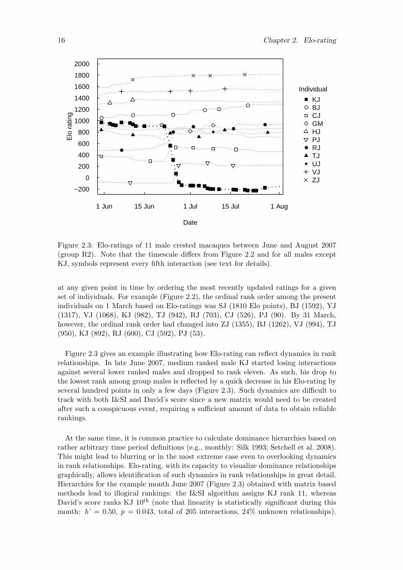
16 Chapter 2. Elo-rating
Date
Elo
rat
ing
−200
0
200
400
600
800
1000
1200
1400
1600
1800
2000
1 Jun 15 Jun 1 Jul 15 Jul 1 Aug
●● ●
● ●●
●
● ●
●
●●
● ●
1:10
●
●
Individual
KJBJCJGMHJPJRJTJUJVJZJ
Figure 2.3: Elo-ratings of 11 male crested macaques between June and August 2007(group R2). Note that the timescale differs from Figure 2.2 and for all males exceptKJ, symbols represent every fifth interaction (see text for details).
at any given point in time by ordering the most recently updated ratings for a givenset of individuals. For example (Figure 2.2), the ordinal rank order among the presentindividuals on 1 March based on Elo-ratings was SJ (1810 Elo points), BJ (1592), YJ(1317), VJ (1068), KJ (982), TJ (942), RJ (703), CJ (526), PJ (90). By 31 March,however, the ordinal rank order had changed into ZJ (1355), BJ (1262), VJ (994), TJ(950), KJ (892), RJ (600), CJ (592), PJ (53).
Figure 2.3 gives an example illustrating how Elo-rating can reflect dynamics in rankrelationships. In late June 2007, medium ranked male KJ started losing interactionsagainst several lower ranked males and dropped to rank eleven. As such, his drop tothe lowest rank among group males is reflected by a quick decrease in his Elo-rating byseveral hundred points in only a few days (Figure 2.3). Such dynamics are difficult totrack with both I&SI and David’s score since a new matrix would need to be createdafter such a conspicuous event, requiring a sufficient amount of data to obtain reliablerankings.
At the same time, it is common practice to calculate dominance hierarchies based onrather arbitrary time period definitions (e.g., monthly: Silk 1993; Setchell et al. 2008).This might lead to blurring or in the most extreme case even to overlooking dynamicsin rank relationships. Elo-rating, with its capacity to visualize dominance relationshipsgraphically, allows identification of such dynamics in rank relationships in great detail.Hierarchies for the example month June 2007 (Figure 2.3) obtained with matrix basedmethods lead to illogical rankings: the I&SI algorithm assigns KJ rank 11, whereasDavid’s score ranks KJ 10th (note that linearity is statistically significant during thismonth: h’ = 0.50, p = 0.043, total of 205 interactions, 24% unknown relationships).

2.4. Advantages of Elo-Rating 17
Elo-rating, in contrast, shows that KJ held a medium rank almost throughout the entiremonth and dropped in rank only during the last week of June.
In Old World monkeys and many other group living mammals, it is sometimes ob-served that young males rise in rank before they eventually leave their natal group (e.g.,Hamilton and Bulger 1990). A common approach to quantify this phenomenon wouldbe to calculate monthly ranks and correlate them with the time to departure. Doingso for 16 natal male crested macaques (see below for details on the study populationand data collection) using David’s score, however, lends only little support to this phe-nomenon (Spearman’s rank correlation: rs = 0.642, p = 0.139, N = 7, Figure 2.4a).As described below, this may be the consequence of high proportions of unknown re-lationships leading to less reliable scores. It could also be due to the fact that David’sscores directly depend on the number of individuals incorporated in the matrix. Incontrast, when using Elo-rating, the hypothesis that natal males rise in rank beforeemigration is strongly supported (rs = 1, p < 0.001, N = 7, Figure 2.4b). We observean almost linear increase in ratings before the migration date. It appears that maleswent through a noticeable surge about three months before emigration, and kept risingbefore their departure. This is, however, a preliminary result and further investigationis warranted. Since Elo-ratings can be obtained at any desired date, even an analysiswith higher time resolution (e.g., weekly) is possible (Figure 2.4c).
In addition, Elo-rating also allows objective identification and quantitative charac-terization of hierarchical stability. Again, the graphical features of Elo-rating providevery useful assistance in this respect. Figure 2.2, for example, shows that individu-als KJ and TJ changed their ordinal rank relative to each other five times within onemonth, suggesting some degree of rank instability (see also individuals RJ, TJ and GMin Figure 2.3).
To quantify the degree of hierarchy stability, we propose to use the ratio of rankchanges per individuals present over a given time period. Formally, the index is ex-pressed as
S =
∑di=1(Ci × wi)∑d
i=1(Ni)(2.5)
where Ci is the sum of absolute differences between rankings of two consecutive days,wi is a weighing factor determined as the standardized Elo-rating of the highest rankedindividual involved in a rank change, and Ni is the number of individuals present onboth days (see appendix 2 for further details). Before division, values are summedover the desired time period, i.e. n days. S can take values between 0, indicatinga stable hierarchy with identical rankings on each day of the analyzed time period,and 2 / max(Ni), indicating that the hierarchy is reversing every other day, i.e. totalinstability. Our data suggest that S typically ranges between 0 and 0.5.
To test the validity of this approach we calculated S before and after the immigrationof male macaques that subsequently achieved high ranks (among the top three, seebelow for details on the study population and data collection). We expected suchevents to induce instability (e.g., Lange and Leimar 2004; Beehner et al. 2005), thusleading to higher S values when compared to periods before such incidents. We found
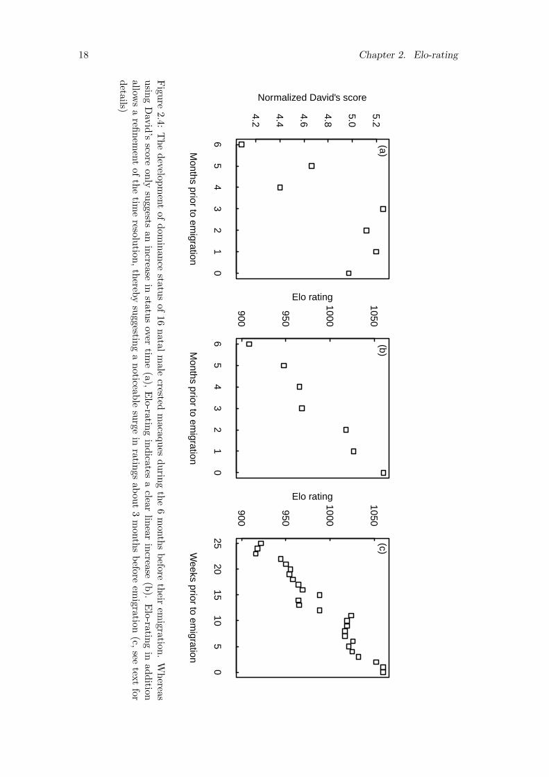
18 Chapter 2. Elo-rating
Months prior to em
igration
Normalized David's score
(a)
65
43
21
0
4.2
4.4
4.6
4.8
5.0
5.2
Months prior to em
igration
Elo rating
(b)
65
43
21
0
900
950
1000
1050
Weeks prior to em
igration
Elo rating
2520
1510
50
900
950
1000
1050(c)
Fig
ure
2.4:T
he
develo
pm
ent
of
dom
inan
cestatu
sof
16n
atalm
alecrested
macaq
ues
du
ring
the
6m
onth
sb
eforeth
eirem
igration.
Wh
ereasu
sing
Dav
id’s
scoreon
lysu
ggests
an
increa
sein
status
overtim
e(a),
Elo-ratin
gin
dicates
aclear
linear
increase
(b).
Elo-ratin
gin
add
itionallow
sa
refin
emen
tof
the
time
resolu
tion
,th
ereby
suggestin
ga
noticeab
lesu
rgein
ratings
abou
t3
mon
ths
before
emigration
(c,see
text
ford
etails)

2.4. Advantages of Elo-Rating 19
less stability, i.e. greater S values, during four-week periods after the immigration ofmales that achieved high rank compared to the four-week periods before (Wilcoxonsigned rank test: V = 87, N = 14, p = 0.030), indicating that hierarchies were lessstable after the immigration of a high ranking male. In contrast, after the immigrationof males that subsequently held low ranks, we observed no such difference in stability(V = 14, N = 7, p = 1.000).
Such a quantitative approach may be advantageous since, so far, hierarchical in-stability has been identified in a non-consistent manner. Sapolsky (1983) for exam-ple, studying baboons, identified periods of instability in male dominance hierarchiesthrough high rates of ambiguously ending agonistic interactions and through high ratesof interactions that ended with the subordinate winning. In a different study of ba-boons, Engh et al. (2006) assessed instability in female dominance hierarchies in a meredescriptive way. On a long-term basis, stability has also been characterised by compar-ison of rankings in consecutive seasons using regression or correlation analysis (e.g., inmountain goats, Cote 2000). By objectively defining stability, Elo-rating may becomean important tool for studies on social instability and its consequences, for exampleon individual stress levels and health (e.g., Sapolsky 2005), territory acquisition (e.g.,Beletsky 1992) or group transfer (e.g., Smith 1987; van Noordwijk and van Schaik2001). In addition, the objective quantification of stability may make comparisonsacross studies possible.
2.4.4 Independence of Time Periods
It is common practice to obtain hierarchies at some arbitrary fixed time interval(e.g. monthly). Given the dynamics of animal societies, both in group compositionand rankings (see above), such an approach is prone to misjudgement of hierarchies fortwo reasons. First, all individuals incorporated in a dominance matrix must have thepossibility to interact with each other at all times. If group composition changes withinthe studied interval, for example in fission/fusion societies or when individuals leaveand join frequently (floaters), applying matrix based methods is unjustified. Second,rank changes that occur will be blurred (see the example above, Figure 2.3).
With Elo-rating it is possible to pinpoint rankings to a specific day. This is ofparticular importance when studying events, such as a male’s rank at the day hisoffspring was conceived or born, or tracking the rank development of individuals beforeand after they migrate.
A related problem to the creation of time periods is the proportion of unknownrelationships. When creating relatively short time periods to account for the abovementioned dynamics, one often faces a high percentage of pairs of individuals thatwere not observed interacting in a given period. Like any statistical test, rankingmethods suffer from decreased power or precision when sample size is low (Appleby1983; de Vries 1995; Koenig and Borries 2006; Wittemyer and Getz 2006), even thoughattempts have been made to counter this problem (see de Vries 1995, 1998; de Vrieset al. 2006; Wittemyer and Getz 2006). As we will show below, Elo-rating seems lessaffected by unknown relationships than matrix based methods, and is therefore alsooperational on very sparse data sets.
20 Chapter 2. Elo-rating
2.4.5 Integrity of Power Assessment
Without demonstrating their application, we finally mention three further advan-tages of Elo-rating that may refine the precision of power assessment of individuals:a) integration of undecided interactions into the rating process, b) discrimination ofagonistic interactions of differing quality, and c) choosing k according to the studyspecies.
Undecided interactions
Though some matrix-based methods (e.g., David’s score or Boyd and Silk’s (1983)index) explicitly allow interactions without unambiguous winners and losers, i.e., drawsor ties, to be taken into account when establishing dominance orders, researchers (in-cluding us) usually choose to discard such observations. Clearly, agonistic interactionsthat end without unambiguous winners and losers contain information about competi-tive abilities of the involved individuals and should therefore not be disregarded. Whenusing Elo-rating, an undecided interaction can be incorporated into the rating processto the disadvantage of the higher rated individual whose rating will decrease, eventhough the decrease will be smaller than had the higher rated individual lost the in-teraction (Albers and de Vries 2001). After a draw the rating for the higher ratedindividual is reduced to Ratingnew = Ratingold – k (p – 0.5), whereas the rating forthe lower rated individual increases to Ratingnew = Ratingold + k (p – 0.5). Hence,a draw between two individuals that had identical ratings before the interaction (i.e.,p = 0.5) will not alter the ratings. In this way, Elo-rating allows for a more completepower assessment of individuals by including interactions into the rating process thatare just as meaningful as clear winner-loser interactions.
Agonistic interactions of different quality
Instead of being fixed throughout the rating process, the constant k could be ad-justed according to the quality of the interaction or the experience of the interactingindividuals. For example, one could distinguish between low- and high-intensity ag-gression (e.g., Adamo and Hoy 1995; Lu et al. 2008) and assign interactions involvinghigh-intensity aggression higher values of k. This results in greater changes in ratingsafter such interactions compared to interactions involving low-intensity aggression.
Choosing k
Prior experience of individuals plays an important role in the outcome of agonisticencounters in many animal taxa: the winner of a previous interaction is more likely towin a future interaction, whereas losers are more likely to lose future interactions (Hsuet al. 2006). A meta-analysis on the magnitude of such winner/loser effects demon-strated that the likelihood of winning an interaction is almost doubled for previouswinners whereas for previous losers the likelihood of winning is reduced almost five-fold(Rutte et al. 2006). Depending on the size of this effect in the study species, k couldtherefore be split into a smaller kw for the winner and a larger kl for the loser to reflectthis phenomenon (de Vries 2009).
Thus, Elo-rating is not limited to decided dominance interactions, but can incorpo-rate undecided interaction and in addition allows for a detailed hierarchy evaluation byweighing interactions according to their properties and the magnitude of winner/loser

2.5. Testing the Reliability and Robustness of Elo-Rating 21
effects. This surplus of information Elo-rating can utilize allows for a much finer as-sessment of dominance relationships.
2.5 Testing the Reliability and Robustness of Elo-Rating
So far, we have shown how Elo-rating circumvents the problems associated withmatrix based methods. However, we have not yet shown how it compares to othermethods in terms of reliability and robustness. We now compare Elo-rating with twowidely used ranking methods that are based on interaction matrices (I&SI and David’sscore), using our own empirical data. Mimicking a variety of social systems, we use datacollected on two species of macaques with different aggression patterns, crested (Macacanigra, aggressive interactions frequent, but of low intensity) and rhesus macaques (M.mulatta, aggressive interactions less frequent, but of higher intensity) (de Waal andLuttrell 1989; Thierry 2007), and calculate dominance hierarchies for females (morestable hierarchies) and males (more dynamic hierarchies) separately. To facilitate theassessment of these analyses we will first briefly review the two methods we use for ourcomparisons.
2.5.1 Short Introduction to I&SI and David’s Score
The I&SI method (de Vries 1998) is an iterative algorithm that tries to find the rankorder that deviates least from a linear rank order. It is based on observed dominanceinteractions (e.g., winning/losing an agonistic interaction) and tries to minimize thenumber of inconsistencies (I) produced when building a dominance hierarchy, i.e., min-imize dyads for which the relationship is not in agreement with the actual rank order.Subsequently, the strength of inconsistencies (SI), i.e., the rank difference between twoindividuals that form an inconsistency, is minimized, under the condition that in theiterated rank order the number of inconsistencies does not increase. The result of theI&SI algorithm is an ordinal rank order.
David’s score (David 1987) is an individual measure of success, in which for eachindividual a score is calculated based on the outcome of its agonistic interactions withother members of the social group as DS = w + w2 – l – l2, where w is the sum of anindividual’s winning proportions and l the summed losing proportions. w2 representsan individual’s summed winning proportions (i.e., w) weighed by the w values of itsinteraction partners and likewise, l2 equals an individual’s summed losing proportions(i.e., l) weighed by the l values of its interaction partners (David 1987; Gammell et al.2003; see de Vries et al. (2006) for an illustrative example). Thus, David’s scoretakes the relative strength of opponents into account, valuing success against strongerindividuals more than success against weaker individuals.
Rank orders generated with I&SI and David’s score are generally very similar to eachother (e.g., Vervaecke et al. 2007; Neumann et al. unpublished data).
2.5.2 Methods
Study populations
For our tests of Elo-rating, we chose two species of macaques (crested, Macaca nigra,and rhesus macaques, M. mulatta). Even though our aim was not to test for species
22 Chapter 2. Elo-rating
differences, we nevertheless aimed at gathering a broad data set including different, butcomparable, species. Macaques fit this condition as the different species are charac-terised by a common social organization but at the same time by pronounced differencesin aggression patterns (Thierry 2007).
Data collection
Between 2006 and 2010, we collected data in three groups (R1, R2, PB) of a pop-ulation of wild crested macaques in the Tangkoko-Batuangus Nature Reserve, NorthSulawesi, Indonesia (1°33’ N, 125°10’ E; e.g., Duboscq et al. 2008; Neumann et al. 2010).Groups comprised between 4 – 18 adult males and 16 – 24 adult females and were com-pletely habituated to human observers and individually recognizable. Between 2007and 2010, data on rhesus macaques were collected in two groups (V, R) on the freeranging population on Cayo Santiago, Puerto Rico (18°09’ N, 65°44’ W). The studygroups comprised between 20 – 60 females and 16 – 54 males (e.g., Dubuc et al. 2009;Widdig unpublished data).
We collected data on dyadic dominance interactions, i.e., agonistic interactions withunambiguous winner and loser, and displacement (approach / leave) interactions duringall occurrence sampling on focal animals and during ad libitum sampling (Altmann1974). Overall, our data set comprised a total of 12,740 interactions involving 252individuals. Dominance hierarchies were created separately for the different species,groups and sexes.
Data analysis
Our first aim was to investigate whether dominance rank orders calculated withElo-rating reflect rankings obtained with more established methods. To answer this,we assessed how similar rank orders generated with Elo-rating are to those obtainedwith the I&SI method and David’s score. From our data on both macaque species,we created time periods based on socio-demographic events, such as changes betweenmating- and birth season, migration or death of individuals, maturing of subadultindividuals and conspicuous status changes (hereafter “full data set”, see Table 2.1)and produced corresponding dominance interaction matrices. Two consecutive timeperiods of a given species/sex combination did not comprise the same set of individualsin the majority of cases (61 out of 66 periods, i.e., 92%).
We tested all 66 matrices for linearity by means of de Vries’ (1995) h’ index. For the29 matrices for which the linearity test yielded a significant result, we applied de Vries’(1998) I&SI method. Next, we calculated normalized David’s scores from all matricesfollowing de Vries et al. (2006). Finally, we calculated Elo-ratings from all interactionsin each of the group/sex combinations as a whole using Elo-ratings on the last day ofeach time period for the comparison with I&SI ranks and David’s scores. Elo-ratingswere calculated with 1000 as initial value and k was set to 100.
We computed Spearman’s rank correlation coefficients between the rankings andscores for each period. To obtain positive correlation coefficients consistently for allcomparisons, we reversed I&SI rank orders (i.e., high-ranking individuals get a highI&SI rank value), since high dominance rank is represented by high David’s scores andElo-ratings. Thus, if two rankings are identical the correlation coefficient will be 1.00.

2.5. Reliability and Robustness of Elo-Rating 23
Tab
le2.
1:G
ener
ald
escr
ipti
onof
the
tim
ep
erio
ds
and
dom
inan
cem
atr
ices
use
din
the
anal
ysi
s.
spec
ies
grou
pse
xN
per
iod
sad
ura
tion
bN
ind
ivid
ual
sU
nkn
own
rela
tion
ship
scIn
tera
ctio
nsd
pro
por
tion
infu
llin
crea
sein
red
uce
d
mu
latt
aR
male
83.
9(3
.1–4
.1)
35(3
4–42
)0.
82(0
.79–
0.88
)0.0
8(0
.06–
0.09)
180
(123–
234)
Vfe
mal
e4
1.8
(1.2
–2.5
)22
(19–
22)
0.66
(0.4
4–0.
86)
0.1
3(0
.07–0
.20)
116
(34–
226)
male
51.4
(1.1
–2.9
)16
(16–
20)
0.67
(0.5
8–0.
71)
0.1
3(0
.12–0
.14)
90
(41–1
25)
nig
raP
Bfe
male
34.
0(3
.5–7
.6)
18(1
8–18
)0.
25(0
.16–
0.30
)0.
19
(0.1
4–0.
22)
299
(228
–644
)
male
62.4
(2.2
–3.5
)8
(7–9
)0.
36(0
.25–
0.40
)0.
14
(0.1
1–0.
16)
91(5
0–11
2)
R1
fem
ale
56.
3(5
.8–1
1.2)
21(2
1–22
)0.
49(0
.47–
0.57
)0.1
4(0
.07–
0.16)
254
(158–
292)
male
162.
6(2
.2–3
.1)
10(1
0–13
)0.
34(0
.09–
0.46
)0.
16
(0.1
0–0.
18)
159
(114
–194
)
R2
fem
ale
76.
7(4
.8–7
.5)
18(1
6–20
)0.
50(0
.45–
0.56
)0.1
3(0
.11–
0.15)
194
(136–
246)
male
123.
1(2
.2–4
.0)
8(6
–9)
0.26
(0.1
3–0.
34)
0.10
(0.0
7–0.
12)
64(3
3–18
1)
Val
ues
are
pre
sente
dp
ersp
ecie
s,gro
up
an
dse
x.
Med
ian
sar
egi
ven
wit
hin
terq
uar
tile
ran
ges.
aN
um
ber
ofti
me
per
iod
scr
eate
db
Du
rati
on
ofti
me
per
iod
sin
month
sc
Pro
port
ion
ofu
nkn
own
rela
tion
ship
sin
the
full
dat
am
atri
ces
and
the
incr
ease
inp
rop
ort
ion
ofu
nkn
own
rela
tion
ship
sin
the
red
uce
dd
ata
set
(see
text)
.d
Nu
mb
erof
agon
isti
cin
tera
ctio
ns
inea
chm
atri
x.

24 Chapter 2. Elo-rating
We present average correlation coefficients with inter-quartile ranges. All calculationsand tests were computed in R 2.12.0 and R 2.13.0 (R Development Core Team 2010). Ascript and manual to calculate and visualize Elo-ratings with R along with an exampledata set can be found in Appendices D-E.
In a second analysis, we explored whether Elo-rating is a robust method under con-ditions of sparse data and whether the performance of Elo-rating under such conditionsis systematically related to the percentage of unknown relationships in the interactionmatrix. Please note that a sparse matrix is not necessarily a matrix with a higherproportion of unknown relationships. For example, a matrix in which each dyad wasobserved five times and all entries are above the diagonal (i.e., there are no unknownrelationships) is more sparse than a matrix with each dyad being observed ten times(likewise, no unknown relationships). Whereas the I&SI ranking will be identical inboth cases, David’s scores will differ between the two, as will Elo-ratings based on theinteractions leading to this matrix.
We created sparse interaction matrices by randomly removing 50% of the observedinteractions in each of the 66 time periods (“reduced data set”: Table 2.1). Theseadditional matrices were again tested for linearity, resulting in 17 matrices retainingsignificant linearity and thus justifying the application of the I&SI algorithm. We thencalculated for each of the three methods separately correlation coefficients betweenrankings obtained from full and reduced data sets. For the 49 matrices that did notallow the use of I&SI due to non-significant linearity, we restricted the analysis toElo-rating and David’s score.
To explore the robustness of the method further, we tested whether Elo-rating isaffected by increased proportions of unknown relationships and how it compared to thetwo other methods. In other words, we investigated whether the methods become lessreliable as the proportion of unknown relationships increases. An increase in unknownrelationships was generated as a consequence of the random deletion of 50% of allobserved interactions (increase per period on average: 12.5%, inter-quartile range: 8 –17%, “reduced data set”: Table 2.1). We tested for an association between the increasein unknown relationships and the correlation coefficient between ratings from the fulland reduced data set.
2.5.3 Results
Our results show that Elo-ratings correlated highly with both I&SI ranks (medianrs = 0.97, quartiles: 0.94–0.99, N = 29 periods) and David’s scores (median rs = 0.97,quartiles: 0.96–0.99, N = 29 periods).
We found that Elo-ratings from the full data set correlated highly with Elo-ratingsfrom the randomly reduced data set (Table 2.2). The performance of Elo-rating isvirtually identical to the one of I&SI and slightly higher compared to David’s score(Table 2.2). Similarly, Elo-rating produced strong correlations with slightly higher cor-relation coefficients compared to those obtained with David’s score from the remaining49 time periods for which I&SI could not be applied (Table 2.2).

2.5. Reliability and Robustness of Elo-Rating 25
Table 2.2: Robustness analysis. Correlation coefficients (rs) between rankings from fulland reduced data sets. (Median and inter-quartile range).
Linearitya N Elo-rating David’s score I&SI
+ 17 0.98 (0.97–0.99) 0.96 (0.95–0.98) 0.98 (0.95–1.00)
– 49 0.94 (0.89–0.98) 0.92 (0.86–0.95)
a Linearity in the reduced data set: + linearity test yielded significanth’ index, i.e., p ≤ 0.05 (de Vries 1995); – linearity test did not yieldsignificant h’ index, i.e., p > 0.05.
Whereas there was no relationship between the increase in unknown relationshipsand the correlation coefficient between full and reduced data sets for Elo-rating (rs= –0.07, N = 17, p = 0.799) and I&SI (rs = –0.36, N = 17, p = 0.162), we foundthat as the proportion of unknown relationships increased the correlation coefficientsdecreased between rankings from full and reduced data sets when using David’s score(rs = –0.52, N = 17, p = 0.031, Figure 2.5). Controlling for the initial proportion ofunknown relationships by means of a partial Spearman correlation test leads to similarresults (Elo-rating: rs = –0.02, N = 17, p = 0.927; I&SI: rs = –0.39, N = 17, p =0.110; David’s score: rs = –0.59, N = 17, p = 0.006).
Overall, our results indicate that Elo-rating produces rank orders very similar tothose obtained with I&SI and David’s score. In addition, results of our tests suggestthat rankings from Elo-rating and I&SI (given significant linearity test) remain stablein sparse data sets, whereas David’s score seems to create less reliable hierarchies insparse data sets as a result of an increase in unknown relationships.
2.5.4 Discussion
Even though there is abundant literature available that compares the concordanceof different methods for the assessment of dominance ranks or scores (e.g., Bayly et al.2006; Bang et al. 2010), this is the first study to test the reliability of Elo-rating withan extensive data set based on observations of free-ranging animals. Our results ondominance interactions in crested and rhesus macaques show that Elo-rating producesdominance rank orders which closely resemble rankings generated with David’s scoreand the I&SI method. Furthermore, our results indicate that Elo-rating is very robustwhen data sets are limited in the number of interactions observed. Elo-rating (and I&SI)even seems to produce more reliable dominance hierarchies than David’s score whenthe proportion of unknown relationships is high. One could argue that this effect isdue to the initial proportion of unknown relationships, i.e., a relatively high proportionof unknown relationships in a “full” matrix leads to some uncertainty in the rankingwhich may make the scores from the further reduced matrix even less reliable. However,when controlling for the initial proportion of unknown relationships, our results showthat the robustness of Elo-rating (and I&SI) is not attributable to this factor.

26 Chapter 2. Elo-rating
0.000.10
0.200.30
0.75
0.80
0.85
0.90
0.95
1.00
Elo rating
Correlation between full and reduced data
(a)
0.000.10
0.200.30
0.75
0.80
0.85
0.90
0.95
1.00
David's S
core
(b)
0.000.10
0.200.30
0.75
0.80
0.85
0.90
0.95
1.00
I&S
I
(c)
Increase in proportion of unknown relationships
Fig
ure
2.5
:C
orrelationb
etween
the
increa
sein
un
kn
own
relationsh
ips
and
the
perform
ance
of(a)
Elo-ratin
g,(b
)D
avid
’sscore
and
(c)I&
SI.
Th
ein
creasein
un
kn
own
relationsh
ips
was
ind
uced
by
rand
omly
remov
ing
50%of
data
poin
tsan
dp
erforman
ceis
exp
ressedas
the
correlationco
efficien
tb
etween
rankin
gsfro
mth
efu
llan
dred
uced
data
sets.E
lo-ratings
and
I&S
Iran
ks
aren
otin
flu
enced
by
high
erp
ercentages
ofu
nkn
own
relationsh
ips,
wh
ereasth
ep
erform
ance
ofD
avid
’sscore
decreases
wh
enu
nkn
own
relationsh
ips
increase.
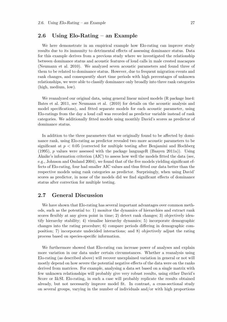
2.6. Using Elo-Rating – an Example 27
2.6 Using Elo-Rating – an Example
We here demonstrate in an empirical example how Elo-rating can improve studyresults due to its immunity to detrimental effects of assessing dominance status. Datafor this example derives from a previous study where we investigated the relationshipbetween dominance status and acoustic features of loud calls in male crested macaques(Neumann et al. 2010). We analyzed seven acoustic parameters and found three ofthem to be related to dominance status. However, due to frequent migration events andrank changes, and consequently short time periods with high percentages of unknownrelationships, we were able to classify dominance only broadly into three rank categories(high, medium, low).
We reanalyzed our original data, using general linear mixed models (R package lme4:Bates et al. 2011, see Neumann et al. (2010) for details on the acoustic analysis andmodel specifications), and fitted separate models for each acoustic parameter, usingElo-ratings from the day a loud call was recorded as predictor variable instead of rankcategories. We additionally fitted models using monthly David’s scores as predictor ofdominance status.
In addition to the three parameters that we originally found to be affected by domi-nance rank, using Elo-rating as predictor revealed two more acoustic parameters to besignificant at p < 0.05 (corrected for multiple testing after Benjamini and Hochberg(1995), p values were assessed with the package languageR (Baayen 2011a)). UsingAkaike’s information criterion (AIC) to assess how well the models fitted the data (see,e.g., Johnson and Omland 2004), we found that of the five models yielding significant ef-fects of Elo-rating, four had smaller AIC values and thus fitted our data better than therespective models using rank categories as predictor. Surprisingly, when using David’scores as predictor, in none of the models did we find significant effects of dominancestatus after correction for multiple testing.
2.7 General Discussion
We have shown that Elo-rating has several important advantages over common meth-ods, such as the potential to: 1) monitor the dynamics of hierarchies and extract rankscores flexibly at any given point in time; 2) detect rank changes; 3) objectively iden-tify hierarchy stability; 4) visualise hierarchy dynamics; 5) incorporate demographicchanges into the rating procedure; 6) compare periods differing in demographic com-position; 7) incorporate undecided interactions; and 8) objectively adjust the ratingprocess based on species-specific information.
We furthermore showed that Elo-rating can increase power of analyses and explainmore variation in our data under certain circumstances. Whether a reanalysis usingElo-rating (as described above) will recover unexplained variation in general or not willmostly depend on how severe the potential negative effects of the data were on the ranksderived from matrices. For example, analysing a data set based on a single matrix withfew unknown relationships will probably give very robust results, using either David’sScore or I&SI. Elo-rating, in such a case will probably replicate the results obtainedalready, but not necessarily improve model fit. In contrast, a cross-sectional studyon several groups, varying in the number of individuals and/or with high proportions
28 Chapter 2. Elo-rating
of unknown relationships (as in our example above), may warrant a reanalysis usingElo-rating.
We can however see one context in which Elo-rating may not be the first choice toassess rank relationships. Unlike the I&SI method (given its application is feasible),Elo-ratings do not necessarily reflect the rank order corresponding to a linear hierarchyin which an alpha individual is dominant (c.f. Drews 1993) over all other individualsand a beta individual is dominant over all other individuals except the alpha, and soon (de Vries 1998). Such a feature of a ranking algorithm may be desirable when, forexample, investigating the relationship between parental and offspring rank (Dewsbury1990; East et al. 2009; reviewed in Holekamp and Smale 1991). Such a situationis found in the matrilineal rank organization of many Old World monkeys, which ischaracterized by a linear structure in which a daughter ranks below her mother, andamong all daughters of one mother the youngest one ranks highest (Kawamura 1958;Missakian 1972; but see Silk et al. 1981). Elo-rating nevertheless produces rankingsclose to a linear hierarchy (see above), and may therefore still allow for appropriaterank assessment in such cases, especially when the I&SI method cannot be applied dueto data limitations.
In conclusion, all the advantages mentioned in this paper make Elo-rating a usefultool for assessing and monitoring changes of dominance relationships – particularly inhighly dynamic animal systems.

Chapter 3
Personality in wild male crestedmacaques Macaca nigra
with
Muhammad Agil, Anja Widdig, Antje Engelhardt
Published in PLoS ONE 8 (2013): e69383.
29
30 Chapter 3. Personality description
3.1 Abstract
Animal personalities, i.e. consistent differences in behavior across time and/or con-text, have received increased attention of behavioral biologists over the last years.Recent research shows that personalities represent traits on which natural and sex-ual selection work and which can have substantial fitness consequences. The aim ofthis study is to establish the personality structure of crested macaque (Macaca nigra)males as foundation for future studies on its adaptive value. We collected behavioraldata through focal animal sampling and additionally conducted two sets of playbackexperiments. Results of a factor analysis on the behavioral data revealed a four factorstructure with components we labeled Anxiety, Sociability, Connectedness and Ag-gressiveness. Results from the experiments revealed an additional and independentBoldness factor but the absence of Neophilia. Overall, this structure resembles othermacaque and animal species with the exception of Connectedness, which might be aconsequence of the species’ tolerant social style. Our results thus not only form thebasis for future studies on the adaptive value of personality in crested macaques butalso contribute an important data point for investigating the evolution of personalitystructure from a comparative perspective by refining, for example, which personalityfactors characterized the last common ancestor of hominids and macaques.
3.2 Introduction
In recent years, the phenomenon that individuals in many, if not all, animal speciesdiffer from each other consistently in their behavior has received increasing attentionfrom biologists and psychologists (Gosling and John 1999; Gosling 2001). If such in-dividual differences are stable over time and/or across contexts they are referred toas animal personality or temperament (Reale et al. 2007). Animal personalities areidentified either by humans familiar with the study subjects via rating items in ques-tionnaires (e.g. Stevenson-Hinde and Zunz 1978; Weiss et al. 2011; Konecna et al. 2012)or through observational/experimental data (e.g. Koski 2011b; Dammhahn 2012; Sey-farth et al. 2012). Both approaches usually subject primary data to factor analysis orrelated statistical methods, which allow identification of underlying dimensions thatare then referred to as personality factors. Generally, both approaches lead to similarresults when describing the personality structure (the combination of all present per-sonality factors) of a given animal species (e.g., Konecna et al. 2008, but see Uher et al.2008, reviewed in Koski 2011a). Since personality can have profound effects on repro-ductive fitness, it is an important feature of animal biology that selective processes canwork on (Dingemanse et al. 2004; Smith and Blumstein 2008; Schuett et al. 2010).
Personalities of non-human primates (from here on: primates) are reasonably wellstudied (reviewed in Freeman and Gosling 2010) due to the phylogenetic proximity ofprimates to humans and the complexity of the social systems exhibited by most primatespecies (Mitani et al. 2012). This growing body of data allows us to investigate thebiological roots of human personality (Gosling and John 1999; Gosling 2001; Uher 2008)and recently, a first formal attempt was made to describe the evolution of personalitywithin the catarrhine primates (Weiss et al. 2011, see also King and Figueredo 1997).Weiss and colleagues (2011) hypothesize that the personality structure of humans isthe evolutionary consequence of a series of changes along our phylogenetic history, withthe human personality structure resembling more other hominid personality structures
3.2. Introduction 31
than those of more distantly related species such as rhesus macaques (Macaca mulatta).They further suggest that degree of sociality (i.e., differences in social organization andsocial relationships) has been the major selective pressure leading to the observed inter-specific differences in personality. This latter proposition however raises the question asto how personality structures differ in closely related species in which sociality may notbe confounded by overall social organization (as is likely to be the case, for example,within the hominids).
In an alternative scenario, it has been suggested that the evolution of different typesof sociality in different species is the result of differences in personality (Thierry et al.2000b; Capitanio 2004). For example, species in which individuals prefer close spa-tial proximity with conspecifics (an exemplified personality factor) may face increasedfeeding competition as compared to species in which individuals prefer greater spatialdistance to conspecifics. This might then lead to more intense or more frequent aggres-sive behavior, which in turn may lead to the evolution of specific conflict managementstrategies not found in species that show lower levels of proximity (Capitanio 2004).This example illustrates how differences in personality could lead to changes in pat-terns of social behavior and shape social styles as sets of correlated behavioral patterns(Thierry et al. 2000b).
Among primates, the macaques (Macaca) represent a particularly well suited genusto look into the evolution of personality structures and its link to social behavior.On the one hand all of the approximately 20 species share some fundamental featuresof social organization such as living in temporally relatively stable multi-male/multi-female groups and male dispersal around sexual maturity (Thierry 2011). On the otherhand, macaques differ markedly in social style ( Thierry 2007, see also de Waal andLuttrell 1989; Thierry 1990, 2000), for example in regard to patterns of aggression andthe degree of dominance asymmetries, conflict management strategies, and degree ofkin bias in social interactions (e.g. Thierry 2000; Thierry et al. 2000b; Berman andThierry 2010; Duboscq et al. 2013). This particular diversity of social traits has led tothe classification of macaque species into four grades of social styles ranging from socalled despotic to tolerant species (Thierry 2007) and therefore represents an interestingmodel to study the link between sociality and personality.
Several macaque species have been studied in the context of personality. Our currentknowledge about macaque personalities nevertheless comes foremost from studies ona single species, the despotic rhesus macaque (e.g., Stevenson-Hinde and Zunz 1978;Bolig et al. 1992; Capitanio 1999; Weiss et al. 2011). In this species, at least three per-sonality factors have been determined consistently across different studies: sociability(also labeled affiliation or not being solitary), aggressiveness (also labeled hostility),and fearfulness (also labeled excitability). These three factors seem to have deep phy-logenetic roots beyond primates given that they appear not only in macaques (Konecnaet al. 2012; Sussman et al. 2013), but also in many other non-primate taxa (reviewedin Gosling and John 1999). Incidentally, they are thought to correspond to three di-mensions of the dominating model of human personality – the Five Factor Model, i.e.Extraversion, Agreeableness, and Neuroticism (Digman 1990; Gosling and John 1999;John and Srivastava 1999). Despite these possible similarities, there are also differencesin personality structure between different macaque species and deviations from the hu-man model. For instance, a distinct and separate personality factor Dominance (King

32 Chapter 3. Personality description
and Figueredo 1997; Weiss et al. 2006, 2011, 2013), has been described for hominids,but not for humans, and similar variation can be observed in the macaques: whereasin despotic rhesus macaques Dominance has been described as a distinct personalityfactor (Weiss et al. 2011), it seems to be absent in the more tolerant Barbary macaques(M. sylvanus, Konecna et al. 2012). Collectively, the available data suggest that per-sonality structures of macaque species share some similarities but simultaneously showdifferences that are possibly linked to differences in species-specific social styles.
As illustrated within the macaques, this interplay of personalities and social styles isstill poorly understood and certainly more data in all these domains are needed to formthe basis for broader inter-species comparisons. An extensive body of data on macaquepersonality, social behavior and ecology already exists, that allows us to investigatethis interaction within this interesting genus. Still, species at the tolerant end of thespectrum of social styles are under-represented in all these respects and to the best ofour knowledge, studies assessing personality structure in the most tolerant macaquespecies are completely missing.
The overall aim of this study is therefore to describe the personality structure ofcrested macaque males (M. nigra) as a foundation for future studies on its adaptivevalue. Following the macaque-typical pattern, crested macaques live in permanentmulti-male/multi-female groups from which males disperse around reaching adulthood.Crested macaques have been classified into the very tolerant end of the macaque socialstyle spectrum (c.f. Thierry 2007), based on the observation that, for example, socialnetworks are diverse and that aggressive conflicts are frequently reconciled, and areof relatively low intensity with frequent occurrence of counter-aggression (Petit et al.1997; Thierry 2000; Thierry et al. 2000b; Sueur et al. 2011; Duboscq et al. 2013).We therefore expect crested macaque personality to be more similar to personalitiesof tolerant species as compared to more despotic species. In particular we expect itto reflect the species-typical tolerant social style, which should manifest itself in theabsence of a Dominance factor and the emphasis of factors in the social positive domain(Koski 2011b; Konecna et al. 2012). In describing the crested macaque personalitystructure, we will enhance our knowledge on personality structures in tolerant primatesas well as contribute to the clarification of the evolutionary history of personality withinthe macaques and primates including humans in general.
3.3 Methods
3.3.1 Ethics Statement
All research was conducted non-invasively on a wild population of crested macaquesand in accordance with the Animal Behaviour Society’s guidelines for the treatmentof animals in behavioural research and teaching. In addition, we adhered to all rele-vant regulations of Indonesia and Germany. Permission to conduct the study in theTangkoko-Batuangus Nature Reserve in Indonesia was granted by the Indonesian StateMinistry of Research and Technology (RISTEK, permit 1189/FRP/SM/VI/2008), theDirectorate General of Forest Protection and Nature Conservation (PHKA, permitSI.154/Set-3/2008) in Jakarta and the Department for the Conservation of Natural Re-sources (BKSDA, permit 58/SIMAKSI/BKSDA-SU/2009) in Manado. Since the studywas non-invasive and approved by the local authorities in Indonesia, our institutions

3.3. Methods 33
did not require approval by an ethics committee. Macaca nigra is classified as criticallyendangered (Supriatna and Andayani 2008) and our study did not affect the animals’welfare.
3.3.2 Study subjects and site
Between March 2009 and May 2011, we studied 37 males of two wild, non-provisioned,groups of crested macaques, groups R1 and PB, living in the Tangkoko Nature Reserve,Sulawesi, Indonesia (Neumann et al. 2010; Duboscq et al. 2013). The two groupscomprised up to 85 individuals each, with 7 – 18 adult males present and are subjectof research intermittently since the 1990’s. All animals were completely habituated tohuman observers and adults were individually recognizable based on facial features andbody markings, e.g., scars or broken limbs.
3.3.3 Data collection
To assess personality, we used a combination of behavioral observations and exper-iments. First, we used focal animal and scan sampling (Altmann 1974) of 37 adultmales (mean = 66.1h, range = 0.6 – 130.0h per male), and collected data on a range ofspecific behaviors and identities of other adults in spatial proximity of focal subjects.The selection of behavioral variables to include (Table 3.1) was designed to cover abroad field of social behavior and was based on a published account of the behavioralrepertoire of crested macaques (Thierry et al. 2000a) and supplemented with variablessuggested by a recent study on chimpanzee personality (Koski 2011b, see also Konecnaet al. 2008). Focal protocols lasted 60 minutes during which continuous data on so-cial and aggressive behavior and interaction partner identities were recorded. Whilefollowing focal animals, these observational data were entered in hand-held computers(Psion Workabout Pro G2) in real-time using spread-sheet software (PTab Spreadsheetv.3.0; Z4Soft). Additionally, we conducted scans at intervals of one, five, and thirtyminutes to record general focal animal activity, identity of adult individuals in proxim-ity, and whether the focal animal was outside vs. inside of the group, respectively (seeTable 3.1). Data were collected by four observers and inter-observer reliability of theobserved behaviors ranged between 0.75 and 1.00 as assessed by Pearson correlationcoefficient and Cohen’s kappa (Martin and Bateson 1993).

34 Chapter 3. Personality description
Table 3.1: Definitions of 22 behavioral variables.
Variable Description
prop time spent active Proportion of scan samples out of all scan samples notspent resting or self-grooming (at one minute interval)
prop time spent outsidegroup
Proportion of scan samples in which animal was not inthe center or periphery of the group; scans were takentwice per focal protocol: after 30 minutes and after 60minutes
rate self-grooming Hourly rate of self-grooming bouts (bouts were con-sidered distinct if separated by >2 seconds)
rate self-scratching Hourly rate of self-scratching bouts (bouts were con-sidered distinct if separated by >2 seconds)
rate yawning Hourly rate of yawns
rate status display Hourly rate of loud call vocalization, a signal indicat-ing dominance status (Neumann et al. 2010)
prop time spentgrooming
Proportion of scan samples out of all scan sam-ples spent grooming other individuals (at one minuteinterval)
diversity groomingpartners
Diversity index of adult females grooming was receivedfrom and given to; assessed from scan samples at oneminute intervals
diversity groominggiven
Diversity index of adult females grooming was givento; assessed from scan samples at one minute interval
number of femaleneighbors
Absolute number of adult female neighbors within fivebody lengths; assessed at scans every five minutes
diversity femaleneighbors (close)
Diversity index of adult females in close proximity(within one body length or in body contact); assessedduring scans every five minutes
diversity femaleneighbors (far)
Diversity index of adult females in proximity (withinfive body lengths, but further than one body length);assessed during scans every five minutes
diversity maleneighbors (close)
Diversity index of adult males in close proximity(within one body length or in body contact); assessedduring scans every five minutes
diversity maleneighbors (far)
Diversity index of adult males in proximity (withinfive body lengths, but further than one body length);assessed during scans every five minutes
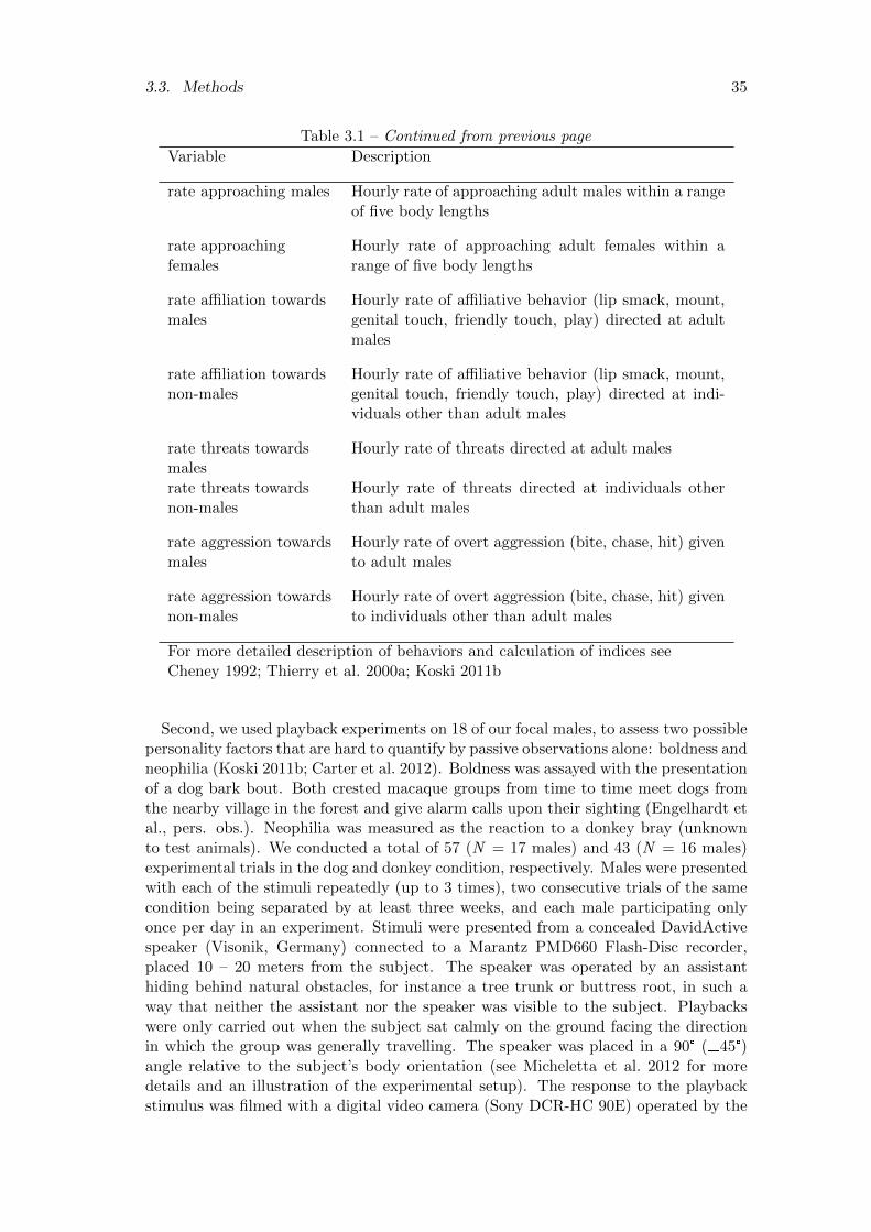
3.3. Methods 35
Table 3.1 – Continued from previous page
Variable Description
rate approaching males Hourly rate of approaching adult males within a rangeof five body lengths
rate approachingfemales
Hourly rate of approaching adult females within arange of five body lengths
rate affiliation towardsmales
Hourly rate of affiliative behavior (lip smack, mount,genital touch, friendly touch, play) directed at adultmales
rate affiliation towardsnon-males
Hourly rate of affiliative behavior (lip smack, mount,genital touch, friendly touch, play) directed at indi-viduals other than adult males
rate threats towardsmales
Hourly rate of threats directed at adult males
rate threats towardsnon-males
Hourly rate of threats directed at individuals otherthan adult males
rate aggression towardsmales
Hourly rate of overt aggression (bite, chase, hit) givento adult males
rate aggression towardsnon-males
Hourly rate of overt aggression (bite, chase, hit) givento individuals other than adult males
For more detailed description of behaviors and calculation of indices seeCheney 1992; Thierry et al. 2000a; Koski 2011b
Second, we used playback experiments on 18 of our focal males, to assess two possiblepersonality factors that are hard to quantify by passive observations alone: boldness andneophilia (Koski 2011b; Carter et al. 2012). Boldness was assayed with the presentationof a dog bark bout. Both crested macaque groups from time to time meet dogs fromthe nearby village in the forest and give alarm calls upon their sighting (Engelhardt etal., pers. obs.). Neophilia was measured as the reaction to a donkey bray (unknownto test animals). We conducted a total of 57 (N = 17 males) and 43 (N = 16 males)experimental trials in the dog and donkey condition, respectively. Males were presentedwith each of the stimuli repeatedly (up to 3 times), two consecutive trials of the samecondition being separated by at least three weeks, and each male participating onlyonce per day in an experiment. Stimuli were presented from a concealed DavidActivespeaker (Visonik, Germany) connected to a Marantz PMD660 Flash-Disc recorder,placed 10 – 20 meters from the subject. The speaker was operated by an assistanthiding behind natural obstacles, for instance a tree trunk or buttress root, in such away that neither the assistant nor the speaker was visible to the subject. Playbackswere only carried out when the subject sat calmly on the ground facing the directionin which the group was generally travelling. The speaker was placed in a 90° (±45°)angle relative to the subject’s body orientation (see Micheletta et al. 2012 for moredetails and an illustration of the experimental setup). The response to the playbackstimulus was filmed with a digital video camera (Sony DCR-HC 90E) operated by the
36 Chapter 3. Personality description
experimenter standing at a distance of about five meters from the subject. In eachexperimental condition, we used the same recording as stimulus during all trials. Wecan therefore not rule out that subjects habituated to the repeated presentations of thesame stimulus. Analytical methods, however, allow accounting for this possible bias inresults (see methods on adjusted repeatabilities below).
3.3.4 Data analysis
Behavioral data
We divided the overall data collection period into blocks of two months and calculatedfrequencies of behaviors, number of individuals in proximity and indices describingthe diversity of individuals in proximity and grooming partners in each of these timeblocks separately for each male (Table 3.1). There are two reasons for creating thesetime blocks. First, we wanted to assess temporal stability of our behavioral variables bycalculating repeatabilities and repeated measurements are needed for each individualto obtain this measure (Lessells and Boag 1987; Nakagawa and Schielzeth 2010). Sec-ond, group composition, particularly with respect to adult males, changed frequently(Chapter 2). Such an approach would lead to difficulties in the calculation of diversityindices, because in order to make these indices comparable they need to be standardizedby accounting for maximum number of potential interaction partners (Cheney 1992).
An individual data point was included if the cumulative observation time for a givenmale and time block was at least six hours. If necessary, the raw behavioral variableswere transformed (log, square root, arcsine) to achieve symmetric distributions. Vari-ables were then standardized to a mean of zero and a standard deviation of one. Sub-sequently, all variables were tested for repeatability (Lessells and Boag 1987; Nakagawaand Schielzeth 2010). We considered variables to be significant if the 95% confidenceinterval around their repeatability estimate did not include zero. Only significantlyrepeatable variables, i.e. variables that showed temporal stability, were subsequentlysubjected to factor analysis (see below). Repeatability estimates we present are well inthe range of other studies on primates and non-primates (e.g., Schuett and Dall 2009;Koski 2011b; David et al. 2012; Carter et al. 2012; Dammhahn and Almeling 2012).We tested the behavioral variables for group differences by means of Mann-Whitney Utests. One variable (number of female neighbors) differed significantly between the twostudy groups. Recalculating repeatability controlling for this group difference loweredthe repeatability estimate of this variable, but did not change its statistical significance.
Since factor analysis requires independent data, and our data structure consistedof repeated measurements of individuals, we averaged values of the two-month timeblocks to obtain single values for each male, thereby avoiding pseudo-replication. Thisprocedure resulted in a data set comprising 30 males, with at least one two-monthtime block during which a male was observed for at least six hours. The Kaiser-Meyer-Olkin measure of sampling adequacy (KMO = 0.60) indicated that our datawere suitable for factor analysis (Field et al. 2012), even though overall sample sizeand case-variable ratio were small. We performed our analysis using the correlationmatrix and a minimum residual solution. We decided to extract four factors basedon visual inspection of a scree plot and eigenvalues (Field et al. 2012). We used anoblique (type “oblimin”) instead of an orthogonal rotation to allow for factors to becorrelated (Budaev 2010). We chose this approach because there is no a priori reason
3.4. Results 37
to assume that personality factors are independent of each other (Field et al. 2012).To gauge the relative importance of the behavioral variables to the extracted factors,we used factor loadings (Field et al. 2012). For interpretation, we considered variablesthat loaded saliently (absolute value greater than 0.40) to contribute to a given factor(Field et al. 2012). If a variable loaded saliently on more than one factor we interpretedthis variable as contributing to the factor on which it loaded with the highest absolutevalue (e.g., Konecna et al. 2008).
Playbacks
Male responses to the playback stimuli from all experimental trials were coded fromvideotapes frame-by-frame by two coders, one being blind to study design and exper-imental condition. We discarded 19 experimental trials that were judged non-valid byboth coders, due to technical problems, or subject distraction. Response variable wasthe time subjects oriented themselves towards the speaker in the first 10 seconds af-ter the start of the stimulus presentation (hereafter: orientation duration) (Michelettaet al. 2012; Maciej et al. 2013). We considered such a response to occur when thesubject oriented its head towards or approached the speaker within an angle of about22.5°. We considered stronger responses, i.e. longer orientation durations, to indicatebolder and more neophilic males. Both raters expressed high agreement in the orienta-tion duration these responses had (Pearson correlation: r = 0.92, N = 81, p < 0.001).Average duration values from both coders were used in subsequent analyses. We calcu-lated adjusted repeatabilities (Radj , c.f. Nakagawa and Schielzeth 2010) controlling fortrial number within male subject and experimental condition to account for possiblehabituation effects. Since this algorithm does not permit confidence interval borders tobe smaller than zero, we used p-values to determine statistical significance (Nakagawaand Schielzeth 2010).
Finally, we computed correlations between the factors as well as between the factorsand the responses to the two experiments. For this we extracted regression scores fromthe factor analysis for those males that were also subjects in the playback experiments,i.e. N = 17 (dog condition) and N = 16 (donkey condition). For the experimental datawe used average male orientation durations (within each condition) for this calculation.We calculated Pearson correlation coefficients and since we had no specific hypothesesregarding possible relationships between personality factors, corrected the resulting p-values for multiple testing (Benjamini and Hochberg 1995). All analyses were conductedin R 2.15.0 (R Core R Development Core Team 2012) with the packages psych (Revelle2012) and rptR (Schielzeth and Nakagawa 2011).
3.4 Results
3.4.1 Behavioral data
The majority of the 22 behavioral variables were moderately repeatable, indicatingthat their expression was stable over time (Table 3.2). Five of the behavioral variableswe considered were not repeatable, from which four reflected behavior towards otheradult males: diversity of male neighbors (in close proximity) and the rates with whichother males were approached, threatened and aggressed. In addition, rates of affiliationdirected at individuals other than adult males, were not repeatable.

38 Chapter 3. Personality description
Table 3.2: Repeatabilities and confidence intervals of behavioral variables. Variables forwhich the confidence interval included zero (bold) were excluded from the subsequentfactor analysis.
behavior R CIl CIuprop time spent active 0.33 0.16 0.51prop time spent outside group 0.21 0.05 0.36rate self-grooming 0.30 0.13 0.47rate self-scratching 0.33 0.16 0.50rate yawning 0.48 0.31 0.65rate status display 0.70 0.57 0.83prop time spent grooming 0.20 0.04 0.35diversity grooming partners 0.16 0.02 0.31diversity grooming given 0.26 0.10 0.42number of female neighborsa 0.55 0.39 0.72diversity female neighbors (close) 0.20 0.05 0.35diversity female neighbors (far) 0.26 0.10 0.43diversity male neighbors (close) 0.10 -0.03 0.23diversity male neighbors (far) 0.23 0.07 0.39rate approaching males 0.09 -0.04 0.21rate approaching females 0.19 0.04 0.34rate affiliation towards non-males 0.12 -0.01 0.26rate affiliation towards males 0.16 0.02 0.31rate threats towards non-males 0.26 0.09 0.42rate threats towards males 0.01 -0.09 0.10rate aggression towards non-males 0.14 0.00 0.28rate aggression towards males -0.01 -0.10 0.08a after controlling for group differences: R = 0.14, CIl = 0.00, CIu = 0.27.
The factor analysis based on the remaining 17 repeatable variables explained 62%of the total variance. All variables loaded on at least one of the four factors withan absolute value of > 0.4 with six variables loading on two factors. The solution ofloadings of variables onto the extracted factors after oblimin rotation is presented inTable 3.3.
The first factor we extracted explained 21% of the variance with loadings of anxietyrelated behaviors (self-grooming, self-scratching). Additionally, males scoring higher onthis factor were less active, gave less dominance displays (loud calls) and approachedfemales more rarely. We labeled this factor Anxiety (Table 3.3).
The second factor explained 17% of variance and included variables that reflect di-versity of male and female neighbors (diversity of close female neighbors, diversity of farfemale neighbors, diversity of far male neighbors) and the diversity of female groomingpartners (female groomees). Additionally, this factor was related to smaller frequenciesof yawning and spending more time in the core of the group. We labeled this factorConnectedness (Table 3.3).
The third factor accounted for 13% of variance with variables reflecting general so-cial behavior, i.e. proportion of time spent grooming, diversity of grooming partners

3.4. Results 39
Tab
le3.
3:L
oad
ings
of
the
fou
rex
trac
ted
per
son
alit
yfa
ctor
saf
ter
obli
min
rota
tion
.O
nly
load
ings
wit
hab
solu
teva
lues
≥0.
40an
dco
mm
un
alit
ies
(h2)
are
rep
orte
d.
Val
ues
inb
rack
ets
wer
en
otin
terp
rete
das
bel
ongi
ng
toth
isfa
ctor
asth
eylo
aded
hig
her
ona
diff
eren
tfa
ctor
.
beh
avio
ral
vari
able
anxie
tya
con
nec
ted
nes
sso
ciab
ilit
yag
gres
sive
nes
sh2
pro
pti
me
spen
tact
ive
-0.8
90.
88
rate
self
-gro
omin
g0.
450.3
4ra
tese
lf-s
cratc
hin
g0.
900.8
4ra
test
atu
sd
isp
lay
-0.4
10.2
4ra
teap
pro
ach
ing
fem
ale
s-0
.74
(0.4
1)0.8
1p
rop
tim
esp
ent
ou
tsid
egro
up
(0.4
8)-0
.49
0.74
div
ersi
tyfe
male
nei
ghb
ors
(clo
se)
0.84
0.88
div
ersi
tyfe
male
nei
ghb
ors
(far)
0.77
0.6
1d
iver
sity
mal
en
eighb
ors
(far
)0.
44(0
.42)
0.49
div
ersi
tygr
oom
ing
giv
en(-
0.46
)0.
470.
48
rate
yaw
nin
g-0
.64
(0.4
6)0.
61
pro
pti
me
spen
tgro
om
ing
0.68
0.50
nu
mb
erof
fem
ale
nei
ghb
ors
(0.4
8)0.
55
0.5
6ra
teaffi
liati
on
tow
ard
sm
ales
-0.7
30.
55
div
ersi
tygr
oom
ing
par
tner
s0.
68
0.8
2ra
teth
reat
sto
war
ds
non
-male
s0.8
90.
80
rate
agg
ress
ion
tow
ard
sn
on-m
ales
0.6
40.
43
Eig
enva
lue
3.52
2.90
2.26
1.9
0P
rop
ort
ion
Vari
an
ceex
pla
ined
0.21
0.17
0.13
0.11
Cu
mu
lati
veV
aria
nce
exp
lain
ed0.
210.
380.
51
0.6
2
An
aly
sis
base
don
corr
elat
ion
mat
rix
(N=
30).
alo
adin
gsw
ere
refl
ecte
d.

40 Chapter 3. Personality description
Table 3.4: Pearson correlation coefficients between personality factors and the responsesto the donkey playback.
conn sociab aggr bold donkey
anxiety –0.19 –0.17 0.09 –0.39 –0.15connectedness 0.37 –0.07 –0.13 –0.04sociability 0.01 0.35 0.14aggressiveness –0.33 –0.39boldness 0.32
N = 17 for correlations with boldness, N = 16 for correlations withresponses to donkey playback, and N = 15 for correlation between bold-ness and responses to donkey playback.
in general, and number of female neighbors. Interestingly, positive (affiliative) behav-ior directed at adult males loaded negatively on this factor. We named this factorSociability (Table 3.3).
The fourth factor explained 11% of variance and reflected threat and overt aggressiondirected at individuals other than adult males. We labeled this factor Aggressiveness(Table 3.3).
3.4.2 Playback experiments
Males reacted to the dog stimulus in all of the 39 trials. In the donkey condition,males reacted in 36 trials, while no reaction of males was visible on the video tapesin 6 trials. We found significant repeatability in response to the dog condition (Radj
= 0.55, 95% CI: 0.20 – 0.63, p = 0.002). We therefore considered the responses tothis playback reflecting Boldness. In contrast, we did not find responses to the donkeycondition to be repeatable (Radj = 0.05, 95% CI: 0.00 – 0.27, p = 0.099) and thereforeconsider Neophilia to be absent.
3.4.3 Relationships between the factors
After controlling for multiple testing, we did not find any significant correlationbetween any pair of the four observationally assessed factors and the boldness factor(Pearson correlation coefficients, mean = –0.05, range = –0.39 – 0.37, p value range:0.047 – 0.940, ten pairwise comparisons, Table 3.4). In addition, we found no significantrelationship between any of these five factors and orientation duration in response tothe donkey playback (Pearson correlation coefficients, mean = –0.02, range = –0.39 –0.32, p value range: 0.131 – 0.877, five pairwise comparisons, Table 3.4).
3.5 Discussion
Our results on observational and experimental data suggest that crested macaquepersonality comprises five distinct and unrelated factors: Anxiety, Connectedness, So-ciability, Aggressiveness and Boldness (summarized in Table 3.5). This structure isgenerally similar to the structures observed in other macaque species (e.g., Weiss et al.2011; Konecna et al. 2012; Sussman et al. 2013). In addition, the structure our datasuggest is characterized by the presence of two distinct factors that reflect socio-positive

3.5. Discussion 41
Table 3.5: Summary of personality factors for crested macaque males. Descriptionsrefer to animals scoring high on the respective factor.
Personality factor Description
Anxiety High rates of self-directed behavior, reluctance to ap-proach females
Connectedness Diverse neighbor and grooming network, spatial positionin the core of the group
Sociability High rate of grooming, high number of female neighbors,diverse grooming network
Aggressiveness High rates of threats and aggression
Boldness Reacts strong towards threatening situation
behavior (Connectedness and Sociability). Most notably, we identified a factor, Con-nectedness, which, to our knowledge, has not been described in studies of primatepersonalities before, and which covers aspects of social network diversity, a feature thatmight be of particular importance in tolerant as opposed to despotic primate species.
Our study is focused on adult males because ultimately we are interested in the fitnessconsequences of personality among males. Given this, we cannot exclude the possibilitythat our description of the personality structure of crested macaques is incomplete.However, to our knowledge no empirical study so far has shown sex-specific differencesin personality structure within a species.
Anxiety, Aggressiveness and Sociability in our study matched factors that have beendescribed in previous studies of macaque personalities (Weiss et al. 2011; Konecna et al.2012; Sussman et al. 2013) and are widespread among other primate and non-primatespecies (reviewed in Gosling and John 1999; Freeman and Gosling 2010). Anxiety iscommonly used to describe general unease and distress (Weiss et al. 2011). That thefactor we name Anxiety reflects the individual degree of unease and distress in ourstudy species is evident through the loading of self-directed behavior onto this factor,which is a behavioral manifestation of physiological stress levels (Maestripieri et al.1992). In our study, males scoring high on Anxiety approached females less frequentlythan less anxious males. Anxiety might therefore reflect the reluctance or willingness ofmales to approach females, possibly mediated through general unease whilst in femaleproximity (see also Evers et al. 2011). In addition, our measure of general activity alsoloaded on the Anxiety factor. Similarly, in Barbary macaques, questionnaire items, i.e.adjectives to be rated by human observers, typically describing distress (e.g., tense,irritable, excitable) loaded on one single factor alongside items that describe generalactivity (active, lazy). Consequently, this factor has been labeled Activity/Excitabilityin this study (Konecna et al. 2012). We suggest, however, that Anxiety might in fact bethe more fitting label for crested and possibly also Barbary macaques since it capturesmore of an intrinsic feature as compared to Activity which may well be constrainedby external factors, such as the environment. For example, Barbary macaques are

42 Chapter 3. Personality description
more active (i.e. they rest less) when their home-range is covered with snow (Majoloet al. 2013). Given that Barbary macaques are also classified as relatively tolerant,this combination of anxiety and activity represented in only one personality factormight constitute a general feature of the more tolerant macaque species. In contrast,in despotic rhesus macaques both factors are distinct (Weiss et al. 2011, see also Koski2011b for this pattern in chimpanzees, Pan troglodytes).
In crested macaque males, the personality factor Aggressiveness covers threat be-havior and overt aggression directed at females, sub-adults, juveniles and infants. In-terestingly, aggressive behavior directed at adult male group members was not partof this factor. The reason for this was that rates of aggression towards adult maleswere not stable over time and hence not included into our factor analysis. As previ-ously mentioned, we observed frequent changes in composition as well as in dominancerelationships among adult males in our groups, whereas among adult females, groupcomposition and dominance hierarchy remained much more stable over the course ofour study (Chapter 2; Duboscq et al. 2013). It could be argued that temporal stabilityor instability in behavior is the consequence of a stable or instable social environment,and consequently, stable behavioral patterns may not reflect an intrinsic property (i.e.personality), but rather are the result of external constraints (Dingemanse et al. 2010;Koski 2011b). Therefore, the lack of repeatability in our study of aggression towardsother males may have been a consequence of these dynamics. Indeed, having a stereo-typic aggression rate towards other males regardless of the dynamics among adult malesmight be mal-adaptive in the sense that this might lead to costs imposed by overly fre-quent and possibly injuring aggression depending on how many males co-reside in thegroup.
Aggressiveness has also been found in other primate (including macaques) and non-primate species, but it is frequently labeled Confidence or Dominance in studies basedon observers’ ratings such as aggressive, bullying, dominant, submissive and confident(Capitanio 1999; Weiss et al. 2011; Konecna et al. 2012, but see Sussman et al. 2013).It often correlates with behaviorally assessed (agonistic) dominance ranks (Caine et al.1983; Mondragon-Ceballos and Santillan-Doherty 1994; Bolig et al. 1992; Konecna et al.2008, 2012). In studies of animal behavior, dominance is however considered a dynamicindividual property that changes over time due to external events (e.g., challenges byother individuals or migration) and which, in the strictest sense, is the property of asingle individual within a dyad where the other individual is subordinate at a giventime (Drews 1993)). Given the possible confusion with the term dominance as used inbehavioral biology (Drews 1993; Gosling and John 1999; see Capitanio (2011) for anillustrative example how such confusion between personality Dominance and behavioraldominance might easily arise) we suggest that the label of the Dominance facet ofprimate personality should be reevaluated. For rhesus macaques, for example, basedon the items that describe it (see above) the label Dominance could, in alignment withour study, be replaced by Aggressiveness. Such more consistent labeling of personalityfactors would facilitate inter-specific comparisons.
The final personality factor that crested macaques share with other macaques is So-ciability. This factor covers behavior that seems essential for building and maintainingsocial relationships with female group members, particularly the amount of grooming,the diversity of grooming partners and the number of female neighbors. Sociability
3.5. Discussion 43
as defined in our study, matches the Friendliness and Sociability components of othermacaque species’ personality structures (Capitanio 1999; Weiss et al. 2011; Konecnaet al. 2012; Sussman et al. 2013), in which it is associated with rating items like sociable,gentle and friendly (Weiss et al. 2011; Konecna et al. 2012).
In addition to the three above mentioned personality factors that appear to generallyoccur in macaques, we found a further personality factor in crested macaques, Con-nectedness. Interestingly, this factor in addition to Sociability also covers behavior inthe socio-positive domain. It describes the diversity of females which are groomed by aspecific male, the diversity of adult individuals in proximity to him and the time malesspend in the core of their social group. Connectedness has no obvious homologue inother macaque species. However, given the overall socio-positive notion of this factorwe speculate that in rhesus and Barbary macaques it may be part of the Friendlinessfactor. Consequently, whereas Friendliness (or Sociability) constitutes a single factorin some species, we find that in crested macaques, socio-positive behavior is reflectedin two distinct personality factors, Sociability and Connectedness.
Finding such an additional socio-positive dimension might be a consequence of thecomplex social network that individuals of tolerant macaque species, such as crestedmacaques, have as compared to individuals of more despotic species (Thierry 2007;Sussman et al. 2013). This wide network connecting also not related individuals showsthat relationships between group members are far less constrained than in despoticspecies where relationships are maintained predominantly within fixed kin networks(e.g., Berman and Thierry 2010; Micheletta and Waller 2012). Two possible ways inwhich scoring high on such a personality factor might thus be biologically adaptive(fitness increase) are through a more diverse network of allies that could provide sup-port in agonistic conflicts or through increased attractiveness to the opposite sex (e.g.,McDonald 2007; Sih et al. 2009; Kulik et al. 2012; Wilson et al. 2013). Further studieswill be necessary to determine whether Connectedness indeed has fitness benefits andwhether it is a general feature of socially tolerant primates such as crested macaques.
The final personality factor we identified in crested macaque males is Boldness as ev-idenced by repeatable reactions towards the auditory presentation of a threating stim-ulus. Boldness has rarely been studied in primates in general (Freeman and Gosling2010). Such a factor might however evolve under the selective pressure of predation,particularly in species in which predators are mobbed upon detection as is the casefor crested macaques on sight of reticulated pythons (Python reticulatus), their pre-sumed primary predator (Micheletta et al. 2012). Scoring high in Boldness could underthese circumstances not only help to roust the predator, but may also be used as apotentially costly signal of social status or as a means of attractiveness to potentialmating partners. In this sense, we cannot rule out the possibility that the compositionof the audience present during the playback trials influenced males’ reactions to thestimulus. Intuitively, crested macaque Boldness appears to be similar to the Confidencefactor found in other macaques. This notion is however rather speculative and basedon rating items used in questionnaire studies, such as fearful or timid (Weiss et al.2011; Konecna et al. 2012). At the same time, since we also consider our Aggressive-ness factor as equivalent to rhesus and Barbary Confidence, we would have to expecta salient positive correlation between crested macaque Boldness and Aggressiveness,which was absent. For now, we hypothesize that Boldness makes up a unique factor in

44 Chapter 3. Personality description
crested macaques, but cannot rule out that this is due to the different approaches withwhich we determined Boldness and Aggressiveness. Given the prevalence of Boldness innon-primate animals in general (Gosling 2001; Reale et al. 2007) and its hypotheticalabsence in primates (Freeman and Gosling 2010, but see Carter et al. 2012), futurestudies of primate personality should incorporate either items like bold into their ques-tionnaires or try to assess Boldness experimentally (Carter et al. 2012). This shouldclarify in how far Boldness constitutes an independent factor of primate personality, oris just a facet of some other factor, such as Aggressiveness or Confidence.
In agreement with most studies of macaques, we found no evidence for the existenceof a distinct Neophilia dimension (but see Openness with the items curious and in-ventive in rhesus macaques, Weiss et al. 2011). Neither did we observe any significantcorrelation between the response to our novelty experiments and any of the other fivepersonality factors. This absence is somewhat surprising, since a Neophilia/Explorationfactor (or the human equivalent Openness) is present in many animal species includingprimates (McGuire et al. 1994; Gosling and John 1999; Reale et al. 2007, see also Drea1998; Bergman and Kitchen 2009). However, the actual correlation coefficients of theplayback response with Aggressiveness and Boldness were modest, but not negligible(-0.39 and 0.32), suggesting that the absence of significant relationships in our studymight potentially have been a problem of statistical power or inappropriate stimuluschoice (Carter et al. 2012). In line with this possible overlap with other factors, studiesin other macaque species found rating items that describe Neophilia such as curiousor exploratory load on diverse factors such as Sociability (Mondragon-Ceballos andSantillan-Doherty 1994; Capitanio 1999), Friendliness (Weiss et al. 2011) or Activi-ty/Excitability (Stevenson-Hinde and Zunz 1978; Konecna et al. 2012). An alternativeexplanation for the absence of Neophilia may be related to the modality in which wepresented the stimulus. Macaques, as many primates, are vision-dominant, suggestingthat an auditory stimulus may be less likely to elicit consistent responses in our exper-imental setup. More studies are certainly needed to confirm or reject the absence ofNeophilia in macaques.
Based on our results, some tentative comparisons can also be made between macaqueand human personality in order to investigate the evolutionary roots of the currenthuman personality structure as posited in the Five Factor Model (Digman 1990;Weiss et al. 2011). The combination of the two socio-positive factors we found incrested macaques (Connectedness and Sociability) appear to match human Extraver-sion, whereas Aggressiveness may reflect the human Agreeableness vs. antagonism axis(Gosling and John 1999). Anxiety and, to a lesser degree, Boldness fit the descriptorsof human Neuroticism (Gosling and John 1999). In contrast, human Conscientiousnessand Openness appear not to be reflected in crested macaque personality as distinct fac-tors. Although crested macaque personality factors do not match perfectly with thoseof humans, our results shed important light onto the evolution of personality structureswithin the primate taxon.
Our attempt to directly link crested macaque with human personality structure ishowever a simplification of the hypothetical evolutionary scenario proposed to explainthe evolution of human personality structure from a macaque-like ancestor (Weiss et al.2011). Here we will use two examples to illustrate how incorporating data from ad-ditional species may help to formulate alternative hypotheses to explain the evolu-

3.5. Discussion 45
tionary history of personality structures. In their personality phylogeny using rhe-sus macaques as an outgroup to hominids, Weiss and colleagues (2011) suggest thatAnxiety and Activity are two distinct ancestral factors. Our data and recent workon Barbary macaques, however, allow an alternative scenario. In both Barbary andcrested macaques, a single factor describes a combination of Anxiety and Activity (la-beled Anxiety in crested macaques (see above) and Activity/Excitability in Barbarymacaques (Konecna et al. 2012)). Given that Barbary macaques represent the sistertaxon to all other extant macaque species (Morales and Melnick 1998; Li et al. 2009), itmay thus be that such a broader, singular Anxiety/Activity factor is the actual ances-tral state. In addition, the presence of a single Sociability factor in Barbary and rhesusmacaques may also represent the ancestral macaque state, whereas the occurrence of thetwo distinct factors we identified in crested macaques (Sociability and Connectedness)most likely is a derived feature. We therefore speculate that a hypothetical ancestorto macaques (and hominids) was characterized by a single Anxiety/Activity factor anda single Sociability factor, similar to present-day Barbary macaques (Konecna et al.2012).
Based on this suggested proto-macaque, we can formulate alternative hypotheses ofhow personality factors evolved in higher lineages. For example, according to a recentlyproposed scenario, the hominid Extraversion factor evolved from a combination of a“pure” Activity factor and a Sociability factor (Weiss et al. 2011). Our results, however,indicate the possibility that such a single Activity factor was not the ancestral stateof catarrhine primates. Hence, in order to evolve Extraversion in the hominid lineage(c.f. Weiss et al. 2011), a separation of our suggested ancestral Anxiety/Activity factorinto two distinct factors needs to occur, after the phylogenetic split of hominids andmacaques. With the currently available data, both scenarios are equally parsimoniousand only future studies that contribute more data will help to fully understand theevolution of primate personality structures.
Whereas a thorough treatment of the possible evolution of primate personalities iswell beyond the scope of this paper, we find overall support for the hypothesis of Weissand colleagues (2011) in that crested macaque personality structure resembles moreother macaque personality structures than hominid personalities. The comparativeapproach is thus surely a promising one and the more data points we acquire the clearerthe overall picture of personality evolution will become. In addition, more and moredata are being generated concerning neurobiological and endocrinological mechanismsunderlying personality variation (e.g., Young and Wang 2004; Anestis 2011; Higley et al.2011; Yokoyama and Onoe 2011). By integrating these approaches with ethological dataand with the recent progress in behavior genetics (e.g., Higley et al. 2011; Adams 2011),new avenues will open to study the evolutionary paths and selective pressures leading tothe striking variation in personality structures we observe across the animal kingdom.

46 Chapter 3. Personality description

Chapter 4
Personality factors predict futuremale dominance rank in a socialmammal
with
Muhammad Agil, Anja Widdig, Antje Engelhardt
Manuscript to be submitted.
47
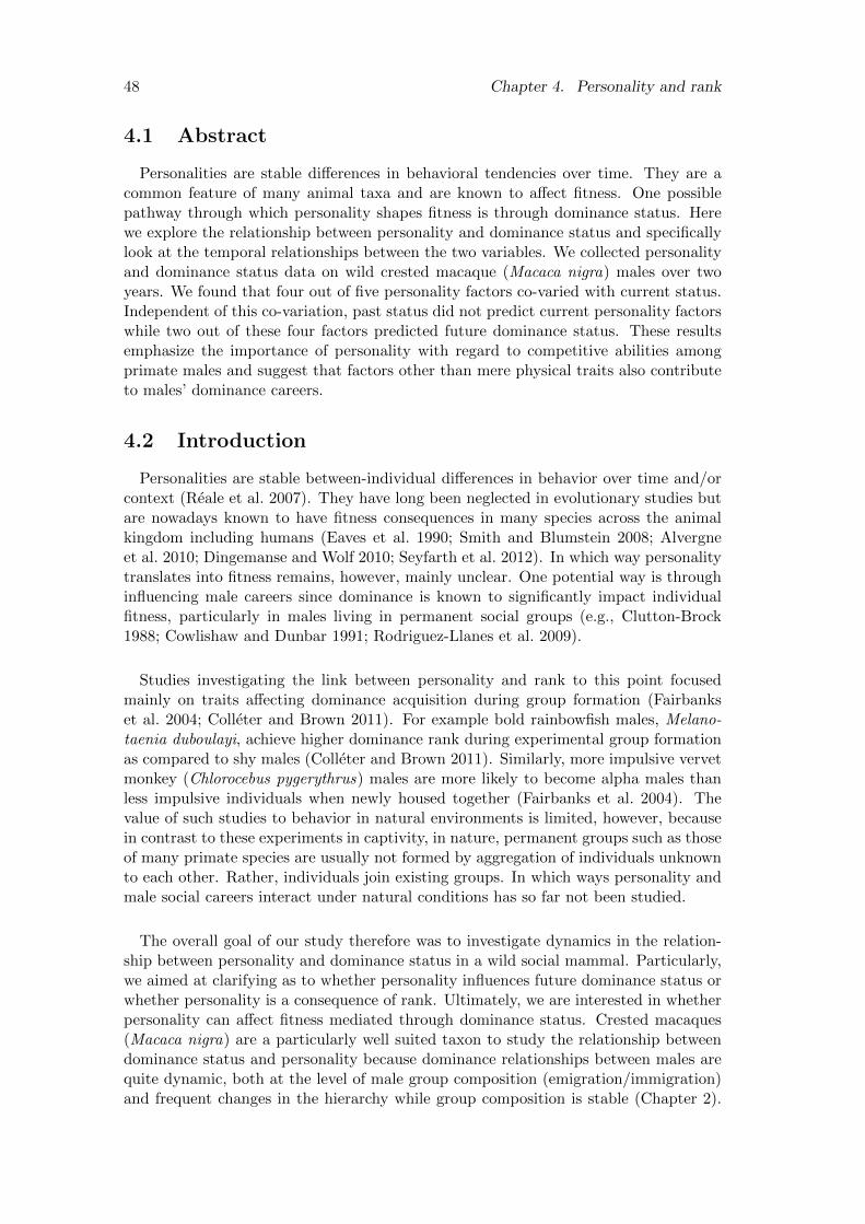
48 Chapter 4. Personality and rank
4.1 Abstract
Personalities are stable differences in behavioral tendencies over time. They are acommon feature of many animal taxa and are known to affect fitness. One possiblepathway through which personality shapes fitness is through dominance status. Herewe explore the relationship between personality and dominance status and specificallylook at the temporal relationships between the two variables. We collected personalityand dominance status data on wild crested macaque (Macaca nigra) males over twoyears. We found that four out of five personality factors co-varied with current status.Independent of this co-variation, past status did not predict current personality factorswhile two out of these four factors predicted future dominance status. These resultsemphasize the importance of personality with regard to competitive abilities amongprimate males and suggest that factors other than mere physical traits also contributeto males’ dominance careers.
4.2 Introduction
Personalities are stable between-individual differences in behavior over time and/orcontext (Reale et al. 2007). They have long been neglected in evolutionary studies butare nowadays known to have fitness consequences in many species across the animalkingdom including humans (Eaves et al. 1990; Smith and Blumstein 2008; Alvergneet al. 2010; Dingemanse and Wolf 2010; Seyfarth et al. 2012). In which way personalitytranslates into fitness remains, however, mainly unclear. One potential way is throughinfluencing male careers since dominance is known to significantly impact individualfitness, particularly in males living in permanent social groups (e.g., Clutton-Brock1988; Cowlishaw and Dunbar 1991; Rodriguez-Llanes et al. 2009).
Studies investigating the link between personality and rank to this point focusedmainly on traits affecting dominance acquisition during group formation (Fairbankset al. 2004; Colleter and Brown 2011). For example bold rainbowfish males, Melano-taenia duboulayi, achieve higher dominance rank during experimental group formationas compared to shy males (Colleter and Brown 2011). Similarly, more impulsive vervetmonkey (Chlorocebus pygerythrus) males are more likely to become alpha males thanless impulsive individuals when newly housed together (Fairbanks et al. 2004). Thevalue of such studies to behavior in natural environments is limited, however, becausein contrast to these experiments in captivity, in nature, permanent groups such as thoseof many primate species are usually not formed by aggregation of individuals unknownto each other. Rather, individuals join existing groups. In which ways personality andmale social careers interact under natural conditions has so far not been studied.
The overall goal of our study therefore was to investigate dynamics in the relation-ship between personality and dominance status in a wild social mammal. Particularly,we aimed at clarifying as to whether personality influences future dominance status orwhether personality is a consequence of rank. Ultimately, we are interested in whetherpersonality can affect fitness mediated through dominance status. Crested macaques(Macaca nigra) are a particularly well suited taxon to study the relationship betweendominance status and personality because dominance relationships between males arequite dynamic, both at the level of male group composition (emigration/immigration)and frequent changes in the hierarchy while group composition is stable (Chapter 2).

4.3. Results 49
Given these dynamics, we expect factors other than age or mere fighting ability to con-tribute to individual rank trajectories, and personality constitutes a promising aspectof individual characteristics to be involved (Sapolsky 1990; Gosling and John 1999).Finally, a link between personality and dominance status would also contribute to ourunderstanding of the mechanisms by which males achieve higher fitness, given that highstatus reflects increased mating and reproductive success for male crested macaques(Engelhardt et al. in prep; Reed et al. 1997; Higham et al. 2012; Engelhardt et al, un-published data). To address these questions, we studied free-ranging crested macaquemales at Tangkoko Nature Reserve on Sulawesi, Indonesia, living in two permanentgroups each comprising around 10 adult males and 20 adult females and totaling up to85 individuals (Neumann et al. 2010; Higham et al. 2012).
In a previous study (Chapter 3), we determined the personality structure of crestedmacaques by means of behavioral observations and playback experiments. Based onthe observational data we identified four distinct and independent factors: Anxiety,Connectedness, Sociability and Aggressiveness. Results from playbacks indicated anadditional Boldness factor. In the current study, we modeled the relationship betweenthese factors and dominance status. For the four observationally assessed factors wecreated two-month time blocks for which we extracted regression scores from the factorsolution for each male (Appendix F). In this way, we obtained 190 data points for eachpersonality factor from 30 males (median = 6.5, range 1 – 11 data points, i.e. timeblocks, per male). To model the response of Boldness we used individual responsesduring playback trials (Chapter 3), resulting in 39 data points from 17 males (median= 2, range 1 – 3 responses per male). To assess dominance status we used Elo-rating(Chapter 2; Albers and de Vries 2001). Elo-rating allows assigning each male a continu-ous rating at any given point in time and independent of changes in group composition(Chapter 2). For our analyses, we determined current male Elo-ratings on the datein the center of the two month time block or on the date an experimental trial wasconducted. With regard to our study question, we extracted Elo-ratings on two addi-tional dates: future and past rating refers to the Elo-rating 90 days after and beforethe current rating, respectively. Since using repeated ratings of the same individualsmay lead to collinearity in our models, we did not use true Elo-ratings but calculateddifferences between current ratings and future and past ratings, respectively.
Overall, we ran two sets of five linear mixed models each (Appendix F). The first setmodeled the five personality factors as a function of current Elo-rating and the ratingdifference between current and past ratings. The second set modeled the differencebetween future and current rating as a function of the personality factors and currentrating. Significance testing was done in a two-step approach. First, we used likelihoodratio tests (Quinn and Keough 2002) to determine whether the full model (includingall fixed and random effects) differed from a reduced model (only including age, therandom effects, an autocorrelation term if applicable (Appendix F) and trial numberin the Boldness models). Only if this step revealed that a full model differed from thecorresponding reduced model did we continue to assess significance of individual effects.
4.3 Results
The first set of linear mixed models revealed that none of the five tested personalityfactors was predicted by the difference between current and past rating. However, four

50 Chapter 4. Personality and rank
out of the five tested personality factors co-varied with current Elo-rating: higher ratedmales were less anxious, more connected, more aggressive and bolder (Table 4.1).
The second set of models revealed that scores of two personality factors predictedsubsequent rating changes. More connected and less anxious males achieved higherfuture Elo-ratings (after three months) than others (Table 4.2). This effect was in-dependent of the co-variation between current factor scores and current rating as wecontrolled for this relationship in the models (i.e. higher-rated males did not increaseor decrease stronger in ratings than lower-rated males).
4.4 Discussion
Our results demonstrate a relationship between dominance status and personalityfactors in males of a wild primate on two levels. Four personality factors, anxiety, con-nectedness, aggressiveness and boldness co-vary with current dominance status. Moreimportantly, independent of the co-variation between current rank and personality,anxiety and connectedness predict whether males will rise or decline in status in thefuture. We however did not find any evidence that personality is a consequence ofdominance status.
Most importantly, our models showed that specific personality factors predict futuredominance rank in male crested macaques. It has already previously been suggestedthat social competence might enable individuals to achieve higher future dominancestatus (McGuire et al. 1994). That is exactly what we find for crested macaque males,in which more connected males achieve higher future dominance status. The mecha-nism by which such a factor could work might be that adult male Old World monkeys,in contrast to females, usually cannot rely on relatives for support in their groups andtherefore need to establish a network of social partners in the groups they migrate into(Kulik et al. 2012). Of course, whether males that score high in connectedness alsoeffectively have more numerous or more diverse partners, for example in the context ofagonistic support, than individuals with lower scores remains to be examined. Inter-estingly, these results point to the possibility that the evolutionary roots of a similarphenomenon observed in humans can be found already in Old World monkeys. Ev-idence from humans shows that more connected males benefit from their networks,as more extraverted (the human personality factor that best reflects connectedness)men not only are more likely to be of high social status but also are more likely to bepolygynous and have more children (Alvergne et al. 2010).
The observation that also less anxious males increase their status might be relatedto physiology (Maestripieri et al. 1992; Capitanio 2004; Anestis 2011). In our case, lowanxiety might reflect a physiological profile that allows individuals that cope betterwith challenging and stressful situations in their social environment, such as increasedcompetition following male immigrations or the loss of an ally due to his emigrationor death. Such social instability has been shown to be stressful in terms of increasedfecal glucocorticoid excretion (Gesquiere et al. 2011). Less anxious individuals may bebetter adapted to cope with such unpredictability (Sapolsky and Ray 1989) and theassociated costs of long-term elevated glucocorticoid levels (Sapolsky 2005). Again,these results hint to the evolutionary roots of similar behavior found in humans, where
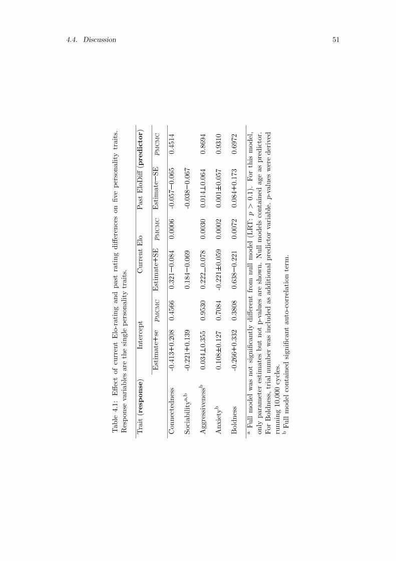
4.4. Discussion 51
Tab
le4.
1:E
ffec
tof
curr
ent
Elo
-rat
ing
and
pas
tra
tin
gd
iffer
ence
son
five
per
son
alit
ytr
ait
s.R
esp
on
seva
riab
les
are
the
sin
gle
per
son
alit
ytr
aits
.
Tra
it(r
esp
on
se)
Inte
rcep
tC
urr
ent
Elo
Past
Elo
Diff
(pre
dic
tor)
Est
imate±
sepMCMC
Est
imat
e±S
EpMCMC
Est
imate±
SE
pMCMC
Con
nec
ted
nes
s-0
.413±
0.20
80.
4566
0.32
1±
0.08
40.
0006
-0.0
57±
0.065
0.451
4
Soci
ab
ilit
ya,b
-0.2
21±
0.13
90.
184±
0.06
9-0
.038±
0.067
Aggre
ssiv
enes
sb0.0
34±
0.35
50.
9530
0.22
2±0.
078
0.00
300.0
14±
0.0
64
0.869
4
An
xie
tyb
0.108±
0.1
270.
7084
-0.2
21±
0.05
90.
0002
0.001±
0.057
0.9
310
Bol
dn
ess
-0.2
66±
0.33
20.
3808
0.63
8±
0.22
10.
0072
0.084±
0.173
0.6
972
aF
ull
mod
elw
as
not
sign
ifica
ntl
yd
iffer
ent
from
nu
llm
od
el(L
RT
:p>
0.1).
For
this
mod
el,
only
par
amet
eres
tim
ates
bu
tn
otp
-val
ues
are
show
n.
Nu
llm
od
els
conta
ined
age
as
pre
dic
tor.
For
Bold
nes
s,tr
ial
nu
mb
erw
asin
clu
ded
asad
dit
ion
alp
red
icto
rva
riab
le.p-v
alu
esw
ere
der
ived
run
nin
g10
,000
cycl
es.
bF
ull
mod
elco
nta
ined
sign
ifica
nt
auto
-cor
rela
tion
term
.

52 Chapter 4. Personality and rank
Tab
le4.2:
Eff
ectof
five
person
alitytraits
ond
ifferen
cesb
etween
curren
tan
dfu
ture
Elo-ratin
gs.
Trait
(pre
dic
tor)
Intercep
tC
urren
tE
loF
utu
reE
loDiff
(resp
on
se)
Estim
ate±
sepMCMC
Estim
ate±
SE
pMCMC
Estim
ate±
SE
pMCMC
Con
nected
ness
0.250±
0.1170.2610
-0.095±
0.0650.1194
0.174±
0.0690.0142
Sociab
ilitya
0.237±
0.119-0.052
±0.063
0.070±
0.063
Aggressiven
essa
0.216±
0.118-0.049
±0.065
0.042±
0.066
An
xiety
0.222±
0.1160.4474
-0.065±
0.0620.2096
-0.143±
0.0610.0146
Bold
ness
a0.2
50±
0.459-0.460
±0.328
0.269±
0.181
aF
ull
mod
elw
as
not
signifi
cantly
diff
erent
fromnu
llm
odel
(LR
T:p>
0.1).F
orth
esem
od
els,on
lyp
ara
meter
estimates
bu
tn
otp-valu
esare
show
n.
Nu
llm
od
elscon
tained
ageas
pred
ictor.F
orB
oldn
ess,trial
nu
mb
erw
asin
clud
edas
add
itional
pred
ictorvariab
le.p-valu
esw
ered
erived
run
nin
g10,00
0cy
cles.

4.4. Discussion 53
more neurotic men are more likely to be of higher social status compared to less neuroticmen (Alvergne et al. 2010).
The above mentioned hypotheses on how personality might influence future successboth relate to male-male competition, and might therefore be under intra-sexual se-lection: higher status, whether current or future, translates into higher mating andreproductive success (Higham et al. 2012; Engelhardt et al. in prep; Engelhardt et al.,unpublished data). An additional, not necessarily mutually exclusive, mechanism bywhich personality might be beneficial for fitness is in the context of female mate choice.Numerous studies have shown female preferences of certain personalities (Schuett et al.2010). For example, female guppies (Poecilia reticulata) prefer brightly colored malesas mates (Godin and Dugatkin 1996). Incidentally, coloration correlates with boldnessin these fish, and when the two traits were experimentally decoupled, females exhib-ited a preference for bolder males regardless of their coloration (Godin and Dugatkin1996). Females therefore can use personality as proxy for male quality including maleabilities/genes to achieve higher (future) status. This might particularly be the casefor traits for which the expression bears costs. Obviously, being bold in the context ofpredator deterrence bears potentials costs related to survival whereas highly connectedmales might be prone to increased risk of diseases transmission. Showing preferencesfor such males ensures females’ offspring being equipped with good genes. In species,like crested macaques, in which female mate choice is likely to be limited given high-ranking males monopolize access to fertile females to a high degree (Engelhardt et al. inprep; Engelhardt et al., unpublished data), female preferences for certain personalitiesmight still manifest themselves by females being more cooperative during male mate-guarding, i.e. females may try less escaping monopolization from males with preferredpersonality than from males with non-preferred personality. Finally, females could usethe assessment of male personalities to ensure reproducing with partners of opposingpersonality, in order to achieve assortative matings. This strategy has been found ingreat tits, Parus major, in which pairs of opposing expression of a particular personal-ity factor had higher reproductive success than pairs with similar expression of a factor(Both et al. 2005). These arguments point to possible links between personality andfitness independent of dominance status as mediator.
Our results are also important for the discussion on whether dominance itself consti-tutes a personality factor. Our data show that personality is not a consequence of dom-inance status, though we found co-variation between personality factors and concurrentstatus. This questions the validity of dominance as part of personality. Dominance asa personality factor has been described for great apes and rhesus macaques (Macacamulatta), but not for humans (King and Figueredo 1997; Weiss et al. 2011, 2013). Fromthis arises the hypothesis that dominance is a personality factor that developed earlyon in primate evolution, but merged with extraversion in humans after chimpanzeesand humans split (Weiss et al. 2011). The notion that such a separate dominancepersonality factor exists in non-human primates however seems unlikely. In many situ-ations, dominance status follows fairly predictable trajectories over an individual’s life(Sprague et al. 1998). For example, in rhesus macaques, males usually attain higherrank by passively queuing, i.e. they rise in rank as a consequence of individuals abovethem in the hierarchy leaving or dying (Missakian 1972; Drickamer and Vessey 1973).Further, dominance status often is not even predictable in such general terms and is theoutcome of dynamics in social relationships between individuals (Chase et al. 2002).

54 Chapter 4. Personality and rank
Yet, personality is, by definition, a temporally stable attribute, even though it maychange over life (Roberts et al. 2006). It seems far more likely that dominance statusis, at least partly, the consequence of personality and that in this sense personality fea-tures may predict strategies individuals follow to maximize their fitness (van Noordwijkand van Schaik 2004; Wolf et al. 2007).
We are at the beginning of understanding the mechanisms by which consistent dif-ferences in behavior (i.e. personalities) contribute to differential fitness in animals,departing from the notion that behavioral tendencies merely vary around an adaptiveaverage. Our results demonstrate that male social careers can be shaped by more thanintrinsic/individual factors such as physical condition, age or aggression. In line withthese thoughts, we speculate that in general, certain personality factors equip maleswith abilities to maintain their status whereas other factors give males advantages inachieving higher future status. As such, personality can also contribute and is likely tointeract with other behavioral, physical and physiological traits to the rank trajectoriesthat males follow and ultimately result in differential fitness outcomes.

Chapter 5
Coalitions and dominance rank inwild male crested macaques(Macaca nigra)
with
Muhammad Agil, Antje Engelhardt, Anja Widdig
Manuscript to be submitted.
55
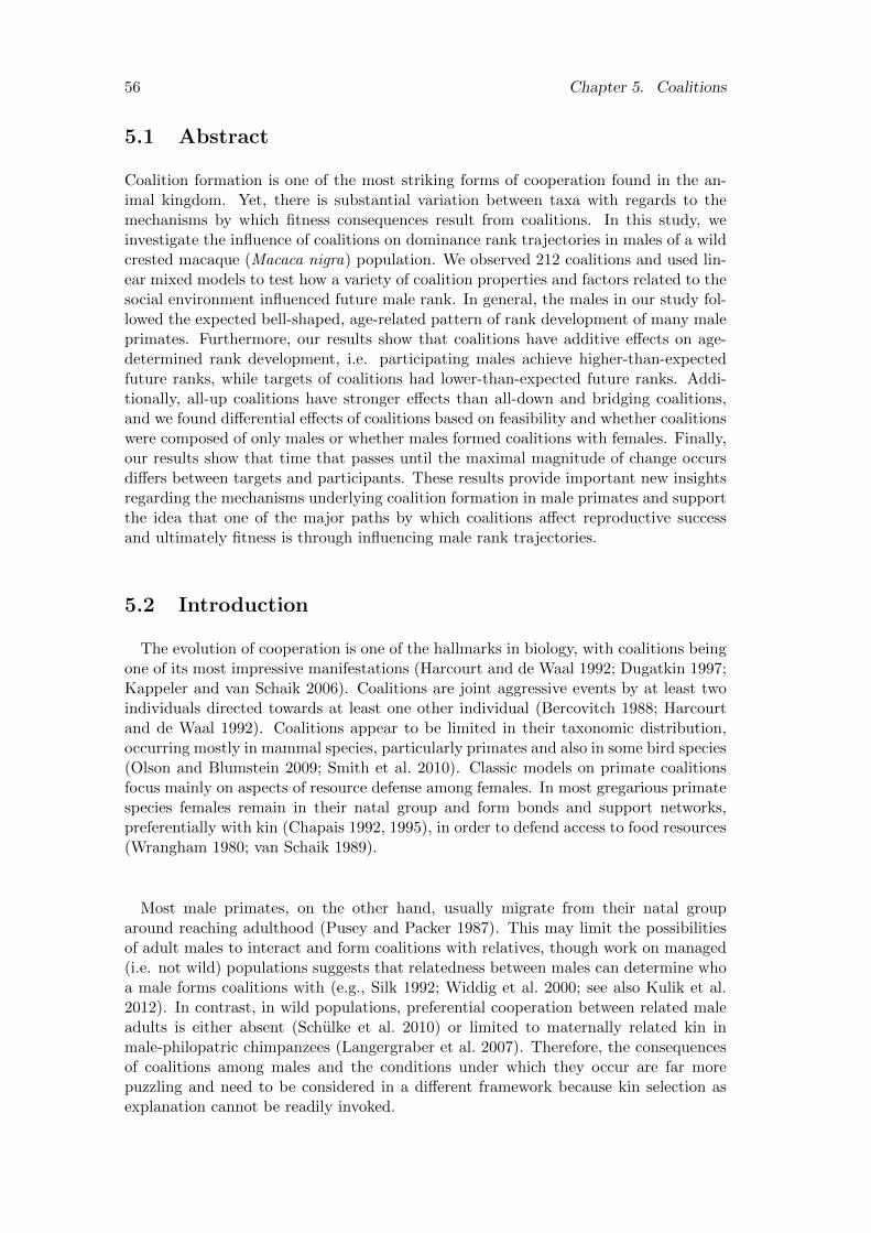
56 Chapter 5. Coalitions
5.1 Abstract
Coalition formation is one of the most striking forms of cooperation found in the an-imal kingdom. Yet, there is substantial variation between taxa with regards to themechanisms by which fitness consequences result from coalitions. In this study, weinvestigate the influence of coalitions on dominance rank trajectories in males of a wildcrested macaque (Macaca nigra) population. We observed 212 coalitions and used lin-ear mixed models to test how a variety of coalition properties and factors related to thesocial environment influenced future male rank. In general, the males in our study fol-lowed the expected bell-shaped, age-related pattern of rank development of many maleprimates. Furthermore, our results show that coalitions have additive effects on age-determined rank development, i.e. participating males achieve higher-than-expectedfuture ranks, while targets of coalitions had lower-than-expected future ranks. Addi-tionally, all-up coalitions have stronger effects than all-down and bridging coalitions,and we found differential effects of coalitions based on feasibility and whether coalitionswere composed of only males or whether males formed coalitions with females. Finally,our results show that time that passes until the maximal magnitude of change occursdiffers between targets and participants. These results provide important new insightsregarding the mechanisms underlying coalition formation in male primates and supportthe idea that one of the major paths by which coalitions affect reproductive successand ultimately fitness is through influencing male rank trajectories.
5.2 Introduction
The evolution of cooperation is one of the hallmarks in biology, with coalitions beingone of its most impressive manifestations (Harcourt and de Waal 1992; Dugatkin 1997;Kappeler and van Schaik 2006). Coalitions are joint aggressive events by at least twoindividuals directed towards at least one other individual (Bercovitch 1988; Harcourtand de Waal 1992). Coalitions appear to be limited in their taxonomic distribution,occurring mostly in mammal species, particularly primates and also in some bird species(Olson and Blumstein 2009; Smith et al. 2010). Classic models on primate coalitionsfocus mainly on aspects of resource defense among females. In most gregarious primatespecies females remain in their natal group and form bonds and support networks,preferentially with kin (Chapais 1992, 1995), in order to defend access to food resources(Wrangham 1980; van Schaik 1989).
Most male primates, on the other hand, usually migrate from their natal grouparound reaching adulthood (Pusey and Packer 1987). This may limit the possibilitiesof adult males to interact and form coalitions with relatives, though work on managed(i.e. not wild) populations suggests that relatedness between males can determine whoa male forms coalitions with (e.g., Silk 1992; Widdig et al. 2000; see also Kulik et al.2012). In contrast, in wild populations, preferential cooperation between related maleadults is either absent (Schulke et al. 2010) or limited to maternally related kin inmale-philopatric chimpanzees (Langergraber et al. 2007). Therefore, the consequencesof coalitions among males and the conditions under which they occur are far morepuzzling and need to be considered in a different framework because kin selection asexplanation cannot be readily invoked.

5.2. Introduction 57
A decade ago, a formal model which aims at explaining under which conditionscoalitions among primate males should occur and what fitness consequences of coali-tions are to be expected was introduced by van Schaik and colleagues (Pandit and vanSchaik 2003; van Schaik et al. 2004, 2006; from here on: PvS model). Two mecha-nisms by which coalition partners increase their fitness are distinguished in the PvSmodel. First, at least one of the partners increases in rank, therefore benefitting inthe long-term assuming that higher rank translates into higher reproductive success.Furthermore, though not explicitly considered in the PvS model, a rank increase couldalso be achieved by forming mixed-sex coalitions, in which males form coalitions withfemales (Chapais 1983; Datta 1983). Second, coalitions among males may serve a level-ing function in the sense that by targeting and displacing a male from monopolizing afertile female at least one of the partners gains direct mating access to a fertile female.Whether these mechanisms are mutually exclusive is unknown, but it is possible thatleveling coalitions could increase the ranks of participants in the long-term in additionto being beneficial immediately.
There is some evidence that in both ways coalitions can have fitness consequences formale primates. For example, in baboons (Papio cynocephalus) and Barbary macaques(Macaca sylvanus), leveling of mating distributions occurs and appears to be a fre-quently used strategy to increase mating success (Young et al. 2013; Bercovitch 1988;Noe and Sluijter 1990; Bissonnette et al. 2009b). In contrast, beyond several casestudies (e.g., Nishida 1983; Higham and Maestripieri 2010), we know surprisingly lit-tle about whether male coalitions influence the dominance ranks of males involved incoalitions. While Silk (1993) found no evidence that coalition rates influenced futuredominance rank in bonnet macaque males (Macaca radiata), two more recent studieson Assamese macaque and chimpanzee males indicate such a link. Gilby and colleagues(2013) suggest that chimpanzee (Pan troglodytes) coalition rates over the course of two-year periods increase the likelihood of rising in rank in the subsequent two-year period.In their study on Assamese macaque males, Schulke and colleagues (2010) found sim-ilar results, suggesting that males with higher coalition rates in a given time period(where time periods were defined “based on changes in male dominance hierarchy”, p.2207) achieved high dominance rank in subsequent time periods. In both these studies,dominance rank also translated into higher reproductive success, suggesting that malesutilize coalitions to ultimately increase their fitness.
An important characteristic determining whether coalitions can have rank-changing(or leveling) effects is coalition configuration, i.e. the relative ranks of target andparticipants. In all-up coalitions (“revolutionary”, c.f. Chapais 1995), all coalitionparticipants rank below the target, whereas in the bridging configuration at least onepartner ranks above the target while at least one partner ranks below. Both configura-tions are profitable (c.f. van Schaik et al. 2006) in the sense that at least one participantbenefits in ways that would not be available to him if he were on his own. In contrast,in all-down coalitions (the third possible configuration, “conservative”, c.f. Chapais1995), neither of the coalition partners can profit per se from the coalition (c.f. vanSchaik et al. 2006; but see below). All partners are already higher ranking than thetarget and can therefore displace males from access to females on their own withoutthe cooperation of a coalition partner (see also Young et al. in press).

58 Chapter 5. Coalitions
In order to predict which combination of the two beneficial configurations (all-upand bridging) and whether coalitions work in a leveling or rank-changing fashion, thePvS model utilizes a single predictive parameter, beta. Beta is the degree of despotismamong males (Pandit and van Schaik 2003) and reflects the level of competition betweenmales for access to fertile females. At its highest value, 1, the highest ranking maleis able to monopolize all fertilizations, whereas towards its lowest value, 0, contestcompetition transforms into pure scramble competition where all males are equallylikely to achieve fertilizations. For instance, in situations with moderate to high betathe PvS model predicts that coalitions should be generally rank-changing and not leadto leveling. At moderate beta, coalitions should be of the all-up configuration wherevery high-ranking (generally the highest-ranking) males are targeted by other high-ranking males ranking just below the target. At high beta, bridging coalitions areexpected in which the highest ranking male (e.g., 1st) together with other high-rankingmales (e.g. 3rd rank) targets another high-ranking male (e.g. 2nd). The PvS modeladditionally predicts that under moderate to high beta values coalitions are expected tobe small and to consist of two or three participants. How to actually measure beta andwhether beta is a static species property or a dynamic attribute that changes alongsidefluctuations in, for example, number of group males or level of reproductive synchronyamong females is still debated (Young et al. in press; van Schaik et al. 2006).
One crucial assumption the PvS model makes is that coalitions need to be feasible,i.e. the combined competitive abilities of the participants need to exceed those ofthe target (van Schaik et al. 2006). The straight-forward approach as suggested by vanSchaik and colleagues (2006, see also Noe and Sluijter 1995) is simply to sum individualcompetitive abilities, though synergetic effects might be possible (Noe 1994). A recentstudy by Bissonnette and colleagues (2009a) suggests that cardinal rank scores, incontrast to ordinal ranks, might have the desired properties to measure feasibility ofcoalitions (see also Chapter 2; Balasubramaniam et al. 2013). With such an approachit becomes possible to distinguish between configurations that are differentially feasibleon a continuous scale. For instance an all-up coalition could be highly feasible if the2nd and 3rd ranking males team up against the 1st rank as compared to 5th and 6th
rank teaming up against the 1st rank (less, if at all, feasible).
Partly because they are always feasible by definition, all-down coalitions are con-sidered as not directly beneficial by the PvS model and are therefore not includedas meaningful coalition type. They have been hypothesized to constitute a counter-strategy employed to prevent all-up and bridging coalitions from occurring (Chapais1995; van Schaik et al. 2006; see Kutsukake and Hasegawa (2005) for an illustrativecase study). However, all-down coalitions can also be directly beneficial if they functionto maintain the ranks of the participants. Empirical evidence for coalitions functioningin such a way to maintain the existing rank order comes from a study on male Tibetanmacaques (Berman et al. 2007, see also Widdig et al. 2000).
As became clear, coalitions are usually studied from the perspective of the cooper-ating individuals, i.e. participants. Following this, there appears to be a predominantdisposition to investigate positive or neutral consequences, i.e. do participants of coali-tions rise or maintain their rank. Though implicit in this approach are the consequencesfor targets (whenever somebody rises in rank someone else needs to drop), such effects

5.3. Methods 59
have, to our knowledge, never been explicitly studied from the perspective of coalitiontargets.
We also know little about the temporal aspects of coalition consequences. The effectsof leveling coalitions are predominantly immediate, i.e. they lead to immediate matingaccess for at least one of the coalition partners. In contrast, the question of whichtime-frame rank-changing coalitions work in has, to our knowledge, never been directlyasked. Researchers usually select time units whose relevance in terms of dominance rankdynamics for the species studied are mostly unclear. In the empirical studies mentionedso far, the rank-changing consequences of coalitions were measured over time periodsranging in duration from one month to two years. Though case studies suggest thatthese rank-changing effects can also occur within a very short time (e.g., Nishida 1983;Higham and Maestripieri 2010), systematic data on this important aspect of coalitionsare lacking.
Here, we study coalitions in crested macaques (Macaca nigra), a species in which themajority of matings during fertile periods of females is monopolized by alpha males(63.5%, Engelhardt et al. in prep). Based on this, we consider crested macaques tohave a moderate to high beta value (c.f. Pandit and van Schaik 2003; van Schaik et al.2006), and therefore expect coalitions to be rank-changing, but refrain from predictingthe predominant configuration. An additional property of this species which makes itinteresting to study coalitions and its effects on rank is that the adult male cohort ishighly dynamic, both at the level of rank relationships and composition (Chapter 2).
The overall goal of this study was therefore to investigate the effects of coalitionson male dominance trajectories in a species with highly dynamic rank relationships.The first specific objective was to describe general patterns of coalition formation.Our second objective was to test the effects of coalition characteristics on subsequentchanges in dominance status of both, participants and targets of coalitions. Here, wespecifically investigated sex-composition, configuration, feasibility and time frame.
5.3 Methods
5.3.1 Study Site
We studied two groups, R1 and PB, of wild crested macaques in the Tangkoko NatureReserve, Sulawesi, Indonesia between March 2009 and May 2011 (Neumann et al. 2010;Duboscq et al. 2013). Each group comprised up to 85 individuals, with the numberof adult males being present at any given time ranging between 7 and 18. All ani-mals of both groups were completely habituated to human observers and adult malesand females were individually recognizable based on facial features and natural bodymarkings, e.g., scars or broken limbs.
5.3.2 Behavioral Data
We collected behavioral data using focal animal sampling (Altmann 1974) of 37 adultmales (mean = 66.1h, range = 0.6 – 130.0h per male, total = 2447.2h). Focal protocolslasted up to 60 minutes during which continuous data on aggressive behavior andinteraction partner identities were recorded. We defined a coalition as simultaneously

60 Chapter 5. Coalitions
occurring aggression by at least two individuals (participants) directed towards at leastone male (target) upon which the target left or fled the participants. This definitionincludes the possibility that males and females form mixed-sex coalitions. Note thattargets were always male as was at least one of the participants. Coalitions could alsotarget more than one individual, however, since we never observed such coalitions (seeresults), our operationalization of coalitions is restricted to single targets.
Since rates with which we observed coalitions during focal animal sampling weresmall compared to other studies on male macaques we supplemented our data set withad libitum observations of coalitionary events. Note however, that this does not implythat we saw all coalitionary events taking place within the group. The habitat wasgenerally dense and groups often were spread over more than 100 m (pers. obs.).Therefore, rates of participation in and being targeted by coalitions are based on focalanimal data, whereas our main analyses are based on single coalitionary events as unitof analysis (see below).
5.3.3 Variables
Current rank, future rank and time distance
We measured rank by calculating Elo-ratings that were based on decided dyadicconflicts and displacements (Chapter 2; Albers and de Vries 2001). In brief, aftereach dyadic dominance interaction, the Elo-rating procedure updates the ratings ofthe two individuals involved in way that the winner receives points whereas the loser’spoints decrease. The amount of points that are won and lost depends on the expectedinteraction outcome. This expected outcome is based on the rating difference beforethe interaction took place. The basic idea being that if a strong individual wins againsta weak one (as expected based on their rating difference), the winner will gain only fewpoints while the loser loses little. If, against such an expectation, a weaker individualwins against a stronger one the points received and lost will be relatively more. Inthis way, ratings of individuals are updated after each single interaction, allowing forfine-tuned monitoring of rank over time (for more details see Chapter 2). For thepurpose of this study, we used ratings at the end of a given observation day, i.e. if anindividual was observed in more than one dyadic interaction on a given day, that day’srating is the one after the last observed interaction. Note also, none of the interactionsconsidered as coalitions contributed to Elo-rating estimation. Elo-ratings have severaladvantages over commonly used dominance indices (Chapter 2). With respect to ourstudy the most important of these advantages are that (1) ratings are continuouslyupdated, which allows estimation of dominance status on small time scales (in our caseon a daily basis), (2) ratings are on an interval scale, i.e. differences between ratingsare meaningful, and (3) ratings are not affected by changes in the group composition.The parameter k was set to 100 for all Elo-rating calculations (Chapter 2).
Current rank of a male was defined as his Elo-rating on the date of the observedcoalition. Future rank was calculated at time steps of 10 days following the coalitionup until 120 days (see data organization, below). This time distance variable wasintroduced in order to investigate in which time frame coalitions have an effect (seebelow for how data were organized). We decided to set the upper limit of the time frameto be considered at about four months (i.e. 120 days) because first, previous studieson male macaques indicated that such effects are expected to occur in the magnitude

5.3. Methods 61
of months (e.g., Silk 1993; Schulke et al. 2010), and second, since we consider singleevents and not rates of coalitions over observation time we expect changes to occur onrelatively small time scales.
We only used ratings that were updated within a maximum of five days from thedate in question (including the date of the interaction itself). This ensures that if arating from a male is identical to the one at the time step before, this is not due to thismale not having been observed during a recent dyadic dominance interaction. In thisway, also cases were excluded if a male emigrated from the group or died and thereforeno current rating was available.
Finally, in order to present results that can be compared to the predictions of thePvS model with regards to what ranks targets and participants held, we transformedElo-ratings into ordinal ranks. For this, we simply ordered the Elo-ratings of all malespresent in the group on the day a coalition occurred and assigned the male with thehighest Elo-rating rank 1, the male with the second-highest rating was assigned rank2, and so on.
Role
Individuals were either targets (victims) of coalitions or participated in aggressiondirected at a target (participants).
Composition
All coalitions considered here were directed at single male targets. Based on the sexcomposition of the participants, we distinguished between mixed (at least one femaleparticipant) and pure (no female participant) types of coalitions.
Configuration
We classified pure (all-male) coalitions into one out of three configurations. Coalitionswere considered all-down (all participants had higher Elo-ratings than the target), all-up (all participants had lower Elo-ratings than the target), or bridging (at least oneparticipant had a higher Elo-rating than the target and at least one participant hada lower Elo-rating than the target). Even though it is theoretically possible to applythe pattern of three configurations also to mixed coalitions we refrained from this.Despite having data to create separate hierarchies for the sexes our data are likelybiased (particularly with regards to ad-libitum sampling) to intra-sexual interactionswhich might lead to less reliable estimation of a mixed-sex hierarchy. Additionally,we refrained from working under the assumption that all adult females rank below alladult males.
Feasibility
For pure male coalitions we calculated feasibility as the difference between the sum ofElo-ratings of all participants and the Elo-rating of the target, as measured on the dayof the coalition (for a comparable continuous assessment of “asymmetry in strength”see Bissonnette et al. 2009a). Prior to this calculation we standardized ratings in sucha way that the highest rating of all males present that day was set to 1 and the lowestto 0 while keeping differences between these standardized ratings proportional to the
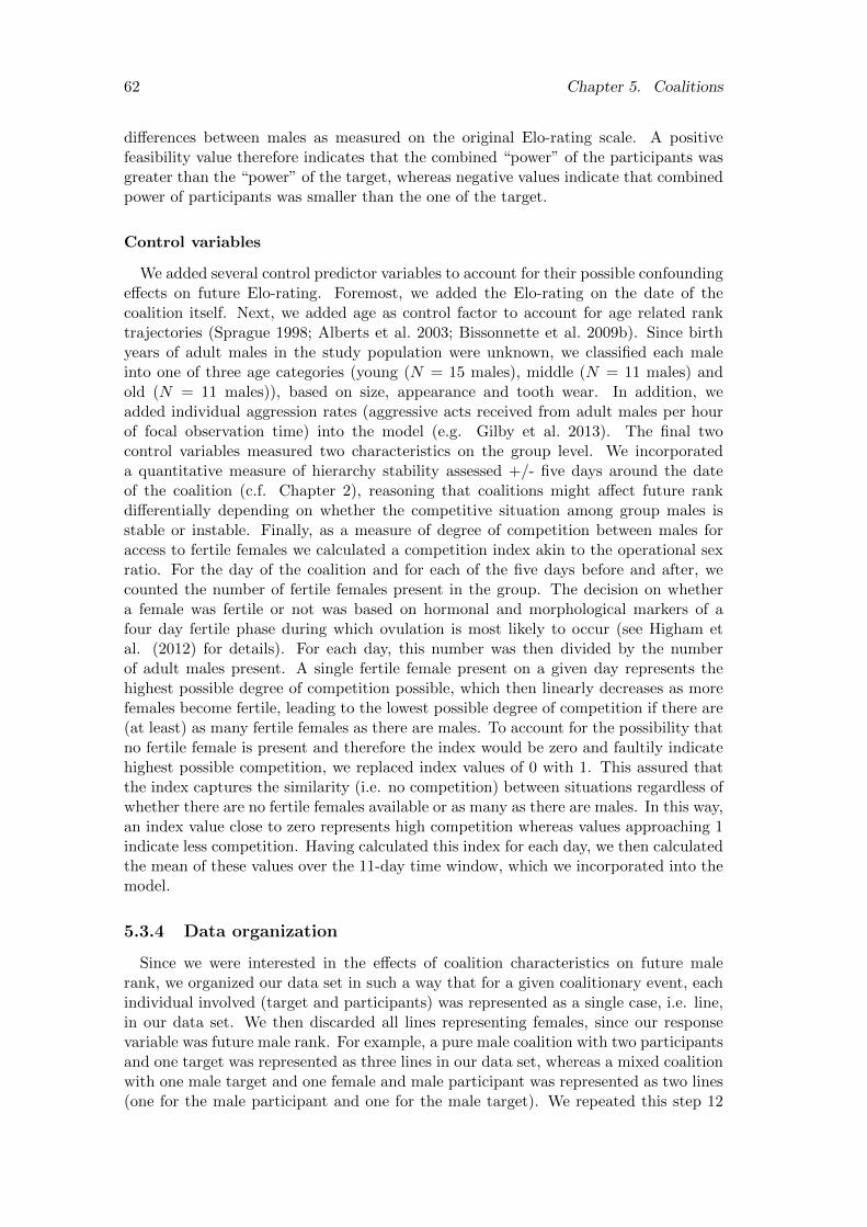
62 Chapter 5. Coalitions
differences between males as measured on the original Elo-rating scale. A positivefeasibility value therefore indicates that the combined “power” of the participants wasgreater than the “power” of the target, whereas negative values indicate that combinedpower of participants was smaller than the one of the target.
Control variables
We added several control predictor variables to account for their possible confoundingeffects on future Elo-rating. Foremost, we added the Elo-rating on the date of thecoalition itself. Next, we added age as control factor to account for age related ranktrajectories (Sprague 1998; Alberts et al. 2003; Bissonnette et al. 2009b). Since birthyears of adult males in the study population were unknown, we classified each maleinto one of three age categories (young (N = 15 males), middle (N = 11 males) andold (N = 11 males)), based on size, appearance and tooth wear. In addition, weadded individual aggression rates (aggressive acts received from adult males per hourof focal observation time) into the model (e.g. Gilby et al. 2013). The final twocontrol variables measured two characteristics on the group level. We incorporateda quantitative measure of hierarchy stability assessed +/- five days around the dateof the coalition (c.f. Chapter 2), reasoning that coalitions might affect future rankdifferentially depending on whether the competitive situation among group males isstable or instable. Finally, as a measure of degree of competition between males foraccess to fertile females we calculated a competition index akin to the operational sexratio. For the day of the coalition and for each of the five days before and after, wecounted the number of fertile females present in the group. The decision on whethera female was fertile or not was based on hormonal and morphological markers of afour day fertile phase during which ovulation is most likely to occur (see Higham etal. (2012) for details). For each day, this number was then divided by the numberof adult males present. A single fertile female present on a given day represents thehighest possible degree of competition possible, which then linearly decreases as morefemales become fertile, leading to the lowest possible degree of competition if there are(at least) as many fertile females as there are males. To account for the possibility thatno fertile female is present and therefore the index would be zero and faultily indicatehighest possible competition, we replaced index values of 0 with 1. This assured thatthe index captures the similarity (i.e. no competition) between situations regardless ofwhether there are no fertile females available or as many as there are males. In this way,an index value close to zero represents high competition whereas values approaching 1indicate less competition. Having calculated this index for each day, we then calculatedthe mean of these values over the 11-day time window, which we incorporated into themodel.
5.3.4 Data organization
Since we were interested in the effects of coalition characteristics on future malerank, we organized our data set in such a way that for a given coalitionary event, eachindividual involved (target and participants) was represented as a single case, i.e. line,in our data set. We then discarded all lines representing females, since our responsevariable was future male rank. For example, a pure male coalition with two participantsand one target was represented as three lines in our data set, whereas a mixed coalitionwith one male target and one female and male participant was represented as two lines(one for the male participant and one for the male target). We repeated this step 12

5.3. Methods 63
times, for each of the time steps we considered. In this way, the example coalitionsfrom above resulted in 3 * 12 = 36 and 2 * 12 = 24 lines in the data set, respectively.The different lines in our data set differed with regard to future rank and the timedistance variable. The data set then comprised 7764 lines, representing 197 coalitionevents. As stated above, 2862 lines (36.9%) were excluded because either future ratingwas not available due to emigration/death or if a rating was not recently updated dueto lack of observation of dyadic dominance interactions.
5.3.5 Statistical analysis
Our general approach was to model future male rank as function of several predic-tor variables that related to single coalitionary events and the time distance from theoriginal event. For our first question, i.e. whether coalitions that differ in sex composi-tion (pure versus mixed) have different effects on a male’s future rank, we used only asubset of predictor variables. In particular, we excluded two parameters that could notbe measured (feasibility) or classified (configuration) for a given event if the coalitionwas of mixed composition. For our second question, i.e. how coalition characteristics,including feasibility and configuration, influence future male ratings, we restricted thedata set to coalitions composed of only males (pure composition).
We built linear mixed effects models (LMMs) in R 2.15.0 (R Development Core Team2012) using the lmer function in the lme4 package (version 0.999999-0, Bates et al.2012). Prior to analysis all numeric variables were checked for symmetric distributionsand transformed if necessary. Following this step, we standardized all variables to mean= 0 and standard deviation = 1 (Schielzeth 2010).
In addition to the main effects described above, we added several additional termsto the models. First, considering the time distance variable, we hypothesized that theeffect might be non-linear, i.e. the effect of time distance on future rank might notbe strictly linear and might show a local optimum at some intermediate time distancevalue. We therefore added the quadratic term of time distance as additional fixedeffect to allow for such a potential local optimum. Next, we added an interaction termbetween time distance (and its quadratic term) and role, expecting that any effectthat time distance might have on future rank, will be different for targets as opposedto participants of coalitions. For the second model, we also added the interactionbetween role and configuration, expecting that future rank of targets and participantsdiffers depending on what configuration the coalition had. In order to account forrepeated observations, we added male and group ID as random effects. Additionally,we incorporated random slope parameters for current rank and role in the random termfor male ID. Finally, we controlled for temporal autocorrelation which is likely to bepresent in our data in the following way: first, we built the two full models with allmain, random and interaction terms as described above. From these models, we derivedthe residuals. For each data point separately, we calculated the weighted average ofthe residuals of all other data points of the same male, with the weights being equal tothe time lag to that particular data point. The weight followed a normal distributionwith its standard deviation determined by minimizing the AIC of the model includingthis autocorrelation term as additional fixed effect (R. Mundry, pers. comm., see alsoBarelli et al. 2011; Furtbauer et al. 2011).

64 Chapter 5. Coalitions
The initial models were then checked for whether the assumptions of linear modelswere met (Quinn and Keough 2002). Several diagnostic tools indicated violations ofthese assumptions. Particularly, Cook’s measure of influence (assessed with the Rpackage influence.ME, Nieuwenhuis et al. 2012) indicated a range of influential cases.Inspection of these cases revealed that most of them could be attributed to data of twospecific males (IM, WJ). Both males underwent severe rank drops in January 2010,likely due to severe injuries they suffered, the origins of which are not known to us.In one case (IM), we suspect that the injuries were the consequence of a dyadic fightbetween IM and OM, both of which were seen with fresh and in the case of IM severewounds within a few minutes. We did, however, not observe the actual event that led tothese injuries. IM, in contrast to OM, dropped to the bottom of the hierarchy and wasrepeatedly harassed by the group, including being targeted by adult coalitions in thedays following his injury. With WJ, the circumstances are less clear. He also sufferedsevere injuries, though no other male showed obvious signs of having been involved ina fight with WJ on the day the injuries were detected by us. Unlike IM, WJ left thegroup for seven days before rejoining the group at the bottom of the hierarchy. Wedecided to exclude these influential cases because we suspect that these rank drops werenot the immediate consequence of coalitions, but more likely were the consequence ofdyadic fights between males and the associated injuries. In addition, in this study, weare interested in the gradual changes in dominance relationships, which in these twocases were interrupted by abrupt changes.
After exclusion of the influential cases, we ran model diagnostics again. Residualswere homogenously and normally distributed. Variance inflation factors were calculatedwith the function vif from the car package (Fox and Weisberg 2011) from linear modelsexcluding the random effects and were all below 10 (max: 2.6), indicating collinearitybetween predictor variables not to be of concern (Quinn and Keough 2002).
To assess the statistical significance of our results, we used the following approach.First, we calculated likelihood ratio tests (LRT, Quinn and Keough 2002) to assesswhether a full model (with all main effects and interactions) was different from itsrespective null model (only comprising the control variables, see above). Next, weassessed the significance of the interaction terms by using likelihood ratio tests tocompare the model including the interaction to the model without the interaction. Ifan interaction was not significant at p < 0.05 as inferred from the likelihood ratiotest, we removed the interaction to be able to interpret the respective main effects.Finally, statistical significance of single main effects was assessed using the pvals.fncfunction from the languageR package (Baayen 2011b). Note that during the resultspresentation, parameter estimates need to be interpreted as being the estimate whileall other numeric variables are at their means, i.e. zero (see above). Similarly, sincewe used dummy coding for our categorical predictors (role, composition, configuration,and age), parameter estimates refer to the situation when the categorical predictors areat their reference level.

5.4. Results 65
5.4 Results
5.4.1 General characteristics of coalitions
We observed a total of 212 coalitionary events between adult individuals, all of whichwere targeted at single adult males. Out of these, 137 (64.6%) were composed of onlymales, while the remaining 75 (35.4%) comprised at least one female participant. Theaverage number of participants was 2.22 (median = 2, range: 2 – 6) in pure coalitionsand 2.28 (median: 2, range: 2 – 5) in mixed coalitions. For 129 pure male coalitions wewere able to identify the target and all participants, and therefore able to determinethe configuration. The majority of pure male coalitions was all-down (N = 90, 69.8%),while bridging (N = 23, 17.8%) and all-up (N = 16, 12.4%) coalitions were rarer.Targets of all-up coalitions had an average ordinal rank derived from Elo-rating of 3.8(range: 1 – 8), while the rank of the highest rated participant was on average 6.5(range: 4 – 14). The average size of these pure all-up coalitions was 2.25 (range: 2 –3). Targets of bridging coalitions had an average ordinal rank of 7.8 (range: 2 – 14),while the highest ranking participant of bridging coalitions had an average ordinal rankof 3.6 (range: 1 – 6). On average, 2.6 males (range: 2 – 6) participated in bridgingcoalitions.
During the cumulative focal animal sampling time of 2447.2h, we observed 81 coali-tions (mixed and pure), i.e. 0.33 events per 10 hours , or one event about every 30h.Individual males were targets of coalitions on average 0.16 times per 10 hours (median:0.00, range: 0.00 – 2.63) and participated 0.15 times per 10 hours (median: 0.00, range:0.00 – 0.86). Only considering pure male coalitions, rates per 10 hours observation timewere 0.09 (median: 0.00, range: 0.00 – 1.97) and 0.11 (median: 0.00, range: 0.00 – 0.86)for targets and participants, respectively. All individual rates are based on data from37 males.
None of the coalitions were observed in the context of displacing a target male frommonopolizing a fertile female to gain mating access to such a female.
5.4.2 Consequences of coalition composition
The full model based on the data set including pure and mixed coalitions wassignificantly different from its respective null model (excluding composition and thecomposition-role interaction, LRT: χ2 = 21.1, df = 2, p < 0.0001). The interactionbetween role and composition by itself did not improve model fit (LRT: χ2 = 1.7, df= 1, p = 0.1869) and was therefore removed at this point. Males had higher futureElo-ratings after pure male coalitions as compared to mixed coalitions including femaleparticipants (b = 0.043, se = 0.010, pMCMC = 0.0001, Figure 5.1). Results of the finalmodel are presented in Table 5.1.
5.4.3 Consequences of pure coalitions
The full model based on the data set comprising only pure coalitions differed fromthe null model (LRT: χ2 = 1115.3, df = 12, p < 0.0001), meaning that the combinationof predictor variables and their interactions which were not present in the null model(role, configuration, time distance, feasibility) significantly improved model fit. Resultsof this model are given in Table 5.2.

66 Chapter 5. Coalitions
Table 5.1: Results of the LMM testing for the effects of coalition composition on futureElo-ratings. For categorical predictor variables, the factor levels not included in theintercept are given in parentheses. Two predictors (configuration and feasibility) in-cluded in model 2 (see Table 5.2) are omitted here because they could not be measuredfor mixed coalitions.
estimate se t
Intercept 0.286 0.258 1.11Composition (pure) 0.043 0.010 4.40Role (target) -0.194 0.118 -1.65Time distance 0.001 0.005 0.19Time distance2 0.006 0.005 1.14Current Elo-rating 0.443 0.041 10.72Aggression rate -0.047 0.067 -0.71Hierarchy stability -0.042 0.004 -9.96Age (old) -0.586 0.234 -2.50Age (young) -0.293 0.246 -1.19Competition index -0.030 0.004 -7.14Autocorrelation 0.342 0.004 90.53Role (target) : Time distance 0.022 0.008 2.72Role (target) : Time distance2 0.015 0.009 1.62
0.20
0.25
0.30
0.35
0.40
Coalition composition
Fut
ure
Elo
−ra
ting
mixed pure
●
●
Figure 5.1: Pure coalitions lead to higher future Elo-ratings than mixed coalitions.Open circles depict parameter estimates with associated standard errors. Note thatthese parameter estimates reflect the difference between mixed and pure coalitions atthe reference levels of the remaining categorical factors in the model (role = participant,age = middle) and at the numerical predictor variables being at their means, i.e. 0.

5.4. Results 67
Table 5.2: Results of the LMM testing for the effects of configuration, feasibility, rolein a coalition and the time distance that passed from the original event on futureElo-ratings. For categorical predictor variables, the factor levels not included in theintercept are given in parentheses.
estimate se t
Intercept 0.149 0.156 0.96Role (target) -0.164 0.156 -1.06Configuration (all down) -0.019 0.014 -1.32Configuration (all up) 0.082 0.022 3.72Feasibility 0.000 0.006 0.02Time distance 0.009 0.005 1.74Time distance2 0.007 0.006 1.18Current Elo-rating 0.550 0.051 10.85Aggression rate 0.025 0.062 0.41Hierarchy stability -0.046 0.005 -9.26Age (old) -0.341 0.196 -1.73Age (young) 0.039 0.221 0.18Competition index -0.053 0.005 -10.20Autocorrelation 0.388 0.004 88.03Role (target) : Time distance 0.039 0.010 3.92Role (target) : Time distance2 0.021 0.011 1.88Role (target) : Configuration (all down) -0.077 0.031 -2.49Role (target) : Configuration (all up) -0.502 0.043 -11.78Role (target) : Feasibility -0.035 0.013 -2.74
Configuration
The effects of coalitions differed between participants and targets depending on theconfiguration of the coalition, i.e. the interaction between configuration and role im-proved model fit (LRT: χ2 = 137.6, df = 2, p < 0.0001). Participating males hadhigher future Elo-ratings than targets regardless of configuration, though this effectwas most pronounced for all-up coalitions (Figure 5.2a). Figure 5.2 also illustrates thatthough participants had higher future Elo-ratings when compared to targets, this doesnot necessarily imply that Elo-ratings of participants generally rose (estimates > 0)while they dropped for targets (estimates < 0) after the occurrence of a coalition. Asa consequence of dummy coding, these results apply only to middle aged males (ourreference level for age). In contrast to middle aged males, old males’ Elo-ratings de-creased regardless of configuration, i.e. the estimates for all combinations of role andconfiguration were negative (Figure 5.2c). Yet, Elo-ratings of old males decreased lessif they participated in coalitions as compared to when they were targets. In contrast,the Elo-ratings of young and middle-aged males generally rose when they were partici-pants and dropped when they were targets (Figures 5.2a, b). The sole exception to thisgeneral pattern were the Elo-ratings of young males who though being targets, rosemarginally after bridging coalitions (Figure 5.2b).
Feasibility
The interaction between role and feasibility improved model fit (LRT: χ2 = 7.5, df =1, p = 0.0062). For participants, feasibility had no obvious effect on future Elo-ratings

68 Chapter 5. Coalitions
−1.0
−0.5
0.0
0.5
1.0
Configuration
Future Elo−rating
bridgeall−
down
all−up
●●
●
●
●
●
●●
participantstargets
(a)
−1.0
−0.5
0.0
0.5
1.0
Configuration
bridgeall−
down
all−up
●●
●
●
●
●
●●
participantstargets
(b)
−1.0
−0.5
0.0
0.5
1.0
Configuration
bridgeall−
down
all−up
●●
●
●
●
●
●●
participantstargets
(c)
Fig
ure
5.2
:E
ffects
ofth
ein
teraction
betw
eenrole
and
coalitioncon
figu
rationon
futu
reE
lo-rating.
(a)m
idd
le-agedm
ales,(b
)you
ng
males,
and
(c)old
males.
Circles
dep
ictp
arameter
estimates
with
associated
stand
arderrors.
Param
eterestim
atesab
oveth
eh
orizontal
line
ind
icatea
risein
Elo-ratin
gs
wh
ileth
oseb
elowin
dicate
ad
rop.
Note
that
the
pan
elsare
separated
by
ageb
ecause
ageis
the
only
remain
ing
categoricalp
redictor
inth
em
od
el.A
lloth
ernu
merical
pred
ictorvariab
lesare
atth
eirm
eans
(i.e.zero).

5.5. Discussion 69
−4 −2 0 2 4
−1.0
−0.5
0.0
0.5
1.0
Feasibility
Fut
ure
Elo
−ra
ting
participantstargets
Figure 5.3: Effects of feasibility on future Elo-ratings for participants and targets ofcoalitions. Note that the plot reflects again the effects of the test variable (here: inter-action between feasibility and role) at the reference levels of the remaining categoricalfactors and the means of the numerical variables (see text).
(Figure 5.3). In contrast, targets had smaller future Elo-ratings when coalitions werehighly feasible as compared to when coalitions were little feasible (Figure 5.3). Overall,targets had smaller future Elo-ratings than participants.
Time course
Finally, we looked at the time course over which coalitions had consequences. Areduced model in which the squared time distance variable and its interaction with rolewere removed differed significantly from the full model (LRT: χ2 = 10.3, df = 2, p =0.0059), indicating that the effects of coalitions differ between participants and targetswith respect to when coalitions show their greatest effect. Figure 5.4 illustrates thepattern for bridging coalitions of middle-aged males (age and configuration being theremaining dummy coded categorical predictor variables in the model, and bridging andmiddle their respective reference levels). For targets, the effect was more pronouncedas compared to participants with a local minimum at about 65 – 70 days, i.e. a littlemore than two months after the coalition event. In contrast, the model shows a muchless obvious pattern for participants, with a local minimum at around 40 days after thecoalition. In other words, targets had smaller future Elo-ratings than participants, butthe biggest rating change for participants occurred a month before the biggest ratingchange measured for targets.
5.5 Discussion
Our results demonstrate a clear relationship between coalitions and dominance ranktrajectories in wild male crested macaques. Coalitions, though relatively rare, appeartherefore to function as rank-changing and not as mechanism to level mating distri-butions. The rank-changing consequences are further corroborated by our finding ofdifferential effects coalitions had on participants and targets. Given that dominance

70 Chapter 5. Coalitions
−0.2
−0.1
0.0
0.1
0.2
0.3
0.4
Time distance from original coalition
Fut
ure
Elo
−ra
ting
0 30 60 90 120
participantstargets
Figure 5.4: The time course over which coalitions influence future Elo-ratings of males.Note that the plot reflects again the effects of the test variable (here: interactionbetween feasibility and role) at the reference levels of the remaining categorical factorsand the means of the numerical variables (see text).
rank translates into reproductive success in male crested macaques (Engelhardt et al.in prep), this suggests that coalition formation is a male strategy to increase fitness.These findings furthermore present the first description of coalition formation in crestedmacaque males, a species for which male coalitions so far have been presumed absent(Plavcan et al. 1995; Olson and Blumstein 2009).
As one would expect, males in our study attained higher ranks after they participatedin coalitions as compared to when males were targeted by coalitions (see Figure 5.2).However, only young and middle aged participants did indeed rise in rank, i.e. they hadhigher rank after a coalition as compared to before. Old participants, on the other hand,dropped in rank, but they dropped less as compared to when being targets. Similarly,males generally dropped in rank after being targeted by coalitions. This illustrates theinterplay between age and the effects of coalitions. Male primates (including crestedmacaques) often follow fairly predictable rank trajectories over their life-time, increasingin rank during young adulthood, reaching their highest status at an intermediate age,and as they age usually rank declines again (e.g., Sprague 1998; Bissonnette et al.2009a). Given that there remains some variance in rank unexplained by age alone –for example, not all middle aged males present at one time in a group can have thehighest rank – factors other than age must contribute to the ability of males to achievethe highest rank possible. Our results indicate that coalitions can act as such a meansto give males an advantage during competition with other males.
In this respect, our results also support the PvS model, in as much as coalitionsin crested macaque males have rank-changing consequences and do not level matingdistributions. However, the PvS model also predicts that among males in species withstrong reproductive skew towards high-ranking males, coalitions should predominantlyoccur in all-up or bridging configuration. Given the ambiguity in how to estimateskew and consequently beta (Young et al. in press; van Schaik et al. 2006), we were not

5.5. Discussion 71
confident in making a more specific prediction other than coalitions in crested macaquesshould be rank-changing in either of the two configurations. In contrast to the secondpart of this prediction, we found that the majority of coalitions among males were ofthe all-down configuration, while the two expected configurations accounted for onlyabout 30% of coalition events. van Schaik and colleagues (2006) argue that all-downcoalitions are not profitable in the sense that they do not provide benefits to coalitionpartners that either of the partners could not obtain alone. They rather see all-downcoalitions as a consequence of rank-changing bridging and all-up coalitions to maintainany changes brought about by previous rank-changing coalitions and also as a meansto ascertain the reliability of the partners’ commitment to each other. In contrast, ourresults do show rank-changing consequences of all-down coalitions, though changes inrank after all-down coalitions were smaller than after all-up coalitions. This suggeststhat all-down coalitions can indeed be profitable beyond pure maintenance of the statusquo (e.g., Kutsukake and Hasegawa 2005; Berman et al. 2007). The winner/loser effectis well established in a range of animal taxa (Hsu et al. 2006), therefore predictablylosing an interaction to an all-down coalition may reduce the victim’s chance of winningsubsequent dyadic encounters. Regular all-down coalitions could also be utilized toinduce stress and anxiety in victims and thereby functioning to prevent challengesfrom low-ranking individuals towards high-rankers (Young et al. in press; van Schaiket al. 2006; see also Silk 2002; Berghanel et al. 2011). It therefore seems that all-downcoalitions can be beneficial, though in a different way from rank-changing all-up andbridging coalitions, and that the non-profitability of all-down coalitions assumed in thePvS model needs to be reevaluated.
In addition to the configuration of coalitions, our results indicate that feasibility ofcoalitions can influence the magnitude of rank changes. While the magnitude of changeis independent of feasibility for participants, changes in rank become smaller with higherfeasibility for targets. In other words, the more pronounced the difference in competitiveabilities is between participants and targets, the smaller are the consequences for thetarget. This suggests a pattern for coalition targets that resembles the underlyingprinciple of Elo-rating, i.e. if an interaction ends with the expected outcome (i.e.high feasibility) the consequences are smaller as when an interaction outcome violatedthe expectations (i.e. small, possibly negative, feasibility) (Chapter 2; Elo 1978). Itfurther adds to our suggestion that we need to distinguish between participants andtargets in coalitions. Differences between individuals in coalition consequences maybe influenced by other factors that are less obvious than whether an individual was atarget or participated. For example, in a study on male Barbary macaques, coalitiontargets were more likely to direct counter aggression at their aggressors if feasibility(‘asymmetry’) was low as when it was high (Bissonnette et al. 2009b). Given thatfeasibility appears to be perceived (likely with some error, Bissonnette et al. 2009b)on a continuous scale, this suggests that the assumption found in current models ofcoalition formation of coalitions being either feasible or not needs to be reevaluated. Thestudy of dyadic conflicts has profited from incorporating such continuous measures ofsymmetry (Flack and de Waal 2004; de Vries et al. 2006; Balasubramaniam et al. 2012)and future studies will have to show, for example, whether the degrees of dyadic andpolyadic power asymmetries are correlated across species and whether these propertiesinteract with each other to influence patterns of coalition formation.

72 Chapter 5. Coalitions
We also found differences between participants and targets with regard to the timecourse over which coalitions had effects. Our model suggests that there is a point in timeat which the effects of coalitions are most pronounced. This seems to be logical giventhat rank trajectories are unlikely to be linear over a male’s entire life (see above). Ourresults also highlight the possibility that the time course which consequences of behavior(here coalitions) take, may differ within the same species based on some confoundingfactor not considered. Imagine we had looked at differences in rank-consequences ofcoalitions between participants and targets with a fixed interval, say two months. Thedifference we had found would have been almost double in magnitude as compared tolooking at the effects as observed after two weeks (Figure 5.4). It suggests that weneed to consider the time frame carefully, when studying behavior and attempting topredict future behavior.
The final result of our study concerns the possible influence which females may haveon male-male relationships. Males had higher future rank after pure coalitions thanafter mixed coalitions (including females). Surprisingly though, the interaction betweencoalition composition and role was not significant and therefore this pattern holds forboth, participants and targets of coalitions. This means that while participants hadhigher ranks after pure coalitions, suggesting that it is more effective for males toparticipate in pure coalitions, targets also had higher ranks after being victim of a(possibly more effective) pure coalition as compared to being victim of a mixed coalition.At present, we have no explanation as to why the pattern did not reverse dependingon the role. The reason for this counterintuitive result may relate to the omission fromthe model of factors that contributed to rank consequences in pure coalitions alone(feasibility and configuration) and indirectly highlights the likely importance of thesetwo factors. Feasibility and configuration were not included since we were not confidentenough due to our data collection regime to include females into hierarchies, which isthe prerequisite to measure feasibility and assign configuration.
Besides the difficulties in interpretation, our results on differences between pure andmixed coalitions nevertheless support the notion that coalition consequences for par-ticipants depend on partner choice. Work on a range of species suggests that coalitionformation occurs more often between individuals of the same sex who form strong so-cial bonds (Seyfarth and Cheney 1984; Hemelrijk 1994; Silk 1994; Schulke et al. 2010;see also Hemelrijk and Puga-Gonzalez 2012). On the other hand, there is no reason toassume that such a mechanism could not work between the sexes. Kulik and colleagues(2012) recently demonstrated that male rhesus macaques are more likely to support fe-males with which they share strong bonds. We do not know whether such male-femalebonds exist in crested macaques and more generally what the factors are which influ-ence the choice of coalition partners. Previous research suggests that crested macaquemales maybe use a strategy of having available a diverse network of potential partners,as opposed to species in which coalition partners are predominantly drawn from a poolof closely bonded partners (e.g., Schulke et al. 2010). We found male crested macaquespossess a personality factor, Connectedness (Chapter 3), which reflects the diversityof a male’s social network, including males and females. Incidentally, this factor posi-tively influences male rank trajectories, i.e. males with more diverse networks achievehigher future rank as compared to males with less diverse networks (Chapter 4). Inaddition, the composition of the male group in our study population is very dynamicwith frequent migration events (Chapter 2), making us speculate that the benefits of

5.5. Discussion 73
building up strong bonds for males may be small as compared to the investment insuch relationships. Therefore, we hypothesize that coalitions among crested macaquemales are opportunistic in as much as partner choice is not driven by social bonds.Clearly, more research is needed to investigate whether the opportunity to form bonds(duration of co-residency) and male personalities influence coalition formation amongcrested macaques specifically and other in species more generally.
Dominance trajectories of male primates are resulting from the interplay of a varietyof individual properties and under the influence of environmental pressures (Alberts2012). Our study describes the consequences of coalitions for male crested macaquesas one important facet of such a dynamic system. Participating in coalitions providesmales with benefits through higher rank than expected without utilization of coalitions.In the future we will investigate whether higher rank translates into higher reproductivesuccess. In this respect, our study contributes to our understanding of the strategiesused by males to maximize fitness given the different career paths available to them(van Noordwijk and van Schaik 2004).

74 Chapter 5. Coalitions

Chapter 6
General Discussion
75
76 Chapter 6. General Discussion
Dominance is a complex phenomenon. The results of this thesis corroborate thisview: not only does dominance status vary within individuals (Chapter 2), but twovariables were found to determine future rank of individual crested macaque males.The first, personality (or more precisely, two specific personality factors, connectednessand anxiety, Chapters 3 and 4) represents an individual feature. The second, coalitions(Chapter 5), goes beyond individual features and represents an influence of the socialenvironment. As dominance rank is associated with benefits in crested macaque males(Engelhardt et al. in prep; Engelhardt et al., unpublished data), being connected andlittle anxious as well as participating in coalitions provides male crested macaques withadvantages in reproduction.
Further, the results of this thesis provide evidence for the complex interplay betweenfactors in the way they collectively contribute to dominance rank trajectories. Both,personality and coalitions added to the effects of age (see Figure 5.2), as a likely mea-sure of general physical prowess. Further interactions must be expected, for examplethrough the hypothesized link between personality and coalition formation. Yet, moreconnections are possible and future studies should take an integrative perspective whenlooking at the determinants of dominance. In sum, there is no single factor that by itselfexplains dominance, but likely it is a suite of traits which interact with each other todetermine collectively an individual’s ability to achieve the optimal dominance status.
6.1 Competitive abilities
A very common assumption about dominance is (regardless of whether it is explicitlystated or not), that dominance relationships are transitive, i.e. if an individual A isdominant over B, and B is dominant over C, then it follows that A is dominant overC. This is the pattern implicit in the pecking order concept. The commonly used I&SImethod adheres to this principle, i.e. it attempts to find an ordering that provides thebest fit of the given data to transitivity (de Vries 1998).
Elo-rating, as a measure originally developed to quantify the performance of chessplayers, lacks this property, and in fact purposefully avoids the issue of transitivity byconsidering competitive ability not as fixed entity, but as an average around which itvaries, for example due to fluctuations in motivation. Therefore, among contestants ofroughly equal abilities, “the poorest player on a good day will play about as well as thebest player on an off day” (Elo 1978, p. 17). The further apart these average abilitiesare, the less likely they are to overlap, and hence the less likely is the competitor withthe smaller average ability to win an encounter.
How are these remarks relevant for the study of animal behaviour? And what, then,are competitive abilities in animals? Originally, Parker (1974, p. 225) defined resourceholding power as a “measure of the absolute fighting ability of a given individual”.Later, de Waal (1989, p. 246) extended this view by defining competitive ability asthe “ability to claim a resource by means of force or the threat of force”. Althoughcompetitive abilities are believed to reflect (at least partly) an individual’s rank (e.g.,Noe 1994), it is noteworthy to repeat that dominance and dominance rank are onlymeaningful within a dyad and a group, respectively, as they represent relationshipproperties. Yet, often dominance rank is treated as if it were an individual attributeeven though it clearly is not (Bernstein 1981; Drews 1993). In contrast, competitive
6.2. The complexity of dominance determinants 77
ability is an individual attribute, which theoretically could be used to predict the out-come of encounters between individuals unknown to each other (an impossible featurefor dominance or dominance rank). Empirically, dominance orders and rank-orders de-rived from competitive abilities often correlate strongly, thereby lessening the problemsomewhat (Chapter 2; Balasubramaniam et al. 2013; de Vries 1998; Bayly et al. 2006).Yet, this becomes more problematic in practice, where competitive abilities and domi-nance rank orders are commonly inferred from the outcomes of observed interactions,rather than measuring actual competitive abilities or dominance rank (see Chapter 1;Bernstein 1981; Bissonnette et al. 2009a).
As such, Elo-rating, as a measure of competitive ability, is similarly meaningful onlywithin the set of individuals that were measured, although not every possible pair hashad to be observed (Chapter 2). If one wanted to compare measures of competitiveability across groups, this were only possible if individuals migrate between groups,and therefore serve to calibrate ratings to an absolute reference. For example, if thestrongest (here: highest rated) individual in one group migrates to another groupand upon arrival is defeated by every individual in the new group, it can be assumedthat all members of the second group have higher competitive abilities. Whether suchcalibration is necessary depends on the research question at hand, and possibly severalmigrations are necessary in order to achieve a reliable calibration. However, a furtherway of dealing with this issue is possible. At the level of statistical analysis, onecan account for such group differences, for example by incorporating random effectsinto regression models, which is the approach taken in this thesis (Chapters 4 and5). A final note on the interpretation of Elo-ratings refers to the fact that changesin competitive abilities do not necessarily correspond to rank changes in the commonsense (in transitive orders, whenever an individual rises in rank, another one has todrop, see for example Chapter 5), but should rather be seen as a more precise estimateof an individual’s competitive abilities.
In this respect, Elo-rating is a measure of competitive ability, from which a rankorder can be inferred, yet without meeting assumptions about transitivity in relation-ships. As such, it provides us with information beyond those reflected in ordinal ranks.Not only does Elo-rating predict whether an individual is able to claim a resource, evenmore so – it predicts how likely it is that an individual can claim a resource. Thatbeing said, it might be time for a paradigm shift away from ordinal and transitiveordering systems towards using a measure of competitive ability that is probabilisticin the sense that it conveys information about the likelihood that an individual canmonopolize a resource. Although, this might be considered a controversial proposition,yet a similar (and rewarding) change has occurred, for example, in the case of inter-preting exaggerated sexual swellings of female primates. Until recently, one of the mostwidely accepted functions of these swelling has been that they “pinpoint the timingof ovulation” (Nunn 1999, p. 237). Nowadays however, sexual swelling are generallybelieved to probabilistically signal that ovulation has occurred (Nunn 1999; Zinner et al.2002, 2004).
6.2 The complexity of dominance determinants
In this thesis, I used personality as an example for how individual attributes canimpact male dominance careers (Chapters 3 and 4). First having suggested a personal-

78 Chapter 6. General Discussion
ity structure, I further demonstrated that personality factors can influence future ranktrajectories of male crested macaques. In contrast, I found no evidence that personalityis the consequence of dominance trajectories.
Several studies have shown that personality factors can be correlated with dominancerank in primates (e.g., Mondragon-Ceballos and Santillan-Doherty 1994; Konecna et al.2008, 2012). However, as described in Chapter 1, such correlations tell us little aboutthe predictive value of personality for individual rank trajectories. Ergo, this thesisaimed at taking a more predictive approach by relating personality factor scores withthe development of rank in the future, i.e. rank trajectories, while testing the reverserelationship as “control” condition.
The two factors with predictive value regarding future rank trajectories were con-nectedness and anxiety. Furthermore, these factors demonstrate to some extent theinteractions between individual properties and social environment in their contributionto dominance careers, which are likely present in social primates. Both, connectednessand anxiety can be seen as describing the propensity of individual males to engage insocial interactions, and with whom – even though this applies somewhat less to theanxiety factor, which mainly represents self-directed behaviour, but also the frequencywith which females are approached. As such, connectedness (and to a lesser degree,anxiety), provides a link between individual characteristics and social interactions.
One way by which connectedness, through social interactions, could contribute tomale dominance careers is the potential for recruiting coalition partners. In Chapter 5,I showed that coalitions impact rank trajectories of crested macaque males. However,an important parameter that remains yet to be investigated for crested macaque malesis partner choice for coalitions, i.e. which males and females team up in coalitions.Combining the results of the personality and coalition studies can give us some ideasabout what to expect. For instance, coalition partners are often recruited from amongclosely bonded individuals (e.g., Silk 1994; Schulke et al. 2010). Given that highly con-nected males, i.e. those males that rise in rank, have more diverse networks than littleconnected males, it seems that for rising males such bonds might be either absent or oflittle importance. Rather, it seems more likely that the strategy of males for recruitingcoalition partners in order to improve their rank might be opportunistic, without theneed for close bonds to facilitate cooperation in the context of coalitions. At the sametime, males that do not rise as a consequence of their connectedness score (i.e. littleconnected males) might form close bonds as indicated by more focussed, as opposedto diverse, networks. Since these males drop in rank it can be expected that bonds,if formed, do not benefit such males in recruiting coalition partners. However, that isnot to say that bonds cannot be beneficial outside the context of partner recruitment.Recent results on rhesus macaques (Macaca mulatta) demonstrate the potential of suchbonds with regards to fitness. Kulik and colleagues (2012) showed that the strength ofsocial bonds determined coalition formation between males and females, while at thesame time males did not benefit from coalition formation in terms of future dominancerank. Crucially, the strength of bonds between males and females determined males’reproductive success (Kulik et al. 2012).
The ability to form bonds as foundation for preferential partnerships in coalitionsmay be further constrained by the time individuals co-reside in a group (e.g., Kulik

6.2. The complexity of dominance determinants 79
et al. 2012). Regardless of the factors underlying migration events (reviewed in vanNoordwijk and van Schaik 2004), co-residence for pairs of crested macaque males variesdramatically from just a few days to more than five years (personal observation), thuslimiting the possibility to form bonds from which to recruit future coalition partners.An interesting follow-up here is the further investigation of whether newly immigratedmales are able to judge the potential value of the resident males in the group, with re-spect to the expected co-residency. Likewise, it would be of great interest to see whetherless connected males have longer residence times, because, as argued above, males withsuch focussed networks presumably might form bonds and could utilize coalitions tosecure benefits other than positive rank trajectories. In this respect, females make bet-ter partners for social bonds given that males can rely on their continued presence inthe group. However, these arguments need to be considered with caution because as ofnow, our data for close social bonds in crested macaques are limited to female-femalebonds (Micheletta and Waller 2012; Micheletta et al. 2012).
In sum, the arguments presented so far show a possible path by which personality fac-tors that relate to network diversity and coalition formation can interact with regardto dominance careers. Moreover, they highlight the likely importance of integratingthe study of male-male relationships alongside male-female relationships. Althoughthe influence of females on patterns of male rank acquisition is generally little studied(Raleigh and McGuire 1989; van Hooff 2000), the results of this thesis suggest thatthis influence indeed exists. Firstly, connectedness comprised the diversity of maleand female individuals in proximity of a given male. Second, males formed coalitionswith both, males and females. However, coalition consequences differed depending onwhether coalitions were composed of only males (pure) or included females (mixed),and this clearly warrants further research because important confounding factors (fea-sibility, configuration) could not be addressed in the model investigating the effectsof sex composition. Finally, a further question that arises relates to the benefits forfemales when participating in disputes between males. Here, it needs to be noted thatthe coalition study (Chapter 5) did not distinguish individual roles beyond participantand target. It remains to be seen whether females did indeed join conflicts that initiallystarted between males, or whether conflicts originally started taking place between afemale and a male, during which an additional male provided support for the female(e.g., Kulik et al. 2012). More detailed studies on social bonds, partner choice, differ-ences between mixed and pure coalitions and patterns of support are certainly neededin order to clarify the exact extent of the complex interplay between personality andcoalition formation and the prospective social consequences of how crested macaquemales benefit from expressing these traits.
For the personality factor anxiety, an additional mechanism appears possible to ac-count for differences between males in how anxiety contributes to differential ranktrajectories. Anxiety, in male crested macaques, represents rates of self-directed be-haviours (i.e. self-scratching and self-grooming), which is usually considered the be-havioural manifestation of stress with higher rates of self-directed behaviour displayedin individuals experiencing more stress (Maestripieri et al. 1992; see also Aureli et al.1999; for a counter example: Higham et al. 2009). Essentially, the results of this thesisshow that low-anxiety males were those that rose in dominance rank, while high-anxietymales dropped. Pioneering studies by Robert Sapolsky on olive baboons (Papio anubis)indicated highly dynamic interactions between personality, dominance dynamics and

80 Chapter 6. General Discussion
stress hormone profiles (e.g., Sapolsky and Ray 1989; Sapolsky 1990; see also Abbottet al. 2003; Gesquiere et al. 2011). Despite high-ranking baboons generally having lowerlevels of cortisol than low-ranking males, Sapolsky and Ray (1989) observed substantialvariation in hormone levels within high-ranking males. Those high-ranking males thatshowed “high degrees of social skilfulness, control, and predictability” (Sapolsky andRay 1989, p. 12) had low cortisol levels, while males lacking these features had cortisollevels similar to those of low-ranking individuals (see also Virgin and Sapolsky 1997).While differences in methodology make it impossible to assess which olive baboonpersonality traits match those described here for crested macaques, it is neverthelesspossible that in crested macaque males, similarly to olive baboon males, differences inpersonality reflect differences in the ability to cope with stress. However, it remains tobe seen whether anxiety can be related to physiological markers of stress, such as fae-cal glucocorticoid metabolites, in crested macaque males, or whether other personalityfactors better reflect physiological stress in this species.
The relationship between endocrine measure of stress, personality and dominancerank is further complicated by the fact that hierarchy dynamics can reverse the rela-tionship between rank and physiological stress. Generally, when hierarchies are stable,i.e. all relationships are settled and no challenges or changes are occurring, high-ranking individuals usually have lower glucocorticoid levels than lower-ranking individ-uals (Sapolsky 1983; Abbott et al. 2003; Gesquiere et al. 2011). As hierarchies becomeunstable (i.e. challenges and changes occur), this relationship reverses (Sapolsky 1983,1993; but see Gesquiere et al. 2011). In this regard, the above described personalitiesof olive baboons are thought to provide males with additional coping mechanisms torespond to such social stressors (Sapolsky and Ray 1989). Future studies will showwhether similar patterns occur in crested macaques. Given the significant effect thathierarchy stability had on future ranks following coalitions (see Tables 5.1 and 5.2), itcan be tentatively assumed that the degree of stability in the hierarchy has at leastsome influence on the interplay between personalities, dominance rank and stress.
6.3 Other benefits of personality and coalitions
Besides the here discussed consequences in terms of rank trajectories, both personal-ity and coalitions can affect individual fitness in other, sometimes more direct ways. Asillustrated by the example of olive baboons above, one focus of animal personality re-search is on the (neuro-) endocrinological basis of personality dimensions (Gosling 2001;Anestis 2011). For instance, in rhesus macaques low levels of the neurotransmitter sero-tonin are linked with certain personality factors, such as impulsive and unrestrainedaggression and risk taking (Mehlman et al. 1995; Higley et al. 1996b). Males that pos-sess these traits show increased mortality rates during adolescence and are less likelyto sire offspring (Higley et al. 1996a; Gerald et al. 2002), indicating a link betweenpersonality and fitness in this species. More recent results on female chacma baboons(Papio h. ursinus) further support the presence of such an endocrinological underpin-ning of personalities and subsequent fitness consequences in primates (see also above).For example, females scoring low on the “loner” factor (i.e. spending much time alone,being “unfriendly”) excreted lower glucocorticoid metabolites and had stronger socialbonds than females scoring high on this factor (Seyfarth et al. 2012). Although nodirect evidence for fitness consequences is presented in this study, the authors argue forthe presence of such benefits of personality given the costs of elevated glucocorticoids

6.4. Conclusions and Outlook 81
and the benefits of social bonds found in separate studies (Crockford et al. 2008; Silket al. 2009, 2010; see also Goymann and Wingfield 2004).
Likewise, coalitions can provide fitness benefits via pathways other than contributingto rank. Often, the proximate strategy to monopolize access to fertile females employedby males comes in the form of mate-guarding, in which a male persistently follows afemale and thereby excludes other males from access to this female (Alberts et al. 1996).In some species, males utilize coalitions to break up such mate-guarding episodes, i.e.several males cooperate to displace the mate-guarding male, thereby gaining matingand possibly reproductive benefits as a direct consequence of coalition formation (e.g.,olive baboons: Bercovitch 1988; Barbary macaques, Macaca sylvanus: Kuester andPaul 1992; Bissonnette et al. 2011). Such levelling coalitions can be extremely effectiveas they can dramatically alter mating distributions as expected by male dominance rankalone (Bercovitch 1988; Alberts et al. 2003; Alberts 2012). Lastly, one additional aspectabout coalitions as a means to increase mating success is the fact that age appears to bean important predictor of which males form such levelling coalitions: mostly old, post-prime males gain access to females through this strategy (Bercovitch 1988; Bissonnetteet al. 2011). In sum, coalitions can be beneficial in ways other than solely increasingfuture rank. Likewise, the mechanisms underlying levelling coalitions further underlinethe importance of considering possible confounding factors (here exemplified by age)when studying reproductive strategies.
6.4 Conclusions and Outlook
The results of this thesis provide evidence for the impact of personality factors andcoalition formation on dominance rank trajectories in male crested macaques. As such,these two characteristics serve as examples of both, individual traits (personality) andinfluences of the social domain (coalitions). Both characteristics were shown to co-varywith age, thereby illustrating the interplay between several factors, both, individualand social, in their collective impact on male careers. The complexity of traits andtheir interactions is highlighted by several additional traits that can be expected tocontribute to male careers (social bonds, endocrine status).
With regards to the overall picture about what determines the ability to becomehigh-ranking in crested macaque males, the most pressing issues surely relate to in-vestigations of what determines coalition formation, i.e. whether males form bonds,and if yes, with whom? Additionally, obtaining hormone profiles of males could helpto clarify the relationship between personality traits and a possible physiological basisof personality and rank trajectories. Finally, data on physical attributes, for examplecanine size, could help untangling general age effects from more direct measures ofphysical condition and fighting abilities.
In general, the results of this thesis suggest that the ability to dominate other in-dividuals is likely not determined by one single trait only. Future studies on rankdeterminants should therefore keep in mind that dominance is a complex phenomenon.That being said, if we want to understand what determines rank-related reproductiveskew, we need to go further than merely considering the complexity of mechanismswithin a single species. Given that the benefits of high rank vary not only within but

82 Chapter 6. General Discussion
also between species, taking a comparative perspective will help us to ultimately dis-entangle the causes and consequences of variation in reproductive performance amongindividual animals.

Appendix A
Example of Elo-rating principles
To illustrate the principles of Elo-rating, it is useful to consider the basic unit of anydominance hierarchy, the dyad. In the example presented here, two individuals A andB interact through a sequence of four interactions. At the start of this sequence theircompetitive abilities are unknown and thus there is no knowledge of their ratings, andboth A and B are assigned an initial rating of 1000. At this stage of the rating process,both individuals are expected to be equally likely to win an interaction between eachother since there is not yet a higher rated individual, i.e., p = 0.5.
If A wins the first interaction against B, the ratings will be updated to EloA = 1000+ (1 – 0.5) Ö 100 = 1050 (Equation 2.1) and EloB = 1000 – (1 – 0.5) Ö 100 = 950(Equation 2.2, Figure 2.1: Interaction 1). Individual A thus gained 50 points whereasB lost 50 points.
Given that A has won the first interaction, A is expected to win the next interactionagainst B with p = 0.64 due to the rating difference between A and B of 100 (Figure 2.1:Interaction 2, upper panel). If A wins the second interaction, ratings will be updatedas follows: EloA = 1050 + (1 – 0.64) Ö 100 = 1086 (Equation 2.1) and EloB = 950 –(1 – 0.64) Ö 100 = 914 (Equation 2.2).
In a third interaction between A and B, the expectation of individual A winningrises to p = 0.73 (Figure 2.1: Interaction 3, upper panel). If A wins again, this leadsto EloA = 1086 + (1 – 0.73) Ö 100 = 1113 and EloB = 914 – (1 – 0.73) Ö 100 =887 (Equation 2.1 and Equation 2.2). Note that the expected probability of A winningagainst B increases alongside the increasing difference between A’s and B’s ratings,while at the same time, the amount of points won and lost by each individual decreases(50, 36, 27, respectively).
If, however, in a fourth interaction, B wins against A against the expectation (A isexpected to win with p = 0.79), the amount of points gained and lost rises to 79, andthe new ratings are EloA = 1113 – 0.79 Ö 100 = 1034 (Equation 2.4) and EloB = 887+ 0.79 Ö 100 = 966 (Equation 2.3, Figure 2.1: Interaction 4).
83

84 Appendix A. Elo-rating example

Appendix B
Details on the stability index S
The calculation of S is based on the assumption that it is justified to linearly ex-trapolate Elo-ratings for days during which individuals were present but not observed.Therefore, S is clearly an approximate index.
We introduced a weighing factor to account for the notion that the higher in thehierarchy a rank change occurs, the more effect such a rank change has on stability.In other words, a rank reversal among the two highest individuals will have a strongerimpact on the stability index than a rank reversal between the two lowest rankingindividuals.
The weighing factor wi, by which the sum of rank changes Ci is multiplied, is thestandardized Elo-rating of the highest rated individual involved in a rank change. Stan-dardized Elo-ratings are set between 0 and 1, for the lowest and highest rated individualpresent on a given day, respectively. Ratings of the remaining individuals are scaled inbetween. Thereby the differences between standardized and original ratings are propor-tional to each other. A rank reversal among the two highest individuals will thereforebe weighed by wi = 1, whereas a rank reversal among the two lowest individuals will beweighed by a value near 0. Please note that in the latter case the value of wi dependson the standardized Elo-rating of the second lowest rated individual and therefore doesnot equal 0.
Additionally, in case one individual leaves, we raised the ranks of all individualsbelow by one, thus defining Ci = 0 in such a case, given that rank changes other thanthose induced by one individual leaving the hierarchy did not occur.
85

86 Appendix B. Stability index

Appendix C
R functions to calculateElo-ratings
This section contains functions written to calculate Elo-ratings based on a sup-plied sequence of interactions (“elo.single”, “elo.sequence”). Addition-ally, functions are provided to extract Elo-ratings from specific individuals and/ordates (“elo.extract”). Finally, a function is provided to create figures akinto those presented in (“elo.plot”), and to calculate the stability index S(“stability.index”). Lines starting with a hashmark (#) denote comments withrespect to the presented R code.
elo.single <-function(ELO1old, ELO2old, outcome, constant_k=100) {
# outcome must be one of the following:# "1" = first individual wins and second looses# "2" = second individual wins and first looses# "0" = interaction ends in a draw/tie (no winner and no looser)
# make sure ELO ratings are given as numericsELO_1 <- as.numeric(as.character(ELO1old))ELO_2 <- as.numeric(as.character(ELO2old))
# calculates the difference between the two ratingsELO_diff <- (ELO_1 - ELO_2)
# z score based on fixed SD=200 (see Elo 1978)z_score <- ELO_diff/(200*sqrt(2))
# calculates the winning probabiltyp_win <- pnorm(z_score)
# product of winning probabilty and k-factorkp <- constant_k * p_win
# the actual updating calculationsif(outcome==1) { ELO1new <- ELO_1 - kp + constant_k
ELO2new <- ELO_2 + kp - constant_k }if(outcome==2) { ELO1new <- ELO_1 - kp
ELO2new <- ELO_2 + kp }
87

88 Appendix C. Elo-rating functions
if(outcome==0) { ELO1new <- ELO_1 - kp + 0.5 * constant_kELO2new <- ELO_2 + kp - 0.5 * constant_k }
# returning the updated ratingsreturn(round(c(ELO1new, ELO2new), 0))
}
#--------------------------------------------------------------
elo.sequence <-function(datafile = "d:\\ESM example data.xls", XLSsheet = "Albers_
deVries2001", startingvalue = 1000, constant_k = 200){
# ’datafile’ : the path and file name of the excel data file withthe interaction data
# ’XLSsheet’ : the worksheet name of the excel data file givenabove
# ’startingvalue’ : the amount of points each individual has atthe beginning of the rating process (default is 1000, seeexample in Albers and de Vries, 2001)
# ’constant_k’ : specify the amount your constant ’k’ should take(default is 200, see example in Albers and de Vries, 2001)
# loads the package that is necessary to open excel files in Rlibrary(xlsReadWrite)
# reads the data file into the R workspaceIA_data <- read.xls(datafile, sheet = XLSsheet , colClasses=c("
isodate", "isotime", "character", "character"))IA_data[, 1] <- as.Date(IA_data[, 1])
# assembles all individuals that are present in the data sheetall_ids <- unique(c(as.character(IA_data$Winner), as.character(IA_
data$Loser)))
# create a temporary table with the most recent Elo rating of eachindividual throughout the following loop
currentELO <- rep(startingvalue, length(all_ids))names(currentELO) <- all_ids
# creating the table, in which the new ratings after eachencounter are saved (the first values equal the initial valuesthat were defined in the step above)
log_table <- as.data.frame(matrix(ncol=4, nrow=(length(IA_data[,1]) * 2 + length(all_ids))))
colnames(log_table) <- c("IA_no", "ID", "Date", "elo")log_table[, 2] <- as.character(log_table[, 2])
# the first (starting) values are now filled into first rows ofthe table (depending on the number of individuals)
# interaction no. ’0’log_table[1:length(all_ids), 1] <- 0log_table[1:length(all_ids), 2] <- as.character(all_ids)# formatting the Date columnclass(log_table$Date) <- "Date"# the starting value of the Elo rating process (e.g. 1000)

89
log_table[1:length(all_ids), 4] <- currentELO
# this is the actual loop that calculates the new Elo-ratingsafter each interaction and adds them into the ’log_table’, andalso keeps the ’currentELO’ table updated
for(i in 1:length(IA_data[,1])) {# makes sure the IDs are formatted as character stringscont1 <- as.character(IA_data$Winner[i])cont2 <- as.character(IA_data$Loser[i])
# calculates the new ratings for the two interacting individualslog_table[(length(all_ids) + (2 * i - 1)):(length(all_ids) + (2
* i)), 4] <- as.numeric(elo.single(currentELO[which(names(currentELO)==cont1)],
currentELO[which(names(currentELO)==cont2)], outcome=1, constant_k=constant_k))
# fills the respective date of the interactionlog_table[(length(all_ids) + (2 * i - 1)):(length(all_ids) + (2
* i)), 3] <- as.Date(IA_data$Date[i])
# fills the IDs of the two interacting individualslog_table[(length(all_ids) + (2 * i- 1)):(length(all_ids) + (2 *
i)), 2] <- c(cont1, cont2)
# count of the interactionlog_table[(length(all_ids) + (2 * i- 1)):(length(all_ids) + (2 *
i)), 1] <- i
# updates the ’currentELO’ table with the above calculatedratings of the two interacting individuals
currentELO[which(names(currentELO)==cont1)] <- log_table[(length(all_ids) + (2 * i - 1)), 4]
currentELO[which(names(currentELO)==cont2)] <- log_table[(length(all_ids) + (2 * i)), 4]
# end of the loop}
# returns a table with all ratingsreturn(log_table)
}
#--------------------------------------------------------------
elo.extract <-function(Elotable, extractDate, individuals = "all"){
# returns the ratings that each individual had on the specifieddate
# if ratings were not updated on the specified date, the mostrecently updated values are given
# along comes the information on how long ago (in days) the ratingwas last updated
# if individuals were not yet rated on the specified date, theirratings (i.e. their starting values) will be omitted from the

90 Appendix C. Elo-rating functions
output# ’Elotable’ : an object resulting from the function ’Elo_rating’# ’extractDate’ : the date on which you want to obtain the ratings
# if not ’all’ is selected as the individuals from which theratings are to be obtained, here the specified individuals areincorporated
ifelse( individuals=="all",IDs <- sort(unique(as.character(Elotable[, 2]))), # obtains all
individual IDs that appear in the dataIDs <- individuals) # otherwise, the IDs are used that were
specified in the function call under ’individuals = ...’
# makes sure the date is correctly formattedextractDate <- as.Date(extractDate)
# creates the table in which the results will be presentedresultstable <- as.data.frame(matrix(ncol=3, nrow=length(IDs)))resultstable[, 1] <- IDs
# checks for every ID the Elo points on the date specifiedfor (i in 1:length(IDs)) {
temp <- Elotable[Elotable[, 2]==IDs[i], ]temp <- temp[temp[, 3] <= extractDate, ]resultstable[i, 2] <- temp[length(temp[, 1]), 4]resultstable[i, 3] <- temp[length(temp[, 1]), 3] - extractDate #
calculating the offset, i.e. how "old" is the rating}
# adds names to the results tablenames(resultstable) <- c("ID", "Elo", "offset")
# sorts the results table by ratings (highest on the top)resultstable <- resultstable[order(resultstable$Elo, decreasing=T)
, ]
# clears the rownumbersrownames(resultstable) <- NULL
# returns the results tablereturn(resultstable)
}
#--------------------------------------------------------------
elo.plot <-function(Elotable, daterange = c("2010-01-01", "2010-02-02"),
individuals = "present"){
# creates a graph of the specified individuals across the selecteddate range
# ’Elotable’ : an object resulting from the function ’Elo_rating’# ’daterange’ : the time range the graph covers# ’individuals’ : specify the individuals that should appear in
the graph, one of two options can be used here:

91
# 1) individuals = "present" : selects those individuals that werepresent (i.e. for which data is available) in the specified
date range (is the default setting)# 2) individuals = "..."
# if an individual had more than one interaction on a given day,the ratings of that day are averaged
Elotable <- aggregate(Elotable[, 4], by=list(Elotable[, 2],Elotable[, 3]), median)
# opens a graphic device for plotting, possibly Windows specificand might need adjustment for Mac and/or Linux
windows(12, 6)
# creates a layout with two ’fields’ for the plot: the bigger oneis for the actual plot, the smaller one is for the legend
layout(matrix(1:2,1), widths=c(8, 1))
# makes sure that the dates are correctly formatted as datesdaterange <- as.Date(daterange)
# if not ’present’ is selected as the individuals to be plotted,here the specified individuals are incorporated
ifelse( individuals=="present",# obtains all individual IDs that appear in the data within the
selected date rangeIDs <- sort(unique(as.character(Elotable[which(Elotable[,2] >=
daterange[1] & Elotable[,2] <= daterange[2]), 1]))),# otherwise, the IDs are used that were specified in the
function call under ’individuals = ...’IDs <- individuals)
# sets the symbols that will be used for plotting (a total of fivedifferent symbols; if more than five individuals, different
colours will be used [see next step])chars <- rep(21:25, ceiling(length(IDs)/5))[1:length(IDs)]
# sets the colors of the symbols that will be used for plottingcols <- sort(rep(heat.colors(ceiling(length(IDs)/5)), 5))[1:length
(IDs)]
# sets the range for the y-axis of the plot to be createdyrange <- range(Elotable[, 3])
# plotting the axes of the graphplot(daterange, yrange, type="n", xlab="Date", ylab="Elo Rating",
las=1)
# prints the lines for each individual of its Elo ratings on agiven date as a function of the date
for(i in 1:length(IDs)) {lines(Elotable[which(Elotable[, 1]==IDs[i]), 2], Elotable[which(
Elotable[, 1]==IDs[i]), 3], lty=3)}

92 Appendix C. Elo-rating functions
# prints a point for each interaction an individual had on top ofthe line
for(i in 1:length(IDs)) {points(Elotable[which(Elotable[, 1]==IDs[i]), 2], Elotable[which
(Elotable[, 1]==IDs[i]), 3], pch=chars[i], bg=cols[i])}
# creates a legend to right of the plotpar(mar=c(0,0,0,0))plot(1:10, 1:10, type="n", axes=FALSE, xlab="")legend(1, 9, legend=IDs, pch=chars, pt.bg=cols, bty="n")
}
#--------------------------------------------------------------
stability.index <-function(Elotable, startdate="2010-01-02", duration=30) {
elo.fill <-function(ratings) {
# for each individual Elo ratings for days without observationare interpolated
# bases are the ratings last known and nearest in the future# intermittent ratings are calculated with linear regression
from these ratings on the number of days without ratings# e.g., day1 = 1000, day2 = NA, day3 = NA, day4 = 1030, then the
new ratings for day2 and 3 are 1010 and 1020, respectively
# remove leading and trailing ’NA’# how many NAs leading and trailing?firstENTRY <- min(which(ratings != "NA")); lastENTRY <- max(
which(ratings != "NA"))TOTAL <- length(ratings)ratings <- ratings[firstENTRY : lastENTRY]
while(length(which(is.na(ratings))) > 0) {
firstNA <- which(is.na(ratings))[1]NAS <- firstNAm <- 1while(is.na(ratings[firstNA + m])) { NAS <- c(NAS, firstNA + m
); m <- m + 1 }
X <- c(firstNA - 1, firstNA + m)Y <- c(ratings[(firstNA - 1)], ratings[firstNA + m])NEW <- data.frame(X = NAS)
ratings[NAS] <- round(as.numeric(predict(lm(Y ˜ X), NEW, se.fit = TRUE)$fit),0)
}
# adding the original leading and trailing NAsif(firstENTRY != 1) ratings <- c(rep(NA, firstENTRY -1), ratings
)

93
if(lastENTRY != TOTAL) ratings <- c(ratings, rep(NA, TOTAL -lastENTRY))
return(ratings)}
elo.stdz <-function(ratings) {
# subfunction to calculate standardized ratings, used forweighing the stability index
# standardized ratings range between 0 (for the individual withthe lowest rating) and 1 (for the individual with the highestrating on the given day)
ratings <- ratings - min(ratings, na.rm=TRUE)return(round(ratings/max(ratings, na.rm=TRUE), 3))
}
elo.daily <-function(Elotable) {
# creates a table with estimated ratings on days on which anindividual was not observed
MyElo <- Elotable
AllIDs <- unique(c(MyElo$ID))MyElo <- MyElo[(length(AllIDs) + 1) : length(MyElo[, 1]), ]AllIDs <- unique(c(MyElo$ID))
# reduction to one value per day and individual (median)MyElo <- aggregate(MyElo[, 4], by=list(MyElo[, 2], MyElo[, 3]),
median)colnames(MyElo) <- c("ID", "Date", "Elo")
# creating a table with the dates of first and last observedinteraction for each ID
First <- AllIDs ; Last <- AllIDs
for(ID in AllIDs){temp <- which(MyElo$ID == ID)First[First==ID] <- as.character(MyElo[min(temp), 2])Last[Last==ID] <- as.character(MyElo[max(temp), 2])
}
MinMaxDates <- data.frame(AllIDs, as.Date(First), as.Date(Last)); colnames(MinMaxDates) <- c("ID", "First", "Last"); rm(temp,First, Last, ID)
# if there are individuals with only one observation (i.e. min =max date), this ID(s) are removed here (and from further
evaluation)ZEROS <- which(MinMaxDates$First==MinMaxDates$Last)if (length(ZEROS) > 0) MinMaxDates <- MinMaxDates[-c(ZEROS),]rm(ZEROS)

94 Appendix C. Elo-rating functions
AllIDs <- as.character(MinMaxDates[,1])
ALLDATES <- seq(min(MinMaxDates$First), max(MinMaxDates$Last), "day")
MAT <- as.data.frame(matrix(ncol=length(AllIDs)+1, nrow=length(ALLDATES)))
class(MAT[,1]) <- "Date"MAT[,1] <- as.Date(ALLDATES)colnames(MAT) <- c("Date", AllIDs)
for(i in 1:length(MyElo[,1])) {
MAT[which(MAT[,1] == MyElo[i,2]), MyElo[i,1]] <- MyElo[i,3] };rm(i)
# generating intermediate values (estimating Elo ratings ondays without observed interaction)
for(ID in AllIDs) {
tempRatings <- MAT[,ID]MAT[,ID] <- round(elo.fill(tempRatings),0)
}
return(MAT)}
# create a matrix with the linearly interpolated ratings so thateach individual gets a rating each day
dailymat <- elo.daily(Elotable)
stability.indexA <-function(dailyratingmatrix) {
# a function to calculate rankings for each day, and based onthose rankings obtain the number of rank changes between twoconsecutive days
drm <- dailyratingmatrix
# get the IDs of all individuals present in the dataAllIDs <- colnames(drm)[2:length(colnames(drm))]
# create empty vectors for the three variables of interestrankdiffs <- c(); Idspresent <- c(); eloweights <- c()
# this loop calculates Ci for each day (except for the first one)
for(u in 2:(length(drm[, 1]))) {
# calculates the ranks the day before the actual dayr1 <- rank(drm[u-1, 2:(length(AllIDs)+1)] * (-1), na.last = NA
, ties.method = c("average"))
# calculates the ranks on the test dayr2 <- rank(drm[u, 2:(length(AllIDs)+1)] * (-1), na.last = NA,
ties.method = c("average"))

95
# which IDs were present on both dayspresent <- c(names(r1), names(r2))[duplicated(c(names(r1),
names(r2)))]
# if one animal leaves, the index increases the ranks of allindividuals below, i.e. if no other rank change occurs, therank difference will be zero in such a case
if(length(r1) > length(r2)) {leavers <- names(which(table(c(names(r1), names(r2))) == 1))for(n in 1:length(leavers)) {
r1[which(r1 > r1[leavers[n]])] <- r1[which(r1 > r1[leavers[n]])] - 1
}r1 <- r1[-c(which(names(r1) %in% leavers))]
}
# calculate the weights of change (if there is none, theweight is ’0’)
standardratings <- elo.stdz(drm[u - 1, present])changers <- r1[r1[present] != r2[present]]stabweight <- 0if(length(changers) > 0) {
stabweight <- as.numeric(standardratings[names(changers)[changers==min(changers)][1]])
rm(changers)}
# calculate the sum of the absolute differences in the tworankings
rankdiffs <- c(rankdiffs, sum(abs(r2[present] - r1[present])))
# how many individuals were present on both daysIdspresent <- c(Idspresent, length(present))
# the standardized elo rating of the highest rated individualinvolved in a rank change
eloweights <- c(eloweights, stabweight)rm(stabweight, present, r2, r1)
} # end of loop through dailyratingmatrix
# the first day of the entire (!) date range is excluded becauseno stability can be assessed (no data for the day before...)
results <- data.frame(drm[2 : (length(drm[,1])), 1], rankdiffs,Idspresent, eloweights)
colnames(results) <- c("Date", "Rank.Differences", "IDs.present", "weight")
return(results)}
step1 <- stability.indexA(dailymat)ST <- startdate; DUR <- duration
stability.indexB <-function(dailystab, startdate=NULL, duration=NULL) {

96 Appendix C. Elo-rating functions
# sums the rank differences over the specified duration, thensums the IDs present over the same period, and gives theratio of the sum of rank differences (after they have beenmultiplied by the day’s weighing factor) and IDs present, i.e. the stability index S
startline <- which(dailystab[, 1] == as.Date(startdate))LINES <- startline : (startline + duration - 1)
results1 <- data.frame(sum(dailystab[LINES, 2]), sum(dailystab[LINES, 3]), round(sum(dailystab[LINES, 2] * dailystab[LINES,4]) / sum(dailystab[LINES, 3]), 3))
names(results1) <- c("rank.differences", "IDs.present", "stability.index")
return(results1)
}
step2 <- stability.indexB(step1, ST, DUR)
return(step2)}

Appendix D
Manual to calculate Elo-ratings
In this manual, we will describe how to calculate Elo ratings and to create simplegraphics with the provided scripts. First, there are some general notes, followed by aworked example (data in Appendix E) and last we include some information to applythe scripts to your own data.
D.1 Before starting
The scripts supplied are working in R, which is a free software environment forstatistical computing. It can be downloaded from http://cran.r-project.org/.
D.1.1 Requirements for R
Once you have a working R environment, there is one additional R package thatneeds to be installed if you would like to use data prepared in MS Excel. You candownload “xlsReadWrite” from http://stat.ethz.ch/CRAN/web/packages/xlsReadWrite/index.html (or use the command
install.packages("xlsReadWrite")
in R directly. This package allows reading Excel files directly into R.
D.1.2 Getting the functions
The functions are supplied in the accompanying text file. To make the functions avail-able in R just paste the entire content of the text file into R, or use the command
source("d:\\Elo_rating_ESM 01 R functions.txt")
where the text file is saved in the root directory of drive D. Alternatively, copy thefunctions (supplied in Appendix C) into the clipboard, and paste them into the activeR workspace. The command ls() should then include the following five entries:
> ls()[1] "elo.extract" "elo.plot" "elo.sequence" "elo.single"
"stability.index"
97
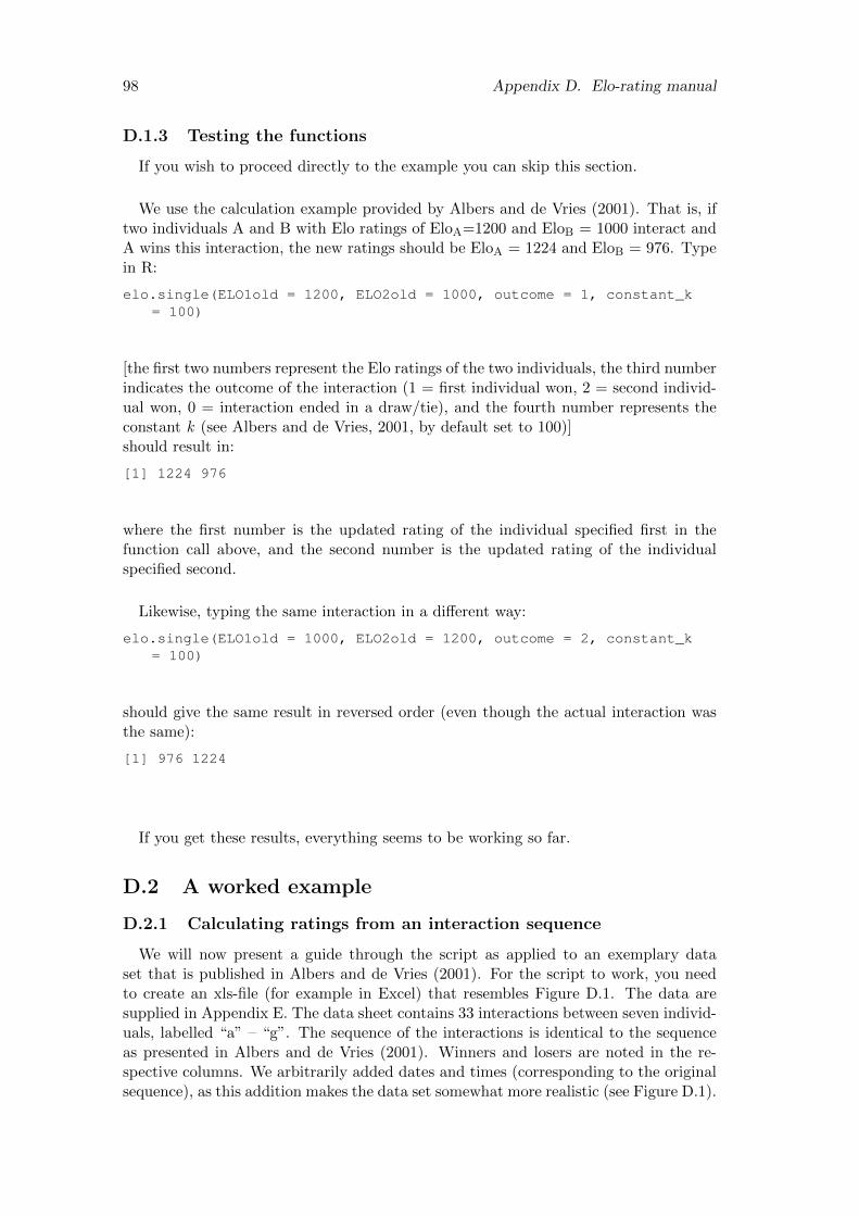
98 Appendix D. Elo-rating manual
D.1.3 Testing the functions
If you wish to proceed directly to the example you can skip this section.
We use the calculation example provided by Albers and de Vries (2001). That is, iftwo individuals A and B with Elo ratings of EloA=1200 and EloB = 1000 interact andA wins this interaction, the new ratings should be EloA = 1224 and EloB = 976. Typein R:
elo.single(ELO1old = 1200, ELO2old = 1000, outcome = 1, constant_k= 100)
[the first two numbers represent the Elo ratings of the two individuals, the third numberindicates the outcome of the interaction (1 = first individual won, 2 = second individ-ual won, 0 = interaction ended in a draw/tie), and the fourth number represents theconstant k (see Albers and de Vries, 2001, by default set to 100)]should result in:
[1] 1224 976
where the first number is the updated rating of the individual specified first in thefunction call above, and the second number is the updated rating of the individualspecified second.
Likewise, typing the same interaction in a different way:
elo.single(ELO1old = 1000, ELO2old = 1200, outcome = 2, constant_k= 100)
should give the same result in reversed order (even though the actual interaction wasthe same):
[1] 976 1224
If you get these results, everything seems to be working so far.
D.2 A worked example
D.2.1 Calculating ratings from an interaction sequence
We will now present a guide through the script as applied to an exemplary dataset that is published in Albers and de Vries (2001). For the script to work, you needto create an xls-file (for example in Excel) that resembles Figure D.1. The data aresupplied in Appendix E. The data sheet contains 33 interactions between seven individ-uals, labelled “a” – “g”. The sequence of the interactions is identical to the sequenceas presented in Albers and de Vries (2001). Winners and losers are noted in the re-spective columns. We arbitrarily added dates and times (corresponding to the originalsequence), as this addition makes the data set somewhat more realistic (see Figure D.1).

D.2. A worked example 99
Figure D.1: Data layout necessary for the R functions to work.
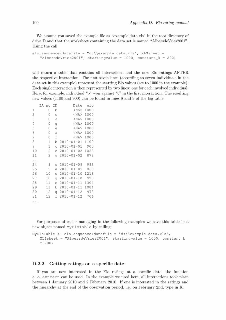
100 Appendix D. Elo-rating manual
We assume you saved the example file as “example data.xls” in the root directory ofdrive D and that the worksheet containing the data set is named “AlbersdeVries2001”.Using the call
elo.sequence(datafile = "d:\\example data.xls", XLSsheet ="AlbersdeVries2001", startingvalue = 1000, constant_k = 200)
will return a table that contains all interactions and the new Elo ratings AFTERthe respective interaction. The first seven lines (according to seven individuals in thedata set in this example) represent the starting Elo values (set to 1000 in the example).Each single interaction is then represented by two lines: one for each involved individual.Here, for example, individual “b” won against “c” in the first interaction. The resultingnew values (1100 and 900) can be found in lines 8 and 9 of the log table.
IA_no ID Date elo1 0 b <NA> 10002 0 c <NA> 10003 0 d <NA> 10004 0 g <NA> 10005 0 e <NA> 10006 0 a <NA> 10007 0 f <NA> 10008 1 b 2010-01-01 11009 1 c 2010-01-01 90010 2 c 2010-01-02 102811 2 g 2010-01-02 872...24 9 e 2010-01-09 98825 9 a 2010-01-09 86026 10 c 2010-01-10 121627 10 g 2010-01-10 92028 11 c 2010-01-11 130429 11 b 2010-01-11 108430 12 g 2010-01-12 97831 12 f 2010-01-12 706...
For purposes of easier managing in the following examples we save this table in anew object named MyEloTable by calling:
MyEloTable <- elo.sequence(datafile = "d:\\example data.xls",XLSsheet = "AlbersdeVries2001", startingvalue = 1000, constant_k= 200)
D.2.2 Getting ratings on a specific date
If you are now interested in the Elo ratings at a specific date, the functionelo.extract can be used. In the example we used here, all interactions took placebetween 1 January 2010 and 2 February 2010. If one is interested in the ratings andthe hierarchy at the end of the observation period, i.e. on February 2nd, type in R:

D.2. A worked example 101
elo.extract(Elotable = MyEloTable, extractDate = "2010-02-02",individuals = "all")
[where \MyEloTable" is the above described table with the Elo ratings after eachinteraction; and "2010-02-02" is the date from which we wish to obtain the Eloratings. If not otherwise specified, all individuals present in your data will appear inthe resulting table]
will result in the following table:
ID Elo offset1 b 1320 -12 c 1184 -13 d 1178 04 f 1048 -105 e 1008 -26 g 732 07 a 530 -3
In this table you can see for all individuals the ratings on the specified date. Thelast column gives the information on “how old” the data point is. In the examplehere, individuals “d” and “g” interacted on the same day the ratings were obtained(the offset is “0”), whereas “b” and “c” interacted the day before (the offset is “–1”).The last observed interaction of “f” was ten days prior the specified date (the offset is“–10”) and thus “f”’s Elo rating is “ten days old”
The individuals presented in the results can be limited by specifying particular IDsin the call to the function elo.extract. If we are interested in the ratings of ‘a’, ‘b’,‘d’ and ‘e’ on 5 January, typing:
elo.extract(Elotable = MyEloTable, extractDate = "2010-01-05",individuals = c("a", "b", "d", "e"))
ID Elo offset1 b 1172 02 e 928 03 d 863 -14 a NA NA
Please note that during the first five interactions (i.e. between 1 and 5 January)individual “a” was not involved in any observed interaction and hence the rating of “a”is not known and thus omitted (represented as \NA" [“not available”.])
D.2.3 Visualizing Elo-ratings
elo.plot is a basic function to visualize the ratings over time. Typing:

102 Appendix D. Elo-rating manual
Jan 04 Jan 11 Jan 18 Jan 25 Feb 01
600
800
1000
1200
Date
Elo
Rat
ing
●
●
●
●
●
●● ●
●
● ●
●
●
●
●●
●
●
●●
1:10
●
●
abcdefg
Figure D.2: Elo-ratings over time from seven individuals.
elo.plot(Elotable = MyEloTable, daterange = c("2010-01-01","2010-02-02"), individuals = "present")
[where ‘MyEloTable’ is the above-described table with the Elo-ratings after eachinteraction; and c(”2010-01-01”, ”2010-02-02”)is the date range to be plotted. If nototherwise specified, all individuals present in the specified date range will appear in theresulting plot]
will result in a figure similar to Figure D.2.
In Figure D.2, each symbol represents one interaction in which a given individual wasinvolved. Since we prepared the data in a way that exactly one interaction occurs eachday, there are exactly two data points in the plot each day representing the updatedratings of the two interacting individuals. In a data set based on real observations,there may be more than one interaction of a specific individual on a given day. In sucha case, the ratings will be averaged over that day. As such, per day there will be one(averaged) data point per interacting individual.
The figure resembles Figure 1 from Albers and de Vries (2001) with some changes:
� the X axis is a timescale whereas in Albers and de Vries’s paper the actual inter-actions are depicted;
� ratings do not originate graphically at the starting point 1000 at the beginningof the interaction sequence and do not extend to the end of the sequence for allindividuals.
Analogously to the elo.extract function, if one is interested only in the ratingsof a subset of individuals and/or a different time window, you can adjust the call toelo.plot, for example, Figure D.3 can be generated with:
elo.plot(Elotable = MyEloTable, daterange = c("2010-01-10","2010-01-20"), individuals = c("c", "f", "g"))

D.3. Your own data 103
Jan 10 Jan 12 Jan 14 Jan 16 Jan 18 Jan 20
600
800
1000
1200
Date
Elo
Rat
ing
●
● ●
1:10
● cfg
Figure D.3: Elo-ratings over time from three individuals during a subset of the obser-vation time.
D.2.4 Calculating the stability index S
Last, we show how to obtain an index to describe the stability of a hierarchy. Thisfunction is made up of several subfunctions, which for ease of use we wrapped into one.
stability.index(Elotable = MyEloTable, startdate="2010-01-02",duration=30)
where "MyEloTable" is once more the above-described table with the Elo-ratings aftereach interaction; and "2010-01-01" is the date from which S is to be calculated fora duration of 30 days. The output of this call is:
rank.differences IDs.present stability.index1 41 181 0.088
Again, the function allows specification of the desired date range:
stability.index(MyEloTable, startdate="2010-01-10", duration=7)
rank.differences IDs.present stability.index1 16 49 0.124
D.3 Your own data
D.3.1 Preparation of the data sheet
We assume data were prepared in a Microsoft Excel 2003 spreadsheet. An examplefile is provided with the data from Albers and de Vries (2001). You may want to usethis file as a template for your data by entering your data directly into this sheet. Ofcourse you can create your data sheet yourself. However, ensure that data files are setup analogously to the figure above, i.e. the NAMES and ORDER of the columns mustbe identical to those seen in the example file.

104 Appendix D. Elo-rating manual
Also, at this stage it is crucial that you put your interactions in the correct sequencein your data sheet. The oldest interactions must be at the top of the file, whereas themost recent interaction must appear at the bottom of the file.
The columns of the file are in detail:
1. Date: use the following format YYYY-MM-DD [obligatory];
2. Time: the ‘time’ column is merely to help put the interactions in the correctorder if there was more than one interaction on a given date; preferred format isHH:MM:SS;
3. Winner: the ID of the winning individual in the given interaction [obligatory];
4. Loser: the ID of the losing individual in the given interaction [obligatory].
To summarize, these are the assumptions that need to be fulfilled by your data(sheet).
� The sequence of interactions in your data file needs to be correct.
� There is a winner and a loser in each interaction.
� Column names are ‘Date’, ‘Time’, ‘Winner’ and ‘Loser’ (first letter capitalized!)
Remove spaces and special characters [ !, $, %, &, (, ), ?, . . . ] from the IDs youuse for your individuals, e.g. use ‘ ’ [under dash] as spacing character instead of blankspace.
There may be future extensions to the functions provided here. For updates andquestions please email [email protected].

Appendix E
Example data to calculateElo-ratings
The data in Table E.1 are fictional dominance interactions adapted from Albers andde Vries (2001) and serve as an example with which Elo-ratings can be calculated (seeAppendix D).
105
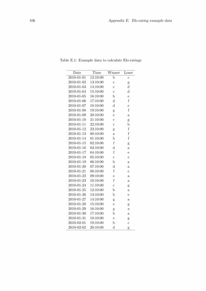
106 Appendix E. Elo-rating example data
Table E.1: Example data to calculate Elo-ratings
Date Time Winner Loser
2010-01-01 12:10:00 b c2010-01-02 13:10:00 c g2010-01-03 14:10:00 c d2010-01-04 15:10:00 c d2010-01-05 16:10:00 b e2010-01-06 17:10:00 d f2010-01-07 18:10:00 d e2010-01-08 19:10:00 g f2010-01-09 20:10:00 e a2010-01-10 21:10:00 c g2010-01-11 22:10:00 c b2010-01-12 23:10:00 g f2010-01-13 00:10:00 a f2010-01-14 01:10:00 b f2010-01-15 02:10:00 f g2010-01-16 03:10:00 d a2010-01-17 04:10:00 f e2010-01-18 05:10:00 c e2010-01-19 06:10:00 b a2010-01-20 07:10:00 d a2010-01-21 08:10:00 f e2010-01-22 09:10:00 e a2010-01-23 10:10:00 f a2010-01-24 11:10:00 c g2010-01-25 12:10:00 b a2010-01-26 13:10:00 b e2010-01-27 14:10:00 g a2010-01-28 15:10:00 e g2010-01-29 16:10:00 g a2010-01-30 17:10:00 b a2010-01-31 18:10:00 e g2010-02-01 19:10:00 b c2010-02-02 20:10:00 d g

Appendix F
Details on methods and resultsfor Chapter 4
F.1 Study subjects and site
We studied 37 males of two wild groups of crested macaques (Macaca nigra), groupsR1 and PB, living in the Tangkoko Nature Reserve, Sulawesi, Indonesia (Neumannet al. 2010; Duboscq et al. 2013). Data collection took place between March 2009 andMay 2011. The two groups comprised up to 85 individuals each, with 7 – 18 adultmales present (see Chapter 2 for details). All animals were completely habituated tohuman observers and adults were individually recognizable based on facial features andbody markings, e.g., scars or broken limbs.
F.2 Personality assessment
Here, we briefly summarize how we determined the personality structure of malecrested macaques. A detailed description of this assessment can be found in Chapter 3.
Behavioral data to quantify personality were collected using focal animal and scansampling (Altmann 1974) of 37 adult males (mean = 66.1h, range = 0.6 – 130.0hper male). During 60 minute focal protocols, we collected data on a range of spe-cific behaviors (socio-positive, agonistic and positional) and noted identities of otheradults in spatial proximity of focal subjects. Data were collected by four observersand inter-observer reliability of the observed behaviors ranged between 0.75 and 1.00as assessed by Pearson correlation coefficient and Cohen’s kappa (Martin and Bateson1993). Factor analysis revealed four distinct and unrelated factors, anxiety, connected-ness, sociability, and aggressiveness.
We additionally conducted two playback experiments on 18 of our focal males, toassess boldness and neophilia. Boldness was assayed by presenting subjects with a dogbark bout (threat to test animals) and neophilia was measured as the reaction to adonkey bray (unknown to test animals). We analyzed a total of 39 (N = 17 males) and42 (N = 16 males) experimental trials in the dog and donkey condition, respectively.Reactions of subjects to playback presentations were recorded on video. All videoswere coded by two raters (Pearson correlation: r = 0.92). We quantified “orientationto the speaker”, which is a composite measure of looking and approaching the speaker
107

108 Appendix F. Methods and results for Chapter 4
(Micheletta and Waller 2012). Reactions to the dog, but not the donkey, treatmentwere repeatable (c.f. Nakagawa and Schielzeth 2010). We therefore considered onlyboldness to represent a personality factor in crested macaques.
F.3 Data analysis
In this study, we model the relationship between five previously described personal-ity factors (anxiety, connectedness, sociability, aggressiveness and boldness) and domi-nance status. For the four observationally assessed factors we created two-month timeblocks for which we extracted regression scores from the factor solution for each male.We discarded time blocks for which the cumulative observation time was less than sixhours. In this way we obtained 190 data points for each personality trait comprising 30males (median = 6.5, range 1 – 11 data points, i.e. time blocks, per male). To be ableto obtain repeated personality factor scores for each male, we used a factor solutionthat was based on this data set (N = 190), contrasting with our original analysis wherewe used a single data point per male (i.e. N = 30) as basis for the factor analysis.Overall, the factors extracted with both approaches were judged similar based on thecongruence coefficient φ = 0.82 (p < 0.001, c.f. Abdi 2010) and Pearson correlationcoefficients between factor loadings of the two solutions (anxiety: r = 0.94, p < 0.001;connectedness: r = 0.87, p < 0.001; sociability: r = 0.57, p = 0.018; aggressiveness:r = 0.81, p < 0.001; all N = 17). To model the Boldness factor we used individualresponses to the playback treatments (Chapter 3), resulting in 39 data points from 17males (median = 2, range 1 – 3 playback responses per male).
We ran two sets of linear mixed models to investigate (1) whether personality factorscan be predicted from past dominance status and (2) whether personality factors predictfuture dominance status. In (1) the response variable is the personality factor score andincluding our predictor of interest (past status) alongside the control variable currentrank might lead to collinearity in these models. We therefore decided to use statusdifferences, i.e. current status – past status, instead of raw status scores as predictorin (1). To facilitate comparison between the model sets we used an analogue approachfor (2), i.e. we modeled the response future status – current status. In all ten models(2 * 5 personality factors) we controlled for current dominance status and male age(three-level age factor: young, middle, old). For the two Boldness models, we alsoincorporated trial number as predictor variable to account for possible habituationeffects (Chapter 3).
To assess dominance status we used Elo-rating (Chapter 2; Elo 1978; Albers andde Vries 2001). Elo-rating sequentially updates dominance ratings after each singledominance interaction between two males. The change in ratings after each interactionis determined by the rating difference between the two contestants prior to that inter-action. Elo-rating therefore allows assigning each male a continuous rating at any givenpoint in time and independent of changes in group composition (Chapter 2). For ouranalyses we used as current rating male Elo-ratings on the date in the center of the twomonth time block or on the date an experimental trial was conducted. With regard toour study question, we extracted Elo-ratings on two additional dates: future and pastrating refers to the Elo-rating 90 days after and before the current rating, respectively.k was set to 100 (Chapter 2). Even though they change over time, current ratings arelikely to be correlated with future ratings, as are past and current ratings. This might

F.4. Model results and figures 109
lead to collinearity in our models. Instead of true Elo-ratings, we therefore calculateddifferences between current and past ratings, and between future and current ratings,respectively. Because males migrated between groups or died over the course of thestudy, we were not able to determine past or future status in some instances. For thefour observationally assessed personality factors sample sizes are N = 165 cases (i.e.time blocks) representing 25 males (model set (1)), and N = 164 cases representing 27males (model set (2)). For boldness the sample size is 36 cases (i.e. playback trials)representing 14 males in both model sets.
Prior to analysis we checked distributions of our numerical variables and if necessarytransformed them to achieve symmetric distributions. We then standardized all nu-merical variables to mean = 0 and standard deviation = 1. Variance inflation factors(VIF, Field et al. 2012) were derived using the function vif of the R-package car (Foxand Weisberg 2011) applied to a standard linear model excluding the random effects(largest VIF: 1.55). We checked whether the assumptions of normally distributed andhomogeneous residuals were fulfilled by visually inspecting a qqplot and the residualsplotted against fitted values. We checked for model stability by excluding data pointsone by one from the data and comparing the parameter estimates derived with thoseobtained for the full model. In models of set 2 (future rank as response) these assump-tions were violated, caused by three particular cases in which two males underwentdrastic status changes, i.e. rapid declines in Elo-ratings. These drops in ranks coin-cided with both males being severely injured. Though we did not observe physicalfights directly, we assume these injuries were caused by aggressive interactions withinor possibly between the social groups. We decided to exclude these three cases becausethey appear not directly relevant for male rank trajectories given our study question,i.e. to relate intrinsic (personality) factors with rank. Excluding these cases from thedata set and running the models again did not change our conclusions with regard toour study aims. Nevertheless, since our models were more stable without these cases,we present model results based on data sets excluding them.
We ran linear mixed models with the function lmer from the lme4 package in R 2.15.0(Bates et al. 2012; R Development Core Team 2012), to be able to additionally controlfor repeated measurements and random intercepts of individuals and social groups. Weadditionally controlled for temporal autocorrelation by calculating an autocorrelationterm (c.f. Furtbauer et al. 2011; R. Mundry, personal communication) which wasincorporated into the models and retained only if it was significant (Furtbauer et al.2011) as indicated by a likelihood ratio test (see below).
Significance testing was done in a two-step approach. First, we used likelihood ratiotests (Quinn and Keough 2002) to determine whether the full model (including allfixed and random effects) differed from a reduced model (only including age, the randomeffects, the autocorrelation term if applicable and trial number in the Boldness models).Only if this step revealed that a full model differed from the corresponding reducedmodel did we interprete significance of individual effects. We used the pvals.fncfunction of the languageR package to calculate individual p values based on 10,000Markov chain Monte Carlo samples (Baayen 2008, 2011b).
F.4 Model results and figures

110 Appendix F. Methods and results for Chapter 4
Table F.1: Connectedness as a function of current status and past status difference.Likelihood ratio test: autocorrelation, χ2 = 2.06, df = 1, p = 0.1511. Likelihood ratiotest: full model vs null model, χ2 = 13.24, df = 2, p = 0.0013.
estimate se t pMCMC
intercept -0.413 0.208 -1.980 0.4566
current status 0.321 0.084 3.839 0.0006
past status difference -0.057 0.065 -0.877 0.4514
age*
old 0.630 0.259 2.429 0.0218
young 0.154 0.302 0.509 0.8204
* reference level for age-factor is “middle”
Table F.2: Sociability as a function of current status and past status difference.Likelihood ratio test: autocorrelation, χ2 = 10.37, df = 1, p = 0.0013. Likelihood ratiotest: full model vs null model, χ2 = 0.60, df = 2, p = 0.7424.
estimate se t pMCMC
intercept -0.221 0.139 -1.591 0.5596
current status 0.184 0.069 2.670 0.0380
past status difference -0.038 0.067 -1.000 0.6094
age*
old 0.415 0.157 2.649 0.0268
young 0.190 0.202 0.943 0.3316
autocorrelation 0.278 0.0617 4.501 0.0004
* reference level for age-factor is “middle”

F.4. Model results and figures 111
Table F.3: Aggressiveness as a function of current status and past status difference.Likelihood ratio test: autocorrelation, χ2 = 3.09, df = 1, p = 0.0787. Likelihood ratiotest: full model vs null model, χ2 = 9.05, df = 2, p = 0.0109.
estimate se t pMCMC
intercept 0.034 0.355 0.095 0.9530
current status 0.222 0.078 2.847 0.0030
past status difference 0.014 0.064 0.213 0.8694
age*
old -0.161 0.211 -0.760 0.4452
young -0.329 0.251 -1.310 0.1800
autocorrelation -0.117 0.059 -1.986 0.1750
* reference level for age-factor is “middle”
Table F.4: Anxiety as a function of current status and past status difference. Likeli-hood ratio test: autocorrelation, χ2 = 57.09, df = 1, p < 0.0001. Likelihood ratio test:full model vs null model, χ2 = 13.58, df = 2, p = 0.0011.
estimate se t pMCMC
intercept 0.108 0.127 0.849 0.7084
current status -0.221 0.059 -3.767 0.0002
past status difference 0.001 0.057 0.011 0.9310
age*
old -0.306 0.133 -2.293 0.0270
young -0.117 0.172 -0.680 0.4716
autocorrelation 0.461 0.052 8.807 0.0001
* reference level for age-factor is “middle”

112 Appendix F. Methods and results for Chapter 4
Table F.5: Boldness as a function of current status and past status difference. Likeli-hood ratio test: autocorrelation, χ2 = 2.42, df = 1, p = 0.1200. Likelihood ratio test:full model vs null model, χ2 = 6.65, df = 2, p = 0.0360.
estimate se t pMCMC
intercept -0.266 0.332 -0.803 0.3808
current status 0.638 0.221 2.889 0.0072
past status difference 0.084 0.173 0.488 0.6972
age*
old 0.557 0.475 1.173 0.2126
young -0.308 0.528 -0.584 0.5150
trial number -0.307 0.124 -2.469 0.0392
* reference level for age-factor is “middle”
Table F.6: Connectedness as predictor of future rating increase. Likelihood ratiotest: autocorrelation, χ2 = 0.39, df = 1, p = 0.5333. Likelihood ratio test: full modelvs null model, χ2 = 6.59, df = 2, p = 0.0371.
estimate se t pMCMC
intercept 0.250 0.117 2.143 0.2610
current status -0.095 0.065 -1.464 0.1194
connectedness 0.174 0.069 2.518 0.0142
age*
old -0.306 0.145 -2.109 0.0402
young 0.049 0.179 0.272 0.8466
* reference level for age-factor is “middle”

F.4. Model results and figures 113
Table F.7: Sociability as predictor of future rating increase. Likelihood ratio test:autocorrelation, χ2 = 1.02, df = 1, p = 0.3122. Likelihood ratio test: full model vs nullmodel, χ2 = 1.61, df = 2, p = 0.4472.
estimate se t pMCMC
intercept 0.237 0.119 1.989 0.3554
current status -0.052 0.063 -0.822 0.3078
sociability 0.070 0.063 1.117 0.2316
age*
old -0.256 0.146 -1.748 0.0650
young 0.039 0.182 0.216 0.9552
* reference level for age-factor is “middle”
Table F.8: Aggressiveness as predictor of future rating increase. Likelihood ratiotest: autocorrelation, χ2 = 1.14, df = 1, p = 0.2846. Likelihood ratio test: full modelvs null model, χ2 = 0.77, df = 2, p = 0.6811.
estimate se t pMCMC
intercept 0.216 0.118 1.834 0.3150
current status -0.049 0.065 -0.762 0.3924
aggressiveness 0.042 0.066 0.633 0.6726
age*
old -0.226 0.144 -1.575 0.1058
young 0.055 0.183 0.301 0.8616
* reference level for age-factor is “middle”
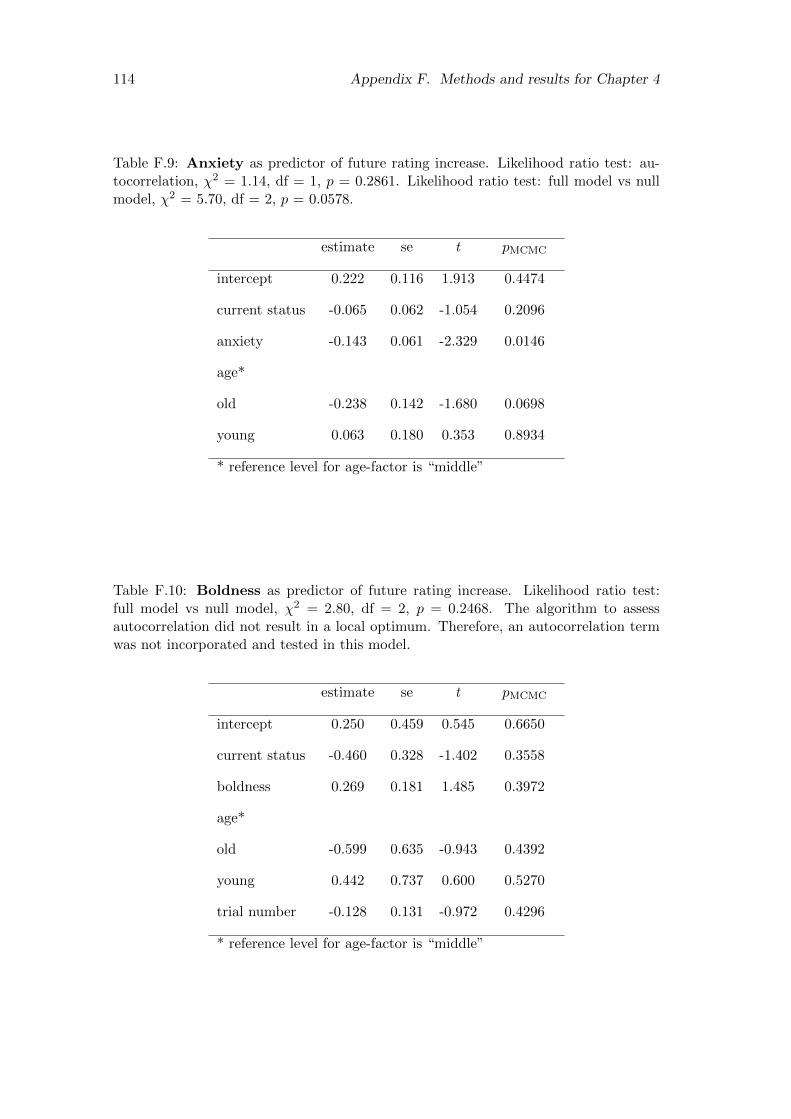
114 Appendix F. Methods and results for Chapter 4
Table F.9: Anxiety as predictor of future rating increase. Likelihood ratio test: au-tocorrelation, χ2 = 1.14, df = 1, p = 0.2861. Likelihood ratio test: full model vs nullmodel, χ2 = 5.70, df = 2, p = 0.0578.
estimate se t pMCMC
intercept 0.222 0.116 1.913 0.4474
current status -0.065 0.062 -1.054 0.2096
anxiety -0.143 0.061 -2.329 0.0146
age*
old -0.238 0.142 -1.680 0.0698
young 0.063 0.180 0.353 0.8934
* reference level for age-factor is “middle”
Table F.10: Boldness as predictor of future rating increase. Likelihood ratio test:full model vs null model, χ2 = 2.80, df = 2, p = 0.2468. The algorithm to assessautocorrelation did not result in a local optimum. Therefore, an autocorrelation termwas not incorporated and tested in this model.
estimate se t pMCMC
intercept 0.250 0.459 0.545 0.6650
current status -0.460 0.328 -1.402 0.3558
boldness 0.269 0.181 1.485 0.3972
age*
old -0.599 0.635 -0.943 0.4392
young 0.442 0.737 0.600 0.5270
trial number -0.128 0.131 -0.972 0.4296
* reference level for age-factor is “middle”

F.4. Model results and figures 115
●
●●
●
●●
●
●
●●
●
●
●
●
●
●
●●
●
●
●
●
●●
●●
●●
●●
●
●
●
●●
●
●
●●
●●●
●
●
●
●
●
●
●●●
●●
●● ●
●
●●
●
●
●
●
●
●
●
●●●
●●
●
●
●
●
●●
●
●●
●
●●
●●
●
●
●
●
●
●
●
●●
●●
●
●●●●
●●
●
●
●
●● ●
●
●●
●
●
●
●●
●●
●●
●
●
●
●●
●
●
●
●
●●
●
●●
●
●
●
●
●●
●
●
●●
●●
●
●
●
●
● ●
●
●
●●
●
●●
●
●
●●
●●
●
●● ●
●
●
●
●
●
●
●
●
●
●●
●
●
●
●
●●
●
●
−4 −2 0 2 4
−4
−2
0
2
4
current Elo−rating
conn
ecte
dnes
s sc
ore
(a)
●●●
●
●
●
●
●
●
●
●
●●
●
●●
●●
●●
●
●●
●
●
●●
●
●
●
●●
●
●●●●●
●
●
●●
●
●
●
●
●
●
●
●
● ●
●
●
●● ●
●
●●●
●
●
●●
●●
●●
●
●
●
●
●
●
●
●●● ●●
●● ● ●
●
●
●
●
●
●
●
●
●
●●
● ●
●
●
●●●
●● ●
●
●●
●
●
●●
●
●
●
●●
●
●
●●
●
●● ●●
●●
●
●
●●
● ●
●●
●
●
●
●
●
●
●
●
●●
●
●
●●
●
●●
●
●●
●
●●
●
●
●
●
−4 −2 0 2 4
−4
−2
0
2
4
connectedness score
futu
re E
lo−
ratin
g di
ffere
nce
(c)
●
● ●
●
●●
●
●
●●
●
●
●
●
●
●
●●
●●
●●
●●
●●
●●
●
●
●●
●
●
● ●
●●●
●
●●
●
●
●●●
●●
●●
●
●
●
●
●
●
●
●
●
●●
●
●
●
●
●●
●
●●
●
●●
●
●
●
●
●
●
●
●●
●●
●
●
●
●●
●
●
●
●● ●
●
●●
●
●
●
●●
● ●
●●
●
●
●
●●
●●
●●
●
●●
●
●
●
●
●●
●
●
●●
●●
●
●
●
●
●
●
●●
●
●
●●
●●
●
●●
●
●
●
●
●
●
●
●
●●
●
●
●●
●
●
past Elo−rating difference
(b)
−4 −2 0 2 4
−4
−2
0
2
4
●●●
●
●
●
●
●
●
●
●
●●
●
●●
●●
●●
●
●●
●
●
●●
●
●
●
●●
●
●●●●●
●
●
●●
●
●
●
●
●
●
●
●
●●
●
●
●●●
●
●●●
●
●
●●
●●●
●●
●
●
●
●
●
●
●●●●●
●●●●
●
●
●
●
●
●
●
●
●
●●
● ●
●
●
●●●●
●●
●
●●●
●
●●
●
●
●
●●
●
●
●●
●
●●●●
●●
●
●
●●
●●
●●
●
●
●
●
●
●
●
●
●●●
●
●●
●
● ●
●
●●
●
●●
●
●
●
●
current Elo−rating
(d)
−4 −2 0 2 4
−4
−2
0
2
4
Figure F.1: (a) and (b) depict the relationships between current and past Elo-ratingdifference and Connectedness score. (c) and (d) show the relationships betweenConnectedness score and current Elo-rating and future Elo-rating difference.

116 Appendix F. Methods and results for Chapter 4
●●●
●
●●
●●
●
●
●●
●
●
● ●
●
●
●●
●
●
●
●●●
●
●●
●
●●
●
●
●●
●
●●●●
●
●
●
●
●
●
●
●
●●
●
●
●
●
●
●
●
●
●
●
●
●
● ●
●
●
●
●
●
●
●
●
●
●●
●
●
●
●●
●●
●●
●
●
●
●●
● ●
●
●
●
●●
●
●●
●
● ●●
●●
●● ●
●
●
●
●●
●
●
●●
●
●
●
●
●
●●●
●
●
●●
●●
●
●●
●
●
●
●
●●
●●●
●
●●●
●●
●
● ●
●●
●●
●●
●
●
●
●●
●●
●● ●
●
●
●●
●
●
●●●
●
●
●
●
●
●
●
●●
●
●
−4 −2 0 2 4
−4
−2
0
2
4
current Elo−rating
soci
abili
ty s
core
(a)
●●●
●
●
●
●
●
●
●
●
●●
●
●●
●●
●●
●
●●
●
●
●●
●
●
●
●●
●
●● ●●
●●
●
●●
●
●
●
●
●
●
●
●
● ●
●
●
● ●●
●
● ●●
●
●
●●
●●
●●
●
●
●
●
●
●
●
●●● ●●
●● ● ●
●
●
●
●
●
●
●
●
●
●●
●●
●
●
●●●
●● ●
●
●●
●
●
●●
●
●
●
●●
●
●
●●
●
●●●
●
●●
●
●
●●
● ●
●●
●
●
●
●
●
●
●
●
●●●
●
●●●
●●
●
●●
●
●●
●
●
●
●
−4 −2 0 2 4
−4
−2
0
2
4
sociability score
futu
re E
lo−
ratin
g di
ffere
nce
(c)
●● ●
●
●●
●●
●
●
●●
●
●
● ●
●
●
●
●
●
●●
●●
●●
●
●
●
●
●●
●
● ●●●
●
●
●●
●
●
●
●●
●
●
●
●
●
●
●
●
●
●
●●
●
●
●●
●
●
●
●
●
●
●
●●
●●
●
●
●
●●
● ●
●
●
●
●●
●
●
● ●●
●●
●● ●
●
●
●
●●
●
●
●●
●
●
●
●
●
● ●●
●
●
●●
●
●●
●
●
●
●
●●
●●●
●
●●
●●
●
●
●●
●●
●
●
●●
●●
●●
●
●
●●
●
●●●
●
●
●
●
●●
●
●
●
past Elo−rating difference
(b)
−4 −2 0 2 4
−4
−2
0
2
4
●●●
●
●
●
●
●
●
●
●
●●
●
●●
●●
●●
●
●●
●
●
●●
●
●
●
●●
●
●●●●●
●
●
●●
●
●
●
●
●
●
●
●
●●
●
●
●●●
●
●●●
●
●
●●
●●●
●●
●
●
●
●
●
●
●●●●●
●●●●
●
●
●
●
●
●
●
●
●
●●
● ●
●
●
●●●●
●●
●
●●●
●
●●
●
●
●
●●
●
●
●●
●
●●●●
●●
●
●
●●
●●
●●
●
●
●
●
●
●
●
●
●●●
●
●●
●
● ●
●
●●
●
●●
●
●
●
●
current Elo−rating
(d)
−4 −2 0 2 4
−4
−2
0
2
4
Figure F.2: (a) and (b) depict the relationships between current and past Elo-ratingdifference and Sociability score. (c) and (d) show the relationships between Sociabilityscore and current Elo-rating and future Elo-rating difference.

F.4. Model results and figures 117
●
●
●
● ●●
●
●
●
●
●●
●
●
●
●
●●
●
●
●
●
●
●
●
●●●
●●
●
●
●●
●
●●
●
●●
●●
●
●
●
●●
●
●●
●●
●
●●●
●
●
●●
●
●
●
●
●
●●●
●
●●
●
●
●
● ●
●
●
●
●
●
●●
●
●●
●●
●
●●
●
●●
●
●
●
●
●●●
●
●
●●
●
●
●
●●
●
●
●
●●
●
●●
●
●●●
●
●●
●●
●
●
●
●
●●●
●
●
●●
●
●●
●
●
●●
●
●
●
●
●●
● ●
●●● ●
●
●
●●
●
●●
●
●
●● ●●
●●●
●
●
●
●
●●
●
●●
●
●
●
●●
●
●
−4 −2 0 2 4
−4
−2
0
2
4
current Elo−rating
aggr
essi
vene
ss s
core
(a)
●●●
●
●
●
●
●
●
●
●
●●
●
●●
●●
●●
●
●●
●
●
●●
●
●
●
●●
●
●●●
●●
●
●
●●
●
●
●
●
●
●
●
●
●●
●
●
● ●●
●
●●●
●
●
●●
●●
●●
●
●
●
●
●
●
●
●●● ●●
●●● ●
●
●
●
●
●
●
●
●
●
●●
●●
●
●
●● ●
●●●
●
●●●
●
●●
●
●
●
●●
●
●
●●
●
●●●
●
●●
●
●
●●
● ●
●●
●
●
●
●
●
●
●
●
●●●
●
●●
●
●●
●
●●
●
●●
●
●
●
●
−4 −2 0 2 4
−4
−2
0
2
4
aggressiveness score
futu
re E
lo−
ratin
g di
ffere
nce
(c)
●
●
●
● ●●
●
●
●
●
●●
●
●
●
●
●●
●
●
●
●
●
●●●
●●
●
●●
●
● ●
●
●●
●●
●
●
●●
●
●●
●●
●
●●
●
●
●
●
●
●
●
●
●●●
●
●
●
●
●
●
●
●
●
●
●●
●
●●
●
●●
●
●●
●
●
●
●●
●
●
●●
●
●
●
●●
●
●
●
●●
●
●●
●
●●●
●
● ●
●●●
●
●●●
●
●
●●
●
●●
●
●
● ●
●
●
●
●●
●
●●●
●
●
●
●●
●
●
●●●
●●●
●
●
●
●●
●
●●
●●
●
●
●
past Elo−rating difference
(b)
−4 −2 0 2 4
−4
−2
0
2
4
●●●
●
●
●
●
●
●
●
●
●●
●
●●
●●
●●
●
●●
●
●
●●
●
●
●
●●
●
●●●●●
●
●
●●
●
●
●
●
●
●
●
●
●●
●
●
●●●
●
●●●
●
●
●●
●●●
●●
●
●
●
●
●
●
●●●●●
●●●●
●
●
●
●
●
●
●
●
●
●●
● ●
●
●
●●●●
●●
●
●●●
●
●●
●
●
●
●●
●
●
●●
●
●●●●
●●
●
●
●●
●●
●●
●
●
●
●
●
●
●
●
●●●
●
●●
●
● ●
●
●●
●
●●
●
●
●
●
current Elo−rating
(d)
−4 −2 0 2 4
−4
−2
0
2
4
Figure F.3: (a) and (b) depict the relationships between current and past Elo-ratingdifference and Aggressiveness score. (c) and (d) show the relationships betweenAggressiveness score and current Elo-rating and future Elo-rating difference.

118 Appendix F. Methods and results for Chapter 4
●
●
●
● ●●●
●
●
●
●
●●
●
●
●
●
●
●● ●
●
●
●●●
●
●●
●
●
●
●
●●
●
●●●●
●
●●
●
●●
●
●●
●●
●●●
●
●
●
●
●●●
●
●
●
●●
●
●
●
●
●●
●●
●●
●● ●
●●
●
●
●●
●
●
●●●
●●●
●
●●
●
●●
●●
●
●●
●●
●●
●●
●
●
●
●
●
●
●●
●●
●
●
●
●●
●
●
●
●●
●
●●●
●● ●
●
●
●● ●●●
●
●
●
●
●
●
●●
●
●
●●●
●
●
●
●●●
●
●
●●
●
● ●
●
●
●
●
●
●
●
●●
●
●●
●●
●
●
●●
●
−4 −2 0 2 4
−4
−2
0
2
4
current Elo−rating
anxi
ety
scor
e
(a)
●●●
●
●
●
●
●
●
●
●
●●
●
●●
●●
●●
●
●●
●
●
●●
●
●
●
● ●
●
●● ● ●
●●
●
●●
●
●
●
●
●
●
●
●
●●
●
●
●●●
●
● ●●
●
●
●●
●●
●●
●
●
●
●
●
●
●
●●● ●●
●●● ●
●
●
●
●
●
●
●
●
●
●●
●●
●
●
●●●
●●●
●
●●
●
●
●●
●
●
●
●●
●
●
●●
●
●●●
●
● ●
●
●
●●
●●
●●
●
●
●
●
●
●
●
●
●●
●
●
●●
●
● ●
●
●●
●
●●
●
●
●
●
−4 −2 0 2 4
−4
−2
0
2
4
anxiety score
futu
re E
lo−
ratin
g di
ffere
nce
(c)
●
●
●
● ●●●
●
●
●
●
●●
●
●
●
●
●
●
●
●
●● ●
●
●●
●
●
●
●●
●
●● ●●
●
●●
●
●
●
●●
●●
●●●
●
●
●●●
●
●
●
●●
●
●
●●
● ●
●●
● ●
●●
●
●
●
●
●●●
●●●
●
●●
●
●
●
●
●●
●●
●●
●●
●
●
●
●
●
●
●●
●●
●
●
●
●●
●
●
●
●
●●●
●● ●
●
●
●● ●●●
●
●
●
●
●
●
●
●
●●
●
●●●
●
●
●●
●
●
●
●
●
●
●
●
●●
●
●●
●●
●●
●
past Elo−rating difference
(b)
−4 −2 0 2 4
−4
−2
0
2
4
●●●
●
●
●
●
●
●
●
●
●●
●
●●
●●
●●
●
●●
●
●
●●
●
●
●
●●
●
●●●●●
●
●
●●
●
●
●
●
●
●
●
●
●●
●
●
●●●
●
●●●
●
●
●●
●●●
●●
●
●
●
●
●
●
●●●●●
●●●●
●
●
●
●
●
●
●
●
●
●●
● ●
●
●
●●●●
●●
●
●●●
●
●●
●
●
●
●●
●
●
●●
●
●●●●
●●
●
●
●●
●●
●●
●
●
●
●
●
●
●
●
●●●
●
●●
●
● ●
●
●●
●
●●
●
●
●
●
current Elo−rating
(d)
−4 −2 0 2 4
−4
−2
0
2
4
Figure F.4: (a) and (b) depict the relationships between current and past Elo-ratingdifference and Anxiety score. (c) and (d) show the relationships between Anxietyscore and current Elo-rating and future Elo-rating difference.

F.4. Model results and figures 119
●
●
●
●
●●
●●
●●
●
●
●
●
●
●
●
●●
●
●
●
●●
●●
●
●
●●●
●
●●
●
●
−4 −2 0 2 4
−4
−2
0
2
4
current Elo−rating
bold
ness
sco
re
(a)
●
● ●
●
●
●
●
● ●●
●
●
●●
●
●
●
●
●●
●
●●
● ●
●
●●
●●
●●●●
●
●
−4 −2 0 2 4
−4
−2
0
2
4
boldness score
futu
re E
lo−
ratin
g di
ffere
nce
(c)
●
●
●
●
●●
● ●
●●
●
●
●
●
●
●
●
●●
●
●
●
●●
●●
●
●
●●●
●
●●
●
●
past Elo−rating difference
(b)
−4 −2 0 2 4
−4
−2
0
2
4
●
●●
●
●
●
●
● ●●
●
●
●●
●
●
●
●
●●
●
●●
●●
●
●●
●●
●●● ●
●
●
current Elo−rating
(d)
−4 −2 0 2 4
−4
−2
0
2
4
Figure F.5: (a) and (b) depict the relationships between current and past Elo-ratingdifference and Boldness score. (c) and (d) show the relationships between Boldnessscore and current Elo-rating and future Elo-rating difference.

120 Appendix F. Methods and results for Chapter 4

Bibliography
Abbott, D., Keverne, E., Bercovitch, F.B., Shively, C., Mendoza, S.P., Saltzman, W.,Snowdon, C.T., Ziegler, T.E., Banjevic, M., Garland Jr., T., Sapolsky, R.M., 2003.Are subordinates always stressed? A comparative analysis of rank differences incortisol levels among primates. Hormones and Behavior 43, 67–82. doi:10.1016/S0018-506X(02)00037-5.
Abdi, H., 2010. Congruence: Congruence coefficient, RV coefficient, and mantel coeffi-cient, in: Salkind, N.J., Dougherty, D.M., Frey, B. (Eds.), Encyclopedia of ResearchDesign. Sage, Thousand Oaks, pp. 222–229.
Abegg, C., Thierry, B., 2002. Macaque evolution and dispersal in insular south-eastAsia. Biological Journal of the Linnean Society 75, 555–576. doi:10.1046/j.1095-8312.2002.00045.x.
Adamo, S.A., Hoy, R.R., 1995. Agonistic behaviour in male and female field crickets,Gryllus bimaculatus, and how behavioural context influences its expression. AnimalBehaviour 49, 1491–1501. doi:10.1016/0003-3472(95)90070-5.
Adams, M.J., 2011. Evolutionary genetics of personality in nonhuman primates, in:Inoue-Murayama, M., Kawamura, S., Weiss, A. (Eds.), From Genes to Animal Be-havior. Springer, Tokyo, pp. 137–164.
Albers, P.C.H., de Vries, H., 2001. Elo-rating as a tool in the sequential estimation ofdominance strengths. Animal Behaviour 61, 489–495. doi:10.1006/anbe.2000.1571.
Alberts, S.C., 2012. Magnitude and sources of variation in male reproductive perfor-mance, in: Mitani, J.C., Call, J., Kappeler, P.M., Palombit, R.A., Silk, J.B. (Eds.),The Evolution of Primate Societies. University Of Chicago Press, Chicago, pp. 412–431.
Alberts, S.C., Altmann, J., Wilson, M.L., 1996. Mate guarding constrains foragingactivity of male baboons. Animal Behaviour 51, 1269–1277. doi:10.1006/anbe.1996.0131.
Alberts, S.C., Buchan, J.C., Altmann, J., 2006. Sexual selection in wild baboons:from mating opportunities to paternity success. Animal Behaviour 72, 1177–1196.doi:10.1016/j.anbehav.2006.05.001.
Alberts, S.C., Watts, H.E., Altmann, J., 2003. Queuing and queue-jumping: long-term patterns of reproductive skew in male savannah baboons, Papio cynocephalus.Animal Behaviour 65, 821–840. doi:10.1006/anbe.2003.2106.
121

122 Bibliography
Alexander, B.K., Hughes, J., 1971. Canine teeth and rank in Japanese monkeys (Macacafuscata). Primates 12, 91–93. doi:10.1007/BF01730385.
Altmann, J., 1974. Observational study of behavior: sampling methods. Behaviour 49,227–266. doi:10.1163/156853974X00534.
Altmann, J., Alberts, S.C., 2003. Variability in reproductive success viewed from a life-history perspective in baboons. American Journal of Human Biology 15, 401–409.doi:10.1002/ajhb.10157.
Altmann, S.A., 1962. A field study of the sociobiology of rhesus monkeys, Macacamulatta. Annals of the New York Academy of Sciences 102, 338–435. doi:10.1111/j.1749-6632.1962.tb13650.x.
Alvergne, A., Jokela, M., Lummaa, V., 2010. Personality and reproductive success ina high-fertility human population. Proceedings of the National Academy of Sciences107, 11745–11750. doi:10.1073/pnas.1001752107.
Anestis, S.F., 2011. Primate personality and behavioral endocrinology, in: Weiss, A.,King, J.E., Murray, L. (Eds.), Personality and Temperament in Nonhuman Primates.Springer, New York, pp. 169–192.
Appleby, M.C., 1983. The probability of linearity in hierarchies. Animal Behaviour 31,600–608. doi:10.1016/S0003-3472(83)80084-0.
Aureli, F., Preston, S.D., de Waal, F.B.M., 1999. Heart rate responses to social inter-actions in free-moving rhesus macaques (Macaca mulatta): a pilot study. Journal ofComparative Psychology 113, 59–65. doi:10.1037/0735-7036.113.1.59.
Baayen, R.H., 2008. Analyzing Linguistic Data: A Practical Introduction to Statisticsusing R. 1 ed., Cambridge University Press, Cambridge.
Baayen, R.H., 2011a. languageR: data sets and functions with ”Analyzing linguis-tic data: A practical introduction to statistics”, version 1.2, http://CRAN.R-project.org/package=languageR.
Baayen, R.H., 2011b. languageR: data sets and functions with ”Analyzing linguis-tic data: A practical introduction to statistics”, version 1.4, http://CRAN.R-project.org/package=languageR.
Balasubramaniam, K.N., Berman, C.M., De Marco, A., Dittmar, K., Majolo, B.,Ogawa, H., Thierry, B., de Vries, H., 2013. Consistency of dominance rank or-der: a comparison of David’s scores with I&SI and Bayesian methods in macaques.American Journal of Primatology 75, 959–971. doi:10.1002/ajp.22160.
Balasubramaniam, K.N., Dittmar, K., Berman, C.M., Butovskaya, M., Cooper, M.A.,Majolo, B., Ogawa, H., Schino, G., Thierry, B., de Waal, F.B.M., 2012. Hierarchicalsteepness, counter-aggression, and macaque social style scale. American Journal ofPrimatology 74, 915–925. doi:10.1002/ajp.22044.
Bang, A., Deshpande, S., Sumana, A., Gadagkar, R., 2010. Choosing an appropriateindex to construct dominance hierarchies in animal societies: a comparison of threeindices. Animal Behaviour 79, 631–636. doi:10.1016/j.anbehav.2009.12.009.
Bibliography 123
Barelli, C., Reichard, U.H., Mundry, R., 2011. Is grooming used as a commodity inwild white-handed gibbons, Hylobates lar? Animal Behaviour 82, 801–809. doi:10.1016/j.anbehav.2011.07.012.
Barrette, C., 1987. Dominance cannot be inherited. Trends in Ecology & Evolution 2,251. doi:10.1016/0169-5347(87)90008-5.
Barrette, C., 1993. The ’inheritance of dominance’, or of an aptitude to dominate?Animal Behaviour 46, 591–593. doi:10.1006/anbe.1993.1225.
Bateman, A.J., 1948. Intra-sexual selection in Drosophila. Heredity 2, 349–368.
Bates, D.M., Maechler, M., Bolker, B.M., 2011. lme4: Linear mixed-effects modelsusing s4 classes, version 0.999375-39, http://CRAN.R-project.org/package=lme4.
Bates, D.M., Maechler, M., Bolker, B.M., 2012. lme4: Linear mixed-effects modelsusing s4 classes. R package version 0.999999-0.
Bayly, K.L., Evans, C.S., Taylor, A., 2006. Measuring social structure: a comparison ofeight dominance indices. Behavioural Processes 73, 1–12. doi:10.1016/j.beproc.2006.01.011.
Beehner, J.C., Bergman, T.J., Cheney, D.L., Seyfarth, R.M., Whitten, P.L., 2005. Theeffect of new alpha males on female stress in free-ranging baboons. Animal Behaviour69, 1211–1221. doi:10.1016/j.anbehav.2004.08.014.
Beehner, J.C., Bergman, T.J., Cheney, D.L., Seyfarth, R.M., Whitten, P.L., 2006.Testosterone predicts future dominance rank and mating activity among malechacma baboons. Behavioral Ecology and Sociobiology 59, 469–479. doi:10.1007/s00265-005-0071-2.
Beletsky, L.D., 1992. Social stability and territory acquisition in birds. Behaviour 123,290–313. doi:10.1163/156853992X00066.
Benjamini, Y., Hochberg, Y., 1995. Controlling the false discovery rate: a practicaland powerful approach to multiple testing. Journal of the Royal Statistical Society.Series B (Methodological) 57, 289–300. doi:10.2307/2346101.
Berard, J.D., Nurnberg, P., Epplen, J.T., Schmidtke, J., 1994. Alternative reproductivetactics and reproductive success in male rhesus macaques. Behaviour 129, 177–201.doi:10.2307/4535194.
Bercovitch, F.B., 1988. Coalitions, cooperation and reproductive tactics among adultmale baboons. Animal Behaviour 36, 1198–1209. doi:10.1016/S0003-3472(88)80079-4.
Bercovitch, F.B., 1993. Dominance rank and reproductive maturation in male rhesusmacaques (Macaca mulatta). Journal of Reproduction and Fertility 99, 113–120.doi:10.1530/jrf.0.0990113. PMID: 8283427.
Bercovitch, F.B., Widdig, A., Trefilov, A., Kessler, M.J., Berard, J.D., Schmidtke,J., Nurnberg, P., Krawczak, M., 2003. A longitudinal study of age-specific repro-ductive output and body condition among male rhesus macaques, Macaca mulatta.Naturwissenschaften 90, 309–312. doi:10.1007/s00114-003-0436-1.

124 Bibliography
Berenstain, L., Wade, T.D., 1983. Intrasexual selection and male mating strategies inbaboons and macaques. International Journal of Primatology 4, 201–235. doi:10.1007/BF02743758.
Berghanel, A., Ostner, J., Schulke, O., 2011. Coalitions destabilize dyadic dominancerelationships in male Barbary macaques (Macaca sylvanus). Behaviour 148, 1256–1274. doi:10.1163/000579511X600628.
Bergman, T.J., Kitchen, D.M., 2009. Comparing responses to novel objects in wildbaboons (Papio ursinus) and geladas (Theropithecus gelada). Animal Cognition 12,63–73. doi:10.1007/s10071-008-0171-2.
Berman, C.M., Ionica, C., Li, J., 2007. Supportive and tolerant relationships amongmale Tibetan macaques at Huangshan, China. Behaviour 144, 631–661. doi:10.1163/156853907781347790.
Berman, C.M., Thierry, B., 2010. Variation in kin bias: species differencesand time constraints in macaques. Behaviour 147, 1863–1887. doi:10.1163/000579510X539691.
Bernstein, I.S., 1981. Dominance: the baby and the bathwater. Behavioral and BrainSciences 4, 419–429. doi:10.1017/S0140525X00009614.
Bernstein, I.S., Baker, S.C., 1988. Activity patterns in a captive group of Celebes blackape (Macaca nigra). Folia Primatologica 51, 61–75. doi:10.1159/000156358.
Birkhead, T.R., Kappeler, P.M., 2004. Post-copulatory sexual selection in birds andprimates, in: Kappeler, P.M., van Schaik, C.P. (Eds.), Sexual Selection in Primates:New and Comparative Perspectives. Cambridge University Press, New York, pp.151–171.
Bissonnette, A., Bischofberger, N., van Schaik, C.P., 2011. Mating skew in bar-bary macaque males: the role of female mating synchrony, female behavior, andmale–male coalitions. Behavioral Ecology and Sociobiology 65, 167–182. doi:10.1007/s00265-010-1023-z.
Bissonnette, A., Lange, E., van Schaik, C.P., 2009a. A cardinal measure of competi-tive ability in Barbary macaque males (Macaca sylvanus). Ethology 115, 671–681.doi:10.1111/j.1439-0310.2009.01652.x.
Bissonnette, A., de Vries, H., van Schaik, C.P., 2009b. Coalitions in male Barbarymacaques, Macaca sylvanus: strength, success and rules of thumb. Animal Behaviour78, 329–335. doi:10.1016/j.anbehav.2009.05.010.
Boehm, C., 1999. Hierarchy in the Forest: The Evolution of Egalitarian Behavior.Harvard University Press, Cambridge, MA.
Bolig, R., Price, C.S., O’Neill, P.L., Suomi, S.J., 1992. Subjective assessment of re-activity level and personality traits of rhesus monkeys. International Journal ofPrimatology 13, 287–306. doi:10.1007/BF02547817.
Both, C., Dingemanse, N.J., Drent, P.J., Tinbergen, J.M., 2005. Pairs of extremeavian personalities have highest reproductive success. Journal of Animal Ecology 74,667–674. doi:10.1111/j.1365-2656.2005.00962.x.

Bibliography 125
Boyd, R., Silk, J.B., 1983. A method for assigning cardinal dominance ranks. AnimalBehaviour 31, 45–58. doi:10.1016/S0003-3472(83)80172-9.
Budaev, S.V., 2010. Using principal components and factor analysis in animal be-haviour research: caveats and guidelines. Ethology 116, 472–480. doi:10.1111/j.1439-0310.2010.01758.x.
Bulger, J.B., 1993. Dominance rank and access to estrous females in male savannababoons. Behaviour 127, 67–103. doi:10.2307/4535144.
Caine, N.G., Earle, H., Reite, M., 1983. Personality traits of adolescent pig-tailed mon-keys (Macaca nemestrina): an analysis of social rank and early separation experience.American Journal of Primatology 4, 253–260. doi:10.1002/ajp.1350040304.
Capitanio, J.P., 1999. Personality dimensions in adult male rhesus macaques: pre-diction of behaviors across time and situation. American Journal of Primatology47, 299–320. doi:10.1002/(SICI)1098-2345(1999)47:4<299::AID-AJP3>3.0.CO;2-P.
Capitanio, J.P., 2004. Personality factors between and within species, in: Thierry, B.,Singh, M., Kaumanns, W. (Eds.), Macaque Societies. Cambridge University Press,Cambridge, pp. 13–37.
Capitanio, J.P., 2011. Nonhuman primate personality and immunity: mechanisms ofhealth and disease, in: Weiss, A., King, J.E., Murray, L. (Eds.), Personality andTemperament in Nonhuman Primates. Springer, New York, pp. 233–255.
Carter, A.J., Marshall, H.H., Heinsohn, R., Cowlishaw, G., 2012. How not to measureboldness: novel object and antipredator responses are not the same in wild baboons.Animal Behaviour 84, 603–609. doi:10.1016/j.anbehav.2012.06.015.
Chapais, B., 1983. Matriline membership and male rhesus reaching high ranks in theirnatal troops, in: Hinde, R.A. (Ed.), Primate Social Relationships. Blackwell, London,pp. 171–175.
Chapais, B., 1988. Rank maintenance in female Japanese macaques: experimentalevidence for social dependency. Behaviour 104, 41–59. doi:10.2307/4534657.
Chapais, B., 1992. The role of alliances in social inheritance of rank among femaleprimates, in: Harcourt, A.H., de Waal, F.B.M. (Eds.), Coalitions and Alliances inHumans and Other Animals. Oxford University Press, Oxford, pp. 29–59.
Chapais, B., 1995. Alliances as a means of competition in primates: evolutionary,developmental, and cognitive aspects. American Journal of Physical Anthropology38, 115–136. doi:10.1002/ajpa.1330380607.
Chase, I.D., Tovey, C., Spangler-Martin, D., Manfredonia, M., 2002. Individual dif-ferences versus social dynamics in the formation of animal dominance hierarchies.Proceedings of the National Academy of Sciences 99, 5744–5749. doi:10.1073/pnas.082104199.
Cheney, D.L., 1992. Intragroup cohesion and intergroup hostility: the relation be-tween grooming distributions and intergroup competition among female primates.Behavioral Ecology 3, 334–345. doi:10.1093/beheco/3.4.334.

126 Bibliography
Clutton-Brock, T.H. (Ed.), 1988. Reproductive Success: Studies of Individual Variationin Contrasting Breeding Systems. 1 ed., University Of Chicago Press, Chicago.
Clutton-Brock, T.H., 2004. What is sexual selection?, in: Kappeler, P.M., van Schaik,C.P. (Eds.), Sexual Selection in Primates. Cambridge University Press, Cambridge,pp. 24–36.
Clutton-Brock, T.H., Albon, S.D., Gibson, R.M., Guinness, F.E., 1979. The logicalstag: adaptive aspects of fighting in red deer (Cervus elaphus L.). Animal Behaviour27, 211–225. doi:10.1016/0003-3472(79)90141-6.
Clutton-Brock, T.H., Harvey, P.H., Rudder, B., 1977. Sexual dimorphism, socio-nomic sex ratio and body weight in primates. Nature 269, 797–800. doi:10.1038/269797a0.
Colleter, M., Brown, C., 2011. Personality traits predict hierarchy rank in male rain-bowfish social groups. Animal Behaviour 81, 1231–1237. doi:10.1016/j.anbehav.2011.03.011.
Cords, M., 2012. The behavior, ecology, and social evolution of cercopithecine monkeys,in: Mitani, J.C., Call, J., Kappeler, P.M., Palombit, R.A., Silk, J.B. (Eds.), TheEvolution of Primate Societies. University Of Chicago Press, Chicago, pp. 91–112.
Cowlishaw, G., Dunbar, R.I.M., 1991. Dominance rank and mating success in maleprimates. Animal Behaviour 41, 1045–1056. doi:10.1016/S0003-3472(05)80642-6.
Crockford, C., Wittig, R.M., Seyfarth, R.M., Cheney, D.L., 2007. Baboons eavesdropto deduce mating opportunities. Animal Behaviour 73, 885–890. doi:10.1016/j.anbehav.2006.10.016.
Crockford, C., Wittig, R.M., Whitten, P.L., Seyfarth, R.M., Cheney, D.L., 2008. Socialstressors and coping mechanisms in wild female baboons (Papio hamadryas ursinus).Hormones and Behavior 53, 254–265. doi:10.1016/j.yhbeh.2007.10.007.
Cote, S.D., 2000. Dominance hierarchies in female mountain goats: stability, ag-gressiveness and determinants of rank. Behaviour 137, 1541–1566. doi:10.1163/156853900502718.
Cote, S.D., Festa-Bianchet, M., 2001. Reproductive success in female mountain goats:the influence of age and social rank. Animal Behaviour 62, 173–181. doi:10.1006/anbe.2001.1719.
Dammhahn, M., 2012. Are personality differences in a small iteroparous mammalmaintained by a life-history trade-off? Proceedings of the Royal Society B: BiologicalSciences 279, 2645–2651. doi:10.1098/rspb.2012.0212.
Dammhahn, M., Almeling, L., 2012. Is risk taking during foraging a personality trait?A field test for cross-context consistency in boldness. Animal Behaviour 84, 1131–1139. doi:10.1016/j.anbehav.2012.08.014.
Darwin, C., 1859. On the Origin of Species by Means of Natural Selection. JohnMurray, London. Published 2004 by Barnes & Noble Classics, New York.

Bibliography 127
Darwin, C., 1871. The Descent of Man and the Selection in Relation to Sex. JohnMurray, London.
Datta, S.B., 1983. Relative power and the acquisition of rank, in: Hinde, R.A. (Ed.),Primate Social Relationships. Blackwell, Oxford, pp. 93–103.
Datta, S.B., 1989. Demographic influences on dominance structure among female pri-mates, in: Standen, V., Foley, R.A. (Eds.), Comparative Socioecology: The Be-havioural Ecology of Humans and other Mammals. Blackwell, Oxford, pp. 265–284.
David, H.A., 1987. Ranking from unbalanced paired-comparison data. Biometrika 74,432–436. doi:10.1093/biomet/74.2.432.
David, M., Auclair, Y., Cezilly, F., 2012. Assessing short- and long-term repeatabilityand stability of personality in captive zebra finches using longitudinal data. Ethology118, 932–942. doi:10.1111/j.1439-0310.2012.02085.x.
Dewsbury, D.A., 1982. Dominance rank, copulatory behavior, and differential repro-duction. The Quarterly Review of Biology 57, 135–159. doi:10.2307/2829552.
Dewsbury, D.A., 1990. Fathers and sons: genetic factors and social dominance indeer mice, Peromyscus maniculatus. Animal Behaviour 39, 284–289. doi:10.1016/S0003-3472(05)80872-3.
Digman, J.M., 1990. Personality structure: emergence of the five-factor model. An-nual Review of Psychology 41, 417–440. doi:10.1146/annurev.ps.41.020190.002221.
Dingemanse, N.J., Both, C., Drent, P.J., Tinbergen, J.M., 2004. Fitness consequencesof avian personalities in a fluctuating environment. Proceedings of the Royal Societyof London. Series B: Biological Sciences 271, 847–852. doi:10.1098/rspb.2004.2680.
Dingemanse, N.J., Kazem, A.J.N., Reale, D., Wright, J., 2010. Behavioural reactionnorms: animal personality meets individual plasticity. Trends in Ecology & Evolution25, 81–89. doi:10.1016/j.tree.2009.07.013.
Dingemanse, N.J., Wolf, M., 2010. Recent models for adaptive personality differences:a review. Philosophical Transactions of the Royal Society B: Biological Sciences 365,3947–3958. doi:10.1098/rstb.2010.0221.
Drea, C.M., 1998. Social context affects how rhesus monkeys explore their envi-ronment. American Journal of Primatology 44, 205–214. doi:10.1002/(SICI)1098-2345(1998)44:3<205::AID-AJP3>3.0.CO;2.
Drews, C., 1993. The concept and definition of dominance in animal behaviour. Be-haviour 125, 283–313. doi:10.1163/156853993X00290.
Drickamer, L.C., Vessey, S.H., 1973. Group changing in free-ranging male rhesus mon-keys. Primates 14, 359–368. doi:10.1007/BF01731357.
Duboscq, J., Micheletta, J., Agil, M., Hodges, K., Thierry, B., Engelhardt, A., 2013.Social tolerance in wild female crested macaques (Macaca nigra) in Tangkoko-Batuangus Nature Reserve, Sulawesi, Indonesia. American Journal of Primatology75, 361–375. doi:10.1002/ajp.22114.
128 Bibliography
Duboscq, J., Neumann, C., Perwitasari-Farajallah, D., Engelhardt, A., 2008. Daytimebirth of a baby crested black macaque (Macaca nigra) in the wild. BehaviouralProcesses 79, 81–84. doi:10.1016/j.beproc.2008.04.010.
Dubuc, C., Brent, L.J.N., Accamando, A.K., Gerald, M.S., MacLarnon, A., Semple,S., Heistermann, M., Engelhardt, A., 2009. Sexual skin color contains informationabout the timing of the fertile phase in free-ranging Macaca mulatta. InternationalJournal of Primatology 30, 777–789. doi:10.1007/s10764-009-9369-7.
Dubuc, C., Muniz, L., Heistermann, M., Engelhardt, A., Widdig, A., 2011. Testing thepriority-of-access model in a seasonally breeding primate species. Behavioral Ecologyand Sociobiology 65, 1615–1627. doi:10.1007/s00265-011-1172-8.
Dugatkin, L.A., 1997. Cooperation Among Animals: An Evolutionary Perspective.Oxford University Press, Oxford.
East, M.L., Honer, O.P., Wachter, B., Wilhelm, K., Burke, T., Hofer, H., 2009. Ma-ternal effects on offspring social status in spotted hyenas. Behavioral Ecology 20,478–483. doi:10.1093/beheco/arp020.
Eaves, L.J., Martin, N.G., Heath, A.C., Hewitt, J.K., Neale, M.C., 1990. Person-ality and reproductive fitness. Behavior Genetics 20, 563–568. doi:10.1007/BF01065872.
Ellis, L., 1995. Dominance and reproductive success among nonhuman animals: across-species comparison. Ethology and Sociobiology 16, 257–333. doi:10.1016/0162-3095(95)00050-U.
Elo, A.E., 1978. The Rating of Chess Players, Past and Present. Arco, New York.Second Printing 2008 by Ishi Press International.
Engelhardt, A., Heistermann, M., Agil, M., Perwitasari-Farajallah, D., Higham, J.P., inprep. A despotic mating system in a socially tolerant primate, the crested macaque.Manuscript in preparation .
Engelhardt, A., Heistermann, M., Hodges, J.K., Nurnberg, P., Niemitz, C., 2006.Determinants of male reproductive success in wild long-tailed macaques (Macacafascicularis)—male monopolisation, female mate choice or post-copulatory mech-anisms? Behavioral Ecology and Sociobiology 59, 740–752. doi:10.1007/s00265-005-0104-x.
Engh, A.L., Beehner, J.C., Bergman, T.J., Whitten, P.L., Hoffmeier, R.R., Seyfarth,R.M., Cheney, D.L., 2006. Female hierarchy instability, male immigration and in-fanticide increase glucocorticoid levels in female chacma baboons. Animal Behaviour71, 1227–1237. doi:10.1016/j.anbehav.2005.11.009.
Evers, E., de Vries, H., Spruijt, B.M., Sterck, E.H.M., 2011. Better safe than sorry -socio-spatial group structure emerges from individual variation in fleeing, avoidanceor velocity in an agent-based model. PLoS ONE 6, e26189. doi:10.1371/journal.pone.0026189.
Fairbanks, L.A., Jorgensen, M.J., Huff, A., Blau, K., Hung, Y.Y., Mann, J.J., 2004.Adolescent impulsivity predicts adult dominance attainment in male vervet monkeys.American Journal of Primatology 64, 1–17. doi:10.1002/ajp.20057.

Bibliography 129
Fedigan, L.M., 1983. Dominance and reproductive success in primates. AmericanJournal of Physical Anthropology 26, 91–129. doi:10.1002/ajpa.1330260506.
Field, A., Miles, J., Field, Z., 2012. Discovering Statistics Using R. 1 ed., Sage Publi-cations, London.
Flack, J.C., de Waal, F.B.M., 2004. Dominance style, social power, and conflict man-agement in macaque societies: a conceptual framework, in: Thierry, B., Singh, M.,Kaumanns, W. (Eds.), Macaque Societies. Cambridge University Press, Cambridge,pp. 157–182.
Fox, J., Weisberg, S., 2011. An R Companion to Applied Regression. 2nd ed., Sage,Thousand Oaks.
Freeman, H.D., Gosling, S.D., 2010. Personality in nonhuman primates: a reviewand evaluation of past research. American Journal of Primatology 72, 653–671.doi:10.1002/ajp.20833.
Furtbauer, I., Mundry, R., Heistermann, M., Schulke, O., Ostner, J., 2011. You mate,I mate: macaque females synchronize sex not cycles. PLoS ONE 6, e26144. doi:10.1371/journal.pone.0026144.
Gammell, M.P., de Vries, H., Jennings, D.J., Carlin, C.M., Hayden, T.J., 2003. David’sscore: a more appropriate dominance ranking method than Clutton-Brock et al.’sindex. Animal Behaviour 66, 601–605. doi:10.1006/anbe.2003.2226.
Gerald, M.S., Higley, S., Lussier, I.D., Westergaard, G.C., Suomi, S.J., Higley, J.D.,2002. Variation in reproductive outcomes for captive male rhesus macaques (Macacamulatta) differing in CSF 5-hydroxyindoleacetic acid concentrations. Brain, Behaviorand Evolution 60, 117–124. doi:10.1159/000065207.
Gesquiere, L.R., Learn, N.H., Simao, M.C.M., Onyango, P.O., Alberts, S.C., Altmann,J., 2011. Life at the top: rank and stress in wild male baboons. Science 333, 357–360.doi:10.1126/science.1207120.
Gilby, I.C., Brent, L.J.N., Wroblewski, E.E., Rudicell, R.S., Hahn, B.H., Goodall,J., Pusey, A.E., 2013. Fitness benefits of coalitionary aggression in male chim-panzees. Behavioral Ecology and Sociobiology 67, 373–381. doi:10.1007/s00265-012-1457-6.
Glickman, M.E., Doan, T., 2010. The USCF rating system, accessed: 2010-01-01,http://www.glicko.net/ratings/rating.system.pdf.
Godin, J.G.J., Dugatkin, L.A., 1996. Female mating preference for bold males in theguppy, Poecilia reticulata. Proceedings of the National Academy of Sciences 93,10262–10267.
Gogarten, J.F., Koenig, A., 2013. Reproductive seasonality is a poor predictor of recep-tive synchrony and male reproductive skew among nonhuman primates. BehavioralEcology and Sociobiology 67, 123–134. doi:10.1007/s00265-012-1432-2.
Gosling, S.D., 2001. From mice to men: what can we learn about personality fromanimal research? Psychological Bulletin 127, 45–86. doi:10.1037/0033-2909.127.1.45.

130 Bibliography
Gosling, S.D., John, O.P., 1999. Personality dimensions in nonhuman animals a cross-species review. Current Directions in Psychological Science 8, 69–75. doi:10.1111/1467-8721.00017.
Goymann, W., Wingfield, J.C., 2004. Allostatic load, social status and stress hormones:the costs of social status matter. Animal Behaviour 67, 591–602. doi:10.1016/j.anbehav.2003.08.007.
Hadidian, J., 1980. Yawning in an old world monkey, Macaca nigra (Primates: Cerco-pithecidae). Behaviour 75, 133–147. doi:10.2307/4534078.
Hamilton, W.J., Bulger, J.B., 1990. Natal male baboon rank rises and successfulchallenges to resident alpha males. Behavioral Ecology and Sociobiology 26, 357–362. doi:10.1007/BF00171102.
Harcourt, A.H., 1989. Social influences on competitive ability: alliances and theirconsequences, in: Standen, V., Foley, R.A. (Eds.), Comparative Socioecology: TheBehavioural Ecology of Humans and other Mammals. Blackwell, Oxford, pp. 223–242.
Harcourt, A.H., Harvey, P.H., Larsos, S.G., Short, R.V., 1981. Testis weight, bodyweight and breeding system in primates. Nature 293, 55–57. doi:10.1038/293055a0.
Harcourt, A.H., de Waal, F.B.M. (Eds.), 1992. Coalitions and Alliances in Humansand Other Animals. Oxford University Press, Oxford.
Hausfater, G., Altmann, J., Altmann, S.A., 1982. Long-term consistency of dominancerelations among female baboons (Papio cynocephalus). Science 217, 752–755. doi:10.1126/science.217.4561.752.
Hemelrijk, C.K., 1994. Support for being groomed in long-tailed macaques, Macacafascicularis. Animal Behaviour 48, 479–481. doi:10.1006/anbe.1994.1264.
Hemelrijk, C.K., Puga-Gonzalez, I., 2012. An individual-oriented model on the emer-gence of support in fights, its reciprocation and exchange. PLoS ONE 7, e37271.doi:10.1371/journal.pone.0037271.
Higham, J., Heistermann, M., Saggau, C., Agil, M., Perwitasari-Farajallah, D., En-gelhardt, A., 2012. Sexual signalling in female crested macaques and the evolu-tion of primate fertility signals. BMC Evolutionary Biology 12, 89. doi:10.1186/1471-2148-12-89.
Higham, J.P., MacLarnon, A.M., Heistermann, M., Ross, C., Semple, S., 2009. Ratesof self-directed behaviour and faecal glucocorticoid levels are not correlated in femalewild olive baboons (Papio hamadryas anubis). Stress 12, 526–532.
Higham, J.P., Maestripieri, D., 2010. Revolutionary coalitions in male rhesus macaques.Behaviour 147, 1889–1908. doi:10.1163/000579510X539709.
Higley, J.D., Mehlman, P.T., Higley, S.B., Fernald, B.J., Vickers, J.H., Lindell, S.G.,Taub, D.M., Suomi, S.J., Linnoila, M.V., 1996a. Excessive mortality in young free-ranging male nonhuman primates with low cerebrospinal fluid 5-hydroxyindoleaceticacid concentrations. Archives of General Psychiatry 53, 537–543. doi:10.1001/archpsyc.53.6.537.

Bibliography 131
Higley, J.D., Mehlman, P.T., Poland, R.E., Taub, D.M., Vickers, J.H., Suomi, S.J.,Linnoila, M.V., 1996b. CSF testosterone and 5-HIAA correlate with differenttypes of aggressive behaviors. Biological Psychiatry 40, 1067–1082. doi:10.1016/S0006-3223(95)00675-3.
Higley, J.D., Suomi, S.J., Chaffin, A.C., 2011. Impulsivity and aggression as personalitytraits in nonhuman primates, in: Weiss, A., King, J.E., Murray, L. (Eds.), Personalityand Temperament in Nonhuman Primates. Springer, New York, pp. 257–283.
Hill, D.A., 1987. Social relationships between adult male and female rhesus macaques:1. Sexual consortships. Primates 28, 439–456. doi:10.1007/BF02380860.
Hinde, R.A., 1978. Dominance and role—two concepts with dual meanings. Jour-nal of Social and Biological Structures 1, 27–38. doi:10.1016/0140-1750(78)90016-7.
Hinde, R.A., Datta, S.B., 1981. Dominance: an intervening variable. Behavioral andBrain Sciences 4, 442. doi:10.1017/S0140525X00009614.
Hogstad, O., 1987. It is expensive to be dominant. The Auk 104, 333–336. doi:10.2307/4087047.
Holekamp, K.E., Smale, L., 1991. Dominance acquisition during mammalian socialdevelopment: the ”inheritance” of maternal rank. American Zoologist 31, 306–317.doi:10.1093/icb/31.2.306.
von Holst, D., Hutzelmeyer, H., Kaetzke, P., Khaschei, M., Rodel, H.G., Schrutka,H., 2002. Social rank, fecundity and lifetime reproductive success in wild Europeanrabbits (Oryctolagus cuniculus). Behavioral Ecology and Sociobiology 51, 245–254.doi:10.1007/s00265-001-0427-1.
van Hooff, J.A.R.A.M., 2000. Relationships among non-human primate males: a de-ductive framework, in: Kappeler, P.M. (Ed.), Primate Males. Cambridge UniversityPress, Cambridge, pp. 183–191.
Hsu, Y., Earley, R.L., Wolf, L.L., 2006. Modulation of aggressive behaviour by fightingexperience: mechanisms and contest outcomes. Biological Reviews 81, 33–74. doi:10.1017/S146479310500686X.
Hvattum, L.M., Arntzen, H., 2010. Using ELO ratings for match result predictionin association football. International Journal of Forecasting 26, 460–470. doi:10.1016/j.ijforecast.2009.10.002.
John, O.P., Srivastava, S., 1999. The big five trait taxonomy: history, measurement,and theoretical perspectives, in: Pervin, L.A., John, O.P. (Eds.), Handbook of Per-sonality: Theory and Research. 2nd ed.. Guilford Press, New York, pp. 102–138.
Johnson, J.B., Omland, K.S., 2004. Model selection in ecology and evolution. Trendsin Ecology & Evolution 19, 101–108. doi:10.1016/j.tree.2003.10.013.
Kappeler, P.M., van Schaik, C.P. (Eds.), 2006. Cooperation in Primates and Humans:Mechanisms and Evolution. Springer, Berlin.
Kawai, M., 1958. On the rank system in a natural group of Japanese monkey (I).Primates 1, 111–130. doi:10.1007/BF01813699.

132 Bibliography
Kawamura, S., 1958. The matriarchal social order in the Minoo-B group. Primates 1,149–156. doi:10.1007/BF01813701.
Keiper, R., Receveur, H., 1992. Social interactions of free-ranging Przewalski horsesin semi-reserves in the Netherlands. Applied Animal Behaviour Science 33, 303–318.doi:10.1016/S0168-1591(05)80068-1.
King, J.E., Figueredo, A.J., 1997. The five-factor model plus dominance in chimpanzeepersonality. Journal of Research in Personality 31, 257–271. doi:10.1006/jrpe.1997.2179.
Kitchen, D.M., Seyfarth, R.M., Fischer, J., Cheney, D.L., 2003. Loud calls as indicatorsof dominance in male baboons (Papio cynocephalus ursinus). Behavioral Ecology andSociobiology 53, 374–384. doi:10.1007/s00265-003-0588-1.
Koenig, A., Borries, C., 2006. The predictive power of socioecological models: areconsideration of resource characteristics, agonism and dominance hierarchies, in:Hohmann, G., Robbins, M.M., Boesch, C. (Eds.), Feeding Ecology of Apes and otherPrimates. Cambridge University Press, Cambridge, pp. 263–284.
Kolmer, K., Heinze, J., 2000. Rank orders and division of labour among unrelated co-founding ant queens. Proceedings of the Royal Society of London. Series B: BiologicalSciences 267, 1729–1734. doi:10.1098/rspb.2000.1202.
Konecna, M., Lhota, S., Weiss, A., Urbanek, T., Adamova, T., Pluhacek, J., 2008. Per-sonality in free-ranging Hanuman langur (Semnopithecus entellus) males: subjectiveratings and recorded behavior. Journal of Comparative Psychology 122, 379–389.doi:10.1037/a0012625.
Konecna, M., Weiss, A., Lhota, S., Wallner, B., 2012. Personality in Barbary macaques(Macaca sylvanus): temporal stability and social rank. Journal of Research in Per-sonality 46, 581–590. doi:10.1016/j.jrp.2012.06.004.
Koski, S.E., 2011a. How to measure animal personality and why does it matter? Inte-grating the psychological and biological approaches to animal personality, in: Inoue-Murayama, M., Kawamura, S., Weiss, A. (Eds.), From Genes to Animal Behavior.Springer, Tokyo, pp. 115–136.
Koski, S.E., 2011b. Social personality traits in chimpanzees: temporal stabilityand structure of behaviourally assessed personality traits in three captive pop-ulations. Behavioral Ecology and Sociobiology 65, 2161–2174. doi:10.1007/s00265-011-1224-0.
Kuester, J., Paul, A., 1992. Influence of male competition and female mate choiceon male mating success in Barbary macaques (Macaca sylvanus). Behaviour 120,192–217. doi:10.2307/4535008.
Kulik, L., Muniz, L., Mundry, R., Widdig, A., 2012. Patterns of interventions andthe effect of coalitions and sociality on male fitness. Molecular Ecology 21, 699–714.doi:10.1111/j.1365-294X.2011.05250.x.
Kurvers, R.H.J.M., Eijkelenkamp, B., van Oers, K., van Lith, B., van Wieren, S.E.,Ydenberg, R.C., Prins, H.H.T., 2009. Personality differences explain leadership inbarnacle geese. Animal Behaviour 78, 447–453. doi:10.1016/j.anbehav.2009.06.002.

Bibliography 133
Kutsukake, N., Hasegawa, T., 2005. Dominance turnover between an alpha and abeta male and dynamics of social relationships in Japanese macaques. InternationalJournal of Primatology 26, 775–800. doi:10.1007/s10764-005-5308-4.
Kutsukake, N., Nunn, C.L., 2006. Comparative tests of reproductive skew in male pri-mates: the roles of demographic factors and incomplete control. Behavioral Ecologyand Sociobiology 60, 695–706. doi:10.1007/s00265-006-0213-1.
Landau, H.G., 1951. On dominance relations and the structure of animal societies: I.Effect of inherent characteristics. The Bulletin of Mathematical Biophysics 13, 1–19.doi:10.1007/BF02478336.
Lange, H., Leimar, O., 2004. Social stability and daily body mass gain in great tits.Behavioral Ecology 15, 549–554. doi:10.1093/beheco/arh044.
Langergraber, K.E., Mitani, J.C., Vigilant, L., 2007. The limited impact of kinship oncooperation in wild chimpanzees. Proceedings of the National Academy of Sciences104, 7786–7790. doi:10.1073/pnas.0611449104.
Lessells, C.M., Boag, P.T., 1987. Unrepeatable repeatabilities: a common mistake. TheAuk 104, 116–121. doi:10.2307/4087240.
Li, J., Han, K., Xing, J., Kim, H.S., Rogers, J., Ryder, O.A., Disotell, T., Yue, B.,Batzer, M.A., 2009. Phylogeny of the macaques (Cercopithecidae: Macaca) basedon Alu elements. Gene 448, 242–249. doi:10.1016/j.gene.2009.05.013.
Lu, A., Koenig, A., Borries, C., 2008. Formal submission, tolerance and socioecologicalmodels: a test with female hanuman langurs. Animal Behaviour 76, 415–428. doi:10.1016/j.anbehav.2008.04.006.
Maciej, P., Patzelt, A., Ndao, I., Hammerschmidt, K., Fischer, J., 2013. Social monitor-ing in a multilevel society: a playback study with male guinea baboons. BehavioralEcology and Sociobiology 67, 61–68. doi:10.1007/s00265-012-1425-1.
Maestripieri, D., Schino, G., Aureli, F., Troisi, A., 1992. A modest proposal: dis-placement activities as an indicator of emotions in primates. Animal Behaviour 44,967–979. doi:10.1016/S0003-3472(05)80592-5.
Majolo, B., Lehmann, J., de Bortoli Vizioli, A., Schino, G., 2012. Fitness-relatedbenefits of dominance in primates. American Journal of Physical Anthropology 147,652–660. doi:10.1002/ajpa.22031.
Majolo, B., McFarland, R., Young, C., Qarro, M., 2013. The effect of climatic factors onthe activity budgets of Barbary macaques (Macaca sylvanus). International Journalof Primatology 34, 500–514. doi:10.1007/s10764-013-9678-8.
Manson, J.H., 1998. Evolved psychology in a novel environment. Human Nature 9,97–117. doi:10.1007/s12110-998-1000-7.
Martin, P.R., Bateson, P., 1993. Measuring Behaviour: An Introductory Guide. 2nded., Cambridge University Press, Cambridge.
McDonald, D.B., 2007. Predicting fate from early connectivity in a social network.Proceedings of the National Academy of Sciences 104, 10910–10914. doi:10.1073/pnas.0701159104.

134 Bibliography
McGuire, M.T., Raleigh, M.J., Pollack, D.B., 1994. Personality features in vervetmonkeys: the effects of sex, age, social status, and group composition. AmericanJournal of Primatology 33, 1–13. doi:10.1002/ajp.1350330102.
Mehlman, P.T., Higley, J.D., Faucher, I., Lilly, A.A., Taub, D.M., Vickers, J.H., Suomi,S.J., Linnoila, M.V., 1995. Correlation of CSF 5-HIAA concentration with socialityand the timing of emigration in free-ranging primates. American Journal of Psychi-atry 152, 907–913.
Micheletta, J., Waller, B.M., 2012. Friendship affects gaze following in a tolerantspecies of macaque, Macaca nigra. Animal Behaviour 83, 459–467. doi:10.1016/j.anbehav.2011.11.018.
Micheletta, J., Waller, B.M., Panggur, M.R., Neumann, C., Duboscq, J., Agil, M.,Engelhardt, A., 2012. Social bonds affect anti-predator behaviour in a tolerant speciesof macaque, Macaca nigra. Proceedings of the Royal Society B: Biological Sciences279, 4042–4050. doi:10.1098/rspb.2012.1470.
Missakian, E.A., 1972. Genealogical and cross-genealogical dominance relations in agroup of free-ranging rhesus monkeys (Macaca mulatta) on Cayo Santiago. Primates13, 169–180. doi:10.1007/BF01840878.
Mitani, J.C., Call, J., Kappeler, P.M., Palombit, R.A., Silk, J.B. (Eds.), 2012. TheEvolution of Primate Societies. University Of Chicago Press, Chicago.
Mitani, J.C., Gros-Louis, J., Richards, A.F., 1996. Sexual dimorphism, the opera-tional sex ratio, and the intensity of male competition in polygynous primates. TheAmerican Naturalist 147, 966–980. doi:10.2307/2463187.
Mondragon-Ceballos, R., Santillan-Doherty, A.M., 1994. The relationship betweenpersonality and age, sex and rank in captive stumptail macaques, in: Roeder, J.J.,Thierry, B., Anderson, J.R., Herrenschmidt, N. (Eds.), Current Primatology, vol. II:Social Development, Learning and Behavior. Universite Loius Pasteur, Strasbourg,pp. 241–250.
Moore, A.J., 1990. The inheritance of social dominance, mating behaviour and at-tractiveness to mates in male Nauphoeta cinerea. Animal Behaviour 39, 388–397.doi:10.1016/S0003-3472(05)80886-3.
Morales, J.C., Melnick, D.J., 1998. Phylogenetic relationships of the macaques(Cercopithecidae: Macaca), as revealed by high resolution restriction site map-ping of mitochondrial ribosomal genes. Journal of Human Evolution 34, 1–23.doi:10.1006/jhev.1997.0171.
Nakagawa, S., Schielzeth, H., 2010. Repeatability for Gaussian and non-Gaussian data:a practical guide for biologists. Biological Reviews 85, 935–956. doi:10.1111/j.1469-185X.2010.00141.x.
Neumann, C., Assahad, G., Hammerschmidt, K., Perwitasari-Farajallah, D., Engel-hardt, A., 2010. Loud calls in male crested macaques, Macaca nigra: a signal ofdominance in a tolerant species. Animal Behaviour 79, 187–193. doi:10.1016/j.anbehav.2009.10.026.

Bibliography 135
Nieuwenhuis, R., te Grotenhuis, M., Pelzer, B., 2012. Influence.ME: tools for detectinginfluential data in mixed effects models. R Journal 4, 38–47.
Nishida, T., 1983. Alpha status and agonistic alliance in wild chimpanzees (Pantroglodytes schweinfurthii). Primates 24, 318–336. doi:10.1007/BF02381978.
Noe, R., 1994. A model of coalition formation among male baboons with fightingability as the crucial parameter. Animal Behaviour 47, 211–213. doi:10.1006/anbe.1994.1024.
Noe, R., Sluijter, A.A., 1990. Reproductive tactics of male savanna baboons. Behaviour113, 117–170. doi:10.2307/4534851.
Noe, R., Sluijter, A.A., 1995. Which adult male savanna baboons form coalitions?International Journal of Primatology 16, 77–105. doi:10.1007/BF02700154.
van Noordwijk, M.A., van Schaik, C.P., 2001. Career moves: transfer and rank challengedecisions by male long-tailed macaques. Behaviour 138, 359–395. doi:10.1163/15685390152032505.
van Noordwijk, M.A., van Schaik, C.P., 2004. Sexual selection and the careers ofprimate males: paternity concentration, dominance-acquisition tactics and transferdecisions, in: Kappeler, P.M., van Schaik, C.P. (Eds.), Sexual Selection in Primates.Cambridge University Press, Cambridge, pp. 208–229.
Nunn, C.L., 1999. The evolution of exaggerated sexual swellings in primates and thegraded-signal hypothesis. Animal Behaviour 58, 229–246. doi:10.1006/anbe.1999.1159.
O’Brien, T.G., Kinnaird, M.F., 1997. Behavior, diet, and movements of the sulawesicrested black macaque (Macaca nigra). International Journal of Primatology 18,321–351. doi:10.1023/A:1026330332061.
Olson, L.E., Blumstein, D.T., 2009. A trait-based approach to understand the evolutionof complex coalitions in male mammals. Behavioral Ecology 20, 624–632. doi:10.1093/beheco/arp040.
Ostner, J., Nunn, C.L., Schulke, O., 2008. Female reproductive synchrony predictsskewed paternity across primates. Behavioral Ecology 19, 1150–1158. doi:10.1093/beheco/arn093.
Palacios, J.F.G., Engelhardt, A., Agil, M., Hodges, J.K., Bogia, R., Waltert, M., 2012.Status of, and conservation recommendations for, the critically endangered crestedblack macaque Macaca nigra in Tangkoko, Indonesia. ORYX 46, 290–297. doi:10.1017/S0030605311000160.
Pandit, S.A., van Schaik, C.P., 2003. A model for leveling coalitions among primatemales: toward a theory of egalitarianism. Behavioral Ecology and Sociobiology 55,161–168. doi:10.1007/s00265-003-0692-2.
Parker, G.A., 1974. Assessment strategy and the evolution of fighting behaviour. Jour-nal of Theoretical Biology 47, 223–243. doi:10.1016/0022-5193(74)90111-8.

136 Bibliography
Paull, G.C., Filby, A.L., Giddins, H.G., Coe, T.S., Hamilton, P.B., Tyler, C.R., 2010.Dominance hierarchies in zebrafish (Danio rerio) and their relationship with repro-ductive success. Zebrafish 7, 109–117. doi:10.1089/zeb.2009.0618.
Pelletier, F., Festa-Bianchet, M., 2006. Sexual selection and social rank in bighornrams. Animal Behaviour 71, 649–655. doi:10.1016/j.anbehav.2005.07.008.
Petit, O., Abegg, C., Thierry, B., 1997. A comparative study of aggression and concili-ation in three cercopithecine monkeys (Macaca fuscata, Macaca nigra, Papio papio).Behaviour 134, 415–432. doi:10.1163/156853997X00610.
Plavcan, J.M., 2004. Sexual selection, measures of sexual selection, and sexual dimor-phism in primates, in: Kappeler, P.M., van Schaik, C.P. (Eds.), Sexual Selection inPrimates. Cambridge University Press, Cambridge, pp. 230–252.
Plavcan, J.M., van Schaik, C.P., 1997. Intrasexual competition and body weight di-morphism in anthropoid primates. American Journal of Physical Anthropology 103,37–68. doi:10.1002/(SICI)1096-8644(199705)103:1<37::AID-AJPA4>3.0.CO;2-A.
Plavcan, J.M., van Schaik, C.P., Kappeler, P.M., 1995. Competition, coalitions andcanine size in primates. Journal of Human Evolution 28, 245–276. doi:10.1006/jhev.1995.1019.
Pomfret, J.C., Knell, R.J., 2006. Sexual selection and horn allometry in the dungbeetle Euoniticellus intermedius. Animal Behaviour 71, 567–576. doi:10.1016/j.anbehav.2005.05.023.
Preuschoft, S., van Schaik, C.P., 2000. Dominance and communication - conflict man-agment in various social settings, in: Aureli, F., de Waal, F.B.M. (Eds.), NaturalConflict Resolution. University of California Press, Berkely, Los Angeles, pp. 77–105.
Porschmann, U., Trillmich, F., Mueller, B., Wolf, J.B.W., 2010. Male reproductivesuccess and its behavioural correlates in a polygynous mammal, the Galapagos sealion (Zalophus wollebaeki). Molecular Ecology 19, 2574–2586. doi:10.1111/j.1365-294X.2010.04665.x.
Pusey, A.E., Packer, C., 1987. Dispersal and philopatry, in: Smuts, B.B., Cheney,D.L., Seyfarth, R.M., Wrangham, R.W., Struhsaker, T.T. (Eds.), Primate Societies.University of Chicago Press, Chicago, pp. 250–266.
Quinn, G.P., Keough, M.J., 2002. Experimental Design and Data Analysis for Biolo-gists. Cambridge University Press, Cambridge.
R Development Core Team, 2010. R: A language and environment for statistical com-puting.
R Development Core Team, 2012. R: A language and environment for statistical com-puting.
Reale, D., Reader, S.M., Sol, D., McDougall, P.T., Dingemanse, N.J., 2007. Integratinganimal temperament within ecology and evolution. Biological Reviews 82, 291–318.doi:10.1111/j.1469-185X.2007.00010.x.

Bibliography 137
Raleigh, M.J., McGuire, M.T., 1989. Female influences on male dominance acquisitionin captive vervet monkeys, Cercopithecus aethiops sabaeus. Animal Behaviour 38,59–67. doi:10.1016/S0003-3472(89)80065-X.
Reed, C., O’Brien, T.G., Kinnaird, M.F., 1997. Male social behavior and dominance hi-erarchy in the Sulawesi crested black macaque (Macaca nigra). International Journalof Primatology 18, 247–260. doi:10.1023/A:1026376720249.
Revelle, W., 2012. psych: Procedures for psychological, psychometric, and personalityresearch. R package version 1.2.8.
Riley, E.P., 2010. The endemic seven: four decades of research on the Sulawesimacaques. Evolutionary Anthropology 19, 22–36. doi:10.1002/evan.20246.
Roberts, B.W., Walton, K.E., Viechtbauer, W., 2006. Patterns of mean-level changein personality traits across the life course: a meta-analysis of longitudinal studies.Psychological Bulletin 132, 1–25. doi:10.1037/0033-2909.132.1.1.
Rodriguez-Llanes, J.M., Verbeke, G., Finlayson, C., 2009. Reproductive benefits of highsocial status in male macaques (Macaca). Animal Behaviour 78, 643–649. doi:10.1016/j.anbehav.2009.06.012.
Rusu, A.S., Krackow, S., 2004. Kin-preferential cooperation, dominance-dependentreproductive skew, and competition for mates in communally nesting femalehouse mice. Behavioral Ecology and Sociobiology 56, 298–305. doi:10.1007/s00265-004-0787-4.
Rutte, C., Taborsky, M., Brinkhof, M.W.G., 2006. What sets the odds of winning andlosing? Trends in Ecology & Evolution 21, 16–21. doi:10.1016/j.tree.2005.10.014.
Samuels, A., Silk, J.B., Altmann, J., 1987. Continuity and change in dominancerelations among female baboons. Animal Behaviour 35, 785–793. doi:10.1016/S0003-3472(87)80115-X.
Samuels, A., Silk, J.B., Rodman, P.S., 1984. Changes in the dominance rank and re-productive behaviour of male bonnet macaques (Macaca radiata). Animal Behaviour32, 994–1003. doi:10.1016/S0003-3472(84)80212-2.
Sapolsky, R.M., 1983. Endocrine aspects of social instability in the olive baboon (Pa-pio anubis). American Journal of Primatology 5, 365–379. doi:10.1002/ajp.1350050406.
Sapolsky, R.M., 1990. Adrenocortical function, social rank, and personality amongwild baboons. Biological Psychiatry 28, 862–878. doi:10.1016/0006-3223(90)90568-M.
Sapolsky, R.M., 1993. The physiology of dominance in stable versus unstable socialhierarchies, in: Mason, W.A., Mendoza, S.P. (Eds.), Primate Social Conflict. StateUniversity of New York Press, New York, pp. 171–204.
Sapolsky, R.M., 2005. The influence of social hierarchy on primate health. Science 308,648–652. doi:10.1126/science.1106477.

138 Bibliography
Sapolsky, R.M., Ray, J.C., 1989. Styles of dominance and their endocrine correlatesamong wild olive baboons (Papio anubis). American Journal of Primatology 18,1–13. doi:10.1002/ajp.1350180102.
van Schaik, C.P., 1989. The ecology of social relationships amongst female primates,in: Standen, V., Foley, R.A. (Eds.), Comparative Socioecology. Blackwell, Oxford,pp. 195–218.
van Schaik, C.P., Pandit, S.A., Vogel, E.R., 2004. A model for within-group coalitionaryaggression among males. Behavioral Ecology and Sociobiology 57, 101–109. doi:10.1007/s00265-004-0818-1.
van Schaik, C.P., Pandit, S.A., Vogel, E.R., 2006. Toward a general model for male-male coalitions in primate groups, in: Kappeler, P.M., van Schaik, C.P. (Eds.),Cooperation in Primates and Humans. Springer, Berlin/Heidelberg, pp. 151–171.
Schielzeth, H., 2010. Simple means to improve the interpretability of regressioncoefficients. Methods in Ecology and Evolution 1, 103–113. doi:10.1111/j.2041-210X.2010.00012.x.
Schielzeth, H., Nakagawa, S., 2011. rptR: repeatability for Gaussian and non-Gaussiandata. R package version 0.6.404/r44.
Schjelderup-Ebbe, T., 1922. Beitrage zur Sozialpsychologie des Haushuhns. Zeitschriftfur Psychologie 88, 226–252.
Schulke, O., Bhagavatula, J., Vigilant, L., Ostner, J., 2010. Social bonds enhancereproductive success in male macaques. Current Biology 20, 2207–2210. doi:10.1016/j.cub.2010.10.058.
Schuett, G.W., 1997. Body size and agonistic experience affect dominance and matingsuccess in male copperheads. Animal Behaviour 54, 213–224. doi:10.1006/anbe.1996.0417.
Schuett, W., Dall, S.R.X., 2009. Sex differences, social context and personality inzebra finches, Taeniopygia guttata. Animal Behaviour 77, 1041–1050. doi:10.1016/j.anbehav.2008.12.024.
Schuett, W., Tregenza, T., Dall, S.R.X., 2010. Sexual selection and animal personality.Biological Reviews 85, 217–246. doi:10.1111/j.1469-185X.2009.00101.x.
Setchell, J.M., Charpentier, M.J.E., Wickings, E.J., 2005. Sexual selection and repro-ductive careers in mandrills (Mandrillus sphinx ). Behavioral Ecology and Sociobiol-ogy 58, 474–485. doi:10.1007/s00265-005-0946-2.
Setchell, J.M., Lee, P.C., 2004. Development and sexual selection, in: Kappeler, P.M.,van Schaik, C.P. (Eds.), Sexual Selection in Primates. Cambridge University Press,Cambridge, pp. 175–195.
Setchell, J.M., Smith, T., Wickings, E.J., Knapp, L.A., 2008. Social correlates oftestosterone and ornamentation in male mandrills. Hormones and Behavior 54, 365–372. doi:10.1016/j.yhbeh.2008.05.004.

Bibliography 139
Setchell, J.M., Wickings, E.J., Knapp, L.A., 2006. Life history in male mandrills(Mandrillus sphinx ): physical development, dominance rank, and group association.American Journal of Physical Anthropology 131, 498–510. doi:10.1002/ajpa.20478.
Seyfarth, R.M., 1981. Do monkeys rank each other? Behavioral and Brain Sciences 4,447–448. doi:10.1017/S0140525X00009614.
Seyfarth, R.M., Cheney, D.L., 1984. Grooming, alliances and reciprocal altruism invervet monkeys. Nature 308, 541–543. doi:10.1038/308541a0.
Seyfarth, R.M., Silk, J.B., Cheney, D.L., 2012. Variation in personality and fitness inwild female baboons. Proceedings of the National Academy of Sciences 109, 16980–16985. doi:10.1073/pnas.1210780109.
Sih, A., Hanser, S.F., McHugh, K.A., 2009. Social network theory: new insights andissues for behavioral ecologists. Behavioral Ecology and Sociobiology 63, 975–988.doi:10.1007/s00265-009-0725-6.
Silk, J.B., 1992. Patterns of intervention in agonistic contests among male bonnetmacaques, in: Harcourt, A.H., de Waal, F.B.M. (Eds.), Coalitions and Alliances inHumans and Other Animals. Oxford University Press, Oxford, pp. 215–232.
Silk, J.B., 1993. Does participation in coalitions influence dominance relation-ships among male bonnet macaques? Behaviour 126, 171–189. doi:10.1163/156853993X00100.
Silk, J.B., 1994. Social relationships of male bonnet macaques: male bonding in amatrilineal society. Behaviour 130, 271–291. doi:10.2307/4535220.
Silk, J.B., 2002. Practice random acts of aggression and senseless acts of intimidation:the logic of status contests in social groups. Evolutionary Anthropology 11, 221–225.doi:10.1002/evan.10038.
Silk, J.B., 2007. Social components of fitness in primate groups. Science 317, 1347–1351.doi:10.1126/science.1140734.
Silk, J.B., Beehner, J.C., Bergman, T.J., Crockford, C., Engh, A.L., Moscovice, L.R.,Wittig, R.M., Seyfarth, R.M., Cheney, D.L., 2009. The benefits of social capital:close social bonds among female baboons enhance offspring survival. Proceedingsof the Royal Society B: Biological Sciences 276, 3099–3104. doi:10.1098/rspb.2009.0681.
Silk, J.B., Beehner, J.C., Bergman, T.J., Crockford, C., Engh, A.L., Moscovice, L.R.,Wittig, R.M., Seyfarth, R.M., Cheney, D.L., 2010. Strong and consistent socialbonds enhance the longevity of female baboons. Current Biology 20, 1359–1361.doi:10.1016/j.cub.2010.05.067.
Silk, J.B., Samuels, A., Rodman, P.S., 1981. Hierarchical organization of female Macacaradiata in captivity. Primates 22, 84–95. doi:10.1007/BF02382559.
Smith, B.R., Blumstein, D.T., 2008. Fitness consequences of personality: a meta-analysis. Behavioral Ecology 19, 448–455. doi:10.1093/beheco/arm144.

140 Bibliography
Smith, D.G., 1994. Male dominance and reproductive success in a captive group of rhe-sus macaques (Macaca mulatta). Behaviour 129, 225–242. doi:10.2307/4535196.
Smith, J.E., van Horn, R.C., Powning, K.S., Cole, A.R., Graham, K.E., Memenis, S.K.,Holekamp, K.E., 2010. Evolutionary forces favoring intragroup coalitions amongspotted hyenas and other animals. Behavioral Ecology 21, 284–303. doi:10.1093/beheco/arp181.
Smith, S.M., 1987. Responses of floaters to removal experiments on winteringchickadees. Behavioral Ecology and Sociobiology 20, 363–367. doi:10.1007/BF00300682.
Sprague, D.S., 1998. Age, dominance rank, natal status, and tenure among malemacaques. American Journal of Physical Anthropology 105, 511–521. doi:10.1002/(SICI)1096-8644(199804)105:4<511::AID-AJPA8>3.0.CO;2-Q.
Sprague, D.S., Suzuki, S., Takahashi, H., Sato, S., 1998. Male life history in naturalpopulations of Japanese macaques: migration, dominance rank, and troop participa-tion of males in two habitats. Primates 39, 351–363. doi:10.1007/BF02573083.
Sprague, D.S., Suzuki, S., Tsukahara, T., 1996. Variation in social mechanisms by whichmales attained the alpha rank among Japanese macaques, in: Fa, J.E., Lindburg,D.G. (Eds.), Evolution and Ecology of Macaque Societies. Cambridge UniversityPress, Cambridge, pp. 444–458.
Stamps, J.A., Krishnan, V., 1994. Territory acquisition in lizards: I. First encounters.Animal Behaviour 47, 1375–1385. doi:10.1006/anbe.1994.1185.
Stevenson-Hinde, J., Zunz, M., 1978. Subjective assessment of individual rhesus mon-keys. Primates 19, 473–482. doi:10.1007/BF02373309.
Sueur, C., Petit, O., De Marco, A., Jacobs, A.T., Watanabe, K., Thierry, B., 2011.A comparative network analysis of social style in macaques. Animal Behaviour 82,845–852. doi:10.1016/j.anbehav.2011.07.020.
Supriatna, J., Andayani, N., 2008. Macaca nigra. IUCN 2012. IUCN Red List ofThreatened Species. Version 2012.2. <www.iucnredlist.org> .
Sussman, A.F., Ha, J.C., Bentson, K.L., Crockett, C.M., 2013. Temperament in rhesus,long-tailed, and pigtailed macaques varies by species and sex. American Journal ofPrimatology 75, 303–313. doi:10.1002/ajp.22104.
Thierry, B., 1990. Feedback loop between kinship and dominance: the macaque model.Journal of Theoretical Biology 145, 511–522. doi:10.1016/S0022-5193(05)80485-0.
Thierry, B., 2000. Covariation of conflict management patterns across macaque species,in: Aureli, F., de Waal, F.B.M. (Eds.), Natural Conflict Resolution. University ofCalifornia Press, Berkely, pp. 106–128.
Thierry, B., 2007. Unity in diversity: lessons from macaque societies. EvolutionaryAnthropology 16, 224–238. doi:10.1002/evan.20147.

Bibliography 141
Thierry, B., 2011. The macaques: a double-layered social organization, in: Campbell,C.J., Fuentes, A., MacKinnon, K.C., Bearder, S.K., Stumpf, R.M. (Eds.), Primatesin Perspective. 2nd ed.. Oxford University Press, Oxford, pp. 229–241.
Thierry, B., Bynum, E.L., Baker, S.C., Kinnaird, M.F., Matsumura, S., Muroyama,Y., O’Brien, T.G., Petit, O., Watanabe, K., 2000a. The social repertoire of Sulawesimacaques. Primate Research 16, 203–226.
Thierry, B., Iwaniuk, A.N., Pellis, S.M., 2000b. The influence of phylogeny on thesocial behaviour of macaques (Primates: Cercopithecidae, genus Macaca). Ethology106, 713–728. doi:10.1046/j.1439-0310.2000.00583.x.
Thornhill, R., 1983. Cryptic female choice and its implications in the scorpionfly Harpo-bittacus nigriceps. The American Naturalist 122, 765–788. doi:10.2307/2460916.
Trivers, R.L., 1972. Parental investment and sexual selection, in: Campbell, B. (Ed.),Sexual selection and the descent of man 1871-1971. Aldine Publishing Company,Chicago, pp. 136–179.
Uher, J., 2008. Comparative personality research: methodological approaches. Euro-pean Journal of Personality 22, 427–455. doi:10.1002/per.680.
Uher, J., Asendorpf, J.B., Call, J., 2008. Personality in the behaviour of great apes:temporal stability, cross-situational consistency and coherence in response. AnimalBehaviour 75, 99–112. doi:10.1016/j.anbehav.2007.04.018.
Vervaecke, H., Stevens, J.M.G., Vandemoortele, H., Sigurjonsdottir, H., de Vries,H., 2007. Aggression and dominance in matched groups of subadult Icelandichorses (Equus caballus). Journal of Ethology 25, 239–248. doi:10.1007/s10164-006-0019-7.
Virgin, C.E., Sapolsky, R.M., 1997. Styles of male social behavior and their endocrinecorrelates among low-ranking baboons. American Journal of Primatology 42, 25–39.doi:10.1002/(SICI)1098-2345(1997)42:1<25::AID-AJP2>3.0.CO;2-0.
de Vries, H., 1995. An improved test of linearity in dominance hierarchies containingunknown or tied relationships. Animal Behaviour 50, 1375–1389. doi:10.1016/0003-3472(95)80053-0.
de Vries, H., 1998. Finding a dominance order most consistent with a linear hierarchy:a new procedure and review. Animal Behaviour 55, 827–843. doi:10.1006/anbe.1997.0708.
de Vries, H., 2009. On using the DomWorld model to evaluate dominance rankingmethods. Behaviour 146, 843–869. doi:10.1163/156853909X412241.
de Vries, H., Stevens, J.M.G., Vervaecke, H., 2006. Measuring and testing the steep-ness of dominance hierarchies. Animal Behaviour 71, 585–592. doi:10.1016/j.anbehav.2005.05.015.
de Waal, F.B.M., 1989. Dominance ’style’ and primate social organization, in: Standen,V., Foley, R.A. (Eds.), Comparative Socioecology. Blackwell, Oxford, pp. 243–263.

142 Bibliography
de Waal, F.B.M., Luttrell, L.M., 1985. The formal hierarchy of rhesus macaques: aninvestigation of the bared-teeth display. American Journal of Primatology 9, 73–85.doi:10.1002/ajp.1350090202.
de Waal, F.B.M., Luttrell, L.M., 1989. Toward a comparative socioecology of the genusMacaca: different dominance styles in rhesus and stumptail monkeys. AmericanJournal of Primatology 19, 83–109. doi:10.1002/ajp.1350190203.
Weckerly, F.W., 1998. Sexual-size dimorphism: influence of mass and mating systemsin the most dimorphic mammals. Journal of Mammalogy 79, 33–52. doi:10.2307/1382840.
Weiss, A., Adams, M.J., Widdig, A., Gerald, M.S., 2011. Rhesus macaques (Macacamulatta) as living fossils of hominoid personality and subjective well-being. Journalof Comparative Psychology 125, 72–83. doi:10.1037/a0021187.
Weiss, A., Gartner, M.C., Gold, K.C., Stoinski, T.S., 2013. Extraversion predicts longersurvival in gorillas: an 18-year longitudinal study. Proceedings of the Royal SocietyB: Biological Sciences 280, 20122231. doi:10.1098/rspb.2012.2231.
Weiss, A., King, J.E., Perkins, L., 2006. Personality and subjective well-being inorangutans (Pongo pygmaeus and Pongo abelii). Journal of Personality and SocialPsychology 90, 501–511. doi:10.1037/0022-3514.90.3.501.
Whitehead, H., 2008. Analyzing Animal Societies: Quantitative Methods for VertebrateSocial Analysis. University of Chicago Press, Chicago.
Widdig, A., Bercovitch, F.B., Streich, W.J., Sauermann, U., Nurnberg, P., Krawczak,M., 2004. A longitudinal analysis of reproductive skew in male rhesus macaques.Proceedings of the Royal Society of London. Series B: Biological Sciences 271, 819–826. doi:10.1098/rspb.2003.2666.
Widdig, A., Streich, W.J., Tembrock, G., 2000. Coalition formation among maleBarbary macaques (Macaca sylvanus). American Journal of Primatology 50,37–51. doi:10.1002/(SICI)1098-2345(200001)50:1<37::AID-AJP4>3.0.CO;2-3.
Wilson, A.D.M., Krause, S., Dingemanse, N.J., Krause, J., 2013. Network position: akey component in the characterization of social personality types. Behavioral Ecologyand Sociobiology 67, 163–173. doi:10.1007/s00265-012-1428-y.
Wittemyer, G., Getz, W.M., 2006. A likely ranking interpolation for resolving dom-inance orders in systems with unknown relationships. Behaviour 143, 909–930.doi:10.1163/156853906778017953.
Wolf, M., van Doorn, G.S., Leimar, O., Weissing, F.J., 2007. Life-history trade-offsfavour the evolution of animal personalities. Nature 447, 581–584. doi:10.1038/nature05835.
Wrangham, R.W., 1980. An ecological model of female-bonded primate groups. Be-haviour 75, 262–300. doi:10.2307/4534085.

Bibliography 143
Yokoyama, C., Onoe, H., 2011. Molecular brain imaging of personality traits in nonhu-man primates: a study of the common marmoset, in: Inoue-Murayama, M., Kawa-mura, S., Weiss, A. (Eds.), From Genes to Animal Behavior. Springer, Tokyo, pp.389–406.
Young, C., Hahndel, S., Majolo, B., Schulke, O., Ostner, J., 2013. Male coalitionsand female behaviour affect male mating success independent of dominance rankand female receptive synchrony in wild Barbary macaques. Behavioral Ecology andSociobiology 67, 1665–1677. doi:10.1007/s00265-013-1577-7.
Young, C., Schulke, O., Ostner, J., in press. Beyond mutual tolerance – how malesform coalitions against group rivals and the Pandit / van Schaik coalition model.Behaviour .
Young, L.J., Wang, Z., 2004. The neurobiology of pair bonding. Nature Neuroscience7, 1048–1054. doi:10.1038/nn1327.
Zhao, Q.K., 1994. Mating competition and intergroup transfer of males in Tibetanmacaques (Macaca thibetana) at Mt. Emei, China. Primates 35, 57–68. doi:10.1007/BF02381486.
Ziegler, T., Abegg, C., Meijaard, E., Perwitasari-Farajallah, D., Walter, L., Hodges,J.K., Roos, C., 2007. Molecular phylogeny and evolutionary history of southeastAsian macaques forming the M. silenus group. Molecular Phylogenetics and Evolu-tion 42, 807–816. doi:10.1016/j.ympev.2006.11.015.
Zinner, D., Alberts, S.C., Nunn, C.L., Altmann, J., 2002. Significance of primate sexualswellings. Nature 420, 142–143. doi:10.1038/420142a.
Zinner, D., Nunn, C.L., van Schaik, C.P., Kappeler, P.M., 2004. Sexual selection andexaggerated sexual swellings of female primates, in: Kappeler, P.M., van Schaik, C.P.(Eds.), Sexual Selection in Primates. Cambridge University Press, Cambridge, pp.71–89.

144 Bibliography

Acknowledgments
First of all, I wish to express my gratitude to my supervisors, Antje Engelhardtand Anja Widdig. Both believed in me from the beginning of the endeavor namedgraduating. The doors to their offices were never closed (not literally, though), andthey always gave the right advice at the right time. Particularly Antje Engelhardtneeds to be acknowledged for the enormous effort it took to establish almost single-handedly the Macaca-Nigra Project. She also taught me that biology is about findingthe balance between understanding evolutionary functions, proximate mechanisms andappreciating the organism one studies. Thank you!
Besides my supervisors, many, many people helped, supported me and gave me adviceduring the becoming of this thesis. Roger Mundry and Lars Kulik were primarilyresponsible for shaping my analytical abilities in statistical matters, yet they are notto blame for any remaining shortcomings in this respect. I benefited greatly fromnumerous discussions with my peers in Gottingen and Leipzig: Cedric, Chris, Doreen,Jerome, Julie, Lars, Pascal, Peter, Philip, Rebecca, Tabby and Tanja. Thank you!
My field work in Indonesia would not have been possible without the logistic andadministrative support which was provided by the Agricultural University of Bogor(IPB), the University Sam Ratulangi in Manado (UNSRAT), the Manado office forthe Conservation of Protected Area (BKSDA Sulut), the Indonesian State Ministry ofResearch and Technology (RISTEK) and the Directorate General of Forest Protectionand Nature Conservation (PHKA). Thank you!
Support in various issues was provided by Stefanie Bley, Constance Dubuc, KurtHammerschmidt, Andrea Heistermann, Michael Heistermann, James Higham, KeithHodges, Jan-Boje Pfeifer, Frederike Schroder, Brandon Wheeler and Ellen Wiese.Thank you!
Among the most important people making my life in Indonesia, particularly inTangkoko, so rewarding are Ade, Antri, Dedi, Eppen, Giyarto, Ginting, Ince, Ito,Iwan, Jerome, Julian, Julie, Mathilde, Meldi, Samuel and Suzi. Thank you!
My friends, Nadja, Christian, Frank, Jan and Johannes. Thank you!
I also would like to thank my family, particularly my parents, who, though notalways quite understanding what drove me to Indonesia in order to collect monkeypoop, always supported me and granted me the freedom to follow my dreams. Thankyou!
145

146
And Julie, you know what you mean to me! Thank you so much!!!
Contributions of co-authors
Assessing dominance hierarchies: validationand advantages of progressive evaluation withElo-rating
Christof Neumann Project idea, data collection and interpretation, data processingand analysis, programming, manuscript writing
Julie Duboscq Data collection and interpretation
Constance Dubuc Data collection and interpretation
Andri Ginting Data collection and interpretation
Ade Maulana Irwan Data collection and interpretation
Muhammad Agil Project infrastructure and logistics
Anja Widdig Project idea and conceptualization, manuscript writing
Antje Engelhardt Project idea and conceptualization, manuscript writing
Personality in wild male crested macaques(Macaca nigra)
Christof Neumann Project idea, data collection and interpretation, data processingand analysis, manuscript writing
Muhammad Agil Project infrastructure and logistics
Anja Widdig Project idea and conceptualization, data interpretation, manuscriptwriting
Antje Engelhardt Project idea and conceptualization, data interpretation, manu-script writing
147
148 Contributions of co-authors
Personality factors predict future male domi-nance rank in a social mammal
Christof Neumann Project idea, data collection and interpretation, data processingand analysis, manuscript writing
Muhammad Agil Project infrastructure and logistics
Anja Widdig Project idea and conceptualization, data interpretation, manuscriptwriting
Antje Engelhardt Project idea and conceptualization, data interpretation, manu-script writing
Coalitions and dominance rank in wild malecrested macaques (Macaca nigra)
Christof Neumann Project idea, data collection and interpretation, data processingand analysis, manuscript writing
Muhammad Agil Project infrastructure and logistics
Antje Engelhardt Project idea and conceptualization
Anja Widdig Project idea and conceptualization, data interpretation
All authors approved of their own contributions and those of the co-authors. Theoriginal signatures of all contributing authors are deposited at Leipzig University.
Publications and conferencecontributions
Journal articles
Neumann, C, Agil, M, Widdig, A & Engelhardt, A 2013. Personality of malecrested macaques (Macaca nigra). PLoS ONE, 8, e69383. DOI: 10.1371/jour-nal.pone.0069383.
Micheletta, J, Waller, BM, Panggur, MR, Neumann, C, Duboscq, J, Agil, M & Engel-hardt, A 2012. Social bonds affect anti-predator behaviour in a tolerant species ofmacaque, Macaca nigra. Proceedings of the Royal Society B: Biological Sciences,279, 4042–4050. DOI: 10.1098/rspb.2012.1470.
Engelhardt, A, Fischer, J, Neumann, C, Pfeifer, J-B & Heistermann, M 2012. Informa-tion content of female copulation calls in wild long-tailed macaques (Macaca fasci-cularis). Behavioral Ecology and Sociobiology, 66, 121–134. DOI: 10.1007/s00265-011-1260-9.
Neumann, C, Duboscq, J, Dubuc, C, Ginting, A, Irwan, AM, Agil, M, Widdig, A &Engelhardt, A 2011. Assessing dominance hierarchies: validation and advantagesof progressive evaluation with Elo-rating. Animal Behaviour, 82, 911–921. DOI:10.1016/j.anbehav.2011.07.016.
Neumann, C, Assahad, G, Hammerschmidt, K, Perwitasari-Farajallah, D & Engel-hardt, A 2010. Loud calls in male crested macaques, Macaca nigra: a sig-nal of dominance in a tolerant species. Animal Behaviour, 79, 187–193. DOI:10.1016/j.anbehav.2009.10.026.
Albert, FW, Carlborg, O, Plyusnina, I, Besnier, F, Hedwig, D, Lautenschlager, S,Lorenz, D, McIntosh, J, Neumann, C, Richter, H, Zeising, C, Kozhemyakina, R,Shchepina, O, Kratzsch, J, Trut, L, Teupser, D, Thiery, J, Schoneberg, T, Anders-son, L & Paabo, S 2009. Genetic architecture of tameness in a rat model of animaldomestication. Genetics, 182, 541–554. DOI: 10.1534/genetics.109.102186.
Duboscq, J, Neumann, C, Perwitasari-Farajallah, D & Engelhardt, A 2008. Daytimebirth of a baby crested black macaque (Macaca nigra) in the wild. BehaviouralProcesses, 79, 81–84. DOI: 10.1016/j.beproc.2008.04.010.
149

150 Publications
Conference contributions
Neumann, C, Heistermann, M, Agil, M, Widdig, A, & Engelhardt, A. Faecal glucocor-ticoid levels, rank changes and hierarchy dynamics in wild male crested macaques(Macaca nigra). (Poster at the 3rd Annual ISWE Conference in Vienna 2012)
Neumann, C, Heistermann, M, Agil, M, Widdig, A, & Engelhardt, A. Stress levels, rankchanges and hierarchy dynamics in wild male crested macaques (Macaca nigra).(Talk at the 105th Annual Meeting of the German Zoological Society in Constance2012)
Neumann, C, Agil, M, Widdig, A, & Engelhardt, A. Personality and status in a maleprimate (Macaca nigra): combining observational and experimental approaches.(Talk at the 1st Joint Congress on Evolution in Ottawa 2012)
Neumann, C, Assahad, G, Perwitasari-Farajallah, D, & Engelhardt, A. Loud callsmediate dominance relationships in male crested macaques (Macaca nigra). (Talkat the 4th EFP meeting in Almada 2011)
Neumann, C, Irwan, AM, Agil, M, Perwitasari-Farajallah, D, Widdig, A, & Engelhardt,A. Calculating dominance hierarchies in a dynamic system: rank and rank changesin male crested macaques (Macaca nigra). (Talk at the IPS meeting in Kyoto 2010)
Neumann, C, Assahad, G, Hammerschmidt, K, Perwitasari-Farajallah, D, & Engel-hardt, A. Male sexual signals in crested macaques (Macaca nigra). (Talk at the3rd EFP meeting in Zurich 2009)
Engelhardt, A, Agil, M, Neumann, C, Heistermann, M & Perwitasari-Farajallah, D.Beyond mandrills: scrotum colour and loud calls in male crested macaques (Macacanigra). (Talk at the ASAB Summer Conference in Oxford 2009)
Engelhardt, A, Neumann, C, Heistermann, M, & Perwitasari-Farajallah, D. Sex skincolouration in male Sulawesi crested black macaques (Macaca nigra). (Talk at theIPS meeting in Edinburgh 2008)
Neumann, C, Assahad, G, Hammerschmidt, K, Perwitasari-Farajallah, D, & Engel-hardt, A. Information content of a secondary sexual trait: loud calls in male crestedblack macaques (Macaca nigra) signal individuality and social status. (Poster atthe Gottinger Freilandtage 2007)
Neumann, C, Assahad, G, Hammerschmidt, K, Perwitasari-Farajallah, D, & Engel-hardt, A. Individual and contextual differences in loud calls of male crested blackmacaques, Macaca nigra. (Poster at the 2nd EFP meeting in Prague 2007)
Assahad, G, Neumann, C, Hammerschmidt, K, Perwitasari-Farajallah, D, & Engel-hardt, A. Rank dependant differences in loud call frequency and structure in Su-lawesi crested black macaques (Macaca nigra). (Poster at the 2nd EFP meeting inPrague 2007)
Reichard, U & Neumann, C. Long-distance solo calls of white-handed gibbon males(Hylobates lar). (Talk at the AAPA meeting in Philadelphia 2007)

Selbststandigkeitserklarung
Hiermit versichere ich, dass ich diese Arbeit selbststandig und nur unter Verwendungder angegebenen Hilfsmittel erstellt habe. Alle wortlichen und sinngemaßen Zitate ausanderen Werken sind als solche gekennzeichnet.
——————————Christof Neumann
151