Accounting Measurement Intensity∗

Ionela Andreicovici†

Laurence van Lent‡

Valeri Nikolaev§

Ruishen Zhang¶

December 2020

Abstract

We propose an empirical measure of firms’ metering problems. We build on the notionthat metering problems are reflected in the intensity with which firms apply GenerallyAccepted Accounting Principles (GAAP) to map economic transactions onto financialstatements. We develop an algorithm to identify textual patterns that uniquely signifythe use of accounting measurements, and construct firm-level scores of accounting mea-surement intensity, AMI. Metering problems are an important source of transactioncosts that affect firm boundaries and productivity; we show that firms with higherAMI exhibit lower levels of investment and hiring. Furthermore, we provide evidencethat metering problems are associated with lower total factor productivity and withlower firm growth, as measured by Tobin’s Q. We then examine metering frictions thatreduce firms’ access to capital. Specifically, we show that AMI is positively associ-ated with the cost of debt as well as with measures of information asymmetry amongequity investors, including the probability of informed trade (PIN) and the coverageof a firm by financial analysts. Finally, we present evidence that metering problemsinfluence firms’ contracts, and show that these problems link to non-price terms indebt contracts and to the pay-performance sensitivity of CEO compensation contracts.Together, these findings are consistent with the predictions in Alchian and Demsetz(1972) that metering problems affect firms’ boundaries and contracts with outsiders.

Keywords: metering problems, accounting measurement, stewardship, theory of the firm,productivity, contractsJEL codes: D22, D23, D24, G12, J23, M40

∗The dataset described in the paper is publicly available at https://doi.org/10.17605/OSF.IO/5ZGK3.We thank John Barrios, Frank Ecker, Christian Leuz, and Ahmed Tahoun for constructive comments. Work-shop participants at Fudan University and Shanghai University of Finance and Economics provided usefulfeedback. Van Lent and Zhang gratefully acknowledge funding from the Deutsche ForschungsgemeinschaftProject ID 403041268 - TRR 266.†Frankfurt School of Finance and Management; Postal Address: Adickesallee 32-34, 60322 Frank-

furt am Main, Germany; E-mail: i.andreicovici@fs.de.‡Frankfurt School of Finance and Management; Postal Address: Adickesallee 32-34, 60322 Frank-

furt am Main, Germany; E-mail: l.vanlent@fs.de.§The University of Chicago; Postal Address: Booth School of Business, 5807 South Woodlawn Avenue,

Chicago, IL 60637; E-mail: valeri.nikolaev@chicagobooth.edu.¶Shanghai University of Finance and Economics; Postal Address: Guoding Road 777, 200433,

Shanghai, China; E-mail: zhangruishen@sufe.edu.cn.

1. Introduction

When Alchian and Demsetz (1972) characterized the key problem of economic organization

as “the economical means of metering input productivity and metering rewards” (p. 778),

they placed accounting squarely at the heart of the theory of the firm (Ball, 1989). This

theory views firms as a nexus of contracts that coordinate cooperation and the allocation of

economic resources (see also: Coase (1937); Jensen and Meckling (1976); Demsetz (1988)).

Firms’ boundaries and productivity are directly affected by informational costs that are re-

lated to the metering of production inputs and to the metering of subsequent productivity

(Holmstrom and Milgrom, 1994; Kanodia, 2007). Despite the early recognition of the im-

portance of accounting in the theory of the firm, quantifying “the metering problem” and its

effect on firms has been hampered by the lack of a validated, large-sample metric of firms’

production of information using the accounting measurement system (Gao, 2013). To this

point, little guidance has been offered, even conceptually, on how such a measure could be

constructed in order to determine the (intensity of the) firm’s metering.

In this paper, we use a simple machine-learning algorithm to construct a new firm-

level, time-varying metric of accounting measurement intensity (henceforth, AMI). The

metric capitalizes on the idea that accounting uses rules to convert a firm’s transactions

into information that meters these transactions’ economic substance. We use a two-step

procedure to quantify the degree of such metering. First, we rely on the textual analysis of

US Generally Accepted Accounting Principles (GAAP) to identify unique language (word

combinations) used to discuss the rules of converting transactions into accounting reports.

Specifically, we identify language that is particular to the measurement process, such as the

use of judgments, assumptions, or estimates. We then quantify the level of measurement-

related language in a firm’s annual reports (10-K filings), adjusted by total length of report,

to obtain a measure of the “intensity” of accounting measurement in a firm’s disclosures.

As far back as Coase (1937), the literature examining the firm through the lens of con-

1

tracts has emphasized the importance of transactions as the unit of analysis. Coase’s fun-

damental insight is that certain transactions are more efficiently organized and coordinated

by a firm than by market mechanisms. Thus, understanding the salient dimensions of a

transaction is imperative to understanding a firm. Frequency, specificity, and uncertainty

are important sources of transaction costs that directly affect firm boundaries and contracts.

For example, asset specificity in the presence of unforeseen contingencies explains owner-

ship structure and integration decisions (Grossman and Hart, 1986). Alchian and Demsetz

(1972) emphasize the additional important transaction characteristic of metering problems.

These metering problems are considered a primitive source of transaction costs that shape

the organization of economic resources and that influence firm boundaries.

Obtaining a broad-based measure of primitive metering problems presents a non-trivial

challenge to researchers. Ideally, one would need to open up a firm’s black box and assess the

measurement complexities related to specific transactions. These measurement complexities

can stem from considerations about applicable accounting rules and from accountants’ de-

cisions on transaction classification, choice of assumptions, and on whether future estimates

are required. While such an approach might be feasible for individual cases, it is unworkable

for providing large-sample evidence.

We address the challenge of large-sample evidence by building on the insight that firms

likely use the same (GAAP) procedures for internally metering transactions as for preparing

financial statements (Hemmer and Labro, 2008). It is possible that firms invest in infor-

mation systems or accounting expertise to improve measurement, or that managers exercise

discretion over reported numbers. However, we assume that when firms communicate fi-

nancial information to outside investors, they have incentives, due to mandatory disclosure

requirements or to other, voluntary motives, to sufficiently explain the accounting principles

and procedures used to construct the reported numbers (Drymiotes and Hemmer, 2013).

Thus, these explanations should be a reliable base for approximating the size of a firm’s ex

ante primitive metering problems.

2

We conduct comprehensive analyses that strengthen our interpretation that AMI mean-

ingfully captures ex ante metering problems. For example, we list the top bigrams (two-word

combinations) from US GAAP in order to identify accounting measurement discussions in

financial statements. We observe that these bigrams correspond to an accountant’s notion

of measurement-related issues. Prime examples include word combinations such as “intangi-

ble asset,” “estimate future,” “business combination,” “tax position,” and “discount rate.”

We also identify top-scoring 10-Ks, and verify that they feature extensive discussions of

measurement-related issues.

We also show that our measure varies over time and across sectors. Across firms, the

mean of AMI increases significantly between 2000 and 2008, coinciding with US GAAP

relying more on fair value-based measurement (as opposed to historical cost measurement).

From 2009, the mean AMI varies somewhat but appears to have reached an overall plateau.

We find high mean AMI for financial services and several manufacturing industries (paper,

textiles), but low mean accounting measurement intensity in tobacco and coal.1

Our validation exercises include an examination of the firm-level associations between

AMI and firm characteristics that are commonly thought to be associated with accounting

measurement issues (Francis et al., 2008).2 More importantly, we demonstrate that auditors

respond to accounting measurement intensity when pricing their certification services. In

line with auditing effort and associated risk depending on the extent of a firm’s ex ante

metering problems, we show that auditors charge significantly higher audit premiums when

a company has elevated levels of accounting measurement intensity.

Taken together, the evidence suggests that we capture economically meaningful varia-

tion in firm-level accounting measurement intensity, i.e., in the magnitude of a firm’s ex

1The financial services sector has the highest across-sector AMI score. For this reason, and given that themetering problems are likely qualitatively different from other sectors, we exclude it from further analyses.

2For example, frequent changes in a firm’s business model and the volatility of a firm’s operating envi-ronment are both expected to add to the magnitude of the metering problem. Furthermore, we examine theassociations between AMI and key accounting properties, e.g., earnings persistence and predictability (see,for example, Francis et al. (2008)). We conclude that traditional accounting properties are conceptually andempirically distinct from our concept of accounting measurement intensity.

3

ante primitive metering problems. Our metric allows us to address a question of central

importance in the theory of the firm, more specifically, whether metering problems influence

an organization’s boundaries, productivity, and growth (Coase, 1937; Alchian and Demsetz,

1972; Jensen and Meckling, 1976). Coase argues that as firm size and complexity increase,

efficiency gains shrink, effectively defining firm boundaries. While firms are generally better

than markets at dealing with metering problems (i.e., when monitoring employees and co-

ordinating hard to observe inputs), firms’ advantages are likely to diminish as measurement

complexities grow (Alchian and Demsetz, 1972). Thus, a firm’s growth is tempered. This

theory motivates our first set of tests.

We examine the relation between metering problems and firm growth, and show that

firms with higher accounting measurement intensity exhibit significantly lower levels of cap-

ital expenditures, investments in intangible assets, and employment growth. These associ-

ations have considerable economic magnitudes and are robust across various specifications.

To shed further light on the correlation between AMI and firm growth, we examine two

potential explanations for this baseline result. First, Alchian and Demsetz (1972) predict

that metering problems result in a looser link between rewards and employee productivity.

Consequently, frictions in providing incentives will lower firm-level productivity directly or

from the distortions in resource allocation. Consistent with these predictions, we show that

AMI is associated with the erosion of firm-level total-factor productivity. We also show that

Tobin’s Q, a measure of firms’ profitable investment opportunities, is negatively associated

with AMI, which suggests that higher accounting measurement intensity is correlated with

lower firm growth. The second explanation is that metering problems introduce financial

frictions, decreasing firm access to capital markets. In Alchian and Demsetz (1972), and

mirrored in the predictions of classic agency theory (Jensen and Meckling, 1976), metering

problems complicate the selling of promises of future returns to prospective capital providers

by introducing barriers to effective monitoring by outsiders. To test this idea, we examine

the role of AMI on capital markets and show that accounting measurement intensity is

4

associated with informational frictions in equity markets. Specifically, AMI is positively

associated with the probability of informed trade (PIN), while higher AMI is connected

with the reduced coverage of the firm by financial analysts; both of these correlates are of-

ten interpreted as measures of information asymmetry. Turning to debt markets, we next

show that AMI has a positive and statistically significant association with the cost of debt.

Finally, consistent with primitive metering problems as a source of financing frictions, we

provide evidence that higher accounting measurement intensity is positively correlated with

the sensitivity of investment to a firm’s internal cash flows.

Having shown that accounting measurement intensity is associated with firm access to

capital markets, we next establish how contracts vary with AMI. Two major contractual

arrangements are plausibly impacted by the rise of metering problems: 1) (the non-price

terms of) debt contracts and 2) compensation contracts. As metering problems become

more pronounced, lenders tighten their grip on a firm by adding a more encompassing array

of covenants to the contract. We show evidence of a positive association between the use of

control rights and AMI. Alchian and Demsetz (1972) also suggest that one way to address

the metering problem is to make the rewards of top management depend on fluctuations

in the residual value of the firm, and we do find that CEO compensation varies with stock

performance. However, to the extent that accounting measurement produces precise, sen-

sitive signals that are informative about residual value, compensation should also respond

to accounting performance measures (Lambert and Larcker, 1987; Banker and Datar, 1989;

Barclay et al., 2005). In line with this conjecture, we find that lower AMI scores (that indi-

cate fewer metering problems) are associated with a higher sensitivity of CEO compensation

to accounting performance measures, whereas the sensitivity of contracts to stock prices

remains unaffected.

We make several contributions to the literature. First, we introduce and empirically val-

idate a new measure that quantifies the intensity of the mapping between economic trans-

actions and financial statements. As such, our measure captures the primitive metering

5

problems that are manifested in the degree to which GAAP is used in converting a firm’s

transactions into reported numbers. Second, based on the proposed measure, we are able

to test several predictions that follow from the theory of the firm and from transaction cost

economics. We establish a link between primitive metering problems, resource allocation,

firm productivity and growth, and access to capital markets. Our evidence suggests that

measurement is a significant determinant of firms’ emergence and growth, as well as their

allocation of resources. The caveat here is that our analysis does not establish causal links.

Future research can take advantage of our proposed AMI measure, but would need to find a

source of exogenous variation, which is beyond the scope of the current study. However, our

results are of general interest as they establish a baseline set of associations that are con-

sistent with the first-order role of accounting measurement in understanding the economic

performance of organizations.

Following Li (2008), a branch of literature has examined how investors process complex

financial reports. The main focus in this literature is the readability and the length of finan-

cial reports as measured dimensions of disclosure complexity that are related to investors’

cognitive and information-processing abilities. We rely on an entirely different approach to

engage with the text of annual reports, and do not analyze linguistic complexity or use the

document’s length to infer human processing costs. Instead of emphasizing the complexity of

the disclosure document, we use the text of annual reports to infer a primitive characteristic

of the firm, namely, the magnitude of its metering problems. Our findings also have more

specific implications for the financial statement complexity literature: As firms use GAAP

to turn hard-to-meter transactions into accounting numbers, investors will likely face more

difficulties in processing the information in financial statements.

The importance of accounting measurement for understanding the organization of pro-

duction and the allocation of resources is well recognized in the accounting literature (Kan-

odia, 2007; Kanodia and Sapra, 2016). The empirical work on this subject remains lim-

ited, however. In recent work, Barrios et al. (2019) examine the relation between financial

6

measurement practices and firm-level productivity. These authors conceptualize a firm’s

investment in audited GAAP-based financial statements as a managerial practice that aids

in executive decision-making, and thus increases productivity. Breuer (2018) examines the

effect of tough financial reporting regulation on resource allocation in product and capital

markets. Both these important studies focus on private (or limited liability) firms, and rely

on stark differences between firms that do and do not have audited financial statements to

measure reporting quality. Adding to these studies, we offer a metric (based on an algorithm)

that can be applied to any sample of firms with publicly available disclosures, complement-

ing the research based on the (proprietary) data sets of private firms. Our measure does

not reflect reporting quality, but centers on metering problems in firms; these problems are

conceptualized as the root cause for inefficiencies in productivity. Furthermore, instead of

focusing on how measurement helps managers improve productivity, we highlight the role

of accounting measurement in reflecting a firm’s primitive metering problems. Understand-

ing these problems is important in view of Choi (2018), whose general equilibrium analysis

suggests that (accrual) accounting systems improve resource allocation and aggregate pro-

ductivity. However, we think that the driving force is not the firm’s choice of accounting

system, but the underlying primitive metering problems at play in a given firm.

Early work on the “stewardship” role of accounting aims to describe how different ac-

counting measurement rules are related to governance outcomes (Gjesdal, 1981; Paul, 1992;

Bushman et al., 2006; Bushman and Indjejikian, 1993). These studies also generally dis-

tinguish between the role of accounting in addressing the “metering problem” (i.e., how to

measure the marginal productivity of inputs and how to appropriately reward the owners

of those inputs) and providing information to decision-making investors. We show that ac-

counting measurement intensity is associated with contracting frictions that manifest in the

performance sensitivity of compensation contracts and in the terms of debt contracts. In

addition, we provide evidence that metering problems are priced in equity and debt mar-

kets, suggesting a valuation role and another potential mechanism through which accounting

7

measurement might be implicated in the scope of the firm (namely, the funding of the firm’s

operations). Our approach is consistent with the ideas in Kanodia (2007), which emphasizes

that alternative accounting measurements have real effects, as the ways in which accountants

measure and report a firm’s economic transactions in capital markets matters for decisions

within the firm and thus for resource allocation in the economy.

2. Measuring Accounting Measurement Intensity

Our method of obtaining a metric of accounting measurement intensity builds on the insight

that the process of transforming transactions into accounting data has been described in a

purposeful vocabulary in the pronouncements of standard setting bodies. Thus, the degree

to which companies use a similar vocabulary to describe their accounting practices should

be a valid measure of the intensity of the process that transforms business transactions into

meaningful accounting reports, and hence of the level of a firm’s metering problems.

While our premise is intuitive, we face three distinct challenges to practical implementa-

tion. First, when identifying uniquely-accounting vocabulary, we must identify expressions

that are used much more frequently in accounting documents than in everyday language.

Following Hassan et al. (2019), we achieve this objective by comparing two-word combi-

nations (bigrams) in a comprehensive set (“a library” A) of FASB pronouncements with a

library of documents capturing non-business English.

We use a large set of (open source) English language novels to build our non-business

English library. However, removing non-business English from our set of bigrams is unlikely

to be sufficient to obtain the metering-specific bigrams in which we are interested. Compli-

cated transactions such as M&A deals can give rise to metering problems, but the two are

still distinct. Thus, we supplement our non-accounting training library (N) with texts that

reflect the non-accounting language used to discuss business-related issues. This is a not

straightforward process, as accounting is the language of business and many non-accounting

texts are steeped in accounting language. Including such “contaminated” texts into the

8

training library would amount to “throwing the baby out with the bathwater.” Thus, we

augment our non-business English library with a collection of texts from a BBC news dataset

(Greene and Cunningham, 2006) and from Webhose Datasets.3 These texts capture a broad

range of topics that span entertainment, sports, technology, and politics. While the texts

likely include business-related words, they also cater to a generalist audience and are likely

to avoid accounting-specific terms. Together, this collection of text documents forms our

non-accounting training library N.

Our third challenge is that conceptually, AMI should reflect variation in metering prob-

lems between firms while a substantial proportion of transactions is common to all firms

and/or pose few measurement issues. The transactions are routine, the implications well

understood, and little judgment is needed to capture them in accounting terms. Thus, these

transactions should have little (if any) contribution to a metric of accounting measurement

intensity. Our choices for pre-processing the text data in the A training library reflect these

considerations. Specifically, we remove bigrams that appear in more than 90 percent of 10-Ks

in an effort to filter out “boilerplate” accounting terminology. Additionally, in accordance

with best-practice in textual analysis, we first lemmatize and stem the texts, removing digits,

punctuation, and stop words.

Having constructed the libraries N and A, we now define the set of uniquely-accounting

bigrams as A \ N. This set forms the basis for computing our AMI metric. We then count

the number of A \ N bigrams in a given firm’s annual report (10-K). We scale each count

by the total number of bigrams in a 10-K, yielding a statistic that represents the degree of

accounting measurement intensity of a firm. We follow this process for every 10-K in our

sample, which we obtain from the SEC Edgar database for all US publicly listed firms with

a 10-K filed between 2001 and 2018. Thus,

(1) AMIit =1

Bit

Bit∑b

(1[b ∈ A \ N]),

3Webhose is a web data provider turning unstructured web content into machine-readable data feeds.

9

where b = 0, 1, ...Bit are the bigrams contained in the 10-K of firm i in year t, and where 1[·]

is the indicator function. We equally weigh bigrams in the construction of AMI, though we

experiment with several alternative weighting schemes.4 We equal weight to avoid largely

capturing a few frequent terms; instead, in line with our objective, we are able to emphasize

the ‘long tail’ of heterogeneous measurement-specific terminology in annual reports. To

facilitate interpretation, we standardize AMI by subtracting its sample mean and dividing

by the sample standard deviation, so that a one-unit change in AMI represents a single

standard deviation.5

2.1. Training libraries

The validity of AMI, which we extensively test below, depends on the effective identifica-

tion of the set of uniquely-accounting (A \ N) bigrams. We identify these bigrams using a

procedure that requires minimal human involvement in order to avoid contaminating the

measure with researcher biases. The only subjective intervention is the researcher’s choice

of training libraries. We more fully justify our choices next.

Accounting training library. We use a comprehensive set of statements issued by

the Financial Accounting Standards Board to capture the unique vocabulary that accoun-

tants use to transfer economic transactions into financial reports. We use the Financial

Accounting Standards Original Pronouncements and Updates (“as amended” and “as is-

sued”), the FASB Interpretations (as amended and as issued), FASB staff position papers,

and the Emerging Issues Task Force Abstracts (including Other Technical Matters) from

1973 to 2019. Collectively, this library contains 70.2 MB of documents (more specifically,

4.7 million unique bigrams excluding digits, punctuation, and stop words) outlining and dis-

4In particular, weighing by a bigram’s tf-idf is common practice in the textual analysis literature (seeLoughran and McDonald (2011)). The “term frequency-inverse document frequency” weighs a bigram by itsfrequency in the training library (tf) and is scaled by discriminatory power across training libraries (idf). Inour setting with only two training libraries, the idf term reduces to a constant scalar, which means that wewould effectively be weighing by the term frequency of the bigram. This method yields very similar AMIrankings and our inferences are not materially impacted.

5When standardizing and throughout most of the analysis, we drop observations from the FinancialServices industry, as they typically have very high raw AMI scores.

10

cussing GAAP in the United States; taken together, these documents shape the then-current

accounting practices of firms.6

Non-accounting training library. To define the non-accounting library N, we start by

taking a set of English-language novels from Project Gutenberg.7 We supplement this base

library with news articles about sports, entertainment, politics, and technology.These texts

include bigrams like “investment economics,” “share price,” “equity owner,” and “credit

financial,” illustrating the texts’ effectiveness at identifying generic business language. Al-

ternatively, we could supplement our base library with news articles that are more directly

related to business (i.e., stories from the finance and economics pages of newspapers). Such

a strategy, however, would likely remove important measurement-related phrases from our

ultimate A\N set of bigrams, as business news is often steeped in accounting language. Our

preferred method, on the other hand, errs on the side of leaving too many business-related

but not uniquely-accounting bigrams in our ultimate set of uniquely-identified accounting bi-

grams. Nevertheless, the overlap between the two alternative N libraries is about 90 percent,

which leads us to conclude that the set of A \ N bigrams is not particularly sensitive to the

choice of non-accounting training libraries. Ultimately, we adopt the non-accounting training

library with news articles aimed at a lay audience. After removing non-accounting bigrams,

our library of uniquely-identified accounting bigrams (A \ N) contains 490,397 terms.

2.2. Validation of AMI as a metric for accounting measurement intensity

In this section, we start validating the output of our method by evaluating the patterns of

bigrams in A \ N. This is an important step, as without the face validity of our building

blocks for the AMI score, we cannot hope to develop an economically meaningful statistic.

6The corresponding pdf files that are transformed into txt format for use in our machine learning algorithmare 211.7 MB.

7We provide a list of the selected novels in Appendix Table 1.

11

2.2.1. Face validity of AMI

We list the top 200 bigrams (measured by occurrence in 10-Ks across the sample period)

in Appendix Table 2. Reassuringly, we find that the top bigrams are generally word com-

binations that reflect the presence of metering problems in the transformation of business

transactions to financial reports. Prominent examples include “intangible asset,” “business

combination,” “loan loss,”“measure fair,” “deferred income,”“unrecognized tax,” and “vari-

able rate.” Indeed, in this list of 200 bigrams, there is very little evidence of clear-cut “false

positives,” i.e., bigrams that fail to capture accounting measurement intensity. Perhaps the

only exception are the bigrams referring to corporate officers (such as“officer principal” and

“director officer”). Interestingly, some top bigrams capture an important aspect of account-

ing measurement intensity, namely, the managerial judgment that is required to adequately

reflect the economics of the transactions mapped into accounting reports. For example,

frequently used bigrams are “management estimate,” “measure fair,” and “company deter-

mine.”

We provide further texture by listing the top-10 bigrams for each sample year in Appendix

Table 3. These lists reveal interesting patterns in the frequency of certain bigrams that

appear to mirror the time-series patterns in accounting standard setters’ concerns. For

example, between 2001 and 2004, two top bigrams were “option plan” and “stock purchase,”

consistent with the FASB’s stated intent to regulate stock option plans and other executive

compensation instruments in response to the 2001 internet bubble crash. Appendix Table 4

records the top-10 bigrams by industry (using the Fama-French 17 industry classification).

Again, the patterns in the bigrams make intuitive sense. In the Financial Services Industry,

top bigrams include “loan loss,” “mortgage loan,” and “capital requirement,” while in the

Oil and Gas Industry, signature bigrams are “gas reserve,” “prove reserve,” and “asset

retirement.”

While establishing the face validity of specific word combinations is useful, individual

bigrams can be misleading as each only contributes a small amount to the final AMI score

12

for a firm’s 10-K (recall that we weight bigrams equally). What should be evaluated is

whether these uniquely-accounting bigrams lead to a AMI score that accurately portrays

the heterogeneity in accounting measurement intensity across firms (and within a given firm

over time). More specifically, we wish to examine the properties of the AMI measure created

by our algorithm. To that end, we test the face validity of the AMI score. This analysis

is particularly important, as some individual bigrams could reflect the nature of a firm’s

business model and economic transactions in addition to capturing accounting measurement.

Our algorithm’s selection of these bigrams might increase measurement error, but given the

sheer volume of bigrams used to compute AMI, their individual effect is likely to be very

small.

We aggregate AMI scores for each firm-year by taking the yearly cross-sectional means

and plotting them over time in Fig. 1. We then compute average AMI scores by industry

(across years), and present the results in Fig. 2. Fig. 1 shows the longitudinal development

of accounting measurement intensity during our sample period. The upward trend of yearly

mean AMI scores is clearly visible, particularly until the start of the Great Recession in 2008,

after which the mean AMI plateaus at about 0.1. The pattern could reflect the increased

attention on “measurement intensive” fair-value accounting in the early 2000s, as well as the

subsequent reduction in emphasis during the financial crisis in 2008. At the industry-level, we

observe high AMI values for Oil, Machinery, and Construction, while Consumer Goods and

Mining are on the opposite side of the spectrum. Variation across industries is perhaps more

important than the difference in mean AMI scores.8 As expected, our proposed measure

captures between-industry heterogeneity in measurement intensity.

We probe the relative contributions of aggregate (i.e., time series), sectoral, and firm-level

accounting measurement intensity more systematically by performing a variance decompo-

sition, reported in Table 1. This analysis examines how much of the variation in AMIit

stems from various sets of fixed effects. We find that time fixed effects explain a modest

8Note that we drop observations from the Financial Services industry.

13

degree of variation in AMI. The trend in aggregate AMI shown in Fig. 1 accounts for

only 5.53 percent of the total variation. Sector fixed effects (at the three-digit SIC level)

and the interaction of sector and time fixed effects account for another 21.29 percent and 4.2

percent, respectively. The remaining variation in AMI scores, 69.98 percent, plays out at

the firm-level rather than at the level of the sector or the economy as a whole. Only 21.01

percent of this variation is not explained by time or firm fixed effects. As expected, adding

granularity to our sector definition increases the explanatory power of sector fixed effects

(which range between 19.74 and 22.81 percent, and moves from SIC 2 to 4 digit precision).

This increase in power is mirrored by a decrease in the explanatory power of firm fixed effects

(from 54.49 to 45.46 percent), putting bounds on the amount of firm-level variation in AMI.

The aggregate patterns above are reassuring as they confirm our priors of the longitu-

dinal trends in accounting measurement and the heterogeneity in the degree of metering

problems across industries. The identity of S&P500 firms with AMI scores in the top 15

is also comforting. Appendix Table 5 presents an overview; the table also includes the top

bigrams in a firm’s 10-K, as well as a top-scoring “snippet” with the highest number of ac-

counting bigrams (scaled by sentence length). A number of noteworthy observations follow

from the table. First, top bigrams include “measurement heavy” concepts such as “value

hierarchy,” “remeasurement gain,” “impairment charge,” and “defer compensation.” Fur-

thermore, consistent with measurement intensity stemming from the measurement of inputs

and from metering rewards, bigrams associated with these rewards are prominent: “post

retirement,” “compensation expense,” and “performance cash.” Third, the snippets capture

prime instances of measurement. For example, the top snippet for the supermarket chain

Kroger reads: “the company assesses, both at the inception of the hedge and on an ongoing

basis, whether derivatives used as hedging instruments are highly effective in offsetting the

changes in the fair value of cash flow of the hedged items.” This excerpt highlights the mea-

surement issues surrounding the use of derivative instruments. The snippet from the truck

manufacturer Paccar deals with the complications of loss reserves: “small balance impaired

14

receivables with similar risk characteristics are evaluated as a separate pool to determine the

appropriate reserve for losses using the historical loss information discussed below.”

2.2.2. AMI and audit premiums

Our next validation exercise moves beyond face validity and builds on the idea that

auditors, experts who specialize in the accounting measurement process, recognize firms with

high accounting measurement intensity and price their certification services accordingly. If

this assumption is valid, we expect a positive association between audit fees (i.e., the price

charged by auditors to client firms) and AMI when controlling for other determinants of

audit fees. To examine this prediction, we compute AMI for 10-Ks filed between 2001 and

2018, which means that our sample of AMI covers firms with fiscal years ending between 2000

to 2018. Next, we match the AMI data set with accounting information from Compustat

using the linking table from WRDS SEC Analytics Suite. This AMI-Compustat sample

serves as the primary dataset for all following analyses. We provide descriptive statistics for

all variables in Table 2 and variable definitions and the data sources in Appendix A.

We use the intersection of the AMI-Compustat sample and the sample of firms with

audit fee information between 2000 and 2018 available on Audit Analytics to estimate the

following regression:

(2) Auditfeeit = δi + δt × δs + αAMIit + βEAi,t−1 + γXi,t−1 + εit

where the dependent variable is Audit fee, AMI is our firm and time-varying proxy for

accounting measurement intensity, and the vector X consists of a standard set of controls,

including the log of total assets to approximate firm scale, sales growth as a measure of

performance, and leverage (debt over total assets) to account for capital structure. All

control variables are lagged by one period. Standard errors are clustered by firm throughout

the paper unless we state otherwise.9 Prior work has shown that auditors charge a premium

9All of our inferences are unaffected by clustering standard errors by firm-year. Further, we conductextensive analysis on the appropriate standard errors in Section 7.2 below.

15

for client firms with poor accounting quality, so we also add controls for accounting attributes

(EA) like earnings persistence and predictability, as well as indicator variables for firms

with restated financial statements and with going concern qualifications. To the extent

that auditors recognize “accounting measurement intensity” as a unique feature of a firm’s

accounting system 10, AMI should be correlated with higher fees even in the presence of our

controls. In our preferred specification in column 2, we add (δt) and (δs), which represent a

full set of time and sector fixed effects; in column 3, we include firm fixed effects (δi) with

the year fixed effect.

Our evidence in Table 3 shows that AMI is positively and significantly correlated with

audit fees. When we build our preferred specification with all the controls (including controls

for the four accounting properties) and with year and firm fixed-effects, we find an estimated

coefficient of 0.034 (std. err. = 0.007) on AMI in column 3. This estimate is somewhat

more attenuated than the estimate using within-sector and time variation in column 2, but

still implies an economically meaningful role for over-time within-firm changes in AMI in

explaining audit fees. Based on the estimate in column 2, a one standard deviation change

in AMI increases audit fees by about seven percent of the sample mean.11 These findings

indicate that AMI is priced by auditors and that this effect cannot be explained by the

correlation of AMI with firm characteristics or with accounting attributes.

2.2.3. Additional validity checks

We report additional validation checks in Online Appendix Table 6. We summarize these

efforts here. We start by systematically examining firm characteristics that are correlated

with AMI. Our intuition is that AMI varies with the firm’s business model and operating

environment (Francis et al., 2008). Our evidence is consistent with this intuition, as AMI is

positively associated with the volatility of a firm’s operating environment, its size, and the

10We provide evidence consistent with AMI and earnings quality attributes being empirically distinct inmore detail in Appendix Table 6

11As we standardize AMI by its panel standard deviation, we compute the economic magnitude usingthe estimated coefficient from column 2, which includes sector-year fixed effects. Using estimates from thefirm fixed effect regression would be inappropriate, as over-time within-firm changes of one (panel) standarddeviation are rare (Mummolo and Peterson, 2018).

16

length of its operating cycle; AMI is also positively associated with a firm’s intangible and

capital intensity.

Accounting quality proxies. We also examine whether and to what extent accounting

measurement intensity is empirically distinct from proxies for well-know earnings attributes,

such as earnings persistence, earnings predictability, or a restated financial statement. We

find a correlation between AMI and these earnings attributes, which is expected given that

they are subject to how well GAAP rules reflect the economic substance of transactions.

Importantly, however, we find little evidence of an “overlap” between AMI and the various

earnings attributes, and conclude that there is little reason to suspect that AMI inadver-

tently picks up firm heterogeneity in earnings attributes rather than in primitive metering

problems.

To this point, our validation strategy has shown that our algorithm identifies bigrams that

are intuitively associated with metering problems and that the frequency of these bigrams

varies over time and across sectors. Consistent with these observations, bigrams produce ac-

counting measurement intensity scores that vary (on average) in an economically meaningful

way, both longitudinally and in the cross-section. The AMI scores are associated with firm

characteristics suggesting more complex business models and operating environments, and

with attributes of accounting information. Furthermore, accounting measurement intensity

is reflected in the pricing decisions of auditors.

3. Metering and Firm Growth

Our validation tests provide first evidence that AMI is a valid firm and time-specific measure

of metering problems. This measure allows us to address fundamental questions about the

role of accounting measurement in the theory of the firm. Recall that this theory views or-

ganizations as a nexus of contracts coordinating economic activities and alleviating metering

problems (Coase, 1937; Alchian and Demsetz, 1972; Demsetz, 1988; Jensen and Meckling,

1976).

17

Coase (1937) argues that firm boundaries are determined by the costs and benefits of or-

ganizing and coordinating economic transactions inside organizations versus in the markets.

Building on this insight, Alchian and Demsetz (1972) argue that the presence of metering

problems associated with economic transactions can explain the rise of firms and can de-

termine their boundaries. Firms are more efficient than market mechanisms at addressing

metering problems because they can resort to direct monitoring or to the use of sophisticated

contracts. However, in line with Coase’s finding that firms have boundaries, increases in me-

tering problems associated with firms’ growth and expansion could temper the efficiency

gains and impose limits on firms’ organizing activities. For example, the problem of (who

is) “monitoring the monitors” worsens as firms grow and ownership disperses. Ultimately,

the metering costs of coordinating transactions in firms (from the monitoring of inputs and

the writing of contracts) can exceed the benefits. Theory implies that in such cases, firms

will stop growing.

We use the data to explore the relation between AMI and a firm’s expansion via capital

and R&D investment decisions as well as its hiring decisions. If metering problems create

contracting frictions inside the firm or in contracting with external parties, the marginal

benefit of investing in physical or human capital diminishes. As a result, we expect that

firms with greater AMI will invest less.12

To test this prediction using the AMI-Compustat sample, our specification regresses

proxies for investments and hiring onto AMI, the standard set of controls (Xi,t−1), and a

full set of fixed effects:

(3) Invit = δi + δt × δs + αAMIit + γXi,t−1 + εit

where Invit is one of our two proxies for investment decisions or net hiring. The capital

investment rate is the ratio Ii,t/Ki,t, which is measured recursively using the perpetual-

12This prediction, however, is not completely straightforward, given that some theoretical models predictan indirect relation between measurement issues and investments; see, e.g., Kanodia et al. (2005).

18

inventory method described in Stein and Stone (2013). We also use Ri,t/Gi,t, which is R&D

expense scaled by the “knowledge stock” (Stein and Stone, 2013)13. Net hiring, Net hiringi,t,

is the change in year-to-year employment divided by last year’s value.

The findings in Table 4, panel A (column 2) suggest that a one standard deviation in

AMI is associated with a 2.2 percentage point decrease in the capital investment rate (std.

err. = 0.002). Similarly, in panels B and C, we find that a one standard deviation change

in AMI decreases the R&D investment rate by 2.4 percentage points (std. err. = 0.003),

and lowers the employment growth rate by 1.9 percentage points (std. err. = 0.002). To

evaluate these magnitudes, it is helpful to compare the effects to the sample mean, so that

the reported coefficients translate to decreases of 10 percent, 11 percent, and 38 percent of

the sample mean, respectively. The results are robust to the use of industry × year and

firm fixed effects, which is is noteworthy, as it suggests that over-time variation in AMI is

economically important.

There are two channels through which metering problems can affect firm expansion. First,

as suggested by Alchian and Demsetz (1972), metering problems are expected to reduce a

firm’s productivity. Second, investment and hiring can be constrained by limited access to

external capital. We explore each of these possibilities in the following sections.

4. Metering and Firm Productivity

The frictions created by metering problems can impair a firm’s ability to efficiently allocate

resources and to contract with employees, and can ultimately impact firm productivity. For

example, better metering helps managers make more informed decisions (Choi, 2018) and

offers opportunities to tie rewards more closely to decision outcomes.

13Stein and Stone (2013) estimate the knowledge stock by assuming that the first year of reported R&Dis consistent with a growth of five percent net a depreciation of 15 percent. The estimation of these capitalstocks involves assigning initial values; for this, we use the complete Compustat history (going back to 1966)and obtain the earliest net value of PPE.

19

4.1. Total factor productivity

Our next test considers whether metering problems (measured by AMI) are related to firm-

level total-factor productivity. Such an outcome is predicted given that metering problems

distort the measured marginal product of capital and labor and/or change the measured

marginal product of one factor relative to the other (Hsieh and Klenow (2009); Barrios et al.

(2019)).

Our tests rely on two alternative metrics for firm-level TFP: tfp1 and tfp2, where tfp2

includes firm age, labor, and capital in the production function. Specifically, the production

function is given by yi,t = β0 + β1li,t + β2ki,t + ωi,t + ηi,t, where yi,t is the log output of the

firm measured as sales minus material expenses. li,t and ki,t are the log values of labor costs

and firm capital, respectively. ωi,t is productivity and ηi,t is the error term. The productivity

ωi,t is recovered by the Olley-Pakes (1996) estimator, which uses investments to proxy for

unobserved productivity shocks. We compute firm-level TFP metrics following Imrohoroglu

and Tuzel (2014), which produces Olley-Pakes (1996) estimates of firm-level TFP that are

free from the effect of industry and aggregate TFP in any given year and that control for

several other econometric problems that hamper the estimation of production functions at

the firm-level.

We regress each alternative proxy onto AMI, the standard set of control variables, and

a full set of fixed effects:

(4) tfpit = δi + δt × δs + αAMIit + γXi,t−1 + εit

where tfpit is one of the two alternative metrics for firm-level total-factor productivity, and

where X (as before) includes the log of a firm’s assets, leverage (debt/assets), and sales

growth as a measure of firm performance, all of which are measured in the previous period.

We report our estimates in Table 5. After accounting for sector-and-year fixed effects in

column 2, we find a negative and significant association between AMI and tfp1 (in panel A)

20

and tfp2 (in panel B). Most of the variation in TFP appears to play out within the sector-year

dimension, as including firm fixed effects in column 3 attenuates the estimated coefficient

on the variable of interest. Overall, we find evidence that AMI -related information frictions

are correlated with over-time within-firm changes in productivity, but the evidence points

more strongly towards the impact of cross-sectional variation in measurement frictions on

resource allocation and productivity within a given sector-year.

A valid potential concern about the data that we (along with others in the literature)

use to measure total factor productivity is that the data itself is based on accounting num-

bers and thus subject to “metering problems” (i.e., measurement error) in capital and labor

inputs. This measurement error could bias the estimates of productivity and lead to a me-

chanical relation between AMI and TFP. Earlier research on the empirical estimation of

production functions has recognized these potential issues (Bartelsman and Doms, 2000;

Syverson, 2011), and has pointed out that such issues result in a downward bias of the

coefficient on capital in the production function (Collard-Wexler and De Loecker, 2016).

This underestimation of the share of capital affects the residual, and consequently overstates

measured productivity(Collard-Wexler and De Loecker, 2016). Together, this yields a posi-

tive (mechanical) correlation between AMI and TFP, but the bias works to understate the

negative effect of AMI on productivity.

4.2. Tobin’s Q

As an alternative market-based measure of productivity, we examine Tobin’s Q, which is de-

fined as the ratio of the market value of equity plus the book value of liabilities to the book

value of assets. Intuitively, Tobin’s Q is thought to reflect the average value generated by

one dollar of investment in assets and hence is closely related to productivity and investment

opportunities. We use the same model as in equation 5, replace total factor productivity

with Tobin’s Q, and report our estimates in Table 6. We find a significant negative associa-

tion between AMI and Tobin’s Q in all three columns. Including firm and year fixed effects

21

in column 3, we find a coefficient estimate of -0.239 that is significant at the one percent

level (std.err. = 0.078). Thus, over-time within-firm increases in accounting measurement

intensity are associated with a lower Tobin’s Q, consistent with the idea that a firm’s pro-

ductivity declines with an increase in metering problems. As before, we use the coefficient

estimate on AMI from the regression with sector-by-year fixed effects to compute economic

effect sizes, and find that a one standard deviation increase in AMI reduces Tobin’s Q by

0.16, which is a considerable economic magnitude.

To summarize, we examine the association between a firm’s metering problems, invest-

ment and hiring decisions, and productivity. We find systematic patterns suggesting that

firms with higher levels of accounting-measurement intensity make lower investments in

fixed assets and intangible capital, hire fewer employees, and record lower factor productiv-

ity. While we do not interpret these findings causally, they offer a tantalizing glimpse of how

metering problems limit a firm’s scope. Theory suggests that the correlation of metering

problems and productivity and investments is related to the ways in which metering prob-

lems hinder a firm’s access to capital markets and its ability to write contracts. We examine

these suggestions next.

5. Accounting Measurement Intensity in Capital Markets

Metering problems create contracting frictions within organizations, but also between firms

and the outside world, e.g., external capital providers. It is likely that financing frictions

are partly responsible for the relatively depressed investment levels in high AMI firms doc-

umented above. In this section, we investigate the link between accounting measurement

intensity and capital market outcomes (such as the cost of capital). Because the cost of

equity capital is not directly observable, we focus on measures of information asymmetry

between investors in equity markets. In addition, in credit markets, we examine the asso-

ciation between AMI and the contractual interest rates charged by lenders in private debt

contracts.

22

5.1. Information asymmetry in equity markets

Metering problems may hinder the ability of investors to judge the economic performance of a

firm and could increase the information asymmetry between firm “insiders” and “outsiders”

as well as among outside investors. We offer two sets of results consistent with this idea. First,

we examine the correlation between AMI and the probability of informed trade (PIN), which

is a common statistic for the level of information asymmetry among (equity) investors Brown

and Hillegeist (2007). Second, as an alternative measure of informational frictions in equity

markets, we examine whether metering problems are correlated with a firm’s coverage by

equity analysts. These professional information intermediaries may help overcome problems

in conveying firm performance in the presence of metering problems. However, these analysts’

ability to mitigate problems is plausibly compromised for measurement intensive firms, e.g.,

buy/sell recommendations are less likely to be informative. We thus expect lower coverage

for firms with high levels of AMI.

We begin by estimating PIN following Easley et al. (2002, 2010) for all firms on the

intersection of NYSE Trade and Quote and Compustat from 2000 to 2018. From IBES, we

collect the number of analysts covering a given firm in each fiscal year ending between 2000

and 2018. We then merge our AMI-Compustat sample with the PIN and analyst data. We

use this merged data to estimate a specification similar to equation 3, but using either the

PIN or the number of analysts covering the firm (Coverage) as the dependent variable.

Table 7 presents our estimates. In panel A, we find that AMI is positively associated with

the probability of informed trading, consistent with the prediction that high measurement

intensity increases information asymmetry in equity markets. The coefficient of interest

drops from 0.007 (std. err. = 0.001) to 0.003 (std. err. = 0.001) as we move from year to

firm and year fixed effects, suggesting that some variation is driven by differences between

firms (within a sector) in a given year. However, the association remains significant at the

one percent level.

In panel B, we examine the association between AMI and Coverage. Our preferred

23

estimate in the most stringent specification in column 3 is equal to -0.039 (std. err. = 0.007)

and is significant at the one percent level. Firms with higher accounting measurement

intensity have a lower following of financial analysts. The drop in the estimate of interest

is about 53 percent from column 2, again indicating that significant variation in AMI plays

out at the sector-year level.

5.2. Debt markets

Next, we examine the extent to which the cost-of-debt capital varies with the degree of

metering problems. We report the association between AMI and the cost of debt based on

a sample of private loans issued from 2000 to 2018 and available in the Dealscan database.

We then use the intersection of Dealscan data and our firm-level AMI-Compustat sample,

aligned by year of loan issuance. Our regression specification is given as:

(5) CoDit = δi + δt × δs + αAMIit + γXi,t−1 + εit,

where CoD is our proxy for the cost of debt, and where X includes the set of previously used

(one period lagged) control variables augmented by contemporaneous controls for contract

characteristics: Maturity and Facility amount.

We use an all-in-drawn spread to proxy for the cost of debt; this spread describes the

amount the borrower pays in basis points over LIBOR for each drawn down dollar. As

reported in Table 8, we find a positive association between AMI and the all-in-drawn spread;

the estimated coefficient ranges between 5.3 and 8.9, and depends on whether we include

time fixed effects or time and firm fixed effects. Using the sector-and-time fixed effects

specification in column 2, we estimate the economic magnitude of a one standard deviation

increase in AMI to be associated with an approximately 7.1 bps increase in the cost-of-debt.

Taken together, our findings on the association between AMI and pricing in capital

markets suggests that firms with elevated metering problems are impeded in their ability to

24

access credit and equity markets.

5.3. Investment-cash-flow sensitivity

In this subsection, we investigate whether the external financing channel can help explain why

firms invest less when they have greater AMI. The classic q-theory of investment (Hayashi,

1982; Erickson and Whited, 2000) suggests that the investment rate It/Kt−1 should only be

a function of the marginal productivity q; the availability of internal funds, in particular,

plays no role in investment decisions. Accordingly, when regressing the capital investment

rate on proxies for q and internal funds (i.e., cash flows) in a world with frictionless capital

markets, the estimated coefficient should be insignificant. Empirically, it is well known that

financial constraints are an important determinant of a firm’s investment decisions. Thus,

investment does depend on the availability of liquid funds (Whited, 1992; Fazzari et al., 1987;

Biddle et al., 2009). If metering problems further limit a firm’s access to cheap capital, as

our findings suggest, a firm’s response to improvements in growth opportunities is expected

to be less elastic, as reflected in an increased sensitivity of investment and hiring decisions to

internally generated cash flows. Thus, we can “triangulate” our findings on capital market

access and information asymmetry by showing that firms’ investment decisions become more

sensitive to internally generated cash flows in the presence of higher AMI.

Our main specification examining whether AMI distorts resource allocation in firms

takes the form:

yi,t = δi + δt × δs + β1AMIi,t + β2qi,t + β3NetCfi,t + β4AMIi,t ×NetCfi,t + ε(6)

where y represents the capital investment rate (Ii,t/Ki,t), the R&D investment rate (Ri,t/Gi,t),

or the employment growth rate (Net hiringi,t). We include qi,t, the proxy for the marginal

benefit of investing an extra dollar, and NetCfi,t, the net cash flow, as well as the interac-

tion of NetCfi,t with AMIi,t. We also include a full set of fixed effects, but otherwise follow

25

Fazzari et al. (1987) and choose not to include further controls.14

Based on the discussion above, we expect that metering problems increase the sensitivity

of investments to internal cash flow. Hence, we expect a positive estimate of β4, which

is the coefficient on the interaction between AMI and NetCf . We test this prediction in

Table 9, and find that accounting measurement intensity is associated with greater sensitivity

of investments and hiring to the availability of internal funds. Specifically, across all three

panels (showing the capital investment rate, the intangible investment rate, and firm hiring),

we observe positive and statistically significant coefficients on the interaction of AMI and

NetCf . This conclusion holds in the within-firm estimation in column 3, implying that

the dynamics in a firm’s metering issues drive a significant part of the observed increase in

investment-cash flow sensitivity. This increased reliance on internal funding can be construed

as evidence of heightened investment distortion in the presence of metering problems.

6. Metering and the Writing of Contracts

Having documented that metering issues are associated with lower investments, lower produc-

tivity, and reduced access to capital markets, we examine the economic mechanism broadly

connecting our results. Specifically, the key prediction from Alchian and Demsetz (1972) is

that metering problems impair an entrepreneur’s ability to write effective contracts. In turn,

we examine whether metering problems, proxied for by AMI, influence the design of two

important types of contracts. First, we examine the link between AMI and the allocation

of control rights in debt contracts. Second, we examine the pay-for-performance sensitivity

in CEO compensation contracts.

14Fazzari et al. (1987) suggests that internal finance might be correlated with sales and with cash flows.If so, controlling for sales growth would subsume part of the relation of interest. However, the tenor of ourresults does not change when we add total assets and leverage as additional controls.

26

6.1. Control rights in debt contracts

Debt contracts represent a useful laboratory to test the idea that metering problems create

a demand for control rights. Indeed, the theory of the firm suggests that firms substitute

price mechanisms for more direct control over employee action. In the context of metering

problems, control is beneficial as it allows management to monitor and influence the direction

of employee action. It is well known, however, that control rights serve a similar purpose

in financial contracting (Aghion and Bolton, 1992). Thus, it follows that elevated metering

problems will create creditor demand for control over managerial decisions, and theoretical

work does suggest that lenders respond to information frictions (poor measurement) by

demanding tighter control rights (Sridhar and Magee, 1996; Garleanu and Zwiebel, 2009).

We expect that lenders favor heavier use of control rights and demand a more comprehen-

sive package of accounting-based covenants in debt contracts. We investigate this prediction

in Table 8 using a sample at the intersection of the Dealscan and AMI-Compustat datasets.

The results indicate a significant positive association between AMI and the number of fi-

nancial covenants. Our estimates suggest that a one-standard deviation increase in AMI

increases the number of covenants by about 0.06, or by 4.9 percent compared to the sample

mean. We conclude that metering problems create a demand for control, in line with the

predictions from the theory of the firm.

6.2. Compensation contracts

Motivated by Alchian and Demsetz’ (1972) characterization of the metering of rewards, which

includes activities like measuring output performance, apportioning rewards, and detecting

and estimating the marginal productivity of employees, we turn to the question of how

AMI correlates with the use of accounting performance measures in compensation contracts.

To the extent that metering problems (indicated by high AMI scores) complicate efficient

contracting with employees, we expect that firms rely less on accounting-based performance

measures. In theory, this can happen if metering problems are associated with greater noise

27

in accounting performance measures (Banker and Datar (1989)), or if these problems stem

from the presence of accounting manipulations (Baker (1992)). Stock price-based measures,

on the other hand, should be unaffected by metering problems (Lambert and Larcker, 1987).

We test this prediction in a standard performance sensitivity framework (see, e.g., Morse

et al. (2011)), where we regress the (log of) total compensation onto two summary measures of

performance: accounting return on assets (ROA) and stock returns (Ret). For this analysis,

we supplement our AMI-Compustat sample with data taken from Execucomp on total CEO

compensation. We then allow the compensation sensitivity to depend on AMI and estimate

the following regression:

(7) Compensationi,t = δi + δs × δt + β1AMIi,t + β2zROAi,t

+ β3AMIi,t × zROAi,t + β4zReti,t + β5(AMIi,t × zReti,t) + γXi,t−1 + ε,

where, following (Morse et al., 2011), z indicates that the variable is standardized by sub-

tracting the mean of each two-digit SIC-year group and dividing by the group’s standard

deviation. Compensation is the log of total CEO compensation and X is our standard set

of controls.

If metering problems reduce the usefulness of accounting performance measures in reward-

ing executives, we expect that β3 < 0. We also expect that the compensation-sensitivity

of stock prices is not significantly affected by the accounting measurement intensity, i.e.,

β5 = 0. We report our estimates in Table 11. The three columns in the table present

estimates based on regressions that include increasingly stringent fixed effects structures.

Regardless of the specification, we find negative and significant estimates on the interaction

term AMI × zROA. Thus, our evidence is consistent with the conjecture that as AMI

increases and metering problems are exacerbated, compensation contracts become less sen-

sitive to measured accounting performance. In fact, we find little evidence that metering

problems (increased AMI) are correlated with the sensitivity of performance to stock re-

28

turns, consistent with the contracting-usefulness of these metrics remaining unaffected by

accounting measurement intensity. The estimated coefficient on AMI × zRet is only signifi-

cant in columns 1 and 2, and then only at the ten percent level. The generally insignificant

coefficient suggests that the interaction between accounting performance and AMI is un-

likely to be explained by an omitted factor correlated with both AMI and the sensitivity of

performance measurement; in such a case, we would expect both sensitivities to behave in a

similar fashion.

In sum, the findings in this section are consistent with the idea that metering problems

provide obstacles to efficient contracting within the firm and with outside investors.

7. Falsification and Alternative Explanations

To this point, we have presented our evidence largely without discussing possible alternative

explanations for our findings. In this section, we consider several alternative explanations in

more detail. We also address the possibly of overstated statistical significance levels.

7.1. Controlling for disclosure complexity, accounting quality, and fair value topics

In our validation of AMI, we argue that accounting measurement intensity is conceptually

different from conventional earnings properties (such as persistence and predictability), and

does not depend on the general complexity of a firm’s disclosure. This allows us to rule out

three possible alternative explanations for our results.

7.1.1. Disclosure complexity

We start by verifying the robustness of our results to a common measure of general

disclosure complexity. Following Li (2010), we use a natural log of the file size of 10-Ks

as a proxy for disclosure complexity.15 We repeat all our tests and summarize our findings

in panel A of Table 12. For the sake of brevity, we only report the coefficient on the

15Another popular disclosure metric is the number of words and/or tables used in a firm’s 10-K (Miller,2010; You and Zhang, 2009; Chakraborty et al., 2019). We avoid this proxy given that the (word) length ofthe 10-K is used to scale AMI.

29

main independent variable of interest, i.e., AMI, AMI × NetCf , or AMI × zROA, using

our preferred specification that includes sector-and-year fixed effects and the original set of

control variables.

The findings indicate that our results are robust to controlling for disclosure complex-

ity, consistent with AMI and report size being empirically distinct constructs. Untabulated

results suggest that while Filesize is often statistically significant, consistent with prior liter-

ature and the notion that accounting disclosures are correlated with capital market outcomes,

file size associations are considerably different from those based on AMI. Specifically, AMI

and File size, which are modestly but significantly positively correlated (ρ = 0.19, p < .01),

tend to enter the model with opposite signs. For example, while AMI increases the proba-

bility of informed trade and decreases coverage by financial analysts, the association between

these dependent variables and File size is exactly opposite, consistent with more disclosure

reducing information asymmetry and attracting analyst coverage. Similar observations hold

for tests on investment rate and hiring. It is also worth noting that including File size does

not materially attenuate the coefficient estimate on AMI, which reassures us that AMI is

not inadvertently subsuming the effect of other accounting-related variables not included in

the specification.

7.1.2. Accounting quality

We also verify the robustness of our inferences to controlling for a set of proxies for

accounting quality. Specifically, we control for (1) an unsigned discretionary accruals proxy,

(2) earnings persistence, and (3) earnings predictability, all of which are constructed following

Francis et al. (2008) (see Appendix A for additional details). As previously, we only report

the coefficient on the main independent variable of interest, i.e., AMI, AMI × NetCf , or

AMI × zROA, using our preferred specification that includes sector-and-year fixed effects

and the original set of control variables. The analysis is reported in panel B of Table 12.

The results indicate that our inferences are largely equivalent to our main results when we

control for accounting quality, consistent with AMI being a conceptually different construct.

30

7.1.3. Fair value measurement

Finally, we examine whether our results are driven by the discussion of fair-value-related

topics and disclosures. The use of fair value accounting standards has increased over the

past decades, and can involve considerable measurement complexities. However, we aim to

construct a general measure that is not primarily driven by fair-value measurement, which

we do by reconstructing our measure of accounting measurement intensity after removing

bigrams related to fair value-related topics.16 The results of this analysis are reported in

panel C of Table 12. Again, we find that our results hold up to the exclusion of fair value-

related topics. We conclude that our results are not driven by fair value measurement.

7.2. Placebo tests

We conduct a series of placebo tests to help dispel the concern that our findings may be

explained by the understatement of standard errors (Noreen, 1989). We randomize (with

replacement) the AMI score assigned to each firm-year, and re-estimate our main regressions

with sector-year fixed effects on the newly created sample using pseudo-AMI scores. We

repeat this procedure 500 times, saving the estimated coefficient of interest and its t-statistic

for each regression. The coefficient estimate on the randomized AMI score is nearly identical

to zero (unreported). In Appendix fig. 1, we report the empirical distribution of t-statistics

to better assess how false positives and negatives affect our inferences. In most of our tests,

these incidences appear to be low and close to the critical value of 2.5 percent. In a few

cases, however, the number of false positives or false negatives is slightly higher, suggesting

that evaluating significance at the 2.5 percent level might be appropriate. So doing, however,

does not affect our inferences materially, as in most cases, the estimated coefficient on AMI

is significant at the one percent level.

16We use the machine learning keyword discovery algorithm proposed by King, Lam, and Roberts (2017)to identify a comprehensive set of bigrams uniquely related to the use of fair value accounting. This algo-rithm searches for bigrams frequently used together with the term “fair value” but that are rarely used inother contexts of FASB documents. Examples of fair value accounting bigrams include “value hierarchy,”“instrument fair,” “measurement categorize,” and “practicability exception.”

31

Based on these falsification exercises, we conclude that the relations between AMI and

firm outcomes do indeed have economic substance.

8. Conclusions

We introduce the idea that the degree of metering problems, a primitive construct in the the-

ory of the firm, can be empirically measured by accounting measurement intensity, which we

recover from firms’ annual reports. We view metering problems as a transaction characteris-

tic, and introduce a machine learning algorithm that identifies word combinations (bigrams)

indicating how measurement-intensive the process is of converting millions of transactions

into a relatively few accounting numbers presented in financial statements and their foot-

notes. We construct the index of accounting measurement intensity based on these bigrams,

and show that this index captures meaningful variation in metering problems in the cross sec-

tion and over time. We show that accounting measurement intensity is priced in audit premi-

ums and is conceptually and empirically different from more traditional accounting/earnings

attributes.

We document that firms with higher accounting measurement intensity exhibit lower lev-

els of investments in capital projects and intangibles, and also lower their levels of hiring.

These associations could stem from the way metering problems affect a firm’s productiv-

ity and ability to raise capital from outsiders. Indeed, we show that firms with higher

measurement intensity have lower total-factor productivity and fewer profitable investment

opportunities. We show that high AMI is associated with informational frictions, such as

information asymmetry among equity investors, lower coverage by financial analysts, and

higher costs of capital. In addition to being associated with capital market frictions, me-

tering problems also affect a firm’s ability to write effective contracts with lenders and with

senior executives.

Taken together, these findings lend credibility to the heretofore untested prediction that

metering problems affect the boundary of firms, given that these problems limit the scale

32

to which operations can effectively be coordinated and monitored by firm management. In

addition to these substantive insights, we produce a new, publicly available dataset, which

should be of interest to those studying the economic consequences (e.g., the real effects) of

accounting measurement. Future work can use this dataset or can build on our algorithm to

explore new avenues of research. For example, Gao (2013), among others, points out that

the production of information generated through the accounting measurement system is

subject to managerial manipulation. One way to accommodate research questions that need

a measure of discretionary accounting measurement intensity is to condition the count of

bigrams on the nearby presence of synonyms for “discretion” or “judgment.” Our algorithm

is sufficiently flexible, however, to be tailored to other important accounting concepts.

33

References

Aghion, P. and P. Bolton (1992). An incomplete contracts approach to financial contracting.The review of economic Studies 59 (3), 473–494.

Alchian, A. A. and H. Demsetz (1972). Production, information costs, and economic orga-nization. The American Economic Review 62 (5), 777–795.

Baker, G. P. (1992). Incentive contracts and performance measurement. Journal of PoliticalEconomy 100 (3), 598–614.

Ball, R. (1989). The firm as a specialist contracting intermediary: application to accountingand auditing. Working paper, University of Rochester .

Banker, R. D. and S. M. Datar (1989). Sensitivity, precision, and linear aggregation of signalsfor performance evaluation. Journal of Accounting Research 27 (1), 21–39.

Barclay, M. J., D. Gode, and S. Kothari (2005). Matching delivered performance. Journalof Contemporary Accounting & Economics 1 (1), 1–25.

Barrios, J., P. Lisowsky, and M. Minnis (2019). Measurement matters: Financial reportingand productivity. Working paper, University of Chicago.

Bartelsman, E. J. and M. Doms (2000). Understanding productivity: Lessons from longitu-dinal microdata. Journal of Economic literature 38 (3), 569–594.

Biddle, G. C., G. Hilary, and R. S. Verdi (2009). How does financial reporting quality relateto investment efficiency? Journal of Accounting and Economics 48 (2-3), 112–131.

Breuer, M. (2018). How does financial-reporting regulation affect market-wide resourceallocation? Available at SSRN 3063320 .

Brown, S. and S. A. Hillegeist (2007). How disclosure quality affects the level of informationasymmetry. Review of Accounting Studies 12 (2-3), 443–477.

Bushman, R., E. Engel, and A. Smith (2006). An analysis of the relation between thestewardship and valuation roles of earnings. Journal of Accounting Research 44 (1), 53–83.

Bushman, R. M. and R. J. Indjejikian (1993). Stewardship value of ”distorted” accountingdisclosures. The Accounting Review 68 (4), 765–782.

Chakraborty, I., A. J. Leone, M. Minutti-Meza, and M. A. Phillips (2019). Financial state-ment complexity and bank lending.

Choi, J. H. (2018). Accrual accounting and resource allocation: A general equilibriumanalysis. Available at SSRN 2977082 .

Coase, R. H. (1937). The nature of the firm. Economica 4 (16), 386–405.

Collard-Wexler, A. and J. De Loecker (2016). Production function estimation with measure-ment error in inputs. Technical report, National Bureau of Economic Research.

Demsetz, H. (1988). The theory of the firm revisited. Journal of Law, Economics, &Organization 4 (1), 141–161.

34

Drymiotes, G. and T. Hemmer (2013). On the stewardship and valuation implications ofaccrual accounting systems. Journal of Accounting Research 51 (2), 281–334.

Easley, D., S. Hvidkjaer, and M. O’Hara (2002). Is information risk a determinant of assetreturns? The Journal of Finance 57 (5), 2185–2221.

Easley, D., S. Hvidkjaer, and M. O’Hara (2010). Factoring information into returns. Journalof Financial and Quantitative Analysis 45 (2), 293–309.

Erickson, T. and T. M. Whited (2000). Measurement error and the relationship betweeninvestment and q. Journal of Political Economy 108 (5), 1027–1057.

Fazzari, S., R. G. Hubbard, and B. C. Petersen (1987). Financing constraints and corporateinvestment. Technical report, National Bureau of Economic Research.

Francis, J., P. Olsson, and K. Schipper (2008). Earnings quality. Foundations and Trendsin Accounting 1 (4), 259–340.

Gao, P. (2013). A two-step representation of accounting measurement. Accounting Hori-zons 27 (4), 861–866.

Garleanu, N. and J. Zwiebel (2009). Design and renegotiation of debt covenants. The Reviewof Financial Studies 22 (2), 749–781.

Gjesdal, F. (1981). Accounting for stewardship. Journal of Accounting Research 19 (1),208–231.

Greene, D. and P. Cunningham (2006). Practical solutions to the problem of diagonaldominance in kernel document clustering. In Proc. 23rd International Conference onMachine learning (ICML’06), pp. 377–384. ACM Press.

Grossman, S. J. and O. D. Hart (1986). The costs and benefits of ownership: A theory ofvertical and lateral integration. Journal of political economy 94 (4), 691–719.

Hassan, T. A., S. Hollander, L. van Lent, and A. Tahoun (2019). Firm-level political risk:Measurement and effects. The Quarterly Journal of Economics 134 (4), 2135–2202.

Hayashi, F. (1982). Tobin’s marginal q and average q: A neoclassical interpretation. Econo-metrica, 213–224.

Hemmer, T. and E. Labro (2008). On the optimal relation between the properties of man-agerial and financial reporting systems. Journal of Accounting Research 46 (5), 1209–1240.

Holmstrom, B. and P. Milgrom (1994). The firm as an incentive system. The AmericanEconomic Review 84 (4), 972–991.

Hsieh, C.-T. and P. Klenow (2009). Misallocation and manufacturing TFP in China andIndia. Quarterly Journal of Economics 124, 1403–1448.

Imrohoroglu, A. and S. Tuzel (2014). Firm-level productivity, risk, and return. ManagementScience 60 (8), 2073–2090.

Jensen, M. C. and W. H. Meckling (1976). Theory of the firm: Managerial behavior, agencycosts and ownership structure. Journal of Financial Economics 3 (4), 305 – 360.

35

Kanodia, C. (2007). Accounting disclosure and real effects. Now Publishers Inc.

Kanodia, C. and H. Sapra (2016). A real effects perspective to accounting measurementand disclosure: Implications and insights for future research. Journal of Accounting Re-search 54 (2), 623–676.

Kanodia, C., R. Singh, and A. E. Spero (2005). Imprecision in accounting measurement:Can it be value enhancing? Journal of Accounting Research 43 (3), 487–519.

King, G., P. Lam, and M. E. Roberts (2017). Computer-assisted keyword and document setdiscovery from unstructured text. American Journal of Political Science 61 (4), 971–988.

Lambert, R. A. and D. F. Larcker (1987). An analysis of the use of accounting and marketmeasures of performance in executive compensation contracts. Journal of AccountingResearch 25, 85–125.

Li, F. (2008). Annual report readability, current earnings, and earnings persistence. Journalof Accounting and Economics 45 (2-3), 221–247.

Li, F. (2010). Textual analysis of corporate disclosures: A survey of the literature. Journalof Accounting Literature 29, 143–165.

Loughran, T. and B. McDonald (2011). When is a liability not a liability? Textual analysis,dictionaries, and 10-Ks. The Journal of Finance 66 (1), 35–65.

Miller, B. P. (2010). The effects of reporting complexity on small and large investor trading.The Accounting Review 85 (6), 2107–2143.

Morse, A., V. Nanda, and A. Seru (2011). Are incentive contracts rigged by powerful CEOs?The Journal of Finance 66 (5), 1779–1821.

Mummolo, J. and E. Peterson (2018). Improving the interpretation of fixed effects regressionresults. Political Science Research and Methods 6 (4), 829–835.

Noreen, E. W. (1989). Computer-intensive methods for testing hypotheses: an introduction.Wiley-Interscience.

Olley, G. S. and A. Pakes (1996). The dynamics of productivity in the telecommunicationsequipment industry. Econometrica 64 (6), 1263–1297.

Paul, J. M. (1992). On the efficiency of stock-based compensation. The Review of FinancialStudies 5 (3), 471–502.

Sridhar, S. S. and R. P. Magee (1996). Financial contracts, opportunism, and disclosuremanagement. Review of Accounting Studies 1 (3), 225–258.

Stein, L. C. and E. C. Stone (2013). The effect of uncertainty on investment, hiring, andR&D: Causal evidence from equity options. Working paper , Available at SSRN 1649108.

Syverson, C. (2011). What determines productivity? Journal of Economic literature 49 (2),326–65.

Whited, T. M. (1992). Debt, liquidity constraints, and corporate investment: Evidence frompanel data. The Journal of Finance 47 (4), 1425–1460.

You, H. and X.-J. Zhang (2009). Financial reporting complexity and investor underreactionto 10-K information. Review of Accounting Studies 14 (4), 559–586.

36

Appendix A: Variables definition

Variable Description

AMI Accounting measurement intensity.

Audit fee Log of one plus audit fees (audit fees). (Au-dit Analytics)

I/K Capital investment rate is calculated recur-sively using a perpetual-inventory methodfollowing Stein and Stone (2013).

R/G R&D investment is measured as R&D ex-pense scaled by the “knowledge stock”.Following Stein and Stone (2013), “knowl-edge stock” is estimated assuming that thefirst year of reported R&D was consistentwith growth of five percent net of depreci-ation of 15 percent.

Net hiring The change in the number of employ-ees scaled by lagged number of employees(emp). (Compustat)

tfp1 Total factor productivity measured follow-ing Imrohoroglu and Tuzel (2014).

tfp2 We modify tfp1 by also including firm agein the estimation of the production func-tion.

q Tobin’s Q, calculated as (at+(prcc f*csho)-ceq)/at. (Compustat)

PIN Probability of informed trading, calculatedfollowing Easley et al. (2002).

Coverage Log of one plus the number of analyst fol-lowing (analys). (IBES)

All in drawn All-in-spread-drawn (allindrawn), definedas the sum of the spread over LIBOR plusthe facility fee. (Dealscan)

NetCf Operating cash flow (oancf) scaled bylagged total assets (at). (Compustat)

No. financial covenants Number of financial covenants included inthe loan agreement. (Dealscan)

37

Variable Description

Compensation Log of total compensation, where totalcompensation includes salary, bonus, otherannual compensation, the total value of re-stricted stock granted, total Black-Scholesvalue of stock options granted, long-termincentive payouts, and all other pays. (Ex-ecucomp)

zROA Standardized ROA, calculated by subtract-ing the mean of each two-digit-SIC-yeargroup and dividing by the group standarddeviation. ROA is measured as net in-come (ni) divided by lagged total assets(at). (Compustat)

zRet Standardized stock return, measured bysubtracting the mean of each two-digit-SIC-year group and dividing by the groupstandard deviation. (Compustat)

Total assets Log of total assets (at). (Compustat)

Sales growth The change in sales scaled by lagged sales(sale). (Compustat)

Leverage Long tem debt (dltt) plus debt in currentliabilities (dlc) divided by total assets (at).(Compustat)

Persistence The estimated coefficient obtained by re-gressing ROA on lag ROA over a 5-yearwindow. We require at least 16 observa-tions. (Compustat)

Predictability The R-squared obtained from firm-specificautoregressive models of ROA. (Compus-tat)

Going concern Indicator variable equal to one if a firm hasa going concern opinion (going concern),zero otherwise. (Audit Analytics)

Restatement Indicator variable equal to one if the firmrestates its earnings. (Audit Analytics)

Maturity Maturity (maturity) of the facility inmonths. (Dealscan)

Facility amount Facility amount ( FacilityAmt) divided bytotal assets. (Dealscan)

File size Log of 10-K file size (fsize). (SEC AnalyticsSuite)

38

Variable Description

DA Discretionary accruals calculated followingthe Dechow and Dichev (2002) model.

(σ)Sales Standard deviation of sales (sale) over thepast ten years scaled by total assets (at).(Compustat)

Operating cycle The length of the operating cy-cle, calculated as log(365*rect/sale+365*invt/cogs), where rect is receivables,sale is sales, invt is the inventory balance,and cogs is the firm’s cost of good sold.(Compustat)

Negative earnings The number of years (out of the past ten)where the firm reported negative values ofnet income (ni). (Compustat)

Intangible intensity Intangible assets (intan) divided by totalassets (at). (Compustat)

Capital intensity Net book value of property, plant, andequipment (ppent) divided by total assets(at). (Compustat)

39

Figure 1: Variation in AMI over time

Notes: This figure plots the variation in AMI over time. We aggregate AMI scores computed for each firm-

year by taking their yearly means. The blue band around the line stands for the 95% confidence interval of

the annual average of AMI.

40

Figure 2: Variation in AMI across industries

Notes: This figure plots the mean AMI across industries using the Fama-French 17 industry classification, but excluding the Financial Services

industry. We aggregate AMI scores computed for each firm-year by taking their industry means.

41

Table 1: Variance decomposition of AMI

(1) (2) (3)

Sector granularity 2-digit SIC 3-digit SIC 4-digit SIC

Time 5.53% 5.53% 5.53%

Sector 15.48% 21.29% 23.27%

Sector×Time 1.69% 4.2% 6.00%

“Firm level” 77.3% 68.98% 65.32%

Permanent differences across firms within

sectors (Firm FE) 54.49% 47.97% 45.46%

Variation over time in identity of the most measurement

intensive firms within sectors (residual) 22.81% 21.01% 19.74%

Number of sectors 69 255 405

Notes: This table shows tabulation of R-squared from a projection of AMI on various sets of fixed effects. Column 2

corresponds to our standard specification, using 244 (3-digit SIC) sectors. Column 1 (3) uses a less (more) granular

definition of sectors at the 2-digit (4-digit) SIC level, respectively.

42

Table 2: Summary statistics

N Mean St.Dev p25 Median p75

AMIi,t 64,245 0.017 0.893 -0.533 0.097 0.648

Audit feei,t 30,790 13.556 1.316 12.586 13.647 14.509

Ii,t/Ki,t 52,765 0.213 0.226 0.071 0.140 0.257

Ri,t/Gi,t 18,677 0.218 0.197 0.093 0.185 0.283

Net hiringi,t 52,000 0.050 0.252 -0.058 0.015 0.119

tfp1i,t 38,275 -0.289 0.693 -0.721 -0.259 0.166

tfp2i,t 38,270 -0.256 0.639 -0.637 -0.228 0.147

qi,t 50,301 3.226 9.199 1.140 1.664 2.819

PINi,t 32,647 0.063 0.082 0.012 0.032 0.072

Coveragei,t 37,416 2.055 0.781 1.386 2.079 2.639

All in drawni,t 19,580 220.535 135.520 125.000 200.000 300.000

NetCfi,t 50,663 -0.061 0.535 -0.043 0.064 0.126

No. financial covenantsi,t 14,313 1.222 1.212 0.000 1.000 2.000

Compensationi,t 13,201 7.911 1.099 7.087 7.919 8.703

zROAi,t 13,201 0.174 0.360 0.077 0.169 0.302

Notes: This table provides descriptive statistics and the number of non-missing observations of the main indepen-

dent and dependent variables used in the subsequent regression analyses. Ii,t/Ki,t, Ri,t/Gi,t, and Net hiringi,t

are winsorized as in Stein and Stone (2013). All the other continuous variables are trimmed at the first and last

percentile. All variables are defined in Appendix A.

43

Table 3: AMI and Audit Fees

Dependent variable: Audit feei,t

(1) (2) (3)

AMIi,t 0.085*** 0.071*** 0.034***

(0.010) (0.009) (0.007)

Total assetsi,t−1 0.494*** 0.550*** 0.357***

(0.004) (0.004) (0.010)

Sales growthi,t−1 0.009 -0.004 0.001

(0.008) (0.008) (0.005)

Leveragei,t−1 -0.032* 0.077*** 0.047***

(0.018) (0.016) (0.012)

Persistencei,t−1 0.219*** -0.014 0.019

(0.040) (0.032) (0.018)

Predictabilityi,t−1 -0.344*** -0.193*** -0.046*

(0.062) (0.053) (0.028)

Going concerni,t−1 0.222*** 0.273*** 0.072***

(0.030) (0.029) (0.022)

Restatementi,t−1 0.068*** 0.069*** 0.029***

(0.013) (0.012) (0.007)

Observations 30,790 29,965 30,061

Adj. R-squared 0.777 0.827 0.944

Year FE Y n.a. Y

Sector×Year FE N Y n.a.

Firm FE N N Y

Notes: This table reports estimates from regressions of audit fees, log(1 +Audit fee), on accounting measure-

ment intensity, AMI. In column (1) we estimate a specification with year fixed effects, in column (2) with

industry-year fixed effects, and in column (3) with both firm and year fixed effects. In all columns we control

for lagged values of log of assets, sales growth, financial leverage, earnings persistence, earnings predictability,

going concern, and the occurrence of a restatement. All continuous variables are trimmed at the first and last

percentile. Standard errors, clustered at the firm level, are in parentheses; *** p<0.01, ** p<0.05, * p<0.1.

All variables are defined in Appendix A.

44

Table 4: AMI, Investment and Employment

Panel A Dependent variable: Ii,t/Ki,t

(1) (2) (3)

AMIi,t -0.016*** -0.022*** -0.012***

(0.002) (0.002) (0.002)

Total assetsi,t−1 0.004*** 0.008*** 0.007***

(0.001) (0.001) (0.003)

Sales growthi,t−1 0.091*** 0.080*** 0.053***

(0.003) (0.003) (0.003)

Leveragei,t−1 -0.033*** -0.026*** -0.027***

(0.003) (0.003) (0.004)

Observations 52,765 52,035 51,518

Adj. R-squared 0.107 0.152 0.415

Panel B Dependent variable: Ri,t/Gi,t

(1) (2) (3)

AMIi,t -0.027*** -0.024*** -0.014***

(0.003) (0.003) (0.003)

Total assetsi,t−1 0.003** 0.010*** 0.036***

(0.001) (0.001) (0.003)

Sales growthi,t−1 0.054*** 0.047*** 0.027***

(0.003) (0.003) (0.003)

Leveragei,t−1 -0.041*** -0.029*** -0.008*

(0.004) (0.004) (0.005)

Observations 18,677 17,575 18,151

Adj. R-squared 0.0894 0.167 0.547

Year FE Y n.a. Y

Sector×Year FE N Y n.a.

Firm FE N N Y

45

Panel C Dependent variable: Net hiringi,t

(1) (2) (3)

AMIi,t -0.017*** -0.019*** -0.027***

(0.001) (0.002) (0.003)

Total assetsi,t−1 -0.001* 0.002*** -0.069***

(0.001) (0.001) (0.003)

Sales growthi,t−1 0.053*** 0.048*** 0.025***

(0.003) (0.003) (0.003)

Leveragei,t−1 -0.030*** -0.024*** -0.039***

(0.004) (0.004) (0.007)

Observations 52,000 51,262 50,689

Adj. R-squared 0.0494 0.0737 0.161

Year FE Y n.a. Y

Sector×Year FE N Y n.a.

Firm FE N N Y

Notes: This table reports estimates from regressions of capital investment, I/K, (Panel A), R&D investment,

R/G, (Panel B), and net hiring, Nethiring, (Panel C) on accounting measurement intensity, AMI. For each

dependent variable, we estimate a specification with year fixed effects, a specification with industry-year fixed

effects, and one with both firm and year fixed effects. In all columns we control for lagged values of log of

assets, sales growth, and financial leverage. Ii,t/Ki,t, Ri,t/Gi,t, and Net hiringi,t are winsorized as in Stein

and Stone (2013). All the other continuous variables are trimmed at the first and last percentile. Standard

errors, clustered at the firm level, are in parentheses; *** p<0.01, ** p<0.05, * p<0.1. All variables are

defined in Appendix A.

46

Table 5: AMI and Total Factor Productivity

Panel A Dependent variable: tfp1i,t

(1) (2) (3)

AMIi,t -0.035*** -0.032*** -0.011**

(0.006) (0.006) (0.005)

Total assetsi,t−1 0.278*** 0.279*** 0.177***

(0.003) (0.003) (0.008)

Sales growthi,t−1 0.110*** 0.096*** 0.113***

(0.012) (0.014) (0.011)

Leveragei,t−1 0.088*** 0.079*** 0.007

(0.017) (0.020) (0.021)

Observations 38,275 37,564 37,278

Adj. R-squared 0.583 0.596 0.811

Panel B Dependent variable: tfp2i,t

(1) (2) (3)

AMIi,t -0.030*** -0.027*** -0.016***

(0.005) (0.006) (0.005)

Total assetsi,t−1 0.253*** 0.251*** 0.187***

(0.003) (0.003) (0.007)

Sales growthi,t−1 0.092*** 0.084*** 0.101***

(0.011) (0.013) (0.011)

Leveragei,t−1 0.031* 0.037* 0.011

(0.017) (0.020) (0.020)

Observations 38,270 37,557 37,277

Adj. R-squared 0.547 0.550 0.783

Year FE Y n.a. Y

Sector×Year FE N Y n.a.

Firm FE N N Y

47

Notes: This table reports estimates from regressions of total factor productivity tfp1 (Panel A) and tfp2

(Panel B) on accounting measurement intensity, AMI. For each dependent variable, we estimate a specifica-tion with year fixed effects, a specification with industry-year fixed effects, and one with both firm and yearfixed effects. In all columns we control for lagged values of log of assets, sales growth, and financial leverage.All continuous variables are trimmed at the first and last percentile. Standard errors, clustered at the firmlevel, are in parentheses; *** p<0.01, ** p<0.05, * p<0.1. All variables are defined in Appendix A .

48

Table 6: AMI and Tobin’s Q

Dependent variable: Tobin′s Qi,t

(1) (2) (3)

AMIi,t -0.608*** -0.533*** -0.239***

(0.067) (0.073) (0.078)

Total assetsi,t−1 -0.893*** -0.847*** -3.369***

(0.049) (0.056) (0.230)

Sales growthi,t−1 1.029*** 0.921*** 0.420***

(0.143) (0.151) (0.108)

Leveragei,t−1 4.651*** 4.886*** 3.707***

(0.476) (0.504) (0.600)

Observations 50,301 49,568 49,065

Adj. R-squared 0.127 0.128 0.445

Year FE Y n.a. Y

Sector×Year FE N Y n.a.

Firm FE N N Y

Notes: This table reports estimates from regressions of Tobin’s Q on accounting measurement intensity,

AMI. In column (1) we estimate a specification with year fixed effects, in column (2) with industry-year

fixed effects, and in column (3) with both firm and year fixed effects. In all columns we control for lagged

values of log of assets, sales growth, and financial leverage. All continuous variables are trimmed at the first

and last percentile. Standard errors, clustered at the firm level, are in parentheses; *** p<0.01, ** p<0.05,

* p<0.1. All variables are defined in Appendix A.

49

Table 7: AMI, PIN and Analyst Coverage

Panel A Dependent variable: Probability of informed trading, PINi,t

(1) (2) (3)

AMIi,t 0.007*** 0.005*** 0.003***

(0.001) (0.001) (0.001)

Total assetsi,t−1 -0.018*** -0.020*** -0.007***

(0.000) (0.000) (0.001)

Sales growthi,t−1 -0.015*** -0.011*** -0.006***

(0.001) (0.001) (0.001)

Leveragei,t−1 0.028*** 0.014*** 0.013***

(0.003) (0.003) (0.003)

Observations 32,647 31,831 31,586

Adj. R-squared 0.311 0.358 0.554

Panel B Dependent variable: Coveragei,t

(1) (2) (3)

AMIi,t -0.089*** -0.092*** -0.039***

(0.008) (0.008) (0.007)

Total assetsi,t−1 0.289*** 0.336*** 0.312***

(0.004) (0.004) (0.007)

Sales growthi,t−1 0.124*** 0.095*** 0.040***

(0.007) (0.007) (0.005)

Leveragei,t−1 -0.271*** -0.123*** -0.057***

(0.027) (0.023) (0.022)

Observations 37,416 36,593 36,444

Adj. R-squared 0.449 0.542 0.795

Year FE Y n.a. Y

Sector×Year FE N Y n.a.

Firm FE N N Y

50

Notes: This table reports estimates from regressions of the probability of informed trading, PIN , and analystcoverage, log(1 + Coverage), on accounting measurement intensity, AMI. For each dependent variable, weestimate a specification with year fixed effects, a specification with industry-year fixed effects, and one withboth firm and year fixed effects. In all columns we control for lagged values of log of assets, sales growth,and financial leverage. All continuous variables are trimmed at the first and last percentile. Standard errors,clustered at the firm level, are in parentheses; *** p<0.01, ** p<0.05, * p<0.1. All variables are defined inAppendix A.

51

Table 8: AMI and Cost of Debt

Dependent variable: All in drawni,t

(1) (2) (3)

AMIi,t 5.302*** 7.118*** 8.978***

(1.634) (1.791) (2.135)

Maturityi,t 20.404*** 13.683*** 5.255*

(2.853) (2.728) (2.728)

Facility amounti,t -80.829*** -69.026*** -52.877***

(7.240) (7.454) (7.686)

Total assetsi,t−1 -31.784*** -30.335*** -23.471***

(1.207) (1.306) (3.449)

Sales growthi,t−1 4.499 1.737 -12.657***

(4.310) (4.778) (4.443)

Leveragei,t−1 170.725*** 169.277*** 102.696***

(7.397) (8.195) (12.160)

Observations 19,580 18,962 18,795

Adj. R-squared 0.247 0.379 0.544

Year FE Y n.a. Y

Sector×Year FE N Y n.a.

Firm FE N N Y

Notes: This table shows estimates from regressions of cost of debt, All in drawn on accounting measurement

intensity, AMI. We estimate a specification with year fixed effects, a specification with industry-year fixed effects,

and one with both firm and year fixed effects. In all columns we control for maturity, facility amount, lagged values

of log of assets, sales growth, and financial leverage. All continuous variables are trimmed at the first and last

percentile. Standard errors, clustered at the firm level, are in parentheses; *** p<0.01, ** p<0.05, * p<0.1. All

variables are defined in Appendix A.

52

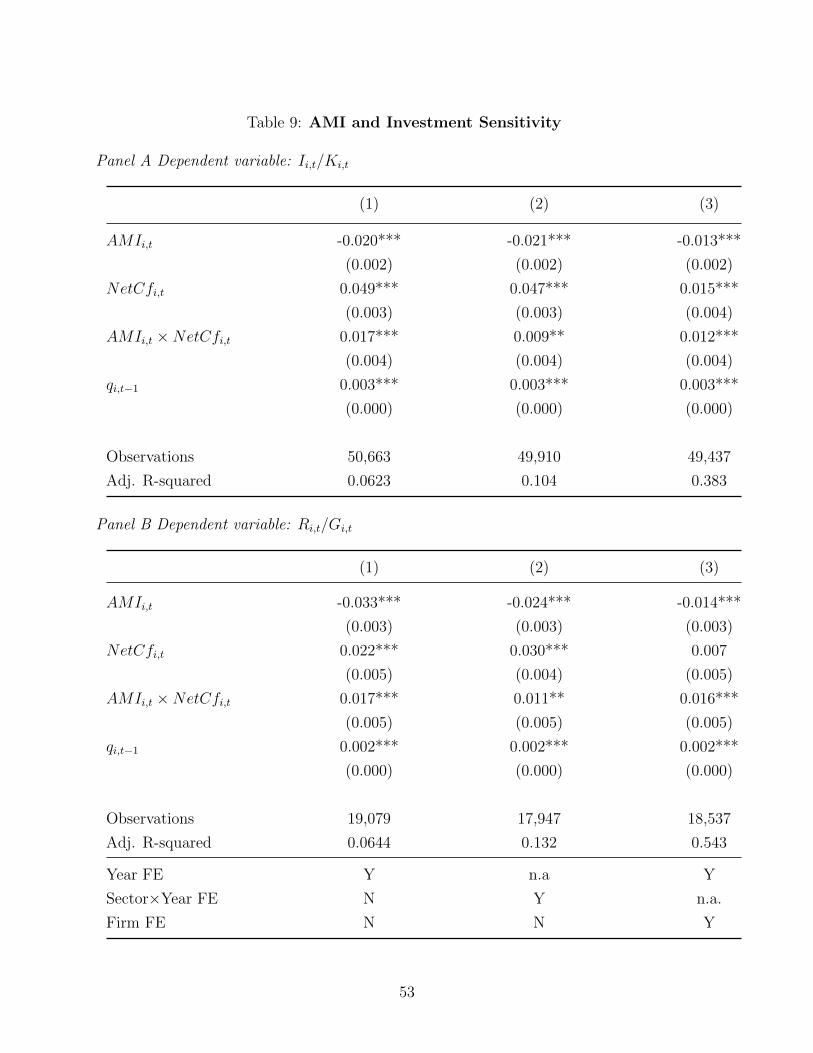
Table 9: AMI and Investment Sensitivity

Panel A Dependent variable: Ii,t/Ki,t

(1) (2) (3)

AMIi,t -0.020*** -0.021*** -0.013***

(0.002) (0.002) (0.002)

NetCfi,t 0.049*** 0.047*** 0.015***

(0.003) (0.003) (0.004)

AMIi,t ×NetCfi,t 0.017*** 0.009** 0.012***

(0.004) (0.004) (0.004)

qi,t−1 0.003*** 0.003*** 0.003***

(0.000) (0.000) (0.000)

Observations 50,663 49,910 49,437

Adj. R-squared 0.0623 0.104 0.383

Panel B Dependent variable: Ri,t/Gi,t

(1) (2) (3)

AMIi,t -0.033*** -0.024*** -0.014***

(0.003) (0.003) (0.003)

NetCfi,t 0.022*** 0.030*** 0.007

(0.005) (0.004) (0.005)

AMIi,t ×NetCfi,t 0.017*** 0.011** 0.016***

(0.005) (0.005) (0.005)

qi,t−1 0.002*** 0.002*** 0.002***

(0.000) (0.000) (0.000)

Observations 19,079 17,947 18,537

Adj. R-squared 0.0644 0.132 0.543

Year FE Y n.a Y

Sector×Year FE N Y n.a.

Firm FE N N Y

53

Panel C Dependent variable: Net hiringi,t

(1) (2) (3)

AMIi,t -0.022*** -0.020*** -0.027***

(0.002) (0.002) (0.003)

NetCfi,t 0.032*** 0.032*** -0.004

(0.004) (0.005) (0.007)

AMIi,t ×NetCfi,t 0.025*** 0.018*** 0.013*

(0.005) (0.005) (0.007)

qi,t−1 0.002*** 0.002*** 0.003***

(0.000) (0.000) (0.000)

Observations 50,683 49,929 49,390

Adj. R-squared 0.0419 0.0590 0.147

Year FE Y n.a Y

Sector×Year FE N Y n.a.

Firm FE N N Y

Notes: This table reports estimates from regressions of capital investment, I/K (Panel A), R&D investment,

R/G, (Panel B), and net hiring, Net hiring, (Panel C) on the interaction term between accounting measure-

ment intensity and net cash flow, AMIi,t×NetCfi,t. For each dependent variable, we estimate a specification

with year fixed effects, a specification with industry-year fixed effects, and one with both firm and year fixed

effects. In all columns we control for lagged values of Tobin’s Q. Ii,t/Ki,t, Ri,t/Gi,t, and Net hiringi,t are

winsorized as in Stein and Stone (2013). All the other continuous variables are trimmed at the first and last

percentile. Standard errors, clustered at the firm level, are in parentheses; *** p<0.01, ** p<0.05, * p<0.1.

All variables are defined in Appendix A.

54

Table 10: AMI and Financial Covenants

Dependent variable: Number financial covenants

(1) (2) (3)

AMIi,t 0.032** 0.060*** 0.038**

(0.015) (0.016) (0.019)

Maturityi,t 0.252*** 0.212*** 0.169***

(0.022) (0.024) (0.023)

Facility amounti,t 0.281*** 0.352*** 0.537***

(0.076) (0.087) (0.098)

Total assetsi,t−1 -0.174*** -0.153*** -0.044

(0.009) (0.011) (0.034)

Sales growthi,t 0.045 0.065 0.035

(0.039) (0.045) (0.044)

Leveragei,t−1 0.012 -0.027 -0.019

(0.063) (0.081) (0.113)

Observations 14,313 13,436 13,149

Adj. R-squared 0.138 0.183 0.345

Year FE Y n.a. Y

Sector×Year FE N Y n.a.

Firm FE N N Y

Notes: This table shows estimates from regressions of financial covenants, Number financial covenants, on

accounting measurement intensity, AMI. We estimate a specification with year fixed effects, a specification

with industry-year fixed effects, and one with both firm and year fixed effects. In all columns we control for

maturity, facility amount, lagged values of log of assets, sales growth, and financial leverage. All continuous

variables are trimmed at the first and last percentile. Standard errors, clustered at the firm level, are in

parentheses; *** p<0.01, ** p<0.05, * p<0.1. All variables are defined in Appendix A.

55

Table 11: AMI and Pay-for-Performance Sensitivity

Dependent variable: Compensationi,t

(1) (2) (3)

AMIi,t -0.015 -0.023 -0.010

(0.013) (0.014) (0.015)

zROAi,t 0.331*** 0.366*** 0.228***

(0.029) (0.037) (0.026)

AMIi,t × zROAi,t -0.060** -0.062** -0.041*

(0.025) (0.027) (0.023)

zReti,t 0.180*** 0.193*** 0.136***

(0.013) (0.016) (0.012)

AMIi,t × zReti,t -0.025* -0.029* -0.010

(0.014) (0.016) (0.013)

Total assetsi,t−1 0.407*** 0.446*** 0.217***

(0.008) (0.010) (0.026)

Sales growthi,t−1 0.159*** 0.093*** 0.097***

(0.029) (0.032) (0.027)

Leveragei,t−1 -0.168*** 0.006 -0.342***

(0.065) (0.073) (0.080)

Observations 13,201 12,307 12,892

Adj. R-squared 0.418 0.465 0.621

Year FE Y n.a. Y

Sector×Year FE N Y n.a.

Firm FE N N Y

Notes: This table shows estimates from regressions of CEO’s compensation, Compensation , on the interac-tion term between accounting measurement intensity and firm performance, AMI × zROA. We standardizecurrent-year ROA, i.e., zROA, by subtracting the mean of each two-digit-SIC-year group and dividing by thegroup standard deviation. We estimate a specification with year fixed effects, a specification with industry-year fixed effects, and one with both firm and year fixed effects. In all columns we control for stock return,lagged values of log of assets, sales growth, and financial leverage. All continuous variables are trimmed atthe first and last percentile. Standard errors, clustered at the firm level, are in parentheses; *** p<0.01, **p<0.05, * p<0.1. All variables are defined in Appendix A.

56

Table 12: Testing alternative explanations

Panel A: Controlling for Disclosure Complexity

Audit feesi,t Ii,t/Ki,t Ri,t/Gi,t Net hiringi,t tfp1i,t tfp2

i,t qi,t PINi,t

(1) (2) (3) (4) (5) (6) (7) (8)

AMIi,t 0.070*** -0.022*** -0.024*** -0.020*** -0.032*** -0.027*** -0.539*** 0.005***

(0.009) (0.002) (0.003) (0.002) (0.006) (0.006) (0.073) (0.001)

Observations 29,448 51,070 17,392 50,366 36,871 36,861 48,963 31,494

Adj. R-squared 0.831 0.154 0.168 0.0759 0.589 0.544 0.131 0.351

Coveragei,t All in drawni,t Ii,t/Ki,t Ri,t/Gi,t Net hiringi,t No fin covi,t Compi,t

(9) (10) (11) (12) (13) (14) (15)

AMIi,t -0.095*** 7.261*** 0.064***

(0.008) (1.801) (0.016)

AMIi,t ×NetCfi,t 0.008** 0.009* 0.018***

(0.004) (0.005) (0.005)

AMIi,t × zROAi,t -0.023

(0.014)

Observations 36,343 18,615 49,210 17,734 49,260 13,161 12,207

Adj. R-squared 0.542 0.380 0.112 0.138 0.0615 0.177 0.462

Controls Y Y Y Y Y Y Y

Sector×Year FE Y Y Y Y Y Y Y

57

Panel B: Controlling for Accounting Quality

Audit feesi,t Ii,t/Ki,t Ri,t/Gi,t Net hiringi,t tfp1i,t tfp2

i,t qi,t PINi,t

(1) (2) (3) (4) (5) (6) (7) (8)

AMIi,t 0.077*** -0.010*** -0.012*** -0.011*** -0.028*** -0.026*** -0.369*** 0.003**

(0.010) (0.002) (0.004) (0.002) (0.007) (0.007) (0.076) (0.001)

Observations 24,329 27,257 9,351 26,549 21,254 21,252 25,264 17,819

Adj. R-squared 0.831 0.128 0.126 0.0464 0.662 0.620 0.0961 0.344

Coveragei,t All in drawni,t Ii,t/Ki,t Ri,t/Gi,t Net hiringi,t No fin covi,t Compi,t

(9) (10) (11) (12) (13) (14) (15)

AMIi,t -0.077*** 7.119*** 0.053***

(0.011) (2.267) (0.021)

AMIi,t ×NetCfi,t 0.002 0.007 0.015*

(0.005) (0.007) (0.008)

AMIi,t × zROAi,t 0.046

(0.040)

Observations 18,856 10,391 26,322 9,598 25,796 7,325 7,920

Adj. R-squared 0.606 0.414 0.100 0.101 0.0362 0.202 0.478

Controls Y Y Y Y Y Y Y

Sector×Year FE Y Y Y Y Y Y Y

58

Panel C: Dropping Fair-Value related topics

Audit feesi,t Ii,t/Ki,t Ri,t/Gi,t Net hiringi,t tfp1i,t tfp2

i,t qi,t PINi,t

(1) (2) (3) (4) (5) (6) (7) (8)

AMIi,t 0.090*** -0.028*** -0.031*** -0.024*** -0.041*** -0.034*** -0.688*** 0.006***

(0.012) (0.002) (0.004) (0.002) (0.008) (0.007) (0.093) (0.001)

Observations 29,975 52,041 17,574 51,267 37,566 37,560 49,576 31,832

Adj. R-squared 0.827 0.152 0.167 0.0738 0.596 0.550 0.128 0.358

Coveragei,t All in drawni,t Ii,t/Ki,t Ri,t/Gi,t Net hiringi,t No fin covi,t Compi,t

(9) (10) (11) (12) (13) (14) (15)

AMIi,t -0.118*** 9.142*** 0.073***

(0.011) (2.428) (0.021)

AMIi,t ×NetCfi,t 0.011** 0.015** 0.023***

(0.005) (0.006) (0.006)

AMIi,t × zROAi,t -0.073**

(0.035)

Observations 36,604 19,204 49,916 17,949 49,935 13,496 12,314

Adj. R-squared 0.542 0.369 0.104 0.132 0.0592 0.174 0.464

Controls Y Y Y Y Y Y Y

Sector×Year FE Y Y Y Y Y Y Y

Notes: This table show estimates of Audit fees (column 1), I/K (column 2) , R/G (column 3), Net hiring(column 4), tfp1(column 5), tfp2 (column 6), q (column 7), PIN (column 8), Coverage (column 9),All in drawn (column 10), and No. financial covenants (column 14) on AMI; estimates of I/K (col-umn 11), R/G (column 12), and Nethiring (column 13) on AMI×NetCf ; and estimates of Compensationon AMI × zROA (column 15), controlling for disclosure complexity in Panel A, controlling for accountingquality, i.e., absolute discretionary accruals, earnings persistence, and earnings predictability in Panel B, anddropping fair value related bigrams in Panel C. For each dependent variable, we estimate a specification withindustry-year fixed effects. The original sets of control variables are included but not reported for brevity.Ii,t/Ki,t, Ri,t/Gi,t, and Net hiringi,t are winsorized as in Stein and Stone (2013). All the other continuousvariables are trimmed at the first and last percentile. Standard errors, clustered at the firm level , are inparentheses; *** p<0.01, ** p<0.05, * p<0.1. All variables are defined in Appendix A..

59

Online Appendixto

“Accounting Measurement Intensity”

by

Ionela Andreicovici, Laurence van Lent, Valeri Nikolaev, and Ruishen Zhang

1

Online Appendix Figure 1: Distribution of t-statistics from placebo regressions

[fig 1] [fig 2]

[fig 3] [fig 4]

[fig 5] [fig 6]

2

[fig 7] [fig 8]

[fig 9] [fig 10]

[fig 11] [fig 12]

3

[fig 13] [fig 14]

[fig 15]

Notes: This figure plots a histogram of the t-statistics from 500 regressions of Audit fees (fig 1), I/K (fig

2) , R/G (fig 3), Net hiring (fig 4), tfp1(fig 5), tfp2 (fig 6), q (fig 7), PIN (fig 8), Coverage (fig 9),

All in drawn (fig 10), and No, financial covenants (fig 14) on AMI; estimates of I/K (fig 11), R/G (fig

12), and Net hiring (fig 13) on AMI ×NetCf ; and estimates of Compensation on AMI × zROA (fig 15),

where AMI belonging to a given firm-year has been randomly assigned (with replacement). The number of

false positives and negatives at the two-sided 95 percent confidence interval in fig 1 is 3.8 and 4.6 percent,

in fig 2 is 3.8 and 3.6, in fig 3 is 3.2 and 4.6, in fig 4 is 5.0 and 4.6, in fig 5 is 4.2 and 5.2, in fig 6 is 4.8 and

4.2, in fig 7 is 5.2 and 2.4, in fig 8 is 4.2 and 3.6, in fig 9 is 3.6 and 5.0, in fig 10 is 4.8 and 4.8, in fig 11 is

4.6 and 4.4, in fig 12 is 5.2 and 6.2, in fig 13 is 2.28 and 4.0, in fig 14 is 2.8 and 4.0, and in fig 15 is 5.0 and

5.6 respectively.

4

Online Appendix Table 1: Non-accounting novels library

1. A Connecticut Yankee in King Arthur’s Court - Mark Twain

2. A Study In Scarlet Arthur - Conan Doyle

3. A Tale of Two Cities - Charles Dickens

4. Anne of Green Gables - Lucy Maud Montgomery

5. Dr. Jekyll and Mr. Hyde - Robert Louis Stevenson

6. Emma - Jane Austen

7. Great Expectations - Charles Dickens

8. Heart of Darkness - Joseph Conrad

9. Little Women - Louisa May Alcott

10. Mansfield Park - Jane Austen

11. Me-Smith - Caroline Lockhart

12. Paradise Lost - John Milton

13. Pride and Prejudice - Jane Austen

14. Sense and Sensibility - Jane Austen

15. The Adventures of Sherlock Holmes - Arthur Conan Doyle

16. The Complete Works of William Shakespeare - William Shakespeare

17. The Importance of Being Earnest – Oscar Wilde

18. The Legend of Sleepy Hollow - Washington Irving

19. The Picture of Dorian Gray – Oscar Wilde

20. The Scarlet Letter – Nathaniel Hawthorne

21. The War of the Worlds - H.G. Wells

22. The Yellow Wallpaper - Charlotte Perkins Gilman

23. Through the Looking-Glass – Charles Dodgson

24. Treasure Island - Robert Louis Stevenson

25. What Is Man And Other Stories – Mark Twain

Notes: This table shows the list of novels included as part of the non-accounting training

library.

5

Online Appendix Table 2: Top 200 bigrams by their occurrence in 10-Ks

Bigram Frequency Bigram Frequency Bigram Frequency

prefer stock 1,063,782 employment agreement 355,694 goodwill impairment 249,749

intangible asset 1,019,493 taxable income 353,527 employee stock 245,814

stock base 668,873 purchase share 348,636 tax liability 245,576

statement operation 626,779 stockholder equity 333,818 measure fair 243,605

restrict stock 616,822 value measurement 333,404 finance activity 240,638

credit agreement 580,707 statement financial 330,313 asset acquire 240,448

partially offset 547,590 tax expense 325,103 goodwill intangible 238,540

compensation expense 512,598 expense increase 312,504 accumulate comprehensive 236,644

net sale 505,195 option plan 311,428 require item 228,284

report unit 490,758 allowance loan 306,493 variable rate 227,211

current report 455,528 rate swap 305,159 employee director 224,182

mortgage loan 446,433 tax position 300,267 investment security 223,947

loan loss 440,870 federal income 299,291 consist follow 222,598

company record 434,283 value share 296,320 method account 222,258

incentive plan 428,673 pay dividend 290,355 impairment test 221,394

income loss 426,535 operate activity 284,402 pre tax 221,116

business combination 416,596 property equipment 277,254 option purchase 220,600

price share 411,577 discount rate 276,371 change rate 219,678

series prefer 410,320 stock purchase 275,873 net asset 219,154

credit risk 401,549 plan asset 271,908 compensation cost 218,841

audit committee 393,636 statement income 269,892 recognize revenue 218,559

subsidiary note 381,486 company subsidiary 269,526 common unit 217,032

derivative instrument 380,248 material impact 264,597 effective tax 216,283

letter credit 379,478 continue operation 263,608 stock award 215,548

discontinue operation 373,203 materially adversely 259,448 senior secure 212,361

impairment charge 370,845 capital requirement 255,910 credit loss 210,931

change control 370,820 debt security 253,864 plant equipment 210,480

operation financial 370,264 stock unit 252,530 primarily result 209,112

6

Bigram Frequency Bigram Frequency Bigram Frequency

non employee 209,106 rule regulation 189,809 account oversight 178,566

sarbanes oxley 208,788 primarily relate 189,724 patent application 178,499

agreement company 208,446 principal financial 189,425 director officer 177,492

development cost 207,904 exhibit company 189,287 product sale 177,091

black scholes 206,986 postretirement benefit 188,907 accordance standard 176,669

agreement provide 206,180 option exercise 188,750 allowance doubtful 176,638

defer income 205,238 unrealized gain 188,483 temporary difference 176,344

period present 202,134 contractual obligation 188,380 total asset 175,871

define benefit 201,858 base payment 188,367 service agreement 175,653

follow thousand 201,629 subsidiary company 187,888 financial asset 175,361

cash provide 201,331 warrant purchase 186,667 adversely impact 175,101

doubtful account 201,326 development expense 186,050 million include 174,646

revenue recognize 199,286 invest activity 185,379 equity method 174,476

company adopt 197,312 effective internal 184,862 expense incur 173,662

value option 196,990 shareholder equity 184,669 account payable 172,231

income expense 196,013 promissory note 184,403 defer compensation 171,913

loan agreement 195,488 critical account 184,274 capital lease 171,129

management estimate 195,067 company internal 183,913 quote price 170,885

oxley act 194,852 limit partnership 182,905 determine fair 170,837

officer principal 194,441 loss share 181,786 accordance generally 170,578

risk relate 193,698 oversight board 181,502 base salary 168,903

stock share 193,423 share series 180,852 option price 167,983

primarily increase 193,041 service revenue 180,554 board unite 167,912

property plant 192,500 convertible prefer 180,349 loss carryforwards 167,866

impairment loss 192,422 dollar thousand 180,072 limit ability 166,941

unrecognized tax 192,412 commercial real 179,604 standard public 166,777

benefit obligation 191,170 line basis 179,182 lease agreement 165,893

sell general 190,049 security holder 178,656 significant portion 165,686

7

Bigram Frequency Bigram Frequency Bigram Frequency

summary significant 164,611 purchase equity 157,274 treadway commission 152,533

company determine 163,729 cost sale 156,450 net defer 152,204

flow hedge 163,604 vest period 156,063 sale security 151,871

unrealized loss 163,567 sponsor organization 156,056 operation include 151,722

statement note 161,981 adverse impact 155,748 result change 151,009

capital stock 161,381 asset impairment 155,628 interim period 150,656

increase decrease 161,327 share class 154,819 account pronouncement 149,477

discount cash 159,061 additional capital 154,535 insurance coverage 148,585

base historical 157,973 rule exchange 154,122 impact financial 148,526

affect ability 157,569 estate loan 153,996 provision income 148,005

offset increase 157,540 event default 153,733

Notes: This table reports top 200 bigrams by their occurrence in 10-Ks.

8

Online Appendix Table 3: Top 10 bigrams per year

2001 2002 2003 2004 2005 2006

option plan option plan statement financial option plan option plan restrict stock

exhibit company statement financial option plan statement financial statement financial subsidiary note

subsidiary note goodwill intangible method account variable entity subsidiary note option plan

statement financial business combination goodwill intangible subsidiary note employee stock statement financial

stock purchase subsidiary note subsidiary note audit committee audit committee audit committee

employee stock stock purchase significant deficiency goodwill intangible restrict stock employee stock

option purchase exhibit company exit disposal stock purchase stock purchase base payment

agreement company employee stock material fact method account management assessment management assessment

hedge activity method account disposal activity impairment charge base payment stock purchase

stock share option purchase stock purchase employee stock impairment charge asset retirement

2007 2008 2009 2010 2011 2012

restrict stock business combination business combination restrict stock restrict stock restrict stock

statement financial restrict stock restrict stock value measurement report unit report unit

subsidiary note statement financial value measurement report unit value measurement value measurement

audit committee subsidiary note financial asset subsidiary note subsidiary note goodwill impairment

base payment tax position subsidiary note impairment charge impairment charge audit committee

option plan value option statement financial audit committee audit committee impairment charge

compensation cost audit committee report unit business combination tax position tax position

employee stock value measurement impairment charge tax position allowance loan subsidiary note

define benefit base payment audit committee measure fair rate swap impairment test

management assessment option plan measure fair rate swap business combination allowance loan

2013 2014 2015 2016 2017 2018

restrict stock restrict stock restrict stock restrict stock restrict stock restrict stock

report unit report unit report unit report unit report unit business combination

value measurement audit committee tax position business combination business combination report unit

audit committee tax position audit committee tax position tax position tax expense

tax position value measurement impairment charge audit committee impairment charge tax act

impairment charge impairment charge tax expense impairment charge stock unit stock unit

allowance loan unrecognized tax business combination common unit audit committee tax position

impairment test tax expense value measurement materially adversely tax expense goodwill impairment

tax expense allowance loan materially adversely stock unit goodwill impairment impairment charge

goodwill impairment accumulate comprehensive allowance loan tax expense materially adversely materially adversely

Notes: This table reports top 10 bigrams per year.

9

Online Appendix Table 4: Top 10 bigrams per industry (using the Fama-French 17 industry classification)

Food Mines Oil Clothes Durables Chemicals

net sale mineral property prove reserve net sale net sale net sale

intangible asset prove probable gas property intangible asset intangible asset intangible asset

prefer stock common unit common unit credit agreement prefer stock prefer stock

partially offset prefer stock gas reserve stock base credit agreement credit agreement

restrict stock mineral resource credit agreement prefer stock stock base partially offset

credit agreement audit committee prefer stock restrict stock statement operation plan asset

stock base statement operation derivative instrument partially offset restrict stock restrict stock

current report probable reserve exploration development letter credit report unit statement operation

audit committee price share future net statement operation company record report unit

report unit exploration development asset retirement company record partially offset define benefit

statement operation asset retirement statement operation employment agreement compensation expense sale volume

Retail Construction Steel Fabricated Products Machinery Cars

net sale net sale net sale net sale intangible asset net sale

prefer stock intangible asset intangible asset intangible asset net sale intangible asset

intangible asset credit agreement credit agreement credit agreement stock base credit agreement

patent application letter credit prefer stock plan asset prefer stock prefer stock

stock base report unit define benefit report unit report unit report unit

milestone payment prefer stock restrict stock partially offset statement operation company record

product sale restrict stock plan asset company record restrict stock partially offset

development expense statement operation report unit restrict stock compensation expense restrict stock

price share stock base benefit pension statement operation credit agreement statement operation

statement operation current report impairment charge define benefit company record stock base

compensation expense impairment charge plant equipment stock base partially offset plan asset

Transportation Utilities Retail Stores Finance Other

credit agreement regulatory asset net sale loan loss intangible asset

intangible asset postretirement benefit intangible asset mortgage loan prefer stock

common unit partially offset prefer stock allowance loan stock base

restrict stock plan asset credit agreement prefer stock statement operation

prefer stock cost recovery stock base credit risk compensation expense

partially offset electric utility statement operation investment security restrict stock

statement operation company subsidiary restrict stock intangible asset report unit

report unit rate case property equipment commercial real credit agreement

current report derivative instrument common unit credit loss price share

incentive plan transmission distribution partially offset estate loan series prefer

operate revenue generate facility company record capital requirement company record

Notes: This table reports top 10 bigrams per industry using the Fama-French 17 industry classification.

10

Online Appendix Table 5: Top S&P firms by AMI score

Firm Year 3-digit SIC Top bigrams Top snippet

PITNEY BOWES INC 2009 357 restrict stock; value hierarchy;value measurement

A reduction in estimated residualvalues could result in an impair-ment charge as well as a reductionin future financing income.

AIR PRODUCTS &CHEMICALS INC

2017 281 discontinue operation; intangibleasset; impairment charge

We accrue a liability for such mat-ters when it is probable that a li-ability has been incurred and theamount of loss can be reasonablyestimated.

SYSCO CORP 2007 514 compensation cost; performancebonus; define benefit; discountrate

Accounting for business combina-tions goodwill and intangible as-sets represent the excess of con-sideration paid over the fair valueof tangible net assets acquired.

INTERPUBLIC GROUP OFCOS

2010 731 performance cash; discount rate;intangible asset; prefer stock

We evaluate our derivative instru-ments for hedge accounting bothat inception and throughout thehedge period.

GENERAL ELECTRIC CO 2012 999 credit agreement; float rate; prorata

In estimating the liability, man-agement must utilize significantjudgment and assumptions in de-termining whether a legal obliga-tion exists to remove assets.

DILLARDS INC -CL A 2004 531 asset impairment; credit agree-ment; account change

The actuarial assumptions usedto calculate pension costs are re-viewed annually.

VULCAN MATERIALS CO 2008 140 report unit; intangible asset; ben-efit obligation

We consider market factors whendetermining the assumptions andestimates used in our valuationmodels.

11

Firm Year 3-digit SIC Top bigrams Top snippet

OMNICOM GROUP 2011 731 goodwill impairment; remeasure-ment gain; benefit obligation

The method of assessing hedge ef-fectiveness and measuring hedgeineffectiveness is formally docu-mented at hedge inception.

KROGER CO 2004 541 impairment charge; plan asset;benefit cost; lease liability

The company assesses, both at theinception of the hedge and on anongoing basis, whether derivativesused as hedging instruments arehighly effective in offsetting thechanges in the fair value or cashflow of the hedged items.

RYDER SYSTEM INC 2001 751 residual value; discontinue opera-tion; intangible asset

Also specifies criteria that intan-gible assets acquired in a pur-chase method business combina-tion must meet to be recognizedand reported apart from goodwill.

PACCAR INC 2017 371 residual value; loan lease; debt se-curity

Small balance impaired receiv-ables with similar risk character-istics are evaluated as a separatepool to determine the appropriatereserve for losses using the histor-ical loss information discussed be-low.

CHESAPEAKE ENERGYCORP

2007 131 prefer stock; derivative instru-ment; defer compensation

The excess of the cost of an ac-quired entity, if any, over the netof the amounts assigned to assetsacquired and liabilities assumed isrecognized as goodwill.

HERSHEY CO 2004 206 derivative instrument; exchangeforward; post retirement

The company is in the process ofobtaining valuations for the ac-quired net assets.

12

Firm Year 3-digit SIC Top bigrams Top snippet

NABORS INDUSTRIES LTD 2009 138 impairment charge; value mea-surement; restrict stock

We perform our impairment testsof goodwill and intangible assetsfor ten reporting units within ouroperating segments.

CATERPILLAR INC 2017 353 report unit; compensation ex-pense; goodwill impairment

Following are the methods andassumptions used in determiningour estimates and an indication ofthe risks inherent in each.

Notes: This table shows transcript excerpts for the top 15 S&P firms ranked by AMI.

13

A. Details of further validity tests: AMI, firm characteristics, and earnings quality

We provide details of tests that we only summarized in the main paper to further validate our proxy ofaccounting measurement intensity. We first examine the correlation between AMI and innate firm charac-teristics and then assess whether the relation between AMI and these firm characteristics changes when weadd proxies for earnings attributes. In case AMI and those earnings attributes are overlapping concepts,empirically, then adding proxies for the latter should not add significantly to the explanatory power of theregression as measured by its adj.R2.

Our model specification takes the form

(8) AMIit = δt × δs + γXit + εit,

where δt, and δs represent a full set of time and sector fixed effects, and the vector Xit contains a set ofvariables that prior work has thought to capture the firm’s “innate” factors (i.e., its business model andoperating environment), namely the log of the firm’s assets, the variability of sales, the operating cycle, theincidence of losses, intangible asset intensity, and capital intensity.

We report Ordinary Least Squares estimates for the relation between AMI and the various innate factorsin Table 6, panel A. We find that more variability in sales (σ(Salesi,t)) is positively associated with AMI(in column 3, coefficient = 0.082, std. err. = 0.015), suggesting that metering problems are higher whenthe operating environment of the firm is more volatile. Larger firms within a sector (in a given year) alsotend to have higher measurement intensity, consistent with these firms having more complex operations thatare more difficult to map into accounting reports. Similarly, firms with longer operating cycles (indicativeof a more lengthy process to transform input into cash) have higher measurement intensity (coefficient =0.035, std. err. = 0.017). As one would also expect, we find that firms with greater fraction of intangibleassets on their balance sheet (higher intangibles intensity) exhibit higher AMI. We also find some evidencethat capital intensive business models, i.e., those characterized by a higher fraction of property, plant andequipment in their asset base exhibit higher AMI.

Second, we examine whether and to what extent accounting measurement intensity overlaps with prox-ies for well-known earnings attributes, such as earnings persistence (Persistence), earnings predictability(Predictability), or whether the financial statement was restated (1[Restatement]). We do so by augment-ing equation 8 with each of these variables separately in columns 1-3. We consider the variation withinsector-time by including the corresponding fixed effects. Our findings indicate that AMI exhibits a negativeassociation with earnings persistence (coefficient = -0.124, std. err. = 0.032), consistent with higher earningspersistence being associated with lower accounting measurement intensity. Similarly, more predictable earn-ings are associated with lower AMI. We also find a positive correlation between AMI and the presence ofa restatement, such that firms that display high measurement intensity are more likely to also have restatedfinancial statements.

One important observation following from this table is that the explanatory power of regressions thatadd the individual earnings attributes remains virtually unchanged compared with our estimates of Adj.R2

in an equivalent specification in Panel A (column 3) that does not include these variables. We conclude,therefore, that AMI and earnings quality are distinct concepts.

14

Online Appendix Table 6: Determinants of Metering Costs

Panel A: Dependent variable: AMIi,t

(1) (2) (3)

Total assetsi,t 0.041*** 0.029*** 0.031***

(0.007) (0.008) (0.008)

(σ)Salesi,t 0.131*** 0.134*** 0.082***

(0.016) (0.016) (0.015)

Operating cyclei,t 0.034** 0.033** 0.035**

(0.016) (0.016) (0.017)

Negative earningsi,t -0.011** -0.021*** -0.002

(0.005) (0.005) (0.005)

Intangible intensityi,t 0.426*** 0.352*** 0.346***

(0.069) (0.069) (0.070)

Capital intensityi,t 0.046 0.064 0.123

(0.064) (0.064) (0.086)

Observations 32,501 32,501 31,711

Adj. R-squared 0.0268 0.0635 0.214

Year FE N Y n.a.

Sector×Year FE N N Y

15

Panel B Dependent variable AMIi,t

(1) (2) (3)

Persistencei,t -0.124***

(0.032)

Predictabilityi,t -0.301***

(0.052)

Restatementi,t 0.106***

(0.020)

Observations 31,711 31,711 31,711

Adj. R-squared 0.216 0.217 0.216

Controls Y Y Y

Sector×Year FE Y Y Y

Notes: This table shows the results from regressions with accounting measurement intensity, AMI,

as the dependent variable. Panel A reports the innate determinants of AMI, while Panel B reports

the association between AMI and different attributes of earnings, i.e., earnings persistence, earnings

predictability, and the occurrence of a restatement. In Panel A, we estimate a specification with no

fixed effects, a specification with year fixed effects, and one with industry-year fixed effects. In Panel

B, all specifications include industry-year fixed effects as well as the innate determinants from Panel

A. All continuous variables are trimmed at the first and last percentile. Standard errors, clustered

at the firm level, are in parentheses; *** p<0.01, ** p<0.05, * p<0.1. All variables are defined in

Appendix A.

16

Online Appendix Table 7: Summary statistics

N Mean St.Dev p25 Median p75 Corresponding table

AMIi,t 30,790 0.185 0.888 -0.310 0.283 0.813 Table 3

Total assetsi,t−1 30,790 5.981 2.290 4.332 6.078 7.686 Table 3

Sales growthi,t−1 30,790 0.111 0.488 -0.048 0.056 0.172 Table 3

Leveragei,t−1 30,790 0.268 0.402 0.026 0.204 0.366 Table 3

Persistencei,t−1 30,790 0.198 0.289 -0.021 0.159 0.408 Table 3

Predictabilityi,t−1 30,790 0.123 0.168 0.008 0.045 0.176 Table 3

Going concerni,t−1 30,790 0.054 0.226 0.000 0.000 0.000 Table 3

Restatementi,t−1 30,790 0.136 0.343 0.000 0.000 0.000 Table 3

AMIi,t 52,765 0.064 0.885 -0.461 0.146 0.682 Table 4 Panel A

Total assetsi,t−1 52,765 5.676 2.292 4.084 5.700 7.353 Table 4 Panel A

Sales growthi,t−1 52,765 0.189 0.659 -0.044 0.071 0.232 Table 4 Panel A

Leveragei,t−1 52,765 0.287 0.448 0.019 0.207 0.388 Table 4 Panel A

AMIi,t 18,677 0.006 0.909 -0.558 0.088 0.654 Table 4 Panel B

Total assetsi,t−1 18,677 5.210 2.269 3.656 5.121 6.781 Table 4 Panel B

Sales growthi,t−1 18,677 0.224 0.755 -0.053 0.075 0.266 Table 4 Panel B

Leveragei,t−1 18,677 0.257 0.507 0.003 0.132 0.322 Table 4 Panel B

AMIi,t 52,000 0.066 0.889 -0.463 0.148 0.690 Table 4 Panel C

Total assetsi,t−1 52,000 5.708 2.278 4.121 5.719 7.380 Table 4 Panel C

Sales growthi,t−1 52,000 0.182 0.642 -0.045 0.070 0.228 Table 4 Panel C

Leveragei,t−1 52,000 0.279 0.430 0.018 0.201 0.381 Table 4 Panel C

AMIi,t 38,275 0.144 0.889 -0.331 0.238 0.756 Table 5 Panel A

Maturityi,t 38,275 6.401 1.898 4.989 6.370 7.771 Table 5 Panel A

Sales growthi,t−1 38,275 0.129 0.386 -0.023 0.070 0.194 Table 5 Panel A

Leveragei,t−1 38,275 0.262 0.262 0.047 0.228 0.383 Table 5 Panel A

AMIi,t 38,270 0.144 0.889 -0.331 0.239 0.757 Table 5 Panel B

Total assetsi,t−1 38,270 6.401 1.899 4.988 6.370 7.772 Table 5 Panel B

Sales growthi,t−1 38,270 0.129 0.384 -0.023 0.070 0.194 Table 5 Panel B

Leveragei,t−1 38,270 0.262 0.262 0.047 0.228 0.383 Table 5 Panel B

AMIi,t 50,301 0.069 0.887 -0.463 0.147 0.696 Table 6

Total assetsi,t−1 50,301 5.564 2.273 4.003 5.578 7.198 Table 6

Sales growthi,t−1 50,301 0.198 0.672 -0.045 0.076 0.246 Table 6

Leveragei,t−1 50,301 0.274 0.448 0.013 0.188 0.376 Table 6

17

N Mean St.Dev p25 Median p75 Corresponding table

AMIi,t 32,647 0.106 0.907 -0.417 0.199 0.753 Table 7 Panel A

Total assetsi,t−1 32,647 6.154 1.899 4.758 6.071 7.496 Table 7 Panel A

Sales growthi,t−1 32,647 0.176 0.553 -0.023 0.080 0.227 Table 7 Panel A

Leveragei,t−1 32,647 0.225 0.243 0.011 0.181 0.351 Table 7 Panel A

AMIi,t 37,416 0.080 0.902 -0.459 0.166 0.723 Table 7 Panel B

Total assetsi,t−1 37,416 6.259 1.885 4.891 6.206 7.589 Table 7 Panel B

Sales growthi,t−1 37,416 0.217 0.645 -0.019 0.091 0.261 Table 7 Panel B

Leveragei,t−1 37,416 0.236 0.274 0.012 0.187 0.363 Table 7 Panel B

Maturityi,t 19,580 3.795 0.573 3.611 4.111 4.111 Table 8

Facility amounti,t 19,580 0.180 0.191 0.051 0.114 0.242 Table 8

Total assetsi,t−1 19,580 7.446 1.709 6.266 7.470 8.642 Table 8

Sales growthi,t−1 19,580 0.135 0.298 -0.009 0.076 0.202 Table 8

Leveragei,t−1 19,580 0.338 0.220 0.182 0.320 0.466 Table 8

AMIi,t 50,663 0.044 0.900 -0.501 0.127 0.682 Table 9 Panel A

qi,t−1 50,663 4.681 15.427 1.166 1.731 3.137 Table 9 Panel A

AMIi,t 19,080 -0.034 0.933 -0.631 0.050 0.639 Table 9 Panel B

qi,t−1 19,080 6.033 18.154 1.253 1.989 4.024 Table 9 Panel B

AMIi,t 50,684 0.043 0.904 -0.508 0.125 0.687 Table 9 Panel C

qi,t−1 50,684 4.525 14.904 1.163 1.724 3.106 Table 9 Panel C

AMIi,t 14,313 0.196 0.986 -0.223 0.342 0.851 Table 10

Maturityi,t 14,313 3.703 0.605 3.584 4.078 4.111 Table 10

Facility amounti,t 14,313 0.185 0.190 0.056 0.120 0.249 Table 10

Total assetsi,t−1 14,313 7.514 1.747 6.285 7.521 8.756 Table 10

Sales growthi,t−1 14,313 0.136 0.313 -0.012 0.074 0.198 Table 10

Leveragei,t−1 14,313 0.320 0.211 0.173 0.305 0.440 Table 10

AMIi,t 13,201 0.162 0.976 -0.322 0.289 0.856 Table 11

zROAi,t 13,201 0.174 0.360 0.077 0.169 0.302 Table 11

zReti,t 13,201 0.011 0.602 -0.285 -0.087 0.205 Table 11

Total assetsi,t−1 13,201 7.302 1.556 6.187 7.259 8.383 Table 11

Sales growthi,t−1 13,201 0.116 0.353 -0.016 0.072 0.181 Table 11

Leveragei,t−1 13,201 0.240 0.211 0.060 0.228 0.357 Table 11

Notes: This table provides the remaining descriptive statistics of the variables used in the previous regression

analyses. All continuous variables are trimmed at the first and last percentile. All variables are defined in

Appendix A.

18