Accelerating Sequential Computer Vision Algorithms Using Commodity Parallel Hardware
287
Accelerating Sequential Computer Vision Algorithms Using Commodity Parallel Hardware Jacob (Jaap) van de Loosdrecht A thesis submitted to Quality and Qualifications Ireland (QQI) for the award of Master of Science. Supervisors: Dr Séamus Ó Ciardhuáin (Limerick Institute of Technology) Walter Jansen (NHL University) September 2013
-
Upload
nhlstenden -
Category
Documents
-
view
1 -
download
0
Transcript of Accelerating Sequential Computer Vision Algorithms Using Commodity Parallel Hardware
Accelerating Sequential Computer Vision Algorithms
Using Commodity Parallel Hardware
Jacob (Jaap) van de Loosdrecht
A thesis submitted to Quality and Qualifications Ireland (QQI)
for the award of Master of Science.
Supervisors: Dr Séamus Ó Ciardhuáin (Limerick Institute of Technology)
Walter Jansen (NHL University)
September 2013
2
Author contact information:
Jaap van de Loosdrecht
Centre of Expertise in Computer Vision
NHL University of Applied Sciences
Leeuwarden, The Netherlands
www.nhl.nl/computervision
Jaap van de Loosdrecht
Van de Loosdrecht Machine Vision BV
Buitenpost, The Netherlands
www.vdlmv.nl
The ownership of the complete intellectual property (including the full copyright) of this
thesis belongs to the author Jacob van de Loosdrecht. No part of this thesis may be
reproduced in any form by any electronic or mechanical means without permission in
writing from the author.
3
“The Free Lunch Is Over: A Fundamental Turn Toward Concurrency in Software”
After Sutter (2005).
“Pluralitas non est ponenda sine necessitate”
In English: “Entities should not be multiplied unnecessarily”
After William of Ockham, 14th
century.
“There are three kinds of lies: lies, damned lies, and benchmarks”
Free after Mark Twain, 19th
century.
“May the GeForce be with you”
Free after Luke Skywalker in Star Wars Episode V: The Empire Strikes Back, 1980.
4
LIT Declaration
The work presented in this thesis is the original work of the author, under the direction
of Dr Séamus Ó Ciardhuáin, and due reference has been made, where necessary, to the
work of others. No part of this thesis has been previously submitted to LIT or any other
institute.
September 2013
Jacob van de Loosdrecht
September 2013
Séamus Ó Ciardhuáin

5
Abstract
Since 2004, the clock frequency of CPUs has not increased significantly. Computer Vision
applications have an increasing demand for more processing power and are limited by the
performance capabilities of sequential processor architectures. The only way to get better
performance using commodity hardware is to adopt parallel programming.
Many other related research projects have considered using one domain specific algorithm to
compare the best sequential implementation with the best parallel implementation on a
specific hardware platform. This project is distinctive because it investigated how to speed up
a whole library by parallelizing the algorithms in an economical way and execute them on
multiple platforms.
In this work the author has:
- Examined, compared and evaluated 22 programming languages and environments for
parallel computing on multi-core CPUs and GPUs.
- Chosen to use OpenMP as the standard for multi-core CPU programming and OpenCL
for GPU programming.
- Re-implemented a number of standard and well-known algorithms in Computer Vision
using both standards.
- Tested the performance of the implemented parallel algorithms and compared the
performance to the sequential implementations of the commercially available software
package VisionLab.
- Evaluated the test results with a view to assessing:
- Appropriateness of multi-core CPU and GPU architectures in Computer Vision.
- Benefits and costs of parallel approaches to implementation of Computer Vision
algorithms.
Both the literature review and the results of the benchmarks in this work have confirmed that
both multi-core CPU and GPU architectures are appropriate for accelerating sequential
Computer Vision algorithms.
Using OpenMP it was demonstrated that many algorithms of a library could be parallelized in
an economical way and that adequate speedups were achieved on two multi-core CPU
platforms. With a considerable amount of extra effort, OpenCL was used to achieve much
higher speedups for specific algorithms on dedicated GPUs.
Abstract
6
At the end of the project, the choice of standards was re-evaluated including newly emerged
ones. Recommendations are given for using standards in the future, and for future research
and development.
The following algorithmic improvements appear to be novel. The literature search has not
found any previous use of them:
- Vectorization of Convolution on grayscale images with variable sized mask utilizing
padding width of vector with zeros.
- Few-core Connect Component Labelling.
- Optimization of a recent many-core Connect Component Labelling approach.
This work resulted directly in innovation in the product VisionLab:
- 170 operators were parallelized using OpenMP. For these operators Automatic Operator
Parallelization, a run-time prediction mechanism for whether parallelization is beneficial,
was implemented. Users of VisionLab can now benefit from parallelization without
having to rewrite their scripts, C++ or C# code.
- An OpenCL toolbox was added to the development environment. Users of VisionLab can
now comfortably write OpenCL host-side code using the script language and develop
their OpenCL kernels.
Based on this work:
- Two papers (Van de Loosdrecht, 2013b) and (Dijkstra, Jansen and Van de Loosdrecht,
2013a) were published.
- Two poster presentations (Dijkstra, Jansen and Van de Loosdrecht, 2013b) and (Dijkstra,
Berntsen, Van de Loosdrecht and Jansen, 2013) were presented at conferences.
- Thirteen lectures have been given by the author at conferences, Universities and trade
shows.

7
Acknowledgements
Firstly I would like to express my gratitude to my supervisor, Séamus Ó Ciardhuáin, for all
his help in guiding me through the academic process of writing this thesis.
I would like to thank the Head of the Department Engineering of the NHL University of
Applied Sciences, Angela Schat, who has given me the opportunity to do this research master
project. Thanks to all my colleagues and students who have been working in NHL Centre of
Expertise in Computer Vision and created the fine ambience for me to work in. Special
thanks to Walter Jansen for his feedback as supervisor, to Wim van Leunen for proof reading
my thesis, and to Klaas Dijkstra who was always there to help with anything.
I wish to thank my wife, Janneke, and my children, Marieke and Johan, for always adding to
my workload and providing me with constant distractions. This provided me with the insight
that there are more important things in life than writing a thesis.
8
Table of contents
List of Tables ........................................................................................................................... 10
List of Figures .......................................................................................................................... 11
1 Introduction ...................................................................................................................... 14
1.1 Computer Vision ...................................................................................................... 14
1.2 NHL Centre of Expertise in Computer Vision ........................................................ 14
1.3 Van de Loosdrecht Machine Vision BV .................................................................. 15
1.4 Motivation for this project ....................................................................................... 16
1.5 Aim and objectives .................................................................................................. 16
1.6 Roadmap .................................................................................................................. 18
1.7 Methodology ............................................................................................................ 19
2 Requirements ................................................................................................................... 20
2.1 Introduction .............................................................................................................. 20
2.2 Earlier preliminary research and experiments ......................................................... 21
2.3 Requirements for multi-core CPUs .......................................................................... 22
2.4 Requirements for GPUs. .......................................................................................... 23
2.5 Requirements for evaluating the parallel algorithms. .............................................. 23
2.6 Moment of choice for the standards......................................................................... 24
3 Literature review .............................................................................................................. 25
3.1 Introduction .............................................................................................................. 25
3.2 Computer Vision ...................................................................................................... 25
3.3 Existing software packages for Computer Vision ................................................... 26
3.4 Performance of computer systems ........................................................................... 27
3.5 Parallel computing and programming standards...................................................... 35
3.6 Computer Vision algorithms and parallelization ..................................................... 71
3.7 Benchmarking .......................................................................................................... 80
3.8 New developments after choice of standards ........................................................... 81
3.9 Summary .................................................................................................................. 84
4 Comparison of standards and choice ............................................................................... 85
4.1 Introduction .............................................................................................................. 85
4.2 Choice of the standard for multi-core CPU programming ....................................... 85
4.3 Choice of the standard for GPU programming ........................................................ 87
5 Design .............................................................................................................................. 89
5.1 Introduction .............................................................................................................. 89
5.2 Interfacing VisionLab with OpenMP....................................................................... 89
5.3 Interfacing VisionLab with OpenCL ....................................................................... 98

Table of contents
9
5.4 Experiment design and analysis methodology ....................................................... 106
5.5 Benchmark setup .................................................................................................... 109
6 Implementation .............................................................................................................. 110
6.1 Introduction ............................................................................................................ 110
6.2 Timing procedure ................................................................................................... 110
6.3 Interfacing VisionLab with OpenMP..................................................................... 111
6.4 Interfacing VisionLab with OpenCL ..................................................................... 113
6.5 Point operators ....................................................................................................... 115
6.6 Local neighbour operators ..................................................................................... 119
6.7 Global operators ..................................................................................................... 126
6.8 Connectivity based operators ................................................................................. 133
6.9 Automatic Operator Parallelization ....................................................................... 137
7 Testing and Evaluation .................................................................................................. 139
7.1 Introduction ............................................................................................................ 139
7.2 Calibration of timer overhead ................................................................................ 140
7.3 Reproducibility of experiments.............................................................................. 140
7.4 Sequential versus OpenMP single core.................................................................. 142
7.5 Data transfer between host and device ................................................................... 143
7.6 Point operators ....................................................................................................... 150
7.7 Local neighbour operators ..................................................................................... 160
7.8 Global operators ..................................................................................................... 179
7.9 Connectivity based operators ................................................................................. 187
7.10 Automatic Operator Parallelization ....................................................................... 200
7.11 Performance portability ......................................................................................... 201
7.12 Parallelization in real projects ................................................................................ 208
8 Discussion and Conclusions .......................................................................................... 215
8.1 Introduction ............................................................................................................ 215
8.2 Evaluation of parallel architectures ....................................................................... 215
8.3 Benchmark protocol and environment ................................................................... 216
8.4 Evaluation of parallel programming standards ...................................................... 216
8.5 Contributions of the research ................................................................................. 222
8.6 Future work ............................................................................................................ 225
8.7 Final conclusions ................................................................................................... 227
References .............................................................................................................................. 229
Glossary ................................................................................................................................. 246
Appendices ............................................................................................................................. 248
10
List of Tables
Table 1. Evaluation of Array Building Blocks ........................................................................ 48
Table 2. Evaluation of C++11 .................................................................................................. 49
Table 3. Evaluation of Cilk Plus .............................................................................................. 50
Table 4. Evaluation of MCAPI ................................................................................................ 52
Table 5. Evaluation of MPI ...................................................................................................... 53
Table 6. Evaluation of OpenMP .............................................................................................. 54
Table 7. Evaluation of Parallel Patterns Library ...................................................................... 57
Table 8. Evaluation of POSIX Threads ................................................................................... 58
Table 9. Evaluation of Thread Building Blocks ...................................................................... 59
Table 10. Evaluation of Accelerator ........................................................................................ 61
Table 11. Evaluation of CUDA ............................................................................................... 62
Table 12. Evaluation of Direct Compute ................................................................................. 64
Table 13. Evaluation of HMPP Workbench ............................................................................ 65
Table 14. Evaluation of OpenCL ............................................................................................. 67
Table 15. Evaluation of PGI Accelerator ................................................................................. 69
Table 16. Comparison table for standards for Multi-core CPU programming ........................ 86
Table 17. Comparison table for standards for GPU programming .......................................... 88
Table 18. Analysis of execution time sequential LabelBlobs operator ................................. 134
Table 19. Antibiotic discs test set .......................................................................................... 210
Table 20. Antibiotic discs OpenMP median of execution times in seconds .......................... 211
Table 21. Speedup table auto-stereoscopic 3-D monitor ....................................................... 213
11
List of Figures
Figure 1. Floating point operations per second comparison between CPU and GPU. ............ 29
Figure 2. Bandwidth comparison between CPU and GPU. ..................................................... 30
Figure 3. Speedup as to be expected according to Amdahl’s Law. ......................................... 31
Figure 4. Speedup as to be expected according to Gustafson’s Law. ...................................... 32
Figure 5. Conceptual OpenCL device architecture. ................................................................. 40
Figure 6. Convolution calculation for first two pixels of destination image ........................... 74
Figure 7. Fork-join programming model. ................................................................................ 90
Figure 8. OpenCL Platform model. ......................................................................................... 99
Figure 9. OpenCL memory model. ........................................................................................ 101
Figure 10. Example of violin plot .......................................................................................... 108
Figure 11. Screenshot quick multi-core calibration. .............................................................. 112
Figure 12. Screenshot full multi-core calibration. ................................................................. 112
Figure 13. Screenshot developing host-side script code and OpenCL kernel. ...................... 114
Figure 14. Screenshot with menu of OpenCL host-side script commands. ........................... 114
Figure 15. Histogram calculation. .......................................................................................... 128
Figure 16. Variance in speedup graph. .................................................................................. 141
Figure 17. Sequential versus OpenMP one core speedup graph ............................................ 142
Figure 18. Data transfer from CPU to GPU speedup graph .................................................. 144
Figure 19. Data transfer from GPU to CPU speedup graph .................................................. 145
Figure 20. Data transfer on CPU from host to device speedup graph ................................... 146
Figure 21. Data transfer on CPU from device to host speedup graph ................................... 147
Figure 22. Host to Device data transfer times in ms. ............................................................. 148
Figure 23. Kernel execution time in ms for several implementations of Threshold.............. 148
Figure 24. Threshold OpenMP speedup graph ...................................................................... 151
Figure 25. Threshold OpenCL GPU one pixel or vector per kernel speedup graph .............. 152
Figure 26. Threshold OpenCL GPU source and destination image speedup graph .............. 153
Figure 27. Threshold OpenCL GPU chunk speedup graph ................................................... 154
Figure 28. Threshold OpenCL GPU unroll speedup graph ................................................... 155
Figure 29. Threshold OpenCL CPU one pixel or vector per kernel speedup graph .............. 156
Figure 30. Threshold OpenCL CPU chunk speedup graph ................................................... 157
Figure 31. Threshold OpenCL CPU unroll speedup graph.................................................... 158
Figure 32. Convolution 3×3 OpenMP speedup graph ........................................................... 161
Figure 33. Convolution 5×5 OpenMP speedup graph ........................................................... 162
Figure 34. Convolution 7×7 OpenMP speedup graph ........................................................... 162
Figure 35. Convolution 15×15 OpenMP speedup graph ....................................................... 163
Figure 36. Convolution 3×3 OpenCL GPU reference speedup graph ................................... 164
Figure 37. Convolution 5×5 OpenCL GPU reference speedup graph ................................... 164
List of figures
12
Figure 38. Convolution 7×7 OpenCL GPU reference speedup graph ................................... 165
Figure 39. Convolution 15×15 OpenCL GPU reference speedup graph ............................... 165
Figure 40. Convolution 3×3 OpenCL GPU local speedup graph .......................................... 167
Figure 41. Convolution 5×5 OpenCL GPU local speedup graph .......................................... 167
Figure 42. Convolution 7×7 OpenCL GPU local speedup graph .......................................... 168
Figure 43. Convolution 15×15 OpenCL GPU local speedup graph ...................................... 168
Figure 44. Convolution 3×3 OpenCL GPU chunking speedup graph ................................... 169
Figure 45. Convolution 5×5 OpenCL GPU chunking speedup graph ................................... 170
Figure 46. Convolution 7×7 OpenCL GPU chunking speedup graph ................................... 170
Figure 47. Convolution 15×15 OpenCL GPU chunking speedup graph ............................... 171
Figure 48. Convolution 3×3 OpenCL GPU 1D reference speedup graph ............................. 172
Figure 49. Convolution 5×5 OpenCL GPU 1D reference speedup graph ............................. 172
Figure 50. Convolution 7×7 OpenCL GPU 1D reference speedup graph ............................. 173
Figure 51. Convolution 15×15 OpenCL GPU 1D reference speedup graph ......................... 173
Figure 52. Convolution 3×3 OpenCL CPU 1D reference speedup graph ............................. 174
Figure 53. Convolution 5×5 OpenCL CPU 1D reference speedup graph ............................. 175
Figure 54. Convolution 7×7 OpenCL CPU 1D reference speedup graph ............................. 175
Figure 55. Convolution 15×15 OpenCL CPU 1D reference speedup graph ......................... 176
Figure 56. Histogram OpenMP speedup graph...................................................................... 180
Figure 57. Histogram simple implementation GPU speedup graph ...................................... 181
Figure 58. Histogram number of local histograms GPU speedup graph ............................... 182
Figure 59. Histogram optimized implementation GPU speedup graph ................................. 183
Figure 60. Histogram simple implementation CPU speedup graph ...................................... 184
Figure 61. Histogram optimized implementation CPU speedup graph ................................. 185
Figure 62. LabelBlobs eight connected on image cells OpenMP speedup graph .................. 188
Figure 63. LabelBlobs eight connected on image smallBlob OpenMP speedup graph ......... 189
Figure 64. LabelBlobs eight connected on image bigBlob OpenMP speedup graph ............ 189
Figure 65. LabelBlobs four connected on image cells OpenMP speedup graph ................... 190
Figure 66. LabelBlobs four connected on image smallBlob OpenMP speedup graph .......... 190
Figure 67. LabelBlobs four connected on image bigBlob OpenMP speedup graph ............. 191
Figure 68. Vectorization of InitLabels kernel speedup graph ................................................ 192
Figure 69. Vectorization of LinkFour kernel on image cells speedup graph ......................... 193
Figure 70. Vectorization of LinkFour kernel on image smallBlob speedup graph ............... 193
Figure 71. Vectorization of LinkFour kernel on image bigBlob speedup graph ................... 194
Figure 72. LabelBlobs eight connected on image cells OpenCL speedup graph .................. 195
Figure 73. LabelBlobs eight connected on image smallBlob OpenCL speedup graph ......... 196
Figure 74. LabelBlobs eight connected on image bigBlob OpenCL speedup graph ............. 196
Figure 75. LabelBlobs four connected on image cells OpenCL speedup graph .................... 197
Figure 76. LabelBlobs four connected on image smallBlob OpenCL speedup graph ........... 197
List of figures
13
Figure 77. LabelBlobs four connected on image bigBlob OpenCL speedup graph .............. 198
Figure 78. Convolution 3×3 OpenMP on ODROID speedup graph ...................................... 202
Figure 79. Convolution 5×5 OpenMP on ODROID speedup graph ...................................... 202
Figure 80. Convolution 7×7 OpenMP on ODROID speedup graph ...................................... 203
Figure 81. Convolution 15×15 OpenMP on ODROID speedup graph .................................. 203
Figure 82. Histogram simple implementation AMD GPU speedup graph ............................ 204
Figure 83. Histogram number of local histograms AMD GPU speedup graph ..................... 205
Figure 84. Histogram optimized implementation AMD GPU speedup graph....................... 206
Figure 85. Antibiotic susceptibility testing by disk diffusion. ............................................... 209
Figure 86. Antibiotic discs OpenMP speedup graph ............................................................. 210
Figure 87. Ride Photography ................................................................................................. 212
Figure 88. Real-time live 3-D images on the auto-stereoscopic 3-D monitor with 34 fps .... 213
1 Introduction - Computer Vision
14
1 Introduction
1.1 Computer Vision
Computer Vision is the field of research which comprises methods for acquiring, processing,
analysing, and understanding images with the objective to result in numerical or symbolic
information. A typical example is the computerization of visual inspections. With the aid of a
computer, images caught on camera are interpreted. The information thus obtained may
subsequently be used to manage other processes. Examples are:
- Quality checks.
- Position finding and orientation.
- Sorting products on conveyor belts.
In many industries that manufacture or handle products, visual inspection or measurement is
of major importance. In many cases, with the aid of Computer Vision, it is possible to have
these inspections or measurements carried out by a computer. In general, this will contribute
to a cheaper, more flexible and/or more labour-friendly production process.
1.2 NHL Centre of Expertise in Computer Vision
The author is founder and manager of the Centre of Expertise in Computer Vision (CECV) of
the NHL University of Applied Sciences (NHL, 2011). In Dutch: Kenniscentrum Computer
Vision van de NHL Hogeschool. The laboratory staff consists of a manager, a researcher and
two project-engineers. At present, more than 450 students have completed their placement- or
graduation assignment in the NHL CECV.
The strength of the NHL CECV lies in the knowledge of, and the equipment necessary for,
the complete chain of:
- Lighting.
- Cameras.
- Optics.
- Set-up.
- Image processing algorithms.
1 Introduction - Van de Loosdrecht Machine Vision BV
15
Since 1996 more than 170 industrial projects have been initiated and successfully completed.
Projects with a total revenue of more than €3,000,000 have been successfully completed.
Customers range from one-man businesses in the surroundings of Leeuwarden to multi-
nationals from all over the Netherlands. Approximately half of the assignments were follow-
up assignments.
From 1997 onwards Computer Vision has been lectured by the author as a subject to NHL
students. This course (Van de Loosdrecht, et al., 2013) is now in use by 10 Universities of
Applied Sciences in the Netherlands and has been taught 16 times, in an abridged form, as a
one week course taught to the industry.
1.3 Van de Loosdrecht Machine Vision BV
The author is also owner and director of Van de Loosdrecht Machine Vision BV (VdLMV).
This company is developing the software package VisionLab (Van de Loosdrecht Machine
Vision BV, 2013).
The development of VisionLab started in 1993. Visionlab provides a development
environment for Computer Vision applications. VisionLab is designed to work with 2D
image data. It incorporates artificial intelligence capabilities such as pattern matching, neural
networks and genetic algorithms. It is implemented as a portable library running on a variety
of operating systems and hardware architectures, like PC based systems, embedded real-time
intelligent cameras, smartphones and tablets.
With the Graphical User Interface (GUI) of VisionLab it is possible to experiment in a
comfortable way with the VisionLab library operators. The script language of VisionLab can
be used for comfortable development and testing of applications.
VisionLab is in use by 10 universities and 20 companies for teaching, research and industrial
applications. VisionLab is the main software product used at the NHL CECV for both
research projects as well as teaching.
However, VisionLab is limited by the performance capabilities of sequential processor
architectures.
1 Introduction - Motivation for this project
16
1.4 Motivation for this project
The last decade has seen an increasing demand from industry for computerized visual
inspection. With the growing importance of product quality checks and increasing cost of
manual inspection this trend is expected to continue.
Due to the increased performance/cost ratio of both processor speed and amount of memory
in the recent decades, low cost Computer Vision applications are now feasible for SMEs
using commodity hardware and/or low cost intelligent cameras. However, applications
rapidly become more complex and often with more demanding real time constraints, so there
is an increasing demand for more processing power. This demand is also accelerated by the
increasing pixel resolution of cameras. With the exception of the simple algorithms, most
vision algorithms will require a more than linear increase of processing power when the pixel
resolution increases. Computer Vision applications are limited by the performance
capabilities of sequential processor architectures.
There has been extensive research and development in parallel architectures for CPUs and
Graphics Processor Units (GPUs). There has also been significant R&D in the development
of programming techniques and systems for exploiting the capabilities of parallel
architectures. This has resulted in the development of standards for parallel programming.
A number of standards exist for parallel programming. These are at different levels of
development and take different approaches to the problem. It is not clear which approach is
the most effective for use in the field of Computer Vision.
This project proposes to apply parallel programming techniques to meet the challenges posed
in Computer Vision by the limits of sequential architectures.
1.5 Aim and objectives
The aim of the project is to investigate the use of parallel algorithms to improve execution
time in the specific field of Computer Vision using an existing product (VisionLab) and
research being undertaken at NHL. The research focus on commodity single system
computers, with multi-core CPUs and/or graphics accelerator cards using shared memory.
The primary objective of this project is to develop knowledge and experience in the field of
multi-core CPU and GPU programming in order to accelerate in an effective manner a huge
base of legacy sequential Computer Vision algorithms. That knowledge and experience can
then be used to develop new algorithms.
1 Introduction - Aim and objectives
17
The specific objectives of the project are to:
1. Examine, compare and evaluate existing programming languages and environments for
parallel computing on multi-core CPUs and GPUs. The output of this is to choose one
standard for multi-core CPU programming and one for GPU programming suitable for
Computer Vision applications (these may be different depending on the outcome of the
evaluation). This provides the basis for the work to be undertaken in the remaining steps
below.
2. Re-implement a number of standard and well-known algorithms in Computer Vision
using a parallel programming approach with the chosen standard(s).
3. Test the performance of the implemented parallel algorithms and compare the
performance to existing sequential implementations. The testing environment is
VisionLab.
4. Evaluate the test results with a view to assessing:
- Appropriateness of multi-core CPU and GPU architectures in Computer Vision.
- Benefits and costs of parallel approaches to implementation of Computer Vision
algorithms.
This project will not investigate:
- Dedicated hardware, like High Performance Computer (HPC) clusters, distributed
memory systems or Field Programmable Gate Arrays (FPGAs).
Customers of both VdLMV and NHL CECV are using affordable off-the-shelf
components. VdLMV and NHL CECV are not planning to access the market requesting
this kind of specialized hardware.
- A quest for the best sequential or parallel algorithms.
The focus of this project is to investigate how to speed up a whole library by parallelizing
the algorithms in an economical way.
- Automatic parallelization of code.
Preliminary research and experiments (section 2.2) have demonstrated that with the
contemporary state-of-the-art compilers this will only work for the inner loops in
algorithms. With the exception of the trivial Computer Vision algorithms this is not good
enough.
1 Introduction - Roadmap
18
1.6 Roadmap
In Chapter 2 the requirements for the standards for parallel programming and the evaluation
of the parallel algorithms are defined.
In Chapter 3 the following literature is reviewed:
- Computer Vision.
- Existing software packages for Computer Vision.
- Performance of computer systems.
- Parallel computing and standards.
- Computer Vision algorithms and parallelization.
- Benchmarking.
- New developments after choice of standards.
In Chapter 4 standards for parallel programming are compared and chosen.
In Chapter 5 the design of the following is described:
- Interfacing VisionLab with OpenMP.
- Interfacing of VisionLab with OpenCL.
- Experiment design and analysis methodology.
- Benchmark protocol and setup.
In Chapter 6 the implementation of the following is described:
- Timing procedure.
- Interfacing VisionLab with OpenMP.
- Interfacing VisionLab with OpenCL.
- Computer Vision algorithms used for benchmarking.
- Automatic Operator Parallelization.
In Chapter 7 the following items are tested and evaluated:
- Calibration of timer overhead.
- Reproducibility of experiments.
- Sequential versus OpenMP single core.
- Data transfer between host and device.
- Computer Vision algorithms used for benchmarking.
- Automatic Operator Parallelization.
- Performance portability.
- Parallelization in real projects.
Chapter 8 concludes this work with discussion and conclusions.

1 Introduction - Methodology
19
1.7 Methodology
Requirements for the cost-effective integration of parallel techniques in VisionLab and NHL
software are identified.
The project has started with desk research to identify parallel programming environments,
languages and standards, and has examined how they support parallel programming using
multi-core CPUs and GPUs.
Based on the above, two standards are chosen for the remaining work:
- A standard to support multi-core CPU programming.
- A standard to support GPU programming.
For both standards an interface to VisionLab is designed and implemented.
A set of algorithms for benchmarking is selected, chosen from the algorithms already
implemented in VisionLab using sequential methods to ensure comparability.
A benchmark protocol and setup is defined to ensure reproducibility of the experiments.
A series of benchmark tests are designed and executed to provide a body of empirical data for
comparison of sequential and parallel approaches to Computer Vision.
Conclusions are drawn, based on the empirical data, about the effectiveness and suitability of
parallel techniques and existing technologies when applied to Computer Vision.
Recommendations for future research and development are made, both in general and with
specific reference to VisionLab and NHL.
2 Requirements - Introduction
20
2 Requirements
2.1 Introduction
The objective for this work is to research ways in which the large base of legacy sequential
code of VisionLab could be accelerated using commodity parallel hardware such as multi-
core processors and graphics cards.
The VisionLab library is written in ANSI C++ and consists of more than 100,000 lines of
source code. The GUI client is written in Delphi. The architecture of VisionLab is
documented in Van de Loosdrecht (2000). VisionLab is designed and written in an object
oriented way and uses C++ templates. VisionLab supports the following types of images:
- Greyscale images: ByteImage, Int8Image, Int16Image, Int32Image, FloatImage and
DoubleImage.
- Color images: RGB888Image, RGB161616Image, HSV888Image, HSV161616Image,
YUV888Image and YUV161616Image.
- Complex images: ComplexFloatImage and ComplexDoubleImage.
For example, if no templates were used in VisionLab, a greyscale operator that supports all
greyscale image types would have to be written and maintained in six almost identical
versions. Many design patterns (Gamma, et al., 1995) are used in VisionLab’s architecture.
For reasons of performance the chosen object granularity is the image class and pixels are not
objects. Below image level traditional C++ pointers to pixels are used and not iterators over
classes. A ‘total’ object oriented approach, where pixels would have been classes with
overloaded virtual functions, would have led to an unacceptable overhead caused by the extra
indirection in the virtual function table (Ellis and Stroustrup, 1990) (Lippman, 1996) of each
pixel class.
2 Requirements - Earlier preliminary research and experiments
21
An important selling point of VisionLab has proved to be that, because it is written in ANSI
C++, it can be easily ported to different platforms like non PC based systems such as
embedded real-time intelligent cameras and mobile systems. Only a very small part of the
code is operating system specific. This code is bundled in the module OSSpecific. A C#
wrapper around the C++ library is available. VisionLab uses its own specific ‘.jl’ file format
to store images. This file format supports all image types of VisionLab and will work
transparently on both little and big endian processors. Currently VisionLab runs on operating
systems Windows, Linux and Android and on x86, x64, ARM and PowerPC processors. Both
the Microsoft Visual Studio C++ compiler and the GNU C++ compiler are used by customers
of VdLMV. The largest share of the turnover comes from customers using x86 and x64
processors with Windows and Visual Studio C++. The remaining part of the turnover comes
from customers using intelligent cameras with ARM or PowerPC processors running Linux
and GNU C++. It is to be expected that the mobile market, like smartphones and tablets, will
become important for Computer Vision.
2.2 Earlier preliminary research and experiments
Based on the research and experiments described in this section the requirements for this
work are defined. From earlier preliminary research and experiments (Van de Loosdrecht
Machine Vision BV, 2010) with parallelization the author has experienced that:
- Some operators can be parallelized for multi-core CPUs with little effort (the so called
embarrassingly parallel problems) and others must be extensively or even completely
rewritten. Some algorithms are embarrassingly sequential; for a parallel implementation a
totally new approach must be found.
- Exploiting the vector capabilities of CPUs is not an easy task and is not possible from
ANSI C++. Some ANSI C++ compilers, like Intel (Intel Corporation, 2010b) and GNU
(GNU, 2009) provide the possibility for auto-vectorization. Microsoft (Microsoft, 2011)
has announced that auto-vectorization will be available in the next version of Visual
Studio. Auto-vectorization will work for simple loops and only if strict guidelines are
followed. The auto-vectorization is guided with non-portable compiler specific pragmas.
Accelerating a large amount of legacy code in this manner is expected to be time
consuming.
- Parallelization will come with some overhead, like forking of processes, extra data
copying and synchronization. In cases where there is little work to do, like on small
images with a simple algorithm, the parallel version can be (much) slower than the
sequential version.
- In many cases not all parts of an algorithm can be parallelized.
- The transition from sequential ANSI C++ algorithms to multi-core CPUs is much simpler
than the transition to the GPUs.
2 Requirements - Requirements for multi-core CPUs
22
- Copying data between CPU memory and GPU memory will introduce considerable
overhead.
- GPUs can give better speedups than multi-core CPUs but complete new algorithms must
be developed in another language than ANSI C++.
- GPUs will only give maximum speedup if the algorithm is fine-tuned to the hardware.
Different GPUs will need different settings.
- Recently hardware manufacturers have started to deliver heterogeneous processors as
commodity products. In a heterogeneous processor CPU(s) and GPUs are merged on one
chip.
2.3 Requirements for multi-core CPUs
The requirements for multi-core CPUs are:
- The primary target system is a conventional PC, embedded intelligent camera or mobile
device with multi-core CPU and shared memory running under Windows or Linux and on
a x86 or x64 processor. Easy porting to other operating systems like Android and other
processors is an important option.
It would be a nice but not a compulsory option if the chosen solution could be scaled to
cache coherent Non-Uniform Memory Access (ccNUMA) distributed memory systems.
- There is no option for a language other than ANSI C++, because the large existing code
base is in ANSI C++.
- It is paramount that the parallelization of VisionLab can be made in an efficient manner
for the majority of the code. Because of Amdahl’s Law (section 3.4.4) many operators of
VisionLab will have to be converted to multi-core versions.
- Exploiting the vector capabilities of multi-core CPUs is a nice but not a compulsory
option. Portability and efficiently parallelizing the code are more important.
- If possible, existing VisionLab scripts and applications using the VisionLab ANSI C++
library should not have to be modified in order to benefit from the multi-core version.
- A procedure to predict at runtime whether running multi-core is expected to be beneficial
will be necessary. It is to be expected that different hardware configurations will behave
differently so there will be a need for a calibration procedure.
- Language extension and/or libraries used should be:
- ANSI C++ based.
- An industry standard.
- Vendor independent.
- Portable to at least Windows and Linux.
- Supported by at least Microsoft Visual Studio and the GNU C++ compiler.
2 Requirements - Requirements for GPUs.
23
2.4 Requirements for GPUs.
The requirements GPUs are:
- The primary target system is a conventional PC, embedded real-time intelligent camera or
mobile device with a single or multi-core CPU with one or more GPUs running under
Windows or Linux and on a x86 or x64 processor. Easy porting to other operating
systems like Android and other processors is an important option.
It would be a nice but not a compulsory option if the chosen solution could be scaled to
systems with multiple graphics cards.
- For GPUs new code design and a new language and runtime environment are expected to
be used. The chosen language and runtime environment must be:
- An industry standard.
- Hardware vendor independent.
- Software vendor independent.
- Able to work on heterogeneous systems.
- Able to collaborate with the legacy ANSI C++ code and multi-core version.
- GPU code must be able to be called from both VisionLab script language and from
the VisionLab ANSI C++ library.
2.5 Requirements for evaluating the parallel algorithms.
In the first stage of this project standards for CPU and GPU programming will be reviewed.
Based on the result of the reviews two standards will be chosen, one for CPU and one for
GPU programming. Those two standards will be used in all subsequent experiments
evaluating the parallel algorithms.
In the next stage of this project an interface to VisionLab will be designed and built for both
standards. This will provide a test environment for the experiments with the parallel
algorithms and a benchmark environment for comparing the already existing sequential
algorithms of VisionLab with the new parallel algorithms.
A benchmark protocol and setup must be defined to ensure reproducibility of the
experiments.
2 Requirements - Moment of choice for the standards.
24
2.6 Moment of choice for the standards.
Currently there is a lot of development around parallel programming. Therefore it is expected
that new standards will emerge after choosing the two standards. New emerging standards
will be included in the literature review but will not alter the choice for the standards. The
reason for this is that the primary objective of this project is to develop knowledge and
experience in the field of multi-core CPU and GPU programming in order to accelerate
sequential Computer Vision algorithms. The main focus of this work is on reviewing
literature and implementing and benchmarking parallel vision algorithms.
A change in standard will result in repeating a lot of work, like:
- Studying the standard in detail.
- Interfacing with VisionLab.
- Converting all algorithms already parallelized.
- Redoing benchmarks.
At the end of the project the choice for the standards will be evaluated including newly
emerged standards and new information about the existing standards. A recommendation for
using standards in the future will be given. Based on the lessons learned from this work it is
to be expected that, it will be easier to change to a new standard in the future if necessary.
3 Literature review - Introduction
25
3 Literature review
3.1 Introduction
In this chapter the following literature topics required for this work are reviewed:
- Computer Vision.
- Existing Computer Vision software packages.
- Performance of computer systems.
- Parallel computing and programming standards.
- Computer Vision algorithms and parallelization.
- Benchmarking.
- New developments after choice of standards.
3.2 Computer Vision
The last decades have seen a rapidly increasing demand from the industries for computerized
visual inspection. With the growing importance of product quality checks, this trend is
expected to continue. Several market surveys confirm this conclusion. Because these market
surveys are only available at a considerable fee, the author can only make an indirect
reference to them.
In Jansen (2011) Jansen, President of the European Machine Vision Association (EMVA),
summarizes the market survey 2010 of the EMVA. The turnover of vision products of
European suppliers decreased in 2009 with 21% and recovered from the recession with an
increase of 35% in 2010. The estimated turnover in Europe for 2010 was more than 2 billion
Euros. According to Jansen (2012) the European market grew by 16% in 2011 with an
estimated turnover of 2.3 billion Euros. It was reported in 2013 (PR Newswire, 2013) that the
global machine vision market in 2012 was worth 4.5 billion Dollars, and that by 2016 it
would be worth 6.75 billion Dollars.
From these market surveys it can be concluded that the vision market is huge and rapidly
expanding. As explained in section 1.4, vision applications become rapidly more complex
and often with more demanding real time constraints, so there is an increasing demand for
more processing power. As is explained in section 3.4, this demand for more processing
power cannot be satisfied using sequential algorithms.
3 Literature review - Existing software packages for Computer Vision
26
There also is a growing interest in using intelligent cameras. A good overview of intelligent
cameras and their applications can be found in the book Smart Cameras (Belbachir, A.N. ed.,
2010).
3.3 Existing software packages for Computer Vision
There are many Computer Vision software packages available, including commercial,
academic and open source. A list with many commercial software packages is published each
year in Vision Systems Design (2010). A good starting point with much information about
commercial, academic and open source software was Carnegie Mellon University (2005a),
but unfortunately this site is no longer maintained. It was outside the scope of this project to
make a full exploration of all existing software packages for Computer Vision.
VisionLab is the main software product used at the NHL CECV for both research projects as
well as teaching. Information about VisionLab can be found in Van de Loosdrecht Machine
Vision BV (2013). A course about Computer Vision with many examples and exercises using
VisionLab can be found in Van de Loosdrecht, et al. (2013). One of the reasons for the
success of both NHL CECV and VdLMV is that VdLMV has access to the source code of a
Computer Vision library. For many projects it is essential that new dedicated algorithms can
be developed in a short time, based on the existing source code.
Evaluation of competing software packages was outside the scope of this project. For both
VdLMV and NHL CECV it is imperative to have the competences to develop source code for
Computer Vision algorithms themselves.
In addition to using VisionLab the NHL CECV also has experiences with other Computer
Vision software packages like:
- Halcon, website (MVTec Software GmbH, 2011) and book (Steger, Ulrich and
Wiedemann, 2007).
- OpenCV, website (OpenCV, 2011a) and book (Bradski and Kaehler, 2008).
- NeuroCheck, website (NeuroCheck GmbH, 2011) and book (Demant, Streicher-Abel and
Waszkewitz , 1999).
3 Literature review - Performance of computer systems
27
3.4 Performance of computer systems
3.4.1 Introduction
This section gives a brief description of the development of the performance of computer
systems. It is intended as a motivation for subsequent material in the literature review. A
good survey of the evolution and the future of parallel computer systems is given in the report
“The Landscape of Parallel Computing Research: A View from Berkeley” (Asanovic et al.,
2006).
3.4.2 Performance of CPUs
In 1965 it was predicted (Moore, 1965) that because of increasing transistor density the
number of transistors that could be placed economically on an integrated circuit would
double every year. In 1975 this prediction (Moore, 1975) was refined to a period of two
years. This prediction was given the name Moore’s law. This prediction is still accurate (Intel
Corporation, 2005) and it is expected (Intel Corporation, 2010a) it will be valid until at least
2020.
Because of this enormous increase of transistor density, manufacturers of CPUs were able to
increase the clock frequency of their CPUs from 1 KHz to about 4 GHz. Due to the increased
clock frequency and the increased efficiency in executing the instructions there was an
enormous increase in processing power of CPUs.
From 2004 onwards (Sutter, 2005) manufacturers of CPUs were not able to significantly
increase the clock frequency of CPUs any more due to problems with the dissipation of heat.
In order to facilitate multi-tasking and parallel computing, manufacturers of CPUs started to
introduce hyper-threading and multi-core CPUs. In an important paper “The Free Lunch Is
Over: A Fundamental Turn Toward Concurrency in Software” Sutter (2005) predicted that
the only way to get more processing power in the future, is to adapt parallel programming,
and that it is not going to be an easy way. This view is confirmed by Asanovic et al. (2006).
They state that programming models for multi-core systems will not be easy scalable to
many-core systems and that for embarrassingly sequential algorithms complete new solutions
must be searched for.
New specialized computer languages and development environments are available for
parallel programming on multi-core CPUs. These are examined in section 3.5.3.2.
3 Literature review - Performance of computer systems
28
3.4.3 Performance of GPUs
An introduction to the history of the GPU can be found in Kirk and Hwu (2010, Chapter 2)
and in Demers (2011). Around the 1990s graphics cards were introduced in PCs in order to
speed up displaying the computer’s graphics. Over time the functionality of graphics cards
was extended with hardware for functions like rendering, shading, texture mapping,
geometric calculations and translation of vertices into different coordinate systems.
Around the 2000s GPUs where added to the graphics cards in order to have programmable
shaders. Due to the explosive growth of the computer game industry, there was an enormous
demand for faster and more complex graphics with increasing resolutions on display
monitors. Companies like NVDIA and AMD (formerly ATI) spent huge amounts of effort in
developing better and faster graphics cards.
After the introduction of programmable shaders it was possible to use graphics cards for
general programming tasks. This was called General Purpose Graphics Processing Unit
(GPGPU) computing. Contemporary graphics cards can contain up to several thousand
processors. New specialized computer languages and software development environments
have been developed to use the graphics card as a device for general programming tasks.
They are examined in section 3.5.3.3.
According to Kirk and Hwu (2010), Corporaal (2010), NVIDIA (2010b) and Lee, et al.
(2010) GPUs have a much better maximum floating point operations performance than
CPUs. Contemporary high end GPUs have a raw performance of about 4 TFLOPS (AMD,
2013a) and high end CPUs about 150 GFLOPS (Intel Corporation, 2012).
3 Literature review - Performance of computer systems
29
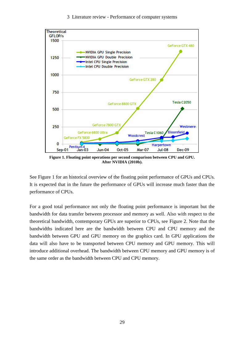
Figure 1. Floating point operations per second comparison between CPU and GPU.
After NVIDIA (2010b).
See Figure 1 for an historical overview of the floating point performance of GPUs and CPUs.
It is expected that in the future the performance of GPUs will increase much faster than the
performance of CPUs.
For a good total performance not only the floating point performance is important but the
bandwidth for data transfer between processor and memory as well. Also with respect to the
theoretical bandwidth, contemporary GPUs are superior to CPUs, see Figure 2. Note that the
bandwidths indicated here are the bandwidth between CPU and CPU memory and the
bandwidth between GPU and GPU memory on the graphics card. In GPU applications the
data will also have to be transported between CPU memory and GPU memory. This will
introduce additional overhead. The bandwidth between CPU memory and GPU memory is of
the same order as the bandwidth between CPU and CPU memory.

3 Literature review - Performance of computer systems
30
Figure 2. Bandwidth comparison between CPU and GPU.
After NVIDIA (2010b).
3.4.4 Parallel speedup factor
If the execution time of an algorithm, given its input data on one processor, is denoted by T1
and the execution time with N processors is denoted by TN we can define the parallel speedup
factor = T1 / TN. Speedup is a measure of the success of the parallelization. In the optimum
case speedup factor is N.
In general all programs will contain both sections that are suitable for parallelization and
sections that are not suitable. Amdahl’s Law (Amdahl, 1967) explains that with using an
increasing number of parallel processors, the time spent in the parallelized sections of the
program will reduce and the time spent in the sequential sections will remain the same. If P
denotes the time spent in the fraction of the program that can be parallelized and S denotes
the time spent in the serial fraction then parallel speedup can be formulated as:
NSSNPPNPS
PSSpeedup Amdahl
/)1(
1
/)1(
1
/

3 Literature review - Performance of computer systems
31
For example, if 80% of the code can be parallelized, then the speedup cannot be larger than 5,
even if an infinite number of processors is used. Amdahl’s Law implies that it is paramount
to parallelize as much of the code as possible, especially if a large number of processors is to
be exploited.
Other possible obstacles for achieving a perfect linear speedup are overheads introduced by
operations like process creation, process synchronization, buffer copying and parallel
memory access.
Amdahl’s Law has been widely cited in parallel program literature and has been misused as
argument against Massively Parallel Processing (MPP). Gustafson (1988) discovered with
experiments on a 1024 processor system that an assumption underlying Amdahl’s Law may
not be valid for larger parallel systems. According to Amdahl’s Law it was expected that the
speedup for small serial fractions would behave as illustrated in Figure 3.
Figure 3. Speedup as to be expected according to Amdahl’s Law.
After Gustafson, Montry and Benner (1988).
3 Literature review - Performance of computer systems
32
In their experiments with embarrassingly parallel problems Gustafson (1988) found speedups
of more than 1000 using 1024 processors. Amdahl’s Law implicitly assumes that P is
independent of N and assumes that the problem size is constant. With the availability of more
processors and more memory many problems are scaled with N, in many cases S decreases
when the problem is scaled to larger proportions. This is described in more detail by
Gustafson, Montry and Benner (1988).
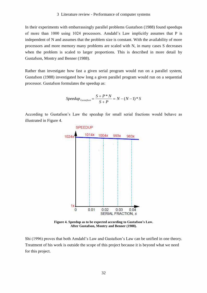
Rather than investigate how fast a given serial program would run on a parallel system,
Gustafson (1988) investigated how long a given parallel program would run on a sequential
processor. Gustafson formulates the speedup as:
SNNPS
NPSSpeedupGustafson *)1(
*
According to Gustafson’s Law the speedup for small serial fractions would behave as
illustrated in Figure 4.
Figure 4. Speedup as to be expected according to Gustafson’s Law.
After Gustafson, Montry and Benner (1988).
Shi (1996) proves that both Amdahl’s Law and Gustafson’s Law can be unified in one theory.
Treatment of his work is outside the scope of this project because it is beyond what we need
for this project.
3 Literature review - Performance of computer systems
33
In rare circumstances speedups larger than N are possible. This is called super linear speedup
(Gustafson, 1990). One possible reason for a super linear speedup is that the accumulated
cache size of a multi-processor system can be much larger than the cache size of a single
processor system. With the larger cache size, more or even all of the data can fit into the
caches and the memory access time reduces dramatically.
There is a lot of discussion about the claims of the speedup of GPUs compared to CPUs,
suggesting GPUs are up to 1000 times faster than CPUs (Lee, et al., 2010). A similar claim
was made at the Genetic and Evolutionary Computation Conference (GECCO) 2011 that the
author attended. In a presentation of an article (Pedemonte, Alba and Luna, 2011) a speedup
of 100 was claimed by the authors. But after discussion with the audience it became clear that
the authors were comparing a simple non-optimized sequential algorithm running on one core
of a CPU without using its vector capabilities with an optimized parallel algorithm running
on a multi-core GPU.
In their article “Debunking the 100X GPU vs. CPU myth: an evaluation of throughput
computing on CPU and GPU” Lee et al. (2010) of Intel Corporation put this kind of claims
in perspective. They agree with others like Kirk and Hwu (2010) and Corporaal (2010) that in
2010 GPUs had about a 10X better maximum floating point operations performance than
CPUs. However, on the test set of 14 algorithms that were used by Lee at al. for comparison,
on average a speedup of 2.5 in favour of the GPUs was found. Their article caused a lot of
debate and rumour both on the internet and in scientific communities like GECCO. The
general conclusion of Lee at al. is confirmed by McIntosh-Smith (2011) and Trinitis (2012).
Note that Lee et al. (2010) and McIntosh-Smith (2011) are comparing the performance of a
system with one multi-core CPU with a system with one GPU card. GPU cards are relatively
cheap and can be scaled to multi-GPU card systems. An increasing number of contemporary
HPC computers are constructed using a huge number of GPU cards (Top500.org, 2012).
3.4.5 Heterogeneous computing
Because of the very different hardware architectures used in design of CPUs and GPUs (see
section 3.5.2) both types of system have their advantages and disadvantages when it comes to
developing software. A nice comparison can be found in Lee, et al. (2010). In order to get the
best of both worlds, major processor manufacturers like Intel, AMD and ARM have recently
started producing combinations of CPU(s) and GPUs on one chip. In order to utilize the full
potential of such heterogeneous systems new programming languages and development
environments are under development. These new languages are reviewed in section 3.5.3.3.
3 Literature review - Performance of computer systems
34
A combination of one larger processor with multiple smaller processors on a chip may help
accelerate inherently sequential code segments. For example, Asanovic etc al. (2006) show,
that using the same amount of resources, a heterogeneous design with one complex and 90
simple processors can achieve almost twice the speed of homogeneous design with 100
simple processors.
3.4.6 Performance of Computer Vision systems
As outlined in section 1.4, there is increasing demand for more processor power in Computer
Vision applications. There has been extensive research and development in parallelizing
Computer Vision algorithms for some decades. In the past these algorithms were executed on
dedicated and expensive hardware. But now that parallel architectures like multi-CPUs and
GPUs have become a commodity, many manufacturers of Computer Vision libraries are
engaged in the process of parallelizing their Computer Vision algorithms.
As mentioned in section 3.3, this project has not exhaustively explored all existing software
packages for Computer Vision. The software packages mentioned in that section have already
parallelized a part of their library.
For a general library like VisionLab, it is not known in advance which parts of the library will
be used in an application. It is questionable whether the effort of performing a full
investigation of how often operators are used and how much time is spent in executing the
operators in an average application is worthwhile. Usage of operators will strongly vary with
the different needs of different customers. This, together with the experience described in
section 2.2 that not all parts of all operators can be parallelized, indicates that parallelization
of the VisionLab library is only profitable if a large proportion of the source code is
parallelized. Because of the amount of source code involved (over 100,000 lines) it is
paramount that the parallelization of VisionLab is made in an efficient manner for the
majority of the code.
In Lu, et al. (2009) a GPU/CPU speedup of 30 is claimed for correlation of images. The CPU
reference used is single core using the vector capabilities. In Park, et al. (2011) several types
of image processing algorithms are benchmarked on multi-core CPUs programmed using
OpenMP and GPUs programmed using CUDA. Park et al. have found GPU/CPU speedups in
the range of 0.35 to 220 depending on the type of algorithm and the size of the image.
3 Literature review - Parallel computing and programming standards
35
From Lee, et al. (2010), Lu, et al. (2009) and Park, et al. (2011) it can be concluded that in
many cases GPUs can give a better speedups than CPUs. In section 3.4.3 it was found that in
future the performance of GPUs is expected to increase much faster than the performance of
CPUs.
The Khronos Group (2011b) announced a new initiative to create a new open standard for
hardware accelerated Computer Vision. The Computer Vision Working Group Proposal for
this initiative can be found in Khronos (2011c).
From the preliminary research and experiments referred in section 2.2 it can be expected that
the programming effort needed for GPU programming will be much higher than for CPU
programming. On GPUs higher speedups can be expected that on CPUs. In this work the
benefits and costs of both parallel approaches to the implementation of Computer Vision
algorithms are investigated.
3.5 Parallel computing and programming standards
3.5.1 Introduction
In this section the following literature topics needed for this work on parallel are reviewed:
- Parallel hardware architectures.
- Parallel programming standards.
3.5.2 Parallel hardware architectures
3.5.2.1 Introduction
A general introduction to this subject can be found in Tanenbaum (2005) and Barney
(2011a). A good introduction to the differences and similarities between CPU and GPU
architectures can be found in Gaster, et al. (2012, Chapter 3). Only a few topics necessary to
understand the main themes in this work are mentioned in this section.
3 Literature review - Parallel computing and programming standards
36
Flynn's taxonomy (Flynn, 1966) is a classification of computer architectures based upon the
number of concurrent instruction and data streams in its design. In Flynn's taxonomy there
are four classes:
- Single Instruction, Single Data stream (SISD).
An example is a one core CPU in a PC. A single processor that executes a single
instruction stream to operate on single data. There is one operation on one data item at a
time, so there is no exploitation of parallelism.
- Single Instruction, Multiple Data stream (SIMD).
Examples are GPUs and the vector processing units in CPUs. Multiple processors execute
the same instruction on a different set of data.
- Multiple Instruction, Single Data stream (MISD).
This is mainly used for fault tolerant systems. Multiple processors execute the same
instruction on the same data and must agree on the result.
- Multiple Instruction, Multiple Data stream (MIMD).
An example is a multi-core CPU in a contemporary PC where multiple autonomous
processors simultaneously execute different instructions on different independent data.
A more recent and more complex taxonomy of computer architectures can be found in
Duncan (1990). He also describes the wavefront array architectures as specialization of
SIMD, see section 3.5.2.3.4.
An important aspect of a parallel computer architecture is the way in which the memory is
organized. In summarizing and partially quoting Barney (2011a) three main types are
distinguished:
- Shared memory:
- All processors have access to all memory as global address space.
- Can be divided into two main classes based upon memory access times: UMA and
NUMA.
- Uniform Memory Access (UMA): Identical processors with equal access and
access times to memory. This is most commonly represented today by Symmetric
Multi-Processor (SMP) machines. If cache coherency is accomplished at the
hardware level, it is called cache coherent UMA (ccUMA).
- Non-Uniform Memory Access (NUMA): Often made by physically linking two or
more SMPs. One SMP can directly access memory of another SMP. Not all
processors have equal access time to all memories; memory access across a link is
slower. If cache coherency is maintained, it is called cache coherent NUMA
(ccNUMA).
- Advantage: due to global address space a user-friendly programming view of memory
and fast access time to memory.
- Disadvantage: lack of scalability, adding more processors will increase traffic on the
shared-memory bus.
3 Literature review - Parallel computing and programming standards
37
- Distributed memory:
- Processors have their own local memory. Memory addresses in one processor do not
map to another processor, so there is no concept of global address space across all
processors.
- Requires a communication network to connect inter-processor memory.
- Because each processor has its own local memory, it operates independently. Changes
it makes to its local memory have no effect on the memory of other processors.
Hence, the concept of cache coherency does not apply.
- When a processor needs access to data in another processor, it is usually the task of
the programmer to use “message passing” in order to explicitly define how and when
data is communicated.
- Often used in Massively Parallel Processor (MPP) HPC systems. This connects
numerous nodes, which are made up of processor, memory, and a network port, via a
specialized fast network.
- Advantage: memory is scalable with the number of processors.
- Disadvantage: more complicated to program and it may be difficult to map existing
data structures based on global memory to this memory organization .
- Hybrid distributed-shared memory:
- Processors are clustered in groups. In each group processors have shared memory and
between the groups the memory is distributed.
Another important notion to understand is the difference between two types of parallel
programming models: data parallel and task parallel (Tsuchiyama, 2010).
- Data Parallel:
All processors run the same code but on different data. For example in a vector addition
application each process will add the elements at a unique index in the vector. Data
parallelism is characterized by relatively simple programming because all processors are
running the same code and that all processors finish their task at around the same time.
This method can be efficient when the dependency between the data being processed by
each processor is minimal.
- Task parallel:
Every processor will run a different code on different data for a different task. Task
parallelism will give a programmer more freedom but also more complexity. An
important challenge will be load balancing: how to avoid processors being idle when
there is work to do. This means that scheduling strategies will have to be implemented
which will introduce complexity and overhead.
3 Literature review - Parallel computing and programming standards
38
It is possible to combine both types of parallel programming models in one application. In
Andrade, Fraguela, Brodman, and Padua (2009) a comparison is made between task parallel
and data parallel programming approaches in multi-core systems. Membarth et al. (2011b)
compare both the data parallelism and the task parallelism approach for image registration.
3.5.2.2 Multi-core CPU
The author assumes that the reader has a general understanding about CPU architectures and
only summarizes some notions important in the context of this work. General introductions to
this subject can be found in Tanenbaum (2005) and Barney (2011a). A contemporary
commodity PC has a multi-core CPU with ccUMA shared memory. The multi-core CPU has
a MIMD architecture and each core has also a vector processing unit with a SIMD
architecture. Both a data parallel and a task parallel programming approach are possible. Lee,
et al. (2010) give a good summary:
“CPUs are designed for a wide variety of applications and to provide fast response
times to a single task. Architectural advances such as branch prediction, out-of-order
execution, and super-scalar (in addition to frequency scaling) have been responsible
for performance improvement. However, these advances come at the price of
increasing complexity/area and power consumption. As a result, main stream CPUs
today can pack only a small number of processing cores on the same die to stay within
the power and thermal envelopes.”
CPUs have a complex hierarchy of cache memory between the cores and the RAM memory.
According to Kirk and Hwu (2010) and NVIDIA (2010b) a large part of the area of the chip
is used for the cache memory and its control logic to keep the caches and memory coherent.
This implies that only a relative small part of the die is used for the cores. In GPU
architectures a large part of the area of the die is used for the cores, see section 3.5.2.3.3. This
is the main reason why contemporary GPUs have a much higher raw floating point
performance than CPUs.
3 Literature review - Parallel computing and programming standards
39
3.5.2.3 GPU
3.5.2.3.1 Introduction
There are of lot of different GPU architectures. Major manufacturers like NVIDIA and AMD
frequently introduce updated or completely new architectures. Understanding the
architectures is complicated by the fact that the manufactures call similar things by different
names. The details of those architectures go well beyond the scope of this work. Only a few
topics necessary to understand the main line in this work are treated here.
A program compiled for running on a GPU is usually called a kernel. GPUs are designed for
data parallel applications. The majority of the contemporary GPUs only allow at one time to
run one and the same kernel on all cores of the GPU. Only high end GPUs like NVIDIA’s
Kepler GK110 (NVIDIA, 2012b) allow concurrent kernel execution where multiple different
kernels can be executed at the same time. On these high end GPUs it is also possible to run
task parallel applications. See Pai, Thazhuthaveeltil and Govindarajan (2013) for a good
introduction and benchmarks.
3.5.2.3.2 GPU architecture
At the lowest level there are many differences in GPU architectures. But from a high level
perspective most GPU architectures are similar.
In order to get a general understanding of GPU architectures the conceptual OpenCL device
architecture is explained, see Figure 5. OpenCL is an open programming standard used for
GPU programming, see for more information section 3.5.3.3.8 and 5.3.2. Manufacturers like
NVIDIA and AMD support OpenCL by mapping their GPU architecture to the conceptual
OpenCL device architecture.

3 Literature review - Parallel computing and programming standards
40
Figure 5. Conceptual OpenCL device architecture.
After Munshi, ed. (2010).
In OpenCL terminology the graphics card in a commodity PC is called the compute device
and the other parts of the PC, including the CPU, are called the host. Contemporary graphics
cards will have a large amount, typically 1 GByte or more, of fast DDR RAM off-chip
memory. This memory is called the compute device memory. The device memory is cached
on the GPU chip.
Note: this device memory is different from the “normal” RAM memory used by the CPU.
Before starting a calculation on the GPU, data has to be transported from CPU memory to the
GPU device memory. When the calculation has finished the results have to be transported
from GPU device memory to CPU memory before they can be used by the CPU.
A compute device contains one or more compute units with local memory. Each compute
unit contains one or more Processor Elements (PEs). The PEs are the processor cores where
the processing is done. Each PE has its own private memory, also called the registers.
3 Literature review - Parallel computing and programming standards
41
3.5.2.3.3 GPU memory hierarchy
On the compute device there is the following hierarchy of memory:
- Compute device memory:
- Accessible by all processor elements.
- Largest memory.
- Slowest access time.
- Divided into a global memory part with read/write access and a constant memory part
with only read access. The constant memory has a much faster access time than the
global part but is usually very limited in quantity.
- Local memory:
- Only accessible by the processor elements in a compute unit.
- Available in lesser quantities than compute global memory but in larger quantity than
private memory.
- Faster access time than global memory but slower than private memory.
- Private memory:
- Only accessible by one processor element.
- Available only in very limited quantity.
- Fastest access time.
In order to get an idea about price and performance, for example a low end (100 euro,
September 2011) AMD graphics card with an ATI Radeon 5750 GPU chip (AMD, 2011a):
- 9 compute units with each 16 processor elements.
- Each processor element is a five-way Very Long Instruction Word (VLIW) SIMD like
vector processor. One of the five sub-processors is also able to execute transcendental
instructions. The total number of sub-processors is 9×16×5 = 720.
- Running at 700 Mhz, delivering a peak performance of 1008 GFlops.
- 1 GByte global memory with a peak bandwidth of 74 GBytes/s.
- 32 KByte local memory for each compute unit with a peak bandwidth of 806 GBytes/s.
- 1024 registers of private memory for each processor element with a peak bandwidth of
4838 GBytes/s.
Note: in the literature about GPUs there is no general agreement about the notion “core”. The
word core is used both for the processor element and for the sub-processor.
3 Literature review - Parallel computing and programming standards
42
According to Kirk and Hwu (2010) and NVIDIA (2010b) in GPUs a large part of the area of
the die is used for the cores. This in contrast to multi-core CPUs. Local and private memory
in GPUs can be compared with the cache hierarchy in multi-core CPUs but there are
significant differences. First the amount of local and private memory of the GPUs is much
smaller than the caches in CPUs. Second in CPUs a significant part of the area of the die is
used for maintaining caches/memory coherence, so the hardware is responsible for the
coherence. In GPUs there is no hardware support for maintaining coherence between private,
local and device memory. Maintaining this coherence is the responsibility of the programmer
of the GPU.
3.5.2.3.4 Warps or wavefronts
A kernel (thread) executed on a core is called a work-item in OpenCL terminology. A host
program, typically on a PC, is necessary to launch the kernels on the GPU. Work-items will
be grouped into work-groups in order to run on a compute unit. Within a work-group work-
items can synchronize and share local memory. Note that work-items running on different
work-groups can only be synchronized using the host program.
The compute units execute the work-items in what is called Single Instruction Multiple
Thread (SIMT) fashion, which is similar to SIMD. In SIMT fashion, vector components are
considered as individual threads that can branch independently. See Kirk and Hwu (2010,
section 6.1) for a more detailed explanation of the differences. All work-items running in one
work-group are organized in warps (NVIDIA terminology) or wavefronts (AMD
terminology). A warp is a group of work-items for which the same instruction is executed in
parallel on all cores of a compute unit. A typical size for a warp is 16, 32 or 64 work-items.
After a branch instruction it is possible that work-items within a warp will diverge. The next
instruction for some work-items will be the ‘then branch’ and for others it will be the ‘else
branch’. This means that the compute unit will have to execute both branches. The compute
unit will first execute the ‘then branch’ with the ‘then branch cores’ enabled and the ‘else
branch core’ disabled and thereafter execute the ‘else branch’ with the reverse enabling of the
cores. If not all work-items choose the same diversion, branch instructions can potentially
degrade the overall performance of GPU algorithms.
3 Literature review - Parallel computing and programming standards
43
When the work-items in a warp issue a global memory operation, that instruction will take a
very long time, typically hundreds of clock cycles, due to the long memory latency. As
shown in Figure 5, GPU architectures have a device memory data cache, but GPUs are
designed for computing performance and compared to CPUs have small and ineffective
caches. GPUs are designed to tolerate memory latency by using a high degree of multi-
threading. Each compute unit supports typically 16 or more active warps. When one warp
stalls on a memory operation, the compute unit selects another ready-to-run warp and
switches to that one. In this way, the cores can be productive as long as there is enough
parallelism to keep them busy. Contemporary GPUs have a zero-overhead warp scheduling,
so switching between warps will cost no clock cycles.
3.5.2.3.5 Coalesced memory access of global memory
In order to optimize the bandwidth the global off-chip memory is accessed by the compute
device in chunks with typical sizes of 32, 64 or 128 bytes. These chunks are cached in the
global memory data cache, see Figure 5. As mentioned before, GPUs have only very small
caches and in order to achieve good performance it is paramount to use these caches
effectively. It is important that all work-items in a warp access the global memory as much as
possible in a coalesced way. In order to facilitate this, special programming techniques are
developed. See Kirk and Hwu (2010, section 6.2), NVIDIA (2010a, section 3.2.1) and AMD
(2011a, section 4.6) for more information about this subject.
3.5.2.3.6 Bank conflicts in accessing local memory
The on-chip local memory has a memory latency which is typically about 10% of the latency
of the global off-chip memory. In order to achieve this high bandwidth the local memory is
divided into equally sized memory banks that can be accessed concurrently. However, if the
work-items in a warp request access at the same time to multiple memory addresses that map
to the same memory bank, these accesses are serialized. See NVIDIA (2010a, section 3.2.2)
AMD (2011a, section 4.7) and Sitaridi and Ross (2012) for more information about this
subject.
3 Literature review - Parallel computing and programming standards
44
3.5.2.3.7 Pinned memory
Contemporary operation systems use a virtual memory system. Each process has its own
dedicated address space. The address space is divided in blocks called pages. The total
amount of memory needed by the address spaces of all processes together can exceed by far
the amount of available primary (RAM) memory. So for each process only a limited amount
of pages can be kept in primary memory. The other pages are stored on secondary memory,
usually a hard disk. If a process needs access to a page that is not in primary memory, a page
fault will be generated. A page in primary memory will be selected and saved to secondary
memory and the page that initiated the page fault will be read from secondary memory to
primary memory. In order to avoid that a page is selected for deletion from primary memory,
a page can be pinned. If the OpenCL runtime knows that data is in pinned host memory, it
can be transferred to, and from, device memory in an enhanced way which is faster than
transferring data from, or to, unpinned memory. See for more details AMD (2011b, section
4.4). Because the amount of available primary memory is limited, only a limited amount of
pages can be pinned.
3.5.2.3.8 Developments in GPU architectures
From the preliminary experiments described in section 2.2 it was clear that optimizing GPU
kernels for maximum performance will be a challenging job. Some of the key issues have
been described in the previous sections:
- Control flow divergence.
- Global memory coalescing.
- Local memory bank conflicts.
New GPU architectures are announced in Mantor and Houston (2011) and Gaster and Howes
(2011) which will reduce the impact of the above issues on the performance.
Another issue concerning the overall system performance is the overhead of copying data
between CPU and GPU memory. In Rogers (2011) a new fused architecture of CPU and GPU
is announced where CPU and GPU will share the same global coherent memory. This will
reduce or even eliminate the copying overhead. See for more details AMD (2011b, section
4.4), Boudir and Sellers (2011), Brose (2005) and section 3.5.2.4.
Intel introduced in 2012 the Xeon Phi, the new brand name for all their products based on
their Many Integrated Core architecture. The Xeon Phi is described in Reinders (2012) and
Newburn, et al. (2013).

3 Literature review - Parallel computing and programming standards
45
3.5.2.4 Heterogeneous Computing
In the context of this work heterogeneous computing is a combination of CPU(s) and GPUs.
Recently hardware manufacturers have started shipping chips with a combination of CPU(s)
and GPUs on one die. More on this development can be found in Rogers (2011), Gaster and
Howes (2011) and Gaster et al. (2012). Examples:
- AMD Fusion, see Brookwood (2010). AMD is calling the combination of CPU and GPU
an Accelerated Processing Unit (APU).
- Intel Core i7-2600K Processor (8M Cache, 3.40 GHz) four core CPU and one GPU (Intel
Corporation, 2011h).
- Mali-T604, an ARM processor with GPU (Davies, 2011).
In 2011 the Heterogeneous System Architecture (HSA) Foundation was founded by several
companies including AMD and ARM. Rogers (2012) gives a roadmap for the HSA
Foundation and Kyriaszis (2012) a technical review. Prominent new architectural features
are:
- Coherent memory regions; fully coherent shared memory, with unified addressing for
both CPU and GPU.
- Shared page table support; this enables shared virtual memory semantics between CPU
and GPU.
- Page faulting; GPU share the same large address space as CPU.
- Hardware scheduling; GPU can switch between task without operating system
intervention.
3.5.2.5 Distributed memory systems and HPC clusters
Although outside of scope of the user requirements it would be a nice option if the chosen
solutions could easily be scaled up to larger systems. A description of those hardware
architectures is outside the scope of this project. An overview about contemporary HPC
systems can be found in Top500.org (2012) and an introduction to technology and
architecture trends can be found in Kogge and Dysart (2011).
3 Literature review - Parallel computing and programming standards
46
3.5.3 Parallel programming standards
3.5.3.1 Introduction
In this section standards for parallel programming are reviewed. The literature review on this
topic is not exhaustive. The review is restricted to systems as described in the requirements in
section 2 and has not enumerated all research projects found in this area.
Section 3.5.3.2 focuses on multi-core CPU standards and section 3.5.3.3 focuses on GPU
standards.
3.5.3.2 Multi-core CPU programming standards
3.5.3.2.1 Introduction
This section reviews several important multi-core CPU programming standards. Each
standard is described, followed by an evaluation with respect to a number of criteria. One of
the criteria is the expectations of effort needed for conversion. The effort scale used is related
to the expected number of lines of code, in order to convert an embarrassingly parallel vision
algorithm, to be added or chanced and its complexity:
- Low: only one line of code with low complexity.
- Medium: more than one but less than five lines of code with low complexity.
- High: more than five lines of code with low complexity or less than five lines of code
with high complexity.
- Huge: more than five lines of code with high complexity.
On 1 October 2011 the choice for the standard was made (Chapter 4). At the end of the
project (section 8.4) the choice for the standard was evaluated including newly emerged
standards and new information about the existing standards. The new information that
became available was added to section 3.8.
For evaluating acceptance by the market the Evans Data Corporation survey in 2011 of the
most popular multi-threaded APIs in North America discussed by Bergman (2011) was used.
In this survey multi-threaded APIs for both CPUs and GPUs are ranked in one list. According
to this survey OpenMP and OpenCL are ranked at position one and two. These positions have
been acknowledged by Shen, Fang, Varbanescu and Sips (2012).
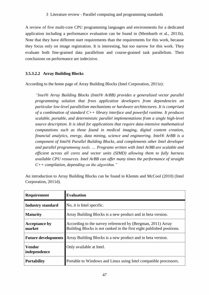
3 Literature review - Parallel computing and programming standards
47
A review of five multi-core CPU programming languages and environments for a dedicated
application including a performance evaluation can be found in (Membarth et al., 2011b).
Note that they have different start requirements than the requirements for this work, because
they focus only on image registration. It is interesting, but too narrow for this work. They
evaluate both fine-grained data parallelism and course-grained task parallelism. Their
conclusions on performance are indecisive.
3.5.3.2.2 Array Building Blocks
According to the home page of Array Building Blocks (Intel Corporation, 2011e):
“Intel® Array Building Blocks (Intel® ArBB) provides a generalized vector parallel
programming solution that frees application developers from dependencies on
particular low-level parallelism mechanisms or hardware architectures. It is comprised
of a combination of standard C++ library interface and powerful runtime. It produces
scalable, portable, and deterministic parallel implementations from a single high-level
source description. It is ideal for applications that require data-intensive mathematical
computations such as those found in medical imaging, digital content creation,
financial analytics, energy, data mining, science and engineering. Intel® ArBB is a
component of Intel® Parallel Building Blocks, and complements other Intel developer
and parallel programming tools. … Programs written with Intel ArBB are scalable and
efficient across all cores and vector units (SIMD) allowing them to fully harness
available CPU resources. Intel ArBB can offer many times the performance of straight
C++ compilation, depending on the algorithm.”
An introduction to Array Building Blocks can be found in Klemm and McCool (2010) (Intel
Corporation, 2011d).
Requirement Evaluation
Industry standard No, it is Intel specific.
Maturity Array Building Blocks is a new product and in beta version.
Acceptance by
market
According to the survey referenced by (Bergman, 2011) Array
Building Blocks is not ranked in the first eight published positions.
Future developments Array Building Blocks is a new product and in beta version.
Vendor
independence
Only available at Intel.
Portability Portable to Windows and Linux using Intel compatible processors.
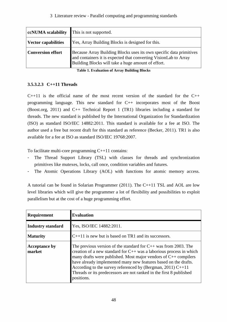
3 Literature review - Parallel computing and programming standards
48
ccNUMA scalability This is not supported.
Vector capabilities Yes, Array Building Blocks is designed for this.
Conversion effort Because Array Building Blocks uses its own specific data primitives
and containers it is expected that converting VisionLab to Array
Building Blocks will take a huge amount of effort.
Table 1. Evaluation of Array Building Blocks
3.5.3.2.3 C++11 Threads
C++11 is the official name of the most recent version of the standard for the C++
programming language. This new standard for C++ incorporates most of the Boost
(Boost.org, 2011) and C++ Technical Report 1 (TR1) libraries including a standard for
threads. The new standard is published by the International Organization for Standardization
(ISO) as standard ISO/IEC 14882:2011. This standard is available for a fee at ISO. The
author used a free but recent draft for this standard as reference (Becker, 2011). TR1 is also
available for a fee at ISO as standard ISO/IEC 19768:2007.
To facilitate multi-core programming C++11 contains:
- The Thread Support Library (TSL) with classes for threads and synchronization
primitives like mutexes, locks, call once, condition variables and futures.
- The Atomic Operations Library (AOL) with functions for atomic memory access.
A tutorial can be found in Solarian Programmer (2011). The C++11 TSL and AOL are low
level libraries which will give the programmer a lot of flexibility and possibilities to exploit
parallelism but at the cost of a huge programming effort.
Requirement Evaluation
Industry standard Yes, ISO/IEC 14882:2011.
Maturity C++11 is new but is based on TR1 and its successors.
Acceptance by
market
The previous version of the standard for C++ was from 2003. The
creation of a new standard for C++ was a laborious process in which
many drafts were published. Most major vendors of C++ compilers
have already implemented many new features based on the drafts.
According to the survey referenced by (Bergman, 2011) C++11
Threads or its predecessors are not ranked in the first 8 published
positions.
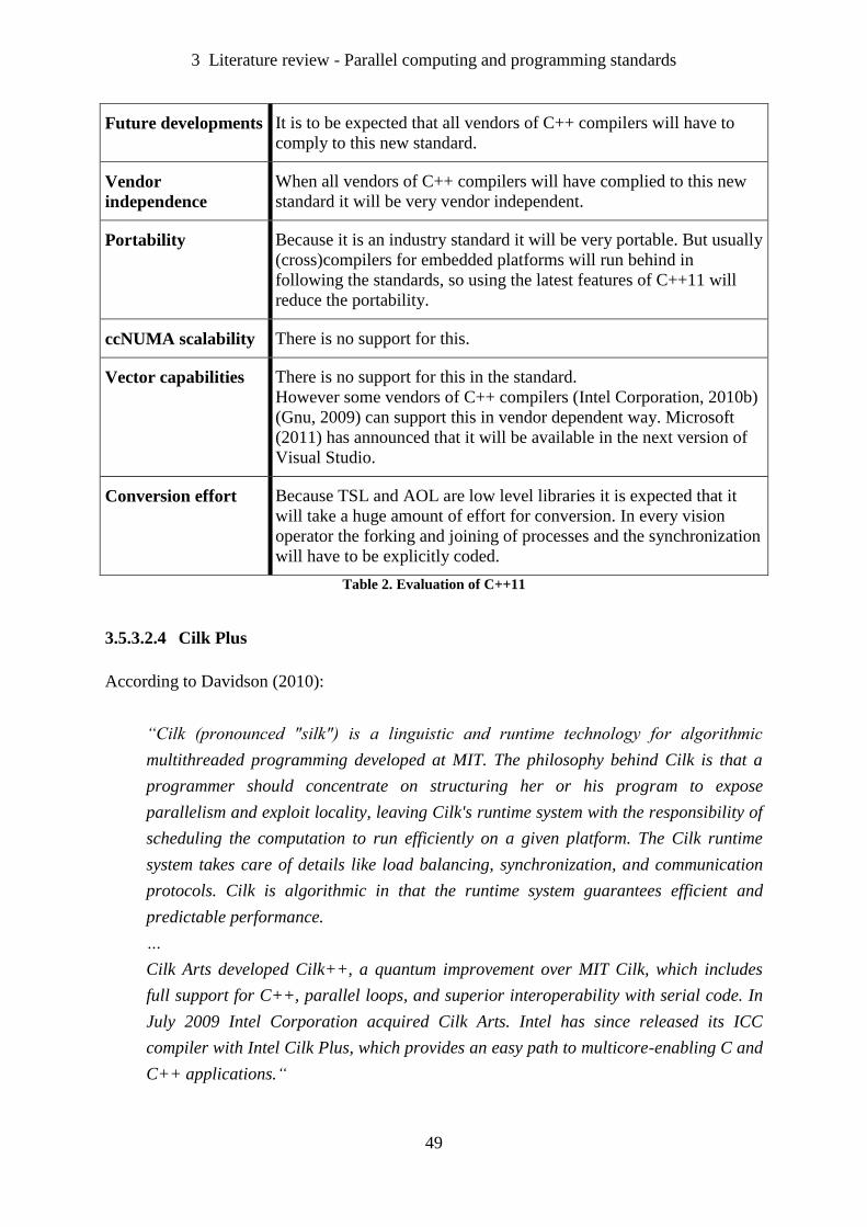
3 Literature review - Parallel computing and programming standards
49
Future developments It is to be expected that all vendors of C++ compilers will have to
comply to this new standard.
Vendor
independence
When all vendors of C++ compilers will have complied to this new
standard it will be very vendor independent.
Portability Because it is an industry standard it will be very portable. But usually
(cross)compilers for embedded platforms will run behind in
following the standards, so using the latest features of C++11 will
reduce the portability.
ccNUMA scalability There is no support for this.
Vector capabilities There is no support for this in the standard.
However some vendors of C++ compilers (Intel Corporation, 2010b)
(Gnu, 2009) can support this in vendor dependent way. Microsoft
(2011) has announced that it will be available in the next version of
Visual Studio.
Conversion effort Because TSL and AOL are low level libraries it is expected that it
will take a huge amount of effort for conversion. In every vision
operator the forking and joining of processes and the synchronization
will have to be explicitly coded.
Table 2. Evaluation of C++11
3.5.3.2.4 Cilk Plus
According to Davidson (2010):
“Cilk (pronounced "silk") is a linguistic and runtime technology for algorithmic
multithreaded programming developed at MIT. The philosophy behind Cilk is that a
programmer should concentrate on structuring her or his program to expose
parallelism and exploit locality, leaving Cilk's runtime system with the responsibility of
scheduling the computation to run efficiently on a given platform. The Cilk runtime
system takes care of details like load balancing, synchronization, and communication
protocols. Cilk is algorithmic in that the runtime system guarantees efficient and
predictable performance.
…
Cilk Arts developed Cilk++, a quantum improvement over MIT Cilk, which includes
full support for C++, parallel loops, and superior interoperability with serial code. In
July 2009 Intel Corporation acquired Cilk Arts. Intel has since released its ICC
compiler with Intel Cilk Plus, which provides an easy path to multicore-enabling C and
C++ applications.“
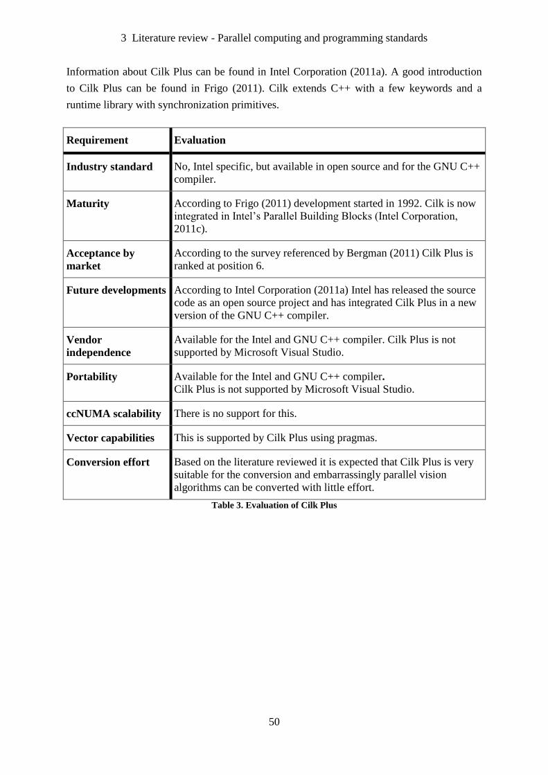
3 Literature review - Parallel computing and programming standards
50
Information about Cilk Plus can be found in Intel Corporation (2011a). A good introduction
to Cilk Plus can be found in Frigo (2011). Cilk extends C++ with a few keywords and a
runtime library with synchronization primitives.
Requirement Evaluation
Industry standard No, Intel specific, but available in open source and for the GNU C++
compiler.
Maturity According to Frigo (2011) development started in 1992. Cilk is now
integrated in Intel’s Parallel Building Blocks (Intel Corporation,
2011c).
Acceptance by
market
According to the survey referenced by Bergman (2011) Cilk Plus is
ranked at position 6.
Future developments According to Intel Corporation (2011a) Intel has released the source
code as an open source project and has integrated Cilk Plus in a new
version of the GNU C++ compiler.
Vendor
independence
Available for the Intel and GNU C++ compiler. Cilk Plus is not
supported by Microsoft Visual Studio.
Portability Available for the Intel and GNU C++ compiler.
Cilk Plus is not supported by Microsoft Visual Studio.
ccNUMA scalability There is no support for this.
Vector capabilities This is supported by Cilk Plus using pragmas.
Conversion effort Based on the literature reviewed it is expected that Cilk Plus is very
suitable for the conversion and embarrassingly parallel vision
algorithms can be converted with little effort.
Table 3. Evaluation of Cilk Plus
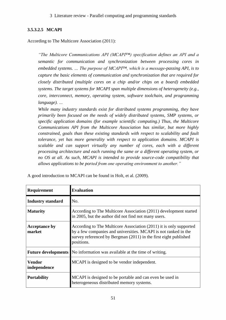
3 Literature review - Parallel computing and programming standards
51
3.5.3.2.5 MCAPI
According to The Multicore Association (2011):
“The Multicore Communications API (MCAPI™) specification defines an API and a
semantic for communication and synchronization between processing cores in
embedded systems. … The purpose of MCAPI™, which is a message-passing API, is to
capture the basic elements of communication and synchronization that are required for
closely distributed (multiple cores on a chip and/or chips on a board) embedded
systems. The target systems for MCAPI span multiple dimensions of heterogeneity (e.g.,
core, interconnect, memory, operating system, software toolchain, and programming
language). …
While many industry standards exist for distributed systems programming, they have
primarily been focused on the needs of widely distributed systems, SMP systems, or
specific application domains (for example scientific computing.) Thus, the Multicore
Communications API from the Multicore Association has similar, but more highly
constrained, goals than these existing standards with respect to scalability and fault
tolerance, yet has more generality with respect to application domains. MCAPI is
scalable and can support virtually any number of cores, each with a different
processing architecture and each running the same or a different operating system, or
no OS at all. As such, MCAPI is intended to provide source-code compatibility that
allows applications to be ported from one operating environment to another.”
A good introduction to MCAPI can be found in Holt, et al. (2009).
Requirement Evaluation
Industry standard No.
Maturity According to The Multicore Association (2011) development started
in 2005, but the author did not find not many users.
Acceptance by
market
According to The Multicore Association (2011) it is only supported
by a few companies and universities. MCAPI is not ranked in the
survey referenced by Bergman (2011) in the first eight published
positions.
Future developments No information was available at the time of writing.
Vendor
independence
MCAPI is designed to be vendor independent.
Portability MCAPI is designed to be portable and can even be used in
heterogeneous distributed memory systems.

3 Literature review - Parallel computing and programming standards
52
ccNUMA scalability Yes.
Vector capabilities There is no support for this in the standard.
However some vendors of C++ compilers (Intel Corporation, 2010b)
(Gnu, 2009) can support this in vendor dependent way. Microsoft
(2011) has announced that it will be available in the next version of
Visual Studio.
Conversion effort Because MCAPI is a very low level library it is expected that it will
take a huge amount of effort for conversion. Beside that in every
vision operator the forking and joining of processes and the
synchronization will have to be explicitly coded, a lot of coding
effort will be necessary to set up the communication channels
between the processes.
Table 4. Evaluation of MCAPI
3.5.3.2.6 MPI
MPI, the Message Passing Interface, was developed in order to facilitate portable
programming for distributed memory computer architectures. The standard (Message Passing
Interface Forum, 2009) defines a set of library routines useful to a wide range of users writing
portable message-passing programs in Fortran 77, C or C++. Several well-tested and efficient
implementations of MPI already exist, including some that are free and in the public domain.
More information can be found at the home page of MPI (Message Passing Interface Forum,
2011). A public domain implementation with open source can be found at Open MPI (2011).
Requirement Evaluation
Industry standard Yes, see Message Passing Interface Forum (2009).
Maturity According to Message Passing Interface Forum (2009) and Open
MPI (2011) since 1992 a very large community of users both
academic and industrial.
Acceptance by
market
According to the survey referenced by Bergman (2011) MPI is
ranked at position 7.
Future developments From Open MPI (2011) it is quite clear that there is a lot of on-going
development on MPI.
Vendor
independence
From several sources binary implementations are available for both
Windows and Linux. An open source implementation is available
from Open MPI (2011). MPI can be used with both GNU C++
compiler and Microsoft Visual Studio.
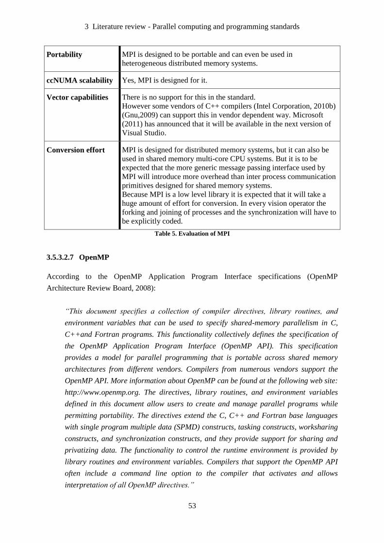
3 Literature review - Parallel computing and programming standards
53
Portability MPI is designed to be portable and can even be used in
heterogeneous distributed memory systems.
ccNUMA scalability Yes, MPI is designed for it.
Vector capabilities There is no support for this in the standard.
However some vendors of C++ compilers (Intel Corporation, 2010b)
(Gnu,2009) can support this in vendor dependent way. Microsoft
(2011) has announced that it will be available in the next version of
Visual Studio.
Conversion effort MPI is designed for distributed memory systems, but it can also be
used in shared memory multi-core CPU systems. But it is to be
expected that the more generic message passing interface used by
MPI will introduce more overhead than inter process communication
primitives designed for shared memory systems.
Because MPI is a low level library it is expected that it will take a
huge amount of effort for conversion. In every vision operator the
forking and joining of processes and the synchronization will have to
be explicitly coded.
Table 5. Evaluation of MPI
3.5.3.2.7 OpenMP
According to the OpenMP Application Program Interface specifications (OpenMP
Architecture Review Board, 2008):
“This document specifies a collection of compiler directives, library routines, and
environment variables that can be used to specify shared-memory parallelism in C,
C++and Fortran programs. This functionality collectively defines the specification of
the OpenMP Application Program Interface (OpenMP API). This specification
provides a model for parallel programming that is portable across shared memory
architectures from different vendors. Compilers from numerous vendors support the
OpenMP API. More information about OpenMP can be found at the following web site:
http://www.openmp.org. The directives, library routines, and environment variables
defined in this document allow users to create and manage parallel programs while
permitting portability. The directives extend the C, C++ and Fortran base languages
with single program multiple data (SPMD) constructs, tasking constructs, worksharing
constructs, and synchronization constructs, and they provide support for sharing and
privatizing data. The functionality to control the runtime environment is provided by
library routines and environment variables. Compilers that support the OpenMP API
often include a command line option to the compiler that activates and allows
interpretation of all OpenMP directives.”
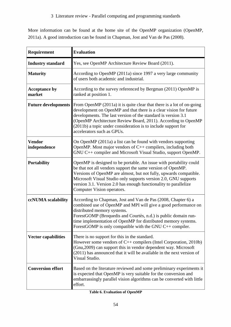
3 Literature review - Parallel computing and programming standards
54
More information can be found at the home site of the OpenMP organization (OpenMP,
2011a). A good introduction can be found in Chapman, Jost and Van de Pas (2008).
Requirement Evaluation
Industry standard Yes, see OpenMP Architecture Review Board (2011).
Maturity According to OpenMP (2011a) since 1997 a very large community
of users both academic and industrial.
Acceptance by
market
According to the survey referenced by Bergman (2011) OpenMP is
ranked at position 1.
Future developments From OpenMP (2011a) it is quite clear that there is a lot of on-going
development on OpenMP and that there is a clear vision for future
developments. The last version of the standard is version 3.1
(OpenMP Architecture Review Board, 2011). According to OpenMP
(2011b) a topic under consideration is to include support for
accelerators such as GPUs.
Vendor
independence
On OpenMP (2011a) a list can be found with vendors supporting
OpenMP. Most major vendors of C++ compilers, including both
GNU C++ compiler and Microsoft Visual Studio, support OpenMP.
Portability OpenMP is designed to be portable. An issue with portability could
be that not all vendors support the same version of OpenMP.
Versions of OpenMP are almost, but not fully, upwards compatible.
Microsoft Visual Studio only supports version 2.0, GNU supports
version 3.1. Version 2.0 has enough functionality to parallelize
Computer Vision operators.
ccNUMA scalability According to Chapman, Jost and Van de Pas (2008, Chapter 6) a
combined use of OpenMP and MPI will give a good performance on
distributed memory systems.
ForestGOMP (Broquedis and Courtès, n.d.) is public domain run-
time implementation of OpenMP for distributed memory systems.
ForestGOMP is only compatible with the GNU C++ compiler.
Vector capabilities There is no support for this in the standard.
However some vendors of C++ compilers (Intel Corporation, 2010b)
(Gnu,2009) can support this in vendor dependent way. Microsoft
(2011) has announced that it will be available in the next version of
Visual Studio.
Conversion effort Based on the literature reviewed and some preliminary experiments it
is expected that OpenMP is very suitable for the conversion and
embarrassingly parallel vision algorithms can be converted with little
effort.
Table 6. Evaluation of OpenMP
3 Literature review - Parallel computing and programming standards
55
3.5.3.2.8 Parallel Building Blocks
According to the home page of Parallel Building Blocks (Intel Corporation, 2011b):
“Intel Parallel Building Blocks is a set of comprehensive parallel development models
that support multiple approaches to parallelism. Since they share the same foundation,
you can mix and match the models that suit your unique parallel implementation needs.
These models easily integrate into existing applications and help preserve investments
in existing code and speeds development of parallel applications.
…
Intel® Parallel Building Blocks Components:
- Intel® Threading Building Blocks is a C++ template library solution that can be
used to enable general parallelism. It is for C++ developers who write general-
purpose loop and task parallelism applications. It includes scalable memory
allocation, load-balancing, work-stealing task scheduling, a thread-safe pipeline
and concurrent containers, high-level parallel algorithms, and numerous
synchronization primitives.
- Intel® Cilk™ Plus is an Intel® C/C++ Compiler-specific implementation of
parallelism: Intel Cilk Plus is for C++ software developers who write simple loop
and task parallel applications. It offers superior functionality by combining
vectorization features with high-level loop-type data parallelism and tasking.
- Intel® Array Building Blocks (Beta available now) provides a generalized vector
parallel programming solution that frees application developers from
dependencies on particular low-level parallelism mechanisms or hardware
architectures. It is for software developers who write compute-intensive, vector
parallel algorithms. It produces scalable, portable, and deterministic parallel
implementations from a single high-level, maintainable, and application-oriented
specification of the desired computation.”
An introduction to Parallel Building Blocks can be found in Intel Corporation (2011c).
The individual components of Parallel Building Blocks are reviewed in separated sections.
- Thread Building Blocks in section 3.5.3.2.12.
- Cilk Plus in section 3.5.3.2.4.
- Array Building Blocks in section 3.5.3.2.2.

3 Literature review - Parallel computing and programming standards
56
Note: in the survey referenced by Bergman (2011) Parallel Building Blocks (PBB) is ranked
at position 4, Thread Building Blocks (TBB) at position 3 and Cilk Plus at position 6. Array
Building Blocks was still in beta and not ranked. It is strange that TBB is ranked higher than
PBB because TBB is a part of PBB. PBB is a set of individual tools that can be used on their
own or in collaboration. The author believes that this is a flaw in the survey. It would have
been clearer if either PBB alone or the three individual tools were used in the survey.
3.5.3.2.9 Parallel Patterns Library
According to the home page of Microsoft’s Parallel Patterns Library (Microsoft, 2011a):
“The Parallel Patterns Library (PPL) provides an imperative programming model that
promotes scalability and ease-of-use for developing concurrent applications. The PPL
builds on the scheduling and resource management components of the Concurrency
Runtime. It raises the level of abstraction between your application code and the
underlying threading mechanism by providing generic, type-safe algorithms and
containers that act on data in parallel. The PPL also lets you develop applications that
scale by providing alternatives to shared state.
The PPL provides the following features:
- Task Parallelism: a mechanism to execute several work items (tasks) in parallel
- Parallel algorithms: generic algorithms that act on collections of data in parallel
- Parallel containers and objects: generic container types that provide safe concurrent
access to their elements
…
The PPL provides a programming model that resembles the Standard Template
Library (STL).”
An introduction to the Parallel Patterns Library can be found in Groff (2011).
Requirement Evaluation
Industry standard No, it is Microsoft specific.
Maturity The Parallel Patterns Library is well integrated in Microsoft Visual
Studio. It was first bundled with Visual Studio 2010.
Acceptance by
market
Parallel Patterns Library is new and not ranked in the survey
referenced by Bergman (2011) .
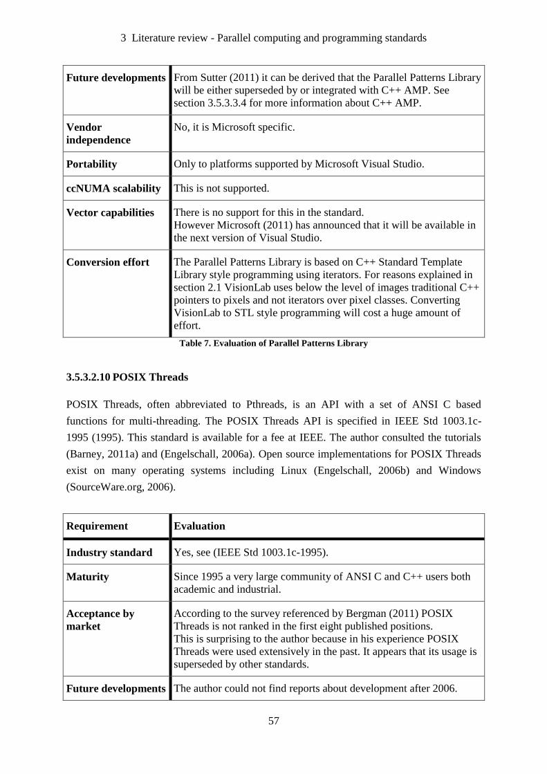
3 Literature review - Parallel computing and programming standards
57
Future developments From Sutter (2011) it can be derived that the Parallel Patterns Library
will be either superseded by or integrated with C++ AMP. See
section 3.5.3.3.4 for more information about C++ AMP.
Vendor
independence
No, it is Microsoft specific.
Portability Only to platforms supported by Microsoft Visual Studio.
ccNUMA scalability This is not supported.
Vector capabilities There is no support for this in the standard.
However Microsoft (2011) has announced that it will be available in
the next version of Visual Studio.
Conversion effort The Parallel Patterns Library is based on C++ Standard Template
Library style programming using iterators. For reasons explained in
section 2.1 VisionLab uses below the level of images traditional C++
pointers to pixels and not iterators over pixel classes. Converting
VisionLab to STL style programming will cost a huge amount of
effort.
Table 7. Evaluation of Parallel Patterns Library
3.5.3.2.10 POSIX Threads
POSIX Threads, often abbreviated to Pthreads, is an API with a set of ANSI C based
functions for multi-threading. The POSIX Threads API is specified in IEEE Std 1003.1c-
1995 (1995). This standard is available for a fee at IEEE. The author consulted the tutorials
(Barney, 2011a) and (Engelschall, 2006a). Open source implementations for POSIX Threads
exist on many operating systems including Linux (Engelschall, 2006b) and Windows
(SourceWare.org, 2006).
Requirement Evaluation
Industry standard Yes, see (IEEE Std 1003.1c-1995).
Maturity Since 1995 a very large community of ANSI C and C++ users both
academic and industrial.
Acceptance by
market
According to the survey referenced by Bergman (2011) POSIX
Threads is not ranked in the first eight published positions.
This is surprising to the author because in his experience POSIX
Threads were used extensively in the past. It appears that its usage is
superseded by other standards.
Future developments The author could not find reports about development after 2006.

3 Literature review - Parallel computing and programming standards
58
For C++, POSIX Threads are superseded by C+11 Threads, see
section 3.5.3.2.3.
Vendor
independence
Open source implementations (Engelschall, 2006b) and
(SourceWare.org, 2006) are reported to work with both GNU C++
compiler and Microsoft Visual Studio.
Portability POSIX Threads is designed to be portable.
ccNUMA scalability This is not supported.
Vector capabilities There is no support for this in the standard.
However some vendors of C++ compilers (Intel Corporation, 2010b)
(Gnu,2009) can support this in vendor dependent way. Microsoft
(2011) has announced that it will be available in the next version of
Visual Studio.
Conversion effort Because POSIX Threads is very low level library it is expected that it
will take a huge amount of effort for conversion. In every vision
operator the forking and joining of processes and the synchronization
will have to be explicitly coded.
Table 8. Evaluation of POSIX Threads
3.5.3.2.11 PVM
According to the home page of PVM (Parallel Virtual Machine, 2011) :
“PVM (Parallel Virtual Machine) is a software package that permits a heterogeneous
collection of Unix and/or Windows computers hooked together by a network to be used
as a single large parallel computer. Thus large computational problems can be solved
more cost effectively by using the aggregate power and memory of many computers.
The software is very portable. The source, which is available free thru netlib, has been
compiled on everything from laptops to CRAYs.”
The latest version of PVM, version 3.4.6, was released in 1997. The author decided not to
review PVM any further because it is out dated.
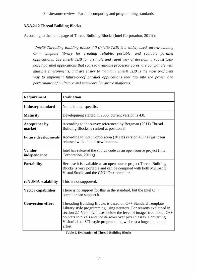
3 Literature review - Parallel computing and programming standards
59
3.5.3.2.12 Thread Building Blocks
According to the home page of Thread Building Blocks (Intel Corporation, 2011f):
“Intel® Threading Building Blocks 4.0 (Intel® TBB) is a widely used, award-winning
C++ template library for creating reliable, portable, and scalable parallel
applications. Use Intel® TBB for a simple and rapid way of developing robust task-
based parallel applications that scale to available processor cores, are compatible with
multiple environments, and are easier to maintain. Intel® TBB is the most proficient
way to implement future-proof parallel applications that tap into the power and
performance of multicore and manycore hardware platforms.”
Requirement Evaluation
Industry standard No, it is Intel specific.
Maturity Development started in 2006, current version is 4.0.
Acceptance by
market
According to the survey referenced by Bergman (2011) Thread
Building Blocks is ranked at position 3.
Future developments According to Intel Corporation (2011f) version 4.0 has just been
released with a lot of new features.
Vendor
independence
Intel has released the source code as an open source project (Intel
Corporation, 2011g).
Portability Because it is available as an open source project Thread Building
Blocks is very portable and can be compiled with both Microsoft
Visual Studio and the GNU C++ compiler.
ccNUMA scalability This is not supported.
Vector capabilities There is no support for this in the standard, but the Intel C++
compiler can support it.
Conversion effort Threading Building Blocks is based on C++ Standard Template
Library style programming using iterators. For reasons explained in
section 2.1 VisionLab uses below the level of images traditional C++
pointers to pixels and not iterators over pixel classes. Converting
VisionLab to STL style programming will cost a huge amount of
effort.
Table 9. Evaluation of Thread Building Blocks
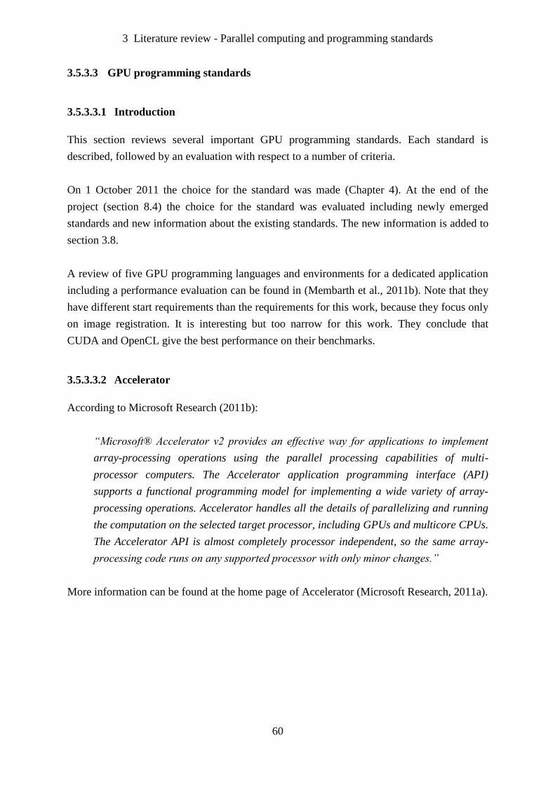
3 Literature review - Parallel computing and programming standards
60
3.5.3.3 GPU programming standards
3.5.3.3.1 Introduction
This section reviews several important GPU programming standards. Each standard is
described, followed by an evaluation with respect to a number of criteria.
On 1 October 2011 the choice for the standard was made (Chapter 4). At the end of the
project (section 8.4) the choice for the standard was evaluated including newly emerged
standards and new information about the existing standards. The new information is added to
section 3.8.
A review of five GPU programming languages and environments for a dedicated application
including a performance evaluation can be found in (Membarth et al., 2011b). Note that they
have different start requirements than the requirements for this work, because they focus only
on image registration. It is interesting but too narrow for this work. They conclude that
CUDA and OpenCL give the best performance on their benchmarks.
3.5.3.3.2 Accelerator
According to Microsoft Research (2011b):
“Microsoft® Accelerator v2 provides an effective way for applications to implement
array-processing operations using the parallel processing capabilities of multi-
processor computers. The Accelerator application programming interface (API)
supports a functional programming model for implementing a wide variety of array-
processing operations. Accelerator handles all the details of parallelizing and running
the computation on the selected target processor, including GPUs and multicore CPUs.
The Accelerator API is almost completely processor independent, so the same array-
processing code runs on any supported processor with only minor changes.”
More information can be found at the home page of Accelerator (Microsoft Research, 2011a).
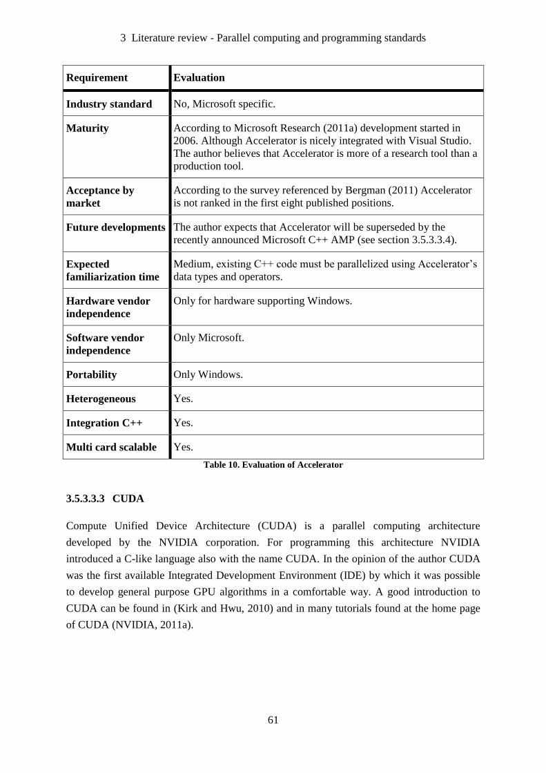
3 Literature review - Parallel computing and programming standards
61
Requirement Evaluation
Industry standard No, Microsoft specific.
Maturity According to Microsoft Research (2011a) development started in
2006. Although Accelerator is nicely integrated with Visual Studio.
The author believes that Accelerator is more of a research tool than a
production tool.
Acceptance by
market
According to the survey referenced by Bergman (2011) Accelerator
is not ranked in the first eight published positions.
Future developments The author expects that Accelerator will be superseded by the
recently announced Microsoft C++ AMP (see section 3.5.3.3.4).
Expected
familiarization time
Medium, existing C++ code must be parallelized using Accelerator’s
data types and operators.
Hardware vendor
independence
Only for hardware supporting Windows.
Software vendor
independence
Only Microsoft.
Portability Only Windows.
Heterogeneous Yes.
Integration C++ Yes.
Multi card scalable Yes.
Table 10. Evaluation of Accelerator
3.5.3.3.3 CUDA
Compute Unified Device Architecture (CUDA) is a parallel computing architecture
developed by the NVIDIA corporation. For programming this architecture NVIDIA
introduced a C-like language also with the name CUDA. In the opinion of the author CUDA
was the first available Integrated Development Environment (IDE) by which it was possible
to develop general purpose GPU algorithms in a comfortable way. A good introduction to
CUDA can be found in (Kirk and Hwu, 2010) and in many tutorials found at the home page
of CUDA (NVIDIA, 2011a).

3 Literature review - Parallel computing and programming standards
62
Thrust (NVIDIA, 2011e) is a C++ template library for CUDA based on the Standard
Template Library. It is expected that using Thrust will decrease the amount of host code to be
written at the cost of less performance. Because Thrust uses its own specific data primitives
and containers it is expected that converting VisionLab to Thrust will take a large amount of
effort. Interesting developments about using CUDA for Computer Vision can be found on the
sites of:
- OpenVIDIA (OpenVIDIA, 2011).
- OpenCV_GPU (OpenCV, 2011b).
- GpuCV (GpuCV, 2010).
- GPU4Vision (Institute for Computer Graphics and Vision, 2011).
- MinGPU (Babenko and Shah, 2008a).
Requirement Evaluation
Industry standard No, it is NVIDIA specific.
Maturity Yes, a large community of users, see (NVIDIA, 2011a).
Acceptance by
market
According to the survey referenced by Bergman (2011) CUDA is
ranked at position 5.
Future developments Recently (NVIDIA, 2011b) a new version of the CUDA language
was introduced including C++ like features such as classes and
templates. But there is no support for Run Time Type Information
(RTTI), exception handling and the C++ Standard Library.
In June 2011 The Portland Group announced a first version of a x86
compiler for CUDA (The Portland Group, 2011a). According to their
planning the full version of this compiler will be available in mid-
2012.
Expected
familiarization time
High. Besides device code in CUDA C, host code in C++ for
launching and synchronizing the device code must be developed.
Hardware vendor
independence
Only NVIDIA hardware, but this will change to include x86/x64
hardware when Portland compiler becomes more mature.
Software vendor
independence
Only NVIDIA but this will change to two vendors when Portland
Group compiler becomes more mature.
Portability CUDA runs on both Windows and Linux using x86 hardware.
Heterogeneous No.
Integration C++ Yes.
Multi card scalable Yes.
Table 11. Evaluation of CUDA
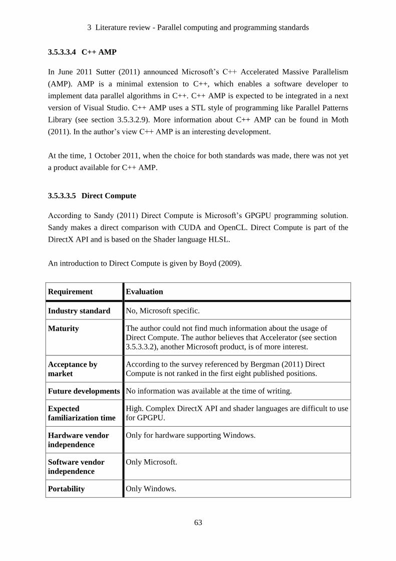
3 Literature review - Parallel computing and programming standards
63
3.5.3.3.4 C++ AMP
In June 2011 Sutter (2011) announced Microsoft’s C++ Accelerated Massive Parallelism
(AMP). AMP is a minimal extension to C++, which enables a software developer to
implement data parallel algorithms in C++. C++ AMP is expected to be integrated in a next
version of Visual Studio. C++ AMP uses a STL style of programming like Parallel Patterns
Library (see section 3.5.3.2.9). More information about C++ AMP can be found in Moth
(2011). In the author’s view C++ AMP is an interesting development.
At the time, 1 October 2011, when the choice for both standards was made, there was not yet
a product available for C++ AMP.
3.5.3.3.5 Direct Compute
According to Sandy (2011) Direct Compute is Microsoft’s GPGPU programming solution.
Sandy makes a direct comparison with CUDA and OpenCL. Direct Compute is part of the
DirectX API and is based on the Shader language HLSL.
An introduction to Direct Compute is given by Boyd (2009).
Requirement Evaluation
Industry standard No, Microsoft specific.
Maturity The author could not find much information about the usage of
Direct Compute. The author believes that Accelerator (see section
3.5.3.3.2), another Microsoft product, is of more interest.
Acceptance by
market
According to the survey referenced by Bergman (2011) Direct
Compute is not ranked in the first eight published positions.
Future developments No information was available at the time of writing.
Expected
familiarization time
High. Complex DirectX API and shader languages are difficult to use
for GPGPU.
Hardware vendor
independence
Only for hardware supporting Windows.
Software vendor
independence
Only Microsoft.
Portability Only Windows.
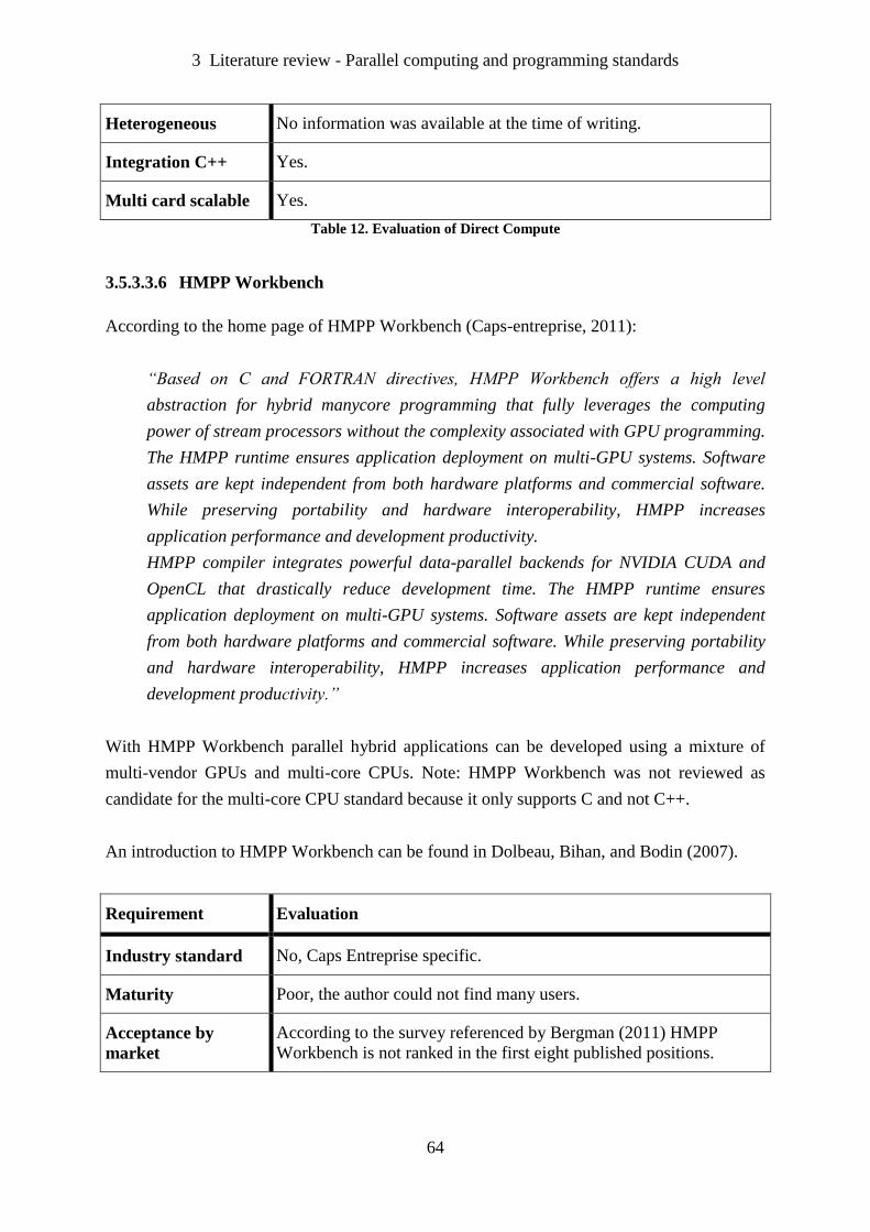
3 Literature review - Parallel computing and programming standards
64
Heterogeneous No information was available at the time of writing.
Integration C++ Yes.
Multi card scalable Yes.
Table 12. Evaluation of Direct Compute
3.5.3.3.6 HMPP Workbench
According to the home page of HMPP Workbench (Caps-entreprise, 2011):
“Based on C and FORTRAN directives, HMPP Workbench offers a high level
abstraction for hybrid manycore programming that fully leverages the computing
power of stream processors without the complexity associated with GPU programming.
The HMPP runtime ensures application deployment on multi-GPU systems. Software
assets are kept independent from both hardware platforms and commercial software.
While preserving portability and hardware interoperability, HMPP increases
application performance and development productivity.
HMPP compiler integrates powerful data-parallel backends for NVIDIA CUDA and
OpenCL that drastically reduce development time. The HMPP runtime ensures
application deployment on multi-GPU systems. Software assets are kept independent
from both hardware platforms and commercial software. While preserving portability
and hardware interoperability, HMPP increases application performance and
development productivity.”
With HMPP Workbench parallel hybrid applications can be developed using a mixture of
multi-vendor GPUs and multi-core CPUs. Note: HMPP Workbench was not reviewed as
candidate for the multi-core CPU standard because it only supports C and not C++.
An introduction to HMPP Workbench can be found in Dolbeau, Bihan, and Bodin (2007).
Requirement Evaluation
Industry standard No, Caps Entreprise specific.
Maturity Poor, the author could not find many users.
Acceptance by
market
According to the survey referenced by Bergman (2011) HMPP
Workbench is not ranked in the first eight published positions.

3 Literature review - Parallel computing and programming standards
65
Future developments Caps Entreprise and PathScale have recently started an initiative for
creating a new open standard called OpenHMPP (OpenHMPP,
2011).
Expected
familiarization time
Medium. HMPP Workbench uses compiler directives to exploit the
parallelism.
Hardware vendor
independence
Supports NVIDIA Tesla and AMD FireStream.
No detailed information about support for multi-core CPUs was
available at the time of writing.
Software vendor
independence
Supports several compilers including Microsoft Visual Studio and
the GNU compiler.
Portability Windows and Linux
Heterogeneous Yes.
Integration C++ Yes.
Multi card scalable Yes.
Table 13. Evaluation of HMPP Workbench
3.5.3.3.7 Liquid Metal
Liquid Metal is a research initiative of IBM in order to unify software development for CPUs,
GPUs and FPGA. According to the home page of Liquid Metal (IBM, n.d.):
“The Liquid Metal project at IBM aims to address the difficulties that programmers
face today when developing applications for computers that feature programmable
accelerators (GPUs and FPGAs) alongside conventional multi-core processors. Liquid
Metal offers a single unified programming language called Lime and a runtime that
allows (all) portions of an application to move fluidly between hardware and software,
dynamically and adaptively. … For programming GPUs, a programmer might use
OpenMP, OpenCL, or CUDA. OpenCL is an increasingly popular approach because it
is backed by a standard specification, and a number of processor vendors are actively
supporting OpenCL on their architectures. FPGAs on the other hand lack a single
programming standard that is considered sufficiently high-level and accessible to
skilled software programmers. Instead, the predominant practice is to write code in
hardware description languages such as Verilog, VHDL, or Bluespec. The semantic
gap between these languages, and high level object-oriented languages such as C++ or
Java is quite wide, leaving FPGAs largely inaccessible to software developers.
3 Literature review - Parallel computing and programming standards
66
Liquid Metal offers a single unified programming language (Lime) and runtime for
programming hybrid computers comprised of multi-core processors, GPUs, and
FPGAs. “
The author could not find any references of Liquid Metal after 2010 and assumes that Liquid
Metal has not yet come out of the research phase. In the survey referenced by Bergman
(2011) among developers for the most popular multi-threaded APIs in North America Liquid
Metal is not mentioned. Liquid Metal was therefore not reviewed any further.
3.5.3.3.8 OpenCL
According to OpenCL 1.1. specification (Munshi, 2010):
“OpenCL (Open Computing Language) is an open royalty-free standard for general
purpose parallel programming across CPUs, GPUs and other processors, giving
software developers portable and efficient access to the power of these heterogeneous
processing platforms.
OpenCL supports a wide range of applications, ranging from embedded and consumer
software to HPC solutions, through a low-level, high-performance, portable
abstraction. By creating an efficient, close-to-the-metal programming interface,
OpenCL will form the foundation layer of a parallel computing ecosystem of platform-
independent tools, middleware and applications. OpenCL is particularly suited to play
an increasingly significant role in emerging interactive graphics applications that
combine general parallel compute algorithms with graphics rendering pipelines.
OpenCL consists of an API for coordinating parallel computation across
heterogeneous processors; and a cross-platform programming language with a well
specified computation environment. The OpenCL standard:
- Supports both data- and task-based parallel programming models
- Utilizes a subset of ISO C99 with extensions for parallelism
- Defines consistent numerical requirements based on IEEE 754
- Defines a configuration profile for handheld and embedded devices
- Efficiently interoperates with OpenGL, OpenGL ES and other graphics APIs”
The specification and standardization of OpenCL is supervised by the Khronos Group
(Khronos Group, 2011a). Good introductions to OpenCL can be found in Tsuchiyama (2010),
NVIDIA (2010a), NVIDIA (2010b), AMD (2011a), Gaster, B.R. et al. (2012) and Munshi et
al. (2011). An OpenCL C++ wrapper for the API code can be found at Gaster (2010). The
performance and portability of OpenCL is evaluated by Van der Sanden (2011).
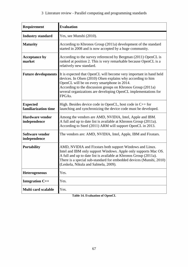
3 Literature review - Parallel computing and programming standards
67
Requirement Evaluation
Industry standard Yes, see Munshi (2010).
Maturity According to Khronos Group (2011a) development of the standard
started in 2008 and is now accepted by a huge community.
Acceptance by
market
According to the survey referenced by Bergman (2011) OpenCL is
ranked at position 2. This is very remarkable because OpenCL is a
relatively new standard.
Future developments It is expected that OpenCL will become very important in hand held
devices. In Olsen (2010) Olsen explains why according to him
OpenCL will be on every smartphone in 2014.
According to the discussion groups on Khronos Group (2011a)
several organizations are developing OpenCL implementations for
FPGAs.
Expected
familiarization time
High. Besides device code in OpenCL, host code in C++ for
launching and synchronizing the device code must be developed.
Hardware vendor
independence
Among the vendors are AMD, NVIDIA, Intel, Apple and IBM.
A full and up to date list is available at Khronos Group (2011a).
According to Steel (2011) ARM will support OpenCL in 2013.
Software vendor
independence
The vendors are: AMD, NVIDIA, Intel, Apple, IBM and Fixstars.
Portability AMD, NVIDIA and Fixstars both support Windows and Linux.
Intel and IBM only support Windows. Apple only supports Mac OS.
A full and up to date list is available at Khronos Group (2011a).
There is a special sub-standard for embedded devices (Munshi, 2010)
(Leskela, Nikula and Salmela, 2009).
Heterogeneous Yes.
Integration C++ Yes.
Multi card scalable Yes.
Table 14. Evaluation of OpenCL
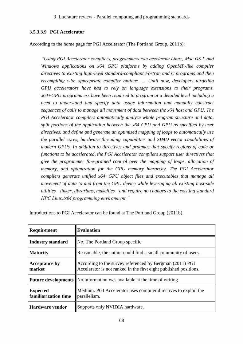
3 Literature review - Parallel computing and programming standards
68
3.5.3.3.9 PGI Accelerator
According to the home page for PGI Accelerator (The Portland Group, 2011b):
“Using PGI Accelerator compilers, programmers can accelerate Linux, Mac OS X and
Windows applications on x64+GPU platforms by adding OpenMP-like compiler
directives to existing high-level standard-compliant Fortran and C programs and then
recompiling with appropriate compiler options. … Until now, developers targeting
GPU accelerators have had to rely on language extensions to their programs.
x64+GPU programmers have been required to program at a detailed level including a
need to understand and specify data usage information and manually construct
sequences of calls to manage all movement of data between the x64 host and GPU. The
PGI Accelerator compilers automatically analyze whole program structure and data,
split portions of the application between the x64 CPU and GPU as specified by user
directives, and define and generate an optimized mapping of loops to automatically use
the parallel cores, hardware threading capabilities and SIMD vector capabilities of
modern GPUs. In addition to directives and pragmas that specify regions of code or
functions to be accelerated, the PGI Accelerator compilers support user directives that
give the programmer fine-grained control over the mapping of loops, allocation of
memory, and optimization for the GPU memory hierarchy. The PGI Accelerator
compilers generate unified x64+GPU object files and executables that manage all
movement of data to and from the GPU device while leveraging all existing host-side
utilities—linker, librarians, makefiles—and require no changes to the existing standard
HPC Linux/x64 programming environment.”
Introductions to PGI Accelerator can be found at The Portland Group (2011b).
Requirement Evaluation
Industry standard No, The Portland Group specific.
Maturity Reasonable, the author could find a small community of users.
Acceptance by
market
According to the survey referenced by Bergman (2011) PGI
Accelerator is not ranked in the first eight published positions.
Future developments No information was available at the time of writing.
Expected
familiarization time
Medium. PGI Accelerator uses compiler directives to exploit the
parallelism.
Hardware vendor Supports only NVIDIA hardware.
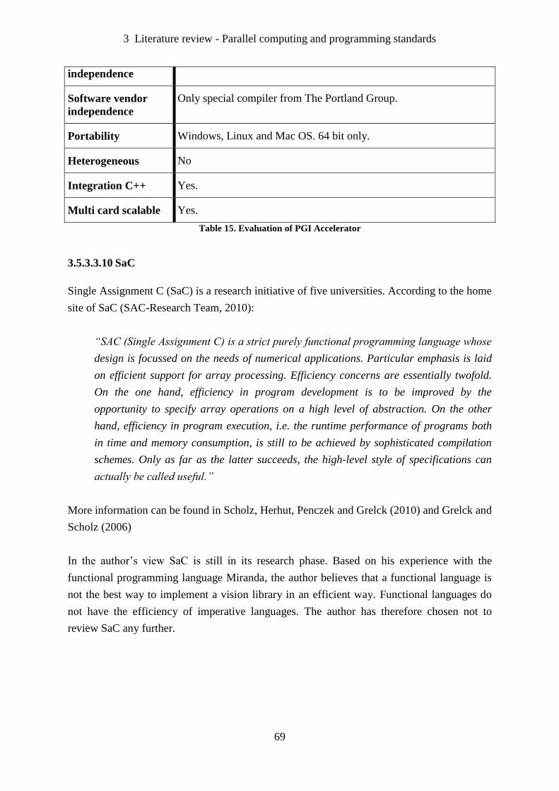
3 Literature review - Parallel computing and programming standards
69
independence
Software vendor
independence
Only special compiler from The Portland Group.
Portability Windows, Linux and Mac OS. 64 bit only.
Heterogeneous No
Integration C++ Yes.
Multi card scalable Yes.
Table 15. Evaluation of PGI Accelerator
3.5.3.3.10 SaC
Single Assignment C (SaC) is a research initiative of five universities. According to the home
site of SaC (SAC-Research Team, 2010):
“SAC (Single Assignment C) is a strict purely functional programming language whose
design is focussed on the needs of numerical applications. Particular emphasis is laid
on efficient support for array processing. Efficiency concerns are essentially twofold.
On the one hand, efficiency in program development is to be improved by the
opportunity to specify array operations on a high level of abstraction. On the other
hand, efficiency in program execution, i.e. the runtime performance of programs both
in time and memory consumption, is still to be achieved by sophisticated compilation
schemes. Only as far as the latter succeeds, the high-level style of specifications can
actually be called useful.”
More information can be found in Scholz, Herhut, Penczek and Grelck (2010) and Grelck and
Scholz (2006)
In the author’s view SaC is still in its research phase. Based on his experience with the
functional programming language Miranda, the author believes that a functional language is
not the best way to implement a vision library in an efficient way. Functional languages do
not have the efficiency of imperative languages. The author has therefore chosen not to
review SaC any further.
3 Literature review - Parallel computing and programming standards
70
3.5.3.3.11 Shader languages
In section 3.4.3 it was explained that after the introduction of programmable shaders it was
possible to use graphics cards for general programming tasks. This was called General
Purpose Graphics Processing Unit (GPGPU) computing. There have been a lot of
developments in Shader languages and a wide variety of languages have been created. A non-
exhaustive list of the most important Shader languages is:
- OpenGL.
- Cg.
- HLSL.
- GLSL.
- Sh.
- BrookGPU.
Good introductions to Shader languages can be found in Babenko and Shah (2008b) and
Pharr, ed. (2005). Based on earlier preliminary research and experiments (see section 2.2)
with Shader languages by the author, and with the arrival of languages specially designed for
GPGPU computing, the author considers using Shader languages for GPGPU computing
obsolete and has decided not to review Shader languages any further.
3 Literature review - Computer Vision algorithms and parallelization
71
3.6 Computer Vision algorithms and parallelization
3.6.1 Introduction
There are many good text books available on Computer Vision. For the author his interest in
Computer Vision started in the nineties with the two volume standard book of Haralick and
Shapiro (1992). A good introduction to Computer Vision can be found in Gonzalez and
Woods (2008). An exhaustive literature review on this topic is outside the scope of this
project.
In this section the classification of low level image operators is reviewed. Low level image
operators are used very frequently in many vision applications. The idea behind classifying
these operators is that if a skeleton for parallelizing one representative in a class is found, this
skeleton can be reused for the other representative in this class. For each class a
representative operator is chosen and parallelization approaches were reviewed. The
following classes of basic low level image operators are reviewed:
- Point operators.
- Local neighbour operators.
- Global operators.
- Connectivity based operators.
There are also high level image operators. These are the more complex operators; often built
using the low level operators. It is to be expected that many of these operators are a class of
their own and a dedicated approach to parallelizing must be found. The literature review of
the high level image operators is outside the scope of this project.
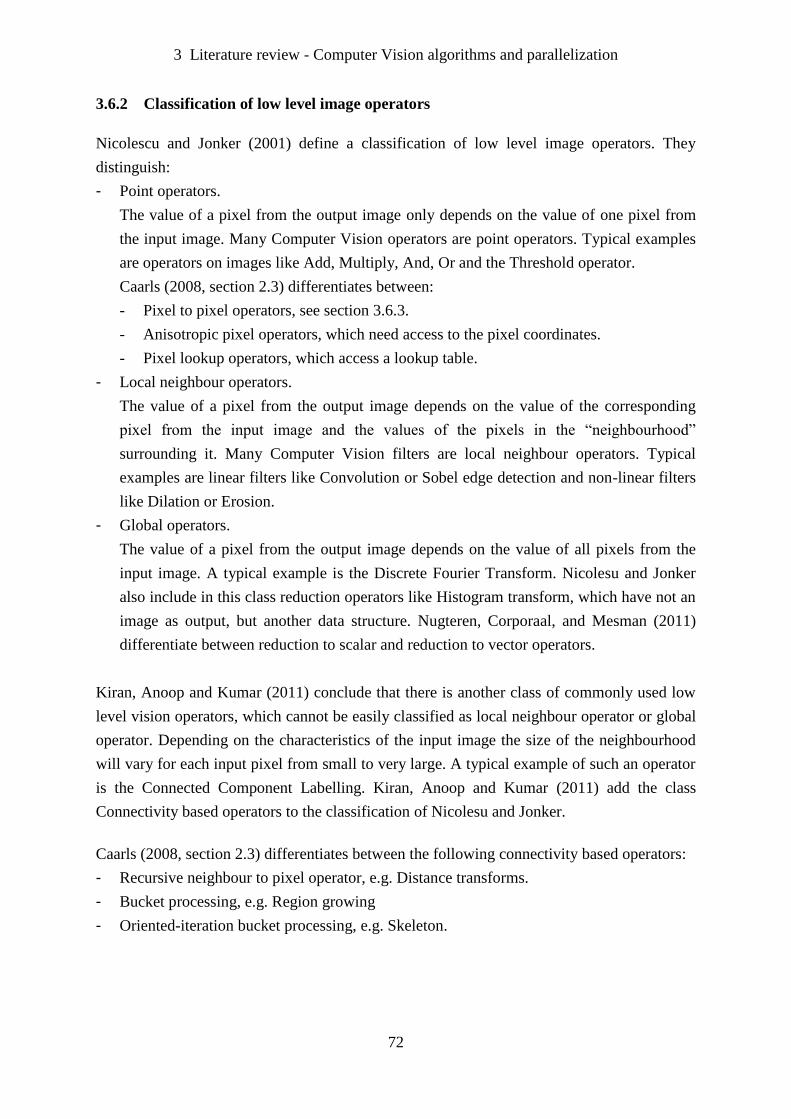
3 Literature review - Computer Vision algorithms and parallelization
72
3.6.2 Classification of low level image operators
Nicolescu and Jonker (2001) define a classification of low level image operators. They
distinguish:
- Point operators.
The value of a pixel from the output image only depends on the value of one pixel from
the input image. Many Computer Vision operators are point operators. Typical examples
are operators on images like Add, Multiply, And, Or and the Threshold operator.
Caarls (2008, section 2.3) differentiates between:
- Pixel to pixel operators, see section 3.6.3.
- Anisotropic pixel operators, which need access to the pixel coordinates.
- Pixel lookup operators, which access a lookup table.
- Local neighbour operators.
The value of a pixel from the output image depends on the value of the corresponding
pixel from the input image and the values of the pixels in the “neighbourhood”
surrounding it. Many Computer Vision filters are local neighbour operators. Typical
examples are linear filters like Convolution or Sobel edge detection and non-linear filters
like Dilation or Erosion.
- Global operators.
The value of a pixel from the output image depends on the value of all pixels from the
input image. A typical example is the Discrete Fourier Transform. Nicolesu and Jonker
also include in this class reduction operators like Histogram transform, which have not an
image as output, but another data structure. Nugteren, Corporaal, and Mesman (2011)
differentiate between reduction to scalar and reduction to vector operators.
Kiran, Anoop and Kumar (2011) conclude that there is another class of commonly used low
level vision operators, which cannot be easily classified as local neighbour operator or global
operator. Depending on the characteristics of the input image the size of the neighbourhood
will vary for each input pixel from small to very large. A typical example of such an operator
is the Connected Component Labelling. Kiran, Anoop and Kumar (2011) add the class
Connectivity based operators to the classification of Nicolesu and Jonker.
Caarls (2008, section 2.3) differentiates between the following connectivity based operators:
- Recursive neighbour to pixel operator, e.g. Distance transforms.
- Bucket processing, e.g. Region growing
- Oriented-iteration bucket processing, e.g. Skeleton.

3 Literature review - Computer Vision algorithms and parallelization
73
3.6.3 Point operators
In order to limit the scope of this project, only pixel to pixel Point operators are considered.
According to the author, this is the most frequently used type of Point operator. A pixel to
pixel Point operator is characterized by that the value of a pixel from the output image only
depends on the value of the corresponding, same position in image, pixel from the input
image. Let PF be a Point Function which has as input the input pixel value and as function
result the desired output pixel value and the image has a size of height by width pixels. A
generalized Point operator algorithm can be described in pseudo code as:
PointOperator (Image image) {
for (x = 0; x < image.width; x++) {
for (y=0; y < image.height; y++) {
image(x,y) = PF(image(x,y));
} // for y
} // for x
} // PointOperator
A typical and frequently often used Point operator is the Threshold operator. Threshold is the
simplest method of image segmentation. The Threshold operator takes a greyscale image and
produces a binary image. The Threshold operator has two extra parameters low and high. All
pixels with values in the range [low..high] are converted to the value Object (=1) and all other
pixels are converted to the value Background (=0). For more information about this operator
and its usage see Van de Loosdrecht, et al. (2013, Chapter Segmentation).
Threshold (Image image, Pixel low, Pixel high) {
for (x = 0; x < image.width; x++)
for (y = 0; y < image.height; y++)
if ((image(x,y) >= low) && (image(x,y) <= high))
image(x,y) = 1;
else
image(x,y) = 0;
} // Threshold
Point operators are embarrassingly parallel problems. A skeleton for parallelizing Point
operators is presented in Nicolescu and Jonker (2001). Because the execution of a Point
Function for a pixel is independent of the execution of the Point Function of all other pixels,
the image can be easily divided in sub-images that can be processed in parallel. Similar
skeletons can be found in Caarls (2008) and Nugteren, Corporaal, and Mesman (2011).
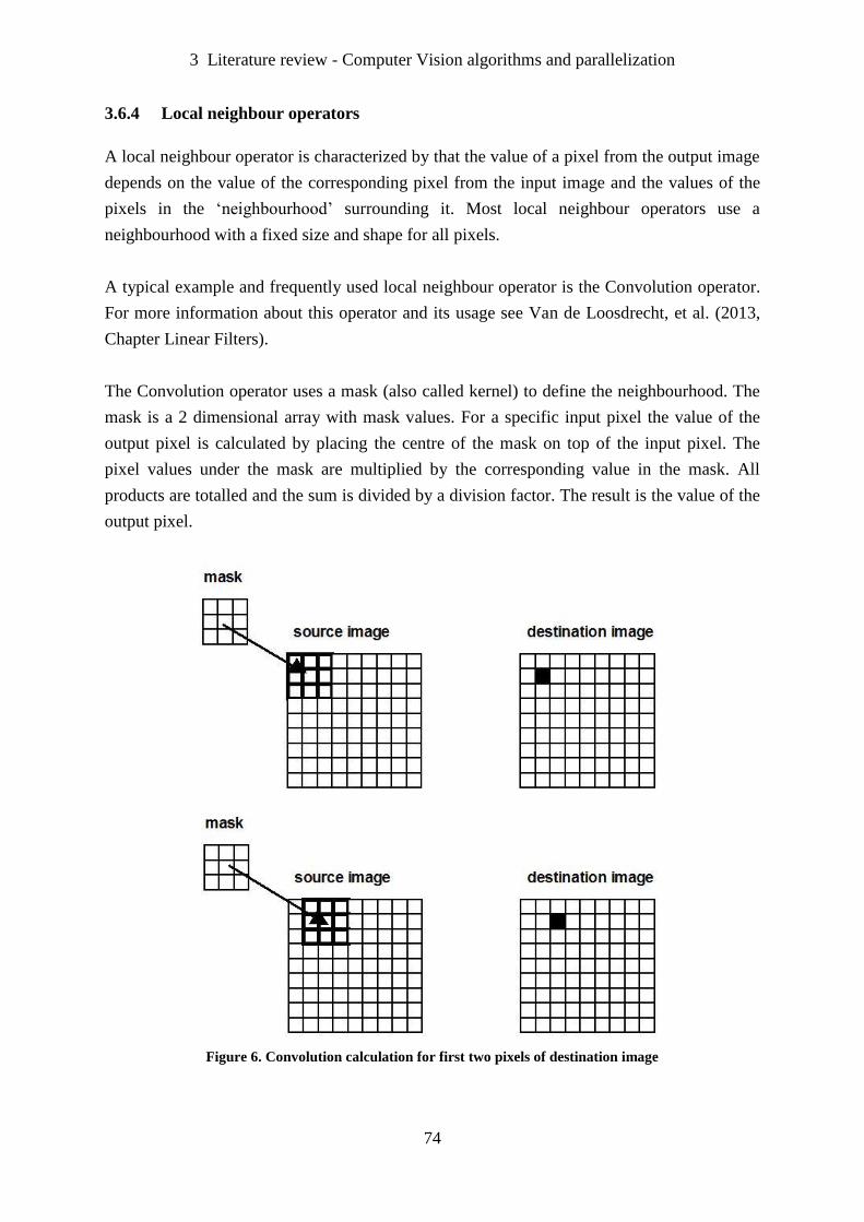
3 Literature review - Computer Vision algorithms and parallelization
74
3.6.4 Local neighbour operators
A local neighbour operator is characterized by that the value of a pixel from the output image
depends on the value of the corresponding pixel from the input image and the values of the
pixels in the ‘neighbourhood’ surrounding it. Most local neighbour operators use a
neighbourhood with a fixed size and shape for all pixels.
A typical example and frequently used local neighbour operator is the Convolution operator.
For more information about this operator and its usage see Van de Loosdrecht, et al. (2013,
Chapter Linear Filters).
The Convolution operator uses a mask (also called kernel) to define the neighbourhood. The
mask is a 2 dimensional array with mask values. For a specific input pixel the value of the
output pixel is calculated by placing the centre of the mask on top of the input pixel. The
pixel values under the mask are multiplied by the corresponding value in the mask. All
products are totalled and the sum is divided by a division factor. The result is the value of the
output pixel.
Figure 6. Convolution calculation for first two pixels of destination image
3 Literature review - Computer Vision algorithms and parallelization
75
The pseudo code for a Convolution with a 3×3 mask:
Convolution (Image src, Image dest, Mask mask, int divFactor) {
for (y = 1; y < src.height-1; y++)
for (x = 1; x < src.width-1; x++) {
dest(x,y) = 0;
for (dy = -1; dy <= 1; dy++)
for (dx = -1; dx <= 1; dx++)
dest(x,y) += src(x+dx,y+dy) * mask(dx+1,dy+1);
dest(x,y) /= divFactor;
} // for x
} // Convolution
Note there are no values calculated for the borders of the image in the pseudo code. There are
several options of how to handle the borders. See Van de Loosdrecht, et al. (2013, Chapter
Linear Filters) for possible options.
Many local neighbour operators like Convolution are easy problems to parallelize in a shared
memory system. A skeleton for parallelizing local neighbour operators is presented in
Nicolesu and Jonker (2001). Because the calculation of the value for a destination pixel is
independent of the execution of the calculation of all other pixels, the image can be divided in
sub-images that can be processed in parallel. There are several options for partition of the
image like row-stripes, column-stripes and blocks. Similar skeletons can be found in Caarls
(2008) and Nugteren, Corporaal, and Mesman (2011).
Bordoloi (2009), Andrade (2011) and Gaster, et al. (2012, Chapter 7) discuss several
optimization approaches for OpenCL implementation of Convolution on RGB images with
floating point pixel values like:
- Using constant memory for mask values.
- Using local memory for tiles.
- Unrolling for loops.
- Vectorization of image channels.
In their approaches they use compilation time fixed sizes for the mask. Experiments are
needed in order to investigate if those techniques are also beneficial for single channel images
with integer pixel values and for run-time specifiable mask sizes. A generic library like
VisionLab requires a Convolution with at run-time specifiable mask sizes.

3 Literature review - Computer Vision algorithms and parallelization
76
Antao and Sousa (2010) discuss four approaches for implementing Convolution in OpenCL
for single channel images with integer pixel values and at compilation time fixed mask sizes:
- The reference scalar Convolution; the “straightforward” implementation.
- The reference vectorized Convolution; the row calculation for one output pixel is
vectorized. The inner-most loop, that browses the mask width, is unrolled to vectorized
operations. Because the mask width may not be a multiple of the vector size, an extra pair
of nested loops is required for handling the remaining pixels in a scalar fashion.
- N-kernel Convolution; the mask is N times replicated in memory. The calculating of the
result values for output pixels is vectorized. The same mask value is simultaneously
multiplied with a vector of pixels producing a vector with different products.
- Complete image coalesced Convolution; with the use of an intermediary image, pixels are
packed in a coalesced ‘pixel’. With the coalesced image the convolution is efficiently
calculated using vectors. Thereafter the coalesced image must be unpacked to the result
image.
Antao, Sousa and Chaves (2011) improve the Complete image coalesced Convolution
approach by packing integer pixels into double precision floating point vectors. Their
approaches are benchmarked on CPUs. Experiments are needed in order to investigate if
these approaches are also beneficial on GPUs.
3.6.5 Global operators
A global operator is characterized by that the output value or the value of a pixel from the
output image depends on the value of all pixels from the input image. A typical and often
used global operator is the Histogram operator. With this operator the distribution of the pixel
values is calculated. For more information about this operator and its usage see Van de
Loosdrecht, et al. (2013, Chapter Contrast Manipulation).
The pseudo code for an Histogram operator on grayscale images with pixels values between 0
and 255:
Histogram (Image image, Histogram his) {
for (i = 0; i <= 255; i++)
his[i] = 0;
for (p = 0; p < image.NrPixels; p++)
his[image[p]]++;
} // Histogram
3 Literature review - Computer Vision algorithms and parallelization
77
With the exception for very tiny images, the majority of the work is performed in the second
for loop. However when parallelizing this loop, it performs many scattered read-write
accesses into the shared histogram data structure. Access to the shared histogram must be
atomized. The size of histograms is usually small. On a CPU the histogram can be cached
with a high rate of reuse. On a GPU the scattered read-write accesses is a worst-case
performance scenario for accessing the global memory. Real-life images have often many
areas with similar pixel values. The rate at which atomic update clashes occur, will depend on
the data of the input image and the sequence in which the pixels are accessed.
Nicolesu and Jonker (2001) and the other authors mentioned in this section propose skeletons
for ‘distribute compute and gather’. The image is split in several parts for which a sub-
histogram is calculated where after the final total-histogram is calculated.
In the early days of GPGPU programming the languages used did not support atomic updates
of the device’s global and shared memory. Shams and Kennedy (2007) suggest a spin locking
method to overcome this problem. Goorts, et al. (2010) compare Histogram implementations
in CUDA based on spin locking with atomic updates on shared memory. The difference in
performance in their tests is only marginal. Nugteren, Van den Braak, Corporaal and
Mesman, (2011) report a 18% increase of performance using atomic updates on more recent
GPUs.
In Gaster et al. (2012, Chapter 9) an optimized Histogram implementation in OpenCL for
GPUs is described. The optimization includes coalesced vectorized global memory access
and bank conflicts reduction for GPU implementations.
Nugteren, Van den Braak, Corporaal and Mesman, (2011) give a good overview of existing
histogram GPU implementations and propose two new methods. Their second method has a
performance which is input data independent. They qualify the Gaster implementation as a
Mapping 1 method for the local histograms. Their more complicated Mapping method 3 has
about 30% better performance than the Mapping 1 method on their test set. They conclude
with the observation that bottleneck is the lack of shared memory, both in terms of size and
number of banks, on contemporary GPUs.
Luna (2012, Chapter 4) introduces a much more complicated ‘R-per-block’ approach for
which he claims that it is more than two times faster than Nugteren’s approach.
Van den Braak, Nugteren, Mesman, and Corporaal (2012) describe a generalized framework
for voting algorithms on GPUs, which is claimed by the authors to be the fastest
implementation for Histograms.
3 Literature review - Computer Vision algorithms and parallelization
78
3.6.6 Connectivity based operators
3.6.6.1 Introduction
In an image a pixel not connected to the border has eight neighbour pixels. In image
processing it is common to distinguish between four and eight connectivity of pixel. The 4-
connected pixels of a pixel are the neighbour pixels that touch the pixel horizontally or
vertically. The 8-connected pixels of a pixel are the neighbour pixels that touch the pixel
horizontally, vertically or diagonally.
An important and often used connectivity based operator is Connected Component Labelling
(CCL). As explained in section 3.6.3 the segmentation of an image will result in a binary
image in which the object pixels have the value 1 and the background pixels have the value 0.
The CCL operator transforms a binary image to a labelled image in which the 4 or 8-
connected object pixels are grouped into Binary Linked Objects (BLOBs). In the labelled
image all the background pixels have the value 0 and all pixels that are part of a blob have the
same unique positive value, called its label. In VisionLab the CCL operator is called
LabelBlobs and the blob numbers are in the range [1 .. number of blobs]. For more
information on CCL and its usage see Van de Loosdrecht, et al. (2013, Chapter Labelling and
Blob measurement).
Many CCL algorithms have been proposed in literature. The author has studied more than 40
articles.
3.6.6.2 Sequential
He, Chao, and Suzuki (2008) give a good overview of sequential approaches and evaluate
them. The most common sequential approach is that an image is scanned in raster direction
and a new provisional label is assigned to each new pixel that is not connected to other
previously scanned pixels. Provisional labels assigned to the same blob are called equivalent
labels. There are different approaches for resolving the label equivalences:
- Multiple iterations of two passes.
The image is scanned in alternated forward and backward passes in order to propagate the
label equivalences until no labels change. The main problem with this method is that the
number of passes depends on the geometrical complexity of the blobs. An example of this
approach can be found in Haralick and Shapiro (1992, Volume 1, pp.32-33).
3 Literature review - Computer Vision algorithms and parallelization
79
- Two passes.
The image is scanned in forward pass and the equivalent labels found are stored in an
equivalence table. The equivalences are resolved by use of a search algorithm. After
resolving the equivalences, the second pass assigns the label to each object pixel. The
challenges for this method are to limit the required amount of memory for the equivalence
table and that the search algorithm should be efficient. Many approaches are proposed in
literature. Examples can be found in Haralick and Shapiro (1992, Volume 1, pp.33-48)
and He, Chao, and Suzuki (2008).
- Multiple iterations of four passes.
This approach is described in Suzuki, Horiba, and Sugie (2003). The maximum number
of iterations required is four. So the calculation time will only depend on the size of the
image and the number of object pixels in the blobs. This is a nice real-time property.
- Contour tracing and label propagation.
This multi-pass approach is described in Chang, Chen and Lu (2004). The image is
scanned for an unlabelled border pixels of a blob. This pixel is assigned a new label
number and the contour of the blob is traced. First all border pixels are found and then all
pixels of the blob are assigned the same label number.
According to He, Chao, and Suzuki (2008) the two passes approach gives the best
performance.
3.6.6.3 Parallel
Rosenfeld and Pfaltz (1966) proved that CCL cannot be implemented with parallel local
operations. Many parallel multi-pass CCL algorithms have been proposed in literature.
Hawick, Leist and Playne (2010) evaluate four approaches using CUDA:
- Neighbour propagation.
- Local neighbour propagation.
- Directional propagation.
- Label equivalence.
They conclude that Label equivalence approach provides the best performance.
3 Literature review - Benchmarking
80
Based on their work Kalentev, Rai, Kemnitz, and Schneider (2011) propose an alternative
implementation of the Label equivalence approach using OpenCL. This alternative
implementation is simpler, does not need extra memory for the equivalence table and does
not use atomic operations. They store the equivalence table in the image and use the offset of
the pixel in the image as a pointer for the equivalence table. This means that for an
Int16Image the maximum size of the image is only 2^15
pixels. This is too small for almost
all applications, so Int32Images must be used. They claim that because of the reduction
algorithm they use, their algorithm is efficient in terms of number of iterations needed
Stava and Benes (2011) claim that their CUDA algorithm is on average 3 times faster than
Hawick, Leist and Playne (2010) but their algorithm only works on images with height and
width with a power of 2.
Niknam, Thulasiraman, Camorlinga (2010) propose an OpenMP implementation of a multi
iterations algorithm.
3.7 Benchmarking
In this section the literature topics for benchmarking multi-core CPU and GPU algorithms are
discussed. As mentioned in section 3.4.4 about the parallel speedup factor there is a lot of
misapprehension in the science community about benchmarking parallel systems.
It seems to the author that the question of accessing the quality, such as reproducibility and
variance in execution time, of benchmarking parallel algorithms has not been fully addressed
in the research literature. Not much literature about this topic could be found, and many
authors do not describe their experiments in a way that they can be replicated. An in-depth
treatment of this subject is outside the scope of this project.
Mazouz,Toutati and Barthou (2010a and 2010b) reached two broad conclusions on
benchmarking parallel systems:
- The measurement process itself affects the results in complex and unforeseeable ways.
- Speedups reported from experimental work are often not seen in practice by end users
because of differences in the execution environment.
Their study has resulted in a protocol called “The Speedup Test” (Touati, Worms and Brains,
2010). This work is focused on benchmark applications like SPEC 2006 and SPEC
OMP2001. In these kind of benchmarks a large collection of algorithms are tested on
different systems and for each system a benchmark value is produced in order to rank the
systems.
3 Literature review - New developments after choice of standards
81
In the current work each time the performance of the sequential, multi-core CPU and GPU
version of one algorithm will be compared. Because of this a simplified kind of
benchmarking, a subset of “The Speedup Test” protocol can be used. This is discussed in
section 5.4.3.
As discussed in section 1.5 this work is not a quest for the best sequential or parallel
algorithms. The focus of this project is to investigate how to speed up a whole library by
parallelizing the algorithms in an economical way.
Benchmarking with other commercial or research software packages is also be highly
impractical because:
- There were found only benchmarks for specialized Computer Vision operators, see
Computer Vision Online (2011), ImageProcessingPlace.com (2011) and Carnegie Mellon
University (2005b).
- There are no benchmarks for generic software packages.
- The cost involved in buying the commercial software.
- The time involved in acquiring research software and building this software.
- The total time involved in benchmarking.
3.8 New developments after choice of standards
3.8.1 Introduction
The following information became available after the choice for the standard had been made
(Chapter 4).
3.8.2 CUDA
NVIDIA (2011d) announced that it will provide the source code for the new NVIDIA CUDA
LLVM-based compiler to academic researchers and software-tool vendors, enabling them to
more easily add GPU support for more programming languages and support CUDA
applications on alternative processor architectures.
The in section 3.5.3.3.3 announced Portland Group CUDA x86 compiler is available now.
The MCUDA translation framework (The Impact research group, 2012) is a Linux-based tool
designed to effectively compile the CUDA programming model to a CPU architecture.
3 Literature review - New developments after choice of standards
82
NVIDIA (2012a) announced CUDA 5 with GPU Library Object Linking and Dynamic
Parallelism.
3.8.3 C++ AMP
The language specification can be found in Microsoft (2013) and it is now available as part of
Visual Studio 2012.
3.8.4 Bolt
AMD (2013b) introduced the Bolt C++ template library for heterogenous computing:
“Bolt provides an STL compatible library of high level constructs for creating
accelerated data parallel applications. Code written using STL or other STL
compatible libraries (example: TBB) can be converted to Bolt in minutes. In its open-
source debut, Bolt supports C++ AMP in addition to OpenCL™ as underlying
supported compute technologies. With Bolt, kernel code to be accelerated is written in-
line in the C++ source file. No OpenCL™ or C++ AMP API calls are required since
all initialization of and communication with the OpenCL™ or C++ AMP device is
handled by the library.”
3.8.5 OpenACC
OpenACC was announced as a new standard on 3 November 2011 (OpenACC, 2011a).
According to the OpenACC 1.0 specification (OpenACC, 2011b):
“This document describes the compiler directives, library routines and environment
variables that collectively define the OpenACC™ Application Programming Interface
(OpenACC API) for offloading code in C, C++ and Fortran programs from a host
CPU to an attached accelerator device. The method outlined provides a model for
accelerator programming that is portable across operating systems and various types
of host CPUs and accelerators. The directives extend the ISO/ANSI standard C, C++
and Fortran base languages in a way that allows a programmer to migrate
applications incrementally to accelerator targets using standards-based C, C++ or
Fortran.
3 Literature review - New developments after choice of standards
83
The directives and programming model defined in this document allow programmers to
create applications capable of using accelerators, without the need to manage data or
program transfers between the host and accelerator, or initiate accelerator startup and
shutdown. Rather, all of these details are implicit in the programming model and are
managed by the OpenACC API-enabled compilers and runtime environments. The
programming model allows the programmer to augment information available to the
compilers, including specification of data local to an accelerator, guidance on mapping
of loops onto an accelerator, and similar performance-related details.”
OpenACC uses compiler pragmas and runtime functions in a similar way to OpenMP
(section 3.5.3.2.7). By using OpenACC it will not be necessary to have a separate host-side
and kernel-side code. Also the transfer of data between host and accelerator device will be
handled automatically by the compiler. It is expected by the OpenMP Architecture Review
Board (NVIDIA, 2011c) that OpenACC and OpenMP will merge in the future. OpenACC is
an initiative of CAPS, CRAY, NVIDIA and The Portland Group.
3.8.6 OpenCL
Altera Corporation (2011) announced an OpenCL Program for FPGAs. Sing (2012) discusses
the usage of a pipe line architecture and a benchmark test.
Rosenberg, Gaster, Zheng, and Lipov (2011) announced a proposal for an OpenCL Static
C++ Kernel Language Extension. This proposal introduces C++ like features such as classes
and templates, but there is no support for Run-Time Type Information (RTTI), exception
handling and the C++ Standard Library. At the moment of writing this new kernel language
is only supported by AMD (AMD, 2012).
The Portland Group (2012) announced an OpenCL compiler for the ARM on Android.
OpenCL is now available on ARM based tablets (Garg, 2013).
The Seoul National University (Center for Manycore Programming, 2013) announced an
Open-source framework for heterogeneous cluster programming and an OpenCL ARM
compiler.
3 Literature review - Summary
84
3.8.7 OpenMP
OpenMP Architecture Review Board (2012a) published the OpenMP Technical Report 1 on
Directives for Attached Accelerators. This report describes a model for the offloading of code
and data onto a target device. Any device may be a target device, including graphics
accelerators, attached multiprocessors, co-processors and DSPs.
OpenMP Architecture Review Board (2012b) published the OpenMP Application Program
Interface Version 4.0 – RC1. This proposal includes thread affinity, SIMD constructs to
vectorize both serial and parallelized loops, user-defined reductions, and sequentially
consistent atomics. It is expected that the Technical Report on directives for attached
accelerators will be integrated in the final Release Candidate 2, to appear in 2013 and
followed by the finalized full 4.0 API specifications thereafter.
3.9 Summary
This chapter has reviewed in depth the performance of computer systems in the context of
computer vision as it relates to the present work.
Technologies for multi-core CPU and GPU approaches to achieving speedups through
parallelization have been described, and the relevant standards presented and reviewed.
Important issues in parallelizing computer vision algorithms have been reviewed.
A review of benchmarking methods for parallel algorithms found that this is as yet a difficult
area, with no satisfactory general methodology available. However, a simplified method was
identified which meets the needs of the current research.
Finally, a number of new developments were described; however, these took place too late to
influence this work.
4 Comparison of standards and choice - Introduction
85
4 Comparison of standards and choice
4.1 Introduction
In this section the reviewed standards for parallel programming are compared and one
standard for multi-core CPU programming and one standard for GPU programming are
chosen based on the requirements in Chapter 2. On 1 October 2011 the choice for both
standards was made. As explained in section 2.6 this choice was remained fixed for the
duration of this project. At the end of the project the choice for the standards was evaluated
(section 8.4) including new emerged standards (section 3.8) and a recommendation for using
standards in the future is given.
4.2 Choice of the standard for multi-core CPU programming
In this section the standards reviewed in section 3.5.3.2 for multi-core CPU programming are
compared and one standard based on the requirements described in section 2.3 is chosen. The
findings are summarized in Table 16.
As discussed in section 3.4.6 the parallelization of the VisionLab library is only profitable
when a large proportion of the source code is parallelized. Because of the amount of source
code involved it is paramount that the parallelization of VisionLab can be done in an efficient
manner for the majority of the code.
As can be seen in Table 16, only Cilk Plus and OpenMP are qualified as low effort for
conversion of embarrassingly parallel vision algorithms.
At the moment of choice OpenMP and Cilk Plus were both not yet available for Android
operating system. According to the requirements, portability to Android is an option, not a
necessity. At the moment of choice only POSIX Threads were available in the Native
Development Kit for Android (Android Developers, 2011). As can be seen in the comparison
table, POSIX Threads is not a viable option. Because OpenMP is an industry standard, is also
supported by Microsoft Visual C++, is more portable and is better accepted by the market,
OpenMP has been chosen as the standard for multi-core CPU programming.
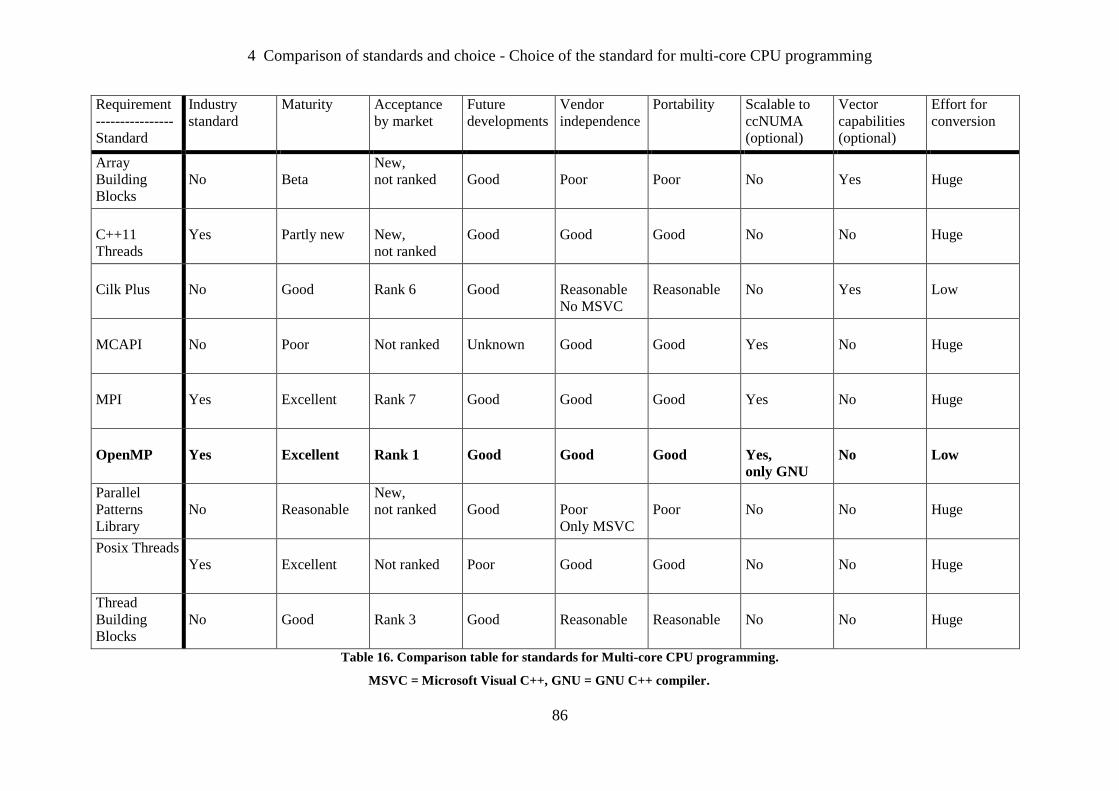
4 Comparison of standards and choice - Choice of the standard for multi-core CPU programming
86
Requirement
----------------
Standard
Industry
standard
Maturity Acceptance
by market
Future
developments
Vendor
independence
Portability Scalable to
ccNUMA
(optional)
Vector
capabilities
(optional)
Effort for
conversion
Array
Building
Blocks
No
Beta
New,
not ranked
Good
Poor
Poor
No
Yes
Huge
C++11
Threads
Yes
Partly new
New,
not ranked
Good
Good
Good
No
No
Huge
Cilk Plus
No
Good
Rank 6
Good
Reasonable
No MSVC
Reasonable
No
Yes
Low
MCAPI
No
Poor
Not ranked
Unknown
Good
Good
Yes
No
Huge
MPI
Yes
Excellent
Rank 7
Good
Good
Good
Yes
No
Huge
OpenMP
Yes
Excellent
Rank 1
Good
Good
Good
Yes,
only GNU
No
Low
Parallel
Patterns
Library
No
Reasonable
New,
not ranked
Good
Poor
Only MSVC
Poor
No
No
Huge
Posix Threads
Yes
Excellent
Not ranked
Poor
Good
Good
No
No
Huge
Thread
Building
Blocks
No
Good
Rank 3
Good
Reasonable
Reasonable
No
No
Huge
Table 16. Comparison table for standards for Multi-core CPU programming.
MSVC = Microsoft Visual C++, GNU = GNU C++ compiler.
87
Manufacturers of Android smartphones and tablets have started producing multi-core CPU
versions of their products since 2011. According to Stallman, et al. (2010, p. 32) the GNU
OpenMP implementation is based on PThreads, which is already available for Android. So
the author is hopeful that OpenMP will soon be available for Android. The GNU C++
compiler is part of the Android Native Development Kit.
4.3 Choice of the standard for GPU programming
In this section the standards reviewed in section 3.5.3.3 for GPU programming is compared
and one standard based on the requirements described in section 2.4 is chosen. The findings
are summarized in Table 17.
All reviewed standards meet the requirements that the standard must be able to integrate with
ANSI C++ code and must be scalable to multiple graphics cards. These requirements are not
selective and are not included in the table.
At the moment of choice, none of the standards were supported by Android. According to the
requirements portability to Android is an option, not a necessity. The Android Native
Development Kit supports only the Shader language OpenGL (Android Developers, 2011),
but as explained in section 3.5.3.3.11 Shader languages are not a viable option.
As can be seen in the table, OpenCL and CUDA are the only viable options. In the author’s
view, CUDA was the first available IDE with which it was possible to develop general
purpose GPU algorithms in a comfortable way. CUDA is more mature than OpenCL. The
kernel languages of CUDA and OpenCL were quite similar until recently CUDA introduced
attractive C++ like extensions.
In recent years OpenCL has gained a lot of momentum and is now supported by a large
community. This view is supported by the higher ranking in the survey referenced by
Bergman (2011). Unlike CUDA, OpenCL is an industry standard, vendor independent,
portable and applicable to heterogeneous systems. According to Olsen (2010) OpenCL
support for Android can be expected in the near future. According to Fang, Varbanescu and
Sips (2011) the performance on GPUs of OpenCL programs is similar to CUDA programs.
These are the reasons why OpenCL is chosen as standard for GPU programming.
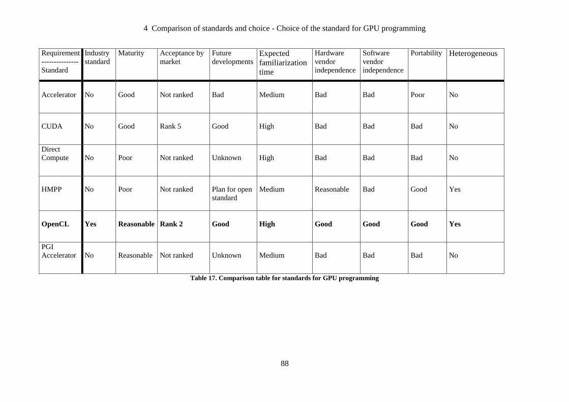
4 Comparison of standards and choice - Choice of the standard for GPU programming
88
Requirement
---------------
Standard
Industry
standard
Maturity Acceptance by
market
Future
developments Expected
familiarization
time
Hardware
vendor
independence
Software
vendor
independence
Portability Heterogeneous
Accelerator
No
Good
Not ranked
Bad
Medium
Bad
Bad
Poor
No
CUDA
No
Good
Rank 5
Good
High
Bad
Bad
Bad
No
Direct
Compute
No
Poor
Not ranked
Unknown
High
Bad
Bad
Bad
No
HMPP
No
Poor
Not ranked
Plan for open
standard
Medium
Reasonable
Bad
Good
Yes
OpenCL
Yes
Reasonable
Rank 2
Good
High
Good
Good
Good
Yes
PGI
Accelerator
No
Reasonable
Not ranked
Unknown
Medium
Bad
Bad
Bad
No
Table 17. Comparison table for standards for GPU programming
5 Design - Introduction
89
5 Design
5.1 Introduction
In this chapter the following is discussed:
- Interfacing VisionLab with OpenMP.
- Interfacing VisionLab with OpenCL.
- Experiment design and analysis methodology.
- Test plans.
5.2 Interfacing VisionLab with OpenMP
5.2.1 Introduction
This section describes the design of the interface between VisionLab and OpenMP. In order
to understand the design decisions, OpenMP is discussed in more detail. After a general
introduction, the components, the scheduling strategies and the memory model of OpenMP
are discussed. Subsequently the design of the Automatic Operator Parallelization and the
integration in the VisionLab framework are discussed.
5.2.2 General introduction to OpenMP
OpenMP is an Application Program Interface (API) that supports multi-platform shared
memory multi-processing programming in C, C++ and Fortran. In this project OpenMP is
chosen as the standard for multi-core CPU programming. For the motivation of this choice,
see section 4.2. An in-depth treatment of the OpenMP API is outside the scope of this project.
Only the topics necessary to understand the main line in this work are discussed here. All
details of OpenMP API can be found in the definition of the standard (OpenMP Architecture
Review Board, 2011). A good introduction to OpenMP can be found in Chapman, Jost and
van de Pas (2008). A tutorial can be found in Barney (2011b).

5 Design - Interfacing VisionLab with OpenMP
90
OpenMP supports the so-called fork-join programming model, which is illustrated in Figure
7. An OpenMP program starts, like a sequential program, as a single thread called the master
thread. The master thread executes sequentially until an OpenMP parallel construct is
encountered. Then the master thread forks a team of threads that is executed in parallel with
the master thread. The threads join when all threads have completed their statements in the
parallel construct. This means that all threads synchronize, all threads in the team terminate
and the master thread continues execution. The default parallelism granularity can be
overruled by specifying loop chunk sizes in combination with several scheduling types.
Figure 7. Fork-join programming model.
After Barney (2011b).
The following piece of C++ code shows both the power and the simplicity of the OpenMP
parallel loop construct. In this example two vectors are added. The for loop is parallelized
just by adding the line with “#pragma omp for” in front of the for loop.
const int SIZE = 1000;
double a[SIZE], b[SIZE], c[SIZE];
// code for initialising array b and c
#pragma omp for
for (int j = 0; j < SIZE; j++) {
a[j] = b[j] + c[j];
} // for j
Assuming that the default settings for OpenMP are applicable and the CPU has four cores, at
executing time the next events will happen when the for loop is executed:
- The master thread forks a team of three threads.
- All four threads will execute in parallel one quarter of the for loop. The first thread will
execute the for loop for 0 <= j < 250, the second thread will execute the for loop for
250 <= j < 500, etc.
- When all threads have completed their work, the threads will join.
5 Design - Interfacing VisionLab with OpenMP
91
If a compiler implementation does not support OpenMP, it will ignore the unknown pragma
found and generate code for the sequential version.
OpenMP is based on the shared-memory model, by default all data is shared among all the
threads. With extra key words in the OpenMP parallel constructs it is possible to deviate from
the all shared-memory model and to use thread-specific private data.
5.2.3 OpenMP components
OpenMP consists of three major components:
- Compiler directives.
- Runtime functions and variables.
- Environment variables.
Only the most important topics are discussed here.
All compiler directives start with “#pragma omp”. There are compiler directives for
expressing the type of parallelism:
- For loop directive for data parallelism.
- Parallel regions directive for task parallelism.
- Single and master directives for sequential executing of code in parallel constructs.
There are also compiler directives for synchronisation primitives, like:
- Atomic variables.
- Barriers.
- Critical sections.
- Flushing (synchronizing) memory and caches between threads.
OpenMP has runtime functions for performing operations like:
- Locking.
- Querying and setting the number of threads to be used in parallel regions.
- Time measurement.
- Setting the scheduling strategy, see section 5.2.4.
With environment variables it is possible to modify the default behaviour of OpenMP, like:
- Setting the maximal number of threads to be used in parallel regions.
- Setting the stack size for the threads.
- Setting the scheduling strategy, see section 5.2.4.
5 Design - Interfacing VisionLab with OpenMP
92
5.2.4 Scheduling strategy OpenMP
The scheduling strategy determines how the iterations of the parallel loop construct are
divided among the threads. According to the OpenMP API (OpenMP Architecture Review
Board, 2011, section 2.5.1):
“A worksharing loop has logical iterations numbered 0,1,...,N-1 where N is the number
of loop iterations, and the logical numbering denotes the sequence in which the
iterations would be executed if the associated loop(s) were executed by a single thread.
The schedule clause specifies how iterations of the associated loops are divided into
contiguous non-empty subsets, called chunks, and how these chunks are distributed
among threads of the team. Each thread executes its assigned chunk(s) in the context of
its implicit task. The chunk_size expression is evaluated using the original list items of
any variables that are made private in the loop construct. ...
The schedule kind can be one of:
- Static. When schedule(static, chunk_size) is specified, iterations are divided
into chunks of size chunk_size, and the chunks are assigned to the threads in
the team in a round-robin fashion in the order of the thread number.
When no chunk_size is specified, the iteration space is divided into chunks that
are approximately equal in size, and at most one chunk is distributed to each
thread. Note that the size of the chunks is unspecified in this case. …
- Dynamic. When schedule(dynamic, chunk_size) is specified, the iterations are
distributed to threads in the team in chunks as the threads request them. Each
thread executes a chunk of iterations, then requests another chunk, until no
chunks remain to be distributed. …
- Guided. When schedule(guided, chunk_size) is specified, the iterations are assigned to
threads in the team in chunks as the executing threads request them. Each thread
executes a chunk of iterations, then requests another chunk, until no chunks remain to
be assigned. For a chunk_size of 1, the size of each chunk is proportional to the number
of unassigned iterations divided by the number of threads in the team, decreasing to 1.
For a chunk_size with value k (greater than 1), the size of each chunk is determined in
the same way, with the restriction that the chunks do not contain fewer than k
iterations. …
- Auto. When schedule(auto) is specified, the decision regarding scheduling is
delegated to the compiler and/or runtime system.”
5 Design - Interfacing VisionLab with OpenMP
93
It is to be expected that there will be a trade-off between scheduling overhead and load
balancing. Two examples at the extreme side of this diversity:
- Static scheduling not specifying the chunk size will divide the work in N approximately
equally sized chunks over the N available cores. This will give the least scheduling
overhead. However if some iterations take more time to calculate than other iterations it is
quite possible that one of the threads will need significantly more time to finish its work
than the other threads. The other threads which have finished their work must wait for this
last thread before the threads can be joined and the parallel construct finishes. This means
that the work load is not evenly balanced over the threads.
This indicates that static scheduling will be the favourable strategy if the time needed for
calculating each chunk is fairly constant. However, this is only true if the computer
running the OpenMP application is dedicated to the application. Let’s assume that N
chunks are divided over N threads on a machine with N cores and one of the cores is
interrupted by a higher priority background task. In this case the thread on the interrupted
core will take more wall clock time to finish and will delay the total parallel construct.
- Guided and dynamic scheduling will give a much better load balancing if the time needed
for calculations of an iteration is expected to fluctuate or if it is likely that one or more
cores will be interrupted by higher priority background tasks. The difference between
guided and dynamic scheduling is that in dynamic scheduling the size of the chunk is
fixed and in guided scheduling the size of the chunk will gradually decrease. Guided
scheduling will give a more fine-tuned load balancing than dynamic scheduling at the
cost of more scheduling overhead.
For each algorithm that will be parallelized the appropriate scheduling strategy will be chosen
based on the expected variance in execution time of one iteration. In case of reasonable doubt
benchmarking must indicate the best strategy.
5 Design - Interfacing VisionLab with OpenMP
94
5.2.5 Memory model OpenMP
According to OpenMP Architecture Review Board (2011, section 1.4):
“The OpenMP API provides a relaxed-consistency, shared-memory model. All
OpenMP threads have access to a place to store and to retrieve variables, called the
memory. In addition, each thread is allowed to have its own temporary view of the
memory. The temporary view of memory for each thread is not a required part of the
OpenMP memory model, but can represent any kind of intervening structure, such as
machine registers, cache, or other local storage, between the thread and the memory.
The temporary view of memory allows the thread to cache variables and thereby to
avoid going to memory for every reference to a variable. Each thread also has access
to another type of memory that must not be accessed by other threads, called thread
private memory.
……
The memory model has relaxed-consistency because a thread’s temporary view of
memory is not required to be consistent with memory at all times. A value written to a
variable can remain in the thread’s temporary view until it is forced to memory at a
later time. Likewise, a read from a variable may retrieve the value from the thread’s
temporary view, unless it is forced to read from memory. The OpenMP flush operation
enforces consistency between the temporary view and memory.”
The flush operation can be specified using the flush directive and is also implied at
various locations in an OpenMP program like:
- during a barrier region.
- at entry to and exit from parallel and critical.
See for a full list to OpenMP Architecture Review Board (2011, section 2.8.6).
5.2.6 Automatic Operator Parallelization
5.2.6.1 Introduction
This section describes the design of the Automatic Operator Parallelization. First the problem
is analysed, then the design of the calibration procedure and run-time decision procedure are
described.
5 Design - Interfacing VisionLab with OpenMP
95
5.2.6.2 Analysis
The preliminary research and experiments described in section 2.2 indicated that on large
images parallelization can give a significant performance benefit. Due to the overhead
involved in parallelization, the use of parallelization on small images can lead to a
performance loss compared to running sequentially.
In section 2.3 about the requirements for multi-core CPUs it is dictated that:
“A procedure to predict at runtime if running multi-core is expected to be beneficial
will be necessary. It is to be expected that different hardware configurations will
behave differently so there will be a need for a calibration procedure.”
From the preliminary research and experiments it became clear that “to predict at runtime if
running multi-core is expected to be beneficial” is not an easy challenge. This is because:
- Speedup is hardware dependent. Import parameters are:
- Processor architecture, number of cores, clock speed, and size of caches.
- Size of memory, number of data channels and access time.
- Performance depends on operating system settings and BIOS settings like:
- Task priority.
- Dynamic voltage scaling.
- There are operators for which the complexity of calculation can vary for each pixel in the
image. Obvious examples are the LabelBlobs and BlobAnalysis operators, see Van de
Loosdrecht, et al. (2013, Chapter Labelling and Blob measurement). The speedup
depends on the content of the image.
- There are operators for which the criterion “number of pixels” for prediction mechanism
is not sufficient to make valid predictions. For example the size of the neighbourhood is
also an important criterion for local neighbour operators.
- There are operators like BlobAnalysis that are so complex that for different parts of the
algorithm different prediction mechanisms can be expected to be applied.
- Performance depends on the load of the background jobs.
Because of the nature of this challenge it will be difficult to design a prediction algorithm that
will work perfectly in all conditions. The prediction must give reasonable results for most
situations. The user of VisionLab will be given the possibility to turn off the prediction
algorithm and to decide for himself if he wants to run in multi-core mode. This option is
given the name “auto multi-core mode”. The user must be able to turn this mode on or off in
both the VisionLab GUI, the script language and in C++.
5 Design - Interfacing VisionLab with OpenMP
96
5.2.6.3 Calibration procedure
As stated in the previous section, calibration is not an easy challenge and it is expected that it
will take a long time if all parallelized operators must be calibrated for all image types. A
perfect calibration will not be possible for all operators because the calibration can be
dependent on the content of the image.
It was decided to first design and test a simplified calibration procedure. This procedure:
- Is based on the most frequent image type for a specific operator.
- Uses one representative calibration image for a specific operator.
- Has a simple and fast procedure for global optimization.
- Has a complex and slow procedure for more optimal optimization.
- Uses a user-defined gain-factor that defines how much profit parallelization must have
compared to running sequential. An example: if the gain-factor is 1.1 then the operator is
executed in parallel if it is to be expected that the parallelization is 10% faster than
executing the operator sequential.
Using this parameter a user can decide whether he wants to use cores for a (small) profit
or keep the cores ready for use in nested parallel regions. See OpenMP Architecture
Review Board (2011, section 1.3).
Based on experiences with the Computer Vision projects mentioned in section 1.2 it is quite
clear that the image type that is most often used for greyscale operators is the Int16Image and
for colour operators the HSV888Image. Furthermore it is expected that the calibration result
for a specific operator will be similar for all images types. This assumption must be validated
by benchmarking. If this assumption is invalid, a calibration for all image types will be
necessary.
The full calibration procedure must determine the break-even point in number of pixels for
each parallelized operator where the parallel execution of the operator is gain-factor times
faster than the sequential version. For one basic operator the result of the calibration is stored
as the number of pixels for the break-even point. All other operators will store their results
relative to the result of the basic operator. The quick calibration procedure only benchmarks
the basic operator and uses default values for relative factors for the other operators.
5 Design - Interfacing VisionLab with OpenMP
97
The idea behind the simple procedure is that this procedure will give a quick and fairly good
idea of the general performance of the system based on the most dominant factors like clock
speed and number of cores available. The idea behind the complex procedure is that this will
give a more fine-tuned and machine-specific calibration. The preliminary research and
experiments described in section 2.2 indicated that different CPU architectures will give
variations in the relative factors for the operators. It is plausible that these differences can be
explained by factors like differences in efficiency of the executing of the instruction set and
differences in memory latency and bandwidth.
In the author’s experience, parallel programming is more vulnerable for making errors than
sequential programming. During the calibration process both the parallel result and the
sequential result of the operator are calculated. The calibration procedure must have a built-in
regression test, which always compares the sequential result with the parallel result. The
overhead involved for this test is negligible.
After calibration the results can be saved to disk. The next time at start-up the calibration file
is read from disk, so that the Automatic Operator Parallelization mechanism can be used
without executing the calibration procedure.
5.2.6.4 Runtime decision
At execution time a parallelized operator has to decide whether parallelization is beneficial.
This decision is based on the size of the image, operator specific parameters and the
calibration result. The OpenMP if clause in the parallel construct facilitates the
implementation this decision in a convenient way. An example:
#pragma omp for if (condition)
If the condition evaluates to true, the for statement following the OpenMP pragma will be
executed in parallel. If the condition evaluates to false the for statement will be executed
sequentially.
5.2.7 Integrating OpenMP in VisionLab
In section 2.3 about the requirements for multi-core CPUs it is stated that:
“If possible existing VisionLab scripts and applications using the VisionLab ANSI C++
library should not have to be modified in order to benefit from the multi-core version.”
5 Design - Interfacing VisionLab with OpenCL
98
The following steps are specified in order to integrate OpenMP in VisionLab:
- Choose one representative example for all four classes of basic low level image operators
(section 3.6.2) and implement a parallel version using OpenMP. From these examples a
framework for the other instances of the same class can be derived.
- Parallelize the operators of VisionLab and handle the Automatic Operator Parallelization
without changing the interface of the operator. This means that the legacy VisionLab
scripts and applications using the VisionLab C++ library can benefit from the
parallelizing without any modification.
- Extend the library and script language of VisionLab with commands to modify the default
behaviour of OpenMP and query the runtime support of OpenMP. Examples:
- Setting the number of threads to be used.
- Querying the number of cores in the system.
- Implement the calibration for Automatic Operator Parallelization as a C++ module.
Extend the script language of VisionLab with commands to perform the calibration and
extend the GUI of the development environment of VisionLab with a form to perform the
calibration in an interactive way.
5.3 Interfacing VisionLab with OpenCL
5.3.1 Introduction
This section describes the design of the interface between VisionLab and OpenCL. In order
to understand the design decisions, the following OpenCL topics are discussed in more detail:
- OpenCL architecture.
- Example of OpenCL application, both host-side code and kernel code.
- Integration of OpenCL in VisionLab.
5.3.2 OpenCL architecture
5.3.2.1 Introduction
According to the OpenCL specification (Munshi, 2010) the OpenCL architecture has the
following hierarchy of models:
- Platform model.
- Execution model.
- Memory model.
- Programming model.
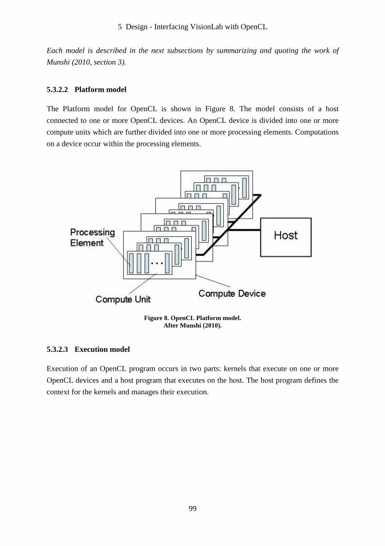
5 Design - Interfacing VisionLab with OpenCL
99
Each model is described in the next subsections by summarizing and quoting the work of
Munshi (2010, section 3).
5.3.2.2 Platform model
The Platform model for OpenCL is shown in Figure 8. The model consists of a host
connected to one or more OpenCL devices. An OpenCL device is divided into one or more
compute units which are further divided into one or more processing elements. Computations
on a device occur within the processing elements.
Figure 8. OpenCL Platform model.
After Munshi (2010).
5.3.2.3 Execution model
Execution of an OpenCL program occurs in two parts: kernels that execute on one or more
OpenCL devices and a host program that executes on the host. The host program defines the
context for the kernels and manages their execution.
5 Design - Interfacing VisionLab with OpenCL
100
When the kernel is submitted to the compute device for computation an index space is
defined. An instance of the kernel called the work-item is created for each index. Work-items
can be identified by this index, which provides a global ID for a work-item. Work-items are
organized into work-groups. The work-groups provide a more coarse-grained decomposition
of the index space. Work-groups are assigned a unique work-group. Work-items are assigned
a unique local ID within a work-group so that a single work-item can be uniquely identified
by its global ID or by a combination of its local ID and work-group ID. The work-items in a
given work-group execute concurrently on the processing elements of a single compute unit.
The indexing space used to partition work-items in OpenCL is called an N-Dimensional
Range (NDRange). The NDRange, as the name suggests, supports multidimensional
indexing. OpenCL supports up to and including three-dimensional indexing.
The host defines a context for the execution of the kernels. The context includes the
following resources:
- Devices: The collection of OpenCL devices to be used by the host.
- Kernels: The OpenCL functions that run on OpenCL devices.
- Program Objects: The program source and executable that implement the kernels.
- Memory Objects: A set of memory objects visible to the host and the OpenCL devices.
A context is created and manipulated by the host using functions from the OpenCL API. The
host creates one or more data structures called command-queues to coordinate execution of
the kernels on the devices. The host places commands into the command-queue(s), which are
then scheduled onto the devices within the context. These include:
- Kernel execution commands: Execute a kernel on the processing elements of a device.
- Memory commands: Transfer data to, from, or between memory objects.
- Synchronization commands: Constrain the order of execution of commands.
A command-queue schedules commands for execution on a device. These commands execute
asynchronously between the host and the device. Commands execute relative to each other in
one of two modes:
- In-order Execution: Commands are launched in the order they appear in the command
queue and complete in order.
- Out-of-order Execution: Commands are issued in order, but do not wait to complete
before following commands execute. Any order constraints are enforced by the
programmer through explicit synchronization commands.
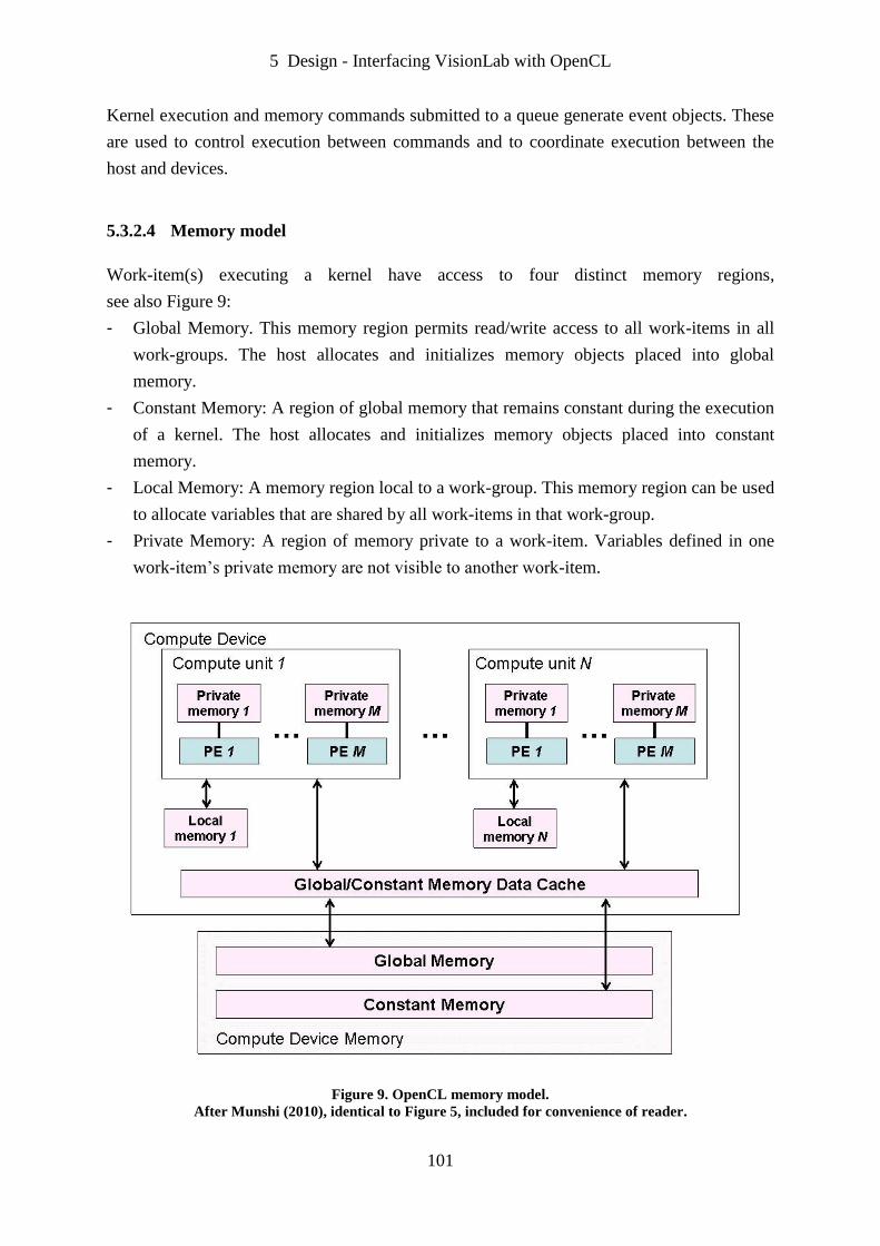
5 Design - Interfacing VisionLab with OpenCL
101
Kernel execution and memory commands submitted to a queue generate event objects. These
are used to control execution between commands and to coordinate execution between the
host and devices.
5.3.2.4 Memory model
Work-item(s) executing a kernel have access to four distinct memory regions,
see also Figure 9:
- Global Memory. This memory region permits read/write access to all work-items in all
work-groups. The host allocates and initializes memory objects placed into global
memory.
- Constant Memory: A region of global memory that remains constant during the execution
of a kernel. The host allocates and initializes memory objects placed into constant
memory.
- Local Memory: A memory region local to a work-group. This memory region can be used
to allocate variables that are shared by all work-items in that work-group.
- Private Memory: A region of memory private to a work-item. Variables defined in one
work-item’s private memory are not visible to another work-item.
Figure 9. OpenCL memory model.
After Munshi (2010), identical to Figure 5, included for convenience of reader.
5 Design - Interfacing VisionLab with OpenCL
102
The application running on the host uses the OpenCL API to create memory objects in global
or constant memory and to enqueue memory commands that operate on these memory
objects. To copy data explicitly, the host enqueues commands to transfer data between the
memory objects and host memory.
OpenCL uses a relaxed consistency memory model; i.e. the state of memory visible to a
work-item is not guaranteed to be consistent across the collection of work-items at all times.
Within a work-item memory has load/store consistency. Local memory is consistent across
work-items in a single work-group at a work-group barrier. Global memory is consistent
across work-items in a single work-group at a work-group barrier, but there are no guarantees
of memory consistency between different work-groups executing a kernel.
Memory objects are categorized into two types: buffer objects and image objects. A buffer
object stores a one-dimensional collection of elements whereas an image object is used to
store a two- or three-dimensional texture, frame-buffer or image. Elements of a buffer object
can be a scalar data type (such as an int, float), vector data type, or a user-defined structure.
Elements in a buffer are stored in sequential fashion and can be accessed using a pointer.
Elements of an image are stored in a format that is opaque to the user and cannot be directly
accessed using a pointer. Built-in functions are provided by the OpenCL kernel language to
allow a kernel to read from or write to images.
5.3.2.5 Programming model
The OpenCL execution model supports data parallel and task parallel programming models,
as well as supporting hybrids of these two models. The primary model driving the design of
OpenCL is data parallel.
For the data parallel model there are two methods to specify how the work-items are
distributed over the processing elements. In the explicit method a programmer defines the
total number of work-items to execute in parallel and also how the work-items are divided
among work-groups. In the implicit method, a programmer specifies only the total number of
work-items to execute in parallel, and the division into work-groups is managed by the
OpenCL implementation.
There are two domains of synchronization in OpenCL:
- Work-items in a single work-group
- Commands enqueued to command-queue(s) in a single context

5 Design - Interfacing VisionLab with OpenCL
103
Synchronization between work-items in a single work-group is done using a work-group
barrier. All the work-items of a work-group must execute the barrier before any are allowed
to continue execution beyond the barrier. Note that the work-group barrier must be
encountered by all work-items of a work-group executing the kernel or by none at all. There
is no mechanism in the Compute Device for synchronization between work-groups.
The synchronization points between commands in command-queues are:
- Command-queue barrier. The command-queue barrier ensures that all previously queued
commands have finished execution and any resulting updates to memory objects are
visible to subsequently enqueued commands before they begin execution. This barrier can
only be used to synchronize between commands in a single command-queue.
- Waiting on an event. All OpenCL API functions that enqueue commands return an event
that identifies the command and memory objects it updates. A subsequent command
waiting on that event will guarantee that updates to those memory objects are visible
before the command begins execution.
5.3.3 Example of OpenCL application, both host-side code and kernel code
In section 5.2.2 an example is given of how to parallelize with OpenMP the adding of two
vectors. In this section the OpenCL version of this algorithm is discussed.
In a simple OpenCL approach a work-item is created for each element of the vector. The
NDRange is a one-dimensional indexing space. The source code for the kernel (after Gaster,
et al., 2012, p.32) is simple:
kernel void VecAdd (global int* c, global int* a, global int* b) {
unsigned int n = get_global_id(0);
c[n] = a[n] + b[n];
}
With get_global_id(0) the global ID for the work-item is retrieved. This global ID is used as
index for the vectors.

5 Design - Interfacing VisionLab with OpenCL
104
The C source code for the host-side calling the OpenCL API functions is given in Gaster, et
al. (2012, pp.32-38). This source code contains 67 (!) C statements, not counting the
comment lines and has no code for error checking after calling OpenCL API functions. The
host code consists of the following steps:
- Allocate space for vectors and initialize.
- Discover and initialize OpenCL platform.
- Discover and initialize compute device.
- Create a context.
- Create a command queue.
- Create device buffers.
- Write host data to device buffers.
- Create and compile the program.
- Create the kernel.
- Set the kernel arguments.
- Configure the NDRange.
- Enqueue the kernel for execution.
- Read the output buffer back to the host.
- Verify result.
- Release OpenCL and host resources.
After writing several OpenCL applications (both host-side and kernel) the author concluded
that:
- The host-side code is labour-intensive and sensitive for errors because the OpenCL API
functions are complex and have many parameters.
- Using the C++ wrapper for the OpenCL host API code (Gaster, 2010) makes error
checking easier because in case of an error an exception is raised.
- Many OpenCL applications have a very similar host code.
5.3.4 Integrating OpenCL in VisionLab
In section 2.4 about the requirements for GPUs it is stated that:
“GPU code must be able to be called from both VisionLab script language and from
the VisionLab ANSI C++ library.”
5 Design - Interfacing VisionLab with OpenCL
105
The following steps are specified in order to integrate OpenCL in VisionLab:
- Design a C++ module with an abstraction layer on top of the C++ wrapper for the
OpenCL host API. By using this C++ module, the access to the OpenCL host API will be
much easier and much of the replication of code (section 5.3.3) can be avoided.
- Extend the script language of VisionLab with commands to call the OpenCL host API.
By using the script language it will be much easier to write the host-side code. Examples
of new commands:
- Querying platform and device properties.
- Creating context, program, queue, buffer, image and event.
- Read/Write buffer and image.
- Building, saving and reading programs.
- Setting parameters for kernel and executing kernel.
- Synchronization.
- Extend the GUI of VisionLab with an editor to create, save and read source code for
OpenCL kernels.
- Choose one representative example for all four classes of basic low level image operators
(section 3.6.2) and implement a parallel version in OpenCL. From these examples a
framework for the other instances of the same class can be derived.
As mentioned in section 2.1 VisionLab uses C++ templates to support a wide variety of
image types. OpenCL does not support something similar to C++ templates. In order to make
the kernels suitable for different image types, macro substitution can be used as a ‘poor man’s
substitute for templates’. If a kernel is defined as:
kernel void Operator (global ImageT* image, const PixelT pixel) {
…
}
it is possible to supply the macro definitions at compile time using the build option string
(Munshi, 2010, section 5.6.3). Some examples:
- With “-DImageT=short -DPixelT=short” the kernel will work as an Int16Image with
image as pointer to shorts.
- With “-DImageT=short4 -DPixelT=short” the kernel will work as an Int16Image with
image as pointer to vectors of shorts.
- With “-DImageT=int -DPixelT=int” the kernel will work as an Int32Image.
5 Design - Experiment design and analysis methodology
106
5.4 Experiment design and analysis methodology
5.4.1 Introduction
In this section the following is discussed:
- Timing.
- Benchmarking protocol.
- Data analysis.
- Benchmark setup.
5.4.2 Timing
With regard to the timing it is important that:
- All execution time measurement, sequential, multi-core and GPU implementation, must
be performed by one timing tool.
- A calibration of overhead for the time measurement must be performed and all
measurements must be corrected for this overhead.
5.4.3 Benchmark protocol
In section 3.7 “The Speedup Test” protocol for benchmarking is reviewed. In this work the
performance of the sequential, multi-core CPU and GPU version of one algorithm must be
compared. For this simplified kind of benchmarking a subset of “The Speedup Test” protocol
can be used supplemented with some specific items for this project.
For this study, the following benchmarking protocol is used:
- Description of hardware used.
- Description of compiler and compiler settings used.
- Calibration of overhead of timer used.
- The test computer must be dedicated during the experiments to the test process.
- Data analysis as described in section 5.4.4 is performed.
5 Design - Experiment design and analysis methodology
107
The test computer must be dedicated during the experiments to the test process in the
following way:
- The test process must have a high task priority.
- As far as possible non-essential background tasks must be suspended.
- Windows 7 desktop must be set to Aero Basic Theme in order to minimalize the overhead
of displaying the desktop.
- Dynamic voltage scaling must be disabled or limited in range if thermal overheating can
be expected. Using the BIOS setup it is possible to disable dynamic voltage scaling. An
alternative way to limit the dynamic voltage scaling is to set the Power Management
feature of Windows minimum and maximum performance on 100%.
- For benchmarking GPUs the power management mode for the graphics card must be set
in maximum performance mode.
- The screen saver must be disabled.
Benchmarking on GPU must only measure the time needed for execution of the kernels. The
time for transferring data between the CPU memory and GPU memory must NOT be
included in the benchmarking. From the preliminary research and experiments described in
section 2.2 it becomes clear that using contemporary GPUs can give a considerable amount
of overhead. The reasons for not including this overhead are:
- It is expected that in many practical cases data will be transferred from CPU to GPU
memory and then more than one kernel will be executed on this data. Thereafter the data
is transferred back from the GPU.
- New fused architecture of CPU and GPU are announced (see section 3.5.2.4), in which
CPU and GPU will share the same global memory. This will reduce or eliminate the
copying overhead.
- The transfer of data between the CPU memory and GPU memory are benchmarked
separately.

5 Design - Experiment design and analysis methodology
108
5.4.4 Data analysis
The data analysis compares execution times and variance in execution times for sequential,
multi-core CPU and GPU implementations. References are the existing sequential algorithms
of VisionLab.
The parallelized operators must be benchmarked according to the protocol based on “The
Speedup Test” described in section 5.4.3. For each experiment:
- All experiments must be repeated at least 30 times.
- No removal of outliers in observed execution times.
- The median of the execution times is calculated.
- The speedup of the parallel versions is calculated based on the median of the execution
times.
- Violin plots are used to visualize the variance in execution times. Violin plots are similar
to box plots, except that they also show the probability density of the data. Violin plots
were introduced into the statistical community by Hintze and Nelson (1998). See Figure
10 for an example of a violin plot and its relation with the box plot.
Figure 10. Example of violin plot.
After Hintze and Nelson (1998).
5 Design - Benchmark setup
109
For statistical analysis and plotting of the graphs the statistical package R (R-project.org,
2011) is used. The script language of VisionLab must be extended with a command to
execute R scripts.
5.5 Benchmark setup
The following benchmark setup must be used to compare the performance of the sequential,
multi-core CPU and GPU versions of an operator:
- The benchmark protocol described in section 5.4.3 is used.
- For each operator one or more typical images are chosen as input images.
- For each operator a suitable range of image sizes is chosen.
- The operators are executed for all chosen input images and in all chosen sizes.
- The data analysis described in section 5.4.4 is used.

6 Implementation - Introduction
110
6 Implementation
6.1 Introduction
In this chapter the issues about the implementation of the following topics are discussed:
- Timing procedure.
- Interfacing VisionLab with OpenMP.
- Interfacing VisionLab with OpenCL.
- Threshold as representative of Point operators.
- Convolution as representative of Local neighbour operators.
- Histogram as representative of Global operators.
- LabelBlobs as representative of Connectivity based operators.
This work is about how to parallelize a large generic Computer Vision library in an efficient
and effective way. In section 3.6, a classification of basic low level image operators is
described. This chapter describes the implementations of one representative for each class.
These implementations can be used as a skeleton to implement the other instances for each
class. Many of the high level operators are built using the basic low level operators. These
operators will directly benefit of the parallelization of the basic low level operators.
In order to gain experience with OpenMP and OpenCL two simple vision operators,
Threshold and Histogram, were selected for the first experiments. The results of these
experiments were used to limit the scope of experiments with the more complex operators.
6.2 Timing procedure
The timing tool already implemented in VisionLab was used for all time measurement.
This is implemented in a portable way. On x86/x64 based platforms it uses the high
resolution multimedia timer (Work and Nguyen, 2009), which has an adequate resolution of
3.31287 MHz on the computer (see Appendix A) used for benchmarking. VisionLab reports
all time measurements in micro seconds.
6 Implementation - Interfacing VisionLab with OpenMP
111
It is possible to use the BIOS setup to disable dynamic voltage scaling, however during the
first benchmarks with disabled dynamic voltage scaling the test computer ‘started to smell’,
indicating possible overheating. It was decided not to disable dynamic voltage scaling using
the BIOS but to limit it with the Power Management feature of Windows. The reason for this
decision was that the author is not an expert in the field of computer hardware and did not
want to overheat his computer.
The alternative way to limit the dynamic voltage scaling was to set the minimum and
maximum performance to 100% in the Windows Power Management. Measurements with
the tool CPU-Z monitor (CPUID, 2011) revealed small variations in processor frequency
running on:
- One core, between 3.5 and 3.8 GHz.
- Two or three cores, between 3.5 and 3.6 GHz.
- Four cores, a stable frequency of 3.5 GHz.
Because there is a decay in frequency when more cores are used, this choice has affected the
accuracy of the calculation of the speedup factors for multi-core CPUs. However in real life
applications the same decay in frequency will be present.
6.3 Interfacing VisionLab with OpenMP
In this section the implementation of the interface of VisionLab with OpenMP is described.
The design of this interface is described in section 5.2.
Twenty-seven commands were added to the command interpreter of VisionLab. With these
commands the user can control the behaviour of OpenMP and Automatic Operator
Parallelization. It is also possible to manually overrule the Automatic Operator Parallelization
mechanism. See documentation of VisionLab (Van de Loosdrecht Machine Vision BV, 2013)
and course material (Van de Loosdrecht, et al., 2013) for the details of these operators.
All 170 operators listed in Appendix G were parallelized using OpenMP and the runtime
decision procedure that determines whether parallelization is beneficial was implemented.
The calibration procedure described in section 5.2.6.3 was implemented. See Figure 11 and
Figure 12 for screenshots.
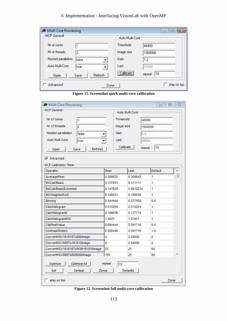
6 Implementation - Interfacing VisionLab with OpenMP
112
Figure 11. Screenshot quick multi-core calibration
Figure 12. Screenshot full multi-core calibration
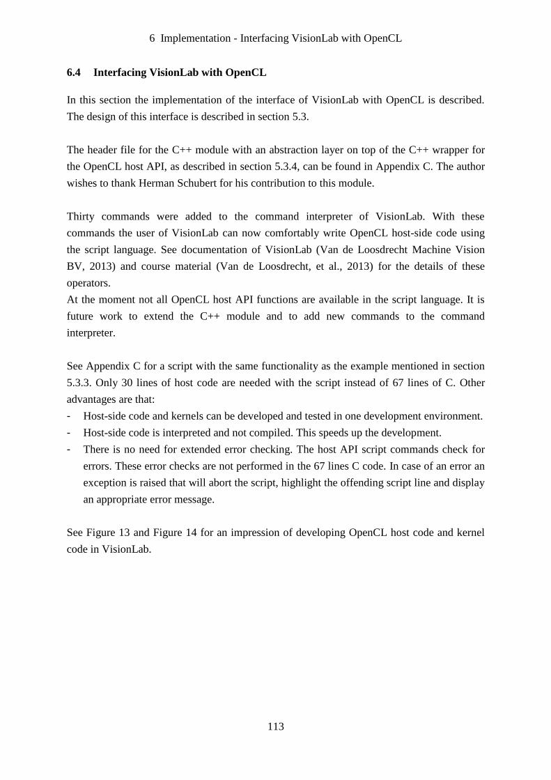
6 Implementation - Interfacing VisionLab with OpenCL
113
6.4 Interfacing VisionLab with OpenCL
In this section the implementation of the interface of VisionLab with OpenCL is described.
The design of this interface is described in section 5.3.
The header file for the C++ module with an abstraction layer on top of the C++ wrapper for
the OpenCL host API, as described in section 5.3.4, can be found in Appendix C. The author
wishes to thank Herman Schubert for his contribution to this module.
Thirty commands were added to the command interpreter of VisionLab. With these
commands the user of VisionLab can now comfortably write OpenCL host-side code using
the script language. See documentation of VisionLab (Van de Loosdrecht Machine Vision
BV, 2013) and course material (Van de Loosdrecht, et al., 2013) for the details of these
operators.
At the moment not all OpenCL host API functions are available in the script language. It is
future work to extend the C++ module and to add new commands to the command
interpreter.
See Appendix C for a script with the same functionality as the example mentioned in section
5.3.3. Only 30 lines of host code are needed with the script instead of 67 lines of C. Other
advantages are that:
- Host-side code and kernels can be developed and tested in one development environment.
- Host-side code is interpreted and not compiled. This speeds up the development.
- There is no need for extended error checking. The host API script commands check for
errors. These error checks are not performed in the 67 lines C code. In case of an error an
exception is raised that will abort the script, highlight the offending script line and display
an appropriate error message.
See Figure 13 and Figure 14 for an impression of developing OpenCL host code and kernel
code in VisionLab.
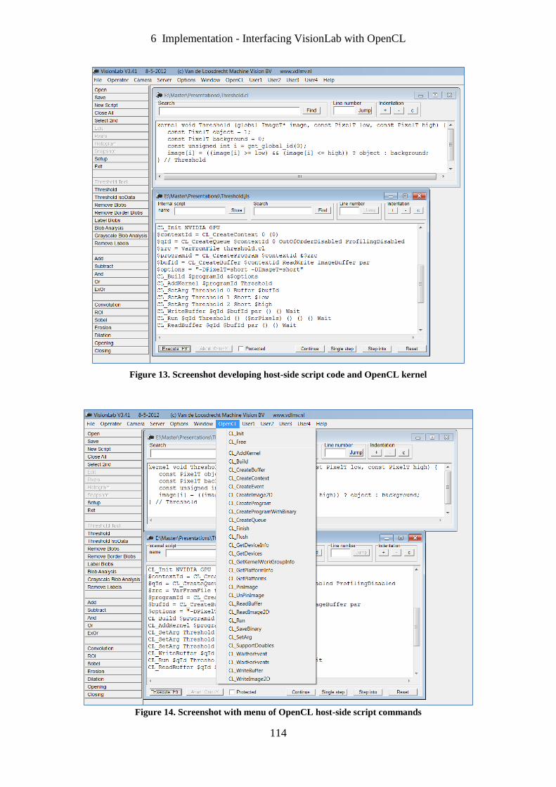
6 Implementation - Interfacing VisionLab with OpenCL
114
Figure 13. Screenshot developing host-side script code and OpenCL kernel
Figure 14. Screenshot with menu of OpenCL host-side script commands
6 Implementation - Point operators
115
6.5 Point operators
6.5.1 Introduction
As representative of the Point operators Threshold was implemented.
6.5.2 Threshold
6.5.2.1 Introduction
The functionality of the Threshold operator is described in section 3.6.3. In this section the
implementation of the Threshold operator is described for the following versions:
- Sequential.
- OpenMP.
- OpenCL.
In order to gain experience with OpenMP and OpenCL many experiments were executed on
this simple vision operator. The results of these experiments were used to limit the scope
experiments with the more complex operators. Because there is only a small amount of code
involved, the source code is presented. Note that for the sake of clarity all code needed for
error checking is omitted.
6.5.2.2 Sequential
As mentioned in section 2.1 VisionLab supports a wide variety of image types. The
Threshold operator must work with all greyscale image types. In order to avoid a lot of code
duplication, C++ templates are used. Implementation of the Threshold operator is
straightforward:
template <class OrdImageT, class PixelT>
void Threshold (OrdImageT &image, const PixelT low, const PixelT high) {
PixelT *pixelTab = image.GetFirstPixelPtr();
int nrPixels = image.GetNrPixels();
for (int i = 0; i < nrPixels; i++) {
pixelTab[i] = ((pixelTab[i] >= low) && (pixelTab[i] <= high)) ?
OrdImageT::Object() : OrdImageT::BackGround();
} // for all pixels
} // Threshold
6 Implementation - Point operators
116
Note: VisionLab also supports a faster implementation of the Threshold operator called
ThresholdFast. This operator can be used if a priori the minimum and maximum pixel value
in the image are known. ThresholdFast uses a lookup table in which for each pixel value the
corresponding object or background value is stored and replaces the if statement by a table
lookup.
6.5.2.3 OpenMP
In order to modify the sequential version for use with OpenMP only one line with the
OpenMP pragma was added. In order to facilitate the Automatic Operator Parallelization
(section 5.2.6.4) “if (calibMCP.TestMultiCore(OC_Threshold,nrPixels))” was added.
Because the time needed for calculating each chunk is constant, the static scheduling strategy
(see section 5.2.4) was chosen.
template <class OrdImageT, class PixelT>
void Threshold (OrdImageT &image, const PixelT low, const PixelT high) {
PixelT *pixelTab = image.GetFirstPixelPtr();
int nrPixels = image.GetNrPixels();
#pragma omp parallel for if (calibMCP.TestMultiCore(OC_Threshold,nrPixels))
for (int i = 0; i < nrPixels; i++) {
pixelTab[i] = ((pixelTab[i] >= low) && (pixelTab[i] <= high)) ?
OrdImageT::Object() : OrdImageT::BackGround();
} // for all pixels
} // Threshold
6.5.2.4 OpenCL
6.5.2.4.1 Introduction
Based on earlier experiences described in section 2.2 the following versions of OpenCL
kernels were developed:
- One pixel or vector of pixels per kernel using one read/write buffer.
- One pixel per kernel using images.
- One pixel or vector of pixels per kernel using a read and a write buffer.
- Chunk of pixels or vectors of pixels per kernel.
- Chunk of pixels or vectors of pixels per kernel with coalesced memory access.
In the next sections the kernels are described and motivated. The client side code is relatively
straightforward and is not discussed here. Where possible, the “poor man’s substitute for
templates” was used (section 5.3.4).
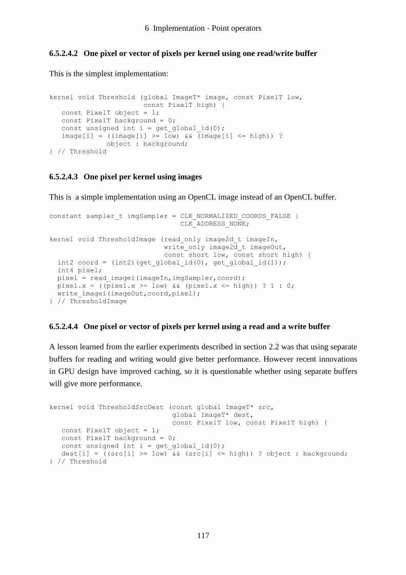
6 Implementation - Point operators
117
6.5.2.4.2 One pixel or vector of pixels per kernel using one read/write buffer
This is the simplest implementation:
kernel void Threshold (global ImageT* image, const PixelT low,
const PixelT high) {
const PixelT object = 1;
const PixelT background = 0;
const unsigned int i = get_global_id(0);
image[i] = ((image[i] >= low) && (image[i] <= high)) ?
object : background;
} // Threshold
6.5.2.4.3 One pixel per kernel using images
This is a simple implementation using an OpenCL image instead of an OpenCL buffer.
constant sampler_t imgSampler = CLK_NORMALIZED_COORDS_FALSE |
CLK_ADDRESS_NONE;
kernel void ThresholdImage (read_only image2d_t imageIn,
write_only image2d_t imageOut,
const short low, const short high) {
int2 coord = (int2)(get_global_id(0), get_global_id(1));
int4 pixel;
pixel = read_imagei(imageIn,imgSampler,coord);
pixel.x = ((pixel.x >= low) && (pixel.x <= high)) ? 1 : 0;
write_imagei(imageOut,coord,pixel);
} // ThresholdImage
6.5.2.4.4 One pixel or vector of pixels per kernel using a read and a write buffer
A lesson learned from the earlier experiments described in section 2.2 was that using separate
buffers for reading and writing would give better performance. However recent innovations
in GPU design have improved caching, so it is questionable whether using separate buffers
will give more performance.
kernel void ThresholdSrcDest (const global ImageT* src,
global ImageT* dest,
const PixelT low, const PixelT high) {
const PixelT object = 1;
const PixelT background = 0;
const unsigned int i = get_global_id(0);
dest[i] = ((src[i] >= low) && (src[i] <= high)) ? object : background;
} // Threshold
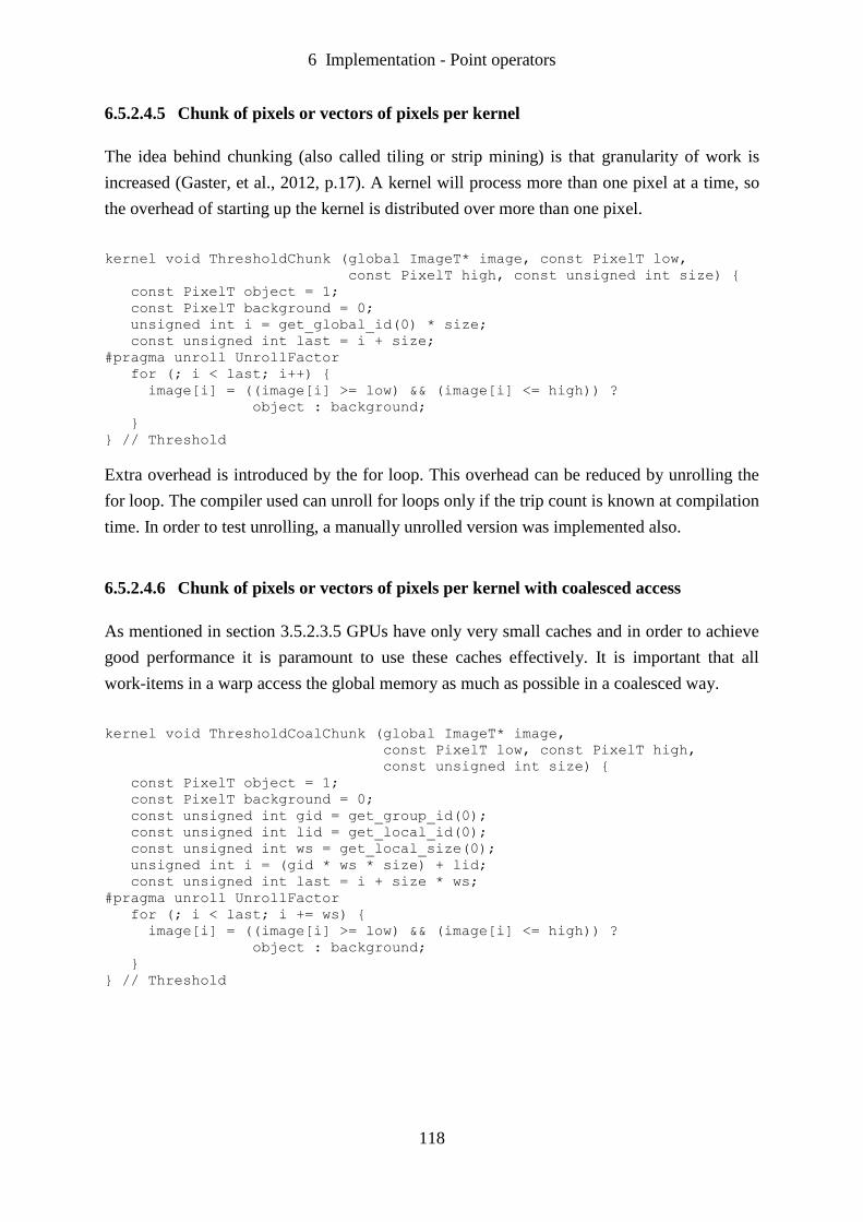
6 Implementation - Point operators
118
6.5.2.4.5 Chunk of pixels or vectors of pixels per kernel
The idea behind chunking (also called tiling or strip mining) is that granularity of work is
increased (Gaster, et al., 2012, p.17). A kernel will process more than one pixel at a time, so
the overhead of starting up the kernel is distributed over more than one pixel.
kernel void ThresholdChunk (global ImageT* image, const PixelT low,
const PixelT high, const unsigned int size) {
const PixelT object = 1;
const PixelT background = 0;
unsigned int i = get_global_id(0) * size;
const unsigned int last = i + size;
#pragma unroll UnrollFactor
for (; i < last; i++) {
image[i] = ((image[i] >= low) && (image[i] <= high)) ?
object : background;
}
} // Threshold
Extra overhead is introduced by the for loop. This overhead can be reduced by unrolling the
for loop. The compiler used can unroll for loops only if the trip count is known at compilation
time. In order to test unrolling, a manually unrolled version was implemented also.
6.5.2.4.6 Chunk of pixels or vectors of pixels per kernel with coalesced access
As mentioned in section 3.5.2.3.5 GPUs have only very small caches and in order to achieve
good performance it is paramount to use these caches effectively. It is important that all
work-items in a warp access the global memory as much as possible in a coalesced way.
kernel void ThresholdCoalChunk (global ImageT* image,
const PixelT low, const PixelT high,
const unsigned int size) {
const PixelT object = 1;
const PixelT background = 0;
const unsigned int gid = get_group_id(0);
const unsigned int lid = get_local_id(0);
const unsigned int ws = get_local_size(0);
unsigned int i = (gid * ws * size) + lid;
const unsigned int last = i + size * ws;
#pragma unroll UnrollFactor
for (; i < last; i += ws) {
image[i] = ((image[i] >= low) && (image[i] <= high)) ?
object : background;
}
} // Threshold
6 Implementation - Local neighbour operators
119
6.5.3 Future work
The Threshold operator is a highly memory bandwidth bound operator, so it is not possible to
draw conclusions for computation bound point operators. This will have to be investigated in
future work.
6.6 Local neighbour operators
6.6.1 Introduction
As representative of the Local neighbour operators Convolution was implemented.
6.6.2 Convolution
6.6.2.1 Introduction
The functionality of the Convolution operator is described in section 3.6.4. It was decided to
implement first the Convolution for single channel (grayscale) images. This decision is based
on the experiences with the 170 Computer Vision projects mentioned in section 1.2. In those
projects grayscale Convolution was more frequently used than color Convolution. The
implementation discussed in this work is a generalized implementation, which means:
- The height and width of the kernel mask are specified by the user.
- The origin of the kernel mask is specified by the user.
- It is assumed that the kernel mask is a non-separable.
The implementation is intended to be used with a small kernel mask, so using the Fast
Fourier Transform is not feasible.
In this section the implementation of the Convolution operator is described for the following
versions:
- Sequential.
- OpenMP.
- OpenCL.
The size of the source code is substantial and only some relevant parts are included in this
work. The full source code is documented in Van de Loosdrecht (2013a).
6 Implementation - Local neighbour operators
120
6.6.2.2 Sequential
The sequential implementation is a generalized version of the algorithm described in section
3.6.4 and is templatized for use with all greyscale image types of Visionlab in a similar way
as described in section 6.5.2.2.
6.6.2.3 OpenMP
In order to modify the sequential version for use with OpenMP, only one line with the
OpenMP pragma omp parallel was added in a similar way as described in section 6.5.2.3.
Because the time needed for calculation each chunk is constant, the static scheduling strategy
(see section 5.2.4) was chosen.
6.6.2.4 OpenCL
6.6.2.4.1 Introduction
All literature reviewed in section 3.6.4 describe implementations with fixed size masks and
the origin in the middle of the mask. The basic optimization approaches found in the
literature and in the preliminary research (section 2.2) were tested on the generalized
Convolution implementation as described in section 6.6.2.1.
In the next section the Reference implementation of the Convolution as described by Antao
and Sousa (2010) was used as a basis and was adapted to a generalized Convolution
implementation. An extra parameter, border, was added. If border is set to the value 1, all
border pixels of the destination image will get the corresponding border values of the input
image. If border is set to the value 0, all border pixels in the destination image will get the
value 0. The subsequent sections describe the following optimization approaches:
- Loop unrolling.
- Vectorization.
- Local memory.
- Chunking.
- One-dimensional NDRange.
The Reference implementation was used to measure the effectiveness of the optimization
approaches. The optimization approaches were used in combinations. On the GPU of the
benchmark machine an adequate amount of constant memory was available for the mask
values. All implementations use constant memory for the mask values. Where possible, the
“poor man’s substitute for templates” was used (section 5.3.4).
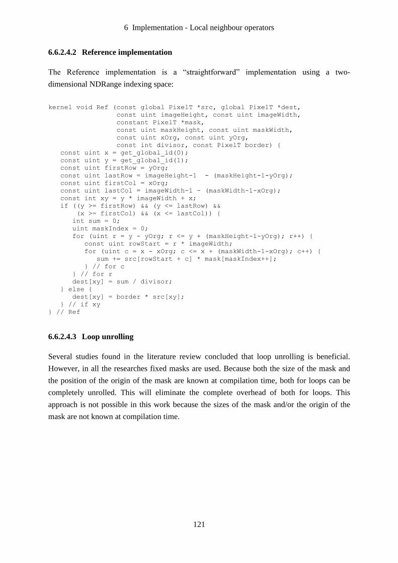
6 Implementation - Local neighbour operators
121
6.6.2.4.2 Reference implementation
The Reference implementation is a “straightforward” implementation using a two-
dimensional NDRange indexing space:
kernel void Ref (const global PixelT *src, global PixelT *dest,
const uint imageHeight, const uint imageWidth,
constant PixelT *mask,
const uint maskHeight, const uint maskWidth,
const uint xOrg, const uint yOrg,
const int divisor, const PixelT border) {
const uint x = get_global_id(0);
const uint y = get_global_id(1);
const uint firstRow = yOrg;
const uint lastRow = imageHeight-1 - (maskHeight-1-yOrg);
const uint firstCol = xOrg;
const uint lastCol = imageWidth-1 - (maskWidth-1-xOrg);
const int xy = y * imageWidth + x;
if ((y >= firstRow) && (y <= lastRow) &&
(x >= firstCol) && (x <= lastCol)) {
int sum = 0;
uint maskIndex = 0;
for (uint r = y - yOrg; r <= y + (maskHeight-1-yOrg); r++) {
const uint rowStart = r * imageWidth;
for (uint c = x - xOrg; c <= x + (maskWidth-1-xOrg); c++) {
sum += src[rowStart + c] * mask[maskIndex++];
} // for c
} // for r
dest[xy] = sum / divisor;
} else {
dest[xy] = border * src[xy];
} // if xy
} // Ref
6.6.2.4.3 Loop unrolling
Several studies found in the literature review concluded that loop unrolling is beneficial.
However, in all the researches fixed masks are used. Because both the size of the mask and
the position of the origin of the mask are known at compilation time, both for loops can be
completely unrolled. This will eliminate the complete overhead of both for loops. This
approach is not possible in this work because the sizes of the mask and/or the origin of the
mask are not known at compilation time.
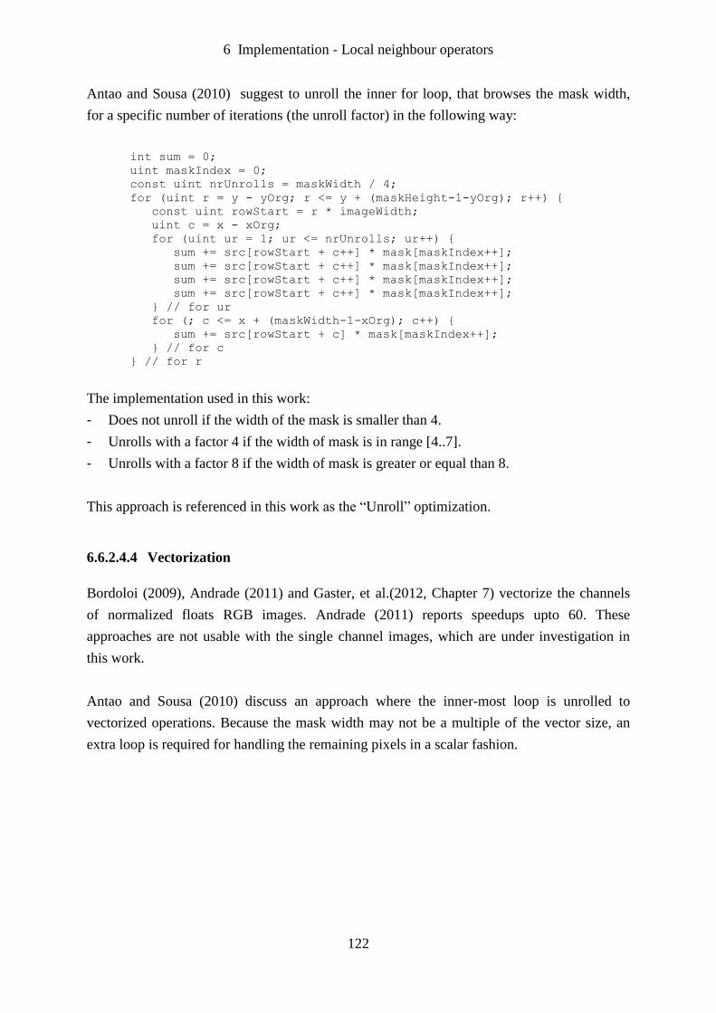
6 Implementation - Local neighbour operators
122
Antao and Sousa (2010) suggest to unroll the inner for loop, that browses the mask width,
for a specific number of iterations (the unroll factor) in the following way:
int sum = 0;
uint maskIndex = 0;
const uint nrUnrolls = maskWidth / 4;
for (uint r = y - yOrg; r <= y + (maskHeight-1-yOrg); r++) {
const uint rowStart = r * imageWidth;
uint c = x - xOrg;
for (uint ur = 1; ur <= nrUnrolls; ur++) {
sum += src[rowStart + c++] * mask[maskIndex++];
sum += src[rowStart + c++] * mask[maskIndex++];
sum += src[rowStart + c++] * mask[maskIndex++];
sum += src[rowStart + c++] * mask[maskIndex++];
} // for ur
for (; c <= x + (maskWidth-1-xOrg); c++) {
sum += src[rowStart + c] * mask[maskIndex++];
} // for c
} // for r
The implementation used in this work:
- Does not unroll if the width of the mask is smaller than 4.
- Unrolls with a factor 4 if the width of mask is in range [4..7].
- Unrolls with a factor 8 if the width of mask is greater or equal than 8.
This approach is referenced in this work as the “Unroll” optimization.
6.6.2.4.4 Vectorization
Bordoloi (2009), Andrade (2011) and Gaster, et al.(2012, Chapter 7) vectorize the channels
of normalized floats RGB images. Andrade (2011) reports speedups upto 60. These
approaches are not usable with the single channel images, which are under investigation in
this work.
Antao and Sousa (2010) discuss an approach where the inner-most loop is unrolled to
vectorized operations. Because the mask width may not be a multiple of the vector size, an
extra loop is required for handling the remaining pixels in a scalar fashion.

6 Implementation - Local neighbour operators
123
This idea was used and implemented in the following way:
const uint vectorSize = vec_step(short4);
const uint nrVectors = maskWidth / vectorSize;
uint maskIndex = 0;
int sum = 0;
short4 sumv = 0;
for (uint r = y - yOrg; r <= y + (maskHeight-1-yOrg); r++) {
const uint rowStart = r * imageWidth;
uint c = x - xOrg;
for (uint v = 1; v <= nrVectors; v++) {
short4 iv = vload4(0, src + (rowStart + c));
short4 mv = vload4(0, mask + maskIndex);
sumv += iv * mv;
c += vectorSize;
maskIndex += vectorSize;
} // for v
for (; c <= x + (maskWidth-1-xOrg); c++) {
sum += src[rowStart + c] * mask[maskIndex++];
} // for c
} // for r
sum += sumv.s0 + sumv.s1 + sumv.s2 + sumv.s3;
This approach is implemented for short4, short8 and short16 vectors and is referenced in this
work as the “UnrollV” optimization.
The last For loop in the “UnrollV” (Antao and Sousa, 2010) approach can be eliminated if the
width of the mask is enlarged to the next multiple of 4, 8 or 16 and the origin of the mask
remains in the same position. The result of the convolution will remain unchanged if the
“extra” mask values are set to zero. Typically the image will be much larger than the mask,
so if the origin of the mask is not at the bottom row, it will be impossible to use pixels outside
the image in the calculation. This approach was implemented for short4, short8 and short16
vectors and is referenced in this work as the “UnrollV2” optimization. This proposed
approach appears to be novel. The literature search has not found any previous use of this
approach.
The UnrollV2 optimization is not using the vector capabilities in an optimal way, because the
extra zeros in the last vector for each row calculation are dummies. Antao and Sousa (2010)
and Antao, Sousa and Chaves (2011) introduce approaches that do not have this
disadvantage. According to their tests these approaches are beneficial on CPUs. These
approaches require to use a auxiliary image, in which the order of the pixels is extensively
rearranged. Future work will have to investigate whether these approaches are beneficial on
GPUs.
6 Implementation - Local neighbour operators
124
6.6.2.4.5 Local memory
Bordoloi (2009), Andrade (2011) and Gaster, et al. (2012, Chapter 7) suggest using local
memory for tiles with pixels. The idea is that at start-up, all work-items in a work-group copy
all image pixels, necessary to calculate the convolution output pixels for the work-group,
from global memory to local memory. After this copy operation the convolution is calculated
with the relatively faster local memory. Because there is overlap between image pixels used
for the calculation of adjacent output pixels, it is expected that the calculation of convolutions
can be accelerated.
The Convolution kernel is now implemented in two steps:
- Copy work-item’s part of tile from global to local memory.
- Calculate Convolution result for output pixel using image pixels stored in local memory
tile.
The two steps must be separated by a barrier function to ensure that the tile has been copied
completely before work-items start with the calculation of the Convolution result.
This tile copying from global to local memory was implemented in two fashions:
- Copying pixel by pixel; This approach is referenced in this work as the “Local”
optimization.
- Copying with vector of pixels; This approach is referenced in this work as the “Local
Vector Read” optimization, abbreviated to “LVR”.
The size the source code is substantial and the source code is not included in this work. The
source code is documented in Van de Loosdrecht (2013a).
6.6.2.4.6 Chunking
With Chunking a kernel will process more than one pixel at a time, so the overhead of
starting up the kernel is distributed over more than one pixel. Chunking can be done in a non-
coalesced and in a coalesced way. These techniques are described in sections 6.5.2.4.5 and
6.5.2.4.6. The non-coalesced approach is referenced in this work as the “Chunk” optimization
and the coalesced approach as the “ChunkStride” optimization. The source code is
documented in Van de Loosdrecht (2013a).
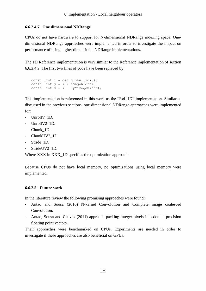
6 Implementation - Local neighbour operators
125
6.6.2.4.7 One dimensional NDRange
CPUs do not have hardware to support for N-dimensional NDRange indexing space. One-
dimensional NDRange approaches were implemented in order to investigate the impact on
performance of using higher dimensional NDRange implementations.
The 1D Reference implementation is very similar to the Reference implementation of section
6.6.2.4.2. The first two lines of code have been replaced by:
const uint i = get_global_id(0);
const uint y = i / imageWidth;
const uint x = i - (y*imageWidth);
This implementation is referenced in this work as the “Ref_1D” implementation. Similar as
discussed in the previous sections, one-dimensional NDRange approaches were implemented
for:
- UnrollV_1D.
- UnrollV2_1D.
- Chunk_1D.
- ChunkUV2_1D.
- Stride_1D.
- StrideUV2_1D.
Where XXX in XXX_1D specifies the optimization approach.
Because CPUs do not have local memory, no optimizations using local memory were
implemented.
6.6.2.5 Future work
In the literature review the following promising approaches were found:
- Antao and Sousa (2010) N-kernel Convolution and Complete image coalesced
Convolution.
- Antao, Sousa and Chaves (2011) approach packing integer pixels into double precision
floating point vectors.
Their approaches were benchmarked on CPUs. Experiments are needed in order to
investigate if these approaches are also beneficial on GPUs.
6 Implementation - Global operators
126
6.7 Global operators
6.7.1 Introduction
As representative of the Global operators Histogram, was implemented.
6.7.2 Histogram
6.7.2.1 Introduction
The functionality of the Histogram operator is described in section 3.6.5.
In this section the implementation of the Histogram operator is described for the following
versions:
- Sequential.
- OpenMP.
- OpenCL.
Because there is only a small amount of code involved, the source code of the kernels is
presented. Note that for clarity all code needed for error checking is omitted.
6.7.2.2 Sequential
As mentioned in section 2.1, VisionLab supports a wide variety of image types. The
Histogram operator must work with all greyscale image types. The generic implementation of
the Histogram operator in VisionLab will work without a predefined range for the pixels and
also supports negative pixel values; before calculating the histogram, the minimum and
maximum pixel value in the image will be calculated. In many cases this is an overkill
because the minimum pixel value is zero and the maximum pixel value is known. For these
cases VisionLab has the faster Histogram0 operator. Implementation of the Histogram0
operator is straightforward.

6 Implementation - Global operators
127
template <class IntImageT>
void Histogram0 (const IntImageT &image, const int hisSize, int *his) {
typedef typename IntImageT::PixelType PixelT;
memset(his, 0, hisSize * sizeof(int));
PixelT *pixelTab = image.GetFirstPixelPtr();
const int nrPixels = image.GetNrPixels();
for (int i = 0; i < nrPixels; i++) {
his[pixelTab[i]]++;
} // for i
} // Histogram0
6.7.2.3 OpenMP
The OpenMP implementation is not complicated. The image is split up into N sub-images.
For each sub-image the local sub-histogram is calculated in parallel. Thereafter the local sub-
histograms are totalled in a critical section. Because the time required for calculating each
chunk is constant, the static scheduling strategy (see section 5.2.4) was chosen.
In order to facilitate the Automatic Operator Parallelization (section 5.2.6.4)
“if (calibMCP.TestMultiCore(OC_CalcHistogram0,nrPixels))” was added.
template <class IntImageT>
void Histogram0 (const IntImageT &image, const int hisSize, int *his) {
typedef typename IntImageT::PixelType PixelT;
memset(his, 0, hisSize * sizeof(int));
PixelT *pixelTab = image.GetFirstPixelPtr();
const int nrPixels = image.GetNrPixels();
#pragma omp parallel if (calibMCP.TestMultiCore(OC_CalcHistogram,nrPixels))
{
int *localHis = new int[hisSize];
memset(localHis, 0, hisSize * sizeof(int));
#pragma omp for nowait
for (int i = 0; i < nrPixels; i++) {
localHis[pixelTab[i]]++;
} // for i
#pragma omp critical (CalcHistogram0)
{
for (int h = 0; h < hisSize; h++) {
his[h] += localHis[h];
} // for h
} // omp critical
delete [] localHis;
} // omp parallel
} // Histogram0
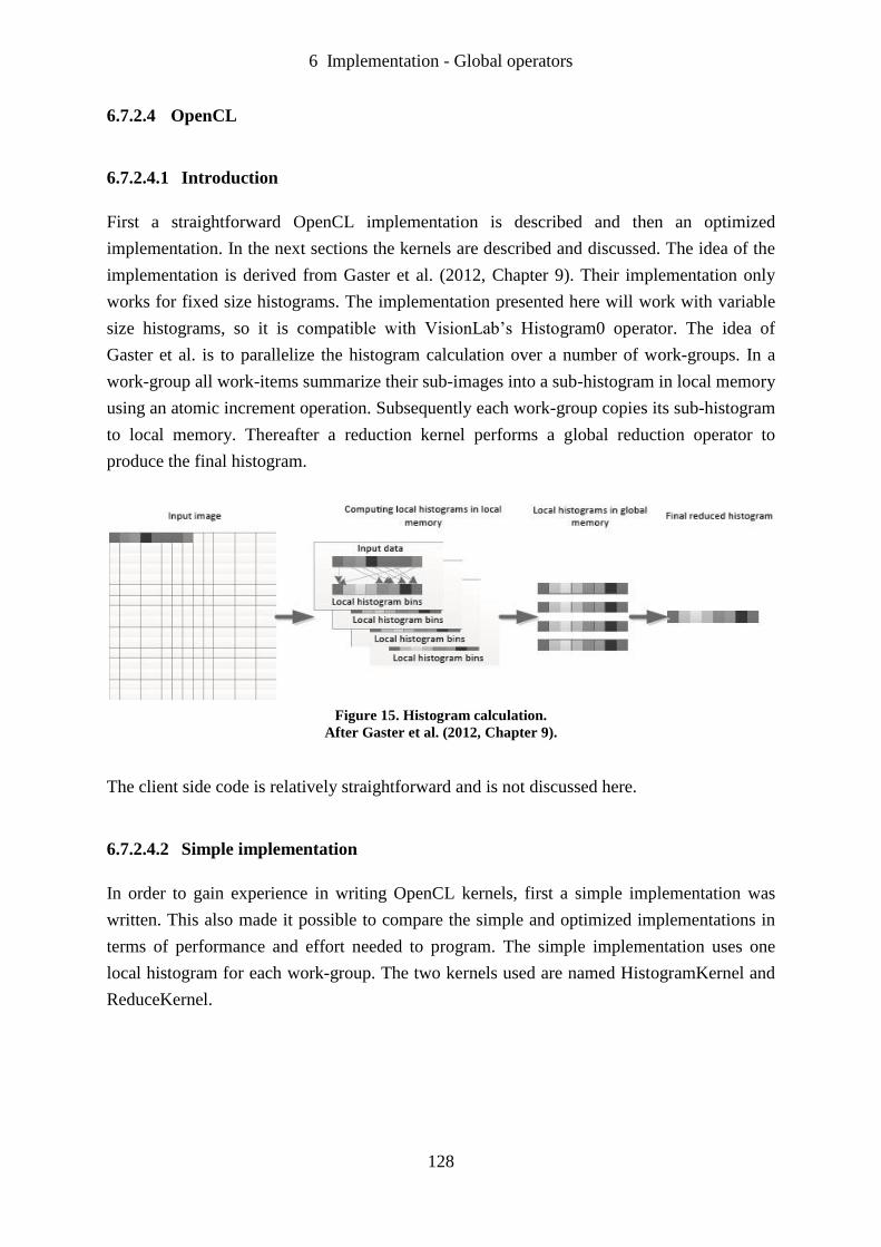
6 Implementation - Global operators
128
6.7.2.4 OpenCL
6.7.2.4.1 Introduction
First a straightforward OpenCL implementation is described and then an optimized
implementation. In the next sections the kernels are described and discussed. The idea of the
implementation is derived from Gaster et al. (2012, Chapter 9). Their implementation only
works for fixed size histograms. The implementation presented here will work with variable
size histograms, so it is compatible with VisionLab’s Histogram0 operator. The idea of
Gaster et al. is to parallelize the histogram calculation over a number of work-groups. In a
work-group all work-items summarize their sub-images into a sub-histogram in local memory
using an atomic increment operation. Subsequently each work-group copies its sub-histogram
to local memory. Thereafter a reduction kernel performs a global reduction operator to
produce the final histogram.
Figure 15. Histogram calculation.
After Gaster et al. (2012, Chapter 9).
The client side code is relatively straightforward and is not discussed here.
6.7.2.4.2 Simple implementation
In order to gain experience in writing OpenCL kernels, first a simple implementation was
written. This also made it possible to compare the simple and optimized implementations in
terms of performance and effort needed to program. The simple implementation uses one
local histogram for each work-group. The two kernels used are named HistogramKernel and
ReduceKernel.
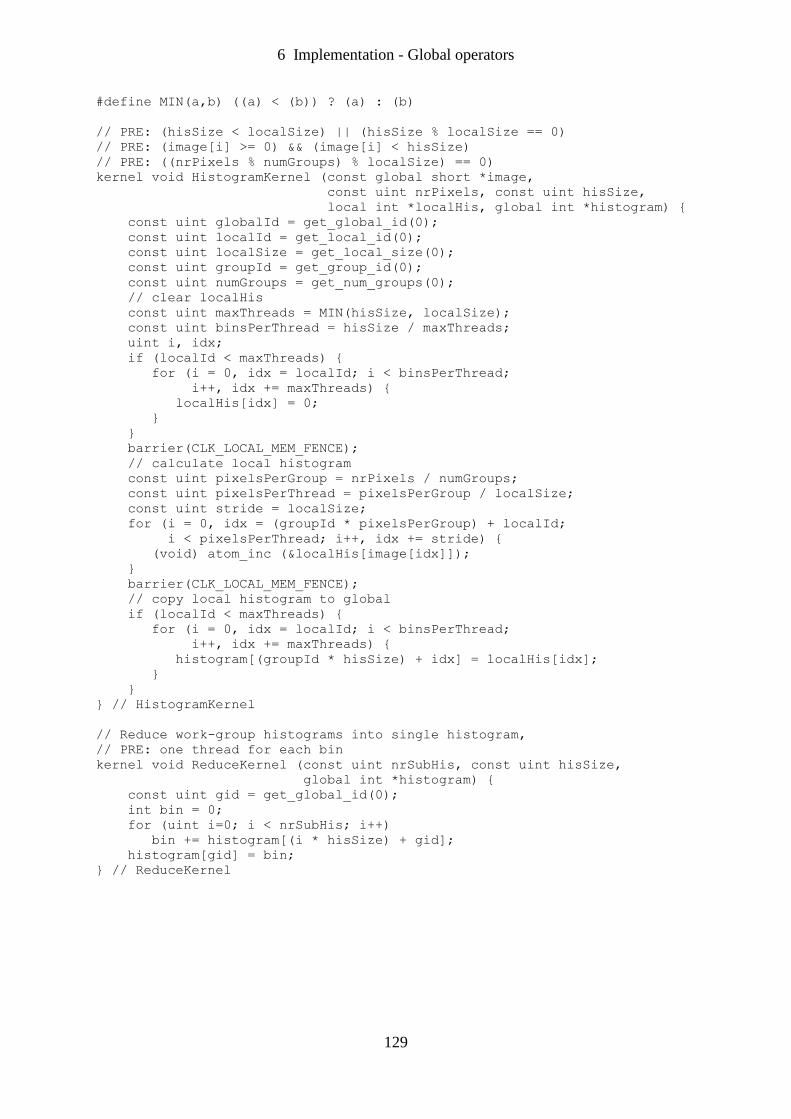
6 Implementation - Global operators
129
#define MIN(a,b) ((a) < (b)) ? (a) : (b)
// PRE: (hisSize < localSize) || (hisSize % localSize == 0)
// PRE: (image[i] >= 0) && (image[i] < hisSize)
// PRE: ((nrPixels % numGroups) % localSize) == 0)
kernel void HistogramKernel (const global short *image,
const uint nrPixels, const uint hisSize,
local int *localHis, global int *histogram) {
const uint globalId = get_global_id(0);
const uint localId = get_local_id(0);
const uint localSize = get_local_size(0);
const uint groupId = get_group_id(0);
const uint numGroups = get_num_groups(0);
// clear localHis
const uint maxThreads = MIN(hisSize, localSize);
const uint binsPerThread = hisSize / maxThreads;
uint i, idx;
if (localId < maxThreads) {
for (i = 0, idx = localId; i < binsPerThread;
i++, idx += maxThreads) {
localHis[idx] = 0;
}
}
barrier(CLK_LOCAL_MEM_FENCE);
// calculate local histogram
const uint pixelsPerGroup = nrPixels / numGroups;
const uint pixelsPerThread = pixelsPerGroup / localSize;
const uint stride = localSize;
for (i = 0, idx = (groupId * pixelsPerGroup) + localId;
i < pixelsPerThread; i++, idx += stride) {
(void) atom_inc (&localHis[image[idx]]);
}
barrier(CLK_LOCAL_MEM_FENCE);
// copy local histogram to global
if (localId < maxThreads) {
for (i = 0, idx = localId; i < binsPerThread;
i++, idx += maxThreads) {
histogram[(groupId * hisSize) + idx] = localHis[idx];
}
}
} // HistogramKernel
// Reduce work-group histograms into single histogram,
// PRE: one thread for each bin
kernel void ReduceKernel (const uint nrSubHis, const uint hisSize,
global int *histogram) {
const uint gid = get_global_id(0);
int bin = 0;
for (uint i=0; i < nrSubHis; i++)
bin += histogram[(i * hisSize) + gid];
histogram[gid] = bin;
} // ReduceKernel
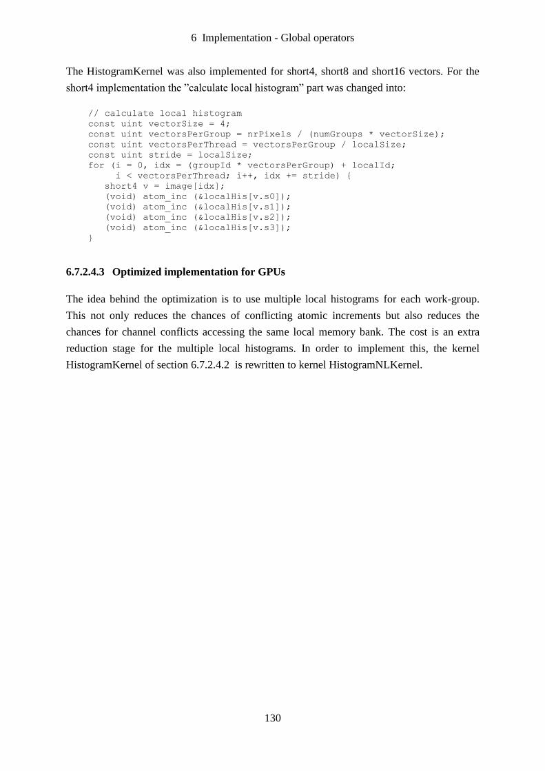
6 Implementation - Global operators
130
The HistogramKernel was also implemented for short4, short8 and short16 vectors. For the
short4 implementation the ”calculate local histogram” part was changed into:
// calculate local histogram
const uint vectorSize = 4;
const uint vectorsPerGroup = nrPixels / (numGroups * vectorSize);
const uint vectorsPerThread = vectorsPerGroup / localSize;
const uint stride = localSize;
for (i = 0, idx = (groupId * vectorsPerGroup) + localId;
i < vectorsPerThread; i++, idx += stride) {
short4 v = image[idx];
(void) atom_inc (&localHis[v.s0]);
(void) atom_inc (&localHis[v.s1]);
(void) atom_inc (&localHis[v.s2]);
(void) atom_inc (&localHis[v.s3]);
}
6.7.2.4.3 Optimized implementation for GPUs
The idea behind the optimization is to use multiple local histograms for each work-group.
This not only reduces the chances of conflicting atomic increments but also reduces the
chances for channel conflicts accessing the same local memory bank. The cost is an extra
reduction stage for the multiple local histograms. In order to implement this, the kernel
HistogramKernel of section 6.7.2.4.2 is rewritten to kernel HistogramNLKernel.
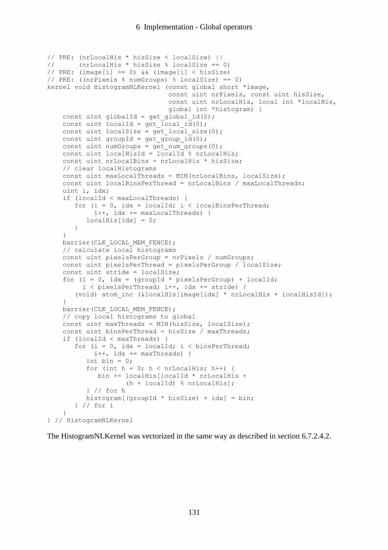
6 Implementation - Global operators
131
// PRE: (nrLocalHis * hisSize < localSize) ||
// (nrLocalHis * hisSize % localSize == 0)
// PRE: (image[i] >= 0) && (image[i] < hisSize)
// PRE: ((nrPixels % numGroups) % localSize) == 0)
kernel void HistogramNLKernel (const global short *image,
const uint nrPixels, const uint hisSize,
const uint nrLocalHis, local int *localHis,
global int *histogram) {
const uint globalId = get_global_id(0);
const uint localId = get_local_id(0);
const uint localSize = get_local_size(0);
const uint groupId = get_group_id(0);
const uint numGroups = get_num_groups(0);
const uint localHisId = localId % nrLocalHis;
const uint nrLocalBins = nrLocalHis * hisSize;
// clear localHistograms
const uint maxLocalThreads = MIN(nrLocalBins, localSize);
const uint localBinsPerThread = nrLocalBins / maxLocalThreads;
uint i, idx;
if (localId < maxLocalThreads) {
for (i = 0, idx = localId; i < localBinsPerThread;
i++, idx += maxLocalThreads) {
localHis[idx] = 0;
}
}
barrier(CLK_LOCAL_MEM_FENCE);
// calculate local histograms
const uint pixelsPerGroup = nrPixels / numGroups;
const uint pixelsPerThread = pixelsPerGroup / localSize;
const uint stride = localSize;
for (i = 0, idx = (groupId * pixelsPerGroup) + localId;
i < pixelsPerThread; i++, idx += stride) {
(void) atom_inc (&localHis[image[idx] * nrLocalHis + localHisId]);
}
barrier(CLK_LOCAL_MEM_FENCE);
// copy local histograms to global
const uint maxThreads = MIN(hisSize, localSize);
const uint binsPerThread = hisSize / maxThreads;
if (localId < maxThreads) {
for (i = 0, idx = localId; i < binsPerThread;
i++, idx += maxThreads) {
int bin = 0;
for (int h = 0; h < nrLocalHis; h++) {
bin += localHis[localId * nrLocalHis +
(h + localId) % nrLocalHis];
} // for h
histogram[(groupId * hisSize) + idx] = bin;
} // for i
}
} // HistogramNLKernel
The HistogramNLKernel was vectorized in the same way as described in section 6.7.2.4.2.
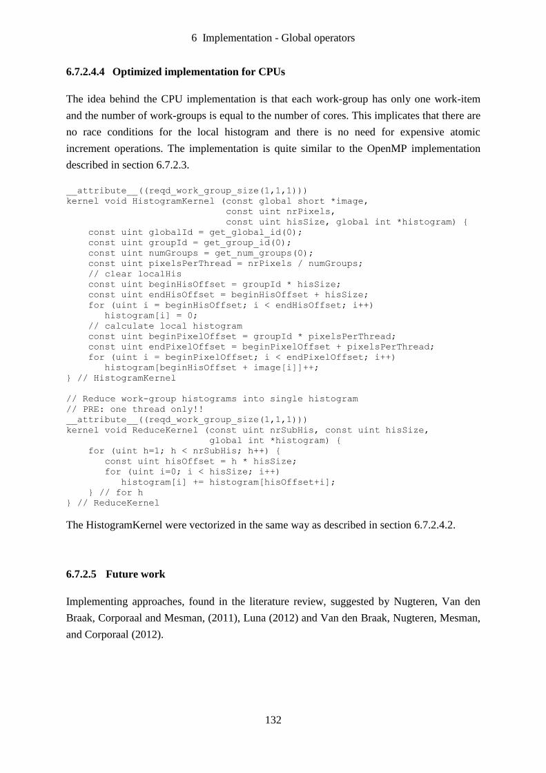
6 Implementation - Global operators
132
6.7.2.4.4 Optimized implementation for CPUs
The idea behind the CPU implementation is that each work-group has only one work-item
and the number of work-groups is equal to the number of cores. This implicates that there are
no race conditions for the local histogram and there is no need for expensive atomic
increment operations. The implementation is quite similar to the OpenMP implementation
described in section 6.7.2.3.
__attribute__((reqd_work_group_size(1,1,1)))
kernel void HistogramKernel (const global short *image,
const uint nrPixels,
const uint hisSize, global int *histogram) {
const uint globalId = get_global_id(0);
const uint groupId = get_group_id(0);
const uint numGroups = get_num_groups(0);
const uint pixelsPerThread = nrPixels / numGroups;
// clear localHis
const uint beginHisOffset = groupId * hisSize;
const uint endHisOffset = beginHisOffset + hisSize;
for (uint i = beginHisOffset; i < endHisOffset; i++)
histogram[i] = 0;
// calculate local histogram
const uint beginPixelOffset = groupId * pixelsPerThread;
const uint endPixelOffset = beginPixelOffset + pixelsPerThread;
for (uint i = beginPixelOffset; i < endPixelOffset; i++)
histogram[beginHisOffset + image[i]]++;
} // HistogramKernel
// Reduce work-group histograms into single histogram
// PRE: one thread only!!
__attribute__((reqd_work_group_size(1,1,1)))
kernel void ReduceKernel (const uint nrSubHis, const uint hisSize,
global int *histogram) {
for (uint h=1; h < nrSubHis; h++) {
const uint hisOffset = h * hisSize;
for (uint i=0; i < hisSize; i++)
histogram[i] += histogram[hisOffset+i];
} // for h
} // ReduceKernel
The HistogramKernel were vectorized in the same way as described in section 6.7.2.4.2.
6.7.2.5 Future work
Implementing approaches, found in the literature review, suggested by Nugteren, Van den
Braak, Corporaal and Mesman, (2011), Luna (2012) and Van den Braak, Nugteren, Mesman,
and Corporaal (2012).
6 Implementation - Connectivity based operators
133
6.8 Connectivity based operators
6.8.1 Introduction
As representative of the Connectivity based operators Connected Component Labelling was
implemented.
6.8.2 LabelBlobs
6.8.2.1 Introduction
The functionality of the Connected Component Labelling operator is described in section
3.6.6. This operator is called in VisionLab ‘LabelBlobs’.
In this section the implementation of the LabelBlobs operator is described for the following
versions:
- Sequential.
- OpenMP.
- OpenCL.
The size of the source code is substantial and the source code is not included in this work.
The source code is documented in Van de Loosdrecht (2012c and 2013d).
6.8.2.2 Sequential
The sequential implementation is based on a Two passes approach as described in section
3.6.6.2. In many applications the LabelBlob operator is followed by the BlobAnalyse
operator or a derivative of this operator. BlobAnalyse performs all kinds of measurements for
each blob. The result of the BlobAnalyse is a table, with for each blob a record containing all
measurements for that blob. The index in the table is the label number. In order to keep the
memory usage of the table as small as possible it is imperative that the LabelBlobs operator
label the blobs with successive label numbers. This means that after resolving equivalence
provisional labels, the table with the resolved provisional labels must be renumbered with
successive label numbers starting at label number 1. After this renumbering the second pass
can assign the successive label numbers to the pixels of the blobs.
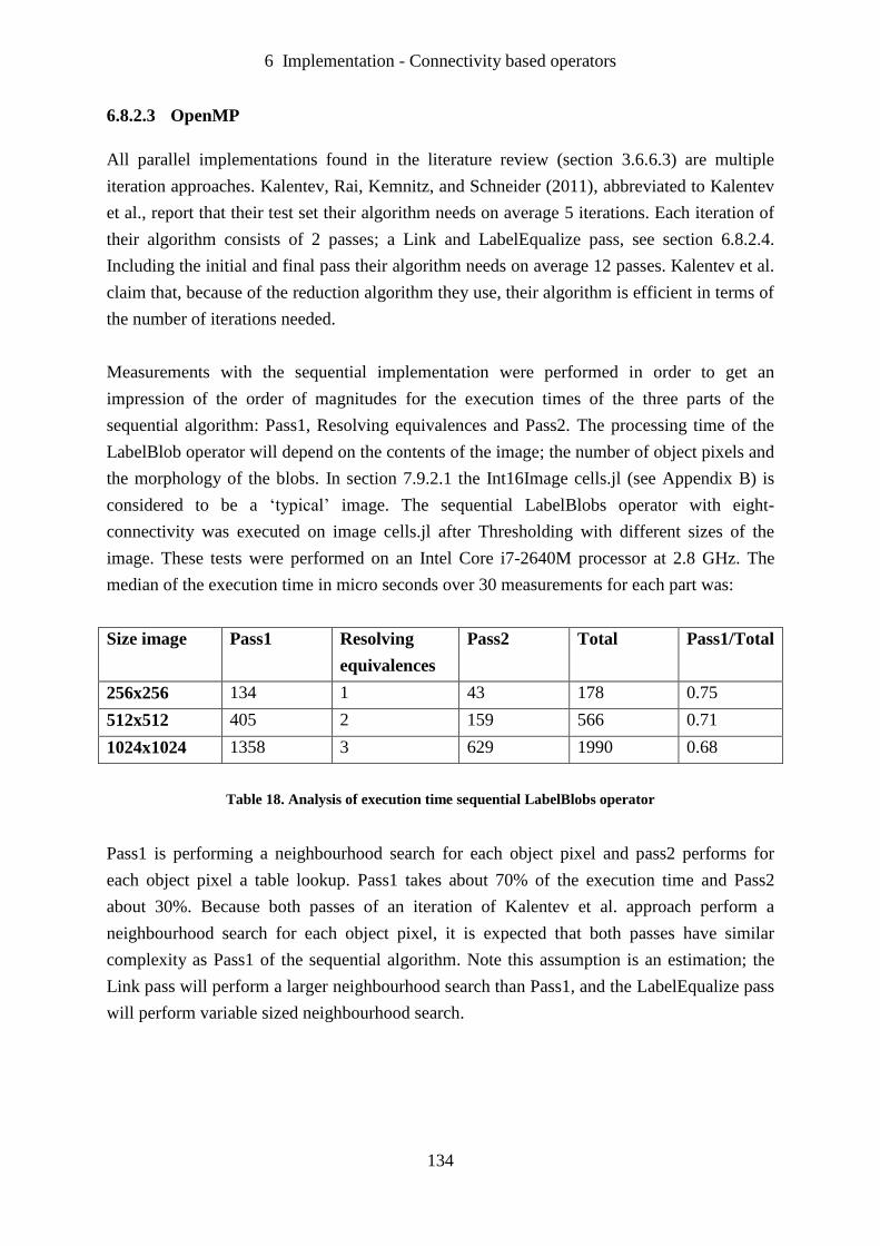
6 Implementation - Connectivity based operators
134
6.8.2.3 OpenMP
All parallel implementations found in the literature review (section 3.6.6.3) are multiple
iteration approaches. Kalentev, Rai, Kemnitz, and Schneider (2011), abbreviated to Kalentev
et al., report that their test set their algorithm needs on average 5 iterations. Each iteration of
their algorithm consists of 2 passes; a Link and LabelEqualize pass, see section 6.8.2.4.
Including the initial and final pass their algorithm needs on average 12 passes. Kalentev et al.
claim that, because of the reduction algorithm they use, their algorithm is efficient in terms of
the number of iterations needed.
Measurements with the sequential implementation were performed in order to get an
impression of the order of magnitudes for the execution times of the three parts of the
sequential algorithm: Pass1, Resolving equivalences and Pass2. The processing time of the
LabelBlob operator will depend on the contents of the image; the number of object pixels and
the morphology of the blobs. In section 7.9.2.1 the Int16Image cells.jl (see Appendix B) is
considered to be a ‘typical’ image. The sequential LabelBlobs operator with eight-
connectivity was executed on image cells.jl after Thresholding with different sizes of the
image. These tests were performed on an Intel Core i7-2640M processor at 2.8 GHz. The
median of the execution time in micro seconds over 30 measurements for each part was:
Size image Pass1 Resolving
equivalences
Pass2 Total Pass1/Total
256x256 134 1 43 178 0.75
512x512 405 2 159 566 0.71
1024x1024 1358 3 629 1990 0.68
Table 18. Analysis of execution time sequential LabelBlobs operator
Pass1 is performing a neighbourhood search for each object pixel and pass2 performs for
each object pixel a table lookup. Pass1 takes about 70% of the execution time and Pass2
about 30%. Because both passes of an iteration of Kalentev et al. approach perform a
neighbourhood search for each object pixel, it is expected that both passes have similar
complexity as Pass1 of the sequential algorithm. Note this assumption is an estimation; the
Link pass will perform a larger neighbourhood search than Pass1, and the LabelEqualize pass
will perform variable sized neighbourhood search.

6 Implementation - Connectivity based operators
135
On average Kalentev et al. approach needs 5 iterations. In total: one simple initial pass, 10
neighbourhood search passes and one simple final pass. It is expected that the initial and final
pass will have similar complexity as Pass2. As will be explained in section 6.8.2.4 Kalentev
et al. approach needs a post processing step with two passes, which are expected to have a
similar complexity as Pass2. The execution time will be dominated by the 10 neighbourhood
search passes.
If the sequential version takes 1 unit of execution time for an image, it is estimated that,
Kalentev et al. will take more than 7.9 units of (sequential) execution time. In order to get a
speedup bigger than 1, it is to be expected that more than 8 cores will be required.
According to the author the proposed parallel algorithms in literature only work for “many-
core” systems and not for “few-core” systems like contemporary CPUs who have typical 2 to
8 cores. The substantial speedup claimed by Niknam, Thulasiraman, Camorlinga (2010) with
their OpenMP implementation was obtained by comparing a sequential multi-pass algorithm
with a parallel multi-pass algorithm. In this work the much faster 2 pass sequential algorithm
is compared with parallel multi-pass algorithms.
So, another approach is necessary for “few-core” systems. The proposed approach is to split
the image into sub-images. This approach is inspired by the work of Park, Looney and Chen
(2000) to limit the amount of memory used for the equivalences table in sequential
implementations. For each sub-image a label equivalences table is calculated in the same
manner as in Pass1 of the sequential algorithm. All used label equivalence numbers must be
unique for the whole image. Thereafter the label equivalences tables are repaired for the
blobs that cross the boundaries of the sub-images. Note that one blob can be in more than two
sub-images. Next, the label equivalences tables are merged into one label equivalences table
and renumbered with successive label numbers. Finally, a last pass is required to assign the
successive label numbers to the pixels of the blobs. This proposed approach appears to be
novel. The literature search has not found any previous use of this approach.
The computational expensive part is the calculation of the label equivalences tables, this
involves a neighbourhood search of the sub-images. Because there are no data dependencies
this part is embarrassingly easy to parallelize. Each sub-image can be processed by a separate
core. The repairing and merging of the label equivalences tables followed by the renumbering
is not computationally expensive because only a small amount of data is to be processed. In
the current implementation this is done sequentially, but an iterative parallel approach is
possible too. The last pass, similar to Pass2 of the sequential algorithm, for assigning the
label numbers to the pixels is implemented with a shared read-only lookup table and is
embarrassingly easy to parallelize.
6 Implementation - Connectivity based operators
136
The number of pixels on the boundaries of the sub-images will increase with the number of
sub-images. This approach will probably not work efficiently on “many-core” systems
because the time needed for repairing label equivalences tables will increase with the number
of sub-images.
6.8.2.4 OpenCL
For the OpenCL implementation a “many-core” system approach on GPUs was chosen. A
“few-core” approach for CPUs is of course also possible, this will be future work. The
implementation of the OpenCL “many-core” implementation is based on the Label
Equivalence approach of Kalentev et al. as described in section 3.6.6.3. Their approach has
the following implications:
- The algorithm cannot handle object pixels at the borders of the image.
- Provisional labels are stored in the image. Because of possible overflow in pixel values,
the Int32Image type must be used.
- The labelling of the blobs is not successive. This is the case for all parallel algorithms
found in the literature research. As explained in section 6.8.2.2 this is mandatory for other
VisionLab operators.
Kalentev et al. suggest the following framework for the host code:
int notDone = 1;
WriteBuffer(image);
RunKernel("InitLabels",image);
while (notDone == 1) {
notDone = 0;
WriteBuffer(notDone);
RunKernel(“Link”,image,notDone)
RunKernel(“LabelEqualize”,image)
ReadBuffer(notDone);
} // while notDone
ReadBuffer(image);
In Kalentev et al. the kernels Link and LabelEqualize are originally named Scanning and
Analysis. The Kalentev et al. approach was extended in the following ways (Van de
Loosdrecht, 2013d):
- The InitLabel kernel is extended to set the border pixels of the image to the background
value.
- Link kernels are implemented for both four and eight connectivity.
- A post processing step with two passes is added in order to make the labelling of the
blobs successive.
6 Implementation - Automatic Operator Parallelization
137
Kalentev et al. approach was optimized in the following ways (Van de Loosdrecht, 2013d):
- Each iteration has a Link pass and a LabelEqualize pass. For the last iteration the
LabelEqualize pass is redundant.
- Many of the kernel execute, read buffer and write buffer commands can be
asynchronously started and synchronized using events. This eliminates a lot of host-side
overhead of unnecessary waiting for operations to finish.
- The write to the “IsNotDone” buffer can be done in parallel to the LabelEqualize pass.
- With the exception of the second pass of the post processing step, all kernels are
vectorized. Vectorization of the InitLabel kernel is straightforward, independent of the
contents of the image and is expected to be beneficial. Vectorization of the other kernels
is not straightforward. The only way found to vectorize was to add a quick test if all
pixels in the vector are background pixels. The advantage of vectorization of the other
kernels is that a whole cache line with pixels can be read with one global memory access.
This indicates that processing background pixels could benefit from vectorization and
processing object pixels could suffer from a little extra overhead because of extra
instructions needed to access a pixel in the vector.
6.8.2.5 Future work
Implementing the few-core approach for CPUs in OpenCL and the approach found in the
literature review suggested by Stava and Benes (2011).
6.9 Automatic Operator Parallelization
In section 5.2.6 the design of the Automatic Operator Parallelization is described. In order to
predict at run-time whether parallelization is beneficial a calibration procedure is needed.
OpenMP was considered (see section 8.4) to be the best candidate to parallelize VisionLab in
an efficient and effective way. The Automatic Operator Parallelization was implemented for
the OpenMP parallelized operators.
In order to calibrate a simple OpenMP parallelized operator like Threshold a “standard”
image is resized to a range of different sizes and the median of execution time for each size is
calculated for sequential and parallel execution. This timing information is used to determine
the break-even point in number of pixels where the parallel execution of the operator is gain-
factor times faster than the sequential version. For more complex operators the decision for
the break-even point is based on a combination of image size and other parameters of the
operator. As an example: for Convolution operator the size of the mask is taken into account.

6 Implementation - Automatic Operator Parallelization
138
A framework based on the Command Pattern (Gamma et al., 1995) was implemented in order
to limit the amount of programming work needed to add a new OpenMP parallelized operator
to the Automatic Operator Parallelization calibration. The calibration procedure also tests for
equality of the sequential and parallel result. Below an example of the implementation of the
class for calibration framework for the Threshold operator is shown.
class ThresholdCmd : public MCPCommand { public: ThresholdCmd (const string &name) : MCPCommand(name) {} bool Init (const int size) { org.Resize(HeightWidth(size,size)); RampPattern(org,32,32,120); return true; } void ZoomXY (const double xy) { Zoom (org,zoom,xy,xy,NearestPixelInterpolation); } void Copy () { dest = zoom; } void Oper () { Threshold(dest,Int16Pixel(0),Int16Pixel(128)); } void Store () { store = dest; } void Test () { if (store != dest) throw (Error (name, "MCP result != single core")); } int NrPixels () { return zoom.GetNrPixels(); } void Finit () { org.Clear(); store.Clear(); zoom.Clear(); dest.Clear(); } private: Int16Image org, store, zoom, dest; };
Besides this class, two lines of code are necessary to add the class to the calibration
procedure.
7 Testing and Evaluation - Introduction
139
7 Testing and Evaluation
7.1 Introduction
In this chapter the testing and evaluation of the following topics are described:
- Calibration of timer overhead.
- Reproducibility of experiments.
- Sequential versus OpenMP single core.
- Data transfer between host and device.
- Computer Vision algorithms used for benchmarking.
- Automatic Operator Parallelization.
- Performance portability.
- Parallelization in real projects.
As mentioned in section 5.2.6.3 the image type that is most often used for greyscale operators
is the Int16Image. Int16Image was used as the default image type of the benchmark images.
The benchmark set was restricted to square images. The following values for the width and
the height of the benchmark images are chosen: 32, 64, 128, 256, 512, 1024, 2048, 4096 and
8192. In the graphs and tables a value of 64 for the parameter HeightWidth means that the
benchmark image has a height and a width of 64; 64×64 = 4096 pixels.
The results are summarized in speedup graphs where the size of the image is plotted against
the speedup obtained. The reference is the execution of the sequential version; a speedup of
1. Note that the lines between the dots in the speedup graphs are only to improve the
visibility, they do not represent measurements. The first OpenMP benchmarks with a repeat
count of 30 showed a lot of variance in execution time and the speedup graphs were not well
reproducible. The standard benchmark procedure described in section 5.4.3 required a
repetition count of at least 30 times. In order to get a better reproducibility, a repetition count
of 90 times was used for the OpenMP benchmarks. See also section 7.3.
The results of the speedup graphs are discussed for each parallel implementation. The
execution time tables with the median in micro seconds for each experiment performed can
be found in Appendix E. Other details of the results, like Violin plots and speedup tables, are
available in electronic form. See Appendix F for some samples.
7 Testing and Evaluation - Calibration of timer overhead
140
OpenCL uses wavefronts in order to hide memory latency (section 3.5.2.3.4). The number of
the wavefronts is determined by the work-group size (section 5.3.2.3). The work-group size
for a kernel is an important parameter in achieving a good performance. For each kernel
described in the next sections, the work-group size that resulted in the highest speedup was
experimentally found. The speedup graphs show the speedup for the optimal work-group size
for each kernel. Tables with optimal work-group size for each benchmark are available in
electronic form.
Many of the OpenCL kernels used will only work with images with restrictions on the size of
those images, like height and/or width, which must be a multiple of 4, 8 or 16. It is possible
to avoid this restriction at the expense of performance.
In many cases the scalar and vector variations of a OpenCL kernel were benchmarked. In the
scalar variation the processing is performed pixel by pixel. In the vector variation N pixels
are grouped to a vector and processed as one vector. In the case of an Int16Pixel the scalar
variation is denominated ‘Short’ and the vector variations ‘Short4’, ‘Short8’ and ‘Short16’.
The digit in ‘ShortX’ specifies the size of the vector. When appropriate for a benchmark these
names are used to distinguish between the scalar and vector variations of a kernel.
7.2 Calibration of timer overhead
VisionLab has been extended with a mechanism to calibrate the overhead of the timer. On the
computer (see Appendix A) used for benchmarking, the overhead for starting and stopping a
timer is less than the timer resolution of 0.30185 micro seconds.
7.3 Reproducibility of experiments
As can be seen in the violin plots in Appendix F, the experiments showed a lot of variance in
execution time. Most probably, the main reason for this is that Windows is a multi-tasking
operating system. The benchmark setup as described in section 5.5 tries to eliminate the
impact of the multi-tasking operating system on the benchmark results.
In order to get an impression of the reproducibility, one of the benchmarks described in
section 7.7.2 was repeated 10 times. The operator used for this experiment is the sequential
implementation of Convolution operator with a 3×3 mask. For each of the 10 runs the
benchmark was repeated 90 times. For this experiment the same benchmark environment was
used as for all other benchmarks. For each run the speedup was calculated in respect to run 1.
See Figure 16 for the results.
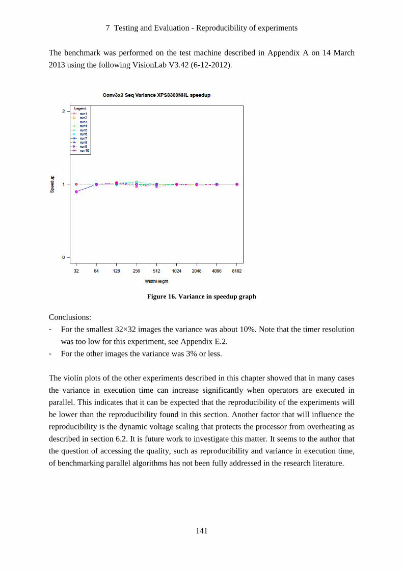
7 Testing and Evaluation - Reproducibility of experiments
141
The benchmark was performed on the test machine described in Appendix A on 14 March
2013 using the following VisionLab V3.42 (6-12-2012).
Figure 16. Variance in speedup graph
Conclusions:
- For the smallest 32×32 images the variance was about 10%. Note that the timer resolution
was too low for this experiment, see Appendix E.2.
- For the other images the variance was 3% or less.
The violin plots of the other experiments described in this chapter showed that in many cases
the variance in execution time can increase significantly when operators are executed in
parallel. This indicates that it can be expected that the reproducibility of the experiments will
be lower than the reproducibility found in this section. Another factor that will influence the
reproducibility is the dynamic voltage scaling that protects the processor from overheating as
described in section 6.2. It is future work to investigate this matter. It seems to the author that
the question of accessing the quality, such as reproducibility and variance in execution time,
of benchmarking parallel algorithms has not been fully addressed in the research literature.
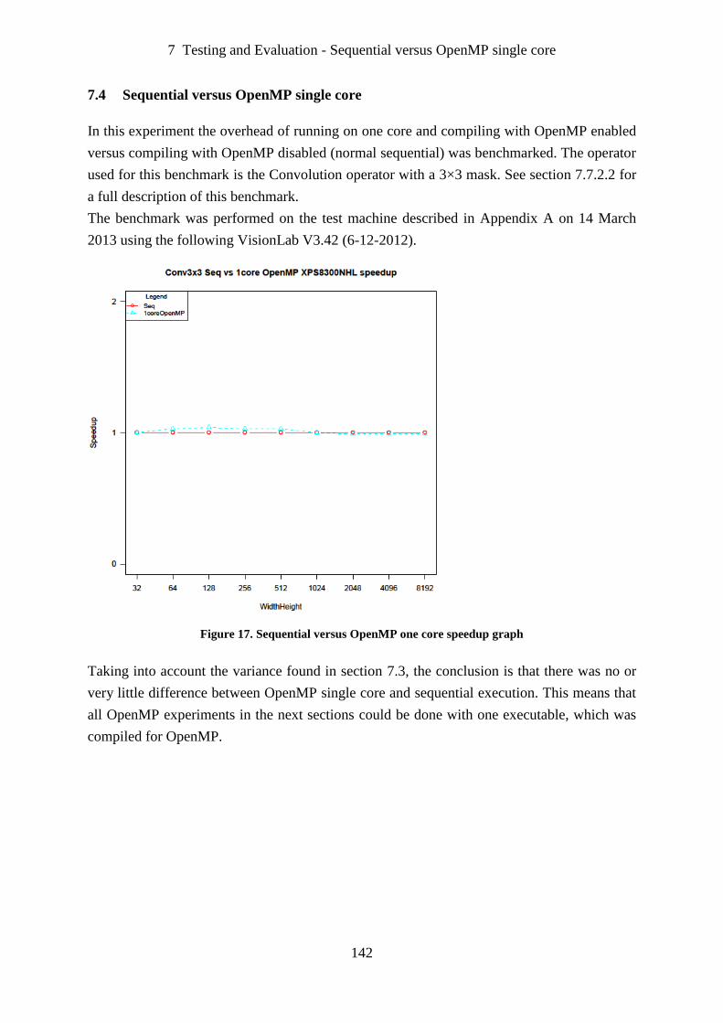
7 Testing and Evaluation - Sequential versus OpenMP single core
142
7.4 Sequential versus OpenMP single core
In this experiment the overhead of running on one core and compiling with OpenMP enabled
versus compiling with OpenMP disabled (normal sequential) was benchmarked. The operator
used for this benchmark is the Convolution operator with a 3×3 mask. See section 7.7.2.2 for
a full description of this benchmark.
The benchmark was performed on the test machine described in Appendix A on 14 March
2013 using the following VisionLab V3.42 (6-12-2012).
Figure 17. Sequential versus OpenMP one core speedup graph
Taking into account the variance found in section 7.3, the conclusion is that there was no or
very little difference between OpenMP single core and sequential execution. This means that
all OpenMP experiments in the next sections could be done with one executable, which was
compiled for OpenMP.

7 Testing and Evaluation - Data transfer between host and device
143
7.5 Data transfer between host and device
7.5.1 Introduction
An issue concerning the overall performance of a system using OpenCL is the overhead of
transferring data between host and device memory. According to section 3.5.2.3.7 using
pinned CPU memory instead of normal paged CPU memory is expected to reduce the data
transfer overhead.
According to Schubert (2012) the pinning of memory is about 3 times as expensive as
copying pinned memory. Schubert concludes that pinning of memory is only beneficial if the
memory is reused more than four times. This means that most real life applications have to
pin their buffers at start-up. In this case the overhead of pinning is only one time at start-up.
The overhead of pinning was not measured in this work.
This section describes the results of the time measure experiments for the:
- Data transfer from CPU to GPU.
- Data transfer from GPU to CPU.
- Data transfer on CPU from host to device.
- Data transfer on CPU from device to host.
All benchmarks were performed using the ‘standard’ OpenCL copy transfer method. Because
the wrapper around the host API interface does not yet support ‘zero copy transfer’, no
benchmarks could be performed using this option. All benchmarks were performed using
OpenCL buffers. The results in section 7.6 suggest that, in general, it is not benificial for
Computer Vision operators to use OpenCL images instead of OpenCL buffers. It is future
work to benchmark data transfer with ‘zero copy transfer’ and OpenCL images.
In the last sub-section the time for data transfers is compared with the time needed to execute
the Threshold operator, one of the most simple vision operators, on the GPU.
This benchmark was performed on the test machine described in Appendix A on 25
September 2012 using the following versions of the software:
- VisionLab V3.42 (19-8-2012).
- OpenCL 1.1 CUDA 4.2.1.
- OpenCL 1.1 AMD-APP-SDK-v2.5 (684.213) .
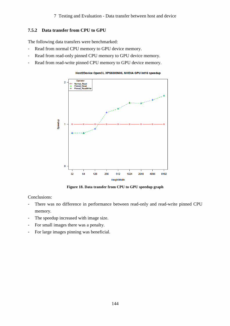
7 Testing and Evaluation - Data transfer between host and device
144
7.5.2 Data transfer from CPU to GPU
The following data transfers were benchmarked:
- Read from normal CPU memory to GPU device memory.
- Read from read-only pinned CPU memory to GPU device memory.
- Read from read-write pinned CPU memory to GPU device memory.
Figure 18. Data transfer from CPU to GPU speedup graph
Conclusions:
- There was no difference in performance between read-only and read-write pinned CPU
memory.
- The speedup increased with image size.
- For small images there was a penalty.
- For large images pinning was beneficial.

7 Testing and Evaluation - Data transfer between host and device
145
7.5.3 Data transfer from GPU to CPU
The following data transfers were benchmarked:
- Write from GPU device memory to normal CPU memory.
- Write from GPU device memory to write-only pinned CPU memory.
- Write from GPU device memory to read-write pinned CPU memory.
Figure 19. Data transfer from GPU to CPU speedup graph
Conclusions:
- The performance between write-only and read-write pinned CPU memory is similar.
- Pinning memory was always beneficial.
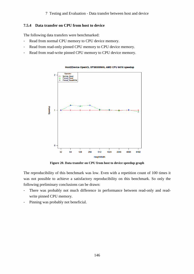
7 Testing and Evaluation - Data transfer between host and device
146
7.5.4 Data transfer on CPU from host to device
The following data transfers were benchmarked:
- Read from normal CPU memory to CPU device memory.
- Read from read-only pinned CPU memory to CPU device memory.
- Read from read-write pinned CPU memory to CPU device memory.
Figure 20. Data transfer on CPU from host to device speedup graph
The reproducibility of this benchmark was low. Even with a repetition count of 100 times it
was not possible to achieve a satisfactory reproducibility on this benchmark. So only the
following preliminary conclusions can be drawn:
- There was probably not much difference in performance between read-only and read-
write pinned CPU memory.
- Pinning was probably not beneficial.
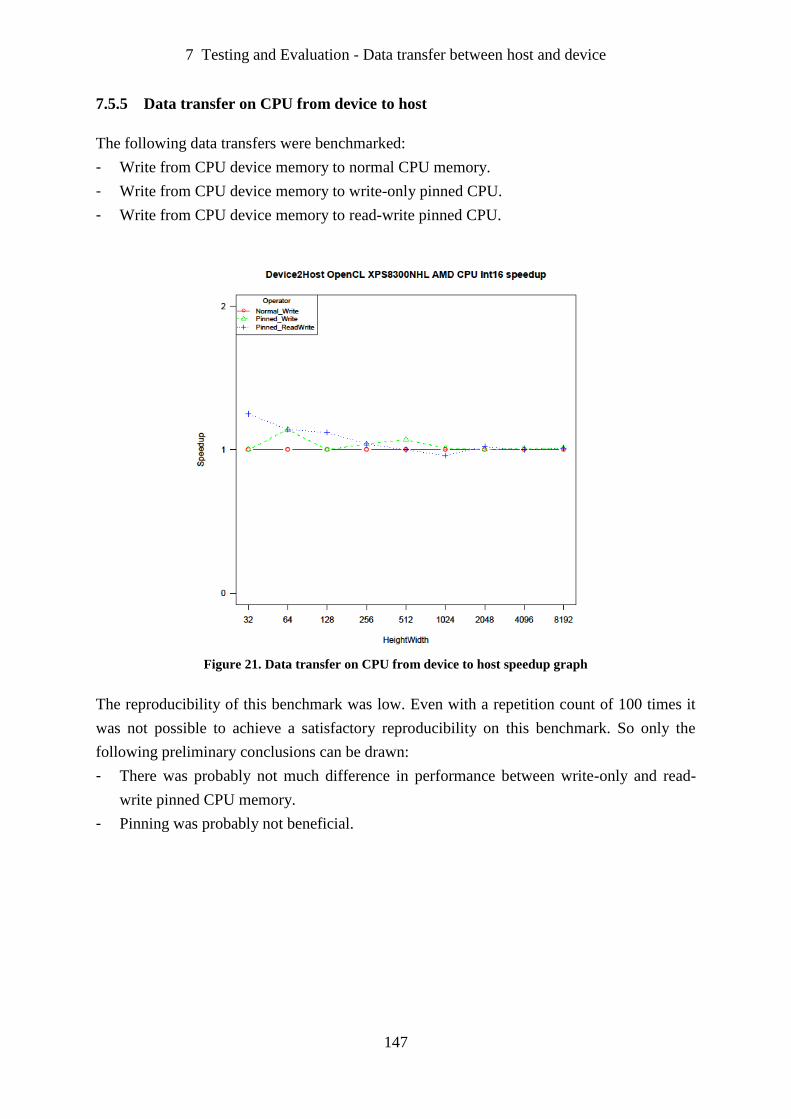
7 Testing and Evaluation - Data transfer between host and device
147
7.5.5 Data transfer on CPU from device to host
The following data transfers were benchmarked:
- Write from CPU device memory to normal CPU memory.
- Write from CPU device memory to write-only pinned CPU.
- Write from CPU device memory to read-write pinned CPU.
Figure 21. Data transfer on CPU from device to host speedup graph
The reproducibility of this benchmark was low. Even with a repetition count of 100 times it
was not possible to achieve a satisfactory reproducibility on this benchmark. So only the
following preliminary conclusions can be drawn:
- There was probably not much difference in performance between write-only and read-
write pinned CPU memory.
- Pinning was probably not beneficial.
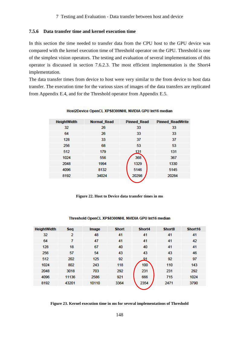
7 Testing and Evaluation - Data transfer between host and device
148
7.5.6 Data transfer time and kernel execution time
In this section the time needed to transfer data from the CPU host to the GPU device was
compared with the kernel execution time of Threshold operator on the GPU. Threshold is one
of the simplest vision operators. The testing and evaluation of several implementations of this
operator is discussed in section 7.6.2.3. The most efficient implementation is the Short4
implementation.
The data transfer times from device to host were very similar to the from device to host data
transfer. The execution time for the various sizes of images of the data transfers are replicated
from Appendix E.4, and for the Threshold operator from Appendix E.5.
Figure 22. Host to Device data transfer times in ms
Figure 23. Kernel execution time in ms for several implementations of Threshold
7 Testing and Evaluation - Data transfer between host and device
149
Conclusions:
- The overhead data transfer for the larger images was massive compared to the kernel
execution time of a simple vision operator.
- Copying an image from the CPU host to the GPU device, executing a simple vision
operator on the GPU and copying the image back to the CPU host is not a feasible option.
7.5.7 Conclusions about data transfer
This section evaluates data transfer between host and device memory using OpenCL.
From the experiments the following conclusions can be drawn:
- The overhead of data transfer was substantial, even for host-device transfer on CPUs. The
reason for this is that the ReadBuffer and WriteBuffer operations on the CPU were
making copies of the data.
- For CPU-GPU transfer it was beneficial to use pinning for the larger images.
- For GPU-CPU transfer it was always beneficial to use pinning.
- For CPU-CPU transfer pinning had no advantages.
- For small images the CPU-CPU transfer was much faster than the CPU-GPU transfer, for
large images the transfer is the same order of magnitude. See Appendix E.4.
- The overhead data transfer for the larger images was massive compared with the kernel
execution time on the GPU of a simple vision operator.
7.5.8 Future work
- Implement in the wrapper around the OpenCL host API interface support for ‘zero copy
transfer’.
- Benchmark data transfer using ‘zero copy transfer’ on CPUs and APUs. According to
Shen, Fang, Sips and Varbanescu (2012) data copying overhead on CPUs is reduced by
more than 80%.
- Benchmarking data transfer using OpenCL images.
7 Testing and Evaluation - Point operators
150
7.6 Point operators
7.6.1 Introduction
As representative of the Point operators the Threshold operator was benchmarked.
7.6.2 Threshold
7.6.2.1 Introduction
Because of the nature of the Threshold operator the processing time does not depend on the
contents of the image. As a consequence all testing was done with one Int16Image (cells.jl,
see Appendix B).
The implementations as described in section 6.5.2 were benchmarked with benchmark
images in the different sizes. Note: the Threshold operator is a computational simple
algorithm; for each pixel at most two comparisons and one assignment are required. This
means that it is to be expected that the operator will be more limited by memory bandwidth
than by computational power.
This benchmark was performed on the test machine described in Appendix A on 25 May
2012 using the following versions of the software:
- VisionLab V3.41b (8-5-2011).
- OpenCL 1.1 CUDA 4.2.1.
- OpenCL 1.1 AMD-APP-SDK-v2.5 (684.213).

7 Testing and Evaluation - Point operators
151
7.6.2.2 OpenMP
The results on the four core benchmark machine, with hyper-threading:
Figure 24. Threshold OpenMP speedup graph
Conclusions:
- The results showed a lot of variation that cannot be explained very easily. Some of the
peaks could possibly be explained by the fact that the cache size fitted the problem.
- Hyper-threading was beneficial.
- A speedup of around 2.5 was possible for the larger images.
- For small images there was a large penalty.
- The violin plots (Appendix F) showed that in many cases parallelizing significantly
increased the variance in execution time.
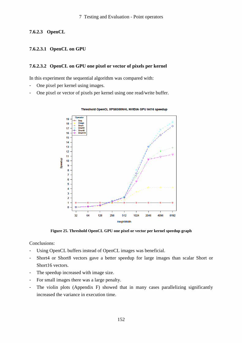
7 Testing and Evaluation - Point operators
152
7.6.2.3 OpenCL
7.6.2.3.1 OpenCL on GPU
7.6.2.3.2 OpenCL on GPU one pixel or vector of pixels per kernel
In this experiment the sequential algorithm was compared with:
- One pixel per kernel using images.
- One pixel or vector of pixels per kernel using one read/write buffer.
Figure 25. Threshold OpenCL GPU one pixel or vector per kernel speedup graph
Conclusions:
- Using OpenCL buffers instead of OpenCL images was beneficial.
- Short4 or Short8 vectors gave a better speedup for large images than scalar Short or
Short16 vectors.
- The speedup increased with image size.
- For small images there was a large penalty.
- The violin plots (Appendix F) showed that in many cases parallelizing significantly
increased the variance in execution time.

7 Testing and Evaluation - Point operators
153
7.6.2.3.3 OpenCL on GPU one pixel or vector of pixels per kernel using a read and a
write buffer
In this experiment the sequential algorithm was compared with one pixel or vector of pixels
per kernel using a read and a write buffer. Due to memory restrictions this experiment was
not executed for an image of 8192×8192.
Figure 26. Threshold OpenCL GPU source and destination image speedup graph
Conclusion:
- Using separate read and write buffers was not beneficial.
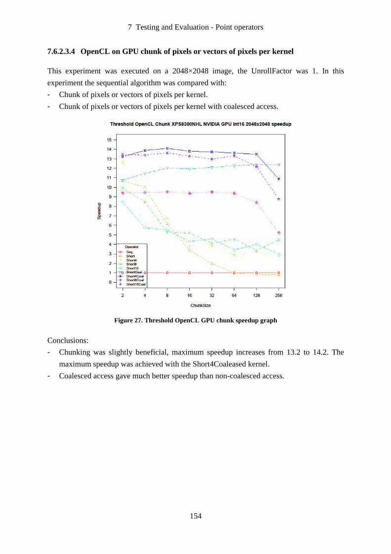
7 Testing and Evaluation - Point operators
154
7.6.2.3.4 OpenCL on GPU chunk of pixels or vectors of pixels per kernel
This experiment was executed on a 2048×2048 image, the UnrollFactor was 1. In this
experiment the sequential algorithm was compared with:
- Chunk of pixels or vectors of pixels per kernel.
- Chunk of pixels or vectors of pixels per kernel with coalesced access.
Figure 27. Threshold OpenCL GPU chunk speedup graph
Conclusions:
- Chunking was slightly beneficial, maximum speedup increases from 13.2 to 14.2. The
maximum speedup was achieved with the Short4Coaleased kernel.
- Coalesced access gave much better speedup than non-coalesced access.

7 Testing and Evaluation - Point operators
155
7.6.2.3.5 OpenCL on GPU chunk of pixels or vectors of pixels per kernel with
UnrollFactor
In this experiment the sequential algorithm was compared with the Short4Coalesed kernel
with a chunk of short4 vectors, the best performing kernel of the chunk experiment in section
7.6.2.3.4. The speedup is plotted against the chunk size and the unroll factor. The experiment
was executed on a 2048×2048 image.
Figure 28. Threshold OpenCL GPU unroll speedup graph
An additional experiment was performed with a variation of the kernel, in which the chunk
size was fixed at compilation type on 16. In this case the trip count of the for loop is known at
compilation time. It was expected that this would help the compiler in unrolling. But a test
with a 2048×2048 pixel image did not show improvement in performance.
Conclusion:
- Unrolling was not significantly beneficial. This is probably due to the fact that this
operator is a highly memory bandwidth bound operator.
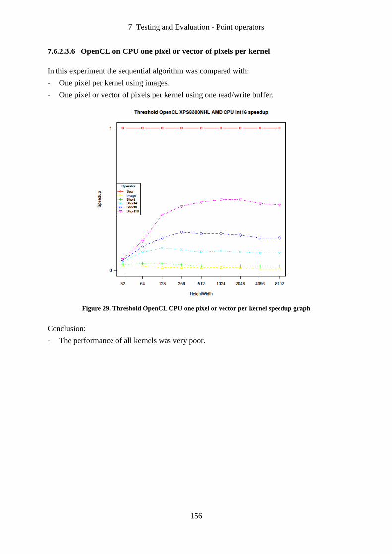
7 Testing and Evaluation - Point operators
156
7.6.2.3.6 OpenCL on CPU one pixel or vector of pixels per kernel
In this experiment the sequential algorithm was compared with:
- One pixel per kernel using images.
- One pixel or vector of pixels per kernel using one read/write buffer.
Figure 29. Threshold OpenCL CPU one pixel or vector per kernel speedup graph
Conclusion:
- The performance of all kernels was very poor.
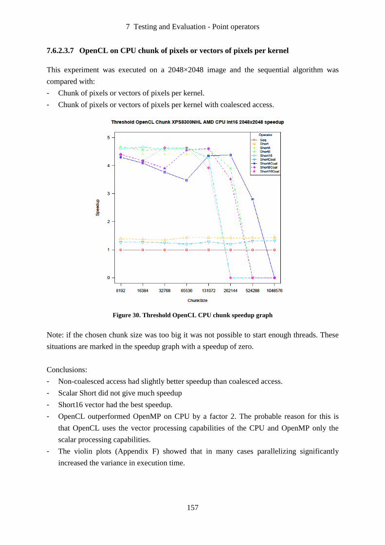
7 Testing and Evaluation - Point operators
157
7.6.2.3.7 OpenCL on CPU chunk of pixels or vectors of pixels per kernel
This experiment was executed on a 2048×2048 image and the sequential algorithm was
compared with:
- Chunk of pixels or vectors of pixels per kernel.
- Chunk of pixels or vectors of pixels per kernel with coalesced access.
Figure 30. Threshold OpenCL CPU chunk speedup graph
Note: if the chosen chunk size was too big it was not possible to start enough threads. These
situations are marked in the speedup graph with a speedup of zero.
Conclusions:
- Non-coalesced access had slightly better speedup than coalesced access.
- Scalar Short did not give much speedup
- Short16 vector had the best speedup.
- OpenCL outperformed OpenMP on CPU by a factor 2. The probable reason for this is
that OpenCL uses the vector processing capabilities of the CPU and OpenMP only the
scalar processing capabilities.
- The violin plots (Appendix F) showed that in many cases parallelizing significantly
increased the variance in execution time.
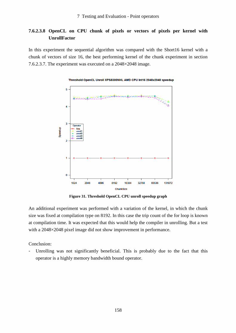
7 Testing and Evaluation - Point operators
158
7.6.2.3.8 OpenCL on CPU chunk of pixels or vectors of pixels per kernel with
UnrollFactor
In this experiment the sequential algorithm was compared with the Short16 kernel with a
chunk of vectors of size 16, the best performing kernel of the chunk experiment in section
7.6.2.3.7. The experiment was executed on a 2048×2048 image.
Figure 31. Threshold OpenCL CPU unroll speedup graph
An additional experiment was performed with a variation of the kernel, in which the chunk
size was fixed at compilation type on 8192. In this case the trip count of the for loop is known
at compilation time. It was expected that this would help the compiler in unrolling. But a test
with a 2048×2048 pixel image did not show improvement in performance.
Conclusion:
- Unrolling was not significantly beneficial. This is probably due to the fact that this
operator is a highly memory bandwidth bound operator.
7 Testing and Evaluation - Point operators
159
7.6.2.4 Conclusions Threshold benchmarks
From the experiments the following conclusions were drawn:
- By adding one line of code to the original C++ code, OpenMP gave a speedup on the
benchmark of around 2.5 for images with more than 256×256 pixels.
- At the cost of some serious programming effort, both kernel code and client side code,
and tuning parameters OpenCL gave a speedup up to:
- 18.4 on the GPU.
- 4.62 on the CPU.
- For small images there was a large penalty using OpenMP or OpenCL.
- Vectorization of OpenCL kernels improved performance for both GPU and CPU.
- The violin plots (Appendix F) showed that in many cases parallelizing significantly
increased the variance in execution time. This increase was more prominent for the
smaller images and more substantial for CPU than GPU.
7.6.2.5 Future work
The Threshold operator is a highly memory bandwidth bound operator. So it is not possible to
draw conclusion for computation bound point operators. This will have to be investigated
with future work.
7 Testing and Evaluation - Local neighbour operators
160
7.7 Local neighbour operators
7.7.1 Introduction
As a representative of the Local neighbour operators the Convolution operator was
benchmarked.
7.7.2 Convolution
7.7.2.1 Introduction
Because of the nature of the Convolution operator the processing time does not depend on the
contents of the image. So all testing was done with one Int16Image (cells.jl, see Appendix B).
The implementations as described in section 6.6.2 were benchmarked with benchmark
images in the different sizes and with masks in different sizes. As mask the smoothing mask
was chosen. All values in the mask have the value one and the dividing factor is the sum of
the mask values. The chosen mask sizes were 3×3, 5×5, 7×7 and 15×15.
The benchmarks were performed on the test machine described in Appendix A on 18 January
2013 using the following versions of the software:
- VisionLab V3.42 (6-12-2012)
- OpenCL 1.1 CUDA 4.2.1
- OpenCL 1.1 AMD-APP-SDK-v2.5 (684.213)
Note: the one dimensional NDRange benchmarks were performed on 28, 31 January and 4
February 2013.
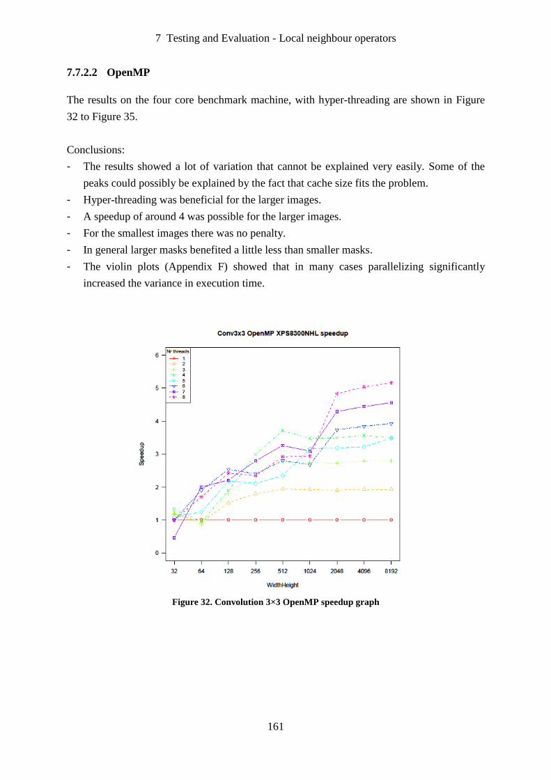
7 Testing and Evaluation - Local neighbour operators
161
7.7.2.2 OpenMP
The results on the four core benchmark machine, with hyper-threading are shown in Figure
32 to Figure 35.
Conclusions:
- The results showed a lot of variation that cannot be explained very easily. Some of the
peaks could possibly be explained by the fact that cache size fits the problem.
- Hyper-threading was beneficial for the larger images.
- A speedup of around 4 was possible for the larger images.
- For the smallest images there was no penalty.
- In general larger masks benefited a little less than smaller masks.
- The violin plots (Appendix F) showed that in many cases parallelizing significantly
increased the variance in execution time.
Figure 32. Convolution 3×3 OpenMP speedup graph
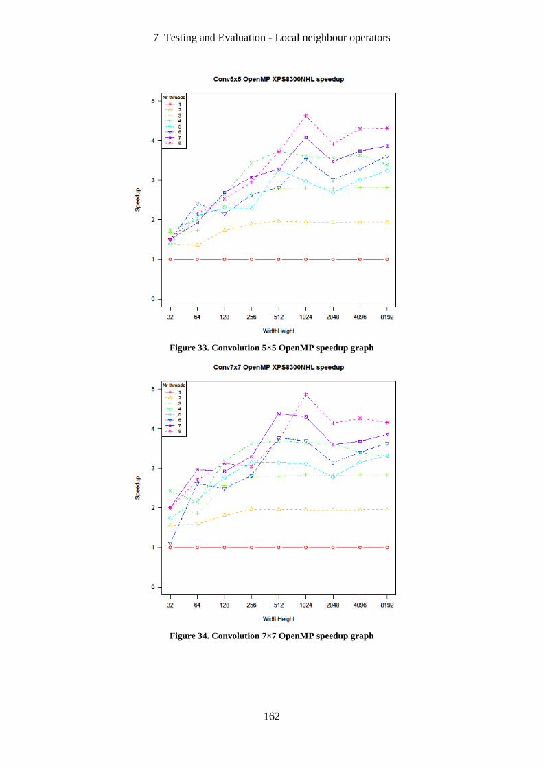
7 Testing and Evaluation - Local neighbour operators
162
Figure 33. Convolution 5×5 OpenMP speedup graph
Figure 34. Convolution 7×7 OpenMP speedup graph
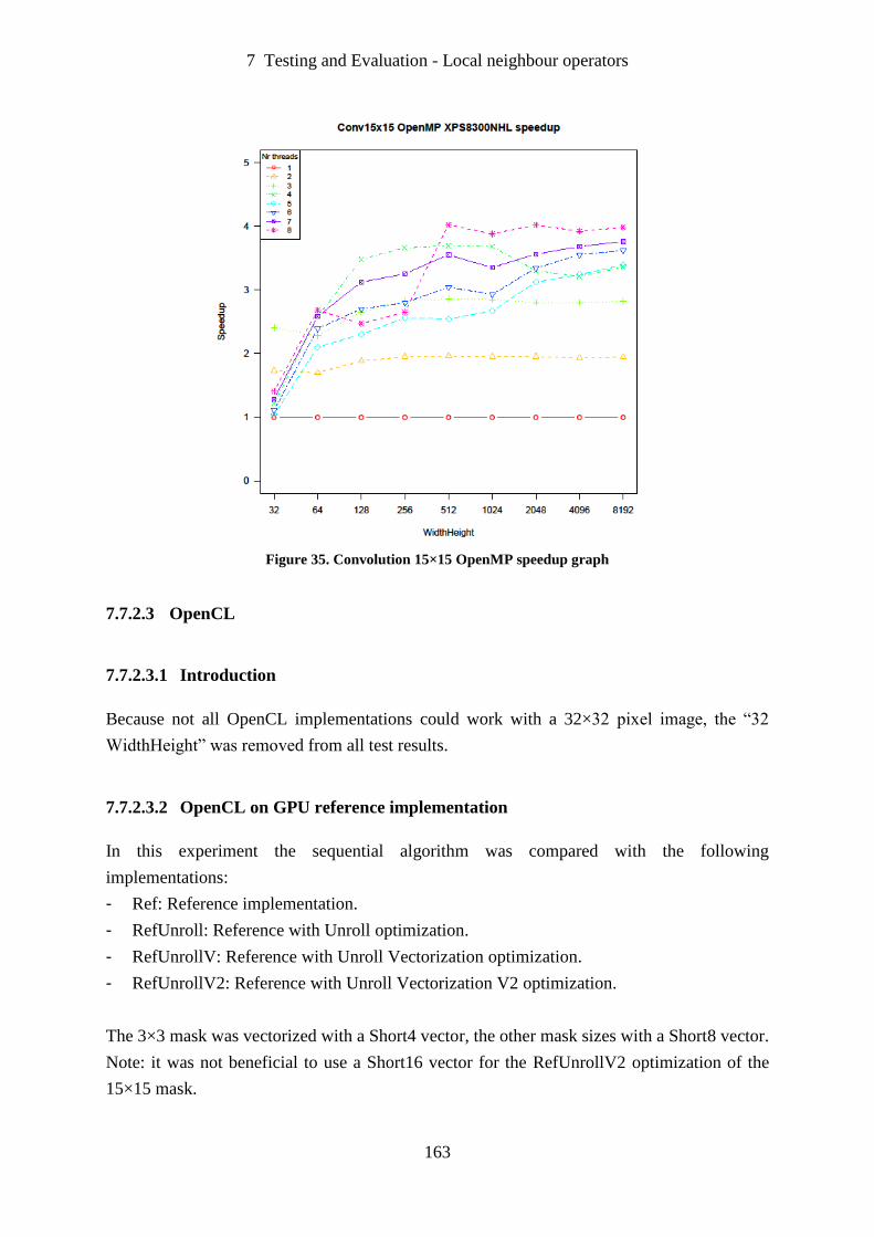
7 Testing and Evaluation - Local neighbour operators
163
Figure 35. Convolution 15×15 OpenMP speedup graph
7.7.2.3 OpenCL
7.7.2.3.1 Introduction
Because not all OpenCL implementations could work with a 32×32 pixel image, the “32
WidthHeight” was removed from all test results.
7.7.2.3.2 OpenCL on GPU reference implementation
In this experiment the sequential algorithm was compared with the following
implementations:
- Ref: Reference implementation.
- RefUnroll: Reference with Unroll optimization.
- RefUnrollV: Reference with Unroll Vectorization optimization.
- RefUnrollV2: Reference with Unroll Vectorization V2 optimization.
The 3×3 mask was vectorized with a Short4 vector, the other mask sizes with a Short8 vector.
Note: it was not beneficial to use a Short16 vector for the RefUnrollV2 optimization of the
15×15 mask.

7 Testing and Evaluation - Local neighbour operators
164
Figure 36. Convolution 3×3 OpenCL GPU reference speedup graph
Figure 37. Convolution 5×5 OpenCL GPU reference speedup graph
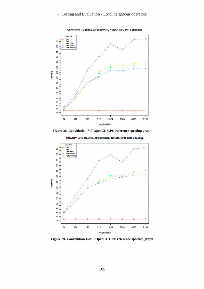
7 Testing and Evaluation - Local neighbour operators
165
Figure 38. Convolution 7×7 OpenCL GPU reference speedup graph
Figure 39. Convolution 15×15 OpenCL GPU reference speedup graph

7 Testing and Evaluation - Local neighbour operators
166
Conclusions:
- The simple Ref implementation performed well.
- The RefUnroll and RefUnrollV optimization for 3×3, 5×5 and 7×7 masks nearly always
performed worse than Ref.
- The RefUnrollV2 performed nearly always better than the Ref.
- The RefUnrollV2 was less effective with a 5×5 mask than with other mask sizes.
For a 5×5 mask the Short8 is filled with three padding zeros. For a 7×7 mask only one
padding zero is needed. A 15×15 mask uses two Short8 vectors and only one padding
zero.
- With the exception of the 3×3 mask, there was no penalty the smallest images.
- Larger masks had better speedups than smaller masks.
- The violin plots (Appendix F) showed that parallelizing can sometimes significantly
increase the variance in execution time. However, in most tests the variance decreased for
the bigger image sizes.
7.7.2.3.3 OpenCL on GPU using local memory
In this experiment the sequential algorithm was compared with the following optimizations:
- Local: Local memory optimization.
- LocalUnroll: Local memory with Unroll optimization.
- LocalUnrollV: Local memory with Unroll Vectorization optimization.
- LocalUnrollV2: Local memory with Unroll Vectorization V2 optimization.
The 3×3 mask was vectorized with a Short4 vector, the other mask sizes with a Short8 vector.
Note: it was not beneficial to use a Short16 vector for the RefUnrollV2 optimization of the
15×15 mask.
In section 6.6.2.4.5 two approaches for tile copying are described. The “Local Vector Read”
implementation was always faster than “Local” implementation. The difference, only a few
percentage, was not as big as found in the literature review for Convolution implementations
with fixed mask sizes. The probable reason for this is that, because variable sized masks are
implemented, more complicated for loops are necessary, which cannot be unrolled. Only the
results of the “Local Vector Read” implementation are discussed here.
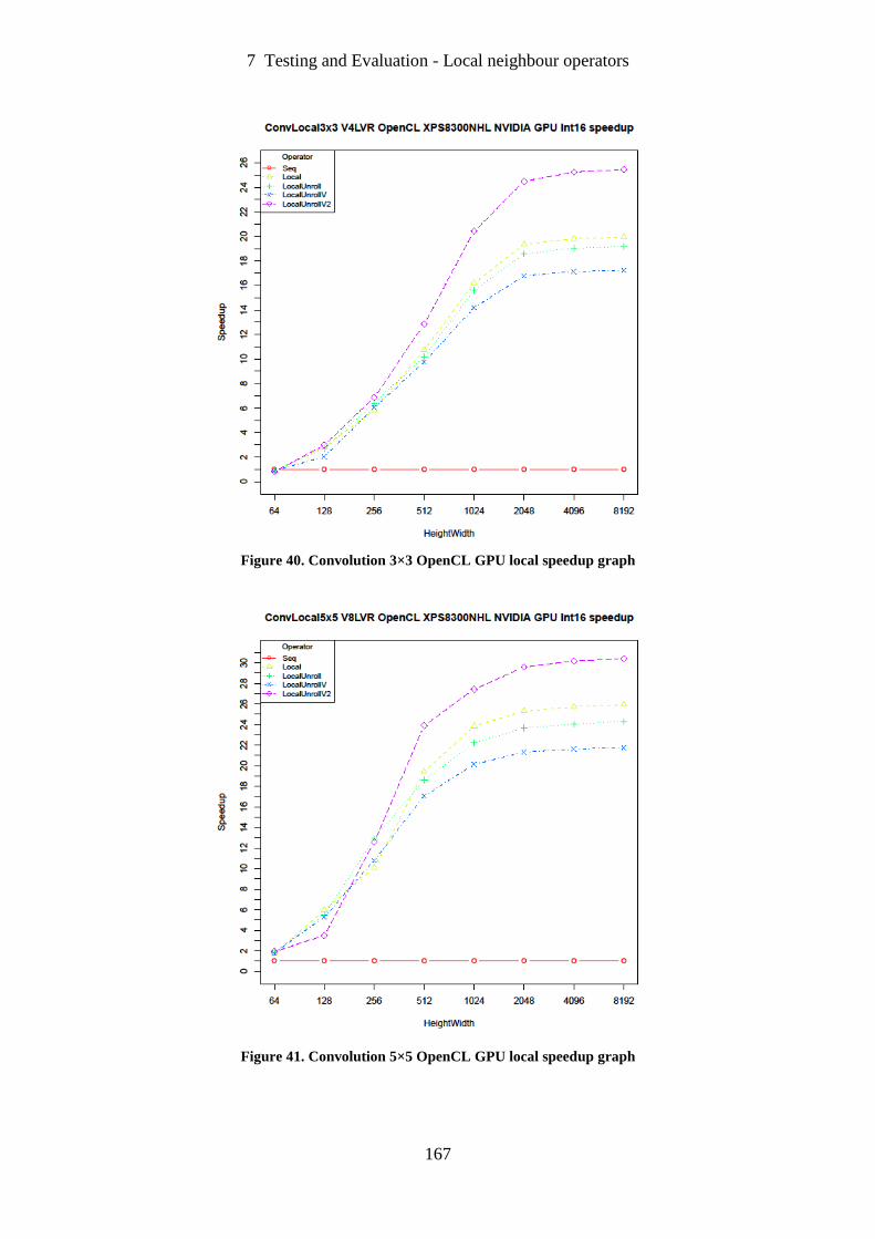
7 Testing and Evaluation - Local neighbour operators
167
Figure 40. Convolution 3×3 OpenCL GPU local speedup graph
Figure 41. Convolution 5×5 OpenCL GPU local speedup graph
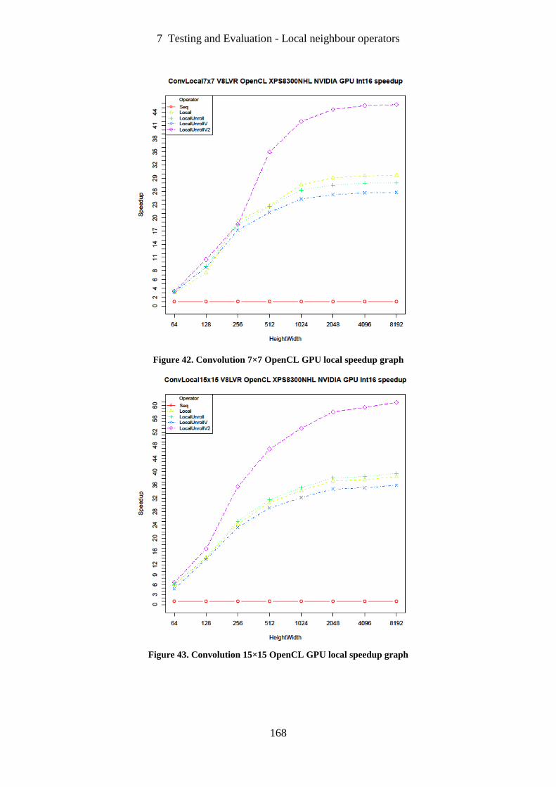
7 Testing and Evaluation - Local neighbour operators
168
Figure 42. Convolution 7×7 OpenCL GPU local speedup graph
Figure 43. Convolution 15×15 OpenCL GPU local speedup graph
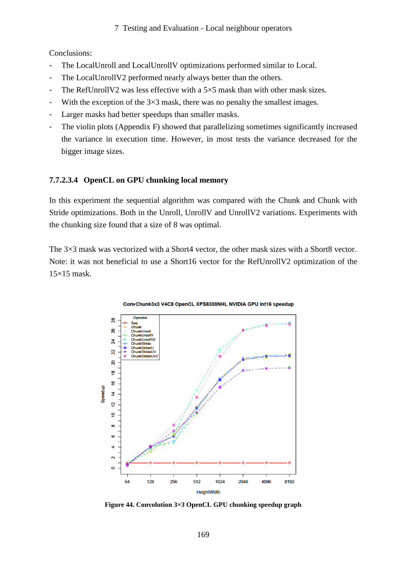
7 Testing and Evaluation - Local neighbour operators
169
Conclusions:
- The LocalUnroll and LocalUnrollV optimizations performed similar to Local.
- The LocalUnrollV2 performed nearly always better than the others.
- The RefUnrollV2 was less effective with a 5×5 mask than with other mask sizes.
- With the exception of the 3×3 mask, there was no penalty the smallest images.
- Larger masks had better speedups than smaller masks.
- The violin plots (Appendix F) showed that parallelizing sometimes significantly increased
the variance in execution time. However, in most tests the variance decreased for the
bigger image sizes.
7.7.2.3.4 OpenCL on GPU chunking local memory
In this experiment the sequential algorithm was compared with the Chunk and Chunk with
Stride optimizations. Both in the Unroll, UnrollV and UnrollV2 variations. Experiments with
the chunking size found that a size of 8 was optimal.
The 3×3 mask was vectorized with a Short4 vector, the other mask sizes with a Short8 vector.
Note: it was not beneficial to use a Short16 vector for the RefUnrollV2 optimization of the
15×15 mask.
Figure 44. Convolution 3×3 OpenCL GPU chunking speedup graph
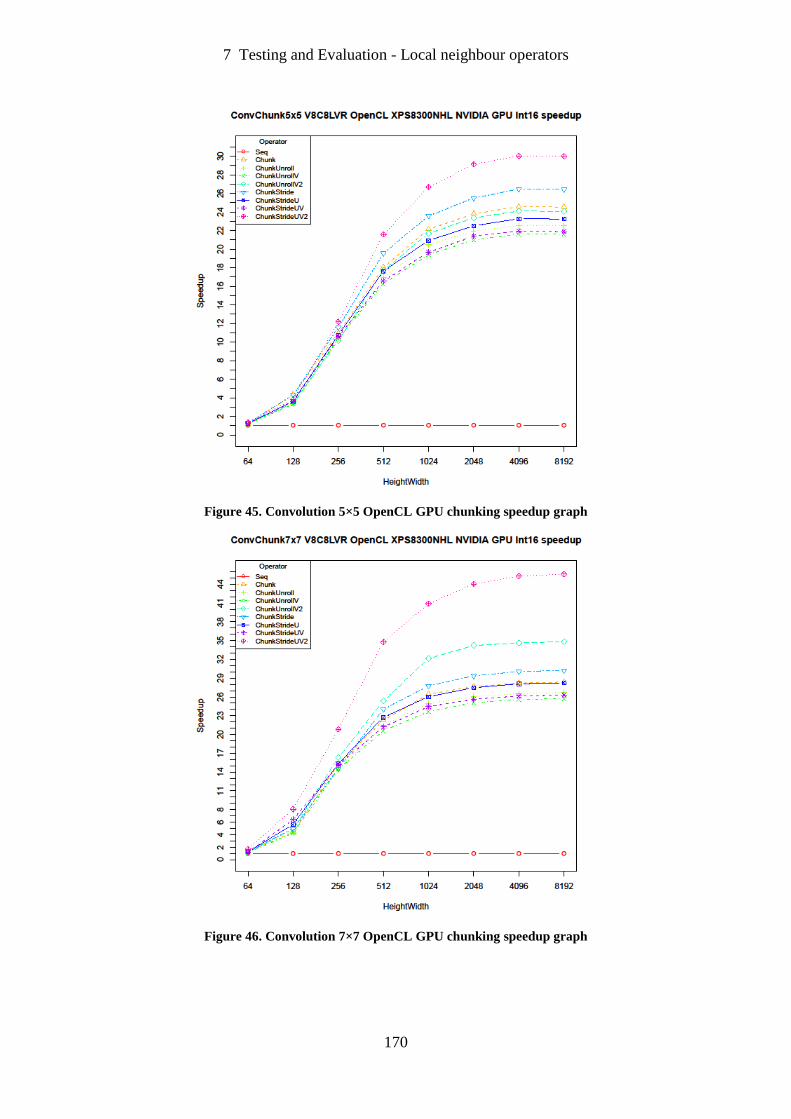
7 Testing and Evaluation - Local neighbour operators
170
Figure 45. Convolution 5×5 OpenCL GPU chunking speedup graph
Figure 46. Convolution 7×7 OpenCL GPU chunking speedup graph
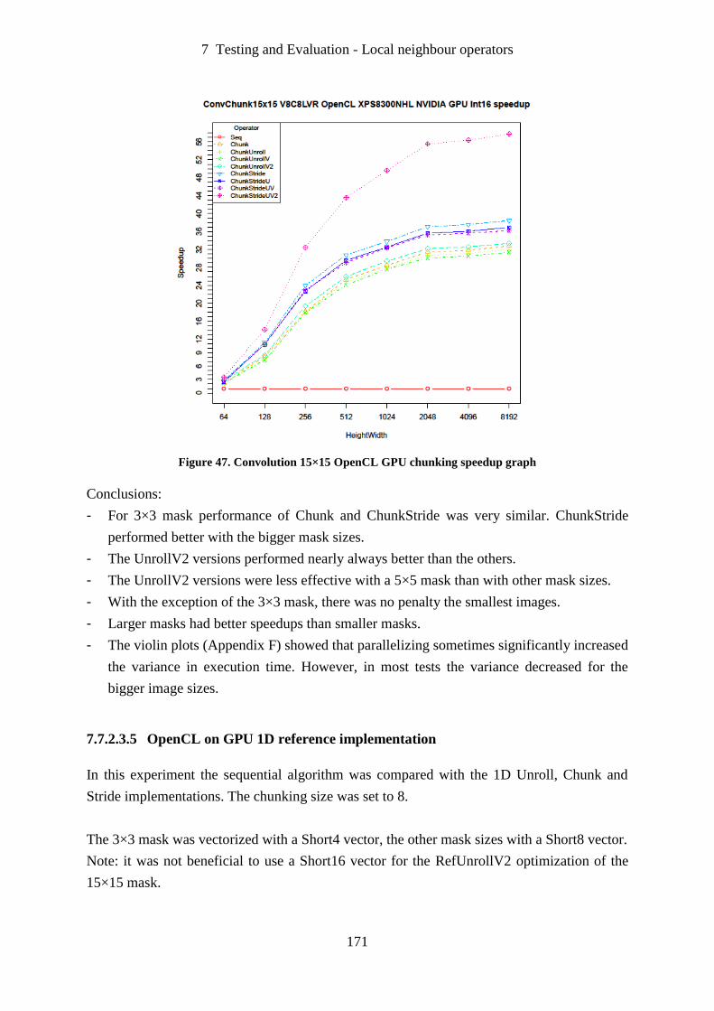
7 Testing and Evaluation - Local neighbour operators
171
Figure 47. Convolution 15×15 OpenCL GPU chunking speedup graph
Conclusions:
- For 3×3 mask performance of Chunk and ChunkStride was very similar. ChunkStride
performed better with the bigger mask sizes.
- The UnrollV2 versions performed nearly always better than the others.
- The UnrollV2 versions were less effective with a 5×5 mask than with other mask sizes.
- With the exception of the 3×3 mask, there was no penalty the smallest images.
- Larger masks had better speedups than smaller masks.
- The violin plots (Appendix F) showed that parallelizing sometimes significantly increased
the variance in execution time. However, in most tests the variance decreased for the
bigger image sizes.
7.7.2.3.5 OpenCL on GPU 1D reference implementation
In this experiment the sequential algorithm was compared with the 1D Unroll, Chunk and
Stride implementations. The chunking size was set to 8.
The 3×3 mask was vectorized with a Short4 vector, the other mask sizes with a Short8 vector.
Note: it was not beneficial to use a Short16 vector for the RefUnrollV2 optimization of the
15×15 mask.
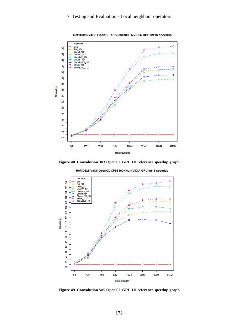
7 Testing and Evaluation - Local neighbour operators
172
Figure 48. Convolution 3×3 OpenCL GPU 1D reference speedup graph
Figure 49. Convolution 5×5 OpenCL GPU 1D reference speedup graph
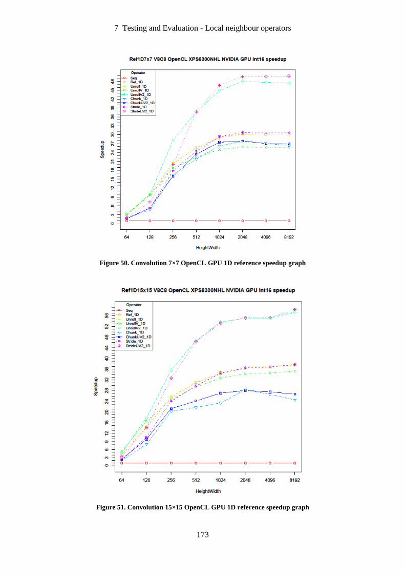
7 Testing and Evaluation - Local neighbour operators
173
Figure 50. Convolution 7×7 OpenCL GPU 1D reference speedup graph
Figure 51. Convolution 15×15 OpenCL GPU 1D reference speedup graph
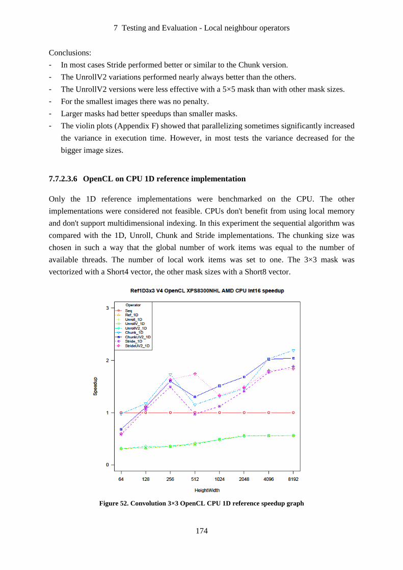
7 Testing and Evaluation - Local neighbour operators
174
Conclusions:
- In most cases Stride performed better or similar to the Chunk version.
- The UnrollV2 variations performed nearly always better than the others.
- The UnrollV2 versions were less effective with a 5×5 mask than with other mask sizes.
- For the smallest images there was no penalty.
- Larger masks had better speedups than smaller masks.
- The violin plots (Appendix F) showed that parallelizing sometimes significantly increased
the variance in execution time. However, in most tests the variance decreased for the
bigger image sizes.
7.7.2.3.6 OpenCL on CPU 1D reference implementation
Only the 1D reference implementations were benchmarked on the CPU. The other
implementations were considered not feasible. CPUs don't benefit from using local memory
and don't support multidimensional indexing. In this experiment the sequential algorithm was
compared with the 1D, Unroll, Chunk and Stride implementations. The chunking size was
chosen in such a way that the global number of work items was equal to the number of
available threads. The number of local work items was set to one. The 3×3 mask was
vectorized with a Short4 vector, the other mask sizes with a Short8 vector.
Figure 52. Convolution 3×3 OpenCL CPU 1D reference speedup graph

7 Testing and Evaluation - Local neighbour operators
175
Figure 53. Convolution 5×5 OpenCL CPU 1D reference speedup graph
Figure 54. Convolution 7×7 OpenCL CPU 1D reference speedup graph

7 Testing and Evaluation - Local neighbour operators
176
Figure 55. Convolution 15×15 OpenCL CPU 1D reference speedup graph
Conclusions:
- The results showed a lot of variation that cannot be explained very easily. Some of the
peaks could possibly be explained by the fact that cache size fits the problem.
- In most cases the performance of Chunk was slightly better than Stride.
- For masks of 5×5 and bigger UnrollV2 variations always performed better than the
others.
- For the smallest images there was no penalty.
- Larger masks had better speedups than smaller masks.
- The violin plots (Appendix F) showed that in many cases parallelizing significantly
increased the variance in execution time.
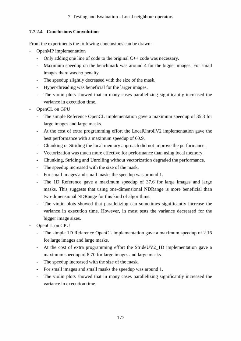
7 Testing and Evaluation - Local neighbour operators
177
7.7.2.4 Conclusions Convolution
From the experiments the following conclusions can be drawn:
- OpenMP implementation
- Only adding one line of code to the original C++ code was necessary.
- Maximum speedup on the benchmark was around 4 for the bigger images. For small
images there was no penalty.
- The speedup slightly decreased with the size of the mask.
- Hyper-threading was beneficial for the larger images.
- The violin plots showed that in many cases parallelizing significantly increased the
variance in execution time.
- OpenCL on GPU
- The simple Reference OpenCL implementation gave a maximum speedup of 35.3 for
large images and large masks.
- At the cost of extra programming effort the LocalUnrollV2 implementation gave the
best performance with a maximum speedup of 60.9.
- Chunking or Striding the local memory approach did not improve the performance.
- Vectorization was much more effective for performance than using local memory.
- Chunking, Striding and Unrolling without vectorization degraded the performance.
- The speedup increased with the size of the mask.
- For small images and small masks the speedup was around 1.
- The 1D Reference gave a maximum speedup of 37.6 for large images and large
masks. This suggests that using one-dimensional NDRange is more beneficial than
two-dimensional NDRange for this kind of algorithms.
- The violin plots showed that parallelizing can sometimes significantly increase the
variance in execution time. However, in most tests the variance decreased for the
bigger image sizes.
- OpenCL on CPU
- The simple 1D Reference OpenCL implementation gave a maximum speedup of 2.16
for large images and large masks.
- At the cost of extra programming effort the StrideUV2_1D implementation gave a
maximum speedup of 8.70 for large images and large masks.
- The speedup increased with the size of the mask.
- For small images and small masks the speedup was around 1.
- The violin plots showed that in many cases parallelizing significantly increased the
variance in execution time.
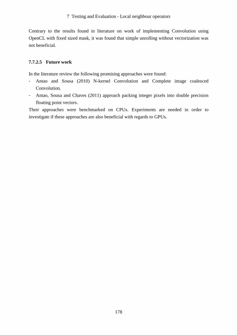
7 Testing and Evaluation - Local neighbour operators
178
Contrary to the results found in literature on work of implementing Convolution using
OpenCL with fixed sized mask, it was found that simple unrolling without vectorization was
not beneficial.
7.7.2.5 Future work
In the literature review the following promising approaches were found:
- Antao and Sousa (2010) N-kernel Convolution and Complete image coalesced
Convolution.
- Antao, Sousa and Chaves (2011) approach packing integer pixels into double precision
floating point vectors.
Their approaches were benchmarked on CPUs. Experiments are needed in order to
investigate if these approaches are also beneficial with regards to GPUs.
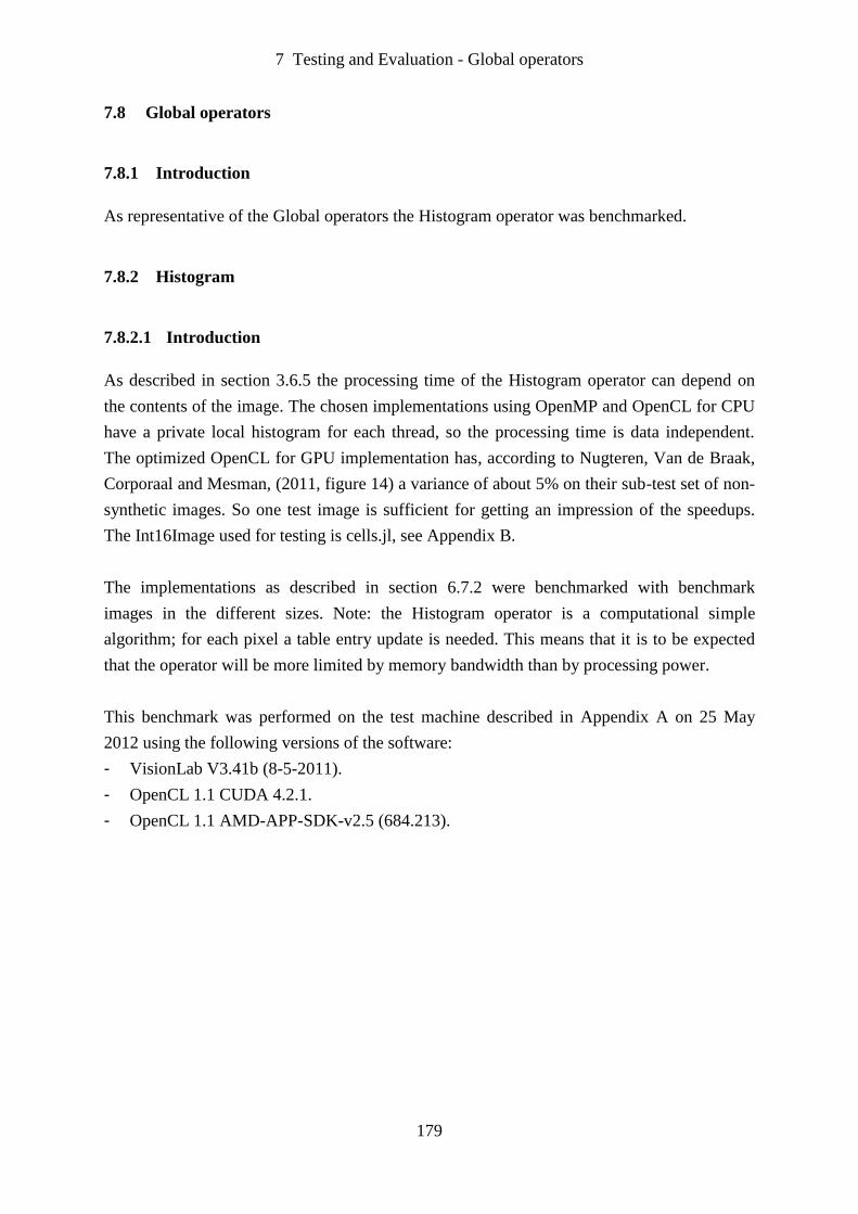
7 Testing and Evaluation - Global operators
179
7.8 Global operators
7.8.1 Introduction
As representative of the Global operators the Histogram operator was benchmarked.
7.8.2 Histogram
7.8.2.1 Introduction
As described in section 3.6.5 the processing time of the Histogram operator can depend on
the contents of the image. The chosen implementations using OpenMP and OpenCL for CPU
have a private local histogram for each thread, so the processing time is data independent.
The optimized OpenCL for GPU implementation has, according to Nugteren, Van de Braak,
Corporaal and Mesman, (2011, figure 14) a variance of about 5% on their sub-test set of non-
synthetic images. So one test image is sufficient for getting an impression of the speedups.
The Int16Image used for testing is cells.jl, see Appendix B.
The implementations as described in section 6.7.2 were benchmarked with benchmark
images in the different sizes. Note: the Histogram operator is a computational simple
algorithm; for each pixel a table entry update is needed. This means that it is to be expected
that the operator will be more limited by memory bandwidth than by processing power.
This benchmark was performed on the test machine described in Appendix A on 25 May
2012 using the following versions of the software:
- VisionLab V3.41b (8-5-2011).
- OpenCL 1.1 CUDA 4.2.1.
- OpenCL 1.1 AMD-APP-SDK-v2.5 (684.213).
7 Testing and Evaluation - Global operators
180
7.8.2.2 OpenMP
The results on the four core benchmark machine, with hyper-threading:
Figure 56. Histogram OpenMP speedup graph
Conclusions:
- The results showed a lot of variation that cannot be explained very easily. Hyper-
threading caused a remarkable increase in speedup between 2048 and 4096 pixels
WidthHeight.
- Hyper-threading was beneficial for the larger images.
- For small images there was a large penalty.
- The violin plots (Appendix F) showed that in many cases parallelizing significantly
increased the variance in execution time.

7 Testing and Evaluation - Global operators
181
7.8.2.3 OpenCL
7.8.2.3.1 OpenCL on GPU simple implementation
In this experiment the simple implementation of the Histogram was benchmarked for
different image sizes.
Figure 57. Histogram simple implementation GPU speedup graph
Conclusions:
- The speedup increased with image size.
- Short16 vectors gave the best speedup.
- For small images there was a large penalty.
- The violin plots (Appendix F) showed that in many cases parallelizing significantly
increased the variance in execution time.
7 Testing and Evaluation - Global operators
182
7.8.2.3.2 OpenCL on GPU optimal number of local histograms for a work-group
In this experiment the GPU optimized implementation of the Histogram was benchmarked
for a 2048×2048 image. In each experiment the number of local histograms for a work-group
was changed. Due to local memory restrictions the maximum number of local histograms was
32.
Figure 58. Histogram number of local histograms GPU speedup graph
Conclusions:
- The best speedup was achieved with 16 local histograms.
- Using 16 local histograms gave a speedup of around 3.5 compared with using one local
histogram.
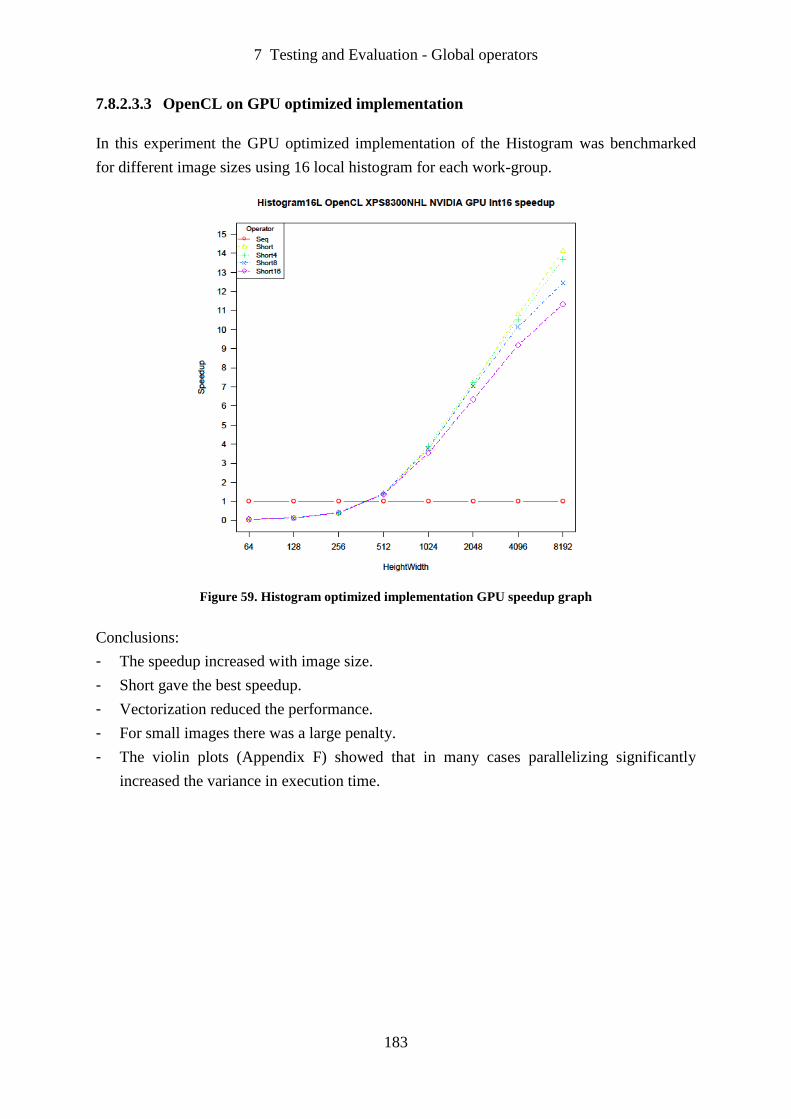
7 Testing and Evaluation - Global operators
183
7.8.2.3.3 OpenCL on GPU optimized implementation
In this experiment the GPU optimized implementation of the Histogram was benchmarked
for different image sizes using 16 local histogram for each work-group.
Figure 59. Histogram optimized implementation GPU speedup graph
Conclusions:
- The speedup increased with image size.
- Short gave the best speedup.
- Vectorization reduced the performance.
- For small images there was a large penalty.
- The violin plots (Appendix F) showed that in many cases parallelizing significantly
increased the variance in execution time.

7 Testing and Evaluation - Global operators
184
7.8.2.3.4 OpenCL on CPU Simple implementation
In this experiment the simple implementation of the Histogram was benchmarked for
different image sizes.
Figure 60. Histogram simple implementation CPU speedup graph
Conclusions:
- The speedup increased with image size.
- The performance of all kernels was very poor.
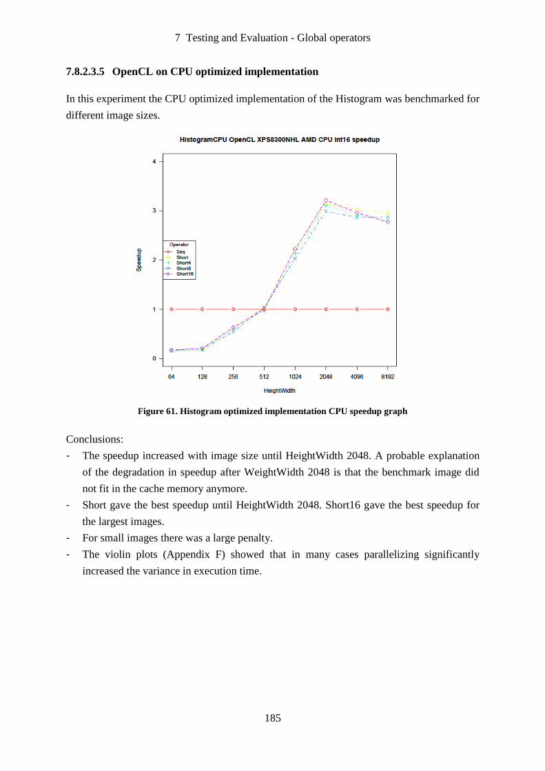
7 Testing and Evaluation - Global operators
185
7.8.2.3.5 OpenCL on CPU optimized implementation
In this experiment the CPU optimized implementation of the Histogram was benchmarked for
different image sizes.
Figure 61. Histogram optimized implementation CPU speedup graph
Conclusions:
- The speedup increased with image size until HeightWidth 2048. A probable explanation
of the degradation in speedup after WeightWidth 2048 is that the benchmark image did
not fit in the cache memory anymore.
- Short gave the best speedup until HeightWidth 2048. Short16 gave the best speedup for
the largest images.
- For small images there was a large penalty.
- The violin plots (Appendix F) showed that in many cases parallelizing significantly
increased the variance in execution time.
7 Testing and Evaluation - Global operators
186
7.8.2.4 Conclusions Histogram
From the experiments the following conclusions can be drawn:
- By adding nine lines of code to the original C++ code, OpenMP gave a speedup on the
benchmark of maximal 5.39 for large images.
- At the cost of some serious programming effort, both kernel code and client side code,
and tuning parameters OpenCL gave a speedup up to:
- 14.1 on the GPU.
- 3.21 on the CPU.
- For small images there was a large penalty using OpenMP or OpenCL.
- Vectorization of OpenCL kernels reduced the performance of the GPU. This is probably
due to the use of atomics.
- The violin plots (Appendix F) showed that parallelizing can significantly increase the
variance in execution time. This increase was more prominent for the smaller images and
more substantial for CPU than GPU.
7.8.2.5 Future work
Testing approaches found in the literature review, suggested by Nugteren, Van den Braak,
Corporaal and Mesman, (2011) and Luna (2012).
7 Testing and Evaluation - Connectivity based operators
187
7.9 Connectivity based operators
7.9.1 Introduction
As representative of the Connectivity based operators the LabelBlobs (Connected Component
Labelling) operator was benchmarked.
7.9.2 LabelBlobs
7.9.2.1 Introduction
As described in section 3.6.6.2 the processing time of the LabelBlob operator will depend on
the contents of the image. In order to limit the time for benchmarking, only three benchmark
images were chosen. As explained in section 6.8.2.4 the performance of the vectorized
OpenCL kernels was expected to depend on the number of object pixels in the image. In
order to test this hypothesis two special images were added to the benchmark. All testing was
done with three images, which are scaled to different sizes. The three benchmark images are:
- Cells: By making an educated guess, Int16Image cells.jl (see Appendix B) is considered
to be a “typical” image. After segmentation with the Threshold operator, with parameters
low = 150 and high = 255, there are about 100 objects in the larger images.
- SmallBlob: Is based on image cells.jl, after segmentation all but one blobs are removed
from the result. This image tests the performance of LabelBlobs if there are only a limited
number of object pixels. This image is expected to give the best performance for
vectorization of the OpenCL kernels.
- BigBlob: The image is filled with one square blob that fits the whole image. This image
tests the performance of LabelBlobs when there are only a limited number of background
pixels. This image is expected to give the worst performance for vectorization of the
OpenCL kernels.
The limitation of only three benchmark images implies that the results can only be used as a
global indication of performance.
The implementations as described in section 6.8.2 are benchmarked with benchmark images
in the different sizes and for both connectivities. For reasons described in section 3.6.6.3 all
benchmark images are converted to type Int32Image.
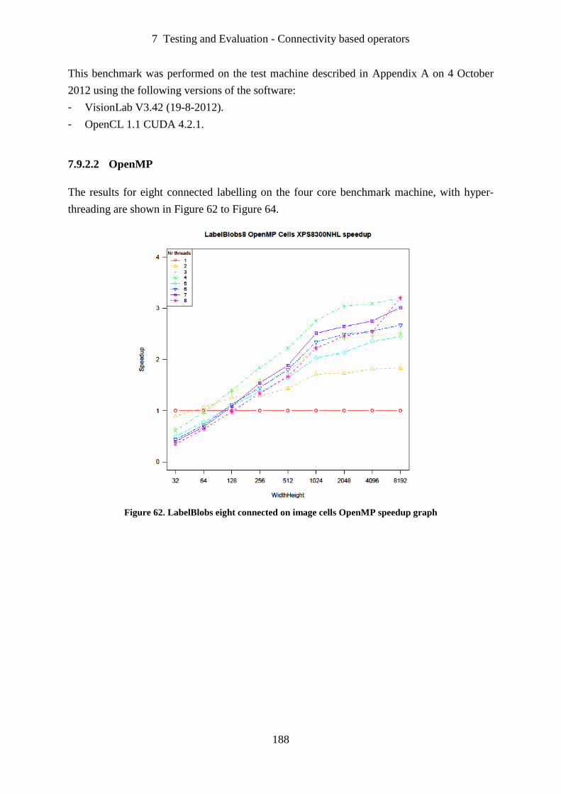
7 Testing and Evaluation - Connectivity based operators
188
This benchmark was performed on the test machine described in Appendix A on 4 October
2012 using the following versions of the software:
- VisionLab V3.42 (19-8-2012).
- OpenCL 1.1 CUDA 4.2.1.
7.9.2.2 OpenMP
The results for eight connected labelling on the four core benchmark machine, with hyper-
threading are shown in Figure 62 to Figure 64.
Figure 62. LabelBlobs eight connected on image cells OpenMP speedup graph
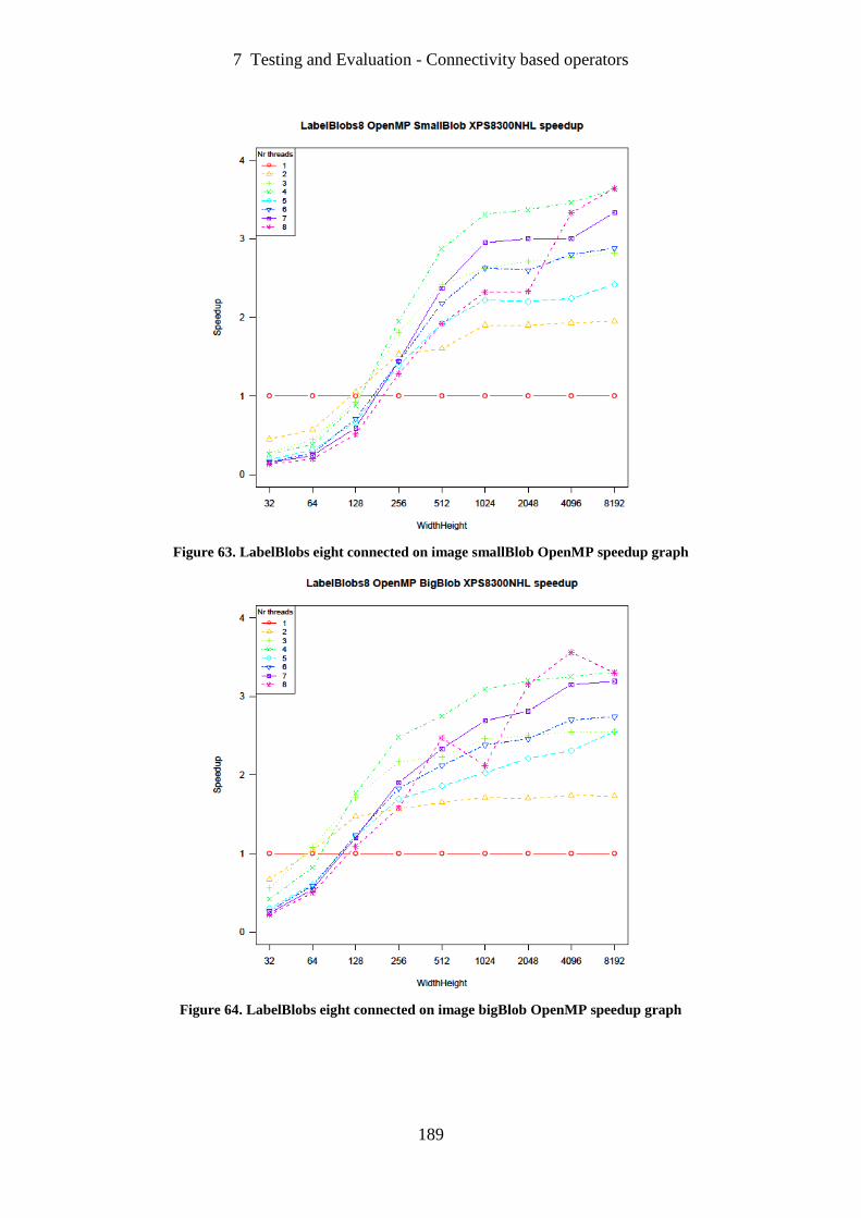
7 Testing and Evaluation - Connectivity based operators
189
Figure 63. LabelBlobs eight connected on image smallBlob OpenMP speedup graph
Figure 64. LabelBlobs eight connected on image bigBlob OpenMP speedup graph
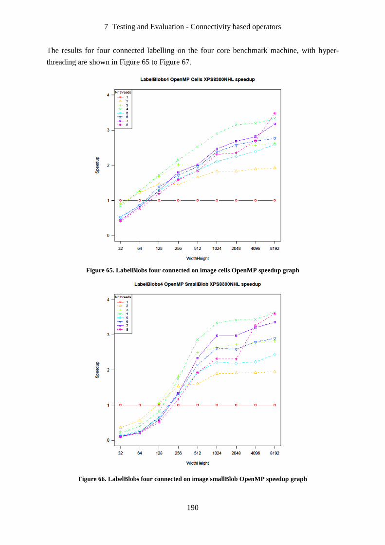
7 Testing and Evaluation - Connectivity based operators
190
The results for four connected labelling on the four core benchmark machine, with hyper-
threading are shown in Figure 65 to Figure 67.
Figure 65. LabelBlobs four connected on image cells OpenMP speedup graph
Figure 66. LabelBlobs four connected on image smallBlob OpenMP speedup graph
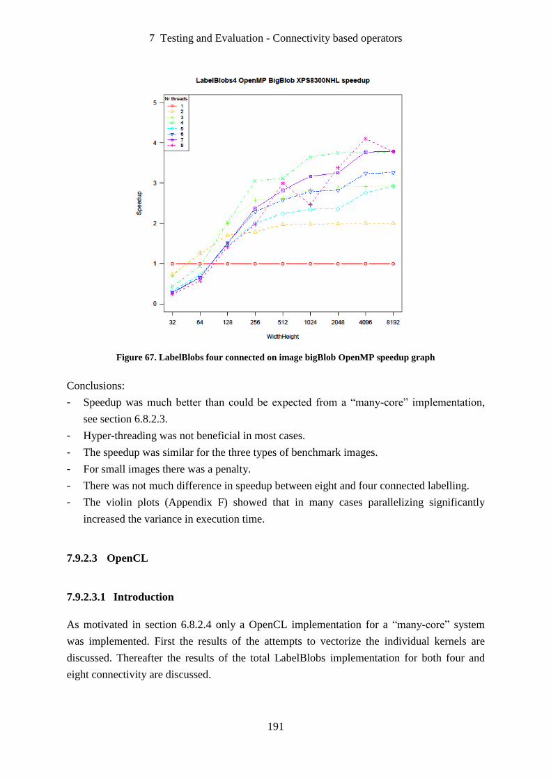
7 Testing and Evaluation - Connectivity based operators
191
Figure 67. LabelBlobs four connected on image bigBlob OpenMP speedup graph
Conclusions:
- Speedup was much better than could be expected from a “many-core” implementation,
see section 6.8.2.3.
- Hyper-threading was not beneficial in most cases.
- The speedup was similar for the three types of benchmark images.
- For small images there was a penalty.
- There was not much difference in speedup between eight and four connected labelling.
- The violin plots (Appendix F) showed that in many cases parallelizing significantly
increased the variance in execution time.
7.9.2.3 OpenCL
7.9.2.3.1 Introduction
As motivated in section 6.8.2.4 only a OpenCL implementation for a “many-core” system
was implemented. First the results of the attempts to vectorize the individual kernels are
discussed. Thereafter the results of the total LabelBlobs implementation for both four and
eight connectivity are discussed.

7 Testing and Evaluation - Connectivity based operators
192
7.9.2.3.2 Vectorization of InitLabels
Note, because the execution time of this kernel is independent of the contents of the image
(section 6.8.2.4), only one type of benchmark image was necessary.
The results for the vectorization of the InitLabels kernel on the benchmark machine GPU are
shown in Figure 68.
Figure 68. Vectorization of InitLabels kernel speedup graph
The conclusion is that the Int4 version always gave an equal or best speedup and was always
equal or better than the non-vectorized Int version.
7.9.2.3.3 Vectorization of LinkFour
As explained in section 6.8.2.4 it is to be expected that the performance of this kernel will
depend on the contents of the image. In order to get an impression of benefits from
vectorization, measurements were performed, in which the LinkFour kernel was tested in
isolation.

7 Testing and Evaluation - Connectivity based operators
193
The results for vectorization of the LinkFour kernel, a four connected implementation of the
Link kernel, on the benchmark machine GPU are shown in Figure 69 to Figure 71.
Figure 69. Vectorization of LinkFour kernel on image cells speedup graph
Figure 70. Vectorization of LinkFour kernel on image smallBlob speedup graph
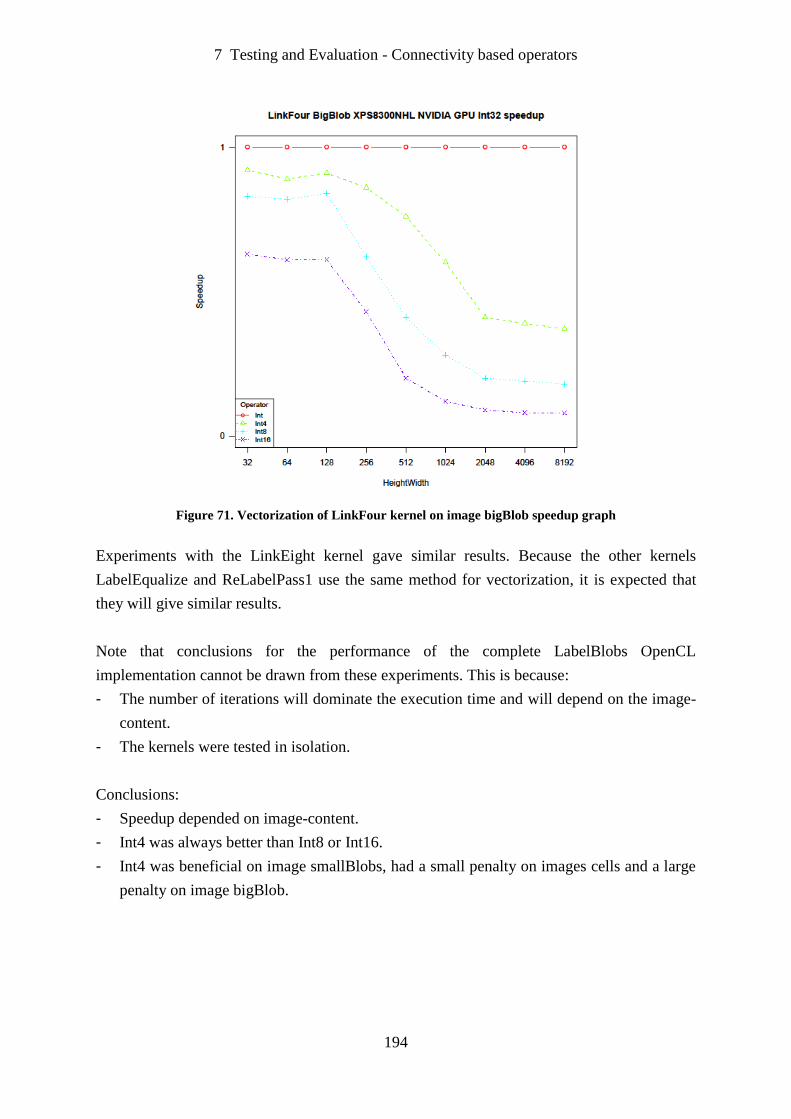
7 Testing and Evaluation - Connectivity based operators
194
Figure 71. Vectorization of LinkFour kernel on image bigBlob speedup graph
Experiments with the LinkEight kernel gave similar results. Because the other kernels
LabelEqualize and ReLabelPass1 use the same method for vectorization, it is expected that
they will give similar results.
Note that conclusions for the performance of the complete LabelBlobs OpenCL
implementation cannot be drawn from these experiments. This is because:
- The number of iterations will dominate the execution time and will depend on the image-
content.
- The kernels were tested in isolation.
Conclusions:
- Speedup depended on image-content.
- Int4 was always better than Int8 or Int16.
- Int4 was beneficial on image smallBlobs, had a small penalty on images cells and a large
penalty on image bigBlob.
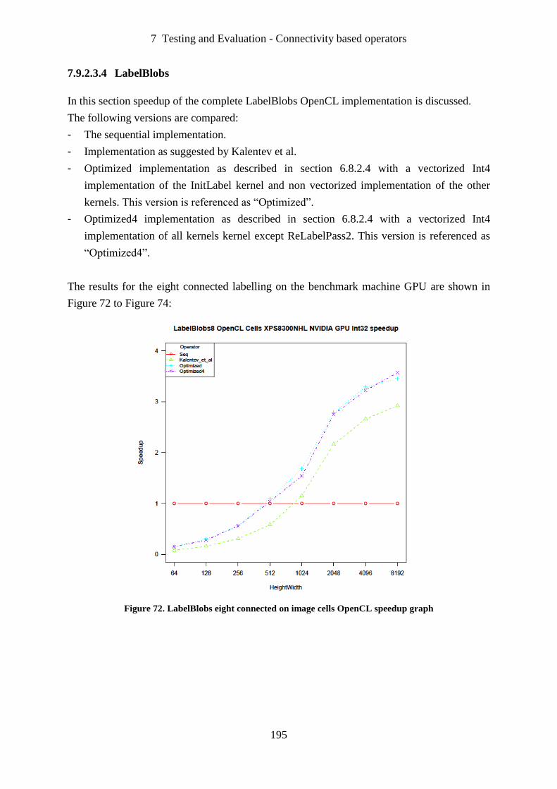
7 Testing and Evaluation - Connectivity based operators
195
7.9.2.3.4 LabelBlobs
In this section speedup of the complete LabelBlobs OpenCL implementation is discussed.
The following versions are compared:
- The sequential implementation.
- Implementation as suggested by Kalentev et al.
- Optimized implementation as described in section 6.8.2.4 with a vectorized Int4
implementation of the InitLabel kernel and non vectorized implementation of the other
kernels. This version is referenced as “Optimized”.
- Optimized4 implementation as described in section 6.8.2.4 with a vectorized Int4
implementation of all kernels kernel except ReLabelPass2. This version is referenced as
“Optimized4”.
The results for the eight connected labelling on the benchmark machine GPU are shown in
Figure 72 to Figure 74:
Figure 72. LabelBlobs eight connected on image cells OpenCL speedup graph
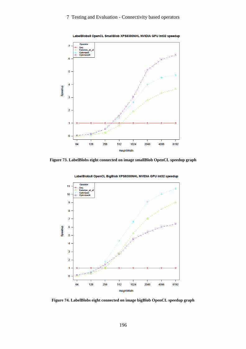
7 Testing and Evaluation - Connectivity based operators
196
Figure 73. LabelBlobs eight connected on image smallBlob OpenCL speedup graph
Figure 74. LabelBlobs eight connected on image bigBlob OpenCL speedup graph
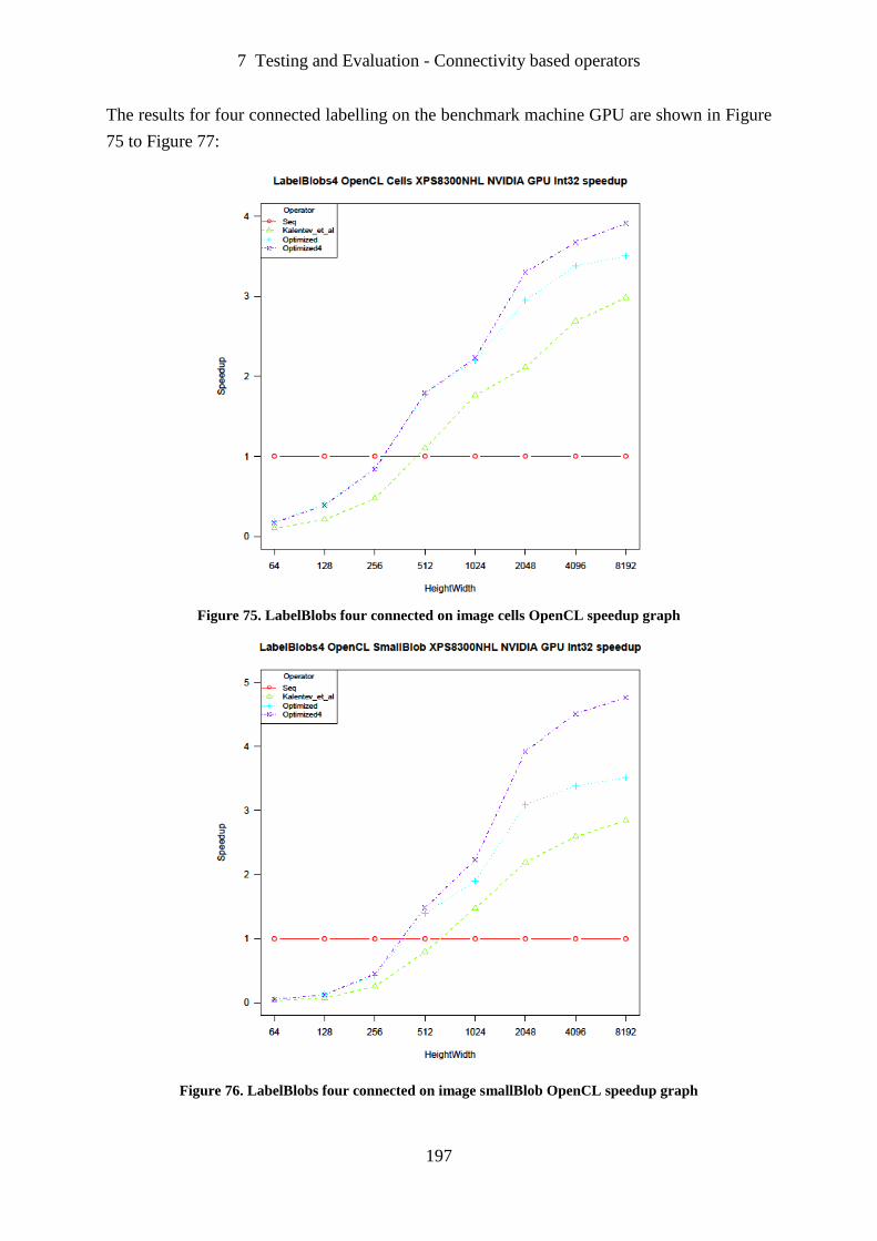
7 Testing and Evaluation - Connectivity based operators
197
The results for four connected labelling on the benchmark machine GPU are shown in Figure
75 to Figure 77:
Figure 75. LabelBlobs four connected on image cells OpenCL speedup graph
Figure 76. LabelBlobs four connected on image smallBlob OpenCL speedup graph
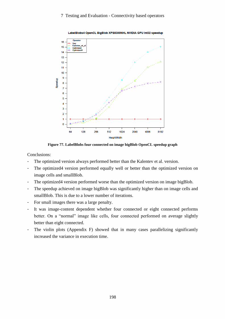
7 Testing and Evaluation - Connectivity based operators
198
Figure 77. LabelBlobs four connected on image bigBlob OpenCL speedup graph
Conclusions:
- The optimized version always performed better than the Kalentev et al. version.
- The optimized4 version performed equally well or better than the optimized version on
image cells and smallBlob.
- The optimized4 version performed worse than the optimized version on image bigBlob.
- The speedup achieved on image bigBlob was significantly higher than on image cells and
smallBlob. This is due to a lower number of iterations.
- For small images there was a large penalty.
- It was image-content dependent whether four connected or eight connected performs
better. On a “normal” image like cells, four connected performed on average slightly
better than eight connected.
- The violin plots (Appendix F) showed that in many cases parallelizing significantly
increased the variance in execution time.

7 Testing and Evaluation - Connectivity based operators
199
7.9.2.4 Conclusions LabelBlobs
From the experiments the following conclusions can be drawn:
- Different parallelization approaches are needed for few-cores and many-cores systems.
- Requiring a significant programming effort, the OpenMP few-cores implementation has
given a speedup on the benchmarks of around 3 for images with more than 512×512
pixels. Hyper-threading was not beneficial. The speedup was similar for all three types of
benchmark images.
- A completely different approach was necessary for the many-cores OpenCL
implementation. This required some serious programming effort, both kernel code and
client side code. The approach suggested by Kalentev et al. was improved significantly.
The speedup achieved depends on the type of benchmark image. For the larger images the
Optimized4 version performed better than the Optimized version on the standard
“typical” benchmark image and the smallBlob image, but performed worse on the
BigBlob image. The advice is to use the Optimized4 version in the general case because
the Optimized4 version does not perform badly on BigBlob image and BigBlob type
images were not found frequently in the vision projects executed by the author.
- For small images there can be a large penalty for using OpenMP or OpenCL.
- The violin plots (Appendix F) showed that in many cases parallelizing significantly
increased the variance in execution time. This increase was more prominent for the
smaller images and more substantial for CPU than GPU.
7.9.2.5 Future work
- Benchmarking OpenCL implementation few-core approach.
- Research in finding the break-even point few-core versus many-core approach.
- Benchmarking approach found in the literature review suggested by Stava and Benes
(2011).
7 Testing and Evaluation - Automatic Operator Parallelization
200
7.10 Automatic Operator Parallelization
OpenMP was considered (see section 8.4) to be the best candidate to parallelize VisionLab in
an efficient and effective way. 170 operators of VisionLab were parallelized using OpenMP.
The Automatic Operator Parallelization mechanism (section 5.2.6) was also implemented for
these operators. VisionLab with the OpenMP parallelization and Automatic Operator
Parallelization is now available as a commercial product.
VisionLab scripts written by users will have, without modification, immediate benefits in
speedup when using the new parallelized version of VisionLab. Users of VisionLab who
write their code in C++ or C# will benefit from the parallelization after linking to the new
library without changing their code. For optimal results users will have to calibrate the
Automatic Operator Parallelization. See section 7.12 for examples of using Automatic
Operator Parallelization in real projects.
The calibration of the Automatic Operator Parallelization is performed using one specific
image for each operator. It is future work to evaluate this calibration process and improve it if
necessary.
7 Testing and Evaluation - Performance portability
201
7.11 Performance portability
7.11.1 Introduction
One of the requirements in Chapter 2 is that the chosen solution must be portable. All
benchmarking in the previous sections of this chapter were performed on a computer with an
Intel Core i7 and NVIDIA graphics card running under Windows 7.
In this section an OpenMP benchmark was performed on quad-core ARM running Linux and
an OpenCL benchmark was performed on a Windows 7 system with an AMD graphics card.
7.11.2 OpenMP on Quad core ARM
The portability of the OpenMP approach was tested on quad core ARM running Linux.
Porting was just recompiling. It passed the VisionLab regression test suite without any
problems. For benchmarking the Convolution algorithm was chosen because it is a frequently
used algorithm and a computationally expensive algorithm.
The Convolution benchmark (section 7.7.2.2) was performed on an ODROID U2
(Hardkernel, 2013). This is a low cost ($89) 4×5 cm mini board with a quad-core ARM
(Cortex-A9) on 1.7 GHz, 2 GByte RAM running Ubuntu 12.10. The benchmark (Boer and
Dijkstra, 2013) was performed on 1 March 2013 using VisionLab V3.42 (12-2-2013). The
process was executed with real-time scheduling policy SCHED_FIFO. Without using this
real-time scheduling policy the benchmark results were erratic. It is future work to investigate
this matter. Due to the limited time available for accessing the hardware, the benchmark was
repeated 30 times and for images in the range 32×32 to 4096×4096 pixels. Hyper-threading
could not be tested because this was not supported on the hardware used. The results are
shown in Figure 78 to Figure 81.
Conclusions:
- Porting was just recompiling. It passed the VisionLab regression test suite without any
problems.
- The results showed far less variation than the results on the standard benchmark machine
under Windows (section 7.7.2.2). The most probable reason for this is the choice for the
real-time scheduling policy SCHED_FIFO.
- Speedups up to 3.97 were reported.
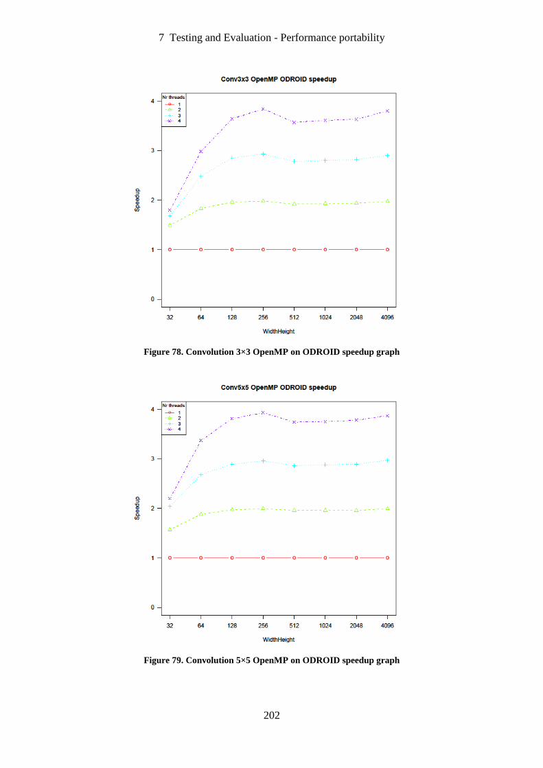
7 Testing and Evaluation - Performance portability
202
Figure 78. Convolution 3×3 OpenMP on ODROID speedup graph
Figure 79. Convolution 5×5 OpenMP on ODROID speedup graph
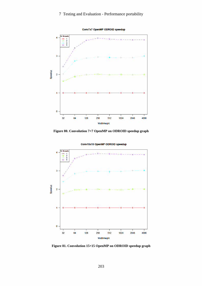
7 Testing and Evaluation - Performance portability
203
Figure 80. Convolution 7×7 OpenMP on ODROID speedup graph
Figure 81. Convolution 15×15 OpenMP on ODROID speedup graph
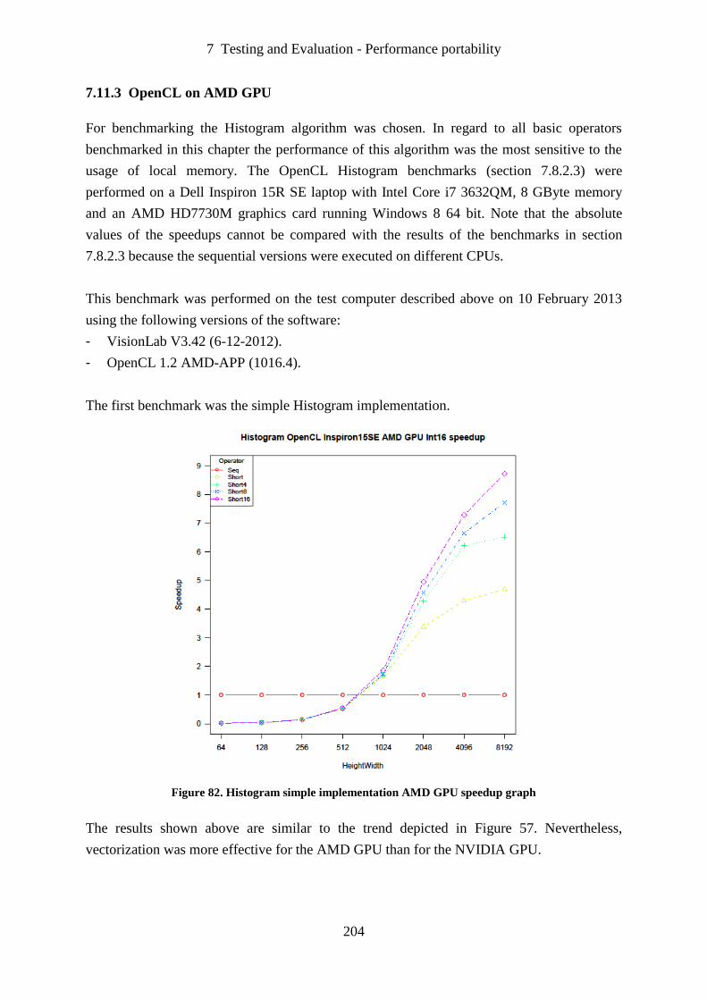
7 Testing and Evaluation - Performance portability
204
7.11.3 OpenCL on AMD GPU
For benchmarking the Histogram algorithm was chosen. In regard to all basic operators
benchmarked in this chapter the performance of this algorithm was the most sensitive to the
usage of local memory. The OpenCL Histogram benchmarks (section 7.8.2.3) were
performed on a Dell Inspiron 15R SE laptop with Intel Core i7 3632QM, 8 GByte memory
and an AMD HD7730M graphics card running Windows 8 64 bit. Note that the absolute
values of the speedups cannot be compared with the results of the benchmarks in section
7.8.2.3 because the sequential versions were executed on different CPUs.
This benchmark was performed on the test computer described above on 10 February 2013
using the following versions of the software:
- VisionLab V3.42 (6-12-2012).
- OpenCL 1.2 AMD-APP (1016.4).
The first benchmark was the simple Histogram implementation.
Figure 82. Histogram simple implementation AMD GPU speedup graph
The results shown above are similar to the trend depicted in Figure 57. Nevertheless,
vectorization was more effective for the AMD GPU than for the NVIDIA GPU.
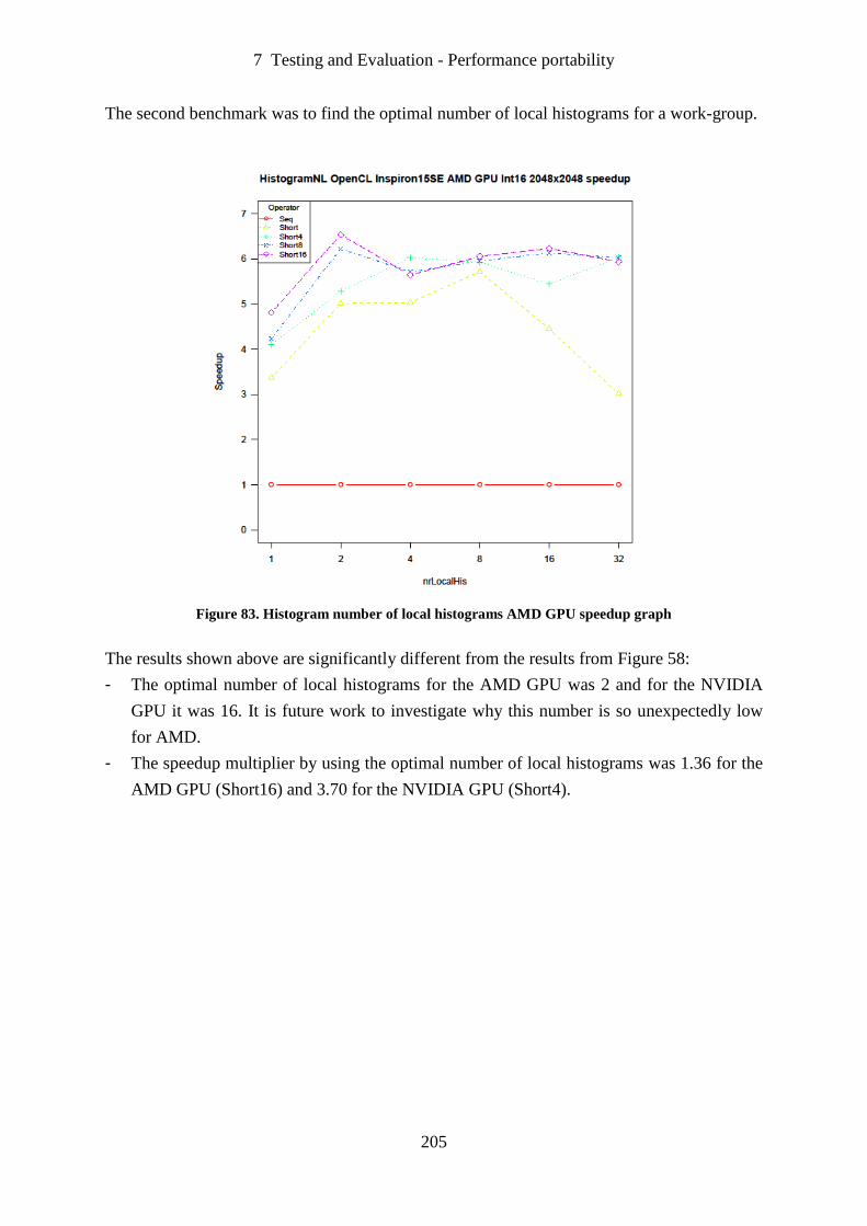
7 Testing and Evaluation - Performance portability
205
The second benchmark was to find the optimal number of local histograms for a work-group.
Figure 83. Histogram number of local histograms AMD GPU speedup graph
The results shown above are significantly different from the results from Figure 58:
- The optimal number of local histograms for the AMD GPU was 2 and for the NVIDIA
GPU it was 16. It is future work to investigate why this number is so unexpectedly low
for AMD.
- The speedup multiplier by using the optimal number of local histograms was 1.36 for the
AMD GPU (Short16) and 3.70 for the NVIDIA GPU (Short4).
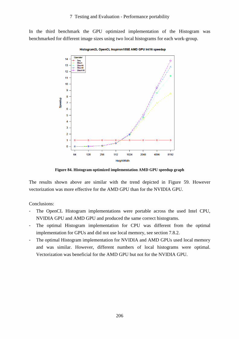
7 Testing and Evaluation - Performance portability
206
In the third benchmark the GPU optimized implementation of the Histogram was
benchmarked for different image sizes using two local histograms for each work-group.
Figure 84. Histogram optimized implementation AMD GPU speedup graph
The results shown above are similar with the trend depicted in Figure 59. However
vectorization was more effective for the AMD GPU than for the NVIDIA GPU.
Conclusions:
- The OpenCL Histogram implementations were portable across the used Intel CPU,
NVIDIA GPU and AMD GPU and produced the same correct histograms.
- The optimal Histogram implementation for CPU was different from the optimal
implementation for GPUs and did not use local memory, see section 7.8.2.
- The optimal Histogram implementation for NVIDIA and AMD GPUs used local memory
and was similar. However, different numbers of local histograms were optimal.
Vectorization was beneficial for the AMD GPU but not for the NVIDIA GPU.
7 Testing and Evaluation - Performance portability
207
7.11.4 Conclusions
The following is concluded:
- The experiments suggest that OpenMP implementations could be portable without
modification across operating systems and CPU architectures and maintain a similar level
of speedups.
- These experiments and the research and experiments described in section 2.2 suggest that
OpenCL implementations could be portable across CPUs and GPUs but the performance
is not easily portable. This view is confirmed by Van der Sanden (2011, section 5.3), Ali,
Dastgeer and Keesler (2012), Zimmer and Moore (2012) and by the audience of the
conference GPGPU-day (Platform Parallel Netherlands, 2012) where the author presented
the preliminary results of his work (Van de Loosdrecht, 2012d).
7.11.5 Future work
- The optimal number of local histograms for the AMD GPU was 2 and for the NVIDIA
GPU was 16. It is future work to investigate why this number is so unexpectedly low for
AMD.
- The performance of OpenCL was not portable. Research is needed to investigate the
possibilities to write generic OpenCL kernels, kernels that run with adequate performance
on multiple platforms. Some preliminary work on this subject can be found in Van der
Sanden (2011, section 5.4). Fang, Varbanescu and Sips (2011) suggest developing an
auto-tuner to adapt general-purpose OpenCL programs to all available specific platforms
to fully exploit the hardware.
7 Testing and Evaluation - Parallelization in real projects
208
7.12 Parallelization in real projects
7.12.1 Introduction
In section 3.6.2 four classes of basic low level image operators are distinguished. For each
class OpenMP and OpenCL versions were implemented and benchmarked. OpenMP was
considered (see section 8.4) to be the best candidate to parallelize VisionLab in an efficient
and effective way. The OpenMP implementations were used as templates to parallelize 170
operators of VisionLab, including many high level operators like the BlobMatcher (section
7.12.2.2). See Appendix G for a full list. The Automatic Operator Parallelization mechanism
was also implemented for these operators. VisionLab with the OpenMP parallelization is now
available as a commercial product.
In this section two examples of real projects of customers of VdLMV are given in order to
demonstrate the benefits of parallelization using OpenMP. The Antibiotics discs case is an
example where almost 100% of the used C++ code for the operators could be parallelized.
This example will give an impression of the best speedup possible for real cases. The 3D
monitor case is an example where a VisionLab script was automatically parallelized.
7.12.2 Antibiotic discs
7.12.2.1 Introduction
The Antibiotic discs project is from BD Kiestra (Drachten, the Netherlands), who are one of
the market leaders in Europe in Total Lab Automation. The following is based on the
description in Dijkstra (2013). One of BD Kiestra’s products automates antibiotic
susceptibility testing by disk diffusion. This analysis is performed on a regular basis in
microbiological laboratories. This method is used to determine the susceptibility to a certain
antibiotic of bacteria found in a patient. This information is used by the physician to
determine which antibiotic to prescribe.
A Petri dish containing agar, a bacterial growth medium, is inoculated with sample material
from a patient. After this, discs are placed on the inoculated Petri dish, where each disc
contains a printed abbreviation of the antibiotic contained in the disc. The antibiotic
contained in the disc flows into the agar. The dish is incubated for a predetermined number of
hours to stimulate bacterial growth. During the incubation process the bacteria start to grow
on the agar at locations where they can still resist the antibiotic concentration.

7 Testing and Evaluation - Parallelization in real projects
209
After incubation the agar contains bacterial growth all over the Petri dish except for circular
areas around the discs. In these circular areas or zones the concentration of the antibiotic is
too high for the bacteria to be able to grow. The diameter of the zone indicates the
susceptibility of the bacteria to the antibiotic contained in the disc. Conceptually the problem
in automating this analysis is two-fold. At the first level, the reading of the antibiotic disc
prints has to be automated, and at the second level the zone measurement has to be
automated. See Figure 85 for an example image.
Figure 85. Antibiotic susceptibility testing by disk diffusion
Dijkstra, Jansen and Van de Loosdrecht (2013a, 2013b) and Dijkstra, Berntsen, Van de
Loosdrecht and Jansen (2013) describe how to automate the reading of the antibiotic disc
prints with an end-user trainable machine vision framework. This project was developed in
collaboration with the NHL Centre of Expertise in Computer Vision.
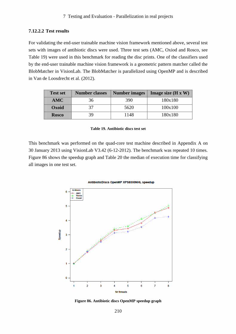
7 Testing and Evaluation - Parallelization in real projects
210
7.12.2.2 Test results
For validating the end-user trainable machine vision framework mentioned above, several test
sets with images of antibiotic discs were used. Three test sets (AMC, Oxiod and Rosco, see
Table 19) were used in this benchmark for reading the disc prints. One of the classifiers used
by the end-user trainable machine vision framework is a geometric pattern matcher called the
BlobMatcher in VisionLab. The BlobMatcher is parallelized using OpenMP and is described
in Van de Loosdrecht et al. (2012).
Test set Number classes Number images Image size (H x W)
AMC 36 390 180x180
Oxoid 37 5620 100x100
Rosco 39 1148 180x180
Table 19. Antibiotic discs test set
This benchmark was performed on the quad-core test machine described in Appendix A on
30 January 2013 using VisionLab V3.42 (6-12-2012). The benchmark was repeated 10 times.
Figure 86 shows the speedup graph and Table 20 the median of execution time for classifying
all images in one test set.
Figure 86. Antibiotic discs OpenMP speedup graph

7 Testing and Evaluation - Parallelization in real projects
211
Table 20. Antibiotic discs OpenMP median of execution times in seconds
7.12.2.3 Conclusions
The following is concluded:
- Speedups between 4.26 (Oxoid) and 5.02 (Rosco) were accomplished. The least speedup
was obtained with the test set with the smallest images.
- Hyper-threading was beneficial.
- The violin plots (Appendix F) showed little variance in execution time over one test set.
7.12.3 3D monitor
7.12.3.1 Introduction
The 3D monitor project is from Image+ (Stadskanaal, The Netherlands), who are one of the
market leaders in Europe in Ride Photography in theme parks. According to Fun World
(2011):
“Image+ introduced a product that has never been seen before in the attractions
industry: 3-D ride photography. The company rolled the system out at Theme Park and
Resort Slagharen in the Netherlands. Guests are photographed with a custom-made 3-
D camera, and within a few seconds those images are converted into 3-D and shown on
3-D monitors. The real perk comes when the 3-D effect can be viewed without the need
for 3-D glasses. Then, if the guest wants the photo, it is printed in 3-D by a specialized
printer.”
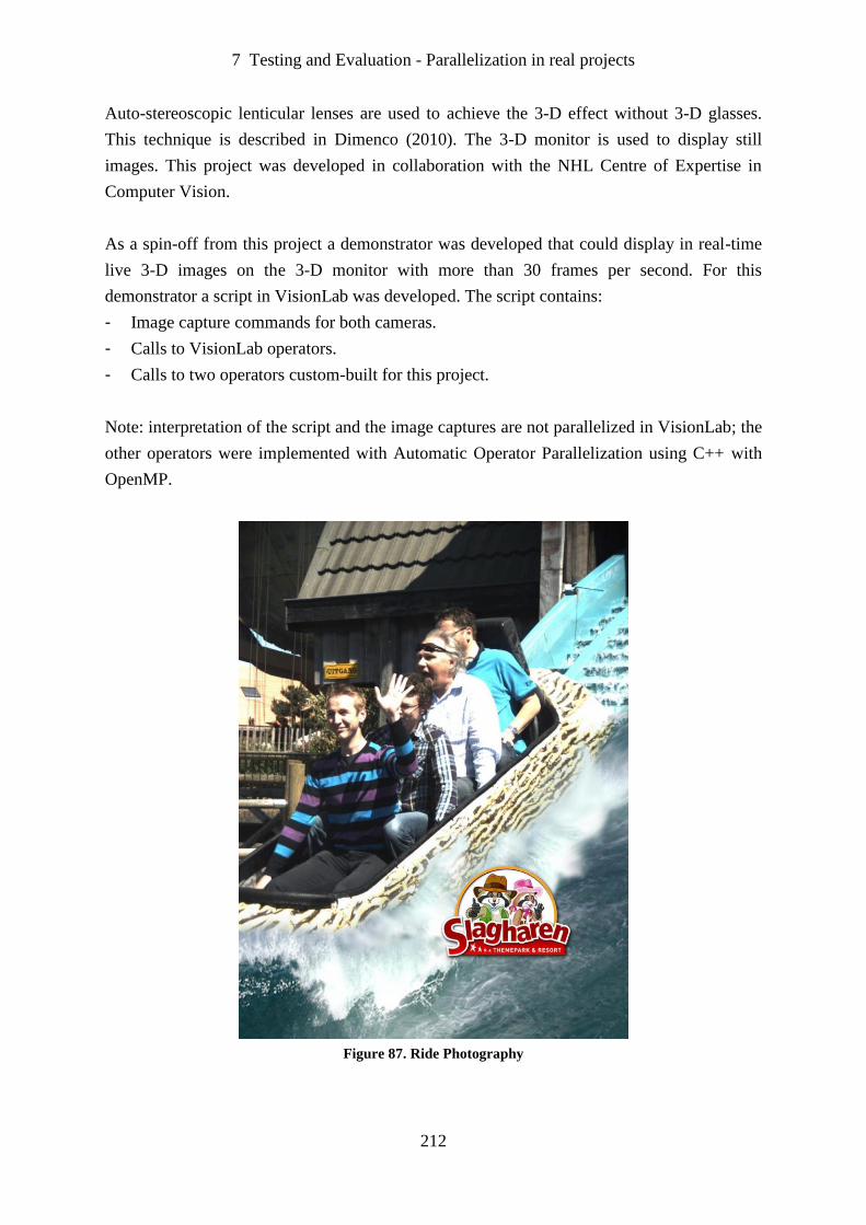
7 Testing and Evaluation - Parallelization in real projects
212
Auto-stereoscopic lenticular lenses are used to achieve the 3-D effect without 3-D glasses.
This technique is described in Dimenco (2010). The 3-D monitor is used to display still
images. This project was developed in collaboration with the NHL Centre of Expertise in
Computer Vision.
As a spin-off from this project a demonstrator was developed that could display in real-time
live 3-D images on the 3-D monitor with more than 30 frames per second. For this
demonstrator a script in VisionLab was developed. The script contains:
- Image capture commands for both cameras.
- Calls to VisionLab operators.
- Calls to two operators custom-built for this project.
Note: interpretation of the script and the image captures are not parallelized in VisionLab; the
other operators were implemented with Automatic Operator Parallelization using C++ with
OpenMP.
Figure 87. Ride Photography
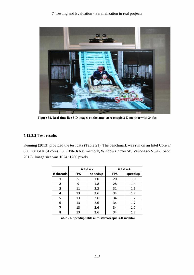
7 Testing and Evaluation - Parallelization in real projects
213
Figure 88. Real-time live 3-D images on the auto-stereoscopic 3-D monitor with 34 fps
7.12.3.2 Test results
Keuning (2013) provided the test data (Table 21). The benchmark was run on an Intel Core i7
860, 2,8 GHz (4 cores), 8 GByte RAM memory, Windows 7 x64 SP, VisionLab V3.42 (Sept.
2012). Image size was 1024×1280 pixels.
# threads FPS speedup FPS speedup
1 5 1.0 20 1.0
2 9 1.8 28 1.4
3 11 2.2 31 1.6
4 13 2.6 34 1.7
5 13 2.6 34 1.7
6 13 2.6 34 1.7
7 13 2.6 34 1.7
8 13 2.6 34 1.7
scale = 2 scale = 4
Table 21. Speedup table auto-stereoscopic 3-D monitor
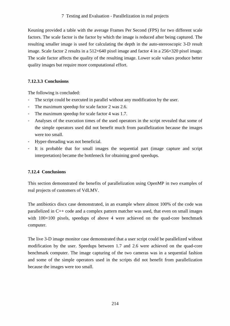
7 Testing and Evaluation - Parallelization in real projects
214
Keuning provided a table with the average Frames Per Second (FPS) for two different scale
factors. The scale factor is the factor by which the image is reduced after being captured. The
resulting smaller image is used for calculating the depth in the auto-stereoscopic 3-D result
image. Scale factor 2 results in a 512×640 pixel image and factor 4 in a 256×320 pixel image.
The scale factor affects the quality of the resulting image. Lower scale values produce better
quality images but require more computational effort.
7.12.3.3 Conclusions
The following is concluded:
- The script could be executed in parallel without any modification by the user.
- The maximum speedup for scale factor 2 was 2.6.
- The maximum speedup for scale factor 4 was 1.7.
- Analyses of the execution times of the used operators in the script revealed that some of
the simple operators used did not benefit much from parallelization because the images
were too small.
- Hyper-threading was not beneficial.
- It is probable that for small images the sequential part (image capture and script
interpretation) became the bottleneck for obtaining good speedups.
7.12.4 Conclusions
This section demonstrated the benefits of parallelization using OpenMP in two examples of
real projects of customers of VdLMV.
The antibiotics discs case demonstrated, in an example where almost 100% of the code was
parallelized in C++ code and a complex pattern matcher was used, that even on small images
with 100×100 pixels, speedups of above 4 were achieved on the quad-core benchmark
computer.
The live 3-D image monitor case demonstrated that a user script could be parallelized without
modification by the user. Speedups between 1.7 and 2.6 were achieved on the quad-core
benchmark computer. The image capturing of the two cameras was in a sequential fashion
and some of the simple operators used in the scripts did not benefit from parallelization
because the images were too small.

8 Discussion and Conclusions - Introduction
215
8 Discussion and Conclusions
8.1 Introduction
The Computer Vision algorithms of VisionLab were limited by the performance capabilities
of sequential processor architectures. From the developments of both CPU and GPU
hardware in the last decade it was evident that the only way to get more processing power
using commodity hardware was to adopt parallel programming. This project investigated how
to speed up a whole library by parallelizing the algorithms in an economical way and
executing them on multiple platforms.
In this chapter the following topics are discussed:
- Evaluation of parallel architectures.
- Benchmark protocol and environment.
- Evaluation of parallel programming standards.
- Contributions of the research.
- Future work.
- Final conclusions.
8.2 Evaluation of parallel architectures
The primary target system for this work was a conventional PC, embedded real-time
intelligent camera or mobile device with a single or multi-core CPU with one or more GPUs
running under Windows or Linux on a x86 or x64 processor. Benchmarks were run on
conventional PCs with graphics cards of NVIDIA and AMD. Because portability to other
processors was an important issue, a benchmark was run on an embedded real-time board
with a multi-core ARM processor. Both the literature review and the results of the
benchmarks in this work confirmed that both multi-core CPU and GPU architectures are
appropriate for accelerating sequential Computer Vision algorithms.
There is a lot of new development in hardware and programming environments for parallel
architectures. It is to be expected that new developments in hardware will have a strong
impact on software design.
Embarrassingly parallel algorithms are fairly easy to parallelize. Embarrassingly sequential
algorithms will need a completely different programming approach. The parallelization of the
Connected Component Labelling algorithm demonstrated that different parallel approaches
will be needed for few-cores and many-cores systems.
8 Discussion and Conclusions - Benchmark protocol and environment
216
8.3 Benchmark protocol and environment
Based on existing literature, a suitable benchmark protocol was defined and used in this
work. A benchmark environment for assessing the benefits of parallelizing algorithms was
designed and implemented. This benchmark environment was integrated in the script
language of VisionLab. By using this benchmark environment it was possible to setup, run
and analyse the benchmarks in a comfortable and repeatable way.
8.4 Evaluation of parallel programming standards
8.4.1 Introduction
In this section the following topics are discussed:
- Survey of standards for parallel programming.
- Evaluation of choice for OpenMP.
- Evaluation of choice for OpenCL.
- Evaluation of newly emerged standards and new developments of standards.
- Recommendations for standards.
8.4.2 Survey of standards for parallel programming
Twenty-two standards for parallel programming were reviewed using the requirements as
specified for this work. OpenMP was chosen as the standard for multi-core CPU
programming and OpenCL as the standard for GPU programming. These two standards were
used throughout this work for all experiments.
8.4.3 Evaluation of choice for OpenMP
Learning OpenMP was easy because there are only a limited number of concepts, which have
a high level of abstraction with only a few parameters. The development environments used,
Visual Studio and the GNU tool chain, have a mature and stable implementation of OpenMP.
OpenMP supports multi-core CPU programming but offers no support for exploiting vector
capabilities.
8 Discussion and Conclusions - Evaluation of parallel programming standards
217
The effort for parallelizing embarrassingly parallel algorithms, like Threshold and
Convolution, is just adding one line with the OpenMP pragma. The parallelized operator also
has to be incorporated in the Automatic Operator Parallelization. This is a run-time prediction
mechanism that will test whether parallelization will be beneficial. To add the parallelized
operator to the Automatic Operator Parallelization calibration procedure will need about 16
lines of code. Those 16 lines of code are very similar for all operators and are of low
complexity. More complicated algorithms like Histogram and LabelBlobs need more effort to
parallelize. The effort for adding to the Automatic Operator Parallelization calibration
procedure remains the same. Speedups between 2.5 and 5 were reported for large images in
the benchmarks on a quad-core Intel i7 running Windows 7. Big penalties for speedup were
reported in almost all benchmarks for small images. So run-time prediction whether
parallelization is expected to be beneficial is a necessity.
Four classes of basic low level image operators were distinguished in this work. For each
class an OpenMP version was implemented and benchmarked. These OpenMP
implementations were used as templates to parallelize 170 operators of VisionLab, including
many high level operators. See Appendix G for a full list. It only took about one man month
of work to parallelize all the 170 operators, including the Automatic Operator Parallelization.
VisionLab with the OpenMP parallelization is now available as a commercial product.
The violin plots showed that parallelizing can significantly increase the variance in execution
time. This increase is more prominent for the smaller images.
VisionLab scripts written by users will, without modification, immediately benefit in speedup
when using the new parallelized version of VisionLab. Users of VisionLab who write their
code in C++ or C# will benefit, without changing their code, from the parallelization after
linking to the new library. For optimal results users will have to calibrate the Automatic
Operator Parallelization. Two cases of test data of real projects were presented in this work,
reporting speedups between 1.7 and 5 on a quad-core Intel i7 running Windows 7.
The portability of the OpenMP approach was tested on a quad-core ARM running Linux.
Porting was just recompiling. It passed the VisionLab regression test suite without any
problems and the Convolution benchmark reported speedups up to 3.97.
It is concluded that OpenMP is very well suited for parallelizing many algorithms of a library
in an economical way and executing them with an adequate speedup on multi-core CPU
platforms.
8 Discussion and Conclusions - Evaluation of parallel programming standards
218
8.4.4 Evaluation of choice for OpenCL
Although the author has a background in parallel programming, learning OpenCL was found
to be difficult and time-consuming because:
- There are many concepts, often with a low level of abstraction and many parameters.
Good understanding of GPU architectures is essential.
- The host-side code is labour-intensive and sensitive to errors because most OpenCL API
functions have many parameters.
- The kernel language itself is not difficult but there are many details to master.
- The logic of an algorithm is divided over the kernel language and host language with
often subtle dependencies.
- OpenCL platforms are ‘in development and have issues’. NVIDIA, AMD and Intel
platforms were used. Platform tools from NVIDIA and Intel were found to interfere with
each other, and for one specific GPU the AMD compiler crashed on some of the kernels.
- The correct tuning of many parameters is laborious but paramount for decent
performance.
Instead of writing the host API code in C or C++, VisionLab scripts were used. The script
language of VisionLab was extended with OpenCL host API commands. Using these
commands greatly reduced the time to develop and test the host-side code.
OpenCL supports both multi-core CPU and GPU programming. OpenCL also has support for
exploiting vector capabilities and heterogeneous computing.
The effort to parallelize embarrassingly parallel algorithms was considerable; both kernel
code and host-side code had to be developed. Four classes of basic low level image operators
were distinguished in this work. OpenCL versions for CPU and GPU were implemented and
benchmarked. In many cases simple implementations demonstrated considerable speedups. In
all cases a considerable amount of effort was necessary to obtain better speedups by using
more complex algorithms and tuning parameters. For the Connected Component Labelling
algorithm a complete new approach was necessary. For contemporary GPUs the overhead of
data transfer between host and device is substantial compared to the kernel execution time of
embarrassingly parallel algorithms like Threshold. When the new heterogeneous architectures
reach the market, such as predicted by the HSA Foundation, this data transfer overhead is
expected to reduce significantly.

8 Discussion and Conclusions - Evaluation of parallel programming standards
219
Speedups up to 60 were reported on benchmarks for large images. Big penalties for speedup
were reported in some of the benchmarks for small images or if wrong tuning parameters
were chosen. Completely different approaches were necessary for CPU and GPU
implementations. The test with the OpenCL Histogram implementations on NVIDIA and
AMD GPUs suggests that GPU implementations for different GPUs need different
approaches and/or parameterization for optimal speedup. It is expected that OpenCL kernels
are portable but the performance will not be portable. In other words, when an OpenCL
kernel is parameterized well with the host code it will run on many OpenCL devices, but the
maximal performance on a device will be obtained only with a device-specific version of the
kernel and with tuned parameters.
The violin plots showed that parallelizing can significantly increase the variance in execution
time. This increase is more prominent for the smaller images and more substantial for CPU
than GPU. The increase of variance using OpenCL on CPU is mostly smaller than when
using OpenMP.
It is concluded that OpenCL is not very well suited for parallelizing all algorithms of a whole
library in an economical way and executing them effectively on multiple platforms.
Nonetheless, OpenCL has the potential to exploit the enormous processor power of GPUs,
the vector capabilities of CPUs and heterogeneous computing.
It is recommended that OpenCL be used for accelerating dedicated algorithms on specific
platforms when the following conditions are met:
- The algorithms are computationally expensive.
- The overhead of data transfer is relatively small compared to the execution time of the
kernels involved.
- It is accepted that a considerable amount of effort is needed for writing and optimizing
the code.
- It is accepted that the OpenCL code is optimized for one device, or that sub-optimal
speedup is acceptable if the code should run on similar but distinct devices.
8 Discussion and Conclusions - Evaluation of parallel programming standards
220
8.4.5 Evaluation of newly emerged standards and new developments of standards
Section 3.8 described which new information became available about standards for parallel
programming after the choices for OpenMP and OpenCL had been made. This new
information is discussed in this section.
- CUDA has become less vendor specific, but is still far from being an industry standard.
- Microsoft released C++ AMP with Visual Studio 2012. This is a great tool, but very
vendor specific.
- An enhancement of the OpenCL kernel languages is proposed with C++ like features
such as classes and templates. At the moment of writing this new kernel language is only
supported by AMD.
- Altera Corporation introduced an OpenCL program for FPGAs. This opens up the
possibility of compiling OpenCL directly to silicon.
- OpenACC was announced and products became available. It is expected that OpenACC
will merge with OpenMP 4.0.
- In 2013 a new standard, OpenMP 4.0 with “directives for attached accelerators”, is
expected that will allow portable OpenMP pragma-style programming on multi-core
CPUs and GPUs. With the new OpenMP standard it will be possible to utilize vector
capabilities of CPUs and GPUs.
Compared with OpenCL this new standard will allow multi-core CPU and GPU
programming at a higher abstraction level than OpenCL. The author expects that with the
new OpenMP standard it will be much easier to program portable code, but the code will
not be as efficient as programmed with OpenCL.
8 Discussion and Conclusions - Evaluation of parallel programming standards
221
8.4.6 Recommendations for standards
Based on the previous sections the following recommendations are made.
- OpenMP is very well suited for parallelizing many algorithms of a library in an
economical way and executing them with an adequate speedup on multiple parallel CPU
platforms. It is recommended that all VisionLab operators are parallelized using
OpenMP.
- OpenCL is not suitable for parallelizing all algorithms of a whole library in an
economical way and executing them effectively on multiple GPU platforms. At the
moment there is no suitable standard for the requirements as formulated in section 2.4. In
the author’s view, OpenCL is still the best choice in this domain. OpenCL has the
potential to exploit the enormous processor power of GPUs, the vector capabilities of
CPUs and heterogeneous computing. When the speedup achieved with OpenMP is not
adequate, it is recommended that OpenCL be used for accelerating dedicated algorithms
on specific platforms.
- In the future OpenMP 4.0 with “directives for attached accelerators” might be a very
good candidate for parallelizing a library in an economical way on both CPUs and GPUs.
The announced proposal looks very promising, however at the time of writing the
standard is not definitive and there are no compilers supporting it.
The first two recommendations are in line with the conclusions in the survey performed by
Diaz, Munoz-Cara and Nino (2012).
8 Discussion and Conclusions - Contributions of the research
222
8.5 Contributions of the research
8.5.1 Introduction
In this section the following contributions of this work are discussed:
- Algorithmic improvements.
- Publications.
- Product innovation.
8.5.2 Algorithmic improvements
The following algorithmic improvements appear to be novel. The literature search has not
found any previous use of them:
- Vectorization of Convolution on grayscale images with variable sized mask utilizing
padding width of vector with zeros, section 6.6.2.4.4.
- Few-core Connect Component Labelling, section 6.8.2.3.
- Optimization of many-core Connect Component Labelling using the approach of
Kalentev et al., section 6.8.2.4.
8.5.3 Publications
In this section the publications related to this work are listed.
Peer review:
- Draft manuscript VLSI1274 On the Image Convolution Supported on OpenCL Compliant
Multicore Processors (Antao, Sousa and Chaves, 2011) in The Journal of Signal
Processing.
Papers:
- Accelerating sequential Computer Vision algorithms using commodity parallel hardware
(Van de Loosdrecht, 2013b) in the proceedings of NIOC2013 in Arnhem (The
Netherlands), 4-5 April 2013.
- Prior knowledge in an end-user trainable machine vision framework (Dijkstra, Jansen
and Van de Loosdrecht, 2013a) in the proceedings of 21st European Symposium on
Artificial Neural Networks, Computational Intelligence and Machine Learning in Bruges
(Belgium), 24 - 26 April 2013. See section 7.12.2 for link with this work.
8 Discussion and Conclusions - Contributions of the research
223
Poster presentations:
- Prior knowledge in an end-user trainable machine vision framework (Dijkstra, Jansen
and Van de Loosdrecht, 2013b), presented by co-author at 21th
European Symposium on
Artificial Neural Networks, Computational Intelligence and Machine Learning in Bruges
(Belgium), 24 - 26 April 2013. See section 7.12.2 for link with this work.
- End-user trainable automatic antibiotic-susceptibility testing by disc diffusion using
machine vision (Dijkstra, Berntsen, Van de Loosdrecht and Jansen, 2013), presented by
co-author at 23rd
European Congress of Clinical Microbiology and Infectious Diseases,
Berlin 27-30 April 2013. See section 7.12.2 for link with this work.
Lectures:
- Accelerating sequential Computer Vision algorithms using commodity parallel hardware
at University Groningen, research group Scientific Visualization and Computer Graphics,
12 March 2012.
- Accelerating sequential Computer Vision algorithms using commodity parallel hardware
at Cluster Computer Vision Noord Nederland, Miedema, Winsum, 13 March 2012.
- Accelerating sequential Computer Vision algorithms using commodity parallel hardware
at Parallel Architecture Research group Eindhoven University of Technology, 13 April
2012.
- Accelerating sequential Computer Vision algorithms using commodity parallel hardware
(Van de Loosdrecht, 2012d) at the GPGPU-day in Amsterdam on 28 June 2012 (Platform
Parallel Netherlands, 2012).
- Accelerating sequential Computer Vision algorithms using OpenMP and OpenCL on
commodity parallel hardware at NHL University on 13 September 2012.
- Accelerating sequential Computer Vision algorithms using commodity parallel hardware
at INCAS3 research group University Groningen on 6 March 2013.
- Parallelliseren van algoritmen mbv OpenMP en OpenCL voor multi-core CPU en GPU
at department of Computer Science, NHL University on 7 March 2013.
- Accelerating sequential Computer Vision algorithms using commodity parallel hardware
at RAAK Vision in Mechatronics and Robotics, Leeuwarden on 8 March 2013.
- Accelerating sequential Computer Vision algorithms using commodity parallel hardware
at NIOC2013 (NIOC, 2013), Arnhem on 4 April 2013.
- Accelerating sequential Computer Vision algorithms using commodity parallel hardware
at Photonics Event 2013 (Photonics, 2013) in Velthoven on 25 April 2013.
- Accelerating sequential Computer Vision algorithms using commodity parallel hardware
at Vision, Robotics & Mechtronics 2013 (Mikrocentrum, 2013) in Velthoven on 23 May
2013.

8 Discussion and Conclusions - Contributions of the research
224
- Connected Component Labelling, an embarrassingly sequential algorithm (Van de
Loosdrecht, 2013c) at the Applied GPGPU-day 2013 in Amsterdam on 20 June 2013
(Platform Parallel Netherlands, 2013).
- Connected Component Labelling, an embarrassingly sequential algorithm (Van de
Loosdrecht, 2013d) at University Groningen, research group Scientific Visualization and
Computer Graphics on 3 September 2013.
Course material:
- Accelerating sequential Computer Vision algorithms using OpenMP and OpenCL on
commodity parallel hardware (Van de Loosdrecht, 2012a). This is a general introduction
to OpenMP en OpenCL and is publicly available on the internet.
- Multi-core processing in VisionLab (Van de Loosdrecht, 2012b). This describes how to
calibrate and to use Automatic Operator Parallelization calibration for multi-core CPUs in
VisionLab and is publicly available on the internet.
8.5.4 Product innovation
This work resulted directly in innovations in the commercially available product VisionLab.
- 170 operators were parallelized using OpenMP and Automatic Operator Parallelization
was implemented. Users of VisionLab can now benefit from parallelization without
having to rewrite their scripts, C++ or C# code.
- OpenCL toolbox was added to the development environment. Users of VisionLab can
now comfortably write OpenCL host-side code using the script language and edit their
kernels. The OpenCL host interface was implemented and tested for NVIDIA, AMD and
Intel OpenCL platforms.
8 Discussion and Conclusions - Future work
225
8.6 Future work
Many of the previous chapters contained sections on future work on the subjects discussed in
that chapter. In this section the main direction for future work is discussed.
8.6.1 Future work in relation to multi-core CPU programming
- At the moment the 170 frequently used operators are parallelized using OpenMP. The
other operators must still be parallelized.
- The Automatic Operator Parallelization mechanism is calibrated with the most frequent
used image type and with one typical image selected for each individual operator.
It is expected that the calibration result for a specific operator will be similar for all image
types. This assumption must be validated by benchmarking. Otherwise a separate
calibration for all image types will be necessary.
Research is needed to investigate whether calibration can be improved with a set of
images for each operator.
- The Automatic Operator Parallelization mechanism uses either the number of threads
specified by the user or one thread. Future research is needed to investigate if a finer
granularity would be beneficial.
- Experiments should be undertaken with portable vectorization when products become
available with the announced OpenMP 4.0 with support for “directives for attached
accelerators”.
- Experiments should be undertaken with OpenMP scheduling strategies to reduce variance
in execution times.
- Experiments should be undertaken with OpenMP on Android when available.
- Research and experiments are needed to investigate the possibilities and limitations of the
scalability to ccNUMA distributed memory systems.
8.6.2 Future work in relation to GPU programming
- More time must be invested in understanding GPU architectures, OpenCL and OpenCL
profiling tools in order to come to a better understanding of the bottlenecks in
performance.
- Time-consuming (combinations of) operators should be selected for pilot projects.
- At the moment not all OpenCL host API functions are available in the script language.
The C++ wrapper around the host API must be extended and new commands added to the
command interpreter of VisionLab.
8 Discussion and Conclusions - Future work
226
- Intelligent buffer management should be implemented in the C++ module with an
abstraction layer on top of OpenCL host API. With intelligent buffer management,
unnecessary transfer of data between host and device can be detected and avoided.
- The performance of OpenCL is not portable. Research is needed to investigate the
possibilities for writing generic OpenCL kernels, i.e. kernels that run with adequate
performance on multiple platforms.
- OpenCL programs have many parameters that need tuning for optimal performance.
Manual tuning of these parameters is laborious. If OpenCL is to be run on multiple
platforms, a mechanism for the automatic tuning of these parameters is required. The
author suggests that a possible line of research is to develop a framework for the
automatic optimization of those parameters using Genetic Algorithms.
- Experiments should be undertaken with GPU programming using the announced
OpenMP 4.0 with “directives for attached accelerators” when products become available.
- Research and experiments are needed to investigate the possibilities and limitations of the
scalability to multiple graphics cards.
8.6.3 Future work in relation to heterogeneous computing
- It is expected that it will be beneficial to combine multi-core CPU and GPU computing.
Research is needed to investigate the possibilities and limitations.
- Research is needed for creating a decision framework for deciding which parts of
algorithms should run on which platforms. Preliminary research on this topic has been
done by Brown (2011).
8.6.4 Future work in relation to automatic parallelization or vectorization of code
- Although world-wide a lot of research has been done in this field, it is still not applicable
to parallelizing a whole library in an economical way and executing it on multiple
platforms.
Experiments with the automatic parallelization and vectorization capabilities of Visual
Studio 2012 were disappointing. The automatic parallelization is a vendor specific
mechanism very similar to OpenMP. Without modification of code, automatic
vectorization (Hogg, 2012) was only profitable for three for loops, all with only a one line
body, in the 100,000 lines of source code of VisionLab.
- Research is needed to investigate the state of the art of other tools.
8 Discussion and Conclusions - Final conclusions
227
8.6.5 Future work in relation to benchmarking parallel algorithms
- The reproducibility of the experiments is low. It seems to the author that the question of
accessing the quality, such as reproducibility and variance in execution time, of
benchmarking parallel algorithms has not been fully addressed in the research literature.
8.6.6 Future work in relation to parallelizing Computer Vision algorithms
- More literature research is needed for parallelizing non-embarrassingly parallel image
operators and for the pattern matchers, neural networks and genetic algorithms used in
VisionLab.
- The Khronos Group has proposed an initiative to create a new open standard for hardware
accelerated Computer Vision. The draft of this standard is expected to be published in
2013. It could be very interesting to join this initiative, and analysis of the proposal is
recommended
8.7 Final conclusions
The complexity of Computer Vision applications continues to increase, often with more
demanding real time constraints, so there is an increasing demand for more processing power.
This demand is also driven by the increasing pixel resolution of cameras.
The author fully agrees with “The Free Lunch Is Over: A Fundamental Turn Toward
Concurrency in Software” (Sutter, 2005) in which it was predicted that the only way to get
more processing power in the future is to adopt parallel programming, and that it is not going
to be an easy way.
At both NHL and LIT there is no tradition of parallel programming. In order to get ideas and
feedback, research groups of other universities were visited, conferences were attended and
lectures presented. In the opinion of the author, Computer Vision is not the only domain with
an increasing need for more processor power and limited by the performance capabilities of
sequential processor architectures. Therefore it is recommended that NHL and LIT start
lecturing parallel programming. Introductory course material has been developed by the
author.
8 Discussion and Conclusions - Final conclusions
228
Many other related research projects have considered one domain specific algorithm to
compare the best sequential with best parallel implementation on a specific hardware
platform. This project is distinctive because it investigated how to speed up a whole library
by parallelizing the algorithms in an economical way and executing them on multiple
platforms.
The aim of this project was to investigate the use of parallel algorithms to improve execution
time in the specific field of Computer Vision using an existing product (VisionLab) and
research being undertaken at NHL. This work demonstrated clearly that execuation times of
algorithms can be improved significantly using a parallel approach.
Twenty-two programming languages and environments for parallel computing on multi-core
CPUs and GPUs were examined, compared and evaluated. One standard, OpenMP, was
chosen for multi-core CPU programming and another standard, OpenCL, was chosen for
GPU programming.
Based on the classification of low level image operators, an often used representative of each
class was chosen and re-implemented using both standards. The performance of the parallel
implementations was tested and compared to the existing sequential implementations in
VisionLab.
The results were evaluated with a view to assessing the appropriateness of multi-core CPU
and GPU architectures in Computer Vision as well to assessing the benefits and costs of
parallel approaches to implementation of Computer Vision algorithms.
Using OpenMP it was demonstrated that many algorithms of a library could be parallelized in
an economical way and that adequate speedups were achieved on two multi-core CPU
platforms. A run-time prediction mechanism that will test whether parallelization will be
beneficial was successfully implemented for this OpenMP approach. With a considerable
amount of extra effort, OpenCL was used to achieve much higher speedups for specific
algorithms on dedicated GPUs.
229
References
Ali, A., Dastgeer, U. and Keesler, C., 2012. OpenCL for programming shared memory
multicore CPUs. MULTIPROG-2012 Workshop at HiPEAC-2012.[pdf] Available at:
http://www.ida.liu.se/~chrke/pub/Ali-HiPEAC-MULTIPROG-2012-wksh-final16.pdf
[Accessed 14 March 2013].
Altera Corporation, 2011. Implementing FPGA Design with the OpenCL Standard. [pdf]
Available at: http://www.altera.com/b/opencl.html [Accessed 18 December 2011].
AMD, 2011a. AMD Accelerated Parallel Processing OpenCL Programming Guide. May
2011. [pdf] Sunnyvale, CA: Advanced Micro Devices, Inc. Available at:
http://developer.amd.com/gpu/AMDAPPSDK/assets/AMD_Accelerated_Parallel_Processing
_OpenCL_Programming_Guide.pdf [Accessed 20 May 2011].
AMD, 2011b. AMD Accelerated Parallel Processing OpenCL Programming Guide. August
2011. [pdf] Sunnyvale, CA: Advanced Micro Devices, Inc. Available at:
http://developer.amd.com/sdks/AMDAPPSDK/assets/AMD_Accelerated_Parallel_Processin
g_OpenCL_Programming_Guide.pdf [Accessed 24 November 2011].
AMD, 2012. Programming Guide AMD Accelerated Parallel Processing OpenCL. July 2012.
[pdf] Sunnyvale, CA: Advanced Micro Devices, Inc. Available at:
http://developer.amd.com/sdks/AMDAPPSDK/assets/AMD_Accelerated_Parallel_Processin
g_OpenCL_Programming_Guide.pdf [Accessed 12 November 2012].
AMD, 2013a. AMD Radeon™ HD 7970 GHz Edition Graphics Cards. [online] Sunnyvale,
CA: Advanced Micro Devices, Inc. Available at:
http://www.amd.com/uk/products/desktop/graphics/7000/7970ghz/Pages/radeon-
7970GHz.aspx#3 [Accessed 11 April 2013].
AMD, 2013b. Bolt C++ Template Library. [online] Sunnyvale, CA: Advanced Micro
Devices, Inc. Available at: http://developer.amd.com/tools-and-sdks/heterogeneous-
computing/amd-accelerated-parallel-processing-app-sdk/bolt-c-template-library/ [Accessed
26 April 2013].
Amdahl, G.M., 1967. Validity of the Single Processor Approach to Achieving Large Scale
Computing Capabilities. AFIPS Conference Proceedings, 30, pp.483-85.
Andrade, D., 2011. Case study: High performance convolution using OpenCL __local
memory. [online] : CMSoft. Available at:
http://www.cmsoft.com.br/index.php?option=com_content&view=category&layout=blog&id
=142&Itemid=201 [Accessed 12 December 2012].
Andrade, D., Fraguela, B.B,. Brodman, J. and Padua, D., 2009. Task-Parallel versus Data-
Parallel Library-Based Programming in Multicore Systems. Proceedings of the 2009 17th
Euromicro International Conference on Parallel, Distributed and Network-based Processing,
p.p.101-110.
Android Developers, 2011. Android NDK. [online] Available at:
http://developer.android.com/sdk/ndk/index.html [Accessed 22 September 2011].
References
230
Antao, S. and Sousa, L., 2010. Exploiting SIMD extensions for linear image processing with
OpenCL. IEEE International Conference on Computer Design (ICCD), 28, pp.425-30.
Antao, S., Sousa, L and Chaves, R., 2011. On the Image Convolution Supported on OpenCL
Compliant Multicore Processors. [draft manuscript VLSI1274, The Journal of Signal
Processing].
Asanovic, K. et al., 2006. The Landscape of Parallel Computing Research: A View from
Berkeley. [pdf] Available at http://www.eecs.berkeley.edu/Pubs/TechRpts/2006/EECS-2006-
183.pdf.
Babenko, P. and Shah, M., 2008a. MinGPU: A minimum GPU library for Computer Vision.
[online] Available at: http://server.cs.ucf.edu/~vision/MinGPU [Accessed 28 May 2011].
Babenko, P. and Shah, M., 2008b. MinGPU: A minimum GPU library for Computer Vision,
IEEE Journal of Real-time Image Processing. [pdf] Available at:
http://server.cs.ucf.edu/~vision/papers/MinGPU.pdf [Accessed 28 May 2011].
Barney, B., 2011a. Introduction to Parallel Computing. [online] : Lawrence Livermore
National Laboratory. Available at:
https://computing.llnl.gov/tutorials/parallel_comp/#MemoryArch [Accessed 27 September
2011].
Barney, B., 2011b. OpenMP. [online] : Lawrence Livermore National Laboratory. Available
at: https://computing.llnl.gov/tutorials/openMP [Accessed 1 December 2011].
Becker, P., 2011. Working Draft, Standard for Programming Language C++. [pdf] Available
at: http://www.open-std.org/jtc1/sc22/wg21/docs/papers/2011/n3242.pdf [Accessed 8
September 2011].
Belbachir, A.N. ed., 2010. Smart Cameras. New York: Springer.
Bergman, R., 2011. AMD Fusion Developers Summit Welcome. [pdf] : AMD Available at:
http://developer.amd.com/afds/pages/keynote.aspx [Accessed 30 July 2011].
Blaise, B., 2011. POSIX Threads Programming. [online] : Lawrence Livermore National
Laboratory. Available at: https://computing.llnl.gov/tutorials/pthreads [Accessed 23 May
2011].
Boer, J. and Dijkstra, M., 2013. Benchmark results OpenMP Convolution on ODROID.
[email] from [email protected] received on 1 March 2013.
Boost.org., 2011. Boost C++ Libraries. [online] Available at: http://www.boost.org
[Accessed 22 September 2011].
Bordoloi, U., 2009. Image Convolution Using OpenCL. [online] AMD : Available at:
http://developer.amd.com/resources/heterogeneous-computing/opencl-zone/programming-in-
opencl/image-convolution-using-opencl/ [Accessed 12 December 2012].
Boudir, P. and Sellers, G., 2011. Memory System on Fusion APUs, The Benefits of Zero
Copy. [pdf] Available at: http://developer.amd.com/afds/assets/presentations/1004_final.pdf
[Accessed 20 December 2011].
References
231
Boyd, C., 2009. Introduction to Direct Compute. [online] : Microsoft Corporation. Available
at:
http://archive.msdn.microsoft.com/DirectComputeLecture/Release/ProjectReleases.aspx?Rel
easeId=4519 [Accessed 26 May 2011].
Bradski, G. and Kaehler, A., 2008. Learning OpenCV. Sebastopol CA: O’Reilly Media, Inc.
Brookwood, N., 2010. AMD Fusion Family of APUs: Enabling a Superior, Immersive PC
Experience. [pdf] : Insight 64. Available at:
http://sites.amd.com/us/Documents/48423B_fusion_whitepaper_WEB.pdf [Accessed 3
October 2011].
Broquedis,F. and Courtès, L., n.d. ForestGOMP: An OpenMP platform for hierarchical
architectures. [online] Bordeaux : Inria. Available at:
http://runtime.bordeaux.inria.fr/forestgomp/ [Accessed 12 September 2011].
Brose, E., 2005. ZeroCopy: Techniques, Benefits and Pitfalls. [pdf] Available at:
http://citeseerx.ist.psu.edu/viewdoc/download?doi=10.1.1.93.9589&rep=rep1&type=pdf.
[Accessed 20 December 2011].
Brown, G., 2011. Creating a decision framework for OpenCL usage. [pdf] : AMD. Available
at: http://developer.amd.com/afds/pages/keynote.aspx [Accessed 30 July 2011].
Caarls, W., 2008. Automated Design of Application-Specific Smart Camera Architecture.
PhD thesis: TUE. [pdf] Available at http://tnw.tudelft.nl/index.php?id=33825&L=1
[Accessed 1 May 2011].
Caps-entreprise, 2011. HMPP Workbench. [online] Available at: http://www.caps-
entreprise.com/fr/page/index.php?id=49&p_p=36 [Accessed 19 October 2011].
Carnegie Mellon University, 2005a. Computer Vision Software. [online] Available at:
http://www.cs.cmu.edu/~cil/v-source.html [Accessed 28 May 2011].
Carnegie Mellon University, 2005b. Computer Vision Test Images. [online] Available at:
http://www.cs.cmu.edu/~cil/v-images.html [Accessed 16 December 2011].
Center for Manycore Programming, 2013. SnuCL. [online] : Seoul National University.
Available at: http://aces.snu.ac.kr/Center_for_Manycore_Programming/SnuCL.html
[Accessed 11 March 2013].
Chang, F., Chen, C.J. and Lu, C.J., 2004. A linear-time component-labeling algorithm using
contour tracing technique. Computer Vision and Image Understanding, 93(2), pp.206-20.
Chapman, B. Jost, G. and Van de Pas, R., 2008. Using OpenMP Portable Shared Memory
Parallel Programming. Cambridge MA: The MIT Press.
Computer Vision Online, 2011. Datasets. [online] Available at:
http://www.computervisiononline.com/datasets [Accessed at 16 December 2011].
CPUID, 2011. CPU-Z. [online] Available at: http://www.cpuid.com/softwares/cpu-z.html
[Accessed at 23 December 2011].

References
232
Davidson, M., 2010. The Clik project. [online] : MIT.edu. Available at:
http://supertech.csail.mit.edu/cilk/ [Accessed 8 September 2011].
Davies, J., 2011. Compute Power with Energy-Efficiency. [pdf] Available at:
http://developer.amd.com/afds/pages/keynote.aspx [Accessed 30 July 2011].
Demant, C. Streicher-Abel, B. and Waszkewitz, P., 1999. Industrial Image Processing.
Translated by Strick, M. and Schmidt, G. Berlin: Springer-Verlag.
Demers, E., 2011. Evolution of AMD grafhics. [pdf] : AMD Available at:
http://developer.amd.com/afds/pages/keynote.aspx [Accessed 30 July 2011].
Diaz, J., Munoz-Caro, C. and Nino, A., 2012. A Survey of Parallel Programming Models and
Tools in the Multi and Many-Core Era. IEEE Transactions on Parallel and Distributed
Systems, 23 (8), pp. 1369-86.
Dijkstra, K., 2013. End-user trainable machine vision systems. [draft master thesis, 18
February 2013] : NHL University of Applied Sciences.
Dijkstra, K., Berntsen, M., Van de Loosdrecht, J. and Jansen, W., 2013. End-user trainable
automatic antibiotic-susceptibility testing by disc diffusion using machine vision. [poster]
23rd European Congress of Clinical Microbiology and Infectious Diseases, Berlin 27-30
April 2013.
Dijkstra, K., Jansen, W. and Van de Loosdrecht, J., 2013a. Prior knowledge in an end-user
trainable machine vision framework. [paper] 21th
European Symposium on Artificial Neural
Networks, Computational Intelligence and Machine Learning, Bruges, Belgium, 24-26 April
2013.
Dijkstra, K., Jansen, W. and Van de Loosdrecht, J., 2013b. Prior knowledge in an end-user
trainable machine vision framework. [poster] 21th
European Symposium on Artificial Neural
Networks, Computational Intelligence and Machine Learning, Bruges, Belgium, 24-26 April
2013.
Dimenco, 2013. Dimenco 3D Interface Specification. Dimenco B.V.
Dolbeau, R., Bihan, S. and Bodin, F., 2007. HMPP™: A Hybrid Multi-core Parallel
Programming Environment. [pdf] Available at:
ftp://inet.keldysh.ru/K_student/AUTO_PARALLELIZATION/GPU/HMPP-CAPS/caps-
hmpp-gpgpu-Boston-Workshop-Oct-2007.pdf [Accessed 19 October 2011].
Duncan, R., 1990. A survey of parallel computer architectures. Computer, 23(2), pp.5-16.
Ellis, M.A. and Stroustrup, B., 1990. The Annotated C++ Reference Manual. Reading:
Addison-Wesley Publishing Company.
Engelschall, R.S., 2006a. GNU Pth - The GNU Portable Threads. [online] : GNU.org.
Available at: http://www.gnu.org/software/pth/pth-manual.html [Accessed 23 May 2011].
Engelschall, R.S., 2006b. GNU Pth - The GNU Portable Threads. [online] : GNU.org.
Available at: http://www.gnu.org/software/pth [Accessed 23 May 2011].
References
233
Fang, J., Varbanescu, A.L. and Sips, H., 2011. A Comprehensive Performance Comparison
of CUDA and OpenCL, International Conference on Parallel Processing (ICPP), 2011,
pp.216-25.
Flynn, M.J., 1966. Very High_speed Computing Systems. Proceedings of the IEEE , (54)12,
pp.1901-09.
Frigo, M., 2011. Cilk Plus: Multicore extensions for C and C++. [pdf] : AMD. Available at:
http://developer.amd.com/afds/assets/presentations/2080_final.pdf [Accessed 5 August
2011].
Fun World, 2011. 3-D Ride Photography... Without the Glasses! IAAPA, August 2011, p.13.
Gamma, E., et al., 1995. Design Patterns Elements of Reusable Object-Oriented Software.
Reading: Addison-Wesley Publishing Company.
Garg, R., 2013. OpenCL drivers discovered on Nexus 4 and Nexus 10 devices. [online] :
AnandTech. Available at: http://www.anandtech.com/show/6804/opencl-drivers-discovered-
on-nexus-4-and-nexus-10-devices [Accessed 8 March 2013].
Gaster, B.R. and Howes, L., 2011. The future of the APU-braided parallelism. [pdf] : AMD.
Available at: http://developer.amd.com/afds/assets/presentations/2901_final.pdf [Accessed 5
August 2011].
Gaster, B.R. et al., 2012. Heterogeneous Computing with OpenCL. Waltham: Morgan
Kaufman.
Gaster, B.R., 2010. The OpenCL C++ Wrapper API. Version 1.1, Document Revision: 04.
[pdf] : Khronos Group. Available at: http://www.khronos.org/registry/cl/specs/opencl-
cplusplus-1.1.pdf [Accessed 20 May 2011].
GNU, 2009. Auto-vectorization in GCC. [online] Available at:
http://gcc.gnu.org/projects/tree-ssa/vectorization.html [Accessed 4 September 2011].
Gonzalez, R.C. and Woods, R.E., 2008. Digital Image Processing. Third edition. Upper
Saddle River: Pearson Education, Inc.
Goorts, P. et al., 2010. Practical examples of GPU computing optimization principles. Signal
Processing and Multimedia Applications 2010, p.46-49.
GpuCV, 2010. GpuCV: GPU-accelerated Computer Vision. [online] Available at:
https://picoforge.int-evry.fr/cgi-bin/twiki/view/Gpucv/Web/WebHome [Accessed 28 May
2011].
Grelck, C. and Scholz, S.B., 2006. SAC—A Functional Array Language for Efficient Multi-
threaded Execution. In: International Journal of Parallel Programming, 34(4), pp.383-427.
Groff, D., 2011. Developing scalable application with Microsoft’s C++ Concurrency
Runtime. [pdf] : AMD. Available at: http://developer.amd.com/afds/pages/sessions.aspx
[Accessed 5 August 2011].
References
234
Gustafson, J.L., 1988. Re-evaluating Amdahl’s law. Communications of the ACM. 31(5),
pp.532-33.
Gustafson, J.L., 1990. Fixed Time, Tiered Memory, and Superlinear Speedup. Proceedings of
the Fifth Distributed Memory Computing Conference, pp.1255-60.
Gustafson, J.L., Montry, G.R. and Benner, R.E., 1988. Development of Parallel Methods For
a 1024-Processor Hypercube. SIAM Journal on Scientific and Statistical Computing. 9(4),
pp.609–38.
Haralick, R.M. and Shapiro, L.G., 1992. Computer and Robot Vision. Volume I and Volume
II. Reading: Addison-Welsey Publishing Company.
Hardkernel Co., Ltd., 2013. ODROID U2 ULTRA COMPACT 1.7GHz QUAD-CORE
BOARD. [online] Available at:
http://www.hardkernel.com/renewal_2011/products/prdt_info.php?g_code=G135341370451
Hawick, K.A., Leist, A. and Playne, D.P., 2010. Parallel graph component labeling with
GPUs and CUDA. Parallel Computing, 36(12), pp.655-78.
He, L., Chao, Y. and Suzuki, K., 2008. A Run-Based Two-Scan Labeling Algorithm. IEEE
Transactions on image processing, 17(5), pp.749-56.
Hintze, J.L. and Nelson, R.D., 1998. Violin Plots: A Box Plot-Desity Trace Synergism. The
American Statistican, 52(2), pp.181-84.
Hogg, J, 2012. Visual Studio 2012: Auto vectorization cookbook. [pdf] Available at:
http://blogs.msdn.com/b/nativeconcurrency/archive/2012/07/10/auto-vectorizer-in-visual-
studio-11-cookbook.aspx [Accessed 20 March 2013].
Holt, J. et al., 2009. Software Standards for the Multicore Era. IEEE Micro, 29(3), pp.40-51.
IBM, n.d. Liquid Metal. [online] Available at:
https://researcher.ibm.com/researcher/view_project.php?id=122 [Accessed 15 September
2011].
ImageProcessingPlace.com, 2011. Image Databases. [online] Available at:
http://www.imageprocessingplace.com/root_files_V3/image_databases.htm [Acccessed 16
December 2011].
Institute for Computer Graphics and Vision, 2011. GPU4VISION. [online] Available at:
http://gpu4vision.icg.tugraz.at/index.php?content=overview.php [Accessed 28 May 2011].
Intel Corporation, 2005. Excerpts from A Conversation with Gordon Moore: Moore’s Law.
[pdf] : Intel Corporation. Available at:
ftp://download.intel.com/museum/Moores_Law/Video-
Transcripts/Excepts_A_Conversation_with_Gordon_Moore.pdf [Accessed 20 May 2011].
Intel Corporation, 2010a. Moore's Law Made real by Intel Innovations. [online] : Intel
Corporation. Available at: http://www.intel.com/technology/mooreslaw [Accessed 3 June
2011].
References
235
Intel Corporation, 2010b. A Guide to Auto-vectorization with Intel® C++ Compilers. [pdf] :
Intel Corporation. Available at: http://software.intel.com/en-us/articles/a-guide-to-auto-
vectorization-with-intel-c-compilers/ [Accessed 4 September 2011].
Intel Corporation, 2011a. A quick, easy and reliable way to improve threaded performance
Intel® CilkTM
Plus. [online] : Intel Corporation. Available at: http://software.intel.com/en-
us/articles/intel-cilk-plus/ [Accessed 8 September 2011].
Intel Corporation, 2011b. Intel® Parallel Building Blocks. [online] : Intel Corporation.
Available at: http://software.intel.com/en-us/articles/intel-parallel-building-blocks/ [Accessed
12 September 2011].
Intel Corporation, 2011c. Intel® Parallel Building Blocks: Getting Started Tutorial and
Hands-on Lab. [pdf] : Intel Corporation. Available at:
http://software.intel.com/sites/products/evaluation-guides/docs/intelparallelstudio-
evaluationguide-pbb.pdf [Accessed 12 September 2011].
Intel Corporation, 2011d. Intel® Array Building Blocks Application Programming Interface
Reference Manual. [online] : Intel Corporation. Available at: http://software.intel.com/en-
us/articles/intel-array-building-blocks-documentation [Accessed 20 September 2011].
Intel Corporation, 2011e. Intel® Array Building Blocks. [online] : Intel Corporation.
Available at: http://software.intel.com/en-us/articles/intel-array-building-blocks [Accessed 20
September 2011].
Intel Corporation, 2011f. Intel® Thread Building Blocks. [online] : Intel Corporation.
Available at: http://software.intel.com/en-us/articles/intel-tbb/ [Accessed 20 September
2011].
Intel Corporation, 2011g. Intel® Thread Building Blocks for Open Source. [online] : Intel
Corporation. Available at: http://threadingbuildingblocks.org [Accessed 20 September 2011].
Intel Corporation, 2011h. Intel® Core™ i7-2600K Processor. [online] : Intel Corporation.
Available at http://ark.intel.com/products/52214/Intel-Core-i7-2600K-Processor-(8M-Cache-
3_40-GHz) [Accessed 20 December 2011].
Intel Corporation, 2012. Intel® Core™ i7-3900 Desktop Processor Extreme Edition Series.
[pdf] : Intel Corporation. Available at:
http://download.intel.com/support/processors/corei7ee/sb/core_i7-3900_d_x.pdf [Accessed
11 April 2013].
ISO/IEC, 2011. ISO/IEC JTC1/SC22/WG21 C++ Standards Committee. [online] : ISO/IEC.
Available at: http://www.open-std.org/jtc1/sc22/wg21 [Accessed 22 May 2011].
Jansen, G., 2011. European Machine Vision Industry Overview of 2010 Results and 2011
Projections. [pdf] : EMVA. Available at:
http://spectronet.de/portals/visqua/story_docs/vortraege_2011/110513_emva_business_confe
rence/110514_01_jansen_jansen_ceo.pdf [Accessed 27 June 2011].
Jansen, G., 2012. European MV market up 16 per cent in 2011: market data presented at
EMVA conference. [online] : imveuropa. Available at:
http://www.imveurope.com/news/news_story.php?news_id=901 [Accessed 27 April 2012].
References
236
Kalentev, O., Rai, A., Kemnitz, S. and Schneider, S., 2011. Connected component labeling
on a 2D grid using CUDA. Journal of Parallel and Distributed Computing, 71 (4), pp.615-
20.
Keuning, W., 2013. Multi-core benchmark 3D Demo.[email] (personal communication 29
January 2013).
Khronos Group, 2011a. Open Standards for Media Authoring and Acceleration. [online] :
Khronos Group. Available at: http://www.khronos.org [Accessed 23 May 2011].
Khronos Group, 2011b. Khronos to Create New Open Standard for Computer Vision.
[online] : Khronos Group. Available at: http://www.khronos.org/news/press/khronos-to-
create-new-open-standard-for-computer-vision [Accessed 30 January 2012].
Khronos Group, 2011c. Computer Vision Working Group Proposal. [pdf] : Khronos Group.
Available at: http://www.khronos.org/assets/uploads/developers/library/Computer-Vision-
Working-Group-Proposal-Dec11.pdf [Accessed 30 January 2012].
Kiran, B.R., Anoop, K.P. and Kumar, Y.S, 2011. Parallelizing connectivity-based image
processing operators in a multi-core environment. International Conference on
Communications and Signal Processing 2011, pp.221-23.
Kirk, D.B. and Hwu, W.W., 2010. Programming Massively Parallel Processors: A Hands-on
Approach. Burlington MA: Morgan Kaufmann.
Klemm, M. and McCool, M., 2010. Intel Array Building Blocks. [pdf]: Intel Corporation.
Available at: http://software.intel.com/en-us/articles/sc10-tutorial-intel-arbb/ [Accessed 6
October 2011].
Kogge, P. M. and Dysart, T. J., 2011. Using the TOP500 to trace and project technology and
architecture trends. In: Proceedings of 2011 International Conference for High Performance
Computing, Networking, Storage and Analysis.
Kyriaszis, G., 2012. Heterogeneous System Architecture: A Technical Review. [pdf]: AMD.
Available at http://developer.amd.com/Resources/hc/heterogeneous-systems-
architecture/Asset/hsa10.pdf [Accessed2 October 2012].
Lee, V.W. et al., 2010. Debunking the 100X GPU vs. CPU myth: an evaluation of throughput
computing on CPU and GPU. In: 37th Annual International Symposium on Computer
Architecture, 2010, pp 451-460.
Leskela,, J. Nikula, J. and Salmela, M., 2009. OpenCL embedded profile prototype in mobile
device. IEEE Workshop on Signal Processing Systems, (2009), pp.279-84.
Lippman, S.B., 1996. Inside the C++ object model. Reading: Addison-Wesley publishing
company.
Lu, P.J. et al., 2009. Orders-of-magnitude performance increases in GPU-accelerated
correlation of images from the International Space Station. Journal of Real-Time Image
Processing, (5)3, pp.179-193.
References
237
Luna, J.G., 2012. Programming issues for video analysis on Graphics Processing Units. [PhD
thesis]. Universidad de Corboda.
Mantor, M. and Houston, M., 2011. AMD Graphic core next. [pdf] : AMD. Available at:
http://developer.amd.com/afds/assets/presentations/2620_final.pdf [Accessed 5 August
2011].
Mazouz, A., Toutati, A.A.A. and Barthou, D., 2010a. Study of Variations of Native Program
Execution Times on Multi-Core Architectures. 2010 International Conference on Complex,
Intelligent and Software Intensive Systems, pp.919-24.
Mazouz, A., Toutati, A.A.A. and Barthou, D., 2010b. Measuring and Analysing the
Variations of Program Execution Times on Multicore Platforms: Case Study. [pdf]: UFR des
sciences. Available at: http://hal.inria.fr/docs/00/51/45/48/PDF/VarExecTime.pdf [Accessed
3 November 2011].
McIntosh-Smith, S., 2011. The GPU Computing Revolution, From Multi-Core CPUs to
Many-Core Graphics Processors. [pdf] London: London Mathematical Society and the
Knowledge Transfer Network for Industrial Mathematics. Available at:
https://connect.innovateuk.org/c/document_library/get_file?uuid=d468f129-9a07-46f8-82e5-
2aa7512f4d59&groupId=47465 [Accessed 19 October 2011].
Membarth, R. et al., 2011a. Frameworks for GPU Accelerators: A comprehensive evaluation
using 2D/3D image registration. 2011 IEEE 9th Symposium on Application Specific
Processors. pp.78-81.
Membarth, R. et al., 2011b. Frameworks for Multi-core Architectures: A comprehensive
evaluation using 2D/3D image registration. 24th International Conference on Architecture of
Computing Systems. [pdf] Available at: http://www12.informatik.uni-
erlangen.de/publications/membarth/membarth2011fmc.pdf [Accessed 19 October 2011].
Message Passing Interface Forum, 2009. MPI: A Message-Passing Interface Standard.
version 2.2. [pdf] : Message Passing Interface Forum. Available at: http://www.mpi-
forum.org/docs/mpi-2.2/mpi22-report.pdf [Accessed 22 May 2011].
Message Passing Interface Forum, 2011. Message Passing Interface Forum. [online]
Available at: http://www.mpi-forum.org/index.html [Accessed 23 May 2011].
Microsoft Research, 2011a. Accelerator. [online] Available at:
http://research.microsoft.com/en-us/projects/accelerator/ [Accessed 15 September 2011].
Microsoft Research, 2011b. An Introduction to Microsoft Accelerator v2. Preview Draft #2 -
Version 2.1. [online] Available at: http://research.microsoft.com/en-
us/projects/accelerator/accelerator_intro.docx [Accessed 15 September 2011].
Microsoft, 2011a. Parallel Patterns Library (PPL). [online] : Microsoft. Available at:
http://msdn.microsoft.com/en-us/library/dd492418.aspx [Accessed 13 September 2011].
Microsoft, 2011b. What's New for Visual C++ in Visual Studio 11 Developer Preview.
[online] : Microsoft. Available at: http://msdn.microsoft.com/en-
us/library/hh409293(v=VS.110).aspx [Accessed 27 September 2011].
References
238
Microsoft, 2013. C++ AMP : Language and Programming Model. Version 1.0. [pdf] :
Microsoft. Available at: http://download.microsoft.com/download/4/0/E/40EA02D8-23A7-
4BD2-AD3A-0BFFFB640F28/CppAMPLanguageAndProgrammingModel.pdf [Accessed 20
March 2013].
Mikrocentrum, 2013.Vision, Robotics & Mechtronics Program Thursday 23 May 2013.
http://www.vision-robotics.nl/assets/Uploads/Programma/Programma-Vision-2013-
Thursday-23-May-v2.pdf [Accessed 11 April 2013].
Moore, G.E., 1965. Cramming more components onto integrated circuits. Electronics, 38(8).
[pdf] ] : Intel Corporation. Available at:
http://download.intel.com/museum/Moores_Law/Articles-
Press_Releases/Gordon_Moore_1965_Article.pdf [Accessed 20 May 2011].
Moore, G.E., 1975. Progress In Digital Integrated Electronics. In: International Electron
Devices Meeting, IEEE, 1975, pp.11-13 [pdf] ] : Intel Corporation. Available at:
http://download.intel.com/museum/Moores_Law/Articles-
Press_Releases/Gordon_Moore_1975_Speech.pdf [Accessed 20 May 2011].
Moth, D., 2011. Blazing fast code using GPUs and more, with Microsoft Visual C++. [pdf] :
Microsoft. Available at:
http://ecn.channel9.msdn.com/content/DanielMoth_CppAMP_Intro.pdf [Accessed 5 July
2011].
Munshi, A. ed., 2010. The OpenCL specification. version 1.1. document revision: 36. [pdf] :
Khronos Group. Available at: http://www.khronos.org/registry/cl/specs/opencl-1.1.pdf
[Accessed 20 May 2011].
Munshi, A. et al., 2011. OpenCL Programming Guide. Boston: Pearson Education, Inc.
MVTec Software GmbH, 2011. Halcon. [online] Available at: http://www.mvtec.com/halcon
[Accessed 23 May 2011 ].
NeuroCheck GmbH, 2011. NeuroCheck. [online] Available at: http://www.neurocheck.com
[Accessed 23 May 2011 ].
Newburn, C.J. et al., 2013. Offload Compiler Runtime for the Intel Xeon Phi Coprocessor.
[pdf] : Intel. Available at: http://software.intel.com/sites/default/files/article/366893/offload-
runtime-for-the-intelr-xeon-phitm-coprocessor.pdf [Accessed 15 March 2013].
NHL, 2011. NHL Kennis en Bedrijf Computer Vision. [online] Available at:
http://www.nhl.nl/computervision [Accessed 23 May 2011 ].
Nicolescu, C. and Jonker, P., 2001. EASY-PIPE - An ”EASY to use” Parallel Image
Processing Environment based on algorithmic skeletons. Proceedings 15th
InternationalParallel and Distributed Processing Symposium, pp.1151-57.
Niknam, M., Thulasiraman, P. and Camorlinga, S., 2010. A Parallel Algorithm for Connected
Component Labeling of Gray-scale Images on Homogeneous Multicore Architectures. High
Performance Computing Symposium 2010. IOP Publishing.
References
239
NIOC, 2013. NIOC2013 Multi-core CPU/GPU. [online]. Available at:
http://www.nioc2013.nl/programma/programma-donderdag-4-april/multi-core-cpugpu/
[Accessed 11 April 2011].
Nugteren, C., Corporaal, H. and Mesman, B., 2011. Skeleton-based Automatic Parallelization
of Image Processing Algorithms for GPUs. SAMOS XI: International Conference on
Embedded Computer Systems. [pdf] Available at: http://parse.ele.tue.nl/publications.
[Accessed 1 May 2012].
Nugteren, C., Van den Braak, G.J.W., Corporaal, H. and Mesman, B., 2011. High
Performance Predictable Histogramming on GPUs: Exploring and Evaluating Algorithm
Trade-offs. GPGPU: Fourth Workshop on General Purpose Processing on Graphics
Processing Units at ASPLOS'11. [pdf] Available at: http://parse.ele.tue.nl/publications.
[Accessed 26 April 2012].
NVIDIA, 2010a. OpenCL Best Practices Guide. [pdf] : NVIDIA. Available at:
http://developer.download.nvidia.com/compute/cuda/3_2_prod/toolkit/docs/OpenCL_Best_P
ractices_Guide.pdf [Accessed 20 May 2011].
NVIDIA, 2010b. OpenCL Programming Guide for the CUDA Architecture. version 3.2. [pdf]
: NVIDIA. Available at:
http://developer.download.nvidia.com/compute/cuda/3_2_prod/toolkit/docs/OpenCL_Progra
mming_Guide.pdf [Accessed 20 May 2011].
NVIDIA, 2011a. NVIDIA Developer zone. [online] : NVIDIA. Available at:
http://developer.nvidia.com/category/zone/cuda-zone [Accessed 15 September 2011].
NVIDIA, 2011b. NVIDIA CUDA C Programming Guide. version 4.0. [pdf] : NVIDIA.
Available at:
http://developer.download.nvidia.com/compute/DevZone/docs/html/C/doc/CUDA_C_Progra
mming_Guide.pdf [Accessed 15 September 2011].
NVIDIA, 2011c. NVIDIA, Cray, PGI, CAPS Unveil 'OpenACC' Programming Standard for
Parallel Computing. [online] : NVIDIA. Available at:
http://pressroom.nvidia.com/easyir/customrel.do?easyirid=A0D622CE9F579F09&version=li
ve&prid=821214&releasejsp=release_157 [Accessed 1 December 2011].
NVIDIA, 2011d. NVIDIA Opens Up CUDA Platform by Releasing Compiler Source Code.
[online] : NVIDIA. Available at:
http://pressroom.nvidia.com/easyir/customrel.do?easyirid=A0D622CE9F579F09&version=li
ve&releasejsp=release_157&xhtml=true&prid=831864 [Accessed 10 January 2012].
NVIDIA, 2011e. CUDA Toolkit 4.0 Thrust Quick Start Guide. [pdf] : NVIDIA. Available at
http://developer.download.nvidia.com/compute/cuda/4_0_rc2/toolkit/docs/Thrust_Quick_Sta
rt_Guide.pdf. [Accessed 15 September 2011].
NVIDIA, 2012a. CUDA Toolkit. [online]: NVIDIA. Available at:
http://developer.nvidia.com/cuda-toolkit [Accessed 21 May 2012].
http://developer.download.nvidia.com/compute/cuda/3_2_prod/toolkit/docs/OpenCL_Programming_Guide.pdf
http://developer.download.nvidia.com/compute/cuda/3_2_prod/toolkit/docs/OpenCL_Programming_Guide.pdf
http://developer.download.nvidia.com/compute/cuda/3_2_prod/toolkit/docs/OpenCL_Programming_Guide.pdf
http://developer.download.nvidia.com/compute/cuda/3_2_prod/toolkit/docs/OpenCL_Programming_Guide.pdf
http://developer.download.nvidia.com/compute/cuda/3_2_prod/toolkit/docs/OpenCL_Programming_Guide.pdf
http://developer.download.nvidia.com/compute/cuda/3_2_prod/toolkit/docs/OpenCL_Programming_Guide.pdf
References
240
NVIDIA, 2012b. Whitepaper NVIDIA’s Next Generation CUDA Compute Architecture:
Kepler GK110. [pdf]: NVIDIA. Available at:
http://www.nvidia.com/content/PDF/kepler/NVIDIA-Kepler-GK110-Architecture-
Whitepaper.pdf [Accessed 11 April 2013].
Olsen, T., 2010. Why OpenCL will be on Every Smartphone in 2014. [online] Available at:
http://blogs.arm.com/multimedia/263-why-opencl-will-be-on-every-smartphone-in-2014/
[Accessed 13 September 2011].
Open MPI, 2011. Open MPI: Open Source High Performance Computing. [online] : Open-
MPI.org. Available at: http://www.open-mpi.org/ [Accessed 8 September 2011].
OpenACC, 2011a. SC2011 OpenACC Joint Press Release. [online] Available at:
http://www.openacc-standard.org/announcements-
1/nvidiacraypgicapsunveil%E2%80%98openacc%E2%80%99programmingstandardforparall
elcomputing [Accessed 1 December 2011].
OpenACC, 2011b. The OpenACC™ Application Programming Interface. Version 1.0
November 2011 [pdf] Available at: http://www.openacc-standard.org/Downloads [Accessed
1 December 2011].
OpenCL vs. OpenMP: A Programmability Debate. 16th Workshop on Compilers for Parallel
Computing. [pdf] Available at:
http://www.pds.ewi.tudelft.nl/fileadmin/pds/homepages/shenjie/papers/CPC2012.pdf
[Accessed at 1 May 2012].
OpenCV, 2011a. OpenCVWiki. [online] Available at:
http://opencv.willowgarage.com/wiki/Welcome [Accessed 23 May 2011].
OpenCV, 2011b. OpenCV_GPU. [online] Available at:
http://opencv.willowgarage.com/wiki/OpenCV_GPU [Accessed 28 May 2011 ].
OpenHMPP, 2011. OpenHMPP, New HPC Open Standard for Many-Core. [online]
Available at: http://www.openhmpp.org/en/OpenHMPPConsortium.aspx [Accessed 19
October 2011].
OpenMP Architecture Review Board, 2008. OpenMP Application Program Interface Version
3.0. [pdf] : OpenMP.org. Available at: http://openmp.org [Accessed 27 February 2010].
OpenMP Architecture Review Board, 2011. OpenMP Application Program Interface Version
3.1. [pdf] : OpenMP.org. Available at: http://openmp.org [Accessed 10 September 2011].
OpenMP Architecture Review Board, 2012a. OpenMP Technical Report 1 on Directives for
Attached Accelerators. [pdf] : OpenMP.org. Available at: http://www.openmp.org/mp-
documents/TR1_167.pdf [Accessed 15 September 2012].
OpenMP Architecture Review Board, 2012b. OpenMP Application Program Interface
Version 4.0 – RC1. [pdf] : OpenMP.org. Available at: http://www.openmp.org/mp-
documents/OpenMP4.0RC1_final.pdf [Accessed 15 September 2012].
OpenMP, 2011. The OpenMP® API specification for parallel programming. [online] :
OpenMP.org. Available at: http://openmp.org [Accessed 23 May 2011].
References
241
OpenMP, 2011b. OpenMP News. [online] : OpenMP.org. Available at:
http://openmp.org/wp/ [Accessed 10 September 2011].
OpenVIDIA, 2011. OpenVIDIA: Parallel GPU Computer Vision. [online] Available at:
http://openvidia.sourceforge.net/index.php/OpenVIDIA [Accessed 28 May 2011].
Pai, S., Thazhuthaveeltil, M.J. and Govindarajan, A., 2013. Improving GPGPU Concurrency
with Elastic Kernels. Proceedings of the 18th International Conference on Architectural
Support for Programming Languages and Operating Systems. March 16--20, 2013. [pdf]
Available at: http://hpc.serc.iisc.ernet.in/papers/2013/asplos13-sree.pdf [Accessed 14 March
2013].
Parallel Virtual Machine, 2011. Parallel Virtual Machine. [online] Available at:
http://www.csm.ornl.gov/pvm/pvm_home.html [Accessed 23 May 2011].
Park, I.K. et al., 2011. Design and Performance Evaluation of Image Processing Algorithms
on GPUs. IEEE Transactions on Parallel and Distributed Systems, 22(1), pp.91-104.
Park, J., Looney, C.G. and Chen, H., 2000. Fast connected component labeling algorithm
using a divide and conquer technique. Proceedings of the ISCA 15th International
Conference Computers and Their Applications, 2000, pp.373-76.
Pedemonte, M. Alba, E. and Luna, F., 2011. Bitwise Operations for GPU Implementation of
Genetic Algorithms. In: Genetic and Evolutionary Computation Conference, 2011, pp.439-
46.
Pharr, M. ed., 2005. GPU Gems 2. Boston: Addison-Wesley.
Photonics Event, 2013. 25 April Morning Program. [online] Available at:
http://www.fotonica-evenement.nl/conference-theme-s-2/25-april-morning-program
[Accessed 28 March 2013].
Platform Parallel Netherlands, 2012. Parallel Programming Conference. [online] Available
at http://www.platformparallel.nl [Accessed 12 June 2012].
Platform Parallel Netherlands, 2013. Applied GPGPU-day 2013. [online] Available at
http://www.platformparallel.nl [Accessed 27 May 2013].
PR Newswire, 2013. Frost & Sullivan: Technological Improvements will Further Enhance
Market Penetration of Machine Vision Solutions. [online] Available at http://www.press-
releases-news.com/press-release/prn-frost-sullivan-technological-improvements-will-further-
enhance-market-penetration-of-machine-vision-solutions [Accessed 20 February 2013].
Reinders, J., 2012. An Overview of Programming for Intel Xeon processors and Intel Xeon
Phi Processors. [pdf] : Intel. Available at:
http://software.intel.com/sites/default/files/article/330164/an-overview-of-programming-for-
intel-xeon-processors-and-intel-xeon-phi-coprocessors.pdf [Accessed at 14 March 2013].
Rogers, P., 2011. The programmer’s guide to the APU galaxy. [pdf] : AMD Available at:
http://developer.amd.com/afds/pages/sessions.aspx [Accessed 30 July 2011].
References
242
Rogers, P., 2012. The programmer’s guide to a universe of possibilities. [pdf] : AMD
Available at: http://www.slideshare.net/hsafoundation/afds2012-the-programmers-guide-to-a-
universe-of-possibility-heterogeneous-system-architecture [Accessed 2 October 2012].
Rosenberg, O., Gaster, B.R., Zheng, B. and Lipov, I., 2011. OpenCL Static C++ Kernel
Language Extension. Document Revision 04. : Advanced Micro Devices.
Rosenfeld, A. and Pfaltz, J.L., 1966. Sequential Operations in Digital Picture Processing.
Journal of the ACM , 13(4), pp.471-94.
R-project.org, 2011. The R Project for Statistical Computing. [online] Available at:
http://www.r-project.org [Accessed 23 december 2011].
SAC-Research Team, 2010. Home page SAC-Home.org. [online] : SAC-Home.org. Available
at: http://www.sac-home.org [Accessed 31 May 2011].
Sandy, M., 2011. DirectCompute hands-on tutorial. [pdf] : AMD. Available at:
http://developer.amd.com/afds/assets/presentations/1005_final.pdf [Accessed 5 August
2011].
Scholz, S.B., Herhut, S. Penczek, F. and Grelck, C., 2010. SaC 1.0 Single Assignment C
Tutorial. [pdf] Available at: University of Hertfordshire School of Computer Science and
University of Amsterdam Institute of Informatics http://www.sac-
home.org/publications/tutorial.pdf [Accessed 31 May 2011].
Schubert, H., 2012. OpenCL onderzoek: Hoe kunnen we geheugen-technieken toepassen om
OpenCL applicaties te versnellen? Leeuwarden: NHL Kenniscentrum Computer Vision.
Shams, R. and Kennedy, R.A., 2007. Efficient Histogram Algorithms for NVIDIA CUDA
Compatible Devices. Proc. Int. Conf. on Signal Processing and Communications Systems
(ICSPCS), pp. 418-22.
Shen, J., Fang, J., Sips, H. and Varbanescu, A.L., 2012. Performance Gaps between OpenMP
and OpenCL for Multi-core CPUs., 41st International Conference on Parallel Processing
Workshops. pp. 116-25
Shen, J., Fang, J., Varbanescu, A.L. and Sips, H., 2012. OpenCL vs. OpenMP: A
Programmability Debate. 16th Workshop on Compilers for Parallel Computing. [pdf]
Available at:
http://www.pds.ewi.tudelft.nl/fileadmin/pds/homepages/shenjie/papers/CPC2012.pdf
[Accessed at 1 May 2012].
Shi, Y., 1996. Reevaluating Amdahl's Law and Gustafson's Law. Philadelphia: Temple
University. [online] Available at: http://www.cis.temple.edu/~shi/docs/amdahl/amdahl.html
[Accessed 19 October 2011].
Sing, D., 2012. Compiling OpenCL to FPGAs: A Standard and Portable Software
Abstraction for System Design. : Altera Corporation. [online] Available at:
http://www.fpl2012.org/Presentations/Keynote_Deshanand_Singh.pdf [Accessed 31 October
2012].
References
243
Sitaridi, E.V. and Ross, K.A., 2012. Ameliorating memory contention of OLAP operators on
GPU processors. Proceedings of the Eighth International Workshop on Data Management on
New Hardware 2012, pp.39-47.
Solarian Programmer, 2011. C++11 multithreading tutorial. [online] :
http://solarianprogrammer.com/2011/12/16/cpp-11-thread-tutorial [Accessed 16 December
2011].
SourceWare.org, 2006. Open Source POSIX Threads for Win32. [online] : SourceWare.org.
Available at: http://sourceware.org/pthreads-win32 [Accessed 23 May 2011].
Stallman, R.M. et al., 2010. Using the GNU Compiler Collection. For gcc version 4.7.0 (pre-
release). Boston : GNU Press. [pdf] Available at: http://gcc.gnu.org/onlinedocs/gcc.pdf
[Accessed 20 September 2011].
Stava, O. and Benes, B., 2011. Connected Component Labeling in CUDA. In: Wen-Mei,
W.H. ed. 2011. Gpu Computing Gems, Emerald edition. Burlington: Morgan Kaufman.
Ch.35.
Steel, S, 2011. ARM® GPUs Now and in the Future. [pdf] Available at
http://www.arm.com/files/event/8_Steve_Steele_ARM_GPUs_Now_and_in_the_Future.pdf
[Accessed 2 February 2012].
Steger, C. Ulrich, M. and Wiedemann, C., 2007. Machine Vision Algorithms and
Applications. Weinheim: Wiley-VCH.
Sutter, H., 2005. The Free Lunch Is Over: A Fundamental Turn Toward Concurrency in
Software. In: Dr. Dobb's Journal, 30(3). [online] Available at: Herb Sutter
http://www.gotw.ca/publications/concurrency-ddj.htm [Accessed 3 June 2011].
Sutter, H., 2011. Heterogeneous Parallelism at Microsoft. [pdf] : AMD. Available at:
http://developer.amd.com/afds/assets/keynotes/4-Sutter_Microsoft-FINAL.pdf [Accessed 30
July 2011].
Suzuki, K., Horiba, I. and Sugie, N., 2003. Linear-time connected-component labeling based
on sequential local operations. Computer Vision and Image Understanding, 89(1), pp.1-23.
Tanenbaum, A.S., 2005. Structured Computer Organisation. 5th
edition. Prentice Hall.
The Impact research group, 2012. MCUDA Download Page. [online] Available at:
http://impact.crhc.illinois.edu/mcuda.aspx [Accessed 1 May 2012].
The Multicore Association, 2011. Multicore Communications API working group. [online]
Available at: http://www.multicore-association.org/workgroup/mcapi.php [Accessed 8
September 2011].
The Portland Group, 2011a. PGI CUDA-x86. [online] : The Portland Group. Available at:
http://www.pgroup.com/resources/cuda-x86.htm [Accessed 15 September 2011].
The Portland Group, 2011b. PGI Accelerator Compilers. [online] : The Portland Group.
Available at: http://www.pgroup.com/resources/accel.htm [Accessed 19 October 2011].
References
244
The Portland Group, 2012. PGI OpenCL Compiler for ARM. [online] : The Portland Group.
Available at: http://www.pgroup.com/products/pgcl.htm [Accessed 21 March 2012].
Top500.org, 2012. 40th edition of TOP500 list of the world’s most powerful supercomputers.
[online] Available at: http://top500.org/lists/2012/11 [Accessed 8 March 2012].
Touati, S.A.A., Worms, J. and Brains, S., 2010. The SpeedupTest. [pdf]: Universite de
Versailles Saint-Quentin en Yvelines. Available at:
http://hal.inria.fr/docs/00/45/02/34/PDF/SpeedupTestDocument.pdf [Accessed 3 November
2011].
Trinitis, C., 2012. Is GPU enthusiasm vanishing? International Conference on High
Performance Computing and Simulation (HPCS 2012), p.410.
Tsuchiyama, R. et al., 2010. The OpenCL Programming Book. Translated from Japanese by
S. Tagawa. s.l.: Fixstars Corporation.
Van de Loosdrecht Machine Vision BV, 2010. VisionLab V3.41.
Van de Loosdrecht Machine Vision BV, 2013. VisionLab. [online] Available at:
http://www.vdlmv.nl/visionlab [13 March 2013].
Van de Loosdrecht, J. et al., 2013. Computer Vision course. [online] Available at:
http://www.vdlmv.nl/course [Accessed 13 March 2013].
Van de Loosdrecht, J., 2000. The Architecture of VisionLab V3. [internal document].
Van de Loosdrecht, J., 2012a. Accelerating sequential computer vision algorithms using
OpenMP and OpenCL on commodity parallel hardware. [pdf] : Van de Loosdrecht Machine
Vision BV. Available at: www.vdlmv.nl/course [Accessed 24 September 2012].
Van de Loosdrecht, J., 2012b. Muli-core processing in VisionLab. [pdf] : Van de Loosdrecht
Machine Vision BV. Available at: www.vdlmv.nl/course [Accessed 2 October 2012].
Van de Loosdrecht, J., 2012c. LabelBlobs source code. [Internal documents: binairy.cpp,
cmdsmaster.cpp and labelblobs.cl] Van de Loosdrecht Machine Vision BV, October 2012.
Van de Loosdrecht, J., 2012d. Accelerating sequential computer vision algorithms using
commodity parallel hardware. [pdf] Van de Loosdrecht Machine Vision BV, 28 June 2012.
Available at: http://www.vdlmv.nl [Accessed 15 February 2013].
Van de Loosdrecht, J., 2013a. Convolution source code. [Internal documents: filter.cpp and
convolution.cl] Van de Loosdrecht Machine Vision BV, January 2013.
Van de Loosdrecht, J., 2013b. Accelerating sequential Computer Vision algorithms using
commodity parallel hardware. Proceedings of NIOC2013 in Arnhem (The Netherlands), 4-5
April 2013. (accepted, to be published in autumn 2013).
Van de Loosdrecht, J., 2013c. Connected Component Labelling, an embarrassingly
sequential algorithm. Van de Loosdrecht Machine Vision BV, 20 June 2013.
References
245
Van de Loosdrecht, J., 2013d. Connected Component Labelling, an embarrassingly
sequential algorithm. Van de Loosdrecht Machine Vision BV, 3 September 2013.
Van den Braak, G.J.W., Nugteren, C., Mesman, B. and Corporaal, H, 2012. GPU-Vote: A
Framework for Accelerating Voting Algorithms on GPU. Euro-Par 2012 parallel processing,
pp. 945-56.
Van der Sanden, J.J.F., 2011. Evaluating the Performance and Portability of OpenCL. [pdf] :
Eindhoven University of Technology. Available at:
http://parse.ele.tue.nl/system/attachments/20/original/Evaluating%20the%20Performance%2
0and%20Portability%20of%20OpenCL.pdf?1314101805 [Accessed 1 May 2012].
Vision Systems Design, 2010. 2010 Buyers Guide. Vision Systems Design. March 2010,
pp.64-66.
Work, P. and Nguyen, K.T., 2009. Measure Code Sections Using The Enhanced Timer. : Intel
Corporation [online] Available at: http://software.intel.com/en-us/articles/measure-code-
sections-using-the-enhanced-timer/
Zimmer, B. and Moore, R., 2012. An analysis of OpenCL for portable imaging. Proc. SPIE
8295, Image Processing: Algorithms and Systems X; and Parallel Processing for Imaging
Applications II, 829516 (February 9, 2012)
246
Glossary
AMP Accelerated Massive Parallelism
API Application Programmers Interface
APU Accelerated Processing Unit
BLOB Binary Linked OBject
CAGR Compound Annual Growth Rate
CCL Connected Component Labelling
ccNUMA cache coherent Non-Uniform Memory Access
ccUMA cache coherent Uniform Memory Access
CECV Centre of Expertise in Computer Vision
EMVA European Machine Vision Association
FPGA Field Programmable Gate Array
FPS Frames Per Second
FSA Fusion System Architecture
GFLOPS Giga FLoating point OPerations per Second
GPGPU General Purpose Graphical Processing Unit
GPU Graphical Processor Unit
GUI Graphical User Interface
HPC High Performance Computer
HSA Heterogeneous System Architecture
IDE Integrated Development Environment
LVR Local Vector Read
MIMD Multiple Instruction, Multiple Data stream
Glossary
247
MISD Multiple Instruction, Single Data stream
MPP Massively Parallel Processor
NUMA Non-Uniform Memory Access
PPL Parallel Patterns Library
RTTI Run-Time Type Information
SIMD Single Instruction, Multiple Data stream
SIMT Single Instruction Multiple Thread
SISD Single Instruction, Single Data stream
SMP Symmetric Multi-Processor
STL Standard Template Library
TFLOPS Tera FLoating point OPerations per Second
UMA Uniform Memory Access
VdLMV Van de Loosdrecht Machine Vision BV
VLIW Very Long Instruction Word
248
Appendices
A Specification benchmark PC .......................................................................................... 249
B Benchmark image .......................................................................................................... 250
C Example of OpenCL host code in VisionLab script language ....................................... 251
D OpenCL abstraction layer .............................................................................................. 252
E Execution time tables ..................................................................................................... 257
E.1. Introduction ............................................................................................................ 257
E.2. Reproducibility of experiments.............................................................................. 257
E.3. Sequential versus OpenMP single core.................................................................. 258
E.4. Data transfer between host and device ................................................................... 258
E.5. Threshold ............................................................................................................... 260
E.6. Convolution............................................................................................................ 263
E.7. Histogram ............................................................................................................... 270
E.8. LabelBlobs ............................................................................................................. 273
E.9. OpenCL Histogram on AMD GPU........................................................................ 279
F Benchmark details .......................................................................................................... 280
G OpenMP parallelized operators...................................................................................... 285
Appendix A Specification benchmark PC
249
A Specification benchmark PC
Dell XPS 8300
- Intel Core i7-2600 CPU @ 3.4 GHz 8 GB RAM
- Windows 7 Ultimate 64 bit
- NVIDIA GeForce GTX 560 Ti (OEM) 1280 MB GDDR5
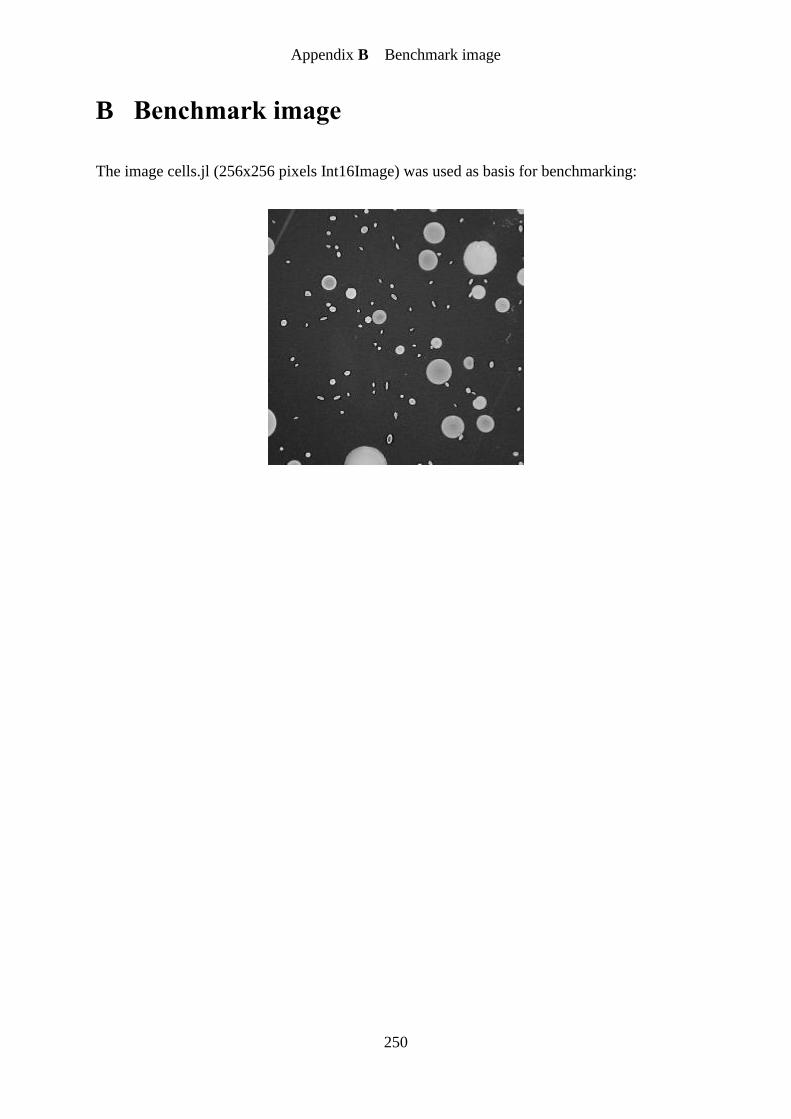
Appendix B Benchmark image
250
B Benchmark image
The image cells.jl (256x256 pixels Int16Image) was used as basis for benchmarking:
Appendix C Example of OpenCL host code in VisionLab script language
251
C Example of OpenCL host code in VisionLab
script language
This example shows the same functionality as the C code example mentioned in section
5.3.3. Only 30 lines of host code are needed instead of 67 lines of C code and the script code
performs error checking and handling.
File VectorAdd.cl:
kernel void VecAdd (global int *c, global int *a, global int *b) {
unsigned int n = get_global_id(0);
c[n] = a[n] + b[n];
}
VisionLab script:
$vectorSize = 100
FOR $i = 0 to ($vectorSize - 1) DO
$A[$i] = 1
$B[$i] = 2
$C[$i] = 0
$exp[$i] = 3
ENDFOR
CL_Init NVIDIA GPU
$nrP = CL_GetPlatforms &$tabP
$platformId = 0
$nrD = CL_GetDevices $platformId &$tabD
$deviceId = 0
$contextId = CL_CreateContext $platformId ($deviceId)
$qId = CL_CreateQueue $contextId $deviceId OutOfOrderEnabled
ProfilingEnabled
$options = ""
$src = VarFromFile VectorAdd.cl
$programId = CL_CreateProgram $contextId &$src
CL_Build $programId &$options
CL_AddKernel $programId VecAdd
$bufA = CL_CreateBuffer $contextId ReadOnly IntArray $vectorSize
$bufB = CL_CreateBuffer $contextId ReadOnly IntArray $vectorSize
$bufC = CL_CreateBuffer $contextId WriteOnly IntArray $vectorSize
CL_SetArg VecAdd 0 Buffer $bufC
CL_SetArg VecAdd 1 Buffer $bufA
CL_SetArg VecAdd 2 Buffer $bufB
CL_WriteBuffer $qId $bufA &$A () () Wait
CL_WriteBuffer $qId $bufB &$B () () Wait
CL_Run $qId VecAdd () ($vectorSize) () () () Wait
CL_ReadBuffer $qId $bufC &$C () () Wait
TestEqualVar &$C &$exp
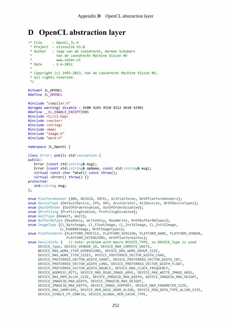
Appendix D OpenCL abstraction layer
252
D OpenCL abstraction layer
/* File : OpenCL_JL.h * Project : visionlib V3.0 * Author : Jaap van de Loosdrecht, Herman Schubert * Van de Loosdrecht Machine Vision BV * www.vdlmv.nl * Date : 1-6-2012 * * Copyright (c) 1993-2013, Van de Loosdrecht Machine Vision BV, * all rights reserved. */ #ifndef JL_OPENCL #define JL_OPENCL #include "compiler.h" #pragma warning( disable : 4100 4245 4510 4512 4610 4290) #define __CL_ENABLE_EXCEPTIONS #include <CL/cl.hpp> #include <vector> #include <string> #include <map> #include "image.h" #include "word.h" namespace JL_OpenCL { class Error: public std::exception { public: Error (const std::string& msg); Error (const std::string& opName, const std::string& msg); virtual const char *what() const throw(); virtual ~Error() throw() {} protected: std::string msg; }; enum PlatformVendor {AMD, NVIDIA, INTEL, AllPlatforms, NrOfPlatformVendors}; enum DeviceType {DefaultDevice, CPU, GPU, Accelerator, AllDevices, NrOfDeviceTypes}; enum QOutOfOrder {OutOfOrderEnabled, OutOfOrderDisabled}; enum QProfiling {ProfilingEnabled, ProfilingDisabled}; enum WaitType {NoWait, Wait}; enum BufferRWType {ReadOnly, WriteOnly, ReadWrite, NrOfBufferRWTypes}; enum ImageType {CL_ByteImage, CL_FloatImage, CL_Int16Image, CL_Int32Image, CL_RGB888Image, NrOfImageTypes}; enum PlatformInfo {PLATFORM_PROFILE, PLATFORM_VERSION, PLATFORM_NAME, PLATFORM_VENDOR, PLATFORM_EXTENSIONS, NrOfPlatformInfos}; enum DeviceInfo { // note: problem with macro DEVICE_TYPE, so DEVICE_Type is used DEVICE_Type, DEVICE_VENDOR_ID, DEVICE_MAX_COMPUTE_UNITS, DEVICE_MAX_WORK_ITEM_DIMENSIONS, DEVICE_MAX_WORK_GROUP_SIZE, DEVICE_MAX_WORK_ITEM_SIZES, DEVICE_PREFERRED_VECTOR_WIDTH_CHAR, DEVICE_PREFERRED_VECTOR_WIDTH_SHORT, DEVICE_PREFERRED_VECTOR_WIDTH_INT, DEVICE_PREFERRED_VECTOR_WIDTH_LONG, DEVICE_PREFERRED_VECTOR_WIDTH_FLOAT, DEVICE_PREFERRED_VECTOR_WIDTH_DOUBLE, DEVICE_MAX_CLOCK_FREQUENCY, DEVICE_ADDRESS_BITS, DEVICE_MAX_READ_IMAGE_ARGS, DEVICE_MAX_WRITE_IMAGE_ARGS, DEVICE_MAX_MEM_ALLOC_SIZE, DEVICE_IMAGE2D_MAX_WIDTH, DEVICE_IMAGE2D_MAX_HEIGHT, DEVICE_IMAGE3D_MAX_WIDTH, DEVICE_IMAGE3D_MAX_HEIGHT, DEVICE_IMAGE3D_MAX_DEPTH, DEVICE_IMAGE_SUPPORT, DEVICE_MAX_PARAMETER_SIZE, DEVICE_MAX_SAMPLERS, DEVICE_MEM_BASE_ADDR_ALIGN, DEVICE_MIN_DATA_TYPE_ALIGN_SIZE, DEVICE_SINGLE_FP_CONFIG, DEVICE_GLOBAL_MEM_CACHE_TYPE,

Appendix D OpenCL abstraction layer
253
DEVICE_GLOBAL_MEM_CACHELINE_SIZE, DEVICE_GLOBAL_MEM_CACHE_SIZE, DEVICE_GLOBAL_MEM_SIZE, DEVICE_MAX_CONSTANT_BUFFER_SIZE, DEVICE_MAX_CONSTANT_ARGS, DEVICE_LOCAL_MEM_TYPE, DEVICE_LOCAL_MEM_SIZE, DEVICE_ERROR_CORRECTION_SUPPORT, DEVICE_PROFILING_TIMER_RESOLUTION, DEVICE_ENDIAN_LITTLE, DEVICE_AVAILABLE, DEVICE_COMPILER_AVAILABLE, DEVICE_EXECUTION_CAPABILITIES, DEVICE_QUEUE_PROPERTIES, DEVICE_NAME, DEVICE_VENDOR, DRIVER_VERSION, DEVICE_PROFILE, DEVICE_VERSION, DEVICE_EXTENSIONS, DEVICE_PLATFORM, DEVICE_DOUBLE_FP_CONFIG, DEVICE_HALF_FP_CONFIG, DEVICE_PREFERRED_VECTOR_WIDTH_HALF, DEVICE_HOST_UNIFIED_MEMORY, DEVICE_NATIVE_VECTOR_WIDTH_CHAR, DEVICE_NATIVE_VECTOR_WIDTH_SHORT, DEVICE_NATIVE_VECTOR_WIDTH_INT, DEVICE_NATIVE_VECTOR_WIDTH_LONG, DEVICE_NATIVE_VECTOR_WIDTH_FLOAT, DEVICE_NATIVE_VECTOR_WIDTH_DOUBLE, DEVICE_NATIVE_VECTOR_WIDTH_HALF, DEVICE_OPENCL_C_VERSION, NrOfDeviceInfos}; enum KernelWorkGroupInfo { KERNEL_WORK_GROUP_SIZE, KERNEL_COMPILE_WORK_GROUP_SIZE, KERNEL_LOCAL_MEM_SIZE, KERNEL_PREFERRED_WORK_GROUP_SIZE_MULTIPLE, KERNEL_PRIVATE_MEM_SIZE, NrOfKernelWorkGroupInfos}; enum AmdBufferType {AMD_LOCAL, AMD_UNCACHED, AMD_CACHABLE}; struct ContextRec { ContextRec (const cl::Context &c, const int pId) { context = c; platformId = pId; } cl::Context context; int platformId; // NOTE: is JL platformId used in deviceTab, // not OpenCL platformId!! }; // ContextRec extern cl::NDRange StrToNDRange(const string &str); extern std::vector<int> WaitEventList (const int nr, ...); class OpenCL_JL { public: OpenCL_JL (); ~OpenCL_JL (); void Init (const PlatformVendor pv, const DeviceType dt); void AddKernel (const int programId, const std::string &name); void Build (const int programId, const std::string &options); std::string BuildInfo (const int programId); int CreateBuffer (const int contextId, const int size, const BufferRWType rw); int CreateHostBufferFromPtr (const int contextId, IN void* buffer, const int size, const BufferRWType rw); int CreateHostBuffer (const int contextId, const int queueId, OUT void** buffer, const int size, const BufferRWType rw); void UnmapHostBuffer (IN void* buffer, const int queueId, const int bufferId); int CreateContext (const int platformId, const std::vector<int> &deviceTab); int CreateEvent (); int CreateImage2D (const int contextId, const ImageType imageType, const int height, const int width, const BufferRWType rw); int CreateProgram (const int contextId, const std::string &src); int CreateProgramWithBinary (const int contextId, const std::string &fileName); int CreateQueue (const int contextId, const int deviceId, const QOutOfOrder qOrder, const QProfiling qProf); void DeleteAll (); void DeleteBuffers (); void DeleteContexts (); void DeleteDevices (); void DeleteEvents ();
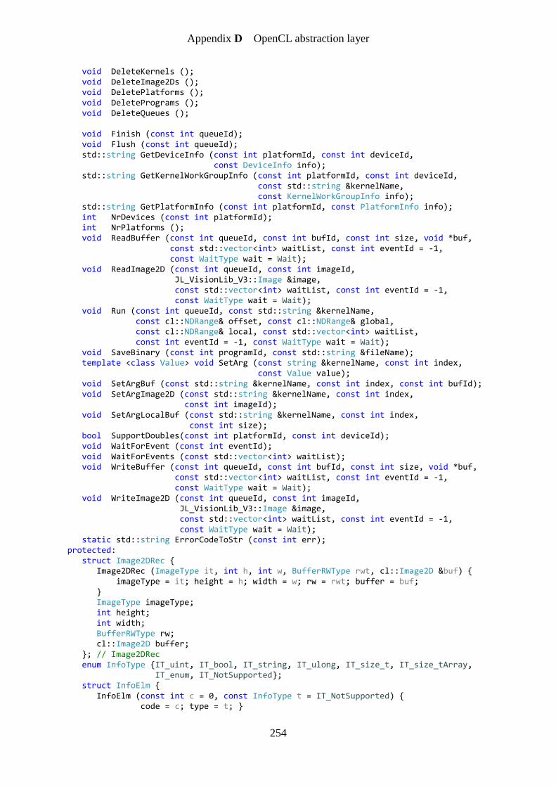
Appendix D OpenCL abstraction layer
254
void DeleteKernels (); void DeleteImage2Ds (); void DeletePlatforms (); void DeletePrograms (); void DeleteQueues (); void Finish (const int queueId); void Flush (const int queueId); std::string GetDeviceInfo (const int platformId, const int deviceId, const DeviceInfo info); std::string GetKernelWorkGroupInfo (const int platformId, const int deviceId, const std::string &kernelName, const KernelWorkGroupInfo info); std::string GetPlatformInfo (const int platformId, const PlatformInfo info); int NrDevices (const int platformId); int NrPlatforms (); void ReadBuffer (const int queueId, const int bufId, const int size, void *buf, const std::vector<int> waitList, const int eventId = -1, const WaitType wait = Wait); void ReadImage2D (const int queueId, const int imageId, JL_VisionLib_V3::Image &image, const std::vector<int> waitList, const int eventId = -1, const WaitType wait = Wait); void Run (const int queueId, const std::string &kernelName, const cl::NDRange& offset, const cl::NDRange& global, const cl::NDRange& local, const std::vector<int> waitList, const int eventId = -1, const WaitType wait = Wait); void SaveBinary (const int programId, const std::string &fileName); template <class Value> void SetArg (const string &kernelName, const int index, const Value value); void SetArgBuf (const std::string &kernelName, const int index, const int bufId); void SetArgImage2D (const std::string &kernelName, const int index, const int imageId); void SetArgLocalBuf (const std::string &kernelName, const int index, const int size); bool SupportDoubles(const int platformId, const int deviceId); void WaitForEvent (const int eventId); void WaitForEvents (const std::vector<int> waitList); void WriteBuffer (const int queueId, const int bufId, const int size, void *buf, const std::vector<int> waitList, const int eventId = -1, const WaitType wait = Wait); void WriteImage2D (const int queueId, const int imageId, JL_VisionLib_V3::Image &image, const std::vector<int> waitList, const int eventId = -1, const WaitType wait = Wait); static std::string ErrorCodeToStr (const int err); protected: struct Image2DRec { Image2DRec (ImageType it, int h, int w, BufferRWType rwt, cl::Image2D &buf) { imageType = it; height = h; width = w; rw = rwt; buffer = buf; } ImageType imageType; int height; int width; BufferRWType rw; cl::Image2D buffer; }; // Image2DRec enum InfoType {IT_uint, IT_bool, IT_string, IT_ulong, IT_size_t, IT_size_tArray, IT_enum, IT_NotSupported}; struct InfoElm { InfoElm (const int c = 0, const InfoType t = IT_NotSupported) { code = c; type = t; }
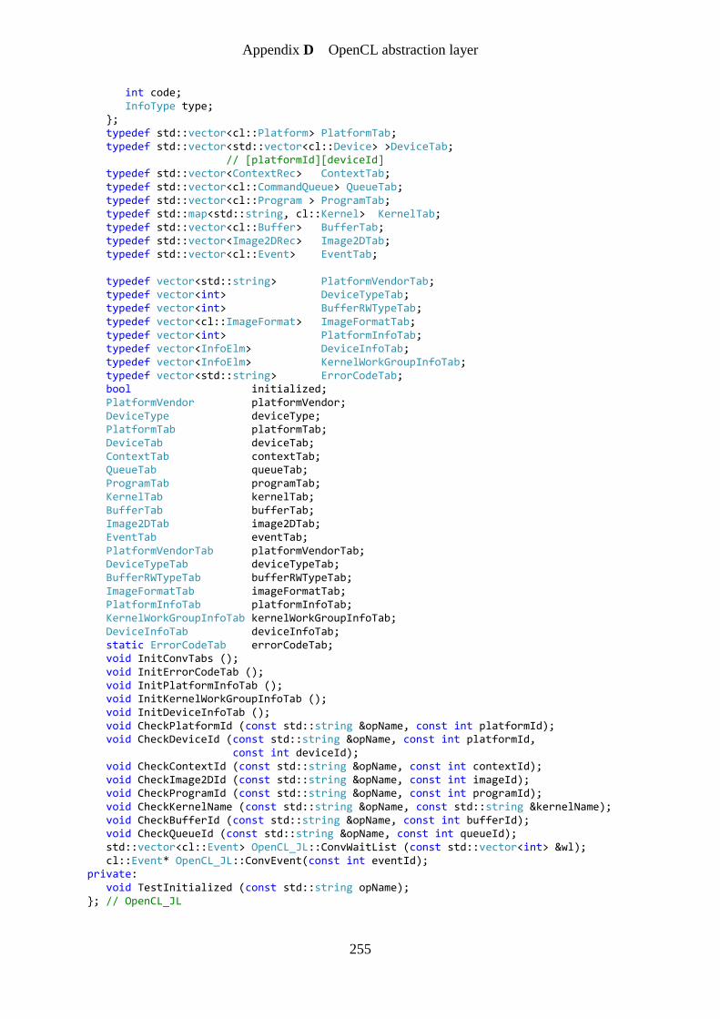
Appendix D OpenCL abstraction layer
255
int code; InfoType type; }; typedef std::vector<cl::Platform> PlatformTab; typedef std::vector<std::vector<cl::Device> >DeviceTab; // [platformId][deviceId] typedef std::vector<ContextRec> ContextTab; typedef std::vector<cl::CommandQueue> QueueTab; typedef std::vector<cl::Program > ProgramTab; typedef std::map<std::string, cl::Kernel> KernelTab; typedef std::vector<cl::Buffer> BufferTab; typedef std::vector<Image2DRec> Image2DTab; typedef std::vector<cl::Event> EventTab; typedef vector<std::string> PlatformVendorTab; typedef vector<int> DeviceTypeTab; typedef vector<int> BufferRWTypeTab; typedef vector<cl::ImageFormat> ImageFormatTab; typedef vector<int> PlatformInfoTab; typedef vector<InfoElm> DeviceInfoTab; typedef vector<InfoElm> KernelWorkGroupInfoTab; typedef vector<std::string> ErrorCodeTab; bool initialized; PlatformVendor platformVendor; DeviceType deviceType; PlatformTab platformTab; DeviceTab deviceTab; ContextTab contextTab; QueueTab queueTab; ProgramTab programTab; KernelTab kernelTab; BufferTab bufferTab; Image2DTab image2DTab; EventTab eventTab; PlatformVendorTab platformVendorTab; DeviceTypeTab deviceTypeTab; BufferRWTypeTab bufferRWTypeTab; ImageFormatTab imageFormatTab; PlatformInfoTab platformInfoTab; KernelWorkGroupInfoTab kernelWorkGroupInfoTab; DeviceInfoTab deviceInfoTab; static ErrorCodeTab errorCodeTab; void InitConvTabs (); void InitErrorCodeTab (); void InitPlatformInfoTab (); void InitKernelWorkGroupInfoTab (); void InitDeviceInfoTab (); void CheckPlatformId (const std::string &opName, const int platformId); void CheckDeviceId (const std::string &opName, const int platformId, const int deviceId); void CheckContextId (const std::string &opName, const int contextId); void CheckImage2DId (const std::string &opName, const int imageId); void CheckProgramId (const std::string &opName, const int programId); void CheckKernelName (const std::string &opName, const std::string &kernelName); void CheckBufferId (const std::string &opName, const int bufferId); void CheckQueueId (const std::string &opName, const int queueId); std::vector<cl::Event> OpenCL_JL::ConvWaitList (const std::vector<int> &wl); cl::Event* OpenCL_JL::ConvEvent(const int eventId); private: void TestInitialized (const std::string opName); }; // OpenCL_JL
Appendix D OpenCL abstraction layer
256
EnumStrIODeclaration(PlatformVendor) EnumStrIODeclaration(DeviceType) EnumStrIODeclaration(QOutOfOrder) EnumStrIODeclaration(QProfiling) EnumStrIODeclaration(WaitType) EnumStrIODeclaration(BufferRWType) EnumStrIODeclaration(ImageType) EnumStrIODeclaration(DeviceInfo) EnumStrIODeclaration(KernelWorkGroupInfo) EnumStrIODeclaration(PlatformInfo) EnumStrIODeclaration(AmdBufferType) } // namespace JL_OpenCL #endif // JL_OPENCL
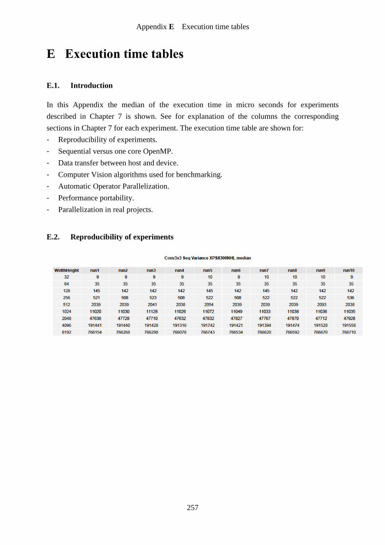
Appendix E Execution time tables
257
E Execution time tables
E.1. Introduction
In this Appendix the median of the execution time in micro seconds for experiments
described in Chapter 7 is shown. See for explanation of the columns the corresponding
sections in Chapter 7 for each experiment. The execution time table are shown for:
- Reproducibility of experiments.
- Sequential versus one core OpenMP.
- Data transfer between host and device.
- Computer Vision algorithms used for benchmarking.
- Automatic Operator Parallelization.
- Performance portability.
- Parallelization in real projects.
E.2. Reproducibility of experiments
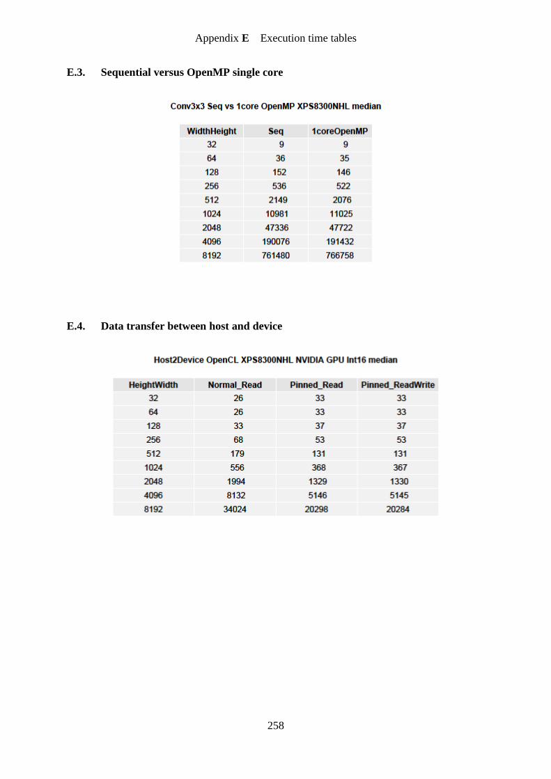
Appendix E Execution time tables
258
E.3. Sequential versus OpenMP single core
E.4. Data transfer between host and device
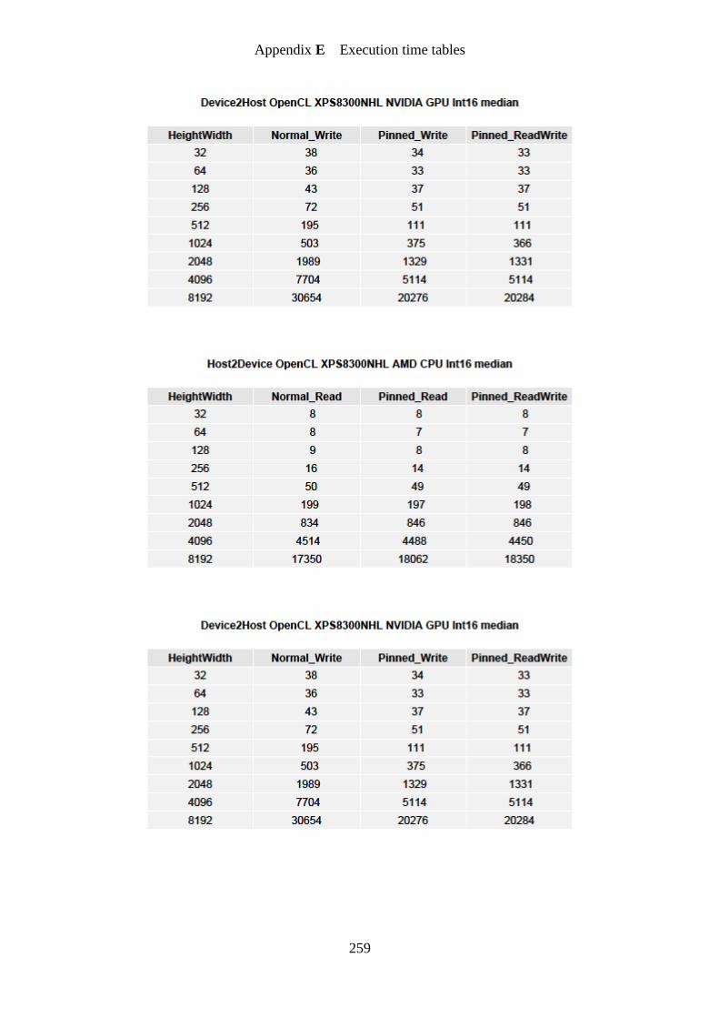
Appendix E Execution time tables
259

Appendix E Execution time tables
260
E.5. Threshold
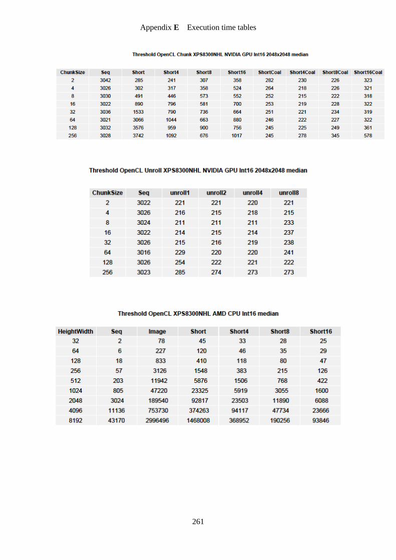
Appendix E Execution time tables
261
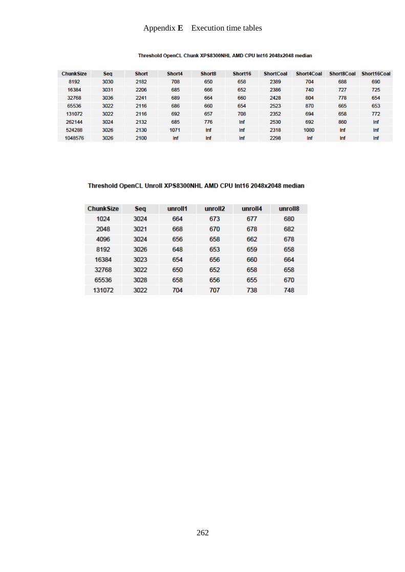
Appendix E Execution time tables
262
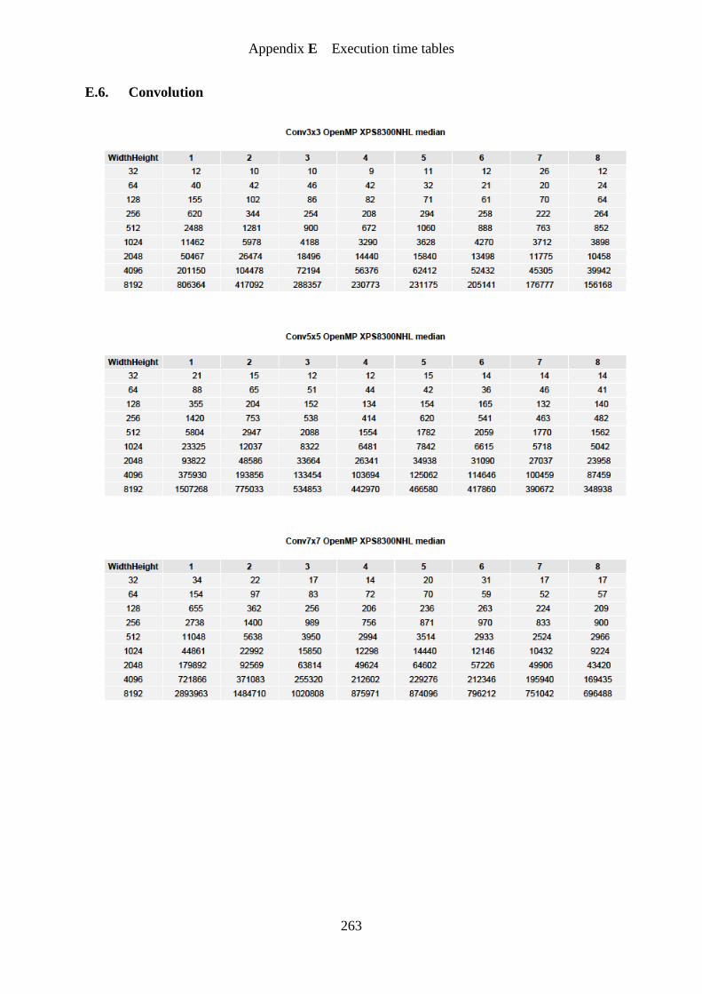
Appendix E Execution time tables
263
E.6. Convolution
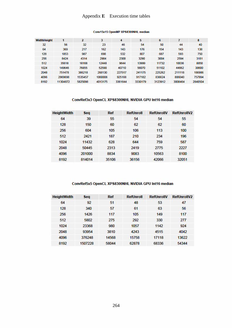
Appendix E Execution time tables
264

Appendix E Execution time tables
265
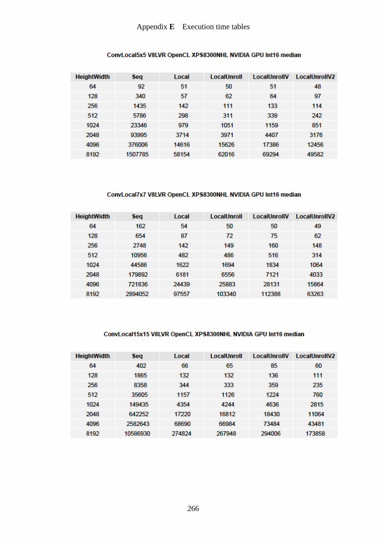
Appendix E Execution time tables
266

Appendix E Execution time tables
267

Appendix E Execution time tables
268

Appendix E Execution time tables
269
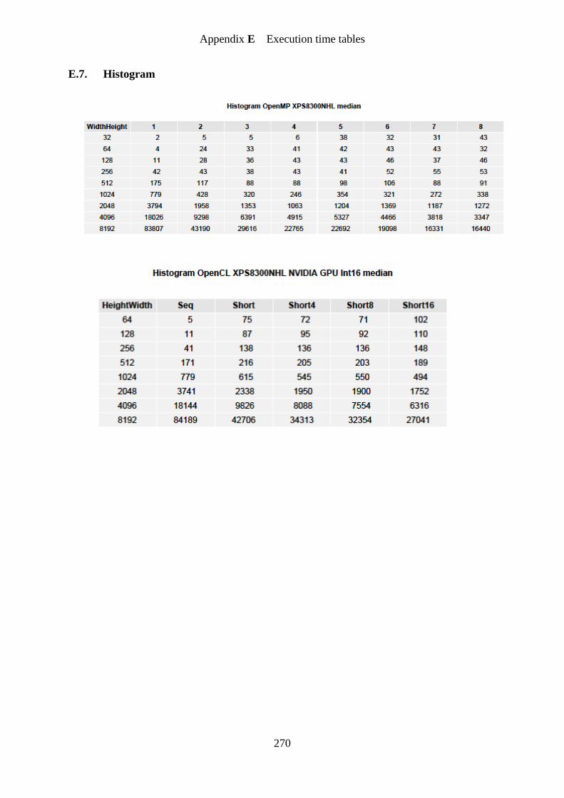
Appendix E Execution time tables
270
E.7. Histogram

Appendix E Execution time tables
271
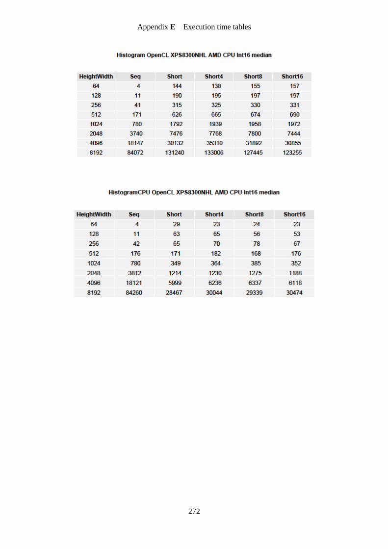
Appendix E Execution time tables
272
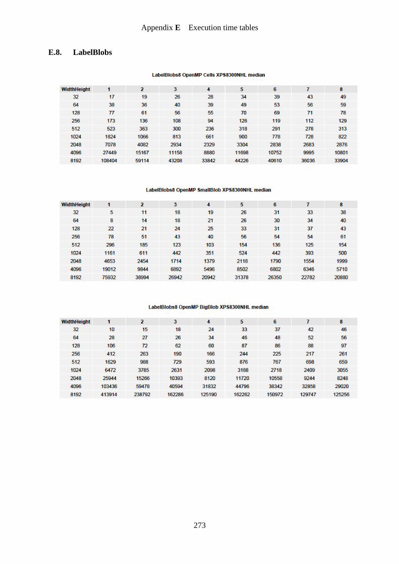
Appendix E Execution time tables
273
E.8. LabelBlobs

Appendix E Execution time tables
274
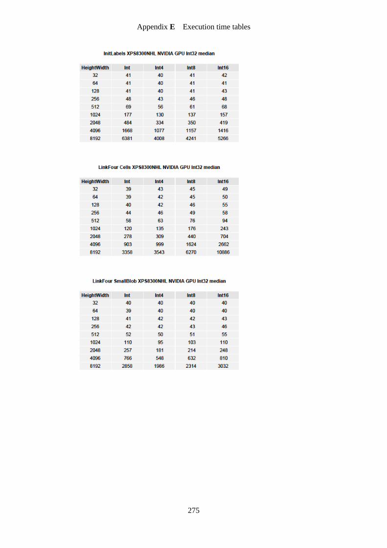
Appendix E Execution time tables
275
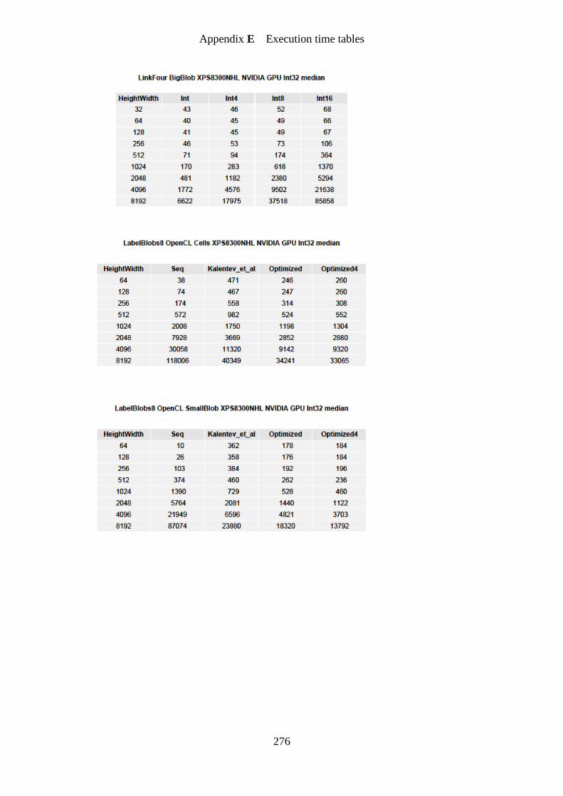
Appendix E Execution time tables
276
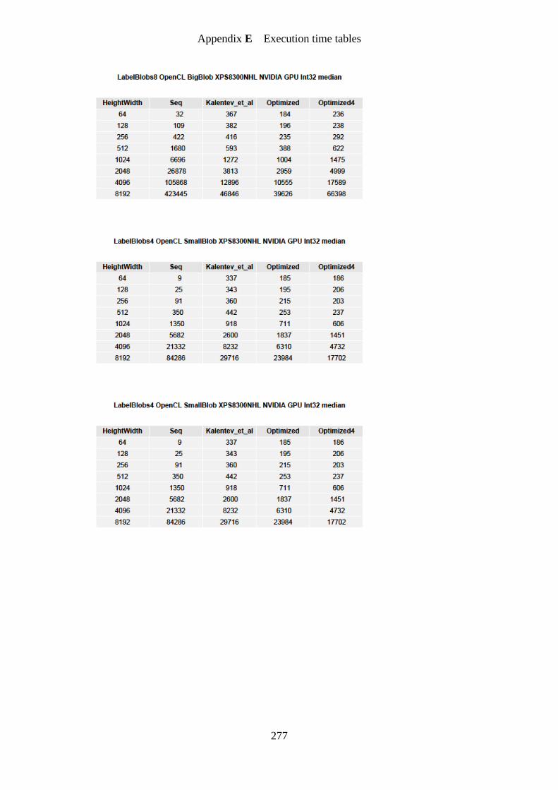
Appendix E Execution time tables
277
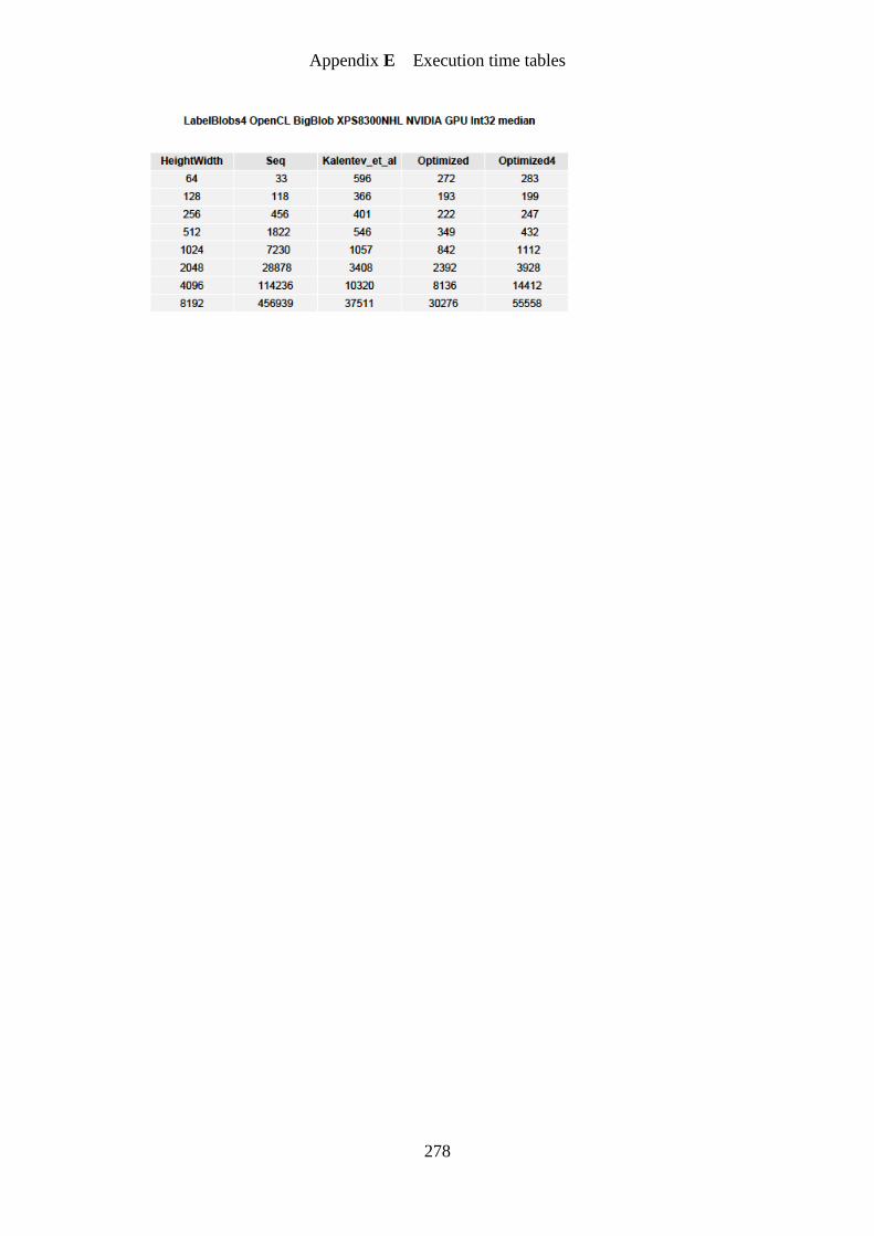
Appendix E Execution time tables
278
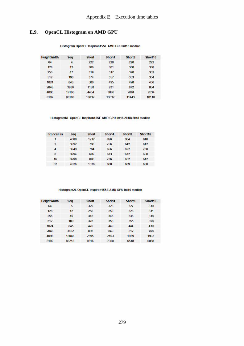
Appendix E Execution time tables
279
E.9. OpenCL Histogram on AMD GPU
Appendix F Benchmark details
280
F Benchmark details
The benchmark details are available in electronic form. For each benchmark performed there
is available:
- Speedup graph: the results are summarized in a graph where the size of the image is
plotted against the speedup obtained. The reference is the execution of the sequential
version; a speedup of 1. The speedup graph for each benchmark conducted is shown in
Chapter 7.
- Speedup table: the speedup factor for each experiment performed.
- Median table: the median of the execution times in micro seconds for each experiment
performed.
- The violin plots for each experiment performed.
- For GPU benchmarks, tables with best workgroup sizes.
As example the results for the OpenMP benchmark for the Threshold operator is included in
this document.
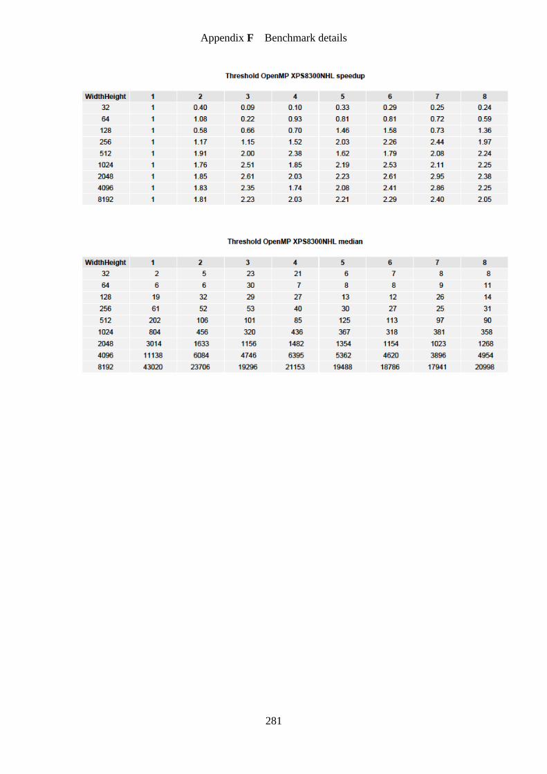
Appendix F Benchmark details
281
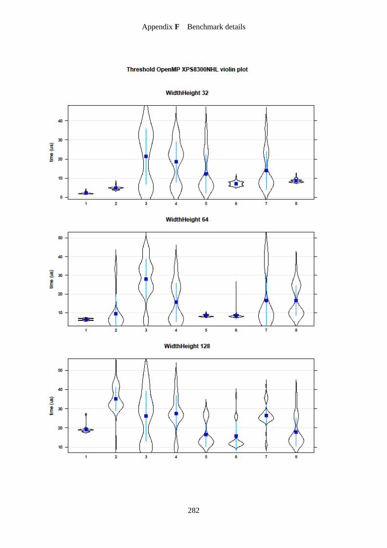
Appendix F Benchmark details
282
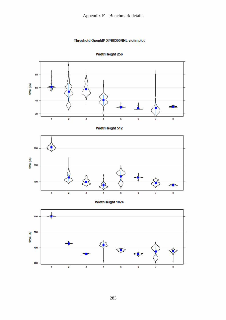
Appendix F Benchmark details
283

Appendix F Benchmark details
284
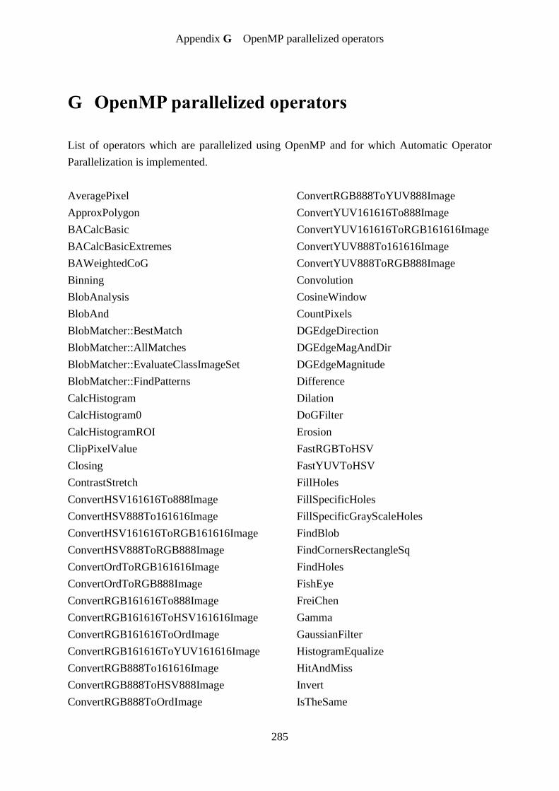
Appendix G OpenMP parallelized operators
285
G OpenMP parallelized operators
List of operators which are parallelized using OpenMP and for which Automatic Operator
Parallelization is implemented.
AveragePixel
ApproxPolygon
BACalcBasic
BACalcBasicExtremes
BAWeightedCoG
Binning
BlobAnalysis
BlobAnd
BlobMatcher::BestMatch
BlobMatcher::AllMatches
BlobMatcher::EvaluateClassImageSet
BlobMatcher::FindPatterns
CalcHistogram
CalcHistogram0
CalcHistogramROI
ClipPixelValue
Closing
ContrastStretch
ConvertHSV161616To888Image
ConvertHSV888To161616Image
ConvertHSV161616ToRGB161616Image
ConvertHSV888ToRGB888Image
ConvertOrdToRGB161616Image
ConvertOrdToRGB888Image
ConvertRGB161616To888Image
ConvertRGB161616ToHSV161616Image
ConvertRGB161616ToOrdImage
ConvertRGB161616ToYUV161616Image
ConvertRGB888To161616Image
ConvertRGB888ToHSV888Image
ConvertRGB888ToOrdImage
ConvertRGB888ToYUV888Image
ConvertYUV161616To888Image
ConvertYUV161616ToRGB161616Image
ConvertYUV888To161616Image
ConvertYUV888ToRGB888Image
Convolution
CosineWindow
CountPixels
DGEdgeDirection
DGEdgeMagAndDir
DGEdgeMagnitude
Difference
Dilation
DoGFilter
Erosion
FastRGBToHSV
FastYUVToHSV
FillHoles
FillSpecificHoles
FillSpecificGrayScaleHoles
FindBlob
FindCornersRectangleSq
FindHoles
FishEye
FreiChen
Gamma
GaussianFilter
HistogramEqualize
HitAndMiss
Invert
IsTheSame

Appendix G OpenMP parallelized operators
286
LabelAnd
LabelBlobs
LoGFilter
LowestButZeroPixel
LUT
LUTVector
Max
MaximumFilter
MaxLabel
MaxPixel
MarrHildreth
Min
Mean
MinimumFilter
MinLabel
MinMaxLabel
MinMaxPixel
MinPixel
Noise
NormaliseRGB
Not
NrOfNeighbours
operator image /= image
operator image /= pixel
operator image = image / image
operator image = pixel / image
operator image = image / pixel
operator image -= image
operator image -= pixel
operator image = image - image
operator image = pixel - image
operator image = image - pixel
operator image *= image
operator image *= pixel
operator image = image * image
operator image = pixel * image
operator image = image * pixel
operator image += image
operator image += pixel
operator image = image + image
operator image = pixel + image
operator image = image + pixel
operator image &= image
operator image &= pixel
operator image = image & image
operator image = pixel & image
operator image = image & pixel
operator image |= image
operator image |= pixel
operator image = image | image
operator image = pixel | image
operator image = image | pixel
operator image ^= image
operator image ^= pixel
operator image = image ^ image
operator image = pixel ^ image
operator image = image ^ pixel
operator !image
Opening
OpticalCorrectionBilinear
OpticalCorrectionNearest
OrdImageConversion
PolarStretch
Pow
PowPixel
Prewitt
RampPattern
RATS
RATSROI
Remainder
RemoveBlobs
RemoveBlobsExp
RemoveLabelsExp
RemoveBorderBlobs
RemoveBorderLabels
RemoveGrayScaleBlobs
RemoveGrayscaleBlobsExp
RemoveGrayScaleLabels

Appendix G OpenMP parallelized operators
287
RemoveGrayscaleLabelsExp
RemoveSelectedLabels
ROI
ROIR
RotateBilinear
RotateFullBilinear
RotateFullNearest
RotateNearest
SetAllPixels
SetMultiToValue
SetMultiToValueLUT
SetSelectedToValue
Scharr
Skeleton
Sobel
StandardDeviation
SumColumns
SumFloatPixels
SumIntPixels
SumRows
Thickening
Thinning
Threshold
ThresholdFast
ThresholdLocal
ThresholdIsoData
ThresholdIsoDataROI
ThresholdHysteresis
ThresholdMulti
ThresholdOnLowestButZero
ThresholdOnHighest
ThresholdOnLowest
ThresholdRATS
ThresholdRATSROI
ThresholdSimple
WarpBilinear
WarpNearest
ZoomBilinear
ZoomNearest