Accelerated hardware object extraction and labelling:

from object segmentation to connected components

labelling

Kofi Appiaha, Andrew Huntera, Hongying Menga, Patrick Dickinsona

aDepartment of Computing and Informatics

University of Lincoln

Brayford Campus

LN6 7TS

Abstract

This paper demonstrates the use of a single-chip FPGA for the segmentationof moving objects in a video sequence. The system maintains highly accuratebackground models, and integrates the detection of foreground pixels withthe conversion into labelled objects using a connected component labellingalgorithm. The background models are based on 24-bit RGB values and 8-bitgreyscale intensity values. A multimodal background differencing algorithmis presented, using a single FPGA chip and four blocks of RAM. The real-time connected component labelling algorithm, also designed for FPGA im-plementation, has efficiently been integrated with the pixel level backgroundsubtraction to extract pixels of a moving object as a single blob. The con-nected component algorithm, run-length encodes the binary image output ofthe background subtraction, and performs connected component analysis onthis representation. The run-length encoding, together with other parts ofthe algorithm, is performed in parallel; sequential operations are minimizedas the number of run-lengths are typically less than the number of pixels.

Key words: Background differencing; Image Segmentation; ConnectedComponent labelling; Object extraction; FPGA.

1. Introduction

Detection and tracking of objects in real-time using a stationary camerais an active field of research in the vision community with a wide range

Preprint submitted to Computer Vision and Image Understanding August 22, 2009

of applications in the fields of monitoring and surveillance, smart rooms,vehicle tracking, biological image analysis and video compression. The firststage in processing for many video-based applications is the segmentationof (usually) moving objects with significant difference in colour and shapefrom the background, a very basic yet computationally expensive task forreal-time purposes. The second stage is the connected-component labellingof the binary image; a highly sequential operation. This is then followed byextracting features of the moving object(s) to support tracking; for example,the centroid, colour histogram, width and height.

Using a Field Programmable Gate Array (FPGA) as an image accelerator,we demonstrate in this paper how real-time extraction of moving objects fromimage sequences taken under variable lighting conditions can be achievedefficiently on an FPGA architecture. The implementation has a number ofuses in embedded systems and automated visual surveillance systems. Real-time image processing is difficult to achieve on a serial processor, due tothe movement of large data sets and complex operations that need to beperformed on the image [15]. Advances in semiconductor technology makes itpossible to design complete embedded System-on-Chip (SoC) by combiningsensor, signal processing and memory onto a single substrate [21]. Newembedded vision systems have emerged as a result of this level of integrationand are likely to proliferate in the coming years. The aim of such computervision systems is to scan scenes and make judgements that remove or decreasethe need for human observers – thus the need to develop imaging functionswith performance comparable to trained human operators [28].

Field Programmable Gate Arrays (FPGAs), have been available for overtwo decades. Recent increases in programmable fabric density have made thisan appealing platform for accelerating computer vision and image processingalgorithms. The potential uses of FPGAs in areas like medical image pro-cessing, computational fluid dynamics, target recognition, embedded visionsystems, gesture recognition and automotive infotainment have been demon-strated in [5, 9, 17, 18, 21]. Digital Image processing or computer vision al-gorithms can be broken down into three major stages [14]: early processing,implemented by local pixel-level functions; intermediate processing, whichincludes segmentation, motion estimation and feature extraction; and lateprocessing, including interpretation and using statistical and artificial intel-ligence algorithms[1]. Typically algorithm sophistication is concentrated inthe later stages, but processing demands dominate in the early stages [32].

In this paper, we preset the integration of two basic image processing al-

2

gorithms: background differencing (background subtraction) and connectedcomponent labelling, designed specifically for efficient FPGA implementa-tion. Published background differencing algorithms tend to focus on ro-bustness in varying lighting conditions, and on shadow extraction [1], whileconnected component labelling algorithms tend to focus on the resolution ofequivalence table[19]. An integrated system, capable of extracting labelledregions of similar pixels (of a moving object) from real-time video sequenceusing FPGA is presented. The gate-rich capabilities of FPGAs offer the po-tential to efficiently implement both algorithms on a single chip for real timeprocessing.

2. Binary Foreground Extraction

Image segmentation, defined as the grouping of pixels that are coher-ent in space, range, and time domain, is usually the first stage in pro-cessing for many video applications. The input image usually defines analgorithm suitable for segmentation. Comaniciu et al [7] presents a tech-nique for segmenting a video frame into representative blobs detected in thespatial and colour domains. Similarly, Boykov et al in [6] demonstrates ageneral-purpose segmentation method for extracting objects using the s/tgraph cuts, with reported success in segmenting photos, video and medicalimages. Fuzzy c-means algorithms based on the idea of clustering pixelswith similar characteristics have successfully been used in segmentation [32].Zhou et al [32, 31, 30] introduced the mean shift based fuzzy c-means algo-rithm, which addresses the computational requirement of the original fuzzyc-means algorithm with reported improved segmentation. Where the inputis a video sequence and the camera is stationary, a natural approach is tomodel the background and detect foreground object by differencing the cur-rent frame with the background. A wide and increasing variety of techniquesfor background modelling have been described; a good comparison is givenby Gutchess et al [11].

The most popular method is unimodal background modelling, in whicha single value is used to represent a pixel, which has been widely used dueto its relatively low computational cost and memory requirements [13, 29].This technique gives a poor results when used in modelling non-stationarybackground scenarios like waving trees, rain and snow. A more powerfulalternative is to use a multimodal background representation, which usesmore than one process (mostly mixture of Gaussians) to represent a single

3

background pixels. However, the computational demands make multimodaltechniques unpopular for real-time purposes; there are also disadvantages inmultimodal techniques [10, 26, 29] including the blending effect, which causesa pixel to have an intensity value which has never occurred at that position(a side-effect of the smoothing used in these techniques). Other techniquesrely heavily on the assumption that the most frequent intensity value duringthe training period represents the background. This assumption may well befalse, causing the output to have a large error level.

2.1. Grimson’s Algorithm

Grimson et al [26, 27] introduced a multimodal approach, modelling thevalues of each pixel as a mixture of Gaussians (MoG). The background ismodelled with the most persistent intensity values. The algorithm has twovariants, colour and gray-scale: in this paper, we concentrate on the gray-scale version. The probability of observing the current pixel value is givenas:

P (Xt) =k

∑

i=1

ωi,tη(Xt, µi,t, σi,t) (1)

Where µi,t, σi,t and ωi,t are the respective mean, standard deviation andweight parameters of the ith Gaussians component of pixel X at time t. η isa Gaussian probability density function

η(Xt, µi,t, σi,t) =1

σi,t

√2π

e

(Xt−µi,t)2

2σ2i,t (2)

A new pixel value is generally represented by one of the major componentsof the mixture model and used to update the model. For every new pixelvalue, Xt, a check is conducted to match it with one of the K Gaussiandistributions. A match is found when Xt is within 2.5 standard deviation ofa distribution. If none of the K distributions match Xt, the least weigheddistribution is replaced with a new distribution having Xt as mean, highvariance and very low weight. The update equations are as follows:

wi,t = wi,t−1 + α(mi,t − wi,t−1) (3)

where α is the learning rate and

mi,t =

{

1 if there is a match0 otherwise

(4)

4

µt = µt−1 − ρ(Xt − µt) (5)

σ2

t = (1− ρ)σ2

t−1 + ρ(Xt − µt)T (Xt − µt) (6)

Only the matched distribution will have its mean and variance updated, allothers remain unchanged. For

ρ = αη(Xt|µt, σt) (7)

The first B distributions (ordered by ωk) are used as a model of the back-ground, where

B = argb min(b

∑

k=1

ωk > T ). (8)

The threshold T is a measure of the minimum portion of the data that shouldbe accounted for by the background.

2.2. Temporal Low-Pass filtering Algorithm

Aleksej [20] introduced a method to avoid false alarms due to illumina-tion, using a temporal filter to update the background model, while a globalthreshold value T was used to extract target regions. The background updatehe used is of the form

B(k, l, n) =(p− c)

pB(k, l, n− 1) +

c

pI(k, l, n)

where c is the number of consecutive frames during which a change is ob-served and is reset to zero each time the new value becomes part of thebackground; p is the adaptation time or insertion delay constant. The mov-ing target is extracted on a pixel level with the following relation:

f(k, l, n) =

{

1 |I(k, l, n)−B(k, l, n)| > L

0 otherwise(9)

where f(k,l,n), B(k,l,n) and I(k,l,n) are the respective foreground, backgroundand greyscale intensity value of pixel (k,l) for the nth frame, and L is theglobal threshold value.

The low-pass filtering algorithm is attractive for two reasons. First itis very simple and hence updating the background information is computa-tionally cheap and memory consumption is minimal. The use of single globalthreshold value as well as a single mode makes it unattractive for scenes with

5

varying lighting intensities. In contrast, Grimson’s algorithm [26] is robust tooutdoor environments where lighting intensity can suddenly change, and ithandles multimodal backgrounds such as moving foliage (cyclical/oscillatingmotion) without manual initialisation. Unfortunately, accurate maintenanceof mean, variance and weight for the MoG at every pixel location requires theuse of floating-point numbers (unsuitable for hardware implementation [3]),or high precision fixed point numbers when implemented in hardware. Toefficiently implement the MoG background subtraction algorithm on a hard-ware architecture for real-time processing, modifications have been made tothe algorithm in section 2.3; trading off some level of accuracy for speed-up.

2.3. Our Approach

We present here a novel hybrid background modelling algorithm [1] thatcombines the attractive features of Grimson’s algorithm [26] and the temporallow-pass filtering [20], with appropriate modifications to improve segmenta-tion of the foreground image. The main contribution of the algorithm pre-sented is its efficient implementation on a reconfigurable hardware platformsuch as Field Programmable Gate Array (FPGA). Following Grimson [26],we maintain a number of clusters, each with weight wk, where 1 ≤ k ≤ K,for K clusters. Rather than modelling a Gaussian distribution, we maintaina model with a central value, ck of 11-bits (8 bits integer part and 3 bitsfractional part). We use an implied global range, [ck − 15, ck + 15], ratherthan explicitly modelling a range for each pixel based on its variance as in[26]. The weights and central values of all the clusters are initialised to 0.

A pixel X = I(i, j) (where X is 11-bit fixed-point) from an image I issaid to match a cluster, k, if X ≥ ck − 15 and X ≤ ck + 15. The highestweight matching cluster is updated, if and only if its weight after the updatewill not exceed the maximum allowed value (i.e. wk ≤ 64, given the datawidth of the weight as 6 bits). The exponential moving average, which iseasier to implement on FPGA has been used in all the update equations.Typically, more weight is given to the observed value to obtain a value closerto the average. The update for the weight is as follows:

wk,t =

{

63

64wk,t−1 + 1

64for the matching cluster

63

64wk,t−1 otherwise

(10)

The central values of all the clusters are also updated as follows:

ck,t,i,j =

{

7

8ck,t−1,i,j + 1

8Xi,j matching cluster

ck,t−1,i,j otherwise(11)

6

Where ck,t,i,j is the central value for cluster k at time t for pixel (i, j). If nomatching cluster is found, then the least weighted cluster’s central value, cK

is replaced with X; its weight is reset to zero. The way we construct andmaintain clusters make our approach gradually incorporate new backgroundobjects. The K distributions are ordered by weight, with the most likelybackground distribution on top. Similar to [26], K (usually set to 3) isthe total number of clusters used to model every single background pixel(multimodal) to accommodate oscillating background objects. The first B

out of K clusters are chosen as the background model, where

B = argb min(b

∑

k=1

ωi > T ) (12)

. The threshold T is a measure of the minimum portion of the data thatshould be accounted for by the background.

We classify a pixel as foreground pixel based on the following two condi-tions:

1. If the intensity value of the pixel matches none of the K clusters.

2. If the intensity value is assigned to the same cluster for two successiveframes, and the intensity values X(t) and X(t − 1) are both outsidethe 40% mid-range [ck − 6, ck + 6].

The second condition makes it possible to detect targets with low contrastagainst the background, while maintaining the concept of multimodal back-grounds. A typical example is a moving object with greyscale intensity closeto that of the background, which would be classified as background in [26].This requires the maintenance of an extra frame, with values representingthe recently processed background intensities.

2.4. Experimental Results

We evaluate the performance of our approach against that of [26] usingK = 3, thus 3 cluster in our case and 3 distributions in [26] per pixel. Weuse twelve randomly selected video sequences; seven outdoor and five indoorscenes with a total of 1600 frames. One of the seven outdoor sequencesis taken from a publicly available dataset (PETS 2000 camera 1) [23], twotaken with a close range camera placed at a distance of about five metersand the last four taken in a reasonably challenging outdoor scene with oscil-lating background objects (river waves and foliage). The five indoor scenes

7

have varying lighting intensity, with two taken in a very reflective room.Reference standard segmentations on these sequences have been constructedby using manually marked frames; results of the algorithms are comparedto this reference standard. The results of the pixel level comparison be-tween the ground truth and the extracted foreground image for each frameof all the 12 sequences are based on true positive(TP ), true negative(TN),false negative(FN) and false positive(FP ) pixels. We have used three mea-sures Sensitivity (SENS) expressed as TP

TP+FN, Jaccard Coefficient (JC) ex-

pressed as TPTP+FP+FN

and Percentage Correct Classification (PCC) expressed

as TP+TNTP+FP+TN+FN

to evaluate the performance of the two algorithms. Table1 shows the superiority of our algorithm against that in [26] in terms ofsensitivity. The algorithm does produce more false positive errors; this isthe side-effect of our approach in detecting targets with low contrast againstthe background. However, in our target application false positive errors ofthe type reported are more acceptable than false negative errors, as subsys-tem tracking stages can discard distracters such as shadows. Figure 1 givessample images of the outputs generated by the two algorithms.

Figure 1: Sample outputs of the algorithms. The top row shows the original images withtheir corresponding manually marked ground truth. The middle and bottom rows showoutputs of Grimson’s algorithm and our approach respectively. Images on the second andfourth columns are the outputs after applying morphology.

8

Grimson’s (%) Our Approach (%)Seq. SENS JC PCC SENS JC PCC1 78.92 62.30 99.86 79.08 60.04 99.842 80.99 76.67 99.34 83.18 79.55 99.433 64.34 59.93 95.86 79.87 75.02 97.444 82.20 72.27 98.06 84.88 73.08 98.075 68.55 48.68 97.10 76.72 41.76 95.716 68.70 49.51 96.11 76.26 52.13 96.127 45.96 32.99 98.56 56.35 35.27 98.408 75.58 53.99 99.52 81.39 51.23 99.429 74.33 64.75 97.50 89.91 69.40 97.5510 48.60 37.48 95.60 83.01 53.69 96.1111 68.50 11.76 80.90 80.23 10.64 74.9512 48.47 17.73 93.62 79.44 17.58 89.43

Table 1: Per-pixel performance in terms of Sensitivity, Jaccard Coefficient and PercentageCorrect Classification for the approach in [26] and our’s. The three measures are computedon the outputs from the algorithms after applying morphological opening. For everysequence, the value in bold signifies the algorithm with the best measure for that particularsequence.

9

3. Connected Components

The foreground extraction algorithms described in section 2 are used toidentify foreground pixels in each new frame while updating the description ofeach pixel’s background data. This is followed by the labelling of the binaryforeground image into regions using the connected components algorithm.We present a run-length based connect component algorithm, which caneasily be integrated with the background subtraction algorithm to avoid theintermediate binary foreground data structure. The algorithm is similar tothe two-pass connected component algorithm, but rather than pixels, weuse run-lengths, which are much more compact that individual pixels. Theoriginal two-pass algorithm (Rosenfeld and Pfaltz [22, 24]), uses two rasterscans of the image and an equivalence table resolution stage[19]. Details ofthe algorithm (using the 4-adjacency definition of connectivity) are as follows:

Initial labelling :-The binary input image is scanned in raster order, tolabel foreground pixels by reference to the left and upper neighbours. If theneighbours are background pixels, a new label is assigned. If they are bothforeground with different labels, the left label is copied to the current pixel,and an entry is made in the equivalence table linking the upper and left labels.If only one neighbour is labelled, or they share the same label, the value ispropagated.

Resolving Equivalences :-The initial labelling step is followed by equiva-lence resolution, after which the image is scanned again and each label isreplaced by the label assigned to its equivalence class. This approach hasbeen used in [16, 25], directly, or modified for implementation as the resolu-tion of label equivalences has a great impact on run time. One drawback ofthis algorithm is the high dynamic storage required for the equivalence table.

To reduce storage requirements, Haralick [12] suggested a multi-pass la-belling algorithm with increased computational time. In this algorithm, aforeground pixel with only background neighbours is assigned a new label.However, where there are any labelled neighbours, the minimum label is as-signed. The algorithm alternates raster and reverse-raster scans until thelabelling stabilises. The algorithm is highly sequential, and the repeated im-age scans make it computationally inefficient, as scan-times tend to dominateconnected component cycles.

Crookes et al [8] successfully implemented the multi-pass connected com-ponent labelling algorithm on an FPGA using off-chip RAM. The implemen-tation fits on a single Xilinx XC4010E chip with 20 × 20 CLBs and for an

10

image size of 256 × 256, the design runs at 76MHz. The implementationsuffers from all the problems associated with the base algorithm and hencethe time taken to process a frame is dependant on the complexity of ob-jects in the scene. A similar implementation is presented in by Benkrid etal. ([4]) using a bigger device, Xilinx Virtex-E FPGA. For an image sizeof 1024 × 1024, the design consumes 583 slices, 5 Block RAMs and runs at72MHz.

3.1. Our Approach

The labelling algorithm as presented in [24] can result in a very largeequivalence table. Resolving the equivalence table has been the focus ofmost labelling algorithms, with little effort to implement such algorithmson hardware architecture for real-time processing. Our algorithm [2] is suit-able for implementation on a hardware platform, and also minimises use ofmemory. Our key contribution is to process using a run-length encoding rep-resentation. This is easily parallelised by processing multiple rows in parallel,and can be integrated with the background differencing algorithm, avoidingthe requirement to calculate a binary foreground image as an intermediatedata structure. The run-length encoded format is also much more compactthan a binary image (individual runs have a single label), and so the sequen-tial label propagation stage is much faster than the conventional algorithm.Details of the algorithm are given below.

The stages involved in our implementation are as follows:

1. Pixels are converted to runs in parallel by rows,

2. Initial labelling and propagation of labels,

3. Equivalence table resolution and

4. Translating run labels to connected component.

The design is parallelised as much as possible. Although stages 2 and 3 aresequential, they operate on runs, which are far less numerous than pixels.Similar to stage 1, stage 4 can be executed in parallel by row. A run hasthe properties {ID,EQ, s, e, r}, where ID is the identity number of the run,EQ is the equivalence value, s the x offset of the start pixel, e the x offsetof the end pixel, and r the row. The first stage involves row-wise parallelconversion from pixels to runs. Depending on the location and access modeof the memory holding the image, the entire image may be partitioned inton parts to achieve n run-length encoding in parallel. The use of runs rather

11

than pixels reduces the size of the equivalence table in some cases similar tofigure 4 and hence makes it easier to resolve.

The following sequential local operations are performed in parallel oneach partition, for an image size M ×N to assign pixels to runs:

Algorithm 3.1: PixelToRuns(T )

∀T : T (x, y) = I(x, y)i← 0isBlock ← 0if T (x, y) = 1 and isBlock = 0

then

{

si ← x

isBlock ← 1if isBlock = 1 and (T (x, y) = 0 or x = M)

then

ei ← (x− 1)ri ← y

IDi ← EQi ← 0i← i + 1isBlock ← 0

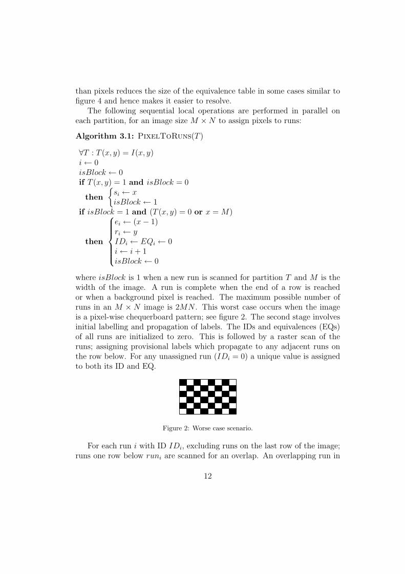
where isBlock is 1 when a new run is scanned for partition T and M is thewidth of the image. A run is complete when the end of a row is reachedor when a background pixel is reached. The maximum possible number ofruns in an M × N image is 2MN . This worst case occurs when the imageis a pixel-wise chequerboard pattern; see figure 2. The second stage involvesinitial labelling and propagation of labels. The IDs and equivalences (EQs)of all runs are initialized to zero. This is followed by a raster scan of theruns; assigning provisional labels which propagate to any adjacent runs onthe row below. For any unassigned run (IDi = 0) a unique value is assignedto both its ID and EQ.

Figure 2: Worse case scenario.

For each run i with ID IDi, excluding runs on the last row of the image;runs one row below runi are scanned for an overlap. An overlapping run in

12

4-adjacency (ie. si ≤ ej and ei ≥ sj) or 8-adjacency (ie. si ≤ ej + 1 andei + 1 ≥ sj) is assigned the ID IDi, if and only if IDj is unassigned. If thereis a conflict (if an overlapping run has assigned IDj), the equivalence of runi, EQi is set to IDj. This is summarized in algorithm 3.2.

Algorithm 3.2: InitLabelling(runs)

m← 1for i← 1 to TotalRuns

do

if IDi = 0

then

{

IDi ← EQi ← m

m← m + 1for each rj ∈ ri+1

do

if IDj = 0 and ei ≥sj and si ≤ ej

then

{

IDj ← IDi

EQj ← IDi

if IDj 6= 0 and ei ≥sj and si ≤ ej

then{

EQi ← IDj

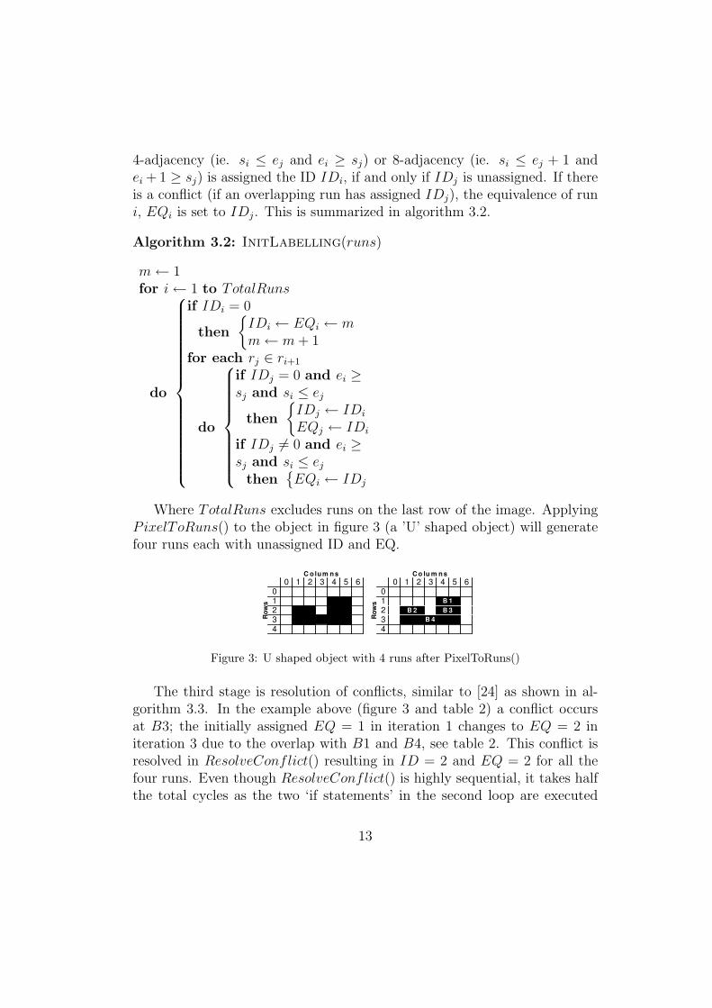
Where TotalRuns excludes runs on the last row of the image. ApplyingPixelToRuns() to the object in figure 3 (a ’U’ shaped object) will generatefour runs each with unassigned ID and EQ.

0 1 2 3 4 5 601234

C o lu m n s

Ro

ws

0 1 2 3 4 5 601234

C o lu m n s

Ro

ws B 1

B 2 B 3

B 4

Figure 3: U shaped object with 4 runs after PixelToRuns()

The third stage is resolution of conflicts, similar to [24] as shown in al-gorithm 3.3. In the example above (figure 3 and table 2) a conflict occursat B3; the initially assigned EQ = 1 in iteration 1 changes to EQ = 2 initeration 3 due to the overlap with B1 and B4, see table 2. This conflict isresolved in ResolveConflict() resulting in ID = 2 and EQ = 2 for all thefour runs. Even though ResolveConflict() is highly sequential, it takes halfthe total cycles as the two ‘if statements’ in the second loop are executed

13

IT B1 B2 B3 B4

1 ID 1 0 1 0EQ 1 0 1 0

2 ID 1 2 1 2EQ 1 2 1 2

3 ID 1 2 1 2EQ 1 2 2 2

Table 2: Results for the object in fig.3 after 3 iterations.

simultaneously. The final IDs (final labels) are written back to the image atthe appropriate pixel location, without scanning the entire image, as eachrun has associated s, e and r values.

Algorithm 3.3: ResolveConflict(runs)

for i← 1 to TotalRuns

do

if IDi 6= EQi

then

TID ← IDi

TEQ← EQi

for j ← 1 to TotalRuns

do

if IDj = TID

then{

IDj ← TEQ

if EQj = TID

then{

EQj ← TEQ

To illustrate the performance of the algorithm, consider the stair-like8-connected component illustrated in figure 4. Using the multiple pass ap-proach, a stair-like component with N steps will require 2(N − 1) scans tocompletely label. Using our approach, both images take two scans to com-pletely label. As shown in figure 4, the runs are extracted in the first scan,while the 8-adjacency labelling is done in the second scan. Tables 3 and 4show results after the first and second scan respectively. It is clear from table4 that no further scans are required. The same image (figure 4) will resultin an equivalence table with five entries if the two-pass algorithm[24] is used,due to the successive offsetting of rows to the left.

14

B1 B2 B3 B4 B5 B6 B7

ID 0 0 0 0 0 0 0EQ 0 0 0 0 0 0 0ST 16 6 14 3 12 0 10EN 17 8 15 5 13 2 11RW 0 1 1 2 2 3 3

Table 3: Results after first image scan, where ST=start, EN=end and RW=row.

B1 B2 B3 B4 B5 B6 B7

ID 1 2 1 2 1 2 1EQ 1 2 1 2 1 2 1

Table 4: Results after second scan. The start, end and row remain unchanged

3.2. Analysis of our algorithm

We compared our implementation and that presented in [4] using a set ofcomplex images of various sizes. The testing environment is an Intel PentiumIV 2.8GHz personal computer with 2.0GB SDRAM running MATLAB/C. Agraph showing the processing time (in seconds) of the two implementations,for 200 naturalistic images each of size 720 × 576 is shown in figure 5. Inthe worse case scenario, where there are no continuous pixels in a row as infigure 2, our approach incurs extra writing overheads. The implementationin hardware running at real-time is a significant advantage.

4. Segmentation and Labelling in Hardware

In this section we present a hardware implementation of the multi-modalbackground modelling algorithm [1] in section 2, followed by the labelling ofthe foreground objects using the run-length encoding algorithm [2] presented

B 2

B 4

B6

B1

B3

B 5

B 7

0 1 2 3 4 5 6 7 8 9 10 1 1 1 2 1 3 1 4 15 16 17

0

1

2

3

Figure 4: Example of a 3 and 4-stairs connected component

15

0

0.2

0.4

0.6

0.8

1

1.2

1.4

1.6

1 14 27 40 53 66 79 92 105 118 131 144 157

Frame

Pro

cess

ing

tim

e (

sec.)

Our's

Benkrid's

Figure 5: Graph showing processing time for 200 images of size 720x576

in section 3. The run-length encoding is integrated with the detection of fore-ground pixels during segmentation, avoiding the intermediate data structureas well as reducing the latency of the entire implementation on FPGA. Multi-modal background modelling is required to model scenes with non-stationarybackground objects, so reducing false positive alerts. To successfully imple-ment our algorithm on a Field Programmable Gate Array, access to 17n bitsof background data is required every clock cycle, where n is the total numberof background clusters and 17 bits is the total number of bits require for thecluster’s weight (6 bits) and central value (11 bits). The hardware setup iscomposed of a digital video camera, two display units (one to output a bi-nary foreground image for diagnostic purposes, and the other to output theconnected component labels) and an FPGA prototyping board. The RC340board is packaged with Xilinx Virtex IV XC4VLX160 FPGA, 4 banks ofZBT SRAM totalling 32MBytes and two DVI output ports. Note that themaximum achievable clock frequency of the FPGA chip, is constrained bythe connected external devices.

Camera data is sent to the FPGA chip every clock cycle. The addressof the pixel data from the camera is used to address the correct backgroundinformation from the external RAM. The RGB data from the camera is con-verted into greyscale intensity and compared with the background data. Theresulting binary pixel from the comparison is then converted into run-lengthfor further processing into a connected component label. Figure 6 is a high-level diagram of the setup. The design on FPGA has six different blocks;

16

the rgb2gray, binarization, background update, initial labelling, conflict res-olution and the output blocks. The initial labelling and conflict resolutionblocks are triggered when an entire frame has been binarized. All the otherfour blocks run in parallel.

FPGA chip

RAM 2

RAM 1

24

34

34

34

34

Figure 6: A high-level block diagram of the FPGA implementation

4.0.1. rgb2gray Block

The rgb2gray block reads 24 bit camera data, converts it into 8 bitgrayscale intensity and further converts the 8 bits into a 11 bit fixed-pointvalue with 8 bits integer part and 3 bits fractional part. The correspond-ing 34 bit background data for the current pixel is read from the externalRAM onto the FPGA chip in 2 clock cycles. The 34 bit data is for the 2background components, each 17 bits long. This block is fully pipelined andit takes exactly three clock cycles to complete. Note the external RAM isa single port RAM, hence the need to use two blocks for double buffering;background data is read from the first and the updated background datawritten onto the other.

4.0.2. Binarization/run Encoding Block

This block identifies foreground pixels and encodes the runs; it also gen-erates the foreground image for verification purposes (this part of the imple-mentation could be discarded in a completed system). The 34 bit backgrounddata from the rgb2gray block is split into two 17 bit bimodal background com-ponents. Each of the 17 bits is then further split into their correspondingbackground intensity value of 11 bits and weight value of 6 bits. A range isthen defined around the 11 bit background value. If the current pixel valuefalls within either of the defined ranges, the pixel is considered background;

17

else it is a foreground pixel. If the current pixel is the first foreground pixel inthe row or the first foreground pixel after the last run-length in the same row,a new run-length encoding starts with this pixel as the first in the run-length.If the pixel is a background pixel or the last in the row, any run-length en-coding already in progress will terminate with the previous pixel as the lastin the run-length.

4.0.3. Background Update Block

The current pixel value is used to update the exiting background valueas shown in equation 11, thus if the pixel is a foreground pixel, the leastweighted background model is replaced with the current pixel value. Thisblock takes exactly 2 clock cycles to complete. The updated value is thenwritten onto the external RAM block and used when the next frame is readfrom the camera.

4.0.4. Initial Labelling Block

This block is only triggered when an entire frame has been processed. Therun-lengths generated from the binarization/run encoding block are used inthis block. Initial run-length labels which may propagate onto overlappingruns are assigned in this block. Two runs overlap if they are a pixel away fromeach other, either horizontally or vertically (for 4-adjacency) and diagonally(for 8-adjacency). This block takes as many clock cycles as there are runs inthe current image.

4.0.5. Conflict Resolution Block

This block is used to resolve any entries in the equivalence table. Thereis an entry in the equivalence table if the ID and EQ of a run-length arenot equal after the initial labelling. This is the most sequential part of theimplementation and can take the same number of clock cycles as the squareof the number of runs in the image to complete in the worse case. However,such a case is unusual in real-world images – with the use of run-lengths thereare normally few or no entries in the equivalence table.

4.1. Output Block

This block is used to control the two external VGA displays and runs atthe same frequency as the display units, typically 60Hz. The binary imagegenerated during the image binarization is written onto a dual-port Block

18

RAM for display for visual verification. The output of the connected compo-nent label is also buffered onto a different dual-port Block RAM for displaypurposes. Three different colours are used to display the connected compo-nents to distinguish between different regions.

Current Pixel

Background value

RAM

y

x

Frame width

Frame height

Minimum cluster

value

Maximum

cluster

value

S1

S2

D

C ENB

Comparator

65 MHz

isBlock

si=xisBlock=1

ei=x-1

ri=y

IDi=EQi=0

i=i+1

isBlock=0

S1

S2

D

C ENB

comparator

S1

S2

D

C ENB

comparator

Run-length

labelling

Figure 7: A block diagram of the entire architecture as implemented on the FPGA fabric.

A block diagram of the FPGA implementation is shown in figure 7. Theoutputs from the design have been compared with that of the software im-plementation in MATLAB/C++ to verify the correctness. Sample outputsfrom the implementation are shown in figure 8. The entire design imple-mented on the Xilinx Virtex IV FPGA has been clocked at a frequency of65MHz. At this reported frequency, the designed is capable of processing 35frames per second for a standard image size of 640 × 480 from binarizationto connected component labelling. Note, the clock frequency includes logicfor controlling all the external devices like the VGA, memory and camera.Resource utilization of the entire implementation is summarized in table 5.

19

Resource Total Used Per.

Flip Flops 1,316 out of 135,168 1%4 input LUTs 1,232 out of 135,168 1%Block RAMs 19 out of 144 6%bonded IOBs 239 out of 768 31%Occupied Slices 1,351 out of 67,584 1%SSRAM (VGA) 20 out of 256 Mbits 7.8%

Table 5: Resource utilization of the bimodal greyscale implementation, using XC4VLX160,package ff1148 and speed grade -10 .

5. Conclusion

We have demonstrated how a single chip FPGA can effectively be usedin the implementation of a highly sequential digital image processing taskin real-time. This paper presents hardware implementations of two differentalgorithms, combined effectively for FPGA implementation. We have pre-sented an architecture for extracting connected components from a binaryimage generated using a multimodal (bimodal) background modelling on anFPGA without a frame buffer when using a camera as the input source.

The connected component algorithm that we have successfully imple-mented is an extension of the very first algorithm present in [24], exploit-ing the desirable properties of run-length encoding, combined with the easeof parallel conversion to run-length encoding. The processing speed andresources used in the implementation make room for other vision analysisalgorithms to be implemented on the hardware platform.

References

[1] K. Appiah and A. Hunter. A single-chip fpga implementation of real-time adaptive background model. IEEE International Conference onFeild-Programmable Technology, 2005.

[2] K Appiah, A. Hunter, P. Dickinson, and J. Owens. A run-length basedconnected component algorithm for fpga implementation. IEEE Inter-national Conference on Feild-Programmable Technology, 2008.

20

Figure 8: Sample outputs of the FPGA implementation. Original images to the left,binary images after segmentation in the middle and the results after connected componentlabelling to the right.

[3] E. Ashari. FPGA Implementation of Real-Time Adaptive Image Thresh-olding. SPIE–The International Society for Optical Engineering, Decem-ber, 2004.

[4] K. Benkrid, S. Sukhsawas, D. Crookes, and A. Benkrid. An fpga-basedimage connected component labeller. In Field-Programmable Logic andApplications, 2003.

[5] V. Bonato, A. Sanches, and M. Fernandes. A Real Time Gesture Recog-nition System for Mobile Robots. International Conference on Informat-ics in Control, Automation and Robotics, Portugal, August, 2004.

[6] Yuri Boykov and Gareth Funka-Lea. Graph cuts and efficient n-d imagesegmentation. International Journal of Computer Vision, 70(2):109–131, 2006.

[7] Dorin Comaniciu, Visvanathan Ramesh, and Peter Meer. The variablebandwidth mean shift and data-driven scale selection. In in Proc. 8thIntl. Conf. on Computer Vision, pages 438–445, 2001.

21

[8] D. Crookes and K. Benkrid. An fpga implementation of image compo-nent labelling. In Proceedings SPIE Configurable Computing: Technol-ogy and Applications, pages 17–23, September 1999.

[9] P. Ekas. Leveraging FPGA coprocessors to optimize automotive info-tainment and telematics systems. Embedded Computing Design, Spring,2004.

[10] A. Elgammal, D. Harwood, and L. Davis. Non-parametric Model forBackground Subtraction. Proceedings of the 6th European Conferenceon Computer Vision, Dublin, Ireland, 2000.

[11] D. Gutchess, M. Trajkovic, E. Cohen-Solal, D. Lyons, and A. K. Jain. ABackground Model Initialization Algorithm for video Surveillance. IEEE,International Conference on Computer Vision, 2001.

[12] R. M. Haralick. Real time Parallel Computing Image Analysis. PlenumPress, New York, 1981.

[13] I. Haritaoglu, D. Harwood, and L. Davis. W 4: Who? When? Where?What? A real time system for detecting and tracking people. IEEE ThirdInternational Conference on Automatic Face and Gesture, 1998.

[14] J.Batlle, J. Martin, P. Ridao, and J. Amat. A New FPGA/DSP-BasedParallel Architecture for Real-Time Image Processing. Elsevier ScienceLtd., 2002.

[15] C. T. Johnston, K. T. Gribbon, and D. G. Bailey. Implementing ImageProcessing Algorithms on FPGAs. Proceedings of the eleventh elec-tronics New Zealand Conference, ENZCON’04, Palmerston North, Nov,2004.

[16] V. Khannac, P. Gupta, and C. J. Hwang. Finding connected compo-nents in digital images. Proceedings of the International Conference onInformation Technology: Coding and Computing, 2001.

[17] M. Leeser, S. Miller, and H. Yu. Smart Camera Based on Reconfigurablehardware Enables Diverse Real-time Applications. Proc. of the 12thannual IEEE Symposium on Field-Programmable Custom ComputingMachines (FCCM’04), 2004.

22

[18] B. Levine, B. Colonna, T. Oblak, E. Hughes, M. Hoffelder, andH. Schmit. Implementation of a Target Recognition Application UsingPipelined Reconfigurable Hardware. Int. Conf. on Military and AerospaceApplications of Programmable Devices and Technologies, 2003.

[19] N. Ma, D. G. Bailey, and C. T. Johnston. Optimised single pass con-nected components analysis. IEEE International Conference on Feild-Programmable Technology, 2008.

[20] A. Makarov. Comparison of Background extraction based intrusion de-tection algorithms. IEEE Int. Conference on Image Processing, 1996.

[21] S. McBader and P. Lee. An FPGA Implementation of a Flexible, Par-allel Image Processing Architecture Suitable for Embedded Vision Sys-tems. Proceedings of the International Parallel and Distributed Process-ing Symposium, IPDPS’03, 2003.

[22] J. Park, C. G. Looney, and H. Chen. Fast Connected Component Label-ing Algorithm Using A Divide and Conquer Technique. Technical report,2000.

[23] PETS2000. First ieee international workshop on performance evaluationof tracking and surveillance, March.

[24] A. Rosenfeld and J. Pfaltz. Sequential operations in digital pictureprocessing. In Journal of the ACM, pages 241–242, 1966.

[25] C. Schmidt and A. Koch. Fast Region Labeling on the ReconfigurablePlatform ACE-V C. Field-Programmable Logic and Applications, 2003.

[26] C. Stauffer and W. E. L. Grimson. Adaptive background mixture mod-els for real-time tracking. IEEE Conference on Computer Vision andPattern Recognition, 1999.

[27] C. Stauffer and W. E. L. Grimson. Learning patterns of activity usingreal-time tracking. IEEE Transactions on Pattern Analysis and MachineIntelligence, 22:747–757, 2000.

[28] R. Williams. Increase Image Processing System Performance with FP-GAs. Xcell Journal, Summer, 2004.

23

[29] C. Wren, A. Azarbayejani, T. Darrel, and A. Pentland. Pfinder: Real-time tracking of the human body. IEEE Transactions on Pattern Analysisand Machine Intelligence, 1997.

[30] Huiyu Zhou and Schaefer Gerald. Fuzzy c-means variants for medicalimage segmentation. International Journal of Tomography & Statistics,13(W10):3–18, 2010.

[31] Huiyu Zhou, Schaefer Gerald, Abdul Sadka, and Celebi Emre.Anisotropic mean shift based fuzzy c-means segmentation of dermoscopyimages. Jour. of Selected Topics in Signal Processing, 3(1):26–34, 2009.

[32] Huiyu Zhou, Schaefer Gerald, and Chunmei Shi. A mean shift basedfuzzy c-means algorithm for image segmentation. 30th Annual Inter-national Conference of the IEEE Engineering in Medicine and BiologySociety, 2008.

24