
academy of information and management sciences journal
151
Volume 6, Numbers 1 and 2 ISSN 1532-5806 ACADEMY OF INFORMATION AND MANAGEMENT SCIENCES JOURNAL An official Journal of the Academy of Information and Management Sciences Stephen M. Zeltmann Editor University of Central Arkansas Editorial and Academy Information may be found on the Allied Academies web page www.alliedacademies.org The Academy of Information and Management Sciences is a subsidiary of the Allied Academies, Inc., a non-profit association of scholars, whose purpose is to support and encourage research and the sharing and exchange of ideas and insights throughout the world. W hitney Press, Inc. Printed by Whitney Press, Inc. PO Box 1064, Cullowhee, NC 28723 www.whitneypress.com
-
Upload
khangminh22 -
Category
Documents
-
view
2 -
download
0
Transcript of academy of information and management sciences journal

Volume 6, Numbers 1 and 2 ISSN 1532-5806
ACADEMY OF INFORMATION AND MANAGEMENT SCIENCES JOURNAL
An official Journal of the
Academy of Information and Management Sciences
Stephen M. ZeltmannEditor
University of Central Arkansas
Editorial and Academy Informationmay be found on the Allied Academies web page
www.alliedacademies.org
The Academy of Information and Management Sciences is a subsidiary of the AlliedAcademies, Inc., a non-profit association of scholars, whose purpose is to supportand encourage research and the sharing and exchange of ideas and insightsthroughout the world.
Whitney Press, Inc.
Printed by Whitney Press, Inc.PO Box 1064, Cullowhee, NC 28723
www.whitneypress.com

ii
Academy of Information and Management Sciences Journal, Volume 6, Numbers 1 & 2, 2003
Allied Academies is not responsible for the content of the individual manuscripts.Any omissions or errors are the sole responsibility of the individual authors. TheEditorial Board is responsible for the selection of manuscripts for publication fromamong those submitted for consideration. The Publishers accept final manuscriptsin digital form and make adjustments solely for the purposes of pagination andorganization.
The Academy of Information and Management Sciences Journal is owned andpublished by the Allied Academies, Inc., PO Box 2689, 145 Travis Road,Cullowhee, NC 28723, USA, (828) 293-9151, FAX (828) 293-9407. Thoseinterested in subscribing to the Journal, advertising in the Journal, submittingmanuscripts to the Journal, or otherwise communicating with the Journal, shouldcontact the Executive Director at [email protected].
Copyright 2003 by the Allied Academies, Inc., Cullowhee, NC

iii
Academy of Information and Management Sciences Journal, Volume 6, Numbers 1 & 2, 2003
This is a combined edition containing bothVolume 6, Number 1, and Volume 6, Number 2

iv
Academy of Information and Management Sciences Journal, Volume 6, Numbers 1 & 2, 2003
This is a combined edition containing bothVolume 6, Number 1, and Volume 6, Number 2

v
Academy of Information and Management Sciences Journal, Volume 6, Numbers 1 & 2, 2003
LETTER FROM THE EDITOR
Welcome to the Academy of Information and Management Sciences Journal, the official journal ofthe Academy of Information and Management Sciences. The Academy is one of several academieswhich collectively comprise the Allied Academies. Allied Academies, Incorporated is a non-profitassociation of scholars whose purpose is to encourage and support the advancement and exchangeof knowledge.
The editorial mission of the AIMS Journal is to publish empirical and theoretical manuscripts whichadvance the disciplines of Information Systems and Management Science. All manuscripts aredouble blind refereed with an acceptance rate of approximately 25%. Manuscripts which addressthe academic, the practitioner, or the educator within our disciplines are welcome. An infrequentspecial issue might focus on a specific topic and manuscripts might be invited for those issues, butthe Journal will never lose sight of its mission to serve its disciplines through its Academy.Accordingly, diversity of thought will always be welcome.
Please visit the Allied Academies website at www.alliedacademies.org for continuing informationabout the Academy and the Journal, and about all the Allied Academies and our collectiveconferences. Submission instructions and guidelines for publication are also provided on thewebsite.
Steven M. Zeltmann, Ph.D.Chair, Department of Management Information SystemsUniversity of Central Arkansas
vi
Academy of Information and Management Sciences Journal, Volume 6, Numbers 1 & 2, 2003
ACADEMY OF INFORMATION ANDMANAGEMENT SCIENCES JOURNAL
CONTENTS OF VOLUME 6, NUMBER 1
SHIFTING THE INTERPRETIVE FRAMEWORK OFBINARY CODED DUMMY VARIABLES . . . . . . . . . . . . . . . . . . . . . . . . . . . . . . . . . . . 1R. Wayne Gober, Middle Tennessee State University
IMPROVING SOFTWARE QUALITY WITH ARELIABILITY IMPROVEMENT WARRANTY . . . . . . . . . . . . . . . . . . . . . . . . . . . . . . 9Raymond O. Folse, Nicholls State UniversityRachelle F. Cope, Southeastern Louisiana UniversityRobert F. Cope III, Southeastern Louisiana University
UNDERSTANDING STRATEGIC USE OF ITIN SMALL & MEDIUM-SIZED BUSINESSES:EXAMINING PUSH FACTORS AND USERCHARACTERISTICS . . . . . . . . . . . . . . . . . . . . . . . . . . . . . . . . . . . . . . . . . . . . . . . . . . . 23Nelson Oly Ndubisi, University Malaysia Sabah
TOWARD AN UNDERSTANDING OF MIS SURVEYRESEARCH METHODOLOGY:CURRENT PRACTICES, TRENDS,AND IMPLICATIONS FOR FUTURE RESEARCH . . . . . . . . . . . . . . . . . . . . . . . . . . . 39Chia-ping Yu, Tamkang University
ARTIFICIAL NEURAL NETWORK APPLICATIONTO BUSINESS PERFORMANCE WITH ECONOMICVALUE ADDED . . . . . . . . . . . . . . . . . . . . . . . . . . . . . . . . . . . . . . . . . . . . . . . . . . . . . . . 57Chang W. Lee, Jinju National University
vii
Academy of Information and Management Sciences Journal, Volume 6, Numbers 1 & 2, 2003
ACADEMY OF INFORMATION ANDMANAGEMENT SCIENCES JOURNAL
CONTENTS OF VOLUME 6, NUMBER 2
EMPLOYEE PERFORMANCE EVALUATION USINGTHE ANALYTIC HIERARCHY PROCESS . . . . . . . . . . . . . . . . . . . . . . . . . . . . . . . . . 67Ramadan Hemaida, University of Southern IndianaSusan Everett, University of Southern Indiana
SAMPLE SIZE AND MODELING ACCURACYOF DECISION TREE BASED DATA MINING TOOLS . . . . . . . . . . . . . . . . . . . . . . . 77James Morgan, Northern Arizona UniversityRobert Daugherty, Northern Arizona University Allan Hilchie, Northern Arizona University Bern Carey, Northern Arizona University
RESPONDING TO A ONE -TIME -ONLY SALE (OTOS)OF A PRODUCT SUBJECT TO SUDDENOBSOLESCENCE . . . . . . . . . . . . . . . . . . . . . . . . . . . . . . . . . . . . . . . . . . . . . . . . . . . . . . 93Prafulla Joglekar, La Salle UniversityPatrick Lee, Fairfield University
SIX SIGMA AND INNOVATION . . . . . . . . . . . . . . . . . . . . . . . . . . . . . . . . . . . . . . . . . . . . . . 107Deborah F. Inman, Louisiana Tech UniversityRebecca Buell, Louisiana Tech UniversityR. Anthony Inman, Louisiana Tech University
A NEURAL EXPERT SYSTEM WITH GOAL SEEKINGFUNCTIONS FOR STRATEGIC PLANNING . . . . . . . . . . . . . . . . . . . . . . . . . . . . . . 117Jae Ho Han, Pukyong National University

viii
Academy of Information and Management Sciences Journal, Volume 6, Number 1, 2003
Manuscriptsfor Volume 6, Number 1
1
Academy of Information and Management Sciences Journal, Volume 6, Number 1, 2003
SHIFTING THE INTERPRETIVE FRAMEWORK OFBINARY CODED DUMMY VARIABLES
R. Wayne Gober, Middle Tennessee State University
ABSTRACT
The traditional binary coding scheme is the starting point, and often the ending point, forthe coding and interpretation of dummy variable coefficients for qualitative variables in regressionanalysis. The binary coding scheme produces an interpretive framework for the coefficients thatmeasure the net effect of being in a given category as compared to an omitted category. This mayresult in coefficients that are as arbitrary as the selection of the omitted categories. Two methodsfor shifting the binary coded coefficients are presented to assist in establishing a more meaningfulinterpretive framework. The shifted frameworks allow for interpretation of the coefficients aboutan "average" of the dependent variable. One method allows for each coefficient to be interpretedas a comparison to the unweighted average of the dependent variable when averaged over allsubcategory means. The second method allows for an interpretation of the coefficients to the overallmean of the dependent variable. Since the shifted framework coefficients are compared to an"average,” the coefficients are insensitive to the omitted categories. The effort to shift theinterpretative framework is minimal and can be effected without the use of a computer program.The shifted frameworks can be determined by incorporating alternative coding schemes using acomputer program.
INTRODUCTION
The use of dummy variables to represent qualitative variables in regression analysis hasbecome quite prevalent in introductory business and economic statistics courses (Daniel & Terrell,1992; Anderson, Sweeney & Williams, 2002). The specific information on coding the dummyvariables is typically presented using a binary coding scheme (0,1). The binary scheme assignsmembers of a particular category for the qualitative variable a code of 1 and members not in thatparticular category receive a code of 0. Usually, the zero coded category is selected to serve as thereference or comparison point for the interpretation of the regression coefficients. These coefficientswill express the difference between a selected category and the reference category for the qualitativevariable. The choice of a reference category is arbitrary and may present problems of interpretation.When a number of binary coded qualitative variables are used for a regression model, a referencecategory for each qualitative variable is selected as the comparison points. The resulting regressioncoefficients may yield unclear and sometimes awkward interpretations as to which categories havebeen designated for comparisons.
The purpose of this paper is to illustrate processes for shifting the interpretive framework ofbinary coded regression coefficients. A major reason for the shifting processes is to providecoefficients that lend themselves to more meaningful interpretations. Starting with binary-coded
2
Academy of Information and Management Sciences Journal, Volume 6, Number 1, 2003
coefficients, usually generated with the assistance of a statistical computer package, the shiftingprocess can be accomplished with or without the assistance of a computer program. The shift in theinterpretative framework is such that the contrast of a regression coefficient for a designatedcategory is made to an "average" value for the dependent variable and not to a specified zero codedcategory. While the shifting processes will yield numerically different coefficients, the overall fitand significance of the regression model remain unchanged. A main advantage of shifting theinterpretative framework of binary coded dummy variables to an "average" is that the coefficientsare no longer sensitive to which class is treated as the omitted class.
FRAMEWORK SHIFTING WITHOUT A COMPUTER PACKAGE
The process of shifting the interpretive framework of binary coded coefficients can be madewithout the use of a computer program by adding a constant, k, to the coefficients within each setof coefficients for a qualitative variable and subtracting k from the regression equation constant orintercept. The general relationship for determining k is
E bi* = E w (bi + k) = 0. (1)
Where bi represent the binary-coded regression coefficients, bi* represent the shifted regressioncoefficients, and w represents a weight for the importance of each coefficient within a set ofregression coefficients for a qualitative variable. The resulting value of k yields the condition thatthe new set of coefficients, bi*, will average zero.
Suits (1983) suggested a shifting process, Shifting Process I, which expresses the categoryregression coefficients as deviations from an "average," where the "average" is the unweighted meanof the dependent variable across all categories for a categorical variable. In calculating theunweighted mean of means, each category receives an equal weight of 1, regardless of the numberof cases in that category. Thus, when binary coded coefficients are shifted using Shifting Process1, the value of w in Equation (1) is set at 1. The unweighted mean of all group means is reported asthe regression equation constant, b0, and is the reference point from which all category differencescan be calculated.
The unweighted mean has the consequence that category means may be based on a few casesand are treated the same as category means based on much large category size. Obviously, whenthe category cases are unequal, the unweighted mean of means and the overall mean are differencemeasures. Thus, the overall mean of the dependent variable may be the more desirable "average"as the comparison measure for the regression coefficients.
Sweeny and Ulveling (1972) suggested a process, referred to as Shifting Process II, forshifting the interpretative framework of the coefficients to an "average," where the "average" isindeed the overall mean of the dependent variable. The shifting process can be accomplished bycomputing the constant k, for Equation (1), using the sample proportion, p, of cases for thecategories within each qualitative variable. For Shifting Process II, the value of w in Equation (1)is set at p. Each coefficient is compared to the regression equation constant, bo, which is the overallmean of the dependent variable.
3
Academy of Information and Management Sciences Journal, Volume 6, Number 1, 2003
Framework Shifting Illustration
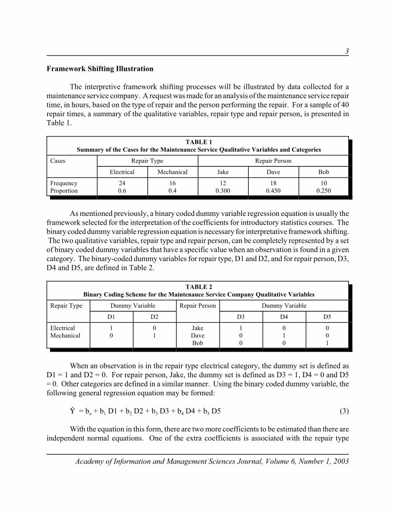
The interpretive framework shifting processes will be illustrated by data collected for amaintenance service company. A request was made for an analysis of the maintenance service repairtime, in hours, based on the type of repair and the person performing the repair. For a sample of 40repair times, a summary of the qualitative variables, repair type and repair person, is presented inTable 1.
TABLE 1Summary of the Cases for the Maintenance Service Qualitative Variables and Categories
Cases Repair Type Repair Person
Electrical Mechanical Jake Dave Bob
FrequencyProportion
240.6
160.4
120.300
180.450
100.250
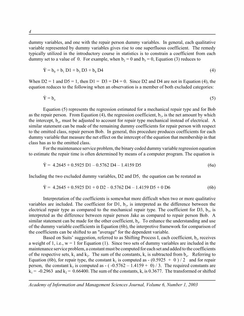
As mentioned previously, a binary coded dummy variable regression equation is usually theframework selected for the interpretation of the coefficients for introductory statistics courses. Thebinary coded dummy variable regression equation is necessary for interpretative framework shifting. The two qualitative variables, repair type and repair person, can be completely represented by a setof binary coded dummy variables that have a specific value when an observation is found in a givencategory. The binary-coded dummy variables for repair type, D1 and D2, and for repair person, D3,D4 and D5, are defined in Table 2.
TABLE 2Binary Coding Scheme for the Maintenance Service Company Qualitative Variables
Repair Type Dummy Variable Repair Person Dummy Variable
D1 D2 D3 D4 D5
ElectricalMechanical
10
01
JakeDaveBob
100
010
001
When an observation is in the repair type electrical category, the dummy set is defined asD1 = 1 and D2 = 0. For repair person, Jake, the dummy set is defined as D3 = 1, D4 = 0 and D5= 0. Other categories are defined in a similar manner. Using the binary coded dummy variable, thefollowing general regression equation may be formed:
ì = bo + b1 D1 + b2 D2 + b3 D3 + b4 D4 + b5 D5 (3)
With the equation in this form, there are two more coefficients to be estimated than there areindependent normal equations. One of the extra coefficients is associated with the repair type
4
Academy of Information and Management Sciences Journal, Volume 6, Number 1, 2003
dummy variables, and one with the repair person dummy variables. In general, each qualitativevariable represented by dummy variables gives rise to one superfluous coefficient. The remedytypically utilized in the introductory course in statistics is to constrain a coefficient from eachdummy set to a value of 0. For example, when b2 = 0 and b5 = 0, Equation (3) reduces to
ì = b0 + b1 D1 + b3 D3 + b4 D4 (4)
When D2 = 1 and D5 = 1, then D1 = D3 = D4 = 0. Since D2 and D4 are not in Equation (4), theequation reduces to the following when an observation is a member of both excluded categories:
ì = bo (5)
Equation (5) represents the regression estimated for a mechanical repair type and for Bobas the repair person. From Equation (4), the regression coefficient, b1, is the net amount by whichthe intercept, bo, must be adjusted to account for repair type mechanical instead of electrical. Asimilar statement can be made of the remaining dummy coefficients for repair person with respectto the omitted class, repair person Bob. In general, this procedure produces coefficients for eachdummy variable that measure the net effect on the intercept of the equation that membership in thatclass has as to the omitted class.
For the maintenance service problem, the binary coded dummy variable regression equationto estimate the repair time is often determined by means of a computer program. The equation is
ì = 4.2645 + 0.5925 D1 – 0.5762 D4 – 1.4159 D5 (6a)
Including the two excluded dummy variables, D2 and D5, the equation can be restated as
ì = 4.2645 + 0.5925 D1 + 0 D2 – 0.5762 D4 – 1.4159 D5 + 0 D6 (6b)
Interpretation of the coefficients is somewhat more difficult when two or more qualitativevariables are included. The coefficient for D1, b1, is interpreted as the difference between theelectrical repair type as compared to the mechanical repair type. The coefficient for D3, b3, isinterpreted as the difference between repair person Jake as compared to repair person Bob. Asimilar statement can be made for the other coefficient, b4. To enhance the understanding and useof the dummy variable coefficients in Equation (6b), the interpretive framework for comparison ofthe coefficients can be shifted to an "average" for the dependent variable.
Based on Suits’ suggestion, referred to as Shifting Process I, each coefficient, bi, receivesa weight of 1, i.e., w = 1 for Equation (1). Since two sets of dummy variables are included in themaintenance service problem, a constant must be computed for each set and added to the coefficientsof the respective sets, k1 and k2. The sum of the constants, k, is subtracted from bo. Referring toEquation (6b), for repair type, the constant k1 is computed as - (0.5925 + 0 ) / 2 and for repairperson, the constant k2 is computed as - ( -0.5762 – 1.4159 + 0) / 3. The required constants arek1 = -0.2963 and k2 = 0.66400. The sum of the constants, k, is 0.3677. The transformed or shifted
5
Academy of Information and Management Sciences Journal, Volume 6, Number 1, 2003
equation is obtained by adding each constant, k1 and k2, to the respective set of coefficients andsubtracting the sum of the constants, k, from the regression equation intercept or constant. The Suits’shifted equation for Equation (6b) is
ì = 3.8968 + 0.2963 D1 - 0.2963 D2 + 0.0878 D3 – 0.7519 D4 + 0.6640 D5 (7)
The interpretation of the coefficients now indicates the extent to which behavior in therespective repair type and in the respective repair person categories vary from the unweightedaverage of repair type, when averaged over all subcategory means for repair time. For the repairtype electrical coefficient, b1 = 0.2963, an electrical repair type adds 0.2963 hours to the unweightedaverage, 3.8968 hours of repair time. Also, repair person Bob subtracts 0.7519 hours from theunweighted average.
To shift the interpretation framework of the coefficients to an "average" that is the overallmean of the dependent variable, referred to as Shifting Process II, Sweeny and Ulveling suggestedusing the sample proportions for categories of each qualitative variable as weights in Equation (1).Using Table 1, for repair type, k1 is computed as ( 0.6*-0.2963 + 0.4*0.2963) and k2 is computedas - ( 0.300 * 0.0878 + 0.450 * -0.7519 + 0.2500 * 0.6640). The required constants are k1 = +0.0593 and k2 = +0 .1460. The sum of the constants, k, is +0.0867. As for Process I, k is subtractedfrom the constant and each constant, k1 and k2, is added to the coefficients of their respectivedummy regression coefficients in Equation (7). The Sweeny and Ulveling's shifted equation is
ì = 3.8100 + 0.2370 D1 – 0.3556 D2 + 0.2339 D3 –0.6059 D4 + 0.8100 D5 (8)
The interpretive framework for comparison of the dummy coefficients now represents thenet effect of being in the category associated with the dummy variable as compared to the overallmean or grand mean of the dependent variable, Y = bo. For example, a mechanical repair typesubtracts 0.3556 hours from the average repair time, 3.810 hours, and repair person Bob adds 0.8100hours to the repair time average hours.
One further note is that a shift in the binary coded dummy regression coefficients, Equation(6) can be made directly to the "average” that is the overall mean of the dependent variable,Equation (8), by using Shifting Process II.
FRAMEWORK SHIFTING WITH A COMPUTER PACKAGE
The interpretive framework of dummy variable coefficients resulting for Shifting ProcessesI and II may also be obtained by using coding schemes that are alternatives to the binary codingscheme (Parker & Wrighton, 1975). The alternative coding schemes require that one category foreach qualitative variable be excluded when calculating the regression equation. Referring to themaintenance service problem, repair type mechanical and repair person Bob are selected as theexcluded categories.
When using the binary coding scheme the reference category is always coded zero. Analternative scheme, referred to as Alternative Scheme I, is to uniformly code the reference category
6
Academy of Information and Management Sciences Journal, Volume 6, Number 1, 2003
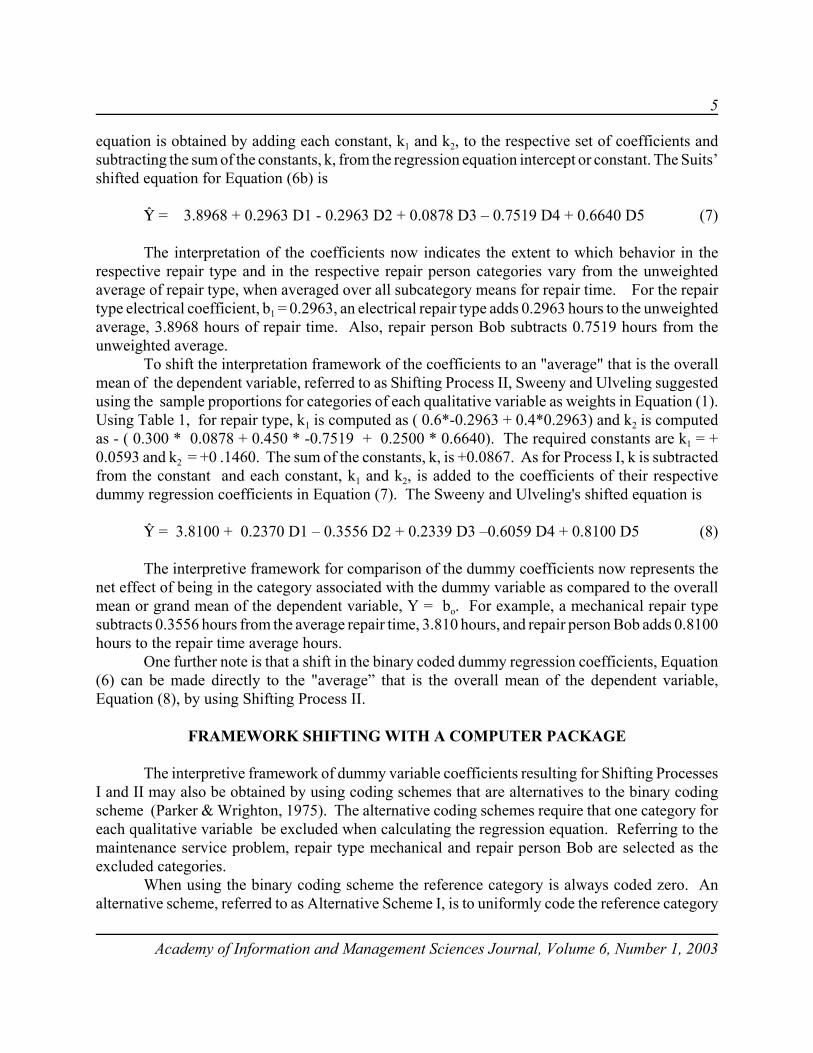
with the value of -1. A value of 1 is assigned to categories in the same manner as the binary codingscheme. When an observation is in the repair type electrical category, D1 = 1, and when the repairtype is mechanical, D1 = -1. For repair person, the selected dummy variables are D3 and D4. Thesedummy variables are defined in Table 3.
TABLE 3Alternative Coding Scheme I for the Maintenance Service Company Qualitative Variables
Repair Type Dummy D1 Dummy D2 Repair Person Dummy D3 Dummy D4 Dummy D5
ElectricalMechanical
1-1
omittedclass
JakeDaveBob
10-1
01-1
omittedclass
For Alternative Coding Scheme I, the following computer regression equation is generated
ì = 3.8968 + 0.2963 D1 + 0.0878 D3 – 0.7519 D4 (9)
Equation (9) does not contain the coefficients, b2 for D2, and b5 for D5. These coefficients are easilydetermined as follow:
b2 = - b1 = -0.2963 and b5 = - (b3 + b4) = - (0.0879 - 0.7519) = 0.6640.
When these coefficients are included in Equation (9) the resulting equation is the same as Equation(7). The coefficients are equivalent to Shifting Process I, as suggested by Suits.
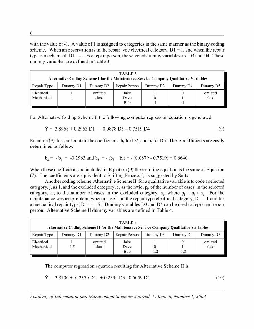
Another coding scheme, Alternative Scheme II, for a qualitative variable is to code a selectedcategory, j, as 1, and the excluded category, e, as the ratio, pj, of the number of cases in the selectedcategory, nj, to the number of cases in the excluded category, ne, where pj = nj / ne. For themaintenance service problem, when a case is in the repair type electrical category, D1 = 1 and fora mechanical repair type, D1 = -1.5. Dummy variables D3 and D4 can be used to represent repairperson. Alternative Scheme II dummy variables are defined in Table 4.
TABLE 4Alternative Coding Scheme II for the Maintenance Service Company Qualitative Variables
Repair Type Dummy D1 Dummy D2 Repair Person Dummy D3 Dummy D4 Dummy D5
ElectricalMechanical
1-1.5
omittedclass
JakeDaveBob
10
-1.2
01
-1.8
omittedclass
The computer regression equation resulting for Alternative Scheme II is
ì = 3.8100 + 0.2370 D1 + 0.2339 D3 –0.6059 D4 (10)
7
Academy of Information and Management Sciences Journal, Volume 6, Number 1, 2003
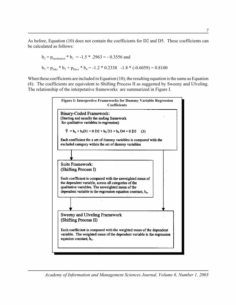
Figure I: Interpretive Frameworks for Dummy Variable RegressionCoefficients
As before, Equation (10) does not contain the coefficients for D2 and D5. These coefficients canbe calculated as follows:
b2 = pmechanical * b1 = -1.5 * .2963 = - 0.3556 and
b5 = pJake * b3 + pDave * b4 = -1.2 * 0.2338 -1.8 * (-0.6059) = 0.8100
When these coefficients are included in Equation (10), the resulting equation is the same as Equation(8). The coefficients are equivalent to Shifting Process II as suggested by Sweeny and Ulveling.The relationship of the interpetative frameworks are summarized in Figure I.

8
Academy of Information and Management Sciences Journal, Volume 6, Number 1, 2003
SUMMARY
Two processes for shifting the interpretive framework of binary-coded dummy variableregression coefficients are summarized in this paper. The frameworks assist in a more meaningfulinterpretation of the coefficients and allow for interpretation of the coefficients about an "average"of the dependent variable. One method suggested by Suits allows for each coefficient to beinterpreted as a comparison of the coefficient to the unweighted average of the dependent variableover all subcategory means. The method suggested by Sweeney and Ulveling allows for aninterpretation of the coefficients to the overall mean of the dependent variable. The effort to shiftthe interpretative framework is minimal and should be worth the effort. Comparing the coefficientsto an "average" makes the coefficients insensitive to the selection of the category to be omitted.The processes of shifting can be accomplished with or without the assistance of a computer package.The shifted interpretive frameworks may be employed by practitioners who will use the shiftedcoefficients to disseminate to individuals are who heterogeneous in regard to the use andinterpretation of the regression model. As an additional note, if quantitative independent variablesare to be included in the regression model, each quantitative variable should be coded as deviationsfrom its mean.
REFERENCES
Anderson, D., D. Sweeney & T. Williams. (2002). Statistics for Business and Economics (Eighth Edition). Cincinnati,OH: South-Western Publishing.
Daniel, W. & J. Terell. (1992). Business Statistics. Boston, MA: Houghton Mifflin Company.
Hardy, M. (1993). Regression With Dummy Variables. Sage University Paper series on Quantitative Applications inthe Social Sciences, 07-093. Newbury Park, CA: Sage Publications.
Parker, C. & F. Wrighton. (1975). Alternative Coding Schemes for Covariance Analysis of Survey Data. Unpublishedworking paper, Louisiana Tech University.
Suits, D. B (1983). Dummy Variables: Mechanics v. Interpretation. The Review of Economics and Statistics, 66, 177-180.
Sweeney, R. & E. Ulveling. (1972). A Transformation for Simplifying the Interpretation of Coefficients of BinaryVariables in Regression Analysis. The American Statistician, 5(26), 30-32.

9
Academy of Information and Management Sciences Journal, Volume 6, Number 1, 2003
IMPROVING SOFTWARE QUALITY WITH ARELIABILITY IMPROVEMENT WARRANTY
Raymond O. Folse, Nicholls State UniversityRachelle F. Cope, Southeastern Louisiana University
Robert F. Cope III, Southeastern Louisiana University
ABSTRACT
A Reliability Improvement Warranty (RIW) contract establishes a fixed price for a givenlevel of performance based upon the anticipated number of failures and the cost of each repairaction. The anticipated number of failures over the warranty period is determined by assuming thatthe reliability of the warranted item will improve from an initial level to some specified level. Thephilosophy behind RIW is that once the fixed price warranty contract is established the profitrealized is dependent upon the equipment's reliability.
In our current software industry, the need for a commitment to software quality is evident.Although the subject of software warranty has been addressed in literature, the subject of RIW forsoftware has not been given much attention. In this research, we explore RIW as a vehicle forimproving the reliability of software. We focus on the development of a model to determine the costof a software-related RIW contract and employ the Pearl-Reed economic growth model to emulatethe effect of equipment modifications on the reliability of an item under contract.
INTRODUCTION
The software industry has been in existence for about five decades. During this time, it hassurvived its backwards progression of maturity, and has taken some strides forward in thedevelopment of quality software. However, the question of software quality still remains an evasiveissue. In an internal e-mail on January 15, 2002 to employees, Bill Gates coined the term"trustworthy computing" to describe his ambitious goal of software improvement. "As an industryleader, we can and must do better," he wrote.
At this point in time, no one would disagree with Bill Gates. Gates' e-mail was sent the veryday the company recovered from a five-day stretch of system glitches causing Microsoft's Windowsupdate feature to fail intermittently. Users were unable to download software or security-relatedupdates. A month earlier, Microsoft had to fix a potentially serious security hole in Windows XP,which it touts as its most secure operating system yet. Also in 2001, a spate of Internet wormsinfected Windows computers at thousands of companies (Hulme, 2002).
Many information technology (IT) professionals consider the commitment long overdue.Poor software quality and security remain major problems for many businesses as they struggle witha continual flow of upgrades and fixes for software applications. It's an issue that keeps ITdepartments busy and one that can put their business data at risk.
10
Academy of Information and Management Sciences Journal, Volume 6, Number 1, 2003
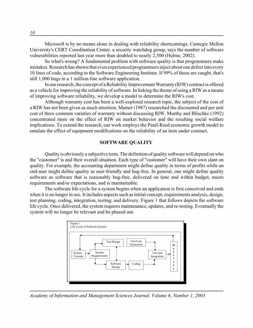
Figure 1 Life Cycle of Software System
Test Design
Software Design
Coding
Test Case Generation
Test and Integration
D e l i v e r y
System Requirements
System Concept
Microsoft is by no means alone in dealing with reliability shortcomings. Carnegie MellonUniversity's CERT Coordination Center, a security watchdog group, says the number of softwarevulnerabilities reported last year more than doubled to nearly 2,500 (Hulme, 2002).
So what's wrong? A fundamental problem with software quality is that programmers makemistakes. Research has shown that even experienced programmers inject about one defect into every10 lines of code, according to the Software Engineering Institute. If 99% of those are caught, that'sstill 1,000 bugs in a 1 million-line software application.
In our research, the concept of a Reliability Improvement Warranty (RIW) contract is offeredas a vehicle for improving the reliability of software. In linking the theme of using a RIW as a meansof improving software reliability, we develop a model to determine the RIW's cost.
Although warranty cost has been a well-explored research topic, the subject of the cost ofa RIW has not been given as much attention. Mamer (1987) researched the discounted and per unitcost of three common varieties of warranty without discussing RIW. Murthy and Blischke (1992)concentrated more on the effect of RIW on market behavior and the resulting social welfareimplications. To extend the research, our work employs the Pearl-Reed economic growth model toemulate the effect of equipment modifications on the reliability of an item under contract.
SOFTWARE QUALITY
Quality is obviously a subjective term. The definition of quality software will depend on whothe "customer" is and their overall situation. Each type of "customer" will have their own slant onquality. For example, the accounting department might define quality in terms of profits while anend-user might define quality as user-friendly and bug-free. In general, one might define qualitysoftware as software that is reasonably bug-free, delivered on time and within budget, meetsrequirements and/or expectations, and is maintainable.
The software life cycle for a system begins when an application is first conceived and endswhen it is no longer in use. It includes aspects such as initial concept, requirements analysis, design,test planning, coding, integration, testing, and delivery. Figure 1 that follows depicts the softwarelife cycle. Once delivered, the system requires maintenance, updates, and re-testing. Eventually thesystem will no longer be relevant and be phased out.
11
Academy of Information and Management Sciences Journal, Volume 6, Number 1, 2003
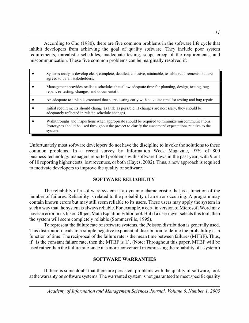
According to Cho (1980), there are five common problems in the software life cycle thatinhibit developers from achieving the goal of quality software. They include poor systemrequirements, unrealistic schedules, inadequate testing, scope creep of the requirements, andmiscommunication. These five common problems can be marginally resolved if:
‚ Systems analysts develop clear, complete, detailed, cohesive, attainable, testable requirements that areagreed to by all stakeholders.
‚ Management provides realistic schedules that allow adequate time for planning, design, testing, bugrepair, re-testing, changes, and documentation.
‚ An adequate test plan is executed that starts testing early with adequate time for testing and bug repair.
‚ Initial requirements should change as little as possible. If changes are necessary, they should beadequately reflected in related schedule changes.
‚ Walkthroughs and inspections when appropriate should be required to minimize miscommunications.Prototypes should be used throughout the project to clarify the customers' expectations relative to thesystem.
Unfortunately most software developers do not have the discipline to invoke the solutions to thesecommon problems. In a recent survey by Information Week Magazine, 97% of 800business-technology managers reported problems with software flaws in the past year, with 9 outof 10 reporting higher costs, lost revenues, or both (Hayes, 2002). Thus, a new approach is requiredto motivate developers to improve the quality of software.
SOFTWARE RELIABILITY
The reliability of a software system is a dynamic characteristic that is a function of thenumber of failures. Reliability is related to the probability of an error occurring. A program maycontain known errors but may still seem reliable to its users. These users may apply the system insuch a way that the system is always reliable. For example, a certain version of Microsoft Word mayhave an error in its Insert Object Math Equation Editor tool. But if a user never selects this tool, thenthe system will seem completely reliable (Sommerville, 1995).
To represent the failure rate of software systems, the Poisson distribution is generally used.This distribution leads to a simple negative exponential distribution to define the probability as afunction of time. The reciprocal of the failure rate is the mean time between failures (MTBF). Thus,if is the constant failure rate, then the MTBF is 1/ . (Note: Throughout this paper, MTBF will beused rather than the failure rate since it is more convenient in expressing the reliability of a system.)
SOFTWARE WARRANTIES
If there is some doubt that there are persistent problems with the quality of software, lookat the warranty on software systems. The warranted system is not guaranteed to meet specific quality
12
Academy of Information and Management Sciences Journal, Volume 6, Number 1, 2003
standards. A software warranty is a manufacturer's guarantee to replace software that proves to bedefective with a working copy of the same product and version. Software warranties do not coverinteroperability problems that may arise from one software program interacting with another.
A software warranty is assurance that the supplier of the system will back the quality of theitem in terms of correcting any legitimate problems with the item at no cost for a particular periodof time or use. Warranties ensure that suppliers accept liability for the level of performance andquality they are offering, making software quality control a necessary element in order to offersoftware warranties (Brennan, 1994).
In order to establish a quality control program for software, the use of statistical qualitycontrol is a reality that cannot be escaped. The use of statistical quality control has come to be apowerful and widely used tool in the manufacturing industry. In manufacturing, a product's warrantyis determined through the methods of statistical quality control (Schulmeyer, 1990). Themanufacturer passes the cost of the warranty on to the customer in the form of a higher priced good.The manufacturer relies on the quality control principles in order to guarantee that the number ofdefective items produced does not cause the manufacturer's costs to exceed the additional costcarried by the customer.
The proposition for software warranties is that statistical quality control is just as applicableto software development. However, this is considered to be a myth by many software professionals,particularly those having no background in statistical quality control. It is not surprising, then, thata total commitment to product quality is lacking in the software industry. It is a widely acceptedbelief in the industry that current technology limits developers from offering a meaningful warranty.In fact, most off-the-shelf software packages offer no warranty at all except disclaimers. However,Cho (1987) has been an advocate of solving the many problems of the software industry in order tomake software warranties an attainable dream to software users and developers. His methodologystresses the use of statistical quality control throughout every stage of the software life cycle.
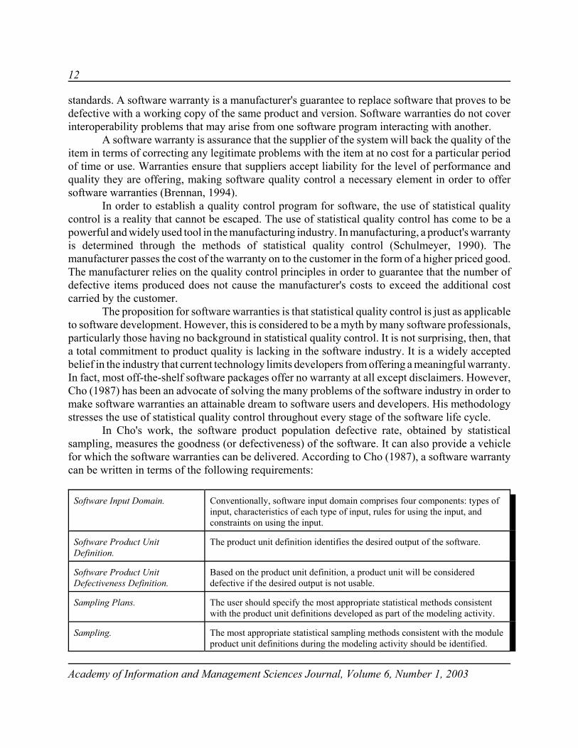
In Cho's work, the software product population defective rate, obtained by statisticalsampling, measures the goodness (or defectiveness) of the software. It can also provide a vehiclefor which the software warranties can be delivered. According to Cho (1987), a software warrantycan be written in terms of the following requirements:
Software Input Domain. Conventionally, software input domain comprises four components: types ofinput, characteristics of each type of input, rules for using the input, andconstraints on using the input.
Software Product UnitDefinition.
The product unit definition identifies the desired output of the software.
Software Product UnitDefectiveness Definition.
Based on the product unit definition, a product unit will be considereddefective if the desired output is not usable.
Sampling Plans. The user should specify the most appropriate statistical methods consistentwith the product unit definitions developed as part of the modeling activity.
Sampling. The most appropriate statistical sampling methods consistent with the moduleproduct unit definitions during the modeling activity should be identified.

13
Academy of Information and Management Sciences Journal, Volume 6, Number 1, 2003
Acceptance Sampling. A statistical sampling plan that most economically meets the specifiedproducer's risk and user's risk levels can be selected.
The Defective Rate Less than ". The user should establish the product unit population defective rate for eachmodule.
RELIABILITY IMPROVEMENT WARRANTY
It is clear that one of the problems with the quality of software development is that there areno incentives for software developers to develop trustworthy software. The Department of Defensehad the same problem of reliability with various subsystems in airplanes and weapons. They havebeen able to offset this problem with the application of the RIW concept, which was first developedin 1966 between Lear Seigler, Inc. and the Navy.
It is important to note initially that a RIW is not a warranty in the classic sense with respectto materials and workmanship. A typical item placed under RIW would be an airplane engine. Itcalls for the contractor to replace or repair, at his option, any warranted item within a specified timeunit (in operating hours, calendar time or both), except on cases of obvious misuse. The contractestablishes a fixed price for a given level of performance. This price is based upon the anticipatednumber of failures and the cost of each repair action. The anticipated number of failures over thewarranty period is determined by assuming that the reliability of the warranted item will improvefrom the initial level to some specified level as a result of the contractor's planned reliabilityimprovement program. The incentive comes in the form of an increased fee paid to the contractorif it can be demonstrated that the reliability of the item has been increased (Blischke and Murthy,1996). In addition, a study by the Logistic Management Institute demonstrated investment in anRIW contract produced a net savings in total cost to the Defense Department, which helped to offsetthe effects of inflation and dwindling defense budgets (Logistic Management Institute, 1974).
The contractor, who is responsible for all failures, initiates an on-going reliabilityimprovement program to improve the warranted item's initial reliability, 2i, to a specified reliability,2*. The contract requires the manufacturer to replace or repair, at his option, any warranted item overthe life of the contract.
Reliability information generated and recorded over time can be used to observe trends inthe reliability of the product. The term "growth" can be used because it is assumed that the reliabilityof the product will increase over time as design changes and repairs are implemented. In otherwords, reliability growth is a projection of the reliability of a system, component, or product at somefuture development time. This projection is based upon information currently available frompredictions or prior experience on identical or similar systems. Monitoring reliability, the MTBFs,and the failure rate of a system, equipment, or product, can establish an increasing trend inreliability, the MTBFs, or a decrease in the failure rate.
Such reliability growth occurs from corrective and/or preventive actions based on experiencegained from early failures and corrective actions to the system, design, production, and operationprocesses. These actions represent an obvious reason for improved reliability. The philosophybehind RIW is that once the fixed price warranty contract is established, the profit realized by the
14
Academy of Information and Management Sciences Journal, Volume 6, Number 1, 2003
contractor is dependent upon the equipment's reliability. Thus, contractors are motivated to focustheir attention on the reliability of the items under contract through the use of "no cost" (to thebuyer) engineering change proposals (USAF, 1974).
The advantages of the RIW for the buyer are reduced maintenance cost and increasedreliability. The seller has the incentive to develop an on-going reliability (quality control) programbecause of the profit potential.
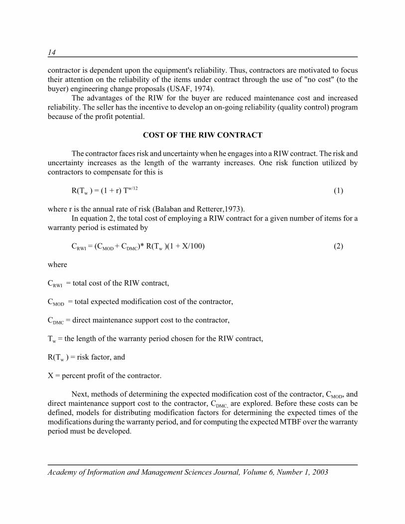
COST OF THE RIW CONTRACT
The contractor faces risk and uncertainty when he engages into a RIW contract. The risk anduncertainty increases as the length of the warranty increases. One risk function utilized bycontractors to compensate for this is
R(Tw ) = (1 + r) Tw/12 (1)
where r is the annual rate of risk (Balaban and Retterer,1973).In equation 2, the total cost of employing a RIW contract for a given number of items for a
warranty period is estimated by
CRWI = (CMOD + CDMC)* R(Tw )(1 + X/100) (2)
where
CRWI = total cost of the RIW contract,
CMOD = total expected modification cost of the contractor,
CDMC = direct maintenance support cost to the contractor,
Tw = the length of the warranty period chosen for the RIW contract,
R(Tw ) = risk factor, and
X = percent profit of the contractor.
Next, methods of determining the expected modification cost of the contractor, CMOD, anddirect maintenance support cost to the contractor, CDMC, are explored. Before these costs can bedefined, models for distributing modification factors for determining the expected times of themodifications during the warranty period, and for computing the expected MTBF over the warrantyperiod must be developed.

15
Academy of Information and Management Sciences Journal, Volume 6, Number 1, 2003
THE EFFECT OF SYSTEM MODIFICATIONS ON THE MTBF
Modifications of a software system under a RIW are made through the use of softwareengineering change proposals. Each change proposal is designed to improve the current MTBF bya factor of M. Namely, if 2new is the current MTBF, then the new MTBF 2new = M* 2old. Within thelifetime of a RIW contract, a finite number of modifications may be implemented to cause the initialMTBF, 2i, to approach a specified MTBF, 2*, which was agreed upon during contract negotiations.Thus, a technique must be found to determine the improvement factor, M, defined by eachmodification.
The value of each M is bound such that M $1 but M < M', where M' is an upper bound forall such modifications pertaining to the particular item. Furthermore, the value of each M isdependent upon 2*, the specified MTBF the contractor must try to reach with each modification,and upon 2, the current MTBF of the population of items procured.
One such function that is consistent with these assumptions is
(3)θ
θ
+=θ
−
−−
*
1M
*MMM1MM '
')'(')(
where
M* = the improvement factor expected if 2 = 2*.
Equation 3 is a form of the Pearl-Reed curve often used in economic growth models. Balaban andRetterer (1973) used a similar form of this equation in their study.
A numerical example is now considered to demonstrate the nature of the function M. Let theinitial MTBF be 50 hours, the specified MTBF be 2* = 111 hours, M' = 4 and M* = 1.3. For thesevalues the modification function is
M(2) = 4 + (1 - 4)[(4 - 1.3)/(4 - 1)](111/ 2) = 4 - 3(0.90) (111/2) .
Table 1 that follows indicates the values of M and the new MTBF, 2new, after eachmodification is employed. Two modifications are required for 2 new to become greater than or equalto the specified MTBF of 111 hours.
Table 1: Modification Functional Values
Modification 2 M(2 ) 2new = M*2
1 50.0000 1.6257 81.2839
2 81.2839 1.4020 113.9818

16
Academy of Information and Management Sciences Journal, Volume 6, Number 1, 2003
TIME OF A MODIFICATION
The time at which a modification can be introduced is a random variable Tm. It is reasonableto assume that modifications will not occur before some minimum time T" has occurred afterprocurement of the items or after a previous modification has been employed. One distribution thatcan be used to define Tm is the negative exponential distribution defined in equation 4,
(4))αTm-d(Tde )mf(T
−=
for Tm T" and where the constant, d, represents the rate of modification. The cumulative> distribution function F is defined in equation 5,
(5)
)Tm
-d(Te 1T)mP(T F(T) α
−−=≤=
for T" Tm # T. Further, assume that a certain procurement results in k-modifications with values< M1, M2, M3, …, Mk, and each modification occurs at some time Tm. The time between modificationsis restricted so that each modification occurs only after some time T" has occurred. Thus ifk-modifications are involved, then the times of each are ordered as
.TT T ... T T T T 0 Wmmm kk2211<<<<<<<< ααα
Given that a modification occurs on some time interval (T" , T$ ), then the expected time of eachsuch modification can be obtained by employing basic principles of probability theory. It can beshown that the expected time of each modification can be found by employing equation 6,
(6) .)(-e1
)(-e) - ( - T )T TT|E(T
TT
TT
mm d
dTT
d
1
αβ
αβ
−−
−
+=<<αβ
αβα
AVERAGE MTBF OVER TW
The average MTBF of the software system over the warranty period represents anotherimportant measure. If we assume that k-modifications occur respectively, at times Tm1, Tm2, Tm3, …Tmn, then the MTBF varies from 20 over [0, Tm1], to 21 over [Tm1, Tm2], to 2 2 over [Tm2, Tm3], …,to 2k over [Tmk, Tw]. The values of the modification times Tm1, Tm2, Tm3, … Tmk can be estimated byemploying equation 6 which defines the expected modification time.
Thus an estimate for the average MTBF is defined in equation 7,
17
Academy of Information and Management Sciences Journal, Volume 6, Number 1, 2003
Figure 2 Graph of the Cost of Modification
Cost 1 Modification Value M'
(7).
wT
) m kT - wT(k wT
) m 1T - m 2T(
wT
)m 1T(10
Θ++
Θ+
Θ=Θ L
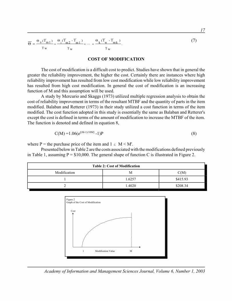
COST OF MODIFICATION
The cost of modification is a difficult cost to predict. Studies have shown that in general thegreater the reliability improvement, the higher the cost. Certainly there are instances where highreliability improvement has resulted from low cost modification while low reliability improvementhas resulted from high cost modification. In general the cost of modification is an increasingfunction of M and this assumption will be used.
A study by Mercurio and Skaggs (1973) utilized multiple regression analysis to obtain thecost of reliability improvement in terms of the resultant MTBF and the quantity of parts in the itemmodified. Balaban and Retterer (1973) in their study utilized a cost function in terms of the itemmodified. The cost function adopted in this study is essentially the same as Balaban and Retterer'sexcept the cost is defined in terms of the amount of modification to increase the MTBF of the item.The function is denoted and defined in equation 8,
C(M) =1.06(e[(M-1)/10M] -1)P (8)
where P = the purchase price of the item and 1 # M < M'.Presented below in Table 2 are the costs associated with the modifications defined previously
in Table 1, assuming P = $10,000. The general shape of function C is illustrated in Figure 2.
Table 2: Cost of Modification
Modification M C(M)
1 1.6257 $415.93
2 1.4020 $208.34
18
Academy of Information and Management Sciences Journal, Volume 6, Number 1, 2003
If it is found that k-modifications are profitable, then the total cost of these modifications canbe found using equation 9,
(9).)C (M U C
k
1iiM O D ∑
=
=
Additionally, the contractor will typically incur modification costs at time Tmi. If we assumethe estimated modification costs are included by the contractor in the price of the RIW contract andthe contractor pays the contract price at time 0, then these costs are discounted. Equation 10 thatfollows determines the total cost of all the modifications by discounting and amortizing each C(Mi)with I = yearly interest rate. The modification times, Tmi, are again estimated by equation 6.
(10)∑
= +=
k
1i miL
miwTiMOD )T - (T
)T - (TI/12)1(1)C(M U C
mi
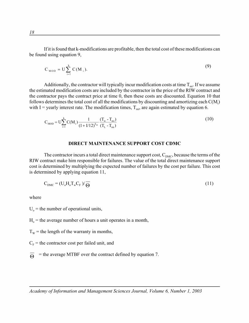
DIRECT MAINTENANCE SUPPORT COST CDMC
The contractor incurs a total direct maintenance support cost, CDMC, because the terms of theRIW contract make him responsible for failures. The value of the total direct maintenance supportcost is determined by multiplying the expected number of failures by the cost per failure. This costis determined by applying equation 11,
CDMC = (UoHoTwCF )/ (11)Θ
where
Uo = the number of operational units,
Ho = the average number of hours a unit operates in a month,
TW = the length of the warranty in months,
CF = the contractor cost per failed unit, and
= the average MTBF over the contract defined by equation 7.Θ

19
Academy of Information and Management Sciences Journal, Volume 6, Number 1, 2003
EXAMPLE - HYPOTHETICAL PURCHASE
Table 3 below defines the parameters to be used for a hypothetical software purchase of anenterprise's information system.
Table 3: Parameters for the Example
Parameter Symbol Value
Expected Lifetime of Software TL 120 months
Minimum period before Modification Twin 3 months
Length of RIW Contract TW 75 months
Discount Interest Rate I 10%
Risk Factor R 4%
Contractor Profit Factor X 10%
Rate of modification d 0.1096
The value of the rate of modification was derived assuming the probability that a softwarecontractor would inaugurate a software modification over a 3 to 24 month period was 0.90. Byemploying equation 5 and the given information, a value for the rate of modification, d, can befound.
The key values M* and M' which are required in the modification improvement function aredefined as M' = 4 and M* = 1 + 0.20(2* - 2i)/ 2i where 2* is the specified MTBF and 2i is the initialMTBF.
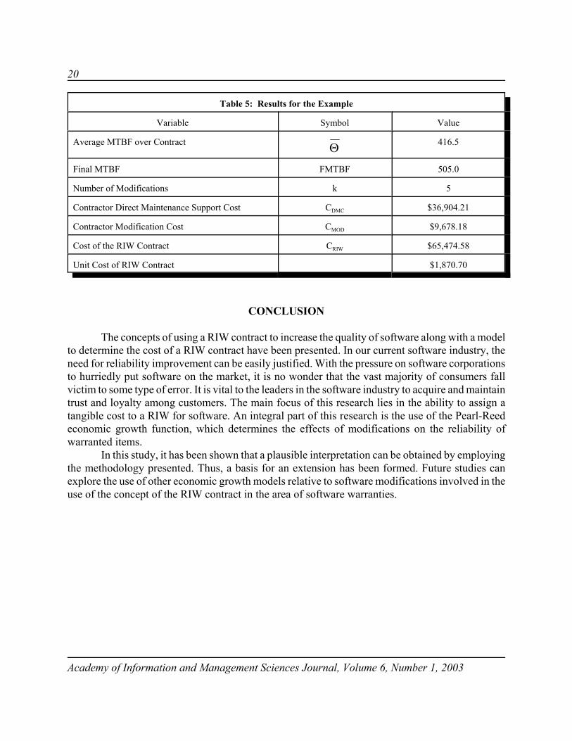
Table 4 lists the data elements for the hypothetical procurement. The results of applying themodel for the cost of a RIW contract are summarized in Table 5. Notice that the unit cost of the RIWcontract is $1,870.70 and the MTBF increases 61.7% from 312.4 hours to 505.0 hours over thewarranty period for the given example.
Table 4: Data for the Example
Variable Symbol Value
Unit Price P $15,461.80
Operating Hours per Month Ho 52
Number of Operational Units Uo 27
Initial MTBF Specified 2i 312.4
MTBF 2* 472.3
Contractor Cost per Failed Unit CF $500.00
20
Academy of Information and Management Sciences Journal, Volume 6, Number 1, 2003
Table 5: Results for the Example
Variable Symbol Value
Average MTBF over Contract Θ 416.5
Final MTBF FMTBF 505.0
Number of Modifications k 5
Contractor Direct Maintenance Support Cost CDMC $36,904.21
Contractor Modification Cost CMOD $9,678.18
Cost of the RIW Contract CRIW $65,474.58
Unit Cost of RIW Contract $1,870.70
CONCLUSION
The concepts of using a RIW contract to increase the quality of software along with a modelto determine the cost of a RIW contract have been presented. In our current software industry, theneed for reliability improvement can be easily justified. With the pressure on software corporationsto hurriedly put software on the market, it is no wonder that the vast majority of consumers fallvictim to some type of error. It is vital to the leaders in the software industry to acquire and maintaintrust and loyalty among customers. The main focus of this research lies in the ability to assign atangible cost to a RIW for software. An integral part of this research is the use of the Pearl-Reedeconomic growth function, which determines the effects of modifications on the reliability ofwarranted items.
In this study, it has been shown that a plausible interpretation can be obtained by employingthe methodology presented. Thus, a basis for an extension has been formed. Future studies canexplore the use of other economic growth models relative to software modifications involved in theuse of the concept of the RIW contract in the area of software warranties.
21
Academy of Information and Management Sciences Journal, Volume 6, Number 1, 2003
REFERENCES
Balaban, H.S. & B.L. Retterer. (1973, June). The use of warranties for defense avionics procurement. Annapolis,Maryland: The ARINC Research Corporation. ARINC Research Corporation Report 0637-02-1-243.
Blischke, W.R. & D.N.P. Murthy. (1996). Product warranty handbook. New York: Marcel Dekker, Inc.
Brennan, J.R. (1994). Warranties: Planning, analysis and implementation. New York: McGraw-Hill, Inc.
Cho, C.K. (1987). Statistical methods applied to software quality control. Published in G.G. Schulmeyer & J.I.McManus, (Eds.), Handbook of software quality assurance, . New York: Van Nostrand Reinhold Company.
Cho, C.K. (1980). An introduction to software quality control. New York: John Wiley & Sons, Inc.
Hayes, M. (2002, May 20). Software quality counts. Information Week Magazine, 38-54.
Hulme, G.V. (2002, January 21). Software's challenge: It's time for developers to think and act differently. InformationWeek Magazine, 20-23.
Logistic Management Institute (1974, March). Criteria for evaluating weapon system reliability, availability and costs.Washington, D.C.: Logistics Management Institute. LMI Task No. 73-111.
Mamer, J.W. (1987, July). Discounted and per unit costs of product warranty. Management Science, 33(7), 916-930. Mercurio, S.P. & C.W. Skaggs (1973). Reliability acquisition cost study. Griffin Air Force Base, New York: Rome Air
Development Center. General Electric Company Report RADC-TR-73-334.
Murthy, D.N.P. & W.R. Blischke (1992). Product warranty management - III: A review of mathematical models.European Journal of Operational Research, 63(1), 1-34.
Schulmeyer, G.G. (1990). Zero defect software. New York: McGraw-Hill, Inc.
Sommerville, I. (1995). Software engineering. Reading, MA: Addison-Wesley Company.
U.S. Department of the Air Force [USAF] (1974). Interim guidelines: Reliability improvement warranty. Washington,D.C.: U.S. Department of the Air Force.

22
Academy of Information and Management Sciences Journal, Volume 6, Number 1, 2003

23
Academy of Information and Management Sciences Journal, Volume 6, Number 1, 2003
UNDERSTANDING STRATEGIC USE OF ITIN SMALL & MEDIUM-SIZED BUSINESSES:
EXAMINING PUSH FACTORS AND USERCHARACTERISTICS
Nelson Oly Ndubisi, University Malaysia Sabah
ABSTRACT
Globalization and competitive pressures have heightened the impetus for strategic use of IT.There is a common belief that if IT is strategically used, it will enable organizations (large or small)to meet their objectives, be competitive, and achieve a favorable business performance for long-termsurvival. This has led to a growing research interest in the use of IT as a strategic weapon byorganizations in recent years. The current research examines the different concept of strategic useof IT, provides a synthesis of various ideas, and empirically investigates the characteristics ofMalaysia small and medium-sized businesses that are strategizing with IT. Important theoretical andpractical implications of the study are discussed.
INTRODUCTION
The term strategic use of IT has been inconsistently used by academicians and practitioners,thereby rendering understanding imprecise (King et al., 1989) and often misleading (Sutherland,1991). Prahalad and Hamel (1990) and Williams (1992) have suggested that a truly strategicapplication must be assessed from the time-based sustainability, which is linked to core competenceof the organization. Pederson (1990) stresses that strategic use of IT must result in observablecompetitive advantage, while Emery (1990) suggests that strategic information system can bedeliberately planned and implemented to meet strategic objectives. As the number of criteria usedgrows, the concept of strategic use of IT becomes more complicated. In view of this, the currentresearch reviews the various definitions of the term in an attempt to answer the question of what isstrategic use of IT? The study also unveils the characteristics of SMBs that are strategizing with ITas well as discusses the strategies and action plans that will further enhance and promote greaterstrategic use of IT in SMBs
LITERATURE
To understand the term strategic use of IT, a review of the concepts of strategy will behelpful.
24
Academy of Information and Management Sciences Journal, Volume 6, Number 1, 2003
Strategy
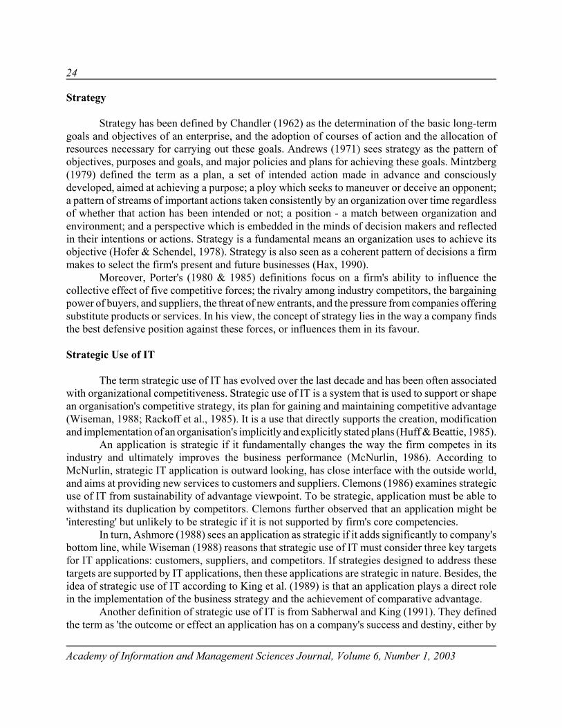
Strategy has been defined by Chandler (1962) as the determination of the basic long-termgoals and objectives of an enterprise, and the adoption of courses of action and the allocation ofresources necessary for carrying out these goals. Andrews (1971) sees strategy as the pattern ofobjectives, purposes and goals, and major policies and plans for achieving these goals. Mintzberg(1979) defined the term as a plan, a set of intended action made in advance and consciouslydeveloped, aimed at achieving a purpose; a ploy which seeks to maneuver or deceive an opponent;a pattern of streams of important actions taken consistently by an organization over time regardlessof whether that action has been intended or not; a position - a match between organization andenvironment; and a perspective which is embedded in the minds of decision makers and reflectedin their intentions or actions. Strategy is a fundamental means an organization uses to achieve itsobjective (Hofer & Schendel, 1978). Strategy is also seen as a coherent pattern of decisions a firmmakes to select the firm's present and future businesses (Hax, 1990).
Moreover, Porter's (1980 & 1985) definitions focus on a firm's ability to influence thecollective effect of five competitive forces; the rivalry among industry competitors, the bargainingpower of buyers, and suppliers, the threat of new entrants, and the pressure from companies offeringsubstitute products or services. In his view, the concept of strategy lies in the way a company findsthe best defensive position against these forces, or influences them in its favour.
Strategic Use of IT
The term strategic use of IT has evolved over the last decade and has been often associatedwith organizational competitiveness. Strategic use of IT is a system that is used to support or shapean organisation's competitive strategy, its plan for gaining and maintaining competitive advantage(Wiseman, 1988; Rackoff et al., 1985). It is a use that directly supports the creation, modificationand implementation of an organisation's implicitly and explicitly stated plans (Huff & Beattie, 1985).
An application is strategic if it fundamentally changes the way the firm competes in itsindustry and ultimately improves the business performance (McNurlin, 1986). According toMcNurlin, strategic IT application is outward looking, has close interface with the outside world,and aims at providing new services to customers and suppliers. Clemons (1986) examines strategicuse of IT from sustainability of advantage viewpoint. To be strategic, application must be able towithstand its duplication by competitors. Clemons further observed that an application might be'interesting' but unlikely to be strategic if it is not supported by firm's core competencies.
In turn, Ashmore (1988) sees an application as strategic if it adds significantly to company'sbottom line, while Wiseman (1988) reasons that strategic use of IT must consider three key targetsfor IT applications: customers, suppliers, and competitors. If strategies designed to address thesetargets are supported by IT applications, then these applications are strategic in nature. Besides, theidea of strategic use of IT according to King et al. (1989) is that an application plays a direct rolein the implementation of the business strategy and the achievement of comparative advantage.
Another definition of strategic use of IT is from Sabherwal and King (1991). They definedthe term as 'the outcome or effect an application has on a company's success and destiny, either by

25
Academy of Information and Management Sciences Journal, Volume 6, Number 1, 2003
influencing or shaping the company's strategy, or by playing a direct role in the implementation ofthe strategy. According to them, an application is strategic if it either provides the company with acompetitive advantage or reduces the competitive advantage of a competitor.
Besides, Bergeron et al., (1991) sees strategic use of IT as a means used to secure gains overcompetitors, while Fripp, (1991) says it is a system, which companies developed that has eithergiven it competitive advantage or has significantly affected the overall conduct and success of theirorganizations. Alter (1991) insists that only if an organisation's production, sales, and servicesfunctions are dependent on the systems can the applications be considered strategic.
Another view of strategic use of IT emanates from Schutzer's (1991), which describesstrategic use of IT as an application that helps to maintain competitive parity over the long term. Heexplains that strategic system may not be necessarily competitive but suffices if it can create anenvironment conducive to the continued generation of innovative solutions and if it can create anenvironment that supports the production of continuous, small improvements.
Some writers have also considered what is not strategic IT application. It is clear that an ITapplication is not strategic by virtue of its sophistication and complexity. In fact there is even thetendency for very highly sophisticated systems to be resented. An application cannot be strategicif it only provides organizational support for greater internal efficiency and fails to produce resultsthat support the company strategy and long term profitability (Zain, 1998), or if an IT investmentserves merely to keep up to actions of competitors (King et al., 1989).
In this paper, the working definitions of strategic use of IT were taken from Zain (1998) andNdubisi and Jantan (2001). Zain asserts that a common view of strategic use of IT often reflects theuse of IT to support planning and management control and operations i.e. tactical and transactionalconsiderations (Zain, 1998). Ndubisi and Jantan (2001) view the concept of strategic use of IT asthe application of IT in critical areas of the business functions of the organization, in order toenhance job effectiveness, improve job performance, and increase productivity above competition.The implication of this definition is that employment of IT resources in critical areas of the businessfunction must result in achievement of goals and objectives (operational effectiveness) competently(operational efficiency).
The views are similar to leveraging IT in the value chain (see Laudon & Laudon, 1997, p48).Laudon and Laudon identified the various examples of strategic information systems and theactivities of the value chain where they can be applied.
METHOD
Participants & Procedure
The Northern Malaysia-based Malay, Chinese and Indian Chambers of Commerce andIndustry as well as the national association of women entrepreneurs in Malaysia were contacted forthe list of the members. The lists serve as the study's sampling frame. A set of questionnaire was sentto all the members of these associations, out of which 177 usable responses were received. The CEOrepresented the firms, as they are in a position to furnish reliable information about their firms since

26
Academy of Information and Management Sciences Journal, Volume 6, Number 1, 2003
they are in charge of the day-to-day management of the business. Primary business activities of thefirms range from manufacturing, to sales, education, interior decoration, fashion designing, etc.
Data were collected using structured questionnaire made up of three parts. Part 1 measuresthe actual system usage with two indicators of the number of job tasks where systems are appliedsuch as for planning and control purposes. These indicators were taken from Rahmah and Arfah(1999). Part 2 measures strategically targeted benefits of the application such as: enhancement ofjob effectiveness (B1), improvement in job performance (B2), and increase in productivity (B3)taken from Ndubisi et al., (2001); Davis et al., (1989). Part 3 of the questionnaire measuresdemographic factors. Reliability analysis of the items measuring IT usage and strategically targetedbenefits were performed to evaluate the Cronbach's Alpha value, which shows a value of .87 forusage and .91 for target benefits. The reliability test results in this study show alpha valuesexceeding .60 to .70 recommended by Hairs (1998) as the lower limit of acceptability. This ensuresthat the items grouping are reliable under the conditions of the local survey. Test of mean differencesand the regression analysis were mainly used in the study.
RESULTS
Key Respondents' Profile
Table 2 shows key organization and CEO characteristics.
Table 2: Profiles of the Firms
1. Industry Type Percent (%) 5. Computing Experience Percent (%)
Manufacturing 24.9 11 years or more 11.3
Service 75.1 1-5 years 44.1
2. Years of Establishment Percent (%) 6-10 years 44.6
5 years or less 31.6 6. Age Percent (%)
More than 5 years 68.4 41 years or more 44.0
3. Number of Employees Percent (%) 40 years or less 56.0
101 or more 14.6 7. Sex Percent (%)
Below 5 25.5 Male 58.2
5-100 59.9 Female 41.8
4. Respondent's Education Percent (%)
University graduate 45.2
Non-University graduate 54.8
The majority (68.4%) of the firms have been established for more than five years.Approximately 15% are considered medium size having between 100-200 employees, 60% are small

27
Academy of Information and Management Sciences Journal, Volume 6, Number 1, 2003
sized (5-100 employees), and 25% are very small in size (below 5 employees). Many of the firms(75%) operate in the service sector, while the rest (25%) are manufacturing outfits. Close to 55%of the respondents are universities graduates, 56% have over five years of computing generalexperience, and 58% are male.
Target Benefits
Respondents have the following perception of systems' strategic benefits: 84.8% ofrespondents either agree or strongly agree that the system improves their job performance (B1),84.2% agree or strongly agree that systems help increase their productivity (B2), and 85.3% at leastagree that system enhances their job effectiveness (B3). The means for B1, B2, and B3 arerespectively 4.21, 4.10, and 4.17 (min. = 1, max. = 5), showing that on the whole, respondents findthe systems to improve their job performance, increase their productivity, and enhance their jobeffectiveness
IT Usage
Table 3 shows the IT usage characteristics of respondents.
Table 3: IT Usage
System Variety Usage (%) Specific Job Tasks Usage (%)
Word processing 91.5 Letters and memos 85.9
Electronic mail 78.0 Producing report 75.1
Spreadsheets 55.9 Communication with others 73.4
Application packages 53.6 Data storage/retrieval 59.9
Graphics 44.6 Planning/Forecasting 46.3
Database 37.3 Budgeting 44.1
Programming languages 26.0 Controlling & guiding activities 38.4
Statistical analysis 25.4 Analyzing trends 34.5
Making decisions 34.5
Analyzing problems/alternatives 23.2
The results show that approximately ninety-two and seventy-eight percents of therespondents are respectively using word processing and electronic mail. Only approximately,twenty-six and twenty-five percents of the entrepreneurs are using programming languages andstatistical analysis tools respectively. Among the job tasks where systems are used, letters andmemos top the list, followed by producing reports, and communication with others, withapproximately eighty-six percent, seventy-five percent, and seventy-three percent respectively, of
28
Academy of Information and Management Sciences Journal, Volume 6, Number 1, 2003
the respondents using an application for these job tasks. It was further observed that 59.88% areusing 4 (one-half) out of the 8 varieties of systems presented, and that 53.11% use a system to do5 (one-half) out of the 10 job tasks listed.
IT Usage Pattern
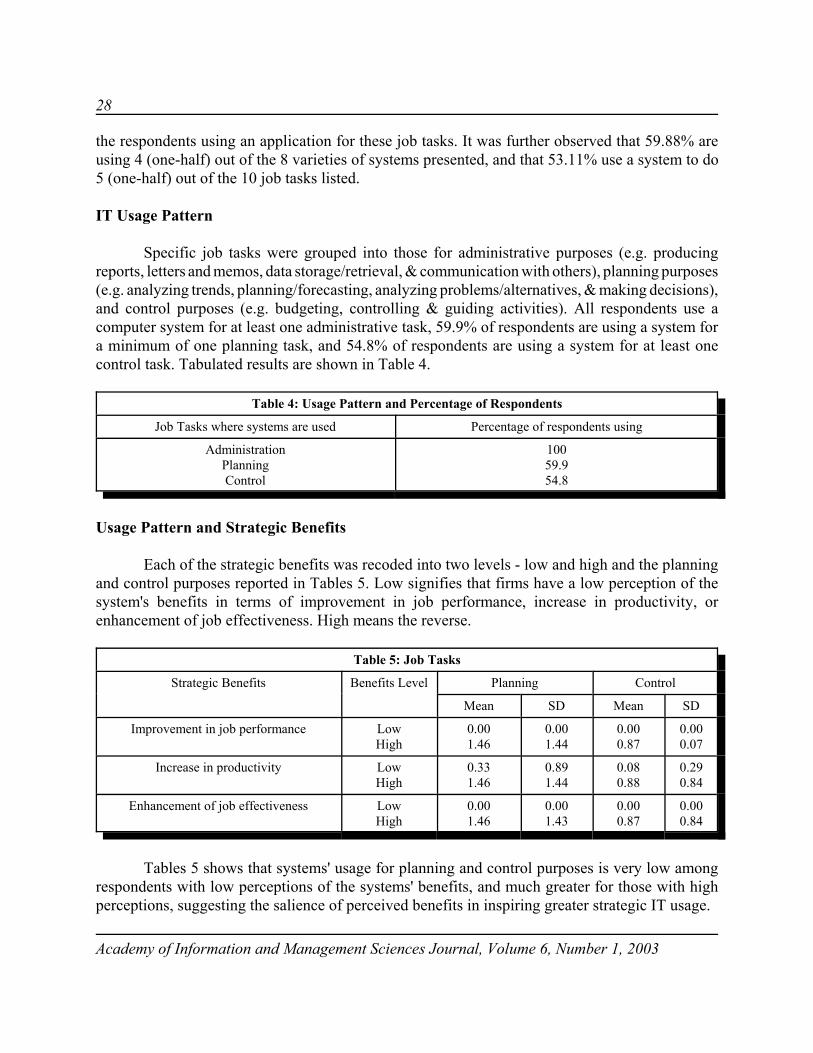
Specific job tasks were grouped into those for administrative purposes (e.g. producingreports, letters and memos, data storage/retrieval, & communication with others), planning purposes(e.g. analyzing trends, planning/forecasting, analyzing problems/alternatives, & making decisions),and control purposes (e.g. budgeting, controlling & guiding activities). All respondents use acomputer system for at least one administrative task, 59.9% of respondents are using a system fora minimum of one planning task, and 54.8% of respondents are using a system for at least onecontrol task. Tabulated results are shown in Table 4.
Table 4: Usage Pattern and Percentage of Respondents
Job Tasks where systems are used Percentage of respondents using
AdministrationPlanningControl
10059.954.8
Usage Pattern and Strategic Benefits
Each of the strategic benefits was recoded into two levels - low and high and the planningand control purposes reported in Tables 5. Low signifies that firms have a low perception of thesystem's benefits in terms of improvement in job performance, increase in productivity, orenhancement of job effectiveness. High means the reverse.
Table 5: Job Tasks
Strategic Benefits Benefits Level Planning Control
Mean SD Mean SD
Improvement in job performance LowHigh
0.001.46
0.001.44
0.000.87
0.000.07
Increase in productivity LowHigh
0.331.46
0.891.44
0.080.88
0.290.84
Enhancement of job effectiveness LowHigh
0.001.46
0.001.43
0.000.87
0.000.84
Tables 5 shows that systems' usage for planning and control purposes is very low amongrespondents with low perceptions of the systems' benefits, and much greater for those with highperceptions, suggesting the salience of perceived benefits in inspiring greater strategic IT usage.

29
Academy of Information and Management Sciences Journal, Volume 6, Number 1, 2003
Tests of Differences
Using multivariate analysis of variance (MANOVA) the study examined differences instrategic use of IT based on demography. MANOVA is an extension of ANOVA to accommodatemore than one dependent variable. Multivariate differences across groups were assessed using theWilks' Lambda criterion (also known as the U statistics). This is because Wilks' Lambda examineswhether groups are somehow different without being concerned with whether they differ on at leastone linear combination of the dependent variable, and also because it is highly immune to violationsof the MANOVA assumptions (Hair et al. 1998, p. 362). Table 6 shows the MANOVA results.
Table 6: MANOVA Results of Test of Differences
Demography F-ratio Sig. Level Group Mean
Job tasks Performance Productivity Effectiveness
Primary activity: .87 .500
Manufacturing 5.71 4.07 4.11 4.14
Service 4.97 4.11 4.19 4.23
Years of Establishment: 2.64 .025
5 years or less 4.71 3.98 3.88 4.05
More than 5 yrs 5.36 4.15 4.31 4.28
Computer experience: 5.98 .000
5 years or below 3.60 3.83 3.92 3.95
6 - 10 years 6.22 4.33 4.39 4.44
11 years or more 7.00 4.20 4.25 4.30
No. of employees: 5.4 .000
Below 5 4.13 4.27 4.44 4.33
5 - 100 4.93 3.98 4.01 4.09
101 or more 7.81 4.27 4.35 4.46
Education qualification: 10.26 .000
Non graduate 3.68 3.80 3.99 3.93
Graduate 6.14 4.29 4.29 4.40
Age: 1.67 .144
40 years or below 5.66 4.13 4.21 4.24
41 years or more 4.51 4.05 4.12 4.17
Sex: 5.28 .000
Male 4.95 3.97 3.93 4.04
Female 5.43 4.27 4.50 4.45

30
Academy of Information and Management Sciences Journal, Volume 6, Number 1, 2003
As reported in table 7, the multivariate F-ratio of MANOVA is significant at five percentlevel for years of company establishment, computing experience, number of employees, educationalqualification, and sex, suggesting that strategic use of IT differ with respect to the businessexperience of the firms, firm size, user computing experience, education level, and sex.
Prior research on gender differences in the salience of instrumentality in decision- makingprocesses about a new system provides a basis to expect that male CEOs will differ significantlyfrom the female in strategizing with IT. Hennig and Jardim state that men adopt strategies focusedon bottom-line results, while women tend to focus on the methods used to accomplish a task -suggesting a greater process orientation (Hennig & Jardim, 1977; Rotter & Portugal, 1969). Otherplausible explanations for the greater strategic use of IT by male CEOs as compared to the femaleare computer anxiety and computer aptitude. Bozionelos (1996) and Morrow et al. (1986) suggestthat women display somewhat higher levels of computer anxiety; and lower computer aptitude(Felter, 1985) compared to men (Chen, 1985).
Both general and computer-based learning are positively associated with strategic use of ITamong SMB CEOs. A number of studies (e.g. Igbaria et al., 1997; Ndubisi et al., 2001) have shownthat the more training users received, the greater usage of systems they make. In fact, Ndubisi et al.,show that graduate users of technologies often make greater usage of applications thannon-graduates. Moreover, that users with more computer-based education make greater use ofadvanced or sophisticated technologies than those with less computer-based training. This researchobserves a similar trend in the strategic use of IT.
In the context of technology adoption and usage in the workplace, there is evidence tosuggest that the availability of support staff is an organizational response to help users overcomebarriers and hurdles to technology use, especially during the early stages of learning and use (e.g.Bergeron, Rivard, & De Serre, 1990). Ndubisi and Ndubisi (2003) have shown that usage oftechnology in the workplace is positively associated with firm's size. Since larger organizations aremore likely to engage more IT support staff, it is therefore logical that such organizations makegreater strategic use of IT than smaller organizations do.
An innumerable body of IS research has related computing experience with adoption andsustained usage of technologies. Taylor and Todd (1995) found a stronger link between behavioralintention and technology acceptance behavior for more experienced users. Others, (e.g. Bagozzi1981; Ndubisi et al; 2001) have found prior experience to be an important determinant of behavior.Experience may make low probability events more salient, thereby ensuring that they are accountedfor in the formation of attitude (Ajzen & Fishbein, 1980), thus, possibly explaining why CEOs withmore computing experienced make greater strategic use of IT than less experienced users.
Mean Differences in Usage Pattern Based on Strategic Benefits
Mean differences in usage pattern were examined in the light of perceived system benefits(i.e. improvement in job performance, increase in productivity, and enhancement of jobeffectiveness) using t-tests. The results are as follows:
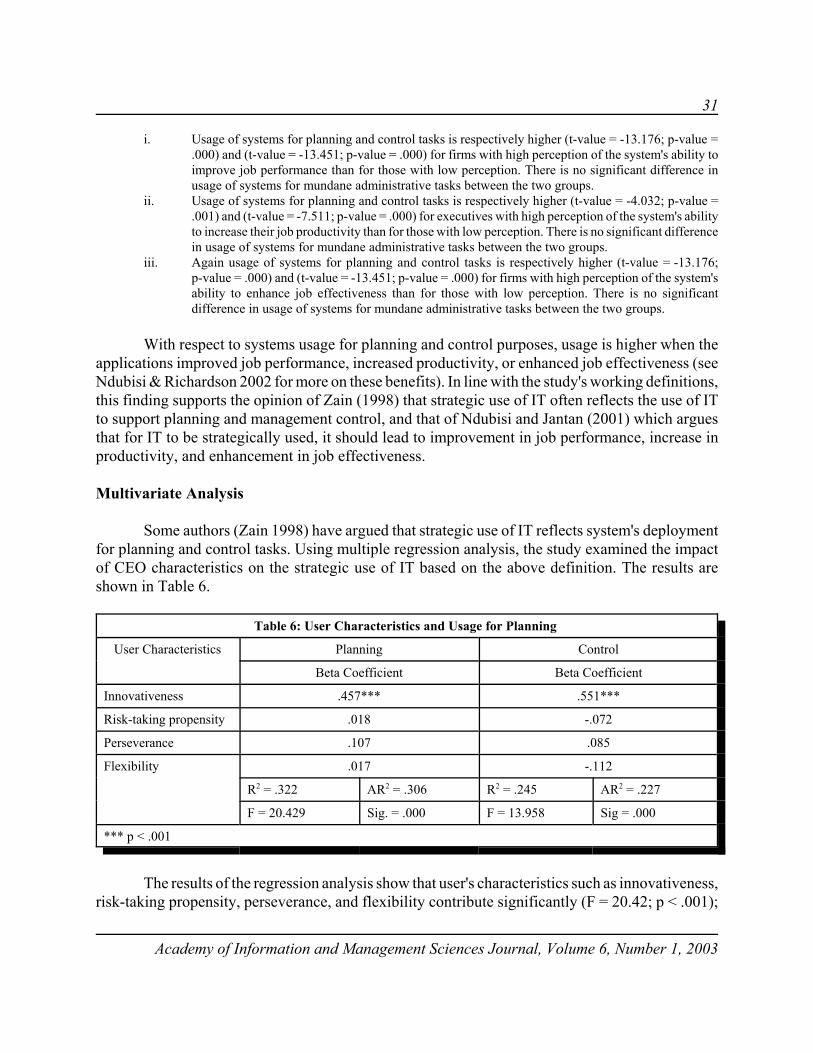
31
Academy of Information and Management Sciences Journal, Volume 6, Number 1, 2003
i. Usage of systems for planning and control tasks is respectively higher (t-value = -13.176; p-value =.000) and (t-value = -13.451; p-value = .000) for firms with high perception of the system's ability toimprove job performance than for those with low perception. There is no significant difference inusage of systems for mundane administrative tasks between the two groups.
ii. Usage of systems for planning and control tasks is respectively higher (t-value = -4.032; p-value =.001) and (t-value = -7.511; p-value = .000) for executives with high perception of the system's abilityto increase their job productivity than for those with low perception. There is no significant differencein usage of systems for mundane administrative tasks between the two groups.
iii. Again usage of systems for planning and control tasks is respectively higher (t-value = -13.176;p-value = .000) and (t-value = -13.451; p-value = .000) for firms with high perception of the system'sability to enhance job effectiveness than for those with low perception. There is no significantdifference in usage of systems for mundane administrative tasks between the two groups.
With respect to systems usage for planning and control purposes, usage is higher when theapplications improved job performance, increased productivity, or enhanced job effectiveness (seeNdubisi & Richardson 2002 for more on these benefits). In line with the study's working definitions,this finding supports the opinion of Zain (1998) that strategic use of IT often reflects the use of ITto support planning and management control, and that of Ndubisi and Jantan (2001) which arguesthat for IT to be strategically used, it should lead to improvement in job performance, increase inproductivity, and enhancement in job effectiveness. Multivariate Analysis
Some authors (Zain 1998) have argued that strategic use of IT reflects system's deploymentfor planning and control tasks. Using multiple regression analysis, the study examined the impactof CEO characteristics on the strategic use of IT based on the above definition. The results areshown in Table 6.
Table 6: User Characteristics and Usage for Planning
User Characteristics Planning Control
Beta Coefficient Beta Coefficient
Innovativeness .457*** .551***
Risk-taking propensity .018 -.072
Perseverance .107 .085
Flexibility .017 -.112
R2 = .322 AR2 = .306 R2 = .245 AR2 = .227
F = 20.429 Sig. = .000 F = 13.958 Sig = .000
*** p < .001
The results of the regression analysis show that user's characteristics such as innovativeness,risk-taking propensity, perseverance, and flexibility contribute significantly (F = 20.42; p < .001);
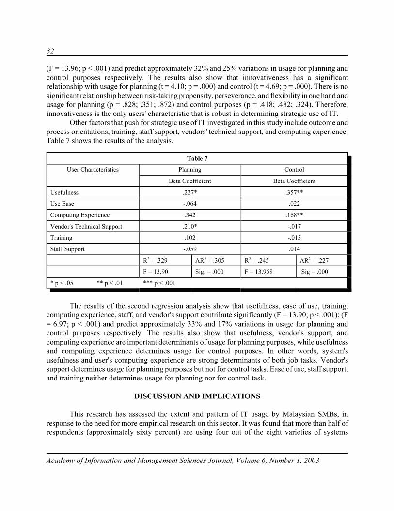
32
Academy of Information and Management Sciences Journal, Volume 6, Number 1, 2003
(F = 13.96; p < .001) and predict approximately 32% and 25% variations in usage for planning andcontrol purposes respectively. The results also show that innovativeness has a significantrelationship with usage for planning (t = 4.10; p = .000) and control (t = 4.69; p = .000). There is nosignificant relationship between risk-taking propensity, perseverance, and flexibility in one hand andusage for planning (p = .828; .351; .872) and control purposes (p = .418; .482; .324). Therefore,innovativeness is the only users' characteristic that is robust in determining strategic use of IT.
Other factors that push for strategic use of IT investigated in this study include outcome andprocess orientations, training, staff support, vendors' technical support, and computing experience.Table 7 shows the results of the analysis.
Table 7
User Characteristics Planning Control
Beta Coefficient Beta Coefficient
Usefulness .227* .357**
Use Ease -.064 .022
Computing Experience .342 .168**
Vendor's Technical Support .210* -.017
Training .102 -.015
Staff Support -.059 .014
R2 = .329 AR2 = .305 R2 = .245 AR2 = .227
F = 13.90 Sig. = .000 F = 13.958 Sig = .000
* p < .05 ** p < .01 *** p < .001
The results of the second regression analysis show that usefulness, ease of use, training,computing experience, staff, and vendor's support contribute significantly (F = 13.90; p < .001); (F= 6.97; p < .001) and predict approximately 33% and 17% variations in usage for planning andcontrol purposes respectively. The results also show that usefulness, vendor's support, andcomputing experience are important determinants of usage for planning purposes, while usefulnessand computing experience determines usage for control purposes. In other words, system'susefulness and user's computing experience are strong determinants of both job tasks. Vendor'ssupport determines usage for planning purposes but not for control tasks. Ease of use, staff support,and training neither determines usage for planning nor for control task.
DISCUSSION AND IMPLICATIONS
This research has assessed the extent and pattern of IT usage by Malaysian SMBs, inresponse to the need for more empirical research on this sector. It was found that more than half ofrespondents (approximately sixty percent) are using four out of the eight varieties of systems
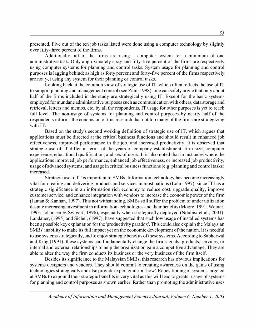
33
Academy of Information and Management Sciences Journal, Volume 6, Number 1, 2003
presented. Five out of the ten job tasks listed were done using a computer technology by slightlyover fifty-three percent of the firms.
Additionally, all of the firms are using a computer system for a minimum of oneadministrative task. Only approximately sixty and fifty-five percent of the firms are respectivelyusing computer systems for planning and control tasks. System usage for planning and controlpurposes is lagging behind; as high as forty percent and forty-five percent of the firms respectivelyare not yet using any system for their planning or control tasks.
Looking back at the common view of strategic use of IT, which often reflects the use of ITto support planning and management control (see Zain, 1998), one can safely argue that only abouthalf of the firms included in the study are strategically using IT. Except for the basic systemsemployed for mundane administrative purposes such as communication with others, data storage andretrieval, letters and memos, etc, by all the respondents, IT usage for other purposes is yet to reachfull level. The non-usage of systems for planning and control purposes by nearly half of therespondents informs the conclusion of this research that not too many of the firms are strategizingwith IT.
Based on the study's second working definition of strategic use of IT, which argues thatapplications must be directed at the critical business functions and should result in enhanced jobeffectiveness, improved performance in the job, and increased productivity, it is observed thatstrategic use of IT differ in terms of the years of company establishment, firm size, computerexperience, educational qualification, and sex of users. It is also noted that in instances where theapplications improved job performance, enhanced job effectiveness, or increased job productivity,usage of advanced systems, and usage in critical business functions (e.g. planning and control tasks)increased.
Strategic use of IT is important to SMBs. Information technology has become increasinglyvital for creating and delivering products and services in most nations (Lohr 1997), since IT has astrategic significance in an information rich economy to reduce cost, upgrade quality, improvecustomer service, and enhance integration with vendors to increase the economic power of the firm(Jantan & Kannan, 1997). This not withstanding, SMBs still suffer the problem of under utilizationdespite increasing investment in information technologies and their benefits (Moore, 1991; Weiner,1993; Johansen & Swigart, 1996), especially when strategically deployed (Ndubisi et al., 2001).Landauer, (1995) and Sichel, (1997), have suggested that such low usage of installed systems hasbeen a possible key explanation for the 'productivity paradox'. This could also explain the MalaysianSMBs' inability to make its full impact yet on the economic development of the nation. It is needfulto use systems strategically, and to enjoy strategic benefits of these systems. According to Sabherwaland King (1991), these systems can fundamentally change the firm's goals, products, services, orinternal and external relationships to help the organization gain a competitive advantage. They areable to alter the way the firm conducts its business or the very business of the firm itself.
Besides its significance to the Malaysian SMBs, this research has obvious implications forsystems designers and vendors. They should commit to creating awareness on the gains of usingtechnologies strategically and also provide expert guide on 'how'. Repositioning of systems targetedat SMBs to expound their strategic benefits is very vital as this will lead to greater usage of systemsfor planning and control purposes as shown earlier. Rather than promoting the administrative uses
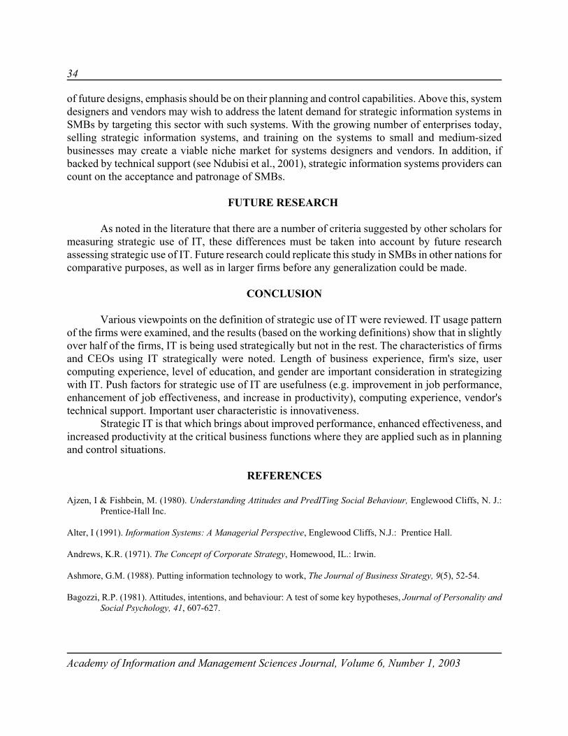
34
Academy of Information and Management Sciences Journal, Volume 6, Number 1, 2003
of future designs, emphasis should be on their planning and control capabilities. Above this, systemdesigners and vendors may wish to address the latent demand for strategic information systems inSMBs by targeting this sector with such systems. With the growing number of enterprises today,selling strategic information systems, and training on the systems to small and medium-sizedbusinesses may create a viable niche market for systems designers and vendors. In addition, ifbacked by technical support (see Ndubisi et al., 2001), strategic information systems providers cancount on the acceptance and patronage of SMBs.
FUTURE RESEARCH
As noted in the literature that there are a number of criteria suggested by other scholars formeasuring strategic use of IT, these differences must be taken into account by future researchassessing strategic use of IT. Future research could replicate this study in SMBs in other nations forcomparative purposes, as well as in larger firms before any generalization could be made.
CONCLUSION
Various viewpoints on the definition of strategic use of IT were reviewed. IT usage patternof the firms were examined, and the results (based on the working definitions) show that in slightlyover half of the firms, IT is being used strategically but not in the rest. The characteristics of firmsand CEOs using IT strategically were noted. Length of business experience, firm's size, usercomputing experience, level of education, and gender are important consideration in strategizingwith IT. Push factors for strategic use of IT are usefulness (e.g. improvement in job performance,enhancement of job effectiveness, and increase in productivity), computing experience, vendor'stechnical support. Important user characteristic is innovativeness.
Strategic IT is that which brings about improved performance, enhanced effectiveness, andincreased productivity at the critical business functions where they are applied such as in planningand control situations.
REFERENCES
Ajzen, I & Fishbein, M. (1980). Understanding Attitudes and PredITing Social Behaviour, Englewood Cliffs, N. J.:Prentice-Hall Inc.
Alter, I (1991). Information Systems: A Managerial Perspective, Englewood Cliffs, N.J.: Prentice Hall.
Andrews, K.R. (1971). The Concept of Corporate Strategy, Homewood, IL.: Irwin.
Ashmore, G.M. (1988). Putting information technology to work, The Journal of Business Strategy, 9(5), 52-54.
Bagozzi, R.P. (1981). Attitudes, intentions, and behaviour: A test of some key hypotheses, Journal of Personality andSocial Psychology, 41, 607-627.
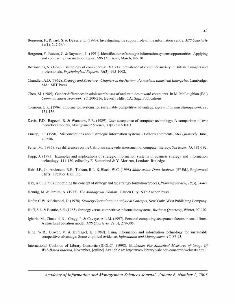
35
Academy of Information and Management Sciences Journal, Volume 6, Number 1, 2003
Bergeron, F., Rivard, S. & DeSerre, L. (1990). Investigating the support role of the information centre, MIS Quarterly14(1), 247-260.
Bergeron, F., Buteau, C. & Raymond, L. (1991). Identification of strategic information systems opportunities: Applyingand comparing two methodologies, MIS Quarterly, March, 89-101.
Bozionelos, N. (1996). Psychology of computer use: XXXIX. prevalence of computer anxiety in British managers andprofessionals, Psychological Reports, 78(3), 995-1002.
Chandler, A.D. (1962). Strategy and Structure - Chapters in the History of American Industrial Enterprise, Cambridge,MA: MIT Press.
Chen, M. (1985). Gender differences in adolescent's uses of and attitudes toward computers. In M. McLaughlan (Ed.)Communication Yearbook, 10, 200-216, Beverly Hills, CA: Sage Publications.
Clemons, E.K. (1986). Information systems for sustainable competitive advantage, Information and Management, 11,131-136.
Davis, F.D., Bagozzi, R. & Warshaw, P.R. (1989). User acceptance of computer technology: A comparison of twotheoretical models, Management Science, 35(8), 982-1003.
Emery, J.C. (1990). Misconceptions about strategic information systems - Editor's comments, MIS Quarterly, June,vii-viii.
Felter, M. (1985). Sex differences on the California statewide assessment of computer literacy, Sex Roles, 13, 181-192.
Fripp, J. (1991). Examples and implications of strategic information systems in business strategy and informationtechnology, 111-130, edited by E. Sutherland & Y. Morieux, London: Rutledge.
Hair, J.F., Jr., Anderson, R.E., Tatham, R.L. & Black, W.C. (1998) Multivariate Data Analysis, (5th Ed.), EnglewoodCliffs: Prentice Hall, Inc.
Hax, A.C. (1990). Redefining the concept of strategy and the strategy formation process, Planning Review, 18(3), 34-40.
Hennig, M. & Jardim, A. (1977). The Managerial Woman, Garden City, NY: Anchor Press.
Hofer, C.W. & Schendel, D. (1978). Strategy Formulation: Analytical Concepts, New York: West Publishing Company.
Huff, S.L. & Beattie, S.E. (1985). Strategy versus competitive information systems, Business Quarterly, Winter, 97-102.
Igbaria, M., Zinatelli, N., Cragg, P. & Cavaye, A.L.M. (1997). Personal computing acceptance factors in small firms:A structural equation model, MIS Quarterly, 21(3), 279-305.
King, W.R., Grover, V. & Hufnagel, E. (1989). Using information and information technology for sustainablecompetitive advantage: Some empirical evidence, Information and Management, 17, 87-93.
International Coalition of Library Consortia (ICOLC), (1998). Guidelines For Statistical Measures of Usage OfWeb-Based Indexed, November, [online] Available at: http://www.library.yale.edu/consortia/webstats.html
36
Academy of Information and Management Sciences Journal, Volume 6, Number 1, 2003
Jantan, M. & Kannan, S. (1997). Information technology deployment and competitive advantage of organisations inPenang, Malaysia. International Conference on Business Development Strategies in Asia Pacific Proceeding,Brunei Darussalam, 371-386.
Johansen, R. & Swigart, R. (1996). Upsizing the Individual in the Downsized Organisation: Managing in the Wake ofReengineering, Globalisation, and Overwhelming Technological Change, Reading, MA: Addison -Wesley.
Landauer, T.K. (1995). The Trouble with Computers: Usefulness, Usability, and Productivity, Cambridge, MA: MITPress.
Laudon, C.K. & Laudon Jane P. (1997), Essentials of Management Information Systems Organisation and Technology,Englewood Cliffs: Prentice Hall Inc.
Lincoln, D. J. & Warberg W. B. (1987). The role of micro computers in small business marketing, Journal of SmallBusiness Management, April, 25( 2), 8-17.
Lohr S. (1997). Information technology field is rated largest U.S. industry, New York Times, November 18. From a studybased on commerce department data titled, Cybernation: The Importance of the High Technology Industry tothe American Economy," sponsored by the American Electronics Association and the NASDAQ stockexchange.
McNurlin, B.C. (Ed.) (1986). Uncovering strategic systems, EDP Analyzer, 24(10), 1-11.
Mintzberg, H. (1979). The Structuring of Organisations, Englewood Cliffs: Prentice Hall.
Moore, G.A. (1991). Crossing the Chasm: Marketing and Selling Technology Products to Mainstream Customers, NewYork: HarperCollings Publishers.
Morrow, P.C. Presll, E.R.& McElroy, J.C. (1986). Attitudinal and behavioral correlates of computer anxiety,Psychological Reports, 59, 1199-1204.
Ndubisi, N.O., Jantan, M. & Richardson, S. (2001). Is the technology acceptance model valid for entrepreneurs? Modeltesting and examining usage determinants, The Asian Academy of Management Journal, 6(2), 31-54.
Ndubisi, N.O. & Jantan, M. (2001). Information technology usage pattern among Malaysian entrepreneurs, AsianAcademy of Management Conference Proceedings, Johor Bahru, 10th-13th November, 312-322.
Ndubisi, N.O. & Richardson, S. (2002). The entrepreneurs' technology acceptance model, Academy of EntrepreneurshipJournal, 8(2), 95-114.
Ndubisi, N.O. & Ndubisi, C.M. (2003). Malaysia women business owners and information and communicationtechnologies: Some marketing implications, International Conference on Operations and QuantitativeManagement Proceedings, Tainan, Taiwan, 2nd-5th January, 140-146.
Pedersen, K.M. (1990). Strategic information systems in manufacturing industries, in J.I. DeGross, M. Alavi & H.Oppelland (Eds.) Proceedings of the Eleventh International Conference on Information Systems, Copenhagen,Denmark, Dec 16-19, 193-203.
Porter, M.E. (1985). Competitive Advantage - Creating and Sustaining Superior Performance, New York: Free Press.
37
Academy of Information and Management Sciences Journal, Volume 6, Number 1, 2003
Porter, M.E. (1980). Competitive Strategy - Techniques for Analysing Industries and Competitors, New York: FreePress.
Porter, M.E. & Miller, V.E. (1985). How information gives you competitive advantage, Harvard Business Review(July-Aug.), 63(4).
Prahalad, C.K. & Hamel, G. (1990). The core competence of the corporation, Harvard Business Review, May-June,79-91.
Rackoff, N., Wiseman, C. & Ullrich, W.A. (1985). Information systems for competitive advantage: Implementation ofa planning process, MIS Quarterly, 9(4), 402-415.
Rahmah H. & Arfah Y.I. (1999). Diffusion of internet: Preliminary findings in Malaysia, Paper presented at theworkshop "Internet in Vietnam", Hanoi, 29th September - 2nd October, [online] Available at:http://www.interasia.org/malaysia/preliminary.html
Rotter, G.S. & Portugal, S.M. (1969). Group and individual effects in problem solving, Journal of Applied Psychology,53, 338-341.
Sabherwal, R. & King, W.R. (1991). Towards a theory of strategic use of information resources: An inductive approach,Information and Management, 20(3), 191-212.
Schutzer, D. (1991). Business Decision with Computers: New Trend in Technology, New York: Van Nostrand Reinhold.
Sichel, D.E. (1997). The Computer Revolution: An Economic Perspective, Washington, DC: The Brookings Institution.
Sjazna, B. (1994). Software evaluation and choice predictive validation of the technology acceptance instrument, MISQuarterly, 18, 319-324.
Sutherland, E. (1991). The meaning of strategic information technology - An analysis of the literature, in E. Sutherland& Y. Morieux, (eds), Business Strategy and Information Technology, London: Rutledge.
Taylor, S. & Todd, P. (1995). Understanding information technology usage: A test of competing models, InformationSystems Research, 6(2) 144-176.
The STAR Newspaper, (August 23, 2001). Minister: Science, technology knowledge stays poor, 4.
Weiner, M. (1993). Some computer science issues in ubiquitous computing, Communications of the ACM, 36(7), (July).
Williams, J.R. (1992). How sustainable is your competitive advantage, California Management Review, Spring, 29-50.
Wiseman, C. (1988). Strategic Information Systems, Homewood, IL: Richard D. Irwin.
Zain, N.M. (1998), Strategic use of information technology: A conceptual approach, Asian Academy of ManagementJournal, 3(2), 83-96.

38
Academy of Information and Management Sciences Journal, Volume 6, Number 1, 2003
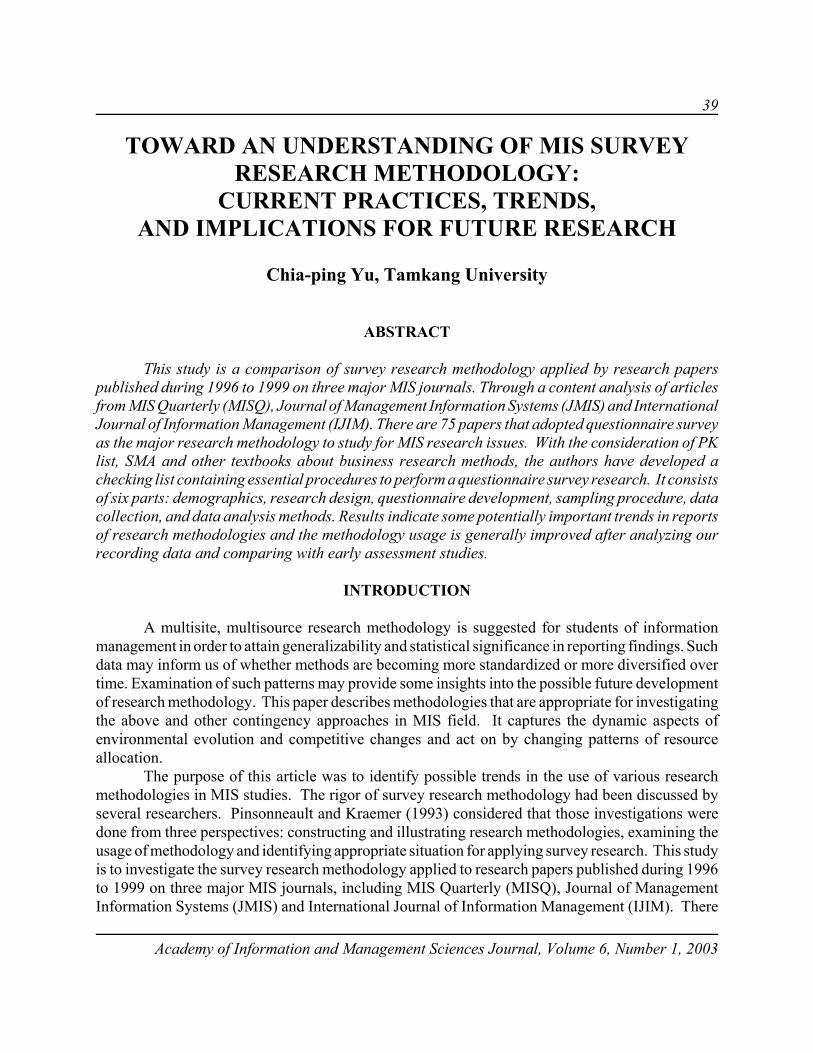
39
Academy of Information and Management Sciences Journal, Volume 6, Number 1, 2003
TOWARD AN UNDERSTANDING OF MIS SURVEYRESEARCH METHODOLOGY:
CURRENT PRACTICES, TRENDS,AND IMPLICATIONS FOR FUTURE RESEARCH
Chia-ping Yu, Tamkang University
ABSTRACT
This study is a comparison of survey research methodology applied by research paperspublished during 1996 to 1999 on three major MIS journals. Through a content analysis of articlesfrom MIS Quarterly (MISQ), Journal of Management Information Systems (JMIS) and InternationalJournal of Information Management (IJIM). There are 75 papers that adopted questionnaire surveyas the major research methodology to study for MIS research issues. With the consideration of PKlist, SMA and other textbooks about business research methods, the authors have developed achecking list containing essential procedures to perform a questionnaire survey research. It consistsof six parts: demographics, research design, questionnaire development, sampling procedure, datacollection, and data analysis methods. Results indicate some potentially important trends in reportsof research methodologies and the methodology usage is generally improved after analyzing ourrecording data and comparing with early assessment studies.
INTRODUCTION
A multisite, multisource research methodology is suggested for students of informationmanagement in order to attain generalizability and statistical significance in reporting findings. Suchdata may inform us of whether methods are becoming more standardized or more diversified overtime. Examination of such patterns may provide some insights into the possible future developmentof research methodology. This paper describes methodologies that are appropriate for investigatingthe above and other contingency approaches in MIS field. It captures the dynamic aspects ofenvironmental evolution and competitive changes and act on by changing patterns of resourceallocation.
The purpose of this article was to identify possible trends in the use of various researchmethodologies in MIS studies. The rigor of survey research methodology had been discussed byseveral researchers. Pinsonneault and Kraemer (1993) considered that those investigations weredone from three perspectives: constructing and illustrating research methodologies, examining theusage of methodology and identifying appropriate situation for applying survey research. This studyis to investigate the survey research methodology applied to research papers published during 1996to 1999 on three major MIS journals, including MIS Quarterly (MISQ), Journal of ManagementInformation Systems (JMIS) and International Journal of Information Management (IJIM). There
40
Academy of Information and Management Sciences Journal, Volume 6, Number 1, 2003
are 75 papers that adopted questionnaire survey as the major research methodology to study MISrelated issues.
Pinsonneault and Kraemer (1993, will be abbreviated as PK later) had implemented anassessment of survey research methodology. They collected 122 MIS research papers published onsixteen journals during 1980 to 1990 and designed a list (will be called PK list later in this paper)to record how the research methodology were processed and described. The PK list examinedsurvey methodologies mainly on research design, sampling procedures, and data collection. Theyconcluded five general misapplications suffered for the survey research: (1) single-method designswhere multiple methods were needed. (2) Unsystematic and often inadequate sampling procedures.(3) Low response rate. (4) Weak linkages between units of analysis and respondents. (5)Overreliance on cross-sectional surveys where longitudinal surveys were really needed.
Grover, Lee and Durand (1993, will be abbreviated as GLD) developed a list called SMA(Survey Methodological Attributes), that consists of nine Boolean statements about the technicalprocesses of the survey methodology, such as sampling, data collection, validity and reliability ofthe instrument (The SMA list is included in the end of Appendix). They used SMA to evaluate 227MIS research papers published during 1980 to 1989. The results showed that most papers havescores between two and four, and the mean score is 3.133. However, SMA didn't include the statisticanalysis methods.
With the consideration of PK list, SMA and other textbooks about business researchmethods, we developed a checking list containing essential procedures to perform a questionnairesurvey research, called LYCHEE (Lin, Yu, and CHen's Empirical Examination for the surveymethodology) (Lin,2001). It consists of seven parts: demographics, research design, questionnairedevelopment, sampling procedure, data collection, data analysis methods, and SMA list. Therecords of SMA list would be used to compare with GLD's result.
Our analyses show some possible patterns in the methodologies employed in MIS studies.Also, examination of the methods reported in MIS field might provide insights for those who aspireto have their research published in top-tier publication outlets. It is thus necessary to begin anexamination of management journal content with respect to research methods. This awareness isimportant, since researchers should be mindful of what methodological procedures are beingrewarded by the top journals (Scandura & Williams, 2000).
The next section is about the contents of LYCHEE (Lin,2001) containing essentialprocedures to perform a questionnaire survey research. The third section describes the researchmethod and the profile of sample papers. The fourth section presents the results with somediscussions. The last section summarizes the results and recommendations that were madethroughout this article.
THE ASSESSMENT INSTRUMENT: LYCHEE
Research design
Kerlinger (1986) defined the research design as a plan and structure of investigation in orderto answer questions. The plan is an outline of research procedures from setting the hypotheses to
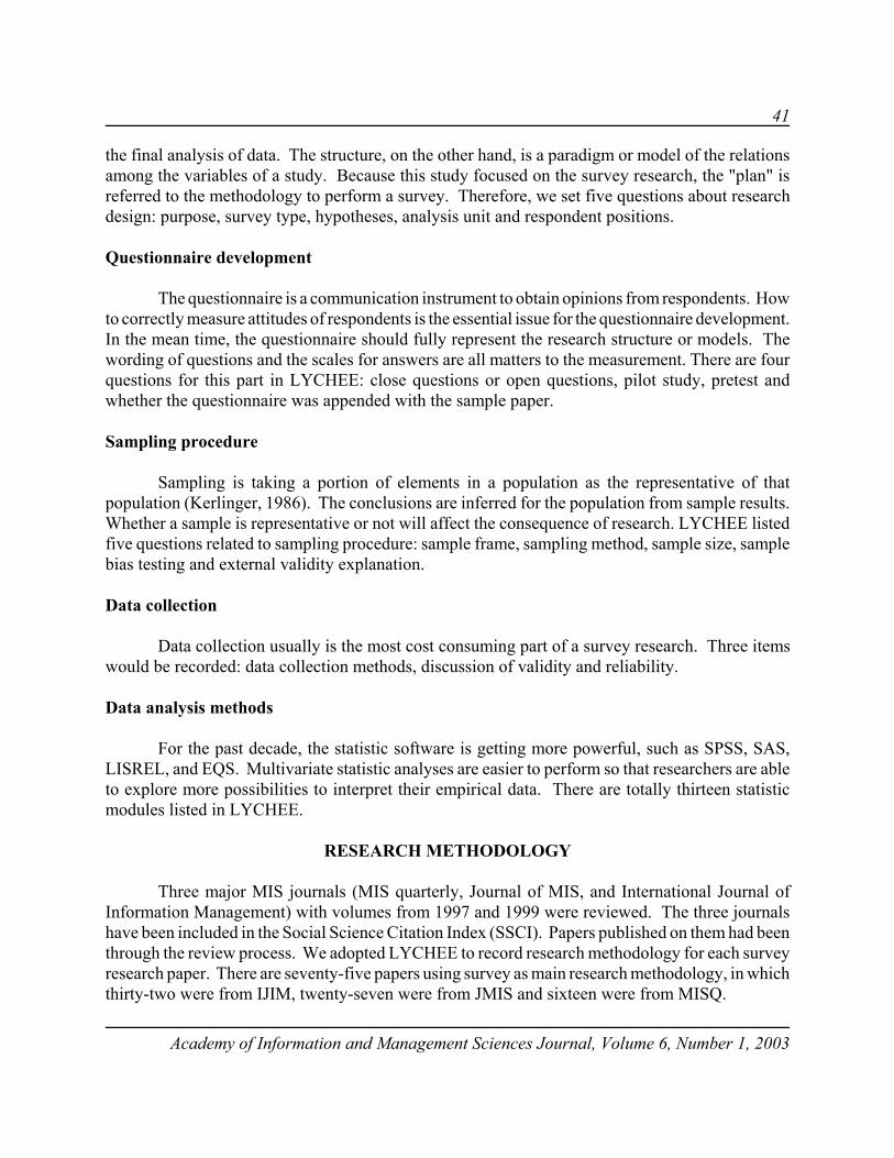
41
Academy of Information and Management Sciences Journal, Volume 6, Number 1, 2003
the final analysis of data. The structure, on the other hand, is a paradigm or model of the relationsamong the variables of a study. Because this study focused on the survey research, the "plan" isreferred to the methodology to perform a survey. Therefore, we set five questions about researchdesign: purpose, survey type, hypotheses, analysis unit and respondent positions.
Questionnaire development
The questionnaire is a communication instrument to obtain opinions from respondents. Howto correctly measure attitudes of respondents is the essential issue for the questionnaire development.In the mean time, the questionnaire should fully represent the research structure or models. Thewording of questions and the scales for answers are all matters to the measurement. There are fourquestions for this part in LYCHEE: close questions or open questions, pilot study, pretest andwhether the questionnaire was appended with the sample paper.
Sampling procedure
Sampling is taking a portion of elements in a population as the representative of thatpopulation (Kerlinger, 1986). The conclusions are inferred for the population from sample results.Whether a sample is representative or not will affect the consequence of research. LYCHEE listedfive questions related to sampling procedure: sample frame, sampling method, sample size, samplebias testing and external validity explanation.
Data collection
Data collection usually is the most cost consuming part of a survey research. Three itemswould be recorded: data collection methods, discussion of validity and reliability.
Data analysis methods
For the past decade, the statistic software is getting more powerful, such as SPSS, SAS,LISREL, and EQS. Multivariate statistic analyses are easier to perform so that researchers are ableto explore more possibilities to interpret their empirical data. There are totally thirteen statisticmodules listed in LYCHEE.
RESEARCH METHODOLOGY
Three major MIS journals (MIS quarterly, Journal of MIS, and International Journal ofInformation Management) with volumes from 1997 and 1999 were reviewed. The three journalshave been included in the Social Science Citation Index (SSCI). Papers published on them had beenthrough the review process. We adopted LYCHEE to record research methodology for each surveyresearch paper. There are seventy-five papers using survey as main research methodology, in whichthirty-two were from IJIM, twenty-seven were from JMIS and sixteen were from MISQ.
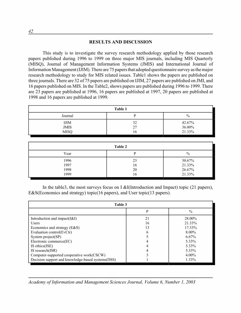
42
Academy of Information and Management Sciences Journal, Volume 6, Number 1, 2003
RESULTS AND DISCUSSION
This study is to investigate the survey research methodology applied by those researchpapers published during 1996 to 1999 on three major MIS journals, including MIS Quarterly(MISQ), Journal of Management Information Systems (JMIS) and International Journal ofInformation Management (IJIM). There are 75 papers that adopted questionnaire survey as the majorresearch methodology to study for MIS related issues. Table1 shows the papers are published onthree journals. There are 32 of 75 papers are published on IJIM, 27 papers are published on JMI, and16 papers published on MIS. In the Table2, shows papers are published during 1996 to 1999. Thereare 23 papers are published at 1996, 16 papers are published at 1997, 20 papers are published at1998 and 16 papers are published at 1999.
Table 1
Journal P %
IJIMJMISMISQ
322716
42.67%36.00%21.33%
Table 2
Year P %
1996199719981999
23162016
30.67%21.33%26.67%21.33%
In the table3, the most surveys focus on I &I(Introduction and Impact) topic (21 papers),E&S(Economics and strategy) topic(16 papers), and User topic(13 papers).
Table 3
P %
Introduction and impact(I&I)UsersEconomics and strategy (E&S)Evaluation control(EvCtr)System project(SP)Electronic commerce(EC)IS ethics(ISE)IS research(ISR)Computer-supported cooperative work(CSCW)Decision support and knowledge-based systems(DSS)
2116136544431
28.00%21.33%17.33%8.00%6.67%5.33%5.33%5.33%4.00%1.33%
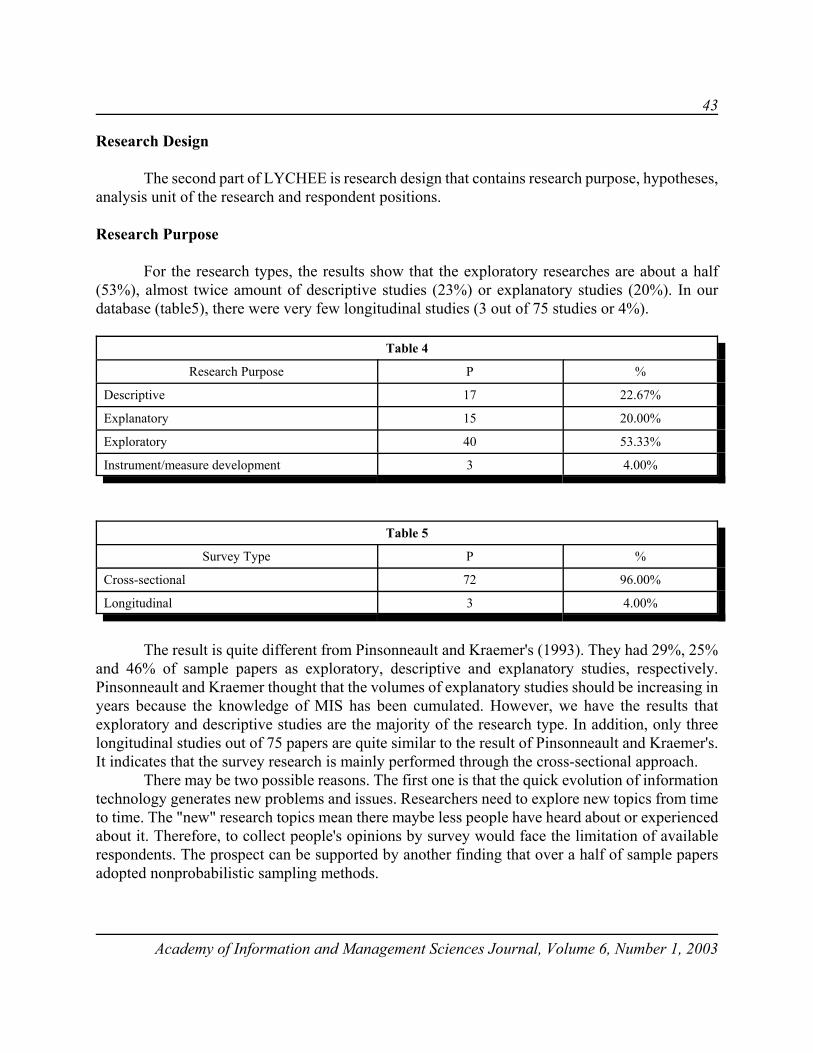
43
Academy of Information and Management Sciences Journal, Volume 6, Number 1, 2003
Research Design
The second part of LYCHEE is research design that contains research purpose, hypotheses,analysis unit of the research and respondent positions.
Research Purpose
For the research types, the results show that the exploratory researches are about a half(53%), almost twice amount of descriptive studies (23%) or explanatory studies (20%). In ourdatabase (table5), there were very few longitudinal studies (3 out of 75 studies or 4%).
Table 4
Research Purpose P %
Descriptive 17 22.67%
Explanatory 15 20.00%
Exploratory 40 53.33%
Instrument/measure development 3 4.00%
Table 5
Survey Type P %
Cross-sectional 72 96.00%
Longitudinal 3 4.00%
The result is quite different from Pinsonneault and Kraemer's (1993). They had 29%, 25%and 46% of sample papers as exploratory, descriptive and explanatory studies, respectively.Pinsonneault and Kraemer thought that the volumes of explanatory studies should be increasing inyears because the knowledge of MIS has been cumulated. However, we have the results thatexploratory and descriptive studies are the majority of the research type. In addition, only threelongitudinal studies out of 75 papers are quite similar to the result of Pinsonneault and Kraemer's.It indicates that the survey research is mainly performed through the cross-sectional approach.
There may be two possible reasons. The first one is that the quick evolution of informationtechnology generates new problems and issues. Researchers need to explore new topics from timeto time. The "new" research topics mean there maybe less people have heard about or experiencedabout it. Therefore, to collect people's opinions by survey would face the limitation of availablerespondents. The prospect can be supported by another finding that over a half of sample papersadopted nonprobabilistic sampling methods.

44
Academy of Information and Management Sciences Journal, Volume 6, Number 1, 2003
Our database indicates that hypothesis is adopted frequently in describing the researchquestions (In the table6, 31 out of 75 papers or 41%). The average number of hypothesizes are aboutthree or four in each study, that means the research variables are around two or three. There arefifteen percent of surveys manipulated over six variables in their research. However, there are 4papers abuse propositions to present their research question in the survey research.
Furthermore, there are more than half of all studies (52 percent or 64 studies) either do notprovide research hypotheses/questions or do not describe them clearly enough to get anunderstanding of the study's aim. This is problematic because research hypotheses or questionsdetermine the research design and shape the sampling procedures, data collection, and data analysis.If there are no questions or hypotheses, or if they are poorly formulated, it is unlikely that the surveyeffort will yield useful results except by accident.
Table 6
P %
HypothesisPropositionQuestionNot Mentioned or Vague
3146
37
41.33%5.33%8.00%
49.33%
Table 7
Number of Hypothesis P %
13~56~78~12Not Mentioned
12375
39
1.33%30.67%9.33%6.67%
52.00%
Analysis Unit
Table8 presents studies group by unit of analysis and journals. It indicates that most surveysused organizations (41%) and individuals (33%). The department, project (6.6%), and application(8 %)are seldom used.
Table 8
Analysis Unit P %
ApplicationDepartmentIndividualOrganizationProjectNot Mentioned
64
253154
8.00%5.33%
33.33%41.33%6.67%5.33%
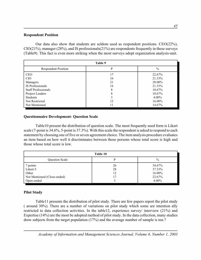
45
Academy of Information and Management Sciences Journal, Volume 6, Number 1, 2003
Respondent Position
Our data also show that students are seldom used as respondent positions. CEO(22%),CIO(21%), manager (28%), and IS professionals(21%) are respondents frequently in these surveys(Table9). This fact is even more striking when the most surveys adopt organization analysis-unit.
Table 9
Respondent Position P %
CEOCIOManagersIS ProfessionalsStaff ProfessionalsProject LeadersStudentsNot RestrictedNot Mentioned
17162116883
1211
22.67%21.33%28.00%21.33%10.67%10.67%4.00%
16.00%14.67%
Questionnaire Development- Question Scale
Table10 present the distribution of question scale. The most frequently used form is Likertscale (7-point is 34.6%, 5-point is 37.3%). With this scale the respondent is asked to respond to eachstatement by choosing one of five or seven agreement choice. The item analysis procedure evaluatesan item based on how well it discriminates between those persons whose total score is high andthose whose total score is low.
Table 10
Question Scale P %
7 pointsLikert-5OtherNot Mentioned (Close-ended)Open-ended
262812173
34.67%37.33%16.00%22.67%4.00%
Pilot Study
Table11 presents the distribution of pilot study. There are few papers report the pilot study( around 30%). There are a number of variations on pilot study which some are intention allyrestricted to data collection activities. In the table12, experience survey/ interview (21%) andExpertise (14%) are the most be adopted method of pilot study. In the data collection, many studiesdraw subjects from the target population (17%) and the average number of sample is ten.?
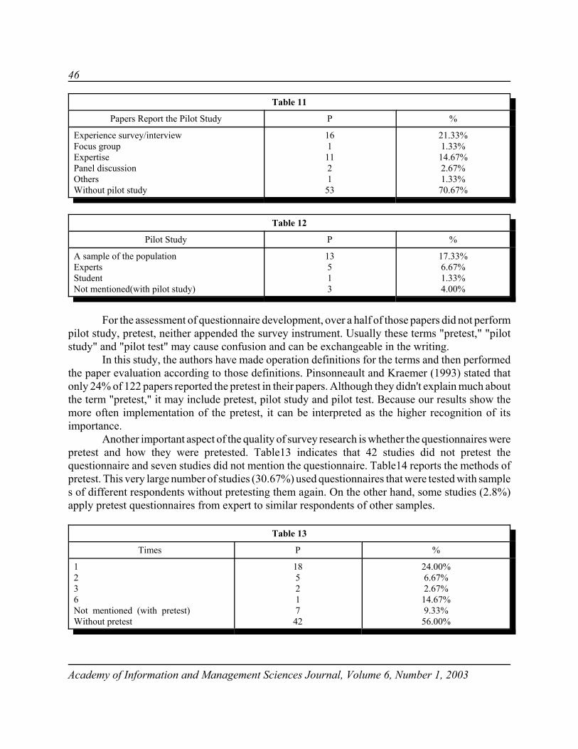
46
Academy of Information and Management Sciences Journal, Volume 6, Number 1, 2003
Table 11
Papers Report the Pilot Study P %
Experience survey/interviewFocus groupExpertisePanel discussionOthersWithout pilot study
161
1121
53
21.33%1.33%
14.67%2.67%1.33%
70.67%
Table 12
Pilot Study P %
A sample of the populationExpertsStudentNot mentioned(with pilot study)
13513
17.33%6.67%1.33%4.00%
For the assessment of questionnaire development, over a half of those papers did not performpilot study, pretest, neither appended the survey instrument. Usually these terms "pretest," "pilotstudy" and "pilot test" may cause confusion and can be exchangeable in the writing.
In this study, the authors have made operation definitions for the terms and then performedthe paper evaluation according to those definitions. Pinsonneault and Kraemer (1993) stated thatonly 24% of 122 papers reported the pretest in their papers. Although they didn't explain much aboutthe term "pretest," it may include pretest, pilot study and pilot test. Because our results show themore often implementation of the pretest, it can be interpreted as the higher recognition of itsimportance.
Another important aspect of the quality of survey research is whether the questionnaires werepretest and how they were pretested. Table13 indicates that 42 studies did not pretest thequestionnaire and seven studies did not mention the questionnaire. Table14 reports the methods ofpretest. This very large number of studies (30.67%) used questionnaires that were tested with samples of different respondents without pretesting them again. On the other hand, some studies (2.8%)apply pretest questionnaires from expert to similar respondents of other samples.
Table 13
Times P %
1236Not mentioned (with pretest)Without pretest
185217
42
24.00%6.67%2.67%
14.67%9.33%
56.00%
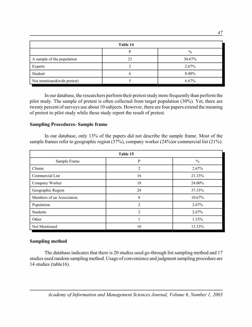
47
Academy of Information and Management Sciences Journal, Volume 6, Number 1, 2003
Table 14
P %
A sample of the population 23 30.67%
Experts 2 2.67%
Student 6 8.00%
Not mentioned(with pretest) 5 6.67%
In our database, the researchers perform their pretest study more frequently than perform thepilot study. The sample of pretest is often collected from target population (30%). Yet, there aretwenty percent of surveys use about 10 subjects. However, there are four papers extend the meaningof pretest to pilot study while these study report the result of pretest.
Sampling Procedures- Sample frame
In our database, only 13% of the papers did not describe the sample frame. Most of thesample frames refer to geographic region (37%), company worker (24%)or commercial list (21%).
Table 15
Sample Frame P %
Clients 2 2.67%
Commercial List 16 21.33%
Company Worker 18 24.00%
Geographic Region 28 37.33%
Members of an Association 8 10.67%
Population 2 2.67%
Students 2 2.67%
Other 1 1.33%
Not Mentioned 10 13.33%
Sampling method
The database indicates that there is 20 studies used go-through list sampling method and 17studies used random sampling method. Usage of convenience and judgment sampling procedure are14 studies (table16).
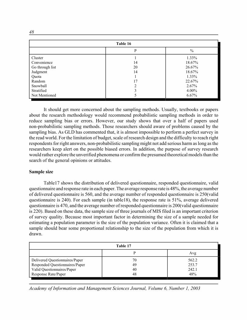
48
Academy of Information and Management Sciences Journal, Volume 6, Number 1, 2003
Table 16
P %
ClusterConvenienceGo through listJudgmentQuotaRandomSnowballStratifiedNot Mentioned
11420141
17235
1.33%18.67%26.67%18.67%1.33%
22.67%2.67%4.00%6.67%
It should get more concerned about the sampling methods. Usually, textbooks or papersabout the research methodology would recommend probabilistic sampling methods in order toreduce sampling bias or errors. However, our study shows that over a half of papers usednon-probabilistic sampling methods. Those researchers should aware of problems caused by thesampling bias. As GLD has commented that, it is almost impossible to perform a perfect survey inthe read world. For the limitation of budget, scale of research design and the difficulty to reach rightrespondents for right answers, non-probabilistic sampling might not add serious harm as long as theresearchers keep alert on the possible biased errors. In addition, the purpose of survey researchwould rather explore the unverified phenomena or confirm the presumed theoretical models than thesearch of the general opinions or attitudes.
Sample size
Table17 shows the distribution of delivered questionnaire, responded questionnaire, validquestionnaire and response rate in each paper. The average response rate is 48%, the average numberof delivered questionnaire is 560, and the average number of responded questionnaire is 250(validquestionnaire is 240). For each sample (in table18), the response rate is 51%, average deliveredquestionnaire is 470, and the average number of responded questionnaire is 200(valid questionnaireis 220). Based on these data, the sample size of three journals of MIS filed is an important criterionof survey quality. Because most important factor in determining the size of a sample needed forestimating a population parameter is the size of the population variance. Often it is claimed that asample should bear some proportional relationship to the size of the population from which it isdrawn.
Table 17
P Avg
Delivered Questionnaires/PaperResponded Questionnaires/PaperValid Questionnaires/PaperResponse Rate/Paper
70494048
562.2253.7242.148%
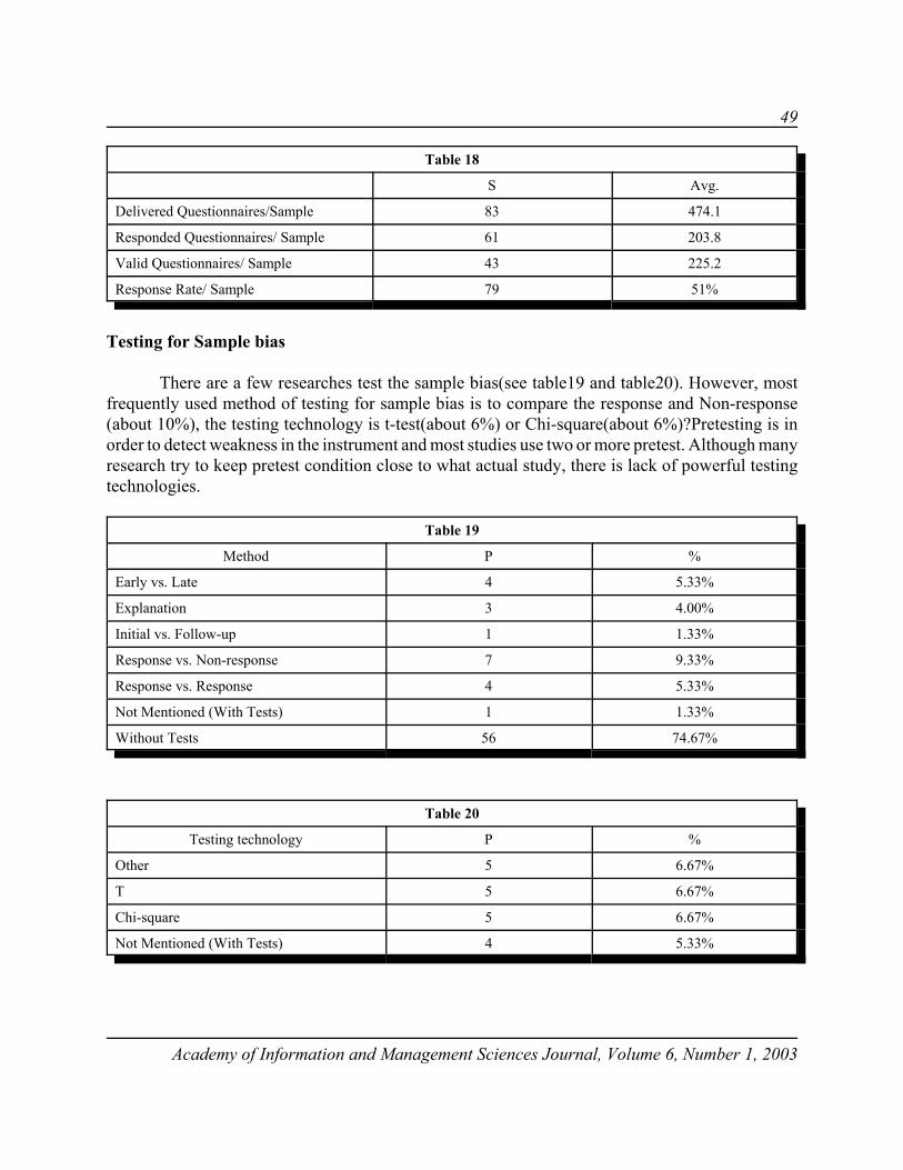
49
Academy of Information and Management Sciences Journal, Volume 6, Number 1, 2003
Table 18
S Avg.
Delivered Questionnaires/Sample 83 474.1
Responded Questionnaires/ Sample 61 203.8
Valid Questionnaires/ Sample 43 225.2
Response Rate/ Sample 79 51%
Testing for Sample bias
There are a few researches test the sample bias(see table19 and table20). However, mostfrequently used method of testing for sample bias is to compare the response and Non-response(about 10%), the testing technology is t-test(about 6%) or Chi-square(about 6%)?Pretesting is inorder to detect weakness in the instrument and most studies use two or more pretest. Although manyresearch try to keep pretest condition close to what actual study, there is lack of powerful testingtechnologies.
Table 19
Method P %
Early vs. Late 4 5.33%
Explanation 3 4.00%
Initial vs. Follow-up 1 1.33%
Response vs. Non-response 7 9.33%
Response vs. Response 4 5.33%
Not Mentioned (With Tests) 1 1.33%
Without Tests 56 74.67%
Table 20
Testing technology P %
Other 5 6.67%
T 5 6.67%
Chi-square 5 6.67%
Not Mentioned (With Tests) 4 5.33%
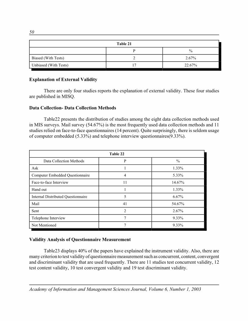
50
Academy of Information and Management Sciences Journal, Volume 6, Number 1, 2003
Table 21
P %
Biased (With Tests) 2 2.67%
Unbiased (With Tests) 17 22.67%
Explanation of External Validity
There are only four studies reports the explanation of external validity. These four studiesare published in MISQ.
Data Collection- Data Collection Methods
Table22 presents the distribution of studies among the eight data collection methods usedin MIS surveys. Mail survey (54.67%) is the most frequently used data collection methods and 11studies relied on face-to-face questionnaires (14 percent). Quite surprisingly, there is seldom usageof computer embedded (5.33%) and telephone interview questionnaires(9.33%).
Table 22
Data Collection Methods P %
Ask 1 1.33%
Computer Embedded Questionnaire 4 5.33%
Face-to-face Interview 11 14.67%
Hand out 1 1.33%
Internal Distributed Questionnaire 5 6.67%
Mail 41 54.67%
Sent 2 2.67%
Telephone Interview 7 9.33%
Not Mentioned 7 9.33%
Validity Analysis of Questionnaire Measurement
Table23 displays 40% of the papers have explained the instrument validity. Also, there aremany criterion to test validity of questionnaire measurement such as concurrent, content, convergentand discriminant validity that are used frequently. There are 11 studies test concurrent validity, 12test content validity, 10 test convergent validity and 19 test discriminant validity.
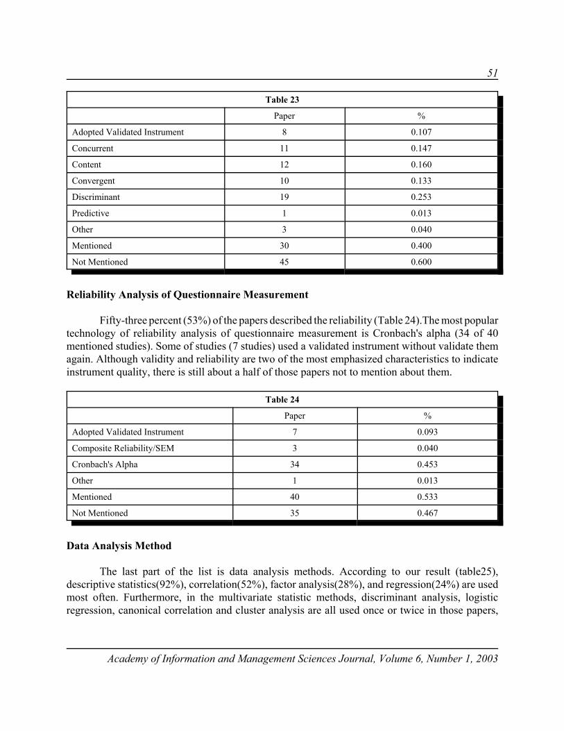
51
Academy of Information and Management Sciences Journal, Volume 6, Number 1, 2003
Table 23
Paper %
Adopted Validated Instrument 8 0.107
Concurrent 11 0.147
Content 12 0.160
Convergent 10 0.133
Discriminant 19 0.253
Predictive 1 0.013
Other 3 0.040
Mentioned 30 0.400
Not Mentioned 45 0.600
Reliability Analysis of Questionnaire Measurement
Fifty-three percent (53%) of the papers described the reliability (Table 24).The most populartechnology of reliability analysis of questionnaire measurement is Cronbach's alpha (34 of 40mentioned studies). Some of studies (7 studies) used a validated instrument without validate themagain. Although validity and reliability are two of the most emphasized characteristics to indicateinstrument quality, there is still about a half of those papers not to mention about them.
Table 24
Paper %
Adopted Validated Instrument 7 0.093
Composite Reliability/SEM 3 0.040
Cronbach's Alpha 34 0.453
Other 1 0.013
Mentioned 40 0.533
Not Mentioned 35 0.467
Data Analysis Method
The last part of the list is data analysis methods. According to our result (table25),descriptive statistics(92%), correlation(52%), factor analysis(28%), and regression(24%) are usedmost often. Furthermore, in the multivariate statistic methods, discriminant analysis, logisticregression, canonical correlation and cluster analysis are all used once or twice in those papers,
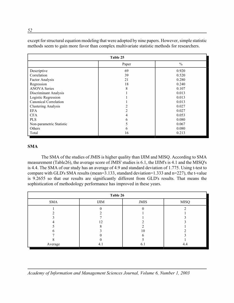
52
Academy of Information and Management Sciences Journal, Volume 6, Number 1, 2003
except for structural equation modeling that were adopted by nine papers. However, simple statisticmethods seem to gain more favor than complex multivariate statistic methods for researchers.
Table 25
Paper %
DescriptiveCorrelationFactor AnalysisRegressionANOVA SeriesDiscriminant AnalysisLogistic RegressionCanonical CorrelationClustering AnalysisEFACFAPLSNon-parametric StatisticOthersTotal
693921188111224656
16
0.9200.5200.2800.2400.1070.0130.0130.0130.0270.0270.0530.0800.0670.0800.213
SMA
The SMA of the studies of JMIS is higher quality than IJIM and MISQ. According to SMAmeasurement (Table26), the average score of JMIS' studies is 6.1, the IJIM's is 4.1 and the MISQ'sis 4.4. The SMA of our study has an average of 4.9 and standard deviation of 1.775. Using t-test tocompare with GLD's SMA results (mean=3.133, standard deviation=1.333 and n=227), the t-valueis 9.2655 so that our results are significantly different from GLD's results. That means thesophistication of methodology performance has improved in these years.
Table 26
SMA IJIM JMIS MISQ
12345678
Average
027
128300
4.1
01122
1065
6.1
21331231
4.4
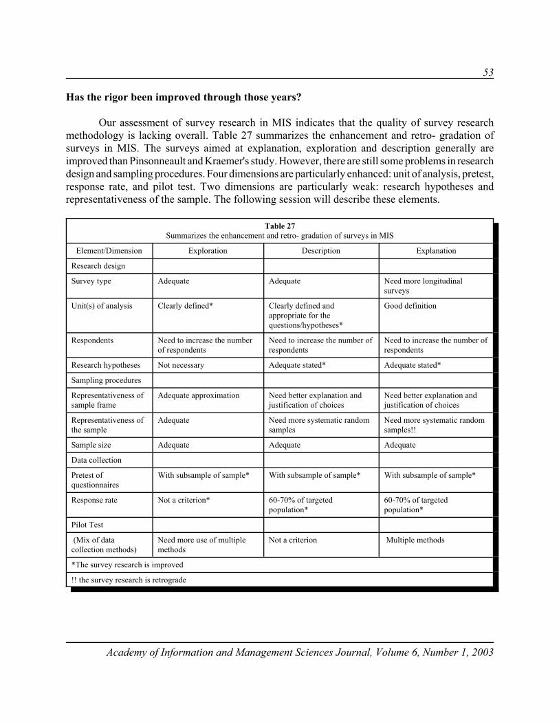
53
Academy of Information and Management Sciences Journal, Volume 6, Number 1, 2003
Has the rigor been improved through those years?
Our assessment of survey research in MIS indicates that the quality of survey researchmethodology is lacking overall. Table 27 summarizes the enhancement and retro- gradation ofsurveys in MIS. The surveys aimed at explanation, exploration and description generally areimproved than Pinsonneault and Kraemer's study. However, there are still some problems in researchdesign and sampling procedures. Four dimensions are particularly enhanced: unit of analysis, pretest,response rate, and pilot test. Two dimensions are particularly weak: research hypotheses andrepresentativeness of the sample. The following session will describe these elements.
Table 27Summarizes the enhancement and retro- gradation of surveys in MIS
Element/Dimension Exploration Description Explanation
Research design
Survey type Adequate Adequate Need more longitudinalsurveys
Unit(s) of analysis Clearly defined* Clearly defined andappropriate for thequestions/hypotheses*
Good definition
Respondents Need to increase the numberof respondents
Need to increase the number ofrespondents
Need to increase the number ofrespondents
Research hypotheses Not necessary Adequate stated* Adequate stated*
Sampling procedures
Representativeness ofsample frame
Adequate approximation Need better explanation andjustification of choices
Need better explanation andjustification of choices
Representativeness ofthe sample
Adequate Need more systematic randomsamples
Need more systematic randomsamples!!
Sample size Adequate Adequate Adequate
Data collection
Pretest ofquestionnaires
With subsample of sample* With subsample of sample* With subsample of sample*
Response rate Not a criterion* 60-70% of targetedpopulation*
60-70% of targetedpopulation*
Pilot Test
(Mix of datacollection methods)
Need more use of multiplemethods
Not a criterion Multiple methods
*The survey research is improved
!! the survey research is retrograde
54
Academy of Information and Management Sciences Journal, Volume 6, Number 1, 2003
CONCLUSION
Pinsonneault and Kraemer (1993) thought that the volumes of explanatory studies should beincreasing in years because the knowledge of MIS has been cumulated. However, our empiricalresult shows that exploratory and descriptive researches were seventy-six percent of the samplepapers, which is contrast to their prediction. The possible reason is that the quick evolution ofinformation technology generates new problems and issues. Researchers need to explore new topicsfrom time to time. The "new" research topics mean there maybe less people have heard about orexperienced about it. Therefore, to collect people's opinions by survey would face the limitation ofavailable respondents. The prospect can be supported by another finding that over a half of samplepapers adopted nonprobabilistic sampling methods. In addition, as if we believe that the MISresearch has grown as PK presumed, multivariate statistics or complex statistics methods were notused as often as we expected. Survey research is based on positivisism paradigm, which suffers froman objectivist illusion in believing that all knowledge is derived from objective facts, and theanalytical supposition that the end-result of sociological investigations can be formulated as 'laws'or 'law like' generalizations of the same kind as those established by natural scientists (Bryant,1985). However, the observations cannot provide an adequate basis for determining the truth orfalsity of theories. It simply takes for granted the socially constructed world. Furthermore,positivism cannot account for the way in which social reality is constructed and maintained, or howpeople interpret their own actions and the actions of others.
The theory means in all empirical science the explicit formulation of determinate relationsbetween a set of variables. The fact that these regularities in the social sciences are restricted in theextent to which they can be generalized, and that they permit prediction to only a limited extent,does not constitute a basic difference between the natural and social sciences. In the MIS field, thevolumes of explanatory studies is not increasing in years, a judgment will have to be made aboutthese criticisms. Though synthesis is not possible, consideration of an alternative avenue might beuseful, and researchers should develop a means for considering multi-paradigm views together(Gioia, et al., 1990).
Finally, we acknowledge that our use of three journals during four years as data points maynot have been sufficient to establish trends, but there do appear to have been some interestingchanges occurring between the periods examined in this study. Clearly, this research needsreplication in studies using other journals and time periods. Despite these limitations, we hope thatwe have suggested a conceptual template and data analyzing and analysis methodology for futurereviews of trends in MIS field.
REFERENCE
Cooper, D. R. & Schindler, P. S. (1998). Business Research Methods, (6th Ed.), Singapore: McGraw-Hill.
Grover, V., Lee, C. C. & Durand, D. (1993). Analyzing methodological rigor of MIS survey research from 1980-1989.Information & Management, 24, 305-317.
Kerlinger, F. N. (1986). Foundations of Behavioral Research, (3rd Ed.), New York: Harcourt Brace.

55
Academy of Information and Management Sciences Journal, Volume 6, Number 1, 2003
Lin, F.H., Yu, C.P. & Chen, Y.T. (2001). A study of MIS survey research methodology, in 30th Western DecisionSciences Institute (WDSI), Vancouver.
Pinsonneault, A. & Kraemer, K. L. (1993). Survey research methodology in management information systems: Anassessment. Journal of Management Information Systems, 10,. 75-105.
Scandura, T. A. & Williams E. A. (2000). Research methodology in management: Current practices, trends, andimplications for future research, Academy of Management Journal, 43(6), 1248-1264.
Zikmund, W. G. (1997). Business Research Methods, (5th Ed.), New York: The Dryden Press.
Appendix LYCHEE Empirical Examination List
‚ Demographic:1. mm(season)/yy [ / 19 ] Vol. [ ], No. [ ], pp[ ~ ]2. Journal name [MISQ] 3. Research theme
[computer-supported cooperative work] [decision support and knowledge-based systems][systems projects] [evaluation control][users] [economics and strategy][introduction and impact] [IS research][electronic commerce] [IS ethics]
‚ Research Design:1. Research purpose: [exploratory] [descriptive] [explanatory] [Instrument/measure development]2. Survey type: [cross-sectional] [longitudinal]3. Number of hypotheses:
1 [not mentioned or vague] 2 [hypothesis] 3 [proposition] 4 [Question] [n= ]4. Analysis unit:
1 [not mentioned] 2 [individual] 3 [department] 4 [organization] 5 [project] 6 [application]5. Respondent positions:
1 [not mentioned] 2 [CEO] 3 [CIO] 4 [managers] 5 [IS professionals] 6 [staff professionals] 7 [students]8 [project leaders] 9 [not restricted]
‚ Questionnaire Development1. Questions:
1-1. Open-ended1-2. Closed-ended: Question scale: 1 [not mentioned] 2 [Likert-5] 3 [7 point] 4 [other]
2. Pilot study? 1 [yes] 2 [no]2-1 Research Method: 1 [experience survey/interview] 2 [focus group] 3 [expertise] 4[panel discussion]2-2 Who were the respondents? 1 [not mentioned] 2 [experts] 3 [student] 4 [a sample of the population]2-3 How many respondents? [n= ]
3. Pretest? 1 [yes] 2 [no]3-1 Times: [ ]3-2 Who were the respondents? 1 [not mentioned] 2 [experts] 3 [students] 4 [a sample of the population]3-3 How many respondents? [n= ]
4. Does the paper append the survey instrument? 1 [none] 2 [whole] 3 [part] 4 [measures of R. V.s] ‚ Sampling Procedures:1. Sample frame: 1 [not mentioned] 2 [population] 3 [clients] 4 [members of an association or subscribers
to a magazine] 5 [attendees of a conference or seminar] 6 [geographic region] 7 [commercial list] 8 [students] 9 [company workers] 10 [other]
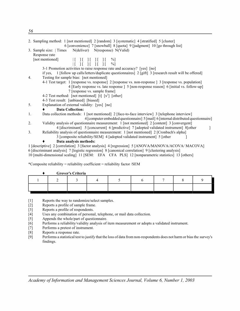
56
Academy of Information and Management Sciences Journal, Volume 6, Number 1, 2003
2. Sampling method: 1 [not mentioned] 2 [random] 3 [systematic] 4 [stratified] 5 [cluster] 6 [convenience] 7 [snowball] 8 [quota] 9 [judgment] 10 [go through list]
3. Sample size: | Times N(deliver) N(response) N(Valid) Response rate [not mentioned] | [ ] [ ] [ ] [ ] [ %]
| [ ] [ ] [ ] [ ] [ %]3-1 Promotion activities to raise response rate and accuracy? [yes] [no]if yes, 1 [follow up calls/letters/duplicate questionnaires] 2 [gift] 3 [research result will be offered]
4. Testing for sample bias: [not mentioned]4-1 Test target: 1 [response vs. response] 2 [response vs. non-response ] 3 [response vs. population]
4 [Early response vs. late response ] 5 [non-response reason] 6 [initial vs. follow-up] 7 [response vs. sample frame]
4-2 Test method: [not mentioned] [t] [x2] [other]4-3 Test result: [unbiased] [biased]
5. Explanation of external validity: [yes] [no] ‚ Data Collection:1. Data collection methods: 1 [not mentioned] 2 [face-to-face interview] 3 [telephone interview]
4 [computer embedded questionnaire] 5 [mail] 6 [internal distributed questionnaire]2. Validity analysis of questionnaire measurement: 1 [not mentioned] 2 [content] 3 [convergent]
4 [discriminant] 5 [concurrent] 6 [predictive] 7 [adopted validated instrument] 8[other ] 3. Reliability analysis of questionnaire measurement: 1 [not mentioned] 2 [Cronbach's alpha]
3 [composite reliability/SEM] 4 [adopted validated instrument] 5 [other ]‚ Data analysis methods:
1 [descriptive] 2 [correlation] 3 [factor analysis] 4 [regression] 5 [ANOVA/MANOVA/ACOVA/ MACOVA]6 [discriminant analysis] 7 [logistic regression] 8 [canonical correlation] 9 [clustering analysis]10 [multi-dimensional scaling] 11 [SEM: EFA CFA PLS] 12 [nonparametric statistics] 13 [others]
*Composite reliability = reliability coefficient = reliability factor /SEM
‚ Grover's Criteria
1 2 3 4 5 6 7 8 9
[1] Reports the way to randomize/select samples.[2] Reports a profile of sample frame.[3] Reports a profile of respondents.[4] Uses any combination of personal, telephone, or mail data collection.[5] Appends the whole/part of questionnaire.[6] Performs a reliability/validity analysis of item measurement or adopts a validated instrument.[7] Performs a pretest of instrument.[8] Reports a response rate.[9] Performs a statistical test to justify that the loss of data from non-respondents does not harm or bias the survey's
findings.
57
Academy of Information and Management Sciences Journal, Volume 6, Number 1, 2003
ARTIFICIAL NEURAL NETWORK APPLICATIONTO BUSINESS PERFORMANCE WITH ECONOMIC
VALUE ADDED
Chang W. Lee, Jinju National University
ABSTRACT
An application of neural networks to classify the performance status of business firms isperformed. An artificial neural network (ANN) model is developed using publicly available datasetas input and output variables. Several different neural network topologies are designed and appliedto the datasets. A neural network model classifies both high and low business performance status.The ANN model can enhance strategic and managerial insights by providing meaningful financialinformation.
INTRODUCTION
Since the development of an artificial neural network (ANN) approximately 50 years ago,it has received considerable attention from researchers. Neural network was once viewed as thetheoretical foundation of building machine learning systems. It was proven to have manylimitations. Recent neural network studies have overcome some previous limitations. ANN hasbeen applied to a variety of problems for classification and prediction. It has been appliedsuccessfully for development of non-parametric statistical models. More robust outcome researcheshave been explored in the topics of pattern classification and pattern prediction. Neural networkmodels are able to identify an existing pattern in data classification in different categories (Archer& Wang, 1993; Hsiao & Huang, 2002; Lotfi et al., 2000; Patuwo et al., 1993; Wang, 1995). Neuralnetworks in business performance applications have been used for audit decision (Hansen et al.,1992; Lenard et al., 1995), initial public offerings (Jain & Nag, 1995), and multi-criteriadecision-making (Malakooti & Zhou, 1994).
One of the most difficult issues in the ANN application discipline is to a proper utilizationof a neural network model to implement a large-scale financial services research dataset. Moreover,if characteristics of the factors are complicated and complex, finding an optimal alternative is verydifficult and may not get the best solution. Many researches have applied a neural network modelto classify desired solutions or to improve methodological perspectives. Even though successfulapplications in ANN models have been made, little interests are given to the economic value added(EVA)-related business performance planning area. The utilization of neural network models inclassification issues of management, finance, and other functional areas has been mostly limited to

58
Academy of Information and Management Sciences Journal, Volume 6, Number 1, 2003
the usage of factors with continuous or ratio variables, rather than categorized values used insocioeconomic settings (Hart, 1992; Lee & Park, 2001; Sharda, 1994; Wilson, 1995).
The purpose of this study is to develop a neural network model to identify a properclassification between high and low business performance status. A neural network model isdeveloped based on the publicly available financial dataset as input and output variables. Theproposed model is expected to provide the factors affecting the classification of high/low EVAstatus, enhance business strategies to meet more appropriately business performance with financialmeasurement, and support decision-makers with more accurate information to implement.
LITERATURE REVIEW
Early studies have recognized that combining many simple nodes into neural network modelsis the source of increased computational power. The weights on the neural network are fixed so thatthe node performs a certain logic function with different nodes performing different functions. Thenodes can be arranged into a network to generate any output that can be represented as anaggregation of logic functions. The learning mechanism has been designed for a neural networkmodel. This mechanism is that the strength of the connection between them should be improved,if two nodes are active simultaneously. This idea is similar to the correlation matrix learningmechanism.
Many studies in neural networks have explored in business and financial areas during the lastseveral decades. A study of Wong and Selvi (1998) provides an extensive literature analysis infinance application of neural network models. Neural network application to business performanceand/or finance appeared in areas such as bankruptcy models (Chen, 1995; Fletcher & Goss, 1993;Markham & Ragsdale, 1995; Tam & Kiang, 1992), bonding models (Dutta et al., 1994; Quah etal., 1996), loan models (Bansal et al., 1993; Piramuthu et al., 1994), mutual fund models (Chianget al., 1996; Hung et al., 1996), options models (Hutchison et al., 1994; Kaastra & Boyd, 1995;Swanson & White, 1995), real estate models (Borst, 1991; Collians & Evans, 1994; Worzala et al.,1995), stock prediction models (Wittkemper & Steiner, 1996; Wong & Long, 1995; Wood &Dasgupta, 1996).
A neural network is an imitating mechanism of human intelligence for the purpose ofderiving certain performance characteristics. A neural network has been developed as generalizationof a nonparametric methodology. A neural network model assumes that nodes have their own valuesfor processing certain data, values are transmitted through nodes over connection links, each linkhas a weight that multiplies the values conveyed in a neural network, and each nodes applies anactivation function to its input to identify the output value.
Assumption of information flow through the network is that a unit time step for data movesfrom one node to the next. This lead-time allows the network to model some perceptional processes.The most typical single layer network is consisted of an input layer connected by paths with fixedweights to associated nodes. The weights on the connection paths are adjustable. The learning ruleof a single layer network uses an iterative weight adjustment. Learning rule can converge to thecorrect weights if weights allow the network to regenerate correctly all of the learning input andtarget output pairs. However, the theoretical proof on the convergence in iterative learning
59
Academy of Information and Management Sciences Journal, Volume 6, Number 1, 2003
mechanism under suitable assumptions represents the limitations regarding what the single layernetwork type can learn.
A neural network model consists of a number of data processing layers interconnected in anetwork. Each layer has a mathematical mechanism with computational functions. A layer receivesinput values from other layers, and synthesizes the values by an input function. The layer createsoutput values by an output function. Then, the output values transferred to other layers as designedby the neural network architecture.
Characteristics of neural network have the architecture (the pattern of connections betweenthe nodes), training or learning (the method of determining the weights on the connections), and theactivation function. Each node is connected to other nodes by direct interaction links, each with anassociated weight. This weight represents information used by the network to find a solution. Eachnode has an activation level that is a function of the inputs. Because a node sends its activation asa value to several other nodes, it can transmit one value at a time, while the value is transmitted toseveral other nodes.
An alternative learning rule can be used to adjust the connection weights to a unit wheneverthe unit response is incorrect. The unit response represents a classification of the input pattern. Theleast-mean-square or delta rule as an alternative learning rule adjusts the weights to reduce thedifference between the input and the target output. This results in the smallest mean-squared error(MSE). The learning rule for a single-layer or multi-layers networks is interpreted as an adaptivelinear system. The difference in learning rule leads to an improved capability of the neural networkmodel to generalize. Some elaborated studies deal with associative memory neural networks withthe development of self-organizing feature maps that use a topology for the cluster units. Thisfeature truncates the linear output to prevent the output from being too large to get an optimalsolution as the network iterates.
One of the advanced features is development of a back propagation algorithm (BPA) in alearning mechanism to train multi-layer networks. The BPA has a linear approximation functionfor the input layer and a logistic function for the output layer. The BPA using the hidden layerallows the data to be classified. A BPA has been developed to overcome the limitation ofsingle-layer networks. It can solve complex problems, lacking a general methodology of learninga multi-layer neural network model. An improved model is derived from a number of neuralnetwork model based on fixed weights and adaptive activation. This neural network can use asassociative memory networks and can be used to solve constraint satisfaction problems. Stochasticneural networks that weights or activations are changed on the basis of a probability density functionincorporate such ideas as simulated annealing and Bayesian decision theory.
MODEL DEVELOPMENT
This study utilizes the financial dataset, which is a longitudinal study dataset of firms withhigh or low business performance. Information has been gathered on 764 high/low business firms.Pattern characteristics of financial services and changes in these factors over the course of thebusiness can be analyzed for high/low EVA firms. Dozens of variables are selected initially fromthe original dataset. After controlling these variables, one output variable (dependent variable) and
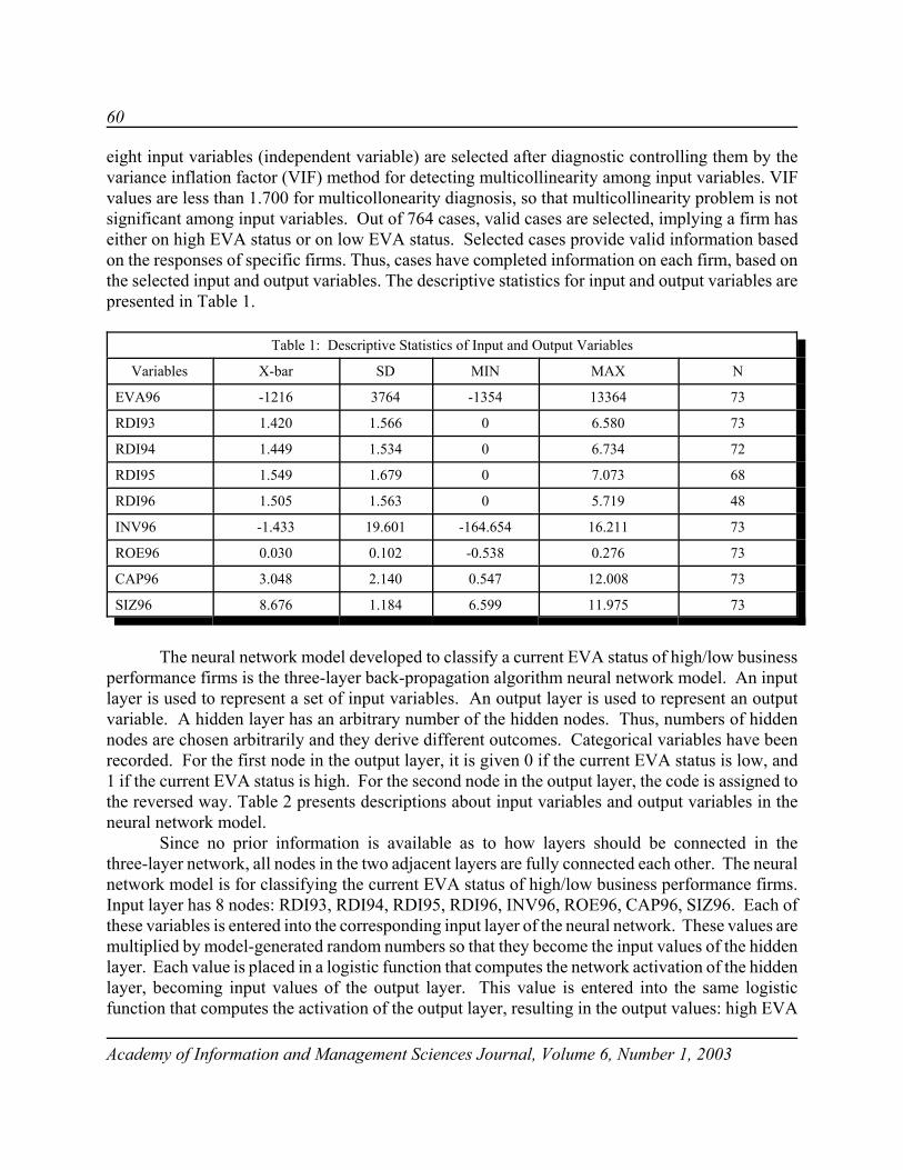
60
Academy of Information and Management Sciences Journal, Volume 6, Number 1, 2003
eight input variables (independent variable) are selected after diagnostic controlling them by thevariance inflation factor (VIF) method for detecting multicollinearity among input variables. VIFvalues are less than 1.700 for multicollonearity diagnosis, so that multicollinearity problem is notsignificant among input variables. Out of 764 cases, valid cases are selected, implying a firm haseither on high EVA status or on low EVA status. Selected cases provide valid information basedon the responses of specific firms. Thus, cases have completed information on each firm, based onthe selected input and output variables. The descriptive statistics for input and output variables arepresented in Table 1.
Table 1: Descriptive Statistics of Input and Output Variables
Variables X-bar SD MIN MAX N
EVA96 -1216 3764 -1354 13364 73
RDI93 1.420 1.566 0 6.580 73
RDI94 1.449 1.534 0 6.734 72
RDI95 1.549 1.679 0 7.073 68
RDI96 1.505 1.563 0 5.719 48
INV96 -1.433 19.601 -164.654 16.211 73
ROE96 0.030 0.102 -0.538 0.276 73
CAP96 3.048 2.140 0.547 12.008 73
SIZ96 8.676 1.184 6.599 11.975 73
The neural network model developed to classify a current EVA status of high/low businessperformance firms is the three-layer back-propagation algorithm neural network model. An inputlayer is used to represent a set of input variables. An output layer is used to represent an outputvariable. A hidden layer has an arbitrary number of the hidden nodes. Thus, numbers of hiddennodes are chosen arbitrarily and they derive different outcomes. Categorical variables have beenrecorded. For the first node in the output layer, it is given 0 if the current EVA status is low, and1 if the current EVA status is high. For the second node in the output layer, the code is assigned tothe reversed way. Table 2 presents descriptions about input variables and output variables in theneural network model.
Since no prior information is available as to how layers should be connected in thethree-layer network, all nodes in the two adjacent layers are fully connected each other. The neuralnetwork model is for classifying the current EVA status of high/low business performance firms.Input layer has 8 nodes: RDI93, RDI94, RDI95, RDI96, INV96, ROE96, CAP96, SIZ96. Each ofthese variables is entered into the corresponding input layer of the neural network. These values aremultiplied by model-generated random numbers so that they become the input values of the hiddenlayer. Each value is placed in a logistic function that computes the network activation of the hiddenlayer, becoming input values of the output layer. This value is entered into the same logisticfunction that computes the activation of the output layer, resulting in the output values: high EVA
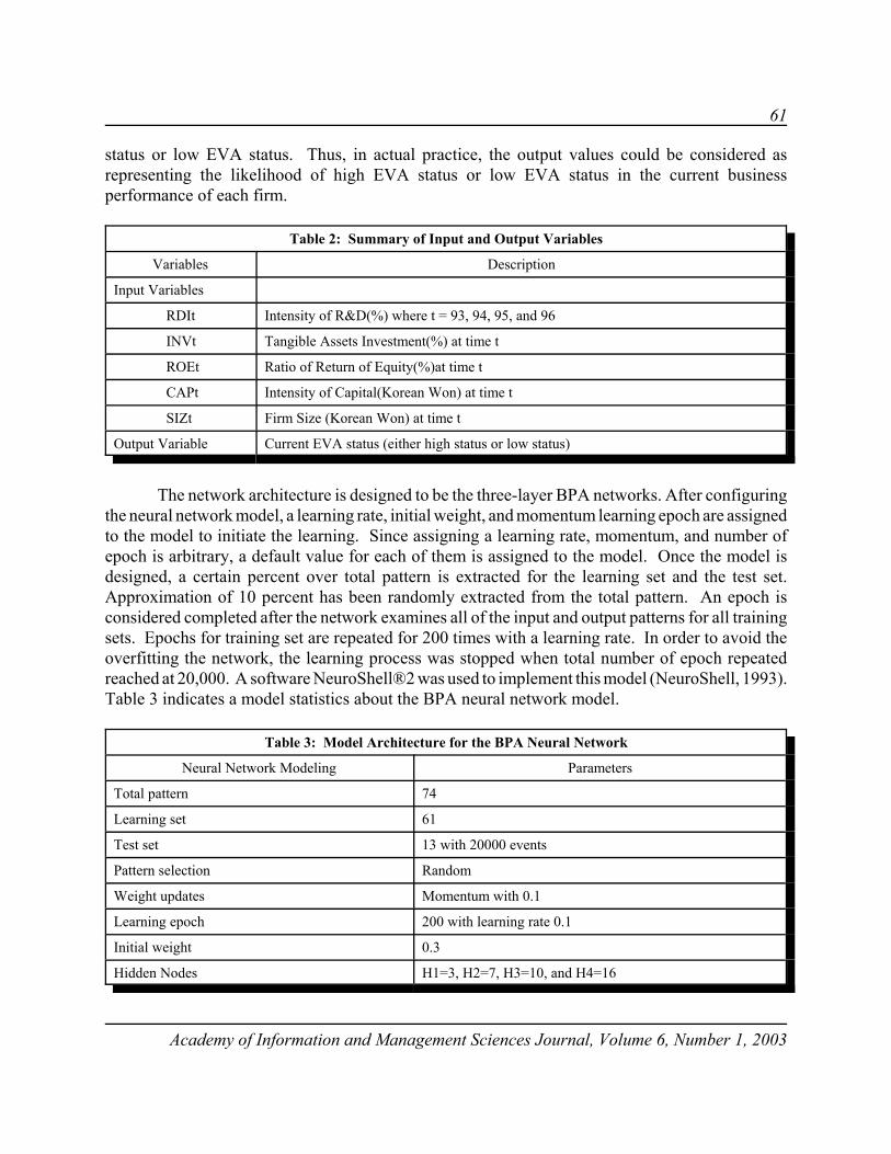
61
Academy of Information and Management Sciences Journal, Volume 6, Number 1, 2003
status or low EVA status. Thus, in actual practice, the output values could be considered asrepresenting the likelihood of high EVA status or low EVA status in the current businessperformance of each firm.
Table 2: Summary of Input and Output Variables
Variables Description
Input Variables
RDIt Intensity of R&D(%) where t = 93, 94, 95, and 96
INVt Tangible Assets Investment(%) at time t
ROEt Ratio of Return of Equity(%)at time t
CAPt Intensity of Capital(Korean Won) at time t
SIZt Firm Size (Korean Won) at time t
Output Variable Current EVA status (either high status or low status)
The network architecture is designed to be the three-layer BPA networks. After configuringthe neural network model, a learning rate, initial weight, and momentum learning epoch are assignedto the model to initiate the learning. Since assigning a learning rate, momentum, and number ofepoch is arbitrary, a default value for each of them is assigned to the model. Once the model isdesigned, a certain percent over total pattern is extracted for the learning set and the test set.Approximation of 10 percent has been randomly extracted from the total pattern. An epoch isconsidered completed after the network examines all of the input and output patterns for all trainingsets. Epochs for training set are repeated for 200 times with a learning rate. In order to avoid theoverfitting the network, the learning process was stopped when total number of epoch repeatedreached at 20,000. A software NeuroShell®2 was used to implement this model (NeuroShell, 1993).Table 3 indicates a model statistics about the BPA neural network model.
Table 3: Model Architecture for the BPA Neural Network
Neural Network Modeling Parameters
Total pattern 74
Learning set 61
Test set 13 with 20000 events
Pattern selection Random
Weight updates Momentum with 0.1
Learning epoch 200 with learning rate 0.1
Initial weight 0.3
Hidden Nodes H1=3, H2=7, H3=10, and H4=16
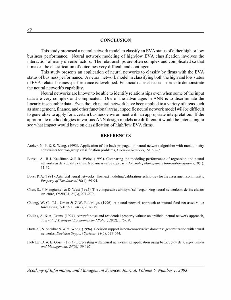
62
Academy of Information and Management Sciences Journal, Volume 6, Number 1, 2003
CONCLUSION
This study proposed a neural network model to classify an EVA status of either high or lowbusiness performance. Neural network modeling of high/low EVA classification involves theinteraction of many diverse factors. The relationships are often complex and complicated so thatit makes the classification of outcomes very difficult and contingent.
This study presents an application of neural networks to classify by firms with the EVAstatus of business performance. A neural network model in classifying both the high and low statusof EVA-related business performance is developed. Financial dataset is used in order to demonstratethe neural network's capability.
Neural networks are known to be able to identify relationships even when some of the inputdata are very complex and complicated. One of the advantages in ANN is to discriminate thelinearly inseparable data. Even though neural network have been applied to a variety of areas suchas management, finance, and other functional areas, a specific neural network model will be difficultto generalize to apply for a certain business environment with an appropriate interpretation. If theappropriate methodologies in various ANN design models are different, it would be interesting tosee what impact would have on classification of high/low EVA firms.
REFERENCES
Archer, N. P. & S. Wang. (1993). Application of the back propagation neural network algorithm with monotonicityconstraints for two-group classification problems, Decision Sciences, 24, 60-75.
Bansal, A., R.J. Kauffman & R.R. Weitz. (1993). Comparing the modeling performance of regression and neuralnetworks as data quality varies: A business value approach, Journal of Management Information Systems,10(1),11-32.
Borst, R.A. (1991). Artificial neural networks: The next modeling/calibration technology for the assessment community,Property of Tax Journal,10(1), 69-94.
Chen, S., P. Mangiameli & D. West (1995). The comparative ability of self-organizing neural networks to define clusterstructure, OMEGA, 23(3), 271-279.
Chiang, W.-C., T.L. Urban & G.W. Baldridge. (1996). A neural network approach to mutual fund net asset value
forecasting, OMEGA, 24(2), 205-215.
Collins, A. & A. Evans. (1994). Aircraft noise and residential property values: an artificial neural network approach,Journal of Transport Economics and Policy, 28(2), 175-197.
Dutta, S., S. Shekhar & W.Y. Wong. (1994). Decision support in non-conservative domains: generalization with neuralnetworks, Decision Support Systems, 11(5), 527-544.
Fletcher, D. & E. Goss. (1993). Forecasting with neural networks: an application using bankruptcy data, Informationand Management, 24(3),159-167.
63
Academy of Information and Management Sciences Journal, Volume 6, Number 1, 2003
Hansen, J.V., J.B. McDonald & J.D. Stice. (1992). Artificial intelligence and generalized qualitative-response models:an empirical test on two audit decision-making domains, Decision Sciences, 23, 708-723.
Hart, A. (1992). Using neural networks for classification tasks-some experiments on datasets and practical advice,Journal of the Operational Research Society, 44, 1129-1145.
Hsiao, S.W. & H.C. Huang. (2002) & A neural network based approach for product form design, Design Studies, 23(1),67-84.
Hung, S.-Y., T.-P. Liang & W.-L. Liu. (1996). Integrating arbitrage pricing theory and artificial neural networks tosupport portfolio management, Decision Support System, 18, 301-316.
Hutchison, A., A.W. Lo & T. Poggio. (1994). A nonparametric approach to pricing and hedging derivative securitiesvia learning networks, The Journal of Finance, 49(3), 851-889.
Jain, B.A. & B.N. Nag. (1995). Artificial neural network models for pricing initial public offerings, Decision Sciences,26, 283-302.
Kaastra, I. & M.S. Boyd (1995). Forecasting futures trading volume using neural networks, The Journal of FuturesMarkets, 15(8), 953-970.
Lee, C.W. & J. A. Park (2001). Assessment of HIV/AIDS-related health performance using an artificial neural network,Information and Management, 38(4), 231-238.
Lenard, M.J., P. Alam, G.R. Madey (1995). The application of neural networks and a qualitative response model to theauditor's going concern uncertainty decision, Decision Sciences, 26, 209-227.
Lotfi, K.G. & M.H. Choueiki. (2000) A neural network model for solving the lot-sizing problem, OMEGA, 28(2),175-184.
Malakooti, B. & Y.Q. Zhou. (1994). Feedforward artificial neural networks for solving discrete multiple criteriadecision making problems, Management Science, 40, 1542-1561.
Markham, I.S. & C.T. Ragsdale. (1995). Combining neural networks and statistical predictions to solve theclassification problem in discriminant analysis, Decision Sciences, 26(2), 229-242.
NeuroShell®2 (1993) Frederick, MD: Ward Systems Groups.
Patuwo, E., M.H. Hu & M.S. Hung. (1993). Two-group Classification using neural networks, Decision Sciences, 24,825-845.
Piramuthu, S., M.J. Shaw & J.A. Gentry. (1994). A classification approach using multi-layered neural networks,Decision Support Systems, 11(5), 509-525.
Quah, T.-S., C.-L. Tan, K.S. Raman & B. Srinivasan. (1996). Towards integrating rule-based expert systems and neuralnetworks, Decision Support Systems, 17, 99-118.
Sharda, R. (1994). Neural networks for the MS/OR analyst: an application bibliography, Interfaces, 24, 116-130.
Swanson, N.R. & H. White (1995). A model-selection approach to assessing the information in the term structure usinglinear models and artificial neural networks, Journal of Business and Economic Statistics, 13(3), 265-275.
64
Academy of Information and Management Sciences Journal, Volume 6, Number 1, 2003
Tam, K.Y. & M. Kiang (1992). Managerial applications of neural networks: The case of bank failure predictions,Management Science, 38(7), 926-947.
Wang, S. (1995). The unpredictability of standard back propagation neural networks in classification applications,Management Science, 41, 555-559.
Wilson, R.L. (1995). Ranking college football teams: a neural Network approach, Interfaces, 25, 44-59.
Wittkemper, H.-G. & M. Steiner. (1996). Using neural networks to forecast the systematic risk of stock, EuropeanJournal of Operational Research, 90, 577-588.
Wong, B.K. & Y. Selvi. (1998). Neural network application in finance: a review and analysis of literature (1990-1996),Information and Management, 34, 129-139.
Wong, S.Q. & J.A. Long. (1995). A neural network approach to stock market holding period returns, American BusinessReview, 13(2), 61-64.
Wood, D. & B. Dasgupta (1996). Classifying trend movements in the MSCI USA capital market index - A comparisonof regression, ARIMA and neural network methods, Computers and Operations Research, 23(6), 611-622.
Worzala, E., M. Lenk & A. Silva. (1995). An exploration of neural networks and its application to real estate valuation,The Journal of Real Estate Research, 10(2), 185-201.

65
Academy of Information and Management Sciences Journal, Volume 6, Number 1, 2003
End of Manuscriptsfor Volume 6, Number 1

66
Academy of Information and Management Sciences Journal, Volume 6, Number 2, 2003Academy of Information and Management Sciences Journal, Volume 6, Number 2, 2003
Manuscriptsfor Volume 6, Number 2
67
Academy of Information and Management Sciences Journal, Volume 6, Number 2, 2003Academy of Information and Management Sciences Journal, Volume 6, Number 2, 2003
EMPLOYEE PERFORMANCE EVALUATION USINGTHE ANALYTIC HIERARCHY PROCESS
Ramadan Hemaida, University of Southern IndianaSusan Everett, University of Southern Indiana
ABSTRACT
Managers do not look forward to giving performance reviews and there is no exception tothat rule. Every year managers struggle with finding just and fair way to allocate salary increasesto their department. They want to find a way that will reward the best performers by given them thelargest salary increases for the years. Identifying the best performers is a very subjective task. So,managers are always searching for a way to make this task as objective as possible. This researchwill utilize the AHP to deal with the performance evaluations and merit increases for a local firmin the state of Indiana. More specifically, the research will help the managers in assigning weightsto the most important factors used in the evaluation process.
INTRODUCTION
"The groans of the managers echo the halls as the reminder comes that it's time once againfor annual performance reviews,"(Molta, 1997). Managers do not look forward to givingperformance reviews and there is no exception to that rule. Every year managers struggle withfinding a way to be fair with the salary increases that are allocated to their department. They wantto find a way that will reward the best performers by given them the largest salary increases for theyears. Identifying the best performers is a very subjective task. So, managers are always searchingfor a way to make this task as objective as possible
The Analytic Hierarchy Process (AHP) would seem to be an effective tool to use in thisdecision process. The overall decision process is complex and involves consideration of bothobjective and subjective factors. AHP would seem to be a useful means to deal with thiscomplexity, force determination of factor weights and evaluations, and provide empirical basis fora sound conclusion. AHP may serve as a means to deal with the current frustration found in thisdecision-making process and assist managers in making better decisions.
This research will utilize the AHP to deal with the performance evaluations and meritincreases for a local firm in the state of Indiana. More specifically, the research will help themanagers in assigning weights to the most important factors used in the evaluation process. Anapplication of the technique will be used in the Management Information System (MIS) departmentof the firm.
68
Academy of Information and Management Sciences Journal, Volume 6, Number 2, 2003Academy of Information and Management Sciences Journal, Volume 6, Number 2, 2003
ANALYTIC HIERARCHY PROCESS
"AHP is about breaking a problem down and then aggregating the solutions of all the subproblems into a conclusion. It facilitates decision making by organizing perceptions, feelings,judgments, and memories into a framework that exhibits the forces that influence a decision. In thesimple and most common case, the forces are arranged from the more general and less controllable.The AHP is based on the innate human ability to make sound judgments about smallproblems."(Saaty, 1994).
"The analytic hierarchy process is a flexible model that allows us to make decisions bycombining judgment and personal values in a logical way," (Saaty, 1994). By reducing the decisionto a series of simple comparisons, then calculating the results, the AHP helps arrive at the bestdecision for allocation of salary increase dollars. In simplified terms the process followed is todetermine what factors are significant; place the factors and alternatives in a decision hierarchy;perform calculations to determine the weighted score.
AHP has been applied successfully in many areas of decision-making. The technique hasbeen applied in: synthesizing group decisions (Gass & Rapcsak, 1998); auditing tax declarations(Iwasaki & Tone, 1998); total quality (Wang, Xie, &Goh, 1998); global locations (Badri, 1999); newproduct screening (Calantone, Benedetto,& Schmidt, 1999); university resource allocations (Kwak& Lee, 1998); and ethical decision making (Ido, 1998) to name just a few. The technique has alsobeen used in the healthcare area such as; choosing a hospital (Javalgi, Rao, & Thomas, 1991); cancertreatment decisions (Kimbore, 1999); and healthcare information resource planning (Lee & Kwak,1999). Other areas where the technique has been applied include arms control, conflict resolution,security assessments, political candidacy and environmental issues (Saaty & Vargas, 2001).
DECISION HIERARCHY
Each year, executive management announces to managers what the target salary increase forthe year will be. This past year was a very tight year so the percentage increase was 2.5%. Thedirector of the MIS department would like to allocate 2.5% of the total salary to the employees ina manner that would give the star performers more and the laggards less.
The decision hierarchy for the employee evaluations has three different levels. The top leveldescribes the overall decision. In our case it would be how to allocate salary increases. The middlelevel describes the factors to be considered for performance evaluation. The lower level shows thealternatives. In our case the alternatives would be the employees in the MIS department.
Many factors were considered for evaluating employee performance. The list includesadaptability, dependability, initiative, job knowledge, quality of work, quantity of work, planningand organization, oral communications, written communications, and work relationships. Thenumber of factors was narrowed down, by the director, to the following five factors: adaptability,initiative, quality of work, job knowledge, and work relationships. These five factors were selectedbecause they seem to capture the essence of the job functions.
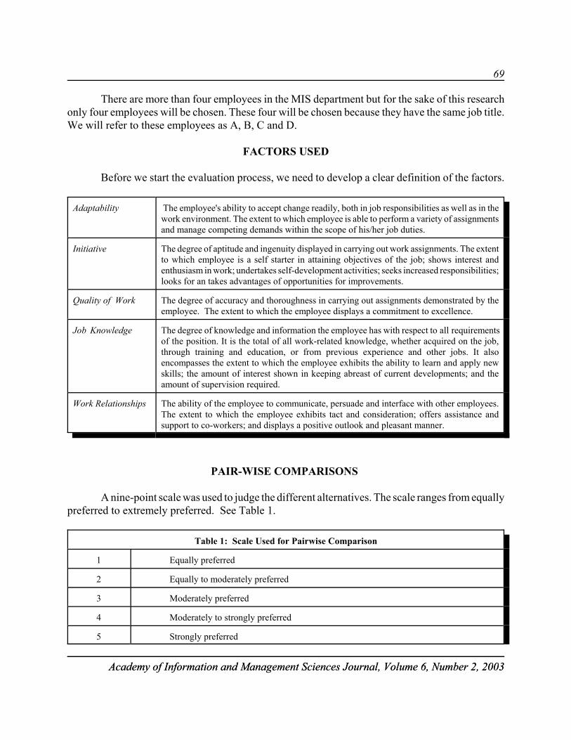
69
Academy of Information and Management Sciences Journal, Volume 6, Number 2, 2003Academy of Information and Management Sciences Journal, Volume 6, Number 2, 2003
There are more than four employees in the MIS department but for the sake of this researchonly four employees will be chosen. These four will be chosen because they have the same job title.We will refer to these employees as A, B, C and D.
FACTORS USED
Before we start the evaluation process, we need to develop a clear definition of the factors.
Adaptability The employee's ability to accept change readily, both in job responsibilities as well as in thework environment. The extent to which employee is able to perform a variety of assignmentsand manage competing demands within the scope of his/her job duties.
Initiative The degree of aptitude and ingenuity displayed in carrying out work assignments. The extentto which employee is a self starter in attaining objectives of the job; shows interest andenthusiasm in work; undertakes self-development activities; seeks increased responsibilities;looks for an takes advantages of opportunities for improvements.
Quality of Work The degree of accuracy and thoroughness in carrying out assignments demonstrated by theemployee. The extent to which the employee displays a commitment to excellence.
Job Knowledge The degree of knowledge and information the employee has with respect to all requirementsof the position. It is the total of all work-related knowledge, whether acquired on the job,through training and education, or from previous experience and other jobs. It alsoencompasses the extent to which the employee exhibits the ability to learn and apply newskills; the amount of interest shown in keeping abreast of current developments; and theamount of supervision required.
Work Relationships The ability of the employee to communicate, persuade and interface with other employees.The extent to which the employee exhibits tact and consideration; offers assistance andsupport to co-workers; and displays a positive outlook and pleasant manner.
PAIR-WISE COMPARISONS
A nine-point scale was used to judge the different alternatives. The scale ranges from equallypreferred to extremely preferred. See Table 1.
Table 1: Scale Used for Pairwise Comparison
1 Equally preferred
2 Equally to moderately preferred
3 Moderately preferred
4 Moderately to strongly preferred
5 Strongly preferred
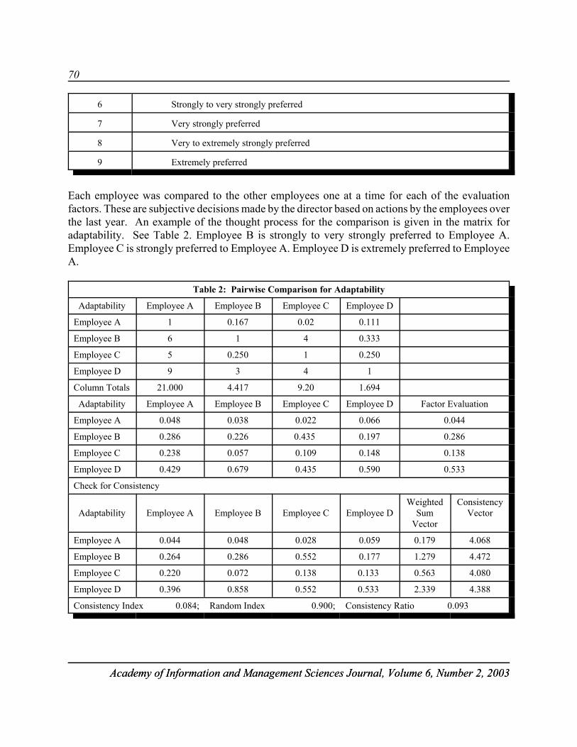
70
Academy of Information and Management Sciences Journal, Volume 6, Number 2, 2003Academy of Information and Management Sciences Journal, Volume 6, Number 2, 2003
6 Strongly to very strongly preferred
7 Very strongly preferred
8 Very to extremely strongly preferred
9 Extremely preferred
Each employee was compared to the other employees one at a time for each of the evaluationfactors. These are subjective decisions made by the director based on actions by the employees overthe last year. An example of the thought process for the comparison is given in the matrix foradaptability. See Table 2. Employee B is strongly to very strongly preferred to Employee A.Employee C is strongly preferred to Employee A. Employee D is extremely preferred to EmployeeA.
Table 2: Pairwise Comparison for Adaptability
Adaptability Employee A Employee B Employee C Employee D
Employee A 1 0.167 0.02 0.111
Employee B 6 1 4 0.333
Employee C 5 0.250 1 0.250
Employee D 9 3 4 1
Column Totals 21.000 4.417 9.20 1.694
Adaptability Employee A Employee B Employee C Employee D Factor Evaluation
Employee A 0.048 0.038 0.022 0.066 0.044
Employee B 0.286 0.226 0.435 0.197 0.286
Employee C 0.238 0.057 0.109 0.148 0.138
Employee D 0.429 0.679 0.435 0.590 0.533
Check for Consistency
Adaptability Employee A Employee B Employee C Employee DWeighted
SumVector
ConsistencyVector
Employee A 0.044 0.048 0.028 0.059 0.179 4.068
Employee B 0.264 0.286 0.552 0.177 1.279 4.472
Employee C 0.220 0.072 0.138 0.133 0.563 4.080
Employee D 0.396 0.858 0.552 0.533 2.339 4.388
Consistency Index 0.084; Random Index 0.900; Consistency Ratio 0.093
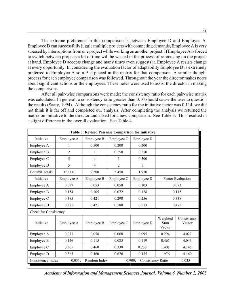
71
Academy of Information and Management Sciences Journal, Volume 6, Number 2, 2003Academy of Information and Management Sciences Journal, Volume 6, Number 2, 2003
The extreme preference in this comparison is between Employee D and Employee A.Employee D can successfully juggle multiple projects with competing demands, Employee A is verystressed by interruptions from one project while working on another project. If Employee A is forcedto switch between projects a lot of time will be wasted in the process of refocusing on the projectat hand. Employee D accepts change and many times even suggests it. Employee A resists changeat every opportunity. In considering the evaluation factor of adaptability Employee D is extremelypreferred to Employee A so a 9 is placed in the matrix for that comparison. A similar thoughtprocess for each employee comparison was followed. Throughout the year the director makes notesabout significant actions or the employees. These notes were used to assist the director in makingthe comparisons.
After all pair-wise comparisons were made; the consistency ratio for each pair-wise matrixwas calculated. In general, a consistency ratio greater than 0.10 should cause the user to questionthe results (Saaty, 1994). Although the consistency ratio for the initiative factor was 0.114, we didnot think it is far off and completed our analysis. After completing the analysis we returned thematrix on initiative to the director and asked for a new comparison. See Table 3. This resulted ina slight difference in the overall evaluation. See Table 4.
Table 3: Revised Pairwise Comparison for Initiative
Initiative Employee A Employee B Employee C Employee D
Employee A 1 0.500 0.200 0.200
Employee B 2 1 0.250 0.250
Employee C 5 4 1 0.500
Employee D 5 4 2 1
Column Totals 13.000 9.500 3.450 1.950
Initiative Employee A Employee B Employee C Employee D Factor Evaluation
Employee A 0.077 0.053 0.058 0.103 0.073
Employee B 0.154 0.105 0.072 0.128 0.115
Employee C 0.385 0.421 0.290 0.256 0.338
Employee D 0.385 0.421 0.580 0.513 0.475
Check for Consistency
Initiative Employee A Employee B Employee C Employee DWeighted
SumVector
ConsistencyVector
Employee A 0.073 0.058 0.068 0.095 0.294 4.027
Employee B 0.146 0.115 0.085 0.119 0.465 4.043
Employee C 0.365 0.460 0.338 0.238 1.401 4.145
Employee D 0.365 0.460 0.676 0.475 1.976 4.160
Consistency Index 0.031; Random Index 0.900; Consistency Ratio 0.035
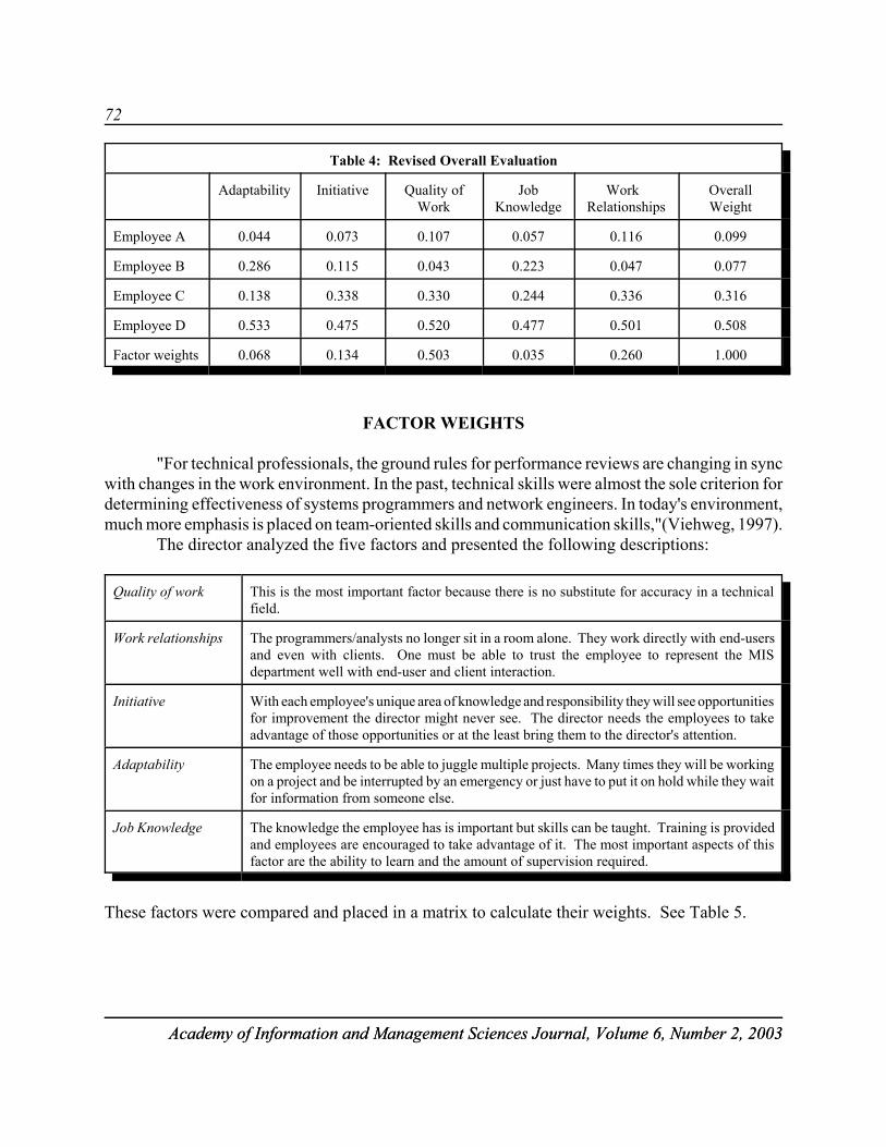
72
Academy of Information and Management Sciences Journal, Volume 6, Number 2, 2003Academy of Information and Management Sciences Journal, Volume 6, Number 2, 2003
Table 4: Revised Overall Evaluation
Adaptability Initiative Quality ofWork
JobKnowledge
Work Relationships
OverallWeight
Employee A 0.044 0.073 0.107 0.057 0.116 0.099
Employee B 0.286 0.115 0.043 0.223 0.047 0.077
Employee C 0.138 0.338 0.330 0.244 0.336 0.316
Employee D 0.533 0.475 0.520 0.477 0.501 0.508
Factor weights 0.068 0.134 0.503 0.035 0.260 1.000
FACTOR WEIGHTS
"For technical professionals, the ground rules for performance reviews are changing in syncwith changes in the work environment. In the past, technical skills were almost the sole criterion fordetermining effectiveness of systems programmers and network engineers. In today's environment,much more emphasis is placed on team-oriented skills and communication skills,"(Viehweg, 1997).
The director analyzed the five factors and presented the following descriptions:
Quality of work This is the most important factor because there is no substitute for accuracy in a technicalfield.
Work relationships The programmers/analysts no longer sit in a room alone. They work directly with end-usersand even with clients. One must be able to trust the employee to represent the MISdepartment well with end-user and client interaction.
Initiative With each employee's unique area of knowledge and responsibility they will see opportunitiesfor improvement the director might never see. The director needs the employees to takeadvantage of those opportunities or at the least bring them to the director's attention.
Adaptability The employee needs to be able to juggle multiple projects. Many times they will be workingon a project and be interrupted by an emergency or just have to put it on hold while they waitfor information from someone else.
Job Knowledge The knowledge the employee has is important but skills can be taught. Training is providedand employees are encouraged to take advantage of it. The most important aspects of thisfactor are the ability to learn and the amount of supervision required.
These factors were compared and placed in a matrix to calculate their weights. See Table 5.
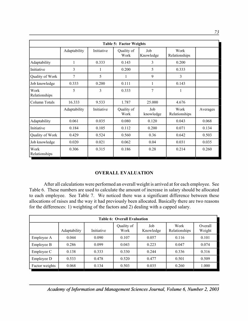
73
Academy of Information and Management Sciences Journal, Volume 6, Number 2, 2003Academy of Information and Management Sciences Journal, Volume 6, Number 2, 2003
Table 5: Factor Weights
Adaptability Initiative Quality of
WorkJob
Knowledge Work
Relationships
Adaptability 1 0.333 0.143 3 0.200
Initiative 3 1 0.200 5 0.333
Quality of Work 7 5 1 9 3
Job knowledge 0.333 0.200 0.111 1 0.143
WorkRelationships
5 3 0.333 7 1
Column Totals 16.333 9.533 1.787 25.000 4.676
Adaptability Initiative Quality ofWork
Jobknowledge
Work Relationships
Averages
Adaptability 0.061 0.035 0.080 0.120 0.043 0.068
Initiative 0.184 0.105 0.112 0.200 0.071 0.134
Quality of Work 0.429 0.524 0.560 0.36 0.642 0.503
Job knowledge 0.020 0.021 0.062 0.04 0.031 0.035
Work Relationships
0.306 0.315 0.186 0.28 0.214 0.260
OVERALL EVALUATION
After all calculations were performed an overall weight is arrived at for each employee. SeeTable 6. These numbers are used to calculate the amount of increase in salary should be allocatedto each employee. See Table 7. We noticed there was a significant difference between theseallocations of raises and the way it had previously been allocated. Basically there are two reasonsfor the differences: 1) weighting of the factors and 2) dealing with a capped salary.
Table 6: Overall Evaluation
Adaptability InitiativeQuality of
WorkJob
KnowledgeWork
RelationshipsOverallWeight
Employee A 0.044 0.090 0.107 0.057 0.116 0.101
Employee B 0.286 0.099 0.043 0.223 0.047 0.074
Employee C 0.138 0.333 0.330 0.244 0.336 0.316
Employee D 0.533 0.478 0.520 0.477 0.501 0.509
Factor weights 0.068 0.134 0.503 0.035 0.260 1.000
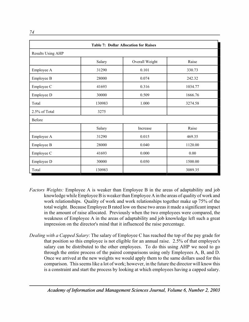
74
Academy of Information and Management Sciences Journal, Volume 6, Number 2, 2003Academy of Information and Management Sciences Journal, Volume 6, Number 2, 2003
Table 7: Dollar Allocation for Raises
Results Using AHP
Salary Overall Weight Raise
Employee A 31290 0.101 330.73
Employee B 28000 0.074 242.32
Employee C 41693 0.316 1034.77
Employee D 30000 0.509 1666.76
Total 130983 1.000 3274.58
2.5% of Total 3275
Before
Salary Increase Raise
Employee A 31290 0.015 469.35
Employee B 28000 0.040 1120.00
Employee C 41693 0.000 0.00
Employee D 30000 0.050 1500.00
Total 130983 3089.35
Factors Weights: Employee A is weaker than Employee B in the areas of adaptability and jobknowledge while Employee B is weaker than Employee A in the areas of quality of work andwork relationships. Quality of work and work relationships together make up 75% of thetotal weight. Because Employee B rated low on these two areas it made a significant impactin the amount of raise allocated. Previously when the two employees were compared, theweakness of Employee A in the areas of adaptability and job knowledge left such a greatimpression on the director's mind that it influenced the raise percentage.
Dealing with a Capped Salary: The salary of Employee C has reached the top of the pay grade forthat position so this employee is not eligible for an annual raise. 2.5% of that employee'ssalary can be distributed to the other employees. To do this using AHP we need to gothrough the entire process of the paired comparisons using only Employees A, B, and D.Once we arrived at the new weights we would apply them to the same dollars used for thiscomparison. This seems like a lot of work; however, in the future the director will know thisis a constraint and start the process by looking at which employees having a capped salary.
75
Academy of Information and Management Sciences Journal, Volume 6, Number 2, 2003Academy of Information and Management Sciences Journal, Volume 6, Number 2, 2003
CONCLUSION
There are no panaceas for giving employee performance reviews. Despite some drawbacksin using the AHP in performance evaluation, the technique has many positive points: (1) The degreeof excellence distributed by one employee will have the affect of challenging all other employeesto that level of performance. (2) Fair distribution of dollars - the best employees get rewarded moremoney. (3) Helps managers objectively - Distributing salary dollars based on the most importantfactors. (4) Can compare employees of differing job titles based on applying the definitions of thefactors to each position. A
AHP applied a sense of objectivity and resulted in a significantly different conclusion fromprevious methods used in the firm. We believe that this alone is enough to convince the director touse this method for future employee evaluations.
REFERENCES
Badri, M. A. (1999). Combining the analytic hierarchy process and goal programming for global facilitylocation-allocation problem. International Journal of Production Economics, 62(3), 237-248.
Calantone, R., Benedetto, C. A. & Schmidt, B. (1999). Using the analytic hierarchy process in new product screening.The Journal of Product Innovation Management, 16(1), 65-76.
Gass, S. & Rapcsak, T. (1998). A note on synthesizing group decisions. Decision Support Systems, 22(1), 59-63.
Ido, M. (1998). Ethical decision making using the analytic hierarchy process. Journal of Business Ethics, 17(11),1197-1204.
Iwasaki, S. & Tone, K. (1998). A search model with subjective judgments: Auditing of incorrect tax declarations.Omega, 26(2), 249-261.
Javalgi, R., Rao, S. R. & Thomas, E. (1991). Choosing a hospital: Analysis of consumer tradeoffs. Journal of HealthCare Marketing, 11(1), 12-23.
Kikano, G. E., Galazka, S. S., Flocke, S. A., Saffran, E. & Zyzanski, S. (1994). Markers of successful recruitment ofstudents to family practice residency programs. Family Medicine, 26, 492-499.
Kimbore, J. C. et al. (1999). Analysis of three decision making methods: A breast cancer patient as a model. MedicalDecision Making, 19(1), 49-58.
Kwak, N. K. & Lee, C. (1998). A multi-criteria decision-making approach to university resource allocation andinformation infrastructure planning. European Journal of Operational Research, 110(2), 234-242.
Lee, C. & Kwak, N. K. (1999). Information resource planning for a health-care system using an AHP- based goalprogramming method. The Journal of Operational Research Society, 50(12), 1191-1198.
Molta, D. (1997, May). The performance (review) of a lifetime. Network Computing, 20-23

76
Academy of Information and Management Sciences Journal, Volume 6, Number 2, 2003Academy of Information and Management Sciences Journal, Volume 6, Number 2, 2003
Randall, C. S., Begus, G. R., Schleche, J. A., McGuinness, G. & Mueller, C. W. (1997). Factors associated with primarycare residents' satisfaction with their training. Family Medicine, 29, 730-735.
Saaty, T. L. (1994). How to make a decision: The analytic hierarchy process. Interfaces, 24, 19-43.
Saaty, T. L. & Vargas, L. (2001). Models, Methods, Concepts & Applications of the Analytic Hierarchy Process.Kluwer Academic Publishers.
Viehweg, L. (1997, June). Maximize your employee appraisal system. Benefits & Compensation Solutions. 24-28
Wang, H; Xie, M. & Goh, T. N. (1998). A comparative study of the prioritization matrix and the analytic hierarchyprocess technique in quality function deployment. Total Quality Management, 9(6), 421-430.
77
Academy of Information and Management Sciences Journal, Volume 6, Number 2, 2003Academy of Information and Management Sciences Journal, Volume 6, Number 2, 2003
SAMPLE SIZE AND MODELING ACCURACYOF DECISION TREE BASED DATA MINING TOOLS
James Morgan, Northern Arizona UniversityRobert Daugherty, Northern Arizona University
Allan Hilchie, Northern Arizona University Bern Carey, Northern Arizona University
ABSTRACT
Given the cost associated with modeling very large datasets and over-fitting issues ofdecision-tree based models, sample based models are an attractive alternative - provided that thesample based models have a predictive accuracy approximating that of models based on allavailable data. This paper presents results of sets of decision-tree models generated acrossprogressive sets of sample sizes. The models were applied to two sets of actual client data usingeach of six prominent commercial data mining tools.
The results suggest that model accuracy improves at a decreasing rate with increasingsample size. When a power curve was fitted to accuracy estimates across various sample sizes,more than 80 percent of the time accuracy within 0.5 percent of the expected terminal (accuracy ofa theoretical infinite sample) was achieved by the time the sample size reached 10,000 records.Based on these results, fitting a power curve to progressive samples and using it to establish anappropriate sample size appears to be a promising mechanism to support sample based modelingfor large datasets.
INTRODUCTION
Data mining has emerged as a practical analytical tool primarily on the basis of its ability todeal with the large volume of data available from databases and data warehouses. Rapid increasesin processor speed coupled with continuing decreases in the cost of mass storage devices and othercomputer hardware have made it practical to collect and maintain massive databases. Data miningsoftware is viewed as a tool that can perform undirected or semi-directed analysis and, thus, can beapplied to the full length and width of very large data sets at much lower costs than analyticaltechniques requiring stronger human direction. While data mining tools have typically been appliedto the full volume of available data, issues of cost and model over-fitting suggest that use of datamining models based on a sample of available data may be appropriate in many instances. Thus,the relationship between sample size and model accuracy is an important issue for data mining.
Despite the increases in processing speeds and reductions in processing cost, applying datamining tools to analyze all available data is costly in terms of both dollars and time required togenerate and implement models. In discussing differences between statistical and data mining
78
Academy of Information and Management Sciences Journal, Volume 6, Number 2, 2003Academy of Information and Management Sciences Journal, Volume 6, Number 2, 2003
approaches, Mannila (2000) suggests that: "The volume of the data is probably not a very importantdifference: the number of variables or attributes often has a much more profound impact on theapplicable analysis methods. For example, data mining has tackled width problems such as whatto do in situations where the number of variables is so large that looking at all pairs of variables iscomputationally infeasible." The above quote suggests that the benefit of data mining tools comesfrom their ability to deal more effectively with complex interactions among variables rather thanfrom the ability to process massive volumes of instances.
It has been noted that decision tree based data mining tools are subject to over-fitting as thesize of the data set increases, Domingos (1998) and Oates and Jensen (1997). As Oates and Jensen[1998] note, "Increasing the amount of data used to build a model often results in a linear increasein model size, even when that additional complexity results in no significant increase in modelaccuracy." In a similar vein Musick, Catlett, and Russell (1993) suggest that "often theeconomically rational decision is to use only a subset of the available data." A variety of pruningalgorithms have been proposed to deal with this problem, and most commercial data miningsoftware using decision tree based algorithms incorporate the use of pruning algorithms. Whilepruning helps to limit the proportion by which model complexity increases as the amount of dataincreases, its effectiveness can only be assessed by examining the responsiveness of modelcomplexity and model accuracy to changes in data set size.
Sampling can also be used as a tool to lower the cost of maintaining data mining basedoperational models. Lee, Cheung, and Kao (1998) have proposed a dynamic sampling techniqueto test for changes in a dataset. Their technique suggests using a sample of data to detect whenenough change has occurred in the structure of a dataset to justify re-estimation of a model usingthe full set of available data. In addition to this monitoring role, periodic re-estimation of a decisiontree model using a moderate sized sample of data may be the most cost effective way to maintaina reliable predictive model. For example, an organization might find it equally costly to re-analyzea model on the basis of a sample of 10,000 records once a month or to re-analyze the model basedon all available data once a year. In such a case, modeling based on a sample will be the mosteffective strategy if the phenomenon being modeled is relatively dynamic and models based on thesample approximate the accuracy of a model based on all available data. In addition, many practicaldata mining scenarios may involve purchase of data from third party sources or the generation ofsupplementary data to directly support a data mining analysis. In these cases, there can clearly besubstantial savings from working with a sample of data provided that sample-based results aresufficiently accurate.
Prior studies of sampling in data mining have used public domain data modeling tools andrelatively small data sets from the UCI repository. In this paper we describe the results of modelsgenerated from the systematic sampling of data from two corporate datasets one of which containedmore than 1.5 million records. The target variable for each data set is a binary variable. Models aregenerated with each of six prominent commercial data mining tools. Statistical analyses across thetools, over varying sample sizes, and with respect to other relevant factors are presented. The resultsprovide an insight into the response of model accuracy with respect to increases in sample size, andalso allow us to examine the extent to which that response varies across different data mining toolsand across varied data sets.
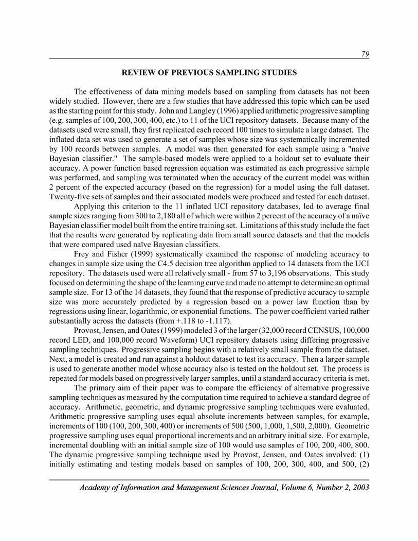
79
Academy of Information and Management Sciences Journal, Volume 6, Number 2, 2003Academy of Information and Management Sciences Journal, Volume 6, Number 2, 2003
REVIEW OF PREVIOUS SAMPLING STUDIES
The effectiveness of data mining models based on sampling from datasets has not beenwidely studied. However, there are a few studies that have addressed this topic which can be usedas the starting point for this study. John and Langley (1996) applied arithmetic progressive sampling(e.g. samples of 100, 200, 300, 400, etc.) to 11 of the UCI repository datasets. Because many of thedatasets used were small, they first replicated each record 100 times to simulate a large dataset. Theinflated data set was used to generate a set of samples whose size was systematically incrementedby 100 records between samples. A model was then generated for each sample using a "naiveBayesian classifier." The sample-based models were applied to a holdout set to evaluate theiraccuracy. A power function based regression equation was estimated as each progressive samplewas performed, and sampling was terminated when the accuracy of the current model was within2 percent of the expected accuracy (based on the regression) for a model using the full dataset.Twenty-five sets of samples and their associated models were produced and tested for each dataset.
Applying this criterion to the 11 inflated UCI repository databases, led to average finalsample sizes ranging from 300 to 2,180 all of which were within 2 percent of the accuracy of a naïveBayesian classifier model built from the entire training set. Limitations of this study include the factthat the results were generated by replicating data from small source datasets and that the modelsthat were compared used naïve Bayesian classifiers.
Frey and Fisher (1999) systematically examined the response of modeling accuracy tochanges in sample size using the C4.5 decision tree algorithm applied to 14 datasets from the UCIrepository. The datasets used were all relatively small - from 57 to 3,196 observations. This studyfocused on determining the shape of the learning curve and made no attempt to determine an optimalsample size. For 13 of the 14 datasets, they found that the response of predictive accuracy to samplesize was more accurately predicted by a regression based on a power law function than byregressions using linear, logarithmic, or exponential functions. The power coefficient varied rathersubstantially across the datasets (from +.118 to -1.117).
Provost, Jensen, and Oates (1999) modeled 3 of the larger (32,000 record CENSUS, 100,000record LED, and 100,000 record Waveform) UCI repository datasets using differing progressivesampling techniques. Progressive sampling begins with a relatively small sample from the dataset.Next, a model is created and run against a holdout dataset to test its accuracy. Then a larger sampleis used to generate another model whose accuracy also is tested on the holdout set. The process isrepeated for models based on progressively larger samples, until a standard accuracy criteria is met.
The primary aim of their paper was to compare the efficiency of alternative progressivesampling techniques as measured by the computation time required to achieve a standard degree ofaccuracy. Arithmetic, geometric, and dynamic progressive sampling techniques were evaluated.Arithmetic progressive sampling uses equal absolute increments between samples, for example,increments of 100 (100, 200, 300, 400) or increments of 500 (500, 1,000, 1,500, 2,000). Geometricprogressive sampling uses equal proportional increments and an arbitrary initial size. For example,incremental doubling with an initial sample size of 100 would use samples of 100, 200, 400, 800.The dynamic progressive sampling technique used by Provost, Jensen, and Oates involved: (1)initially estimating and testing models based on samples of 100, 200, 300, 400, and 500, (2)
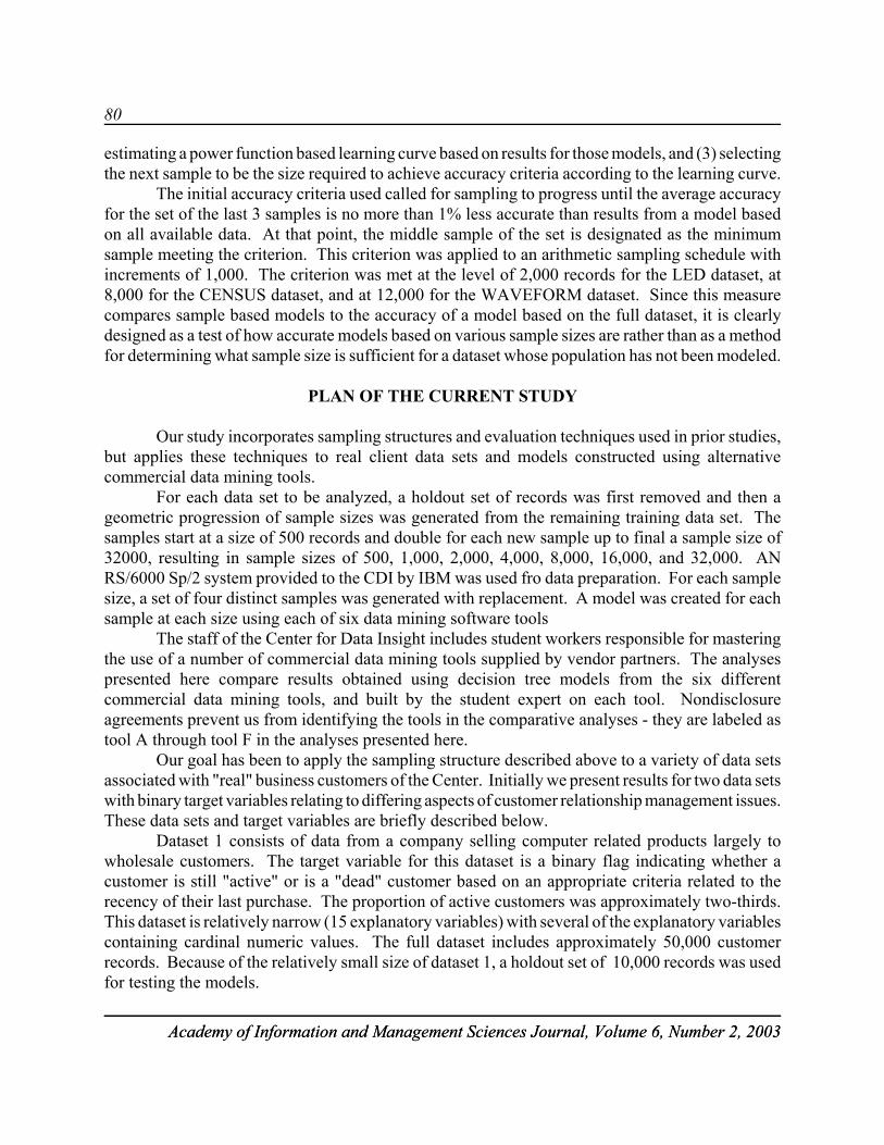
80
Academy of Information and Management Sciences Journal, Volume 6, Number 2, 2003Academy of Information and Management Sciences Journal, Volume 6, Number 2, 2003
estimating a power function based learning curve based on results for those models, and (3) selectingthe next sample to be the size required to achieve accuracy criteria according to the learning curve.
The initial accuracy criteria used called for sampling to progress until the average accuracyfor the set of the last 3 samples is no more than 1% less accurate than results from a model basedon all available data. At that point, the middle sample of the set is designated as the minimumsample meeting the criterion. This criterion was applied to an arithmetic sampling schedule withincrements of 1,000. The criterion was met at the level of 2,000 records for the LED dataset, at8,000 for the CENSUS dataset, and at 12,000 for the WAVEFORM dataset. Since this measurecompares sample based models to the accuracy of a model based on the full dataset, it is clearlydesigned as a test of how accurate models based on various sample sizes are rather than as a methodfor determining what sample size is sufficient for a dataset whose population has not been modeled.
PLAN OF THE CURRENT STUDY
Our study incorporates sampling structures and evaluation techniques used in prior studies,but applies these techniques to real client data sets and models constructed using alternativecommercial data mining tools.
For each data set to be analyzed, a holdout set of records was first removed and then ageometric progression of sample sizes was generated from the remaining training data set. Thesamples start at a size of 500 records and double for each new sample up to final a sample size of32000, resulting in sample sizes of 500, 1,000, 2,000, 4,000, 8,000, 16,000, and 32,000. ANRS/6000 Sp/2 system provided to the CDI by IBM was used fro data preparation. For each samplesize, a set of four distinct samples was generated with replacement. A model was created for eachsample at each size using each of six data mining software tools
The staff of the Center for Data Insight includes student workers responsible for masteringthe use of a number of commercial data mining tools supplied by vendor partners. The analysespresented here compare results obtained using decision tree models from the six differentcommercial data mining tools, and built by the student expert on each tool. Nondisclosureagreements prevent us from identifying the tools in the comparative analyses - they are labeled astool A through tool F in the analyses presented here.
Our goal has been to apply the sampling structure described above to a variety of data setsassociated with "real" business customers of the Center. Initially we present results for two data setswith binary target variables relating to differing aspects of customer relationship management issues.These data sets and target variables are briefly described below.
Dataset 1 consists of data from a company selling computer related products largely towholesale customers. The target variable for this dataset is a binary flag indicating whether acustomer is still "active" or is a "dead" customer based on an appropriate criteria related to therecency of their last purchase. The proportion of active customers was approximately two-thirds.This dataset is relatively narrow (15 explanatory variables) with several of the explanatory variablescontaining cardinal numeric values. The full dataset includes approximately 50,000 customerrecords. Because of the relatively small size of dataset 1, a holdout set of 10,000 records was usedfor testing the models.
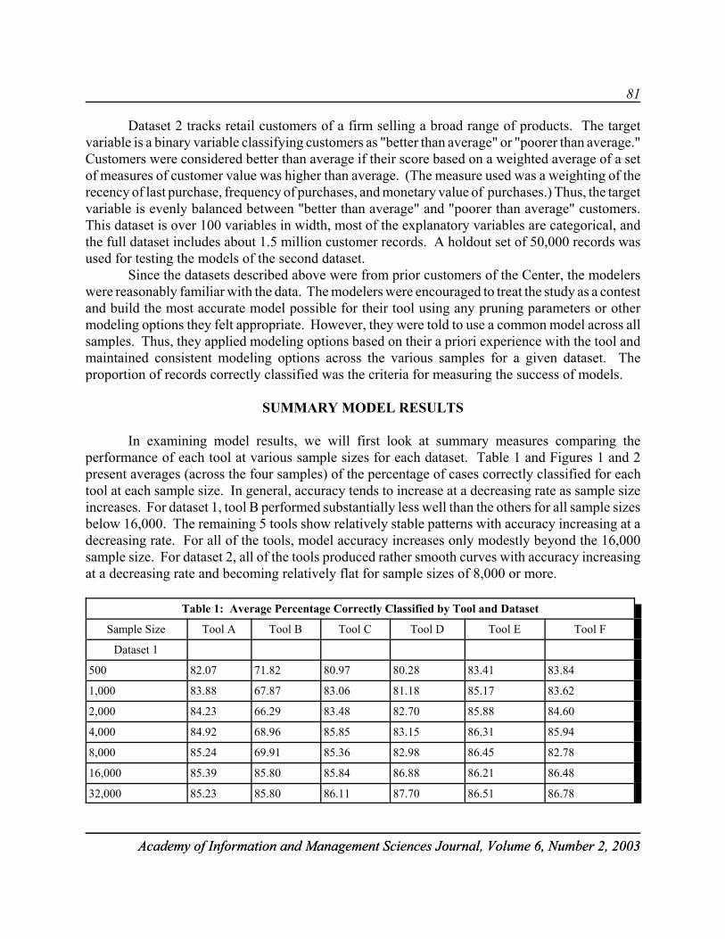
81
Academy of Information and Management Sciences Journal, Volume 6, Number 2, 2003Academy of Information and Management Sciences Journal, Volume 6, Number 2, 2003
Dataset 2 tracks retail customers of a firm selling a broad range of products. The targetvariable is a binary variable classifying customers as "better than average" or "poorer than average."Customers were considered better than average if their score based on a weighted average of a setof measures of customer value was higher than average. (The measure used was a weighting of therecency of last purchase, frequency of purchases, and monetary value of purchases.) Thus, the targetvariable is evenly balanced between "better than average" and "poorer than average" customers.This dataset is over 100 variables in width, most of the explanatory variables are categorical, andthe full dataset includes about 1.5 million customer records. A holdout set of 50,000 records wasused for testing the models of the second dataset.
Since the datasets described above were from prior customers of the Center, the modelerswere reasonably familiar with the data. The modelers were encouraged to treat the study as a contestand build the most accurate model possible for their tool using any pruning parameters or othermodeling options they felt appropriate. However, they were told to use a common model across allsamples. Thus, they applied modeling options based on their a priori experience with the tool andmaintained consistent modeling options across the various samples for a given dataset. Theproportion of records correctly classified was the criteria for measuring the success of models.
SUMMARY MODEL RESULTS
In examining model results, we will first look at summary measures comparing theperformance of each tool at various sample sizes for each dataset. Table 1 and Figures 1 and 2present averages (across the four samples) of the percentage of cases correctly classified for eachtool at each sample size. In general, accuracy tends to increase at a decreasing rate as sample sizeincreases. For dataset 1, tool B performed substantially less well than the others for all sample sizesbelow 16,000. The remaining 5 tools show relatively stable patterns with accuracy increasing at adecreasing rate. For all of the tools, model accuracy increases only modestly beyond the 16,000sample size. For dataset 2, all of the tools produced rather smooth curves with accuracy increasingat a decreasing rate and becoming relatively flat for sample sizes of 8,000 or more.
Table 1: Average Percentage Correctly Classified by Tool and Dataset
Sample Size Tool A Tool B Tool C Tool D Tool E Tool F
Dataset 1
500 82.07 71.82 80.97 80.28 83.41 83.84
1,000 83.88 67.87 83.06 81.18 85.17 83.62
2,000 84.23 66.29 83.48 82.70 85.88 84.60
4,000 84.92 68.96 85.85 83.15 86.31 85.94
8,000 85.24 69.91 85.36 82.98 86.45 82.78
16,000 85.39 85.80 85.84 86.88 86.21 86.48
32,000 85.23 85.80 86.11 87.70 86.51 86.78

82
Table 1: Average Percentage Correctly Classified by Tool and Dataset
Sample Size Tool A Tool B Tool C Tool D Tool E Tool F
Academy of Information and Management Sciences Journal, Volume 6, Number 2, 2003Academy of Information and Management Sciences Journal, Volume 6, Number 2, 2003
Dataset 2
500 86.04 86.78 90.35 82.40 87.41 89.70
1,000 87.38 89.16 93.58 88.33 88.60 89.91
2,000 88.08 90.36 93.19 88.65 89.63 91.19
4,000 90.33 91.45 93.45 89.85 90.63 91.96
8,000 89.92 91.94 93.63 90.10 91.42 92.40
16,000 90.34 92.57 93.07 90.23 91.56 92.87
32,000 90.60 93.11 93.95 90.55 91.61 93.34
Data Mining Figures
Figure 1
Model Accuracy vs Sample Size: Dataset 1
80
82
84
86
88
0 5000 10000 15000 20000 25000 30000 35000Sample Size
Pct.
Cor
rect
ly C
lass
ified
Tool A
Tool B
Tool C
Tool D
Tool E
Tool F

83
Academy of Information and Management Sciences Journal, Volume 6, Number 2, 2003Academy of Information and Management Sciences Journal, Volume 6, Number 2, 2003
Figure 2
Model Accuracy vs. Sample Size: Dataset 2
86
88
90
92
94
0 5000 10000 15000 20000 25000 30000 35000
Sample Size
Pct.
Cor
rect
ly C
lass
ified
Tool ATool BTool CTool DTool ETool F
Within a given dataset tools that do well for small sample sizes also tended to do well for largersizes, however, there was no clear pattern of dominance across the two datasets. Tool E providedthe most consistent performance on dataset 1, while tool D showed the best performance at thelargest sample sizes. Both of these tools were near the bottom in their performance for dataset 2.At the same time, tool C provided the strongest accuracy for dataset 2 (particularly at small samplesizes), but had average performance for dataset 1.
Table 2 presents summary univariate analysis of variance results for the two datasets. Thesample size and the tool used as well as the interaction between those 2 factors were used asexplanatory factors. As Table 2 indicates, both factors and their interaction are statisticallysignificant for both datasets.
Also presented are results of the Tukey test for homogeneous subsets for each factor. Thistest identifies sets of values for each factor whose means do not differ significantly at the .05 level.Results for both datasets show that accuracy increases with sample size. Results for dataset 2 showa plateauing of accuracy - accuracy for all sample sizes above 4,000 fit into the same homogeneoussubset. Dataset 1 results place only the 16,000 and 32,000 sample sizes in the final homogeneoussubset. This is primarily due to the unusual pattern of results for Tool B. If tool B is excluded fordataset 1, all sample sizes greater than 4,000 once again fit in the same homogeneous subset. TheTukey test for the tool factor shows that there are significant differences in average accuracy, butno strong systematic patterns that hold up across both datasets.
FINDING AN OPTIMAL SAMPLE SIZE
In the previous section all of the data presented was based on average responses across thefour separate samples that were generated for each sample size. While this information is of interest,
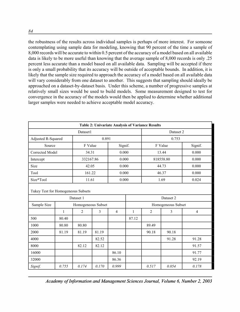
84
Academy of Information and Management Sciences Journal, Volume 6, Number 2, 2003Academy of Information and Management Sciences Journal, Volume 6, Number 2, 2003
the robustness of the results across individual samples is perhaps of more interest. For someonecontemplating using sample data for modeling, knowing that 90 percent of the time a sample of8,000 records will be accurate to within 0.5 percent of the accuracy of a model based on all availabledata is likely to be more useful than knowing that the average sample of 8,000 records is only .25percent less accurate than a model based on all available data. Sampling will be accepted if thereis only a small probability that its accuracy will be outside of acceptable bounds. In addition, it islikely that the sample size required to approach the accuracy of a model based on all available datawill vary considerably from one dataset to another. This suggests that sampling should ideally beapproached on a dataset-by-dataset basis. Under this scheme, a number of progressive samples atrelatively small sizes would be used to build models. Some measurement designed to test forconvergence in the accuracy of the models would then be applied to determine whether additionallarger samples were needed to achieve acceptable model accuracy.
Table 2: Univariate Analysis of Variance Results
Dataset1 Dataset 2
Adjusted R-Squared 0.891 0.753
Source F Value Signif. F Value Signif.
Corrected Model 34.31 0.000 13.44 0.000
Intercept 332167.86 0.000 818558.80 0.000
Size 42.05 0.000 44.73 0.000
Tool 161.22 0.000 46.37 0.000
Size*Tool 11.61 0.000 1.69 0.024
Tukey Test for Homogeneous Subsets
Dataset 1 Dataset 2
Sample Size Homogeneous Subset Homogeneous Subset
1 2 3 4 1 2 3 4
500 80.40 87.12
1000 80.80 80.80 89.49
2000 81.19 81.19 81.19 90.18 90.18
4000 82.52 91.28 91.28
8000 82.12 82.12 91.57
16000 86.10 91.77
32000 86.36 92.19
Signif. 0.755 0.174 0.170 0.999 0.517 0.054 0.178

85
Table 2: Univariate Analysis of Variance Results
Academy of Information and Management Sciences Journal, Volume 6, Number 2, 2003Academy of Information and Management Sciences Journal, Volume 6, Number 2, 2003
Tool Used Homogeneous Subset Homogeneous Subset
1 2 3 1 2 3 4
Tool A 84.42 84.42 88.96
Tool B 73.78 90.77 90.77
Tool C 84.38 84.38 93.03
Tool D 83.55 88.59
Tool E 85.71 90.12
Tool F 84.86 84.86 91.62
Signif. 0.089 0.083 0.894 0.428 0.133
The models created in this study followed a fixed sampling scheme using progressivesamples form 500 to 32,000 records. However, tests of progressive sampling methodologies can beapplied ex-post. We can evaluate the sample size that would have been required to meet a particularconvergence criterion. Two alternative methods for measuring convergence across progressivesamples are presented here. The first is based on using moving averages of model accuracy whilethe second uses statistical analysis of model results.
Oates and Jensen (1997) used a convergence measure based on examining the improvementin model accuracy as the sample size was progressively increased to test for convergence. Underthis scheme, when the improvement in accuracy drops below a prescribed level sampling isterminated. For this criterion to be effective, the improvement in model accuracy as sample sizeincreases needs to be relatively stable and monotonically decreasing in magnitude. If this is thecase, it is reasonable to assume that, once the improvement in model accuracy drops below aspecified limit, it would stay below that limit for all larger sample sizes as well, and that a plateauin model accuracy has been achieved. To minimize the chance of improperly terminating due to asingle non-representative sample, a moving average of the accuracy of the last three samples ismaintained and sampling is terminated when the improvement in this moving average drops belowa specified convergence criterion (1 percent in Oates and Jensen's paper).
In adapting this technique, we used a weighted average of the last 3 samples. That is, themoving average model accuracy for a given sample sizes is:
AccMAn = (Szn*Accn + Szn-1*Accn-1 + Szn-2*Accn-2)/( Szn + Szn-1 + Szn-2)
where Accn is the measured model accuracy for the nth progressive sample, Szn is the size of the nthprogressive sample, and AccMAn is the moving average accuracy measure for the nth progressivesample. The convergence test applied calls for sampling to terminate if
AccMAn - AccMAn-1 < *
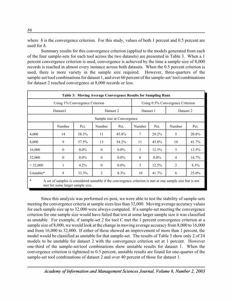
86
Academy of Information and Management Sciences Journal, Volume 6, Number 2, 2003Academy of Information and Management Sciences Journal, Volume 6, Number 2, 2003
where * is the convergence criterion. For this study, values of both 1 percent and 0.5 percent areused for *.
Summary results for this convergence criterion (applied to the models generated from eachof the four sample-sets for each tool across the two datasets) are presented in Table 3. When a 1percent convergence criterion is used, convergence is achieved by the time a sample size of 8,000records is reached in almost every instance across both datasets. When the 0.5 percent criterion isused, there is more variety in the sample size required. However, three-quarters of thesample-set/tool combinations for dataset 1, and over 60 percent of the sample-set/ tool combinationsfor dataset 2 reached convergence at 8,000 records or less.
Table 3: Moving Average Convergence Results for Sampling Runs
Using 1% Convergence Criterion Using 0.5% Convergence Criterion
Dataset1 Dataset 2 Dataset 1 Dataset 2
Sample size at Convergence
Number Pct. Number Pct. Number Pct. Number Pct.
4,000 14 58.3% 11 45.8% 7 29.2% 5 20.8%
8,000 9 37.5% 13 54.2% 11 45.8% 10 41.7%
16,000 0 0.0% 0 0.0% 3 12.5% 3 12.5%
32,000 0 0.0% 0 0.0% 0 0.0% 4 16.7%
> 32,000 1 4.2% 0 0.0% 3 12.5% 2 8.3%
Unstable* 8 33.3% 2 8.3% 10 41.7% 6 25.0%
* A set of samples is considered unstable if the convergence criterion is met at one sample size but is notmet for some larger sample size.
Since this analysis was performed ex-post, we were able to test the stability of sample-setsmeeting the convergence criteria at sample sizes less than 32,000. Moving average accuracy valuesfor each sample size up to 32,000 were always computed. If a sample-set meeting the convergencecriterion for one sample size would have failed that test at some larger sample size it was classifiedas unstable. For example, if sample-set 2 for tool C met the 1 percent convergence criterion at asample size of 8,000, we would look at the change in moving average accuracy from 8,000 to 16,000and from 16,000 to 32,000. If either of these showed an improvement of more than 1 percent, themodel would be classified as unstable for that sample-set. The results of Table 3 show only 2 of 24models to be unstable for dataset 2 with the convergence criterion set at 1 percent. Howeverone-third of the sample-set/tool combinations show unstable results for dataset 1. When theconvergence criterion is tightened to 0.5 percent, unstable results are found for one-quarter of thesample-set tool combinations of dataset 2 and over 40 percent of those for dataset 1.
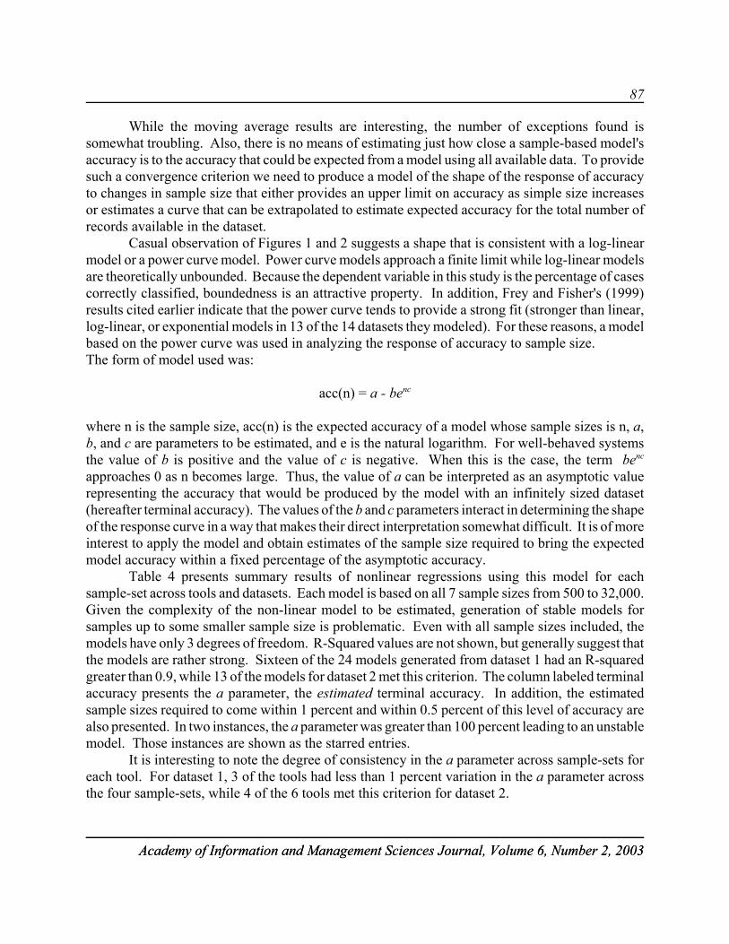
87
Academy of Information and Management Sciences Journal, Volume 6, Number 2, 2003Academy of Information and Management Sciences Journal, Volume 6, Number 2, 2003
While the moving average results are interesting, the number of exceptions found issomewhat troubling. Also, there is no means of estimating just how close a sample-based model'saccuracy is to the accuracy that could be expected from a model using all available data. To providesuch a convergence criterion we need to produce a model of the shape of the response of accuracyto changes in sample size that either provides an upper limit on accuracy as simple size increasesor estimates a curve that can be extrapolated to estimate expected accuracy for the total number ofrecords available in the dataset.
Casual observation of Figures 1 and 2 suggests a shape that is consistent with a log-linearmodel or a power curve model. Power curve models approach a finite limit while log-linear modelsare theoretically unbounded. Because the dependent variable in this study is the percentage of casescorrectly classified, boundedness is an attractive property. In addition, Frey and Fisher's (1999)results cited earlier indicate that the power curve tends to provide a strong fit (stronger than linear,log-linear, or exponential models in 13 of the 14 datasets they modeled). For these reasons, a modelbased on the power curve was used in analyzing the response of accuracy to sample size. The form of model used was:
acc(n) = a - benc
where n is the sample size, acc(n) is the expected accuracy of a model whose sample sizes is n, a,b, and c are parameters to be estimated, and e is the natural logarithm. For well-behaved systemsthe value of b is positive and the value of c is negative. When this is the case, the term benc
approaches 0 as n becomes large. Thus, the value of a can be interpreted as an asymptotic valuerepresenting the accuracy that would be produced by the model with an infinitely sized dataset(hereafter terminal accuracy). The values of the b and c parameters interact in determining the shapeof the response curve in a way that makes their direct interpretation somewhat difficult. It is of moreinterest to apply the model and obtain estimates of the sample size required to bring the expectedmodel accuracy within a fixed percentage of the asymptotic accuracy.
Table 4 presents summary results of nonlinear regressions using this model for eachsample-set across tools and datasets. Each model is based on all 7 sample sizes from 500 to 32,000.Given the complexity of the non-linear model to be estimated, generation of stable models forsamples up to some smaller sample size is problematic. Even with all sample sizes included, themodels have only 3 degrees of freedom. R-Squared values are not shown, but generally suggest thatthe models are rather strong. Sixteen of the 24 models generated from dataset 1 had an R-squaredgreater than 0.9, while 13 of the models for dataset 2 met this criterion. The column labeled terminalaccuracy presents the a parameter, the estimated terminal accuracy. In addition, the estimatedsample sizes required to come within 1 percent and within 0.5 percent of this level of accuracy arealso presented. In two instances, the a parameter was greater than 100 percent leading to an unstablemodel. Those instances are shown as the starred entries.
It is interesting to note the degree of consistency in the a parameter across sample-sets foreach tool. For dataset 1, 3 of the tools had less than 1 percent variation in the a parameter acrossthe four sample-sets, while 4 of the 6 tools met this criterion for dataset 2.
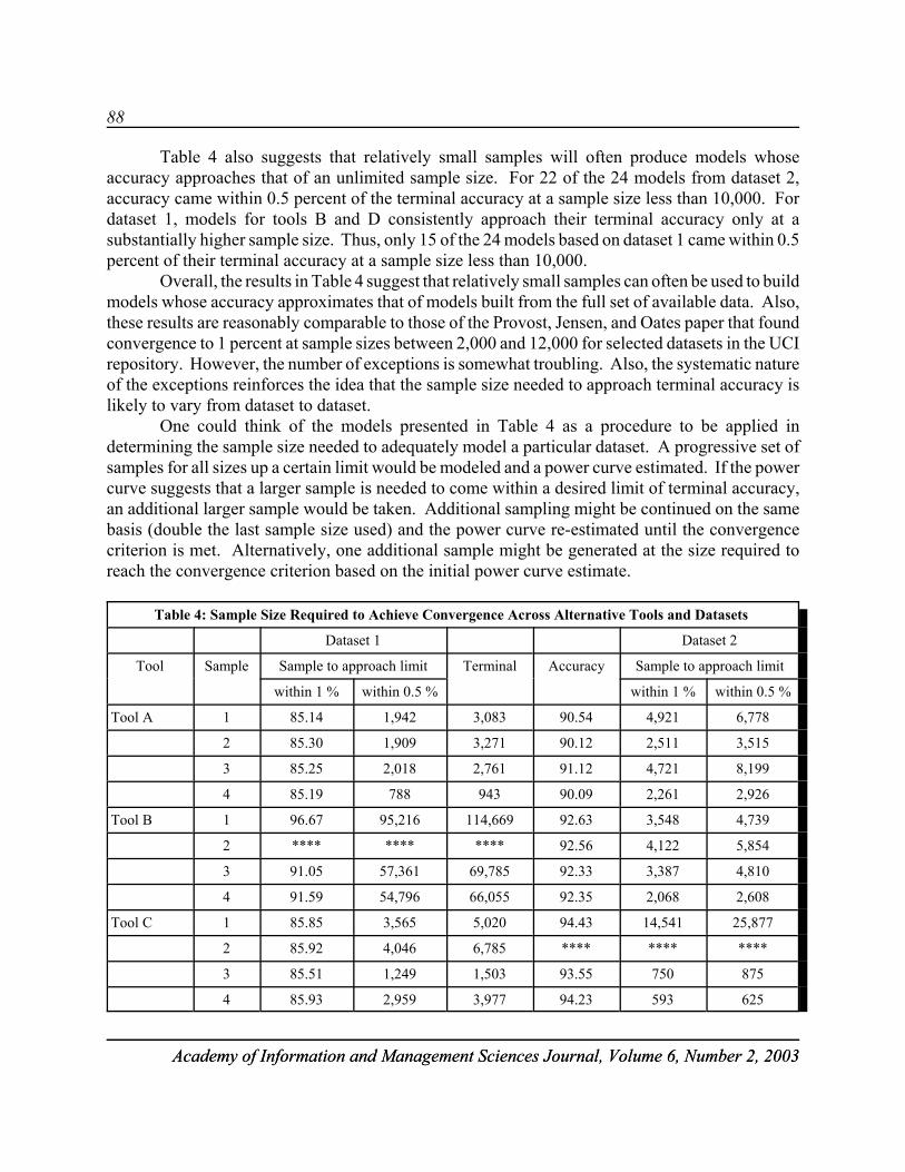
88
Academy of Information and Management Sciences Journal, Volume 6, Number 2, 2003Academy of Information and Management Sciences Journal, Volume 6, Number 2, 2003
Table 4 also suggests that relatively small samples will often produce models whoseaccuracy approaches that of an unlimited sample size. For 22 of the 24 models from dataset 2,accuracy came within 0.5 percent of the terminal accuracy at a sample size less than 10,000. Fordataset 1, models for tools B and D consistently approach their terminal accuracy only at asubstantially higher sample size. Thus, only 15 of the 24 models based on dataset 1 came within 0.5percent of their terminal accuracy at a sample size less than 10,000.
Overall, the results in Table 4 suggest that relatively small samples can often be used to buildmodels whose accuracy approximates that of models built from the full set of available data. Also,these results are reasonably comparable to those of the Provost, Jensen, and Oates paper that foundconvergence to 1 percent at sample sizes between 2,000 and 12,000 for selected datasets in the UCIrepository. However, the number of exceptions is somewhat troubling. Also, the systematic natureof the exceptions reinforces the idea that the sample size needed to approach terminal accuracy islikely to vary from dataset to dataset.
One could think of the models presented in Table 4 as a procedure to be applied indetermining the sample size needed to adequately model a particular dataset. A progressive set ofsamples for all sizes up a certain limit would be modeled and a power curve estimated. If the powercurve suggests that a larger sample is needed to come within a desired limit of terminal accuracy,an additional larger sample would be taken. Additional sampling might be continued on the samebasis (double the last sample size used) and the power curve re-estimated until the convergencecriterion is met. Alternatively, one additional sample might be generated at the size required toreach the convergence criterion based on the initial power curve estimate.
Table 4: Sample Size Required to Achieve Convergence Across Alternative Tools and Datasets
Dataset 1 Dataset 2
Tool Sample Sample to approach limit Terminal Accuracy Sample to approach limit
within 1 % within 0.5 % within 1 % within 0.5 %
Tool A 1 85.14 1,942 3,083 90.54 4,921 6,778
2 85.30 1,909 3,271 90.12 2,511 3,515
3 85.25 2,018 2,761 91.12 4,721 8,199
4 85.19 788 943 90.09 2,261 2,926
Tool B 1 96.67 95,216 114,669 92.63 3,548 4,739
2 **** **** **** 92.56 4,122 5,854
3 91.05 57,361 69,785 92.33 3,387 4,810
4 91.59 54,796 66,055 92.35 2,068 2,608
Tool C 1 85.85 3,565 5,020 94.43 14,541 25,877
2 85.92 4,046 6,785 **** **** ****
3 85.51 1,249 1,503 93.55 750 875
4 85.93 2,959 3,977 94.23 593 625
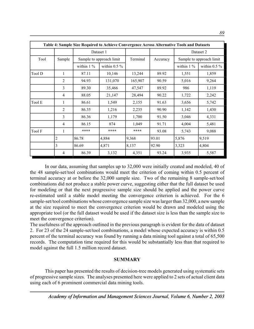
89
Table 4: Sample Size Required to Achieve Convergence Across Alternative Tools and Datasets
Dataset 1 Dataset 2
Tool Sample Sample to approach limit Terminal Accuracy Sample to approach limit
within 1 % within 0.5 % within 1 % within 0.5 %
Academy of Information and Management Sciences Journal, Volume 6, Number 2, 2003Academy of Information and Management Sciences Journal, Volume 6, Number 2, 2003
Tool D 1 87.11 10,146 13,244 89.92 1,551 1,859
2 94.93 131,070 165,907 90.59 5,016 9,264
3 89.30 35,466 47,547 89.92 986 1,119
4 88.05 21,147 28,494 90.22 1,722 2,242
Tool E 1 86.61 1,549 2,155 91.63 3,656 5,742
2 86.35 1,216 2,235 90.90 1,142 1,430
3 86.36 1,179 1,700 91.50 3,046 4,331
4 86.15 874 1,049 91.71 4,004 5,481
Tool F 1 **** **** **** 93.08 5,743 9,088
2 86.78 4,884 9,368 93.01 5,876 9,519
3 86.69 4,871 8,137 92.90 3,323 4,804
4 86.39 3,132 4,351 93.24 3,935 5,587
In our data, assuming that samples up to 32,000 were initially created and modeled, 40 ofthe 48 sample-set/tool combinations would meet the criterion of coming within 0.5 percent ofterminal accuracy at or before the 32,000 sample size. Two of the remaining 8 sample-set/toolcombinations did not produce a stable power curve, suggesting either that the full dataset be usedfor modeling or that the next progressive sample size should be applied and the power curvere-estimated until a stable model meeting the convergence criterion is achieved. For the 6sample-set/tool combinations whose convergence sample size was larger than 32,000, a new sampleat the size required to meet the convergence criterion would be drawn and modeled using theappropriate tool (or the full dataset would be used if the dataset size is less than the sample size tomeet the convergence criterion).The usefulness of the approach outlined in the previous paragraph is evident for the data of dataset2. For 23 of the 24 sample-set/tool combinations, a model whose expected accuracy is within 0.5percent of the terminal accuracy was found by running a data mining tool against a total of 65,500records. The computation time required for this would be substantially less than that required tomodel against the full 1.5 million record dataset.
SUMMARY
This paper has presented the results of decision-tree models generated using systematic setsof progressive sample sizes. The analyses presented here were applied to 2 sets of actual client datausing each of 6 prominent commercial data mining tools.
90
Academy of Information and Management Sciences Journal, Volume 6, Number 2, 2003Academy of Information and Management Sciences Journal, Volume 6, Number 2, 2003
Comparisons of results across tools indicated significant differences in the effectiveness ofthe various tools in modeling particular datasets. However, there was not a consistent pattern of toolperformance across the 2 datasets. The tools that performed best on dataset 1 were not particularlystrong for dataset 2 and vice-versa.
In general, our results suggest that model accuracy tends to increase at a decreasing rate withincreases in sample size. In most cases, the results were fit rather well by a model that assumes thatthe response of accuracy to increases in sample size can be specified by a power curve with a finiteterminal value less than 100 percent. The power curve is characterized by a long plateau, withvalues close to the terminal value at large sample sizes. While rather erratic performance wasobserved for some of the small samples from dataset 1, accuracy almost universally reached aplateau by the time the 16,000 record sample size was reached. More than 80 percent of the time,accuracy within 0.5 percent of the expected terminal accuracy was achieved by the time the samplesize reached 10,000 records. Results for dataset 2 were substantially more consistent than those fordataset 1, reinforcing the idea that the size of sample needed to achieve adequate model performsis likely to vary substantially across dataset and target variable characteristics.
Our results do suggest that systematic progressive sampling often produces models whoseexpected accuracy is very close to the accuracy expected from a model based on the full dataset.Fitting a power curve to a set of progressive samples and using its results to assess the adequacy ofthe samples used and determine the appropriate size for an additional sample, if needed, appears tobe a promising mechanism for sample-based mining of a large dataset.
This preliminary work suggests a number of avenues for further research. Examination ofsampling responsiveness should be extended to broader types of datasets and to non-binary targetvariables and target variables whose distribution is skewed to varying degrees. Another interestingextension to this study would be the systematic application of bagging of the samples required toproduce the accuracy responsiveness estimates, which might provide a low cost means to fullyutilize all the samples required to apply this technique.
91
Academy of Information and Management Sciences Journal, Volume 6, Number 2, 2003Academy of Information and Management Sciences Journal, Volume 6, Number 2, 2003
REFERENCES
Domingos, P. (1998). Occam's two razors: The sharp and the blunt. Proceedings of the Fourth International Conferenceon Knowledge Discovery and Data Mining, Menlo Park, CA: AAAI Press, 37-43.
Frey, L. & Fisher, D. (1999). Modeling decision tree performance with the power law. Proceedings of the SeventhInternational Workshop on Artificial Intelligence and Statistics, San Francisco, CA: Morgan-Kaufmann, 59-65.
John, G. & Langley, P. (1996). Static versus dynamic sampling for data mining. Proceedings of the SecondInternational Conference on Knowledge Discovery and Data Mining, AAAI Press, 367-370.
Lee, S., Cheung, D. & Kao, B. (1998). Is sampling useful in data mining? A case in the maintenance of discoveredassociation rules. Data Mining and Knowledge Discovery, 2, Kluwer Academic Publishers, 232-262.
Mannila, H. (2000). Theoretical frameworks for data mining. SIGKDD Explorations, 1(2), ACM SIGKDD, 30-32.
Musick, R., Catlett, J. & Russel, S. (1993). Decision theoretic subsampling for induction on large databases.Proceedings of the Tenth International Conference on Machine Learning, San Mateo, CA: Morgan Kaufmann,212-219.
Oates, T. & Jensen, D. (1997). The effects of training set size on decision tree complexity. Machine learning,Proceedings of the Fourteenth International Conference, Morgan Kaufmann, 254-262.
Oates, T. & Jensen, D. (1998). Large data sets lead to overly complex models: An explanation and a solution.Proceedings of the Fourth International Conference on Knowledge Discovery and Data Mining, Menlo Park,CA: AAAI Press, 294-298.
Provost, F., Jensen, D. & Oates, T. (1999). Efficient progressive sampling. Proceedings of the Fifth InternationalConference on Knowledge Discovery and Data Mining, San Diego, CA: ACM SIGKDD, 23-32.

92
Academy of Information and Management Sciences Journal, Volume 6, Number 2, 2003Academy of Information and Management Sciences Journal, Volume 6, Number 2, 2003
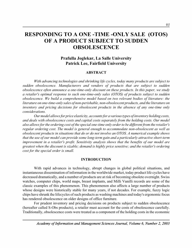
93
Academy of Information and Management Sciences Journal, Volume 6, Number 2, 2003Academy of Information and Management Sciences Journal, Volume 6, Number 2, 2003
RESPONDING TO A ONE -TIME -ONLY SALE (OTOS)OF A PRODUCT SUBJECT TO SUDDEN
OBSOLESCENCE
Prafulla Joglekar, La Salle UniversityPatrick Lee, Fairfield University
ABSTRACT
With advancing technologies and shrinking life cycles, today many products are subject tosudden obsolescence. Manufacturers and vendors of products that are subject to suddenobsolescence often announce a one-time-only discount on these products. In this paper, we studya retailer's optimal response to such one-time-only sales (OTOS) of products subject to suddenobsolescence. We build a comprehensive model based on two relevant bodies of literature: theliterature on one-time-only sales of non-perishable, non-obsolescent products, and the literature oninventory and pricing decisions for obsolescent products in the absence of any one-time onlyconsiderations.
Our model allows for price elasticity, accounts for a various types of inventory holding costs,and deals with obsolescence costs and capital costs separately from the holding costs. Our modelalso allows for the ordering cost of the special one-time only order to be different from the retailer'sregular ordering cost. The model is general enough to accommodate non-obsolescent as well asobsolescent products in situations that do or do not involve an OTOS. A numerical example showsthat the use of our model can provide some long-term gain and a particularly attractive short-termimprovement in a retailer's profit. Sensitivity analysis shows that the benefits of our model aregreatest when the discount is sizable; demand is highly price sensitive; and the retailer's orderingcost for the special order is small.
INTRODUCTION
With rapid advances in technology, abrupt changes in global political situations, andinstantaneous dissemination of information in the worldwide market, today product life cycles havedecreased dramatically, and a number of products are at risk of becoming obsolete overnight. Swisswatches, computer chips, world maps, breast implants, and Milli Vanilli records are some of theclassic examples of this phenomenon. This phenomenon also affects a large number of productswhose designs were historically stable for many years, if not decades. For example, fuzzy logicchips have shrunk the lifecycles of such products as washing machines and today's ergonomic focushas rendered obsolescence on older designs of office furniture.
For prudent inventory and pricing decisions on products subject to sudden obsolescence(hereafter called S-Obs products), a retailer must account for the costs of obsolescence carefully.Traditionally, obsolescence costs were treated as a component of the holding costs in the economic
94
Academy of Information and Management Sciences Journal, Volume 6, Number 2, 2003Academy of Information and Management Sciences Journal, Volume 6, Number 2, 2003
order quantity (EOQ) model (Hadley & Whitin, 1963; Naddor, 1966; Silver & Peterson, 1985).Then, some authors dealt with obsolescence costs separately from other inventory carrying costs(Barbosa & Friedman, 1979; Brown, 1982; Hill, Girard & Mabert, 1989). However, these earlyworks were focused on gradual rather than sudden obsolescence.
Masters (1991) defined sudden obsolescence as a situation when a product's lifetime isnegative exponentially distributed, and consequently, the probability of obsolescence is constant atany time. Using an approximate model, Masters (1991) concluded that for S-Obs products, the useof the EOQ model was appropriate, provided that the obsolescence component was computed as thereciprocal of the product's expected life. Joglekar and Lee (1993, 1996) pointed out that the thencurrent industry practice of estimating annual obsolescence costs at 1 to 3% of a product's costrepresented a serious underestimate of the true cost. By Master's (1991) formula even a 3%obsolescence cost implies an expected life of 33 years! Masters (1991) warned that in cases ofshort-life products, failure to use the proper formula could lead to costs that were five to fortypercent higher than the optimal costs.
Masters' (1991) model was an approximate one. Using an exact formulation, Joglekar andLee (1993) showed that Masters' model also underestimated the true lifetime costs of his optimalpolicy while overestimating the optimal order quantity. The associated errors were substantialparticularly in the cases of S-Obs products with very short expected lives. Joglekar and Lee (1996)developed a profit maximization model to determine a retailer's optimal order quantity in the faceof a manufacturer's quantity discount for S-Obs products. Unlike cost minimization models, a profitmaximization model also warns a retailer not to stock a product at all when such a stock results inloss for the retailer.
Not too different from situations of quantity discounts are the commonly observed situationsof one-time-only sales (OTOS) of many products. An OTOS occurs because amanufacturer/wholesaler wants to reduce some excess inventory caused by factors such as incorrectforecasts, deliberate excess production, or the threat of impending obsolescence. OTOS allowmanufacturers to pass on reduced raw material costs to the reseller, to meet short-term sales goals,to maximize capacity utilization, and/or to add excitement to otherwise mature and mundaneproducts (Abad, 2003). Aucamp and Kuzdrall (1986) have also observed that the situation of anannounced permanent price increase, with one last opportunity to buy before that price increase, ismathematically equivalent to an OTOS. Fashion clothes, pop music, and trendy toys are examplesof S-Obs products where at the time of a product-introduction, a manufacturer often offers asubstantial one-time-only discount to the retailer. Yet, available literature has not studied a retailer'soptimal response to such OTOS offers for S-Obs products.
On the other hand, how a retailer should respond to an OTOS of a non-perishable,non-obsolescent product has been studied by a number of authors over the last three decades. Usingstandard EOQ assumptions, earlier works (Naddor, 1966; Brown, 1967; Tersine & Grasso, 1978;Taylor & Bradley, 1985; Lev & Weiss, 1990) developed prescriptive models for determining anoptimal special order quantity for a retailer in a variety of OTOS situations. These works assumeda constant demand. Considering price-elasticity, Ardalan (1994; 1995) suggested that, in OTOSsituations, in addition to using a special order quantity, a retailer could increase his demand and
95
Academy of Information and Management Sciences Journal, Volume 6, Number 2, 2003Academy of Information and Management Sciences Journal, Volume 6, Number 2, 2003
profits by charging a lower retail price for it. Ardalan (1994) also focused on maximizing the netpresent value (NPV) of a retailer's cash flows rather than maximizing the per-period profit.
In this paper, we combine Joglekar and Lee's (1996) methodology of analyzing orderquantity decisions pertaining to S-Obs products with Ardalan's (1994) approach of simultaneouslydetermining the special price and the special order quantity in the face of an OTOS. In what follows,we establish our notation and develop a model for a retailer's optimal price and order quantitydecisions for a price-sensitive S-Obs product in the regular situation, i.e., in the absence of anOTOS. Our model allows for price elasticity, accounts for various types of inventory holding costs,and deals with obsolescence costs and capital costs separately. The model is general enough so thatit can be used for obsolescent as well as non-obsolescent products.
Next, we extend the regular situation model to accommodate an OTOS situation. Unlikeother available models, we do not assume that a reseller's cost of ordering the special quantity in anOTOS situation will be the same as his regular cost of ordering. We believe that decision-makingunder special circumstances requires a new model, additional data and greater analytical effort.Hence, the cost of ordering the special quantity is often substantially greater than the regularordering cost. In order to obtain an accurate estimate of the net advantage of our model's optimaldecisions, we use a comparison of the lifetime NPV of the no OTOS situation with the lifetime NPVof a situation involving an OTOS. To gain a clearer perspective on the long term and short-termsignificance of the net advantage, we look at the net advantage as both, percentage of lifetime NPVand percentage of one cycle NPV.
A numerical example, along with a fairly exhaustive sensitivity analysis, is provided. Thenumerical example shows that, in many OTOS situations, the use of our model can provide somelong-term gain and a particularly attractive short-term improvement in the retailer's NPV. Ouranalysis also identifies situations where the retailer may be better off not accepting the OTOSdiscount. The final section provides the conclusion along with some directions for further work.
THE MODEL
Consider a retailer dealing in an S-Obs product characterized by a price sensitive demandfunction that is time-invariant until obsolescence. Product obsolescence occurs abruptly andcompletely at a random point in time, which is negative exponentially distributed. At obsolescence,the product is disposed off at a salvage value. Other than these characteristics, standard EOQassumptions, such as known and constant ordering and carrying costs, zero lead-time, and nostockouts are applicable. In a "regular" situation, i.e., in the absence of an OTOS, the retailer seeksto maximize the NPV of his lifetime cash flows by determining the optimal order quantity and theoptimal selling price. Similarly, when faced with an OTOS, a retailer seeks to maximize his lifetimeNPV from the special price and order quantity of the OTOS followed by all regular cycles for therest of the product's life. To evaluate the exact advantage of the optimal OTOS decisions, we lookat the difference between these two NPVs.
Throughout this paper, we use the following notation.

96
Academy of Information and Management Sciences Journal, Volume 6, Number 2, 2003Academy of Information and Management Sciences Journal, Volume 6, Number 2, 2003
A = a constant for the demand function, representing the theoretical maximum demand at zeroprice
c = retailer's regular unit cost Cr = retailer's regular ordering cost per order Cs = ordering cost per order during special cycle
Note: We believe that the commonly used assumption Cs = Cr is unrealistic. Cs is likely tobe substantially greater than Cr for three reasons: (i) OTOS policy determination requires theuse of a different model, (ii) The OTOS order quantity is likely to be several times theregular order quantity, and (iii) Cs must also include costs of announcing the special retailprice, Ps to the retailer's customers.
d = the OTOS discount per unit H = annual holding costs (such as storage space, and material inspection and handling costs)
that are fixed per unit, regardless of the unit cost of the product. h = annual holding costs (such as deterioration, damage, and pilferage costs) that are fixed per
dollar of inventory, but that vary in per unit terms with the unit cost of the product.Note: Most inventory models assume all holding costs to be of either the H type or of the htype. In real life,one encounters both types. Note also that we deal with the obsolescencecosts and the capital costs explicitly and separately. Consequently, neither H nor h includesthem.
Hr = total annual holding costs (all except the obsolescence cost) per unit of regular purchaseHr = [H + (h + i)c].
Hs = total annual holding costs (all except the obsolescence cost) per unit of special OTOSpurchase Hs = [H + (h + i)(c - d)].
i = cost of capital per dollar per year (used as both, the cost of capital factor in the inventoryholding cost and the discount rate for NPV calculations).
kr = probability, at the beginning of a regular inventory cycle of Qr/Rr years, that the productdoes not become obsolete during the cycle. kr = e-Qr/(RrL) (Joglekar & Lee, 1993, 288).
ks = probability, at the beginning of the special OTOS inventory cycle of Qs/Rs years, that theproduct does not become obsolete during the cycle. ks = e-Qs/(RsL) (Joglekar & Lee, 1993,288).
L = expected life of the product in yearsNr = NPV factor for a cashflow occurring at the end of a regular inventory cycle. Nr = e-iQr/Rr.
Ns = NPV factor for a cashflow occurring at the end of the special OTOS inventory cycle. Ns= e-iQs/Rs.
Pr = selling price per unit during regular cycle prior to obsolescencePs = selling price per unit during special cycle prior to obsolescenceQr = order quantity per order during regular cycle Qs = order quantity for the OTOS special orderRr = demand per year during regular cycle, given by the function Rr = A - gPr.Rs = demand per year during special cycle, given by the function Rs = A - gPs.
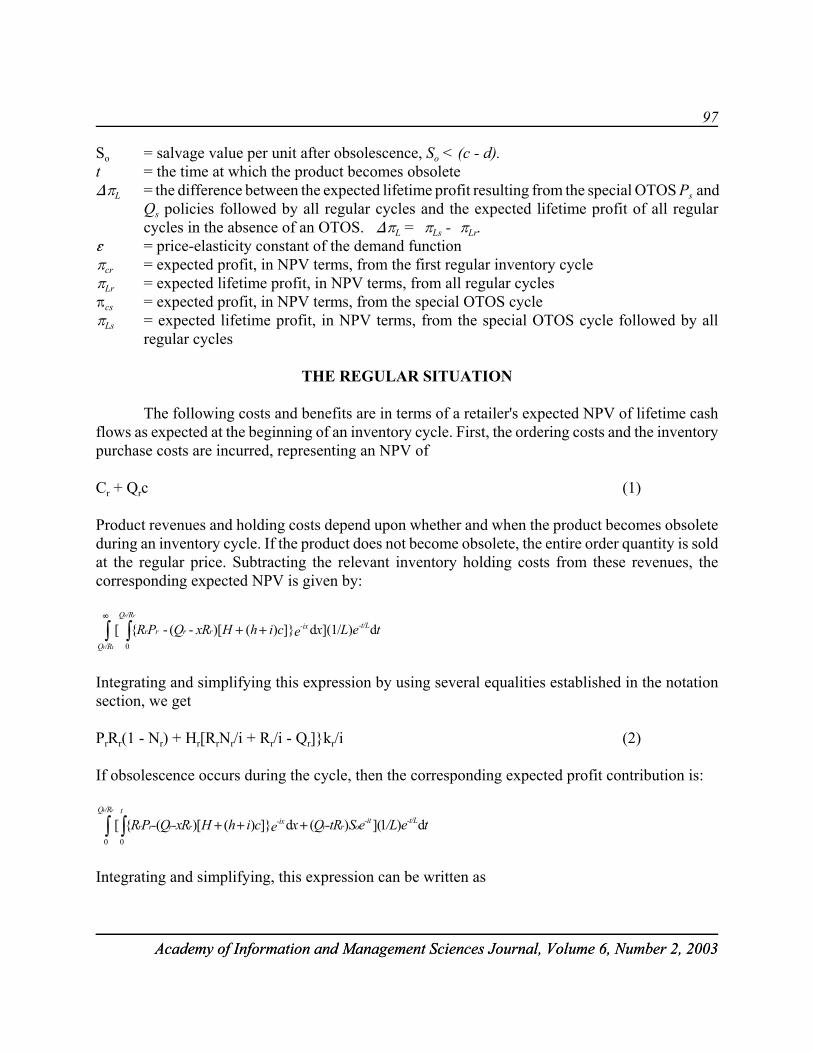
97
Academy of Information and Management Sciences Journal, Volume 6, Number 2, 2003Academy of Information and Management Sciences Journal, Volume 6, Number 2, 2003
So = salvage value per unit after obsolescence, So < (c - d).t = the time at which the product becomes obsolete)BL = the difference between the expected lifetime profit resulting from the special OTOS Ps and
Qs policies followed by all regular cycles and the expected lifetime profit of all regularcycles in the absence of an OTOS. )BL = BLs - BLr.
g = price-elasticity constant of the demand functionBcr = expected profit, in NPV terms, from the first regular inventory cycleBLr = expected lifetime profit, in NPV terms, from all regular cyclesBcs = expected profit, in NPV terms, from the special OTOS cycleBLs = expected lifetime profit, in NPV terms, from the special OTOS cycle followed by all
regular cycles
THE REGULAR SITUATION
The following costs and benefits are in terms of a retailer's expected NPV of lifetime cashflows as expected at the beginning of an inventory cycle. First, the ordering costs and the inventorypurchase costs are incurred, representing an NPV of
Cr + Qrc (1)
Product revenues and holding costs depend upon whether and when the product becomes obsoleteduring an inventory cycle. If the product does not become obsolete, the entire order quantity is soldat the regular price. Subtracting the relevant inventory holding costs from these revenues, thecorresponding expected NPV is given by:
teLxecihHxRQ PR -t/L
/RQ
/RQ-ix
rrrr
r
rr
d)](1/d]})()[-(-{[r 0
∫ ∫∞
++
Integrating and simplifying this expression by using several equalities established in the notationsection, we get
PrRr(1 - Nr) + Hr[RrNr/i + Rr/i - Qr]}kr/i (2) If obsolescence occurs during the cycle, then the corresponding expected profit contribution is:
te/LeS-tRQxecihH-xRQ-PR -t/L-itorr
/RQ t-ix
rrrr
rr
d)1]()(d]})()[({[0 0
+++∫ ∫
Integrating and simplifying, this expression can be written as
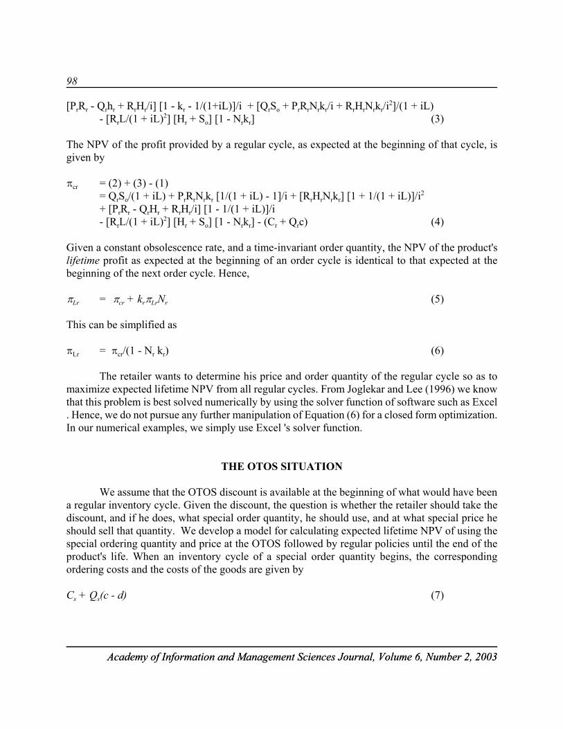
98
Academy of Information and Management Sciences Journal, Volume 6, Number 2, 2003Academy of Information and Management Sciences Journal, Volume 6, Number 2, 2003
[PrRr - Qrhr + RrHr/i] [1 - kr - 1/(1+iL)]/i + [QrSo + PrRrNrkr/i + RrHrNrkr/i2]/(1 + iL)- [RrL/(1 + iL)2] [Hr + So] [1 - Nrkr] (3)
The NPV of the profit provided by a regular cycle, as expected at the beginning of that cycle, isgiven by
Bcr = (2) + (3) - (1) = QrSo/(1 + iL) + PrRrNrkr [1/(1 + iL) - 1]/i + [RrHrNrkr] [1 + 1/(1 + iL)]/i2 + [PrRr - QrHr + RrHr/i] [1 - 1/(1 + iL)]/i - [RrL/(1 + iL)2] [Hr + So] [1 - Nrkr] - (Cr + Qrc) (4)
Given a constant obsolescence rate, and a time-invariant order quantity, the NPV of the product'slifetime profit as expected at the beginning of an order cycle is identical to that expected at thebeginning of the next order cycle. Hence,
BLr = Bcr + krBLrNr (5)
This can be simplified as
BLr = Bcr/(1 - Nr kr) (6)
The retailer wants to determine his price and order quantity of the regular cycle so as tomaximize expected lifetime NPV from all regular cycles. From Joglekar and Lee (1996) we knowthat this problem is best solved numerically by using the solver function of software such as Excel. Hence, we do not pursue any further manipulation of Equation (6) for a closed form optimization.In our numerical examples, we simply use Excel 's solver function.
THE OTOS SITUATION
We assume that the OTOS discount is available at the beginning of what would have beena regular inventory cycle. Given the discount, the question is whether the retailer should take thediscount, and if he does, what special order quantity, he should use, and at what special price heshould sell that quantity. We develop a model for calculating expected lifetime NPV of using thespecial ordering quantity and price at the OTOS followed by regular policies until the end of theproduct's life. When an inventory cycle of a special order quantity begins, the correspondingordering costs and the costs of the goods are given by
Cs + Qs(c - d) (7)
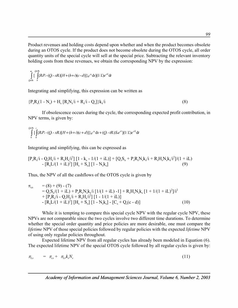
99
Academy of Information and Management Sciences Journal, Volume 6, Number 2, 2003Academy of Information and Management Sciences Journal, Volume 6, Number 2, 2003
Product revenues and holding costs depend upon whether and when the product becomes obsoleteduring an OTOS cycle. If the product does not become obsolete during the OTOS cycle, all orderquantity units of the special cycle will sell at the special price. Subtracting the relevant inventoryholding costs from these revenues, we obtain the corresponding NPV by the expression:
teLxedcihHxRQPR -t/L
Qs/Rs
Qs/Rs-ix
ssss d)/1](d)]}-)(()[-(-{[0
∫ ∫∞
++
Integrating and simplifying, this expression can be written as
{PsRs(1 - Ns) + Hs [RsNs/i + Rs/i - Qs]}ks/i (8)
If obsolescence occurs during the cycle, the corresponding expected profit contribution, inNPV terms, is given by:
teLeStRQxedcihHxRQPR -t/L-itoss
Qs/Rs t-ix
ssss d)/1]()-(d)]})(()[-(-{[0 0
++++∫ ∫
Integrating and simplifying, this can be expressed as
[PsRs/i - QsHs/i + RsHs/i2] [1 - ks - 1/(1 + iL)] + [QsSo + PsRsNsks/i + RsHsNsks/i2]/(1 + iL) - [RsL/(1 + iL)2] [Hs + So] [1 - Nsks] (9)
Thus, the NPV of all the cashflows of the OTOS cycle is given by
Bcs = (8) + (9) - (7)= QsSo/(1 + iL) + PsRsNsks/i [1/(1 + iL) -1] + RsHsNsks [1 + 1/(1 + iL)2]/i2
+ [PsRs/i - QsHs/i + RsHs/i2] [1 - 1/(1 + iL)]- [RsL/(1 + iL)2] [Hs + So] [1 - Nsks] - [Cs + Qs(c - d)] (10)
While it is tempting to compare this special cycle NPV with the regular cycle NPV, theseNPVs are not comparable since the two cycles involve two different time durations. To determinewhether the special order quantity and price policies are more desirable, one must compare thelifetime NPV of those special policies followed by regular policies with the expected lifetime NPVof using only regular policies throughout.
Expected lifetime NPV from all regular cycles has already been modeled in Equation (6).The expected lifetime NPV of the special OTOS cycle followed by all regular cycles is given by:
BLs = Bcs + BLrksNs (11)
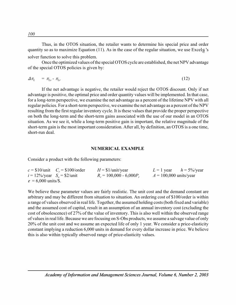
100
Academy of Information and Management Sciences Journal, Volume 6, Number 2, 2003Academy of Information and Management Sciences Journal, Volume 6, Number 2, 2003
Thus, in the OTOS situation, the retailer wants to determine his special price and orderquantity so as to maximize Equation (11). As in the case of the regular situation, we use Excel 's solver function to solve this problem.
Once the optimized values of the special OTOS cycle are established, the net NPV advantageof the special OTOS policies is given by:
)BL = BLs - BLr (12)
If the net advantage is negative, the retailer would reject the OTOS discount. Only if netadvantage is positive, the optimal price and order quantity values will be implemented. In that case,for a long-term perspective, we examine the net advantage as a percent of the lifetime NPV with allregular policies. For a short-term perspective, we examine the net advantage as a percent of the NPVresulting from the first regular inventory cycle. It is these values that provide the proper perspectiveon both the long-term and the short-term gains associated with the use of our model in an OTOSsituation. As we see it, while a long-term positive gain is important, the relative magnitude of theshort-term gain is the most important consideration. After all, by definition, an OTOS is a one time,short-run deal.
NUMERICAL EXAMPLE
Consider a product with the following parameters:
c = $10/unit Cr = $100/order H = $1/unit/year L = 1 year h = 5%/yeari = 12%/year So = $2/unit Rr = 100,000 - 6,000Pr A = 100,000 units/year g = 6,000 units/$.
We believe these parameter values are fairly realistic. The unit cost and the demand constant arearbitrary and may be different from situation to situation. An ordering cost of $100/order is withina range of values observed in real life. Together, the assumed holding costs (both fixed and variable)and the assumed cost of capital, result in an assumption of an annual inventory cost (excluding thecost of obsolescence) of 27% of the value of inventory. This is also well within the observed rangeof values in real life. Because we are focusing on S-Obs products, we assume a salvage value of only20% of the unit cost and we assume an expected life of only 1 year. We consider a price-elasticityconstant implying a reduction 6,000 units in demand for every dollar increase in price. We believethis is also within typically observed range of price-elasticity values.
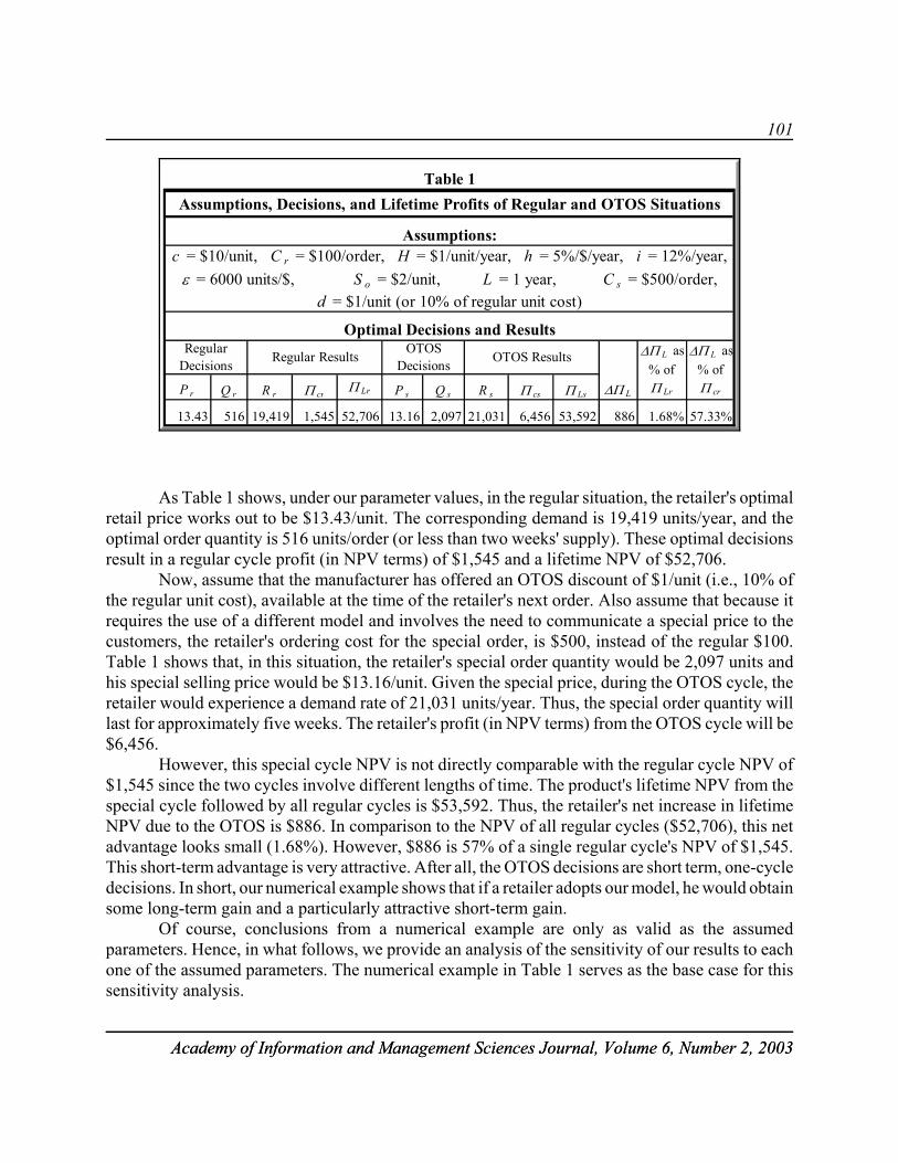
101
Academy of Information and Management Sciences Journal, Volume 6, Number 2, 2003Academy of Information and Management Sciences Journal, Volume 6, Number 2, 2003
Assumptions, Decisions, and Lifetime Profits of Regular and OTOS Situations
Assumptions:c = $10/unit, C r = $100/order, H = $1/unit/year, h = 5%/$/year, i = 12%/year,
ε = 6000 units/$, S o = $2/unit, L = 1 year, C s = $500/order, d = $1/unit (or 10% of regular unit cost)
Optimal Decisions and Results
Q r R r Π cr Π Lr P s Q s R s Π cs Π Ls
516 19,419 1,545 52,706 13.16 2,097 21,031 6,456 53,592 886 1.68% 57.33%
P r
13.43
Regular Decisions
OTOS DecisionsRegular Results OTOS Results
Table 1
∆Π L
∆Π L as % of Π Lr
∆Π L as % of Π cr
As Table 1 shows, under our parameter values, in the regular situation, the retailer's optimalretail price works out to be $13.43/unit. The corresponding demand is 19,419 units/year, and theoptimal order quantity is 516 units/order (or less than two weeks' supply). These optimal decisionsresult in a regular cycle profit (in NPV terms) of $1,545 and a lifetime NPV of $52,706.
Now, assume that the manufacturer has offered an OTOS discount of $1/unit (i.e., 10% ofthe regular unit cost), available at the time of the retailer's next order. Also assume that because itrequires the use of a different model and involves the need to communicate a special price to thecustomers, the retailer's ordering cost for the special order, is $500, instead of the regular $100.Table 1 shows that, in this situation, the retailer's special order quantity would be 2,097 units andhis special selling price would be $13.16/unit. Given the special price, during the OTOS cycle, theretailer would experience a demand rate of 21,031 units/year. Thus, the special order quantity willlast for approximately five weeks. The retailer's profit (in NPV terms) from the OTOS cycle will be$6,456.
However, this special cycle NPV is not directly comparable with the regular cycle NPV of$1,545 since the two cycles involve different lengths of time. The product's lifetime NPV from thespecial cycle followed by all regular cycles is $53,592. Thus, the retailer's net increase in lifetimeNPV due to the OTOS is $886. In comparison to the NPV of all regular cycles ($52,706), this netadvantage looks small (1.68%). However, $886 is 57% of a single regular cycle's NPV of $1,545.This short-term advantage is very attractive. After all, the OTOS decisions are short term, one-cycledecisions. In short, our numerical example shows that if a retailer adopts our model, he would obtainsome long-term gain and a particularly attractive short-term gain.
Of course, conclusions from a numerical example are only as valid as the assumedparameters. Hence, in what follows, we provide an analysis of the sensitivity of our results to eachone of the assumed parameters. The numerical example in Table 1 serves as the base case for thissensitivity analysis.
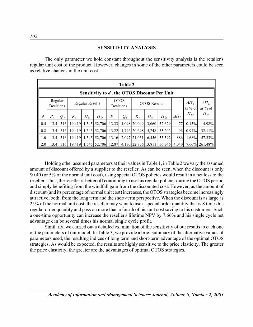
102
Academy of Information and Management Sciences Journal, Volume 6, Number 2, 2003Academy of Information and Management Sciences Journal, Volume 6, Number 2, 2003
SENSITIVITY ANALYSIS
The only parameter we hold constant throughout the sensitivity analysis is the retailer'sregular unit cost of the product. However, changes in some of the other parameters could be seenas relative changes in the unit cost.
Sensitivity to d , the OTOS Discount Per Unit
OTOS Results
P r Q r R r Π cr Π Lr P s Q s R s Π cs Π Ls
0.4 13.4 516 19,419 1,545 52,706 13.33 1,098 20,049 3,060 52,629 -77 -0.15% -4.98%
0.8 13.4 516 19,419 1,545 52,706 13.22 1,746 20,698 5,248 53,202 496 0.94% 32.11%
1.0 13.4 516 19,419 1,545 52,706 13.16 2,097 21,031 6,456 53,592 886 1.68% 57.33%
2.0 13.4 516 19,419 1,545 52,706 12.87 4,170 22,776 13,811 56,746 4,040 7.66% 261.48%
Regular Results OTOS Decisions
Table 2
∆Π L
∆Π L
as % of Π Lr
∆Π L
as % of Π cr
Regular Decisions
d
Holding other assumed parameters at their values in Table 1, in Table 2 we vary the assumedamount of discount offered by a supplier to the reseller. As can be seen, when the discount is only$0.40 (or 5% of the normal unit cost), using special OTOS policies would result in a net loss to thereseller. Thus, the reseller is better off continuing to use his regular policies during the OTOS periodand simply benefiting from the windfall gain from the discounted cost. However, as the amount ofdiscount (and its percentage of normal unit cost) increases, the OTOS strategies become increasinglyattractive, both, from the long term and the short-term perspective. When the discount is as large as25% of the normal unit cost, the reseller may want to use a special order quantity that is 8 times hisregular order quantity and pass on more than a fourth of his unit cost saving to his customers. Sucha one-time opportunity can increase the reseller's lifetime NPV by 7.66% and his single cycle netadvantage can be several times his normal single cycle profit.
Similarly, we carried out a detailed examination of the sensitivity of our results to each oneof the parameters of our model. In Table 3, we provide a brief summary of the alternative values ofparameters used, the resulting indices of long term and short-term advantage of the optimal OTOSstrategies. As would be expected, the results are highly sensitive to the price elasticity. The greaterthe price elasticity, the greater are the advantages of optimal OTOS strategies.
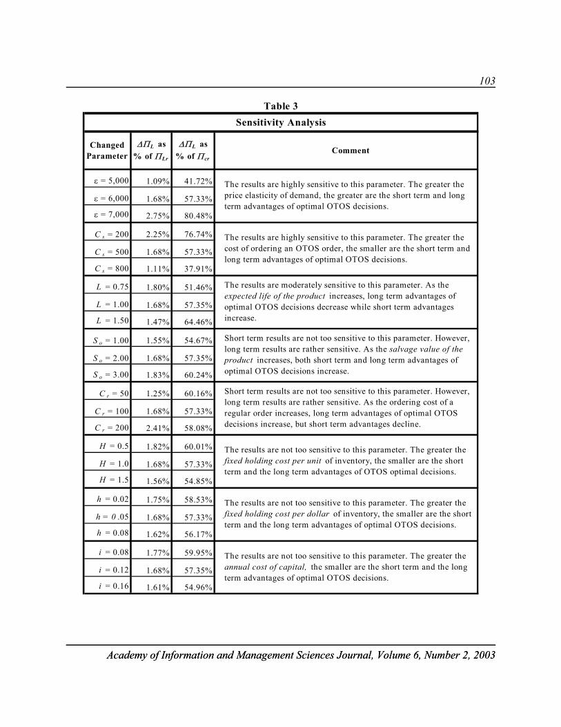
103
Academy of Information and Management Sciences Journal, Volume 6, Number 2, 2003Academy of Information and Management Sciences Journal, Volume 6, Number 2, 2003
ε = 5,000 1.09% 41.72%
ε = 6,000 1.68% 57.33%
ε = 7,000 2.75% 80.48%
C s = 200 2.25% 76.74%
C s = 500 1.68% 57.33%
C s = 800 1.11% 37.91%
L = 0.75 1.80% 51.46%
L = 1.00 1.68% 57.35%
L = 1.50 1.47% 64.46%
S o = 1.00 1.55% 54.67%
S o = 2.00 1.68% 57.35%
S o = 3.00 1.83% 60.24%
C r = 50 1.25% 60.16%
C r = 100 1.68% 57.33%
C r = 200 2.41% 58.08%
H = 0.5 1.82% 60.01%
H = 1.0 1.68% 57.33%
H = 1.5 1.56% 54.85%
h = 0.02 1.75% 58.53%
h = 0 .05 1.68% 57.33%
h = 0.08 1.62% 56.17%
i = 0.08 1.77% 59.95%
i = 0.12 1.68% 57.35%
i = 0.16 1.61% 54.96%
∆ΠL as % of ΠLr
∆ΠL as % of Π cr
Changed Parameter
Short term results are not too sensitive to this parameter. However, long term results are rather sensitive. As the ordering cost of a regular order increases, long term advantages of optimal OTOS decisions increase, but short term advantages decline.
Table 3Sensitivity Analysis
Comment
The results are not too sensitive to this parameter. The greater the annual cost of capital, the smaller are the short term and the long term advantages of optimal OTOS decisions.
The results are not too sensitive to this parameter. The greater the fixed holding cost per dollar of inventory, the smaller are the short term and the long term advantages of optimal OTOS decisions.
The results are not too sensitive to this parameter. The greater the fixed holding cost per unit of inventory, the smaller are the short term and the long term advantages of OTOS optimal decisions.
The results are moderately sensitive to this parameter. As the expected life of the product increases, long term advantages of optimal OTOS decisions decrease while short term advantages increase.
The results are highly sensitive to this parameter. The greater the cost of ordering an OTOS order, the smaller are the short term and long term advantages of optimal OTOS decisions.
The results are highly sensitive to this parameter. The greater the price elasticity of demand, the greater are the short term and long term advantages of optimal OTOS decisions.
Short term results are not too sensitive to this parameter. However, long term results are rather sensitive. As the salvage value of the product increases, both short term and long term advantages of optimal OTOS decisions increase.
104
Academy of Information and Management Sciences Journal, Volume 6, Number 2, 2003Academy of Information and Management Sciences Journal, Volume 6, Number 2, 2003
The results are also highly sensitive to the ordering cost of the special order. As the orderingcost of the special order increases, the advantage of the special OTOS policies declines. From apractical point of view this is rather important to understand. In the past, researchers have assumedthat, in an OTOS, there would be no change in the ordering cost. That assumption is not onlyunrealistic; it inflates the advantage attributable to optimal OTOS policies.
The results are moderately sensitive to the product's expected life. As expected life increases,the short-term advantages of the OTOS policies increase while the long-term advantages decline.Note also that as a product's salvage value increases the OTOS decisions are increasinglyadvantageous both in the long run and in the short run. Thus, it seems that OTOS decisions are morebeneficial for non-obsolescent products than they are for obsolescent products.
Finally, Table 3 indicates that, from both, the long-term and the short-term perspectives, theresults are not very sensitive to changes in regular ordering costs, holding costs, or cost of capital.
CONCLUSION
Today many products are characterized by price elasticity, sudden obsolescence, and shortexpected lives. Drawing on the relevant literature, first we built a model for a retailer's optimal priceand order quantity decisions for such products in the regular situation, i.e., in the absence of aone-time-only discount. Our model is comprehensive. It allows for price elasticity, accounts for avariety of types of inventory holding costs, and deals with obsolescence costs and capital costs inprecise and theoretically correct manner. Because manufacturers and vendors of S-Obs productsoften offer a one-time-only discount for such products, we then extended our model to accommodatethe OTOS situations. Because a special order requires the use of a different model and additionalcosts of announcing a price change, our model used an explicitly different ordering cost for thespecial OTOS order. A numerical example showed that the use of our model could provide somelong-term gain and a particularly attractive short-term improvement in a retailer's profit. A retailerstands to benefit the most from our model if the discount is substantial, the product demand is highlyprice sensitive, and the retailer's ordering cost for the special order is substantial. Also, it seems thatOTOS decisions are more beneficial for non-obsolescent products than they are for obsolescentproducts.
There are several directions for further work on this topic. First, we assumed a linear anddeterministic demand function. A non-linear function is likely to be more realistic in most situations.An extension of our model to a non-linear demand relationship should be straight forward,particularly since we do not derive any closed-form solutions but depend on Excel® to solve theproblem. Also, a stochastic demand function is more likely to be encountered in real life. Anextension to allow for a stochastic demand function would be relatively more complicated butdoable.
A critical assumption in our model is that the fact that a manufacturer has offered an OTOSdoes not in itself change a retailer's assessment of the product's life expectancy and/or salvage value.In real life, a retailer may assume, often correctly, that an OTOS is a signal of an imminentobsolescence. Thus, in view of the OTOS, a retailer's perceived life expectancy and/or salvage value
105
Academy of Information and Management Sciences Journal, Volume 6, Number 2, 2003Academy of Information and Management Sciences Journal, Volume 6, Number 2, 2003
for the product may be reduced. On the other hand, as we have pointed out, an impending priceincrease with one last opportunity to buy at the lower price is a situation that is mathematicallyequivalent to an OTOS. In such situations of impending price increase, a retailer may deduce thatthe product's life expectancy may be greater than his original estimate of that expectancy. In anycase, an extension of our model to allow for such a change in the perceived life expectancy of aproduct offered on an OTOS would also be an interesting and productive direction for further work.Finally, two recent models of OTOS situations for non-obsolescent products suggest that a retailer'soptimal strategy is not to sell the entire special order quantity at the special price. Instead, a retailershould sell only a portion of his special order quantity at a special price, reverting to his regularselling price for the remaining portion of the special order quantity (Abad, 2003; Arcelus, Shah &Srinivasan, 2003). It seems that this type of a strategy may be optimal also for products subject tosudden obsolescence.
REFERENCES
Abad, P. L. (2003). Optimal price and lot size when the supplier offers a temporary price reduction over an interval.Computers and Operations Research, 30, 63-74.
Arcelus, F.J., N. H. Shah & G. Srinivasan. (2003). Retailer's Pricing, Credit and inventory policies for deteriorating itemsin response to temporary price/credit incentives. International Journal of Production Economics, 81-82,153-152.
Ardalan, A. (1994). Optimal prices and order quantities when temporary price discounts result in increase in demand.European Journal of Operational Research, 72, 52-61.
Ardalan, A. (1995). A comparative analysis of approaches for determining optimal price and order quantity when a saleincreases demand. European Journal of Operational Research, 84, 416-430.
Aucamp, D. C. & P. J. Kuzdrall. (1986). Lot sizes for one-time-only sales. Journal of Operational Research Society,37, 79-86.
Barbosa, L. C. & M. Friedman. (1979). Inventory lot size models with vanishing markets. Journal of the OperationsResearch Society, 30(2), 1129-1132.
Brown, G. W., J. Y Lu & R. J. Wolfson. (1964). Dynamic modeling of inventories subject to sudden obsolescence.Management Science, 11(1), 51-63.
Brown, R. G. (1967). Decision rules for inventory management. New York: Holt, Rinehart & Winston.
Brown, R. G. (1982). Advanced Service Parts Management. Norwitch, VT: Materials Management Systems, Inc.
Hadley, G. & T. M. Whitin. (1963). Analysis of Inventory Systems. Englewood Cliffs, NJ: Prentice-Hall.
Hill, A. V., V. Girard & V. A. Mabert. (1989). A decision support system for determining optimal retention stocks forservice parts inventories. IIE Transactions, 21(3), 236:248.

106
Academy of Information and Management Sciences Journal, Volume 6, Number 2, 2003Academy of Information and Management Sciences Journal, Volume 6, Number 2, 2003
Joglekar, P. & P. Lee. (1993). An exact formulation of inventory costs and optimal lot size in face of suddenobsolescence. Operations Research Letters, 14, 283-290.
Joglekar P. & P. Lee. (1996). A profit maximization model for a retailer's stocking decisions on products subject tosudden obsolescence, Production and Operations Management, 5(3), 288-294.
Lev, B. & H. J. Weiss. (1990). Inventory models with cost changes. Operations Research, 38, 53-63.
Masters, J. M. (1991). A note on the effect of sudden obsolescence on the optimal lot size. Decision Sciences, 22,1180-1186.
Naddor, E. (1966). Inventory Systems, New York: John Wiley & Sons. Nahmias, S. (1974). Inventory depletion management when the field life is random. Management Science, 20,
1276-1284.
Nose, T., H. Ishii & T.Nishida. (1984). Perishable inventory management with stochastic lead-time and different sellingprices. European Journal of Operations Research, 18, 322-338.
Silver, E. A. & R. Peterson. (1985). Decision Systems for inventory management and production planning. New York:John Wiley & Sons.
Taylor, S. G. & C. E. Bradley. (1985). Optimal ordering strategies for announced price increases. Operations Research,33(2), 312-325.
Tersine, R. J. & E. T. Grasso. (1978). Forward buying in response to announced price increases. Journal of Purchasingand Materials Management, 14(2), 20-22.
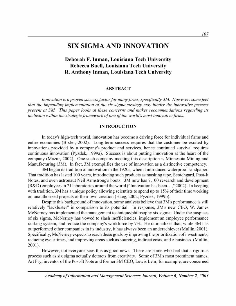
107
Academy of Information and Management Sciences Journal, Volume 6, Number 2, 2003Academy of Information and Management Sciences Journal, Volume 6, Number 2, 2003
SIX SIGMA AND INNOVATION
Deborah F. Inman, Louisiana Tech UniversityRebecca Buell, Louisiana Tech University
R. Anthony Inman, Louisiana Tech University
ABSTRACT
Innovation is a proven success factor for many firms, specifically 3M. However, some feelthat the impending implementation of the six sigma strategy may hinder the innovative processpresent at 3M. This paper looks at these concerns and makes recommendations regarding itsinclusion within the strategic framework of one of the world's most innovative firms.
INTRODUCTION
In today's high-tech world, innovation has become a driving force for individual firms andentire economies (Bixler, 2002). Long-term success requires that the customer be excited byinnovations provided by a company's product and services, hence continued survival requirescontinuous innovation (Pyzdek, 1999a). Success is about putting innovation at the heart of thecompany (Mazur, 2002). One such company meeting this description is Minnesota Mining andManufacturing (3M). In fact, 3M exemplifies the use of innovation as a distinctive competency.
3M began its tradition of innovation in the 1920s, when it introduced waterproof sandpaper.That tradition has lasted 100 years, introducing such products as masking tape, Scotchgard, Post-ItNotes, and even astronaut Neil Armstrong's boots. 3M now has 7,100 research and development(R&D) employees in 71 laboratories around the world ("Innovation has been…," 2002). In keepingwith tradition, 3M has a unique policy allowing scientists to spend up to 15% of their time workingon unauthorized projects of their own creation (Haeg, 2002; Pyzdek, 1999b).
Despite this background of innovation, some analysts believe that 3M's performance is stillrelatively "lackluster" in comparison to its potential. In response, 3M's new CEO, W. JamesMcNerney has implemented the management technique/philosophy six sigma. Under the auspicesof six sigma, McNerney has vowed to slash inefficiencies, implement an employee performanceranking system, and reduce the company's workforce by 7%. He rationalizes that, while 3M hasoutperformed other companies in its industry, it has always been an underachiever (Mullin, 2001).Specifically, McNerney expects to reach these goals by improving the prioritization of investments,reducing cycle times, and improving areas such as sourcing, indirect costs, and e-business. (Mullin,2001).
However, not everyone sees this as good news. There are some who feel that a rigorousprocess such as six sigma actually detracts from creativity. Some of 3M's most prominent names,Art Fry, inventor of the Post-It Note and former 3M CEO, Lewis Lehr, for example, are concerned
108
Academy of Information and Management Sciences Journal, Volume 6, Number 2, 2003Academy of Information and Management Sciences Journal, Volume 6, Number 2, 2003
that six sigma's structure will stifle employee creativity (Haeg, 2002). So, are companiesimplementing six sigma destined to suffer from a lack of future innovations? Is six sigma toostructured and controlling for processes such as R&D? This possibility is the key issue of this paper.We look at the innovation process and the potential impact of six sigma upon this process. Afterdiscussion of the issues, recommendations are made for 3M and others who wish to incorporate thesix sigma process.
WHAT IS SIX SIGMA?
A cost-saving, inefficiency-slashing program, six sigma is a business concept that toutsimproving quality and business processes. Specifically, it is "a disciplined method of usingextremely rigorous data-gathering and statistical analysis to pinpoint sources of errors and ways ofeliminating them" (Harry & Schroeder, 1999). The Greek letter sigma (s) represents a standarddeviation from the mean or average. The objective is to reduce process variation so that plus orminus (±) six standard deviations lie between the mean and the nearest specification limit (Statisticalsix sigma definition, 2003). This translates to no more than 3.4 defective parts per millionopportunities. Hence, six sigma implementation begins by measuring defects per millionopportunities, allowing only 3.4 defects. Most companies do no better than three sigma (Arndt,2002) and are pleased with their performance. However, even four sigma performance would stillallow 500 incorrect surgical operations per week, 20,000 incorrectly filled pharmaceuticalprescriptions each year, and 2,000 lost articles of mail each hour (Marash, 2000). Six sigmacompanies then set aggressive short-term objectives but strive toward long-term goals.
A six sigma project succeeds by reducing subjective errors in the assessment of problems.Six sigma firms follow a five step process which includes defining a process measuring the processto assess current performance, analyzing information to determine where the errors lie, improvingthe process and eliminating the errors, and finally setting up controls to prevent future errors (Arndt,2002).
Developed by Motorola in the 1980s, the six sigma philosophy has spread to other companiessuch as GE, Allied Signal, and Texas Instruments. The difference between six sigma and previousquality philosophies is that six sigma is being promoted by top management, not just by qualitymanagers. It is being touted not only in technical journals but also on the business pages ofnewspapers and magazines (Marash, 2000).
There are definitely some success stories. Dow Chemical, DuPont, GE Plastics, Air Productsand Chemical, Avery Denison, Great Lakes Chemical, Honeywell, (Schmitt, 2002), W.R. Grace(Sauer, 2001) and Rockwell International (Hasek, 2000) have all embraced six sigma, with quickmonetary results. Allied Signal saved $1.5 billion through 1998 and was looking at a subsequent$600 million per year savings thereafter ("Six sigma secrets," 1998).
Six sigma is not limited to manufacturing processes alone. Advocates feel it may also beapplied to functions such as accounts receivable, sales, and research and development. While moredifficult to evaluate areas in which processes are not standardized, six sigma can still be applied(Arndt, 2002).
109
Academy of Information and Management Sciences Journal, Volume 6, Number 2, 2003Academy of Information and Management Sciences Journal, Volume 6, Number 2, 2003
THE INNOVATION PROCESS
Innovation is defined as "an iterative process initiated by the perception of a new marketand/or new service opportunity for a technology-based invention which leads to development,production, and marketing tasks striving for the commercial success of the invention" (Garcia &Calatone, 2001). Once a product moves through the production and marketing phases and entersthe marketplace, it's status moves from invention to innovation (Garcia & Calatone, 2001). As theproduct becomes an innovation, value is provided to customers. "Value consists of the performancecharacteristics and attributes that a company offers in the form of a good or service for whichcustomers are willing to pay" (Hitt, Ireland & Hoskisson, 2001). The effect of value is felt in acompany's bottom line; therefore, creating value in a good or service is necessary for a firm'scompetitive success.
Students of innovation argue that a firm's ability to innovate is a function of its localenvironment (Afuah, 1998). A study of creativity among corporate research scientists found thatenvironment was a critical factor in stimulating or blocking creativity (Kiely, 1997). Badawy (1997)states that "in order to stimulate and reinforce creativity [innovation], appropriate organizationalclimates [environments] should be established." A review of innovation literature reveals that anenvironment conducive to innovation is marked by the absence of three factors present in mosthighly structured or hierarchical organizations: fear of uncertainty, fear of failure and productivitymeasurement. Uncertainty, failure and measurement, as they pertain to innovation, are nowdiscussed.
Uncertainty
There seems to a general consensus, in the literature, that innovation is unpredictable andcharacterized by uncertainty (Brown, 2001; Afuah, 1998; Badawy, 1997, Peters, 1997). As such,unexpected occurrences can be good sources of innovation (Afuah, 1998). For example, whenUpjohn was testing minoxidil for treatment of high blood pressure, they found hair growth to be aside effect. The result was the marketing of Rogaine (minoxidil) to treat baldness.
Failure
Manners, Steger and Zimmerer (1997) say that "people who have spent their lives buildingself-esteem based upon technical competence will go to great lengths to avoid losing that fragilebase." Badawy (1997) goes further to warn that engineers are professional individuals who demandspecial treatment and cannot be managed like other labor. Others (Pyzdek, 2001b) even feel thatthe big risk is not fear of failure but the failure to risk. Examples of "successful failures" includeArt Fry's failed superglue experiment (Post-it Notes) and James Wright's failed attempt atdeveloping a synthetic rubber for airplane tires and soldiers' boots (Silly Putty). Other "failure"discoveries include X-rays, Frisbees, Velcro, penicillin, Coca-Cola and the slinky (Niemann, 2003).
110
Academy of Information and Management Sciences Journal, Volume 6, Number 2, 2003Academy of Information and Management Sciences Journal, Volume 6, Number 2, 2003
Measurement
Innovation is the result of creative activity not of analysis (Pyzdek, 1999a). Creativitycannot be achieved "by the numbers" (Pyzdek, 1999a) nor can it be measured (Kiely, 1997).Pyzdek, (1999a, 1999b) points out that the creative organization is one that exhibits variability,resource redundancy, quirky design and slack. Trying to measure and control all aspects of theinnovation process causes engineers and scientists to restrict the depth of their exploration, leavinglittle room for pursuit of novel ideas (Katz & Allen, 1997). Therefore, an organization that istolerant of a large variety of deviation from the norm is more likely to enhance creativity (Shapero,1997).
SIX SIGMA AND THE INNOVATION PROCESS
The current rapid rate of change in technology places a higher premium on being able toquickly offer [new] goods and services to the marketplace. "With the rapid and widespreaddiffusion of technologies used to produce goods and services, speed to market may be the onlysource of competitive advantage" (Hitt, Ireland & Hoskisson, 2001). As innovation is pushed intothis rapid product development cycle, heightened expectations of the marketplace call for bettertools to improve the productivity of the innovation process. Six sigma, often viewed as a toolboxfull of new devices (Sauer, 2001), is seen by some as potentially helpful to the innovation process.
Christensen (2002) believes that innovation isn't random; its outcomes only appear to berandom because we don't understand all the factors, such as management strategies, degree ofcompany integration, capabilities, and resources, that affect successful innovation. If we can usesix sigma to master these variables, the products, processes, and services created will have morepredictable outcomes. This implies that six sigma can also serve to eliminate waste of time andresources in the conception process by linking it directly to customer wants and needs. Barry Siadat,AlliedSignal's chief growth officer feels that six sigma will shorten cycle time and increase speedto market, and finally, it will reduce costs ("Six sigma secrets," 1998). These sentiments arereflected by Daniel Laux, president of Six Sigma Academy, who feels that six sigma can now beapplied to all industries and all functions and can even be used in R&D to find innovative products(Gilbert, 2002).
At one time, product development generally occurred by happenstance (Six sigma secrets,1998). In the chemical industry, research scientists produced a new substance, while analyticalchemists performed measurements and added specifications later (Sauer, 2001). For discreteproducts, the conventional R&D approach started from a developer and proceeded to design andprototype through build and test iterations, later resulting in design changes and wasteful rework(Management innovation…, 2000). With a six sigma approach, researchers first find what thecustomer wants and then look at the process capability study (Sauer, 2001). Then the customer'sneed and problems can be clearly defined and non-value work eliminated (Managementinnovation…, 2000), thereby shortening the innovation process.
111
Academy of Information and Management Sciences Journal, Volume 6, Number 2, 2003Academy of Information and Management Sciences Journal, Volume 6, Number 2, 2003
Studies showing that as much as 80% of quality problems originate in design (Who needs…,2002) have led firms to look to six sigma's toolbox for design improvement. An aerospace firmexperienced a mismatch between the part dimensions represented in the model itself and themeasurement specified by designers. Because of the design error, the first products wereconsistently wrong. Each individual model was always fixed but because the design process thatproduced the error was not fixed, the error continued to occur and had to be continually fixed; at acost of $150,000 each time. Proper use of six sigma could have avoided this fiasco (Finn, 2000).
Successful examples include AlliedSignal who used six sigma to reduce variation inperformance in the "upfront" design of their AS900 engine. This resulted in reductions of 30% inwork-hours, 50% in fan module variability, and 9 months in time-to-certification (Six sigma secrets,1998). A major innovation in metal injection molding material, developed by a Honeywell sixsigma team, enabled the production of a new variable-weight golf putter for a customer, capturing$1 million in sales for Honeywell (Six sigma plus, 2001). Both Dell Computer and IBM utilized sixsigma to evaluate products before the first shipment, resulting in savings from detection ofmanufacturing and design issues (Design for six sigma…, 2002). Even 3M has already realized $1million savings after a six sigma review found that a dental ceramic wasn't being properly cured(3M: A lab for growth, 2002).
Despite these success stories, the application of six sigma to innovation has its detractors.Johnson (2002) states that "R&D activities involve inquiry, analysis, synthesis and other activitiesthat naturally reshape and change as they proceed-and so naturally defy systematic improvementefforts." Thomas Pyzdek , a regular columnist for Quality Digest adds that You would kill thecreativity of research if you tried to apply six sigma there" (Dusharme, 2001). Craig Hickman andChristopher Raia (2002) use the terms convergent and divergent thinking systems to further illustratethis contrast. They (Hickman & Raia, 2002) state that "convergent thinking system, which includemost established business organizations, survive on order, measurement, and predictability. Incontrast, most innovations result from divergent thinking environments that thrive on disorder,imagination, and ambiguity."
"Not so successful" stories include a multinational firm that upon achieving six sigmasuccess in one division, decreed that the entire company should follow suit. Six sigma worked finein areas of high volume or repeatable processes, but low volume departments had to go looking fordata to feed the tool. Often, this data had little or no relevance to customer satisfaction, yielding adistorting effect on quality management (Six sigma-A true story, 2003). While IBM focused onreducing defects and making incremental improvements using six sigma, EMC Corp. and CiscoSystems, Inc. were pioneering innovations that took the leading position in their markets away fromIBM (Gilbert, 2002).
A more than cursory look at these success stories will reveal that six sigma's utilizationseems to be ensuring success during the development process after the innovation is conceived; whatis known as application development. But what about the actual conception of the idea behind theproduct, the application itself?
Can a company such as 3M, one whose most well-known attribute is innovation, afford to"tinker" with success? Not according to Thomas Pyzdek. Pyzdek (2001) feels that companies that

112
Academy of Information and Management Sciences Journal, Volume 6, Number 2, 2003Academy of Information and Management Sciences Journal, Volume 6, Number 2, 2003
apply six sigma wall-to-wall are going about the philosophy in the wrong manner. He believes thatmanagement should not take the idea (six sigma) too far and try to apply it "across the board"(Dusharme, 2001). R&D departments should apply six sigma to the development aspect but neverto the research aspect, as six sigma brings too much organization to a process that should be rathercasual and disorganized (Dusharme, 2001; Pyzdek, 1999a).
Six sigma is methodical and organized, rigorous and structured, which seems in contrast tothe productive innovation environment. Pyzdek (2000) feels that the greatest enemy of creativityis hierarchy. An overly-structured R&D organization with numerous levels of hierarchy, anabundance of rules and regulations, and a flow of paperwork can sap energy that would otherwisebe used for the creation, application, utilization and generalization of knowledge (Pasmore, 1997).
For all firms, six sigma seems to result in compressed product-development times andproducts that have a much higher hit rate, i.e., are more successful in the marketplace (Stevens,1998). And six sigma can generate increased sales through better customer relations that promoteimprovements and innovations (Schmitt, 2002). But a misdirected focus of six sigma in R&D maymake an organization less creative, crushing the innovation that is the essence of R&D's contributionto the success of the firm (Johnson, 2002). Hence, a number of recommendations are in order.
RECOMMENDATIONS
As applied to R&D and innovation, six sigma's usefulness lies in solving quality problemsthat can be reduced to sub-problems; projects can then be planned with a more narrow focus. Sixsigma's power is optimized when applied to "inside the box" problems" (Spanyi & Wurtzel, 2003)as encountered in the product development stage. Were six sigma to be applied during these earlydesign phases, it would catch design problems early on, instead of much further in the process.American firms spend about 95% of R&D budgets on product technology and only 5% on processtechnology. Conversely, the Asian automobile industry spends about 75% of R&D on processtechnology and only 25% on product (Treichler, Carmichael, Kusmanoff, Lewis & Berthiez, 2002).If more companies adopt a six sigma framework stressing process technology more than product andsignificantly reducing manufacturing defects in the process, they can expect to save significant costs,increase product life cycles, and reduce warranty and other service costs (Treichler et al., 2002).
However, care should be taken to ensure that creativity, the backbone of any innovativecompany, is not stifled. In order to ensure this, the creative environment must be protected.Manners et. al (1997) relates that "In research work, the basic tenet of protection typically meansprotection from the consequences of failure. In order to keep work excitement and openness high,the manager must communicate that you take some risks and I will protect you if you fail."
In addition to protection from the fear of failure, firms should take steps to ensure that R&Demployees are protected from the fear of uncertainty. Instead of building a product simply becausewe have the technology and the wherewithal to do so, should we only consider products that havea ready market? But did customers really know they wanted or needed Post-It Notes? Innovationdoes not always produce a product or concept that is readily embraced by a market. Peters (1997)claims that throughout the history of successful corporate innovation, neither the first nor the second
113
Academy of Information and Management Sciences Journal, Volume 6, Number 2, 2003Academy of Information and Management Sciences Journal, Volume 6, Number 2, 2003
prototype has ever worked. Hence, procedures should not be so strict that experimentation ishindered (Johnson, 2002) or R&D departments alienated (Treichler et al., 2002). Use methods thatestablish appropriate protocols but be careful not to overcontrol in such a way that inhibitsexperimentation and innovation (Johnson, 2002).
Finally, don't try to manage innovation "by the numbers." Innovation thrives in chaos(Peters, 1997) so productivity is difficult if not impossible to quantify. Why shackle it with ameasurement system, especially if measurement adds little or no value to the outcome. Don't beafraid to build variability, slack and redundancy into an organization (Pyzdek, 1999a). Remember,an organization that is tolerant of deviation is more likely to enhance creativity (Shapero, 1997).
Utilizing the discussion on fear of failure and uncertainty and measurement, the innovationprocess can be described as in Figure 1. The innovation-conducive environment, when coupled withrigorous structure and hierarchy results in the results emphasized earlier: sapped energy, decreasedknowledge generation and utilization and decreased creativity. The innovation-conduciveenvironment coupled with protection from fear of failure and uncertainty and unnecessarymeasurement results in increased motivation to perpetuate innovation via creation, application,utilization and generalization of knowledge.
Figure 1The Effect(s) of Protection and Structure on the Innovation-Conductive Environment
Innovation-Conducive EnvironmentFear of Failure
Fear of UncertaintyMeasurement
+ Protection = 8Motivation
+ Structure = 9Creativity9Knowledge Creation9Knowledge Application9Knowledge Utilization9Knowledge Generalization
CONCLUSION
Innovation perpetuates an organization. Employees are interested in the future of theircompany and like to work to ensure it. From innovation you get esprit de corps and fulfillment.Innovation is exciting. It is crucial to sustaining the enterprise (Stevens, 1998). It can't always bejudged in terms of costs and benefits, especially if it is critical to sustaining the firm. Successfulinnovation includes the right to fail (Mazur, 2002), uncertainty and measurement slack, somethingsix sigma does not allow.
For firms generating "improved" products or advances in existing technology, six sigma maybe appropriate to the research and creation process. However, for firms, such as 3M, that rely almostexclusively on "new" and previously unconceived of products and services, six sigma may proveto be a detriment to the creative process. Therefore, while six sigma is a useful managementphilosophy, it should not be applied across the board in these organizations.
114
Academy of Information and Management Sciences Journal, Volume 6, Number 2, 2003Academy of Information and Management Sciences Journal, Volume 6, Number 2, 2003
Six sigma can vastly reduce development time, generate increased sales through bettercustomer relations (Schmitt, 2002), contain costs, create alignment between strategic planning andoperations (Sauer, 2001), create an infrastructure of change agents not employed in the qualitydepartment (Pyzdek, 2001a) and unleash the creativity of everyone in the organization, providinga flood of ideas along with a method to manage the flood. Just don't let it dry up the flood.
REFERENCES
Afuah, A. (1998). Innovation management: Strategies, implementation and profits. New York: Oxford University Press.
Arndt, M. (2002). Quality isn't just for widgets. Business Week, July 22, 72-73.
Badawy, M.K. (1997). One more time: how to motivate your engineers. In R. Katz (Ed.), The Human Side of ManagingTechnological Innovation (pp. 10-18). New York: Oxford University Press.
Bixler, C. (2002). Knowledge management: A practical catalyst for innovation. Km World, 11( 6), June, 18, 25.
Brown, S. (2001). Strategic reconfiguration: Manufacturing's key role in innovation. Production & InventoryManagement Journal, 42(3-4), 9-16.
Christensen, C.M. (2002). The rules of innovation. Technology Review, 105(5), 32-38.
Design for six sigma. (2002). PWC Consulting. Retrieved April 2002, from http://www.pwcconsulting.com/us/pwccons.nsf/.
Dusharme, D. (2001). Six sigma survey: Breaking through the six sigma hype. Quality Digest, 221(11), 27-32.
Finn, G. (2000). Building quality into design engineering. Quality Digest, 20(2), 35-38.
Garcia, R. & R. Calantone. (2002). A critical look at technological innovation typology and innovativeness terminology:A literature review. The Journal of Product Innovation Management, 19(2), 110-132.
Gilbert, B. (2002). Sick sigma? Retrieved August 20, 2003 from www.contextmag.com/archives/200208/Feature2SickSigmma.asp?.
Haeg, A. (2002). 3M at 100: On the right path for growth? Minnesota Public Radio. Retrieved April, 2002 fromhttp://news.mpr.org/features/200206/03_haega_3Mhistory/index.shtml.
Harry, M & R. Schroeder. (1999). Six Sigma: The breakthrough management strategy revolutionizing the world's topcorporations. New York, Doubleday.
Hasek, G. (2000). Merger marries quality efforts. Industry Week, 249(13), 89-92.
Hickman, C. & C. Raia. (2002). Incubating innovation. The Journal of Business Strategy, 23(3), 14-18.
Hitt, M., R.D. Ireland & R. E. Hoskisson. (2001). Strategic management: Competitiveness and globalization. Mason,OH: South-Western College Publishing.

115
Academy of Information and Management Sciences Journal, Volume 6, Number 2, 2003Academy of Information and Management Sciences Journal, Volume 6, Number 2, 2003
Innovation has been 3M's passion for 100 years. (2002). DSN Retailing Today, 41(10), S1-S3.
Johnson, A. (2002). Six sigma in R&D. Research Technology Management, 45(2), 12-16.
Katz, R. & T.J. Allen. (1997). Organizational issues in the introduction of new technologies. In R. Katz (Ed.), TheHuman Side of Managing Technological Innovation (pp. 384-397). New York: Oxford University Press.
Kiely, T. (1997). The idea makers. In R. Katz (Ed.), The Human Side of Managing Technological Innovation (pp.60-67). New York: Oxford University Press.
Management innovation. (2000). Retrieved April, 2002 from, www.sait.samsung.com.kr/newsait/about/e4.html.
Manners, G.E., J.A. Steger & T.W. Zimmerer. (1997). Motivating your R&D staff. In R. Katz (Ed.), The Human Sideof Managing Technological Innovation (pp. 3-9). New York: Oxford University Press.
Marash, S.A. (2000). Six sigma: Business results through innovation. Annual Quality Congress Proceedings, ASQC,Milwaukee, 627.
Mazur, L. (2002). It will take more than funding to grow innovation. Marketing, July 4, 16.
Mullin, R.(2001). Analysts rate 3M's new culture. Chemical Week, 163(36), 39-42.
Niemann, P. (2003). Accidental inventions. Retrieved on August 21, 2003 from: http://archives.lincolndailynews.com.2003/Jun/05/News_new/bsns_invent.shtml
Pasmore, W.A. (1997) Managing organizational deliberations in nonroutine work. In R. Katz (Ed.), The Human Sideof Managing Technological Innovation (pp. 413-423). New York: Oxford University Press.
Peters, T.J. (1997). A skunkworks tale. In R. Katz (Ed.), The Human Side of Managing Technological Innovation (pp.347-355). New York: Oxford University Press.
Pyzdek, T. (2001a). Why six sigma is not TQM. Quality Digest, 21(2), 26.
Pyzdek, T. (2001b). Ignore six sigma at your peril. Quality Digest, 21(4), 22.
Pyzdek, T. (2000). Freedom vs. permission. Quality Digest, 20(11), 20.
Pyzdek, T. (1999a). Why six sigma is not enough. Quality Digest, 19(11), 26.
Pyzdek, T (1999b). The six sigma management paradox. Quality Digest, 19(9), 24.
Sauer, P.(2001)/ Six sigma and the bottom line. Chemical Market Reporter, 260(3), 10.
Schmitt, B. (2002). A slow spread for six sigma. Chemical Week, 164(6), 34-35.
Shapero, A. (1997). Managing creative professionals. In R. Katz (Ed.), The Human Side of Managing TechnologicalInnovation (pp. 39-46). New York: Oxford University Press.
Six sigma-a true story (2003). Retrieved August 22, 2003 from: http://www.users.globalnet.co.uk/~rxv/projmgt/sixsigma.htm.
116
Academy of Information and Management Sciences Journal, Volume 6, Number 2, 2003Academy of Information and Management Sciences Journal, Volume 6, Number 2, 2003
Six sigma plus (2001). Honeywell. Retrieved April, 2002 from, http://www.honeywell.com/sigsigma/.
Six sigma secrets (1998). Industry Week, 247(2), 42-43.
Spanyi, A. & M. Wurtzel. (2003). Six sigma for the rest of us. Quality Digest, 23(7), 22-26.
Statistical six sigma definition. Retrieved August 26, 2003 from: http://www.isixsigma.com/library/content/c010101a.asp
Stevens, T. (1998). Structure breeds success. Industry Week, 247(20), 39-44.
3M: A lab for growth. (2002). Business Week, January 21, 2002, 50.
Treichler, D., R. Carmichael, A. Kusmanoff, J. Lewis & G. Berthiez. (2002). Design for six sigma: 15 lessons learned.Quality Progress, 35(1), 33-42.
Who needs breakthrough design (2002). Six Sigma Academy. Retrieved April 2002 from: http://6-sigma.com/GrowAndInnovate.htm.

117
Academy of Information and Management Sciences Journal, Volume 6, Number 2, 2003Academy of Information and Management Sciences Journal, Volume 6, Number 2, 2003
A NEURAL EXPERT SYSTEM WITH GOAL SEEKINGFUNCTIONS FOR STRATEGIC PLANNING
Jae Ho Han, Pukyong National University
ABSTRACT
This paper presents a neural expert system approach to designing an intelligent strategicplanning system. The main recipe of the proposed neural expert system is an inference mechanismcapable of performing backwards. Four strategic planning portfolio models are considered: BCGmatrix, Growth/Gain matrix, GE matrix, and Product/Market Evolution Portfolio matrix. Theproposed neural expert system could provide "goal-seeking" functions, which prove to be very usefulfor unstructured decision-making problems, specifically in strategic planning. Goal seekingfunctions are realized through the backward inference mechanism, enabling the neural expertsystem to show the appropriate inputs (or conditions) to guarantee the desired level of outputs. Toimplement our idea, we developed a prototype system, named StratPlanner, which runs on Windows2000. Using Korean automobile industry data, we performed experiments under competitivelydesigned situations. Results support our supposition that the neural expert systems approach isuseful for performing competitive analyses. Further research topics associated with the currentresearch are also discussed.
INTRODUCTION
Recently, a number of researchers in Operations Research/Management Science (OR/MS)have attempted to build intelligent expert systems for solving a wide variety of problems includingproduction scheduling, finance, personnel, marketing, accounting, etc. (Waterman, 1990). Commonmotivation underlying this research is to intelligently assist decision-makers who have to solve poorstructure problems.
The strategic planning problem is one of many highly ill structured OR/MS problems. Intoday’s business environment, organizations must define a plan for strategic problem solving. Inbroad terms, strategy is an articulation of the kinds of products the organization will produce, thebasis on which its products will compete with those of its competitors, and the types of resourcesand capabilities the firm must have or develop to implement the strategy successfully (Oliver, 2001).Strategy, in effect, is the managerial action plan for achieving organizational objectives; it ismirrored in the pattern of moves and approaches devised by management to achieve desiredperformance. Strategy is therefore the “how” of pursuing the organization's mission and reachingtarget objectives (Thompson and Strickland III, 1990).
Today's managers must think strategically about their company's position and the impact ofchanging conditions. Organizations must monitor external situations very closely, to determinewhen the current strategy needs to be changed. They must understand the structure and dynamics
118
Academy of Information and Management Sciences Journal, Volume 6, Number 2, 2003Academy of Information and Management Sciences Journal, Volume 6, Number 2, 2003
of the industry in an effort to make any necessary organizational adjustments (Oliver, 2001). Theadvantages of successful strategic thinking and conscious strategic planning activities include: (1)providing better guidance to the entire organization on the crucial point of "what it is we are tryingto achieve," (2) increasing management’s awareness to change, new opportunities, and threateningdevelopments, (3) providing managers with a greatly needed rationale for steering resources intostrategy-supportive, results-producing areas, (4) helping unify the numerous strategy-relateddecisions by managers across the organization, and (5) creating a more pro-active managementposture to counteract the tendency of decisions to be reactive and defensive. The decisive advantageof being pro-active versus re-active is the enhancement of long-term performance. Business historyshows that high-performing enterprises often initiate and lead, not just react and defend. They seestrategy as a tool for securing a sustainable, competitive advantage, and for pushing performanceto superior levels.
Computer-based strategic planning systems play an increasingly relevant role in assistingboth the diagnosis of strategic problems likely to threaten the organization's performance, and thesuggestion of strategic alternatives to solve those problems. When designing such systems, certainobjectives must be considered carefully. First, strategy analysts or managers in organizations shouldhave access to reliable, low-cost, user-friendly instruments - for example, programs running onpersonal computers. Nevertheless, to meet strategy analysts' requirements, processing time shouldbe relatively short. Since any failure of such systems could prove seriously harmful to anorganization's competitive position and performance, both reliability and fault tolerance are crucialproperties needing to be satisfied by such computer-based strategic planning systems. At the sametime, the strategy analysts must be provided with as much information as possible about how theprocess is carried out.
In an effort to accomplish these objectives, developers of computer aids for strategy analystsface a variety of problems deriving from the complex nature of strategic planning-related data. Suchdata is characterized by an intrinsic variability, resulting from spontaneous internal mechanisms ora reaction to occasional external stimuli. Furthermore, most events related to strategic planningresult from the interaction of many factors and sub-factors whose different effects are almostindistinguishable.
Strategy analysts are accustomed to such problems, but their skills cannot be easilyincorporated into computer programs. Most strategic planning decisions are based on experienceas well as on complex inferences and extensive strategic knowledge. Such experience and/orknowledge cannot be condensed into a small set of relations or rules, and this limits the performanceof algorithmic approaches or conventional expert systems approaches to many strategic planningtasks. The breadth of strategic planning knowledge is therefore, an obstacle to the creation ofsymbolic knowledge bases, (for example, IF-THEN rules) comprehensive enough to cope with thediverse exceptions that occur in practice. Experience-based learning, fault tolerance, gracefuldegradation, and signal enhancement are properties of neural networks that make the neuralnetwork-assisted expert systems effective in solving strategic planning problems. This points to away for implementing reliable computer-based strategic planning systems that can closely emulatea strategy analyst's expertise.
119
Academy of Information and Management Sciences Journal, Volume 6, Number 2, 2003Academy of Information and Management Sciences Journal, Volume 6, Number 2, 2003
This paper presents the basic part of a prototype neural expert system for diagnosing strategicproblems, and suggests strategic alternatives that seem appropriate for current competitivesituations. We will focus on two main issues: (1) the design of a neural expert system which issuitable for performing "goal-seeking" analysis and (2) the competence of neural expert systems-driven strategic planning process in real strategic planning situations. Section 2 briefly discussesa basic theory of strategic planning and neural networks. Strategic planning techniques that are usedin this paper are introduced in Section 3. Backward inference mechanism is presented in Section4. In Section 5, architecture of a prototype system is presented. In Section 6, the performance ofa prototype system is illustrated with extensive experimental results in the Korean automobileindustry. This paper ends with concluding remarks in Section 6.
STRATEGIC PLANNING AND NEURAL NETWORKS
A survey of the huge volume of contemporary practical and theoretical literature on neuralnetwork analysis yields the following three observations: (1) There exists a great variety ofviewpoints and approaches to neural network analysis (2) A general design principle that will helpdetermine an appropriate architecture of neural networks for a particular application does not exist.It varies with the characteristics of applications (3) Major emphasis has been put upon experimentalresults obtained from extensive simulations, not upon rigorous theoretical derivations or proofs.
These general observations also prevail in neural network applications to OR/MS topics.Literature reporting the neural network applications to the OR/MS problems has begun to appearsince the late 1980s. White (1988) suggested a neural network analysis for economic predictionusing the IBM daily stock that returns data. Some neural network studies were performed to analyzea stock market prediction (Kamijo & Tanigawa 1990; Kimoto & Asakawa 1990). A current exampleincludes the implementation of a neural network in the strategic planning of a major food industryleader in Taiwan (Chien, Lin & Tan, 1999). In addition, investors have begun using neural networksfor currency exchange rate systems, in particular, the UK pound/US dollar exchange rate (Zhang &Hu, 1998). Nevertheless, few studies still exist that use neural networks for solving strategicplanning problems.
In a broad sense, neural networks utilize data mining, fuzzy logic, mathematics and softwareagents in an effort to differentiate technical patterns (Lang, 1999). Neural networks have usefulproperties such as generalization capability, graceful degradation, heuristic mapping, fault tolerance,multiple inputs, and the capacity to treat Boolean and continuous entities simultaneously (Gallant1988; Zeidenberg 1990). These vital properties ensure organizational strategy and data arereplenished, and rules are redefined (Lang, 1999). Accordingly, the neural networks seem highlysuitable for handling strategic planning problems that are characterized by their unstructured natureand uncertainty.
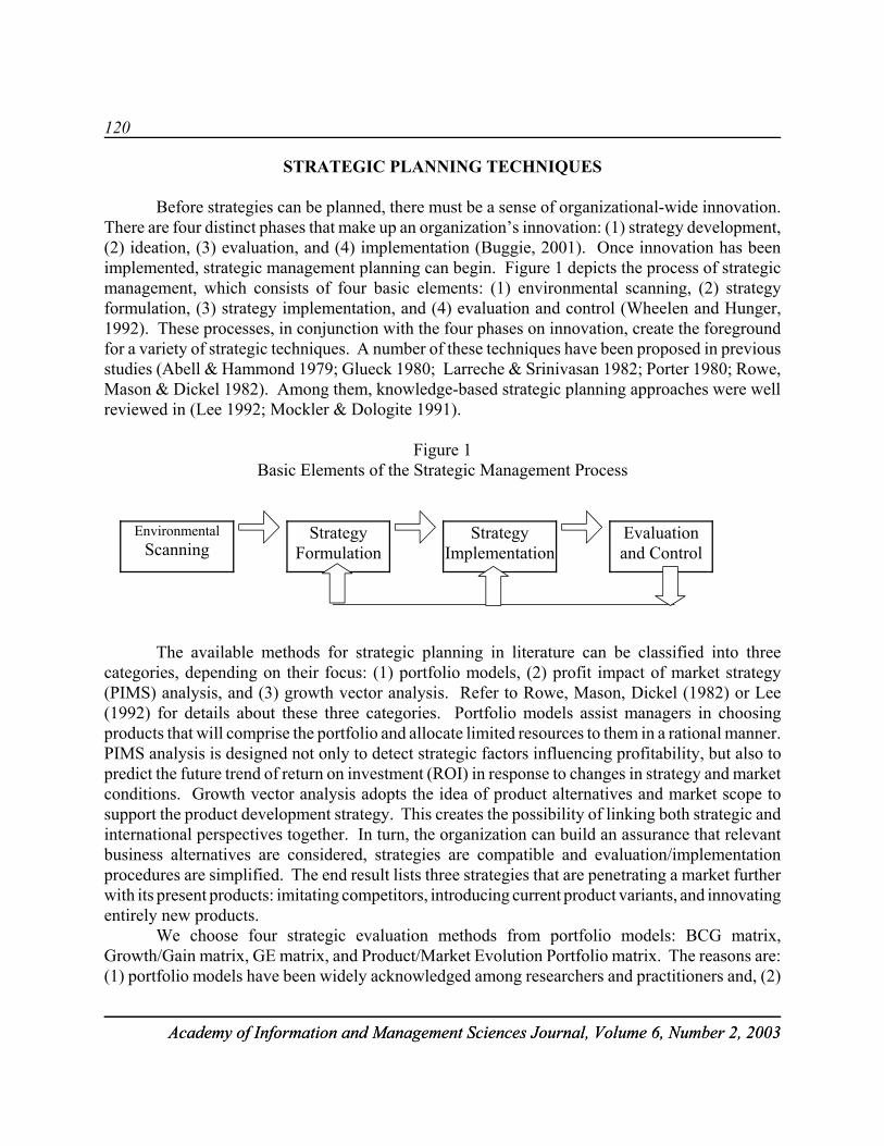
120
Academy of Information and Management Sciences Journal, Volume 6, Number 2, 2003Academy of Information and Management Sciences Journal, Volume 6, Number 2, 2003
STRATEGIC PLANNING TECHNIQUES
Before strategies can be planned, there must be a sense of organizational-wide innovation.There are four distinct phases that make up an organization’s innovation: (1) strategy development,(2) ideation, (3) evaluation, and (4) implementation (Buggie, 2001). Once innovation has beenimplemented, strategic management planning can begin. Figure 1 depicts the process of strategicmanagement, which consists of four basic elements: (1) environmental scanning, (2) strategyformulation, (3) strategy implementation, and (4) evaluation and control (Wheelen and Hunger,1992). These processes, in conjunction with the four phases on innovation, create the foregroundfor a variety of strategic techniques. A number of these techniques have been proposed in previousstudies (Abell & Hammond 1979; Glueck 1980; Larreche & Srinivasan 1982; Porter 1980; Rowe,Mason & Dickel 1982). Among them, knowledge-based strategic planning approaches were wellreviewed in (Lee 1992; Mockler & Dologite 1991).
Figure 1Basic Elements of the Strategic Management Process
The available methods for strategic planning in literature can be classified into threecategories, depending on their focus: (1) portfolio models, (2) profit impact of market strategy(PIMS) analysis, and (3) growth vector analysis. Refer to Rowe, Mason, Dickel (1982) or Lee(1992) for details about these three categories. Portfolio models assist managers in choosingproducts that will comprise the portfolio and allocate limited resources to them in a rational manner.PIMS analysis is designed not only to detect strategic factors influencing profitability, but also topredict the future trend of return on investment (ROI) in response to changes in strategy and marketconditions. Growth vector analysis adopts the idea of product alternatives and market scope tosupport the product development strategy. This creates the possibility of linking both strategic andinternational perspectives together. In turn, the organization can build an assurance that relevantbusiness alternatives are considered, strategies are compatible and evaluation/implementationprocedures are simplified. The end result lists three strategies that are penetrating a market furtherwith its present products: imitating competitors, introducing current product variants, and innovatingentirely new products.
We choose four strategic evaluation methods from portfolio models: BCG matrix,Growth/Gain matrix, GE matrix, and Product/Market Evolution Portfolio matrix. The reasons are:(1) portfolio models have been widely acknowledged among researchers and practitioners and, (2)
EnvironmentalScanning
StrategyFormulation
StrategyImplementation
Evaluationand Control
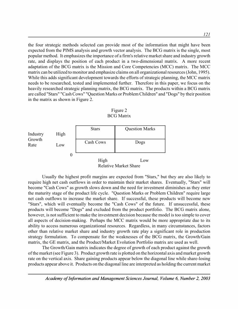
121
Academy of Information and Management Sciences Journal, Volume 6, Number 2, 2003Academy of Information and Management Sciences Journal, Volume 6, Number 2, 2003
Stars Question Marks
Cash Cows Dogs
the four strategic methods selected can provide most of the information that might have beenexpected from the PIMS analysis and growth vector analysis. The BCG matrix is the single, mostpopular method. It emphasizes the importance of a firm's relative market share and industry growthrate, and displays the position of each product in a two-dimensional matrix. A more recentadaptation of the BCG matrix is the Mission and Core Competencies (MCC) matrix. The MCCmatrix can be utilized to monitor and emphasize claims on all organizational resources (John, 1995).While this adds significant development towards the efforts of strategic planning, the MCC matrixneeds to be researched, tested and implemented further. Therefore in this paper, we focus on theheavily researched strategic planning matrix, the BCG matrix. The products within a BCG matrixare called "Stars" "Cash Cows" "Question Marks or Problem Children" and "Dogs" by their positionin the matrix as shown in Figure 2.
Figure 2BCG Matrix
Industry HighGrowthRate Low
0High LowRelative Market Share
Usually the highest profit margins are expected from "Stars," but they are also likely torequire high net cash outflows in order to maintain their market shares. Eventually, "Stars" willbecome "Cash Cows" as growth slows down and the need for investment diminishes as they enterthe maturity stage of the product life cycle. "Question Marks or Problem Children" require largenet cash outflows to increase the market share. If successful, these products will become new"Stars", which will eventually become the "Cash Cows" of the future. If unsuccessful, theseproducts will become "Dogs" and excluded from the product portfolio. The BCG matrix alone,however, is not sufficient to make the investment decision because the model is too simple to coverall aspects of decision-making. Perhaps the MCC matrix would be more appropriate due to itsability to access numerous organizational resources. Regardless, in many circumstances, factorsother than relative market share and industry growth rate play a significant role in productionstrategy formulation. To compensate for the weaknesses of the BCG matrix, the Growth/Gainmatrix, the GE matrix, and the Product/Market Evolution Portfolio matrix are used as well.
The Growth/Gain matrix indicates the degree of growth of each product against the growthof the market (see Figure 3). Product growth rate is plotted on the horizontal axis and market growthrate on the vertical axis. Share gaining products appear below the diagonal line while share-losingproducts appear above it. Products on the diagonal line are interpreted as holding the current market
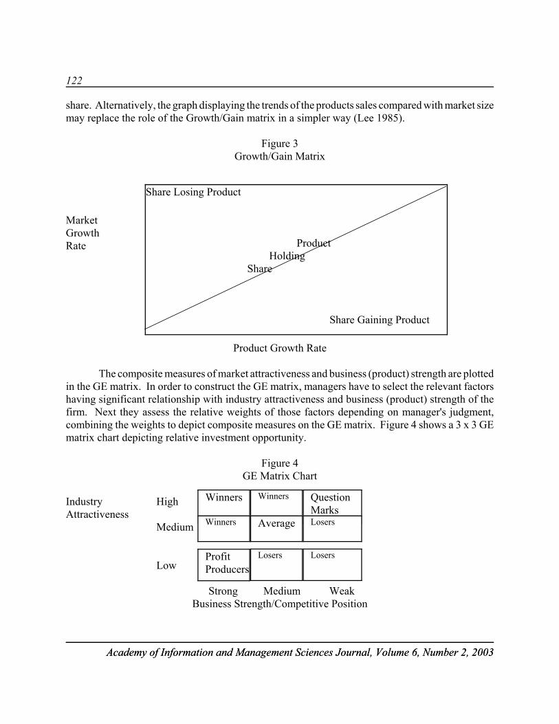
122
Academy of Information and Management Sciences Journal, Volume 6, Number 2, 2003Academy of Information and Management Sciences Journal, Volume 6, Number 2, 2003
Winners Winners QuestionMarks
Winners Average Losers
ProfitProducers
Losers Losers
Share Losing Product
Product Holding Share
Share Gaining Product
share. Alternatively, the graph displaying the trends of the products sales compared with market sizemay replace the role of the Growth/Gain matrix in a simpler way (Lee 1985).
Figure 3Growth/Gain Matrix
MarketGrowthRate
Product Growth Rate
The composite measures of market attractiveness and business (product) strength are plottedin the GE matrix. In order to construct the GE matrix, managers have to select the relevant factorshaving significant relationship with industry attractiveness and business (product) strength of thefirm. Next they assess the relative weights of those factors depending on manager's judgment,combining the weights to depict composite measures on the GE matrix. Figure 4 shows a 3 x 3 GEmatrix chart depicting relative investment opportunity.
Figure 4GE Matrix Chart
Industry HighAttractiveness
Medium
Low
Strong Medium WeakBusiness Strength/Competitive Position

123
Academy of Information and Management Sciences Journal, Volume 6, Number 2, 2003Academy of Information and Management Sciences Journal, Volume 6, Number 2, 2003
1. GrowthConcentrationvia VerticalIntegration
2. GrowthConcentrationvia Horizontal
Integration
3. Retrenchment
5. GrowthConcentrationvia Horizontal
Integration
StabilityNo Change inProfit Strategy
4. StabilityPause or Proceed
with Caution
6. RetrenchmentCaptive Company or
Divestment
7. GrowthConcentric
Diversification
8. GrowthConglomerateDiversification
9. RetrenchmentBankruptcy
or Liquidation
IndustryAttract-iveness
Strategic managers may decide the overall direction of the firm through its corporate strategyby combining market attractiveness with the company's business strength/competitive position intoa nine-cell matrix similar to the GE matrix (Wheelen and Hunger 1992). The resulting matrix,depicted in Figure 5, is used as a model to suggest some alternative corporate strategies that mightapply to the company's situation. Cells 1, 2, 5, 7, and 8 suggest that growth strategies are eitherconcentrated, which signifies expansion within the firm's current industry, or diversified, wheregrowth is generated outside of the firm's current industry. Cells 4 and 5 represent stability strategies,which are a firm's choice to retain its current mission and objectives without any significant changein strategic direction. Cell 3, 6, and 9 display retrenchment strategies, which are the reduction inscope and magnitude of the firm's efforts.
Figure 5Contingency Corporate Strategy (Wheelen and Hunger, 1992)
Business Strengths/Competitive PositionStrong Average Weak
High
Medium
Low
The GE matrix does not depict as effectively as it might the positions of new businesses thatare starting to grow in fledgling industries. In that case, Hofer and Schendel (1978) proposed to usea Product/Market Evolution matrix in which businesses are plotted in terms of their relativecompetitive position and stage of product/market evolution. It is vital that organizations preparethemselves for all potential stages of the business life cycle, whether the market initiates atechnology push or demand-pull. In an effort to meet these competitive stages, the product matrixproposes four main strategies: (1) sub-contracting, (2) cooperation, (3) networking, and (4) joint
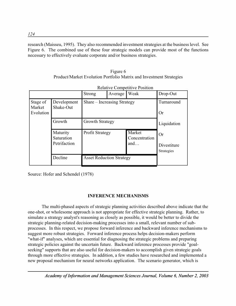
124
Academy of Information and Management Sciences Journal, Volume 6, Number 2, 2003Academy of Information and Management Sciences Journal, Volume 6, Number 2, 2003
research (Maisseu, 1995). They also recommended investment strategies at the business level. SeeFigure 6. The combined use of these four strategic models can provide most of the functionsnecessary to effectively evaluate corporate and/or business strategies.
Figure 6Product/Market Evolution Portfolio Matrix and Investment Strategies
Relative Competitive Position
Source: Hofer and Schendel (1978)
INFERENCE MECHANISMS
The multi-phased aspects of strategic planning activities described above indicate that theone-shot, or wholesome approach is not appropriate for effective strategic planning. Rather, tosimulate a strategy analyst's reasoning as closely as possible, it would be better to divide thestrategic planning-related decision-making processes into a small, relevant number of sub-processes. In this respect, we propose forward inference and backward inference mechanisms tosuggest more robust strategies. Forward inference process helps decision-makers perform"what-if" analyses, which are essential for diagnosing the strategic problems and preparingstrategic policies against the uncertain future. Backward inference processes provide "goal-seeking" supports that are also useful for decision-makers to accomplish given strategic goalsthrough more effective strategies. In addition, a few studies have researched and implemented anew proposal mechanism for neural networks application. The scenario generator, which is
Strong Weak Average Drop-Out
Stage of Market Evolution
Development Shake-Out
Growth
Maturity Saturation Petrifaction
Decline
Share – Increasing Strategy
Growth Strategy
Profit Strategy
Asset Reduction Strategy
Market Concentration and…
Turnaround
Or
Liquidation
Or
Divestiture Strategies
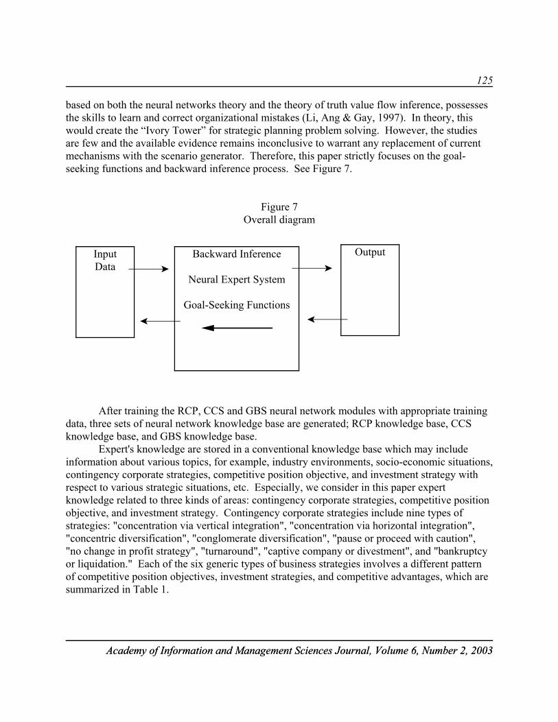
125
Academy of Information and Management Sciences Journal, Volume 6, Number 2, 2003Academy of Information and Management Sciences Journal, Volume 6, Number 2, 2003
InputData
Backward Inference
Neural Expert System
Goal-Seeking Functions
Output
based on both the neural networks theory and the theory of truth value flow inference, possessesthe skills to learn and correct organizational mistakes (Li, Ang & Gay, 1997). In theory, thiswould create the “Ivory Tower” for strategic planning problem solving. However, the studiesare few and the available evidence remains inconclusive to warrant any replacement of currentmechanisms with the scenario generator. Therefore, this paper strictly focuses on the goal-seeking functions and backward inference process. See Figure 7.
Figure 7Overall diagram
After training the RCP, CCS and GBS neural network modules with appropriate trainingdata, three sets of neural network knowledge base are generated; RCP knowledge base, CCSknowledge base, and GBS knowledge base.
Expert's knowledge are stored in a conventional knowledge base which may includeinformation about various topics, for example, industry environments, socio-economic situations,contingency corporate strategies, competitive position objective, and investment strategy withrespect to various strategic situations, etc. Especially, we consider in this paper expertknowledge related to three kinds of areas: contingency corporate strategies, competitive positionobjective, and investment strategy. Contingency corporate strategies include nine types ofstrategies: "concentration via vertical integration", "concentration via horizontal integration","concentric diversification", "conglomerate diversification", "pause or proceed with caution","no change in profit strategy", "turnaround", "captive company or divestment", and "bankruptcyor liquidation." Each of the six generic types of business strategies involves a different patternof competitive position objectives, investment strategies, and competitive advantages, which aresummarized in Table 1.
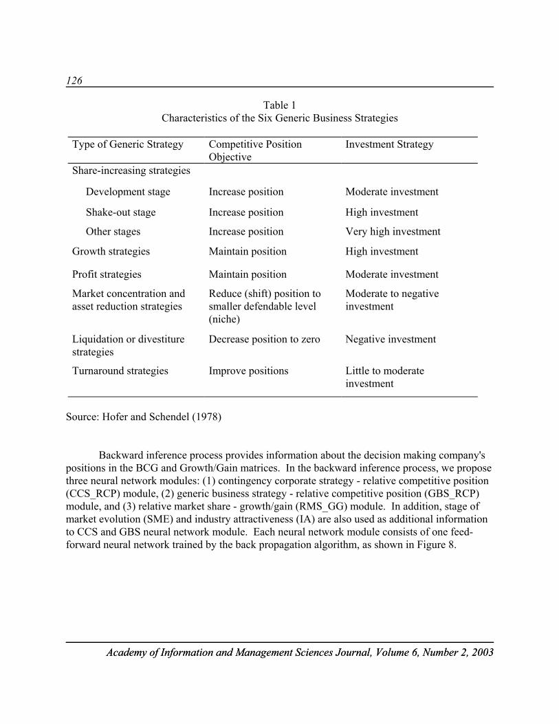
126
Academy of Information and Management Sciences Journal, Volume 6, Number 2, 2003Academy of Information and Management Sciences Journal, Volume 6, Number 2, 2003
Table 1Characteristics of the Six Generic Business Strategies
Type of Generic Strategy Competitive PositionObjective
Investment Strategy
Share-increasing strategies
Development stage Increase position Moderate investment
Shake-out stage Increase position High investment
Other stages Increase position Very high investment
Growth strategies Maintain position High investment
Profit strategies Maintain position Moderate investment
Market concentration andasset reduction strategies
Reduce (shift) position tosmaller defendable level(niche)
Moderate to negativeinvestment
Liquidation or divestiturestrategies
Decrease position to zero Negative investment
Turnaround strategies Improve positions Little to moderateinvestment
Source: Hofer and Schendel (1978)
Backward inference process provides information about the decision making company'spositions in the BCG and Growth/Gain matrices. In the backward inference process, we proposethree neural network modules: (1) contingency corporate strategy - relative competitive position(CCS_RCP) module, (2) generic business strategy - relative competitive position (GBS_RCP)module, and (3) relative market share - growth/gain (RMS_GG) module. In addition, stage ofmarket evolution (SME) and industry attractiveness (IA) are also used as additional informationto CCS and GBS neural network module. Each neural network module consists of one feed-forward neural network trained by the back propagation algorithm, as shown in Figure 8.

127
Academy of Information and Management Sciences Journal, Volume 6, Number 2, 2003Academy of Information and Management Sciences Journal, Volume 6, Number 2, 2003
CCS_RCP
KB
GBS_RCP
KB
RMS_GG
KB
Final
Conclusion
Figure 8Backward Inference Diagram
First, if one of the contingency corporate strategies is selected as a target strategy, thecorresponding cell within the GE matrix is determined by a decision-maker. IA value is alsodetermined. With this information, the CCS_RCP module provides information about thecompetitive position in the market relative to that of the target competitor. The architecture ofCCS_RCP neural network module has 14 neurons in the input layer and 4 neurons in the outputlayer. Output of the CCS_RCP module is then used as input to the RMS_GG module. Figure 9shows the architecture of the CCS_RCP module.
USER
Neural NetworkKnowledgeBases
ConventionalKnowledgeBase
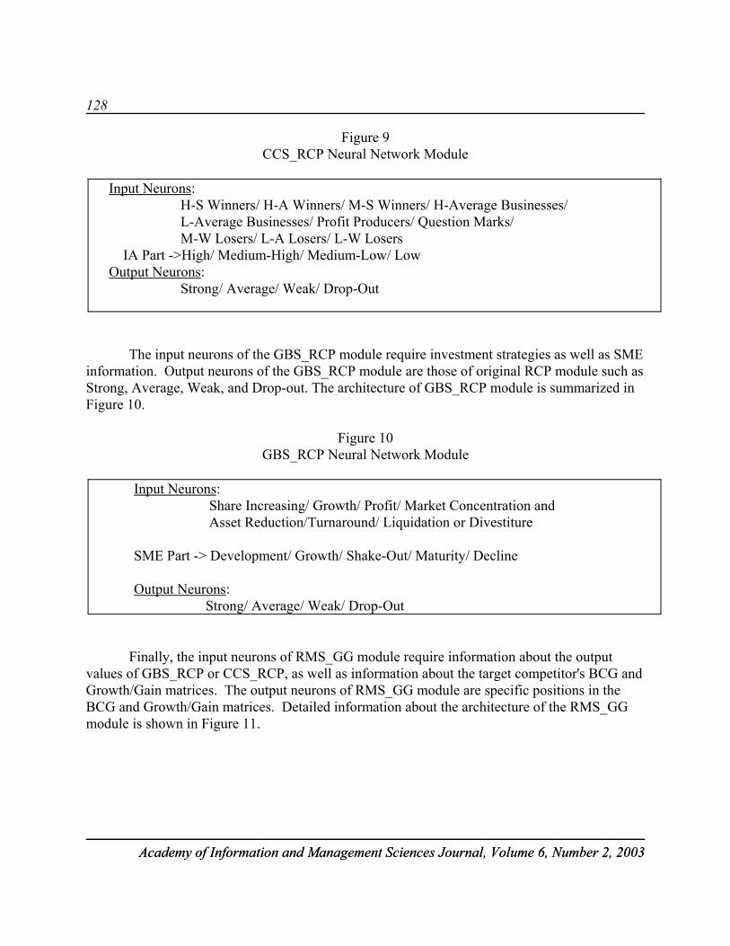
128
Academy of Information and Management Sciences Journal, Volume 6, Number 2, 2003Academy of Information and Management Sciences Journal, Volume 6, Number 2, 2003
Figure 9CCS_RCP Neural Network Module
Input Neurons: H-S Winners/ H-A Winners/ M-S Winners/ H-Average Businesses/ L-Average Businesses/ Profit Producers/ Question Marks/ M-W Losers/ L-A Losers/ L-W Losers IA Part ->High/ Medium-High/ Medium-Low/ Low Output Neurons: Strong/ Average/ Weak/ Drop-Out
The input neurons of the GBS_RCP module require investment strategies as well as SMEinformation. Output neurons of the GBS_RCP module are those of original RCP module such asStrong, Average, Weak, and Drop-out. The architecture of GBS_RCP module is summarized inFigure 10.
Figure 10GBS_RCP Neural Network Module
Input Neurons: Share Increasing/ Growth/ Profit/ Market Concentration and
Asset Reduction/Turnaround/ Liquidation or Divestiture SME Part -> Development/ Growth/ Shake-Out/ Maturity/ Decline
Output Neurons: Strong/ Average/ Weak/ Drop-Out
Finally, the input neurons of RMS_GG module require information about the outputvalues of GBS_RCP or CCS_RCP, as well as information about the target competitor's BCG andGrowth/Gain matrices. The output neurons of RMS_GG module are specific positions in theBCG and Growth/Gain matrices. Detailed information about the architecture of the RMS_GGmodule is shown in Figure 11.

129
Academy of Information and Management Sciences Journal, Volume 6, Number 2, 2003Academy of Information and Management Sciences Journal, Volume 6, Number 2, 2003
Figure 11RMS_GG Neural Network Module
Input Neurons: Strong/ Average/ Weak/ Drop-Out
< Competitor > BCG : Stars/ Cash Cows/ H-Question Marks/ M-Question
Marks/ L-Question Marks/ H-Dogs/ M-Dogs/ L-Dogs Growth/Gain: Share Gainer/ Share Holder/ Share Loser
Output Neurons: < Decision Making Company > BCG : Stars/Cash Cows/ H-Question Marks/ M-Question
Marks/ L-Question Marks/ H-Dogs/ M-Dogs/ L-Dogs Growth/Gain: Share Gainer/ Share Holder/ Share Loser
After training the CCS_RCP, GBS_RCP and RMS_GG module with appropriate trainingdata, three kinds of neural network knowledge bases are generated; CCS_RCP knowledge base,GBS_RCP knowledge base, and RMS_GG knowledge base.
Architecture of a Prototype System
We developed a prototype system running on Windows 2000. It is coded in MicrosoftVisual C++ language. Its main menu is composed of five sub-menus as shown in Figures 12 and13.
Figure 12Structure of Main Menu in a Prototype System
Main Menu
RuleExtractionSubsystem
Goal-SeekingAnalysis
Subsystem
What-If AnalysisSubsystem
EnvironmentAnalysis
Subsystem
File HandlingSubsystem

130
Academy of Information and Management Sciences Journal, Volume 6, Number 2, 2003Academy of Information and Management Sciences Journal, Volume 6, Number 2, 2003
Figure 13Main Menu Screen
As mentioned in the introduction, we will illustrate the performance of backward goal-seeking analysis. Goal-seeking analysis is performed in the following steps summarized inFigure 14.
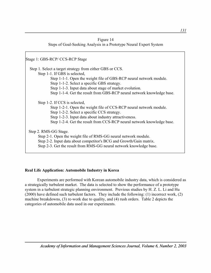
131
Academy of Information and Management Sciences Journal, Volume 6, Number 2, 2003Academy of Information and Management Sciences Journal, Volume 6, Number 2, 2003
Figure 14Steps of Goal-Seeking Analysis in a Prototype Neural Expert System
Stage 1: GBS-RCP/ CCS-RCP Stage Step 1. Select a target strategy from either GBS or CCS. Step 1-1. If GBS is selected,
Step 1-1-1. Open the weight file of GBS-RCP neural network module.Step 1-1-2. Select a specific GBS strategy.Step 1-1-3. Input data about stage of market evolution.Step 1-1-4. Get the result from GBS-RCP neural network knowledge base.
Step 1-2. If CCS is selected,Step 1-2-1. Open the weight file of CCS-RCP neural network module.Step 1-2-2. Select a specific CCS strategy.Step 1-2-3. Input data about industry attractiveness. Step 1-2-4. Get the result from CCS-RCP neural network knowledge base.
Step 2. RMS-GG Stage.Step 2-1. Open the weight file of RMS-GG neural network module.Step 2-2. Input data about competitor's BCG and Growth/Gain matrix.Step 2-3. Get the result from RMS-GG neural network knowledge base.
Real Life Application: Automobile Industry in Korea
Experiments are performed with Korean automobile industry data, which is considered asa strategically turbulent market. The data is selected to show the performance of a prototypesystem in a turbulent strategic planning environment. Previous studies by H. Z. L. Li and Hu(2000) have defined such turbulent factors. They include the following: (1) incorrect work, (2)machine breakdowns, (3) re-work due to quality, and (4) rush orders. Table 2 depicts thecategories of automobile data used in our experiments.

132
Academy of Information and Management Sciences Journal, Volume 6, Number 2, 2003Academy of Information and Management Sciences Journal, Volume 6, Number 2, 2003
Table 2 Categories of Korean Automobile Data
Car Type Company Name
KIA HYUNDAI DAEWOO
Small Pride Excel Lemans
Compact CapitalSephia
Elantra Espero
Medium Concord Sonata Prince
Large Potentia Grandeur Super Salon
Monthly domestic sales data of three companies' passenger cars from May 1990 toAugust 1994, as well as miscellaneous strategic planning data from May 1990 to August 1994,was collected. The domain knowledge from two experts, a strategy analyst in 'K' automobilecompany and a strategy expert in a university are also used in this experiment. Table 3 shows thetype and description of data used in our experiments.
Table 3Type and Description of Data Used in Experiments
Type of Data Description of Data
Quantitative Data Monthly Sales Data o Market Growth Rate o Relative Market Share o Product Growth Rate
Qualitative Data Expert Knowledge o Preparation of Input/Output Pairs used in Supervised Learning o Preparation of Desired Output used in Test o Knowledge related to three kinds of areas : - Contingency corporate strategies - Competitive Position Objectives by the type of Generic Strategy - Investment Strategies by the type of Competitive Position Objectives
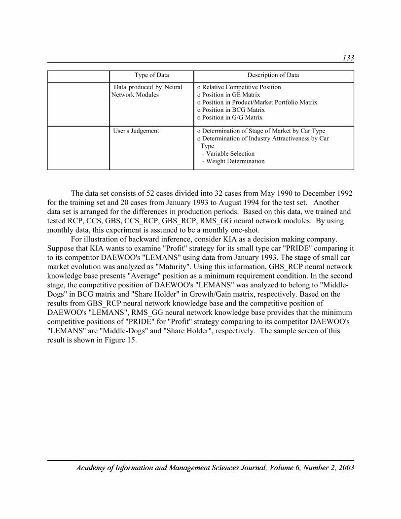
133
Type of Data Description of Data
Academy of Information and Management Sciences Journal, Volume 6, Number 2, 2003Academy of Information and Management Sciences Journal, Volume 6, Number 2, 2003
Data produced by Neural Network Modules
o Relative Competitive Position o Position in GE Matrix o Position in Product/Market Portfolio Matrix o Position in BCG Matrix o Position in G/G Matrix
User's Judgement o Determination of Stage of Market by Car Type o Determination of Industry Attractiveness by Car Type - Variable Selection - Weight Determination
The data set consists of 52 cases divided into 32 cases from May 1990 to December 1992for the training set and 20 cases from January 1993 to August 1994 for the test set. Anotherdata set is arranged for the differences in production periods. Based on this data, we trained andtested RCP, CCS, GBS, CCS_RCP, GBS_RCP, RMS_GG neural network modules. By usingmonthly data, this experiment is assumed to be a monthly one-shot.
For illustration of backward inference, consider KIA as a decision making company.Suppose that KIA wants to examine "Profit" strategy for its small type car "PRIDE" comparing itto its competitor DAEWOO's "LEMANS" using data from January 1993. The stage of small carmarket evolution was analyzed as "Maturity". Using this information, GBS_RCP neural networkknowledge base presents "Average" position as a minimum requirement condition. In the secondstage, the competitive position of DAEWOO's "LEMANS" was analyzed to belong to "Middle-Dogs" in BCG matrix and "Share Holder" in Growth/Gain matrix, respectively. Based on theresults from GBS_RCP neural network knowledge base and the competitive position ofDAEWOO's "LEMANS", RMS_GG neural network knowledge base provides that the minimumcompetitive positions of "PRIDE" for "Profit" strategy comparing to its competitor DAEWOO's"LEMANS" are "Middle-Dogs" and "Share Holder", respectively. The sample screen of thisresult is shown in Figure 15.
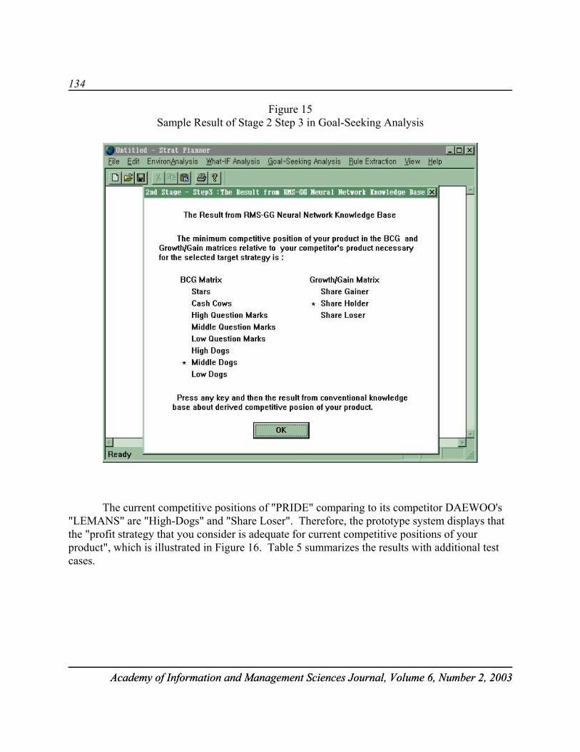
134
Academy of Information and Management Sciences Journal, Volume 6, Number 2, 2003Academy of Information and Management Sciences Journal, Volume 6, Number 2, 2003
Figure 15Sample Result of Stage 2 Step 3 in Goal-Seeking Analysis
The current competitive positions of "PRIDE" comparing to its competitor DAEWOO's"LEMANS" are "High-Dogs" and "Share Loser". Therefore, the prototype system displays thatthe "profit strategy that you consider is adequate for current competitive positions of yourproduct", which is illustrated in Figure 16. Table 5 summarizes the results with additional testcases.

135
Academy of Information and Management Sciences Journal, Volume 6, Number 2, 2003Academy of Information and Management Sciences Journal, Volume 6, Number 2, 2003
Figure 16Sample Result of Stage 2 Step 4 in Goal Analysis
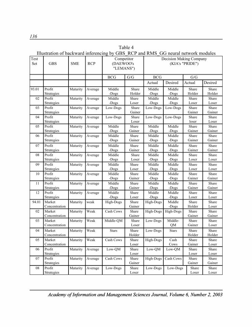
136
Academy of Information and Management Sciences Journal, Volume 6, Number 2, 2003Academy of Information and Management Sciences Journal, Volume 6, Number 2, 2003
Table 4Illustration of backward inferencing by GBS_RCP and RMS_GG neural network modules
Test Set GBS SME
RCP
Competitor(DAEWOO's "LEMANS")
Decision Making Company(KIA's "PRIDE")
BCG G/G BCG G/G Actual Desired Actual Desired
93.01 ProfitStrategies
Maturity Average Middle-Dogs
ShareHolder
Middle-Dogs
Middle-Dogs
ShareHolder
ShareHolder
02 ProfitStrategies
Maturity Average Middle-Dogs
ShareLoser
Middle-Dogs
Middle-Dogs
ShareLoser
ShareLoser
03 ProfitStrategies
Maturity Average Low-Dogs ShareGainer
Low-Dogs Low-Dogs ShareGainer
ShareGainer
04 ProfitStrategies
Maturity Average Low-Dogs ShareLoser
Low-Dogs Low-Dogs Shareloser
ShareLoser
05 ProfitStrategies
Maturity Average Middle-Dogs
ShareGainer
Middle-Dogs
Middle-Dogs
ShareGainer
ShareGainer
06 ProfitStrategies
Maturity Average Middle-Dogs
ShareGainer
Middle-Dogs
Middle-Dogs
ShareGainer
ShareGainer
07 ProfitStrategies
Maturity Average Middle-Dogs
ShareGainer
Middle-Dogs
Middle-Dogs
ShareGainer
ShareGainer
08 ProfitStrategies
Maturity Average Middle-Dogs
ShareLoser
Middle-Dogs
Middle-Dogs
ShareLoser
ShareLoser
09 ProfitStrategies
Maturity Average Middle-Dogs
ShareLoser
Middle-Dogs
Middle-Dogs
ShareLoser
ShareLoser
10 ProfitStrategies
Maturity Average Middle-Dogs
ShareGainer
Middle-Dogs
Middle-Dogs
ShareGainer
ShareGainer
11 ProfitStrategies
Maturity Average Middle-Dogs
ShareGainer
Middle-Dogs
Middle-Dogs
ShareGainer
ShareGainer
12 ProfitStrategies
Maturity Average Middle-Dogs
ShareLoser
Middle-Dogs
Middle-Dogs
ShareLoser
ShareLoser
94.01 MarketConcentration
Maturity weak High-Dogs ShareGainer
High-Dogs Middle-Dogs
ShareHolder
ShareLoser
02 MarketConcentration
Maturity Weak Cash Cows ShareGainer
High-Dogs High-Dogs ShareGainer
ShareGainer
03 MarketConcentration
Maturity Weak Middle-QM ShareLoser
Low-Dogs Middle-QM
ShareGainer
ShareLoser
04 MarketConcentration
Maturity Weak Stars ShareHolder
Low-Dogs Stars ShareHolder
ShareHolder
05 MarketConcentration
Maturity Weak Cash Cows ShareLoser
High-Dogs CashCows
ShareGainer
ShareLoser
06 ProfitStrategies
Maturity Average Low-QM ShareLoser
Low-QM Low-QM ShareLoser
ShareLoser
07 ProfitStrategies
Maturity Average Cash Cows ShareGainer
High-Dogs Cash Cows ShareGainer
ShareGainer
08 ProfitStrategies
Maturity Average Low-Dogs ShareLoser
Low-Dogs Low-Dogs ShareLoser
ShareLoser
137
Academy of Information and Management Sciences Journal, Volume 6, Number 2, 2003Academy of Information and Management Sciences Journal, Volume 6, Number 2, 2003
CONCLUDING REMARKS
In this paper, we proposed a neural expert system capable of performing a backwardinference so that strategic planning problems may be solved more effectively. The proposedneural expert system is designed to provide a "goal-seeking" inference function, based oncombining the generalization capability of neural networks with an expert system. A prototypesystem has been developed to prove our approach. Its performance was illustrated with real lifedata of the automobile industry in Korea. However, much room exists for further research. Inthis respect, we are currently developing an improved version of the prototype system byincorporating what-if analysis, refined mechanisms of environmental analysis, competitoranalysis, and advanced strategic planning models.
REFERENCES
Abell, D.F. & J.S. Hammond. Strategic market planning: problems and analytical approach, Prentice-Hall,Englewood Cliffs, NJ, 1979.
Ackley, D.H., Hinton, G.E. & T.J. Sejnowski. “A learning algorithm for Boltzmann machines,” Cognitive Science 9,1985, 147-169.
Buggie, F. (2001). The four phases of innovation. Journal of Business Strategy, 22, 36-42.
Chien, T.W., Lin, C., & Bertram, T. (1999). A neural networks-based approach for strategic planning. Information& Management, 35, 357.
Cohen, M.A. & S. Grossberg. “Absolute stability of global pattern formation and parallel memory storage bycompetitive neural networks,” IEEE Transactions on Systems, Man, and Cybernetics, SMC 13, September1983, 815-825.
Daniels, J.D. (1994). Combining strategic and international business approaches through growth vector analysis. Management International Review, 34, 21.
Fukushima, K., Neocognitron. “A self-organizing neural network model for a mechanism of pattern recognition,”IEEE Transactions on Pattern Analysis and Machine Intelligence, PAMI 8, September 1983, 398-404.
Gallant, S.I. “Connectionist expert system”, Communications of the ACM, 31(2), February 1988, 152-169.
Glueck, W.F. Business policy and strategic management, McGraw-Hill, 1980.
Grossberg, S. “Adaptive pattern classification and universal recording: Part 1. Parallel development and coding ofneural feature detectors,” Biological Cybernetics, 23, 1976, 121-134.
Grossberg, S. Studies of mind and brain, Reidel, Hingham, Mass. 1982.
Hofer, C.W. & D. Schendel. Strategy formulation: analytical concepts, West Publishing Co., 1978.
138
Academy of Information and Management Sciences Journal, Volume 6, Number 2, 2003Academy of Information and Management Sciences Journal, Volume 6, Number 2, 2003
Hopfield, J.J. “Neural networks and physical systems with emergent collective computational abilities,” Proceedingsof the National Academy of Sciences USA, National Academy of Sciences, Washington, D.C., 79, 1982,2554-2558.
Hopfield, J.J.. “Neurons with graded response have collective computational properties like those of two-stateneurons,” Proceedings of the National Academy of Sciences USA, 81, 1984, 3088-3092.
Hopfield, J.J.. & D.W. Tank, “Neural computation of decision in optimization problems,” Biological Cybernetics,52, 1985, 141-152.
Jacobs, R.A. “Increased rates of convergence through learning rate adaptation,” Neural Networks, 1 , 1988, 285-307.
Kamijo, K. & T. Tanigawa. “Stock price pattern recognition: A recurrent neural network approach,” Int'l JointConference on Neural Networks, San Diego, Calif., 1, 1990, 215-221.
Kimoto, T. & K. Asakawa. “Stock market prediction system with modular neural networks,” Int'l Joint Conferenceon Neural Networks, San Diego, Calif.,1, 1990, 1-6.
Kohonen, T. “State of the art in neural computing,” Int'l Joint Conference on Neural Networks, San Diego, Calif., 1,1987, 79-90.
Lang, S. (1999). The fabulous four. Insurance & Technology, 24, 32.
Larreche, J.C. & V. Srinivasan. “STRATPORT: A Model for the Evolution and Formulation of Business PortfolioStrategies,” Management Science 28(9), 1982, 979-1001.
Lee, H.K. Interactions of Long-term Planning and Short-term Planning: An Intelligent DSS by Post Model AnalysisApproach, Master’s Thesis, Dept. of Management Science, Korea Advanced Institute of Science andTechnology, 1985.
Lee, K.C. “Synergism of Knowledge-based Decision Support Systems and Neural Networks to Design an IntelligentStrategic Planning System,” Journal of the MIS Research (in Korea), 1992, 35-56.
Li, H., Li, Z., Li, X.L., & Hu, B. (2000). A production rescheduling expert simulation system. European Journalof Operational Research, 124, 283.
Li, X., Ang, C.L., & Gay, R. (1997). An intelligent scenario generator for strategic business planning. Computer inIndustry, 34, 261.
Lippmann, R.P. “An introduction to computing with neural nets,” IEEE ASSP Magazine, 3, 1992, April 1987, 4-22.
Maisseu, A.P. (1995). Managing technological flows into corporate strategy. International Journal of Technology,10, 3.
McClelland, J.L. & D.E. Rumelhart. “Distributed memory and the representation of general and specificinformation,” Journal of Expert Psychology: General, 114, 1985, 158-188.
McClelland, J.L.. Parallel distributed processing: explorations in the microstructures of cognition, Vol. 2, MITPress, Cambridge, Mass., 1986.
139
Academy of Information and Management Sciences Journal, Volume 6, Number 2, 2003Academy of Information and Management Sciences Journal, Volume 6, Number 2, 2003
Mockler, R.J., & D.G. Dologite. “Knowledge-based systems to support strategic planning decision making,”Proceedings of the Twenty-Fourth Annual Hawaii International Conference on System Sciences, 3, 1991,173-180.
Nicholls, J. (1995). The MCC decision matrix: A tool for applying strategic logic to everyday activity. Management Decision, 33, 4.
Oliver, R.W. (2001). Real-time strategy: What is strategy, anyway? Journal of Business Strategy, 22, 7-10.
Porter, M.E. Competitive strategy: techniques for analyzing industries and competition, MacMillan, NY, 1980.
Rabiner, L.R & B.H. Juang. “An introduction to hidden Markov models,” IEEE ASSP Magazine, 3, January 1986, 4-16.
Rosenblatt, F. Principles of Neurodynamics: Perceptrons and the Theory of Brain Mechanisms. Spartan,Washington, D.C.
Rowe, A.J., R.O. Mason & K. Dickel, Strategic management & business policy: a methodological approach,Addison-Wesley, Reading, Massachusetts, 1982.
Rumelhart, D.E., G.E. Hinton, & R.J. Williams. Learning internal representations by error propagation, in ParallelDistributed Processing (PDP): Exploration in the Microstructure of Cognition Vol. I, Cambridge, MA:MITPress, ch.8, 1986, 318-362.
Rumelhart, D.E. & D. Zipser. Feature discovery by competitive learning, Cognitive Science, 9, 1985, 75-112.
Steinbush, K. The learning matrix , Cybernetics, 1961, 36-45.
Thompson, A.Jr. & A.J. Strickland III. Strategic management: concepts and cases, Irwin, 5th Edition, 1990.
Waalewijn, P., & R.H. Boulan. Strategic planning on a personal computer, Long Range Planning, 23(4), 1990, 97-103.
Waterman, D.A. A guide to expert systems, Addison-Wesley Publishing Co, 1986.
Wheelen, T.L. & J.D. Hunger, Strategic management and business policy, Addison-Wesley Publishing Co, 1992.
White, H. Economic prediction using neural networks: The case of IBM daily stock returns, Int'l Joint Conferenceon Neural Networks, San Diego, Calif., 2, 1988, 451-458.
Widrow, G. & M.E. Hoff. Adaptive switching circuits , Institute of Radio Engineers, Western Electronic Show andConvention, Convention Record Part 4, 1960, 96-104.
Willshaw, D.J. Models of distributed associative memory models, Ph.D. Dissertation, University of Edinburgh,Scotland, 1971.
Zeidenberg, M. Neural network models in artificial intelligence, Ellis Homewood, England, 1990.
Zhang, G. & Hu, M. (1998). Neural network forecasting of the British pound/US dollar exchange rate. Omega, 26,495.

140
Academy of Information and Management Sciences Journal, Volume 6, Number 2, 2003Academy of Information and Management Sciences Journal, Volume 6, Number 2, 2003
Allied Academies
invites you to check our website at
www.alliedacademies.orgfor information concerning
conferences and submission instructions

141
Academy of Information and Management Sciences Journal, Volume 6, Number 2, 2003Academy of Information and Management Sciences Journal, Volume 6, Number 2, 2003
Allied Academies
invites you to check our website at
www.alliedacademies.orgfor information concerning
conferences and submission instructions

117
Academy of Information and Management Sciences Journal, Volume 6, Number 2, 2003Academy of Information and Management Sciences Journal, Volume 6, Number 2, 2003
Allied Academies
invites you to check our website at
www.alliedacademies.orgfor information concerning
conferences and submission instructions

118
Academy of Information and Management Sciences Journal, Volume 6, Number 2, 2003Academy of Information and Management Sciences Journal, Volume 6, Number 2, 2003
Allied Academies
invites you to check our website at
www.alliedacademies.orgfor information concerning
conferences and submission instructions