Abrupt Changes Detection in Fatigue Data Using the Cumulative Sum Method

Abrupt Changes Detection in Fatigue Data Using the Cumulative Sum Method

Z. M. NOPIAH, M.N.BAHARIN, S. ABDULLAH, M. I. KHAIRIR AND C. K. E. NIZWAN

Department of Mechanical and Materials Engineering Universiti Kebangsaan Malaysia

43600 UKM Bangi, Selangor MALAYSIA

[email protected]

Abstract: - The detection of abrupt changes refers to a time instant at which properties suddenly change, but before and after which properties are constant in some sense. CUSUM (Cumulative Sum) is a sequential analysis technique that is used in the detection of abrupt changes. The objective in this study is to apply CUSUM technique in analysing fatigue data for detection of abrupt changes. For the purpose of this study, a collection of nonstationary data that exhibits a random behavior was used. This random data was measured in the unit of microstrain on the lower suspension arm of a car. Experimentally, the data was collected for 60 seconds at a sampling rate of 500 Hz, which gave 30,000 discrete data points. By using CUSUM method, a CUSUM plot was constructed in monitoring the mean changes for fatigue data. Global signal statistical value indicated that the data were non Gaussian distribution in nature. The result of the study indicates that CUSUM method is only applicable for certain type of data with mixed high amplitude in a random background data. Key-Words: - Abrupt changes, CUSUM, nonstationary data, mean changes, global statistics 1 Introduction In fatigue data analysis, data editing plays an important role in calculating the damage caused by the stress loading. The function of fatigue data editing is to remove the small amplitude cycles for reducing the test time and cost. By using this approach, large amplitude cycles that cause the majority of the damage are retained and thus only shortened loading consists of large amplitude cycles is produced [1]. This paper discusses on the use of Cumulative Sum (CUSUM) method for detection of abrupt changes. A comparison between CUSUM and time series plot for four sets of data were made in order to evaluate whether this method can be used to extract the important features that exist in the fatigue data. It is predicted that by using the CUSUM algorithm, the important features that underlies within the data could be extracted and suited for fatigue data editing.

2 Literature Background 2.1 Signal A signal is a series of number that come from a measurement, typically obtained using some recording method as a function of time [2]. In real

applications, signals can be classified into two types which are stationary and non-stationary behavior. A signal representing a random phenomenon can be characterised as either stationary or nonstationary behaviour. The stationary signals exhibit the statistical properties remain unchanged with the changes in time. On the other hand, statistics of non-stationary signal is dependent on the time of measurement [3]. In the case of fatigue research, the signal consists of a measurement of cyclic loads, i.e. force, strain and stress against time.

Since all the data that were measured from this experiment are recorded as strain time histories, it is also important to have a better understanding about the behavior of this data before applying the detection of abrupt changes algorithm. The identification of fatigue data behavior is based on the existence of time series component which involves with the identification of trend, cyclical, seasonal and irregular component in time period t The method used in the identification of this component is called “classical decomposition” of time series. This process is used to segregate and to analyse the existence components in a systematic manner. The trend component represents the long-run growth or decline over time. On the other hand, the cyclical component refers to the rises and falls of

WSEAS TRANSACTIONS on MATHEMATICS Z. M. Nopiah, M. N.Baharin, S. Abdullah, M. I. Khairir, C. K. E. Nizwan

ISSN: 1109-2769 708 Issue 12, Volume 7, December 2008

the series over unspecified period of time. The seasonal component also known as seasonal variation refers to the characterization of regular fluctuations occurring within a specific period of time. Although this component is individually identified, in fact it also related to each other in a certain mathematical functional form. The type of relationship that these components have is divided into two which are multiplicative effect and additive effect. Multiplicative effect means that the components are interacted to each other such that the sizes of the seasonal variation increase in accordance with in the level of data. On the other part, additive effect involve with the assumption that the components of the series are interacted in additive manner [4]. The observations of a variable were taken at equally spaced intervals of time [2]. 2.1.1 Abrupt Changes Abrupt changes are rapid changes that occur with respect to the sampling period of measurement, if not instantaneously. Whilst, the detection of abrupt changes refer to tools that help us in deciding whether such a change occurred in the characteristics of the considered object [5]. The generic problem of detecting abrupt changes in process parameters has been widely studied. These changes may be due to shifts that exist in the mean value (edge detection) or a variation in signal dynamics [6]. 2.1.2 Cumulative Sums

CUSUM method is one of the tools that is used in the detection of abrupt changes. It was first proposed in 1954 and has been studied by many authors particularly [7].. The CUSUM method is easy to handle and useful for detecting the locations of change points. In particular, it has been utilized for testing a change of mean, variance and distribution function [8]. An advantage of the method lies in the fact that the sample means, variance and distribution function are all expressed as the sum of independent and identically (i.i.d) random variables [7]. It has the advantage of taking into account the history of the forecast series and is capable of detecting model failure more rapidly when forecast errors are relatively small [8].

The CUSUM chart directly incorporates all the information in the sequence of sample by plotting the cumulative sums of the deviations of the sample values from a target value [8]. In this study, the basic CUSUM equation is taken into account. CUSUM is explained by Equation (1) which target µ0 as the process mean. The cumulative control

chart is formed by plotting the quantity

)( 01

µ−= ∑=

i

jji xC (1)

against the sample number i. Ci is the cumulative sum up to and including the ith sample. Iteratively CUSUM can be written as:

1i0ii C)x(C −+−= µ n,...3,2,1i, = (2) where the starting value for the CUSUM, C0, is taken to be zero. CUSUM may be constructed both for individual observations and for the averages of rational subgroups. The case of individual observations occurs very often in practice, thus that situation will be treated first.

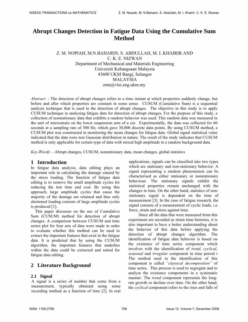
3 Methodology The data that was used in this study is variable fatigue strain loading data. It was collected from an automobile component during vehicle road testing. It was obtained from a fatigue data acquisition experiment using strain gauges and data logging instrumentation. The collected fatigue data were measured on the car’s front lower arm suspension as it was subjected to the road load service. All the data that were measured from this experiment are recorded as strain time histories. Fig. 1 explained the procedure that was used in measuring the fatigue data during the test. The strain value from this test was measured using a strain gauge that was connected to a device “Somat eDaq® “, a data logger for data acquisition. Experimental parameters that need to be controlled in this test such as sampling frequency and type of output data being measured were specified in TCE eDAQ V 3.90 software.



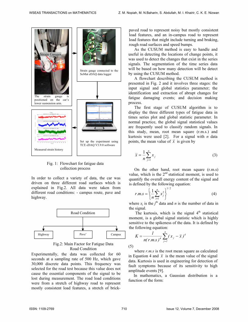
Fig. 1: Flowchart for fatigue data collection process

In order to collect a variety of data, the car was driven on three different road surfaces which is explained in Fig.2. All data were taken from different road conditions: - campus route, pave and highway.

Experimentally, the data was collected for 60 seconds at a sampling rate of 500 Hz, which gave 30,000 discrete data points. This frequency was selected for the road test because this value does not cause the essential components of the signal to be lost during measurement. The road load conditions were from a stretch of highway road to represent mostly consistent load features, a stretch of brick-

paved road to represent noisy but mostly consistent load features, and an in-campus road to represent load features that might include turning and braking, rough road surfaces and speed bumps.

As the CUSUM method is easy to handle and useful in detecting the locations of change points, it was used to detect the changes that exist in the series signals. The segmentation of the time series data will be based on how many detection will be detect by using the CUSUM method.

A flowchart describing the CUSUM method is presented in Fig. 2 and it involves three stages: the input signal and global statistics parameter; the identification and extraction of abrupt changes for fatigue damaging events; and decision making process.

The first stage of CUSUM algorithm is to display the three different types of fatigue data in times series plot and global statistic parameter. In normal practice, the global signal statistical values are frequently used to classify random signals. In this study, mean, root mean square (r.m.s.) and kurtosis were used [2]. For a signal with n data points, the mean value of x is given by

∑=

=n

jjx

nx

1

1 (3)

On the other hand, root mean square (r.m.s)

value, which is the 2nd statistical moment, is used to

quantify the overall energy content of the signal and is defined by the following equation:

2/1

1

21..⎭⎬⎫

⎩⎨⎧

= ∑=

n

ijx

nsmr (4)

where xj is the jth data and n is the number of data in the signal. The kurtosis, which is the signal 4th statistical moment, is a global signal statistic which is highly sensitive to the spikeness of the data. It is defined by the following equation:

4j

n

1j4 )xx(

)s.m.r(n1K −= ∑

=

(5) where r.m.s is the root mean square as calculated

in Equation 4 and x is the mean value of the signal data. Kurtosis is used in engineering for detection of fault symptoms because of its sensitivity to high amplitude events [9]. In mathematics, a Gaussian distribution is a function of the form:

The strain gauge is positioned on the car’s lower suspension arm.

Measured strain history

Strain gauge connected to the SoMat eDAQ data logger

Strain Gauges

Set up the experiment using TCE eDAQ V3.9.0 software

Road Condition

Highway Pave’ Campus

Fig.2: Main Factor for Fatigue Data Road Condition



2c2

2)bx(

ae)x(f−−

= for a real constant α � 0, b, c> 0, and e≈2.7183 (Euler’s number).

The graph of a Gaussian distribution is a characteristic symmetric “bell shape curve” that quickly falls of toward plus/minus infinity. The parameter a is the height of the curve’s peak, b is the position of the centre of the peak, and c controls the width of the “bell”. Gaussian distribution is widely used in statistics where to describe the normal distribution of the sample data especially in signal and image processing. In this study, the graph of a Gaussian distribution is used to identify the how well the fatigue data for each road type fits the distribution.

For a Gaussian distribution, the kurtosis value is approximately 3.0. Therefore, kurtosis value which are higher than 3.0 indicates the presence of more extreme values than should be found in a Gaussian distribution.

In the stage of “classical decomposition” for time series, a few methods has been selected in identify for the whole time series component. The method in detecting the existence of trend, cyclical, seasonal and irregular are by using linear trend line, the residual method, method of seasonal differencing and then also by using linear trend line respectively.

The third stage of the CUSUM algorithm is to identify and extract the abrupt changes for fatigue damaging events. Areas that exhibit abrupt changes were identified (circled) and compared with the origin data.

The last stage involve with the identification on whether the CUSUM technique can detect transient events in fatigue data. It is assumed that the CUSUM algorithm can be used in predicting the abrupt changes that exist in fatigue data. In the algorithm, Equation (2) was used in calculating the cumulative sum for all the collected fatigue data. By taking a sum of squares approach for the Equation (2), it was used as another method in detecting the fatigue damage event in the data.

Fig. 3: The CUSUM algorithm flowchart

The CUSUM is represented as an ordered set of points C where C is defined as,

}c)x(c:c{C 1i2

0iii −+−== µ , (6)

,n,...,3,2,1i = where 0c is equal to zero ix is the ith element of data 0µ is the global mean statistics The data that was used in this study was then run under (CUSUM) algorithm (Fig.4). All the features that has been identified by the CUSUM algorithm in the fatigue data were then extracted. The data was then segmented depending on the detection of abrupt changes in the CUSUM plot.

Input time history

Display the input signal & Global Statistical Parameters

The identification and extraction of abrupt changes for fatigue damaging

events

CUSUM applied as abrupt changes tool

Implementation

CUSUM plot fails, revised algorithm

“Classical decomposition” of signal behaviour



Fig. 4: The CUSUM algorithm

4 Results and Discussion Referring to Table 1, the campus route gives the highest value of mean and RMS which are 72.48 and 83.34 respectively. Kurtosis results show that all of the data are non-Gaussian distribution since all of kurtosis values exceed 3. From Table 2, it shows that all the effect has a similar behavior except for the Pave data which have a negative trend in order.

Global Statistics Mean RMS Kurtosis Campus Route 72.48 83.34 10.53 Pave' 58.23 74.53 6.70

Highway 66.32 70.13 3.58 Table 1: The Global Statistic

From Table 2, it shows that all the data has a similar behavior in terms of time series component except for the Pave data which have a negative trend in order. In this analysis behavior of time series, seasonality component was not considered as important such as the event that occur in the fatigue data is not the regular fluctuations occurring within a specific period of time. The existence of regular fluctuations which involve with high amplitude events in fatigue data are independent each other. These high amplitude events are recognized as the fatigue damaging events.

Data Trend Cyclical Irregularities Pave Negative Yes Random Highway Positive Yes Random Campus Route Positive Yes Random

Table 2: The Analysis of Fatigue Behavior

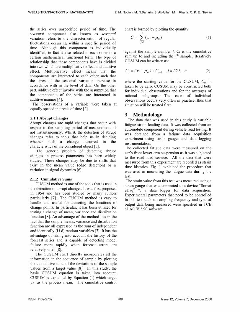
From Fig. 5, it shows that the distribution for campus route is negatively skewed to the right. It can be concluded that the Gaussian distribution does not fit the data. On the other hand, Fig.6 shows that the Gaussian distribution does also not fit the Pave’ data very well since the distribution are negatively skewed to the left. Fig.7 shows that there is no existence of skewed for the distribution pattern. It can be concluded that the Gaussian distribution can fit the highway data relatively.

%Program Cumulative Sums (CUSUM) for Fatigue Data clear load pave.txt; x=pave(1:30000); %average(mean)value ave_val=mean(x); N=length(x); Fs=500; % sampling frequency at 500 Hz T=1/Fs; ts=N/Fs; t=[ts/N:ts/N:ts]; subplot(2,1,1); plot(t,x); ylabel ('Amplitude[Microstrain]'); xlabel('Time[seconds]'); %program to plot cumulative sum charts %Ci=cumulative sum value %xi=process mean %Ci-1=previous value of Ci %First compute for i=1:length(x) Ci1(i)=(x(i)-ave_val).^2; if i==1 Ci(i)=Ci1(i); else Ci(i)=Ci1(i)+Ci(i-1); end end subplot(2,1,2); plot(t,Ci) ylabel ('Cumulative Amplitude[Microstrain]'); xlabel('Time[seconds]');



-300 -200 -100 0 100 200 300 400 500 6000

0.002

0.004

0.006

0.008

0.01

0.012

0.014

0.016

0.018

Data

Den

sity

Datafit 1

Fig. 5: The Gaussian distribution plot for Campus Route Data

-150 -100 -50 0 50 100 150 200 250 300 3500

0.002

0.004

0.006

0.008

0.01

0.012

0.014

Data

Den

sity

Datafit 1

Fig. 6: The Gaussian distribution plot for Pavé Data



-150 -100 -50 0 50 100 150 2000

0.002

0.004

0.006

0.008

0.01

0.012

0.014

0.016

0.018

Data

Den

sity

Datafit 1

Fig. 7: The Gaussian distribution plot for Highway Data

Using Equation (2) in the algorithm, it was found that the CUSUM plot did not shows any significant findings in detecting the fatigue damage event/abrupt changes that exist in all selected data. However by using Equation (6), it shows that there is an improvement in detecting the existence of

transient event in the fatigue data. Fig. 8, 9 and 10 show the comparison between the CUSUM and time series plot for fatigue data. The CUSUM plot in Fig. 8 shows that there exist several jumps which related to fatigue damage event.

0 10 20 30 40 50 60-500

0

500

Am

plitu

de[M

icro

stra

in]

Time[seconds]

0 10 20 30 40 50 600

2

4

6x 107

Cum

ulat

ive

Am

plitu

de[M

icro

stra

in]

Time[seconds]

Fig. 8: Comparison between CUSUM and time series plot for Campus Route Data



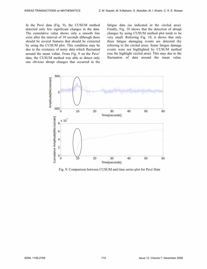
In the Pavé data (Fig. 9), the CUSUM method detected only few significant changes in the data. The cumulative value shows only a smooth line exist after the interval of 10 seconds although there should be several features that should be extracted by using the CUSUM plot. This condition may be due to the existence of noisy data which fluctuated around the mean value. From Fig. 9 on the Pave’ data, the CUSUM method was able to detect only one obvious abrupt changes that occurred in the

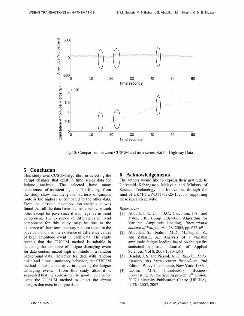
fatigue data (as indicated in the circled area). Finally, Fig. 10 shows that the detection of abrupt changes by using CUSUM method plot tends to be very small. Referring Fig. 10, it shows that only three fatigue damaging events are detected (by referring to the circled area). Some fatigue damage events were not highlighted by CUSUM method (see the highlight circled area). This may due to the fluctuation of data around the mean value.

0 10 20 30 40 50 60-500

0

500

Am

plitu

de[M

icro

stra

in]

Time[seconds]

0 10 20 30 40 50 600

2

4

6

8x 107

Cum

ulat

ive

Am

plitu

de[M

icro

stra

in]

Time[seconds]

Fig. 9: Comparison between CUSUM and time series plot for Pavé Data



0 10 20 30 40 50 60-500

0

500

Am

plitu

de[M

icro

stra

in]

Time[seconds]

0 10 20 30 40 50 600

0.5

1

1.5

2x 107

Cum

ulat

ive

Am

plitu

de[M

icro

stra

in]

Time[seconds]

Fig.10: Comparison between CUSUM and time series plot for Highway Data

5 Conclusion This study uses CUSUM algorithm in detecting the abrupt changes that exist in time series data for fatigue analysis. The selected have many occurrences of transient signals. The findings from the study show that the global kurtosis of campus route is the highest as compared to the other data. From the classical decomposition analysis, it was found that all the data have the same behavior each other except for pave since it was negative in trend component. The existence of differences in trend component for this study may be due to the existence of short term memory random shock in the pave data and also the existence of difference values of high amplitude event in each data. The study reveals that the CUSUM method is suitable in detecting the existence of fatigue damaging event for data contain mixed high amplitude in a random background data. However for data with random noise and almost stationary behavior, the CUSUM method is not that sensitive in detecting the fatigue damaging event. From this study also, it is suggested that the kurtosis can be good indicator for using the CUSUM method to detect the abrupt changes that exist in fatigue data.

6 Acknowledgements The authors would like to express their gratitude to Universiti Kebangsaan Malaysia and Ministry of Science, Technology and Innovation, through the fund of UKM-GUP-BTT-07-25-152, for supporting these research activitie References: [1] Abdullah, S., Choi, J.C., Giacomin, J.A., and

Yates, J.R., Bump Extraction Algorithm for Variable Amplitude Loading, International Journal of Fatigue, Vol 28, 2005, pp. 675-691.

[2] Abdullah, S., Ibrahim, M.D., M.,Nopiah, Z., and Zaharin, A., Analysis of a variable amplitude fatigue loading based on the quality statistical approach, Journal of Applied Sciences, Vol 8, 2008,1590-1593

[3] Bendat, J. S. and Piersol, A. G., Random Data: Analysis and Measurement Procedures, 2nd Edition, Wiley-Interscience, New York. 1986.

[4] Lazim, M.A, Introductory Business Forecasting: A Practical Approach, 2nd edition, 2007,University Publication Centre (UPENA), UiTM 2005, 2007



[5] M., Basseville, and I.V., Nikirov, Detection of

abrupt changes: Theory and application,3rd edition ,1993, Prentice-Hall

[6] S.,Lee, J.,Ha, O.,Na, and S.,Na, The Cusum test for parameter change in time series model, Board of the Scandinavian Journal of Statistics, Vol 30, 2003,781-796

[7] D.C. Montgomery, Introduction to statistical quality control, 5th edition, 2005, Wiley International Edition

[8] Marko, Baarola, Mika, Ruusunen, and Mika, Pirittima, Some change detection and time series forecasting algorithms for an electronic manufacturing process, Control Engineering Laboratory Report, A No.26, 2005,1-27

[9] Qu, L. and He, Z., Mechanical Diagnostics, Shanghai Science and Technology Press, Shanghai, P. R. China. 1986.



Abrupt Changes Detection in Fatigue Data Using the Cumulative Sum Method

Documents

Transcript of Abrupt Changes Detection in Fatigue Data Using the Cumulative Sum Method